15 Responsible Engineering
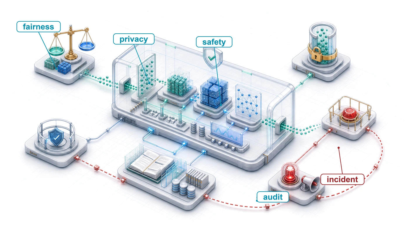
Purpose
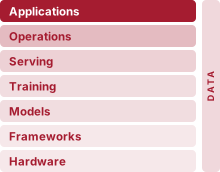
Architecture stack focus for this chapter.
Why can a system that does exactly what it was told to do still cause harm?
Latency, availability, and accuracy targets do not say whether they describe the right behavior, whom the system serves, or which costs its specification leaves unmeasured. An ML system can satisfy latency, throughput, and aggregate accuracy requirements while reproducing historical discrimination, rewarding harmful engagement, consuming unjustified energy, or using data without adequate privacy and accountability controls. Such a system has not malfunctioned; it is efficiently optimizing an incomplete specification. The omitted constraints appear as uneven outcomes across populations, lifetime cost and emissions, decisions people cannot understand or contest, and evidence that cannot be reconstructed after harm occurs. If those consequences are not defined as requirements before deployment and monitored afterward, conventional health checks can remain green while harm accumulates. A credit model that treats groups unevenly can repeat that decision millions of times before anyone aggregates the outcomes, while its dashboards report healthy latency and accuracy throughout. Responsible engineering treats such outcomes as system failures to be diagnosed, measured, and mitigated with the same rigor as latency or accuracy regressions. That work requires translating broad obligations into testable bounds, documented assumptions, traceable data, and response paths that remain enforceable in production, so that a harm found after launch can be traced and corrected. In D·A·M terms, responsibility broadens the definition of correctness: data must be examined for encoded harms and lawful use, algorithms must be bounded by defensible outcome and efficiency requirements, and machine infrastructure must monitor, document, and enforce those boundaries throughout the system lifecycle.
Learning Objectives
- Explain how a model that meets its training objective can still cause harm when that objective is a proxy that drifts from the goal
- Apply data-algorithm-machine diagnosis to localize responsibility failures in data, algorithm objectives, or monitoring infrastructure
- Calculate fairness metrics from confusion matrices and compare trade-offs on the fairness-accuracy Pareto frontier
- Design disaggregated release gates and per-group monitoring, fitting the bias feedback model to project when a passed gate will fail
- Analyze total cost, inference dominance, and carbon impact as measurable responsibility constraints
- Construct model cards, datasheets, lineage records, and audit trails for accountability
- Evaluate privacy, access-control, and compliance designs against regulatory and human-review requirements
Explore the concepts in this chapter
The volume’s concept map, opened on this chapter. Select a concept to read how it connects to ideas in other chapters. Open the full map ↗
15.1 Responsibility as Systems Engineering
A credit model decides whose loan applications are approved, a ranking model decides which items millions of people see, and a voice assistant decides when audio from a private room leaves the device. None of these outcomes appears in a loss curve or a latency dashboard, yet every deployed model settles them. A system can meet every latency, uptime, and aggregate accuracy target while rejecting qualified minority applicants, amplifying clickbait, or leaking private audio. Responsible engineering is systems engineering applied to the consequences that a model’s objective leaves unstated: whose errors the system makes, how much energy and money each decision draws, and whether a harmful decision can later be explained, traced, and corrected. Each of those outcomes is fixed by concrete engineering choices about data, objectives, and infrastructure.
ML Operations built the machinery that keeps a deployed model faithful to its objective as data and traffic change, and that machinery assumes the objective was the right one. If MLOps is the control loop for reliability, then responsible engineering is the control loop for safety. Where MLOps monitors runtime health and predictive quality to guide operational response, responsible engineering monitors outcome distributions to guide intervention when systems generate harm. In systems engineering terms, a model can pass verification (conforming exactly to its specified training objective) while failing validation (failing to satisfy operational, safety, or legal requirements) (National Aeronautics and Space Administration 2016). The verification gap (principle 9) concerns the first of these activities. It bounds how much any finite test can establish about conformance to a specification, whereas validation asks whether the specification was the right one. The failure stems from an incomplete specification rather than a fault in compiler execution or numerical optimization.
National Aeronautics and Space Administration. 2016. NASA Systems Engineering Handbook. NASA/SP-2016-6105 Rev2. National Aeronautics; Space Administration.
↩︎ Continuous telemetry and automated retraining control loops for operational reliability are established in Five operational principles.
Traditional software engineering isolates defects within modules, though shared dependencies can still propagate faults. Machine learning systems introduce data-dependent coupling: data flows through shared representations, so corrupted or biased inputs alter the dense parameter matrices that serve every subsequent inference. A biased training dataset does not trigger a compile-time assertion or runtime crash; it silently shifts decision boundaries across the entire system. Read for responsibility rather than performance, the D·A·M taxonomy isolates where such failures originate: unrepresentative or biased inputs (Data), misaligned loss formulations (Algorithm), or telemetry blind spots and unjustified resource footprints in the serving infrastructure (Machine). Responsibility therefore has to be designed in rather than patched on after deployment.
↩︎ The D·A·M taxonomy, which classifies a system bottleneck along its data, algorithm, and machine axes, is established in Defining ML Systems.
Responsible engineering expands the definition of correctness for machine learning systems. Traditional correctness (numerical stability, bounded latency, and high service availability) remains necessary, but insufficient. A production system must satisfy broader operational bounds: bounded error disparities across demographic slices, defensible energy expenditure, and verifiable data lineage. This expanded correctness applies engineering discipline to failure modes that aggregate performance metrics ignore. A p99 latency spike triggers automated alerts on an operational dashboard. A demographic fairness regression remains invisible to aggregate loss metrics until real-world harm occurs, and when the model’s decisions shape its own future training data, the hidden disparity can grow with every retraining cycle (principle 13). Both demand rigorous telemetry and automated regression testing. The optimizations of the preceding chapters inherit the same blind spot, because each was judged by the cost terms its benchmark measured.
Systems Perspective 15.1: The full cost of the iron law
The iron law of ML systems (principle 3) decomposes execution time into data movement, computation, and fixed overhead. Compressing models, accelerating hardware, and automating operations each optimize these terms. Yet an optimization can create or shift costs that its benchmark omits.
A model quantized for edge deployment can consume less energy, but its accuracy loss need not fall evenly across demographic groups, so the compressed model must be revalidated on the same subgroup slices as the original. A ranking model such as the DLRM service, optimized for engagement, maximizes a business metric but may amplify harmful content. Responsible engineering extends this accounting to include broader impacts: the carbon cost of computation, the fairness cost of optimization choices, and the societal cost of deployment at scale. The iron law accounts for how fast a system runs and says nothing about whom it serves well.
Three running cases carry the chapter, each chosen because it exposes a different kind of responsibility failure. The first is a credit service, a labeled composite rather than a documented deployment: a classifier that approves or rejects loan applications, constructed so that every fairness criterion in the chapter can be computed from its confusion matrices. Fairness criteria need labeled decisions about people, which none of the lighthouse models makes, so the composite carries the stages that specify, measure, explain, and monitor such decisions. The second is the DLRM ranking service, the capacity-bound lighthouse, whose model alone occupies 100 GB in its registry entry, more than the 80 GB of memory on one H100. Its rankings decide what people see, so the clicks it trains on are shaped by its own earlier outputs, and its request volume makes it the chapter’s case for feedback, exposure, cost, and carbon. The third is the keyword spotting (KWS) system, the power-bound lighthouse, an always-listening microphone in private homes whose design must decide what audio may leave the device, which makes it the case for privacy, lineage, and audit.
The chapter follows those cases through the lifecycle stages at which each failure is still cheap to prevent (table 1). Section 15.2 explains why optimization can succeed while the system fails, through proxy targets, feedback loops, and distribution shift that leave every health check green. Section 15.3 then works through four chained stages on the credit service: specifying requirements before training, measuring fairness criteria as release gates, explaining decisions and documenting models, and operating the deployed model so that its disparity stays bounded under feedback. Section 15.4 measures the energy, carbon, and money that every stage consumes on the DLRM service. Section 15.5 builds, on the KWS system, the governance infrastructure (access control, privacy, regulatory capabilities, lineage, and audit) that makes each earlier guarantee provable to someone outside the team.
| Section or Stage | Failure It Addresses | What It Costs the Machine | Running Case |
|---|---|---|---|
| Engineering Responsibility Gap | Proxy targets, feedback loops, and shift that leave health checks green | Nothing yet; the diagnosis locates the failure on the data, algorithm, or machine axis | Credit service, DLRM |
| Lifecycle: Specify | Requirements nobody wrote down: target, populations, human oversight | Labeled evaluation data for every named subgroup; reviewer hours per escalated decision | Credit service |
| Lifecycle: Measure | Disparities hidden by aggregate accuracy | Per-slice evaluation; mitigation training with a second network head and a larger search | Credit service |
| Lifecycle: Explain and document | Decisions no one can contest; models reused outside their envelope | Explanation compute on the serving path, exponential in feature count for exact attribution | Credit service, MobileNetV2 |
| Lifecycle: Operate | Disparity that grows through retraining feedback | Per-group telemetry; randomized exploration traffic served at lower expected value | Credit service, DLRM |
| Environmental and Cost Awareness | Energy, emissions, and cost the task does not justify | Accelerator-hours, kilowatt-hours, and kilograms of CO2 over the service lifetime | DLRM |
| Data Governance and Compliance | Evidence that cannot be reconstructed after harm | Audit-log bytes, lineage storage, privacy noise and its memory cost, retraining for erasure | KWS |
Self-Check: Question
An AI recruiting tool meets its latency SLA, maintains 99.9% availability, and achieves 87% aggregate accuracy, yet it systematically downgrades resumes containing the word “women’s” or graduates of women’s colleges. Applying the systems-engineering verification-versus-validation framing, which diagnosis correctly explains this outcome?
- The system failed verification because any discriminatory outcome is by definition a low-level coding defect in the model implementation.
- The failure is primarily an operational reliability defect that responsible engineering addresses only after serving infrastructure destabilizes.
- The root cause is insufficient model capacity, which can be resolved by scaling up model parameters without altering the optimization objective.
- The system passed verification by meeting its stated technical requirements, but failed validation because the specification itself did not capture the organization’s true goal of fair hiring.
A team argues that a one-time ethics sign-off before deployment is sufficient because their model passes all latency and aggregate accuracy checks. Using the MLOps control-loop analogy, explain why responsible engineering must instead operate as a continuous control loop, and identify one specific production metric that a one-time pre-launch review cannot capture.
True or False: Because ML systems are constructed from modular software components, a fairness defect originating from biased training data can be isolated and patched within a single function without altering data pipelines, training objectives, or shared representations.
15.2 Engineering Responsibility Gap
The credit service can approve 90 percent of qualified majority-group applicants but only 60 percent of equally qualified minority-group applicants and still report high aggregate accuracy, because the minority group contributes only a small share of the evaluated applicants. The worked example in section 15.3.2.1 computes exactly this outcome from its confusion matrices. The responsibility gap between this technical correctness and responsible outcomes is the distance that conventional testing does not measure. That gap opens at training time when an optimizer faithfully learns biased historical signals or a flawed proxy target, and it widens in production through distribution shift, metric misalignment, and feedback loops that conventional health checks leave invisible.
15.2.1 When optimization succeeds but systems fail
The first pathway appears before a model ever meets live traffic, when optimization succeeds on training data or targets that already encode harm. In Amazon’s experimental recruiting tool (a war story in Constraint layers), a model trained on a decade of historical hiring data optimized faithfully for the objective it was given, yet those historical patterns encoded gender bias that the system reproduced directly in candidate ratings (Dastin 2018). That failure sits on the data axis of the D·A·M taxonomy, because it stemmed from the historical training signal rather than from an algorithmic or software defect.

The Amazon failure turns on the data axis, not the algorithm.
Bolukbasi, Tolga, Kai-Wei Chang, James Y. Zou, Venkatesh Saligrama, and Adam Tauman Kalai. 2016. “Man Is to Computer Programmer as Woman Is to Homemaker? Debiasing Word Embeddings.” Advances in Neural Information Processing Systems (NeurIPS), 4349–57.
Under empirical risk minimization, the model reduced classification loss by finding word-level correlations across the resume corpus. Because past technical hires were mostly men, words tied to women’s colleges, organizations, or activities correlated negatively with positive hiring labels. The optimizer faithfully extracted the empirical distribution of the training data, but that distribution reflected past hiring practices rather than candidate competence. High-dimensional text representations pick up and amplify these statistical patterns, baking social biases directly into the vectors that downstream models consume (Bolukbasi et al. 2016).
Amazon tried to fix the model by stripping explicit gender indicators and gendered words from the training pipeline. That change failed to produce unbiased recommendations because high-dimensional feature spaces contain proxy variables that retain demographic signal.1 Scrubbing isolated attributes leaves correlated features intact: ZIP codes correlate with race through residential segregation, applicant names correlate with ethnicity, and healthcare spending correlates with socioeconomic conditions. In Amazon’s resume pipeline, even after explicit gender terms were removed, remaining vocabulary (attendance at specific colleges or participation in particular student organizations) continued to encode sex-correlated patterns (Dastin 2018). Removing protected attributes from training data is therefore not enough to guarantee fairness.
1 Proxy variable: Removing one proxy may have little effect when other correlated features retain similar signal. Conversely, correlation alone does not prove discrimination or identify the appropriate intervention. Protected-attribute removal, subgroup evaluation, counterfactual tests, causal analysis, and review of the full decision process provide complementary evidence; no single diagnostic is a complete defense.
Dastin, Jeffrey. 2018. “Amazon Scraps Secret AI Recruiting Tool That Showed Bias Against Women.” Reuters.
Closing that gap takes changes across the full system lifecycle rather than a surface-level data filter. Before deployment, evaluating each demographic subgroup separately measures how scores differ across groups. When those slices expose a disparity, training-time mitigations such as adversarial debiasing (developed with the credit-service worked example in section 15.3.2.1) can suppress protected-attribute signal in learned representations, though they still require continuous subgroup validation. Once the model is live, human review for borderline scores provides an operational safeguard only when reviewers are trained, empowered, and audited rather than used to rubber-stamp model outputs. Downstream monitoring also tracks hiring outcomes over time to catch disparate impact that offline loss metrics conceal. Because bolting these defenses onto an existing pipeline proved unworkable, Amazon scrapped the project (Dastin 2018).
The same outcome can originate on the algorithm axis instead, in the choice of target rather than in the data. When the target itself reflects historical inequities, the training objective encodes those disparities into the model’s decision boundaries, and the harm lands on the subgroup the target mismeasures. Curating the data would not repair such a failure, because the data faithfully record the wrong quantity. That algorithm-axis version appeared with life-threatening consequences in clinical care management.
War Story 15.1: The proxy variable trap (2019)
Context: In 2019, Ziad Obermeyer and colleagues at UC Berkeley audited a commercial Optum algorithm used by health systems to enroll patients with complex needs into high-risk care management programs, examining roughly fifty thousand patients across one large academic hospital (Obermeyer et al. 2019).
Mechanism: The model predicted “future healthcare cost” as a proxy for “future health need.” Because the US healthcare system spends less on Black patients than on White patients with the same illness level, the algorithm learned this pattern and assigned lower risk scores to Black patients.
Impact: At any given risk score, Black patients carried substantially more chronic conditions than White patients, reducing the share of Black patients enrolled in specialized care.
Response: The study showed that replacing cost with a direct measure of health need would raise the share of Black patients identified for additional care from 17.7 percent to 46.5 percent at the analyzed threshold.
Systems lesson: Optimizing for a proxy inherits the biases of the system that generated the proxy. The proxy-target relationship must be audited across every demographic subgroup the system serves.
Obermeyer, Ziad, Brian Powers, Christine Vogeli, and Sendhil Mullainathan. 2019. “Dissecting Racial Bias in an Algorithm Used to Manage the Health of Populations.” Science 366 (6464): 447–53. https://doi.org/10.1126/science.aax2342.
The recruiting tool and the care-management algorithm show that optimization success can coexist with system failure. Neither disparity requires a software bug or hardware malfunction to explain why a technically functioning model can fail its intended use. The architectural question is whether the problem specification captures acceptable outcomes. When the technical objective (such as minimizing empirical prediction error) diverges from the system specification (fair, defensible outcomes across user populations), improving the training objective can preserve or amplify harm.
Standard production telemetry cannot detect specification failures. Monitoring pipelines track inference latency, memory use, throughput, and aggregate validation loss, all of which remain green while a model systematically misallocates errors across subgroups. Preventing silent specification failures requires making responsibility metrics part of the primary test harness: verifying whether the loss function acts as a defensible proxy for the true system goal, and enforcing the justified, application-specific fairness criterion before deployment.
Checkpoint 15.1: Responsible design
Responsibility is a system property, not a model property.
Failure modes
Check
15.2.2 Silent failure modes

One upstream change; many silently affected.
Even a model whose training data and target were audited before launch can fail silently in production when the environment around it changes. Consider the credit service after a change to its online application form alters how self-employed applicants’ income is recorded. The model begins declining applicants it would have approved a week earlier. A single upstream modification propagates across the system’s blast radius (the set of downstream decisions, and the applicants behind them, that one upstream change reaches) without raising an alert. The model’s confidence scores remain high, its inference latency stays within its service level agreement, and all system health checks pass green. The failure is silent. The input data distribution has shifted, but the service’s pipeline monitors only service health and carries no drift monitors.
↩︎ Drift monitors that quantify distributional divergence between serving and training data are established in Statistical monitoring and drift detection.
Availability-focused monitoring cannot detect this class of failure. It is the silent degradation of When ML Systems Fail Silently, in which statistical failure modes produce degraded outputs indistinguishable from valid predictions while every kernel completes within its latency budget. The responsibility question is whom the degraded outputs reach.
Distribution shift, a deployment input distribution that differs from the one used to develop and evaluate the model, represents the first major mechanism behind this silent degradation. Its covariate, label, and concept forms, and the divergence statistics that detect them, are developed with data engineering (see the margin). The failure is environmental. The physical distribution of inputs changed after training, yet the model has no internal telemetry to detect the discrepancy. Through the responsibility lens the pitfall sharpens, because shift often lands on one subgroup first, where a population-wide divergence statistic barely moves, and concept drift on that slice stays invisible until its outcomes are labeled. A monitor that is adequate for the population can therefore be blind to the people the shift reaches first.
↩︎ Covariate, label, and concept drift, with the divergence statistics that detect them, are established in Data drift detection and response.
Retraining on fresh data can partially restore accuracy under distribution shift. However, retraining cannot resolve a second, deeper mechanism of silent failure that persists even when the data distribution is perfectly stationary: metric misalignment.
Metric misalignment occurs when the objective function optimizes an observable proxy metric that diverges from the unobserved outcome the system is intended to deliver. Goodhart’s Law, the benchmark trap in which a measure optimized as a target stops measuring the goal, applies with more force here than in benchmarking, because the training objective is the target. Gradient descent searches that target far more exhaustively than a team tuning against a benchmark. Up to a point the proxy and the goal improve together; past that point further optimization buys proxy gains at the goal’s expense.
↩︎ Goodhart’s law, under which a benchmark metric optimized as a target ceases to measure the goal, is established in The Benchmark–Production Gap.
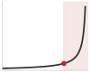
Past the knee, the proxy decouples from the goal.
Systems Perspective 15.2: The alignment gap
The DLRM ranking service optimizes a proxy metric (Clicks) because the true metric (User Satisfaction) is unobservable, and the two can diverge sharply. In an illustrative version of the service, \(\text{Correlation}(\text{Clicks}, \text{Satisfaction})\) might begin at 0.8; once ranking maximizes clicks, it may find clickbait with high clicks but low satisfaction, and the correlation could fall to 0.2.
The falling correlation is the symptom. The quantity that matters is how far the proxy’s movement overstates the goal’s, which equation 1 captures for metrics normalized to a common scale: \[ \text{Gap} = \mathbb{E}[\text{Proxy}] - \mathbb{E}[\text{True}] \tag{1}\]
Suppose both metrics start at the same normalized value \(\NormalizedMetricBaseline\), so the gap is zero. A ranking change that raises Clicks by 20 percent and lowers Satisfaction by 5 percent moves them to \(1.20\NormalizedMetricBaseline\) and \(0.95\NormalizedMetricBaseline\), opening a gap of \(0.25\NormalizedMetricBaseline\). Every dashboard that reports Clicks shows a 20 percent win, while the goal the system exists to serve has moved the other way.
Systems insight: Engineers cannot directly optimize an unobserved goal. They need defensible proxy validation. A randomized holdout, a small random slice of users served without the new ranking, can estimate the ranking’s causal effect on the gap, but only when the holdout’s measured outcome reflects the goal or a justified surrogate for it.
The alignment gap illustrates a failure originating on the algorithm axis, where the loss function optimizes a misspecified objective, so even a model that generalizes with zero test error drives outcomes that conflict with organizational or societal goals. Distribution shift, by contrast, originates on the data axis. The model logic remains intact, but the input distribution departs from the training distribution. Both failures can be silent, but they suggest different first interventions: objective redesign for a misspecified target, or pipeline investigation and possible adaptation for shifted inputs. These remedies can be complementary when both mechanisms are present. Isolating the root cause is the job the D·A·M taxonomy already performs for performance bottlenecks, and perspective 15.3 reads the same three axes for responsibility failures.
↪ The performance-bottleneck form of the D·A·M diagnosis, from profiler symptom to binding axis, is collected for reference in The D·A·M Taxonomy.
Systems Perspective 15.3: Diagnosing responsibility failures with D·A·M
When a system causes harm, use the D·A·M taxonomy to identify the root cause. Responsibility failures are rarely “algorithm bugs”; they are structural flaws along one of the three axes:
- Data (information): The training corpus reflects historical bias or unrepresentative sampling (such as Amazon’s recruiting tool learning from biased historical applicant data).
- Algorithm (logic): The objective function optimizes an unconstrained proxy metric that amplifies harm (such as engagement optimization driving polarization).
- Machine (physics): The serving and governance infrastructure cannot see or bound the harm, through telemetry that never slices outcomes by subgroup, missing lineage and audit records, or an energy and carbon footprint that exceeds the societal benefit of deployment (such as an overparameterized foundation model serving a low-complexity task).
Locating the dominant failure in the taxonomy identifies the first remediation to test: better curation (Data), safer objectives (Algorithm), or better instrumented and more efficient infrastructure (Machine). Real failures can span axes, so the intervention must still be evaluated end to end.
The D·A·M taxonomy isolates where a failure starts, while production telemetry must catch when it manifests; statistical failures (data-quality defects, distribution shift, and fairness violations) can persist for days or months behind green health checks (Production Monitoring), and a fairness violation is the slowest to surface because it is visible only on a subpopulation and only once outcomes are labeled. Worse, the hardest silent failures do not stay confined to one D·A·M axis.
When a model’s predictions reshape the user behavior that generates future training data, a third silent failure mechanism, the feedback loop, couples the algorithm and data axes across retraining cycles. The YouTube recommendation feedback loop illustrates this dynamic at scale (M. H. Ribeiro et al. 2020).2 M. H. Ribeiro et al. (2020) audited radicalization pathways on YouTube, finding migration from milder to more extreme channel categories and recommendation reachability between those categories. The broader systems lesson is that feedback loops can work exactly as designed while producing outcomes that conflict with societal values. Recommendation objectives must therefore be tested against downstream harms, not only against engagement proxies.
Ribeiro, M. H., R. Ottoni, R. West, V. A. F. Almeida, and Jr. Meira Wagner. 2020. “Auditing Radicalization Pathways on YouTube.” Proceedings of the 2020 Conference on Fairness, Accountability, and Transparency, 131–41. https://doi.org/10.1145/3351095.3372879.
2 Goodhart’s law in feedback loops: Recommendation feedback loops are the canonical ML manifestation of Goodhart’s law. Gradient descent optimizes watch-time proxies at a speed no human curator can match, and the system’s own outputs reshape the training distribution. Users who consume extreme content generate data that can reinforce extremity and can decouple the proxy from user welfare faster than manual editorial processes would.
↩︎ The YouTube feedback loop as a production technical-debt pattern is established in Production debt patterns.
Mosseri, Adam. 2018. Bringing People Closer Together. Meta Newsroom.
Facebook’s 2018 change to News Feed ranking shows the converse decision. The team moved the ranking objective from short-term engagement proxies (clicks, watch time) toward meaningful social interactions between people, accepting lower short-term engagement to arrest the proxy’s decoupling from user welfare (Mosseri 2018). The DLRM ranking service faces the same choice whenever its objective is set, because the clicks it can observe are a proxy for the value it is meant to deliver.
Silent failure modes change what verification can establish. Traditional software verification relies on deterministic assertions. A unit test asserts that an output matches an exact value, memory bounds checkers assert that buffer allocations do not overflow, and watchdog timers ensure RPC latencies do not breach service level agreements. In an ML system, correctness cannot be verified by deterministic invariants alone, because, as the credit service’s form change showed, every such invariant can hold while the model serves biased, uncalibrated, or harmful predictions. What can be verified is the statistical bound of the verification gap (principle 9), which holds only over a named deployment population, task distance, and tolerance. A bound stated over the aggregate population says nothing about a subgroup that the aggregate averages away, so a responsible specification names each consequential subgroup as a population in its own right. Turning responsibility goals into routine engineering practice means running statistical checks continuously: watching for covariate shift within each demographic slice, auditing how well proxies track the real goal, and bounding closed-loop feedback before silent errors spread through production.
15.2.3 The testing challenge
Writing those subgroup checks exposes a bind that deterministic software testing never meets. Suppose two engineers test the same credit model and agree that it should treat demographic groups fairly. One checks whether qualified applicants in both groups are approved at the same rate; the other checks whether a given risk score means the same repayment probability in both groups. When the two groups have different base repayment rates and prediction is imperfect, passing the first test forces the model to fail the second (Chouldechova 2017; Kleinberg et al. 2017). Traditional software testing never faces that bind because it checks behavior against unambiguous specifications: an arithmetic function must return the exact sum of its operands, and a relational database must preserve foreign-key integrity. Those deterministic properties map directly to executable assertions.
Responsible ML properties resist that kind of single assertion. Fairness has multiple mathematical definitions that can conflict under conditions such as unequal base rates and imperfect prediction (Chouldechova 2017; Kleinberg et al. 2017). What counts as fair depends on context, values, and trade-offs that technical systems cannot resolve alone. Individual fairness requires that similar individuals receive similar treatment, while group fairness requires equitable outcomes across demographic categories. These criteria can conflict, and choosing between them requires value judgments beyond the scope of optimization.
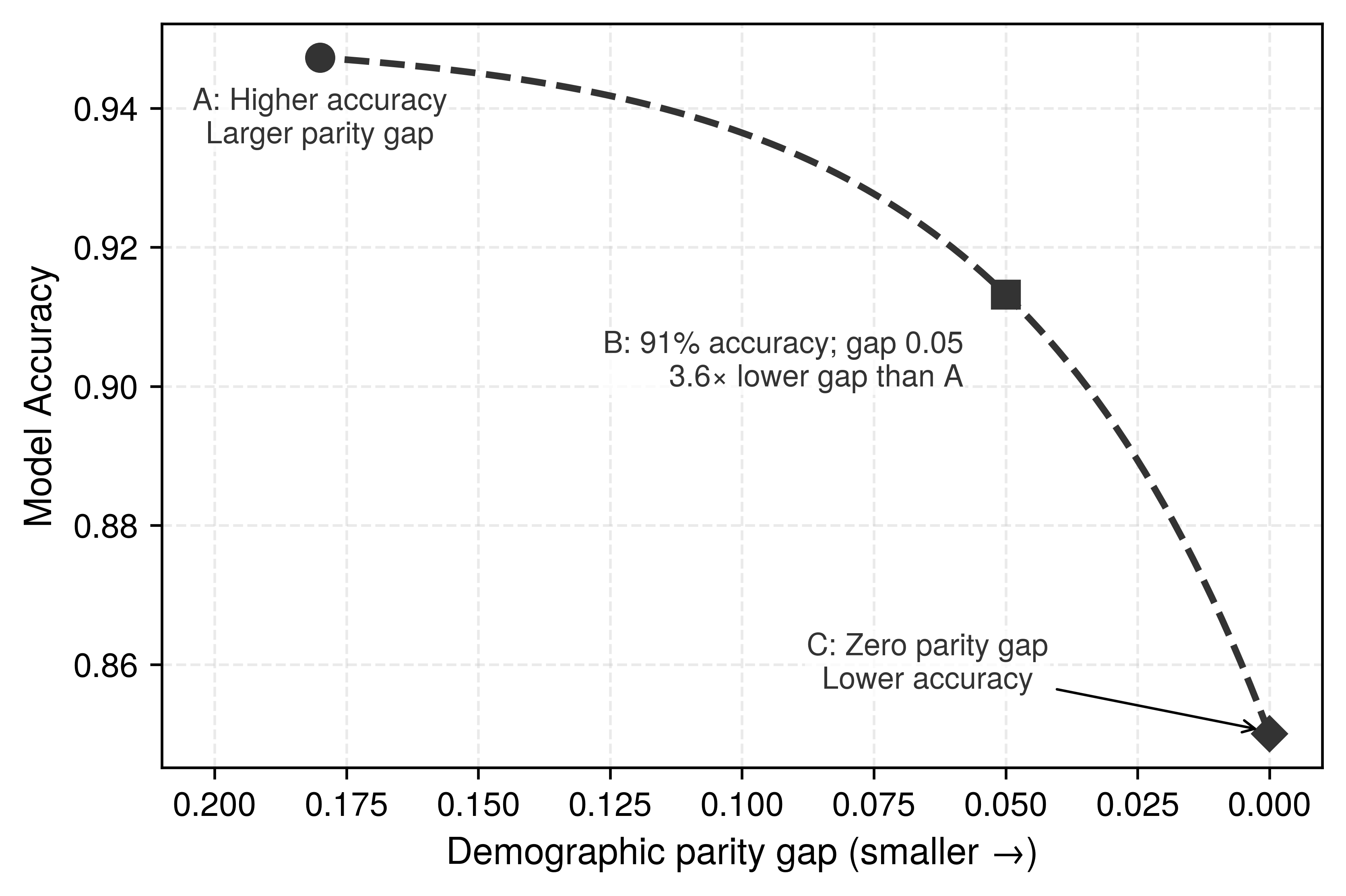
Fairness constraints and predictive performance can also trade off, by an amount that depends on the application. The Pareto frontier (principle 5) carries over unchanged, and section 15.3.2.2 measures one such trade-off once the criteria have been defined. Choosing criteria is only half of the testing problem. Aggregate metrics cannot show which groups a model fails, so testing also requires deciding which slices to evaluate, which invariances to demand, and which stresses to apply. Section 15.3.2 turns these choices into release gates.
These testing choices complement traditional software testing rather than replacing it, and no single group can make them alone. Legal specialists cannot specify which demographic slices matter for a healthcare algorithm, and product managers cannot determine appropriate invariance tests for a loan model. Domain experts, affected stakeholders, policy specialists, and engineers must define the relevant harms together; engineers then encode those requirements as measurable tests and production controls. Where deployed systems have closed the responsibility gap, they succeeded by turning shared value judgments into explicit engineering constraints that can gate a release.
15.2.4 When responsible engineering succeeds
When the 2018 Gender Shades audit exposed error rates on darker-skinned women more than thirty times higher than on lighter-skinned men in commercial gender classifiers (Buolamwini and Gebru 2018), “be fairer” was not an instruction an engineering team could execute. Where teams have closed that gap, each documented success did the same thing: it turned a vague responsibility goal into an engineering constraint that can be specified, tested, communicated, and, when necessary, used to stop deployment. Following Gender Shades, Microsoft invested in improving gender-classification performance across demographic groups. Targeted data collection, model changes, and systematic disaggregated evaluation gave the team an explicit error-rate target, bringing audited error rates for darker-skinned subjects below 2 percent (Raji and Buolamwini 2019). Publishing these disaggregated benchmarks established a verifiable baseline and turned external audit findings into an operational release gate.
Raji, Inioluwa Deborah, and Joy Buolamwini. 2019. “Actionable Auditing: Investigating the Impact of Publicly Naming Biased Performance Results of Commercial AI Products.” Proceedings of the 2019 AAAI/ACM Conference on AI, Ethics, and Society, 429–35. https://doi.org/10.1145/3306618.3314244.
↩︎ Gender Shades, and the way aggregate benchmark metrics conceal subgroup disparities, are established in Accuracy metrics and their blind spots.
Yee, Kyra, Uthaipon Tantipongpipat, and Shubhanshu Mishra. 2021. “Image Cropping on Twitter: Fairness Metrics, Their Limitations, and the Importance of Representation, Design, and Agency.” Proceedings of the ACM on Human-Computer Interaction 5 (CSCW2): 1–24. https://doi.org/10.1145/3479594.
Twitter’s automatic image cropping system shows the same discipline under a different constraint. In 2020, users raised concerns about racial and gender bias in preview thumbnails. Twitter audited the system, reported measured disparities and limitations, and shifted toward uncropped previews that gave users more control (Yee et al. 2021). In that case, responsible engineering changed the product design rather than relying on an incremental adjustment to an automated ranking threshold.
Differential privacy applies the same move to privacy. It turns a privacy requirement into a mathematical bound on how much any one record can change a system’s outputs, a bound that can be budgeted and audited rather than asserted (Dwork 2008). Its mechanism and systems cost are developed with the privacy protections in section 15.5.2.
Dwork, Cynthia. 2008. “Differential Privacy: A Survey of Results.” In Theory and Applications of Models of Computation. Springer Berlin Heidelberg. https://doi.org/10.1007/978-3-540-79228-4_1.
In each case the constraint sat on a D·A·M axis, whether in curated training data, a bounded loss function, or a privacy budget tracked in the runtime. Enforcing such constraints requires the operational authority to halt deployment or retire components that violate specified bounds, and that authority has to sit with the people who can still change the design.
15.2.5 Engineering leadership on responsibility
That authority belongs in engineering because a prelaunch review two weeks before release arrives after the cheap fixes have already been closed off. When a late review flags a model that cannot explain why it rejected a loan applicant or a pipeline that never recorded the demographic attributes needed to audit disparity, tuning a threshold cannot repair the design. Correcting a flawed target means changing what the model predicts, and adding slice evaluation means rebuilding the data pipeline. Responsible AI engineering cannot be delegated exclusively to ethics boards or legal departments. These groups provide essential oversight, but they lack the early technical access required to catch problems while the architecture is still fluid.
Legal or ethics review can identify a problem near deployment, but it cannot recover design options the system has already foreclosed. If the team trained the model without fairness constraints, chose an architecture that cannot support interpretability requirements, or built a data pipeline without the demographic attributes needed for monitoring, review can only accept, reject, or demand expensive redesign. Engineers therefore occupy a critical position in the ML development lifecycle, because their choices define the solution space for all subsequent interventions. Architecture determines which fairness constraints can apply, the optimization objective determines which patterns the system learns, and the data pipeline determines whether disaggregated evaluation is possible.
Definition 15.1: Responsible AI engineering
Responsible AI engineering is the engineering discipline of designing, deploying, and maintaining systems with probabilistic outputs by turning societal and regulatory requirements into testable constraints on the D·A·M axes. Those constraints cover permissible data contents, provenance, and composition; allowable model behavior and robustness properties; and infrastructure bounds such as latency, energy, compute budget, carbon emissions, and audit-log retention.
- Significance: Each D·A·M axis acquires concrete governance constraints. The data axis is bounded by privacy regulations such as the General Data Protection Regulation (GDPR), which limits which records, fields, and features can be collected. The algorithm axis is bounded by fairness and robustness metrics (for example, positive prediction rates that differ across protected groups by no more than 5 percentage points, or accuracy that degrades by less than 2 percent when an adversary may shift every normalized input feature by at most 0.01). The machine axis is bounded by resource and infrastructure budgets such as latency, energy per inference, carbon emissions, and audit-log retention. Violating these bounds is a system failure, not a research shortcoming.
- Distinction: Unlike AI ethics (which articulates aspirational values), responsible AI engineering translates those values into measurable, testable invariants that can be verified through automated testing and continuous monitoring, using the same lifecycle practices that enforce latency SLOs.
- Common pitfall: Stating a bound the system cannot measure. A disparity limit is an intention when the pipeline never collected the demographic attribute needed to check it, and a retention rule is an intention when no storage was provisioned to hold the evidence. Late-stage remediation may remain possible, but it is often narrower, slower, and more expensive.
An engineering-centered approach does not diminish the importance of diverse perspectives in identifying potential harms. Product managers, user researchers, affected communities, and policy experts contribute essential knowledge about how systems fail socially despite technical success. Engineers translate these concerns into measurable requirements and testable properties that can be verified throughout the development lifecycle.
Organizations also need a reason to fund that work, and three reasons recur. Systematic disaggregated evaluation, documentation, and monitoring reduce the legal and financial exposure that ML system failures create, and they preserve evidence of the engineering process if problems emerge. Regulation attaches risk-management, data-governance, transparency, and human-oversight duties to high-risk applications, and controls built in from the start are cheaper than evidence reconstructed after deployment (section 15.5.3). Demonstrated practice also differentiates: organizations that can show model cards, audit trails, and published disaggregated results may qualify for deployments that competitors cannot. Each reason pays off only through repeatable workflows (checklists, documentation standards, and testing protocols) that embed responsibility constraints in the engineering lifecycle itself.
Self-Check: Question
In an audited commercial healthcare algorithm (Optum), predicting future healthcare costs as a proxy for health needs resulted in Black patients receiving lower risk scores despite having more chronic conditions than White patients with identical scores. What systems mechanism explains why this proxy failed?
- The model suffered from severe overfitting due to an excessive number of gradient descent epochs on a small training dataset.
- The proxy variable inherited historical systemic disparities in healthcare spending, so predicting costs faithfully reproduced unequal access to care rather than actual medical need.
- The failure was caused by real-time concept drift that occurred after deployment when hospital billing codes suddenly changed.
- The algorithm used an unconstrained loss function that optimized inference latency at the expense of regression calibration.
A hospital sepsis prediction model begins recommending aggressive treatments for low-risk patients after an EHR update alters how vital signs are logged. System health checks, latency, and prediction confidence remain normal. Explain why this constitutes a silent failure, and identify two monitoring signals that would support investigation without assuming either proves the cause.
A content recommendation service reports that optimizing a ranker for short-term user clicks increased click-through rate by 20%, but long-term user satisfaction dropped by 5% and 30-day retention declined. Which systems-engineering concept best explains this divergence, and what is the appropriate mitigation?
- The alignment gap governed by Goodhart’s Law, where optimizing an observable proxy metric degrades the unobserved true objective; mitigated by maintaining counterfactual holdouts and multi-objective optimization with explicit satisfaction constraints.
- Model capacity collapse, where the embedding table runs out of capacity for rare items; mitigated by increasing embedding dimension and memory bandwidth.
- Hardware-level numerical underflow in attention layers; mitigated by upgrading from FP16 to FP32 mixed precision across serving clusters.
- Training-serving skew in network protocol buffers; mitigated by implementing automated schema validation in feature pipelines.
15.3 Responsible Engineering Across the Lifecycle
The recruiting tool and the care-management algorithm were both found to fail after the design options that could have addressed them were closed, so the lesson concerns timing more than vigilance. Each responsibility failure in this chapter has a point in the ML lifecycle before which it is cheap to prevent and after which it becomes expensive or impossible to repair, so responsible engineering is organized around that lifecycle rather than around a list of concerns.
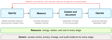
Six stages follow from that premise, and the first four form a chain in which each stage depends on the output of the one before it. Specify comes first because a system cannot be tested against a requirement nobody wrote down. The target, the populations that matter, the evaluation data those populations demand, and the boundary of human oversight must all be fixed before training forecloses the alternatives. Measure turns those written requirements into release gates, evaluating each named population separately and quantifying the trade-offs among fairness criteria. Evidence that lives only in an engineer’s notebook cannot be contested, audited, or reused, so Explain and document makes individual decisions legible to the people they affect and whole models legible to the teams that inherit them. The documented operating envelope then tells Operate what to watch after launch, when feedback loops and distribution shift erode a model that passed every gate. The last two stages span the whole lifecycle rather than following it, so each receives its own section, while the four chained stages structure the subsections of this one, each worked on the credit service. Resource accounts for the energy, carbon, and money that every stage consumes (section 15.4). Govern supplies the regulatory obligations and the data infrastructure of access control, privacy, lineage, and audit that make each earlier stage provable to someone outside the team that built it (section 15.5). The four chained stages and the two that span them form one loop (figure 1).
15.3.1 Specify: Requirements before training
The proxy variable trap (war story 15.1) was a specification failure. The care-management model predicted exactly what it was asked to predict, and the request was wrong. Specification is the stage with the most leverage and the least visibility, because its errors surface only after the model has learned them. Before the credit service reaches production, its team must therefore determine the provenance of the training data, identify who is represented and who is missing, anticipate failure modes, and define recourse for affected users. Table 2 organizes these questions by pipeline phase, distinguishing critical-path blockers from high-priority items that can proceed with documented risk acceptance. Its rows follow the pipeline rather than the six stages because specification must anticipate every phase in advance. The Evaluation row fixes what Measure will gate, and the Deployment and Monitoring rows fix what Operate will watch and how it will respond.
| Phase | Priority | Key Questions | Documentation Required |
|---|---|---|---|
| Data | Critical Path | Where did this data come from? Who is represented? Who is missing? What historical biases might be encoded? | Data provenance records, demographic composition analysis, collection methodology documentation |
| Training | High Priority | What is the system optimizing for? What does the loss implicitly penalize? How do architecture choices affect outcomes? | Objective function specification, regularization choices, hyperparameter selection rationale |
| Evaluation | Critical Path | Does performance hold across different user groups? What edge cases exist? How were test sets constructed? | Disaggregated metrics by demographic group, edge case testing results, test set composition analysis |
| Deployment | Critical Path | Who will this system affect? What happens when it fails? What recourse do affected users have? | Impact assessment, stakeholder identification, rollback procedures, user notification protocols |
| Monitoring | High Priority | How are anomalies detected? Who reviews system behavior? What triggers intervention? | Monitoring dashboard specifications, alert thresholds, review schedules, escalation procedures |
The Training and Monitoring rows mix release prerequisites with later refinements: teams must specify the objective and test the minimum monitoring and response controls before launch, while the remaining refinements may proceed with documented risk acceptance and a remediation timeline. The Evaluation row in table 2 belongs to specification rather than to testing because naming the groups that matter also fixes a data budget. Showing that performance holds for each group requires a statistically valid test set per group, and the cost of that set grows with the group’s rarity.
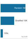
Random sampling needs 100× more images to reach a 1 percent subgroup.
Napkin Math 15.1: The statistics of representation
Problem: An engineering team needs to verify that a Face ID model works for a minority group representing 1 percent of the user base. The group’s error rate must be known to within 1 percentage point at 95 percent confidence. The binomial standard error behind the statistical confidence trap of Statistical and methodological issues is largest at an error rate of 0.5. The worst-case margin of error on \(\SubgroupSampleSize\) images is therefore \(1.96\sqrt{0.25/\SubgroupSampleSize}\), which falls to one percentage point near \(\SubgroupSampleSize\) = 10,000 images for this group.
Random sampling: To get 10,000 images of a 1 percent group in expectation via independent random sampling, the team must collect and label: \(\RandomSampleCollectionSize\) = 10,000 images / 0.01 = 1,000,000 images
Stratified sampling: Recruiting a representative, independently sampled evaluation set within this group requires 10,000 images.
Systems insight: Under these assumptions, natural-population sampling requires 100× as much total collection as direct subgroup recruitment, in expectation rather than as a guaranteed quota. Targeted recruitment must still represent the deployment subgroup; active selection of difficult cases cannot be treated as an unbiased evaluation sample without accounting for its sampling design. Fairness requires intentional data engineering rather than uncurated volume.
The representation cost derived in napkin math 15.1 settles what the evaluation must contain, but even a representative evaluation cannot prevent harm at deployment when human oversight is inadequate. The Deployment row of table 2 forces a second decision that cannot be deferred to launch: where people sit in the decision loop once the model is live, and what that arrangement must be designed to withstand.
War Story 15.2: The automation paradox (2018)
Context: Uber’s Advanced Technologies Group (ATG) was testing self-driving cars in Arizona, relying on a human safety driver to intervene if the autonomous perception system failed (National Transportation Safety Board 2019).
Mechanism: The perception system detected a pedestrian crossing the road but repeatedly toggled its classification between vehicle, bicycle, and unknown, resetting its trajectory prediction while automatic emergency braking was intentionally disabled.
Impact: The safety driver was visually distracted by a personal phone and failed to take control, resulting in a fatal collision.
Fix: Uber retrofitted the fleet with driver-monitoring cameras, re-enabled automatic emergency braking, and established dual-operator staffing during autonomous road testing.
Systems lesson: Adding a human backup creates a new system with its own failure modes. High automation reliability can encourage complacency and reduce vigilance, so an effective fallback requires workload design, attention monitoring, and a safety case for the combined human-machine system.
National Transportation Safety Board. 2019. Collision Between Vehicle Controlled by Developmental Automated Driving System and Pedestrian, Tempe, Arizona, March 18, 2018. HAR-19/03. National Transportation Safety Board.

If reviewer hours stay fixed, rising alert volume eventually leaves too little time per alert for real review.
For high-stakes applications, the specification should state where human oversight is required. Human-in-the-loop (HITL) systems route uncertain, high-consequence, or flagged decisions to human reviewers rather than acting autonomously; the clinician approval gates of ClinAIOps (ClinAIOps case study) are one proposed design. Effective HITL design must specify four requirements: the review scope (which decisions require human review), the confidence thresholds that trigger escalation, the training reviewers receive, and the mechanisms for monitoring reviewer performance. HITL is not a catch-all solution. Human reviewers can rubber-stamp automated decisions, introduce their own biases, or become overwhelmed by alert volume, so the human-machine boundary must be calibrated to the application’s risks and the reviewers’ capabilities.
↩︎ The ClinAIOps clinician oversight loop, in which a clinician approves, modifies, or rejects each therapy recommendation, is established in Clinician oversight loop.
Like an aviation preflight checklist, the assessment standardizes the questions a team must answer under schedule pressure, but answering them does not show that the system is safe. That evidence comes from measuring the model against the populations the specification named, which turns each written requirement into a gate the release must pass.
15.3.2 Measure: Fairness criteria as release gates
Turning the populations that specification named into release gates is what catches disparities that an aggregate metric hides. In the Gender Shades audit3 introduced in section 15.2.4, a commercial face classifier posted high overall accuracy while misclassifying more than a third of darker-skinned women (table 3), demonstrating how disaggregated evaluation across demographic categories exposes failures that an aggregate score averages away (Buolamwini and Gebru 2018). Measurement selects the slices, metrics, and thresholds that decide whether a system such as the credit service may deploy, and each slice carries the representation cost that specification budgeted (napkin math 15.1) because small subgroups contribute few samples to a randomly drawn test set.
3 Gender Shades: A 2018 study by Joy Buolamwini (MIT Media Lab) and Timnit Gebru (Microsoft Research) that audited commercial gender-classification systems from Microsoft, IBM, and Face++ using the Fitzpatrick skin type scale, a dermatological classification developed in 1975 for UV sensitivity (Fitzpatrick 1988) and repurposed here as a demographic benchmark for algorithmic auditing.
Fitzpatrick, Thomas B. 1988. “The Validity and Practicality of Sun-Reactive Skin Types i Through VI.” Archives of Dermatology 124 (6): 869. https://doi.org/10.1001/archderm.1988.01670060015008.
Buolamwini, Joy, and Timnit Gebru. 2018. “Gender Shades: Intersectional Accuracy Disparities in Commercial Gender Classification.” Conference on Fairness, Accountability and Transparency, 77–91.
| Demographic Group | Error Rate (%) | Relative to Light-Skinned Males |
|---|---|---|
| Light-skinned males | 0.8% | Baseline (1.0\(\times\)) |
| Light-skinned females | 9.8% | 12.2× |
| Dark-skinned males | 0.7% | 0.9× |
| Dark-skinned females | 34.5% | 43.1× |
As table 3 quantifies, disaggregated evaluation revealed what an aggregate score concealed. The audit measured Face++ error rates of 0.8 percent for light-skinned males and 34.5 percent for dark-skinned females (accuracies of 99.2 percent and 65.5 percent). The aggregate metric gave no indication that the dark-female error rate was 43.1× the light-male rate.
No universal threshold defines acceptable disparity, but teams should establish explicit, justified bounds before deployment. A team might adopt an error-rate ratio below 1.25\(\times\) or a false-positive-rate difference under 5 percentage points as an application-specific release policy. In US employment law, the disparate impact doctrine4 shapes regulatory oversight, while the four-fifths rule5 provides a separate, non-dispositive selection-rate diagnostic. Criteria must fit the application and its governing law, and one domain’s threshold should not be borrowed for another.
4 Disparate impact: In Griggs v. Duke Power Co. (1971), the US Supreme Court held under Title VII that an employment practice may be unlawful because of its operation even without discriminatory intent (Supreme Court of the United States 1971). Disparate impact is a legal claim with statute- and context-specific elements, not a synonym for any statistical disparity. Model outcomes and proxies can supply relevant evidence, but metrics alone do not establish liability.
Supreme Court of the United States. 1971. Griggs v. Duke Power Co., 401 U.S. 424. Legal decision.
5 Four-fifths rule: The 1978 Uniform Guidelines on Employee Selection Procedures use the four-fifths rule as a practical employment-selection diagnostic (Equal Employment Opportunity Commission et al. 1978). A selection rate below 80 percent of the rate for the group with the highest rate is generally regarded as evidence of adverse impact, but the Guidelines also recognize that smaller differences may matter and that the ratio is not dispositive.
Equal Employment Opportunity Commission, Civil Service Commission, Department of Labor, and Department of Justice. 1978. Uniform Guidelines on Employee Selection Procedures. Code of Federal Regulations.
Systems Perspective 15.4: The flaw of averages
A bridge that is “safe on average” but collapses under a heavy truck illustrates the flaw of averages (Savage 2009). An ML system that is “accurate on average” but fails for a specific demographic cohort presents the same design mistake. As with tail latency (p99), a release gate must test the conditions its aggregate metric conceals; disaggregated evaluation makes cohort-specific failures visible.
Savage, Sam L. 2009. The Flaw of Averages: Why We Underestimate Risk in the Face of Uncertainty. John Wiley & Sons.
Selecting those conditions requires application knowledge. A vision classifier fails differently from a recommendation engine or an audio wake-word detector, so fairness metrics and evaluation slices must reflect the application domain. In healthcare diagnostics, demographic cohorts such as age and biological sex govern slice definitions. In content moderation, dialect and linguistic context dominate. In financial underwriting, credit regulations mandate auditing legally protected categories.
Lighthouse 15.1: Fairness concerns by lighthouse
The lighthouse workloads of Workload archetypes were defined by the resource that binds each one, but their fairness risks come from somewhere else, from the data each learns from and the context each serves. Table 4 maps each lighthouse’s data source and deployment context to a primary risk and metric.
Table 4: Fairness Risk by Lighthouse: Fairness risks follow each lighthouse’s data source and deployment context, not the resource that binds it.
Architecture alone does not determine fairness; each row identifies a deployment-specific risk to test first, not a universal property of the model family or its bottleneck.
| Lighthouse (Home Regime) | Primary Fairness Risk | Key Evaluation Metric | Real-World Example |
|---|---|---|---|
| ResNet-50 (compute-bound) | Training data bias (underrepresentation of deployment-relevant groups) | Disaggregated accuracy by demographic group | Commercial face classifiers erred most on darker-skinned women (Gender Shades audited those systems, not ResNet-50) |
| GPT-2 (bandwidth-bound) | Corpus bias (overrepresentation of majority viewpoints in web text) | Toxicity rate by demographic prompt context; stereotype score | LLMs produce more toxic completions for prompts mentioning minority groups |
| DLRM (capacity-bound) | Feedback-loop amplification (popular items get more data) | Share of recommendation impressions by item category and supplier or creator group | Filter bubbles: the system recommends similar content to similar users, reducing discovery of niche creators |
| KWS DS-CNN (power-bound) | Deployment-context mismatch (trained on clean audio, deployed in noisy real-world environments) | False positive rate by acoustic environment and speaker accent | Voice assistants perform worse on accented speech; wake-word triggers on TV audio in some languages |
Systems insight: Fairness evaluation must match each lighthouse’s failure mode. Vision models require stratified demographic accuracy; large language models (LLMs) need toxicity and stereotype probes; recommenders need exposure audits; TinyML needs acoustic-environment tests. The KWS lighthouse faces exactly this challenge for its depthwise-separable convolutional neural network (DS-CNN). Trained on clean studio audio, it must perform equitably across accents, background noise levels, and speaker demographics in production homes, so its release gate needs accent and acoustic-environment slices, each reported with its own confidence interval.
Once the application has fixed those slices, a release test suite pairs disaggregated slice evaluation with two further verification regimes that probe failures a static validation split misses. Slice-based evaluation establishes the cohort baseline first, catching a credit model that achieves 95 percent accuracy overall while dropping to 78 percent on low-income or rural applicants, before the suite tests whether individual features or distribution edges drive those errors.
Invariance testing checks that model decisions stay unchanged when features that should not matter are swapped. Swapping candidate names such as “John” and “Jamal” in a loan application must not alter approval probabilities when demographic features are legally and technically irrelevant to creditworthiness. Behavioral testing frameworks such as CheckList put this principle to work by organizing validation suites around behavioral capabilities and input swaps rather than a single static validation loss (M. T. Ribeiro et al. 2020).
Ribeiro, Marco Tulio, Tongshuang Wu, Carlos Guestrin, and Sameer Singh. 2020. “Beyond Accuracy: Behavioral Testing of NLP Models with CheckList.” Proceedings of the 58th Annual Meeting of the Association for Computational Linguistics, 4902–12. https://doi.org/10.18653/v1/2020.acl-main.442.
Boundary and stress testing probe input regimes where empirical validation data is sparse or unrepresentative. Boundary evaluation maps behavior at the edges of the data distribution (extreme ages, rare transaction amounts, or sparse geographic categories), where prediction variance climbs sharply. Stress testing extends these margins into adversarial conditions: corrupted feature pipelines, sudden covariate shift, and synthetic edge cases designed to test safety margins under degradation. Stakeholder red-teaming complements automated suites by introducing adversarial domain probes from affected communities, surfacing failure modes that statistical benchmarks overlook.
Turning these three regimes into an automated release harness requires four linked capabilities in the testing infrastructure. Stratified evaluation automates per-cohort scoring across every named slice, and intersectional analysis extends that scoring across combinations of attributes (such as skin type and gender in the Gender Shades audit) so that compounding failure modes invisible in single-factor slices are caught as well. Because partitioning the test set into finer intersections leaves each slice with fewer examples, the harness must attach confidence intervals to every point estimate. The binomial resolution limit that the statistical confidence trap of Statistical and methodological issues exposed for an aggregate test set binds hardest here, where each slice holds only a fraction of the evaluation data. Once the model ships, temporal monitoring carries the same cohort checks into production, catching distribution drift that degrades minority slices before it registers on aggregate health checks.
Open-source evaluation suites such as Fairlearn (Bird et al. 2020), AI Fairness 360 (Bellamy et al. 2019), and the What-If Tool (Wexler et al. 2020) compute stratified and intersectional metrics once the team has specified the metrics, slices, and alert thresholds. They compute whichever metric an engineer queries; they cannot decide which demographic boundaries matter, calibrate paging thresholds for on-call engineers, or select the legally appropriate fairness constraint.
Bird, Sarah, Miro Dudı́k, Richard Edgar, Brandon Horn, Roman Lutz, Vanessa Milan, Mehrnoosh Sameki, Hanna Wallach, and Kathleen Walker. 2020. “Fairlearn: A Toolkit for Assessing and Improving Fairness in AI.” Microsoft Technical Report MSR-TR-2020-32.
Bellamy, Rachel K. E., Kuntal Dey, Michael Hind, Seung Hoffman, Sylvain Houde, Karthikeyan Kannan, Pradeep Lohia, et al. 2019. “AI Fairness 360: An Extensible Toolkit for Detecting and Mitigating Algorithmic Bias.” IBM Journal of Research and Development 63 (4/5): 4:1–15. https://doi.org/10.1147/jrd.2019.2942287.
Wexler, James, Mahima Pushkarna, Tolga Bolukbasi, Martin Wattenberg, Fernanda Viégas, and Jimbo Wilson. 2020. “The What-If Tool: Interactive Probing of Machine Learning Models.” IEEE Transactions on Visualization and Computer Graphics 26 (1): 56–65. https://doi.org/10.1109/TVCG.2019.2934619.
An operational release gate must distinguish absence of evidence from evidence of parity. If a slice lacks sufficient labeled validation data to bound the error rate with statistical confidence, the CI/CD gate must report insufficient data rather than a false pass, which triggers targeted data acquisition or restricts deployment scope. Every population test therefore returns one of three results (pass, fail, or insufficient evidence), and only a pass permits release.
Worked example: Fairness analysis of the credit service
Applying that release gate to the credit service shows how a model that passes a coarse aggregate check can fail a subgroup gate. Across the evaluated applicants, the classifier reports 85 percent accuracy on the majority group and 82.5 percent overall accuracy, yet evaluating the cohorts separately exposes a large disparity. This constructed evaluation assumes observed repayment outcomes for every applicant, independent of the model’s approval predictions; those predictions are not the lending actions that produced the labels. The two cohorts’ outcomes appear side by side, the majority cohort (Group A) in table 5 and the minority cohort (Group B) in table 6.
| Approved (pred) | Rejected (pred) | |
|---|---|---|
| Repaid (actual) | 4,500 (TP) | 500 (FN) |
| Defaulted (actual) | 1,000 (FP) | 4,000 (TN) |
| Approved (pred) | Rejected (pred) | |
|---|---|---|
| Repaid (actual) | 600 (TP) | 400 (FN) |
| Defaulted (actual) | 200 (FP) | 800 (TN) |
Every rate in the calculations that follow can be reconstructed from the approved/rejected and repaid/defaulted cells of these two matrices. Three standard criteria for equitable treatment capture distinct operational objectives, and the credit service’s two matrices violate all three.
Demographic parity (Dwork et al. 2012) requires equal positive selection rates across groups regardless of underlying qualification (\(\Pr(\PredictedDecision=1 \mid \ProtectedGroupMembership=\text{A}) = \Pr(\PredictedDecision=1 \mid \ProtectedGroupMembership=\text{B})\)). Group A receives approval at \((4{,}500 + 1{,}000) / 10{,}000 = 55\%\), whereas Group B receives approval at \((600 + 200) / 2{,}000 = 40\%\). The resulting 15 percentage-point disparity indicates unequal selection outcomes between cohorts.
Dwork, Cynthia, Moritz Hardt, Toniann Pitassi, Omer Reingold, and Richard Zemel. 2012. “Fairness Through Awareness.” Proceedings of the 3rd Innovations in Theoretical Computer Science Conference, 214–26. https://doi.org/10.1145/2090236.2090255.
Equal opportunity requires equal true positive rates among qualified applicants (\(\Pr(\PredictedDecision=1 \mid \TrueOutcome=1, \ProtectedGroupMembership=\text{A}) = \Pr(\PredictedDecision=1 \mid \TrueOutcome=1, \ProtectedGroupMembership=\text{B})\)). Group A achieves a TPR of \(4{,}500 / (4{,}500 + 500) = 90\%\), meaning 90 percent of creditworthy applicants secure loans. Group B achieves only \(600 / (600 + 400) = 60\%\). This 30 percentage-point disparity reveals that qualified applicants in Group B suffer disproportionate rejection relative to equally qualified peers in Group A.
Equalized odds tightens the constraint, demanding parity in both true positive and false positive rates (\(\Pr(\PredictedDecision=1 \mid \TrueOutcome=\TrueOutcomeLevel, \ProtectedGroupMembership=\text{A}) = \Pr(\PredictedDecision=1 \mid \TrueOutcome=\TrueOutcomeLevel, \ProtectedGroupMembership=\text{B})\) for \(\TrueOutcomeLevel\in \{0,1\}\)).6 Neither group may then bear a disproportionate share of unjustified rejections (false negatives) or unjustified approvals (false positives). Group A yields an FPR of \(1{,}000 / (1{,}000 + 4{,}000) = 20\%\), matching Group B at \(200 / (200 + 800) = 20\%\). Although false positive rates align, the substantial true positive rate deficit violates equalized odds.
6 Equalized odds: Formalized by Hardt et al. (2016), requiring that both TPR and FPR be equal across protected groups; the weaker “equal opportunity” relaxes this to TPR alone. Equalized-odds postprocessing may require randomized, group-dependent decisions rather than deterministic thresholds alone. It also requires protected-group information at decision time and must be evaluated under applicable law; for example, US credit regulation generally restricts using protected bases to assess creditworthiness.
Hardt, Moritz, Eric Price, and Nathan Srebro. 2016. “Equality of Opportunity in Supervised Learning.” Advances in Neural Information Processing Systems (NeurIPS) 29: 3315–23.
Chouldechova, Alexandra. 2017. “Fair Prediction with Disparate Impact: A Study of Bias in Recidivism Prediction Instruments.” Big Data 5 (2): 153–63. https://doi.org/10.1089/big.2016.0047.
Kleinberg, Jon, Sendhil Mullainathan, and Manish Raghavan. 2017. “Inherent Trade-Offs in the Fair Determination of Risk Scores.” 8th Innovations in Theoretical Computer Science Conference (ITCS 2017), Leibniz international proceedings in informatics (LIPIcs), vol. 67: 43:1–23. https://doi.org/10.4230/LIPIcs.ITCS.2017.43.
Both groups in this scenario have the same base rate (5,000 of 10,000 and 1,000 of 2,000 applicants repaid), so the impossibility results for unequal base rates do not bind here. Remediation remains possible in principle, but these matrices do not identify the cause of the disparity or which intervention would close it. Those results involve a fourth criterion, calibration within groups, which applies the probability calibration that evaluation already checks to each group separately. Among applicants in group \(\SubgroupIndex\) who receive score \(\ModelScore\), the fraction who repay should be \(\ModelScore\), that is, \(\Pr(\TrueOutcome=1 \mid \text{score}=\ModelScore, \ProtectedGroupMembership=\SubgroupIndex) = \ModelScore\) for every group. Real populations often have unequal base rates, and with unequal base rates and imperfect prediction, calibration-style criteria and error-rate balance can conflict (Chouldechova 2017; Kleinberg et al. 2017). When one group has a higher base repayment rate than another and the score is calibrated within both groups, a larger share of the higher-rate group must receive high scores above the approval cutoff. Because prediction is imperfect, some applicants above that cutoff still default, so the group with more applicants concentrated above the cutoff accumulates more false approvals per non-repaying applicant (a higher false positive rate) and fewer false rejections per repaying applicant (a lower false negative rate). A score calibrated within each group therefore generally assigns the groups different false positive or false negative rates, and the operational guarantee must be selected and defended for the application rather than deduced from aggregate accuracy or calibration.
These metrics disagree because they encode different policy choices about which error rates matter most. In this scenario, the model rejects qualified applicants from Group B at a much higher rate (40 percent false negative rate vs. 10 percent) while maintaining similar false positive rates. These confusion matrices establish an operational disparity, not whether it arose from classification thresholds, labeling bias, omitted features, sampling skew, or historical discrimination. The COMPAS risk assessment system7 shows the same disagreement in a deployed system whose groups had unequal base rates.
7 COMPAS: Correctional Offender Management Profiling for Alternative Sanctions.
War Story 15.3: The COMPAS recidivism algorithm audit (2016)
Context: COMPAS is a risk assessment tool used in US courtrooms to predict re-offending for bail and sentencing decisions (Angwin et al. 2016).
Mechanism: The audited scores combined approximate calibration across racial groups (a given score corresponded to about the same observed re-offense rate in every group) with unequal error rates. These observations expose a policy choice about acceptable errors; they do not establish which objective the original optimizer used.
Impact: Black defendants who did not re-offend were incorrectly flagged as high-risk at nearly twice the rate of White defendants (44.9 percent vs. 23.5 percent), while White recidivists were far more often mislabeled low-risk.
Response: The audit exposed why calibration alone could not settle whether the error distribution was acceptable. Any jurisdiction using such scores needs an explicit policy for which fairness criteria matter, independent validation across groups, and review of how the score enters the decision workflow.
Systems lesson: The scores were approximately calibrated by race but violated equalized odds, the criterion that requires equal true positive and false positive rates across groups. The credit service’s confusion matrices show the error-rate side of the conflict, and COMPAS adds the calibration side, which is why the team must explicitly choose which fairness constraint governs.
Angwin, Julia, Jeff Larson, Surya Mattu, and Lauren Kirchner. 2016. Machine Bias. ProPublica investigation.
Where collection and use of protected attributes are lawful and justified, production systems can automate these calculations and trigger review when disparities exceed predefined thresholds. Listing 1 handles the failure case explicitly, reporting undefined group rates as insufficient data rather than comparing them against a threshold. These denominator checks establish arithmetic validity only. A production release gate also needs minimum labeled sample counts and uncertainty checks for each relevant slice; a defined rate from one observation is not sufficient evidence.
def compute_fairness_metrics(confusion_matrix):
    tp, fp, tn, fn = (
        confusion_matrix[k] for k in ["TP", "FP", "TN", "FN"]
    )
    total = tp + fp + tn + fn
    return {
        # Demographic parity
        "approval_rate": (tp + fp) / total if total else None,
        # Equal opportunity
        "tpr": tp / (tp + fn) if (tp + fn) else None,
        # Equalized odds (with TPR)
        "fpr": fp / (fp + tn) if (fp + tn) else None,
    }


# Compare groups and flag disparities exceeding threshold
for metric in ["approval_rate", "tpr", "fpr"]:
    if metrics_a[metric] is None or metrics_b[metric] is None:
        report_insufficient_data(metric)
        continue
    disparity = abs(metrics_a[metric] - metrics_b[metric])
    # e.g., 0.05 for high-stakes applications
    if disparity > FAIRNESS_THRESHOLD:
        trigger_alert(metric, disparity)
Automated monitoring tracks fairness metrics repeatedly at a scale manual auditing cannot reach and alerts when sufficient labeled evidence reveals a disparity. Label availability and the time needed to accumulate observations bound detection speed. The 30 percentage-point TPR disparity far exceeds this scenario’s 5-percentage-point release threshold, indicating the model requires fairness intervention before deployment. Table 7 summarizes the computed metrics and resulting disparities across both cohorts.
| Metric | Group A | Group B | Disparity |
|---|---|---|---|
| Approval Rate | 55% | 40% | 15 pp |
| True Positive Rate | 90% | 60% | 30 pp |
| False Positive Rate | 20% | 20% | 0 pp |
Shared classification thresholds applied to differing score distributions illustrate how aggregate performance masks severe subgroup divergence (Barocas and Selbst 2016). Shifting between the two candidate decision boundaries (figure 2) lifts overall accuracy from 75 percent to 81.25 percent by achieving perfect separation in Subgroup A, yet simultaneously triples the misclassifications in Subgroup B. Because the two subgroups’ scores are distributed differently, one shared boundary cannot sit at the best point for both. The move that raises the global metric does so by trading away Subgroup B’s outcomes. Aggregate accuracy alone cannot determine whether those outcomes are equitable for either cohort.
Barocas, Solon, and Andrew D. Selbst. 2016. “Big Data’s Disparate Impact.” California Law Review 104: 671–732. https://doi.org/10.2139/ssrn.2477899.
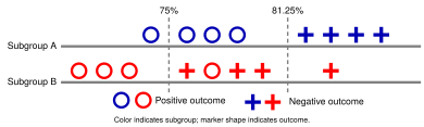
Mitigating these disparities means intervening before, during, or after training, and each stage imposes its own systems trade-offs. Preprocessing via sample reweighting fixes a weight for every training instance before training begins. The training loss then scales each Group B instance’s penalty by its weight, amplifying gradient signal for underrepresented cohorts without discarding data.8 The trade-off appears across the broader loss surface, where reweighting can degrade accuracy on majority slices.
8 Reweighting: The technique descends from importance sampling in statistics, which corrects an estimate drawn from one distribution by weighting each sample toward a target distribution. Kamiran and Calders (2012) showed that appropriately chosen weights can reduce disparate impact from training data.
Kamiran, Faisal, and Toon Calders. 2012. “Data Preprocessing Techniques for Classification Without Discrimination.” Knowledge and Information Systems 33 (1): 1–33. https://doi.org/10.1007/s10115-011-0463-8.
In-processing via adversarial debiasing turns the training loop into a minimax game between two neural networks. A primary model (encoder and predictor) transforms input features \(\InputFeatureVector\) (such as qualifications or income) into an intermediate latent representation \(\EncoderLatentRepresentation\). A task head uses it to predict the target label \(\ModelPrediction\) under a loss \(\TaskLoss(\ModelPrediction, \ExampleLabel)\) rewarding high predictive accuracy. Concurrently, an adversary head taps directly into the latent vector \(\EncoderLatentRepresentation\) and attempts to predict the protected attribute \(\ProtectedAttribute\) (such as demographic group) by minimizing an adversarial loss \(\AdversaryLoss(\PredictedProtectedAttribute, \ProtectedAttribute)\). During backpropagation, the adversary’s gradient is negated as it flows into the shared feature encoder: \[\DebiasingTotalLoss = \TaskLoss - \AdversarialPenaltyWeight\AdversaryLoss\]
Here \(\AdversarialPenaltyWeight\) weights the adversarial penalty against the task loss. The adversary head minimizes \(\AdversaryLoss\) alone, trying to recover \(\ProtectedAttribute\) from \(\EncoderLatentRepresentation\). The encoder and task head minimize \(\DebiasingTotalLoss\), so the encoder lowers its objective only by making the adversary’s task harder. It is therefore forced to purge latent features that correlate with the protected attribute. The resulting representations remain informative for the task while suppressing, not eliminating, protected-attribute signal under the evaluated distribution.9 The systems cost is real: a second (adversary) head to train, adversarial gradients that destabilize convergence, and a larger hyperparameter search.
9 Adversarial debiasing: The key differentiating property is representation pressure: the adversary discourages the primary model from encoding protected-attribute information, which can reduce protected-attribute leakage and help satisfy selected fairness criteria under the evaluated distribution (Zhang et al. 2018). It does not provide a general fairness guarantee under arbitrary deployment shift, because any guarantee depends on assumptions about invariance, labels, causal structure, and the type of shift. Postprocessing methods such as threshold adjustment may also be appropriate under different assumptions but must be revalidated when deployment demographics or label processes change. The cost is additional training, hyperparameter tuning, and slice-level validation rather than a universal percentage overhead.
Zhang, Brian Hu, Blake Lemoine, and Margaret Mitchell. 2018. “Mitigating Unwanted Biases with Adversarial Learning.” Proceedings of the 2018 AAAI/ACM Conference on AI, Ethics, and Society, 335–40. https://doi.org/10.1145/3278721.3278779.
Postprocessing via threshold adjustment decouples the decision boundary across groups, lowering the approval cutoff for Group B to equalize TPR. The operational trade-off is an increase in false positives within that cohort, admitting applicants who may subsequently default. The lever is also legally constrained. In the US, group-specific cutoffs are prohibited in employment selection and restricted in credit, so this intervention often exists only in principle, and teams move instead to reweighting, feature and label repair, or objective changes.
Selecting among these interventions requires stakeholder alignment on acceptable trade-offs for the specific deployment domain. Whichever intervention is chosen, its trade-off should be stated as a number that stakeholders can argue about.
Checkpoint 15.2: Fairness criteria
Fairness is not a single metric; it is a constrained design choice.
Quantifying the fairness-accuracy trade-off
Each mitigation on the credit service, whether sample reweighting, adversarial debiasing, or threshold adjustment, reduces demographic disparity by moving the model to a new operating point, and stakeholders need to see what predictive utility that move gives up. Along a fairness-accuracy Pareto frontier (principle 5), neither objective can improve without degrading the other (figure 3). When disparity is measured by the demographic parity gap from section 15.3.2.1, the horizontal axis places smaller gaps to the right. Among the assumed candidates, A has the highest accuracy, B has a smaller parity gap, and C has zero gap with lower accuracy. The ratio attached to B describes the reduction in that gap alone. These choices do not imply that unconstrained training always maximizes accuracy at high disparity, that zero disparity must reduce accuracy, or that every application has a preferred compromise.
A real deployment locates its own candidate configurations on the plane of figure 3 by pricing each type of error in the domain’s units. The credit service of section 15.3.2.1 makes the resulting penalty concrete because each lending outcome carries an explicit dollar value, the margin on a repaid loan on one side and the loss on a default on the other.
Napkin Math 15.2: The price of fairness
Problem: Stakeholders demand elimination of the credit service’s 30 percentage-point true positive rate (TPR) disparity. What is the “Price of Fairness” in lending outcomes?
Physics: TPRs can be equalized by adjusting the classification threshold \((\ClassificationThreshold)\) for the disadvantaged group.
- Original state: Group A (\(\text{TPR} =\) 90 percent), Group B (\(\text{TPR} =\) 60 percent, \(\text{FPR} =\) 20 percent).
- Intervention: Lower \(\DisadvantagedGroupClassificationThreshold\) until \(\text{TPR}_{\SubgroupIndex=\text{B}} =\) 90 percent. (US credit law restricts group-specific cutoffs, as the mitigation discussion noted, so the calculation quantifies the trade-off rather than a deployable intervention.)
- The cost: Lowering the threshold increases false positives (approving applicants who later default).
Math:
- Under the scenario’s assumed threshold response, closing the 30 percentage-point TPR gap produces a 20 percentage-point increase in false positives for the disadvantaged group.
- If 50 percent of Group B applicants would repay, a repaid loan earns a margin of $1,500, and a default loses $3,000, both sides of the intervention must be counted:
- Group B baseline utility evaluates the original expected payoff: \(0.60 \times 0.50 \times \$1{,}500 - 0.20 \times 0.50 \times \$3{,}000 = \$150\) per applicant.
- Evaluating the intervention requires counting both marginal terms: \(\FiniteChange\text{Utility} = \FiniteChange\text{TPR} \times \text{Base Rate} \times \text{Loan Margin} - \FiniteChange\text{FPR} \times (1 - \text{Base Rate}) \times \text{Default Loss}\).
- The added true-positive value is $225 per Group B applicant, while the added false-positive cost is $300, producing a net loss of $75.
- Dividing this $75 net loss by the $150 baseline yields a 50 percent within-group utility loss. With Group B at 17 percent of applicants, the population-average loss is $12.50 per applicant; calculating an aggregate percentage also requires the other group’s baseline utility.
Systems insight: The “Price of Fairness”, the fairness literature’s name for the utility a system gives up to satisfy a fairness constraint, in this scenario is a 50 percent within-group utility loss, not a derivable aggregate percentage. The loss is not automatic: when a TPR gap reflects a miscalibrated threshold, closing it can raise net utility. It appears when the baseline threshold is near the utility optimum and the marginal approvals skew toward default. Engineering teams owe stakeholders both the Pareto frontier and the operational assumptions that produced it.
The calculation gives stakeholders a way to choose and defend a point on the fairness-accuracy frontier, where Group B’s 60 percent true positive rate is weighed against Group A’s 90 percent rate, but cohort-level release metrics live inside the engineering team. Once the model ships, neither the applicant it rejects nor a downstream team that inherits the checkpoint can act on a cohort average; both need the system’s individual decisions and its operating boundaries made legible.
15.3.3 Explain and document: Decisions and models made legible
When the credit service rejects a borrower with a bare probability score of 0.41, the applicant cannot tell whether the denial came from a high debt-to-income ratio or a corrupted credit-bureau field. Six months later, another team reuses that same classifier to screen rental tenants without knowing which populations it was tested on, and the organization inherits a second failure at the model level. Explanation and documentation answer that single demand for legibility at two timescales. An explanation makes one decision understandable, at the moment it is made, to the person it affects. Documentation makes the model understandable across its lifetime to the engineers, auditors, and downstream teams who inherit it: what it was trained on, where it was validated, and what it must not be used for. Both exist for the same systems reason, since a guarantee that no one outside the team can inspect cannot be contested, audited, or safely reused.
Explainability requirements
At the decision timescale, an applicant denied with that 0.41 score may be entitled under applicable law to specific adverse-action factors that state which inputs drove the rejection and what could change it. Explainability10 is the capability that articulates how input features contributed to a specific prediction, enabling human oversight of automated decisions, supporting incident debugging, and satisfying applicable requirements for decision transparency.
10 Explainability and interpretability: Interpretability usually describes how readily a person can understand a model or its behavior, often through a constrained structure such as a short rule list or sparse linear model. Explainability is broader and includes post-hoc methods such as LIME and SHAP. Neither property is automatic: a linear model with opaque features can be difficult to interpret, and a feature attribution is not a causal account of a decision. The systems implication is that intrinsic constraints affect model selection, while post-hoc methods add a computation and validation path whose cost depends on the method, model, and serving workflow. GDPR access and automated-decision provisions use the phrase “meaningful information about the logic involved” for covered processing (European Parliament and Council of the European Union 2016), leaving the appropriate technical approach dependent on the decision and governing law.
The level of explainability required varies by application context and regulatory environment (table 8), and the requirement constrains architecture rather than logging. Where credit underwriting may require principal reasons disclosed to the applicant and medical diagnosis requires clinical review support, fraud detection must balance notice duties against adversarial gaming. Serving an outside reader raises the bar beyond the SHAP values that localized mispredictions during incident debugging, because the explanation requirement determines before training which model families are eligible and what additional computation the serving path must carry.
↩︎ SHAP values, which estimate how much each input feature contributed to one prediction, are established as a debugging tool in Feature attribution for debugging.
| Application Domain | Explainability Level | Typical Requirements |
|---|---|---|
| Credit decisions | Specific reasons for covered actions | Principal reasons may have to be disclosed to the applicant |
| Medical diagnosis | Decision support | Support clinical review and applicable documentation |
| Content moderation | Context-dependent | Support notices or appeals where required |
| Recommendation | Context-dependent | Provide transparency appropriate to the use and governing rules |
| Fraud detection | Controlled disclosure | Balance applicable notice duties with adversarial-gaming risk |
Whatever the requirement, the candidate models lie along a gradient continuum from intrinsic interpretability to post-hoc explanation (figure 4). On the left, small trees and sparse linear or logistic models with meaningful features can expose decision logic to human inspection. Large trees or opaque engineered features can defeat that advantage. On the right, high-capacity representations, such as random forests, deep neural networks, and convolutional neural networks (CNNs) or transformers, often need supplementary explanation methods. LIME and SHAP require fidelity checks; attention maps alone do not establish faithful explanations. The spectrum organizes candidate approaches, not a categorical guarantee for any model family.
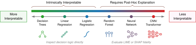
Selecting an explainability strategy along this spectrum requires balancing explanation fidelity, serving latency, and architectural flexibility across three distinct design paradigms. Post-hoc explanation methods, including SHAP and LIME, generate feature importance scores for individual predictions without modifying model internals.11 Model-agnostic explainers evaluate perturbed inputs or sampled feature subsets, introducing additional computation and approximation. Model-specific SHAP algorithms can exploit internal structure instead; the explanation method and where it runs determine latency and fidelity.
11 LIME (local interpretable model-agnostic explanations) and SHAP (SHapley additive explanations): LIME (Ribeiro et al. 2016) fits a local interpretable surrogate around each prediction; SHAP (Lundberg and Lee 2017) adapts Shapley values from cooperative game theory to compute feature contributions under a unified additive framework. Exact Shapley computation requires evaluating a feature’s marginal contribution across all possible feature subsets, scaling exponentially with the feature count \(\AttributionFeatureCount\) (\(\mathcal{O}(2^{\AttributionFeatureCount})\)); practical production deployments therefore rely on polynomial-time model-specific algorithms (such as TreeSHAP for decision trees) or sampling approximations (such as KernelSHAP) to avoid unacceptable serving latency. The systems trade-off is that explanation fidelity, latency, and implementation complexity must be budgeted explicitly rather than treated as free.
Ribeiro, Marco Tulio, Sameer Singh, and Carlos Guestrin. 2016. “Why Should I Trust You?: Explaining the Predictions of Any Classifier.” Proceedings of the 22nd ACM SIGKDD International Conference on Knowledge Discovery and Data Mining, 1135–44. https://doi.org/10.1145/2939672.2939778.
Lundberg, Scott M., and Su-In Lee. 2017. “A Unified Approach to Interpreting Model Predictions.” Advances in Neural Information Processing Systems (NeurIPS) 30: 4765–74.
The explanation path has a measurable serving cost. For the credit service’s 20 input features, exact Shapley attribution evaluates the model on every feature subset, 1,048,576 evaluations to explain a decision that took one evaluation to make. Sampling explainers bound that work by evaluating a fixed number of subsets, but even 1,000 samples multiply the compute of every explained decision by the sample count. The explanation path rather than the model can therefore set the service’s accelerator budget and its tail latency.
For the rejected credit application, a LIME explanation is dependable only if its local surrogate agrees with the model near the applicant and stays stable across resampling. The check fits the surrogate on perturbed applications drawn from a neighborhood of plausible applications (valid feature ranges, with dependencies such as income and debt-to-income ratio preserved). It then measures the surrogate’s prediction error and approval agreement against the model on an independent set from the same neighborhood. The check also repeats the fit across sampling seeds and neighborhood widths to see whether the leading features and their signs persist. Acceptable error and stability must be specified before the check, and even a faithful surrogate describes model behavior without supplying a causal explanation or a legally sufficient reason.
Avoiding that per-request attribution cost moves the design to the left side of the interpretability spectrum, where inherently interpretable models enforce transparency through structural constraints such as shallow decision trees, sparse linear models, or generalized additive models with inspectable feature effects, trading away expressive capacity on high-dimensional inputs when the feature set stays compact and meaningful. Where inherently interpretable models constrain the architecture from the start, a third paradigm, concept-based explanations, probes what a trained network has already learned. It projects internal activations onto directions derived from labeled examples of a human concept, such as a “striped texture” direction in a vision model. The projection shows whether a representation encodes the concept; whether the prediction uses it requires a further test of how the output changes along that direction, and every concept needs its own annotated example set.
Example 15.1: The hospital shortcut
Scenario: Pneumonia detection vision models trained at Mount Sinai achieved high internal accuracy but failed on external hospital datasets (Zech et al. 2018).
Diagnosis: The neural network learned shortcut features (hospital-specific scanner artifacts and text tags) rather than true biological lung pathology.
Systems lesson: A model can learn whichever feature predicts the label most easily, including one unrelated to the disease. External validation is essential for detecting shortcut learning. Saliency maps, per-pixel heat maps of how strongly each input region influences the output, can provide supporting evidence but do not establish that the model learned the intended mechanism.
Zech, John R., Marcus A. Badgeley, Manway Liu, Anthony B. Costa, Joseph J. Titano, and Eric Karl Oermann. 2018. “Variable Generalization Performance of a Deep Learning Model to Detect Pneumonia in Chest Radiographs: A Cross-Sectional Study.” PLOS Medicine 15 (11): e1002683. https://doi.org/10.1371/journal.pmed.1002683.
The hospital shortcut shows why interpretability is a systems requirement rather than presentation polish. Teams need sufficient transparency to detect and isolate spurious correlations before deployment. The choice among these paradigms depends on the application’s accountability requirements. Credit law requires specific reasons for covered decisions but does not mandate a particular model architecture, and other applications face different transparency, safety, or contestability duties. Section 15.5.3 maps those duties to the capabilities they demand. The spectrum does not imply “simple is always better,” because a highly interpretable model that makes inaccurate predictions may also cause harm. An explanation, however, covers one decision at a time. The assumptions behind every decision the model makes need a durable record of their own, one that travels with the artifact.
Model documentation standards
When a team inherits a production model without that durable record, the artifact may post 94 percent accuracy on a designated test set while leaving the origin of the test set, the composition of the training data, and the evaluated demographic or environmental slices unrecorded. Updating or redeploying the model then risks unmeasured regressions under distribution shift. Model cards provide standardized documentation for trained models12 (Mitchell et al. 2019). Analogous to component datasheets in computer engineering, model cards document operational boundaries, evaluation conditions, and intended operating regimes alongside the model artifact.
12 Model cards: The primary failure mode model cards address is scope creep, the gradual expansion from “it worked for case A” to “try it for case B” without revalidating intended use. In practice, cards are often written after deployment decisions are made, documenting observed behavior rather than constraining it. The companion “Datasheets for Datasets” (Gebru et al. 2021) applies the same principle to training data. Without both, the card becomes a historical record rather than an engineering guardrail.
Gebru, Timnit, Jamie Morgenstern, Briana Vecchione, Jennifer Wortman Vaughan, Hanna Wallach, Hal Daumé III, and Kate Crawford. 2021. “Datasheets for Datasets.” Communications of the ACM 64 (12): 86–92. https://doi.org/10.1145/3458723.
Mitchell, Margaret, Simone Wu, Andrew Zaldivar, Parker Barnes, Lucy Vasserman, Ben Hutchinson, Elena Spitzer, Inioluwa Deborah Raji, and Timnit Gebru. 2019. “Model Cards for Model Reporting.” Proceedings of the Conference on Fairness, Accountability, and Transparency, 220–29. https://doi.org/10.1145/3287560.3287596.
A complete model card covers seven core sections that together define the model’s safe operating envelope. It begins with technical details (architecture, training procedures, and hyperparameters) that enable reproducibility and auditing. It specifies intended use alongside explicit out-of-scope applications, preventing scope creep where models trained for consumer photo indexing get repurposed for high-stakes surveillance. The card then documents which factors (demographic groups, environmental conditions, or sensor variations) affect performance, guiding both evaluation slicing and production monitoring.
The remaining sections quantify and bound empirical behavior. Performance metrics must report disaggregated results across the operational factors identified in section 15.3.2, because aggregate accuracy conceals systematic subpopulation disparities. Documenting the training and evaluation datasets isolates potential sampling biases and defines the distribution over which the reported metrics hold. Finally, ethical considerations, caveats, and recommendations make deployment trade-offs explicit by recording known failure modes, unmodeled edge cases, and operational mitigations.
Applying this schema to MobileNetV2 illustrates how these categories translate into concrete deployment constraints. Table 9 fills five of the seven sections for an edge classification service, and its accuracy entries reuse the illustrative FP32 and INT8 values of the compression validation in Compression validation: The efficiency-quality frontier.
| Section | Content |
|---|---|
| Model Details | MobileNetV2 architecture with 3.5M parameters, trained on ImageNet using depthwise separable convolutions. INT8 quantized for edge deployment. |
| Intended Use | Real-time image classification on mobile devices with less than 50 ms latency requirement. Suitable for consumer applications including photo organization and accessibility features. |
| Factors | Performance varies with image quality (blur, lighting), object size in frame, and categories outside ImageNet distribution. |
| Metrics | 70.9% top-1 accuracy on ImageNet validation after INT8 quantization (full precision: 71.8%). Accuracy varies by category: 85% on common objects, 45% on fine-grained distinctions. |
| Ethical Considerations | Training data reflects ImageNet biases in geographic and demographic representation. Not validated for high-stakes applications (medical diagnosis, security screening). Performance may degrade on images from underrepresented regions. |
Datasheets for datasets provide the complementary record for the data tier (Gebru et al. 2021), capturing provenance, collection methodology, curation filters, and demographic composition. In D·A·M terms, a model card specifies the algorithmic and machine boundaries (including quantization precision and inference latency budgets), and a datasheet specifies the data that produced them. Together they state what the system is designed to tolerate and preserve the evidence that measurement produced, but both describe the system at the moment of release. Operation is the stage that keeps that description true once the model meets live traffic.
↩︎ Datasheets, as part of the governance pillar of a data pipeline, are established in Four foundational pillars.
15.3.4 Operate: Fairness as loop stability
A credit model that passes its 5-percentage-point fairness gate and ships with a complete model card at launch can still breach that gate six quarters later without a single code change, because every quarterly retraining learns only from the applicants the previous model approved. Release gates and documentation certify the system at one instant, before live traffic and closed-loop retraining shift its behavior over time. Operating the service responsibly requires the incident-response sequence that operations already runs (detection, assessment, mitigation, communication, and remediation) to treat a fairness violation or a slice-level regression as an incident in its own right. Operations must also verify each control before launch, including alert thresholds tested against historical replay, a rollback path exercised under load, and an on-call rotation with documented escalation, so that monitoring and response exist before the model takes production traffic.
The feedback begins at the decision that determines which outcomes can be observed. Figure 5 distinguishes the routine repayment stream from a declared intervention that obtains additional observations.
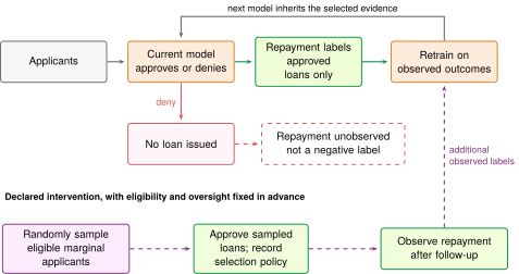
An absent repayment label cannot be treated as a default or a successful repayment. An audit of existing records cannot reveal how a loan that was never issued would have performed. Obtaining evidence outside the routine approval stream requires an explicitly justified observation strategy, with its selection policy and follow-up recorded; estimating population disparities still depends on what that evidence supports.
↩︎ The ML incident-response sequence of severity classification, detection, impact assessment, mitigation, and root-cause analysis is established in Incident response for ML systems.
Where service-health monitoring catches crashes and timeouts, the technical debt that ML systems accumulate surfaces as silent degradation (Sculley et al. 2015), so the production telemetry surface must add two responsibility signals alongside input drift and delayed outcomes. Subgroup parity becomes a first-class monitor, tracking false-negative and false-positive rates per cohort over time with response plans that account for label delay, while user complaints, contested decisions, and appeals feed the same surface because aggregation over millions of queries smooths away the rare harms that affected people report first. Parity monitoring matters most when the system’s decisions shape its own future training data. In that regime the bias feedback model (principle 13) describes a disparity that evolves as \(\GroupDisparity(\FeedbackIntervalCount) \approx \GroupDisparity(0) \cdot \BiasFeedbackFactor^\FeedbackIntervalCount\) across feedback intervals rather than staying fixed, and the credit service shows what that recurrence implies for a release gate.
↩︎ Production monitoring architectures for performance stability and distribution drift are established in Production Monitoring.
Napkin Math 15.3: Fairness as loop stability
Problem: After mitigation, the credit service from section 15.3.2.1 ships with a residual TPR gap of 3 percentage points, inside the scenario’s 5 percentage-point release gate. Denied applicants generate no repayment labels in the routine training stream, so each quarterly retraining learns from a population the previous model selected. For this illustration, an independent audit sample provides observed repayment outcomes across both groups, including applicants not approved by the production policy. Without such outcome evidence or a justified missing-outcome correction, the all-qualified-applicant TPR gap would not be directly measurable. The next quarterly audit measures a gap of 3.3 percentage points. If the locally fitted growth factor persisted, when would the gap breach the release threshold?
Math:
- Fit the feedback factor: \(\BiasFeedbackFactor= \GroupDisparity(1)/\GroupDisparity(0) =\) 1.10 per quarter.
- Time to breach under the fitted model: The projected gap exceeds the gate once \(\GroupDisparity(0)\,\BiasFeedbackFactor^\FeedbackIntervalCount\) passes it, that is, for \(\FeedbackIntervalCount> \ln(\text{gate}/\GroupDisparity(0)) / \ln \BiasFeedbackFactor\). The model projects a breach after 6 quarterly retraining cycles, when the gap reaches 5.3 percentage points.
- Without mitigation: The same factor would grow the original 30 percentage-point gap to 43.9 percentage points within 4 cycles, one year of retraining.
- Changing the loop: If the team approves a small randomized sample of marginal applicants and observes their repayment, the loop again sees outcomes it previously censored. Suppose the refitted factor falls to 0.90; the same launch gap then decays to 1.6 percentage points over the same number of cycles.
Systems insight: A release gate passed at launch is a statement about \(\FeedbackIntervalCount= 0\). Under feedback, fairness is a stability property of the retraining loop. The projected breach time motivates a shorter audit interval, but two observations do not validate future dynamics. An intervention can change \(\BiasFeedbackFactor\) (through what data the loop collects) as well as \(\GroupDisparity(0)\). The fitted factor is a local model; it must be refitted at every audit because intervention, saturation, or a shifting applicant pool changes the dynamics.
The DLRM ranking service runs the same loop with far more severe censoring. With 10 million daily users each shown 20 ranked items from a catalog of 1 million items, the service logs 200 million impressions a day. Yet each user’s feedback covers only 0.002 percent of the catalog, and the previous model chose every item in it. Items and creators the ranker stops showing generate no clicks and therefore no evidence that they deserved to be shown, which is the exposure form of the bias feedback model. The remedy mirrors the credit service’s randomized approvals. Reserving 1 percent of slots for randomized exploration yields 2 million impressions a day that the previous model did not select, a sample from which each creator group’s exposure share and engagement can be estimated against an unbiased baseline. The cost is measurable like any other serving change, because that share of slots is served at lower expected engagement, and it is what keeping the feedback factor below one costs.
Neither the credit service’s quarterly parity audits nor the DLRM service’s exploration slice protects users if the resulting signals sit on a passive dashboard. Both loops stay bounded only when scheduled audit cadences, clear on-call ownership, and explicit escalation thresholds tie an observed rise in \(\BiasFeedbackFactor\) or a drop in creator exposure directly to a retraining hold, an exploration adjustment, or a rollback.
Checkpoint 15.3: Ethical deployment
Deployment is where safeguards must become operational.
Safety net
Monitoring plan
Equitable performance across demographic cohorts addresses only one dimension of responsible engineering. The resource stage of the lifecycle addresses another, because every training run, inference request, and monitoring pipeline draws electrical power that converts to carbon emissions and operating expenditure. A pipeline can satisfy demographic parity while consuming orders of magnitude more compute than the task warrants, so responsible engineering must govern both whom the system serves and the physical resources consumed in serving them.
Self-Check: Question
An engineering team is evaluating a facial verification model. To estimate the error rate of a minority demographic group representing 1% of the population with a margin of error of \(\pm 1\) percentage point at 95% confidence, they require 10,000 labeled evaluation samples from that group. Under uniform random sampling from the natural population distribution, how many total images must the team collect and label in expectation?
- About 10,000 total images, because evaluating subgroup accuracy requires only that the total test set contains 10,000 images.
- About 100,000 total images, because statistical confidence intervals scale with the square root of the overall dataset size.
- About 1,000,000 total images in expectation, because a 1% subgroup yields only 1 target image per 100 randomly sampled images, imposing a \(100\times\) multiplier.
- About 10,000,000 total images, because the binomial confidence interval width expands exponentially for minority subgroups.
A team plans to write their model card six months after launch so that it accurately reflects observed production behavior. Explain why this timing constitutes a guard-rail failure, and describe one concrete scope-creep risk that a pre-deployment model card with automated deployment gates prevents.
A loan approval classifier is evaluated on a fully labeled sample whose repayment outcomes are observed independently of its approval predictions. Group A (Majority): 4,500 True Positives, 500 False Negatives (TPR = 90%), 1,000 False Positives, 4,000 True Negatives (FPR = 20%). Group B (Minority): 600 True Positives, 400 False Negatives (TPR = 60%), 200 False Positives, 800 True Negatives (FPR = 20%). Which statement accurately diagnoses the fairness metrics for this system?
- Demographic parity is satisfied because both groups share an identical False Positive Rate of 20%.
- Equalized odds is satisfied because matching False Positive Rates compensate for differences in True Positive Rates.
- Equal opportunity is violated due to the 30 percentage-point TPR gap, and equalized odds is also violated because equalized odds strictly requires parity in both TPR and FPR.
- Calibration is the only metric affected, because True Positive Rate disparities impact accuracy but do not constitute algorithmic bias.
For the credit service, closing the 30 percentage-point TPR gap for Group B via threshold adjustment adds \(\$225\) in margin on newly approved loans that are repaid but creates \(\$300\) in losses on newly approved loans that default, per Group B applicant, whose baseline utility is \(\$150\) per applicant. Using the chapter’s two-sided accounting, calculate the net utility change per applicant and explain what deliverable engineers owe stakeholders.
After mitigation, the credit service ships with a 3 percentage-point TPR gap under a 5-point release gate, and the next quarterly audit measures 3.3 points. Using the bias feedback model, estimate the fitted feedback factor and the retraining cycle in which the projected gap first exceeds the gate. Why does the projection motivate changing what the loop observes rather than only shortening the audit interval?
A team is designing a fairness and robustness testing suite for the credit service. Explain why subgroup representation and labeled sample sufficiency must be checked before interpreting subgroup error rates. How do invariance tests and boundary/stress tests complement those rates, and when can the team compare candidate configurations on a fairness-accuracy Pareto frontier?
15.4 Environmental and Cost Awareness
In 2019, researchers estimated that development-scale training and architecture search for a large natural language processing (NLP) model could emit as much carbon as five cars over their entire lifetimes (Strubell et al. 2019). Later analysis showed that the most quoted architecture-search estimate was highly sensitive to proxy-task, hardware, data-center efficiency, and grid carbon-intensity assumptions (Patterson et al. 2021). The correction narrows the estimate without removing the point. Training runs consume megawatt-hours of electricity, inference at scale multiplies per-request inefficiencies into measurable environmental impact, and resource-intensive models exclude organizations that lack large compute budgets. The techniques that improve efficiency therefore also serve as instruments of responsible engineering, tying computational efficiency to environmental sustainability and economic accessibility. On the DLRM ranking service, request volume makes serving rather than training the term that dominates both the bill and the emissions.
Strubell, Emma, Ananya Ganesh, and Andrew McCallum. 2019. “Energy and Policy Considerations for Deep Learning in NLP.” Proceedings of the 57th Annual Meeting of the Association for Computational Linguistics, 3645–50. https://doi.org/10.18653/v1/p19-1355.
15.4.1 Efficiency as responsibility
Training a single large language model consumes thousands of GPU hours and energy measured in megawatt-hours. The bitter lesson predicts that this footprint will keep growing, because the methods that win are the ones that convert additional compute into capability. Much of this expense, however, is not intrinsic to the learning task but represents accidental complexity: training from scratch when fine-tuning would suffice, deploying larger architectures than tasks require, and running hyperparameter searches that explore redundant configurations. Computational cost depends on engineering choices as well as model physics. Green AI treats that efficiency as a primary metric rather than an afterthought.13
13 Green AI: Schwartz et al. (2020) contrasted “Red AI” (performance at any cost) with “Green AI” (efficiency as primary metric). The compute-growth anchor comes from AI and Compute’s 2012–2018 trend analysis (the fit that gives a 3.4-month doubling time), which reported a 300,000\(\times\) increase in compute used in the largest AI training runs over that six-year window (Amodei and Hernandez 2018); comparisons that extend to later frontier models span a longer window and report larger factors. The Green AI proposal (reporting FLOPs alongside accuracy for every published result) reframes efficiency from an engineering preference into a scientific reporting obligation, making the resource cost of marginal accuracy gains visible and comparable across research groups.
Schwartz, Roy, Jesse Dodge, Noah A. Smith, and Oren Etzioni. 2020. “Green AI.” Communications of the ACM 63 (12): 54–63. https://doi.org/10.1145/3381831.
Amodei, Dario, and Danny Hernandez. 2018. “AI and Compute.” OpenAI Blog 6.
↩︎ The bitter lesson, the historical pattern in which methods that scale with compute overtake hand-built knowledge, is established in The Bitter Lesson.
The growth in training compute carries a price, and the price decides who can take part. Figure 6 plots the estimated compute cost of training notable models since 2016 in constant 2023 dollars. Across the models that Epoch AI flags as frontier at release, the cost of a training run rose about 2.9× per year, and the most expensive run in the data, Grok 4 in 2025, cost about $388M (Epoch AI 2026). Cottier et al. (2024), using their own selection of frontier runs, estimate 2.4\(\times\) per year. Either rate concentrates frontier training in the few organizations able to fund it, so efficiency is a question of access as well as of energy. For a frontier model the training run dominates the cost; for a high-traffic service such as DLRM, as section 15.4.2 shows, serving does.
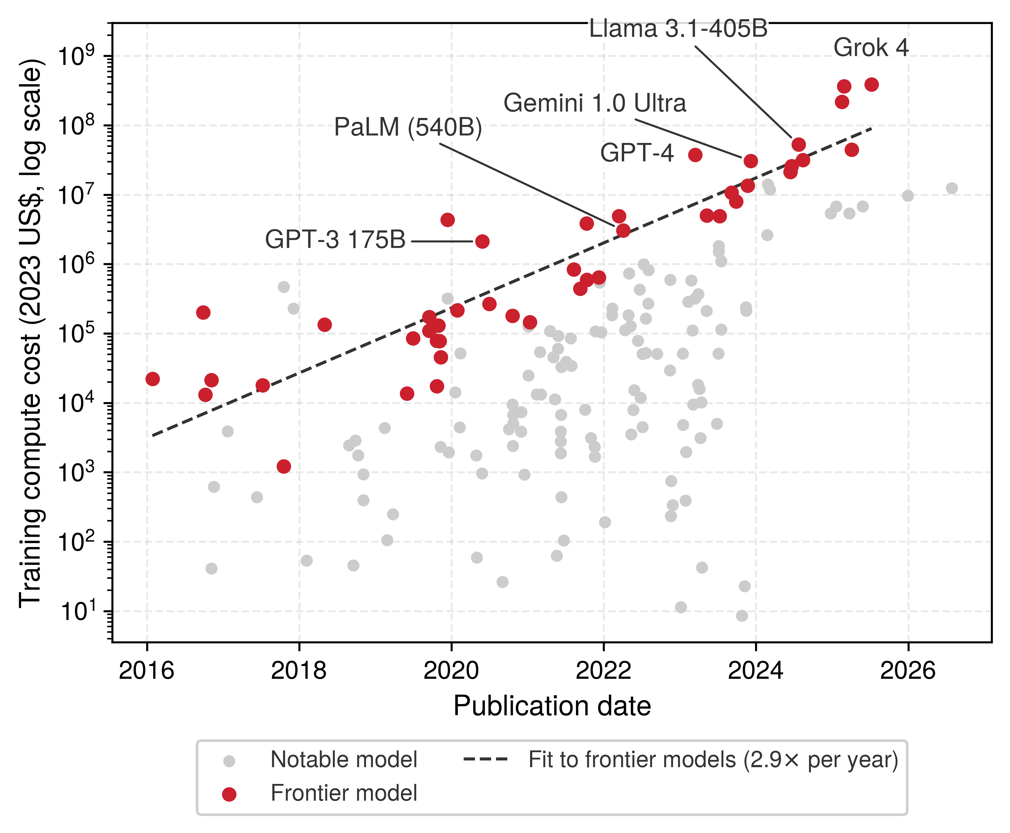
Cottier, Ben, Robi Rahman, Loredana Fattorini, Nestor Maslej, Tamay Besiroglu, and David Owen. 2024. “The Rising Costs of Training Frontier AI Models.” arXiv Preprint arXiv:2405.21015.
Epoch AI. 2026. Notable AI Models.
At the hardware level, environmental impact scales with total electrical energy draw across the machine lifecycle, mediated by accelerator utilization, data-center cooling overhead (power usage effectiveness), and the carbon intensity of the local electrical grid, the mass of CO2eq emitted per kilowatt-hour it delivers. Within the accelerator package, data movement can dominate energy dissipation. In the 45 nm reference behind the energy-movement principle (7), a single off-chip DRAM access costs two to three orders of magnitude more energy than a 32-bit floating-point operation, although total energy also depends on access width, event counts, reuse, and the device. Algorithmic and runtime optimizations reduce environmental burden only when they reduce measured watt-hours for a verified quality target under production load, curbing this physical dissipation at the silicon level.
↩︎ The physical energy disparity between off-chip memory access and arithmetic execution is established in Machine learning hardware specialization.
Physical resource demands also dictate deployment accessibility. Oversized models that need multi-accelerator nodes linked by high-bandwidth interconnects (such as NVLink) only to hold their weights in memory confine deployment to centralized cloud facilities. Compressing models so their working sets fit within commodity DRAM or the unified memory of edge processors opens up who can run them. Running locally removes the need for a constant high-bandwidth network link and recurring cloud API bills, letting client devices run low-latency, private inference right where data is captured.
At production scale, where serving systems process millions of requests daily, per-query inefficiencies compound rapidly across accelerator fleets. Under the iron law of ML systems (\(\Time = \DataVolume / \Bandwidth + \Operations / (\PeakRate \cdot \EfficiencyHw) + \Latency\)), per-query execution latency dictates the request throughput that an individual accelerator can sustain before violating service-level latency objectives. Reducing execution time allows a smaller provisioned cluster to support the same aggregate traffic, and capacity planning can turn that reduced service demand into lower provisioned-capacity costs. A fixed fleet may also save dynamic energy, although idle and baseline power remain. A valid comparison therefore measures total energy over the same traffic and quality target and distinguishes that result from savings on a capacity-based bill.
Each optimization developed earlier in this book attacks a specific term of these equations, and each reduces environmental burden only under the conditions its own chapter states. Quantization and pruning shrink the bytes moved \(\DataVolume\) and the operation count \(\Operations\) when supported kernels retain the smaller representation, and knowledge distillation moves a large model’s behavior into a smaller one (Model Compression). Selecting the data a model trains on removes training operations before they run (Data Selection), and specialized datapaths and fused kernels raise hardware efficiency \(\EfficiencyHw\) (Hardware Acceleration).
Responsible engineering treats these optimizations as design constraints established before training and deployment, rather than post-hoc remedies applied to an oversized model. System requirements specify explicit upper bounds on latency, memory capacity, and energy consumption alongside target predictive quality, and the task is to find the most compact architecture and execution strategy that satisfies them. In practice this begins by establishing bounded machine envelopes (thermal design power, battery capacity, and peak latency) before choosing or training an architecture. Targeted optimizations such as quantization or kernel fusion come only after the most compact adequate architecture has been selected.
Edge deployment makes these limits immediate, because passive thermal dissipation and battery capacity enforce power budgets that cannot be relaxed after the fact. A wearable with an illustrative 500 mW inference budget shows the consequence for model choice. Under the active-power profiles assumed here, the KWS lighthouse’s DS-CNN (200K parameters at 50 mW) leaves a 10× power margin, while MobileNetV2 (3.5M parameters at 1.2 W) exceeds the same budget by 2.4× before sustained thermals are considered. Fitting the envelope is necessary but not sufficient: a keyword detector does not substitute for a vision model merely because it fits, and per-inference energy compounds into aggregate emissions and operating cost once the model is deployed at scale. Techniques that lower measured energy per inference reduce lifecycle energy only when their savings outweigh any added training, preprocessing, or other workload costs, while cloud and cluster financial savings depend directly on provisioning and hardware utilization.
↩︎ The power, memory, and latency envelopes that separate cloud, edge, mobile, and TinyML deployment are established in Physical Constraints on Deployment.
15.4.2 Total cost of ownership
On the DLRM ranking service, a training cycle that costs $3,200 is followed by roughly $500,000 per year in serving compute. That contrast shows how total cost of ownership,14 the upfront and recurring expense of a system over its lifetime, can be dominated by recurring inference at high traffic. Where the cloud-versus-edge comparison used that total to choose a deployment, the lifecycle view splits one deployment’s total into training cycles, recurring inference, and operations to find which term dominates. Other systems may be dominated by training, data, staffing, or idle capacity, so measurement determines where optimization should focus.
14 TCO (total cost of ownership): ML TCO also includes labeling, monitoring, retraining, remediation, energy, audits, and compliance, costs that an estimate of compute alone omits. Utilization and update cadence determine how the balance between training and inference falls for a given service.

At production scale, recurring inference can dominate lifetime cost.
↩︎ Total cost of ownership as a comparison of cloud and edge deployments, weighing capital against operating expense, is established in Cloud ML trade-offs and constraints.
Walking the DLRM service’s numbers for its 10 million daily users shows why those two terms sit so far apart. A single training cycle appears considerable on its own: data preparation consumes 100 GPU-hours at approximately $4/hour ($400), hyperparameter search across multiple configurations requires 500 GPU-hours ($2,000), and the final training run uses 200 GPU-hours ($800), for a cycle total of $3,200.
Recurring inference dwarfs that figure because the 10 million daily users and 20 ranked items per user from the exposure-feedback analysis require 200 million inferences every day. Treating 10 milliseconds per inference as unbatched, non-overlapped dedicated GPU service demand yields approximately 23.1 GPUs running continuously. At $2.50/GPU-hour, the scenario’s annual GPU cost reaches $506,944. That rate sits below the $4/hour the training runs pay because an always-on fleet is bought as continuously reserved capacity rather than on demand.
Over a three-year operational period, twelve total quarterly training cycles, including the initial cycle, produce training costs of approximately $38,400, while inference costs over the same period total $1.5M. The resulting 40:1 ratio is specific to these assumptions, but it dictates where optimization effort yields the highest return: inference latency and serving efficiency.
↩︎ Cost per inference, the serving cost that capacity planning divides among requests, is established in Cost per inference across hardware.
Per-query optimization becomes important when serving billions of requests. Shaving a fifth off the per-query accelerator service demand can reduce required hardware when other workload assumptions remain fixed. Hardware selection among CPUs, GPUs, and Tensor Processing Units changes costs and carbon footprint in workload- and deployment-dependent ways. Model compression through quantization and pruning can reduce high-volume inference costs when it lowers measured service demand without unacceptable quality loss.
The third term of the lifecycle total cost of ownership (TCO) is operations: monitoring, maintenance, retraining, and incident response, all of which scale with system complexity and with the rate of distribution shift in the application domain. Resources consumed by one ML system also cannot be used for other purposes, so wasteful consumption in one project constrains what other projects can attempt. Engineers should therefore evaluate return on investment (ROI), asking whether the value an ML system delivers justifies its resource consumption. A recommendation system that increases engagement by 1 percent might not justify millions of dollars in computational costs, while a medical diagnosis system that saves lives does. Deployment-to-training cost ratios vary with traffic, utilization, hardware, update cadence, staffing, and incident burden, so the right model choice depends on measured lifecycle cost and task value, not on a fixed ratio.
Accounting for cost and carbon
Converting the same scenario into carbon requires measured or estimated energy use, facility overhead, and applicable grid carbon intensity. The accounting keeps the walk-through’s traffic, service demand, and training budget, adds the operations work that the walk-through left unquantified, and converts every accelerator-hour into emissions with one conversion factor. Training recurs with each retraining cycle, inference recurs with every request, and operations accumulate through telemetry, on-call engineering, and incident response, so each enters the three-year total on its own basis.
Napkin Math 15.4: The carbon cost of compute
Problem: The cost accounting must convert GPU-only electrical energy into “kg CO2eq.” What carbon factor does one GPU-hour carry under the scenario baseline, excluding host, facility, and embodied impacts?
Variables:
- Power: 400 W per GPU (scenario baseline).
- Intensity: 0.4 kg/kWh CO2eq (rounded grid baseline).
Math: Equation 2 captures the standard conversion: \[ \text{Carbon} = \text{Energy (kWh)} \times \text{Carbon Intensity (kg/kWh)} \tag{2}\] Applying the baseline assumptions: \[\begin{gather*} \left(\text{0.4 kW} \times \text{1 hour}\right) \times \text{0.4 kg/kWh} = \text{0.16 kg CO}_2\text{eq per GPU-hour} \end{gather*}\] Systems insight: This GPU-only conversion factor lets the accounting track a modeled accelerator-carbon subtotal alongside dollar cost. Whole-system and facility emissions require incorporating the host, facility overhead, and embodied energy boundaries.
In table 10, inference accounts for 73.5 percent of the three-year cost, operations for 24.6 percent, and training for only 1.9 percent. Those proportions turn efficiency from a tuning preference into a responsibility check, because small serving-path reductions compound across every request the fleet handles.
| Category | Basis | 3-Year Cost | Share | Modeled Accelerator Carbon |
|---|---|---|---|---|
| Training | 12 cycles \(\times\) $3,200 per cycle | $38K | 1.9% | 1.5 t |
| Inference | 556 GPU-hours/day \(\times\) 365 \(\times\) 3 years \(\times\) $2.50/GPU-hour | $1.52M | 73.5% | 97.3 t |
| Operations | $170K/year \(\times\) 3 years | $510K | 24.6% | Not estimated |
| Total TCO | $2.07M | 100% | ~98.9 t modeled subtotal |
Checkpoint 15.4: Efficiency as responsibility
Total cost of ownership reveals where responsible optimization has the most leverage.
15.4.3 Environmental impact
Two data centers can run the exact same DLRM serving fleet at the same dollar bill while one emits several times more carbon than the other because its local power grid burns coal instead of hydroelectricity. A team that replaces working servers early to save 10 percent on electricity can raise net lifetime emissions once the carbon spent manufacturing the new silicon is counted (Gupta et al. 2022). The TCO accounting in section 15.4.2 paired billed compute dollars with a GPU-only carbon subtotal under one baseline grid, but full environmental accounting must include physical overheads that no cloud invoice itemizes. Operational emissions depend on whole-system energy, facility power usage effectiveness (PUE), and regional grid carbon intensity (\(\text{gCO}_2\text{e}/\text{kWh}\)), while embodied manufacturing impacts require separate accounting. In power benchmarking, PUE separates server-plug energy from facility overhead. In carbon accounting, the same ratio, total facility energy divided by IT-equipment energy, becomes the multiplier that converts measured IT energy into the energy the facility actually draws. The same measurement boundary keeps server fans inside the IT term so that their energy is not counted twice.
Gupta, Udit, Young Geun Kim, Sylvia Lee, Jordan Tse, Hsien-Hsin S Lee, Gu-Yeon Wei, David Brooks, and Carole-Jean Wu. 2022. “Chasing Carbon: The Elusive Environmental Footprint of Computing.” IEEE Micro 42 (4): 37–47. https://doi.org/10.1109/MM.2022.3163226.
↩︎ The power measurement boundary that separates server-plug energy from facility overhead is established in Power measurement boundaries.
Henderson, Peter, Jieru Hu, Joshua Romoff, Emma Brunskill, Dan Jurafsky, and Joelle Pineau. 2020. “Towards the Systematic Reporting of the Energy and Carbon Footprints of Machine Learning.” CoRR abs/2002.05651 (248): 1–43. https://doi.org/10.48550/arxiv.2002.05651.
A first-order operational emissions estimate is \(\text{Energy}_{\text{hardware}} \times \text{PUE} \times \text{Carbon Intensity}\), where the hardware term covers the full IT-equipment boundary over the accounting window, not GPU-only energy. Operational carbon includes electricity consumed by both active work and idle provisioned equipment. In contrast, embodied carbon encompasses the greenhouse gases emitted across the hardware supply chain (silicon wafer fabrication, packaging, transport, and facility construction) before a chip executes its first cycle. Embodied carbon can account for a large share of lifetime emissions, and on low-carbon grids a majority (Gupta et al. 2022), so prematurely replacing older servers for slight operational efficiency gains can paradoxically increase net lifetime emissions. Per-request energy is measured in joules per inference, whereas joules per FLOP characterizes hardware work efficiency. An optimization that reduces TCO may not reduce energy or emissions if it changes utilization, hardware, or workload placement. Data-center electricity use makes workload design, hardware, cloud region, and timing part of responsible engineering (Henderson et al. 2020).
The DLRM accounting in table 10 shows how lopsided the carbon split can be. Under its service-demand assumptions, inference emits 63× as much modeled accelerator CO2 as all 12 training cycles combined, so for a service of this kind the serving path, not the training run, is where carbon reductions have leverage. Efficiency optimization and environmental responsibility align when measured lifecycle energy and emissions fall for the required workload and quality target. Broader accounting frameworks extend that measurement across time and organizational boundaries: lifecycle assessment sums impact from hardware manufacture through decommissioning, Scope 1, 2, and 3 reporting separates direct site emissions from purchased electricity and supply-chain or use-phase footprints, and carbon-aware scheduling acts on those signals by shifting batch jobs to lower-carbon hours or regions.
The same physical quantities that govern performance also affect responsibility. Data movement and computation contribute to chip-level energy, while data-center emissions additionally depend on utilization, facility overhead, grid intensity, and embodied impacts. Pareto analysis applies to fairness, latency, and carbon alike, and the first question is always whether the current design lies on the frontier, because a dominated design can improve several objectives at once. Responsible engineering extends the constrained optimization problem this book has been teaching to objectives that include societal impact alongside throughput and latency. The magnitude of the carbon term becomes clearer in a scale calculation for training a large foundation model; under the grid assumption of napkin math 15.5, one such run exceeds a hundred passenger-car years of emissions (see the margin).
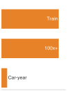
This training scenario exceeds 100 passenger-car years of emissions.
Napkin Math 15.5: The carbon cost of scale
Problem: A foundation model is being trained at the scale of GPT-3, consuming 1,287 MWh of electricity (Patterson et al. 2021). What is the operational carbon impact under the stated grid-intensity assumption?
Math:
- Energy consumption: 1,287 MWh = 1,287,000 kWh.
- Carbon intensity: This scenario uses \(\approx\) 429 g/kWh CO2 (0.429 kg/kWh) (Patterson et al. 2021), a US grid-average figure slightly above the rounded 0.4 kg/kWh baseline of the cost accounting. Each calculation states its own grid assumption, and the difference changes the result by less than a tenth.
- Total emissions: 1,287,000 kWh \(\times\) 0.429 kg/kWh = 552,123 kg CO2 (552 t).
- Comparison: The scenario assumes 4.6 t CO2 per passenger-car year. This per-year basis differs from the lifetime-car basis of the 2019 five-car estimate, so the two car comparisons are not directly comparable.
Systems insight: Under this training-energy scenario, the operational emissions equal the assumed annual emissions of 120 passenger cars. A 1 percent reduction in total training energy under the same grid mix would remove the equivalent of about 1.2 cars taken off the road for a year from the calculation.
Patterson, David, Joseph Gonzalez, Quoc Le, Chen Liang, Lluis-Miquel Munguia, Daniel Rothchild, David So, Maud Texier, and Jeff Dean. 2021. “Carbon Emissions and Large Neural Network Training.” arXiv Preprint arXiv:2104.10350.
Pricing compute in kilowatt-hours, tonnes of CO2, and three-year operating dollars places resource consumption alongside fairness and explainability as a measurable boundary of the system. Specification, measurement, documentation, and resource accounting together define what a responsible system must satisfy, but none of those bounds is self-verifying. The Govern stage of the lifecycle makes them provable to someone outside the team through infrastructure that controls data access, bounds privacy leakage, and preserves lineage and audit evidence in production.
Self-Check: Question
A team optimizes an inference model using INT8 quantization and structured pruning, reducing dedicated accelerator compute by \(4\times\) while preserving accuracy. According to the chapter, why is this efficiency improvement classified as a responsible engineering intervention rather than a pure performance optimization?
- Because quantization mathematically guarantees that disparate impact across all protected demographic groups drops to zero.
- Because reducing model parameters eliminates the need for data governance and audit logging in production pipelines.
- Because efficiency optimizations are relevant only for one-time training runs, where carbon emissions are legally regulated.
- Because it can lower lifecycle energy and cost and broaden hardware access when the actual runtime reduces measured service demand at the required quality and the deployment converts that gain into savings.
A wearable device has an inference power budget of 500 mW. Under the chapter’s assumed active-power profiles (KWS DS-CNN: 50 mW; MobileNetV2: 1.2 W), which statement about the resource screen is correct?
- MobileNetV2 passes, because its power overage can always be removed by offloading inference to the cloud.
- The DS-CNN passes with a 10\(\times\) power margin and MobileNetV2 exceeds the budget by 2.4\(\times\); passing the screen still does not establish that the DS-CNN suits the intended task.
- Both pass, because duty cycling makes any active power draw acceptable on a wearable.
- Neither passes, because no ML model can run within a sub-watt budget.
In the chapter’s illustrative three-year TCO model of the DLRM ranking service (Training: ~2%, Operations: ~25%, Inference: ~73%), assume one intervention halves total training cost, while another reduces total inference cost by 20% under unchanged traffic and quality. Which intervention saves more dollars, and by what approximate ratio? Why would halving only the final training run time not establish the first saving?
True or False: For an identical serving workload, relocating an inference deployment from a carbon-intensive fossil-fuel grid region to a region powered predominantly by low-carbon renewable energy can reduce operational carbon emissions more than a modest algorithmic efficiency improvement.
In data-center environmental accounting, the metric defined as the ratio of total facility energy to the energy consumed specifically by computing equipment is known as
____(abbreviated PUE).
15.5 Data Governance and Compliance
The keyword spotting system makes the governance problem physical. An always-listening voice assistant samples audio continuously in private homes, stores enrolled speaker profiles, and periodically syncs with cloud pipelines that retrain on population-wide audio. Every guarantee the earlier stages established now therefore depends on what data the system may hold, who may touch it, and what evidence survives. Data governance, the engineering discipline that turns regulatory and ethical obligations into verifiable technical controls, is the enforcement layer that makes accountability operational. Fairness metrics, model cards, and impact assessments have practical force only if the system can prove what data it ingested, which principals accessed it, which legal basis authorized processing, and whether applicable deletion or contestability requests were executed. The legal-basis question alone can decide an enforcement outcome. In 2023, Ireland’s Data Protection Commission found that Meta had relied on an invalid legal basis for personalized advertising and had violated transparency and fairness requirements, a governance failure that involved no security breach at all (Data Protection Commission 2023).
Data Protection Commission. 2023. Data Protection Commission Announces Conclusion of Two Inquiries into Meta Ireland. Regulatory press release.
Storage architectures also serve as governance enforcement mechanisms that determine which principals access data, how queries are tracked, and whether pipelines satisfy legal requirements. Every architectural decision, from ingestion strategies through extract, transform, load (ETL) pipelines to persistent storage layout, carries governance implications that surface during regulatory audits, privacy investigations, or model recalls. Data governance translates abstract policy into concrete systems engineering through authenticated access controls on training partitions, immutable audit infrastructure that logs dataset access, privacy-preserving transformations during feature extraction, and deterministic lineage systems that trace training snapshots to deployed model checkpoints.
↩︎ The database, warehouse, and data-lake storage architectures, and the access patterns each one serves, are established in Storage system options.
Principle: Compliance as engineering constraint
Invariant: Data governance obligations are engineering requirements, not optional policy overlays.
Implication: Systems that process regulated data must map applicable duties to technical and organizational controls. Access control, erasure, contestability, audit, and lineage may be required or useful depending on the jurisdiction, data, actor, and use case. The General Data Protection Regulation (GDPR), California Consumer Privacy Act (CCPA), Brazil’s General Data Protection Law (LGPD, Lei Geral de Proteção de Dados), and China’s Personal Information Protection Law (PIPL) differ in scope and duties, so no single control checklist establishes compliance across them.
Data governance turns security, privacy, compliance, and lineage into mutually dependent engineering constraints, and the KWS system shows where each one binds. Continuous capture, enrolled profiles, and fleet-wide retraining create obligations across consent management, data minimization, access auditing, and deletion rights, and the four domains map directly to hardware and pipeline enforcement points in this architecture. Security comes first by protecting raw features, training partitions, and model artifacts across the ingestion lifecycle through mutual authentication, role-based authorization, encryption at rest and in transit, and hardware-rooted key management. Hardware keystores on edge microcontrollers protect stored speaker templates, mutual TLS authenticates telemetry in transit, and role-based access controls gate access to centralized training audio in cloud storage. Because access control alone does not limit what an authenticated consumer can learn from the records it reads, privacy regulates information exposure inside that boundary through differential privacy, k-anonymity, and automated feature redaction. These measures keep ambient KWS audio inside a circular SRAM buffer until an on-device trigger and bound information leakage during fleet-wide acoustic model retraining.
Where privacy governs what leaves the device, compliance translates jurisdiction-specific statutes (such as GDPR, CCPA, and LGPD) into retention windows, consent verification, and cross-border replication rules once data arrives in the cloud. Compliance thereby determines the legal basis for processing and the scope of any revocation or erasure workflow that removes in-scope voice profiles and acoustic data across primary stores and backups. Proving that those security, privacy, and retention rules were followed requires lineage and audit systems that render the entire data lifecycle inspectable. Retained lineage linking deployed weights through training snapshots to authorized source records supports verification of security claims and applicable obligations. In the KWS pipeline, such lineage establishes provenance through content hashes and signed manifests that link each deployed DS-CNN binary back through specific training splits and acoustic augmentation seeds to the original raw recordings.
Governance works as an operating model rather than a single control. The framework in figure 7 arranges eight elements, from organizational oversight and compliance policies to data catalogs, sourcing, quality metrics, runtime operations, and security, around a central governance hub. Technical mechanisms and organizational processes must function as mutually reinforcing subsystems: encrypted storage without identity-mapped access controls still lets an insider copy data out, and compliant storage without verifiable audit trails cannot pass a regulatory inspection. Within the D·A·M taxonomy, data governance is the control plane of the Data axis. It enforces lawful sourcing, privacy bounds, and lifecycle integrity for the data that feeds the Algorithm, and it runs on Machine-axis infrastructure such as encrypted storage, access control, and audit logs.
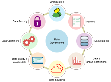
Engineering teams do not operate in isolation. Team-level technical practices such as audit logging, bias testing, and explainable interfaces sit at the core of expanding organizational, industry, and regulatory structures (figure 8). Requirements and legal mandates flow inward across each boundary, and the technical controls at the center supply the evidence that external compliance rests on. The rest of this section works at that innermost ring, starting with who may reach the data at all.
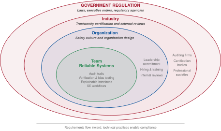
Shneiderman, B. 2022. Human-Centered AI. Oxford University Press. https://doi.org/10.1093/oso/9780192845290.001.0001.
15.5.1 Security and access control architecture
When a data scientist queries the KWS feature store for training data, she can read aggregated voice features but cannot access the raw audio recordings from which they were derived. The serving pipeline, by contrast, can read online features for inference without writing to the training dataset or modifying source data. That separation reflects a layered security architecture in which governance requirements translate into enforceable technical controls at each pipeline stage. Feature stores enforce role-based access control (RBAC) by mapping organizational policies to authenticated identities and database permissions. These controls operate across distinct storage tiers. Object storage enforces bucket-level access policies, data warehouses implement column-level security and dynamic masking for sensitive fields, and feature stores maintain isolated read and write paths that separate low-latency online inference key-value lookups from high-throughput offline batch training extracts.
↩︎ The dual-storage architecture of offline columnar stores and online key-value caches is established in Feature stores.
Access control mechanisms remain incomplete without encryption, which protects data at rest and in transit but does not prevent misuse after decryption or authorized access. Training corpora in data lakes use envelope encryption with keys held in a dedicated key management service. Feature stores encrypt tables at rest and authenticate every service-to-service transfer. KWS edge devices combine transport encryption for payload confidentiality with asymmetric code signing to verify model-update integrity. Each of these controls is only as strong as its key management and update authorization.
Protecting data while it is being computed on is a further layer, confidential computing. Hardware secure enclaves and trusted execution environments isolate protected memory and execution from host software outside their trust boundary, and attestation lets a client verify the approved configuration before releasing keys or data to it. The guarantee covers only the declared attacker boundary and supported configuration, and it does not protect data from the application authorized to process it. The technique matters most when training and serving run on infrastructure that the data owner does not control.
Serialized weights and checkpoints require the same protection as training data. Deserializing an unverified checkpoint in a format that can embed executable objects (Python pickle archives are the common case) gives an attacker arbitrary code execution on training nodes and inference workers. Restricted serialization formats that store only tensors avoid that mechanism, and write-protected promotion gates with cryptographic signatures verify artifact integrity and authorized provenance before loading. These controls do not establish that a model is free of backdoors or that every parser and runtime is secure.
Authorized loading also leaves the model’s behavior to be evaluated. Poisoned training samples can induce backdoors, perturbed inference inputs can induce misclassification (evasion attacks), and systematic queries can extract model functionality (Tramèr et al. 2016). Access control, cryptographic enclaves, and artifact verification therefore establish who can reach data and models and how they are protected across storage, transit, and execution, yet controlling access is only half the problem. Even authorized callers can compromise individual privacy if the data or model outputs themselves expose too much. Prediction APIs or raw weights can reveal whether a particular record was present in training (Shokri et al. 2017), so artifact integrity and limits on information exposure require distinct controls.
Tramèr, Florian, Fan Zhang, Ari Juels, Michael K Reiter, and Thomas Ristenpart. 2016. “Stealing Machine Learning Models via Prediction APIs.” 25th USENIX Security Symposium (USENIX Security 16), 601–18.
15.5.2 Technical privacy protection methods
Even when role-based access control works as designed, a data scientist querying a training table does not need, and should not see, individual user records when aggregate statistics suffice, nor should a released checkpoint or prediction API reveal whether a specific customer’s record was in the training set (Shokri et al. 2017). Privacy-preserving techniques15 close that exposure gap by bounding what queries and model outputs reveal even to authorized callers. Differential privacy bounds changes in an exported output distribution under a specified neighboring-dataset relation.16 One training mechanism is Differentially Private Stochastic Gradient Descent (DP-SGD) (Abadi et al. 2016). Unlike standard gradient clipping, which caps the batch-averaged gradient for numerical stability, DP-SGD clips each individual sample’s gradient to an \(\ell_2\) norm threshold \(\GradientClippingNorm\) before summing across the batch. Bounding each sample’s contribution is necessary because an unclipped outlier record could shift the batch sum by an arbitrarily large amount, leaving no finite noise scale able to hide whether that record was in the batch. Once every sample’s influence is bounded by \(\GradientClippingNorm\), DP-SGD adds calibrated Gaussian noise with distribution \(\GaussianDistribution(0, \PrivacyNoiseMultiplier^2 \GradientClippingNorm^2 \IdentityMatrix)\) to the sum of clipped gradients, where \(\PrivacyNoiseMultiplier\) is the noise multiplier. A privacy accountant tracks the privacy loss composed across the sampled training steps and checks it against the chosen epsilon budget.
15 Privacy-preserving techniques: K-anonymity (Sweeney 2002) ensures each record is indistinguishable from at least \(\AnonymitySetSize-1\) others with respect to chosen quasi-identifiers, l-diversity adds attribute variety within equivalence classes (Machanavajjhala et al. 2007), and t-closeness bounds distribution distance (Li et al. 2007). These syntactic guarantees address different threats from differential privacy and do not by themselves protect against all ML-specific leakage: a model trained on de-identified data can still memorize examples or reveal membership signal under some conditions (Shokri et al. 2017). Differential privacy instead bounds the influence of one record under a specified mechanism and privacy budget, offering a semantic guarantee designed to remain meaningful in the presence of side information; the methods are therefore not a simple strength hierarchy, and the appropriate protection depends on the release, threat model, and utility requirements.
Sweeney, Latanya. 2002. “K-ANONYMITY: A MODEL for PROTECTING PRIVACY.” International Journal of Uncertainty, Fuzziness and Knowledge-Based Systems 10 (05): 557–70. https://doi.org/10.1142/s0218488502001648.
Li, Ninghui, Tiancheng Li, and Suresh Venkatasubramanian. 2007. “t-Closeness: Privacy Beyond k-Anonymity and l-Diversity.” 2007 IEEE 23rd International Conference on Data Engineering, 106–15. https://doi.org/10.1109/ICDE.2007.367856.
16 Differential privacy: Introduced by Dwork et al. (2006), a randomized mechanism \(\RandomizedMechanism\) satisfies \((\PrivacyBudget, \PrivacyAdditiveSlack)\)-differential privacy if for all neighboring datasets \(\NeighboringDataset, \AdjacentNeighboringDataset\) differing by one record and output sets \(\MechanismOutputSet\), \(\Pr(\RandomizedMechanism(\NeighboringDataset) \in \MechanismOutputSet) \leq e^\PrivacyBudget\cdot \Pr(\RandomizedMechanism(\AdjacentNeighboringDataset) \in \MechanismOutputSet) + \PrivacyAdditiveSlack\). Here \(\PrivacyBudget\) controls the multiplicative bound and \(\PrivacyAdditiveSlack\) is additive slack in the inequality; their acceptable values depend on the neighboring-dataset relation, release, and policy. The systems trade-off is utility rather than mere implementation complexity: stronger privacy often requires more noise or tighter sampling, and privacy loss composes across repeated queries or training steps. Engineers must therefore track cumulative privacy loss with a valid accountant and report the assumptions behind the chosen budget.
Dwork, Cynthia, Frank McSherry, Kobbi Nissim, and Adam Smith. 2006. “Calibrating Noise to Sensitivity in Private Data Analysis.” In Theory of Cryptography Conference (TCC), edited by Shai Halevi and Tal Rabin, vol. 3876. Lecture Notes in Computer Science. Springer Berlin Heidelberg. https://doi.org/10.1007/11681878_14.
Abadi, M., A. Chu, I. Goodfellow, H. B. McMahan, I. Mironov, K. Talwar, and L. Zhang. 2016. “Deep Learning with Differential Privacy.” Proceedings of the 2016 ACM SIGSAC Conference on Computer and Communications Security, CCS ’16, 308–18. https://doi.org/10.1145/2976749.2978318.
Standard backpropagation kernels sum weight gradients across the batch dimension in place as they execute, so they never expose an individual sample’s gradient norm. Clipping needs each sample’s gradient norm before that sum occurs, and the direct way to obtain it materializes one full gradient buffer per sample, so gradient storage grows by the batch size. For the KWS acoustic model (200K parameters), one FP32 gradient occupies 800 KB and a batch of 256 per-sample gradients 204.8 MB. The same approach for the 1.5B-parameter GPT-2 would need 1.5 TB, far beyond the 80 GB of one H100. Specialized two-pass clipping implementations compute each sample’s gradient norm directly from layer activations and backpropagated output gradients before accumulating the rescaled weight updates, avoiding per-sample weight-gradient buffers, and small sequential microbatches trade the memory back for lost parallelism. The cost of DP-SGD must therefore be measured for the chosen implementation with its clipping, noise, sampling, and accounting assumptions intact.
Empirical attacks complement these formal checks. Membership inference attacks measure whether an observer can tell that a specific record was in the training set, and model inversion attacks use confidence outputs to reconstruct sensitive feature values or a training subject’s likeness (Fredrikson et al. 2015). A successful attack reveals practical leakage, but no empirical attack can prove that an \((\PrivacyBudget, \PrivacyAdditiveSlack)\) bound holds.17 Reducing confidence-score precision or restricting outputs to top-\(\TopClassCount\) classes reduces what some APIs expose, but neither is a complete defense. Their value depends on the attacker’s access and auxiliary information, while differential privacy provides a separate bound under its stated mechanism and accounting assumptions.
Fredrikson, Matt, Somesh Jha, and Thomas Ristenpart. 2015. “Model Inversion Attacks That Exploit Confidence Information and Basic Countermeasures.” Proceedings of the 22nd ACM SIGSAC Conference on Computer and Communications Security, 1322–33. https://doi.org/10.1145/2810103.2813677.
17 Membership inference attack: The attack uses model behavior to infer whether a record appeared in training; overfitting can increase the signal (Shokri et al. 2017). In practice, higher confidence on training samples can help distinguish members from nonmembers. Its measured success depends on model access, data distribution, and defense assumptions.
Shokri, Reza, Marco Stronati, Congzheng Song, and Vitaly Shmatikov. 2017. “Membership Inference Attacks Against Machine Learning Models.” 2017 IEEE Symposium on Security and Privacy (SP), 3–18. https://doi.org/10.1109/SP.2017.41.
While differential privacy bounds information leakage from model outputs, collecting continuous raw sensor streams creates an immediate vulnerability if raw data leaves the capture device. Always-listening edge architectures, such as the lighthouse KWS system, operate under severe privacy constraints because continuous ambient microphone sampling must coexist with strict minimization and retention boundaries. To reduce routine transmission exposure, this design confines acoustic feature extraction and wake-word detection to local low-power microcontrollers or digital signal processors (DSPs). Incoming audio samples stream through a small volatile circular buffer in on-chip SRAM, where older frames are continuously overwritten by newly sampled pulse-code modulation (PCM) data. The policy allows saving or sending audio only after an on-device wake-word trigger. Because detection can produce false wakes, validation must cover both the detector and the buffer and egress controls, including which pre-trigger audio becomes accessible after activation.
Confining raw audio to the device enforces data minimization but starves centralized training of the acoustic variety that improves accuracy. Federated learning recovers that variety by moving training to the data. Training-capable clients such as paired phones or home hubs train on authorized local examples and send model updates instead of raw audio, and a coordinator combines those updates into a shared model.18 The constrained KWS microcontroller only runs the result. The approach exchanges centralization risk for physical bottlenecks. Every round moves parameter updates over constrained wireless uplinks, battery-powered clients drop out mid-round, data that differ from home to home make local updates diverge, and raw updates can still leak training examples through reconstruction attacks (Zhu et al. 2019). Compression of those updates reduces communication but provides no privacy guarantee by itself.
18 Federated learning: McMahan et al. (2017) introduced Federated Averaging (FedAvg), in which each client runs several local training steps before the coordinator averages the resulting models. Averaging after many local steps rather than after every gradient cuts the number of communication rounds, which is what makes training over constrained client uplinks practical.
McMahan, Brendan, Eider Moore, Daniel Ramage, Seth Hampson, and Blaise Agüera y Arcas. 2017. “Communication-Efficient Learning of Deep Networks from Decentralized Data.” International Conference on Artificial Intelligence and Statistics (AISTATS), Proceedings of machine learning research, vol. 54: 1273–82.
Zhu, Ligeng, Zhijian Liu, and Song Han. 2019. “Deep Leakage from Gradients.” Advances in Neural Information Processing Systems (NeurIPS) 32: 14774–84.
Bonawitz, Keith, Vladimir Ivanov, Ben Kreuter, Antonio Marcedone, H. Brendan McMahan, Sarvar Patel, Daniel Ramage, Aaron Segal, and Karn Seth. 2017. “Practical Secure Aggregation for Privacy-Preserving Machine Learning.” Proceedings of the 2017 ACM SIGSAC Conference on Computer and Communications Security, 1175–91. https://doi.org/10.1145/3133956.3133982.
Secure aggregation lets the coordinator learn only the aggregate of participating clients’ updates, under the protocol’s participation, dropout, and collusion assumptions (Bonawitz et al. 2017). What that aggregate and the final model reveal remains outside its protection; differential privacy bounds that release by limiting the effect of any one record or client, provided the training mechanism and privacy accountant support the chosen neighboring relation. A design that needs both must account separately for what a curious coordinator observes during training and what recipients can infer from released checkpoints.
When triggered audio recordings or aggregated model checkpoints must be retained on centralized infrastructure for verification or downstream training, privacy protection shifts to automated lifecycle management. Automated retention workflows apply time-to-live policies across primary stores, caches, training partitions, and backups. Cryptographic erasure destroys the keys needed to decrypt covered copies; physical overwrite is a distinct storage-sanitization mechanism. Neither removes every copy automatically. The workflow must inventory replicas, key copies, and backups, define applicable retention exceptions, and verify that in-scope data is no longer recoverable under the chosen threat model. Differential privacy, on-device minimization, federated training, and automated retention supply the technical mechanisms that bound exposure, while external statutes decide which of those mechanisms are mandatory and what rights affected people can invoke.
15.5.3 Regulation as architecture
When the credit service denies an applicant who then asks why, contests the decision, and requests access to or deletion of the data used about her, those retention, erasure, and explanation paths stop being internal engineering preferences and become statutory rights. To satisfy them, the system must do more than report an accuracy score. It must produce an explanation tied to the specific decision, preserve the model and data lineage that led to that output, route the dispute to a substantive human review path, retain audit logs, and support deletion or access workflows where data rights apply. Explicit regulatory frameworks turn transparency, oversight, and accountability into non-negotiable architecture requirements.
Regulation first enters the architecture through risk classification. The EU AI Act establishes a comprehensive framework, classifying AI systems by risk level and mandating requirements accordingly.19 The Act entered into force on August 1, 2024 and applies in phases: prohibited-practice rules began applying in 2025, while high-risk and other operator obligations phase in by system category and implementation guidance (European Parliament and Council of the European Union 2024).
19 EU AI Act (Regulation 2024/1689): The first comprehensive AI legal framework, defining four risk tiers with penalties that vary by infringement category. The Act has extraterritorial reach: non-EU organizations may need to comply when they place systems on the EU market or when system outputs are used in the EU. Systems engineering implications are concrete: high-risk AI requires logging infrastructure for audit trails, human oversight mechanisms built into the architecture, and CE marking (the EU conformity mark), all capabilities that must be designed in from inception, not retrofitted after deployment.
European Parliament and Council of the European Union. 2024. Regulation (EU) 2024/1689 of the European Parliament and of the Council of 13 June 2024 Laying down Harmonised Rules on Artificial Intelligence (AI Act). Official Journal of the European Union, L 2024/1689.
20 High-risk AI (EU AI Act Annex III): Annex III enumerates specified use cases in areas including biometrics, critical infrastructure, education, employment, essential services, law enforcement, migration, and justice. Classification depends on intended use and the Article 6 criteria, including exclusions for some systems that do not materially influence decisions or pose significant risk; profiling systems within Annex III remain high-risk. Model architecture alone does not determine classification.
For systems engineers, compliance hinges on architectural capabilities rather than fine schedules. Covered high-risk systems20 must implement risk management, data governance, technical documentation, transparency, human oversight, and accuracy, robustness, and security requirements. A covered credit-decision system therefore needs auditability from inception: model versions, training data provenance, validation evidence, human-oversight design, logging, and postdeployment monitoring must be part of the architecture rather than documents assembled after launch.
Contestability adds a second architectural requirement. GDPR moves the same applicant workflow into data-subject rights. Article 22 grants EU data subjects the right not to be subject to decisions based solely on automated processing that produce legal or similarly significant effects, subject to specified exceptions and safeguards.21 Article 15(1)(h) separately gives data subjects access to meaningful information about the logic involved in automated decision-making referred to in Article 22. Engineering teams should determine which decisions are covered and design the required explanation and human-review capabilities accordingly. Where a substantive review path is required, it must be operationally staffed and supported by summaries, provenance, and audit tools. That staffing scales with decision volume. If 0.1 percent of 1M daily decisions are appealed or escalated, trained reviewers must work through 1,000 cases/day, a workload assumption rather than a model-error rate. The review tooling must also surface each case’s explanation, lineage, and model version fast enough for that queue to clear.
21 GDPR (General Data Protection Regulation) articles 15 and 22: Article 22 restricts certain solely automated decisions with legal or similarly significant effects and, for specified exceptions, requires safeguards including human intervention, the ability to express a point of view, and the ability to contest the decision; article 15(1)(h) contains the access right to meaningful information about the logic involved in such automated decision-making (European Parliament and Council of the European Union 2016). The European Data Protection Board’s guidance emphasizes that required human oversight must be substantive and not merely a “rubber-stamping” exercise (European Data Protection Board 2018).
European Data Protection Board. 2018. Guidelines on Automated Individual Decision-Making and Profiling for the Purposes of Regulation 2016/679.
Consumer Financial Protection Bureau. 2023. 12 CFR 1002.9: Notifications (Regulation B, Equal Credit Opportunity Act).
22 HIPAA (Health Insurance Portability and Accountability Act): Enacted in 1996, with Privacy Rule and Security Rule requirements establishing standards for protected health information (United States Congress 1996; U.S. Department of Health and Human Services 2003, 2005); PHI may be used for training under applicable authorization or another permitted pathway, such as an IRB or Privacy Board waiver; de-identified data and limited data sets with data-use agreements provide additional pathways. Model outputs may remain PHI when they identify or can reasonably identify individuals, and security-rule documentation retention must be reflected in audit and evidence design.
United States Congress. 1996. Health Insurance Portability and Accountability Act of 1996. Public Law 104-191.
U.S. Department of Health and Human Services. 2003. “Summary of the HIPAA Privacy Rule.”
US sectoral law reaches similar capabilities through domain-specific evidence requirements, less unified than the EU AI Act. In the credit example, the Equal Credit Opportunity Act (ECOA) and its implementing Regulation B require specific principal reasons for covered adverse actions, and those reasons must accurately describe the factors actually considered or scored (Consumer Financial Protection Bureau 2023). Healthcare regulation, including the Health Insurance Portability and Accountability Act (HIPAA)22 and Food and Drug Administration (FDA) guidance, imposes the same pattern with different artifacts: protected-health-information controls, validation records, audit logs, and incident response. Across domains, the task is to translate each obligation into a concrete capability: explanation, human review, lineage, access control, deletion, monitoring, or incident response. Because the same safeguards recur across regimes, table 11 organizes them by capability rather than by jurisdiction.
| Obligation (Example Source) | Capability the System Must Provide | Machine Cost |
|---|---|---|
| Risk management and record keeping for high-risk systems (EU AI Act) | Versioned models, data provenance, validation evidence, automatic event logs | Log storage and lineage-graph maintenance |
| Contestable automated decisions (GDPR Article 22) | Substantive human-review path with case summaries, explanations, and provenance | Reviewer hours that scale with decision volume |
| Reasons for a decision (GDPR Article 15; ECOA adverse-action notices) | Per-decision explanation or reason codes tied to the factors actually used | Explanation compute on the serving path |
| Data minimization and erasure (GDPR) | Retention limits, lineage-driven deletion, retraining or unlearning when weights are in scope | Retraining accelerator-hours; deletion workflows |
| Protected health information (HIPAA) | Access control, encryption, audit logs, retained documentation | Audit-log bytes over the retention window |
| Nondiscrimination (employment, credit, and housing law) | Disaggregated evaluation and monitoring against justified thresholds | Labeled per-group evaluation data; parity telemetry |
Data-protection law reaches deeper into the pipeline than decision-level duties do, because its obligations attach to the data itself rather than to a decision. When a European user invokes an applicable right to erasure under GDPR, the voice assistant must determine which personal data and downstream artifacts are in scope and execute the appropriate workflow within the regulation’s response deadlines (European Parliament and Council of the European Union 2016). These obligations become architecture constraints in pipeline design, storage choices, and operational procedures. GDPR’s data minimization principle requires limiting collection and retention to what is necessary for stated purposes. Article 15 access rights cover personal data undergoing processing and specified information about that processing, not every artifact merely associated with a user.
Voice assistants operating globally face overlapping regulatory regimes because requirements vary by jurisdiction and apply differently based on user age and data sensitivity. GDPR cross-border-transfer rules permit transfers through adequacy decisions, appropriate safeguards, or limited derogations rather than imposing categorical data localization. These rules can still drive regional storage, replication, and processing choices. A structured data card turns these operational metadata requirements into reviewable fields. The card in figure 9, adapted from the Open Images Extended (MIAP) specification (Pushkarna et al. 2022), partitions authorship, primary motivations, explicit safety prohibitions (such as forbidding age or gender classification), and methodological caveats. Although documenting these boundaries does not alone guarantee legal compliance, it provides the verifiable baseline necessary for pipeline ingestion checks.
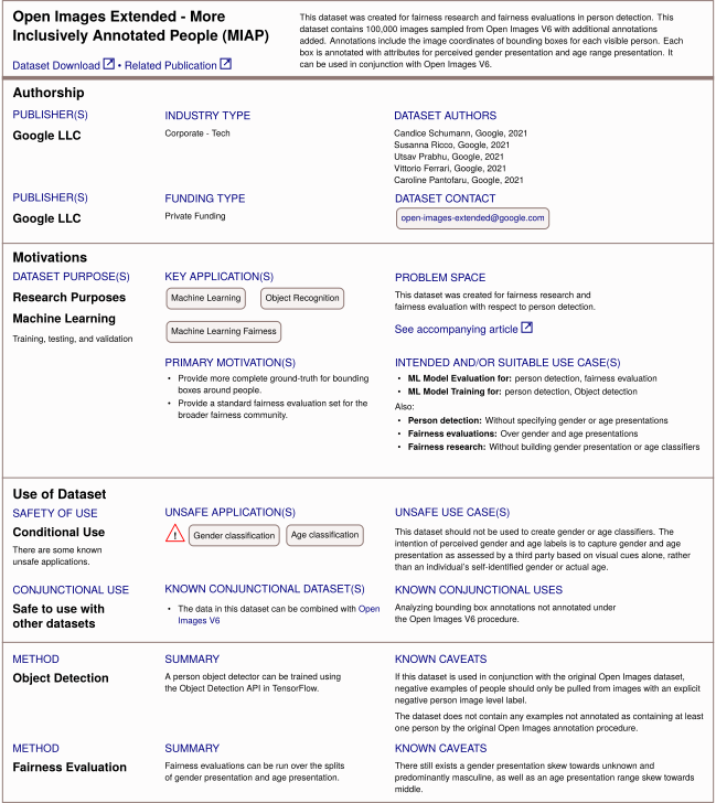
Pushkarna, Mahima, Andrew Zaldivar, and Oddur Kjartansson. 2022. “Data Cards: Purposeful and Transparent Dataset Documentation for Responsible AI.” Proceedings of the 2022 ACM Conference on Fairness, Accountability, and Transparency (FAccT), 1776–826. https://doi.org/10.1145/3531146.3533231.
The engineering response to these regulatory requirements is proactive architectural design. Teams that build documentation, monitoring, explainability, and human oversight into systems from inception demonstrate compliance efficiently. Teams that must retrofit these capabilities face expensive pipeline redesigns or deployment blocks. Nearly every regulatory obligation eventually asks the infrastructure the same two questions: which data produced this model, and who touched that data under what authority. Lineage and audit systems answer them.
15.5.4 Building data lineage infrastructure
When a regulator audits which training data produced a deployed model, or a user invokes an applicable right to erasure, the organization must answer from infrastructure rather than manual investigation. The lineage graph built for reproducibility in Transformation lineage and Versioning and lineage, a directed acyclic graph (DAG) of artifact versions and transformation tasks, is the same structure an audit queries.23 Governance adds obligations to that graph rather than a new system. Ingestion records must link each KWS recording to its acquisition method and consent basis, and the use boundaries declared on a data card (figure 9) decide which training jobs may consume which feature partitions.
23 Data lineage systems: Systems such as Apache Atlas and DataHub capture metadata about data flows from pipeline execution, creating graphs in which nodes are datasets and edges are transformations. GDPR Article 30 requires records of processing activities (European Parliament and Council of the European Union 2016), not automated model-level lineage specifically.
European Parliament, and Council of the European Union. 2016. Regulation (EU) 2016/679 of the European Parliament and of the Council of 27 April 2016. Official Journal of the European Union.
The obligation that lineage serves most directly is lineage-driven deletion. When an erasure request arrives, traversing the graph from the source recording identifies candidate derived artifacts (cached spectrograms, feature embeddings, training snapshots, and checkpoint weights) for scope determination and possible invalidation, retraining, or legal review. Deployment edges extend the same traversal to the field. Because lineage records which model version each device downloaded, a quality or compliance defect later found in the training data can be traced to the devices running the affected models and recalled there. Lineage captures provenance, but accountable operation also requires access history: who touched the data, when, and under which authority.
↩︎ Transformation lineage, which records the code version, parameters, and processing history behind each dataset, is established in Transformation lineage.
15.5.5 Audit infrastructure and accountability
Audit volume can outgrow the storage budget while the dataset stays flat.
24 Audit trail: Audit integrity requires controls against unauthorized alteration, but retention and deletion duties vary by record type and law; append-only object storage with retention controls, or cryptographic hash chains, can provide tamper evidence without creating a universal rule that records are never deleted. A large platform may log billions of events daily; HIPAA’s Security Rule also imposes multi-year documentation-retention obligations for required policies and procedures (U.S. Department of Health and Human Services 2005). Retention planning must distinguish records that must be preserved from personal data that must be minimized or deleted.
U.S. Department of Health and Human Services. 2005. “Summary of the HIPAA Security Rule.”
Recording that access history for HIPAA or Sarbanes-Oxley (SOX) audits creates a write-amplification bottleneck if a production feature store logs the full feature vector and intermediate activation tensor on every read. The audit log can then outgrow the training dataset itself and blow past its storage budget while the dataset stays flat. Accountability trails24 record access events to meet legal obligations, and for a fixed event schema, retained volume depends on recorded events per unit time, bytes per event, and the retention window. More accesses or instrumented stages raise the event count, while logging full feature payloads and intermediate activation tensors greatly increases bytes per event. Separating compact audit metadata from raw payload data controls that multiplier.
Production keyword spotting architectures resolve this trade-off through a tiered audit topology that reconciles capture fidelity with storage overhead and edge bandwidth limits. At the edge tier, microcontrollers operating within strict SRAM budgets log local state transitions, wakeup timestamps, and power states to volatile circular ring buffers. To conserve radio energy and uplink bandwidth, devices batch telemetry over secure transport rather than streaming it continuously. Scheduled maintenance windows or charging cycles can provide upload opportunities only if the required evidence survives until then.
The retention requirement determines which events can use this volatile path. Dividing usable buffer capacity by the encoded telemetry byte rate gives the time to fill an empty buffer; the upload schedule must leave room for bursts and retries. Summaries may discard detail only when the retained fields still answer the specified audit questions. Events that must survive power loss require durable local storage until central storage acknowledges durable receipt, adding write energy and storage wear to the device budget. Sequence numbers and restart markers expose missing intervals after reconnection; an incomplete interval cannot establish that no incident occurred. If retention requirements exceed the available storage or uplink budget, the design must reduce optional telemetry or provision additional capacity before deployment.
Once telemetry reaches centralized infrastructure, auditing shifts from bandwidth-constrained edge devices to high-throughput feature stores. At this feature tier, offline and online feature stores emit append-only audit events for every read and write transaction. Rather than duplicating high-dimensional feature vectors, these events record requesting service identities, authorized subject pseudonyms, feature group hashes, and read timestamps. This metadata-only logging strategy enables fine-grained access verification while keeping log volume proportional to access transactions rather than payload sizes.
From feature stores, data flows into training pipelines running across accelerator clusters. At this training tier, cluster schedulers record deterministic manifests mapping training jobs directly to immutable data partition hashes, git commit SHAs, and hyperparameter configurations. While these manifests support checks of pipeline integrity and reproducibility, they reveal an inherent systems boundary: access logs confirm which records were processed, but they cannot demonstrate whether deleted user data persists within learned model weights. If the applicable erasure obligation covers a deployed model artifact, teams must evaluate retraining, validated machine unlearning (removing a training record’s influence from learned weights without retraining from scratch (Cao and Yang 2015; Bourtoule et al. 2021)), or other legally appropriate controls. Database access logs alone cannot establish removal of the training contribution.
Cao, Yinzhi, and Junfeng Yang. 2015. “Towards Making Systems Forget with Machine Unlearning.” 2015 IEEE Symposium on Security and Privacy, 463–80. https://doi.org/10.1109/sp.2015.35.
Bourtoule, Lucas, Varun Chandrasekaran, Christopher A. Choquette-Choo, Hengrui Jia, Adelin Travers, Baiwu Zhang, David Lie, and Nicolas Papernot. 2021. “Machine Unlearning.” 2021 IEEE Symposium on Security and Privacy (SP), 141–59. https://doi.org/10.1109/sp40001.2021.00019.
Regulatory requirements extend audit responsibility from data access to prediction-time inference behavior. Reconstructing why the credit service denied a specific applicant in section 15.3.2.1, or why an edge voice assistant triggered a false wake-word activation, requires auditing the exact operational state at inference time. Without inference-time logging, an audit trail may confirm database access without capturing which model checkpoint, decision threshold, and runtime features produced a given decision. Saving raw input tensors for every inference request would overwhelm storage write bandwidth; production serving systems instead record compact, purpose-limited decision manifests. These manifests capture the active model version hash, runtime decision threshold, output confidence scores or reason codes, and cryptographic hashes of input features, supporting indexed retrieval of decision evidence. An input hash identifies content but cannot reconstruct it; replay also requires an appropriately retained source or an authorized recoverable representation, along with the relevant execution artifacts. Across these edge, feature, training, and serving tiers, governance uses Machine-axis logging and access control to prove Data-axis promises. Even with that infrastructure in place, however, a team can still undermine its own safeguards when it applies intuitions from deterministic software to statistical systems.
Self-Check: Question
In 2023, Ireland’s Data Protection Commission found that Meta had processed user data for behavioral advertising without a valid legal basis and in violation of transparency and fairness requirements, an infraction involving no data breach or server compromise. Which systems-engineering principle does this case demonstrate?
- Security encryption at rest and in transit is sufficient to guarantee total regulatory compliance across all data privacy laws.
- Data governance is an enforceable technical constraint across the data lifecycle, requiring infrastructure to verify lawful basis, purpose limitation, and consent rather than relying on policy assertions.
- Regulatory compliance applies only to static tabular data lakes and exempts real-time streaming feature stores.
- Publishing a public datasheet for a dataset eliminates all downstream corporate liability for unlawful processing.
A voice assistant receives an erasure request. Explain how retained lineage helps identify derived artifacts, why database deletion alone may be insufficient, and why identifying an artifact does not automatically require deleting it.
A smart-home voice assistant (such as the Lighthouse KWS system) is designed with an always-listening microphone. Which combination of architectural choices best embodies privacy-by-design for this deployment?
- Stream continuous raw ambient audio to a centralized cloud cluster where access is protected exclusively by role-based access control (RBAC).
- Store all raw acoustic recordings permanently on local edge flash memory so that future model versions can be trained without cloud connectivity.
- Perform wake-word detection locally, bound the audio window released after a trigger and test false wakes and egress controls, apply retention/deletion policies, and use training-capable clients with appropriately accounted differential privacy for federated model improvements.
- Rely on third-party cloud data warehouses to handle all privacy filtering after raw audio ingestion has completed.
A team plans to ingest raw audio, transform it into features, and only then configure feature-store RBAC and encryption. It will add lineage and inference logging after deployment. Explain which safeguards must exist before the corresponding data handling begins, and how retained lineage supports a later erasure request.
An empirical privacy attack in which an adversary analyzes model output probabilities to determine whether a specific individual’s record was part of the model’s training dataset is known as a
____.A European financial institution deploys an automated machine learning system to make sole decisions on credit applications. Under the EU AI Act (high-risk classification) and GDPR Article 22, which set of architectural capabilities must the engineering team build into the system from inception?
- Post-hoc saliency map visualization tools only, because EU regulations apply strict requirements exclusively to generative foundation models.
- A manual spreadsheet of training dataset URLs and an annual retrospective fairness report submitted after year-end financial audits.
- An unconstrained deep neural network optimized for accuracy, since high aggregate predictive power automatically satisfies legal safety criteria.
- Automated risk management, training data provenance logging, explainable adverse-action factor generation, and an operational workflow supporting substantive human review and user contestability.
A randomized algorithm \(\mathcal{M}\) satisfies \((\epsilon, \delta)\)-
____if for any two neighboring datasets \(D, D'\) differing by at most one record, the probability of any output set \(\mathcal{S}\) satisfies \(\mathbb{P}[\mathcal{M}(D) \in \mathcal{S}] \le e^\epsilon \cdot \mathbb{P}[\mathcal{M}(D') \in \mathcal{S}] + \delta\), providing a mathematical upper bound on privacy loss.
15.6 Fallacies and Pitfalls
Teams can still fail after assembling assessment frameworks, fairness metrics, explainability mechanisms, efficiency analyses, and governance infrastructure. A team may retrofit fairness after benchmark success, trust aggregate accuracy, or treat compliance evidence as paperwork rather than system behavior, drawing on intuitions from traditional software engineering where bugs are local and testing is deterministic.
Fallacy: Responsibility can be addressed after the system achieves technical objectives.
Teams assume fairness constraints can be retrofitted once models demonstrate strong benchmark performance. In production, early architectural decisions constrain what interventions remain feasible. Amazon’s recruiting tool, abandoned after remediation failed (section 15.2.1), is the case in point. Integrating fairness constraints early can be less costly than retrofitting them after data contracts, monitoring, and release gates are fixed.
Pitfall: Relying on aggregate metrics to assess fairness.
Engineers assume high overall accuracy indicates the system works well for all users. The flaw of averages (section 15.3.2) shows why this intuition fails, because aggregate metrics can conceal large subgroup disparities. The credit-service analysis in section 15.3.2.1 showed a 30 percentage-point TPR gap, with qualified minority applicants rejected at 4× the majority-group rate. These disparities can persist undetected when standard monitoring tracks only aggregates. Production systems require disaggregated evaluation with application-specific thresholds, such as the 5-percentage-point TPR threshold used for the credit service.
Fallacy: Removing sensitive attributes from training data eliminates bias.
Teams remove gender, race, and protected attributes expecting this ensures fairness. Other features can act as proxy variables when they correlate with sensitive characteristics. ZIP codes, purchase patterns, browsing history, college names, and language choices can carry indirect demographic signal. Amazon’s recruiting tool kept encoding sex through college and organization names after explicit gender terms were removed (section 15.2.1), and the care-management algorithm (war story 15.1) reproduced racial disparity through its cost target, a proxy that no attribute filter would remove. Removing protected attributes does not by itself establish fairness.
Pitfall: Treating documentation as sufficient accountability.
Teams invest effort in model cards, then consider responsibility requirements satisfied. Documentation provides transparency (section 15.3.3.2) but not enforcement. A model card specifying “not validated for high-stakes decisions” has no effect when the system is repurposed for loan approvals without technical restrictions. Accountability requires operational integration: monitoring dashboards, documented subgroup-disparity alert thresholds, incident response procedures, and access controls preventing deployment beyond validated use cases.
Fallacy: Responsible AI is primarily a legal compliance issue.
Teams treat responsibility as external oversight rather than engineering practice. Engineering decisions made months before legal review constrain the solution space more than any compliance assessment. Architecture selection determines what fairness interventions are feasible, while data pipeline design establishes whether disaggregated evaluation is even possible. As section 15.2.5 establishes, systems designed with responsibility as an engineering objective enable efficient validation; systems where responsibility is added at late-stage review face redesign or deployment with documented risks.
Pitfall: Measuring the environmental impact of training but not inference.
Public discourse focuses on training-run carbon, and engineers often follow this framing when assessing environmental responsibility. The illustrative TCO analysis in section 15.4.2 shows why this focus is incomplete: under its unbatched service-demand assumptions for the DLRM ranking service (table 10), the inference-to-training cost ratio is about 40:1, and inference emits about 63× as much CO2 as training. A model trained periodically but served millions of times daily can have a lifecycle footprint dominated by inference rather than training. These values are scenario-dependent, but they show why lifecycle accounting must include both terms.
Fallacy: Model weights are exempt from data governance and deletion requests.
Teams often assume that once training data has been compiled into model weights, the data is gone and compliance obligations cannot reach the artifact. In reality, models can memorize training data, and membership inference attacks can reveal whether a sensitive record appeared in the training set (Shokri et al. 2017). Unlike a database delete, a neural network diffuses each training point’s statistical influence across its parameters through gradient updates, so verifiably purging that influence forces systems trade-offs. Exact retraining from scratch on a cleaned dataset provides a reference for removing the excluded records’ contribution, but it re-expends the training budget (potentially thousands of accelerator-hours) and its carbon emissions. It also does not erase other copies or facts inferable from retained data. Machine unlearning, introduced with audit infrastructure (section 15.5.5), aims to bound that cost, but verifying that an intervention removes statistical influence without degrading model utility remains an open systems challenge. Engineering teams must track data-to-model lineage and evaluate retraining, machine unlearning, or compensating controls with legal and privacy specialists whenever an erasure request affects deployed artifacts.
Across these failures, the recurring mistake is to treat responsibility as something added after the system is built rather than as a system property. Measurable constraints, continuous monitoring, and enforceable governance carry responsibility through the full lifecycle.
Self-Check: Question
A deployed automated lending model achieves an impressive 88% overall accuracy on its global test set. However, a disaggregated audit reveals that qualified minority applicants experience a 60% True Positive Rate compared to 90% for majority applicants (a 30 percentage-point gap) and face \(4\times\) higher false rejection rates. Which engineering pitfall does this scenario illustrate?
- Relying on aggregate metrics to assess fairness, which conceals severe subgroup disparities behind strong overall averages (the Flaw of Averages).
- Treating documentation as sufficient accountability, assuming a model card automatically prevents operational misuse.
- The belief that model weights are exempt from data governance and right-to-erasure regulations.
- Assuming that edge deployment power budgets scale linearly with dataset sample size.
A team removes race and gender columns from their training dataset, asserting that “the model cannot discriminate on features it cannot see.” Drawing on the Amazon recruiting and Optum healthcare cases, explain why this naive attribute removal creates false confidence, and identify the specific engineering analyses required.
True or False: Because a model card explicitly specifies that a vision model is “not validated for high-stakes medical or security screening,” publishing the model card guarantees operational compliance without requiring technical access controls or deployment release gates.
True or False: For a high-traffic production ML service, measuring and reporting only the electricity consumed during model training runs provides an accurate accounting of the system’s long-term environmental carbon footprint.
15.7 Summary
Responsible engineering is ML systems engineering done completely, not a separate discipline. The chapter traced a path from failure diagnosis through prevention to enforcement, beginning with the responsibility gap (the distance between technical performance and responsible outcomes) and demonstrating how proxy variables, feedback loops, and distribution shift can harm users while conventional metrics remain acceptable. The engineering response follows the model’s lifecycle. Specification fixes targets, populations, and oversight before training forecloses them. Fairness metrics make disparities measurable. Explanation and documentation are selected for applicable stakeholder and regulatory requirements. Monitoring infrastructure can surface silent failures and connect signals to response.
Translating responsibility concerns into measurable properties makes them tractable. A justified, application-specific bound on disparity is testable; “be fair” is not. This translation extends beyond fairness: in the chapter’s illustrative TCO scenario, a 20 percent accelerator-service-demand reduction saves $304K and is modeled to avoid 19 t of CO2 under the stated assumptions. Documentation becomes model cards with explicit intended use and known limitations. Governance becomes access control, lineage tracking, and audit infrastructure that makes compliance evidence available rather than merely aspirational. Across these cases, abstract ethical obligations become concrete engineering requirements that can be specified, tested, monitored, and enforced.
Every row of the chapter map (table 1) now carries a measured machine cost. Specification needs labeled evaluation data in proportion to how rare each named population is, and mitigation needs a second network head. Exact attribution needs explanation compute that grows exponentially with feature count, and keeping feedback in check needs randomized exploration traffic. The DLRM service consumes accelerator-hours and tonnes of CO2, and governance consumes log bytes, privacy noise, and retraining hours. These practices share one principle: a responsibility property can be enforced only at a lifecycle stage that still has the freedom to change it. Measurement can gate only the populations that specification named, documentation can record only what measurement produced, and governance can prove only what the pipeline retained. A system that defers fairness, efficiency, transparency, or governance to a late review is therefore incomplete in the same sense as a system shipped without a latency budget; the requirement exists, but nothing in the architecture can meet it. The chapter’s quantitative tools fit in one table (table 12), and each turns a responsibility requirement into a number a team can compute before launch and monitor after it.
| Quantity | Formula | Where Derived |
|---|---|---|
| Alignment gap | \(\text{Gap} = \mathbb{E}[\text{Proxy}] - \mathbb{E}[\text{True}]\) for metrics on a common scale | equation 1 |
| Demographic parity | \(\Pr(\PredictedDecision=1 \mid \ProtectedGroupMembership=\text{A}) = \Pr(\PredictedDecision=1 \mid \ProtectedGroupMembership=\text{B})\), gated on the difference | section 15.3.2.1 |
| Equal opportunity | \(\Pr(\PredictedDecision=1 \mid \TrueOutcome=1, \ProtectedGroupMembership=\text{A}) = \Pr(\PredictedDecision=1 \mid \TrueOutcome=1, \ProtectedGroupMembership=\text{B})\) | section 15.3.2.1 |
| Equalized odds | Equal opportunity for both \(\TrueOutcomeLevel\in \{0,1\}\), so true and false positive rates both match | section 15.3.2.1 |
| Slice sample size | Worst-case margin \(1.96\sqrt{0.25/\SubgroupSampleSize}\); random collection \(\RandomSampleCollectionSize\) = per-group target divided by the group’s share | section 15.3.1 |
| Exact attribution cost | \(\mathcal{O}(2^{\AttributionFeatureCount})\) model evaluations per explained decision | section 15.3.3.1 |
| Bias feedback | \(\GroupDisparity(\FeedbackIntervalCount) \approx \GroupDisparity(0) \cdot \BiasFeedbackFactor^\FeedbackIntervalCount\) | section 15.3.4 |
| Operational carbon | \(\text{Energy}_{\text{hardware}} \times \text{PUE} \times \text{Carbon Intensity}\) | section 15.4.3 |
| Audit log volume | Recorded events per unit time, times bytes per event, times the retention window | section 15.5.5 |
Key Takeaways: Reliable for whom?
- Aggregate correctness hides harm: A model can look accurate in aggregate while one subgroup’s error rate is 43.1× another subgroup’s rate, as in the Face++ Gender Shades audit. Responsible evaluation therefore starts with disaggregated and intersectional slices, not aggregate accuracy alone.
- Responsibility becomes testable through thresholds: “Be fair” is not testable, but bounded disparity, documented intended use, and explainability requirements are. Translating values into measurable constraints lets teams review trade-offs among fairness, accuracy, latency, and cost.
- Efficiency is a social constraint: An efficient model can reduce energy and cost and broaden who can deploy it. In the chapter’s illustrative scenario, the inference-to-training cost ratio is 40:1, making per-query optimization responsible engineering.
- Monitoring must watch outcomes: Bias and privacy failures can continue with green uptime dashboards because harmful predictions look operationally normal. Production monitoring must track subgroup outcomes, data lineage, feedback loops, and incident paths with the same rigor as latency regressions.
- Governance has to be built in: Model cards, datasheets, access controls, erasure workflows, human-review paths, and audit trails are technical infrastructure, not optional policy overlays. Regulations such as GDPR require capabilities that should be designed into the pipeline; later remediation may remain possible but can be narrower and costlier once the system is serving decisions.
A system that does exactly what it was told is dangerous precisely because the telling is never complete. Every objective a model is given is a specification with gaps, and an optimizer is a machine for finding them. It can reproduce the bias latent in its data, chase the proxy instead of the goal, and call the result success because nothing in the objective said otherwise. Responsible engineering is the discipline of writing back in what the specification left out. Constraints and monitoring reduce the risk that optimization amplifies harms encoded in the data. The constraint is the same kind the rest of the book imposed in latency and memory, except that here it protects people the objective never named. A model that is fast and accurate while wrong about whom it serves has not failed less than one that crashes, only more quietly.
What’s Next: From local targets to the whole system
Responsibility was the last constraint this book added, and it behaves like the ones before it. A disparity bound, a carbon budget, or a lineage requirement can be met only if every upstream stage preserved the freedom to meet it, exactly as a latency budget can. Every constraint so far has been taught one layer at a time, yet the costliest failures arise where layers interact, when each component meets its own target and the system still misses its goal. Conclusion returns to the voice-assistant request that opened the book, follows it across every layer the chapters built, and gathers their quantitative principles, from the iron law (principle 3) onward, into one framework for reasoning across the whole stack.
15.8 Self-Check Answers
Self-Check: Answer
An AI recruiting tool meets its latency SLA, maintains 99.9% availability, and achieves 87% aggregate accuracy, yet it systematically downgrades resumes containing the word “women’s” or graduates of women’s colleges. Applying the systems-engineering verification-versus-validation framing, which diagnosis correctly explains this outcome?
- The system failed verification because any discriminatory outcome is by definition a low-level coding defect in the model implementation.
- The failure is primarily an operational reliability defect that responsible engineering addresses only after serving infrastructure destabilizes.
- The root cause is insufficient model capacity, which can be resolved by scaling up model parameters without altering the optimization objective.
- The system passed verification by meeting its stated technical requirements, but failed validation because the specification itself did not capture the organization’s true goal of fair hiring.
Answer: The correct answer is D. In systems engineering, verification asks whether the system was built correctly against stated specifications, while validation asks whether the right system was built to meet true needs. The tool met all monitored technical targets (passing verification) but optimized a flawed objective that reproduced historical hiring bias (failing validation). The low-level defect claim is incorrect because the code executed without error on the objective it was assigned. The operational reliability option conflates service uptime with specification correctness. The model capacity explanation is flawed because a larger model would simply fit and reproduce the biased historical patterns more faithfully.
Learning Objective: Classify an ML deployment failure using the systems-engineering verification-versus-validation framework.
A team argues that a one-time ethics sign-off before deployment is sufficient because their model passes all latency and aggregate accuracy checks. Using the MLOps control-loop analogy, explain why responsible engineering must instead operate as a continuous control loop, and identify one specific production metric that a one-time pre-launch review cannot capture.
Answer: MLOps functions as a continuous control loop for operational reliability because data distributions drift over time; responsible engineering is the corresponding control loop for safety because outcome quality degrades as downstream user populations, proxies, and deployment environments evolve. A one-time sign-off cannot detect post-deployment subgroup-level error rate disparities (such as a widening true-positive-rate gap between demographic slices) that emerge as input distributions shift while overall latency and availability dashboards remain green.
Learning Objective: Explain why responsible engineering requires a continuous production control loop analogous to MLOps rather than a static pre-deployment review.
True or False: Because ML systems are constructed from modular software components, a fairness defect originating from biased training data can be isolated and patched within a single function without altering data pipelines, training objectives, or shared representations.
Answer: False. Unlike traditional software where defects can often be isolated within a specific function or module, ML systems exhibit tight data-dependent coupling. Data flows through shared representations (such as embeddings and learned feature weights), meaning a biased training signal propagates across multiple downstream predictions. Remediating such a failure requires architectural interventions across the D·A·M axes—including data curation, constrained optimization objectives, and disaggregated outcome monitoring.
Learning Objective: Distinguish localized software bugs from data-coupled ML specification failures across shared representations.
Self-Check: Answer
In an audited commercial healthcare algorithm (Optum), predicting future healthcare costs as a proxy for health needs resulted in Black patients receiving lower risk scores despite having more chronic conditions than White patients with identical scores. What systems mechanism explains why this proxy failed?
- The model suffered from severe overfitting due to an excessive number of gradient descent epochs on a small training dataset.
- The proxy variable inherited historical systemic disparities in healthcare spending, so predicting costs faithfully reproduced unequal access to care rather than actual medical need.
- The failure was caused by real-time concept drift that occurred after deployment when hospital billing codes suddenly changed.
- The algorithm used an unconstrained loss function that optimized inference latency at the expense of regression calibration.
Answer: The correct answer is B. Because less money is spent on Black patients than on White patients with the same level of illness due to systemic barriers, using healthcare cost as a proxy for medical need meant the model learned to predict spending disparities rather than actual health need. Correcting the target from cost to chronic condition count raised the proportion of Black patients identified for high-risk care management from 17.7% to 46.5%. The overfitting distractor is incorrect because the model generalized its cost-prediction task accurately. The concept drift distractor misattributes the failure to post-deployment environmental change rather than training-target proxy bias. The latency optimization choice conflates infrastructure performance tuning with loss function specification.
Learning Objective: Analyze how proxy variables inherit and amplify systemic disparities in training targets.
A hospital sepsis prediction model begins recommending aggressive treatments for low-risk patients after an EHR update alters how vital signs are logged. System health checks, latency, and prediction confidence remain normal. Explain why this constitutes a silent failure, and identify two monitoring signals that would support investigation without assuming either proves the cause.
Answer: This is a silent failure because harmful recommendations occur while the monitored service properties remain normal. The logging change motivates investigation of input semantics and distributions; it does not establish covariate shift, which additionally requires the label relationship to remain stable. Two complementary signals are: (1) input-feature distribution drift detection using divergence metrics such as Jensen-Shannon divergence (\(\mathcal{D}_{\text{JS}}(P_t \parallel P_0)\)) on vital-sign feature distributions, and (2) disaggregated clinical outcome tracking with mature labels, coverage, and comparable cohorts. Input divergence can warn of change without proving quality loss; outcome evidence can establish a quality change, while matched-input replay and pipeline inspection test the suspected logging defect.
Learning Objective: Analyze silent distribution-shift failures in production ML and identify statistical and outcome-based monitoring signals.
A content recommendation service reports that optimizing a ranker for short-term user clicks increased click-through rate by 20%, but long-term user satisfaction dropped by 5% and 30-day retention declined. Which systems-engineering concept best explains this divergence, and what is the appropriate mitigation?
- The alignment gap governed by Goodhart’s Law, where optimizing an observable proxy metric degrades the unobserved true objective; mitigated by maintaining counterfactual holdouts and multi-objective optimization with explicit satisfaction constraints.
- Model capacity collapse, where the embedding table runs out of capacity for rare items; mitigated by increasing embedding dimension and memory bandwidth.
- Hardware-level numerical underflow in attention layers; mitigated by upgrading from FP16 to FP32 mixed precision across serving clusters.
- Training-serving skew in network protocol buffers; mitigated by implementing automated schema validation in feature pipelines.
Answer: The correct answer is A. When a measurable proxy (clicks) becomes the optimization target, Goodhart’s Law dictates that it ceases to be a reliable measure of the true underlying goal (user satisfaction), creating a signed alignment gap \((\text{Gap} = \mathbb{E}[\text{Proxy}] - \mathbb{E}[\text{True}])\). The appropriate mitigation combines multi-objective optimization with safety constraints and randomized counterfactual holdouts that track true long-term satisfaction. The capacity collapse option misattributes a loss-function specification failure to memory constraints. The numerical underflow option confuses mathematical representation limits with metric misalignment. The schema validation option addresses data pipeline serialization rather than proxy divergence.
Learning Objective: Apply Goodhart’s Law and alignment gap mechanics to diagnose metric divergence in recommendation systems.
Self-Check: Answer
An engineering team is evaluating a facial verification model. To estimate the error rate of a minority demographic group representing 1% of the population with a margin of error of \(\pm 1\) percentage point at 95% confidence, they require 10,000 labeled evaluation samples from that group. Under uniform random sampling from the natural population distribution, how many total images must the team collect and label in expectation?
- About 10,000 total images, because evaluating subgroup accuracy requires only that the total test set contains 10,000 images.
- About 100,000 total images, because statistical confidence intervals scale with the square root of the overall dataset size.
- About 1,000,000 total images in expectation, because a 1% subgroup yields only 1 target image per 100 randomly sampled images, imposing a \(100\times\) multiplier.
- About 10,000,000 total images, because the binomial confidence interval width expands exponentially for minority subgroups.
Answer: The correct answer is C. Dividing the required subgroup sample size (\(10{,}000\)) by the subgroup prevalence (\(0.01\)) yields an expected total collection size of \(D_{\text{eval,total}} = 10{,}000 / 0.01 = 1{,}000{,}000\) images—a \(100\times\) data collection multiplier. This demonstrates why relying on natural random distributions for fairness evaluation is prohibitively expensive and why intentional stratified data engineering is required. The 10,000 total images choice confuses subgroup sample requirements with overall dataset size, yielding only ~100 minority samples. The 100,000 total images choice underestimates the collection requirement by a factor of 10. The 10,000,000 total images choice applies an incorrect \(1{,}000\times\) scaling factor.
Learning Objective: Calculate the expected data collection multiplier required for minority subgroup evaluation under random versus stratified sampling.
A team plans to write their model card six months after launch so that it accurately reflects observed production behavior. Explain why this timing constitutes a guard-rail failure, and describe one concrete scope-creep risk that a pre-deployment model card with automated deployment gates prevents.
Answer: A model card functions as an operational guard rail only when written before deployment to explicitly define intended use, validated populations, and excluded use cases that automated release gates can enforce. Writing the card after deployment turns it into a passive historical record that fails to constrain ongoing misuse. A concrete scope-creep risk prevented by pre-deployment gating is when a lightweight vision model validated only for consumer photo organization is repurposed without re-validation for high-stakes security screening or medical diagnostics.
Learning Objective: Explain how pre-deployment model cards operate as enforced guard rails to prevent deployment scope creep.
A loan approval classifier is evaluated on a fully labeled sample whose repayment outcomes are observed independently of its approval predictions. Group A (Majority): 4,500 True Positives, 500 False Negatives (TPR = 90%), 1,000 False Positives, 4,000 True Negatives (FPR = 20%). Group B (Minority): 600 True Positives, 400 False Negatives (TPR = 60%), 200 False Positives, 800 True Negatives (FPR = 20%). Which statement accurately diagnoses the fairness metrics for this system?
- Demographic parity is satisfied because both groups share an identical False Positive Rate of 20%.
- Equalized odds is satisfied because matching False Positive Rates compensate for differences in True Positive Rates.
- Equal opportunity is violated due to the 30 percentage-point TPR gap, and equalized odds is also violated because equalized odds strictly requires parity in both TPR and FPR.
- Calibration is the only metric affected, because True Positive Rate disparities impact accuracy but do not constitute algorithmic bias.
Answer: The correct answer is C. Equal opportunity requires equal True Positive Rates among qualified applicants (\(P(\hat{Y}=1 \mid Y=1, A=a) = P(\hat{Y}=1 \mid Y=1, A=b)\)); the 30 percentage-point gap (90% vs. 60%) directly violates it. Equalized odds requires equality in both TPR and FPR (\(P(\hat{Y}=1 \mid Y=y, A=a) = P(\hat{Y}=1 \mid Y=y, A=b)\) for \(y \in \{0,1\}\)); matching FPRs (20% vs. 20%) cannot satisfy the criterion when TPRs differ. Demographic parity requires equal overall approval rates regardless of true qualifications, which is not measured by FPR. The calibration-only option incorrectly dismisses severe true-positive-rate disparities as benign accuracy differences.
Learning Objective: Analyze equal-opportunity and equalized-odds violations directly from group confusion matrices.
For the credit service, closing the 30 percentage-point TPR gap for Group B via threshold adjustment adds \(\$225\) in margin on newly approved loans that are repaid but creates \(\$300\) in losses on newly approved loans that default, per Group B applicant, whose baseline utility is \(\$150\) per applicant. Using the chapter’s two-sided accounting, calculate the net utility change per applicant and explain what deliverable engineers owe stakeholders.
Answer: The net change is \(\FiniteChange\text{Utility} = \$225 - \$300 = -\$75\) per Group B applicant, a 50% within-group utility loss relative to that group’s \(\$150\) baseline. Rather than treating threshold adjustment as an automatic fix or imposing a value judgment, engineers owe stakeholders the explicit Pareto frontier along with all economic and base-rate assumptions, showing the exact trade-offs between fairness metrics and utility.
Learning Objective: Calculate two-sided utility changes under fairness threshold adjustments and justify presenting Pareto frontiers to stakeholders.
After mitigation, the credit service ships with a 3 percentage-point TPR gap under a 5-point release gate, and the next quarterly audit measures 3.3 points. Using the bias feedback model, estimate the fitted feedback factor and the retraining cycle in which the projected gap first exceeds the gate. Why does the projection motivate changing what the loop observes rather than only shortening the audit interval?
Answer: The fitted factor is \(3.3/3.0 = 1.10\) per quarter. The projected gap \(3.0 \times 1.10^{\FeedbackIntervalCount}\) first exceeds 5 points when \(\FeedbackIntervalCount > \ln(5/3)/\ln 1.10 \approx 5.4\), so on the sixth quarterly cycle, at about 5.3 points. Two audits do not validate future dynamics, so the factor must be refitted at every audit. Denied applicants generate no repayment labels, so each retraining learns from a population the previous model selected. Approving a small randomized sample of marginal applicants restores the censored outcomes and can bring the factor below one, so the gap decays instead of growing; a shorter audit interval only detects the breach sooner.
Learning Objective: Apply the bias feedback model to project when a launch-time fairness gap breaches its gate and identify the loop change that stabilizes it.
A team is designing a fairness and robustness testing suite for the credit service. Explain why subgroup representation and labeled sample sufficiency must be checked before interpreting subgroup error rates. How do invariance tests and boundary/stress tests complement those rates, and when can the team compare candidate configurations on a fairness-accuracy Pareto frontier?
Answer: Representation and labeled sample checks establish whether each subgroup rate has enough relevant evidence and acceptable uncertainty. Insufficient evidence cannot support a parity claim. Invariance tests probe decision stability under defensible, semantically irrelevant substitutions; they do not alone establish a causal account of discrimination. Boundary and stress tests probe sparse or corrupted input regimes. Once candidate configurations have comparable evaluation evidence, stakeholders can review their measured fairness-accuracy trade-offs. The chapter presents complementary testing regimes, not a mandatory unique order between invariance and stress testing.
Learning Objective: Explain the evidence dependencies and complementary roles of subgroup, invariance, stress, and trade-off evaluations.
Self-Check: Answer
A team optimizes an inference model using INT8 quantization and structured pruning, reducing dedicated accelerator compute by \(4\times\) while preserving accuracy. According to the chapter, why is this efficiency improvement classified as a responsible engineering intervention rather than a pure performance optimization?
- Because quantization mathematically guarantees that disparate impact across all protected demographic groups drops to zero.
- Because reducing model parameters eliminates the need for data governance and audit logging in production pipelines.
- Because efficiency optimizations are relevant only for one-time training runs, where carbon emissions are legally regulated.
- Because it can lower lifecycle energy and cost and broaden hardware access when the actual runtime reduces measured service demand at the required quality and the deployment converts that gain into savings.
Answer: The correct answer is D. Supported kernels and representations must reduce measured service demand for the required traffic and predictive quality, including consequential subgroup slices. Lower demand can permit fewer provisioned devices or more accessible hardware, but dollar savings depend on billing and provisioning. Lifecycle energy and emissions must include added training or preprocessing, idle power, facility overhead, and the grid boundary. Compression does not guarantee demographic parity or remove governance duties. Recurring inference can dominate at sufficient traffic; measured lifecycle accounting determines whether it does in this deployment.
Learning Objective: Explain the conditions under which efficiency optimizations improve energy, cost, and hardware accessibility.
A wearable device has an inference power budget of 500 mW. Under the chapter’s assumed active-power profiles (KWS DS-CNN: 50 mW; MobileNetV2: 1.2 W), which statement about the resource screen is correct?
- MobileNetV2 passes, because its power overage can always be removed by offloading inference to the cloud.
- The DS-CNN passes with a 10\(\times\) power margin and MobileNetV2 exceeds the budget by 2.4\(\times\); passing the screen still does not establish that the DS-CNN suits the intended task.
- Both pass, because duty cycling makes any active power draw acceptable on a wearable.
- Neither passes, because no ML model can run within a sub-watt budget.
Answer: The correct answer is B. The DS-CNN’s assumed 50 mW is one-tenth of the 500 mW budget, while MobileNetV2’s 1.2 W exceeds it by 2.4\(\times\) before sustained thermals are considered. Offloading changes the system design and its latency, privacy, and connectivity assumptions, so it does not make MobileNetV2 fit this budget. Duty cycling lowers average draw but not the active power the budget bounds. Passing the screen does not establish suitability, since the DS-CNN is the keyword-spotting lighthouse and its inputs and outputs must match the intended application.
Learning Objective: Apply an edge power budget to screen candidate models while separating resource fit from task suitability.
In the chapter’s illustrative three-year TCO model of the DLRM ranking service (Training: ~2%, Operations: ~25%, Inference: ~73%), assume one intervention halves total training cost, while another reduces total inference cost by 20% under unchanged traffic and quality. Which intervention saves more dollars, and by what approximate ratio? Why would halving only the final training run time not establish the first saving?
Answer: Using the rounded shares, the inference intervention saves 20% of 73%, or approximately 14.6% of total TCO. Halving all training cost saves 50% of 2%, or approximately 1.0% of TCO, so the ratio is about 14.6:1. Halving only final-run time does not halve data preparation, hyperparameter search, or every retraining cost. The comparison assumes that the interventions actually reduce the stated billed costs; lower service demand on an unchanged provisioned fleet need not reduce the bill. These scenario shares establish where savings have more leverage here, not a universal optimization priority.
Learning Objective: Compare the financial leverage of training versus inference optimizations using a lifecycle TCO breakdown.
True or False: For an identical serving workload, relocating an inference deployment from a carbon-intensive fossil-fuel grid region to a region powered predominantly by low-carbon renewable energy can reduce operational carbon emissions more than a modest algorithmic efficiency improvement.
Answer: True. Operational carbon emissions are computed as \(\text{Carbon} = \text{Energy (kWh)} \times \text{PUE} \times \text{Carbon Intensity (kg CO}_2\text{e/kWh})\). Because regional grid carbon intensity varies widely (e.g., from over \(0.6\text{ kg/kWh}\) in fossil-heavy grids to under \(0.05\text{ kg/kWh}\) in renewable-dominated regions—more than a \(10\times\) difference), shifting workloads to cleaner regions or using carbon-aware scheduling can reduce emissions by factors that far exceed a typical 10% to 20% algorithmic speedup.
Learning Objective: Evaluate the carbon reduction impact of grid-carbon-intensity region selection versus algorithmic efficiency.
In data-center environmental accounting, the metric defined as the ratio of total facility energy to the energy consumed specifically by computing equipment is known as
____(abbreviated PUE).Answer: The correct answer is power usage effectiveness (or Power Usage Effectiveness). Power Usage Effectiveness (PUE) measures data center infrastructure energy efficiency by dividing total facility power (including cooling, lighting, and power distribution) by IT equipment power; an ideal PUE is 1.0, with modern hyperscale facilities typically achieving 1.1 to 1.2.
Learning Objective: Explain the definition and operational significance of power usage effectiveness (PUE) in ML data center carbon accounting.
Self-Check: Answer
In 2023, Ireland’s Data Protection Commission found that Meta had processed user data for behavioral advertising without a valid legal basis and in violation of transparency and fairness requirements, an infraction involving no data breach or server compromise. Which systems-engineering principle does this case demonstrate?
- Security encryption at rest and in transit is sufficient to guarantee total regulatory compliance across all data privacy laws.
- Data governance is an enforceable technical constraint across the data lifecycle, requiring infrastructure to verify lawful basis, purpose limitation, and consent rather than relying on policy assertions.
- Regulatory compliance applies only to static tabular data lakes and exempts real-time streaming feature stores.
- Publishing a public datasheet for a dataset eliminates all downstream corporate liability for unlawful processing.
Answer: The correct answer is B. Data governance requires demonstrable, technically enforceable controls across the entire data engineering lifecycle: establishing a lawful basis for processing, verifying purpose limitation in feature pipelines, tracking consent, and enforcing retention limits. Meeting encryption standards (security) does not satisfy lawful processing or transparency obligations (governance). The static lake exemption is incorrect because governance binds all storage and streaming tiers. The datasheet liability claim is false because documentation does not substitute for lawful processing and technical compliance.
Learning Objective: Explain why data governance requires enforceable technical infrastructure across the ML pipeline rather than standalone security or policy documents.
A voice assistant receives an erasure request. Explain how retained lineage helps identify derived artifacts, why database deletion alone may be insufficient, and why identifying an artifact does not automatically require deleting it.
Answer: Source audio can feed features, caches, training snapshots, and model artifacts, so deleting one database record does not establish removal of every in-scope copy or training contribution. Retained lineage identifies candidate dependencies for scope review. The team determines applicable duties, exceptions, and retention boundaries, then executes and verifies appropriate deletion, restriction, retraining, or validated unlearning. Lineage supplies evidence for that decision; it does not establish that every linked artifact is covered or that automation alone proves completion.
Learning Objective: Explain how lineage supports scoped erasure workflows and why database deletion alone may be insufficient.
A smart-home voice assistant (such as the Lighthouse KWS system) is designed with an always-listening microphone. Which combination of architectural choices best embodies privacy-by-design for this deployment?
- Stream continuous raw ambient audio to a centralized cloud cluster where access is protected exclusively by role-based access control (RBAC).
- Store all raw acoustic recordings permanently on local edge flash memory so that future model versions can be trained without cloud connectivity.
- Perform wake-word detection locally, bound the audio window released after a trigger and test false wakes and egress controls, apply retention/deletion policies, and use training-capable clients with appropriately accounted differential privacy for federated model improvements.
- Rely on third-party cloud data warehouses to handle all privacy filtering after raw audio ingestion has completed.
Answer: The correct answer is C. Local detection and bounded buffers reduce routine audio exposure, but false wakes can still release ambient speech. Testing must cover false-activation rates, pre-trigger audio, and buffer and egress controls. Retention policies must cover in-scope copies. Federated training requires capable clients, and model updates can leak information; differential privacy supplies a bound only under the declared mechanism, neighboring-dataset relation, and accounting assumptions. RBAC alone does not minimize continuously uploaded audio, permanent local retention preserves an exposure surface, and filtering after ingestion does not avoid the initial collection.
Learning Objective: Design privacy-by-design architectures for always-listening edge ML systems using data minimization and on-device processing.
A team plans to ingest raw audio, transform it into features, and only then configure feature-store RBAC and encryption. It will add lineage and inference logging after deployment. Explain which safeguards must exist before the corresponding data handling begins, and how retained lineage supports a later erasure request.
Answer: The team must establish lawful processing authority and appropriate access and encryption controls before handling the covered raw audio or features. Provenance must be captured at ingestion, and lineage must be captured as transformations and training create artifacts. Privacy-preserving training needs its clipping, noise, sampling, and accounting controls in place before the protected training or release. Decision logging must operate when inference decisions occur. A later erasure request uses retained lineage to identify candidate derived artifacts, determine applicable scope and exceptions, and execute the appropriate deletion, restriction, retraining, or unlearning workflow. These are dependencies between safeguards and the actions they protect, not a unique order in which all governance work must occur.
Learning Objective: Explain when governance safeguards must operate and how lineage supports scoped erasure workflows.
An empirical privacy attack in which an adversary analyzes model output probabilities to determine whether a specific individual’s record was part of the model’s training dataset is known as a
____.Answer: The correct answer is membership inference attack (or membership inference). In a membership inference attack, the adversary exploits the fact that machine learning models often exhibit higher confidence and lower loss on samples seen during training compared to unseen test samples, allowing them to infer individual participation in private training datasets.
Learning Objective: Analyze the mechanism and vulnerability surface of membership inference attacks in ML privacy auditing.
A European financial institution deploys an automated machine learning system to make sole decisions on credit applications. Under the EU AI Act (high-risk classification) and GDPR Article 22, which set of architectural capabilities must the engineering team build into the system from inception?
- Post-hoc saliency map visualization tools only, because EU regulations apply strict requirements exclusively to generative foundation models.
- A manual spreadsheet of training dataset URLs and an annual retrospective fairness report submitted after year-end financial audits.
- An unconstrained deep neural network optimized for accuracy, since high aggregate predictive power automatically satisfies legal safety criteria.
- Automated risk management, training data provenance logging, explainable adverse-action factor generation, and an operational workflow supporting substantive human review and user contestability.
Answer: The correct answer is D. Covered high-risk systems under the EU AI Act and solely automated decision pipelines under GDPR Article 22 require technical infrastructure for risk management, dataset provenance and lineage logging, explainability (providing meaningful information about the automated logic), and substantive human oversight with the ability for affected individuals to contest decisions. Saliency maps alone do not satisfy comprehensive risk-management or adverse-action requirements. The retrospective spreadsheet option fails the requirement for continuous, built-in audit trails. The unconstrained optimization option ignores the explicit legal mandate that high accuracy does not exempt systems from governance, transparency, and human oversight controls.
Learning Objective: Analyze how EU AI Act and GDPR Article 22 mandates translate into technical architecture requirements for automated decision systems.
A randomized algorithm \(\mathcal{M}\) satisfies \((\epsilon, \delta)\)-
____if for any two neighboring datasets \(D, D'\) differing by at most one record, the probability of any output set \(\mathcal{S}\) satisfies \(\mathbb{P}[\mathcal{M}(D) \in \mathcal{S}] \le e^\epsilon \cdot \mathbb{P}[\mathcal{M}(D') \in \mathcal{S}] + \delta\), providing a mathematical upper bound on privacy loss.Answer: The correct answer is differential privacy (or differential-privacy). The stated inequality bounds the change in the output distribution under the declared neighboring-dataset relation. Epsilon controls the multiplicative bound, and delta is additive slack in that inequality. The bound comes from the mechanism and valid accounting of its releases, not from an empirical privacy attack.
Learning Objective: Explain the mathematical definition and core parameters of \((\epsilon, \delta)\)-differential privacy.
Self-Check: Answer
A deployed automated lending model achieves an impressive 88% overall accuracy on its global test set. However, a disaggregated audit reveals that qualified minority applicants experience a 60% True Positive Rate compared to 90% for majority applicants (a 30 percentage-point gap) and face \(4\times\) higher false rejection rates. Which engineering pitfall does this scenario illustrate?
- Relying on aggregate metrics to assess fairness, which conceals severe subgroup disparities behind strong overall averages (the Flaw of Averages).
- Treating documentation as sufficient accountability, assuming a model card automatically prevents operational misuse.
- The belief that model weights are exempt from data governance and right-to-erasure regulations.
- Assuming that edge deployment power budgets scale linearly with dataset sample size.
Answer: The correct answer is A. The Flaw of Averages demonstrates that aggregate accuracy is a weighted average across all samples that masks severe performance degradation in minority subgroups. A model can boast 88% aggregate accuracy while rejecting qualified minority applicants at \(4\times\) the majority rate (\(40\%\) vs. \(10\%\) False Negative Rate). The documentation-as-accountability choice addresses written model cards versus active deployment gates, not metric aggregation. The model-weights governance choice refers to post-training compliance, not metric illusions. The edge power budget choice confuses physical hardware limits with statistical evaluation metrics.
Learning Objective: Identify the pitfall of relying on aggregate metrics to assess system fairness.
A team removes race and gender columns from their training dataset, asserting that “the model cannot discriminate on features it cannot see.” Drawing on the Amazon recruiting and Optum healthcare cases, explain why this naive attribute removal creates false confidence, and identify the specific engineering analyses required.
Answer: Naive attribute removal fails because non-sensitive features act as proxy variables that reconstruct protected attributes through statistical correlations: Amazon’s tool penalized terms such as ‘women’s’ and women’s colleges without a gender label, and Optum’s algorithm used healthcare spending as a proxy for need, under-enrolling Black patients because of unequal historical access to care. Eliminating protected attributes creates false confidence while preserving discriminatory patterns. Engineers must instead conduct proxy and causal correlation analyses, perform disaggregated subgroup evaluations across demographic slices, implement constrained optimization objectives (such as equal opportunity constraints), and monitor per-group production outcomes continuously.
Learning Objective: Explain why proxy variables defeat naive attribute removal and specify the necessary statistical and monitoring countermeasures.
True or False: Because a model card explicitly specifies that a vision model is “not validated for high-stakes medical or security screening,” publishing the model card guarantees operational compliance without requiring technical access controls or deployment release gates.
Answer: False. This illustrates the pitfall of treating documentation as sufficient accountability. A model card provides transparency but has no technical enforcement mechanism. When downstream teams repurpose an artifact, documentation alone cannot prevent scope creep. True accountability requires operationalizing model card constraints through technical deployment gates, RBAC permissions, monitoring alerts, and automated policy enforcement that actively block unvalidated deployments.
Learning Objective: Evaluate why documentation without operational enforcement fails to prevent deployment scope creep.
True or False: For a high-traffic production ML service, measuring and reporting only the electricity consumed during model training runs provides an accurate accounting of the system’s long-term environmental carbon footprint.
Answer: False. Training-only accounting omits recurring inference and provisioned serving equipment. The chapter’s illustrative service-demand scenario has an inference-to-training dollar-cost ratio of about 40:1, and its separate accelerator-carbon accounting also shows inference dominance under the stated power and traffic assumptions. The 73% inference and 2% training shares describe dollar TCO, not carbon shares. Responsible carbon accounting measures lifecycle energy and applies the relevant grid and facility boundaries, including idle energy and other omitted impacts; the dominant term depends on the deployment.
Learning Objective: Evaluate why training-only carbon accounting fails to capture lifecycle environmental impacts in production ML.