9 Data Selection

Purpose

Architecture stack focus for this chapter.

How can a carefully selected subset retain most of the value of a much larger dataset?

Training pays to acquire, label, score, move, and process examples even though their learning value differs. Large datasets contain redundant, noisy, or target-misaligned samples, while scarce regions may lack the cases a model needs, such as the rare conditions under which a deployed system is most likely to fail. Training on every example treats a near-duplicate and a rare failure case as equally worth paying for, and at scale much of the compute budget can go to relearning what the model already knows. That heterogeneity turns the choice of examples into a systems optimization rather than a data-cleaning chore. The objective is therefore not the smallest dataset but the lowest end-to-end cost of reaching target quality without losing rare cases, underrepresented groups, or deployment-relevant coverage. Every strategy adds its own overhead: examples must be scored, generated, shuffled, stored, or validated, and those costs can erase the savings they promise. That judgment must be made end to end, because gains in labeling or training can be erased by selection latency, storage access, or distributed coordination. A method is worth applying only when the learning it preserves or creates exceeds the work required to apply it. This distinction matters across repeated experiments, where useful reductions compound, and across adaptation, where the value of an example changes with the model and target distribution. In D·A·M terms, it is data-algorithm co-design: shape the training signal so each unit of machine work yields more useful learning.

Learning Objectives

• Explain data selection as data-algorithm co-design that controls sample value, training work, and labeling cost
• Calculate the information-compute ratio and apply the compute-optimal tokens-per-parameter check to diagnose a data-starved run
• Apply the selection inequality to test whether selection overhead beats full-dataset training cost
• Compare deduplication, coreset selection, and quality pruning for reducing redundant pretraining data
• Design curriculum, active learning, synthetic-data, or label-free strategies for changing data value during training
• Evaluate whether a selection pipeline keeps the accelerator fed under storage locality, data echoing, and multi-accelerator consistency constraints
• Select data-selection investments using return on investment, break-even, and amortization analysis

9.1 The Data Wall

Every example a training run processes costs the same forward pass, backward pass, and optimizer update, whether it teaches the model something new or repeats what the model already knows. A duplicated image, a mislabeled record, and a rare boundary case cost the same arithmetic while contributing very different learning signals. This waste becomes acute at the data wall, the point at which the compute available for training grows faster than the supply of novel, high-quality examples to spend it on.¹ Model Training made each of those steps as cheap as one machine allows and accounted for a whole run as roughly \(6\Parameters\DatasetSize\) floating-point operations for \(\Parameters\) parameters and \(\DatasetSize\) tokens. Once each step is cheap, the next saving lies upstream, in choosing which examples deserve a step at all. For the full GPT-2 XL run that Model Training costed on one H100, the question becomes how many of those steps were worth taking.

¹ Data wall: Unlike compute (which scales with capital expenditure) or algorithms (which improve through research), the stock of high-quality human-generated text grows slowly; Epoch AI’s updated projections estimated that, under the paper’s modeled consumption assumptions, models could use datasets roughly equal in size to the stock of public human-generated text between 2026 and 2032 (Villalobos et al. 2024). The point for systems design is not a fixed calendar deadline; it is that data can become a supply constraint rather than merely an economic one. The wall does not change how many operations \((\Operations)\) a run performs. It lowers the learning each of those operations yields, because once quality data runs short, additional compute spent on repeated or weaker data yields diminishing accuracy regardless of hardware throughput.

Villalobos, Pablo, Anson Ho, Jaime Sevilla, Tamay Besiroglu, Lennart Heim, and Marius Hobbhahn. 2024. “Position: Will We Run Out of Data? Limits of LLM Scaling Based on Human-Generated Data.” Proceedings of the 41st International Conference on Machine Learning (ICML), Proceedings of machine learning research, vol. 235: 49523–44.

Compute outruns high-quality data supply; the widening gap is the data wall.

² Scaling laws: Jared Kaplan and colleagues at Johns Hopkins and OpenAI empirically demonstrated in 2020 that language model loss follows power-law relationships with model size, dataset size, and compute budget over the regimes they studied (Kaplan et al. 2020). Their fitted data exponent was approximately \(\Glyph{\alpha} = 0.095\) in \(\LossFunction \propto \DataScalingLossFactor\). The value is not universal, but the diminishing-return shape makes it possible to reason about when selection becomes more cost-effective than collection.

Kaplan, Jared, Sam McCandlish, Tom Henighan, Tom B. Brown, Benjamin Chess, Rewon Child, Scott Gray, Alec Radford, Jeffrey Wu, and Dario Amodei. 2020. “Scaling Laws for Neural Language Models.” ArXiv Preprint abs/2001.08361.

Increasing the amount of training data has long been a standard way to improve models. Scaling laws² (Kaplan et al. 2020; Hoffmann et al. 2022) quantify how model performance can improve with dataset size, and teams have responded by collecting and generating more examples. Accelerator fleets, however, can expand usable compute faster than the supply of novel, high-quality human-generated text and images. Much of the easily accessible public web has already been incorporated into large training corpora, and expert labeling capacity grows slowly; Data Engineering measured the growth of training corpora, and Training Data Approaching the Stock of Public Text sets the largest of them against the estimated stock of public text, between \(10^{14}\) and \(10^{15}\) tokens, which they reach late this decade at the fitted rate. That is the wall at frontier scale, on fleets far larger than one machine, and it shifts engineering effort from collecting everything available to extracting more learning signal from each stored and processed sample.

GPT-2 XL shows the same wall on one machine. The arithmetic needs only the corpus size, the token budget of the original run, and the fitted compute-optimal balance between parameters and tokens.

↩︎ GPT-2, the bandwidth-bound lighthouse for decoder-only language models, is established in Autoregressive decoding.

Radford, Alec, Jeffrey Wu, Rewon Child, David Luan, Dario Amodei, and Ilya Sutskever. 2019. Language Models Are Unsupervised Multitask Learners. OpenAI.

WebText, GPT-2’s training corpus (Radford et al. 2019), holds 40 GB of text, about 10 billion tokens at roughly 4 bytes per token. The compute-optimal balance fitted by the Chinchilla study, about 20 training tokens per parameter (developed in section 9.2.3), asks for 30 billion unique tokens for GPT-2’s 1.5 billion parameters, 3× what WebText holds. The original run spent about 1.5 × 10²¹ FLOPs, which at six FLOPs per parameter per token processed about 167 billion tokens, so the model saw its corpus roughly 17 times. One machine with 8 H100 accelerators running at 50 percent model FLOPs utilization (MFU), the fraction of peak arithmetic a training run actually delivers (definition 8.3), completes that budget in about 4.4 days and 590 kWh of accelerator energy. Less than a week of one machine’s compute therefore passes over the whole corpus many times. An engineering team in that position can repeat epochs over the same text, where gradient updates on familiar tokens yield diminishing loss reductions, or it can lower quality thresholds to admit uncurated web text, where noisy and misaligned tokens degrade downstream evaluation. Instead of accepting either penalty, the team can invest in data selection (refining quality filters, constructing difficulty curricula, and synthesizing missing edge cases) to raise the learning return per FLOP.

When compute is abundant and quality data is scarce, the optimization priority inverts. Selection, not faster kernels, then extracts more learning per dollar, and for teams whose accelerator budget exceeds their curated corpus, the bottleneck shifts from accelerator access to the quality, legality, and diversity of the training data.

The bitter lesson applies here in data terms. A filter written from human intuition about which examples matter is the hand-built expertise the lesson warns against, whereas selection that uses the model’s own signals, such as loss, gradient norms, or embedding similarity, scales with compute. Either way, improved rankings must be established against downstream quality and coverage.

↩︎ The bitter lesson, that general methods using more computation outperform encoded human expertise, is established in The Bitter Lesson.

Data engineering makes data correct; data selection asks which correct examples are worth training on. When selection removes processing at matched quality, it shrinks the Data factor (\(\text{Samples/Task}\)) and therefore the total operations \((\Operations)\) term in the iron law (principle 3). Selection therefore needs sample value stated relative to compute cost, and the information-compute ratio of section 9.2.1 measures that value as learning signal gained per unit of training compute.

Definition 9.1: Data selection

Data selection is the process of retaining, prioritizing, or generating training examples to minimize the end-to-end cost of reaching target quality while preserving required coverage.

1. Significance: Each excluded example removes a forward pass, a backward pass, and an optimizer update, so selection reduces \(\text{Samples/Task}\) and therefore total operations \((\Operations)\) directly.
2. Distinction: A dataset can pass every data engineering check and still contain many examples that teach the model nothing new; selection judges informativeness and diversity, not correctness.
3. Common pitfall: Minimizing dataset size instead of end-to-end cost. Scoring, labeling, and lost coverage can erase the savings of a smaller set.

Holding epoch count, batch size, and per-sample work fixed, a 50 percent reduction in dataset size directly halves the required forward passes, backward passes, and gradient updates. For the GPT-2 run above, it would halve both the 4.4 days on one eight-H100 machine and the 590 kWh of accelerator energy, provided the training schedule does not compensate by adding optimization steps. When data selection is combined with model compression and hardware acceleration, those reductions compound across all three axes of the iron law.

Systems Perspective 9.1: Data selection and the iron law

In the multiplicative D·A·M form of the iron law of ML systems (equation 1.2, where \(\Time = (\text{Samples/Task}) \times (\text{FLOPs/Sample}) \times (\text{Seconds/FLOP})\)), data selection reduces the first factor (\(\text{Samples/Task}\)), model-level optimizations reduce the second (\(\text{FLOPs/Sample}\)), and machine-level optimizations reduce the third (\(\text{Seconds/FLOP}\), by increasing \(\PeakRate \cdot \EfficiencyHw\) and cutting memory and latency stalls). Selection removes work before those downstream optimizations execute it.

Because the three D·A·M factors multiply, their speedups compound. A 2× reduction in dataset size with 2× fewer operations per sample and 2× higher effective machine throughput yields an 8× reduction in run time because each axis divides the work or time the next axis sees. Unpacking the machine factor into the three physical terms of equation 1.3 (\(\Time = \frac{\DataVolume}{\Bandwidth} + \frac{\Operations}{\PeakRate \cdot \EfficiencyHw} + \Latency\)) states the condition for realizing that full product: while halving the number of training steps cuts all three terms in half, the algorithmic and hardware speedups achieve their full multiplier only when the dominant physical bottleneck, whether compute, data movement \((\DataVolume/\Bandwidth)\), or fixed overhead \((\Latency)\), falls in step.

These compute savings propagate throughout the hardware hierarchy. By decreasing total data volume (\(\DataVolume\)), deduplication and coreset selection alleviate storage bandwidth demands, network fabric ingress, and host-to-accelerator PCIe transfers that otherwise leave the accelerator’s arithmetic units waiting on input. Upstream, active learning curbs annotation budgets by directing human labeling to samples chosen for uncertainty, diversity, or other task-relevant query criteria.

Yet selection is not free. Every selection strategy incurs its own runtime overhead to score, filter, shuffle, or coordinate samples. An online selection algorithm that executes additional forward passes to rank sample difficulty can consume more accelerator cycles than it saves if its selection overhead exceeds the subsequent reduction in training time. A pipeline claiming a training-time saving must make filtering plus subset training faster than full-data training at the same target quality, the selection inequality of section 9.2.6. Labeling savings and reusable representations require the broader cost accounting of section 9.8.

A learning-theory view of this problem counts the samples needed to reach a test error and treats each sample as free. The systems view counts the FLOPs, bytes, labels, seconds, and joules needed to reach the same quality, including the cost of choosing the samples. In the D·A·M taxonomy, data selection works on the data axis, deciding whether an example warrants processing at all before the algorithm fixes the operations each example costs and the machine fixes how fast those operations run. Removing an example therefore lightens both adjacent boundaries, the storage and input traffic between data and machine and the learning return between data and algorithm.

↩︎ The D·A·M taxonomy and its three diagnostic axes are established in Defining ML Systems.

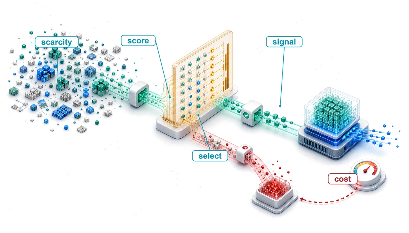
The engineering toolkit for intelligent data selection follows a deliberate optimization ordering, first asking whether a sample is worth processing and only then how to process the remaining workload efficiently. Static pruning acts first by fixing the retained subset before target-model training begins, even when its scoring step uses a smaller proxy model. Because a sample’s usefulness changes as the model learns, dynamic selection then adapts which examples the training loop sees and which receive human labels during training through curriculum learning and active learning. Where real data still falls short after pruning and reordering, synthetic generation creates missing high-value samples on demand through augmentation, simulation, or examples labeled by a larger trained model (a teacher). Learning from unlabeled data complements these three levers by redefining what constitutes a supervision signal: rather than selecting among labeled examples, semi-supervised and self-supervised methods derive learning targets from the structure of unannotated data, and which levers to use, in what order, depends on the workload (figure 1).

Figure 1: An Example Data Selection Pipeline: One possible combination of interventions for increasing data value. The three intervention points are Static Pruning before target training, Dynamic Selection during training, and Synthetic Generation on demand. The sequence is illustrative rather than required: synthetic data can enter independently and can itself be pruned or dynamically selected. The final evaluation determines whether the quality gain justifies the compute cost through the Information-Compute Ratio (ICR).

Two lighthouses carry the chapter, each in its own role. GPT-2 XL, bandwidth-bound when it decodes one token at a time but compute-bound when it trains on long batches (Model Training), carries the wall itself, the compute-optimal diagnosis of whether a run is data-starved, and token-level deduplication. ResNet-50 on ImageNet, the book’s compute-bound lighthouse, carries coresets, labels, augmentation, the input pipeline that must feed it, and the decision of which lever to fund. Its training crosses into an input-bound regime whenever the host cannot decode images as fast as the accelerator consumes them (Pipeline stages and accelerator bubbles), and that crossing returns when selection runs on the machine. The measures of value in the next section use both, and both run on the book’s reference machine, the H100, so every saving can be stated in accelerator seconds and joules. The recommendation lighthouse (DLRM), MobileNetV2, and keyword spotting return only in the closing comparison of section 9.8, where each turns out to be bound by a different resource.

Every lever in the chapter removes work at one stage of the machine and adds work of its own, so each must pass a test before it is accepted (table 1). Each test in the right-hand column depends on measuring what an example is worth, which is the subject of the next section.

Table 1: Chapter Map: Each section of the chapter, the work its lever removes and adds on the machine, and the test the lever must pass before it is accepted.

Section	Lever and when it acts	Work it removes	Work it adds	Test it must pass
Measuring Data Value	Yardsticks for every lever	None	Pilot runs at several data sizes	Defines the tests below
Static Pruning	Deduplication, quality filtering, coreset; before training	Tokens and examples processed in every epoch	Hashing and proxy scoring passes	Selection inequality at matched quality and coverage
Dynamic Selection	Curriculum learning, active learning; during training	Warmup FLOPs; labels	Difficulty scoring, pool scoring rounds, retraining	Time to target quality; label cost against a random baseline
Synthetic Data Generation	Augmentation, generative synthesis, distillation; on demand	Collection and labeling of scarce cases	Host transforms, generator inference, stored teacher targets	Validation on real deployment data
Learning from Unlabeled Data	Semi-supervised and self-supervised learning	Task-specific labels	Extra training compute; pretraining	Total label and compute cost; reuse across tasks
Selection Engineering	Running any lever on the machine	Accelerator idle time	Scoring latency, random reads, worker coordination	The accelerator stays fed and the inequality holds end to end
Choosing a Selection Strategy	Costing the levers and picking among them	Investment in levers that do not pay	Engineering and infrastructure investment	Return on investment over the runs that share it

Self-Check: Question

1. In an ML infrastructure scaling scenario where available GPU compute grows by approximately \(10\times\) every 3 years while high-quality web data grows by only \(2\times\) every 5 years, what primary systems regime emerges, and what is the appropriate systems response?

   1. A compute-rich, data-constrained data wall regime where intelligent data selection and curation must maximize the learning signal extracted per token
   2. A memory bandwidth-bound regime where model parallel sharding must replace data parallelism across all training clusters
   3. An I/O ingestion bottleneck where disk read bandwidth must be quadrupled to keep GPUs saturated
   4. A compute-starved regime where synthetic data generation should be eliminated to avoid wasting accelerator cycles

2. True or False: Doubling the amount of raw, deduplicated web data will always double the total information learned by the model.

3. Order the following stages as they are presented in this chapter’s conceptual map of the data-selection pipeline: (1) Dynamic Selection, (2) Static Pruning, (3) Synthetic Data Generation.

See Answers →

9.2 Measuring Data Value

A ResNet-50 trained on an aggressively filtered ImageNet subset can hold its aggregate accuracy while failing on rare classes that the filter discarded as low-density noise, and a GPT-2 run on a filtered corpus can cost less per epoch while needing more epochs to reach the same loss. A measurement framework is therefore needed to show what a reduction actually saves. Every data selection technique claims to improve efficiency, but only measurement separates genuine training savings from work that has merely moved to another pipeline stage, or from degradation on safety-critical tail distributions. The measures build from the information-compute ratio through a diagnostic of whether a run is data-limited, metrics that tie sample reduction to accuracy, and checks that a reduced set still covers the cases deployment needs, to the selection inequality that every training-time claim must satisfy.

9.2.1 The information-compute ratio

Retaining every example in a training corpus preserves coverage at the cost of spending FLOPs on redundant signal, whereas over-aggressive pruning saves compute at the expense of rare-slice recall. Data selection therefore moves along a Pareto frontier (principle 5) between accuracy and cost, the set of operating points that no alternative beats on one objective without losing on the other. Weighing that trade-off requires measuring how much learning signal each sample yields per unit of hardware work. Data engineering already measured task-relevant signal against one cost, the data gravity of moving bytes, in the data selection gain of equation 4.3. Selection needs the same ratio with training compute in the denominator, because a sample that is cheap to move can still cost a full forward and backward pass. That ratio is the information-compute ratio (ICR).

↪ Locating a model’s operating point on the accuracy-efficiency frontier, and moving along it with compression, is developed in The accuracy-efficiency frontier.

Let \(\FiniteChange\DataInformationContent\) be the learning signal a sample or batch adds and \(\FiniteChange\Operations\) the training operations spent processing it. In practice \(\FiniteChange\DataInformationContent\) is measured as the gain in a fixed evaluation metric, such as percentage points of validation accuracy, so ICR carries units of metric gain per FLOP. The ratio relates the two: \[\text{ICR} = \frac{\FiniteChange\DataInformationContent}{\FiniteChange\Operations}\]

A higher ICR indicates that each FLOP of training yields more measured learning signal over the stated interval. Validation gain and training FLOPs can be observed for a specified experiment with a fixed evaluation protocol; the causal contribution of an individual example generally cannot. Uncertainty and gradient-based scores instead rank candidate examples before their downstream benefit is known. Those rankings require validation against measured quality, compute cost, and deployment-critical slice coverage. The core metrics in section 9.2.4 supply complementary evidence for that evaluation rather than interchangeable measurements of per-example information, and they also track how ICR decays as the dataset grows.

9.2.2 Diminishing returns and the ICR frontier

As a training run adds more examples from the same source, a growing share of those examples repeat patterns the model has already seen, and the information-compute ratio falls. The ICR frontier is the dataset size beyond which the marginal ICR, the learning returned by the next FLOP spent on more data, drops below what that FLOP could return elsewhere: a larger model, a different data source, or an earlier stop.

To illustrate diminishing returns, let \(\DataInformationContent(\DatasetSize)\) be the information content of a dataset of size \(\DatasetSize\) and assume \(\DataInformationContent(\DatasetSize) \propto \log \DatasetSize\). This is a simplified analytical model rather than a universal law. If compute cost scales linearly with the per-sample operation count \(\OperationsPerSample\), then total operations are \(\Operations = \OperationsPerSample \cdot \DatasetSize\), and the resulting marginal ICR follows equation 1: \[\text{ICR}(\DatasetSize) = \frac{\DerivativeOperator\DataInformationContent/d\DatasetSize}{d\Operations/d\DatasetSize} \approx \frac{1/\DatasetSize}{\OperationsPerSample} = \frac{1}{\OperationsPerSample\cdot \DatasetSize} \tag{1}\]

The derivative ratio describes the return on an infinitesimal increase in dataset size. For two controlled finite allocations, the corresponding incremental ratio divides the additional evaluation gain by the additional training FLOPs, using the same evaluation metric and protocol. The coreset comparison that follows instead averages gain over one epoch of each dataset; that average does not establish the return on the next increment.

Under this illustrative model, marginal ICR falls as \(1/(\OperationsPerSample \cdot \DatasetSize)\), so doubling the dataset halves the learning each additional FLOP yields. Inverted, the compute spent per unit of learning grows linearly with \(\DatasetSize\). ICR never reaches zero in this model and the curve has no knee of its own, so the frontier is located by comparing marginal ICR with the threshold the engineer sets, not read off the curve. That saturation is distinct from the data wall (a limit on how much new, high-quality data exists), but the two compound. When new data is scarce and marginal data is weak, selection becomes the main lever. Beyond the frontier, additional data still adds compute but returns less learning than the threshold demands. In this regime additional data inflates the \(\Operations\) term of the iron law without a commensurate gain in ICR. Measured in dollars rather than FLOPs, the same excess lowers the return on compute (RoC) of equation 1.6, the accuracy gained per added dollar of infrastructure.

↩︎ Return on compute, the economic lens that measures accuracy gains against infrastructure spending, is established in Return on compute: Weighing accuracy against cost.

Data selection turns the total operations \((\Operations)\) term in the iron law from a fixed constant into a variable. A 2\(\times\) improvement in measured ICR halves the FLOPs required to reach the same measured gain. It produces the same ideal time reduction as a 2\(\times\) throughput increase only when the workload is compute-bound and the saved work lies on the critical path. ICR focuses specifically on compute; the cost model of section 9.8.1 extends the same reasoning to acquisition, labeling, and storage costs.

The ratio becomes concrete on a coreset, a deliberately selected subset intended to preserve the full dataset’s learning signal. Computing ICR for an ImageNet coreset used to train the ResNet-50 lighthouse shows how large the efficiency gap could become once dataset size, per-sample model cost, and selection strategy meet concrete FLOP budgets. The scenario uses assumed accuracy gains to illustrate the arithmetic; it is not a reported result for the scoring method (EL2N) that section 9.3.4 develops.

Napkin Math 9.1: Computing ICR: Coresets

Problem: Training the ResNet-50 lighthouse model on ImageNet for one epoch costs 3.2 × 10¹⁶ FLOPs. Under the scenario’s assumed accuracy gains, how would retaining 50 percent of the data change the information-compute ratio? The calculation holds the per-sample work fixed and does not include selection overhead.

Setup:

• Dataset: ImageNet (1.28M)
• Model: ResNet-50 lighthouse (~8.2 GFLOP per forward pass, roughly 24.6 GFLOP for a forward plus backward training step, depending on implementation)
• One epoch: 1.28M \(\times\) 24.6 GFLOP = 3.2 × 10¹⁶ FLOPs
• Assumed accuracy improvement per epoch (early training): 5 percentage points

Random selection (baseline):

• Process all 1.28M samples uniformly
• Accuracy gain: 5 percentage points
• \(\text{ICR}_{\text{random}}\) = 5 percentage points / (3.2 × 10¹⁶ FLOPs) = \(1.6 \times 10^{-16}\) per FLOP

Difficulty-scored coreset (EL2N, a training-dynamics score defined in section 9.3.4; 50 percent of data):

• Process 640.6K selected samples
• Assumed accuracy gain: 4.5 percentage points (90 percent of the full-data gain)
• Compute: 640.6K \(\times\) 24.6 GFLOP = 1.6 × 10¹⁶ FLOPs
• \(\text{ICR}_{\text{coreset}}\) = 4.5 percentage points / (1.6 × 10¹⁶ FLOPs) = \(2.9 \times 10^{-16}\) per FLOP

Systems insight: Under these assumptions, the selected subset achieves 1.8× higher ICR with a 0.5 percentage points smaller accuracy gain. The comparison is learning per FLOP over one epoch of each dataset. It does not show that the coreset reaches the full-data run’s final accuracy, which must be checked separately at equal quality, and a real decision also requires measured gains, selection overhead, and coverage checks.

Checkpoint 9.1: Data selection efficiency

The goal is to improve ICR subject to target quality and required coverage, then verify that the resulting pipeline reduces the cost it is intended to address.

Metric checks

• ICR application: Given two training runs with identical accuracy gains but different compute budgets, determine which achieved higher ICR.
• Data efficiency: The coreset notebook reports 1.8× higher ICR but a smaller per-epoch gain. Explain what would have to change for a 50 percent subset to match the full-data gain, which would give it 2\(\times\) higher ICR and so deliver the same measured gain for half the training FLOPs.

Pipeline checks

• The three stages: Map static pruning, dynamic selection, and synthetic generation to the training lifecycle.

A reduction in sample count remains a claim until it is shown to translate into end-to-end efficiency without silently compromising generalization. Notebook 9.1 holds per-sample work fixed and assumes its accuracy gains. Testing the claim on a real workload first requires knowing whether the run is limited by data at all, and then measured metrics that weigh arithmetic savings, data movement overhead, and task quality across the complete pipeline.

9.2.3 The compute-optimal frontier

Pruning a dataset when the model is already starved for unique tokens hurts accuracy rather than saving time, whereas collecting more data for an under-trained model wastes money on collection. Before evaluating any selection technique, a team must therefore test whether the training run is limited by data or by compute. Neural scaling-law experiments (Kaplan et al. 2020; Hoffmann et al. 2022) fit power-law relationships over particular model families, datasets, and compute ranges. Controlled sweeps can use those fitted relationships to compare model and data allocations, though no single ratio diagnoses every training run.

³ Chinchilla: Chinchilla is a 70-billion-parameter language model trained on 1.4 trillion tokens. In the experiments reported by Hoffmann et al. (2022), it outperformed the larger GPT-3 on most evaluated tasks under a similar training-compute budget. The fitted compute-optimal allocation scaled parameters and tokens at roughly equal rates within the study’s experimental regime; it is not a universal prescription for every architecture, dataset, or training recipe.

Hoffmann, Jordan, Sebastian Borgeaud, Arthur Mensch, Elena Buchatskaya, Trevor Cai, Eliza Rutherford, Diego de Las Casas, et al. 2022. “Training Compute-Optimal Large Language Models.” Advances in Neural Information Processing Systems (NeurIPS) 35: 30016–30. https://doi.org/10.52202/068431-2176.

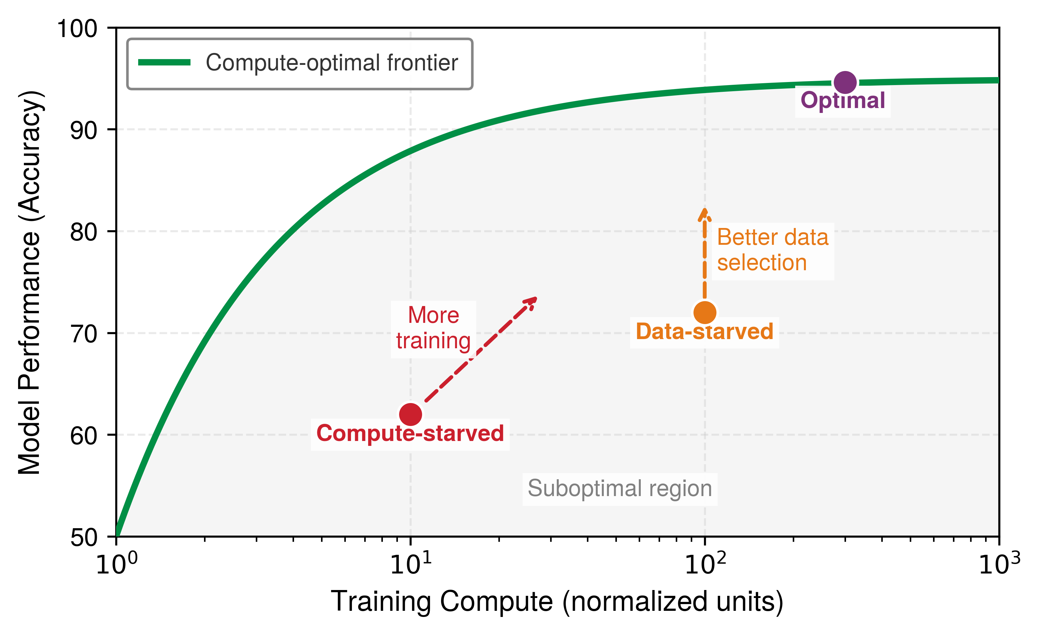
The Chinchilla study³ (Hoffmann et al. 2022) fit a compute-optimal balance between model size and training data within its experimental regime. Allocations on either side of that fitted balance used the study’s compute budget less effectively. The optimal balance defines a compute-optimal frontier: the best achievable performance at each compute budget when data and model size are properly balanced. Plotted over normalized training compute, the frontier separates the optimal operating envelope from the compute-starved and data-starved allocations in the suboptimal region below it (figure 2).

Figure 2: Illustrative Compute-Optimal Frontier: The green curve is a conceptual frontier over normalized compute, not a fitted result from Chinchilla. Points below it illustrate allocations that a controlled model-size and token-count sweep might identify as data- or compute-limited.

The frontier answers one allocation question, whether the next unit of compute at a given budget should go to more parameters or to more training tokens. A run is data-starved when it trains on too few unique, useful tokens for its parameter count, so its tokens-per-parameter ratio sits well under the fitted balance, and the same compute would yield more accuracy with more or better data. Against a frontier fitted from controlled sweeps, an operating point’s location motivates further experiments. The directional vectors charted in figure 2 illustrate two candidate interventions: additional training compute and improved data selection at fixed compute. Controlled changes to model size, data, and training allocation determine which intervention helps; a point below the frontier does not identify a unique remedy. Points near a fitted frontier remain specific to the model family, dataset, objective, and compute range used to estimate it.

Interpreting the Chinchilla result

Within the fitted Chinchilla regime, compute-optimal model parameters and training tokens grew at roughly equal rates.⁴ Training a dense transformer costs approximately \(6\Parameters\DatasetSize\) FLOPs for \(\Parameters\) parameters and \(\DatasetSize\) tokens, the forward-plus-backward accounting derived for the GPT-2 lighthouse in Running cases: GPT-2 XL and ResNet-50. Under an equal scaling regime where parameters and tokens grow proportionally (\(\Parameters \propto \DatasetSize\)), total compute scales quadratically (\(\Operations \propto \DatasetSize^2\)), directly implying that optimal token count scales as the square root of the compute budget (\(\ComputeOptimalTokenCount \propto \sqrt{\Operations}\)). Doubling compute therefore corresponds to about \(\sqrt{2} - 1\), or 41.4 percent, more tokens under those assumptions. The commonly quoted 20 tokens per parameter is a useful reference point from that study, not a universal optimum.

⁴ Tokens per parameter: The ratio \(\DatasetSize/\Parameters\) compares training tokens with model parameters; GPT-3 used approximately 1.7 tokens per parameter (Brown et al. 2020), while Llama 2 70B used approximately 28.6 (Touvron et al. 2023). These descriptive ratios do not establish whether either run is compute-optimal under a different architecture, corpus, objective, or hardware budget. Controlled model-size and token-count sweeps are required for that diagnosis.

Brown, Tom B., Benjamin Mann, Nick Ryder, Melanie Subbiah, Jared Kaplan, Prafulla Dhariwal, Arvind Neelakantan, et al. 2020. “Language Models Are Few-Shot Learners.” Advances in Neural Information Processing Systems 33: 1877–901. https://doi.org/10.48550/arxiv.2005.14165.

Touvron, Hugo, Louis Martin, Kevin Stone, Peter Albert, Amjad Almahairi, Yasmine Babaei, Nikolay Bashlykov, et al. 2023. “Llama 2: Open Foundation and Fine-Tuned Chat Models.” arXiv Preprint arXiv:2307.09288.

GPT-2 sits well short of that reference. WebText supplies about 6.7 unique tokens per parameter, a third of the fitted balance, and the original run made up the difference by repeating those tokens about 17 times (section 9.1). Repetition keeps the arithmetic budget but not the learning per FLOP, which is the regime where selection, rather than more compute, moves the run toward the frontier.

Applying the diagnostic

If a training run underperforms expectations, extending one run can reveal whether additional optimization steps still help, but a plateau does not identify data starvation by itself. Learning-rate schedules, optimization limits, model capacity, and data quality can all produce a plateau. A reliable diagnosis compares controlled runs that vary model size, token count, and compute allocation while holding the evaluation protocol fixed. When controlled runs do point to the data, the remedy that keeps compute fixed is better selection, which changes the shape of the learning curve itself. Seeing that change requires switching axes, from the frontier’s training compute to dataset size, where the core metrics measure what a reduction preserves.

9.2.4 Core metrics

Reporting accuracy at a single subset size hides whether a selection method learned faster early on, plateaued lower, or never reached the full dataset’s target quality. Three metrics track those distinct behaviors across the learning curve and complement the measured information-compute ratio (section 9.2.1). Performance-per-data (PPD) measures average accuracy gain per sample, which becomes gain per FLOP once per-sample cost is fixed; the area under the learning curve (AULC) summarizes performance across a common dataset-size range; and the data compression ratio (DCR) measures retained sample reduction at a fixed target accuracy. None of the three establishes the causal value of an individual example.

Performance-per-data

The most direct metric, performance-per-data (PPD), measures accuracy gain per sample: \[ \text{PPD}(\LearningCurveSampleCount) = \frac{\text{Accuracy}(\LearningCurveSampleCount) - \text{Accuracy}(0)}{\LearningCurveSampleCount} \] where \(\LearningCurveSampleCount\) is the number of training samples. A higher PPD indicates greater average improvement per sample over the stated interval. Its shape must be measured because diminishing returns and their onset are workload-dependent.

Area under the learning curve

Rather than comparing at a single point, the area under the learning curve (AULC) integrates performance across all dataset sizes: \[ \text{AULC} = \int_0^\DatasetSize\text{Accuracy}(\LearningCurveSampleCount) \, d\LearningCurveSampleCount\] where \(\LearningCurveSampleCount\) is the dataset size and \(\DatasetSize\) is the total dataset size.

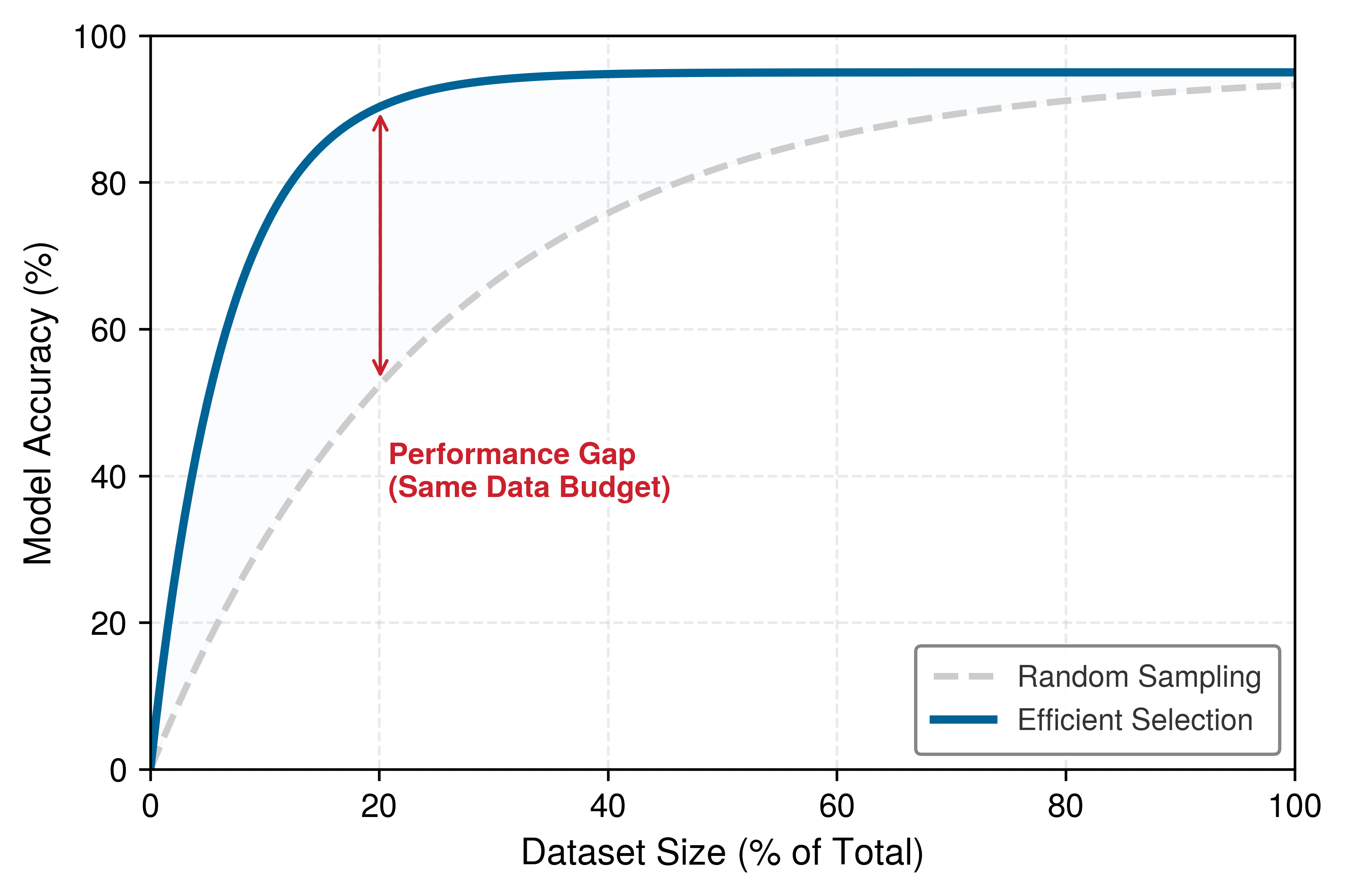
For the same metric and integration range, a higher AULC means stronger integrated performance across dataset sizes, though one strategy need not outperform the other at every size. Comparisons must use the same upper limit \(\DatasetSize\) or normalize the integral. Measuring AULC requires training at several dataset sizes, so the metric itself spends compute, and when it guides a selection decision that cost belongs to the selection overhead.

In the illustrative curves of figure 3, efficient selection bends into an accuracy plateau near 25 percent of the data while uniform random sampling climbs gradually across the entire budget, so over the same range the efficient curve encloses the larger area. The horizontal separation between the curves is the reduction in required samples, and at an identical 20 percent data budget the vertical gap is the accuracy that selection adds without any additional compute.

Figure 3: Illustrative Diminishing Returns of Data: The synthetic data-efficient curve (blue) reaches the same plateau with fewer samples than random sampling (gray). The vertical red arrow marks the modeled performance gap at a fixed dataset size; measured curves need not have this shape.

Data compression ratio

For coreset methods, the data compression ratio (DCR) measures how much data reduction is achieved at a target accuracy: \[ \text{DCR} = \frac{\FullDatasetSize}{\SubsetDatasetSize} \text{ at } \text{Accuracy}_{\text{target}} \]

A DCR of 5\(\times\) means the coreset achieves target accuracy with 20 percent of the data. Applied to the coreset notebook, the three metrics behave differently. Over one epoch, the full ImageNet set gains 5 percentage points while the half-size coreset gains 4.5 percentage points, so the coreset’s PPD is higher by the same 1.8× as its ICR, because per-sample work is fixed. DCR cannot be computed from that notebook at all, because the two runs never reach a common target accuracy. Exposing that missing equal-quality check is exactly the job DCR is designed for, and even when a reduced dataset matches the full dataset’s aggregate accuracy, those learning-curve metrics cannot show whether the retained subset still covers every slice deployment needs.

9.2.5 Validating a reduced dataset

When the half-size ImageNet coreset drops 640,000 images, it can hold top-1 test accuracy while quietly stripping out a rare class, shifting the training distribution away from production traffic, or concentrating mislabeled examples in the retained subset. Validating a curated dataset therefore requires checking coverage, distribution alignment, and label quality alongside aggregate accuracy. Coverage metrics check whether coreset selection kept enough examples from each class and demographic group. Even when class counts hold, the retained subset can skew toward atypical examples, so distribution alignment metrics (such as KL divergence and the population stability index, the drift statistics of Data drift detection and response) test whether the curated training set has drifted from the deployment distribution. Where selection also guides annotation, label quality metrics (inter-annotator agreement and confident learning, which flags examples whose given label disagrees with a model’s confident out-of-sample prediction) verify that active learning did not introduce systematic labeling errors. A 50 percent dataset reduction is worth keeping only when all three checks pass alongside target accuracy, calibration, and robustness.

↪ Coverage, label-quality, and distribution-alignment checks are developed into a full data-benchmarking protocol in Data benchmarking.

The validation target can itself be unreliable. Benchmark accuracy can overstate generalization when test sets fail to capture operational distribution shifts, demanding the same scrutiny for evaluation benchmarks as for curated training sets.

Example 9.1: The benchmark replication gap

Scenario: Classifiers evaluated on newly collected test sets experienced 3 to 15 percentage-point accuracy drops on CIFAR-10 and 11 to 14 points on ImageNet (Recht et al. 2019).

Diagnosis: The replicated collection produced slightly harder images than the original test sets. The study found that benchmark adaptivity did not explain the gap, even though repeated use of a fixed test set remains a general evaluation risk.

Systems lesson: Evaluation-set construction affects measured generalization. Data-selection pipelines should validate curated subsets on independently collected and deployment-relevant test sets rather than trusting one long-reused benchmark.

Recht, Benjamin, Rebecca Roelofs, Ludwig Schmidt, and Vaishaal Shankar. 2019. “Do ImageNet Classifiers Generalize to ImageNet?” Proceedings of the 36th International Conference on Machine Learning (ICML), 5389–400.

An efficiency gain measured against a single benchmark can evaporate under distribution shift, so a curated subset must demonstrate consistent quality across multiple held-out distributions before its reported reduction ratio is trusted. Even when quality holds across those distributions, the time spent selecting the subset must still be weighed against the training time it saves.

9.2.6 The selection inequality

The efficiency measures so far count learning against training compute alone, yet a selection method also spends time choosing, and a claim that it shortens training must count that time. To reduce overall training time at a fixed quality target, selection plus subset training must take less time than training on the full corpus. Let \(\SelectionTime\) be total wall-clock selection overhead, including candidate scoring and any prerequisite scorer preparation charged to the training run. Let \(\TrainingTime(\DatasetSize)\) be wall-clock training time for a dataset of size \(\DatasetSize\), and let \(\SubsetDatasetSize\) and \(\FullDatasetSize\) be the retained and full sample counts. Equation 2 formalizes this break-even condition as the selection inequality: \[ \SelectionTime+ \TrainingTime(\SubsetDatasetSize) < \TrainingTime(\FullDatasetSize) \tag{2}\]

Equivalently, isolating the allowable selection overhead yields \(\SelectionTime< \TrainingTime(\FullDatasetSize) - \TrainingTime(\SubsetDatasetSize)\). The upper bound on selection latency depends strictly on how much training execution the subset eliminates; no arbitrary overhead fraction applies across workloads. When an engineering pipeline can amortize scorer preparation or checkpoint extraction across multiple downstream training runs (section 9.8.3), \(\SelectionTime\) reflects only the marginal scoring pass over the candidate pool. Conversely, if an auxiliary proxy must be trained from scratch for a single isolated run, that preparatory compute adds directly to \(\SelectionTime\). When \(\SelectionScoreFunction(\ModelInput)\) repeatedly scores the candidate pool with the full target model, those extra scoring passes and their cross-worker coordination can take longer than the training steps they remove, making the run slower overall.

Example 9.2: Selection inequality in practice

Scenario: A computer vision team selects a 128,117-image coreset (10 percent) from the 1.28 million ImageNet training images to shorten ResNet-50 training on one H100 sustaining 25 percent of its peak, the training chapter’s compute-bound rate. Pretrained checkpoints for both the target architecture and a lightweight proxy are already available from earlier exploration, so this comparison accounts only for a marginal scoring pass over the candidate pool.

Diagnosis: Against a 211-minute full-data run of 100 epochs, marginal full-model scoring (Option A: target ResNet-50) adds 42 seconds of selection overhead and still saves 188.8 minutes (89.7 percent). Marginal proxy-model scoring (Option B: ResNet-18) drops selection overhead to 18 seconds and saves 189.1 minutes (89.9 percent), only 24 seconds more.

Systems lesson: Both options satisfy the selection inequality by a wide margin, because a single scoring pass costs at most one forward pass over the dataset (one-third of a full-data epoch for the target ResNet-50) and less with the proxy, while training on the 10 percent coreset shrinks every one of the 100 epochs. Scorer choice also becomes decisive when selection rescores dynamically every epoch or when the scoring architecture is significantly larger than the target, multiplying selection latency while subset training savings remain fixed.

End-to-end wall-clock time divides into selection overhead and subset training, and the split decides the outcome across three regimes (figure 4): lightweight proxy scoring limits selection overhead to 5 percent while training on the 40 percent subset (yielding 55 percent net savings), whereas heavyweight scoring expends 60 percent overhead on selection, wiping out all subset-training efficiency gains.

Figure 4: The Selection Inequality: In this illustrative example, data selection only improves end-to-end training time at matched quality if the overhead of selection plus training on the subset is less than training on the full dataset. A lightweight selection function (proxy model, cached embeddings) keeps selection overhead low; an expensive selection function (full model forward pass) can negate the savings.

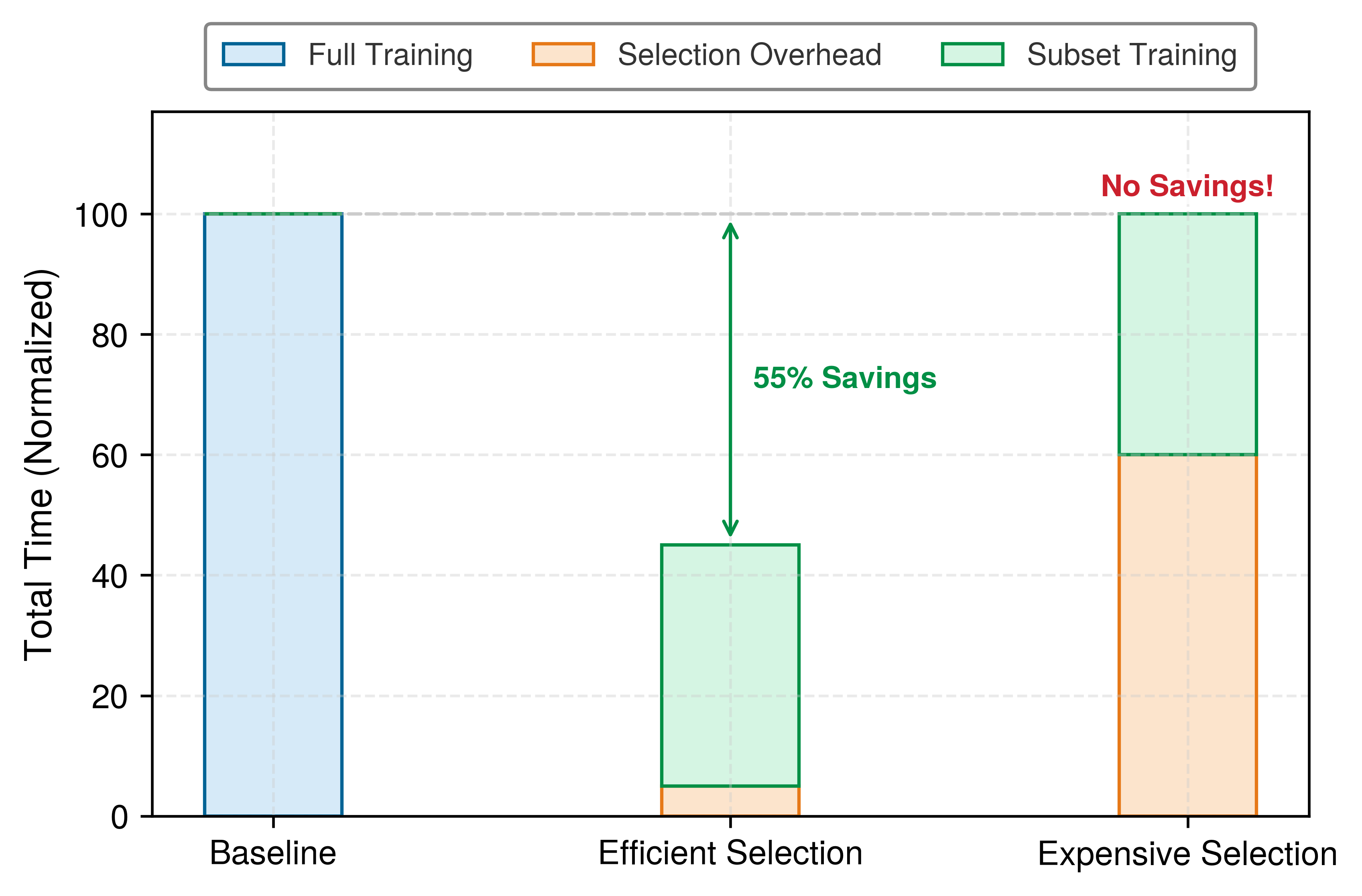
This overhead compounds when selection runs dynamically across epochs rather than once offline. If per-epoch rescoring approaches the training work saved by the pruned subset, the net systems advantage vanishes. Measured this way, a selection strategy is judged against its stated objective, counting the overhead of scoring, filtering, and staging samples alongside the training, labeling, or reuse savings it claims at target quality. Teams that optimize selection algorithms against isolated benchmarks rather than end-to-end pipeline constraints find that intuitive heuristics backfire: scoring overhead consumes accelerator cycles, optimization trajectories destabilize, or generalization silently degrades. These measures apply to the three levers in the order in which they act, and static pruning comes first because it fixes the subset before target-model training, though its scoring process may use a trained proxy.

Self-Check: Question

1. Under the illustrative analytical model where dataset information content scales as \(\mathcal{I}(D) \propto \log D\) and training compute scales linearly as \(O = O_{\text{sample}} \cdot D\), how does the marginal Information-Compute Ratio \(\mathrm{ICR}(D)\) scale with dataset size \(D\)?

   1. It remains constant at \(\mathcal{O}(1)\) because additional compute scales proportionally with dataset size
   2. It decays as \(\mathcal{O}\!\left(\frac{1}{O_{\text{sample}}D}\right)\), so under this illustrative model additional data eventually adds compute faster than marginal information
   3. It grows logarithmically as \(\mathcal{O}(\log D / O_{\text{sample}})\) due to power-law parameter scaling
   4. It decays exponentially as \(\mathcal{O}(\exp(-D))\) once the training corpus exceeds accelerator memory capacity

2. Explain why a dataset where \(100\%\) of the sample labels are verifiably correct can still exhibit a very low Information-Compute Ratio (ICR).

3. An ML systems diagnostic plot maps normalized training compute on the horizontal axis against model performance on the vertical axis. A 10M-parameter run sits well below a fitted frontier under a fixed evaluation protocol and fixed total budget. A controlled sweep then shows that reallocating the same budget toward a larger model improves performance. What is the most defensible diagnosis of the original operating point?

   1. Data-starved regime
   2. I/O bandwidth-saturated regime
   3. The model/data allocation was suboptimal under the tested budget
   4. Over-echoing regime

4. A team wants one metric for how much smaller a selected dataset is at a target accuracy, and another for how much learning is gained per sample over a measured interval. Which pair of chapter metrics matches that need?

   1. Data Curation Rate and Accuracy Reduction Ratio
   2. Data Compression Ratio and Performance-Per-Data
   3. Dynamic Checkpoint Rate and Active Retention Rate
   4. Data Convergence Ratio and Amortized Risk Ratio

5. Why is Area Under the Learning Curve (AULC) a more informative metric than single-point final validation accuracy when comparing data selection methods across dataset sizes?

6. A training team reduces a dataset from \(1{,}000{,}000\) to \(100{,}000\) images. Full-data training takes 10 hours, subset training takes 1 hour, and scoring the full pool with the production model takes 12 hours. Which conclusion and next step best fit the selection inequality?

   1. Yes, the inequality is satisfied because a \(90\%\) dataset reduction guarantees positive ROI
   2. Yes, because the 9 hours saved in training outweigh the scoring cost; the team only needs more GPUs
   3. No, because \(12+1=13\) hours exceeds the 10-hour baseline; a plausible fix is proxy scoring or cached embeddings, but the team must verify that scoring drops below 9 hours while target quality holds
   4. No, because coreset training always increases memory-bandwidth consumption; the team should switch from NVMe SSDs to HDDs

See Answers →

9.3 Static Pruning

Web-scale scraping routinely gathers boilerplate text, duplicate images, and malformed records, and each one costs GPT-2 six FLOPs per parameter for every token, or ResNet-50 a full forward and backward pass, before a single useful gradient is calculated. Static pruning removes these low-value records upstream of the training loop. By dropping redundant and corrupt records before target-model training begins, static pruning shrinks the operation count \((\Operations)\) without changing model architectures or execution kernels.

9.3.1 The case for smaller datasets

In many training runs, a large fraction of examples contributes almost no gradient signal while still costing a full forward and backward pass. Empirical scaling studies confirm that dataset volume alone does not determine model accuracy, because large corpora carry substantial redundancy. On CIFAR-10, Paul et al. (2021) report that EL2N pruning (which scores each example by its prediction error early in training) removed half of the training data without reducing accuracy. On ImageNet-1K, Sorscher et al. (2022) report that a self-supervised prototype metric discarded 20 percent of the data without sacrificing performance. The pattern extends to language modeling, where web-scraped corpora like The Pile⁵ and C4⁶ contain enough duplicate and templated content to make deduplication a systems issue. In the datasets studied by Lee et al. (2022), deduplicated training reduced memorization while preserving or improving perplexity. Still, these reported gains are benchmark-specific: pruning effectiveness depends on how redundant the dataset is, which selection algorithm is used, and the capacity of the target model, so teams must validate aggressive pruning on their own task before committing to it.

Sorscher, Ben, Robert Geirhos, Shashank Shekhar, Surya Ganguli, and Ari S. Morcos. 2022. “Beyond Neural Scaling Laws: Beating Power Law Scaling via Data Pruning.” Advances in Neural Information Processing Systems (NeurIPS) 35: 19523–36. https://doi.org/10.52202/068431-1419.

⁵ The Pile: An approximately 886 GB English text corpus (reported as 825 gibibytes by the source) aggregating twenty-two sub-datasets, including PubMed, ArXiv, GitHub, Project Gutenberg, Common Crawl, Stack Exchange, Wikipedia, and USPTO patents (Gao et al. 2020). Its multi-source design makes it a useful example of data diversity: each source family has a different duplication, quality, and domain-coverage profile, so selection pipelines must preserve coverage while removing redundant text.

Gao, Leo, Stella Biderman, Sid Black, Laurence Golding, Travis Hoppe, Charles Foster, Jason Phang, et al. 2020. “The Pile: An 800GB Dataset of Diverse Text for Language Modeling.” arXiv Preprint arXiv:2101.00027.

⁶ C4 (Colossal Clean Crawled Corpus): C4 applies filtering to Common Crawl data, including language detection, deduplication of repeated three-sentence spans, and removal of pages that fail heuristic quality checks, producing approximately 750 GB of cleaned English text (Raffel et al. 2020). Filtering has its own compute cost and can remove useful material, so its ROI and quality effects must be measured rather than inferred from corpus size alone.

Raffel, C., N. Shazeer, A. Roberts, K. Lee, S. Narang, M. Matena, Y. Zhou, W. Li, and P. J. Liu. 2020. “Exploring the Limits of Transfer Learning with a Unified Text-to-Text Transformer.” Journal of Machine Learning Research 21 (140): 1–67.

Individual data points need not provide equal value for training. This heterogeneity follows in part from how classifiers learn decision boundaries. Many samples fall far from a boundary: a picture of a dog in good lighting may become easy once the model has learned its dominant features, while ambiguous and underrepresented cases can remain informative. Label quality also affects data requirements. Conflicting labels can push updates in opposing directions, so reaching a target error may require more examples or more passes over them. The size of that penalty depends on the task and training procedure. A data quality multiplier therefore comes from comparing learning curves at the same held-out error, rather than assigning a universal convergence rate to all noisy data.

Napkin Math 9.2: The data quality multiplier

Problem: Two hypothetical pilot learning curves reach the same held-out error using different amounts of clean and noisy data. With epoch count and per-sample work held fixed, what training-work multiplier do these sample counts imply?

Setup: Consider a representative evaluation where a fixed model architecture and training recipe reach target error \(\TargetError\) = 0.01 (1 percent) under clean versus noisy training partitions:

• Clean data: \(\CleanLabelSampleCount\) = 10,000
• Noisy data: \(\NoisyLabelSampleCount\) = 16,000

Result: Dividing the noisy-data count by the clean-data count gives 1.6×. Under the fixed training recipe, the noisy dataset therefore requires 1.6× as much training work to reach the same error.

Systems insight: The avoided training work sets a budget for cleaning. Cleaning pays for itself only when correction or review costs less than the work it removes, with required coverage preserved. If the two learning curves require different epoch counts, compare total examples processed to the target instead of unique sample counts. The decision depends on measured learning curves and pipeline costs, not on the presence of noise alone.

9.3.2 Data deduplication

The cheapest samples to remove are the ones that repeat what the dataset already contains. Repeated content costs a full forward and backward pass on every presentation, even when that repetition adds little useful learning signal. Exact hashing and shingle-based near-duplicate detection can identify candidates for removal without training a scoring model. Deduplication therefore comes first among the static levers, but near-duplicate thresholds must be validated so the pipeline does not remove useful distributional signal.

The simplest form of deduplication uses hash-based methods for exact matches. By computing a cryptographic hash (MD5 or SHA-256) for each sample and removing those with identical hashes, practitioners can eliminate the byte-for-byte duplicates that accumulate in large web-scraped corpora. This process is computationally cheap, scaling linearly with dataset size, and can be parallelized trivially.

↩︎ Deduplication as a deterministic data-cleaning step that keeps training and serving pipelines consistent is established in Training-serving consistency.

⁷ MinHash: Invented by Broder (1997) to detect duplicate web pages for AltaVista, the algorithm creates compact signatures using random hash functions such that similar documents produce similar signatures with high probability. Each signature compresses a document to a fixed-size sketch, enabling pairwise similarity estimation in \(\mathcal{O}(\MinHashSketchSize)\) time for sketch size \(\MinHashSketchSize\).

Broder, A. Z. 1997. “On the Resemblance and Containment of Documents.” Proceedings. Compression and Complexity of SEQUENCES 1997 (Cat. No.97TB100171), 21–29. https://doi.org/10.1109/sequen.1997.666900.

⁸ Locality-sensitive hashing (LSH): LSH hashes MinHash signatures into buckets so that similar signatures are more likely to collide. Candidate generation avoids an exhaustive all-pairs comparison, while runtime and memory depend on signature width, banding, bucket sizes, and the number of candidates that require verification.

⁹ Jaccard similarity: Defined as \(|\FirstJaccardSet\cap \SecondJaccardSet| / |\FirstJaccardSet\cup \SecondJaccardSet|\) for two sets \(\FirstJaccardSet\) and \(\SecondJaccardSet\), ranging from 0 (disjoint) to 1 (identical). For deduplication, the metric compares sets of shingles across documents of different lengths. The threshold must be calibrated for the shingle definition, corpus, and downstream quality because no universal cutoff separates duplicates from legitimately related documents.

Near-duplicate detection addresses content that differs at the byte level while retaining substantial token- or character-shingle overlap. For text, MinHash⁷ with Locality-Sensitive Hashing⁸ (LSH) approximates Jaccard similarity⁹ efficiently. In practice, the pipeline converts each document into a set of overlapping character or word \(\ShingleLength\)-shingles, compresses these sets into fixed-length MinHash signatures where the probability of hash collision equals Jaccard similarity, and partitions the signatures into \(\LshBandCount\) bands of \(\LshRowsPerBand\) rows using LSH. Documents matching across all rows in any single band collide in the same bucket, restricting expensive similarity verification to likely candidates and avoiding an impossible \(\mathcal{O}(\DatasetSize^2)\) all-pairs comparison across a corpus of \(\DatasetSize\) web documents numbering in the billions. It can detect lightly edited content with high overlap, but it does not establish semantic paraphrase equivalence.

For images, perceptual hashing produces signatures robust to minor transformations like resizing and compression, identifying visually similar candidates stored in different formats. Embedding-based similarity can retrieve semantic near-neighbor candidates by computing dense representations (CLIP¹⁰ (Radford et al. 2021) for images, sentence transformers for text), though proximity does not itself prove duplication and the approach incurs higher computational overhead. Across both modalities, deduplication can reduce repeated-content memorization and avoid spending FLOPs on exact or near duplicates, yet it can also alter the corpus’s intentional empirical weighting, so thresholds and downstream quality must be validated rather than assuming that every duplicate is harmful.

¹⁰ CLIP (Contrastive Language-Image Pretraining): Pretrained on 400 million image-text pairs, CLIP maps semantically related images and text into a shared embedding space (Radford et al. 2021). Embeddings can retrieve candidates for review, but semantic proximity is not proof that two samples are duplicates. Generating embeddings also costs substantially more than computing perceptual hashes, with the ratio depending on model and hardware.

Radford, Alec, Jong Wook Kim, Chris Hallacy, Aditya Ramesh, Gabriel Goh, Sandhini Agarwal, Girish Sastry, et al. 2021. “Learning Transferable Visual Models from Natural Language Supervision.” International Conference on Machine Learning (ICML), 8748–63.

On GPT-2’s run, deduplication costs little and returns hours of accelerator time. Lee et al. (2022) found that near-duplicate removal affected between 3.04 percent (C4) and 13.63 percent (RealNews) of the corpora they studied. If WebText carried a comparable share, removing it would cut the same fraction of the 167 billion tokens GPT-2 processed, saving about 3 hours to 14 hours of the 4.4 days that one eight-H100 machine needs, or 18 kWh to 80 kWh of accelerator energy. Finding the duplicates reads the 40 GB corpus once, about 6 seconds at the 7 GB/s of the machine’s local NVMe storage, and holds a 128-hash MinHash signature for each of WebText’s roughly 8 million documents, about 4.1 GB of host memory. Hashing runs on host CPUs rather than on the accelerators, so the cost of deduplication lands on a different stage of the machine from the work it removes; the open question for a corpus this size is which near-duplicates are safe to remove, not whether the machine can afford to find them. Once those duplicates are gone, the next target is records that are unique but broken.

9.3.3 Data pruning by quality

A unique training example can still waste compute or actively damage the model if its content is garbled or its label contradicts the true class. Quality-based pruning removes samples that carry no usable signal or push gradients in the wrong direction. In supervised datasets, label error detection is often the highest-return form of quality pruning. Tools like Cleanlab identify samples where the assigned label may be incorrect based on model confidence patterns across training: a sample that the model consistently predicts as class A while its label says class B may be a hard boundary case, a distribution shift, a model blind spot, or an annotation mistake. Because those causes call for different remedies, the score should trigger review rather than automatic deletion, so confirmed errors can be corrected or removed without discarding hard examples.

Where label error detection checks whether the target contradicts the input, outlier removal checks whether the input itself sits far from any cluster center in feature space. Such points can indicate sensor noise, annotation errors, or file corruption, whereas in heavy-tailed domains they can also be the rare edge cases that define deployment risk, so outlier thresholds must stay conservative and the affected slices should be reviewed before removal.

Unlabeled pretraining corpora have no class labels to audit, so low-information filtering instead applies domain-specific heuristics to drop samples that carry too little signal to justify a training step. For text corpora, pipelines remove high-perplexity garbled strings (perplexity measures how surprising a text is to a language model, so high values can flag incoherent text as well as valid specialist or rare-language writing) alongside low-perplexity boilerplate or repetitive templates; for image datasets, they filter blurry, corrupted, or near-uniform frames. Because hand-written heuristics can miss subtler quality differences across billions of documents, industrial pretraining pipelines pair them with classifier-based filtering, which trains a lightweight linear classifier (such as fastText) using curated reference text (e.g., Wikipedia, books, and scientific papers) as positive examples and uncurated web dumps as negative examples. The classifier assigns each scraped document a continuous quality score, allowing the pipeline to drop millions of low-quality pages at gigabyte-per-second ingestion speeds before ranking the clean examples that remain.

9.3.4 Coreset selection algorithms

Once duplicates and defective records are gone, the remaining samples are unique and valid but still unequal in value, which is the heterogeneity described in section 9.3.1. Ranking them requires systematic selection criteria. Coreset selection¹¹ turns the static pruning decision into a coverage problem: keep the smallest subset that preserves the statistical properties of the entire dataset. The systems decision is where to spend the selection budget, whether on cheap coverage metrics that preserve distributional structure or on costlier training-dynamics scores that better target the decision boundary. That decision also needs a guardrail before any score is applied: classes, demographic groups, time windows, and rare failure modes that matter at deployment require minimum representation, because the highest-average-ICR subset can still remove the examples that define production risk.

¹¹ Coreset (core set): In computational geometry, a small subset can approximate a specified geometric objective within a controlled error factor (Agarwal et al. 2005). Machine learning adapts this idea as a selection principle, but a guarantee for an embedding and distance objective does not by itself guarantee neural-network accuracy. The retained subset must still be validated on the target task.

Agarwal, Pankaj K., Sariel Har-Peled, and Kasturi R. Varadarajan. 2005. “Geometric Approximation via Coresets.” In Combinatorial and Computational Geometry, edited by Jacob E. Goodman, János Pach, and Emo Welzl, vol. 52. MSRI Publications. Cambridge University Press. https://doi.org/10.1017/9781009701259.002.

¹² k-center algorithm: Its greedy strategy iteratively picks the point farthest from the existing centers under a chosen embedding and metric. Sener and Savarese use this core-set framing for convolutional-neural-network active learning (Sener and Savarese 2018). The resulting coverage bound applies to that geometric objective, not directly to downstream accuracy or rare-class preservation.

Sener, Ozan, and Silvio Savarese. 2018. “Active Learning for Convolutional Neural Networks: A Core-Set Approach.” International Conference on Learning Representations (ICLR).

Welling, Max. 2009. “Herding Dynamical Weights to Learn.” Proceedings of the 26th Annual International Conference on Machine Learning, 1121–28. https://doi.org/10.1145/1553374.1553517.

Geometry-based methods select samples that cover a chosen representation without requiring target-model training. The \(\CenterCount\)-Center algorithm,¹² a facility-location-style objective, selects samples that reduce the maximum distance from any point to its nearest selected center under the chosen embedding and metric. Herding takes a different approach: Welling’s original procedure iteratively constructs representative pseudo-samples whose feature statistics approximate observed moments (Welling 2009), and related moment-matching objectives can guide subset selection from a fixed pool. These methods are computationally attractive because they operate on feature representations, but their scores are not inherently label-aware.

Training-dynamics methods use a proxy model to identify examples that may be important. GraNd (Gradient Normed) and EL2N (error L2-norm)¹³ score samples by gradient magnitude or prediction error early in training (Paul et al. 2021). The exact alternative, influence functions (Koh and Liang 2017), measures how removing a sample changes validation loss, but it requires the inverse Hessian \(\LossHessian^{-1}\) of the loss across all \(\Parameters\) parameters, with \(\mathcal{O}(\Parameters^2)\) memory and \(\mathcal{O}(\Parameters^3)\) arithmetic, which rules it out for models with millions or billions of parameters.

¹³ EL2N (error L2-norm) and GraNd (gradient normed): These methods score samples based on their error or gradient norm early in training, identifying samples the model finds most difficult. The practicality of this approach relies on transferability, where scores from a small proxy model can guide data selection for a much larger target model. For instance, a proxy trained for five epochs can generate scores to curate a dataset for a full 90-epoch production training run (Paul et al. 2021).

Paul, Mansheej, Surya Ganguli, and Gintare Karolina Dziugaite. 2021. “Deep Learning on a Data Diet: Finding Important Examples Early in Training.” Advances in Neural Information Processing Systems (NeurIPS) 34: 20596–607.

Koh, Pang Wei, and Percy Liang. 2017. “Understanding Black-Box Predictions via Influence Functions.” International Conference on Machine Learning (ICML), Proceedings of machine learning research, vol. 70: 1885–94.

¹⁴ Forgetting events: This method identifies valuable examples by tracking when the model “forgets” them, transitioning from a correct to an incorrect classification during training. The central trade-off is the high cost of this analysis, which requires a full training run. However, the resulting importance scores can transfer from small proxy models to larger target models (for example, ResNet-18 to ResNet-50), enabling inexpensive proxy-based selection when ranking quality holds for the target task (Toneva et al. 2019).

Toneva, Mariya, Alessandro Sordoni, Remi Tachet des Combes, Adam Trischler, Yoshua Bengio, and Geoffrey J Gordon. 2019. “An Empirical Study of Example Forgetting During Deep Neural Network Learning.” International Conference on Learning Representations (ICLR).

Systems methods circumvent this barrier by relying on lightweight first-order approximations: GraNd scores samples using expected gradient norm (\(\|\nabla_\ModelParameters\LossFunction\|_2\)), while EL2N observes that early in training, the gradient norm with respect to linear layers is strongly correlated with output prediction error (\(\|\PredictedOutput - \LabelVector\|_2\), the distance between the predicted probability vector \(\PredictedOutput\) and the one-hot label \(\LabelVector\)). This enables practitioners to score prediction error using a single forward pass without computing backward-pass gradients. Error and uncertainty differ: a confident prediction of the wrong class can have high EL2N despite low predictive uncertainty. High scores identify examples the proxy finds difficult, but they can also identify noise or unrepresentative samples and therefore need coverage and quality checks. The same work reports useful score transfer across several architectures, which can enable less expensive proxy-based selection. A third training-dynamics signal, forgetting events,¹⁴ tracks how often a sample is correctly classified and later misclassified during training (Toneva et al. 2019).

Each algorithm in table 2 balances upfront scoring computation against downstream training reduction. Because geometry-based and training-dynamics methods optimize different proxies, their relative ranking depends on dataset scale, feature representations, target model capacity, and scoring budgets; a score is computationally justified only when downstream training savings exceed evaluation overhead.

Table 2: Coreset Selection Algorithm Comparison: \(\DatasetSize =\) dataset size, \(\CoresetBudget=\) coreset size. Geometry-based and training-dynamics methods optimize different proxies, so their quality ranking depends on the dataset, representation, target model, and scoring budget.

Method	Compute Cost	Requires Training	Best For	Limitation
k-Center	\(\mathcal{O}(\DatasetSize^2)\) or \(\mathcal{O}(\DatasetSize \CoresetBudget)\)	No	Coverage, exploration	Ignores label information
Herding	\(\mathcal{O}(\DatasetSize \CoresetBudget)\)	No	Distribution matching	Matches chosen moments
GraNd	\(\mathcal{O}(\text{epochs} \times \DatasetSize)\)	Yes (few epochs)	Decision boundaries	Requires proxy training
EL2N	\(\mathcal{O}(\text{epochs} \times \DatasetSize)\)	Yes (few epochs)	Error-based scoring	Can rank noise as hard
Forgetting	\(\mathcal{O}(\text{full training})\)	Yes (full)	Hard examples	Expensive to compute

Geometry-based methods prioritize coverage in a chosen feature representation, while training-dynamics methods use signals such as error or forgetting. Uncertainty sampling, which active learning uses as a query rule (section 9.4.2), concentrates the budget near the current decision boundary; EL2N instead ranks prediction error, which can also be high for confidently wrong examples away from the boundary. Figure 5 contrasts that boundary-focused allocation with uniform random sampling of the same five-point budget. It illustrates one family of selection rules; a geometry-based method such as \(\CenterCount\)-center would instead spread its picks to cover the feature space.

Figure 5: Illustrative Boundary-Focused Selection: Both panels select five samples, isolating allocation rather than budget. Random sampling distributes those choices across the feature space; a boundary-focused rule such as uncertainty sampling concentrates them in the shaded band around the current decision boundary.

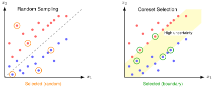
EL2N with a small proxy model offers one practical balance between scoring cost and selection quality. The approach trains a lightweight model for a few epochs, computes EL2N scores, and selects a subset subject to coverage and quality checks. The proxy must provide rankings that transfer to the target model, and the investment pays off only when downstream training savings exceed selection overhead. A concrete scenario shows the workflow; whether its 10 percent subset preserves accuracy is exactly what validation must establish.

Example 9.3: Coreset selection in practice

Scenario: An engineering team aims to select a 128,117-image coreset (10 percent) from the 1.28 million ImageNet training images for faster ResNet-50 iteration.

Diagnosis: Naive random subsampling can miss rare classes and boundary examples. Training a lightweight proxy model for 5 epochs calculates EL2N error scores, prioritizing high-error examples while checking rare-class coverage.

Systems lesson: Proxy-based coreset selection replaces some full-data passes with targeted scoring compute. It accelerates full-model training only when the proxy ranking transfers and coverage checks preserve rare classes and edge cases.

Listing 1 turns proxy prediction error into reusable selected indices. The compute_el2n_scores function spends a small amount of probe compute to measure which samples still confuse a briefly trained model, and select_coreset retains the highest-scoring examples. This top-\(\Glyph{k}\) sketch needs quality and coverage checks before its subset replaces the full training pool. The scoring pass requires an unshuffled dataloader so each score position remains aligned with its dataset index.

Listing 1: EL2N-Based Coreset Selection: The compute_el2n_scores function trains a proxy model for a few epochs, then measures prediction error via L2 distance from one-hot labels. High scores identify samples the proxy finds difficult, including potentially noisy examples. The select_coreset function illustrates ranking by this score; production use also requires coverage, noise, and target-quality validation.

def compute_el2n_scores(model, dataloader, num_epochs=5):
    """Compute EL2N scores.

    Returns L2 norm of (prediction - one_hot_label).
    """
    # Train proxy model for a few epochs to get meaningful predictions
    train_proxy(model, dataloader, num_epochs)

    scores = []
    model.eval()
    for x, y in dataloader:
        logits = model(x)
        probs = softmax(logits, dim=1)
        # One-hot encode labels
        one_hot = zeros_like(probs).scatter_(1, y.unsqueeze(1), 1)
        # EL2N score = L2 distance between probabilities and one-hot target
        el2n = (probs - one_hot).norm(dim=1)  # High = large prediction error
        scores.extend(el2n.tolist())
    return scores


def select_coreset(scores, dataset, fraction=0.1):
    """Select top-k samples with the largest prediction errors."""
    k = int(len(dataset) * fraction)
    # Sort by score descending (largest prediction error first)
    indices = argsort(scores, descending=True)[:k]
    return Subset(dataset, indices)


# Illustrative 10% subset; validate accuracy and coverage before use
scores = compute_el2n_scores(proxy_model, full_loader)
coreset = select_coreset(scores, full_dataset, fraction=0.1)
train_full_model(model, coreset)

A coverage floor changes the indices retained by the score ranking. Consider disjoint classes A and B, a total coreset budget \(\CoresetBudget\) as in table 2, and task-validated minimum counts \(\FirstClassCoverageFloor\) and \(\SecondClassCoverageFloor\) for the respective classes. First reserve the highest-scoring \(\FirstClassCoverageFloor\) eligible examples from A and the highest-scoring \(\SecondClassCoverageFloor\) from B. Fill the remaining \(\CoresetBudget-\FirstClassCoverageFloor-\SecondClassCoverageFloor\) slots from the global ranking, skipping indices already reserved. The allocation is infeasible if \(\CoresetBudget<\FirstClassCoverageFloor+\SecondClassCoverageFloor\), if either class lacks enough eligible examples to meet its floor, or if the eligible pool is smaller than \(\CoresetBudget\); the pipeline must revise the budget or acquire missing coverage before training.

Suppose the unconstrained top-\(\CoresetBudget\) ranking contains only A examples and the budget can meet both floors. Reserving B’s floor replaces the lowest-scoring \(\SecondClassCoverageFloor\) members of that all-A subset with the highest-scoring eligible B examples, while the remaining slots still follow the score order. Coverage thus has an explicit opportunity cost in the selection score. Overlapping demographic or operational slices require joint constraint handling because one example may satisfy several floors; summing those floors as if the slices were disjoint can reject a feasible budget. Even a feasible allocation establishes only retained counts. Independent evaluation must still establish target quality and performance on the required slices.

Together, these three static pruning techniques (deduplication, quality filtering, and coreset selection) shrink \(\Operations\) before training begins, subject to the same fixed-schedule caveat as before: a schedule that adds compensating epochs or steps gives back part of the saving. Static pruning answers a question about what to keep, but it treats the answer as fixed, training every epoch on the same retained subset. A sample’s usefulness, however, can change as the model learns, because examples that challenge an undertrained model may become easy after sufficient gradient updates. Dynamic selection techniques address this limitation by adapting the training data at each stage based on what the model has already mastered.

Self-Check: Question

1. A team wants to score a dataset cheaply before training a large production model. They plan to train a small proxy for a few epochs and rank examples by prediction error, knowing that confidently wrong predictions can still score highly. Which method best matches that plan and its trade-off?

   1. \(k\)-Center clustering on raw pixel inputs, because it guarantees zero-cost label-aware boundary identification
   2. Forgetting Events scoring on the full production model, because it requires no proxy architecture and computes in \(\mathcal{O}(1)\) time
   3. EL2N (Error L2-Norm) scoring with a briefly trained proxy model, accepting that high error can reflect hard examples or noise
   4. Herding on Gaussian-distributed features, because it completely avoids computing feature representations

2. Why is Locality-Sensitive Hashing (LSH) with MinHash preferred over exhaustive pairwise Jaccard similarity comparison for large-scale text deduplication?

   1. MinHash LSH guarantees \(100\%\) precision in detecting semantic paraphrases across different natural languages
   2. MinHash eliminates the need to tokenize or shingle input documents before hashing
   3. Exhaustive pairwise Jaccard comparison requires training a deep neural network, whereas LSH is purely rule-based
   4. Exhaustive pairwise comparison requires \(\mathcal{O}(D^2)\) document comparisons, whereas MinHash LSH hashes compact signatures into sublinear candidate collision buckets

3. True or False: Removing near-duplicate documents with MinHash LSH always improves model accuracy because duplicate data has zero statistical value in all training regimes.

4. The training-dynamics coreset metric that measures the Euclidean norm of the difference between predicted class probabilities and the one-hot target vector early in training is known as ____.

See Answers →

9.4 Dynamic Selection

How much a sample teaches changes as the model learns. Early in optimization, broad coverage provides stable gradients that establish general feature representations. As parameters converge, the gradient norms of mastered examples decay toward zero; on a ResNet-50 run over ImageNet, these are the clean, centered images of common classes. Executing forward and backward passes on these samples continues to consume accelerator execution cycles and high-bandwidth memory (HBM) transfers while producing negligible parameter updates, driving their effective ICR toward zero. Dynamic selection mitigates this waste by adapting batch composition to the model’s current state. This shifts selection from an offline preprocessing step into the active execution loop, modifying the operation count (\(\Operations\)) at runtime. The same adaptive logic extends to labels, where active learning decides which examples receive a human label as the model’s uncertainty shifts.

9.4.1 Curriculum learning

Random shuffling feeds hard boundary cases, noisy labels, and outliers to an untrained model before its early features have stabilized, while still spending full epochs on simple examples long after the model has mastered them. Curriculum learning¹⁵ (Bengio et al. 2009; Soviany et al. 2022) orders the training stream instead of shuffling it uniformly, starting with simpler examples and gradually introducing harder ones as parameters converge. Ordering the stream changes which gradients dominate at each stage of training: easy examples provide stable early signals, while examples scored as hard can contain useful boundary information, label noise, or outliers. An easy-to-hard schedule can smooth training on some workloads, but its benefit depends on the difficulty score, pacing rule, model, and data; any claimed epoch reduction must therefore be treated as illustrative rather than guaranteed.

¹⁵ Curriculum learning: From Latin currere (“to run”), originally meaning “the course to be run,” a metaphor that maps directly to the technique, with training data as a course run in deliberate order and the easy stretches first. Curriculum learning can act as a continuation method for nonconvex optimization, with easier examples shaping the early optimization trajectory before harder examples are introduced. From a systems perspective, the ICR of a sample can vary during training, which motivates changing the mix of examples over time.

Bengio, Yoshua, Jérôme Louradour, Ronan Collobert, and Jason Weston. 2009. “Curriculum Learning.” Proceedings of the 26th Annual International Conference on Machine Learning, 41–48. https://doi.org/10.1145/1553374.1553380.

Soviany, Petru, Radu Tudor Ionescu, Paolo Rota, and Nicu Sebe. 2022. “Curriculum Learning: A Survey.” International Journal of Computer Vision 130 (6): 1526–65. https://doi.org/10.1007/s11263-022-01611-x.

Implementing a curriculum requires two components: a difficulty scorer that ranks samples, and a pacing function that controls how quickly hard samples are introduced. A common choice is linear pacing: \[ \text{samples}_{\EpochIndex} = \texttt{sort\_by\_difficulty}[:\DatasetSize\cdot \min(1, \EpochIndex/\WarmupEpochCount)] \] where \(\EpochIndex\) is the current epoch, \(\DatasetSize\) is the total dataset size, and \(\WarmupEpochCount\) is the number of warmup epochs before the full dataset becomes available. Early epochs train on the easiest fraction \(\EpochIndex/\WarmupEpochCount\) of the \(\DatasetSize\) samples; after warmup, training proceeds on the full dataset. From a systems standpoint, dynamically re-sorting multi-terabyte datasets epoch-by-epoch destroys sequential I/O read-ahead and stalls accelerators on storage latency. Production data loaders implement curricula by pre-sorting data offline into discrete difficulty-tiered shards or buckets. During training, workers stream shards sequentially from storage while maintaining local shuffle buffers within each tier, preserving high sequential storage bandwidth while maintaining batch diversity and gradient stability.

The pacing rule fixes one saving before any benchmark is run. Summed over the warmup, the loader serves \(\sum_{\EpochIndex=1}^{\WarmupEpochCount} \DatasetSize \cdot \EpochIndex/\WarmupEpochCount= \DatasetSize (\WarmupEpochCount+1)/2\) samples in place of \(\WarmupEpochCount\cdot \DatasetSize\), so the warmup epochs cost roughly half their full-data FLOPs. A curriculum can therefore save compute in two distinct ways, through cheaper warmup epochs and through any reduction in the total epochs needed to reach target quality, and a claimed saving must say which of the two it measured.

The difficulty scorer is a systems choice because it trades probe-compute overhead against ordering quality, as table 3 shows. Loss and confidence scoring gain better ordering at the cost of extra inference, heuristics avoid compute but require domain knowledge, and self-paced scoring moves adaptation into the training loop itself.

Table 3: Difficulty Scoring Strategies for Curriculum Learning: The rows compare each scorer’s signal source with the system prerequisite or trade-off it introduces.

Strategy	Difficulty Score	Best For
Loss-Based	Loss from probe model (low = easy)	General-purpose; requires probe training
Confidence-Based	Teacher model confidence (high = easy)	When teacher available; distillation setups
Domain Heuristics	Sentence length, image complexity	No extra compute; domain knowledge required
Self-Paced	Current model’s loss (updated each epoch)	Adaptive; no probe needed

To see how curriculum savings translate to systems accounting, consider an illustrative workload where a linear-warmup curriculum reaches target accuracy in 115 epochs compared to 150 epochs for the standard shuffled baseline, an apparent 23.3 percent epoch reduction. Counting epochs alone, however, obscures the actual systems cost. Because linear pacing serves fewer samples during warmup, early epochs consume fewer FLOPs than post-warmup epochs; conversely, difficulty scoring and shard reordering introduce data-loading overhead that must be offset by the training speedup.

Alternative curriculum strategies diverge further in their computational demands. In a learned curriculum, an auxiliary network dynamically weights examples, down-weighting likely mislabeled instances, rather than enforcing a fixed difficulty schedule. Conversely, anti-curriculum presents the hardest examples first when boundary definition accelerates early convergence, while self-paced learning continuously updates sample difficulty using the current model’s training loss. Because optimal sample ordering depends on the architecture, optimizer, and label noise, curriculum gains cannot be assumed from nominal epoch reductions; they must be verified by measuring end-to-end wall-clock time at the target quality metric, and they still assume that every candidate sample already has a label.

9.4.2 Active learning

Curriculum learning optimizes the order in which samples are presented but assumes all samples are already labeled. This assumption breaks down in specialized domains where labeling requires substantial expertise, time, or money. Active learning¹⁶ (Settles 2012; Ren et al. 2021), which Scaling with AI-assisted labeling introduced as a way to stretch a labeling budget, becomes a selection loop here. Rather than labeling everything upfront, it shifts the optimization target from choosing which labeled samples to train on to choosing which unlabeled samples are worth labeling.

¹⁶ Active learning: The “active” component is the learning algorithm itself selecting which unlabeled samples a human expert should label next. This reframes the problem from a computational optimization (training on given data) to a financial one: maximizing model improvement per dollar spent on expert labeling. Querying the most informative examples can substantially reduce labeling needs compared with random sampling, but the multiplier is task-, model-, and oracle-dependent.

Settles, Burr. 2012. Active Learning. Synthesis Lectures on Artificial Intelligence and Machine Learning. Springer Cham. https://doi.org/10.1007/978-3-031-01560-1.

Ren, Pengzhen, Yun Xiao, Xiaojun Chang, Po-Yao Huang, Zhihui Li, Brij B. Gupta, Xiaojiang Chen, and Xin Wang. 2021. “A Survey of Deep Active Learning.” ACM Computing Surveys 54 (9): 1–40. https://doi.org/10.1145/3472291.

↩︎ The labeling budget, and what each label costs at scale, are established in Labeling economics.

Settles, Burr. 2009. Active Learning Literature Survey. Computer Sciences Technical Report 1648. University of Wisconsin-Madison.

Active learning replaces one-shot collection with an iterative loop of five stages (figure 6): the selection strategy queries the unlabeled pool based on model uncertainty, routes ambiguous instances to a human oracle, merges newly labeled data into the training set, and retrains the model to update uncertainty scores over the remaining pool. The effectiveness of this loop depends critically on the query strategy used to select samples for annotation (Settles 2009, 2012; Ren et al. 2021). The simplest approach, uncertainty sampling, selects samples where the model is least confident, such as predictions near 0.5 probability for binary classification. Scoring with a single model is inexpensive, yet it can overconcentrate queries near one ambiguous region and miss parameters the model is confidently wrong about. Query-by-committee addresses that single-model blind spot by training multiple models and selecting samples where they disagree most, capturing epistemic uncertainty at the cost of ensemble inference. When practitioners can invest even more compute per candidate, expected model change selects the samples that would induce the largest gradient update if labeled, trading per-sample gradient evaluations for a more direct estimate of parameter impact. Because any purely uncertainty- or gradient-driven rule can still cluster an entire acquisition batch inside one narrow pocket of feature space, diversity sampling complements these methods by selecting samples that are dissimilar from currently labeled data, spreading the annotation budget across the input distribution.

Figure 6: The Active Learning Closed Loop: The selection cycle trades proxy-scoring compute for queries chosen from an unlabeled pool for oracle annotation. Uncertainty, diversity, and coverage criteria seek more useful information per annotation than undirected sampling.

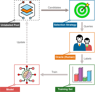
Active learning pays off most clearly in domains where every label requires scarce specialist judgment. When a ResNet-50-class image classifier moves from ImageNet to chest X-rays, for instance, every label requires a radiologist, and the model may be confident on common conditions but uncertain about rarer cases. By focusing human annotation on these ambiguous cases, active learning directs expensive expert time toward the examples most likely to move the decision boundary. Because annotation cost and turnaround in such domains dominate the compute needed to score candidates, routing only the examples the model is least sure about to the expert changes the economics of both labeling and per-epoch training work.

Napkin Math 9.3: The active learning ROI

Problem: A hospital team has 1 Million unlabeled scans, a $5/label specialist-label cost, and a $500,000 budget. How does uncertainty sampling change labeling cost and per-epoch training work relative to the budget-matched random baseline?

Scenario A: Naive Labeling

• Cost: Labeling all 1 Million scans would cost $5,000,000 (10× over budget).
• Budget-matched baseline: \(\$500,000 \div \$5/\text{label} = 100,000\) random scans.
• Naive labeling outcome: Random selection does not guarantee rare-pathology coverage.

Scenario B: Active Learning

• Strategy: Uncertainty sampling selects 50,000 scans for specialist labeling.
• Cost: \(50,000 \times \$5/\text{label} = \$250,000\) (50 percent under budget).
• Training work: \(100,000 \div 50,000 = 2×\) fewer examples per epoch than the budget-matched random baseline.
• Active learning outcome: Matching 100,000 random scans requires empirical validation.

Systems insight: Against the budget-matched random baseline, selection saves \(\$500,000 - \$250,000 = \$250,000\); accuracy still requires empirical validation.

The notebook’s 2× label reduction is an assumption, and the size of that multiplier is what decides the outcome. In the illustrative learning curves of figure 7, uncertainty sampling reaches 90 percent accuracy with roughly 2,500 annotations while uniform random sampling needs about 10,000, a 4\(\times\) gap.

Figure 7: The Active Learning Multiplier: Model accuracy is plotted against labeled samples on a logarithmic axis. In this illustrative scenario, active learning (green solid) reaches the same accuracy with fewer labels than random sampling (gray dashed); the arrow marks an approximately 4\(\times\) label-efficiency gap near 90 percent accuracy.

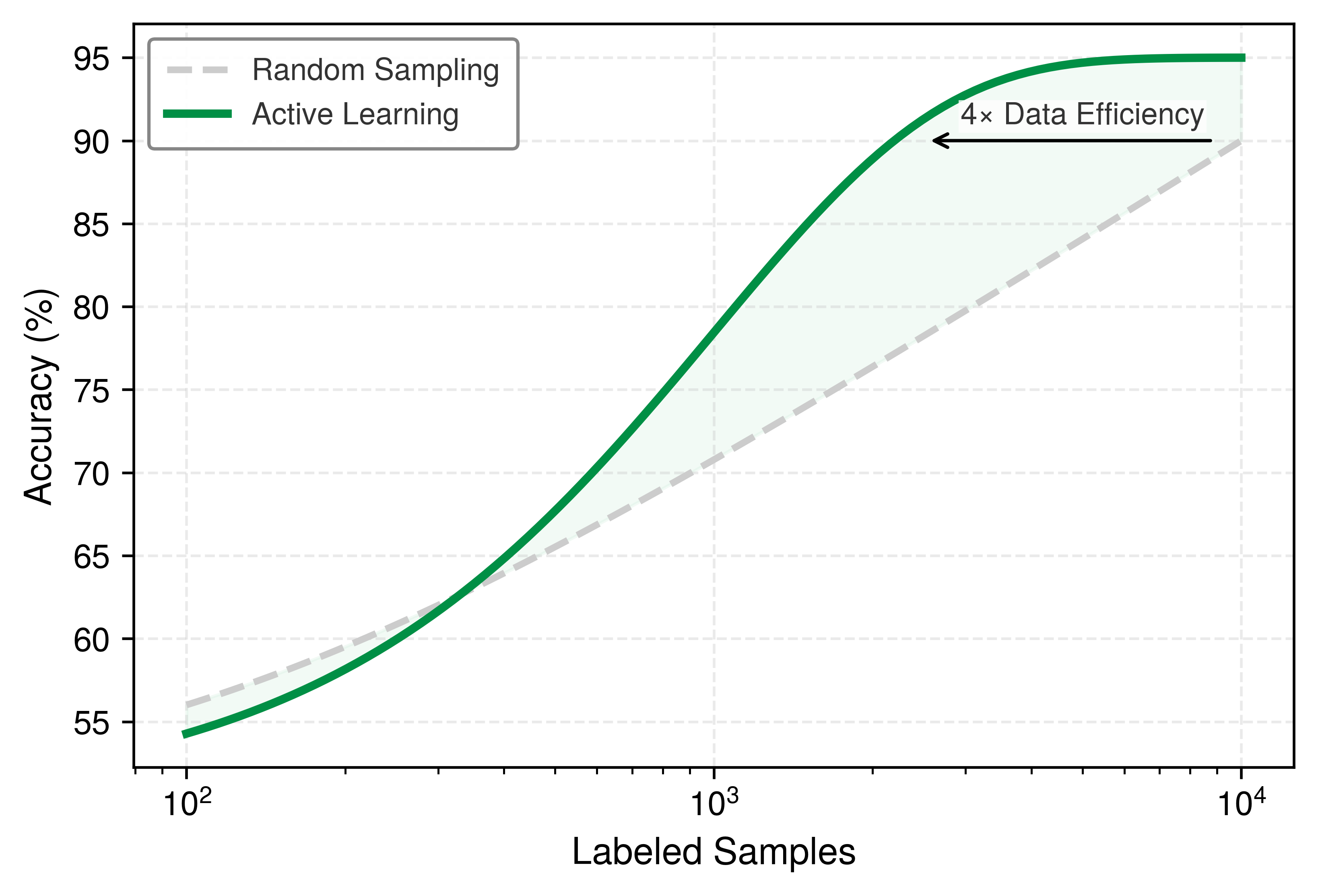
At a fixed price per label, label count and labeling dollars are the same axis, so the figure and notebook 9.3 differ only in the multiplier they assume. The notebook plans on the conservative 2×; the figure shows what a more favorable task would look like. Because the realized multiplier depends on the task, the model, and the query rule, a team budgets on the conservative value and measures the real one on its own data. Active learning also incurs scoring, acquisition, and repeated-retraining costs, so end-to-end savings can be smaller than the label-count gap; beyond saving labeling cost, however, a suitable query rule concentrates review on uncertain, diverse, or failure-relevant examples that uniform sampling rarely surfaces.

Example 9.4: Hard negative mining in a smart doorbell

Scenario: A smart doorbell vision detector receives continuous video feeds dominated by empty backgrounds (easy negatives) and normal pedestrian poses.

Diagnosis: Random frame sampling can miss rare false positives such as statues, laundry piles, and human-shaped shadows. Active learning routes uncertain predictions (“Person: 51%”) and sampled production errors to human reviewers for targeted labeling.

Systems lesson: Hard-negative mining can improve labeling efficiency by spending review effort on suspected false positives and other difficult negatives. The query stream still needs diversity and coverage checks so confident but systematically wrong cases are not excluded.

Curriculum learning and active learning both choose among examples that already exist. When the pool itself lacks the cases a model needs (rare classes with too few examples, edge cases that never appear in the wild, records that privacy rules keep out of reach), no ordering or labeling policy can supply them, and the remaining lever is to create them.

Self-Check: Question

1. In curriculum learning, an engineer implements an easy-to-hard pacing schedule that controls the fraction of the sorted training pool available at each stage. What is the primary objective of this pacing strategy?

   1. To guide early optimization with more stable examples before gradually introducing harder ones
   2. To eliminate the need for backward passes during the first half of training
   3. To maximize GPU memory bandwidth utilization by sorting tensors strictly by length in bytes
   4. To replace human labelers with an automated oracle during the late stages of training

2. An active learning pipeline chooses unlabeled examples for costly radiologist annotation. The team notices that simple uncertainty sampling repeatedly selects images from a single ambiguous artifact class, starving other disease categories. Which query strategy should they adopt to resolve this pathology?

   1. Least-confidence sampling, because it strictly selects the lowest top-1 probability prediction
   2. Diversity sampling or hybrid uncertainty-diversity sampling (such as BADGE), which balances uncertainty near decision boundaries with feature-space coverage
   3. Random undersampling of the entire unlabeled pool to reduce dataset size before scoring
   4. Uniform zero-shot pseudo-labeling without confidence thresholds

3. Order the steps in an active learning closed-loop iteration: (1) Select top query samples via query strategy, (2) Acquire expert annotations from the oracle, (3) Score unlabeled pool using current model, (4) Retrain or update model on expanded dataset, (5) Add newly labeled samples to the training set.

See Answers →

9.5 Synthetic Data Generation

Real-world data collection encounters physical and legal boundaries: autonomous fleets cannot safely crash vehicles to acquire catastrophic collision trajectories, healthcare systems cannot transmit protected patient telemetry across institutional firewalls, and edge products must handle acoustic environments before any deployed fleet exists to record them. When the source corpus contains few or none of the cases deployment will face, neither static pruning nor dynamic selection can extract signal that is not there. Synthetic data generation, which Scaling acquisition introduced as one acquisition channel among several, becomes here a deliberate lever for constructing the training distribution directly. The strategy shifts from curation, choosing among existing records, to creation, making new inputs, perturbations, or supervisory targets.

9.5.1 Data augmentation

A vision model trained repeatedly on identical images can memorize their exact pixel layouts rather than the object class, yet storing multiple transformed copies of every image on disk would multiply the archive’s storage footprint. Data augmentation avoids that storage cost by transforming existing samples on the fly during ingestion; every ResNet-50 epoch on ImageNet sees freshly cropped, flipped, and color-shifted variants of the same images. Label-preserving transformations add diversity without expanding durable storage or acquiring new data, but they move cost into the training pipeline. On host CPU worker threads, decoding and spatial transformations can saturate the cores and starve the accelerator across the PCIe bus. Offloading them to accelerator kernels relieves the CPU, yet inputs still cross the host-to-device link, and the transformations consume HBM and compute cycles that would otherwise perform gradient updates.

For image data, transformations encode invariances required at deployment (Shorten and Khoshgoftaar 2019). Geometric operations (rotation, flipping, cropping, scaling) encourage viewpoint invariance when they preserve the label, while photometric adjustments (brightness, contrast, color jitter) simulate sensor noise and varying illumination. Stronger methods mask or mix images: Cutout¹⁷ applies random rectangular zero-masks to prevent reliance on localized features; MixUp (Zhang et al. 2018) constructs virtual samples by taking linear combinations of image pairs and their one-hot labels (\(\MixupSample= \MixupWeight \ModelInput_i + (1 - \MixupWeight) \ModelInput_j\), with mixing weight \(\MixupWeight\in [0, 1]\)); and CutMix¹⁸ pastes rectangular patches from one image into another while blending labels proportionally to the patch area. Both mixing methods operate through linear combinations and block copies in device memory, so they add negligible FLOP overhead.

Shorten, Connor, and Taghi M. Khoshgoftaar. 2019. “A Survey on Image Data Augmentation for Deep Learning.” Journal of Big Data 6 (1): 1–48. https://doi.org/10.1186/s40537-019-0197-0.

¹⁷ Cutout: Randomly masks square regions of input images during training, forcing the model to recognize objects from partial information rather than relying on any single discriminative region (DeVries and Taylor 2017). Unlike dropout (which zeroes neurons in feature space), Cutout operates in input space. The original Cutout experiments produced 0.3–2.0 percentage-point gains across CIFAR-10/100 and SVHN with negligible compute overhead, making it a high-ICR augmentation technique when occlusion-style invariance matches the task: more information per sample at near-zero additional cost to the pipeline.

DeVries, Terrance, and Graham W. Taylor. 2017. “Improved Regularization of Convolutional Neural Networks with Cutout.” arXiv Preprint arXiv:1708.04552.

Zhang, Hongyi, Moustapha Cisse, Yann N. Dauphin, and David Lopez-Paz. 2018. mixup: Beyond Empirical Risk Minimization. OpenReview.net.

¹⁸ CutMix: Replaces Cutout’s zeroed-out region with a patch from a different training image, mixing labels proportionally to patch area (30 percent of image A replaced by image B yields a 70/30 label split) (Yun et al. 2019). This addresses Cutout’s weakness: zeroed regions waste pixel information that could carry learning signal. The CutMix paper reports ImageNet top-1 improvements of 2.28 percentage points for ResNet-50 and 1.70 percentage points for ResNet-101, while also improving localization behavior. The method provides stronger regularization than either Cutout or MixUp alone with little additional data-pipeline cost.

Yun, Sangdoo, Dongyoon Han, Seong Joon Oh, Sanghyuk Chun, Junsuk Choe, and Youngjoon Yoo. 2019. “CutMix: Regularization Strategy to Train Strong Classifiers with Localizable Features.” 2019 IEEE/CVF International Conference on Computer Vision (ICCV), 6023–32. https://doi.org/10.1109/ICCV.2019.00612.

¹⁹ Back-translation: In the method described by Sennrich et al. (2016), target-language monolingual text is translated into the source language, and the synthetic source is paired with the unchanged target for machine-translation training. The systems trade-off is latency because each synthetic source requires translation-model inference. Pipelines can precompute these examples offline rather than generating them in the data loader.

Sennrich, Rico, Barry Haddow, and Alexandra Birch. 2016. “Improving Neural Machine Translation Models with Monolingual Data.” Proceedings of the 54th Annual Meeting of the Association for Computational Linguistics (Volume 1: Long Papers), 86–96. https://doi.org/10.18653/v1/P16-1009.

Text has no smooth geometric transformations, because tokens are discrete. Back-translation¹⁹ paraphrases by passing target-language text through a translation model to produce synthetic source sentences. Simpler transforms such as synonym substitution, token insertion, or deletion risk corrupting labels unless validated for the task.

Automated policy searches replace hand-tuned transformation schedules. AutoAugment²⁰ uses reinforcement learning to search over operations, at a search cost of about 15,000 GPU-hours on ImageNet. RandAugment²¹ eliminates this search cost by parameterizing the policy with just two values: the number of transformations applied to each image and a single global distortion magnitude. Even the best augmentation schedule, however, can only perturb examples the dataset already contains.

²⁰ AutoAugment: Treats augmentation policy design as a reinforcement learning search problem: a controller selects operations (rotate, translate, shear, equalize), their magnitudes, and application probabilities to maximize validation accuracy (Cubuk et al. 2019). The original ImageNet search used approximately 15,000 GPU-hours, motivating later methods that reduce the search space.

Cubuk, Ekin D., Barret Zoph, Dandelion Mané, Vijay Vasudevan, and Quoc V. Le. 2019. “AutoAugment: Learning Augmentation Strategies from Data.” 2019 IEEE/CVF Conference on Computer Vision and Pattern Recognition (CVPR), 113–23. https://doi.org/10.1109/cvpr.2019.00020.

²¹ RandAugment: Collapses AutoAugment’s policy search to two hyperparameters, a transformation count and a shared magnitude (Cubuk et al. 2020). That small search space matches or exceeds AutoAugment on the reported benchmarks at far lower search cost, making it practical when 15,000 GPU-hours of policy search cannot be justified.

Cubuk, Ekin D., Barret Zoph, Jonathon Shlens, and Quoc V. Le. 2020. “Randaugment: Practical Automated Data Augmentation with a Reduced Search Space.” 2020 IEEE/CVF Conference on Computer Vision and Pattern Recognition Workshops (CVPRW), 3008–17. https://doi.org/10.1109/cvprw50498.2020.00359.

9.5.2 Generative synthesis

Cropping or color-shifting existing images cannot invent a rare object class, an unseen weather condition, or a collision scenario that never occurred in the recorded dataset. When a pipeline needs examples that perturbations of existing records cannot supply, generative synthesis constructs new input-label pairs \((\ModelInput, \ExampleLabel)\) by sampling from generative models or physical simulators. The three main engines differ in cost per sample and in how realistic their outputs are:

1. Generative Adversarial Networks (GANs) train a generator against a discriminator. Once trained, feed-forward generator inference requires a single forward pass, providing low latency and high sample throughput. However, GAN training is vulnerable to mode collapse, in which the generator covers only part of the data distribution and loses the tail variety needed for edge-case coverage.
2. Diffusion models generate samples by iteratively removing noise over many sequential steps. Latent diffusion systems such as Stable Diffusion²² enable precise semantic conditioning from text prompts while operating in a compressed latent space. A sampling recipe with 20 to 50 denoising steps runs the backbone that many times per generated batch, so offline generation is often preferable.
3. Physical simulation engines (such as CARLA for autonomous driving or Isaac Sim and Unity for robotics) generate data without neural inference, by running physics and rendering pipelines. They produce exact ground-truth annotations (3D bounding boxes, depth maps, velocity vectors) from internal state at no labeling cost, and the bottleneck shifts to host CPU physics and graphics rendering throughput.

²² Stable Diffusion: Performs iterative denoising in a compressed latent space, enabling targeted text-to-image examples (Rombach et al. 2022). Its iterative generation is substantially more compute-intensive than geometric transforms, so it fits cases where novelty matters more than per-sample throughput.

Rombach, Robin, Andreas Blattmann, Dominik Lorenz, Patrick Esser, and Bjorn Ommer. 2022. “High-Resolution Image Synthesis with Latent Diffusion Models.” 2022 IEEE/CVF Conference on Computer Vision and Pattern Recognition (CVPR), 10674–85. https://doi.org/10.1109/cvpr52688.2022.01042.

Regardless of the generative engine, synthetic samples inevitably diverge from the statistical distributions of real deployment environments. That divergence determines whether synthetic training transfers to production or fails on the first real-world input.

9.5.3 Bridging the domain gap

A model trained purely on synthetic data can reach high validation accuracy in the simulator while failing in production because it latched onto rendering or generator artifacts that do not exist in the real world. This domain gap²³ is the statistical shift between the synthetic training distribution and production deployment data. Synthetic and real feature densities can sit at different locations in feature space, misaligning the decision boundaries learned from each (figure 8). The marginal densities alone do not determine either decision boundary; class-conditional structure and real-data evaluation are needed to establish how the shift affects classification.

²³ Domain gap: The statistical divergence between synthetic and real data distributions, measurable with metrics such as maximum mean discrepancy (MMD) or Frechet Inception Distance (FID). For ML systems, the gap becomes training-serving skew: a simulator-trained model can validate well on synthetic data while failing silently on real deployment data.

Figure 8: The Domain Gap Problem: Synthetic data (blue) and real data (orange) occupy shifted feature distributions. The dashed red synthetic boundary and dotted green real-data boundary illustrate possible misalignment; marginal feature densities alone do not determine class boundaries.

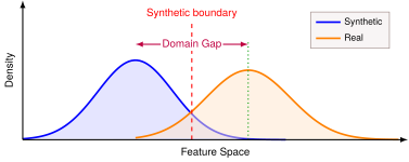
Two complementary strategies address this distribution mismatch. Domain randomization²⁴ takes an aggressive approach: rather than trying to match the real world precisely, it trains on varied synthetic data by randomizing lighting, textures, backgrounds, and camera parameters during generation. The aim is to make deployment conditions fall within the variation seen during training, though coverage is never guaranteed by randomization alone; the method is effective in robotics and autonomous-driving settings when the simulator spans the relevant physical and visual factors and the result is validated on real data.

²⁴ Domain randomization: Makes synthetic data deliberately varied by randomizing textures, colors, lighting, and physical properties. The goal is not photorealism; it is enough variation to improve coverage of deployment conditions, shifting the cost bottleneck from rendering fidelity to coverage.

Domain adaptation takes the opposite approach by explicitly aligning synthetic and real distributions. Feature alignment methods train on synthetic data while simultaneously minimizing the distance between synthetic and real feature distributions, often using adversarial training to learn domain-invariant representations. Fine-tuning offers a simpler path: pretrain on abundant synthetic data to learn general features, then fine-tune on a small real dataset to adapt to deployment conditions. Self-training combines these ideas by using a synthetic-trained model to pseudo-label real unlabeled data, then retraining on the combined labeled set. In practice, mixing synthetic and real data provides a real-data anchor while retaining some synthetic coverage: moving the mix from all-synthetic toward all-real trades a larger domain gap for a higher collection cost, and the best ratio depends on the domain, simulator fidelity, model family, and validation protocol rather than on any universal recipe.

Augmentation, noise injection, and simulation can grow a small seed set into a training corpus; the keyword spotter’s data budget, including how much synthetic augmentation saves against recording real utterances, is worked through in KWS design space. The same creation strategy becomes riskier when samples come from learned generators. In recursive training, model collapse²⁵ can amplify errors and reduce diversity over generations. Synthetic data therefore requires provenance, mixture controls, and validation against real deployment data rather than an unverified assumption that more generated samples help. When the input examples themselves are already on disk, a trained model can instead enrich their labels.

²⁵ Model collapse: Formally analyzed by Shumailov et al. (2024), this phenomenon can arise when errors and missing tail coverage compound during recursive training. Tail distributions contain rare but important patterns that appear infrequently in training data. When generation \(\ModelGenerationIndex+1\) trains on output from generation \(\ModelGenerationIndex\) under these conditions, successive generations can further compress the tails, producing increasingly homogeneous data. The degradation can be rapid in recursive training settings, which is why training on unanchored synthetic outputs risks catastrophic collapse of tail diversity.

Shumailov, Ilia, Zakhar Shumaylov, Yiren Zhao, Nicolas Papernot, Ross Anderson, and Yarin Gal. 2024. “AI Models Collapse When Trained on Recursively Generated Data.” Nature 631 (8022): 755–59. https://doi.org/10.1038/s41586-024-07566-y.

9.5.4 Knowledge distillation

A hard one-hot label such as \([1, 0, 0]\) tells a classifier which class is right, but discards everything a stronger model knows about which wrong classes look similar. Where augmentation (section 9.5.1) and generative synthesis (section 9.5.2) create new inputs, knowledge distillation²⁶ (Hinton et al. 2015; Gou et al. 2021) creates richer targets for inputs the corpus already holds. A larger trained model (the teacher) labels each training example with its full probability distribution over classes, such as \([0.70, 0.20, 0.10]\) in place of \([1, 0, 0]\), and a compact student network trains against those soft targets, smoothed by a temperature parameter \(\DistillationTemperature\). Because each soft target records which wrong classes the teacher found plausible, every example carries more supervision than its one-hot label. Distillation mathematics develops distillation as a compression technique, including its loss and temperature mechanics; as a data lever, its cost lies in generating, storing, and reading those targets.

²⁶ Knowledge distillation: Soft teacher probabilities reveal structural similarities across classes that one-hot encodings omit, and a temperature parameter controls how strongly those probabilities are smoothed. Distillation introduces teacher inference costs that must be justified by improved student sample efficiency or accuracy.

Hinton, Geoffrey, Oriol Vinyals, and Jeff Dean. 2015. “Distilling the Knowledge in a Neural Network.” arXiv Preprint.

Gou, Jianping, Baosheng Yu, Stephen J. Maybank, and Dacheng Tao. 2021. “Knowledge Distillation: A Survey.” International Journal of Computer Vision 129 (6): 1789–819. https://doi.org/10.1007/s11263-021-01453-z.

Distillation trades accelerator HBM capacity against storage I/O bandwidth:

• Online distillation: The teacher model resides directly in accelerator memory alongside the student model during training. The system computes teacher forward passes concurrently with student execution, eliminating persistent storage overhead for soft targets. However, co-locating an overparameterized teacher consumes accelerator memory and arithmetic throughput, restricting the student’s maximum per-accelerator batch size and increasing step latency.
• Offline distillation: The teacher generates predictions across the corpus during an offline precomputation pass, storing dense logit vectors to disk. This frees accelerator memory entirely for student training, but expands dataset storage volume and input pipeline bandwidth. For a classification vocabulary of \(\ClassCount\) classes, storing uncompressed float32 logits increases the per-sample label footprint from a single integer index (\(\lceil \log_2 \ClassCount \rceil\) bits) to \(4\ClassCount\) bytes, an expansion of more than three orders of magnitude once \(\ClassCount\) reaches the thousands.

For ResNet-50 on ImageNet the offline footprint is concrete. Storing FP32 logits for 1,000 classes across every training image takes 5.1 GB, against 2.6 MB for the integer labels they replace, a 2,000× expansion that every epoch must read back through the input pipeline. That storage and read traffic, rather than the loss function, is what data selection must budget for. Generation and distillation both supply labeled signal the corpus lacks; a complementary route reduces how many labels training needs in the first place, by extracting supervision from the unlabeled data the corpus already holds.

Self-Check: Question

1. What causes the phenomenon of ‘model collapse’ when generative models are trained recursively on synthetic data generated by earlier model iterations?

   1. GPU memory fragmentation caused by variable-length synthetic sequences during distributed training
   2. Overfitting to floating-point rounding errors during fp16 mixed-precision matrix multiplication
   3. A failure of the I/O storage subsystem to deliver synthetic batches at line rate
   4. Systematic underrepresentation and erosion of tail patterns across generations, so recursive retraining compounds missing or distorted rare cases

2. A team distills a ResNet-50 student on ImageNet and chooses offline distillation, precomputing the teacher’s FP32 logits for every training image instead of keeping the teacher in accelerator memory. Which cost does this choice move onto the data path?

   1. Every epoch must read per-class logit vectors in place of single integer labels, multiplying the label bytes the storage tier and input pipeline must deliver
   2. Every training step must run a teacher forward pass beside the student, restricting the student’s per-accelerator batch size
   3. The student must be trained with a lower learning rate, because soft targets produce larger gradients than one-hot labels
   4. The teacher must be retrained once per student epoch, so preparation cost grows linearly with the number of epochs

3. Why is training exclusively on \(100\%\) synthetic data from a simulation engine often suboptimal for real-world deployment, and how does synthetic-to-real data mixing bridge this gap?

4. True or False: Using a high-capacity diffusion model or state-of-the-art LLM to generate synthetic training data guarantees that the resulting training set will be completely free of distribution shift relative to the real deployment environment.

See Answers →

9.6 Learning from Unlabeled Data

Labels are often the scarcest input in a training pipeline. Active learning still pays an expert for every example it selects, and synthesis pays for every example it creates. Learning from unlabeled data attacks that cost from the other side. Semi-supervised learning lets a model trained on a small labeled seed supply provisional labels for the rest of the pool. Self-supervised learning removes task labels from pretraining altogether, and foundation models spread the resulting pretraining cost across many downstream tasks. Each approach trades additional training compute for fewer labels, so each is judged by total cost at matched quality rather than by label count alone.

9.6.1 Semi-supervised learning

In the chest X-ray adaptation of section 9.4.2, a hospital may hold 50,000 scans of which only 500 have been reviewed and labeled²⁷ by radiologists, a labeling rate of 1 percent. Semi-supervised learning puts the remaining 49,500 images to work by shifting the trade-off from human annotation to accelerator compute: it uses the small labeled subset to anchor training on the larger unlabeled pool, extracting supervisory signals from unannotated inputs. Models trained this way can approach fully supervised accuracy with far fewer manual labels, provided the unlabeled pool matches the target distribution and the result is validated on labeled data.

²⁷ Illustrative clinical labeling economics: The review-rate and hourly-rate ranges are scenario assumptions rather than reported measurements. Under those inputs, labeling 500 scans requires 7–10 hours and costs $1,000–3,000; labeling all 50,000 costs $94,000–300,000. The arithmetic illustrates why semi-supervised learning can be attractive when expert labels are expensive, but actual review time, adjudication, prevalence, and validation requirements must be measured.

Unlabeled data, although it cannot teach the mapping from inputs to outputs, contains structural information about the input distribution \(\InputDistribution\) that can constrain the hypothesis space. Under smoothness and cluster assumptions, a decision boundary that cuts through a dense region assigns different labels to nearby inputs and is less plausible than one in a low-density region. Semi-supervised methods exploit these assumptions, which must be checked against the target task.

Three techniques implement this distribution-regularization insight. Pseudo-labeling²⁸ trains on the labeled subset, generates model predictions on the unlabeled pool, and incorporates samples exceeding a confidence threshold as synthetic ground truth for subsequent retraining. The confidence threshold governs a critical systems trade-off: setting it too low admits label noise that degrades learning, while setting it too high discards informative examples and wastes the unlabeled pool. Confident mistakes can survive either threshold, so confidence must be checked against labeled validation evidence rather than treated as proof of correctness.

²⁸ Pseudo-labeling: Uses a trained model’s own confident predictions as ground-truth labels for unlabeled data; the technique’s effectiveness depends on a virtuous cycle in which accurate predictions on easy unlabeled examples expand the training set and improve the model, which then labels harder examples accurately. The failure mode is equally self-reinforcing, because incorrect pseudo-labels feed the model’s own misclassifications back into training through confirmation bias.

²⁹ Consistency regularization: The method rests on a task-dependent smoothness assumption, that two inputs \(\ModelInput_1\) and \(\ModelInput_2\) related by a label-preserving perturbation should receive the same prediction. It is conceptually distinct from data augmentation (which creates more training examples) because it explicitly enforces prediction consistency as a loss term, even for unlabeled data where the “correct” label is unknown. The systems consequence is additional computation for generating and comparing predictions under multiple perturbations, a trade-off that can favor compute-rich, label-poor settings.

³⁰ FixMatch: The confidence gate is strict; in the original experiments a pseudo-label is kept only when the prediction on the weak view exceeds 0.95 (Sohn et al. 2020). Every unlabeled image still costs a forward pass on its weak view whether or not it passes the gate, part of the extra training compute that buys the reduction in manual labels.

Sohn, Kihyuk, David Berthelot, Nicholas Carlini, Zizhao Zhang, Han Zhang, Colin A Raffel, Ekin Dogus Cubuk, Alexey Kurakin, and Chun-Liang Li. 2020. “FixMatch: Simplifying Semi-Supervised Learning with Consistency and Confidence.” Advances in Neural Information Processing Systems (NeurIPS) 33: 596–608.

Consistency regularization²⁹ enforces that the model produce invariant predictions across perturbed versions of the same input. When transformations such as cropping, rotation, or color shifts preserve the task label, the loss function penalizes prediction divergence between two stochastic views of an unlabeled sample. Hybrid approaches like FixMatch³⁰ unify both mechanisms: they generate a pseudo-label on a weakly augmented view when prediction confidence exceeds a threshold, then train the model to predict that label on a strongly augmented variant of the same input.

Label propagation frames semi-supervised learning as graph diffusion: it constructs an affinity graph over sample representations and propagates labels from labeled nodes to unlabeled neighbors. This approach works well when representations form well-separated clusters, though constructing and querying the similarity graph across large datasets introduces substantial memory and nearest-neighbor search overhead.

Example 9.5: FixMatch on CIFAR-10

Scenario: A semi-supervised image classification pipeline trains on CIFAR-10 with only 250 labeled samples (25 per class) alongside unlabeled data (Sohn et al. 2020).

Diagnosis: The fully labeled CIFAR-10 training set contains 50K labels. FixMatch generates high-confidence pseudo-labels (>0.95 threshold) on weakly augmented unlabeled images and enforces consistency on strongly augmented variants, reaching 94.9 percent accuracy in the cited experiment.

Systems lesson: Semi-supervised learning trades additional training compute for fewer manual labels. In an illustrative cost scenario at $1 per label, a supervised baseline with 4,000 labels costs $4,000 in labels plus $50 of compute, or $4,050. FixMatch at 250 labels costs $250 in labels but 5× the compute, $250, for $500. Preparation expense falls by 8.1×; the end-to-end saving depends on the real unlabeled-data and compute costs.

The objective of semi-supervised learning is lower total labeling and compute cost at matched quality, which can justify a lower ICR when annotation savings exceed the added training expense. Neither the label reduction nor the compute increase carries over unchanged from one task to another; table 4 shows how far the label count fell on one benchmark.

Table 4: FixMatch Label Efficiency on CIFAR-10: With 250 labels (0.5 percent of the dataset), FixMatch reaches 94.9 percent accuracy while using 200× fewer labels than the full training set contains.

Label Budget	Method	Accuracy	Label Efficiency
50,000 (100%)	Full training set	—	Label-count reference
4,000 (8%)	FixMatch	95.7%	12.5× more efficient
250 (0.5%)	FixMatch	94.9%	200× more efficient
40 (0.08%)	FixMatch	88.6%	1250× more efficient

The efficiency column counts labels only, relative to the full labeled set. It does not claim that FixMatch matches a fully supervised model, which would have to be compared at equal accuracy. These efficiency gains also depend on benign distribution assumptions. Semi-supervised learning assumes that unlabeled data comes from the same distribution as labeled data, and it struggles when unlabeled data contains out-of-distribution samples (the model confidently mislabels them), when class imbalance is severe (pseudo-labels amplify majority class bias), or when the labeled set does not cover all classes (preventing label propagation for unseen classes). A held-out set with true labels is the check that catches such a mismatch.

Each technique can reduce dependence on task-specific labels, but none eliminates the need for labeled evaluation. The progression raises a related possibility, that task-specific labels may not be necessary for pretraining. The structure of data itself (cat images resemble other cat images, and coherent sentences follow grammatical patterns) may provide a supervision signal, while downstream quality still requires task-aligned validation.

9.6.2 Self-supervised learning

GPT was trained to predict the next token in a sequence. BERT was trained to fill in masked tokens. Neither pretraining objective required task-specific human labels. Self-supervised learning³¹ (SSL) generalizes this insight: by designing pretext tasks that derive supervision from the data’s structure, models can learn reusable representations from unlabeled data at scale. Where active and semi-supervised learning reduce the demand for labels, SSL changes the accounting by making unlabeled structure the pretraining signal. Within the intervention map of figure 1, SSL sits beside the three levers and extends the usable pool; the question shifts from which labeled samples to train on to how unlabeled samples can support pretraining. It responds to one aspect of the data wall introduced in section 9.1 by broadening what counts as a training signal, while leaving corpus quality, licensing, coverage, and labeled evaluation requirements intact.

³¹ Self-supervised learning: The pretext task, such as next-token or masked-token prediction, provides a supervisory signal derived from the data itself. This reduces dependence on task-specific human labels but can require substantial pretraining compute. Amortization depends on how broadly the resulting model is reused.

Labels are one form of supervision; a pretext task can also derive a learning signal from the structure of the data, as table 5 summarizes.

Table 5: Self-Supervised Pretext Tasks by Modality: Each task extracts supervision from data structure rather than human labels, enabling pretraining on large-scale unlabeled corpora.

Modality	Self-Supervised Task	Supervision Signal
Text	Masked language modeling	Predict [MASK] from context
Text	Next-token prediction	Predict next token in sequence
Images	Contrastive learning	Same image (augmented) vs. different images
Images	Masked autoencoding	Reconstruct masked patches
Multi-modal	CLIP-style alignment	Match image-text pairs

Pretext tasks generate supervision signals automatically. Masked-token objectives can encourage models to learn grammatical and semantic structure; next-token prediction teaches continuation structure; and contrastive image objectives encourage visual features that are invariant to selected transformations. These approaches build on convolutional neural network and transformer families, but the systems accounting matters: self-supervision removes task-specific annotation from the pretraining gate rather than removing data cost. Pretraining can begin on unlabeled corpora without waiting for example-level labels, but collection, filtering, licensing, storage, and processing remain. If the representation transfers, one pretraining run serves many tasks and each task needs far fewer labels; task-specific adaptation and evaluation still carry their own data requirements.

When its pretraining cost is reused across tasks, SSL supports the foundation model paradigm³² (Bommasani et al. 2021). The core data selection principles (coreset selection, curriculum learning, and active learning) remain essential within this paradigm. Pretraining corpus curation applies deduplication and quality filtering at web scale, while downstream selection dictates which fine-tuning examples maximize task-specific transfer.

³² Foundation model: The name emphasizes that these models serve as a shared base for many downstream tasks, but this creates a single point of failure. Defects in the foundation model’s pretraining data (biases, factual errors, memorized private content) can propagate to multiple applications built upon it, depending on transfer and downstream adaptation. From a systems perspective, this homogenization risk means that data selection quality during pretraining has an outsized blast radius: a curation error that would affect one task in the train-from-scratch paradigm can affect many downstream deployments.

Bommasani, Rishi, Drew A. Hudson, Ehsan Adeli, Russ Altman, Simran Arora, Sydney von Arx, Michael S. Bernstein, et al. 2021. “On the Opportunities and Risks of Foundation Models.” arXiv Preprint arXiv:2108.07258.

One pretraining corpus defect can affect many downstream tasks.

Chen, Ting, Simon Kornblith, Mohammad Norouzi, and Geoffrey Hinton. 2020. “A Simple Framework for Contrastive Learning of Visual Representations.” Proceedings of the 37th International Conference on Machine Learning, ICML’20, vol. 119: 1597–607.

He, Kaiming, Haoqi Fan, Yuxin Wu, Saining Xie, and Ross Girshick. 2020. “Momentum Contrast for Unsupervised Visual Representation Learning.” 2020 IEEE/CVF Conference on Computer Vision and Pattern Recognition (CVPR), 9726–35. https://doi.org/10.1109/cvpr42600.2020.00975.

Pretext objectives differ in what they stress on the machine. Contrastive learning trains a model to map two augmented views of the same image to nearby representations while pushing the representations of different images apart. Those other images are the negatives, and the objective learns better with more of them. SimCLR (Chen et al. 2020) draws its negatives from the rest of the mini-batch, with batches of up to 8,192 examples, so the negative count is paid for in activation memory and, across accelerators, in all-gather traffic that collects every device’s representations. Momentum Contrast (MoCo) (He et al. 2020) instead keeps recent representations in a queue produced by a slowly updated copy of the encoder (the momentum encoder), which decouples the number of negatives from batch size. Masked autoencoders split an image into small square patches, hide most of them, and train the model to reconstruct what is hidden; because the encoder sees only the visible patches, it spends far less memory and compute per image. Autoregressive pretraining, by contrast, scales with tokens. For data selection, the common point is that pretraining turns raw structure into reusable signal that multiplies the value of scarce labels; because the pretraining run itself is expensive, however, whether self-supervised pretraining pays off depends on how many downstream tasks reuse it.

9.6.3 Foundation-model amortization

Pretraining a self-supervised model on a massive unlabeled corpus can consume thousands of accelerator hours, an upfront bill that rarely pays off if the resulting checkpoint serves only a single downstream classifier. Cost amortization makes that investment economical by splitting work into two phases: an expensive pretraining pass run once on unlabeled data, and lightweight task-specific adaptations, usually fine-tuning, reused across many applications (table 6).

↩︎ Fine-tuning’s memory and compute cost on one accelerator, set by which parameters it updates, is established in Fine-tuning memory on one accelerator.

Table 6: Illustrative Foundation-Model Amortization: The label and compute ranges are scenario assumptions. They illustrate why reuse can lower marginal task cost when representations transfer, not a universal fine-tuning ratio.

Approach	Labels per Task	Compute per Task	Data Acquisition
Train from scratch	100K–1M labeled	100% full training	Task-specific collection
Fine-tune foundation model	100–1K labeled	1–5% of full training	Reuse pretraining corpus

Take a company building 10 specialized classifiers. Under the scenario assumptions, each task trained from scratch needs 100,000 labels at $1 per label, for $1M across all tasks and a modeled compute burden of 10,000 GPU-hours. The fine-tuning scenario instead pays 10,000 GPU-hours once, then assigns 1,000 labels and 50 GPU-hours of compute to each task, bringing the modeled fine-tuning label bill across all 10 tasks to $10K. Assuming both approaches reach the same target quality on every downstream task, labeling cost drops by 100× and per-task marginal compute by 20× as direct consequences of the chosen scenario values, while total compute becomes favorable only after enough downstream tasks amortize pretraining.

The compute-only crossover occurs when enough downstream tasks share the pretraining cost, provided the representations transfer at the required quality. A dollar crossover also depends on labeling savings, compute prices, and other costs that differ between the approaches. The side-by-side bar charts in figure 9 contrast the cost structures across ten downstream tasks: training from scratch expends a constant 1,000 GPU-hours per task (totaling 10,000 GPU-hours), whereas the foundation model approach absorbs a 10,000 GPU-hour pretraining bar upfront but collapses subsequent task fine-tuning to just 50 GPU-hours per bar.

Figure 9: Cost Amortization in Foundation Models: In this illustrative scenario, training from scratch (left) requires 1,000 GPU-hours per task (10,000 GPU-hours total for 10 tasks). The foundation model approach (right) pays 10,000 GPU-hours upfront for pretraining but reduces each subsequent task to just 50 GPU-hours. At 10 tasks the totals are comparable (10,000 GPU-hours vs. 10,500 GPU-hours), but the per-task marginal cost drops by 20×, and the compute-only crossover favoring the foundation model occurs around 10.5 tasks. The plotted 10-task snapshot therefore remains just below that break-even point.

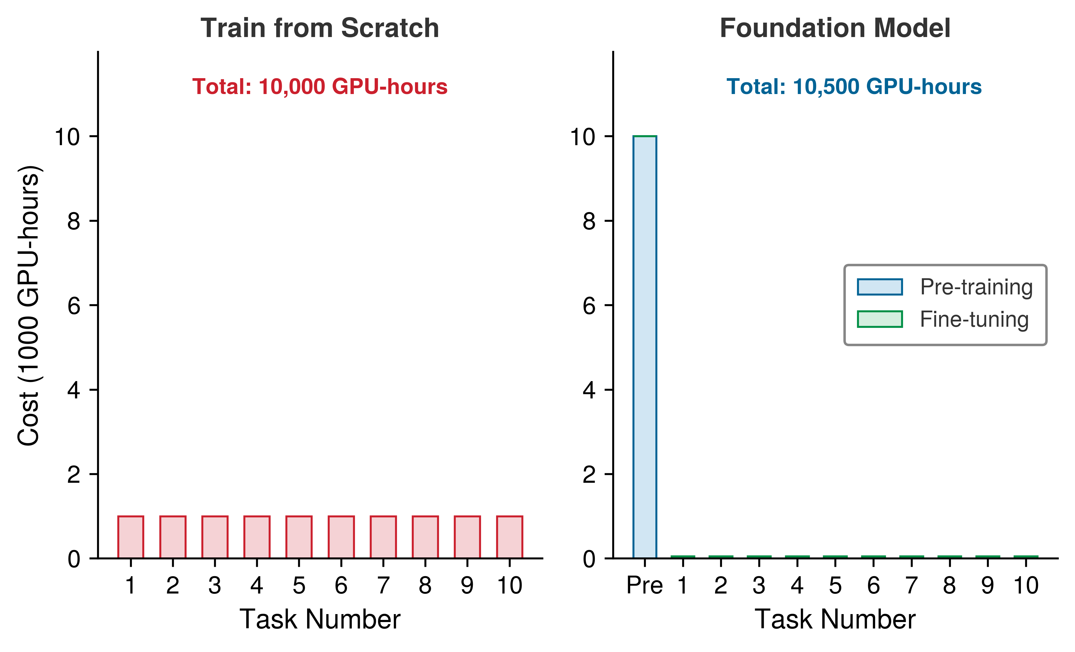
Every lever is now in view: pruning, reordering, labeling, creating, and learning without labels. Each has been judged so far by the work it removes; the next question is whether the machine can run it without giving that saving back.

Self-Check: Question

1. Explain the mechanism of confirmation bias in semi-supervised pseudo-labeling, and specify how confidence thresholding mitigates it.

2. True or False: Consistency regularization methods such as FixMatch assume that label-preserving perturbations of an input should not change the model’s predicted class distribution much.

3. In the economics of foundation models, an organization invests \(C_{\text{pretrain}} = 10{,}000\) GPU-hours in self-supervised pretraining. Each downstream task fine-tuning costs \(C_{\text{finetune}} = 50\) GPU-hours. Training each task from scratch would cost \(C_{\text{scratch}} = 1{,}000\) GPU-hours. What is the minimum number of downstream tasks \(N^*\) required to break even on the pretraining investment?

   1. \(N^* = 5\) downstream tasks
   2. \(N^* = 8\) downstream tasks
   3. \(N^* = 11\) downstream tasks (\(10{,}000 + 11 \times 50 = 10{,}550 < 11 \times 1{,}000 = 11{,}000\))
   4. \(N^* = 50\) downstream tasks

4. How does the MoCo (Momentum Contrast) framework reduce the hardware and memory constraints of contrastive self-supervised learning compared to naive SimCLR?

   1. By replacing convolutional backbones with rule-based lookup tables to avoid backpropagation
   2. By requiring fully supervised class labels to filter out false negative pairs
   3. By using a dynamic queue of negative keys and a slowly updating momentum encoder, decoupling negative dictionary size from mini-batch size
   4. By computing exact pairwise Jaccard similarities on raw byte sequences rather than latent embeddings

5. What is the systems-level ‘homogenization risk’ (or blast radius) of pretraining a shared foundation model on an uncurated dataset?

6. True or False: Because self-supervised pretraining learns general representations from unlabeled data, it completely eliminates the need for data selection or quality filtering during the pretraining stage.

See Answers →

9.7 Selection Engineering

A naive active learning loop that scans the entire dataset every epoch to select the “best” samples can turn a compute-bound training job into an I/O-bound bottleneck. Selection engineering is the work of making a chosen technique deliver its promised speedup on real hardware and real data pipelines. The pipeline must keep scoring cheap, reads sequential, and the accelerator fed.

The machine sets the scale for every one of those patterns. One ImageNet epoch of ResNet-50 on one H100 passes through four stages: images are read from local storage, decoded and augmented on host CPUs, copied across PCIe into accelerator memory, and consumed by the accelerator’s arithmetic. Pruning shrinks the last stage directly; whether the other stages shrink, stay the same, or grow depends on how the selection is engineered (figure 10).

Figure 10: ResNet-50 Data Path on One H100: One ImageNet epoch crosses four stages: local storage, host decoding and augmentation, the PCIe link, and the accelerator. Loads under each stage are per full epoch at the compute-bound rate; notes above each stage name the lever that acts there. A materialized coreset halves the storage read and the arithmetic, stream-and-discard filtering halves only the arithmetic, offline distillation targets add bytes to every stage before the accelerator, and a scoring pass adds one third of an epoch of forward arithmetic once. The host stage, outlined in red, must decode and augment every image at the accelerator’s rate.

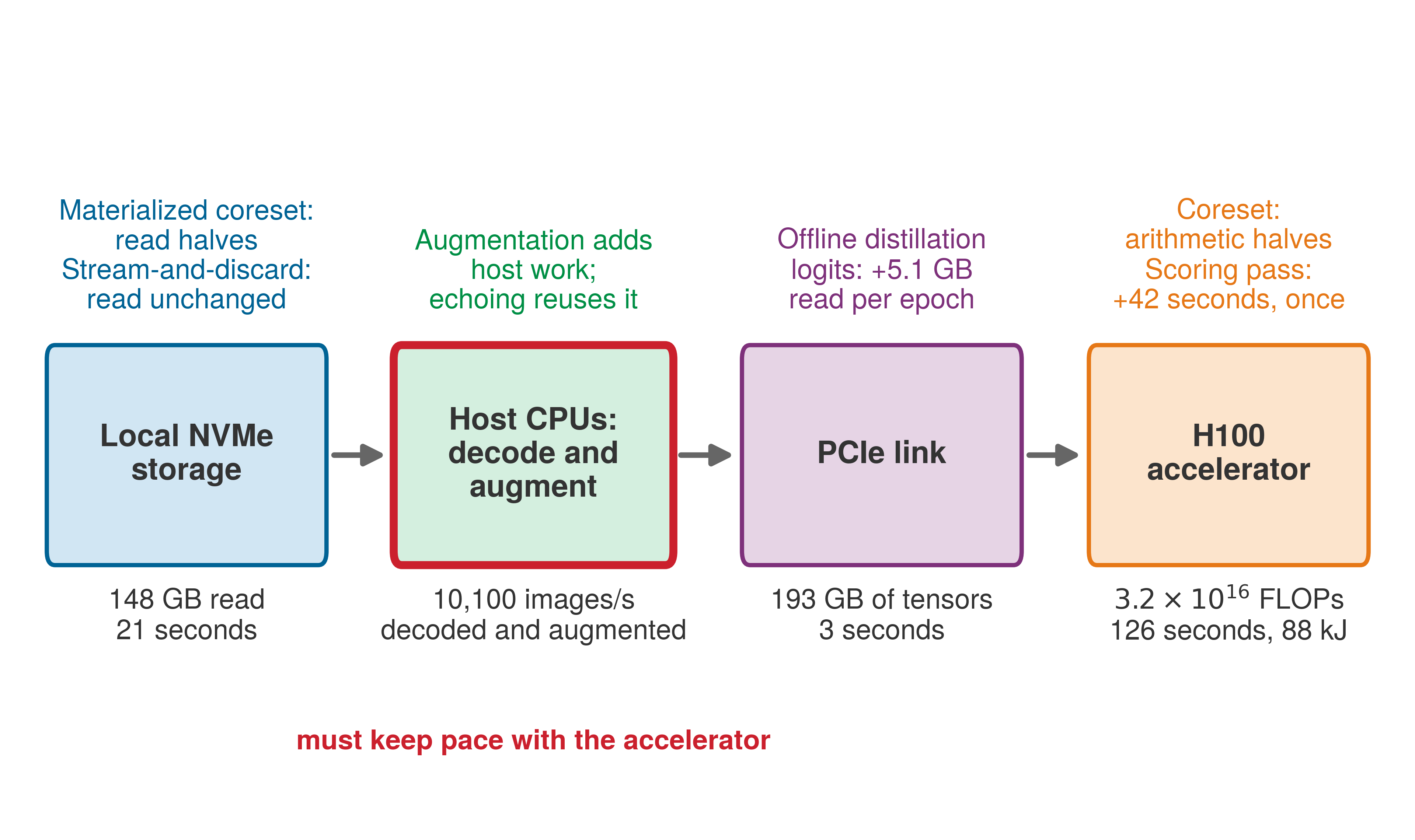
Napkin Math 9.4: One pruned ResNet-50 epoch on the H100

Problem: ResNet-50 trains on the 1.28 million ImageNet training images for 90 epochs on one H100, and a coreset keeps 50 percent of the images. How much accelerator time and energy does the coreset save once its scoring pass is paid?

Compute: Each image costs 24.6 GFLOP forward and backward, so a full epoch is 3.2 × 10¹⁶ FLOPs. At the 25 percent of peak that ResNet-50 sustains in training (Data pipeline), the H100 finishes it in about 126 seconds, which at its 700 W board power is about 88 kJ. The pruned epoch takes about 63 seconds and 44 kJ.

Selection: An EL2N-style scoring pass is one forward pass over the full pool, a third of an epoch’s arithmetic, about 42 seconds and 29 kJ, paid once. Over 90 epochs the coreset saves about 4 MJ and 2 hours of accelerator time, 135× the scoring energy.

Data path: To stay compute-bound, the accelerator must receive about 10,100 images per second. Reading the 148 GB ImageNet archive from local NVMe at 7 GB/s takes about 21 seconds per epoch, and copying the decoded 8-bit tensors (193 GB) across PCIe at 64 GB/s takes about 3 seconds, both inside even the pruned epoch. The stage that must keep up is the host CPU, which has to decode and augment 10,100 JPEG images every second. The training chapter’s host supplies only about 5,250 per accelerator, so an epoch actually takes about 244 seconds until decode capacity grows; the seconds below are the compute-bound figures selection can claim once the host keeps up.

Systems insight: Pruning halves the Data factor (\(\text{Samples/Task}\)), cutting total arithmetic \(\Operations\) and accelerator energy in half, but it halves the storage read (\(\DataVolume/\Bandwidth\)) only if the retained subset is written out as its own shards; streaming the full archive and discarding half leaves storage traffic unchanged. The seconds come from FLOPs, and whether they are realized depends on the slowest stage of the data path, which for ResNet-50 is often host decoding (Pipeline stages and accelerator bubbles).

Each lever also adds memory or storage of its own and compute or I/O of its own, and those costs land on different stages of the same data path (table 7).

Table 7: Memory and Compute Cost of Each Lever: Values for the chapter’s two lighthouses on the reference H100 machine. Each lever adds memory or I/O at one stage of the data path while removing work at another, so the stage it loads must not become the new bottleneck.

Lever (lighthouse)	Memory or storage it adds	Compute or I/O it adds	Work it removes
MinHash deduplication (GPT-2, WebText)	4.1 GB of signatures in host memory	One 40 GB read (6 seconds) plus host hashing	3.04% to 13.63% of tokens processed
EL2N coreset scoring (ResNet-50, ImageNet)	One score per image (5.1 MB)	One forward pass over the pool (42 seconds, 29 kJ)	Half of every epoch (63 seconds, 44 kJ)
Coreset materialization	A 74 GB repacked subset, written once	One read and one partial write of the archive	Half of every later epoch’s storage read
Stream-and-discard filtering	None	The full 148 GB read every epoch (21 seconds)	Accelerator work only; storage traffic unchanged
Offline distillation targets (ResNet-50)	5.1 GB of FP32 logits in place of 2.6 MB of labels	One teacher forward pass over the pool, then a 5.1 GB read every epoch	Teacher residency in accelerator memory during training

Those added costs surface in four places (scoring, storage reads, host preparation, and coordination across workers), and each has an engineering pattern that keeps it off the critical path.

9.7.1 The selection bottleneck

Evaluating a selection function \(\SelectionScoreFunction(\ModelInput)\) over a large candidate pool before forming every batch can easily cost more compute than training on the unselected data. While a conventional loader follows a predetermined sampling plan, active learning and adaptive curricula score candidates dynamically during training, introducing selection latency. In the ResNet-50 example of section 9.2.6, one static scoring pass with the target model costs a third of an epoch and is paid once. Rescoring the full ImageNet pool before every one of the 100 epochs instead adds 70 minutes of forward passes to 21 minutes of subset training, more than three times the training it serves, and cuts the saving from 90 percent to 57 percent. The selection inequality (equation 2) still holds, but scoring has become the largest term, and a heavier scorer or a smaller retained fraction would break it.

Engineering pipelines keep selection latency off the critical path through proxy models, cached embeddings, and indexed retrieval. A smaller proxy model curtails scoring time provided its sample ranking transfers accurately to the target architecture, and running the scoring pass in reduced numerical precision raises arithmetic throughput and cuts memory traffic when ranking fidelity permits. For similarity-based or diversity-based selection, vector indices such as FAISS³³ replace expensive corpus-wide scans with approximate nearest-neighbor retrieval over precomputed embeddings. These techniques decouple selection evaluation from primary model training and shrink \(\SelectionTime\), but even zero-cost scoring can still slow down training if fetching the selected indices stalls the storage layer.

³³ FAISS (Facebook AI Similarity Search): Provides GPU-accelerated similarity search using exact, approximate, and compressed-domain index designs (Johnson et al. 2019); Johnson, Douze, and Jegou report billion-vector graph construction on multiple GPUs, showing why vector-index infrastructure matters for web-scale selection. For data selection pipelines, FAISS-style indexing supports \(\NeighborCount\)-nearest-neighbor retrieval for coreset selection, embedding-based deduplication, and stratified clustering for balanced sampling. Without this infrastructure, embedding-based selection would often fall back to expensive full-corpus scans.

Johnson, Jeff, Matthijs Douze, and Hervé Jégou. 2019. “Billion-Scale Similarity Search with GPUs.” IEEE Transactions on Big Data 7 (3): 535–47. https://doi.org/10.1109/tbdata.2019.2921572.

9.7.2 The random-access penalty

Selecting a sparse subset of examples scattered across a dataset turns large sequential shard transfers into thousands of nonsequential reads, forfeiting hardware readahead, OS page caching, and bulk controller prefetching. Training already pays for shuffling through the access factor \(\StorageAccessFactor\) that scales effective storage throughput in the data-pipeline model of Core components, and selection pushes that factor lower by design because the retained records no longer sit contiguously on disk. Because disk heads must physically seek and flash controllers must execute random block lookups, two subsets of equal size can differ sharply in wall-clock training time according to their access locality. Table 8 quantifies this small-read penalty across storage tiers for 4 KB transfers.

↩︎ Random access is measured in IOPS and streaming access in sequential throughput, the two storage metrics established in Storage system options.

Table 8: Illustrative Small-Read Penalty: Registry device anchors compare sequential bandwidth with random 4 KB reads under a simplified IOPS conversion. Real throughput depends on request size, queue depth, concurrency, caching, and service configuration; the cloud row is only a qualitative scenario.

Storage Tier	Sequential Throughput	Random I/O (IOPS)	Random Throughput (approx)	Random Penalty
HDD (7.2k)	~150 MB/s	~100 IOPS	~0.4 MB/s	375×
SATA SSD	~550 MB/s	~10K IOPS	~40 MB/s	13.8×
NVMe SSD	~3,500 MB/s	~500K IOPS	~2,000 MB/s	1.75×
Cloud (S3)	Configuration-dependent	Not IOPS-comparable	Configuration-dependent	Potentially extreme

Data loaders (whose general mechanism Data loading develops) avoid the problem by packing examples into large shards and shuffling inside a memory buffer. Sharded dataset formats, such as WebDataset and FFCV, pack thousands of individual examples into contiguous, sequentially readable archive chunks. Rather than fetching scattered individual samples from disk, the loader streams large sequential shards into host memory and populates a shuffle buffer. The training loop samples pseudo-randomly from this in-memory buffer, preserving peak storage read bandwidth while satisfying the statistical requirement of randomized mini-batches.

Converting a logical set of selected indices into sequential physical reads requires choosing between two storage strategies. For static pruning (such as a fixed coreset or a deduplicated corpus), the pipeline can materialize the subset offline by repacking the retained records into new, contiguous shards. This step incurs a one-time sequential read and write cost alongside additional disk storage, but ensures that every subsequent training epoch transfers only retained bytes from storage. Conversely, when the selection policy updates dynamically across training iterations or active-learning rounds, repeatedly repacking multi-terabyte shards on disk would choke the filesystem on write bandwidth. Data loaders instead stream the original, full-volume shards sequentially into host memory and discard unselected records before populating the shuffle buffer. This online filtering preserves sequential read throughput and eliminates seek penalties, but it leaves physical storage traffic unchanged: the host continues to read 100 percent of the corpus bytes from disk even when accelerators train on only a 10 percent subset. Systems engineers must count this ongoing read traffic on storage-bound nodes and include offline materialization costs when evaluating the selection inequality, and even after storage reads are streaming at full speed, host-side decoding and augmentation can still starve the accelerator.

Checkpoint 9.2: Selection overhead and storage access

Equation checks

• Selection cost: Explain why \(\SelectionTime+ \TrainingTime(\SubsetDatasetSize)\) must be strictly less than \(\TrainingTime(\FullDatasetSize)\) for the technique to reduce end-to-end training time.
• Overhead management: Explain how proxy models and cached embeddings keep \(\SelectionTime\) low.

Systems implications

• I/O patterns: Explain why nonsequential access for dynamic selection reduces data-loader throughput relative to sequential reads.

9.7.3 Data echoing

Even with sequential reads, the host CPU often cannot decode and augment samples fast enough. Heavy data transformations, such as 3D rotations, MixUp, JPEG decoding, or on-the-fly generative synthesis, demand substantial host processing per sample. When the host pipeline produces batches slower than the accelerator executes forward and backward passes, the accelerator idles, starved for input; this is the feeding problem reappearing inside the selection loop. The resulting collapse in accelerator utilization extends training wall-clock time, neutralizing the efficiency gains achieved by pruning the dataset.

↩︎ Accelerator bubbles, which open when the data-loading stage cannot keep pace with the accelerator, are established in Pipeline stages and accelerator bubbles.

³⁴ Data echoing: The key subtlety is where in the pipeline to insert the echo point. Echoing before augmentation (upstream echoing) can apply different random augmentations to each repetition, while echoing after augmentation feeds identical tensors to the accelerator. Useful echo factors and realized speedups depend on the workload, batch size, insertion point, and shuffling policy (Choi et al. 2019).

Choi, Dami, Alexandre Passos, Christopher J. Shallue, and George E. Dahl. 2019. “Faster Neural Network Training with Data Echoing.” arXiv Preprint, ahead of print. https://doi.org/10.48550/arXiv.1907.05550.

Data echoing³⁴ (Choi et al. 2019) reuses data multiple times before fetching new samples, trading freshness for accelerator utilization when the input pipeline is slower than training. Echoing before randomized augmentation can produce different transformed inputs on each repetition, while echoing later in the pipeline may repeat identical tensors.

The optimal echo factor depends on the ratio \(\InputPipelineRatio\) of upstream processing time to downstream training time, where \(\HostPreparationTime\) is the time the data pipeline needs to produce a batch and \(\AcceleratorBatchTime\) is the time the accelerator needs to train on it: \[ \InputPipelineRatio= \frac{\HostPreparationTime}{\AcceleratorBatchTime} \]

In this two-stage rate model, \(\InputPipelineRatio> 1\) means the data pipeline bottlenecks training. An echo factor \(\EchoFactor< \InputPipelineRatio\) partially recovers idle accelerator cycles, while \(\EchoFactor\ge \InputPipelineRatio\) removes input waiting entirely, provided repeated samples remain statistically productive. Raising \(\EchoFactor\) beyond \(\InputPipelineRatio\) adds no throughput and only reduces gradient diversity. When \(\InputPipelineRatio< 1\), the input pipeline already outruns the accelerator, so echoing has nothing to recover.

Echoing raises accelerator utilization until \(\EchoFactor\) reaches \(\InputPipelineRatio\); beyond it, nothing is gained.

Napkin Math 9.5: Worked example: Data echoing ROI

Scenario: Training ResNet-50 on ImageNet on one H100 fed by the training chapter’s host, where host preparation is the slow stage (Data pipeline).

Rates:

• Data pipeline throughput: 5,250 images/s (the host cores available to one accelerator, each reading, decoding, and augmenting about 375 images/s)
• Accelerator training throughput: 10,100 images/s (forward and backward pass at the compute-bound rate of notebook 9.4)
• Ratio \(\InputPipelineRatio= \HostPreparationTime / \AcceleratorBatchTime\) = (1/5,250 images/s) / (1/10,100 images/s) = 10,100 images/s/5,250 images/s ≈ 1.92 (accelerator waiting 48.0 percent of the time)

Without echoing:

• Effective throughput: 5,250 images/s (limited by data pipeline)
• Training time for 90 epochs: \(90 \times 1.28\text{M}\) / 5,250 images/s = 21,963 seconds (6.1 hours)
• Accelerator utilization: 52.0 percent

With echo factor: \(\EchoFactor\) = 2, inserted after the measured reading, decoding, and augmentation stage.

• Each already-augmented batch is processed twice, amortizing the measured upstream work; the repeated pass introduces no fresh augmentation
• Effective throughput: 10,100 images/s, the accelerator’s full rate, because an echo factor above the ratio leaves the accelerator no time waiting
• Unique images per second: 5,250 images/s (unchanged)
• Training time: \(90 \times 1.28\text{M}\) / 10,100 images/s = 11,416 seconds (3.2 hours) if echoed data is equally valuable

Trade-off: Repeated samples are not guaranteed to be as useful as fresh samples; the data echoing paper evaluates echo factor, insertion point, and shuffling because those choices determine whether reuse preserves predictive performance. In one network-fed ResNet-50/ImageNet configuration, Choi et al. (2019) reports a 3.25\(\times\) reduction in wall-clock time to the target metric.

Systems insight: Data echoing can trade sample diversity for accelerator utilization when the input pipeline is the bottleneck. For the training chapter’s input-bound ResNet-50, overlap alone left the accelerator about half idle; an echo factor of 2 closes that gap without adding host cores. The useful echo factor must be measured for the workload because it depends on the batch size, insertion point, augmentation, shuffling, and target metric.

Echoing can introduce correlations when the same example appears within or across nearby batches, so implementations must preserve adequate shuffling and validate the target metric. Choi et al. (2019) did not observe a negative batch-normalization interaction in their ResNet-50 or Single Shot MultiBox Detector (SSD) experiments, but that result does not guarantee the same behavior for every workload.

These implementation patterns determine whether data selection yields net systems throughput. Proxy selection curtails probe compute when scoring rankings transfer to target architectures. Sharded file formats and shuffle buffers reconcile pseudo-random batch creation with hardware-level sequential streaming, while data echoing recovers stalled accelerator cycles when ingestion throughput limits the training loop. They still leave a coordination question when several accelerator workers share one host: each worker scores or trains on its own shard, yet the selected indices and scoring checkpoint must still describe one coherent dataset, because shared storage and host memory do not automatically make each worker’s local view representative of the corpus.

9.7.4 Selection across multiple accelerators

When parallel worker processes divide a dataset into local shards across two to eight accelerators on one host, each worker sees only a fraction of the corpus and may score its shard with a slightly different model checkpoint. Without cross-worker coordination, shard-local coreset rankings miss rare global classes, independent hash tables fail to catch duplicates split across workers, and asynchronous active-learning workers select samples using stale uncertainty scores. While a single-process pipeline sorts one global ranking, follows one curriculum schedule, and queries one shared candidate pool, a multi-accelerator pipeline must reconstruct a representative global subset from local shard views while all workers contend for the same host memory capacity, storage bandwidth, and host-to-device links.

Whether distributed selection stays faithful to the global dataset or collapses into local shard heuristics depends on how much cross-worker coordination each technique requires against the bandwidth available to sustain it. On one host, score gathering and index dispatch compete for CPU time and memory bandwidth with decoding and batch preparation. Evaluating selection therefore requires analyzing statistical fidelity alongside these shared resources.

These are independent requirements. A coreset can remain representative yet cost too much to coordinate, while a cheap shard-local method can scale but systematically miss rare groups visible only in the global corpus. A distributed design therefore needs two acceptance tests: compare selected-data quality with a centralized or otherwise auditable reference, and compare selection overhead with the end-to-end training time it saves. Passing only one test is insufficient.

Strategies for distributed selection

In a basic data-parallel layout, each worker processes a distinct shard and model synchronization is handled separately. Data selection can add dependencies across those shards (table 9).

Table 9: Selection Dependencies in Distributed Training: The table starts from a common centralized formulation of each technique and identifies the coordination problem introduced by sharding. Distributed variants may relax rather than reproduce the centralized result exactly.

Technique	Single-Process Assumption	Distributed Challenge
Coreset Selection	Global view of dataset	Each worker sees only its shard
Active Learning	Centralized uncertainty scoring	Scoring requires model synchronization
Curriculum Learning	Global difficulty ordering	Workers may have different “hardest” samples
Deduplication	One shared duplicate map	Shard-local hashes miss cross-shard duplicates

The selection dependencies admit two broad architectures, each at a different point in the trade-off between consistency and scalability. Centralized selection keeps selection global while training stays distributed. A coordinator process scores the full dataset and dispatches the selected indices to the workers, which preserves selection quality but makes the coordinator a single bottleneck that can serialize scoring or index dispatch. Whether that overhead is acceptable depends on the selection payload, refresh rate, worker count, and copies through shared host memory, and adding accelerator workers does not increase the host memory available to the coordinator. Hierarchical selection distributes the selection computation itself. Each worker selects candidates from its own shard, and the coordinator merges and reranks them before dispatching the final indices (figure 11). Shard-local selection reduces coordinator load but introduces a quality trade-off, because local quotas and score distributions may not preserve the global ranking or rare groups spread unevenly across shards. The merge step therefore needs normalization, coverage constraints, or a second global pass.

Figure 11: Distributed Coreset Selection Architecture: Parallel shard-local scoring reduces the work assigned to a centralized rank-merging coordinator. Workers send local EL2N scores upward; the coordinator merges them and broadcasts final coreset indices. All boxes are processes on one host; the coordinator is a selection role, and each worker drives one accelerator. The design is beneficial only when this coordination overhead remains below the training time saved by the coreset.

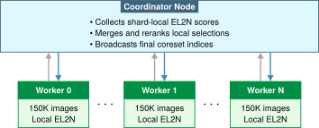
Shard locality affects training as well as selection. Each worker maintains an independent shuffle buffer over a non-overlapping shard, and because randomization is local to each worker’s memory buffer rather than global across the corpus, rare classes or boundary cases concentrated in specific shards receive uneven exposure across workers unless the dataset is stratified and shards are balanced prior to distribution.

Cross-shard deduplication needs the same global view as hierarchical selection. Workers can compute MinHash signatures locally, but a shared merge must compare candidates across shard boundaries. Independent local hash tables cannot detect a duplicate whose counterpart belongs to another worker. The merge must fit the host’s memory budget or operate in bounded batches, rather than assuming that more workers supply more host capacity.

Consistency challenges in active learning

Shard-local selection already needs a coherent score scale, but active learning introduces an additional complication because the model changes during selection. Consider what happens when Worker A scores samples using the model at step \(\OptimizerStepIndex\) while Worker B simultaneously updates the model to step \(\OptimizerStepIndex+1\). Worker A’s scores are now stale and may select samples that the updated model would rank differently.

The scoring schedule therefore defines the meaning of a query, not merely its cost. A reproducible system versions the model checkpoint, candidate-pool snapshot, scoring rule, and selected indices together. It can then measure how much ranking agreement decays with checkpoint age and choose a refresh interval from that evidence rather than from an arbitrary number of steps.

Several strategies mitigate this staleness problem, each with distinct overhead characteristics:

• Synchronous scoring: All workers pause training and score simultaneously, guaranteeing consistency but at substantial cost in accelerator utilization.
• Periodic score refresh: Workers re-score every \(\ScoreRefreshInterval\) epochs rather than every batch, trading freshness for reduced overhead.
• Checkpoint-robust selection: The system selects samples that show high uncertainty under multiple model checkpoints, favoring decisions that are less sensitive to checkpoint choice. Agreement across past checkpoints is a robustness heuristic; ranking quality still needs validation as the model evolves.

Positive ROI can erode quickly when workers coordinate frequently during training. Selection across workers adds coordination overhead whose size depends on what is synchronized and how often. That overhead must remain smaller than the training time saved, and when it approaches that limit, a simpler strategy or a longer refresh interval restores the margin.

The communication path adds a further constraint. Gradient synchronization may use accelerator collectives over local interconnects, while embedding vectors, score arrays, and coreset indices may pass through host memory and CPU dispatch. Selection can therefore expose host-memory, PCIe, storage, or process-synchronization bottlenecks that the training profile alone does not reveal. Extending the design to independent machines adds network topology and remote-storage constraints; those are a further scaling problem beyond the one-host design developed here.

Operational feasibility, however, does not guarantee economic viability. A deduplication pipeline that costs more to build than one training run saves loses money on a single run and pays off only if enough runs reuse it. Deploying selection techniques therefore requires financial accounting of capital, compute, and human annotation budgets.

Self-Check: Question

1. Why do naive random sample lookups across non-contiguous indices in large un-sharded dataset files severely degrade I/O throughput on storage hardware, and how do shuffle buffers mitigate this?

   1. Random lookups bypass host CPU caches, forcing floating-point registers to re-encode all labels
   2. Random lookups violate PCIe parity checks, causing GPU kernel timeouts during backward passes
   3. Random lookups trigger hash collisions in the Python garbage collector, halting dataloading threads
   4. Random 4 KB reads achieve only a tiny fraction of peak sequential storage bandwidth due to IOPS limits, whereas shuffle buffers read large sequential chunks and randomize locally in memory

2. Contrast upstream data echoing (echoing before data augmentation) with downstream data echoing (echoing after augmentation) in terms of computational overhead and sample diversity.

3. True or False: If the GPU training step takes 20 ms and the CPU data loading/augmentation pipeline takes 10 ms (\(R = T_{\text{pipeline}} / T_{\text{GPU}} = 0.5\)), applying a data echoing factor of \(e = 2\) will double the end-to-end training throughput.

4. On one host with two to eight accelerator workers, how can centralized coreset selection become a bottleneck, and what trade-off does hierarchical selection introduce?

   1. Centralized selection requires all workers to share a single GPU; hierarchical selection distributes weights across SSDs
   2. Centralized selection fails because sharding prevents network cards from transmitting floating-point values
   3. Centralized selection can bottleneck host memory and coordinator dispatch; hierarchical selection prunes locally per shard, risking loss of globally rare samples across shards
   4. Centralized selection eliminates gradient synchronization; hierarchical selection disables local backpropagation

5. In distributed active learning, Worker A scores candidate samples using checkpoint step \(t\), while Worker B has already advanced the shared model to step \(t+100\). What consistency challenge arises, and what is the best response?

   1. Worker A encounters deadlock in CUDA streams; disable autograd during scoring
   2. Worker B overwrites Worker A’s local storage; mount the dataset read-only
   3. Worker A’s GPU runs out of memory; reduce batch size to 1
   4. Worker A may produce stale rankings that differ from fresher ones; version checkpoints and choose the score-refresh interval from measured ranking agreement

6. Explain why performing independent, shard-local coreset pruning on an unstratified, partitioned dataset can cause minority class collapse during distributed training.

See Answers →

9.8 Choosing a Selection Strategy

The hospital team in notebook 9.3 could not label every scan, because doing so would have cost $5,000,000, 10× over its budget. Allocating capital between human annotation and accelerator compute is a primary systems decision, and a team under a fixed budget must determine whether the next dollar buys more downstream accuracy as specialist annotations or as additional accelerator hours. A cost model settles the question, and the choice among levers follows from it in four steps: the total cost of data, the break-even point of a selection pipeline, the amortization of one-time investments across the runs that share them, and a decision process worked on the ResNet-50 vision team of section 9.2.6.

9.8.1 Data costs and return on investment

Budgeting a training project from cloud GPU and object-storage invoices alone misses the licensing and human annotation bills that often dwarf compute cost. The total cost of training data spans acquisition, labeling, storage retention, and accelerator compute across the full data lifecycle: \[ \TotalDataCost= \DataAcquisitionCost+ \DataLabelingCost+ \DataStorageCost+ \DataProcessingCost\] Labeling (\(\DataLabelingCost\)) represents the expenditure that data selection targets most directly, whereas storage (\(\DataStorageCost\)) and processing (\(\DataProcessingCost\)) scale mechanically with retained byte volume and the number of accelerator passes. Table 10 itemizes these four cost components alongside their operational drivers.

Table 10: Total Cost of Training Data: The four cost components span the full data lifecycle. Here \(\DatasetSize\) is the total sample count, \(\LabeledSampleCount\) is the labeled subset, \(\StoredDataVolume\) is stored byte volume, \(\StorageRetentionTime\) is retention time, \(\EpochCount\) is the number of training passes, and \(\OperationsPerSample\) is per-sample training work. The ranges are scenario anchors rather than universal market prices.

Component	Formula	Illustrative Range
\(\DataAcquisitionCost\)	\(\DatasetSize\times \SampleAcquisitionPrice\)	$0.001–$10/sample (web scrape vs. licensed)
\(\DataLabelingCost\)	\(\LabeledSampleCount\times \SampleLabelingPrice\)	$0.01–$200/sample (crowd vs. expert)
\(\DataStorageCost\)	\(\StoredDataVolume\times \StoragePrice\times \StorageRetentionTime\)	$0.02–$0.10/GB/month
\(\DataProcessingCost\)	\(\DatasetSize\times \EpochCount\times \OperationsPerSample\times \FlopPrice\)	Proportional to training FLOPs

The interplay of these four cost terms becomes concrete when evaluating an ImageNet-scale vision model training run. Calculating each term explicitly shows how easily data acquisition and human labeling outspend the accelerator hours needed to fit the weights.

Napkin Math 9.6: Cost breakdown: ImageNet-scale training

Table 11 itemizes one illustrative acquisition, labeling, storage, and compute scenario at ImageNet scale. The resulting ratio follows from the stated licensing, annotation, storage, runtime, and compute-cost assumptions; it is not a typical ratio for every supervised workload.

Table 11: Illustrative ImageNet-Scale Cost Breakdown: Itemized acquisition, labeling, storage, and compute costs under the stated scenario assumptions. Each amount follows from the rate shown beside it, using the book’s published crowd-labeling, object-storage, and cloud-GPU rates. Data costs dominate this particular calculation because licensing and annotation are included while the training run itself is short.

Cost Component	Calculation	Amount
Raw data (1.2M images)	Licensed dataset, flat fee	$50,000
Labels (crowd annotation)	1.2M \(\times\) $0.05/label	$60,000
Storage (cloud object store)	150 GB \(\times\) $0.02/GB/month \(\times\) 12 months	$36
Training campaign (30 runs, each 100 epochs in 3.5 h on 1 H100)	105 GPU-hours \(\times\) $4/GPU-hour	$421
Total		$110,457
Data vs. Compute ratio		99.6% data, 0.4% compute

Systems insight: Acquisition and labeling can dwarf compute cost in supervised vision workloads, as they do under these assumptions. The compute figure covers the whole training campaign at the compute-bound rate of notebook 9.4, not one run: a published model is the survivor of sweeps, restarts, and ablations, and costing a single run would understate compute roughly thirtyfold. Even so, acquisition and labeling remain the larger share. The run count is an assumption like any other, so a complete ROI calculation must state it and count both categories rather than assuming which one dominates.

Data selection techniques insert algorithmic filtering into the training pipeline to reduce downstream costs. Scoring consumes accelerator cycles, generates host-device memory traffic, or requires custom pipeline stages, so a strategy is justified only if the downstream savings exceed these overheads. Return on investment (ROI), the savings net of the investment per unit invested, makes that test explicit. Because a selection investment is often reused across a training campaign, the general form counts the \(\TrainingRunCount\) runs that share it, the amortized ROI: \[ \text{Amortized ROI} = \frac{\TrainingRunCount\times \text{Per-Run Savings} - \text{One-Time Investment}}{\text{One-Time Investment}} \times 100\% \tag{3}\]

A single run sets \(\TrainingRunCount= 1\) and recovers the ordinary ratio of savings minus investment to investment, whereas the balance between investment and savings varies across selection strategies. Table 12 maps the primary cost drivers and benefit mechanisms across four standard techniques; their net return depends on corpus volume, model scale, and existing pipeline infrastructure.

Table 12: ROI Profiles for Data Selection Techniques: The table identifies costs and possible savings. No technique guarantees positive ROI. A training-time claim must satisfy the selection inequality; labeling savings or reusable data investments require their corresponding total-cost comparison at target quality.

Technique	Investment (Cost)	Savings (Benefit)
Deduplication	One-time compute for hashing + infrastructure	Reduced storage and repeated-sample processing
Coreset Selection	Proxy model training + selection compute	Fewer retained samples if target quality and coverage hold
Active Learning	Inference on unlabeled pool + human-in-the-loop latency	Lower labeling demand when query selection transfers
Data Augmentation	CPU/GPU cycles for transforms	Effective dataset size increase without new data acquisition

The profiles in table 12 compare those costs directly. Deduplication requires an upfront investment in hashing or embedding infrastructure, but can pay off across many epochs and runs by eliminating redundant storage and compute. Coreset selection demands training a proxy model to score the dataset; it only breaks even if the compute saved by dropping samples exceeds the cost of that proxy training. Active learning shifts the cost from human labelers to machine inference, generating high ROI when human time is expensive, though it introduces human-in-the-loop latency that can stall automated pipelines. Finally, data augmentation requires zero new data acquisition but shifts the burden to the CPU or GPU, trading compute cycles for effective dataset expansion. Each technique is worth adopting only when its savings exceed what it costs to set up and run, which makes locating that exact crossover threshold the next step.

9.8.2 Break-even analysis

If candidate scoring is computationally heavy or the unlabeled pool is massive, a selection policy can spend more money scoring candidates than it saves on omitted labels or training steps. The break-even point marks the operating boundary where the financial savings from omitted samples exactly equal the computational and operational overhead of selecting them.

Suppose labeling costs $10/sample, active learning starts from 1,000 labeled samples ($10,000), issues 100 queries per round at $50 inference cost (the expense of scoring the candidate pool \(\UnlabeledPool\) with the active model), and the random-labeling baseline requires 5,000 samples for target accuracy. If active learning reaches target accuracy with only 2,000 labeled samples, the following comparison reports net savings relative to the stated labels-plus-scoring cost. This calculation includes labels and pool scoring only, assumes both methods reach the same target accuracy, and excludes retraining, engineering, storage, and annotation-delay costs. It reports net savings per dollar of that stated active-learning budget, using a different denominator from the investment ROI of equation 3: \[\begin{gather*} \text{Random labeling cost} = \text{5,000} \times \text{\$10/sample} = \text{\$50,000} \\ \text{Active learning cost} = \text{2,000} \times \text{\$10/sample} + \text{10 rounds} \times \text{\$50} = \text{\$20,500} \\ \text{ROI} = \frac{\text{\$50,000} - \text{\$20,500}}{\text{\$20,500}}= \text{$143.9\%$} \end{gather*}\]

Within this labels-plus-scoring boundary, break-even occurs when avoided labeling costs equal selection overhead. A complete dollar comparison must also deduct any additional retraining, engineering, storage, and delay-related expense relative to the random-labeling baseline. When an unlabeled candidate pool \(\UnlabeledPool\) contains millions of uncurated examples, repeatedly scoring it across multiple rounds scales scoring cost with \(|\UnlabeledPool| \times \CandidateScoringCost\), meaning an algorithmic reduction in labeled samples can be erased if proxy inference costs are not carefully bounded. When one fixed budget funds both scoring and labeling, every dollar spent scoring the pool is a dollar withdrawn from labels, so practical loops narrow \(\UnlabeledPool\) with metadata or a cheap heuristic before the active model scores it. Even a pipeline that loses money on a single run, however, can cross break-even once its output is reused across an entire training campaign.

9.8.3 Amortization across training runs

Charging the entire engineering and preprocessing bill of a static curation pipeline to a single training run makes a profitable campaign investment look like a net loss. Filters such as MinHash deduplication, exact \(\NgramLength\)-gram indexing, and embedding clustering require substantial upfront engineering and compute to build once, while production model development is inherently iterative: hyperparameter search, architecture sweeps, ablation studies, and seed checks repeatedly train on the same curated corpus. The amortized ROI of equation 3 therefore spreads that upfront curation investment across every run in the campaign, as table 13 itemizes for an illustrative MinHash deduplication pipeline.

Table 13: Deduplication Infrastructure Cost Components: The one-time investment covers engineering effort and initial compute; the per-run savings accrue with every subsequent training run on the deduplicated data.

Component	Cost
Build deduplication pipeline	$50,000 (engineering time)
Compute MinHash signatures (one-time)	$5,000
Per-run savings	$10,000/run

Because the initial infrastructure and signature-generation costs are fixed, each subsequent training run compounds the net financial return. Three operational factors govern whether curation infrastructure reaches break-even:

• Repeated training runs: Hyperparameter search, model iterations, and scheduled retraining reuse the same selection infrastructure many times.
• Shared datasets: A cleaned or deduplicated corpus can support multiple teams or model architectures.
• Broadly reusable techniques: Methods such as deduplication transfer across models, whereas task-specific coresets may not.

Table 14 tracks how amortized return scales with campaign run count under these cost parameters. A pipeline that loses money on a one-off experiment crosses break-even within a handful of retraining cycles and compounds its savings across larger campaigns.

Table 14: Amortized ROI over Multiple Training Runs: Under this scenario’s costs and savings, a deduplication pipeline that loses money on its first use becomes profitable when reused across enough runs. Infrastructure investments should be evaluated over their expected lifetime rather than from one use.

Number of Runs	Amortized ROI
1 run	-81.8% (net loss)
5 runs	-9.1% (near break-even)
10 runs	+81.8% (positive)
50 runs	+809.1% (highly profitable)

Deduplication achieves high investment leverage because eliminating redundant sequences reduces host-storage footprint and avoids wasted gradient updates across every downstream architecture. Sample-selection methods conditioned on proxy gradients or uncertainty scores transfer within a model family or between related architectures, but their rankings must be revalidated when the target model, task, or data changes, which narrows their amortization window relative to deduplication. For exploratory or one-off training runs, low-overhead methods like uniform random sampling or basic augmentation may offer better ROI. A static scoring pass can still pay for itself in one run if its measured savings exceed its cost at target quality.

Checkpoint 9.3: Accepting a data intervention

A smaller training pool is one observation in the acceptance decision. Connect the measurements to the constraint the intervention was meant to relieve.

• Time savings: Identify the scoring, coordination, and training times needed to compare a selected subset with full-data training at the same target quality.
• Cost objective: Explain how an active-learning pipeline could reduce total expenditure even if it takes longer to train, and identify the costs that must enter that comparison.
• Coverage: Decide whether unchanged aggregate accuracy is sufficient when a deployment-critical rare slice regresses, and name the additional validation evidence needed. For the disjoint-class allocation in section 9.3.4, explain why reducing \(\CoresetBudget\) below \(\FirstClassCoverageFloor+\SecondClassCoverageFloor\) requires revising the selection plan before training, even if every remaining example has a high score.

With time, labeling, and amortized costs expressed in one accounting, every technique in the chapter can now be weighed against the claim it makes. A training-time saving must satisfy the selection inequality, a labeling saving must beat the random-labeling baseline after scoring and any other differing costs, and a reusable investment must recover its one-time cost across the runs or tasks that share it. Costing each technique separately, however, does not say which one to reach for first when several of them compete for the same budget.

9.8.4 Decision process

When labeling budget, redundancy, rare classes, privacy, and convergence speed conflict, systems engineering requires identifying the primary binding constraint. Table 15 collects the three levers with order-of-magnitude ranges drawn from scenarios like those worked in this chapter; each must reduce the cost it targets after counting its overhead and preserving target quality and required coverage. Self-supervised pretraining, which changes the training signal rather than the sample set, enters the decision through the labeling-cost branch of the tree that follows.

Table 15: Three-Stage Data Selection Pipeline: The ranges illustrate possible outcomes rather than portable expectations. Actual gains depend on the dataset, model, selection method, and target metric.

Stage	When Applied	Techniques	Order-of-Magnitude Scenario Range
Static pruning	Before training	Coreset Selection, Deduplication, Quality Filtering	30–50% dataset reduction
Dynamic selection	During training	Curriculum Learning, Active Learning, Semi-Supervised	10–30% faster curricula; 2–100\(\times\) fewer labels
Synthetic generation	On-demand	Augmentation, Generative Models, Distillation	2–10\(\times\) effective data expansion

Once the dominant constraint is named, it points to a candidate technique, and the five lighthouse workloads, each bound by a different resource, show the pairing in practice. Privacy carries a condition of its own. When privacy requirements limit direct use of real records, privacy-audited synthesis can reduce that use, provided the synthetic data is checked for leakage of the records it was derived from.

Lighthouse 9.1: Lighthouse data selection

Data selection principles apply to all five lighthouse models, though the dominant constraint determines the technique. Table 16 maps each workload to a priority. Compute-bound ResNet-50 training benefits from coreset selection, while GPT-2 XL training relies on deduplication and quality filtering to cut the raw tokens it must process. MobileNetV2 is compute-bound in its efficient regime, and its binding deployment constraints, latency and power, apply at inference, where no choice of training data changes the cost of a prediction. The data lever that matters is therefore the one that helps a small model generalize, augmentation matched to its capacity (compact networks underfit under distortion that a large model absorbs), and the work is validating that the augmentation preserves the invariances the deployment environment requires. DLRM, the capacity-bound lighthouse, spends much of its terabyte-scale embedding capacity on cold IDs that appear rarely in training data. It uses interaction deduplication to cut redundant examples and embedding pruning to shrink those tables, but removing repeated interactions shrinks a table only when IDs disappear or the allocation, hashing, or sharing policy changes. Finally, keyword spotting, the power-bound lighthouse, is bound for data selection by a scarce, costly seed set as much as by its power and memory budget, and it overcomes that scarcity by using augmentation and synthesis to build robust datasets from minimal seed samples.

Table 16: Data Selection Priorities by Lighthouse: Primary bottleneck and candidate data-selection priority for each lighthouse workload. The pairing suggests a hypothesis to test; the dominant resource constraint alone does not guarantee that a technique pays off.

Lighthouse	Primary Bottleneck	Data Selection Priority
ResNet-50	Compute	Coreset selection directly reduces training FLOPs
GPT-2 XL	Training compute (tokens \(\times\) FLOPs/token)	Deduplication and quality filtering cut tokens processed; curriculum may improve token efficiency
MobileNetV2	Latency/Power	Validate augmentation against the target model and deployment invariances
DLRM	Memory capacity	Interaction deduplication cuts examples; embedding pruning shrinks tables only when cold IDs are dropped or rehashed
Keyword Spotting	Data scarcity (small seed set)	Augmentation and synthesis create datasets from minimal seeds

Across these workloads, data selection functions as a systems optimization tailored to relieve whichever physical resource binds the pipeline.

The lighthouse mapping assumes a single dominant constraint, but real projects face several at once. The triage flowchart in figure 12 therefore routes candidate strategies hierarchically from the root bottleneck (labeling expense, compute limits, or data scarcity) through operational checks on oracle availability, dataset redundancy, teacher or simulator support, and unlabeled-pool size to isolate actionable techniques.

Figure 12: Data Selection Decision Tree: The tree begins with the primary bottleneck (labeling cost, compute cost, or data scarcity) and narrows each branch using available pools, oracles, redundancy, teachers, or simulators. Its leaves identify candidate techniques; projects with multiple binding constraints may require more than one branch.

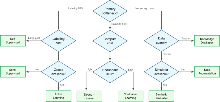
The tree identifies candidates; an engineering decision must still test their cost and quality. The vision workload in example 9.2 provides a concrete comparison. Its target-model and proxy scorers retain the same fraction of data, but they need not retain the same examples. A cheaper ranking can therefore win the time comparison and lose the deployment-quality comparison.

Step 1: Assess the bottleneck

The vision team’s stated objective is shorter training turnaround at the existing quality target. The full-data baseline takes 211 minutes, and both candidates retain 10 percent of the images. This places the decision in the compute-cost branch. The retained fraction alone does not settle it; the selection inequality and the slice-coverage check do.

A different binding constraint would change the comparison. If labels were the limiting expense, fewer annotations could justify additional training time. If controlled sweeps instead diagnosed a shortage of useful tokens, the data-scarcity branch would be relevant even with idle accelerators. Naming the objective determines which saving the candidate must actually deliver.

Step 2: Check prerequisites

Both vision candidates require access to the full image pool, a scoring model, and stable sample indices. The proxy additionally needs a ranking that transfers to the target model; its lower execution cost does not establish that prerequisite. Table 17 places these requirements alongside those of the alternative branches.

Table 17: Technique Prerequisites: Each technique carries specific infrastructure and data requirements that must be verified before implementation. A technique with excellent theoretical gains but unmet prerequisites will fail in practice, making this checklist the first step in technique selection.

Technique	Prerequisites
Active Learning	Access to oracle, unlabeled pool, retraining infrastructure
Coreset selection	Proxy model or embedding extractor, full dataset accessible
Curriculum Learning	Difficulty scoring method, pacing schedule
Semi-Supervised	Some labeled data, unlabeled data from same distribution
Self-Supervised	Large unlabeled corpus, pretraining compute budget
Augmentation	Domain knowledge of invariances, augmentation library
Synthetic Generation	Generative model or simulator, domain gap mitigation

Step 3: Estimate ROI

For the stated vision scenario, target-model scoring plus subset training takes 21.8 minutes (Option A), while proxy scoring plus subset training takes 21.4 minutes (Option B). These figures evaluate the marginal scoring pass using existing checkpoints. Both options beat the full-data baseline in the cost model. The proxy reduces only the scoring term; the retained training work is identical.

Suppose pilot validation in this hypothetical decision confirms that both runs reach the aggregate target under the modeled schedule, but only Option A meets every deployment-critical slice threshold. Option B regresses on a rare class. Option A is then the acceptable choice despite its more expensive scoring pass, saving 188.8 minutes against the baseline. Option B remains a candidate for repair, not deployment: enforce the coverage floor from section 9.3.4, rescore or enlarge the subset as needed, and repeat the time-to-quality comparison. Additional examples or passes change its cost, so the original proxy saving cannot simply be carried forward. If both candidates passed all quality gates at the stated times, Option B would win this time comparison.

A time saving must still justify any engineering investment. If the proxy checkpoint does not already exist and its training is charged entirely to a single run, that preparatory training erases Option B’s modest time advantage over Option A. Section 9.8.1 accounts for that investment, and section 9.8.3 spreads one-time costs across the \(\TrainingRunCount\) planned experiments. Reusing the proxy is economically useful only while its ranking continues to pass the same quality checks.

Step 4: Combine techniques

Data selection techniques are not mutually exclusive, but combining them does not guarantee additive gains. A representative workflow deduplicates the raw corpus, applies a coverage-aware coreset filter, orders retained batches through an empirical curriculum, and applies runtime augmentations during batch collation. Pretrained representations alter the baseline trajectory further. Every additional stage must justify its compute overhead, because cascading filters frequently discard overlapping subsets while their scoring latencies accumulate; stages compound efficiency gains only when their effects do not overlap and their overhead remains small, so combined savings must be measured rather than assumed.

A choice made at the data layer does not stay there. This decision process weighs a technique by its own scoring cost and the training work it removes, but a smaller or reordered corpus also changes what the model learns to represent, and the compression and deployment stages downstream inherit that representation. A selection that looks optimal in isolation can therefore move cost into those later stages, so the chosen strategy must be checked against the layers it feeds.

Self-Check: Question

1. A company invests \(\$30{,}000\) to compute a high-quality coreset. Training on the full dataset costs \(\$10{,}000\) per run, whereas training on the coreset costs \(\$4{,}000\) per run. What is the break-even number of training runs, and what is the ROI after 10 runs?

   1. Break-even is 5 runs, and ROI after 10 runs is \(100\%\)
   2. Break-even is 3 runs, and ROI after 10 runs is \(300\%\)
   3. Break-even is 8 runs, and ROI after 10 runs is \(50\%\)
   4. Break-even is 10 runs, and ROI after 10 runs is \(0\%\)

2. Using the chapter’s cost model \(C_{\text{total}} = C_{\text{acquire}} + C_{\text{label}} + C_{\text{store}} + C_{\text{process}}\), which scenario best justifies an upstream filtering investment?

   1. Skip filtering so that maximum raw volume reaches training, regardless of downstream processing and labeling cost
   2. Spend \(\$5{,}000\) on automated filtering only if measured avoided labeling, storage, and processing costs exceed that amount while task coverage and target quality still hold
   3. Double human labeling effort to manually review every raw sample before filtering, because filtering cost is always worse than labeling cost
   4. Cut evaluation entirely to offset the cost of training on unfiltered data

3. Explain why calculating Return on Investment (ROI) for data selection requires tracking engineering implementation and pipeline maintenance costs in addition to raw accelerator compute hours.

4. According to the chapter’s decision framework, if an ML team has an abundant pool of unlabeled domain data, very limited annotation budget, and access to human domain experts for selective queries, which technique branch is recommended?

   1. Pure transformation-based data augmentation without labeling
   2. Active learning (human-in-the-loop selective query) or semi-supervised learning
   3. Generative self-instruct synthesis to replace all human annotators entirely
   4. Exhaustive pairwise Jaccard deduplication across all unlabeled samples

5. When deciding between static coreset pruning and dynamic online active selection for a production pipeline, what role does the expected number of training runs (\(N\)) play in the architectural choice?

6. In recommendation systems like DLRM where embedding tables consume terabytes of memory, how does interaction deduplication differ in systems impact from cold embedding pruning?

See Answers →

9.9 Cross-Layer Interactions

Halving a training corpus halves the forward and backward passes, yet the resulting model may be no cheaper to compress or serve. Real ML systems combine data selection with model compression and hardware acceleration, and these cross-layer interactions amplify or undermine each other in ways no single layer reveals.

Model compression (post-training weight pruning, lower-precision representation, and distillation) acts on the trained network, and its arithmetic reductions reach serving latency only when the target execution substrate and runtime kernels support the resulting sparsity or precision patterns (Hoefler et al. 2021). The training corpus shapes the representations that compression later works on. A model trained on an uncurated, repetitive corpus can spend capacity on redundant features that post-training pruning then discards, whereas a curated corpus of diverse, informative examples can yield more compact representations from the start. That effect is an empirical hypothesis to verify, not a property of every selected dataset. The two levers therefore compose without substituting for each other. Data selection reduces training work and shapes learned representations, model compression shrinks the deployment artifact, and their combined impact is measured on serving latency and task accuracy rather than inferred from the upstream dataset reduction.

Hoefler, Torsten, Dan Alistarh, Tal Ben-Nun, Nikoli Dryden, and Alexandra Peste. 2021. “Sparsity in Deep Learning: Pruning and Growth for Efficient Inference and Training in Neural Networks.” Journal of Machine Learning Research 22 (241): 1–124.

↪ Why accelerators turn structured sparsity patterns into wall-clock speedup while unstructured sparsity rarely pays off is developed in N:M structured sparsity mechanics.

↪ Co-designing post-training pruning and quantization under the silicon contract is developed in Fitting the Deployment Budget.

Production deployments execute these techniques as one pipeline in two stages: data selection and training turn raw inputs into a trained model, and post-training compression and hardware acceleration then deploy that artifact (figure 13). Every stage along this end-to-end path amplifies or attenuates downstream efficiency.

Figure 13: The Optimization Stack: Data artifacts flow through selection and training before the resulting model enters compression and deployment. Upstream changes propagate quality and cost effects downstream, but reducing training data does not automatically simplify the model or deployment hardware.

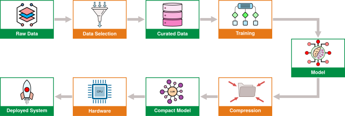
Tracing artifacts through the pipeline in figure 13 shows why data selection sits at the head of the optimization stack: pruning raw inputs reduces upstream training FLOPs, but does not automatically shrink parameter footprint, improve quantization headroom, or relax serving latency constraints in the downstream compression and hardware stages. Each downstream tier inherits both the computational savings and any representational deficits created upstream; an aggressive filter that discards rare but critical edge cases can force downstream engineers to train longer or abandon aggressive quantization to preserve task accuracy. The failure modes that follow show how data selection breaks down in production.

Self-Check: Question

1. In an idealized compute-bound training scenario with fixed target quality and negligible new overheads, a team halves the number of processed examples, halves the operations per processed example on the same compute-critical path, and doubles realized arithmetic throughput. What total speedup follows from the chapter’s multiplicative D·A·M reasoning?

   1. An \(8\times\) speedup, because halving workload, halving per-sample work, and doubling throughput multiply on the same critical path
   2. A \(6\times\) speedup, because the factors add across layers
   3. A \(2\times\) speedup, because only the hardware improvement matters once arithmetic throughput doubles
   4. A \(4\times\) speedup, because reducing training examples and reducing per-sample work are the same effect

2. Why are upstream data selection and downstream model compression complementary rather than interchangeable?

   1. Model compression can only be applied to computer vision models, whereas data selection is restricted to NLP
   2. Data selection eliminates backward passes entirely, whereas model compression eliminates forward passes
   3. Data selection optimizes only inference latency on edge devices, whereas model compression only affects training time
   4. Data selection reduces how many examples are processed, whereas model compression reduces the artifact size and can lower execution cost per example on compatible hardware

3. A team curates its training corpus to half its original size and reports that the resulting model will be cheaper to deploy. What does the reduction actually change, and what evidence would support the deployment claim?

4. Explain how an aggressive data filter that discards rare but critical edge cases can raise costs in the compression and deployment stages of the optimization stack.

See Answers →

9.10 Fallacies and Pitfalls

Scaling a training corpus tenfold can multiply storage, I/O, and accelerator bills while barely moving test accuracy, yet an uncalibrated selection filter can just as easily spend more time scoring candidates than it saves in training or silently erase a safety-critical rare class. These failures fall into three groups: conceptual fallacies about what data selection can achieve, implementation pitfalls that arise when correct strategies meet systems bottlenecks, and transfer errors that occur when benchmark results are applied uncritically to new domains.

Fallacy: More data always improves the model enough to justify its cost.

More data does not imply proportional accuracy gains because learning curves follow power-law diminishing returns. Test loss diminishes sub-linearly with dataset size (\(\LossFunction(\DatasetSize) \propto \DataScalingLossFactor\) for a fitted exponent \(\DataScalingExponent\)), meaning each successive error reduction demands a multiplicatively larger corpus. In an illustrative learning-curve scenario, scaling a dataset tenfold from 1M to 10M samples yields only 4 percentage points of accuracy gain. That 10\(\times\) volume expansion still costs a tenfold increase in storage I/O, host-to-device transfers, and accelerator FLOPs. Teams should measure the learning curve of their own workload rather than assume that more data delivers proportional value.

Pitfall: Replacing real-data validation with synthetic-only training data.

Synthetic samples cost almost nothing to acquire, so generative models can look like a replacement for data collection. Synthetic-only training fails in two ways. First, synthetic data can differ from the deployment distribution (section 9.5.3, figure 8), so the model learns features that fail to transfer; only real-data labels reveal the effect. Second, recursive training on model-generated data can trigger model collapse (Shumailov et al. 2024), which progressively erodes distribution tails: in this scenario, evaluation accuracy degrades from 95 percent to 78 percent across five recursive generations, suffering a 17 percentage-point collapse. Synthetic mixtures must therefore be validated against curated real data.

Illustrative model collapse: accuracy erodes with each recursive synthetic generation.

Fallacy: Data selection is merely data cleaning.

A dataset can be completely clean and correctly labeled yet redundant: once the model has minimized loss on a feature cluster, further identical samples add almost no gradient signal and still consume memory bandwidth and accelerator FLOPs. Cleaning corrects intrinsic defects; selection raises the learning return per FLOP by choosing examples for task-relevant information and coverage (figure 5; section 9.3.4). In the worked coreset scenario of notebook 9.1, the selected subset reached 1.8× higher ICR.

Pitfall: Treating data selection as a budget-only tactic.

Selection can look like a technique for resource-constrained teams, as if frontier foundation models could brute-force convergence by scaling the cluster. The data wall binds at every scale. At frontier scale, token consumption converges toward the finite ceiling of high-quality human text (Training Data Approaching the Stock of Public Text); at GPT-2 scale, one eight-H100 machine passes over the whole WebText corpus about 17 times in 4.4 days (section 9.1). The economic return of selection also scales with cluster expenditure: a 10 percent efficiency gain on a $100M frontier training run saves $10M under these assumptions. Amortizing scores and cached embeddings across repeated runs (section 9.8.3) strengthens the case further.

Fallacy: Selection overhead is too small to change training economics.

The selection inequality (equation 2) requires \(\SelectionTime+ \TrainingTime(\SubsetDatasetSize) < \TrainingTime(\FullDatasetSize)\) at matched quality. Consider a baseline training run requiring 8 hours, where training on an optimized coreset takes 2 hours. If a complex selection algorithm requires 10 hours to compute sample importance, the selection step alone consumes 5× the duration of the accelerated training run and exceeds the full training baseline itself, a net wall-clock loss. In the illustrative comparison, proxy-based EL2N scoring completes in 30 minutes, just 6.2 percent of the full-training baseline, which satisfies the inequality.

Pitfall: Pruning rare classes without a coverage floor.

Standard selection objectives minimize aggregate loss, which gives tail slices little influence over sampling. In a 1M dataset where rare classes comprise 0.1 percent of the data (1,000 examples), an unstratified 10 percent coreset retains only 100 rare-class examples in expectation, far below the illustrative 150-sample retention floor assumed here. An appropriate floor must be validated from task-specific learning curves and critical-slice performance. Importance sampling can compensate by weighting losses by inverse selection probabilities, but extreme weights inflate gradient variance and force smaller learning rates. As recommended in section 9.3.4, production coreset pipelines enforce hard stratification floors per class or critical slice before spending the remaining selection budget.

Fallacy: Deduplicating training data is enough to make evaluation reliable.

Web-scale pipelines scrape training, validation, and benchmark splits from common crawls, which introduces silent cross-split leakage. When an evaluation set contains near-duplicates of training documents, the metric measures memorization rather than generalization. A deduplication study found that train-test overlap affects over 4 percent of validation examples across standard language-modeling benchmarks (Lee et al. 2022). Deduplicating the training partition alone leaves this contamination untouched; cross-partition deduplication is required, using \(\NgramLength\)-gram matching or MinHash LSH (section 9.3.2). For a frozen evaluation set, the fix removes the overlapping training records and preserves the evaluation set and its provenance.

Lee, Katherine, Daphne Ippolito, Andrew Nystrom, Chiyuan Zhang, Douglas Eck, Chris Callison-Burch, and Nicholas Carlini. 2022. “Deduplicating Training Data Makes Language Models Better.” Proceedings of the 60th Annual Meeting of the Association for Computational Linguistics (Volume 1: Long Papers), 8424–45. https://doi.org/10.18653/v1/2022.acl-long.577.

Pitfall: Active learning without considering annotation latency.

Textbook formulations of active learning assume an oracle that labels queries instantly. Production annotation queues introduce delays such as the illustrative 14-day latency between sample dispatch and label return assumed here. This latency breaks the active learning feedback loop in two ways. If accelerator clusters halt training while awaiting labels, expensive hardware sits idle, destroying cluster compute utilization. Conversely, if training continues asynchronously on background data while annotations are pending, model weights drift across training steps; by the time the labels arrive, the uncertainty scores that justified querying those samples are obsolete. Dispatching large batches to amortize the turnaround adds redundancy within the batch unless diversity penalties are applied.

Fallacy: If a technique works on ImageNet, it will work on my dataset.

CIFAR-10 and ImageNet are highly redundant across canonical object classes, which allows coreset pruning of often 30 to 50 percent without measurable accuracy loss. Histopathology, satellite imagery, and industrial defect detection have heavy-tailed feature distributions in which safety-critical patterns appear in a few rare samples. A 50 percent cut tuned on ImageNet can remove the few examples that separate subtle pathologies. Geometric coreset algorithms also depend on embeddings, and a feature extractor pretrained on natural images may not resolve fine-grained domain distinctions. Teams should measure the redundancy of their own data and validate retention across critical slices before pruning.

Pitfall: Optimizing data selection metrics instead of deployment metrics.

Selection algorithms optimize aggregate surrogates such as area under the learning curve (AULC) or performance-per-data (PPD, section 9.2.4). A selection policy retaining a 10 percent coreset can achieve superior aggregate PPD by prioritizing dense clusters of common, easy samples that accelerate average convergence, while discarding ambiguous edge cases and rare slices. Production failures, however, occur on tail slices, edge cases, and protected sub-populations rather than on averages. A policy without subgroup constraints can pass global validation and still fail in deployment. As the measurement framework of section 9.2 requires, policies must be evaluated on stratified, slice-level benchmarks, even when doing so slightly lowers average PPD.

Self-Check: Question

1. A research paper reports that an EL2N coreset selection method successfully pruned \(50\%\) of CIFAR-10 with \(0\%\) loss in accuracy. A medical imaging team applies the exact same \(50\%\) pruning ratio to a rare tumor detection dataset and suffers a disastrous \(28\%\) drop in recall. What fallacy explains this failure?

   1. The team failed to use GPU acceleration during the inference pass
   2. The team used float32 precision instead of bfloat16 mixed precision
   3. CIFAR-10 contains more total classes than medical imaging datasets
   4. Assuming that benchmark coreset pruning ratios transfer directly to specialized, highly imbalanced production domains with rare failure modes

2. A team implements an elaborate multi-stage active learning pipeline that reduces training dataset size by \(40\%\). However, the continuous clustering, proxy scoring, and cross-worker all-gather synchronization take 3 times longer than the GPU time saved during training. Which pitfall does this represent?

   1. Violating the Selection Inequality by incurring selection overheads that exceed downstream training savings (\(T_{\text{selection}} > \Delta T_{\text{train}}\))
   2. Encountering model collapse due to recursive generator loops
   3. Failing to implement 4 KB small-read alignment on host NVMe storage
   4. Violating the smoothness assumption in semi-supervised consistency regularization

3. Why is evaluating a data selection strategy solely on aggregate validation accuracy a dangerous pitfall when dealing with imbalanced datasets?

4. True or False: Because modern high-capacity generative models produce photorealistic images and fluent text, a model trained on recursively generated synthetic data will never suffer performance degradation.

See Answers →

9.11 Summary

Feeding every available example into a training run wastes accelerator compute, storage bandwidth, and annotation budget on redundant or noisy records because marginal learning signal varies by orders of magnitude across raw samples. Data selection therefore treats training volume as an engineering variable rather than a fixed constraint, minimizing total cost across compute, storage, labeling, energy, and wall-clock time so a curated subset can match or outperform a much larger uncurated corpus.

This systems perspective becomes actionable through three quantitative tools: the ICR, the selection inequality, and the total data cost model. The information-compute ratio quantifies learning gained per floating-point operation, providing a proxy for sample value that must be evaluated alongside coverage and target quality. The selection inequality tests a training-time claim by requiring scoring plus subset training to take less time than full-data training at matched quality. Together with return-on-investment and break-even analysis, these formulations determine whether a proposed selection mechanism saves resources or merely shifts expenditure between stages.

The three levers act at different points: static pruning removes redundancy before training, dynamic selection prioritizes informative examples during training, and synthetic generation creates data where none exists. Together, these levers answer the data wall, the gap between rapidly growing compute capacity and slowly growing high-quality data.

Learning from unlabeled data sits beside these levers rather than within them. Semi-supervised learning stretches a small labeled seed across an unlabeled pool, and self-supervised pretraining moves the bulk of representation learning into an unannotated upstream phase, so downstream tasks can reach target quality with far fewer task-specific labels; the worked amortization scenario assumes 100× fewer. The compute-only crossover occurs at roughly 10.5 tasks under the scenario assumptions. Labeling savings enter a separate dollar comparison that also requires compute prices and other differing costs.

In production, the difficult part is rarely the scoring rule itself. It is keeping selection from becoming the next bottleneck. Proxy models and cached embeddings bound scoring time, shard-based loaders keep storage access sequential, and data echoing recovers accelerator cycles when ingestion lags. On one H100, a half-size ResNet-50 coreset saves about 63 seconds and 44 kJ per epoch against a one-time scoring pass of about 42 seconds, and those seconds are realized only when the host keeps the accelerator fed. Controlled model-size and data sweeps diagnose whether a run is data-limited or compute-limited in the first place, and PPD, AULC, and DCR then show whether a reduction delivered what it promised at the binding resource.

Every row of the opening chapter map (table 1) has now been derived, and the formulas behind its tests fit on one page (table 18). Together they let an engineer estimate, before committing a training run, whether a lever saves more than it costs.

Table 18: Key Equations: The chapter’s counting rules in the notation of the sections that derive them. The training-compute rule is the dense-transformer accounting of the GPT-2 lighthouse; the curriculum rule assumes linear pacing over \(\WarmupEpochCount\) warmup epochs.

Quantity	Formula	Where derived
Information-compute ratio	\(\text{ICR} = \FiniteChange\DataInformationContent/\FiniteChange\Operations\)	section 9.2.1
Marginal ICR (log-information)	\(\text{ICR}(\DatasetSize) \approx 1/(\OperationsPerSample\cdot \DatasetSize)\)	equation 1
Training compute	\(\Operations \approx 6\Parameters\DatasetSize\); compute-optimal tokens \(\ComputeOptimalTokenCount \propto \sqrt{\Operations}\)	section 9.2.3
Performance-per-data	\(\text{PPD}(\LearningCurveSampleCount) = [\text{Accuracy}(\LearningCurveSampleCount) - \text{Accuracy}(0)]/\LearningCurveSampleCount\)	section 9.2.4
Data compression ratio	\(\text{DCR} = \FullDatasetSize/\SubsetDatasetSize\) at target accuracy	section 9.2.4
Selection inequality	\(\SelectionTime+ \TrainingTime(\SubsetDatasetSize) < \TrainingTime(\FullDatasetSize)\)	equation 2
Curriculum warmup samples	\(\DatasetSize (\WarmupEpochCount+1)/2\) in place of \(\WarmupEpochCount\cdot \DatasetSize\)	section 9.4.1
Offline distillation targets	\(4\ClassCount\) bytes per sample in place of \(\lceil \log_2 \ClassCount \rceil\) bits	section 9.5.4
Input-pipeline ratio	\(\InputPipelineRatio= \HostPreparationTime/\AcceleratorBatchTime\); echoing helps up to \(\EchoFactor= \InputPipelineRatio\)	section 9.7.3
Total cost of data	\(\TotalDataCost= \DataAcquisitionCost+ \DataLabelingCost+ \DataStorageCost+ \DataProcessingCost\)	section 9.8.1
Amortized return on investment	Savings across \(\TrainingRunCount\) runs, less the one-time investment, per unit invested	equation 3

Key Takeaways: Curate, do not accumulate

• Selection optimizes system cost: The objective is minimizing total cost across compute, storage, labeling, and energy rather than reducing sample counts alone. The information-compute ratio measures learning gained per FLOP spent; total-cost accounting and pipeline measurements establish whether that gain serves the system objective.
• Start with deduplication: Exact deduplication is often the lowest-risk first technique because it removes repeated bytes without a learned scoring pass. Apply near-duplicate and semantic deduplication only after validating thresholds against downstream quality metrics.
• Training-time savings must exceed selection overhead: At matched quality, \(\SelectionTime+ \TrainingTime(\SubsetDatasetSize) < \TrainingTime(\FullDatasetSize)\). Lightweight proxy models and cached embeddings keep \(\SelectionTime\) low, whereas unoptimized selection algorithms can consume all the compute they save.
• Dynamic selection adapts the training mix: Curriculum learning changes presentation order, while active learning changes which samples receive labels. Either improves efficiency when its scoring rule, coverage, and refresh overhead are validated.
• Self-supervised pretraining can amortize adaptation cost: Pretraining once and fine-tuning many times spreads pretraining cost across downstream tasks. The worked scenario assumes a 100× label reduction and a 20× marginal-compute reduction; realized savings depend on transfer quality and reuse.
• Synthetic data is a supplement, not a replacement: Synthetic samples augment scarce tail cases effectively, but cannot substitute entirely for empirical data. Unanchored synthetic training introduces domain-gap degradation, and recursive synthetic loops trigger catastrophic model collapse.
• Validated workload reduction compounds downstream: When selection safely eliminates examples or tokens without adding compensating steps, that work never reaches later model or machine optimizations. Dynamic scoring and synthesis add their own costs, so the combined saving must be measured rather than assumed.

Examples differ greatly in how much they teach per byte transferred and per FLOP executed, and selection spends compute on the ones that teach most. Within the D·A·M taxonomy, selection operates at the head of the system: every redundant sample or uninformative token safely eliminated directly reduces operation count (\(\Operations\)) in the iron law of ML systems (principle 3) and can avoid downstream training reads. Scoring may still read the entire pool, and shard streaming may read discarded records, so reductions in data volume (\(\DataVolume\)) must count scoring and shard-read traffic separately. When selection overhead satisfies the inequality at matched quality, the reduction removes work before downstream compression or hardware acceleration sees it. Model-based scoring offers a way to invest additional compute in selection, consistent with the bitter lesson, but a stronger scorer justifies that investment only if its improved rankings save more downstream work than it costs. The Pareto frontier (principle 5) applies upstream of the model as well. Each retained fraction is an operating point that trades coverage and rare-slice accuracy against compute, and no single fraction is optimal for every workload.

What’s Next: From data to algorithms

Data selection changes what the system learns from. Model Compression turns to how the model represents what it has learned. It starts from the deployment envelope the model must fit and adjusts three things to fit it: the model’s structure through pruning and distillation, its numerical precision through quantization, and the way the remaining operations map onto the hardware that executes them.

9.12 Self-Check Answers

Self-Check: Answer

1. In an ML infrastructure scaling scenario where available GPU compute grows by approximately \(10\times\) every 3 years while high-quality web data grows by only \(2\times\) every 5 years, what primary systems regime emerges, and what is the appropriate systems response?

   1. A compute-rich, data-constrained data wall regime where intelligent data selection and curation must maximize the learning signal extracted per token
   2. A memory bandwidth-bound regime where model parallel sharding must replace data parallelism across all training clusters
   3. An I/O ingestion bottleneck where disk read bandwidth must be quadrupled to keep GPUs saturated
   4. A compute-starved regime where synthetic data generation should be eliminated to avoid wasting accelerator cycles

   Answer: The correct answer is A. Compute throughput growing faster than accessible high-quality human data creates a compute-to-data imbalance known as the data wall. In this regime, additional raw compute yields diminishing returns on uncurated corpora, making data selection essential to maximize the Information-Compute Ratio (ICR). Shifting model parallelism addresses parameter memory limits rather than data scarcity, scaling disk bandwidth solves I/O stalls rather than token information quality, and eliminating synthetic generation ignores a key strategy for expanding scarce data pools.

   Learning Objective: Analyze the systems implications of the compute-to-data scaling asymmetry and diagnose the data wall regime.

2. True or False: Doubling the amount of raw, deduplicated web data will always double the total information learned by the model.

   Answer: False. The section argues for diminishing returns, not a universal doubling law: additional data can add much less marginal signal than its extra compute cost. That is why teams must evaluate learning curves and target quality empirically instead of assuming linear gains from corpus size.

   Learning Objective: Evaluate the misconception that information value scales linearly with raw corpus volume.

3. Order the following stages as they are presented in this chapter’s conceptual map of the data-selection pipeline: (1) Dynamic Selection, (2) Static Pruning, (3) Synthetic Data Generation.

   Answer: The correct order is: (2) Static Pruning, (1) Dynamic Selection, (3) Synthetic Data Generation. This is the chapter’s presentation order: prune low-value data before target training, adapt sample usage during training, then create missing coverage when needed. The sequence is a conceptual map rather than a mandatory runtime chronology, because synthetic data can also be created earlier and then pruned or selected before final training.

   Learning Objective: Identify the chapter’s conceptual ordering of the three main data-selection intervention points.

← Back to Questions

Self-Check: Answer

1. Under the illustrative analytical model where dataset information content scales as \(\mathcal{I}(D) \propto \log D\) and training compute scales linearly as \(O = O_{\text{sample}} \cdot D\), how does the marginal Information-Compute Ratio \(\mathrm{ICR}(D)\) scale with dataset size \(D\)?

   1. It remains constant at \(\mathcal{O}(1)\) because additional compute scales proportionally with dataset size
   2. It decays as \(\mathcal{O}\!\left(\frac{1}{O_{\text{sample}}D}\right)\), so under this illustrative model additional data eventually adds compute faster than marginal information
   3. It grows logarithmically as \(\mathcal{O}(\log D / O_{\text{sample}})\) due to power-law parameter scaling
   4. It decays exponentially as \(\mathcal{O}(\exp(-D))\) once the training corpus exceeds accelerator memory capacity

   Answer: The correct answer is B. Under the chapter’s illustrative model, \(d\mathcal{I}/dD \propto 1/D\) and \(dO/dD = O_{\text{sample}}\), so their ratio is \(\mathrm{ICR}(D) \approx 1/(O_{\text{sample}}D)\). This captures diminishing marginal learning signal under the stated log-information and linear-compute assumptions. A constant or growing answer ignores the derivative of \(\log D\), while the exponential-decay choice introduces a memory-capacity mechanism that is not part of this model.

   Learning Objective: Calculate the scaling behavior of the Information-Compute Ratio under the section’s illustrative logarithmic-information model.

2. Explain why a dataset where \(100\%\) of the sample labels are verifiably correct can still exhibit a very low Information-Compute Ratio (ICR).

   Answer: Label correctness measures ground-truth accuracy, whereas ICR measures evaluation gain per unit of training compute over a stated interval. A dataset of completely correct examples will have near-zero ICR if the samples are redundant, easily classified by the current model state, or already mastered, because processing them consumes forward and backward FLOPs without producing a corresponding evaluation gain; parameter updates alone do not establish learning value.

   Learning Objective: Compare data correctness with data value in the Information-Compute Ratio framework.

3. An ML systems diagnostic plot maps normalized training compute on the horizontal axis against model performance on the vertical axis. A 10M-parameter run sits well below a fitted frontier under a fixed evaluation protocol and fixed total budget. A controlled sweep then shows that reallocating the same budget toward a larger model improves performance. What is the most defensible diagnosis of the original operating point?

   1. Data-starved regime
   2. I/O bandwidth-saturated regime
   3. The model/data allocation was suboptimal under the tested budget
   4. Over-echoing regime

   Answer: The correct answer is C. Under the chapter’s measurement framework, a point below a fitted frontier does not identify a unique cause by itself. What the controlled sweep supports is that the original allocation of budget across model size and data was suboptimal for the tested regime. Calling it purely data-starved or purely capacity-limited would overclaim from one observation, and the other choices describe different bottlenecks entirely.

   Learning Objective: Interpret a controlled compute-optimal-frontier sweep without over-inferring a unique bottleneck from a single operating point.

4. A team wants one metric for how much smaller a selected dataset is at a target accuracy, and another for how much learning is gained per sample over a measured interval. Which pair of chapter metrics matches that need?

   1. Data Curation Rate and Accuracy Reduction Ratio
   2. Data Compression Ratio and Performance-Per-Data
   3. Dynamic Checkpoint Rate and Active Retention Rate
   4. Data Convergence Ratio and Amortized Risk Ratio

   Answer: The correct answer is B. Data Compression Ratio (DCR) asks how much the dataset can be reduced while still reaching a target accuracy, and Performance-Per-Data (PPD) measures accuracy gain per sample over a stated interval. The other choices introduce names the chapter does not use. AULC is another valid core metric, but it summarizes performance across dataset sizes rather than serving as the per-sample interval metric in the question.

   Learning Objective: Match the chapter’s core metrics to the measurement goals they are designed to answer.

5. Why is Area Under the Learning Curve (AULC) a more informative metric than single-point final validation accuracy when comparing data selection methods across dataset sizes?

   Answer: AULC integrates performance over dataset size \(n\), so it rewards methods that achieve stronger accuracy earlier in the data-allocation range rather than judging them only at one endpoint. Under the same evaluation protocol and integration limits, a higher AULC means better aggregate performance over that same dataset-size range. The practical caveat is that this does not automatically imply the method is better at every dataset size, nor does it guarantee lower total FLOPs if per-sample cost differs across methods.

   Learning Objective: Justify AULC as a data-efficiency metric by relating it to performance across dataset sizes rather than a single endpoint.

6. A training team reduces a dataset from \(1{,}000{,}000\) to \(100{,}000\) images. Full-data training takes 10 hours, subset training takes 1 hour, and scoring the full pool with the production model takes 12 hours. Which conclusion and next step best fit the selection inequality?

   1. Yes, the inequality is satisfied because a \(90\%\) dataset reduction guarantees positive ROI
   2. Yes, because the 9 hours saved in training outweigh the scoring cost; the team only needs more GPUs
   3. No, because \(12+1=13\) hours exceeds the 10-hour baseline; a plausible fix is proxy scoring or cached embeddings, but the team must verify that scoring drops below 9 hours while target quality holds
   4. No, because coreset training always increases memory-bandwidth consumption; the team should switch from NVMe SSDs to HDDs

   Answer: The correct answer is C. The chapter’s time-saving test is \(T_{\text{selection}}+T_{\text{train}}(D_{\text{subset}})<T_{\text{train}}(D_{\text{total}})\). Here, \(12+1=13\) hours, which is worse than the 10-hour baseline. Proxy models or cached embeddings are sensible candidate fixes, but they only restore training-time saving if measured scoring time falls below the 9-hour savings window and the selected subset still preserves target quality. A large reduction ratio alone does not prove success, and slower storage would move in the wrong direction.

   Learning Objective: Apply the selection inequality to diagnose when scoring overhead erases subset-training savings and identify what must be re-measured after a proposed fix.

← Back to Questions

Self-Check: Answer

1. A team wants to score a dataset cheaply before training a large production model. They plan to train a small proxy for a few epochs and rank examples by prediction error, knowing that confidently wrong predictions can still score highly. Which method best matches that plan and its trade-off?

   1. \(k\)-Center clustering on raw pixel inputs, because it guarantees zero-cost label-aware boundary identification
   2. Forgetting Events scoring on the full production model, because it requires no proxy architecture and computes in \(\mathcal{O}(1)\) time
   3. EL2N (Error L2-Norm) scoring with a briefly trained proxy model, accepting that high error can reflect hard examples or noise
   4. Herding on Gaussian-distributed features, because it completely avoids computing feature representations

   Answer: The correct answer is C. EL2N ranks samples by early prediction error \(\lVert \hat{\mathbf{y}}-\mathbf{y} \rVert_2\), so a cheap proxy can score examples without a full target-model run. The section also warns that high EL2N can include noisy samples and that transfer from proxy to target is useful but not guaranteed. Geometry-based \(k\)-Center is not label-aware boundary scoring, Forgetting Events is much more expensive, and Herding still depends on feature representations.

   Learning Objective: Compare proxy-based EL2N scoring with other coreset methods in terms of cost, signal, and validation needs.

2. Why is Locality-Sensitive Hashing (LSH) with MinHash preferred over exhaustive pairwise Jaccard similarity comparison for large-scale text deduplication?

   1. MinHash LSH guarantees \(100\%\) precision in detecting semantic paraphrases across different natural languages
   2. MinHash eliminates the need to tokenize or shingle input documents before hashing
   3. Exhaustive pairwise Jaccard comparison requires training a deep neural network, whereas LSH is purely rule-based
   4. Exhaustive pairwise comparison requires \(\mathcal{O}(D^2)\) document comparisons, whereas MinHash LSH hashes compact signatures into sublinear candidate collision buckets

   Answer: The correct answer is D. Comparing all pairs in a dataset of \(D\) documents requires \(\mathcal{O}(D^2)\) comparisons, which is computationally intractable for web-scale datasets (\(D \ge 10^7\)). MinHash compresses documents into fixed-size sketches where collision probability equals Jaccard similarity, and LSH bands these sketches into hash buckets so only candidate pairs colliding in a bucket are compared. MinHash LSH does not detect cross-lingual semantic paraphrases, still requires shingling/tokenization, and pairwise Jaccard comparison is an exact set operation rather than a deep learning method.

   Learning Objective: Analyze the computational scaling benefits of MinHash and Locality-Sensitive Hashing for web-scale deduplication.

3. True or False: Removing near-duplicate documents with MinHash LSH always improves model accuracy because duplicate data has zero statistical value in all training regimes.

   Answer: False. While deduplication reduces redundant computation and memorization risk, in some domains duplicate frequency reflects natural empirical data distributions or intentional weighting. Aggressive deduplication with miscalibrated thresholds can prune legitimate variations or distort class priors, necessitating empirical validation on downstream accuracy.

   Learning Objective: Evaluate the systems and statistical trade-offs of aggressive near-duplicate filtering.

4. The training-dynamics coreset metric that measures the Euclidean norm of the difference between predicted class probabilities and the one-hot target vector early in training is known as ____.

   Answer: EL2N. It measures \(\lVert p(x)-y \rVert_2\) early in training as an error-based difficulty score. The chapter notes that proxy-model rankings can transfer usefully to larger targets, but that transfer must be validated rather than assumed universal.

   Learning Objective: Identify EL2N from its mathematical definition and explain why proxy-based use still requires validation.

← Back to Questions

Self-Check: Answer

1. In curriculum learning, an engineer implements an easy-to-hard pacing schedule that controls the fraction of the sorted training pool available at each stage. What is the primary objective of this pacing strategy?

   1. To guide early optimization with more stable examples before gradually introducing harder ones
   2. To eliminate the need for backward passes during the first half of training
   3. To maximize GPU memory bandwidth utilization by sorting tensors strictly by length in bytes
   4. To replace human labelers with an automated oracle during the late stages of training

   Answer: The correct answer is A. The chapter presents curriculum learning as a way to shape the optimization trajectory: easier examples can provide steadier early gradients, while harder examples are introduced later as the model matures. That is not a guarantee against divergence on every task, and ‘easy’ depends on the scoring rule, but it is the pacing mechanism this section teaches. The other choices confuse curriculum with memory-layout tricks or active-learning workflows.

   Learning Objective: Analyze how curriculum pacing can stabilize early learning by controlling when harder examples appear.

2. An active learning pipeline chooses unlabeled examples for costly radiologist annotation. The team notices that simple uncertainty sampling repeatedly selects images from a single ambiguous artifact class, starving other disease categories. Which query strategy should they adopt to resolve this pathology?

   1. Least-confidence sampling, because it strictly selects the lowest top-1 probability prediction
   2. Diversity sampling or hybrid uncertainty-diversity sampling (such as BADGE), which balances uncertainty near decision boundaries with feature-space coverage
   3. Random undersampling of the entire unlabeled pool to reduce dataset size before scoring
   4. Uniform zero-shot pseudo-labeling without confidence thresholds

   Answer: The correct answer is B. Pure uncertainty sampling often suffers from sampling bias by selecting clustered points near a single ambiguous boundary region. Diversity sampling (or hybrid strategies like BADGE that incorporate gradient embeddings) ensures that selected queries span diverse clusters across the feature space while still targeting model uncertainty. Least-confidence sampling exacerbates the clustering issue, random undersampling discards informative candidates arbitrarily, and unthresholded pseudo-labeling introduces catastrophic label noise.

   Learning Objective: Compare active learning query strategies to mitigate sampling bias and redundancy.

3. Order the steps in an active learning closed-loop iteration: (1) Select top query samples via query strategy, (2) Acquire expert annotations from the oracle, (3) Score unlabeled pool using current model, (4) Retrain or update model on expanded dataset, (5) Add newly labeled samples to the training set.

   Answer: The correct order is: (3) Score unlabeled pool using current model, (1) Select top query samples via query strategy, (2) Acquire expert annotations from the oracle, (5) Add newly labeled samples to the training set, (4) Retrain or update model on expanded dataset. The cycle begins with proxy or model scoring over the candidate pool, selecting candidate queries, querying the human oracle, incorporating verified labels into the dataset, and updating the model.

   Learning Objective: Design the closed-loop workflow of an iterative active learning system.

← Back to Questions

Self-Check: Answer

1. What causes the phenomenon of ‘model collapse’ when generative models are trained recursively on synthetic data generated by earlier model iterations?

   1. GPU memory fragmentation caused by variable-length synthetic sequences during distributed training
   2. Overfitting to floating-point rounding errors during fp16 mixed-precision matrix multiplication
   3. A failure of the I/O storage subsystem to deliver synthetic batches at line rate
   4. Systematic underrepresentation and erosion of tail patterns across generations, so recursive retraining compounds missing or distorted rare cases

   Answer: The correct answer is D. The section’s model-collapse mechanism is recursive tail erosion: generated data underrepresents rare but important patterns, and retraining on later synthetic generations compounds those omissions and errors. High-probability modes dominating the sample stream is part of that story, but it does not prove universal collapse under every sampling regime. The other choices are execution problems, not the chapter’s statistical mechanism.

   Learning Objective: Analyze how recursive synthetic training can degrade tail coverage and diversity over generations.

2. A team distills a ResNet-50 student on ImageNet and chooses offline distillation, precomputing the teacher’s FP32 logits for every training image instead of keeping the teacher in accelerator memory. Which cost does this choice move onto the data path?

   1. Every epoch must read per-class logit vectors in place of single integer labels, multiplying the label bytes the storage tier and input pipeline must deliver
   2. Every training step must run a teacher forward pass beside the student, restricting the student’s per-accelerator batch size
   3. The student must be trained with a lower learning rate, because soft targets produce larger gradients than one-hot labels
   4. The teacher must be retrained once per student epoch, so preparation cost grows linearly with the number of epochs

   Answer: The correct answer is A. Offline distillation stores one logit per class for every sample, so the per-sample label grows from a single integer index to four bytes per class, an expansion of more than three orders of magnitude for ImageNet’s thousand classes, and every epoch reads it back through the input pipeline. Teacher residency and the reduced student batch size are the costs of online distillation, which this choice avoids. Soft targets do not force a lower learning rate, and the teacher pass runs once during precomputation rather than once per epoch.

   Learning Objective: Analyze knowledge distillation as a data-synthesis lever by locating its storage and input-pipeline cost.

3. Why is training exclusively on \(100\%\) synthetic data from a simulation engine often suboptimal for real-world deployment, and how does synthetic-to-real data mixing bridge this gap?

   Answer: Simulation engines have an inherent domain gap (\(\mathcal{D}_{\text{synth}} \ne \mathcal{D}_{\text{real}}\)) caused by simplified physics, missing sensor artifacts, and unmodeled environmental noise. Mixing synthetic data with a curated set of real-world examples anchors the model to real feature distributions while using synthetic samples to expand volume, cover edge cases, and balance rare classes.

   Learning Objective: Analyze domain gap challenges and justify synthetic-to-real mixing ratios.

4. True or False: Using a high-capacity diffusion model or state-of-the-art LLM to generate synthetic training data guarantees that the resulting training set will be completely free of distribution shift relative to the real deployment environment.

   Answer: False. Generator quality does not eliminate domain gap. Synthetic generators can amplify subtle distribution shifts, introduce generator-specific artifacts, and omit edge cases present in real-world deployment environments, requiring domain validation against real ground truth.

   Learning Objective: Evaluate the misconception that advanced generative models eliminate domain shift.

← Back to Questions

Self-Check: Answer

1. Explain the mechanism of confirmation bias in semi-supervised pseudo-labeling, and specify how confidence thresholding mitigates it.

   Answer: Confirmation bias arises when the model trains on its own wrong pseudo-labels and reinforces those mistakes in later rounds. A high confidence threshold filters out low-confidence predictions, but confidently wrong pseudo-labels can still survive, so thresholding is only a partial defense. The practical check is to compare the model’s confidence against held-out labeled validation evidence before trusting the expanded training set.

   Learning Objective: Explain confirmation bias in pseudo-labeling and evaluate what confidence thresholding can and cannot fix.

2. True or False: Consistency regularization methods such as FixMatch assume that label-preserving perturbations of an input should not change the model’s predicted class distribution much.

   Answer: True. The method relies on a task-valid smoothness assumption: if the augmentation preserves the label, predictions across the two views should stay consistent. The key caveat is that closeness in raw input space alone is not enough—rotations, crops, or other perturbations can change the true label on some tasks.

   Learning Objective: Evaluate the task-dependent assumption behind consistency regularization.

3. In the economics of foundation models, an organization invests \(C_{\text{pretrain}} = 10{,}000\) GPU-hours in self-supervised pretraining. Each downstream task fine-tuning costs \(C_{\text{finetune}} = 50\) GPU-hours. Training each task from scratch would cost \(C_{\text{scratch}} = 1{,}000\) GPU-hours. What is the minimum number of downstream tasks \(N^*\) required to break even on the pretraining investment?

   1. \(N^* = 5\) downstream tasks
   2. \(N^* = 8\) downstream tasks
   3. \(N^* = 11\) downstream tasks (\(10{,}000 + 11 \times 50 = 10{,}550 < 11 \times 1{,}000 = 11{,}000\))
   4. \(N^* = 50\) downstream tasks

   Answer: The correct answer is C. The break-even condition is \(C_{\text{pretrain}} + N \cdot C_{\text{finetune}} \le N \cdot C_{\text{scratch}}\), which gives \(10{,}000 + 50N \le 1000N\), or \(950N \ge 10{,}000\). Solving for \(N\) yields \(N \ge 10{,}000 / 950 \approx 10.53\). Thus, at least 11 downstream tasks are required for the foundation model approach to use fewer total GPU-hours under these assumptions. This is a compute-only crossover at matched target quality; a dollar comparison must also price labels, accelerator hours, and other differing costs. At 10 tasks, scratch training costs \(10{,}000\) hours while the foundation model costs \(10{,}500\) hours. At 11 tasks, scratch training costs \(11{,}000\) hours while the foundation model costs \(10{,}550\) hours.

   Learning Objective: Calculate the break-even threshold for amortizing self-supervised pretraining across downstream tasks.

4. How does the MoCo (Momentum Contrast) framework reduce the hardware and memory constraints of contrastive self-supervised learning compared to naive SimCLR?

   1. By replacing convolutional backbones with rule-based lookup tables to avoid backpropagation
   2. By requiring fully supervised class labels to filter out false negative pairs
   3. By using a dynamic queue of negative keys and a slowly updating momentum encoder, decoupling negative dictionary size from mini-batch size
   4. By computing exact pairwise Jaccard similarities on raw byte sequences rather than latent embeddings

   Answer: The correct answer is C. Contrastive learning requires large sets of negative examples for effective representation learning. While SimCLR scales the mini-batch size (batches of up to 8,192 examples, paid for in activation memory and all-gather traffic), MoCo decouples the dictionary size from the mini-batch size by maintaining a memory queue of negative keys updated with a momentum-averaged teacher encoder. MoCo still uses neural backbones and backpropagation, operates in an unsupervised manner without human labels, and computes cosine similarities in latent space rather than raw byte Jaccard comparisons.

   Learning Objective: Compare contrastive self-supervised learning architectures and their memory-compute scaling trade-offs.

5. What is the systems-level ‘homogenization risk’ (or blast radius) of pretraining a shared foundation model on an uncurated dataset?

   Answer: A shared base model can propagate the same upstream defect into many downstream tasks, so a bad pretraining-data choice has a much larger blast radius than in train-from-scratch workflows. For example, a memorized private pattern or systematic bias in the base model may affect many adaptations built on top of it. The actual impact is not universal, because downstream fine-tuning and validation can reduce or expose some defects.

   Learning Objective: Analyze why pretraining-data defects in a shared foundation model can affect many downstream adaptations.

6. True or False: Because self-supervised pretraining learns general representations from unlabeled data, it completely eliminates the need for data selection or quality filtering during the pretraining stage.

   Answer: False. Self-supervised pretraining at web scale remains highly sensitive to pretraining data quality; uncurated corpora containing boilerplate, corrupted text, toxic samples, or pervasive duplicates degrade representation quality and inflate training FLOPs without improving downstream transfer.

   Learning Objective: Evaluate the misconception that self-supervised learning eliminates data curation requirements.

← Back to Questions

Self-Check: Answer

1. Why do naive random sample lookups across non-contiguous indices in large un-sharded dataset files severely degrade I/O throughput on storage hardware, and how do shuffle buffers mitigate this?

   1. Random lookups bypass host CPU caches, forcing floating-point registers to re-encode all labels
   2. Random lookups violate PCIe parity checks, causing GPU kernel timeouts during backward passes
   3. Random lookups trigger hash collisions in the Python garbage collector, halting dataloading threads
   4. Random 4 KB reads achieve only a tiny fraction of peak sequential storage bandwidth due to IOPS limits, whereas shuffle buffers read large sequential chunks and randomize locally in memory

   Answer: The correct answer is D. Storage devices (HDDs, SATA SSDs, NVMe SSDs, and cloud object stores) provide peak throughput under large, contiguous sequential reads. Non-contiguous random reads drop realized bandwidth dramatically (e.g. from gigabytes/sec to megabytes/sec on SSDs, or hundreds of times worse on HDDs). Shuffle buffers co-design data loading by reading large sequential shards into host RAM and performing pseudo-random shuffling locally within memory, preserving peak sequential disk bandwidth. The other choices describe fictitious hardware or software failures.

   Learning Objective: Analyze the hardware empathy principles governing storage I/O and shuffle buffer design.

2. Contrast upstream data echoing (echoing before data augmentation) with downstream data echoing (echoing after augmentation) in terms of computational overhead and sample diversity.

   Answer: Upstream echoing amortizes work before augmentation and lets repeated passes receive fresh random augmentations, so it can preserve more view diversity while still reducing some repeated upstream overhead. Downstream echoing amortizes earlier work through augmentation, but repeats the same already-augmented tensors rather than creating new views. The practical implication is to place the echo point after the bottleneck stage whose work you want to amortize, then check whether the repeated data still preserves target quality.

   Learning Objective: Compare upstream and downstream echoing by how much pipeline work they amortize and how much sample diversity they preserve.

3. True or False: If the GPU training step takes 20 ms and the CPU data loading/augmentation pipeline takes 10 ms (\(R = T_{\text{pipeline}} / T_{\text{GPU}} = 0.5\)), applying a data echoing factor of \(e = 2\) will double the end-to-end training throughput.

   Answer: False. When \(R < 1\), the training job is accelerator-bound (the data pipeline is already faster than the GPU), so the GPU is never starved for data. Applying data echoing in this regime provides zero throughput gain and merely feeds duplicate or stale data to the accelerator.

   Learning Objective: Evaluate pipeline balance conditions under which data echoing provides zero throughput improvement.

4. On one host with two to eight accelerator workers, how can centralized coreset selection become a bottleneck, and what trade-off does hierarchical selection introduce?

   1. Centralized selection requires all workers to share a single GPU; hierarchical selection distributes weights across SSDs
   2. Centralized selection fails because sharding prevents network cards from transmitting floating-point values
   3. Centralized selection can bottleneck host memory and coordinator dispatch; hierarchical selection prunes locally per shard, risking loss of globally rare samples across shards
   4. Centralized selection eliminates gradient synchronization; hierarchical selection disables local backpropagation

   Answer: The correct answer is C. Centralized selection gathers candidate scores or embeddings at a coordinator process on the same host. Its memory demand and CPU dispatch can compete with decoding and batch preparation, so adding accelerator workers does not necessarily accelerate selection. Hierarchical selection distributes selection by having workers select local coresets on their shards before merging at the coordinator; however, this shard-local pruning can introduce distribution skew if rare classes or boundary cases are unevenly distributed across shards. The other choices state incorrect hardware, communication, or backpropagation limitations.

   Learning Objective: Compare centralized, shard-local, and hierarchical architectures for distributed coreset selection.

5. In distributed active learning, Worker A scores candidate samples using checkpoint step \(t\), while Worker B has already advanced the shared model to step \(t+100\). What consistency challenge arises, and what is the best response?

   1. Worker A encounters deadlock in CUDA streams; disable autograd during scoring
   2. Worker B overwrites Worker A’s local storage; mount the dataset read-only
   3. Worker A’s GPU runs out of memory; reduce batch size to 1
   4. Worker A may produce stale rankings that differ from fresher ones; version checkpoints and choose the score-refresh interval from measured ranking agreement

   Answer: The correct answer is D. The issue is ranking staleness: uncertainty scores from an older checkpoint can differ from those produced by a newer model. The chapter’s remedy is not to assume such rankings are automatically invalid, but to make them reproducible with checkpoint versioning and to set refresh frequency from measured agreement decay. The other choices confuse the problem with autograd deadlock, storage overwrites, or memory exhaustion.

   Learning Objective: Analyze score staleness in distributed active learning and choose a reproducible refresh strategy based on measured rank agreement.

6. Explain why performing independent, shard-local coreset pruning on an unstratified, partitioned dataset can cause minority class collapse during distributed training.

   Answer: When a dataset is sharded across workers without stratification, rare minority classes may appear in very few shards. If each worker independently selects its top-\(k\) coreset based on local metrics, workers with only a few minority samples may discard them as outliers, systematically erasing the minority class from the global training corpus.

   Learning Objective: Explain how unstratified data sharding leads to minority class loss during distributed pruning.

← Back to Questions

Self-Check: Answer

1. A company invests \(\$30{,}000\) to compute a high-quality coreset. Training on the full dataset costs \(\$10{,}000\) per run, whereas training on the coreset costs \(\$4{,}000\) per run. What is the break-even number of training runs, and what is the ROI after 10 runs?

   1. Break-even is 5 runs, and ROI after 10 runs is \(100\%\)
   2. Break-even is 3 runs, and ROI after 10 runs is \(300\%\)
   3. Break-even is 8 runs, and ROI after 10 runs is \(50\%\)
   4. Break-even is 10 runs, and ROI after 10 runs is \(0\%\)

   Answer: The correct answer is A. Each run saves \(\$10{,}000-\$4{,}000=\$6{,}000\), so break-even is \(\$30{,}000/\$6{,}000=5\) runs. After 10 runs, gross savings are \(10\times\$6{,}000=\$60{,}000\), net savings are \(\$60{,}000-\$30{,}000=\$30{,}000\), and ROI is \(\$30{,}000/\$30{,}000=1.0\), or \(100\%\). The other answers use the wrong per-run savings or the wrong ROI arithmetic.

   Learning Objective: Calculate break-even run count and ROI for a one-time static-selection investment.

2. Using the chapter’s cost model \(C_{\text{total}} = C_{\text{acquire}} + C_{\text{label}} + C_{\text{store}} + C_{\text{process}}\), which scenario best justifies an upstream filtering investment?

   1. Skip filtering so that maximum raw volume reaches training, regardless of downstream processing and labeling cost
   2. Spend \(\$5{,}000\) on automated filtering only if measured avoided labeling, storage, and processing costs exceed that amount while task coverage and target quality still hold
   3. Double human labeling effort to manually review every raw sample before filtering, because filtering cost is always worse than labeling cost
   4. Cut evaluation entirely to offset the cost of training on unfiltered data

   Answer: The correct answer is B. The chapter’s four-term cost model says filtering earns its place only when the costs it avoids downstream exceed the filtering investment at matched quality. That means measuring reductions in later labeling, storage, or processing costs rather than assuming that filtering a large fraction of samples automatically saves money. Sending everything downstream ignores preventable cost, the full-manual-review claim is wrong because it asserts filtering is always worse than labeling without the measurements needed to support that universal comparison, and eliminating evaluation removes the evidence needed to claim target-quality preservation.

   Learning Objective: Analyze when an upstream filtering cost is justified under the chapter’s four-term total-cost model.

3. Explain why calculating Return on Investment (ROI) for data selection requires tracking engineering implementation and pipeline maintenance costs in addition to raw accelerator compute hours.

   Answer: A data selection method that saves GPU training hours may require custom storage infrastructure, indexing services, proxy model scoring pipelines, and human maintenance. If these engineering overheads exceed the cloud compute savings, the net systems ROI is negative despite apparent model FLOP reductions.

   Learning Objective: Evaluate non-compute engineering overheads in the data selection ROI equation.

4. According to the chapter’s decision framework, if an ML team has an abundant pool of unlabeled domain data, very limited annotation budget, and access to human domain experts for selective queries, which technique branch is recommended?

   1. Pure transformation-based data augmentation without labeling
   2. Active learning (human-in-the-loop selective query) or semi-supervised learning
   3. Generative self-instruct synthesis to replace all human annotators entirely
   4. Exhaustive pairwise Jaccard deduplication across all unlabeled samples

   Answer: The correct answer is B. When the primary bottleneck is labeling cost, the decision framework routes based on oracle availability: if a human oracle is available, active learning queries the most informative samples; when combined with unlabeled data, semi-supervised learning leverages structural priors. Pure augmentation does not provide ground truth for novel concepts, generative self-instruct cannot replace domain experts where ground-truth verification is required, and pairwise deduplication is a pruning step rather than a labeling strategy.

   Learning Objective: Apply the data selection decision framework to match operational constraints with appropriate selection paradigms.

5. When deciding between static coreset pruning and dynamic online active selection for a production pipeline, what role does the expected number of training runs (\(N\)) play in the architectural choice?

   Answer: The expected run count determines how much upfront static-selection cost can be amortized. If the same curated subset will support many retrains, sweeps, or ablations, a static investment can pay off quickly; if there is only one run, that same cost may still be worth it, but only if its measured quality and savings beat the one-run baseline. Dynamic selection is not automatically cheaper, because it can add repeated scoring cost during training instead of paying once upfront.

   Learning Objective: Compare static and dynamic selection choices using amortization, reuse, and measured cost-quality trade-offs.

6. In recommendation systems like DLRM where embedding tables consume terabytes of memory, how does interaction deduplication differ in systems impact from cold embedding pruning?

   Answer: Interaction deduplication removes repeated user-item examples, so under a fixed epoch count and fixed per-sample work it means fewer examples are actually processed, reducing total traffic and total training work. Cold-ID pruning or reindexing reduces allocated embedding capacity only when IDs disappear from the table design, but that alone does not guarantee lower realized memory traffic or bandwidth cost. A useful deployment check is whether removing rare IDs hurts recommendation quality on sparse users or items.

   Learning Objective: Compare how interaction deduplication and cold-ID pruning affect training work, embedding capacity, and quality risk in recommendation systems.

← Back to Questions

Self-Check: Answer

1. In an idealized compute-bound training scenario with fixed target quality and negligible new overheads, a team halves the number of processed examples, halves the operations per processed example on the same compute-critical path, and doubles realized arithmetic throughput. What total speedup follows from the chapter’s multiplicative D·A·M reasoning?

   1. An \(8\times\) speedup, because halving workload, halving per-sample work, and doubling throughput multiply on the same critical path
   2. A \(6\times\) speedup, because the factors add across layers
   3. A \(2\times\) speedup, because only the hardware improvement matters once arithmetic throughput doubles
   4. A \(4\times\) speedup, because reducing training examples and reducing per-sample work are the same effect

   Answer: The correct answer is A. Under the chapter’s ideal multiplicative setup, halving examples gives a \(2\times\) workload reduction, halving compute on the same path gives another \(2\times\), and doubling realized throughput gives a final \(2\times\), for \(2\times2\times2=8\times\). This reasoning assumes fixed target quality, fixed effective batch/schedule assumptions, negligible new overheads, and that the saved work lies on the compute-critical path. Measured end-to-end speedup can be smaller once other bottlenecks appear.

   Learning Objective: Calculate ideal multiplicative speedup across data, algorithm, and machine levers under the chapter’s fixed-assumption scenario.

2. Why are upstream data selection and downstream model compression complementary rather than interchangeable?

   1. Model compression can only be applied to computer vision models, whereas data selection is restricted to NLP
   2. Data selection eliminates backward passes entirely, whereas model compression eliminates forward passes
   3. Data selection optimizes only inference latency on edge devices, whereas model compression only affects training time
   4. Data selection reduces how many examples are processed, whereas model compression reduces the artifact size and can lower execution cost per example on compatible hardware

   Answer: The correct answer is D. The chapter separates two different levers: data selection changes how much workload is processed during training, while model compression changes properties of the trained model artifact and can reduce execution cost per example when the deployment hardware and software stack can exploit it. Post-training compression can help serving, but it does not retroactively remove past training work. The two are therefore complementary rather than interchangeable, and their gains are not guaranteed to multiply cleanly in every pipeline.

   Learning Objective: Compare how workload reduction and model compression target different cost terms in the optimization stack.

3. A team curates its training corpus to half its original size and reports that the resulting model will be cheaper to deploy. What does the reduction actually change, and what evidence would support the deployment claim?

   Answer: Halving the corpus halves the forward and backward passes of training, but the trained model keeps the same architecture and parameter count, so its serving cost is unchanged by the reduction itself. A curated corpus may yield more compact representations that later compression can exploit, but that is a hypothesis to verify, not a property of every selected dataset. Supporting the deployment claim requires compressing the model and measuring serving latency and task accuracy on the target hardware, rather than inferring deployment savings from the upstream dataset reduction.

   Learning Objective: Distinguish the training-work reduction that data selection delivers from the deployment savings that require model compression and measurement.

4. Explain how an aggressive data filter that discards rare but critical edge cases can raise costs in the compression and deployment stages of the optimization stack.

   Answer: Each downstream stage inherits both the computational savings and any representational deficits created upstream. If the filter removes rare edge cases, the trained model may already sit close to its accuracy threshold on those cases, leaving little headroom for compression. Engineers may then have to train longer or abandon aggressive quantization to preserve task accuracy, which gives back part of the saving. The practical implication is that a selection policy must be evaluated on the deployed model’s accuracy and latency, not only on training FLOPs saved.

   Learning Objective: Explain how representational deficits introduced by data selection propagate into compression and deployment costs.

← Back to Questions

Self-Check: Answer

1. A research paper reports that an EL2N coreset selection method successfully pruned \(50\%\) of CIFAR-10 with \(0\%\) loss in accuracy. A medical imaging team applies the exact same \(50\%\) pruning ratio to a rare tumor detection dataset and suffers a disastrous \(28\%\) drop in recall. What fallacy explains this failure?

   1. The team failed to use GPU acceleration during the inference pass
   2. The team used float32 precision instead of bfloat16 mixed precision
   3. CIFAR-10 contains more total classes than medical imaging datasets
   4. Assuming that benchmark coreset pruning ratios transfer directly to specialized, highly imbalanced production domains with rare failure modes

   Answer: The correct answer is D. Pruning ratios calibrated on balanced, homogeneous academic benchmarks like CIFAR-10 rarely transfer to specialized production domains like medical imaging. In domains with extreme class imbalance or subtle pathological features, a \(50\%\) global prune disproportionately discards rare minority samples and critical edge cases, causing severe domain-specific performance drops. Hardware precision and class counts are irrelevant to this transfer fallacy.

   Learning Objective: Analyze why benchmark data pruning ratios fail to transfer to specialized production domains.

2. A team implements an elaborate multi-stage active learning pipeline that reduces training dataset size by \(40\%\). However, the continuous clustering, proxy scoring, and cross-worker all-gather synchronization take 3 times longer than the GPU time saved during training. Which pitfall does this represent?

   1. Violating the Selection Inequality by incurring selection overheads that exceed downstream training savings (\(T_{\text{selection}} > \Delta T_{\text{train}}\))
   2. Encountering model collapse due to recursive generator loops
   3. Failing to implement 4 KB small-read alignment on host NVMe storage
   4. Violating the smoothness assumption in semi-supervised consistency regularization

   Answer: The correct answer is A. This is the canonical violation of the Selection Inequality: an engineering team designs a selection algorithm that successfully reduces sample count, but the computational and synchronization overhead of scoring and filtering (\(T_{\text{selection}}\)) exceeds the training time saved on the reduced subset, leading to a net increase in total wall-clock time. Model collapse relates to recursive generative training, NVMe alignment relates to I/O access patterns, and the smoothness assumption belongs to semi-supervised learning.

   Learning Objective: Analyze violations of the Selection Inequality in complex data selection architectures.

3. Why is evaluating a data selection strategy solely on aggregate validation accuracy a dangerous pitfall when dealing with imbalanced datasets?

   Answer: In imbalanced datasets, aggregate accuracy is heavily dominated by majority classes. A data pruning algorithm could discard \(90\%\) of rare minority or safety-critical examples to optimize overall compute while aggregate accuracy appears unchanged, completely compromising model performance on rare real-world failure modes.

   Learning Objective: Evaluate the pitfall of aggregate metric optimization under severe class imbalance.

4. True or False: Because modern high-capacity generative models produce photorealistic images and fluent text, a model trained on recursively generated synthetic data will never suffer performance degradation.

   Answer: False. The chapter warns that recursive synthetic training can cause model collapse by progressively eroding rare patterns and compounding earlier errors. High generator quality can reduce the risk in some settings, but it does not make degradation impossible.

   Learning Objective: Evaluate the misconception that high synthetic fidelity rules out recursive-training failure modes.

← Back to Questions