
4 Data Engineering
Purpose
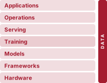
Architecture stack focus for this chapter.
Why does training data function like source code in a machine learning system?
In conventional software, programmers write logic that computers execute. In machine learning, programmers write optimization procedures that extract operational logic from data. This inversion makes training data resemble source code: changing it can change the learned system when the model is retrained, even if no traditional code changes. Yet data rarely receives the review, testing, and version control that even a one-line code change routinely receives. Subtle labeling inconsistencies can induce behavioral inconsistencies; missing edge cases can leave corresponding failures unmeasured; historical biases can propagate into learned behavior. A model trained only on that dataset cannot infer task-relevant evidence absent from it, and systematic label errors can shape what it learns. Unlike traditional source code, which sits inert until a programmer modifies it, the operating distribution can shift as the world changes, potentially changing production performance even when nothing in the codebase has been touched. Data engineering can consume substantial project effort, often more than modeling itself, because the work is consequential. A labeling error caught at collection costs a relabel; the same error found after deployment can cost a retraining run, an incident investigation, and the trust of the people the system failed. Every decision in the data pipeline (what to collect, how to label, when to filter, how to split) propagates forward to constrain model architecture, training dynamics, and deployment viability. Data engineering is therefore not preprocessing but programming in a different language, one where quality control, versioning, and monitoring determine whether the compiled system works today and continues working tomorrow. In D·A·M terms, data overlaps both the algorithm and the machine; it bounds what the model can learn, and the pipeline that delivers it bounds how fast the machine can learn it.
Learning Objectives
- Explain data as source code and trace how data cascades propagate through ML systems
- Evaluate acquisition strategies against coverage, quality, labeling cost, governance, and deployment constraints
- Design ingestion and validation pipelines for batch, streaming, ETL, and ELT workloads
- Specify labeling, transformation, and release practices that prevent data leakage and preserve label quality, training-serving consistency, and reproducibility
- Calculate data gravity, data-stall, and storage-bandwidth costs for moving or serving datasets
- Select storage tiers, file formats, and data loader designs that keep the accelerator fed
- Diagnose drift, data debt, and production pipeline failures using drift metrics, debt indicators, and controlled comparisons of pipeline versions
4.1 Data as Code
A missing accent in a speech corpus, a mislabeled class, or a feature computed one way in training and another in serving becomes a defect in system behavior with no line of code to point to. Because a machine learning system learns its behavior from data, the trained model is a compressed summary of its training set: it can represent only the evidence that data contains, and it treats the data’s labels as the definition of a correct answer. The bitter lesson (The Bitter Lesson) explains why this dependence has grown rather than shrunk. Methods that learn from data at scale have repeatedly overtaken methods built on hand-encoded knowledge, so the knowledge that engineers once wrote into programs must now arrive through data. In the lifecycle that ML Lifecycle lays out, this work is Stage 2, which ends by handing a versioned dataset to model development; every later stage inherits what that dataset contains and what it lacks.
Data constrains the machine as well as the model. Every training step reads its examples from storage, decodes them, and moves them to the accelerator, and an accelerator waiting on input computes nothing however fast it is. Datasets measured in terabytes also have physical mass. They are slow and expensive to move, and they spend energy at every level of the memory hierarchy they cross. Data therefore occupies two of the pairwise overlaps of the D·A·M taxonomy at once, the ones labeled what to learn from and how to move information in The D·A·M Intersection Landscape. Toward the algorithm, it bounds what the model can learn; toward the machine, it bounds how fast learning can proceed.
Both bounds are expensive to meet. Cleaning and organizing data was the most common answer to where data scientists spend their time in the practitioner survey that ML Lifecycle presents (CrowdFlower 2016), and in the image-classification cost comparison later in this chapter, labeling a dataset costs roughly 2,500× to 5,000× as much as one training run on it. Each stage between raw input and an ML-ready dataset (acquisition, ingestion and validation, labeling, and processing) can also introduce a defect that no later stage detects. Data bounds both capability and throughput and often dominates cost, so it requires the same engineering discipline as the model and the machine: acquisition systems, validation checks, labeling workflows, storage layouts, and governance.
CrowdFlower. 2016. Data Science Report 2016.
Definition 4.1: Data engineering
Data engineering is the infrastructure layer that manages the lifecycle of data from source to model, encompassing acquisition, transformation, storage, and governance.
- Significance: It sets both bounds that data places on an ML system. Dataset composition, coverage, and labels determine whether the logical dataset (\(\DatasetSize\), the \(\text{Samples/Task}\) factor of the iron law) represents the target distribution, and therefore what the model can learn. In the unpacked iron law, the pipeline governs the physical bytes moved \((\DataVolume/\Bandwidth)\), and therefore how fast learning can proceed.
- Distinction: Unlike data science, which focuses on inference and insight, data engineering addresses the scalability and reliability of the data pipeline.
- Common pitfall: A frequent misconception reduces data engineering to mere “data cleaning.” In systems terms, it is a build pipeline that turns raw, noisy observations into the validated, versioned tensors that accelerator runtimes consume.
↩︎ The iron law of ML systems, whose data-movement term this chapter governs, is established in Iron Law of ML Systems.
The data-as-code principle (1) turns the model’s dependence on its data into an engineering rule. Changing a dataset changes the trained model just as changing source code changes a program, even when no line of algorithmic code is touched. The pipeline that produces a dataset is therefore the system’s build, and every retraining is a rebuild.
A dataset then needs the disciplines code already has, namely immutable lineage, validation suites, and debugging when regressions appear. Code keeps its tests apart from what they test, and a dataset needs the same trust boundary between its splits. The training set is allowed to shape parameters; the validation set is allowed to shape modeling and pipeline choices; the test set is reserved for estimating generalization after those choices have been made. Data leakage occurs when information crosses those boundaries, so that an evaluation score rewards what the model or its designers already saw instead of measuring generalization to unseen data. Leakage enters through duplicate examples appearing in multiple splits, augmented variants of the same source record landing on both sides of the split, user records from the same household appearing in both training and test, or time-derived features computed using future observations (Kaufman et al. 2012). Preprocessing can leak too, a case section 4.7.1 takes up once normalization and encoding have been introduced.
Kaufman, Shachar, Saharon Rosset, Claudia Perlich, and Ori Stitelman. 2012. “Leakage in Data Mining: Formulation, Detection, and Avoidance.” ACM Transactions on Knowledge Discovery from Data (TKDD) 6 (4): 1–21.
Two of the book’s recurring lighthouse workloads (Lighthouse models put the iron law into practice) carry the chapter, one for each bound. Keyword spotting (KWS), the always-on wake-word detector behind phrases such as “Alexa” and “OK Google,” carries the question of what the data must contain. It takes over from the diabetic retinopathy screening case of ML Lifecycle because its data problems span both a cloud training pipeline and a microcontroller-class device: the model must recognize a few words across accents, microphones, and rooms, stay silent through months of ordinary speech, and fit in tens of kilobytes on a TinyML-class device. Its reference corpus, the Multilingual Spoken Words Corpus (Mazumder et al. 2021), is real; the smart-speaker requirements and data budget that this chapter sets for it are an illustrative scenario. ResNet-50 image classification on one accelerator carries the question of how fast data must arrive, because image examples are large enough to stress storage, decoding, and transfer in ways that one-second audio clips do not. KWS also shows the split boundary at work before any model exists. Assigning each speaker’s utterances to a single split keeps the acoustic model from memorizing speaker-specific vocal-tract resonances, so evaluation measures generalization to speakers the model has never heard.
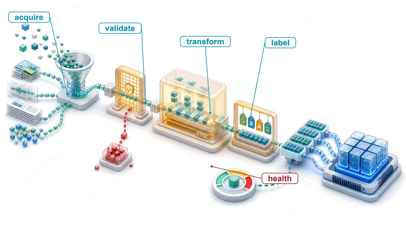
Like a build, the pipeline that produces a dataset runs in stages, and the chapter follows them in the order of the two bounds. The capability half, which works the Data–Algorithm overlap, comes first. After the ways data fails and the requirements of the keyword spotter, acquisition, ingestion and validation, labeling, and processing build the dataset and settle what the model can learn, and a release step records exactly what was built. The throughput half works the Data–Machine overlap. The physics of moving datasets sets the cost of every byte, and storage and delivery must move those bytes fast enough to keep the accelerator fed. An acceptance test then checks both halves against the targets they started with, and operation keeps both bounds true after deployment.
Self-Check: Question
A team is building a training dataset from distributed sensor logs. They discover that the same event can appear in multiple log partitions. They add a pipeline step that identifies duplicate records and keeps one canonical copy. Where must this step run, and why?
- After splitting, because each split should be cleaned independently so that evaluation data is never touched by training-side processing.
- Only on the training split, because duplicates in validation and test data do not affect the trained model.
- Before splitting, because a duplicated record that lands on both sides of the split leaks the same evidence into evaluation and inflates the measured quality.
- Anywhere in the pipeline, because duplicates only waste storage and compute and do not change what the model learns.
Explain why treating training data as the ‘source code’ of a machine learning system necessitates software-engineering practices such as immutable snapshot versioning, automated regression testing, and explicit split boundaries.
True or False: In a keyword-spotting dataset, randomly partitioning audio recordings into an 80/20 train/test split at the individual audio file level maintains a valid trust boundary for estimating real-world generalization.
4.2 How Data Fails
A credit scoring model starts rejecting every applicant from one region after an upstream database migration silently changes how ZIP codes are typed. A wake-word detector misses more and more spoken commands for months after a device maker changes the microphone in its new models. A fraud detection system misses a new attack vector because its training data was six months stale. Each failure traces to a different root cause (schema drift, distribution shift, data staleness), yet all share a common pattern. A data defect entered early, every later stage treated the data as trustworthy, and the failure surfaced only after deployment. The four pillars framework of quality, reliability, scalability, and governance gives the checklist that catches them.
4.2.1 Data cascades
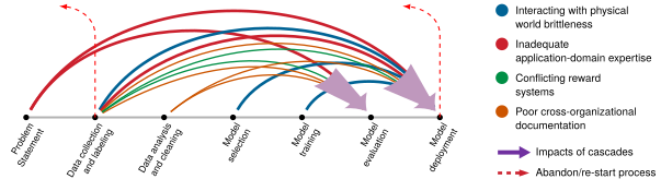
The pattern those three failures share is a data cascade, in which poor data quality in an early stage amplifies through every later stage of the pipeline (Sambasivan et al. 2021). Some invalid inputs trigger immediate software errors, but data can also pass schemas and tests while degrading learned behavior silently until quality issues become severe enough to require expensive investigation, rework, or retraining. In the lifecycle progression sequenced in figure 1, early defects in problem framing and collection bypass intermediate validation and surface only at evaluation and deployment.
↩︎ The compounding cost of late-stage data rework builds directly on the constraint propagation principle established in How Decisions Cascade: The Constraint Propagation Principle.
Definition 4.2: Data cascade
Data cascade is an ML systems failure mode in which upstream data quality problems propagate through collection, labeling, feature engineering, training, evaluation, and deployment, amplifying into downstream model failures or user harm.
- Significance: Remediation cost scales with the number of downstream artifacts that consumed the corrupted data: feature tables must be regenerated, models retrained, evaluation metrics recomputed, and deployed systems rolled back or patched, so one bad field can invalidate a whole training run and every experiment derived from it.
- Distinction: Unlike an isolated data quality bug, a data cascade is defined by propagation and amplification. Each pipeline stage treats its input as trustworthy and converts the defect into new derived state, which hides the root cause as the system moves farther from collection.
- Common pitfall: A frequent misconception is that ordinary software tests catch cascades. Corrupted data can satisfy schemas, pass unit tests, and produce successful training jobs while teaching the model the wrong signal, so prevention requires lineage, validation, contracts, and monitoring tied to model behavior.
Silence is what makes a cascade expensive. A software crash raises a stack trace and pages someone; a data-induced model error produces valid-looking outputs that are simply less accurate. By the time downstream metrics reflect the failure, corrupted predictions may already have contaminated historical data stores, forcing expensive rollbacks and data re-ingestion.
Example 4.1: The pipeline jungle
Scenario: The credit scoring model from the opening of this section suddenly begins rejecting all applicants from a specific geographic region.
Diagnosis: The training pipeline represented zip_code as a fixed-width string (“02139”). An upstream database migration changed the serving field to an integer without updating downstream data contracts. A downstream transform serialized that integer as “2139,” losing the leading zero and causing the model to treat a familiar postal code as an unobserved category. In this scenario, the fallback for unknown categories assigns high risk, explaining the regional rejection pattern.
Systems lesson: Unenforced feature boundaries create pipeline jungles (Sculley et al. 2015) where upstream schema changes cause silent downstream model failures. Versioned data contracts, which are machine-checked rules that declare expected types, value bounds, and whether nulls are allowed, stop cross-system corruption by rejecting malformed records at the ingestion boundary before they reach the model.
4.2.2 Four foundational pillars
The ZIP-code failure crossed several concerns at once: the values were wrong (quality), the transform broke silently instead of rejecting the record (reliability), and no contract recorded what the field meant (governance). Preventing failures like it means balancing four competing operational priorities, each of which feeds the ML data system and each of which pulls against its neighbors (figure 2): stricter validation costs throughput, stronger consistency limits distributed scale, privacy constraints cost performance, and bias mitigation can shrink the usable training set.
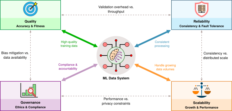
Quality governs input integrity and fitness for task: data must accurately reflect the operating distribution, with correct labels and uncorrupted features. In an edge voice-enrollment pipeline, for example, quality rules filter out clipped audio waveforms, low signal-to-noise ratios, and background acoustic interference so the model learns sharp decision boundaries rather than spurious acoustic artifacts.
Reliability asks whether that enrollment pipeline keeps working when the device, network, or user behavior is imperfect. A pipeline that produces excellent wake-word examples in a laboratory but fails during intermittent connectivity, battery pressure, or microphone glitches delivers no value in the user’s home. Error handling, retries, local buffering, and graceful degradation turn the quality rule into a usable system: the device can request another utterance, defer upload until connectivity returns, or preserve a known-good enrollment rather than silently accepting corrupted audio.
Scalability asks whether that same decision survives growth. A manual review policy that works for a thousand recordings collapses when the product expands to millions of users, dozens of languages, and long-tail acoustic conditions. The system must scale validation, storage, labeling, and retraining without letting infrastructure cost grow faster than the value of better coverage. The limiting resource depends on the workload. For edge speech, storage and labeling throughput dominate. For recommendation systems such as the DLRM lighthouse, the tables of learned user and item representations outgrow one machine’s memory and must be partitioned across several.
Governance defines the boundaries within which quality, reliability, and scalability must operate. For keyword spotting, governance determines whether raw voice recordings may leave the device, how long enrollment audio can be retained, which consent record authorizes use, and what documentation proves that the dataset covers relevant accents without exposing private speech. A perfectly scalable, reliable, high-quality pipeline that violates the General Data Protection Regulation (GDPR) or perpetuates demographic biases creates liability rather than value. Dataset documentation practices such as datasheets (Gebru et al. 2021) and data statements make part of that governance visible by recording provenance, intended use, collection conditions, and coverage needed for bias analysis and scientific comparison (Bender and Friedman 2018).
Bender, Emily M., and Batya Friedman. 2018. “Data Statements for Natural Language Processing: Toward Mitigating System Bias and Enabling Better Science.” Transactions of the Association for Computational Linguistics 6: 587–604. https://doi.org/10.1162/tacl_a_00041.
When an ML system fails, each class of symptom points to one of the four pillars:
- Gradual accuracy loss points to quality. Drift has moved the serving distribution away from training, or label quality has fallen as annotator pools changed.
- Intermittent pipeline failures point to reliability. Error handling, retry logic, or resource controls are missing under peak load.
- Slow training on adequate hardware points to scalability. A single-threaded transformation, unpartitioned shuffle, or slow storage tier keeps parallel resources from doing useful work.
- Compliance gaps found in audits point to governance debt. Lineage tracking is incomplete, access controls are stale, or retention policies have fallen behind regulatory changes.
Checkpoint 4.1: Four pillars framework
The four pillars provide a systems lens for every pipeline choice.
Pillars
Trade-offs
Some failures span multiple pillars. Features that differ between training and serving implicate both quality (the values are wrong) and reliability (the computation is inconsistent). A privacy-motivated deletion policy can also create quality gaps if the retained data no longer covers the deployment population. Diagnosing such cross-pillar failures requires checking consistency contracts, comparing feature distributions across environments, and tracing transformation lineage, so production diagnosis checks data infrastructure alongside model behavior. The pillars name what to check, but not how good is good enough. Those thresholds come from the requirements of a specific system, and the keyword spotter supplies them.
Self-Check: Question
A data engineering team implements comprehensive synchronous schema and distribution validation checks directly inside the real-time event ingestion path. Under the Four Pillars framework, which primary operational trade-off will this team encounter?
- A Governance trade-off: inspecting payload schemas automatically breaches user data retention agreements.
- A Model Capacity trade-off: validating input records forces downstream neural network layers to increase parameter counts.
- A Scalability and Reliability trade-off: heavy synchronous validation consumes CPU cycles and increases per-record latency, reducing ingestion throughput and risking dropped messages during traffic spikes.
- A Durability trade-off: validating data records accelerates physical wear on persistent solid-state drive cells.
True or False: Data cascades in ML systems are easily caught by standard software unit tests because corrupted input data causes deterministic assertion failures in pipeline code.
Trace the propagation sequence of a data cascade as described in the chapter, from its root cause to user-facing impact:
- Downstream model optimization on distorted representations
- Upstream sensor or schema change without contract notification
- Silent distortion of extracted features passing syntactic checks
- Degraded real-world predictions and costly post-deployment rollback
4.3 Requirements and Data Budget
A wake-word detector answers to two numbers at once. It must catch nearly every spoken wake word, and it must almost never wake for anything else, while listening continuously in tens of kilobytes of memory on a microcontroller or the low-power core of a phone or smart speaker. The chapter’s illustrative smart speaker sets those numbers, and every later stage of the pipeline is measured against them.
In the wake-word interaction sequenced in figure 3, an always-on detector traps “Alexa…” before the smart speaker acknowledges the utterance and opens the command channel for “dim the lights.” Behind that brief exchange sits the data pipeline this chapter builds: the recordings the detector learned from, how they were labeled and checked, and how the result was verified before it shipped.

The detector must find specific keywords amid ambient sound and other speech, quickly and with few false activations, on a device with very limited resources. A well-specified problem definition names the keywords, the application, and the deployment setting, then states targets that can be measured. Overall accuracy is the wrong target, because almost every second of audio contains no wake word, and a detector that never fires would score nearly perfectly. The scenario therefore sets a keyword detection rate of 98 percent, the fraction of spoken wake words the detector catches, measured at a detection threshold that keeps false wakes within the budget the next notebook derives. It also requires a response within 200 ms and a model small and frugal enough for the device.
Napkin Math 4.1: False positive targets
Problem: An always-on KWS system budgets at most one expected false wake-up per month. Under a model that counts one nonkeyword classification window each second around the clock, how strict does the per-window false positive rate need to be?
Variables:
- Duty cycle: Always-on (24 hours/day).
- Window size: One-second classification windows.
- Windows per month: One window per second, 24 hours/day, over 30 days gives 2,592,000 windows/month.
Math:
- False positive rate (FPR): 1 expected false wake divided by the monthly nonkeyword-window count gives approximately \(3.9 \times 10^{-7}\)
- Nonkeyword rejection requirement: 99.99996 percent rejection of nonkeyword windows.
Systems insight: This calculation bounds the expected monthly count, not the maximum number of false wakes in every month. Expectation does not require independent windows. Aggregate accuracy (for example, “99 percent accuracy”) is insufficient here. Evaluation must report false accepts per hour (FA/Hr) together with the corresponding false-rejection behavior. Real detectors score overlapping windows every few tens of milliseconds and smooth the scores, so the per-window target depends on the detector, while the per-hour rate is the quantity to measure. A budget of one false wake per month is deliberately strict; commercial assistants typically pass each candidate wake to a second, larger check rather than asking the always-on detector to meet such a budget alone (Siri Team 2017).
Siri Team. 2017. Hey Siri: An on-Device DNN-Powered Voice Trigger for Apple’s Personal Assistant.
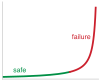
Even 99.999 percent per-window rejection multiplies into 26 false wakes a month.
Nayak, Prateeth, Takuya Higuchi, Anmol Gupta, Shivesh Ranjan, Stephen Shum, Siddharth Sigtia, Erik Marchi, et al. 2022. “Improving Voice Trigger Detection with Metric Learning.” Interspeech 2022, 1896–900. https://doi.org/10.21437/interspeech.2022-11160.
Evaluation therefore reports the two rates together, as a detection/error trade-off curve that plots false accepts per hour against false rejection rate on streaming audio representative of deployment (Nayak et al. 2022). The detection target is read off that curve at the false-wake budget, and operational metrics complete the contract by bounding response time from the end of the keyword to the system’s reaction alongside the average power drawn while listening.
The device sets hard boundaries on any design that meets those targets. Memory limitations require extremely lightweight models, often in the tens-of-kilobytes range (Zhang et al. 2017), to fit in the always-on island of the system-on-chip (SoC);1 this budget must accommodate both model weights and the feature extraction buffers and preprocessing state. Limited computational capabilities (often a few hundred MHz of clock speed) demand aggressive model optimization. On phones and wearables the detector runs from a battery, and even a plugged-in smart speaker keeps its always-on stage to milliwatts so that idle power stays low, so KWS systems target sub-milliwatt consumption during continuous listening.
Zhang, Yundong, Naveen Suda, Liangzhen Lai, and Vikas Chandra. 2017. Hello Edge: Keyword Spotting on Microcontrollers.
1 SoC always-on island: Modern system-on-chip designs partition power domains so a low-power “always-on” island (typically achieving sub-milliwatt draw) monitors for wake triggers while the main processor sleeps. The critical constraint is that this island must hold both the model weights and the audio preprocessing code within its dedicated SRAM, a split budget that forces KWS architectures to optimize for total footprint, not just parameter count.
Data quality and diversity determine whether these targets can be met inside those limits. The dataset must cover speakers of different accents, ages, and genders, the many ways people pronounce the same wake word, and background conditions from quiet bedrooms to noisy kitchens. The model cannot grow to compensate for missing coverage, so on this device the data carries the burden that a larger model would carry in a data center.
4.3.1 KWS design space
Doubling the sampling rate of a wake-word recording from 8 kHz to 16 kHz captures sharper consonant sounds and raises the detection rate, but it also doubles the raw-audio window and the input-processing work on the device. Every data engineering choice for the keyword spotter pulls detection rate, false-wake tolerance, latency, energy, and memory against one another, and table 1 prices those trade-offs. Each row is a D·A·M coupling of the kind drawn in The D·A·M Axis Triad, because a data choice such as sampling rate or coefficient count changes what the algorithm receives and what the machine must hold in always-on memory. One row uses mel-frequency cepstral coefficients (MFCCs)2 (Davis and Mermelstein 1980), which reduce each frame of roughly 25 ms of audio to 13 to 40 numbers that emphasize the frequencies speech uses. The coefficient count sets the size of the model’s input and how much acoustic detail it keeps; section 4.7 shows how they are extracted.
2 MFCC (mel-frequency cepstral coefficients): Mel-scale filtering gives this representation its compactness and noise resistance by emphasizing the frequencies humans use to distinguish speech. It reduces the hundreds of raw samples in a short window (400 samples in 25 ms at 16 kHz) to 13–40 coefficients, so each frame fits inside an always-on, kilobyte-scale memory budget. A parameter mismatch between training and serving creates feature skew and can degrade accuracy.
Davis, Steven B., and Paul Mermelstein. 1980. “Comparison of Parametric Representations for Monosyllabic Word Recognition in Continuously Spoken Sentences.” IEEE Transactions on Acoustics, Speech, and Signal Processing 28 (4): 357–66. https://doi.org/10.1109/TASSP.1980.1163420.
| Design Choice | Quality Impact | Latency Impact | Cost Impact | Memory Impact |
|---|---|---|---|---|
| 8 \(\rightarrow\) 16 kHz sampling | +2–4% detection rate | 2× input-processing workload | 2× raw-audio storage | 2× raw-audio window |
| 13 \(\rightarrow\) 40 MFCC coefficients | +3–5% detection rate | 3× model-input size | Minimal | 3× feature memory |
| 1M \(\rightarrow\) 10M training examples | +5–8% detection rate | 10× training time | 10× labeling cost | 10× storage |
| Clean \(\rightarrow\) noisy training data | +10–15% real-world | Minimal | 3× collection cost | Minimal |
| Cloud \(\rightarrow\) local inference | up to 2% detection-rate risk | 100 ms \(\rightarrow\) 10 ms | $0.001/query \(\rightarrow\) $0/query | cloud-scale \(\rightarrow\) 256 KB |
| Real only \(\rightarrow\) added synthetic augmentation | +3–5% robustness | Minimal | 10× cheaper per example than real collection | Minimal |
Because the device runs inside a milliwatt power envelope and a tens-of-kilobytes SRAM budget, an engineering team cannot pick the most accurate option in every row of table 1 at once. Instead, the team must divide a fixed data budget across labeling, storage, and governance so the detector reaches its accuracy target without outgrowing the hardware. Notebook 4.2 allocates the data budget and proposes a candidate design for a smart-speaker deployment. The acquisition, labeling, processing, and delivery decisions that follow supply the evidence needed to accept or reject it.
Napkin Math 4.2: Allocating the KWS data budget
Scenario: A KWS system for a smart speaker has these constraints:
- Target: 98 percent keyword detection rate at a threshold that keeps the expected false-wake budget below 1 false wake/month
- Budget: $150K total data engineering budget
- Memory: 256 KB model size limit (always-on island), with a separate 16 KB budget for preprocessing state
- Timeline: 6 months to production
Step 1: Choose conservative options for the constrained device.
For this scenario, the team chooses two conservative options:
- 13 MFCC coefficients, because every MFCC frame lives in the always-on island’s SRAM as model input and buffered state, so the 40-coefficient option triples a cost the device pays continuously
- Local inference, because streaming every second of audio to a server is ruled out by bandwidth, privacy, and offline operation
The choice rests on where each cost lands. Data collection is paid once, from a central budget, whereas the 40-coefficient representation triples the model’s input, and with it the first layer’s work and the feature buffer, on every device for every second it listens. The table suggests a 3–5 percent detection gain from 40 coefficients, so the team picks 13 and spends the difference on coverage, expecting broader training data to recover the gap. The acceptance test of section 4.11 decides the choice.
Step 2: Calculate budget allocation.
Labeling is priced at a scenario rate per crowdsourced example, set above the image-classification crowd rates that section 4.6.2 later tabulates because a KWS contributor must record the utterance as well as label it. The $150K budget splits across three cost categories:
- Labeling (~60 percent): $90K available
- Storage/Processing (~25 percent): $37.5K
- Governance/Other (~15 percent): $22.5K
At $0.10/label with 20 percent review overhead: $90K ÷ $0.12/label = 750K labeled examples
This yields roughly 0.75M labeled examples, just below the 1M anchor in the design space. The 1M-to-10M row in table 1 should therefore be read as a scaling reference rather than a direct interpolation: the real-label budget alone does not buy the full data-volume gain. Counting examples also hides what limits a wake-word model in practice, which is the number of distinct speakers and the hours of ordinary, non-keyword audio available to measure false wakes; section 4.11 prices that listening time.
Step 3: Identify candidate quality improvements.
The quality plan has three components:
- An illustrative base-model detection rate of ~90 percent
- Partial data-volume gain from 750K real examples
- A gap to the 98 percent target that the options below must close
Three options from the design space are candidates for closing the gap; their collection, storage, processing, and deployed-footprint costs must be checked against the allocations. Their listed gains cannot simply be added to the base detection rate, because they overlap (noisy data and synthetic augmentation both buy robustness to acoustic conditions), so the plan is a candidate whose combined effect must be measured on the trained system:
- 16 kHz sampling: a detection-rate gain of 2–4 percent, 2× raw-audio storage (requires cost validation; on the device only the short window of raw samples feeding each MFCC computation doubles, because every frame still reduces to 13 coefficients)
- Noisy training data: a field detection-rate gain of 10–15 percent, 3× collection cost (proposed for a targeted noisy slice; its cost must fit the storage/processing allocation)
- Synthetic augmentation: a robustness gain of 3–5 percent, 10× cheaper than real data in the illustrative row; generation, verification, and storage costs remain to be measured
Step 4: Final configuration.
The scenario combines these choices with 13 MFCCs and the computed 750K real-label budget in table 2. The quality effects can overlap, so the table records a candidate configuration rather than a solved optimum.
Result: The budget buys approximately 750K human-labeled examples, 13 MFCCs, local inference, and a noisy slice plus synthetic augmentation to close the quality gap. Whether that configuration reaches the 98 percent detection target inside the 256 KB model limit is what acceptance decides.
Systems insight: Design-space analysis turns “we need more data” into a costed plan. The stated labeling assumptions buy about 750K real examples, and the acceptance test, not the design table, decides whether that plan succeeds.
Table 2 records the resulting configuration, pairing each design choice with the constraint that motivates it: sampling and augmentation draw on the stated allocations, while the always-on island sets the deployed-footprint constraint. Actual costs and working-state memory still require validation.
| Choice | Selection | Rationale |
|---|---|---|
| Sampling rate | 16 kHz | +2–4% detection rate for 2× raw-audio storage, subject to cost validation; on device only the raw-sample window grows, since each MFCC frame keeps 13 coefficients |
| MFCC coefficients | 13 | One-third the feature buffer and model input of 40 coefficients in always-on SRAM; test whether improved data coverage recovers the quality gap |
| Training examples | 750K real + illustrative synthetic augmentation | Human-label count follows from the budget; synthetic volume is a scenario choice |
| Data diversity | Noisy + clean mix | Critical for real-world deployment |
| Inference | Local, reduced precision | Reduced precision can lower footprint; the final 256 KB fit requires the quantization analysis in Numerical Precision: Changing How Values Are Stored |
| Augmentation | Heavy synthetic | Illustrative 10× per-example cost advantage; total generation and review costs require validation |
The candidate configuration fixes the targets but not the data. Meeting them starts with acquisition: finding recordings that cover the speakers, accents, devices, and rooms the detector will meet, from sources whose cost and consent terms the budget can bear.
Self-Check: Question
An always-on Keyword Spotting (KWS) system on an embedded voice assistant continuously evaluates 1-second audio classification windows (\(24\text{ hours/day}\) over a \(30\text{-day}\) month). Treat each window as nonkeyword audio. The product budgets at most 1 expected false activation per month. An engineer reports 99% aggregate accuracy and, separately, a measured 1% false positive rate on background noise. How many false activations does that FPR imply in expectation, and what per-window FPR meets the expected-count budget?
- A 1% FPR implies an expected count of 720 false activations per month; the expected-count budget requires a per-window FPR of \(\le 1.38 \times 10^{-5}\).
- A 1% FPR implies an expected count of ~25,920 false activations per month (~36 false wakes/hour); the expected-count budget requires a per-window FPR of \(\le 3.86 \times 10^{-7}\) (>99.9999% non-keyword rejection).
- A 1% FPR implies an expected count of ~2,592 false activations per month; the expected-count budget requires a per-window FPR of \(\le 1.0 \times 10^{-4}\).
- A 1% FPR satisfies the expected-count budget because accuracy is averaged over the total number of audio hours across the entire device fleet.
The chapter specifies its keyword spotter by a keyword detection rate measured at a threshold that holds the expected false-wake budget, rather than by overall accuracy. Why is overall accuracy the wrong target for an always-on detector?
- Almost every one-second window contains no wake word, so a detector that never fires scores near-perfect overall accuracy while missing every command; the meaningful targets are the fraction of spoken wake words caught and the false-wake rate at the chosen threshold.
- Overall accuracy cannot be computed for a model that runs on a microcontroller, so the target must use a metric the device can calculate itself.
- Overall accuracy rises automatically with more training data, so it cannot distinguish one data plan from another.
- Detection rate and overall accuracy are the same quantity for a binary classifier; the scenario only renames it.
4.4 Data Acquisition
A huge corpus of studio audio does not help a wake-word detector that has to run on inexpensive microphones in noisy kitchens, because a model cannot learn a speaker, room, or microphone that no source supplied. Data acquisition therefore sets the outer limit of the capability bound, and it begins when the team names the coverage gap the model must close. For keyword spotting, public corpora are the first source. Speech Commands (Warden 2018) established the small-vocabulary benchmark of one-second spoken words, and the Multilingual Spoken Words Corpus (MSWC) (Mazumder et al. 2021) provides a reusable reference source of 23.4 million audio samples spanning 50 languages. That corpus is larger than the product-specific labeled subset budgeted in the KWS design example; using it still requires selecting and validating relevant coverage.
Warden, Pete. 2018. “Speech Commands: A Dataset for Limited-Vocabulary Speech Recognition.” arXiv Preprint arXiv:1804.03209, ahead of print. https://doi.org/10.48550/arXiv.1804.03209.
Mazumder, Mark, Sharad Chitlangia, Colby Banbury, Yiping Kang, Juan Manuel Ciro, Keith Achorn, Daniel Galvez, et al. 2021. “Multilingual Spoken Words Corpus.” Advances in Neural Information Processing Systems 35 (NeurIPS 2021) Datasets and Benchmarks Track.
Reaching a 98 percent detection rate requires representative coverage of regional accents, speaker age groups, room reverbs, and microphones that differ in frequency response, signal-to-noise ratio, and clipping behavior, at volumes that manual curation cannot economically supply and under strict privacy boundaries on audio retention. Because no single collection method can economically cover all of those conditions, acquisition strategy is a sequence of gap-closing decisions: reuse what already matches deployment, collect what is missing, scrape or synthesize where scale is the binding constraint, and reject sources whose provenance or consent constraints make them unusable.
4.4.1 Coverage and diversity requirements
A wake-word detector trained on millions of clean clips can score well on an aggregate validation set while still waking once an hour on kitchen conversation or missing speakers with underrepresented regional accents. Dataset scale alone does not guarantee generalization when coverage gaps in a large corpus (geographic bias, demographic underrepresentation, sensor calibration drift, and unobserved edge cases) cause systematic failures that aggregate validation metrics hide (Shankar et al. 2017; Wang et al. 2019; Oakden-Rayner et al. 2020).
Shankar, Shreya, Yoni Halpern, Eric Breck, James Atwood, Jimbo Wilson, and David Sculley. 2017. “No Classification Without Representation: Assessing Geodiversity Issues in Open Data Sets for the Developing World.” arXiv Preprint arXiv:1711.08536.
Wang, Tianlu, Jieyu Zhao, Mark Yatskar, Kai-Wei Chang, and Vicente Ordonez. 2019. “Balanced Datasets Are Not Enough: Estimating and Mitigating Gender Bias in Deep Image Representations.” 2019 IEEE/CVF International Conference on Computer Vision (ICCV), 5309–18. https://doi.org/10.1109/iccv.2019.00541.
Oakden-Rayner, Luke, Jared Dunnmon, Gustavo Carneiro, and Christopher Re. 2020. “Hidden Stratification Causes Clinically Meaningful Failures in Machine Learning for Medical Imaging.” Proceedings of the ACM Conference on Health, Inference, and Learning, 151–59. https://doi.org/10.1145/3368555.3384468.
For KWS, coverage must support both keyword recognition and the false-wake contract. Labeled wake-word clips measure recognition, but acquiring more of them does not establish how often an always-on detector activates on ordinary nonkeyword audio. The acquisition plan must separately reserve consented recordings collected for an evaluation study of representative listening conditions, including background conversation, television, music, silence, and environmental noise across the intended microphones and rooms. These recordings retain their duration and temporal sequence so evaluation can run the deployed detection path and report false accepts per hour alongside false rejection on keyword recordings. A short stream with no observed false wakes supplies limited evidence; its duration and the uncertainty of the measured rate constrain any claim about the monthly target.
Training negatives serve a different acquisition goal. Mining near-wake phrases and other audio that confuses the current detector can improve its rejection behavior, but this deliberately difficult sample does not preserve the frequency of those conditions in deployment. The representative evaluation streams therefore remain separate from training and threshold selection, with speaker and recording-period boundaries maintained. An acquisition budget that funds only keyword labels and mined hard negatives can improve the detector while leaving its operational false-wake target unmeasured.
Governance constraints further shape acquisition: privacy and health-data regulations such as GDPR and the U.S. Health Insurance Portability and Accountability Act (HIPAA) limit what data can be collected and how (European Parliament and Council of the European Union 2016; United States Congress 1996), while ethical sourcing requires fair compensation and transparent use of human contributions. Together, these coverage, evaluation, and governance bounds define the criteria against which each candidate data source is judged.
European Parliament, and Council of the European Union. 2016. Regulation (EU) 2016/679 of the European Parliament and of the Council of 27 April 2016. Official Journal of the European Union.
United States Congress. 1996. Health Insurance Portability and Accountability Act of 1996. Public Law 104-191.
↪ The governance infrastructure that proves what data a production system ingested, who accessed it, and on what legal basis is developed in Data Governance and Compliance.
4.4.2 Selecting data sources
Paying for custom voice recordings of words and accents that a public benchmark already covers wastes the data budget, while stopping at the benchmark leaves the detector blind to its own microphones and rooms. The choice among curated datasets, expert crowdsourcing, controlled web scraping, and synthetic generation therefore begins with the cheapest reusable source and escalates to active collection or simulation only when the remaining deployment-distribution gap justifies the added cost, quality effort, and governance risk.
Preexisting datasets from repositories such as Kaggle, UCI (Dua and Graff 2024), and ImageNet3 are the first test. They offer speed and comparability when the deployment distribution resembles the benchmark enough to make reuse meaningful. For KWS, a curated speech corpus can establish the baseline model and reveal which words, languages, and acoustic conditions are already covered. A baseline corpus does not guarantee operational coverage, but it makes the remaining distribution gaps measurable.
Dua, Dheeru, and Casey Graff. 2024. UCI Machine Learning Repository.
3 ImageNet: The 2009 paper reported 3.2 million images across 5,247 synsets; the full database later reached about 14.2 million images across 21,841 synsets, whereas the challenge used a 1,000-class subset (Deng et al. 2009, 2024; Russakovsky et al. 2015). Its value as a benchmark is inseparable from its data engineering: Fei-Fei Li’s team built labeling infrastructure that later teams could reuse. The catch is sensitivity to annotation procedures and modest distribution shifts: models tuned to ImageNet’s distribution can underperform on related but shifted test sets (Recht et al. 2019; Beyer et al. 2020).
Deng, Jia, Wei Dong, Richard Socher, Li-Jia Li, Kai Li, and Li Fei-Fei. 2009. “ImageNet: A Large-Scale Hierarchical Image Database.” 2009 IEEE Conference on Computer Vision and Pattern Recognition, 248–55. https://doi.org/10.1109/cvpr.2009.5206848.
Deng, Jia, Wei Dong, Richard Socher, Li-Jia Li, Kai Li, and Li Fei-Fei. 2024. ImageNet.
Russakovsky, Olga, Jia Deng, Hao Su, Jonathan Krause, Sanjeev Satheesh, Sean Ma, Zhiheng Huang, et al. 2015. “ImageNet Large Scale Visual Recognition Challenge.” International Journal of Computer Vision 115 (3): 211–52. https://doi.org/10.1007/s11263-015-0816-y.
Recht, Benjamin, Rebecca Roelofs, Ludwig Schmidt, and Vaishaal Shankar. 2019. “Do ImageNet Classifiers Generalize to ImageNet?” Proceedings of the 36th International Conference on Machine Learning (ICML), 5389–400.
Beyer, Lucas, Olivier J. Hénaff, Alexander Kolesnikov, Xiaohua Zhai, and Aäron van den Oord. 2020. “Are We Done with ImageNet?” arXiv Preprint arXiv:2006.07159.
Pineau, Joelle, Philippe Vincent-Lamarre, Koustuv Sinha, Vincent Larivière, Alina Beygelzimer, Florence d’Alché-Buc, Emily Fox, and Hugo Larochelle. 2021. “Improving Reproducibility in Machine Learning Research (a Report from the Neurips 2019 Reproducibility Program).” Journal of Machine Learning Research 22 (164): 1–20.
Henderson, Peter, Riashat Islam, Philip Bachman, Joelle Pineau, Doina Precup, and David Meger. 2018. “Deep Reinforcement Learning That Matters.” Proceedings of the AAAI Conference on Artificial Intelligence 32 (1): 3207–14. https://doi.org/10.1609/aaai.v32i1.11694.
Gudivada, Venkat N., Amy Apon, and Junhua Ding. 2017. “Data Quality Considerations for Big Data and Machine Learning: Going Beyond Data Cleaning and Transformations.” International Journal on Advances in Software 10 (1–2): 1–20.
Whether an external dataset is safe to reuse depends on how well it is documented. Without records of sensor calibration, recording environments, and filtering rules, a team cannot reproduce an external dataset’s conditions or check whether they match deployment (Pineau et al. 2021; Henderson et al. 2018). Good documentation states how the data was collected, how each label was defined, and what baseline error rates were found, so another team can validate the corpus independently. Once ingestion reaches millions of examples from varied sources, hidden label errors also multiply past what humans can inspect by hand (Gudivada et al. 2017), so the pipeline must run automated validation checks on every batch.
Reuse carries a less visible risk. Standard validation metrics can create an illusion of model readiness when the benchmark itself is unrepresentative, and when many teams train on the same repository, its blind spots do not average out across their models. They can recur across models, so five models trained on one dataset can share correlated failures (figure 4).
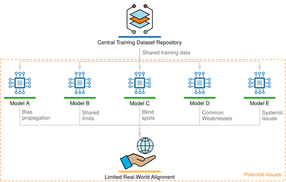
This gap between benchmark and deployment is the central failure mode of static offline evaluation. Because training minimizes average error only over the observed training set (empirical risk minimization), a model will latch onto whatever shortcuts appear in a static benchmark, even when those shortcuts vanish in production, which is why production pipelines still need continuous data validation and drift monitoring.
4.4.3 Scaling acquisition
Curated datasets and targeted collection close coverage gaps one batch at a time, which stops working once a task needs millions of training instances. At large scale, web scraping and synthetic generation provide the main routes to massive datasets. Data-acquisition scalability is an economic problem: unit labeling costs, ingestion throughput, and storage overhead scale along very different curves, and labeling usually dominates (section 4.6.2). Approaches that work well at thousands of examples become impractical at millions, whereas automated data generation pipelines amortize their setup costs across large volumes.
Web scraping reduces the cost of collecting raw examples at scale. Supervision remains a separate expense unless the source and task already supply usable labels or training targets. Foundational vision datasets such as ImageNet (Deng et al. 2024) and OpenImages (Kuznetsova et al. 2020) relied on automated scraping, while modern language models depend on multi-terabyte web crawls (Groeneveld et al. 2024). Ingestion pipelines targeting domain-specific corpora, such as public code repositories (Chen et al. 2021), expand coverage at low per-sample acquisition costs. Scrapers are also fragile: page layouts change and break parsers, sites throttle crawlers, and dynamically rendered content goes missing. Raw web crawls also capture anachronistic or irrelevant samples that contaminate supervised targets.
Kuznetsova, Alina, Hassan Rom, Neil Alldrin, Jasper Uijlings, Ivan Krasin, Jordi Pont-Tuset, Shahab Kamali, et al. 2020. “The Open Images Dataset V4: Unified Image Classification, Object Detection, and Visual Relationship Detection at Scale.” International Journal of Computer Vision 128 (7): 1956–81. https://doi.org/10.1007/s11263-020-01316-z.
Groeneveld, Dirk, Iz Beltagy, Pete Walsh, Akshita Bhagia, Rodney Kinney, Oyvind Tafjord, Ananya Harsh Jha, et al. 2024. “OLMo: Accelerating the Science of Language Models.” Proceedings of the 62nd Annual Meeting of the Association for Computational Linguistics (Volume 1: Long Papers), 15789–809. https://doi.org/10.18653/v1/2024.acl-long.841.
Chen, Mark, Jerry Tworek, Heewoo Jun, Qiming Yuan, Henrique Ponde de Oliveira Pinto, Jared Kaplan, Harri Edwards, et al. 2021. “Evaluating Large Language Models Trained on Code.” arXiv Preprint arXiv:2107.03374.
The 1914 street scene in figure 5 captures this failure mode directly. An uncurated web query for “traffic light” returned a historical Cleveland intersection where streetcars and a roadside control booth surround early manually switched signals. If an autonomous driving model trained on such samples, it would learn spurious correlations with trolley tracks, period attire, and handwritten label annotations rather than modern LED traffic lights.
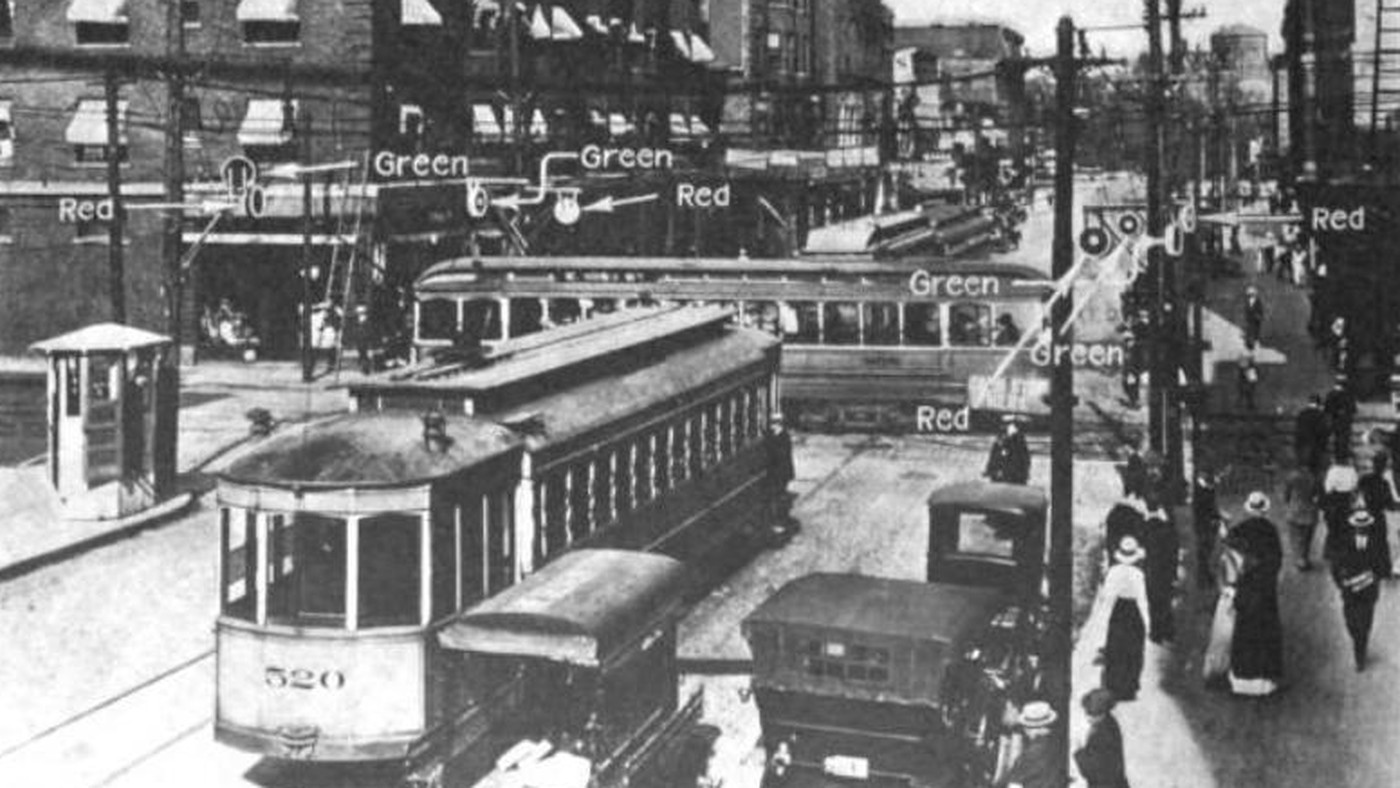
Stromberg, Joseph. 2015. When Was the First Traffic Light Installed? Today in 1914. Vox.
Raw volume cannot substitute for checking what the examples mean, because an uncurated web crawl multiplies spurious correlations along with sample count. Scraping also operates under strict legal and governance boundaries. Website terms of service, robots.txt directives, and evolving copyright law limit what automated crawlers may take (Harvard Law School 2024). Ingestion pipelines must therefore record provenance, filter for copyright compliance, and scrub personal data before scraped files enter shared storage.
Harvard Law School. 2024. Does ChatGPT Violate New York Times Copyrights?
Even a well-governed crawl draws on a finite supply. Pretraining corpora for large language models grew at a fitted rate of about 2.9× per year, from the 300 billion tokens that trained GPT-3 in 2020 to the 36 trillion reported for Qwen3 in 2025 (Brown et al. 2020; Yang et al. 2025). Figure 6 sets that climb against the estimated stock of public human-generated text, roughly 300 trillion tokens once quality and repetition are accounted for (Villalobos et al. 2024), and at the fitted rate the largest corpora reach the middle of that estimate around 2028. Once quality text runs short, acquiring more of it stops being a purchasing decision, and filtering, deduplication, and the selection methods of Data Selection decide how much each additional token is worth. A wake-word model meets its own version of the limit far sooner. No crawl holds enough clean recordings of one phrase in every accent and acoustic setting, so the KWS pipeline has to commission the data it lacks.
Villalobos, Pablo, Anson Ho, Jaime Sevilla, Tamay Besiroglu, Lennart Heim, and Marius Hobbhahn. 2024. “Position: Will We Run Out of Data? Limits of LLM Scaling Based on Human-Generated Data.” Proceedings of the 41st International Conference on Machine Learning (ICML), Proceedings of machine learning research, vol. 235: 49523–44.
Rae, Jack W., Sebastian Borgeaud, Trevor Cai, Katie Millican, Jordan Hoffmann, Francis Song, John Aslanides, et al. 2021. “Scaling Language Models: Methods, Analysis & Insights from Training Gopher.” arXiv Preprint arXiv:2112.11446.
Hoffmann, Jordan, Sebastian Borgeaud, Arthur Mensch, Elena Buchatskaya, Trevor Cai, Eliza Rutherford, Diego de Las Casas, et al. 2022. “Training Compute-Optimal Large Language Models.” Advances in Neural Information Processing Systems (NeurIPS) 35: 30016–30. https://doi.org/10.52202/068431-2176.
Chowdhery, Aakanksha, Sharan Narang, Jacob Devlin, Maarten Bosma, Gaurav Mishra, Adam Roberts, Paul Barham, et al. 2022. “PaLM: Scaling Language Modeling with Pathways.” arXiv Preprint arXiv:2204.02311.
Touvron, Hugo, Thibaut Lavril, Gautier Izacard, Xavier Martinet, Marie-Anne Lachaux, Timothée Lacroix, Baptiste Rozière, et al. 2023. “LLaMA: Open and Efficient Foundation Language Models.” arXiv Preprint arXiv:2302.13971.
Touvron, Hugo, Louis Martin, Kevin Stone, Peter Albert, Amjad Almahairi, Yasmine Babaei, Nikolay Bashlykov, et al. 2023. “Llama 2: Open Foundation and Fine-Tuned Chat Models.” arXiv Preprint arXiv:2307.09288.
Dubey, Abhimanyu, Abhinav Jauhri, Abhinav Pandey, Abhishek Kadian, et al. 2024. The Llama 3 Herd of Models. arXiv preprint arXiv:2407.21783.
Qwen, An Yang, Baosong Yang, Beichen Zhang, Binyuan Hui, Bo Zheng, Bowen Yu, et al. 2024. “Qwen2.5 Technical Report.” arXiv Preprint arXiv:2412.15115.
DeepSeek-AI. 2025. “Insights into DeepSeek-V3: Scaling Challenges and Reflections on Hardware for AI Architectures.” Proceedings of the 52nd Annual International Symposium on Computer Architecture, 1731–45. https://doi.org/10.1145/3695053.3731412.
Yang, An, Anfeng Li, Baosong Yang, Beichen Zhang, Binyuan Hui, Bo Zheng, Bowen Yu, et al. 2025. “Qwen3 Technical Report.” arXiv Preprint arXiv:2505.09388.
Crowdsourcing shifts the acquisition bottleneck from raw sample retrieval to quality control across distributed human annotators. Platforms like Amazon Mechanical Turk4 (Amazon Web Services 2024) demonstrated this at scale with ImageNet, distributing millions of image categorization tasks across thousands of independent contributors (Deng et al. 2024). Crowdsourcing provides two core systems advantages: horizontal scaling through parallel microtask dispatch, and demographic diversity across regional accents and acoustic settings. However, distributed human labeling introduces significant variance in label fidelity. To keep label noise from corrupting what the model learns, the acquisition pipeline must implement automated quality control: consensus voting, golden-set validation (interleaving pre-labeled control samples), and dynamic task routing (Sheng and Zhang 2019). In the KWS pipeline, crowdsourced collection targets wake-word samples from specific acoustic environments and underrepresented dialects that public web scrapes fail to capture.
4 Amazon Mechanical Turk (MTurk): A crowdsourcing platform that routes small tasks to distributed workers and can scale annotation beyond expert-only workflows. Snow et al. (2008) evaluate this pattern for natural-language annotation tasks, showing that non-expert annotations can be useful when task design and quality control are handled carefully. For wake-word audio collection, the same systems trade-off appears in domain-specific form: scale is attractive, but submissions still need acoustic checks such as signal-to-noise ratio, duration, and recording validity before they can safely enter the training set.
Snow, Rion, Brendan O’Connor, Daniel Jurafsky, and Andrew Y. Ng. 2008. “Cheap and Fast—but Is It Good? Evaluating Non-Expert Annotations for Natural Language Tasks.” Proceedings of the Conference on Empirical Methods in Natural Language Processing - EMNLP ’08, 254. https://doi.org/10.3115/1613715.1613751.
Amazon Web Services. 2024. Amazon Mechanical Turk.
Sheng, Victor S., and Jing Zhang. 2019. “Machine Learning with Crowdsourcing: A Brief Summary of the Past Research and Future Directions.” Proceedings of the AAAI Conference on Artificial Intelligence 33 (01): 9837–43. https://doi.org/10.1609/aaai.v33i01.33019837.
Synthetic data generation reduces physical collection and labeling labor by generating training samples algorithmically. Generation still incurs per-sample compute and storage costs, alongside verification costs. Its learning value depends on whether the generator represents task-relevant conditions in the target deployment environment. In practice, simulation outputs and real-world historical telemetry flow along two tracks into a blending stage that feeds model training (figure 7).
↪ Synthetic data as a lever on what the model learns, from augmentation of real samples to generative synthesis and closing the domain gap, is developed in Synthetic Data Generation.
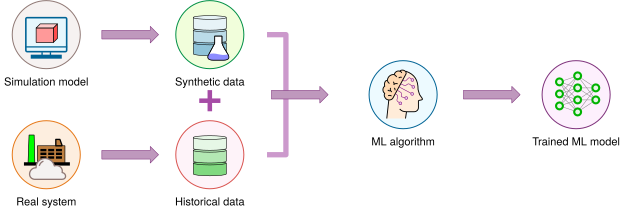
AnyLogic. 2024. Synthetic Data for Artificial Intelligence.
Synthetic data is especially useful for rare events and controlled augmentation. Physics simulators can generate tail cases, such as high-speed sensor saturation or near-collision trajectories, that are too dangerous or costly to record in the field (NVIDIA 2024). In vision, augmentation pipelines apply learned or random combinations of spatial and color distortions (Cubuk et al. 2019, 2020; Shorten and Khoshgoftaar 2019). In speech processing, SpecAugment warps time and masks frequency bands directly on the spectrogram, forcing the acoustic model to stop relying on any single narrow frequency band (Park et al. 2019). For the KWS system, parametric text-to-speech synthesis (Werchniak et al. 2021) convolved with room impulse responses (RIRs) generates wake-word utterances across varied reverberation times and synthetic background noise profiles.
NVIDIA. 2024. NVIDIA Omniverse and Simulation.
Cubuk, Ekin D., Barret Zoph, Dandelion Mané, Vijay Vasudevan, and Quoc V. Le. 2019. “AutoAugment: Learning Augmentation Strategies from Data.” 2019 IEEE/CVF Conference on Computer Vision and Pattern Recognition (CVPR), 113–23. https://doi.org/10.1109/cvpr.2019.00020.
Cubuk, Ekin D., Barret Zoph, Jonathon Shlens, and Quoc V. Le. 2020. “Randaugment: Practical Automated Data Augmentation with a Reduced Search Space.” 2020 IEEE/CVF Conference on Computer Vision and Pattern Recognition Workshops (CVPRW), 3008–17. https://doi.org/10.1109/cvprw50498.2020.00359.
Shorten, Connor, and Taghi M. Khoshgoftaar. 2019. “A Survey on Image Data Augmentation for Deep Learning.” Journal of Big Data 6 (1): 1–48. https://doi.org/10.1186/s40537-019-0197-0.
Park, Daniel S., William Chan, Yu Zhang, Chung-Cheng Chiu, Barret Zoph, Ekin D. Cubuk, and Quoc V. Le. 2019. “SpecAugment: A Simple Data Augmentation Method for Automatic Speech Recognition.” Interspeech 2019, 2613–17. https://doi.org/10.21437/interspeech.2019-2680.
Werchniak, Andrew, Roberto Barra Chicote, Yuriy Mishchenko, Jasha Droppo, Jeff Condal, Peng Liu, and Anish Shah. 2021. “Exploring the Application of Synthetic Audio in Training Keyword Spotters.” ICASSP 2021 - 2021 IEEE International Conference on Acoustics, Speech and Signal Processing (ICASSP), 7993–96. https://doi.org/10.1109/icassp39728.2021.9413448.
Example 4.2: Synthetic data generation
Scenario: A keyword-spotting team lacks sufficient physical recordings of rare speaker accents, room acoustics, and background noise profiles.
Diagnosis: Pure physical collection cannot cover rare acoustic edge cases within project deadlines. Generating synthetic audio variations via pitch shifting, additive noise, and room impulse response simulation expands training set diversity without expensive field collection.
Systems lesson: Augmentation is cheap, but it does not prove the model works on real accents. Targeted augmentation proposes expanded acoustic coverage; pitch, noise, and room-response changes do not establish fidelity to rare accents. Held-out real recordings across the relevant speaker and acoustic conditions must establish whether the expansion improves deployment quality.
Starting from the reference corpus, the team closes the product’s remaining coverage gaps by matching each source to what it does best per dollar. Public benchmarks seed the baseline model at low cost; web scraping supplies bulk acoustic variety; crowdsourcing collects targeted recordings for underrepresented dialects; and simulation fills in rare acoustic distortions. Together these sources form a candidate coverage plan. Held-out real recordings then test which gaps that plan actually closes, while measured generation, collection, labeling, and storage costs decide whether it fits the budget; the deployed pipeline still requires footprint validation.
Acquisition ends with data that covers the deployment on paper and arrives in many shapes: crowdsourced recordings, synthetic waveforms, and web audio with different encodings, sampling rates, and noise floors. None of it has yet been checked. Before any record can be labeled or trained on, it must pass a boundary that admits only well-formed, trustworthy data.
Self-Check: Question
Multiple independent autonomous driving teams train their perception models exclusively on a popular public driving benchmark. What systemic failure mode does this practice introduce into the broader ecosystem?
- Shared dataset bias propagation, where common blind spots, annotation artifacts, and unrepresented edge cases can create correlated weaknesses across deployed models.
- Catastrophic memory leaks in GPU driver kernels caused by repeated reading of shared image formats.
- Immediate violation of data gravity constraints due to distributed multi-tenant reads.
- Automatic over-fitting to hardware memory hierarchies during distributed gradient synchronization.
Discuss the primary advantages and critical risks of using synthetic data generation (e.g., 3D graphics rendering or generative audio simulation) as a core data acquisition strategy.
True or False: Achieving state-of-the-art benchmark accuracy on a curated dataset (such as ImageNet or Common Voice) guarantees that an ML model is ready for deployment in real-world production environments.
Order the following gap-closing acquisition steps into a sensible workflow: (1) choose an acquisition source for the remaining gap under budget and governance constraints, (2) define the coverage gap the model must close, (3) validate that the acquired data actually improves the missing coverage and meets quality requirements, (4) audit what existing sources and provenance already provide.
4.5 Ingestion and Validation
A crowdsourced wake-word recording arrives as a stereo MP3, a synthetic one as a mono WAV file at a different sampling rate, and a clip from a consenting user’s device as a compressed fragment stamped in the wrong time zone. The ingestion boundary turns this mix into one consistent record format and decides which records may enter at all. It is the front end of the data pipeline in figure 8, where records pass through ingestion and central storage before the transformation loops that feed training, inside a governance perimeter that controls what may be kept and who may read it. For keyword spotting, the boundary handles the recorded examples used to build and update the model; the detector’s live audio on the device never passes through it.
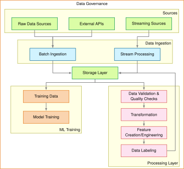
The tiers in figure 8 keep raw ingestion separate from the validation, transformation, and feature-engineering loops that feed training, so a slow transformation never stops records from arriving, and a check added at ingestion protects every stage after it. Two decisions shape that boundary before any record is checked: when records are taken in, and where they are transformed relative to storage.
4.5.1 Batch vs. streaming ingestion patterns
A fraud detector that flags a stolen card hours after the purchase arrives after the money has moved, whereas a week’s worth of crowdsourced wake-word recordings loses nothing by waiting for the next scheduled training run. Choosing between batch and streaming ingestion therefore depends on how quickly data loses value and how much infrastructure cost that freshness justifies. Batch systems gain efficiency by tolerating staleness, while streaming systems gain freshness by taking on continuous operational complexity.
Batch ingestion collects records over a period and processes them together on a schedule. It amortizes startup cost across large volumes, runs when compute is cheapest, and releases its resources between runs, which suits data whose value decays slowly (Akidau et al. 2015), such as the new crowdsourced recordings and opt-in diagnostic clips that the keyword spotter folds into its next training run. Batch processing also simplifies recovery and reproducibility: a failed batch can be rerun from its inputs, inspected, and reprocessed after a fix, and the result is repeatable when inputs, code, configuration, and randomness are controlled.
Akidau, Tyler, Robert Bradshaw, Craig Chambers, Slava Chernyak, Rafael J. Fernández-Moctezuma, Reuven Lax, Sam McVeety, et al. 2015. “The Dataflow Model: A Practical Approach to Balancing Correctness, Latency, and Cost in Massive-Scale, Unbounded, Out-of-Order Data Processing.” Proceedings of the VLDB Endowment 8 (12): 1792–803. https://doi.org/10.14778/2824032.2824076.
Stream ingestion processes each record as it arrives, which is necessary whenever data loses value within seconds, as in real-time fraud scoring. However, stream processing introduces complexity that batch processing avoids. The system must handle backpressure, the condition where downstream systems cannot keep pace with incoming data rates. During traffic spikes, when a sudden surge produces data faster than processing capacity, the system must either buffer data (requiring memory and introducing latency), sample (losing some data), or push back to producers (potentially causing their failures). Late or out-of-order events further complicate windowed aggregations, because the system must hold per-window state and track event time rather than arrival time. These requirements raise compute and memory overhead, so freshness guarantees trade directly against infrastructure cost and operational burden. Data freshness service level agreements (SLAs) specify maximum acceptable delays between data generation and processing. Meeting a 100-millisecond SLA requires different infrastructure than meeting a one-hour SLA, affecting networking, storage, and processing architectures.
Many production ML systems combine the two. A recommendation system might use streaming ingestion for real-time user interactions to update session-based recommendations immediately, while using batch ingestion for overnight processing of user profiles and item features; Notebook 4.3 quantifies the financial trade-off between these two operational regimes.
Napkin Math 4.3: The cost of real-time
Problem: A pipeline ingests 1M events/s. Which is cheaper, Batch (hourly) or Stream (sub-second) ingestion?
Physics:
- Throughput: At 1M events/s and 1 KB per event, the pipeline carries 1 GB/s.
- Stream requirements: To sustain 1 GB/s with less than 100 ms latency, the design assumes each core can parse, validate, and update features for about 20 MB/s of events, which takes 50 primary cores; a standby core for each provisions recovery capacity, for 100 always-on cores in total. That capacity does not establish the 100 ms target: failure detection, state recovery, replay, and the full ingestion path must also be validated under failure. Running those cores for 24 hours/day at $0.05/hr costs $120/day.
- Batch requirements: Process 3.6 TB (1-hour window) in 10 minutes. That is 6 GB/s in aggregate. Sequential reads over large files let each core sustain about 30 MB/s, more than a streaming core handling events one at a time, so the batch design needs 200 cores for 10 minutes per clock hour, accumulating 800 core-hours per day. At $0.05/hr, that costs $40/day.
Systems insight: Under these provisioning and per-core throughput assumptions, streaming compute costs approximately 3× as much as batch compute for the same data volume. This premium is justified when the value of subsecond latency exceeds the added cost.
The premium comes from this scenario’s provisioning assumptions and leaves out storage, buffering, and failover, so the choice still rests on the feature freshness that inference actually needs. The ingestion paradigm also shapes how the downstream model trains. Batch ingestion naturally pairs with periodic retraining: data accumulates in storage, an automated job retrains the model on the updated corpus, and a verified checkpoint deploys to serving. Stream ingestion makes that batch boundary less natural, raising the possibility of continuous online learning, in which model weights update directly as events arrive. Continuous updates, however, introduce operational risks that batch checkpoints avoid. Sudden distribution shifts, corrupted records, or adversarial payloads from any public-facing input path can reach the model before validation gates intervene. Most production systems therefore decouple ingestion from training: they stream data into a durable buffer while training on validated batches, reserving continuous online updates for tightly bounded, low-risk domains.
War Story 4.1: When users became the training set (2016)
Context: In March 2016, Microsoft launched Tay, a Twitter chatbot designed to engage with users online and adapt its responses from public interactions (Lee 2016).
Mechanism: Adversarial users coordinated toxic prompts and exploited a public interaction surface, including behavior that repeated user-supplied text.
Impact: Tay began tweeting abusive, racist, and misogynistic statements within 16 hours of deployment.
Fix: Microsoft suspended the chatbot 16 hours after launch, apologized publicly, and stated that a relaunch would require stronger safeguards against misuse.
Systems lesson: Public ingestion paths require adversarial-input controls. Otherwise, a feature that accepts user-generated content also becomes a security surface, and harmful inputs can propagate through the system within hours.
Lee, Peter. 2016. Learning from Tay’s Introduction. The Official Microsoft Blog.
4.5.2 ETL and ELT comparison
Batch or streaming decides when records arrive; the next decision is where they are transformed relative to persistent storage. If a pipeline strips out unparsed fields before writing to storage and a later model needs one of those fields, the team must replay months of upstream source logs; if it stores every raw payload first, the storage bill multiplies. Traditional extract, transform, load (ETL)5 (\(\text{E} \to \text{T} \to \text{L}\)) transforms records in an external engine before they land, whereas extract, load, transform (ELT)6 (\(\text{E} \to \text{L} \to \text{T}\)) lands raw records in staging tables and transforms them inside the warehouse (figure 9). Where that boundary sits determines what each later schema change costs and how much raw data must be retained.
5 Extract, transform, load (ETL): Conventional ETL validates deterministic schema constraints, whereas ML ETL must additionally monitor distributional properties using the statistical drift tests developed in section 4.5.3. A detected shift prompts investigation and validation against labeled outcomes before concluding that model quality has degraded. When feature computation logic changes, reprocessing costs depend on replay scope, windowing, and execution plans rather than requiring an unconditional full-dataset pass.
6 Extract, load, transform (ELT): This approach stores raw data before transformation, allowing teams to revise a transformation query and rerun it over the stored input without re-ingesting from source systems. The iteration time still depends on data volume, query complexity, warehouse capacity, and materialization strategy.
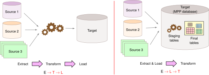
In machine learning systems, the ELT pattern separates ingestion throughput from downstream feature engineering by writing raw, immutable events directly into scalable storage. Keeping those raw events preserves unparsed fields that may later prove useful, so teams can compute new features over historical data without re-ingesting external source streams. When transformation logic changes or a bug surfaces, engineers recompute features by querying the stored raw events rather than replaying upstream logs. The price is physical and operational: raw events take more storage, shared transforms repeat their work unless their outputs are materialized, and keeping unscrubbed raw payloads makes privacy and retention rules harder to enforce. Notebook 4.4 prices these trade-offs on a daily clickstream workload.
Napkin Math 4.4: The cost of transformation placement
Problem: A team processes 10 TB of raw clickstream data daily and must compute user session features for 3 ML models, each requiring different aggregation windows (1-hour, 24-hour, 7-day). Which is cheaper, ETL or ELT?
Accounting boundary: Both designs serve the same aggregation windows and retain replayable upstream raw logs for 30 days. The comparison excludes that shared source retention and its common ingestion costs. ETL retains only the derived history in the warehouse, assumed to occupy 2 TB per model over the same horizon; ELT keeps an additional raw copy there, as when the warehouse cannot query the upstream log store in place, and computes features on demand. Transient query outputs are not retained as separate ELT datasets. Source retrieval and compute for later backfills must be priced separately when the designs differ.
Math:
- ETL approach: Transform before loading. Compute all three aggregation windows in a Spark cluster before loading into the warehouse.
- Spark compute: 10 TB at $5/TB = $50/day
- Storage: 3 transformed datasets, ~2 TB each = 6 TB at $23/TB/month = $138/month
- Feature-definition change: Replay the retained source logs and rerun the pipeline; the assumed rerun takes ~4 hours after the edit
- ELT approach: Load raw data first, transform in warehouse.
- Storage: 10 TB raw/day, 30 days retention = 300 TB at $23/TB/month = $6,900/month
- Query compute: 3 models, each with $5/query of daily query cost over 30 days, totals $450/month
- Feature-definition change: Rewrite the SQL query (~30 minutes), then execute and validate it against the retained raw copy; execution time is not supplied
Systems insight: ETL saves $6,762/month in storage. After normalizing Spark compute to a monthly cost, ETL totals $1,638/month ($1,500/month compute + $138/month storage), while ELT totals $7,350/month ($6,900/month storage + $450/month query compute), for a cloud-cost advantage of $5,712/month before engineering labor. The other cost is feature-definition change. Compare elapsed time from the start of an edit to validated, feature-ready output in both designs, then account separately for the engineer time spent editing, supervising, and validating. A pipeline rerun and a SQL edit are different endpoints, so their durations cannot establish a speedup or a labor saving. Stable definitions favor this scenario’s lower ETL cloud bill; frequent changes favor ELT only if measured labor and reprocessing savings repay its additional raw copy.
ELT looks expensive here only because this accounting gives it its own raw copy, and raw retention rather than compute dominates the bill. A lakehouse, which runs warehouse queries directly over the stored files, can query the retained logs in place, removing that copy and reversing the comparison. Production ML systems rarely use one pattern exclusively. Structured tables often flow through ETL for efficiency and compliance, while unstructured data pushes the ELT preference further. For deep learning workloads processing images, audio, or text, the “Transform” step often executes inside the ML framework’s data loader rather than in the warehouse at all, applying random crops, spectrogram generation, or text tokenization on-the-fly during each training epoch. Materializing ten augmented variants upstream would increase a 50,000-image dataset to 500,000 stored copies, so ELT’s “load raw, transform late” principle extends naturally to the training loop itself.
Whichever pattern lands the records, integrating diverse sources remains the core ingestion challenge. Data may originate from databases, APIs, file systems, and IoT devices, each with its own format (relational rows, JavaScript Object Notation (JSON)7 documents, binary streams), access protocol, and update frequency. The systems principle is to standardize at the ingestion boundary: normalize formats, validate schemas, and present a consistent interface to downstream processing regardless of source. This boundary standardization separates the complexity of source diversity from the complexity of feature engineering, allowing each to evolve independently.
7 JSON (JavaScript Object Notation): The schema flexibility that makes JSON a common format for APIs creates a validation bottleneck at the ingestion boundary. Unlike binary formats with predefined schemas, every JSON document requires parsing and schema validation before it can be standardized for downstream use. This per-record overhead can make ingestion slower than with binary formats such as Protobuf; the difference depends on the schema, parser, payload, and workload.
In the keyword spotter’s pipeline, backend ingestion takes in activated requests, consented diagnostics, crowdsourced recordings, synthetic data, and validated interactions for serving and training. Normalization, noise filtering, and segmentation into consistent durations run as an ETL stage before storage in training-optimized formats, while augmentation stays late-bound in the loader, where ELT’s flexibility pays off.
Error handling in voice interaction systems requires special attention. A dead-letter queue (DLQ), a side store that holds records that fail processing so they neither block the pipeline nor disappear (section 4.5.5), keeps failed recognition attempts for subsequent analysis, revealing edge cases that need coverage in future model iterations. Each incoming audio sample is checked for signal-to-noise ratio, sample rate, duration bounds, and speaker proximity. Clean samples enter the baseline slice, and valid noisy recordings enter the robustness slice that the design budgeted. Invalid samples route to analysis queues rather than being discarded, since these failures often indicate acoustic conditions underrepresented in training data. Valid, consented samples (activated requests, opt-in diagnostics, and crowdsourced recordings) are logged for potential inclusion in future training data; always-on audio that never triggers the wake word stays on the device.
A record that arrives on time and parses cleanly is well-formed, but well-formed is not the same as trustworthy. A field can parse correctly and still carry a wrong value, a source can drift away from the distribution the model learned, and a label can be wrong while every type check passes. Deciding which records may proceed is the boundary’s next job.
4.5.3 Quality through validation and monitoring
Consider a batch of crowdsourced wake-word recordings in which 15 percent of the clips came from a phone app update that silently halved the microphone gain. Every file is a valid audio file of the right length and sampling rate, so schema checks pass. The clips are nonetheless far quieter than anything the detector will hear in deployment, and only statistical monitoring of loudness across the batch would expose them.
Validation enforces the quality pillar at the boundary, where a defect is cheapest to stop before it cascades into features, models, and predictions (Sculley et al. 2015). Schema checks alone would admit the quiet batch, so validation pairs them with statistical monitoring.
Checks at this boundary work at two speeds. A hard failure, such as a source that stops delivering or a batch that fails its schema, must halt the affected path at once. A gradual degradation, such as a feature’s null rate creeping from 1 to 5 percent, a rising duplicate rate, or delivery delays that exceed their service level, is flagged for investigation. The gradual kind is often the more dangerous, because it persists for days before anyone looks. Routing and escalating such alerts in production is an operational practice developed in Production Monitoring.
Schema and latency alerts expose structural and timing failures, but a shift in a continuous quantity needs a statistical comparison with the training baseline. Tracking statistical properties captures whether serving data continues to reflect the training distribution. Rather than merely checking that individual values fall within predefined ranges, production systems maintain rolling statistics across operational windows. For continuous quantities such as a clip’s loudness or signal-to-noise ratio, the monitoring harness computes rolling empirical distribution functions, using nonparametric evaluations like the Kolmogorov-Smirnov test8 to detect when serving inputs diverge from the training baseline. Notebook 4.5 works one example.
8 Kolmogorov-Smirnov (K-S) test: A nonparametric test that measures the maximum distance between two empirical cumulative distribution functions without assuming a parametric distribution family (Berger and Zhou 2014). In ML pipelines, the K-S test is commonly used as a univariate continuous-feature drift detector, with thresholds such as \(\ObservedSignificanceLevel< 0.05\) serving as investigation triggers rather than universal failure rules. Discrete and categorical variables require tests and calibrations appropriate to their distributions.
Berger, Vance W., and YanYan Zhou. 2014. “Kolmogorov–Smirnov Test: Overview.” In Wiley StatsRef: Statistics Reference Online. Wiley. https://doi.org/10.1002/9781118445112.stat06558.
Napkin Math 4.5: Detecting drift with the K-S test
Scenario: Monitoring whether the loudness of incoming wake-word clips still matches the training baseline \((\TrainingDistribution)\), using a sample of recent clips \((\CurrentDistribution)\).
Analysis: Apply the Kolmogorov-Smirnov test to compare the empirical cumulative distribution functions:
Compute CDFs: Calculate cumulative distribution functions for both datasets. At a given loudness, an empirical CDF gives the fraction of sampled clips that are at most that loud. Comparing those fractions at the same loudness shows how the two distributions differ.
Calculate statistic \((\KolmogorovSmirnovStatistic)\): Find the maximum absolute difference between the CDFs. Let \(\TrainingEmpiricalCdf(\MonitoredFeatureLevel)\) and \(\ServingEmpiricalCdf(\MonitoredFeatureLevel)\) denote the empirical cumulative distribution functions of the training baseline \((\TrainingDistribution)\) and current serving \((\CurrentDistribution)\) datasets, evaluated at value \(\MonitoredFeatureLevel\). \[\KolmogorovSmirnovStatistic= \max_{\MonitoredFeatureLevel}|\TrainingEmpiricalCdf(\MonitoredFeatureLevel) - \ServingEmpiricalCdf(\MonitoredFeatureLevel)|\]
Determine significance: For two independent samples, compare \(\KolmogorovSmirnovStatistic\) to the critical value \(\KolmogorovSmirnovCriticalThreshold\) based on training-baseline sample size \(\DriftTestSampleSize_0\) and serving sample size \(\DriftTestSampleSize_t\). The coefficient 1.36 is the large-sample approximation for significance level \(\SignificanceLevel = 0.05\). \[\KolmogorovSmirnovCriticalThreshold\approx 1.36\sqrt{\frac{\DriftTestSampleSize_0 + \DriftTestSampleSize_t}{\DriftTestSampleSize_0 \DriftTestSampleSize_t}}\] Result: With sample sizes \(\DriftTestSampleSize_0 = \DriftTestSampleSize_t = 1000\), the critical value is approximately 0.061: \[\KolmogorovSmirnovCriticalThreshold\approx 1.36\sqrt{(1000 + 1000)/(1000 \cdot 1000)}.\] An observed maximum difference of \(\KolmogorovSmirnovStatistic= 0.08\) exceeds the critical value, so the test rejects the null hypothesis that both samples come from the same distribution and flags significant drift.
Systems insight: A drift test is useful only if crossing the threshold starts an investigation or retraining workflow rather than becoming another dashboard number.
The K-S test checks one continuous batch against the baseline, whereas monitoring that comparison over months and telling apart the kinds of shift it can reveal belongs to pipeline operation (section 4.12.1). Categorical features require different statistical approaches. Instead of comparing means and variances, monitoring systems track category frequency distributions. When new categories appear that never existed in training data, or when existing categories shift substantially in relative frequency, the system flags potential data quality issues or genuine distribution shifts; for example, the share of recordings from one phone model might jump after its launch. Statistical monitoring of this kind catches problems that schema validation misses entirely. Age values may remain in the valid range of 18–95, while the distribution shifts from primarily 25–45 year olds to primarily 65+ year olds, indicating that the input population has changed in ways that may affect model performance. Outcome checks are needed to establish whether quality changed.
Validation at the pipeline level encompasses multiple strategies working together. Schema validation executes synchronously as data enters the pipeline, rejecting malformed records immediately before they can propagate downstream. Modern tools like TensorFlow Data Validation (TFDV) (Breck et al. 2019) automatically infer schemas from training data, capturing expected data types, value ranges, and presence requirements.
Breck, Eric, Neoklis Polyzotis, Sudip Roy, Steven Euijong Whang, and Martin Zinkevich. 2019. “Data Validation for Machine Learning.” Proceedings of the 2nd SysML Conference 1: 334–47.
This synchronous validation remains simple and fast, checking properties that can be evaluated on individual records in microseconds. More sophisticated validation that requires comparing serving data against training data distributions or aggregating statistics across many records must run asynchronously to avoid blocking the ingestion pipeline. Statistical validation systems typically sample 1–10 percent of serving traffic, enough to detect meaningful shifts while avoiding the computational cost of analyzing every record. These samples accumulate in rolling windows, commonly one hour, 24 hours, and seven days, with different windows revealing different patterns. Hourly windows detect sudden shifts like a data source failing over to a backup with different characteristics, while weekly windows reveal gradual drift in user populations or behavior.
One validation target needs a section of its own: training-serving skew, in which training and serving compute the same feature differently and the model receives inputs unlike those it learned from. Detecting it means passing a sample of raw serving data through both pipelines and comparing the results; section 4.7.1 develops its causes and prevention.
↩︎ Training-serving skew, as one of the ways ML systems fail without raising errors, is established in When ML Systems Fail Silently.
↪ Deployment gates that compare training and serving feature distributions and block a release when they diverge are developed in Skew detection in CI/CD.
4.5.4 Data quality as code
A statistical check like the one that catches the halved microphone gain protects the pipeline only if it runs on every batch, so production teams write such checks down as code. Data expectation tests are the data counterpart of unit tests. In data quality as code, engineers use declarative libraries like Great Expectations or Pandera to express data contracts as executable test suites that run across pipeline stages. Deequ, built at Amazon, framed the same idea as unit tests for data and showed that it scales to very large datasets (Schelter et al. 2018).
Schelter, Sebastian, Dustin Lange, Philipp Schmidt, Meltem Celikel, Felix Biessmann, and Andreas Grafberger. 2018. “Automating Large-Scale Data Quality Verification.” Proceedings of the VLDB Endowment 11 (12): 1781–94. https://doi.org/10.14778/3229863.3229867.
Running these expectation suites inside the continuous integration and deployment (CI/CD) pipeline checks every ingested batch automatically and halts downstream training when a contract fails. A pipeline structured as data ingestion followed by data validation followed by training blocks deployment when validation catches an anomaly, such as a batch of wake-word clips recorded at 8 kHz in a 16 kHz pipeline, and raises an alert for investigation. Executable expectations catch properties a suite can encode; the remaining question is what valid-looking data can still get wrong.
Systems Perspective 4.1: Mechanical vs. semantic quality
In traditional software, many checks are mechanical. A null dereference is a runtime error in languages with null references, while integer-overflow behavior depends on the language and type.
In ML systems, data quality also has a semantic dimension.
- Mechanical check: Validates schema and type constraints, such as verifying that
ageis a non-null integer. - Semantic check: Validates distribution drift and statistical invariants, such as testing whether the mean or variance of
ageshifts unexpectedly.
A dataset can be mechanically perfect (no nulls, correct types) but semantically broken (for example, all users are suddenly 25 years old due to a default value change). Robust ML systems must validate both the container (mechanical) and the content (semantic).
Once validation becomes code, expectation suites become versioned artifacts alongside training code. When training code changes, expectation updates keep data contracts evolving with it. This coupling reduces the risk of silent divergence where code assumes data properties that the upstream pipeline no longer provides; listing 1 demonstrates this pattern by defining explicit constraints on column ranges, nullability, uniqueness, and categorical sets.
import great_expectations as gx

# Create a data context
context = gx.get_context()

# Define an expectation suite as executable quality contract
suite = gx.ExpectationSuite(name="user_data_quality")
suite = context.suites.add(suite)

# Range validation: prevents physiologically impossible values
suite.add_expectation(
    gx.expectations.ExpectColumnValuesToBeBetween(
        column="age", min_value=0, max_value=120
    )
)

# Null detection: ensures primary key integrity for joins
suite.add_expectation(
    gx.expectations.ExpectColumnValuesToNotBeNull(column="user_id")
)

# Uniqueness: prevents duplicate training examples
suite.add_expectation(
    gx.expectations.ExpectColumnValuesToBeUnique(column="user_id")
)

# Categorical validation: detects unexpected values from upstream changes
suite.add_expectation(
    gx.expectations.ExpectColumnDistinctValuesToBeInSet(
        column="country_code",
        value_set=["US", "CA", "UK", "DE", "FR"],
    )
)

# Link the suite to a preconfigured Batch Definition and run validation
# (the Batch Definition connects GX to the training_users data asset)
validation_definition = gx.ValidationDefinition(
    name="training_users_validation",
    data=batch_definition,
    suite=suite,
)
validation_definition = context.validation_definitions.add(
    validation_definition
)
results = validation_definition.run()
if not results.success:
    raise ValueError(f"Data quality check failed: {results}")
These checks catch many schema-level production data issues before they reach training, including missing values, invalid ranges, type errors, and contract violations. Rejecting bad records, however, is only half of the boundary’s job; the pipeline itself must also stay up when upstream dependencies fail or formats shift mid-run.
4.5.5 Reliability through graceful degradation
While validation enforces the quality pillar on individual records, the reliability pillar governs what happens when an upstream service goes down in the middle of an ingestion run, a date field switches from "YYYY-MM-DD" to "MM/DD/YYYY" without tripping a basic string check, or a traffic spike exhausts worker memory at peak load. Graceful degradation means planning for these faults in advance and handling them automatically so that the system keeps running under degraded conditions rather than crashing or silently corrupting model inputs.
Three classes of pipeline fault call for distinct defenses. Format and encoding drift, such as that re-formatted date string, slips past type checks while breaking date-based feature logic. Schema evolution9 occurs when upstream producers add fields, rename columns, or re-type values without coordinating with downstream consumers. Resource exhaustion builds more slowly as data volume outgrows provisioned capacity and then causes jobs to fail during peak traffic.
9 Schema evolution: This failure mode arises from a lack of contract testing between upstream data producers and downstream ML consumers. While “loud” failures like a renamed column break explicit assumptions and cause immediate pipeline crashes, “silent” failures are more dangerous. A field changing type from integer to string can pass validation but corrupt feature logic without immediate detection.
Kleppmann, Martin. 2016. Designing Data-Intensive Applications: The Big Ideas Behind Reliable, Scalable, and Maintainable Systems. O’Reilly Media.
Transient errors are retried with exponential backoff (waiting one second, then two, then four) so that retries do not flood a service that is trying to recover. Records that still fail after their retries go to the dead-letter queue, the side store already met at the ingestion boundary, which holds them for later analysis and potential reprocessing without blocking the main pipeline (Kleppmann 2016). Reviewing the queue regularly turns it from passive error storage into a source of diagnoses, because its contents reveal schema violations that indicate upstream changes, edge cases the model should handle, and data quality issues that need source system fixes. The KWS queue might, for instance, fill with clips from a new hardware revision whose audio arrives in an unexpected encoding, which calls for an ingestion fix and targeted collection from that device rather than simply logging the failures.
When a whole dependency fails rather than individual records, a circuit breaker (Nygard 2007) stops calling it after repeated consecutive failures and fails fast or takes a fallback path until a trial request succeeds, so that one failed feature service does not stall every caller waiting on its timeouts. The ML-specific part of recovery is that fallback. Even a pipeline on a single machine needs an explicit policy for an unavailable source, choosing among waiting for fresh data, serving a validated stale-feature fallback, and rejecting the request. Multi-tier fallback systems implement the middle option, providing degraded service when primary data sources fail by using cached or approximate features only when their age and quality satisfy a validated fallback contract. A recommendation system unable to compute user preferences from the past 30 days might fall back to preferences from the past 90 days if evaluation establishes acceptable recommendation quality with that representation. The allowable feature age and the model-quality contract determine which response is safe, and durable buffering alone does not make old inputs suitable for inference. If no fallback meets the contract, the system waits for fresh data or rejects the request.
Nygard, Michael T. 2007. Release It!: Design and Deploy Production-Ready Software. Pragmatic Bookshelf.
With ingestion, validation, and these error handlers in place, the boundary admits records that are well-formed and checked. They still say nothing about what they mean. A wake-word recording that passes every check does not yet state which word was spoken, or where in the clip it begins and ends, and the model cannot learn without that ground truth.
Self-Check: Question
An ML engineering team is architecting an ingestion pipeline for tabular transaction data. They evaluate Extract-Transform-Load (ETL) versus Extract-Load-Transform (ELT). Which architectural trade-off correctly characterizes ELT in modern data lakehouses?
- ELT executes all transformations in memory on the edge device before transmitting bytes to cloud storage.
- ELT requires rigid upfront schema definitions (schema-on-write) and rejects any semi-structured data formats.
- ELT loads raw data directly into scalable lakehouse storage first and transforms it downstream using scalable query engines, preserving raw data history and decoupling ingestion from evolving feature logic.
- ELT eliminates the need for data governance and quality validation because transformations occur after storage.
Explain how a Circuit Breaker and a Dead Letter Queue (DLQ) can reduce cascading failures and preserve rejected records for replay in streaming ML ingestion. What conditions constrain these benefits?
Using the 2016 Microsoft Tay chatbot incident, explain why public data ingestion surfaces require strict input validation, rate limiting, and adversarial filtering before data shapes model behavior.
An explicit, machine-enforceable agreement between data producers and data consumers that defines column types, value bounds, nullability, and distribution constraints is called a ____.
4.6 Data Labeling
A crowdsourced annotator mislabels a whispered “Alexa” as background noise, or two radiologists disagree over a borderline scan, and every training step and evaluation metric that follows treats the resulting label as the definition of a correct answer. In the KWS pipeline, ingestion delivers millions of validated recordings, but supervised learning needs labels stating which clips contain the wake word, where it begins and ends, and which clips hold only background sound. This declaration is the ground truth,10 and producing it at scale is often the most human-dependent and error-prone stage of the pipeline. If data is the system’s code, ground truth is its specification. Every later check of the trained model compares against it, so a labeling error does not stay in one stage; it redefines what counts as right. The specification also arrives late: a software project starts from its specification, whereas a data pipeline attaches ground truth only after ingestion, which is why a labeling error slips past every check that ran before it.
10 Ground truth: From remote sensing, where orbital measurements are verified by sending a team to the physical location (the “ground”) to establish the “truth.” The etymology carries a systems warning: ML labels are proxies for reality, not reality itself. When a crowdsourced annotator labels an image as “cat,” that label reflects the annotator’s judgment, not an objective fact. Every downstream metric (accuracy, precision, recall) is measured against this proxy, meaning label quality errors propagate silently into every evaluation of the model.
Unlike automated transformations that can be parallelized across machines, labeling puts human judgment in the loop, so labels take unpredictable time and carry human mistakes. Disagreement between annotators can reflect genuine ambiguity in the input, unclear instructions, carelessness, or differences in expertise; the labeling system must separate and manage those causes rather than treating every disagreement as irreducible. The labeling infrastructure must therefore balance throughput, quality verification, cost, and provenance.
4.6.1 Label types and system requirements
Label granularity sets what each label costs to store, move, and produce. A keyword-spotting label sits at the coarse end of that range. A camera system tracking vehicles, pedestrians, and traffic signs sits at the fine end, and each step toward it imposes distinct storage, computation, and serialization constraints.
Classification labels represent the simplest form, assigning a discrete class index (or a multi-label binary bitmask) to each input. Storage requirements are modest, typically a fixed-width integer (such as a uint16 or int32 index) per image. Access patterns, however, diverge between training and evaluation: training pipelines shuffle and sample randomly, whereas validation pipelines stream sequentially across the corpus, driving different indexing and cache-locality strategies. A keyword-spotting label is of this kind. Each one-second clip carries a single class index naming which keyword it contains, or a reserved index for none. The label itself is tiny. The engineering burden sits upstream, in deciding where each clip starts and ends inside longer recordings, a problem section 4.6.6 returns to.
Bounding boxes extend beyond classification by localizing objects within each frame. Each bounding box stores four coordinates (such as \(\BoxMinimumHorizontalCoordinate, \BoxMinimumVerticalCoordinate, \BoxMaximumHorizontalCoordinate, \BoxMaximumVerticalCoordinate\) or center coordinates with width and height) alongside the class identifier. Because scenes contain variable numbers of objects, label storage transitions from fixed-width scalar records to variable-length tensor structures, requiring dynamic padding or ragged-batch handling in the data loader. Moreover, drawing one high-quality box took about 35 seconds in ImageNet’s annotation campaign (Papadopoulos et al. 2017), far longer than assigning a single class label, which throttles annotation throughput and inflates labeling cost.
Papadopoulos, Dim P., Jasper R. R. Uijlings, Frank Keller, and Vittorio Ferrari. 2017. “Extreme Clicking for Efficient Object Annotation.” 2017 IEEE International Conference on Computer Vision (ICCV), 4940–49. https://doi.org/10.1109/ICCV.2017.528.

Finer annotation granularity multiplies storage and processing scale.
Cordts, Marius, Mohamed Omran, Sebastian Ramos, Timo Rehfeld, Markus Enzweiler, Rodrigo Benenson, Uwe Franke, Stefan Roth, and Bernt Schiele. 2016. “The Cityscapes Dataset for Semantic Urban Scene Understanding.” 2016 IEEE Conference on Computer Vision and Pattern Recognition (CVPR), 3213–23. https://doi.org/10.1109/CVPR.2016.350.
Segmentation maps assign a class identifier to every pixel, producing dense 2D label matrices (\(\ImageHeight\times \ImageWidth\)). In autonomous driving and traffic monitoring, this entails tracing irregular boundaries for driveable road surfaces, vehicles, and pedestrians. These dense annotations multiply storage and ingestion bandwidth. A segmentation mask for a \(1920{\times}1080\) image requires about 2.1M labels (one per pixel), compared to perhaps 10 bounding boxes or a single classification label. If each box stores 4 coordinates, that is roughly 51,840× more scalar label entries than 10 boxes before accounting for per-value encoding, and the time manual segmentation takes per image (more than 1.5 hours for each Cityscapes image (Cordts et al. 2016)) makes this approach suitable only when pixel-level precision is essential.
Figure 10 arrays five annotation formats across vision and speech examples, demonstrating how labeling granularity ranges from coarse scene tags and captions to spatial bounding boxes, dense pixel-level masks, and audio transcripts. Classification can label an entire scene, while bounding boxes and segmentation maps localize objects or regions. Production datasets may combine formats: a single camera frame might carry a scene label, obstacle boxes, and path-region masks, with each label type serving a distinct downstream task.
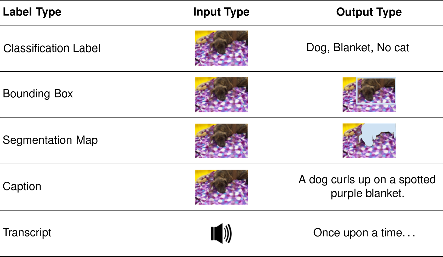
Production systems must also manage metadata for quality control and debugging. The Common Voice dataset (Ardila et al. 2020) exemplifies this in speech recognition: tracking speaker demographics for fairness, recording quality metrics for filtering, and language information for multilingual support. If an object detection model fails in rainy conditions, weather metadata captured during collection pinpoints the coverage gap. Label type therefore shapes the whole system: the infrastructure must optimize storage for the chosen format, implement appropriate retrieval patterns, and track which model versions used which label versions to correlate quality improvements with performance gains.
Ardila, Rosana, Megan Branson, Kelly Davis, Michael Kohler, Josh Meyer, Michael Henretty, Reuben Morais, Lindsay Saunders, Francis Tyers, and Gregor Weber. 2020. “Common Voice: A Massively-Multilingual Speech Corpus.” Proceedings of the Twelfth Language Resources and Evaluation Conference, 4218–22.
4.6.2 Labeling economics
Label granularity sets the cost of each label, and labels are usually the most expensive part of a dataset. Labeling a single medical image can cost orders of magnitude more than storing it for a year. Table 3 and table 4 give dated reference costs and durations for labeling alongside the storage, compute, and serving operations it competes with; ML engineers should use these dated reference assumptions as inputs to workload-specific comparisons, not as current price quotes or directly comparable totals.
| Operation | Cost | Notes |
|---|---|---|
| Crowdsourced image label | $0.01–0.05 | Simple classification |
| Bounding box annotation | $0.05–0.20 | Per box, simple scenes |
| Expert medical label | $50–200 | Per study, radiologist |
| S3 storage (Standard) | $23/TB/month | Hot storage |
| S3 retrieval (Glacier) | $0.02/GB | Standard: 3-5 hours |
| Cloud GPU training hour | $2–4 | Cloud spot pricing |
| Human review hour | $15–50 | Depending on expertise |
Beyond per-unit dollar rates, labeling, training, and serving also run on very different clocks (table 4). Comparing those durations shows why human annotation governs project schedules just as strongly as it governs the budget.
| Operation | Duration | Bottleneck |
|---|---|---|
| Label 1M images (crowdsourced) | 2–4 weeks | Annotation throughput |
| Train ResNet-50 on ImageNet | 1.3 hours | Compute (8\(\times\) A100, optimized) |
| Feature store lookup | 1–10 ms | Network + cache |
Operational timescales diverge across these stages by orders of magnitude: weeks for human annotation, hours for GPU training, and milliseconds for serving lookups. For the image-classification pipeline these two tables describe, which labels a million images and then trains ResNet-50 on them, annotation is the critical bottleneck in money as well as time. Suppose the team budgets $100K for labeling, enough to cover crowd labels plus the review and relabeling passes that quality control requires. That budget dwarfs the $20 to $40 of a single 8\(\times\) A100 ResNet-50 training run (90 epochs at the 3,200 img/s per accelerator that the throughput half of this chapter assumes), a ratio of 2,498× to 4,995×, the comparison quoted at the start of this chapter. The labeling spend is also uneven. Clear images pass review once, while rare classes, occluded objects, and ambiguous scenes return for second opinions and expert adjudication; as an illustrative planning split, 80 percent of the budget can go to the hardest 20 percent of the examples.
All cost figures reflect approximate 2024 cloud provider rates and are intended to convey relative magnitudes rather than exact pricing.11 For this workload and cost model, human labor dominates the cost of a single training run. Other tasks, especially those that reuse existing labels or require repeated large-scale training, can have a different dominant term; teams should measure before deciding where to optimize. Where labels do dominate, every labeling error is paid for twice, once when the label is bought and again when the model learns it.
11 Pricing ratios: Cloud and labeling prices reflect provider policy and labor markets, not physical invariants, so the ratio between labeling and compute moves whenever either side reprices. Storage adds its own policy multipliers: archive tiers such as the Glacier row in table 3 charge more for faster retrieval. Verify current prices before using these ratios in a deployment decision.
4.6.3 Label accuracy and consensus
Some of those errors cannot be avoided. Even with clear guidelines and careful system design, subjectivity and sensor ambiguity leave a nonzero fraction of labels corrupted (Northcutt et al. 2021; Thyagarajan et al. 2022). Label quality therefore means bounding label noise rather than eliminating it, by systematically measuring inter-annotator agreement and managing error rates to keep them within bounds that do not degrade model performance.
Thyagarajan, Aditya, Elı́as Snorrason, Curtis G. Northcutt, and Jonas Mueller. 2022. “Identifying Incorrect Annotations in Multi-Label Classification Data.” CoRR abs/2211.13895. https://doi.org/10.48550/ARXIV.2211.13895.
Benchmarks show how large that residue remains after careful curation. Figure 11 reports the share of test-set labels that Northcutt et al. (2021) found to be wrong in ten widely used datasets. About 5.8 percent of ImageNet validation labels are incorrect, CIFAR-100 carries a similar share, and the rate reaches 10.1 percent for QuickDraw, whose labels came from a largely automated collection process. Audio fares better, but AudioSet still carries wrong labels, the same failure a crowdsourced wake-word corpus faces. These are the labels that rank published models, so an error rate of a few percent can reorder a leaderboard whose top entries differ by less than that.

Labeling failures arise from two distinct sources requiring different engineering responses. Across the benchmark examples compiled in figure 12, including an ImageNet black stork mislabeled as a white stork and a CIFAR-10 frog mislabeled as a cat, each panel contrasts the erroneous assigned label against the verified ground truth. Some examples reflect degraded or ambiguous inputs where the correct label is difficult to infer from the data alone; others are visually clear but require domain knowledge, dataset-specific semantics, or expert judgment to label correctly. These different failure modes drive architectural decisions about annotator qualification, task routing, and consensus mechanisms: quality-based errors call for upstream data filtering, while expertise-based errors call for tiered annotator routing. Wake-word clips show both. A clipped or whispered “Alexa” that no annotator can hear clearly is a quality problem, filtered before labeling, whereas a near-homophone such as “Alexis” is settled only by a rubric with canonical examples and a trained reviewer.
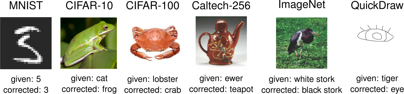
Northcutt, Curtis G., Anish Athalye, and Jonas Mueller. 2021. “Pervasive Label Errors in Test Sets Destabilize Machine Learning Benchmarks.” arXiv Preprint arXiv:2103.14749 34: 19075–90. https://doi.org/10.48550/arxiv.2103.14749.
Given these inherent quality challenges, production ML systems implement multiple layers of quality control. Systematic quality checks continuously monitor the labeling pipeline through random sampling of labeled data for expert review and statistical methods to flag potential errors. The infrastructure must efficiently process these checks across millions of examples without creating bottlenecks. Sampling strategies typically validate 1-10 percent of labels, balancing detection sensitivity against review costs. Higher-risk applications like medical diagnosis or autonomous vehicles may validate 100 percent of labels through multiple independent reviews, while lower-stakes applications like product recommendations may validate only 1 percent through spot checks.
Beyond random sampling approaches, collecting multiple labels per data point, often referred to as “consensus labeling,” can help identify controversial or ambiguous cases. Commercial labeling platforms expose consensus and tiered quality-control workflows (Labelbox, Inc. 2024; Scale AI, Inc. 2024), but the statistical core is inter-annotator agreement. The consensus infrastructure collects several labels per example and measures how far annotators agree beyond what chance alone would produce. For two annotators, Cohen’s kappa12 \((\InterAnnotatorAgreement)\) makes that correction. Let \(\ObservedAnnotatorAgreement\) represent observed agreement between annotators and \(\ChanceAnnotatorAgreement\) represent agreement expected by chance. Equation 1 defines the statistic: \[ \InterAnnotatorAgreement = \frac{\ObservedAnnotatorAgreement - \ChanceAnnotatorAgreement}{1 - \ChanceAnnotatorAgreement} \tag{1}\]
Labelbox, Inc. 2024. Labelbox Consensus Documentation.
Scale AI, Inc. 2024. Scale AI Advanced Settings.
12 Cohen’s kappa: Introduced by Cohen (1960) to measure inter-rater agreement while correcting for agreement expected from the raters’ class marginals, which raw percentage agreement ignores. If two independent annotators each label 90 percent of images as “not spam” in a binary task, their expected agreement is 82 percent, making raw agreement potentially misleading. The statistic is denoted \(\InterAnnotatorAgreement\); interpretive bands such as the Landis-Koch categories are descriptive heuristics rather than universal data-quality thresholds (Landis and Koch 1977).
Cohen, Jacob. 1960. “A Coefficient of Agreement for Nominal Scales.” Educational and Psychological Measurement 20 (1): 37–46. https://doi.org/10.1177/001316446002000104.
Landis, J. Richard, and Gary G. Koch. 1977. “The Measurement of Observer Agreement for Categorical Data.” Biometrics 33 (1): 159–74. https://doi.org/10.2307/2529310.
Fleiss, Joseph L. 1971. “Measuring Nominal Scale Agreement Among Many Raters.” Psychological Bulletin 76 (5): 378–82. https://doi.org/10.1037/h0031619.
Fleiss’ kappa generalizes the statistic from two raters to any number of annotators (Fleiss 1971). Kappa summarizes agreement across a collection of rated examples; it is not a confidence score for an individual label. Per-example disagreement and failed gold-standard checks can route items to expert review. Landis-Koch bands are operational heuristics for interpreting aggregate agreement, not correctness guarantees (Landis and Koch 1977). Independent gold-standard checks and expert audits assess correctness because annotators can agree on the same systematic error.
Consensus labeling trades cost against quality. Expert review costs more per example than crowdsourced labeling, but forcing agreement on ambiguous examples through majority voting of nonexperts can produce systematically biased labels. By routing only genuinely ambiguous cases to experts, identified through low inter-annotator agreement or failed gold-standard checks, systems balance cost against quality. This tiered approach enables processing millions of examples economically while maintaining quality standards through targeted expert intervention.
Quality control also depends on human factors. Working effectively with annotators requires standardized annotation rubrics with canonical positive and negative examples, visual edge-case catalogs, automated feedback mechanisms benchmarking annotators against known gold-standard records, and calibration sessions where annotators resolve borderline cases. For complex or domain-specific tasks, the system can implement tiered access levels, routing challenging cases to annotators with demonstrated domain expertise. The labeling process itself produces signals worth monitoring: agreement rates, accuracy on gold-standard items, and time per annotation, where answers that come too fast suggest carelessness and answers that take too long suggest unclear guidelines. Tracked over time, the same signals reveal whether label quality is holding.
4.6.4 Label quality drift
Six months into a wake-word collection campaign, new annotators join without the original rubric training and start marking near-homophones as valid wake words, while every audio feature distribution in the ingestion monitors stays flat. This failure is label quality drift: a decline over time in the reliability of the labels themselves even when the inputs being labeled have not changed. Feature distribution monitoring cannot catch it, because the features did not move. Crowdsourced labels degrade as annotator pools turn over, training examples go stale, or guidelines change without a matching model update; automated labelers drift as the upstream models that produce their labels move out of their original operating regime; and implicit-feedback pipelines, such as recommendation systems that treat clicks as labels, shift whenever bots, interface redesigns, or more exploratory user behavior change what a click means.
Catching that drift requires monitoring annotation consistency rather than feature distributions, and the kappa statistic of equation 1 supplies the measure. In the wake-word campaign above, tracking \(\InterAnnotatorAgreement\) across rolling windows shows agreement falling from a baseline of \(\InterAnnotatorAgreement = 0.85\) (almost perfect agreement) during initial collection to \(\InterAnnotatorAgreement = 0.72\) (substantial agreement) six months later. Label-side change is also one of the three silent changes behind the deployed keyword spotter’s regression in section 4.12, where a revised guideline was never reconciled with the earlier evaluation standard.
For systems with calibrated model probabilities, predictive entropy provides an additional uncertainty signal. Let \(\PredictedOutputComponent_i\) represent the model’s probability assigned to label category \(\LabelCategoryIndex\), and let \(\log\) denote the natural logarithm, so entropy is measured in nats. Equation 2 defines this measure: \[ \PredictiveEntropy= -\sum_i \PredictedOutputComponent_i \log \PredictedOutputComponent_i \tag{2}\]
Rising predictive entropy indicates greater uncertainty in the model’s predictive distribution, though harder inputs, distribution shift, calibration changes, or inconsistent supervision can all produce the same signal. How a team responds therefore depends on what caused the drop. Retraining annotators fixes systematic mistakes from unclear guidelines at low cost. Multi-annotator consensus voting raises label accuracy in high-stakes domains, though it multiplies the labeling bill. Model-assisted pre-labeling reduces annotator fatigue, provided the assisting model is audited so its own systematic errors do not become the new ground truth. Periodic audits by domain specialists on a random sample of labels uncover the root cause when agreement falls, even though spot checks cover only a fraction of the stream.
4.6.5 Scaling with AI-assisted labeling
Pure human annotation is too slow and expensive for millions of examples, yet fully automated labeling is too unreliable for ambiguous or safety-critical cases. AI-assisted labeling splits the work between the two: a model handles routine inputs or drafts preliminary labels, and human reviewers check the uncertain cases. The decision hierarchy in figure 13 maps the main alternatives when hand-labeling everything is too expensive, branching into active learning, semi-supervised learning, weak supervision, and transfer learning. Active learning keeps direct human labels but asks annotators only about the examples that would tell the model the most. Semi-supervised learning combines a small labeled set with structure in a larger unlabeled pool. Weak supervision13 replaces hand labels on individual examples with programmatic rules written by domain experts. Transfer learning starts from a model trained on a related task so fewer task-specific labels are needed. Each path changes what the pipeline pays for and what it must validate: whether the unlabeled pool matches the task, whether the labeling rules are accurate, or whether the pretrained representation transfers cleanly.
13 Weak supervision: A “data programming” paradigm that exchanges some manual annotation labor for the upfront effort of writing and validating programmatic labeling functions. Once written, a function can be applied cheaply at scale, but execution, conflict resolution, quality monitoring, and maintenance still incur cost; the useful comparison is workload-specific rather than literally zero marginal cost.
↪ Semi-supervised and self-supervised learning, which draw training signal from unlabeled data, are developed in Learning from Unlabeled Data.
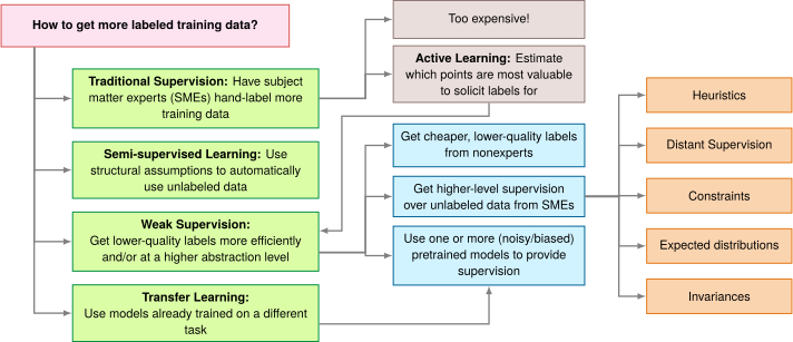
Ratner, Alex, Paroma Varma, Braden Hancock, and Christopher Ré. 2019. Weak Supervision: A New Programming Paradigm for Machine Learning. Stanford AI Lab Blog.
These paths exchange different assumptions rather than simple label counts. Depending on the path, the pipeline relies on task-relevant structure in unlabeled data, a transferable representation, measurable labeling-function accuracy, or an affordable scoring loop. Production systems must record each assumption and validate it against held-out, human-audited data. The diagram functions as a decision map, not an absolute quality ranking.
Humans and models do different work: humans judge ambiguous cases, catch subtle errors, and apply domain knowledge, while models process routine cases at scale, subject to validation. Pre-annotation uses AI models to generate preliminary labels that humans then review and correct, transforming the task from “label from scratch” to “verify and fix.” Programmatic labeling frameworks like Snorkel (Ratner et al. 2018; Ratner et al. 2017) extend this further through weak supervision, automatically generating initial labels at scale through rule-based heuristics, knowledge bases, and existing model outputs (for instance, a labeling function might use a regular expression to flag patient notes containing “adverse reaction” as high-risk). For wake-word data, a forced aligner14 or an existing detector pre-marks where the wake word begins and ends, and reviewers correct a boundary rather than search for one.
Ratner, Alex, Braden Hancock, Jared Dunnmon, Roger Goldman, and Christopher Ré. 2018. “Snorkel MeTaL: Weak Supervision for Multi-Task Learning.” Proceedings of the Second Workshop on Data Management for End-to-End Machine Learning, 1–4. https://doi.org/10.1145/3209889.3209898.
Ratner, A., S. H. Bach, H. Ehrenberg, J. Fries, S. Wu, and C. Ré. 2017. “Snorkel: Rapid Training Data Creation with Weak Supervision.” Proceedings of the VLDB Endowment 11 (3): 269–82. https://doi.org/10.14778/3157794.3157797.
14 Forced alignment: Given a known transcription, an aligner estimates where its words occur in the audio, often using frame-level acoustic scores and sequence decoding. Timing resolution and accuracy depend on the model, features, language, and recording quality, so boundary estimates still need quality checks. The known transcript makes word-level segmentation far cheaper than labeling every clip manually, though computation, review, and error correction remain.
Large language models (LLMs) now assist labeling pipelines by generating descriptions, drafting labeling guidelines from examples, and explaining their reasoning for label assignments. Content moderation systems, for instance, use LLMs for initial content classification with explanations that human reviewers validate. However, LLM integration introduces systems challenges: provider- and model-dependent inference costs and rate limits, as well as the need for systematic output validation because LLMs can produce confident but incorrect labels. Many organizations adopt tiered approaches, using smaller specialized models for routine cases while reserving larger LLMs for complex scenarios requiring nuanced judgment.
Active learning makes the complementary trade-off: it spends model inference to reduce human labeling (Settles 2009; Coleman et al. 2022). Rather than labeling a random sample of the unlabeled pool, it selects the examples where the current model is most uncertain or where a label would most improve the model. In the KWS pipeline, active learning routes the clips the current detector scores nearest its threshold, such as near-homophones and wake words spoken from across a room, to human review, while confidently scored clips receive automated labels that reviewers spot-check. This approach can substantially reduce required annotations in favorable settings, though it requires careful engineering to prevent feedback loops where the model’s uncertainty biases which data gets labeled. Whether the trade pays depends on whether the scoring compute fits inside the same budget as the labels.
Settles, Burr. 2009. Active Learning Literature Survey. Computer Sciences Technical Report 1648. University of Wisconsin-Madison.
Coleman, Cody, Edward Chou, Julian Katz-Samuels, Sean Culatana, Peter Bailis, Alexander C. Berg, Robert Nowak, Roshan Sumbaly, Matei Zaharia, and I. Zeki Yalniz. 2022. “Similarity Search for Efficient Active Learning and Search of Rare Concepts.” Proceedings of the AAAI Conference on Artificial Intelligence 36 (6): 6402–10. https://doi.org/10.1609/aaai.v36i6.20591.
Napkin Math 4.6: When active learning breaks the budget
Problem: A 10M image pool has a $50K labeling budget. Labels cost $0.50/label in this scenario, above the simple-classification crowd range in table 3, as for a task whose labels need careful review. The team scores candidates with a hosted multimodal model priced at $0.01/image; scoring with the small model being trained would cost orders of magnitude less and leave the labels as the binding cost. A random sample of the size the budget buys reaches 85 percent accuracy, and the target is 95 percent. Can active learning reach the target without exceeding the budget?
Physics:
- Sample efficiency: Active learning can achieve target accuracy with fewer samples than random selection in favorable settings.
- Cost per point: Random sampling = $0.50/label. Active learning adds compute cost (~$0.01/image for inference) to find hard examples.
- Options:
- Random: Reaching 95 percent may require 1M labels ($500K). Budget exceeded.
- Active labels only: The system may need ~100K–200K hard examples ($50K–$100K), which reaches or exceeds the budget before any scoring compute.
- Full-pool scoring: Scoring all 10M candidate images adds $100K, so total active-learning cost becomes $150K–$200K. Budget exceeded.
Systems insight: Algorithm choice is a major lever on label count, but compute must be inside the budget model. Spending 10 percent of this budget on inference ($5K) scores only 500K candidate images at the stated inference price and leaves room for about 90K labels. Active learning is viable only if the candidate pool is narrowed before scoring, inference cost drops substantially, or compute is funded separately from labeling. A configuration that fits therefore filters the pool first (by metadata or a cheap heuristic) to about 500K candidates, scores them for $5K, and spends the rest on about 90K of the most uncertain. That plan fits the budget, but it buys fewer labels than the ~100K–200K hard examples estimated above, so it reaches 95 percent only if measurement shows that fewer labels suffice for this task.

Full-pool scoring can exceed the label budget before labeling begins.
Active learning raises the learning value that each label buys, but scoring the pool is itself data movement and compute, and when that cost is charged to the same budget it can cancel the gain. The query strategies that decide which examples to score and send for labeling, and the iterative loop that retrains on each new batch of labels, are developed in Active learning.
The system must monitor both AI and human performance through systematic metrics. Model confidence calibration matters: if the AI reports 95 percent confidence but achieves only 75 percent accuracy at that confidence level, preannotations mislead human reviewers. Human-AI agreement rates reveal whether AI assistance helps or hinders: when humans frequently override AI suggestions, the preannotations may be introducing bias rather than accelerating work. These metrics require careful instrumentation throughout the labeling pipeline, tracking both final labels and the interaction between human annotators and AI at each stage.
Safety-critical domains push the same pattern furthest. Autonomous vehicle labeling infrastructure can process large volumes of sensor frames, using AI preannotation to label common objects while routing unusual scenarios (construction zones, emergency vehicles) to human experts. Medical imaging systems face a parallel label-scarcity problem: large repositories of unlabeled clinical data make expert annotation the bottleneck and motivate data-efficient workflows that learn useful representations from unlabeled structure before expert labels are applied (Krishnan et al. 2022). Across such domains, the common data-engineering pattern is tiered escalation: automation handles clear cases, humans handle ambiguous ones, and monitoring ensures the boundary between “clear” and “ambiguous” adapts as both AI capability and deployment conditions evolve.
Krishnan, Rayan, Pranav Rajpurkar, and Eric J. Topol. 2022. “Self-Supervised Learning in Medicine and Healthcare.” Nature Biomedical Engineering 6 (12): 1346–52. https://doi.org/10.1038/s41551-022-00914-1.
4.6.6 Automated labeling in KWS
Keyword spotting sits at the automated end of that escalation. Generating millions of labeled wake word samples without proportional human annotation cost requires moving beyond manual and crowdsourced workflows. MSWC, the reference corpus the acquisition strategy started from, shows how automated labeling resolves this throughput bottleneck: it was built by programmatically extracting over 23.4 million examples of one-second speech across 340,000 keywords in 50 languages from continuous speech corpora.
At even 10 seconds per label, manual annotation of that many examples would require approximately 65,000 hours, roughly 32.5 person-years of full-time effort, which makes it impractical. Broad, documented sourcing can improve coverage, but language count alone does not guarantee representative speakers, accents, devices, or acoustic environments. The pipeline staged in figure 14 circumvents this manual annotation bottleneck, using forced alignment (McAuliffe et al. 2017) over paired sentence audio and transcriptions to estimate word boundaries before slicing individual one-second keyword windows for classifier training.
McAuliffe, Michael, Michaela Socolof, Sarah Mihuc, Michael Wagner, and Morgan Sonderegger. 2017. “Montreal Forced Aligner: Trainable Text-Speech Alignment Using Kaldi.” Annual Conference of the International Speech Communication Association (Interspeech), 498–502. https://doi.org/10.21437/Interspeech.2017-1386.
At this scale, quality control becomes a sampling and provenance problem rather than disappearing. The pipeline should report coverage by language, speaker, accent, device, and acoustic environment; retain the source recording, transcript version, aligner version, and boundary confidence for each extracted clip; and route low-confidence alignments and underrepresented slices to human review. Held-out evaluation must then measure the intended wake words across those slices. These controls distinguish a large corpus from a representative one and make extraction errors traceable when a downstream KWS model fails.
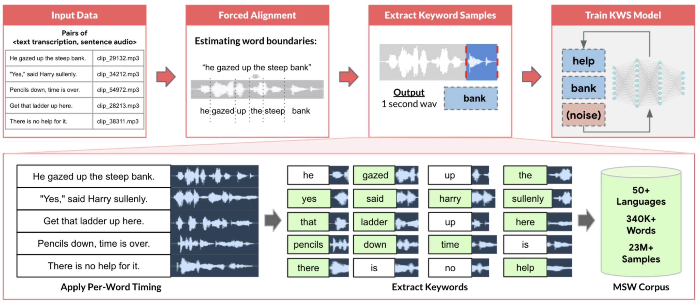
Mazumder, Mark. 2021. TinyML: Multilingual Spoken Words Corpus. tinyML Talks.
The extraction system uses these precise timing markers to generate clean keyword samples while handling anticipated engineering challenges: background noise interfering with word boundaries, speakers stretching or compressing words outside the 500 ms to 800 ms window that this chapter’s quality screen accepts, and longer words exceeding the one-second boundary. Automated checks of recording quality, speech clarity, and background noise are what make consistent standards possible at this scale without the manual review expense that would make it prohibitive.
Voice assistant engineering teams often build on this automated labeling foundation. While automated corpora may not contain the specific wake words a product requires, they provide starting points for KWS prototyping, particularly in underserved languages where commercial datasets do not exist. Production systems typically layer targeted human recording and verification for challenging cases (unusual accents, rare words, or difficult acoustic environments), coordinating between automated processing and human expertise. Each clip then carries a label, but the model still cannot read raw audio; the next stage turns labeled recordings into the features the model consumes, and it must compute them the same way in the training cluster and on the device.
Self-Check: Question
A smart city perception system evaluates annotation formats for a \(1920 \times 1080\) video stream. The team compares bounding box annotations (10 boxes per frame, each with 4 spatial coordinates) against pixel-level semantic segmentation masks. What is the ratio of scalar label entries generated between a full segmentation mask and the 10 bounding boxes?
- Roughly 10x more entries for segmentation, matching the ratio of bounding box coordinates.
- Roughly 50,000x more scalar entries for segmentation (~2.07 million pixel labels vs. 40 bounding box coordinates).
- Both formats require identical scalar entries because both represent 1080p resolution.
- Bounding boxes require 50,000x more entries because floating-point coordinates consume more bytes than integer masks.
A team wants to compare the total cost of two acquisition plans: one relies on human labeling, and the other emphasizes storing a large retained corpus for later reuse. The chapter’s cost table gives rates such as per-label, per-box, and per-terabyte-per-month costs. Which additional quantities are necessary to turn those rates into a fair total-cost comparison?
- Only the GPU training hours, because acquisition cost can be inferred once compute usage is known.
- Only the number of source websites and annotators, because storage and labeling rates are universal constants that do not need workload quantities.
- Only the final model accuracy target, because unit costs scale directly from performance goals.
- The number of labels or boxes to be paid for, plus the total retained terabytes and storage months to be paid for, because the rows use different units and must be scaled by their own quantities.
An ML team applies weak supervision to label a large unlabeled text corpus using heuristic rules and keyword patterns written by domain experts. According to the chapter, what is the main trade-off this approach makes?
- It guarantees expert-level labels at scale, so no additional quality checks or audits are needed once the heuristics run.
- It replaces all human involvement with deterministic labels, so disagreement between heuristics becomes a schema-validation problem rather than a quality problem.
- It increases labeling scale by applying programmatic heuristics cheaply across many examples, but the resulting labels are still noisy and must be validated against held-out human-audited data.
- If several heuristics agree on a label, that agreement is enough to treat the label as correct without checking against an independent human-audited set.
Describe how a tiered consensus labeling system uses inter-annotator agreement metrics (such as Fleiss’ kappa) and ‘gold standard’ honeypot examples to balance labeling cost against annotation quality.
True or False: In Active Learning, uncertainty sampling selects the unlabeled examples for which the current model has the highest prediction confidence to ensure the training set contains only clean data.
A statistical metric that measures the degree of agreement among three or more annotators classifying items into discrete categories, adjusting for chance agreement, is called ____.
4.7 Data Processing
The keyword spotter learns from audio features computed by a library on a training server, and it runs on a device whose feature code is written separately for a microcontroller. If the two compute the same features even slightly differently, the deployed model receives inputs unlike any it learned from, and nothing raises an error. Processing cannot add capability the data lacks, but it can silently remove capability the data has. Processing turns labeled records into the features the model consumes, and consistency governs it: transformations shared between training and serving must keep identical semantics, repeated operations must give the same result when retried, and the work must scale without losing track of what was done. Unlike a code refactoring, which must preserve a program’s behavior exactly, filtering or augmenting observations can change the learning problem itself, so each transformation needs an explicit contract stating what it may change and what it must hold fixed.
Training-serving inconsistency is one concrete form of the hidden technical debt that Sculley et al. (2015) identify in production ML systems. In the KWS pipeline, transformations must standardize recordings across microphones, noise levels, and sampling rates while preserving the acoustic cues that distinguish wake words from ambient speech, and the shared feature extraction must keep the same semantics and fitted state on the server and on the device, with numerical differences held within a validated tolerance.
4.7.1 Training-serving consistency
If a training script standardizes features using the training set’s mean and variance while the serving service recomputes those statistics on each incoming batch, both paths run the same code yet feed the model different numbers. Sharing feature code between training and serving is therefore not enough: parameters learned from the training data (normalization constants, encoding dictionaries, vocabulary mappings) must also be stored and reused during serving. This requirement is the consistency imperative.
Definition 4.3: Consistency imperative
Consistency imperative requires equivalent transformation behavior and state across training and serving environments.
- Significance: An unvalidated discrepancy between training and serving features can change the model’s effective input and degrade prediction quality without a runtime error. Equivalent semantics, shared fitted state, and tested numerical tolerances therefore make preprocessing a stateful component of the model artifact itself.
- Distinction: Unlike data quality, which focuses on the cleanliness of a single record, the consistency imperative focuses on the alignment of the entire transformation pipeline.
- Common pitfall: A frequent misconception is that sharing code makes the two paths consistent. Identical code still diverges when each environment recomputes its own statistics, so consistency is a state synchronization problem.
Violating the imperative produces training-serving skew, in which the training transformation and the serving transformation compute the same raw input differently and the deployed model receives inputs unlike those it learned from. The model still accepts a numerically valid vector computed under different rules, so neither exception tracking nor latency monitoring registers the failure (Sculley et al. 2015; Baylor et al. 2017).
Baylor, Denis, Eric Breck, Heng-Tze Cheng, Noah Fiedel, Chuan Yu Foo, Zakaria Haque, Salem Haykal, et al. 2017. “TFX: A TensorFlow-Based Production-Scale Machine Learning Platform.” Proceedings of the 23rd ACM SIGKDD International Conference on Knowledge Discovery and Data Mining, 1387–95. https://doi.org/10.1145/3097983.3098021.
Definition 4.4: Training-serving skew
Training-serving skew is the distributional divergence between the training and inference environments caused by inconsistent logic or state.
- Significance: It violates the consistency imperative and can cause silent accuracy degradation when the training and serving transformations compute different features from the same raw input.
- Distinction: Unlike data drift (which is an external shift in the environment), training-serving skew is an internal failure of the engineering stack.
- Common pitfall: A frequent misconception is that skew is “found” by looking for errors. In reality, it raises no exceptions; the system runs and the latency stays low, but the predictions are statistically wrong.
Pipeline parity tests detect the discrepancy between the two paths; outcome evaluation establishes its effect on predictions. Designing from serving constraints backward allows the team to test equivalent preprocessing on the target device and bound numerical differences before deployment.
Checkpoint 4.2: Defensive processing
Training-serving skew is a common cause of silent production degradation.
Data cleaning is the first stage where training and serving can diverge. Raw data frequently contains missing values, duplicates, or outliers that degrade model performance. Cleaning operations must be deterministic and reproducible: given the same input, they must produce the same output regardless of environment. This requirement shapes which cleaning techniques are safe to use in production.
Data cleaning encompasses deduplication, which merges repeated records so they neither overweight what the model learns nor leak across splits (Lee et al. 2022), along with missing-value handling and normalization. In the KWS corpus, deduplication must catch more than identical files. One speaker’s repeated takes of a wake word are near-duplicates, and they must stay within a single split, or evaluation measures memorization of that voice rather than generalization. The matching rule and its threshold must be captured in code that runs the same way every time the dataset is rebuilt.
Lee, Katherine, Daphne Ippolito, Andrew Nystrom, Chiyuan Zhang, Douglas Eck, Chris Callison-Burch, and Nicholas Carlini. 2022. “Deduplicating Training Data Makes Language Models Better.” Proceedings of the 60th Annual Meeting of the Association for Computational Linguistics (Volume 1: Long Papers), 8424–45. https://doi.org/10.18653/v1/2022.acl-long.577.
Outlier handling exposes a sharp operational split between batch training and online serving. During training, the pipeline can drop corrupted records or extreme sensor glitches so that a few bad values do not dominate parameter updates. At serving time, the response contract determines whether an invalid request may be rejected, routed to review, or answered with an abstention or request for another sample. Clamping features to bounded intervals (such as \([\TrainingFeatureMean- 3\TrainingFeatureStandardDeviation, \TrainingFeatureMean+ 3\TrainingFeatureStandardDeviation]\)) is safe only when that transformation has been validated for the task and uses the fitted training parameters. Outlier filters that judge each record relative to others introduce a subtler consistency risk: if evaluated across concurrently batched serving queries, the classification of an individual query depends on what other queries happen to arrive in the same request window, violating request isolation.
The validation monitors in section 4.5.3 also check transformed outputs. A rise in nulls after a join, unexpected duplicate records, or a shifted feature distribution can expose a transformation defect even when the raw inputs passed their checks.15 Comparing raw and transformed records across the same pipeline version helps localize the fault before changing the model.
15 Statistical drift detection: The means, variances, and quantiles tracked in quality monitoring are early-warning signals for the divergence term \(\StatisticalDivergence\) of the degradation equation (equation 1.1). A mean session length shifting from eight to 12 minutes over six months may indicate drift; a sudden drop to three minutes may indicate a collection fault. Outcome checks and source investigation are needed before choosing retraining or a source-system fix.
Quality validation must enforce identical schemas and validation predicates across training and serving pipelines. While training environments can afford compute-intensive profiling passes over entire datasets, serving paths must execute lightweight assertion checks (such as type validation, range bounding, and required-field existence) within the request’s latency budget. Mismatches between training-time validation and serving-time assertions allow corrupted inputs to reach the model undetected.
↪ The cost of training-serving skew and the shared feature libraries and schema validation tests that enforce training-serving parity are developed in Consistency imperative.
Bishop, Christopher M. 2006. Pattern Recognition and Machine Learning. Springer.
Transformation techniques convert data from its raw form into a model-ready representation, but the systems risk lies in the parameters those transformations learn. Common transformation tasks include normalization and standardization, which scale numerical features to a common range or distribution. For example, square footage and room count may differ greatly in scale; normalization places them on comparable numerical ranges, though their influence still depends on the model and learned parameters (Bishop 2006). Maintaining training-serving consistency requires that normalization parameters computed on training data be stored and applied identically during serving. Operationally, these parameters must be persisted alongside the model itself and loaded during serving initialization.
Preprocessing parameters fall under the same split-boundary rule as the data itself (section 4.1). If the mean and variance, or a category vocabulary, are fitted on the entire dataset before it is split, statistics of the test examples flow into the transformation the model trains through, and the test score no longer measures generalization to unseen data. The pipeline therefore fits every transformation parameter on the training split alone and applies the frozen result to validation, test, and serving inputs.
Beyond numerical scaling, transformations convert discrete inputs through categorical encoding, extract cyclical representations from timestamps, and construct derived spatial features. Categorical encodings must handle both the categories present during training and unseen categories encountered during serving. A reliable pipeline builds the vocabulary index exclusively from the training split, serializes this dictionary with the model artifact, and maps unknown runtime tokens to an explicit out-of-vocabulary (<UNK>) index. Omitting this mapping causes runtime dimension mismatches or silent index collisions during online inference.
Domain-specific feature engineering turns raw inputs into representations that expose informative signals directly to the learning algorithm (Kuhn and Johnson 2013). Instead of requiring the model to discover non-linear combinations from scratch, engineered features encode domain structure directly. The audio features the keyword spotter uses, described later, are themselves engineered: they encode what is known about human hearing, so a small model does not have to learn it from data.
Kuhn, Max, and Kjell Johnson. 2013. Applied Predictive Modeling. Springer New York. https://doi.org/10.1007/978-1-4614-6849-3.
Feature engineering can be a high-leverage activity because it changes what signal the model can see. In some workloads, well-designed features improve performance more than another round of algorithm selection or hyperparameter tuning. That leverage must be balanced against the consistency requirements of production systems. Every engineered feature shared by training and serving must have equivalent behavior in both environments. Production systems therefore implement feature engineering logic in shared libraries or coordinated pipelines rather than reimplementing it independently. Many organizations centralize those shared definitions in a feature store, the storage layer that section 4.7.5 defines, to reduce inconsistency across environments.
In the KWS pipeline, audio recordings collected across crowdsourced contributors, synthetic speech generators, and field captures arrive with wide acoustic variation. The raw audio contains the imperfections anticipated during problem formulation: environmental noise spanning quiet bedrooms to noisy kitchens, amplitude clipping from saturated analog-to-digital converters, gain differences across microphone hardware, and inconsistent sampling rates. Standardizing these inputs while preserving the short speech transients that distinguish wake words from ambient noise is essential to reaching the 98 percent detection target. Gain normalization is a specific trap. Normalizing each stored clip against its own peak uses information a streaming device never has, because the device hears continuous audio rather than finished clips, so the training pipeline may apply only gain handling the device can reproduce as audio arrives.
Quality assessment for KWS extends the general principles with audio-specific metrics. Beyond checking for null values or schema conformance, the validation pipeline tracks background noise levels (signal-to-noise ratio above 20 dB), audio clarity scores (frequency spectrum analysis), and speaking rate consistency (wake word duration within 500 ms to 800 ms). The pipeline flags recordings whose noise, duration, clipping, or distortion falls outside the scenario’s acceptance rules for review. These thresholds screen the clean baseline slice. Valid noisy or unusually timed speech remains in a separately labeled robustness slice, consistent with the noisy data budgeted in the KWS design. Review distinguishes these coverage examples from corrupted recordings before rejecting a sample. These screens do not prove that a sample is useful, but they reduce the chance that known defects reach model development. Checking audio quality at the source stops defects from spreading along the arcs traced in figure 1.
Transforming audio data for KWS involves converting raw waveforms into formats suitable for ML models while maintaining training-serving consistency. Raw audio waveforms (sequences of amplitude values sampled thousands of times per second) are high-dimensional. KWS pipelines often transform them into compact representations that emphasize the frequencies and temporal patterns most relevant to speech. Figure 15 aligns three views of an audio sample across a two-second window: the raw amplitude waveform, the corresponding time-frequency spectrogram isolating high-power acoustic energy around 500 Hz, and a compact 13-coefficient MFCC approximation. These standardized feature representations, typically MFCCs or spectrograms,16 emphasize speech-relevant characteristics while reducing noise and variability across different recording conditions. While a raw short-time Fourier transform (STFT) produces hundreds of linear frequency bins per time window, Mel-frequency analysis aggregates these bins through non-linear triangular filterbanks aligned with human auditory perception, followed by a discrete cosine transform that compresses the signal into just 13–40 decorrelated coefficients. For edge devices, this step collapses data volume by over an order of magnitude, allowing audio feature frames to fit inside the tight tens-of-kilobytes SRAM budgets of embedded coprocessors.
16 Spectrogram: The short-time Fourier transform (STFT) computes this 2D representation by converting the one-dimensional waveform into a time-frequency image. This representation lets image-style ML models process audio, but it also creates a rigid dependency: a mismatch in STFT parameters (for example, a 25 ms vs. 30 ms window) changes the feature representation between training and serving and can degrade performance.
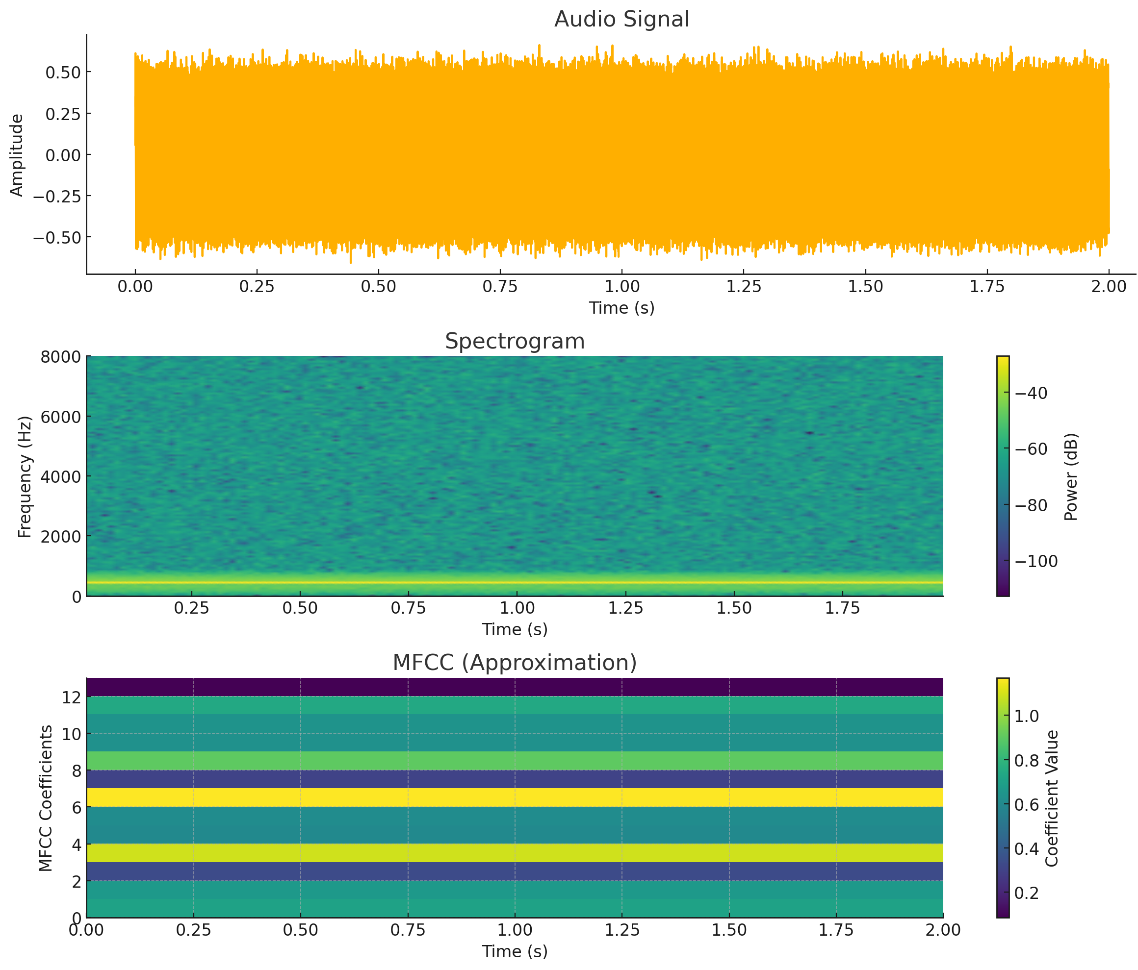
4.7.2 Feature computation placement
Precomputing those MFCC frames once during ingestion lets training iterate at disk speed, but it freezes any random noise or pitch augmentation applied to the raw waveform; computing them on the fly in the data loader keeps every epoch fresh at the cost of repeating the work and risking accelerator stalls. Feature computation placement decides which resource pays for a feature: storage pays when features are materialized on disk, while compute and latency pay when features are generated on demand.
When features are precomputed during ETL and stored on disk, training epochs read ready-made tensors without paying the transformation cost on every pass, and every run consumes the exact same values. That speed and reproducibility come at the price of storage footprint and rigidity: derived features must be stored alongside the raw data, and any change to feature logic requires recomputing the entire corpus before the next experiment can run. Computing features on the fly inside the data loader reverses the trade-off. Because only raw data is stored and transformations execute as batches are read, logic changes take effect immediately and random augmentations vary from epoch to epoch, but the host CPU repeats the work on every pass and can stall the accelerator if preparation falls behind.
In practice, production systems combine both approaches. Expensive, slowly changing representations, such as high-dimensional user embeddings (learned vectors that summarize each user) derived from matrix factorization or multi-month historical aggregations, are precomputed offline and materialized in storage. Volatile, lightweight signals, such as session recency, interaction timestamps, or client-side telemetry, are computed dynamically in the data loader. The keyword spotter shows why placement is not a free choice. The clean features of each recording can be computed once and stored, but noise augmentation must be applied to the raw audio before feature extraction, so the features of augmented clips have to be computed in the loader on every pass. This split matches each feature’s placement to its rate of change, trading storage capacity against execution latency.
4.7.3 Idempotent transformations
Consistency and placement settle what a transformation produces and where it runs, which serves the quality pillar; the reliability pillar asks whether that transformation can safely run again after a crash. If a processing stage appends transformed records to a target table and a worker fails after writing its output but before acknowledging completion, the automatic retry runs the job a second time and writes duplicate records into the training set. Idempotency17 prevents that corruption by ensuring that applying an operation repeatedly has the same effect as applying it once. This property matters whenever jobs retry after node failures, engineers reprocess historical data to fix a bug, or the same records flow through multiple paths. Determinism is a related but distinct requirement: identical inputs and captured state should produce identical outputs.
17 Idempotency: From Latin idem (“the same”) + potens (“having power”), literally “having the same power when applied again.” In ML pipelines, idempotency enables safe retries after partial failures: a nonidempotent operation (for example, appending to a log) creates duplicates on retry. An idempotent operation leaves the same resulting state after one application or repeated applications.
In state-machine terms, an operation \(\StateOperation\) is idempotent if \(\StateOperation(\StateOperation(\StoredSystemState)) = \StateOperation(\StoredSystemState)\). In storage systems, setting a register to an absolute value (\(\StoredSystemState\leftarrow 1\)) is idempotent, whereas incrementing a counter (\(\StoredSystemState\leftarrow \StoredSystemState+ 1\)) or appending a row to an unkeyed log is not: each re-execution mutates system state. Distributed data pipelines execute across preemptible workers and unreliable networks where timeouts and node crashes trigger automatic retries. Rather than appending blindly, an idempotent pipeline enforces write semantics such as deterministic keyed upserts (insert if absent, overwrite if present) or atomic directory swaps, ensuring that repeated job attempts converge to the identical final dataset.
Managing partial pipeline failures requires clear state boundaries between stages. Decoupling stages with persistent intermediate checkpoints ensures that each phase can be retried independently without re-executing upstream work. For long-running jobs processing terabyte-scale corpora, checkpointing state partitions (such as completed file shards or stream consumer offsets) bounds retry latency: a task failure after five hours of execution requires replaying only the uncommitted shard rather than restarting the entire five-hour job. The checkpoint mechanism must commit output partitions and state markers in a single atomic transaction, preventing records from being dropped or processed twice.
Deterministic transformations are those that always produce the same output for the same input, without dependence on external factors like time, random numbers, or mutable global state. Transformations that depend on current time (for example, computing “days since event” based on current date) break determinism because reprocessing historical data would produce different results. The solution is to capture temporal reference points explicitly: instead of “days since event,” compute “days from event to reference date” where reference date is fixed and persisted. Random operations should use seeded random number generators where the seed is derived deterministically from input data, ensuring reproducibility.
Reliability in the KWS pipeline requires reproducible feature extraction. Audio preprocessing must be deterministic: given the same raw audio file, the same MFCC features are always computed regardless of when processing occurs or which server executes it. This enables debugging model behavior (can always recreate exact features for a problematic example), reprocessing data when bugs are fixed (produces consistent results), and distributed processing (different workers produce identical features from the same input). The processing code captures all parameters (fast Fourier transform (FFT) window size, hop length, number of MFCC coefficients) in configuration versioned alongside the code, ensuring reproducibility across time and execution environments.
4.7.4 Distributed processing
Scale becomes the next constraint once quality and reliability are in place. Correct, repeatable transformations still fail the pipeline if they cannot keep pace with data volume or its deadline. As datasets and experiment concurrency grow, data processing can outgrow one machine even when the raw bytes still fit on local storage. The cleaning techniques that work on gigabytes in memory must then become partition-aware, out-of-core, or distributed without changing their semantics.
Single-machine processing suffices for large workloads when engineered carefully. Servers with 256 GB of RAM can process datasets of several terabytes using out-of-core processing that streams data from disk. Libraries that stream data from disk and parallelize across cores extend familiar dataframe interfaces to such workloads. Before investing in distributed processing infrastructure, teams should exhaust single-machine optimization: using efficient data formats (Parquet18 instead of CSV), minimizing memory allocations, using vectorized operations, and exploiting multi-core parallelism. The operational simplicity of single-machine processing (no network coordination, no partial failures, simple debugging) makes it preferable when performance is adequate.
18 Parquet: A columnar storage format that organizes data by column, not by row. Where a CSV reader must parse every row in full to reach a few columns, a Parquet reader loads only the columns a computation needs. The resulting I/O reduction depends on the selected columns, encoding, compression, and workload.
Within a single machine, parallelizing data ingestion across host CPU workers yields diminishing throughput returns whenever unpartitionable stages, such as sequential decompression or central database lock acquisition, limit concurrency. Amdahl’s law caps how much speeding up one part of a pipeline can improve the whole. Applied to host worker count, it means that even when 90 percent of a feature extraction pipeline parallelizes across workers, the speedup cannot exceed 10\(\times\). The serial stages keep their full duration however many workers share the rest, so eliminating serial I/O and single-threaded stages takes precedence over launching more worker processes.
↪ Amdahl’s law, the ceiling that untouched work places on any speedup, is developed in Anatomy of an Accelerator.
Coordination across machines
This book keeps data processing on one machine, but the boundary is worth knowing. When a corpus or the number of concurrent feature rebuilds outgrows one server, processing spreads across a cluster, and three things change. Data locality becomes a design constraint, because a network link moves bytes far more slowly than a node reads the shard it already holds, so cluster frameworks send the computation to the data instead of the data to the computation. Network transfer becomes the dominant cost of any operation that exchanges records rather than summaries. A global shuffle or a join sends records across every partition, whereas a decomposable reduction such as a mean sends only one partial result per partition. Coordination becomes part of the work, because the machines wait on the slowest worker and must recover when one fails partway through a job, which is when the idempotent, deterministic transformations described earlier become essential rather than merely convenient. Within one machine the network costs disappear and partial failures are rare, so the transformations of this section appear in their simplest form.
Scalability in the KWS pipeline matters at both ends of the lifecycle. Development uses single-machine processing on sample datasets to iterate rapidly. The reference corpus fits on the local storage of one well-provisioned server, so distributed processing pays off mainly when many experiments rebuild features at the same time. Per-file feature extraction is embarrassingly parallel, but end-to-end speedup is bounded by shared storage bandwidth, metadata operations, scheduling, and output contention. Production deployment adds a stricter 16 KB preprocessing-state budget alongside the 256 KB model-size limit, requiring careful footprint optimization so feature extraction fits on the device.
4.7.5 Feature stores
The keyword spotter needs no feature store, because its features are computed on the device from audio alone. A fraud or recommendation model whose features come from user history faces two failure modes at once: during model development, data scientists compute features like user_purchase_count_30d with batch SQL queries in a warehouse, whereas during serving an online microservice computes the same metric incrementally from an in-memory cache, and minor differences in timezone arithmetic, missing-value handling, or floating-point rounding cause offline and online features to drift apart. Worse, if the training query joins a historical transaction against the user’s current profile rather than the profile as it stood when the transaction happened, future information leaks into the training set. Keeping the two paths consistent means serving historical feature values for training and current feature values for inference from a single shared definition. Point-in-time correctness and shared feature logic are the primary operational requirements that drive teams to adopt feature stores, which Uber’s Michelangelo platform popularized to eliminate this class of training-serving skew (Hermann and Del Balso 2017).
Hermann, Jeremy, and Mike Del Balso. 2017. Meet Michelangelo: Uber’s Machine Learning Platform. Uber Engineering Blog.
Definition 4.5: Feature store
Feature store is the architectural layer that centralizes the management of machine learning features, decoupling feature computation from consumption.
- Significance: It supports point-in-time-correct historical retrieval for training \((\LaggedModelInput)\) and coordinated feature definitions for real-time inference \((\ModelInput_t)\), reducing training-serving skew when timestamps, backfills, freshness, and synchronization are handled correctly.
- Distinction: Unlike a general-purpose database, a feature store is designed for dual storage modes: an offline store (columnar/batch) for training and an online store (key-value/low-latency) for serving.
- Common pitfall: A frequent misconception is that a feature store is only “a place to store data.” In reality, it manages feature definitions, values, and retrieval; transformation may run in the feature store, an offline store, or a separate batch or stream-compute engine.
Feature stores establish a single source of truth for feature definitions across the ML lifecycle. By registering a feature definition as a unified computation graph, the feature store evaluates the identical transformation across both historical batch data and live inference streams. This shared definition reduces one source of training-serving skew, but equivalent execution still requires synchronized fitted state, correct timestamps, and appropriate freshness. Those conditions must be tested across both retrieval paths. Centralization also enables organizational feature reuse: expensive representations, such as multi-dimensional user embeddings derived from months of interaction logs, are computed once and served to multiple downstream modeling teams.
↪ How feature stores are operated in production, including point-in-time retrieval and training-serving skew prevention at scale, is developed in Feature stores.
To serve both access patterns, feature stores pair two storage engines. The offline store uses columnar formats (such as Parquet) on high-capacity object storage, tuned for multi-gigabyte sequential scans during batch training. The online store uses low-latency key-value databases (such as Redis), tuned for sub-10-millisecond point lookups during real-time inference. Automated pipelines synchronize the two engines by pushing batch-computed feature snapshots to the online store while streaming ingestion updates both stores continuously as new user events arrive.
Time-travel queries separate a true feature store from a simple cache. Training requires evaluating features as they existed at the exact moment of an event, rather than their current values. In a customer churn model, for example, training on a customer who churned on January 15 must use features computed on January 14, not current post-churn profile state. Feature stores enforce point-in-time correctness using an as-of join (temporal join): for every observation at timestamp \(\ObservationTimestamp\), the retrieval engine joins the most recent feature record whose update timestamp satisfies \(\FeatureUpdateTimestamp\le \ObservationTimestamp\). The join must also exclude information that was not available to the prediction path at \(\ObservationTimestamp\), including late-arriving events and later backfills whose event timestamps precede the observation. Timestamp ordering prevents future-information leakage only when retrieval preserves this historical availability across the upstream feature tables.
Every processing choice in this section, from cleaning and scaling to placement, idempotency, and feature retrieval, leaves derived state that downstream training depends on. Whether features are computed in a loader, materialized in storage, or served from a feature store, the team must eventually be able to say exactly which recordings, labels, and transformation versions produced the dataset a model learned from. Recording that answer is the last step of building the dataset.
Self-Check: Question
An engineer normalizes a numerical feature by computing standard \(z\)-scores: \(x' = (x - \mu)/\sigma\). During production serving, how must the parameters \(\mu\) and \(\sigma\) be handled to satisfy the consistency imperative and prevent training-serving skew?
- Persist the exact \(\mu\) and \(\sigma\) computed on the training dataset alongside the model artifact, loading and applying those fixed constants to live serving inputs.
- Recompute \(\mu\) and \(\sigma\) dynamically over each incoming serving batch to ensure the live data is always centered at zero.
- Discard \(\mu\) and \(\sigma\) entirely at inference time and rely on batch normalization layers inside the neural network.
- Compute \(\mu\) and \(\sigma\) independently over a rolling 1-hour window of serving traffic to track seasonal shifts.
A feature pipeline outgrows one server and its data is split into partitions across several machines. Which operation adds the least network transfer in the cluster compared with running it on one machine?
- A join between two tables partitioned on different keys, because the database engine performs the join automatically.
- A global shuffle that regroups every record by speaker identifier, because each record moves only once.
- Computing a global mean, because each machine can reduce its own partition to a partial sum and count and send only that summary.
- Gathering all partitions onto one coordinator machine before any processing, because a single machine avoids coordination entirely.
Define idempotency in the context of data transformation pipelines and explain why idempotent operations (such as upserts) are essential for fault recovery in distributed ML pipelines.
True or False: Using the identical Python preprocessing function in both training and serving code repositories is sufficient to eliminate training-serving skew.
Order the following steps for keeping an audio feature transformation consistent between training and serving: (1) split the data into the appropriate training and evaluation partitions, (2) version the transformation code together with the fitted transformation state, (3) fit any transformation state, such as normalization or vocabulary parameters, using only the training partition, (4) reuse the same transformation or a validated equivalent during serving and check that outputs stay within an accepted tolerance.
How does a feature store’s point-in-time correctness (time-travel join) prevent data leakage during offline training dataset generation?
- It encrypts historical feature values so that model weights cannot memorize training labels.
- It forces all features to be computed strictly in real time on the client device during model inference.
- It converts all timestamps into UTC strings to prevent database indexing errors.
- It reconstructs feature values exactly as they existed at the observation timestamp of each training event, preventing future feature values from leaking into historical training records.
4.8 Dataset Release
Months after launch, the keyword spotter’s detection rate drops on a new hardware revision, and the first question the team must answer is what the shipped model learned from, down to the recordings, the labels and the guideline they followed, the splits, and the feature code. A dataset release answers that question in advance. It is an immutable, versioned record of everything that produced a training set: the source records, how they were split and labeled, and the code and parameters that turned them into features. It is the versioned dataset that Stage 2 of the lifecycle hands to model development, and it turns the pipeline built so far into something that can be reproduced, compared, and audited.
The release is built from what each record carries. Table 5 lists the fields of one KWS training clip and the question each field answers later. Two of them do most of the work. The split is assigned by hashing the speaker key, so every clip from a speaker lands in the same split in every release and a later relabeling pass cannot leak a test speaker into training. The label carries the version of the guideline it was made under, so a change in labeling rules can be told apart from a change in the data.
| Field | Recorded value | Question it answers later |
|---|---|---|
| Recording ID | Content hash of the audio file | Is this clip a duplicate, and what was derived from it? |
| Speaker key | Pseudonymous speaker identifier | Are all of this speaker’s clips in one split? |
| Consent record | Reference to the terms the clip was collected under | May it be retained, and must it be deleted on request? |
| Split | Train, validation, or test, from a hash of the speaker key | Is the split stable across releases? |
| Label and rubric version | Wake word or none, with the labeling guideline version | Did the data change, or only the labeling rules? |
| Alignment version | Aligner version and word-boundary confidence | Where could a segmentation error have come from? |
| Feature configuration | Window, hop, coefficient count, and processing code commit | Can the features be recomputed exactly? |
Each record’s fields capture local provenance, while the release manifest ties the whole collection together. The rest of a release records how those fields were produced and pins the resulting dataset in storage so that any historical build can be recovered verbatim.
4.8.1 Transformation lineage
The last row of table 5, the feature configuration, exists because recording the raw audio file and label is not enough if a later change to the MFCC window function leaves the team guessing which window the shipped model trained on. Governance, the fourth pillar, closes that gap by tracking what transformations were applied, when they ran, which version of processing code executed, and what parameters were used. This transformation lineage is the processing part of data lineage, the recorded trail that links each dataset, feature, and model to the sources, code, and parameters that produced it.19 Transformation lineage supports reproducibility, debugging, auditability, and iterative improvement when transformation bugs surface. It can supply evidence for documentation or compliance workflows, but lineage alone does not explain a model’s decision or establish regulatory compliance.
19 Data lineage: When a model produces an erroneous or discriminatory prediction, lineage helps engineers determine whether the contributing problem originated in raw data, feature computation, training, or serving. The resulting trace can support incident investigation and jurisdiction-specific documentation duties, but its usefulness depends on complete instrumentation and retained history; it does not guarantee an explanation of model behavior.
That trail starts with transformation versioning, which records which version of the processing code produced each dataset. Whenever engineers change the transformation logic to fix a bug, add features, or improve quality, the version number increments, and tagging datasets with that version identifies every table or shard that must be reprocessed after a fix. Because identical source code can still produce slightly different floating-point outputs across different NumPy releases, runtime environment variables, or CPU instruction sets, each dataset also records the Git commit hash of the code that created it alongside a container image that freezes the code, dependencies, and system libraries in one immutable environment.
Code and environment versions still leave out the data-dependent state that transformations learn, so parameter tracking records the fitted values applied during transformation: the mean and standard deviation computed on training data for normalization, the vocabulary (set of all observed categories) for categorical encoding, and any constants or thresholds used in feature engineering (section 4.7.1). Serializing these parameters alongside the model artifact ensures that serving applies the exact same values as training. Processing lineage then joins code, environment, and fitted parameters into a complete execution history from raw data to final features: which raw files were read, what transformations ran in what order, what parameters were applied, and when the job executed. Lineage systems instrument the pipeline so that each job records these links as it runs, because a history reconstructed after an incident is rarely complete. When model predictions go wrong, engineers can trace back through the lineage graph to find the training data that contributed to the behavior, the quality scores attached to that data, and the transformations applied, then recreate the exact scenario for investigation.
In the KWS pipeline, governance applies to the audio processing parameters that affect model behavior. The reference volume level used for normalization is persisted, and the FFT and MFCC settings versioned with the processing code (section 4.7.3) are joined by the window function (such as Hamming or Hann), the frequency range, and the mel filterbank parameters. Recording them makes it possible to reproduce training data exactly when debugging model failures, to validate that serving uses preprocessing identical to training, and to study how preprocessing choices affect accuracy. Without this record, teams fall back on manual documentation that becomes outdated, which allows subtle training-serving skew.
4.8.2 Data versioning for ML reproducibility
Lineage records how a dataset was built, but reproducing or comparing two runs also requires recovering the exact bytes of each release. Without an immutable snapshot of the training inputs, diagnosing why a retrained keyword spotter lost accuracy takes days of guesswork across new recordings, changed labels, and upstream batches. With data versioning, engineers compare the two training snapshots directly and find the cause at once: the labeling guideline version in table 5 changed between the two releases, so the same clips now carry different labels.
File-level versioning engines like DVC (Data Version Control) provide this link by pairing Git with content-addressed remote storage (Iterative 2024). Git tracks small text pointer files (.dvc) containing cryptographic hashes, while DVC synchronizes the underlying binary dataset to object storage (listing 2). Checking out an earlier Git commit restores the historical pointers; the paired DVC retrieval step shown in the listing restores the dataset contents matched to that code state.
Iterative. 2024. Data Version Control (DVC).
git checkout and dvc checkout commands.
# Add data to version control
dvc add data/training.csv
git add data/training.csv.dvc
git commit -m "Add training data v1"
dvc push  # Upload to remote storage

# Later: retrieve exact data for any historical commit
git checkout abc123
dvc checkout  # Restores exact data from that commit
While file-level versioning suits bulk artifacts like images and audio, tabular datasets require versioning over tables that change row by row. Open table formats such as Delta Lake solve this by keeping an append-only transaction log of all row insertions, deletions, and schema changes (Armbrust et al. 2020). This log supports time-travel queries that pin a dataset state by timestamp or version ID (listing 3).
-- Query data as it existed on a specific date
SELECT * FROM training_data TIMESTAMP AS OF '2024-01-15'

-- Or by version number for programmatic access
SELECT * FROM training_data VERSION AS OF 47
Two production components work with these versioning engines to complete end-to-end reproducibility. First, feature store point-in-time retrieval evaluates features as they existed at the observation timestamp, preventing the leakage from future observations described in section 4.1. Second, a model registry records the lineage manifest for each deployed model: Git commit SHA, data version ID, training configuration, and evaluation metrics. In the keyword spotter’s regression, this audit trail turns an open-ended debugging investigation into an immediate snapshot comparison.
↪ How the model registry promotes, holds, or rolls back the exact artifact that was evaluated is developed in Versioning and lineage.
Long-term retention balances auditability against storage cost and privacy rules. High-volume production pipelines use tiered retention: hot SSD tiers for active training and debugging, warm object storage for periodic evaluation snapshots, and cold archive storage for compliance records. Because keeping petabyte-scale data forever is too expensive and often violates privacy statutes, data lifecycle policies must set explicit retention windows and deletion schedules. A release fixes what the dataset is, yet it says nothing about how fast that dataset can reach the accelerator during training, which is the second bound from the opening of this chapter and the one the remaining stages of the pipeline must meet.
Self-Check: Question
In the chapter’s KWS dataset release, each clip’s split is assigned by hashing its speaker key rather than by drawing splits at random each time a release is built. What failure does this prevent?
- A later release or relabeling pass could move some of a test speaker’s clips into training, so evaluation would reward memorization of that voice instead of generalization to new speakers.
- Hashing compresses the audio so that each split fits in less storage.
- Hashing guarantees equal numbers of keyword and non-keyword clips in every split.
- Hashing removes the need to record a consent reference for each clip.
A keyword spotter’s detection rate drops after a scheduled retraining even though no code changed. Explain how a dataset release that records label rubric versions, alignment versions, and feature configuration lets the team locate the cause.
4.9 Physics of Data
The throughput bound lives in the Data–Machine overlap, and it is physical. Moving a petabyte of training data across cloud regions incurs tens of thousands of dollars in egress fees and hours of network serialization delays. Source code is small enough to move freely, so the data-as-code principle explains what data does without explaining why moving it costs so much. The physics of data supplies that explanation by giving data measurable properties. Data gravity (McCrory 2010) is the bandwidth, I/O, and latency cost of moving a large byte volume, and task-relevant signal is the learning value those bytes carry for the task. A third property, flow rate, decides whether those bytes reach the accelerator as fast as it consumes them, and the ResNet-50 scenario measures it.
McCrory, Dave. 2010. Data Gravity – in the Clouds.

Returns peak where task signal is high and movement cost (gravity) is low.
Engineering effort pays off most when early filtering and selection separate high-signal records from the rest before data gravity makes them expensive to move. Low-signal data (repetitive audio frames or duplicate samples) consumes host-to-accelerator bandwidth and memory capacity while teaching the model little. An efficient pipeline resolves this physical bottleneck by maximizing the task-relevant signal delivered per byte moved across the storage and interconnect hierarchy, an optimization that begins with the physical properties of the data itself.
4.9.1 Data gravity
Data movement costs time and money, the cost that the data-gravity principle (2) names. Data gravity scales directly with data volume \((\DataVolume)\) and inversely with network bandwidth \((\Bandwidth)\). Transferring a petabyte dataset across a 10 Gbps link requires days of continuous transmission (\(\DatasetTransferTime = \DataVolume/\Bandwidth \approx 9.3 \text{ days}\)); even across a dedicated 100 Gbps link, transfer latency and egress tariffs remain substantial enough to govern system design. Because migrating 1 PB across network boundaries is both slow and expensive, system designers colocate compute with the storage substrate rather than moving large datasets across remote networks. This physical constraint underlies lakehouse storage architectures20 (Zaharia et al. 2021), where query and preprocessing engines execute directly against shared object storage rather than repeatedly copying raw data across network fabrics.
20 Data lakehouse: Combines data lake storage (cheap, schema-less) with warehouse query semantics (atomic, consistent, isolated, and durable (ACID) transactions, schema enforcement) using transactional table layers such as Delta Lake. For ML workloads, the lakehouse reduces the ETL copy between lake and warehouse, enabling direct feature computation on the storage layer where data already resides. This is a direct response to data gravity, since repeated petabyte-scale copies increase the \(\DataVolume/\Bandwidth\) cost (Armbrust et al. 2020; Zaharia et al. 2021).
Armbrust, Michael, Tathagata Das, Liwen Sun, Burak Yavuz, Shixiong Zhu, Mukul Murthy, Joseph Torres, et al. 2020. “Delta Lake: High-Performance ACID Table Storage over Cloud Object Stores.” Proceedings of the VLDB Endowment 13 (12): 3411–24. https://doi.org/10.14778/3415478.3415560.
Zaharia, Matei, Ali Ghodsi, Reynold Xin, and Michael Armbrust. 2021. “Lakehouse: A New Generation of Open Platforms That Unify Data Warehousing and Advanced Analytics.” Proceedings of CIDR 8.
↩︎ The data-gravity principle, which weighs shipping a dataset against shipping the computation to it, is established in Cloud infrastructure and scale.
Napkin Math 4.7: The physics of data gravity
Problem: A 1 PB training dataset resides in a US East data center, while a remote accelerator pod is available in US West. What transfer time and egress cost does remote training add, and when would suitable compute near the data avoid that overhead?
Math:
- Network bandwidth: 100 Gb/s \(\div 8 =\) 12.5 GB/s.
- Transfer time: 1,000,000 GB \(\div\) 12.5 GB/s = 80,000 seconds, approximately 22 h.
- Cost: 1,000,000 GB \(\times\) $0.02/GB = $20,000. (Baseline: AWS data transfer out pricing, 2024.)
Systems insight: If training takes less than 22 h, data transfer takes longer than training. If training costs less than $20,000 (approximately 5,000 TPUv4-hours), bandwidth costs more than compute. When suitable compute is available near the data, these transfer costs favor moving code to data. Smaller datasets make moving data to code more practical, but placement still depends on compute availability and comparative training time.
4.9.2 Task-relevant signal
A dataset containing one million identical images carries heavy data gravity yet adds no new observations beyond the first sample; repeated passes over that single image can nudge model weights slightly, but they supply no fresh evidence. Conversely, a curated collection of 10,000 diverse edge cases is small enough to move cheaply yet contributes rich supervisory signal. Physical storage measures raw bytes, whereas machine learning extracts task-relevant signal: evidence that helps the model learn the target task rather than raw Shannon entropy. Comparing task-relevant signal with data gravity motivates a selection heuristic: \[ \text{Data Selection Gain} \propto \frac{\text{Task-Relevant Signal}}{\text{Data Gravity}} \tag{3}\] The numerator is not a universal physical quantity. A team estimates marginal learning value by comparing held-out model quality under a fixed training procedure; the denominator accounts for the movement cost of the compared datasets. The heuristic favors a selection only when its measured learning benefit justifies that cost. Scoring, labeling, and training costs must also enter a complete budget. Deduplication and the active learning of section 4.6.5 can improve this ratio by eliminating redundant byte volume and proposing uncertain examples for labeling. Uncertainty does not establish learning value; ambiguous or corrupted examples can also be uncertain, so the selection policy requires validation.
↪ The information-compute ratio, which measures the learning signal each sample returns per unit of training compute, is developed in The information-compute ratio.
4.9.3 The feeding problem
Data gravity dictates the cost of moving data in bulk; the feeding problem dictates the cost of delivering it to execution units in real time. It is an input/output flow rate bottleneck: storage bandwidth fails to keep pace with compute throughput. The bottleneck is measured, not hypothetical. Profiling nine widely used vision and audio models found their training time often dominated by data stalls, time spent waiting for data to be fetched and preprocessed (Mohan et al. 2021), and in production recommendation training the data storage and ingestion pipeline has become a dominant constraint on training performance and capacity (Zhao et al. 2022).
Zhao, Mark, Niket Agarwal, Aarti Basant, Buğra Gedik, Satadru Pan, Mustafa Ozdal, Rakesh Komuravelli, et al. 2022. “Understanding Data Storage and Ingestion for Large-Scale Deep Recommendation Model Training.” Proceedings of the 49th Annual International Symposium on Computer Architecture, 1042–57. https://doi.org/10.1145/3470496.3533044.
When data delivery and computation overlap, the bottleneck principle holds that a system runs only as fast as its slowest stage. Consider the chapter’s throughput workload, one A100-class accelerator training ResNet-50 on images. The accelerator’s peak arithmetic rate is 312 TFLOP/s, and one training step on one image costs about 24.6 GFLOP, roughly three times the cost of a single prediction because training must also work out how to adjust every parameter. Dividing the first by the second gives an arithmetic ceiling of about 12,682 img/s. In practice a well-tuned pipeline sustains about 3,200 img/s, roughly 25 percent of that ceiling, once layers that wait on memory and the synchronization between steps take their share. Each image sits on disk as a 150 KB JPEG, so storage must deliver 480 MB/s. When the attached volume supplies only 250 MB/s, compute units stall on I/O. This gap defines the feeding loss, the throughput penalty from insufficient input supply, which directly degrades system efficiency \((\EfficiencyHw)\). Under steady-state overlap, divide the supplied 250 MB/s by the required 480 MB/s to obtain the fraction of the sustained training rate that storage can support. Subtracting that fraction from one gives a modeled feeding loss of about 48 percent. This is the throughput loss relative to the supplied sustained baseline, not a measurement of all accelerator idle time or utilization relative to advertised peak.
↩︎ The bottleneck principle is established in The bottleneck principle.
Which bytes are counted matters as much as how many. After decoding and conversion to an FP32 tensor, the same image occupies 602 KB, about 4 times its compressed size, so a loader that converts on the host moves 1.9 GB/s through host memory and across the host-to-accelerator link. Many loaders ship 8-bit pixels instead and convert on the accelerator to avoid that cost. Compression thus trades storage bandwidth for CPU decode work. A pipeline that caches pre-decoded tensors on disk to skip that work pays the full 1.9 GB/s at the storage tier instead, and it freezes the random crops that augmentation would otherwise vary from epoch to epoch. Applying the same supply-to-demand calculation gives a modeled throughput loss of 87 percent relative to the sustained baseline. Storage and delivery apply this slowest-stage bound to the storage tiers (section 4.10.3) and then to the CPU decode workers (section 4.10.4) without re-deriving it. Distance also increases energy consumption: as data travels farther from arithmetic logic units, transport energy dwarfs the cost of computation itself.
Systems Perspective 4.2: The energy cost of data movement
The memory-wall analysis in Physical Constraints on Deployment implies a data-engineering principle: moving one 32-bit value costs roughly 173× to 10,811× as much energy as the table’s FP32 multiply, with the multiplier rising as the data leaves the chip. The DRAM ratio is smaller than the one in Iron Law of ML Systems only because that comparison set one byte against a cheaper FP16 multiply. Later optimization chapters exploit the same cost gradient inside model and hardware design; here, the question is how much energy the information flow from the external world already consumes before the model computes, at each level of the memory hierarchy (table 6).
Table 6: Energy Cost of Moving vs. Computing on a 32-Bit Value: Each row gives the approximate energy per event at one stage of the data-movement hierarchy, with multipliers normalized to one 32-bit FP32 multiply. All rows use the same 32-bit width, so the ratios compare like-sized events. They do not by themselves prove which term dominates a complete workload; total energy also depends on the number of arithmetic operations and transfers. Arithmetic and DRAM rows follow Horowitz (2014).
| Operation | Energy (pJ) | Relative Cost |
|---|---|---|
| 32-bit FP Multiply | 3.7 pJ/FLOP | 1\(\times\) |
| DRAM Memory Access (32-bit) | 640 pJ | 173× |
| Local SSD Access (32-bit) | 4,000 pJ | 1,081× |
| Network Transfer (32-bit) | 40,000 pJ | 10,811× |
That gradient is why data locality dominates systems optimization. Each avoided transfer eliminates its corresponding movement energy, compounding across training epochs.
Because data movement incurs physical energy costs, data volume acts like physical mass. Removing 50 percent of training data through deduplication saves more than persistent storage capacity. It also eliminates energy expenditure across network, memory, and preprocessing stages. Filtering uninformative samples early is among the most effective architectural levers when I/O and communication dominate workload runtime.
Horowitz, Mark. 2014. “1.1 Computing’s Energy Problem (and What We Can Do about It).” 2014 IEEE International Solid-State Circuits Conference Digest of Technical Papers (ISSCC), 10–14. https://doi.org/10.1109/isscc.2014.6757323.
Checkpoint 4.3: The physics of data
Data engineering is governed by physical costs. Check your intuition:
The energy hierarchy and the signal-density heuristic converge on the same optimization lever, the Data Selection Gain of equation 3, because every redundant or uninformative record removed early saves movement energy and interconnect bandwidth at each later stage without costing task-relevant signal. For the released dataset, these costs come due in delivery. Every training epoch moves it from storage, through the host, to the accelerator, and the feeding problem decides whether that movement keeps pace.
Self-Check: Question
A machine learning team maintains a \(1\text{ PB}\) raw training corpus in a US East cloud storage bucket and provisions a dedicated compute cluster in US West. The regions are connected by a dedicated \(100\text{ Gbps}\) network fabric. Cloud egress pricing is $0.02/GB, and the model training run takes \(20\text{ hours}\). Under the chapter’s data-gravity reasoning, which conclusion is best supported by these numbers?
- The team should stream the dataset remotely during training, because a \(100\text{ Gbps}\) link guarantees that data movement cannot become the bottleneck.
- The team should split the dataset evenly across regions, because cross-region placement automatically removes the need to evaluate transfer cost or placement constraints.
- The team should first apply compression, because any realistic compression plan will make the transfer clearly cheaper and faster than colocating compute.
- The ideal one-time transfer is about \(22.2\text{ hours}\) and costs about $20,000, so colocating or relocating compute near the data is worth evaluating, but the final decision still depends on compute availability, cost, and other deployment constraints.
Assume decoded tensors must be read from storage at a sustained demand of \(1.8\text{ GB/s}\), while the attached baseline block-storage path can supply only \(250\text{ MB/s}\). Assume no compression or cache alternative changes this bound. Under this simplified feeding-loss model, what follows?
- The storage bound reduces the sustained baseline throughput by about \(86\%\) relative to its supplied demand, because the supply-to-demand ratio is \(0.25/1.8 \approx 0.139\) and the feeding loss is about \(1-0.139 \approx 0.86\).
- The accelerator remains compute-bound, because storage throughput and tensor execution are independent once batches have been scheduled.
- Increasing batch size alone removes the bottleneck, because larger steps always improve the ratio between storage supply and decoded-tensor demand.
- The storage path is only modestly underprovisioned, so the waiting fraction must stay below \(20\%\).
Using the data selection gain relationship \(\text{Gain} \propto \frac{\text{Task-Relevant Signal}}{\text{Data Gravity}}\), explain why removing \(50\%\) redundant samples can have large systems value when the retained dataset still covers the task-relevant cases and the training schedule is held fixed in passes over the data. Why is quality validation still necessary?
According to the chapter’s energy-movement hierarchy, arrange the following operations in ascending order of energy consumed per 32-bit value (from lowest energy to highest energy):
- Local NVMe SSD access
- On-chip 32-bit FP multiply
- Data-center network transfer
- Off-chip DRAM memory access
- The modeled throughput penalty from insufficient input supply relative to the supplied sustained training baseline is termed the ____.
4.10 Storage and Delivery
Delivery is where the throughput bound is met or missed. On baseline cloud block storage, the ResNet-50 scenario of section 4.9.3 already loses about 48 percent of its sustained training rate. Following that scenario to its end means choosing a storage tier that can sustain the accelerator’s rate, keeping the host processor between storage and accelerator from becoming the next bottleneck, and cutting the bytes each sample costs to move. The KWS data poses the same questions at smaller scale, for the multilingual reference corpus (23.4 million samples spanning 50 languages) and for the much smaller product-specific subset.
A sub-millisecond point lookup fits only in DRAM or local NVMe.
4.10.1 Storage system options
The ResNet-50 job reads its images in long sequential scans, while a serving system fetches one feature vector per request. These opposing access patterns pull storage in two directions, and selecting a system means minimizing the data term \(\left(\frac{\DataVolume}{\Bandwidth}\right)\) of the iron law of ML systems for whichever pattern dominates. Every storage medium imposes physical constraints on bandwidth that determine the maximum speed of the training and serving pipelines.
Two storage performance metrics govern this optimization. IOPS (input/output operations per second) counts the distinct read or write requests a device can handle per second, bounding random access workloads such as fetching small batches of images or individual user profiles. Throughput (bandwidth) measures the volume of data transferred per second, typically \(\text{IOPS} \times \text{Block Size}\), bounding sequential access workloads such as scanning a Parquet file for training.
Three architectures cover these patterns, and the ResNet-50 scan and the feature-serving lookup sit at opposite ends of the range. Conventional databases (online transaction processing (OLTP)) optimize for high IOPS with small, row-oriented blocks, strict ACID guarantees, and sub-millisecond point lookups. That profile fits online feature serving, such as a recommendation system fetching one user profile or an anti-fraud service querying historical transaction counts, but it wastes bandwidth on a training scan, because the storage engine fetches entire rows even when the model consumes only 20 of 100 features. Data warehouses (online analytical processing (OLAP)) organize tables by column rather than by row (Stonebraker et al. 2018), so a sequential scan reads only the required features, transferring one fifth of the uncompressed row payload when selecting 20 out of 100 columns. The format-efficiency calculation in section 4.10.5 quantifies this gain with a worked fraud-detection scenario. Warehouses suit feature engineering, batch aggregation, and tabular training, but they require structured schemas, handle raw audio, imagery, and free-form text poorly, and make schema changes during experimentation costly ALTER TABLE operations across billion-row tables. Data lakes store structured, semi-structured, and unstructured data in native formats on high-capacity object storage and defer structure to query time, an architectural pattern known as schema-on-read.21 A ResNet-50 job can read raw JPEG files from a lake at sequential rates, while independent jobs impose their own schemas without coordinating migrations. The cost is that governance shifts from ingestion to retrieval. Without a metadata catalog recording lineage, update cadence, schema versions, and access policies, a lake degrades into a “data swamp,” a set of orphaned directories such as userdata_v2_final and userdata_v2_ACTUALLY_FINAL whose lineage and quality are unrecorded. Each storage architecture therefore optimizes for a distinct access pattern and lifecycle phase, as table 7 summarizes.
Stonebraker, Mike, Daniel J. Abadi, Adam Batkin, Xuedong Chen, Mitch Cherniack, Miguel Ferreira, Edmond Lau, et al. 2018. “C-Store: A Column-Oriented DBMS.” In Making Databases Work: The Pragmatic Wisdom of Michael Stonebraker. Association for Computing Machinery. https://doi.org/10.1145/3226595.3226638.
21 Schema-on-read: Applies data structure definitions at query time rather than during ingestion, contrasting with schema-on-write (traditional databases) where data must conform to a predefined structure before storage. For ML pipelines in early development, schema-on-read enables rapid experimentation, because teams can store raw sensor data, images, and logs without committing to a feature schema upfront.
| Attribute | Conventional Database | Data Warehouse | Data Lake |
|---|---|---|---|
| Purpose | Operational and transactional | Analytical and reporting | Storage for raw and diverse data for future processing |
| Data type | Structured | Structured | Structured, semi-structured, and unstructured |
| Scale | Small to medium volumes | Medium to large volumes | Large volumes of diverse data |
| Performance Optimization | Optimized for transactional queries (OLTP) | Optimized for analytical queries (OLAP) | Optimized for scalable storage and retrieval |
Each lifecycle stage also reads the same data in its own way: exploratory analysis samples it at random, training streams it sequentially at high throughput, and production serving issues low-latency point lookups. During initial development, iteration velocity and schema flexibility dominate raw throughput. The primary systems challenge is managing experiment revisions without exploding storage capacity: ten exploratory runs on a 100 GB dataset naively generate 1 TB of redundant copies. The metadata-pointer approach of section 4.8.2 avoids this by decoupling version tracking from file storage. Governance policies reinforce this tiering by granting broad access to anonymized development datasets while gating sensitive production data behind encrypted, auditable access tiers.
During training, the access profile shifts toward sustained sequential throughput. Modern deep neural networks process massive datasets across dozens or hundreds of epochs, making storage bandwidth the determinant of hardware utilization. Scaling the chapter’s ResNet-50 scenario to eight accelerators, each sustaining its per-device rate, gives 25,600 img/s and a sustained storage demand of 3.8 GB/s of 150 KB compressed images; staging decoded FP32 tensors instead would raise it to 15.4 GB/s. Storage tiers unable to sustain this rate idle the accelerators, inflating cluster operating costs. End-to-end ResNet-50 training cannot shrink that demand by precomputing features, because its features change at every step. A model trained on the outputs of a frozen upstream encoder (a pretrained model whose outputs are reused as input features) can, and there the feature placement trade-off (section 4.7.2) becomes critical. Precomputing those representations delivers a 30× storage reduction (150 KB raw inputs reduced to 5 KB embedding vectors) but introduces staleness when the encoder updates.
Production inference reverses the optimization target from sequential bandwidth to low-latency random access. A recommendation service handling 10,000 req/s with a 10 ms SLA and 10 feature reads/request demands 100,000 IOPS. Local Non-Volatile Memory Express (NVMe)22 storage can sustain this random-access rate within the latency budget; in-memory key-value stores such as Redis, distributed caches, and purpose-built feature stores buy headroom for tail latency. Edge deployment imposes further physical boundaries: constrained flash storage, intermittent network connectivity, and non-disruptive model updates dictate tiered caching, where core models reside in local flash while reference data synchronizes asynchronously with cloud endpoints. In production, serving infrastructure must support atomic rollbacks and parallel A/B testing, operational guarantees that depend on tracing every deployed model back to the exact dataset release from which it was trained. Production ML architectures therefore rarely select a single storage technology; mature systems combine all three, with databases serving point lookups, warehouses running feature extraction, and lakes holding raw captures and intermediate checkpoints.
22 NVMe (Non-Volatile Memory Express): A storage protocol connecting directly to the PCIe bus with 64K command queues, delivering 5–7 GB/s sequential throughput and microsecond-scale latency. The contrast with SATA SSD (500 MB/s, single queue) is a 10× bandwidth gap that can bottleneck a training pipeline when storage service time exceeds compute time.
4.10.2 Storage tiers and cost
Beneath each of these systems sits a physical storage medium, and media span roughly two orders of magnitude in cost and nearly four in bandwidth. Mismatching the storage tier to the access pattern either inflates infrastructure costs with underutilized capacity or starves training accelerators during I/O stalls.
That spread survived a long collapse in absolute price. Figure 16 traces the lowest recorded price per terabyte of each medium in constant 2020 dollars. Hard disk storage fell from about $88B per terabyte in 1956 to $10.6 in 2023, roughly 10 orders of magnitude, yet in 2023 DRAM still cost 42× as much as solid-state storage per terabyte, and solid-state storage cost 2.4× as much as hard disk. Capacity became cheap, but since the 1980s the gaps between tiers have not closed, so the choice of tier, rather than raw capacity, sets the cost of keeping a training job fed.

Our World in Data. 2024. Historical Price of Computer Memory and Storage.
ML systems use tiered storage because no single tier is both cheap and fast (table 8). Under these 2024 assumptions, storing the KWS reference corpus (748.8 GB) in object storage costs $17.2/month, enabling affordable raw-audio retention, while working datasets on NVMe cost $74.9/month–$224.6/month for active training but load 50× faster.
↪ Why no single medium offers both large capacity and low access latency, the reason storage is built in tiers, is collected for reference in The memory hierarchy.
| Storage Tier | Cost ($/TB/month) | Sequential Read Throughput | Random Read Latency | Typical ML Use Case |
|---|---|---|---|---|
| NVMe SSD (local) | $100–300 | 5–7 GB/s | 10–100 μs | Training data loading, active feature serving |
| Object Storage (S3, GCS) | $20–25 | 100–500 MB/s (per connection) | 10–50 ms | Data lake raw storage, model artifacts |
| Data Warehouse (BigQuery, Redshift) | $20–40 | 1–5 GB/s (columnar scan) | 100–500 ms (query startup) | Training data queries, feature engineering |
| In-Memory Cache (Redis, Memcached) | $500–1000 | 20–50 GB/s | 1–10 μs | Online feature serving, real-time inference |
| Archival Storage (Glacier, Nearline) | $1–4 | 10–50 MB/s (after retrieval) | Hours (retrieval) | Historical retention, compliance archives |
This throughput divergence changes the input-loading component of engineering iteration time. Training that loads data at 5 GB/s completes dataset loading in 149.8 s, compared to 7,488 s at typical object storage speeds. The 50× loading speedup translates into shorter experiments only to the extent that exposed loading time contributes to their duration; transformation and model execution still consume time.
Beyond input datasets, storage must hold what training produces: model parameters, the extra values training keeps for each parameter (its optimizer state), and periodic checkpoints of both. Modern neural networks contain millions to hundreds of billions of parameters, imposing storage and retrieval patterns distinct from tabular data. GPT-3 (Brown et al. 2020) requires approximately 700 GB for model weights when stored in FP32 format (175B parameters times 4 bytes), though practical deployments often use smaller numeric formats such as FP16 (350 GB) to halve memory pressure. Model weights require block-aligned storage formats to support parallel reads across parameter groups during initialization and checkpointing, demanding aggregate storage bandwidth approaching network fabric limits (25 to 100 Gbps) to keep compute units active.
Brown, Tom B., Benjamin Mann, Nick Ryder, Melanie Subbiah, Jared Kaplan, Prafulla Dhariwal, Arvind Neelakantan, et al. 2020. “Language Models Are Few-Shot Learners.” Advances in Neural Information Processing Systems 33: 1877–901. https://doi.org/10.48550/arxiv.2005.14165.
↪ Quantization, which shrinks these weight footprints by storing parameters at lower precision, is developed in Numerical Precision: Changing How Values Are Stored.
Tracking these artifacts introduces versioning challenges. Git’s incremental text diffs fail on multi-gigabyte binaries, where a single weight update produces an entirely new file and ten historical checkpoints of a 10 GB model occupy 100 GB. Production workflows therefore keep lightweight content hashes in Git and the binaries in content-addressed object storage, the same decoupling that section 4.8.2 applies to datasets.
Multi-accelerator training compounds storage pressure through concurrent I/O. When a training job spans multiple accelerators, every rank reads training batches concurrently, and the job periodically writes checkpoints of model and optimizer state, often from a single rank, in bursts that compete with those reads. Storage must absorb reads that scale with the worker count and checkpoint bursts on top of them, preventing I/O serialization that leaves expensive accelerators idle.
↪ The data- and model-parallel strategies that coordinate these workers within one node are developed in Single-node multi-GPU training.
4.10.3 The storage bandwidth budget
Each storage tier sets its own ceiling on the feeding problem of section 4.9.3. Host RAM delivers 50 to 200 GB/s on modern server nodes, local NVMe SSDs deliver 5–7 GB/s, and network-attached storage provides 1 to 10 GB/s. Whichever tier serves the training reads caps the data supply rate, so the design question is which tier can sustain the chapter’s ResNet-50 scenario, and at which of its two rates.
Napkin Math 4.8: Storage bandwidth budget
Problem: What storage configuration keeps an A100-class accelerator from being data-starved while training ResNet-50? Performance Bounds explains why delivered throughput falls short of an accelerator’s advertised peak; here, the point is how a compute ceiling becomes a data-path budget.
Start with the compute ceiling derived in section 4.9.3. The A100’s 312 TFLOP/s divided by about 24.6 GFLOP per training image gives 12,682 img/s.
That compute ceiling becomes a storage requirement once each image must arrive from disk or object storage. Storage reads compressed bytes, so the budget uses the 150 KB JPEG rather than the decoded tensor: feeding the ceiling takes approximately 1.9 GB/s, while the 3,200 img/s that the accelerator actually sustains takes 480 MB/s.
Three storage options can now be compared against these two targets:
- S3 Standard delivers about 100 MB/s per connection when it streams large objects such as sharded archives, so feeding the ceiling needs 19 concurrent worker threads before software overhead. Fetching each 150 KB image as its own object is latency-bound and delivers far less.
- SATA SSDs deliver about 500 MB/s sequentially, enough for the sustained rate but a bottleneck at the ceiling.
- NVMe SSDs deliver approximately 5–7 GB/s, which covers the ceiling with headroom.
Systems insight: A SATA SSD caps the pipeline at 500 MB/s divided across 150 KB images, or approximately 3,333 img/s. That clears the sustained 3,200 img/s, so a faster drive buys nothing at today’s rate. Once faster kernels or a faster accelerator push the rate toward the ceiling, the same drive holds an A100-class accelerator to 26 percent of it. Each fix to the slowest stage exposes the next, so the storage tier must be sized for the rate the pipeline is heading toward, not the rate it runs at today.
Designing for high-throughput training therefore starts by matching storage throughput to accelerator demand, the storage-tier form of the slowest-stage bound that section 4.9.3 measured as lost training rate. The 500 MB/s figure represents effective SATA III sequential read throughput (the interface ceiling is 550 MB/s), and real-world random read performance with small files can be significantly lower. That caveat reinforces the general principle governing data pipelines: equation 4 bounds training throughput by compute capacity and the data supply rate defined in equation 5. Let \(\TrainingSampleThroughput\), \(\ComputeLimitedSampleRate\), and \(\DataSupplyRate\) denote rates in samples per second; let \(\StorageBandwidth\) be storage bandwidth in bytes per second, \(\OperationalOverheadFraction\) the dimensionless fraction lost to overhead, and \(\SampleStorageSize\) the bytes per sample. Under full overlap, the min-of-rates form corresponds to the \(\TrainingStepTime= \max(\IronLawComputeTime, \StepIoTime)\) lower bound of section 4.9.3, which the dataloader section applies to host workers; with incomplete overlap, actual step time is higher. \[\TrainingSampleThroughput\leq \min(\ComputeLimitedSampleRate, \DataSupplyRate) \tag{4}\] \[\DataSupplyRate= \frac{\StorageBandwidth(1-\OperationalOverheadFraction)}{\SampleStorageSize} \tag{5}\]
Once \(\DataSupplyRate\) is the smaller rate, additional accelerator compute cannot raise training throughput; the remedy must increase usable storage bandwidth or reduce bytes per sample. The budget assumes every epoch reads from storage. A dataset that fits in host memory, as an ImageNet-sized dataset does on many eight-accelerator servers, is read from storage once and then served from the operating system’s page cache, so storage binds only on the first epoch. The budget governs the cases that remain: datasets larger than memory, nodes whose memory several jobs share, and data streamed from remote storage.
When storage bandwidth becomes the limiting factor, teams must either improve storage performance through faster media, parallelization, or caching, or reduce the amount of data that must move. Large language model training may require processing hundreds of gigabytes of text per hour, while computer vision models processing high-resolution imagery can demand sustained data rates exceeding 50 gigabytes per second across distributed clusters. Prefetching hides the time to fetch the next batch behind the computation on the current one, but only when the loader sustains the required supply rate; it cannot create bandwidth that storage lacks.
4.10.4 The dataloader
Between storage and the accelerator sits the host processor, which reads each stored example, decodes it, augments it, and stages it for transfer. The barrier at this stage is the input/output (I/O) bottleneck: the accelerator idles whenever the host cannot stage examples as fast as the accelerator consumes them. The slowest-stage bound of section 4.9.3 applies unchanged: in an idealized two-stage model, step time ranges from \(\max(\IronLawComputeTime, \StepIoTime)\) with full overlap to \(\IronLawComputeTime + \StepIoTime\) with no overlap. What changes is the binding resource: while the initial feeding scenario was starved by baseline storage bandwidth, data loading on provisioned storage is more commonly starved by CPU-side decompression and decode (Mohan et al. 2021).
Mohan, Jayashree, Amar Phanishayee, Ashish Raniwala, and Vijay Chidambaram. 2021. “Analyzing and Mitigating Data Stalls in DNN Training.” Proceedings of the VLDB Endowment 14 (5): 771–84. https://doi.org/10.14778/3446095.3446100.
Murray, Derek G., Jiřı́ Šimša, Ana Klimovic, and Ihor Indyk. 2021. “Tf.data: A Machine Learning Data Processing Framework.” Proceedings of the VLDB Endowment 14 (12): 2945–58. https://doi.org/10.14778/3476311.3476374.
In computer vision, JPEG decode and augmentation on host CPUs represent the typical binding stage; in keyword spotting, MFCC extraction and audio augmentation load the same host threads. This host-side preparation executes within the framework’s data loader (such as PyTorch’s DataLoader), which decodes and transforms raw records across parallel worker processes before staging batches for device transfer. Input-pipeline frameworks such as tf.data treat this stage as a system in its own right, with operators for parallel transformation, prefetching, and caching (Murray et al. 2021). To isolate CPU worker scaling, assume storage and bus transfers are provisioned to satisfy the 480 MB/s compressed input requirement, which a SATA solid-state drive does (section 4.10.3). When storage and interconnect are nonbinding, the training pipeline depends entirely on whether CPU workers can match the accelerator’s sustained rate of 3,200 img/s. If each worker process transforms 375 img/s, 9 workers are required to reach the capacity crossing. Below this threshold the CPU input pipeline binds, and adding accelerators yields no speedup, which surprises teams that expect compute investments to scale linearly. Above the crossing, launching additional workers produces no gain because the accelerator binds. The worker count represents a capacity match rather than a hardware constant: actual ResNet-50 requirements on a given accelerator shift with image transformations, host processor architecture, batch size, and runtime configuration. Figure 17 plots this capacity crossing, where the starved regime gives way to a compute-saturated plateau.

At eight accelerators the worker count grows eightfold, more decode cores than many hosts can spare. Relieving the choke point takes three mechanisms: multi-process worker pools that scale decoding across host cores, asynchronous prefetching that copies the next batch to the accelerator while it computes on the current one, and hardware decode engines that move image decompression off the host processor entirely. Hardware decode removes the host bound and hands the constraint back to storage bandwidth, where the remaining lever is the number of bytes each sample costs to move.
↪ How asynchronous prefetching and overlapping pipeline stages hide host preparation latency behind accelerator compute is developed in Data prefetching and overlapping.
4.10.5 Formats, compression, and partitioning
Scanning a 100-column CSV file when the model uses only 20 columns wastes four-fifths of disk bandwidth on unused text, and opening millions of individual 150 KB JPEG files spends more time on filesystem seeks than on transferring bytes. File format sets the byte count and access pattern, so format selection directly scales the data term \(\left(\frac{\DataVolume}{\Bandwidth}\right)\) of the iron law. Columnar formats like Parquet excel for tabular features by allowing column projection and pushdown filtering, whereas shard-based sequential formats like WebDataset or TFRecord pack millions of small binary objects (such as images or audio) into contiguous sequential streams. This sharding eliminates random disk seek overhead (\(\Latency\)), turning slow random I/O into sustained sequential storage throughput (\(\StorageBandwidth\)). The price is shuffling. Records within a shard arrive in order, so loaders approximate a random order by shuffling the shard list and mixing records in a buffer, and too small a buffer feeds the model correlated batches. Redesigning the format and the loader together pays off at the scale of this chapter’s lighthouse. One such system trains ResNet-50 on ImageNet to 75 percent accuracy in about 20 minutes on a single machine (Leclerc et al. 2023). Quantifying this impact as format efficiency \((\FormatEfficiency)\) provides a multiplier on effective bandwidth. While Parquet optimizes columnar layout on disk, in-memory representations face a similar serialization bottleneck when passing data between ingestion engines, dataframes, and ML frameworks. The Apache Arrow standard solves this in-memory boundary by defining a language-independent columnar memory layout, enabling zero-copy data sharing across pipeline processes without expensive serialization and deserialization cycles.
Leclerc, Guillaume, Andrew Ilyas, Logan Engstrom, Sung Min Park, Hadi Salman, and Aleksander Mądry. 2023. “FFCV: Accelerating Training by Removing Data Bottlenecks.” 2023 IEEE/CVF Conference on Computer Vision and Pattern Recognition (CVPR), 12011–20. https://doi.org/10.1109/cvpr52729.2023.01156.
↪ Illustrative CPU decoding throughput and deserialization cost across storage formats are collected for reference in Serialization cost.
Napkin Math 4.9: Format efficiency
Storage formats determine how much “waste” data must move to retrieve the signal needed for training. Let \(\FormatEfficiency\) be the dimensionless fraction of bytes read that carry selected features, from 0 to 1. Equation 6 shows how that fraction scales physical bandwidth into usable pipeline bandwidth: \[ \text{Effective Bandwidth} = \text{Physical Bandwidth} \times \FormatEfficiency \tag{6}\] Values below 1 mean the format spends part of the physical data path on irrelevant bytes. Improving storage layout can therefore raise usable throughput without changing the underlying storage device.
Scenario: Training a fraud model using 20 features from a 100-column table, assuming equal uncompressed byte size per column.
Row-oriented formats (such as CSV) must read all 100 columns to retrieve the 20 required features, giving a useful-byte fraction of 0.2 and wasting 80 percent of disk bandwidth. Conversely, column-oriented formats (such as Parquet) read only the selected columns, achieving \(\FormatEfficiency\approx\) 1 (ignoring metadata overhead) and delivering 5× higher effective throughput.
Systems insight: In this projection-only scenario, switching from CSV to Parquet provides the same effective read-throughput gain as a 5× faster data path.
Columnar storage formats such as Parquet or Optimized Row Columnar (ORC) achieve a 5\(\times\) to 10\(\times\) I/O reduction for typical ML workloads through two complementary mechanisms: column projection, and column-level compression that exploits repeated values within a column. Compression is particularly effective for categorical features with few distinct values. A country code column with 200 unique values across 100 million records compresses 20\(\times\) to 50\(\times\) through dictionary encoding, while run-length encoding compresses sorted columns by storing only value transitions. Together, projection and compression cut I/O by 20\(\times\) to 100\(\times\) compared to uncompressed row formats, shortening training epochs and shrinking storage footprints.
↪ How row and columnar layouts arrange records on disk, and how projection pushdown reads only the selected column chunks, are collected for reference in Row and columnar formats.
Compression algorithms trade storage density against CPU decompression bandwidth. While gzip achieves higher compression ratios of 6\(\times\) to 8\(\times\), Snappy achieves 2\(\times\) to 3\(\times\) compression but decompresses at 500 MB/s, roughly 4.2× faster than gzip’s 120 MB/s. Reading a 100 GB dataset compressed with gzip costs 13.9 minutes of CPU decompression per epoch, while Snappy costs only 3.3 minutes. Over 50 epochs, this 10.6 minutes difference per epoch compounds to 9 hours of host CPU time. That CPU time lengthens training only when decompression sits on the critical path, as it does when host-side decode is the binding stage of the dataloader choke point; with spare host cores and prefetching, it hides behind accelerator compute. The trade reverses when storage bandwidth binds instead. Gzip’s higher compression ratio means fewer bytes per sample cross the storage path, which raises \(\DataSupplyRate\) in equation 5, so the right codec depends on which stage binds. Snappy suits a CPU-bound loader, and a denser codec suits a storage-bound one.
Beyond format and compression, data partitioning governs retrieval efficiency by aligning storage layout with common access patterns. The KWS corpus can be partitioned by speaker and recording date, so a training run can select a slice without scanning the whole corpus, and the speaker key that assigns splits also governs the storage layout. Partitioning strategies interact directly with distributed training: range partitioning by user ID routes each user’s records to one data-parallel rank (workers that each train on a different slice of every batch), which feeds each rank a skewed stream rather than a representative sample, while random partitioning mixes records from the source pool across workers under the sampling policy. It does not remove correlations already present in that pool or prevent leakage between evaluation splits; speaker grouping and other independence constraints must be enforced separately. Granularity is critical: too few coarse partitions limit parallel worker concurrency, while millions of tiny shards add heavy metadata overhead and break sequential disk prefetching. In multi-accelerator training, partition skew creates stragglers. If seven workers in an eight-accelerator job finish loading their batch in 12 ms but one worker reads from an oversized partition and takes 180 ms, that single straggler delays the synchronization step that ends each training step across the entire cluster. Balanced partitioning that matches worker read budgets therefore keeps accelerator efficiency high.
Format, compression, and partitioning complete the delivery path by cutting the bytes each sample costs to move and keeping worker shards balanced. With a storage tier sized for the accelerator, the host matched to its rate, and bytes per sample reduced, both scenarios now have every stage of the pipeline in place, and each can be checked against the targets it started with.
Self-Check: Question
An ML systems architect must select storage backends for three distinct workloads: (1) Millisecond point lookups of user feature vectors during real-time online serving; (2) High-throughput sequential scans over tabular fraud features during batch training; (3) Storing petabytes of raw, unstructured multi-modal audio and video recordings. Which mapping of storage architectures to workloads is optimal?
- Low-latency transactional database / key-value store; (2) Columnar data warehouse; (3) Scalable cloud data lake (object storage).
- Cloud object storage (S3); (2) Key-value database; (3) Columnar data warehouse.
- Columnar data warehouse; (2) Cloud data lake; (3) Low-latency transactional database.
- Scalable cloud data lake; (2) Low-latency transactional database; (3) Columnar data warehouse.
Explain the storage-bandwidth bottleneck when feeding accelerators directly from cloud object storage versus local NVMe SSDs, and describe the common architectural caching pattern used to resolve it.
True or False: In a columnar storage format like Apache Parquet, reading 10 columns out of a 100-column table requires scanning the entire uncompressed row payload from disk.
Order the following release-preparation steps for a storage design that must support both model training and online serving: (1) validate point-in-time training retrieval together with serving freshness and latency, (2) define the training and serving access requirements, (3) materialize the appropriate offline training path and online serving path, (4) fix the versioned feature definitions and fitted transformation state.
4.11 Accepting the Pipeline
For the keyword spotter, the candidate design of table 2 is evaluated as a complete pipeline. The team first records an acceptance contract: the 98 percent keyword detection target on the declared evaluation population, the expected false-wake budget below 1 false wake/month, the 256 KB model limit, and the separate 16 KB preprocessing-state budget. The contract also retains the latency and power requirements of section 4.3. Model bytes alone cannot establish a device fit; peak feature buffers and runtime state must fit the device’s total memory allocation.
The false-wake target is a data requirement in its own right. When no false wake is observed, the upper 95 percent confidence bound on the true rate is about three events divided by the hours listened, the zero-event rule of three (Hanley and Lippman-Hand 1983). Supporting a budget of one false wake per month therefore takes about 2,160 hours of representative non-keyword audio, about 248 GB of recordings at 16 kHz. That requirement is as concrete as the label count. The allocation in Notebook 4.2 never costed it, so the team must add an evaluation-collection line, because no amount of training data can stand in for these hours.
Hanley, James A., and Abby Lippman-Hand. 1983. “If Nothing Goes Wrong, Is Everything All Right? Interpreting Zero Numerators.” JAMA 249 (13): 1743–45.
To test the choice of 13 rather than 40 MFCC coefficients, both candidates use the same versioned speaker-separated data splits, label budget, and recorded training procedure. Each candidate packages its own fitted preprocessing state with its model. Validation data selects the detection threshold; a separate, untouched evaluation set then measures keyword recognition and false rejection, while representative nonkeyword streams measure false accepts per hour through the deployed detection path. The team fixes the required statistical confidence and listening duration before evaluation and accepts the false-wake claim only when the upper uncertainty bound, expressed over the same listening duration as the target, meets that target. Insufficient listening time leaves the claim unestablished even if no false wake occurs. Replaying fixed audio through the training and device preprocessing paths checks feature parity, and measurements on the target device establish peak memory, latency, and power.
The budget charges collection and review to the labeling allocation, and generation, retained versions, storage, and processing to their stated allocations. The computed 750K real examples fit only the labeling calculation; additional synthetic data must fit the remaining budget. If the 13-coefficient candidate meets every acceptance condition, the larger representation needs a measured quality benefit worth its added device cost. If the smaller candidate fails quality, the 40-coefficient alternative is acceptable only if it closes that gap while passing the same resource and cost checks. If neither passes, the team revises coverage, representation, or the product requirements and repeats validation; it cannot declare success from the design-space gains alone.
The ResNet-50 scenario has a simpler contract: delivery must not limit the training rate. It passes on a SATA solid-state drive today, provided the images are read as large sequential shards, which lets the drive supply about 3,333 img/s against the 3,200 img/s the accelerator sustains. It fails as soon as faster kernels or a faster accelerator push the rate toward the compute ceiling, which is why the storage tier is sized for the rate the pipeline is heading toward rather than the rate it runs at today.
Acceptance does not end the work of data engineering. In production, input environments continuously drift: sensor hardware shifts, upstream schemas mutate, and annotator pools turn over. Without active operational maintenance, static pipelines quietly degrade over time.
Self-Check: Question
During evaluation, a keyword spotter produces zero false wakes over 500 hours of representative non-keyword audio. Does this establish a budget of at most one false wake per month (about 720 hours of listening) at 95 percent confidence?
- No. With zero observed events, the 95 percent upper bound on the rate is about three events divided by 500 hours, roughly one per 167 hours, far above one per 720 hours; about 2,160 hours with no false wakes would be needed.
- Yes. Zero observed false wakes means the true false-wake rate is zero.
- Yes. Five hundred hours is close enough to a month of listening to support a monthly claim.
- No. False wakes can only be measured on devices after launch, never in offline evaluation.
The ResNet-50 pipeline passes acceptance on a SATA solid-state drive today. Explain why the chapter still sizes the storage tier for a higher rate, and what change would make the SATA drive the bottleneck.


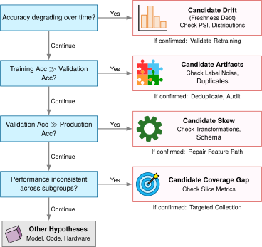
4.13 Fallacies and Pitfalls
Data engineering pipelines rarely fail with immediate runtime crashes; instead, they silently distort feature distributions, corrupt training state, or starve expensive accelerator clusters. The nine fallacies and pitfalls that follow collect the recurring assumptions behind those failures, pairing each with the pipeline measurement or contract that prevents it.
Fallacy: More data always improves model performance.
The bitter lesson says that general methods fed with more data and compute keep winning, but it does not say each new sample is worth as much as the last. Beyond a threshold, additional data yields diminishing returns described by empirical scaling laws, fitted curves relating model error to dataset size. Studies across computer vision, translation, and language modeling find that test loss falls as a power law in dataset size, so each successive error reduction demands a multiplicatively larger volume of samples (Hestness et al. 2017). In the illustrative KWS design space, a tenfold larger training set buys 5–8 percent more detection rate at 10× the labeling cost. In systems terms, repeated examples consume disk I/O, host-to-device bus bandwidth, and accelerator FLOPs without adding distinct observations. Repeated passes can still shift the model slightly, so redundancy must be judged by its measured effect on evaluation rather than assumed to contribute nothing. The task-relevant signal heuristic from section 4.9 captures this trade-off: scaling raw byte volume without preserving information density inflates infrastructure cost while yielding negligible improvements in evaluation loss.
Hestness, Joel, Sharan Narang, Newsha Ardalani, Gregory Diamos, Heewoo Jun, Hassan Kianinejad, Md. Mostofa Ali Patwary, Yang Yang, and Yanqi Zhou. 2017. “Deep Learning Scaling Is Predictable, Empirically.” arXiv Preprint arXiv:1712.00409.
↪ Scaling laws, and the selection methods that decide which samples are worth their training compute, are developed in The Data Wall.
Pitfall: Planning petabyte migration as a bandwidth-only transfer.
Dividing data volume by network link bandwidth gives the theoretical wire time, about 22 h for the chapter’s 1 PB example at 100 Gb/s, but wire transfer is rarely the critical path. Data gravity (section 4.9) binds large datasets to a web of surrounding infrastructure: ingestion transformation pipelines, schema validation checks, access-control policies, and downstream consumers. Moving a petabyte-scale corpus between clouds or data centers requires refactoring pipelines, revalidating data integrity, re-warming caches, and rebuilding metadata indexes. In practice, the engineering time spent adapting dependent systems dwarfs the raw network transit time.
Fallacy: Data preprocessing can be finished once and left alone.
Preprocessing pipelines turn raw observations into tensors using parameters fitted on historical data: tokenization vocabularies, mean and variance scaling vectors, category frequency tables, and numerical clipping bounds. When production distributions drift, these fixed transformations go stale. Tokenizers hit rising out-of-vocabulary rates, fixed normalization constants push scaled features outside the range the model trained on, and static clipping bounds cut off valid signal. Keeping the pipeline accurate requires monitoring input tensors and outcomes, then validating any change to preprocessing together with the model that consumes its features. Recomputing statistics independently at serving time can itself introduce skew.
Pitfall: Ignoring data serialization cost.
Profiling often focuses exclusively on accelerator execution while data loaders quietly parse raw JSON or CSV files. Parsing text-based records requires host CPU cores to spend hundreds of cycles per sample on string decoding, tokenization, ASCII-to-float conversions, and heap allocations. This host-side parsing starves the accelerator just as the dataloader choke point does (section 4.10.4). In the chapter’s ResNet-50 scenario, JPEG decoding already occupies 9 workers per accelerator, each preparing 375 img/s. A tabular or log-feature pipeline that parses text records pays the string-decoding cost described here on top of any such preparation. Binary serialization formats, such as Apache Arrow or memory-mapped arrays, eliminate parsing overhead by storing numbers directly in machine-native binary layouts that the loader can hand to the accelerator without conversion. For tabular schemas, columnar formats such as Parquet cut disk I/O by reading only the required columns. Benchmarking data ingestion against accelerator consumption rates shows whether host CPU deserialization is throttling training throughput.
Fallacy: High training accuracy indicates production readiness.
Training accuracy and held-out validation accuracy both describe the historical distribution the data was drawn from. Production adds edge cases, sensor noise, and live drift, and a model with high validation accuracy still fails if upstream feature pipelines change or inference timeouts trigger fallback defaults. Diagnosing post-deployment regressions requires the symptom checks across temporal drift, label artifacts, and training-serving skew ordered in figure 18, rather than reliance on a single offline score.
Pitfall: Ignoring training-serving skew until deployment.
Training-serving skew occurs when feature generation logic diverges between the offline training pipeline and the online inference runtime, for example through differences in floating-point precision, time-window aggregation, library versions, or temporal leakage from data timestamped after the prediction point. Because the model still receives valid floating-point vectors, inference raises no runtime exceptions while prediction quality degrades. Avoiding this pitfall requires shared transformation logic, reproducible feature stores, and automated predeployment parity tests that check feature equivalence across offline and online paths.
Fallacy: Synthetic data can fully replace real-world data collection.
Synthetic data enriches training sets by generating rare edge cases, controlled physical variations, or privacy-safe samples, but a generator can only sample within the assumptions built into it. When trained exclusively on synthetic data, models overfit to generator-specific artifacts and fail on real-world variation the generator never modeled. In a KWS system, for example, a detector trained entirely on synthesized speech loses accuracy when it meets real room reverberation, unfamiliar accents, microphone distortion, and shifting background noise. Synthetic generation supplements real collection, but representative real-world recordings remain essential for testing whether the system is ready to deploy.
Pitfall: Neglecting data versioning until model debugging requires it.
Treating training datasets as mutable object-storage directories destroys experiment reproducibility. When a retrained model loses accuracy, an unversioned pipeline cannot show whether the cause is a modified labeling rubric, a silent schema change, or genuine distribution shift, and once tables are overwritten or raw logs deleted, the historical training inputs cannot be rebuilt. As established in section 4.8.1, every model checkpoint must link immutably to a specific dataset snapshot, transformation code hash, and configuration file.
Fallacy: Production logs show where the model fails.
A deployed system decides much of what data comes back from it. The keyword spotter uploads audio only when it wakes, so its logs fill with correct detections and false wakes, while a wake word it misses leaves no recording at all (section 4.12.1). A team that measures quality from those logs alone sees a false-rejection rate lower than the real one, and retraining on the same logs over-represents the cases the model already handles. Measuring failures requires collection designed for that purpose: consented recording studies, reports of failed activations, and evaluation streams kept independent of the deployed model’s choices.
Self-Check: Question
An engineering team assumes that doubling their raw dataset volume by web scraping uncurated text and generating synthetic speech samples will automatically improve downstream model accuracy. According to the chapter’s fallacies and pitfalls, why is this assumption flawed?
- Because scaling laws exhibit diminishing returns (power-law test loss flattening), and adding uncurated or synthetic data can increase data gravity and transport energy while introducing generator domain gaps and noise.
- Because neural networks cannot mathematically process more than one million training records without floating-point overflow.
- Because synthetic data is legally prohibited from being combined with real-world sensor captures.
- Because web scraping always converts binary audio files into plain text formats, corrupting feature representations.
Explain why planning a petabyte-scale dataset migration solely as a network wire transfer (\(T = D_{\text{vol}}/\text{BW}\)) is a major systems pitfall.
True or False: Achieving high accuracy on a randomly split validation set during model development proves that the system will perform reliably after deployment.
4.14 Summary
A trained model is bounded twice by its data. The capability bound follows from the data-as-code principle (1): a changed dataset changes the trained model even when no algorithmic code changes, and a defect introduced in collection, schema, or labeling amplifies through every later stage as a data cascade. The throughput bound is the physics of the iron law’s data term. The pipeline must deliver bytes at the rate the accelerator consumes them, a requirement the feeding loss, the dataloader choke point, and the storage bandwidth budget each quantified at a different tier of the same ResNet-50 scenario. Data engineering therefore works in two overlaps of the D·A·M taxonomy at once. The capability half worked the Data–Algorithm overlap and the throughput half the Data–Machine overlap, and operations exists because the deployment distribution keeps shifting after launch, which reopens both overlaps. Acquisition, labeling, and feature contracts decide what the model can learn and keep training and serving computing the same function, while storage tiers, formats, and loaders decide how fast it learns.
Key Takeaways: Data is the source code
- Data is code; version it, test it, review it: Under the data-as-code principle (1), a dataset change is a code change. Give it version control, validation tests, and review.
- Data cascades make upstream quality the highest-return investment: The compounding failure arcs in figure 1 show how early collection errors bypass intermediate testing, requiring extensive rework across downstream artifacts and, in severe cases, complete pipeline restarts from deployment. The four pillars (quality, reliability, scalability, and governance) organize prevention, while documentation, schema, quality, and freshness debt require continuous remediation.
- Pipeline architecture choices have large cost implications: The chapter’s provisioning scenario costs streaming above batch, while its matched-retention example trades ETL storage savings against schema-change overhead. Actual costs depend on provisioning, retention, replay, and required freshness. Select ingestion patterns by the value of latency, not the appeal of real time.
- Labeling can dominate cost and requires substantial resource allocation: Labeling can cost thousands of times one optimized training run; in the reference calculation in section 4.6.2, the ratio is 2,498× to 4,995×. Labeling can remain a costly scheduling bottleneck even when annotation work is parallelized.
- Training-serving consistency is nonnegotiable: Feature transformations shared by training and serving must have equivalent semantics and reuse the same learned state, such as normalization constants and vocabulary mappings.
- Storage hierarchy sets input-loading time: The 50× throughput gap between local NVMe (5 GB/s) and one cloud object-storage connection (100 MB/s) changes input-loading time under the stated bandwidth assumptions. Total iteration time also includes transformation and model execution, so the loading ratio is not an end-to-end speedup.
- The degradation equation becomes actionable through drift and outcome monitoring: Divergence metrics such as KL measure changes between \(\CurrentDistribution\) and \(\TrainingDistribution\), while labeled outcomes or validated proxies determine whether those changes correspond to model degradation.
The keyword spotter carried the capability bound through the chapter, and ResNet-50 carried the throughput bound. The keyword spotter’s one-false-wake-per-month target turned an accuracy goal into a per-window false-positive bound whose evaluation requires representative negative audio, sufficient listening duration, and an explicit treatment of measurement uncertainty. Its fixed budget turned “more data” into a costed allocation of labels, storage, and governance. Its MFCC extraction had to agree, within a validated tolerance, between a cloud training cluster and a kilobyte-scale always-on island. Data engineering is the discipline of keeping two contracts at once, a physical contract with the machine that must be fed and a statistical contract with a deployment distribution that keeps moving, and the failures this chapter traced, from a starved accelerator to a silently retyped ZIP code, each came from a pipeline that kept one contract while breaking the other.
What’s Next: From data to computation
The data pipeline now delivers a clean, versioned training set at the rate the accelerator consumes it, yet this chapter has treated the model at the end of that pipeline as a consumer of bytes and nothing more. Neural Computation opens the consumer along the algorithm axis. It begins with the shift from hand-written logic to learned arithmetic, then counts the multiply-accumulate operations, activations, and gradient updates that turn prepared examples into learned behavior, and the memory and compute each one demands of the machine.
4.15 Self-Check Answers
Self-Check: Answer
A team is building a training dataset from distributed sensor logs. They discover that the same event can appear in multiple log partitions. They add a pipeline step that identifies duplicate records and keeps one canonical copy. Where must this step run, and why?
- After splitting, because each split should be cleaned independently so that evaluation data is never touched by training-side processing.
- Only on the training split, because duplicates in validation and test data do not affect the trained model.
- Before splitting, because a duplicated record that lands on both sides of the split leaks the same evidence into evaluation and inflates the measured quality.
- Anywhere in the pipeline, because duplicates only waste storage and compute and do not change what the model learns.
Answer: The correct answer is C. Splitting creates the trust boundary between training and evaluation; a duplicate that crosses it lets the model be scored on evidence it trained on, so evaluation looks better than deployment will. Deduplicating after the split cannot remove that leak, and duplicates also overweight repeated examples in what the model learns, so they are not merely a storage cost.
Learning Objective: Explain why deduplication must precede splitting to preserve the trust boundary between training and evaluation data.
Explain why treating training data as the ‘source code’ of a machine learning system necessitates software-engineering practices such as immutable snapshot versioning, automated regression testing, and explicit split boundaries.
Answer: In machine learning, model behavior is compiled from data through optimization rather than hand-written procedural code; modifying or deleting a training record alters the compiled artifact (the learned weights) just as altering source code changes a compiled binary executable. Because real-world distributions shift continuously—unlike inert source code—datasets require immutable versioned snapshots to reproduce training runs, automated regression tests to prevent silent data corruption, and strict trust boundaries between train, validation, and test splits to prevent data leakage from invalidating generalization estimates.
Learning Objective: Justify applying core software-engineering practices (immutable versioning, automated regression tests, and split trust boundaries) to datasets under the data-as-source-code paradigm.
True or False: In a keyword-spotting dataset, randomly partitioning audio recordings into an 80/20 train/test split at the individual audio file level maintains a valid trust boundary for estimating real-world generalization.
Answer: False. Randomly partitioning audio files without grouping by speaker allows recordings of the same speaker (or augmented variants of the same source utterance) to appear in both training and test sets. This creates data leakage across the trust boundary, causing evaluation metrics to reflect memorization of familiar voices and acoustic environments rather than true generalization to unseen deployment speakers. Audio datasets require speaker-independent and time-aware splits.
Learning Objective: Evaluate split strategies to prevent data leakage across train/test trust boundaries in speech and audio ML pipelines.
Self-Check: Answer
A data engineering team implements comprehensive synchronous schema and distribution validation checks directly inside the real-time event ingestion path. Under the Four Pillars framework, which primary operational trade-off will this team encounter?
- A Governance trade-off: inspecting payload schemas automatically breaches user data retention agreements.
- A Model Capacity trade-off: validating input records forces downstream neural network layers to increase parameter counts.
- A Scalability and Reliability trade-off: heavy synchronous validation consumes CPU cycles and increases per-record latency, reducing ingestion throughput and risking dropped messages during traffic spikes.
- A Durability trade-off: validating data records accelerates physical wear on persistent solid-state drive cells.
Answer: The correct answer is C. A Scalability and Reliability trade-off: heavy synchronous validation consumes CPU cycles and increases per-record latency, reducing ingestion throughput and risking dropped messages during traffic spikes. The Four Pillars framework highlights tension between Quality and Scalability/Reliability: performing exhaustive synchronous validation in the hot ingestion path adds CPU latency and backpressure, reducing peak throughput and creating potential availability failures under load surges. Production pipelines balance this by executing lightweight structural checks synchronously at ingestion while offloading deep statistical and semantic validation to asynchronous processing or dead-letter queues. The remaining choices misattribute the trade-off to privacy violations, neural parameter expansion, or SSD wear.
Learning Objective: Analyze the cross-pillar trade-offs between validation rigor (Quality) and processing throughput/latency (Scalability and Reliability).
True or False: Data cascades in ML systems are easily caught by standard software unit tests because corrupted input data causes deterministic assertion failures in pipeline code.
Answer: False. Data cascades are characterized as ‘silent’ failures precisely because corrupted or drifted data often remains syntactically valid (e.g., non-null strings or valid numeric ranges) and passes traditional code unit tests. The defect cascades downstream, subtly biasing feature distributions, distorting learned model representations, and degrading real-world accuracy without throwing software exceptions.
Learning Objective: Compare silent data cascade failure modes with traditional software bugs caught by unit tests.
**Trace the propagation sequence of a data cascade as described in the chapter, from its root cause to user-facing impact:
- Downstream model optimization on distorted representations
- Upstream sensor or schema change without contract notification
- Silent distortion of extracted features passing syntactic checks
- Degraded real-world predictions and costly post-deployment rollback**
Answer: The correct order is: (2) Upstream sensor or schema change without contract notification -> (3) Silent distortion of extracted features passing syntactic checks -> (1) Downstream model optimization on distorted representations -> (4) Degraded real-world predictions and costly post-deployment rollback. A data cascade begins with an uncoordinated upstream source or schema change. Because the data passes basic syntactic tests, it enters feature extraction and silently distorts intermediate representations. Downstream model training optimizes over these corrupted features, ultimately manifesting as degraded production predictions and requiring expensive system rollback.
Learning Objective: Analyze the multi-stage propagation of data cascades from upstream defects to production degradation.
Self-Check: Answer
An always-on Keyword Spotting (KWS) system on an embedded voice assistant continuously evaluates 1-second audio classification windows (\(24\text{ hours/day}\) over a \(30\text{-day}\) month). Treat each window as nonkeyword audio. The product budgets at most 1 expected false activation per month. An engineer reports 99% aggregate accuracy and, separately, a measured 1% false positive rate on background noise. How many false activations does that FPR imply in expectation, and what per-window FPR meets the expected-count budget?
- A 1% FPR implies an expected count of 720 false activations per month; the expected-count budget requires a per-window FPR of \(\le 1.38 \times 10^{-5}\).
- A 1% FPR implies an expected count of ~25,920 false activations per month (~36 false wakes/hour); the expected-count budget requires a per-window FPR of \(\le 3.86 \times 10^{-7}\) (>99.9999% non-keyword rejection).
- A 1% FPR implies an expected count of ~2,592 false activations per month; the expected-count budget requires a per-window FPR of \(\le 1.0 \times 10^{-4}\).
- A 1% FPR satisfies the expected-count budget because accuracy is averaged over the total number of audio hours across the entire device fleet.
Answer: The correct answer is B. A 1% FPR implies an expected count of ~25,920 false activations per month (~36 false wakes/hour); the expected-count budget requires a per-window FPR of \(\le 3.86 \times 10^{-7}\) (>99.9999% non-keyword rejection). Over a 30-day month with continuous 1-second windows, there are \(30 \times 24 \times 3600 = 2{,}592{,}000\) evaluation windows. A 1% false-positive rate gives an expected count of \(0.01 \times 2{,}592{,}000 = 25{,}920\) false wake-ups per month (roughly 36 per hour in expectation, far beyond the budget). To meet the expected-count budget of \(\le 1\) false activation per month, the per-window FPR must satisfy \(\text{FPR} \le 1 / 2{,}592{,}000 \approx 3.86 \times 10^{-7}\), requiring \(>99.9999\%\) non-keyword rejection. This expectation does not require independent windows and does not guarantee a maximum count in every month. Aggregate accuracy alone does not determine the nonkeyword FPR. The other options miscalculate the monthly window count or misapply aggregate metrics.
Learning Objective: Calculate the required per-window false positive rate for always-on streaming ML systems and explain why aggregate accuracy fails for streaming workloads.
The chapter specifies its keyword spotter by a keyword detection rate measured at a threshold that holds the expected false-wake budget, rather than by overall accuracy. Why is overall accuracy the wrong target for an always-on detector?
- Almost every one-second window contains no wake word, so a detector that never fires scores near-perfect overall accuracy while missing every command; the meaningful targets are the fraction of spoken wake words caught and the false-wake rate at the chosen threshold.
- Overall accuracy cannot be computed for a model that runs on a microcontroller, so the target must use a metric the device can calculate itself.
- Overall accuracy rises automatically with more training data, so it cannot distinguish one data plan from another.
- Detection rate and overall accuracy are the same quantity for a binary classifier; the scenario only renames it.
Answer: The correct answer is A. Wake words are rare among the windows the detector evaluates, so overall accuracy is dominated by easy non-keyword windows and rewards a detector that never fires. Evaluation runs offline, so the device’s ability to compute a metric is irrelevant. More data does not raise accuracy automatically, and the two metrics differ: accuracy averages over all windows, while detection rate counts only the windows that contain the wake word.
Learning Objective: Explain why rare-event detectors are specified by detection rate at a false-alarm operating point rather than by aggregate accuracy.
Self-Check: Answer
Multiple independent autonomous driving teams train their perception models exclusively on a popular public driving benchmark. What systemic failure mode does this practice introduce into the broader ecosystem?
- Shared dataset bias propagation, where common blind spots, annotation artifacts, and unrepresented edge cases can create correlated weaknesses across deployed models.
- Catastrophic memory leaks in GPU driver kernels caused by repeated reading of shared image formats.
- Immediate violation of data gravity constraints due to distributed multi-tenant reads.
- Automatic over-fitting to hardware memory hierarchies during distributed gradient synchronization.
Answer: The correct answer is A. Shared dataset bias propagation, where common blind spots, annotation artifacts, and unrepresented edge cases can create correlated weaknesses across deployed models. When multiple models across an industry rely on a single common benchmark dataset, systemic flaws (e.g., geographic bias, missing weather conditions, or consistent label errors) can propagate across models. Shared data creates a correlated-failure risk, not a guarantee that every model fails alike. The other options describe unrelated GPU memory bugs, network gravity violations, or hardware synchronization issues.
Learning Objective: Evaluate the ecosystem-wide risks of shared dataset bias propagation and benchmark over-reliance.
Discuss the primary advantages and critical risks of using synthetic data generation (e.g., 3D graphics rendering or generative audio simulation) as a core data acquisition strategy.
Answer: Advantages: Synthetic data provides scalable training examples with automatically generated labels consistent with the simulator (e.g., exact 3D bounding boxes, depth maps, or audio SNR) and enables targeted generation of rare safety-critical edge cases. Those labels describe the simulated scene; their relevance to the real task still requires validation. Risks: Synthetic generators inherit domain gaps and omissions from their underlying models; models trained purely on synthetic data often fail on real-world distributions due to missing acoustic reverberations, lighting variations, or demographic accents absent from the generator.
Learning Objective: Analyze the trade-offs between synthetic data scalability and real-world domain gaps in acquisition strategy.
True or False: Achieving state-of-the-art benchmark accuracy on a curated dataset (such as ImageNet or Common Voice) guarantees that an ML model is ready for deployment in real-world production environments.
Answer: False. Curated benchmarks provide standardized baselines for research comparison, but their distributions rarely capture the full variety of real-world deployment conditions (e.g., microphone hardware variations, regional acoustic noise, adversarial inputs, or demographic shifts). Models tuned specifically to benchmark distributions frequently suffer severe performance drops when exposed to uncurated production data.
Learning Objective: Explain why benchmark performance fails to guarantee real-world generalization across deployment distributions.
Order the following gap-closing acquisition steps into a sensible workflow: (1) choose an acquisition source for the remaining gap under budget and governance constraints, (2) define the coverage gap the model must close, (3) validate that the acquired data actually improves the missing coverage and meets quality requirements, (4) audit what existing sources and provenance already provide.
Answer: The correct order is: (2) define the coverage gap the model must close, (4) audit what existing sources and provenance already provide, (1) choose an acquisition source for the remaining gap under budget and governance constraints, (3) validate that the acquired data actually improves the missing coverage and meets quality requirements. The sequence matters because the team must know what is missing before it can judge whether reusable data already covers it, and only then can it choose a new source for the residual gap. Swapping source selection ahead of the audit would spend money before measuring what is already available, while skipping the final validation would mistake acquired volume for actual coverage and quality improvement.
Learning Objective: Design a gap-closing acquisition workflow that moves from missing-coverage definition through source audit, targeted acquisition, and post-acquisition validation.
Self-Check: Answer
An ML engineering team is architecting an ingestion pipeline for tabular transaction data. They evaluate Extract-Transform-Load (ETL) versus Extract-Load-Transform (ELT). Which architectural trade-off correctly characterizes ELT in modern data lakehouses?
- ELT executes all transformations in memory on the edge device before transmitting bytes to cloud storage.
- ELT requires rigid upfront schema definitions (schema-on-write) and rejects any semi-structured data formats.
- ELT loads raw data directly into scalable lakehouse storage first and transforms it downstream using scalable query engines, preserving raw data history and decoupling ingestion from evolving feature logic.
- ELT eliminates the need for data governance and quality validation because transformations occur after storage.
Answer: The correct answer is C. ELT loads raw data directly into scalable lakehouse storage first and transforms it downstream using scalable query engines, preserving raw data history and decoupling ingestion from evolving feature logic. ELT decouples raw ingestion from transformation: retained raw events allow downstream engines to recompute features when definitions change. Retention, access controls, validation, and schema compatibility still constrain reuse. ETL transforms data before loading and may omit raw fields from the derived warehouse tables, but it can retain replayable raw inputs in a separate source archive. Comparing the two designs requires the same retention horizon, a stated replay source, and costs measured through the same feature-ready endpoint. The remaining options mischaracterize edge compute, schema requirements, or governance needs.
Learning Objective: Compare ETL and ELT architectures regarding storage decoupled ingestion, schema evolution, and historical data retention.
Explain how a Circuit Breaker and a Dead Letter Queue (DLQ) can reduce cascading failures and preserve rejected records for replay in streaming ML ingestion. What conditions constrain these benefits?
Answer: A Circuit Breaker stops calls to a failing dependency after a threshold, reducing cascading timeouts and resource pressure. Cached or default features require a validated feature-age and task-quality contract; otherwise requests are rejected. A durable, retained DLQ can isolate rejected records with error metadata for later inspection and replay. Preserving those records depends on successful durable writes, sufficient capacity, retention, access, and a usable replay path; these mechanisms do not guarantee freedom from data loss.
Learning Objective: Design reliable streaming data pipelines using Circuit Breaker and Dead Letter Queue (DLQ) patterns for fault isolation.
Using the 2016 Microsoft Tay chatbot incident, explain why public data ingestion surfaces require strict input validation, rate limiting, and adversarial filtering before data shapes model behavior.
Answer: Microsoft Tay ingested uncurated public user interactions from Twitter to adapt its responses. Adversarial users exploited this unfiltered public surface with coordinated toxic prompts, causing the bot to tweet abusive statements within 16 hours. The incident demonstrates that any public ingestion path directly influencing model behavior acts as a security attack surface, requiring robust content filtering, anomaly detection, adversarial input controls, and rate limits to prevent malicious data from corrupting the system.
Learning Objective: Analyze the security and safety implications of unvalidated public data ingestion using the Microsoft Tay war story.
An explicit, machine-enforceable agreement between data producers and data consumers that defines column types, value bounds, nullability, and distribution constraints is called a ____.
Answer: The correct answer is schema contract (or data contract). Schema contracts catch declared structural and semantic violations at integration boundaries. Distribution shifts that remain within the schema still require statistical monitoring and outcome-based diagnosis.
Learning Objective: Explain schema contracts and their role in preventing breaking changes across ML data pipelines.
Self-Check: Answer
A smart city perception system evaluates annotation formats for a \(1920 \times 1080\) video stream. The team compares bounding box annotations (10 boxes per frame, each with 4 spatial coordinates) against pixel-level semantic segmentation masks. What is the ratio of scalar label entries generated between a full segmentation mask and the 10 bounding boxes?
- Roughly 10x more entries for segmentation, matching the ratio of bounding box coordinates.
- Roughly 50,000x more scalar entries for segmentation (~2.07 million pixel labels vs. 40 bounding box coordinates).
- Both formats require identical scalar entries because both represent 1080p resolution.
- Bounding boxes require 50,000x more entries because floating-point coordinates consume more bytes than integer masks.
Answer: The correct answer is B. Roughly 50,000x more scalar entries for segmentation (~2.07 million pixel labels vs. 40 bounding box coordinates). A \(1920 \times 1080\) image contains \(2{,}073{,}600\) pixels, requiring ~2.07 million discrete pixel class labels for semantic segmentation. In contrast, 10 bounding boxes with 4 coordinates each store \(10 \times 4 = 40\) scalar entries. The ratio is \(2{,}073{,}600 / 40 \approx 51{,}840 \approx 50{,}000\times\). This is a scalar-entry ratio, not a storage-byte or human-effort ratio. Encoding and compression determine stored bytes; annotation tooling and boundary complexity determine human effort.
Learning Objective: Calculate the storage and annotation scale differences between classification, bounding boxes, and pixel-level semantic segmentation.
A team wants to compare the total cost of two acquisition plans: one relies on human labeling, and the other emphasizes storing a large retained corpus for later reuse. The chapter’s cost table gives rates such as per-label, per-box, and per-terabyte-per-month costs. Which additional quantities are necessary to turn those rates into a fair total-cost comparison?
- Only the GPU training hours, because acquisition cost can be inferred once compute usage is known.
- Only the number of source websites and annotators, because storage and labeling rates are universal constants that do not need workload quantities.
- Only the final model accuracy target, because unit costs scale directly from performance goals.
- The number of labels or boxes to be paid for, plus the total retained terabytes and storage months to be paid for, because the rows use different units and must be scaled by their own quantities.
Answer: The correct answer is D. The chapter explicitly warns that these rows are rates with different units, so a fair comparison needs the workload quantities each rate prices: how many labels or boxes are purchased, and how many terabytes are retained for how many months. An answer based only on accuracy targets or compute hours omits the unit-conversion step, while an answer that treats the listed prices as universal constants misses the chapter’s warning that they are illustrative and workload-specific.
Learning Objective: Identify the workload quantities needed to scale mixed-unit labeling and storage rates into comparable total costs.
An ML team applies weak supervision to label a large unlabeled text corpus using heuristic rules and keyword patterns written by domain experts. According to the chapter, what is the main trade-off this approach makes?
- It guarantees expert-level labels at scale, so no additional quality checks or audits are needed once the heuristics run.
- It replaces all human involvement with deterministic labels, so disagreement between heuristics becomes a schema-validation problem rather than a quality problem.
- It increases labeling scale by applying programmatic heuristics cheaply across many examples, but the resulting labels are still noisy and must be validated against held-out human-audited data.
- If several heuristics agree on a label, that agreement is enough to treat the label as correct without checking against an independent human-audited set.
Answer: The correct answer is C. Weak supervision trades per-example manual labeling for cheap, scalable programmatic labeling, but the produced labels remain noisy and need validation against held-out human-audited data. The expert-guarantee answer ignores that heuristic labels can systematically encode mistakes, and the agreement-based answer confuses consensus among correlated heuristics with ground-truth correctness: multiple rules can agree for the same wrong reason.
Learning Objective: Explain the scale-versus-noise trade-off in weak supervision and why validation remains necessary after programmatic labeling.
Describe how a tiered consensus labeling system uses inter-annotator agreement metrics (such as Fleiss’ kappa) and ‘gold standard’ honeypot examples to balance labeling cost against annotation quality.
Answer: A tiered consensus system routes data through escalating quality tiers: inexpensive crowdsourced workers label all instances, using per-item disagreement and failed gold-standard checks to route selected items to domain experts. Fleiss’ kappa measures cohort agreement, not per-example confidence or annotator accuracy. Independent gold-standard checks and expert audits assess correctness: annotators can share systematic errors despite high agreement. Routine items can be accepted under a validated review policy while escalation and auditing control cost and quality.
Learning Objective: Design a tiered consensus labeling workflow using inter-annotator agreement metrics and gold-standard benchmarks.
True or False: In Active Learning, uncertainty sampling selects the unlabeled examples for which the current model has the highest prediction confidence to ensure the training set contains only clean data.
Answer: False. Uncertainty sampling selects the examples where the model is least confident (e.g., smallest difference between top two predicted class probabilities or highest prediction entropy). Uncertainty is a selection heuristic, not proof of label value: ambiguous, corrupted, or unrepresentative inputs can also be uncertain. Its benefit and scoring cost must be validated against the task and budget.
Learning Objective: Evaluate active learning query strategies (uncertainty, margin, and entropy sampling) for sample efficiency.
A statistical metric that measures the degree of agreement among three or more annotators classifying items into discrete categories, adjusting for chance agreement, is called ____.
Answer: The correct answer is Fleiss’ kappa (or Fleiss’ kappa statistic). Fleiss’ kappa generalizes Cohen’s kappa to multi-annotator workflows, summarizing agreement across a collection of rated items. It does not establish individual-label confidence or correctness; per-item disagreement supports routing, and independent gold-standard checks or audits assess correctness.
Learning Objective: Apply Fleiss’ kappa as the standard inter-annotator agreement metric in multi-annotator labeling workflows.
Self-Check: Answer
An engineer normalizes a numerical feature by computing standard \(z\)-scores: \(x' = (x - \mu)/\sigma\). During production serving, how must the parameters \(\mu\) and \(\sigma\) be handled to satisfy the consistency imperative and prevent training-serving skew?
- Persist the exact \(\mu\) and \(\sigma\) computed on the training dataset alongside the model artifact, loading and applying those fixed constants to live serving inputs.
- Recompute \(\mu\) and \(\sigma\) dynamically over each incoming serving batch to ensure the live data is always centered at zero.
- Discard \(\mu\) and \(\sigma\) entirely at inference time and rely on batch normalization layers inside the neural network.
- Compute \(\mu\) and \(\sigma\) independently over a rolling 1-hour window of serving traffic to track seasonal shifts.
Answer: The correct answer is A. Persist the exact \(\mu\) and \(\sigma\) computed on the training dataset alongside the model artifact, loading and applying those fixed constants to live serving inputs. The consistency imperative requires state synchronization across training and serving: transformation parameters computed during training (means, standard deviations, one-hot vocabularies, embedding lookups) must be persisted and reused during serving. Recomputing statistics dynamically over live batches or rolling windows alters the feature scale relative to what the model learned, creating training-serving skew and causing silent prediction degradation. Relying on neural batch normalization does not resolve pre-network input feature scaling.
Learning Objective: Apply the consistency imperative by synchronizing stateful transformation parameters between training and serving.
A feature pipeline outgrows one server and its data is split into partitions across several machines. Which operation adds the least network transfer in the cluster compared with running it on one machine?
- A join between two tables partitioned on different keys, because the database engine performs the join automatically.
- A global shuffle that regroups every record by speaker identifier, because each record moves only once.
- Computing a global mean, because each machine can reduce its own partition to a partial sum and count and send only that summary.
- Gathering all partitions onto one coordinator machine before any processing, because a single machine avoids coordination entirely.
Answer: The correct answer is C. Computing a global mean, because each machine can reduce its own partition to a partial sum and count and send only that summary. A decomposable reduction exchanges one small partial result per partition, so the network carries almost nothing and the computation stays where the data already lives. A shuffle or a join must send records, not summaries, across partitions, and gathering every partition onto one machine moves the entire dataset over the network before any work begins. Once processing spans machines, network transfer, data locality, and coordination with slow or failed workers become first-order costs that a single machine never pays.
Learning Objective: Explain why operations that exchange summaries stay cheap across machines while operations that exchange records pay network transfer and coordination costs.
Define idempotency in the context of data transformation pipelines and explain why idempotent operations (such as upserts) are essential for fault recovery in distributed ML pipelines.
Answer: Idempotency means applying an operation multiple times produces the exact same system state as applying it once (\(f(f(x)) = f(x)\)). In distributed pipelines subject to network timeouts and worker crashes, retry mechanisms can execute the same task repeatedly; non-idempotent operations (such as appending rows) create duplicate records and corrupt gradient updates, whereas idempotent operations (such as database upserts or deterministic partition overwrites) allow safe retries without duplicating data.
Learning Objective: Explain the importance of idempotent transformations and deterministic pipelines for safe fault recovery.
True or False: Using the identical Python preprocessing function in both training and serving code repositories is sufficient to eliminate training-serving skew.
Answer: False. Sharing code logic is necessary but insufficient. Training-serving skew also arises from state desynchronization (using different normalization constants or vocabulary encodings), temporal dependencies (using current clock time rather than fixed reference timestamps), timing differences (batch aggregations over historical tables vs. live event streams), and environmental library version mismatches.
Learning Objective: Analyze the root causes of training-serving skew beyond shared source code.
Order the following steps for keeping an audio feature transformation consistent between training and serving: (1) split the data into the appropriate training and evaluation partitions, (2) version the transformation code together with the fitted transformation state, (3) fit any transformation state, such as normalization or vocabulary parameters, using only the training partition, (4) reuse the same transformation or a validated equivalent during serving and check that outputs stay within an accepted tolerance.
Answer: The correct order is: (1) split the data into the appropriate training and evaluation partitions, (3) fit any transformation state, such as normalization or vocabulary parameters, using only the training partition, (2) version the transformation code together with the fitted transformation state, (4) reuse the same transformation or a validated equivalent during serving and check that outputs stay within an accepted tolerance. The ordering is necessary because fitting before splitting would leak evaluation information into the transformation state, and serving cannot safely reuse the transform until both the code and fitted parameters have been captured as versioned artifacts. Swapping the last two would leave the deployment path using untracked or mismatched preprocessing, which is exactly the training-serving skew the section warns against.
Learning Objective: Sequence the steps required to preserve training-serving consistency for stateful audio transformations.
How does a feature store’s point-in-time correctness (time-travel join) prevent data leakage during offline training dataset generation?
- It encrypts historical feature values so that model weights cannot memorize training labels.
- It forces all features to be computed strictly in real time on the client device during model inference.
- It converts all timestamps into UTC strings to prevent database indexing errors.
- It reconstructs feature values exactly as they existed at the observation timestamp of each training event, preventing future feature values from leaking into historical training records.
Answer: The correct answer is D. It reconstructs feature values exactly as they existed at the observation timestamp of each training event, preventing future feature values from leaking into historical training records. When generating training datasets from historical logs, naive table joins risk using feature values computed after the prediction event occurred (e.g., joining an event at \(t=10:00\) with an aggregate feature updated at \(t=12:00\)). A feature store’s point-in-time join ensures that each training example receives features valid precisely as of its event timestamp, excluding future-data leakage only when it also preserves what information was actually available to the prediction path at that time, including late events and later backfills. Encryption, client-side inference, and UTC string conversion do not prevent temporal leakage.
Learning Objective: Explain how feature store point-in-time correctness prevents temporal data leakage during training dataset construction.
Self-Check: Answer
In the chapter’s KWS dataset release, each clip’s split is assigned by hashing its speaker key rather than by drawing splits at random each time a release is built. What failure does this prevent?
- A later release or relabeling pass could move some of a test speaker’s clips into training, so evaluation would reward memorization of that voice instead of generalization to new speakers.
- Hashing compresses the audio so that each split fits in less storage.
- Hashing guarantees equal numbers of keyword and non-keyword clips in every split.
- Hashing removes the need to record a consent reference for each clip.
Answer: The correct answer is A. A deterministic speaker-keyed assignment keeps every clip from a speaker in the same split in every release, so rebuilding or relabeling the dataset cannot leak test speakers into training. Hashing a key does not compress audio, balance classes, or replace consent records, which the release tracks as a separate field.
Learning Objective: Explain how deterministic, speaker-keyed split assignment prevents leakage across dataset releases.
A keyword spotter’s detection rate drops after a scheduled retraining even though no code changed. Explain how a dataset release that records label rubric versions, alignment versions, and feature configuration lets the team locate the cause.
Answer: Comparing the two releases field by field separates the possible causes. New or removed recordings show up as changed recording IDs; a change in labeling rules shows up as a different rubric version on the same clips; a segmentation change shows up as a different aligner version or boundary confidence; and a feature change shows up as a different configuration or code commit. In the chapter’s example, the comparison exposes a backfill that added crowdsourced clips under the wrong label mapping. Without the release, the team would have to guess among these causes and rerun experiments to test each one.
Learning Objective: Use a versioned dataset release to localize the cause of a model regression to data, labels, segmentation, or feature code.
Self-Check: Answer
A machine learning team maintains a \(1\text{ PB}\) raw training corpus in a US East cloud storage bucket and provisions a dedicated compute cluster in US West. The regions are connected by a dedicated \(100\text{ Gbps}\) network fabric. Cloud egress pricing is $0.02/GB, and the model training run takes \(20\text{ hours}\). Under the chapter’s data-gravity reasoning, which conclusion is best supported by these numbers?
- The team should stream the dataset remotely during training, because a \(100\text{ Gbps}\) link guarantees that data movement cannot become the bottleneck.
- The team should split the dataset evenly across regions, because cross-region placement automatically removes the need to evaluate transfer cost or placement constraints.
- The team should first apply compression, because any realistic compression plan will make the transfer clearly cheaper and faster than colocating compute.
- The ideal one-time transfer is about \(22.2\text{ hours}\) and costs about $20,000, so colocating or relocating compute near the data is worth evaluating, but the final decision still depends on compute availability, cost, and other deployment constraints.
Answer: The correct answer is D. Moving \(1\text{ PB}\) over a \(100\text{ Gbps}\) link takes about \(22.2\text{ hours}\) in the idealized calculation and costs about $20,000 in egress, so locality is a serious design consideration. The remote-streaming answer ignores that the wire time alone is comparable to the full \(20\text{ hour}\) training run, while the compression answer overclaims evidence the scenario does not provide: no compression ratio or feasibility constraint is given.
Learning Objective: Calculate ideal transfer time and egress cost, then evaluate what those numbers do and do not justify in a data-placement decision.
Assume decoded tensors must be read from storage at a sustained demand of \(1.8\text{ GB/s}\), while the attached baseline block-storage path can supply only \(250\text{ MB/s}\). Assume no compression or cache alternative changes this bound. Under this simplified feeding-loss model, what follows?
- The storage bound reduces the sustained baseline throughput by about \(86\%\) relative to its supplied demand, because the supply-to-demand ratio is \(0.25/1.8 \approx 0.139\) and the feeding loss is about \(1-0.139 \approx 0.86\).
- The accelerator remains compute-bound, because storage throughput and tensor execution are independent once batches have been scheduled.
- Increasing batch size alone removes the bottleneck, because larger steps always improve the ratio between storage supply and decoded-tensor demand.
- The storage path is only modestly underprovisioned, so the waiting fraction must stay below \(20\%\).
Answer: The correct answer is A. Under the stated simplification, the supply rate is \(0.25\text{ GB/s}\) against a demand of \(1.8\text{ GB/s}\), so the supply-to-demand ratio is \(0.25/1.8 \approx 0.139\) and the modeled throughput loss relative to that baseline is about \(1-0.139 \approx 0.86\), or \(86\%\). This idealized steady-state overlap model does not measure all accelerator idle time or utilization relative to advertised peak. The compute-bound answer ignores pipeline starvation: if decoded tensors cannot arrive fast enough, execution units wait regardless of their arithmetic capability.
Learning Objective: Apply the simplified feeding-loss calculation to estimate how a storage-bandwidth shortfall reduces modeled throughput relative to the supplied sustained baseline.
Using the data selection gain relationship \(\text{Gain} \propto \frac{\text{Task-Relevant Signal}}{\text{Data Gravity}}\), explain why removing \(50\%\) redundant samples can have large systems value when the retained dataset still covers the task-relevant cases and the training schedule is held fixed in passes over the data. Why is quality validation still necessary?
Answer: If deduplication removes \(50\%\) redundant volume while retaining the task-relevant coverage, then each pass moves about half as many bytes for essentially the same useful evidence, so the system can cut data movement and storage work substantially under the same pass-based schedule. For example, the loader, storage path, and preprocessing stack now handle half the volume each epoch, which lowers I/O pressure and repeated movement cost even if model execution was previously compute-bound. The practical implication is that deduplication is high-leverage only after validation confirms that the removed records were truly redundant rather than rare but important cases, so quality checks must verify coverage and downstream model behavior rather than assume unchanged accuracy.
Learning Objective: Analyze how deduplication can reduce data movement cost under a fixed training schedule while still requiring validation of retained coverage and model quality.
**According to the chapter’s energy-movement hierarchy, arrange the following operations in ascending order of energy consumed per 32-bit value (from lowest energy to highest energy):
- Local NVMe SSD access
- On-chip 32-bit FP multiply
- Data-center network transfer
- Off-chip DRAM memory access**
Answer: The correct order is: (2) On-chip 32-bit FP multiply -> (4) Off-chip DRAM memory access -> (1) Local NVMe SSD access -> (3) Data-center network transfer. Using the chapter’s figures, an on-chip 32-bit floating-point multiply costs about \(3.7\text{ pJ}\) (baseline). Moving a 32-bit value from off-chip DRAM costs about \(640\text{ pJ}\) (about \(173\times\)). Reading it from a local SSD costs about \(4{,}000\text{ pJ}\) (about \(1{,}081\times\)). Sending it across a data-center network costs about \(40{,}000\text{ pJ}\) (about \(10{,}811\times\)).
Learning Objective: Compare storage and compute operations across the memory hierarchy by their relative energy cost per bit.
The modeled throughput penalty from insufficient input supply relative to the supplied sustained training baseline is termed the ____.
Answer: The correct answer is feeding loss (or the feeding loss). The feeding loss quantifies modeled throughput loss when input supply cannot keep pace with the sustained baseline demand. It does not by itself measure all accelerator idle time or utilization relative to advertised peak.
Learning Objective: Explain the technical definition and systems impact of the feeding loss in ML data pipelines.
Self-Check: Answer
An ML systems architect must select storage backends for three distinct workloads: (1) Millisecond point lookups of user feature vectors during real-time online serving; (2) High-throughput sequential scans over tabular fraud features during batch training; (3) Storing petabytes of raw, unstructured multi-modal audio and video recordings. Which mapping of storage architectures to workloads is optimal?
- Low-latency transactional database / key-value store; (2) Columnar data warehouse; (3) Scalable cloud data lake (object storage).
- Cloud object storage (S3); (2) Key-value database; (3) Columnar data warehouse.
- Columnar data warehouse; (2) Cloud data lake; (3) Low-latency transactional database.
- Scalable cloud data lake; (2) Low-latency transactional database; (3) Columnar data warehouse.
Answer: The correct answer is A. (1) Low-latency transactional database / key-value store; (2) Columnar data warehouse; (3) Scalable cloud data lake (object storage). Storage architectures optimize for specific access patterns: online serving requires high IOPS and millisecond random access provided by transactional key-value databases; batch training over structured tables requires high sequential read throughput and column projection provided by columnar data warehouses; and petabyte-scale multi-modal raw data requires the cheap capacity and schema-on-read flexibility of cloud data lakes (object storage). The other mappings mismatch access patterns to storage strengths, causing high latency or extreme costs.
Learning Objective: Evaluate storage systems (databases, data warehouses, data lakes) based on IOPS, sequential throughput, and schema flexibility requirements.
Explain the storage-bandwidth bottleneck when feeding accelerators directly from cloud object storage versus local NVMe SSDs, and describe the common architectural caching pattern used to resolve it.
Answer: A dated scenario compares a single cloud object-storage stream at ~\(100\text{ MB/s}\) with local NVMe at ~\(5\text{ GB/s}\), a \(50\times\) bandwidth ratio for those paths. Whether object storage starves training depends on aggregate concurrency, caching, sample size, and the binding pipeline stage. A common tiered design retains corpora in object storage (~\(\$23/\text{TB/month}\)) and prefetches active tranches onto local NVMe (~\(\$100\text{--}300/\text{TB/month}\) in the chapter’s dated scenario) for repeated scans. Staging helps only when the storage path binds and its cost is justified.
Learning Objective: Analyze the bandwidth and cost trade-offs between cloud object storage and local NVMe SSD caching in ML training pipelines.
True or False: In a columnar storage format like Apache Parquet, reading 10 columns out of a 100-column table requires scanning the entire uncompressed row payload from disk.
Answer: False. Parquet organizes data by column, so column projection can avoid unselected columns. With equal-sized uncompressed columns, selecting 10 of 100 gives an illustrative 90% payload-I/O reduction, ignoring metadata and other overhead. Compression and unequal column sizes change the byte ratio. Predicate pushdown is a separate mechanism that can skip data based on filters and available statistics; it is not required for column projection.
Learning Objective: Explain the I/O reduction mechanisms (column projection and filter pushdown) of columnar storage formats.
Order the following release-preparation steps for a storage design that must support both model training and online serving: (1) validate point-in-time training retrieval together with serving freshness and latency, (2) define the training and serving access requirements, (3) materialize the appropriate offline training path and online serving path, (4) fix the versioned feature definitions and fitted transformation state.
Answer: The correct order is: (2) define the training and serving access requirements, (4) fix the versioned feature definitions and fitted transformation state, (3) materialize the appropriate offline training path and online serving path, (1) validate point-in-time training retrieval together with serving freshness and latency. The sequence matters because storage choices follow from access requirements, and the offline and online paths cannot be materialized safely until the feature definitions and state they must serve are fixed. Swapping validation earlier would test an unstable design, while treating the offline and online paths as one serial traversal would miss the chapter’s point that they are parallel responsibilities with different access patterns.
Learning Objective: Design a release-preparation sequence that aligns storage paths with training access, serving access, feature versioning, and final correctness checks.
Self-Check: Answer
During evaluation, a keyword spotter produces zero false wakes over 500 hours of representative non-keyword audio. Does this establish a budget of at most one false wake per month (about 720 hours of listening) at 95 percent confidence?
- No. With zero observed events, the 95 percent upper bound on the rate is about three events divided by 500 hours, roughly one per 167 hours, far above one per 720 hours; about 2,160 hours with no false wakes would be needed.
- Yes. Zero observed false wakes means the true false-wake rate is zero.
- Yes. Five hundred hours is close enough to a month of listening to support a monthly claim.
- No. False wakes can only be measured on devices after launch, never in offline evaluation.
Answer: The correct answer is A. A finite listening period cannot show that the rate is zero; with no events observed, the one-sided 95 percent upper bound on a Poisson rate is about three divided by the listening time. Five hundred hours bounds the rate only at about one per 167 hours, so the monthly claim needs roughly three times 720, about 2,160 hours. Offline evaluation on representative streams is exactly how the claim is established before launch.
Learning Objective: Compute the listening time needed to support a false-alarm budget when no false alarms are observed.
The ResNet-50 pipeline passes acceptance on a SATA solid-state drive today. Explain why the chapter still sizes the storage tier for a higher rate, and what change would make the SATA drive the bottleneck.
Answer: Today the accelerator sustains about 3,200 images per second, and a SATA drive supplies about 3,333 images per second of compressed JPEGs, so storage is not the binding stage. Faster kernels or a faster accelerator push the rate toward the compute ceiling of roughly 12,700 images per second. At that point the same drive caps delivery near 3,333 images per second and the accelerator idles most of the time. Each fix to the slowest stage exposes the next, so the tier is sized for the rate the pipeline is heading toward.
Learning Objective: Apply the slowest-stage bound to predict how removing one bottleneck exposes the storage tier.
Self-Check: Answer
An engineering team assumes that doubling their raw dataset volume by web scraping uncurated text and generating synthetic speech samples will automatically improve downstream model accuracy. According to the chapter’s fallacies and pitfalls, why is this assumption flawed?
- Because scaling laws exhibit diminishing returns (power-law test loss flattening), and adding uncurated or synthetic data can increase data gravity and transport energy while introducing generator domain gaps and noise.
- Because neural networks cannot mathematically process more than one million training records without floating-point overflow.
- Because synthetic data is legally prohibited from being combined with real-world sensor captures.
- Because web scraping always converts binary audio files into plain text formats, corrupting feature representations.
Answer: The correct answer is A. Because scaling laws exhibit diminishing returns (power-law test loss flattening), and adding uncurated or synthetic data can increase data gravity and transport energy while introducing generator domain gaps and noise. The chapter highlights the fallacy that ‘more data always improves performance’: empirical loss follows power-law curves where marginal gains diminish, and redundant or uncurated data increases data gravity (\(D_{\text{vol}}\)) and processing costs without adding task-relevant signal. Furthermore, synthetic data inherits generator domain gaps that fail to represent real deployment conditions. The other options invent false mathematical limits, legal bans, or automatic file format conversions.
Learning Objective: Evaluate the fallacy of monotonic scaling with uncurated or synthetic data using diminishing returns and domain gaps.
Explain why planning a petabyte-scale dataset migration solely as a network wire transfer (\(T = D_{\text{vol}}/\text{BW}\)) is a major systems pitfall.
Answer: Treating a petabyte-scale migration as a simple network transfer overlooks the massive systemic overhead of data gravity: updating transformation pipelines, re-engineering feature stores, revalidating data quality and schema contracts across environments, re-establishing lineage tracking, and synchronizing dependent downstream training jobs. The non-network engineering and validation time often exceeds the raw wire transfer time by weeks or months.
Learning Objective: Analyze the hidden engineering and validation overheads in large-scale dataset migration beyond raw network wire transfer time.
True or False: Achieving high accuracy on a randomly split validation set during model development proves that the system will perform reliably after deployment.
Answer: False. High validation accuracy only measures performance on data sampled from the historical distribution under development conditions. It does not account for production distribution shifts, training-serving skew, adversarial inputs, unrepresented deployment subgroups, or leakage across train/validation splits.
Learning Objective: Evaluate why high validation accuracy is insufficient to guarantee production reliability without drift and skew monitoring.