Introduction {#sec-introduction}

1 Introduction

Purpose

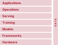
Architecture stack focus for this chapter.

Why does an accurate machine learning model not guarantee a reliable, efficient system?

Machine learning systems have a physics. Data moves through memory hierarchies governed by bandwidth, arithmetic executes on silicon governed by power, and predictions must arrive within strict latency windows. These constraints are not secondary implementation details. Moving an operand from main memory can cost far more energy than performing arithmetic on it, and a prediction that arrives a few hundred milliseconds late can be worth nothing to the real-time process waiting for it. An architecture that fits comfortably in a data center is useless on a mobile phone, and a training pipeline that converges in days on high-bandwidth accelerators can stall for weeks on standard hardware. These systems also diverge from conventional software because empirical data, rather than explicit logic alone, defines their behavior. When a conventional program misbehaves, it often crashes or throws an exception. When an ML system misbehaves, the runtime may operate flawlessly while learned predictions fail because the input distribution has shifted or the training data was unrepresentative. No assertion fails and no exception is raised; the only symptom is deteriorated decisions, discovered weeks later through lost revenue, erroneous predictions, or compromised safety. Testing, version control, and profiling remain necessary but are no longer sufficient. A unit test confirms that code computes what it was written to compute, but it cannot establish that learned behavior still matches a non-stationary world, and optimizing one component in isolation frequently moves the bottleneck to another layer of the stack. In D·A·M terms, data, algorithm, and machine must be engineered together as one problem.

Learning Objectives

• Explain why data-defined behavior lets predictive quality decline while model code and execution remain unchanged
• Apply a data-algorithm-machine lens to diagnose a system bottleneck and reassess it after an intervention
• Calculate execution time with the iron law and assess how a component improvement changes end-to-end time
• Analyze when scalable search and learning can benefit from additional computation within data and machine constraints
• Compare algorithmic, compute, and data-selection efficiency by the iron-law term each changes and the accuracy gained per added cost
• Evaluate whether predictive quality and resource use meet deployment requirements using evaluation and lifecycle monitoring

1.1 The AI Systems Moment

Artificial intelligence is no longer confined to research demonstrations. When a user queries a smartphone voice assistant, learned components convert speech to text, interpret intent, retrieve information, and generate a response within seconds. Search engines rank results, recommendation systems decide what people see, lenders use models to assess risk, and driver-assistance systems detect hazards. In each case, a prediction participates in a larger decision that can affect attention, money, access, or safety. Even a single voice query is therefore a chain of models and services operating in the world.

Modern AI systems became practical when three forces converged: digital services generated large datasets, learning algorithms extracted predictive structure from those examples, and parallel hardware made the resulting computation feasible. Yet the most consequential change was conceptual. Data stopped being merely an input to software; it became a mechanism defining program behavior. Instead of hand-coding every decision rule, engineers build a training process through which examples shape the behavior a system learns.

This convergence creates a dual mandate. Every ML system must establish that its learned behavior is trustworthy and that the machine can produce that behavior within the available time, memory, energy, and cost. A model that is accurate but too slow is unusable; a fast model trained on unrepresentative data is wrong at machine speed. At scale, both obligations span the entire stack. Conversational services coordinate pools of GPUs¹ while managing memory, networks, and cooling. Driver-assistance systems must fuse sensor streams within milliseconds. A search service processing more than 13.7B queries per day (Srinivasan 2025) must also meet strict latency targets. These systems succeed only when learned behavior and physical execution are engineered together. That co-design begins with the shift from code-defined logic to data-defined behavior.

¹ GPU (graphics processing unit): Originally designed to render graphics by performing many calculations in parallel. Neural networks also require large numbers of similar arithmetic operations, especially matrix multiplications, making this hardware useful for training. Keeping those operations supplied with data remains a separate engineering challenge.

Srinivasan, Vidhya. 2025. AI, Personalization and the Future of Shopping. The Keyword (Google blog).

Self-Check: Question

1. A production autonomous vehicle perception model reliably detects obstacles under clear daytime conditions, but fails to identify a pedestrian at dusk even though all code executes without runtime exceptions and strictly within its 50 ms latency window. Which core challenge of ML systems engineering does this failure demonstrate?

   1. The latency added by serial interconnect communication across distributed accelerators
   2. A hardware execution failure caused by GPU thermal throttling and clock frequency scaling
   3. The dual mandate requirement that learned behavior must remain statistically trustworthy while executing within physical execution constraints
   4. The failure of traditional continuous integration pipelines to compile stochastic gradient descent operations

2. True or False: In a production ML system, if all code executes without runtime exceptions, CPU and GPU utilization are normal, and latency requirements are met, the system is guaranteed to be operating correctly.

3. Why does the shift from code-defined logic to data-defined behavior turn large-scale AI deployment into an end-to-end orchestration problem rather than an isolated modeling exercise?

4. The fundamental engineering obligation requiring that an ML system’s learned behavior be statistically trustworthy while the machine delivers that behavior within finite time, memory, energy, and cost budgets is known as the ____.

See Answers →

1.2 From Code-Defined Logic to Data-Defined Behavior

An email spam filter built from hand-written rules fails as soon as attackers rephrase their messages or disguise forbidden keywords. Instead of encoding those decision rules directly into source code, an ML team pairs historical emails with binary spam labels and runs an optimization procedure that adjusts millions of numerical weights² until the model’s predictions align with the labels. Live inference³ then applies those trained weights to incoming messages whose labels are unknown, and evaluation against a separate test set checks whether the learned decision boundary generalizes reliably beyond the training corpus.

² Model weights: The learned numerical parameters of a neural network. They must be stored and accessed during execution, so their number and numerical representation affect memory use, data movement, and cost.

³ Inference: Applying a trained model to inputs, whether during evaluation or deployment. Interactive serving often imposes a response-time limit, whereas offline inference may prioritize the total number of examples processed per second. These workloads can require different execution choices even for the same model (see Model Serving).

⁴ Andrej Karpathy: A founding member of OpenAI and former director of AI at Tesla. His “Software 2.0” essay described neural network weights as a new form of “source code” (Karpathy 2017). The analogy shifts debugging attention toward the examples that shaped those weights and the conditions under which the model is evaluated.

Karpathy, Andrej. 2017. Software 2.0. Medium.

Andrej Karpathy⁴ framed this transition from code-defined logic to data-defined behavior as the shift from Software 1.0 to Software 2.0 (Karpathy 2017). As summarized in table 1, Software 1.0 encodes procedural logic in human-written instructions, whereas Software 2.0 searches a high-dimensional parameter space for a model configuration that satisfies an empirical objective.

Software 2.0 does not eliminate traditional software engineering. Engineers still write data ingestion pipelines, loss functions, distributed training loops, and low-latency serving harnesses. However, the core operational logic no longer resides in human-readable control flow, but in millions of numerical weights shaped by data. Static analysis and manual code review cannot reveal what decision the system will make for a novel input. Both paradigms can suffer from undetected faults, but learned systems add a distinct failure mode in which predictive accuracy falls silently even when source code, compiler binaries, and execution environments remain unchanged.

Table 1: The Paradigm Shift from Software 1.0 to Software 2.0: In Software 2.0, the “programmer” curates the dataset and designs the training process that shapes learned behavior. Debugging expands to include the data. The “compiler” analogy is approximate: unlike a deterministic compiler, the training process is stochastic and may produce different learned weights from the same training data.

Feature	Software 1.0 (Traditional)	Software 2.0 (Machine Learning)
Source Code	C++, Python, Java	Learned weights, shaped by training data
Compiler	GCC, LLVM	Training loop (stochastic gradient descent)
Logic	Explicit (Hand-coded)	Implicit (Learned)
Failure Mode	Crashes or silent logic errors	Also statistical quality loss
Debugging	Trace execution and inputs	Also inspect data and learned behavior

The data-centered workflow changes what engineers must build and maintain. Sculley and colleagues described how model code occupies only a small fraction of a production ML system (Sculley et al. 2015). The surrounding system includes data collection, verification, feature extraction, resource management, serving, and monitoring, each with its own maintenance obligations.

Production ML work is mostly the surrounding system, not the model code alone.

That imbalance creates hidden technical debt, the accumulating cost of maintaining undocumented dependencies and brittle infrastructure around the model. Each surrounding component encodes assumptions about how an example is sampled, what a label means, when a feature is computed, which version reaches serving, and how degradation is detected. None of those assumptions appears in the matrix multiplication that produces a prediction, yet any of them can change the result. Improving the model alone cannot repair a measurement that no longer tracks its target, a broken feature pipeline, or a missing feedback signal.

Production data is therefore not a passive input. It is a measurement of the world, collected through a particular product and transformed by a changing pipeline. If that measurement stops representing the intended target, the model can remain numerically healthy while the system becomes wrong. Google Flu Trends had an enormous, timely stream of search data, but the meaning of that data changed beneath the model.

War Story 1.1: When search logs mistook attention for illness (2013)

Context: Google Flu Trends (GFT) estimated influenza activity from patterns in aggregated search queries (Ginsberg et al. 2009; Lazer et al. 2014). Its attraction came from the speed and scale at which searches arrived relative to clinical reports. If people searched for flu symptoms when they became ill, query volume appeared to offer a timely proxy, or indirect measurement, for infection.

Failure mode: The proxy was not stable. News coverage could change what people searched for, and autocomplete could change how they expressed those searches. Query volume could therefore reflect public attention and product behavior as well as illness. During the 2012–2013 season, GFT estimated roughly twice the CDC-reported proportion of doctor visits for influenza-like illness, and from August 2011 onward it overestimated in 100 of 108 weeks.

Systems lesson: The remedy was not simply a larger search dataset or a better-tuned model. Researchers combined search signals with U.S. Centers for Disease Control and Prevention (CDC) sentinel clinical data and recalibrated the relationship over time. Data volume is not ground truth. A behavioral proxy needs a feedback loop to a trusted measurement and continual evidence that the proxy still represents the quantity the system claims to estimate.

Lazer, David, Ryan Kennedy, Gary King, and Alessandro Vespignani. 2014. “The Parable of Google Flu: Traps in Big Data Analysis.” Science 343 (6176): 1203–5. https://doi.org/10.1126/science.1248506.

Ginsberg, Jeremy, Matthew H. Mohebbi, Rajan S. Patel, Lynnette Brammer, Mark S. Smolinski, and Larry Brilliant. 2009. “Detecting Influenza Epidemics Using Search Engine Query Data.” Nature 457 (7232): 1012–14. https://doi.org/10.1038/nature07634.

⁵ Stochastic gradient descent (SGD): A training algorithm, descended from the stochastic approximation method of Robbins and Monro (1951), that repeatedly adjusts model parameters using small, randomly sampled groups of examples, called batches, rather than processing the entire dataset for each update.

Robbins, Herbert, and Sutton Monro. 1951. “A Stochastic Approximation Method.” The Annals of Mathematical Statistics 22 (3): 400–407. https://doi.org/10.1214/aoms/1177729586.

In Google Flu Trends, predictive quality deteriorated while the software kept operating. The input distribution, meaning the kinds of inputs and how frequently they occur, and the relationship between proxy and target can change. Under the data-as-code principle, training data does not merely enter a fixed program; it helps determine the operational logic that the model implements. Engineers still write the optimization procedure, but the examples shape the model weights through stochastic gradient descent⁵ and related methods. Changing the dataset can therefore change system behavior as surely as changing source code.

Data-defined behavior is a property of machine learning; data-centric AI is a development strategy for improving that behavior (Ng 2021). A model-centric approach holds the data comparatively fixed and improves the model, whereas a data-centric approach holds the model comparatively fixed and makes data curation an explicit route to better predictions.

Ng, Andrew. 2021. MLOps: From Model-Centric to Data-Centric AI. DeepLearning.AI.

⁶ AlexNet: Alex Krizhevsky, Ilya Sutskever, and Geoffrey Hinton trained this image-recognition network across two GPUs. At ILSVRC 2012, its 15.3 percent top-5 error, meaning the correct class was absent from its five highest-scoring predictions, substantially beat the second-place system’s 26.2 percent (Krizhevsky et al. 2012). Section 1.3.3 returns to its architecture and systems co-design.

Krizhevsky, Alex, Ilya Sutskever, and Geoffrey E. Hinton. 2012. “ImageNet Classification with Deep Convolutional Neural Networks.” Advances in Neural Information Processing Systems (NeurIPS) 25.

Data-defined behavior adds a testing obligation: assessing predictive quality over the population of inputs the system will encounter. Conventional software can also have input spaces too large to enumerate, so exhaustive testing is not a realistic expectation for either kind of system. In the 2012 ImageNet challenge, AlexNet’s decisive win⁶ helped set the deep learning era in motion, yet the benchmark could evaluate only a vanishing fraction of the inputs the model might encounter. Each input is a \(224{\times}224\) RGB image with \(256^{150{,}528}\) possible pixel configurations, a number with 362,508 digits. Real photographs occupy only a tiny region of that space, but even that region is far too large to enumerate. The ImageNet Large Scale Visual Recognition Challenge (ILSVRC) validation set contains only 50,000 images (Krizhevsky et al. 2012; Russakovsky et al. 2015). The ratio of evaluated inputs to possible configurations (\(\text{Test Set Coverage} / \text{Total Input Space}\)) is effectively zero. That disparity between what any test set can cover and what a deployed system will meet is the verification gap.

This disparity does not make evaluation futile; it changes what testing can establish. Predeployment evaluation provides statistical evidence over sampled inputs, while continuous production monitoring verifies whether the operating population and observed outcomes continue to support that empirical baseline. Statistical confidence replaces any expectation of exhaustive proof. The chapters on deployment and operations return to this gap and bound it statistically over a specified operating population.

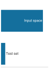
Test coverage is a vanishing fraction of the input space.

A unit assertion verifies that a given input and state follow an explicit execution path, while a machine learning claim describes aggregate performance over a population that changes over time. Robustness therefore cannot mean immunity to change. It means instrumenting the system to detect when production evidence no longer supports the model, and acting on that evidence.

Debugging an ML system therefore starts with inspecting datasets and pipeline transformations rather than tracing Python call stacks alone. Version control must record dataset snapshots and feature configurations alongside source-code commits, and evaluation harnesses must measure statistical distribution shifts and subpopulation outcomes rather than branch coverage. These practices establish reproducibility and provenance, even though they cannot transform empirical sampling into formal verification.

↪ Versioning training datasets so that a model can be reproduced and traced to its inputs is developed in Data versioning for ML reproducibility.

Checkpoint 1.1: The paradigm shift

Before tracing the history of AI, verify your understanding of the paradigm shift in how software is built:

• Software 1.0 vs. 2.0: can you distinguish Software 1.0 (explicit instructions) from Software 2.0 (behavior learned from data)?
• Debugging shift: can you identify which dataset evidence to inspect when accuracy falls without a code change?
• Verification gap: can you explain why finite test coverage can provide statistical evidence but never exhaustive proof, and why production monitoring must continue gathering that evidence?

Learning behavior from data can seem inevitable in hindsight, but its adoption also reflects the scaling limits of earlier approaches. Many AI systems attempted to program intelligence directly through hand-crafted symbols and rules. Reading that history through a systems lens reveals recurring binding constraints, the limits whose relaxation would most improve the whole system: logic, knowledge acquisition, feature design, and the physical infrastructure that the rest of this book studies.

Self-Check: Question

1. In Andrej Karpathy’s Software 1.0 vs. Software 2.0 framing, how do the roles of source code, the compiler, and debugging map to machine learning workflows?

   1. Learned weights shaped by training data act as source code, the training loop (stochastic gradient descent) acts as the compiler, and debugging expands from execution traces to the data and learned behavior.
   2. Python scripts act as source code, the deep learning framework acts as the compiler, and debugging focuses on stepping through tensor operations in an interactive debugger.
   3. Training datasets act as source code, GPU hardware acts as the compiler, and debugging focuses on profiling memory bandwidth utilization.
   4. Pretrained model weights act as source code, inference serving runtimes act as the compiler, and debugging focuses on network packet inspection.

2. A computer vision test suite evaluates a \(224{\times}224\) RGB image classifier on 50,000 validation images. Why does passing 100% of these test cases still leave a substantial ‘verification gap’ in production?

   1. Validation sets evaluate floating-point weights, whereas production inference engines always run in integer precision.
   2. The total input space of possible pixel configurations (\(256^{150{,}528}\), spanning over 300,000 decimal digits) vastly exceeds the sample coverage of any finite test set, making exhaustive testing mathematically impossible.
   3. Convolutional neural networks cannot generalize beyond the exact batch size used during validation testing.
   4. Test suites only evaluate forward inference passes, whereas production systems must continuously execute backward gradient updates.

3. How did Google Flu Trends fail despite having access to hundreds of billions of real-time search queries, and what systems engineering lesson does this failure provide regarding behavioral proxies?

4. The development paradigm where engineering teams hold model architecture code relatively fixed and systematically improve dataset quality, labels, and coverage to program model behavior is known as ____ AI.

See Answers →

1.3 The Evolution of AI Bottlenecks

Each era of AI history encountered a different limit, in representation, data, or computing resources. When Alan Turing⁷ proposed evaluating machine intelligence through observable responses (Turing 1950), computing machinery had little memory or processing capacity. Early systems pursued two contrasting paths: Frank Rosenblatt’s Perceptron (1958) (Rosenblatt 1958) attempted to learn weights directly from sensory inputs, whereas Joseph Weizenbaum’s ELIZA⁸ (Weizenbaum 1966) executed hand-coded pattern substitutions. Both soon met structural limits, as a single-layer perceptron could separate classes only with a linear boundary (Minsky and Papert 1969) while practical methods for training deeper networks remained out of reach, and ELIZA’s scripts broke whenever inputs strayed from their hand-written templates. Four eras organize this history around recurring bottlenecks (symbolic AI, expert systems, statistical learning, and deep learning), although the approaches overlapped in time.

⁷ Alan Turing: His “Imitation Game” approached machine intelligence through observable responses rather than a definition of its internal nature (Turing 1950). It provides an early example of evaluating a system through what it does.

Turing, Alan M. 1950. “I.—Computing Machinery and Intelligence.” Mind LIX (236): 433–60. https://doi.org/10.1093/mind/lix.236.433.

⁸ ELIZA: A natural-language program whose scripts could store selected inputs and reuse them in later responses (Weizenbaum 1966). This limited memory was programmed explicitly rather than learned from conversations. Extending its coverage required changing the scripts, even when the existing program ran correctly.

Weizenbaum, Joseph. 1966. “ELIZA–a Computer Program for the Study of Natural Language Communication Between Man and Machine.” Communications of the ACM 9 (1): 36–45. https://doi.org/10.1145/365153.365168.

Minsky, Marvin, and Seymour A. Papert. 1969. Perceptrons: An Introduction to Computational Geometry. The MIT Press.

⁹ AI winters as systems failures: The first AI winter (1974–1980) unfolded amid funding cuts; the 1973 Lighthill Report criticized the gap between AI promises and delivered results (Lighthill 1973). The second winter (1987–1993) involved a market and funding collapse around expert systems and specialized Lisp machines as general-purpose workstations undercut their economics (Hendler 2008). These episodes involved technical limitations, unmet expectations, and economics; hardware capacity alone does not explain them.

Lighthill, James. 1973. “Artificial Intelligence: A General Survey.” In Artificial Intelligence: A Paper Symposium. Science Research Council.

Hendler, James A. 2008. “Avoiding Another AI Winter.” IEEE Intelligent Systems 23 (2): 2–4. https://doi.org/10.1109/MIS.2008.20.

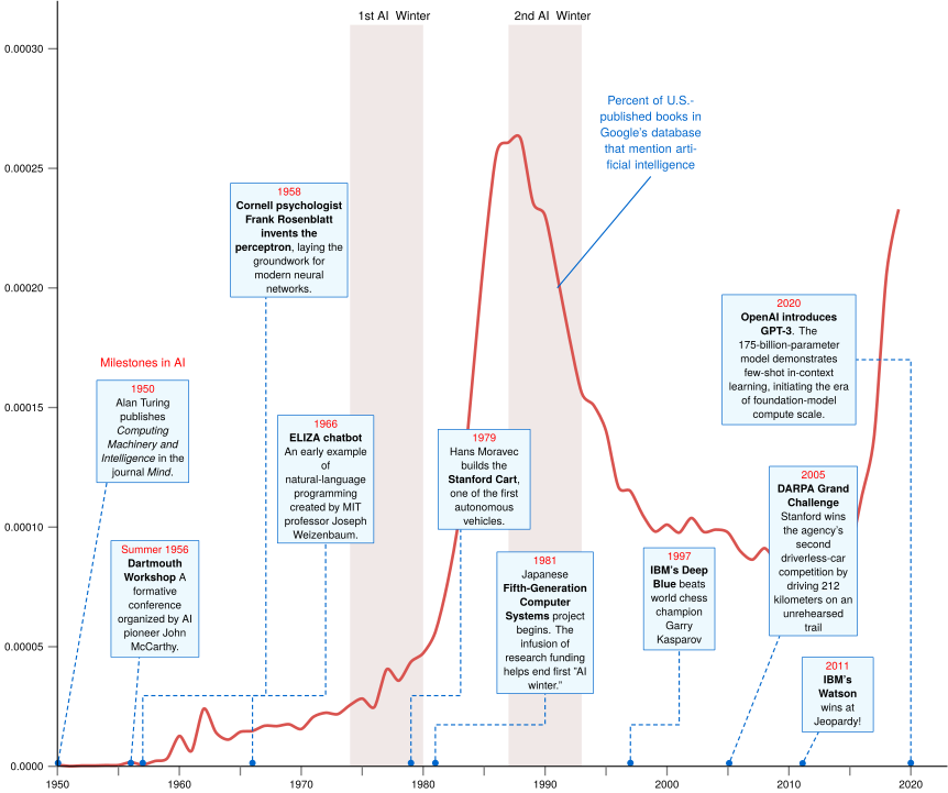
Figure 1 traces attention to AI across seven decades of published literature and shades two “AI winter” intervals (1974–1980 and 1987–1993) marked by funding cuts and unmet expectations.⁹ These setbacks reflected gaps between expectations and what systems could deliver. Later advances combined changes in algorithms, data, and computing resources; the sections below examine how those changes shifted the limiting constraint.

Figure 1: AI Development Timeline: The red curve tracks how often published books mention artificial intelligence, a measure of attention rather than capability, and the light-brown bands mark the two AI winters. Callout boxes place milestones such as Turing’s 1950 paper (Turing 1950), the Dartmouth conference (McCarthy et al. 1955), the Perceptron (Rosenblatt 1958), ELIZA (Weizenbaum 1966), Deep Blue (Campbell et al. 2002), and GPT-3 (Brown et al. 2020) against that curve. Adapted from Michel et al. (2011).

Rosenblatt, Frank. 1958. “The Perceptron: A Probabilistic Model for Information Storage and Organization in the Brain.” Psychological Review 65 (6): 386–408. https://doi.org/10.1037/h0042519.

Michel, Jean-Baptiste, Yuan Kui Shen, Aviva Presser Aiden, Adrian Veres, Matthew K. Gray, William Brockman, Joseph P. Pickett, et al. 2011. “Quantitative Analysis of Culture Using Millions of Digitized Books.” Science 331 (6014): 176–82. https://doi.org/10.1126/science.1199644.

1.3.1 Rule-based approaches: Logic and knowledge bottlenecks

Rule-based approaches attempted to build intelligent systems by making knowledge explicit. Symbolic AI encountered a logic bottleneck when its rules could not capture real-world ambiguity. Expert systems narrowed the task to a domain but encountered a knowledge bottleneck: acquiring and maintaining the rules required extensive expert effort.

The symbolic AI era and the logic bottleneck

Early AI research (1950s–1970s) pursued symbolic AI, representing knowledge and reasoning through explicit symbols and rules, an approach later crystallized in the physical-symbol-system hypothesis (Newell and Simon 1976). Researchers at the 1956 Dartmouth Conference¹⁰ (McCarthy et al. 1955) hypothesized that aspects of intelligence could be precisely described and simulated by machines. Even then, Arthur Samuel at IBM demonstrated a different path in 1959 when a checkers program improved through self-play. His work coined the term “machine learning” (Samuel 1959), though the dominant paradigm remained symbolic. Daniel Bobrow’s STUDENT¹¹ system (Bobrow 1964) took this approach to algebra word problems.

Newell, Allen, and Herbert A. Simon. 1976. “Computer Science as Empirical Inquiry: Symbols and Search.” Communications of the ACM 19 (3): 113–26. https://doi.org/10.1145/360018.360022.

¹⁰ Dartmouth Conference (1956): The workshop organized around the term “artificial intelligence,” already used in its 1955 proposal (McCarthy et al. 1955). The proposal discussed limits in computer speed and memory while treating programming as the larger obstacle. Physical capacity was part of the problem from the outset, even as researchers focused on language, abstraction, problem solving, and self-improvement.

McCarthy, John, Marvin L. Minsky, Nathaniel Rochester, and Claude E. Shannon. 1955. A Proposal for the Dartmouth Summer Research Project on Artificial Intelligence, August 31, 1955. No. 4. Vol. 27. Dartmouth College. https://doi.org/10.1609/aimag.v27i4.1904.

Samuel, A. L. 1959. “Some Studies in Machine Learning Using the Game of Checkers.” IBM Journal of Research and Development 3 (3): 210–29. https://doi.org/10.1147/rd.33.0210.

¹¹ STUDENT: An early program that translated algebra word problems into equations using hand-written language rules (Bobrow 1964). Its success depended on the wording fitting those rules; an algebra solver could solve the resulting equations without establishing that the program had interpreted the original problem correctly.

Bobrow, Daniel G. 1964. “Natural Language Input for a Computer Problem Solving System.” PhD thesis, Massachusetts Institute of Technology.

¹² Moravec’s paradox: Hans Moravec observed that skills people acquire with little conscious effort, such as perception and movement, can be harder to reproduce computationally than formal reasoning tasks (Moravec 1988). Human familiarity with a task is therefore a poor guide to its engineering difficulty or resource requirements.

Moravec, Hans. 1988. Mind Children: The Future of Robot and Human Intelligence. Harvard University Press.

These systems could produce impressive demonstrations, yet they were operationally brittle. Their success depended on manually coded rules that mapped each acceptable input form to a symbolic representation. STUDENT could solve an algebra problem once it translated English into equations, but a minor variation in phrasing could prevent that translation. The difficulty extended beyond language to perception and movement.¹²

Example 1.1: STUDENT (1964)

STUDENT separated language interpretation from algebra:

language  "Two numbers sum to 30; one is twice the other."
parse     x + y = 30, x = 2y
solve     x = 20, y = 10

Once the equations were written, solving was routine. The bottleneck was the translation. Each unfamiliar phrasing needed another hand-written rule, so linguistic coverage grew only as fast as the rule base.

The expert systems era and the knowledge bottleneck

In the expert-systems era, engineers narrowed the problem. Instead of constructing general reasoning systems, they encoded deep knowledge from a specific domain. MYCIN, designed to diagnose blood infections, let medical knowledge be expressed as production rules (Shortliffe et al. 1975).

Shortliffe, Edward H., Randall Davis, Stanton G. Axline, Bruce G. Buchanan, C.Cordell Green, and Stanley N. Cohen. 1975. “Computer-Based Consultations in Clinical Therapeutics: Explanation and Rule Acquisition Capabilities of the MYCIN System.” Computers and Biomedical Research 8 (4): 303–20. https://doi.org/10.1016/0010-4809(75)90009-9.

Example 1.2: MYCIN (1975)

MYCIN made its reasoning explicit. Patient facts triggered readable production rules:

facts  stain=gram-positive, shape=coccus, arrangement=clumps
rule   IF facts match THEN organism=staphylococcus (certainty=0.7)
cycle  match facts -> fire rule -> update certainty -> repeat

An inference engine repeated this match-and-fire cycle across hundreds of rules and propagated certainty factors (numerical confidence weights) toward a diagnosis. A physician could inspect every step, but coverage still grew one rule at a time: each exception had to be elicited, encoded, and reconciled with the existing rule base.

MYCIN performed well in specific tests, but its success exposed the knowledge acquisition bottleneck.¹³ The problem was no longer whether a rule could express expertise. It was how tacit judgment entered the system and remained consistent as the rule base grew.

¹³ Knowledge acquisition bottleneck: Feigenbaum (1984) treated extracting and representing expert knowledge as a central challenge in building applied AI systems. Experts could exercise judgment without being able to state every rule behind it, so acquiring knowledge required more than transcribing a ready-made list.

Feigenbaum, Edward A. 1984. “Knowledge Engineering: The Applied Side of Artificial Intelligence.” Annals of the New York Academy of Sciences 426: 91–107. https://doi.org/10.1111/j.1749-6632.1984.tb16513.x.

Faster machines could evaluate production rules at higher frequencies, but raw processor speed could not accelerate the extraction or maintenance of human expertise. Scaling meant learning decision boundaries from examples instead of asking domain specialists to enumerate every contingency. This transition did not eliminate human design; it relocated engineering effort. Instead of hand-coding decision logic, engineers shifted to curating datasets, selecting mathematical representations, and formulating learning objectives from which models could optimize their own parameters. The next era exchanged the knowledge acquisition bottleneck for a new one, the manual design of features extracted from raw data.

1.3.2 The statistical learning era and the feature engineering bottleneck

The 1990s marked the shift to statistical learning and probabilistic systems. Instead of hard-coded logic, systems estimated probabilities from data, such as the conditional distribution \(\ConditionalDistribution\) of a label \(\ExampleLabel\) given an input \(\ModelInput\). This transition was driven by the availability of digital data and the “unreasonable effectiveness”¹⁴ of large datasets. Early spam filters illustrated the change: rather than maintaining lists of forbidden words, statistical filters learned the probability that a word implies spam from millions of examples.

¹⁴ Unreasonable effectiveness of data: The observation that a simple statistical model with abundant data can outperform a more sophisticated model with less data (Halevy et al. 2009). The benefit depends on the task, model, and data quality. This makes collecting and preparing useful examples part of the engineering work, rather than merely a preliminary step.

Halevy, Alon, Peter Norvig, and Fernando Pereira. 2009. “The Unreasonable Effectiveness of Data.” IEEE Intelligent Systems 24 (2): 8–12. https://doi.org/10.1109/mis.2009.36.

Example 1.3: Early spam detection systems

Statistical filters shifted the decision from a hand-written rule to a probability estimated from labeled messages:

rules: if "free" or "winner" appears -> spam
learn: labeled email -> word likelihoods -> Pr(spam | email)

Maintenance did not disappear. It moved from editing keyword lists to curating representative examples and checking whether the learned probabilities still tracked current email.

Learning the decision boundary from data reduced one source of manual work but exposed another. Many statistical classifiers relied on engineers to convert raw inputs into features, measurable properties such as word counts or image edges. In computer vision, engineers designed feature extractors such as SIFT (Scale-Invariant Feature Transform) (Lowe 1999) and HOG (Histogram of Oriented Gradients) (Dalal and Triggs 2005) to summarize local image patterns. Classifiers such as support vector machines (SVMs) (Cortes and Vapnik 1995) then learned decision boundaries from those features. The learner adjusted the boundary; engineers decided which evidence it could see. Extending the system to a new problem often meant rebuilding the preprocessing stack, creating the feature engineering bottleneck.

Lowe, David G. 1999. “Object Recognition from Local Scale-Invariant Features.” Proceedings of the Seventh IEEE International Conference on Computer Vision 2: 1150–1157 vol.2. https://doi.org/10.1109/iccv.1999.790410.

Dalal, Navneet, and Bill Triggs. 2005. “Histograms of Oriented Gradients for Human Detection.” 2005 IEEE Computer Society Conference on Computer Vision and Pattern Recognition (CVPR’05) 1: 886–93. https://doi.org/10.1109/cvpr.2005.177.

Cortes, Corinna, and Vladimir Vapnik. 1995. “Support-Vector Networks.” Machine Learning 20 (3): 273–97. https://doi.org/10.1007/BF00994018.

¹⁵ Viola-Jones algorithm: The detector applied a sequence of classifiers, rejecting likely nonface regions early and spending more computation on promising regions. On the reported test set, it evaluated an average of ten features per candidate image region, although the complete cascade contained over 6,000 features (Viola and Jones 2001). Its speed depended on how little work most inputs required, not just on how fast each operation ran.

Viola, Paul, and Michael J. Jones. 2001. “Rapid Object Detection Using a Boosted Cascade of Simple Features.” Proceedings of the 2001 IEEE Computer Society Conference on Computer Vision and Pattern Recognition. CVPR 2001 1: I-511-I-518. https://doi.org/10.1109/cvpr.2001.990517.

This hybrid approach combined human-engineered features with statistical learning. The Viola-Jones algorithm¹⁵ (Viola and Jones 2001), typical of this era, achieved real-time frontal-face detection using simple rectangular features and cascaded classifiers. It showed that well-engineered features could enable practical low-latency applications, but only within narrow domains where experts could hand-craft the right representations. A conventional vision pipeline makes that manual effort visible, because several hand-crafted stages preceded any learning at all.

Example 1.4: Traditional computer vision pipeline

A conventional vision system separated representation from classification:

image -> resize -> HOG/SIFT features -> SVM -> label

Moving from faces to pedestrians or another domain meant redesigning the feature extractor and often the entire preprocessing stack.

1.3.3 The deep learning era and the infrastructure bottleneck

Redesigning hand-crafted feature extractors for every new domain could not scale, so deep learning (LeCun et al. 2015) moved feature extraction inside the model itself. A neural network computes in layers, stages of arithmetic on learned weights in which each layer transforms the output of the one before. Instead of receiving features designed by humans, deep networks with many such layers learned representations directly from raw inputs such as pixels and audio waveforms. The training process could now shape both the representation and the decision boundary, enabling “end-to-end” learning.

LeCun, Yann, Yoshua Bengio, and Geoffrey Hinton. 2015. “Deep Learning.” Nature 521 (7553): 436–44. https://doi.org/10.1038/nature14539.

LeCun, Yann, Bernhard Boser, John S. Denker, Donald Henderson, Richard E. Howard, Wayne Hubbard, and Lawrence D. Jackel. 1989. “Backpropagation Applied to Handwritten Zip Code Recognition.” Neural Computation 1 (4): 541–51. https://doi.org/10.1162/neco.1989.1.4.541.

The breakthrough was not algorithmic alone. Convolutional neural networks (CNNs), whose convolutional layers slide small learned weight patterns called filters across an image to detect the same feature at every position, existed earlier (LeCun et al. 1989, 1998); AlexNet paired architecture and training with systems co-design, choosing the model, training procedure, and hardware mapping together (Krizhevsky et al. 2012). Its parallel matrix operations matched GPU capabilities. With 60 million parameters distributed across two GTX 580 GPUs, AlexNet achieved 15.3 percent top-5 error, a 41.6 percent relative improvement over the next-best entry that year. The hardware partition in figure 2 carries the immediate systems lesson: the network divided work between the two GPUs and exchanged intermediate results only at selected layers to limit communication across the link between them (Krizhevsky et al. 2012). Model structure and machine organization were designed together.

Figure 2: AlexNet Architecture: Two parallel GPU streams process \(224{\times}224\) input images through convolutional layers (green blocks) that extract spatial features at decreasing resolutions, converging through three fully connected layers to 1,000 output classes. Because each stream holds half of the network, the figure also shows how the model was partitioned across two GPUs. Adapted from Krizhevsky et al. (2012).

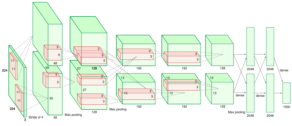
Hardware still shaped what could be learned. In 2012, storing AlexNet’s 60 million 32-bit parameters required roughly 240 megabytes, well within a single card’s capacity. Training also needs working storage for intermediate results and for calculating and retaining parameter updates. These quantities, developed later as activations, gradients, and optimizer state, make training memory larger than the stored model alone, and the intermediate results grow with the number of images processed together. Each GTX 580 offered only 3 GB of video random-access memory (VRAM), and the original paper reports that this limit made the network too large to train on one card (Krizhevsky et al. 2012). AlexNet therefore divided convolutional and dense layers between two GPU streams communicating over the PCIe bus, the host’s general-purpose peripheral interconnect. This early model-parallel design foreshadowed modern multi-GPU training. Deep learning reduced the need for hand-crafted features, but it moved the binding constraint to the infrastructure required to store data, move parameters, and coordinate computation.

↪ Model parallelism, which partitions a model across accelerators when it outgrows one device’s memory, as AlexNet’s two-GPU split did, is developed in Model parallelism.

Brown, Tom B., Benjamin Mann, Nick Ryder, Melanie Subbiah, Jared Kaplan, Prafulla Dhariwal, Arvind Neelakantan, et al. 2020. “Language Models Are Few-Shot Learners.” Advances in Neural Information Processing Systems 33: 1877–901. https://doi.org/10.48550/arxiv.2005.14165.

Kaplan, Jared, Sam McCandlish, Tom Henighan, Tom B. Brown, Benjamin Chess, Rewon Child, Scott Gray, Alec Radford, Jeffrey Wu, and Dario Amodei. 2020. “Scaling Laws for Neural Language Models.” ArXiv Preprint abs/2001.08361.

This shift produced the infrastructure bottleneck, in which physical memory capacity, interconnect bandwidth, and hardware orchestration dictate the boundaries of what models can learn. GPT-3 (Generative Pre-trained Transformer 3), with 175 billion parameters, was trained on roughly 300 billion tokens (the word fragments a language model reads and predicts) curated from filtered web text, books, and Wikipedia (Brown et al. 2020). The dense-training approximation (Kaplan et al. 2020) (\(\Operations \approx 6 \cdot \Parameters \cdot \DatasetSize\) operations for a model with \(\Parameters\) parameters trained on \(\DatasetSize\) tokens, counting both the forward and backward passes) agrees with the roughly 314 zettaFLOPs of total computation that the GPT-3 authors report, where one zettaFLOP is \(10^{21}\) floating-point operations (FLOPs). A retrospective audit by Patterson et al. (2021) estimated that this single training run consumed roughly 405 V100 GPU-years. The hard part had moved from designing edge detectors to keeping some 10,000 accelerators running in parallel across high-speed fabrics without failures that halt training midway. Viewed through this systems lens, each transition traded one binding constraint for the next, first in human effort (rules, knowledge, features) and then in physical infrastructure (table 2).

↪ The dense-training approximation used for this operation count is developed in Running cases: GPT-2 XL and ResNet-50.

Table 2: AI Paradigm Evolution: Each era is viewed through a recurring systems bottleneck. Deep learning (far right) reduced the need for manual feature engineering while increasing demands on computing infrastructure.

Aspect	Symbolic AI	Expert Systems	Statistical Learning	Deep Learning
Key Strength	Logical reasoning	Domain expertise	Versatility	Pattern recognition
Bottleneck	Brittleness (Rules break)	Knowledge Acquisition (Experts are scarce)	Feature Engineering (Manual preprocessing)	Infrastructure (Compute and data scale)
Data Handling	Minimal data needed	Domain knowledge-based	Moderate data required	Massive data processing

Across the four eras, engineering effort migrated from handcrafting domain heuristics toward building scalable compute and data pipelines. The bitter lesson explains why this shift recurred.

Self-Check: Question

1. Which historical transition correctly pairs an AI era with the primary systems bottleneck that limited its scalability and forced the transition to the subsequent paradigm?

   1. Symbolic AI was limited by compute throughput, forcing the transition to expert systems; Deep Learning was limited by human rule maintenance, forcing the transition to statistical learning.
   2. Expert Systems were limited by GPU memory bandwidth, forcing the transition to statistical learning; Statistical Learning was limited by formal logic ambiguity, forcing the transition to deep learning.
   3. Statistical Learning was limited by a complete lack of training labels, forcing the transition to symbolic logic; Symbolic AI was limited by hardware integer arithmetic, forcing the transition to neural networks.
   4. Expert Systems were limited by the knowledge acquisition bottleneck (serial human expert elicitation bandwidth), forcing the transition to statistical learning; Statistical Learning was limited by the feature engineering bottleneck (manual extraction of hand-crafted representations), forcing the transition to deep learning.

2. Moravec’s paradox observes that tasks humans find easy (such as visual perception, walking, and grasping) require vast computational resources, while tasks humans find hard (such as playing chess or solving algebra) require comparatively little compute. What is the direct implication of this paradox for ML systems hardware?

   1. Symbolic reasoning algorithms require multi-GPU accelerator clusters, whereas computer vision pipelines run efficiently on single-threaded CPUs.
   2. High-level reasoning tasks saturate off-chip memory bandwidth, while low-level perceptual tasks are strictly compute-bound.
   3. Perceptual and physical-world AI tasks demand massive parallelism, high memory bandwidth, and specialized hardware accelerators to process dense, high-dimensional sensor streams in real time.
   4. Robotic perception models can be deployed on microcontrollers without model compression or accuracy degradation.

3. Place the four historical AI engineering eras in chronological order based on when their primary paradigm dominated, and identify the key bottleneck that constrained each era:

1. Deep Learning Era
2. Expert Systems Era
3. Symbolic AI Era
4. Statistical Learning Era

4. Why was AlexNet’s 2012 ImageNet victory considered a breakthrough in systems co-design rather than purely an algorithmic advance?

5. True or False: The Viola-Jones face detection algorithm achieved real-time execution on early-2000s CPUs by using a cascade of simple rectangular features that evaluated an average of about ten features per candidate region, although the full cascade contained over 6,000 features.

See Answers →

1.4 The Bitter Lesson

Expert systems invested engineering effort in encoding domain knowledge; deep learning systems invest much of that effort in learning from data at scale. The bitter lesson captures the historical advantage of general methods, especially search and learning, that can make effective use of increasing computation. Richard Sutton¹⁶ crystallized this insight in his 2019 essay “The Bitter Lesson” (Sutton 2019). Sutton wrote, “The biggest lesson that can be read from 70 years of AI research is that general methods that leverage computation are ultimately the most effective, and by a large margin.”

¹⁶ Richard Sutton: A reinforcement learning pioneer whose essay emphasizes search and learning as methods that scale with computation (Sutton 2019). The lesson is “bitter” because carefully encoded human knowledge has repeatedly been overtaken by more general methods. It is a lesson about long-term progress, not a claim that domain knowledge has no engineering value.

Sutton, Richard S. 2019. “The Bitter Lesson.” Incompleteideas.net 43.

Training scale at the frontier is often stated in accelerator-days (GPU-days when the accelerator is a GPU): one reference accelerator running continuously for 24 hours. Table 3 pairs representative benchmark milestones with their hardware. Its final column runs from CPU-based learning to multi-thousand-accelerator clusters, using 2.5 million reference GPU-days as an estimated frontier-training anchor (Patel and Wong 2023).

Table 3: AI Performance Evolution Across Paradigms: Representative systems illustrate the growth in computational scale across eras. GPT-4 training details are estimated reference anchors rather than official disclosures.

Era	Approach	Representative Task	Performance	Computational Resources
Statistical ML (1990s–2000s)	Feature engineering + learning	Handwritten digit recognition	about 98–99% on MNIST-era benchmarks (LeCun et al. 1998)	CPU-era feature pipelines; resources varied by implementation
Deep Learning (2012)	End-to-end neural networks	ImageNet top-5 accuracy	84.7% (AlexNet)	6 days on 2 GPUs
Modern Deep Learning (2020+)	Large-scale transformers (Vaswani et al. 2017)	ImageNet top-1 accuracy	88.55% (ViT-H/14) (Dosovitskiy et al. 2021)	Large-scale Tensor Processing Unit (TPU) pretraining
Modern Deep Learning (2023)	Foundation models	MMLU benchmark	86.4% (GPT-4) (OpenAI et al. 2023)	Estimated ~2.5 million reference GPU-days (on the order of 25,000 reference GPUs run for 100 days) (Patel and Wong 2023)

LeCun, Yann, Léon Bottou, Yoshua Bengio, and Patrick Haffner. 1998. “Gradient-Based Learning Applied to Document Recognition.” Proceedings of the IEEE 86 (11): 2278–324. https://doi.org/10.1109/5.726791.

Vaswani, Ashish, Noam Shazeer, Niki Parmar, Jakob Uszkoreit, Llion Jones, Aidan N. Gomez, Lukasz Kaiser, and Illia Polosukhin. 2017. “Attention Is All You Need.” Advances in Neural Information Processing Systems (NeurIPS) 30: 5998–6008.

Dosovitskiy, Alexey, Lucas Beyer, Alexander Kolesnikov, Dirk Weissenborn, Xiaohua Zhai, Thomas Unterthiner, Mostafa Dehghani, et al. 2021. “An Image Is Worth 16x16 Words: Transformers for Image Recognition at Scale.” International Conference on Learning Representations (ICLR).

Patel, Dylan, and Gerald Wong. 2023. GPT-4 Architecture, Infrastructure, Training Dataset, Costs, Vision, MoE. SemiAnalysis Blog.

Digit recognition, ImageNet classification, and Massive Multitask Language Understanding (MMLU) measure different capabilities under separate metrics, so table 3 does not compare methods on one task. It shows instead that each new capability threshold demanded orders of magnitude more hardware, from single-node CPU routines to multi-megawatt accelerator clusters. Testing Sutton’s lesson, whether general methods powered by raw computation surpass hand-engineered representations, requires holding the task fixed and comparing competing approaches within one domain.

Game playing separates the roles of search and learning. In chess, IBM’s Deep Blue¹⁷ defeated world champion Garry Kasparov in 1997 by combining custom chess hardware, large-scale search, and chess-specific evaluation knowledge. In Go, DeepMind’s AlphaGo learned from expert games and self-play, using neural networks to guide tree search, but still used some engineered input features (Silver et al. 2016). AlphaGo Zero¹⁸ provides the clearer example of Sutton’s lesson: it learned through self-play without human game records or those hand-engineered features (Silver et al. 2017). The advance depended on methods that could turn computation into improved play, not merely on a faster machine.

¹⁷ Deep Blue: Its 480 custom chess chips worked alongside general-purpose processors, searching about 100 million positions per second in tactical positions and approaching 200 million in quieter positions (Campbell et al. 2002). The hardware accelerated chess-specific search and evaluation; it did not remove the system’s reliance on encoded chess knowledge.

Campbell, Murray, Jr. Hoane A.Joseph, and Feng-hsiung Hsu. 2002. “Deep Blue.” Artificial Intelligence 134 (1-2): 57–83. https://doi.org/10.1016/s0004-3702(01)00129-1.

Silver, David, Aja Huang, Chris J. Maddison, Arthur Guez, Laurent Sifre, George van den Driessche, Julian Schrittwieser, et al. 2016. “Mastering the Game of Go with Deep Neural Networks and Tree Search.” Nature 529 (7587): 484–89. https://doi.org/10.1038/nature16961.

¹⁸ AlphaGo Zero: After three days of self-play training, it defeated AlphaGo Lee, the version that had beaten Lee Sedol, by 100 games to 0 (Silver et al. 2017). Self-play generated the training examples, allowing search and learning to improve play without a dataset of human games.

Silver, David, Julian Schrittwieser, Karen Simonyan, Ioannis Antonoglou, Aja Huang, Arthur Guez, Thomas Hubert, et al. 2017. “Mastering the Game of Go Without Human Knowledge.” Nature 550 (7676): 354–59. https://doi.org/10.1038/nature24270.

The lesson is “bitter” because encoding human expertise can appear to be the most direct path to a solution. Sutton’s examples show how scalable search and learning repeatedly overtook such approaches. More computation does not guarantee better results; the method must use it productively, and the data and objective must support the intended task.

Modern language models such as GPT-4 (OpenAI et al. 2023) and image generation systems such as DALL-E (Ramesh et al. 2021) illustrate the engineering demands of learning at scale. Much of their behavior is learned from large datasets rather than expressed as explicit linguistic or artistic rules. Training GPT-3 alone was estimated to consume roughly 1.3 GWh of energy¹⁹ (Patterson et al. 2021), and serving these models to millions of users turns inference into a continuous data-center power, cooling, and capacity-planning problem.

OpenAI, Josh Achiam, Steven Adler, Sandhini Agarwal, Lama Ahmad, Ilge Akkaya, Florencia Leoni Aleman, et al. 2023. “GPT-4 Technical Report.” arXiv Preprint arXiv:2303.08774, ahead of print. https://doi.org/10.48550/arXiv.2303.08774.

Ramesh, A., M. Pavlov, G. Goh, S. Gray, C. Voss, A. Radford, M. Chen, and I. Sutskever. 2021. “Zero-Shot Text-to-Image Generation.” In Proceedings of the 38th International Conference on Machine Learning, ICML 2021, 18-24 July 2021, Virtual Event, edited by Marina Meila and Tong Zhang, vol. 139. Proceedings of Machine Learning Research. PMLR.

¹⁹ GPT-3 training energy: Patterson et al. (2021) estimated that GPT-3’s training consumed approximately 1,287 MWh and produced 552 metric tons of CO₂-equivalent emissions. The energy estimate corresponds to the annual electricity use of about 120 US households at a baseline of 10.7 MWh/household-year. Emissions also depend on how that electricity is generated.

Patterson, David, Joseph Gonzalez, Quoc Le, Chen Liang, Lluis-Miquel Munguia, Daniel Rothchild, David So, Maud Texier, and Jeff Dean. 2021. “Carbon Emissions and Large Neural Network Training.” arXiv Preprint arXiv:2104.10350.

²⁰ Memory bandwidth: The rate at which a memory interface transfers data, measured in bytes per second. A processor must receive the values an operation needs before it can perform the arithmetic. When moving those values takes longer than computing with them, faster arithmetic alone cannot remove the delay; reducing transfers or increasing the available bandwidth addresses the limiting resource.

When model capability scales with raw computation, the binding limits shift to physical infrastructure: memory bandwidth,²⁰ interconnect latency, thermal dissipation, and data pipeline throughput. Data movement, arithmetic throughput, and operational reliability must therefore be designed as one problem. Designing for continuous computational growth is the responsibility that defines AI engineering, which section 1.9 formalizes once its system boundaries and quantitative foundations are in place.

Self-Check: Question

1. Why did Richard Sutton describe the fundamental finding of 70 years of AI research as a ‘bitter’ lesson for researchers and engineers?

   1. Human intuition naturally seeks to build intelligence by encoding domain expertise and linguistic rules into models, yet historical progress repeatedly demonstrates that general-purpose search and learning leveraging raw computation outperform hand-crafted human knowledge.
   2. Hardware accelerators have reached physical thermodynamic scaling limits, preventing further increases in neural network parameter counts.
   3. Stochastic gradient descent algorithms produce models whose internal mathematical representations cannot be formally proven correct.
   4. Open-source models consistently match the performance of proprietary industrial foundation models trained at hundred-million-dollar compute budgets.

2. In comparing IBM’s Deep Blue (1997) and DeepMind’s AlphaGo Zero (2017), how do their designs reflect the progression toward Sutton’s bitter lesson?

   1. Deep Blue relied entirely on deep reinforcement learning, whereas AlphaGo Zero returned to hand-coded expert evaluation tables.
   2. Deep Blue combined custom silicon search (100 to 200 million positions/second) with hand-coded chess heuristics, whereas AlphaGo Zero learned through self-play without human game records or hand-engineered features, using neural networks to guide tree search.
   3. Both systems avoided the use of custom silicon or GPUs, relying strictly on algorithmic elegance over compute scale.
   4. AlphaGo Zero eliminated all tree search mechanisms in favor of pure single-step feedforward classification.

3. If the bitter lesson states that computation-leveraging methods dominate over time, why does realizing this advantage depend primarily on systems engineering rather than pure algorithmic theory?

4. True or False: According to the bitter lesson, building domain-specific linguistic or perceptual rules into deep neural network architectures provides a permanent, compounding advantage over general architectures as compute budgets expand.

See Answers →

1.5 Defining ML Systems

Absorbing computational growth takes a working system, not only a model, and even a familiar service shows how many parts such a system has. A production spam filter needs more than a model that recognizes unwanted messages. It needs representative training data, a way to update learned behavior as attacks change, and infrastructure that classifies incoming mail within the delivery budget. Global email traffic is measured in hundreds of billions of sent and received messages per day (Statista Research Department 2024), making this a substantial systems problem for large providers.

Statista Research Department. 2024. Number of Sent and Received e-Mails Per Day Worldwide from 2017 to 2027. Statista.

The challenge begins with data. The filter is trained on labeled examples and needs updated training data and periodic retraining as spam tactics change. It is also an algorithmic problem, because the model must generalize from those examples to messages it has never seen before. Precision measures the fraction of flagged messages that are actually spam; recall measures the fraction of all spam messages that the filter catches. Flagging more messages may catch more spam while also hiding legitimate mail, so the system must evaluate both consequences. Finally, it is an infrastructure problem. Providers must handle incoming traffic, store and update models, and return predictions within their delivery latency budget. The classifier is therefore only one component of an evolving data, software, and hardware system.

When a new phishing template appears, the data layer must capture representative messages, the algorithm must learn to separate attacks from legitimate mail, and the infrastructure must deploy and serve the updated model. Any layer can fail while the others continue working, so the full chain from measurement through learning to execution is the right unit of analysis.

Definition 1.1: Machine learning systems

Machine learning systems combine models that learn from data with the software and hardware needed to train, deploy, and maintain them. Their performance depends jointly on data quality, algorithm choice, and machine capacity.

1. Significance: Requirements are end to end, so a failure in any layer changes the user-visible result even while the other layers operate correctly.
2. Distinction: The system includes every path an input travels, not only the model. A feature computed one way in training and another in serving changes what the system predicts even when the model and its weights are identical.
3. Common pitfall: The model is not the system. Data pipelines, feature transformations, serving infrastructure, monitoring, and feedback loops surround the learned parameters and often dominate the engineering burden (Sculley et al. 2015).

Sculley, D., Gary Holt, Daniel Golovin, Eugene Davydov, Todd Phillips, Dietmar Ebner, Vinay Chaudhary, Michael Young, Jean-François Crespo, and Dan Dennison. 2015. “Hidden Technical Debt in Machine Learning Systems.” Advances in Neural Information Processing Systems (NeurIPS) 28: 2503–11.

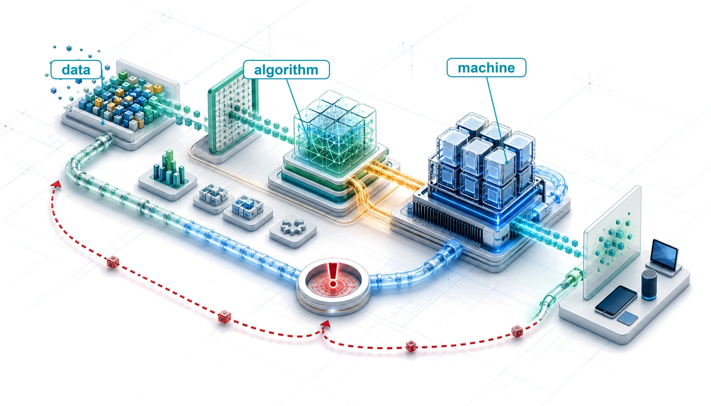
The definition exposes three diagnostic axes: the data that describes the task, the algorithm that turns examples into behavior, and the machine that executes that behavior within the operating budget. The same user-visible symptom can originate in any of the three. Treating every miss as a model problem risks improving the wrong component. The D·A·M taxonomy separates these causes for diagnosis.

Each explanation calls for different evidence. The data hypothesis sends the engineer to coverage, labels, and distribution shift. The algorithm hypothesis sends the engineer to error slices (errors grouped by input type), model capacity, and the learning objective. The machine hypothesis sends the engineer to latency, throughput, memory, and utilization. These investigations are not interchangeable. Faster hardware cannot supply examples that were never collected, while a larger dataset cannot repair a serving path that misses its deadline because memory is saturated.

The relevant constraint is the one whose relaxation improves the end-to-end result. This idea of a binding constraint, used informally in the history above, prevents teams from optimizing the most visible component instead of the component that governs the outcome. The purpose of D·A·M is therefore operational: it identifies the next hypothesis to test and the class of intervention capable of changing system behavior. The diagnosis is provisional. Once an intervention relaxes one limit, the system must be measured again because a different axis may now bind. D·A·M is a loop, not a one-time label.

Definition 1.2: D·A·M taxonomy

D·A·M taxonomy is a diagnostic framework for examining machine learning system bottlenecks along three axes. Data determines what examples and bytes the system must process, Algorithm determines the model structure and work required to learn or predict, and Machine determines the hardware capacity available to execute that work. The goal is to identify which axis is the binding constraint.

1. Significance: The diagnostic power is concrete even before detailed hardware arithmetic enters the story. If the spam filter misses a new phishing campaign because the training set never contained that tactic, the binding axis is Data. If the training examples are adequate but the model cannot express the pattern, the binding axis is Algorithm. If both are adequate but the service cannot classify messages quickly enough during a traffic spike, the binding axis is Machine. Quantitative diagnosis begins by asking which axis is limiting the system.
2. Distinction: The D·A·M taxonomy connects predictive quality to physical execution. Algorithm choice shapes both the data needed to learn useful behavior and the machine resources needed to run it. Those requirements depend on the task and training procedure, so model size alone does not determine either generalization or runtime.
3. Common pitfall: A frequent misconception is that the three axes are independent. Changing from a simple classifier to a larger model can require more memory, different serving infrastructure, and a broader data distribution. Because changing one of Data, Algorithm, and Machine can change the requirements imposed on the other two, every edge of the triangle in figure 3 points both ways.

Figure 3: The D·A·M Axis Triad: Each vertex is one diagnostic axis, and each double-headed edge is a path along which a relaxed bottleneck can reappear on the neighboring axis.

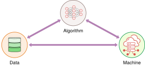
An operational diagnosis earns confidence only when an intervention validates it, that is, when relaxing the identified constraint improves full-system behavior. Resolving one bottleneck frequently migrates the binding constraint across an adjacent edge of figure 3, so interventions rarely end the optimization process. Upgrading to faster accelerators (Machine) leaves execution units idling if storage I/O cannot stream input batches quickly enough (Data); conversely, expanding dataset volume (Data) exposes model architectures that lack the expressive capacity to absorb new patterns (Algorithm), and scaling model capacity to close that gap (Algorithm) soon exceeds accelerator memory, triggering out-of-memory faults or expensive paging across the PCIe bus (Machine). Engineering an ML system therefore requires identifying the currently binding constraint while anticipating where the bottleneck will migrate once that constraint is relaxed.

While the triad separates the three axes to simplify initial diagnosis, practical systems operate at their boundaries. Data formats govern memory traffic, model architectures dictate hardware functional unit utilization, and deployment budgets reshape both data representation and algorithmic design. Figure 4 partitions these interfaces into a three-set Venn diagram whose pairwise overlaps each pose one question: what the system can learn from (\(\text{D} \cap \text{A}\)), how information moves (\(\text{D} \cap \text{M}\)), and how computation executes efficiently (\(\text{A} \cap \text{M}\)).

Figure 4: The D·A·M Intersection Landscape: Each circle lists the concerns that belong to one axis, and each pairwise overlap is titled with the question that axis pair must answer jointly. The central region, where all three circles overlap, is labeled ML systems engineering.

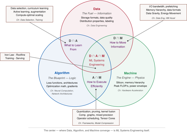
At the center, all three questions must be answered together: data selection and training determine which examples help the model learn useful behavior, data engineering and hardware acceleration deliver that information to the machine at speed, and frameworks and execution techniques turn the model’s computations into efficient work on that silicon. Pruning a model (Algorithm), which removes parameters that contribute little to its predictions, alters its memory footprint and how much of it stays in fast on-chip memory (Machine). Compressing input features can likewise reduce transfers while adding preparation work (Data). These changes must be evaluated across the interfaces, because a local improvement may leave the end-to-end result unchanged, and even when every component executes without error, a shift on the data axis can still degrade predictions silently.

↪ How pruning shrinks a model’s memory footprint, and why its effect on speed depends on the sparsity pattern the hardware can exploit, is developed in Pruning.

Self-Check: Question

1. An ML engineering team trains a 70-billion-parameter language model. When profiling the distributed cluster, they notice that accelerator compute engines remain idle for 45% of execution time waiting for batch tensors to be loaded from remote object storage over the network. Along which D·A·M axis does the primary binding constraint lie, and which intersection represents the appropriate optimization space?

   1. Machine axis; \(\text{Algorithm} \cap \text{Machine}\) (mixed precision quantization and kernel fusion)
   2. Algorithm axis; \(\text{Data} \cap \text{Algorithm}\) (curriculum learning and active data selection)
   3. Data axis; \(\text{Data} \cap \text{Machine}\) (I/O pipelining, prefetching, and storage memory hierarchy)
   4. Workload axis; \(\text{Data} \cap \text{Algorithm} \cap \text{Machine}\) (reinforcement learning from human feedback)

2. Explain what the concept of a ‘binding constraint’ means in the D·A·M framework, and describe the risk of optimizing a non-binding axis.

3. In the D·A·M intersection landscape, the intersection between Algorithm and Machine (\(\text{A} \cap \text{M}\)) addresses the core question of ‘How to ____’, focusing on how the model’s mathematical work is mapped onto hardware execution and data movement efficiently.

See Answers →

1.6 When ML Systems Fail Silently

In an automotive driver-assistance system, diagnostic trouble codes and hardware watchdog timers expose hardware or communication faults, yet they do not measure how often a perception model detects pedestrians. When seasonal conditions introduce low-angle winter sunlight, heavy precipitation, or bulky clothing underrepresented in training, pedestrian recall can decline from 95 percent to 85 percent even while the accelerator processes images at full frame rate without raising a hardware fault. Correct execution and predictive quality are separate properties, and an ML system must be engineered and monitored for both.

Crashes, unhandled exceptions, and failed health checks make some software defects directly observable, though conventional software can also produce silent numerical errors or logic bugs. Machine learning adds another route to silent degradation: learned behavior loses predictive quality as the operating population changes, even while the runtime executes instructions without error, memory allocations succeed, and inference servers return predictions well within latency service level agreements (SLAs).

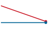
Recall falls while health metrics stay flat.

In this example, the miss rate triples, from 1 in 20 pedestrian frames to 3 in 20. That is a substantial change in detection quality, but it does not imply a tripling of vehicle-level safety risk, because temporal filtering, sensor fusion, and downstream control affect how missed detections influence a driving decision.

Input distributions can drift as environmental conditions, user behavior, or sensor calibrations change (Gama et al. 2014; Quiñonero-Candela et al. 2009). A model may then apply its fixed weights to inputs unlike those on which it was evaluated. The machine can execute every operation correctly while producing predictions whose quality no longer meets the requirement.

Gama, João, Indrė Žliobaitė, Albert Bifet, Mykola Pechenizkiy, and Abdelhamid Bouchachia. 2014. “A Survey on Concept Drift Adaptation.” ACM Computing Surveys 46 (4): 1–37. https://doi.org/10.1145/2523813.

Quiñonero-Candela, Joaquin, Masashi Sugiyama, Anton Schwaighofer, and Neil D. Lawrence, eds. 2009. Dataset Shift in Machine Learning. Neural Information Processing Series. The MIT Press.

Outcome measurements establish whether predictive quality has fallen; distribution-divergence signals can prompt investigation before those outcomes arrive. When both are observed, model degradation can be approximated locally as a function of distribution shift. Let \(\InitialAccuracy\) denote the baseline accuracy at deployment, \(\StatisticalDivergence\) represent the statistical divergence between current production distribution \(\CurrentDistribution\) and training distribution \(\TrainingDistribution\), and \(\FittedSensitivity\) denote the locally fitted sensitivity to that shift measure, so that \(\AccuracyAfterDeployment(\DeploymentAge)\) is the accuracy after the model has been deployed for time \(\DeploymentAge\). This relationship, formalized in equation 1, is the degradation equation: \[ \AccuracyAfterDeployment(\DeploymentAge) \approx \InitialAccuracy - \FittedSensitivity \cdot \StatisticalDivergence \tag{1}\]

This approximation describes a local trend fitted from observed inputs and labeled outcomes; it is not a universal law of accuracy loss. The chapters on deployment return to it as a statistical drift diagnostic. Data drift occurs when \(\CurrentDistribution\) differs from \(\TrainingDistribution\). Such a shift can reduce inference quality even when the model and execution environment remain unchanged, but the shift alone does not establish a quality loss. Large changes may fall outside the range where the fitted relationship holds. The divergence measure \(\DivergenceMeasure(\cdot \lVert \cdot)\) is left general here.

↪ The statistics that measure distribution shift and detect drift in production data are developed in Data drift detection and response.

The equation separates baseline quality from sensitivity to shift. Better data, objectives, and architectures can change both quantities, so an improved baseline does not by itself establish robustness to drift. For the driving example, training on representative winter images may reduce sensitivity to seasonal conditions; evaluating pedestrian recall under those conditions establishes whether it does. Monitoring \(\StatisticalDivergence\) provides a warning that prompts engineers to seek outcome evidence. That evidence determines whether retraining or another intervention is needed. Knowing when to reevaluate is as important as knowing how to train.

↪ How drift signals and labeled outcomes become an operational decision to retrain, made only when the expected benefit exceeds the cost, is developed in Retraining decision framework.

Silent degradation can also originate inside the system through training-serving skew. Training and serving may use separate implementations to transform raw inputs into model features. If those transformations differ, for example by resizing images with a different interpolation method or applying different missing-value defaults, the model receives inputs unlike those used in training. The model can execute cleanly and return predictions on time while accuracy falls. This is a software consistency defect whose consequence is degraded learned behavior.

↪ Keeping transformation code and its fitted parameters identical across training and serving is developed in Training-serving consistency.

Host-health signals such as CPU utilization, memory residency, network I/O, and HTTP status codes remain necessary, but do not measure whether predictions are useful. Machine learning operations must track these infrastructure metrics alongside data quality, feature distributions, and prediction accuracy. Because an ML system can fail silently while infrastructure metrics appear nominal, system design must integrate continuous evaluation from data ingestion through inference serving.

Useful predictions satisfy the first half of the ML systems mandate. The second half requires producing them within the available latency, memory, energy, and cost budgets. Meeting those budgets requires a quantitative account of where execution time goes.

Self-Check: Question

1. In the degradation equation \(\text{Accuracy}(t) \approx \text{Accuracy}_0 - \lambda \cdot \mathcal{D}(P_t \lVert P_0)\), what do the terms \(\mathcal{D}(P_t \lVert P_0)\) and \(\lambda\) represent, and which engineering lever addresses \(\lambda\)?

   1. \(\mathcal{D}(P_t \lVert P_0)\) is hardware clock jitter, \(\lambda\) is GPU temperature sensitivity, and it is addressed by dynamic voltage and frequency scaling.
   2. \(\mathcal{D}(P_t \lVert P_0)\) is statistical divergence between live production data and training data, \(\lambda\) is model sensitivity to distribution shift, and it is addressed by robust training and domain adaptation to flatten the degradation curve.
   3. \(\mathcal{D}(P_t \lVert P_0)\) is the memory bandwidth ratio, \(\lambda\) is cache miss penalty, and it is addressed by prefetching weights into on-chip memory.
   4. \(\mathcal{D}(P_t \lVert P_0)\) is training loss divergence, \(\lambda\) is the learning rate decay, and it is addressed by tuning the optimization algorithm.

2. A production fraud detection model begins misclassifying high-risk transactions immediately after deployment. An audit reveals that the training pipeline extracted user account age in integer days, while the live inference microservice computed account age in fractional floating-point seconds. What type of systems failure does this scenario illustrate?

   1. Training-serving skew, where discrepancies in feature computation between training and serving pipelines cause silent model degradation despite bug-free code execution.
   2. Hardware memory corruption caused by unaligned tensor strides in the GPU inference runtime.
   3. Unbounded latency growth where deserialization overhead violates the service-level agreement.
   4. Concept drift caused by macroeconomic shifts in consumer purchasing behavior over multiple years.

3. Why does the degradation equation indicate that tracking statistical data drift (\(\mathcal{D}(P_t \lVert P_0)\)) alone is necessary but not sufficient to determine whether a deployed model must be retrained?

4. True or False: Holding drift sensitivity fixed, improving the initial training accuracy (\(\text{Accuracy}_0\)) of an ML model shifts the starting point of the degradation curve upward, but does not change the model’s rate of accuracy decline (\(\lambda\)) with respect to distribution drift over time.

See Answers →

1.7 Iron Law of ML Systems

Computational scale has a physical cost, and it shows up as two familiar failures. A training job stalls when storage cannot feed an accelerator; an inference path misses its deadline when model state moves too slowly through memory or across the network. Their symptoms differ, but both are governed by how the three D·A·M axes combine to consume wall-clock time. Across Data (D), Algorithm (A), and Machine (M), every ML task completes by processing a set of samples (examples in vision or tabular workloads, tokens in language models) through an algorithm’s operations on hardware. By dimensional cancellation, total execution time \(\Time\) (seconds) is the product of these three factors (equation 2): \[\Time = \underbrace{\left(\frac{\text{Samples}}{\text{Task}}\right)}_{\text{Data}} \times \underbrace{\left(\frac{\text{FLOPs}}{\text{Sample}}\right)}_{\text{Algorithm}} \times \underbrace{\left(\frac{\text{Seconds}}{\text{FLOP}}\right)}_{\text{Machine}} \tag{2}\]

The same equation governs both training and inference because only the definition of the task and the scale of each factor change. The product of the first two factors sets the total arithmetic work \(\Operations\) (FLOPs), while the third factor (\(\text{Seconds/FLOP}\)) is the realized time the machine takes per operation:

• Training: A task is a training run (or an optimization step), where \(\text{Samples/Task}\) is the corpus token budget \(\DatasetSize\) (billions to trillions of tokens) and \(\text{FLOPs/Sample}\) spans the forward and backward passes (\(\approx 6\Parameters\) FLOPs per token for a dense transformer, giving \(\Operations \approx 6\Parameters\DatasetSize\)). Because large training batches reuse model weights across thousands of tokens per step, the machine amortizes memory transfers and dispatch overhead, keeping realized \(\text{Seconds/FLOP}\) low and near the hardware’s compute ceiling.
• Inference: A task is serving a request or generating a response, where \(\text{Samples/Task}\) shrinks to a small request batch (\(\BatchSize\)) or a stream of generated tokens, and \(\text{FLOPs/Sample}\) covers only the forward pass (\(\approx 2\Parameters\) FLOPs per token). With far fewer samples per invocation to amortize weight reads and orchestration, realized \(\text{Seconds/FLOP}\) rises sharply as memory bandwidth and fixed latency overtake arithmetic.

A real machine does not run at its datasheet peak rate \(1/\PeakRate\) because physical execution requires moving data across memory and interconnect buses, driving arithmetic units at some realized utilization, and paying fixed control overheads. Assuming these three physical costs occur sequentially, the iron law of ML systems unpacks total execution time \(\Time\) (seconds) into their sum (equation 3): \[\Time = \underbrace{\frac{\DataVolume}{\Bandwidth}}_{\text{Memory Time}} + \underbrace{\frac{\Operations}{\PeakRate \cdot \EfficiencyHw}}_{\text{Compute Time}} + \underbrace{\Latency}_{\text{Latency Overhead}} \tag{3}\]

Together, equation 2 and equation 3 account for the physical-execution half of the dual mandate introduced in section 1.1:

1. The memory term \((\DataVolume/\Bandwidth)\) represents the physical cost of moving bits. \(\DataVolume\) is the volume of data moved (bytes), and \(\Bandwidth\) is the memory or network bandwidth (bytes/s). Whether loading terabytes from cloud storage or fetching weights from high-bandwidth memory (HBM), the stacked dynamic random-access memory (DRAM) packaged beside an accelerator, performance is often limited by I/O physics. Part I develops this foundation.
2. The compute term \((\Operations/(\PeakRate \cdot \EfficiencyHw))\) represents the cost of arithmetic. \(\Operations\) is the number of floating-point operations (FLOPs) set by the product of \(\text{Samples/Task}\) and \(\text{FLOPs/Sample}\), \(\PeakRate\) is the hardware’s theoretical peak throughput (FLOP/s), and \(\EfficiencyHw\) is dimensionless realized compute utilization \((0 \le \EfficiencyHw \le 1)\). Parts II and III develop this term.
3. The latency term \((\Latency)\) represents orchestration, networking, and serialization overhead (seconds), treated as fixed for the modeled execution. Engineering changes can reduce this overhead, which can dominate small, latency-critical requests where little data moves and little arithmetic runs. Part IV develops this term.

Consider a hypothetical task that spends 2 seconds moving data, 8 seconds computing, and 1 second on overhead. Its total is 11 seconds. Doubling the arithmetic rate reduces computation to 4 seconds, but leaves movement and overhead unchanged. The task now takes 7 seconds, rather than half its original time. A faster component helps only through the portion of the time budget it changes.

Data enters equation 2 and equation 3 in two distinct ways: logical samples versus physical bytes. In equation 2, the Data factor counts how many examples or tokens the task processes (such as the dataset size \(\DatasetSize\) in the \(6 \cdot \Parameters \cdot \DatasetSize\) training estimate), which multiplies \(\text{FLOPs/Sample}\) to fix total arithmetic work \(\Operations\). In equation 3, by contrast, \(\DataVolume\) counts the physical bytes moved across a memory or interconnect bus, including model weights (\(\Parameters\)), activations, cached sequence state, and gradients alongside the raw inputs. When a language model decodes a single token at batch size one, the logical input is one token (\(\text{Samples/Task} = 1\)), yet \(\DataVolume\) spans gigabytes of model weights streamed from high-bandwidth memory.

Systems Perspective 1.1: The iron law analogy

The name “iron law” follows the processor performance equation of Patterson and Hennessy (2017), \(\text{Time/Program} = (\text{Instructions/Program}) \times (\text{Cycles/Instruction}) \times (\text{Seconds/Cycle})\). Equation 2 is the direct ML counterpart: the Data (\(\text{Samples/Task}\)) and Algorithm (\(\text{FLOPs/Sample}\)) factors multiply to set total operations \(\Operations\) just as program path length and instruction set determine instruction count, while the Machine factor (\(\text{Seconds/FLOP}\)) mirrors cycles per instruction times clock period. Reducing \(\text{FLOPs/Sample}\) (for example, through unstructured sparsity) can still slow down execution if irregular memory accesses inflate \(\text{Seconds/FLOP}\), just as complex CPU instructions that cut instruction count can lose performance by inflating cycles per instruction. Equation 3 then takes the same second step that computer architects take when decomposing processor time into compute cycles, memory-stall cycles, and pipeline overhead.

The additive form assumes sequential execution. When movement and computation overlap, the critical-path lower bound replaces the sum in equation 4: \[\PipelinedExecutionTime\ge \max\left(\frac{\DataVolume}{\Bandwidth}, \frac{\Operations}{\PeakRate \cdot \EfficiencyHw}\right) + \Latency \tag{4}\] This max-based formulation reflects hardware that transfers the next block of data while computing on the current one, so the slower of the two stages hides the faster. Equality requires ideal overlap and assumes that \(\Latency\) remains outside the overlapped phases.

Even as a sum, the iron law identifies which physical constraint dominates before any optimization begins. Amdahl’s law (Amdahl 1967) plays the same role for speedups. Accelerating only part of a task leaves the untouched remainder in place, and that remainder caps the whole task’s speedup however fast the accelerated part becomes; equation 11.1 states that cap quantitatively as a bound on overall speedup. From sum to max presents the refined treatment, including pipelining and overlap techniques that transform the additive model into the max-based formulation used in practice.

Amdahl, Gene M. 1967. “Validity of the Single Processor Approach to Achieving Large Scale Computing Capabilities.” Proceedings of the April 18-20, 1967, Spring Joint Computer Conference on - AFIPS ’67 (Spring), AFIPS ’67 (spring), 483–85. https://doi.org/10.1145/1465482.1465560.

Hennessy, John L., and David A. Patterson. 2017. Computer Architecture: A Quantitative Approach. 6th ed. Morgan Kaufmann.

Diagnosing the limiting term requires comparing the workload with the machine. Arithmetic intensity \((\ArithmeticIntensity = \Operations/\DataVolume)\) counts the operations performed per byte moved. Each machine has an intensity at which its memory and compute terms balance, set by its peak compute rate divided by its memory bandwidth. A workload below that balance point waits on memory; one above it waits on arithmetic. Improving the smaller of the two terms yields a limited end-to-end gain. Actual performance also depends on realized utilization, and overhead \((\Latency)\) sits outside this comparison and can dominate small requests. A single-accelerator estimate applies these ideas below.

↪ The roofline model, which bounds attainable throughput by arithmetic intensity and locates the ridge point, is developed in Performance Bounds.

Napkin Math 1.1: Estimating one local execution

Problem: A hypothetical workload on one accelerator moves 2 GB at 100 GB/s, performs 1 GFLOP at an effective arithmetic rate of 100 GFLOP/s, and incurs 5 ms of fixed overhead. Movement precedes computation. What execution time does the iron law predict, and which rate should be improved first?

Math: Dividing bytes by bytes/s gives a movement time of 20 ms. Dividing FLOPs by FLOP/s gives a compute time of 10 ms; the supplied effective rate already includes \(\EfficiencyHw\), so it must not be multiplied by efficiency again. Adding these durations and overhead gives 35 ms. Movement is the largest term.

Result: Raising bandwidth to 200 GB/s reduces movement to 10 ms and total sequential time to 25 ms. Arithmetic and overhead remain unchanged, so doubling bandwidth does not halve the total.

Systems insight: If movement and computation could instead overlap ideally, with overhead still outside both phases, the lower bound would be 25 ms before the upgrade and 15 ms afterward. The upgrade balances the two stages; further bandwidth increases alone would leave that ideal bound unchanged. Whether the sum or the bound describes a measured run depends on its execution schedule.

A larger training estimate returns to equation 2 under an explicit compute-dominated assumption, folding all non-arithmetic delays into an effective end-to-end utilization factor \(\EfficiencyHw\) so that the realized machine factor across \(\AcceleratorCount\) parallel accelerators is \((\AcceleratorCount \cdot \PeakRate \cdot \EfficiencyHw)^{-1}\) seconds per FLOP. Its efficiency factor accounts for the losses involved in coordinating many accelerators, beyond the local execution just calculated. A multi-machine cluster of that kind lies outside this book’s single-machine scope; the estimate appears here only to show the scale the compute term can reach.

↪ The training-time form of the iron law, which converts an operation count into days of training at a realized utilization, is developed in Training-Time Law.

Napkin Math 1.2: Training GPT-3

Problem: How long would a GPT-3-class model take to train on a hypothetical modern cluster of 1,024 accelerators? This reference cluster uses A100-class accelerators, a generation newer than the V100 GPUs of the original run estimated earlier at roughly 405 V100 GPU-years, so the result shows what the same work could cost on newer hardware at the utilization assumed below. The original run achieved lower utilization, so part of the speedup comes from that assumption rather than from the hardware.

Given:

• Operations \((\Operations)\): \(\approx 3.14 \times 10^{23}\ \text{FLOPs}\) (the product of the Data factor, 300 billion tokens, and the Algorithm factor, \(6\Parameters\) FLOPs/token for 175 billion parameters)
• Peak Rate \((\PeakRate)\): 312 TFLOP/s
• Efficiency \((\EfficiencyHw)\): ≈ 45 percent (an assumed planning value for large-scale distributed training, where communication and stalls keep realized throughput well below peak)
• Accelerator Count \((\AcceleratorCount)\): 1,024 accelerators

Math:

Assume that the training workload reuses data sufficiently to make arithmetic dominant and overlaps data loading with computation. Under this compute-dominated approximation, folding remaining communication and memory stalls into the effective end-to-end utilization \(\EfficiencyHw\) across \(\AcceleratorCount\) parallel accelerators yields the training time \(\TrainingTime\):

• \(\TrainingTime \approx \frac{\Operations}{\AcceleratorCount \cdot \PeakRate \cdot \EfficiencyHw}\) \(\approx \frac{3.14 \times 10^{23}}{1024 \times 312 \times 10^{12} \times 0.45}\) \(\approx 25\ \text{days}\)

Result: 25 days.

Systems insight: If hardware utilization \((\EfficiencyHw)\) improves from 45 percent to 60 percent through better scheduling and more efficient execution, training time drops to 19 days, saving 6 days of expensive compute time.

Each term of the iron law resolves to seconds, making the equation dimensionally consistent, yet execution time is not the only physical constraint. For battery-powered edge devices and warehouse-scale accelerator clusters alike, energy dissipation and thermal limits often bind the system before throughput limits are reached. Moving bits across the memory hierarchy exacts an energy tax that parallels the delay of the memory term.

↪ The term-by-term unit check behind this statement, and its use as a test for any performance equation, are collected for reference in Dimensional analysis.

Let \(\DataVolume\) be the total data volume moved (bytes), \(\EnergyPerByteMoved\) the energy per byte moved, \(\Operations\) the total operation count, and \(\EnergyPerOperation\) the energy per operation. Equation 5 formalizes this relationship, following the hardware-energy observation that data movement can dominate arithmetic energy (Horowitz 2014): \[ \TotalEnergy \approx \underbrace{ \DataVolume \times \EnergyPerByteMoved }_{\text{Movement Term}} + \underbrace{ \Operations \times \EnergyPerOperation }_{\text{Compute Term}} \tag{5}\]

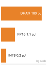
Moving a byte from DRAM costs about 145 times the energy of a 16-bit floating-point multiply, so data movement, not arithmetic, dominates the energy cost.

Horowitz, Mark. 2014. “1.1 Computing’s Energy Problem (and What We Can Do about It).” 2014 IEEE International Solid-State Circuits Conference Digest of Technical Papers (ISSCC), 10–14. https://doi.org/10.1109/isscc.2014.6757323.

The energy comparison depends on the transfer size and arithmetic operation being counted. Under the energy constants used in this text, moving one byte from off-chip DRAM consumes roughly 145× the energy of a 16-bit floating-point (FP16) multiply and 800× that of an INT8 (8-bit integer) multiply (Horowitz 2014). Whether movement dominates a complete workload also depends on the number and width of transfers relative to its operation count. The physical reason for the per-access gap is that data movement requires charging and discharging wires over longer distances, while arithmetic occurs locally within a processing unit’s circuits. Minimizing avoidable data movement \((\DataVolume)\) can therefore improve both speed and energy efficiency.

↪ The energy ladder from on-chip arithmetic to off-chip memory, and why its gap makes data movement a primary target for accelerator design, are developed in Machine learning hardware specialization.

Checkpoint 1.2: The iron law

Before proceeding, verify that you can manipulate both forms of the iron law (equation 2 and equation 3, where \(\Time = \frac{\DataVolume}{\Bandwidth} + \frac{\Operations}{\PeakRate \cdot \EfficiencyHw} + \Latency\)):

• D·A·M product (equation 2): identify which two factors multiply to set \(\Operations\), and explain the difference between logical samples or tokens (\(\DatasetSize\)) in the Data factor and physical bytes moved (\(\DataVolume\)) in the memory term.
• Memory term \((\DataVolume/\Bandwidth)\): identify the physical resource that bounds this term and name one workload regime where it dominates.
• Compute term \((\Operations/(\PeakRate \cdot \EfficiencyHw))\): identify the hardware quantity and utilization factor that bound this term.
• Latency term \((\Latency)\): identify which costs remain after data movement and arithmetic have been optimized.
• Peak throughput: holding the other quantities fixed, if you double \(\PeakRate\), which term improves, and why does total execution time fall by less than half when movement and overhead also contribute?

1.7.1 Lighthouse models put the iron law into practice

Each term of the iron law suggests an engineering intervention. The memory term can be reduced by moving fewer bytes or increasing effective bandwidth. The compute term can be reduced by performing fewer operations or using arithmetic units more effectively. The latency term calls for reducing orchestration and communication overhead. The equation alone does not say which intervention a system needs; that depends on its measured workload and whether the required data fits in memory.

Concrete workloads answer that question. Five recurring lighthouse models serve as diagnostic probes for the iron law throughout this book; later chapters explain the model structures and execution mechanisms behind their constraints. Each is a distinct stress case under the workload conditions stated for it:

• Image classification (ResNet-50) (He et al. 2016) probes compute throughput. With sufficient reuse of learned filters across image positions and batched inputs, the arithmetic term (\(\Operations/(\PeakRate \cdot \EfficiencyHw)\)) can dominate execution time.
• Text generation (GPT-2/Llama) probes memory bandwidth, with GPT-2 (Radford et al. 2019) anchoring the lighthouse and Llama (Touvron et al. 2023) representing its larger successors. Generating text token by token, the phase called decode, for one request at a time offers little weight reuse per token, so fetching weights from memory (\(\DataVolume/\Bandwidth\)) can become the binding constraint.
• Recommendation (DLRM), the Deep Learning Recommendation Model (Naumov et al. 2019), probes memory capacity, which determines whether the model can run at all. Embedding tables store numerical vectors for user and item IDs. Large tables can reach about a hundred gigabytes in reference models (Naumov et al. 2019), and terabytes in production (Mudigere et al. 2022), exceeding single-accelerator device memory.
• Mobile vision (MobileNetV2) (Sandler et al. 2018) probes compute throughput within a power envelope. Its efficient operators cut arithmetic far enough that a phone-class processor can classify frames in real time while sharing a battery and thermal budget with other applications.
• Keyword spotting (KWS) probes the power envelope, because an always-on microcontroller²¹ must listen continuously for a wake word within a milliwatt budget and kilobytes of memory (Zhang et al. 2017).

He, Kaiming, Xiangyu Zhang, Shaoqing Ren, and Jian Sun. 2016. “Deep Residual Learning for Image Recognition.” 2016 IEEE Conference on Computer Vision and Pattern Recognition (CVPR), 770–78. https://doi.org/10.1109/cvpr.2016.90.

Radford, Alec, Jeffrey Wu, Rewon Child, David Luan, Dario Amodei, and Ilya Sutskever. 2019. Language Models Are Unsupervised Multitask Learners. OpenAI.

Touvron, Hugo, Thibaut Lavril, Gautier Izacard, Xavier Martinet, Marie-Anne Lachaux, Timothée Lacroix, Baptiste Rozière, et al. 2023. “LLaMA: Open and Efficient Foundation Language Models.” arXiv Preprint arXiv:2302.13971.

Naumov, Maxim, Dheevatsa Mudigere, Hao-Jun Michael Shi, Jianyu Huang, Narayanan Sundaraman, Jongsoo Park, Xiaodong Wang, et al. 2019. “Deep Learning Recommendation Model for Personalization and Recommendation Systems.” arXiv Preprint arXiv:1906.00091.

Mudigere, Dheevatsa, Yuchen Hao, Jianyu Huang, Zhihao Jia, Andrew Tulloch, Srinivas Sridharan, Xing Liu, et al. 2022. “Software-Hardware Co-Design for Fast and Scalable Training of Deep Learning Recommendation Models.” International Symposium on Computer Architecture (ISCA), 993–1011. https://doi.org/10.1145/3470496.3533727.

Sandler, Mark, Andrew Howard, Menglong Zhu, Andrey Zhmoginov, and Liang-Chieh Chen. 2018. “MobileNetV2: Inverted Residuals and Linear Bottlenecks.” 2018 IEEE/CVF Conference on Computer Vision and Pattern Recognition, 4510–20. https://doi.org/10.1109/cvpr.2018.00474.

²¹ Microcontrollers: Single-chip computers integrating a processor, memory, and interfaces to sensors or other devices. The keyword-spotting lighthouse has a kilobyte-scale memory budget and a milliwatt-scale power budget. A candidate model must fit those limits as well as meet its prediction-quality requirement.

Zhang, Yundong, Naveen Suda, Liangzhen Lai, and Vikas Chandra. 2017. Hello Edge: Keyword Spotting on Microcontrollers.

Mattson, Peter, Christine Cheng, Cody Coleman, Greg Diamos, Paulius Micikevicius, David Patterson, Hanlin Tang, et al. 2020. “MLPerf Training Benchmark.” Proceedings of Machine Learning and Systems (MLSys) 2: 336–49.

Gupta, Udit, Carole-Jean Wu, Xiaodong Wang, Maxim Naumov, Brandon Reagen, David Brooks, Bradford Cottel, et al. 2020. “The Architectural Implications of Facebook’s DNN-Based Personalized Recommendation.” 2020 IEEE International Symposium on High Performance Computer Architecture (HPCA), 488–501. https://doi.org/10.1109/HPCA47549.2020.00047.

These five are deliberately not the newest models. Each marks a point where the field turned and isolates one binding constraint in its cleanest form. ResNet-50 made deep convolutional training on accelerators routine and became a reference workload of the MLPerf training benchmark (Mattson et al. 2020). GPT-2 showed that scaling a decoder-only language model changes what it can do. DLRM represents the recommendation models that accounted for most AI inference cycles in Facebook’s data centers when it was introduced (Gupta et al. 2020). Later models grow in scale, but the same terms of the iron law bind them, so the analysis in this book should transfer to models that do not yet exist.

The iron law makes these differences actionable under the stated workload conditions. Raising peak compute \(\PeakRate\) helps convolutions when arithmetic dominates, while increasing memory bandwidth \(\Bandwidth\) helps generation when weight transfers dominate. Batch size, reuse, and serving patterns can change that diagnosis, so the bottleneck belongs to the workload on a particular machine rather than to the model name alone, which is why table 4 identifies each lighthouse by the regime it probes.

Same iron law, opposite dominant term, opposite fix.

Table 4: Lighthouse Models as Reference Workloads: Each workload illustrates a resource constraint under the stated conditions, providing a concrete setting for investigating how system constraints affect architectural choices. Each model’s architectural background appears in Network Architectures, and its quantitative specifications in Arithmetic intensity across workloads.

Lighthouse Model	System Bottleneck	What It Reveals	Diagnostic Target
ResNet-50	Compute throughput under reuse	GPU utilization, batching	Arithmetic throughput versus memory stalls
GPT-2/Llama	Memory bandwidth	Weight and sequence-state movement	Weight and cached-context transfer rates
Deep Learning Recommendation Model (DLRM)	Memory capacity	Embedding tables, memory budgeting	Device memory capacity and partitioning
MobileNetV2	Compute within a power envelope	Efficient operator design	Real-time latency deadlines within battery limits
Keyword spotting (KWS)	Power envelope	Tiny memory and energy budgets	Continuous inference within milliwatt power budgets

The lighthouse models supply the book’s recurring workloads; the deployment paradigms described later in this chapter supply the operating envelopes those workloads must fit. The iron law estimates the execution time of one run on one machine. Over the past decade, however, training workloads grew faster than hardware improvements alone could accommodate, making efficiency a central concern.

Self-Check: Question

1. In the Iron Law of ML Systems, \(T = \frac{D_{\text{vol}}}{\text{BW}} + \frac{O}{R_{\text{peak}} \cdot \eta_{\text{hw}}} + L_{\text{lat}}\), how do the terms differ when analyzing small-batch autoregressive LLM token decode versus large-batch ResNet-50 image inference?

   1. LLM decode is dominated by the latency term \(L_{\text{lat}}\), while ResNet-50 is dominated by the data movement term \(D_{\text{vol}}/\text{BW}\).
   2. Both workloads are dominated strictly by the compute term \(\frac{O}{R_{\text{peak}} \cdot \eta_{\text{hw}}}\), making memory bandwidth irrelevant.
   3. ResNet-50 is memory-capacity bound by embedding tables, while LLM decode is bound by network serialization overhead.
   4. Small-batch LLM decode is bound by the data movement term (\(D_{\text{vol}}/\text{BW}\)) because billions of weights and cached context must be fetched from memory for every single token generated, whereas batched ResNet-50 reuses weight parameters across many inputs and spatial locations, making the compute term (\(\frac{O}{R_{\text{peak}} \cdot \eta_{\text{hw}}}\)) dominant.

2. When data transfers and arithmetic are overlapped in a pipelined ML runtime, so that the next block of data loads while the current block is computed, how is the sequential additive Iron Law modified, and what determines execution time?

   1. \(T_{\text{pipelined}} = \frac{D_{\text{vol}}}{\text{BW}} \times \frac{O}{R_{\text{peak}} \cdot \eta_{\text{hw}}} \times L_{\text{lat}}\)
   2. \(T_{\text{pipelined}} = \min\left(\frac{D_{\text{vol}}}{\text{BW}}, \frac{O}{R_{\text{peak}} \cdot \eta_{\text{hw}}}\right) + L_{\text{lat}}\)
   3. \(T_{\text{pipelined}} \ge \max\left(\frac{D_{\text{vol}}}{\text{BW}}, \frac{O}{R_{\text{peak}} \cdot \eta_{\text{hw}}}\right) + L_{\text{lat}}\), where the slower pipeline stage dictates the critical path while hiding the latency of the faster stage.
   4. \(T_{\text{pipelined}} = \frac{D_{\text{vol}} + O}{\text{BW} + R_{\text{peak}}} + L_{\text{lat}}\)

3. Based on the energy cost model \(E_{\text{total}} \approx D_{\text{vol}} \times E_{\text{move}} + O \times E_{\text{compute}}\), explain why moving a byte from off-chip DRAM costs roughly 145 times more energy than an FP16 arithmetic operation, and state one system optimization that mitigates this energy tax.

4. A hypothetical sequential workload moves 1 GB at 100 GB/s, performs 2 GFLOPs at an effective rate of 100 GFLOP/s, and incurs 5 ms of fixed overhead. Calculate its execution time. Which single upgrade gives the larger reduction: doubling bandwidth or doubling the effective arithmetic rate? What is the ideal-overlap lower bound before either upgrade if overhead remains outside the overlapping phases?

See Answers →

1.8 Three Dimensions of ML Efficiency

Because training compute grew faster than hardware, every term of the iron law also had to shrink through better algorithms, better utilization, and better data. AlexNet’s 2012 run is where that pressure began. Read through the D·A·M taxonomy, its breakthrough was coordination across all three axes rather than algorithmic novelty in isolation: a convolutional architecture whose parallel matrix operations matched GPU capabilities, the 1.3M labeled images of the 2012 ImageNet challenge training split²² (Deng et al. 2009), and two consumer GPUs running for about six days. A university laboratory could afford that budget. Modern foundation models demand training compute roughly 8 orders of magnitude larger.

²² ImageNet: The full image collection grew from 3.2 million images reported in the initial paper to about 14.2 million across thousands of labeled categories (Deng et al. 2009; Russakovsky et al. 2015). The 2012 challenge used a subset of this collection; AlexNet’s training split contained about 1.3M labeled images. Distinguishing the full collection from a benchmark split matters when comparing dataset sizes and training costs.

Deng, Jia, Wei Dong, Richard Socher, Li-Jia Li, Kai Li, and Li Fei-Fei. 2009. “ImageNet: A Large-Scale Hierarchical Image Database.” 2009 IEEE Conference on Computer Vision and Pattern Recognition, 248–55. https://doi.org/10.1109/cvpr.2009.5206848.

Russakovsky, Olga, Jia Deng, Hao Su, Jonathan Krause, Sanjeev Satheesh, Sean Ma, Zhiheng Huang, et al. 2015. “ImageNet Large Scale Visual Recognition Challenge.” International Journal of Computer Vision 115 (3): 211–52. https://doi.org/10.1007/s11263-015-0816-y.

Scale drives AI progress, as the bitter lesson (section 1.4) argued, but ever-larger datasets and compute budgets narrow participation to the most resource-rich organizations. Even those organizations eventually meet physical limits in data center power, memory bandwidth, and the diminishing returns of adding more parameters. Using existing compute more efficiently is therefore a complementary path to progress.

Efficiency offers three complementary choices that align with the three factors of equation 2: perform less computation per sample, execute that computation in fewer seconds per FLOP, or choose more informative examples so the task needs fewer samples. Algorithmic efficiency reduces computational requirements (\(\text{FLOPs/Sample}\)) through model design and training procedures. Compute efficiency lowers realized machine time per operation (\(\text{Seconds/FLOP}\)) by raising hardware utilization \(\EfficiencyHw\) and cutting memory and latency stalls, turning more of the machine’s theoretical capacity into useful work. Data selection identifies examples that contribute useful learning signal, reducing \(\text{Samples/Task}\) (and therefore \(\Operations\)) when training processes fewer examples; under a fixed computation budget, it can instead redirect work toward more informative examples.

Choosing among them calls for a bottleneck diagnosis across the interfaces in figure 4. All three must account for information movement: reducing \(\text{FLOPs/Sample}\) alone has little effect on wall-clock time when the memory term \(\DataVolume/\Bandwidth\) dominates \(\text{Seconds/FLOP}\).

Part III develops these dimensions in the order work flows through a system. Data selection asks which examples merit training computation. Model compression²³ asks how much storage and arithmetic a trained model requires. Hardware acceleration explains how the remaining operations map onto memory and compute units. This teaching order does not prescribe an optimization sequence. The measured binding constraint and deployment budget determine where to intervene first, and hardware limits inform data and model choices from the outset.

²³ Model compression: A family of techniques that reduces model storage or computation, including quantization (storing values in fewer bits), pruning (removing parameters that contribute little), and distillation (training a smaller model to imitate a larger one). Its size and accuracy effects depend on the model, method, workload, and target hardware.

²⁴ Moore’s law: Gordon Moore’s 1965 observation described rapid growth in the number of components that could be economically integrated on a chip (Moore 1998); later industry summaries often expressed the cadence as roughly a two-year doubling.

Moore, G. E. 1998. “Cramming More Components onto Integrated Circuits.” Proceedings of the IEEE 86 (1): 82–85. https://doi.org/10.1109/jproc.1998.658762.

The historical trajectory of computer vision models isolates the compounding effect of architectural design. Hernandez and Brown (2020) held accuracy fixed at the AlexNet level and asked how much training computation successive architectures needed to reach it. Because they counted operations rather than seconds, hardware speed does not enter the measurement. Between AlexNet in 2012 and EfficientNet in 2019, the required compute fell by 44×, a halving roughly every 15 months between those two endpoints (figure 5). The dashed line in the figure is an exponential fit to those measured points. The reduction measures algorithmic progress at fixed task quality. Comparing it with hardware progress would require a matching measure of useful throughput or energy efficiency; Moore’s law describes transistor integration,²⁴ which alone does not determine either quantity.

Figure 5: Algorithmic Efficiency Trajectory: Each point shows how much less training compute an ImageNet architecture needed than AlexNet to reach AlexNet-level accuracy, so height measures algorithmic progress with hardware speed held out. Most later architectures sit well above AlexNet, although individual points vary; VGG-11 needed more compute than AlexNet. The dashed line is a least-squares exponential fit to the measured points. Data from Hernandez and Brown (2020).

Hernandez, Danny, and Tom B. Brown. 2020. “Measuring the Algorithmic Efficiency of Neural Networks.” arXiv Preprint arXiv:2005.04305, ahead of print. https://doi.org/10.48550/arxiv.2005.04305.

Architecture-by-architecture gains tell only half the story, because over the same years aggregate training compute in published frontier runs climbed far faster than algorithms could offset. Figure 6 charts that climb on a logarithmic scale, from early deep learning models near \(10^{18}\) FLOPs to frontier systems beyond \(10^{25}\) FLOPs. Sevilla et al. (2022) measured a doubling time of roughly six months across the deep learning era, and a least-squares fit to the runs in the figure gives a similar cadence. An earlier study over 2012 through 2018 found a 3.4-month doubling (Amodei and Hernandez 2018); different windows and sets of runs yield different estimates. Both studies found training compute growing faster than the roughly two-year doubling associated with Moore’s law. This divergence motivates efficiency improvements across algorithms, software runtimes, and hardware architectures, helping keep useful systems within reach as workload demands grow.

Figure 6: The Era of Scale: Each point plots a third-party training-compute estimate (FLOPs) for a notable model against its publication year on a log scale. Runs below \(10^{22}\) FLOPs appear in blue; larger runs appear in red. The dashed line is a least-squares fit to these points and doubles every 5 months. From AlexNet (2012) to GPT-4-class training scale (2023), compute requirements increased by roughly 8 orders of magnitude (about 44.7M times). This endpoint comparison is distinct from training-compute trend studies (Amodei and Hernandez 2018; Sevilla et al. 2022) and is used here to motivate the specialized infrastructure described in this book. Data from Epoch AI’s Notable AI Models database (Epoch AI 2026).

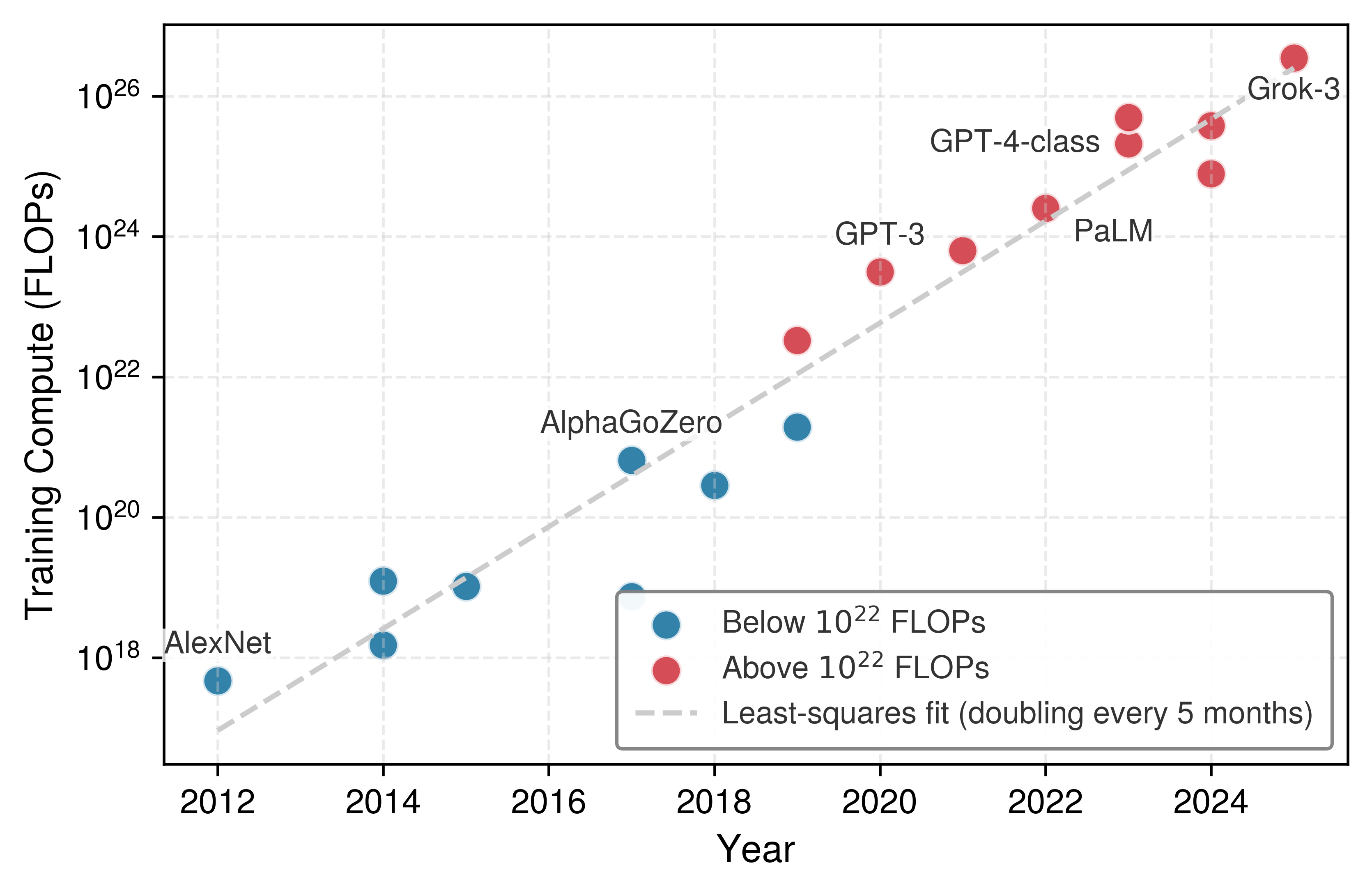
Amodei, Dario, and Danny Hernandez. 2018. “AI and Compute.” OpenAI Blog 6.

Sevilla, Jaime, Lennart Heim, Anson Ho, Tamay Besiroglu, Marius Hobbhahn, and Pablo Villalobos. 2022. “Compute Trends Across Three Eras of Machine Learning.” 2022 International Joint Conference on Neural Networks (IJCNN), 1–8. https://doi.org/10.1109/ijcnn55064.2022.9891914.

Epoch AI. 2026. Notable AI Models.

The two plots show how efficiency gains can coexist with growth in training scale. Figure 5 reports a 44× reduction in compute for a fixed accuracy target, while figure 6 illustrates roughly 8 orders of magnitude of growth in selected training runs. They measure different quantities and include contextual estimates, so they do not by themselves establish an economic cause. Efficiency makes a given capability less expensive; organizations can use the savings to reduce spending, broaden access, or pursue more demanding targets.

Systems Perspective 1.2: The efficiency paradox

Jevons paradox (Jevons 1865) describes cases in which more efficient resource use leads to greater total consumption because demand expands. A similar response is possible in AI. If EfficientNet needs 44× less compute than AlexNet to reach the same accuracy, an organization can reinvest the savings in larger models or more experiments. It can also choose a smaller budget or serve more users at the same cost. Reinvestment is a possible consequence of efficiency, not an inevitable one, and the plotted trends alone do not establish it.

Jevons, William Stanley. 1865. The Coal Question: An Inquiry Concerning the Progress of the Nation, and the Probable Exhaustion of Our Coal Mines. Macmillan; Co.

Whether reinvestment pays is an economic question. The same physical terms that determine time and energy also determine cost: every byte moved, operation executed, and millisecond of latency consumes infrastructure budget. The test is whether added compute buys enough model improvement to justify the expenditure.

1.8.1 Return on compute: Weighing accuracy against cost

A model upgrade that raises accuracy by 1 percentage point can still be the wrong choice if it requires a 10\(\times\) increase in \(\Operations\) (total operations) whose cost exceeds the application’s budget or the gain’s value. Return on compute (RoC) measures the incremental accuracy gain per added dollar of infrastructure investment, in accuracy points per dollar: \[ \text{RoC} = \frac{\FiniteChange\text{Accuracy}}{\FiniteChange\text{Compute Cost}} \tag{6}\]

The RoC test compares that ratio against what each point of accuracy is worth to the application. Each alternative is compared against the same baseline, and the ratio is defined only when the added cost is positive. The GPT-3 estimate above demonstrates a different benefit: assuming scheduling changes preserve model quality, raising \(\EfficiencyHw\) from 45 percent to 60 percent saves 6 days of cluster time for the same training work. This is a cost saving, not an accuracy gain. It can free budget for another experiment, whose incremental accuracy and cost must then be measured. The iron law helps estimate what computation costs; RoC asks whether an additional investment is worthwhile. Efficiency choices must therefore be evaluated against the system’s goals and deployment constraints.

Self-Check: Question

1. Between 2012 (AlexNet) and 2019 (EfficientNet), algorithmic efficiency for ImageNet classification improved by approximately 44\(\times\) for a fixed accuracy target. Separately, the chapter uses AlexNet-to-GPT-scale growth as an illustrative endpoint comparison showing that training compute expanded by roughly \(10^8\times\). How can the ‘efficiency paradox’ (Jevons paradox in ML systems) reconcile these two observations?

   1. Efficiency lowers the compute needed for a fixed accuracy, and organizations can reinvest the savings in larger models or more experiments, although the plotted trends alone do not establish that they did.
   2. Algorithmic efficiency metrics only apply to inference workloads, while training compute growth applies exclusively to cloud data centers.
   3. Hardware manufacturers deliberately slowed down clock frequencies to increase total data center power consumption.
   4. The 44\(\times\) algorithmic gain was an artifact of integer quantization that could not be replicated in 16-bit floating-point training.

2. The chapter contrasts a 3.4-month doubling in training compute (2012–2018) with the roughly two-year doubling associated with Moore’s law. Why does this divergence motivate efficiency work?

   1. The latency gap between CPU cache access and local register access in accelerator memory hierarchies.
   2. The widening divergence between the rate at which frontier AI model compute demand has grown (doubling roughly every 3.4 months) and the rate at which semiconductor physics advances hardware density via Moore’s Law (doubling roughly every 24 months).
   3. The difference in training loss between supervised fine-tuning and reinforcement learning from human feedback.
   4. The discrepancy between open-source framework code and proprietary GPU driver implementations.

3. Name the three dimensions of ML efficiency described in the chapter and explain how the pedagogical order in which they are taught (Data Selection -> Model Compression -> Hardware Acceleration) differs from a prescribed optimization sequence.

4. True or False: The 44\(\times\) reduction in training compute from AlexNet to EfficientNet can be directly compared with Moore’s-law transistor growth to show that algorithms outpaced hardware.

5. In economic analysis of ML systems, the quantitative metric that measures the incremental gain in model accuracy achieved per added dollar of infrastructure investment is called the ____.

See Answers →

1.9 AI Engineering as a Discipline

A cloud service may optimize throughput across racks of accelerators, while an edge device must remain within a strict battery and thermal envelope, so the same model can be efficient in one setting and unusable in another. Holding predictive quality and resource cost to one specification across such different operating budgets requires combining the three quantitative tools developed above: the degradation equation judges predictive quality in both settings, the iron law judges execution time and energy, and the efficiency framework judges the cost of improving either. Applying them draws on computer science, electrical engineering, statistics, and established software and systems engineering practice.

Definition 1.3: AI engineering

AI engineering is the discipline of designing, deploying, and maintaining ML systems whose predictive quality and execution meet stated deployment requirements. It integrates decisions about data, algorithms, and machines, using statistical evidence to assess learned behavior and measurements to assess resource use.

1. Significance: A model improvement must still satisfy the other system requirements. AI engineering jointly considers data quality and governance, prediction quality, execution time, memory, energy, and cost. A model that achieves 95 percent accuracy in research but violates a 100 ms deployment latency requirement does not meet the system specification.
2. Distinction: A model-level evaluation establishes evidence under a stated dataset and protocol. AI engineering must carry that evidence into a complete system whose latency, throughput, accuracy, cost, fairness, and robustness meet deployment requirements, and reassess it when operating conditions change.
3. Common pitfall: A frequent misconception is that AI engineering is just “software engineering for ML.” Software correctness remains necessary, but the system specification also includes statistical claims about learned behavior over an operating population. Code tests cannot establish those claims by themselves, making continuing evaluation and monitoring part of the system design.

A requirement can be fixed while the evidence for meeting it remains uncertain. Pedestrian recall of at least 95 percent over a stated population is a fixed target; evaluation estimates recall from sampled outcomes, with uncertainty that must be reported and reassessed as conditions change. Execution requirements also need a defined workload and measurement protocol. Sampled response times support a statistical latency claim; a hard bound requires assumptions and analysis covering the specified execution conditions. Combining these obligations resembles the earlier convergence of computing and electrical engineering in computer engineering.²⁵ In this book’s usage, AI engineering names the discipline and its shared principles, while ML systems engineering names the work of applying them to build and operate a specific system under its deployment constraints.

²⁵ Computer engineering: A discipline spanning digital circuits, processor design, and the software that runs on them. Moving a function from software into specialized hardware can change its speed, power use, and flexibility. ML systems engineering extends this shared design problem to include learned behavior and the data that shapes it.

1.9.1 Engineering across the ML lifecycle

Shipping a trained model to production does not end the engineering work, because the first shift in user behavior or upstream data can force a deployed system back into data collection and training. Putting an algorithmic advance into service requires data ingestion and preprocessing, computation within the available machine budget, reliable serving, and ongoing evidence of real-world performance. These obligations form a recurring lifecycle rather than a linear sequence that ends at deployment, and the engineering object is no longer only code but also data, model behavior, deployment context, and monitoring evidence evolving together.

At the project level, six responsibilities organize this work: problem definition, data collection and preparation, model development and training, evaluation and validation, deployment and integration, and monitoring and maintenance. Problem definition sets the task and acceptance requirements before any data is collected, so figure 7 begins after it and splits the data stage into collection and preparation to show where each feedback path re-enters.

The structural difference shows up first in tooling. Version control, continuous integration, and static analysis have long supported code-defined behavior. For learned behavior, these practices must also track dataset and model versions and test predictive quality, because source-code changes alone do not describe changes to the deployed system.

↪ The workflow controls that learned behavior adds to established software practice are developed in ML vs. traditional software.

Feedback must therefore assess learned behavior as well as software execution. In figure 7, a failed evaluation sends work back to data preparation, while degraded production performance sends it back to data collection. Feedback determines which work must be repeated; it does not make every alert a retraining instruction. The six stages and the feedback paths that join them into a loop are developed in The Lifecycle as a Loop.

Figure 7: ML System Lifecycle: Forward arrows carry work from data collection to monitoring, and the two labeled return arrows mark where evidence sends it back. The return arrows end at different stages, so a failed evaluation and a confirmed production problem trigger different amounts of rework.

Each stage of this cycle carries resource demands of its own. Those demands are not uniform, because the binding physical constraints depend on where the system is deployed.

1.9.2 Deployment context shapes the lifecycle

Deployment context determines which lifecycle pressures dominate. The same stages apply across ML systems, but a megawatt-scale data center and a milliwatt-scale embedded device impose different bottlenecks on data collection, model updates, monitoring, and serving. Four deployment paradigms span that range (cloud, edge, mobile, and TinyML), and their envelopes sit orders of magnitude apart.

From cloud to TinyML, the endpoints differ by roughly \(10^{5}\) in memory and \(10^{6}\) in compute. Because a cloud model cannot fit directly on a microcontroller, moving down that scale requires compression, a smaller architecture, or a narrower task. At the upper end, cloud ML systems offer large computing budgets alongside capacity limits, operational complexity, and substantial infrastructure bills; at the lower end, TinyML systems on microcontrollers make memory and energy feasibility an immediate concern, as a sensor may need to detect anomalies on a single battery for years. Between these poles, placement determines where work and resource demands fall: edge ML systems move computation toward data sources to reduce latency²⁶ and network traffic, mobile ML systems share memory, thermal headroom, and battery power with foreground applications, and hybrid systems split work across tiers to balance latency, privacy, bandwidth, and update control.

²⁶ Latency at the edge: Every millisecond of delay is distance traveled before a decision takes effect. A vehicle traveling at 30 m/s moves 3 cm during each millisecond of delay. Sensing, communication, computation, and actuation all contribute to the time before braking can begin, so reducing network delay addresses only part of the response budget.

↪ The light barrier, power wall, and memory wall that shape these operating envelopes are developed in Physical Constraints on Deployment.

Tight response deadlines or unreliable connectivity can require local execution, as in vehicle control, whereas fraud detection can run on cloud infrastructure whenever network and service latency fit the decision budget, and large language-model services rely on centralized clusters to accommodate their memory and compute footprint. In turn, cloud capacity and cost govern how often models are retrained, what historical data is retained, and how inference load is distributed, while edge and mobile limits constrain model size and update frequency.

As computation spreads across tiers, operational complexity grows alongside it. Edge and hybrid deployments must coordinate data collection across sensors with intermittent connectivity, track model versions across thousands of devices, push remote updates with safe rollback, and aggregate monitoring signals from distant endpoints. Data pressures pull in opposite directions at the same time: privacy rules and data sovereignty push computation toward the edge, whereas training high-capacity models pulls data back toward centralized clusters. Production architectures resolve this tension by running inference locally at the edge while routing sampled telemetry to cloud clusters for retraining.

In every deployment context, the model eventually meets inputs its evaluation never sampled. Autonomous driving illustrates this hybrid loop, running perception on the vehicle while cloud clusters train updated weights on logged fleet data. Because the Waymo Open Dataset shows pronounced domain gaps among San Francisco, Phoenix, and Mountain View (Sun et al. 2020), and because models that score well on benchmarks often lose accuracy when deployment inputs shift (Koh et al. 2021), every remote update must be revalidated against the population it will actually serve. Beyond predictive accuracy and latency, deployed systems must also satisfy fairness, interpretability, and privacy requirements across data, models, and governance: training sets can encode societal biases, regulated fields such as healthcare and finance require decisions that auditors and clinicians can interpret, and inference attacks²⁷ can leak sensitive information from trained weights. Meeting these technical, operational, and governance obligations across all four deployment regimes sets the structure of the book that follows.

Sun, Pei, Henrik Kretzschmar, Xerxes Dotiwalla, Aurelien Chouard, Vijaysai Patnaik, Paul Tsui, James Guo, et al. 2020. “Scalability in Perception for Autonomous Driving: Waymo Open Dataset.” Proceedings of the IEEE/CVF Conference on Computer Vision and Pattern Recognition, 2446–54. https://doi.org/10.1109/CVPR42600.2020.00252.

Koh, Pang Wei, Shiori Sagawa, Henrik Marklund, Sang Michael Xie, Marvin Zhang, Akshay Balsubramani, Weihua Hu, et al. 2021. “WILDS: A Benchmark of in-the-Wild Distribution Shifts.” In Proceedings of the 38th International Conference on Machine Learning, ICML 2021, 18-24 July 2021, Virtual Event, edited by Marina Meila and Tong Zhang, vol. 139. Proceedings of Machine Learning Research. PMLR.

²⁷ Inference attack: An attempt to deduce sensitive information about training data from a model’s outputs. Memorization can expose information, but the risk depends on the data, training procedure, and access available to the attacker. Defensive techniques include adding calibrated noise during training (differential privacy) and restricting the information returned by the system.

Self-Check: Question

1. The ML project responsibilities run from Problem Definition through Data Collection & Preparation, Model Development & Training, Evaluation & Validation, Deployment & Integration, and Monitoring & Maintenance. Which feedback pattern correctly interprets the finer-grained pipeline shown in the chapter?

   1. Deployment returns to Training on compiler warnings, and Collection returns to Preparation on memory leaks.
   2. Monitoring returns to Deployment on network timeouts, and Preparation returns to Collection on syntax errors.
   3. Evaluation can return work to preparation when investigation identifies a data problem, and monitoring can motivate new collection when outcome evidence and diagnosis identify a coverage gap.
   4. Model Training returns to Hardware Design on arithmetic overflow, and Deployment returns to Operating System Kernel on driver faults.

2. The chapter uses autonomous driving to show a challenge that production ML systems share. What does the Waymo Open Dataset’s report of domain gaps among San Francisco, Phoenix, and Mountain View imply for engineering such a system?

   1. A model that scores well on inputs from one setting can lose accuracy where deployment inputs differ, so every remote update must be revalidated against the population it will meet.
   2. Domain gaps disappear once perception runs on the vehicle rather than in the cloud, because local execution removes network effects.
   3. Domain gaps show that a perception model must be retrained from scratch for each city before any deployment is possible.
   4. Domain gaps are labeling errors that a larger annotation budget eliminates, after which one evaluation covers every city.

3. Place the six ML project responsibilities in their initial progression from defining the task to maintaining the deployed system:

1. Evaluation & Validation
2. Model Development & Training
3. Monitoring & Maintenance
4. Problem Definition
5. Data Collection & Preparation
6. Deployment & Integration

4. The chapter compares AI engineering with the earlier emergence of computer engineering. What do the two disciplines share, and what does AI engineering add?

5. Across the four deployment paradigms in the chapter (Cloud, Edge, Mobile, TinyML), approximately what orders-of-magnitude span exists between the highest tier (Cloud) and the lowest tier (TinyML) in memory capacity and compute throughput?

   1. \(10^2\) (100\(\times\)) span in memory capacity and \(10^3\) (1,000\(\times\)) span in compute throughput
   2. \(10^3\) (1,000\(\times\)) span in memory capacity and \(10^4\) (10,000\(\times\)) span in compute throughput
   3. \(10^{12}\) (one trillion\(\times\)) span in memory capacity and \(10^{15}\) span in compute throughput
   4. \(10^5\) (100,000\(\times\)) span in memory capacity and \(10^6\) (one million\(\times\)) span in compute throughput

6. A team designing a battery-powered smart doorbell vision system chooses a TinyML microcontroller node over a cloud-offloaded architecture. What primary constraint tradeoff drove this architectural decision?

   1. The doorbell must operate under a strict milliwatt power envelope on battery while preserving user visual privacy and avoiding reliance on intermittent wireless connectivity, accepting severe kilobyte-scale memory limits.
   2. TinyML microcontrollers provide higher FP16 peak FLOP/s throughput than multi-GPU cloud nodes.
   3. Cloud-based serving architectures cannot support visual wake-word classification algorithms.
   4. Microcontrollers eliminate the need for dataset annotation and model evaluation.

See Answers →

1.10 Book Organization

Production ML work divides into responsibilities that engineering teams own: data engineering, training systems, deployment infrastructure, operations and monitoring, and ethics and governance (Paleyes et al. 2022). Those boundaries leak. Upstream data pipelines limit what training can reach, training choices fix the memory and latency footprint at serving time, and governance constrains every stage, so the book does not follow an organization chart. Its four parts follow the order in which constraints must be understood. The organizing principle is context before theory: physical hardware limits and data ingestion bottlenecks constrain algorithmic choices, whose resource demands must in turn be checked against the machine. Readers establish operational boundaries and vocabulary (Part I) before constructing models (Part II), optimizing computational efficiency (Part III), and deploying systems under production service-level agreements (Part IV), the progression summarized in table 5.

Table 5: Book Organization: The four parts progress from foundations through model construction and training to optimization, deployment, and operations. This introduction precedes them and Conclusion follows them. Each part builds on the vocabulary and methods of its predecessors.

Part	Question It Answers	Key Chapters
I: Foundations of ML Systems	What is being built, under which constraints, and from what inputs?	System Paradigms, ML Lifecycle, Data Engineering
II: Development and Training	How does a model compute, how is it structured, and how is it trained?	Neural Computation, Network Architectures, ML Frameworks, Model Training
III: Optimization and Acceleration	How can the model be made cheaper, and how is the gain proven?	Data Selection, Model Compression, Hardware Acceleration, Benchmarking
IV: Deployment and Operations	Does the system survive real users, changing data, and its obligations?	Model Serving, ML Operations, Responsible Engineering

Each part opens with the named principles it develops. These are numbered across the book so later chapters can refer back to them. The deployment part, for example, opens with the verification gap stated over a deployment population.

This book focuses on the single-node regime of one host with one to eight accelerators, each typically using local device memory and communicating through an on-node interconnect such as PCIe or NVLink. The binding constraint depends on the workload and may be memory capacity, memory bandwidth, compute throughput, or communication. Larger fleets add coordination and network constraints across many hosts. For reading paths, learning outcomes, prerequisites, and guidance on using the textbook, the preface provides the orientation.

Self-Check: Question

1. What is the primary pedagogical rationale behind organizing the textbook into the four sequential parts: Part I (Foundations of ML Systems), Part II (Development and Training), Part III (Optimization and Acceleration), and Part IV (Deployment and Operations)?

   1. To teach low-level CUDA kernel programming before introducing high-level machine learning concepts.
   2. To ensure students deploy production systems in the cloud before learning how neural networks compute predictions.
   3. To establish the systems landscape, constraints, and vocabulary (context before theory) before constructing models, optimizing their physical execution, and managing them in production.
   4. To separate data science students who only read Part II from hardware engineering students who only read Part III.

2. What distinguishes the single-node execution regime covered in this volume from the fleet-scale orchestration regime addressed in advanced distributed systems?

3. True or False: In the textbook’s pedagogical build order, model compression and hardware acceleration (Part III) are introduced before neural computation and network architectures (Part II).

See Answers →

1.11 Fallacies and Pitfalls

A passing code test, a high held-out score, and a faster inference stage each provide useful evidence, but none alone establishes that an ML system meets its requirements. Mistaking code-level checks for validation of learned behavior overlooks the verification gap and silent degradation, treating a held-out score as proof of deployment readiness ignores distribution shift and execution budgets, and extrapolating a component speedup to the whole system overlooks the untouched costs captured by Amdahl’s law. Each of these errors applies evidence beyond the conditions that support it.

Fallacy: Better algorithms automatically produce better systems.

A more accurate spam classifier can still be a worse production choice if it needs too much memory or cannot classify incoming messages within the delivery budget. The iron law (section 1.7) explains why algorithmic quality alone does not settle that decision. Model selection must maximize task quality subject to latency, memory, energy, cost, and reliability requirements. A simpler model supported by representative data and reliable infrastructure can meet those requirements more effectively than a sophisticated model whose surrounding system is inadequate.

Pitfall: Treating ML systems as traditional software that happens to include a model.

Established testing and deployment practices remain necessary for ML systems, but code-level checks alone cannot validate learned behavior (section 1.6). Both conventional and ML software can fail silently. In the driver-assistance example, pedestrian recall can fall from 95 to 85 percent while the accelerator keeps its full frame rate and raises no fault. ML systems additionally require outcome monitoring to detect declining predictive quality, with observation windows and sample sizes sufficient to resolve relevant differences across subpopulations. Teams deploying ML with only continuous integration and continuous deployment (CI/CD) pipelines risk silent failures, in which test suites and health checks report green while user-facing prediction quality degrades.

Fallacy: High accuracy on benchmark datasets indicates production readiness.

A benchmark score describes performance on a stated dataset under an evaluation protocol; it does not establish deployment readiness (section 1.9.2). The ILSVRC validation set holds 50,000 images, while the number of possible inputs has 362,508 digits, so even a perfect score is evidence about a sample, not proof about the population. A sentiment model may lose accuracy when users employ slang or context absent from the test set. Deployment also introduces resource requirements: mobile memory and latency limits may make a multi-model ensemble impractical, while network round trips can consume the response budget. Production validation must cover the intended operating conditions, relevant subgroups, resource use, and monitoring needed to detect change.

Pitfall: Optimizing individual components without considering system interactions.

Amdahl’s law, which holds that the untouched share of a task caps the speedup of the whole, explains why improving inference alone may produce a small end-to-end gain. Consider a team that reduces model inference from 45 ms to 15 ms, expecting proportional improvement. Preprocessing still consumes 60 ms and postprocessing adds 25 ms, so total latency drops only from 130 ms to 100 ms. That is a 23 percent improvement in total latency rather than the 67 percent improvement of the inference stage alone. Most of the request path was untouched. Measuring the whole request prevents a component speedup from being mistaken for a system speedup; the bound in equation 11.1 computes the overall speedup from the share of time a component occupies and its local gain.

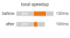
Making the model three times faster trims end-to-end latency by only 23 percent.

Fallacy: ML systems can be deployed once and left to run indefinitely.

Deployed ML systems cannot assume static performance over time: environmental distribution shifts can degrade a frozen model even when underlying execution code remains untouched. In this illustrative scenario, a recommendation system deployed at 85 percent accuracy drops to 80.2 percent within 6 months as purchasing patterns shift, losing 4.8 percentage points without any code changes. The ML lifecycle (section 1.9.1) therefore treats outcome monitoring and evidence-based retraining as operational requirements. Without continuous monitoring, systems can appear healthy while prediction quality silently erodes.

Pitfall: Assuming that ML expertise alone is sufficient for ML systems engineering.

Production ML (section 1.9.2) requires expertise across algorithms, software, systems, and operations. A team with strong ML skills can still miss throughput targets if storage layout or serving infrastructure is inadequate. Conversely, infrastructure built without attention to model inputs can introduce preprocessing defects that degrade predictions. Deployment case studies show the need for coordinated attention to data, models, infrastructure, and organizational workflow (Paleyes et al. 2022). Failures can arise at the boundaries, where one team’s assumptions become another team’s inputs.

Paleyes, Andrei, Raoul-Gabriel Urma, and Neil D. Lawrence. 2022. “Challenges in Deploying Machine Learning: A Survey of Case Studies.” ACM Computing Surveys 55 (6): 1–29. https://doi.org/10.1145/3533378.

Self-Check: Question

1. An inference pipeline consists of three sequential stages: data preprocessing taking 60 ms, model inference taking 45 ms, and output postprocessing taking 25 ms (total latency = 130 ms). An engineering team applies kernel fusion and quantization to achieve a \(3\times\) speedup on the model inference stage alone (reducing it from 45 ms to 15 ms). What is the resulting end-to-end pipeline latency and approximate overall system speedup, and what principle does this demonstrate?

   1. New latency is 100 ms (an overall speedup of \(\approx 1.30\times\), or a 23% reduction in execution time), illustrating Amdahl’s Law that component-level speedups yield only marginal end-to-end gains when non-optimized stages dominate.
   2. New latency is 43.3 ms (a \(3.0\times\) overall speedup, or 67% reduction), illustrating linear speedup scaling across modular microservices.
   3. New latency is 15 ms, illustrating that hardware acceleration bypasses pre- and post-processing stages.
   4. New latency is 115 ms, illustrating that quantization overhead cancels out inference gains.

2. Why does high accuracy on curated benchmark datasets (such as ImageNet or GLUE) frequently fail to guarantee production readiness in real-world deployments?

   1. Benchmarks are evaluated on GPUs, whereas all production models run on CPUs.
   2. Benchmark datasets contain only synthetic, computer-generated data that lacks realistic labels.
   3. Neural networks automatically lose their learned weights when exported to production formats.
   4. Benchmarks evaluate models on static, clean distributions without operational constraints (e.g., sub-100 ms latency budgets, memory limits, noise, and ongoing distribution shift), whereas production systems face uncurated edge cases, shifting user behavior, and hardware precision limits.

3. Why can code and infrastructure checks in a standard CI/CD pipeline fail to detect a loss of predictive quality, and how should drift and outcome monitoring guide the response?

4. True or False: In production ML systems engineering, selecting a model that provides a 1% higher benchmark accuracy is always preferable, even if it requires doubling inference latency and memory footprint beyond the client application’s SLA.

See Answers →

1.12 Summary

Machine learning systems must satisfy two obligations at once: learned behavior must remain trustworthy, and the machine must deliver that behavior within physical and economic limits. Every ML system answers to three questions: what shapes its predictions, what limits its execution, and what evidence supports its deployment. The D·A·M taxonomy organizes that diagnosis, the degradation equation and the iron law quantify the trade-offs, and efficiency together with return on compute guides the choice of interventions. Because data and operating conditions keep changing, those answers never stay fixed, and five lighthouse models (ResNet-50, GPT-2/Llama, DLRM, MobileNetV2, and keyword spotting) recur throughout the book to ground these methods in concrete workloads.

Return to the smartphone interaction that opened the chapter. What appeared to be one intelligent action depended on representative data, a learned model, a machine within its operating budget, and feedback that could reveal changing behavior. That chain answers the question posed at the outset: an accurate model alone does not establish a reliable, efficient system. AI engineering coordinates these decisions and uses measured evidence to assess whether the complete system meets its requirements.

Key Takeaways: Constraints drive architecture

• Relieving a bottleneck can expose another: Data, Algorithm, and Machine constraints interact. After an intervention, measure the complete system again to determine which constraint now limits the result.
• Learned behavior can decay silently: ML systems can lose predictive quality while code and infrastructure stay fixed because deployment inputs change. Drift metrics prompt investigation; labeled outcomes establish whether prediction quality has fallen.
• End-to-end time is the whole path: Data movement, computation, and overhead all spend from the same time budget. Cutting inference from 45 ms to 15 ms gives only 23 percent improvement when preprocessing (60 ms) and postprocessing (25 ms) dominate, so optimize the term that binds end-to-end behavior.
• Scale needs useful computation: The bitter lesson emphasizes search and learning methods that can use increasing computation effectively. Their benefit depends on data, objectives, and a supporting machine. Efficiency gains of 44× at a fixed accuracy target coexisted with roughly 8 orders of magnitude of growth in selected training runs.
• AI engineering is continuous co-design: Deployment requirements guide decisions about data, models, and execution. Evaluation and lifecycle monitoring provide evidence that predictive quality and resource use continue to meet those requirements.

An intended capability becomes an engineering result only when measured behavior meets the goal within a feasible resource budget. Data, learning objectives, design choices, and hardware all shape that result. The first engineering act is therefore a measurement of the complete system, not an optimization of its most visible part.

What’s Next: From vision to architecture

This chapter asserted that the four deployment paradigms have operating envelopes orders of magnitude apart without deriving the gap. System Paradigms derives it from physical limits and turns it into a decision framework for choosing among them when requirements conflict.

1.13 Self-Check Answers

Self-Check: Answer

1. A production autonomous vehicle perception model reliably detects obstacles under clear daytime conditions, but fails to identify a pedestrian at dusk even though all code executes without runtime exceptions and strictly within its 50 ms latency window. Which core challenge of ML systems engineering does this failure demonstrate?

   1. The latency added by serial interconnect communication across distributed accelerators
   2. A hardware execution failure caused by GPU thermal throttling and clock frequency scaling
   3. The dual mandate requirement that learned behavior must remain statistically trustworthy while executing within physical execution constraints
   4. The failure of traditional continuous integration pipelines to compile stochastic gradient descent operations

   Answer: The correct answer is C. The dual mandate requires that an ML system satisfy both physical constraints (latency, compute, memory, power) and statistical trustworthiness (accurate, reliable predictions across operational domains). In this scenario, the perception stack met its physical execution budget (running in under 50 ms without crashing) but failed its statistical obligation because its learned representations did not generalize to dusk conditions. Thermal throttling or serial interconnect latency would manifest as latency spikes rather than silent perceptual misses. Compiling stochastic gradient descent relates to training pipelines rather than inference execution.

   Learning Objective: Distinguish between physical execution failures and statistical trustworthiness failures within the dual-mandate framework.

2. True or False: In a production ML system, if all code executes without runtime exceptions, CPU and GPU utilization are normal, and latency requirements are met, the system is guaranteed to be operating correctly.

   Answer: False. Healthy execution telemetry shows that the software and hardware path is functioning, but it does not guarantee good predictions. In an ML system, the code can run correctly and on time while the live data has drifted away from the training distribution, causing silent degradation in prediction quality.

   Learning Objective: Explain why traditional software health metrics such as uptime and exception logging are insufficient to verify ML system correctness.

3. Why does the shift from code-defined logic to data-defined behavior turn large-scale AI deployment into an end-to-end orchestration problem rather than an isolated modeling exercise?

   Answer: When data defines system behavior, correctness depends on continuous data pipelines, feature consistency, and representative distributions rather than static code logic alone. Deploying these models at scale requires coordinating distributed accelerator clusters, memory hierarchies, and real-world latency budgets while managing the risk of silent statistical decay under shifting operational data.

   Learning Objective: Analyze why data-defined behavior transforms AI deployment into a full-stack orchestration challenge.

4. The fundamental engineering obligation requiring that an ML system’s learned behavior be statistically trustworthy while the machine delivers that behavior within finite time, memory, energy, and cost budgets is known as the ____.

   Answer: dual mandate. It names the requirement to engineer trustworthy learned behavior together with feasible physical execution within the available budgets.

   Learning Objective: Identify the foundational term defining the dual constraints of ML systems engineering.

← Back to Questions

Self-Check: Answer

1. In Andrej Karpathy’s Software 1.0 vs. Software 2.0 framing, how do the roles of source code, the compiler, and debugging map to machine learning workflows?

   1. Learned weights shaped by training data act as source code, the training loop (stochastic gradient descent) acts as the compiler, and debugging expands from execution traces to the data and learned behavior.
   2. Python scripts act as source code, the deep learning framework acts as the compiler, and debugging focuses on stepping through tensor operations in an interactive debugger.
   3. Training datasets act as source code, GPU hardware acts as the compiler, and debugging focuses on profiling memory bandwidth utilization.
   4. Pretrained model weights act as source code, inference serving runtimes act as the compiler, and debugging focuses on network packet inspection.

   Answer: The correct answer is A. In Software 2.0, learned weights shaped by training data act as source code, and the training loop (stochastic gradient descent) plays the role of the compiler that produces those weights from the curated examples. Debugging still traces execution, but it also expands to the data and the learned behavior. Treating Python scripts or raw datasets as source code misplaces where the program logic lives, and treating hardware or serving runtimes as compilers confuses the execution platform with the training process that produces the weights.

   Learning Objective: Compare the structural components of Software 1.0 with their Software 2.0 counterparts.

2. A computer vision test suite evaluates a \(224{\times}224\) RGB image classifier on 50,000 validation images. Why does passing 100% of these test cases still leave a substantial ‘verification gap’ in production?

   1. Validation sets evaluate floating-point weights, whereas production inference engines always run in integer precision.
   2. The total input space of possible pixel configurations (\(256^{150{,}528}\), spanning over 300,000 decimal digits) vastly exceeds the sample coverage of any finite test set, making exhaustive testing mathematically impossible.
   3. Convolutional neural networks cannot generalize beyond the exact batch size used during validation testing.
   4. Test suites only evaluate forward inference passes, whereas production systems must continuously execute backward gradient updates.

   Answer: The correct answer is B. The verification gap, the disparity between what a test set covers and the inputs a deployed system meets, arises because the input space of \(224{\times}224\) 8-bit RGB images contains \(256^{150{,}528}\) possible configurations (a number with over 300,000 digits in base 10), whereas a 50,000-image test set evaluates a vanishingly small fraction. Predeployment testing provides statistical evidence over sampled inputs, not exhaustive mathematical proof. Explanations invoking integer precision describe quantization effects rather than the fundamental input-space disparity. Explanations suggesting batch-size limits or backward pass requirements in production confuse inference serving with training mechanics.

   Learning Objective: Calculate and explain the mathematical origin of the verification gap in high-dimensional ML systems.

3. How did Google Flu Trends fail despite having access to hundreds of billions of real-time search queries, and what systems engineering lesson does this failure provide regarding behavioral proxies?

   Answer: Google Flu Trends failed because search query volume was a behavioral proxy reflecting news coverage and search autocomplete features (public attention) as well as actual influenza infection (clinical ground truth), causing overestimates for 100 out of 108 weeks. The systems lesson is that massive data volume cannot substitute for a feedback loop to validated ground-truth measurements (such as CDC clinical sentinel data) to continuously detect proxy drift.

   Learning Objective: Analyze the failure mechanism of Google Flu Trends to evaluate the risks of uncalibrated behavioral proxies.

4. The development paradigm where engineering teams hold model architecture code relatively fixed and systematically improve dataset quality, labels, and coverage to program model behavior is known as ____ AI.

   Answer: data-centric. It emphasizes improving the data while holding the code comparatively fixed to shape model behavior.

   Learning Objective: Identify the term for data-centric AI versus model-centric AI.

← Back to Questions

Self-Check: Answer

1. Which historical transition correctly pairs an AI era with the primary systems bottleneck that limited its scalability and forced the transition to the subsequent paradigm?

   1. Symbolic AI was limited by compute throughput, forcing the transition to expert systems; Deep Learning was limited by human rule maintenance, forcing the transition to statistical learning.
   2. Expert Systems were limited by GPU memory bandwidth, forcing the transition to statistical learning; Statistical Learning was limited by formal logic ambiguity, forcing the transition to deep learning.
   3. Statistical Learning was limited by a complete lack of training labels, forcing the transition to symbolic logic; Symbolic AI was limited by hardware integer arithmetic, forcing the transition to neural networks.
   4. Expert Systems were limited by the knowledge acquisition bottleneck (serial human expert elicitation bandwidth), forcing the transition to statistical learning; Statistical Learning was limited by the feature engineering bottleneck (manual extraction of hand-crafted representations), forcing the transition to deep learning.

   Answer: The correct answer is D. Expert systems hit the knowledge acquisition bottleneck because extracting and maintaining consistent rules was bound by the serial bandwidth of human experts; statistical learning overcame this by estimating probabilities from data, but hit the feature engineering bottleneck because humans still had to manually design feature extractors (e.g., SIFT, HOG); deep learning overcame this by learning representations end-to-end from raw data. Compute throughput and GPU memory bandwidth constrained deep learning, not early symbolic or expert systems. Formal logic ambiguity was the logic bottleneck of symbolic AI, not statistical learning.

   Learning Objective: Compare the four historical AI eras across their primary limiting systems bottlenecks.

2. Moravec’s paradox observes that tasks humans find easy (such as visual perception, walking, and grasping) require vast computational resources, while tasks humans find hard (such as playing chess or solving algebra) require comparatively little compute. What is the direct implication of this paradox for ML systems hardware?

   1. Symbolic reasoning algorithms require multi-GPU accelerator clusters, whereas computer vision pipelines run efficiently on single-threaded CPUs.
   2. High-level reasoning tasks saturate off-chip memory bandwidth, while low-level perceptual tasks are strictly compute-bound.
   3. Perceptual and physical-world AI tasks demand massive parallelism, high memory bandwidth, and specialized hardware accelerators to process dense, high-dimensional sensor streams in real time.
   4. Robotic perception models can be deployed on microcontrollers without model compression or accuracy degradation.

   Answer: The correct answer is C. Moravec’s paradox explains why perception, vision, and motor control—which humans execute effortlessly—require processing high-dimensional data at high frame rates, driving the requirement for massive arithmetic parallelism, high memory bandwidth, and domain-specific accelerators (GPUs, TPUs). The claim that symbolic reasoning requires accelerator clusters reverses the computational requirements. The assertion that high-level reasoning saturates bandwidth while perception is only compute-bound ignores the massive data movement required for continuous video streams. Microcontroller deployment for perception requires aggressive compression due to strict hardware limits.

   Learning Objective: Apply Moravec’s paradox to explain why perceptual AI workloads drive modern hardware accelerator design.

3. **Place the four historical AI engineering eras in chronological order based on when their primary paradigm dominated, and identify the key bottleneck that constrained each era:

1. Deep Learning Era
2. Expert Systems Era
3. Symbolic AI Era
4. Statistical Learning Era**

Answer: The correct order is (3) -> (2) -> (4) -> (1). - (3) Symbolic AI Era (1950s–1970s): Constrained by the logic bottleneck (brittle hand-coded rules unable to handle real-world ambiguity). - (2) Expert Systems Era (1970s–1980s): Constrained by the knowledge acquisition bottleneck (serial human expert elicitation bandwidth). - (4) Statistical Learning Era (1990s–2000s): Constrained by the feature engineering bottleneck (manual extraction of hand-crafted features prior to statistical classification). - (1) Deep Learning Era (2010s–present): Constrained by the compute and infrastructure bottleneck (hardware scaling, memory bandwidth, and distributed coordination).

Learning Objective: Classify the chronological progression of AI engineering eras and their respective systems bottlenecks.

4. Why was AlexNet’s 2012 ImageNet victory considered a breakthrough in systems co-design rather than purely an algorithmic advance?

   Answer: AlexNet co-designed the convolutional neural network architecture with the physical hardware constraints of two GTX 580 GPUs, splitting convolutional and dense layers across parallel GPU streams. While convolutional networks had existed for more than a decade, AlexNet aligned dense matrix arithmetic directly with parallel GPU architectures and massive labeled data (ImageNet), achieving a 15.3% top-5 error rate (a 42% relative improvement over the 26.2% runner-up).

   Learning Objective: Evaluate AlexNet as an achievement of systems co-design linking architecture, dataset scale, and GPU hardware.

5. True or False: The Viola-Jones face detection algorithm achieved real-time execution on early-2000s CPUs by using a cascade of simple rectangular features that evaluated an average of about ten features per candidate region, although the full cascade contained over 6,000 features.

   Answer: True. Viola-Jones exemplified the statistical learning era: expert feature engineering (integral image rectangular features) and a cascaded classifier allowed early rejection of non-face regions, achieving real-time performance within narrow domains while remaining constrained by manual feature engineering when applied to new tasks.

   Learning Objective: Explain how cascaded classifiers and hand-engineered features enabled real-time inference during the statistical learning era.

← Back to Questions

Self-Check: Answer

1. Why did Richard Sutton describe the fundamental finding of 70 years of AI research as a ‘bitter’ lesson for researchers and engineers?

   1. Human intuition naturally seeks to build intelligence by encoding domain expertise and linguistic rules into models, yet historical progress repeatedly demonstrates that general-purpose search and learning leveraging raw computation outperform hand-crafted human knowledge.
   2. Hardware accelerators have reached physical thermodynamic scaling limits, preventing further increases in neural network parameter counts.
   3. Stochastic gradient descent algorithms produce models whose internal mathematical representations cannot be formally proven correct.
   4. Open-source models consistently match the performance of proprietary industrial foundation models trained at hundred-million-dollar compute budgets.

   Answer: The correct answer is A. The lesson is ‘bitter’ because researchers persistently try to hand-craft human domain heuristics (such as chess evaluation tables, linguistic grammars, or hand-tuned visual filters), only to discover that general methods (search and learning) powered by massive computation consistently surpass hand-engineered representations as scale increases. Thermodynamic scaling limits describe hardware physical bounds rather than Sutton’s philosophical thesis. Lack of formal verification concerns how learned systems are checked, not Sutton’s thesis. The comparison between open-source and proprietary models is a market dynamic unrelated to Sutton’s essay.

   Learning Objective: Explain why the bitter lesson prioritizes scalable computation and learning over hand-crafted human domain expertise.

2. In comparing IBM’s Deep Blue (1997) and DeepMind’s AlphaGo Zero (2017), how do their designs reflect the progression toward Sutton’s bitter lesson?

   1. Deep Blue relied entirely on deep reinforcement learning, whereas AlphaGo Zero returned to hand-coded expert evaluation tables.
   2. Deep Blue combined custom silicon search (100 to 200 million positions/second) with hand-coded chess heuristics, whereas AlphaGo Zero learned through self-play without human game records or hand-engineered features, using neural networks to guide tree search.
   3. Both systems avoided the use of custom silicon or GPUs, relying strictly on algorithmic elegance over compute scale.
   4. AlphaGo Zero eliminated all tree search mechanisms in favor of pure single-step feedforward classification.

   Answer: The correct answer is B. Deep Blue paired custom hardware search (480 custom chess chips searching roughly 100 to 200 million positions per second) with chess-specific evaluation knowledge. AlphaGo Zero advanced this trajectory by learning through self-play without human game records or hand-engineered features, using neural networks to guide tree search so that computation, rather than encoded human knowledge, improved play. The claim that Deep Blue used deep reinforcement learning reverses the historical paradigms. The assertion that neither system used specialized compute contradicts the custom silicon of Deep Blue and the large-scale self-play computation of AlphaGo Zero. AlphaGo Zero used neural networks to guide tree search rather than eliminating search.

   Learning Objective: Compare how Deep Blue and AlphaGo Zero balanced hardware acceleration, search scale, and learned representations.

3. If the bitter lesson states that computation-leveraging methods dominate over time, why does realizing this advantage depend primarily on systems engineering rather than pure algorithmic theory?

   Answer: Harnessing computation at scale requires solving physical systems bottlenecks: memory bandwidth, cluster interconnects, distributed fault tolerance, thermal dissipation, and gigawatt-hour energy budgets (\(E_{\text{move}} \gg E_{\text{compute}}\)). An algorithm designed to scale with compute is ineffective if memory systems cannot supply weights fast enough or if infrastructure cannot coordinate thousands of accelerators without stalling.

   Learning Objective: Justify why systems engineering is the prerequisite for realizing the benefits of the bitter lesson.

4. True or False: According to the bitter lesson, building domain-specific linguistic or perceptual rules into deep neural network architectures provides a permanent, compounding advantage over general architectures as compute budgets expand.

   Answer: False. Sutton’s bitter lesson demonstrates that domain-specific human heuristics are a depreciating asset; as computational scale increases by orders of magnitude, general architectures (such as transformers) that leverage raw compute and learning consistently surpass specialized, rule-infused designs.

   Learning Objective: Evaluate the long-term trade-off between domain-specific inductive biases and general scalable architectures under expanding compute budgets.

← Back to Questions

Self-Check: Answer

1. An ML engineering team trains a 70-billion-parameter language model. When profiling the distributed cluster, they notice that accelerator compute engines remain idle for 45% of execution time waiting for batch tensors to be loaded from remote object storage over the network. Along which D·A·M axis does the primary binding constraint lie, and which intersection represents the appropriate optimization space?

   1. Machine axis; \(\text{Algorithm} \cap \text{Machine}\) (mixed precision quantization and kernel fusion)
   2. Algorithm axis; \(\text{Data} \cap \text{Algorithm}\) (curriculum learning and active data selection)
   3. Data axis; \(\text{Data} \cap \text{Machine}\) (I/O pipelining, prefetching, and storage memory hierarchy)
   4. Workload axis; \(\text{Data} \cap \text{Algorithm} \cap \text{Machine}\) (reinforcement learning from human feedback)

   Answer: The correct answer is C. The binding bottleneck is data movement and storage throughput starving the compute engines, placing the constraint along the Data axis. The corresponding design space is the \(\text{Data} \cap \text{Machine}\) intersection (‘How to Move Information’), which includes I/O bandwidth optimization, asynchronous prefetching, efficient storage formats, and memory hierarchy management. Optimizing mixed precision quantization (\(\text{A} \cap \text{M}\)) accelerates compute execution but does not resolve storage starvation. Curriculum learning (\(\text{D} \cap \text{A}\)) selects which samples to present but does not fix I/O pipeline bandwidth.

   Learning Objective: Analyze the binding constraint in an ML system using the D·A·M taxonomy and identify the corresponding optimization intersection.

2. Explain what the concept of a ‘binding constraint’ means in the D·A·M framework, and describe the risk of optimizing a non-binding axis.

   Answer: A binding constraint is the specific physical, algorithmic, or data bottleneck whose relaxation directly improves end-to-end system performance (e.g., latency, throughput, or cost). Optimizing a non-binding axis (such as upgrading to faster GPUs when the system is bounded by disk I/O, or collecting more data when model capacity is saturated) expends engineering resources while leaving overall system throughput or prediction quality virtually unchanged.

   Learning Objective: Explain the principle of the binding constraint and the consequences of optimizing non-binding components.

3. In the D·A·M intersection landscape, the intersection between Algorithm and Machine (\(\text{A} \cap \text{M}\)) addresses the core question of ‘How to ____’, focusing on how the model’s mathematical work is mapped onto hardware execution and data movement efficiently.

   Answer: Execute Efficiently. In the D·A·M taxonomy, the Algorithm-Machine intersection (A ∩ M) asks how the model’s computation is carried out on physical hardware so arithmetic and movement are organized efficiently.

   Learning Objective: Identify the core engineering focus of the Algorithm-Machine intersection in the D·A·M taxonomy.

← Back to Questions

Self-Check: Answer

1. In the degradation equation \(\text{Accuracy}(t) \approx \text{Accuracy}_0 - \lambda \cdot \mathcal{D}(P_t \lVert P_0)\), what do the terms \(\mathcal{D}(P_t \lVert P_0)\) and \(\lambda\) represent, and which engineering lever addresses \(\lambda\)?

   1. \(\mathcal{D}(P_t \lVert P_0)\) is hardware clock jitter, \(\lambda\) is GPU temperature sensitivity, and it is addressed by dynamic voltage and frequency scaling.
   2. \(\mathcal{D}(P_t \lVert P_0)\) is statistical divergence between live production data and training data, \(\lambda\) is model sensitivity to distribution shift, and it is addressed by robust training and domain adaptation to flatten the degradation curve.
   3. \(\mathcal{D}(P_t \lVert P_0)\) is the memory bandwidth ratio, \(\lambda\) is cache miss penalty, and it is addressed by prefetching weights into on-chip memory.
   4. \(\mathcal{D}(P_t \lVert P_0)\) is training loss divergence, \(\lambda\) is the learning rate decay, and it is addressed by tuning the optimization algorithm.

   Answer: The correct answer is B. In the degradation equation, \(\mathcal{D}(P_t \lVert P_0)\) measures statistical divergence (such as KL divergence or Wasserstein distance) between the current operational data distribution \(P_t\) and the baseline training distribution \(P_0\), while \(\lambda\) represents the model’s sensitivity to that shift. The engineering lever for \(\lambda\) is making the model more robust to shift through domain generalization, data augmentation, and regularized training, which flattens the degradation slope. Explanations referring to clock jitter, memory bandwidth ratios, or learning rate schedules confuse statistical data drift with hardware execution or optimization hyperparameters.

   Learning Objective: Analyze the mathematical terms of the degradation equation and map them to their corresponding engineering interventions.

2. A production fraud detection model begins misclassifying high-risk transactions immediately after deployment. An audit reveals that the training pipeline extracted user account age in integer days, while the live inference microservice computed account age in fractional floating-point seconds. What type of systems failure does this scenario illustrate?

   1. Training-serving skew, where discrepancies in feature computation between training and serving pipelines cause silent model degradation despite bug-free code execution.
   2. Hardware memory corruption caused by unaligned tensor strides in the GPU inference runtime.
   3. Unbounded latency growth where deserialization overhead violates the service-level agreement.
   4. Concept drift caused by macroeconomic shifts in consumer purchasing behavior over multiple years.

   Answer: The correct answer is A. This is a classic example of training-serving skew: the mathematical representation of a feature (account age in days vs. seconds) differed between the offline training environment and the online serving path. Both pipelines executed without software exceptions, yet the model received inputs outside its learned numerical distribution, causing silent prediction degradation. It is not hardware corruption, deserialization latency, or multi-year macroeconomic drift.

   Learning Objective: Identify and diagnose training-serving skew as a structural cause of silent degradation in ML systems.

3. Why does the degradation equation indicate that tracking statistical data drift (\(\mathcal{D}(P_t \lVert P_0)\)) alone is necessary but not sufficient to determine whether a deployed model must be retrained?

   Answer: Statistical divergence (\(\mathcal{D}(P_t \lVert P_0)\)) indicates that the input distribution has shifted, but divergence alone does not dictate whether prediction accuracy has actually dropped or by how much. Determining whether retraining is necessary requires monitoring labeled ground-truth outcomes or calibrated business proxies alongside drift metrics to confirm whether the shift has caused meaningful performance degradation.

   Learning Objective: Explain why drift monitoring must be paired with outcome evaluation to justify model retraining decisions.

4. True or False: Holding drift sensitivity fixed, improving the initial training accuracy (\(\text{Accuracy}_0\)) of an ML model shifts the starting point of the degradation curve upward, but does not change the model’s rate of accuracy decline (\(\lambda\)) with respect to distribution drift over time.

   Answer: True. Under the fixed-drift-sensitivity assumption in the degradation equation (\(\text{Accuracy}(t) \approx \text{Accuracy}_0 - \lambda \cdot \mathcal{D}(P_t \lVert P_0)\)), increasing \(\text{Accuracy}_0\) raises the baseline intercept, while the rate of decline is still governed by \(\lambda\). Better models can also change sensitivity, but this statement holds only when \(\lambda\) is assumed fixed.

   Learning Objective: Distinguish between baseline accuracy improvements and distribution shift sensitivity in ML model degradation.

← Back to Questions

Self-Check: Answer

1. In the Iron Law of ML Systems, \(T = \frac{D_{\text{vol}}}{\text{BW}} + \frac{O}{R_{\text{peak}} \cdot \eta_{\text{hw}}} + L_{\text{lat}}\), how do the terms differ when analyzing small-batch autoregressive LLM token decode versus large-batch ResNet-50 image inference?

   1. LLM decode is dominated by the latency term \(L_{\text{lat}}\), while ResNet-50 is dominated by the data movement term \(D_{\text{vol}}/\text{BW}\).
   2. Both workloads are dominated strictly by the compute term \(\frac{O}{R_{\text{peak}} \cdot \eta_{\text{hw}}}\), making memory bandwidth irrelevant.
   3. ResNet-50 is memory-capacity bound by embedding tables, while LLM decode is bound by network serialization overhead.
   4. Small-batch LLM decode is bound by the data movement term (\(D_{\text{vol}}/\text{BW}\)) because billions of weights and cached context must be fetched from memory for every single token generated, whereas batched ResNet-50 reuses weight parameters across many inputs and spatial locations, making the compute term (\(\frac{O}{R_{\text{peak}} \cdot \eta_{\text{hw}}}\)) dominant.

   Answer: The correct answer is D. In small-batch autoregressive decode, a language model must stream its entire weight footprint and cached context from memory to produce each single token, resulting in low arithmetic intensity where memory bandwidth (\(\text{BW}\)) binds execution time (\(D_{\text{vol}}/\text{BW}\)). In contrast, batched convolutional networks like ResNet-50 repeatedly reuse filter weights across pixels and batch elements, amortizing memory transfers and making arithmetic throughput (\(\frac{O}{R_{\text{peak}} \cdot \eta_{\text{hw}}}\)) the binding constraint. The other options misidentify the binding physical terms or misattribute DLRM’s embedding table capacity constraint to ResNet-50.

   Learning Objective: Apply the Iron Law of ML Systems to compare memory-bandwidth-bound and compute-bound workloads.

2. When data transfers and arithmetic are overlapped in a pipelined ML runtime, so that the next block of data loads while the current block is computed, how is the sequential additive Iron Law modified, and what determines execution time?

   1. \(T_{\text{pipelined}} = \frac{D_{\text{vol}}}{\text{BW}} \times \frac{O}{R_{\text{peak}} \cdot \eta_{\text{hw}}} \times L_{\text{lat}}\)
   2. \(T_{\text{pipelined}} = \min\left(\frac{D_{\text{vol}}}{\text{BW}}, \frac{O}{R_{\text{peak}} \cdot \eta_{\text{hw}}}\right) + L_{\text{lat}}\)
   3. \(T_{\text{pipelined}} \ge \max\left(\frac{D_{\text{vol}}}{\text{BW}}, \frac{O}{R_{\text{peak}} \cdot \eta_{\text{hw}}}\right) + L_{\text{lat}}\), where the slower pipeline stage dictates the critical path while hiding the latency of the faster stage.
   4. \(T_{\text{pipelined}} = \frac{D_{\text{vol}} + O}{\text{BW} + R_{\text{peak}}} + L_{\text{lat}}\)

   Answer: The correct answer is C. When data transfers and compute execute concurrently in an overlapped pipeline, the execution time is governed by the critical path: \(T_{\text{pipelined}} \ge \max\left(\frac{D_{\text{vol}}}{\text{BW}}, \frac{O}{R_{\text{peak}} \cdot \eta_{\text{hw}}}\right) + L_{\text{lat}}\). The slower stage bounds performance while completely or partially hiding the latency of the faster stage (assuming \(L_{\text{lat}}\) represents non-overlapped orchestration overhead). Multiplicative forms, min formulations, and adding bytes directly to FLOPs in the numerator violate physical laws and dimensional consistency.

   Learning Objective: Calculate the pipelined critical-path lower bound of the Iron Law under overlapped data movement and compute.

3. Based on the energy cost model \(E_{\text{total}} \approx D_{\text{vol}} \times E_{\text{move}} + O \times E_{\text{compute}}\), explain why moving a byte from off-chip DRAM costs roughly 145 times more energy than an FP16 arithmetic operation, and state one system optimization that mitigates this energy tax.

   Answer: Data movement requires charging and discharging physical capacitive wires across millimeters of silicon and printed circuit board traces to off-chip DRAM, whereas arithmetic operations occur locally within microscopic on-chip arithmetic circuits. Optimizations that mitigate this tax include operator fusion, weight quantization (e.g., INT8/INT4 to reduce \(D_{\text{vol}}\)), and tiling data to maximize reuse in local on-chip SRAM caches.

   Learning Objective: Explain the physical basis of the data-movement energy tax and identify hardware/software techniques to reduce it.

4. A hypothetical sequential workload moves 1 GB at 100 GB/s, performs 2 GFLOPs at an effective rate of 100 GFLOP/s, and incurs 5 ms of fixed overhead. Calculate its execution time. Which single upgrade gives the larger reduction: doubling bandwidth or doubling the effective arithmetic rate? What is the ideal-overlap lower bound before either upgrade if overhead remains outside the overlapping phases?

   Answer: Movement takes 10 ms, computation takes 20 ms, and overhead adds 5 ms, giving 35 ms sequential time. Doubling bandwidth reduces movement to 5 ms and the total to 30 ms. Doubling effective arithmetic rate reduces computation to 10 ms and the total to 25 ms, so it gives the larger reduction. Ideal overlap yields a lower bound of max(10 ms, 20 ms) + 5 ms = 25 ms before either upgrade; equality requires the stated ideal overlap. The effective arithmetic rate already includes hardware efficiency.

   Learning Objective: Calculate all iron-law terms and choose an intervention under sequential and ideal-overlap execution assumptions.

← Back to Questions

Self-Check: Answer

1. Between 2012 (AlexNet) and 2019 (EfficientNet), algorithmic efficiency for ImageNet classification improved by approximately 44\(\times\) for a fixed accuracy target. Separately, the chapter uses AlexNet-to-GPT-scale growth as an illustrative endpoint comparison showing that training compute expanded by roughly \(10^8\times\). How can the ‘efficiency paradox’ (Jevons paradox in ML systems) reconcile these two observations?

   1. Efficiency lowers the compute needed for a fixed accuracy, and organizations can reinvest the savings in larger models or more experiments, although the plotted trends alone do not establish that they did.
   2. Algorithmic efficiency metrics only apply to inference workloads, while training compute growth applies exclusively to cloud data centers.
   3. Hardware manufacturers deliberately slowed down clock frequencies to increase total data center power consumption.
   4. The 44\(\times\) algorithmic gain was an artifact of integer quantization that could not be replicated in 16-bit floating-point training.

   Answer: The correct answer is A. The efficiency paradox explains that improving algorithmic efficiency lowers the compute needed to hit a fixed target, which makes additional scale more affordable rather than unnecessary. Organizations can reinvest those savings into larger models and broader datasets to pursue higher capabilities. The endpoint compute-growth comparison is illustrative, not a historical doubling-rate fit, so the key contrast is fixed-target efficiency gain versus expanded training ambition. Explanations based on inference-only metrics, deliberate hardware throttling, or quantization artifacts misread the chapter’s argument.

   Learning Objective: Analyze the interaction between algorithmic efficiency gains and aggregate compute growth through Jevons paradox.

2. The chapter contrasts a 3.4-month doubling in training compute (2012–2018) with the roughly two-year doubling associated with Moore’s law. Why does this divergence motivate efficiency work?

   1. The latency gap between CPU cache access and local register access in accelerator memory hierarchies.
   2. The widening divergence between the rate at which frontier AI model compute demand has grown (doubling roughly every 3.4 months) and the rate at which semiconductor physics advances hardware density via Moore’s Law (doubling roughly every 24 months).
   3. The difference in training loss between supervised fine-tuning and reinforcement learning from human feedback.
   4. The discrepancy between open-source framework code and proprietary GPU driver implementations.

   Answer: The correct answer is B. Training compute grew faster than the roughly two-year doubling associated with Moore’s law, motivating efficiency improvements across algorithms, software runtimes, and hardware. Because transistor scaling alone cannot keep pace with that growth, data selection, model compression, and hardware acceleration all help keep useful systems within reach.

   Learning Objective: Evaluate the divergence between training-compute growth and Moore’s law scaling.

3. Name the three dimensions of ML efficiency described in the chapter and explain how the pedagogical order in which they are taught (Data Selection -> Model Compression -> Hardware Acceleration) differs from a prescribed optimization sequence.

   Answer: The three dimensions are data selection, algorithmic efficiency through model compression, and compute efficiency through hardware acceleration. The chapter teaches them in that order as a pedagogical sequence: first decide which examples merit computation, then reduce the model work and storage the task requires, and only then study how the remaining work maps efficiently onto hardware. In practice, this is not a rigid historical or operational timeline, because the right intervention follows the diagnosed binding constraint and hardware limits can shape data and model choices from the start.

   Learning Objective: Compare the three dimensions of ML efficiency and justify their pedagogical build order.

4. True or False: The 44\(\times\) reduction in training compute from AlexNet to EfficientNet can be directly compared with Moore’s-law transistor growth to show that algorithms outpaced hardware.

   Answer: False. Hernandez and Brown counted operations at fixed accuracy, so the figure measures algorithmic progress only. Moore’s law describes transistor integration, which does not by itself determine useful throughput or energy efficiency, so the two are not a matched comparison.

   Learning Objective: Interpret what the algorithmic-efficiency measurement does and does not show about hardware progress.

5. In economic analysis of ML systems, the quantitative metric that measures the incremental gain in model accuracy achieved per added dollar of infrastructure investment is called the ____.

   Answer: return on compute. It measures the incremental accuracy gained per added dollar of compute cost.

   Learning Objective: Identify the definition and term for Return on Compute (RoC).

← Back to Questions

Self-Check: Answer

1. The ML project responsibilities run from Problem Definition through Data Collection & Preparation, Model Development & Training, Evaluation & Validation, Deployment & Integration, and Monitoring & Maintenance. Which feedback pattern correctly interprets the finer-grained pipeline shown in the chapter?

   1. Deployment returns to Training on compiler warnings, and Collection returns to Preparation on memory leaks.
   2. Monitoring returns to Deployment on network timeouts, and Preparation returns to Collection on syntax errors.
   3. Evaluation can return work to preparation when investigation identifies a data problem, and monitoring can motivate new collection when outcome evidence and diagnosis identify a coverage gap.
   4. Model Training returns to Hardware Design on arithmetic overflow, and Deployment returns to Operating System Kernel on driver faults.

   Answer: The correct answer is C. Failed evaluation and production warnings initiate investigation against the requirements established during Problem Definition. A data coverage problem can return work to collection or preparation; a pipeline defect may need a software repair, and a model limitation may need a model update. Drift alone does not establish quality loss or select retraining. Any selected update passes through evaluation before redeployment. The figure separates collection from preparation to show pipeline detail, while the six project responsibilities include the upstream task definition.

   Learning Objective: Analyze the feedback loops of the ML system lifecycle and explain how they manage degradation.

2. The chapter uses autonomous driving to show a challenge that production ML systems share. What does the Waymo Open Dataset’s report of domain gaps among San Francisco, Phoenix, and Mountain View imply for engineering such a system?

   1. A model that scores well on inputs from one setting can lose accuracy where deployment inputs differ, so every remote update must be revalidated against the population it will meet.
   2. Domain gaps disappear once perception runs on the vehicle rather than in the cloud, because local execution removes network effects.
   3. Domain gaps show that a perception model must be retrained from scratch for each city before any deployment is possible.
   4. Domain gaps are labeling errors that a larger annotation budget eliminates, after which one evaluation covers every city.

   Answer: The correct answer is A. The gaps show that evaluation inputs and deployment inputs can differ, and a model’s measured accuracy holds only for the population it was evaluated on. Where perception runs does not change what inputs the model sees. Retraining from scratch per city is one possible remedy, not what the evidence implies, and the gaps reflect real differences in driving environments rather than labeling mistakes.

   Learning Objective: Explain why benchmark accuracy does not carry over to deployment populations that differ from evaluation data.

3. **Place the six ML project responsibilities in their initial progression from defining the task to maintaining the deployed system:

1. Evaluation & Validation
2. Model Development & Training
3. Monitoring & Maintenance
4. Problem Definition
5. Data Collection & Preparation
6. Deployment & Integration**

Answer: The correct order is (4) -> (5) -> (2) -> (1) -> (6) -> (3). - (4) Problem Definition: Specify the task, operating population, constraints, and acceptance requirements. - (5) Data Collection & Preparation: Gather representative evidence and construct the inputs used for learning. - (2) Model Development & Training: Choose and train a model within the resource budget. - (1) Evaluation & Validation: Assess task quality and system requirements under a stated protocol. - (6) Deployment & Integration: Integrate the validated artifact into its operating environment. - (3) Monitoring & Maintenance: Gather production evidence and diagnose whether earlier work needs revision. This is an initial progression, not a rule that every alert repeats every stage.

Learning Objective: Classify the sequential stages of the ML system lifecycle.

4. The chapter compares AI engineering with the earlier emergence of computer engineering. What do the two disciplines share, and what does AI engineering add?

   Answer: Both combine methods from established disciplines around a common set of requirements: computer engineering joined digital circuits, processor design, and software, so that moving a function between hardware and software could be judged by speed, power, and flexibility. AI engineering extends that shared design problem to learned behavior and the data that shapes it. Its requirements can be fixed, such as a recall target over a stated population, while the evidence that a system meets them stays statistical and must be reassessed as operating conditions change.

   Learning Objective: Explain the disciplinary emergence and core mandate of AI engineering.

5. Across the four deployment paradigms in the chapter (Cloud, Edge, Mobile, TinyML), approximately what orders-of-magnitude span exists between the highest tier (Cloud) and the lowest tier (TinyML) in memory capacity and compute throughput?

   1. \(10^2\) (100\(\times\)) span in memory capacity and \(10^3\) (1,000\(\times\)) span in compute throughput
   2. \(10^3\) (1,000\(\times\)) span in memory capacity and \(10^4\) (10,000\(\times\)) span in compute throughput
   3. \(10^{12}\) (one trillion\(\times\)) span in memory capacity and \(10^{15}\) span in compute throughput
   4. \(10^5\) (100,000\(\times\)) span in memory capacity and \(10^6\) (one million\(\times\)) span in compute throughput

   Answer: The correct answer is D. The deployment spectrum spans approximately five orders of magnitude (\(10^5\times\)) in memory capacity (from \(\approx 10^{11}\text{ bytes}\) in cloud accelerator nodes down to \(\approx 10^6\text{ bytes}\) in TinyML microcontrollers) and six orders of magnitude (\(10^6\times\)) in compute throughput (from \(\approx 10^{15}\text{ ops/s}\) in cloud down to \(\approx 10^9\text{ ops/s}\) in TinyML). This divergence of five to six orders of magnitude prevents arbitrary model transfer across tiers. Compression or redesign may be needed, and the resulting model must satisfy the target memory, timing, energy, and quality requirements. Spans of \(10^2\) or \(10^3\) drastically underestimate the divergence between cloud data centers and microcontrollers, while spans of \(10^{12}\) to \(10^{15}\) exceed physical realities.

   Learning Objective: Quantify the multi-order-of-magnitude memory and compute span across cloud, edge, mobile, and TinyML deployment paradigms.

6. A team designing a battery-powered smart doorbell vision system chooses a TinyML microcontroller node over a cloud-offloaded architecture. What primary constraint tradeoff drove this architectural decision?

   1. The doorbell must operate under a strict milliwatt power envelope on battery while preserving user visual privacy and avoiding reliance on intermittent wireless connectivity, accepting severe kilobyte-scale memory limits.
   2. TinyML microcontrollers provide higher FP16 peak FLOP/s throughput than multi-GPU cloud nodes.
   3. Cloud-based serving architectures cannot support visual wake-word classification algorithms.
   4. Microcontrollers eliminate the need for dataset annotation and model evaluation.

   Answer: The correct answer is A. The stated design prioritizes battery operation, local privacy, and independence from intermittent connectivity, accepting a small memory envelope. Local execution avoids sending the visual inputs needed for remote inference, but the chosen model must still fit and meet its timing and energy budgets. Cloud execution is computationally feasible; its complete cost includes radio transfers, network delay, and remote inference, with transfer energy depending on frame volume and duty cycle. Microcontrollers still require dataset curation and evaluation.

   Learning Objective: Evaluate the constraint trade-offs governing TinyML microcontroller deployments versus cloud architectures.

← Back to Questions

Self-Check: Answer

1. What is the primary pedagogical rationale behind organizing the textbook into the four sequential parts: Part I (Foundations of ML Systems), Part II (Development and Training), Part III (Optimization and Acceleration), and Part IV (Deployment and Operations)?

   1. To teach low-level CUDA kernel programming before introducing high-level machine learning concepts.
   2. To ensure students deploy production systems in the cloud before learning how neural networks compute predictions.
   3. To establish the systems landscape, constraints, and vocabulary (context before theory) before constructing models, optimizing their physical execution, and managing them in production.
   4. To separate data science students who only read Part II from hardware engineering students who only read Part III.

   Answer: The correct answer is C. The organizing principle is ‘context before theory’: establishing the physical constraints, deployment tiers, and diagnostic vocabulary in Part I (Foundations of ML Systems) provides the mental model needed before constructing models in Part II (Development and Training), tuning their arithmetic and memory efficiency in Part III (Optimization and Acceleration), and managing their lifecycle in Part IV (Deployment and Operations).

   Learning Objective: Explain the pedagogical progression and architectural logic of the textbook’s four parts.

2. What distinguishes the single-node execution regime covered in this volume from the fleet-scale orchestration regime addressed in advanced distributed systems?

   Answer: The single-node regime focuses on one host with 1 to 8 accelerators coordinating over high-speed on-node interconnects and local device memory (where bottlenecks include memory bandwidth, capacity, and compute throughput), whereas fleet scale coordinates thousands of nodes across data center networks where bisection bandwidth and cluster-wide network fabrics become the binding bottleneck.

   Learning Objective: Distinguish between the physical constraints of the single-node regime and fleet-scale cluster orchestration.

3. True or False: In the textbook’s pedagogical build order, model compression and hardware acceleration (Part III) are introduced before neural computation and network architectures (Part II).

   Answer: False. The curriculum follows ‘context before theory’: neural computation and network architectures are developed in Part II (Development and Training) to establish model mechanisms before Part III (Optimization and Acceleration) explores techniques like quantization, pruning, and hardware acceleration to optimize their execution.

   Learning Objective: Identify the dependency ordering between model architecture fundamentals and performance optimization techniques.

← Back to Questions

Self-Check: Answer

1. An inference pipeline consists of three sequential stages: data preprocessing taking 60 ms, model inference taking 45 ms, and output postprocessing taking 25 ms (total latency = 130 ms). An engineering team applies kernel fusion and quantization to achieve a \(3\times\) speedup on the model inference stage alone (reducing it from 45 ms to 15 ms). What is the resulting end-to-end pipeline latency and approximate overall system speedup, and what principle does this demonstrate?

   1. New latency is 100 ms (an overall speedup of \(\approx 1.30\times\), or a 23% reduction in execution time), illustrating Amdahl’s Law that component-level speedups yield only marginal end-to-end gains when non-optimized stages dominate.
   2. New latency is 43.3 ms (a \(3.0\times\) overall speedup, or 67% reduction), illustrating linear speedup scaling across modular microservices.
   3. New latency is 15 ms, illustrating that hardware acceleration bypasses pre- and post-processing stages.
   4. New latency is 115 ms, illustrating that quantization overhead cancels out inference gains.

   Answer: The correct answer is A. Total initial time is \(60 + 45 + 25 = 130\text{ ms}\). With a \(3\times\) speedup on inference alone (\(45 / 3 = 15\text{ ms}\)), the new total latency is \(60 + 15 + 25 = 100\text{ ms}\). The overall speedup is \(130 / 100 = 1.30\times\), representing a 23% overall latency reduction \((1 - 1/1.30 = 0.231)\). This is a classic demonstration of Amdahl’s Law: because the inference component accounted for only \(45/130 \approx 34.6\%\) of total execution time, even a dramatic \(3\times\) component improvement yields a modest 23% end-to-end gain. Assuming a \(3\times\) overall pipeline speedup commits the pitfall of ignoring system interactions.

   Learning Objective: Calculate end-to-end pipeline speedup under Amdahl’s Law when optimizing individual ML system components.

2. Why does high accuracy on curated benchmark datasets (such as ImageNet or GLUE) frequently fail to guarantee production readiness in real-world deployments?

   1. Benchmarks are evaluated on GPUs, whereas all production models run on CPUs.
   2. Benchmark datasets contain only synthetic, computer-generated data that lacks realistic labels.
   3. Neural networks automatically lose their learned weights when exported to production formats.
   4. Benchmarks evaluate models on static, clean distributions without operational constraints (e.g., sub-100 ms latency budgets, memory limits, noise, and ongoing distribution shift), whereas production systems face uncurated edge cases, shifting user behavior, and hardware precision limits.

   Answer: The correct answer is D. Curated benchmarks evaluate accuracy on fixed, preprocessed test distributions in unconstrained compute environments. Production deployments encounter domain shifts, slang, sensor noise, demographic variations, strict real-time latency budgets, and hardware precision/memory constraints that offline benchmarks never capture. Explanations regarding CPU execution, synthetic benchmark data, or weight erasure during export are factually inaccurate.

   Learning Objective: Analyze the fallacies of relying exclusively on benchmark accuracy to assess production readiness.

3. Why can code and infrastructure checks in a standard CI/CD pipeline fail to detect a loss of predictive quality, and how should drift and outcome monitoring guide the response?

   Answer: Compilation, unit tests, and container health can remain healthy while the operating population changes and predictive quality falls. Drift monitoring warns that the input distribution has changed; outcome measurements establish whether relevant quality has declined. Engineers then diagnose the cause and select a repair, which may involve the pipeline, data, model, or deployment requirements. Neither degradation nor retraining follows inevitably from a drift signal.

   Learning Objective: Explain why traditional CI/CD pipelines cannot detect silent degradation in deployed ML systems.

4. True or False: In production ML systems engineering, selecting a model that provides a 1% higher benchmark accuracy is always preferable, even if it requires doubling inference latency and memory footprint beyond the client application’s SLA.

   Answer: False. Production model selection is a constrained multi-objective optimization problem where task accuracy must be balanced against latency, memory, power, and cost budgets; a model that violates a real-time SLA has effectively zero utility regardless of its benchmark accuracy.

   Learning Objective: Evaluate model selection trade-offs between incremental accuracy gains and production execution budgets.

← Back to Questions