The Scale Moment
Introduction
Purpose
Why do the engineering principles that work on single machines break down at production scale?
Machine learning at scale has a physics of its own. On one node, performance is governed by the memory wall: data must reach the accelerator fast enough to keep the math busy. In a distributed cluster, that same problem stretches across machines. Data must move through network links between racks, and the slowest shared crossing can limit the entire job. Hardware failures also change character. When a single-accelerator training job fails, it is an inconvenience; when one node in a 10,000-node cluster fails, it can stall the machine learning fleet this chapter defines. This discontinuity explains why mastery of single-machine ML is no longer sufficient: scale is not more of the same, but fundamentally different engineering terrain requiring different principles, different architectures, and different ways of thinking about what makes systems work. That terrain carries a societal dimension that small models do not, because its impact is amplified by the billions of users these systems serve: when a local model exhibits bias, the harm is contained; when a foundation model exhibits bias, it propagates through digital life. In C³ terms, the discipline this book builds is the physics of distribution, where compute, communication, and coordination turn algorithmic choices into questions of topology, fault tolerance, security, and governance. Each Volume II part introduces the principles for one layer of that progression: fleet foundations, distributed execution, deployment at scale, and responsible operation. Later chapters return to those Volume II principles as the system grows, without collapsing them into the Volume I principle set.
Learning Objectives
- Explain how Compute, Communication, and Coordination replace single-node Data-Algorithm-Machine constraints in production fleets
- Apply the fleet law to estimate coordination tax and classify scaling regimes
- Analyze scaling-law limits when reliability, network bandwidth, power, or governance constraints dominate growth
- Diagnose fleet-scale distribution risks using reliability gaps, consistency-availability trade-offs, communication intensity, and routine failure rates
- Synthesize fleet-stack design principles across physical infrastructure, operational control, and societal governance
Machine learning on a single accelerator is governed by local memory hierarchy and arithmetic intensity: the physics of silicon. The boundary left open by Volume I appears when that local machine is no longer the system. As models move from research prototypes to global services, the binding constraints move outward into racks, networks, power delivery, and recovery machinery. That change is not a smooth extrapolation; it is the Scale Moment.
The scale moment is the physical and operational transformation that occurs when models cross the three fundamental walls: memory, network, and energy. These three walls are the canonical triad this volume navigates by. On one accelerator the memory wall binds; as we move from a single GPU to a machine learning fleet comprising thousands of nodes, the network wall replaces the local memory wall as the primary performance bottleneck. Its hard limits are bisection bandwidth, the aggregate bandwidth across the narrowest cut that splits the fleet, and speed-of-light latency. Serving billions of users then hits the energy wall, making thermodynamic efficiency a first-order engineering requirement. Crossing those walls opens a reliability gap alongside them, making hardware failure a routine event rather than a rare exception.
Between 2012 and the mid-2020s, public and third-party estimates place training compute growth from roughly \(10^{18}\) FLOPs for AlexNet to approaching \(10^{25}\) FLOPs for leading large models, roughly seven orders of magnitude. The difference is qualitative, not merely quantitative: Compute, Communication, and Coordination now turn algorithmic choices into questions of topology, fault tolerance, security, and governance.

Fleet reliability collapses as node count climbs.
Consider a GPT-4-class training scenario using a hypothetical A100-class cluster of 25,000 GPUs running for 90 days. These values are illustrative rather than disclosed by OpenAI (OpenAI et al. 2023). In a cluster of this size, the probability of at least one failure over an interval \(t\), \(\Pr(\text{failure before } t) = 1 - e^{-t/\text{MTBF}_{\text{system}}}\), becomes a binding constraint. The worked example below establishes the arithmetic for one cluster; The MTBF cascade formalizes the MTBF cascade that governs failure rates across multi-thousand-GPU fleets, so a reader can predict the interruption cadence for any fleet size.
Napkin Math 1.1: Scale and reliability
Problem: A training run for a GPT-4-class model uses 25,000 GPUs. If each individual GPU has a mean time between failures (MTBF) of 50,000 hours (the canonical data center-grade figure used for fleet-scale reliability examples), how often will the training job be interrupted by hardware failure?
Math:
- System MTBF: The system MTBF is the component MTBF divided by the number of independent GPUs. With this scenario’s values, 50,000 hours divided by 25,000 GPUs is about 2 hours.
- Daily failure rate: 24 hours divided by 2 hours is about 12 failures per day.
- Total annual failures: 25,000 GPUs times (8,760 hours divided by 50,000 hours) is about 4,380 failures per year.
Systems insight: In this regime, the system is always in a state of partial failure. Traditional software recovery (manual restart) collapses; the system must be architected for fault tolerance as a first-class citizen. Hardware can no longer be treated as a reliable abstraction; it is a probabilistic resource that requires constant, automated state preservation (checkpointing).
Meta’s published Llama 3 training run shows the same reliability arithmetic in a real large-scale system.
War Story 1.1: The training run that failed every few hours (2024)
Context: Meta reports training Llama 3 405B on 16,384 H100 GPUs for a 54-day pretraining run (Dubey et al. 2024).
Failure mode: At that scale, failures were not rare disruptions. The run experienced 419 unexpected interruptions, averaging one interruption every few hours.
Consequence: Training at that scale became an exercise in continuous recovery: checkpointing, automated diagnosis, and restart workflows determined whether the cluster produced useful model progress or burned time waiting for humans.
Systems lesson: The scale moment turns reliability from a hardware specification into a distributed-systems design requirement. A fleet-scale model is trained by the recovery machinery as much as by the optimizer.
Dubey, Abhimanyu, Abhinav Jauhri, Abhinav Pandey, Abhishek Kadian, et al. 2024. The Llama 3 Herd of Models. arXiv preprint arXiv:2407.21783.
The recovery machinery that defined the Llama 3 run exists because cluster sizes exploded; to see why a run now needs hundreds of restart cycles, it helps to trace the compute trajectory that pushed fleets to this scale. The history of machine learning is defined by scale: each major capability leap has emerged from the ability to apply computation at previously impossible scales, making systems engineering central to AI advancement.
Compute requirements have grown exponentially. AlexNet trained on two GTX 580 GPUs for approximately 5–6 days (Krizhevsky et al. 2012). BERT required 64 Tensor Processing Unit (TPU)1 chips for 4 days, roughly 6,144 chip hours (Devlin et al. 2019).
Krizhevsky, Alex, Ilya Sutskever, and Geoffrey E. Hinton. 2012. “ImageNet Classification with Deep Convolutional Neural Networks.” Advances in Neural Information Processing Systems 25.
1 Tensor Processing Unit (TPU): Google’s custom ASIC, built around a \(256{\times}256\) systolic array, a grid of multiply-accumulate cells that passes partial sums between neighboring cells, trading GPU flexibility for 15–30\(\times\) better performance-per-watt on matrix-heavy ML workloads. The fleet-scale consequence is what matters here: TPU v4 pods reach 1.1 EFLOP/s aggregate, but their dedicated Inter-Chip Interconnect (ICI), at 4,800 Gb/s per chip, is what makes them a single distributed computer rather than a collection of fast chips. Without that interconnect, BERT’s 64-chip training would have been communication-bound long before it was compute-bound.
Devlin, Jacob, Ming-Wei Chang, Kenton Lee, and Kristina Toutanova. 2019. “BERT: Pre-Training of Deep Bidirectional Transformers for Language Understanding.” Proceedings of the 2019 Conference of the North, 4171–86. https://doi.org/10.18653/v1/n19-1423.
Chowdhery, Aakanksha, Sharan Narang, Jacob Devlin, Maarten Bosma, Gaurav Mishra, Adam Roberts, Paul Barham, et al. 2022. “PaLM: Scaling Language Modeling with Pathways.” arXiv Preprint arXiv:2204.02311.
Amodei, Dario, and Danny Hernandez. 2018. “AI and Compute.” OpenAI Blog 2.
Sevilla, Jaime, Lennart Heim, Anson Ho, Tamay Besiroglu, Marius Hobbhahn, and Pablo Villalobos. 2022. “Compute Trends Across Three Eras of Machine Learning.” 2022 International Joint Conference on Neural Networks (IJCNN), 1–8. https://doi.org/10.1109/ijcnn55064.2022.9891914.
GPT-3 consumed an estimated 3.14 × 10²³ FLOPs during training on V100 GPUs in a Microsoft high-bandwidth cluster (Brown et al. 2020). The surrounding Microsoft infrastructure for this era reached roughly 10,000 GPUs, which is the cluster-size anchor used in figure 1. PaLM trained on 6,144 TPU v4 chips for roughly 60 days, consuming approximately \(10^{24}\) FLOPs (Chowdhery et al. 2022). OpenAI’s GPT-4 report did not disclose model size, training hardware, or training compute, so the GPT-4-class scenario in this section should be read as illustrative rather than a published configuration (OpenAI et al. 2023). These examples sit within the rapid training-compute growth trend documented by earlier compute-trend studies (Amodei and Hernandez 2018; Sevilla et al. 2022). Table 1 makes the scale shift explicit: training budgets move from single-machine experiments into distributed systems where hardware count, wall-clock time, and operational coordination are part of the model design.
| Model | Year | GPUs/TPUs | Training Time | Estimated FLOPs |
|---|---|---|---|---|
| AlexNet | 2012 | 2 GPUs | 5–6 days | ~\(10^{18}\) |
| BERT-Large | 2018 | 64 TPUs | 4 days | ~\(10^{20}\) |
| GPT-3 | 2020 | 1,024 V100 GPUs (run est.) | at least 29 days | 3.14 × 10²³ FLOPs |
| PaLM | 2022 | 6,144 TPUs | ~60 days | ~\(10^{24}\) |
| GPT-4-class scenario | 2023 | ~25,000 GPUs (illustrative) | ~90 days (illustrative) | ~\(10^{25}\) scenario |
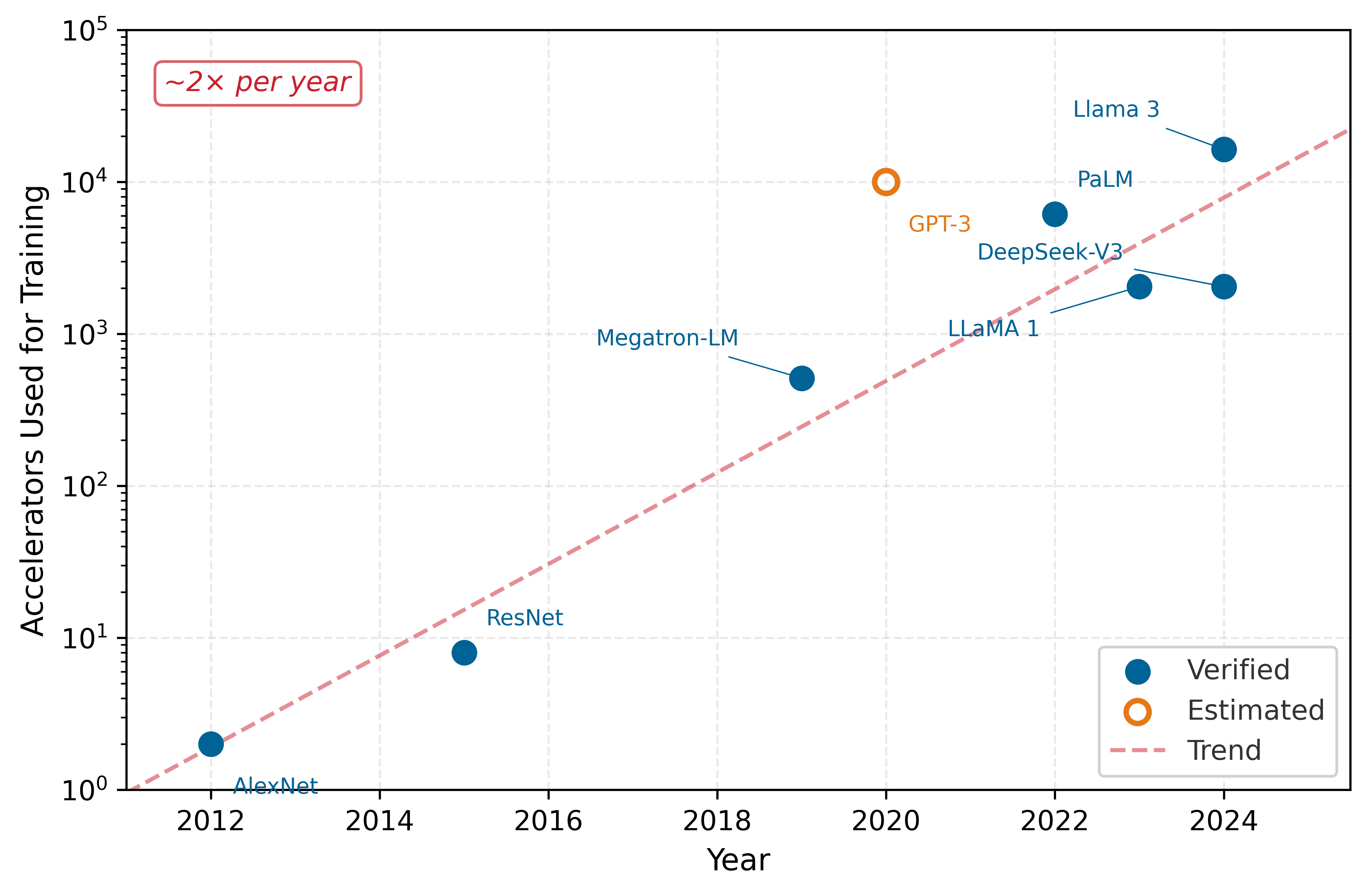
Training compute is only one dimension. Figure 1 traces the related growth in cluster size itself by plotting the number of accelerators used to train landmark models over the past decade.
Figure 1 reveals that cluster sizes have grown by roughly four orders of magnitude in just over a decade, from two GPUs for AlexNet to over 16,000 H100s for Llama 3. This empirical trajectory is the foundation of the scale moment: leading models have required far larger accelerator fleets than earlier deep-learning landmarks. The curve alone, however, does not explain which constraint breaks first. Large language-model training, recommendation serving, and federated mobile learning all encounter fleet scale, but each stresses a different part of the system.
Lighthouse 1.1: Lighthouse archetypes at scale
Lighthouse Archetypes are the canonical workloads that keep the scale moment concrete throughout this book. At this point, their role is to show that “more machines” is not one engineering problem: the dominant constraint depends on what must cross the fleet boundary. The full roster with the C\(^3\) taxonomy mapping and binding-constraint analysis appears at section 1.5.1.
- Archetype A (GPT-4/Llama-3): Very large language models move from memory bounds on one device to multi-node model parallelism and pipeline parallelism, so communication becomes the bottleneck.
- Archetype B (DLRM at Scale): Deep Learning Recommendation Model (DLRM) workloads move from fitting embedding tables in local memory to Embedding Sharding across hundreds of nodes, so sparse all-to-all traffic becomes the bottleneck.
- Archetype C (Federated MobileNet): Mobile inference and on-device adaptation move from one device to federated learning across billions of devices, so unreliable clients, privacy constraints, and stragglers become the bottleneck.
These archetypes turn the growth curve into an engineering question. The same increase in accelerator count can produce a network wall, an embedding-shard bottleneck, or a fleet of unreliable edge participants. Where the archetypes focus attention on the workload, a parallel set of systems lenses does the same for the substrate, directing attention to data-center physics, network topology, and distributed consistency. Combined with the rise of federated learning2, that diversity has transformed ML from a discipline where algorithms dominate to one where systems engineering determines success. A sophisticated algorithm that cannot scale often provides less practical value than a simpler algorithm deployed efficiently across scalable infrastructure.
2 Federated Learning: A distributed learning paradigm where models are trained across millions of decentralized edge devices holding local data. Edge Intelligence analyzes the privacy and coordination challenges of federated fleets.
The transition from single-machine to distributed training introduces qualitative changes in system behavior. Figure 2 contrasts the two regimes: the single-machine world governed by the memory wall vs. the fleet-scale world governed by communication dominance, routine failure, and governance complexity.

The discontinuity captured in figure 2 is qualitative, not merely quantitative: at fleet scale, the binding constraint shifts from silicon to the network fabric, and the engineering discipline shifts from optimization to resilience. The unit of compute is no longer a single server but a Machine Learning Fleet: a massive, interconnected distributed system that must act as a single coherent engine.
Definition 1.1: Machine learning fleet
Machine Learning Fleet is a distributed system of thousands of interconnected accelerators, storage arrays, and network fabrics designed to operate as a single coherent computer.
- Significance: It coordinates synchronous state across all nodes, where the total time \(T\) is governed by the Slowest Worker (Straggler). It requires Bisection Bandwidth (\(\text{BW}_{\text{bisect}}\)) that scales with the aggregate compute capacity (\(R_{\text{peak}}\)) of the fleet.
- Distinction: Unlike Traditional Clusters (for example, Spark, MapReduce) that manage independent, asynchronous jobs, an ML Fleet operates under Synchronous Tight Coupling: all workers must reach the training-step barrier before any can advance, so near-perfect reliability is required to maintain throughput.
- Common pitfall: A frequent misconception is that an ML Fleet is “just more servers.” In reality, it is a Warehouse-Scale Computer (WSC) where the network is the system bus and the orchestrator is the operating system.
As systems scale beyond a single node, a fundamental physical constraint emerges: the bisection bandwidth wall3, which limits how fast data can cross the network midpoint. At fleet scale, networking often determines model throughput more than compute does.
3 Bisection Bandwidth (from graph theory): The minimum aggregate bandwidth of all links that, if cut, would partition the network into two equal-sized sets of nodes. In distributed ML, this “worst-case” cut determines the cluster’s synchronization bottleneck: an AllReduce synchronization can move no faster than the bisection bandwidth, regardless of how many GPUs are added.
4 Hardware Failure Rates at Scale: Individual GPUs fail at 1–2 percent annually under typical conditions, but rates exceed 9 percent under intensive training workloads. Multiply by fleet size and failure becomes routine: Meta reported 419 unexpected interruptions during Llama 3’s 54-day training on 16,384 H100s, roughly one every three hours, with GPU and HBM3 faults causing over half. Automated checkpointing and recovery maintained over 90 percent effective training time, illustrating that at fleet scale the engineering challenge shifts from preventing failure to minimizing recovery latency.
On a single GPU, training proceeds deterministically: the same code, data, and random seed produce identical results. At the scale of thousands of GPUs, new phenomena emerge. Network partitions can split clusters into groups that train independently, causing model divergence. Stragglers (workers that process data slower than peers due to hardware variation or thermal throttling) can bottleneck entire training runs. Hardware failures that occur once per machine-year become daily events when operating 10,000 machines4. Systems must checkpoint frequently enough that losing a day’s progress becomes acceptable rather than catastrophic.
These scale-induced challenges have driven infrastructure investment by large AI organizations. Meta’s Research SuperCluster (RSC), announced in 2022, contained 16,000 NVIDIA A100 GPUs connected by 200 Gb/s InfiniBand5 networking (AI 2022). Google’s TPU v4 pods contain 4,096 chips with 1.1 EFLOP/s of aggregate compute capacity (Zu et al. 2024). Microsoft’s Azure supercomputer for OpenAI reached more than 10,000 GPUs in 2020, and later Azure AI data center announcements describe tens-of-thousands-GPU training fabrics (Langston 2020; Microsoft 2025). The scale of the models dictates the scale of the infrastructure. The α-β Communication Model catalogs these interconnect bandwidth constants and feeds them into the \(\alpha\)-\(\beta\) communication model, which lets a reader turn a link’s bandwidth and latency into a predicted transfer cost.
5 InfiniBand (IB): Born in 1999 from the merger of Intel’s NGIO and the Compaq/IBM Future I/O initiatives, InfiniBand was originally designed to replace the PCI bus. Its defining feature for ML is RDMA (Remote Direct Memory Access), which bypasses the OS kernel to transfer data directly between application memory on different machines at microsecond-scale latency. HDR IB provides about 25 GB/s line-rate bandwidth per link; NDR reaches about 50 GB/s. This bandwidth gap compared with common Ethernet links determines whether large-model training is compute-bound or communication-bound.
AI, Meta. 2022. Building the Most Powerful AI Supercomputer: Meta’s AI Research SuperCluster. Meta AI Blog.
Zu, Y., A. Ghaffarkhah, H.-V. Dang, B. Towles, S. Hand, S. Huda, A. Bello, et al. 2024. “Resiliency at Scale: Managing Google’s TPUv4 Machine Learning Supercomputer.” 21st USENIX Symposium on Networked Systems Design and Implementation (NSDI 24), 761–74.
Langston, Jennifer. 2020. Microsoft Announces New Supercomputer, Lays Out Vision for Future AI Work. Microsoft Source.
Microsoft. 2025. Inside the World’s Most Powerful AI Datacenter. The Official Microsoft Blog.
The scale moment establishes the why: exponential growth in compute demand forces ML systems beyond any single machine, creating communication dominance, routine failure, and governance obligations. The next question is how to organize the engineering response. Distributed systems frameworks designed for independent tasks cannot satisfy the tight coupling that ML training demands; a different architectural hierarchy is needed.
The Fleet Stack: A Hierarchy of Architecture
Apache Spark (Zaharia et al. 2016) processes independent data partitions; a web microservice handles isolated requests. The Machine Learning Fleet does neither. Its workload requires synchronous state updates across thousands of accelerators every few hundred milliseconds, a coupling intensity that existing distributed frameworks were never designed to sustain. The workload characteristics of ML systems differ fundamentally from traditional distributed systems, even though the underlying hardware (network, compute, storage) is identical. To reason about these differences systematically, this book formalizes the engineering crux of scale as a four-layer stack, the fleet stack, which transforms raw cluster resources into global-scale AI applications.
Zaharia, M., R. S. Xin, P. Wendell, T. Das, M. Armbrust, A. Dave, X. Meng, et al. 2016. “Apache Spark: A Unified Engine for Big Data Processing.” Communications of the ACM 59 (11): 56–65. https://doi.org/10.1145/2934664.
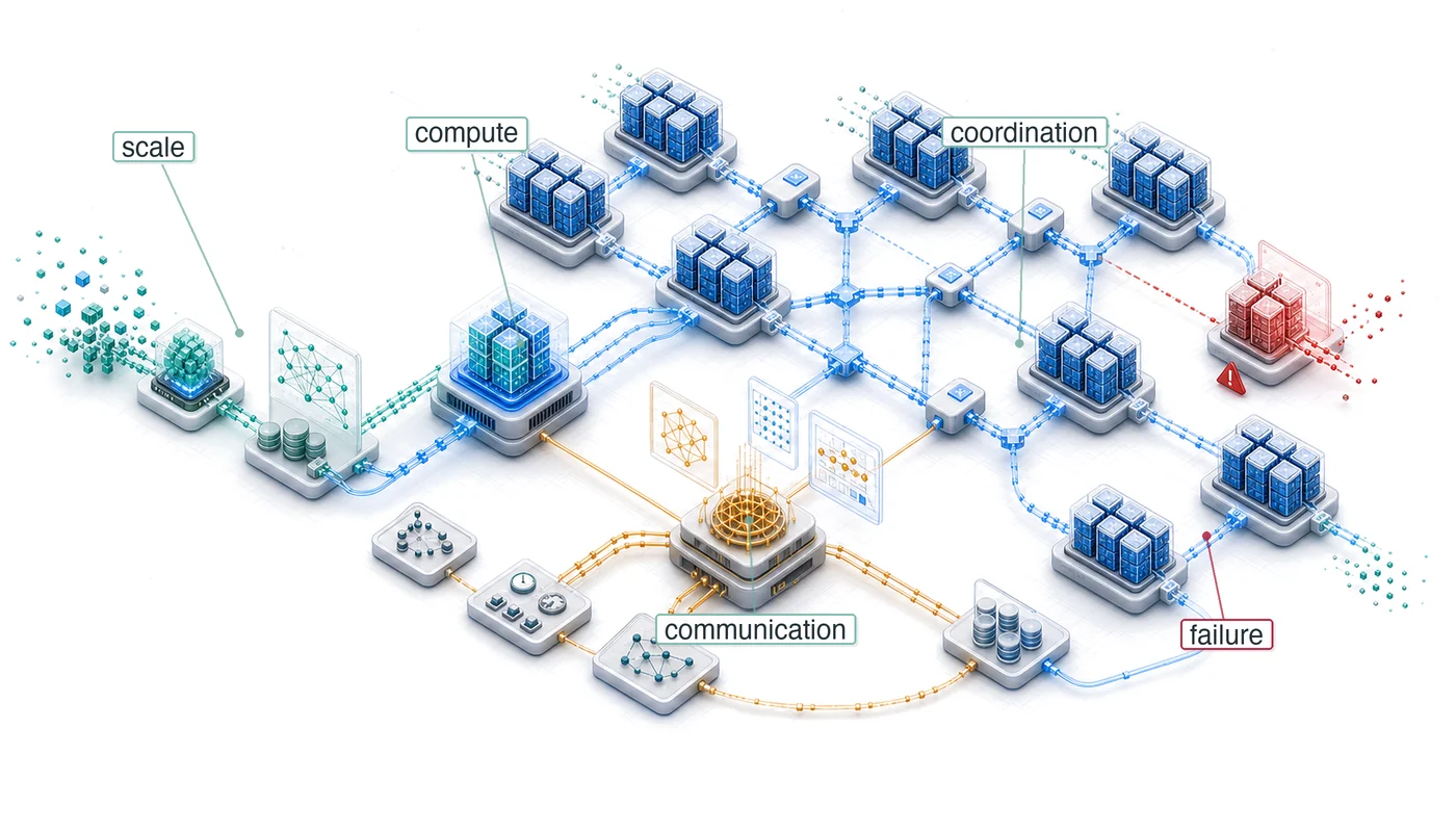
Figure 3 visualizes the transition from single-node to fleet. The left side of the diagram summarizes the single-node regime: 1–8 accelerators connected by shared memory, where the binding constraint is the memory wall. The scaling arrow crosses into the distributed fleet regime, where thousands of nodes coordinate across a high-speed switch fabric and the bottleneck shifts to the bisection bandwidth wall: network congestion and message-passing latency dominate.

The stack architecture in figure 3 does not change when we scale: every ML system still has hardware, a system envelope, a workload, and a mission. What changes is the physics at each layer. Read the figure from bottom to top. At the bottom row, Hardware (NVLink at 900 GB/s within one node) becomes Infrastructure (InfiniBand RDMA fabric spanning racks at 400 Gb/s per link), and the bottleneck shifts from the memory wall to the bisection bandwidth wall. One row up, System Software (a single CUDA runtime managing PCIe DMA) becomes Distribution (NCCL and RDMA libraries coordinating thousands of processes across the fabric).
The upper two layers undergo an equally profound transformation. ML Framework (PyTorch or JAX executing a training loop on one node) becomes Serving/Ops (orchestration and continuous integration/continuous deployment (CI/CD) pipelines that schedule distributed jobs and manage rolling deployments). At the top, Application (a single training script or inference service) becomes Governance (responsible AI policy, security auditing, and multi-tenant access control), because fleet-scale deployment introduces organizational concerns absent from a single machine. Four layers compose the fleet stack:
- Infrastructure (Hardware, the Engine): The physical foundation. This layer defines the fleet’s raw capabilities: per-node \(R_{\text{peak}}\) and \(\text{BW}\), interconnected by InfiniBand RDMA fabric. The recurring hardware anchor for this introduction is the NVIDIA H100, which serves as a concrete reference accelerator rather than an abstract placeholder.
- Distribution (Systems, the Car): The communication substrate. This layer defines the cluster envelope: NCCL, the collective library that implements reductions and broadcasts on GPU fabrics; RDMA collectives that coordinate thousands of accelerators; bisection bandwidth; power usage effectiveness (PUE), the facility-energy overhead above IT load; and failure rates (MTBF).
- Serving/Ops (Workloads, the Route): The orchestration layer. This layer manages the mathematical workload sharded across the cluster \((O, D_{\text{vol}}, \text{CI})\) through deployment pipelines and scheduling, where \(O\) is local operation count, \(D_{\text{vol}}\) is data volume, and \(\text{CI}\) previews the communication-intensity ratio: network bytes per local FLOP. We use Lighthouse Workloads like GPT-4 and DLRM.
- Governance (Missions, the Destination): The mission context. This is the top of the stack, where responsible AI policy, security, and multi-tenant access control shape fleet-wide behavior. A mission (such as Frontier Model Training) introduces high-level requirements (for example, “99.99 percent service availability”) that dictate the configuration of every layer below.
This hierarchy ensures that every distributed engineering decision is grounded in its “Mission Context.” For example, the Frontier Training mission instantiates Archetype A (GPT-4/Llama-3) from the volume’s canonical roster (section 1.5.1), and operates on a cluster of H100 hardware. By standardizing these protagonists, we ensure that the “Physics of Scale” remains traceable across every chapter.
Traditional vs. ML fleet dynamics
Traditional systems (for example, a search engine or a banking database) optimize for independent, asynchronous tasks. A web server handles millions of requests, each isolated from the other. When one request fails, the others continue. This model, exemplified by systems like MapReduce (Dean and Ghemawat 2004), achieves scale by partitioning data into independent chunks that require minimal coordination.
Dean, Jeffrey, and Sanjay Ghemawat. 2004. “MapReduce: Simplified Data Processing on Large Clusters.” Proceedings of the 6th Symposium on Operating Systems Design and Implementation (OSDI), 137–50.
Li, M., D. G. Andersen, J. W. Park, A. J. Smola, A. Ahmed, V. Josifovski, J. Long, E. J. Shekita, and B.-Y. Su. 2014. “Scaling Distributed Machine Learning with the Parameter Server.” Proceedings of the 2014 International Conference on Big Data Science and Computing, 583–98. https://doi.org/10.1145/2640087.2644155.
The Machine Learning Fleet, by contrast, operates under Synchronous Tight Coupling. While the parameter server architecture (Li et al. 2014) introduced ways to manage distributed state, large synchronous models often require even tighter synchronization to maintain performance. Iterative statefulness makes ML training repeat the same math millions of times while updating a massive shared state, the model weights, rather than processing independent one-and-done jobs. Barrier synchronization means that 10,000 GPUs in a synchronous training step must wait for the slowest worker before any can proceed, so a 10 percent performance drop on one node can reduce the entire cluster’s throughput by 10 percent. Bisection bandwidth dominance makes ML training bandwidth-bound rather than user-latency-bound, because gigabytes of gradient data must cross the network every second and require non-blocking topologies that traditional data centers rarely implement.
Figure 4 illustrates this contrast directly: in MapReduce, workers write independently to shared storage and a straggler delays only its own partition, whereas in the ML Fleet, every worker must arrive at an AllReduce barrier before the training step can proceed.

The barrier synchronization pattern in figure 4 explains why ML fleets cannot borrow fault-tolerance strategies from MapReduce: in a barrier-coupled system, every worker’s progress depends on every other worker’s health.
Checkpoint 1.1: The fleet mindset
These questions check whether the fleet mindset is clear:
The shift to the warehouse-scale computer
The ML Fleet demands the Warehouse-Scale Computer (WSC)6 perspective. In traditional computing, the data center is a building that houses many computers. In the ML Fleet, the data center is the computer.
6 [offset=-60mm] Warehouse-Scale Computer (WSC): Barroso and Hölzle, later with Clidaras, framed the data center itself as the computer. For ML fleets, power delivery, cooling topology, optical network layout, and bisection bandwidth become first-order constraints; a 100 MW facility can limit training throughput more than any single accelerator’s TFLOP/s.
- Network Fabric: The system bus.
- Distributed Storage: The local disk.
- Fleet Orchestrator: The operating system.
Mastering this material requires making this mental shift: the engineer is no longer writing code for a CPU but writing logic for a 100-Megawatt computer spanning thousands of racks. The warehouse-scale computer is a common paradigm for large models, while alternative architectures like wafer-scale engines attempt to collapse this entire hierarchy back into a single piece of silicon, trading the modularity of a distributed cluster for the extreme bandwidth of on-chip communication.

Gradient synchronization becomes the defining cost of distributed training.
Communication becomes dominant
These workload characteristics produce two further consequences at scale, both expressions of the canonical triad introduced at the scale moment: communication becomes the dominant cost (the network wall), and failure becomes routine (the reliability gap that accompanies it). At small scale, computation dominates. Training a model on a single GPU spends most of its time performing matrix multiplications. Communication overhead is a small fraction of total time.
At large scale, communication dominates. Distributed training requires synchronizing gradients across workers after each batch. For a model with 175B parameters, FP32 gradients occupy about 700 GB before any collective algorithm is applied. In Ring All-Reduce, each worker sends and receives roughly \(2(N-1)/N\) times the gradient tensor size, because each gradient byte makes about two trips around the ring, one to reduce and one to broadcast back; Collective Communication derives this factor. Network traffic therefore depends on precision, worker count, and collective implementation, and on slower interconnects communication can consume a large fraction of each iteration rather than a negligible one.
This ratio explains why distributed training systems optimize communication so aggressively. Horovod uses Ring All-Reduce, NCCL integration, and Tensor Fusion to improve collective communication (Sergeev and Balso 2018); Megatron-LM applies model parallelism (Shoeybi et al. 2019); and ZeRO reduces memory redundancy (Rajbhandari et al. 2020). For the present argument, the important mapping is role-based: Horovod represents the collective runtime, NCCL the GPU communication backend, Tensor Fusion the gradient-fusion path, Megatron-LM model partitioning, and ZeRO optimizer-state sharding. At fleet scale, these techniques are requirements for viability, not optional performance improvements.
Sergeev, Alexander, and Mike Del Balso. 2018. “Horovod: Fast and Easy Distributed Deep Learning in TensorFlow.” CoRR abs/1802.05799.
Shoeybi, Mohammad, Mostofa Patwary, Raul Puri, Patrick LeGresley, Jared Casper, and Bryan Catanzaro. 2019. “Megatron-LM: Training Multi-Billion Parameter Language Models Using Model Parallelism.” arXiv Preprint arXiv:1909.08053.
Rajbhandari, Samyam, Jeff Rasley, Olatunji Ruwase, and Yuxiong He. 2020. “ZeRO: Memory Optimizations Toward Training Trillion Parameter Models.” SC20: International Conference for High Performance Computing, Networking, Storage and Analysis, 1–16. https://doi.org/10.1109/sc41405.2020.00024.
Failure becomes routine
The reliability arithmetic established at the scale moment already showed the second consequence: with thousands of GPUs, hardware fails every few hours, manual intervention becomes impossible, and the system must self-heal through frequent checkpointing, redundant workers, and automated recovery. The formal availability model and its architectural consequences follow in section 1.3.1.
Communication dominance and routine failure are consequences of the scale moment, but they do not explain what drives the relentless growth in fleet size. The answer lies in a set of empirical relationships that connect model quality to resource investment, relationships that have made warehouse-scale infrastructure an economic necessity rather than an engineering luxury.
Self-Check: Question
Volume I established a four-layer single-node stack: Application, ML Framework, System Software, Hardware. The section maps each single-node layer to its distributed analogue. Which mapping matches the section’s explicit correspondence?
- Hardware -> Distribution; System Software -> Infrastructure; ML Framework -> Governance; Application -> Serving/Ops
- Hardware -> Infrastructure; System Software -> Distribution; ML Framework -> Serving/Ops; Application -> Governance
- Hardware -> Serving/Ops; System Software -> Governance; ML Framework -> Infrastructure; Application -> Distribution
- Hardware -> Infrastructure; System Software -> Serving/Ops; ML Framework -> Distribution; Application -> Governance
Explain why a 10 percent slowdown on one of 1,000 worker nodes in a synchronous training job produces roughly a 10 percent slowdown of the entire cluster, while the same 10 percent slowdown on one of 1,000 MapReduce workers typically produces less than a 0.1 percent effect on total job completion time.
GPT-3 synchronization moves 700 GB of gradient per iteration, and the section reports that Ring AllReduce across 1,000 workers on InfiniBand can consume up to 40 percent of total iteration time. A team observes this 40 percent figure in their own profile. Which intervention is most consistent with the section’s argument for recovering step time?
- Raise per-device compute ceiling by swapping to a GPU with 2\(\times\) the FP16 peak TFLOP/s, since more arithmetic throughput always reduces wall clock.
- Switch from synchronous training to a pure asynchronous protocol because that always improves throughput without introducing any trade-off.
- Double the number of workers from 1,000 to 2,000, since Amdahl’s law guarantees a linear speedup under an AllReduce-bound workload.
- Overlap gradient exchange with the next forward pass and compress the gradient volume through techniques such as ZeRO partitioning, which the section names as responses to exactly this regime.
Under the Warehouse-Scale Computer framing, the datacenter is not a building full of computers but is itself the computer: its network fabric serves as the system bus, its distributed storage as local disk, and its orchestrator as the operating system. Use this analogy to explain why a team debugging a slow training job should profile the fleet orchestrator alongside per-GPU CUDA traces, rather than treating orchestration as infrastructure plumbing.
True or False: At fleet scale, the shape of the physical computation on each accelerator (the same forward and backward passes as on a single node) is preserved, so distributing an existing training job cannot add any new categories of failure — only amplify the single-node ones.
AI Scaling Laws
Training GPT-3 consumed roughly \(3 \times 10^{23}\) floating-point operations (Brown et al. 2020). Public GPT-4-class training estimates are often on the order of \(10^{25}\) FLOPs, although OpenAI did not disclose the actual training compute or hardware configuration (OpenAI et al. 2023; SemiAnalysis 2023). These estimates matter here because each order-of-magnitude increase in compute demanded a corresponding expansion of the Machine Learning Fleet.
OpenAI, Josh Achiam, Steven Adler, Sandhini Agarwal, Lama Ahmad, Ilge Akkaya, Florencia Leoni Aleman, et al. 2023. “GPT-4 Technical Report.” arXiv Preprint arXiv:2303.08774, ahead of print. https://doi.org/10.48550/arXiv.2303.08774.
SemiAnalysis. 2023. GPT-4 Architecture, Infrastructure, Training Dataset, Costs, Vision, MoE. SemiAnalysis Blog.
Sutton, Richard S. 2019. “The Bitter Lesson.” Incompleteideas.net 43.
This pattern is not coincidental. Rich Sutton’s “bitter lesson” articulated the underlying principle: performance in machine learning is primarily driven by applying general methods at massive scale rather than encoding human knowledge into algorithms (Sutton 2019). Scaling laws formalize this observation quantitatively: model loss improves sublinearly as a power-law function of compute, dataset size, and parameters, \(\mathcal{L}(X) \propto X^{-\alpha_{\text{scale}}}\) (Kaplan et al. 2020; Hoffmann et al. 2022). Each equal-sized loss improvement therefore requires disproportionately more resources, a systems consequence this volume later names as the universal scaling law. Each scaling dimension (parameters, data, and compute) interacts with infrastructure constraints differently, making multi-dimensional efficiency optimization essential at production scale.
Empirical evidence for scaling laws
The rapid evolution in AI capabilities since the late 2010s exemplifies this scaling trajectory. GPT-1 (2018) contained 117 million parameters and performed basic sentence completion. GPT-2 (2019) scaled to 1.5 billion parameters and achieved coherent paragraph generation.
GPT-3 (2020) expanded to 175B parameters and achieved sophisticated text generation across diverse domains. Each increase in model size brought substantially improved capabilities at exponentially increasing costs.
The pattern extends beyond language models. In computer vision, parameter counts climbed roughly an order of magnitude from AlexNet (2012) to large vision transformers, and each generation traded better accuracy for proportionally more compute and training data, the same coupling that forced vision training onto multi-accelerator infrastructure.
The scaling hypothesis underlies this progress: larger models capture more intricate data patterns, yielding improved accuracy and generalization. This trajectory, however, introduces critical resource constraints. Training GPT-3 required approximately \(3.14 \times 10^{23}\) floating-point operations, equivalent to running a consumer gaming PC continuously for hundreds of years, at substantial financial and environmental costs.
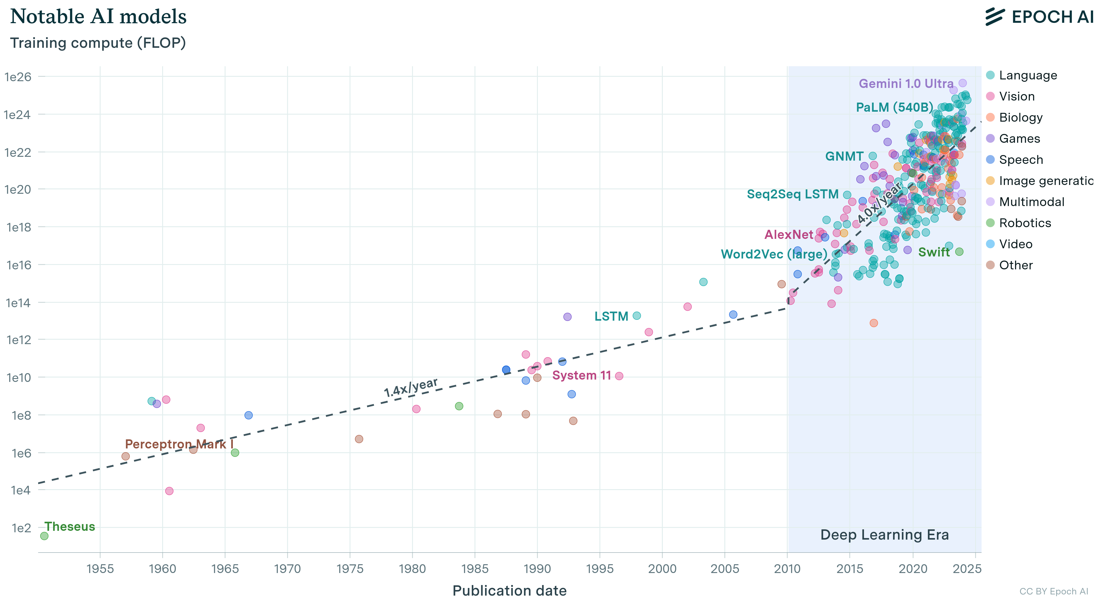
These resource demands reveal why scaling laws are necessary for efficient resource allocation. Figure 5 traces how computational demands of training large models have escalated at an unsustainable rate, growing faster than Moore’s Law improvements in hardware.
These scaling relationships provide a quantitative framework for navigating the trade-offs. Model performance follows power-law relationships where improvements are consistent but exhibit diminishing returns. Optimal resource allocation therefore requires coordinating model size, dataset size, and computational budget rather than scaling any single dimension in isolation. The computational characteristics that drive these workloads’ resource demands determine how they stress distributed infrastructure.
Systems Perspective 1.1: Transformer compute refresher
Transformers process sequences using self-attention mechanisms that compute relationships between all token pairs. This architecture’s computational cost scales quadratically with sequence length (\(\mathcal{O}(S^2)\) where \(S\) is sequence length), making resource allocation particularly critical for language models. The term “FLOPs” (floating-point operations) quantifies total computational work, while “tokens” represent the individual text units (typically subwords) that models process during training.
Compute-optimal resource allocation
Empirical studies of large language models (LLMs) reveal a key insight. For any fixed computational budget, there exists an optimal balance between model size and dataset size (measured in tokens7) that minimizes training loss.
7 Tokens: Subword units produced by algorithms like Byte-Pair Encoding (BPE), which iteratively merges the most frequent character pairs in a corpus. Token vocabulary size creates a direct systems trade-off: larger vocabularies can reduce sequence length for some languages and domains, but they expand the embedding table roughly in proportion to vocabulary size. GPT-3 used a 50,257-token vocabulary; moving to 100K+ tokens in newer models therefore trades tokenization efficiency against additional embedding memory.
8 FLOPs vs. FLOP/s: A critical distinction: FLOPs denotes total computational work (operations performed), while FLOP/s denotes hardware throughput (operations per second). Confusing the two leads to incorrect cost estimates. GPT-3 required 3.14 × 10²³ FLOPs of work; an A100 delivers 312 TFLOP/s of throughput. Dividing work by peak throughput gives ideal wall-clock time; actual time is approximately \(\text{work}/(\eta_{\text{hw}} R_{\text{peak}})\), so utilization below one multiplies ideal time by \(1/\eta_{\text{hw}}\).
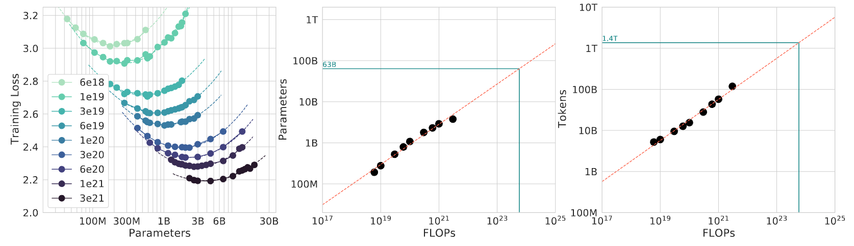
Figure 6 illustrates this principle through three related views. The left panel shows IsoFLOP curves where each curve corresponds to a constant number of floating-point operations (FLOPs8) during transformer training. The valleys in these curves identify the most efficient model size for each computational budget. The center and right panels reveal how the optimal number of parameters and tokens scales predictably as computational budgets increase, confirming that compute-optimal training requires coordinated scaling. The annotated markers extrapolate those fits to a frontier-scale budget near \(10^{24}\) FLOPs, where the compute-optimal point lands at roughly 63 billion parameters trained on roughly 1.4 trillion tokens. That pairing is the roughly 20 tokens per parameter Chinchilla ratio in action: parameters and tokens grow together rather than either dimension racing ahead.
Kaplan et al. (2020) demonstrated that transformer-based language-model loss follows predictable power-law relationships with model parameters, dataset size (measured in tokens), and total computational budget. The result was not a license to increase every dimension blindly; it showed that model quality depends on coordinated allocation across those resources, a point later sharpened by Chinchilla’s compute-optimal scaling analysis (Hoffmann et al. 2022).
Figure 7 presents test loss curves for models spanning from \(10^3\) to \(10^9\) parameters, revealing two insights. Larger models achieve superior sample efficiency, reaching target performance levels with fewer training tokens. As computational resources increase, the optimal model size grows correspondingly, with loss decreasing predictably when compute is allocated efficiently.

Optimal compute allocation follows the Chinchilla result that model size and training tokens should scale approximately proportionally for compute-optimal training, with a ratio on the order of 20 training tokens per parameter (Hoffmann et al. 2022). This corrected earlier guidance that favored making models larger while training them on comparatively fewer tokens.
Narayanan, Deepak, Mohammad Shoeybi, Jared Casper, Patrick LeGresley, Mostofa Patwary, Vijay Korthikanti, Dmitri Vainbrand, et al. 2021. “Efficient Large-Scale Language Model Training on GPU Clusters Using Megatron-LM.” Proceedings of the International Conference for High Performance Computing, Networking, Storage and Analysis, 1–15. https://doi.org/10.1145/3458817.3476209.
These predictions assume perfect compute utilization, an assumption that breaks down in distributed training. Communication overhead scales unfavorably with system size, creating bandwidth bottlenecks that reduce effective utilization. At multi-thousand-GPU scale, utilization depends on partitioning and interconnect: Narayanan et al. (2021) report Megatron-LM runs on 3,072 A100 GPUs at 52 percent of peak device throughput and note that slower interconnects or communication-heavy partitions hinder scaling.
Mathematical foundations and operational regimes
Power-law relationships express scaling behavior mathematically, though the intuition behind these patterns matters more for system design than precise formulation. The equations in this section explain why the same fleet can enter different operational regimes governed by how compute and data are allocated, by where diminishing returns set in, and by how much computation a system spends before answering.
Theorem 1.1: Power-law scaling formulation
Scaling laws are expressed formally as power-law relationships. The general formulation is:
\[ \mathcal{L}(X) = A_{\mathcal{L}} X^{-\alpha_{\text{scale}}} + C_{\mathcal{L}} \]
where loss \(\mathcal{L}\) decreases as resource quantity \(X\) increases, following a power-law decay with rate \(\alpha_{\text{scale}}\), plus a baseline constant \(C_{\mathcal{L}}\). Here, \(\mathcal{L}(X)\) represents the loss achieved with a resource quantity such as parameters, tokens, or compute; \(A_{\mathcal{L}}\) and \(C_{\mathcal{L}}\) are task-dependent constants; and \(\alpha_{\text{scale}}\) is the scaling exponent that characterizes the rate of performance improvement. A larger value of \(\alpha_{\text{scale}}\) signifies more efficient performance improvements with respect to scaling.
These predictions find strong empirical support across multiple model configurations. Figure 8 shows how early-stopped test loss varies predictably with both dataset size and model size, confirming that learning curves across configurations align through appropriate parameterization.
Resource-constrained scaling regimes
Applying scaling laws in practice is a scarcity diagnosis: the useful question is which resource prevents balanced growth first. Compute budget, data availability, and model size create three regimes with different optimal responses.

Scaling regimes are compute-scarce, data-scarce, or balanced.
Three regimes determine the appropriate scaling response:
- Compute-limited regime: Compute scarcity restricts scaling potential despite abundant training data, so academic institutions, startups, and time-constrained teams often train smaller models for longer periods to maximize utilization.
- Data-limited regime: Data scarcity appears when computational resources exceed what the available dataset can support, so teams in specialized, proprietary, or privacy-constrained domains often train larger models for fewer optimization steps to extract more information from limited examples.
- Optimal regime: Balanced compute and data follow compute-optimal scaling laws, as DeepMind’s Chinchilla model demonstrated by outperforming much larger models through proportional scaling of model size and training data (Hoffmann et al. 2022).
Recognizing which regime governs a given project prevents common inefficiencies: over-parameterized models with insufficient training data, or under-parameterized models that waste available compute.

Performance improvements follow predictable patterns, but the relevant design action changes with resource availability and with the point in the ML lifecycle where compute is spent. Two further distinctions matter for system design: how performance changes with dataset size, and when in the lifecycle additional compute is applied.
Dataset size passes through three phases of its own (figure 9). With few examples, generalization error is high and erratic; as data grows it falls predictably along a power law, the regime where additional data buys the most; eventually it saturates against a noise floor where more data yields negligible gain. The systems consequence is that finite high-quality data, not compute, becomes the binding constraint once a model enters the saturation regime, which is why data efficiency complements brute-force scaling. Distributed Training develops where this saturation reshapes training-data pipelines and budgets.

The lifecycle distinction names three points where a fleet can invest compute, as figure 10 traces: pretraining, the long, failure-sensitive run that realizes the scaling law in wall-clock time; posttraining adaptation, where fine-tuning and preference optimization replace one massive run with many smaller, coordination-heavy jobs; and test-time computation, where extra reasoning steps per query trade serving latency and throughput for accuracy. Each shifts the binding constraint to a different part of the fleet, so the full treatments belong with their workloads: Distributed Training for the pretraining and posttraining runs, and Inference at Scale for test-time compute at serving. For resource-constrained deployments, posttraining and test-time scaling often prove more practical than retraining a model from scratch.

Practical applications in system design
When OpenAI sized GPT-3, it did not run an exhaustive architecture search; it extrapolated scaling curves from smaller experiments to pick a model size and token budget in advance. That decision is the clearest illustration of how scaling laws inform practical system design and resource planning. Within well-defined operational regimes, model performance depends predominantly on scale rather than idiosyncratic architectural innovations, though diminishing returns mean each additional improvement demands exponentially increased resources for progressively smaller benefits.
Concretely, the authors used scaling-law extrapolations to choose model size and training data under the guidance available at the time (Brown et al. 2020; Kaplan et al. 2020). They scaled an established transformer architecture to 175B parameters and approximately 300 billion tokens, enabling advance prediction of model performance and resource requirements; later Chinchilla results showed that this point was undertrained relative to compute-optimal token allocation (Hoffmann et al. 2022).
Brown, Tom B., Benjamin Mann, Nick Ryder, Melanie Subbiah, Jared Kaplan, Prafulla Dhariwal, Arvind Neelakantan, et al. 2020. “Language Models Are Few-Shot Learners.” Advances in Neural Information Processing Systems 33: 1877–901. https://doi.org/10.48550/arxiv.2005.14165.
Kaplan, J., S. McCandlish, T. Henighan, T. B. Brown, B. Chess, R. Child, S. Gray, A. Radford, J. Wu, and D. Amodei. 2020. “Scaling Laws for Neural Language Models.” ArXiv Preprint abs/2001.08361.
Scaling laws serve multiple practical functions. During resource budgeting, empirical scaling curves help estimate returns on investment across model size, dataset expansion, and training duration under fixed computational budgets. Scaling trends also reveal when architectural changes yield significant improvements relative to gains from scaling alone, reducing the need for exhaustive architecture search. When a model family exhibits favorable scaling behavior, scaling the existing architecture is often more effective than transitioning to unvalidated designs.
The same principles apply in reverse for resource-constrained settings. In edge and embedded environments, scaling laws enable designers to select smaller configurations that deliver acceptable accuracy within deployment constraints. By quantifying scale-performance trade-offs, these laws identify when brute-force scaling becomes inefficient and point toward model compression, knowledge transfer, and hardware-aware design.
Scaling laws also function as diagnostic instruments. A performance plateau despite increased resources may indicate dimensional saturation (inadequate data relative to model size) or inefficient compute utilization. This diagnostic capability makes scaling laws both predictive and prescriptive: they forecast what resources a target capability requires and reveal why a system underperforms its predicted trajectory.
Sustainability and cost implications
Scaling laws reveal performance pathways while exposing rapidly escalating resource demands. As models expand, training and deployment costs grow disproportionately, creating tension between performance gains and system efficiency. Training the largest models demands distributed infrastructures comprising hundreds or thousands of accelerators, consuming tens of thousands of GPU-days and millions of kilowatt-hours of electricity. Distributed Training examines how distributed training introduces additional complexity around communication overhead, synchronization, and scaling efficiency.
Large models also require extensive, high-quality datasets to reach their potential. As models approach saturation of available high-quality data, particularly in natural language processing, performance gains from data scaling can become marginal. Data efficiency is therefore a necessary complement to brute-force scaling.
The sharpest of these costs is environmental, and it turns on a decision the fleet operator actually makes: where to site the cluster. The same training run can differ by roughly 40\(\times\) in CO2 emissions depending on grid location, from Quebec hydropower at ~20 g CO2/kWh to Poland coal at ~800 g CO2/kWh.9 That single placement choice, together with job scheduling that shifts workloads to low-carbon hours, makes data-center siting a first-order infrastructure decision rather than an afterthought. Financial cost moves in parallel: training a large foundation model runs into the millions of dollars, which limits who can do large-scale research at all. Sustainable AI develops the full energy and carbon accounting that turns these pressures into design constraints.
9 Carbon Intensity of Training: GPT-3 training emitted an estimated 552 tons of CO2, and published estimates place large-language-model training in the \(10^2\) to \(10^3\) ton range, though figures vary widely with hardware, utilization, and electricity mix (Patterson et al. 2021).
Patterson, David, Joseph Gonzalez, Quoc Le, Chen Liang, Lluis-Miquel Munguia, Daniel Rothchild, David So, Maud Texier, and Jeff Dean. 2021. “Carbon Emissions and Large Neural Network Training.” arXiv Preprint arXiv:2104.10350.
10 Scaling Law Saturation: While power-law relationships suggest unbounded gain, empirical evidence identifies Semantic Saturation points where adding data or parameters yields negligible improvement in downstream utility. This “diminishing returns” regime forces systems engineers to pivot from brute-force scale to data efficiency and model compression to extract further value within fixed power budgets.
Scaling laws do not guarantee unbounded improvement. Each incremental performance gain must be weighed against its resource cost. As systems approach practical scaling limits, the emphasis shifts from scaling alone to efficient scaling: balancing performance, cost, energy consumption, and environmental impact.10
Scaling law breakdown conditions
Scaling laws hold within specific operational regimes but break down at their boundaries. As systems expand, they encounter conditions where the assumptions of smooth, predictable scaling cease to apply. These breakdown points expose inefficiencies that demand refined design approaches.
Most of these breakdowns share one root cause: growth in one dimension that outpaces the others. Hoffmann et al. (2022) show that many large language models were undertrained because model size grew faster than training-token budgets, and that compute-optimal training requires scaling parameters and tokens together. The same imbalance appears in other guises. Schedules and learning rates that are not retuned to a larger model leave it short of its potential despite the infrastructure spent on it; finite high-quality data eventually yields diminishing marginal utility, so larger models begin to memorize rather than generalize; and hardware ceilings on memory bandwidth, interconnect capacity, and I/O throughput cap how far a trillion-parameter model can be distributed at all. At the extreme, even balanced scaling reaches the limits of what a training distribution can teach: benchmark numbers keep rising while generalization does not, and models grow brittle to adversarial or out-of-distribution inputs. Table 2 organizes these failure modes, mapping each breakdown type to its underlying cause and a representative scenario, so practitioners can anticipate the inefficiency before committing the budget.
Hoffmann, Jordan, Sebastian Borgeaud, Arthur Mensch, Elena Buchatskaya, Trevor Cai, Eliza Rutherford, Diego de Las Casas, et al. 2022. “Training Compute-Optimal Large Language Models.” Advances in Neural Information Processing Systems 35 35: 30016–30. https://doi.org/10.52202/068431-2176.
| Dimension Scaled | Type of Breakdown | Underlying Cause | Example Scenario |
|---|---|---|---|
| Model Size | Overfitting | Model capacity exceeds available data | Billion-parameter model on limited dataset |
| Training Data Size | Diminishing Returns | Saturation of new or diverse information | Scaling web text beyond useful threshold |
| Compute Budget | Underutilized Resources | Insufficient training steps or inefficient use | Large model with truncated training duration |
| Imbalanced Scaling | Inefficiency | Uncoordinated increase in model/data/compute | Doubling model size without more data or time |
| All Dimensions | Semantic Saturation | Exhaustion of learnable patterns in the domain | No further gains despite scaling all inputs |
Checkpoint 1.2: Applying scaling laws
These questions check whether scaling laws are being used as resource-allocation tools:
These breakdown points demonstrate that scaling laws describe empirical regularities under specific conditions, conditions that become difficult to maintain at scale. Discerning where and why scaling ceases to be effective drives the development of strategies that enhance performance without relying solely on scale.
Integrating efficiency with scaling
Scaling laws reveal the walls; efficiency engineering builds the paths around them. Data saturation, infrastructure bottlenecks, and diminishing returns set hard limits on what brute-force scaling can achieve. The same constraints, however, point toward solutions along three interconnected dimensions:
- Algorithmic efficiency: Techniques such as sparsity and distillation extract more capability per FLOP.
- Data efficiency: Curriculum learning and active selection extract more information per training example.
- Systems efficiency: Communication hiding and pipeline overlap extract more utilization per accelerator.
Each dimension addresses a different breakdown condition from table 2, and each receives detailed treatment in the chapters that follow.
Scaling laws and efficiency techniques determine how much computation large models require and how well the fleet uses it. They do not, however, address the physical and logical constraints that the fleet itself imposes. Hardware fails, bandwidth saturates, distributed systems face fundamental impossibility results, and societal impact at scale demands governance. These constraints cannot be optimized away; they must be engineered around.
Self-Check: Question
A product team interprets the scaling-law curves in this section and concludes: ‘We saw a 2 percent loss improvement from doubling compute last quarter, so doubling compute again should give us another 2 percent.’ Which critique most directly matches the section’s characterization of power-law behavior?
- The interpretation is correct because power-law curves are linear in linear space, so equal compute additions produce equal loss reductions.
- The interpretation misreads the predictability: improvements follow a power law, so each equal-sized capability gain typically requires a larger, not equal, compute increase, and the next 2 percent may demand far more than a second doubling.
- The interpretation is correct in principle but only for training compute above \(10^{26}\) FLOPs, a regime the team cannot reach.
- The interpretation is discontinuous, not power-law, so the team’s prediction is unfounded because scaling laws never give quantitative guidance.
A team has a 500-A100 cluster available for one month but only a 5-billion-token domain corpus of audited medical transcripts. The compute budget exceeds what that dataset can use efficiently under Chinchilla-style co-scaling. Applying the section’s resource-constrained regime analysis, which strategy is most defensible?
- Train a much larger model for fewer update steps, so the available capacity extracts more signal per example from the scarce corpus; do not artificially inflate the data by many repeated passes that risk memorization.
- Train a smaller model for many more epochs, since additional passes over the same data are always equivalent to fresh tokens in the scaling law.
- Ignore the data limit and run the Chinchilla-optimal compute budget regardless, since the scaling law guarantees proportional capability gains from compute alone.
- Replace training entirely with test-time scaling on a pre-trained general model, since domain specialization is unnecessary when the compute budget is generous.
Explain why compute-optimal scaling requires coordinated growth of model size, dataset size, and compute budget, rather than independently maximizing each axis. Use a concrete example of what goes wrong when one axis grows alone.
A team with a fixed 10,000 A100-hour budget chooses model size and token count together so that loss is minimized under the constraint. The section calls this co-scaling operating point the ____-optimal frontier, named after the 2022 paper whose empirical study established that earlier language models had been consistently undertrained relative to their parameter counts.
A fleet-planning team extrapolates from a 10-billion-parameter training run to a planned 100-billion-parameter run using a straight line in log-log space. At the small scale, coordination and communication overhead consumed 5 percent of wall clock; at the planned scale, they consume 40 percent. Which failure mode of the scaling-law extrapolation is the team most likely encountering?
- A healthy extrapolation because the scaling law governs model capability and is insensitive to the coordination share of wall clock.
- A breakdown of the scaling law because imbalanced data-to-parameter ratios at the 100B scale push the point off the Chinchilla frontier.
- A breakdown of the extrapolation because distributed-efficiency losses at the larger scale consume a large share of compute that the smaller-scale experiment never exposed, so the effective FLOPs applied to training are well below the nominal budget.
- A healthy extrapolation because communication overhead always scales exactly linearly with model size and cancels out of the log-log relationship.
Once a training program approaches the data wall, the energy wall, or the bisection-bandwidth ceiling, the section argues that efficiency engineering becomes mandatory rather than optional. Walk through why brute-force scaling collides with these walls and explain the engineering question that replaces ‘how do we scale bigger?’
Constraints of Scale
The three walls describe where performance binds; the constraints behind them are broader. The Machine Learning Fleet operates under three categories of irreducible constraint: physical (the memory, network, and energy walls themselves, plus the reliability gap that opens as fleet size grows), logical (distributed systems face impossibility results like the CAP theorem), and societal (scale amplifies the impact of every technical decision). Understanding these constraints is a prerequisite for the diagnostic framework that follows.
The reliability gap
In traditional software, we treat hardware as a reliable abstraction. A single server typically has an availability of “four nines” (99.99 percent), meaning it fails for roughly 53 minutes a year. The Machine Learning Fleet, however, operates at a scale where this abstraction collapses, opening the reliability gap: hardware that is reliable in isolation becomes unreliable as a fleet. When a fleet coordinates 25,000 GPUs, equation 1 multiplies the individual component probabilities to give the probability that the entire system is healthy (\(R_{\text{system}}(t)\)):
\[ R_{\text{system}}(t) = (R_{\text{component}}(t))^N = e^{-N\lambda t} \tag{1}\]
Here, \(N\) is the number of independent components in the fleet, \(\lambda\) is the per-component failure rate per unit time, \(t\) is the time window, and \(R_{\text{component}}(t)\) is the probability that one component survives that window. The engineering implication is the exponent: every added component multiplies the failure opportunity, so reliability engineering becomes a scaling problem rather than a cleanup task.
If each node in a cluster is 99.9 percent reliable, a 1,000-node cluster is healthy only 36.8 percent of the time. Scale that to a 10,000-node fleet, and the probability of the entire system being healthy at any given second drops to 0.0045 percent. Figure 11 traces this exponential decay for two per-node reliability levels across fleet sizes from 1 to 10,000 GPUs.

The exponential decay in figure 11 makes the architectural consequence inescapable: no amount of per-node improvement can sustain fleet-wide availability at scale. Here we establish the idea with a single per-node reliability figure; Failure Probability at Scale derives the full failure-probability cascade and the fleet-wide availability formula a reader needs to size checkpoint intervals and redundancy. The engineering lesson is that failure is the common case. At scale, resilience replaces prevention as the governing objective: the system trades absolute uptime for recovery speed, checkpoint quality, and automated repair. The defining challenge of Fault Tolerance is this shift from keeping every component running to ensuring that the fleet self-heals when components fail.
Communication intensity (the CI ratio)
If the single-machine iron law governs how a system executes, communication intensity (CI) governs where it stalls. On a single accelerator, the roofline model determines whether a kernel is compute-bound or memory-bound. At fleet scale, this analysis elevates to the network.
Equation 2 defines communication intensity as the ratio of data moved across the network to the operations performed locally:
\[\text{CI} = \frac{\text{Bytes Transferred (Network)}}{\text{FLOPs Executed (Local)}} \tag{2}\]

Past the communication-intensity cliff, adding GPUs stops helping.
Low communication intensity, \(\text{CI} < 0.01\), describes compute-heavy workloads whose GPUs spend most of their time doing math, so scaling is relatively easy. High communication intensity, \(\text{CI} > 0.1\), describes network-bound workloads limited by bisection bandwidth, where adding more GPUs can slow training rather than speed it up.
Communication and scaling optimizations, from gradient sparsification (sending fewer gradient bytes) to 3D parallelism (partitioning data, tensor, and pipeline dimensions across different fabric tiers), try to lower exposed communication intensity so that the Machine Learning Fleet acts as a single, massive computer rather than a collection of idling processors waiting for the wire. We define the ratio here and apply it qualitatively; The communication-computation ratio works communication intensity through concrete regimes and shows the bandwidth-saturation point at which adding accelerators stops helping.
Checkpoint 1.3: The scale mandate
These questions check whether the scale mindset has shifted from local execution to distributed constraints:
Why distribution is hard
Scale forces distribution: no single machine provides the compute required for the largest models, and no centralized system can collect every data source that global user bases generate. Coordinating computation across physically separated machines connected by finite-bandwidth networks, however, creates constraints that no engineering can eliminate.
The first stressor appears inside data centers, where synchronous training must choose how much consistency to preserve under partitions and failures. The second appears at the edge, where the devices themselves are unreliable, power-limited, and policy-constrained.
The CAP theorem reality
The CAP Theorem11 establishes that distributed systems can provide at most two of three properties: Consistency, Availability, and Partition Tolerance. The ML fleet encounters all three constraints, forcing explicit trade-offs.
11 CAP Theorem (Brewer’s Theorem): Brewer formulated the conjecture (Brewer 2000), and Gilbert and Lynch gave the formal proof that in the face of a network partition (P), a system must choose between absolute Consistency (C) and high Availability (A) (Gilbert and Lynch 2002). For the ML Fleet, this manifests as a choice between Synchronous Training (Consistency prioritized; the job stalls if a node fails) and Asynchronous Training (Availability prioritized; training continues but with stale gradients).
Brewer, Eric A. 2000. “Towards Robust Distributed Systems (Abstract).” Proceedings of the Nineteenth Annual ACM Symposium on Principles of Distributed Computing, 7. https://doi.org/10.1145/343477.343502.
Gilbert, Seth, and Nancy Lynch. 2002. “Brewer’s Conjecture and the Feasibility of Consistent, Available, Partition-Tolerant Web Services.” ACM SIGACT News 33 (2): 51–59. https://doi.org/10.1145/564585.564601.
Distributed ML systems make different trade-offs depending on their requirements. Synchronous training chooses consistency: all workers see the same model state, but training halts if any worker becomes unreachable. Asynchronous training chooses availability: training continues even with stragglers, but workers may operate on stale model versions. Federated learning often chooses availability with eventual consistency, accepting temporary divergence for continuous operation on edge devices.
Edge distribution complexity
The coordination challenges discussed so far assume data-center distribution, where machines run in managed facilities. At the network edge, these challenges intensify along every dimension.
Billions of smartphones and IoT devices operate in uncontrolled environments with unreliable connectivity and limited power. Privacy, consent, or policy constraints may prevent raw data from leaving the device, making federated learning a natural architecture (McMahan et al. 2017). Intermittent connectivity forces the system to tolerate asynchronous updates spanning days. These constraints require architectural approaches (differential privacy, on-device inference, and model compression) that differ fundamentally from data-center ML.
McMahan, Brendan, Eider Moore, Daniel Ramage, Seth Hampson, and Blaise Agüera y Arcas. 2017. “Communication-Efficient Learning of Deep Networks from Decentralized Data.” International Conference on Artificial Intelligence and Statistics (AISTATS), Proceedings of machine learning research, vol. 54: 1273–82.
When ML systems operate at the scale of billions of users, their societal impact demands consideration beyond technical excellence. Governance becomes an engineering requirement.
Why governance matters at scale

At fleet scale, a technical bug becomes societal risk.
Scale and distribution amplify impact beyond engineering. When a system serves billions of users, a technical bug becomes a societal risk. This amplification creates governance requirements that small-scale systems can safely ignore. We frame governance as the Control Plane of the Machine Learning Fleet, not a set of external rules.
That control plane first has to defend the fleet. ML systems face unique security threats that intensify at production scale. Model extraction attacks steal proprietary intellectual property through API queries. Data poisoning injects backdoors into models that remain dormant until triggered by a specific input. At fleet scale, these threats become economically attractive targets for sophisticated attackers. Defending the fleet requires systematic approaches: access controls, differential privacy12, and continuous behavioral monitoring that go far beyond traditional perimeter security.
12 Differential Privacy (DP): A mathematical framework for adding calibrated noise to computations to bound information leakage about individual data points. Security & Privacy examines how DP protects user privacy in large-scale ML systems.
The same control plane must make the fleet auditable. Systems operating at scale attract regulatory attention. Regimes such as the EU AI Act and local privacy laws make Auditability an architectural requirement for many deployments. Proving that a model trained on 10,000 GPUs did not ingest prohibited data requires end-to-end data lineage tracking. Generating a human-interpretable explanation for a sub-millisecond recommendation demands techniques designed into the serving architecture. Meeting these requirements calls for technical capabilities (audit trails, bias testing, and consent management) built into the infrastructure from day one.
Beyond legal compliance, the Machine Learning Fleet carries ethical obligations. Recommendation algorithms shape public discourse; hiring algorithms affect livelihoods. These systems do not fail loudly with a crash log; they fail silently through bias and polarization. Responsible AI is the engineering practice of treating fairness, transparency, and accountability as invariants: hard constraints that, if violated, should trigger a system-wide halt.
Self-Check: Question
A fleet operator plans an upgrade that will raise per-node reliability from 99.9 percent uptime to 99.99 percent, arguing that this 10\(\times\) improvement makes a 10,000-node cluster ‘effectively as healthy as a small lab cluster.’ Using the section’s reliability-gap equation, which critique best matches the section’s argument?
- The upgrade makes the cluster behave like a single 99.99-percent node, so the lab-cluster analogy is valid under multiplicative composition.
- The upgrade moves fleet availability from near zero to roughly 37 percent at 10,000 nodes; this is a large improvement but still far from lab-cluster behavior, because even with 99.99 percent per-node reliability the product (0.9999)^10000 remains bounded below 0.4.
- The upgrade is irrelevant because fleet availability is dominated by the orchestrator, not by per-node hardware reliability.
- The upgrade guarantees 99.99 percent fleet availability because the CAP theorem forces each node to operate independently at the same reliability level.
A team measures two distributed training workloads on the same 1,024-GPU cluster. Workload Alpha transfers 10 MB of gradient per iteration while performing \(10^{14}\) FLOPs locally per GPU; Workload Beta transfers 1 GB of gradient per iteration while performing \(10^{13}\) FLOPs locally per GPU. Using the section’s CI ratio, which workload is more likely to scale poorly on additional nodes and why?
- Alpha scales worse because its lower per-GPU FLOPs mean the arithmetic units are underutilized regardless of the network.
- Alpha scales worse because higher per-GPU FLOPs always cause more network pressure through gradient accumulation.
- Both scale identically because CI is a per-workload property and does not interact with fleet size.
- Beta scales worse: its CI = \(10^9 / 10^{13} = 10^{-4}\) is 1,000\(\times\) higher than Alpha’s CI = \(10^7 / 10^{14} = 10^{-7}\), so Beta is farther toward the network-bound regime and adding GPUs grows gradient volume while leaving bisection bandwidth unchanged.
A distributed training system faces a 30-second network partition that disconnects one of 64 worker nodes. Explain what the CAP theorem predicts will happen if the system is configured for synchronous training versus asynchronous training, and why neither mode can sidestep the trade-off.
A company’s leadership proposes that its EU AI Act compliance work can happen in a year-end review cycle, separate from the engineering roadmap, since ‘governance is policy, not performance.’ Which critique best matches the section’s framing of governance as the Control Plane of the fleet?
- The proposal is correct because the section treats governance as a documentation exercise that runs in parallel with engineering rather than constraining it.
- The proposal is correct in principle but should be quarterly instead of annual to keep pace with regulatory change.
- The proposal is incorrect because auditability, access control, differential privacy, and data-lineage tracking are runtime capabilities that must be built into the infrastructure from day one; retrofitting them after deployment requires re-architecting the data and model pipelines.
- The proposal is incorrect because governance is primarily a legal-risk concern with no implications for the training system’s architecture.
When a training fleet’s end-to-end availability falls exponentially as \(N\) grows — even with each node individually at 99.99 percent uptime — the section gives this phenomenon a name that captures the growing distance between the per-node reliability an engineer is used to and the fleet-wide health a production system can actually deliver. The phenomenon is called the ____ Gap.
The C\(^3\) Taxonomy: Foundations of Scale
The physical, logical, and societal constraints just surveyed all manifest as wasted wall-clock time, so navigating them demands a diagnostic that says where that time actually goes. The single-machine foundation for that analysis is the Data · Algorithm · Machine (D·A·M) taxonomy, which The D·A·M Taxonomy develops as a complete diagnostic framework. Data is the information the system learns from, and performance becomes data-bound when the I/O pipeline cannot feed the processor fast enough. The algorithm is the mathematical logic being executed, and performance becomes compute-bound when arithmetic units are the limiting factor. The machine is the physical hardware substrate, and performance becomes memory-bound when memory bandwidth or capacity limits throughput.
Scaling from one machine to a fleet introduces three new fundamental resources that compete for wall-clock time. Where the canonical triad of walls names where the fleet binds, these three resources name where its time is spent. The C\(^3\) Taxonomy extends the D·A·M lens to the fleet, identifying the physical and logical boundaries of the Machine Learning Fleet. Compute (\(C_1\), the math) is the local execution of matrix operations on individual accelerators, where the goal is to keep the math engine running at peak utilization. Communication (\(C_2\), the wire) is the movement of data across the network fabric, governed by bisection bandwidth and the speed of light. Coordination (\(C_3\), the logic) is the synchronous management of state across thousands of nodes, where collective algorithms, fault tolerance, and distributed consensus determine how efficiently \(N\) independent nodes can act as a single computer.
These three dimensions form the Triad of Distributed Efficiency. If the fleet spends too much time on communication or coordination, the expensive compute capacity sits idle. The central challenge is engineering the fleet to minimize the C\(^3\) Gap: the difference between theoretical hardware peak and actual distributed throughput. We introduce the three dimensions here as a framing device; The C^3 Taxonomy develops the complete taxonomy and the diagnostic structure that lets a reader localize a bottleneck to one of the three C’s.
The projection: From D·A·M to C\(^3\)
The D·A·M taxonomy describes the workload: the nouns of our system (the data we have, the algorithm we want to run, the machine we bought). The C\(^3\) taxonomy describes the execution tax: the verbs of the fleet (computing the math, communicating the results, coordinating the state). The D·A·M Taxonomy reviews the single-node D·A·M lens; the C\(^3\) taxonomy projects that workload onto a distributed fleet. Stretching an algorithm across nodes creates communication, such as AllReduce operations to synchronize gradients. Stretching data across nodes requires coordination through distributed samplers and checkpointing. Machine failures in a fleet require coordination through fault tolerance and straggler mitigation.
The intersection of these two taxonomies defines the entire design space of fleet-scale ML systems engineering. We do not solve D·A·M or C\(^3\) in isolation; we solve their cross-products.
The fleet law
The C\(^3\) taxonomy yields a diagnostic equation for every distributed training step. To reason about performance at scale, we must distinguish the efficiency of a single component from the efficiency of the entire system. On a single machine, execution time is often governed by the iron law of performance, \(T \approx D_{\text{vol}}/\text{BW} + O/(R_{\text{peak}}\eta_{\text{hw}}) + L_{\text{lat}}\), decomposing into data movement, computation, and overhead. At fleet scale, that single-machine view no longer suffices: we care about the efficiency of the fleet across time and energy, and a parallel decomposition emerges. Equation 3 states the Fleet Law (the distributed step time law), which decomposes distributed execution into its canonical distributed-step components:
\[ T_{\text{step}}(N) = \frac{T_{\text{compute}}}{N} + T_{\text{comm}}(N) + T_{\text{sync}}(N) - T_{\text{overlap}} \tag{3}\]
where \(T_{\text{compute}}/N\) is the idealized local arithmetic time after distributing work across \(N\) devices, \(T_{\text{comm}}(N)\) is the time moving data across the network (gradient synchronization, parameter broadcasts), \(T_{\text{sync}}(N)\) is time consumed by synchronization logic (barriers, scheduling decisions, fault recovery), and \(T_{\text{overlap}}\) is the communication hidden behind useful compute. Equation 4 rewrites this decomposition as the compute-time fraction, defined as the fraction of wall-clock time spent on useful math:
\[ f_{\text{compute}} = \frac{T_{\text{compute}}/N}{T_{\text{step}}(N)} \tag{4}\]
This decomposition is a diagnostic instrument. When \(f_{\text{compute}}\) drops below 0.5, more than half the fleet’s expensive silicon sits idle. The C\(^3\) taxonomy identifies where the time goes: if \(T_{\text{comm}}(N)\) dominates, upgrade interconnects or overlap communication with computation; if \(T_{\text{sync}}(N)\) dominates, consider asynchronous methods or reduce barrier frequency; if \(T_{\text{compute}}/N\) dominates, the fleet is doing its job. Crucially, the Displacement of Overhead dictates that overhead cannot be eliminated, only relocated among the three C’s. Asynchronous training eliminates coordination barriers but introduces gradient staleness; pipeline parallelism reduces communication volume but adds bubble time. There is no free lunch in distributed systems.
Google’s ML Productivity Goodput metric provides the production-scale instantiation of this framework. Goodput decomposes end-to-end training productivity into three multiplicative factors: Program Goodput (\(\eta_{\text{program}}\)), measuring how efficiently code uses hardware (Compute); Runtime Goodput (\(\eta_{\text{runtime}}\)), capturing losses from communication stalls and failures (Communication); and Scheduling Goodput (\(\eta_{\text{scheduling}}\)), capturing wasted time from preemptions and reconfigurations (Coordination). The C\(^3\) taxonomy is the theoretical framework; Goodput is how production teams measure it.
Figure 12 visualizes the C\(^3\) framework as a three-column layout, with Compute, Communication, and Coordination each occupying their own column of subtopics and the inter-column gaps highlighting the bottlenecks that arise where the dimensions meet. The same framework can be drawn as a triangle in which the vertices are the three resources, the edges are the trade-offs, and the center embodies the displacement of overhead—the unavoidable consequence of distributing computation across independent machines.

The fleet law is the time-side diagnostic of fleet efficiency across time and energy: it asks how much of each distributed step remains useful compute after communication, synchronization, and overlap are accounted for. The Fleet Law develops the full derivation and attributes each term to a physical cause.
The energy-scale invariant
While the fleet law governs time, the Energy-Scale Invariant governs the sustainability and economic viability of the fleet. At scale, every training step is a thermodynamic event. Equation 5 defines the fleet energy productivity (\(\rho_{\text{energy}}\)), measured in FLOP/J, as the ratio of useful work to total energy consumed:
\[ \rho_{\text{energy}} = \frac{O_{\text{useful}}}{E_{\text{compute}} + E_{\text{cooling}} + E_{\text{network}}} \tag{5}\]
where \(O_{\text{useful}}\) is useful work in FLOPs and \(E_{\text{network}}\) often becomes a nonnegligible fraction of the total budget as we move terabytes across optical fabrics. Mastery of scale requires optimizing for the Pareto frontier of both laws: minimizing \(T_{\text{step}}\) while maximizing \(\rho_{\text{energy}}\). We introduce the invariant here; The energy hierarchy at scale details the energy hierarchy at scale and the thermodynamic constraints that bound how far \(\rho_{\text{energy}}\) can be pushed.
The energy-side metric is only half of the scaling diagnosis. A production team also needs a time-side efficiency scalar that says whether extra devices are shortening the training step or merely increasing coordination overhead.
The scaling efficiency (\(\eta_{\text{scaling}}\)) of the fleet is the ratio of ideal parallel step time to actual step time: \[ \eta_{\text{scaling}} = \frac{T_1}{N \times T_N} \] where \(T_1\) is the single-device time for the same work and \(T_N = T_{\text{step}}(N)\) is the step time on \(N\) devices. Component decomposition provides the component-decomposition technique and worked examples for splitting \(T_{\text{step}}(N)\) into its terms, equipping a reader to compute \(\eta_{\text{scaling}}\) numerically.
Systems Perspective 1.2: Amdahl's distributed pitfall
The fleet law is a specialized form of Amdahl’s Law. The maximum speedup of a distributed system is limited by its most tightly coupled component, usually the network synchronization. If a model spends 20 percent of its time waiting for the network (\(T_{\text{comm}}(N)\)), no amount of faster GPUs can make it more than 5\(\times\) faster, regardless of how many are added. Scale is limited by coordination, not compute alone.
Applying both laws to a GPT-3-class synchronization estimate makes the coordination tax and its thermodynamic counterpart visible in the same terms as the scaling equation: the same Ring AllReduce that starves the accelerators of time also burns energy on every step.

At scale only about 4 percent of step time is compute; sync dominates.
Napkin Math 1.2: The coordination and energy tax
Problem: What scaling efficiency and energy cost result when training GPT-3 (175B params) on a cluster connected by 100 Gb/s Ethernet versus 200 Gb/s InfiniBand?
Physics: To synchronize 175B parameters (FP16), a Ring AllReduce must move approximately 700 GB of data through each participating accelerator endpoint per iteration.
Analysis: The fleet law exposes the communication tax.
- InfiniBand (200 Gb/s): High bandwidth and low latency yield a scaling efficiency of only 4.1 percent, meaning the accelerators compute for just 4.1 seconds out of every 100 seconds while the rest is consumed by synchronization.
- Ethernet (100 Gb/s): Lower bandwidth and higher overhead collapse the scaling efficiency further to 2.1 percent, leaving the accelerators productive for roughly 2.1 seconds out of every 100 seconds.
Energy: The energy wall is the thermodynamic cost of the same synchronization. Each endpoint’s gradient synchronization consumes approximately 84 J across the network fabric (at 15 pJ/bit). In a training run of 1,000,000 steps, the endpoint network movement alone accounts for about 84 MJ of energy before multiplying by the number of participating accelerators.
Systems insight: Scale makes the network the primary “processor.” If the network is inefficient, the GPUs sit idle, wasting millions of dollars in compute capacity. Furthermore, the thermodynamic cost of data movement (the energy wall) means that “more GPUs” is not a sustainable scaling strategy without communication-hiding and compression.
Self-Check: Question
A team instruments a distributed training step and reports that 12 percent of wall clock is spent on the NCCL AllReduce transfers themselves, 18 percent is spent at barriers where ranks are waiting for stragglers and fault-recovery logic to complete before the next collective begins, and the remainder is useful forward and backward passes. In the C\(^3\) taxonomy, how do these two 12-percent and 18-percent shares map to the three C’s?
- Both are Communication, because they both involve messages on the network.
- Both are Coordination, because the Fleet Law does not distinguish network time from barrier time.
- The 12 percent of NCCL transfer time is Communication (\(C_2\) — the wire), and the 18 percent of barrier and fault-recovery waiting is Coordination (\(C_3\) — the logic of synchronizing state across ranks); Compute (\(C_1\)) is the remaining useful arithmetic.
- The 18 percent of barrier waiting is Compute, because every rank is sitting on a GPU that is technically powered on.
The section describes D·A·M as the nouns of the workload and C\(^3\) as the verbs of the fleet. Using one concrete example per projection, explain how stretching Data, Algorithm, and Machine across a fleet each generates one of the three C’s.
A team analyzing their distributed training run finds compute-time fraction \(f_{\text{compute}} = 0.43\) with a Fleet Law breakdown of \(T_{\text{compute}}/N = 0.9\ \text{s}\), \(T_{\text{comm}}(N) = 0.8\ \text{s}\), and \(T_{\text{sync}}(N) = 0.4\ \text{s}\) per step. Which intervention is most directly supported by the section’s Fleet Law as diagnostic instrument?
- Buy faster GPUs, because \(T_{\text{compute}}/N\) is the largest single term.
- Do nothing; \(f_{\text{compute}} = 0.43\) is above the 0.3 threshold the section names as acceptable.
- Target \(T_{\text{sync}}(N)\) first by switching to fully asynchronous training, because it is the smallest term and therefore easiest to eliminate completely.
- Target \(T_{\text{comm}}(N)\) first, either by upgrading the interconnect or by overlapping gradient exchange with computation, because it is the largest overhead term and total overhead already exceeds useful compute.
True or False: The Displacement of Overhead means that if a team replaces synchronous training with asynchronous training to eliminate the \(T_{\text{sync}}(N)\) term, the total overhead budget in \(f_{\text{compute}}\) must fall because one of the three C’s has been removed from the equation.
In the Law of Distributed Efficiency, \(T_{\text{step}}(N) = T_{\text{compute}}/N + T_{\text{comm}}(N) + T_{\text{sync}}(N) - T_{\text{overlap}}\), a team reports single-GPU compute time \(T_{\text{compute}} = 1000\) s, \(T_{\text{comm}}(1000) = 0.5\) s, \(T_{\text{sync}}(1000) = 0\) s, and measures \(T_{\text{step}}(1000) = 1.3\) s on a 1000-worker cluster. What is \(T_{\text{overlap}}\), and what does it represent in this framework?
- \(T_{\text{overlap}}\) cannot be determined from the given information, because the Law of Distributed Efficiency does not connect \(T_{\text{step}}\) to the other terms algebraically.
- \(T_{\text{overlap}} = 0.2\) s, representing the portion of communication time hidden by concurrent useful computation, so the effective communication tax is reduced from 0.5 s to 0.3 s of step time.
- \(T_{\text{overlap}} = 1.3\) s, representing the total step time itself, since overlap and step time are defined identically.
- \(T_{\text{overlap}} = 0.5\) s, representing the full communication cost, since perfect overlap eliminates all communication time.
The section says that if a model spends 20 percent of its time waiting for the network (\(T_{\text{comm}}(N)\) at 20 percent of step time), no amount of faster GPUs can make it more than 5\(\times\) faster overall. Derive this bound from Amdahl’s Law and explain which of the three C’s it identifies as the binding constraint for a team adding more accelerators.
Foundational Concepts
The fleet stack is the organizing spine for this book. The C\(^3\) taxonomy introduced earlier (figure 12) gives the local diagnostic lens for one distributed step: where wall-clock time goes among compute, communication, and coordination. Scaling laws predict how much computation a target capability level demands, and governance constraints define what the fleet must never do. Those lenses support the stack rather than competing with it. When a chapter needs to trace how a change propagates, we will use the AI Triad at Scale; when it needs to assign ownership, we will use the Five-Pillar map. The dependency order comes from the fleet stack. Figure 13 organizes the complexity of this book into The Fleet Stack, a four-layer framework where engineering decisions at the bottom constrain possibilities at the top.

This layered progression structures the textbook’s four parts: the physical substrate, the logic of distribution, deployment at scale, and the responsible fleet. The detailed chapter map appears in section 1.6; here the stack establishes the dependency order.
The AI Triad at Scale is the dependency reminder inside that stack. Every machine learning system comprises three interdependent components: data that guides behavior, algorithms that learn patterns, and computational infrastructure that enables both training and inference. At production scale, these interdependencies intensify. A GPT-4-class scenario at roughly \(10^{25}\) FLOPs would demand infrastructure capable of efficient gradient synchronization across tens of thousands of GPUs. Training data at this scale requires distributed storage systems with access patterns optimized for ML workloads. Figure 14 visualizes these dependencies between data, algorithms, and infrastructure, revealing the optimization landscape that ML systems engineers must address.

The Five-Pillar Framework turns those layer-level constraints into ownership domains. Data engineering defines what the fleet must ingest, transform, and serve; model development defines the architectures and training procedures that consume that data at scale. Optimization then bridges the model to its deployment constraints, compressing or accelerating the workload when latency, memory, or power budgets become binding. Deployment infrastructure supplies the cloud platforms, network fabrics, and storage hierarchies that make the fleet runnable. Operations (MLOps) closes the loop by measuring whether the deployed system remains reliable, secure, and effective as production data and hardware conditions change.
Production frameworks matter because each implements the same abstract primitives with different names and ownership boundaries. Table 3 provides a cross-framework mapping as a translation aid for the primitives developed across the fleet stack, not as a tool ranking.
| Abstract Primitive | PyTorch (Native) | DeepSpeed | Megatron-LM | JAX/XLA | Ray |
|---|---|---|---|---|---|
| Data Parallel | DDP | DeepSpeedEngine | DistributedDataParallel | pmap/jit(sharded) | Ray Train |
| Sharded DP | FSDP | ZeRO-1/2/3 | FullyShardedDataParallel | sharding.Mesh | FSDP Strategy |
| Tensor Parallel | DTensor | InferenceTP | Column/RowParallel | xmap/spmd | Ray Train TP |
| Pipeline Parallel | PiPPy | PipelineModule | PipelineParallel | GSPMD | Ray Train PP |
| Grad Accumulation | backward(accumulate) | grad_accum_steps | grad_acc_steps | lax.scan | Ray Train Config |
| Checkpointing | torch.save/DCP | save_checkpoint | save_checkpoint | orbax | ray.checkpoint |
| Orchestration | torchrun | deepspeed CLI | megatron_main.py | jax.distributed | Ray Core |
These primitives recur throughout the book; the table is a reference to return to as each one is introduced, not a syllabus to memorize now. The Six Systems Engineering Principles provide the standard for individual design decisions: instrument first, design for 10\(\times\) headroom, expect bottlenecks to migrate, treat failure as steady state, compound small efficiency gains across the fleet, and co-design hardware with algorithms. At fleet scale, a claim about performance or reliability is only useful when it is instrumented, because the cause may sit in the model, the scheduler, the network, the storage tier, or the serving path. That measurement discipline supports 10\(\times\) design: a prototype is not yet an architecture until it shows where headroom remains. As scale rises, bottlenecks move from local compute toward communication and coordination, hardware failures become routine, and small efficiency gains become material because they repeat across the fleet. Hardware co-design follows from the same logic, since network topology, storage hierarchy, and accelerator choice shape which algorithms remain practical. These are the practices a fleet engineer applies; the volume closes by distilling what they ultimately serve into the durable principles of distributed ML systems.
Together, these frameworks assume familiarity with single-machine ML systems: how models are trained, optimized, and deployed on individual devices. This book teaches engineers to scale, distribute, and govern them across the global Machine Learning Fleet.
Three systems archetypes
Abstract frameworks become concrete through specific workloads. This book traces three Lighthouses at Scale through every chapter. Each archetype occupies a distinct corner of the C\(^3\) taxonomy, stressing communication, coordination, or compute in fundamentally different ways, ensuring that every principle is tested against the diversity of real-world fleet engineering.
Archetype A (GPT-4/Llama-3)
GPT-4 and Llama-3 are autoregressive transformer architectures that generate text one token at a time. At single-accelerator scale, autoregressive language models are memory-bandwidth probes; at the scale of hundreds of billions of parameters, and in some proprietary systems potentially more, these models define the throughput-bound regime: training demands ExaFLOP/s of sustained compute distributed across thousands to tens of thousands of accelerators, while serving requires memory bandwidth sufficient to load billions of weights for every generated token. The fleet challenge is partitioning very large models across accelerator fleets using 3D Parallelism (data, tensor, and pipeline) without the network fabric becoming the binding bottleneck. In the C\(^3\) taxonomy, Archetype A is dominated by communication—gradient synchronization and activation transfers across the cluster consume more wall-clock time than the arithmetic itself.
Archetype B (DLRM at scale)
DLRM is Meta’s production architecture for personalized content ranking. Unlike LLMs, which are dominated by dense matrix multiplications, recommendation models derive their capacity from massive embedding tables—sparse lookup structures that map billions of user and item features into dense vectors. A single production DLRM instance may contain 10 TB or more of embedding parameters, far exceeding any single accelerator’s memory. The fleet challenge is sharding these embedding tables across hundreds of nodes while processing millions of queries per second (QPS) with <100 ms tail latency, all while managing \(\mathcal{O}(N^2)\) all-to-all communication contention between embedding shards and dense layers. In the C\(^3\) taxonomy, Archetype B stresses coordination: sparse feature routing, shard placement, request scheduling, and embedding-update consistency determine whether the all-to-all traffic can be served within tail-latency limits.
Archetype C (federated MobileNet)
MobileNet is a family of efficient convolutional neural networks designed for on-device inference under tight power and memory budgets. In a federated learning setting, MobileNet instances train locally on millions of heterogeneous edge devices (smartphones, IoT sensors, medical wearables) without raw data ever leaving the device. The constraint regime is qualitatively different from the data-center archetypes: compute budgets are measured in milliwatts rather than megawatts, and privacy or policy constraints can prohibit centralized data aggregation. In the C\(^3\) taxonomy, Archetype C is dominated by compute at the per-device level: each local training step is bound by the milliwatt-scale silicon envelope of the edge device, not by fleet-level network bandwidth or coordination protocols. The fleet challenge is coordinating model updates across millions of such compute-constrained, unreliable devices using Federated Averaging, which periodically averages device updates at a coordinator, while maintaining convergence guarantees despite data distributions that are not independent and identically distributed (i.i.d.) and intermittent connectivity.
Read the three archetypes as constraint probes, not as a catalog of model families. The LLM case asks whether dense synchronization can keep thousands of accelerators useful, the DLRM case asks whether sparse feature routing can meet tail-latency budgets, and the federated MobileNet case asks whether local device constraints can be coordinated into a statistically coherent update. Table 4 summarizes the three canonical workloads tracked throughout this book.
| Archetype | C\(^3\) Dominant Constraint | Fleet Challenge |
|---|---|---|
| Archetype A (GPT-4/Llama-3) | Communication (fleet-wide) | Partition hundreds of billions of parameters, and potentially larger proprietary models, across thousands to tens of thousands of GPUs using 3D Parallelism without the network becoming the bottleneck. |
| Archetype B (DLRM at Scale) | Coordination (routing and placement) | Shard 10 TB+ embedding tables across hundreds of nodes; process millions of QPS with <100 ms tail latency while managing sparse feature routing, shard placement, and \(\mathcal{O}(N^2)\) all-to-all contention. |
| Archetype C (Federated MobileNet) | Compute (per-device envelope) | Coordinate learning across millions of compute-constrained, unreliable edge devices using Federated updates; raw data cannot leave the device. |
Self-Check: Question
A systems architect reviewing the Fleet Stack diagram claims: ‘The four layers are independent — we can optimize Infrastructure, Distribution, Serving, and Governance in parallel teams with no cross-layer coupling.’ Which critique best matches the section’s claim about the Fleet Stack?
- The architect is correct because the Fleet Stack is a taxonomy of independent domains with no directional constraint between them.
- The architect is incorrect because the Fleet Stack requires one team per layer and forbids cross-functional work.
- The architect is correct only for Infrastructure and Distribution, since Serving and Governance are genuinely independent of the physical substrate.
- The architect is incorrect because the Fleet Stack is a constraint-propagation framework where lower layers constrain what upper layers can do: infrastructure bandwidth and power bound distribution strategy, distribution strategy bounds serving architecture, and serving architecture bounds governance capabilities like auditability and access control.
A GPT-4-scale training project doubles its intended parameter count halfway through capacity planning, while keeping the target training window fixed. Using the AI Triad at Scale (Data, Algorithms, Infrastructure), walk through how this single Algorithms change cascades into specific requirements on the other two vertices, with at least one concrete implication per vertex.
A fleet engineer is asked to match each of the three Lighthouse Archetypes to its dominant \(C^3\) stress regime as the section defines it. Which matching is correct?
- Archetype A (GPT-4/Llama-3) stresses Communication through gradient and activation transfers; Archetype B (DLRM at scale) stresses Coordination through all-to-all contention between embedding shards and dense layers under tight latency; Archetype C (Federated MobileNet) stresses the Compute envelope on each unreliable, power-constrained edge device.
- All three archetypes stress Compute equally, since they are chosen to maximize per-device arithmetic.
- Archetype A stresses Coordination through fault recovery; Archetype B stresses Compute through dense embeddings; Archetype C stresses Communication through centralized aggregation.
- The archetypes are interchangeable because each one is a proxy for any fleet-scale workload regardless of constraint.
Observability on a single node is a local concern: profile the process, inspect GPU traces, read logs. At fleet scale, observability itself becomes a distributed-systems problem. Describe what concretely changes — give at least two specific instrumentation requirements — when a team needs to diagnose whether a 10,000-GPU training job is compute-bound, communication-bound, or coordination-bound.
A student asks why the volume carries three Lighthouse Archetypes through every chapter instead of consolidating them into one canonical workload. Which answer best matches the section’s pedagogical rationale?
- Because the three archetypes span distinct corners of the \(C^3\) taxonomy (Communication-dominant, Coordination-dominant via all-to-all, Compute-dominant at the per-device edge envelope), so every principle can be tested against different kinds of fleet stress rather than a single one.
- Because the three archetypes represent the only three production ML workloads in existence, so the volume is comprehensive by covering them.
- Because the archetypes are chosen to maximize historical accuracy, and each corresponds to a specific company that invented the technique.
- Because the archetypes are designed to all hit the same bottleneck (bisection bandwidth), so the reader learns one lens applied three times.
The Structure of This Textbook
This textbook organizes around the fleet stack, progressing from the physical substrate through the logic of distribution to societal governance. The chapter sequence is a dependency map rather than a topic inventory: the physical constraints of silicon and cooling dictate how we wire the network; the network limits dictate how we partition training algorithms; partitioned algorithms dictate how we handle fault tolerance and orchestration; and fleet orchestration dictates how we operate, secure, and govern systems in production. Each part addresses a fundamental scale impediment that prevents a single-machine solution from working at production scale.
The infrastructure arc begins with the impediment no algorithm can ignore: no single server has enough memory, power, cooling, or I/O to train the largest models. Compute Infrastructure therefore starts with high-density silicon and facility physics, Network Fabrics turns isolated machines into a cluster-scale “Gradient Bus,” and Data Storage completes the substrate by keeping accelerators fed without letting storage become the hidden bottleneck.
The distribution arc begins once the physical fleet exists and the coordination tax becomes unavoidable. Splitting math across machines creates two new problems: replicas must exchange state fast enough to behave like one optimizer, and failures become routine rather than exceptional. Distributed Training develops partitioning strategies for models with hundreds of billions to trillions of parameters, Collective Communication explains the communication primitives that bind independent nodes into a coherent computer, Fault Tolerance treats recovery speed as more important than individual-node uptime, and Fleet Orchestration manages the multi-tenant cluster where those jobs must be placed, isolated, and rescheduled.
The deployment arc shifts from training a model to serving it economically. Once a model reaches production, the binding question is no longer only time-to-train; it is whether latency, utilization, and lifetime serving cost stay inside the operating envelope. Performance Engineering closes the gap between hardware peak and actual throughput through kernel fusion and compilation, Inference at Scale turns those local optimizations into serving systems for millions of users, Edge Intelligence moves intelligence toward devices with milliwatt power budgets, and ML Operations at Scale develops the control plane for monitoring health, drift, and performance across global deployments.
The governance arc treats responsibility as an engineering layer rather than an afterword. At global scale, technical bugs become societal hazards: adversaries can poison data or extract weights, open-world inputs can break brittle models, energy use becomes a fleet constraint, and governance failures can turn technical capability into social harm. Security & Privacy, Robust AI, Sustainable AI, and Responsible AI develop those obligations as system properties that must be designed, measured, and operated.
Self-Check: Question
Order the textbook’s four Parts as they appear from the physical substrate upward: (1) The Responsible Fleet, (2) The Fleet, (3) Distributed ML, (4) Deployment at Scale.
Which pairing of each textbook Part with its Scale Impediment matches the section’s explicit mapping?
- The Fleet -> Physical limits; Distributed ML -> Coordination tax; Deployment at Scale -> Operational economics; The Responsible Fleet -> Societal impact
- The Fleet -> Societal impact; Distributed ML -> Physical limits; Deployment at Scale -> Coordination tax; The Responsible Fleet -> Operational economics
- The Fleet -> Coordination tax; Distributed ML -> Operational economics; Deployment at Scale -> Physical limits; The Responsible Fleet -> Data scarcity
- The Fleet -> Physical limits; Distributed ML -> Data labeling overhead; Deployment at Scale -> Carbon accounting only; The Responsible Fleet -> Hardware procurement
The section organizes Volume II bottom-up from infrastructure to governance rather than top-down from policy to silicon. Explain why starting at the bottom is a pedagogical consequence of the Fleet Stack’s constraint-propagation structure, and give one concrete example of a topic that would be impossible to teach meaningfully without the preceding layer.
Fallacies and Pitfalls
The following fallacies and pitfalls capture architectural mistakes that waste development resources, miss performance targets, or deploy systems critically mismatched to their operating constraints. Each represents a pattern we have seen repeatedly in the transition from single-machine ML to the Machine Learning Fleet.
Fallacy: Focusing on algorithmic efficiency while ignoring hardware-system alignment.
Engineers often optimize FLOPs and parameter counts assuming these metrics predict deployment performance. Real efficiency depends on how well the math aligns with the underlying hardware. For example, unstructured pruning achieves 80 percent sparsity but delivers no speedup on dense hardware (like NVIDIA Tensor Cores), while structured pruning at 50 percent sparsity can enable up to 2\(\times\) sparse-math throughput on supported hardware and kernels, but does not guarantee end-to-end speedup. A model reduced from 10B to 3B parameters (70 percent FLOPs reduction) might achieve only 20 percent latency improvement because memory bandwidth bottlenecks dominate and the pruning pattern lacks hardware-friendly structure.

Cutting FLOPs alone leaves latency memory-bound.
Pitfall: Optimizing one metric without checking system-wide trade-offs.
The Universal Efficiency Fallacy assumes that optimizations like quantization or distillation are “free wins.” In production, each optimization introduces specific trade-offs. INT8 quantization achieves 4\(\times\) memory reduction but typically incurs 1–2 percent accuracy loss. Knowledge distillation enables 2–4\(\times\) compression but demands expensive teacher model training. The optimal architecture requires balancing accuracy, latency, and power, not merely minimizing resource consumption.
Fallacy: Edge deployment efficiency requirements are simply scaled-down versions of cloud requirements.
This “Cloud-Lite” Fallacy treats edge systems as resource-constrained cloud systems. Edge devices face qualitatively different constraints. For example, autonomous vehicles at 120 km/h convert every 100 ms of processing delay into 3.33 m of positional uncertainty. While cloud deployments scale to kilowatts, edge systems operate under 5–15 W power budgets. A cloud-optimized model with 95 percent accuracy and 50 ms latency might be unusable on an edge device where thermal throttling increases latency to 200 ms and drains the battery in under an hour.
Pitfall: Assuming scaling laws predict efficiency requirements linearly across all scales.
The Linear Scaling Fallacy occurs when teams extrapolate resource requirements using power-law relationships without accounting for coordination overhead. \(\mathcal{L}(X) = A_{\mathcal{L}} X^{-\alpha_{\text{scale}}} + C_{\mathcal{L}}\) works within validated ranges but fails at the boundaries. A team training 100B-parameter models by extrapolating from 10B-parameter experiments might predict a 3× improvement but achieve only 1.8× if coordination and communication overhead consumes 40 percent of the scaled step time. Production systems designed assuming linear scaling have experienced 2–3\(\times\) cost overruns when empirical performance deviated from power-law predictions beyond validated thresholds.
Self-Check: Question
True or False: A research team publishes a pruning technique that achieves 80 percent unstructured sparsity with less than 0.5 percent accuracy loss, so a production team can reliably expect roughly a 5\(\times\) inference-latency speedup when deploying this pruned model on NVIDIA Tensor Cores.
A production team prunes a 10B-parameter model down to 3B parameters — a 70 percent FLOPs reduction — and deploys it on the same GPU used for the 10B model. They measure a 20 percent latency improvement, far below the 70 percent they expected. Which diagnosis best matches the section’s fallacies-and-pitfalls framing?
- The model is necessarily communication-bound at fleet scale, so single-GPU deployment hardware choice is irrelevant.
- The result proves that pruning is ineffective unless combined with expensive teacher-model distillation, so the team should retrain.
- The measurement is a benchmark bug, because FLOP reduction and latency reduction are the same quantity under the roofline model.
- The team has hit the hardware-system alignment failure: memory bandwidth is the binding constraint at inference for this model size, so shrinking FLOPs without correspondingly shrinking memory traffic (or converting to a sparsity pattern the hardware accelerates) produces a latency gain dominated by bandwidth, not FLOPs.
A fleet-planning team trains a 10B-parameter model and measures that coordination and communication overhead consume 5 percent of compute time. They use a power-law fit to predict capability at 100B parameters and budget accordingly. In production, the 100B run instead spends 40 percent of wall clock on coordination and communication, and delivers only a 6.3\(\times\) effective-FLOP improvement despite a 10\(\times\) nominal compute increase. Explain why the section calls this naive linear extrapolation a production pitfall, and what the team should have measured before budgeting.
Summary
This volume opens with a fundamental challenge: the principles that enable success on single machines become the obstacles that prevent success at scale. We have moved from the laboratory to the Machine Learning Fleet, where communication costs dominate computation, failures are a statistical certainty, and societal impact demands rigorous governance.
The transition from building systems that work to building systems that scale represents the next regime of engineering. The core principles of machine learning systems (measure everything, optimize the bottleneck, design for failure) remain essential, but their application changes fundamentally when the system spans thousands of nodes. Network topology becomes as important as memory hierarchy, and fleet coordination replaces local synchronization: updates, failures, and shared state must be managed across many machines.
These principles collectively reshape how engineers reason about system design. When failure is routine rather than exceptional, and when communication cost eclipses computation, the diagnostic instincts developed on single machines must be recalibrated. The engineer who internalizes these constraints moves from local speedup questions to fleet-governance questions: where coordination overhead appears, what fails when a node disappears, and which consistency guarantee can be relaxed. That shift, from optimizing a component to governing a fleet, is what separates practitioners who can architect at scale from those who can only prototype on one machine.
Key Takeaways: Scale makes a new machine
- More GPUs change the problem: Techniques that work on one node stop being merely slower at fleet scale; they can become wrong. Bisection bandwidth, power delivery, reliability, and governance create constraints that do not appear in single-accelerator experiments.
- The network spends every speedup: Adding accelerators divides local compute but adds synchronization, gradient traffic, and tail-latency exposure. A 175B-parameter model can move hundreds of gigabytes of gradients per step, so useful FLOPs depend on communication, not peak arithmetic alone.
- Failure becomes steady state: A 25,000-GPU training run with per-GPU MTBF measured in tens of thousands of hours still sees cluster-level failures every few hours. Checkpointing, recovery, and observability are baseline design requirements, not cleanup work.
- C\(^3\) replaces local intuition: The single-machine Data, Algorithm, Machine lens projects to Compute, Communication, and Coordination at fleet scale. The fleet law makes this shift explicit: scaling depends on synchronization, overlap, and consistency as much as hardware count.
- Impact needs a control plane: Foundation-scale systems amplify security, privacy, fairness, and policy failures across large user populations. Governance is not an appendix to infrastructure; it is the mechanism that decides what the fleet is permitted to optimize and deploy.
Everything this introduction has argued converges on one reversal. At scale, the techniques that made a single machine fast become the very things that hold a fleet back, because the binding constraint moves outside the box. On one accelerator, computation is the cost and the memory hierarchy sets the limit; across ten thousand, computation is the easy part, and the limit is everything between the machines, the communication that carries every gradient and the coordination that keeps thousands of nodes agreeing on one state. That is the physics of distribution, and it answers to its own three-letter law: where a single node is governed by Data, Algorithm, and Machine, the fleet is governed by Compute, Communication, and Coordination. The rest of this book works out that shift, from the silicon upward to the governance that decides what the fleet is permitted to do.
What’s Next: From requirements to silicon
The requirements of scale are established: we know why we must distribute, what physical costs arise, and which principles govern the Machine Learning Fleet. Requirements alone, however, do not compute gradients. The fleet needs a physical foundation (silicon, power, and cooling) capable of sustaining the workloads we have described. Compute Infrastructure begins building that foundation, examining the accelerator architectures, memory hierarchies, and power delivery systems that form the Infrastructure Layer of the fleet stack.
Self-Check: Question
A senior engineer summarizing the chapter says: ‘Volume I taught us to make one machine fast; Volume II is just the same optimization problem repeated across many machines.’ Which critique best captures the chapter’s central argument?
- The summary is correct because the physics of one node replicates cleanly across the fleet: memory bandwidth, arithmetic intensity, and kernel-level optimization remain the only first-order concerns.
- The summary is correct because compute throughput stops mattering once a model is distributed, so the optimization problem simplifies rather than changes kind.
- The summary misses the chapter’s thesis: at fleet scale, qualitatively new constraints become first-order — communication dominance, routine hardware failure, CAP trade-offs, and governance obligations — that have no single-node analogue. Compute still matters, but it is one of several binding constraints rather than the only one.
- The summary is correct because distributed systems eliminate the need for careful measurement, so the Volume-I diagnostic toolkit applies unchanged.
The chapter closes by saying the engineer’s diagnostic mindset must shift from ‘how do I make this faster?’ to three new questions. State those three questions in the chapter’s terms and, for one of them, give a concrete architectural move it would produce that would not have surfaced under the old framing.
True or False: The chapter concludes that security, privacy, and fairness are properties that can be audited and added to a trained-and-deployed fleet after the fact, since they concern the model’s outputs rather than the engineering system that produced them.
Self-Check Answers
Self-Check: Answer
Volume I established a four-layer single-node stack: Application, ML Framework, System Software, Hardware. The section maps each single-node layer to its distributed analogue. Which mapping matches the section’s explicit correspondence?
- Hardware -> Distribution; System Software -> Infrastructure; ML Framework -> Governance; Application -> Serving/Ops
- Hardware -> Infrastructure; System Software -> Distribution; ML Framework -> Serving/Ops; Application -> Governance
- Hardware -> Serving/Ops; System Software -> Governance; ML Framework -> Infrastructure; Application -> Distribution
- Hardware -> Infrastructure; System Software -> Serving/Ops; ML Framework -> Distribution; Application -> Governance
Answer: The correct answer is B. The section walks the stack from the bottom up: HBM/NVLink becomes the InfiniBand/RDMA fabric (Infrastructure), CUDA plus PCIe DMA becomes NCCL and RDMA collective libraries (Distribution), PyTorch-on-one-node becomes orchestration and CI/CD of many training jobs (Serving/Ops), and the training script becomes the policy envelope of responsible AI and multi-tenant access control (Governance). Swapping System Software with Hardware at the bottom — as the first option does — severs the physical substrate from the coordination software built on top of it. Placing Governance in the middle of the stack contradicts the section’s argument that mission context sits above, not beneath, the coordination software.
Learning Objective: Map each layer of the single-node stack to its fleet-scale analogue in the fleet stack hierarchy.
Explain why a 10 percent slowdown on one of 1,000 worker nodes in a synchronous training job produces roughly a 10 percent slowdown of the entire cluster, while the same 10 percent slowdown on one of 1,000 MapReduce workers typically produces less than a 0.1 percent effect on total job completion time.
Answer: Synchronous training halts at an AllReduce barrier every step: the next step cannot begin until every worker arrives, so the barrier pulls the fleet’s effective rate down to the slowest worker’s rate. One slow worker therefore propagates its slowdown to every other worker on every step, producing a roughly proportional cluster-wide slowdown. MapReduce workers commit their output independently, so a slow partition delays only its own completion; the other 999 finish at their own rates and the job’s makespan is set by the slowest partition, not by the average. The system consequence is that ML fleets are hypersensitive to tail performance: even a single thermally throttled node erodes the throughput of thousands of peers, which is why fleet orchestration treats straggler detection and worker replacement as first-class concerns.
Learning Objective: Analyze why synchronous barriers make ML fleet throughput a function of worst-case worker speed rather than average worker speed.
GPT-3 synchronization moves 700 GB of gradient per iteration, and the section reports that Ring AllReduce across 1,000 workers on InfiniBand can consume up to 40 percent of total iteration time. A team observes this 40 percent figure in their own profile. Which intervention is most consistent with the section’s argument for recovering step time?
- Raise per-device compute ceiling by swapping to a GPU with 2\(\times\) the FP16 peak TFLOP/s, since more arithmetic throughput always reduces wall clock.
- Switch from synchronous training to a pure asynchronous protocol because that always improves throughput without introducing any trade-off.
- Double the number of workers from 1,000 to 2,000, since Amdahl’s law guarantees a linear speedup under an AllReduce-bound workload.
- Overlap gradient exchange with the next forward pass and compress the gradient volume through techniques such as ZeRO partitioning, which the section names as responses to exactly this regime.
Answer: The correct answer is D. The section explicitly names communication overlap (hiding gradient exchange behind useful computation) and frameworks like ZeRO and Megatron-LM (reducing the gradient volume through partitioning and model parallelism) as the interventions that target a 40-percent-AllReduce regime. Raising the compute ceiling does not touch the wire — it leaves the 40 percent untouched and potentially grows it as a share of the faster step. Doubling workers at fixed bisection bandwidth does the opposite of Amdahl’s prediction here: more workers move more bytes through the same pipe and the AllReduce share rises, often reducing end-to-end throughput. A pure asynchronous switch trades consistency for availability, which is a real trade-off — calling it ‘no trade-off’ contradicts the CAP reasoning the chapter develops.
Learning Objective: Select interventions that reduce communication share of step time when distributed training becomes communication-dominant.
Under the Warehouse-Scale Computer framing, the datacenter is not a building full of computers but is itself the computer: its network fabric serves as the system bus, its distributed storage as local disk, and its orchestrator as the operating system. Use this analogy to explain why a team debugging a slow training job should profile the fleet orchestrator alongside per-GPU CUDA traces, rather than treating orchestration as infrastructure plumbing.
Answer: If the orchestrator plays the role of the OS, its cluster-wide scheduling and recovery decisions sit on the critical path of the workload, just as OS thread scheduling does on a single machine. A slow training step may have nothing to do with a local CUDA kernel and everything to do with the orchestrator taking too long to detect a hardware failure or replace a straggler. Because the entire fleet waits at a synchronous barrier for that node to recover, the system consequence is that production debugging must span both tiers: per-GPU traces locate local compute waste, but orchestrator traces expose the recovery delays and fleet-wide synchronization stalls that dominate warehouse-scale execution.
Learning Objective: Apply the warehouse-scale-computer analogy to justify profiling the orchestrator as a first-class performance target rather than as background infrastructure.
True or False: At fleet scale, the shape of the physical computation on each accelerator (the same forward and backward passes as on a single node) is preserved, so distributing an existing training job cannot add any new categories of failure — only amplify the single-node ones.
Answer: False. The section explicitly enumerates phenomena that do not exist on a single node: network partitions that split the cluster into divergent subsets, stragglers that stall a global barrier, and AllReduce congestion that has no single-node analogue. The per-device math is unchanged, but the coupling across devices creates entirely new failure modes that no single-node mechanism can amplify or predict.
Learning Objective: Identify failure modes that emerge only under distributed coupling and do not exist as amplifications of single-node phenomena.
Self-Check: Answer
A product team interprets the scaling-law curves in this section and concludes: ‘We saw a 2 percent loss improvement from doubling compute last quarter, so doubling compute again should give us another 2 percent.’ Which critique most directly matches the section’s characterization of power-law behavior?
- The interpretation is correct because power-law curves are linear in linear space, so equal compute additions produce equal loss reductions.
- The interpretation misreads the predictability: improvements follow a power law, so each equal-sized capability gain typically requires a larger, not equal, compute increase, and the next 2 percent may demand far more than a second doubling.
- The interpretation is correct in principle but only for training compute above \(10^{26}\) FLOPs, a regime the team cannot reach.
- The interpretation is discontinuous, not power-law, so the team’s prediction is unfounded because scaling laws never give quantitative guidance.
Answer: The correct answer is B. The section frames scaling-law predictions as log-linear: equal fractional gains in capability require equal fractional (not equal absolute) increases in resources, so successive doublings produce diminishing absolute loss improvements. Treating the curve as linear confuses a log-log straight line for a linear one and will systematically over-predict what the next doubling buys. The \(10^{26}\) threshold claim is fabricated — the section uses scaling laws across many orders of magnitude. The ‘discontinuous’ answer contradicts the section’s entire point: scaling laws are predictive, just with diminishing returns.
Learning Objective: Interpret power-law scaling to recognize that equal capability gains require geometrically growing resource investments.
A team has a 500-A100 cluster available for one month but only a 5-billion-token domain corpus of audited medical transcripts. The compute budget exceeds what that dataset can use efficiently under Chinchilla-style co-scaling. Applying the section’s resource-constrained regime analysis, which strategy is most defensible?
- Train a much larger model for fewer update steps, so the available capacity extracts more signal per example from the scarce corpus; do not artificially inflate the data by many repeated passes that risk memorization.
- Train a smaller model for many more epochs, since additional passes over the same data are always equivalent to fresh tokens in the scaling law.
- Ignore the data limit and run the Chinchilla-optimal compute budget regardless, since the scaling law guarantees proportional capability gains from compute alone.
- Replace training entirely with test-time scaling on a pre-trained general model, since domain specialization is unnecessary when the compute budget is generous.
Answer: The correct answer is A. The section explicitly identifies the data-limited regime — abundant compute, scarce tokens — and prescribes larger models over fewer steps because a bigger model has more capacity to extract signal from the fixed corpus; repeated passes over the same data plateau and invite memorization. The ‘many more epochs’ option violates the section’s warning that naive data repetition does not recover the scaling-law gains of fresh tokens. Ignoring the data limit assumes a monotonic return from compute that only holds in the balanced regime. Abandoning training for pure test-time scaling gives up domain specialization that the medical-transcripts corpus is specifically meant to capture.
Learning Objective: Apply the data-limited resource regime to select a training configuration when compute exceeds what the dataset can support.
Explain why compute-optimal scaling requires coordinated growth of model size, dataset size, and compute budget, rather than independently maximizing each axis. Use a concrete example of what goes wrong when one axis grows alone.
Answer: The section shows that scaling laws hold only within a balanced operating regime: when model size, tokens, and compute grow together, each additional unit of resource produces its predicted loss improvement. Holding one axis fixed while growing another pushes the system off the frontier into waste. A concrete failure: doubling parameters while leaving the dataset fixed consumes roughly 2\(\times\) the compute to train the larger model, but the extra capacity has no new signal to absorb, so the model overfits and the marginal loss improvement falls far below the power-law prediction. Symmetrically, adding tokens without adding parameters starves an undersized model of useful capacity, and adding compute without either leaves hardware idle or re-runs the same training at higher utilization without better results. The practical consequence is that a fleet-planning decision is always three-axis: provision parameters, tokens, and FLOPs together, and treat a compute surplus as a signal to rebalance, not to double down on the dimension that was already saturated.
Learning Objective: Explain why single-axis scaling drops the system off the Chinchilla-optimal frontier and what rebalancing move corrects it.
A team with a fixed 10,000 A100-hour budget chooses model size and token count together so that loss is minimized under the constraint. The section calls this co-scaling operating point the ____-optimal frontier, named after the 2022 paper whose empirical study established that earlier language models had been consistently undertrained relative to their parameter counts.
Answer: Chinchilla. The Chinchilla-optimal frontier pairs model size with roughly 20\(\times\) as many training tokens as parameters, and the section frames it as the empirical argument for treating data and parameters as co-equal resources rather than scaling parameters independently.
Learning Objective: Infer the Chinchilla-optimal frontier from a description of balanced model/token co-scaling under a fixed compute budget.
A fleet-planning team extrapolates from a 10-billion-parameter training run to a planned 100-billion-parameter run using a straight line in log-log space. At the small scale, coordination and communication overhead consumed 5 percent of wall clock; at the planned scale, they consume 40 percent. Which failure mode of the scaling-law extrapolation is the team most likely encountering?
- A healthy extrapolation because the scaling law governs model capability and is insensitive to the coordination share of wall clock.
- A breakdown of the scaling law because imbalanced data-to-parameter ratios at the 100B scale push the point off the Chinchilla frontier.
- A breakdown of the extrapolation because distributed-efficiency losses at the larger scale consume a large share of compute that the smaller-scale experiment never exposed, so the effective FLOPs applied to training are well below the nominal budget.
- A healthy extrapolation because communication overhead always scales exactly linearly with model size and cancels out of the log-log relationship.
Answer: The correct answer is C. The section explicitly names naive linear extrapolation as a production pitfall precisely because large-scale runs accumulate coordination and communication overhead invisible at small scale. A 5-percent-overhead run extrapolates effective FLOPs close to nominal; a 40-percent-overhead run loses nearly half its compute to the wire and synchronization, so the loss prediction undershoots by the distributed-efficiency gap. Calling the extrapolation ‘healthy’ because the scaling law is capability-only ignores that capability is a function of effective compute, not nominal compute. The Chinchilla-frontier distractor describes a real failure mode but a different one — the team’s imbalance is between nominal and effective compute, not between parameters and tokens.
Learning Objective: Diagnose a scaling-law breakdown caused by distributed-efficiency losses that grow with scale and are invisible in smaller experiments.
Once a training program approaches the data wall, the energy wall, or the bisection-bandwidth ceiling, the section argues that efficiency engineering becomes mandatory rather than optional. Walk through why brute-force scaling collides with these walls and explain the engineering question that replaces ‘how do we scale bigger?’
Answer: Brute-force scaling assumes each resource axis is expandable. The data wall arrives when high-quality tokens run out, so more compute cannot find fresh signal to absorb. The energy wall arrives when the marginal cost of each additional megawatt exceeds the marginal capability it buys — a 100 MW facility cannot simply become a 200 MW one without new substation capacity, cooling, and carbon budget. The bisection-bandwidth ceiling arrives when more accelerators add gradient volume faster than the fabric can carry it, so fleet efficiency falls and the additional devices spend their time waiting. At each wall, the marginal capability purchased by another unit of resource collapses. The engineering question therefore shifts from ‘how do we scale bigger?’ to ‘how do we extract more capability per FLOP, per token, per watt, and per dollar?’ That question motivates algorithmic efficiency (better architectures, lower-precision compute), data efficiency (curation, deduplication, synthetic augmentation), and systems efficiency (overlap, kernel fusion, interconnect utilization), and it is why the rest of the volume treats these techniques as core, not auxiliary.
Learning Objective: Analyze why approaching the data, energy, or bandwidth walls inverts the scaling problem from expansion to extraction.
Self-Check: Answer
A fleet operator plans an upgrade that will raise per-node reliability from 99.9 percent uptime to 99.99 percent, arguing that this 10\(\times\) improvement makes a 10,000-node cluster ‘effectively as healthy as a small lab cluster.’ Using the section’s reliability-gap equation, which critique best matches the section’s argument?
- The upgrade makes the cluster behave like a single 99.99-percent node, so the lab-cluster analogy is valid under multiplicative composition.
- The upgrade moves fleet availability from near zero to roughly 37 percent at 10,000 nodes; this is a large improvement but still far from lab-cluster behavior, because even with 99.99 percent per-node reliability the product (0.9999)^10000 remains bounded below 0.4.
- The upgrade is irrelevant because fleet availability is dominated by the orchestrator, not by per-node hardware reliability.
- The upgrade guarantees 99.99 percent fleet availability because the CAP theorem forces each node to operate independently at the same reliability level.
Answer: The correct answer is B. The multiplicative equation \(R_{\text{fleet}} = R_{\text{node}}^N\) gives \((0.9999)^{10000} = \exp(10000 \cdot \ln(0.9999)) = \exp(-1.0001) = 0.368\), roughly 37 percent. Moving from \((0.999)^{10000} = 4.5 \times 10^{-5}\) to 37 percent is indeed a huge improvement, but it is still not ‘lab-cluster healthy’ — a lab cluster of 10 machines at 99.9 percent each runs at 99 percent fleet availability. The lab-cluster analogy therefore understates the reliability gap even after the upgrade. Attributing the gap to the orchestrator contradicts the section’s physical framing: the gap is probabilistic, not software-caused. Invoking CAP is a category error; CAP governs consistency-versus-availability under partitions, not independent-hardware failure composition.
Learning Objective: Apply the multiplicative reliability equation to quantify how per-node improvements translate (or fail to translate) into fleet-wide availability.
A team measures two distributed training workloads on the same 1,024-GPU cluster. Workload Alpha transfers 10 MB of gradient per iteration while performing \(10^{14}\) FLOPs locally per GPU; Workload Beta transfers 1 GB of gradient per iteration while performing \(10^{13}\) FLOPs locally per GPU. Using the section’s CI ratio, which workload is more likely to scale poorly on additional nodes and why?
- Alpha scales worse because its lower per-GPU FLOPs mean the arithmetic units are underutilized regardless of the network.
- Alpha scales worse because higher per-GPU FLOPs always cause more network pressure through gradient accumulation.
- Both scale identically because CI is a per-workload property and does not interact with fleet size.
- Beta scales worse: its CI = \(10^9 / 10^{13} = 10^{-4}\) is 1,000\(\times\) higher than Alpha’s CI = \(10^7 / 10^{14} = 10^{-7}\), so Beta is farther toward the network-bound regime and adding GPUs grows gradient volume while leaving bisection bandwidth unchanged.
Answer: The correct answer is D. CI = bytes-transferred / FLOPs-executed: Alpha at \(10^{-7}\) sits far to the compute-heavy end; Beta at \(10^{-4}\) is three orders of magnitude higher, moving it farther toward the network-bound regime where adding GPUs grows bytes-moved but does not raise bisection bandwidth, often producing sub-linear or even negative speedup. The ‘Alpha scales worse’ answers confuse per-GPU utilization with the distributed property that CI actually measures — a fully utilized GPU can still produce a scaling-friendly workload if its per-FLOP byte budget is small. The ‘both identical’ answer ignores the section’s central claim that CI is the distributed analogue of arithmetic intensity.
Learning Objective: Apply the CI ratio to rank two distributed workloads by their expected scaling behavior on a fixed-bandwidth cluster.
A distributed training system faces a 30-second network partition that disconnects one of 64 worker nodes. Explain what the CAP theorem predicts will happen if the system is configured for synchronous training versus asynchronous training, and why neither mode can sidestep the trade-off.
Answer: Under a partition the system must choose between consistency (all workers see the same model state) and availability (training continues to make progress). Synchronous training chooses consistency: the AllReduce barrier cannot complete without the disconnected worker, so the job stalls for the 30-second partition — no gradients are applied and wall-clock time is lost, but once the partition heals, every worker resumes with identical state. Asynchronous training chooses availability: the remaining 63 workers keep applying updates using stale gradients from the missing worker’s last transmission, so progress continues but the global model drifts from what it would have been with perfect synchronization, and when the partition heals the disconnected worker merges potentially stale gradients into a now-different model. Neither mode sidesteps the trade-off because partitions are a physical property of any network spanning thousands of machines: choosing consistency costs time, choosing availability costs model coherence, and CAP forbids buying both simultaneously once the partition is in progress.
Learning Objective: Translate the CAP theorem into the synchronous-versus-asynchronous training trade-off and explain why partition tolerance is not optional at fleet scale.
A company’s leadership proposes that its EU AI Act compliance work can happen in a year-end review cycle, separate from the engineering roadmap, since ‘governance is policy, not performance.’ Which critique best matches the section’s framing of governance as the Control Plane of the fleet?
- The proposal is correct because the section treats governance as a documentation exercise that runs in parallel with engineering rather than constraining it.
- The proposal is correct in principle but should be quarterly instead of annual to keep pace with regulatory change.
- The proposal is incorrect because auditability, access control, differential privacy, and data-lineage tracking are runtime capabilities that must be built into the infrastructure from day one; retrofitting them after deployment requires re-architecting the data and model pipelines.
- The proposal is incorrect because governance is primarily a legal-risk concern with no implications for the training system’s architecture.
Answer: The correct answer is C. The section explicitly frames governance as the Control Plane — the runtime layer that shapes what the fleet does, not a review that happens after the fact. Proving a model did not ingest prohibited data, generating interpretable explanations for sub-millisecond recommendations, and enforcing differential privacy require instrumentation, lineage, and access-control hooks that are impractical to retrofit once training and serving are in production. Characterizing governance as ‘documentation’ or ‘quarterly review’ contradicts the section’s core claim. Treating it as purely legal ignores the architectural requirements the section names directly.
Learning Objective: Evaluate the claim that governance is a post-deployment policy review by contrasting it with the section’s runtime-control-plane framing.
When a training fleet’s end-to-end availability falls exponentially as \(N\) grows — even with each node individually at 99.99 percent uptime — the section gives this phenomenon a name that captures the growing distance between the per-node reliability an engineer is used to and the fleet-wide health a production system can actually deliver. The phenomenon is called the ____ Gap.
Answer: Reliability. The Reliability Gap names the exponential collapse of fleet-wide health as \(N\) grows: even at 99.99 percent per-node uptime, a 10,000-node cluster runs at only 37 percent fleet availability, which is why the engineering investment shifts from preventing failure to minimizing recovery latency through automated checkpointing and redundant workers.
Learning Objective: Infer the Reliability Gap from the described mechanism of exponential fleet-availability decay under multiplicative composition.
Self-Check: Answer
A team instruments a distributed training step and reports that 12 percent of wall clock is spent on the NCCL AllReduce transfers themselves, 18 percent is spent at barriers where ranks are waiting for stragglers and fault-recovery logic to complete before the next collective begins, and the remainder is useful forward and backward passes. In the C\(^3\) taxonomy, how do these two 12-percent and 18-percent shares map to the three C’s?
- Both are Communication, because they both involve messages on the network.
- Both are Coordination, because the Fleet Law does not distinguish network time from barrier time.
- The 12 percent of NCCL transfer time is Communication (\(C_2\) — the wire), and the 18 percent of barrier and fault-recovery waiting is Coordination (\(C_3\) — the logic of synchronizing state across ranks); Compute (\(C_1\)) is the remaining useful arithmetic.
- The 18 percent of barrier waiting is Compute, because every rank is sitting on a GPU that is technically powered on.
Answer: The correct answer is C. The section defines Communication as the movement of bytes across the fabric and Coordination as the synchronous management of state — barriers, fault recovery, and collective orchestration. NCCL transfer time is data on the wire; barrier-and-recovery time is state-management logic. Conflating them as ‘both Communication’ or ‘both Coordination’ collapses a distinction the Fleet Law explicitly uses to diagnose which intervention applies — faster interconnects address Communication, while asynchronous methods or reduced barrier frequency address Coordination. Counting idle barrier time as Compute confuses wall-clock billing with useful arithmetic.
Learning Objective: Classify specific wall-clock time shares into the Compute, Communication, and Coordination categories of the C\(^3\) taxonomy.
The section describes D·A·M as the nouns of the workload and C\(^3\) as the verbs of the fleet. Using one concrete example per projection, explain how stretching Data, Algorithm, and Machine across a fleet each generates one of the three C’s.
Answer: Stretching an Algorithm across nodes creates Communication because a distributed forward-backward pass must move gradients or activations between ranks at every step — for instance, AllReduce to synchronize a 700 GB GPT-3 gradient is Communication that does not exist on a single node. Stretching Data across nodes creates Coordination because the fleet must agree on which shards each worker processes, checkpoint their positions, and replay correctly after failure — a distributed data loader with shard-level checkpointing is a coordination task that the single-machine DataLoader never had to solve. A Machine failing in a fleet creates Coordination because the remaining ranks must detect the failure, exclude the dead node from the next AllReduce, restart the failed rank from the latest checkpoint, and resynchronize state — fault tolerance is entirely a coordination problem, not a computation or communication one. The system consequence is that distributed engineering cannot optimize D·A·M or C\(^3\) separately; it must reason about their cross-product, because every workload noun generates specific execution-tax verbs at fleet scale.
Learning Objective: Explain the D·A·M-to-C\(^3\) projection by pairing each workload axis with the specific execution tax it generates at fleet scale.
A team analyzing their distributed training run finds compute-time fraction \(f_{\text{compute}} = 0.43\) with a Fleet Law breakdown of \(T_{\text{compute}}/N = 0.9\ \text{s}\), \(T_{\text{comm}}(N) = 0.8\ \text{s}\), and \(T_{\text{sync}}(N) = 0.4\ \text{s}\) per step. Which intervention is most directly supported by the section’s Fleet Law as diagnostic instrument?
- Buy faster GPUs, because \(T_{\text{compute}}/N\) is the largest single term.
- Do nothing; \(f_{\text{compute}} = 0.43\) is above the 0.3 threshold the section names as acceptable.
- Target \(T_{\text{sync}}(N)\) first by switching to fully asynchronous training, because it is the smallest term and therefore easiest to eliminate completely.
- Target \(T_{\text{comm}}(N)\) first, either by upgrading the interconnect or by overlapping gradient exchange with computation, because it is the largest overhead term and total overhead already exceeds useful compute.
Answer: The correct answer is D. The Fleet Law diagnostic asks which overhead term dominates; here \(T_{\text{comm}}(N) = 0.8\ \text{s}\) is twice \(T_{\text{sync}}(N) = 0.4\ \text{s}\), and total overhead exceeds useful compute. The section’s Amdahl-style reasoning says the maximum speedup from fixing any other overhead term is bounded while communication remains large. The ‘faster GPUs’ answer chases useful compute without asking which overhead term is the actual bottleneck — cutting \(T_{\text{compute}}/N\) in half while leaving \(T_{\text{comm}}(N)\) at 0.8 s lowers \(f_{\text{compute}}\) from 0.42 to about 0.27, because communication now dominates the shrunken denominator. The ‘eliminate \(T_{\text{sync}}(N)\)’ answer misreads the Displacement of Overhead — switching to asynchronous training shifts some coordination cost into staleness and convergence loss rather than eliminating it. The ‘do nothing’ answer fabricates a 0.3 threshold the section does not state; the section names 0.5 as the level below which more than half the fleet is idle.
Learning Objective: Use the Fleet Law diagnostically to identify which term dominates step time and what intervention family matches it.
True or False: The Displacement of Overhead means that if a team replaces synchronous training with asynchronous training to eliminate the \(T_{\text{sync}}(N)\) term, the total overhead budget in \(f_{\text{compute}}\) must fall because one of the three C’s has been removed from the equation.
Answer: False. Displacement of Overhead says overhead is relocated, not eliminated: replacing synchronous barriers with asynchronous updates removes barrier-waiting time but introduces gradient staleness, pipeline bubbles, or additional convergence steps that reappear as effective overhead in the time or step count required to reach a target loss. The \(f_{\text{compute}}\) denominator may even grow because extra training steps are now needed to recover the accuracy lost to staleness.
Learning Objective: Interpret Displacement of Overhead as a trade-off principle that redistributes cost among the three C’s rather than eliminating any of them.
In the Law of Distributed Efficiency, \(T_{\text{step}}(N) = T_{\text{compute}}/N + T_{\text{comm}}(N) + T_{\text{sync}}(N) - T_{\text{overlap}}\), a team reports single-GPU compute time \(T_{\text{compute}} = 1000\) s, \(T_{\text{comm}}(1000) = 0.5\) s, \(T_{\text{sync}}(1000) = 0\) s, and measures \(T_{\text{step}}(1000) = 1.3\) s on a 1000-worker cluster. What is \(T_{\text{overlap}}\), and what does it represent in this framework?
- \(T_{\text{overlap}}\) cannot be determined from the given information, because the Law of Distributed Efficiency does not connect \(T_{\text{step}}\) to the other terms algebraically.
- \(T_{\text{overlap}} = 0.2\) s, representing the portion of communication time hidden by concurrent useful computation, so the effective communication tax is reduced from 0.5 s to 0.3 s of step time.
- \(T_{\text{overlap}} = 1.3\) s, representing the total step time itself, since overlap and step time are defined identically.
- \(T_{\text{overlap}} = 0.5\) s, representing the full communication cost, since perfect overlap eliminates all communication time.
Answer: The correct answer is B. Plugging into the equation: \(1.3 = 1000/1000 + 0.5 + 0 - T_{\text{overlap}}\) gives \(T_{\text{overlap}} = 1 + 0.5 - 1.3 = 0.2\) s. The section defines \(T_{\text{overlap}}\) as the portion of communication overhead hidden by performing communication while useful computation proceeds — so of the 0.5 s of raw communication, 0.2 s is overlapped and only 0.3 s remains visible in step time. The claim that the equation is not algebraic is a direct misreading: the section presents \(T_{\text{step}}\), \(T_{\text{compute}}/N\), \(T_{\text{comm}}(N)\), \(T_{\text{sync}}(N)\), and \(T_{\text{overlap}}\) in a closed-form relationship precisely so the fourth can be inferred from the other terms. Equating \(T_{\text{overlap}}\) with \(T_{\text{step}}\) conflates the variable with the whole step-time budget. Claiming perfect overlap eliminates all communication contradicts the equation’s subtraction form, which caps \(T_{\text{overlap}}\) at \(T_{\text{comm}}(N)\).
Learning Objective: Interpret the \(T_{\text{overlap}}\) term in the Law of Distributed Efficiency as communication hidden behind ongoing computation, not as checkpoint recovery or total step time.
The section says that if a model spends 20 percent of its time waiting for the network (\(T_{\text{comm}}(N)\) at 20 percent of step time), no amount of faster GPUs can make it more than 5\(\times\) faster overall. Derive this bound from Amdahl’s Law and explain which of the three C’s it identifies as the binding constraint for a team adding more accelerators.
Answer: Amdahl’s Law says the maximum speedup from accelerating a fraction \(f_{\text{accel}}\) of a program is \(1 / ((1 - f_{\text{accel}}) + f_{\text{accel}}/r)\), where \(r\) is the speedup applied to the accelerated part. When 20 percent of step time is Communication that does not benefit from faster GPUs, the non-accelerated fraction is 0.20, so even taking compute to infinity (\(r_{\text{compute}} \to \infty\)) gives \(r_{\text{total}} \to 1 / 0.20 = 5\times\). The binding constraint is Communication (\(C_2\)): adding GPUs makes the remaining 80 percent faster per device but leaves the 20 percent network share untouched, so the step-time floor is set by the wire, not the silicon. The practical consequence is that a team with a 20-percent-communication profile should spend its next dollar on interconnect bandwidth, communication overlap, or gradient compression before buying faster accelerators, because those are the interventions that shrink the un-accelerable fraction and actually raise the 5\(\times\) ceiling.
Learning Objective: Derive the Amdahl-style speedup ceiling from the Communication share of step time and identify which C is the binding constraint on adding accelerators.
Self-Check: Answer
A systems architect reviewing the Fleet Stack diagram claims: ‘The four layers are independent — we can optimize Infrastructure, Distribution, Serving, and Governance in parallel teams with no cross-layer coupling.’ Which critique best matches the section’s claim about the Fleet Stack?
- The architect is correct because the Fleet Stack is a taxonomy of independent domains with no directional constraint between them.
- The architect is incorrect because the Fleet Stack requires one team per layer and forbids cross-functional work.
- The architect is correct only for Infrastructure and Distribution, since Serving and Governance are genuinely independent of the physical substrate.
- The architect is incorrect because the Fleet Stack is a constraint-propagation framework where lower layers constrain what upper layers can do: infrastructure bandwidth and power bound distribution strategy, distribution strategy bounds serving architecture, and serving architecture bounds governance capabilities like auditability and access control.
Answer: The correct answer is D. The section presents the Fleet Stack as a directional constraint-propagation framework: infrastructure decisions (400 Gb/s fabric vs 100 Gb/s) determine which distribution strategies are feasible (3D parallelism vs data-parallel only), which in turn determine which serving topologies and SLOs can be met, which in turn determine which governance guarantees (p99 latency budgets for explainability, security policies) the fleet can actually uphold. Treating the layers as independent assumes an abstraction that the section directly argues against; claiming Serving and Governance are independent of infrastructure contradicts the volume’s central thesis. The team-organization claim is fabricated and not the critique the section makes.
Learning Objective: Evaluate a claim that the Fleet Stack layers are independent by applying the section’s lower-constrains-upper framing.
A GPT-4-scale training project doubles its intended parameter count halfway through capacity planning, while keeping the target training window fixed. Using the AI Triad at Scale (Data, Algorithms, Infrastructure), walk through how this single Algorithms change cascades into specific requirements on the other two vertices, with at least one concrete implication per vertex.
Answer: On the Data vertex, doubling parameters raises the Chinchilla-optimal token count roughly in proportion, so the project needs approximately twice the training tokens of comparable quality to avoid dropping below the compute-optimal frontier; that translates into expanding the data-acquisition pipeline, de-duplication, and filtering stages that supply the corpus. On the Infrastructure vertex, doubling parameters roughly doubles the gradient volume that every AllReduce must move per step, which implies either increasing accelerator count and fabric bisection bandwidth together, or accepting longer per-step wall clock and therefore missing the fixed training window. Both responses require coordinated capacity planning: more H100s, more InfiniBand switches, and more HBM per node for the larger activations and optimizer state. The system consequence is that a single Algorithm change is never local at fleet scale; the Triad is a coupling constraint, and the project cannot honor the fixed training window without re-provisioning Data and Infrastructure in lockstep.
Learning Objective: Trace how a change on one vertex of the AI Triad at Scale propagates concrete requirements to the other two vertices in a frontier-training scenario.
A fleet engineer is asked to match each of the three Lighthouse Archetypes to its dominant \(C^3\) stress regime as the section defines it. Which matching is correct?
- Archetype A (GPT-4/Llama-3) stresses Communication through gradient and activation transfers; Archetype B (DLRM at scale) stresses Coordination through all-to-all contention between embedding shards and dense layers under tight latency; Archetype C (Federated MobileNet) stresses the Compute envelope on each unreliable, power-constrained edge device.
- All three archetypes stress Compute equally, since they are chosen to maximize per-device arithmetic.
- Archetype A stresses Coordination through fault recovery; Archetype B stresses Compute through dense embeddings; Archetype C stresses Communication through centralized aggregation.
- The archetypes are interchangeable because each one is a proxy for any fleet-scale workload regardless of constraint.
Answer: The correct answer is A. The section is explicit: language-model training is Communication-dominant because gradient and activation volumes across large accelerator fleets exceed the bisection budget; DLRM is Coordination-dominant because its all-to-all traffic between embedding shards and dense layers creates routing and placement pressure under tight latency; Federated MobileNet is Compute-dominant at the per-device envelope because each local training step is bound by milliwatt-scale silicon, even though the fleet still must coordinate updates across unreliable devices. The ‘all stress Compute’ answer ignores the section’s point that the archetypes span distinct \(C^3\) corners. The swapped mapping inverts the LLM and federated cases. The ‘interchangeable’ answer erases the pedagogical rationale for having three archetypes in the first place.
Learning Objective: Classify the three Lighthouse Archetypes by their dominant \(C^3\) stress regime as defined in the section.
Observability on a single node is a local concern: profile the process, inspect GPU traces, read logs. At fleet scale, observability itself becomes a distributed-systems problem. Describe what concretely changes — give at least two specific instrumentation requirements — when a team needs to diagnose whether a 10,000-GPU training job is compute-bound, communication-bound, or coordination-bound.
Answer: At fleet scale, the measurement infrastructure becomes a first-class system with its own scalability, consistency, and storage challenges. First, per-rank traces must be synchronized across 10,000 hosts — a local timestamp on rank 9,873 must be comparable to one on rank 42 within microseconds, or a ‘straggler’ shown in the trace is an artifact of unaligned timestamps rather than a real slowdown; this requires synchronizing hardware clocks across the fleet. Second, per-rank metrics must be aggregated into a fleet-wide telemetry pipeline that can ingest millions of events per second without dropping samples, and the pipeline itself must be profiled because a congested telemetry pipeline will mask the very bottlenecks the profile is trying to reveal. Third, diagnosing compute- vs communication- vs coordination-bound behavior requires instrumenting not only GPU kernels but also collective communication timings, barrier wait times, scheduler decisions, and checkpoint-recovery events — single-node profilers see only the first of these and will report a healthy GPU while the fleet waits on a barrier. The system consequence is that fleet observability is an engineering investment comparable to the training infrastructure itself, and teams that try to reuse single-node tools typically cannot distinguish a 40-percent-communication step from a 40-percent-coordination step, which leaves them unable to choose between network upgrades and scheduler changes.
Learning Objective: Analyze how observability requirements transform from a local concern into a distributed-systems engineering problem when diagnosing fleet-scale bottlenecks.
A student asks why the volume carries three Lighthouse Archetypes through every chapter instead of consolidating them into one canonical workload. Which answer best matches the section’s pedagogical rationale?
- Because the three archetypes span distinct corners of the \(C^3\) taxonomy (Communication-dominant, Coordination-dominant via all-to-all, Compute-dominant at the per-device edge envelope), so every principle can be tested against different kinds of fleet stress rather than a single one.
- Because the three archetypes represent the only three production ML workloads in existence, so the volume is comprehensive by covering them.
- Because the archetypes are chosen to maximize historical accuracy, and each corresponds to a specific company that invented the technique.
- Because the archetypes are designed to all hit the same bottleneck (bisection bandwidth), so the reader learns one lens applied three times.
Answer: The correct answer is A. The section chooses archetypes deliberately to span different \(C^3\) corners: LLM training for Communication pressure, DLRM for all-to-all Coordination under latency, and Federated MobileNet for the Compute envelope on unreliable edge devices. This ensures that a principle introduced in one chapter can be pressure-tested against workloads that stress the fleet differently, rather than collapsing into a single case. The ‘only three workloads’ claim is a caricature that no section of the book makes. Historical accuracy is not the organizing principle. The ‘all same bottleneck’ answer directly contradicts the section’s rationale — the archetypes exist precisely because they stress different dimensions.
Learning Objective: Justify the pedagogical use of multiple Lighthouse Archetypes by appealing to their coverage of distinct \(C^3\) stress regimes.
Self-Check: Answer
Order the textbook’s four Parts as they appear from the physical substrate upward: (1) The Responsible Fleet, (2) The Fleet, (3) Distributed ML, (4) Deployment at Scale.
Answer: The correct order is: (2) The Fleet, (3) Distributed ML, (4) Deployment at Scale, (1) The Responsible Fleet. Part I (The Fleet) builds the physical substrate — compute, network, storage — which constrains what Part II (Distributed ML) can do with parallelism, collective communication, fault tolerance, and orchestration. Those distributed capabilities in turn determine what Part III (Deployment at Scale) can serve under latency SLOs, and only with all three layers present can Part IV (The Responsible Fleet) govern a running system with auditability, security, sustainability, and responsible engineering. Swapping Distributed ML and Deployment at Scale would force a serving discussion that cannot yet explain how gradients are synchronized or how jobs are scheduled; placing The Responsible Fleet first leaves governance constraints unanchored because the reader has not yet seen the systems being governed.
Learning Objective: Sequence the textbook’s four Parts according to the Fleet Stack’s bottom-up dependency chain.
Which pairing of each textbook Part with its Scale Impediment matches the section’s explicit mapping?
- The Fleet -> Physical limits; Distributed ML -> Coordination tax; Deployment at Scale -> Operational economics; The Responsible Fleet -> Societal impact
- The Fleet -> Societal impact; Distributed ML -> Physical limits; Deployment at Scale -> Coordination tax; The Responsible Fleet -> Operational economics
- The Fleet -> Coordination tax; Distributed ML -> Operational economics; Deployment at Scale -> Physical limits; The Responsible Fleet -> Data scarcity
- The Fleet -> Physical limits; Distributed ML -> Data labeling overhead; Deployment at Scale -> Carbon accounting only; The Responsible Fleet -> Hardware procurement
Answer: The correct answer is A. The section ties each Part to exactly one Scale Impediment: The Fleet answers the physical-limits barrier (no single server has enough memory, power, or cooling for a frontier model); Distributed ML answers the coordination tax that emerges when math is split across machines; Deployment at Scale answers operational economics once inference costs dwarf training costs; The Responsible Fleet answers societal impact at global user scale. The alternate mappings either scramble the sequence or replace the stated impediments with concerns the section does not use — data labeling and carbon accounting are real issues but are not the organizing Scale Impediments of the four Parts.
Learning Objective: Match each textbook Part to the Scale Impediment it is organized around.
The section organizes Volume II bottom-up from infrastructure to governance rather than top-down from policy to silicon. Explain why starting at the bottom is a pedagogical consequence of the Fleet Stack’s constraint-propagation structure, and give one concrete example of a topic that would be impossible to teach meaningfully without the preceding layer.
Answer: The Fleet Stack is a directional constraint-propagation framework: each layer’s design space is bounded by decisions in the layers below. Teaching top-down would require the reader to reason about governance capabilities without knowing what the fleet can actually enforce at runtime, or to reason about serving architectures without understanding the distributed-training decisions that produced the models being served. A concrete example: a discussion of responsible-AI auditability — proving a model did not train on prohibited data — is impossible to teach without first establishing how distributed data pipelines, collective communication, and fleet orchestration track and attribute every training token. The auditability guarantee is a property of the infrastructure, not of the policy, and a reader without the infrastructure-and-distribution foundation would either accept the governance claim on faith or misunderstand what the engineering work actually is. The practical consequence is that bottom-up ordering makes the dependency chain visible: readers learn to reason from physical limits toward policy and operations, rather than treating the layers as independently selectable abstractions.
Learning Objective: Justify the textbook’s bottom-up sequencing by appealing to the Fleet Stack’s constraint-propagation structure with a concrete cross-layer example.
Self-Check: Answer
True or False: A research team publishes a pruning technique that achieves 80 percent unstructured sparsity with less than 0.5 percent accuracy loss, so a production team can reliably expect roughly a 5\(\times\) inference-latency speedup when deploying this pruned model on NVIDIA Tensor Cores.
Answer: False. NVIDIA Tensor Cores accelerate dense, structured computation and support only specific sparsity patterns (such as structured pruning at 50 percent sparsity), so the 80 percent unstructured sparsity delivers negligible latency improvement on this hardware. The section names this exact gap as the hardware-system alignment fallacy: FLOP reduction is not the same as speedup when the hardware cannot exploit the sparsity pattern.
Learning Objective: Evaluate a claim that unstructured sparsity translates proportionally to inference latency on dense-matrix accelerator hardware.
A production team prunes a 10B-parameter model down to 3B parameters — a 70 percent FLOPs reduction — and deploys it on the same GPU used for the 10B model. They measure a 20 percent latency improvement, far below the 70 percent they expected. Which diagnosis best matches the section’s fallacies-and-pitfalls framing?
- The model is necessarily communication-bound at fleet scale, so single-GPU deployment hardware choice is irrelevant.
- The result proves that pruning is ineffective unless combined with expensive teacher-model distillation, so the team should retrain.
- The measurement is a benchmark bug, because FLOP reduction and latency reduction are the same quantity under the roofline model.
- The team has hit the hardware-system alignment failure: memory bandwidth is the binding constraint at inference for this model size, so shrinking FLOPs without correspondingly shrinking memory traffic (or converting to a sparsity pattern the hardware accelerates) produces a latency gain dominated by bandwidth, not FLOPs.
Answer: The correct answer is D. The section’s central message — and the specific 10B-to-3B example it gives — is that FLOP reduction translates into latency only when it reduces the binding constraint; for inference on modern accelerators, that constraint is typically HBM bandwidth, not compute, so a 70 percent FLOP cut that still requires reading a 3B-parameter weight matrix per token produces the 20-percent-ish latency result the team observed. The distillation answer invents a requirement that the section does not name. Claiming FLOP reduction equals latency reduction literally restates the fallacy the section is trying to refute. The communication-bound framing applies to fleet-scale training, not to single-GPU inference, and is a category error here.
Learning Objective: Diagnose a deployment result where FLOP reduction underperforms on latency by identifying memory bandwidth as the binding constraint.
A fleet-planning team trains a 10B-parameter model and measures that coordination and communication overhead consume 5 percent of compute time. They use a power-law fit to predict capability at 100B parameters and budget accordingly. In production, the 100B run instead spends 40 percent of wall clock on coordination and communication, and delivers only a 6.3\(\times\) effective-FLOP improvement despite a 10\(\times\) nominal compute increase. Explain why the section calls this naive linear extrapolation a production pitfall, and what the team should have measured before budgeting.
Answer: Power-law scaling-law fits are valid within the operating regime where they were measured, but distributed-efficiency losses typically grow super-linearly with fleet size because bisection bandwidth does not scale with the number of accelerators and because coordination overhead (barriers, fault recovery, scheduler contention) increases with \(N\). A 10B-parameter run at 5 percent overhead has 95 percent effective FLOPs; a 100B-parameter run at 40 percent overhead has only 60 percent, so the 10\(\times\) nominal compute budget delivers at most 6.3\(\times\) effective compute — and the scaling-law’s capability prediction was computed against the nominal, not effective, number. The team should have measured communication and coordination overhead as a function of cluster size through an intermediate-scale pilot (for example, a 30B run) before committing to the 100B budget, used those measurements to estimate the distributed-efficiency curve, and applied the resulting effective-FLOPs number to the scaling law. The practical consequence is that fleet-scale resource planning must include a distributed-efficiency projection, not just a curve fit on parameter count — treating scaling laws as a one-variable extrapolation is exactly the 2-to-3\(\times\) cost overrun the section warns about.
Learning Objective: Analyze why naive linear scaling-law extrapolation fails at production scale and specify the distributed-efficiency measurement that corrects it.
Self-Check: Answer
A senior engineer summarizing the chapter says: ‘Volume I taught us to make one machine fast; Volume II is just the same optimization problem repeated across many machines.’ Which critique best captures the chapter’s central argument?
- The summary is correct because the physics of one node replicates cleanly across the fleet: memory bandwidth, arithmetic intensity, and kernel-level optimization remain the only first-order concerns.
- The summary is correct because compute throughput stops mattering once a model is distributed, so the optimization problem simplifies rather than changes kind.
- The summary misses the chapter’s thesis: at fleet scale, qualitatively new constraints become first-order — communication dominance, routine hardware failure, CAP trade-offs, and governance obligations — that have no single-node analogue. Compute still matters, but it is one of several binding constraints rather than the only one.
- The summary is correct because distributed systems eliminate the need for careful measurement, so the Volume-I diagnostic toolkit applies unchanged.
Answer: The correct answer is C. The summary emphasizes that scale changes the rules: the engineering problem gains new binding constraints that do not exist on a single node. Multiplicative failure, barrier synchronization, bisection bandwidth, CAP trade-offs, and governance as a runtime control plane are all qualitatively new — not just ‘the same problem at larger \(N\).’ The ‘physics replicates cleanly’ answer contradicts the chapter’s central thesis. Claiming compute no longer matters is a strawman of the argument — the chapter explicitly keeps compute as one of the three C’s. The ‘measurement unnecessary’ answer inverts the chapter’s insistence that observability becomes more important at fleet scale, not less.
Learning Objective: Evaluate a characterization of Volume II as ‘Volume I at larger \(N\)’ against the chapter’s thesis that scale introduces qualitatively new constraints.
The chapter closes by saying the engineer’s diagnostic mindset must shift from ‘how do I make this faster?’ to three new questions. State those three questions in the chapter’s terms and, for one of them, give a concrete architectural move it would produce that would not have surfaced under the old framing.
Answer: The chapter prescribes three new diagnostic questions: (1) ‘where is the coordination overhead?’ — asking the engineer to decompose wall-clock time into the three C’s and identify which is dominating; (2) ‘what fails when this node disappears?’ — asking the engineer to reason about node loss as the common case and design for recovery rather than prevention; (3) ‘which consistency guarantee can I relax?’ — asking the engineer to evaluate synchronous-versus-asynchronous trade-offs under the CAP reality rather than assuming consistency is free. Taking the first question: under the old ‘make this faster’ framing, an engineer seeing a 1.3 s step time would profile per-GPU CUDA kernels and look for slow operators. Under the new ‘where is the coordination overhead?’ framing, the same engineer would decompose the 1.3 s into \(T_{\text{compute}}\), \(T_{\text{comm}}(N)\), and \(T_{\text{sync}}(N)\) before touching a kernel, and might discover that 0.8 s is spent on AllReduce and 0.4 s at barriers — producing the architectural move of overlapping gradient exchange with the next forward pass or switching to ZeRO partitioning, interventions that would never surface under kernel-centric optimization because the GPU was not the bottleneck.
Learning Objective: State the three diagnostic questions that replace component-centric optimization at fleet scale and derive a specific architectural move from one of them.
True or False: The chapter concludes that security, privacy, and fairness are properties that can be audited and added to a trained-and-deployed fleet after the fact, since they concern the model’s outputs rather than the engineering system that produced them.
Answer: False. The summary frames governance as the Control Plane of the fleet — an operational invariant that must be architected into infrastructure, distribution, and serving layers from day one. Proving a model did not ingest prohibited data requires end-to-end lineage tracking built into the data pipeline; enforcing differential privacy requires training-time instrumentation; access control and auditability are runtime capabilities that cannot be retrofitted onto a system whose logs and state do not record them.
Learning Objective: Evaluate the claim that governance is a post-deployment audit layer against the chapter’s characterization of governance as a runtime control plane.