The Memory Wall and Roofline Diagnosis

Performance Engineering

Purpose

How do we make billion-parameter models run on millisecond timescales?

Model compression reduces the size of the model’s computation. Performance engineering reshapes that computation to match the physics of the hardware. The distinction matters: a quantized model loaded naively into an accelerator kernel that reads every weight from off-chip memory wastes the very bandwidth savings that quantization was designed to provide. Real performance comes from understanding the full path a tensor travels, from registers through on-chip memory to high-bandwidth memory and back, and then engineering each step to eliminate wasted movement. This chapter develops the system-level optimization techniques that bridge the gap between a theoretically efficient model and a production artifact that saturates hardware. The levers are operator fusion and tiling strategies that keep data in fast local memory, precision formats that double effective bandwidth, compilation frameworks that automate kernel selection, and algorithmic innovations like speculative decoding and sparse expert routing that change the performance equation. Together, they transform a model that should be fast into one that is fast, often by an order of magnitude. That order of magnitude comes entirely from the compute term of the C³ taxonomy: performance engineering extracts more useful work from the cycles the fleet already owns.

Learning Objectives

Apply roofline analysis to classify ML kernels as compute-bound, memory-bound, or launch-limited on target accelerators
Analyze prefill, decode, and batch-size regimes to predict latency-throughput behavior in LLM serving
Design fusion, tiling, and CUDA graph strategies that reduce HBM traffic and launch overhead
Select precision, compilation, and runtime optimizations from bandwidth, quality, and deployment constraints
Evaluate speculative decoding and MoE routing using acceptance rates, batching limits, and AllToAll costs
Diagnose serving bottlenecks with profilers, roofline plots, and fleet-efficiency metrics
Synthesize a 70B serving optimization plan across compute, communication, coordination, and quality trade-offs

An H100 GPU capable of 989 TFLOP/s of FP16 compute can still show single-digit compute utilization during small-batch language-model decode. The processor is not short on arithmetic; it is starving for data. Performance engineering operates inside that constraint: the memory wall, where moving bytes from memory to compute units can cap throughput long before Tensor Cores reach their advertised peak.

Placement, synchronization, recovery, and scheduling can put the workload on the right hardware and keep it alive. The remaining problem is local execution: expensive silicon can still sit idle after work arrives. In the fleet stack shown in The Fleet Stack, performance engineering is the optimization discipline within the Serving Layer, reaching down into the Distribution and Infrastructure layers when kernels, memory hierarchy, interconnects, or framework overhead determine achieved throughput. The answer is usually data movement, so performance engineering begins with the memory hierarchy and then follows the consequences through fusion, precision, compilation, and algorithmic changes that move fewer bytes, launch less overhead, or do different work entirely.

The iron law of ML performance

The memory wall is one term in a larger budget. Equation 1 states the iron law of ML system performance, decomposing execution time into three competing costs:

\[ T = \frac{D_{\text{vol}}}{\text{BW}} + \frac{O}{R_{\text{peak}} \cdot \eta_{\text{hw}}} + L_{\text{lat}} \tag{1}\]

In overlapped execution, the roofline-style simplification replaces the sum of compute and data movement with the slower exposed term:

\[ T \approx \max\left( \frac{O}{R_{\text{peak}} \cdot \eta_{\text{hw}}}, \; \frac{D_{\text{vol}}}{\text{BW}} \right) + L_{\text{lat}} \]

The inherited iron law decomposes execution time into three terms. The compute fraction represents the total floating-point operations divided by realized hardware throughput. The data fraction represents total bytes transferred divided by memory bandwidth. The roofline approximation then asks which exposed term dominates at a given operating point: increasing compute throughput for a memory-bound workload, for example, does not materially improve performance until the memory term is reduced. The overhead term captures everything else: kernel launch latency, synchronization, communication, and software stack inefficiency. PyTorch training loops expose a particularly large slice of this term: every kernel launch must traverse the Python Global Interpreter Lock (GIL) and the framework’s CPU dispatcher before reaching the GPU command queue, spending tens of microseconds in Python dispatch per operation before any GPU work begins. This is precisely why ML framework developers prioritized torch.compile(mode="reduce-overhead") and CUDA Graphs: both trace away the Python dispatch path entirely, converting repeated GPU submissions into a single native replay that bypasses the GIL and dispatcher on every step.

Autoregressive transformer decode is often memory-bound: the data-movement term dominates the iron law.

Standard model compression (pruning, quantization, distillation) shrinks the model’s intrinsic work, performing fewer operations on smaller data. System optimization addresses the complementary problem: shrinking the gap between that work and the hardware’s peak by moving the same terms through implementation rather than model change, keeping data in fast memory, packing each transfer more densely, and removing software overhead.

Several levers map directly to those terms. When memory traffic dominates, operator fusion and tiling reduce the exposed data-volume term by eliminating intermediate HBM round-trips. A fused sequence that keeps its intermediates in SRAM can shrink the exposed memory-access term dramatically, often by 10–30$\times$ for attention computation. Precision engineering attacks the same numerator from a different angle: FP8, INT4, and KV-cache compression (storing the per-token attention keys and values in fewer bytes) represent each value in fewer bytes, so the same physical bandwidth carries more useful model state.

Other levers change the overhead or compute terms. Graph compilation, including torch.compile, Accelerated Linear Algebra (XLA), and TensorRT, reduces overhead by eliminating kernel launch gaps, fusing operations, and optimizing memory allocation across the graph. Communication-computation overlap makes distributed communication concurrent with useful work, removing it from the critical path when $T_{\text{comm}}(N) - T_{\text{overlap}} \leq T_{\text{compute}}/N$ (that is, communication finishes before the next layer’s computation completes). This inequality is the exposed-time test, not a new law: overlap helps only when useful computation is large enough to cover the communication. Algorithmic innovations such as speculative decoding and mixture-of-experts (MoE) change the compute term itself by making the model perform a different computation that preserves the output contract at lower exposed cost.

Each technique attacks a different term, and this taxonomy guides optimization strategy: diagnose which term dominates (using the roofline model from section 1.0.5), then apply the technique targeting that term. Applying a technique that targets the nondominant term wastes engineering effort.

Before using this diagnostic process, check how each term in the iron law maps to a practical optimization lever.

Checkpoint 1.1: The iron law of performance

Verify your understanding of system-level performance diagnosis:

Memory-bound limit: Determine whether increasing the GPU’s clock frequency (increasing FLOP/s) improves a memory-bound workload.
Quantization term: Identify which term in equation 1 changes when quantization moves the representation from FP16 to INT4.
Overhead term: Define the “Overhead” term in the iron law and explain why graph compilation targets it specifically.
Compute-bound bandwidth: Evaluate the claim that memory bandwidth is irrelevant to the performance of a compute-bound system.
Iron-law decomposition: For a step that is 60 percent data movement, 30 percent compute, and 10 percent latency, estimate which single optimization buys the most wall-clock time, and what the iron law predicts once you halve that dominant term.

The same diagnostic process can be codified as a decision flowchart, mapping each bottleneck to its corresponding optimization technique. The flowchart in figure 1 makes the sequencing explicit: rule out I/O, CPU, and communication overheads before classifying the remaining workload as compute-bound or memory-bound.

Figure 1: **Iron Law Diagnostic Flowchart**: A training-slow-down troubleshooting flow that starts from observed symptoms (slow training, low GPU utilization), branches through I/O, CPU, and communication-overhead checks, and classifies the workload as compute-bound or memory-bound at the leaves. Compute-bound paths point to precision engineering and algorithmic change; memory-bound paths point to operator fusion and tiling. Overhead-bound symptoms (graph dispatch, communication) are surfaced earlier in the flow and addressed before the final compute/memory classification.

The central lesson of figure 1 is that profiling must precede optimization: applying operator fusion to a compute-bound workload, or precision engineering to an overhead-bound one, yields zero improvement regardless of implementation quality. Misdiagnosis is not only wasted effort; a performance change shipped blind can move the system to the wrong point on its operating boundary.

That boundary is the efficiency frontier, the Pareto-optimal curve of model quality vs. system throughput. A model on the frontier cannot improve throughput without sacrificing quality, or vice versa. Thompson et al. (2021) show why this frontier matters for deep learning: quality improvements have required rapidly increasing compute, making efficiency gains central to continued progress. Performance engineering pushes the frontier outward by making each quality level achievable at higher throughput, or equivalently, by making each throughput level achievable at higher quality. An organization’s goal is not merely to reach the frontier but to find the point on it that best matches their latency, throughput, cost, and quality requirements.

Thompson, N. C., K. Greenewald, K. Lee, and G. F. Manso. 2021. “Deep Learning’s Diminishing Returns: The Cost of Improvement Is Becoming Unsustainable.” IEEE Spectrum 58 (10): 50–55. https://doi.org/10.1109/mspec.2021.9563954.

The multi-dimensional nature of this frontier makes optimization challenging. Table 1 identifies the five dimensions that performance engineers must balance before choosing an optimization target.

Table 1: Efficiency Frontier Dimensions: Performance optimization balances measurable throughput, latency, cost, quality, and memory constraints rather than a single hardware-utilization number.

Dimension	How it is measured	What it constrains	Typical tension
Throughput	Tokens/second or requests/second	How much work the system completes per unit time	Larger batches improve throughput but often degrade latency
Latency	Time-to-first-token and inter-token latency	How quickly the system responds to individual requests	Lower latency can require smaller batches and higher per-token cost
Cost	Dollars per million tokens	Economic efficiency of the system	Cheapest configurations may miss latency or quality targets
Quality	Perplexity, benchmark accuracy, or human preference	Accuracy and usefulness of model outputs	Precision reduction and speculation require quality guardrails
Memory	Peak GPU memory	Feasible batch size and sequence length	Larger contexts and batches consume capacity needed for model state

The dimensions in table 1 interact in nonobvious ways. Increasing batch size improves throughput and cost efficiency but degrades latency. Reducing precision improves throughput and memory but may degrade quality. Speculative decoding improves latency but may increase per-token cost. The performance engineer’s task is to navigate these trade-offs guided by the application’s specific requirements.

A real-time chatbot prioritizes latency (time-to-first-token under 200 ms, inter-token latency under 50 ms) and may tolerate higher per-token cost. A batch processing pipeline for document summarization prioritizes throughput and cost, tolerating seconds of latency. A medical diagnostic system prioritizes quality above all else, accepting lower throughput and higher cost. Each application maps to a different optimal point on the efficiency frontier, and the performance-engineering toolbox provides the methods for reaching that point. To make this concrete, consider two deployment configurations for the same 70B large language model (LLM).

Configuration A is latency-optimized: FP16 weights, batch size 1, speculative decoding enabled. The model replica produces approximately 50 tokens/second with 20 ms inter-token latency while occupying 8 H100 GPUs for a single user stream. Cost: approximately $0.12 per 1,000 output tokens.

Configuration B is throughput-optimized: INT4 weights, batch size 64, no speculation. Each H100 serves approximately 4,000 tokens/second aggregate throughput across all batched requests, with 120 ms inter-token latency per request. Cost: 4 GPUs serving 64 concurrent users, approximately $0.002 per 1,000 output tokens.

Configuration B achieves 60$\times$ lower cost per token than Configuration A, but at 6$\times$ higher latency. Neither configuration is objectively “better”; they represent different points on the efficiency frontier, optimized for different applications. Performance engineering is the discipline of navigating between these points.

The memory wall

The efficiency frontier establishes what we are optimizing toward. The physics of memory bandwidth determines where we start. Many accelerator-based ML performance problems begin with the same observation: memory bandwidth, not compute, is the bottleneck. Consider a single autoregressive decoding step in a large language model. The model reads its full weight matrix from High Bandwidth Memory (HBM)¹ to generate a single token, performing only one or two multiply-accumulate operations per weight loaded.

¹ HBM (High Bandwidth Memory): Achieves its bandwidth by vertically stacking DRAM dies connected through thousands of through-silicon vias (TSVs), a 3D packaging technique first commercialized by SK Hynix in 2013. Despite the “high bandwidth” label, HBM’s 3.35 TB/s on the H100 is still 200–600$\times$ slower than on-chip SRAM access, making the memory hierarchy gap the central constraint of performance optimization.

An NVIDIA H100 delivers 1979 TFLOP/s of FP8 compute but only 3.35 TB/s of memory bandwidth. If every byte loaded from memory does fewer than 590.7 FLOP/byte arithmetic operations, the compute units sit idle, starved for data. This gap between compute capability and memory delivery rate is the memory wall, and it defines the landscape within which all performance engineering operates.

The memory wall represents a fundamental physical constraint rather than a temporary engineering limitation. Moving data costs energy proportional to distance. Accessing a value from on-chip SRAM (L1 cache) costs approximately 0.5 pJ, while fetching the same value from off-chip HBM costs roughly 640 pJ, a ratio of 1280×. Manufacturing constraints limit the amount of SRAM that can sit close to the compute units. HBM provides capacity (the H100 offers 80 GB) but at physically greater distance, requiring the data to traverse longer wires. The fundamental tension is that models need gigabytes of parameters and state, but physics dictates that only kilobytes of data can be near the compute units at any given moment.

Access energy climbs from registers out to HBM.

The capacity-bandwidth tension shapes the optimization space. Operator fusion reduces the number of trips to HBM by combining operations so that intermediate results stay in SRAM. Precision engineering reduces the number of bytes per trip by representing values in FP8 or INT4 instead of FP16. Tiling strategies restructure algorithms to maximize data reuse within SRAM. Graph compilers automate these transformations. Each technique attacks a different term in the same fundamental equation: minimize the ratio of bytes moved to operations performed.

The GPU memory hierarchy

To understand why the memory wall exists, consider the physical structure of a GPU memory system. Table 2 summarizes the four levels by scale, access cost, and the optimization constraint each one imposes.

Table 2: GPU Memory Hierarchy Constraints: Faster GPU storage is smaller, closer to the compute units, and more explicitly managed, while HBM supplies capacity at much higher latency and energy cost.

Level	Scale on H100	Access cost	Optimization constraint
Registers	256 KB per SM across 132 SMs, about 33 MB total	One clock cycle and ~0.01 pJ per access	Private to each thread; FP32 accumulators can force register spilling to L1/shared memory at 20–30 clock cycles per access
Shared memory (SRAM)	Up to 228 KB configurable shared memory per SM	20–30 clock cycles (~20 ns) and ~0.5 pJ per access	Shared within a thread block; operator fusion is profitable when intermediates fit here instead of returning to HBM
L2 cache	50 MB on-chip buffer	About 200 clock cycles (~130 ns)	Captures reuse automatically across SMs but cannot be explicitly managed by kernel authors
High Bandwidth Memory (HBM)	80 GB at 3.35 TB/s bandwidth	About 300 ns and 640 pJ per access	Supplies model and activation capacity, but reading the full device takes about 24 ms, far longer than real-time inference latency targets

The table makes register pressure a first-class design constraint in custom Triton and CUDA kernels: tile size controls both arithmetic intensity and register demand. It also explains why shared memory and L2 reuse matter so much for attention. If KV cache entries or fused intermediates remain on chip, the kernel avoids the slow, high-energy HBM round trip that dominates low-arithmetic-intensity operations.

The energy cost of data movement has a direct economic consequence at data center scale. Consider a training cluster of 1,000 H100 GPUs, each performing approximately $10^{12}$ memory accesses per second during a memory-bound workload. If each access reads from HBM at 640 pJ, the memory subsystem alone consumes approximately 640 W per GPU, a significant fraction of the H100’s 700 W TDP. If operator fusion moves half of those accesses from HBM to SRAM (at 0.5 pJ each), the per-GPU memory power drops by approximately 320 W. Across 1,000 GPUs, this saves 320 kW, equivalent to powering roughly 250 homes. This is not a secondary consideration; at cloud electricity prices, the annual cost difference is substantial, and it scales linearly with cluster size. The physics of data movement is not merely a performance constraint; it is an economic one.

The performance engineering challenge reduces to a data placement problem: keep the data that the compute units need in the fastest memory that can hold it. When a kernel reads a tensor from HBM, processes it, and writes the result back to HBM, the HBM round-trip dominates execution time for any operation with low arithmetic intensity. Every technique here shares the same goal: keeping data closer to compute for longer.

Systems Perspective 1.1: Analogy: The scholar's library

The GPU memory hierarchy parallels a scholar researching in a library:

Registers (33 MB) are working memory: instant access, but capacity is small enough to hold only a few values at once.
Shared Memory (SRAM) is a desk: very fast to reach, but capacity fits only a few open references.
L2 Cache (50 MB) is a book cart beside the desk: a small access cost, holding a moderate working set.
HBM (80 GB) is the library basement: holds everything that could be needed, but each round trip costs hundreds of nanoseconds.

Performance engineering is the art of minimizing trips to the basement.

The widening gap

The memory wall is not static; in the accelerator generations compared here, compute throughput has grown faster than off-chip memory bandwidth. Memory bandwidth improves more slowly because the physics of off-chip signaling and the economics of HBM manufacturing limit how fast data can leave the chip.

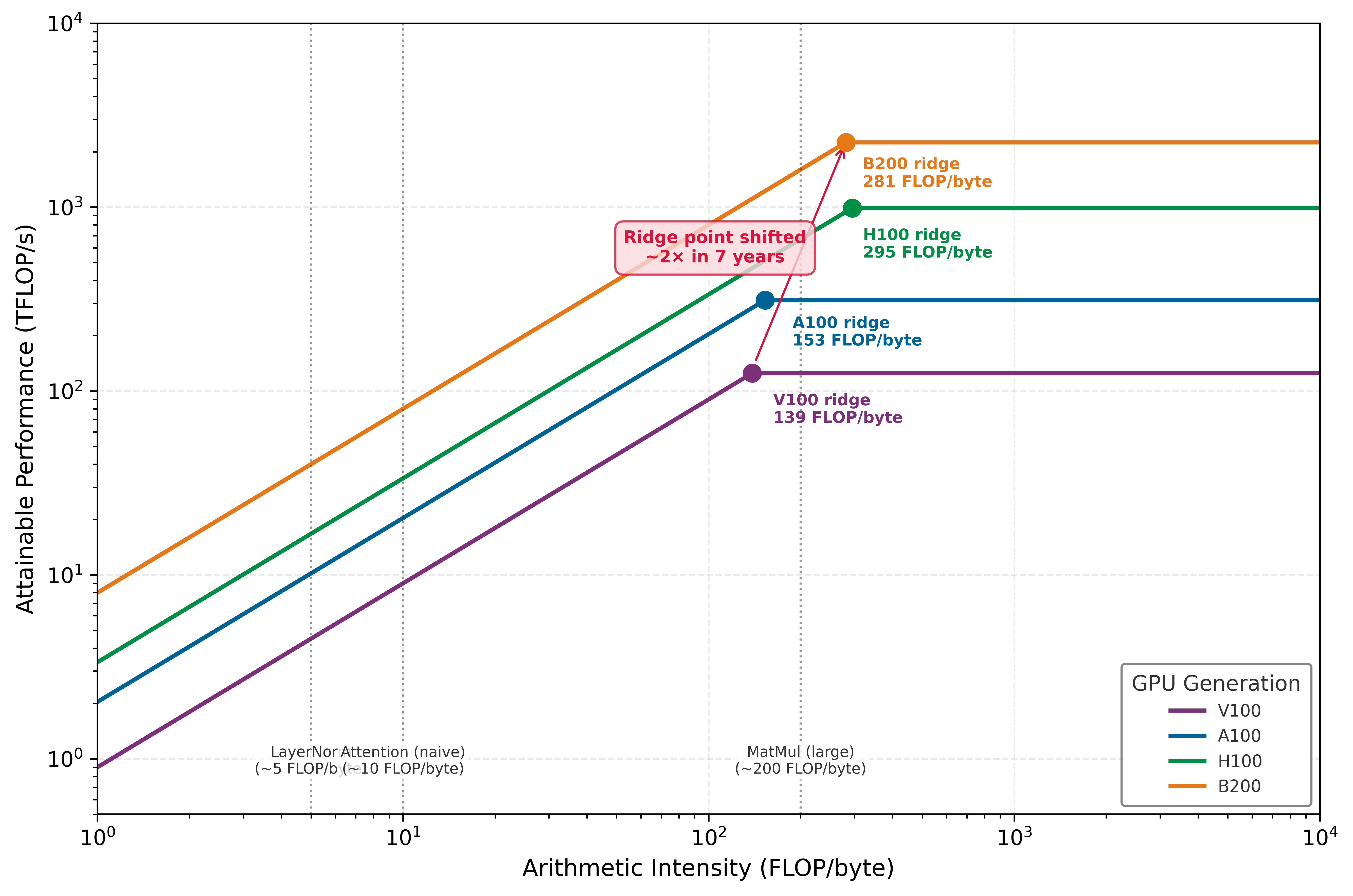
Table 3 quantifies how the hardware balance shifts across accelerator generations. The key column is the ridge point: as compute grows faster than bandwidth, more operators need higher arithmetic intensity just to remain compute-bound.

Table 3: The Widening Memory Wall: Compute throughput has increased 18× from V100 to B200 over seven years, while memory bandwidth has increased only 8.9×. The ridge point has roughly doubled overall (V100 to B200), pulling more workloads into the memory-bound regime over time, though the per-generation movement is not monotonic (B200 sits slightly below H100).

GPU	Year	Peak FP16 (TFLOP/s)	HBM BW (TB/s)	Ridge Point (FLOP/byte)
V100	2017	125	0.9	139
A100	2020	312	2.04	153
H100	2022	989	3.35	295
B200	2024	2,250	8	281

For the FP16/BF16 table as written, the ridge point increased from 139 FLOP/byte on the V100 to 281 FLOP/byte on the B200, about a 2× increase. An operation with arithmetic intensity of 200 FLOP/byte was compute-bound on the V100 and A100, but memory-bound on the H100 and B200. Performance engineering techniques targeting memory efficiency, fusion, precision, and tiling therefore become more important as the ridge point rises, not less. The systems lesson is not that one named kernel lasts forever, but that reducing exposed memory traffic becomes more valuable when compute grows faster than bandwidth.

The roofline model

Roofline model introduced the Roofline Model² (Williams et al. 2009) and arithmetic intensity as the framework for diagnosing whether a workload is compute-bound or memory-bound on a given accelerator, and computed the H100’s ridge point. We recall it here only to push it to fleet scale: how the ridge point shifts across hardware generations, how FP8 moves it, where production ML workloads fall relative to it, and how batch size walks a workload across it. As a reminder, the model plots achievable performance as a function of arithmetic intensity, the ratio of floating-point operations to bytes transferred from memory, and the intersection of the two regimes is the ridge point³.

² Roofline Model: The original framing targets multicore CPUs, but the same ceiling diagram applies to accelerators: two numbers (peak FLOP/s and peak bandwidth) define the entire performance envelope. This same simplicity informs GPU purchasing decisions for ML inference, where the ridge point determines whether a workload benefits from faster compute or faster memory.

Williams, Samuel, Andrew Waterman, and David Patterson. 2009. “Roofline: An Insightful Visual Performance Model for Multicore Architectures.” Communications of the ACM 52 (4): 65–76. https://doi.org/10.1145/1498765.1498785.

³ Ridge Point: The intersection of the memory-bound and compute-bound lines on a Roofline plot. It represents the minimum arithmetic intensity required to reach peak hardware performance $(R_{\text{peak}})$. For an H100 GPU (FP16), the ridge point is roughly 295 FLOP/byte; if an operator’s intensity is below this “ridge,” it will never saturate the Tensor Cores, regardless of how much compute is available.

Definition 1.1: Arithmetic intensity

Arithmetic Intensity $(I)$ is the ML workload ratio of floating-point operations performed to the number of bytes transferred from memory (FLOP per byte).

Significance: It characterizes the computational density of a workload. It is the independent variable in the Roofline Model, determining whether a system operates in the bandwidth-bound ($\text{BW}$) or compute-bound ($R_{\text{peak}}$) regime.
Distinction: Unlike peak throughput (a hardware property), arithmetic intensity is an algorithmic property that measures how effectively a workload reuses data once it is loaded into the processor.
Common pitfall: A frequent misconception is that arithmetic intensity is fixed for a model. In reality, it varies by implementation: techniques like operator fusion increase arithmetic intensity by keeping data in local registers, while increasing batch size increases arithmetic intensity for layers with high parameter reuse.

For a given accelerator with peak compute $R_{\text{peak}}$ (in FLOP/s) and peak memory bandwidth $\text{BW}$ (in bytes/s), equation 2 gives the achievable performance of a workload with arithmetic intensity $I$ (in FLOP/byte):

\[ \text{Achievable FLOP/s} = \min(R_{\text{peak}}, \; \text{BW} \times I) \tag{2}\]

Equation 3 locates the ridge point where these two limits intersect:

\[ I_{\text{ridge}} = \frac{R_{\text{peak}}}{\text{BW}} \tag{3}\]

Workloads with $I < I_{\text{ridge}}$ are memory-bound: their performance is limited by how fast data can be loaded, not how fast it can be processed. Workloads with $I > I_{\text{ridge}}$ are compute-bound: the arithmetic units are the bottleneck. Figure 2 illustrates this relationship graphically.

Figure 2: **The Roofline Model**: Achievable performance (y-axis) as a function of arithmetic intensity (x-axis) on a log-log plot. The sloped line represents the memory bandwidth ceiling; the flat line represents the compute ceiling at the labeled precision (FP8 tensor-core throughput on H100, approximately 2,000 TFLOP/s); their intersection is the ridge point at roughly 600 FLOP/byte for FP8. Most transformer inference operations fall in the memory-bound region (left of the ridge point), while large batched GEMMs fall in the compute-bound region (right). The corresponding FP16 ridge point is roughly 295 FLOP/byte (989 TFLOP/s divided by 3.35 TB/s).

The ridge point of the NVIDIA H100 at FP16 precision is:

\[ I_{\text{ridge}}^{\text{H100, FP16}} = \frac{989 \text{ TFLOP/s}}{3.35 \text{ TB/s}} \approx 295 \text{ FLOP/byte} \]

Any operation performing fewer than 295.2 FLOP/byte floating-point operations per byte loaded is memory-bound on the H100 at FP16. At FP8 precision, where compute doubles to 1979 TFLOP/s and bandwidth remains 3.35 TB/s, the ridge point rises to approximately 590.7 FLOP/byte. The A100, with 312 TFLOP/s and 2.04 TB/s, has a lower ridge point of approximately 153 FLOP/byte at FP16. Across the generations in table 3, compute has outgrown bandwidth and the ridge point has roughly doubled (V100 to B200), so more workloads fall into the memory-bound regime over time; the per-generation movement is not monotonic, however, because each chip pairs its own compute and bandwidth (the B200 ridge sits slightly below the H100). The durable trend, not any single step, is what makes memory-efficiency techniques more valuable as hardware advances.

Figure 3 overlays the roofline models for four GPU generations on a single log-log plot, making the generational ridge-point shift tabulated earlier visible at a glance. An operation like naive self-attention, with an arithmetic intensity near 10 FLOP/byte, is memory-bound on every generation and falls progressively further below the ridge with each new chip. More critically, operations near 200 FLOP/byte, such as some matrix multiplications and fused blocks, can change regime as hardware changes. The same kernel can change performance regime across hardware generations, a fact that demands re-profiling whenever hardware is upgraded.

Figure 3: **The Shifting Roofline Across GPU Generations**: Overlaid FP16/BF16 roofline models for V100 through B200 show the ridge point growing from 139 to 281 FLOP/byte. Operations near 200 FLOP/byte can change regime as the roofline shifts. The same kernel can change performance regime across hardware generations.

Where ML workloads fall

ML operations span three orders of magnitude in arithmetic intensity, and the position of each operation on the roofline determines which optimization strategies apply.

Large general matrix multiply (GEMM) operations are the most compute-intensive operations in ML. A square matrix multiplication of dimension $4096{\times}4096$ in FP16 performs approximately 137.4 billion FLOPs while loading roughly 100.7 MB of data, yielding an arithmetic intensity of approximately 1365.3 FLOP/byte. This sits well above the H100’s ridge point, making large GEMMs firmly compute bound.

Element-wise operations tell the opposite story. A Gaussian Error Linear Unit (GELU) activation applied to a $4096{\times}4096$ tensor performs roughly 5 operations per element but must load and store each element, yielding an arithmetic intensity of approximately 1.2 FLOP/byte. The GPU spends almost all its time waiting for data transfers rather than computing, making these operations profoundly memory-bound.

Autoregressive LLM decoding at batch size one represents the extreme case. Each decoding step reads the entire weight matrix (gigabytes of data) to produce a single output token. With a hidden dimension of 4096 and batch size 1, the arithmetic intensity is approximately 1 FLOP/byte, deep in the memory-bound regime. The arithmetic intensity explains why LLM token generation achieves a tiny fraction of peak FLOP/s: the GPU spends nearly all its time reading weights, not multiplying them.

Table 4 reveals the central pattern behind these examples: batched GEMM can reach the compute-bound regime, but attention, element-wise work, and batch-1 decode sit below the ridge point and are governed by bytes moved rather than FLOPs advertised.

Table 4: Arithmetic Intensity of Common ML Operations: Many transformer inference operations, aside from large batched GEMMs, fall below the H100’s ridge point and are therefore memory-bound. Performance engineering focuses on reducing the memory traffic of these operations.

Operation	Arithmetic Intensity	H100 FP16 Regime	Primary Bottleneck
GEMM ($4096{\times}4096$)	~1,365 FLOP/byte	Compute-bound	Tensor core throughput
Self-Attention (seq=2048)	~50–200 FLOP/byte	Memory-bound	HBM bandwidth
Element-wise (GELU, LayerNorm)	~1–3 FLOP/byte	Memory-bound	HBM bandwidth
LLM Decode (batch=1)	~1–2 FLOP/byte	Memory-bound	HBM bandwidth

The majority of operations in a transformer inference pipeline are memory-bound. Training workloads with large batch sizes shift more operations into the compute-bound regime because GEMM dimensions scale with batch size. Inference, however, especially autoregressive generation, is dominated by memory-bound operations. Fusion, tiling, reduced precision, and algorithmic shortcuts all target the same fundamental problem: reducing bytes moved per operation.

The memory-bound nature of inference also explains a common source of confusion: GPU benchmarks reporting peak TFLOP/s often fail to predict real inference performance. Two GPUs with different TFLOP/s but identical memory bandwidth will achieve virtually identical LLM decode throughput at batch size 1, because decode is entirely memory bound. The correct metric for comparing GPUs for LLM inference is not FLOP/s but rather the combination of memory bandwidth and memory capacity. Bandwidth determines the token generation rate, and capacity determines the maximum batch size (and therefore throughput). Only at large batch sizes, where decode approaches the compute-bound regime, do the FLOP/s differences between GPUs translate into throughput differences.

Serving Regimes: Batch Size and Prefill-Decode

Diagnosis locates a workload on the roofline; the serving regime determines which knobs move it. Two structural features of LLM inference, the batch dimension and the split between prompt processing and token generation, decide whether decode stays pinned to the memory-bound slope or climbs toward the compute roof. Both are levers the rest of the chapter’s techniques act through.

Batch size as the universal control knob

For memory-bound LLM serving, batch size is often the first performance lever to test, and also one of the most constrained. Increasing the batch size transforms the arithmetic intensity of every operation. For an LLM decode step, the arithmetic intensity scales linearly with batch size:

\[ I_{\text{decode}}(B) = \frac{2PB}{P b_{\text{param}} + B d_{\text{model}} b_{\text{elem}}} \]

Here, $P$ is parameter count, $B$ is batch size, $d_{\text{model}}$ is hidden width, $b_{\text{param}}$ is bytes per stored parameter, and $b_{\text{elem}}$ is bytes per activation element. At batch size 1, the denominator is dominated by the weight term $(P b_{\text{param}})$, and $I \approx 2/b_{\text{param}} \approx 1$ FLOP/byte for FP16. At batch size 256, the weight term still dominates, but the same weight bytes are amortized across more requests, so $I \approx 2 \times 256/b_{\text{param}} \approx 256$ FLOP/byte, approaching the compute-bound regime.

Larger batches raise arithmetic intensity toward the ridge.

At large batch sizes, the GPU transitions from memory-bound to compute-bound, and utilization increases dramatically. A single H100 achieving 5 percent utilization at batch size 1 may achieve 40 percent utilization at large batch sizes. The economic implication is stark: the cost per token decreases by roughly 8× as batching carries the workload from the memory-bound to the compute-bound regime.

The constraint is memory: each additional request in the batch requires its own KV cache (the per-request store of attention keys and values for every token generated so far), and the total KV cache across all requests must fit in GPU memory alongside the model weights. The 70B-model-on-8-H100 deployment introduced here is the chapter’s recurring example, revisited with full quantitative detail in the precision dividend (section 1.3.3) and the case study (section 1.9.3). A 70B model with 140 GB of weights in FP16 must be sharded across multiple GPUs; on an 8-GPU node that leaves about 62.5 GB per GPU for KV cache before overhead. The precision engineering techniques in this chapter address exactly this constraint: INT4 weight quantization reduces the per-GPU weight footprint to about 4.4 GB and frees roughly 13 GB per GPU for KV cache, enabling batch sizes that transform the economics of serving.

A serving scheduler can keep the effective batch full by adding new requests as older requests finish, but that policy only works when memory is available for the active requests. Performance engineering’s role is to make that scheduler’s job feasible by minimizing the per-request memory footprint, primarily through KV cache compression and weight quantization. Inference serving (Inference at Scale) develops the full scheduler; the local point here is that memory optimization expands the batch sizes the scheduler can safely admit.

A critical enabler for large batch sizes is PagedAttention⁴, vLLM’s paged KV cache management technique (Kwon et al. 2023). Traditional KV cache implementations preallocate contiguous memory for each request’s maximum possible sequence length.

⁴ PagedAttention: Named by direct analogy to OS virtual memory paging, where the OS maps noncontiguous physical pages to contiguous virtual addresses. The vLLM paper presented this insight at SOSP 2023: the same mechanism eliminates internal fragmentation in KV caches, recovering the 60–80 percent of GPU memory wasted by worst-case preallocation (Kwon et al. 2023). This single abstraction transformed LLM serving economics by enabling 2–4$\times$ larger batch sizes without any change to model weights or precision.

Kwon, Woosuk, Zhuohan Li, Siyuan Zhuang, Ying Sheng, Lianmin Zheng, Cody Hao Yu, Joseph Gonzalez, Hao Zhang, and Ion Stoica. 2023. “Efficient Memory Management for Large Language Model Serving with PagedAttention.” Proceedings of the 29th Symposium on Operating Systems Principles, 611–26. https://doi.org/10.1145/3600006.3613165.

If the maximum is 4,096 tokens but the average is 500, approximately 88 percent of the allocated memory is wasted. PagedAttention divides the KV cache into fixed-size blocks (pages), allocated on demand as the sequence grows. This eliminates memory fragmentation and enables near-100 percent utilization of the KV cache memory budget. The performance impact is indirect but substantial: by reducing memory waste, PagedAttention enables 2–4$\times$ larger effective batch sizes, which in turn improve throughput and GPU utilization through the batch size mechanism described earlier.

PagedAttention and KV cache quantization interact multiplicatively. PagedAttention reduces memory waste (from fragmentation), while quantization reduces memory usage (from precision). Together, they increase the effective batch size by 8–16$\times$ compared to a baseline system with preallocated FP16 KV caches, fundamentally changing the economics of LLM serving.

The prefill-decode decomposition

Modern LLM serving systems decompose each request into two distinct phases with fundamentally different performance characteristics. The distinction between these phases drives system architecture and optimization strategy.

The prefill phase processes the entire input prompt in parallel. If the prompt contains $S$ tokens, the prefill phase executes a single forward pass over all $S$ tokens simultaneously. The GEMM operations have shape $[S,d_{\text{model}}]{\times}[d_{\text{model}},d_{\text{model}}]$, making the batch dimension equal to $S$. For a prompt of 1024 tokens, this is arithmetically intensive: the arithmetic intensity is approximately $2 \times 1024/2 = 1024$ FLOP/byte for FP16 weights, well into the compute-bound regime. Prefill is therefore limited by Tensor Core throughput, not memory bandwidth.

The decode phase generates output tokens one at a time, autoregressively. Each step has a batch dimension of 1 (for a single request) or the number of concurrent requests (for batched serving). At batch size 1, decode is deeply memory-bound as analyzed in section 1.0.6.

The prefill-decode decomposition has direct implications for system design. A system optimized for prefill (maximizing FLOP/s utilization) would use large matrix sizes and high compute throughput. A system optimized for decode (maximizing bandwidth utilization) would use aggressive quantization and memory optimization. A real serving system must handle both phases, often simultaneously across different active requests.

Disaggregated serving addresses this mismatch by running prefill and decode on separate hardware pools. Here, disaggregation is evidence that prefill and decode have different bottlenecks; Inference at Scale develops the routing, admission-control, and serving-policy machinery. Prefill servers are optimized for compute (fewer, higher-FLOP/s GPUs), while decode servers are optimized for memory bandwidth and capacity (more memory per GPU, aggressive quantization). The KV cache computed during prefill is transferred to a decode server, which handles the subsequent autoregressive generation. This disaggregation allows each phase to use hardware and software configurations tuned for its specific bottleneck.

The performance characteristics of each phase determine which optimization techniques apply. FlashAttention provides its largest gains during prefill, where the quadratic attention computation dominates. KV cache quantization and speculative decoding apply exclusively to the decode phase. Precision engineering (FP8/INT4 weights) benefits both phases, but through different mechanisms: prefill benefits from doubled compute throughput (FP8 Tensor Cores), while decode benefits from doubled effective bandwidth (half the bytes per weight read).

A quick decode calculation shows why the memory wall dominates even when the accelerator has abundant unused FLOP/s.

Napkin Math 1.1: The Roofline diagnostic

Problem: A 70B parameter LLM is deployed on 8$\times$ H100 GPUs with tensor parallelism. At batch size 1, each GPU holds approximately 8.75B parameters in FP16 (17.5 GB of weights). Each decode step reads its weight shard to produce one token. What is the achieved arithmetic intensity, and what is the theoretical maximum token generation rate?

Math:

Step 1: Arithmetic intensity. Each decode step per GPU: FLOPs $=$ $2 \times 8.75 \times 10^{9}$ $=$ 17.5B FLOPs. Bytes loaded $=$ $8.75 \times 10^{9} \times 2 \text{ bytes}$ $=$ 17.5 GB.

$I = \frac{1.75 \times 10^{10} \text{ FLOP}}{1.75 \times 10^{10} \text{ bytes}} = 1 \text{ FLOP/byte}$

At 1 FLOP/byte, the operation sits far below the H100 ridge point of ~295 FLOP/byte: deeply memory-bound.

Step 2: Token rate. Since the operation is memory-bound, performance is limited by bandwidth, not compute:

$t_{\text{decode}} = \frac{17.5\,\text{GB}}{3.35\,\text{TB/s}} \approx 5.2\,\text{ms per token}$

This yields approximately 191.4 tokens/s per GPU, or about 191.4 tokens/s for the model (since tensor parallelism does not multiply throughput for memory-bound decode). In practice, overheads from KV cache reads and NVLink synchronization reduce this substantially below the ideal bandwidth-only limit.

Systems insight: At batch size 1, only about 0.3 percent of the H100’s FP16 FLOP/s are in use. The improvement paths all attack the same weight-streaming cost: larger batches amortize each weight read across more requests, quantization reduces the bytes read for each weight, and speculative decoding tries to obtain multiple accepted tokens from one target-model weight pass.

The roofline model establishes the physics that constrains all subsequent optimization. The first and most impactful strategy for breaking through the memory wall is keeping data in SRAM instead of round-tripping through HBM.

Operator Fusion and Kernel Engineering

Consider the simple sequence of operations $Y = \text{LayerNorm}(\text{GELU}(XW + b))$. In a naive implementation, the GPU writes the output of the matrix multiply back to main memory, reads it back for the GELU, writes it out again, and reads it one final time for the LayerNorm. This redundant data movement shatters performance. Operator fusion eliminates these intermediate round-trips by keeping results in ultra-fast registers, executing the entire sequence in a single trip to memory.

Systems Perspective 1.2: Analogy: The short-order cook

Imagine a kitchen where one chef chops vegetables, puts them in the fridge (HBM), then another chef takes them out to boil them, puts them back in the fridge, and a third chef takes them out to plate them. This is unfused execution: the bottleneck is not the cooking but the constant walking to the fridge.

Operator fusion assigns the recipe to a single chef who keeps the ingredients on their cutting board (SRAM/Registers) and performs all three steps consecutively without ever returning to the fridge until the final dish is ready.

The kernel launch problem

Each GPU kernel launch involves overhead: the CPU must prepare launch parameters, dispatch to the GPU command queue, and the GPU must schedule thread blocks across its streaming multiprocessors (SMs). For a small element-wise operation on an accelerator such as an H100, this overhead can be 5–20 $\mu$s, a time during which a memory-bound kernel might have already completed its useful work. When a transformer layer comprises dozens of small operations (add, multiply, normalize, activate), the cumulative launch overhead becomes significant.

Each unfused kernel must also materialize its output in HBM. Consider a sequence of three operations: $Y = \text{LayerNorm}(\text{GELU}(XW + b))$. Without fusion, this requires three passes through HBM:

GEMM kernel: Read $X$ and $W$ from HBM, compute $XW + b$, write result $Z_1$ to HBM.
GELU kernel: Read $Z_1$ from HBM, compute $\text{GELU}(Z_1)$, write $Z_2$ to HBM.
LayerNorm kernel: Read $Z_2$ from HBM, compute $\text{LayerNorm}(Z_2)$, write $Y$ to HBM.

Intermediate tensors $Z_1$ and $Z_2$ each occupy the same memory as the output $Y$. For a hidden dimension of 4096 and batch size of 2048 in FP16, each intermediate tensor is 16.8 MB. The unfused execution materializes 33.6 MB of intermediate tensors and performs 67.1 MB of intermediate HBM traffic, writing and then rereading each tensor. A fused kernel avoids that traffic entirely by holding $Z_1$ and $Z_2$ in registers or shared memory (SRAM) within the SM. Figure 4 contrasts these two execution paths, making the HBM traffic savings visible.

Figure 4: **Operator Fusion: Before and After**: Top: three separate kernels each read from and write to HBM, materializing intermediates $Z_1$ and $Z_2$, with six HBM round-trips along the unfused path. Bottom: a single fused kernel reads inputs once, holds intermediates in SRAM, and writes only the final output, leaving just two HBM round-trips. The fused path delivers roughly a 3$\times$ reduction in HBM traffic per layer.

As figure 4 makes concrete, fusion reduces HBM round-trips from six to two per layer, a roughly 3$\times$ reduction in off-chip memory traffic for this layer block. In a naive implementation without operator fusion, executing one transformer layer requires roughly 50 separate kernel launches. If each launch incurs a 10-microsecond overhead, the system spends 500 microseconds purely on dispatch latency. If the actual arithmetic execution of the layer takes only 2 milliseconds, the launch overhead consumes 20 percent of the total wall-clock time, leaving the GPU compute units idle for one-fifth of the inference cycle. This “launch-bound” regime limits the benefits of faster hardware; doubling the GPU’s FLOP/s does nothing to reduce the 500-microsecond fixed cost. Operator fusion addresses this by compiling these 50 discrete operations into a small handful of fused kernels, often reducing the count to 5–10 launches, thereby reclaiming the lost cycles and shifting the workload away from dispatch overhead and back toward the hardware limits captured by the roofline model.

Fusion categories

Fusion is profitable when the HBM traffic it removes is worth the kernel complexity it introduces. The three common categories differ by that trade-off: how much data movement they eliminate, how much synchronization they require, and how often a compiler can apply them automatically.

Element-wise fusion sits at the low-complexity end: consecutive element-wise operations (add, multiply, activation functions) combine into a single kernel. Because each output element depends on exactly one input element, this fusion is always legal and straightforward to implement. Deep learning frameworks commonly perform element-wise fusion automatically for supported patterns.

When the sequence includes a reduction, the fusion decision becomes more constrained. Reduction fusion combines an element-wise operation with a subsequent reduction (such as summing elements for a loss function, or computing mean and variance for layer normalization). Reductions require inter-thread communication within the kernel, using warp-level shuffle instructions or shared memory to aggregate partial results across threads. Despite this complexity, the memory savings are substantial: the intermediate tensor before the reduction never materializes in HBM. For layer normalization specifically, reduction fusion avoids writing the large prenormalization tensor to HBM and reading it back for the mean/variance computation.

The highest-payoff case is operator-specific fusion. These are custom kernels designed for a specific sequence of operations, such as fused attention or fused GEMM-bias-activation. The kernel architect must reason about data flow, shared memory allocation, and thread scheduling simultaneously. The payoff is substantial: FlashAttention, which we examine next, removes the quadratic attention workspace and keeps the online softmax state linear in sequence length.

To appreciate the quantitative impact, consider each category applied to a single transformer layer with hidden dimension 4096 and batch size 2048 in FP16. Element-wise fusion of a bias-GELU-dropout chain in this shape eliminates two intermediate tensors of 16.8 MB each, saving 67.1 MB of HBM traffic per layer. Across 80 layers, this reclaims about 5.4 GB of HBM traffic per forward pass. Reduction fusion of LayerNorm avoids materializing large prenormalization tensors and intermediate statistics. Operator-specific attention fusion (FlashAttention) provides the largest single gain by removing the quadratic score and probability matrices that dominate long-context attention. The cumulative effect of all three fusion categories can remove a large fraction of HBM traffic for a memory-bound transformer forward pass, but the end-to-end speedup must still be verified with profiling because the bottleneck may shift.

CUDA graphs: Eliminating launch overhead

An orthogonal technique for reducing the overhead term in the iron law is CUDA Graphs⁵. While operator fusion combines multiple operations into fewer kernels, CUDA Graphs eliminate the CPU overhead of launching those kernels.

⁵ CUDA Graphs: Introduced in CUDA 10 (2018), originally for graphics rendering pipelines that replay identical command sequences every frame. The strict determinism requirement – identical operations, shapes, and memory addresses per replay – directly conflicts with the dynamic shapes and variable batch sizes of LLM serving, restricting their use primarily to the decode phase where the computation pattern repeats per token.

In standard PyTorch execution, each kernel launch requires the CPU to push a command to the GPU’s command queue. For a transformer decoder layer with 30+ kernels, this CPU-to-GPU roundtrip (typically 5–10 $\mu$s per launch) accumulates to 150–300 $\mu$s per layer. For a 70-layer model, kernel launch overhead alone contributes 10–20 ms per forward pass, a significant fraction of the total time for memory-bound inference.

CUDA Graphs address this by recording a sequence of GPU operations (kernel launches, memory copies) into a replayable graph. The recording happens once during a warmup phase. On subsequent iterations, replaying the graph requires only a single CPU-to-GPU command that dispatches the entire recorded sequence, reducing launch overhead to approximately 5–10 $\mu$s total regardless of the number of kernels.

The benefit is substantial: for a model with 30+ kernels per layer and 70+ layers, the baseline kernel launch overhead can exceed 15 ms per forward pass. CUDA Graphs reduce this to under 0.1 ms, reclaiming 15 ms that translates directly to higher token generation rates.

The constraint is that CUDA Graphs require deterministic execution: the sequence of operations, tensor shapes, and memory addresses must be identical across replays. This conflicts with dynamic inference patterns like variable-length sequences, changing batch sizes, and conditional computation (early exit, MoE routing). In practice, CUDA Graphs are most effective for the decode phase of LLM serving, where the computation pattern is repetitive (same operations per token), and less useful for the prefill phase, where input lengths vary.

The combination of operator fusion (reducing the number of kernels) and CUDA Graphs (reducing the per-kernel overhead) can together eliminate nearly all noncompute overhead from the forward pass. When profiling reveals that kernel launch gaps constitute more than 10 percent of execution time, CUDA Graphs should be the first intervention considered.

FlashAttention: Tiled attention as a system primitive

Standard self-attention computes $\text{Softmax}(QK^T / \sqrt{d_k})V$, where $Q$, $K$, and $V$ are matrices of shape $[\text{sequence length}{\times}\text{head dimension}]$. The na"ive implementation materializes the full $S{\times}S$ attention matrix $A = QK^T$ in HBM, where $S$ is the sequence length. For $S = 8192$ and FP16 precision, this matrix alone consumes $8192 \times 8192 \times 2 \approx 134$ MB per attention head, so the quadratic score tensors run to several gigabytes per layer. The canonical accounting below makes this precise for a 64-head Llama-style layer, counting the score and probability traffic alongside the persistent $Q$, $K$, $V$, and output tensors.

FlashAttention (Dao et al. 2022) reformulates attention using tiling. Instead of materializing the full $S{\times}S$ attention matrix, it processes $Q$, $K$, and $V$ in small blocks that fit in on-chip SRAM. The algorithm loads tiles of $Q$, $K$, and $V$, computes partial attention scores, and maintains running statistics (online softmax) to produce the exact result without ever storing the full attention matrix in HBM.

FlashAttention shrinks attention memory about 65 times.

The reduction in materialized attention state is dramatic. For a sequence length of 8192, 64 heads, and head dimension 128 in FP16, the naive implementation materializes and revisits approximately 34.9 GB of HBM-resident tensors for the full layer, or 545.3 MB per head. FlashAttention avoids the quadratic score and probability tensors; its persistent HBM-visible tensors are dominated by $Q$, $K$, $V$, and output $Y$, totaling approximately 536.9 MB for the full layer, or 8.4 MB per head. This simplified accounting excludes schedule-dependent tile reloads inside a particular kernel, but it captures the important scaling result: a 65× reduction in HBM-visible attention state for this configuration.

The key insight behind FlashAttention is the online softmax⁶ trick, which makes tiling possible for an operation that appears to require global information. Standard softmax computes $\text{softmax}(s_i) = e^{s_i} / \sum_j e^{s_j}$, but for numerical stability it first subtracts the global maximum: $\text{softmax}(s_i) = e^{s_i - m} / \sum_j e^{s_j - m}$ where $m = \max_j s_j$. Finding this global maximum seems to require seeing all scores first, which would force materializing the full $S{\times}S$ matrix.

⁶ Online Softmax: Online here is an algorithmic term meaning the computation processes data incrementally in a single pass without storing the full input – the same sense as in online learning or online algorithms. This property is what makes tiling possible: the algorithm never needs the complete $S{\times}S$ score matrix in memory simultaneously, reducing attention memory from $\mathcal{O}(S^2)$ to $\mathcal{O}(S)$ and making long-context inference feasible on fixed-size SRAM.

The online algorithm avoids this by maintaining running statistics that are updated incrementally as each tile is processed. When processing tile $t$, the algorithm executes four steps:

Computes a local block of scores $A_t = Q_{\text{block}} K_t^T$.
Updates the running maximum: $m_{\text{new}} = \max(m_{\text{old}}, \max(A_t))$.
Rescales the previous running sum and output: multiply by $e^{m_{\text{old}} - m_{\text{new}}}$ to correct for the updated maximum.
Computes the local softmax contribution using $m_{\text{new}}$ and accumulates into the running output.

After processing all tiles, the running output contains the mathematically equivalent result to the standard algorithm up to the floating-point roundoff of the chosen precision. The rescaling step (step 3) is the critical innovation: it allows the algorithm to “fix up” previous partial results when a new tile reveals a larger maximum value. The algorithm is exact in the mathematical sense, but floating-point execution order can still change the last few bits relative to an unfused implementation.

The cost of this tiling is additional arithmetic: the rescaling operations in step 3 add FLOPs that the standard algorithm does not perform. Because the operation is profoundly memory-bound (standard attention’s arithmetic intensity falls to roughly 1–10 FLOP/byte once its materialized score and probability tensors are counted against the HBM traffic they generate, below the higher regime-dependent figures in table 4), the additional compute is “free” in the sense that the GPU’s arithmetic units would otherwise be idle, waiting for HBM data transfers. Trading extra compute for fewer memory accesses is profitable whenever the operation is memory-bound, the central principle of this entire chapter.

The mechanism that delivers the materialized-state reduction quantified above is tiling. FlashAttention processes the computation in tiles (typically $128{\times}128$ on H100). For one tile, the algorithm loads a block of $Q$ ($128 \times 128 \times 2 \approx$ 32.8 KB), a block of $K$ ($128 \times 128 \times 2 \approx$ 32.8 KB), and a block of $V$ (32.8 KB), totaling approximately 98.3 KB. This fits comfortably in the H100’s 228 KB of shared memory per SM. The tile score $A_{\text{tile}} = Q_{\text{tile}} K_{\text{tile}}^T$ is computed and consumed entirely within SRAM; it is never written to HBM. The algorithm iterates over $8192/128 =$ 64 column tiles for each of 64 row tiles, reloading tiles as required by the kernel schedule. The important point is that the quadratic $S{\times}S$ score and probability matrices are never materialized: the persistent per-head tensors are $Q$, $K$, $V$, $Y$, and $\mathcal{O}(S)$ softmax statistics, instead of the hundreds of megabytes of quadratic intermediates the canonical accounting above counted.

FlashAttention-2 (Dao 2023) further optimizes the algorithm for GPU architectures with many streaming multiprocessors by restructuring the parallelism pattern. The original FlashAttention parallelizes over batch and head dimensions, meaning each thread block handles one (batch, head) pair and iterates over the full sequence. FlashAttention-2 additionally parallelizes over the sequence dimension of the query matrix, distributing work across thread blocks more efficiently and achieving better occupancy. It also reduces the number of non-GEMM FLOPs by restructuring the rescaling operations and exploiting the asymmetry between the Q loop (outer) and K/V loop (inner).

Dao, Tri. 2023. “FlashAttention-2: Faster Attention with Better Parallelism and Work Partitioning.” arXiv Preprint arXiv:2307.08691.

Newer FlashAttention-family kernels target Hopper-era hardware features such as FP8 Tensor Cores and the Tensor Memory Accelerator (TMA), a hardware path for asynchronous bulk tensor movement between HBM and shared memory. The systems principle is the same as the original algorithm: as the hardware exposes faster movement and lower-precision execution paths, the attention schedule must be rewritten to use those paths without materializing the quadratic workspace.

The original breakthrough was a change in how engineers understood the bottleneck: the constraint on attention was the memory hierarchy, not the matrix multiplication.

Example 1.1: The FlashAttention breakthrough

Context: In 2022, Tri Dao and coauthors introduced FlashAttention (Dao et al. 2022), showing that the attention mechanism’s performance bottleneck could be treated as an IO-aware data-movement problem rather than only as a matrix multiplication tuning problem.

Mechanism: The bottleneck was memory hierarchy, not compute. Standard attention materialized the massive $S{\times}S$ attention score matrix in high-latency HBM. FlashAttention restructured the algorithm using tiling to keep running statistics in on-chip SRAM, computing the softmax without ever writing the full matrix to global memory. This reduced memory complexity to linear $\mathcal{O}(S)$ and wall-clock time by 2–4$\times$ on relevant attention workloads.

Systems lesson: FlashAttention matters because it changes where the attention state lives. The durable optimization is not “a faster kernel” but a data-movement reduction that keeps quadratic intermediates out of HBM.

Dao, T., D. Y. Fu, S. Ermon, A. Rudra, and C. Ré. 2022. “FlashAttention: Fast and Memory-Efficient Exact Attention with IO-Awareness.” Advances in Neural Information Processing Systems 35 35: 16344–59. https://doi.org/10.52202/068431-1189.

Before turning to the scaling plot, pause on the mechanism: FlashAttention trades a small amount of extra arithmetic for the elimination of quadratic HBM-resident state.

Checkpoint 1.2: FlashAttention mechanics

Verify your understanding of memory-aware attention:

Sequence-length scaling: Explain why FlashAttention provides a larger speedup for longer sequences (for example, 32K) than for short sequences (for example, 512).
Online softmax storage: Identify whether the “online softmax” statistics in the FlashAttention algorithm reside in HBM, L2 Cache, or SM SRAM.
FLOPs unchanged: Evaluate the claim that FlashAttention reduces the total number of floating-point operations (FLOPs) required for attention.
Memory to batch size: Explain how reducing the attention memory from $\mathcal{O}(S^2)$ to $\mathcal{O}(S)$ enables larger batch sizes for serving.

The 65× figure above is the canonical, full-layer materialized-state reduction; it is the number to carry forward. Figure 5 adds only the scaling shape: because standard-attention workspace grows quadratically while FlashAttention’s running state grows linearly, the advantage widens with sequence length. The plot’s larger ratios reflect a narrower accounting boundary, comparing only the quadratic score workspace against the linear running statistics rather than the full set of HBM-visible tensors, so they are not directly comparable to the 65× figure; the takeaway is that the gap grows, not its exact value at a given length.

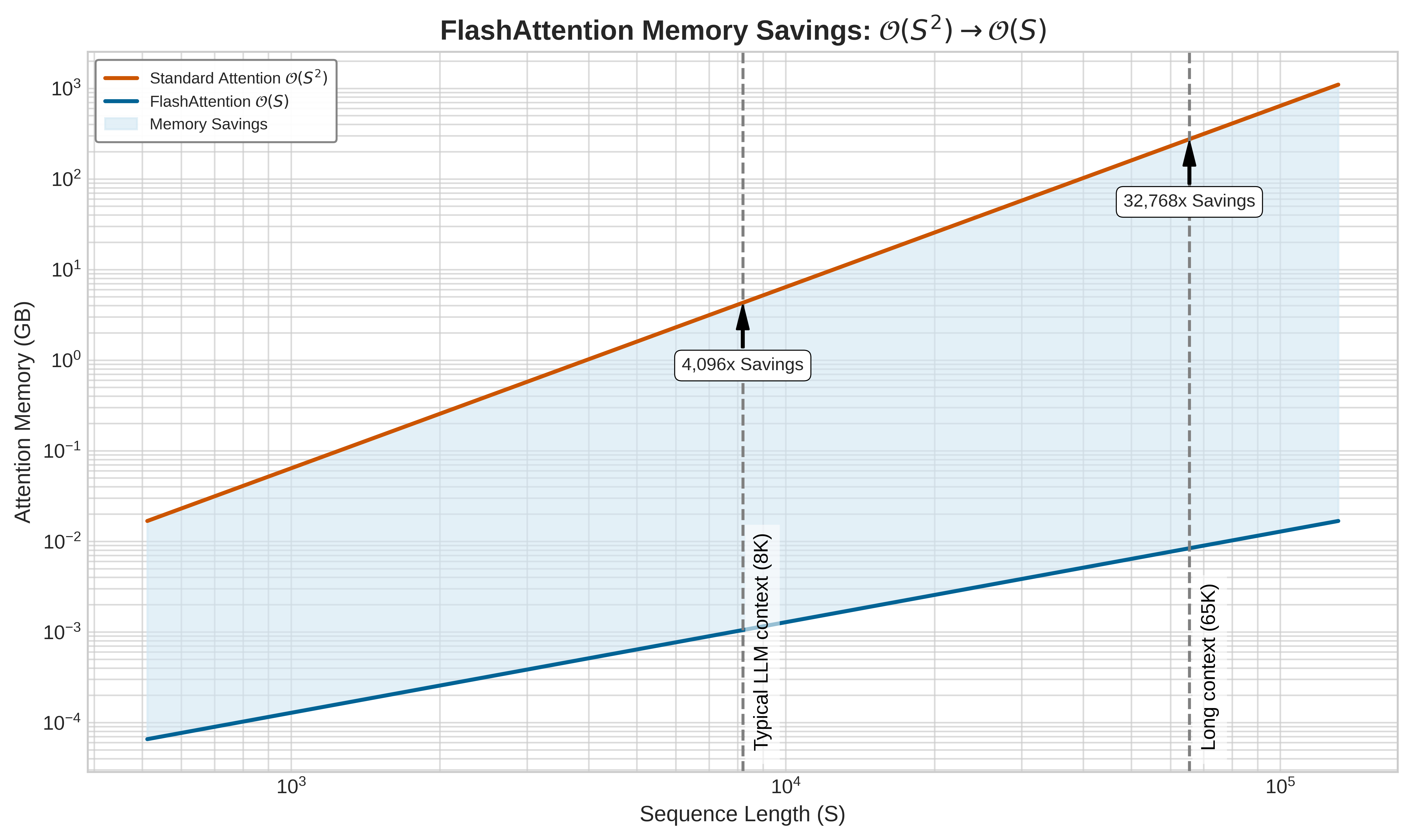
Figure 5: **FlashAttention Memory Savings**: $\mathcal{O}(S^2) \rightarrow \mathcal{O}(S)$. Standard attention allocates the full $S{\times}S$ score matrix in HBM, while FlashAttention maintains only $\mathcal{O}(S)$ running statistics. The shaded region represents memory freed for KV cache, activations, or larger batch sizes. This workspace-only comparison uses a narrower boundary than the full-layer materialized-state accounting in the text; its point is the widening shape of the gap as context grows, not a headline ratio.

FlashAttention reduces the memory wall within a single GPU by tiling across the SRAM-HBM boundary. For sequence lengths that exceed the memory capacity of a single GPU, the same tiling principle extends across multiple GPUs via Ring Attention (Liu et al. 2023). By distributing the sequence blocks across a ring of accelerators and overlapping communication with computation, Ring Attention enables context windows that would be impractical on single-GPU configurations. Tensor parallelism examines the distributed mechanics of Ring Attention within the broader tensor-parallelism discussion.

Liu, Hao, Matei Zaharia, and Pieter Abbeel. 2023. “Ring Attention with Blockwise Transformers for Near-Infinite Context.” arXiv Preprint arXiv:2310.01889, ahead of print. https://doi.org/10.48550/arXiv.2310.01889.

Self-Check: Question

A profile of one transformer layer shows dozens of short kernels and repeated writes of intermediate activations to HBM. Why does fusing a sequence like GEMM → GELU → LayerNorm often speed up inference even though the mathematical function is unchanged?
1. It reduces redundant HBM reads and writes of intermediate tensors and can also cut kernel launch overhead
2. It turns the layer from memory-bound into communication-bound, which GPUs handle more efficiently
3. It removes model parameters from the layer, so fewer weights must be loaded in future tokens
4. It forces every operation to run in FP32, eliminating numerical error from separate kernels
Order the following steps in FlashAttention’s tiled computation: (1) update the running maximum and rescale prior partial results, (2) compute a local score tile from Q and K blocks, (3) accumulate the tile’s contribution into the running output.
Which workload is the best fit for CUDA Graphs?
1. A research notebook where control flow changes every iteration and sequence lengths vary unpredictably
2. A decode loop with repetitive per-token execution, fixed shapes, and stable memory addresses across replays
3. An MoE model whose routing decisions change the executed operators for each token
4. A prefill service whose prompt lengths and batch sizes vary widely from request to request
Explain why FlashAttention’s speedup tends to grow with sequence length, especially compared with naive attention.
A kernel author is deciding between writing a fused attention variant in raw CUDA at the thread level or in Triton at the tile level. Explain why the tile-centric abstraction more readily exposes the SRAM reuse and fusion opportunities that FlashAttention depends on, given the chapter’s memory-hierarchy framing.

See Answers →

Precision Engineering

Fusion reduces the number of trips through HBM; precision engineering reduces the payload of each trip. Moving FP16 weights through HBM consumes twice as many bytes as FP8. For bandwidth-bound kernels, shrinking weights from 2 bytes to 1 byte can roughly halve weight-read traffic and increase effective memory bandwidth. The engineering decision is where numerical noise can be tolerated to reduce bandwidth pressure and where quality demands higher precision. While FP8 for distributed training examines 8-bit floating point (FP8) as a training-time primitive, here we focus on the quantization techniques that enable efficient inference at scale.

Block-wise quantization

The first inference-side precision decision is how to shrink weights while protecting the channels that carry rare but essential signal. Post-training quantization to INT8 or INT4 delivers even greater bandwidth savings for inference, but LLMs present a unique challenge: outlier features⁷. Dettmers et al. (2022) discovered that large language models develop a small number of hidden dimensions (about 0.1 percent of features) with activation magnitudes roughly 3–20$\times$ larger than the rest. Applying uniform per-tensor INT8 quantization clips these outliers, destroying the information they carry, or expands the quantization range to accommodate them, wasting precision on the majority of near-zero values.

⁷ Outlier Features: Large-scale transformers develop emergent “outlier” dimensions with activation magnitudes up to about 20$\times$ larger than typical values (Dettmers et al. 2022). While these outliers constitute about 0.1 percent of all features, clipping them during INT8 quantization destroys the model’s reasoning capabilities. This physical property of large models is the reason post-training quantization (PTQ) requires “outlier-aware” strategies like LLM.int8() or Activation-Aware Weight Quantization (AWQ).

Dettmers, Tim, Mike Lewis, Younes Belkada, and Luke Zettlemoyer. 2022. “LLM.int8(): 8-Bit Matrix Multiplication for Transformers at Scale.” Advances in Neural Information Processing Systems 35, 30318–32. https://doi.org/10.52202/068431-2198.

Definition 1.2: Block-wise quantization

Block-wise Quantization is an ML quantization scheme that partitions a weight tensor into nonoverlapping groups of $G_{\text{block}}$ elements and computes a per-group scale $s_i = (x_{\max,i} - x_{\min,i}) / (2^b - 1)$, bounding worst-case quantization error within each group independently.

Significance: With block size $G_{\text{block}} = 64$ and $b = 4$ bits, weights compress from 16 bits to 4 bits (a 4$\times$ memory reduction) while each FP16 scale adds $16/64 = 0.25$ bits per weight. This yields an effective bit-width of $4.25$ bits per weight: 6.25 percent overhead relative to the INT4 payload, or about 1.6 percent of the original FP16 weight size.
Distinction: Unlike Per-Tensor Quantization, which applies a single scale across the entire weight matrix and forces that scale to accommodate outlier values at the cost of wasting precision on the majority of near-zero weights, Block-wise Quantization contains outlier damage within individual blocks, preventing a single extreme value from degrading quantization fidelity for the whole tensor.
Common pitfall: A frequent misconception is that block size is a free hyperparameter. Smaller blocks ($G_{\text{block}} = 32$) reduce quantization error but double the metadata overhead vs. $G_{\text{block}} = 64$. At $G_{\text{block}} = 16$, the scale adds 1 bit per weight: 25 percent overhead relative to the INT4 payload, or 6.25 percent of the original FP16 weight size.

The deployment choice is where to pay for outlier protection. Each widely used method protects the same sensitive information, but it moves the cost to a different place in the serving pipeline.

LLM.int8() keeps the outlier cost at runtime by decomposing each matrix multiplication into two parts: a small set of outlier dimensions processed in FP16, and the remaining dimensions processed in INT8. The system identifies outlier dimensions at runtime (those exceeding a magnitude threshold, typically 6.0), routes them to an FP16 GEMM, and routes the remaining dimensions to an INT8 GEMM. The results are combined to produce the final output. This achieves nearly lossless INT8 inference for models that would otherwise degrade substantially under uniform quantization.

GPTQ (Frantar et al. 2023) moves the cost into calibration through weight-only quantization using second-order information. Instead of quantizing each weight independently, GPTQ performs a layer-wise reconstruction pass that uses an approximate Hessian inverse from calibration activations to estimate which quantization errors matter most, then compensates for those errors in the remaining unquantized weights. This produces INT4 weight representations with low accuracy loss for many transformer models. The key insight is that quantization error in one weight can sometimes be offset through correlated weights in the same layer.

Frantar, Elias, Saleh Ashkboos, Torsten Hoefler, and Dan Alistarh. 2023. “GPTQ: Accurate Post-Training Quantization for Generative Pre-Trained Transformers.” In CoRR, abs/2210.17323. https://doi.org/10.48550/ARXIV.2210.17323.

Lin, Ji, Jiaming Tang, Haotian Tang, Shang Yang, Wei-Ming Chen, Wei-Chen Wang, Guangxuan Xiao, Xingyu Dang, Chuang Gan, and Song Han. 2023. “AWQ: Activation-Aware Weight Quantization for LLM Compression and Acceleration.” arXiv Preprint arXiv:2306.00978 abs/2306.00978.

AWQ [Activation-Aware Weight Quantization; Lin et al. (2023)] reduces the calibration burden by observing that not all weights are equally important: weights connected to high-activation channels contribute disproportionately to model output. AWQ identifies these salient weights by analyzing activation magnitudes across a calibration dataset, then applies per-channel scaling to protect them before uniform group quantization. This achieves INT4 weight quantization with quality competitive with reconstruction-based PTQ methods while avoiding GPTQ-style Hessian reconstruction.

SmoothQuant (Xiao et al. 2023) shifts the outlier burden from activations to weights before inference. Rather than handling outliers at runtime (LLM.int8()) or through weight optimization (GPTQ, AWQ), SmoothQuant smooths the activation distribution before quantization by migrating the quantization difficulty from activations to weights. The key observation is that activation outliers are channel-specific: certain hidden dimensions consistently produce large values across all tokens. SmoothQuant applies a per-channel scaling transformation that divides the activation by a smoothing factor and multiplies the corresponding weight by the same factor. This mathematically equivalent transformation reduces activation outlier magnitudes at the cost of slightly increasing weight magnitudes, making both tensors more amenable to uniform INT8 quantization. The result is efficient W8A8 (weight-8-bit, activation-8-bit) quantization that exploits INT8 Tensor Cores for both bandwidth and compute benefits.

Xiao, Guangxuan, Ji Lin, Mickaël Seznec, Hao Wu, Julien Demouth, and Song Han. 2023. “SmoothQuant: Accurate and Efficient Post-Training Quantization for Large Language Models.” Proceedings of the 40th International Conference on Machine Learning, 38087–99.

The practical choice depends on the binding resource and the quality budget. LLM.int8() handles outliers at runtime with mixed-precision decomposition but limits compression to INT8. GPTQ uses second-order information for aggressive INT4 weight compression but requires hours of calibration per model. AWQ reaches similar INT4 quality with minutes of calibration by focusing on activation-aware scaling. SmoothQuant enables W8A8 quantization by preprocessing the weight-activation pairs. For weight-only LLM serving, AWQ is often attractive when calibration time matters; for workloads that need activation quantization and INT8 Tensor Cores, SmoothQuant is the more relevant option.

The choice among these techniques also depends on the deployment target. For GPU inference with Tensor Core support, GPTQ and AWQ produce INT4 weight representations that are dequantized to FP16 during the GEMM computation, using the GPU’s FP16 Tensor Cores. For CPU inference or edge deployment, INT8 representations (LLM.int8() or static per-channel INT8 quantization) can directly exploit integer arithmetic units without dequantization overhead.

The storage cost for block-wise quantization is minimal. Storing one FP32 scale (32 bits) for every block of 128 INT8 weights (1024 bits) increases total model size by only 3 percent. This small overhead allows block-wise quantization to isolate the destructive impact of outliers, preserving the effective dynamic range for the 99 percent of normal weights, without the bandwidth penalty of higher-precision formats. At the extreme end of the deployment spectrum, quantization moves from an optimization to a physical necessity. A mobile or federated deployment provides that limiting case: when the device has only kilobytes or megabytes of memory, precision is no longer a tuning knob after the model is chosen; it is part of the feasibility test.

Lighthouse 1.1: Archetype C (Federated MobileNet): TinyML survival

For Archetype C (Federated MobileNet), quantization is a prerequisite for survival, not an optimization. On a microcontroller with only 512 KB of SRAM, an FP16 model is physically impossible to load. Binary neural networks (BNNs) and 1-bit quantization push this to the extreme, representing weights as single bits (+1/-1). While this trades significant accuracy, it reduces the weight memory footprint by 16$\times$ relative to FP16 (32$\times$ relative to FP32) and the energy per operation by up to 100$\times$, enabling intelligence on devices that operate on harvested energy (microwatts).

Post-training vs. quantization-aware training

When a post-training recipe misses the quality budget, the precision decision shifts from calibration to training cost. The trade-off between Post-Training Quantization (PTQ) and Quantization-Aware Training (QAT) centers on the balance between engineering agility and model fidelity. For a model like Llama-2-70B, PTQ is a common first choice for immediate deployment. Techniques like GPTQ or AWQ process the model layer-by-layer using a small calibration dataset (typically 128–1024 samples) to minimize reconstruction error. This process is computationally cheap, often requiring hours rather than a distributed training run for a 70B model. While PTQ is usually robust at INT8, aggressive quantization to INT4 or INT3 can incur a visible penalty: perplexity may degrade, and reasoning benchmarks such as Massive Multitask Language Understanding (MMLU) can drop several percentage points if the quantization recipe does not protect sensitive layers and outlier channels.

When PTQ fails to meet quality thresholds, QAT provides the remedy by integrating quantization noise directly into the training loop. By simulating low-precision rounding during the forward pass and approximating gradients during the backward pass via the straight-through estimator⁸ (STE), the network learns to adjust its weights to be robust to quantization.

⁸ Straight-Through Estimator (STE): Discussed by Bengio et al. (2013) for hard stochastic neurons, the STE handles a fundamental calculus problem that also appears in quantization: the gradient of a rounding function is zero almost everywhere, making backpropagation through quantized layers impossible by standard rules. The STE passes the upstream gradient through the rounding step as a surrogate gradient, pretending the rounding did not happen. This approximation is useful in practice for training networks with discrete or quantized operations, but it is a heuristic rather than a general convergence guarantee for every QAT setup.

Bengio, Yoshua, Nicholas Léonard, and Aaron Courville. 2013. “Estimating or Propagating Gradients Through Stochastic Neurons for Conditional Computation.” arXiv Preprint arXiv:1308.3432.

The cost is substantial: QAT is effectively a full fine-tuning run, often requiring hundreds of GPU-hours and a distributed training cluster. For a 70B model, this can mean a multi-day multi-GPU job instead of an hours-scale PTQ calibration run. Adapter-based quantized fine-tuning narrows the gap by freezing the low-precision base model and updating only small low-rank adapter matrices rather than all model weights. This hybrid approach offers some of the quality recovery of QAT with a memory footprint small enough to run on much smaller hardware, but it is a task-adaptation remedy rather than a universal replacement for full quantization-aware retraining.

In many deployment environments, a practical workflow follows a two-stage approach: deploy with PTQ first when it meets quality requirements, then apply QAT or adapter-based quantized fine-tuning if the PTQ model fails at the target precision. This sequence minimizes engineering effort while preserving the option of higher quality when needed.

Weight-only vs. weight-activation quantization

The final precision choice is whether the optimization should stop at the weights or include activations as well. Weight-only quantization (GPTQ, AWQ) reduces weight precision to INT4 or INT3 while keeping activations in FP16. During a GEMM, the INT4 weights are dequantized to FP16 on-the-fly, and the computation proceeds using FP16 Tensor Cores. The benefit is reduced memory for weight storage and reduced HBM bandwidth for weight reads, but the GEMM itself still operates at FP16 precision. This approach is ideal for memory-bound inference (batch size 1 decode), where the bottleneck is reading weights from HBM.

Weight-activation quantization (SmoothQuant, FP8 training) reduces both weights and activations to lower precision, enabling the GEMM to execute using lower-precision arithmetic (INT8 Tensor Cores, FP8 Tensor Cores). This provides both bandwidth and compute benefits but is more challenging to implement without quality degradation, because activation distributions are more dynamic and harder to quantize than weight distributions.

The choice depends on the operational regime. For memory-bound inference (small batch sizes), weight-only INT4 quantization often provides the largest speedup per unit of quality degradation. For compute-bound inference (large batch sizes) or training, weight-activation FP8 quantization provides throughput gains that weight-only quantization cannot match. High-performance serving systems often use different quantization strategies for different operating points: INT4 weight-only at low batch sizes (for latency) and FP8 weight-activation at high batch sizes (for throughput).

The same precision problem extends to the key-value (KV) cache, which determines whether weight savings become larger batches. In decode, weights may be compressed aggressively while per-request cache state still grows with sequence length, so a precision change that leaves the cache untouched may fail to move the serving bottleneck. Numerical compression reduces the bytes stored per cached key or value, while grouped query attention (GQA) reduces how many key-value heads must be cached for each layer. Both mechanisms matter because the scheduler admits requests against the combined memory footprint of weights plus active cache state. The calculation below isolates the local capacity effect before Inference at Scale returns to full serving policy.

A capacity calculation makes the serving impact of precision choices concrete.

Lower precision frees memory, enlarging the feasible batch.

Napkin Math 1.2: The precision dividend

Problem: A 70B parameter model is served on 8$\times$ H100 GPUs. The model weights in FP16 consume 140 GB (17.5 GB per GPU). KV cache at FP16 consumes 1.34 GB per request. How does quantizing weights to INT4 and KV cache to INT8 change the maximum batch size?

Before optimization (all FP16):

Weights: 17.5 GB/GPU
Available for KV cache: 80 GB - 17.5 GB = 62.5 GB/GPU
KV cache per request: 1.34 GB total, or approximately 0.17 GB/GPU
Maximum batch size: approximately 372 requests

After optimization (INT4 weights, INT8 KV cache):

Weights: 17.5 GB $\times$ (4/16) = 4.4 GB/GPU (INT4)
Available for KV cache: 80 GB - 4.4 GB = 75.6 GB/GPU
KV cache per request (INT8): approximately 0.67 GB total, or 0.08 GB/GPU
Maximum batch size: approximately 901 requests

Systems insight: Precision engineering changes serving economics by enabling larger batch sizes. Larger batches amortize the fixed cost of weight loading, shifting operations from memory-bound toward compute-bound. This single optimization can increase throughput by 2.4× or more.

Precision engineering reduces the bytes per memory transaction. Operator fusion reduces the number of transactions. Together, they attack the same fundamental bottleneck from complementary directions: when data must traverse a slow bus, move less of it (precision) and move it fewer times (fusion). The multiplicative interaction between these two techniques explains why high-performance serving stacks often deploy both simultaneously: FlashAttention removes the quadratic attention intermediates, and INT8 KV cache compression further halves the remaining KV-cache bytes. The combined effect exceeds what either technique achieves alone. Because these fusion and precision patterns recur across stable layer structures, the next question is when a compiler can own the transformations across the whole model graph.

Self-Check: Question

Why do large language models often require outlier-aware quantization methods rather than a single uniform per-tensor INT8 scale?
1. Because tensor cores can only execute quantized kernels if every hidden dimension has identical variance
2. Because a small number of activation dimensions can be much larger than the rest, so one global scale either clips them or wastes precision on typical values
3. Because LLMs always require activation quantization and cannot be served with weight-only quantization
4. Because block-wise scales increase arithmetic intensity enough to make decode compute-bound
A team needs to deploy a 70B model quickly and can tolerate a small quality drop, but they do not have budget for a multi-day distributed fine-tuning run. Which path best matches the chapter’s recommended workflow?
1. Start with QAT immediately because PTQ is only useful for small models
2. Use PTQ first with methods like AWQ or GPTQ, then escalate to QAT or adapter-based quantized fine-tuning only if the resulting quality is unacceptable
3. Avoid quantization entirely and rely on CUDA Graphs to recover the lost throughput
4. Use FP32 weights first, then prune after deployment if latency is too high
Explain why weight-only INT4 quantization is usually more helpful for batch-1 decode, while weight-activation FP8 or INT8 quantization becomes more valuable at large batch sizes.
True or False: Once paged attention eliminates KV cache fragmentation, quantizing the KV cache adds little additional value for batch-size scaling.
Suppose a serving system is limited by maximum batch size because KV cache memory crowds out request slots. Which change most directly increases the effective batch size?
1. Increase the router capacity factor in an MoE layer
2. Use larger prompts so prefill does more parallel work
3. Apply CUDA Graphs so the CPU launches fewer kernels per token
4. Quantize weights and compress the KV cache so more requests fit alongside the model on GPU memory

See Answers →

Graph Compilation

After precision and fusion expose repeatable optimization patterns, graph compilation asks whether those patterns are stable enough for the compiler to own. Manually writing fused CUDA kernels for every possible combination of layers in a massive neural network is a Sisyphean task for human engineers. A graph compiler analyzes the model’s computational graph and generates optimized, hardware-aware machine instructions, transforming high-level PyTorch code into specialized kernels when shape stability and replay volume justify the compilation cost.

Systems Perspective 1.3: Hardware-software co-design

The deeper payoff of compilation is spatial, not just arithmetic. A compiler like XLA or TensorRT reshapes the computation to fit the physical layout of the target accelerator: it tiles a matrix multiply to the dimensions of a systolic array, places intermediates to match the memory hierarchy, and routes element-wise work to Vector ALUs while reserving the systolic array for GEMMs. This is what makes heterogeneous execution at scale tractable. The same model graph maps onto different silicon by changing the mapping, not the math.

The compilation pipeline

A graph compiler transforms a high-level model definition (Python code) into optimized hardware instructions through a multi-stage pipeline. To visualize this process, consider a standard transformer FFN block consisting of a projection, an activation, a second projection, and a layer normalization: LayerNorm(Linear(GELU(Linear(x)))). In standard PyTorch eager execution, this sequence triggers four separate kernel launches, each reading from and writing to HBM.

In the graph capture stage, the compiler traces the model’s execution to construct a computational graph, a directed acyclic graph where nodes represent operations and edges represent tensor dependencies. For the FFN block, this results in a graph with four primary nodes plus their associated parameter tensors. Dynamic Python control flow (loops, conditionals) must be handled by either tracing through a representative execution path or by using compiler-specific annotations to mark dynamic dimensions.

During graph-level optimization, the compiler applies algebraic simplifications and operation rewriting. It identifies that the bias addition in the first Linear layer can be folded into the matrix multiplication kernel. It also recognizes that the GELU activation is an element-wise operation that depends only on the output of the first Linear. These standard compiler optimizations can reduce graph size by 10–30 percent before any hardware-specific work begins.

The operator fusion pass is the most critical for performance. It identifies sequences of operations that can be combined into single kernels to reduce memory traffic. For the FFN block, the compiler fuses the GELU activation into the tail of the first Linear kernel (if supported as an epilogue) or fuses the GELU and the subsequent LayerNorm into a single kernel. Instead of writing the intermediate result of the first Linear to HBM and reading it back for GELU, the fused kernel keeps the data in the GPU’s SRAM or registers. This typically reduces the number of HBM accesses by 30–50 percent, directly alleviating the memory bandwidth bottleneck.

The memory planning pass determines when to allocate and free tensors. Without optimization, a transformer might allocate separate buffers for every intermediate activation. The compiler analyzes tensor lifetimes, recognizing that the input to the first Linear is no longer needed after the second Linear computes its output, and reuses the same physical memory addresses. For inference and other forward-only workloads, this buffer reuse can turn peak temporary memory from the sum of many layer-local buffers into the maximum live working set. Training activations that must be saved for the backward pass require checkpointing or rematerialization; ordinary buffer reuse cannot make those saved tensors disappear. Memory planning also interacts with operator fusion: fusing two operations eliminates the intermediate tensor between them, which both removes the HBM traffic and removes the memory allocation. The compiler must reason about both effects jointly to make profitable decisions.

The kernel selection pass maps each fused operation to a specific machine code implementation. For the computationally heavy linear projections, the compiler selects a vendor-optimized cuBLAS or CUTLASS GEMM kernel. For the fused GELU-LayerNorm sequence, it generates a custom Triton kernel that keeps data in SRAM. The result for the FFN block is a reduction from 4 separate kernels to 2 highly optimized kernels, with a corresponding reduction in global memory traffic.

torch.compile

For workloads already written in PyTorch, torch.compile is the least disruptive compiler intervention: it tries to capture enough static graph to fuse memory-bound regions while preserving PyTorch’s dynamic Python execution model. It operates through three components: TorchDynamo for graph capture, TorchInductor for code generation, and AOTAutograd for ahead-of-time backward graph construction when training workloads need compiled backward passes.

TorchDynamo operates at the Python bytecode level⁹, a design choice that distinguishes it from earlier tracing approaches. Previous tracing methods (torch.jit.trace, torch.fx) operated at the Python source or abstract syntax tree (AST) level, requiring users to avoid unsupported Python constructs. TorchDynamo intercepts the bytecode interpreter itself, capturing a computational graph without requiring the user to modify their model code. When TorchDynamo encounters Python constructs it cannot trace (data-dependent control flow, unsupported operations), it inserts a graph break that splits the trace into multiple subgraphs, each compiled independently. The goal is to capture as large a subgraph as possible while gracefully handling dynamic Python behavior.

⁹ TorchDynamo Bytecode Interception: By hooking CPython’s frame evaluation function (PEP 523, added in Python 3.6), TorchDynamo captures the computation graph at the lowest level of the Python interpreter, below any source-level abstractions. This is why it can trace through decorators, closures, and third-party libraries that defeated earlier tracing approaches. The trade-off is tight coupling to CPython internals: TorchDynamo must be updated for each new Python version, and it cannot run on alternative interpreters like PyPy.

TorchInductor generates optimized Triton kernels (for GPU) or C++/OpenMP code (for CPU) from the captured graph. Triton is a domain-specific language for writing GPU kernels in Python-like syntax, abstracting away thread block management and memory coalescing while still exposing tiling and fusion decisions. TorchInductor automatically fuses element-wise operations, reduces memory traffic by combining operations that share inputs, and selects tile sizes through autotuning.

A minimal example illustrates the usage:

import torch


def transformer_block(x, w1, w2, ln_weight, ln_bias):
    """Unfused transformer FFN block."""
    h = x @ w1  # Linear projection
    h = torch.nn.functional.gelu(h)  # Activation
    h = h @ w2  # Output projection
    # Layer normalization
    mean = h.mean(dim=-1, keepdim=True)
    var = h.var(dim=-1, keepdim=True, unbiased=False)
    h = (h - mean) / torch.sqrt(var + 1e-5)
    h = h * ln_weight + ln_bias
    return h


# Compile the function—TorchDynamo traces, TorchInductor optimizes
compiled_block = torch.compile(transformer_block)

# First call triggers compilation; subsequent calls use compiled code
output = compiled_block(x, w1, w2, ln_weight, ln_bias)

In this example, torch.compile will fuse the GELU activation with surrounding operations, combine the layer normalization mean/variance/normalize steps into a single kernel, and potentially fuse the bias addition with the preceding GEMM. Model code remains standard PyTorch; the compiler handles the optimization.

XLA and TPU optimization

XLA pays for performance with static structure. Used as the backend for JAX and TensorFlow, it generates the High Level Optimizer (HLO) intermediate representation that targets multiple backends, including Google Tensor Processing Units (TPUs), NVIDIA GPUs, and CPUs. Unlike TorchInductor, which generates Triton code targeting NVIDIA GPUs while preserving more Python flexibility, XLA enforces whole-program compilation, tracing the entire computation as a single static graph and enabling global optimizations that span across layers and even across the forward and backward passes.

The global view enables XLA’s most distinctive capability: General and Scalable Parallelization for ML Computation Graphs (GSPMD), where SPMD denotes the single program, multiple data execution model in which every device runs the same program over a different shard of the data. In distributed training, GSPMD automatically partitions the computation graph across thousands of TPU cores based on a few high-level user annotations. While a PyTorch user must manually wrap models with DistributedDataParallel or FullyShardedDataParallel, an XLA user defines the computation for a single device and allows the compiler to infer the necessary communication primitives (AllReduce, AllGather) and insert them into the graph. This allows for complex hybrid sharding strategies that are difficult to implement manually.

For TPU hardware specifically, XLA performs layout optimizations unavailable on other platforms. It maps matrix multiplications onto the TPU’s systolic array architecture, padding dimensions to align with the $128{\times}128$ hardware units and scheduling instructions to hide the latency of HBM fetches. The impact of these optimizations is visible in MFU metrics. On large-scale LLM training workloads, highly tuned JAX/XLA TPU runs have reported MFU in the 55–65 percent range, while less-tuned PyTorch/GPU setups can sit lower.

The trade-off for XLA’s performance is compilation latency and rigidity. Because XLA must analyze the full static graph, initial compilation can take minutes for large models, compared to seconds for torch.compile. Any change in input shape triggers a full recompilation. This makes XLA excellent for steady-state production workloads where the graph is static and the model runs for days or weeks, but challenging for research environments involving dynamic shapes or rapid experimental iteration. The choice between torch.compile and XLA often follows the hardware and software stack: NVIDIA GPU workflows commonly start from PyTorch, while TPU workflows commonly use JAX or TensorFlow with XLA.

TensorRT: Inference optimization

NVIDIA TensorRT is a specialized inference compiler that treats the model not as a flexible program but as a rigid global optimization problem. Because inference requires no backward pass and no gradient storage, TensorRT applies aggressive transformations that would be mathematically invalid or impractically slow for training. It performs a calibration pass where it runs the model on representative data to determine the numerical range of every activation tensor.

This calibration enables mixed-precision quantization at a granular level. Blindly quantizing all layers of a 70B parameter LLM to INT8 often degrades perplexity. TensorRT can calibrate INT8 ranges from representative data and can build mixed-precision inference engines when precisions are enabled or constrained; for LLMs, layer-wise fallback policies usually require explicit quantization analysis or user-specified precision constraints. TensorRT also eliminates training-only operations (dropout, batch normalization running statistics updates), optimizes for static shapes by generating kernels tuned for exact dimensions, and plans memory precisely since no gradient tensors are needed.

TensorRT performs kernel autotuning far beyond simple heuristics. For every operation in the graph, it benchmarks dozens of candidate kernels, varying tile sizes, thread block configurations, and unrolling factors, on the actual target hardware. It selects the fastest implementation for that specific GPU and input shape. The performance gap between TensorRT and general-purpose compilers can be substantial, especially for stable inference workloads where the engine can specialize aggressively to a fixed shape range and GPU architecture.

The trade-off for TensorRT’s aggressive optimization is reduced flexibility and high compilation cost. Compilation times are measured in minutes to hours (30–60 minutes for a 70B model), and the resulting engine is strictly tied to the specific GPU architecture and input shape range. Changing any of these requires recompilation. This makes TensorRT a common fit for stable, high-volume production deployments, while torch.compile is often a better fit for development and lower-volume services where rapid iteration matters more than extracting the last percentage of throughput.

Compilation overhead and trade-offs

Graph compilation is not free. The compilation process itself takes time, ranging from seconds for small models with torch.compile to minutes or hours for large models with TensorRT’s full optimization pipeline. This overhead must be amortized over the number of times the compiled model executes.

For training workloads that run for hours or days, compilation overhead is negligible. For inference workloads that serve millions of requests, the one-time compilation cost is similarly amortized. The problematic case is dynamic or infrequent workloads: a model that is compiled once but serves only a few hundred requests before being replaced by a new version may not recoup the compilation cost.

Graph breaks are a related challenge specific to torch.compile. When TorchDynamo encounters Python code it cannot trace (data-dependent control flow, calls to uncompiled libraries, dynamic tensor shapes that change between iterations), it inserts a graph break. Each break produces a separate compiled subgraph with its own compilation overhead and potential optimization boundaries. A model with 50 graph breaks produces 50+ small compiled regions, each potentially too small for meaningful fusion. Reducing graph breaks requires refactoring the model code to be more “compiler-friendly,” replacing Python control flow with tensor operations and ensuring static shapes where possible.

Dynamic shapes present a fundamental tension between compilation and flexibility. A model compiled for input shape [batch=32, seq=512] will recompile when it encounters [batch=16, seq=1024]. TorchInductor supports “dynamic shapes” by generating kernels with symbolic dimensions, but this generality comes at the cost of reduced optimization compared to kernels specialized for exact shapes. TensorRT sidesteps this by requiring the user to specify a range of input shapes at compilation time, generating kernels that handle the specified range but nothing outside it.

Despite these limitations, graph compilation remains one of the most accessible optimization techniques: it requires no model modifications, no custom kernels, and minimal code changes. For many stable-shape PyTorch workloads with launch overhead or fusible element-wise regions, a single torch.compile call can provide 10–40 percent speedup, making it a natural early optimization to test before considering more specialized techniques.

Graph compilation has reshaped the performance engineering workflow. For workloads that match the compiler’s assumptions, a single line of code can capture a significant fraction of the improvement that once required manual kernel optimization, freeing the engineer to focus on algorithmic and architectural optimizations such as speculative decoding, MoE, and precision engineering that compilers cannot automate. The compiler handles routine graph transformations; the engineer handles the workload-specific design choices. As compiler coverage improves, this division of labor makes the higher-level system design skills in this chapter more valuable relative to routine low-level kernel tuning.

Compilation modes and backends

torch.compile mode selection is an amortization decision: spend more compile time only when the workload will replay stable shapes enough times to recover that cost. The default mode is the development baseline, applying standard optimizations such as element-wise fusion, memory planning, and pretuned kernel selection with compilation times suitable for iteration. The reduce-overhead mode is the launch-bound choice, adding CUDA Graphs (discussed in section 1.2.3) to eliminate kernel launch overhead when small models spend a meaningful fraction of time in dispatch. The max-autotune mode is the production specialization choice, benchmarking multiple tile sizes, thread-block configurations, and memory-access patterns per operation to select the fastest kernel; the 10–30 minute compile cost is justified only when a stable deployment will reuse the optimized graph many times.

Backend choice follows the same constraint: the more stable and deployment-specific the workload, the more specialized the runtime can be. TorchInductor (the default) generates Triton kernels for GPU and C++ for CPU. For deployment-specific optimization, the model can be exported through torch.export to an intermediate representation that can be consumed by TensorRT, Open Neural Network Exchange (ONNX) Runtime, or other inference-specialized runtimes. Each backend applies its own optimization passes on top of the common graph-level transformations.

The triton language

Between hand-written CUDA and fully automated graph compilers sits Triton¹⁰, a Python-based language for writing GPU kernels. Triton occupies a middle ground: the programmer specifies the algorithm (tiling strategy, fusion pattern) while Triton handles low-level concerns (thread block scheduling, memory coalescing, shared memory management).

¹⁰ Triton: Introduced by Tillet, Kung, and Cox as an intermediate language and compiler for tiled neural-network computations (Tillet et al. 2019), and later developed at OpenAI. The key design decision was making the tile – not the thread – the fundamental programming abstraction. This choice directly mirrors the tiling strategy of FlashAttention: the programmer reasons about blocks of data that fit in SRAM, and the compiler maps those blocks to GPU threads and shared memory. This abstraction reduces exposure to low-level CUDA concerns such as warp divergence, bank conflicts, and coalescing while preserving control over the memory hierarchy decisions that determine ML kernel performance.

Tillet, Philippe, H. T. Kung, and David Cox. 2019. “Triton: An Intermediate Language and Compiler for Tiled Neural Network Computations.” Proceedings of the 3rd ACM SIGPLAN International Workshop on Machine Learning and Programming Languages, 10–19. https://doi.org/10.1145/3315508.3329973.

A Triton kernel for fused GELU activation illustrates the programming model:

import triton
import triton.language as tl


@triton.jit
def fused_gelu_kernel(
    input_ptr,
    output_ptr,
    n_elements,
    BLOCK_SIZE: tl.constexpr,
):
    # Each program instance handles BLOCK_SIZE elements
    pid = tl.program_id(0)
    offsets = pid * BLOCK_SIZE + tl.arange(0, BLOCK_SIZE)
    mask = offsets < n_elements

    # Load input tile from HBM into registers
    x = tl.load(input_ptr + offsets, mask=mask)

    # Fused GELU computation (tanh approximation)
    # GELU(x) = 0.5 * x * (1 + tanh(sqrt(2/pi) * (x + 0.044715 *
    # x^3)))
    x_cubed = x * x * x
    inner = 0.7978845608 * (x + 0.044715 * x_cubed)
    gelu = 0.5 * x * (1.0 + tl.math.tanh(inner))

    # Store result back to HBM
    tl.store(output_ptr + offsets, gelu, mask=mask)

The programmer thinks in terms of tiles (BLOCK_SIZE elements), not individual threads. Triton compiles this to Parallel Thread Execution (PTX)/SASS instructions, handling thread-to-data mapping, memory coalescing, and register allocation automatically. This makes it feasible for ML engineers (rather than GPU specialists) to write custom fused kernels when the automatic compiler misses a fusion opportunity.

The real power of Triton emerges when fusing multiple operations. A Triton kernel that implements y = LayerNorm(GELU(x)) loads x once from HBM, computes both GELU and LayerNorm in registers/shared memory, and writes y once to HBM. Without fusion, this sequence requires three HBM round-trips: read x, write GELU(x), read GELU(x), write norm_input, read norm_input, write y. The fused kernel reduces HBM traffic by 3$\times$, and for memory-bound operations, this translates directly to a 3$\times$ speedup.

The performance-engineering consequence is that Triton turns many custom fusion opportunities into compiler output. When torch.compile identifies a fusion opportunity that requires a custom kernel, TorchInductor automatically generates Triton code for the fused operation. Many of the fusion benefits described in this section therefore come through a single torch.compile call, without hand-written Triton code. For advanced cases where the compiler’s heuristics miss the bottleneck, hand-written Triton kernels provide a middle ground between the accessibility of PyTorch and the performance of hand-tuned CUDA.

A simple profile breakdown shows how compiler optimizations convert overhead into useful throughput.

Napkin Math 1.3: The compilation dividend

Problem: A 13B parameter model is deployed for inference. Without compilation, the PyTorch eager mode processes 120 tokens/s on a single H100. The Nsight Systems trace reveals that 35 percent of step time is spent in element-wise kernels (LayerNorm, GELU, residual additions) and 15 percent is kernel launch overhead. Applying torch.compile with the max-autotune backend, estimate the new throughput.

Math:

Step 1: Identify the addressable overhead. Element-wise kernels (35 percent) and launch overhead (15 percent) total 50 percent of execution time. torch.compile fuses element-wise operations (reducing their time by approximately 70 percent due to eliminated HBM round-trips) and reduces kernel launches (eliminating most launch overhead).

Step 2: Estimate postcompilation time. Original time per token: $1 / 120 = 8.33\,\text{ms}$.

GEMM time (unchanged): $8.33 \times 0.50 = 4.17\,\text{ms}$
Element-wise time (70 percent reduction): $8.33 \times 0.35 \times 0.30 = 0.87\,\text{ms}$
Launch overhead (80 percent reduction): $8.33 \times 0.15 \times 0.20 = 0.25\,\text{ms}$

New time per token: $4.17 + 0.87 + 0.25 = 5.29\,\text{ms}$, yielding approximately 189 tokens/s.

Systems insight: torch.compile delivers a 1.58× speedup by fusing element-wise operations and reducing launch overhead, without touching the GEMM kernels. The remaining bottleneck is now the GEMM itself (79 percent of step time), indicating that further improvement requires either precision reduction or batching.

Graph compilation automates what manual kernel engineering achieves for individual operations, applying it systematically across the entire model graph. It also exposes a boundary: compilers can reorganize known operations, but they cannot invent a different computation. The next section turns to optimizations that cross that boundary.

Self-Check: Question

Order the following graph compilation stages for a transformer block: (1) operator fusion, (2) graph capture, (3) kernel selection and code generation, (4) memory planning.
Which scenario most strongly favors XLA over torch.compile?
1. A steady-state TPU training job with mostly static shapes, where whole-program optimization and automatic distributed partitioning matter
2. An exploratory PyTorch workflow with frequent graph breaks and changing Python control flow on NVIDIA GPUs
3. A low-volume inference service where compilation time must stay in the seconds range and models change daily
4. A custom attention kernel that needs manual algorithm design beyond compiler rewrite rules
A team enables torch.compile on a model with data-dependent Python branches and shape changes between iterations. What is the main performance danger if many graph breaks appear?
1. Every fused kernel will fall back to FP32 arithmetic
2. Tensor parallel collectives will be disabled, increasing communication volume
3. The model will be split into many small compiled regions, limiting fusion and adding compilation overhead that may not amortize
4. CUDA streams will be forced into synchronous execution, eliminating overlap
Explain why TensorRT often outperforms general-purpose compilers for stable production inference, and why many teams still start with torch.compile.
A performance engineer needs a fused attention variant that computes an attention-score mask not available in any existing kernel library. Why is Triton usually a better starting point than a full graph compiler like torch.compile or XLA for this task?
1. Triton eliminates the need to reason about SRAM budgets because it automatically chooses tile sizes for every kernel
2. Triton replaces the GPU’s memory hierarchy with a flat address space, so HBM round-trips disappear by construction
3. Triton exposes a tile-level programming model that lets the author write a single custom kernel where fusion and on-chip reuse are explicit, whereas graph compilers can only rearrange and select among pre-existing kernel implementations
4. Triton guarantees higher throughput than CUDA for every workload because its scheduler bypasses the Tensor Cores

See Answers →

Algorithmic Performance Transformations

The preceding sections optimized the same dense computation by moving fewer bytes, using narrower formats, or letting compilers reorganize kernels. Algorithmic transformations change the work itself. Speculative decoding attacks the memory-bound decode loop by trying to accept multiple tokens per target-model pass, while MoE attacks dense-model cost by activating only the experts a token needs. Both techniques can improve the iron-law budget, but both can also create new bottlenecks if their extra control logic, communication, or imbalance exceeds the work they remove.

Speculative decoding

Speculative decoding shifts decode toward the compute-bound ridge.

¹¹ Speculative Decoding: The draft model may produce tokens that the target model rejects, so the technique trades extra draft-model compute for reduced target-model memory bandwidth pressure. The target model’s weights are loaded from HBM once to process $K$ candidate tokens, effectively increasing the arithmetic intensity of the decode phase by $K\times$ when enough tokens are accepted.

Leviathan, Yaniv, Matan Kalman, and Yossi Matias. 2023. “Fast Inference from Transformers via Speculative Decoding.” Proceedings of the 40th International Conference on Machine Learning, 19274–86.

Chen, C., S. Borgeaud, G. Irving, J.-B. Lespiau, L. Sifre, and J. Jumper. 2023. “Accelerating Large Language Model Decoding with Speculative Sampling.” arXiv Preprint arXiv:2302.01318.

Speculative decoding¹¹ is a latency optimization that breaks the sequential bottleneck of autoregressive generation by using a smaller draft model to predict multiple tokens, which are then verified in parallel by the target model (Leviathan et al. 2023; Chen et al. 2023). The performance-engineering relevance is arithmetic intensity: a single target-model forward pass can process $K$ candidate tokens for roughly the same weight-streaming cost as one token, shifting the decode operating point from the memory-bound slope toward the roofline ridge.

Figure 6 contrasts the two decode paths: standard decoding advances one token per sequential target-model pass, while speculative decoding lets the draft model propose a block of $K$ tokens that the target model verifies in a single parallel pass, emitting the accepted prefix together and resampling only at the first rejection.

The transformation is useful only when the draft model is accurate enough and cheap enough. If too many draft tokens are rejected, the target model still loads its weights but accepts little useful work. If the draft model is too expensive, verification becomes compute-bound and erases the bandwidth benefit. Batching changes the calculation as well: at large batch sizes the decode phase is already closer to compute-bound, so the marginal benefit of speculation shrinks. This chapter uses speculative decoding to show how an algorithm can alter the performance equation; Speculative decoding as a serving policy treats it as a serving policy with admission control and SLA consequences.

Figure 6: **Speculative Decoding Process**: Instead of generating tokens sequentially with the large target model, a small draft model proposes a sequence of $K$ tokens. The target model verifies all $K$ tokens in a single parallel forward pass. Drafted tokens that pass the acceptance test are emitted together; the first rejected token triggers a corrected sample and discards the remaining draft.

Algorithm 1 makes the acceptance test precise: after the single target-model pass, each drafted token is accepted with probability $\min(1, p_\theta/q_\phi)$, and a rejection resamples from the normalized positive residual $(p_\theta - q_\phi)_+$, so the emitted sequence is distributed exactly as the target model would have produced unaided. That correctness guarantee is what lets speculative decoding trade draft-model compute for latency without shifting the output distribution.

\begin{algorithm} \caption{Speculative decoding} \begin{algorithmic} \Require target distribution $p_\theta(\cdot \mid \cdot)$; draft distribution $q_\phi(\cdot \mid \cdot)$; prefix $y_{1:t}$; draft length $K$ \Ensure one or more new tokens distributed as $p_\theta$ \For{$i = 1$ to $K$} \State draft $\hat{y}_{t+i}$ from $q_\phi(\cdot \mid y_{1:t}, \hat{y}_{t+1:t+i-1})$ \EndFor \State run $p_\theta$ once on the prefix plus all $K$ drafts to obtain target distributions for the drafted positions and final next-token position \For{$i = 1$ to $K$} \State $a_i \gets \min\!\left(1,\frac{p_\theta(\hat{y}_{t+i}\mid y_{1:t},\hat{y}_{t+1:t+i-1})}{q_\phi(\hat{y}_{t+i}\mid y_{1:t},\hat{y}_{t+1:t+i-1})}\right)$ \State accept $\hat{y}_{t+i}$ with probability $a_i$ \If{$\hat{y}_{t+i}$ is rejected} \State sample one corrected token from the normalized positive residual $(p_\theta-q_\phi)_+$ \State emit accepted draft tokens and the corrected token; discard the remaining draft; start a new round \EndIf \EndFor \State if all $K$ drafts were accepted, emit them and sample one extra token from the target distribution \end{algorithmic} \end{algorithm}

Speculative decoding pays off when the draft model is cheap and its proposed tokens agree with the target model often enough that one target pass validates several tokens. The limiting cost is the rejection rate: rejected drafts waste draft-model work and shorten the accepted run, so the serving system must tune draft length and draft-model quality together rather than treating speculation as free parallelism.

Mixture of experts

A 1-trillion parameter dense model delivers superior reasoning capabilities, but its latency and compute costs are prohibitive for most serving budgets. The Mixture-of-Experts (MoE) architecture resolves this tension by training a massive model but activating only a small, relevant fraction of it for any given token. By routing inputs to specialized sub-networks, MoE breaks the iron link between model size and inference cost.

For performance engineering, the local question is whether active-parameter savings exceed the costs of routing and communication. Sparse activation improves the iron law budget only when inactive experts stay off the critical path and the router avoids creating a new AllToAll or load-imbalance bottleneck.

A standard MoE transformer layer replaces the feed-forward network (FFN) with multiple parallel “expert” FFNs and a lightweight router (also called a gating network) that selects which experts process each token. That architecture shifts the performance problem from dense matrix throughput to routing, memory residency, and load balance. When experts are distributed across GPUs, expert parallelism places different experts on different devices, and an AllToAll exchange moves each token’s hidden state to its assigned expert before returning the result. The active-parameter savings are valuable only if that routing traffic and any expert imbalance remain smaller than the dense compute they replace.

Self-Check: Question

A team deploys speculative decoding with a 1B draft model that proposes 4 tokens per step to a 70B target model. Production traces show the draft model’s tokens are accepted only 25 percent of the time on their customer workload. Using the chapter’s memory-wall framework, explain the system consequences of this low acceptance rate for throughput and for tail latency, and what it implies about whether speculative decoding should stay enabled.
True or False: On a serving stack that has already scaled batch size to the point where decode is close to compute-saturated, enabling speculative decoding reliably improves throughput because it replaces some sequential target-model steps with parallel verification.
A serving team measures that plain batch-1 decode on their 70B model runs at roughly 8 percent H100 FP16 utilization and 88 percent HBM bandwidth utilization. Which of the following makes speculative decoding a more credible next step on this workload than an alternative precision or fusion fix?
1. Speculative decoding raises HBM bandwidth above the hardware ceiling, which other techniques cannot.
2. Speculative decoding exploits the workload’s spare FP16 compute headroom by converting idle Tensor Core cycles into parallel verification of multiple draft tokens, effectively getting more accepted tokens per expensive target-weight read.
3. Speculative decoding eliminates the need to store the target-model weights in HBM, collapsing the memory-bound regime.
4. Speculative decoding is mathematically equivalent to INT4 weight quantization, so the team can skip it if they already quantized.
A team replaces a dense transformer with a Mixture of Experts (MoE) architecture distributed across 8 GPUs using expert parallelism. The active parameter count per token drops by 8$\times$, but end-to-end latency increases. Which of the following is the most likely system bottleneck causing this regression?
1. The router network requires a full dense pass over all parameters, negating the sparse activation.
2. The communication overhead required to route tokens to their assigned experts across the network, combined with load imbalance, exceeded the compute time saved by activating fewer parameters.
3. MoE architectures fundamentally require higher arithmetic intensity than dense models, which starves the Tensor Cores.
4. Expert parallelism copies the entire model to every GPU, increasing the memory bandwidth required per token.
When a Mixture of Experts model uses expert parallelism to distribute experts across multiple GPUs, it requires an ____ exchange to move each token’s hidden state to its assigned device and return the result.

See Answers →

Communication-Computation Overlap

After changing the local work through fusion, precision, compilation, speculation, or sparse expert routing, the next exposed iron-law term is often communication. Communication-Computation Overlap established overlap as the technique that removes communication from the critical path when enough useful compute remains to hide it; this section supplies the single-node mechanics those chapters assumed, namely the CUDA streams, SM partitioning, and bucket hooks that actually run computation and communication concurrently on one accelerator.

Consider a concrete example: a 70B model with tensor parallelism across 8 H100 GPUs. Each transformer layer requires two AllReduce operations (one after attention, one after FFN). Each AllReduce transfers approximately $2 \times d_{\text{model}} \times B \times 2$ bytes at FP16 (where $d_{\text{model}} = 8192$ for a 70B model and $B$ is batch size). At batch size 1, the data volume is $2 \times 8192 \times 1 \times 2 =$ 32.8 KB per AllReduce. At 900 GB/s NVLink bandwidth, this transfer takes approximately 36.4 ns. However, the AllReduce launch overhead (approximately 5 $\mu$s) dominates the actual data transfer time by 100$\times$. At batch size 1, the AllReduce overhead is dominated by software launch latency, not bandwidth, and overlap provides limited benefit because there is insufficient compute to hide behind.

At batch size 64, the data volume per AllReduce grows to $2 \times 8192 \times 64 \times 2 =$ 2.1 MB, taking approximately 2.3 μs at NVLink bandwidth. The compute path over a shard is now a bundle of kernels, not a single GEMM: the attention and FFN work together take on the order of 20 $\mu$s for this configuration, while the communication remains around 2.3 μs. Here, the compute time exceeds the communication time by about 9$\times$, and overlap becomes highly effective. This illustrates why batch size is the universal control knob: it simultaneously improves arithmetic intensity, GPU utilization, and communication overlap effectiveness.

This per-layer tensor-parallel example is the small-payload side of the overlap problem. Training gradient synchronization uses the same exposed-time test with much larger payloads, so the gradient-overlap calculation switches from activation exchanges to ring AllReduce over the gradient tensor.

Quantifying the overlap opportunity

The potential benefit of communication-computation overlap depends on the relative magnitudes of communication and computation time, which vary dramatically across system configurations.

Consider a 7B parameter model trained on 8 H100 GPUs within a single node connected by NVLink at 450 GB/s per direction. The gradient tensor contains 16.1 GB of FP16 values. By the ring AllReduce analysis in Ring AllReduce, synchronization transfers $2 \times (N-1)/N =$ 1.75× times the gradient volume, taking approximately 62.5 ms at NVLink bandwidth. The backward pass computation, at 40 percent Model FLOPs Utilization (MFU, the fraction of peak throughput spent on useful model FLOPs, defined in Scaling Efficiency and Convergence), takes approximately 166.3 ms.

Without overlap, the training step requires 311.9 ms (forward + backward + AllReduce). With overlap, the AllReduce is fully hidden behind the backward pass, reducing the step time to 249.4 ms, a 1.25× improvement. This example illustrates a critical property: overlap is most effective when backward compute time exceeds AllReduce time. As figure 7 shows, as cluster scale increases from 8 to 1024 GPUs, overlap efficiency degrades from ~90 percent to ~18 percent because communication overhead eventually exceeds the computation budget. In that figure, each bar is normalized to the fixed compute budget of 100 units, and the bar height grows roughly fivefold across the x-axis because the exposed-communication segment stacked on top of that budget is precisely the portion of communication that overlap can no longer hide. For smaller models or slower interconnects (for example, PCIe at 64 GB/s instead of NVLink at 900 GB/s), the AllReduce would exceed the backward pass, and no amount of overlap can fully hide the communication.

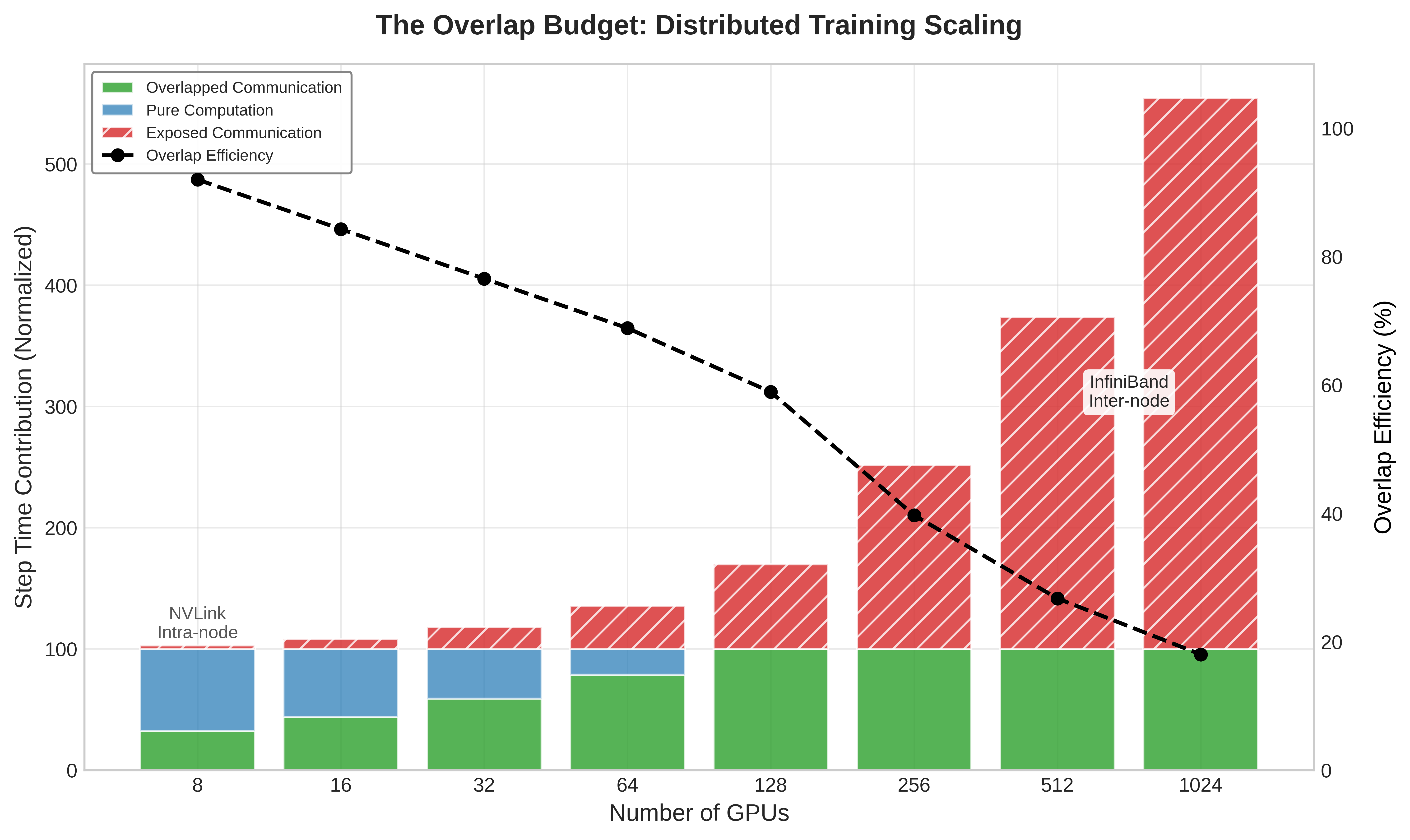
Figure 7: **The Overlap Budget**: As cluster scale increases (8 to 1024 GPUs), the communication overhead grows, eventually exceeding the computation budget. The overlap efficiency (black line) represents the percentage of communication hidden behind computation, which degrades from ~90 percent to ~18 percent due to inter-node latency and bandwidth constraints on a 70B parameter model.

CUDA streams and asynchronous execution

The mechanism enabling overlap on NVIDIA GPUs is CUDA streams. A CUDA stream is an ordered sequence of GPU operations (kernel launches, memory copies, NCCL collectives) that execute sequentially within the stream but can execute concurrently with operations in other streams. The application maintains two distinct streams: a compute stream for matrix multiplications and element-wise kernels, and a communication stream for NCCL operations. The workflow proceeds by launching a compute kernel on the first stream and immediately triggering an asynchronous communication call on the second:

compute_stream = torch.cuda.Stream()
comm_stream = torch.cuda.Stream()

with torch.cuda.stream(compute_stream):
    output = torch.matmul(A, B)  # Non-blocking compute

with torch.cuda.stream(comm_stream):
    dist.all_reduce(gradients, async_op=True)  # Non-blocking comm

torch.cuda.synchronize()  # Wait for both to complete

The GPU hardware scheduler interleaves execution units from both streams, running the GEMM on the SMs while the NVLink engine handles the AllReduce data transfer. However, while streams provide logical concurrency, they contend for physical resources. The SMs must manage the data movement instructions for the communication kernel. On an H100 with 132 SMs, a heavy NCCL operation might occupy 4–8 SMs solely for protocol processing and memory copying, leading to SM partitioning: the available compute throughput is reduced by 3–6 percent during communication. If the compute kernel is dense enough to saturate 100 percent of the SMs, enabling overlap can paradoxically slow down execution due to this resource contention, a phenomenon known as interference. In practice, the 3–6 percent compute throughput reduction is far smaller than the communication time that would otherwise be exposed, making the trade-off overwhelmingly favorable.

In practice, achieving effective overlap requires attention to several details. The communication operation must be launched early enough to overlap with subsequent compute; in backward passes, DDP starts each bucket’s AllReduce as soon as that bucket is ready so NCCL launch latency is hidden behind later gradient kernels. Synchronization points (where one stream waits for another) must be minimized, as each synchronization serializes execution.

PyTorch’s Distributed Data Parallel (DDP) module implements gradient overlap by registering backward hooks on each parameter. When a parameter’s gradient is computed during the backward pass, the hook triggers an asynchronous AllReduce on a separate NCCL stream. DDP synchronizes this communication stream with the main compute stream at the end of the backward pass, so every gradient reduction is guaranteed complete before the optimizer step reads the gradients. This design overlaps gradient communication with gradient computation automatically, without requiring user intervention.

When engineers create their own side streams for custom overlap patterns, a set of PyTorch-specific footguns regularly causes silent correctness or performance failures. The default behavior in PyTorch is that all operations enqueue onto the default stream. A tensor produced on the default stream and consumed on a side stream is not automatically safe: without an explicit event.record() / event.wait() barrier between them, the GPU may begin consuming the tensor before it is fully written. Similarly, memory copies launched without non_blocking=True insert implicit synchronization points that serialize the streams the engineer was trying to overlap, often eliminating the overlap benefit entirely. DDP avoids these hazards by managing record_event() calls inside its bucket hooks, ensuring each AllReduce starts only after the corresponding gradient compute event has completed. Manually written overlap code must replicate this discipline or risk data races that produce incorrect gradients with no error signal at the framework level.

The techniques covered so far – fusion, precision, compilation, speculative decoding, MoE, and communication overlap – address different aspects of the performance equation. Identifying which technique to apply in a given situation requires systematic measurement, and the profiling tools that make this diagnosis possible are the final piece of the optimization toolkit.

Self-Check: Question

Under what condition can communication-computation overlap remove communication from the critical path?
1. When communication time is less than or equal to the compute time available to hide it behind
2. When communication uses FP16 tensors instead of FP32 tensors
3. When all collectives are launched after the backward pass completes
4. When the network bandwidth exceeds peak GPU FLOP/s
Why does increasing batch size often improve overlap effectiveness in tensor-parallel workloads?
1. It reduces the number of collectives per layer to zero
2. It makes communication launch overhead disappear completely
3. It shortens GEMM kernels so communication can start earlier
4. It increases compute time per layer, creating a larger window in which communication can be hidden
Explain how CUDA streams enable overlap, and why overlap can still slightly reduce compute throughput even when it improves end-to-end step time.
True or False: If communication is overlapped with compute, it no longer consumes any GPU resources and therefore cannot interfere with kernel execution.

See Answers →

System Profiling

An engineer spends two weeks rewriting a PyTorch module into a custom CUDA kernel to make it 5$\times$ faster, only to discover the overall model latency did not budge because the system was entirely I/O bound. Performance engineering without measurement is expensive guesswork. System profiling provides the surgical diagnostics required to identify exactly where the GPU is waiting, allowing us to apply our optimizations with precision.

Systems Perspective 1.4: The physics of profiling (the Heisenberg effect)

Observing a distributed ML system fundamentally alters its behavior. Gathering high-resolution telemetry (such as tracking every CUDA kernel launch or memory allocation) consumes PCIe bandwidth, CPU cycles, and memory capacity. In heavily optimized serving pipelines, the overhead of profiling can artificially induce the very latency spikes the engineer is trying to diagnose. This “Heisenberg Effect” requires a deliberate strategy: deploying low-overhead, sampling-based telemetry for continuous production monitoring, and only enabling high-fidelity, synchronous tracing in isolated diagnostic environments.

The effect is particularly pronounced in PyTorch workloads. Enabling torch.autograd.profiler or torch.cuda.memory._record_memory_history() instructs the framework to retain references to intermediate activation tensors beyond their normal lifetime so that allocation metadata can be recorded. This prevents the memory allocator from reusing tensor buffers as it normally would, inflating peak HBM consumption and, in borderline cases, triggering Out-Of-Memory errors that do not occur in unobserved execution. Additionally, graph-optimization passes in torch.compile detect tensor observation and conservatively disable certain buffer-reuse fusions, causing the profiled execution to follow a slower code path than the production path. The practical consequence is that a profiling run must be treated as a distinct experiment: it characterizes the structure of the computation accurately, but its absolute latency and memory numbers will overstate production measurements.

The profiling hierarchy

Profiling levels are useful only if they guide the drill-down from symptom to intervention. ML system profiling operates at four levels, each providing different granularity and targeting different bottleneck categories. Figure 8 makes this drill-down explicit, starting from application-level symptoms and descending toward kernel and hardware-counter evidence.

The drill-down starts at the application level, where end-to-end metrics such as tokens per second, time-to-first-token, P99 latency, and GPU utilization over time reveal that the user-facing system has missed its target. It then descends to distributed profiling across GPUs and nodes, where communication patterns show whether collectives overlap with compute, which operation dominates step time, and whether load imbalance exists across ranks. Trace-level profiling narrows the diagnosis to the timeline of GPU kernels, CPU operations, and data transfers within a training step or inference request, exposing launch gaps, idle bubbles, sequential bottlenecks, and overlap opportunities. Operation-level profiling completes the chain with tools like NVIDIA Nsight Compute, where achieved memory bandwidth, compute utilization, occupancy, and instruction mix determine whether a specific kernel is memory-bound, compute-bound, or limited by implementation details—including whether it is issuing Tensor Core instructions (HMMA for FP16/BF16, IMMA for INT8) rather than falling back to scalar CUDA Core instructions (FMA/ALU). A matrix multiplication whose hidden-dimension or sequence-length tile is not divisible by the Tensor Core alignment requirement (multiples of 8 for FP16, 16 for INT8) silently bypasses Tensor Cores entirely and executes on CUDA Cores at a fraction of the peak throughput. This shape mismatch is one of the most common silent performance bugs in custom ML kernels and is invisible without inspecting the instruction mix counter.

Diagnosing performance requires a drill-down approach, moving from global symptoms to local causes. When profiling a 70B model serving pipeline, the application level might reveal “end-to-end latency is 150 ms/token, 3$\times$ above the SLO.” Descending to the distributed level, traces might show one GPU consistently lagging in AllReduce operations, pointing to a straggler or network congestion. Zooming into the trace level on that specific GPU reveals the timeline of kernel execution, exposing gaps where the SMs are idle due to scheduling overhead. Finally, kernel-level profiling (using Nsight Compute) inspects the specific instruction mix of a single matrix multiplication, revealing cache misses or register pressure. Skipping levels often leads to optimizing the wrong bottleneck: optimizing a kernel is futile if the GPU is spending 40 percent of its time waiting on the network.

Key performance metrics

Metrics are not interchangeable; each answers a different bottleneck question. MFU and MBU diagnose useful hardware work, TTFT and ITL diagnose serving latency, and throughput exposes capacity under batching. Understanding their relationships and trade-offs is essential for performance engineering.

Table 5 maps the common metrics to the bottleneck question each one answers.

Table 5: Performance Metrics and Their Diagnostic Use: Each metric measures a different layer of the system, so choosing the wrong metric can hide the real bottleneck.

Metric	Definition	Best diagnostic use	Caveat or target
Model FLOPs Utilization (MFU)	Fraction of hardware peak FLOP/s productively used by model computation	Training efficiency across memory limits, launch overhead, communication wait, and software overhead	40–60% is common in well-tuned LLM training; above 60% is excellent
Hardware FLOPs Utilization (HFU)	Total arithmetic operations executed, including recomputation, divided by peak FLOP/s	Separating useful model work from overhead such as activation recomputation	Usually exceeds MFU, and the HFU–MFU gap estimates wasted compute
Time-to-first-token (TTFT)	Latency from request arrival to the first generated token	Interactive serving responsiveness, including queueing, prefill, and initialization	Below 500 ms is generally acceptable; below 200 ms feels responsive
Inter-token latency (ITL)	Time between consecutive generated tokens during decode	Perceived generation speed after the first token	Below 50 ms supports comfortable reading; real-time speech may require below 25 ms
Throughput	Tokens/second for the system, or tokens/second/GPU for per-device efficiency	Aggregate serving or training capacity under batching	Large batches improve throughput but increase per-request latency; Queuing theory for batched inference covers the queueing trade-off
Model Bandwidth Utilization (MBU)	Achieved memory bandwidth divided by hardware peak bandwidth	Memory-bound inference, especially decode workloads	An H100 decode step can show 2% MFU but 85% MBU, which indicates a memory-saturated and well-optimized path

Using the roofline for diagnosis

The metric choice in table 5 reflects the fundamental bottleneck shift between training and inference: MFU is usually the right training-efficiency lens, while MBU is often the right inference-efficiency lens when decode is limited by HBM traffic. The roofline model from section 1.0.5 becomes a diagnostic tool when combined with profiling data. Diagnosis follows three steps:

Measure the achieved FLOP/s and memory bandwidth for a kernel using Nsight Compute.
Compute the operational arithmetic intensity from the algorithm (FLOP/byte).
Plot the measured performance against the roofline ceiling.

A kernel that falls far below both the compute ceiling and the bandwidth ceiling has an implementation problem: launch overhead, poor memory access patterns, or low occupancy. A kernel that reaches the bandwidth ceiling but falls below the compute ceiling is memory-bound, and further optimization requires reducing memory traffic (fusion, precision) rather than improving compute efficiency. A kernel at the compute ceiling is compute-bound and can only be improved by algorithmic changes (reducing FLOPs) or faster hardware.

Consider a concrete example: a LayerNorm kernel profiled on an H100 reports 15 TFLOP/s of achieved compute and 2.8 TB/s of achieved memory bandwidth. Its arithmetic intensity is 15 TFLOP/s / 2.8 TB/s $\approx$ 5.4 FLOP/byte. The H100’s ridge point is approximately 295.2 FLOP/byte at FP16. Since 5.4 FLOP/byte is far below 295.2 FLOP/byte, the kernel is strictly memory-bound. Its achieved 2.8 TB/s (84 percent of the H100’s 3.35 TB/s peak bandwidth) confirms it is operating near the physical limit of the memory subsystem. The diagnosis is clear: further FLOP-level optimizations will yield little gain; performance can only be improved materially by reducing data movement, either through fusion (eliminating the HBM round-trip) or precision reduction (halving the bytes per element).

PyTorch profiler workflow

The PyTorch Profiler is most useful when application metrics show a slowdown but the responsible layer is still unknown. Its role is to narrow a global symptom to a layer, kernel family, or synchronization point before a heavier tool is used. It integrates with the training loop to capture detailed traces with minimal code modification:

import torch
from torch.profiler import (
    profile,
    schedule,
    tensorboard_trace_handler,
)

# Profile 2 warmup steps + 3 active steps
with profile(
    activities=[
        torch.profiler.ProfilerActivity.CPU,
        torch.profiler.ProfilerActivity.CUDA,
    ],
    schedule=schedule(wait=1, warmup=2, active=3, repeat=1),
    on_trace_ready=tensorboard_trace_handler("./profiler_logs"),
    record_shapes=True,
    profile_memory=True,
    with_stack=True,
) as prof:
    for step, batch in enumerate(dataloader):
        if step >= 6:  # 1 wait + 2 warmup + 3 active
            break
        output = model(batch)
        loss = criterion(output, labels)
        loss.backward()
        optimizer.step()
        optimizer.zero_grad()
        prof.step()

The schedule parameter defines a warmup period where the profiler runs but does not record, allowing CUDA caches and just-in-time (JIT) compilation to stabilize before measurement begins. Without warmup, the first few iterations include one-time costs (kernel compilation, memory allocation, CUDA context initialization) that inflate the measured times and misrepresent steady-state performance.

The resulting trace, viewable in TensorBoard or Chrome’s trace viewer, matters only insofar as each view maps to an intervention. Table 6 turns those views into a diagnostic checklist.

Table 6: Profiler Views and Interventions: PyTorch profiler views are useful when each visual signal points to a concrete next experiment.

Trace view	Diagnostic signal	Likely intervention
Kernel timeline	CUDA kernels, their duration, GPU idle gaps, and unexpectedly long kernels	Fuse operators, use CUDA Graphs, or investigate long kernels with Nsight Compute
Memory timeline	Allocation and deallocation spikes or gradual memory growth	Reuse buffers, plan allocations, or investigate leaks
CPU-GPU synchronization	Points where the CPU waits for the GPU, or the GPU waits for CPU launch work	Remove blocking synchronization and reduce launch overhead
Communication events	NCCL collective duration relative to compute kernels	Tune overlap, bucket sizing, or parallelization strategy

Nsight systems: Reading the timeline

The profiler is therefore a triage tool, not the final performance proof: it identifies whether the next experiment should target fusion, memory planning, CUDA Graphs, or overlap. NVIDIA Nsight Systems answers the trace-level question raised by higher-level profiling: whether the GPU timeline is continuous, whether the CPU is feeding it fast enough, and whether communication overlaps compute. The tool captures every GPU kernel launch, CUDA memory operation, NCCL communication, and CPU thread activity onto a unified timeline.

Nsight Systems becomes useful when the question has shifted from which layer is slow to why the full timeline has gaps. A typical workflow begins with capturing a trace of a few training or inference iterations:

nsys profile --trace=cuda,nvtx,osrt,cudnn,cublas \
    --output=llm_profile \
    --force-overwrite=true \
    python3 inference_server.py --num-steps=5

The --trace flags control which activities are recorded. The cuda flag captures kernel launches and memory operations. The nvtx flag captures user-annotated regions (PyTorch automatically annotates module boundaries with NVTX markers). The cublas and cudnn flags capture library-level operations, which helps identify whether a GEMM is using cuBLAS or a custom kernel. The command is useful because these rows expose whether the bottleneck is launch overhead, communication serialization, or kernel implementation.

The resulting .nsys-rep file is opened in the Nsight Systems GUI, which presents a multi-row timeline. Four rows carry the most diagnostic weight.

The CUDA HW row shows the actual kernel execution on the GPU. Each colored bar represents a kernel, with width proportional to execution time. Gaps between bars indicate GPU idle time, which represents wasted potential. For a well-optimized inference pipeline, the CUDA HW row should show nearly continuous kernel execution with minimal gaps.

The CUDA API row shows CPU-side CUDA API calls (kernel launches, memory allocations, synchronization). If CUDA API bars are significantly wider than the corresponding CUDA HW bars, the CPU is the bottleneck: it cannot launch kernels fast enough to keep the GPU busy. CUDA Graphs and torch.compile address exactly this kernel launch overhead problem.

The NCCL row (for distributed workloads) shows collective communication operations. Comparing the NCCL row with the CUDA HW row reveals whether communication overlaps with computation. If NCCL bars appear during gaps in the CUDA HW row, communication is serialized. If NCCL bars overlap with CUDA HW bars, overlap is working correctly.

The NVTX row shows user-annotated regions, which PyTorch maps to module names (Linear, LayerNorm, Attention). This connects low-level kernel names (often cryptic strings like volta_fp16_s1688gemm_fp16_256x128_ldg8_f2f_nn) to the model-level operations that produced them.

Five patterns reveal the most diagnostic information from a Nsight Systems trace. Table 7 maps each visual pattern to the bottleneck question it answers.

Table 7: Nsight Timeline Diagnostic Patterns: Timeline patterns connect visual structure to utilization, fusion, overlap, allocation, and arithmetic-efficiency questions.

Timeline pattern	Diagnostic question	Optimization direction
Kernel execution vs. idle gaps	How much of the trace is useful GPU execution rather than waiting?	Investigate launch overhead, CPU stalls, or input starvation
Distribution of kernel durations	Are many short kernels fragmenting the workload?	Try fusion, CUDA Graphs, or compiler capture
NCCL alignment with CUDA HW rows	Does communication overlap with computation?	Tune bucket sizes, scheduling, or parallelization layout
Memory allocation spikes	Are tensors being materialized or allocated repeatedly?	Add memory planning, buffer reuse, or fused kernels
GEMM vs. non-GEMM time	How much execution is useful matrix arithmetic vs. overhead?	Move non-GEMM work into fused kernels or reduce memory traffic

Experienced performance engineers develop pattern recognition for these traces, quickly identifying the dominant bottleneck from the visual structure of the timeline. A trace dominated by thin, closely packed kernel bars with minimal gaps indicates a well-optimized pipeline. A trace with large gaps between kernels, or with NCCL bars that do not overlap with CUDA HW bars, immediately reveals the primary optimization target.

Common bottleneck patterns

Profiling is valuable because recurring trace patterns map directly to optimization choices. Table 8 turns that pattern recognition into a diagnostic map: first identify the visual signature, then connect it to the likely cause and the intervention that changes the system.

Table 8: Common Bottleneck Trace Patterns: Diagnostic map from trace signature to likely cause, intervention, and trade-off. The table is most useful after the profiler has already localized the bottleneck to launch overhead, memory movement, communication, load balance, allocation behavior, or input preparation.

Trace Pattern	Likely Cause	Primary Intervention	Trade-Off to Check
Small gaps between many kernels	Kernel launch overhead dominates	Graph compilation with `torch.compile`, CUDA Graphs, or fusion	Compilation warmup and debugging complexity
Large memory spikes	Unfused operators materialize intermediate tensors	FlashAttention or custom Triton fusion	Numerical validation and kernel maintenance
Low FLOP/s with high bandwidth	Memory-bound operations dominate	Precision reduction, batching, or algorithmic changes	Accuracy, cache pressure, and quality guardrails
NCCL bars during GPU idle gaps	Communication is serialized rather than overlapped	DDP gradient overlap or pipeline restructuring	Bucket size, schedule complexity, and synchronization
Some GPUs wait for stragglers	Uneven work distribution or MoE load imbalance	MoE capacity tuning, auxiliary loss adjustment, or even tensor-parallel splits	Routing quality and utilization balance
Repeated large allocations	Buffers are recreated rather than reused	Memory planning, preallocated buffer pools, or checkpointing	Recompute cost and allocator behavior
Periodic GPU utilization drops	CPU preprocessing or tokenization is not pipelined	More data workers, preprocessing services, or pretokenized datasets	Storage cost and data freshness

A full decode trace shows how several of these smaller bottlenecks can combine into the dominant loss.

Napkin Math 1.4: The profiler detective

Problem: A 7B parameter LLM runs on a single H100 and shows 45 tokens/s during autoregressive generation at batch size 1. The pure FP16 weight-read roofline is higher, but after budgeting roughly 35 GB of total per-token traffic for weights, KV-cache reads, sampling, synchronization, and launch overhead, the bandwidth-limited full-decode ceiling is approximately 96 tokens/s. Where is the remaining 53 percent of realizable decode-step performance hiding?

Investigation:

Step 1: Kernel-level analysis. Run Nsight Compute on the dominant GEMM kernel. Result: achieves 2.8 TB/s effective bandwidth out of the H100’s 3.35 TB/s peak. Efficiency: 84 percent. This kernel is performing well.

Step 2: Trace-level analysis. Run Nsight Systems on a full decode step. Result: 42 percent of step time is spent in GEMM kernels. The remaining 58 percent is split between:

Attention kernels (including KV cache reads): 28 percent
Layer normalization and activation kernels: 12 percent
Softmax and top-$k$ sampling: 8 percent
Kernel launch gaps: 10 percent

Step 3: Identify optimization targets.

The KV cache attention kernel achieves only 1.9 TB/s bandwidth because of irregular memory access patterns. Fix: Implement KV cache quantization (INT8) with better memory layout.
Kernel launch gaps (10 percent of time) come from 120+ individual kernel launches per layer. Fix: Apply torch.compile to fuse element-wise operations, reducing to ~30 kernels per layer.
Layer normalization and activation kernels are unfused. Fix: Fused LayerNorm-GELU kernel via Triton.

Systems insight: The dominant GEMM is near-optimal, but secondary operations and launch overhead consume over half the execution time. Systematic profiling reveals that the bottleneck is not where intuition suggests (the largest kernel) but in the accumulated overhead of many small operations.

The profiling feedback loop

Effective performance engineering follows an iterative cycle: profile, diagnose, optimize, verify. The verification step is critical and often skipped. After applying an optimization, reprofile to confirm that the targeted bottleneck was addressed and that no new bottleneck emerged. Performance optimization is a waterbed problem: fixing one bottleneck often exposes the next.

A common trap is optimizing based on microbenchmarks rather than end-to-end traces. A kernel that appears 2$\times$ faster in isolation may deliver only 5 percent improvement in end-to-end throughput if it was not the bottleneck, or if the surrounding code cannot take advantage of its speedup due to data dependencies. Always measure impact at the application level (tokens/second, step time, P99 latency) in addition to kernel-level metrics. The same measurement discipline governs rollout risk: a change that looks local can consume a global resource once it reaches production traffic.

War Story 1.1: The regex that saturated the edge

Context: Cloudflare’s Web Application Firewall runs on edge machines that process HTTP and HTTPS traffic across the global network (Cloudflare 2019).

Failure mode: On July 2, 2019, a newly deployed managed WAF rule caused excessive CPU consumption on every HTTP/HTTPS-handling core across Cloudflare’s network.

Consequence: Cloudflare reported losing most of its traffic until the team identified the WAF as the cause and used a global disable mechanism to restore service.

Systems lesson: Performance engineering includes algorithmic complexity and rollout design. A small rule change can become a global outage when it is deployed everywhere before bounded-runtime checks, canaries, and kill switches catch the cost. ML deployments follow the same pattern: a new model, a recalibrated threshold, or a retrained feature can ship a worst-case latency cliff into production that no unit test catches, which is why canarying, request shadowing, and per-request kill switches are first-class ML serving infrastructure.

Cloudflare. 2019. Details of the Cloudflare Outage on July 2, 2019. Cloudflare incident report.

Profiling itself can also perturb the system being measured. The PyTorch profiler adds approximately 10–20 percent overhead when recording full traces with memory profiling enabled. Nsight Systems adds less overhead but still affects scheduling. Profile warmup steps before active measurement, and discount the first few profiled iterations where JIT compilation or CUDA context initialization may dominate.

Profiling at scale

Profiling a single GPU is straightforward; profiling a distributed system with hundreds or thousands of GPUs introduces unique challenges. The volume of trace data grows linearly with the number of GPUs: a 5-second Nsight Systems trace for one GPU is approximately 500 MB; the same trace for 1,000 GPUs would be 500 GB, impractical to store or analyze.

Production systems address this through hierarchical profiling. At the top level, application-level metrics (MFU, throughput, step time) are collected continuously from every GPU with negligible overhead. These aggregate metrics detect when performance degrades. When a degradation is detected, targeted profiling is triggered on a representative subset of GPUs (typically one GPU per pipeline stage, per data-parallel group) for a short window (a few training steps). The resulting traces are analyzed to identify the specific bottleneck.

Another approach is statistical profiling, where each GPU randomly samples a small fraction of its kernels for detailed timing. Over many training steps, the aggregated samples provide a statistically accurate picture of the kernel time distribution without the overhead of full tracing. The approach is analogous to the sampling profilers (like Linux perf) used in traditional systems engineering, adapted for the GPU context.

The most challenging profiling scenario is intermittent stragglers: GPUs that are occasionally slow due to thermal throttling, memory errors, or network congestion, but fast most of the time. These stragglers may not appear in a short profiling window but can reduce training throughput by 10–20 percent over hours. Detecting them requires continuous per-GPU step-time monitoring with statistical anomaly detection, a form of profiling infrastructure that operates at the monitoring layer rather than the kernel layer.

The profiling tools and techniques described in this section provide the measurement foundation for all optimization work. Without measurement, performance engineering degenerates into guesswork. With measurement, it becomes a systematic discipline guided by quantitative evidence.

Self-Check: Question

A batch-1 LLM decode workload on H100 shows 2 percent MFU but 85 percent memory-bandwidth utilization. What is the best interpretation?
1. The serving stack is badly broken because both compute and memory utilization should be high simultaneously
2. The workload is memory-bound and may already be close to the hardware limit for decode, despite low compute utilization
3. The kernel is compute-bound, so the next step is to optimize Tensor Core scheduling
4. The profiler is likely wrong because MFU and bandwidth utilization cannot disagree by that much
Which profiling level is the right starting point if the only symptom you have is that end-to-end latency is 3$\times$ above the service SLO?
1. Kernel-level profiling only, because the largest kernel is almost always the bottleneck
2. Application-level profiling first, then drill down through distributed and trace-level views to local causes
3. Immediately rewrite the attention kernel before collecting any traces
4. Skip profiling and compute arithmetic intensity from the model architecture alone
A LayerNorm kernel achieves about 2.8 TB/s on an H100 and has arithmetic intensity around 5.4 FLOP/byte. Explain what the roofline diagnosis is and what optimization class it suggests.
In an Nsight Systems timeline, what pattern most strongly suggests kernel-launch overhead is a meaningful bottleneck?
1. A few very long GEMM bars with no idle gaps between them
2. Many short kernels separated by repeated idle gaps and noticeable CPU-side launch activity
3. NCCL bars fully overlapped under long backward kernels
4. A memory timeline whose peak usage is flat and stable across iterations
True or False: Once an optimization improves a microbenchmark, it is safe to assume end-to-end throughput will improve by a similar factor.

See Answers →

Measurement at Scale

Optimizing a single node is a prerequisite, but the ultimate test of performance engineering is efficiency at fleet scale. When we move from 8 GPUs to 1,024 GPUs, new sources of overhead emerge that are invisible in local traces. A profiler can explain why one kernel stalls; it cannot by itself say whether thousands of accelerators are converting power, memory bandwidth, and network time into useful model progress. Measurement at scale requires shifting from kernel-level micro-benchmarks to global efficiency metrics that capture the interaction of computation, communication, and hardware variability.

The fleet efficiency metric

While Hardware Utilization reports how often GPUs are busy, it fails to distinguish between useful work and wasted cycles (such as activation recomputation or communication bubbles). Fleet measurement therefore needs a useful-work utilization metric. By focusing on the “useful” FLOPs required by the model architecture, this metric provides an invariant measure of system efficiency that remains comparable across different software stacks and parallelization strategies.

Definition 1.3: Model FLOPs utilization (MFU)

Model FLOPs Utilization (MFU), introduced in Scaling Efficiency and Convergence, is the fraction of the hardware’s theoretical peak throughput ($R_{\text{peak}}$) consumed by FLOPs that directly advance model training or inference, excluding overhead from recomputation, padding, and synchronization. The new content here is its fleet-scale behavior: how the per-node figure aggregates across thousands of accelerators and how the scaling tax pulls it down.

Significance: At fleet scale, MFU aggregates across all nodes: communication overhead, load imbalance, and pipeline bubbles each compound the utilization loss, so fleet MFU is consistently below single-node MFU. It is the primary diagnostic for whether hardware investment is translating into model progress, and a 1 percent improvement in MFU across a 10,000-GPU cluster reduces cost by the equivalent of 100 GPUs.
Distinction: Unlike Hardware Utilization (which reports how often the accelerator is “busy”), MFU reports how much of that activity contributes to Model Convergence or inference, excluding waste FLOPs from recomputation, padding, and gradient checkpointing overhead.
Common pitfall: A frequent misconception is that high GPU utilization implies high efficiency. A system can show 90 percent hardware utilization while achieving 30 percent MFU if it is wasting cycles on communication bubbles or inefficient kernel implementations, making MFU the correct metric for optimization decisions, not raw utilization.

With MFU defined as useful work rather than raw busyness, the next calculation shows how distributed overhead turns a strong single-node number into a weaker fleet-wide result.

Napkin Math 1.5: The scaling tax

Problem: A 70B parameter model achieves 65 percent MFU on a single 8-GPU node. When training scales to 128 GPUs, how much MFU does inter-node communication overhead consume?

Local node baseline: A single 8-GPU node achieves 65 percent MFU.
Fleet performance: At 128 GPUs, the step time increases to 245 ms, dropping MFU to 48 percent.

Math: Scaling tax is computed as $1 - \text{Fleet MFU}/\text{Local MFU}$, giving 26.2 percent.

Systems insight: The 26.2 percent scaling tax represents the cost of inter-node communication (InfiniBand latency) and synchronization barriers. In a healthy fleet, this tax should remain stable; a sudden increase in the scaling tax signals a scaling regression, typically caused by a misaligned parallelization strategy or a “gray failure” in the network fabric.

The communication tax erodes local MFU into fleet MFU.

Detecting scaling regressions

At scale, the system is nonlinear. A code change that introduces a minor memory overhead on a single GPU can trigger a catastrophic performance collapse at 1,000 GPUs due to increased garbage collection pauses or exhausted InfiniBand credit buffers. Table 9 shows how tiered tests catch that collapse before it becomes a fleet incident.

Table 9: Scaling Regression Test Tiers: Fleet performance testing moves from small canaries to production baselines and gray-failure detection so that local changes are checked against distributed behavior.

Testing tier	What it measures	Regression caught
Small-scale canaries	Model behavior on 8 and 64 GPUs to establish a scaling efficiency curve	Code changes that look harmless on one GPU but bend the curve before full-fleet launch
Fleet baseline comparison	Every production run’s MFU against the reference baseline for that model architecture	Architecture, compiler, or configuration changes that reduce useful fleet work
Gray failure detection	Distribution of step times across the fleet	Straggler nodes, such as one 10% slower node that can reduce synchronous data-parallel MFU by 10%

Those same measurements also explain why benchmark numbers cannot be copied directly into production capacity plans.

Systems Perspective 1.5: Benchmark vs. reality: The hero run tax

Industry benchmarks like MLPerf are often “hero runs”—highly tuned configurations where logging is disabled, safety checks are bypassed, and the hardware is freshly rebooted.

In production, achieved MFU typically sits 10–20 percent lower than these hero numbers. Essential operational overhead consumes the difference:

Observability: Metrics collection and logging.
Reliability: Checkpointing and health heartbeats.
Entropy: Thermal throttling, memory fragmentation, and multi-tenant network noise.

When planning capacity, engineers must budget for the reality tax. If a benchmark projects 30 days of training, the production plan should assume 35–40 days.

Measurement without action is overhead. The optimization playbook translates node-level traces and fleet-wide MFU into a surgical sequence of interventions, each targeting the specific bottleneck that measurement identified.

Self-Check: Question

A 128-GPU training cluster reports 92 percent hardware utilization on every node, but MFU for the same run sits at 30 percent, a drop from 65 percent measured on an 8-GPU baseline. Which metric better exposes the fleet’s actual efficiency problem, and why?
1. Hardware utilization, because 92 percent is close to ideal and the MFU number is likely a measurement artifact of the larger cluster
2. MFU, because hardware utilization counts any time the SMs are busy, including cycles spent on activation recomputation, communication bubbles, and synchronization, whereas MFU counts only FLOPs that advance training
3. Neither, because both metrics track only compute and the real problem must be in HBM bandwidth utilization
4. Both metrics report the same thing at fleet scale, so either one is adequate
Explain what the chapter means by the scaling tax, and give one reason it can increase when moving from a single node to a large cluster.
True or False: In a synchronous distributed workload, one node running 10 percent slower than the rest can reduce effective fleet MFU even if every other node is healthy.

See Answers →

The Optimization Playbook: A 70B LLM Case Study

Consider a raw, unoptimized 70-billion parameter PyTorch model that must serve 1,000 tokens per second in production by next week. The optimization sequence begins with baseline measurement, followed by roofline classification to identify the dominant bottleneck. Applying optimization techniques indiscriminately is ineffective. The optimization playbook requires a systematic, prioritized attack: first unblocking the memory wall, then fusing operators, and finally applying algorithmic techniques like speculative decoding in a specific, compounding sequence.

The diagnostic sequence

Optimization begins by measuring the whole workload before touching individual kernels. End-to-end throughput, an Nsight Systems trace, and Model FLOPs Utilization (MFU) from section 1.8 establish whether the system has substantial headroom. The next diagnostic move is roofline classification: compute arithmetic intensity for the dominant kernels and place them against the machine balance point. That classification determines the primary bottleneck, and the primary bottleneck determines which remedy should be tried first. For memory-bound, compute-bound, and communication-bound workloads, table 10 turns that decision into a compact map: identify the binding resource, use the typical setting as a sanity check, and try the interventions in order until a reprofiled trace shows the bottleneck has moved.

Table 10: Optimization Paths by Primary Bottleneck: Diagnostic map from bottleneck class to the ordered interventions that should be tried before the next profiling pass.

Primary bottleneck	Typical setting	Optimization path
Memory-bound	Inference, especially token decode	Reduce precision to raise effective bandwidth; fuse operators to eliminate intermediate HBM traffic; compile the graph to catch remaining fusion opportunities; then consider algorithmic changes such as speculative decoding or MoE if the bottleneck remains.
Compute-bound	Large-batch training	Ensure Tensor Cores are in use; apply graph compilation for kernel selection and memory planning; consider FP8 for 2$\times$ compute throughput; overlap communication so compute does not idle.
Communication-bound	Distributed training at scale	Overlap gradient communication with the backward pass; compress gradients or use reduced-precision communication; restructure pipeline schedules so stage-to-stage communication is hidden under useful compute; use topology-aware placement to minimize cross-node traffic.

The fourth step is to apply and verify. Implement the highest-impact optimization, reprofile, and verify improvement. Then iterate from the roofline classification step with the new profile, as the bottleneck may have shifted.

Combining techniques

Production systems combine techniques because no single intervention covers every term in the iron law. A highly optimized LLM serving system may use FlashAttention-2 or later FlashAttention-family kernels to reduce attention memory traffic, INT4 weight quantization with GPTQ or AWQ to reduce HBM reads, and INT8 KV cache compression with per-channel scaling to increase feasible batch size. Compiler and runtime tools such as torch.compile or TensorRT then handle element-wise fusion and kernel selection.

The serving layer adds another set of controls. Speculative decoding reduces latency at low batch sizes, continuous batching refills the batch as requests finish (introduced in section 1.1.1), dynamic sequence grouping improves throughput, and tensor parallelism spreads the model across GPUs while overlapping AllReduce. These techniques belong together only when the profile shows that each one moves a currently binding term.

The speedups from these techniques are not additive; they interact in ways that demand careful sequencing. For instance, INT4 weight quantization reduces per-token HBM traffic by 4$\times$, which might shift the bottleneck from memory-bound to compute-bound. Once compute-bound, further bandwidth optimizations (KV cache compression) yield diminishing returns, and compute optimizations (FP8 Tensor Cores) become the priority. This is why the iterative profile-optimize-verify loop is essential: the optimal combination depends on the specific model, hardware, and workload characteristics.

The interaction between optimizations creates a dependency graph that the performance engineer must navigate. Some combinations are synergistic: FlashAttention removes attention intermediates, and INT8 KV cache compression reduces KV cache memory, together freeing enough memory for larger batch sizes that transform the economics of serving. Other combinations are redundant: applying both CUDA Graphs and the reduce-overhead mode of torch.compile achieves the same result, since reduce-overhead internally uses CUDA Graphs. Still other combinations conflict: speculative decoding benefits most at small batch sizes (where decode is memory-bound), while many throughput optimizations work by increasing batch size. At large batch sizes, speculation adds overhead without proportional benefit.

A practical heuristic for sequencing optimizations is to apply the cheapest bottleneck-moving intervention before adding new algorithmic machinery. The first step depends on the measured bottleneck. Compiler-first is a common starting point for stable-shape workloads when memory is not obviously the binding constraint. For batch-1 70B decode, precision comes first because weight bandwidth and KV capacity dominate before graph overhead does.

Primary bottleneck fix: apply torch.compile when the trace shows launch overhead and stable shapes, or apply weight/KV precision first when the profile is memory-capacity or bandwidth bound.
FlashAttention-family kernels (library swap): Apply when attention materialization or attention HBM traffic remains visible in the profile.
Weight quantization (INT4/FP8, calibration required): Apply early for memory-bound serving, but validate quality before treating the speedup as usable.
KV cache compression (INT8, library support, 2$\times$ cache reduction): Apply fourth. Enables larger batches.
Speculative decoding (requires draft model, engineering effort): Apply last, only if latency target not met. Most complex to deploy.

This ordering reflects the principle that passive optimizations (compiler, library swaps) should precede active ones (algorithmic changes, new model components). Each step is validated by reprofiling before proceeding to the next.

Checkpoint 1.3: Optimization strategy

Test your ability to design an optimization plan:

Top optimizations: Given an LLM serving workload at batch size 1 that achieves 25 percent of peak bandwidth, identify the three most impactful optimizations and their expected interaction.
FP8 on comm-bound: Explain why applying FP8 quantization to a workload that is already communication-bound provides no speedup.
Profiling workflow: Describe the iterative profiling workflow and explain why verifying each optimization is as important as applying it.
Compile pitfalls: Identify a scenario where applying torch.compile would degrade performance.

Case study: Optimizing a 70B LLM serving pipeline

To illustrate how the diagnostic sequence and combining principles work in practice, consider the task of optimizing a 70B parameter LLM for production serving. The target is a real-time chatbot application requiring time-to-first-token (TTFT) under 500 ms, inter-token latency (ITL) under 50 ms, and throughput of at least 1,000 tokens/second across the cluster. The model is deployed on a node of 8 H100 GPUs connected by NVLink.

Baseline measurement

The initial deployment uses FP16 weights, standard PyTorch eager execution, and tensor parallelism across 8 GPUs. The 70B model in FP16 requires 140 GB of weight storage, distributed as approximately 17.5 GB per GPU. Four baseline measurements reveal the optimization gap:

TTFT: 1,200 ms (well above the 500 ms target)
ITL: 85 ms (above the 50 ms target)
Throughput: 280 tokens/second (below the 1,000 token/second target)
Maximum batch size: 4 (limited by KV cache memory)

A Nsight Systems trace breaks down a single decode step at batch size 1 into five time categories:

GEMM kernels: 38 percent of step time
Attention (including KV cache reads): 24 percent of step time
Element-wise operations (LayerNorm, GELU, residual): 14 percent of step time
AllReduce communication (tensor parallelism): 12 percent of step time
Kernel launch gaps and overhead: 12 percent of step time

The roofline analysis confirms that decode is deeply memory-bound, with arithmetic intensity approximately 1 FLOP/byte at batch size 1. The GPU achieves 2.7 TB/s effective bandwidth (80 percent of peak), indicating reasonable kernel-level efficiency but a fundamental algorithmic limitation.

Optimization round 1: Precision engineering

The first optimization targets the largest opportunity: reducing the bytes per weight read from HBM. Applying AWQ INT4 weight quantization reduces the per-GPU weight footprint from 17.5 GB to about 4.4 GB on an 8-GPU node. The raw weight-read traffic drops by 4$\times$, and the effective bandwidth for weight reads roughly doubles once on-the-fly dequantization to FP16 is included.

Simultaneously, applying INT8 quantization to the KV cache reduces per-request cache size by 2$\times$. The combined effect on memory budget is dramatic: each GPU now has approximately 75.6 GB available for KV cache, up from 62.5 GB. Under the 4096-token GQA cache calculation from section 1.3.3, this would permit much larger batches; in this deployment, the serving policy reserves memory for longer contexts, fragmentation headroom, and tail-latency protection. With that policy cap, the maximum admitted batch size increases from 4 to approximately 32.

Postoptimization metrics show that batch-1 ITL reaches 48 ms, meeting the 50 ms target, while throughput at batch size 32 reaches 720 tokens/second and remains below target.

The Nsight Systems trace shows that GEMM time decreased by approximately 45 percent due to reduced weight reads, but attention and element-wise operations remain unchanged. The bottleneck has partially shifted.

Optimization round 2: Operator fusion

The second round targets the 14 percent of step time consumed by element-wise operations and the 24 percent consumed by attention. Applying torch.compile with the max-autotune backend fuses element-wise operations (GELU, LayerNorm, residual additions), reducing their contribution from 14 percent to approximately 4 percent of step time. Simultaneously, enabling FlashAttention-2 replaces the standard attention implementation, reducing attention HBM traffic by approximately 16$\times$ for the prefill phase.

For the decode phase, FlashAttention’s impact is more modest because decode attention is dominated by KV cache reads rather than the $S{\times}S$ score matrix. However, the combination of INT8 KV cache compression and FlashAttention’s efficient PagedAttention kernel reduces attention decode time by approximately 30 percent. The reduce-overhead mode in torch.compile wraps the decode step in a CUDA Graph, eliminating the 12 percent kernel launch overhead almost entirely.

Postoptimization metrics show TTFT at 380 ms, meeting the 500 ms target; ITL at 32 ms for batch size 1, well below the 50 ms target; and throughput at batch size 32 at 1,050 tokens/second, meeting the throughput target.

Optimization round 3: Speculative decoding

With the throughput target met, the team focuses on further reducing ITL for the best user experience. Speculative decoding with a 1.5B draft model (AWQ INT4 quantized to 0.75 GB) is deployed on the same GPUs. The draft model generates 5 candidate tokens in 4 ms (benefiting from the INT4 quantization applied in Round 1). The target model verifies the candidate block in approximately 32 ms, comparable to one optimized autoregressive decode step.

Under the standard geometric-acceptance model, where each draft token is independently accepted with probability $p_{\text{acc}}$ and one bonus token always follows the last accepted one, the expected accepted tokens per round for $k$ draft tokens is $(1 - p_{\text{acc}}^{k+1})/(1 - p_{\text{acc}})$. At $p_{\text{acc}} = 0.78$ and $k = 5$, this gives $(1 - 0.78^{6})/(1 - 0.78) \approx 3.5$ tokens per round. The effective ITL becomes:

\[ \text{ITL}_{\text{effective}} = \frac{4 + 32}{3.5} \approx 10.3 \text{ ms per token} \]

The result is a 3.1$\times$ improvement over the Round 2 ITL of 32 ms. However, speculative decoding interacts with batching. At batch size 32, the verification step is no longer “free” because the GPU is closer to compute saturation. The system therefore applies speculation only when the current batch size is below 16, falling back to standard autoregressive decoding at higher loads. This adaptive policy maintains both the latency benefit at low load and the throughput benefit at high load.

Lessons from the case study

This optimization journey illustrates the principle that optimization order matters because each step moves the bottleneck. Precision engineering (Round 1) was applied first because it yields the largest single improvement and enables subsequent optimizations by freeing memory for larger batch sizes. Fusion (Round 2) addressed the new bottleneck exposed by precision engineering. Speculative decoding (Round 3) provided latency improvement once the throughput target was met.

Each optimization changed the bottleneck. Before Round 1, the system was purely memory-bandwidth-bound. After INT4 quantization and batching, the system was partially compute-bound at large batch sizes. After fusion, kernel launch overhead was negligible, making the remaining bottleneck the fundamental memory-bandwidth limit for decode. Each optimization was validated by reprofiling to confirm the bottleneck shift.

The final system combines five distinct techniques: INT4 weight quantization, INT8 KV cache compression, FlashAttention-2, torch.compile with CUDA Graphs, and adaptive speculative decoding. These techniques are not independent; they interact. INT4 quantization enables larger batch sizes, which changes whether speculative decoding is profitable. FlashAttention’s benefit depends on sequence length, which grows during generation. The performance engineer must reason about these interactions holistically, guided by profiling data at each stage.

The case study demonstrates how disparate optimizations compound sequentially, transforming an unusable prototype into a production-grade deployment. The path to these speedups, however, is lined with conventional wisdom that often proves disastrous at scale.

Self-Check: Question

Order the first four steps of the optimization playbook for a new ML workload: (1) select the primary bottleneck category, (2) baseline measurement, (3) roofline classification, (4) apply the highest-impact optimization and verify.
A serving stack is memory-bound at batch size 1. Which optimization sequence best matches the chapter’s recommended ordering for large gains with modest engineering effort?
1. Implement speculative decoding first, then profile only if latency remains high
2. Start with torch.compile, then apply weight quantization, then FlashAttention, then KV cache compression
3. Tune GEMM kernels by hand before collecting any trace data
4. Increase MoE expert count before reducing weight precision
Explain why an optimization that succeeds in Round 1 can change which optimization is best in Round 2, using the 70B case study as an example.
Why did the case study apply speculative decoding adaptively rather than unconditionally at all loads?
1. Because speculative decoding only works when TTFT is above 500 ms
2. Because at high batch sizes the verification pass is no longer nearly free, so speculation can add compute overhead without proportional latency benefit
3. Because FlashAttention cannot coexist with speculative decoding in the same serving stack
4. Because CUDA Graphs require speculation to be disabled whenever quantization is enabled
A team first applies INT4 weight quantization and sees a 3.1$\times$ throughput gain on their 70B serving stack, then applies FlashAttention on top and sees only a 1.4$\times$ additional gain instead of the 1.9$\times$ FlashAttention delivers in isolation. Which explanation best fits the chapter’s warning that speedups do not simply multiply?
1. FlashAttention and INT4 quantization interfere numerically because tile-based attention is incompatible with low-precision weights
2. torch.compile must already be enabled for FlashAttention to deliver any benefit, so the missing 0.5$\times$ is attributable to a disabled compiler
3. INT4 quantization already relieved much of the HBM pressure that FlashAttention was designed to eliminate, so the remaining memory-traffic savings are smaller and the stack is closer to the overhead-bound or compute-bound regime where FlashAttention helps less
4. FlashAttention’s gains scale with sequence length, and INT4 quantization silently truncates context length, eroding the baseline FlashAttention was measured against

See Answers →

Fallacies and Pitfalls

A team upgrades their inference cluster from A100s to H100s, expecting a 3$\times$ latency reduction based on the spec sheet’s teraFLOP/s rating, only to find their generative model barely runs 15 percent faster. The trap is pervasive: assuming that raw compute capacity dictates inference speed when the workload is entirely bound by memory bandwidth.

Fallacy: More FLOP/s means faster inference.

The roofline model demonstrates that most inference operations are memory-bound, not compute-bound. A GPU with 2$\times$ the peak FLOP/s but the same memory bandwidth will not generate tokens any faster for batch-1 LLM decode. The correct metric for memory-bound workloads is bandwidth, not FLOP/s. This fallacy leads organizations to purchase the most expensive compute hardware when a mid-range GPU with equivalent HBM bandwidth would deliver identical inference throughput.

Pitfall: Planning FP8 adoption as an automatic training-time halving.

FP8 doubles the peak TFLOP/s and doubles the effective memory bandwidth, but these gains are realized only for operations that are bottlenecked by compute or bandwidth at FP16. Element-wise operations like activation functions are already limited by kernel launch overhead, not by precision. Communication-bound distributed training steps gain nothing from reduced arithmetic precision if the communication volume (gradient sizes) is not also reduced. The actual speedup depends on the fraction of execution time spent in precision-sensitive operations.

Fallacy: The largest kernel is the whole performance problem.

The profiling case study in section 1.9.3 illustrates this pitfall. Engineers naturally focus on the single largest kernel, which is often the GEMM in a transformer layer. When the GEMM is already near-optimal, however, the remaining performance budget is distributed across dozens of smaller operations: normalization, activation, attention scoring, KV cache management, and kernel launch overhead. Collectively, these “small” operations can consume more than half of total execution time. Graph compilation and systematic fusion address this long tail more effectively than further GEMM optimization.

Pitfall: Applying speculative decoding without considering batch dynamics.

Speculative decoding excels at batch size 1, where decode is deeply memory-bound and the verification step is essentially “free” (the GPU has ample spare compute). At large batch sizes, decode approaches the compute-bound regime, and the verification step adds meaningful compute cost. Furthermore, the variable number of accepted tokens per request complicates continuous batching schedulers. In high-throughput serving scenarios with large batches, the overhead of speculation may outweigh its latency benefits.

Fallacy: MoE expert count is a free scaling knob.

Increasing the number of experts in an MoE model increases total parameters (capacity) without proportionally increasing per-token compute, which seems like a free lunch. Each additional expert, however, increases: (1) total memory requirements, requiring more GPUs; (2) AllToAll communication volume for expert routing; (3) load balancing difficulty, since the router must distribute tokens across more experts; and (4) training instability, as more experts compete for activation. Beyond approximately 64–256 experts, the system-level costs often outweigh the capacity benefits.

Pitfall: Using graph compilers as a substitute for kernel analysis.

Graph compilers have improved dramatically, but they remain limited by their cost models and fusion heuristics. FlashAttention required human insight to recognize that attention could be reformulated as a tiled algorithm with online softmax, an algorithmic insight beyond the scope of ordinary compiler rewrite rules. Similarly, speculative decoding and MoE routing require algorithmic innovation that compilers cannot discover. Compilers automate known optimizations; human engineers discover new ones.

Fallacy: The lowest supported precision is always the best precision.

Aggressive quantization (INT4 weights, INT4 KV cache, FP8 activations) can degrade model quality in ways that are difficult to detect with standard benchmarks but visible to users. Perplexity on a held-out dataset may change by less than 1 percent, but the model may produce subtly worse responses for edge cases, rare languages, or complex reasoning tasks. The correct approach is targeted quantization: apply the most aggressive precision to the least sensitive components (KV cache, intermediate activations) and preserve higher precision for the most sensitive (first and last layers, attention logits). Calibration on a representative dataset, followed by evaluation on diverse quality benchmarks, is essential before deploying any quantized model to production.

Pitfall: Measuring throughput without measuring quality.

A model serving system that generates 200 tokens/second is not twice as good as one generating 100 tokens/second if the first system achieves that throughput by using INT4 quantization that degrades answer quality by 15 percent. Performance metrics must always be reported alongside quality metrics. The correct optimization target is the Pareto frontier of throughput vs. quality, not throughput alone.

Fallacy: A single profiling run is sufficient to characterize performance.

ML system performance is nonstationary. GPU thermal throttling reduces clock speeds (and therefore FLOP/s) after sustained workloads, sometimes by 10–15 percent. Memory fragmentation accumulates over hours of serving, gradually reducing effective batch size. Network congestion varies with cluster-wide traffic patterns. A profiling run during a cold start may show different bottleneck patterns than one after hours of production serving. Reliable performance characterization requires profiling under realistic, sustained conditions, ideally sampling multiple times across a production run.

Pitfall: Optimizing for average case while ignoring tail latency.

A serving system may achieve excellent average inter-token latency (30 ms) while exhibiting P99 latency of 500 ms due to garbage collection pauses in the Python runtime, CUDA memory allocation stalls, or occasional AllReduce delays from network congestion. For interactive applications, the user experience is dominated by the worst case, not the average. Performance engineering for production systems must profile and optimize tail latency specifically, often through techniques orthogonal to the throughput optimizations in this chapter: preallocated memory pools, CUDA graph replay (which eliminates allocation variance), and priority scheduling for latency-sensitive requests.

Self-Check: Question

A team upgrades from A100s to a GPU with much higher peak FLOP/s but similar memory bandwidth, and batch-1 decode improves only modestly. Which explanation best fits the chapter’s framework?
1. The workload was memory-bound, so similar bandwidth means token generation rate changes little despite the larger compute peak
2. The new GPU likely disabled tensor parallelism, so all gains were canceled by communication
3. Speculative decoding must have been active on the old hardware and inactive on the new hardware
4. The larger FLOP/s number only matters for training workloads, never for inference of any kind
True or False: If a graph compiler is enabled, manual kernel engineering and algorithmic innovation become unnecessary for top-tier performance.
Explain why measuring throughput alone can lead a team to ship a worse serving system, even if the tokens/second number improves.

See Answers →

Summary

Recognizing these pitfalls saves teams from wasting months optimizing the wrong layer of the stack. Performance engineering transforms a model that should be efficient into one that is, by attacking a fundamental bottleneck of accelerator-based ML systems: the memory wall. The Roofline Model provides the diagnostic framework, classifying operations as compute-bound or memory-bound based on their arithmetic intensity relative to the hardware’s ridge point. For the NVIDIA H100, this ridge point is approximately 295.2 FLOP/byte at FP16, meaning most transformer operations fall in the memory-bound regime.

The chapter’s techniques form an optimization stack rather than a menu. Operator fusion eliminates redundant HBM round-trips by combining sequences of operations into single kernels. FlashAttention is the canonical example, avoiding the quadratic attention intermediates that dominate long sequences through tiling and online softmax; in the 8K attention example, this is a 65× reduction in materialized attention state. Precision engineering then reduces the bytes in the trips that remain: FP8 formats improve effective bandwidth on H100 hardware, block-wise quantization protects the outlier features that defeat uniform quantization, and KV cache compression directly increases the batch sizes a serving node can admit.

Graph compilation moves those local transformations from hand-written kernels into the model graph. torch.compile/TorchInductor generates optimized Triton kernels from standard PyTorch code, XLA provides whole-program optimization for JAX/TPU workloads, and TensorRT specializes stable inference graphs. Communication-computation overlap applies the same bottleneck logic at the distributed boundary, hiding network latency when communication can run under useful compute. Speculative decoding and MoE go one level higher: instead of optimizing the same dense computation, they restructure the computation itself by obtaining more accepted tokens per target-model pass or by activating only the experts a token needs. System profiling closes the loop by showing which term dominates after each change, so the next intervention follows the new bottleneck rather than the old intuition.

The case study in section 1.9.3 demonstrated how these techniques compound in practice: INT4 quantization freed memory for larger batches, which changed the arithmetic intensity, which determined whether further bandwidth or compute optimizations were profitable. Each optimization shifted the bottleneck in a continuous displacement of overhead, requiring reprofiling and a new optimization decision. That profile-optimize-reprofile loop is the discipline of performance engineering: not making hardware faster, but making software match the physics of the hardware it runs on. The memory wall is a physical constraint that grows wider with each hardware generation, so the engineer’s response is to keep data close to compute, reduce precision to the minimum that preserves quality, and restructure algorithms to avoid unnecessary work. Profiling is not merely the first step; it is every step.

This iterative mindset also determines which skills endure as hardware evolves. Individual techniques may change as accelerator generations shift the ridge point of the Roofline Model and as architectures alter the dominant computational patterns. The fundamental discipline endures: measure the system, identify the binding constraint, apply the optimization that addresses that specific constraint, and then measure again. Engineers who internalize this cycle treat performance engineering as a continuous practice rather than a checklist, and that practice is what separates systems that merely run from systems that run efficiently at scale.

Key Takeaways: Match the software to the silicon

Bytes usually bind: On H100-class accelerators, the chapter’s roofline recap places most transformer work below the FP16 ridge point of 295.2 FLOP/byte, so useful speedups come first from reducing HBM traffic, keeping intermediates in SRAM, and spending compute only when it moves the active bottleneck.
Fusion makes locality real: Operator fusion, CUDA graphs, and FlashAttention are not just kernel tricks; they remove launch overhead and materialized attention state. In the 8K example, tiled attention cuts stored intermediate state by 65×, turning memory pressure into usable throughput.
Precision buys bandwidth with risk: FP8, INT8, and INT4 increase effective bandwidth and batch capacity only when outliers, scale factors, and quality checks are managed. Quantization is a systems contract between numerical format, kernel implementation, serving memory, and acceptable model behavior.
Algorithms can move the roofline: Speculative decoding and mixture-of-experts change how much useful work each target-model pass performs, but they introduce acceptance-rate, routing, AllToAll, and load-balancing constraints. The win is real only after communication and scheduler costs are measured.
Profiling is every step: The 70B case study shows optimization as bottleneck displacement: INT4 changes batch size, batch size changes arithmetic intensity, and the next limit moves. Fleet performance engineering means measure, optimize the binding term, then measure again before believing the speedup.

Hardware is sold by its peak. It is paid for by what it sustains, and the gap between the two is almost entirely data movement. Every technique here, FlashAttention most visibly, narrows that gap by keeping bytes off the slow path between memory and compute. This is the memory wall again, the same physical limit met one layer up in the stack: in the hardware it set the ceiling, and here it is the thing the software spends all its effort trying to reach. The accelerator’s advertised number was always real; this chapter is how much of it the fleet actually gets to keep.

What’s Next: From optimization to serving

Operator fusion, precision reduction, graph compilation, and algorithmic innovations like speculative decoding and MoE extract maximum computational efficiency from a single model executing on bare metal. Optimizing an isolated forward pass, however, is merely the precursor to deployment. In production, the same model must handle bursts of concurrent requests, share accelerators with other work, and preserve latency budgets while request lengths and arrival rates change. Inference at Scale transitions from local execution mechanics to the architecture of robust serving systems. The low-level optimizations developed here become the primitives that make high-availability serving possible: they reduce per-request memory, increase useful batch size, and give the scheduler more room to protect tail latency.

Self-Check: Question

Which statement best captures the chapter’s unifying principle of performance engineering?
1. Performance comes mainly from making hardware faster through larger FLOP/s numbers
2. Performance engineering is mostly about reducing the number of model parameters, regardless of bottleneck
3. The goal is to match software structure to hardware physics by identifying the active bottleneck and reducing unnecessary data movement, overhead, or compute
4. Once a model is quantized, the rest of the optimization stack contributes little additional value
Which pairing correctly matches an optimization family to the part of the iron law it most directly attacks, based on the chapter’s decomposition?
1. Graph compilation attacks the overhead term through launch-gap and scheduling reductions; operator fusion and precision engineering attack the memory-access term by cutting HBM traffic and bytes per element
2. Operator fusion attacks the compute term by raising Tensor Core utilization, while speculative decoding attacks the memory term by halving weight bandwidth
3. Communication-computation overlap attacks the memory term by increasing HBM capacity, while MoE attacks the overhead term by removing synchronization barriers
4. Graph compilation attacks the compute term by autotuning GEMMs, while precision engineering attacks the overhead term by reducing kernel launch counts
True or False: The profile-optimize-reprofile loop is mainly useful at the beginning of a project; once the first bottleneck is fixed, later reprofiling adds little value.

See Answers →

Self-Check Answers

Self-Check: Answer

A profile of one transformer layer shows dozens of short kernels and repeated writes of intermediate activations to HBM. Why does fusing a sequence like GEMM → GELU → LayerNorm often speed up inference even though the mathematical function is unchanged?
1. It reduces redundant HBM reads and writes of intermediate tensors and can also cut kernel launch overhead
2. It turns the layer from memory-bound into communication-bound, which GPUs handle more efficiently
3. It removes model parameters from the layer, so fewer weights must be loaded in future tokens
4. It forces every operation to run in FP32, eliminating numerical error from separate kernels
Answer: The correct answer is A. Fusion keeps intermediates in registers or shared memory instead of materializing them in HBM, and it replaces many small launches with fewer kernels. Claims about changing the workload into a communication problem or shrinking the parameter count confuse kernel structure with model architecture, and fusion neither changes numerical precision nor removes weights.

Learning Objective: Explain how operator fusion improves inference by reducing both intermediate memory traffic and dispatch overhead
Order the following steps in FlashAttention’s tiled computation: (1) update the running maximum and rescale prior partial results, (2) compute a local score tile from Q and K blocks, (3) accumulate the tile’s contribution into the running output.

Answer: The correct order is: (2) compute a local score tile from Q and K blocks, (1) update the running maximum and rescale prior partial results, (3) accumulate the tile’s contribution into the running output. The score tile must exist before the algorithm can compare its local maximum against the running one. Rescaling must happen before accumulation; otherwise partial outputs would be normalized against inconsistent maxima and the final softmax would be wrong. Swapping (1) and (3) would commit stale normalization constants and silently corrupt the exact-attention guarantee the algorithm was designed to preserve.

Learning Objective: Apply the logical sequence of online softmax operations in tiled attention
Which workload is the best fit for CUDA Graphs?
1. A research notebook where control flow changes every iteration and sequence lengths vary unpredictably
2. A decode loop with repetitive per-token execution, fixed shapes, and stable memory addresses across replays
3. An MoE model whose routing decisions change the executed operators for each token
4. A prefill service whose prompt lengths and batch sizes vary widely from request to request
Answer: The correct answer is B. CUDA Graphs work best when the operation sequence, tensor shapes, and addresses remain identical across iterations, which matches repetitive decode. Dynamic-shape prefill, routing-dependent MoE execution, and notebook-style changing control flow all break the determinism requirement, forcing expensive graph rebuilds that wipe out the launch-latency savings.

Learning Objective: Classify when CUDA Graphs are appropriate based on execution determinism constraints
Explain why FlashAttention’s speedup tends to grow with sequence length, especially compared with naive attention.

Answer: Naive attention materializes quadratic-size score and probability matrices in HBM, so its memory traffic grows with $\mathcal{O}(S^2)$, where S is sequence length. FlashAttention tiles the computation and keeps running statistics in SRAM, so it avoids those quadratic intermediates. At long sequence lengths such as 8K or 32K, that gap dominates execution time, frees memory for larger batches, and produces much larger wall-clock gains than at short contexts. The practical consequence is that long-context serving stacks treat FlashAttention as a prerequisite, not an optimization.

Learning Objective: Analyze how sequence length changes the relative benefit of tiled attention by comparing quadratic and linear memory traffic growth
A kernel author is deciding between writing a fused attention variant in raw CUDA at the thread level or in Triton at the tile level. Explain why the tile-centric abstraction more readily exposes the SRAM reuse and fusion opportunities that FlashAttention depends on, given the chapter’s memory-hierarchy framing.

Answer: The tile-centric model lets the programmer explicitly name and manipulate the block of data that must fit in on-chip SRAM, so the compiler can reason about which intermediates live in shared memory, which get spilled to HBM, and where cross-tile barriers are needed. Thread-level CUDA forces the author to hand-schedule warps, bank-conflict avoidance, and per-thread register usage across every stage, and fusion across several operations (scores, masking, softmax, output) quickly exceeds what a person can hold in their head. The practical consequence is that FlashAttention-class kernels are feasible to maintain in Triton but become brittle research artifacts in raw CUDA, which is why performance engineering teams standardize on tile-centric kernels when the attack is on HBM bytes rather than per-thread ALU usage.

Learning Objective: Justify why tile-level kernel programming better exposes memory-hierarchy reuse than thread-level programming for fused attention

← Back to Questions

Self-Check: Answer

Why do large language models often require outlier-aware quantization methods rather than a single uniform per-tensor INT8 scale?
1. Because tensor cores can only execute quantized kernels if every hidden dimension has identical variance
2. Because a small number of activation dimensions can be much larger than the rest, so one global scale either clips them or wastes precision on typical values
3. Because LLMs always require activation quantization and cannot be served with weight-only quantization
4. Because block-wise scales increase arithmetic intensity enough to make decode compute-bound
Answer: The correct answer is B. The section emphasizes that a few hidden dimensions become extreme outliers; a single scale must either preserve those at the expense of most values or clip them and lose critical information. Claims about mandatory activation quantization or arithmetic-intensity shifts confuse the core numerical issue, and tensor cores do not require equal variance across dimensions.

Learning Objective: Explain why outlier features break uniform quantization in large language models
A team needs to deploy a 70B model quickly and can tolerate a small quality drop, but they do not have budget for a multi-day distributed fine-tuning run. Which path best matches the chapter’s recommended workflow?
1. Start with QAT immediately because PTQ is only useful for small models
2. Use PTQ first with methods like AWQ or GPTQ, then escalate to QAT or adapter-based quantized fine-tuning only if the resulting quality is unacceptable
3. Avoid quantization entirely and rely on CUDA Graphs to recover the lost throughput
4. Use FP32 weights first, then prune after deployment if latency is too high
Answer: The correct answer is B. The chapter recommends PTQ as the default deployment path because it is fast and operationally cheap, while QAT-like approaches are the fallback when aggressive low-bit PTQ misses quality targets. Jumping straight to full retraining ignores the engineering-cost trade-off, skipping quantization leaves the memory-bound bottleneck untouched, and leading with FP32 weights simply preserves the original problem.

Learning Objective: Evaluate deployment trade-offs between PTQ and QAT under resource and quality constraints
Explain why weight-only INT4 quantization is usually more helpful for batch-1 decode, while weight-activation FP8 or INT8 quantization becomes more valuable at large batch sizes.

Answer: At batch-1 decode, the bottleneck is reading weights from HBM, so shrinking weight storage directly reduces memory traffic even if the GEMM still runs in FP16 after dequantization. At large batch sizes, the workload moves closer to compute-bound, so lowering both weight and activation precision can speed the arithmetic itself because Tensor Cores deliver more TFLOP/s at lower precision. The practical consequence is that serving stacks often deploy different precision strategies for latency-oriented and throughput-oriented operating points, sometimes even on the same GPU fleet with request-level routing.

Learning Objective: Compare quantization strategies across memory-bound and compute-bound inference regimes
True or False: Once paged attention eliminates KV cache fragmentation, quantizing the KV cache adds little additional value for batch-size scaling.

Answer: False. Paged attention reduces wasted allocation from fragmentation, but the cache entries still consume bytes for every stored key and value. KV cache quantization cuts those bytes directly, so the two techniques address different constraints and compound to increase effective batch size.

Learning Objective: Distinguish fragmentation reduction from byte-per-entry reduction when analyzing KV cache scaling strategies
Suppose a serving system is limited by maximum batch size because KV cache memory crowds out request slots. Which change most directly increases the effective batch size?
1. Increase the router capacity factor in an MoE layer
2. Use larger prompts so prefill does more parallel work
3. Apply CUDA Graphs so the CPU launches fewer kernels per token
4. Quantize weights and compress the KV cache so more requests fit alongside the model on GPU memory
Answer: The correct answer is D. The batch-size constraint here is memory capacity, not launch overhead or routing policy. Reducing both weight footprint and KV cache bytes frees GPU memory for more concurrent requests, which then raises arithmetic intensity and throughput. The MoE router adjustment changes which experts run, not how many requests fit; larger prompts aggravate KV pressure; and launch-overhead optimizations do not free a single byte of HBM.

Learning Objective: Analyze how precision engineering changes serving economics through memory budget reallocation

← Back to Questions

Self-Check: Answer

Order the following graph compilation stages for a transformer block: (1) operator fusion, (2) graph capture, (3) kernel selection and code generation, (4) memory planning.

Answer: The correct order is: (2) graph capture, (1) operator fusion, (4) memory planning, (3) kernel selection and code generation. The compiler must first obtain a graph before rewriting it. Fusion changes tensor lifetimes and eliminates intermediates, so memory planning should reason over the optimized graph. Only then can the backend choose or generate kernels for the final transformed operations. Running kernel selection before fusion would lock in code generated against intermediate tensors that fusion will later eliminate, wasting compile time and producing slower binaries.

Learning Objective: Apply the logical sequence of graph compilation pipeline stages
Which scenario most strongly favors XLA over torch.compile?
1. A steady-state TPU training job with mostly static shapes, where whole-program optimization and automatic distributed partitioning matter
2. An exploratory PyTorch workflow with frequent graph breaks and changing Python control flow on NVIDIA GPUs
3. A low-volume inference service where compilation time must stay in the seconds range and models change daily
4. A custom attention kernel that needs manual algorithm design beyond compiler rewrite rules
Answer: The correct answer is A. XLA’s strength is whole-program static compilation and global optimization, especially on TPUs and large distributed jobs. Dynamic exploratory workflows fit torch.compile better, low-volume services pay XLA’s long compile times without amortizing them, and writing a new attention algorithm points to human kernel engineering rather than a different compiler choice.

Learning Objective: Evaluate which compiler framework matches a workload’s hardware and execution characteristics
A team enables torch.compile on a model with data-dependent Python branches and shape changes between iterations. What is the main performance danger if many graph breaks appear?
1. Every fused kernel will fall back to FP32 arithmetic
2. Tensor parallel collectives will be disabled, increasing communication volume
3. The model will be split into many small compiled regions, limiting fusion and adding compilation overhead that may not amortize
4. CUDA streams will be forced into synchronous execution, eliminating overlap
Answer: The correct answer is C. Graph breaks fragment the trace into smaller subgraphs, so the compiler cannot optimize across those boundaries and may spend time compiling pieces too small to deliver meaningful gains. The other claims misattribute graph-break behavior to precision mode, collective scheduling, or stream execution, none of which torch.compile silently alters.

Learning Objective: Analyze how graph breaks can reduce the runtime payoff of compilation in dynamic PyTorch programs
Explain why TensorRT often outperforms general-purpose compilers for stable production inference, and why many teams still start with torch.compile.

Answer: TensorRT can calibrate ranges, autotune kernels aggressively, specialize to exact deployment shapes, and optimize purely for inference without backward-pass constraints, so it often achieves higher throughput on fixed production workloads. Teams still start with torch.compile because it needs minimal code change, compiles faster, tolerates more model dynamism, and delivers immediate speedups during development. The practical consequence is a staged deployment: torch.compile for the weeks between model change and production lock-in, TensorRT for the months the model spec stays frozen.

Learning Objective: Compare deployment trade-offs between general-purpose and inference-specialized compilers
A performance engineer needs a fused attention variant that computes an attention-score mask not available in any existing kernel library. Why is Triton usually a better starting point than a full graph compiler like torch.compile or XLA for this task?
1. Triton eliminates the need to reason about SRAM budgets because it automatically chooses tile sizes for every kernel
2. Triton replaces the GPU’s memory hierarchy with a flat address space, so HBM round-trips disappear by construction
3. Triton exposes a tile-level programming model that lets the author write a single custom kernel where fusion and on-chip reuse are explicit, whereas graph compilers can only rearrange and select among pre-existing kernel implementations
4. Triton guarantees higher throughput than CUDA for every workload because its scheduler bypasses the Tensor Cores
Answer: The correct answer is C. The chapter positions Triton as the right tool when the missing primitive is a custom fused kernel: its tile-level abstraction makes SRAM reuse and fusion decisions first-class, while torch.compile and XLA largely rewrite and schedule existing kernels rather than author new ones. The other choices overstate Triton’s automation, misdescribe the memory hierarchy, or invent a throughput guarantee that contradicts the chapter’s emphasis on Tensor Core usage.

Learning Objective: Select the right level of the compilation stack (graph compiler vs. tile-level kernel DSL) for a given optimization task

← Back to Questions

Self-Check: Answer

A team deploys speculative decoding with a 1B draft model that proposes 4 tokens per step to a 70B target model. Production traces show the draft model’s tokens are accepted only 25 percent of the time on their customer workload. Using the chapter’s memory-wall framework, explain the system consequences of this low acceptance rate for throughput and for tail latency, and what it implies about whether speculative decoding should stay enabled.

Answer: Speculative decoding amortizes target-model weight reads across multiple proposed tokens: a single 70B verification pass commits up to 4 candidates at roughly the cost of one plain decode step. When acceptance exceeds about 75 percent, the amortization wins and effective throughput can rise 2 to 3 times because each HBM weight read produces several accepted tokens. At 25 percent acceptance, only one of every four proposals survives, so on average every accepted token still costs a full 70B weight read plus the wasted 1B draft work - the team is paying more HBM bandwidth than plain decoding while still running two models. Tail latency degrades in the same direction because rejected proposals force the target to re-emit from the last accepted position, adding a synchronization step absent from straight autoregressive decode. The practical consequence is that acceptance rate is a deployment-gate metric rather than a tuning knob: below roughly 50 percent on the production workload, speculative decoding should be disabled even though it was profitable in offline evaluation.

Learning Objective: Analyze how the acceptance rate of speculative decoding determines whether throughput and tail latency improve or degrade relative to plain autoregressive decoding.
True or False: On a serving stack that has already scaled batch size to the point where decode is close to compute-saturated, enabling speculative decoding reliably improves throughput because it replaces some sequential target-model steps with parallel verification.

Answer: False. Speculative decoding only helps when the target model has idle compute waiting on memory-bound weight reads, which is the batch-1 regime. Once the target is compute-saturated the draft model becomes pure added work and the verification pass competes for the same Tensor Cores, so throughput typically falls or stays flat.

Learning Objective: Evaluate the misconception that speculative decoding helps uniformly across batch sizes.
A serving team measures that plain batch-1 decode on their 70B model runs at roughly 8 percent H100 FP16 utilization and 88 percent HBM bandwidth utilization. Which of the following makes speculative decoding a more credible next step on this workload than an alternative precision or fusion fix?
1. Speculative decoding raises HBM bandwidth above the hardware ceiling, which other techniques cannot.
2. Speculative decoding exploits the workload’s spare FP16 compute headroom by converting idle Tensor Core cycles into parallel verification of multiple draft tokens, effectively getting more accepted tokens per expensive target-weight read.
3. Speculative decoding eliminates the need to store the target-model weights in HBM, collapsing the memory-bound regime.
4. Speculative decoding is mathematically equivalent to INT4 weight quantization, so the team can skip it if they already quantized.
Answer: The correct answer is B. The profile (saturated HBM, idle compute) matches the regime where amortizing weight reads across several accepted tokens wins. Speculative decoding trades spare compute for fewer effective HBM round-trips per emitted token. The claim about exceeding bandwidth is physically impossible, the claim about eliminating weight storage misdescribes verification (which still loads the target weights once per step), and the equivalence with INT4 quantization ignores that the two techniques attack different terms of the iron law.

Learning Objective: Justify when speculative decoding fits a diagnosed memory-bound workload under the chapter’s iron-law framework.
A team replaces a dense transformer with a Mixture of Experts (MoE) architecture distributed across 8 GPUs using expert parallelism. The active parameter count per token drops by 8$\times$, but end-to-end latency increases. Which of the following is the most likely system bottleneck causing this regression?
1. The router network requires a full dense pass over all parameters, negating the sparse activation.
2. The communication overhead required to route tokens to their assigned experts across the network, combined with load imbalance, exceeded the compute time saved by activating fewer parameters.
3. MoE architectures fundamentally require higher arithmetic intensity than dense models, which starves the Tensor Cores.
4. Expert parallelism copies the entire model to every GPU, increasing the memory bandwidth required per token.
Answer: The correct answer is B. Expert parallelism distributes experts across devices, which requires a network exchange to route tokens and return results. If this network traffic and any straggler delay from imbalanced routing exceed the time saved by doing less dense compute, the system slows down. The router-size explanation is incorrect because the gating network is a lightweight projection layer, not a full dense pass. The arithmetic-intensity claim is false because MoE’s primary goal is to reduce total compute per token. The full-model-copy explanation confuses expert parallelism with data parallelism; expert parallelism partitions the experts to save memory.

Learning Objective: Analyze the performance trade-off in Mixture of Experts architectures between sparse compute savings and the communication/imbalance costs of expert parallelism.
When a Mixture of Experts model uses expert parallelism to distribute experts across multiple GPUs, it requires an ____ exchange to move each token’s hidden state to its assigned device and return the result.

Answer: AllToAll. Expert parallelism partitions the model across devices, meaning tokens must cross the network to reach their assigned expert. This specific collective operation shifts the performance bottleneck from dense matrix throughput to network communication and load balancing.

Learning Objective: Identify the specific collective communication primitive required by expert parallelism in Mixture of Experts routing.

← Back to Questions

Self-Check: Answer

Under what condition can communication-computation overlap remove communication from the critical path?
1. When communication time is less than or equal to the compute time available to hide it behind
2. When communication uses FP16 tensors instead of FP32 tensors
3. When all collectives are launched after the backward pass completes
4. When the network bandwidth exceeds peak GPU FLOP/s
Answer: The correct answer is A. Overlap only eliminates exposed communication when the communication finishes before the compute window it is hiding behind ends. Lower precision shrinks communication volume but does not by itself determine whether the transfer fits under compute; serializing collectives after backward defeats overlap entirely; and comparing bandwidth to peak FLOP/s conflates two unrelated quantities.

Learning Objective: Analyze the timing condition required for communication-computation overlap to be effective
Why does increasing batch size often improve overlap effectiveness in tensor-parallel workloads?
1. It reduces the number of collectives per layer to zero
2. It makes communication launch overhead disappear completely
3. It shortens GEMM kernels so communication can start earlier
4. It increases compute time per layer, creating a larger window in which communication can be hidden
Answer: The correct answer is D. Larger batch sizes make per-layer GEMMs heavier, so there is more compute time available to cover communication. The chapter explicitly contrasts tiny batch-1 collectives, where software overhead dominates, with larger-batch cases where communication fits comfortably under compute. Collective counts and launch overhead do not vanish with batch size, and larger batches make GEMMs longer, not shorter.

Learning Objective: Explain how batch size changes the overlap budget in distributed execution
Explain how CUDA streams enable overlap, and why overlap can still slightly reduce compute throughput even when it improves end-to-end step time.

Answer: Separate compute and communication streams let the GPU schedule GEMMs and asynchronous NCCL collectives concurrently instead of serializing them on one timeline. The catch is that communication still consumes hardware resources, including some SM capacity and data-movement machinery, so dense compute kernels may lose a few percent of throughput during overlap. That small interference is usually worth it because it hides far more communication time than it costs, which is why overlap remains the default training-stack optimization despite the measurable per-kernel slowdown.

Learning Objective: Explain the mechanism and resource trade-off of stream-based asynchronous overlap
True or False: If communication is overlapped with compute, it no longer consumes any GPU resources and therefore cannot interfere with kernel execution.

Answer: False. The chapter notes that overlap uses separate streams but still contends for physical resources such as SM capacity and communication engines. Overlap reduces exposed latency, not resource usage to zero.

Learning Objective: Evaluate a misconception about overlap as free concurrency

← Back to Questions

Self-Check: Answer

A batch-1 LLM decode workload on H100 shows 2 percent MFU but 85 percent memory-bandwidth utilization. What is the best interpretation?
1. The serving stack is badly broken because both compute and memory utilization should be high simultaneously
2. The workload is memory-bound and may already be close to the hardware limit for decode, despite low compute utilization
3. The kernel is compute-bound, so the next step is to optimize Tensor Core scheduling
4. The profiler is likely wrong because MFU and bandwidth utilization cannot disagree by that much
Answer: The correct answer is B. Inference decode often saturates bandwidth long before it uses much of the available FLOP/s, so low MFU with high MBU is consistent with a healthy memory-bound implementation. Treating low MFU alone as failure confuses training-style metrics with inference bottlenecks, and a profiler that shows divergent MFU and MBU is reporting the expected signature of memory-bound decode.

Learning Objective: Interpret profiling metrics correctly for memory-bound inference workloads
Which profiling level is the right starting point if the only symptom you have is that end-to-end latency is 3$\times$ above the service SLO?
1. Kernel-level profiling only, because the largest kernel is almost always the bottleneck
2. Application-level profiling first, then drill down through distributed and trace-level views to local causes
3. Immediately rewrite the attention kernel before collecting any traces
4. Skip profiling and compute arithmetic intensity from the model architecture alone
Answer: The correct answer is B. The section recommends a drill-down workflow from global symptoms to local causes. Starting at application level tells you whether the problem is queueing, communication, launch gaps, or a specific kernel, whereas jumping straight to one kernel risks optimizing the wrong layer of the stack, and model-architecture reasoning alone cannot expose runtime stalls.

Learning Objective: Design a profiling workflow that moves from global symptoms to local causes
A LayerNorm kernel achieves about 2.8 TB/s on an H100 and has arithmetic intensity around 5.4 FLOP/byte. Explain what the roofline diagnosis is and what optimization class it suggests.

Answer: Because 5.4 FLOP/byte is far below the H100 ridge point, the kernel is firmly memory-bound, and the high achieved bandwidth shows it is already close to the hardware bandwidth ceiling. That means better FLOP scheduling alone will not help much. The right interventions reduce data movement instead, such as fusion to eliminate an HBM round-trip or lower precision to cut bytes per element, because the only way to raise effective throughput is to shrink the bytes the kernel has to move.

Learning Objective: Analyze profiler and roofline data to classify a kernel and choose an optimization class aligned with the diagnosed bottleneck
In an Nsight Systems timeline, what pattern most strongly suggests kernel-launch overhead is a meaningful bottleneck?
1. A few very long GEMM bars with no idle gaps between them
2. Many short kernels separated by repeated idle gaps and noticeable CPU-side launch activity
3. NCCL bars fully overlapped under long backward kernels
4. A memory timeline whose peak usage is flat and stable across iterations
Answer: The correct answer is B. Frequent short kernels with visible gaps indicate the GPU is repeatedly going idle between launches, exactly the pattern that fusion, CUDA Graphs, or compilation can address. Long continuous GEMMs, well-overlapped NCCL, and flat memory timelines each point to different bottleneck classes (compute-bound, communication-healthy, allocator-healthy respectively).

Learning Objective: Identify launch-bound execution patterns from a timeline trace
True or False: Once an optimization improves a microbenchmark, it is safe to assume end-to-end throughput will improve by a similar factor.

Answer: False. The chapter emphasizes that optimization is a waterbed problem: speeding up a non-dominant kernel may barely change end-to-end performance, and fixing one bottleneck often exposes another. Verification requires reprofiling at the application level.

Learning Objective: Evaluate why end-to-end verification is necessary after localized performance improvements

← Back to Questions

Self-Check: Answer

A 128-GPU training cluster reports 92 percent hardware utilization on every node, but MFU for the same run sits at 30 percent, a drop from 65 percent measured on an 8-GPU baseline. Which metric better exposes the fleet’s actual efficiency problem, and why?
1. Hardware utilization, because 92 percent is close to ideal and the MFU number is likely a measurement artifact of the larger cluster
2. MFU, because hardware utilization counts any time the SMs are busy, including cycles spent on activation recomputation, communication bubbles, and synchronization, whereas MFU counts only FLOPs that advance training
3. Neither, because both metrics track only compute and the real problem must be in HBM bandwidth utilization
4. Both metrics report the same thing at fleet scale, so either one is adequate
Answer: The correct answer is B. High hardware utilization with low MFU is the exact signature the chapter warns about: the GPUs are busy, but much of that activity is non-useful work like recomputation, padding, and pipeline bubbles. MFU isolates FLOPs that actually advance the model, so it exposes the scaling tax that hardware utilization conceals. Dismissing MFU as an artifact misses the defining fleet-scale diagnosis; blaming HBM bandwidth ignores that MFU already incorporates that effect through its denominator; and claiming the metrics are equivalent contradicts the scenario.

Learning Objective: Select the right fleet-scale efficiency metric given a scenario where hardware utilization hides wasted cycles
Explain what the chapter means by the scaling tax, and give one reason it can increase when moving from a single node to a large cluster.

Answer: The scaling tax is the drop from strong local-node efficiency to lower fleet-wide efficiency once inter-node communication, synchronization, and variability are included. For example, a model that achieves high MFU on 8 GPUs may lose efficiency at 128 GPUs because InfiniBand latency and synchronization barriers stretch step time, and because gradient checkpointing or pipeline bubbles that were hidden on a single node are amplified by cross-node all-reduces. A sudden increase in that tax is a warning sign of scaling regression or infrastructure trouble, and the chapter treats it as the primary fleet-level health metric.

Learning Objective: Explain the concept of scaling tax and diagnose one of its fleet-level causes
True or False: In a synchronous distributed workload, one node running 10 percent slower than the rest can reduce effective fleet MFU even if every other node is healthy.

Answer: True. The slow node becomes a straggler, forcing the rest of the fleet to wait at synchronization points. That idle waiting lowers effective cluster efficiency even though the majority of nodes are operating normally.

Learning Objective: Analyze how gray failures and stragglers propagate into fleet-wide efficiency loss

← Back to Questions

Self-Check: Answer

Order the first four steps of the optimization playbook for a new ML workload: (1) select the primary bottleneck category, (2) baseline measurement, (3) roofline classification, (4) apply the highest-impact optimization and verify.

Answer: The correct order is: (2) baseline measurement, (3) roofline classification, (1) select the primary bottleneck category, (4) apply the highest-impact optimization and verify. Measurement comes first so the team has real end-to-end evidence. Roofline analysis then identifies the regime, which determines the bottleneck category. Only after diagnosis should the engineer intervene and reprofile to confirm that the bottleneck actually moved. Skipping measurement and jumping to a bottleneck guess is the exact anti-pattern the chapter warns against.

Learning Objective: Apply the chapter’s optimization workflow in the correct diagnostic order
A serving stack is memory-bound at batch size 1. Which optimization sequence best matches the chapter’s recommended ordering for large gains with modest engineering effort?
1. Implement speculative decoding first, then profile only if latency remains high
2. Start with torch.compile, then apply weight quantization, then FlashAttention, then KV cache compression
3. Tune GEMM kernels by hand before collecting any trace data
4. Increase MoE expert count before reducing weight precision
Answer: The correct answer is B. The playbook explicitly recommends beginning with low-effort passive optimizations like torch.compile, then applying precision and library-level memory optimizations before algorithmic additions like speculation. Starting with hand-written kernels, speculation, or MoE architecture changes ignores the measured bottlenecks and sequencing logic.

Learning Objective: Select an optimization sequence consistent with the chapter’s recommended playbook
Explain why an optimization that succeeds in Round 1 can change which optimization is best in Round 2, using the 70B case study as an example.

Answer: Optimizations shift the dominant term in the performance equation. In the case study, INT4 weights and INT8 KV cache first reduced memory pressure and enabled larger batch sizes, which improved throughput but exposed attention, element-wise kernels, and launch overhead as the next major costs. That is why FlashAttention and torch.compile became the next best moves: after the first bottleneck moved, the optimization priority changed with it, and applying more precision tricks at that point would have yielded diminishing returns.

Learning Objective: Analyze how bottleneck shifts alter the optimal next intervention in an iterative workflow
Why did the case study apply speculative decoding adaptively rather than unconditionally at all loads?
1. Because speculative decoding only works when TTFT is above 500 ms
2. Because at high batch sizes the verification pass is no longer nearly free, so speculation can add compute overhead without proportional latency benefit
3. Because FlashAttention cannot coexist with speculative decoding in the same serving stack
4. Because CUDA Graphs require speculation to be disabled whenever quantization is enabled
Answer: The correct answer is B. The chapter stresses that speculation is most attractive at low batch sizes where decode is strongly memory-bound. As batch size grows and the GPU approaches compute saturation, verification becomes materially expensive and the trade-off worsens. The other choices invent preconditions (a TTFT threshold, incompatibility with FlashAttention, a CUDA Graphs constraint) that the chapter never states.

Learning Objective: Evaluate when speculative decoding should be applied based on operating point and bottleneck regime
A team first applies INT4 weight quantization and sees a 3.1$\times$ throughput gain on their 70B serving stack, then applies FlashAttention on top and sees only a 1.4$\times$ additional gain instead of the 1.9$\times$ FlashAttention delivers in isolation. Which explanation best fits the chapter’s warning that speedups do not simply multiply?
1. FlashAttention and INT4 quantization interfere numerically because tile-based attention is incompatible with low-precision weights
2. torch.compile must already be enabled for FlashAttention to deliver any benefit, so the missing 0.5$\times$ is attributable to a disabled compiler
3. INT4 quantization already relieved much of the HBM pressure that FlashAttention was designed to eliminate, so the remaining memory-traffic savings are smaller and the stack is closer to the overhead-bound or compute-bound regime where FlashAttention helps less
4. FlashAttention’s gains scale with sequence length, and INT4 quantization silently truncates context length, eroding the baseline FlashAttention was measured against
Answer: The correct answer is C. Both techniques primarily attack the memory-access term, so once one has moved the system away from the memory-bound regime, the other has less room to help - the same bottleneck-shift effect the case study illustrates. The numerical-interference claim contradicts production practice, the torch.compile claim invents a dependency, and INT4 quantization does not alter context length.

Learning Objective: Analyze how bottleneck shifts among memory-, compute-, and overhead-bound regimes make combined speedups sub-multiplicative

← Back to Questions

Self-Check: Answer

A team upgrades from A100s to a GPU with much higher peak FLOP/s but similar memory bandwidth, and batch-1 decode improves only modestly. Which explanation best fits the chapter’s framework?
1. The workload was memory-bound, so similar bandwidth means token generation rate changes little despite the larger compute peak
2. The new GPU likely disabled tensor parallelism, so all gains were canceled by communication
3. Speculative decoding must have been active on the old hardware and inactive on the new hardware
4. The larger FLOP/s number only matters for training workloads, never for inference of any kind
Answer: The correct answer is A. The chapter’s central warning is that batch-1 decode is dominated by memory bandwidth, not raw compute peak. Saying FLOP/s never matters for inference overstates the point; large-batch inference can become compute-bound, but this specific operating point does not. The tensor-parallelism and speculative-decoding claims invent configuration changes the scenario does not describe.

Learning Objective: Evaluate the common misconception that more FLOP/s automatically means faster inference
True or False: If a graph compiler is enabled, manual kernel engineering and algorithmic innovation become unnecessary for top-tier performance.

Answer: False. The chapter explicitly argues that compilers automate known transformations, but breakthroughs like FlashAttention and speculative decoding required human algorithmic insight beyond compiler heuristics.

Learning Objective: Differentiate compiler automation from human-led algorithmic performance innovation
Explain why measuring throughput alone can lead a team to ship a worse serving system, even if the tokens/second number improves.

Answer: Throughput can rise while answer quality, tail latency, or both get worse. For example, aggressive quantization might double tokens per second but degrade reasoning on hard cases, or a scheduler optimized for average throughput might create bad P99 latency spikes that break the SLA. The chapter’s efficiency frontier requires judging performance jointly with quality and user-facing latency, not throughput in isolation, because a higher-throughput stack that misses the quality or tail-latency bar is strictly worse than the lower-throughput baseline.

Learning Objective: Justify why performance must be evaluated jointly with quality and tail-latency metrics

← Back to Questions

Self-Check: Answer

Which statement best captures the chapter’s unifying principle of performance engineering?
1. Performance comes mainly from making hardware faster through larger FLOP/s numbers
2. Performance engineering is mostly about reducing the number of model parameters, regardless of bottleneck
3. The goal is to match software structure to hardware physics by identifying the active bottleneck and reducing unnecessary data movement, overhead, or compute
4. Once a model is quantized, the rest of the optimization stack contributes little additional value
Answer: The correct answer is C. The summary repeatedly frames performance engineering as fitting computation to the memory hierarchy, bandwidth limits, and execution overheads revealed by measurement. The other choices reduce the chapter to one mechanism or ignore the diagnose-first discipline that the playbook, profiling, and fallacies sections all reinforce.

Learning Objective: Synthesize the chapter’s central principle linking profiling, bottlenecks, and hardware-aware optimization
Which pairing correctly matches an optimization family to the part of the iron law it most directly attacks, based on the chapter’s decomposition?
1. Graph compilation attacks the overhead term through launch-gap and scheduling reductions; operator fusion and precision engineering attack the memory-access term by cutting HBM traffic and bytes per element
2. Operator fusion attacks the compute term by raising Tensor Core utilization, while speculative decoding attacks the memory term by halving weight bandwidth
3. Communication-computation overlap attacks the memory term by increasing HBM capacity, while MoE attacks the overhead term by removing synchronization barriers
4. Graph compilation attacks the compute term by autotuning GEMMs, while precision engineering attacks the overhead term by reducing kernel launch counts
Answer: The correct answer is A. The summary organizes techniques by which term they reduce: compilers largely attack the overhead term (fewer launches, better scheduling, memory planning), while fusion and precision both reduce bytes moved through the memory hierarchy. The alternative pairings misattribute fusion to compute, misdescribe speculative decoding as a bandwidth halving, claim MoE removes synchronization, or invent a precision-to-overhead link that contradicts the chapter’s decomposition.

Learning Objective: Classify optimization families by the dominant term of the iron law they target
True or False: The profile-optimize-reprofile loop is mainly useful at the beginning of a project; once the first bottleneck is fixed, later reprofiling adds little value.

Answer: False. The chapter closes by emphasizing that every optimization shifts the bottleneck, so profiling is not just the first step but every step. Reprofiling is what tells the engineer what to do next.

Learning Objective: Evaluate the importance of iterative reprofiling in performance engineering

← Back to Questions