Why Distribution Is Necessary
Distributed Training
Purpose
Why does the linear logic of “more hardware = faster training” collapse at the bisection bandwidth wall?
Distributed training appears simple: split the work across machines and combine the results. As the machine learning fleet grows, however, a new physics emerges. Communication costs scale with the number of machines while computation per machine shrinks, until synchronization overhead dominates and adding hardware actively degrades performance. When a job trains on a single accelerator, the design optimizes for arithmetic intensity; when it trains on 10,000 accelerators, the design optimizes for communication intensity. The scaling ceiling is not a bug to be fixed but a fundamental property of the reliability gap and communication-computation ratio: coordinating independent machines requires moving terabytes of state across networks that are orders of magnitude slower than on-chip memory. The art of distributed training is managing this tension—partitioning work to minimize the coordination tax, overlapping communication with computation to hide latency, and choosing synchronization strategies that balance consistency against throughput. Without this understanding, organizations waste millions on hardware that sits idle waiting for gradients to arrive, or produce models that never converge because stale updates corrupted the optimization. Distributed training is the C³ taxonomy in motion: every design choice trades parallelized compute against network-bound communication and synchronizing coordination.
Learning Objectives
- Apply the fleet law to diagnose compute-, memory-, communication-, or coordination-bound distributed training regimes
- Calculate scaling efficiency, critical batch limits, and synchronization overhead for data-parallel training jobs
- Design memory-sharding plans that trade accelerator capacity for additional communication
- Map tensor, pipeline, expert, and data parallelism onto hardware bandwidth tiers and model structure
- Construct microbatch pipeline schedules that minimize bubbles while preserving throughput and convergence stability
- Select synchronization and low-precision policies using staleness, straggler tolerance, numerical stability, and cluster heterogeneity
- Synthesize hybrid parallelism configurations for frontier, recommendation, and alignment training constraints
The accelerator hierarchy, network fabric, and storage pipeline form the physical foundation of the fleet. The remaining challenge is algorithmic: partitioning a single training job across thousands of resources without losing the semantics of one coherent optimization process. The universal scaling law (principle 9) explains why this pressure keeps increasing: frontier quality improvements demand disproportionately more compute, data, and parameters, so the training problem eventually outgrows any single machine.
A single accelerator with 100 terabytes of memory and an exaflop of compute would make distributed training unnecessary. Real systems instead impose finite HBM capacity, finite interconnect bandwidth, and finite failure budgets, so training must be partitioned across many independent chips. In the fleet stack framework shown in The Fleet Stack, distributed training represents the distribution layer: the logic that partitions the mathematical workload across the physical fleet. The strategies defined here, including data, tensor, pipeline, and hybrid parallelism, create the traffic patterns that the interconnect must carry.
The physics of the cluster
Before optimizing algorithms, we must understand the physical constraints of the Machine Learning Fleet. The performance of any distributed training job is governed by the fleet law (principle 10), introduced in The fleet law, which decomposes the per-step time:
\[ T_{\text{step}}(N) = \frac{T_{\text{compute}}}{N} + T_{\text{comm}}(N) + T_{\text{sync}}(N) - T_{\text{overlap}} \]
The critical term is the communication-computation ratio, \(\rho = T_{\text{comm}}(N)/(T_{\text{compute}}/N)\). This ratio determines whether a cluster behaves as a supercomputer or a collection of idling heaters.

Past a communication-to-compute threshold, scaling stops being ideal.
Two regimes follow from this ratio. A compute-bound cluster, where \(T_{\text{compute}}/N \gg T_{\text{comm}}(N)\), spends most of its time multiplying matrices; this is the ideal state, typical for large batch sizes on dense models such as ResNet. A communication-bound cluster, where \(T_{\text{comm}}(N) \approx T_{\text{compute}}/N\), spends significant time waiting for gradients or activations to arrive, the common state for large language models (LLMs) and DLRM-style recommendation models, where parameter synchronization saturates the network. The bottleneck diagnostic table works this ratio into a diagnostic framework that classifies a workload as compute-bound, memory-bound, or communication-bound from its measured bandwidth and arithmetic intensity, turning the qualitative regimes above into a repeatable test.
Multi-machine training requirements
Three concrete signals indicate when distributed training becomes necessary rather than merely beneficial. The first signal is memory exhaustion: model parameters, optimizer states, and activation storage exceed single-device capacity. For full mixed-precision training with Adam, the parameter, gradient, and optimizer-state budget alone can exceed an 80 GB accelerator at roughly 5 billion parameters before activations; larger 10–20B models require sharding, offload, or other memory-saving techniques (Rajbhandari et al. 2020). Assumption Provenance records the 80 GB H100 and A100 capacity figures used in these budgets throughout the chapter, so the reader can trace every memory ceiling back to a single documented source.
Brown, Tom B., Benjamin Mann, Nick Ryder, Melanie Subbiah, Jared Kaplan, Prafulla Dhariwal, Arvind Neelakantan, et al. 2020. “Language Models Are Few-Shot Learners.” Advances in Neural Information Processing Systems 33: 1877–901. https://doi.org/10.48550/arxiv.2005.14165.
The second signal is unacceptable training duration. Even when a model fits, single-device training may require weeks or months to converge, making wall-clock time itself a systems constraint. GPT-3’s 175B-parameter training run used a cluster of V100 GPUs (Brown et al. 2020), illustrating why the calendar, not just HBM capacity, forces distribution at this scale.
The third signal is dataset scale. When training data reaches multiple terabytes, as occurs in large-scale vision or language modeling tasks, a single machine is no longer the natural unit of storage or input throughput. Distributed training then becomes a way to feed the model as much as a way to hold it.
Distributed training complexity trade-offs
Distribution changes the optimization problem by adding costs that do not exist inside one machine. Three complexity dimensions decide whether a parallelism strategy is viable, because any one of them can become the binding ceiling. Communication overhead is the cost of synchronizing gradients: for a model with \(P\) parameters distributed across \(N\) devices, all-reduce operations must transfer approximately \(2P(N-1)/N\) gradient values per step, multiplied by the bytes per gradient element, and on commodity networks this can dominate computation time. Fault tolerance grows harder as the cluster grows, because the expected number of failures per unit time rises linearly with cluster size while the probability that the entire cluster survives an interval without any failure decays exponentially; if a 100-node cluster has 99.9 percent per-node hourly survival, the cluster-level failure probability is 9.5 percent per hour, corresponding to an MTBF of about 10 hours. The MTBF cascade derives this cascade from per-node survival to cluster MTBF and works the same calculation through a full example, so the reader can reproduce why MTBF collapses as the cluster grows. Algorithmic stability closes the set, because large batch sizes from data parallelism affect convergence behavior, requiring learning rate scaling and warmup strategies that single-machine training does not require (Goyal et al. 2017). Together, these costs explain why distributed training is a constraint satisfaction problem rather than a hardware multiplication exercise.
Single-machine to distributed transition
The systematic optimization methodology established for single-machine training extends to distributed environments with important adaptations. Profiling must capture inter-device communication patterns and synchronization overhead in addition to computation and memory metrics. The solution space expands to include data parallelism, model parallelism, pipeline parallelism, and hybrid approaches. Figure 1 visualizes this three-dimensional configuration space.

The key insight from figure 1 is that the total accelerator count is \(N_{\text{total}} = d \times p \times t\): each axis is independent, and training systems select a specific coordinate in this cube based on the memory, compute, and bandwidth constraints of the target model and cluster.
Engineering trade-offs: Selecting a parallelism strategy
Choosing the right parallelism strategy is not a matter of preference; it is a constraint satisfaction problem governed by parameter count \((P)\), batch size \((B)\), and interconnect bandwidth. Table 1 quantifies the parallelism communication costs for each strategy, revealing which approaches are physically feasible for a given hardware topology.
| Strategy | Communication Pattern | Comm. Volume | Hardware Constraint |
|---|---|---|---|
| Data Parallel (DP) | AllReduce Gradients | \(\propto M_{\text{grad}}\) (gradient bytes) | Requires high bisection BW |
| Tensor Parallel (TP) | AllReduce Activations | \(\propto B \times N_L\) (Layers) | Critical: Needs NVLink |
| Pipeline Parallel (PP) | Point-to-Point (P2P) | \(\propto B \times S \times d_{\text{model}}\) (Activations) | Low BW (Ethernet is sufficient) |
The bandwidth requirements impose a hard constraint on hardware placement: each parallelism strategy must be matched to the interconnect available between the GPUs that need to communicate, or the design fails before it leaves the whiteboard. A quick back-of-envelope bandwidth feasibility check catches that mismatch before any code is written.
Systems Perspective 1.1: Bandwidth feasibility check
Tensor parallelism across server racks connected by standard Ethernet will stall. The communication volume scales with batch size \(B\) and layer count \(N_L\). It requires the 600 GB/s–900 GB/s throughput of NVLink. For cross-rack scaling, the design must switch to pipeline or data parallelism to respect the physics of the network.
Figure 2 formalizes this constraint satisfaction process as a decision tree, showing how model size and hardware topology determine the viable parallelism strategies.

The decision tree reveals that parallelism strategy selection is not a preference but a consequence of physical constraints. This is a constraint-level preview: the communication-volume formulas above name what each strategy moves, but their full meaning depends on the mechanics of tensor, pipeline, and hybrid parallelism developed over the rest of the chapter. Section 1.8 completes the filter once those mechanics are in place. The next question is how these constraints shape the mechanics of a distributed training step on a real cluster.
The Distributed Training Step
The selection constraints of the previous section assumed the job must be split; the question now is what a distributed step must guarantee. The central challenge is ensuring that 1,024 GPUs, operating completely independently, agree on a single, mathematically rigorous set of updated weights at the end of each training iteration.
Definition 1.1: Distributed training
Distributed Training is a training methodology that partitions the optimization loop across multiple compute nodes (distributing either data, model layers, or individual tensor operations) and coordinates their outputs through synchronized communication primitives to produce a single coherent model.
- Significance: Distributed training becomes necessary when a model’s memory requirement exceeds a single accelerator’s capacity. GPT-3 (175B parameters) requires approximately 350 GB in BF16—more than 4\(\times\) the 80 GB capacity of a single H100. Training it requires at least 5 H100s for model sharding alone, while large runs may use hundreds or thousands of accelerators to reach tractable wall-clock time.
- Distinction: Unlike distributed systems for independent requests (web serving, database reads) where nodes share no mutable state, distributed training requires every node to maintain a consistent view of model parameters—making gradient synchronization a mandatory coordination step, not an optional optimization.
- Common pitfall: A frequent misconception is that distributed training scales linearly with node count. In practice, communication overhead grows with cluster size and the serial fraction of each step (Amdahl’s Law): with 30 percent of a step’s time spent on synchronization, the theoretical scaling ceiling is \(1/0.30 \approx 3\times\) regardless of how many accelerators are added.
A useful mental model frames these distributed strategies as loop transformations, the same conceptual toolkit that compilers use to optimize sequential code. If we view the training process as a massive loop over data and layers, distributed strategies are simply loop transformations applied by the cluster-level compiler. The logical training loop nests three iterators (epochs, batches, layers), and each parallelism strategy unrolls one of them across devices:
Data parallelism is the parallel for-loop, unrolling the outer loop (the batch dimension) across devices so that each device runs the same code body on different data indices. Tensor parallelism is vectorization, or single instruction, multiple data (SIMD), splitting the inner loops (matrix multiplication) across devices in a cluster-scale SIMD where NVLink acts as the vector register file. Pipeline parallelism is instruction pipelining, splitting the sequential operations (layers) across devices; just as a CPU pipeline stages fetch, decode, and execute, the cluster stages Layer 1, Layer 2, and Layer 3 to keep all ALUs busy.
Whichever loop a strategy unrolls, distributed training1 spreads the workload across machines that must coordinate to train a single model. Coordination here means keeping every model shard or replica on a compatible training step. Basic barriers can keep a small research run ordered, but long-running training jobs also need timeout, checkpoint, and recovery mechanisms so one failed worker does not waste days of compute. Fault Tolerance examines those reliability engineering challenges in depth.
1 Distributed Training: Google’s DistBelief (2012) was an early framework for training neural networks across thousands of machines, but its parameter server architecture created bandwidth bottlenecks at central nodes. This limitation drove the shift to decentralized AllReduce patterns in successors like Horovod and PyTorch DistributedDataParallel (DDP), where replicated data-parallel workers synchronize gradients at cost \(2(N-1)/N\) per worker rather than concentrating traffic at a single server (Dean et al. 2012; Sergeev and Balso 2018; Li et al. 2020; Patarasuk and Yuan 2009).
Dean, Jeffrey, Greg Corrado, Rajat Monga, Kai Chen 0010, Matthieu Devin, Quoc V. Le, Mark Z. Mao, et al. 2012. “Large Scale Distributed Deep Networks.” In Advances in Neural Information Processing Systems (NeurIPS), edited by Peter L. Bartlett, Fernando C. N. Pereira, Christopher J. C. Burges, Léon Bottou, and Kilian Q. Weinberger, vol. 25. Curran Associates.
Sergeev, Alexander, and Mike Del Balso. 2018. “Horovod: Fast and Easy Distributed Deep Learning in TensorFlow.” CoRR abs/1802.05799.
Li, Shen, Yanli Zhao, Rohan Varma, Omkar Salpekar, Pieter Noordhuis, Teng Li, Adam Paszke, et al. 2020. “PyTorch Distributed: Experiences on Accelerating Data Parallel Training.” Proceedings of the VLDB Endowment 13 (12): 3005–18. https://doi.org/10.14778/3415478.3415530.
Patarasuk, Pitch, and Xin Yuan. 2009. “Bandwidth Optimal All-Reduce Algorithms for Clusters of Workstations.” Journal of Parallel and Distributed Computing 69 (2): 117–24. https://doi.org/10.1016/j.jpdc.2008.09.002.
2 NVLink: NVIDIA’s point-to-point GPU interconnect delivers 600 GB/s–900 GB/s bidirectional bandwidth, roughly 24×–36× InfiniBand HDR per port. This bandwidth gap is why tensor parallelism, which requires AllReduce on every layer, is confined to intra-node communication, while pipeline and data parallelism tolerate the slower inter-node fabric.
3 NCCL (NVIDIA Collective Communications Library): NCCL provides topology-aware inter-GPU collective communication primitives, including AllReduce, across PCIe, NVLink, InfiniBand, and IP networks. Current NCCL deployments expose ring, tree, and related algorithm families through runtime selection and tuning controls, so training frameworks can avoid naive mappings that route all traffic through the slowest inter-node path (Jeaugey 2017; NVIDIA 2026).
Jeaugey, Sylvain. 2017. NCCL 2.0. GPU Technology Conference presentation.
NVIDIA. 2026. NCCL User Guide.
Each rung of the scaling path inherits the previous one’s challenges. Single-GPU training needs only local memory management and forward/backward passes. Scaling to multiple GPUs within a node adds high-bandwidth communication, handled through NVLink2 or PCIe with NCCL3 optimization while preserving single-machine fault tolerance and scheduling.
The leap to multi-node training adds network communication overhead, fault tolerance requirements, and cluster orchestration. Because each stage compounds the previous one’s bottlenecks, single-GPU performance must be optimized before scaling out, so inefficiency does not multiply across the fleet. Although frameworks abstract away much of this through sharded data parallelism and communication libraries, implementing distributed training efficiently still demands careful network configuration (InfiniBand tuning, topology-aware routing), infrastructure management through cluster schedulers, and debugging of nonlocal issues such as synchronization hangs and communication bottlenecks.
Despite this complexity, the core workflow is mechanically straightforward; the engineering challenge is making it fast and reliable at scale. The recurring cost is the gradient synchronization that aggregates results across devices, an overhead that compounds as systems scale, as section 1.3 quantifies.
Four approaches address different constraint regimes. Data parallelism divides the training data across machines while each maintains a full model copy, making it the simplest approach for models that fit in single-device memory. Model parallelism splits the model itself across devices when parameters exceed single-device memory. Pipeline parallelism partitions models into sequential stages that process microbatches concurrently, improving utilization over naive model parallelism. Hybrid approaches integrate multiple strategies, enabling training at scales where any single approach would fail. Each strategy becomes necessary only after its predecessor reaches a physical ceiling.
Self-Check: Question
What structural property most fundamentally distinguishes distributed training from a stateless distributed web service that handles independent HTTP requests across many replicas?
- Distributed training requires every worker to maintain a consistent view of mutable model parameters, so gradient synchronization becomes a mandatory coordination step rather than an optional optimization
- Distributed training always uses strictly more machines than the web service, because neural networks never run on small clusters
- Distributed training is compute-bound while web serving is always latency-bound, so the two systems cannot share hardware
- Distributed training cannot tolerate any node failures, because synchronization protocols physically prevent checkpoint-based recovery
Order the following phases of one synchronous distributed training iteration: (1) synchronize gradients across workers, (2) update local parameters using the aggregated gradient, (3) compute forward and backward passes on each worker’s shard, (4) assign each worker a distinct shard of the global minibatch.
The chapter frames distributed strategies as loop transformations borrowed from compiler optimization. Which transformation corresponds to tensor parallelism?
- Unrolling the outer batch loop across devices so each worker processes a disjoint data slice
- Pipelining a sequence of model layers across stages, with microbatches flowing through in an overlapped schedule
- Vectorizing the inner matrix-multiplication operations across devices, so NVLink acts as a cluster-scale vector register file
- Replicating the entire computation across machines so that each worker produces an independent, redundant result
A 1,024-GPU BSP training job reports 180 ms average per-worker compute time but observed per-step latency averaging 340 ms with a p99 of 720 ms, and cluster MFU is poor. Explain the likely mechanism and why it grows worse as cluster size increases.
A distributed training job begins hanging indefinitely during AllReduce, but only on batches that contain variable-length sequences and conditional computation paths (mixture-of-experts routing). Workers report no CUDA errors — they are simply waiting. Which failure mode best matches this signature?
- Bandwidth underutilization caused by choosing a tree AllReduce algorithm on a large gradient tensor, which is a throughput loss rather than a deadlock
- Workers disagreeing on which tensors should participate in the current collective, so some wait forever on messages that others never enqueue
- Pipeline bubbles created by uneven stage depth, which is a utilization problem visible on all batches rather than only on variable-length ones
- Optimizer drift caused by asynchronous parameter servers, which is a convergence pathology that does not produce hangs
Data Parallelism
The simplest approach gives each GPU a complete, identical copy of the model and assigns it a distinct slice of the data. Data parallelism is the natural starting point for distributed training because it requires minimal changes to the single-device training loop.
Definition 1.2: Data parallelism
Data Parallelism is a distributed training strategy in which each worker holds a complete replica of the model and processes an independent shard of the minibatch, then synchronizes gradient updates via AllReduce so all replicas apply identical parameter changes each step.
- Significance: With \(N\) workers each processing batch size \(B\), the effective global batch size is \(N \times B\), scaling throughput linearly while keeping per-worker memory constant. For a 1B-parameter model at 2 GB in BF16, 1,024 workers achieve 1,024\(\times\) the single-GPU throughput—until the gradient AllReduce (2 GB per step at ring-optimal \(2(N-1)/N\) per worker) exceeds backward compute time and creates the communication bottleneck.
- Distinction: Unlike model parallelism, where parameters are partitioned so no single worker holds the full model, data parallelism requires every worker to have sufficient memory capacity to store the complete model state—making it inapplicable for models larger than a single accelerator’s memory without combining it with optimizer-state or parameter sharding.
- Common pitfall: A frequent misconception is that data parallelism scales indefinitely with worker count. Scaling the effective batch size \(B\) beyond the workload-dependent critical batch size degrades statistical efficiency, requiring more training steps to reach target loss and eroding the throughput gains from adding more workers (Shallue et al. 2019).
Each device trains a complete copy of the model using its assigned subset of the data. When training an image classification model on 1 million images using 4 GPUs, each GPU processes 250,000 images while maintaining an identical copy of the model architecture.
Data parallelism is most effective when the dataset size is large but the model size remains manageable, since each device must store a full copy of the model in memory. This method is widely used in image classification and natural language processing, where the dataset can be processed in parallel without dependencies between data samples. When training a ResNet model (He et al. 2016) on ImageNet, each GPU can independently process its portion of images because the classification of one image does not depend on the results of another.
He, Kaiming, Xiangyu Zhang, Shaoqing Ren, and Jian Sun. 2016. “Deep Residual Learning for Image Recognition.” 2016 IEEE Conference on Computer Vision and Pattern Recognition (CVPR), 770–78. https://doi.org/10.1109/cvpr.2016.90.
The effectiveness of data parallelism stems from a property of stochastic gradient descent. Gradients computed on different minibatches can be averaged while preserving mathematical equivalence to single-device training. This property enables parallel computation across devices, with the mathematical foundation following directly from the linearity of expectation.
Consider a model with parameters \(\theta\) training on a dataset \(D\). The loss function for a single data point \(x_i\) is \(\mathcal{L}(\theta, x_i)\). In standard SGD with batch size \(B\), the gradient update for a minibatch is: \[ g = \frac{1}{B} \sum_{i=1}^B \nabla_{\theta} \mathcal{L}(\theta, x_i) \]
In data parallelism with \(N\) devices, each device \(k\) computes gradients on its own minibatch \(B_k\): \[ g_k = \frac{1}{|B_k|} \sum_{x_i \in B_k} \nabla_{\theta} \mathcal{L}(\theta, x_i) \]
When all workers use the same local batch size, the global update averages these local gradients: \[ g_{\text{global}} = \frac{1}{N} \sum_{k=1}^N g_k \]
Under that equal-batch assumption, the averaging is mathematically equivalent to computing the gradient on the combined batch \(B_{\text{total}} = \bigcup_{k=1}^N B_k\): \[ g_{\text{global}} = \frac{1}{|B_{\text{total}}|} \sum_{x_i \in B_{\text{total}}} \nabla_{\theta} \mathcal{L}(\theta, x_i) \]
For unequal local batch sizes, the combined-batch gradient is the weighted average \(g_{\text{global}} = (1/|B_{\text{total}}|)\sum_k |B_k|g_k\). The equivalence shows why data parallelism maintains the statistical properties of SGD training: distributing distinct data subsets across devices, computing local gradients independently, and averaging them approximates the full-batch gradient. The averaging step itself is an AllReduce over the local gradient tensors; AllReduce derives the ring and tree AllReduce cost models that set the price of this synchronization, so the reader can predict when it overtakes the local compute saved by parallelism.
Checkpoint 1.1: Data parallelism mechanics
Verify your understanding of how data parallelism distributes work:
The method parallels gradient accumulation, where a single device accumulates gradients over multiple forward passes before updating parameters. Both techniques use the additive properties of gradients to process large batches efficiently. However, moving the same idea into a cluster introduces operational challenges beyond this theoretical equivalence. Communication overhead, node failures, and cost constraints each impose second-order effects that the single-machine derivation does not capture.
Data parallelism implementation
The implementation details matter because the SGD equivalence only holds when each phase preserves disjoint data, complete local gradients, and a single synchronized update. The concrete workflow therefore traces the path from distributing data subsets to synchronizing the computed gradients. Consider figure 3: it traces the complete workflow from dataset splitting through gradient aggregation, showing how each GPU processes its assigned batch before synchronization brings all gradients together for parameter updates.

As figure 3 shows, the critical synchronization point is stage 4: AllReduce must complete before any GPU can update parameters, making gradient communication the dominant bottleneck as the device count grows.
Dataset splitting
Data splitting is the first place where the SGD equivalence can fail: each worker must see a unique, deterministic slice of the epoch. With a dataset of 100,000 training examples and 4 GPUs, each GPU receives 25,000 examples per epoch. The DistributedSampler must ensure no overlap between subsets to maintain gradient estimation validity: if two GPUs process the same example, the resulting gradient average would overweight that example, violating the unbiased gradient assumption that makes data parallelism mathematically equivalent to single-device training.
The sampler is therefore part of the training system, not only an input-loader convenience. Modern distributed training frameworks handle this distribution automatically through a distributed sampler that implements prefetching and caching mechanisms to keep accelerators fed without changing sample ownership. The sampler coordinates across workers using the process rank, the integer worker identifier assigned by the distributed runtime, to deterministically partition indices, ensuring reproducibility when the same random seed is used. For a 1.2 million example dataset distributed across 32 GPUs, each GPU processes approximately 37,500 examples per epoch, with the sampler padding the final batch to maintain consistent batch sizes across all workers.
Compute phase: Forward and backward passes
The defining feature of data parallelism is that the computation phase, both forward and backward, is embarrassingly parallel. Each GPU operates as an isolated island, executing an identical copy of the model on a unique micro-batch of data. Here, micro-batch means the per-GPU local slice used for activation accounting; pipeline microbatching uses the same word for a different mechanism, subdividing a global batch to keep pipeline stages occupied. For our 175B parameter reference model, this isolation is critical: during the forward pass, each GPU independently computes activations for its local batch (micro-batch size 4, sequence length 2048). Without optimization, storing these activations for backpropagation would consume roughly 1.1 TB of HBM, an order of magnitude beyond the capacity of even an H100 GPU. Activation checkpointing, which recomputes activations during the backward pass rather than storing them, becomes necessary in this scenario to suppress the footprint to ~19.3 GB.
The backward pass mirrors this independence but introduces the system’s primary bottleneck. As the GPU traverses the computation graph in reverse, it computes gradients for the parameters held by that replica or shard. Under pure data parallelism, a full 175B FP16 replica would imply a 350 GB gradient tensor per worker, which exceeds single-accelerator memory budgets; large runs therefore combine data parallelism with sharding, tensor parallelism, or pipeline parallelism. The computation itself requires zero communication, yet the resulting gradients represent a fractured view of the true loss surface, valid only for the local micro-batch. Before the optimizer step can occur, the corresponding local gradients or gradient shards must be aggregated across data-parallel workers to form a valid global update. The transition from isolated, high-throughput compute to synchronization defines the rhythm of data parallel training: long periods of silent, intense arithmetic punctuated by bursts of heavy network traffic.
Gradient synchronization
Gradient synchronization is where independent SGD estimates become one update, so its cost determines whether data parallelism still behaves like a scaling strategy rather than a network benchmark. The immediate training requirement is simple: every data-parallel replica must apply the same averaged gradient before it moves to the next step. AllReduce is the primitive that performs this operation for replicated tensors: each worker contributes its local gradient tensor, the fleet sums the tensors, and every worker receives the same reduced result. In sharded variants, ReduceScatter and AllGather move corresponding pieces rather than the full tensor on every device, but the same synchronization cost remains. Small tensors are dominated by synchronization latency because each communication round has a startup cost; large tensors are dominated by bandwidth because the relevant gradient payload must cross links. Collective Communication later derives the ring, tree, and hierarchical algorithms that implement this averaging operation on real fabrics.
When synchronization performance deviates from theoretical expectations, the fleet stack framework provides a structured approach to isolating the bottleneck.
Example 1.1: Debugging slow gradient synchronization
Scenario: An AllReduce of a 3 GB gradient tensor across 128 nodes (1,024 GPUs) takes 100 ms. This chapter treats AllReduce as the synchronization primitive created by data parallelism; Collective Communication derives the ring, tree, and hierarchical algorithms in detail. For now, the useful debugging move is to compare the observation against two coarse bounds: a pessimistic flat communication path and a topology-aware path that separates fast intra-node traffic from slower inter-node traffic.
Context:
- Topology: 128 nodes, 8 GPUs per node
- Fast local path: NVLink at 300 GB/s bidirectional between GPUs
- Slower network path: InfiniBand HDR at 200 Gb/s (25 GB/s) per port
- Diagnostic bounds: A flat all-GPU path over the network would land near 239.8 ms; a topology-aware local-then-network path predicts roughly 48.5 ms because each node sends only its share across the slower link
Analysis:
- Diagnosis: The collective library is using a hierarchical path that treats the node boundary as the expensive communication boundary
- Expected behavior: The inter-node phase should scale with each node’s reduced share rather than with the full tensor from every GPU
- Diagnosis check: A flat single ring over all 1,024 GPUs would have measured close to 239.8 ms, so the algorithm is already hierarchical
Observation:
- Observed latency: 100 ms (well below the 239.8 ms flat-ring upper bound, but about 51.5 ms above the hierarchical ideal)
- Bandwidth utilization: Switch counters during the inter-node phase show only 60 percent of theoretical InfiniBand throughput on the affected uplinks (end-to-end efficiency is lower still, since the intra-node phases add time)
- Network counters: Show congestion on specific switch uplinks
Diagnosis: NCCL is already using a hierarchical algorithm (100 ms vs. the 239.8 ms flat-ring prediction confirms this). The remaining gap between observed and modeled latency can come from switch congestion on a handful of inter-node uplinks, effective-bandwidth loss, or implementation overhead, not from a fully flat algorithm.
Solution: Monitor InfiniBand switch port utilization to identify hot spots. Consider the rail-optimized topology in Rail-optimized topology or further tuning of the hierarchical hand-off so it explicitly partitions intra-node (NVLink) from inter-node (InfiniBand) communication. The residual gap likely represents achievable optimization through better network provisioning and bandwidth utilization rather than a wholesale algorithm change.
Systems lesson: The analysis demonstrates how the fleet stack layers interact: Physical constraints (bandwidth) bound Operational choices (algorithm), which manifest in Service metrics (latency). Debugging requires examining all three layers, not just tuning one in isolation.
Stepping back from that specific cluster to the design space, figure 4 contrasts three high-level synchronization topologies: the bandwidth-optimal Ring AllReduce, the centralized Parameter Server, and the fully connected All-to-All mesh. In dense synchronous data-parallel settings, ring AllReduce can avoid a single reducer bottleneck by distributing traffic evenly across participating links, as Baidu’s implementation illustrates (Gibiansky 2017).
Gibiansky, A. 2017. Bringing HPC Techniques to Deep Learning. Baidu Research Technical Blog.

The trade-off visible in figure 4 is between bandwidth and latency: a ring spreads bandwidth evenly but adds a latency step per hop, while an all-to-all mesh collapses the latency path to constant rounds at the cost of a link count that grows quadratically with the node count. High-performance libraries such as NCCL select among these topologies automatically based on message size and cluster topology. Collective Communication formalizes the latency complexity of each topology and derives when a ring beats the alternatives.
Synchronization models
Distributed training systems operate under explicit synchronization models that govern when workers observe each other’s updates. The choice of model determines whether the system guarantees mathematical equivalence to single-device training or trades consistency for throughput. The baseline model, Bulk Synchronous Parallel (BSP)4 (Valiant 1990), requires all workers to complete their local computation in forward and backward passes, synchronize gradients through a barrier with AllReduce, and then simultaneously update parameters.
4 Bulk Synchronous Parallel (BSP): Introduced by Valiant (1990) as a “bridging model” between hardware and software for parallel computation. BSP divides work into supersteps (compute, communicate, barrier), guaranteeing mathematical equivalence to sequential execution. The cost: iteration time equals the slowest worker’s time, and at 1,000 GPUs with 1 percent straggler probability per device, roughly 10 GPUs straggle every step, making the barrier increasingly expensive.
Valiant, Leslie G. 1990. “A Bridging Model for Parallel Computation.” Communications of the ACM 33 (8): 103–11. https://doi.org/10.1145/79173.79181.
BSP provides strong guarantees where every worker sees identical parameter values at each step, ensuring mathematical equivalence to single-device training. The cost is that the slowest worker determines iteration time, creating the straggler problem.
Stale Synchronous Parallel (SSP) relaxes this constraint by allowing workers to proceed up to \(s\) iterations ahead of the slowest worker before blocking. This bounds staleness while reducing synchronization delays. SSP requires careful learning rate tuning since workers compute gradients on slightly different parameter versions. The bounded staleness guarantee provides a middle ground between BSP’s strong consistency and fully asynchronous approaches (Ho et al. 2013).
Asynchronous SGD eliminates synchronization barriers entirely as workers update parameters independently. This maximizes hardware utilization but introduces gradient staleness that can degrade convergence. The operational guarantee determines how much convergence risk the system accepts; section 1.3.4 develops the convergence rates, the staleness penalty, and the compensation techniques each model requires.
The key trade-offs across synchronization models are summarized in table 2, and figure 5 illustrates how each strategy schedules work across workers over time.
| Model | Consistency | Throughput | Convergence | Use Case |
|---|---|---|---|---|
| BSP | Strong | Bounded by slowest worker | Equivalent to single-GPU | Final training runs, reproducibility |
| SSP | Bounded staleness | Higher than BSP | Near-equivalent with tuning | Hyperparameter search |
| Async | Weak | Maximum | Degraded, requires compensation | Large heterogeneous clusters |
The same trade-off becomes clearer when the schedules are placed on a timeline.

The choice of synchronization model directly affects both system throughput and model convergence. Training teams often use BSP for final runs to preserve reproducibility, while exploring SSP or async approaches during hyperparameter search where exact reproducibility is less critical.
Barrier semantics and failure modes
AllReduce operations implement implicit barriers where no worker can proceed until all workers have contributed their gradients. This coupling creates failure modes absent from single-device training.
Worker failures during AllReduce cause all other workers to block indefinitely while waiting for the missing contribution. Without timeout mechanisms, the entire training job hangs rather than failing cleanly. Deployed systems often implement watchdog timers on the order of minutes to detect and terminate stuck jobs.

One missing worker stalls the entire AllReduce barrier.
Gradient mismatches occur when workers disagree on which tensors to synchronize due to conditional computation paths or dynamic batching. AllReduce operations may block waiting for tensors that some workers never send. This commonly occurs with variable-length sequences in NLP models, dynamic computation graphs, and mixture-of-experts with different routing decisions.
Straggler-induced delays arise because iteration time equals the slowest worker’s time plus synchronization overhead. A single slow worker, whether due to thermal throttling, network congestion, or OS jitter, delays all workers and reduces cluster utilization. At 1000 GPUs with 1 percent probability of straggler per GPU per step, approximately 10 GPUs straggle every iteration.
Deployed systems address these issues through timeouts, heartbeat monitoring, and elastic training mechanisms. Fault Tolerance provides comprehensive coverage of failure detection, checkpointing strategies, and recovery mechanisms that enable training jobs to complete despite inevitable hardware failures.
Parameter updating
Parameter updating closes the data-parallel invariant: after aggregation, every device must apply the same optimizer update from the same gradient values. Each device independently updates model parameters using the chosen optimization algorithm such as SGD with momentum or Adaptive Moment Estimation (Adam). This decentralized update strategy avoids a central coordination server because synchronization has already made the local gradients identical.
In a system with 8 GPUs training a ResNet model, each GPU computes local gradients based on its data subset. After gradient averaging via ring all-reduce (Patarasuk and Yuan 2009), every GPU has the same global gradient values. Each device then independently applies these gradients using the optimizer’s update rule. With SGD and learning rate 0.1, the update becomes weights = weights - 0.1 * gradients. The example shows why the update can remain decentralized without sacrificing mathematical equivalence to single-device training.
The cycle of splitting data, computing gradients, synchronizing results, and updating parameters repeats for each batch. Frameworks automate this cycle, but they cannot remove the ordering constraint that makes the replicas coherent: every worker must update only after the synchronized gradient is complete.
Trade-offs: The communication wall
Data parallelism is a common starting strategy for a reason: it scales throughput linearly with device count, provided the model fits in memory and communication is not the bottleneck. However, it hits a hard ceiling defined by the communication-computation ratio: once gradient exchange dominates useful computation, more workers mainly add synchronization work (Ben-Nun and Hoefler 2019).
Ben-Nun, Tal, and Torsten Hoefler. 2019. “Demystifying Parallel and Distributed Deep Learning: An in-Depth Concurrency Analysis.” ACM Computing Surveys 52 (4): 1–43. https://doi.org/10.1145/3320060.
Data parallelism offers three principal advantages. Throughput scales linearly for compute-bound models: scaling ResNet-50 on ImageNet from 1 to 256 GPUs yields near-linear speedup because the gradient exchange is small relative to the compute time. The model architecture also remains unchanged; the framework wraps the model in a data-parallel container that intercepts backward-pass hooks to trigger gradient synchronization automatically. Utilization stays high because, unlike model parallelism, there are no pipeline bubbles: all GPUs work on the forward and backward pass simultaneously.
Three hard ceilings limit these advantages. The memory wall requires every GPU to hold a full copy of the model parameters, gradients, and optimizer states; for a 175B parameter model, this demands more than 1 TB of memory per GPU, exceeding per-device HBM budgets without ZeRO sharding. The bandwidth wall emerges as \(N\) grows: the AllReduce cost \(\frac{2(N-1)}{N} \times \frac{M}{\text{BW}_{\text{net}}}\) eventually dominates, and for large language models gradient synchronization can consume more than 50 percent of the step time, collapsing efficiency. The batch size trap compounds the problem because scaling to thousands of GPUs requires increasing the global batch size \((B_{\text{global}} = N \times B_{\text{local}})\), and eventually the critical batch size is reached, where adding more data per step yields diminishing returns in convergence.
Napkin Math 1.1: GPT-2 data parallel scaling: single node
A GPT-2 scaling scenario makes the efficiency loss concrete by holding the model fixed and changing only the communication domain. The first case keeps all eight GPUs inside a single NVLink node.
Single GPU Baseline
- Batch size: 16 (with gradient checkpointing, fits in 32 GB)
- Time per step: 1.8 s
- Time to 50K steps: 25 hours
8 GPUs: Single Node with NVLink
- Per-GPU batch: 16, global batch: 128
- Gradient synchronization: 5.2 GB @ 450 GB/s (NVLink, per direction) \(\approx\) 11.7 ms
Performance results:
- Compute: 1800 ms per step
- Communication: 11.7 ms per step
- Total: 1811.7 ms per step
- Speedup (throughput): 8×
- Parallel efficiency: 99.4 percent
Training time: 25 hours ÷ 8 = 3.1 hours
Inside the node, NVLink keeps gradient exchange small relative to compute, so efficiency stays near 99.4 percent. The picture inverts once the same model must synchronize across nodes over a commodity network.
Napkin Math 1.2: GPT-2 data parallel scaling: commodity scale-out
The second case scales the same GPT-2 run across multiple nodes, replacing the intra-node NVLink hop with inter-node Ethernet for the bulk of the AllReduce.
Commodity network configuration: 32 GPUs across 4 nodes
- Per-GPU batch: 16, global batch: 512
- Intra-node communication: 11.7 ms (NVLink)
- Inter-node communication: 5.8 GB @ 1.25 GB/s (10GbE) \(\approx\) 4650 ms
Performance results:
- Compute: 1800 ms (27.9 percent of time)
- Communication: 4661.7 ms (72.1 percent of time), so communication dominates and becomes the bottleneck.
- Total: 6461.7 ms per step
- Speedup (throughput): 8.9× faster → 2.8 hours
- Parallel efficiency: 27.9 percent
Gradient accumulation offers a direct remedy by keeping all communication within a single node’s NVLink domain while still training on an equivalently large effective batch.
Napkin Math 1.3: Gradient accumulation speedup
Problem: A GPT-2 run on a commodity 10G network is communication-bound at 32 GPUs, costing $3,021 for a fixed number of samples. Can a single 8-GPU node achieve the same effective batch size more efficiently using gradient accumulation?
Math:
- Effective batch size: 8 GPUs \(\times\) batch 16 \(\times\) 4 accumulation steps = 512.
- Communication overhead: With 4-step accumulation, we AllReduce once every 4 steps.
- Overhead = 5.8 ms / (4 \(\times\) 1800 ms) \(\approx\) \(0.081\%\).
- Training duration: Total time is 3.1 hours.
- Total cost: 3.1 hours \(\times\) $128/hr = $400.
Systems insight: Gradient accumulation saves $2,621 (86.7 percent) by concentrating computation where bandwidth is abundant (NVLink within the node) and minimizing the frequency of synchronization. When the network is slow, do not scale out—scale the batch size locally.
The calculation changes the scaling decision: when inter-node bandwidth is the binding constraint, gradient accumulation on a bandwidth-rich node can beat naive scale-out even if the wall-clock run becomes modestly longer. Four insights emerge. NVLink enables efficient scaling within single nodes (99.4 percent efficiency), while inter-node communication kills efficiency (dropping to 27.9 percent). Gradient accumulation beats naive scale-out for communication-bound runs when the scale-out network is slow, so the sweet spot for this GPT-2 scenario is 8 GPUs per node with gradient accumulation, not naive scaling to 32+ GPUs. OpenAI’s GPT-2 paper reports training on 32 V100s across 4 nodes using optimized communication (likely gradient accumulation combined with pipeline parallelism), not pure data parallelism.
Memory-efficient data parallelism: ZeRO and FSDP
The memory constraints of data parallelism motivate a family of techniques that shard memory state across workers while preserving the simplicity of data parallel training. ZeRO (Zero Redundancy Optimizer)5 (Rajbhandari et al. 2020) and its PyTorch implementation FSDP (Fully Sharded Data Parallel) (Zhao et al. 2023) enable training models that would otherwise require model parallelism.
5 ZeRO (Zero Redundancy Optimizer): Published by Microsoft Research in 2019, ZeRO partitions optimizer states, gradients, and optionally parameters across workers instead of replicating them. At ZeRO Stage 3 with 64 GPUs, per-device memory drops from 16 bytes/parameter (full replication) to 0.25 bytes/parameter, converting a 112 GB memory footprint into 1.75 GB. The trade-off: FSDP (PyTorch’s ZeRO-3 implementation) adds AllGather and ReduceScatter on every forward and backward layer, introducing 10–25 percent communication overhead that only pays off when memory pressure justifies it.
Rajbhandari, Samyam, Jeff Rasley, Olatunji Ruwase, and Yuxiong He. 2020. “ZeRO: Memory Optimizations Toward Training Trillion Parameter Models.” SC20: International Conference for High Performance Computing, Networking, Storage and Analysis, 1–16. https://doi.org/10.1109/sc41405.2020.00024.
Zhao, Yanli, Andrew Gu, Rohan Varma, Liang Luo, Chien-Chin Huang, Min Xu, Less Wright, et al. 2023. “PyTorch FSDP: Experiences on Scaling Fully Sharded Data Parallel.” Proceedings of the VLDB Endowment 16 (12): 3848–60. https://doi.org/10.14778/3611540.3611569.
Definition 1.3: Sharded data parallelism
Sharded Data Parallelism is the data-parallelism variant (implemented as the ZeRO stages and FSDP) that partitions optimizer state, gradients, and at the deepest stage the parameters themselves across the data-parallel workers, reconstructing each shard on demand through collectives so that per-worker memory falls toward \(1/N\) of the full training state while every worker still processes its own minibatch shard.
- Significance: Mixed-precision Adam training carries 16 bytes of state per parameter, so a 7B-parameter model requires 112 GB of training state, out of memory on any 80 GB accelerator even though the model fits comfortably for inference. ZeRO Stage 3 across 64 workers cuts the per-device state to 1.75 GB (0.25 bytes per parameter), converting the memory wall into a communication cost: the AllGather and ReduceScatter traffic that reassembles shards on demand adds 10–25 percent overhead per step.
- Distinction: Unlike vanilla data parallelism (which replicates the complete training state on every worker) and unlike model parallelism (which partitions the computation itself), sharded data parallelism partitions only the storage: every worker still executes the full forward and backward pass, gathering each layer’s parameters just in time and discarding them immediately after use.
- Common pitfall: A frequent misconception is that sharding is free memory. The on-demand AllGathers place parameter traffic on the critical path of every layer in every step; on slower interconnects or at small per-worker batch sizes, the exposed communication erodes throughput faster than the memory savings help. Capacity is purchased with bandwidth.
To understand the scale of memory savings ZeRO provides, consider the concrete memory budget for a large language model.
Napkin Math 1.4: ZeRO memory savings
Problem: Training a 7B parameter Llama-2 model in mixed precision requires 16 bytes per parameter for weights, gradients, and optimizer state. Does the full training state fit on a single A100-80 GB, and how does ZeRO Stage 3 with 64 GPUs change the per-device memory requirement?
Baseline: Standard DDP (Replicated State) Per-Parameter Memory Cost:
- Weights (FP16): 2 bytes
- Gradients (FP16): 2 bytes
- Optimizer state (FP32): 12 bytes (4 master weight + 4 momentum + 4 variance)
- Total: 16 bytes/parameter
Total Memory for 7B Model:
\[C_{\text{state,total}} = 7 \times 10^9 \times 16 \text{ bytes} \approx 112 \text{ GB}\]
Baseline outcome: out-of-memory (OOM) on A100-80 GB.
Optimization: ZeRO-3 (Fully Sharded) With \(N =\) 64 GPUs, state is partitioned:
- Weights: \(2/N\) bytes
- Gradients: \(2/N\) bytes
- Optimizer: \(12/N\) bytes
- Total: 16\(/N =\) 0.25 bytes/parameter effective storage!
Per-GPU Memory:
\[C_{\text{state,ZeRO3}} = \frac{112 \text{ GB}}{64} \approx 1.75 \text{ GB}\]
Result: Fits easily, leaving ~78 GB for activations (batch size).
ZeRO addresses this redundancy through progressive sharding, as figure 6 illustrates and table 3 summarizes.

| Stage | What is Sharded | Memory Reduction | Communication Overhead |
|---|---|---|---|
| ZeRO-1 | Optimizer states only | ~4\(\times\) | None (same as DDP) |
| ZeRO-2 | + Gradients | ~8\(\times\) | ReduceScatter replaces AllReduce |
| ZeRO-3/FSDP | + Parameters | ~\(N\) (linear in workers) | AllGather before each layer |
ZeRO-1 shards optimizer states across GPUs. Each GPU stores only \(1/N\) of the Adam optimizer-related state. After gradient AllReduce, each GPU updates only its shard of parameters, then broadcasts updates to other GPUs. Under the 12-byte convention that counts FP32 master weights, momentum, and variance, memory savings reduce optimizer state from \(12N\) bytes/param to \(12\) bytes/param total across the cluster.
ZeRO-2 additionally shards gradients. Instead of AllReduce, which leaves full gradients on each GPU, ZeRO-2 uses ReduceScatter so each GPU receives \(1/N\) of the reduced gradients. Under the FP16-gradient convention used here, memory savings reduce gradients from \(2N\) bytes/param replicated across \(N\) workers to \(2\) bytes/param total, or \(2/N\) bytes/param per GPU.
ZeRO-3 and FSDP shard parameters themselves. Each GPU stores only \(1/N\) of the model. Before each layer’s forward pass, parameters are gathered via AllGather; after backward pass, gradients are reduced via ReduceScatter, then parameters are discarded. This achieves maximum memory efficiency at the cost of additional communication that FSDP introduces relative to standard DDP.
This sharding places communication on the critical path that DDP avoids. The forward pass needs an AllGather to reconstruct each layer’s parameters (\(M_{\text{layer}}\) bytes); the backward pass needs a second AllGather to reconstruct them when parameters are resharded after the forward pass (\(M_{\text{layer}}\) bytes), followed by a ReduceScatter for gradients (\(M_{\text{layer}}\) bytes). For a model with \(N_L\) layers, full-shard FSDP with resharding therefore performs about \(3N_L\) collective operations per training step against the single AllReduce that DDP needs, raising total communication volume to roughly \(3M_{\text{state}}\) bytes versus \(2M_{\text{state}}\) for DDP. The collectives are spread across more operations with overlap opportunities, however: while layer \(i\) computes, layer \(i+1\) can prefetch its parameters.
The choice between FSDP and DDP depends on model size and memory constraints. When the model fits in GPU memory with room for activations, DDP usually wins because it avoids the repeated AllGather work. As memory pressure rises, ZeRO-2 becomes attractive because it shards gradients and optimizer state while leaving parameters replicated; once parameters themselves exceed single-GPU memory, ZeRO-3/FSDP becomes necessary even though it puts AllGather on the critical path. For training 70B+ models on 80 GB, FSDP typically has to combine with tensor parallelism rather than replace it.
Memory-efficient data parallelism requires careful tuning of sharding strategy (by layer, by transformer block, or flat) and mixed precision settings. The sharding granularity determines the trade-off: finer sharding reduces per-GPU memory but increases communication frequency as more AllGather and ReduceScatter operations must execute per training step.
Eliminating memory as the bottleneck through ZeRO and FSDP makes it tempting to scale data parallelism to hundreds of GPUs. Doing so, however, changes the optimization landscape in ways the communication analysis alone does not predict. Large global batch sizes alter gradient noise statistics, and learning-rate schedules tuned for eight-GPU runs can diverge catastrophically at 256 GPUs. A landmark large-scale demonstration of this failure mode, and an engineering response that became widely influential, came from a single experiment.
War Story 1.1: The one-hour ImageNet run (2017)
Context: Facebook AI Research set out to train ResNet-50 on ImageNet in one hour using 256 GPUs, pushing data parallelism far beyond the batch sizes that earlier practice treated as safe (Goyal et al. 2017).
Failure mode: Naively increasing the global batch size destabilized optimization. The communication system could supply more throughput, but the optimizer no longer behaved like the single-machine run.
Consequence: The team recovered accuracy by pairing the linear scaling rule with gradual learning-rate warmup, stabilizing a global batch size of 8,192 while preserving convergence.
Systems lesson: Distributed training is not just parallel hardware. Scaling changes the optimization regime, so the cluster, communication schedule, batch size, and learning-rate schedule must be tuned as one system.
Self-Check: Question
In standard synchronous data parallelism (for example, PyTorch DDP without ZeRO or FSDP), which component is replicated across workers and which is partitioned?
- The full model (parameters, gradients, optimizer state) is replicated on every worker, while the global minibatch is partitioned into disjoint shards
- The model is partitioned into layer shards across workers, while the minibatch is replicated so every worker processes the same examples
- Both the model and the minibatch are replicated everywhere, and only the optimizer state is partitioned to save memory
- Neither is replicated because all workers share a remote tensor store accessed over the network on each access
A synchronous data-parallel configuration runs 8 GPUs, each processing a local minibatch of 32 examples before a single AllReduce and optimizer step. Because the aggregated gradient averages the per-worker gradients computed on non-overlapping shards, the optimizer update behaves as if it were applied to one batch of 256 examples — this is the run’s effective ____ size, and it is the quantity that governs learning-rate scaling rules.
The chapter’s GPT-2 scaling analysis concluded that 8 GPUs on one NVLink-connected node running gradient accumulation can beat naive scale-out to 32 GPUs across a 10 Gb/s commodity network. Explain the quantitative mechanism that drives this counterintuitive result, naming the relevant bandwidths.
A 7B-parameter model in mixed precision requires about 112 GB of total training state (parameters + gradients + Adam optimizer state) under replicated DDP, so it does not fit on any single 80 GB H100. Under ZeRO-3 or FSDP on 64 GPUs, why does per-GPU memory for this state drop to roughly 1.75 GB?
- Because gradients are eliminated entirely and parameter updates are delegated to a separate central server that holds all state
- Because optimizer state, gradients, and parameters are each partitioned across the 64 workers so each GPU stores only about 1/64 of the replicated state
- Because all tensors are compressed to INT4 during training, which makes subsequent communication essentially free
- Because activations are recomputed on CPU rather than stored on GPU, which removes the parameter memory burden entirely
True or False: If a model already fits comfortably under DDP with spare memory per GPU, switching to FSDP will usually increase throughput because each GPU has less state to move during AllReduce.
Why did modern production systems (Horovod, PyTorch DDP, NCCL-backed collectives) largely replace parameter servers with AllReduce-based topologies for dense synchronous training?
- Parameter servers require no synchronization at all, making them mathematically incorrect for SGD regardless of scale
- AllReduce distributes communication load symmetrically across all workers, whereas a parameter server concentrates dense gradient traffic at a single hotspot whose inbound bandwidth becomes the chokepoint
- Parameter servers can only be used for sparse recommendation workloads and physically cannot represent dense neural-network gradients
- AllReduce removes the need for network-topology awareness, while parameter servers require fine-tuned placement even at small scale
Scaling Efficiency and Convergence
When doubling the number of GPUs yields only 1.5\(\times\) speedup, communication overhead and synchronization barriers have consumed the missing 25 percent of compute budget. Data parallelism revealed the practical mechanics of gradient synchronization and memory sharding, but understanding why scaling efficiency degrades and how convergence changes with parallelism requires a quantitative framework. The metrics and convergence theory in this section apply to all parallelism strategies—data, model, pipeline, and hybrid—governing the fundamental trade-offs between throughput, communication cost, and optimization quality.
The mathematics of scaling efficiency
Before examining specific parallelism strategies, we must understand the metric that determines whether scaling from one device to many is worthwhile: scaling efficiency. If a model trains in time \(T_1\) on one device, ideal (linear) scaling would train it in time \(T_1/N\) on \(N\) devices. In practice, communication overhead, pipeline bubbles, and load imbalances reduce the speedup. Scaling efficiency is defined by equation 1:
\[\eta_{\text{scaling}} = \frac{T_1}{N \times T_N} \tag{1}\]
where \(T_N\) is the training time on \(N\) devices. An efficiency of 1.0 means perfect linear scaling; an efficiency of 0.5 means we achieve only half the expected speedup.
Definition 1.4: Scaling efficiency
Scaling Efficiency \((\eta_{\text{scaling}})\) is the ratio of actual training throughput to ideal linear throughput when increasing the number of ML compute devices (\(N\)).
- Significance: It is the most important metric for cluster productivity (\(\eta_{\text{scaling}} = \frac{T_1}{N \times T_N}\)). A scaling efficiency of 0.50 means that a 10,000-GPU cluster is delivering only the same useful work as a 5,000-GPU cluster, wasting 50 percent of the hardware investment.
- Distinction: Unlike single-node efficiency (which captures local bottlenecks like \(\text{BW}\)), scaling efficiency captures the cluster-level overhead of communication time \((T_{\text{comm}}(N))\) and synchronization.
- Common pitfall: A frequent misconception is that scaling efficiency is constant. In reality, it is a function of problem size: as \(N\) increases, the communication-to-compute ratio typically worsens (Amdahl’s Law), making it harder to maintain high efficiency for small models.
For data-parallel training of our 175B model, the communication cost per step is dominated by the AllReduce of 350 GB of gradients.
Using ring-AllReduce over InfiniBand at 50 GB/s effective bandwidth, the raw communication time is approximately \(2 \times (N-1)/N \times 350 / 50\), which for large \(N\) approaches \(2 \times 350 / 50\) seconds. With 75 percent overlap between gradient communication and the backward pass, the effective exposed communication time drops to \(T_{\text{comm}}(N) \approx 3.5\) seconds. Under the same assumptions, the compute term is \(T_{\text{compute}}/N \approx 2.1\) seconds, so the exposed step time is about 5.6 s and naive data-parallel scaling efficiency is 2.1 s/5.6 s \(\approx\) 37.5 percent. Well-configured systems can recover much of this loss by combining tensor parallelism, pipeline parallelism, topology-aware placement, and more effective communication overlap.
The scaling efficiency depends critically on the ratio of computation to communication. Three factors govern this ratio. Larger models have more computation per training step (more FLOPs per weight update), so the same communication overhead represents a smaller fraction of total step time; this model-communication ratio is why scaling efficiency improves as models grow larger. Larger batches push in the same direction, raising the computation per step without proportionally raising communication, because gradients are the same size regardless of batch size; the catch is that large batches can harm convergence and so require learning rate tuning and warmup schedules. Network bandwidth enters most directly, since doubling the InfiniBand bandwidth halves the communication time and improves scaling efficiency in proportion. The network fabric is therefore a first-order determinant of cluster productivity, not a secondary concern; its cost (10–15 percent of total system cost) is easily justified if it lifts scaling efficiency by even a few percentage points, because poor scaling efficiency wastes the other 85–90 percent of the investment.
Paradoxically, larger models are easier to scale than smaller ones.
These three factors interact in important ways. Larger models with larger batch sizes achieve better scaling efficiency, which means that the most expensive training workloads are also the ones that benefit most from scale. This creates a virtuous cycle for large-scale infrastructure: the workloads that justify building thousand-GPU clusters are also the workloads that use them most efficiently. Conversely, small models and small batch sizes scale poorly, which is why teams training 1B-parameter models on 64 GPUs often achieve only 40–60 percent scaling efficiency.
However, even for large models, scaling does not continue indefinitely. There exists a scaling cliff beyond which adding more GPUs actually reduces cost-efficiency. Under the assumptions of our 175B model, the cost-efficient region is approximately 1,024–4,096 GPUs, where the communication-to-compute ratio remains favorable and scaling efficiency stays above 70 percent. Beyond 8,192 GPUs, the AllReduce communication time begins to dominate the backward pass computation time, and the efficiency drops below 50 percent. While the wall-clock training time may still decrease slightly with more GPUs, the cost per useful FLOP increases because the organization is paying for 8,000 GPUs to do the work of 4,000. The nonlinear relationship dictates that the economic viability of training large models is bounded by the physics of interconnect latency, not merely by hardware availability. The cluster must be sized to operate in the linear regime of the scaling curve, and the model architecture (batch size, sequence length, parallelism dimensions) must be co-designed with the cluster size to maintain this balance.
Napkin Math 1.5: Scaling efficiency for a 175B model
Setup: Training a 175B model on a DGX H100 cluster with 400 Gb/s InfiniBand per GPU.
Compute per step (assuming batch size 2M tokens, 6 FLOPs per parameter per token): \(O_{\text{step}} = 6 \times 175 \times 10^9 \times 2 \times 10^6 \approx 2.1 \times 10^{18}\) FLOPs
Per-GPU compute time on 1,024 GPUs, each at 1979 TFLOP/s FP8 peak (50 percent utilization): \(T_{\text{compute}}/N \approx 2.1\) seconds
AllReduce time for 350 GB of gradients using ring-AllReduce with overlap: \(T_{\text{comm}}(N) \approx 3.5\) seconds (raw transfer is about 14 seconds; this example assumes 75 percent overlap with the backward pass)
Scaling efficiency: \(\eta_{\text{scaling}} \approx \frac{T_{\text{compute}}/N}{T_{\text{compute}}/N + T_{\text{comm}}(N) + T_{\text{sync}}(N) - T_{\text{overlap}}} = 2.1/5.6 \approx 0.375\) in this simplified example, where synchronization is included in the AllReduce term and 75 percent communication overlap has already been applied.
The low efficiency (37.5 percent) shows why naive data parallelism at this scale is insufficient. Hierarchy-aware systems recover much of that lost efficiency by combining data parallelism with tensor parallelism, which communicates over NVLink, and pipeline parallelism, which overlaps computation with communication.
Parallelism-infrastructure interaction
The scaling efficiency analysis reveals a deeper insight: the effective parallelism strategy is not determined by the model architecture alone but by the interaction between the model’s communication requirements and the infrastructure’s bandwidth hierarchy. Each combination of parallelism strategy and infrastructure topology produces a different scaling efficiency curve, and selecting the wrong combination can waste a significant fraction of the cluster’s capacity. The napkin math above already showed pure data parallelism stalling near 37.5 percent efficiency at this scale; recovering that lost capacity means mapping each parallelism dimension onto the bandwidth tier that can carry its traffic. Section 1.6 works that combination through three concrete configurations and formalizes it as hierarchy-aware parallelism, once tensor and pipeline parallelism have been developed.
Selecting and combining parallelism strategies therefore leads directly to the traffic they create. Network Fabrics examined how topology is co-designed with the parallelism mapping to maximize scaling efficiency; here the next question is how the collective operations themselves shape the step time. AllReduce operations can consume 10–40 percent of total training time in data parallel systems, and this overhead grows with cluster size. BERT-Large on 128 GPUs can experience communication overhead reaching a large fraction of total runtime, while GPT-3-scale models require tensor, pipeline, and data parallelism plus communication overlap to avoid data-parallel gradient synchronization dominating the step.
AllReduce complexity depends on two components: latency \((\alpha)\) and bandwidth \((\beta)\). Ring AllReduce achieves bandwidth-efficient communication with \((N-1)/N\) utilization, while tree-based approaches offer lower latency at \(\mathcal{O}(\log N)\) steps. The choice depends on message size: tree algorithms win for latency-dominated small messages, ring algorithms win for bandwidth-dominated large gradients. High-performance implementations such as NCCL use hierarchical algorithms that combine tree latency within nodes and ring bandwidth between nodes. Collective Communication provides detailed algorithm analysis, including complexity formulas, hierarchical variants, and topology-aware optimizations for large-scale collective operations.
Interconnect selection determines whether large-scale deployments remain compute-bound or collapse into communication-bound regimes, and the bandwidth requirements for efficient distributed training are substantial, particularly for transformer models. Efficient systems often require 100–400 GB/s aggregate bandwidth per node for transformer architectures. BERT-Base (110M parameters) requires approximately 440 MB of gradient synchronization per iteration in FP32, while BERT-Large (340M parameters) requires approximately 1.4 GB. Across 64 GPUs, these synchronization demands require 100–200 GB/s sustained bandwidth for sub-50 ms synchronization latency. For 175B-parameter language models, exact bandwidth requirements depend on the 3D-parallel configuration, gradient accumulation, overlap, and interconnect topology rather than a single universal number.
Synchronization frequency presents a trade-off between communication efficiency and convergence behavior. Accumulating gradients for 4 microsteps reduces synchronization frequency by 75 percent, but the realized step-time reduction depends on the compute/communication mix and how much communication can overlap with backpropagation. In standard implementations, gradient accumulation reuses one resident gradient buffer and accumulates in place; memory pressure comes from keeping that buffer resident and from any larger microbatch or activation choices, not from storing 4 independent gradient tensors. Asynchronous methods eliminate synchronization costs entirely but introduce staleness that degrades convergence by 15–30 percent for large learning rates.
The physics of scaling: Amdahl’s Law with communication
Just as the Iron Law of Processor Performance governs single-thread execution, distributed training is governed by an extended version of Amdahl’s Law that explicitly accounts for communication overhead. The time to complete one training step on \(N\) devices is not simply \(T_{\text{single}} / N\), but is constrained by the sequential nature of synchronization. Amdahl's Law at fleet scale derives the speedup ceiling at fleet scale and works it through a concrete example; here we establish the idea that a fixed synchronization fraction caps speedup no matter how many accelerators are added.
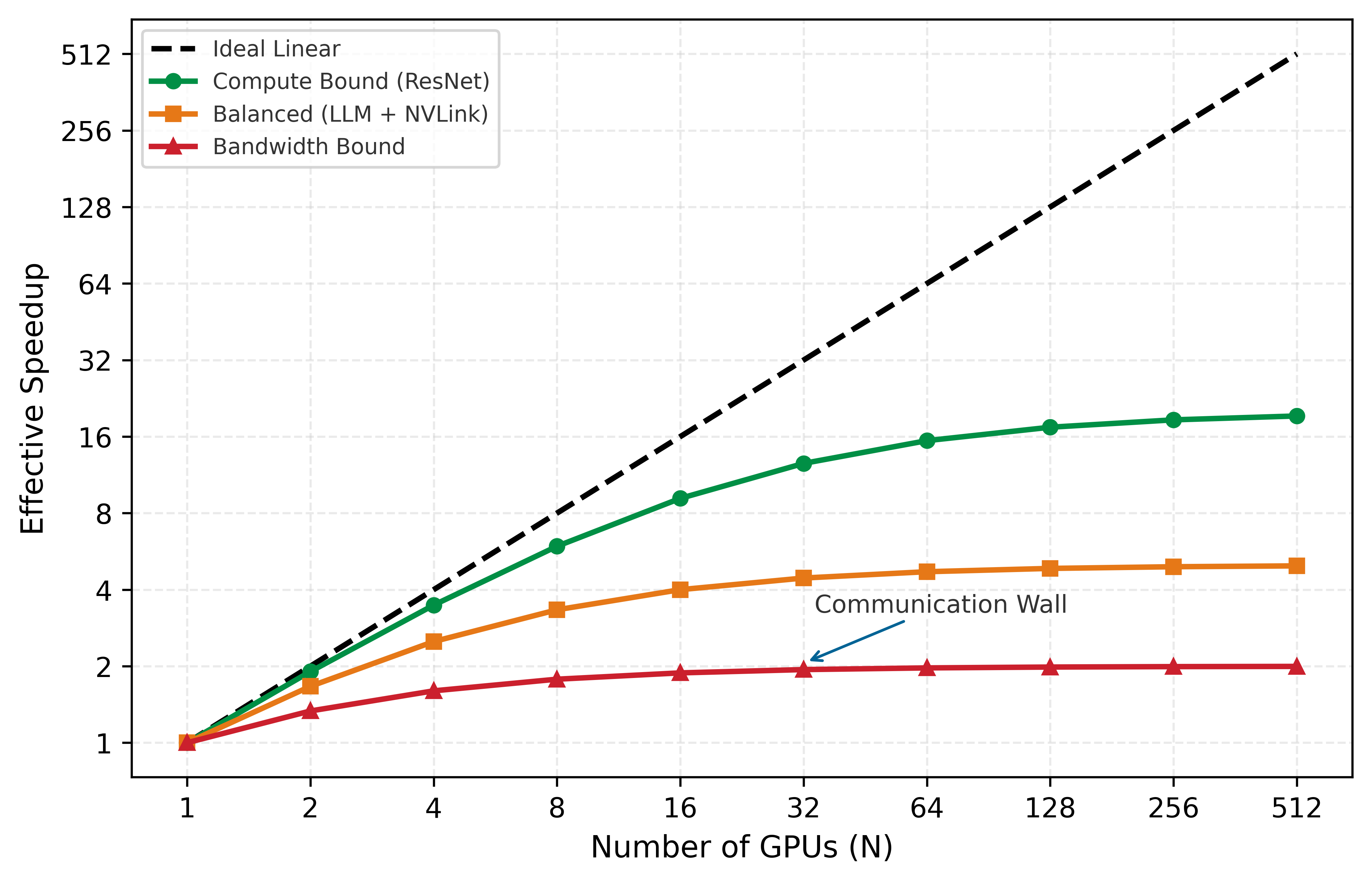
Figure 7 visualizes this divergence from ideal linear scaling as the Scaling Tax—a direct consequence of the scaling efficiency bound (principle 8). It shows how communication overhead \((r)\) acts as a drag on performance, creating a communication wall where adding more GPUs yields diminishing returns.
The fleet law (principle 10) maps directly onto the iron law’s variables, separating compute, bandwidth, and coordination into additive terms:
\[ T_{\text{step}}(N) = \underbrace{\frac{T_{\text{compute}}}{N}}_{\text{Compute-Time Term}} + \underbrace{T_{\text{comm}}(N)}_{\text{Bandwidth Term}} + \underbrace{T_{\text{sync}}(N)}_{\text{Coordination Term}} - T_{\text{overlap}} \]
The fleet-law terms separate step time into four distinct costs:
- Compute-Time Term \((T_{\text{compute}}/N)\): The total computation required for the batch after ideal partitioning across \(N\) devices.
- Bandwidth Term \((T_{\text{comm}}(N))\): The time spent moving data. This is governed by the iron law’s data-movement term, \(D_{\text{vol}}/\text{BW}\). For Ring AllReduce, this term is \(\frac{2(N-1)}{N} \times \frac{M}{\text{BW}_{\text{net}}}\), where \(M\) is the communicated gradient or model-state bytes and \(\text{BW}_{\text{net}}\) is network bandwidth.
- Coordination Term \((T_{\text{sync}}(N))\): The nonoverlapped cost of barriers, ordering, and straggler waiting.
- Overlap \((T_{\text{overlap}})\): The portion of communication hidden behind computation.
The fleet law leads to the scaling efficiency metric for fixed global work, where \(T_{\text{compute}}\) is the single-device compute time for that work:
\[ \eta_{\text{scaling}} = \frac{T_{\text{compute}}}{N \times T_{\text{step}}(N)} = \frac{1}{1 + \frac{N(T_{\text{comm}}(N) + T_{\text{sync}}(N) - T_{\text{overlap}})}{T_{\text{compute}}}} \]
This is the scaling efficiency bound (principle 8): perfect linear scaling \((\eta_{\text{scaling}} = 1.0)\) is a theoretical limit, not a practical target. Well-configured systems can achieve \(\eta_{\text{scaling}} = 0.85\)–\(0.95\) at moderate scale and degrade further as \(N\) grows. The gap between \(\eta_{\text{scaling}} = 1.0\) and the achieved efficiency is the communication tax and coordination tax: the price of distributed execution.
The equation reveals the scaling wall: as \(N\) increases, the compute term \((T_{\text{compute}}/N)\) shrinks, but the communication and synchronization terms can remain constant or grow. Eventually, the denominator is dominated by overhead, driving efficiency toward zero. Beyond wall-clock time, this communication overhead imposes an energy tax that scales with physical distance between devices.

Communication energy climbs from HBM out to the network.
Systems Perspective 1.2: The energy tax of scale
Distributed training is a race against energy as much as against time. In a single GPU, moving a byte from HBM to the cores costs roughly 1–2 pJ/bit. Moving that same byte across an NVLink interconnect costs 5–10 pJ/bit. Moving it across an InfiniBand network through switches costs 20–50 pJ/bit.
At the scale of 10,000 GPUs, the multiplication by aggregate bandwidth is what changes the engineering problem. A full H100 NVLink envelope is roughly 9 PB/s across the cluster; at 7.5 pJ/bit, that movement represents about 540 kW before cooling and switch overhead. The aggregate NDR InfiniBand envelope is smaller (500 TB/s), but at 35 pJ/bit it still represents about 140 kW. Communication-computation overlap is therefore necessary for wall-clock efficiency, but avoiding unnecessary movement is the direct way to reduce the power term itself.
Wall-clock efficiency and the energy tax degrade together as \(N\) grows, following predictable patterns across GPU counts. As a representative rule of thumb, systems in the linear scaling regime of 2–32 GPUs often achieve 85–95 percent parallel efficiency because communication overhead remains small. The communication-bound regime emerges at 64–256 GPUs, where efficiency can drop to 60–80 percent even with well-matched interconnects. Beyond 512 GPUs, coordination overhead can become dominant and limit efficiency to 40–60 percent due to collective operation latency.
Hardware selection critically impacts these scaling characteristics. NVIDIA DGX A100 systems provide 600 GB/s of bidirectional NVLink bandwidth per GPU, with aggregate NVSwitch bandwidth at the system level, enabling high parallel efficiency inside an 8-GPU node. Multi-node scaling requires a network fabric with enough bisection bandwidth; EDR-class 100 Gbps links can support smaller multi-node jobs, while HDR-class 200 Gbps links can support larger clusters when topology, placement, and overlap are well matched.
The efficiency metrics directly influence the choice of parallelism strategy. Data parallelism works well in the linear scaling regime but becomes communication bound at scale. Model parallelism addresses memory constraints but introduces sequential dependencies that limit efficiency. Pipeline parallelism reduces device idle time but introduces complexity in managing microbatches. The effective strategy depends on which constraint—memory, bandwidth, or synchronization—dominates the target workload.
Hardware efficiency metrics govern throughput, but convergence theory determines whether distributed training reaches the same solution quality as single-device training. Parallelism affects optimization convergence in three ways: convergence rate changes with batch size, adding workers yields diminishing returns beyond the critical batch size, and learning rates must scale with batch size.
Convergence rate for synchronous data parallel SGD
The fundamental convergence result for distributed SGD explains why adding workers can reduce iteration count without changing the optimizer’s meaning. The theorem uses two standard regularity assumptions: the loss is smooth enough that gradients cannot change arbitrarily fast, and each stochastic gradient has bounded variance around the true gradient. Written formally, for a loss function \(\mathcal{L}(\theta)\) with \(L_s\)-Lipschitz gradients and variance-bounded stochastic gradients \(\mathbb{E}[\|g_i - \nabla \mathcal{L}(\theta)\|^2] \leq \sigma^2\), synchronous data parallel SGD with \(N\) workers achieves the following convergence rate.
Theorem 1.1: Convergence rate for distributed SGD
For synchronous data parallel SGD with \(N\) workers, each computing gradients on a local batch of size \(b\), after \(K\) total iterations the expected optimization error satisfies:
\[ \mathbb{E}[\mathcal{L}(\theta_K)] - \mathcal{L}^{\star} \leq \underbrace{\frac{L_s \|\theta_0 - \theta^{\star}\|^2}{2K}}_{\text{optimization error}} + \underbrace{\frac{\eta L_s \sigma^2}{2Nb}}_{\text{variance floor}} \]
where \(\eta\) is the learning rate, \(L_s\) is the smoothness constant, \(\mathcal{L}^{\star}\) is the optimal loss value, \(\theta^{\star}\) is an optimal parameter vector, and \(\sigma^2\) is the gradient variance. The effective convergence rate is \(\mathcal{O}(1/\sqrt{NbK})\) when the learning rate is tuned optimally as \(\eta = \mathcal{O}(\sqrt{Nb/K})\).
The theorem reveals several important insights. First, the variance floor decreases linearly with the number of workers \(N\), explaining why distributed training can achieve the same final loss with fewer iterations in the linear scaling regime. With equal local batch size \(b\), synchronous data-parallel SGD computes the same minibatch gradient as a single worker using batch size \(Nb\) for that step; convergence speed still depends on learning-rate scaling and critical-batch-size effects. Second, the convergence rate \(\mathcal{O}(1/\sqrt{NbK})\) shows that workers, local batch size, and iteration count jointly determine statistical progress, assuming infinite bandwidth. This is the statistical efficiency of distributed training, distinct from hardware efficiency.
However, the theorem assumes perfect synchronization (BSP). When workers proceed at different rates or use stale gradients, convergence guarantees degrade, as we examine next.
Staleness impact: BSP vs. SSP vs. ASP
The operational guarantees of BSP, SSP, and ASP established in section 1.2.1.4 have a convergence cost, which this section sketches with stylized smooth-objective bounds. The staleness parameter \(\tau_{\text{stale}}\) quantifies how many iterations behind a gradient may be when applied to parameters, and it is the variable that ties throughput to solution quality (Ho et al. 2013; Dutta et al. 2018).
Ho, Qirong, James Cipar, Henggang Cui, Seunghak Lee, Jin Kyu Kim, Phillip B. Gibbons, Garth A. Gibson, Greg Ganger, and Eric P. Xing. 2013. “More Effective Distributed ML via a Stale Synchronous Parallel Parameter Server.” Advances in Neural Information Processing Systems 26.
Dutta, Sanghamitra, Gauri Joshi, Soumyadip Ghosh, Parijat Dube, and Priya Nagpurkar. 2018. “Slow and Stale Gradients Can Win the Race: Error-Runtime Trade-Offs in Distributed SGD.” Proceedings of the Twenty-First International Conference on Artificial Intelligence and Statistics 84: 803–12.
Definition 1.5: Gradient staleness
Gradient Staleness (\(\tau_{\text{stale}}\)) is the number of parameter updates that occur between the time a gradient is computed and the time it is applied to the global model state.
- Significance: It represents the synchronization error in distributed optimization. Increasing \(\tau_{\text{stale}}\) can improve throughput by reducing barrier waits \((T_{\text{sync}}(N))\), but it typically degrades the rate of convergence, requiring more operations \((O)\) to reach the same accuracy.
- Distinction: Unlike network latency, which is a physical delay, staleness is an algorithmic offset that arises from the choice of synchronization protocol (e.g., ASP, SSP).
- Common pitfall: A frequent misconception is that staleness is “always bad.” In reality, it is a throughput-convergence trade-off: for some large-scale workloads, allowing bounded staleness is one practical way to keep thousands of GPUs in use.
The convergence behavior differs across these models in ways that directly affect training cost and solution quality. In Bulk Synchronous Parallel (BSP, \(\tau_{\text{stale}} = 0\)), all workers compute gradients on the same parameter version, then synchronize via barrier before updating. This guarantees mathematical equivalence to single-device training with larger batch size, an optimal convergence rate of \(\mathcal{O}(1/\sqrt{NbK})\), and no hyperparameter adjustment beyond batch size scaling.
Stale Synchronous Parallel (SSP, \(\tau_{\text{stale}} \leq s\)) relaxes the barrier by allowing workers to proceed up to \(s\) iterations ahead of the slowest worker. In a stylized bound, the convergence rate gains an additive delay term:
\[ \mathbb{E}[\mathcal{L}(\theta_K)] - \mathcal{L}^{\star} \leq \mathcal{O}\left(\frac{1}{\sqrt{NbK}}\right) + \mathcal{O}\left(\frac{s^2 \eta^2 L_s^2}{Nb}\right) \]
The second term represents the staleness penalty. For bounded staleness \(s\), this penalty is controlled by keeping delay small and retuning the learning rate. Deployments that choose bounded staleness accept convergence degradation for throughput improvement on heterogeneous clusters.
Asynchronous SGD (ASP, \(\tau_{\text{stale}} = \infty\)) eliminates waiting entirely: workers update parameters immediately. While this maximizes throughput, the same teaching model shows a larger delay-dependent term:
\[ \mathbb{E}[\mathcal{L}(\theta_K)] - \mathcal{L}^{\star} \leq \mathcal{O}\left(\frac{1}{\sqrt{K}}\right) + \mathcal{O}\left(\bar{\tau}_{\text{stale}}^2 \eta^2 L_s^2\right) \]
where \(\bar{\tau}_{\text{stale}}\) is the average staleness. The staleness penalty now scales with the square of average delay, and critically, the variance reduction from \(N\) workers disappears in the dominant term. Several techniques compensate for this. Learning rate decay (\(\eta' = \eta / \sqrt{1 + \bar{\tau}_{\text{stale}}}\)) reduces the staleness penalty but slows convergence. Momentum correction adjusts the momentum term to account for delayed updates. Gradient clipping prevents stale gradients with large magnitudes from destabilizing training.
Table 4 summarizes the convergence properties of each synchronization model.
| Model | Staleness | Convergence Rate | Variance Reduction | Best For |
|---|---|---|---|---|
| BSP | \(\tau_{\text{stale}} = 0\) | \(\mathcal{O}(1/\sqrt{NbK})\) | Full (\(1/N\)) | Final training, reproducibility |
| SSP | \(\tau_{\text{stale}} \leq s\) | \(\mathcal{O}(1/\sqrt{NbK}) + \mathcal{O}(s^2\eta^2 L_s^2/Nb)\) | Partial | Heterogeneous clusters |
| ASP | \(\tau_{\text{stale}} = \infty\) | \(\mathcal{O}(1/\sqrt{K}) + \mathcal{O}(\bar{\tau}_{\text{stale}}^2\eta^2 L_s^2)\) | None | Maximum throughput, early exploration |
Learning rate scaling rules
When increasing the effective batch size through data parallelism, the learning rate must be adjusted to maintain convergence quality. Two primary scaling rules have emerged from both theory and practice.
The linear scaling rule (Goyal et al. 2017) states that when the batch size is multiplied by \(k\), the learning rate should also be multiplied by \(k\):
\[ \eta_{\text{large}} = k \cdot \eta_{\text{base}} \]
This rule is justified by approximating one large-batch step at learning rate \(k\eta\) as \(k\) consecutive small-batch steps each at learning rate \(\eta\). With batch size \(kB\), the gradient variance decreases by factor \(k\), so the larger step is well-conditioned; the approximation holds when parameters do not move much during those \(k\) small-batch steps. The rule is empirical rather than universal: Goyal et al. validated it for ResNet-50/ImageNet at global batch size 8,192 with gradual warmup, while LARS and LAMB extend large-batch recipes through layer-wise adaptation for ImageNet and BERT-style pretraining (Goyal et al. 2017; You et al. 2017; You et al. 2020). A warmup period that increases the learning rate linearly from \(\eta_{\text{base}}\) to \(k \cdot \eta_{\text{base}}\) over the first \(W\) iterations lets the model reach a region of the loss landscape where large learning rates are stable:
\[ \eta_t = \eta_{\text{base}} + \frac{t}{W}(k \cdot \eta_{\text{base}} - \eta_{\text{base}}) \quad \text{for } t < W \]
The square root scaling rule applies when batch sizes grow so large that linear scaling fails:
\[ \eta_{\text{large}} = \sqrt{k} \cdot \eta_{\text{base}} \]
The more conservative square root rule is motivated by the observation that gradient noise (not just magnitude) affects optimization dynamics. The square root rule better preserves the signal-to-noise ratio of gradient updates. Empirically, square root scaling becomes necessary when batch sizes exceed the critical batch-size regime.
For extreme batch sizes (32K–1M), layer-wise adaptive learning rate scaling (LARS) (You et al. 2017) and its Adam variant LAMB (You et al. 2020) automatically adjust learning rates per layer based on the ratio of weight norm to gradient norm:
\[ \eta_\ell = \eta_{\text{global}} \cdot \frac{\|w_\ell\|}{\|g_\ell\| + \lambda_{\text{wd}}\|w_\ell\|} \]
Here \(\lambda_{\text{wd}}\) is the optimizer’s weight-decay coefficient in the LARS/LAMB update, avoiding collision with the failure-rate parameter used in reliability analysis. Layer-wise scaling prevents layers with small weights from receiving disproportionately large updates. LAMB enabled BERT training with batch sizes up to 64K while maintaining convergence quality.
Critical batch size and diminishing returns
A fundamental property of distributed training is that adding more workers stops helping past a threshold. The critical batch size \(B^{*}\) marks the transition point beyond which increasing batch size yields diminishing returns in convergence per sample seen.
Definition 1.6: Critical batch size
Critical Batch Size \((B^{*})\) is the distributed-training batch size at which the gradient noise scale is large enough that further batch growth yields diminishing returns in sample efficiency (McCandlish et al. 2018; Shallue et al. 2019).
- Significance: It marks the transition point for parallel scaling efficiency. Below \(B^{*}\), increasing the batch size linearly improves the convergence per step. Above \(B^{*}\), larger batches yield diminishing returns, requiring proportionally more samples \((D)\) to reach the same loss.
- Distinction: Unlike the memory-limited batch size (determined by memory capacity and activation footprint), the critical batch size is an algorithmic property of the model and dataset.
- Common pitfall: A frequent misconception is that training can be sped up indefinitely by adding GPUs. In reality, \(B^{*}\) defines the physical ceiling for data parallelism: adding workers beyond this point wastes energy and compute \((O)\) without reducing total training time \((T)\).
The gradient-noise-scale proxy for the critical batch size can be estimated as:
\[ B^{*} \approx \frac{\text{tr}(\Sigma)}{\|\nabla \mathcal{L}(\theta)\|^2} \]
where \(\text{tr}(\Sigma)\) is the trace of the gradient covariance matrix (total gradient variance) and \(\|\nabla \mathcal{L}(\theta)\|^2\) is the squared gradient norm (signal strength). Intuitively, \(B^{*}\) is the batch size at which averaging reduces gradient variance to the level of the true gradient magnitude.
Published large-batch regimes illustrate the scale rather than providing fixed thresholds. On ImageNet, Goyal et al. stabilized ResNet-50 at global batch 8,192 with warmup, and LARS extends ImageNet large-batch training further in some settings (Goyal et al. 2017; You et al. 2017). For BERT-Large pretraining, LAMB reports training at 32K–64K batch sizes with layer-wise adaptive updates (You et al. 2020). Across other domains, McCandlish et al. show useful batch-size limits ranging from tens of thousands in ImageNet-like settings to millions in reinforcement-learning workloads, so new frontier-language-model thresholds should be measured rather than copied (McCandlish et al. 2018).
You, Yang, Igor Gitman, and Boris Ginsburg. 2017. “Large Batch Training of Convolutional Networks.” arXiv Preprint arXiv:1708.03888.
You, Y., J. Li, S. Reddi, J. Hseu, S. Kumar, S. Bhojanapalli, X. Song, J. Demmel, K. Keutzer, and C.-J. Hsieh. 2020. “Large Batch Optimization for Deep Learning: Training BERT in 76 Minutes.” International Conference on Learning Representations.
The scaling law regime exhibits three distinct behaviors. Below the critical batch size \((B < B^{*})\), linear scaling holds: doubling the batch size halves the iterations needed to reach the target loss, and hardware efficiency determines throughput. At the critical point \((B \approx B^{*})\), samples-per-second efficiency is maximized, the optimal trade-off. Above it \((B > B^{*})\), returns diminish, because doubling the batch size requires more than double the total samples, so additional workers add throughput but not sample efficiency.
Figure 8 illustrates this relationship between batch size and training efficiency.

The critical batch size has important implications for distributed training system design. Adding workers beyond \(B^{*}/b\) (where \(b\) is the per-worker batch size) improves throughput but not sample efficiency, though it may still be worthwhile for cost if the marginal cost of additional workers is low. The learning rate schedule matters too, because above \(B^{*}\) aggressive warmup becomes essential, since the loss landscape near initialization may not support the large updates that linear scaling would produce. Communication trade-offs shift as well, because above \(B^{*}\) the reduced benefit of larger batches makes communication overhead relatively more costly, strengthening the case for gradient compression or asynchronous methods.
Checkpoint 1.2: Scaling decisions
Given a 7B parameter model distributed across a cluster of 64 A100 GPUs (80 GB HBM2e each), determine the maximum useful batch size. Use a pilot trace with \(\text{tr}(\Sigma)=1.6 \times 10^6\), \(\|\mu\|^2=100\), per-GPU batch \(b=4\), and a proposed gradient-accumulation depth of 32 steps, giving \(B_{\text{global}} = 64 \times 4 \times 32 = 8192\) samples.
Worked example: Convergence comparison for 8 vs. 64 workers
To illustrate these concepts concretely, consider scaling from 8 to 64 workers when training a transformer language model with baseline batch size \(B = 32\) per worker.
Napkin Math 1.6: Scaling from 8 to 64 workers
Setup: Transformer model with 1.3B parameters, target perplexity 15, baseline training: 100K iterations on single GPU with \(b =\) 32.
Table 5: Scaling SGD across cluster sizes: Iteration count, communication overhead, wall-clock speedup, and sample efficiency for the same training job at 1, 8, and 64 GPUs.
8 Workers (BSP)
- Effective batch size: \(B =\) 8 \(\times\) 32 = 256
- Learning rate: \(\eta =\) 8 \(\times \eta_{\text{base}}\) (linear scaling with warmup)
- Expected iterations: 100K \(/\) 8 = 12.5K iterations
- Convergence: Reaches target perplexity in 12.8K iterations (98 percent efficiency)
- Communication overhead: 15 percent (NVLink intra-node)
- Wall-clock speedup: 100K \(\times\) 1 \(/\) (12.8K \(\times\) 1.15×) = 6.8×
64 Workers (BSP)
- Effective batch size: \(B =\) 64 \(\times\) 32 = 2,048
- Learning rate (\(N =\) 64 workers): \(\eta = N \times \eta_{\text{base}}\) (if \(B < B^*\)) or \(\eta = \sqrt{N} \times \eta_{\text{base}}\) (if \(B > B^*\))
- Assuming \(B^* \approx\) 4,000 (below critical): Linear scaling applies
- Expected iterations: 100K \(/\) 64 = 1.56K iterations
- Convergence: Reaches target perplexity in 1.72K iterations (91 percent efficiency)
- Communication overhead: 45 percent (InfiniBand inter-node, 8 nodes)
- Wall-clock speedup: 100K \(\times\) 1 \(/\) (1.72K \(\times\) 1.45×) = 40.1×
SSP workers: 64 workers (\(s =\) 4)
- Same effective batch size: \(B =\) 2,048
- Learning rate: \(\eta' = \eta_{\text{BSP}} / \sqrt{1 + s}\) with \(s =\) 4, giving \(\eta' \approx\) 0.45 \(\times \eta_{\text{BSP}}\)
- Expected iterations: Higher due to staleness penalty
- Convergence: Reaches target perplexity in 2.1K iterations (74 percent efficiency)
- Communication overhead: 25 percent (reduced synchronization)
- Wall-clock speedup: 100K \(\times\) 1 \(/\) (2.1K \(\times\) 1.25×) = 38.1×
Analysis (table 5)
| Configuration | Iterations | Comm. Overhead | Wall-clock Speedup | Sample Efficiency |
|---|---|---|---|---|
| 1 GPU (baseline) | 100,000 | 0% | 1\(\times\) | 100% |
| 8 GPU BSP | 12,800 | 15% | 6.8× | 98% |
| 64 GPU BSP | 1,720 | 45% | 40.1× | 91% |
| 64 GPU SSP | 2,100 | 25% | 38.1× | 74% |
The 64-GPU BSP configuration achieves 40× speedup despite only 91 percent sample efficiency because the communication overhead (45 percent) is offset by the massive parallelism. SSP provides comparable wall-clock time with lower communication overhead but requires more total samples.
Cost Analysis (assuming $3/GPU-hour):
- 8: 12.8K iters \(\times\) 0.4 s/iter \(\times\) 8/3600 \(\times\) $3/GPU-hour = $34
- 64 BSP: 1.72K iters \(\times\) 0.58 s/iter \(\times\) 64/3600 \(\times\) $3/GPU-hour = $53
- 64 SSP: 2.1K iters \(\times\) 0.50 s/iter \(\times\) 64/3600 \(\times\) $3/GPU-hour = $56
Despite higher parallelism, 64-GPU training costs more per run due to communication overhead and reduced sample efficiency. The 8-GPU configuration is more cost-efficient but takes 6\(\times\) longer wall-clock time. The choice depends on whether minimizing cost or minimizing time-to-result is the priority.
Trade-off: Communication cost vs. convergence speed
The fundamental trade-off in distributed training is between communication efficiency and convergence quality. Figure 9 visualizes this trade-off space.

Several techniques occupy different positions on this trade-off curve. Gradient compression reduces communication volume by transmitting compressed gradient information through quantization, sparsification, or low-rank approximation. Examples include sign-based updates (Bernstein et al. 2018), Deep Gradient Compression (Lin et al. 2018), PowerSGD (Vogels et al. 2019), QSGD quantization with convergence analysis (Alistarh et al. 2017), and empirical sparse gradient dropping for neural machine translation (Aji and Heafield 2017).
Bernstein, Jeremy, Yu-Xiang Wang, Kamyar Azizzadenesheli, and Animashree Anandkumar. 2018. “signSGD: Compressed Optimisation for Non-Convex Problems.” Proceedings of the 35th International Conference on Machine Learning 80: 560–69.
Lin, Yujun, Song Han, Huizi Mao, Yu Wang, and William J Dally. 2018. “Deep Gradient Compression: Reducing the Communication Bandwidth for Distributed Training.” International Conference on Learning Representations.
Vogels, Thijs, Sai Praneeth Karimireddy, and Martin Jaggi. 2019. “PowerSGD: Practical Low-Rank Gradient Compression for Distributed Optimization.” Advances in Neural Information Processing Systems 32.
Alistarh, Dan, Demjan Grubic, Jerry Li 0001, Ryota Tomioka, and Milan Vojnovic. 2017. “QSGD: Communication-Efficient SGD via Gradient Quantization and Encoding.” Advances in Neural Information Processing Systems 30: 1709–20.
Aji, Alham Fikri, and Kenneth Heafield. 2017. “Sparse Communication for Distributed Gradient Descent.” Proceedings of the 2017 Conference on Empirical Methods in Natural Language Processing, 440–45. https://doi.org/10.18653/v1/d17-1045.
Stich, Sebastian U. 2019. “Local SGD Converges Fast and Communicates Little.” International Conference on Learning Representations.
Local SGD takes a different approach: workers perform \(H_{\text{local}}\) local updates before synchronizing, reducing communication frequency by factor \(H_{\text{local}}\). Convergence analysis shows that for smooth, strongly convex objectives, Local SGD achieves the same asymptotic rate as synchronous SGD with appropriately tuned learning rates (Stich 2019).
Decentralized SGD restricts workers to communicating only with neighbors in a communication graph rather than performing global AllReduce. This reduces bandwidth requirements at the cost of slower mixing, making it suitable for geo-distributed training where global synchronization is expensive.
The choice among these methods depends on the specific bottleneck. When network bandwidth limits throughput, gradient compression provides the best trade-off. When synchronization latency dominates, Local SGD or SSP are preferred. When network topology constraints exist, decentralized approaches may be necessary.
Self-Check: Question
The scaling-efficiency equation decomposes step time into compute per GPU plus communication and synchronization overhead: \(\eta_{\text{scaling}} = 1/(1 + N(T_{\text{comm}}(N) + T_{\text{sync}}(N) - T_{\text{overlap}})/T_{\text{compute}})\). As \(N\) grows, compute per worker shrinks while \(T_{\text{comm}}(N)\) and \(T_{\text{sync}}(N)\) either stay flat or grow. What happens to efficiency in the limit, and why does a ‘better collective algorithm’ not save it?
- Efficiency approaches 100 percent because \(T_{\text{compute}}\) keeps falling with more workers
- Efficiency degrades as the ratio \((T_{\text{comm}}(N) + T_{\text{sync}}(N) - T_{\text{overlap}}) / (T_{\text{compute}}/N)\) grows, eventually making overhead the dominant step-time term
- Efficiency is flat as long as Ring AllReduce is chosen, because ring AllReduce is bandwidth-optimal
- Efficiency only improves once the optimizer is changed from SGD to Adam, because Adam reduces communication requirements
Explain the difference between hardware efficiency and statistical efficiency in a distributed training run, and give a concrete scenario where a cluster configuration wins on one and loses on the other.
Why does stale-synchronous parallel (SSP) training typically require a smaller effective learning rate than bulk-synchronous parallel (BSP) at the same global batch size?
- Because SSP workers compute exact full-batch gradients instead of stochastic gradients, so Lipschitz constants are larger
- Because bounded staleness introduces an additional convergence-penalty term, so the base learning rate must shrink to preserve stability under stale parameter views
- Because SSP eliminates all inter-worker communication, making gradient magnitudes larger than under BSP
- Because BSP uses strictly fewer workers by definition, so the two approaches are never compared at the same scale
A team scales a run’s global batch size from 512 to 4,096 by moving from 8 to 64 data-parallel workers. The model is still operating comfortably below its critical batch size. Which learning-rate adjustment is the default rule, and what complement must accompany it?
- Keep the learning rate unchanged, because large-batch variance reduction already stabilizes training without tuning
- Multiply the learning rate by 64, matching the worker count rather than the batch-size ratio
- Multiply the learning rate by 8 and include a warmup schedule, so optimizer state builds up before the full scaled rate applies
- Multiply the learning rate by the square root of 8 from step zero, because linear scaling is reserved for inference
True or False: Once a run exceeds its model’s critical batch size, adding more data-parallel workers (and therefore growing the global batch) still raises step throughput proportionally and also produces proportional gains in convergence per sample.
A 64-worker BSP run reaches target loss in 20 percent fewer total samples than a 64-worker SSP run on the same cluster, but the SSP run has 30 percent lower per-step communication overhead. How should an engineer reason about this trade-off when the cluster has a few known straggler nodes?
Model Parallelism
When model state, activations, optimizer state, or an individual tensor operation exceeds the memory or communication budget of one accelerator group, data parallelism entirely collapses. This is the memory capacity gap (principle 3) in operational form: model parameter growth outpaces device memory growth, forcing the model’s computation and state to be partitioned. Data-parallel memory optimizations extend replication’s reach, but eventually the model itself must be partitioned.
Definition 1.7: Model parallelism
Model Parallelism is a distributed training strategy that partitions a single neural network’s parameters or operations across multiple devices so each device computes a distinct portion of the model.
- Significance: If a model with parameter state \(S_{\text{model}}\) is split across \(N_{\text{mp}}\) devices, the ideal per-device parameter footprint falls toward \(S_{\text{model}}/N_{\text{mp}}\), enabling training of models that exceed single-device memory. The cost is extra communication for activations and gradients plus idle time from sequential dependencies, so the memory gain must exceed the transfer and pipeline-bubble overhead introduced by the partition.
- Distinction: Unlike data parallelism, which replicates the full model on every worker and shards the minibatch, model parallelism shards the model itself. Pipeline parallelism and tensor parallelism are implementation forms of model parallelism: one partitions layers into stages, while the other partitions individual tensor operations.
- Common pitfall: A frequent misconception is that model parallelism automatically speeds up training. Its primary benefit is capacity, not throughput; without careful scheduling and overlap, downstream devices wait for upstream activations and utilization can fall below a single-device baseline.

Optimizer state, not weights, dominates the per-replica training budget.
Even with ZeRO-3 fully deployed, sharding optimizer states, gradients, and parameters across workers, some architectures remain intractable. Tensor parallelism, illustrated in figure 10, addresses this by partitioning individual weight matrices across devices; pipeline parallelism partitions layers across stages and is introduced later in section 1.4.2.2. For a 175B parameter model, weights alone occupy 350 GB, or about 5.5 GB per GPU across 64 GPUs. Full mixed-precision Adam training state is much larger: 2,800 GB globally, or roughly 43.8 GB per GPU before activations. This distinction matters because optimizer sharding reduces static state, but it does not eliminate the activation and per-layer capacity constraints that force model parallelism.

For long-context transformers where activation memory dominates, a 2048-token sequence through 175B parameters generates on the order of a terabyte of intermediate activations at even a small micro-batch (roughly 1.1 TB at micro-batch 4, as computed earlier), and no amount of optimizer sharding addresses this constraint. Model parallelism addresses these limitations by splitting the model architecture itself across devices, rather than replicating it with sharded state.
Napkin Math 1.7: The memory wall of scale
Problem: Training a 175B parameter model (like GPT-3) on NVIDIA A100s (80 GB). Can data parallelism with ZeRO-3 handle this?
Math:
- Parameter storage: 175B params \(\times\) 2 bytes (FP16) = 350 GB.
- Gradients and optimizer state: gradients add 175B params \(\times\) 2 bytes = 350 GB, while Adam FP32 master weights, momentum, and variance add 175B params \(\times\) 12 bytes = 2,100 GB.
- Total static memory: 2,800 GB.
- ZeRO-3 sharding: With 64 GPUs, per-GPU static memory = 2,800 GB/64 GPUs \(\approx\) 43.8 GB.
- Activation memory: For sequence length 2048 and batch size 1, a 96-layer transformer generates \(\approx\) 50 GB of activations per GPU.
Systems insight: 43.8 GB (static) + 50 GB (dynamic) = 93.8 GB. This exceeds the 80 GB capacity of the A100. Even with full ZeRO-3 sharding, pure data parallelism fails. The only recourse is tensor parallelism to split the layers themselves.
Model parallelism addresses this limitation by distributing the model architecture itself across devices, but the placement decision is where to cut the model. Layer-based splitting assigns devices to sequential layer groups, such as layers 1–4 on one device and layers 5–8 on the next. Channel-based splitting divides the channels within a layer, such as 512 channels on one device and the remaining channels on another. Transformer architectures add attention-head splitting, where separate devices own different heads. Each cut changes a different cost: layer cuts save memory but serialize the pipeline, while channel and head cuts expose more parallel work but require faster intra-layer communication.
These cuts enable the large-scale cases that exceed a single device for different reasons. GPT-3, with 175B parameters, relies on model parallelism for training. Vision transformers processing high-resolution \(16k{\times}16k\) pixel images use model parallelism to manage activation and memory constraints. Mixture-of-Experts architectures use this approach to distribute their conditional computation paths across hardware (Shazeer et al. 2017; Lepikhin et al. 2021; Fedus et al. 2022).
Device coordination proceeds in three phases. In the forward pass, data flows sequentially through model segments on different devices. The backward pass propagates gradients in reverse order through these segments. During parameter updates, each device modifies only its assigned portion of the model. The coordination ensures mathematical equivalence to training on a single device while enabling models that exceed individual device memory capacities. The cost is sequential dependency between stages: while one device computes its forward pass, downstream devices sit idle, creating the pipeline bubble that dominates utilization analysis for model-parallel systems.
Checkpoint 1.3: Model parallelism foundations
Verify your understanding of model sharding:
Model parallelism implementation
Once the model itself is the object being partitioned, the implementation problem is placement: every cut must save enough memory to justify the activation transfer and idle time it introduces. Figure 11 captures this bidirectional data flow: input data propagates forward through sequentially assigned model partitions while gradients flow backward to update parameters, with intermediate results transferring across device boundaries at each stage.

Consider our running example: the 175B parameter model requires 350 GB of memory in FP16, exceeding the 80 GB capacity of a single A100 by a factor of four. Model parallelism addresses this capacity wall by partitioning model weights across multiple devices, effectively stitching them into a single super-accelerator. Unlike data parallelism, where every GPU holds a full replica of the model and processes a unique fraction of the global batch, model parallelism requires each GPU to hold a unique fraction of the model and process the same data stream sequentially. With 8-way partitioning on A100s, BF16 weights alone occupy approximately 44 GB per GPU. That is only the weights budget: full training still needs activations, gradients, and optimizer state, so pure 8-way model parallelism is not sufficient by itself. Training requires additional sharding or offload for optimizer and gradient state, plus pipeline or hybrid parallelism to keep activation memory within capacity.
In a typical pipeline parallel implementation, the training loop operates as a relay race. The forward pass initiates on GPU 1, which computes the initial transformer blocks and transmits the resulting intermediate activation tensor across the interconnect to GPU 2. For our 175B model with a hidden dimension of 12,288 and a micro-batch size of 4 sequences at 2,048 tokens each, this handoff involves moving approximately 200 MB of data per stage boundary per step. GPU 2 must wait for this payload before it can begin its computation, creating a strict dependency chain that propagates through all stages. The backward pass mirrors this path in reverse, propagating error gradients from the final layer back to the input, with each device computing gradients only for its local parameters.
The architecture fundamentally changes the optimization dynamics compared to data parallelism. Instead of a global AllReduce to average gradients across replicas, each GPU performs a local optimizer step (Adam (Kingma and Ba 2014), AdaFactor, or similar) on its specific slice of parameters. A device holding transformer layers 1–12 updates only those layers’ weights and biases, with no cross-device synchronization required during the optimization step. While this eliminates the bandwidth-heavy gradient synchronization of data parallelism, it trades one bottleneck for another: pipeline bubbles. If the layers assigned to GPU 1 are computationally heavier than those on GPU 2 (common when attention layers have different head counts or when embedding layers are unevenly sized), valuable compute cycles are lost to waiting. The primary engineering challenge thus shifts from maximizing arithmetic intensity to minimizing serialization latency and ensuring balanced load across the partitioned fleet (Rasley et al. 2020).
Kingma, Diederik P., and Jimmy Ba. 2014. “Adam: A Method for Stochastic Optimization.” ICLR in press.
Rasley, Jeff, Samyam Rajbhandari, Olatunji Ruwase, and Yuxiong He. 2020. “DeepSpeed: System Optimizations Enable Training Deep Learning Models with over 100 Billion Parameters.” Proceedings of the 26th ACM SIGKDD International Conference on Knowledge Discovery &Amp; Data Mining, 3505–6. https://doi.org/10.1145/3394486.3406703.
Parallelism variations
Partitioning strategy determines which cost the model pays after memory no longer fits on one device. Layer-wise partitioning spends idle time to reduce per-device memory; pipeline parallelism spends scheduling complexity to hide that idle time; tensor parallelism spends NVLink bandwidth to split a single layer. The approaches below separate these choices by the architecture and interconnect that make each viable.
Layer-wise partitioning
Layer-wise partitioning is the least invasive model cut: it saves memory by assigning consecutive layers to separate devices, but it preserves the model’s sequential dependence. In transformer architectures, this translates to specific devices managing defined sets of attention and feed-forward blocks. Figure 12 demonstrates this partitioning for a 16-layer transformer: four consecutive blocks reside on each of four devices, with forward activations flowing left-to-right and backward gradients propagating right-to-left across the device boundaries.

Sequential processing introduces device idle time, as each device must wait for the previous device to complete its computation before beginning work. While device 1 processes the initial blocks, devices 2, 3, and 4 remain inactive. Similarly, when device 2 begins its computation, device 1 sits idle. This pattern of waiting and idle time reduces hardware utilization efficiency compared to other parallelization strategies.
Pipeline parallelism
Pipeline parallelism extends layer-wise partitioning by introducing microbatching to minimize device idle time. Instead of waiting for an entire batch to sequentially pass through all devices, the computation is divided into smaller segments called microbatches, with overlapping execution across pipeline stages. Figure 13 shows how this overlapping works: while device 1 processes microbatch \(i+1\), device 2 computes microbatch \(i\), device 3 handles \(i-1\), and device 4 executes \(i-2\), creating a continuous flow that keeps all devices active simultaneously.
As figure 13 shows, each device, as represented by the rows in the drawing, processes its assigned model layers for different microbatches simultaneously. The forward pass involves devices passing activations to the next stage, such as \(F_{0,0}\) to \(F_{1,0}\). The backward pass transfers gradients back through the pipeline, such as \(B_{3,3}\) to \(B_{2,3}\). This overlapping computation reduces idle time and increases throughput while maintaining the logical sequence of operations across devices, giving the strategy its formal shape.

Definition 1.8: Pipeline parallelism
Pipeline Parallelism is a model parallelism technique that partitions a neural network’s layers into sequential stages assigned to different devices, passing activations forward and gradients backward between stages while overlapping computation across stages using micro-batches to maintain throughput.
- Significance: Inter-stage communication transmits only the activation tensor at each stage boundary, sized as \(B_{\mu} \times S \times d_{\text{model}} \times 2\) bytes at BF16, where \(B_{\mu}\) is the micro-batch size. For a hidden dimension of 8,192 with micro-batch size 1 and a 2,048-token sequence, this is approximately \(8{,}192 \times 2{,}048 \times 2 \approx 32\) MB per boundary, compared to the gigabytes required for gradient AllReduce in data parallelism. This low communication volume makes pipeline parallelism the primary technique for scaling model depth across nodes connected by 50 GB/s InfiniBand. The pipeline bubble wastes approximately \((p-1)/(m+p-1)\) of total compute, where \(p\) is the number of stages and \(m\) is the number of micro-batches—with \(p=8\) stages and \(m=32\) micro-batches, bubble overhead is about 18 percent.
- Distinction: Unlike tensor parallelism, which shards individual matrix multiplications within a single layer and requires AllReduce on every layer’s output (demanding NVLink-class bandwidth within each stage), pipeline parallelism shards at layer boundaries and requires only point-to-point activation transfers between stages—tolerating InfiniBand bandwidth between nodes.
- Common pitfall: A frequent misconception is that adding more pipeline stages always improves throughput. The pipeline bubble fraction grows as \((p-1)/(m+p-1)\): with \(p=16\) stages and \(m=16\) micro-batches, 48 percent of compute is wasted idle—requiring large micro-batch counts (\(m \gg p\)) to keep the bubble below 10 percent, which in turn increases peak activation memory and the memory pressure on each stage.

More stages require enough microbatches or the bubble dominates utilization.
The same bubble term becomes concrete in the worked example below, where an 8-stage pipeline and 32 microbatches still leave a measurable idle-time tax.
Napkin Math 1.8: The cost of the pipeline bubble
Problem: A large-model training run uses pipeline parallelism across 8 stages. To hide the sequential delay, the batch is split into 32 microbatches. What is the “bubble tax”—the fraction of GPU cycles lost to idle waiting?
Math: In a synchronous pipeline (1F1B), the bubble fraction is determined by the ratio of stages to microbatches.
- Wait time: At the start and end of each batch, GPUs sit idle for \(p-1\) steps.
- Productive time: GPUs compute for \(m\) steps.
- Bubble fraction: \((p-1) / (p-1+m) =\) 7 \(/\) (7 \(+\) 32) \(\approx\) 17.9 percent.
Systems insight: Pipeline parallelism is a utilization-memory trade-off. Reducing the bubble from 18 percent to 5 percent requires more microbatches \((m)\), which consume additional activation memory on each GPU. In the machine learning fleet, depth does not scale for free; the cluster pays a 17.9 percent capacity tax just to keep the stages coordinated. This is why techniques like interleaved pipelining are essential: they chop the bubble into smaller pieces to recover that lost 18 percent of fleet capacity.
GPipe6 (Huang et al. 2019) introduced synchronous pipeline parallelism with micro-batch accumulation, while PipeDream (Narayanan et al. 2019) developed asynchronous approaches with weight stashing. Modern systems employ 1F1B (One-Forward-One-Backward)7 scheduling to reclaim activation memory earlier; that lower memory pressure makes larger microbatch counts practical, and the larger \(m\) is what shrinks the bubble term.
6 GPipe: Published by Google in 2019, GPipe introduced synchronous micro-batch pipelining that trained a 557M-parameter AmoebaNet across 8 Tensor Processing Units (TPUs) with near-linear scaling. The key trade-off GPipe exposed: the pipeline bubble fraction \((p-1)/(m+p-1)\) means that with \(p=4\) stages and \(m=4\) micro-batches, 43 percent of compute is wasted in idle time – driving the field toward schedules that reduce activation residency and make larger micro-batch counts feasible.
Huang, Y., Y. Cheng, A. Bapna, O. Firat, D. Chen, M. X. Chen, H. Lee, et al. 2019. “GPipe: Efficient Training of Giant Neural Networks Using Pipeline Parallelism.” Advances in Neural Information Processing Systems 32: 103–12.
Narayanan, Deepak, Aaron Harlap, Amar Phanishayee, Vivek Seshadri, Nikhil R. Devanur, Gregory R. Ganger, Phillip B. Gibbons, and Matei Zaharia. 2019. “PipeDream: Generalized Pipeline Parallelism for DNN Training.” Proceedings of the 27th ACM Symposium on Operating Systems Principles, 1–15. https://doi.org/10.1145/3341301.3359646.
7 1F1B Scheduling: “One-Forward-One-Backward.” Unlike GPipe (which processes all forward passes before any backward passes), 1F1B interleaves them. This reduces the peak activation memory footprint from \(\mathcal{O}(m \times p)\) to \(\mathcal{O}(p)\), where \(m\) is the number of micro-batches and \(p\) is the number of pipeline stages. This memory reclamation is what enables the massive micro-batch counts \((m \gg p)\) required to keep the pipeline bubble small.
At the schedule level, 1F1B is a warmup, steady-state, and drain loop. Algorithm 1 makes the contract explicit: each stage alternates forward work for newer microbatches with backward work for older microbatches once gradients arrive, so activations can be released before the whole batch has completed.
\begin{algorithm} \caption{One-forward-one-backward pipeline schedule} \begin{algorithmic} \Require $p$ ordered pipeline stages; $m$ microbatches; activation links $j\to j{+}1$ and gradient links $j{+}1\to j$ \Ensure one optimizer update after gradients accumulate across all $m$ microbatches \State split the global batch into $m$ microbatches; assign consecutive layers to the $p$ stages \State warm-up: launch forwards from stage 0, forwarding each activation downstream as produced \For{each stage in steady state} \State alternate one backward (oldest ready microbatch) with one forward (next microbatch) \State release a microbatch's activation as soon as that stage's backward consumes it \EndFor \State drain: finish the remaining backward passes in reverse stage order \State apply the optimizer update once every stage has accumulated gradients for all $m$ microbatches \end{algorithmic} \end{algorithm}
The warm-up and drain phases still leave a bubble of roughly \((p-1)/(m+p-1)\), but interleaving backward work in the steady state frees each activation as soon as its backward consumes it, so peak activation memory grows with the stage count rather than the microbatch count. That is the gain over GPipe-style all-forward-then-all-backward scheduling, and it lets the system raise \(m\) until activation memory, recomputation, or the global-batch constraint becomes the next limit. In a transformer model distributed across four devices, device 1 would process blocks 1-6 for microbatch \(i+1\) while device 2 computes blocks 7-12 for microbatch \(i\). Simultaneously, device 3 executes blocks 13-18 for microbatch \(i-1\), and device 4 processes blocks 19-24 for microbatch \(i-2\). Each device maintains its assigned transformer blocks but operates on a different microbatch, creating a continuous flow of computation.
The transfer of hidden states between devices occurs continuously rather than in distinct phases. When device 1 completes processing a microbatch, it immediately transfers the output tensor of shape \(B_{\mu} \times S \times d_{\text{model}}\) to device 2 and begins processing the next microbatch. This overlapping computation pattern maintains full hardware utilization while preserving the model’s mathematical properties.
One important variant targets the remaining bubble directly. GPUs at the beginning of the pipeline are idle while waiting for gradients to flow back from the end, and vice versa. These bubbles represent wasted compute. The 1F1B schedule in algorithm 1 keeps SMs busy during the steady state and reduces activation residency, but the fill and drain bubble remains unless the system increases \(m\) or schedules useful work into those otherwise idle slots.
Zero-bubble pipeline schedules further reduce idle time by overlapping weight gradient computation with activation gradient communication. In a standard backward pass, the GPU computes \(\partial \mathcal{L} / \partial W\) (weight gradient) and \(\partial \mathcal{L} / \partial X\) (activation gradient, sent to the previous stage) together. Zero-bubble scheduling splits these into separate kernels: a \(B\) kernel that computes only the activation gradient \(\partial \mathcal{L} / \partial X\) and sends it to the previous stage, and a \(W\) kernel that computes the weight gradient \(\partial \mathcal{L} / \partial W\) locally. The \(B\) kernel must execute promptly (it is on the critical path), but the \(W\) kernel can be scheduled opportunistically to fill bubbles.
The scheduling freedom provided by this B/W split is substantial. In a 4-stage pipeline with 8 microbatches, the standard 1F1B schedule has a bubble fraction of approximately \((p-1)/(m+p-1)\) where \(p\) is the number of stages and \(m\) is the number of microbatches. For \(p=4, m=8\), this is \(3/11 \approx 27\%\) idle time. Zero-bubble scheduling can reduce this to near zero by filling the startup and teardown bubbles with W computations.
The trade-off is memory: zero-bubble scheduling requires storing intermediate activations for longer (because the W computation is deferred), increasing peak memory usage. Some implementations address this by combining zero-bubble scheduling with activation checkpointing, selectively recomputing certain activations rather than storing them. The interaction between these techniques creates a three-way trade-off among pipeline bubble size, memory consumption, and recomputation overhead, an example of the displacement of overhead (principle 13).
Tensor parallelism
Pipeline parallelism, examined above, addresses device idle time by overlapping microbatch processing across stages. Each device holds complete layers and processes them sequentially, with communication only at stage boundaries when activations transfer between devices. This approach tolerates moderate interconnect bandwidth because communication occurs infrequently, once per layer boundary per microbatch. However, pipeline parallelism cannot help when individual layers themselves exceed device memory, or when the communication pattern within layers benefits from a different granularity than layer boundaries.
Tensor parallelism takes a fundamentally different approach: instead of assigning complete layers to devices, it splits the weight matrices within each layer. This operator-level parallelism (also called intra-layer parallelism) enables finer-grained distribution but requires high-bandwidth interconnects for the frequent intra-layer communication it introduces.
Definition 1.9: Tensor parallelism
Tensor Parallelism is a model parallelism technique that partitions individual tensor operations—primarily matrix multiplications—across multiple devices using column-parallel or row-parallel weight splits, typically requiring two AllReduce operations per transformer layer in Megatron-style transformer blocks to sum partial results from all participating devices.
- Significance: Megatron-LM style tensor parallelism places two AllReduce operations per transformer block—one after attention and one after the MLP—with each collective reducing an activation tensor of size \(B_{\text{batch}} \times S \times d_{\text{model}} \times 2\) bytes in BF16. A ring AllReduce moves roughly \(2(t-1)/t\) times that payload per GPU. At degree \(t=8\) on NVLink with 900 GB/s bandwidth, each AllReduce takes approximately 0.1–0.5 ms. The same operation over InfiniBand (50 GB/s) takes 2–10 ms per layer—with 96 transformer blocks, this adds 200–960 ms of pure synchronization overhead per step, collapsing MFU to single digits.
- Distinction: Unlike pipeline parallelism, which communicates only at layer boundaries and transfers small activation slices, tensor parallelism synchronizes within every layer via AllReduce, making it sensitive to the per-operation latency of the interconnect and restricting it to within-node NVLink fabrics in practice.
- Common pitfall: A frequent misconception is that tensor parallelism can simply be scaled across nodes over InfiniBand. NVLink delivers approximately 900 GB/s bidirectional, or 450 GB/s per direction; InfiniBand NDR delivers 50 GB/s per port—a 9× per-direction gap. Running tensor parallelism across InfiniBand typically collapses MFU to single-digit percentages, making the communication overhead larger than the compute benefit of distributing the matrix multiplication.
The interconnect topology dictates which form of model parallelism is viable at each level of the cluster hierarchy. Tensor parallelism’s per-layer synchronization demands NVLink-class bandwidth; pipeline parallelism’s boundary-only communication tolerates InfiniBand. This bandwidth pattern creates the design pressure for a hybrid: use tensor parallelism for bandwidth-intensive intra-layer splits and pipeline parallelism for coarser inter-layer splits.

Tensor parallelism needs NVLink bandwidth; pipeline parallelism tolerates slower fabric.
8 Megatron-LM: NVIDIA’s 2019 framework that trained an 8.3B-parameter transformer – 24\(\times\) BERT and 5.6\(\times\) GPT-2 at the time – by strategically placing only two AllReduce operations per transformer block (one after attention, one after the multilayer perceptron (MLP)). This column-then-row partitioning eliminates inter-GPU communication between the two linear layers within each block, achieving 76 percent scaling efficiency across 512 GPUs and establishing tensor parallelism patterns that remain influential in large-scale transformer training.
Shoeybi, Mohammad, Mostofa Patwary, Raul Puri, Patrick LeGresley, Jared Casper, and Bryan Catanzaro. 2019. “Megatron-LM: Training Multi-Billion Parameter Language Models Using Model Parallelism.” arXiv Preprint arXiv:1909.08053.
Megatron-style tensor parallelism8 (Shoeybi et al. 2019) partitions matrix multiplications in two ways. Examine figure 14: column-parallel splitting divides weight matrices along columns for QKV projections, allowing independent computation across GPUs, while row-parallel splitting divides along rows for output layers, requiring AllReduce to combine partial sums at the end of each block.
Column-parallel linear layers split weights along columns. For input \(X\) and weight matrix \(W = [W_1 | W_2]\) split across 2 GPUs: \[Y = XW = X[W_1 | W_2] = [XW_1 | XW_2]\] Each GPU computes its partition independently, and the outputs are concatenated without communication when the next operation is row-parallel. The row-parallel half of the pattern splits weights along rows, \(W = \begin{bmatrix} W_1 \\ W_2 \end{bmatrix}\): \[Y = XW = X_1 W_1 + X_2 W_2\] Each GPU computes a partial sum, and the system pays one AllReduce to combine the partial outputs.

The column-then-row arrangement shown in figure 14 is the key design insight. By pairing a column-parallel layer with a row-parallel layer, the intermediate activations flow directly between them without communication, confining synchronization to the end of the pair. Megatron applies that pattern twice in each transformer block: the QKV projection is column-parallel and its attention output projection is row-parallel, then the first feed-forward layer is column-parallel and the second feed-forward layer is row-parallel. The design places AllReduce operations strategically, one after attention and one after the feed-forward network, for two AllReduce operations per transformer layer. Communication volume per transformer layer depends on sequence length \(S\), hidden dimension \(d_{\text{model}}\), tensor-parallel degree \(t\), and batch size \(B\). The activation payload is: \[M_{\text{act}} = B \times S \times d_{\text{model}} \times \text{sizeof(dtype)}\]
A ring AllReduce transfers approximately \(2(t-1)/t \times M_{\text{act}}\) bytes per GPU, which is close to \(2M_{\text{act}}\) for large \(t\). With \(S=2048\), \(d_{\text{model}}=4096\), \(B=4\), and FP16, the activation payload is \(4 \times 2048 \times 4096 \times 2 \approx 67\) MB. Applying the ring factor gives roughly 134 MB per AllReduce. For a 96-layer model with two AllReduce operations per layer, this totals approximately 25.7 GB per forward pass; including the symmetric backward AllReduces brings per-training-step communication to roughly 51 GB, requiring NVLink bandwidth to avoid becoming the bottleneck.
Tensor parallelism scaling degrades rapidly beyond 8-way parallelism because the same split that reduces memory also reduces the computation available to hide communication. As the tensor-parallel degree grows, per-GPU work falls while collective latency and aggregate traffic rise; per-GPU ring AllReduce bytes approach 2\(\times\) the activation tensor size rather than growing linearly without bound, but the smaller local matrix multiply leaves less useful work to cover that exchange. Once NVLink bandwidth saturates, adding another tensor-parallel shard mainly exposes more synchronization rather than more throughput. Published systems such as Llama 3 405B use TP=8 within NVLink-connected H100 nodes (Dubey et al. 2024), and similar node-local tensor parallelism is a common design pattern for large LLM training (Jiang et al. 2024).
Jiang, Ziheng, Haibin Lin, Yinmin Zhong, Qi Huang, Yangrui Chen, Zhi Zhang, Yanghua Peng, et al. 2024. “MegaScale: Scaling Large Language Model Training to More Than 10,000 GPUs.” 21st USENIX Symposium on Networked Systems Design and Implementation (NSDI 24), 745–60.
Liu, Hao, Matei Zaharia, and Pieter Abbeel. 2023. “Ring Attention with Blockwise Transformers for Near-Infinite Context.” arXiv Preprint arXiv:2310.01889, ahead of print. https://doi.org/10.48550/arXiv.2310.01889.
The same partitioning idea can apply to sequence length as well as matrix dimensions. While standard tensor parallelism tiles computation across the HBM-NVLink boundary within a node, Ring Attention partitions the attention state across GPUs rather than forcing every device to hold the full prefix (Liu et al. 2023). This becomes relevant for sequences that exceed a single GPU’s memory, such as million-token context windows. Each GPU owns a block of queries \(Q\) and circulates the key/value (\(K\)/\(V\)) blocks around a ring, computing attention against the block currently resident in memory and then forwarding that block to its neighbor.
The algorithm proceeds in \(N - 1\) communication rounds (where \(N\) is the number of GPUs). In each round, each GPU computes attention between its local \(Q\) block and the currently resident \(K\)/\(V\) block, sends that \(K\)/\(V\) block to its ring neighbor, and receives the next block from its other neighbor. The implementation overlaps this exchange with computation: while GPU \(i\) computes attention using \(K_j\)/\(V_j\), it simultaneously receives \(K_{j+1}\)/\(V_{j+1}\) from the ring.
If the compute time for one tile exceeds the communication time for transferring one tile over NVLink, the communication is fully hidden. On an H100 with 3.35 TB/s HBM bandwidth and 900 GB/s NVLink bandwidth, this overlap is achievable for typical tile sizes.
The practical impact of Ring Attention is measured in context length. Without it, a single GPU’s attention computation is limited by HBM capacity: the key/value state for a sequence of length \(S\) must fit entirely in one GPU’s memory. With Ring Attention across \(N\) GPUs, each GPU holds \(S/N\) tokens of that state, enabling context lengths of \(N \times S_{\text{single}}\). Performance Engineering later connects this sequence-level distribution to FlashAttention’s tile-level HBM reuse; here, the distributed-training lesson is that sequence length can become a partitioning dimension just like layers, tensors, or data.
Parameter servers and embedding sharding
While AllReduce dominates dense model training, the Parameter Server (PS) architecture, formalized by Li et al. (2014), remains common for recommendation systems and other sparse workloads. A Parameter Server architecture separates workers (who compute gradients) from servers (who store parameters and apply updates).
For dense models (like ResNet or BERT), the PS architecture creates a bottleneck: with \(N\) workers, the server’s inbound bandwidth must absorb \(N\) gradient streams simultaneously, saturating the server’s network bandwidth and making it the communication chokepoint. This “incast” problem drove the adoption of Ring AllReduce, where each worker sends and receives at its own link rate, achieving \(N\)-fold higher aggregate bandwidth by distributing the load across all nodes. For dense models beyond 4–8 GPUs, decentralized AllReduce wins decisively.
However, for Recommendation Systems—specifically DLRM—the model parameters are dominated by massive Embedding Tables (often 10 TB+) that cannot fit on any single GPU. Furthermore, the updates are sparse: a batch of users interacts with only a tiny fraction (e.g., 0.001 percent) of the items.
In this sparse regime, the parameter server avoids dense synchronization by moving only the rows that a batch touches:
- Embedding Sharding: The massive tables are partitioned across the PS fleet (often CPU nodes with massive DRAM).
- Sparse Lookups: Workers send a list of IDs to the PS.
- Sparse Pull: The PS returns only the requested embedding vectors, not the full table.
- Sparse Push: Workers send gradients only for the touched embedding rows.
The Sparse Pull/Sparse Push pattern avoids the bandwidth bottleneck of dense AllReduce. Implementations such as TorchRec or Meta’s hierarchical sharding place “hot” embeddings on GPUs and “cold” embeddings on CPU PS nodes, creating a tiered memory hierarchy for model parameters.
Expert parallelism (mixture of experts)
While tensor parallelism splits dense layers across devices, expert parallelism enables scaling model capacity (parameters) without increasing compute cost (FLOPs) by using conditional computation. In a Mixture-of-Experts (MoE) architecture (Shazeer et al. 2017), the feed-forward network (FFN) of each transformer block is replaced by a set of \(E\) “experts” (independent FFNs). For each token, a gating network selects a small subset (typically top-1 or top-2) of experts to process it.
Shazeer, Noam, Azalia Mirhoseini, Krzysztof Maziarz, Andy Davis, Quoc Le, Geoffrey Hinton, and Jeff Dean. 2017. “Outrageously Large Neural Networks: The Sparsely-Gated Mixture-of-Experts Layer.” International Conference on Learning Representations.
In a distributed setting, experts are partitioned across workers. If we have 8 GPUs and 8 experts, each GPU hosts one expert. The training process introduces a distinct communication pattern, as figure 15 illustrates:
- Gating: Each token determines its destination expert.
- All-to-All Dispatch: Tokens are routed across the network to the device hosting their selected expert.
- Computation: Experts process their assigned tokens.
- All-to-All Combine: Processed tokens are routed back to their original device to resume the sequence.

The primary advantage is decoupling model size from compute budget. A trillion-parameter MoE model might use only 10B parameters per token, enabling training on feasible hardware budgets. The constraint is the All-to-All communication, which is bandwidth-intensive and sensitive to load imbalance.
Definition 1.10: Expert parallelism
Expert Parallelism is the distribution strategy for mixture-of-experts models that places different experts on different devices and routes each token’s activations to the devices hosting its selected experts through All-to-All collectives, scaling total parameter count across the cluster without scaling the compute each token consumes.
- Significance: It decouples model capacity from compute budget: a trillion-parameter MoE model may activate on the order of 10B parameters per token, so per-token FLOPs remain near those of a 10B dense model while capacity grows roughly 100\(\times\). The price is communication structure: every MoE layer requires two All-to-All shuffles per pass (dispatch and combine) whose volume scales with tokens moved times hidden dimension, stressing the cluster’s bisection bandwidth rather than any single link.
- Distinction: Unlike tensor parallelism, which splits dense operations so that every device computes a fraction of every token, expert parallelism is conditional computation: each device computes only the tokens routed to its experts, making both the communication pattern and the load distribution data-dependent rather than fixed by the architecture.
- Common pitfall: A frequent misconception is that experts share work evenly. Natural token distributions are skewed: a hot expert can receive 3–5\(\times\) its fair share of traffic, overflowing its device’s activation buffer while sibling devices idle, which is why production MoE systems cap per-expert token budgets and penalize routing skew during training rather than trusting the router alone.
At the heart of expert parallelism lies the All-to-All communication primitive, which shuffles tokens across the cluster based on dynamic routing decisions. Consider a configuration with \(E=64\) experts distributed across 64 GPUs, processing a batch of \(B=4\) sequences at length \(S=2048\) with hidden dimension \(d_{\text{model}}=4096\). For every MoE layer, the system must dispatch \(B \times S\) tokens to their assigned experts. In FP16, this moves \(B \cdot S \cdot d_{\text{model}} \cdot 2\) bytes—approximately 67 MB—in a single direction. Since the processed embeddings must return to their original device for the residual connection, the total network overhead is roughly 134 MB per transformer block. While manageable in isolation, this latency accumulates rapidly in deep, sparse architectures like the Switch Transformer (Fedus et al. 2022) (up to 2,048 experts) or GShard (Lepikhin et al. 2021).
Fedus, William, Barret Zoph, and Noam Shazeer. 2022. “Switch Transformers: Scaling to Trillion Parameter Models with Simple and Efficient Sparsity.” Journal of Machine Learning Research 23 (120): 1–39.
Lepikhin, Dmitry, HyoukJoong Lee, Yuanzhong Xu, Dehao Chen, Orhan Firat, Yanping Huang, Maxim Krikun, Noam Shazeer, and Zhifeng Chen. 2021. “GShard: Scaling Giant Models with Conditional Computation and Automatic Sharding.” International Conference on Learning Representations.
Network efficiency relies on the assumption of uniform token distribution, but natural language is inherently skewed: specific experts handling common syntax or connector words may receive 3–5\(\times\) their fair share of traffic. A hot expert is both a memory problem and a scheduling problem. If one expert receives too many tokens, its GPU runs out of activation buffer while other experts sit underused.
MoE systems therefore enforce a hard limit defined by the capacity factor \(C\), typically set between 1.25 and 1.5. This parameter caps the maximum number of tokens an expert processes at roughly \(C \cdot (B \times S)/E\) for the routing group. If the routing gate assigns more tokens than this buffer allows, the excess tokens are dropped, passing through the layer unprocessed via the residual connection. To reduce that data loss, training objectives include an auxiliary load balancing loss, weighted at 0.01–0.1 relative to the main cross-entropy loss, that penalizes the router for favoring specific experts. Models such as Mixtral 8x7B use top-2 routing across 8 experts, achieving a favorable balance between capacity scaling and routing stability.
The sparse communication pattern distinguishes recommendation and MoE workloads (Archetype B (DLRM at Scale)) from dense LLM training (Archetype A (GPT-4/Llama-3)) (Three systems archetypes).
Lighthouse 1.1: Archetype B (DLRM at Scale): DLRM vs. LLM scaling
Each scales through a different mechanism, bound by a different resource:
- LLMs (Dense): Scale via Tensor/Pipeline Parallelism. Constraint: compute and interconnect bandwidth (NVLink).
- DLRM-style models (Sparse): Scale via Embedding Sharding (Parameter Servers). Constraint: memory capacity and interconnect latency (Random Access).
The distinction dictates fundamentally different cluster designs: dense GPU pods for LLMs vs. memory-rich CPU/GPU hybrids for RecSys.
Trade-offs: The bubble vs. bandwidth dilemma
Model parallelism breaks the memory wall but introduces sequential dependencies that reduce hardware utilization. The engineering challenge is balancing pipeline bubbles (idle time) against all-to-all bandwidth (communication time).
Model parallelism offers three principal advantages. Memory scaling enables training of models that exceed single-device capacity: with 8-way tensor parallelism, the FP16 weight slice of a 175B model fits within A100 HBM before optimizer state and activation budgets are counted. Splitting the model also allows larger global batch sizes without out-of-memory errors, since each GPU processes a smaller parameter slice. The approach maps naturally to the physical structure of transformers, where attention heads split via tensor parallelism and layers split via pipeline parallelism.
The advantages come at the cost of three fundamental limitations. Pipeline bubbles cause GPUs to sit idle while filling and draining the pipeline; the bubble fraction is approximately \((p-1)/(m+p-1)\), where \(p\) is pipeline stages and \(m\) is microbatches, and achieving more than 90 percent efficiency requires \(m \gg p\), which increases activation memory. Communication intensity in tensor parallelism is equally constraining: two AllReduce operations execute per layer on the critical path, demanding extremely high-bandwidth, low-latency interconnects (NVLink) and typically preventing scaling beyond a single node (8 GPUs) before hitting the bandwidth wall. Implementation complexity rounds out the trade-off, requiring invasive changes to the model definition—replacing standard linear layers with column-parallel and row-parallel variants—unlike data parallelism, which wraps the model externally without modifying internals.
Self-Check: Question
A team runs ZeRO-3 on a very large transformer and finds per-GPU memory is still exhausted during the forward pass, even though optimizer state, gradients, and parameters are all sharded across 256 workers. What is the most likely remaining memory pressure?
- ZeRO-3 increased optimizer memory so much that gradients no longer fit on any device
- Activation memory — the intermediate tensors produced during the forward pass — still scales with \(B \times S \times d_{\text{model}}\) on each worker regardless of state sharding
- ZeRO-3 blocks backward propagation from crossing node boundaries, so all activations must be retained on one device
- Data parallelism cannot be combined with activation checkpointing, so recomputation is unavailable
Pipeline parallelism routinely runs across nodes on InfiniBand, but tensor parallelism is almost always confined within a single NVLink-connected node. Explain the communication-structure reason for this split, naming the messages each strategy actually sends.
Megatron-style tensor parallelism reduces inter-GPU communication to exactly two AllReduce operations per transformer block. What design choice makes that possible?
- Using only row-parallel linear layers so that all intermediate activations happen to remain local to each GPU and never require synchronization
- Pairing a column-parallel linear layer with a row-parallel linear layer in sequence so the intermediate activation stays local and a single AllReduce at the block boundary suffices
- Replacing multi-head attention with parameter servers so that collectives are avoided in favor of sparse pull/push operations
- Running tensor-parallel splits only during the backward pass, so the forward pass requires no cross-device synchronization
A production recommendation system has a 10 TB embedding table with sparse lookups — each minibatch touches roughly 0.01 percent of the embedding rows. Which distributed architecture remains attractive for this workload, and why?
- Dense Ring AllReduce across workers, because every worker should exchange the full embedding table on every step for consistency
- Tensor parallelism within a node, because embedding tables behave mathematically like dense transformer linear layers
- Parameter servers that hold embedding shards, because sparse pull/push traffic moves only the rows a minibatch actually touches — a tiny fraction of total table size
- Pipeline parallelism over layers, because embeddings naturally form a sequential stage at the start of the model
True or False: If a model is memory-bound, increasing the number of pipeline stages always improves throughput because each GPU holds fewer layers.
Explain how mixture-of-experts (MoE) models let parameter count grow while keeping per-token FLOPs roughly fixed, and describe the new distributed-systems bottleneck this architecture introduces.
FP8 for distributed training
Numerical precision is itself a distribution lever: halving the bytes per value halves the gradient and activation payloads that the AllReduce and tensor-parallel collectives move, shrinking the \(T_{\text{comm}}(N)\) term that dominates step time at scale. The 8-bit floating point (FP8) format exploits this lever by reducing the numerical precision of computation while trying to preserve enough range for stable optimization.
FP8 matters to distributed training when its narrower formats reduce communication without destabilizing optimization. Traditional mixed-precision training uses FP32 master weights with FP16 forward and backward passes. FP8-capable accelerators such as the NVIDIA H100 add support for FP8, offering two formats optimized for different phases of training (Micikevicius et al. 2022).
Micikevicius, Paulius, Dusan Stosic, Neil Burgess, Marius Cornea, Pradeep Dubey, Richard Grisenthwaite, Sangwon Ha, et al. 2022. “FP8 Formats for Deep Learning.” arXiv Preprint arXiv:2209.05433.
The choice between the two FP8 formats is therefore not an instruction-set detail; it decides which tensors can be narrowed without breaking the optimizer. E4M3 (4-bit exponent, 3-bit mantissa) provides a range of approximately \(\pm 448\) with moderate precision, making it suitable for weights and activations in the forward pass where values cluster in predictable distributions. E5M2 (5-bit exponent, 2-bit mantissa) provides a much larger range of approximately \(\pm 57344\) but coarser precision, which is why it is used for gradients that can span many orders of magnitude during backpropagation. Using E4M3 for gradients would cause frequent overflow and underflow, while E5M2 captures the full gradient distribution at the cost of slightly noisier updates. Read table 6 as a distribution constraint map: each row changes the balance among range, precision, memory traffic, and trainability.
| Format | Exponent | Mantissa | Range | Precision | Use Case |
|---|---|---|---|---|---|
| FP32 | 8 bits | 23 bits | \(\pm 3.4 \times 10^{38}\) | Very high | Master weights |
| FP16 | 5 bits | 10 bits | \(\pm 65504\) | High | Mixed-precision |
| BF16 | 8 bits | 7 bits | \(\pm 3.4 \times 10^{38}\) | Moderate | Training |
| E4M3 | 4 bits | 3 bits | \(\pm 448\) | Low | FP8 forward pass |
| E5M2 | 5 bits | 2 bits | \(\pm 57344\) | Very low | FP8 gradients |
As table 6 summarizes, the critical engineering challenge in FP8 training is dynamic scaling. FP8’s narrow dynamic range means that a fixed scale factor will cause either overflow or underflow. Per-tensor scaling multiplies each tensor by a scale factor before casting to FP8, then divides by that factor after the FP8 computation. The scale factor is adjusted dynamically, typically by tracking the running maximum absolute value of each tensor and choosing a scale that maps this maximum to near the FP8 maximum representable value.
The three-precision approach (FP32 master weights, FP8 general matrix multiply (GEMM) operations, FP16 accumulation) can achieve near-FP16 training quality while improving effective throughput on FP8-capable hardware for suitable workloads. The systems implication is concrete but hardware-dependent: FP8 halves the bytes moved relative to FP16/BF16 tensors, while operation throughput and energy gains depend on the accelerator implementation. The throughput gain is therefore a performance expression of narrower movement and hardware support, not an additional multiplicative factor.
For distributed training, FP8 earns its place only when smaller payloads reduce communication while dynamic scaling protects convergence. It changes the payload size, not the parallelization axis. If precision reduction is still insufficient, the system must decide how data, tensor, and pipeline parallelism map onto the hardware hierarchy.
Self-Check: Question
The two FP8 formats, E4M3 (4 exponent bits, 3 mantissa bits) and E5M2 (5 exponent bits, 2 mantissa bits), are used in different positions in the three-precision training stack. Which pairing matches their roles?
- E4M3 for weights and forward-pass activations, E5M2 for gradients
- E4M3 for gradients, E5M2 for weights and forward-pass activations
- E4M3 for optimizer state only, E5M2 for post-training INT8 quantization
- Both formats are interchangeable because they carry identical dynamic range
Why is dynamic scaling necessary in FP8 training, and what would fail if a fixed scale factor were used throughout a long run?
True or False: In the three-precision training stack, FP8 is used only as a post-training deployment format for inference quantization, not for the main GEMM kernels during training itself.
Hybrid Parallelism
Training a large model when data parallelism runs out of memory and model parallelism runs out of network bandwidth requires orchestrating both strategies simultaneously across three dimensions. The preceding sections revealed a fundamental tension: data parallelism scales throughput but demands massive memory, while model parallelism enables large models but starves the compute.
Hybrid parallelism resolves this tension by applying both strategies orthogonally: model parallelism splits the architecture to fit available memory, while data parallelism scales throughput across multiple model replicas. Training a 175B parameter language model on a dataset of 300 billion tokens demonstrates this approach in practice. The neural network layers distribute across multiple GPUs through model parallelism, while data parallelism enables different GPU groups to process separate batches. This dual strategy addresses both memory constraints from model size and computational demands from dataset scale simultaneously, and it is precisely this combination that defines Archetype A training at large-model scale.
Lighthouse 1.2: Archetype A (GPT-4/Llama-3): physics of 3D parallelism
Archetype A (GPT-4/Llama-3) is the primary driver for hybrid parallelism. Because the model parameters \((P)\) exceed the memory of any single accelerator \((C_{\text{mem,device}})\), and the training dataset \((D)\) requires massive throughput, we must split the problem along three orthogonal axes:
- Tensor parallelism: Splits individual layers to fit \(P\) within a node’s memory.
- Pipeline parallelism: Splits layers across nodes when the parameter footprint exceeds a single node.
- Data parallelism: Replicates the entire split-model pipeline to scale throughput on \(D\).
Only by combining all three can we train Archetype A systems efficiently.
To see why the combination matters, consider three parallelism configurations for training the 175B model on a 1,024-GPU cluster organized as 128 nodes of 8 GPUs each. The progression from pure data parallelism through tensor and pipeline parallelism makes the efficiency gain concrete.
Configuration A: Pure Data Parallelism (DP-1024). All 1,024 GPUs replicate the full model (using ZeRO to shard optimizer states), and each GPU processes a different data shard. The gradient AllReduce exchanges 350 GB across the full InfiniBand fabric. As the scaling-efficiency analysis showed, this achieves approximately 37.5 percent efficiency because the inter-node communication dominates.
Configuration B: TP-8, DP-128. Within each node, 8 GPUs use tensor parallelism over NVLink. Across nodes, 128 data-parallel groups synchronize gradients over InfiniBand. Each data-parallel group now needs to AllReduce only the gradients for its 1/8 shard of the model (43.75 GB instead of 350 GB), and the TP communication is contained within the fast NVLink domain. The inter-node AllReduce time drops from 14 seconds to approximately 1.75 seconds. If the compute time is still 2.1 seconds, the efficiency improves to \(2.1 / (2.1 + 1.75) \approx 54.5\) percent, and with communication-computation overlap, practical efficiency reaches 75–85 percent.
Configuration C: TP-8, PP-4, DP-32. Within each node, 8 GPUs use tensor parallelism. Across 4 nodes, pipeline parallelism divides the model into 4 stages. Across the remaining 32 data-parallel groups, gradient synchronization occurs over InfiniBand. Pipeline parallelism reduces the gradient AllReduce volume further (each stage has roughly 1/4 of the parameters), and the pipeline communication (forwarding activations between stages) has lower volume than a full AllReduce. The trade-off is the pipeline bubble: at the beginning and end of each microbatch, some pipeline stages are idle while waiting for activations from earlier stages or gradients from later stages. The bubble fraction is approximately \((p-1)/m\), so with 4 pipeline stages and 32 microbatches per training step, the bubble wastes roughly 9 percent of compute.
The three-way comparison reveals a clear pattern: configurations that keep high-bandwidth communication (tensor parallelism) within the fast NVLink domain and push only low-bandwidth communication (data-parallel AllReduce of smaller gradient shards) onto the slower InfiniBand fabric achieve the highest efficiency. The infrastructure hierarchy dictates the parallelism hierarchy. The resulting principle is called hierarchy-aware parallelism, and it is a common approach for large-scale training systems.
Definition 1.11: Hierarchy-aware parallelism
Hierarchy-Aware Parallelism is the strategy of mapping different parallel execution modes to the physical bandwidth tiers of the cluster.
- Significance: It ensures that high-frequency synchronization (for example, tensor parallelism) stays on the fastest links (NVLink), while lower-frequency tasks (for example, data parallelism) use slower tiers (InfiniBand). This alignment maximizes scaling efficiency \((\eta_{\text{scaling}})\) by reducing exposed communication time \((T_{\text{comm}}(N))\) and latency \((L_{\text{lat}})\).
- Distinction: Unlike Uniform Parallelism, which treats all node-to-node links as equal, Hierarchy-Aware strategies respect the Bandwidth Cliffs between die, node, and rack boundaries.
- Common pitfall: A frequent misconception is that any model can be sharded across any number of nodes. In reality, if the Hierarchy Mapping is wrong (for example, sharding a large tensor across a slow inter-rack link), the communication time will dwarf the compute time, making the scale-out useless.
The interaction also flows in the reverse direction: the choice of parallelism strategy influences infrastructure design. A training system that uses TP-8, PP-4, DP-32 generates a communication pattern where the most bandwidth-intensive traffic (tensor-parallel AllReduce) is confined to within each node, the moderate-bandwidth traffic (pipeline stage communication) flows between groups of 4 neighboring nodes, and the lowest-bandwidth traffic (data-parallel AllReduce of reduced gradient shards) flows across the full cluster.
The layered communication pattern favors a hierarchical network topology where nearby nodes have higher bandwidth between them (a “locality-aware” topology) over a flat topology where all node pairs have equal bandwidth (a uniform fat-tree). Rail-optimized and hierarchical fat-tree designs exploit this locality, placing the nodes that communicate most frequently on the same switch or in the same rack, minimizing the number of switch hops for the most bandwidth-intensive traffic.
The practical implication for infrastructure procurement is that the network topology must be co-designed with the parallelism strategy, not selected independently. An organization that purchases a flat fat-tree fabric (optimized for any-to-any communication) but trains exclusively with hierarchy-aware parallelism (where most traffic is local) has over-provisioned the network’s global bandwidth while potentially under-provisioning local bandwidth. Conversely, an organization that purchases a rail-optimized fabric (optimized for local communication) but later needs to run Mixture-of-Experts models with AllToAll communication (which requires global bandwidth) will find the fabric inadequate. The network fabric, which represents 10–15 percent of total system cost, must be matched to the anticipated workload mix, and changing the fabric after deployment is prohibitively expensive and disruptive.
The 3D training loop
Training a 175B parameter model requires 3D parallelism: the coordinated composition of data, pipeline, and tensor parallelism across thousands of devices.9 This approach does not merely sum the benefits of individual parallelism strategies; it composes them geometrically to match the physical topology of the hardware.
9 3D Parallelism: Named after the three orthogonal axes of decomposition: (1) Data Parallelism (batch), (2) Pipeline Parallelism (depth), and (3) Tensor Parallelism (layer width). Organizations visualize their training fleets as a 3D grid \((d, p, t)\), where the product \(N_{\text{total}} = d \times p \times t\) equals the total GPU count. This geometric perspective is essential for balancing the tiered bandwidth constraints of high-bandwidth clusters.
Consider a training fleet configured with Tensor Parallelism (TP) of 8 GPUs, Pipeline Parallelism (PP) of 16, and Data Parallelism (DP) of 128. This configuration uses 16,384 GPUs (8 GPUs \(\times\) 16 \(\times\) 128) organized into a hierarchy of bandwidth domains.
The training step begins at the data-parallel level. Each of the 128 model replicas receives a distinct slice of the global batch. Within each replica, the model is split across 16 pipeline stages (nodes), with micro-batches flowing sequentially from the embedding layer on Node 0 to the loss calculation on Node 15. At the finest granularity, within each node, the 8 GPUs fuse into a single “super-accelerator” via TP. Every matrix multiplication in the forward pass is fractured across these devices, which must exchange partial results via high-bandwidth NVLink after every operation. For a 175B-scale hidden dimension, the activation payload is roughly 201.3 MB; the resulting tensor-parallel traffic is about 4.2 GB per pipeline stage per microbatch in the forward pass, or 8.5 GB including the backward pass. Across the full 96-layer replica, the forward tensor-parallel traffic is about 67.6 GB. This traffic is the highest-intensity in the system, but its exposed latency can remain small relative to compute because the chips communicate over 600 GB/s–900 GB/s local bandwidth.
The backward pass inverts this flow and exposes the critical dependencies between parallelism dimensions. As gradients flow backward through the pipeline, nodes exchange activation gradients point-to-point. This traffic is relatively light—roughly 201.3 MB per stage boundary—allowing it to traverse slower inter-node InfiniBand links without stalling the pipeline. The true bottleneck emerges at the end of the step: data-parallel synchronization. The full model’s gradient state is still about 350 GB, but in a 3D-parallel layout each data-parallel group synchronizes the corresponding parameter shards for its tensor- and pipeline-parallel replica rather than every GPU moving the full tensor. Gradient bucketing groups ready layer-gradient tensors into larger messages as backward computation proceeds; when the bucket schedule and cross-sectional bandwidth line up, synchronization runs under useful computation instead of extending the critical path.
The architectural imperative is bandwidth matching: the communication volume of each algorithm must map inversely to the latency of the hardware interconnects. Chatty, blocking TP communication stays within the NVLink domain (600 GB/s or higher). Serialized, point-to-point PP transfers traverse the cluster spine at InfiniBand speeds. The massive but infrequent DP synchronization amortizes across the full training step. Attempting to run TP across racks, or DP without gradient accumulation, can violate this hierarchy and leave the 16,000-GPU fleet waiting for data to traverse the wire. This bandwidth-matching principle completes the feasibility check introduced in section 1.0.5.
Hybrid-parallelism worked example
Applying this bandwidth-matching principle to physical infrastructure transforms cluster design into a placement problem: each parallelism dimension must sit on the network tier that can tolerate its traffic. Tensor parallelism is the most latency-sensitive because it launches frequent AllReduce operations inside transformer blocks, so it belongs on the intra-node NVLink domain (600 GB/s–900 GB/s). Pipeline parallelism moves activation tensors only at stage boundaries, so it can span nearby nodes over InfiniBand (50 GB/s–100 GB/s). Data parallelism produces the largest payload, the gradient synchronization, but it occurs once per step and can be overlapped with backward computation. Memory capacity per device (80 GB–80 GB) sets the hard limit for every placement.
For a DGX A100-style deployment, this reasoning leads to a concrete layout. Fix tensor parallelism at \(t=8\) so the bandwidth-heavy matrix-multiplication collectives stay within one 8-GPU node. Map pipeline parallelism across nodes in the same high-bandwidth rack or island, often \(p=8\) or \(p=16\) depending on the memory footprint. Use data parallelism for the remaining scale-out dimension across pods. The result is not a generic rule but a consequence of matching each traffic pattern to the cheapest fabric tier that can carry it.
With the placement fixed, the next question is whether the static model state fits inside each accelerator’s HBM budget.
The memory budget for training a 175B-parameter model is dominated by model states and requires aggressive sharding to fit within the 80 GB HBM capacity of H100-class accelerators. The FP16 weights alone consume approximately 350 GB (175 \(\times 10^9 \times 2\) bytes). If we relied solely on Tensor Parallelism with 8-way sharding, each GPU would hold a 43.75 GB slice of the weights. However, the optimizer state presents a larger hurdle. In the simplified optimizer-state convention used for this 3D-parallelism budget, Adam’s FP32 momentum and variance consume 8 bytes per parameter, adding about 1.4 TB globally; the fuller 12-byte accounting that also includes FP32 master weights would be about 2.1 TB. Even with 8-way tensor parallelism, the simplified combined weight and optimizer state would exceed 218.8 GB per GPU, causing an Out-Of-Memory (OOM) error. Consequently, we must employ Pipeline Parallelism (\(p\)) to further partition the model layers. With a hybrid configuration of tensor parallelism 8 and pipeline parallelism 16, the simplified static memory footprint drops to 13.7 GB per GPU (often budgeted as roughly 15 GB after framework buffers), leaving the remaining HBM available for the dynamic activation memory \((A)\) generated during the forward pass, which scales linearly with micro-batch size and sequence length. Under the fuller 12-byte Adam convention, the same 8-way tensor, 16-stage pipeline split would be 19.1 GB per GPU.
Once the configuration fits in memory, the same layout has to satisfy the communication hierarchy that motivated it. Each parallelism dimension imposes a distinct traffic profile on the network. Tensor parallelism is the most chatty, requiring two AllReduce operations for every transformer block (one for the Attention projection, one for the MLP) in both the forward and backward passes. These messages are relatively small but occur thousands of times per step, making them strictly latency-bound and necessitating NVLink. Pipeline parallelism, in contrast, involves point-to-point transfers of activation tensors (size \(B_{\mu} \times S \times d_{\text{model}}\)) only at the boundaries of the pipeline stages. While these messages are moderate in size, they occur less frequently, making them manageable over standard InfiniBand links. Data parallelism generates the largest burst of traffic, requiring a global AllReduce of the entire 350 GB gradient buffer. However, this communication occurs only once per global batch update. By using gradient bucketing to overlap this transmission with the compute-intensive backward pass, the effective cost of DP communication can often be hidden, provided the cluster maintains sufficient cross-sectional bandwidth.
The last cost is not bandwidth but scheduling: a pipelined model is only efficient when enough micro-batches are in flight to keep all stages busy. This remaining cost is the pipeline bubble developed in section 1.4.2.2. Applying its bubble fraction \(\frac{p-1}{m + p - 1}\) to this hybrid layout, a GPT-175B configuration with \(p=16\) stages and \(m=32\) micro-batches wastes \(\frac{15}{47} \approx 31.9\%\) of theoretical compute capacity, nearly one-third. The 1F1B scheduling that reclaims activation memory, and the larger micro-batch counts it makes practical, drive that fraction down asymptotically.
Blackwell-class scaling example
The Blackwell architecture provides a concrete example of how accelerator packaging changes the 3D parallelism trade-offs. First, NVLink 5 provides 1.8 TB/s of bidirectional bandwidth per GPU, doubling the intra-node capacity of the Hopper generation. This allows for larger tensor parallelism \((t)\) groups (for example, \(t=\) 16 or \(t=\) 32 across multiple nodes) with lower latency overhead. Second, Blackwell adds FP4 Tensor Core support, improving low-precision throughput and memory efficiency for supported workloads; whether FP4 is used for training depends on the numerical recipe and software stack.
For a 1 trillion parameter model, a Blackwell-class configuration can use \(t=\) 16 (spanning two 8-GPU nodes via NVLink Switch) and \(p=\) 32, reducing the total number of pipeline stages and associated bubble overhead relative to a 16,384-GPU Hopper-scale fleet reference configuration. The 10 TB/s die-to-die interconnect within the Blackwell GPU further collapses the distinction between intra-chip and intra-package communication, allowing the two reticle-limited dies to function as a single high-bandwidth tensor parallel unit. The general systems lesson is that improving local bandwidth shifts pressure outward: once intra-node communication is less binding, rail-optimized topologies (Rail-optimized topology) and All-to-All optimization become more important for larger Machine Learning Fleet configurations.
The same placement constraints can be made operational through design-space search.
Example 1.2: Automated design space search (Tier 3 optimizer)
Scenario: An engineering team needs to schedule Archetype A (a 175B parameter model) on a cluster of 8,192 H100 GPUs. Manually searching the 3D-parallelism space (TP \(\times\) PP \(\times\) DP) is error-prone: a split that maximizes DP might exceed the 80 GB HBM capacity, while a split that maximizes TP might saturate the NVLink interconnect.
Approach: Instead of trial and error, we invoke a constrained design-space search over TP, PP, and DP factorizations, implemented here as the Tier 3 Optimizer (ParallelismOptimizer) in our physics engine, configured to maximize Model FLOPs Utilization (MFU). The optimizer performs a constrained grid search over all valid algebraic factorizations and, in under a second, selects the best strategy under the stated objective:
- Tensor parallelism (TP): 8 GPUs
- Pipeline parallelism (PP): 8
- Data parallelism (DP): 128
Systems insight: The optimizer formalizes what engineers discover empirically: TP should match the intra-node GPU count (8 GPUs) to avoid traversing the slower inter-node fabric, while the best pipeline depth under this objective is only PP=8 once tensor parallelism and sharded state make the memory budget fit. Deeper pipelines would reduce per-stage memory further, but they also increase the pipeline bubble and reduce MFU. This automated synthesis achieves a projected 25.9 MFU, demonstrating that empirical engineering heuristics often reflect structural mathematical laws.
Adjusting any one dimension shifts the pressure onto the other two, making the factorization TP \(\times\) PP \(\times\) DP a tightly coupled system rather than three independent knobs.
Checkpoint 1.4: Hybrid 3D parallelism
Verify your understanding of how parallelism strategies combine:
The MFU values need a historical utilization baseline to show how published systems approached 50 percent utilization. Figure 16 traces the evolution of Model FLOPs Utilization across published training systems from 2020 to 2024. The progression from GPT-3’s 21 percent MFU to PaLM’s 46 percent MFU reflects not improvements in raw hardware speed but advances in the parallelism strategies, communication overlap techniques, and scheduling optimizations discussed throughout this chapter. The plateau near 40–46 percent reveals that the theoretical ceiling imposed by communication overhead, pipeline bubbles, and memory management remains formidable even in highly optimized hybrid-parallel systems. Notably, Meta’s Llama 3 training at 16,384 H100 GPUs achieved slightly lower MFU (41 percent) than the same model at 8,192 GPUs (43 percent), confirming that the scaling tax described in section 1.3.2 is not merely theoretical but measurable in large published runs.
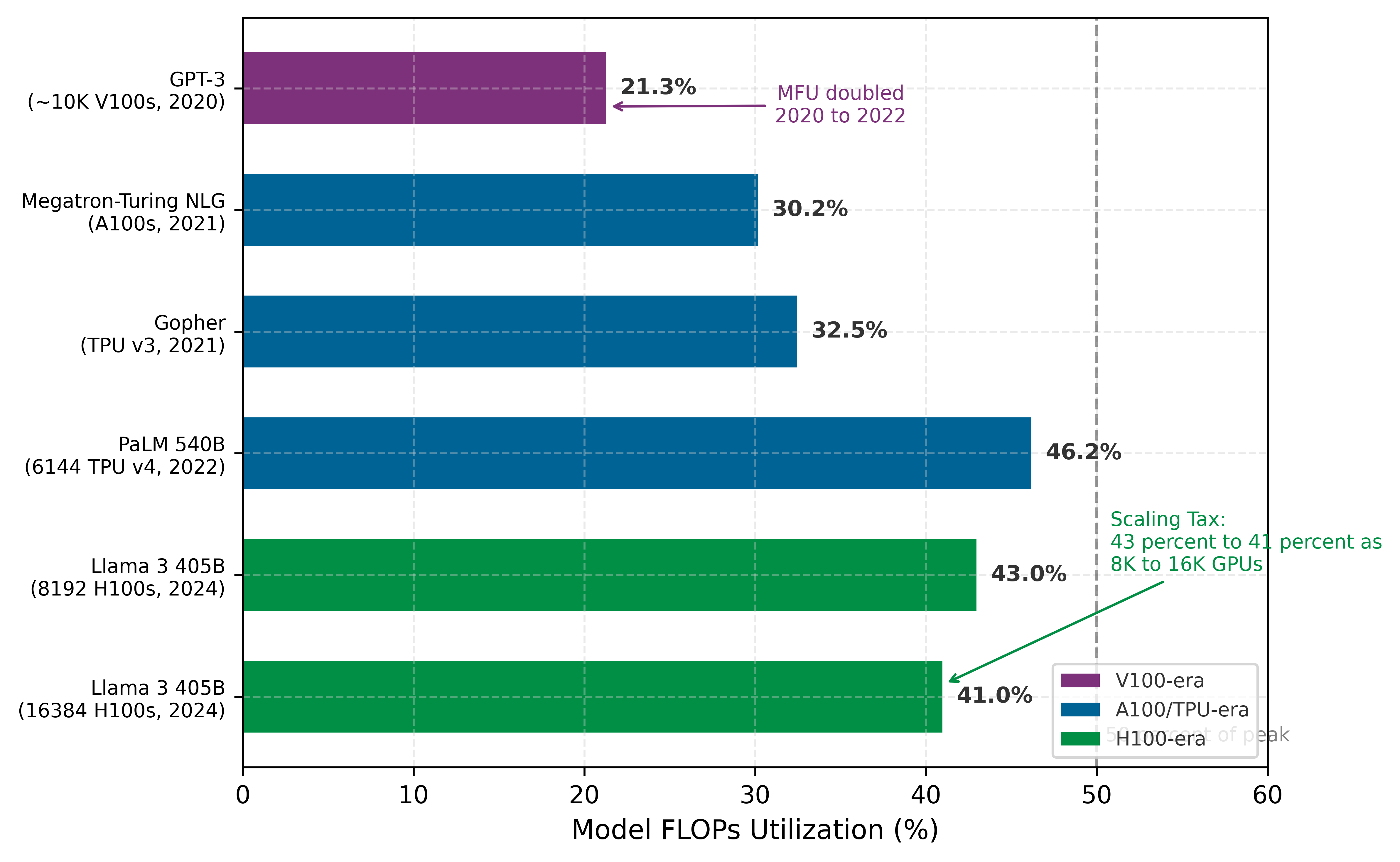
Chowdhery, Aakanksha, Sharan Narang, Jacob Devlin, Maarten Bosma, Gaurav Mishra, Adam Roberts, Paul Barham, et al. 2022. “PaLM: Scaling Language Modeling with Pathways.” arXiv Preprint arXiv:2204.02311.
Dubey, Abhimanyu, Abhinav Jauhri, Abhinav Pandey, Abhishek Kadian, et al. 2024. The Llama 3 Herd of Models. arXiv preprint arXiv:2407.21783.
Self-Check: Question
A frontier training configuration runs TP=8, PP=16, and DP=128. If the team doubles DP from 128 to 256 while keeping TP=8 and PP=16 fixed, the cluster grows from 16,384 to 32,768 GPUs. Which communication domain’s traffic volume grows most directly as a result?
- The intra-node tensor-parallel AllReduce volume per block, because TP groups are now tied together across the full fleet
- The pipeline-stage activation transfer volume per microbatch, because each microbatch now crosses twice as many stage boundaries
- The cluster-wide data-parallel gradient-synchronization collective, because the number of DP replicas whose gradients must be averaged has doubled
- The expert-routing all-to-all volume, because DP scaling implicitly increases the number of experts in an MoE layer
Which placement of the three parallelism axes onto a typical cluster hierarchy (GPU, NVLink-connected node, InfiniBand-connected pod, cross-pod pool) best follows the bandwidth-matching principle?
- Tensor parallelism within an NVLink-connected node, pipeline parallelism across InfiniBand-connected nodes, data parallelism across the broadest pod-level domain
- Data parallelism within an NVLink-connected node, tensor parallelism across InfiniBand pods, pipeline parallelism confined inside a single GPU’s streaming multiprocessors
- Pipeline parallelism within a single streaming multiprocessor, tensor parallelism across Ethernet racks, data parallelism only across CPU hosts
- All three parallelism dimensions spread uniformly across every network layer to maximize architectural symmetry
Explain why frontier-scale training (e.g., a 1T-parameter dense transformer) cannot be solved by pure data parallelism or pure model parallelism alone, and how hybrid parallelism resolves the constraints that each pure strategy leaves open.
In a hybrid 3D training step that runs TP within nodes, PP across nodes, and DP across pods, which communication pattern is the single largest once-per-global-step burst in aggregate traffic volume across the cluster?
- The tensor-parallel intra-layer AllReduce inside each transformer block, because it runs twice per block at the highest frequency
- The pipeline-stage activation transfer, because it crosses slower inter-node links at moderate volume
- The data-parallel gradient AllReduce across all replicas at the end of the step, whose tensor size equals the full model’s gradient and spans the entire cluster
- The sparse embedding-server pull for KV-cache lookups, which scales with sequence length during generation
True or False: Reducing pipeline parallelism from PP=16 to PP=8 can improve utilization by shrinking the pipeline bubble, but this redesign is only valid if the model still fits within the doubled per-stage memory footprint.
Blackwell-era accelerators offer roughly double the previous NVLink bandwidth per GPU and introduce faster die-to-die interconnects. Explain how these hardware changes shift the optimal 3D parallelism mix for a 400B-parameter model, and identify the new bottleneck.
Multi-Model Training: RLHF and Alignment
The parallelism strategies examined so far assume a single model being trained on a single objective. Reinforcement Learning from Human Feedback (RLHF) and its variants break this assumption by requiring multiple models to coordinate within a single training loop, each with different memory footprints, compute profiles, and gradient requirements. At a high level, RLHF generates model outputs, scores them with preference-derived reward signals, regularizes updates against a reference model, and then updates the policy; Proximal Policy Optimization (PPO) implements this online loop with separate policy, reference, reward, and value models, while Direct Preference Optimization (DPO)-style methods remove much of that rollout and value-model machinery. This creates a heterogeneous fleet management problem that cannot be solved by any single parallelism strategy and represents a qualitatively different distributed systems challenge from standard pretraining.
The multi-model coordination problem
Standard pretraining involves one model, one loss function, and one gradient stream. RLHF alignment, by contrast, orchestrates a system of models that interact during every training step. In Proximal Policy Optimization (PPO) (Schulman et al. 2017), as used in InstructGPT-style RLHF systems (Ouyang et al. 2022), four distinct models must operate in concert. Table 7 separates those models by role, execution mode, and memory burden.
Schulman, John, Filip Wolski, Prafulla Dhariwal, Alec Radford, and Oleg Klimov. 2017. “Proximal Policy Optimization Algorithms.” arXiv Preprint arXiv:1707.06347, ahead of print. https://doi.org/10.48550/arXiv.1707.06347.
Ouyang, L., J. Wu, X. Jiang, D. Almeida, C. L. Wainwright, P. Mishkin, C. Zhang, et al. 2022. “Training Language Models to Follow Instructions with Human Feedback.” Advances in Neural Information Processing Systems 35 35: 27730–44. https://doi.org/10.52202/068431-2011.
| Model | Role in PPO-style RLHF | Execution mode | Memory burden |
|---|---|---|---|
| Policy model | The model being aligned and optimized. | Training mode with gradients, optimizer moments, and activations. | For a 70B parameter model in mixed precision with Adam, memory is approximately 70B \(\times\) (2 \(+\) 2 \(+\) 12) = 1,120 GB, the same budget as standard pretraining. |
| Reference model | A frozen copy of the pretrained policy that supplies the KL-divergence penalty. | Inference mode only. | FP16/BF16 parameters without gradients or optimizer state; a 70B model needs about 70B \(\times\) 2 = 140 GB, roughly 8\(\times\) less than the training configuration. |
| Reward model | A preference-trained scorer that produces scalar rewards for generated sequences. | Inference mode only. | Often smaller than the policy; a 13B reward model requires approximately 26 GB in FP16, but it must process every generated sequence. |
| Value model | The PPO critic that estimates expected future reward. | Training mode, either separate or sharing a policy backbone. | A full-size separate critic can add another 1,120 GB; smaller models or shared-backbone designs reduce this to 200–400 GB. |
The aggregate memory demand of the four-model PPO system dwarfs standard pretraining. A naive co-location of a 70B policy, 70B reference, 13B reward, and 13B value model requires approximately 1,494 GB of accelerator memory, before accounting for the KV caches and intermediate activations generated during sequence generation. On H100 GPUs with 80 GB of HBM each, this system requires a minimum of 19 GPUs for parameter storage alone. Once generation-phase KV caches (which grow linearly with output sequence length) and training-phase activations are included, the practical minimum rises to 64–128 GPUs for a single RLHF training instance.
Infrastructure asymmetry: Training vs. inference models
The defining infrastructure challenge of RLHF is not the total memory footprint but the asymmetry between the models’ compute profiles. The policy and value models require full backward passes with gradient computation, activation checkpointing, and optimizer updates—compute-intensive operations that benefit from tensor parallelism and high arithmetic intensity. The reference and reward models, by contrast, perform only forward passes: they are inference workloads embedded within a training loop, with memory access patterns dominated by KV cache management rather than gradient accumulation.
The asymmetry creates a placement dilemma. Co-locating training and inference models on the same GPUs wastes compute during the generation phase (when the training models sit idle) and wastes memory during the gradient phase (when the inference models’ parameter storage could be reclaimed for activations). Separating them onto dedicated GPU pools eliminates waste but introduces network latency for reward queries—each generated token batch must traverse the interconnect to reach the reward model and return a scalar signal before the policy gradient can be computed.
The generation phase itself introduces a sequential bottleneck absent from standard pretraining. RLHF requires the policy model to generate complete sequences (typically 256–2,048 tokens) autoregressively before computing rewards and policy gradients. Autoregressive generation is memory bandwidth bound, not compute bound: each token requires a full forward pass through the model to produce a single output token. For a Llama-2-70B-style grouped-query attention policy, the KV cache grows by approximately \(2 \times N_L \times H_{\text{KV}} \times d_{\text{head}} \times 2\) bytes per generated token per sequence. With 80 layers, 8 KV heads, 128-dimensional heads, 1,024 generated tokens, and a batch of 256 prompts, the cache consumes 85.9 GB: \(2 \times 80 \times 8 \times 128 \times 1024 \times 256 \times 2\) bytes. A dense multi-head attention model using the full 8,192-wide hidden state for K and V would yield 687.2 GB. Even with GQA, the cache uses about one H100 GPU’s worth of HBM for intermediate attention state that is discarded after reward computation.
RLHF systems address this asymmetry through temporal multiplexing. During the generation phase, the cluster behaves like an inference system: the policy model generates sequences while the reference model computes log-probabilities, and the dominant resource is HBM reserved for token-by-token attention state. During the training phase, the same fleet switches back to training mode: gradients are computed through the policy and value models using the 3D parallelism configuration developed earlier in the chapter. Serving systems handle that phase with request batching and KV-cache placement; here, the important point is the mode switch. RLHF is not one steady training loop, but an alternation between inference-shaped work and training-shaped work, and standard training frameworks rarely manage that transition by themselves.
DPO: Simplifying the fleet
Direct Preference Optimization (DPO) (Rafailov et al. 2023) eliminates the reward model and value model entirely by reformulating the alignment objective as a classification loss over preference pairs. Instead of generating sequences, computing rewards, and estimating advantages, DPO directly optimizes the policy to assign higher log-probability to preferred responses over dispreferred ones, using the reference model only to compute a KL-divergence regularization term.
Rafailov, R., A. Sharma, E. Mitchell, S. Ermon, C. D. Manning, and C. Finn. 2023. “Direct Preference Optimization: Your Language Model Is Secretly a Reward Model.” Advances in Neural Information Processing Systems (NeurIPS) 36: 53728–41. https://doi.org/10.52202/075280-2338.
The infrastructure implications are substantial. DPO reduces the multi-model system from four models to two: the policy model (training mode) and the reference model (inference mode). For the 70B policy with 13B reward and value models quantified below, static parameter memory drops from about 1,494 GB to 1,260 GB, a 16 percent reduction. If the PPO value model is policy-sized, the reduction is much larger: about 2,406 GB to 1,260 GB, or roughly 48 percent. DPO also eliminates the autoregressive generation phase entirely. Training operates on a fixed dataset of (prompt, preferred response, dispreferred response) triples, restoring the standard pretraining data pipeline: fixed-length sequences, deterministic batching, and no sequential token-by-token generation. The training loop becomes a standard supervised learning step with a modified loss function, amenable to the same 3D parallelism, gradient accumulation, and communication overlap techniques used for pretraining.
The trade-off is capability. DPO operates on a static preference dataset, meaning the policy cannot explore new responses and receive feedback during training. PPO’s online generation allows the policy to improve iteratively on its own outputs, potentially discovering better strategies that the static dataset does not contain. For deployment scenarios where the preference data comprehensively covers the target distribution, DPO’s infrastructure simplification dominates. For scenarios requiring adaptive exploration (training models to solve novel reasoning tasks, for example), PPO’s online feedback loop may justify the 2\(\times\) infrastructure overhead.
Quantitative analysis: PPO vs. DPO resource requirements
To make the infrastructure trade-off concrete, consider aligning a 70B policy model on a cluster of 256 H100 GPUs (80 GB HBM each).
Napkin Math 1.9: RLHF infrastructure budget: PPO vs. DPO
Problem: Aligning a 70B policy model requires co-locating it with a 70B reference model and, for PPO, a 13B reward model and a 13B value model. Under 3D parallelism (TP=8 GPUs, PP=4, DP=8), how much per-GPU memory does each approach consume, and how much headroom does DPO free by eliminating the reward model, value model, and generation-phase KV cache?
Table 8: PPO vs. DPO Memory and MFU: Per-GPU memory and effective training MFU for PPO and DPO on the same accelerator budget.
PPO memory budget (per-GPU, with TP=8 GPUs, PP=4, DP=8 for policy)
The policy model under 3D parallelism with TP=8 GPUs and PP=4 distributes its 1,120 GB training state across 32 GPUs, yielding 35 GB per GPU. The reference model, requiring only 140 GB for inference, can be sharded across a separate pool of 8 GPUs at 17.5 GB each, or co-located with the policy GPUs at an additional 4.4 GB per GPU (140 GB / 32 GPUs). The 13B reward model adds 26 GB shared across its pool. The 13B value model in training mode adds approximately 208 GB (13B \(\times\) 16 bytes/param) across its pool.
Total static memory (co-located policy + reference on 32 GPUs): 35 GB + 4.4 GB \(\approx\) 39.4 GB per GPU, leaving \(\sim\) 40.6 GB for activations and KV cache. With generation-phase KV caches for a rollout batch containing 256 sequences and 1,024 tokens inside one \(TP{\times}PP\) policy replica, each policy GPU must reserve an additional 85.9 GB/32 GPUs \(\approx\) 2.7 GB for its KV cache shard. The remaining \(\sim\) 37.9 GB constrains the micro-batch size during the training phase.
DPO Memory Budget (same parallelism configuration)
The policy model uses the same 35 GB per GPU. The reference model adds 4.4 GB per GPU (co-located). No reward model, no value model, no KV cache for generation.
On the policy GPUs, total static memory is 35 GB + 4.4 GB = 39.4 GB per GPU, identical to PPO’s co-located policy/reference footprint. Cluster-wide, however, DPO avoids the PPO reward and value model memory, and it also removes the generation-phase KV cache burden. The full \(\sim\) 40.6 GB remaining on each policy GPU is available for training activations, permitting modestly larger micro-batches (about 1.07× under this co-located policy/reference memory budget) or reducing the need for activation checkpointing that PPO requires.
Throughput Comparison
PPO’s two-phase design (generate then train) introduces a fundamental throughput penalty. If generation consumes 60 percent of the step time (typical for autoregressive decoding of long sequences), the training hardware achieves only 40 percent utilization during an RLHF step. DPO, operating as a standard training loop, achieves the same 40 percent–55 percent MFU as pretraining. Table 8 compares the two regimes side by side.
| Metric | PPO (70B policy) | DPO (70B policy) |
|---|---|---|
| Models required | 4 (policy, ref, reward, value) | 2 (policy, reference) |
| Total parameter memory | \(\sim\) 1,494 GB | \(\sim\) 1,260 GB |
| Minimum GPUs (memory) | 64–128 GPUs | 32–64 GPUs |
| Generation phase | Yes (sequential, BW-bound) | None |
| Effective training MFU | 15–25% | 40–55% |
| Data pipeline | Online generation | Static preference pairs |
Systems insight: In this 13B reward/value-model scenario, DPO reduces static parameter memory by 15.7 percent and doubles the effective compute utilization by eliminating the reward model, value model, and autoregressive generation phase. The choice between PPO and DPO is not only a modeling preference but an infrastructure constraint: organizations with limited GPU budgets may prefer DPO because it restores the workload to a fixed-data training loop. If the PPO value model is policy-sized rather than 13B, the memory reduction approaches the larger 2,406 GB to 1,260 GB comparison discussed earlier.
Sequence length variance and batching challenges
Both PPO and DPO face a data engineering challenge absent from standard pretraining: extreme variance in sequence length. Pretraining typically uses fixed-length sequences (2,048 or 4,096 tokens, padded or packed to fill each position), enabling uniform batch shapes and predictable memory consumption. RLHF training data consists of variable-length prompts (10–500 tokens) concatenated with variable-length completions (50–2,048 tokens), producing sequence lengths with 10–50\(\times\) variance within a single batch.
Length variance creates two interacting problems. Fixed-size batching pads all sequences to the maximum length in the batch, wasting compute on padding tokens. A batch containing one 2,048-token sequence and fifteen 128-token sequences wastes 88 percent of the compute on padding. Dynamic batching groups sequences by similar length to minimize padding, but introduces load imbalance across data-parallel workers: one worker may receive a batch of long sequences consuming 60 GB of activation memory while another processes short sequences using only 8 GB, causing the short-sequence worker to stall at the synchronization barrier while the long-sequence worker completes.
RLHF systems mitigate this through a combination of sequence packing (concatenating multiple short sequences into a single fixed-length input with attention masking to prevent cross-contamination) and adaptive micro-batching (dynamically adjusting the number of sequences per micro-batch based on the aggregate token count rather than the sequence count). These techniques can recover much of the compute lost to padding variance but add complexity to the data pipeline that standard pretraining frameworks do not provide. The interaction between variable-length data and distributed synchronization remains an active area of systems engineering research, because every worker must process the same number of tokens per step to maintain gradient consistency.
RLHF is therefore not a detour from parallelism strategy; it is the case that shows why no strategy is sufficient by itself. The policy model may need tensor and pipeline parallelism, the reference and reward models behave like inference services, the value model may require training state, and the rollout data pipeline changes shape from step to step. With that stress test in view, the final comparison can return to the general engineering question: identify the binding constraint first, then choose the parallelism pattern that moves the least data while fitting the required state.
Self-Check: Question
In PPO-style RLHF with four models (policy, reference, reward, value), which pair requires full training-mode state — parameters plus gradients plus optimizer moments plus activations — as opposed to inference-only parameter storage?
- Reference model and reward model, because both compute scalar signals that the policy uses during updates
- Policy model and value model, because both have loss terms whose gradients are used to update their own parameters
- Policy model and reference model, because both are forward copies of the same pretrained network
- Value model and reward model, because both emit scalars and therefore need gradient flow to calibrate
Explain why RLHF creates an infrastructure-orchestration problem that standard pretraining does not, naming the two operating regimes a single RLHF step alternates between.
DPO roughly halves the GPU requirement compared to PPO for the same 70B policy model. What is the mechanism behind this reduction?
- DPO removes the policy model and trains only a reward classifier, which is much smaller than a full policy
- DPO eliminates the reward model and value model from the training fleet, and it also eliminates the online autoregressive rollout phase — both reducing memory and compute
- DPO retains all four models but shrinks each to INT4 precision, which makes the total footprint smaller
- DPO replaces distributed training with single-GPU fine-tuning, which trivially reduces cluster size
True or False: During PPO’s rollout phase, the system is memory-bandwidth-bound even on H100-class accelerators because each generated token requires a full forward pass over model state plus an ever-growing KV cache read.
RLHF training data has 10–50\(\times\) variance in sequence length within a single batch. Why does this variance create a distributed-batching problem that fixed-length pretraining does not face?
- Because every worker must use a different optimizer when prompt lengths differ across shards
- Because fixed-size batches pad every sequence to the batch maximum, wasting compute on padding, while dynamic length-based grouping creates load imbalance that forces workers on short sequences to stall at the synchronization barrier behind workers on long sequences
- Because variable-length inputs cannot be stored in KV caches, preventing any form of autoregressive decoding
- Because preference datasets cannot be sharded across workers at all, so scaling is impossible regardless of strategy
Parallelism Strategy Comparison
A parallelism strategy is useful only if it moves the binding constraint without creating a larger one. The feasibility filter previewed by the decision tree in section 1.0.5 named those constraints; now that tensor, pipeline, and hybrid parallelism have been developed, the same filter can be stated as engineering signals rather than a generic ranking. For a new 50-billion parameter model, the decisive questions are which memory state fits, how often communication occurs, where the pipeline bubble appears, and which abstraction cost the engineering team can tolerate. Table 9 turns those questions into engineering signals.
| Strategy | Binding constraint | Primary movement | Placement decision | Validation signal |
|---|---|---|---|---|
| DDP | Model state fits on one accelerator | AllReduce gradients every step | Replicate full model across data-parallel workers | Step time dominated by compute, not synchronization |
| FSDP/ZeRO | Model state exceeds one accelerator | Shard and gather parameters or optimizer state | Place shards to minimize gather and reduce-scatter cost | Peak memory remains below device budget |
| Tensor parallelism | One layer or tensor operation exceeds local capacity | AllReduce or AllGather within layer blocks | Keep tightly coupled partitions on fast intra-node links | Layer latency stays below activation handoff cost |
| Pipeline parallelism | Layer stack fits only when split by stage | Activations and gradients between stages | Balance stages so bubbles are smaller than useful work | Bubble fraction falls as microbatch count increases |
| Hybrid parallelism | More than one constraint binds at once | Multiple collectives on different axes | Align data, tensor, pipeline, and shard groups to topology | MFU improves without exceeding memory or network budget |
Figure 17 converts the same filter into a decision tree. It begins with memory fit because capacity failure is nonnegotiable, then asks whether data scale alone justifies replication. The tree is intentionally simplified; hardware heterogeneity, communication bandwidth, and workload imbalance enter as second-order checks after the binding constraint has been identified.

The table and flowchart are intentionally coarse, but their purpose is precise: identify the binding constraint before choosing the implementation stack.
Self-Check: Question
A 120B-parameter model exceeds the memory of any single 8-GPU NVLink node, the dataset exceeds any one machine’s storage, and the cluster is organized as 16 NVLink-connected nodes wired together by InfiniBand. Pure pipeline parallelism fits the model across nodes but yields only 35 percent MFU because the microbatch count is small. FSDP-only data parallelism still exhausts activation memory at the batch sizes needed for good throughput. Which strategy is the best next step, and why does it beat each tempting alternative?
- Pure tensor parallelism across all 128 GPUs, because it shards everything most aggressively regardless of interconnect topology
- Hybrid parallelism: tensor parallelism within each NVLink node, pipeline parallelism across the InfiniBand-connected nodes, and data parallelism across replica groups — each axis placed where the interconnect supports its communication pattern
- Pure pipeline parallelism with more microbatches, because any bubble problem is always solvable purely by increasing microbatch count
- FSDP-only data parallelism with aggressive gradient accumulation, because sharding always substitutes for model parallelism when memory is tight
Explain why implementation complexity is substantially higher for hybrid parallelism than for plain data parallelism, and name two concrete engineering responsibilities that hybrid adds.
True or False: Communication overhead, memory requirement, scalability, and implementation complexity are interdependent design dimensions, so no single parallelism strategy dominates all others for every workload — strategy choice is constraint-driven rather than a universal ranking.
From Principles to Systems
Choosing DDP, FSDP/ZeRO-style sharding, tensor parallelism, or pipeline parallelism is a decision about which constraints the runtime owns and which constraints the engineer must manage directly. The parallelism strategies examined throughout this chapter (gradient averaging, AllReduce synchronization, tensor splitting, pipeline scheduling) translate into deployed training systems through this layered abstraction hierarchy.
At the data-parallel layer, the simplest distributed training abstraction wraps a model so that the framework automatically replicates it across available accelerators, splits each batch, and averages gradients after the backward pass. Historically, parameter-server systems organized this work with server nodes that store shared parameters while workers push and pull updates (Li et al. 2014). As section 1.4.3 established, that design concentrates gradient bandwidth at the server tier, so dense synchronous training favors the decentralized collectives below.
Li, M., D. G. Andersen, J. W. Park, A. J. Smola, A. Ahmed, V. Josifovski, J. Long, E. J. Shekita, and B.-Y. Su. 2014. “Scaling Distributed Machine Learning with the Parameter Server.” Proceedings of the 2014 International Conference on Big Data Science and Computing, 583–98. https://doi.org/10.1145/2640087.2644155.
Large-scale data parallelism eliminates this bottleneck by replacing the central server with decentralized AllReduce. Each worker participates symmetrically in the reduction: every device both sends and receives gradient chunks at its own link rate, distributing the bandwidth load across all nodes rather than concentrating it. The framework initializes a process group that maps workers to the physical topology, selects an appropriate collective algorithm (ring, tree, or hierarchical) based on the detected interconnect, and inserts gradient synchronization hooks into the backward pass automatically. Gradient bucketing further improves efficiency by grouping small tensors into larger messages before transmission, and computation-communication overlap allows the AllReduce for early layers to proceed while later layers are still computing gradients. These optimizations can reach high parallel efficiency at moderate scale—not because the API is simple, but because the underlying runtime makes topology-aware decisions that a manual implementation would otherwise need to reproduce.
Model and pipeline parallelism require a fundamentally different abstraction because the framework must manage cross-device tensor placement and the sequential data flow between partitions. The core principle is explicit device assignment: the engineer specifies which layers reside on which devices, and the framework handles the activation transfers between devices during the forward pass and the gradient flow in reverse during backpropagation. Explicit device assignment makes the sequential dependencies of model parallelism visible, since each downstream device must wait for its upstream neighbor to complete. The engineer must reason about pipeline bubbles and load balance at the architecture level rather than hiding them behind an opaque wrapper.
For large-scale model parallelism, the key architectural insight is that tensor splitting and pipeline scheduling require different levels of framework support. Tensor parallelism replaces standard linear layers with column-parallel and row-parallel variants that automatically insert AllReduce operations at the correct points in the transformer computation graph, as described in section 1.4.2.3. Pipeline parallelism adds microbatch scheduling logic that interleaves forward and backward passes across stages to minimize bubble overhead. Memory-efficient sharding integrates ZeRO-3 style parameter partitioning by wrapping model layers with automatic AllGather operations before each forward pass and ReduceScatter after each backward pass. The critical design decision is which abstraction levels to compose: pure data parallelism suffices when the model fits in memory, memory-efficient sharding extends data parallelism to memory-constrained regimes, and full tensor or pipeline parallelism becomes necessary when individual layers or the full model depth exceed single-device capacity.
Across these abstraction layers, distributed training ultimately reduces to a small set of collective communication primitives. Rather than exploring the network mechanics of how these primitives physically route data across the cluster, which is extensively covered in Collective Communication, framework abstractions focus on when and why these primitives are invoked.
The primitives compose into the communication patterns that define each parallelism strategy. Data parallelism uses one AllReduce per training step. Full-shard FSDP with resharding uses about \(3N_L\) collectives per step (two AllGathers and one ReduceScatter for each of \(N_L\) layers). Tensor parallelism uses 2 AllReduce operations per transformer block on the critical path. The choice of primitive, its message size, and its frequency relative to computation determine whether the system operates in the compute-bound or communication-bound regime. No framework abstraction changes the underlying physics: the efficiency of distributed training ultimately depends on physical interconnect bandwidth, memory capacity, and synchronization latency.
Self-Check: Question
A framework exposes a one-line wrapper (for example, DistributedDataParallel in PyTorch) that appears to make data parallelism trivial at the API level, yet the underlying runtime remains complex. Which set of runtime responsibilities is the wrapper hiding?
- No runtime work at all — data parallelism really is topology-agnostic once the wrapper is applied, because AllReduce is deterministic
- Selecting collective algorithms based on detected topology, bucketing small gradients into larger messages, and overlapping backward-pass computation with concurrent AllReduce calls
- Recompiling the model to a different mathematical form suited to distributed execution, because distributed training is algorithmically distinct from single-GPU training
- Rewriting the optimizer to replace SGD with parameter-server pushes, because AllReduce cannot implement standard optimizers
Explain why model parallelism and pipeline parallelism require more explicit framework abstractions than ordinary data parallelism, and what structural knowledge the engineer must provide to use them.
Consider one full forward-and-backward pass of a single transformer layer under FSDP. Before the forward pass, each GPU holds only its shard of the layer’s parameters. Which pair of collective primitives must the runtime execute, and in which positions, to complete the layer?
- AllGather the sharded parameters to every GPU before the forward pass, then run forward and backward, then ReduceScatter the gradient shards so each GPU ends the step holding only its piece of the averaged gradient
- ReduceScatter the parameters before forward, then AllGather the gradients after backward, inverting the canonical FSDP order
- AllReduce the parameters before forward and AllReduce the gradients after backward, with no AllGather or ReduceScatter needed
- Broadcast the parameters from rank 0 before forward and Scatter the gradient shards after backward, replacing both collectives with point-to-point sends
Fallacies and Pitfalls
Many engineering teams who scale cluster capacity by \(4\times\) find that their training iterations take longer to complete, reflecting a fundamental misunderstanding of distributed training physics. The following misconceptions capture errors that waste compute resources and delay research.
Fallacy: Linear speedup is achievable with sufficient engineering effort.
Amdahl’s Law establishes hard limits: any sequential component bounds maximum speedup regardless of parallelism. In distributed training, gradient synchronization is inherently sequential since all gradients must be collected before any update proceeds. As section 1.3 demonstrates, the scaling efficiency equation \(\eta_{\text{scaling}} = 1/(1 + N(T_{\text{comm}}(N) + T_{\text{sync}}(N) - T_{\text{overlap}})/T_{\text{compute}})\) reveals how communication and synchronization overhead dominate as \(N\) increases. Even with perfect overlap and ideal algorithms, communication overhead grows with cluster size. For data parallelism, AllReduce time increases logarithmically with tree algorithms or linearly in the latency term with ring algorithms as GPU count grows. A 1000-GPU cluster will never train 1000\(\times\) faster than a single GPU; achieving 500\(\times\) speedup would be exceptional, and 100–200\(\times\) is more typical for communication-heavy workloads. Organizations that budget projects assuming linear scaling inevitably miss deadlines and overspend on compute.
Pitfall: Optimizing MFU without considering scaling efficiency.
A team achieves 50 percent MFU on a single node, scales to 1,024 GPUs, and expects 512 GPU-equivalents of useful work. Scaling efficiency at 1,024 GPUs can be near 50 percent for communication-heavy workloads, so actual useful throughput is roughly \(0.50 \times 0.50 = 0.25\) of peak, or 256 GPU-equivalents: half the expected value. MFU and scaling efficiency are independent multiplicative factors. Optimizing one without measuring the other produces capacity estimates that are off by 2\(\times\) or more. Capacity planning at fleet scale requires reporting both metrics together and tracking their product as “useful goodput.”
Fallacy: Hyperparameters tuned on small clusters transfer directly to large-scale training.
Engineers tune hyperparameters on 8-GPU workstations then deploy to 256-GPU clusters expecting identical behavior. At scale, convergence patterns change fundamentally. The most critical hyperparameter is learning rate: as section 1.2 explains, batch size increases proportionally with GPU count in data parallelism, requiring learning rate adjustments. The “linear scaling rule”10 (Goyal et al. 2017) suggests \(\eta_{\text{large}} = \eta_{\text{base}} \times (B_{\text{large}}/B_{\text{base}})\), but this relationship holds only within bounds. As models scale, they eventually encounter the critical batch size11, where adding more data per step yields diminishing returns in convergence.
10 Linear Scaling Rule: Established by Goyal et al. (2017) at Facebook AI Research, who trained ResNet-50 on ImageNet in one hour across 256 GPUs with a batch size of 8,192 while matching small-batch accuracy. The rule – multiply learning rate by \(k\) when batch size increases by \(k\) – works only while the large-batch approximation remains valid. Above the workload’s measured critical-batch-size regime, gradient noise drops below the useful signal scale and additional parallelism yields diminishing convergence returns (McCandlish et al. 2018; Shallue et al. 2019).
Goyal, Priya, Piotr Dollár, Ross Girshick, Pieter Noordhuis, Lukasz Wesolowski, Aapo Kyrola, Andrew Tulloch, Yangqing Jia, and Kaiming He. 2017. “Accurate, Large Minibatch SGD: Training ImageNet in 1 Hour.” arXiv Preprint arXiv:1706.02677 abs/1706.02677.
Shallue, Christopher J, Jaehoon Lee, Joseph Antognini, Jascha Sohl-Dickstein, Roy Frostig, and George E Dahl. 2019. “Measuring the Effects of Data Parallelism on Neural Network Training.” Journal of Machine Learning Research 20: 1–49.
11 Critical Batch Size: The gradient-noise-scale view introduced by McCandlish et al. treats the largest useful batch size as a measurable statistic that varies by domain, model, optimizer, and training phase (McCandlish et al. 2018). Scaling beyond that measured point improves hardware throughput but does not proportionally reduce the number of optimization steps needed to reach target quality, collapsing the scaling efficiency \((\eta_{\text{scaling}})\).
McCandlish, Sam, Jared Kaplan, Dario Amodei, and OpenAI Dota Team. 2018. “An Empirical Model of Large-Batch Training.” arXiv Preprint arXiv:1812.06162, ahead of print. https://doi.org/10.48550/arXiv.1812.06162.
Beyond the critical batch size, this relationship breaks down in a model-, data-, and optimizer-dependent way. A team that takes a small-cluster learning rate, multiplies it mechanically with GPU count, and jumps directly to a much larger global batch may see lower final quality or slower sample efficiency even though hardware throughput improved. Warmup schedules, weight decay adjustment, layer-wise optimizers such as LARS/LAMB, and careful momentum tuning can recover accuracy in some regimes, but require systematic experimentation at target scale. Organizations that skip these scaling studies waste thousands of GPU-hours on suboptimal runs.
Pitfall: Adding GPUs to data-parallel jobs without modeling communication.
Engineers assume more GPUs always accelerate training. At scale, statistical efficiency limits overwhelm hardware gains. As section 1.2 establishes, data parallelism increases effective batch size proportionally with GPU count \((B_{\text{total}} = N \times B_{\text{local}})\), but gradient quality grows sublinearly beyond model-specific thresholds. A 100K-sample batch may provide only 2\(\times\) the gradient information of a 10K-sample batch, not 10\(\times\), because samples become redundant within the loss landscape. The critical batch size defines where marginal returns collapse: the chapter’s earlier examples put ResNet-50 around 8K–16K and BERT-Large around 32K–65K, with exact thresholds depending on optimizer, schedule, and target quality. Beyond this threshold, doubling GPU count doubles cost but provides minimal convergence acceleration. In a representative cost model, a 1024-GPU run that converges in 18 hours at $45,000 compute cost may be worse than a 512-GPU run that converges in 19 hours at $22,000, demonstrating how exceeding critical batch size wastes resources without meaningful time savings.
Fallacy: Memory capacity alone determines the parallelism strategy.
Engineers see that a 70B model exceeds 80 GB memory and immediately choose tensor parallelism or pipeline parallelism to split weights. In a deployed run, the effective strategy depends on the interaction between memory pressure, computation patterns, and communication topology. As section 1.8 explains, tensor parallelism splits each layer across devices with AllReduce synchronization per layer, achieving even memory distribution but placing communication on the critical path. Pipeline parallelism assigns complete layers to stages with point-to-point transfers between stages, reducing per-step communication but introducing pipeline bubble overhead that wastes 10–30 percent of cycles. For a 175B model on 64 A100 GPUs where tensor parallelism degree-8 enables training, pipeline parallelism with 8 stages achieves 23 percent higher throughput due to reduced all-to-all communication despite similar memory footprints. The decision requires profiling communication patterns and bubble overhead, not just checking if weights fit in memory.
Pitfall: Applying FSDP or ZeRO without measuring efficiency trade-offs.
Engineers adopt FSDP universally after reading that it “reduces memory and enables larger models”. In a deployed run, sharding introduces 10–25 percent communication overhead that only pays off when memory pressure justifies it. FSDP reduces memory footprint by sharding optimizer state, gradients, and optionally parameters across GPUs, but requires AllGather operations before each forward pass and ReduceScatter after backward pass. For a 7B model on A100-80 GB with batch size 4, standard DDP achieves 145 samples/second while FSDP achieves only 118 samples/second (19 percent slower) because the model fits comfortably without sharding and the added communication overhead provides no benefit. FSDP provides value when model plus optimizer state exceeds single-GPU memory, when enabling larger per-GPU batch sizes justifies the overhead, or when ZeRO-Offload to CPU memory extends capacity. A 65B model that cannot fit on 80 GB becomes trainable with FSDP ZeRO-3, accepting 15 percent throughput loss to enable training at all. Applying FSDP universally without measuring memory pressure wastes performance.
Fallacy: Parallelism overhead is roughly constant regardless of model size.
Engineers benchmark parallelism strategies on convenient small models then apply conclusions to large-scale training. At scale, the ratio between computation and communication time changes dramatically with model size, inverting strategic decisions. AllReduce communication time depends primarily on gradient tensor size and network bandwidth, growing roughly linearly with parameter count, while forward and backward pass computation time grows superlinearly due to larger matrix operations. For a 1B parameter model where forward/backward pass takes 50 ms and AllReduce takes 25 ms, communication overhead consumes 33 percent of step time. For a 70B parameter model where forward/backward takes 2400 ms and AllReduce takes 180 ms, communication overhead drops to 7 percent despite the gradient size being 70\(\times\) larger. Decisions made on small models (“pipeline parallelism’s 15 percent bubble overhead makes it always slower than data parallelism”) can invert at scale where data parallelism’s communication overhead reaches 25–40 percent. Reliable strategy selection requires either profiling at target scale or analytical models that account for how computation scales as \(\mathcal{O}(n^2)\) to \(\mathcal{O}(n^3)\) while communication scales as \(\mathcal{O}(n)\).
Pitfall: Treating scaling efficiency as a property of the hardware alone.
Vendor benchmarks publish “85 percent scaling efficiency at 1,024 GPUs” and procurement teams plan capacity as if that number is a cluster constant. Scaling efficiency is a joint property of four things: the workload’s communication-to-computation ratio, the parallelism strategy (data, pipeline, tensor, hybrid), the network topology (fat-tree vs. torus vs. dragonfly), and the software stack (NCCL version, kernel fusion, overlap quality). Reference numbers from large-language-model training benchmarks may overstate scaling for graph neural networks with irregular communication, and they may understate scaling for embedding-heavy recommendation models with mostly local computation. Capacity planning should use measured scaling on the target workload, not a vendor hero benchmark.
Fallacy: Gradient accumulation is free.
Engineers use gradient accumulation to simulate larger batch sizes, reducing synchronization frequency from every step to every \(K\) steps. The technique appears cost-free since it eliminates \((K-1)/K\) of synchronization events. In a real training loop, accumulation introduces update latency, memory-residency, and numerical precision risks. Standard implementations accumulate into one resident gradient buffer rather than allocating a separate full gradient tensor per microstep; for a 7B model, that FP16 gradient buffer is still 14 GB and must remain live throughout the accumulation window. If the implementation retains computation graphs, overlaps multiple outstanding microbatches, or increases local microbatch size, activation memory can grow further and exhaust HBM. Effective optimizer-step latency increases proportionally with accumulation steps, so accumulating 8 steps means optimizer updates occur 8\(\times\) less frequently, potentially slowing convergence despite higher throughput. Most critically, accumulated FP16 gradients risk overflow when summing hundreds of gradient tensors, particularly in early training when loss values are large. A team training a transformer model with 16-step gradient accumulation in FP16 experienced loss spikes and divergence at step 1200; switching to 4-step accumulation with more frequent synchronization resolved the instability despite higher communication costs. Gradient accumulation trades communication frequency for update latency, memory residency, and numerical stability.
Pitfall: Using fixed checkpoint intervals regardless of system characteristics.
Engineers checkpoint distributed training “every hour” or “every 1000 steps” based on intuition rather than analysis. Fault Tolerance derives the Young-Daly checkpoint law (principle 12); the training lesson here is that checkpoint cadence is not a constant. It depends on the mathematical relationship between checkpoint write cost and failure rate.
The formula sets the optimal checkpoint interval to \(\tau_{\text{opt}} = \sqrt{2 \cdot T_{\text{write}} \cdot \text{MTBF}_{\text{system}}}\), where \(T_{\text{write}}\) is checkpoint write time and \(\text{MTBF}_{\text{system}}\) is mean time between system failures. For a 1024-GPU cluster at the canonical 50,000-hour per-GPU MTBF, the cluster-level \(\text{MTBF}_{\text{system}}\) is 48.8 hours (\(\text{MTBF}_{\text{GPU}}/N\)). With a 5-minute checkpoint time, the optimal interval is approximately 171.2 minutes (~2.9 hours), with an unavoidable checkpoint-plus-rework tax of 5.8 percent. Checkpointing every 15 minutes “to be safe” raises the total tax to 33.6 percent, while checkpointing every 8 hours risks losing significant work on failure. For larger models where checkpoint time increases to 15 minutes due to model size and storage bandwidth, the optimal interval shifts again. The cost of guessing scales with the cluster: a 1024-GPU run loses approximately $13,638 per day to excessive checkpointing when it uses a 15-minute interval instead of the Young-Daly optimum.

The optimal checkpoint cadence balances write overhead against rework risk.
Self-Check: Question
Why is the claim ‘with enough engineering effort, linear speedup is achievable at any scale’ a fallacy in distributed training?
- Because GPU kernels cannot run in parallel once any communication begins on the same device
- Because Amdahl’s Law imposes a hard ceiling whenever any sequential synchronization fraction exists: speedup is bounded by 1 / (serial fraction) regardless of engineering polish
- Because only fully asynchronous training scales past 8 GPUs; synchronous SGD hits a wall before that
- Because distributed training always becomes memory-bound long before it becomes communication-bound
A team takes the hyperparameters (learning rate, warmup, momentum, weight decay) that worked on an 8-GPU run with global batch 512 and applies them unchanged to a 256-GPU run with global batch 16,384. Why is this unsafe, and what should they change?
When is adopting FSDP or ZeRO most justified over plain DDP, according to the chapter’s operational guidance?
- Whenever a model already fits comfortably under DDP, because sharding always increases throughput by reducing per-worker data movement
- Primarily when memory pressure is the binding constraint — the model or training state does not fit under DDP, or a larger useful batch size requires reclaimed memory for activations
- Only for inference serving, because training adds too many collectives to make sharding worthwhile
- Whenever the network fabric is slow, because FSDP eliminates inter-worker communication entirely
True or False: Gradient accumulation is effectively free because it only reduces synchronization frequency and has no important costs elsewhere.
A 1,024-GPU cluster has \(\text{MTBF}_{\text{system}}\) of 4 hours and a checkpoint write time \(T_{\text{write}}\) of 5 minutes. The Young-Daly formula gives an optimal checkpoint interval near \(\sqrt{2 T_{\text{write}} \text{MTBF}_{\text{system}}} \approx 49\) minutes. Which checkpoint policy best reflects this trade-off, and why do the tempting fixed-interval alternatives fail?
- Checkpoint every 5 minutes to match the checkpoint cost, because minimizing lost work is always the right objective
- Checkpoint only once per day, because checkpoint overhead always exceeds the cost of recomputation on modern hardware
- Choose an interval near the Young-Daly optimum (roughly 50 minutes for this cluster): the 5-minute policy spends half of elapsed time writing checkpoints, while the daily policy risks losing about 2 hours of work on average at each failure, and both extremes pay far more than the \(\sqrt{2 T_{\text{write}} \text{MTBF}_{\text{system}}}\) balance point
- Use a fixed 30-minute interval regardless of hardware, because optimal checkpointing does not depend on cluster size or checkpoint cost
Summary
This chapter introduced the “scaling wall”: the point where adding more GPUs eventually makes training slower rather than faster. Distributed training is not a simple hardware problem; it is a constraint satisfaction problem governed by the interaction between model size, batch size, and interconnect bandwidth.
The 3D Parallelism Cube (figure 18) is a useful framework for scaling large models. Data parallelism unrolls the outer loop of training to scale throughput; tensor parallelism vectorizes the inner loops of matrix multiplication to fit memory; and pipeline parallelism stages sequential layers to reduce communication frequency. Together, these strategies map models larger than any single memory bank onto a fleet of accelerators with finite bandwidth.

Ultimately, the choice of parallelism is a loop transformation applied by the cluster-level compiler. By matching logical communication patterns to physical hardware hierarchies, the system moves from the “linear scaling regime” of small clusters to the “communication-bound” reality of very large accelerator fleets.
Throughout this chapter, the partitioning strategies were developed directly for dense large-model training and recommendation-style workloads. Table 10 also shows how the same constraint logic reaches the federated edge case, where the bottleneck shifts from accelerator memory and fabric bandwidth to unreliable devices, privacy, and intermittent connectivity.
Lighthouse 1.3: Distributed archetype spectrum
The operating point in the 3D Parallelism Cube shifts depending on the system’s primary bottleneck:
| Archetype | Primary Partitioning Strategy | The Logic |
|---|---|---|
| Archetype A (GPT-4/Llama-3) | Hybrid 3D Parallelism | Combine Tensor (width), Pipeline (depth), and Data (throughput) to fit 3.5 TB of weights. |
| Archetype B (DLRM at Scale) | Embedding Sharding | Partition massive 10 TB+ tables across a Parameter Server fleet; use sparse AllToAll updates. |
| Archetype C (Federated MobileNet) | Federated Learning | The same logic extends to coordinating on-device MobileNet updates across unreliable, privacy-constrained edge devices; Edge Intelligence develops this regime. |
The parallelism strategies explored throughout this chapter (data, tensor, pipeline, and expert) provide the conceptual toolkit for partitioning any training workload across a cluster. The key insight is that these strategies are not mutually exclusive alternatives but complementary dimensions of a unified optimization space. Systems such as Megatron-LM achieve efficient scaling precisely because they combine multiple strategies, using tensor parallelism within nodes, pipeline parallelism across node groups, data parallelism for throughput, and expert parallelism for capacity scaling.
Key Takeaways: Parallelism relocates the tax
- Splitting work moves the bottleneck: Distributed training does not make the underlying computation smaller; it converts memory pressure into communication volume, synchronization delay, or idle pipeline time. The winning strategy is the split that sends overhead to the least binding part of the fleet.
- Data parallelism ends at convergence: Replicas scale throughput cleanly only while larger global batches still improve optimization. Past the critical batch size, AllReduce cost and reduced gradient noise turn “more workers” into slower or less stable learning unless schedules, warmup, and accumulation change.
- Sharding buys memory with messages: ZeRO and FSDP make 100B+ parameter models feasible by partitioning optimizer state, gradients, and parameters. The price is a stricter communication schedule of ReduceScatter and AllGather operations that must be overlapped or hidden.
- Tensor parallelism belongs near NVLink: Tensor parallelism splits matrix operations inside layers, so it needs the high-bandwidth intra-node fabric that A100 and H100 NVLink provide. Stretching that traffic across racks turns a memory-capacity solution into a communication bottleneck.
- Pipeline parallelism trades bytes for bubbles: Layer staging reduces communication frequency, but fill and drain slots leave accelerators idle. Microbatching with \(m \gg p\) is the mechanism that turns model depth into throughput rather than pipeline slack.
- The 3D cube is a hardware map: Real frontier training combines data, tensor, pipeline, expert, and sharded parallelism because no single axis fits the model and the fleet. Logical groups must map to HBM, NVLink, InfiniBand, and failure domains together.
Beneath the cube and its three axes lies a single trade. No way of splitting a model makes the underlying work smaller; each only moves it, turning a memory limit into a communication cost or a communication cost into idle time. Data, tensor, and pipeline parallelism spend communication to win the memory headroom no single accelerator has, and coordination is the tax paid to keep the split consistent. This is displacement of overhead, the law the rest of the volume turns on: the execution tax of scale cannot be removed, only relocated among compute, communication, and coordination. The cube is the map of where the tax can be sent; the engineering is choosing the destination that binds least.
What’s Next: From logic to traffic
We have defined the logical traffic patterns of the Machine Learning Fleet, the how of splitting the math. These logical patterns, however, eventually hit the physical wires of the data center. In Collective Communication, we open the black box of the collective operations (AllReduce, AllToAll) that make this consistency possible. We move from the logic of what to send to the mechanics of how to route it through rings, trees, and rails.
Self-Check: Question
What does the chapter identify as the main physical ceiling on distributed training speedup across all parallelism strategies?
- The communication-computation ratio and the mandatory synchronization cost it implies at each step
- The number of optimizer hyperparameters that must be tuned when batch size grows
- The inability of modern accelerators to execute matrix multiplications in parallel once collectives begin
- A structural constraint that only one parallelism strategy can be used in a single configuration
Why does the chapter describe data, tensor, and pipeline parallelism as loop transformations on the training loop rather than as unrelated engineering tricks?
Which archetype-to-strategy pairing best matches the chapter’s closing framework?
- Archetype A (GPT-4 / Llama-3 dense LLMs): hybrid 3D parallelism with TP inside nodes, PP across nodes, and DP across pods
- Archetype B (DLRM-scale recommendation): hybrid 3D parallelism on a single dense-transformer backbone, with no embedding sharding
- Archetype C (federated MobileNet on edge devices): tensor parallelism across a centralized datacenter cluster, ignoring device-local constraints
- Archetype A (GPT-4 / Llama-3 dense LLMs): parameter-server embedding sharding with no tensor or pipeline parallelism
Self-Check Answers
Self-Check: Answer
What structural property most fundamentally distinguishes distributed training from a stateless distributed web service that handles independent HTTP requests across many replicas?
- Distributed training requires every worker to maintain a consistent view of mutable model parameters, so gradient synchronization becomes a mandatory coordination step rather than an optional optimization
- Distributed training always uses strictly more machines than the web service, because neural networks never run on small clusters
- Distributed training is compute-bound while web serving is always latency-bound, so the two systems cannot share hardware
- Distributed training cannot tolerate any node failures, because synchronization protocols physically prevent checkpoint-based recovery
Answer: The correct answer is A. Stateless web replicas can serve independent requests without ever agreeing on shared state, but distributed training must produce a single coherent set of updated weights after every iteration — that mandatory consensus on mutable state is what forces barriers, collectives, and the whole coordination stack. A machine-count answer misses the structural point (small training clusters exist; web services can be huge). A claim that checkpointing is impossible inverts reality: production training clusters rely on checkpointing precisely to survive failures.
Learning Objective: Identify the mutable-shared-state requirement as the structural feature that separates training from stateless distributed services
Order the following phases of one synchronous distributed training iteration: (1) synchronize gradients across workers, (2) update local parameters using the aggregated gradient, (3) compute forward and backward passes on each worker’s shard, (4) assign each worker a distinct shard of the global minibatch.
Answer: The correct order is: (4) assign each worker a distinct shard of the global minibatch, (3) compute forward and backward passes on each worker’s shard, (1) synchronize gradients across workers, (2) update local parameters using the aggregated gradient. Shard assignment must precede computation because workers need their inputs before they can do any math; forward and backward must precede synchronization because the gradients being averaged do not exist until backprop produces them; and the parameter update must come last because applying a gradient before synchronization would cause replicas to diverge immediately, breaking the mathematical equivalence to SGD on the global batch.
Learning Objective: Sequence the four phases of one synchronous distributed SGD step and justify why each dependency is causally necessary
The chapter frames distributed strategies as loop transformations borrowed from compiler optimization. Which transformation corresponds to tensor parallelism?
- Unrolling the outer batch loop across devices so each worker processes a disjoint data slice
- Pipelining a sequence of model layers across stages, with microbatches flowing through in an overlapped schedule
- Vectorizing the inner matrix-multiplication operations across devices, so NVLink acts as a cluster-scale vector register file
- Replicating the entire computation across machines so that each worker produces an independent, redundant result
Answer: The correct answer is C. Tensor parallelism splits the inner matrix operations within a single layer across devices, making the cluster behave like a distributed SIMD unit — the same operation, multiple data tiles, with NVLink providing the low-latency fabric that a vector register file provides inside one chip. The pipelining analogy describes pipeline parallelism instead (sequential layers staged across stages), and the outer-loop-unroll analogy is data parallelism (independent batch slices).
Learning Objective: Classify each parallelism strategy by the compiler loop-transformation it corresponds to at cluster scale
A 1,024-GPU BSP training job reports 180 ms average per-worker compute time but observed per-step latency averaging 340 ms with a p99 of 720 ms, and cluster MFU is poor. Explain the likely mechanism and why it grows worse as cluster size increases.
Answer: BSP enforces a barrier after every gradient synchronization, so the slowest worker on each step determines iteration time — the straggler effect. Even if 1,023 GPUs finish compute in 180 ms, a single node experiencing thermal throttling, OS jitter, a congested NCCL link, or a slow host memcpy can extend the step to 340 ms, and a rare outlier drags p99 to 720 ms. The cluster-size dependence is statistical: with \(N\) workers drawing independent delay samples, the expected maximum of those samples grows with \(N\), so straggler-induced waste is not a fixed tax but an amplifying one. The practical consequence is that BSP’s barrier cost grows faster than linearly with cluster size and is why production systems layer elastic scheduling, heartbeat monitoring, and asynchronous variants on top.
Learning Objective: Analyze how BSP barriers amplify rare per-worker delays into cluster-wide inefficiency as worker count grows
A distributed training job begins hanging indefinitely during AllReduce, but only on batches that contain variable-length sequences and conditional computation paths (mixture-of-experts routing). Workers report no CUDA errors — they are simply waiting. Which failure mode best matches this signature?
- Bandwidth underutilization caused by choosing a tree AllReduce algorithm on a large gradient tensor, which is a throughput loss rather than a deadlock
- Workers disagreeing on which tensors should participate in the current collective, so some wait forever on messages that others never enqueue
- Pipeline bubbles created by uneven stage depth, which is a utilization problem visible on all batches rather than only on variable-length ones
- Optimizer drift caused by asynchronous parameter servers, which is a convergence pathology that does not produce hangs
Answer: The correct answer is B. Collective primitives such as AllReduce require every participant to call the collective with matching tensor shapes and dtypes; when conditional computation causes some workers to enqueue a tensor that others skip, those others enter the collective expecting the old tensor set and deadlock on a message that never arrives. A bandwidth-utilization diagnosis describes slow AllReduces, not hangs. A pipeline-bubble answer confuses idle scheduling with deadlock at a collective barrier, and an optimizer-drift answer names a convergence effect that does not stall execution.
Learning Objective: Diagnose a collective-hang failure caused by mismatched synchronization semantics across workers running conditional computation
Self-Check: Answer
In standard synchronous data parallelism (for example, PyTorch DDP without ZeRO or FSDP), which component is replicated across workers and which is partitioned?
- The full model (parameters, gradients, optimizer state) is replicated on every worker, while the global minibatch is partitioned into disjoint shards
- The model is partitioned into layer shards across workers, while the minibatch is replicated so every worker processes the same examples
- Both the model and the minibatch are replicated everywhere, and only the optimizer state is partitioned to save memory
- Neither is replicated because all workers share a remote tensor store accessed over the network on each access
Answer: The correct answer is A. Standard data parallelism carries a full model copy on each worker and splits the global batch so each worker computes gradients on a disjoint shard, then averages through AllReduce — this is what makes it mathematically equivalent to SGD on the global batch. A model-sharded-and-batch-replicated answer describes tensor parallelism or a ZeRO variant, not plain DDP. Partitioning only the optimizer state is ZeRO-1, which is a refinement of this baseline, not the baseline itself.
Learning Objective: Identify which state is replicated and which is partitioned in standard synchronous data parallelism
A synchronous data-parallel configuration runs 8 GPUs, each processing a local minibatch of 32 examples before a single AllReduce and optimizer step. Because the aggregated gradient averages the per-worker gradients computed on non-overlapping shards, the optimizer update behaves as if it were applied to one batch of 256 examples — this is the run’s effective ____ size, and it is the quantity that governs learning-rate scaling rules.
Answer: global batch. Global batch size is the aggregate number of examples that contribute to one synchronous parameter update, equal to \(B_{\text{local}} \times N\). It is the relevant quantity for linear learning-rate scaling and for checking whether the run is operating below the critical batch size, because the optimizer mathematically sees only this aggregate.
Learning Objective: Infer the ‘global batch’ term from a description of synchronous gradient averaging across disjoint worker shards
The chapter’s GPT-2 scaling analysis concluded that 8 GPUs on one NVLink-connected node running gradient accumulation can beat naive scale-out to 32 GPUs across a 10 Gb/s commodity network. Explain the quantitative mechanism that drives this counterintuitive result, naming the relevant bandwidths.
Answer: Gradient accumulation keeps a large effective batch but reduces how often gradients must be synchronized, so the AllReduce traffic stays inside the fast NVLink fabric (roughly 600–900 GB/s) rather than crossing a 10 Gb/s (about 1.25 GB/s) inter-node link. A roughly 1.5B-parameter GPT-2 model creates a roughly 3 GB FP16 gradient tensor; ring AllReduce traffic is about 5.25 GB per sync on 8 GPUs and about 5.8 GB on 32 GPUs. One intra-node AllReduce completes in a few milliseconds while an inter-node AllReduce over commodity 10G saturates for multiple seconds; on 32 GPUs the per-step communication tax can exceed the per-step compute, collapsing efficiency to around 30 percent. The 8-GPU node achieves over 95 percent scaling efficiency because the step stays compute-bound. The practical consequence is that local batching on a strong fabric is often cheaper and nearly as fast as scaling out over a weak one — interconnect class matters more than raw GPU count.
Learning Objective: Analyze why gradient accumulation on one fast-fabric node can outperform scale-out across a weak network
A 7B-parameter model in mixed precision requires about 112 GB of total training state (parameters + gradients + Adam optimizer state) under replicated DDP, so it does not fit on any single 80 GB H100. Under ZeRO-3 or FSDP on 64 GPUs, why does per-GPU memory for this state drop to roughly 1.75 GB?
- Because gradients are eliminated entirely and parameter updates are delegated to a separate central server that holds all state
- Because optimizer state, gradients, and parameters are each partitioned across the 64 workers so each GPU stores only about 1/64 of the replicated state
- Because all tensors are compressed to INT4 during training, which makes subsequent communication essentially free
- Because activations are recomputed on CPU rather than stored on GPU, which removes the parameter memory burden entirely
Answer: The correct answer is B. ZeRO-3 and FSDP eliminate the replication redundancy of DDP by sharding the three largest pieces of training state — parameters, gradients, and optimizer moments — across workers. On 64 GPUs, each holds roughly 112 GB / 64 ≈ 1.75 GB of this state, and the full parameters are reconstructed just in time for each layer via AllGather, then released. A central-server answer describes parameter servers, not sharded data parallelism; these techniques still use collectives. INT4 compression is not the mechanism in ZeRO-3, and activation recomputation is an orthogonal optimization — it does not address parameter or optimizer memory at all.
Learning Objective: Compute per-GPU memory for sharded optimizer state and explain how parameter-sharding reduces replication overhead in ZeRO-3 / FSDP
True or False: If a model already fits comfortably under DDP with spare memory per GPU, switching to FSDP will usually increase throughput because each GPU has less state to move during AllReduce.
Answer: False. FSDP saves memory by sharding state but adds AllGather calls before each forward pass and ReduceScatter after each backward pass on top of the standard gradient reduction. When memory is not the binding constraint, those extra collectives land directly on the critical path and typically slow training relative to plain DDP. FSDP is a memory-capacity tool, not a throughput tool.
Learning Objective: Evaluate when FSDP’s memory savings do and do not justify its additional collective-communication cost
Why did modern production systems (Horovod, PyTorch DDP, NCCL-backed collectives) largely replace parameter servers with AllReduce-based topologies for dense synchronous training?
- Parameter servers require no synchronization at all, making them mathematically incorrect for SGD regardless of scale
- AllReduce distributes communication load symmetrically across all workers, whereas a parameter server concentrates dense gradient traffic at a single hotspot whose inbound bandwidth becomes the chokepoint
- Parameter servers can only be used for sparse recommendation workloads and physically cannot represent dense neural-network gradients
- AllReduce removes the need for network-topology awareness, while parameter servers require fine-tuned placement even at small scale
Answer: The correct answer is B. With N dense-gradient workers all pushing to one parameter server, the server’s inbound bandwidth is the single point of congestion and scaling collapses past 4–8 GPUs. Ring and hierarchical AllReduce spread the bandwidth demand so every worker sends and receives in parallel, with per-worker traffic bounded by roughly 2M(N−1)/N. A claim that parameter servers are ‘mathematically incorrect’ is wrong — they implement SGD correctly, they just bottleneck. A topology-unawareness claim is the opposite of the truth: hierarchical AllReduce is explicitly topology-aware, which is a major reason these implementations achieve high utilization.
Learning Objective: Compare centralized and decentralized synchronization topologies in terms of bandwidth bottlenecks for dense gradient traffic
Self-Check: Answer
The scaling-efficiency equation decomposes step time into compute per GPU plus communication and synchronization overhead: \(\eta_{\text{scaling}} = 1/(1 + N(T_{\text{comm}}(N) + T_{\text{sync}}(N) - T_{\text{overlap}})/T_{\text{compute}})\). As \(N\) grows, compute per worker shrinks while \(T_{\text{comm}}(N)\) and \(T_{\text{sync}}(N)\) either stay flat or grow. What happens to efficiency in the limit, and why does a ‘better collective algorithm’ not save it?
- Efficiency approaches 100 percent because \(T_{\text{compute}}\) keeps falling with more workers
- Efficiency degrades as the ratio \((T_{\text{comm}}(N) + T_{\text{sync}}(N) - T_{\text{overlap}}) / (T_{\text{compute}}/N)\) grows, eventually making overhead the dominant step-time term
- Efficiency is flat as long as Ring AllReduce is chosen, because ring AllReduce is bandwidth-optimal
- Efficiency only improves once the optimizer is changed from SGD to Adam, because Adam reduces communication requirements
Answer: The correct answer is B. The numerator of the ratio is communication cost net of overlap, and the denominator is compute per worker — which shrinks like \(1/N\). So even if \(T_{\text{comm}}(N)\) stays flat, the ratio’s growth drives efficiency toward zero; once communication cost per step exceeds compute per step, the cluster spends most of its time synchronizing. Bandwidth-optimal collectives reduce \(T_{\text{comm}}(N)\)’s constant but cannot overturn this scaling law. An optimizer swap is unrelated to the communication-compute ratio.
Learning Objective: Interpret how the communication-to-compute ratio limits scaling efficiency as worker count grows
Explain the difference between hardware efficiency and statistical efficiency in a distributed training run, and give a concrete scenario where a cluster configuration wins on one and loses on the other.
Answer: Hardware efficiency measures wall-clock speedup per device after paying coordination cost — essentially how well the cluster’s peak FLOP/s translates to step throughput. Statistical efficiency measures how many iterations or examples are needed to reach a target loss — an optimization-quality property. Consider a 256-worker run that pushes the global batch past the model’s critical batch size: throughput per step is near ideal (high hardware efficiency), but convergence-per-sample degrades because each large-batch update contains proportionally less gradient information, so reaching target loss requires far more total examples (low statistical efficiency). The practical consequence is that the fastest-per-step cluster configuration is not always the fastest or cheapest path to target accuracy — system choice must be evaluated on time-to-target-loss, not step throughput alone.
Learning Objective: Compare time-per-step hardware efficiency with convergence-per-sample statistical efficiency in distributed optimization
Why does stale-synchronous parallel (SSP) training typically require a smaller effective learning rate than bulk-synchronous parallel (BSP) at the same global batch size?
- Because SSP workers compute exact full-batch gradients instead of stochastic gradients, so Lipschitz constants are larger
- Because bounded staleness introduces an additional convergence-penalty term, so the base learning rate must shrink to preserve stability under stale parameter views
- Because SSP eliminates all inter-worker communication, making gradient magnitudes larger than under BSP
- Because BSP uses strictly fewer workers by definition, so the two approaches are never compared at the same scale
Answer: The correct answer is B. SSP relaxes the BSP barrier: workers may proceed using a parameter view that is up to \(\tau_{\text{stale}}\) updates stale. The resulting gradient is no longer taken at the current parameters but at a slightly older point, which contributes an additional error term to the convergence bound that scales with the learning rate. Shrinking the learning rate keeps that staleness error controlled. A claim that SSP computes ‘exact’ gradients inverts the truth — staleness makes gradients less exact, not more. A claim that SSP eliminates all communication confuses fewer barriers with zero coordination.
Learning Objective: Explain how bounded staleness changes optimizer tuning in distributed training
A team scales a run’s global batch size from 512 to 4,096 by moving from 8 to 64 data-parallel workers. The model is still operating comfortably below its critical batch size. Which learning-rate adjustment is the default rule, and what complement must accompany it?
- Keep the learning rate unchanged, because large-batch variance reduction already stabilizes training without tuning
- Multiply the learning rate by 64, matching the worker count rather than the batch-size ratio
- Multiply the learning rate by 8 and include a warmup schedule, so optimizer state builds up before the full scaled rate applies
- Multiply the learning rate by the square root of 8 from step zero, because linear scaling is reserved for inference
Answer: The correct answer is C. Below the critical batch size, linear scaling is the empirical rule: \(\eta_{\text{new}} = \eta_{\text{old}} \times (B_{\text{new}} / B_{\text{old}}) = 8\eta_{\text{old}}\). Warmup is the essential complement — jumping to the scaled rate at step zero triggers instability before Adam moment estimates have calibrated to the new gradient regime, so the rate ramps from 0 to 8\(\times\) over a few hundred steps. A square-root rule is the more conservative fallback for batches past the critical point, where linear scaling breaks down; applying it immediately here would under-use the available signal. Keeping the rate unchanged wastes the update budget by shrinking the effective step size per pass through the data.
Learning Objective: Apply linear learning-rate scaling with warmup for a concrete 8\(\times\) batch-size increase below the critical batch size
True or False: Once a run exceeds its model’s critical batch size, adding more data-parallel workers (and therefore growing the global batch) still raises step throughput proportionally and also produces proportional gains in convergence per sample.
Answer: False. Past the critical batch size, the relationship between batch size and optimization quality enters a regime of sharply diminishing returns: each doubling of the batch no longer halves the iterations needed. Throughput per step may still rise (more workers, more FLOPs per step), but each update extracts less statistical value per example, so wall-clock time-to-target-loss stops improving proportionally and can even get worse.
Learning Objective: Challenge the misconception that throughput scaling past the critical batch size translates into proportional convergence gains
A 64-worker BSP run reaches target loss in 20 percent fewer total samples than a 64-worker SSP run on the same cluster, but the SSP run has 30 percent lower per-step communication overhead. How should an engineer reason about this trade-off when the cluster has a few known straggler nodes?
Answer: BSP’s sample efficiency advantage comes from every worker using the same parameter version, which produces cleaner gradient estimates but also forces the whole cluster to wait at each barrier for its slowest node. SSP trades a staleness penalty (more samples to target) for reduced barrier waiting, which helps exactly when stragglers are present — a few slow nodes can cost BSP far more in wall-clock than SSP loses in extra iterations. The engineer should compare time-to-target-loss end-to-end: if the cluster’s p99 compute time per step is more than 30 percent above its median, SSP’s lower barrier cost likely wins despite needing more samples. If the cluster is homogeneous and barrier waste is small, BSP’s stronger convergence wins. The decision rests on measured straggler distribution, not on either metric alone.
Learning Objective: Evaluate a BSP-vs-SSP trade-off using both statistical efficiency and measured straggler behavior
Self-Check: Answer
A team runs ZeRO-3 on a very large transformer and finds per-GPU memory is still exhausted during the forward pass, even though optimizer state, gradients, and parameters are all sharded across 256 workers. What is the most likely remaining memory pressure?
- ZeRO-3 increased optimizer memory so much that gradients no longer fit on any device
- Activation memory — the intermediate tensors produced during the forward pass — still scales with \(B \times S \times d_{\text{model}}\) on each worker regardless of state sharding
- ZeRO-3 blocks backward propagation from crossing node boundaries, so all activations must be retained on one device
- Data parallelism cannot be combined with activation checkpointing, so recomputation is unavailable
Answer: The correct answer is B. ZeRO-3 shards the three biggest static-state categories (parameters, gradients, optimizer moments) but activations are dynamic — they are produced at every layer on every worker’s current minibatch shard and must be stored for backward unless checkpointed. On deep transformers with large sequences, activation memory can dominate the per-GPU footprint, which is exactly why model parallelism becomes necessary: reducing the effective layer width or depth seen by each worker is the only way to cut activation memory. A claim that ZeRO-3 blocks backward propagation or excludes checkpointing is factually wrong — checkpointing is a standard complement.
Learning Objective: Explain why activation memory can force model parallelism even when ZeRO-3 has already sharded all static state
Pipeline parallelism routinely runs across nodes on InfiniBand, but tensor parallelism is almost always confined within a single NVLink-connected node. Explain the communication-structure reason for this split, naming the messages each strategy actually sends.
Answer: Pipeline parallelism only transmits stage-boundary activations between consecutive pipeline stages — typically a forward activation of size \(B \times S \times d_{\text{model}}\) passed point-to-point between two devices per microbatch. That is moderate-volume, low-frequency, and maps well to the point-to-point structure of InfiniBand at hundreds of Gb/s. Tensor parallelism, by contrast, AllReduces activations inside every transformer block (twice per block in the Megatron pattern), so communication happens on the critical path at sub-millisecond frequency. That cadence demands NVLink-class bandwidth (many hundreds of GB/s) because cross-rack Ethernet or InfiniBand add milliseconds of per-AllReduce latency that compound across hundreds of blocks per step. The practical consequence is that the tensor-parallel group is bounded by the fast-fabric domain (today, typically 8 GPUs per node), while pipeline stages can safely cross that boundary.
Learning Objective: Compare the communication volume, frequency, and bandwidth requirements of pipeline and tensor parallelism
Megatron-style tensor parallelism reduces inter-GPU communication to exactly two AllReduce operations per transformer block. What design choice makes that possible?
- Using only row-parallel linear layers so that all intermediate activations happen to remain local to each GPU and never require synchronization
- Pairing a column-parallel linear layer with a row-parallel linear layer in sequence so the intermediate activation stays local and a single AllReduce at the block boundary suffices
- Replacing multi-head attention with parameter servers so that collectives are avoided in favor of sparse pull/push operations
- Running tensor-parallel splits only during the backward pass, so the forward pass requires no cross-device synchronization
Answer: The correct answer is B. The Megatron factoring splits the first linear (column-parallel: output-dim sharded) and the second linear (row-parallel: input-dim sharded) so that the activation between them is naturally partitioned the same way both layers need it — no synchronization between the two linears is required. An AllReduce is needed only at the block boundary to combine the row-parallel output. A row-only scheme would force an extra AllReduce between the two linears; running TP only on backward does not correspond to any real scheme and would leave forward activations inconsistent.
Learning Objective: Identify the column-then-row transformer-block factoring as the design choice that minimizes tensor-parallel AllReduce frequency
A production recommendation system has a 10 TB embedding table with sparse lookups — each minibatch touches roughly 0.01 percent of the embedding rows. Which distributed architecture remains attractive for this workload, and why?
- Dense Ring AllReduce across workers, because every worker should exchange the full embedding table on every step for consistency
- Tensor parallelism within a node, because embedding tables behave mathematically like dense transformer linear layers
- Parameter servers that hold embedding shards, because sparse pull/push traffic moves only the rows a minibatch actually touches — a tiny fraction of total table size
- Pipeline parallelism over layers, because embeddings naturally form a sequential stage at the start of the model
Answer: The correct answer is C. Sparse lookups mean a step touches perhaps 0.01 percent of the 10 TB table — megabytes of traffic instead of 10 TB. Parameter servers or embedding servers can hold the table sharded by row id and respond to pull/push requests for just the touched rows, matching the traffic pattern perfectly. Dense Ring AllReduce ignores sparsity and would move the full table, wasting interconnect bandwidth by five orders of magnitude. Tensor parallelism treats embeddings as dense, which they are not. Pipeline parallelism does not address the sparse-access pattern; it partitions layers sequentially.
Learning Objective: Select a distributed architecture whose communication pattern matches the sparsity of the workload’s parameter accesses
True or False: If a model is memory-bound, increasing the number of pipeline stages always improves throughput because each GPU holds fewer layers.
Answer: False. Deeper pipelines reduce per-stage memory but enlarge the pipeline bubble — the idle fraction at fill and drain phases scales with stage count. Unless the number of microbatches grows in step to keep all stages busy, the bubble cancels the memory gain and can actually reduce throughput. Pipeline depth is a memory-vs-utilization trade-off, not a free throughput lever.
Learning Objective: Evaluate why deeper pipelines do not uniformly improve throughput despite reducing per-device memory
Explain how mixture-of-experts (MoE) models let parameter count grow while keeping per-token FLOPs roughly fixed, and describe the new distributed-systems bottleneck this architecture introduces.
Answer: MoE replaces a single dense feed-forward block with K experts plus a small router; each token activates only the top-k experts (typically k = 2 of K = 64 or more), so total model capacity grows linearly in K while per-token FLOPs grow only with k. The compute side is a clear win. The cost is that every minibatch’s tokens must be routed to the devices holding the chosen experts, producing an all-to-all exchange of tokens whose aggregate volume scales with \(B \times S \times d_{\text{model}}\). That all-to-all stresses bisection bandwidth — the chattiest collective pattern — and suffers badly from hot experts (imbalanced load) and token-count variance across experts. In practice the bottleneck shifts from dense arithmetic in standard transformers to network coordination in MoE, which is why MoE training is highly sensitive to interconnect class and load-balancing losses in the router.
Learning Objective: Analyze how sparse expert activation trades dense compute for bisection-bandwidth-intensive token routing
Self-Check: Answer
The two FP8 formats, E4M3 (4 exponent bits, 3 mantissa bits) and E5M2 (5 exponent bits, 2 mantissa bits), are used in different positions in the three-precision training stack. Which pairing matches their roles?
- E4M3 for weights and forward-pass activations, E5M2 for gradients
- E4M3 for gradients, E5M2 for weights and forward-pass activations
- E4M3 for optimizer state only, E5M2 for post-training INT8 quantization
- Both formats are interchangeable because they carry identical dynamic range
Answer: The correct answer is A. E4M3 spends one more bit on the mantissa and one fewer on the exponent, giving it better precision but narrower range — a good match for weights and forward activations, which have bounded magnitudes and benefit from precision. E5M2 spends the extra bit on the exponent, giving it the wider range gradients need once scaled across many layers. An interchangeable-format view misses the central trade-off that motivates having two FP8 formats in the first place.
Learning Objective: Match each FP8 format to the training quantity whose range-precision profile it supports
Why is dynamic scaling necessary in FP8 training, and what would fail if a fixed scale factor were used throughout a long run?
Answer: FP8’s dynamic range is roughly \(10^4\) to \(10^5\) smaller than FP16 or BF16, so a single fixed scale cannot keep all training tensors inside the representable window as training evolves. Early in training, activations are small and a fixed large scale causes underflow to zero; later, activations grow and the same scale causes overflow to infinity. Either failure corrupts the gradient signal. Per-tensor dynamic scaling recalibrates each tensor’s scale based on recent magnitude statistics, keeping values near the usable range throughout the run. The practical consequence is that FP8 training depends on scale management as a first-class system component, not an afterthought — without it, the format cannot sustain convergence.
Learning Objective: Explain how dynamic scaling preserves numerical usability across the changing magnitudes of FP8 training
True or False: In the three-precision training stack, FP8 is used only as a post-training deployment format for inference quantization, not for the main GEMM kernels during training itself.
Answer: False. FP8 is the active compute format on modern accelerators (for example, Hopper’s Transformer Engine): the dominant matrix multiplies in the forward and backward passes run in FP8, accumulation happens in higher precision, and FP32 master weights preserve training stability. Treating FP8 as deployment-only misses the point — it is a training-time format on current generation hardware.
Learning Objective: Distinguish FP8 training-time computation from post-training quantization
Self-Check: Answer
A frontier training configuration runs TP=8, PP=16, and DP=128. If the team doubles DP from 128 to 256 while keeping TP=8 and PP=16 fixed, the cluster grows from 16,384 to 32,768 GPUs. Which communication domain’s traffic volume grows most directly as a result?
- The intra-node tensor-parallel AllReduce volume per block, because TP groups are now tied together across the full fleet
- The pipeline-stage activation transfer volume per microbatch, because each microbatch now crosses twice as many stage boundaries
- The cluster-wide data-parallel gradient-synchronization collective, because the number of DP replicas whose gradients must be averaged has doubled
- The expert-routing all-to-all volume, because DP scaling implicitly increases the number of experts in an MoE layer
Answer: The correct answer is C. The TP and PP groups are structural — their sizes (8 and 16) control intra-block and inter-stage traffic, and those per-step communication patterns are unaffected by changing DP. Doubling DP doubles the number of model replicas whose gradients must be averaged at the end of each step, so the data-parallel AllReduce spans twice as many nodes and its traffic volume grows accordingly. Pipeline stage transfers depend on PP, not DP. MoE experts are an orthogonal architectural choice — DP scaling does not add experts.
Learning Objective: Identify which communication domain’s traffic grows when one axis of a 3D parallelism configuration is scaled
Which placement of the three parallelism axes onto a typical cluster hierarchy (GPU, NVLink-connected node, InfiniBand-connected pod, cross-pod pool) best follows the bandwidth-matching principle?
- Tensor parallelism within an NVLink-connected node, pipeline parallelism across InfiniBand-connected nodes, data parallelism across the broadest pod-level domain
- Data parallelism within an NVLink-connected node, tensor parallelism across InfiniBand pods, pipeline parallelism confined inside a single GPU’s streaming multiprocessors
- Pipeline parallelism within a single streaming multiprocessor, tensor parallelism across Ethernet racks, data parallelism only across CPU hosts
- All three parallelism dimensions spread uniformly across every network layer to maximize architectural symmetry
Answer: The correct answer is A. Place the chattiest, latency-sensitive collective (tensor-parallel AllReduce every block) on the fastest fabric (NVLink); place the moderate, point-to-point activation transfers (pipeline) on the next fastest fabric (InfiniBand); and amortize the once-per-step gradient AllReduce (data parallelism) across the broadest domain, where its latency cost is absorbed because it fires least often. A uniform-spread placement ignores the enormous gap in per-step communication frequency among the three axes; mapping TP to cross-pod InfiniBand would collapse throughput.
Learning Objective: Map TP, PP, and DP onto a cluster hierarchy based on their per-step communication frequency and volume
Explain why frontier-scale training (e.g., a 1T-parameter dense transformer) cannot be solved by pure data parallelism or pure model parallelism alone, and how hybrid parallelism resolves the constraints that each pure strategy leaves open.
Answer: Pure data parallelism replicates the full model on every worker, so it fails the memory test: a 1T-parameter model needs roughly 2 TB in BF16 for parameters alone, far beyond any single GPU. Even ZeRO-3 sharding cannot help if activation memory dominates. Pure model parallelism (TP or PP) makes the model fit, but each pure variant has a ceiling: tensor parallelism is confined to a single NVLink domain (roughly 8 GPUs), so it cannot absorb enough devices to achieve tractable wall-clock time; pipeline parallelism can extend across nodes but exposes bubbles that cap utilization unless microbatch count grows proportionally. Hybrid parallelism layers the three axes so each one operates in the regime where it is efficient — TP inside the node to fit memory, PP across nodes to extend the model, and DP across pods to multiply throughput. The practical consequence is that frontier-scale training is a topology-aware composition problem, not a single-strategy choice.
Learning Objective: Justify why frontier-scale training requires composing multiple parallelism dimensions rather than selecting one
In a hybrid 3D training step that runs TP within nodes, PP across nodes, and DP across pods, which communication pattern is the single largest once-per-global-step burst in aggregate traffic volume across the cluster?
- The tensor-parallel intra-layer AllReduce inside each transformer block, because it runs twice per block at the highest frequency
- The pipeline-stage activation transfer, because it crosses slower inter-node links at moderate volume
- The data-parallel gradient AllReduce across all replicas at the end of the step, whose tensor size equals the full model’s gradient and spans the entire cluster
- The sparse embedding-server pull for KV-cache lookups, which scales with sequence length during generation
Answer: The correct answer is C. TP AllReduce is the most frequent local communication but its per-call volume is bounded by activation size, and it stays inside the node. PP stage transfers are moderate but also per-microbatch, not cluster-wide. The once-per-step DP gradient AllReduce carries the full gradient (roughly \(2P\) bytes in BF16 for \(P\) parameters) across all replicas spanning the entire cluster — its aggregate volume dominates any single burst. The embedding-server answer confuses inference-time sparse lookups with training-step traffic.
Learning Objective: Identify the cluster-wide synchronization event whose aggregate volume dominates one global 3D training step
True or False: Reducing pipeline parallelism from PP=16 to PP=8 can improve utilization by shrinking the pipeline bubble, but this redesign is only valid if the model still fits within the doubled per-stage memory footprint.
Answer: True. Halving PP depth doubles the number of layers each stage must hold, so per-stage parameter + activation memory roughly doubles. The bubble-shrink throughput gain is real — fewer stages mean a smaller fill-and-drain penalty for the same microbatch count — but the memory constraint is a hard precondition: if a stage exceeds GPU capacity at PP=8, the configuration is infeasible regardless of bubble improvement.
Learning Objective: Evaluate the utilization-vs-memory trade-off when changing pipeline depth
Blackwell-era accelerators offer roughly double the previous NVLink bandwidth per GPU and introduce faster die-to-die interconnects. Explain how these hardware changes shift the optimal 3D parallelism mix for a 400B-parameter model, and identify the new bottleneck.
Answer: Faster and wider NVLink domains let the tensor-parallel group grow past the previous 8-GPU ceiling to span multiple nodes, which both reduces per-stage memory and cuts pipeline depth because more of the model fits in the fast domain. Shorter pipelines shrink the bubble and raise MFU. The bottleneck shifts upward: with more capacity absorbed locally, the binding constraint moves to the inter-rack and inter-pod fabric, making rail-optimized topologies and all-to-all optimization the next front. The practical consequence is that hardware generations do not just relax old constraints — they move the location of the binding constraint, changing which team (kernel, collective, fabric) makes the next throughput improvement.
Learning Objective: Analyze how next-generation interconnect changes shift the optimal 3D parallelism mix and relocate the binding system constraint
Self-Check: Answer
In PPO-style RLHF with four models (policy, reference, reward, value), which pair requires full training-mode state — parameters plus gradients plus optimizer moments plus activations — as opposed to inference-only parameter storage?
- Reference model and reward model, because both compute scalar signals that the policy uses during updates
- Policy model and value model, because both have loss terms whose gradients are used to update their own parameters
- Policy model and reference model, because both are forward copies of the same pretrained network
- Value model and reward model, because both emit scalars and therefore need gradient flow to calibrate
Answer: The correct answer is B. The policy is being aligned; its parameters move under a policy-gradient loss. The value model is the PPO critic that estimates expected future reward; its parameters also move, under a value-regression loss. Both therefore need the roughly 16-bytes-per-parameter training-mode footprint (weights + gradients + Adam moments). The reference model is a frozen snapshot used only to compute a KL penalty — inference mode. The reward model is frozen once preference training is done — also inference mode. Pairing the two inference-mode models or the two scalar-emitters inverts the training-vs-inference distinction that governs RLHF memory budgeting.
Learning Objective: Identify which RLHF components require full training-state memory versus inference-only memory
Explain why RLHF creates an infrastructure-orchestration problem that standard pretraining does not, naming the two operating regimes a single RLHF step alternates between.
Answer: A single PPO step has two phases whose workload characters are opposites. During rollout, the policy and reference models run as an inference fleet: forward-only, memory-bandwidth-bound autoregressive generation, with KV caches growing token-by-token and throughput limited by HBM reads per token. During the update, the same cluster flips into training mode: backward passes through the policy and value, optimizer state updates, gradient AllReduces, and the usual 3D-parallel communication pattern. Standard pretraining runs one regime only — a steady training loop — so no scheduler needs to swap parallelism configurations, KV-cache allocations, and kernel choices per step. The practical consequence is that RLHF requires an orchestration layer that can multiplex inference and training configurations on the same hardware across tens of milliseconds, which standard training frameworks do not provide natively.
Learning Objective: Explain why RLHF alternates between inference-like and training-like cluster regimes within each step
DPO roughly halves the GPU requirement compared to PPO for the same 70B policy model. What is the mechanism behind this reduction?
- DPO removes the policy model and trains only a reward classifier, which is much smaller than a full policy
- DPO eliminates the reward model and value model from the training fleet, and it also eliminates the online autoregressive rollout phase — both reducing memory and compute
- DPO retains all four models but shrinks each to INT4 precision, which makes the total footprint smaller
- DPO replaces distributed training with single-GPU fine-tuning, which trivially reduces cluster size
Answer: The correct answer is B. DPO reformulates the alignment objective so the reward and value models are unnecessary — the policy is optimized directly against preference pairs with a KL term from the reference. Eliminating two models cuts parameter storage roughly in half (from about 2,400 GB to about 1,260 GB for a 70B policy), and eliminating autoregressive generation removes the sequential, memory-bandwidth-bound rollout phase that dominates PPO step time. An answer claiming DPO drops the policy inverts what DPO does. INT4 precision is not the DPO mechanism, and single-GPU fine-tuning is not a 70B option.
Learning Objective: Compare PPO and DPO resource demands and identify which components and phases DPO eliminates
True or False: During PPO’s rollout phase, the system is memory-bandwidth-bound even on H100-class accelerators because each generated token requires a full forward pass over model state plus an ever-growing KV cache read.
Answer: True. Autoregressive generation reads every parameter and the full KV cache per token to emit the next token, with effectively no batch-amortization opportunity across time. Arithmetic per token is small while bytes-moved per token is large, placing the operation far to the left of the accelerator’s roofline — memory-bandwidth-bound. This is why rollout MFU is typically 15–25 percent rather than the 40–55 percent seen in training passes.
Learning Objective: Recognize why autoregressive rollout is bandwidth-bound and why its MFU trails training MFU
RLHF training data has 10–50\(\times\) variance in sequence length within a single batch. Why does this variance create a distributed-batching problem that fixed-length pretraining does not face?
- Because every worker must use a different optimizer when prompt lengths differ across shards
- Because fixed-size batches pad every sequence to the batch maximum, wasting compute on padding, while dynamic length-based grouping creates load imbalance that forces workers on short sequences to stall at the synchronization barrier behind workers on long sequences
- Because variable-length inputs cannot be stored in KV caches, preventing any form of autoregressive decoding
- Because preference datasets cannot be sharded across workers at all, so scaling is impossible regardless of strategy
Answer: The correct answer is B. Padding to the maximum length in a batch is a proportional compute waste — a 2048-token outlier among fifteen 128-token sequences wastes roughly 88 percent of the batch’s compute. Dynamic batching avoids the padding tax but replaces it with a barrier tax: if one worker gets a batch of long sequences (60 GB activations, slow) while its peer gets short sequences (8 GB, fast), the short-sequence worker sits idle at the synchronization barrier. A claim that KV caches cannot be used is too strong; the real problem is uneven cost across workers. An ‘unshardable’ dataset claim is factually wrong — the issue is shard balance, not shard possibility.
Learning Objective: Analyze how sequence-length variance degrades both compute efficiency and synchronization balance in distributed RLHF
Self-Check: Answer
A 120B-parameter model exceeds the memory of any single 8-GPU NVLink node, the dataset exceeds any one machine’s storage, and the cluster is organized as 16 NVLink-connected nodes wired together by InfiniBand. Pure pipeline parallelism fits the model across nodes but yields only 35 percent MFU because the microbatch count is small. FSDP-only data parallelism still exhausts activation memory at the batch sizes needed for good throughput. Which strategy is the best next step, and why does it beat each tempting alternative?
- Pure tensor parallelism across all 128 GPUs, because it shards everything most aggressively regardless of interconnect topology
- Hybrid parallelism: tensor parallelism within each NVLink node, pipeline parallelism across the InfiniBand-connected nodes, and data parallelism across replica groups — each axis placed where the interconnect supports its communication pattern
- Pure pipeline parallelism with more microbatches, because any bubble problem is always solvable purely by increasing microbatch count
- FSDP-only data parallelism with aggressive gradient accumulation, because sharding always substitutes for model parallelism when memory is tight
Answer: The correct answer is B. Hybrid fits memory via TP+PP and recovers throughput via DP replicas, placing each axis on the right fabric class (TP on NVLink, PP across InfiniBand, DP across pods). Pure TP across 128 GPUs fails the bandwidth test: TP needs per-layer AllReduce on NVLink-class bandwidth, not cross-node InfiniBand. More microbatches alone does not uniformly fix the 35 percent MFU — if activation memory is already tight, microbatch size is bounded. FSDP-only still replicates activations on every worker, which is the constraint that just failed; sharding optimizer and parameter state does not shrink per-worker activation memory.
Learning Objective: Apply the chapter’s decision framework to select hybrid parallelism over tempting pure-strategy or FSDP-only alternatives under combined memory and topology constraints
Explain why implementation complexity is substantially higher for hybrid parallelism than for plain data parallelism, and name two concrete engineering responsibilities that hybrid adds.
Answer: Plain data parallelism wraps an existing training loop with a gradient-averaging collective — the engineer writes a single-device forward pass and the framework handles replication. Hybrid parallelism makes communication and placement first-class design choices that the engineer (or the framework, at a much more complex level) must solve. Two concrete additions are (1) designing a layer-partition map that splits the transformer blocks correctly across TP and PP groups, including matching the Megatron column-then-row pattern for attention and MLP blocks, and (2) constructing a microbatch pipeline schedule (1F1B or interleaved-1F1B) and sizing the microbatch count to balance bubble overhead against activation memory. Each interacts with the others: a change in TP depth changes per-stage memory, which changes feasible microbatch size, which changes PP bubble cost. The practical consequence is that hybrid systems scale much further but demand a careful configuration-search process and much harder debugging — most bugs manifest as throughput cliffs rather than crashes.
Learning Objective: Justify why integrating multiple parallelism dimensions raises implementation complexity and identify the specific engineering responsibilities that compose
True or False: Communication overhead, memory requirement, scalability, and implementation complexity are interdependent design dimensions, so no single parallelism strategy dominates all others for every workload — strategy choice is constraint-driven rather than a universal ranking.
Answer: True. Each strategy wins on some dimensions and loses on others: data parallelism is simplest but memory-heavy; tensor parallelism reduces per-device memory but demands NVLink-class bandwidth; pipeline parallelism tolerates weaker fabrics but incurs bubble cost. The right choice depends on which constraint (memory, bandwidth, or complexity budget) is actually binding, which is why the chapter frames selection as a multidimensional trade-off rather than a ranking.
Learning Objective: Evaluate distributed parallelism choices as a multidimensional trade-off rather than a universal ranking
Self-Check: Answer
A framework exposes a one-line wrapper (for example, DistributedDataParallel in PyTorch) that appears to make data parallelism trivial at the API level, yet the underlying runtime remains complex. Which set of runtime responsibilities is the wrapper hiding?
- No runtime work at all — data parallelism really is topology-agnostic once the wrapper is applied, because AllReduce is deterministic
- Selecting collective algorithms based on detected topology, bucketing small gradients into larger messages, and overlapping backward-pass computation with concurrent AllReduce calls
- Recompiling the model to a different mathematical form suited to distributed execution, because distributed training is algorithmically distinct from single-GPU training
- Rewriting the optimizer to replace SGD with parameter-server pushes, because AllReduce cannot implement standard optimizers
Answer: The correct answer is B. The wrapper’s simplicity is exactly an abstraction: the runtime must (1) pick ring-or-tree-or-hierarchical AllReduce based on NVLink/InfiniBand topology through NCCL, (2) bucket gradients so many small parameter tensors become one large AllReduce that saturates bandwidth, and (3) start each bucket’s AllReduce the moment its gradient is ready, overlapping with continuing backward-pass computation. A ‘no runtime work’ claim is false — the whole point of the wrapper is that the runtime handles the hard parts. Claims about model recompilation or optimizer replacement describe different, unrelated techniques.
Learning Objective: Identify the runtime responsibilities (topology-aware collective selection, gradient bucketing, compute-communication overlap) that make data-parallel APIs appear simpler than the underlying system
Explain why model parallelism and pipeline parallelism require more explicit framework abstractions than ordinary data parallelism, and what structural knowledge the engineer must provide to use them.
Answer: Data parallelism operates on the existing computation graph by wrapping it and reducing gradients at the end, so the framework does not need to know where individual tensors live. Model and pipeline parallelism alter the graph itself: the framework must manage cross-device tensor placement and the sequential flow between partitions. To use these abstractions, the engineer must provide explicit device assignments, such as specifying which layers reside on which devices for pipeline parallelism, or replacing standard layers with column-parallel and row-parallel variants for tensor parallelism. The practical consequence is that the engineer must reason about pipeline bubbles, load balancing, and the physical cluster topology, rather than hiding the cluster behind an opaque wrapper.
Learning Objective: Compare the abstraction demands of data-parallel wrappers with the explicit structural knowledge required by model- and pipeline-parallel frameworks
Consider one full forward-and-backward pass of a single transformer layer under FSDP. Before the forward pass, each GPU holds only its shard of the layer’s parameters. Which pair of collective primitives must the runtime execute, and in which positions, to complete the layer?
- AllGather the sharded parameters to every GPU before the forward pass, then run forward and backward, then ReduceScatter the gradient shards so each GPU ends the step holding only its piece of the averaged gradient
- ReduceScatter the parameters before forward, then AllGather the gradients after backward, inverting the canonical FSDP order
- AllReduce the parameters before forward and AllReduce the gradients after backward, with no AllGather or ReduceScatter needed
- Broadcast the parameters from rank 0 before forward and Scatter the gradient shards after backward, replacing both collectives with point-to-point sends
Answer: The correct answer is A. FSDP’s canonical step uses AllGather on the forward path to reconstruct each layer’s full parameters from the per-GPU shards so every GPU can compute forward activations, then releases them; on the backward path, once each GPU has a full-layer gradient, ReduceScatter averages the gradient across ranks while simultaneously partitioning the result so each rank ends holding only its shard of the averaged gradient — exactly the state it needs for the next step. Swapping these two would leave gradients unreduced and parameters unreconstructed. Substituting AllReduce loses the per-rank sharding benefit FSDP exists to provide. Broadcast-and-Scatter would force all traffic through a single rank, defeating the symmetric-bandwidth design of FSDP.
Learning Objective: Apply AllGather and ReduceScatter to the correct positions in an FSDP forward-and-backward pass and explain why the ordering is necessary
Self-Check: Answer
Why is the claim ‘with enough engineering effort, linear speedup is achievable at any scale’ a fallacy in distributed training?
- Because GPU kernels cannot run in parallel once any communication begins on the same device
- Because Amdahl’s Law imposes a hard ceiling whenever any sequential synchronization fraction exists: speedup is bounded by 1 / (serial fraction) regardless of engineering polish
- Because only fully asynchronous training scales past 8 GPUs; synchronous SGD hits a wall before that
- Because distributed training always becomes memory-bound long before it becomes communication-bound
Answer: The correct answer is B. Gradient synchronization is inherently sequential — all gradients must be aggregated before any update can proceed — and Amdahl’s Law says any sequential fraction caps speedup. At 10 percent serial, 10\(\times\) is the ceiling no matter how good the implementation. Improving collective algorithms shrinks the fraction but cannot eliminate it. A claim that only asynchronous systems scale is too extreme: well-engineered synchronous systems routinely reach 500–700\(\times\) on 1,000 GPUs, just not 1,000\(\times\). A claim about memory preceding communication is workload-dependent and not the structural reason linear speedup is impossible.
Learning Objective: Evaluate why synchronization imposes a hard Amdahl ceiling on distributed speedup
A team takes the hyperparameters (learning rate, warmup, momentum, weight decay) that worked on an 8-GPU run with global batch 512 and applies them unchanged to a 256-GPU run with global batch 16,384. Why is this unsafe, and what should they change?
Answer: Scaling out 32\(\times\) grows the global batch by the same factor, which changes three things at once: per-step gradient noise shrinks as \(1/\sqrt{\text{batch}}\), so the optimizer sees less stochastic exploration; the total number of parameter updates per epoch falls by 32\(\times\), so each update must cover proportionally more of the loss surface; and the per-step communication regime shifts from compute-bound to communication-bound, which can change the effective step cadence. Without retuning, the model undertravels in weight space per epoch and can diverge early. The default remediation is linear learning-rate scaling (multiply by 32) paired with an extended warmup (typically 1–10 percent of total steps) so Adam moments build up before the full scaled rate applies. If the new batch pushes past the critical batch size, linear scaling needs to be replaced or dampened (square-root scaling, LAMB-style layer-wise adaptation) and weight decay may need adjustment. The practical consequence is that ‘same model, more GPUs’ never means ‘same hyperparameters, more GPUs’ — optimization must be revalidated at the target scale.
Learning Objective: Explain why optimizer settings must be revalidated when scaling a run to a much larger cluster
When is adopting FSDP or ZeRO most justified over plain DDP, according to the chapter’s operational guidance?
- Whenever a model already fits comfortably under DDP, because sharding always increases throughput by reducing per-worker data movement
- Primarily when memory pressure is the binding constraint — the model or training state does not fit under DDP, or a larger useful batch size requires reclaimed memory for activations
- Only for inference serving, because training adds too many collectives to make sharding worthwhile
- Whenever the network fabric is slow, because FSDP eliminates inter-worker communication entirely
Answer: The correct answer is B. FSDP and ZeRO trade memory for collectives — they add AllGather before forward and ReduceScatter after backward on top of the standard gradient reduction, which extends the critical path. That trade pays when memory is the constraint that would otherwise stop the run entirely or force an infeasibly small batch. When memory is not binding, the extra collectives slow training. A claim that FSDP removes communication is backwards (it adds collectives). An inference-only answer is wrong (FSDP is a training technique). Universal throughput improvement is a myth these techniques are repeatedly assumed to possess.
Learning Objective: Judge when state-sharding techniques are justified by memory constraints rather than assumed throughput gains
True or False: Gradient accumulation is effectively free because it only reduces synchronization frequency and has no important costs elsewhere.
Answer: False. Accumulation adds its own costs: activation memory must be retained for all accumulated microbatches unless each microbatch’s backward pass releases it, optimizer updates happen less often so effective update frequency falls, and low-precision accumulated gradients can overflow or lose precision without a master-accumulator in higher precision. The technique is a useful tool, not a no-cost trick.
Learning Objective: Recognize the memory, optimization, and numerical costs that gradient accumulation introduces
A 1,024-GPU cluster has \(\text{MTBF}_{\text{system}}\) of 4 hours and a checkpoint write time \(T_{\text{write}}\) of 5 minutes. The Young-Daly formula gives an optimal checkpoint interval near \(\sqrt{2 T_{\text{write}} \text{MTBF}_{\text{system}}} \approx 49\) minutes. Which checkpoint policy best reflects this trade-off, and why do the tempting fixed-interval alternatives fail?
- Checkpoint every 5 minutes to match the checkpoint cost, because minimizing lost work is always the right objective
- Checkpoint only once per day, because checkpoint overhead always exceeds the cost of recomputation on modern hardware
- Choose an interval near the Young-Daly optimum (roughly 50 minutes for this cluster): the 5-minute policy spends half of elapsed time writing checkpoints, while the daily policy risks losing about 2 hours of work on average at each failure, and both extremes pay far more than the \(\sqrt{2 T_{\text{write}} \text{MTBF}_{\text{system}}}\) balance point
- Use a fixed 30-minute interval regardless of hardware, because optimal checkpointing does not depend on cluster size or checkpoint cost
Answer: The correct answer is C. Young-Daly balances checkpoint cost against recomputation loss: a too-frequent policy (every 5 minutes) overpays checkpoint overhead — here 5 minutes written every 5 minutes is a 50-percent runtime tax, which dominates expected loss from failures; a too-rare policy (daily) underpays checkpoint cost but overpays recomputation, losing on average half the system MTBF (2 hours) at each failure. The \(\sqrt{2 T_{\text{write}} \text{MTBF}_{\text{system}}}\) balance point sets the marginal checkpoint-minute equal to the marginal lost-recomputation-minute. A hardware-independent fixed 30-minute rule ignores that \(T_{\text{write}}\) and \(\text{MTBF}_{\text{system}}\) both enter the formula, so a cluster with different checkpoint cost or reliability would have a different optimum.
Learning Objective: Apply the Young-Daly checkpoint-interval formula to choose a reliability policy and explain why fixed-interval alternatives fail
Self-Check: Answer
What does the chapter identify as the main physical ceiling on distributed training speedup across all parallelism strategies?
- The communication-computation ratio and the mandatory synchronization cost it implies at each step
- The number of optimizer hyperparameters that must be tuned when batch size grows
- The inability of modern accelerators to execute matrix multiplications in parallel once collectives begin
- A structural constraint that only one parallelism strategy can be used in a single configuration
Answer: The correct answer is A. The step-time law \(T_{\text{step}} = T_{\text{compute}}/N + T_{\text{comm}}(N) + T_{\text{sync}}(N) - T_{\text{overlap}}\) makes clear that coordination cost, not raw accelerator count, bounds scaling — once communication and synchronization overhead exceeds per-worker compute, adding GPUs stops producing speedup regardless of the strategy. The optimizer-hyperparameter answer confuses a tuning task with a physical ceiling. A claim that GPUs cannot execute matrix multiplications during collectives is wrong — compute and communication overlap is a standard technique. A single-strategy claim contradicts the entire 3D cube framing.
Learning Objective: Identify the communication-computation ratio as the physical ceiling on distributed speedup
Why does the chapter describe data, tensor, and pipeline parallelism as loop transformations on the training loop rather than as unrelated engineering tricks?
Answer: The training loop has three nested loops: outer over batches, middle over layers (sequential), and inner over matrix-multiply tiles. Each parallelism strategy transforms exactly one of those loops. Data parallelism is parallel-for on the batch loop — independent iterations scattered across workers. Tensor parallelism is vectorization on the inner matmul loop — the same operation applied to multiple data tiles across devices, with NVLink acting as a cluster-scale vector register file. Pipeline parallelism is instruction pipelining on the layer loop — sequential stages overlapped across microbatches. The unifying framing matters because it reveals that the three strategies are not arbitrary choices but exhaust the natural decompositions of the training loop, which is why combining them (3D parallelism) is the complete strategy space rather than a random hybrid. The practical consequence is that choosing a configuration becomes a structured mapping problem: decide, for each loop, which worker dimension will absorb its iterations.
Learning Objective: Explain how the loop-transformation view unifies the chapter’s parallelism strategies into a single design space
Which archetype-to-strategy pairing best matches the chapter’s closing framework?
- Archetype A (GPT-4 / Llama-3 dense LLMs): hybrid 3D parallelism with TP inside nodes, PP across nodes, and DP across pods
- Archetype B (DLRM-scale recommendation): hybrid 3D parallelism on a single dense-transformer backbone, with no embedding sharding
- Archetype C (federated MobileNet on edge devices): tensor parallelism across a centralized datacenter cluster, ignoring device-local constraints
- Archetype A (GPT-4 / Llama-3 dense LLMs): parameter-server embedding sharding with no tensor or pipeline parallelism
Answer: The correct answer is A. Dense frontier LLMs map to hybrid 3D parallelism because they combine a memory constraint (TP+PP fit the model), a throughput requirement (DP multiplies replicas), and a fast intra-node fabric that enables TP. DLRM instead maps to embedding-server architectures because it is dominated by sparse TB-scale embedding tables; applying dense-transformer hybrid 3D parallelism to DLRM ignores sparsity and wastes bandwidth on rows no minibatch touches. Federated MobileNet maps to distributed data rather than centralized datacenter sharding — it runs on user devices and centralizes only aggregated updates; centralizing it in one cluster defeats the entire federated premise. Mapping GPT-4 to parameter-server embeddings confuses a dense-LLM workload with a sparse-recommendation architecture.
Learning Objective: Match each lighthouse archetype to its primary distributed training strategy and reject architecturally incompatible pairings