Failure Analysis at Scale

Fault Tolerance

Purpose

Why does scale transform hardware failure from rare exception to routine condition that systems must absorb continuously?

A single accelerator can run for years between hardware failures. A thousand accelerators turn that same component risk into failures every couple of days. A ten-thousand-device cluster sees failures every few hours once host, power, and network domains are included. This arithmetic is inescapable: individual component reliability does not change, but aggregate system reliability degrades multiplicatively as components are added. At large fleet scale, the question is not whether failures occur during a training run but how many, and systems that cannot absorb failures without losing progress cannot operate at all. The same logic applies to serving: a globally distributed inference system experiences regional outages, network partitions, and capacity fluctuations as continuous background conditions rather than exceptional events. Fault tolerance at scale is not about preventing failures, because prevention is impossible. It is about designing systems where failures are expected, detected, isolated, and recovered from automatically, allowing useful work to continue despite the constant churn of components entering and leaving operational status. In C³ terms, fault tolerance spends compute and communication on coordination: preserving state and recovering work because at fleet scale component failure is a statistical certainty, not an anomaly.

Learning Objectives

• Calculate fleet-level MTBF from component failure rates and estimate failure frequency for large training clusters
• Classify hardware, software, and silent-data-corruption failures by detectability, blast radius, and recovery path
• Derive checkpoint intervals that balance write overhead, lost work, and cluster failure rates
• Design distributed checkpointing and elastic recovery plans for multi-terabyte model state across GPU fleets
• Evaluate fault injection and observability evidence to validate detection, isolation, and recovery behavior
• Implement serving redundancy, failover, and state replication under millisecond latency and partial-failure constraints
• Select graceful degradation strategies that preserve useful service when models, features, regions, or capacity fail

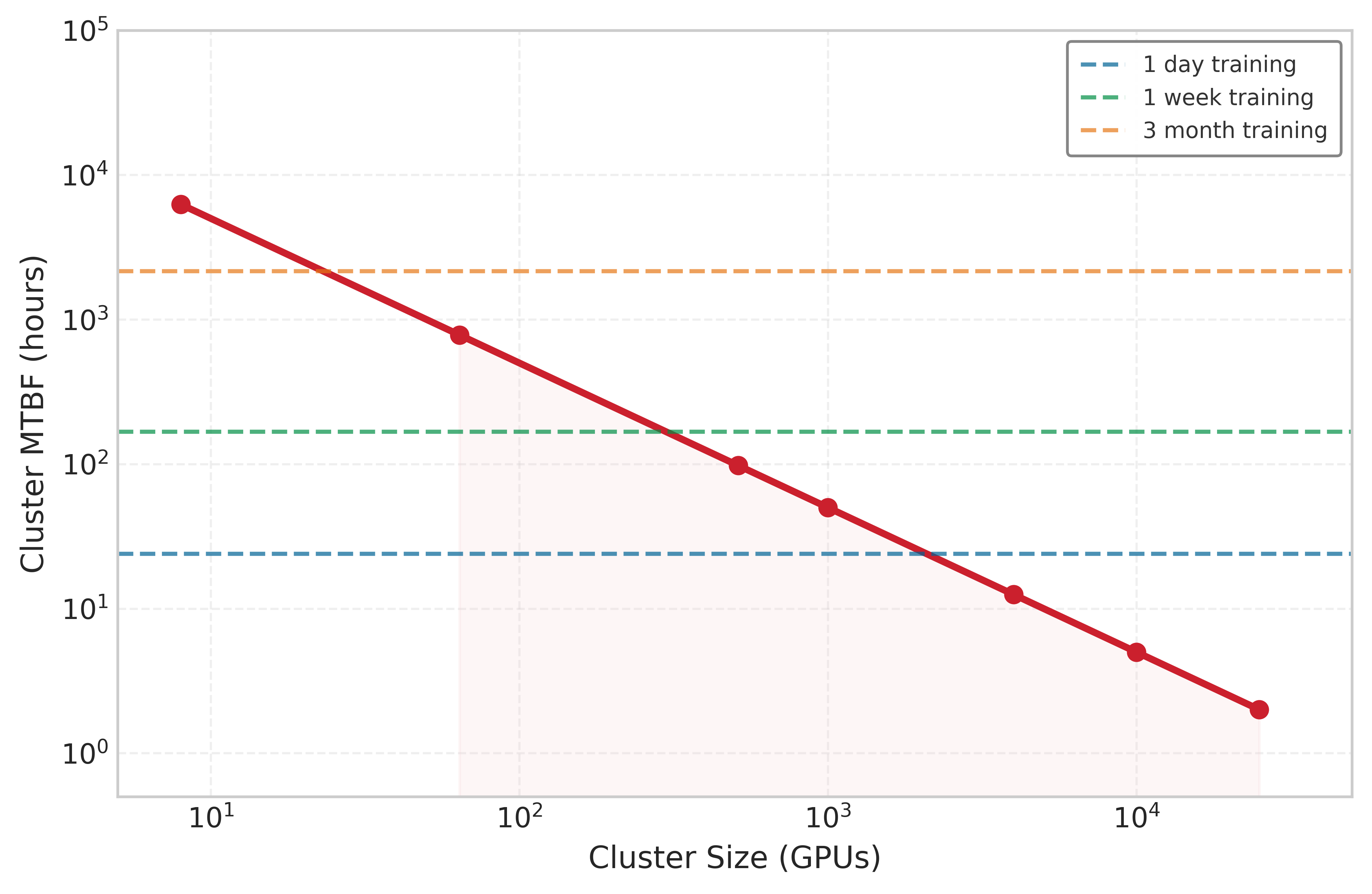
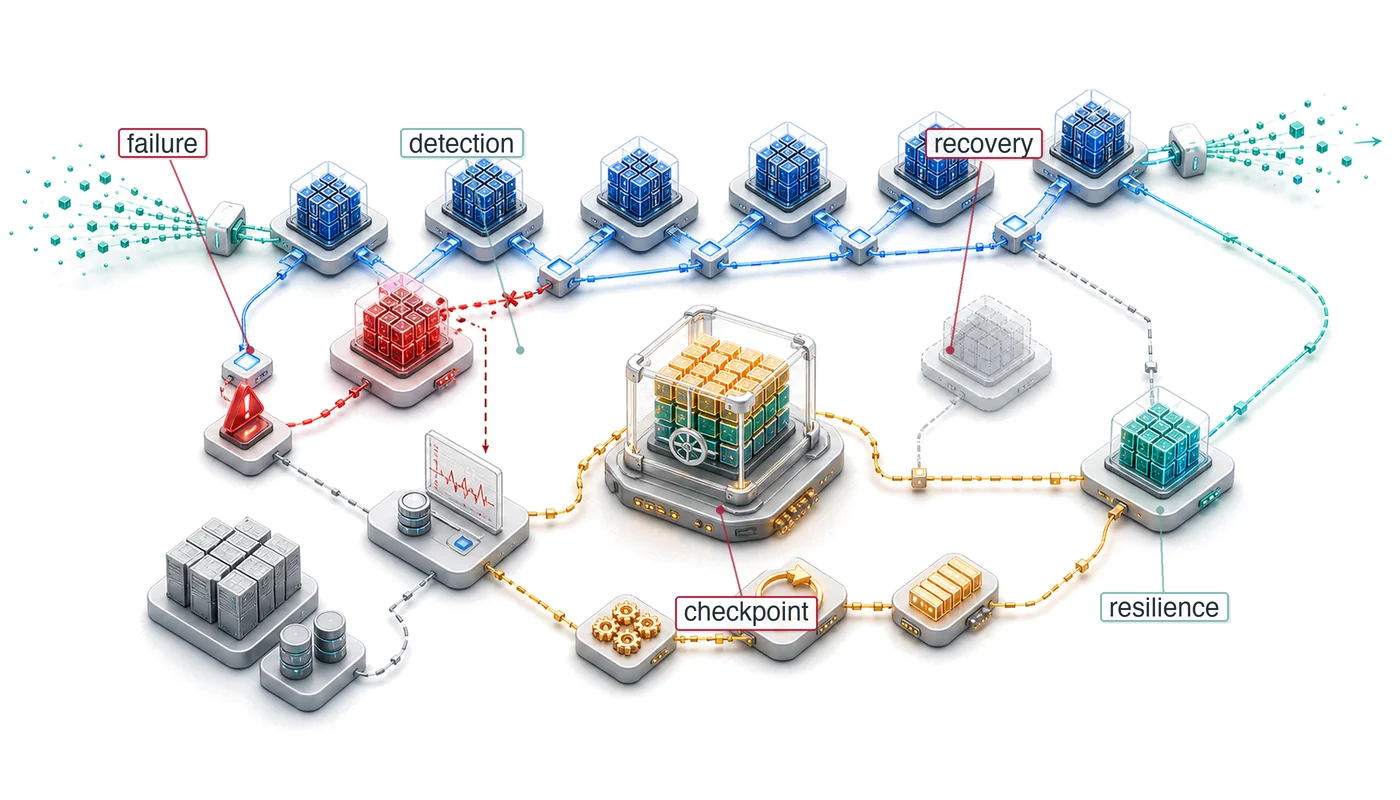
Imagine a 10,000-GPU cluster midway through a three-month training run for a new foundation model. The communication layer has done its job: thousands of devices exchange gradients through AllReduce, AllGather, and AllToAll as if they were one machine. Then the arithmetic of scale catches up. A GPU fails every few hours, and if the system cannot absorb that ordinary physical event, synchronized training halts and millions of dollars of compute sit idle. Fault tolerance is the system property that lets distributed execution continue making useful progress when components fail, degrade, or disappear. In the fleet stack shown in The Fleet Stack, fault tolerance acts as the resilience layer for distributed execution. The challenges span the full failure spectrum, from transient bit flips through intermittent aging-related errors to permanent component failures, as figure 1 illustrates. The per-category failure rates and the mean time between failures (MTBF) scaling, \(\text{MTBF}_{\text{system}} = \text{MTBF}_{\text{component}}/N\), annotated in that figure are previews; later analysis derives the inverse scaling and tabulates the cluster rates. Gray failures and silent data corruption (SDC) add a second axis of difficulty: low detection rate, high blast radius.

Figure 1: The ML Failure Spectrum: Reliability challenges at scale span a temporal taxonomy from transient errors (bit flips, single-event upsets) through intermittent errors (aging, marginal components) to permanent errors (stuck-at faults, dead components). Each category demands different detection latency and recovery strategy, and fault tolerance engineering must address all three to maintain fleet-scale throughput.

That fragility is the direct consequence of successful synchronization. Distributed training systems achieve massive throughput by coordinating thousands of devices, and collective communication keeps that coordination synchronized through rigid exchanges. The same synchronization means one stalled device can stall the fleet. Fault-tolerant ML systems preserve progress by detecting failure, checkpointing recoverable state, restarting or elastically reshaping jobs, and treating hardware churn as normal execution rather than an exceptional path.

The transition from small-scale experimentation to large-scale production changes the relationship between systems and failures. A researcher training a model on a single GPU can go years without a hardware failure. That same workload on a 1,000-GPU cluster sees GPU-only failures every couple of days, and a production cluster fails more often once PCIe, power, storage, and network domains enter the failure budget. This shift from rare exception to routine occurrence demands different engineering approaches. The mathematical analysis that follows makes this transition precise and quantitative.

System MTBF collapses as the fleet grows: 50,000 h to 5 h.

Because failures cannot be eliminated at this scale, the engineering challenge is not to prevent them but to keep making progress despite them: fault-tolerant systems verify completion rather than assume it, treat failure as a normal code path, exercise recovery continuously rather than occasionally, and account for partial failures that leave the system in states naive error handling never anticipates. The techniques that achieve this draw on decades of distributed systems research, but ML workloads change the economics. Training exhibits properties that enable fault tolerance strategies unavailable to general distributed systems: the mathematical properties of stochastic gradient descent tolerate certain errors that would corrupt other computations, checkpoint sizes are large but predictable, and recovery targets need only be approximate rather than exact. Exploiting these properties makes ML-specific fault tolerance cheaper than the general-purpose approaches it descends from.

The mathematics of inevitable failure

System reliability engineering provides the foundational framework for understanding failure at scale (Birolini 2017). Individual components exhibit failure rates characterized by the failure rate parameter \(\lambda\),¹ measured in failures per unit time. For a single component with constant failure rate \(\lambda\), the probability of surviving without failure until time \(t\) follows an exponential distribution,² as in equation 1:

¹ Failure Rate (\(\lambda\)): Expressed in FITs (Failures In Time), where 1 FIT equals one failure per billion device-hours. A data center GPU with 50000 hours MTBF has \(\text{FIT} = 20{,}000\), corresponding to \(\lambda_{\text{hour}} = 2.0 \times 10^{-5}\) failures/hour. That seems negligible for one device but becomes dominant at fleet scale: a cluster with 10,000 GPUs accumulates 200,000,000 FITs from GPUs alone, translating to an expected GPU failure every 5 hours.

² Poisson Process: A statistical model for events occurring independently at a constant average rate. Reliability models assume hardware failures follow a Poisson distribution, leading to the exponential survival function \(R(t) = e^{-\lambda t}\). This assumption simplifies fleet planning: the probability of at least one failure in a 10,000-component cluster is \(1 - e^{-N \lambda t}\), making failure risk scale linearly with \(N\) but exponentially with \(t\).

\[ R_{\text{single}}(t) = e^{-\lambda t} \tag{1}\]

MTBF for this component equals \(1/\lambda\). By the book’s convention, mean time to failure (MTTF) names a single component’s expected time to its first failure while MTBF names the repairable system’s expected time between successive failures; under the constant-rate exponential model used here the two coincide numerically, and the fault-tolerance model uses MTTF for per-component constants and MTBF for composed system rates. Data center GPUs often use planning MTBF values in the tens of thousands of hours, with field behavior depending on operating conditions, cooling effectiveness, manufacturing variation, and workload stress.³ Component failure rates catalogs the canonical per-component MTTF values (H100, A100, TPU, PCIe, power, network) that anchor these \(\lambda\) and FIT figures, so a reader can substitute the constant for any device and reproduce the rates used throughout the fault-tolerance analysis.

³ GPU MTBF Variation: This chapter uses 50,000 hours as an A100-class planning constant, not as a guarantee for every deployed GPU. Published fleet studies from Google TPUv4 pods and Meta GPU clusters report that field reliability depends on topology, cooling, workload, and operational practice (Zu et al. 2024; Kokolis et al. 2025; Dubey et al. 2024). The planning constant therefore anchors the arithmetic, while operators should substitute measured fleet rates when they have them.

Zu, Y., A. Ghaffarkhah, H.-V. Dang, B. Towles, S. Hand, S. Huda, A. Bello, et al. 2024. “Resiliency at Scale: Managing Google’s TPUv4 Machine Learning Supercomputer.” 21st USENIX Symposium on Networked Systems Design and Implementation (NSDI 24), 761–74.

Kokolis, Apostolos, Michael Kuchnik, John Hoffman, Adithya Kumar, Parth Malani, Faye Ma, Zach DeVito, Shubho Sengupta, Kalyan Saladi, and Carole-Jean Wu. 2025. “Revisiting Reliability in Large-Scale Machine Learning Research Clusters.” 2025 IEEE International Symposium on High Performance Computer Architecture (HPCA), 1259–74. https://doi.org/10.1109/hpca61900.2025.00096.

Dubey, Abhimanyu, Abhinav Jauhri, Abhinav Pandey, Abhishek Kadian, et al. 2024. The Llama 3 Herd of Models. arXiv preprint arXiv:2407.21783.

When multiple independent components operate in a system where any single failure causes system failure, equation 2 formalizes how system reliability becomes the product of individual component reliabilities:

\[ R_{\text{system}}(t) = \prod_{i=1}^{N} R_i(t) = \prod_{i=1}^{N} e^{-\lambda_i t} \tag{2}\]

For \(N\) identical components with individual failure rate \(\lambda\), equation 3 gives the identical-component simplification:

\[ R_{\text{system}}(t) = e^{-N\lambda t} \tag{3}\]

The system failure rate becomes \(N\lambda\), and equation 4 expresses how the system MTBF scales inversely with component count. This inverse scaling reveals the counterintuitive reality of the 9s of reliability at cluster scale:

\[ \text{MTBF}_{\text{system}} = \frac{1}{N\lambda} = \frac{\text{MTBF}_{\text{component}}}{N} \tag{4}\]

Figure 2 visualizes the fundamental tension: as clusters grow, the expected time between failures shrinks below common training durations, making fault tolerance necessary for long-running fleet jobs.

Figure 2: The Reliability Gap: As GPU count increases, cluster MTBF drops below common training durations. A 10,000-GPU cluster experiences a failure roughly every 5 hours, making a 3-month training run impossible without fault tolerance mechanisms.

The Young-Daly law: Optimal checkpointing

When failure is inevitable, the key engineering decision is how often to save progress. Checkpointing too frequently wastes time on I/O; checkpointing too rarely wastes time re-computing work after a failure. The Young-Daly formula⁴ (principle 12) resolves that tension with a single square-root law:

⁴ Young-Daly Formula: J. W. Young derived the first-order optimal checkpoint interval in a 1974 Communications of the ACM paper; John Daly independently refined it in 2006 with tighter second-order bounds (Young 1974; Daly 2006). The formula’s square-root relationship \((\tau_{\text{opt}} = \sqrt{2 \cdot T_{\text{write}} \cdot \text{MTBF}_{\text{system}}})\) means that halving system MTBF only increases optimal checkpoint frequency by \(\sqrt{2}\approx 1.4\times\), explaining why doubling cluster size does not demand doubling checkpoint I/O bandwidth.

Young, John W. 1974. “A First Order Approximation to the Optimum Checkpoint Interval.” Communications of the ACM 17 (9): 530–31. https://doi.org/10.1145/361147.361115.

Daly, J. T. 2006. “A Higher Order Estimate of the Optimum Checkpoint Interval for Restart Dumps.” Future Generation Computer Systems 22 (3): 303–12. https://doi.org/10.1016/j.future.2004.11.016.

\[ \tau_{\text{opt}} = \sqrt{2 \cdot T_{\text{write}} \cdot \text{MTBF}_{\text{system}}} \]

\(T_{\text{write}}\) in distributed ML training is not the time to flush a small process state—it is the time required to transfer hundreds of gigabytes of FP32 optimizer state (momentum and variance tensors for every trainable parameter) plus model weights to durable storage. For a 70B-parameter model with full Adam state, a single checkpoint can reach several hundred gigabytes; for the later 175B-parameter running example, that figure exceeds a terabyte. Compressing \(T_{\text{write}}\) therefore requires purpose-built high-bandwidth storage, and \(T_{\text{write}}\) itself is the central constraint that determines how tightly the checkpoint interval can be set before I/O overhead displaces productive training compute.

The optimal interval balances the cost of writing checkpoints against the expected cost of reworking lost progress, the U-shaped trade-off figure 3 plots. Its scaling consequence is the one to carry forward: as clusters grow, system MTBF drops, so the optimal interval shrinks, demanding higher-bandwidth storage (Data Storage) to keep \(T_{\text{write}}\) small before the “checkpoint tax” consumes the cluster’s compute capacity. Because the relationship is a square root, halving MTBF tightens the interval by only \(\sqrt{2}\approx 1.4\times\), so doubling cluster size does not demand doubling checkpoint I/O bandwidth. The Young-Daly model carries out the full derivation and the tighter second-order bounds; the later Checkpointing section (section 1.5.1) applies the formula to the local cluster once its system MTBF is in hand.

Figure 3: The Young-Daly Optimal Checkpoint: Total wasted work is the sum of checkpointing overhead (which decreases with interval \(\tau_{\text{ckpt}}\)) and rework cost (which increases with \(\tau_{\text{ckpt}}\)). The minimum point defines the optimal interval \(\tau_{\text{opt}} = \sqrt{2 \cdot T_{\text{write}} \cdot \text{MTBF}_{\text{system}}}\). For an illustrative cluster with a five-hour system MTBF and 15-minute write time, the optimal interval is approximately 1.6 hours.

A quick availability calculation shows the same scaling pressure from another angle.

Napkin Math 1.1: The 9s of reliability

Problem: A cluster of 10,000 GPUs runs with each GPU at 99.99 percent availability (only 52.6 minutes of downtime per year). What is the probability that the entire cluster is up at the same instant?

Math:

1. Single GPU availability probability \((R_{\text{GPU}})\): A GPU with 99.99 percent availability has an all-up probability \(R_{\text{GPU}} =\) 0.9999 at a randomly chosen instant.
2. Cluster availability probability \((R_{\text{cluster}})\): \(R_{\text{cluster}} = (R_{\text{GPU}})^{N}\).
3. Result: \((R_{\text{GPU}})^{N} \approx\) 0.37.

Systems insight: Even with 99.99 percent reliable hardware, a 10,000-GPU cluster has only a 37 percent chance that every GPU is simultaneously available. Hardware reliability alone is insufficient; software must handle failures automatically.

The linear relationship between component count and failure rate has a direct implication: adding GPUs turns rare component failures into a continuous system condition.

Systems Perspective 1.1: Scale transforms failure

A single GPU with an MTBF of 50,000 hours (5.7 years) absorbs the occasional failure with manual intervention, but a 10,000-GPU cluster with that same per-GPU reliability has a GPU-only system MTBF of just 5 hours: failures arrive multiple times per day. Systems must be designed expecting failure, not hoping to avoid it.

Quantitative reliability analysis

The GPU-only calculation in the opening reliability example supplies the scale intuition; a real training system then composes GPUs, HBM, links, power supplies, storage paths, and redundancy into one failure budget. With MTBF and the FIT rate already defined (\(\text{FIT} = 10^9/\text{MTBF}\), so a 50,000-hour GPU contributes 20,000 FIT), the new question is how component rates compose. The composition rule depends on the redundancy structure. For series systems (for example, a node where all 8 GPUs must work), failure of any component fails the whole, so reliabilities multiply and rates add: \[R_{\text{system}}(t) = \prod_{i=1}^{N} R_i(t), \qquad \text{MTBF}_{\text{system}} = \frac{1}{\sum \lambda_i}\] which is why adding components reduces system MTBF linearly. For parallel systems providing redundancy (for example, active-active model replicas), failure occurs only when all redundant components fail simultaneously: \[R_{\text{system}}(t) = 1 - \prod_{i=1}^{N} (1 - R_i(t))\]

Composition also exposes which subsystem dominates the budget, and memory is the consequential case. Consider training an Archetype A (GPT-4/Llama-3) 70B model (Three systems archetypes) on 1,024 A100 GPUs. Unprotected HBM is the binding term: at roughly 250 FIT per megabit, the cluster’s \(1,024 \times 80 \text{ GB}\) of memory accumulates so many failure sites that uncorrected corruption would strike roughly every 20 seconds, making large-scale training impossible. Error-correcting-code (ECC) memory protection is therefore not optional. ECC detects and corrects common single-bit errors, cutting the effective soft-error rate by roughly two orders of magnitude and pushing memory back below the logic and interconnect terms in the budget, though residual multi-bit or escaped corruptions remain as the silent-data-corruption problem.

These per-component FIT figures describe the silicon’s intrinsic soft-error budget, which is why they differ from the 50,000-hour whole-device MTTF used in the worked cascade that follows: the device MTTF folds in every field failure mode (thermal stress, power events, mechanical wear), not just the logic and memory soft-error rates isolated here. The cascade composes those whole-device rates into the cluster figure that actually sets the checkpoint interval; this estimate only establishes why memory protection is the precondition for everything that follows.

Worked example: Cluster MTBF calculation

Consider a training cluster designed for large language model development with the following specifications:

• 10,000 NVIDIA H100 GPUs
• Individual GPU MTBF: 50,000 hours
• Each GPU connected to host via PCIe (MTBF: 200,000 hours)
• Each node contains 8 GPUs with shared power supply (MTBF: 100,000 hours)
• Network infrastructure per node (NIC, cables): MTBF 150,000 hours

Together, these components define the failure domain used in the rate calculation below.

Step 1: Calculate failure rate per GPU subsystem

Each GPU operates within a failure domain that includes the GPU itself, its PCIe connection, and proportional shares of the power supply and network infrastructure.

\[ \lambda_{\text{GPU}} = \frac{1}{50{,}000} = 2.0 \times 10^{-5} \text{ failures/hour} \]

\[ \lambda_{\text{PCIe}} = \frac{1}{200{,}000} = 0.5 \times 10^{-5} \text{ failures/hour} \]

\[ \lambda_{\text{power/GPU}} = \frac{1}{8} \times \frac{1}{100{,}000} = 0.125 \times 10^{-5} \text{ failures/hour} \]

\[ \lambda_{\text{network/GPU}} = \frac{1}{8} \times \frac{1}{150{,}000} = 0.083 \times 10^{-5} \text{ failures/hour} \]

Step 2: Calculate total per-GPU failure rate

\[ \lambda_{\text{total/GPU}} = (2.0 + 0.5 + 0.125 + 0.083) \times 10^{-5} = 2.708 \times 10^{-5} \text{ failures/hour} \]

Step 3: Calculate system failure rate and MTBF

\[ \lambda_{\text{system}} = 10{,}000 \times 2.708 \times 10^{-5} = 0.2708 \text{ failures/hour} \]

\[ \text{MTBF}_{\text{system}} = \frac{1}{0.2708} = 3.69 \text{ hours} \]

This result means the cluster experiences a failure approximately every 3.7 hours on average. The expected failure cadence is 6.5 failures/day; a training run lasting one week will experience approximately 45 failures. Any training system operating at this scale must treat failure as a continuous condition, not an exceptional event. The MTBF cascade works this same cascade through step by step, composing per-component rates into a fleet-wide system MTBF, so a reader can rerun the calculation for a different node design or cluster size.

The cluster MTBF scaling in table 1 isolates the GPU-only baseline across cluster sizes. The full-system calculation is lower once PCIe, power, and network failure domains are included.

Table 1: Cluster MTBF Scaling: GPU-only mean time between failures decreases linearly with cluster size, transforming failures from rare events to continuous operating conditions at scale. Additional host, power, storage, and network failure domains reduce system-level MTBF further.

Cluster Size (GPUs)	Individual GPU MTBF	Cluster MTBF	Expected Failures per Day
8	50,000 hours	6250 hours (260 days)	0.004
64	50,000 hours	781.2 hours (33 days)	0.03
512	50,000 hours	97.7 hours (4 days)	0.25
1,000	50,000 hours	50 hours (2 days)	0.48
4,000	50,000 hours	12.5 hours	1.9
10,000	50,000 hours	5 hours	4.8
25,000	50,000 hours	2 hours	12

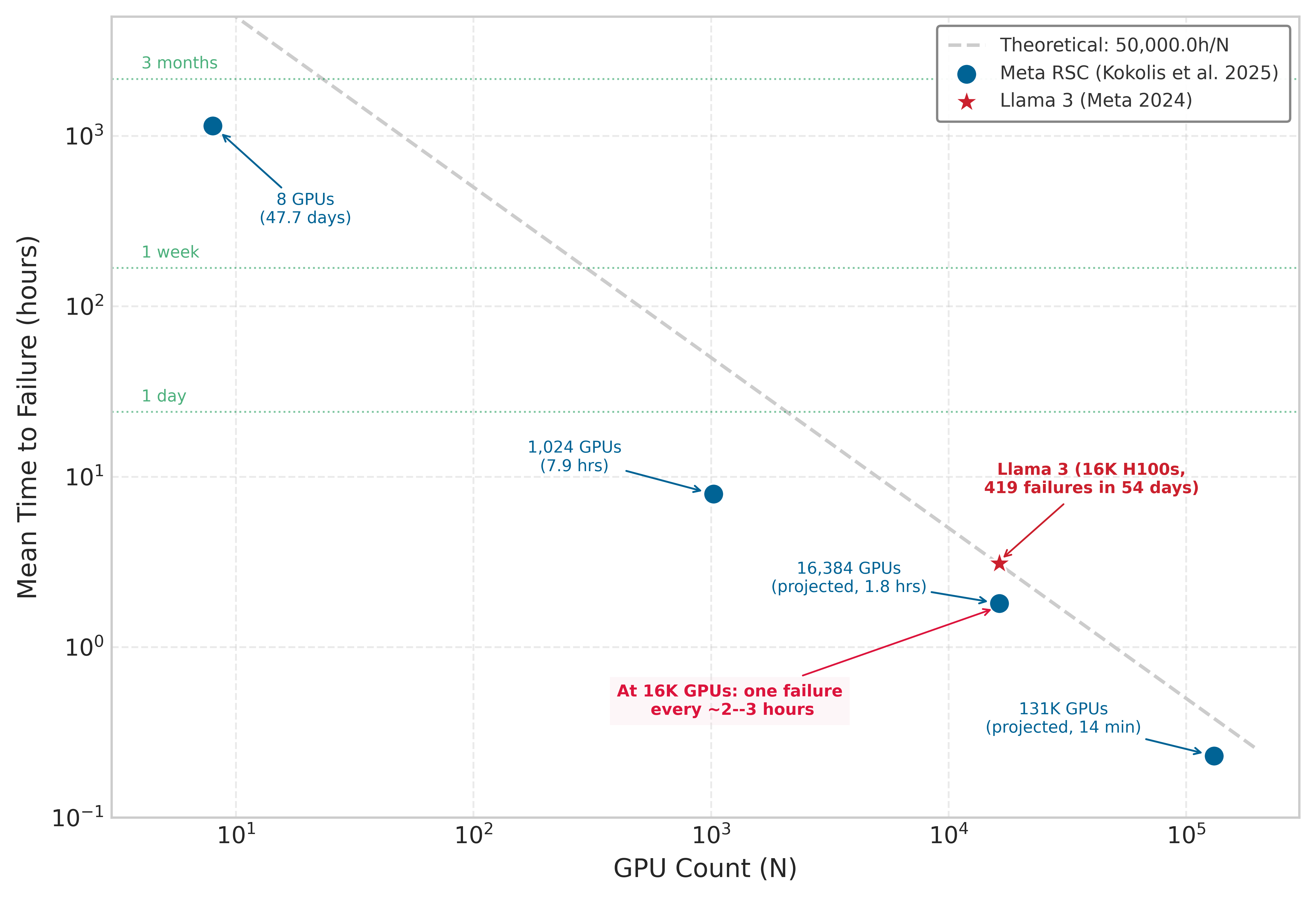
The theoretical \(1/N\) scaling in table 1 is not merely a textbook exercise. Figure 4 overlays published measurements and fitted projections from Meta’s production clusters against the theoretical curve. The Kokolis et al. (2025) study of Meta’s Research SuperCluster reported measured MTTF values for observed RSC job sizes and projected a 1.8-hour MTTF for 16,384-GPU jobs; Meta’s Llama 3 training report independently documented 419 failures across 54 days on 16,384 H100 GPUs, an observed MTTF of about 3.1 hours. Together, the measured Llama run and Kokolis projection put 16,384-GPU training on a 2-to-3-hour failure cadence. This evidence transforms the theoretical argument from an abstract scaling law into an engineering constraint that determines checkpoint frequency, recovery architecture, and infrastructure investment.

Figure 4: Published Failure Rates from Production Clusters: Measured MTTF values and fitted projections from Meta’s RSC clusters (Kokolis et al. 2025) plotted with Llama 3 training measurements (Dubey et al. 2024) against the theoretical 1/N curve. At 16,384 GPUs, the Kokolis projection and Llama 3 empirical measurement both fall in the 2-to-3-hour failure range, confirming that fault tolerance is a mathematical necessity, not an edge case. Data sources: Kokolis et al., arXiv:2410.21680; Meta, arXiv:2407.21783.

Failure taxonomy

The MTBF calculations in the reliability analysis quantify how often failures occur, which is critical for setting checkpoint intervals and sizing recovery infrastructure. Designing effective fault tolerance also requires understanding what kind of failures occur. Use the vocabulary carefully: a fault is the underlying defect or event, an error is the corrupted state it produces, and a failure is the externally visible behavior the training system must handle (Avizienis et al. 2004). A network partition that resolves in seconds demands different handling than a permanent GPU failure. A silent memory corruption that produces incorrect gradients requires different detection mechanisms than a node crash that stops responding entirely. Failure characteristics guide the selection of appropriate recovery mechanisms. The taxonomy presented here classifies failures along two primary dimensions: temporal behavior (transient vs. persistent) and failure manifestation (fail-stop vs. Byzantine) (Constantinescu 2008; Lamport et al. 1982).

Transient failures

Transient failures occur temporarily and resolve without intervention, so the recovery question is whether the system can retry or validate the affected work before corrupted state propagates. Four common transient patterns matter for ML systems:

• Network packet loss: Drops packets while retransmission succeeds.
• Memory bit flips: Corrupt individual bits through cosmic ray induced single-event upsets.⁵
• Thermal throttling: Temporarily reduces performance during temperature spikes.
• Software timeouts: Arise from temporary resource contention.

⁵ Single-Event Upset (SEU): From particle physics, where “upset” denotes a nondestructive state change. Cosmic rays and alpha particles from chip packaging can flip bits in memory and logic; the observed rate depends on altitude, process technology, packaging materials, shielding, and workload (Ziegler et al. 1996; Baumann 2005). ECC memory corrects single-bit errors but cannot handle every multi-bit upset in the same word, leaving a residual silent-corruption risk that compounds across the terabytes of state in large-scale ML training.

Ziegler, J. F., H. W. Curtis, H. P. Muhlfeld, C. J. Montrose, B. Chin, M. Nicewicz, C. A. Russell, et al. 1996. “IBM Experiments in Soft Fails in Computer Electronics (1978–1994).” IBM Journal of Research and Development 40 (1): 3–18. https://doi.org/10.1147/rd.401.0003.

Baumann, R. 2005. “Soft Errors in Advanced Computer Systems.” IEEE Design and Test of Computers 22 (3): 258–66. https://doi.org/10.1109/mdt.2005.69.

⁶ Silent Data Corruption (SDC): At fleet scale, SDC can bypass normal exception paths: infrastructure studies have documented defective hardware producing valid-looking but wrong results, while DRAM field studies show memory errors are common enough that fleet-level monitoring matters. For ML training, the practical debugging consequence is that the absence of an error message does not imply correct computation; systems need statistical checks on loss, gradients, and model state.

Transient failures are particularly insidious in ML training because they may not trigger explicit errors. A transient memory bit flip during gradient computation produces incorrect gradients that propagate through subsequent training steps. The model continues training but produces subtly degraded results. Large-scale SDC studies show escaped corruption, while DRAM field studies show memory errors are common enough that fleet-level monitoring matters (Dixit et al. 2021; Sridharan et al. 2015; Schroeder et al. 2009). In ML training, that same undetected-corruption pattern can surface as degraded gradients, anomalous loss curves, or rollback-worthy checkpoints rather than an explicit crash⁶.

The appropriate response to transient failures depends on detection capability. Errors that trigger explicit exceptions can be handled through retry logic. Silent corruption requires validation mechanisms such as gradient checksums, periodic model evaluation, and statistical monitoring of training dynamics.

Fail-stop failures

Fail-stop failures cause components to cease operation entirely and detectably. The failed component stops responding to requests and can be identified through timeout mechanisms:

• GPU hardware failure: Makes a device unresponsive.
• Node crash: Terminates all processes on a machine.
• Network partition: Isolates the node from the cluster.
• Storage failure: Prevents checkpoint reads or writes.

In synchronous distributed training, fail-stop failures carry a particularly severe consequence: they stall the entire job. AllReduce collectives require every participating rank to contribute its gradient shard before the reduction can complete. A single GPU that goes silent—whether from a hardware fault, a process crash, or a network partition—blocks every other GPU in the ring until the timeout expires. On a 10,000-GPU job, that means 9,999 accelerators sitting idle, accumulating billable hours against a run that has made zero forward progress, until the coordinator finally declares the missing rank failed and triggers recovery.

Fail-stop failures are the easiest class to handle because detection is straightforward: the component stops responding. Recovery involves replacing the failed component and restoring state from the most recent checkpoint. The primary challenge is minimizing detection time and recovery latency.

Detection time \(T_{\text{detect}}\) typically involves heartbeat mechanisms where each GPU rank periodically signals liveness to a coordinator. If no heartbeat arrives within the timeout period \(T_{\text{timeout}}\), the coordinator declares failure. Setting \(T_{\text{timeout}}\) requires balancing false positive rate against detection latency. False positives declare healthy workers failed due to transient delays, while slow detection wastes compute during the detection window—a cost that scales linearly with the number of GPUs blocked in the collective.

For a heartbeat interval of \(H\) seconds and network-delay standard deviation \(\sigma_d\) in seconds, equation 5 defines the timeout heuristic:

\[ T_{\text{timeout}} = H + k\sigma_d \tag{5}\]

Here, \(k\) is a dimensionless safety multiplier that typically ranges from three to five to achieve low false positive rates while maintaining reasonable detection speed. ML training clusters built on dedicated high-bandwidth fabrics (InfiniBand, NVLink) exhibit very low baseline jitter, so \(\sigma_d\) is functionally small under normal conditions. The practical difficulty is distinguishing a genuinely dead rank from one that is temporarily slow—for example, a GPU lagging because it is writing a large checkpoint to attached storage while the collective is already waiting. Tuning \(T_{\text{timeout}}\) too tightly causes checkpoint writes to trigger false failure declarations; tuning it too loosely extends the window during which every other rank in the AllReduce collective is blocked idle.

Byzantine failures

Where a fail-stop component simply goes silent and is detected and replaced, a far more insidious class keeps running but produces incorrect results. A GPU that returns wrong gradients without throwing errors, a network that delivers corrupted packets that pass CRC checks, or a worker that computes different results for identical inputs all exemplify Byzantine failures, the most challenging class in distributed systems (Lamport et al. 1982). In ML systems, this category includes silent data corruption, numerical instability, determinism violations, and adversarial corruption; the common property is that the worker still participates while the value it contributes can poison shared state.

Lamport, Leslie, Robert Shostak, and Marshall Pease. 1982. “The Byzantine Generals Problem.” The Byzantine generals problem in Concurrency: The Works of Leslie Lamport, vol. 4. Association for Computing Machinery. https://doi.org/10.1145/3335772.3335936.

The physics of silent corruption

At the nanometer scale of advanced transistors, hardware is not deterministic; it is probabilistic. Silent data corruption (SDC) is driven by two primary mechanisms. Single-event upsets (SEUs) occur when high-energy particles (cosmic rays at sea level, alpha particles from packaging materials) strike memory cells or logic gates, flipping a bit from 0 to 1; at 10,000+ GPUs, this is a statistical certainty. Manufacturing variances appear when “marginal” chips that pass initial QA exhibit bit flips only under specific voltage/temperature conditions, such as the intense \(di/dt\) swings of a backward pass.

Facebook documented a pervasive SDC issue where a hardware fault caused a valid file to be reported as “size zero” during decompression (Dixit et al. 2021). As figure 5 illustrates, the system “worked” (no crash), but data was silently deleted. In ML, this manifests as valid-looking but numerically corrupted gradients.

Figure 5: Silent Data Corruption Propagation: Unexpected faults can return incorrect file sizes, leading to data loss during decompression and propagating errors through distributed querying systems. This example from Facebook emphasizes how silent errors bypass standard exception handlers. Source: (Dixit et al. 2021).

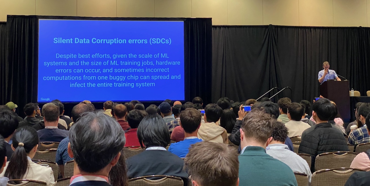
Real-world evidence of SDC in production systems confirms these risks. Figure 6 shows corrupted data blocks accumulating in a shuffle and merge database at Google, where even a small fraction of corrupted blocks can cascade into significant data quality degradation.

Figure 6: Silent Data Corruption in Spark: AI systems that use large-scale data processing frameworks such as Spark are vulnerable to silent data corruption (SDC) accumulating during data transfer and storage. SDC manifests in a shuffle and merge database, highlighting corrupted data blocks (red) amidst healthy data (blue/gray). Source: (Dean 2024).

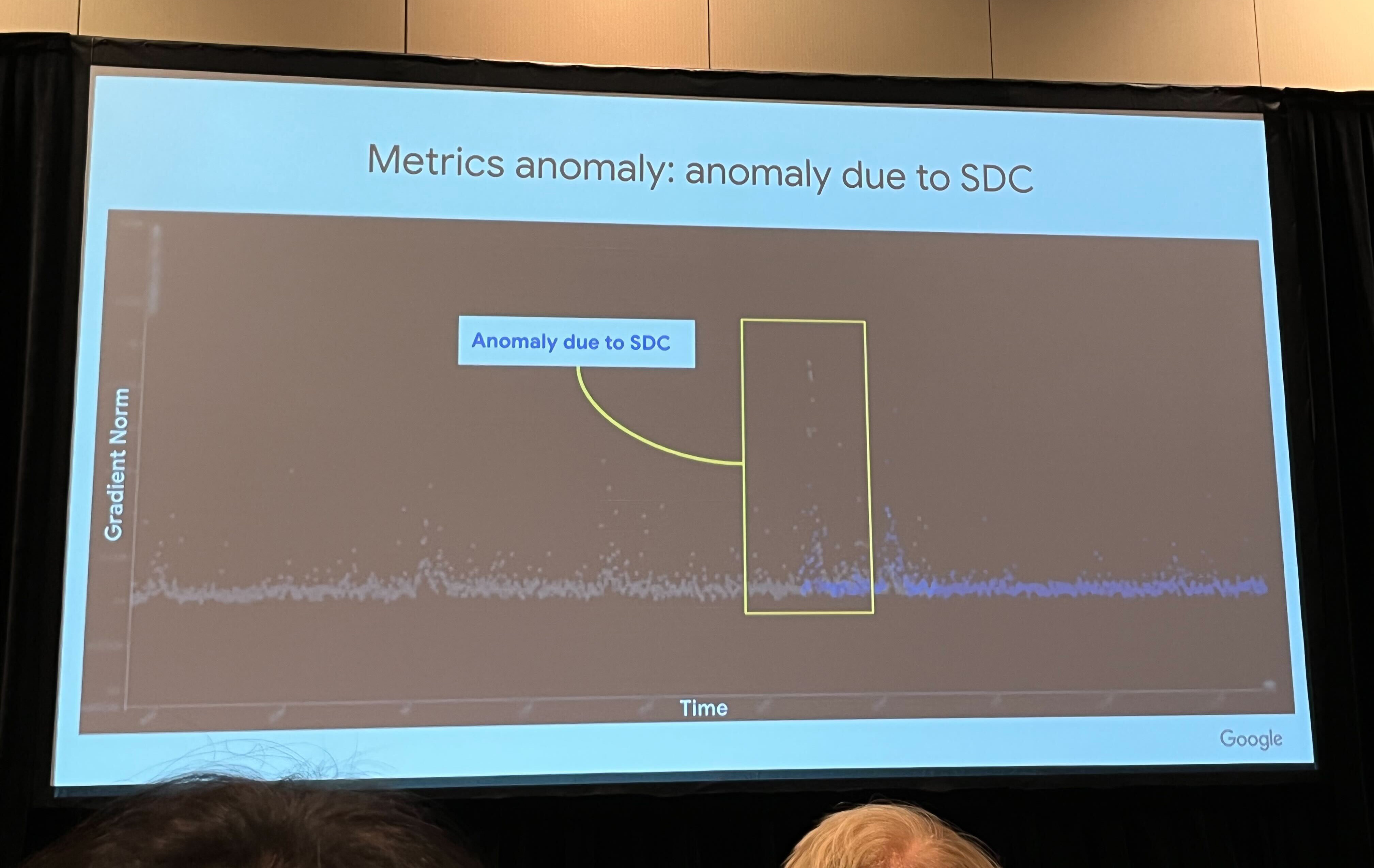
Google reported that SDC in TPU pods can manifest as sudden, inexplicable spikes in gradient norm (figure 7) (Dean 2024). A single bit flip in an exponent can turn a small gradient into a numerically enormous value, corrupting the training trajectory if the anomaly is not detected.

Figure 7: Gradient Norm Deviation: Transient hardware faults, such as silent data corruption (SDC), can disrupt optimization by causing abrupt changes in gradient norms. Google’s production examples show SDC anomalies surfacing as visible gradient-norm spikes. Source: (Dean 2024).

Google addresses this class of failure with system-level mitigation, including spare capacity and sanity checks that can drain suspect chips when loss or gradient monitors flag anomalies (figure 8) (Dean 2024). This moves reliability from the component, which we cannot trust, to the system, which verifies the result.

Figure 8: Hot Spare Redundancy: Google’s data-center examples use spare capacity and sanity checking to keep ML training moving despite hardware faults, transitioning work away from suspect resources when monitors flag anomalies. This approach contrasts with parallel redundancy techniques such as dual modular redundancy and triple modular redundancy by providing a reactive fault-tolerance mechanism. Source: (Dean 2024).

Dean, Jeff. 2024. Exciting Directions in Systems for Machine Learning. MLSys 2024 invited talk.

The hot spare pattern in figure 8 illustrates one approach to SDC mitigation, but recognizing silent corruption in the first place requires understanding what distinguishes it from benign training noise.

Checkpoint 1.1: Detecting silent corruption

Verify your understanding of Byzantine failures and SDC:

• SDC danger: Explain why silent data corruption (SDC) is more dangerous for ML training than a simple node crash.
• Hot spare vs. restart: Compare a hot spare redundancy strategy with traditional checkpoint-restart in terms of recovery latency.
• Sanity checker: Identify the metric used as a “sanity checker” to identify potential hardware faults: GPU temperature or gradient norm.
• Byzantine scope: Assess the True or False claim that Byzantine failures only occur when a malicious actor intentionally sabotages the training cluster.

Silent-corruption detection is the first defense, but the same logic extends to any Byzantine worker whose output remains syntactically valid. These failures are particularly dangerous in distributed training because the standard assumption that workers compute identical gradients for identical data no longer holds. A single Byzantine worker can corrupt the averaged gradient, potentially causing training to diverge or converge to a poor solution. Figure 9 contrasts the straightforward detection of fail-stop failures with the insidious nature of Byzantine corruption.

Figure 9: Fail-Stop vs. Byzantine Failures: In the fail-stop model (left), a failed worker simply ceases to send messages, which is easily detected by timeouts. In the Byzantine model (right), a failed worker continues to participate but sends incorrect data (for example, corrupted gradients reported as valid), which can poison the global model state if not detected by redundant validation.

Detection of Byzantine failures requires redundant computation. Multiple workers computing gradients for the same data enable comparison of results. Statistical outlier detection can identify workers consistently producing anomalous gradients. These detection mechanisms add computational overhead and may not catch subtle corruption.

Byzantine-resilient distributed training algorithms exist but impose significant overhead. Algorithms such as Krum (Blanchard et al. 2017) and coordinate-wise trimmed mean (Yin et al. 2018) compute aggregates that are robust to a bounded number of Byzantine workers, but they require more communication and computation than simple averaging. The systems consequence is visible here: corrupted gradients can push the optimizer toward an unreliable model state while the training job appears healthy. Reliability therefore has to protect semantic correctness, not only process liveness.⁷

Yin, Dong, Yudong Chen, Kannan Ramchandran, and Peter Bartlett. 2018. “Byzantine-Robust Distributed Learning: Towards Optimal Statistical Rates.” International Conference on Machine Learning, 5650–59.

⁷ [offset=-35mm] Byzantine-Resilient ML: Named after Lamport’s 1982 “Byzantine Generals Problem,” these algorithms (Krum, trimmed mean, signSGD) tolerate a bounded fraction of corrupted workers, with the exact bound depending on the algorithm and assumptions. The trade-off is concrete: for \(N\) workers, Krum requires pairwise distance computations over worker gradients, so overhead grows quadratically with worker count and directly competes with the throughput gains of data parallelism (Blanchard et al. 2017).

Blanchard, Peva, El Mahdi El Mhamdi, Rachid Guerraoui, and Julien Stainer. 2017. “Machine Learning with Adversaries: Byzantine Tolerant Gradient Descent.” Advances in Neural Information Processing Systems, 119–29.

Correlated failures

The reliability calculations in section 1.0.1 assume independent failures. Real systems exhibit correlated failures when shared dependencies fail many components at once:

• Power supply failure: Takes down every GPU in a node.
• Network switch failure: Isolates all attached nodes.
• Cooling system failure: Forces thermal shutdown across racks.
• Software bug: Crashes every process using a faulty CUDA driver version.
• Operator error: Misconfigures an entire cluster.

Correlated failures violate the independence assumption underlying equation 3. When failures are correlated, the actual system reliability is lower than the formula predicts. Correlated failures can also defeat redundancy strategies. Three replicas of a model provide no availability benefit if all three run on the same power domain and a power failure takes out all three simultaneously.

Defending against correlated failures requires understanding failure domains and ensuring redundancy spans independent failure domains. Table 2 catalogs common failure domains in ML infrastructure, from single GPUs to entire data center regions, each requiring distinct mitigation strategies. Figure 10 illustrates how these domains nest hierarchically, with failures propagating downward through the containment structure.

Table 2: Failure Domains in ML Infrastructure: Understanding failure domain boundaries enables placement of redundant components across independent domains, preventing correlated failures from defeating redundancy strategies.

Failure Domain	Impact Scope	Typical Recovery Time	Mitigation Strategy
Single GPU	1 GPU	Seconds (spare)	Hot spare, elastic training
Node (power/OS)	8 GPUs	Minutes	Checkpoint, node replacement
Rack (ToR switch)	32–64 GPUs	Minutes to hours	Cross-rack redundancy
Power domain	100–500 GPUs	Hours	Multiple power feeds
Data Center region	All GPUs	Hours to days	Geographic distribution
Software version	All GPUs running version	Minutes (rollback)	Staged rollouts

The nesting of failure domains in table 2 has direct consequences for redundancy placement: placing replicas within the same domain provides zero protection against that domain’s failure mode.

Figure 10: Hierarchy of Failure Domains: Failure domains are often nested or overlapping. A GPU failure affects one device. A node failure affects 8 GPUs. A rack switch failure affects 32-64 GPUs. A power distribution unit (PDU) failure may affect multiple racks. Effective fault tolerance requires placing replicas across independent domains (for example, different racks or rows) to survive correlated failures.

The key insight from figure 10 is that redundancy is effective only when replicas span independent failure domains: placing three model replicas on the same rack provides no protection against the rack switch or PDU that all three share.

Checkpoint 1.2: Mapping failure domains

Verify your understanding of how failure domains nest and their operational impact:

• Blast radius: Calculate how many 8-GPU nodes a rack switch failure typically affects in a standard data center configuration.
• Zone correlation: Explain why placing all 3 model replicas in the same Zone (for example, us-east-1a) fails to provide protection against a regional power outage.
• Staged rollouts: Identify the failure domain addressed by Staged Rollouts rather than hardware redundancy.
• Nested domains: Explain Hierarchical Containment and decide whether the corresponding Rack failure domain still matters when a Zone fails.

War Story 1.1: The supercomputer that rerouted around faults (2024)

Context: Google’s TPUv4 machine-learning supercomputer used 4,096 TPU chips connected by a custom 3D torus Inter-Chip Interconnect (ICI) fabric, and Google engineers published their operating experience with automatic fault resiliency and hardware recovery (Zu et al. 2024).

Failure mode: At that scale, a failed machine, chip, ICI cable, or optical circuit switch was not merely a lost component. It could disrupt the topology that synchronous training jobs relied on for collective communication.

Consequence: Google built a control plane that detected faults, reconfigured the ICI fabric, and routed jobs around failures or onto spare healthy cubes. The paper reports 99.98 percent system availability while gracefully handling hardware outages experienced by about 1 percent of training jobs.

Systems lesson: Fault tolerance is a topology-management problem. In tightly coupled accelerator fleets, recovery must preserve the communication graph, not merely replace an individual component; otherwise one local hardware fault can become a cluster-wide training interruption.

The bathtub curve and hardware lifecycle

The failure taxonomy classifies failure types and domains, answering what kind of failures occur. Equally important for designing fault tolerance is understanding when in a component’s lifetime failures are most likely to occur. Hardware failure rates are not constant over component lifetime. Figure 11 illustrates the bathtub curve, a well-established model in reliability engineering that describes how failure rates vary across three distinct phases:

The first phase, infant mortality, exhibits elevated failure rates from manufacturing defects, improper installation, and early-life wear-out of marginal components. This phase typically lasts days to weeks for electronic components. Burn-in testing⁸ operates components under stress conditions before deployment to precipitate infant mortality failures before production use.

⁸ Burn-in Testing: Components operate at elevated temperature (85–125 degrees C) and voltage for 24–168 hours to precipitate infant mortality failures before production. Large operators may burn in accelerators before deployment, reducing the infant-mortality failures that fresh bare-metal hardware can otherwise expose to early jobs.

Birolini, A. 2017. Reliability Engineering: Theory and Practice. 8th ed. Springer Berlin Heidelberg. https://doi.org/10.1007/978-3-662-54209-5.

Klutke, G., P. C. Kiessler, and M. A. Wortman. 2003. “A Critical Look at the Bathtub Curve.” IEEE Transactions on Reliability 52 (1): 125–29. https://doi.org/10.1109/tr.2002.804492.

After surviving infant mortality, components enter the useful life phase, where they exhibit relatively constant failure rates under the standard reliability-engineering model (Birolini 2017; Klutke et al. 2003). This phase represents the longest portion of component lifetime and is the period where the exponential reliability model in equation 1 applies most accurately. For data center GPUs, the useful-life window is an operational planning concept shaped by refresh cycles, cooling, utilization, and observed fleet health rather than a fixed physical duration.

As components age, they enter the wear-out phase, where failure rates increase due to accumulated wear. For GPUs, wear mechanisms include electromigration⁹ in circuits, thermal cycling stress on solder joints, and degradation of thermal interface materials. The onset of wear-out depends heavily on operating conditions; components operated at high temperatures or with frequent thermal cycling enter wear-out earlier.

⁹ Electromigration: Gradual displacement of metal atoms in conductors by electron momentum transfer, first characterized in early electromigration studies and later modeled in Black’s reliability equation (Black 1969). Mean time to failure decreases with higher current density and higher temperature, so sustained high-power accelerator workloads make thermal management a direct determinant of fleet lifespan.

The practical implication for ML systems is that fleet-wide failure rates depend on age distribution. A cluster populated entirely with new GPUs will experience elevated failure rates during the first few weeks, followed by a stable period, then increasing failures as the fleet ages. Mixed-age fleets exhibit more consistent aggregate failure rates because different cohorts are in different lifecycle phases.

Figure 11: The Bathtub Curve: Hardware failure rates \(\lambda(t)\) vary over time. (1) Infant Mortality: high failure rate initially due to manufacturing defects. (2) Useful Life: constant, low failure rate where random failures dominate. (3) Wear-Out: increasing failure rate as components age. Burn-in testing aims to filter out infant mortality failures before deployment.

The three phases in figure 11 have direct operational consequences: burn-in testing filters infant mortality before deployment, while predictive analytics using GPU telemetry (temperature trends, error counts, performance degradation) targets the wear-out phase, enabling scheduled component replacement during maintenance windows rather than unplanned outages during training runs. ML infrastructure teams apply this model directly to cluster scheduling and fleet admission. Rather than treating fresh accelerator pods as immediately equivalent to proven production nodes, operators often run stress workloads before assigning the hardware to high-value training. Sustained matrix-multiply loops, memory tests, and communication tests expose marginal devices before they touch a multi-week pretraining run. Operators repair or replace an accelerator that fails during this screening phase before it ever touches a high-value training run; an accelerator that survives enters the useful-life period where the constant-rate exponential model applies. This discipline matters because the cost asymmetry is stark: catching an infant-mortality failure during screening costs a few hours of idle accelerator time, while the same failure during a multi-week foundation model pretraining run can invalidate days of gradient accumulation and force a checkpoint rollback. Scheduling policy reflects this asymmetry: cluster operators typically assign fresh or recently repaired nodes to short exploratory jobs or inference serving first, not to months-long pretraining jobs, until they have accumulated enough operating hours to leave the infant-mortality risk window.

Model-type diversity in failure impact

While the mathematics of failure rates apply universally, the failure impact by model type differs dramatically. The impact of losing an hour of training depends on what that training costs, how much state must be recovered, and how long recovery takes. Table 3 quantifies these factors across model architectures, revealing orders-of-magnitude variation from LLMs incurring millions of dollars in wasted compute to vision models losing modest amounts of progress.

Table 3: Failure Impact by Model Type: The cost of training failures varies dramatically by model type, driven by training duration, checkpoint overhead, and the value of accumulated training state. These differences demand model-specific fault tolerance strategies.

Model Type	Typical Training Duration	Checkpoint Size	State Sensitivity	Failure Cost
Archetype A (70B-class dense LLM)	2–4 weeks	350–700 GB	High (position in curriculum)	$2–5M compute per 24hr loss
Vision (ViT-Large)	1–3 days	1–2 GB	Medium (augmentation state)	$10–50K per day loss
Archetype B (DLRM at Scale)	Continuous	2–4 TB (embeddings)	Very High (embedding freshness)	Revenue impact per hour
Speech (Whisper-scale)	3–7 days	5–10 GB	Medium	$50–200K per day loss
Scientific (AlphaFold)	Days to weeks	10–50 GB	High (exploration state)	Research delay

Large Language Models experience the highest absolute failure costs due to their extended training durations and the computational expense of each training hour. For example, a large training run consuming 25,000 GPUs at approximately $2 per GPU-hour incurs $1.2M in compute costs per day. A failure that loses 24 hours of training progress costs $1.2M in wasted compute plus schedule delay. The checkpoint overhead spans a wide range: 70B-class dense LLM checkpoints can reach hundreds of gigabytes, and the 175B-parameter running example reaches 3.7 TB once FP32 Adam optimizer state is included.

Recommendation Systems present unique challenges because their training is often continuous rather than episodic. The value of a RecSys model derives partly from its freshness. Embeddings that capture recent user behavior outperform stale embeddings. A failure that loses hours of embedding updates may degrade recommendation quality in ways that directly impact revenue. Meta has documented that recommendation model freshness directly correlates with engagement metrics, making recovery time a business-critical metric.¹⁰

¹⁰ RecSys Freshness: Meta’s DLRM infrastructure documents that embedding staleness measured in hours produces measurable degradation in recommendation relevance and engagement metrics. This inverts the typical fault tolerance priority: for recommendation systems, minimizing recovery time matters more than minimizing checkpoint overhead, because stale embeddings directly reduce revenue.

Vision Models occupy a middle ground with moderate training durations and manageable checkpoint sizes. The relatively small checkpoints enable frequent checkpointing with minimal overhead. A ViT-Large checkpoint in the 1–2 GB range imposes little overhead compared with large language or embedding-heavy recommendation workloads. Data augmentation state represents the primary state beyond model weights that must be preserved for reproducible recovery. The augmentation parameters and data shuffling seed must be captured.

Scientific Models such as those used in protein structure prediction or climate simulation often have unique state requirements beyond model parameters. AlphaFold-style training may maintain exploration state tracking which protein families have been sampled, preventing repetition during recovery. Drug discovery models may track which molecular configurations have been evaluated. This domain-specific state complicates checkpoint and recovery design.

Economic framework for fault tolerance investment

Fault tolerance mechanisms consume resources: storage for checkpoints, bandwidth for checkpoint writes, compute cycles for redundant calculations, and engineering time for implementation and maintenance. Rational investment in fault tolerance requires quantifying both the cost of failures and the cost of prevention.

Failure costs include wasted compute, schedule delay, opportunity cost, and engineering time. Wasted compute measures GPU-hours expended on training steps that must be repeated. Schedule delay captures how extended time to a trained model impacts business timelines. Opportunity cost recognizes that compute consumed by recovery cannot be used for other training. Engineering cost accounts for time spent debugging failures and manually recovering.

Prevention costs include storage, throughput overhead, recovery infrastructure, and complexity. Storage cost scales with model size and checkpoint frequency. Checkpoint writes consume memory bandwidth and may stall training. Recovery infrastructure requires spare capacity and automated recovery systems. Fault tolerant systems are harder to develop and debug.

Optimal investment in fault tolerance balances these costs. For small-scale training on a few GPUs where failures are rare, minimal fault tolerance may be cost-optimal. Infrequent checkpoints and manual recovery suffice. For large-scale training on thousands of GPUs where failures occur multiple times daily, extensive fault tolerance provides positive return on investment. Frequent checkpoints, automatic recovery, and elastic training become essential. Figure 3 visualizes how the trade-off between checkpoint overhead and recovery cost reaches an optimum that depends on both system MTBF and checkpoint write time.

Equation 6 presents a simplified economic model for expected cost per training run:

\[ C_{\text{total}} = C_{\text{compute}} + E[N_{\text{failures}}] \times C_{\text{per-failure}} + C_{\text{ft}} \tag{6}\]

where \(C_{\text{compute}}\) is the base compute cost, \(E[N_{\text{failures}}]\) is the expected number of failures during training, \(C_{\text{per-failure}}\) is the cost per failure, and \(C_{\text{ft}}\) is the cost of fault tolerance mechanisms. The cost per failure includes wasted compute plus overhead.

Equation 7 formalizes when fault tolerance investment is justified:

\[ \frac{\partial C_{\text{ft}}}{\partial x} < \frac{\partial (E[N_{\text{failures}}] \times C_{\text{per-failure}})}{\partial x} \tag{7}\]

where \(x\) represents investment in fault tolerance mechanisms. In practice, this means investing in fault tolerance until the marginal cost of additional protection exceeds the marginal reduction in failure costs.

Three foundational principles guide every design decision in this domain.

Systems Perspective 1.2: Three rules of failure at scale

1. At scale, failures are continuous, not exceptional. A 10,000-GPU cluster experiences failures every few hours. Systems must be designed expecting failure as normal operation.
2. Checkpoint intervals have an optimum. The Young-Daly formula, \(\tau_{\text{opt}} = \sqrt{2 \times T_{\text{write}} \times \text{MTBF}_{\text{system}}}\), provides quantitative guidance for checkpoint frequency. This formula is derived in section 1.0.2.
3. Training and serving have fundamentally different fault tolerance requirements. Training tolerates minutes of recovery time; serving requires milliseconds. This difference demands entirely different approaches.

Rule 3—the training/serving divergence—sets the sequence: training recovery comes first, serving resilience later. Before either, the physical realities of what breaks must be understood, starting with the hardware faults that trigger these failures.

Hardware Fault Taxonomy

Consider what happens when a cosmic ray flips a single bit in a GPU’s High Bandwidth Memory, or when thermal expansion causes a microscopic fracture in an NVLink connector. These physical events cascade into software errors that can corrupt a multi-week training run, but the recovery system does not observe “cosmic ray” or “fracture” directly. It observes symptoms: a gradient spike with no process crash, a rank that disappears from the collective, or a node that fails only when it heats under sustained load. Hardware taxonomy is useful only when it turns those symptoms into a recovery decision.

Hardware fault impact on ML systems

ML systems amplify the consequences of hardware faults beyond what traditional applications experience. Computational intensity creates millions of opportunities per second for faults to corrupt results. Training runs lasting days or weeks increase the probability of encountering faults. Small corruptions in model weights can cause large changes in output predictions, and distributed dependencies mean that a single-point failure can disrupt entire workflows.

A single bit-flip in a weight matrix illustrates the severity. If a critical weight in a ResNet-50 model flips from 0.5 to -0.5 due to a transient fault affecting the sign bit in the IEEE 754¹¹ floating-point representation, the sign of a feature map reverses, causing a cascade of errors through subsequent layers. Fault-injection studies show that DNN resilience depends sharply on model, layer, structure, and bit position, so a small number of faults in vulnerable locations can cause disproportionate accuracy loss (Reagen et al. 2018). Unlike traditional software where a single bit error might cause a crash, in neural networks it can silently corrupt the learned representations that determine system behavior.

¹¹ IEEE 754: The IEEE 754 floating-point standard defines the binary32 format with 1 sign bit, 8 exponent bits, and 23 fraction bits (IEEE Standards Association 2019). The bit layout creates an asymmetric vulnerability for ML: a sign-bit flip inverts a weight entirely (\(0.5 \to -0.5\)), while an exponent-bit flip can shift magnitude by orders of magnitude, so resilience mechanisms often prioritize the most sensitive bit positions rather than treating all bits as equally important.

IEEE Standards Association. 2019. IEEE 754-2019: Standard for Floating-Point Arithmetic. https://doi.org/10.1109/IEEESTD.2019.8766229.

Reagen, B., U. Gupta, L. Pentecost, P. Whatmough, S. K. Lee, N. Mulholland, D. Brooks, and G.-Y. Wei. 2018. “Ares: A Framework for Quantifying the Resilience of Deep Neural Networks.” 2018 55th ACM/ESDA/IEEE Design Automation Conference (DAC), 1–6. https://doi.org/10.1109/dac.2018.8465834.

Reliability remains a design pressure as accelerator devices scale. Smaller geometries and lower operating voltages can reduce the charge needed to disturb a stored value, increasing sensitivity to some soft-error mechanisms (Baumann 2005), while large ML fleets expose rare hardware faults often enough that software-level detection and recovery become part of the training system design (He et al. 2023). ML system architects must treat hardware as an unreliable substrate, where algorithmic fault tolerance (gradient checksums, weight replication, periodic production consistency checks) is a mandatory requirement rather than an HPC specialty.

The temporal signature of a hardware fault determines that response. A one-time corruption asks for detection and rollback, a persistent defect asks for quarantine and replacement, and a recurring load-sensitive defect asks for evidence collection before the node poisons more jobs. Figure 12 summarizes the three categories that matter operationally.

Transient Fault (Bit Flip)

Permanent Fault (Stuck-at)

Transient Timing

Intermittent Timing

Figure 12: Temporal Taxonomy of Hardware Faults: Four panels show how the three temporal categories manifest in practice. Transient panels (bit flip and timing glitch) show temporary disruptions that do not cause permanent damage. The Intermittent panel shows sporadic errors driven by unstable conditions or aging. The Permanent panel (stuck-at-0/1) shows irreversible physical damage that requires replacement.

The three categories differ by what the recovery system should infer:

• Transient faults are temporary disruptions caused by external factors such as cosmic rays or electromagnetic interference (Ziegler et al. 1996). Their danger is silent corruption: a rank may keep participating while sending a wrong gradient or activation.
• Permanent faults represent irreversible damage from physical defects or component wear-out, such as stuck-at faults or device failures that require hardware replacement. Their danger is repeatability: retrying the same device reproduces the same bad computation or hard failure.
• Intermittent faults appear and disappear sporadically due to unstable conditions like loose connections, aging components, or thermal stress. Their danger is ambiguity: the job may pass validation during one run and fail under a slightly different load.

The recovery strategy changes because each category fails on a different time scale and leaves different evidence behind.

Transient faults

The failure taxonomy classified transients by recovery posture, asking whether the system could retry or validate the affected work. This pass asks a different question: the physical mechanism that produces them and the detection it demands. Transient faults are the most common category, and figure 13 illustrates the basic mechanism: a bit-flip error occurs when a single bit in memory unexpectedly changes state, potentially altering critical data or computations in ways that cascade through neural network layers.

Figure 13: Bit-Flip Error: Transient faults can alter individual bits in memory, corrupting data or program instructions and potentially causing system malfunctions. These single-bit errors exemplify the vulnerability of hardware to transient faults like those induced by radiation or electromagnetic interference.

Transient faults matter because they can leave no damaged component to find after the incident. A Single Event Upset from radiation, a voltage fluctuation from an unstable power path (Reddi and Gupta 2013), electromagnetic interference, electrostatic discharge, crosstalk, ground bounce, a timing violation, or a soft error in combinational logic (Mukherjee et al. 2005) can all collapse to the same ML symptom: one tensor, packet, or instruction differs from what the collective expected. The recovery design therefore emphasizes online detection, correction where possible, and rollback from a known-good state rather than manual hardware replacement.

Reddi, Vijay Janapa, and Meeta Sharma Gupta. 2013. Resilient Architecture Design for Voltage Variation. Synthesis Lectures on Computer Architecture. Springer International Publishing. https://doi.org/10.1007/978-3-031-01739-1.

Mukherjee, S. S., J. Emer, and S. K. Reinhardt. 2005. “The Soft Error Problem: An Architectural Perspective.” 11th International Symposium on High-Performance Computer Architecture, 243–47. https://doi.org/10.1109/hpca.2005.37.

Quantitative fault rates

Advanced semiconductor processes can increase soft-error sensitivity as node capacitance, supply voltage, and stored charge shrink (Baumann 2005). For GPUs¹², the practical risk is amplified by massive parallelism: thousands of execution lanes and high-bandwidth memories create many sites where transient faults can affect weights, activations, or gradients. Operational MTBF¹³ values are therefore workload-, component-, and environment-dependent rather than universal. For the checkpointing analysis below, the important systems rule is compounding: a cluster of 1,000 accelerators with an illustrative per-accelerator MTBF of 50,000 hours experiences an expected failure every 50 hours, necessitating robust checkpointing.

¹² GPU Fault Rates: GPUs concentrate thousands of execution lanes and high-bandwidth memory stacks in a single package. ML accelerators also run sustained high-power kernels with large volumes of weight, activation, and gradient data in flight, so transient faults can affect both computation and communication state.

¹³ MTBF (Mean Time Between Failures): Formalized by the U.S. military in MIL-HDBK-217 (1965), MTBF assumes exponential failure distributions during the useful-life period. For ML training, MTBF feeds directly into the Young-Daly formula: a cluster with 50,000-hour per-device MTBF and 1,000 devices has a system MTBF of 50 hours, demanding checkpoints every 1–2 hours to keep wasted compute below 1 percent of total training time.

Memory subsystems are the most vulnerability-prone components, and fault tolerance mechanisms impose a direct bandwidth tax. Table 4 quantifies this cost across memory technologies:

The memory bandwidth protection analysis shows the throughput tax that error protection can impose on different memory technologies.

Table 4: Memory Bandwidth Protection Analysis: Impact of ECC protection on effective memory bandwidth across different memory technologies used in ML accelerators. The bandwidth overhead directly affects training throughput for memory-bound workloads.

Memory Technology	Base Bandwidth	ECC Overhead	Effective Bandwidth
DDR4-3200	51.2 GB/s	12.5%	44.8 GB/s
HBM2	900 GB/s	12.5%	787.5 GB/s
HBM3	1600 GB/s	12.5%	1400 GB/s
GDDR6X	760 GB/s	Typically none	760 GB/s

The bandwidth table should not be read as a universal ranking of memory error rates. HBM, GDDR, and DDR reliability depend on device generation, operating temperature, protection scheme, and how errors are counted. The durable systems lesson is narrower: error protection consumes bandwidth and capacity, while fleet studies show that memory errors occur often enough to justify ECC, scrubbing, and monitoring in large deployments (Schroeder et al. 2009; Sridharan et al. 2015; Dixit et al. 2021). Background memory scrubbing (periodic reads and rewrites to detect accumulating soft errors) is usually engineered so that the bandwidth tax is small compared with foreground training traffic.

Schroeder, Bianca, Eduardo Pinheiro, and Wolf-Dietrich Weber. 2009. “DRAM Errors in the Wild: A Large-Scale Field Study.” ACM SIGMETRICS Performance Evaluation Review 37 (1): 193–204. https://doi.org/10.1145/2492101.1555372.

Transient fault impact on ML

Figure 14 shows the same charge-disturbance mechanism the failure taxonomy introduced (section 1.0.5.3.1), now at the device level: a cosmic ray strikes a memory cell or transistor and the induced charge alters stored or transmitted data. What this pass adds is the downstream effect on the model rather than the physics.

Figure 14: Transient Fault Mechanism: Cosmic rays and electromagnetic interference induce bit flips within hardware by altering electrical charges in memory cells and transistors, potentially corrupting data and causing system errors. Understanding these fault sources is critical for building robust AI systems that can tolerate unpredictable hardware behavior. Source: NTT.

During training, transient faults in the memory storing model weights or gradients can lead to incorrect updates that compromise convergence and accuracy (He et al. 2023). During inference, a bit flip in the activation values of a neural network can alter the final classification or regression output (Mahmoud et al. 2020). In safety-critical applications, these faults can result in incorrect decisions that compromise safety (Li et al. 2017; Jha et al. 2019; Wan et al. 2021). Resource-constrained environments amplify these vulnerabilities: Binarized Neural Networks (BNNs) (Courbariaux et al. 2016), which represent weights in single-bit precision, suffer performance degradation from 98 percent to 70 percent test accuracy when random bit-flipping soft errors are inserted with 10 percent probability (Aygun et al. 2021). In distributed training, network partitions¹⁴¹⁵ can isolate ranks, and in synchronous training, even a single partitioned rank blocks the entire AllReduce collective.

Li, Guanpeng, Siva Kumar Sastry Hari, Michael Sullivan, Timothy Tsai, Karthik Pattabiraman, Joel Emer, and Stephen W. Keckler. 2017. “Understanding Error Propagation in Deep Learning Neural Network (DNN) Accelerators and Applications.” Proceedings of the International Conference for High Performance Computing, Networking, Storage and Analysis, 1–12. https://doi.org/10.1145/3126908.3126964.

Jha, S., S. Banerjee, T. Tsai, S. K. S. Hari, M. B. Sullivan, Z. T. Kalbarczyk, S. W. Keckler, and R. K. Iyer. 2019. “ML-Based Fault Injection for Autonomous Vehicles: A Case for Bayesian Fault Injection.” 2019 49th Annual IEEE/IFIP International Conference on Dependable Systems and Networks (DSN), 112–24. https://doi.org/10.1109/dsn.2019.00025.

Wan, Z., A. Anwar, Y.-S. Hsiao, T. Jia, V. J. Reddi, and A. Raychowdhury. 2021. “Analyzing and Improving Fault Tolerance of Learning-Based Navigation Systems.” 2021 58th ACM/IEEE Design Automation Conference (DAC), 841–46. https://doi.org/10.1109/dac18074.2021.9586116.

Courbariaux, Matthieu, Itay Hubara, Daniel Soudry, Ran El-Yaniv, and Yoshua Bengio. 2016. “Binarized Neural Networks: Training Deep Neural Networks with Weights and Activations Constrained to +1 or -1.” arXiv Preprint arXiv:1602.02830.

Aygun, Sercan, Ece Olcay Gunes, and Christophe De Vleeschouwer. 2021. “Efficient and Robust Bitstream Processing in Binarised Neural Networks.” Electronics Letters 57 (5): 219–22. https://doi.org/10.1049/ell2.12045.

¹⁴ Network Partition: A network partition leaves one subset of workers unable to communicate with another. In synchronous training, even a single partitioned rank blocks the entire AllReduce collective, making partition tolerance a prerequisite for training jobs that run long enough to encounter routine fabric or control-plane disruptions.

¹⁵ [offset=-20mm] InfiniBand Subnet Manager (SM): A centralized software entity that discovers all nodes and switches, assigns Local Identifiers (LIDs), and calculates routing tables. In a network partition, the SM’s role is critical: it must re-discover the new topology and update routing before training can safely resume. If the SM itself is partitioned, the fabric can enter a “zombie” state where nodes are physically connected but cannot route messages, a common cause of \(T_{\text{detect}}\) delays in large training runs.

Permanent faults

Permanent faults are irreversible hardware defects that persist until the faulty component is repaired or replaced. The operational clue is repeatability: the same accelerator, memory cell, link, or storage device fails again after retry, often at the same address, path, or workload phase. Manufacturing defects (improper etching, incorrect doping, contamination) and wear-out mechanisms (electromigration¹⁶, oxide breakdown¹⁷, thermal stress¹⁸) can all produce this signature. The most common abstract model is the stuck-at fault (Seong et al. 2010), where a signal or memory cell becomes permanently fixed at 0 or 1 regardless of input.

¹⁶ Electromigration: Gradual displacement of metal atoms in conductors by electron momentum transfer, first characterized in early electromigration studies and later modeled in Black’s reliability equation (Black 1969). Mean time to failure decreases with higher current density and higher temperature, so sustained high-power accelerator workloads make thermal management a direct determinant of fleet lifespan.

Black, James R. 1969. “Electromigration–a Brief Survey and Some Recent Results.” IEEE Transactions on Electron Devices 16 (4): 338–47. https://doi.org/10.1109/T-ED.1969.16754.

¹⁷ Oxide Breakdown: Irreversible gate oxide failure creating conductive paths through the transistor insulator. Gate oxide thickness shrank from roughly 100 nm in 1980s processes to nanometer-scale dimensions in FinFET-era devices, increasing susceptibility. Time-dependent dielectric breakdown (TDDB) constrains chip reliability projections, making oxide integrity a fleet-planning concern for ML accelerator deployments spanning 3–5 year hardware refresh cycles.

¹⁸ Thermal Stress: Degradation from repeated temperature cycling that cracks solder joints and degrades thermal interface materials. ML accelerators under sustained training loads can experience thermal throttling as clock speeds drop to prevent damage. The trade-off is direct: aggressive cooling (liquid, immersion) extends component lifespan and maintains training throughput but increases data center infrastructure cost, so cooling must be evaluated against both reliability and facility cost.

Seong, N. H., D. H. Woo, V. Srinivasan, J. A. Rivers, and H.-H. S. Lee. 2010. “SAFER: Stuck-at-Fault Error Recovery for Memories.” 2010 43rd Annual IEEE/ACM International Symposium on Microarchitecture, 115–24. https://doi.org/10.1109/micro.2010.46.

The most consequential permanent faults in ML accelerators are those that corrupt arithmetic silently and repeatably. A stuck-at fault in a Tensor Core’s multiply-accumulate datapath, or a defective cell in an HBM bank that stores weight shards, produces the same wrong value every time the same computation runs. In training, this means every forward pass through the affected matrix produces a deterministically biased result, and every backward pass accumulates a skewed gradient. Because the error is reproducible but numerically small, training loss may decline normally for hundreds of steps before the accumulated bias manifests as gradient divergence or unexpectedly poor validation accuracy. In inference, the same defect deterministically skews specific output logits—a safety-critical property in medical or autonomous-driving deployments, where the fault does not crash the system but systematically tilts every decision involving the affected weight tile.

The Intel Pentium FDIV bug, discovered in 1994, provides the canonical illustration of this failure mode in a general-purpose processor. An error in the lookup table used by the Pentium processor’s division unit caused incorrect results for specific operations (figure 15). The error was small—a mistake in the fifth digit—but it compounded across operations, corrupting precision-critical applications. The ML accelerator case differs in geometry but not in principle: where the FDIV bug corrupted scalar divisions, a stuck-at fault in a Tensor Core corrupts specific rows or columns of every matrix-multiply output that routes through the defective lane, affecting all feature maps or gradient shards that touch that partition of the computation. In safety-sensitive applications, the persistent arithmetic error becomes a safety hazard because every downstream decision inherits the biased computation.

Figure 15: FDIV Error Regions: The downward spikes piercing the surface mark where the Pentium processor’s faulty division unit produced incorrect results when calculating 4195835/3145727. Ideally, all values should round to 1.3338, but the bug dropped affected results from 1.33384 to 1.33368, an error in the fifth digit. Source: Byte Magazine.

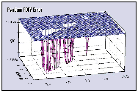
Figure 16 visualizes how stuck-at faults propagate through logic gates and interconnects, causing incorrect computations or persistent data corruption that affects downstream model behavior.

Figure 16: Stuck-at Fault Model: Digital circuits can experience permanent faults where a signal line becomes fixed at a logical 0 or 1, regardless of input; this figure represents a simplified depiction of a stuck-at-0 fault, where a signal is persistently low, potentially leading to incorrect computations or system failures. Source: accendo reliability.

For ML systems, the recovery decision is to stop trusting the component. A permanent accelerator datapath fault can keep producing bad gradients until the device is drained from the cluster (He et al. 2023; J. J. Zhang et al. 2018), while a permanent storage fault can compromise both the training dataset and the checkpoints needed for recovery. Checksum validation, replicated storage, hardware redundancy, error-correcting codes (Kim et al. 2015), and checkpoint-restart recovery¹⁹ (Egwutuoha et al. 2013) work together because each mechanism helps identify the durable copy that can still be trusted. The Young-Daly formula introduced in section 1.0.2 then gives the economic boundary. Hardware hardening increases MTBF, but the square-root relationship means reliability investment must be balanced against faster checkpointing and restart infrastructure.

Zhang, Jeff Jun, Tianyu Gu, Kanad Basu, and Siddharth Garg. 2018. “Analyzing and Mitigating the Impact of Permanent Faults on a Systolic Array Based Neural Network Accelerator.” 2018 IEEE 36th VLSI Test Symposium (VTS), 1–6. https://doi.org/10.1109/vts.2018.8368656.

Kim, Jungrae, Michael Sullivan, and Mattan Erez. 2015. “Bamboo ECC: Strong, Safe, and Flexible Codes for Reliable Computer Memory.” 2015 IEEE 21st International Symposium on High Performance Computer Architecture (HPCA), 101–12. https://doi.org/10.1109/hpca.2015.7056025.

¹⁹ Checkpoint-Restart: Originated in 1960s mainframe batch processing, where restarting multi-hour jobs from scratch was prohibitively expensive. Large distributed training jobs can checkpoint 100+ GB model states every 10–30 minutes; Google’s TPUv4 resiliency study reports coordinated checkpointing and reconfiguration that kept wasted computation from node failures below 1 percent of total training time.

Egwutuoha, I. P., D. Levy, B. Selic, and S. Chen. 2013. “A Survey of Fault Tolerance Mechanisms and Checkpoint/Restart Implementations for High Performance Computing Systems.” The Journal of Supercomputing 65 (3): 1302–26. https://doi.org/10.1007/s11227-013-0884-0.

Intermittent faults

Intermittent faults are the hardest category because they create evidence, then disappear. A node may pass a reboot test, rejoin the fleet, and fail again only when the next training job drives the package into the same thermal, voltage, or communication regime. Physical degradation (cracks in solder joints, aging ball grid arrays, residue-induced electrical connections) creates those load-dependent conditions (figure 17) (Constantinescu 2008; Rashid et al. 2015). Voltage-underscaling studies such as ThUnderVolt show a separate timing-error route: reduced voltage margins can make signal propagation unreliable and cause incorrect computations that are difficult to reproduce (J. Zhang et al. 2018).

Zhang, Jeff, Kartheek Rangineni, Zahra Ghodsi, and Siddharth Garg. 2018. “ThUnderVolt: Enabling Aggressive Voltage Underscaling and Timing Error Resilience for Energy Efficient Deep Learning Accelerators.” 2018 55th ACM/ESDA/IEEE Design Automation Conference (DAC), 1–6. https://doi.org/10.1109/dac.2018.8465918.

Figure 17: Intermittent Fault Mechanism: Increased resistance from cracks between copper bumps and package solder represents a common source of intermittent faults, disrupting signal transmission and potentially causing unpredictable system behavior. Microscopic material defects like these highlight the vulnerability of hardware to latent failures that are difficult to detect during testing but can manifest during operation. Source: constantinescu.

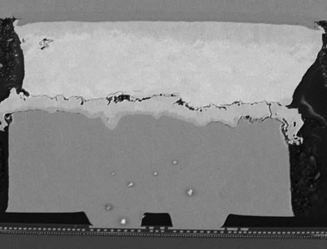
Figure 18 reveals how residue-induced intermittent faults in DRAM chips create unreliable electrical connections that lead to sporadic failures.

Figure 18: DRAM Residue Fault: Intermittent failures in DRAM chips commonly arise from microscopic residue accumulation and create unreliable electrical connections. Physical defects can induce sporadic errors and highlight the need for fault-tolerant system design and hardware testing. Source: Constantinescu.

For ML systems, intermittent faults should be treated as suspect until enough evidence proves otherwise. Sporadic processing or memory errors can accumulate across iterations, degrading convergence without triggering explicit failures (He et al. 2023; Rashid et al. 2015). Runtime monitoring and anomaly detection provide the first hint, environmental controls reduce thermal and voltage triggers, and adaptive resource management can drain, downclock, or avoid a suspect component while preserving job progress (Rashid et al. 2012). The goal is not merely to keep the node alive; it is to prevent a nondeterministic component from making validation and recovery untrustworthy.

He, Yi, Mike Hutton, Steven Chan, Robert De Gruijl, Rama Govindaraju, Nishant Patil, and Yanjing Li. 2023. “Understanding and Mitigating Hardware Failures in Deep Learning Training Systems.” Proceedings of the 50th Annual International Symposium on Computer Architecture, 1–16. https://doi.org/10.1145/3579371.3589105.

Rashid, Layali, Karthik Pattabiraman, and Sathish Gopalakrishnan. 2015. “Characterizing the Impact of Intermittent Hardware Faults on Programs.” IEEE Transactions on Reliability 64 (1): 297–310. https://doi.org/10.1109/tr.2014.2363152.

Rashid, Layali, Karthik Pattabiraman, and Sathish Gopalakrishnan. 2012. “Intermittent Hardware Errors Recovery: Modeling and Evaluation.” 2012 Ninth International Conference on Quantitative Evaluation of Systems, 220–29. https://doi.org/10.1109/qest.2012.37.

Hardware fault detection and mitigation

Hardware fault mitigation works only when the detection mechanism matches the fault signature. Permanent defects are best exposed before deployment, transient bit flips need online correction, and intermittent or silent errors require runtime evidence. At the hardware level, two foundational mechanisms protect against the fault classes described earlier.

Built-in self-test (BIST) (Bushnell and Agrawal 2002) incorporates additional circuitry for self-testing using scan chains²⁰ that apply predefined test patterns to internal logic during system startup. BIST catches manufacturing defects and permanent faults before they corrupt production workloads.

Bushnell, Michael L, and Vishwani D Agrawal. 2002. “Built-in Self-Test.” Essentials of Electronic Testing for Digital, Memory and Mixed-Signal VLSI Circuits 1: 489–548. https://doi.org/10.1007/0-306-47040-3_15.

²⁰ Scan Chains: Test infrastructure linking internal flip-flops into shift registers, developed in the 1970s for IC design-for-testability. The trade-off is concrete: 5–15 percent silicon area overhead buys 95 percent+ manufacturing fault coverage. For ML accelerators with billions of transistors in matrix-multiply units, scan-based testing during burn-in catches the stuck-at faults that would otherwise silently corrupt weight and gradient computations in production.

²¹ Hamming Codes (1950): Richard Hamming invented error-correcting codes at Bell Labs after repeated frustration with relay computer failures corrupting weekend batch jobs. His SECDED (single-error-correcting, double-error-detecting) scheme uses parity bits at power-of-2 positions to locate errors with \(\mathcal{O}(\log n)\) overhead. ECC memory modules descend from this design, protecting the terabytes of model weights and optimizer state in ML training from the soft errors that would otherwise accumulate silently.

Hamming, R. W. 1950. “Error Detecting and Error Correcting Codes.” Bell System Technical Journal 29 (2): 147–60. https://doi.org/10.1002/j.1538-7305.1950.tb00463.x.

²² CRC (Cyclic Redundancy Check): Polynomial checksum family introduced by Peterson and Brown (1961). CRC coverage depends on the polynomial, frame length, and error model; it is best understood as a low-cost detection layer rather than a universal guarantee. In distributed ML training, checksums or hashes can validate gradient payloads exchanged during collectives; without a verification layer, a corrupted gradient packet can silently poison the parameter update for every worker in the collective.

Peterson, W. W., and D. T. Brown. 1961. “Cyclic Codes for Error Detection.” Proceedings of the IRE 49 (1): 228–35. https://doi.org/10.1109/jrproc.1961.287814.

Error detection and correction codes²¹ (Hamming 1950) add redundant bits to detect and correct bit errors. Figure 19 illustrates the simplest form: parity checks append an extra bit to each data word, enabling immediate detection when a bit flip occurs. More advanced codes such as cyclic redundancy checks (CRC)²² compute checksums that detect over 99.9 percent of transmission errors, a capability critical for validating gradient payloads during the distributed AllReduce operations covered in Collective Communication.

Figure 19: Parity Bit Error Detection: This figure provides a simple error detection scheme where an extra bit (the parity bit) ensures the total number of 1s in a data sequence is either even or odd. The second sequence includes a flipped bit, triggering the parity check and indicating a data corruption event during transmission or storage. Source: computer hope.

Hardware redundancy uses component duplication and voting to detect and mask faults (Sheaffer et al. 2007). Double modular redundancy (DMR)²³ duplicates computation and compares outputs at 100 percent silicon overhead; triple modular redundancy (TMR)²⁴ performs computation three times and takes a majority vote at 200 percent overhead, enabling automatic single-fault correction (Arifeen et al. 2020). Figure 21 shows how a TMR voter circuit masks a single faulty unit by selecting the majority output. Tesla’s Full Self-Driving computer uses DMR across two independent system on chip (SoC) units (figure 20), while the Boeing 777 uses TMR in its primary flight computer for safety-critical aviation control (Yeh 1996; Bannon et al. 2019).

Sheaffer, J. W., D. P. Luebke, and K. Skadron. 2007. “A Hardware Redundancy and Recovery Mechanism for Reliable Scientific Computation on Graphics Processors.” Graphics Hardware 2007: 55–64. https://doi.org/10.2312/eggh/eggh07/055-064.

²³ DMR (Double Modular Redundancy): Duplicates computation and compares outputs to detect disagreements, at 100 percent silicon overhead vs. TMR’s 200 percent. DMR detects mismatch but cannot choose the correct output by itself, so its coverage depends on the comparator, fault model, and safe fallback policy. Tesla’s Full Self-Driving computer uses DMR across two independent SoCs, reflecting the design trade-off: DMR halves the hardware cost of TMR while requiring a safe fallback policy when outputs disagree (Bannon et al. 2019).

Bannon, Pete, Ganesh Venkataramanan, Debjit Das Sarma, and Emil Talpes. 2019. “Computer and Redundancy Solution for the Full Self-Driving Computer.” 2019 IEEE Hot Chips 31 Symposium (HCS), 1–22. https://doi.org/10.1109/hotchips.2019.8875645.

²⁴ TMR (Triple Modular Redundancy): Performs computation three times and takes a majority vote, enabling automatic single-fault correction at 200 percent hardware overhead. First applied in early fault-tolerant mainframes in the 1950s, TMR remains a longstanding pattern for radiation-exposed and safety-critical inference where single-fault correction matters more than hardware efficiency.

Arifeen, Tooba, Abdus Sami Hassan, and Jeong-A Lee. 2020. “Approximate Triple Modular Redundancy: A Survey.” IEEE Access 8: 139851–67. https://doi.org/10.1109/access.2020.3012673.

Yeh, Y. C. 1996. “Triple-Triple Redundant 777 Primary Flight Computer.” 1996 IEEE Aerospace Applications Conference. Proceedings 1: 293–307. https://doi.org/10.1109/aero.1996.495891.

Figure 20: Dual Modular Redundancy (DMR): Tesla’s full self-driving computer employs a DMR architecture, replicating critical computations across two independent system-on-chips (SoCs). A hardware comparator unit validates that both chips produce matching outputs before allowing a control command to reach the vehicle’s actuators, ensuring that a single-chip hardware failure or bit flip cannot trigger dangerous driving behavior.

Figure 21: Error Masking via Voting: In triple modular redundancy (TMR), the same computation runs on three independent units. A voter circuit takes a majority vote of the results. Even if one unit suffers a fault (for example, bit flip), the system ‘masks’ the error by selecting the matching outputs from the other two units, allowing continuous operation without interruption.

At the software level, the same decision tree continues, with each fault signature routed to the one evidence stream that exposes it most cheaply. Silent statistical drift appears when gradients, losses, activations, or latencies no longer match the expected distribution, and runtime monitoring plus anomaly detection (statistical outlier tests, One-Class SVM) catches it at the cheapest layer because those checks ride on metrics the training loop already emits (Francalanza et al. 2017; Chandola et al. 2009). A corrupted-but-live state or checkpoint is caught by data-consistency checks that confirm it still corresponds to trusted data (Lindholm et al. 2019). A fail-stop node is separated from a merely slow one by heartbeat mechanisms (Kawazoe Aguilera et al. 1997), and a task that stalls without crashing is caught by watchdog timers (Pont and Ong 2002) that trigger recovery on lost progress. Only when none of these passive signals suffice, because the computation itself may be wrong with no statistical tell, does the system pay for software-implemented redundancy (SWIFT-style instruction duplication, N-version programming, Reed-Solomon reconstruction) (Reis et al. 2005; Avizienis et al. 2004; Plank 1997; Reed and Solomon 1960), whose duplicated or reconstructed computation is the most expensive layer and so is reserved for the highest-value state.

Francalanza, Adrian, Luca Aceto, Antonis Achilleos, Duncan Paul Attard, Ian Cassar, Dario Della Monica, and Anna Ingólfsdóttir. 2017. “A Foundation for Runtime Monitoring.” In Runtime Verification. Springer International Publishing. https://doi.org/10.1007/978-3-319-67531-2_2.

Chandola, Varun, Arindam Banerjee, and Vipin Kumar. 2009. “Anomaly Detection: A Survey.” ACM Computing Surveys 41 (3): 1–58. https://doi.org/10.1145/1541880.1541882.

Lindholm, Andreas, Dave Zachariah, Petre Stoica, and Thomas B. Schon. 2019. “Data Consistency Approach to Model Validation.” IEEE Access 7: 59788–96. https://doi.org/10.1109/access.2019.2915109.

Kawazoe Aguilera, Marcos, Wei Chen, and Sam Toueg. 1997. “Heartbeat: A Timeout-Free Failure Detector for Quiescent Reliable Communication.” In Lect. Notes Comput. Sci. Springer Berlin Heidelberg. https://doi.org/10.1007/bfb0030680.

Pont, Michael J, and Royan HL Ong. 2002. “Using Watchdog Timers to Improve the Reliability of Single-Processor Embedded Systems: Seven New Patterns and a Case Study.” Proceedings of the First Nordic Conference on Pattern Languages of Programs, 159–200.

Reis, G. A., J. Chang, N. Vachharajani, R. Rangan, and D. I. August. 2005. “SWIFT: Software Implemented Fault Tolerance.” International Symposium on Code Generation and Optimization, 243–54. https://doi.org/10.1109/cgo.2005.34.

Avizienis, Algirdas, Jean-Claude Laprie, Brian Randell, and Carl Landwehr. 2004. “Basic Concepts and Taxonomy of Dependable and Secure Computing.” IEEE Transactions on Dependable and Secure Computing 1 (1): 11–33. https://doi.org/10.1109/TDSC.2004.2.

Plank, James S. 1997. “A Tutorial on Reed-Solomon Coding for Fault-Tolerance in RAID-Like Systems.” Software: Practice and Experience 27 (9): 995–1012. https://doi.org/10.1002/(SICI)1097-024X(199709)27:9<995::AID-SPE111>3.0.CO;2-6.

Reed, I. S., and G. Solomon. 1960. “Polynomial Codes over Certain Finite Fields.” Journal of the Society for Industrial and Applied Mathematics 8 (2): 300–304. https://doi.org/10.1137/0108018.

These mechanisms reduce the unreliable substrate risk, but they do not protect against faults introduced by the software stack itself. The next layer must reason about bugs that look like valid computation while corrupting the ML pipeline.

Checkpoint 1.3: Classifying a hardware fault

Verify your understanding of the transient, permanent, and intermittent fault categories and the fault, error, failure progression:

• Transient fault: Classify a GPU that produces a wrong result once after a cosmic-ray strike and then computes correctly for the rest of the run, and justify why error correction codes, not node replacement, match that fault.
• Intermittent vs. permanent: Distinguish an intermittent fault from a permanent one when both can produce a stuck-at value, including the diagnostic signal that separates them.
• Fault-error-failure chain: Trace a single bit flip through the fault, error, failure chain, identifying where error correction codes and checkpoint-restart each intervene.
• Silent corruption: Explain why silent corruption sits apart from the other fault manifestations even when its underlying fault is an ordinary transient bit flip.

Self-Check: Question

1. A ResNet-50 training job suddenly shows 1 incorrect layer output in 10 million forward passes, with no repeat at the same address after a memory scrub. No further errors are observed for the next 24 hours on that device. Which hardware fault category best matches this signature?

   1. Transient fault
   2. Permanent fault
   3. Intermittent fault
   4. Wear-out fault

2. A single bit flip in a ResNet-50 weight can drop ImageNet top-1 accuracy from 76 percent to below 10 percent. Explain what about ML workloads amplifies a single-bit hardware fault into this scale of output collapse, drawing on the chapter’s IEEE 754 layout argument.

3. Why can software-only fault injection overestimate or underestimate real system vulnerability compared with physical hardware fault injection?

   1. Because software tools always inject larger faults than hardware produces.
   2. Because software tools ignore the computational graph and can only modify weights.
   3. Because software tools miss low-level masking and microarchitectural effects that may prevent a hardware fault from reaching the application.
   4. Because hardware faults never affect memory, only logic units.

4. True or False: Triple modular redundancy corrects a single faulty computation by majority voting, but it does so at much higher hardware cost than double modular redundancy.

5. Order the following protection path from earliest to latest in a typical hardware fault-defense flow: (1) Correct or detect the error with ECC/CRC, (2) A fault occurs in hardware, (3) Trigger higher-level recovery if corruption escapes local protection.

See Answers →

Software Faults

A team spends three months testing an LLM against complex prompt-level failure cases, only to realize that its preprocessing script accidentally truncated all inputs at 512 tokens, silently discarding the system prompt entirely. In the pursuit of complex algorithmic robustness, engineers often overlook a common source of ML failure: mundane software bugs. In ML systems, a logic error in a data loader does not crash the pipeline; it subtly degrades the gradient, making software faults uniquely damaging.

Software faults require a different recovery lens from hardware failures. Hardware faults enter from silicon, electrons, and physical wear; software faults enter through design choices, dependency versions, and pipeline glue. The fault-tolerance problem shifts from replacing a failed component to identifying which valid-looking transformation corrupted data, gradients, or predictions.

The practical challenge is that software faults interact with every other system threat. A bug in data preprocessing can create distribution shifts, an implementation error in numerical computation can corrupt model behavior while preserving valid tensor shapes, and a race condition in distributed training can make different workers update from inconsistent state. These interactions arise because AI software stacks span frameworks, libraries, runtime environments, distributed systems, and deployment infrastructure. Each layer boundary creates an opportunity for faults to emerge and propagate, making software-level mitigation essential for production-scale reliability.

Software fault properties and propagation

Software faults in ML frameworks range from syntactic and logical errors to memory leaks,²⁵ concurrency bugs, and integration failures. They propagate across system boundaries: an error in a tensor allocation routine can cascade to disrupt training, inference, or evaluation in seemingly unrelated modules. Some faults are intermittent, manifesting only under specific conditions such as high system load, particular hardware configurations, or rare data inputs.

²⁵ Memory Leak: A programming error where allocated memory is never released. In ML systems, GPU memory leaks are uniquely destructive because accelerator memory is scarce (40–80 GB per device) and shared across the entire training pipeline. A single leaked tensor per batch—perhaps from a debugging hook left in production—can exhaust GPU memory within hours, causing silent OOM failures that kill long-running training jobs without checkpointing.

Resource mismanagement is a prominent failure class. GPU memory allocations accumulate across training iterations as intermediate activations, optimizer states, and gradient buffers are allocated but not released, until the allocator exhausts available capacity and raises an out-of-memory error mid-batch. A 70B parameter model in BF16 with AdamW optimizer states requires roughly 840 GB of GPU memory across a node, leaving virtually no headroom for unexpected buffer growth. Memory pressure builds gradually over hundreds of iterations, making root-cause attribution difficult without per-layer memory profiling.

Concurrency and synchronization errors constitute another recurring fault class. In distributed or multi-threaded environments, incorrect coordination among parallel processes leads to race conditions,²⁶ or inconsistent states.

²⁶ Race Condition: A timing bug where system behavior depends on the uncontrolled sequence of concurrent events. In asynchronous distributed training, if multiple workers update the same parameter weight simultaneously without proper locking or versioning, updates can be lost or overwritten, leading to divergence or “ghost” weights that ruin convergence without triggering an error.

²⁷ Deadlock: A state where two or more processes are permanently blocked, each waiting for the other to release a resource. In pipelined training, a deadlock can occur if Stage 1 is waiting for a free buffer to send activations to Stage 2, while Stage 2 is waiting for Stage 1 to receive backward gradients, halting the entire fleet.

Deadlocks²⁷ create a related synchronization failure, where workers wait indefinitely on resources or messages that never arrive. A bug in a high-level library might only manifest when paired with a specific version of a low-level numerical library such as cuDNN or MKL, requiring a holistic view of the system to identify root causes.

Software fault detection and prevention

Because many software faults leave the pipeline running while corrupting gradients, software fault mitigation strategies must assign each lifecycle phase a detection job. The prompt-truncation bug from the opening example should not survive until production monitoring: a unit test should catch the tokenizer boundary, an integration test should catch the batch shape and metadata path, a regression test should protect representative prompts, and runtime monitoring should detect any unexpected truncation distribution that escapes development. Table 5 organizes these gates by the kind of corruption they are designed to catch.

Table 5: Fault Mitigation Strategies: Software faults in ML systems require layered gates that catch different corruption modes: tokenizer boundary errors, batch-shape drift, unsafe slicing, dependency incompatibility, and runtime anomalies.

Category	Technique	Corruption caught	When to Apply
Testing and Validation	Unit testing, integration testing, regression testing	Tokenizer boundaries, batch shapes, golden-example regressions	During development
Static Analysis and Linting	Static analyzers, linters, code reviews	Unsafe slicing, implicit casts, unguarded shape assumptions	Before integration
Runtime Monitoring & Logging	Metric collection, error logging, profiling	Length-distribution shifts, NaN gradients, memory-growth anomalies	During training and deployment
Fault-Tolerant Design	Exception handling, modular architecture, checkpointing	Bad batches fail closed and recovery resumes from known-good state	Design and implementation phase
Update Management	Dependency auditing, test staging, version tracking	Tokenizer, data-collator, framework, and CUDA compatibility drift	Before system upgrades or deployment
Environment Isolation	Containerization (for example, Docker, Kubernetes), virtual environments	Environment-specific behavior and irreproducible dependency stacks	Development, testing, deployment
CI/CD and Automation	Automated test pipelines, monitoring hooks, deployment gates	Untested model, data, or preprocessing changes reaching production	Continuously throughout development

These safeguards matter only when each gate targets a concrete corruption path. A unit test that checks only whether the tokenizer runs is too weak; it must assert that system prompts, labels, masks, and sequence-length metadata survive preprocessing with the intended semantics. Integration tests then follow one batch through loading, sharding, collation, and model input construction, while regression tests preserve representative prompts and edge cases before they enter distributed execution (figure 22). The continuous integration/continuous deployment (CI/CD) structure in figure 23 is useful only when the release pipeline treats model, data, and preprocessing changes as ML artifacts that can corrupt the training objective; otherwise, it is just a generic software-delivery diagram. Automated gates make those checks release requirements instead of optional habits.

Figure 22: Automated Regression Testing: The recurring concerns of regression testing, spanning platform coverage, risk-based selection, parallel execution, unit and API coverage, performance impact, and continuous methodologies. For ML pipelines, these same gates must preserve tokenizer behavior, feature semantics, and batch construction across code changes. Source: UTOR.

Figure 23: A CI/CD Pipeline: The standard software-delivery flow, from developer commit through version control, build, automated unit and UI testing, packaging, and release to general availability, grouped into a continuous-integration build pipeline and a continuous-delivery release pipeline. The accompanying text explains the additional gates, on model artifacts, data contracts, dependency versions, and preprocessing semantics, that this structure must add to become fault-tolerant for ML. Source: geeksforgeeks.

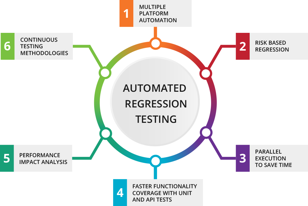
These software practices catch implementation faults that surface through tests or deployment gates. Silent corruption is harder because the system may continue running while producing wrong values, so the next layer is explicit verification.

Self-Check: Question

1. Which software fault is most likely to halt a distributed training pipeline without crashing the processes, leaving workers waiting on one another indefinitely?

   1. Memory leak
   2. Deadlock
   3. Syntax error
   4. Model drift

2. Explain why a software bug in ML can be harder to detect than a bug in a traditional application that simply crashes.

3. Two data-loader workers update a shared epoch counter without a lock; after several runs, accuracy silently drifts on the second worker even though no errors are thrown. Explain what is going wrong and describe one synchronization or versioning mechanism that would eliminate the class of bug involved.

4. A team wants to reduce environment-specific bugs caused by inconsistent library and runtime versions across development, testing, and deployment. Which mitigation from the section is most directly targeted at that problem?

   1. Containerization and environment isolation
   2. Increasing checkpoint frequency
   3. Adding more model replicas
   4. Reducing batch size

See Answers →

Check-and-Verify: Defending Against Silent Data Corruption

Silent data corruption accumulates until it becomes routine.

As clusters scale to 100,000+ GPUs, the probability of a “Silent Data Corruption” (SDC) event (in which an ALU or HBM bit flip occurs without triggering ECC or hardware alerts) approaches certainty during large collective operations. Standard AllReduce algorithms assume that if a node is alive, its data is correct. In the machine learning fleet, we must transition to a Byzantine fault tolerance mindset: “Trust, but verify.”

Check-and-verify methods turn that mindset into a data-path invariant. The system computes a checksum, hash, or redundant reduction over each gradient shard or reduced buffer, compares the result across ranks or against an independently computed digest, and blocks the optimizer step when the verification disagrees. A quick estimate makes the exposure concrete.

Napkin Math 1.2: The SDC certainty

Problem: Calculate the probability that at least one GPU in a 100,000-GPU fleet experiences a silent ALU error during a single 2 s training step.

1. Fleet size: 100,000 accelerators.
2. Individual risk: \(10^{-6}\) per hour (a conservative estimate for SDC).
3. The exposure: In a 2-second window, the fleet has \(100{,}000 \times (2/3600) \approx 56\) “GPU-hours” of exposure.
4. The probability: \(\Pr(\text{at least one SDC}) \approx\) 0.0056 percent.

Systems insight: In a 100k-GPU fleet, a silent error occurs every 18,000 steps (roughly every 10 hours). Check-and-verify methods compute a CRC or hash for each gradient shard or reduced buffer, compare the digest across ranks or against a redundant reduction, and block the optimizer step when the digest disagrees. Without checksummed collectives or hash-and-verify gradients on the AllReduce path, model parameters silently accumulate corrupted contributions and drift within half a day. Robustness moves from being a restart problem to a verification problem: the fleet must perform redundant reductions or use parity-protected gradients to catch silent parameter corruption.

The calculation makes check-and-verify mandatory, but verification only earns trust when tested against realistic failures. The next step is therefore to inject faults deliberately and confirm that the same checks catch the corruption before it reaches model state.

Self-Check: Question

1. True or False: In a 100,000-GPU training fleet, if every worker still responds to heartbeats, the main remaining risk is delay rather than correctness, so restart-based handling is usually sufficient.

2. A 100,000-GPU fleet performs a 2-second training step while each GPU has roughly \(10^{-6}\) chance of SDC per hour. Explain why checksummed collectives or hash-and-verify gradients become valuable even though each individual device’s hourly risk is tiny, and what the practical cadence of corruption looks like at this scale.

3. A team is scaling synchronous training to 100,000 GPUs and sees occasional unexplained loss anomalies even though no node crashes. Which design change best matches the section’s recommendation?

   1. Assume the anomalies are harmless because the collectives completed successfully.
   2. Reduce checkpoint frequency so fewer anomalous states are saved.
   3. Add checksummed or redundant verification of collective results so live-but-corrupted workers can be detected.
   4. Spread requests across more load balancers so corrupted gradients are less concentrated.

See Answers →

Fault Injection Tools and Frameworks

Verification only has value when the injected failure resembles the production failure the system must survive. A multi-node training cluster that claims to tolerate network partitions should have that connection severed in a staging environment so engineers can observe what the orchestration layer does. Fault injection is the engineering discipline of deliberately perturbing a system to empirically verify that robustness mechanisms work before production traffic discovers the gap. ML/tensor/GPU fault-injection tools cover bit flips, tensor faults, and accelerator-oriented failures (Chen et al. 2020; Tsai et al. 2021; Gräfe et al. 2023), while network partitions, latency injection, dependency termination, and API-response faults belong to chaos and distributed-systems testing practice (Basiri et al. 2016).

Chen, Zitao, Niranjhana Narayanan, Bo Fang, Guanpeng Li, Karthik Pattabiraman, and Nathan DeBardeleben. 2020. “TensorFI: A Flexible Fault Injection Framework for TensorFlow Applications.” 2020 IEEE 31st International Symposium on Software Reliability Engineering (ISSRE), 426–35. https://doi.org/10.1109/issre5003.2020.00047.

Tsai, Timothy, Siva Kumar Sastry Hari, Michael Sullivan, Oreste Villa, and Stephen W. Keckler. 2021. “NVBitFI: Dynamic Fault Injection for GPUs.” 2021 51st Annual IEEE/IFIP International Conference on Dependable Systems and Networks (DSN), 284–91. https://doi.org/10.1109/dsn48987.2021.00041.

Gräfe, Ralf, Qutub Syed Sha, Florian Geissler, and Michael Paulitsch. 2023. “Large-Scale Application of Fault Injection into PyTorch Models -an Extension to PyTorchFI for Validation Efficiency.” 2023 53rd Annual IEEE/IFIP International Conference on Dependable Systems and Networks - Supplemental Volume (DSN-s), 56–62. https://doi.org/10.1109/dsn-s58398.2023.00025.

Fault and error models

That resemblance is a modeling decision, not an implementation detail. A transient bit flip, a permanent accelerator defect, and a corrupted gradient require different detection logic, so the experiment must specify duration, location, granularity, and propagation path before it begins.

These choices define the fault model: how a hardware fault manifests in the system. The corresponding error model represents how that fault propagates and affects the system’s behavior.

The first modeling choice fixes the physical signature of the fault. Duration determines whether recovery should expect a transient event, a permanent defect, or an intermittent condition that is hard to reproduce. Location determines whether the injected fault enters through memory cells, functional units, or interconnects. Granularity determines whether the experiment studies a single bit, such as a bit flip, or a multi-bit burst error.

The error model carries that physical signature into the ML system. It describes how an initial hardware-level disturbance becomes corrupted weights, miscomputed activations, or higher-level logical errors in an ML framework. The abstraction level matters because each level exposes different propagation paths and masks different effects.

The choice of fault or error model is central to robustness evaluation. For example, a system built to study single-bit transient faults (Sangchoolie et al. 2017) will not offer meaningful insight into the effects of permanent multi-bit faults, since its design and assumptions are grounded in a different fault model entirely.

Binkert, Nathan, Bradford Beckmann, Gabriel Black, Steven K. Reinhardt, Ali Saidi, Arkaprava Basu, Joel Hestness, et al. 2011. “The Gem5 Simulator.” ACM SIGARCH Computer Architecture News 39 (2): 1–7. https://doi.org/10.1145/2024716.2024718.

The implementation context of an error model also matters. A single-bit flip at the architectural register level, modeled using simulators like gem5 (Binkert et al. 2011), differs meaningfully from a similar bit flip in a PyTorch model’s weight tensor. While both simulate value-level perturbations, the lower-level model captures microarchitectural effects that are often abstracted away in software frameworks.

Some fault behavior patterns transfer across abstraction levels, while others do not. Studies that compare single-bit and multi-bit fault models show that impact depends on where the fault lands and how it propagates, so robustness results from one injected-fault model should not be treated as universal (Sangchoolie et al. 2017; Papadimitriou and Gizopoulos 2021). Other important behaviors like error masking (Mohanram and Touba 2003) may only be observable at lower abstraction levels. This masking phenomenon can cause faults to be filtered out before they propagate to higher levels (figure 24) (Ko 2021), meaning software-based tools may miss these effects entirely.

Sangchoolie, Behrooz, Karthik Pattabiraman, and Johan Karlsson. 2017. “One Bit Is (Not) Enough: An Empirical Study of the Impact of Single and Multiple Bit-Flip Errors.” 2017 47th Annual IEEE/IFIP International Conference on Dependable Systems and Networks (DSN), 97–108. https://doi.org/10.1109/dsn.2017.30.

Papadimitriou, George, and Dimitris Gizopoulos. 2021. “Demystifying the System Vulnerability Stack: Transient Fault Effects Across the Layers.” 2021 ACM/IEEE 48th Annual International Symposium on Computer Architecture (ISCA), 902–15. https://doi.org/10.1109/isca52012.2021.00075.

Mohanram, K., and N. A. Touba. 2003. “Partial Error Masking to Reduce Soft Error Failure Rate in Logic Circuits.” Proceedings. 18th IEEE International Symposium on Defect and Fault Tolerance in VLSI Systems, 433–40. https://doi.org/10.1109/dftvs.2003.1250141.

Ko, Y. 2021. “Characterizing System-Level Masking Effects Against Soft Errors.” Electronics 10 (18): 2286. https://doi.org/10.3390/electronics10182286.

Figure 24: Error Masking: Microarchitectural redundancy can absorb single-bit faults before they propagate to observable system errors, highlighting a discrepancy between hardware-level and software-level fault models. This figure details how fault masking occurs within microarchitectural components, demonstrating that software-based error detection tools may underestimate the true resilience of a system to transient errors.

Fault injection methods

Fault injection methods trade realism against experimental scale. Hardware-based injection is the calibration point: it introduces faults into physical systems so software-level assumptions can be checked against real hardware behavior. Software-based injection is the scalable counterpart: it covers many model states quickly but must be calibrated against hardware behavior before its conclusions become production reliability claims.

Hardware-based fault injection

The method choice depends on whether the experiment needs bit-level targeting or physical radiation realism. FPGA-based fault injection uses field-programmable gate arrays (FPGAs)²⁸, reconfigurable integrated circuits that can be programmed to implement various hardware designs. By modifying the FPGA configuration, faults can be introduced at specific locations and times during the execution of an ML model.

²⁸ FPGA (Field-Programmable Gate Array): Reconfigurable hardware containing millions of programmable logic blocks. For fault injection, FPGAs provide bit-level targeting precision that software-based tools cannot match.

Velazco, Raoul, Gilles Foucard, and Paul Peronnard. 2010. “Combining Results of Accelerated Radiation Tests and Fault Injections to Predict the Error Rate of an Application Implemented in SRAM-Based FPGAs.” IEEE Transactions on Nuclear Science 57 (6): 3500–3505. https://doi.org/10.1109/tns.2010.2087355.

Radiation or beam testing (Velazco et al. 2010) exposes hardware running ML models to high-energy particles like protons or neutrons. Specialized test facilities enable controlled radiation exposure to induce bitflips and other hardware-level faults, providing highly realistic fault scenarios that mirror conditions in radiation-rich environments.

Software-based fault injection

Software-based fault injection trades physical realism for experimental scale. These tools simulate the effects of hardware faults by modifying a model’s underlying computational graph, tensor values, or intermediate computations. They integrate directly with ML development pipelines, require no specialized hardware, and allow researchers to conduct large-scale fault injection experiments quickly and cost-effectively.

PyTorchFI (Mahmoud et al. 2020), a dedicated fault injection library for PyTorch developed in collaboration with Nvidia Research, is useful when the question is how tensor-visible perturbations affect model behavior. It injects faults into weights, activations, and gradients, showing that even simple bit-level faults can cause severe visual and classification errors, including the appearance of “phantom” objects where none exist.

Mahmoud, A., N. Aggarwal, A. Nobbe, J. R. S. Vicarte, S. V. Adve, C. W. Fletcher, I. Frosio, and S. K. S. Hari. 2020. “PyTorchFI: A Runtime Perturbation Tool for DNNs.” 2020 50th Annual IEEE/IFIP International Conference on Dependable Systems and Networks Workshops (DSN-w), 25–31. https://doi.org/10.1109/dsn-w50199.2020.00014.

Bridging hardware-software gap

The abstraction choice is the central risk in software-based fault injection. These tools offer speed and flexibility, but they do not always capture the full range of effects that hardware faults can impose on a system. The abstraction gap arises because software-based tools operate at a higher level and may overlook low-level hardware interactions or nuanced error propagation mechanisms.

Tools like Fidelity (He et al. 2020) address this gap by mapping low-level hardware error behavior to software-visible effects. By studying how faults originating in hardware move through architectural registers, memory hierarchies, and numerical operations, Fidelity makes software-injected faults resemble the way faults would manifest in a physical system.

He, Yi, Prasanna Balaprakash, and Yanjing Li. 2020. “FIdelity: Efficient Resilience Analysis Framework for Deep Learning Accelerators.” 2020 53rd Annual IEEE/ACM International Symposium on Microarchitecture (MICRO), 270–81. https://doi.org/10.1109/micro50266.2020.00033.

Example 1.1: Software fault injection limits

Scenario: A team validates a training system with software fault injection and concludes that a particular tensor bit flip always corrupts model output.

Mechanism: Physical beam testing can produce a different result because hardware includes masking effects below the software abstraction. A bit flip in a hardware register might be corrected by ECC memory or masked by logical gates before it ever reaches the variable that software tools mutate directly.

Systems lesson: Software fault injection is useful for fast coverage of model-visible states, but it can overstate vulnerability when it bypasses circuit-level defenses. Production resilience claims therefore need a hardware-calibrated fault model, not software injection alone.

Hardware fault summary

While hardware and software faults represent distinct failure mechanisms, they ultimately manifest as system-level events that must be managed by the reliability logic established earlier in this chapter. The fault characteristics in table 6 close the loop from fault model to recovery choice. The table compares transient, permanent, and intermittent faults across duration, persistence, causes, and ML system impact so the detection and mitigation strategy matches the fault category being tested.

Table 6: Fault Characteristics: Transient, permanent, and intermittent faults differ by duration, persistence, and recurrence, impacting system reliability and requiring distinct mitigation strategies for robust AI deployments (Constantinescu 2008). Understanding these distinctions guides the design of fault-tolerant systems capable of handling diverse hardware failures during operation.

Constantinescu, C. 2008. “Intermittent Faults and Effects on Reliability of Integrated Circuits.” 2008 Annual Reliability and Maintainability Symposium, 370–74. https://doi.org/10.1109/rams.2008.4925824.

Dimension	Transient Faults	Permanent Faults	Intermittent Faults
Duration	Short-lived, temporary	Persistent, remains until repair or replacement	Sporadic, appears and disappears intermittently
Persistence	Disappears after the fault condition passes	Consistently present until addressed	Recurs irregularly, not always present
Causes	External factors (for example, electromagnetic interference or cosmic rays)	Hardware defects, physical damage, wear-out	Unstable hardware conditions, loose connections, aging components
Manifestation	Bit flips, glitches, temporary data corruption	Stuck-at faults, broken components, complete device failures	Occasional bit flips, intermittent signal issues, sporadic malfunctions
Impact on ML systems	Introduces temporary errors or noise in computations	Causes consistent errors or failures, affecting reliability	Leads to sporadic and unpredictable errors, challenging to diagnose and mitigate
Detection	Error detection codes, comparison with expected values	Built-in self-tests, error detection codes, consistency checks	Monitoring for anomalies, analyzing error patterns and correlations
Mitigation	Error correction codes, redundancy, checkpoint and restart	Hardware repair or replacement, component redundancy, failover mechanisms	Robust design, environmental control, runtime monitoring, fault-tolerant techniques

Self-Check: Question

1. A team wants to answer a specific question: ‘Does microarchitectural masking reduce the number of faults from cosmic rays that actually reach our deployed image classifier?’ Which experimental setup most directly answers that question, and why?

   1. Inject single-bit flips into weight tensors in PyTorch and count prediction changes, because tensor-level injection is the fastest way to measure resilience.
   2. Run FPGA-based injection or beam testing that targets architectural registers, because this is the only setup where ECC, overwrite, and speculative-squash masking can actually intervene before the fault reaches software.
   3. Compute an analytical bound from ECC coverage rates and skip empirical injection, because masking can be derived from datasheet parameters.
   4. Use a tool like Fidelity in software-only mode and assume the mapping fully captures masking, because it is designed to bridge the hardware-software gap.

2. A researcher wants to study whether ECC and microarchitectural masking reduce the number of faults that actually reach an ML application. Why is beam testing or other hardware-based injection more informative than injecting tensor bit flips in software?

3. Why might a tool like Fidelity be useful when studying ML robustness?

   1. It eliminates the need for any physical testing.
   2. It maps low-level hardware fault behavior into software-visible effects to narrow the abstraction gap.
   3. It guarantees that single-bit faults are harmless in neural networks.
   4. It replaces all error models with a single universal model.

See Answers →

Checkpointing: Preserving Progress

The practical question is how distributed training systems detect these faults and recover from them without losing days of computation. When a top-of-rack switch dies two weeks into a 175-billion parameter model training run, the cluster loses 64 GPUs instantly. The system cannot simply restart from scratch; the sunk cost is too high. The failure analysis in Failure Analysis at Scale established that large-scale training systems will experience such failures frequently, requiring robust mechanisms to preserve and resume progress.

Training fault tolerance has three obligations: preserve state, detect and classify failures, and resume or resize the job. Checkpointing supplies the first obligation. The sections that follow then build the rest of the recovery model: failure detection decides what happened, recovery procedures restore a consistent process group, and elastic recovery decides whether the job can continue with a changed worker set.

Definition 1.1: Checkpointing

Checkpointing is the periodic serialization of the complete training state (parameters, optimizer state, and data loader position) to persistent storage.

1. Significance: It minimizes lost work after a system failure by trading checkpoint I/O against rework. Writing too often wastes accelerator time on storage traffic; writing too rarely risks replaying many completed steps after a failure. The Young-Daly formula \((\tau_{\text{opt}} = \sqrt{2 \cdot T_{\text{write}} \cdot \text{MTBF}_{\text{system}}})\) captures that local trade-off by choosing the interval that balances write cost against expected lost work.
2. Distinction: Unlike incremental backups, checkpointing must capture the exact execution context (including random seeds and learning rate schedules) to ensure deterministic resumption of the optimization loop.
3. Common pitfall: A frequent misconception is that checkpointing is “just writing to disk.” In reality, for large models, it is a storage-system stress test: the simultaneous write from thousands of GPUs can trigger a checkpoint storm that saturates the entire network fabric \((\text{BW})\).

A training cluster that loses power without state preservation loses millions of dollars worth of gradient updates computed over the preceding weeks. The defense is to periodically write the model state to durable storage. Checkpointing captures sufficient state to resume training from a recorded point: model parameters, optimizer state,²⁹ training progress indicators, and random state for reproducibility.

²⁹ Adam Optimizer State: Adaptive Moment Estimation (Adam) maintains per-parameter first-moment (\(m\)) and second-moment (\(v\)) estimates, tripling memory requirements compared to vanilla SGD (3\(\times\): parameters + two state vectors). For a 175B parameter model, optimizer state alone reaches 2.1 TB, which typically dominates checkpoint size and recovery time, making optimizer state the primary bottleneck in checkpoint I/O design.

Optimizer state, not weights, dominates checkpoint size.

Checkpoint interval from failure analysis

The Young-Daly formula stated in section 1.0.2 gives the optimal checkpoint interval, \(\tau_{\text{opt}} = \sqrt{2 \times T_{\text{write}} \times \text{MTBF}_{\text{system}}}\), but it cannot be applied until both inputs are known. The failure analysis earlier in this chapter supplies the system MTBF term, and the checkpoint payload established above supplies \(T_{\text{write}}\). With both in hand, the formula stops being an abstract law and becomes a concrete schedule for the chapter’s own cluster.

Figure 25 plots that trade-off for an illustrative 175B-parameter cluster: save overhead falls as intervals lengthen while expected rework rises, and the Young-Daly interval sits at the minimum of their sum. Its round inputs convey the curve’s shape; the worked calculation below pins the exact interval from this chapter’s own computed MTBF and write time.

Figure 25: The Checkpoint Trade-Off: Checkpoint save overhead decreases with longer intervals, but wasted computation from failures increases. The Young-Daly optimal interval minimizes total overhead. For an illustrative 175B-model cluster (~2.5-minute checkpoint writes, 2-hour MTBF), the optimal interval is approximately 24 minutes; the worked calculation below derives the exact interval for this chapter’s 10,000-GPU cluster.

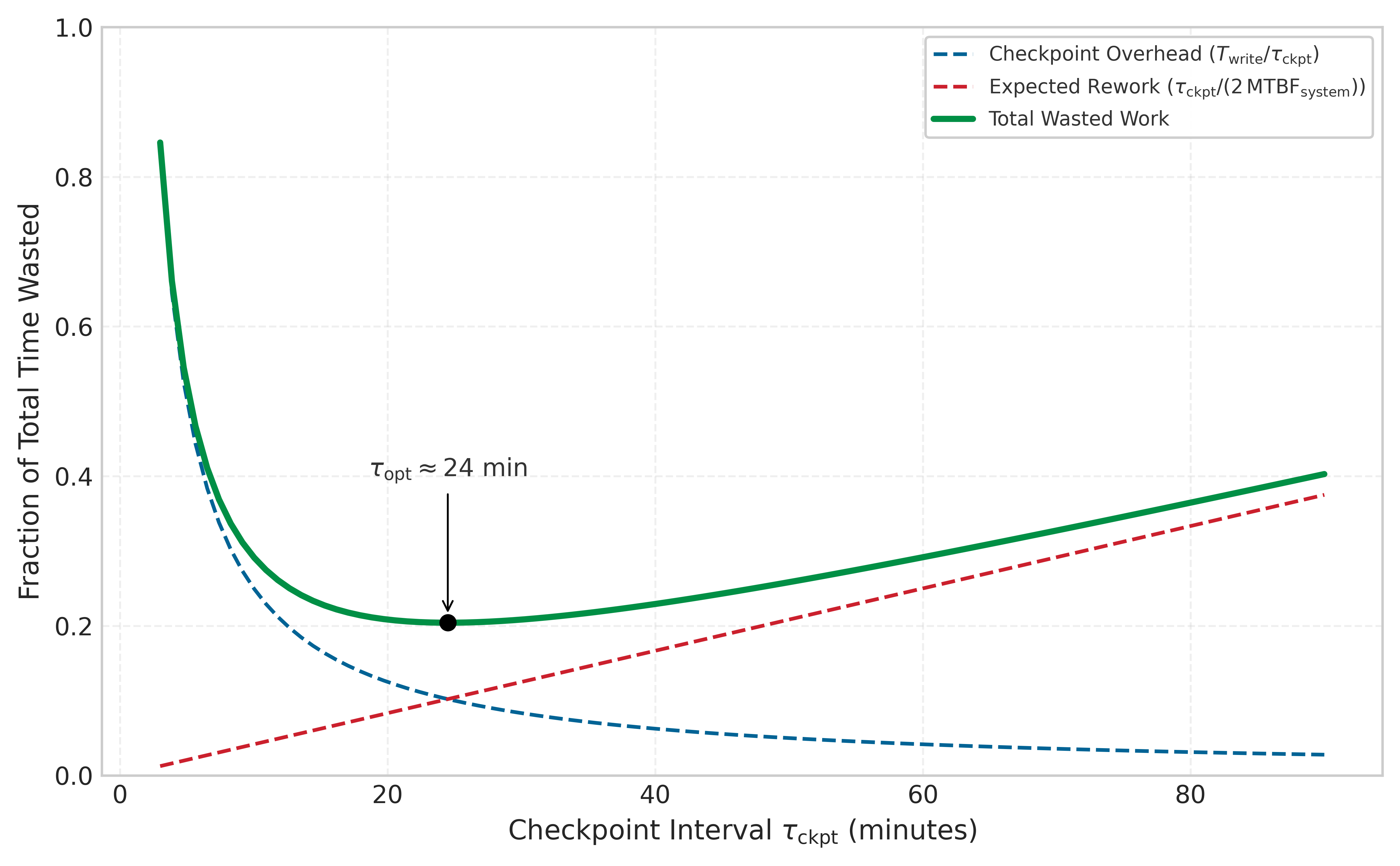
The chapter’s own 10,000-GPU cluster supplies both inputs, replacing the round figures in figure 25 with computed values. The worked cascade (section 1.0.4) put system MTBF at 3.69 hours, and the checkpoint payload above writes in 37 s (a 3.7 TB checkpoint at 100 GB/s). Substituting these into the Young-Daly formula gives the canonical interval for this cluster.

Napkin Math 1.3: The Young-Daly optimal interval

Problem: A 10,000-GPU cluster has an MTBF of 3.69 hours. A full model checkpoint takes 37 s to write. What is the optimal checkpoint frequency?

Math: Apply the Young-Daly formula: \(\tau_{\text{opt}} = \sqrt{2 \cdot T_{\text{write}} \cdot \text{MTBF}_{\text{system}}}\)

1. Convert to common units: \(\text{MTBF}_{\text{system}} =\) 3.69 hours \(\times\) 3600 s/hour = 13284 s.
2. Substitute and solve: With \(T_{\text{write}} =\) 37 s and \(\text{MTBF} =\) 13284 s, the formula gives \(\tau_{\text{opt}} \approx\) 991.4 s, or about 16.5 min.

Systems insight: At this interval, the “checkpoint tax” (time spent saving + time spent re-computing) is minimized to approximately 7.5 percent. Checkpointing every hour instead would increase failure risk, wasting about 14.6 percent of the cluster’s capacity. As clusters scale, the optimal interval must shrink to keep up with the falling MTBF.

This result demonstrates why failure analysis matters: without knowing the system MTBF, we cannot set checkpoint intervals rationally. With this interval, checkpoint overhead consumes approximately 7.5 percent of training time, but the estimate depends on assumptions that often fail in production.

Systems Perspective 1.3: Young-Daly formula assumptions

The Young-Daly formula provides valuable intuition but rests on assumptions that may not hold in practice:

• Exponentially distributed failures: Assumes a constant failure rate. Real systems exhibit “bathtub curve” behavior with higher rates during burn-in and wear-out phases.
• Deterministic checkpoint time: Assumes \(T_{\text{write}}\) is constant. In practice, checkpoint time varies 2–3\(\times\) due to storage contention, network congestion, and memory pressure.
• Recovery time equals checkpoint time: Assumes recovery reads the same data written during checkpoint. Often recovery takes 3–5\(\times\) longer due to job scheduling delays, topology reconstruction, and warmup.
• Single failure mode: Assumes one failure at a time. Correlated failures (power, cooling, shared switch) violate this assumption.
• Infinite timeline: Optimizes for long training runs. Short runs, where total time is comparable to MTBF, require different analysis.

When assumptions are violated, the optimal interval may shift significantly, but restart overhead should not be treated as if it were paid at every checkpoint. In the first-order lost-time model, restart time adds a per-failure recovery term to total expected waste; it does not replace \(T_{\text{write}}\) inside \(\sqrt{2 \cdot T_{\text{write}} \cdot \text{MTBF}_{\text{system}}}\) unless a recovery-aware Daly-style model is explicitly derived and calibrated.

Figure 26 makes the temporal cost of failures concrete by showing the sequence of events during a training run: productive computation, periodic checkpoints, a failure event, and the recovery process with its associated wasted work.

Figure 26: Checkpoint-Recovery Timeline: A training run proceeds through alternating phases of computation (green) and checkpoint writes (blue). When a failure occurs (red lightning bolt), all work since the last completed checkpoint is lost (hatched gray). Recovery involves job restart overhead, checkpoint loading, and pipeline warmup before productive training resumes. The total cost of a failure includes both the lost work and the recovery latency.

The timeline in figure 26 reveals why \(T_{\text{restart}}\) matters as much as \(T_{\text{write}}\): the total failure cost is the sum of lost work (bounded by \(\tau_{\text{opt}}\)) and recovery time, which includes job scheduling, checkpoint loading, and pipeline warmup. Production systems where \(T_{\text{restart}}\) exceeds \(T_{\text{write}}\) by 3–5\(\times\) should include recovery time in their total-waste and SLO budgets, and should use a cited recovery-aware checkpoint model rather than folding restart time into the per-checkpoint write term.

Checkpoint overhead analysis

Beyond the time consumed by checkpoint writes, checkpointing imposes additional overhead through memory consumption and training disruption. Checkpoint serialization requires memory buffers for gathering distributed state and preparing data for write. For synchronous checkpointing, all workers must hold their checkpoint data in memory until the checkpoint completes. This potentially requires significant additional memory allocation.

Synchronous checkpointing pauses training while the checkpoint writes. Even with fast storage, the pause disrupts the training pipeline and may cause GPU idle time. Data loading and forward passes cannot proceed during checkpoint operations.

Equation 8 quantifies the wasted time due to checkpointing:

\[ f_{\text{ckpt}} = \frac{T_{\text{write}}}{\tau_{\text{ckpt}}} + \frac{T_{\text{pause}}}{\tau_{\text{ckpt}}} \tag{8}\]

Here, \(f_{\text{ckpt}}\) is the dimensionless fraction of time lost to checkpointing, \(T_{\text{write}}\) is checkpoint write time, \(\tau_{\text{ckpt}}\) is the checkpoint interval, and \(T_{\text{pause}}\) is any training pause beyond the checkpoint write itself. This includes memory allocation, coordination, and serialization.

The “stop-the-world” cost

The financial impact of synchronous checkpointing at scale is severe. When a 10,000-GPU cluster pauses for the 2 minutes a multi-TB checkpoint typically takes on shared storage, it burns \(10,000 \times \frac{2}{60} \approx 333\) idle GPU-hours, which at roughly $3 per GPU-hour costs about $1,000 in wasted compute for a single checkpoint. If checkpoints occur hourly, that idle time compounds to $24,000 per day spent waiting for storage I/O. This economic reality drives the aggressive adoption of asynchronous checkpointing strategies that move data movement off the critical path. Table 7 reveals how checkpoint characteristics vary dramatically by model architecture: larger models require longer write times but also benefit from correspondingly longer optimal intervals.

The Archetype A row below uses the mixed-precision optimizer footprint (2.1 TB), not the full FP32 training-state total (3.7 TB) cited in the introduction.

Table 7: Checkpoint Overhead by Model Type: Checkpoint sizes use the mixed-precision optimizer footprint for large LLMs (see Archetype A note above), not the 3.7 TB full FP32 training-state total from the introduction. Larger models require longer save times but also benefit from longer optimal checkpoint intervals. The percentage column reports save-only checkpoint write tax, not total Young-Daly waste; at the optimum, expected rework adds a comparable term.

Model Type	Mixed-Precision Checkpoint Size	Write Time (100 GB/s)	Optimal Interval (5 h GPU-only MTBF)	Save Overhead
Archetype A (175B dense LLM)	2.1 TB	21 s	14.5 min	2.4%
20B dense transformer class	240 GB	2.4 s	4.9 min	0.8%
BERT-Large	1.4 GB	0.014 s	22 s	0.06%
Archetype B (DLRM at Scale)	4 TB	40 s	20 min	3.3%
ResNet-50	102.4 MB	0.001 s	6 s	0.02%
Vision transformer class	1.2 GB	0.012 s	21 s	0.06%

While the theoretical overhead of checkpointing appears manageable for individual models, writing these massive state files introduces a new bottleneck. When thousands of GPUs simultaneously attempt to write gigabytes of data to a shared file system, the resulting I/O congestion threatens to bring the entire cluster to a halt. The scale of that I/O burst is easiest to see by expanding the example from one model to thousands of simultaneous writers.

Example 1.2: The checkpoint storm

Scenario: A training job saves a distributed checkpoint from thousands of accelerators at the same instant.

Mechanism: For the 2.1 TB mixed-precision optimizer footprint in the Archetype A row above—not the 3.7 TB full FP32 total—1,000 workers would each write roughly 2.1 GB of state. The same mechanism becomes catastrophic in embedding-heavy recommendation or trillion-parameter mixture-of-experts jobs: 10,000 GPUs, each holding a 10 GB shard of model or embedding state, can flood the network fabric with 100 TB of simultaneous writes.

Systems lesson: A checkpoint storm occurs when massive parallel writes overwhelm the cluster’s I/O infrastructure, causing switch buffers to overflow and storage controllers to lock up.

While table 7 suggests modest overhead percentages, real deployments often encounter checkpoint times far exceeding these theoretical estimates. Diagnosing such discrepancies requires examining the full system stack.

Example 1.3: Debugging checkpoint overhead

Problem: A team training a 70B parameter model observes that checkpointing takes 10 minutes per checkpoint, far exceeding their expected 2 minutes target. Training throughput has dropped 30 percent because the cluster sits idle during checkpoints. Diagnose the bottleneck and identify the recovery path.

Diagnosis: The fleet stack exposes where the checkpoint overhead comes from.

The fleet stack framework in The Fleet Stack structures our investigation across three layers.

Analysis: The infrastructure layer reveals the hardware constraints.

The diagnosis begins at the bottom of the stack:

• Model state size: 70B parameters \(\times\) 2 bytes (BF16) = 140 GB for weights, plus 560 GB for FP32 Adam optimizer states (first and second moments), totaling approximately 700 GB per checkpoint before gradients, master weights, metadata, or framework overhead
• Storage system: Shared NFS filer with 10 Gbps network attachment
• Theoretical bandwidth: 10 Gbps = 1.25 GB/s maximum throughput
• Minimum write time: 700 GB / 1.25 GB/s = 560 s (9.3 min)

The infrastructure layer reveals our first insight: even with perfect efficiency, the NFS bandwidth cannot achieve a 2-minute checkpoint for this model size.

Analysis: The distribution layer shifts the diagnosis from raw bandwidth to checkpoint coordination.

• Checkpoint mode: Synchronous, all 512 GPUs pause and wait
• Write pattern: All 64 nodes writing simultaneously to shared NFS
• Observed behavior: writes that take 10 minutes instead of the 9.3 min theoretical minimum

The Distribution Layer reveals the shared-storage bottleneck. With 64 nodes competing for 10 Gbps, each node effectively receives only 20 MB/s, the 10 Gbps link split evenly across all 64 nodes. If the checkpoint is sharded evenly, each node writes about 10.9 GB, so the write still lands near 9.3 min. The observed 10 minutes is therefore close to the bandwidth floor, not something more simultaneous NFS writers can solve.

Analysis: The governance layer connects the bottleneck to the completion target.

• SLA requirement: Training must complete within 2 weeks
• Current trajectory: 30 percent overhead extends training to 2.6 weeks
• Budget impact: Extended training incurs additional $500K in compute costs

Fix: A layer-aware checkpoint path removes the critical-path storage bottleneck.

1. Infrastructure layer: Install local Non-Volatile Memory Express (NVMe) staging drives (3.5 GB/s per node).
2. Distribution Layer: Implement asynchronous checkpointing:
   • Phase 1: GPU \(\rightarrow\) CPU memory copy (fast, 32 GB/s PCIe)
   • Phase 2: CPU \(\rightarrow\) local NVMe (3.5 GB/s, training resumes)
   • Phase 3: Background NVMe \(\rightarrow\) NFS copy (overlapped with training)
3. Validation: The critical-path data copy drops to approximately 0.34 s if GPU-to-CPU staging proceeds in parallel across 64 nodes (or 21.9 s if serialized through one 32 GB/s path), reducing training impact from 30 percent to under 1 percent once background NVMe and NFS copies are overlapped.

Systems lesson: Diagnosing distributed systems failures requires examining all layers. A purely algorithmic fix (Distribution Layer) would fail because the physical bandwidth was insufficient. A purely hardware fix (infrastructure layer) would be wasteful without understanding the coordination pattern. The solution required changes at multiple layers working in concert.

The interval calculation chooses when the system should preserve state. The next implementation question is how that state is written and recovered without turning the checkpoint itself into the critical path.

Synchronous vs. asynchronous checkpointing

The synchronous and asynchronous checkpointing approaches create different failure recovery trade-offs. Synchronous checkpointing guarantees a globally consistent state, with all workers at the same training step, simplifying recovery logic. All workers coordinate to reach a consistent state, write their portions, and resume training only after all writes complete.

Asynchronous checkpointing reduces training disruption but requires tracking which workers have completed which checkpoints, adding complexity to recovery coordination. Workers snapshot their state to CPU memory or staging storage, then continue training while a background process writes the snapshot to persistent storage.³⁰

³⁰ Asynchronous Checkpointing: Pipelines the checkpoint write behind training computation by staging GPU state to CPU memory via CUDA streams, then writing to storage on a background thread. Implementations such as DeepSpeed can approach very low checkpoint overhead when sufficient CPU staging memory is available, decoupling the checkpoint I/O latency from the training critical path at the cost of higher peak host memory consumption.

Checkpoint storage and recovery

The tiered checkpoint storage architecture described in Checkpoint Storage, with local NVMe for speed, distributed filesystem for durability, and object storage for long-term retention, provides the storage foundation on which recovery mechanisms operate. The fault-tolerance question is how recovery mechanisms use that infrastructure rather than how the storage hierarchy is designed.

For fault tolerance, the critical concern is not where checkpoints are stored but how quickly they can be read during recovery. Recovery time depends on storage tier bandwidth: local NVMe enables fastest recovery (5–10 GB/s per node), distributed filesystems provide moderate speed with durability (50–200 GB/s aggregate), while object storage offers slowest recovery but highest durability for disaster recovery scenarios.

Checkpoint coordination patterns

Recovery from distributed checkpoints for sharded models requires understanding the coordination protocols that ensure checkpoint consistency. When training spans multiple workers, two primary approaches exist: centralized checkpointing where a coordinator gathers all state and writes a single checkpoint, and distributed checkpointing where each worker writes its own portion of the checkpoint.

Centralized checkpointing

In centralized checkpointing, workers send their state to a coordinator process that assembles and writes the complete checkpoint. This approach simplifies checkpoint management and produces self-contained checkpoint files, but every benefit is paid for at the coordinator: all state crosses the coordinator’s network links, the coordinator needs memory for the entire checkpoint, and coordinator failure loses the checkpoint operation. The pattern works acceptably for tens of workers, where the management simplicity may outweigh the bottleneck, but it becomes impractical for hundreds or thousands of workers because the coordinator becomes both the throughput limiter and the single point of failure.

The decision boundary is the size of the state and the number of writers. Centralized checkpointing is attractive when operational simplicity matters more than aggregate bandwidth, but distributed and sharded approaches become necessary once the checkpoint itself is a fleet-scale object.

Distributed checkpointing

In distributed checkpointing, each worker writes its portion of the checkpoint to a shared filesystem or object storage, as figure 27 contrasts with the centralized approach. A coordinator signals when to checkpoint and confirms completion, but state flows directly from workers to storage without aggregation.

Figure 27: Distributed Checkpoint Architecture: Comparison of centralized vs. distributed patterns. (Top) Centralized aggregation creates bottlenecks at the coordinator. (Bottom) Distributed sharding enables every worker to write directly to the Parallel File System (PFS) in parallel, aggregating bandwidth across the storage fabric and minimizing the training pause.

The coordination protocol proceeds in six steps:

1. Coordinator broadcasts checkpoint request with checkpoint ID
2. Each worker reaches a consistent state (barrier synchronization)
3. Each worker writes its shard to checkpoint_<id>/worker_<rank>.pt
4. Each worker confirms write completion to coordinator
5. Coordinator writes checkpoint metadata after all confirmations
6. Coordinator broadcasts checkpoint complete, training resumes

This protocol ensures that either all workers complete their writes or the checkpoint is incomplete. Valid checkpoints have complete metadata. Incomplete checkpoints have missing metadata and can be detected. Partial checkpoints can be garbage collected. In practice, that strictness determines whether the system can claim strict, bounded-asynchronous, or eventual consistency.

Systems Perspective 1.4: Checkpoint consistency models

The idealized protocol assumes step 2 completes quickly. At scale, this barrier synchronization becomes the dominant checkpoint cost because there is almost always at least one slow worker in a 10,000+ GPU cluster.

Strict Synchronous: All workers checkpoint at exactly the same training step. Provides strongest consistency but highest overhead from barrier synchronization.

Bounded Asynchronous: Workers may be within \(k\) steps of each other (typically \(1 \le k \le 3\)). The checkpoint manager tracks the “checkpoint wavefront” across workers. Recovery uses the earliest consistent cut across all shards. This trades perfect consistency for dramatically reduced synchronization overhead and is what production systems actually use.

Eventual Consistency: Workers checkpoint when convenient, reconcile during recovery. Lowest overhead but requires complex recovery logic to reconstruct consistent state.

The basic protocol has a subtle correctness bug: if the coordinator crashes after some workers confirm but before writing metadata, those workers believe the checkpoint succeeded while the system has no valid checkpoint. Production systems use two-phase commit³¹, a classic distributed systems protocol (Gray 1978), to make the checkpoint decision atomic:

³¹ Two-Phase Commit (2PC): Formalized by Gray (1978), 2PC ensures all participants either commit or abort atomically. The protocol’s known weakness is blocking: if the coordinator fails between prepare and commit, participants wait indefinitely. For distributed checkpointing this blocking is acceptable because a stuck checkpoint can be timed out and retried, whereas the alternative (partial checkpoint writes) would leave the system with an unrecoverable inconsistent state.

Gray, J. N. 1978. “Notes on Data Base Operating Systems.” In Operating Systems: An Advanced Course. Springer Berlin Heidelberg. https://doi.org/10.1007/3-540-08755-9_9.

In the prepare phase, workers write to a staging location and report success to the coordinator. In the commit phase, the coordinator atomically renames or commits all shards together, moving files from staging/ to checkpoints/, for example. If the coordinator fails between phases, workers detect the failure during the next heartbeat and roll back staged writes, so either all shards commit together or none do. Consistency remains a separate requirement: synchronous gradient updates naturally create step boundaries where all workers have applied the same updates, but asynchronous training and pipeline parallelism require more careful coordination to define a consistent cut.

Sharded checkpointing

Modern distributed training frameworks partition model state across workers using techniques like ZeRO (Zero Redundancy Optimizer) and FSDP (Fully Sharded Data Parallel). In these configurations, no single worker holds complete model state. Each worker holds only its assigned parameter shard plus corresponding optimizer state.

Sharded checkpointing³² (Rajbhandari et al. 2020) uses this distribution: each worker writes only its shard, dramatically reducing per-worker write volume. Recovery loads shards and redistributes state to workers based on the recovery configuration.

³² Sharded Checkpointing: Each worker saves only its local partition rather than gathering state to a single writer. For ZeRO-3 or FSDP with 1,024 workers training a 175B model, each worker writes approximately 3.6 GB instead of one writer handling 3.7 TB, parallelizing I/O across all nodes. The trade-off: recovery requires all shards to be present and consistent, making the checkpoint protocol more complex and the failure of any single shard’s storage fatal to the entire checkpoint.

This approach enables efficient checkpointing even for massive models. A 175B parameter model with a 3.7 TB checkpoint distributed across 1,024 workers requires each worker to write only 3.6 GB, achievable in seconds with local NVMe storage.

When recovering with a different number of workers than the checkpoint, shard redistribution must remap state to the new worker configuration. This occurs due to elastic scaling or hardware changes. Framework support for flexible resharding enables recovery even when the worker count changes. However, possessing a valid checkpoint is not sufficient on its own. Sharded checkpointing mitigates the I/O storm, but the system must still identify the failure, trigger restoration, and coordinate the distributed shards before training can resume. The speed of detection and recovery determines the true cost of the interruption.

Checkpoint 1.4: Reasoning about the checkpoint tax

Verify your understanding of how failure rate and checkpoint cost set the optimal checkpoint interval:

• Young-Daly shift: Use the Young-Daly formula to estimate how the optimal interval \(\tau_{\text{opt}}\) shifts when a cluster doubles in size and its system MTBF halves, with \(T_{\text{write}}\) held fixed. State whether the interval lengthens or shortens and by about what factor.
• Two-sided tax: Explain why writing checkpoints too frequently and writing them too rarely both raise the checkpoint tax, including the two costs \(\tau_{\text{opt}}\) balances.
• Faster writes: Determine how an order-of-magnitude reduction in \(T_{\text{write}}\) from sharded checkpointing changes the optimal interval and expected lost work per failure.
• Square-root scaling: Explain why the Young-Daly interval depends on the square root of MTBF rather than scaling linearly with it.

Self-Check: Question

1. A team measures checkpoint save time at 2 minutes and cluster MTBF at 3 hours. According to the Young-Daly formula, what should happen to the optimal checkpoint interval if MTBF drops to 45 minutes while save time stays constant?

   1. It should shrink, but only with square-root sensitivity rather than linearly.
   2. It should remain unchanged because save time dominates the formula.
   3. It should double because failures are more frequent.
   4. It should grow because shorter MTBF implies more overhead from writing.

2. Explain why a large-model checkpoint is described as a storage system stress test rather than ‘just writing to disk.’

3. A team’s 70B-model checkpoints are causing long stop-the-world pauses on shared storage. Which change most directly attacks the pause on the training critical path, even if total bytes written eventually stay similar?

   1. Move to asynchronous checkpointing with staging in CPU memory or local NVMe so persistent writes happen in the background.
   2. Increase heartbeat timeouts so workers are less likely to restart during a checkpoint.
   3. Have rank 0 gather all state and write a single unified file to simplify recovery.
   4. Write checkpoints less often but keep the same synchronous all-workers pause.

4. Order the following distributed checkpoint protocol steps: (1) Workers confirm shard write completion, (2) Coordinator broadcasts a checkpoint request with an ID, (3) Coordinator writes metadata after all confirmations, (4) Each worker writes its shard.

5. Why do production checkpoint systems often add two-phase commit or atomic rename semantics on top of a simple worker-write protocol?

   1. To reduce checkpoint size by compressing optimizer state during commit.
   2. To ensure the coordinator can safely shuffle worker ranks after every checkpoint.
   3. To avoid a state where some shards appear written but no globally valid checkpoint exists after coordinator failure.
   4. To guarantee that recovery always uses the newest checkpoint regardless of corruption.

6. A team uses the Young-Daly interval but still sees much higher effective overhead than predicted. Explain two assumptions from the section that could be violated and how each would shift the practical optimum.

See Answers →

Failure Detection and Recovery

A GPU silently hangs, dropping its utilization to zero while its peer GPUs wait indefinitely at an AllReduce barrier. Every minute the system takes to notice this straggler and reboot the node costs thousands of dollars in idle cluster time. Checkpoints preserve state, but the recovery process itself determines how much compute a failure wastes.

Equation 9 decomposes recovery time into four primary components:

\[ T_{\text{recovery}} = T_{\text{detect}} + T_{\text{restart}} + T_{\text{load}} + T_{\text{warmup}} \tag{9}\]

where:

• \(T_{\text{detect}}\): Time between the actual hardware fault and the system classifying it as a failure
• \(T_{\text{restart}}\): Time for the job scheduler to allocate new resources and launch replacement processes
• \(T_{\text{load}}\): I/O time to read checkpoint state from distributed storage into GPU memory
• \(T_{\text{warmup}}\): Time for the system to refill the data pipeline, compile just-in-time (JIT) kernels, and stabilize throughput

Each component presents distinct optimization opportunities, and the dominant term varies by cluster configuration. Understanding this decomposition enables targeted investment in the bottleneck rather than uniform improvement across all components.

Failure detection mechanisms

Detection latency climbs from seconds (crash) to hours (silent corruption).

Detection is the first line of defense, governed by a fundamental trade-off between speed and false positive rate. A timeout that is too aggressive mistakes temporary network jitter for a node failure, triggering an unnecessary and expensive restart. A timeout that is too conservative allows the entire cluster to sit idle while a dead node holds up synchronization.

Heartbeat monitoring is the standard mechanism: each worker periodically sends “I am alive” signals to a central coordinator or monitoring service. Missing heartbeats trigger failure classification. The heartbeat interval \(H\) and timeout \(T_{\text{timeout}}\) control the trade-off. In high-scale clusters, heartbeat arrival times often follow a heavy-tailed distribution due to network congestion, necessitating adaptive timeouts rather than static thresholds. Production systems typically use \(T_{\text{timeout}} = H + k\sigma_d\) where \(k\) ranges from 3 to 5 and \(\sigma_d\) is the observed standard deviation of network delay.

Collective communication timeouts provide a second detection layer. During synchronous training, collective operations (AllReduce, Broadcast) are blocking: if a single rank fails silently (a frozen GPU driver, for instance) every other rank in the communicator hangs indefinitely waiting for data that will never arrive. NCCL³³ provides configurable transport and RAS timeout parameters for this purpose, while higher-level frameworks may impose process-group operation timeouts. These settings are often set conservatively to avoid crashing jobs during legitimate periods of slow communication, which unfortunately extends \(T_{\text{detect}}\).

³³ NCCL Timeout: NVIDIA’s collective communication library exposes transport and RAS timeout controls such as NCCL_IB_TIMEOUT and NCCL_RAS_TIMEOUT_FACTOR (NVIDIA 2026). Higher-level launch and distributed-training frameworks can add their own restart and operation-timeout behavior (PyTorch Contributors 2026b). Aggressive timeout settings accelerate failure detection but risk false positives during legitimate long collective operations on large models, forcing a trade-off between detection latency and training stability that has no universal optimum.

NVIDIA. 2026. NCCL User Guide.

PyTorch Contributors. 2026b. Torchrun (Elastic Launch). PyTorch documentation.

Container orchestration health checks provide a third layer. Kubernetes and SLURM offer liveness probes (verifying that processes are running) and readiness probes (verifying that processes are ready to handle requests). These operate independently of the training framework, catching failures that application-level heartbeats might miss—such as a process that is alive but deadlocked.

Loss spike detection catches the most insidious failure mode: silent data corruption. Hardware errors that do not crash the process but corrupt the mathematical result (bit flips in ALU logic, for instance) manifest as sudden, catastrophic spikes in the loss function. The loss jumps 10–100\(\times\) or collapses to NaN instantly. Unlike gradient explosions caused by high learning rates, these spikes occur without hyperparameter changes. Robust systems instrument the training loop to pause immediately upon detecting such anomalies, pinpoint the rank with the corrupted gradient via checksums or replay, and drain that node before restarting from the last healthy checkpoint.

Training dynamics monitoring extends detection beyond explicit errors. Monitoring loss values, gradient norms, and activation statistics can detect Byzantine failures that produce incorrect results without triggering exceptions. Sudden loss spikes, gradient explosions, or statistical anomalies in per-rank gradient distributions may indicate silent corruption that would otherwise go undetected for hours.

The operational question is therefore how long detection really takes once these layers interact.

Systems Perspective 1.5: Realistic failure detection latencies

Production experience shows that failure detection takes significantly longer than theoretical heartbeat timeouts suggest. The core challenge is distinguishing failures from stragglers, as table 8 records. These latencies exist because aggressive timeouts cause false positives (killing healthy-but-slow workers), while conservative timeouts delay real failure detection. Production systems typically use multi-stage detection: fast initial timeout triggers investigation, slower confirmation timeout triggers recovery.

Table 8: Production Failure Detection Latencies: Realistic detection times for process crashes, GPU hangs, network partitions, and silent data corruption, with the dominant cause of latency for each category, showing why static heartbeat timeouts alone are insufficient.

Failure Type	Typical Detection Time	Why
Process crash	5–30 seconds	Heartbeat timeout + verification retries
GPU hang	30–120 seconds	Must distinguish from legitimately slow kernel
Network partition	60–180 seconds	Must distinguish from temporary congestion
Silent data corruption	Minutes to hours	Requires statistical anomaly detection

Recovery procedures

Once a failure is classified, the recovery procedure executes a rigid sequence to restore consistency:

1. Job termination: A SIGTERM is broadcast to all surviving workers. In synchronous distributed data parallel (DDP) training, the loss of one worker invalidates the global communicator, forcing a full tear-down.

2. Resource reclamation: The scheduler marks the failed node as “draining” to prevent immediate rescheduling and requests a replacement from the spare pool.

3. Job restart: New containers are launched (from cache if available), and the training binary is re-initialized on all nodes.

4. Checkpoint loading: Each worker reads its state shard from the distributed filesystem. For sharded checkpoints, each worker loads only its partition.

5. State synchronization: Ranks handshake to establish a new communicator (for example, ncclCommInitRank), and workers verify they are all at the same training step.

6. Training resumption: The data loader fast-forwards to the correct batch index, and the training loop resumes from the checkpoint step.

Automatic recovery systems perform these steps without human intervention. Modern training frameworks integrate with cluster managers to automate parts of the sequence. DeepSpeed documents save/load routines for model and ZeRO optimizer checkpoints, which provide the durable state needed after failure (DeepSpeed Developers 2026a). PyTorch’s torchrun elastic launch documents failure and membership-change behavior through its rendezvous mechanism, the coordinator-backed protocol by which surviving workers agree on membership and ranks after a restart (PyTorch Contributors 2026b, 2026a).³⁴

³⁴ Rendezvous: From French “rendez-vous” (present yourselves), this coordination protocol requires all surviving workers to discover each other and agree on the new group membership before training can resume. The protocol’s cost is a synchronization barrier that blocks all workers until the slowest one arrives, creating a recovery latency proportional to cluster heterogeneity.

Recovery validation is the final and often overlooked step. After loading a checkpoint, validation confirms successful recovery by verifying model parameters match expected shapes and dtypes, running a few training steps and checking that the loss is consistent with prefailure values, and confirming gradient computations produce expected statistics. If the loss diverges immediately after recovery, the checkpoint itself may be corrupted, requiring fallback to an earlier snapshot.

Napkin Math 1.4: The recovery time budget

Problem: Consider our 175B parameter model training on 1,024 GPUs. The checkpoint size is approximately 3.7 TB (weights + Adam optimizer state). Estimate the cost of a single failure event.

Setup: The recovery budget \(T_{\text{recovery}}\) has four terms.

• \(T_{\text{detect}}\): 60 s (conservative heartbeat timeout with verification retries).
• \(T_{\text{restart}}\): 3 min (scheduler queue time + container launch + Python import overhead + NCCL initialization).
• \(T_{\text{load}}\): 37 s (this is the aggregate-shared-storage read of the full 3.7 TB checkpoint at 100 GB/s aggregate; with sharded local-NVMe reads at 5 GB/s, each 3.6 GB shard loads in well under one second).
• \(T_{\text{warmup}}\): 2 min (JIT kernel compilation, data pipeline buffer fill, TCP connection re-establishment).

Total: \(T_{\text{recovery}} = T_{\text{detect}} + T_{\text{restart}} + T_{\text{load}} + T_{\text{warmup}} \approx\) 6.6 min per failure event.

Impact: Recovery time optimization matters more as clusters grow. With the GPU-only baseline from table 1, a 1,024-GPU cluster has MTBF of 49 hours and experiences about 0.49 failures/day, losing about 3 minutes daily, a modest 0.2 percent overhead. However, a 10,000-GPU cluster has GPU-only MTBF of 5 hours and experiences about 4.8 failures/day, losing about 32 minutes daily—a 2.2 percent overhead equivalent to wasting roughly 5,293 GPU-hours every day (the daily lost minutes multiplied across all 10,000 GPUs).

Warm restart vs. cold restart

The standard recovery procedure described earlier is a cold restart: every process in the cluster is killed, and the entire state is reloaded from persistent storage. Cold restart is robust and simple (it makes no assumptions about the validity of in-memory state) but it is wasteful. When a single GPU fails in a 1,000-GPU cluster, a cold restart discards the valid memory state of 999 healthy workers, forcing them all to reload from disk.

A warm restart preserves the state of surviving workers. When a rank fails, surviving ranks detect the failure but do not exit. They enter a waiting state, preserving loaded model weights and optimizer states in GPU memory. The scheduler replaces only the failed node. The new node joins, loads its partition of the state from disk (or receives it via broadcast from a peer), and the communicator is rebuilt. Training resumes with minimal disruption.

Warm restarts can reduce \(T_{\text{load}}\) and \(T_{\text{warmup}}\) to near-zero for 99.9 percent of the cluster, cutting total recovery time from minutes to seconds. For the 1,024 GPUs example, a warm restart avoids reloading 3.7 TB from storage, saving the 37 s \(T_{\text{load}}\) and 2-minute \(T_{\text{warmup}}\) for all but the replacement node.

The trade-off is software complexity. Warm restarts require the application to handle dynamic membership changes without leaking CUDA memory, corrupting shared state, or deadlocking during communicator reconstruction. Frameworks like TorchElastic and DeepSpeed provide this capability, but the failure modes during warm restart itself (a crash during communicator rebuild, for instance) must be handled by falling back to cold restart. A mature deployment can use warm restart as the fast path with cold restart as the safety net. Table 9 contrasts the two strategies:

Table 9: Cold vs. Warm Restart Trade-Offs: Cold restart kills every process and reloads from disk; warm restart preserves surviving workers and replaces only the failed node. Warm restart cuts recovery from minutes to seconds for the typical single-node failure but introduces software complexity around dynamic membership management. Mature deployments can run warm restart as the fast path and cold restart as the safety net.

Aspect	Cold Restart	Warm Restart
Recovery time	4–10 minutes (full reload)	30–90 seconds (single node reload)
State guarantee	Clean: all state from checkpoint	Assumes surviving state is valid
Implementation	Simple: kill all, reload all	Complex: dynamic membership management
Failure during recovery	Retry cold restart	Fall back to cold restart
Best for	Correlated failures, SDC events	Single-node failures, GPU errors

Recovery automation pipeline

At the scale of 10,000+ GPUs, human intervention for every failure is impossible: failures occur multiple times per day. Recovery must be an autonomous control loop managed by the cluster’s control plane. Published large-scale systems from Meta, Google, and Microsoft illustrate multi-stage automation pipelines that classify failures and select the minimum viable remediation.

The pipeline operates in four ordered stages:

1. Health monitoring daemon: Continuously scrapes GPU telemetry (ECC error counters, temperature, fan speed, NVLink status) alongside application metrics like training loss and step throughput, often from a sidecar container.
2. Failure classifier: Determines whether a signal indicates a fatal error (for example, NVIDIA Xid error 48: double-bit ECC error), a transient stall (for example, temporary network congestion), or a performance degradation (for example, thermal throttling).
3. Action selector: Chooses the appropriate response. A process hang triggers a container restart (fast, local); a GPU hardware error triggers node drain and replacement (slower, requires spare capacity); a network partition triggers a pause-and-wait strategy (preserving in-memory state).
4. Validation stage: Runs a “canary batch” after recovery to confirm the loss matches prefailure values. If the loss diverges immediately, the checkpoint may be corrupted, triggering automatic fallback to an earlier snapshot.

This automation reduces Mean Time To Recovery (MTTR) from the 30–60 minutes typical of manual intervention to under 10 minutes for most failure types. The classification stage is critical: treating every failure as a cold restart wastes compute on transient issues, while treating a hardware failure as transient allows corrupted computation to continue.

Distinguishing stragglers from failures

Definition 1.2: Straggler

Straggler is a worker in a distributed training job that processes tasks significantly slower than its peers, creating a synchronization bottleneck.

1. Significance: In a synchronous system (BSP), cluster throughput is bounded by the speed of the slowest rank. A single 10 percent performance drop on one node can reduce the effective compute capacity of thousands of nodes by 10 percent.
2. Distinction: Unlike a hardware failure (where the node stops), a straggler continues to produce correct results but violates the temporal consistency required for efficient parallel execution.
3. Common pitfall: A frequent misconception is that stragglers are caused only by “bad hardware.” In reality, they are often caused by system jitter: background OS processes, network congestion, or thermal throttling that varies across the data center floor.

A straggler is a worker that remains functionally correct but performs significantly slower than its peers. In synchronous training, stragglers are performance poison: the speed of the entire cluster is determined by its slowest component, because AllReduce cannot complete until every rank has submitted its gradients.

For the simplified no-overlap straggler model, the step time becomes: \[ T_{\text{step,straggler}}(N) = \max(T_{\text{rank}_0}, T_{\text{rank}_1}, \dots, T_{\text{rank}_{N-1}}) + T_{\text{comm}}(N) \]

Stragglers arise from “gray failures” that do not trigger explicit errors: thermal throttling reduces clock speed, degrading interconnect cables increase communication latency, OS background processes (memory scrubbing, log rotation) consume CPU cycles, and data loading from a congested network filesystem introduces variable I/O delays. Unlike hard failures, stragglers do not trigger timeouts, allowing them to silently drag down global efficiency for hours.

The challenge is distinguishing stragglers from failures. Stragglers should trigger mitigation (redistribute work, replace the slow node). Failures should trigger recovery (checkpoint-restart). Aggressive timeouts treat stragglers as failures, causing unnecessary job restarts that waste more compute than the straggler itself. Conservative timeouts waste compute waiting for stragglers that will never speed up.

Straggler mitigation strategies span a spectrum of aggressiveness:

• Backup workers: Replicate work assigned to slow workers and use the first result, trading compute for latency.
• Bounded staleness: Allows training to proceed with stale gradients from slow workers, accepting a small convergence penalty.
• Dynamic load balancing: Redistributes data shards away from slow workers, reducing their per-step workload.
• Proactive replacement: Uses GPU telemetry trends (rising temperature, increasing ECC error counts) to detect degrading workers and replace them before they become stragglers.

A simple cost calculation shows why a severe straggler may be cheaper to replace than tolerate.

A single straggler idles every healthy accelerator.

Napkin Math 1.5: The straggler tax

Consider our 1,024-GPU cluster where a normal training iteration takes 1 second. A single GPU enters a thermally throttled state, clocking down to 50 percent speed, and now takes 2 seconds to complete its computation.

Because AllReduce cannot complete until every rank has submitted its gradients, the other 1,023 healthy GPUs sit idle waiting for the straggler.

Impact:

• Normal step time: 1 second
• Straggler step time: 2 seconds
• Effective cluster speed: 1 step/2s = 0.5 steps/sec

A single failing device (0.1 percent of the hardware) has reduced the throughput of the entire cluster by 50 percent. At $3/GPU-hour, this straggler wastes $1,536/hour in idle compute.

Systems insight: It is mathematically optimal to treat a severe straggler as a hard failure. Detecting and killing a slow node to force a restart onto healthy hardware yields higher long-term throughput than tolerating the degradation. The break-even point: if a straggler slows the cluster by more than \(T_{\text{recovery}}/\text{MTBF}_{\text{system}}\) (the fraction of time spent recovering from failures), replacing it immediately is cheaper than waiting.

However, killing a slow node and restarting the job implies waiting for a replacement to maintain the original GPU count. The checkpoint-restart recovery model assumes restoring the same resource allocation: checkpoint, wait for a replacement, restart. Elastic recovery breaks that assumption by allowing the job to continue with fewer workers rather than idling the entire cluster until the original count is restored.

Checkpoint 1.5: Tuning detection and recovery

Verify your understanding of how detection latency and recovery strategy trade against one another:

• Timeout tuning: Given the heartbeat timeout rule \(T_{\text{timeout}} = H + k\sigma_d\), explain what failure mode you trade away when you lower \(k\) from 5 to 3, and which one you make worse.
• Warm vs. cold restart: Choose a warm restart or a cold restart for a single GPU failure in a 1,000-GPU job with surviving state intact, and identify two conditions that push recovery back toward the cold path.
• Hot spare cost: Explain why a hot spare cuts recovery latency relative to detect-then-restart, including the standing cost the cluster pays to keep that spare available.
• Straggler decision: Determine what governs whether to wait out a slowed node or kill it and recover onto healthy hardware.

Self-Check: Question

1. A team measures total recovery time after a training failure as 18 minutes but their checkpoint load takes only 3 minutes. Explain why the remaining 15 minutes is not wasted overhead but a real cost they must budget for, and name the two recovery-time components most likely to dominate it.

2. Why is setting failure-detection timeouts too aggressively dangerous in large synchronous training clusters?

   1. It makes checkpoint files too large for distributed storage.
   2. It can misclassify temporary congestion or slow kernels as failures, causing unnecessary expensive restarts.
   3. It prevents silent data corruption from being detected statistically.
   4. It forces all workers to use warm restart instead of cold restart.

3. Explain why warm restart can be much faster than cold restart, and why it is still not always the right default.

4. A single thermally throttled GPU doubles its step time in a 1,000-GPU synchronous job but still returns correct gradients. What is the best interpretation from the section?

   1. It is a fail-stop failure because its throughput dropped.
   2. It is a Byzantine failure because the cluster is slower.
   3. It is a straggler, and severe cases may be cheaper to replace than to tolerate.
   4. It is harmless because only one GPU is affected.

5. True or False: A checkpoint that loads without shape or dtype errors should always be trusted, so post-recovery validation is optional.

See Answers →

Elastic Recovery

Suppose a 1,024-GPU training job loses an 8-GPU node to a hardware fault, but the cluster has no spare nodes available. Under checkpoint-restart recovery, the remaining 1,016 GPUs sit idle for hours waiting for a repair. Elastic recovery instead allows the job to dynamically resize and continue with slightly less compute, breaking the rigid assumption of a fixed worker count.

Definition 1.3: Elastic training

Elastic Training is the capability of a distributed training job to dynamically adjust its worker count during execution without requiring a full restart.

1. Significance: It converts hard failures into throughput degradations rather than full stops. A 1,024-GPU job that loses 8 GPUs continues at 99.2 percent capacity instead of dropping to zero. It requires learning rate recalibration and gradient accumulation adjustment to maintain mathematical consistency as the global batch size changes.
2. Distinction: Unlike checkpoint-restart recovery (which halts the job, waits for replacement hardware, and reloads state), elastic recovery is always-live: the optimization loop never stops, it only changes its parallel width.
3. Common pitfall: A frequent misconception is that elasticity is “automatic.” In reality, recovery requires coordinated adaptation: the training framework, the data loader, and the orchestrator must all synchronize their state to ensure that no data samples are lost or double-counted during the resize.

Figure 28 traces the recovery sequence: detect the failure, pause, rescale across the surviving workers, and resume.

Figure 28: Elastic Training Recovery: Unlike static training which aborts on failure, elastic training adapts. When a worker fails, the job pauses, redistributes the dataset and model shards across the remaining \(N-1\) workers, and resumes training from the last consistent state. This capability transforms hard failures into temporary throughput degradations.

Recovery adaptation mechanisms

As figure 28 illustrates, elastic recovery converts what would otherwise be hard failures into graceful capacity adjustments: a lost worker reduces the active count rather than aborting the job, the running step adapts to the smaller resource allocation, and the cluster resumes productive work within seconds rather than waiting minutes to hours for replacement hardware. When a failure reduces the worker count, the surviving workers must adapt several training components before they can resume. Each adaptation addresses a specific consistency requirement that, if violated, would corrupt the model or waste computation.

Batch size adjustment is the first concern: with fewer workers, each worker must process more samples to maintain the global batch size, or the global batch size must be reduced. Reducing global batch size during recovery may require learning rate adjustment to preserve convergence properties.

The relationship between batch size and optimal learning rate determines how aggressively the job can resize without destabilizing training. Goyal et al. (2017) demonstrated that a linear scaling rule works well for large-batch ImageNet training with warmup: when scaling the batch size by factor \(k\), scale the learning rate also by factor \(k\). Equation 10 expresses an alternative square-root heuristic that provides more conservative adjustment during recovery:

\[ \eta_{\text{new}} = \eta_{\text{base}} \times \sqrt{\frac{N_{\text{new}}}{N_{\text{base}}}} \tag{10}\]

where \(N\) represents the number of workers (and thus the global batch size). The linear rule (Goyal et al. 2017) is often preferred for large-batch training with warmup when the other optimizer assumptions match the original recipe, while square-root scaling is a conservative recovery policy rather than a paper-backed law.

Goyal, Priya, Piotr Dollár, Ross Girshick, Pieter Noordhuis, Lukasz Wesolowski, Aapo Kyrola, Andrew Tulloch, Yangqing Jia, and Kaiming He. 2017. “Accurate, Large Minibatch SGD: Training ImageNet in 1 Hour.” arXiv Preprint arXiv:1706.02677 abs/1706.02677.

Gradient accumulation offers an alternative to learning rate adjustment: to maintain the original effective batch size with fewer workers, each surviving worker can accumulate gradients over multiple micro-batches before synchronization. If worker count drops by half, doubling the accumulation steps preserves the same effective batch size and avoids any learning rate change, at the cost of doubling per-step wall time.

Data loader redistribution is a coordination requirement that recovery must handle atomically. When workers are lost, the data loader must redistribute data shard assignments to ensure all training data is still processed and no samples are duplicated or dropped. A failed redistribution silently corrupts the training distribution.

State resharding adds further complexity when using sharded model parallelism (ZeRO/FSDP), because the loss of a worker means one shard of the model state is no longer locally resident. Recovery can proceed online (migrating the orphaned shard to a surviving worker) or through checkpoint reload (resharding from the last durable checkpoint).

Spot instance preemption as a failure class

Hardware faults are not the only event that removes workers from a running job. Cloud providers often price preemptible (“spot”) instances below on-demand capacity, with the caveat that they can be reclaimed with little warning. From the training framework’s perspective, a spot reclamation is indistinguishable from a hardware failure: workers vanish, and the job must decide whether to halt or adapt.

Traditional static jobs cannot survive spot preemption because a single lost node kills the entire run. Elastic recovery handles preemption identically to hardware faults:

1. The job detects the node loss (the mechanism is the same timeout or heartbeat failure).
2. It pauses briefly to redistribute the workload among surviving nodes.
3. Training resumes at reduced scale.

This recovery capability can unlock a significant cost advantage. Organizations can train on cheaper, preemptible hardware because elastic recovery converts each preemption into a temporary throughput reduction rather than a fatal error. In a scenario where spot capacity costs $0.60/hour instead of $3.00/hour, the savings can outweigh the efficiency loss from occasional resizing pauses.

Framework support for elastic recovery

The framework question is which resize invariants it can enforce automatically: group membership, shard ownership, data coverage, and batch math. The recovery adaptation mechanisms above (batch size adjustment, learning rate recalibration, data loader redistribution, state resharding) must be implemented by the training framework, and frameworks differ in how much of this recovery logic they automate after a failure.

PyTorch Elastic (TorchElastic) detects worker failures through a rendezvous mechanism³⁵ that re-executes whenever the worker group changes (PyTorch Contributors 2026b, 2026a). Surviving workers re-form the communication group with new RANK and WORLD_SIZE assignments after restart. TorchElastic handles rank reassignment and communication-group reconstruction, but leaves batch size, learning rate, and checkpoint semantics to user code.

³⁵ Rendezvous: From French “rendez-vous” (present yourselves), this coordination protocol requires all surviving workers to discover each other and agree on the new group membership before training can resume. The protocol’s cost is a synchronization barrier that blocks all workers until the slowest one arrives, creating a recovery latency proportional to cluster heterogeneity.

PyTorch Contributors. 2026a. Torch Distributed Elastic Rendezvous. PyTorch documentation.

DeepSpeed (Rasley et al. 2020) provides ZeRO-based distributed training and checkpointing building blocks for large models (DeepSpeed Developers 2026a). Its recovery model is checkpoint-based: after a failure, the job reloads from the last durable checkpoint, and Universal Checkpointing addresses portability across some changes in parallelism and topology (DeepSpeed Developers 2026b). The elastic behavior still depends on the surrounding launcher and resource manager rather than being made transparent by the framework alone.

Ray Train, built on Ray’s actor model, provides a checkpoint-oriented recovery path for worker failure and node preemption. Ray can restart a worker group after a failure and resume from the latest available checkpoint, while the training function remains responsible for saving and loading sufficient state (Ray Project 2026).

Ray Project. 2026. Ray Train: Handling Failures and Node Preemption. Ray documentation.

Sergeev, Alexander, and Mike Del Balso. 2018. “Horovod: Fast and Easy Distributed Deep Learning in TensorFlow.” CoRR abs/1802.05799.

Horovod Developers. 2026. Elastic Horovod. Horovod documentation.

Horovod Elastic builds on Horovod’s data parallel training system (Sergeev and Balso 2018) with a documented elastic state API for worker additions and removals (Horovod Developers 2026). When the worker group changes, Horovod can reset ranks and reconstruct communication, while the training script remains responsible for convergence-sensitive choices such as learning-rate or batch-size policy.

The elastic training framework support summarized in table 10 compares the recovery automation and state management approaches across these frameworks.

Table 10: Elastic Recovery Framework Comparison: Frameworks differ in how they detect worker failures and how much of the recovery sequence (group reconstruction, state redistribution, batch size adjustment) they automate.

Framework	Failure Detection	Automatic Recovery	State Resharding	Cluster Integration
PyTorch Elastic	Rendezvous timeout	Yes	Manual	Kubernetes
DeepSpeed	External	Checkpoint-based	Deployment-dependent	External schedulers
Ray Train	Actor supervision	Checkpoint retry path	Checkpoint reload	Ray Cluster
Horovod Elastic	Driver heartbeat	Yes	Manual	SLURM, Kubernetes

Model-specific training fault tolerance

The checkpoint and recovery strategies developed above require adaptation because workloads lose different kinds of state when they fail. The design question is therefore not simply how often to checkpoint, but which state variable would make a restart mathematically or economically wrong. For recommendation workloads, incremental checkpointing, tiered checkpointing, and embedding versioning protect freshness when full-state exactness is too expensive. Table 11 turns that question into a compact recovery map.

Table 11: Training Recovery State Invariants: Workloads require different checkpoint contents because they make different state variables quality-bearing. The correct recovery policy starts from the state that would make a restart wrong, then chooses sharding, incrementality, or domain-state capture accordingly.

Workload	State at Risk	Checkpoint Implication
LLM training	Optimizer state, curriculum position, document position, long-context schedule	Preserve the FP32 optimizer state where precision matters, shard writes with ZeRO/FSDP, move serialization off the critical path, and include the data-schedule position so the optimization trajectory resumes correctly.
Recommendation	Embedding freshness, feature-store version	Favor freshness over full-state exactness with incremental checkpointing, tiered checkpointing, and embedding versioning.
Vision	Augmentation seeds, shuffling order, batch-normalization statistics, progressive-resizing schedule	Capture the stochastic and normalization state that controls the input stream; weights alone are not enough to reproduce the training trajectory.
Scientific ML	Simulator state, search frontier, explored configurations, validation seeds	Treat the model, simulator, search process, and random state as one consistency unit so recovery does not duplicate exploration or invalidate comparisons.

The common pattern is that recovery correctness is broader than weight restoration. LLMs can reload weights but resume with the wrong curriculum position; recommendation models can reload dense parameters but serve stale embeddings; vision models can reload weights but alter augmentation or normalization state; and scientific models can reload a neural network while losing the simulator state that made the data meaningful.

Elasticity and checkpointing provide the necessary resilience for long-running batch training jobs, but the operational calculus changes completely once the model is deployed to users. The challenge shifts from protecting weeks of batch computation to protecting milliseconds of real-time latency.

Self-Check: Question

1. A 1,024-GPU training job loses one 8-GPU node and no spare is immediately available. What is the defining advantage of elastic training over static training in this situation?

   1. It allows training to continue with fewer workers after redistributing state and workload.
   2. It guarantees the original checkpoint interval remains optimal.
   3. It eliminates the need to adjust learning rate or batch size.
   4. It makes failures impossible as long as enough data parallelism exists.

2. A team halves its worker count mid-run using elastic training but leaves learning rate and gradient accumulation untouched. Within hours, validation loss starts diverging. Using the linear scaling rule and the section’s discussion of effective batch size, explain what went wrong and describe two alternative adjustments that would have preserved training dynamics.

3. Why does elastic training make spot or preemptible instances economically attractive?

   1. Because spot instances have better MTBF than on-demand instances.
   2. Because spot instances remove the need for checkpointing entirely.
   3. Because elastic jobs always run faster on smaller clusters.
   4. Because elasticity converts preemption from a fatal job-ending event into a recoverable resizing event.

4. True or False: In ZeRO or FSDP-style training, changing worker count during recovery may require redistributing model and optimizer shards.

5. A recommendation model with giant embedding tables and a vision model with small checkpoints both lose workers. Explain why elastic recovery may be operationally harder for the recommendation model.

See Answers →

Serving Fault Tolerance

When a user asks a voice assistant to turn off the lights, they will not tolerate a five-minute pause while the inference server reloads from a checkpoint. Serving models presents a fundamentally different challenge: users expect millisecond-level responsiveness even when backend GPUs crash.

Serving systems rely on replicas, routing, readiness checks, load balancing, KV cache state (cached transformer attention state), and graceful degradation as building blocks. Serving fault tolerance asks how those mechanisms behave when replicas, GPUs, or state stores fail under live latency budgets. The focus here is narrower than a complete serving architecture: each mechanism is treated as a reliability boundary for real-time inference.

Stateless vs. stateful serving

The first serving decision is where request state lives, because that choice determines whether failover is a retry or a state-reconstruction problem. In stateless serving, each request is independent. The serving system maintains no per-session state; all information needed to process a request is contained in the request itself plus the static model weights.

The stateless pattern appears when the input itself carries all context: an image classifier processes one image, an object detector processes one frame, a single-turn text classifier processes one snippet, and an embedding service maps one input to one vector. Fault tolerance can then focus on replica health and request routing. Redundant replicas serve requests in parallel, load balancing sends traffic only to healthy replicas, health checks remove failed replicas from rotation, and automatic replacement starts a new replica when capacity falls. When a replica fails, in-flight requests to that replica can be retried elsewhere, because no quality-bearing session state has been lost.

The simplicity of stateless serving makes it the simpler architecture when the application permits it. However, many ML applications inherently require state across requests. Consider a chatbot: a single-turn question-answering system can operate statelessly, processing each question independently. A conversational assistant that remembers previous exchanges, however, must maintain conversation history, transforming fault tolerance from simple retry to state preservation.

Stateful serving appears wherever the current request depends on earlier requests. LLM conversations accumulate KV cache (the cached key and value projections for all prior tokens, whose management Inference at Scale develops in full) across turns, streaming speech recognition maintains context from previous audio, recommendation sessions accumulate user context, and interactive editing maintains document state across edits. The fault-tolerance consequence is that failure loses quality-bearing state, not just serving capacity. KV cache loss requires reprocessing previous turns, session context loss forces users to repeat previous interactions, and accumulated user state loss degrades quality when context is unavailable. The mitigation choice follows the size, update rate, and quality value of that state: session affinity routes a session to the same replica, state checkpointing periodically saves session state, state replication maintains a standby copy, and graceful degradation keeps the service available at reduced quality if state cannot be recovered.

Table 12 contrasts stateless and stateful serving fault tolerance, showing how the fundamental difference manifests in every aspect of design, from request routing to recovery complexity.

Table 12: Stateless vs. Stateful Serving Fault Tolerance: Stateful serving introduces significant complexity in fault tolerance due to the need to preserve accumulated session state.

Aspect	Stateless Serving	Stateful Serving
Request routing	Any replica	Session-affine replica
Failure impact	Retry on another replica	Potential state loss
Recovery complexity	Restart and load weights	Reload state + reconstruct context
Redundancy approach	Active-active replicas	Replicated state + standby
Failover latency	Milliseconds (load balancer)	Seconds (state transfer)

Redundancy and replication

Redundancy buys availability only when replica placement and spare capacity match the failure domain being defended against. Multiple copies of serving capability let the system continue operating when individual replicas fail.

Availability calculations

For a single replica with availability \(A_{\text{single}}\) (probability of being operational at any given time), equation 11 quantifies how multiple independent replicas achieve higher system availability:

\[ A_{\text{system}} = 1 - (1 - A_{\text{single}})^k \tag{11}\]

where \(k\) is the number of replicas. For a service whose single replica is available 99 percent of the time, redundancy compounds as follows.

For a single replica, \(A_{\text{single}} = 99\%\) corresponds to 3.65 days of downtime per year. Adding independent replicas changes the tail of the failure distribution quickly: two replicas give \(A = 1 - (0.01)^2 = 99.99\%\), or 52.6 minutes of downtime per year, and three replicas give \(A = 1 - (0.01)^3 = 99.9999\%\), or 31.5 seconds. The math is powerful, but it rests on the independence assumption; shared power, shared networking, and shared software bugs reduce actual availability below these theoretical values.

Redundancy turns days of downtime into seconds.

Replication strategies

The availability equation says how much redundancy can help; the replication strategy determines what that redundancy costs during normal operation and failover. In active-active replication (figure 29, left), all replicas actively serve requests, so capacity is used efficiently but a failed replica immediately increases load on the survivors. In active-passive replication (figure 29, right), a primary serves traffic while standby replicas remain idle but ready, simplifying failover at the cost of unused resources during normal operation.

Figure 29: Serving Redundancy Strategies: Comparison of Active-Active vs. Active-Passive replication. Active-Active (left) distributes load across three active replicas, each receiving roughly one-third of traffic, maximizing utilization but requiring capacity headroom to absorb failures. Active-Passive (right) keeps standby replicas idle and synchronized via heartbeat, simplifying failover logic at the cost of idle resource utilization.

Geographic replication extends the same choice across regions. It protects against data-center or regional network failures, but requests routed to distant regions pay additional latency. Multi-tier designs combine several replication policies at once: edge caches replicate for latency, regional serving clusters replicate for availability, and a global primary or coordination layer preserves consistency and freshness.

Replica placement and failure domains

Effective redundancy requires placing replicas in independent failure domains. Different machines tolerate individual machine failures; different racks tolerate rack-level failures from power or top-of-rack switch issues; different availability zones tolerate data-center-section failures; and different regions tolerate entire data-center failures. The independence level should match the availability requirement and cost constraint: regional replication is expensive because it duplicates compute and network capacity, but it is necessary when regional failure must not become user-visible downtime.

Placement only creates the possibility of recovery. The serving system still needs a control loop that notices the failure, removes the affected replica from traffic, and preserves enough state that the user-visible service continues with bounded degradation.

Failover mechanisms

When a replica fails, traffic must be redirected to healthy replicas. The speed and reliability of this failover determines the impact of failures on users. The mechanism decomposes into three questions: how the system detects health, how the routing layer acts on that signal, and what happens to stateful sessions already attached to the failed replica.

Health checking

Health checks decide when traffic should move, so they must test not only liveness but readiness and inference correctness. Liveness checks verify that the process is running and responsive, often through a simple HTTP endpoint that returns 200 and triggers restart when it fails. Readiness checks go further: for ML serving, a replica is not ready until model weights are loaded, the GPU is initialized and responsive, warmup has completed, and dependencies such as feature stores and caches are available. Inference health checks add a correctness probe by running a known input through the model and verifying the expected output, catching silent failures where the process is healthy but the model response is wrong.

Health check parameters set the false-positive/latency trade-off. A check interval such as 5 s controls sampling frequency, a 2 s timeout controls patience, a failure threshold of 3 missed probes marks a replica unhealthy, and a success threshold of 2 clean probes returns it to service.

Load balancer integration

Load-balancer design sets how much request context the routing tier can use during failover. L4 load balancing routes based on IP and port, offering simple and fast operation. L7 load balancing routes based on HTTP and gRPC content, enabling more specific routing. Service mesh adds traffic management, observability, and security around those routing decisions.

Load-balancer failover latency depends on health check frequency and failure detection logic. Aggressive settings enable fast failover but increase false positives, marking healthy replicas as unhealthy during transient issues.

Session affinity and stateful failover

For stateful serving, session affinity routes all requests within a session to the same replica. Load balancers maintain session-to-replica mapping through sticky sessions implemented with cookies, headers, or IP hashing. State failover choices then trade recovery speed against consistency and operational complexity: state loss accepts degraded quality by regenerating state from scratch, checkpointing periodically saves session state for recovery, replication copies state to a standby replica, and distributed state stores move session state into external systems such as Redis or Memcached.

The choice depends on state size, update frequency, and the quality impact of state loss; table 13 summarizes the trade-offs across the four common approaches:

Table 13: Stateful Failover Approaches: Four strategies for handling session state when a serving replica fails. State loss is fastest and simplest but discards quality on failover; checkpointing trades recovery latency for eventual consistency; synchronous replication offers strong consistency at the cost of operational complexity; distributed state stores split state management into a separate tier with configurable consistency.

Approach	Recovery Latency	Consistency	Operational Complexity
State loss	Fast	None	Low
Checkpointing	Medium	Eventual	Medium
Synchronous replication	Fast	Strong	High
Distributed state	Fast	Configurable	Medium

Model-specific serving fault tolerance

Model-specific serving differences follow from what state is expensive to lose and how quickly the user needs a response. The policy question is therefore a state-loss budget: which state can be rebuilt, which state must be replicated, and which state may be degraded temporarily without violating the product contract. Table 14 maps that question across the three common regimes.

Table 14: Serving Recovery State Invariants: Serving fault tolerance starts from the state whose loss changes user-visible quality. LLMs protect live context, recommendation systems protect feature freshness, and vision services protect preprocessing and device correctness.

Serving workload	State expensive to lose	Fault-tolerance policy	Degradation path
LLM conversation	KV cache, conversation context, prefix state	Replicate or checkpoint high-value session state; regenerate only when the latency budget allows.	Rebuild from transcript, reuse cached prefixes, or ask for retry.
Recommendation	Fresh user features, item features, embeddings	Replicate feature stores, cache hot features, and monitor freshness as a reliability signal.	Serve stale or default features with measured quality loss.
Vision service	Preprocessing state, device health, edge input	Retry stateless requests on healthy replicas and fail closed on preprocessing or accelerator-health faults.	Use a smaller local model, defer prediction, or return low confidence.

The KV cache³⁶ can be substantial (gigabytes for long contexts across attention layers). Losing the KV cache requires regenerating all previous turns, which can take seconds to minutes.

³⁶ [offset=-34mm] KV Cache: Stores key and value projections for all previous tokens across all attention layers, scaling as \(2 \times N_L \times H_{\text{KV}} \times S \times d_{\text{head}} \times \text{bytes}\). For a Llama-family 70B model with 80 layers, 8 key-value heads, 128K context, 128-dimension heads, and BF16 storage, the KV cache is about 43 GB per conversation; using 64 independent key-value heads would be about 344 GB. Losing this state on failure forces regeneration of all prior tokens, converting a sub-second failover into a minutes-long re-computation that violates serving latency SLAs.

A long conversation carries tens of GB of live state.

LLM serving choices trade KV-cache recovery latency against memory and storage overhead. The simplest strategy is to accept regeneration cost by rebuilding KV cache from conversation history after failure, but this can turn a long conversation into a multi-second or multi-minute restart. KV-cache checkpointing saves live state periodically and bounds the amount of regeneration, while KV-cache replication keeps a standby copy for fast failover at the cost of extra memory. Prefix caching narrows the state that must be recovered by storing common system prompts and shared context separately, so only session-specific state requires regeneration. Productized as prompt caching services like those offered by cloud providers, this approach stores and reuses KV cache for common prefixes, reducing both cost and recovery time for failures.

Recommendation serving protects freshness rather than conversational continuity. Recommendations depend on user and item features from feature stores, so feature-store unavailability can either degrade ranking quality or block recommendations entirely. The serving decision is the staleness budget: replicated feature stores keep recent features available across zones, local caches cover hot features, fallback to stale features accepts measured quality loss, and default features let the service return a lower-quality result when lookup fails. Real-time features such as recent user actions make freshness monitoring part of fault tolerance, because a pipeline that keeps serving old features is available operationally but wrong semantically. Large embedding tables may also sit behind dedicated embedding services, which need their own replication and failover plan.

Vision serving is usually closer to the stateless end of the spectrum because each image or frame can be retried on another replica. That simplicity does not eliminate fault tolerance work; it changes where the checks belong. GPU health monitoring must remove replicas with thermal throttling or memory errors before they return corrupted results, and preprocessing must fail closed when resize, crop, color conversion, or normalization stages malfunction. For edge vision, the main failure mode may be disconnection rather than a data-center replica crash, so the system often degrades by using a smaller local model, delaying nonurgent predictions, or returning a lower-confidence result until cloud connectivity returns.

When full redundancy fails (such as when an edge device loses connectivity, or a massive traffic spike overwhelms the available data center replicas), the system cannot simply crash. Instead, it must actively trade output quality for continued availability, a strategy known as graceful degradation.

Self-Check: Question

1. Why is fault tolerance usually simpler for stateless serving than for stateful serving?

   1. Stateless services never need load balancers or health checks.
   2. Stateless models are always smaller than stateful ones.
   3. Stateful services cannot use replication at all.
   4. Stateless requests can be retried on another healthy replica without reconstructing session-specific state.

2. Explain why placing multiple serving replicas in different failure domains matters as much as having multiple replicas at all.

3. A serving system must detect replicas that are running but producing wrong outputs due to silent corruption. Which health-check style is most appropriate?

   1. A liveness probe that only verifies the process returns HTTP 200
   2. A readiness probe that only checks whether weights were loaded at startup
   3. An inference health check using a known input and expected output pattern
   4. A load balancer policy that rotates traffic every second

4. A stateful LLM chatbot fails over to a new replica mid-conversation without session affinity, so the new replica has no KV cache for this user. Explain what goes wrong for the user and for the system, and describe one trade-off that session-affine routing introduces compared with round-robin load balancing.

5. Why is LLM serving particularly difficult to fail over compared with most vision inference services?

   1. LLMs cannot be replicated across zones.
   2. LLMs maintain large KV caches or conversation context whose loss can force expensive regeneration.
   3. Vision models do not use GPUs and therefore fail less often.
   4. LLM requests are always batch jobs rather than online requests.

6. A recommendation service loses access to its real-time feature store. Explain a reasonable fault-tolerance response and why it differs from training recovery logic.

See Answers →

Graceful Degradation

During a major regional network outage, an e-commerce site suddenly loses access to its heavy, GPU-accelerated recommendation cluster. Rather than showing users empty pages or crashing, the site instantly switches to serving precomputed, generic popular items. The serving fault tolerance mechanisms developed above aim to maintain full service, but graceful degradation dictates what happens when those defenses are overwhelmed.

Definition 1.4: Graceful degradation

Graceful Degradation is a fault tolerance strategy in which a system responds to resource exhaustion or component failure by deliberately reducing service quality (falling back to a smaller model, serving cached results, or returning partial outputs) rather than failing completely, maintaining measurable availability at reduced capability.

1. Significance: Graceful degradation converts total outage risk into a controlled quality reduction. A recommendation system that falls back from a 7B-parameter ranker to a collaborative-filtering model on GPU failure may reduce click-through rate by 8–15 percent but maintains request availability instead of turning every affected request into an error. The engineering calculation changes from total outage duration to measured quality loss during fallback.
2. Distinction: Unlike complete system failure (where the service returns errors to all requests), graceful degradation provides a managed transition through a predefined capability hierarchy—each fallback level has known accuracy, latency, and resource characteristics that allow the system to continue satisfying SLOs at reduced quality.
3. Common pitfall: A frequent misconception is that degradation is automatic in well-designed systems. Graceful degradation requires explicit preengineering: fallback models must be preloaded or precomputed, switchover logic must detect the failure condition and trigger the transition without human intervention, and each degradation level must have been validated to actually satisfy its reduced SLO before it is needed in production.

Degradation dimensions

A degradation plan must name which service property will be sacrificed before an incident begins. Table 15 summarizes the main levers. The table is a pre-incident design checklist, not an outage-time brainstorming aid: each sacrificed property needs a measured quality budget, an activation condition, and a recovery path before the failure occurs.

Table 15: Graceful Degradation Dimensions: Degradation plans choose which service property can be reduced while still returning a useful answer. Naming the dimension in advance prevents the system from treating every failure as a binary serve-or-crash decision.

Dimension	What the System Sacrifices	Typical Fallback
Quality	Model accuracy or ranking quality	Use a simpler model, such as a collaborative-filtering fallback for a multi-tower recommender.
Latency	Response speed	Batch more requests together to preserve throughput and model quality under high load.
Coverage	Result completeness	Return top-10 search results instead of top-100.
Freshness	Recency of computed results	Serve cached or stale candidates, such as hour-old news recommendations during an outage.
Feature completeness	Input richness	Use content features when user history or real-time context is unavailable.

These dimensions are not interchangeable. A search product may sacrifice coverage by returning fewer results while keeping freshness intact; a recommender may sacrifice freshness by serving cached candidates while preserving latency; and an interactive assistant may sacrifice quality by using a smaller model while keeping the session alive. The correct fallback is therefore workload-specific: it follows the property whose temporary loss least harms the application and whose recovery path can be validated before the incident.

Graceful degradation strategies

The dimensions in table 15 become operational only when the service binds each sacrificed property to a specific fallback mechanism. The strategy ladder starts with model fallback when the primary inference path is too expensive or unavailable, then moves to feature fallback when input quality degrades, and finally to load shedding when demand exceeds capacity and the system must preserve the highest-value requests first.

Model fallback

Model fallback turns quality into an explicit availability lever by maintaining multiple model versions with different resource requirements. The primary model provides full capability at the highest resource cost, a secondary model reduces capability and resource demand, a tertiary model preserves minimal capability, and a static fallback serves precomputed defaults with no inference at all. When the primary path is unavailable or overloaded, the policy descends only as far as resource pressure requires, then returns upward after the primary path is healthy again.

An image classification cascade makes the trade-off concrete. The primary path might run a ViT-Large model with 307 million parameters and 88 percent ImageNet top-1 accuracy, fall back to EfficientNet-B4 with 19 million parameters and 83 percent accuracy under pressure, then fall back again to MobileNet-V3-Large with 5.4 million parameters and 75 percent accuracy when only minimal classification remains affordable. If even that path cannot meet the SLO, the service can return cached labels, a coarse category, or “classification unavailable” rather than blocking the request indefinitely. For that ladder to be real rather than aspirational, the production system must keep multiple models deployed, route requests to the appropriate level, monitor fallback frequency, and measure the quality impact of each level.

Recommendation and ranking systems use the same pattern when a complex deep learning model falls back to a top-n popularity list, a linear ranker, or a cached response during primary serving failures. Complex models often fight for the last mile of accuracy while simple heuristics provide the bulk of the utility, so the fallback path must be monitored as a first-class quality signal rather than treated as a silent failover. Otherwise the product appears healthy while quality is silently traded for availability.

Feature fallback

Feature fallback controls how much input quality the model may lose before the request must be blocked. When feature retrieval fails, precomputed population-level defaults can substitute for missing user or item features: a recommender might use the average user embedding, genre-level item defaults, or the most recent cached value for a real-time signal. When defaults are too weak, the system can compute approximate features from available data, such as demographic similarity for missing user history, text embeddings for missing item attributes, or time-based defaults for missing context.

The key design step is prioritizing features by their contribution to prediction quality. Table 16 summarizes a four-level policy in which critical features block the request, important features use defaults, useful features use cached values, and optional features can be omitted with bounded quality impact:

Table 16: Graceful Feature Degradation Tiers: Features classified by importance to prediction quality, with the corresponding response when each tier is unavailable. Critical features block the request entirely; lower tiers allow the system to fall back to defaults, cached values, or omission with bounded quality impact. The tiers convert a binary “feature available or not” question into a four-step degradation ladder.

Tier	Example Features	Missing Action	Quality Impact
Critical	User ID, Item ID	Block request	Cannot serve
Important	User history, Item attributes	Use defaults	5–10% quality loss
Useful	Real-time context	Use cached	2–5% quality loss
Optional	Secondary signals	Omit	< 2% quality loss

Load shedding

Load shedding protects the system by sacrificing selected requests before overload spreads to every request. Random shedding is the simplest policy: drop a fraction of incoming requests and preserve enough capacity for the rest. Its weakness is that it treats all requests as equally valuable. Priority-based shedding turns quality-of-service degradation into an explicit policy by serving premium users before free users, revenue-generating requests before analytics requests, and interactive traffic before background batch work. The system is still degrading, but it is degrading according to a predeclared service contract rather than whichever queue happens to fill first.

Admission control applies the same idea at system entry points. It rejects requests that would exceed capacity rather than accepting work that will degrade every request already in the system. Circuit breakers³⁷ protect downstream dependencies by failing fast when a model replica, feature store, or supporting service is unhealthy.

³⁷ Circuit Breaker: Named after the electrical safety device that cuts power during overload. In software (popularized by Michael Nygard’s 2007 Release It!), the pattern wraps service calls and “trips open” after a failure threshold, failing fast instead of waiting on a dead dependency. For ML serving, this prevents a single failing model replica or feature store from exhausting connection pools and cascading failures across the entire inference fleet.

Circuit breakers operate in three states: closed (normal operation), open (failing fast to prevent resource exhaustion), and half-open (probing for recovery). Figure 30 shows how these state transitions both shield the system from cascading failures and automatically test whether conditions have improved.

Figure 30: Circuit Breaker States: The circuit breaker protects the system from cascading failure. Closed: normal operation. Open: error threshold exceeded; all requests fail fast to prevent resource exhaustion. Half-Open: after a timeout, a limited number of requests are allowed through to probe the dependency’s health. Success resets to Closed; failure returns to Open.

Graceful degradation implementation

The three-state cycle prevents a single failing dependency from consuming the entire system’s connection pool: the open state fails fast, and the half-open state probes for recovery before restoring full traffic. Implementation begins by turning the degradation ladder into a control loop. Tail-latency percentiles show when users experience delay, error rates show which dependency is failing, CPU/GPU/memory utilization shows whether the system is saturated, and queue depth shows whether the service is accepting work faster than it can finish it. These health signals choose when to enter and leave each degradation level.

Degradation triggers define conditions that activate degradation. Listing 1 illustrates three common trigger conditions that progressively activate fallback mechanisms based on latency, error rate, and feature store health.

Listing 1: Progressive Degradation Triggers: Conditions that activate graceful degradation based on tail latency, error rate, and feature store health. Each trigger activates a different fallback mechanism appropriate to the detected problem.

# Monitor tail latency for user-facing impact
if p99_latency > threshold:
    activate_model_fallback()  # Switch to faster, simpler model

# Track error rates to detect downstream failures
if error_rate > threshold:
    activate_circuit_breaker()  # Fail fast, prevent cascade

# Feature store slowdowns degrade recommendation quality
if feature_store_latency > threshold:
    activate_feature_fallback()  # Use cached/default features

Degradation should increase progressively as conditions worsen rather than switch at one cliff. The system can raise the fallback percentage gradually as load increases, then require sustained improvement before traffic returns to higher-capability paths. Hysteresis prevents oscillation between primary and fallback modes when the service hovers near a threshold.

Degradation monitoring and alerting

Because graceful degradation trades quality for availability, monitoring must make that trade visible rather than letting the system appear healthy while serving lower-fidelity results. The monitoring surface must expose how much service quality has been traded away. Table 17 turns that surface into an action map: fallback share reveals how often model quality was reduced, default-feature share reveals input-quality loss, drop rate reveals capacity protection, and the primary-vs-fallback quality gap reveals whether the degraded path remains acceptable.

Table 17: Degradation Monitoring Action Map: Graceful degradation is safe only when the quality trade is observable. Each signal ties a degraded serving mode to the escalation and postincident question that prevent silent quality loss.

Signal	Quality trade exposed	Escalation rule	Postincident question
Fallback-model request share	Model capability reduced to preserve serving	Sustained activation beyond 5 minutes becomes a warning.	Did the fallback preserve enough user value?
Default-feature request share	Input richness reduced because dependencies lag	Severe degradation affecting over 50% of requests becomes critical.	Which feature dependency needs replication or caching?
Load-shed request rate	Coverage reduced to protect the service	Any growth after the circuit breaker opens triggers capacity investigation.	Was admission control early enough to prevent cascade?
Primary-vs-fallback quality gap	Product quality lost during the incident	Degradation beyond 1 hour escalates even when availability metrics look healthy.	Is the fallback path still a valid product experience?

After the event, postincident analysis should identify the root cause, evaluate fallback effectiveness, measure user and business impact, and define improvements that prevent recurrence. Implementing these fallback mechanisms safely requires deep visibility into the system’s runtime state. When a complex recommendation pipeline begins degrading, operators must rapidly determine which microservice is failing, and that diagnosis depends on distributed debugging and observability.

Self-Check: Question

1. What is the core systems purpose of graceful degradation?

   1. To maximize model accuracy even if availability drops to zero
   2. To eliminate the need for redundancy in serving clusters
   3. To increase checkpoint frequency during serving incidents
   4. To preserve some level of service by intentionally reducing quality or scope instead of failing completely

2. Explain why a system might intentionally serve a smaller fallback model during an outage instead of waiting for the primary model to recover.

3. A feature store becomes slow, but the model servers remain healthy. Which degradation strategy best matches the section’s recommendation?

   1. Trigger feature fallback to cached or default values
   2. Immediately terminate all inference replicas and cold restart them
   3. Force every request through the full primary model anyway
   4. Disable health checks to avoid false alarms

4. True or False: Circuit breakers help prevent a single unhealthy dependency from causing cascading failures by failing fast instead of exhausting shared resources.

5. Why does a well-engineered graceful degradation plan require monitoring fallback frequency and quality impact, not just whether the service stayed up?

See Answers →

Distributed Debugging and Observability

At 2:00 AM, latency on the flagship generative API spikes from 200 ms to 5 seconds, but CPU, memory, and network metrics all look perfectly normal. Deciding whether to shed load, restart replicas, or degrade gracefully requires knowing exactly where the request is stalling across hundreds of microservices. Distributed debugging and observability provide the diagnostic capability required to locate these invisible bottlenecks.

Why distributed ML systems are hard to debug

Distributed ML debugging is hard because the evidence needed for recovery is split across timing, state, scale, and model behavior. Distributed systems exhibit nondeterministic behavior³⁸ from multiple sources. Network timing variations change execution order, thread scheduling differences alter race conditions, GPU kernel execution order varies across runs, and floating-point operation ordering changes results. A bug that manifests on one execution may not reproduce on subsequent executions. These “Heisenbugs” appear to disappear when observed.

³⁸ Heisenbug: Coined in hacker culture circa 1983, formalized by Jim Gray in his 1985 analysis of computer failures, as a pun on Heisenberg’s uncertainty principle. The bug disappears under observation because adding instrumentation changes timing. In distributed ML training, this is especially pernicious: inserting gradient logging alters NCCL collective timing, masking the very race condition that caused the silent corruption.

Partial failures turn that nondeterminism into a recovery problem. Unlike single-machine systems where failures are typically total, distributed systems experience partial failures where some components fail while others continue, and the interaction between working and failed components produces complex failure modes. Scale then removes manual inspection as a viable debugging method: with thousands of components, automated tools must filter massive telemetry streams and identify the few signals that explain the incident. ML systems add model behavior to the same diagnostic problem because silent accuracy degradation produces wrong results without errors, numerical issues like NaN and infinity propagate through computation, data-dependent bugs manifest only for specific inputs, and learning causes expected behavior changes that can resemble bugs.

Observability pillars

Observability is useful only when it connects a symptom to an action: shed load, restart a replica, roll back a checkpoint, or degrade gracefully. Suppose a recommendation service suddenly violates its latency SLO while the model replicas still report healthy GPU utilization. Metrics establish the timing and scope of the symptom, traces show which service span is consuming the request budget, and logs explain what happened inside that service at the moment the cascade began. Figure 31 summarizes those three evidence types, but the operating rule is correlation: no signal is sufficient unless it can be joined to the same request, model version, feature version, and deployment event.

Figure 31: The Three Pillars of Observability: Diagnosis of fleet failures requires correlating three signal types. Metrics reveal when and where a problem occurs (for example, GPU utilization drops). Logs provide the what through event context (for example, Out-of-Memory exception). Traces provide the why by linking events across the distributed lifecycle (for example, identifying the specific request that triggered the memory spike).

Metrics are the first evidence because they compress fleet behavior into time series that can trigger action. In ML fleets, useful metrics span infrastructure signals such as CPU and GPU utilization, memory allocation, network bandwidth, and storage I/O; application signals such as request rate, latency percentiles, error counts, queue depths, and cache hit rates; and ML-specific signals such as inference latency by model, batch utilization, feature retrieval latency, feature freshness, and prediction distributions for drift detection. A metric stream becomes fault-tolerance infrastructure only when an alert maps to a recovery decision. High p99 latency may trigger load shedding, a falling cache hit rate may trigger fallback features, and a sudden prediction-distribution shift may block a rollout before it corrupts user-facing decisions.

Logs provide the event context that a metric intentionally discards. Structured logging uses formats such as JavaScript Object Notation (JSON) with consistent fields, so incident tooling can search by service, request, model version, GPU, feature store, or trace identifier. Listing 2 shows a GPU memory allocation failure that records both the local failure context and the trace identifiers needed to connect the event to distributed metrics and spans.

Listing 2: Structured JSON Log Entry: A structured log entry for a GPU memory allocation failure, including trace and span identifiers for correlation with distributed traces and resource metrics for diagnosis.

{
  "timestamp": "2024-01-15T10:23:45.123Z",
  "level": "ERROR",
  "service": "inference-server",
  "trace_id": "abc123",
  "span_id": "def456",
  "message": "GPU memory allocation failed",
  "gpu_id": 3,
  "requested_bytes": 4294967296,
  "available_bytes": 2147483648
}

For fault tolerance, the important logging property is consistent correlation rather than the particular backend. Log levels should map incidents to escalation consistently across components, but the recovery system depends more on whether operators can query events by the same request, trace, model version, feature version, and deployment identifiers that appear in metrics and spans. Log aggregation is therefore useful because it preserves the join between local failure context and fleet-wide symptoms.

Traces show where latency or failure propagated across distributed components. A trace is the end-to-end journey of a request, a span is one operation within that journey, and context propagation carries the trace identity across service boundaries. A trace through an ML inference pipeline illustrates how these spans compose:

Trace: user-request-12345
├── Span: api-gateway (5 ms)
│   └── Span: auth-service (2 ms)
├── Span: feature-service (15 ms)
│   ├── Span: user-feature-lookup (8 ms)
│   └── Span: item-feature-lookup (12 ms)
├── Span: inference-service (45 ms)
│   ├── Span: preprocessing (3 ms)
│   ├── Span: model-inference (40 ms)
│   └── Span: postprocessing (2 ms)
└── Span: response-formatting (1 ms)
Total: 66 ms

OpenTelemetry provides a standard API for distributed tracing. Backend systems like Jaeger, Zipkin, or cloud tracing services store and visualize traces. The durable requirement is not the particular tracing backend; it is preserving enough context to answer whether the fault lives in request routing, feature retrieval, model execution, postprocessing, or a dependency outside the model service.

ML-specific debugging

Operational signals are not enough when a computation is numerically valid but wrong for the model. ML systems also require specialized debugging capabilities.

Numerical debugging

Numerical debugging targets failures where tensors remain valid objects but contain invalid values. NaN detection³⁹ is essential because NaN values propagate silently through all downstream computations. Listing 3 shows a minimal check that catches corruption before it reaches users.

³⁹ NaN Propagation: IEEE 754 specifies that any arithmetic operation involving NaN produces NaN, meaning a single NaN in one gradient computation silently corrupts every downstream parameter update. Common triggers in ML training include division by zero in normalization layers (batch norm with zero variance), log of nonpositive values, and FP16 overflow to infinity. Without per-step NaN detection, an entire training run can produce a model full of NaN weights before any monitoring alarm fires.

Listing 3: NaN Detection: Checking model outputs for NaN values prevents silent corruption from propagating to downstream consumers. Logging the input hash enables reproducibility during diagnosis.

# Check tensor for NaN values
# (propagate from any corrupted computation)
if torch.isnan(output).any():
    log.error("NaN detected in output", input_hash=hash(input))
    # Log input hash for reproducibility, then fallback or fail fast

During training, gradient statistics make numerical faults visible before they corrupt the whole run. Gradient norm detects explosion or vanishing, gradient distribution detects anomalies, and layer-wise gradients identify problematic layers.

Mixed-precision training⁴⁰ can introduce numerical issues. Monitor for loss scale adjustments indicating underflow, gradient overflow exceeding FP16 range, and inconsistency between FP16 and FP32 results.

⁴⁰ Mixed-Precision Numerical Issues: FP16’s dynamic range spans only \(6 \times 10^{-8}\) to 65,504, compared to FP32’s \(1.2 \times 10^{-38}\) to \(3.4 \times 10^{38}\). Loss scaling (multiplying loss by 1,024 before backpropagation, then dividing gradients) prevents underflow, but overflow still triggers automatic step-skipping that wastes computation. BF16 mitigates this by matching FP32’s exponent range at the cost of reduced mantissa precision, trading numerical resolution for training stability.

Data debugging and validation

Data bugs surface as valid-looking but wrong inputs, so the debugging target is not just numerical validity but semantic correctness at each pipeline boundary. Validation checks expected format, shape, value ranges, required fields, and encoding before data reaches the model, catching malformed examples while the failure is still local to the input path.

Once the input passes those static checks, the system needs evidence about behavior over time. Distribution monitors track feature drift, null-rate changes, and outliers as they emerge, while transformation instrumentation logs intermediate shapes and statistics so teams can compare each stage against known-good data. Together, these signals separate a corrupted input path from a numerical failure inside the model.

Straggler detection and analysis

Straggler diagnosis asks which component is slow enough to become a failure-equivalent bottleneck. The same request may succeed on every replica, but the slowest replica still determines tail latency and can force retries that look like failure under load. Operation-level timing instrumentation measures time for each operation, enabling latency attribution across pipeline stages. Listing 4 wraps operations in context managers that emit per-span timing metrics, making it straightforward to compare performance across replicas.

Listing 4: Operation-Level Timing: Context manager instrumentation attributes latency to individual pipeline stages, enabling straggler detection by comparing the same span across replicas.

# Wrap operations in timing context managers for latency attribution
with timer("feature_lookup"):
    features = feature_store.lookup(
        ids
    )  # Often the latency bottleneck
with timer("model_inference"):
    predictions = model(features)  # GPU time, compare across replicas

Compare component timing across replicas using percentile analysis. p50 shows typical performance, while p99 shows tail latency. Comparing p99 across replicas identifies workers whose slow path has become a fleet-wide bottleneck.

The diagnosis must then separate the root causes that produce the same slow-worker symptom. Hardware issues include thermal throttling and memory errors, data skew means some inputs are slower to process, resource contention occurs when other processes consume resources, and network issues create slow connections to data stores.

Common failure patterns

The observability pillars enable detection of recurring failure patterns that experience with large-scale ML systems has identified. Figure 32 catalogs the most common training loss signatures, each requiring a different diagnostic and recovery response.

Training failures

A training-loss signature is useful because it maps a curve to a recovery decision. Figure 32 shows the curves first; table 18 then makes the operational mapping explicit, treating the curve as evidence for a specific recovery action.

Figure 32: Training Failure Signatures: Common patterns of model loss over time that indicate underlying system or algorithmic failures. (A) Normal Training. (B) Gradient Explosion. (C) Loss Plateau. (D) NaN Divergence. Identifying these signatures automatically is essential for rapid recovery in autonomous training pipelines.

Table 18: Training Failure Response Map: Training-loss curves are operational evidence only when they lead to different recovery actions. The response map ties each signature to the failure class most likely to explain it and to the first action operators should take.

Signature	Likely Interpretation	Recovery Response
Spike followed by recovery	Transient data issue or numerical instability	Continue training, but investigate the incident to rule out a systematic input problem.
Spike followed by plateau	Learning rate too high, corrupted checkpoint, or data bug	Roll back to an earlier checkpoint and validate the data path before resuming.
Gradual divergence	Silent data corruption, hardware error, or distributed-training desynchronization	Isolate the failing rank, validate checkpoint integrity, and compare telemetry across workers.
Hang without an error	Collective deadlock or crashed worker blocking synchronization	Use timeout detection and restart or reconstruct the worker group.

Serving failures

Serving failures require the same symptom-to-action mapping under much tighter latency constraints. Table 19 separates the common symptoms by what they reveal and what the serving system must do first.

Table 19: Serving Failure Response Map: Serving incidents must be classified quickly because every diagnosis competes with a user-facing latency budget. The table ties each symptom to the first operational response rather than treating all serving failures as generic errors.

Symptom	Likely Interpretation	Immediate Response
Latency spikes	Resource contention, garbage collection, cold caches, or model reloads	Check placement and capacity; repeated spikes usually mean the problem is no longer transient.
Rising error rates	Dependency failure, data-format change, or model bug	Investigate immediately because errors compound across dependent services.
Silent quality degradation	Model drift, feature degradation, or data-pipeline fault	Use quality monitoring beyond standard operational metrics.
Cascade failure	Timeout exhaustion, resource depletion, or error propagation from one failing component	Trip circuit breakers and preserve isolation boundaries before the failure spreads.

Cascade failures are particularly insidious because the root cause is obscured by the symptoms it generates. A concrete diagnosis shows how the three observability pillars work together to trace a cascade back to its origin.

Example 1.4: Diagnosing a cascade failure

Scenario: A recommendation system experiences sudden latency spikes.

Diagnosis: The three observability pillars work together to diagnose the root cause. Metrics reveal the symptom: p99 latency jumped from 45 ms to 800 ms at 14:32, with error rate increasing from 0.1 percent to 15 percent. Traces isolate the bottleneck: the feature-service span consumes 700 ms instead of the normal 12 ms, while the model-inference span remains normal at 40 ms. Logs identify the root cause: feature-service logs show repeated connection timeouts to the user embedding cache at 14:31, followed by cache miss storms as requests bypass the failed cache and hit the embedding database directly.

Systems lesson: The cache node failure caused a cache-miss avalanche, overwhelming the embedding database and propagating latency to all requests. The fix is a circuit breaker on cache access, falling back to default embeddings when cache is unavailable.

Self-Check: Question

1. If an operator needs to determine where a single request spent time across an API gateway, feature service, and inference service, which observability pillar is most directly suited to that task?

   1. Metrics
   2. Static analysis
   3. Checkpoint metadata
   4. Distributed traces

2. A recommendation service shows rising p99 latency. Metrics show the spike at 07:14 UTC, traces show feature-service spans jumping from 20 ms to 700 ms for the same feature_id range, and logs show repeated redis cache timeouts on the feature-store path. Walk through how you would combine these three signals to reach a root-cause diagnosis, and explain why any one signal alone would have been insufficient.

3. Which symptom most strongly suggests a deadlock or blocked collective rather than numerical instability during training?

   1. A sudden gradient norm spike followed by recovery
   2. A gradual loss divergence over many steps
   3. Training throughput flatlines and progress stops without an explicit error
   4. A feature distribution shift in serving data

4. A training job’s gradient norm suddenly becomes NaN and the NaN propagates through every subsequent step. Explain why this behaves operationally differently from a fail-stop worker crash, and describe one monitoring signal that would distinguish a transient hardware-origin NaN (silent corruption) from a persistent data-origin NaN (bad batch).

5. A recommendation system shows rising p99 latency. Metrics show the spike, traces show feature-service spans are now 700 ms, and logs show repeated cache timeouts. What is the most plausible diagnosis?

   1. Model weights are too small for the GPU cache.
   2. A feature-store or cache dependency failed, causing a latency cascade into the serving pipeline.
   3. The request rate must have dropped below the autoscaling threshold.
   4. The load balancer is overreplicating stateless sessions.

See Answers →

Case Studies

Published production systems make the chapter’s scale lesson concrete: failure detection, state preservation, and observability reappear as checkpoint tax, topology reconfiguration, chaos testing, and elastic recovery. The cases below use public reports from Meta, Google, Netflix, and Microsoft to show representative engineering patterns. Treat the operational numbers as reported magnitudes that reveal the design pressure, not as universal constants. Meta’s OPT-175B training run on a 992-GPU cluster provides the first example: dozens of hardware failures had to be absorbed without aborting training.

Large-scale LLM training at Meta

The training of the Open Pre-trained Transformer (OPT-175B) at Meta provides a well-documented study in the physics of failure for large deep-learning jobs (Zhang et al. 2022). Using a cluster of 992 NVIDIA A100 GPUs continuously for two months, the engineering team faced a statistical certainty: hardware components would fail, and they would fail often. Over the course of the training run, the team logged approximately 90 manual restarts driven by hardware failures (ECC memory errors, NCCL/InfiniBand network issues, lost GPUs) and training-stability incidents, alongside the cycling of more than 100 hosts (Meta AI Research 2022). In a synchronous data-parallel regime, a single GPU failure halts the entire cluster, making the mean time between failures (MTBF) of the aggregate system a fraction of any individual component’s reliability. For OPT-175B, roughly two machines went down per day, dropping the effective system-wide MTBF to a fraction of a day and necessitating a fault tolerance strategy that treated interruption as the norm rather than the exception.

During the OPT run, the team monitored progress through train-log freshness checks: the public logbook records a 15-minute modified-file threshold, later relaxed to one hour, as part of restart monitoring (Meta AI Research 2022). Detection was only half the battle; the critical engineering challenge was minimizing the “restart tax”—the time lost reloading the model and optimizer states from persistent storage. Early in the project, synchronous checkpointing to a remote distributed file system consumed nearly 12 percent of the total effective training time, a prohibitive overhead that extended the project timeline by weeks. To combat this, the team implemented asynchronous checkpointing, offloading the serialization of the 350 GB model state to CPU memory first, then streaming it to disk in the background while computation for the next batch resumed immediately. This optimization reduced checkpoint overhead to less than 3 percent, reclaiming hundreds of GPU-hours.

Recovery procedures also had to account for nonhardware failures, specifically “loss spikes” caused by numerical instabilities. Unlike a hardware crash where the last checkpoint is valid, a loss spike implies the model weight trajectory has become corrupted. The recovery strategy combined a “last good checkpoint” rollback with intervention in the optimizer: when gradient overflows or loss-scale floors were observed, the team reverted to an earlier checkpoint and resumed training with a lowered learning rate (ultimately running at roughly two-thirds of the rate OpenAI used for GPT-3) to stabilize the trajectory (Meta AI Research 2022). This dual-layer resilience—handling both physical silicon failures and mathematical divergence—allowed Meta to sustain approximately 147 TFLOP/s per A100 (near 50 percent of FP16 peak) despite daily interruptions (Zhang et al. 2022). The enduring lesson from OPT-175B is that at scale, the trade-off between checkpoint frequency and training throughput is a central variable in determining the feasibility of a model; checkpointing too often wastes compute, while checkpointing too rarely risks losing days of progress to a single bit flip.

Meta AI Research. 2022. OPT-175B Training Logbook. Companion repository to the OPT-175B model release.

Zhang, Susan, Stephen Roller, Naman Goyal, Mikel Artetxe, Moya Chen, Shuohui Chen, Christopher Dewan, et al. 2022. OPT: Open Pre-Trained Transformer Language Models.

Google TPU pod resilience

Google’s TPUv4 supercomputer takes a fundamentally different architectural approach to fault tolerance, driven by a custom Inter-Chip Interconnect (ICI) fabric and a network of Optical Circuit Switches (OCS) that dynamically reconfigure the topology. A TPUv4 pod contains 4,096 chips organized as 64 “cubes” of 64 chips each, with each cube arranged in a \(4{\times}4{\times}4\) 3D mesh (Zu et al. 2024). In this architecture, the network effectively is the computer: a single chip or optical link failure does not merely reduce capacity by \(1/4096\)th—it creates a hole in the communication topology that would deadlock the synchronous mesh required for collective operations such as AllReduce.

Consequently, Google’s strategy focuses on slice abstraction rather than in-place repair. The OCS network combines multiple healthy cubes into logical “slices” sized to the training job’s needs. When a fault is detected—via two software components, libtpunet and healthd, that monitor link integrity and machine health—the orchestration system does not attempt to route around the failure within the active slice. Instead, the control plane preempts the job and reconfigures the OCS fabric to attach the workload to spare healthy cubes elsewhere in the pod. This treats hardware as immutable infrastructure during a job’s execution: rather than repairing the running topology, the system reconstitutes one with identical shape from surviving healthy components.

The quantitative success of this approach is measured in system availability. Across Google’s production TPUv4 fleet, the dynamic reconfiguration strategy achieves 99.98 percent system availability while gracefully handling hardware outages experienced by approximately 1 percent of training jobs (Zu et al. 2024). Daily component failure rates are low in relative terms—0.08 percent of TPU machines, 0.005 percent of ICI cables, and 0.04 percent of OCS units—but at fleet scale they aggregate to a steady stream of reconfiguration events that the control plane must absorb without disrupting training throughput. The key lesson from the TPU experience is that for tightly coupled, high-bandwidth systems, attempting to repair a running topology is often futile; it is more efficient to treat the cube as the atomic unit of failure and reconfigure the optical fabric to assemble a fresh slice around the surviving healthy components.

Netflix chaos engineering for serving dependencies

While training resilience focuses on long-running batch jobs, Netflix’s published work on Chaos Engineering (Basiri et al. 2016) provides the serving-side contrast. The premise is simple but operationally demanding: because production systems have many interacting dependencies, teams should validate steady-state behavior by deliberately injecting failures instead of waiting for real incidents to discover whether fallbacks work.

Basiri, A., N. Behnam, R. de Rooij, L. Hochstein, L. Kosewski, J. Reynolds, and C. Rosenthal. 2016. “Chaos Engineering.” IEEE Software 33 (3): 35–41. https://doi.org/10.1109/ms.2016.60.

For ML serving, the same discipline applies to feature stores, model-serving dependencies, caches, and fallback paths. A model endpoint can be healthy while a feature service is slow, stale, or unavailable; if the system lacks a tested fallback, a local dependency problem can become user-visible latency or degraded recommendations. Chaos tests make those assumptions executable by injecting latency, terminating dependencies, or forcing fallback paths in controlled conditions.

The recovery procedure for these injected faults centers on fallback hierarchies. If the primary deep learning model fails or times out, the serving system can switch to a lighter model, cached response, or simple popularity-based default. The systems lesson is that resilience in ML serving is not a static property but a continuous practice of active verification: a fallback path that is never exercised is just documentation, not fault tolerance.

Microsoft DeepSpeed fault tolerance

Microsoft’s DeepSpeed library illustrates a narrower framework-level lesson: large-model fault tolerance has to coordinate checkpointing, sharded optimizer state, and resource management instead of relying on a monolithic restart script. DeepSpeed provides ZeRO-based distributed training and checkpointing building blocks for models with more than 100 billion parameters (Rasley et al. 2020; DeepSpeed Developers 2026a). With the Zero Redundancy Optimizer (ZeRO), the model parameters, gradients, and optimizer states are sharded across all available GPUs rather than replicated (Rajbhandari et al. 2020). A single node failure can therefore strand the state shard it held, so recovery depends on durable checkpoints and orchestration that knows how to restore or redistribute those shards.

Rasley, Jeff, Samyam Rajbhandari, Olatunji Ruwase, and Yuxiong He. 2020. “DeepSpeed: System Optimizations Enable Training Deep Learning Models with over 100 Billion Parameters.” Proceedings of the 26th ACM SIGKDD International Conference on Knowledge Discovery &Amp; Data Mining, 3505–6. https://doi.org/10.1145/3394486.3406703.

DeepSpeed Developers. 2026a. DeepSpeed Model Checkpointing. DeepSpeed documentation.

Rajbhandari, Samyam, Jeff Rasley, Olatunji Ruwase, and Yuxiong He. 2020. “ZeRO: Memory Optimizations Toward Training Trillion Parameter Models.” SC20: International Conference for High Performance Computing, Networking, Storage and Analysis, 1–16. https://doi.org/10.1109/sc41405.2020.00024.

DeepSpeed Developers. 2026b. DeepSpeed Universal Checkpointing with DeepSpeed: A Practical Guide. DeepSpeed tutorial.

Rather than implying in-memory repair after every node loss, the supported recovery model is checkpoint-centered. Each rank writes its state shard as part of a distributed checkpoint, and after a failure the job reloads the last durable checkpoint under the worker topology chosen by the launcher and resource manager. Universal Checkpointing extends that model by making checkpoints more portable across selected parallelism and topology changes, but it still relies on explicit save/load discipline (DeepSpeed Developers 2026b). If replacement capacity exists, the job can resume at the original scale; if the surrounding elastic launcher resumes with fewer workers, the training script must still preserve data coverage and batch-size or learning-rate invariants.

The systems lesson is therefore not that DeepSpeed alone makes worker loss transparent. It is that sharded training frameworks must expose checkpointing and state-management primitives that schedulers can compose into elastic recovery policies. Building those primitives into the framework layer reduces bespoke recovery engineering, but the end-to-end guarantee still comes from the combination of framework support, checkpoint discipline, and scheduler integration.

These case studies reveal three universal principles:

• Detection speed determines recovery cost: Meta’s log-freshness monitoring, Google’s automated ICI reconfiguration, and Netflix’s chaos experiments all demonstrate that faster detection means less state lost.
• The atomic unit of failure matters: Google reroutes the communication fabric, DeepSpeed restores shards through checkpoints, and Netflix validates service-level fallbacks. Each organization chose the granularity that matches its architecture’s coupling.
• Fault tolerance is a spectrum, not a binary: From Meta’s checkpoint-rollback to Netflix’s graceful degradation hierarchy, systems implement multiple layers of defense, each trading fidelity for speed.

Despite these patterns, engineering teams frequently stumble over common misconceptions when designing resilient ML systems.

Self-Check: Question

1. Why does Google’s TPUv4 fault-tolerance story treat chip, cable, and optical-switch failures as topology problems rather than isolated capacity losses?

   1. Because TPU failures are always Byzantine rather than fail-stop.
   2. Because checkpointing is impossible on TPUs.
   3. Because standby capacity is cheaper than using accelerator slices efficiently.
   4. Because a failed component can disrupt the tightly coupled communication graph that synchronous training depends on.

2. Compare Netflix’s chaos-engineering approach with Meta’s checkpointing-focused training resilience. What different operational goal does each emphasize?

3. Meta, Google, and Netflix all invest in fast failure detection, but the detection target differs in each case. Match the detection target (worker heartbeat, ICI topology fault, service-level dependency failure) to the organization, and explain why each target is appropriate for that workload’s cost function.

See Answers →

Fallacies and Pitfalls

An infrastructure team might spend weeks hardening their storage layer against disk failures, only to have their entire training run destroyed by a subtle software bug in their PyTorch distributed backend. Fault tolerance for distributed ML systems involves counterintuitive mathematics and subtle trade-offs where conventional data center wisdom often fails.

Fallacy: Hardware failures are the main concern.

This intuition comes from traditional systems where disk failures, power outages, and network partitions dominate. In ML systems, hardware failures are only one part of a broader incident mix.

Industry experience from large-scale ML systems points to a broader failure mix because ML jobs are long-lived, stateful, and sensitive to small control-plane mistakes. Hardware failures still matter, but software bugs, configuration errors, resource exhaustion, and cross-layer causes often dominate the incident count: a malformed checkpoint path can make recovery impossible, a mismatched collective library can hang all ranks, an undersized shared-memory limit can crash data loaders, and a stale feature schema can silently corrupt training. These failures are not less serious because they are “software”; they can destroy the same multi-day job that hardware redundancy was meant to protect.

Investing heavily in hardware redundancy while neglecting software robustness (input validation, gradual rollouts, configuration management) leaves many important failure modes unaddressed. The most reliable ML systems treat software bugs as inevitable and design defensively.

Pitfall: Setting checkpoint interval by intuition.

Organizations commonly set checkpoint intervals based on “feels right”: “every hour seems reasonable” or “every 1000 steps.” The Young-Daly formula reveals these intuitions are often wrong. For a 1000-GPU cluster with MTBF of 4 hours and checkpoint time of 5 minutes:

\[\tau_{\text{opt}} = \sqrt{2 \times 5 \times 240} = \sqrt{2400} \approx 49 \text{ minutes}\]

The intuitive “every hour” is close but suboptimal. If checkpoint time increases to 15 minutes (larger model, slower storage), the optimal interval becomes 85 minutes, not the “every 15 minutes” that some teams adopt to “stay safe.” Too-frequent checkpointing wastes more compute than it saves. The quantitative approach reveals that intuition-based intervals often deviate 2–3\(\times\) from optimal in either direction.

Fallacy: If each GPU is 99.99 percent reliable, a 10,000-GPU cluster is also 99.99 percent reliable.

Reliability does not compose by averaging—it compounds by multiplication. For \(N\) serial components each with availability \(A\), and assuming their failures are independent, the aggregate availability is \(A^N\). With \(A = 0.9999\) and \(N = 10{,}000\), the cluster availability is \(0.9999^{10{,}000} \approx 0.37\): the cluster is down 63 percent of the time. Individual component reliability is necessary but nowhere near sufficient at fleet scale. System-level fault tolerance (checkpointing, elastic recovery, redundancy across failure domains) must be designed explicitly, not assumed to emerge from per-component MTTF.

Pitfall: Using MTBF calculations as if failures were independent.

The reliability equation \(\text{MTBF}_{\text{system}} = \text{MTBF}_{\text{component}}/N\) assumes component failures are statistically independent. In production, failures correlate:

• Shared power domain: UPS failure takes down an entire rack.
• Shared switch: Top-of-rack switch failure partitions all connected GPUs.
• Shared software: A bug triggered by specific input fails all replicas simultaneously.
• Thermal correlation: Cooling failure causes clustered GPU throttling.

Correlated failures change two quantities that the simple MTBF equation hides: incident frequency and blast radius. A cluster with 1000 independent GPUs each with 50,000-hour MTBF has a first-GPU-failure MTBF of 50 hours. If a shared power, cooling, or software hazard adds an incident rate 10 times larger than that independent first-failure rate, the effective incident MTBF drops to about 5 hours. Separately, a correlated incident may take out 10 GPUs at once, increasing recovery cost even if the independent GPU failure rate itself has not changed. Reliability engineering must identify and mitigate correlation through diversity: different power feeds, different network paths, different software versions in canary deployments.

Fallacy: Component MTTF values predict individual failure timing.

Engineers read a GPU MTTF of 50000 hours and plan around a five-year replacement cadence per device. MTTF is a statistical property of a population, not a prediction for any single component. A GPU with MTTF 50000 hours might fail at 200 hours or last 100,000 hours; the distribution is broad. What MTTF reliably predicts is the aggregate failure rate: in a fleet of 10,000 GPUs, the steady-state failure rate is approximately \(10{,}000/50{,}000 = 0.2\) failures per hour, or roughly one failure every 5 hours. Fleet-scale reliability engineering relies on this statistical regularity to size automated recovery, spare-pool depth, and on-call rotations. Trying to predict which individual GPU will fail next is a category error and a waste of monitoring effort.

Pitfall: Ignoring restart overhead in checkpoint planning.

The Young-Daly formula accounts for checkpoint save time, but practitioners often forget restart overhead:

• Job scheduling delay: Acquiring replacement GPUs takes minutes in shared clusters.
• Checkpoint loading: Reading distributed checkpoint from storage.
• Warmup time: Learning rate warmup, batch normalization statistics recalculation.
• Communication re-establishment: NCCL ring topology reconstruction.

Total restart time can be 3–5\(\times\) checkpoint save time. A 5-minute checkpoint save followed by a 20-minute restart means each failure costs 25 minutes before accounting for lost work since the last checkpoint. That recovery term should be included in the expected waste and recovery-SLO budget; it should not be added to \(T_{\text{write}}\) as though it were paid at every checkpoint unless a specific recovery-aware checkpoint model derives that dependency.

Fallacy: Every failure should be handled as a full restart.

Engineers often treat all failures as “node crashed, restart from checkpoint,” but different failure modes require different responses. Transient failures (network congestion, thermal throttling) should trigger retry/pause, not restart, since state remains in memory. Permanent failures (GPU death, node crash) require checkpoint-restart with migration to new hardware. Silent corruption (bit flips, ECC errors) demands rollback to a previous checkpoint, not just the latest one, requiring checkpoint history retention. Resource exhaustion (OOM, memory fragmentation) needs reconfiguration before restart; otherwise the job crashes again immediately. As section 1.0.5 details, misdiagnosing failure type wastes compute: treating transient network blips as permanent failures wastes hours re-initializing, while ignoring silent corruption poisons model weights undetected.

Pitfall: Assuming checkpoints are consistent without validating state.

Modern frameworks checkpoint transparently, creating the illusion of automatic consistency. In practice, distributed checkpoints require coordination that can fail subtly:

• Rank desynchronization: If rank 0 checkpoints iteration 1000 while rank 1 checkpoints iteration 1001, the checkpoint is inconsistent.
• Partial writes: Storage failure mid-checkpoint leaves incomplete shards.
• Optimizer state lag: Sharded optimizer state may not match model weights if captured at different times.
• In-flight gradients: AllReduce in progress during checkpoint may or may not be included.

Production systems must implement checkpoint validation: verify all shards exist, verify iteration numbers match, verify optimizer state matches model state. Organizations that discover corrupted checkpoints during recovery from a failure have no recourse except restarting from an earlier (potentially much earlier) checkpoint.

Fallacy: Fault tolerance can be tested only when failures happen.

Fault tolerance mechanisms are code paths that execute rarely in normal operation. Like backup systems never tested until disaster strikes, fault tolerance code paths accumulate bugs:

• Checkpoint restoration logic untested because training never crashed
• Fallback model never loaded because primary never failed
• Circuit breaker thresholds tuned for old traffic patterns

Chaos engineering (intentionally injecting failures) transforms fault tolerance from “we think it works” to “we know it works.” Organizations that regularly kill random GPUs during training, inject network partitions, and fail primary models discover bugs before they matter. The cost of regular fault injection (some failed experiments, some minor outages) is far less than the cost of discovering broken fault tolerance during an actual failure.

Pitfall: Using elastic training as a substitute for checkpointing.

Elastic training adjusts parallelism degree when workers fail, continuing with reduced capacity, which appears to eliminate checkpoint-restart overhead. However, state consistency challenges remain: reducing the active worker count requires redistributing model shards, optimizer states, and data assignments consistently. Below some minimum viable size, training becomes infeasible (model does not fit, batch size too small), requiring checkpoint-restart regardless. Each removed worker reduces throughput; accumulated failures progressively degrade training speed until checkpoint-restart becomes preferable to continued degradation. If a failure was caused by a software bug triggered by specific data, the bug persists in remaining workers. Elastic training is complementary to checkpointing, not a replacement; the reduced checkpoint frequency still requires occasional checkpoints for catastrophic failures and training completion.

Fallacy: Overhead budgets are fixed fractions of training time.

Reference tables that show “pipeline bubble: 10 percent, checkpoint overhead: 5 percent, failure recovery: 3 percent” are easy to read as physical laws and pass through as line items in capacity plans. They are engineering targets, not constants. Pipeline bubble overhead depends on the number of microbatches and the interleaved schedule; failure-recovery overhead drops dramatically with elastic training that avoids full restarts; checkpoint overhead is a function of model size, storage bandwidth, and whether checkpointing is synchronous or asynchronous. Treating these numbers as fixed percentages leads to passive acceptance of avoidable inefficiency. The Young-Daly formula already shows that checkpoint cadence is a decision; the same is true of every other overhead listed in the reference tables.

Pitfall: Adding GPUs without accounting for communication and recovery overhead.

Capacity plans typically account for Amdahl’s Law and AllReduce overhead but treat reliability as a fixed background condition. At extreme scale, each additional GPU increases the aggregate failure rate, which inflates the expected recovery and replay time per job. There exists a cluster size beyond which the time lost to failures and recovery exceeds the time saved by additional parallelism, and wall-clock training time increases rather than decreasing with \(N\). This is the reliability version of diminishing returns and it applies on top of the Amdahl ceiling. The two effects must be modeled together: useful goodput equals MFU \(\times\) scaling efficiency \(\times\) (1 - failure overhead), and the failure-overhead term grows with \(N\).

Fallacy: Silent data corruption is negligible because hardware has ECC.

GPUs and memory systems include extensive error correction (ECC, CRC, parity), creating the intuition that silent data corruption is negligible. Large-scale CPU SDC and memory-error studies reveal otherwise: silent corruptions and memory faults still occur at fleet scale and can escape ordinary error reporting (Dixit et al. 2021; Sridharan et al. 2015). For a 10,000-GPU cluster, even rare per-device corruption events become operationally relevant because the system continuously executes enormous volumes of memory and arithmetic operations. Silent corruption causes mysterious training anomalies: loss spikes attributed to “bad batches” may be hardware errors, gradient NaNs blamed on learning rates may be bit flips, and models failing to converge despite correct hyperparameters may have corrupted weights. Detection strategies include redundant computation (computing batches on multiple workers and comparing), gradient checksums (verifying AllReduce consistency), and statistical monitoring of gradient/activation distributions. Unlike detectable failures, silent corruption does not trigger errors; training “succeeds” but produces subtly broken models, requiring detection mechanisms as discussed in section 1.10.3.

Dixit, H. D., S. Pendharkar, M. Beadon, C. Mason, T. Chakravarthy, B. Muthiah, and S. Sankar. 2021. Silent Data Corruptions at Scale. arXiv preprint arXiv:2102.11245.

Sridharan, V., N. DeBardeleben, S. Blanchard, K. B. Ferreira, J. Stearley, J. Shalf, and S. Gurumurthi. 2015. “Memory Errors in Modern Systems: The Good, the Bad, and the Ugly.” ACM SIGPLAN Notices 50 (4): 297–310. https://doi.org/10.1145/2775054.2694348.

Pitfall: Relying only on hardware ECC instead of end-to-end validation.

ECC is a necessary layer, but it is not an end-to-end correctness proof for a training run. The pipeline also needs checksums on data shards, validation of checkpoint shards, gradient and activation anomaly detection, and replayable tests that can distinguish a bad batch from corrupted state. End-to-end validation makes the silent-corruption problem observable at the ML-system boundary, where the damage would otherwise appear only as unexplained training behavior.

Recognizing these fallacies prevents engineers from optimizing for the wrong failure modes. The core principles required to build resilient machine learning fleets follow from the quantitative reasoning developed throughout this chapter.

Self-Check: Question

1. An engineering team chooses a checkpoint interval by saying, ‘every 15 minutes feels safer than every hour.’ Which correction from the section best addresses that reasoning?

   1. Set checkpoint intervals from save cost and failure behavior using a quantitative model such as Young-Daly, not intuition alone.
   2. Checkpoint as often as storage allows, because lower lost work always dominates I/O cost.
   3. Ignore restart overhead because reloading is usually cheaper than saving.
   4. Stop checkpointing once elastic training is enabled.

2. Explain why correlated failures make naive MTBF calculations dangerously optimistic.

3. Why is regular fault injection or chaos testing recommended even when a system’s fault tolerance mechanisms have already been implemented?

   1. Because production failures only happen if operators inject them first.
   2. Because chaos testing removes the need for observability.
   3. Because it guarantees every failure becomes transient rather than permanent.
   4. Because rare recovery paths accumulate bugs and stale assumptions if they are never exercised under realistic conditions.

See Answers →

Summary

Fault tolerance transforms the statistical certainty of hardware failure from a project-ending catastrophe into a manageable operational routine. The mathematics are unforgiving: individual component reliability compounds multiplicatively across thousands of devices, driving system-level MTBF from years down to hours. At large fleet scale, failure is not an exceptional event to be debugged but a continuous background condition that systems must absorb without losing forward progress. The engineering challenge, therefore, is not to prevent failures but to build systems where recovery is automatic, fast, and invisible to the training or serving workload.

Checkpointing provides the foundational mechanism for preserving training progress across failures. Synchronous checkpointing offers simplicity but imposes I/O overhead that scales with model size, while asynchronous approaches overlap checkpoint writes with computation at the cost of additional consistency complexity. The Young-Daly formula, \(\tau_{\text{opt}} = \sqrt{2 \times T_{\text{write}} \times \text{MTBF}_{\text{system}}}\), gives engineers a principled way to balance checkpoint frequency against overhead; depending on checkpoint size and cluster MTBF, the optimum can range from seconds for small models to tens of minutes for large jobs. Beyond basic checkpointing, elastic training breaks the rigid assumption that worker count must remain fixed: when nodes fail, the system redistributes data and model shards across the surviving workers, adjusts batch size and learning rate, and resumes training with reduced throughput rather than halting entirely.

Serving fault tolerance presents a fundamentally different challenge from training. Training tolerates minutes of recovery latency and benefits from SGD’s mathematical tolerance of approximate restarts, while serving demands millisecond-level responsiveness and must preserve per-session state such as KV caches and conversation histories. Stateless serving achieves fault tolerance through straightforward replica redundancy and load balancing, but stateful serving for LLMs requires active state replication, session-affine routing, and graceful degradation hierarchies that fall back to lighter models when primary systems are unavailable. The case studies examined in this chapter, from Meta’s OPT-175B training through roughly 90 restarts driven by hardware failures and training-stability incidents to Netflix’s chaos engineering for ML serving, demonstrate that these principles are not theoretical but operational necessities at production scale.

Engineers who internalize these principles gain a diagnostic framework for reasoning about resilience at any scale. When a training run stalls, they can immediately assess whether the bottleneck is checkpoint I/O overhead, insufficient detection speed, or a failure mode that elastic training cannot absorb. When a serving system drops requests, they can trace the fault through the redundancy hierarchy to determine whether the root cause is replica health, state replication lag, or an inadequate fallback strategy. This systematic reasoning distinguishes organizations that treat fault tolerance as an afterthought from those that engineer it as a first-class system property. As ML systems scale, the cost of unplanned downtime grows proportionally: a 10,000-GPU cluster idled for an hour represents tens of thousands of dollars in wasted compute, making the techniques developed in this chapter economic necessities rather than optional refinements.

Key Takeaways: Failure is normal operation

• Scale makes failure routine: A 10,000-GPU cluster encounters hardware failures every few hours under the chapter’s component-rate assumptions; software must treat failure as a normal state.
• Checkpointing is the baseline: Synchronous checkpointing is simple but incurs high overhead; asynchronous approaches hide I/O latency at the cost of consistency complexity.
• The Young-Daly formula governs checkpoint intervals: The optimal checkpoint interval \(\tau_{\text{opt}} = \sqrt{2 \times T_{\text{write}} \times \text{MTBF}_{\text{system}}}\) balances the cost of saving state against the cost of lost work, often landing in the tens-of-minutes range for large training jobs while remaining much shorter for small checkpoints.
• Elasticity enables persistence: Designing training jobs to be “elastic” (reconfiguring around lost nodes, as figure 28 illustrates) can reduce idle time and lost work when the training script preserves the necessary data, batch-size, learning-rate, and checkpoint invariants.
• Stateful serving exposes the serving-side state problem: For LLMs, the KV cache represents a massive serving state that must be replicated or migrated to prevent high-latency session restarts, with strategy trade-offs summarized in table 13.
• Training and serving require different strategies: Training fault tolerance is checkpoint-centric and tolerates minutes of recovery, while serving fault tolerance is state-migration-centric and demands sub-second failover.
• Production scale validates the theory: The chapter’s training and serving case studies show that large systems only stay reliable when fault tolerance is continuously exercised rather than assumed.

If failure cannot be prevented, the only move left is to make it cheap, and that is what turns resilience from a wish into a calculation. Checkpointing spends compute and communication on nothing a user ever asked for, copies of state held only against the day a node dies, and the Young-Daly interval is the arithmetic of how much to spend: not how to avoid losing work, but how much work is affordable to lose between saves. Set it well and a dead node costs minutes, not days. The failures still arrive exactly as often; what changes is that they stop deciding the outcome. This is the coordination tax made explicit, paid on purpose so that at fleet scale, where component failure is a statistical certainty, the certainty stops mattering.

What’s Next: From resilience to resource management

Keeping the fleet running despite inevitable hardware failures requires three layers: checkpointing preserves progress, elasticity absorbs node losses, and redundancy protects stateful serving sessions. A fault-tolerant cluster still needs orchestration, however, to decide which jobs run where, when to preempt, and how to share resources fairly among competing workloads. Fleet Orchestration examines the orchestration layer, from Slurm and Kubernetes scheduling to gang scheduling, multi-tenancy, and capacity planning, that transforms a collection of fault-tolerant nodes into a managed production system.

Self-Check: Question

1. True or False: Because software bugs and configuration errors cause more incidents in ML systems than hardware failures do, additional spending on hardware redundancy (ECC memory, redundant PSUs) generally yields higher resilience ROI than equivalent spending on software robustness (input validation, gradual rollouts, configuration management).

2. Compare the chapter’s recommended fault-tolerance emphasis for training and for serving.

3. A team running both a 10,000-GPU LLM training job and a millisecond-SLO LLM serving fleet proposes to use checkpointing as the single unifying resilience mechanism for both. Which critique from the chapter is most decisive?

   1. Reliability problems disappear once hardware MTBF exceeds one year per device, so a single mechanism is fine.
   2. Checkpointing suffices because it preserves model weights, which is all either workload needs.
   3. Observability matters mainly for debugging software faults, so the unified checkpoint strategy is adequate as long as software is tested.
   4. Checkpoint-restart takes minutes and cannot preserve KV-cache or session state, so serving needs redundancy, session affinity, and graceful degradation alongside any training-style checkpointing.

See Answers →

Self-Check Answers

Self-Check: Answer

1. A ResNet-50 training job suddenly shows 1 incorrect layer output in 10 million forward passes, with no repeat at the same address after a memory scrub. No further errors are observed for the next 24 hours on that device. Which hardware fault category best matches this signature?

   1. Transient fault
   2. Permanent fault
   3. Intermittent fault
   4. Wear-out fault

   Answer: The correct answer is A. A single non-repeating event at a memory cell, with normal operation resuming afterward, fits the transient-fault profile caused by cosmic rays or electromagnetic interference. A permanent fault would reproduce at the same location until repair, and an intermittent fault would recur sporadically under the same conditions; neither matches a one-off upset with clean 24-hour follow-up.

   Learning Objective: Classify hardware faults by temporal signature using concrete ML-system observations

2. A single bit flip in a ResNet-50 weight can drop ImageNet top-1 accuracy from 76 percent to below 10 percent. Explain what about ML workloads amplifies a single-bit hardware fault into this scale of output collapse, drawing on the chapter’s IEEE 754 layout argument.

   Answer: A sign-bit flip on a key weight inverts that weight’s contribution entirely (for example, 0.5 to -0.5), and an exponent-bit flip can scale a weight by \(2^{64}\) or more, pushing activations far outside the range the downstream layers were trained on. Because a deep network composes many layers, that single perturbation is multiplied through every subsequent matrix multiply and nonlinearity, so a tiny physical event becomes a large functional error at the output. The system consequence is that hardware must be treated as an unreliable substrate: algorithmic defenses (checksums, redundancy, periodic consistency checks) are mandatory rather than optional once models and fleets reach scale.

   Learning Objective: Explain how the IEEE 754 bit layout and deep compositional structure together amplify low-level hardware faults into large ML output errors

3. Why can software-only fault injection overestimate or underestimate real system vulnerability compared with physical hardware fault injection?

   1. Because software tools always inject larger faults than hardware produces.
   2. Because software tools ignore the computational graph and can only modify weights.
   3. Because software tools miss low-level masking and microarchitectural effects that may prevent a hardware fault from reaching the application.
   4. Because hardware faults never affect memory, only logic units.

   Answer: The correct answer is C. Hardware faults can be masked by ECC, overwritten register state, or microarchitectural behavior (dead instructions, speculative squashing) before software ever sees them, so injecting directly into tensors bypasses those defenses and may overstate vulnerability; it can also understate it by missing low-level propagation patterns. The claim that software tools ‘only modify weights’ ignores activation and gradient injection paths, and the ‘hardware only hits logic units’ claim is simply wrong.

   Learning Objective: Analyze how abstraction level changes the interpretation of fault-injection results

4. True or False: Triple modular redundancy corrects a single faulty computation by majority voting, but it does so at much higher hardware cost than double modular redundancy.

   Answer: True. TMR can mask one faulty unit by voting among three replicas, while DMR only detects disagreement. The trade-off is roughly 3\(\times\) hardware cost versus roughly 2\(\times\) for detection-only, which is why TMR is reserved for the highest-consequence paths.

   Learning Objective: Compare redundancy mechanisms by relating fault coverage to hardware overhead

5. Order the following protection path from earliest to latest in a typical hardware fault-defense flow: (1) Correct or detect the error with ECC/CRC, (2) A fault occurs in hardware, (3) Trigger higher-level recovery if corruption escapes local protection.

   Answer: The correct order is: (2) A fault occurs in hardware, (1) Correct or detect the error with ECC/CRC, (3) Trigger higher-level recovery if corruption escapes local protection. Physical faults happen first, local protection mechanisms are the first containment layer, and only residual or uncorrectable faults should escalate to software recovery. Swapping the last two would assume recovery can occur before the system has even determined whether hardware-level correction succeeded.

   Learning Objective: Sequence the layered handling of hardware faults from physical event to system-level recovery

← Back to Questions

Self-Check: Answer

1. Which software fault is most likely to halt a distributed training pipeline without crashing the processes, leaving workers waiting on one another indefinitely?

   1. Memory leak
   2. Deadlock
   3. Syntax error
   4. Model drift

   Answer: The correct answer is B. A deadlock leaves processes alive but permanently blocked while each waits for a resource or signal from another stage, producing the characteristic hang-with-no-error signature. A memory leak usually builds toward an out-of-memory crash that does terminate the process, and model drift is a data-distribution phenomenon rather than a synchronization bug.

   Learning Objective: Identify software fault patterns that create non-crashing pipeline failures in distributed ML systems

2. Explain why a software bug in ML can be harder to detect than a bug in a traditional application that simply crashes.

   Answer: Many ML software faults degrade outputs rather than terminating execution, so the pipeline appears healthy while gradients, features, or predictions become subtly wrong. For example, an off-by-one in a tokenizer or a silently broken data augmentation can still produce plausible tensors that pass every type check, yet model accuracy slowly drifts over weeks. The practical consequence is that ML correctness requires behavioral monitoring, data validation, and training-serving-skew detection, not just crash logs and stack traces.

   Learning Objective: Explain why silent degradation makes software reliability especially difficult in ML systems

3. Two data-loader workers update a shared epoch counter without a lock; after several runs, accuracy silently drifts on the second worker even though no errors are thrown. Explain what is going wrong and describe one synchronization or versioning mechanism that would eliminate the class of bug involved.

   Answer: The bug is a race condition: the final value of the shared counter depends on which worker’s update lands last, so reads and writes interleave in ways that occasionally drop updates or reorder epoch boundaries. The effect is silent because the counter still holds a plausible integer; the model just trains on the wrong slice of data for some workers. Introducing a mutex around the counter update, replacing it with an atomic compare-and-swap, or switching to an immutable per-worker epoch state that is reconciled through a coordinator all eliminate the race; any of these turns ‘whichever update happens first’ into a deterministic order, which is what distributed training state requires to be reproducible.

   Learning Objective: Diagnose race conditions in distributed shared-state updates and prescribe synchronization primitives that eliminate them

4. A team wants to reduce environment-specific bugs caused by inconsistent library and runtime versions across development, testing, and deployment. Which mitigation from the section is most directly targeted at that problem?

   1. Containerization and environment isolation
   2. Increasing checkpoint frequency
   3. Adding more model replicas
   4. Reducing batch size

   Answer: The correct answer is A. Containerization pins dependencies, runtimes, and system libraries to a reproducible image that moves together across stages, directly attacking version-skew bugs. More checkpointing is a recovery mechanism, extra replicas address availability, and smaller batches change memory footprint; none of these three touch the root cause of ‘works on my laptop’ failures.

   Learning Objective: Select lifecycle controls that prevent environment-specific software regressions

← Back to Questions

Self-Check: Answer

1. True or False: In a 100,000-GPU training fleet, if every worker still responds to heartbeats, the main remaining risk is delay rather than correctness, so restart-based handling is usually sufficient.

   Answer: False. The section’s point is that liveness does not imply correctness at this scale. A worker can stay alive while contributing corrupted gradients from a silent ALU or HBM bit flip, so the system must verify collective results rather than treating the problem as only a restart or timeout issue.

   Learning Objective: Evaluate why liveness checks are insufficient under fleet-scale silent corruption risk

2. A 100,000-GPU fleet performs a 2-second training step while each GPU has roughly \(10^{-6}\) chance of SDC per hour. Explain why checksummed collectives or hash-and-verify gradients become valuable even though each individual device’s hourly risk is tiny, and what the practical cadence of corruption looks like at this scale.

   Answer: Per-device risk is low, but fleet-wide exposure multiplies: 100,000 GPUs times 2/3600 hours per step is about 55 GPU-hours of exposure per step, which pushes per-step SDC probability into the \(10^{-5}\) range and means roughly one silent error every 18,000 steps, or every 10 hours. At that cadence, unverified AllReduce results silently poison parameters within half a day of training. Checksummed collectives and hash-and-verify gradients convert this from a restart problem into a detection problem: the fleet catches corruption during communication instead of discovering it hours later as divergent loss or dead models.

   Learning Objective: Analyze how low per-device fault rates aggregate into fleet-scale correctness risk and justify verification-oriented collectives

3. A team is scaling synchronous training to 100,000 GPUs and sees occasional unexplained loss anomalies even though no node crashes. Which design change best matches the section’s recommendation?

   1. Assume the anomalies are harmless because the collectives completed successfully.
   2. Reduce checkpoint frequency so fewer anomalous states are saved.
   3. Add checksummed or redundant verification of collective results so live-but-corrupted workers can be detected.
   4. Spread requests across more load balancers so corrupted gradients are less concentrated.

   Answer: The correct answer is C. The section argues for a Byzantine-style ‘trust, but verify’ approach once silent corruption becomes a fleet-scale certainty; verifying the reduction itself catches workers that pass heartbeat but contribute bad data. Lowering checkpoint frequency does nothing to validate a corrupted reduction, and load balancers address traffic distribution rather than mathematical integrity.

   Learning Objective: Select verification-oriented defenses for live-but-corrupted participants in distributed collectives

← Back to Questions

Self-Check: Answer

1. A team wants to answer a specific question: ‘Does microarchitectural masking reduce the number of faults from cosmic rays that actually reach our deployed image classifier?’ Which experimental setup most directly answers that question, and why?

   1. Inject single-bit flips into weight tensors in PyTorch and count prediction changes, because tensor-level injection is the fastest way to measure resilience.
   2. Run FPGA-based injection or beam testing that targets architectural registers, because this is the only setup where ECC, overwrite, and speculative-squash masking can actually intervene before the fault reaches software.
   3. Compute an analytical bound from ECC coverage rates and skip empirical injection, because masking can be derived from datasheet parameters.
   4. Use a tool like Fidelity in software-only mode and assume the mapping fully captures masking, because it is designed to bridge the hardware-software gap.

   Answer: The correct answer is B. The question is specifically about whether microarchitectural masking absorbs faults; that effect is only measurable when faults enter below the software interface, which is what FPGA bit-targeting and radiation beam testing do. A PyTorch tensor-level injection starts after the masking layers have been bypassed, so it cannot tell you anything about them. Analytical bounds miss workload-dependent masking like dead-instruction squashing. Fidelity improves realism but is itself calibrated from hardware experiments; treating it as a standalone substitute for the hardware-visibility question begs the very question being asked.

   Learning Objective: Apply the fault-model / error-model decomposition by selecting the injection level that can actually observe the mechanism under study

2. A researcher wants to study whether ECC and microarchitectural masking reduce the number of faults that actually reach an ML application. Why is beam testing or other hardware-based injection more informative than injecting tensor bit flips in software?

   Answer: Hardware-based injection exposes the system to faults before masking, correction, or overwriting occurs, so it captures effects that may never reach software-visible tensors. Injecting directly into tensors skips those lower-level defenses entirely, measuring what happens only after every intervening mitigation has already succeeded or been bypassed. The practical consequence is that software-only injection typically overestimates vulnerability to real-world faults because it ignores the hardware layers that actually absorb most of them in production silicon.

   Learning Objective: Justify tool choice based on the abstraction level of the resilience question being tested

3. Why might a tool like Fidelity be useful when studying ML robustness?

   1. It eliminates the need for any physical testing.
   2. It maps low-level hardware fault behavior into software-visible effects to narrow the abstraction gap.
   3. It guarantees that single-bit faults are harmless in neural networks.
   4. It replaces all error models with a single universal model.

   Answer: The correct answer is B. Fidelity is presented as a bridge from hardware-originated behavior to software-visible fault injection, making higher-level experiments more realistic without requiring a beam facility for every run. It does not eliminate the need for physical validation (its mappings are themselves calibrated from hardware experiments), nor does it guarantee harmlessness or collapse all error models into one.

   Learning Objective: Analyze how bridging tools improve the realism of software-level fault-injection experiments

← Back to Questions

Self-Check: Answer

1. A team measures checkpoint save time at 2 minutes and cluster MTBF at 3 hours. According to the Young-Daly formula, what should happen to the optimal checkpoint interval if MTBF drops to 45 minutes while save time stays constant?

   1. It should shrink, but only with square-root sensitivity rather than linearly.
   2. It should remain unchanged because save time dominates the formula.
   3. It should double because failures are more frequent.
   4. It should grow because shorter MTBF implies more overhead from writing.

   Answer: The correct answer is A. Young-Daly gives \(\tau_{\text{opt}} = \sqrt{2 \cdot T_{\text{write}} \cdot \text{MTBF}_{\text{system}}}\), so changing system MTBF from 3 hours to 45 minutes is a 4\(\times\) reduction and halves the optimal interval. More generally, the interval changes with the square root of system MTBF, not linearly. The ‘unchanged’ view ignores the MTBF term entirely, doubling the interval goes in the wrong direction, and claiming the interval grows confuses save overhead with failure frequency.

   Learning Objective: Apply the Young-Daly relationship to predict how checkpoint intervals change with reliability

2. Explain why a large-model checkpoint is described as a storage system stress test rather than ‘just writing to disk.’

   Answer: The checkpoint includes parameters, optimizer state, and execution context, often written concurrently by many workers, so it loads the storage network, metadata path, memory buffers, and coordination layer all at once. For example, thousands of GPUs writing shards simultaneously can create a checkpoint storm that saturates shared storage bandwidth, and a 350 GB LLM checkpoint can take minutes to reach persistent media even on fast parallel filesystems. The practical consequence is that I/O architecture and coordination protocol directly shape training throughput, not just total bytes written.

   Learning Objective: Explain why checkpointing performance depends on system-wide I/O coordination rather than simple serialization speed

3. A team’s 70B-model checkpoints are causing long stop-the-world pauses on shared storage. Which change most directly attacks the pause on the training critical path, even if total bytes written eventually stay similar?

   1. Move to asynchronous checkpointing with staging in CPU memory or local NVMe so persistent writes happen in the background.
   2. Increase heartbeat timeouts so workers are less likely to restart during a checkpoint.
   3. Have rank 0 gather all state and write a single unified file to simplify recovery.
   4. Write checkpoints less often but keep the same synchronous all-workers pause.

   Answer: The correct answer is A. Asynchronous checkpointing shortens the period where GPUs must wait by moving durable I/O off the critical path into CPU or NVMe staging. Gathering on rank 0 creates a serial bottleneck and a huge network fan-in, timeout tuning does nothing about the pause itself, and writing less often reduces frequency but leaves the stop-the-world mechanism unchanged per event.

   Learning Objective: Compare checkpointing architectures by analyzing which one shortens training pauses under storage contention

4. Order the following distributed checkpoint protocol steps: (1) Workers confirm shard write completion, (2) Coordinator broadcasts a checkpoint request with an ID, (3) Coordinator writes metadata after all confirmations, (4) Each worker writes its shard.

   Answer: The correct order is: (2) Coordinator broadcasts a checkpoint request with an ID, (4) Each worker writes its shard, (1) Workers confirm shard write completion, (3) Coordinator writes metadata after all confirmations. The coordinator must first initiate a specific checkpoint, workers then produce shards, confirmations establish completeness, and only then can metadata mark the checkpoint as valid. Writing metadata earlier would risk declaring an incomplete checkpoint usable, which is exactly the atomicity failure two-phase commit exists to prevent.

   Learning Objective: Sequence the core steps required for consistent distributed checkpoint creation

5. Why do production checkpoint systems often add two-phase commit or atomic rename semantics on top of a simple worker-write protocol?

   1. To reduce checkpoint size by compressing optimizer state during commit.
   2. To ensure the coordinator can safely shuffle worker ranks after every checkpoint.
   3. To avoid a state where some shards appear written but no globally valid checkpoint exists after coordinator failure.
   4. To guarantee that recovery always uses the newest checkpoint regardless of corruption.

   Answer: The correct answer is C. The goal is atomicity: either every shard becomes part of a valid checkpoint or none do, so a coordinator crash mid-write cannot leave an orphaned half-checkpoint that later looks usable. Compression is a size optimization unrelated to consistency, rank shuffling is not the problem being solved, and ‘always use the newest’ would be dangerous when the newest is precisely the one that might be half-written.

   Learning Objective: Analyze why atomic commit protocols are necessary for correct distributed checkpointing

6. A team uses the Young-Daly interval but still sees much higher effective overhead than predicted. Explain two assumptions from the section that could be violated and how each would shift the practical optimum.

   Answer: One violated assumption is deterministic save time: if storage contention makes save time vary widely, the observed checkpoint tax rises above the nominal formula value and the optimum drifts toward longer intervals than Young-Daly suggests. Another is that restart cost roughly equals save cost; in practice restart often includes scheduler delay, distributed reload, warmup, and communicator rebuild, so the true per-failure cost can be 3–5\(\times\) the save cost even if the first-order interval formula is unchanged. The practical consequence is that engineers should empirically calibrate checkpoint planning against observed save-time distributions and include recovery time in total-waste and recovery-SLO budgets rather than blindly adding restart time to the per-checkpoint write term.

   Learning Objective: Evaluate how real-system deviations from Young-Daly assumptions alter checkpoint-planning decisions

← Back to Questions

Self-Check: Answer

1. A team measures total recovery time after a training failure as 18 minutes but their checkpoint load takes only 3 minutes. Explain why the remaining 15 minutes is not wasted overhead but a real cost they must budget for, and name the two recovery-time components most likely to dominate it.

   Answer: Recovery time is not just checkpoint load; it includes scheduler delay to acquire replacement nodes, distributed reload, communicator (NCCL) rebuild, and warmup where data pipelines refill and just-in-time kernels recompile. The two components most likely to dominate the 15-minute gap are scheduling delay (minutes to reacquire GPUs in a shared cluster) and warmup (minutes before the job reaches steady-state throughput again). The practical implication is that checkpoint-interval planning must account for \(T_{\text{write}} + T_{\text{restart}}\) in the total failure-cost budget, not just \(T_{\text{write}}\); otherwise the ‘optimal’ interval systematically underestimates the true failure cost by 3–5\(\times\).

   Learning Objective: Decompose total recovery time into its components and evaluate which ones dominate in practice

2. Why is setting failure-detection timeouts too aggressively dangerous in large synchronous training clusters?

   1. It makes checkpoint files too large for distributed storage.
   2. It can misclassify temporary congestion or slow kernels as failures, causing unnecessary expensive restarts.
   3. It prevents silent data corruption from being detected statistically.
   4. It forces all workers to use warm restart instead of cold restart.

   Answer: The correct answer is B. Aggressive timeouts reduce detection latency but raise false positives, so healthy but slow workers get killed unnecessarily, triggering restarts whose true cost (reload plus warmup) often exceeds the tail-latency they were avoiding. SDC detection is a statistical problem at a different layer, timeout settings have no effect on checkpoint size, and warm-vs-cold restart is an independent recovery-policy choice.

   Learning Objective: Analyze the trade-off between detection speed and false positives in failure monitoring

3. Explain why warm restart can be much faster than cold restart, and why it is still not always the right default.

   Answer: Warm restart preserves valid in-memory state on surviving workers, so most of the cluster avoids full reload and warmup; when one node fails in a 1,000-GPU job, only the replacement node pays the reload cost instead of all 1,000. The downside is much higher software complexity, and if the surviving state is itself suspect (e.g. silent corruption) warm restart can perpetuate a bad computation. Production systems therefore use warm restart as a fast path when health signals are clean and fall back to cold restart for suspected Byzantine or stateful-integrity failures.

   Learning Objective: Compare warm and cold restart by relating recovery speed to implementation and correctness trade-offs

4. A single thermally throttled GPU doubles its step time in a 1,000-GPU synchronous job but still returns correct gradients. What is the best interpretation from the section?

   1. It is a fail-stop failure because its throughput dropped.
   2. It is a Byzantine failure because the cluster is slower.
   3. It is a straggler, and severe cases may be cheaper to replace than to tolerate.
   4. It is harmless because only one GPU is affected.

   Answer: The correct answer is C. A straggler remains correct but slows the entire synchronized cluster because step time is bounded by the slowest rank; in this case one throttled GPU imposes a 2\(\times\) tax on 999 healthy ones. Calling it fail-stop confuses slow execution with no execution, Byzantine requires incorrect output rather than slow output, and ‘harmless’ ignores the cluster-wide throughput tax.

   Learning Objective: Distinguish stragglers from hard failures and evaluate when replacement is economically justified

5. True or False: A checkpoint that loads without shape or dtype errors should always be trusted, so post-recovery validation is optional.

   Answer: False. A checkpoint can be structurally readable (right shapes, right dtypes) yet still produce immediate divergence, NaN gradients, or off-distribution loss, which is why the section requires semantic validation of loss and gradient statistics after every restart before resuming productive training.

   Learning Objective: Evaluate why semantic validation is required after apparently successful checkpoint restoration

← Back to Questions

Self-Check: Answer

1. A 1,024-GPU training job loses one 8-GPU node and no spare is immediately available. What is the defining advantage of elastic training over static training in this situation?

   1. It allows training to continue with fewer workers after redistributing state and workload.
   2. It guarantees the original checkpoint interval remains optimal.
   3. It eliminates the need to adjust learning rate or batch size.
   4. It makes failures impossible as long as enough data parallelism exists.

   Answer: The correct answer is A. Elastic training treats a worker-count change as a resizing event rather than a fatal stop, so the remaining 1,016 GPUs keep making progress after state redistribution. It does not freeze optimizer hyperparameters (batch size and learning rate may need rescaling), and it certainly does not make failures impossible.

   Learning Objective: Identify the core operational advantage of elastic training under partial hardware loss

2. A team halves its worker count mid-run using elastic training but leaves learning rate and gradient accumulation untouched. Within hours, validation loss starts diverging. Using the linear scaling rule and the section’s discussion of effective batch size, explain what went wrong and describe two alternative adjustments that would have preserved training dynamics.

   Answer: Halving workers halves the global batch size if nothing else changes, and the linear scaling rule says the optimal learning rate scales with batch size, so the unchanged LR is now effectively 2\(\times\) too large for the new batch size, producing instability and divergence. One fix is to halve the learning rate to follow the linear rule (or use \(\sqrt{0.5}\) for square-root scaling if stability is a concern). A second is to double gradient accumulation steps so the effective global batch stays constant at the original size, leaving LR untouched. The system consequence is that elastic resizing is not just a scheduler event; it must preserve the optimizer regime, or optimization dynamics break silently.

   Learning Objective: Analyze how elastic resizing interacts with learning-rate and batch-size choices, and prescribe specific adjustments that preserve training dynamics

3. Why does elastic training make spot or preemptible instances economically attractive?

   1. Because spot instances have better MTBF than on-demand instances.
   2. Because spot instances remove the need for checkpointing entirely.
   3. Because elastic jobs always run faster on smaller clusters.
   4. Because elasticity converts preemption from a fatal job-ending event into a recoverable resizing event.

   Answer: The correct answer is D. Elastic training absorbs node loss and continues, so a $0.60/hour spot instance preemption becomes a resizing pause rather than a run-killing event; this is what enables the 50-90 percent cost savings cloud vendors advertise. Spot instances are not inherently more reliable, elasticity complements rather than replaces checkpointing, and smaller clusters are not automatically faster.

   Learning Objective: Evaluate how elasticity changes the cost-benefit trade-off of unreliable cloud capacity

4. True or False: In ZeRO or FSDP-style training, changing worker count during recovery may require redistributing model and optimizer shards.

   Answer: True. When state is sharded across workers, resizing changes the mapping from state partitions to ranks, so recovery may require online migration or resharding from checkpoint, which is why DeepSpeed and FSDP document explicit resharding paths.

   Learning Objective: Explain why elasticity is more complex when model state is sharded across workers

5. A recommendation model with giant embedding tables and a vision model with small checkpoints both lose workers. Explain why elastic recovery may be operationally harder for the recommendation model.

   Answer: Large embedding tables make resharding and state movement expensive: hundreds of gigabytes of embedding rows must be rebalanced across surviving workers, and recommendation quality depends on embedding freshness, so interruptions can directly hurt business metrics like click-through rate. A vision model usually has much smaller checkpoints and dense (not sharded-by-key) state, making redistribution and restart cheaper. The practical implication is that recommendation workloads need fast elastic handling of huge, mutable keyed state, while vision workloads often tolerate simpler recovery paths.

   Learning Objective: Compare how model structure changes the operational difficulty of elastic training recovery

← Back to Questions

Self-Check: Answer

1. Why is fault tolerance usually simpler for stateless serving than for stateful serving?

   1. Stateless services never need load balancers or health checks.
   2. Stateless models are always smaller than stateful ones.
   3. Stateful services cannot use replication at all.
   4. Stateless requests can be retried on another healthy replica without reconstructing session-specific state.

   Answer: The correct answer is D. Stateless requests do not depend on accumulated session context, so any healthy replica can absorb a retry immediately; a stateful service must transfer KV cache, conversation history, or session data before the new replica can answer correctly. The claims that stateful services cannot replicate or that model size is the defining factor are incorrect.

   Learning Objective: Compare fault-tolerance complexity between stateless and stateful serving architectures

2. Explain why placing multiple serving replicas in different failure domains matters as much as having multiple replicas at all.

   Answer: Replication only improves availability if replicas fail independently. Three replicas on one rack share a top-of-rack switch, power feed, and software rollout, so a single correlated event can remove all three at once, leaving the service with the availability of a single replica. The practical consequence is that availability SLOs depend on placement policy (cross-rack, cross-zone, canary-staggered rollouts), not just replica count.

   Learning Objective: Analyze how failure-domain placement affects the real availability gains of serving replication

3. A serving system must detect replicas that are running but producing wrong outputs due to silent corruption. Which health-check style is most appropriate?

   1. A liveness probe that only verifies the process returns HTTP 200
   2. A readiness probe that only checks whether weights were loaded at startup
   3. An inference health check using a known input and expected output pattern
   4. A load balancer policy that rotates traffic every second

   Answer: The correct answer is C. An inference health check runs a canary input through the model and compares against an expected output signature, which catches silent corruption that liveness probes miss entirely. HTTP-200 probes only detect process failures, startup-only readiness probes cannot catch runtime weight corruption, and traffic rotation does not test correctness at all.

   Learning Objective: Select serving health checks that can detect correctness failures rather than mere process availability

4. A stateful LLM chatbot fails over to a new replica mid-conversation without session affinity, so the new replica has no KV cache for this user. Explain what goes wrong for the user and for the system, and describe one trade-off that session-affine routing introduces compared with round-robin load balancing.

   Answer: Without affinity the new replica must either regenerate the KV cache by replaying the entire conversation history (high latency spike and extra compute), or respond without prior context (degraded coherence, jarring user experience). Either way, the service violates its latency SLO or its quality contract for that session. Session-affine routing preserves cache validity on a single replica, but the trade-off is uneven load distribution: a popular user may pin a replica near capacity while other replicas sit idle, and a replica failure now requires explicit state migration or graceful fallback rather than a simple retry elsewhere. The system consequence is that stateful serving gets faster failover only by accepting harder load-balancing and placement constraints.

   Learning Objective: Evaluate the trade-offs of session-affine routing in stateful serving and its consequences for failover and load balancing

5. Why is LLM serving particularly difficult to fail over compared with most vision inference services?

   1. LLMs cannot be replicated across zones.
   2. LLMs maintain large KV caches or conversation context whose loss can force expensive regeneration.
   3. Vision models do not use GPUs and therefore fail less often.
   4. LLM requests are always batch jobs rather than online requests.

   Answer: The correct answer is B. Stateful LLM serving accumulates KV-cache state proportional to context length; losing a replica can force replaying thousands of tokens on a fresh replica, which blows the latency budget. Vision services are typically stateless per-request, the claim that vision models do not use GPUs is false, and LLM serving is clearly not batch-only.

   Learning Objective: Explain how model-specific state changes serving failover requirements

6. A recommendation service loses access to its real-time feature store. Explain a reasonable fault-tolerance response and why it differs from training recovery logic.

   Answer: A serving system should continue with cached or default features, accepting some quality degradation to preserve request availability and latency. For example, it may fall back to last-known user features or population defaults rather than erroring every request, which preserves revenue even if personalization quality drops a few points. Unlike training, which can pause for minutes to restart from a checkpoint, serving must respond within a sub-second SLO, so fallback quality trade-offs are almost always preferable to hard restarts.

   Learning Objective: Evaluate serving-specific recovery choices under strict latency and availability constraints

← Back to Questions

Self-Check: Answer

1. What is the core systems purpose of graceful degradation?

   1. To maximize model accuracy even if availability drops to zero
   2. To eliminate the need for redundancy in serving clusters
   3. To increase checkpoint frequency during serving incidents
   4. To preserve some level of service by intentionally reducing quality or scope instead of failing completely

   Answer: The correct answer is D. Graceful degradation trades quality, freshness, coverage, or latency in a controlled way so the service remains available; an 8 percent CTR reduction on a $1M/day business is far cheaper than a full outage costing about $7K over 10 minutes, or about $694 per minute. Accuracy-above-all ignores the availability side of the trade-off, redundancy is still required, and serving-side checkpoint frequency is not the lever here.

   Learning Objective: Explain the operational goal of graceful degradation in ML systems

2. Explain why a system might intentionally serve a smaller fallback model during an outage instead of waiting for the primary model to recover.

   Answer: A smaller fallback model can keep responses within the latency SLO when the primary path is overloaded or unavailable, at the cost of lower personalization or accuracy. For example, a recommendation service may fall back from a 7B-parameter deep ranker to a collaborative-filtering model, sacrificing some click-through rate but avoiding a 100 percent outage. The practical implication is that degraded service is almost always economically preferable to zero service on a revenue-critical path.

   Learning Objective: Justify model fallback as a controlled availability-preserving response to partial failure

3. A feature store becomes slow, but the model servers remain healthy. Which degradation strategy best matches the section’s recommendation?

   1. Trigger feature fallback to cached or default values
   2. Immediately terminate all inference replicas and cold restart them
   3. Force every request through the full primary model anyway
   4. Disable health checks to avoid false alarms

   Answer: The correct answer is A. Feature fallback is designed for dependency failure where inference can proceed with lower-quality inputs, so serving latency is preserved while the slow feature store recovers. Restarting healthy inference replicas does nothing about the dependency bottleneck and adds failures, and disabling health checks only hides the problem while it propagates.

   Learning Objective: Select degradation mechanisms that match a failed dependency in the serving path

4. True or False: Circuit breakers help prevent a single unhealthy dependency from causing cascading failures by failing fast instead of exhausting shared resources.

   Answer: True. When a dependency is unhealthy, the open state stops repeated slow calls from tying up connection pools, worker threads, and latency budgets, which is what turns a localized dependency incident into a full-system latency cascade in the absence of a breaker.

   Learning Objective: Explain how circuit breakers limit cascade propagation during dependency failures

5. Why does a well-engineered graceful degradation plan require monitoring fallback frequency and quality impact, not just whether the service stayed up?

   Answer: Availability alone can hide substantial business or user harm if most requests are being served by weak fallback paths: the service looks ‘up’ while large fractions of traffic receive default features or the lightweight fallback model, eroding CTR or accuracy unnoticed. For example, a recommendation service may quietly spend a week at 40 percent fallback rate because nobody alerted on the ratio. The operational consequence is that teams need explicit degradation-rate metrics and quality-delta alerts, so overused resilience mechanisms do not mask ongoing failures.

   Learning Objective: Evaluate degraded operation using both availability and quality-impact signals

← Back to Questions

Self-Check: Answer

1. If an operator needs to determine where a single request spent time across an API gateway, feature service, and inference service, which observability pillar is most directly suited to that task?

   1. Metrics
   2. Static analysis
   3. Checkpoint metadata
   4. Distributed traces

   Answer: The correct answer is D. Distributed traces follow one request across components and attribute latency to spans along the path, which is exactly what the question asks for. Metrics aggregate across requests and are good for detecting that something is wrong but not for reconstructing one request’s end-to-end journey.

   Learning Objective: Choose the observability signal best suited for end-to-end request-path diagnosis

2. A recommendation service shows rising p99 latency. Metrics show the spike at 07:14 UTC, traces show feature-service spans jumping from 20 ms to 700 ms for the same feature_id range, and logs show repeated redis cache timeouts on the feature-store path. Walk through how you would combine these three signals to reach a root-cause diagnosis, and explain why any one signal alone would have been insufficient.

   Answer: Start with metrics to confirm the incident (p99 spike starting at 07:14) and its scope. Traces then localize the problem to the feature-service spans, ruling out the API gateway and inference path, and isolating the affected feature_id range. Logs at that span provide the mechanism: redis timeouts on cache reads, suggesting a feature-store dependency failure cascading into serving latency. Metrics alone would show only that p99 rose; traces alone would not say why the feature-service was slow; logs alone would flag cache timeouts without proving they actually drove the user-visible latency. The practical consequence is that root-cause analysis in distributed ML serving requires correlation across all three pillars, not any single one.

   Learning Objective: Synthesize metrics, traces, and logs to diagnose a cascading serving failure in an ML-specific dependency path

3. Which symptom most strongly suggests a deadlock or blocked collective rather than numerical instability during training?

   1. A sudden gradient norm spike followed by recovery
   2. A gradual loss divergence over many steps
   3. Training throughput flatlines and progress stops without an explicit error
   4. A feature distribution shift in serving data

   Answer: The correct answer is C. A hang with no error is the signature of a deadlock or a worker blocked at a collective barrier; no process crashes and no exception fires, but forward progress stops. A gradient norm spike points to transient numerical or corruption issues, gradual divergence suggests optimization or data problems, and serving distribution shift is a different failure class entirely.

   Learning Objective: Distinguish training failure signatures by mapping symptoms to likely underlying mechanisms

4. A training job’s gradient norm suddenly becomes NaN and the NaN propagates through every subsequent step. Explain why this behaves operationally differently from a fail-stop worker crash, and describe one monitoring signal that would distinguish a transient hardware-origin NaN (silent corruption) from a persistent data-origin NaN (bad batch).

   Answer: A fail-stop crash kills the process and surfaces a clear error; a NaN propagation keeps the job running but silently poisons weights and gradients because every subsequent multiply and add with a NaN produces a NaN, so there is no crash to trigger detection. The system consequence is that recovery requires rollback to a pre-NaN checkpoint, not just a restart, plus mechanisms to catch NaNs at the step boundary. To distinguish origins: replay the same data batch on a different worker (or the same worker after a memory scrub). If the NaN reproduces on the same batch across workers, it is a persistent data-origin issue (e.g. a bad preprocessing step on that batch); if it does not reproduce, it is most likely a transient hardware-origin bit flip or SDC event that warrants hardware health follow-up rather than a data fix.

   Learning Objective: Compare NaN propagation with fail-stop failures and design a monitoring test that separates hardware-origin from data-origin numerical corruption

5. A recommendation system shows rising p99 latency. Metrics show the spike, traces show feature-service spans are now 700 ms, and logs show repeated cache timeouts. What is the most plausible diagnosis?

   1. Model weights are too small for the GPU cache.
   2. A feature-store or cache dependency failed, causing a latency cascade into the serving pipeline.
   3. The request rate must have dropped below the autoscaling threshold.
   4. The load balancer is overreplicating stateless sessions.

   Answer: The correct answer is B. The combined evidence (p99 metric spike, elongated feature-service trace spans, cache timeouts in logs) points straight at the feature-store dependency path as the cascade source, not at the model-inference path. A falling request rate would not produce longer feature spans, and ‘overreplicating stateless sessions’ is not a real failure pattern in this diagnostic chain.

   Learning Objective: Synthesize metrics, traces, and logs to diagnose a cascading serving failure

← Back to Questions

Self-Check: Answer

1. Why does Google’s TPUv4 fault-tolerance story treat chip, cable, and optical-switch failures as topology problems rather than isolated capacity losses?

   1. Because TPU failures are always Byzantine rather than fail-stop.
   2. Because checkpointing is impossible on TPUs.
   3. Because standby capacity is cheaper than using accelerator slices efficiently.
   4. Because a failed component can disrupt the tightly coupled communication graph that synchronous training depends on.

   Answer: The correct answer is D. In a 3D toroidal ICI fabric, a failed machine, chip, cable, or optical circuit switch can change the communication graph that collective training operations depend on. The relevant recovery problem is therefore preserving or restoring a usable topology, not merely replacing one unit of capacity. Claiming TPUs cannot checkpoint is wrong, failures are not inherently Byzantine, and the issue is topology coupling rather than standby-cost accounting.

   Learning Objective: Analyze why recovery granularity depends on communication-topology coupling in large training systems

2. Compare Netflix’s chaos-engineering approach with Meta’s checkpointing-focused training resilience. What different operational goal does each emphasize?

   Answer: Meta’s OPT-175B strategy emphasizes preserving expensive long-running training progress and minimizing the restart tax after inevitable interruptions: asynchronous checkpointing cut overhead from 12 percent to under 3 percent, reclaiming hundreds of GPU-hours. Netflix’s chaos-engineering approach emphasizes proactively breaking serving systems to verify fallback hierarchies and expose hidden failure modes before real incidents. Training resilience is checkpoint- and rollback-centric because the cost function is lost compute over hours; serving resilience is verification- and degradation-centric because the cost function is user-visible latency over milliseconds. The system consequence is that one unified ‘resilience’ doctrine would serve neither workload well.

   Learning Objective: Compare how workload context changes the primary objective of resilience engineering across organizations

3. Meta, Google, and Netflix all invest in fast failure detection, but the detection target differs in each case. Match the detection target (worker heartbeat, ICI topology fault, service-level dependency failure) to the organization, and explain why each target is appropriate for that workload’s cost function.

   Answer: Meta uses a worker heartbeat timeout for OPT-175B because synchronous training can tolerate minute-scale detection latency but not hours of silent hang; the timeout balances detection speed with false-positive cost on slow kernels. Google monitors ICI topology faults because the TPUv4 supercomputer’s communication fabric is part of the training system: a failed chip, cable, or optical circuit switch can disrupt collective communication unless the fabric is reconfigured or the job is routed around the fault. Netflix targets service-level dependency failures because serving failures often appear as latency, unavailable dependencies, or broken fallback paths rather than a clean hardware signal. The cross-case principle is that detection speed matters, but the mechanism must match the failure mode the workload is actually vulnerable to.

   Learning Objective: Map detection mechanisms to workload cost functions across Meta, Google, and Netflix case studies

← Back to Questions

Self-Check: Answer

1. An engineering team chooses a checkpoint interval by saying, ‘every 15 minutes feels safer than every hour.’ Which correction from the section best addresses that reasoning?

   1. Set checkpoint intervals from save cost and failure behavior using a quantitative model such as Young-Daly, not intuition alone.
   2. Checkpoint as often as storage allows, because lower lost work always dominates I/O cost.
   3. Ignore restart overhead because reloading is usually cheaper than saving.
   4. Stop checkpointing once elastic training is enabled.

   Answer: The correct answer is A. The section’s criticism is aimed at intuition-based scheduling: ‘safer’ intervals can waste more compute than they save because overcheckpointing pays the full save tax at every interval. The ‘as often as storage allows’ answer makes exactly that mistake; ‘ignore restart overhead’ contradicts the pitfall about 3–5\(\times\) restart costs; and stopping checkpointing after enabling elasticity ignores that elasticity is complementary, not a replacement.

   Learning Objective: Evaluate checkpoint scheduling decisions using quantitative cost models rather than safety intuition

2. Explain why correlated failures make naive MTBF calculations dangerously optimistic.

   Answer: Simple MTBF scaling assumes independent component failures, but shared power, switches, software versions, or cooling can take down many components together. For example, a 1,000-GPU cluster with 10,000-hour per-GPU MTBF looks like a 10-hour system MTBF under independence, but a shared hazard that raises incident frequency by 10\(\times\) drops the effective incident MTBF to about 1 hour. Separately, a correlated incident that takes out 10 GPUs at once increases blast radius and recovery cost even if incident frequency is unchanged. The practical consequence is that reliability engineering must deliberately diversify failure domains (power feeds, network paths, software versions) rather than just adding more components.

   Learning Objective: Explain how correlated failures invalidate independence-based reliability reasoning

3. Why is regular fault injection or chaos testing recommended even when a system’s fault tolerance mechanisms have already been implemented?

   1. Because production failures only happen if operators inject them first.
   2. Because chaos testing removes the need for observability.
   3. Because it guarantees every failure becomes transient rather than permanent.
   4. Because rare recovery paths accumulate bugs and stale assumptions if they are never exercised under realistic conditions.

   Answer: The correct answer is D. Recovery code, fallback logic, and checkpoint restore paths execute rarely in normal operation, so they rot silently (circuit-breaker thresholds drift, fallback models go stale, restore logic develops bugs); intentional failure exercises validate them before a real incident. Chaos testing complements observability rather than replacing it, and it cannot change the physical nature of faults.

   Learning Objective: Evaluate why resilience mechanisms must be continuously exercised rather than merely implemented

← Back to Questions

Self-Check: Answer

1. True or False: Because software bugs and configuration errors cause more incidents in ML systems than hardware failures do, additional spending on hardware redundancy (ECC memory, redundant PSUs) generally yields higher resilience ROI than equivalent spending on software robustness (input validation, gradual rollouts, configuration management).

   Answer: False. The chapter’s industry breakdown puts hardware at 15-25 percent of incidents while software bugs, configuration errors, and resource exhaustion together dominate the remaining 65-85 percent, so additional hardware redundancy attacks a minority of the failure surface while software defenses attack the majority; ROI favors the latter at the margin.

   Learning Objective: Evaluate where the highest marginal resilience ROI lies by integrating incident-breakdown statistics with redundancy-investment reasoning

2. Compare the chapter’s recommended fault-tolerance emphasis for training and for serving.

   Answer: Training fault tolerance is centered on preserving progress through checkpointing, elastic resizing, and recovery over minutes, because long runs can absorb modest interruption but not lost optimization state; SGD’s mathematical tolerance of approximate restarts helps. Serving fault tolerance prioritizes redundancy, failover, and graceful degradation under millisecond constraints, including per-session state like KV caches and conversation histories. For example, training can restart from a 20-minute-old checkpoint, while serving must fail over within a single request budget or fall back to a lighter model. The practical implication is that one unified resilience doctrine cannot satisfy both batch-optimization and user-facing-latency cost functions.

   Learning Objective: Compare the dominant resilience strategies for training workloads versus serving workloads

3. A team running both a 10,000-GPU LLM training job and a millisecond-SLO LLM serving fleet proposes to use checkpointing as the single unifying resilience mechanism for both. Which critique from the chapter is most decisive?

   1. Reliability problems disappear once hardware MTBF exceeds one year per device, so a single mechanism is fine.
   2. Checkpointing suffices because it preserves model weights, which is all either workload needs.
   3. Observability matters mainly for debugging software faults, so the unified checkpoint strategy is adequate as long as software is tested.
   4. Checkpoint-restart takes minutes and cannot preserve KV-cache or session state, so serving needs redundancy, session affinity, and graceful degradation alongside any training-style checkpointing.

   Answer: The correct answer is D. Training tolerates minute-scale recovery and benefits from checkpoint rollback, but serving operates under millisecond SLOs and holds per-session KV-cache state that checkpointing cannot reconstruct in time; the chapter consistently argues that training resilience is checkpoint-centric while serving resilience is redundancy- and degradation-centric. Hardware MTBF exceeding a year per device would still imply hourly cluster failures at 10,000 GPUs, model weights are not the only state, and observability does not replace architectural resilience mechanisms.

   Learning Objective: Compare which resilience mechanisms best match training versus low-latency serving under partial failures

← Back to Questions