The Synchronization Backbone

Network Fabrics

Purpose

Why does the network connecting accelerators matter more than the accelerators themselves at scale?

A single accelerator can perform trillions of operations per second, but distributed training requires those operations to coordinate across thousands of devices. Every synchronization point, whether gradient averaging, activation exchange, or parameter update, depends on network bandwidth and latency. When network capacity cannot keep pace with accelerator throughput, accelerators sit idle waiting for data to arrive, and adding more accelerators makes the problem worse rather than better. At sufficient scale, network design dominates system performance: the topology determines which communication patterns are efficient, the bandwidth determines how large models can be partitioned, and the latency determines how tightly coupled training can be. Organizations that treat networking as an afterthought discover that their expensive accelerators deliver a fraction of theoretical performance because the network became the bottleneck nobody planned for. In C³ terms, the fabric is where the communication tax is levied: its topology and bandwidth set how tightly communication bounds compute across the fleet.

Learning Objectives

Model network communication cost using the $\alpha$-$\beta$ framework and identify bandwidth-dominated vs. latency-dominated regimes
Compare high-performance transport protocols by latency, lossless guarantees, and operational complexity
Analyze network topologies (fat-tree, rail-optimized, dragonfly) by computing $\text{BW}_{\text{bisect}}$ and hop count for ML collective patterns
Evaluate congestion-control mechanisms and their impact on tail latency during distributed training
Design network virtualization strategies for multi-tenant GPU clusters using device sharing and traffic isolation
Diagnose network performance bottlenecks using RDMA counters, link-level telemetry, and bandwidth testing tools

One slow link stalls every peer that waits on it.

Consider a 175-billion-parameter language model partitioned across 1,024 GPUs, where dense accelerator nodes are no longer useful unless they synchronize as one machine. Each training step requires an AllReduce of 350 GB of gradient data, meaning every GPU must send and receive its share before the next step can begin. If even one link in the fabric is slow, all 1023 other GPUs wait. The network fabric is not auxiliary infrastructure; it is the synchronization backbone that determines whether this cluster trains efficiently or wastes millions of dollars in idle compute. The 350 GB figure follows from the model-size and gradient-volume assumptions used throughout the fleet examples.

In the fleet stack shown in The Fleet Stack, the fabric turns isolated accelerator nodes into a coherent training system. Accelerators, power delivery, cooling, racks, and pods define what each node can compute in isolation; the fabric determines whether the nodes can act together before communication cost overwhelms computation. Figure 1 organizes that design space into five co-dependent levels, from physical signaling to cluster-scale orchestration. The acronyms in the figure are a roadmap: each mechanism is defined when it becomes the binding constraint.

Figure 1: **The Five-Level Network Model for ML Training**: Five layered levels span from the physical wire to cluster-scale design. Level 1, Wire and Link: PAM4/NRZ signaling, SerDes, DAC, AOC, pluggable optics, Ethernet and InfiniBand link layers. Level 2, Transport: RDMA, GPUDirect, RoCEv2, zero-copy DMA, and the $\alpha$-$\beta$ communication model. Level 3, Switch and Topology: fat-tree, rail-optimized, Dragonfly, adaptive routing. Level 4, Fabric Behavior: PFC, DCQCN, HPCC congestion control, adaptive routing, incast handling. Level 5, Cluster Design: NVIDIA SuperPOD, Meta Grand Teton, and other production fabric integrations.

At scale, communication cost can dominate computation cost. The fleet law in equation makes this explicit: the nonoverlapped communication term $T_{\text{comm}}(N) - T_{\text{overlap}}$ determines how much of each training step is exposed to the network fabric. The fabric constrains every layer above it in the stack by determining whether communication can be overlapped, which collective algorithms are viable, and how network partitions interact with node failures.

The physical network fabric exists to carry three fundamental collective communication patterns:

AllReduce: An AllReduce¹ sums gradients across thousands of GPUs so that every device holds the identical average, forming the heartbeat of synchronous training.
AllGather: An AllGather² collects different model portions so that every GPU can reconstruct the full model state.
AllToAll: An AllToAll, the most demanding pattern, requires every GPU to send unique data to every other GPU, a requirement critical to expert parallelism³.

¹ AllReduce: A collective operation that sums data from all nodes and distributes the result back to all nodes. Collective Communication develops the mathematical cost models for ring and tree-based AllReduce implementations.

² Collective Primitives: Higher-level communication patterns involving groups of nodes. While Collective Communication derives the algorithms for AllGather, ReduceScatter, and AllToAll, this chapter addresses the physical fabric requirements ($\text{BW}_{\text{bisect}}$, switch radix) that enable them at scale.

³ Mixture-of-Experts (MoE): An architecture that activates only a subset of model “experts” per input, necessitating AllToAll communication. Expert parallelism for MoE models examines how MoE decouples model capacity from per-token compute cost ($O$).

Collective Communication covers the algorithms that orchestrate these patterns; the fabric layer supplies the physics of the wires and switches that carry them. The distinction matters because the fabric’s physical properties (bandwidth, latency, and topology) determine which patterns are efficient and which become bottlenecks.

Systems Perspective 1.1: The network as a gradient bus

In a single machine, the memory bus moves data between the processor and memory. In a distributed training cluster, the network fabric serves the analogous role: it is the Gradient Bus that moves parameter updates between workers. Just as the memory wall in The Memory Wall limits single-device throughput, network fabric bandwidth determines multi-device throughput (the communication wall). Protocols, topologies, congestion control, and collective-routing choices all determine how close that bus comes to its physical limits.

The concrete bandwidth cliff that separates intra-node from inter-node communication makes this gradient bus analogy precise. Compute Infrastructure established that a single H100 delivers 989 TFLOP/s of FP16 throughput with 3.35 TB/s of memory bandwidth. Within a node, eight such accelerators communicate through NVLink at 900 GB/s of aggregate bidirectional bandwidth. The moment computation crosses a node boundary, however, the available per-direction bandwidth drops by a factor of 9×, from 450 GB/s of NVLink (one direction of that bidirectional link) to 50 GB/s (NDR InfiniBand per port). This cliff, the transition from intra-node to inter-node communication, is the central challenge of network fabric design. Numbers Every Fleet Engineer Should Know collects the canonical NVLink and InfiniBand bandwidth specifications and the 1K-GPU cluster reference configuration that anchor these figures. For our 175B model, moving 350 GB of gradients through 50 GB/s links means that the AllReduce alone can take seconds, during which every GPU in the cluster sits idle unless the fabric and collective algorithms can overlap that transfer with computation. Figure 2 makes this hierarchy concrete by plotting the bandwidth at each level across four GPU generations.

Figure 2: **The Bandwidth Hierarchy**: Bandwidth at four levels of the communication hierarchy across four GPU generations, on a logarithmic scale. While HBM and NVLink bandwidth have grown roughly 9$\times$ and 6$\times$ respectively from V100 to B200, InfiniBand has grown only 4$\times$. The annotations show the ratio of NVLink bidirectional-total bandwidth to one InfiniBand port, quantifying the cliff that distributed training must cross at every synchronization point; on a like-with-like per-direction basis the H100-to-NDR cliff is about half that, roughly 9$\times$ (see text).

Figure 2 reveals that this cliff is not an artifact of one accelerator generation. Its annotations compare NVLink’s bidirectional-total bandwidth against one InfiniBand port, so they read larger (about 19$\times$ for the H100 generation) than the like-with-like cliff. On a per-direction basis, crossing from the local NVLink domain to one InfiniBand port reduces bandwidth by roughly 9$\times$, despite absolute bandwidth improvements at every tier. The persistent cliff reflects fundamental physics: on-package interconnects (NVLink) operate over millimeters of copper, while inter-node links (InfiniBand) span meters of cable and must traverse switches. The ratio determines which parallelism strategies are efficient. Tensor parallelism, which requires continuous high-bandwidth exchange of activations, is viable within a node but impractical across nodes. Pipeline and data parallelism, which tolerate lower inter-node bandwidth, must carry the burden of cross-node communication. Every topology and protocol decision in this chapter attempts to minimize the impact of this hierarchy on collective communication performance.

The ratio becomes visible during a single training step. Figure 3 uses a normalized timeline: the compute phases are held fixed at 100 ms, and the AllReduce block represents a small gradient shard chosen to make the intra-node and inter-node contrast visible. It is not the full 175B-parameter gradient exchange; it isolates how crossing the node boundary changes utilization.

Figure 3: **The Bandwidth Cliff in a Training Step**: Illustrative normalized timelines for the same compute phases: an 8-GPU intra-node job (top) using NVLink at 900 GB/s, and a 64-GPU inter-node job (bottom) using InfiniBand at 50 GB/s. The AllReduce phase (red) grows from a thin sliver to a dominant fraction of the step. Without communication–computation overlap, GPUs sit idle during the entire AllReduce, and the utilization gap between the two scenarios is 12.5 percentage points (99.5 percent versus 87 percent).

The 12.5 percentage-point utilization gap represents millions of dollars in wasted compute over a months-long training run. Network fabric design is therefore the central engineering challenge of distributed training, not an afterthought.

How ML Networking Inverts Data-Center Assumptions

A network architect from the world of large-scale web services would find the traffic patterns of a distributed training cluster counter-intuitive. Traditional data-center traffic is characterized by a vast number of small, independent, and asynchronous flows. Millions of users accessing a web service generate a stochastic traffic pattern that is well-served by standard Transmission Control Protocol/Internet Protocol (TCP/IP) and statistically multiplexed, oversubscribed networks.

ML training workloads are the complete opposite: synchronous, periodic, and dominated by a small number of massive, collective communication operations. This ML networking inversion reverses the core assumptions of traditional network design. Table 1 shows the practical consequence: the fabric is optimized for global synchronization time, not average per-flow throughput.

Table 1: ML Networking Inverts Traditional Data-Center Assumptions: Where web services require fairness for millions of independent flows, ML training requires a globally synchronized, lossless fabric optimized for a handful of massive collective operations.

Workload Pattern	Traditional Data-Center Assumption	ML Reality
Traffic Pattern	Asynchronous, stochastic, many-to-many	Synchronous, periodic collectives
Flow Type	Millions of small, short-lived flows	A few massive, long-lived “elephant” flows
Performance Metric	Average throughput, per-flow fairness	Tail latency, global synchronization time
Loss Tolerance	Tolerant (TCP retransmits)	Intolerant (one dropped packet stalls all)
Congestion	Localized, independent events	Global, correlated (incast)

As table 1 summarizes, the synchronicity inversion is the most fundamental. Web traffic is asynchronous; one user’s slow connection does not affect another’s. The Bulk Synchronous Parallel (BSP)⁴ model governs distributed training: all 1,024 GPUs in a training job must complete their gradient exchange before any of them can proceed to the next step. The slowest link therefore dictates the performance of the entire cluster. A single congested switch port that delays one GPU’s packets by 100 ms effectively wastes 100 ms of compute time for all 1,024 GPUs. Tail latency is not an outlier; it is the bottleneck.

⁴ [offset=-14mm] BSP (Bulk Synchronous Parallel): Proposed by Valiant (1990) as a bridging model between parallel hardware and software. Synchronous data-parallel training has the same barrier shape: workers compute local gradients, exchange them, and update from a shared step boundary, making tail latency a binding throughput constraint (Goyal et al. 2017; Li et al. 2020).

Valiant, Leslie G. 1990. “A Bridging Model for Parallel Computation.” Communications of the ACM 33 (8): 103–11. https://doi.org/10.1145/79173.79181.

Goyal, Priya, Piotr Dollár, Ross Girshick, Pieter Noordhuis, Lukasz Wesolowski, Aapo Kyrola, Andrew Tulloch, Yangqing Jia, and Kaiming He. 2017. “Accurate, Large Minibatch SGD: Training ImageNet in 1 Hour.” arXiv Preprint arXiv:1706.02677 abs/1706.02677.

Li, Shen, Yanli Zhao, Rohan Varma, Omkar Salpekar, Pieter Noordhuis, Teng Li, Adam Paszke, et al. 2020. “PyTorch Distributed: Experiences on Accelerating Data Parallel Training.” Proceedings of the VLDB Endowment 13 (12): 3005–18. https://doi.org/10.14778/3415478.3415530.

⁵ [offset=-10mm] Elephant and Mice Flows: In network measurement literature, “mice” are many short flows and “elephants” are rare massive flows that dominate bandwidth. In ML clusters, one AllReduce elephant flow can carry 350 GB, and ECMP’s static hash cannot subdivide it across every available path.

The flow inversion compounds this problem. Traditional networks are designed for fairness among millions of “mice flows”⁵, yet ML training is dominated by a few “elephant flows” corresponding to the gradient AllReduce. A single AllReduce on a 175B parameter model can involve exchanging 350 GB of data. Standard flow control and routing mechanisms like Equal-Cost Multi-Path (ECMP), which hash each flow onto one of several equal-cost paths, are poorly suited to this traffic pattern. A static hash cannot subdivide one elephant flow across all available links, and it can inadvertently map multiple elephant flows to the same link, creating massive congestion while other links sit idle.

The loss inversion completes the picture. TCP/IP was designed for unreliable networks and handles packet loss gracefully through retransmission. RDMA-based protocols used in ML clusters (InfiniBand, RoCE) assume a lossless fabric. A single dropped packet can trigger Go-Back-N recovery, which restarts transmission from the missing packet rather than only repairing the one lost frame, and can stall the sender for milliseconds, creating a catastrophic straggler that delays the entire synchronous training step. ML fabrics must therefore be engineered for zero packet loss. InfiniBand uses credit-based flow control; Ethernet-based RoCE deployments use carefully tuned Priority Flow Control (PFC), a link-layer backpressure mechanism that pauses senders before buffers overflow and therefore depends on sufficient switch buffering.

These inversions explain why running large-scale distributed training over a standard enterprise Ethernet network is inefficient or impossible. The network fabric for ML is a distributed, high-performance “bus” for collective communication, designed from the ground up for the unique physics of synchronous, large-scale parallelism.

The five-level model

Each of these inversions traces back to a specific physical or protocol constraint. A Five-Level Model specific to high-performance interconnects makes these constraints concrete:

Level 1: Wire and Link (section 1.2). Signal integrity (PAM4, SerDes) and the speed of light in fiber impose hard constraints on latency and cluster geometry.
Level 2: Transport (section 1.3). InfiniBand and RoCE provide the RDMA primitives; the $\alpha$-$\beta$ model quantifies the latency-vs.-bandwidth trade-off for different message sizes.
Level 3: Switch and Topology (section 1.4). Fat-trees, rail-optimized designs, and dragonflies achieve the $\text{BW}_{\text{bisect}}$ needed for global collectives through different structural trade-offs.
Level 4: Fabric Behavior (section 1.5). Congestion control mechanisms such as DCTCP-style Explicit Congestion Notification (ECN) response, DCQCN, and HPCC determine whether theoretical bandwidth translates to realized throughput; adaptive routing and incast behavior determine whether that throughput survives real collective traffic (Alizadeh et al. 2010; Zhu et al. 2015; Li et al. 2019; Gangidi et al. 2024).
Level 5: Cluster Design (section 1.6). Production supercomputers like the NVIDIA SuperPOD and Meta Grand Teton integrate these layers into a unified Gradient Bus (NVIDIA 2023; Meta Engineering 2024).

Alizadeh, Mohammad, Albert Greenberg, David A. Maltz, Jitendra Padhye, Parveen Patel, Balaji Prabhakar, Sudipta Sengupta, and Murari Sridharan. 2010. “Data Center TCP (DCTCP).” Proceedings of the ACM SIGCOMM 2010 Conference, 63–74. https://doi.org/10.1145/1851182.1851192.

The levels are not an inventory of networking topics; they are the causal chain that turns synchronous ML traffic into infrastructure requirements. Large gradient messages first stress the wire and transport, then force topology choices that preserve bisection bandwidth, then expose congestion behavior that ordinary enterprise networks can hide, and finally determine whether the whole cluster behaves like one training machine.

The remainder of this chapter ascends this stack, starting from the copper and glass at the bottom. Having reached the top rung, the chapter then turns to the operational layers that surround the fabric in production: sharing it across tenants, observing it under load, and evolving it as the underlying technology moves the ceiling.

Self-Check: Question

Which performance metric becomes the binding constraint in synchronous ML training, unlike in traditional web-oriented datacenter traffic?
1. Average per-flow fairness across millions of concurrent users.
2. Tail latency of the slowest communication path, because every worker waits at the global barrier.
3. Aggregate storage capacity allocated per compute rack.
4. CPU interrupt rate on individual servers handling network packets.
A single congested switch port delays one GPU’s packets by 100 ms during a 1,024-GPU synchronous training step. Compute the GPU-seconds of compute wasted by this single event and explain why this reframes tail latency from an outlier metric into the chapter’s binding constraint.
A training job launches a handful of long-lived 350 GB gradient exchanges. Why is static ECMP hashing a poor routing fit for this traffic pattern?
1. ECMP requires optical physical links and fails when gradient traffic crosses copper DAC cables.
2. ECMP is designed around statistical multiplexing of many short-lived stochastic flows, so a few large persistent flows that hash-collide onto one path pin that path for the entire training run while equal-cost siblings sit idle.
3. ECMP only handles inference RPCs and cannot carry RDMA traffic at all.
4. ECMP reorders packets aggressively enough on every flow to break RDMA collectives.
True or False: A 1 percent packet loss rate has comparable impact on an RoCE AllReduce and on a TCP-based backup transfer, because both protocols retransmit lost data and both eventually deliver every byte.
Order the following five-level model components from the level most directly constrained by physics to the level where cluster-scale operational decisions are made: (1) Cluster design, (2) Fabric behavior, (3) Wire and link, (4) Switch and topology, (5) Transport.

See Answers →

Level 1: Wire and Link

Before analyzing protocols and topologies, we must understand the physical medium. Every network design decision is ultimately constrained by what the wire can carry. At 400 Gb/s and beyond, the physics of signal transmission imposes hard limits on cable length, power consumption, and error rates. These are not engineering inconveniences; they are fundamental constraints that shape cluster geometry.

Signal integrity and PAM4

Definition 1.1: PAM4 signaling

PAM4 Signaling is an electrical modulation scheme used in high-speed ML cluster fabrics that encodes two bits per symbol period with four distinct voltage levels, doubling the data rate achievable over a given physical medium without requiring a higher symbol rate.

Significance: PAM4 enables 400 Gb/s and 800 Gb/s link speeds that sustain the $\text{BW}$ required for large-scale gradient synchronization. However, the reduced gap between voltage levels increases susceptibility to noise, requiring Forward Error Correction (FEC), typically Reed-Solomon RS(544,514), that adds about 100 ns of host-FEC processing latency per link in common high-speed Ethernet discussions (Anslow 2016; Yin et al. 2022). Across a three-tier fat-tree (three hops each way), FEC alone can contribute hundreds of nanoseconds of fixed latency to every packet, setting a hard floor on the fabric’s fixed per-message startup latency, the quantity that section 1.3.4 formalizes as the $\alpha$ term of the communication cost model.
Distinction: Unlike NRZ (Non-Return-to-Zero) binary signaling, which uses only two voltage levels and offers better noise margin but is limited to half the data rate per lane, PAM4 trades signal-to-noise ratio for bandwidth density—the same copper trace carries twice the data at the cost of requiring FEC at every port.
Common pitfall: A frequent misconception is that doubling bits per symbol is a free throughput gain. PAM4 links require FEC at both endpoints, making them fundamentally higher-latency than equivalent NRZ links; latency-sensitive collectives like AllReduce pay this FEC tax on every packet regardless of message size.

To achieve 400 Gb/s, we cannot simply toggle a voltage on and off faster. Signal attenuation in copper and chromatic dispersion in fiber impose a hard ceiling on the symbol rate (the number of signal transitions per second). High-speed links overcome this by using PAM4 to pack more information into each transition.

However, the gap between adjacent voltage levels in PAM4 shrinks by a factor of three compared to NRZ, making the link highly susceptible to noise. Consequently, high-speed links operate near the physical limits of reliable detection and require Forward Error Correction (FEC) at the physical layer, commonly using Reed-Solomon RS(544,514)-family codes in high-speed Ethernet designs (Anslow 2016; Ethernet Alliance 2025). FEC processing is an implementation-dependent latency term; IEEE 802.3df operator material treats roughly 100 ns of host KP4 FEC and hundreds of nanoseconds of end-to-end module latency as meaningful at AI/HPC fabric timescales (Yin et al. 2022). For our 175B model training, which generates 350 GB of gradient traffic per step across 1,024 GPUs, this latency floor is nonnegotiable. A packet crossing three switch hops in a fat-tree incurs a scenario budget of 300 ns–600 ns of one-way FEC decoding and encoding latency, or 600 ns–1200 ns over a three-hop path in each direction. This “physics tax” sets a hard floor on the fabric’s fixed startup latency, formalized in section 1.3.4 as the $\alpha$ term, limiting the speed of latency-sensitive collectives like AllReduce regardless of software optimizations. Figure 4 shows the signaling trade-off directly: PAM4 doubles the bits per symbol relative to NRZ, but the smaller voltage gaps reduce noise margin and make FEC part of the link’s latency floor.

Yin, Shuang, Xiang Zhou, and Cedric Lam. 2022. FEC Requirements for 800GbE/1.6TbE Optics: An Operator’s Perspective. IEEE 802.3df Task Force.

Figure 4: **Signaling Evolution: NRZ vs. PAM4**: To increase bandwidth without doubling clock frequency, high-speed interconnects moved from NRZ (2 voltage levels, 1 bit per symbol) to PAM4 (4 voltage levels, 2 bits per symbol). The trade-off is reduced noise margin: the ‘eye’ of the signal is smaller, necessitating Forward Error Correction (FEC) and increasing the irreducible $\alpha$ latency of the fabric.

Reach and medium: Copper vs. optics

The choice of physical medium determines how far a link can reach before latency, power, and cost reshape the cluster geometry. Table 2 compares the recurring cable and optics options by the attributes that decide where each one belongs.

Table 2: Cable and Optics Placement Trade-Offs: Common interconnect media occupy different reach, latency, and cost points, so cluster designers use copper inside racks and optics as distance begins to dominate placement.

Medium	Reach	Cost profile	Latency impact	Typical placement
DAC (Direct Attach Copper)	~3 meters	Lowest cost (~$50) and no optical module power	Lowest media latency; passive copper avoids optical conversion	Within a rack
AOC (Active Optical Cable)	3 to 30 meters	Higher cost (~$500) from permanently attached transceivers	Electrical/optical conversion plus Forward Error Correction (FEC) adds hundreds of nanoseconds	Rack-to-rack or row-scale links
Pluggable optics	More than 30 meters	Highest module and power cost, but replaceable optics and fiber cords	Optical conversion and FEC add latency; distance enables topology reach	Network core and pod-scale links

For optical links, Forward Error Correction (FEC)⁶ is part of the latency budget that makes reach a topology decision rather than a simple cable choice. The comparison in table 2 is the cluster-geometry trade-off in miniature: copper is cheap and low latency but keeps accelerators close together, optical interconnects extend a row or pod at higher power and latency, and pluggable optics reaches the core only when the topology needs distance more than it needs minimum per-hop cost.

⁶ FEC (Forward Error Correction): At 400G and 800G speeds, signal integrity is fragile enough that Ethernet PHY designs rely on FEC to reconstruct corrupted bits (Anslow 2016; Ethernet Alliance 2025). The exact latency depends on the PHY and module architecture; for ML fabric modeling, treating FEC as a per-hop latency budget is the conservative point, because a multi-hop path accumulates that budget before software can hide it.

Anslow, Pete. 2016. RS(544,514) FEC Performance Including Precoding. IEEE P802.3cd Task Force.

Ethernet Alliance. 2025. 2025 Ethernet Roadmap. Ethernet Alliance roadmap.

Systems Perspective 1.2: The cost of distance

In an ML fleet, distance is money. A 10,000 GPUs cluster requires ~20,000 optical links at the spine layer alone. At $500 each with 20 W per pluggable link, that represents $10 million in cabling and 400 kW of continuous power for transceivers alone. The cost dictates cluster geometry: architects pack accelerators as densely as possible (70–100 kW per rack) to maximize cheap copper and minimize expensive optics.

SerDes, link budget, and power

Every port depends on a Serializer/Deserializer (SerDes) circuit that converts parallel data from the switch ASIC into a serial stream. As bandwidth scales, these circuits have become the dominant power consumer in the network fabric. Consider the energy implications for our cluster of 1,024 GPUs: maintaining full $\text{BW}_{\text{bisect}}$ for the 350 GB of gradient traffic requires roughly 3,000 high-speed links. If each 400 Gb/s port consumes 25 W (combined SerDes and optical transceiver power), the interconnect alone draws 75 kW continuously—10.5 percent of the cluster’s power budget dedicated merely to moving bits, not computing on them.

The link budget, a strict decibel (dB) allowance for signal attenuation, governs the reach of these links. As signals traverse copper, they lose energy to skin effect and dielectric absorption. The link budget is the difference between the transmitter’s output power and the receiver’s sensitivity limit. For a standard 50G PAM4 lane, the budget might be 30 dB. If a 3-meter DAC cable introduces 18 dB of loss and the connectors add another 2 dB, 10 dB of margin remains. However, as frequency doubles to support 100G lanes (for 800 Gb/s ports), the loss per meter increases sharply. The physics forces a brutal trade-off: to maintain signal integrity without exceeding the power budget, cable reach must decrease. Copper links operating at 800 Gb/s are limited to roughly 1–2 meters, physically constraining the diameter of a compute rack and forcing the use of expensive, power-hungry optics for any connection leaving the cabinet. In 1.6 Tb/s-class planning scenarios, SerDes and optical power can account for a large fraction of cluster energy, making power-per-bit a primary scaling constraint. The wire sets hard limits on reach and speed; the transport layer must build a reliable communication primitive on top of these physical links.

Self-Check: Question

Why do modern 400 Gb/s and 800 Gb/s links use PAM4 rather than continuing to raise the NRZ symbol rate?
1. PAM4 encodes two bits per symbol period by using four voltage levels, so it doubles data rate without doubling the symbol rate that copper and fiber physics can actually sustain.
2. PAM4 eliminates the need for forward error correction on high-speed links.
3. PAM4 guarantees lower per-message latency than NRZ for every message size.
4. PAM4 allows copper cables to reach much further than optical fiber links.
A small 4 KB control message crosses three switch hops in a fat-tree built from PAM4 links, each hop adding 100 to 200 ns of FEC latency. Compute the fixed FEC contribution to round-trip time and explain why this irreducible latency sets a hard floor on the $\alpha$ term of the communication cost model.
A cluster architect is specifying cables for an H100 node’s intra-rack NVLink-adjacent connections, where each run is under two meters and the design goal is minimum cost and minimum per-hop latency. Which medium is the appropriate default, and what is the key limit that forbids extending this choice across the entire cluster?
1. Pluggable optics on every connection, because flexibility dominates and cost is irrelevant at this scale.
2. AOC for every length, because its permanently attached transceivers always outperform passive copper over any distance.
3. Passive DAC copper, because it is cheapest (~$50) and lowest-latency for short runs, but its roughly 3-meter reach forbids any inter-rack or spine-facing use.
4. Fixed wireless links, because they sidestep link-budget attenuation limits entirely.
A 50G PAM4 lane offers roughly 30 dB of link budget. A 3-meter DAC cable introduces 18 dB of cable loss and connectors add 2 dB. Compute the remaining margin, then explain how doubling the lane rate to 100G erodes this margin and forces a practical copper reach under 2 meters for 800 Gb/s ports.
A 1,000-GPU cluster maintains full bisection bandwidth with roughly 3,000 high-speed ports, each consuming about 25 W of combined SerDes and transceiver power. Calculate the interconnect’s continuous power draw and argue why, as lanes approach 1.6 Tb/s, power-per-bit becomes a primary scaling constraint, not just a cost concern.

See Answers →

Level 2: Transport and the Performance Model

Large-scale training requires sustained, synchronized bulk transfers. A single AllReduce operation across 1,024 accelerators may move terabytes of gradient data. This pattern demands networks optimized for Remote Direct Memory Access (RDMA) to eliminate CPU overhead and lossless delivery to ensure predictable performance.

RDMA and GPUDirect

Definition 1.2: Remote direct memory access (RDMA)

Remote Direct Memory Access (RDMA) is a networking technology used in ML training fabrics that allows one machine to read or write the memory of another machine directly, bypassing the operating system kernel and CPU of both endpoints by offloading transport processing to the network interface card.

Significance: RDMA reduces end-to-end message latency from the 50–100 μs typical of kernel TCP to approximately 1–2 μs, cutting the $L_{\text{lat}}$ term in the iron law by 25–50$\times$. For a 175B-parameter model exchanging 350 GB of gradient data across 1,024 GPUs, RDMA also eliminates 700 GB of redundant memory copies per step by allowing the NIC to read GPU memory directly without staging through host RAM (GPUDirect RDMA).
Distinction: Unlike traditional TCP/IP, where the CPU processes every packet through the kernel network stack (consuming tens of CPU cores to saturate a 400 Gb/s link), RDMA offloads the entire transport to dedicated NIC hardware, freeing the CPU to orchestrate computation rather than move data.
Common pitfall: A frequent misconception is that RDMA works reliably on any Ethernet network. RDMA lacks TCP’s retransmission logic; a single dropped packet can stall an entire 1,024-GPU AllReduce for 100–500 ms as the Go-Back-N recovery retransmits from the loss point. RDMA requires a lossless fabric—InfiniBand or Ethernet with Priority Flow Control—to operate correctly at scale.

Standard TCP/IP is architecturally unfit for the 400 Gb/s era. The protocol stack was designed when network speeds were orders of magnitude slower than CPU memory bandwidth, but at these line rates that relationship has inverted. Processing a 400 Gb/s stream through the Linux kernel imposes a crushing interrupt tax: copying payload data between user space and kernel buffers can consume the entire memory bandwidth of a dual-socket server, requiring tens of CPU cores merely to keep the pipe full. The result is a CPU wall where the host processor becomes the bottleneck for network traffic, starving the application logic it is meant to serve.

RDMA bypasses this entire layer. By offloading the transport logic to the NIC hardware, it allows applications to read and write directly to remote memory. For ML, GPUDirect RDMA⁷ extends this zero-copy principle to the accelerators themselves (NVIDIA 2026a). Without GPUDirect, a gradient update follows a tortuous path: GPU memory $\rightarrow$ CPU system RAM $\rightarrow$ kernel buffer $\rightarrow$ NIC. GPUDirect short-circuits this to a single PCIe transaction: GPU $\rightarrow$ NIC, as figure 5 contrasts. For our 175B model’s 350 GB gradient exchange, the optimization eliminates 700 GB of redundant memory copies across the cluster per step, reducing latency and freeing the CPU to orchestrate complex pipelining logic rather than acting as a data mover.

⁷ GPUDirect RDMA: Introduced by NVIDIA for Kepler-class GPUs and CUDA 5.0, GPUDirect RDMA enables a direct PCIe path between GPU memory and third-party peer devices such as network interfaces (NVIDIA 2026a). Before GPUDirect, every gradient transfer had to stage through host memory, consuming CPU memory bandwidth that competes with data loading. Eliminating this bounce path is one reason overlapping communication with backward-pass computation is feasible at scale.

NVIDIA. 2026a. GPUDirect RDMA.

Figure 5: **GPUDirect RDMA Data Path**: Comparison of traditional vs. GPUDirect data paths. Traditional RDMA (top) requires data to be copied to host RAM before transfer to the NIC. GPUDirect RDMA (bottom) enables the NIC to access GPU memory directly via the PCIe bus, eliminating redundant copies and reducing latency for bulk gradient transfers.

InfiniBand and RoCE

GPU clusters commonly choose between two RDMA transport stacks, and the decision is a reliability-versus-operations trade-off. Table 3 compares where each stack places the burden of losslessness and congestion control.

Table 3: RDMA Transport Stack Trade-Offs: InfiniBand and RoCE expose RDMA semantics through different operational contracts, one built around native losslessness and the other around Ethernet compatibility.

Stack	Fabric behavior	Operational burden	Typical fit
InfiniBand (IB)	Purpose-built HPC switched fabric (InfiniBand Trade Association 2000) with credit-based flow control, so losslessness is native at the link layer	Subnet Manager (SM) and Virtual Lanes (VLs) govern routing and traffic isolation	Dedicated training clusters where predictable tail latency outweighs Ethernet ecosystem flexibility
RoCE (RDMA over Converged Ethernet)	RoCEv2 carries RDMA semantics by encapsulating InfiniBand transport headers in UDP/IP packets	Priority Flow Control (PFC), ECN, and workload-aware routing or admission control must approximate InfiniBand’s native losslessness (Guo et al. 2016; Gangidi et al. 2024)	Multi-vendor Ethernet fleets that can absorb more congestion-control tuning

InfiniBand Trade Association. 2000. InfiniBand Architecture Specification Volume 1. InfiniBand Trade Association.

The InfiniBand⁸ row reflects a protocol heritage that favors hardware-managed losslessness over Ethernet compatibility.

⁸ InfiniBand: Formed in 1999 from the merger of two competing server I/O standards (Future I/O and NGIO), InfiniBand was originally designed to replace PCI as a general-purpose system interconnect. Its pivot to HPC networking preserved the credit-based, hardware-managed flow control that server I/O demanded—and this heritage is precisely why InfiniBand provides native losslessness without the PFC fragility that plagues Ethernet-based RDMA fabrics.

This stack choice is visible at the protocol boundary. Figure 6 compares the two stacks, showing how RDMA-based protocols expose a user-space Verbs API that bypasses the kernel’s traditional TCP/IP stack.

Figure 6: **Traditional TCP/IP vs. RDMA/RoCE v2 Stacks**: Side-by-side comparison. Traditional TCP/IP (left) traverses application, OS kernel (context switch), Socket API, TCP/UDP, IP/Ethernet, and NIC, with latency of 10–20 μs and 2–3$\times$ CPU copies. RDMA/RoCE v2 (right) exposes a user-space Verbs API that bypasses the kernel, offloading transport to the RDMA NIC (GPUDirect reads GPU HBM directly), with latency of 1–3 μs and zero-copy CPU overhead.

Losslessness and the go-back-n problem

The critical takeaway from figure 6 is that the Verbs API provides a uniform programming model, but the reliability guarantees beneath it differ fundamentally: InfiniBand enforces losslessness in hardware, while RoCE must construct it from Ethernet’s best-effort foundations using PFC and ECN. ML collectives assume in-order, lossless delivery, but the hardware implementation of this reliability introduces a critical fragility. TCP handles packet loss gracefully via Selective Acknowledgement, retransmitting only the specific missing segment. RDMA protocols like RoCEv2, by contrast, typically rely on simpler recovery paths such as Go-Back-N retransmission when rare packet drops occur (Gangidi et al. 2024). The NIC’s physical constraints drive this choice: implementing complex reassembly logic for out-of-order packets requires substantial on-chip SRAM, which consumes precious die area needed for SerDes blocks and packet processing engines. The NIC hardware is optimized for throughput, not state management.

The trade-off is a severe penalty upon failure. If a network switch drops a single packet 900 MB into a 1 GB gradient transfer, the receiver discards all subsequent packets, forcing the sender to retransmit the entire tail of the message, potentially 100 MB of data for a single missed frame. At 400 Gb/s, this retransmission triggers a latency spike orders of magnitude larger than the wire delay. In a synchronous training loop where thousands of GPUs wait for the slowest member, a single dropped packet idles the entire cluster. The network fabric must therefore behave as a lossless medium, pushing the complexity of flow control into the switches via Priority Flow Control (PFC) to ensure buffers never overflow.

Checkpoint 1.1: Protocol selection

Consider a 2,048-GPU training cluster that will run both large language model training (gradient messages of several gigabytes) and reinforcement learning (frequent small control messages).

Protocol fit: Recommend a protocol and justify the choice for both the large gradient messages and the frequent small control messages.
RoCE requirements: Specify the additional infrastructure RoCE needs compared to InfiniBand.
Shared fabric: Reevaluate the protocol choice when the cluster also serves inference traffic to external users over the same physical network.

The $\alpha$-$\beta$ performance model

Protocol choice determines whether the fabric can behave as a lossless medium; performance modeling then asks how fast that medium can carry a given message. The $\alpha$-$\beta$ model decomposes message transfer time as $T(n) = \alpha + n/\beta$, where $\alpha$ is the fixed startup latency and $\beta$ is the sustained bandwidth (Hockney 1994). The α-β Communication Model develops the full derivation and works the model through concrete message regimes, separating latency-dominated from bandwidth-dominated transfers; The alpha-beta cost model: Startup tax and transit fee later applies the same decomposition to collective algorithms. Topology choice directly shifts both parameters: a fat-tree minimizes $\alpha$ by providing short equal-cost paths, while a ring amplifies $\alpha$ with cluster size because messages traverse a hop count that grows with the number of participants $N$.

Hockney, Roger W. 1994. “The Communication Challenge for MPP: Intel Paragon and Meiko CS-2.” Parallel Computing 20 (3): 389–98. https://doi.org/10.1016/s0167-8191(06)80021-9.

The model reveals two regimes that lead to different engineering responses. For messages with $n < \alpha\beta$, startup cost $\alpha$ dominates the transfer time; small control messages and pipeline bubbles fall in this latency-bound region. For messages with $n > \alpha\beta$, the $n/\beta$ term dominates; gradient AllReduce falls in this bandwidth-bound region.

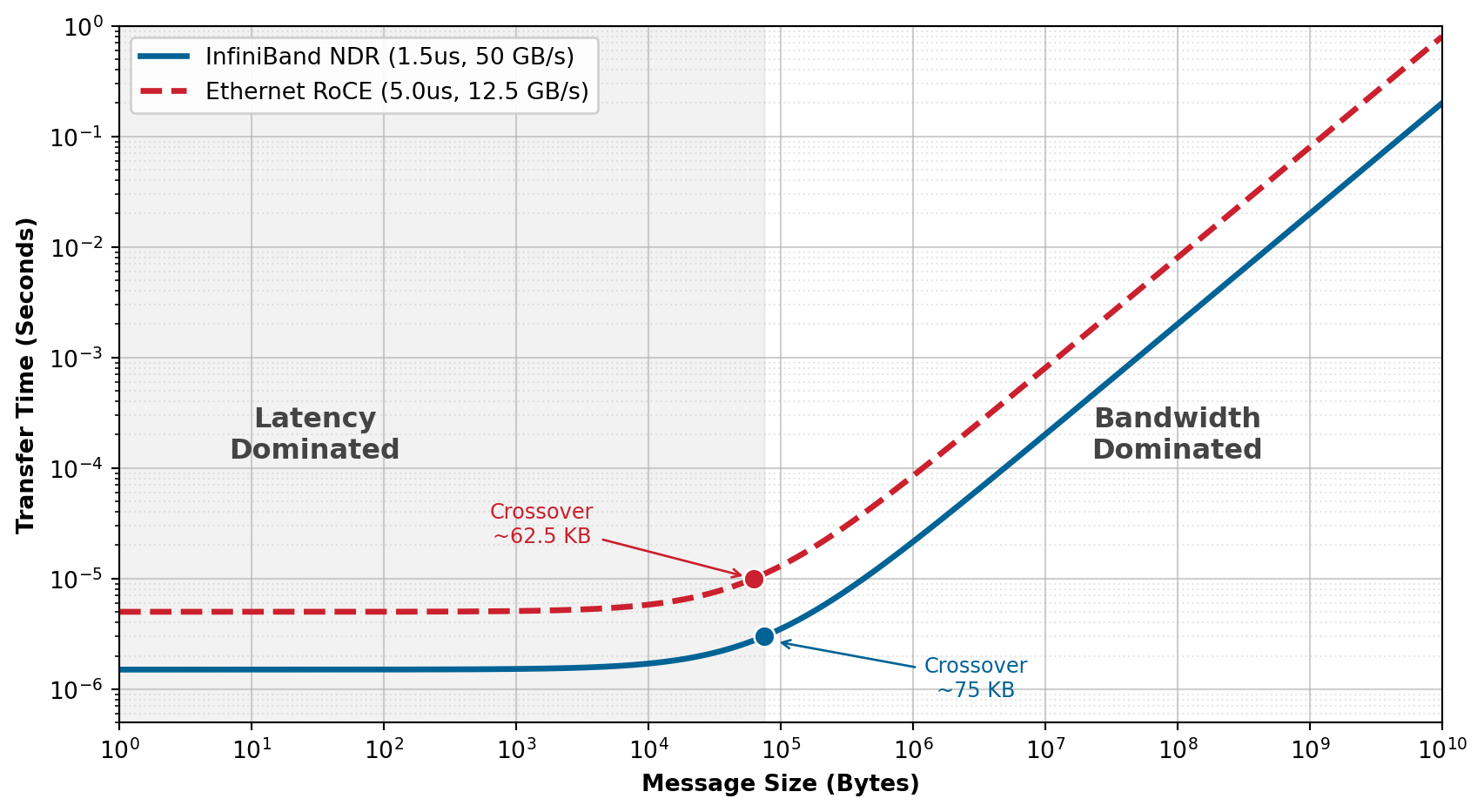
For NDR InfiniBand with $\alpha \approx$ 1.5 μs and $\beta \approx$ 50 GB/s, the crossover point $n^* = \alpha \cdot \beta \approx$ 75 KB. Messages smaller than this gain little from more bandwidth; messages larger than this gain little from lower latency. That crossover separates two fundamentally different optimization strategies: reducing hop count to lower $\alpha$, or adding link bandwidth to raise $\beta$. Applying the model to the concrete message sizes that our 175B training job generates on every iteration makes this distinction actionable.

Napkin Math 1.1: The alpha-beta crossover

Problem: A fabric designer is comparing InfiniBand NDR (1.5 μs, 50 GB/s) against a slower Ethernet baseline (5 μs, 12.5 GB/s). For a 4 KB control message and a 350 MB gradient shard, which part of $T(n)=\alpha+n/\beta$ dominates, and why does the faster fabric help for different reasons in each regime?

Math: Apply $T(n) = \alpha + n/\beta$ for a 4 KB control message and a 350 MB gradient shard.

Small message (4 KB):
- InfiniBand: $1.5\,\mu\text{s} + 4\,\text{KB}/50\,\text{GB/s} = 1.5 + 0.08 = \mathbf{1.58\,\mu\text{s}}$
- Ethernet: $5.0\,\mu\text{s} + 4\,\text{KB}/12.5\,\text{GB/s} = 5.0 + 0.32 = \mathbf{5.32\,\mu\text{s}}$
- Result: InfiniBand is 3.4× faster purely due to lower $\alpha$.
Large message (350 MB):
- InfiniBand: $T = \alpha + n/\beta =$ 7.0 ms
- Ethernet: $T = \alpha + n/\beta =$ 28.01 ms
- Result: InfiniBand is 4× faster purely due to higher $\beta$.

Systems insight: For large-scale training, the crossover point $(n^* = \alpha\beta)$ is typically around 75 KB. Since gradients are megabytes to gigabytes, we are almost always in the bandwidth-dominated regime. However, pipeline parallelism and distributed coordination rely on small messages in the latency-dominated regime, where wire-speed upgrades provide zero benefit and only topology and hop-count reductions matter.

To see why this distinction matters in practice, consider two messages that our 175B model training job sends every iteration. The first is a 4 KB pipeline-scheduling control message that coordinates microbatch handoffs between pipeline stages. Applying the model: $T(n) \approx$ 1.58 μs for the control message. The bandwidth term contributes only 5.1 percent of the total. Doubling the link speed would save a negligible fraction of a microsecond. For this message, the most direct way to reduce transfer time is to reduce the hop count (which lowers $\alpha$), not to buy faster links.

The second message is a 350 MB gradient shard for one layer’s AllReduce. Now: $T(n) \approx$ 7.0 ms. The latency term is invisible. Doubling bandwidth to 100 GB/s would halve this transfer time, a direct and proportional gain. These two cases illustrate why network design must address both $\alpha$ and $\beta$ simultaneously: topology and hop count control the latency-dominated regime, while link speed and path diversity control the bandwidth-dominated regime.

Figure 7 makes these two regimes visible across the full range of message sizes. For InfiniBand, the crossover occurs at approximately 75 KB: messages smaller than this are latency-dominated (the flat region on the left), while larger messages are bandwidth-dominated (the linear region on the right). Ethernet RoCE crosses slightly earlier, at about 62.5 KB, because its lower per-link bandwidth makes the transfer term overtake the higher fixed latency at a smaller message size. The 5$\times$ latency gap between InfiniBand and Ethernet RoCE dominates for small messages but becomes irrelevant for the multi-megabyte gradient transfers that dominate training communication.

Figure 7: **The $\alpha$-$\beta$ Crossover**: Transfer time as a function of message size for InfiniBand NDR and Ethernet RoCE. Small messages are latency-dominated (flat region), while large messages are bandwidth-dominated (linear region). The crossover point marks where investing in bandwidth begins to pay off more than reducing latency.

Beyond classifying individual transfers, the same model identifies when communication overtakes computation. The $\alpha$-$\beta$ analysis above focused on the transfer time of individual messages across a single link, treating the network as a point-to-point channel. In a data-parallel training loop, however, the relevant question is whether the collective AllReduce across the full cluster finishes before the next compute step is ready to begin. When the gradient vector grows large enough, the aggregate transfer time for a ring AllReduce exceeds the per-step computation time, and the network becomes the pacing constraint for the entire training job.

Napkin Math 1.2: AllReduce bottleneck threshold

Problem: When does Ring AllReduce become the bottleneck for a 1024-GPU H100 cluster training models at GPT-2 scale and beyond?

Setup: The baseline cluster trains a GPT-2-scale model with 1.5 billion parameters (6 GB of FP32 gradients). Each GPU computes at 989 TFLOP/s FP16/BF16 peak. The network uses NDR InfiniBand ($\alpha = 1.5 \;\mu\text{s}$ and $\beta = 50 \;\text{GB/s}$ per link).

Step 1: Compute time per iteration. Assume each GPU processes a synthetic microbatch requiring $5.00 \times 10^{13}$ FLOPs, chosen to produce a compute phase of about 101 ms for this bottleneck example. At 989 TFLOP/s with 50 percent utilization:

\[ T_{\text{compute}} = 101.1 \text{ ms} \]

Step 2: Communication time for Ring AllReduce. With $N$ = 1024 and a gradient payload $M$ of about 6 GB:

Ring cost model: $T_{\text{ring}} \approx \frac{2(N-1)}{N}\frac{M}{\beta} + 2(N-1)\alpha$; Collective Communication derives the algorithmic steps behind this expression.
Total Communication: $T_{\text{ring}} \approx 242.8 \text{ ms}$

Step 3: Communication fraction. \[ \text{Comm. fraction} = 70.6 \% \]

With overlap between communication and computation (possible because the backward pass produces gradients layer by layer), the effective overhead can be reduced, but the network is already a major contributor to iteration time for this configuration.

At 70 billion parameters (280 GB of gradients), the bandwidth term becomes the bottleneck if per-GPU computation stays similar through batch-size scaling:

\[ T_{\text{ring}} \approx 11192.1 \text{ ms} \]

Now communication dominates computation under pure data parallelism. Our 175B model, far larger than this scale, would be even more severely bottlenecked. Models beyond a few billion parameters therefore require tensor and pipeline parallelism to partition the model, rather than relying solely on data parallelism, which must AllReduce the full gradient vector.

The $\alpha$-$\beta$ model quantifies the speed of a single link, but our 175B-parameter model requires 1,024 GPUs to work in concert. Scaling these transport primitives from a pair of nodes to a warehouse-scale supercomputer demands a network topology: a specific pattern of connections that maximizes $\text{BW}_{\text{bisect}}$ while minimizing the hop count and cabling cost for global collective operations.

Self-Check: Question

What is the primary systems benefit of RDMA for large-scale ML communication, and what does that benefit cost in terms of fabric requirements?
1. RDMA lets the NIC offload transport and access remote memory directly, cutting end-to-end latency from 50–100 $\mu\text{s}$ (kernel TCP) to 1–2 $\mu\text{s}$, but requires a lossless fabric because its error recovery is much more brittle than TCP’s.
2. RDMA makes packet loss harmless because retransmissions are always selective, regardless of transport protocol.
3. RDMA raises effective accelerator FLOP/s by executing arithmetic inside the NIC rather than on the GPU.
4. RDMA removes the need for a lossless fabric because its kernel-bypass path is inherently error-free.
A 1,000-GPU cluster exchanges 350 GB of gradient data per training step. Explain why GPUDirect RDMA is nearly mandatory at this scale, naming at least one mechanism it removes and the system consequence of not using it.
A team wants to build a 2,000-GPU training cluster using Ethernet switches for multi-vendor flexibility and ecosystem reuse, but still needs RDMA semantics for collective throughput. Which transport choice matches this constraint, and what operational burden does it impose?
1. InfiniBand, because it inherits Ethernet’s best-effort behavior and therefore must be configured with PFC and ECN to approximate losslessness.
2. RoCE, which delivers RDMA semantics over Ethernet, but must approximate the losslessness that InfiniBand gets natively via credits by layering PFC and ECN on the fabric, with all the PFC-storm and congestion-spreading risk that entails.
3. Kernel TCP, because the OS network stack provides the same zero-copy path to GPU memory that GPUDirect RDMA provides.
4. UDP sockets, because moving networking into user space automatically makes the fabric lossless.
True or False: In an RDMA fabric running Go-Back-N, a single packet dropped late in a 1 GB message transfer produces a delay close to the pure wire-time of the missing frame, because only that frame must be resent.
On NDR InfiniBand with approximate $\alpha = 1.5\ \mu\text{s}$ and $\beta = 50\ \text{GB/s}$, giving an $\alpha$-$\beta$ crossover near 75 KB, which transfer below is most clearly in the latency-dominated regime, and what optimization lever matters most for it?
1. A 350 MB gradient shard during AllReduce — the dominant lever is reducing fixed per-message overhead like FEC latency.
2. A 4 KB pipeline-scheduling control message — far below the 75 KB crossover, so startup cost dominates and flattening the topology (reducing hop count) matters more than adding bandwidth.
3. A 100 MB activation checkpoint between pipeline stages — the dominant lever is adding lanes to raise $\beta$.
4. A 2 GB checkpoint shard written to storage — the dominant lever is increasing PCIe width.
Order the following reasoning steps for applying the $\alpha$-$\beta$ model to a new message type in a new fabric: (1) Compare the message size $n$ to the $\alpha\beta$ crossover, (2) compute transfer time as $\alpha + n/\beta$, (3) decide whether reducing latency (lowering $\alpha$) or increasing bandwidth (raising $\beta$) is the more promising optimization, (4) identify the values of $\alpha$, $\beta$, and message size $n$ for the fabric and the collective.

See Answers →

Level 4: Fabric Behavior (Congestion, Routing)

Real fabrics deviate from theoretical full $\text{BW}_{\text{bisect}}$ due to congestion, and the impact of this congestion is qualitatively different in ML clusters than in general-purpose networks. The BSP barrier introduced earlier is what makes the difference: web traffic is stochastic and asynchronous, so one user’s 50 ms delay does not penalize the thousands of others, but under BSP the slowest flow in the fabric dictates the iteration time for the entire cluster. If a single link out of 10,000 becomes congested and doubles its latency, the effective throughput of the entire supercomputer drops for that step. In this synchronized regime, tail latency is the dominant performance constraint, not an outlier metric.

Definition 1.6: Bulk synchronous parallel (BSP)

Bulk Synchronous Parallel (BSP) is a parallel execution model in which every worker completes a local computation phase, exchanges data with all other workers, and then waits at a global barrier before any worker begins the next phase—making the slowest participant the pacing constraint for the entire cluster.

Significance: BSP makes system efficiency $\eta_{\text{scaling}}$ directly proportional to the slowest worker: if one GPU in a 1,024-GPU cluster runs 10 percent slower due to thermal throttling or network jitter, the barrier stalls the remaining 1,023 GPUs for that fraction of the step, wasting effectively 102 GPU-steps of compute per iteration. At $3/GPU-hour, a 5 percent straggler gap across a $50M training run wastes roughly $2.5M in idle accelerator time.
Distinction: Unlike asynchronous parallelism, which allows workers to proceed with stale weights from previous steps, BSP enforces a global state update at every barrier, providing mathematical equivalence to single-device training and predictable convergence behavior.
Common pitfall: A frequent misconception is that BSP is simply inefficient compared to async models. Asynchronous training often requires more total steps to converge because stale gradient updates introduce noise—in practice, BSP with careful straggler mitigation typically reaches the same loss in fewer wall-clock hours than async alternatives.

This is why tail latency (P99), not average throughput, is the metric that governs a training fabric: one congested switch port stalls the barrier, and the barrier stalls the cluster. The mechanisms that keep tail latency bounded therefore become the central concern of fabric behavior.

Priority flow control (PFC)

The BSP weakest-link property means that even a single dropped packet can trigger a retransmission timeout that stalls the global barrier for milliseconds, an eternity in a training loop where each compute step finishes in tens of milliseconds. RoCEv2 fabrics mitigate this with priority flow control (PFC), operating in lossless mode: rather than allowing switch buffers to overflow and drop packets, the fabric uses a link-layer backpressure mechanism to pause upstream senders before any buffer saturates (Guo et al. 2016; Gangidi et al. 2024).

Definition 1.7: Priority flow control

Priority Flow Control (PFC) is a link-layer mechanism used by RoCEv2 ML cluster fabrics to prevent switch buffer overflow by sending PAUSE frames to an upstream sender when a port’s queue depth crosses a configured threshold, throttling injection on a per-priority basis without dropping packets.

Significance: PFC is the foundation for lossless Ethernet required by RoCEv2 RDMA. A PFC PAUSE frame must reach the upstream sender within one round-trip time (roughly 1–5 μs at switch-to-switch distances) before the buffer overflows. In a 1,000-node cluster, a single slow receiver can trigger PAUSE frames that propagate 3–5 hops upstream within 10–50 ms, halting gradient traffic across thousands of unrelated GPU pairs and collapsing cluster throughput to near zero.
Distinction: Unlike standard IEEE 802.3 flow control, which pauses all traffic classes on a link, PFC operates per priority class, allowing latency-sensitive control messages to continue flowing while only pausing the congested gradient data queue.
Common pitfall: A frequent misconception is that PFC solves congestion. It transforms packet loss into congestion spreading: a backpressure cascade can freeze the entire fabric within 200 ms of a single faulty transceiver, because no mechanism limits how far PAUSE frames propagate across the network.

The danger of PFC lies in its cascading nature. When a switch port’s buffer fills, it sends a PAUSE frame upstream, which causes that switch’s buffers to fill, which triggers another PAUSE frame further upstream. In theory, this backpressure should throttle the source. In practice, a single slow receiver can propagate pauses across the entire fabric in milliseconds, freezing links that have no direct relationship to the original congestion point. This cascading behavior, known as congestion spreading or victim flows, is the primary operational risk of PFC-based lossless Ethernet. The root cause is incast, a many-to-one traffic pattern inherent to distributed synchronization, as illustrated in figure 11; this deterministic overload is what triggers the PFC backpressure cascades.

One paused receiver can freeze unrelated flows.

Figure 11: **The Incast Problem in Distributed Training**: During AllReduce synchronization, every GPU node sends line-rate traffic to a common aggregation switch port, producing a many-to-one traffic burst. The figure shows 256 GPU nodes each at 50 GB/s converging on a switch port with 400 Gb/s (50 GB/s) capacity and a 32 MB buffer: 12.8 TB/s of offered load against 50 GB/s of capacity oversubscribes the egress port by 256$\times$. This deterministic overload is the root cause of the PFC backpressure cascades described later in this section.

A production incident shows how this cascade can freeze a cluster.

War Story 1.1: Microsoft's PFC deadlock (2016)

Context: A team led by Chuanxiong Guo at Microsoft Research deployed RoCEv2 across Microsoft’s data centers—a fleet operating at the scale of tens of thousands of servers—to support latency-sensitive services. RoCEv2 requires a lossless fabric, so the network used Priority Flow Control (PFC), and the team developed a DSCP-based PFC mechanism to extend the deployment beyond VLAN boundaries (Guo et al. 2016). DSCP marks packet priority, VLANs define layer-2 traffic boundaries, ARP resolves an IP address to a MAC address, and switches learn MAC-to-port forwarding entries.

Failure mode: PFC interacted with Ethernet flooding to create a cyclic buffer dependency. In Microsoft’s reported example, a dead server with an incomplete ARP/MAC mapping caused upstream switches to flood lossless packets to every port; PFC PAUSE frames then propagated upstream in response to the flooded traffic, eventually forming a closed loop of paused buffers among switches.

Consequence: Once the PFC deadlock formed, restarting servers did not clear it. Microsoft’s fix was architectural: block broadcast and multicast traffic from entering lossless traffic classes, and drop lossless packets when the corresponding ARP entry is incomplete rather than fall back to flooding.

Systems lesson: PFC congestion spreading is a structural vulnerability of lossless Ethernet at hyperscale. RoCE fabrics require packet-class discipline, PFC pause telemetry, and hardware-level safeguards because a mechanism designed to avoid packet loss can itself become the failure mode. ML training fabrics built on RoCE inherit this risk directly: a single stale ARP entry can cascade into a PFC storm that stalls a multi-thousand-GPU training run, with the cluster appearing healthy while no gradient flows between workers.

Guo, Chuanxiong, Haitao Wu, Zhong Deng, Gaurav Soni, Jianxi Ye, Jitendra Padhye, and Marina Lipshteyn. 2016. “RDMA over Commodity Ethernet at Scale.” Proceedings of the 2016 ACM SIGCOMM Conference, 202–15. https://doi.org/10.1145/2934872.2934908.

A simple probability calculation shows that such incidents are not rare edge cases but recurring operational risks at scale.

Napkin Math 1.5: The probability of a PFC storm

Problem: A 4096-GPU RoCE cluster is in operation. If the probability of a single transceiver degrading and triggering PFC pauses is just 0.001 percent per day, what is the chance of a cluster-wide “PFC Storm” occurring in a given day?

Math: In a lossless Ethernet fabric, one bad link can pause its neighbor, which pauses its neighbor, eventually freezing the entire tree.

Total exposure: 4096 $\times$ 3 link tiers = 12,288 links, or 24,576 transceivers.
Probability of zero transceiver failures: $\Pr(\text{safe}) = (1 - 0.00001)^{24,576} \approx 0.782$.
Probability of at least one storm: $\Pr(\text{storm}) = 1 - 0.782 = \mathbf{0.218}$ (about 21.8 percent).

Systems insight: Even with “five-nines” reliable components, a large-scale RoCE cluster faces a 21.8 percent daily risk of a fabric-wide freeze. That is not guaranteed to happen every day, but it is frequent enough to be a weekly-scale operational concern. RoCE deployments therefore require aggressive PFC watchdogs and hardware-level telemetry, because at scale, “rare” link degradations become recurring operational realities that must be handled automatically.

Proactive congestion control: DCQCN and HPCC

To avoid the blunt instrument of PFC pauses, high-performance fabrics rely on proactive congestion control to modulate injection rates before buffers overflow. In BSP workloads, proactive control is a latency requirement, not an optional throughput optimization: if a single packet is delayed by a congested switch queue, the entire cluster must wait for that straggler to complete the synchronization step. The tail latency of the network effectively becomes the average step time of the training job.

The first widely deployed solution, DCQCN¹², operates as a reactive feedback loop using Explicit Congestion Notification (ECN) (Zhu et al. 2015). When a switch’s queue depth exceeds a configured threshold, it marks the ECN bit in the packet header. The receiver echoes this mark back to the sender via a Congestion Notification Packet (CNP), prompting the sender to reduce its injection rate using a multiplicative-decrease algorithm. DCQCN is widely supported, but production AI collectives expose a tuning problem: ECN thresholds and NIC firmware behavior can trade off PFC avoidance, throughput, visibility, and tail latency rather than offering one stable optimum (Gangidi et al. 2024).

¹² DCQCN (Data Center Quantized Congestion Notification): Introduced at SIGCOMM 2015 by Microsoft and Mellanox, DCQCN was designed for large-scale RDMA fabrics (Zhu et al. 2015). Its binary ECN/CNP feedback loop is simpler to deploy than telemetry-rich schemes, but it can become a tuning surface for training collectives: Meta’s SIGCOMM 2024 RoCE study reports that tighter ECN thresholds could reduce PFC in some settings while hurting collective completion time, and that 400G deployments exposed firmware and visibility issues (Gangidi et al. 2024).

Zhu, Y., H. Eran, D. Firestone, C. Guo, M. Lipshteyn, Y. Liron, J. Padhye, S. Raindel, M. H. Yahia, and M. Zhang. 2015. “Congestion Control for Large-Scale RDMA Deployments.” ACM SIGCOMM Computer Communication Review 45 (4): 523–36. https://doi.org/10.1145/2829988.2787484.

Gangidi, Adi, Rui Miao, Sandeep Hebbani, Gaya Nagarajan, Omar Baldonado, Lixin Gao, Hany Morsy Goes, et al. 2024. “RDMA over Ethernet for Distributed AI Training at Meta Scale.” Proceedings of the ACM SIGCOMM 2024 Conference, 56–69. https://doi.org/10.1145/3651890.3672233.

¹³ HPCC (High Precision Congestion Control): Developed by Alibaba and presented at SIGCOMM 2019, HPCC replaced binary ECN with per-packet in-network telemetry and reported large reductions in flow completion time under evaluated incast-heavy workloads. The trade-off is hardware dependency: HPCC requires programmable switch ASICs capable of appending telemetry metadata at line rate, limiting deployment to clusters with newer switching silicon (Li et al. 2019).

Li, Yuliang, Rui Miao, Hongqiang Harry Liu, Yan Zhuang, Fei Feng, Lingbo Tang, Zheng Cao, et al. 2019. “HPCC: High Precision Congestion Control.” Proceedings of the ACM Special Interest Group on Data Communication (SIGCOMM), 44–58. https://doi.org/10.1145/3341302.3342085.

A more precise alternative, HPCC¹³, addresses this opacity by using In-Network Telemetry (INT) (Li et al. 2019). Instead of a simple bit mark, switches append precise metadata to every packet header: current queue depth, link utilization, and timestamps. The sender receives a full dashboard of the network state, allowing it to calculate the exact allowable transmission rate within a single round-trip time. By reacting to precise telemetry rather than binary signals, HPCC reduces queue buildup and tail-latency variance in the evaluated incast-heavy workloads. The primary trade-off is hardware support: DCQCN functions on standard ECN-capable Ethernet switches, whereas HPCC requires programmable switches capable of pushing INT metadata at line rate.

Adaptive routing

Static routing protocols like ECMP¹⁴ (Equal-Cost Multi-Path) distribute traffic by hashing flow headers to fixed paths. While statistically sound for millions of small web requests, this approach fails for the elephant flows typical of ML training. Consider a scenario with 4 equal-cost paths and 8 large gradient flows. A perfect distribution would place 2 flows on each link. However, static hashing frequently results in collisions where one link carries 4 flows while another sits idle. In a synchronized training step, the completion time is dictated by the overloaded link, effectively halving the network’s useful bandwidth.

¹⁴ ECMP (Equal-Cost Multi-Path): ECMP selects a path by hashing on the 5-tuple (source/destination IP, source/destination port, protocol), which means the same flow always takes the same path. This determinism is a feature for packet ordering but a liability for ML: because a single AllReduce ring produces a small number of persistent flows, hash collisions are not transient statistical events but permanent hot spots that persist for the entire training run.

¹⁵ Packet Spraying: Unlike standard Ethernet (which hashes flows to single paths to avoid reordering), packet spraying sends individual packets of a single flow across multiple paths. This can improve $\text{BW}_{\text{bisect}}$ for AllReduce elephant flows when the transport can tolerate or repair reordering. UEC’s Ultra Ethernet Transport design explicitly includes multi-path packet spraying and flexible ordering to reduce the ECMP collision problem for AI/HPC traffic (Ultra Ethernet Consortium 2025).

Ultra Ethernet Consortium. 2025. Ultra Ethernet Specification V1.0. Ultra Ethernet Consortium.

Adaptive routing mitigates this problem by allowing switches to dynamically select the output port based on real-time queue depth rather than a static hash. The implementation is protocol-dependent: InfiniBand fabrics perform packet-level adaptive routing, spraying¹⁵ individual packets across all available lanes because the hardware transport guarantees in-order delivery at the destination.

Ethernet fabrics typically employ flowlet switching, rerouting bursts of packets only when a sufficient time gap is detected, to avoid the performance penalties associated with packet reordering. This mechanism becomes essential for Mixture-of-Experts (MoE) models. Unlike the predictable Ring AllReduce pattern, MoE models use AllToAll communication, where every GPU sends data to every other GPU containing active experts. For a 175B-parameter model using expert parallelism with 64 experts, this generates a dense $64{\times}64$ traffic matrix—4,096 simultaneous flows. Under static ECMP, hash collisions are statistically guaranteed to create stragglers; adaptive routing is required to distribute this traffic evenly across the fabric’s $\text{BW}_{\text{bisect}}$.

The incast problem in ML

Congestion control and adaptive routing manage flows that traverse the interior of the fabric. A different failure mode occurs at the edge, where the traffic pattern itself overwhelms a single port regardless of how much capacity the fabric interior provides.

Definition 1.8: Incast

Incast is a many-to-one ML cluster traffic pattern in which a large number of senders simultaneously transmit data to a single receiver port, concentrating line-rate traffic from multiple sources into a single switch queue and causing buffer overflow even when the rest of the fabric is uncongested.

Significance: In the reduce phase of AllReduce, every participating GPU simultaneously sends gradients toward the same aggregation points. With 256 senders each at 50 GB/s targeting one switch port, the instantaneous incast reaches 12.8 TB/s, orders of magnitude above a 400 Gb/s port’s absorption capacity. A 32 MB switch buffer holds about 640 μs of one 400 Gb/s egress stream, but under 256× incast the net fill rate is roughly 12.75 TB/s after subtracting the single 50 GB/s egress port, so overflow arrives in about 2.5 μs. That sudden overflow triggers either PFC cascade or packet drops that elevate $L_{\text{lat}}$ cluster-wide.
Distinction: Unlike general congestion (which occurs on shared internal links when aggregate traffic exceeds link capacity), incast is an endpoint bottleneck: it occurs even if every internal spine and leaf link is completely uncongested, because the bottleneck is the single destination port, not the fabric interior.
Common pitfall: A frequent misconception is that incast is rare or unpredictable. Because ML training synchronizes all GPUs at each backward pass, incast is a deterministic event at the end of every layer’s gradient computation—it occurs hundreds of times per training step and must be architecturally mitigated through layer-staggered AllReduce or tree-based collective algorithms, not treated as an edge case.

ML training is structurally susceptible to incast because of its synchronized communication patterns. When a layer finishes backward computation, thousands of nodes simultaneously initiate AllReduce, targeting the same switch ports. In our 175B model training across 1,024 GPUs, each AllReduce involves every node injecting data simultaneously, creating a burst that can momentarily exceed the fabric’s capacity at specific switch ports. Production clusters mitigate this through three complementary techniques:

Layer-staggering: Trigger each gradient bucket’s AllReduce as soon as backpropagation produces it. Final-layer gradients reduce while earlier layers are still computing, so communication is staggered instead of released as one burst.
Algorithm selection: Choose collectives that limit the fan-in at any single port. Hierarchical and rail-local reductions aggregate gradients in stages so that no switch port must absorb all senders at once, in contrast to a flat reduction in which every node targets one aggregation point. Bandwidth-optimal ring AllReduce is itself point-to-point and creates no single aggregation hotspot; the incast pressure comes from many such flows converging on oversubscribed ports, which topology-aware placement and rail-optimized wiring relieve.
Quality of Service (QoS) classification: Tag gradient traffic with the highest service class so background storage or management traffic does not delay the synchronization path.

Together, these mitigations spread the burst in time, space, and priority, but they do not eliminate congestion or tail latency. The question becomes how to build end-to-end clusters that perform despite these realities.

Self-Check: Question

Why is tail latency the dominant network performance metric in BSP-style distributed training, not average throughput?
1. The global barrier makes the slowest worker or packet determine when the next training step can begin; average throughput can look healthy while one outlier stalls every GPU.
2. Average throughput is only a concern in inference serving, never in training.
3. Switches report only P99 percentile metrics and not averages in modern deployments.
4. GPU memory capacity is directly determined by network latency.
Explain why Priority Flow Control (PFC) both solves and creates a problem for RoCE fabrics, and describe one concrete failure pattern operators must monitor for.
In an incast-heavy ML workload where many senders converge on one receiver, what is HPCC’s main advantage over DCQCN, and what is the key limitation neither mechanism can overcome?
1. HPCC uses precise in-network telemetry (INT) to set rates accurately, reducing queue buildup and tail-latency variance compared to DCQCN’s coarser ECN-based signal; however, neither can create bandwidth where capacity is physically missing (e.g., across an oversubscribed cut).
2. HPCC avoids switch telemetry entirely, so it converges faster with less information than DCQCN.
3. HPCC physically adds bisection bandwidth to an oversubscribed topology, which DCQCN cannot do.
4. HPCC disables sender feedback and lets traffic transmit at line rate until packet loss begins.
True or False: Incast can occur even when every spine and leaf switch in a fabric is running well below its capacity, because the bottleneck is the receiver-port queue absorbing many simultaneous senders.
Why is adaptive routing particularly important for ML elephant flows and MoE-style AllToAll traffic on a fat-tree?
1. It lets switches steer packets or flowlets away from congested paths based on real-time queue conditions, instead of ECMP’s static hash pinning a long-lived elephant onto one unlucky link for the whole job.
2. It guarantees zero packet reordering on standard Ethernet without any additional mechanism.
3. It eliminates the need for congestion control by ensuring packets never encounter queues.
4. It converts an oversubscribed topology into a non-blocking fat-tree.
A fabric experiences repeated incast at aggregation points during the backward pass of a 1,024-GPU training run. Describe two complementary mitigations from the section and explain the mechanism each one targets.

See Answers →

Level 5: Cluster Design and Case Studies

The final level of the stack is cluster design, where wires, transport, topology, and congestion control combine into a coherent system. The goal of cluster design is to provide an end-to-end Gradient Bus that makes thousands of distributed GPUs feel like a single machine. At this level, the abstraction layers collapse into concrete engineering decisions: which cables to buy, how to wire the racks, which protocol to deploy, and how to validate that the resulting fabric actually delivers the bandwidth the training job expects. Two representative large-scale architectures, one built on InfiniBand and one on Ethernet, illuminate the trade-offs that define ML infrastructure (NVIDIA 2023; Meta Engineering 2024; Gangidi et al. 2024).

The GPU-to-GPU “gradient bus”

In a well-designed cluster, the network fabric acts as a scheduler-aware extension of the system bus, not a passive pipe. The intra-node (NVLink) bandwidth is ~9× higher than inter-node (InfiniBand/RoCE) bandwidth, and the primary mechanism for hiding this cliff is communication-computation overlap. During the backward pass, gradients for the final layers are computed first. Instead of waiting for the entire backward pass to finish, the system triggers an asynchronous AllReduce for these gradients immediately while the GPUs continue computing gradients for earlier layers. If the backward pass requires 500 ms of computation and the AllReduce takes 300 ms, perfect overlap masks the entire communication cost behind computation, reducing the effective overhead to $\max(0, 300 - 500) = 0$. In practice, dependency chains and resource contention limit this efficiency to 60–80 percent, leaving a last-mile problem: the gradients for the very first layer (computed last) have no subsequent computation to hide behind, exposing their raw transfer time to the critical path.

The bandwidth hierarchy plotted in figure 2 dictates the parallelism strategy to mitigate this cliff. Tensor parallelism, requiring massive bandwidth for frequent activation exchanges, is confined to the NVLink domain within a node. Pipeline parallelism, involving point-to-point transfers of activations between pipeline stages, spans the InfiniBand links between nodes. Data parallelism, tolerant of lower bandwidth through gradient accumulation and overlap, stretches across the full fabric.

Case study: NVIDIA DGX SuperPOD

The NVIDIA DGX SuperPOD architecture connects DGX H100 nodes using an NDR InfiniBand network, serving as a concrete implementation of the Gradient Bus concept (NVIDIA 2023). Each node acts as a dense compute island, with eight H100 GPUs connected via NVSwitch to provide 900 GB/s of internal bandwidth. Externally, each GPU pairs with a ConnectX-7 NIC delivering 400 Gb/s of injection bandwidth. Across a standard scalable unit of 32 nodes (256 GPUs), this yields an aggregate injection bandwidth of 12.8 TB/s (256 $\times$ 50 GB/s), ensuring the fabric can ingest gradients as fast as the accelerators produce them.

NVIDIA. 2023. NVIDIA DGX SuperPOD: Next Generation Scalable Infrastructure for AI Leadership. RA-11333-001 V11. NVIDIA.

This architecture explicitly instantiates the five-level model constructed in this chapter. At Level 1, it minimizes latency by using passive copper (DAC) within the rack and active optics only for spine connections. At Level 2, it relies on InfiniBand’s native credit-based flow control to guarantee a lossless medium without the fragility of Ethernet PFC. Level 3 implements a rail-optimized fat-tree: GPU rails are aligned across a scalable unit so same-rail traffic stays close and cross-rail traffic traverses the spine layer. At Level 4, hardware-based adaptive routing can select among spine paths to improve bisection behavior for cross-rank communication. At Level 5, the design is modular: multiple SuperPOD scalable units connect through additional switching to form larger clusters (NVIDIA 2023). For our 175B-parameter model, the physical infrastructure would consist of approximately four SuperPOD scalable units wired together, allowing about 1,024 GPUs to function as a single synchronous instrument.

Case study: Meta Grand Teton

Meta disclosed two Grand Teton-based 24,576-H100 clusters: one using RoCE over an Arista/OCP Ethernet fabric and one using NVIDIA Quantum-2 InfiniBand, both with 400 Gb/s endpoints. Meta used both for Llama 3 training and reported ongoing Llama 3 training on the RoCE cluster (Meta Engineering 2024). The primary motivation for Ethernet is operational scale and supply chain resilience: by using Ethernet, Meta can source switches from multiple vendors and use the same optical infrastructure and management tooling shared by their front-end serving fleet, avoiding the operational silo of a dedicated InfiniBand island.

Meta Engineering. 2024. Building Meta’s GenAI Infrastructure. Engineering at Meta Blog.

Making Ethernet perform like a dedicated HPC fabric at this scale requires significant engineering at Level 4. Meta’s RoCE study describes PFC watchdogs for long-duration pause events, iterative routing designs beyond plain ECMP, future-oriented flowlet switching experiments, and a 400G deployment experience in which DCQCN tuning proved difficult enough that Meta proceeded without DCQCN while relying on PFC plus higher-layer collective controls (Gangidi et al. 2024). While this architecture achieves high line-rate bandwidth for large gradient transfers, it accepts a trade-off: small-message latency can remain higher than InfiniBand because RoCE deployments rely on Ethernet buffering, QoS, PFC/ECN/DCQCN tuning, routing policy, and switch/NIC implementation choices rather than InfiniBand’s native credit-based fabric semantics. For giant models where bandwidth dominates, this is an acceptable exchange; for latency-sensitive MoE routing, the penalty requires careful algorithmic compensation.

Systems Perspective 1.3: InfiniBand vs. RoCE: The industry verdict

The coexistence of InfiniBand (NVIDIA DGX SuperPOD) and RoCE (Meta Grand Teton, Google) in production reflects a genuine trade-off rather than a clear winner. InfiniBand can provide lower tail latency and simpler lossless configuration. RoCE can provide lower switch costs and multi-vendor flexibility. For training runs where iteration time is measured in seconds, the latency difference is often absorbed into the noise. For inference serving with tight SLOs, the latency difference may matter.

The design space is converging. NVIDIA’s Spectrum-4 Ethernet switches incorporate InfiniBand-inspired adaptive routing and congestion control. Broadcom’s Memory DCS chips add hardware support for RDMA-optimized switching. The distinction between the two ecosystems is narrowing, though it has not disappeared.

These case studies close the five-level stack by showing how the physical wire, transport protocol, topology, and congestion controls become one production fabric. The remaining operational problem is not how to build a single fast cluster, but how to share that expensive substrate across teams and workloads without sacrificing the predictable performance that training demands.

Self-Check: Question

Why is communication-computation overlap the central design goal for the cluster-level Gradient Bus, rather than simply adding bandwidth?
1. Overlap starts AllReduce on each layer’s gradients as they are produced in the backward pass, hiding part of the inter-node communication behind still-running compute and reducing the exposed critical-path synchronization cost.
2. Overlap eliminates the need for collective-communication libraries such as NCCL entirely.
3. Overlap raises NVLink bandwidth to match InfiniBand bandwidth without hardware changes.
4. Overlap guarantees that every layer’s gradient takes the same amount of wall-clock time to transfer.
Explain the last-mile problem in overlapped gradient communication: why even near-perfect overlap leaves exposed critical-path latency, and what design responses (from this section or the topology section) help bound that residual cost.
Which comparison best matches the chapter’s characterization of NVIDIA DGX SuperPOD and Meta Grand Teton, and what does the contrast illustrate?
1. SuperPOD uses Ethernet with PFC as its main lossless mechanism while Grand Teton relies on native InfiniBand credits — the opposite of reality.
2. SuperPOD is rail-optimized InfiniBand with native credit-based losslessness, while Grand Teton uses large-scale RoCE over Ethernet with DCQCN tuning and flowlet switching — trading ecosystem flexibility for operational complexity.
3. Both systems use identical transport and congestion control, differing only in which vendor supplies the cables.
4. Grand Teton avoids congestion control because Ethernet switches inherently provide perfect fairness.

See Answers →

Network Virtualization

Production ML clusters are rarely dedicated to a single training job, creating a massive economic imperative for efficient multi-tenancy. A $300 million supercomputer that sits 30 percent idle because it cannot securely isolate concurrent workloads represents a $90 million waste of capital. To recover this utility, the network must support virtualization along three orthogonal dimensions: bandwidth partitioning (guaranteeing minimum throughput), latency determinism (preventing head-of-line blocking), and security isolation (preventing memory snooping between tenants). Technologies like SR-IOV (Single Root I/O Virtualization) and virtual lanes decouple the training job from the physical wire, much as hypervisors decoupled the operating system from the CPU. For our 175B model, this means the training job can reliably consume 80 percent of the cluster’s $\text{BW}_{\text{bisect}}$ while a high-priority inference service and a background data preprocessing job share the remaining 20 percent, with the fabric enforcing hard boundaries that prevent the preprocessor’s bursty traffic from stalling gradient updates.

SR-IOV: Hardware NIC virtualization

Cloud providers can deliver near bare-metal RDMA performance to virtualized GPU instances through Single Root I/O Virtualization (SR-IOV), a standard that allows a physical NIC to present itself as multiple independent Virtual Functions (VFs). Each VF has its own hardware queues, doorbell registers, and DMA mappings. By assigning a dedicated VF to each VM or container, the hardware creates a direct path for DMA operations that bypasses the host kernel and hypervisor completely. The passthrough architecture is critical for ML training because it can reduce virtualization overhead to low levels, often within a few percent of bare metal when the NIC, hypervisor, and placement policy are configured correctly. The cluster-management consequence is immediate: VFs become allocatable network resources, so placement logic must reserve NIC capacity and QoS policy alongside GPUs rather than treating the network as an unbounded shared pool.

However, hardware-level isolation still needs explicit bandwidth policy. SR-IOV exposes multiple VFs that share the NIC’s physical resources; administrators can add per-VF or per-group QoS policies to cap or guarantee bandwidth, such as assigning eight VFs 50 Gb/s each on a 400 Gb/s NIC. For our 175B-parameter model training on a multi-tenant cluster, that configured partitioning can prevent a neighboring tenant from stealing bandwidth, but it also enforces a hard ceiling on peak throughput. The training job must be architected to operate within this slice, as no amount of software optimization can burst beyond the configured VF limit.

Traffic isolation and quality of service

Consider a worst-case contention scenario on a shared cluster: our 175B model is midway through a latency-sensitive AllReduce operation when a neighboring job initiates a massive checkpoint save. Without strict isolation, a bursty 100 GB write (taking 2 seconds at full 400 Gb/s line rate) could saturate the shared spine links, introducing queuing delays that increase the AllReduce time by 50 percent or more. To prevent this noisy-neighbor effect, high-performance fabrics rely on Quality of Service (QoS) mechanisms that enforce fairness at the packet level.

The primary tool is the Virtual Lane (VL) in InfiniBand (or Traffic Class in RoCE), which provides up to 16 independent logical channels on a single physical link. By mapping different traffic types to separate VLs, the network ensures that a saturation event in one lane does not block progress in another. Each VL maintains its own independent credit-based flow control: if the storage traffic for the checkpoint fills up its buffer, the switch pauses only that specific lane. Gradient updates, tagged with a high-priority service level, continue to flow through their reserved lane unimpeded. On the Ethernet side, Enhanced Transmission Selection (ETS) provides analogous bandwidth guarantees per traffic class, while advanced switch ASICs can partition their forwarding tables and buffer pools into isolated network slices, ensuring that congestion in one tenant’s slice cannot trigger PFC pauses in another’s.

Virtualization solves the sharing problem but makes performance diagnosis harder. When a training job slows down on a multi-tenant cluster, the cause could be a physical link degradation, a noisy neighbor exceeding its bandwidth allocation, or a misconfigured QoS policy. Systematic monitoring is essential to distinguish these cases.

Self-Check: Question

What is the main role of SR-IOV in a multi-tenant GPU cluster, and what does it not do?
1. SR-IOV lets one physical NIC present multiple virtual functions (VFs) so VMs or containers can access RDMA-capable hardware queues with near-bare-metal latency, but it does not isolate tenants from each other at the fabric level — that still requires switch-level QoS and virtual lanes.
2. SR-IOV converts Ethernet into InfiniBand by adding software credit-based flow control.
3. SR-IOV guarantees that each tenant can burst above the physical NIC’s line rate when needed.
4. SR-IOV removes the need for cluster schedulers to reason about network resource allocation.
A 400 Gb/s NIC is split across eight SR-IOV virtual functions for multi-tenancy. A training job running in one VF expects to consume full-NIC bandwidth when the other VFs are idle. Explain why this expectation is wrong and the trade-off the partitioning actually creates.
Why do virtual lanes (VLs) or Ethernet traffic classes matter when a training job shares the fabric with checkpoint or storage bursts?
1. They force every packet onto the same physical switch path for easier debugging.
2. They provide separate queues and flow-control state per traffic class, so a burst of storage traffic filling the storage queue does not head-of-line-block gradient packets sitting in the collective-communication queue.
3. They raise the raw physical line rate of each link proportionally to the number of lanes configured.
4. They eliminate the need for congestion control on Ethernet fabrics entirely.
True or False: Once SR-IOV gives each tenant near-bare-metal RDMA access to the NIC, shared switches and spine links no longer need QoS policies because the NIC-level virtualization handles all isolation.

See Answers →

Monitoring and Debugging

Network performance problems in ML clusters are insidious because they manifest as silent waste rather than explicit failures. A degraded transceiver causing a 10 percent reduction in effective bandwidth might slow each training iteration by only 2–3 percent, a drift easily masked by the natural variance of checkpointing or data loading. Over a 30-day training run on 1,024 GPUs, this invisible drag accumulates to roughly 15,000–22,000 wasted GPU-hours, burning about $45,000–$66,000 at $3/GPU-hour without triggering a single alarm. Traditional IT monitoring tools like SNMP or ICMP ping measure connectivity, not the sustained throughput required by RDMA. Effective observability requires a three-layer approach: physical monitoring (FEC errors, signal attenuation), transport monitoring (PFC pause frames, retransmission rates), and application monitoring (NCCL algorithmic bandwidth) (Jeaugey 2017; Gangidi et al. 2024). Only by correlating signals across these layers can operators detect that a “slow training run” is actually caused by a single degraded cable in one rack.

Jeaugey, Sylvain. 2017. NCCL 2.0. GPU Technology Conference presentation.

Link-level telemetry

At the physical layer, hardware counters answer whether the wire still behaves like the model assumed. Every RDMA NIC and switch maintains these counters, accessible via the perfquery utility (Linux man-pages project 2026). PortXmitData and PortRcvData provide the raw byte counts used to compute real-time link utilization, while PortXmitDiscards tracks packets dropped by the switch—in a properly configured lossless fabric, discards should be exactly zero. Physical signal integrity is tracked via the SymbolErrorCounter, which increments on bit-level errors caused by loose cables or dirty optics, and the LinkDownedCounter, which logs link flaps often triggered by intermittent hardware faults or overheating transceivers.

Linux man-pages project. 2026. Perfquery(8): Query InfiniBand Port Counters on a Single Port.

These metrics are typically polled by a centralized monitoring system (for example, Prometheus with Grafana dashboards) at 10–30 second intervals to catch silent degradation. A common failure mode involves a QSFP56 cable negotiating at HDR speed (200 Gb/s) instead of NDR (400 Gb/s), or silently dropping from 4 lanes to 2 lanes due to a single bad connector pin. The link remains “up” and functional, but its bandwidth is halved. In a cluster of 1,024 GPUs with over 3,000 links, a 0.1 percent point-in-time component degradation rate implies about 3 degraded links in expectation, with a high probability that at least one link is degraded. Because distributed training algorithms like Ring AllReduce are synchronous, a single degraded link throttles the entire job to the speed of that straggler, transforming a minor hardware fault into a massive waste of idle compute cycles.

Bandwidth and latency validation

Once counters rule out visible link faults, validation must test the bandwidth and latency that the training job can actually use. A healthy NDR InfiniBand link can approach the raw 50 GB/s rate after encoding and protocol overheads, but the only useful number is the delivered payload bandwidth on the specific host pair. Operators rely on periodic health checks, often running perftest tools such as ib_write_bw between selected node pairs and assembling the results into an all-pairs bandwidth matrix (linux-rdma project 2026). This heatmap immediately visualizes cold spots in the fabric where specific spine switches or cable bundles are underperforming, allowing for targeted maintenance before jobs are scheduled.

linux-rdma project. 2026. perftest: InfiniBand Verbs Performance Tests.

For latency-sensitive synchronization, ib_write_lat measures round-trip times for small RDMA writes. Baseline NDR latency should remain below 2 $\mu$s for directly connected nodes. Latencies exceeding 5 $\mu$s suggest switch-buffer congestion or routing imbalances, while values spiking above 100 $\mu$s usually indicate the RDMA path has fallen back to TCP/IP emulation—a catastrophic configuration error. Before launching a massive training job, robust validation includes application-level tests such as nccl-tests, which verify that the fabric can sustain the expected AllReduce bandwidth across the specific collective topology (ring or tree) used by the workload. This ensures that the physical network reality matches the theoretical design before expensive compute resources are allocated.

Systematic debugging workflow

When a training job reports lower-than-expected throughput, the diagnostic order should preserve the layer model rather than starting with cables. The following sequence moves from application symptoms toward physical causes:

Check GPU utilization: Rule out compute bottlenecks using dcgmi or nvidia-smi. If SM utilization is 100 percent, the network is not the bottleneck. Low utilization does not automatically implicate the fabric, however: a starved input pipeline (data loading or storage) produces the same symptom, so confirm the data path is keeping the accelerators fed before investigating the network.
Inspect NCCL logs: Set NCCL_DEBUG=INFO to reveal which network transport was selected, the detected bandwidth between nodes, and any fallbacks to slower protocols.
Run point-to-point tests: Use ib_write_bw between specific nodes in the job. A single degraded link can bottleneck the entire ring in a Ring AllReduce.
Check PFC/ECN counters: Inspect switch counters along the path. Sustained PFC activity indicates persistent congestion that should be investigated at the scheduler or routing level.
Validate Physical Layer: Check symbol errors and CRC counts to identify failing transceivers or cables.

The diagnostic sequence preserves the chapter’s layer model: application symptoms identify the failing path, transport counters show whether congestion or fallback is involved, and physical telemetry confirms whether the wire itself is degrading.

Checkpoint 1.5: Diagnosing a training slowdown

Your 175B model training job has been running for 3 days on 512 GPUs. You notice that the iteration time has gradually increased from 4.2 seconds to 4.8 seconds (a 14 percent slowdown). The GPU utilization reported by nvidia-smi has dropped from 92 percent to 85 percent.

First diagnostic: Choose the first diagnostic step, name the tool that confirms whether the bottleneck is communication-bound or compute-bound, and cite the evidence that distinguishes the two.
Physical layer: Identify physical-layer causes that could explain a 50 percent bandwidth drop when ib_write_bw finds one node pair at 24 GB/s instead of the expected 48 GB/s, and verify them using switch counters.
Collective impact: Estimate the impact on overall AllReduce time when the degraded link lies in the Ring AllReduce path, then evaluate whether switching to a Tree AllReduce algorithm helps.

Self-Check: Question

Why does this section describe network problems in ML clusters as silent waste rather than obvious outages?
1. Most fabric degradations show up as modest iteration slowdowns and lower MFU rather than link-down events, so expensive accelerator time is wasted without triggering alerts.
2. RDMA hardware hides all its counters from monitoring systems by design.
3. Training jobs automatically reroute around every bad cable with no performance effect on the training run.
4. Network issues affect only storage traffic and never collective communication.
Which tool is the correct fit for validating the actual data path used by RDMA-based ML training on an InfiniBand fabric?
1. iperf, because kernel TCP behavior mirrors RDMA closely enough for validation.
2. ping, because latency alone is sufficient to infer collective bandwidth.
3. ib_write_bw from the perftest suite, because it exercises RDMA verbs and measures the same GPU-to-GPU data path NCCL uses.
4. traceroute, because path discovery directly reports NCCL collective performance.
A node pair that normally sustains 48–49 GB/s on NDR InfiniBand suddenly measures 24 GB/s. Diagnose what physical-layer cause is most likely, name two specific counters you would check, and explain the fabric-wide risk this creates if left unresolved.
Order the following debugging steps from the highest-level application symptom to the lowest-level physical-layer root cause check: (1) Check PFC or ECN counters on relevant switches, (2) Inspect NCCL logs for collective completion times, (3) Validate physical-layer counters such as SymbolErrorCounter, (4) Check GPU utilization on each worker, (5) Run point-to-point ib_write_bw between suspected node pairs.
Explain why running an all-pairs ib_write_bw bandwidth matrix before launching a multi-week 1,000-GPU training job is a high-leverage preflight investment, not operational paranoia.

See Answers →

Network Technologies That Move the Ceiling

Monitoring keeps deployed fabrics honest, but observability cannot push past a physical ceiling that copper approaches at high signaling rates. The physical ceiling that monitoring exposes is the reason new fabrics deserve attention: they matter only when they move a bound the synchronization backbone cannot cross. As clusters scale toward 100,000 nodes, the durable design variables are power per bit, reach, and the ratio of compute to memory to network capacity, not the product names attached to a particular roadmap.

Protocol convergence and link density

The first pressure point is reliability. The Ultra Ethernet Consortium (UEC) targets that constraint by trying to make Ethernet behave more like an HPC fabric without inheriting RoCEv2’s PFC fragility. Its Ultra Ethernet Transport design combines packet spraying across multiple paths, flexible ordering, multiple transport delivery services, congestion-control changes, and telemetry intended for AI/HPC traffic (Ultra Ethernet Consortium 2025). The goal is to preserve Ethernet’s ubiquity and multi-vendor economics while moving its failure behavior closer to InfiniBand’s lossless fabric model. Specific mechanisms such as packet trimming or link-layer retry are implementation details of that broader direction, so they should be evaluated against the same durable criteria: whether the fabric can repair congestion locally before it becomes a synchronous-training straggler.

NVIDIA. 2026b. NVIDIA Quantum-X800 InfiniBand Platform. NVIDIA product documentation.

Broadcom Inc. 2025. Broadcom Ships Tomahawk 6: World’s First 102.4 Tbps Switch. Broadcom press release.

Higher port rates attack hop count as well as raw bandwidth. XDR InfiniBand pushes 800 Gb/s per port, and Ethernet roadmaps include 800GbE and 1.6TbE link speeds (NVIDIA 2026b; Ethernet Alliance 2025). Ethernet switch silicon with 1.6 Tb/s ports pushes aggregate capacity to 102.4 Tb/s in current Tomahawk 6-class designs (Broadcom Inc. 2025). A single 1.6 Tb/s port delivers the bandwidth of 4 400G ports. The increased density allows architects to flatten the topology: a cluster that previously required three tiers of switches may be served by two when radix, port rate, and placement constraints line up, halving the transceiver count and reducing tail latency by removing an entire hop of switching and FEC overhead.

Optical interconnects

Each extra meter pushes the fabric from copper toward optics.

Optical interconnects attack the power-per-bit and reach terms that copper makes worse as data rates increase. At 112 Gb/s per lane (the PAM-4 signaling rate used by NVLink 4.0 and InfiniBand NDR), copper SerDes transceivers consume approximately 7–10 pJ per bit and are limited to distances of 2–3 meters before signal integrity degrades beyond the point where equalization can recover the data.

The 224 Gb/s-per-lane class pushes copper even harder. At 224 Gb/s, the SerDes power consumption roughly doubles to 15–20 pJ per bit, and the reach shrinks to 1–1.5 meters over passive copper cables. Active electrical cables (which include retimer chips to regenerate the signal mid-cable) extend the reach but add latency and power.

Co-packaged optics (CPO) addresses these limitations by integrating optical transceivers directly into the switch or accelerator package, rather than placing them at the end of a pluggable cable module. In CPO, a silicon photonics chip sits on the same package substrate as the processor, converting electrical signals to light at the die boundary. The optical signal then travels through a fiber at the speed of light, with negligible attenuation over distances of tens of meters, and is converted back to electrical at the receiving package.

CPO changes the link budget through three independent physical effects:

Shorter electrical path: Moving the optical transceiver from the switch faceplate to the package substrate reduces the SerDes-to-optics path from centimeters to millimeters, lowering the power consumed by electrical signal conditioning.
Distance-stable bandwidth: Optical fiber has no distance-dependent bandwidth degradation over data center-relevant distances up to 100 meters, eliminating retimers and enabling more flexible physical layouts.
Lighter cable plant: Fiber is lighter and thinner than copper cables, simplifying cable management in dense racks.

Together, these effects shift the fabric from a copper-limited layout problem toward an optics-limited packaging and power problem.

A quick estimate makes the power dividend concrete.

Napkin Math 1.6: The optical dividend

Problem: Calculate the power savings of moving a 51.2 Tb/s switch from pluggable transceivers to Co-Packaged Optics (CPO).

Pluggable Architecture: 128 ports $\times$ 20 W = 2.56 kW for optics alone.
CPO Architecture: 128 engines $\times$ 10 W = 1.28 kW.
Savings: The savings reach 1.28 kW of power per switch.

Systems insight: In a cluster with 1,000 switches, pluggable optics consume 2.56 MW just to move light. CPO halves this “network tax,” saving 1.28 MW and redirecting enough power to fuel roughly 1,800 H100 GPUs. At the $\text{BW}_{\text{bisect}}$ wall, sustainability is not a choice; it is an architectural requirement driven by the thermal limits of the faceplate.

For a 10,000-GPU cluster, eliminating pluggable modules could save more than a megawatt of power that can be redirected to computation. CPO also removes the transceiver as a discrete field-replaceable unit, eliminating a common point of mechanical failure.

For ML infrastructure, CPO could flatten the bandwidth hierarchy by narrowing the gap between intra-node and inter-node bandwidth. If inter-node links achieve bandwidth comparable to NVLink-class local fabrics (hundreds of GB/s per GPU), the constraint that confines tensor parallelism to within a single node would relax. This would enable new parallelism strategies where tensor parallelism spans two to four nodes rather than being confined to a single 8-GPU node, potentially improving scaling efficiency for very large models.

The product roadmap is less durable than the constraint it illustrates: as link speed rises, optics moves closer to silicon to control power and reach. Products that integrate optics into switch packages or accelerator packages are concrete attempts to pay less power and latency for the same physical distance. Whether a specific product generation succeeds is less important than the systems direction: the electrical path shrinks, the optical path begins closer to the die, and package-level thermals become part of network design.

However, CPO introduces new challenges. Optical components are sensitive to temperature (laser wavelength shifts with temperature, requiring active thermal management), and integrating photonics on the same package as a 1,000 W GPU creates a hostile thermal environment for the optical components. The manufacturing processes for silicon photonics and CMOS transistors are similar but not identical, requiring separate fabrication steps that increase package cost and complexity. These challenges are being addressed through hybrid integration approaches where the photonics chiplet is placed on a cooler region of the package substrate, thermally isolated from the GPU die.

Disaggregated and composable architectures

The conventional node bundles a fixed ratio of compute, memory, and networking, and Compute express link (CXL) established why that ratio is wasteful when one workload needs more memory capacity per GPU and another needs more network bandwidth: CXL memory pooling lets a processor in one chassis reach memory in another with load/store semantics, and disaggregated designs decouple compute, memory, and networking into independently composable pools. The fabric-specific consequence is what concerns this chapter. Once memory pooling and resource composition cross the node boundary, the rigid distinction between intra-node NVLink domains and inter-node InfiniBand domains softens into a single memory fabric, and the synchronization backbone shifts from a fixed node boundary to a composable one.

That shift does not repeal the physics this chapter has developed. A composed virtual node still pays the same $\alpha$-$\beta$ costs on every cross-pool access, the same power-per-bit limits on the links that carry it, and the same observability requirements that keep an oversubscribed path from masquerading as slow accelerators. The systems lesson is the displacement of overhead: disaggregation relocates the synchronization backbone rather than eliminating it. Whether a composable fabric works is decided by the same fabric properties that decide whether a fixed-node fabric works.

Self-Check: Question

The Ultra Ethernet Consortium (UEC) proposes changes like packet spraying and local loss-repair to give Ethernet the reliability of an HPC fabric, specifically aiming to reduce the protocol’s historical reliance on ____ for managing congestion in AI workloads.
A network architect upgrades a cluster’s switches from 400 Gb/s ports to 1.6 Tb/s ports, maintaining the same total number of compute nodes. By using denser switches, they flatten the network topology from three tiers to two. What is the primary performance benefit of this architectural change for synchronous distributed training?
1. It removes a layer of priority flow control buffers, allowing RoCEv2 to perfectly emulate the lossless delivery guarantees of InfiniBand.
2. It increases the total bisection bandwidth of the cluster, because a two-tier topology intrinsically provides more aggregate capacity than a three-tier topology.
3. It removes an entire hop of switching and forwarding-error-correction overhead, which directly reduces the tail latency of blocking collective operations.
4. It allows the scheduler to decouple GPU compute from memory using CXL memory pooling across the flattened Ethernet fabric.
A team is designing a cluster using 224 Gb/s-per-lane signaling and notices that using active electrical cables for 5-meter rack-to-rack links consumes an unacceptably large portion of the total power budget. Why does moving to co-packaged optics (CPO) solve this specific power constraint?
1. CPO moves the electro-optical conversion to the package substrate, shrinking the power-hungry electrical trace from centimeters to millimeters, while fiber carries the signal losslessly over the remaining distance.
2. CPO increases the arithmetic intensity of the workload by keeping intermediate activations in on-chip SRAM instead of spilling them to network links.
3. Fiber optics execute data transfers asynchronously, hiding the latency of the 5-meter transmission distance from the synchronous training loop.
4. CPO eliminates the need to cool the transceivers, because optical components do not generate heat when converting electrical signals to light.
True or False: If co-packaged optics (CPO) successfully flattens the bandwidth hierarchy so that inter-node links achieve the same bandwidth as local NVLink domains, tensor parallelism will still be confined to a single 8-GPU node due to the speed-of-light propagation delay between racks.
Explain why the fixed-ratio node architecture (e.g., 8 GPUs, 640 GB of HBM, 8 network interfaces) forces a trade-off between training large models and serving inference traffic, and how a CXL-based disaggregated architecture resolves this tension.

See Answers →

Fallacies and Pitfalls

Designing and operating high-performance fabrics for ML requires unlearning assumptions from traditional data-center networking. The following fallacies and pitfalls capture the most common errors that stall training and degrade cluster productivity.

Fallacy: More bandwidth always means faster training.

Engineers assume upgrading from HDR (200 Gb/s) to NDR (400 Gb/s) will yield proportional gains, but the $\alpha$-$\beta$ model (section 1.3.4) reveals this is only true in the bandwidth-dominated regime. For small models or the small-message phases of pipeline parallelism, the latency term $\alpha$, dominated by switch hops and FEC (~1 $\mu\text{s}$), dictates performance. If a workload is latency-bound, a 2$\times$ bandwidth increase may deliver only a small fraction of the line-rate gain while adding substantial power and transceiver cost.

Consider a 10 KB message (typical for control synchronization). On 200 Gb/s InfiniBand, it takes 1.90 μs. Upgrading to 400 Gb/s reduces this to 1.70 μs, a 10.5 percent improvement despite doubling the link rate.

Pitfall: Treating InfiniBand as just fast Ethernet.

Procurement teams compare InfiniBand and high-speed Ethernet on link rate alone and conclude they are equivalent at the same Gb/s. InfiniBand and Ethernet differ architecturally, not just in speed. InfiniBand provides kernel-bypass (RDMA), hardware-managed flow control, and credit-based congestion avoidance, all standardized and predictable. Ethernet relies on software-managed TCP/IP stacks with orders-of-magnitude higher latency and requires PFC/ECN approximations to behave losslessly under RDMA. The choice between InfiniBand and Ethernet is a system architecture decision, not a bandwidth selection: it determines whether failure modes are bounded by hardware credits or by software configuration discipline.

Fallacy: Lossless Ethernet is as reliable as InfiniBand.

RoCE over Ethernet can achieve throughput comparable to InfiniBand for large transfers, but the “lossless” property is an approximation maintained by PFC (section 1.5.1). A misconfigured switch or a firmware bug can trigger a PFC storm, where PAUSE frames propagate in a loop, freezing the entire fabric. InfiniBand’s credit-based flow control is inherently immune to such cascades because it operates on per-hop buffer availability rather than reactive signals. Teams deploying RoCE must invest substantially more engineering effort in fabric testing and monitoring to avoid multi-day outages caused by “lossless” deadlocks.

Pitfall: Accepting oversubscription because most traffic is local.

In general-purpose clouds, 4:1 or 8:1 oversubscription at the spine is common because traffic is stochastic. However, ML training is bulk synchronous. When an AllReduce starts, the barrier’s coordination forces every node to inject full bandwidth simultaneously. As shown in the bisection bottleneck analysis (section 1.4.2), even a 4:1 oversubscription slows the entire synchronization by 4×. For a $300M cluster where sync accounts for 30 percent of time, this “cost optimization” wastes over $142.1M in idle GPU cycles.

Fallacy: TCP bandwidth tests are sufficient for ML fabric validation.

Standard benchmarks like iperf measure kernel-based TCP/IP performance. Because TCP requires CPU-managed buffer copies and context switches, it often caps at 20–40 Gb/s regardless of the wire speed. ML training uses RDMA, which bypasses the kernel entirely. A link that appears “broken” at 30 Gb/s in iperf might be perfectly healthy and deliver 390 Gb/s in ib_write_bw. Validation protocols must use RDMA-specific tools from the perftest suite to match the workload’s data path.

Pitfall: Relying on adaptive routing instead of topology-aware placement.

Adaptive routing distributes traffic across available paths, but it cannot create bandwidth that does not exist. If a scheduler places a 1,024-GPU job across two oversubscribed spine groups, adaptive routing will balance the traffic, but it will still be throttled by the group-to-group links. Topology-aware placement, discussed in Topology-Aware Scheduling, and adaptive routing are complementary: the former ensures bandwidth exists, while the latter ensures it is used efficiently.

Fallacy: Network fabric problems always appear as hard failures.

Network performance issues in ML clusters often manifest as subtle training slowdowns rather than errors. A 10 percent reduction in throughput due to intermittent congestion can waste thousands of GPU-hours before being noticed, because jobs continue to run while gradients arrive late.

Pitfall: Treating PFC and ECN counters as optional production details.

Operators must alert on PortXmitDiscards and PFC Pause frame rates. A gradual increase in these counters is often the leading indicator for a failing transceiver or a routing imbalance that will eventually lead to a job failure.

Self-Check: Question

True or False: A team upgrading from HDR (25 GB/s) to NDR (50 GB/s) InfiniBand expects all-reduce of a 4 KB scheduling control message to complete in roughly half the time, because the link bandwidth doubled.
Which pitfall most directly explains why a RoCE cluster can be operationally riskier than an InfiniBand cluster, even when large-transfer steady-state throughput looks similar on both?
1. RoCE has no user-space API for RDMA verbs, so application code must be rewritten.
2. RoCE depends on Ethernet-layer PFC and ECN to approximate the losslessness InfiniBand gets natively from credit-based flow control, creating failure modes such as PFC storms, DCQCN tuning fragility, and congestion spreading that InfiniBand does not expose.
3. RoCE cannot use optical links at all and is confined to copper within a rack.
4. RoCE always has lower raw per-port bandwidth than InfiniBand at every generation.
Why is using iperf to validate an ML training fabric a misleading benchmark?
1. iperf measures kernel TCP/IP behavior, not the RDMA data path that NCCL and GPUDirect collectives actually use, so healthy iperf numbers can coexist with poor RDMA performance (and vice versa).
2. iperf runs only on Ethernet hosts, never on InfiniBand-connected ones.
3. iperf is too accurate and its precision masks network faults.
4. iperf always reports full line rate regardless of the actual link performance.
Explain why enabling adaptive routing does not eliminate the need for topology-aware job placement in an oversubscribed fabric, and describe the scheduler policy this complementarity forces.

See Answers →

Summary

The Five-Level Model shown in figure 1 structures our analysis of high-bandwidth fabrics, ascending from the physics of signal transmission to the architecture of warehouse-scale clusters. The framework reveals that network performance is the product of interactions between physical reach, transport protocols, topology, and congestion control, not link speed in isolation. Level 1 (Wire) established that PAM4 encoding and FEC impose irreducible latency floors constraining cluster diameter. At Level 2 (Transport), InfiniBand’s native credit-based flow control and RoCE’s reliance on PFC yield different reliability guarantees, and the $\alpha$-$\beta$ model quantifies the bandwidth-latency trade-offs inherent in distributed collectives.

Level 3 (Topology) demonstrated how non-blocking fat-trees and rail-optimized designs provide the structural $\text{BW}_{\text{bisect}}$ required by global AllReduce patterns. However, Level 4 (Behavior) showed that structure alone is insufficient: in the synchronous world of BSP training, tail latency is the dominant constraint, necessitating proactive congestion control mechanisms like DCQCN and HPCC to prevent incast-induced stalling. Level 5 (Cluster Design) integrated these layers into production architectures like the NVIDIA SuperPOD and Meta Grand Teton, illustrating how virtualization and multi-tenancy allow these massive instruments to be shared safely.

At the physical limit, the constraints of copper and the operational complexity of Ethernet drive new interconnect designs. Ultra Ethernet Consortium (UEC) standards, Co-Packaged Optics (CPO), and CXL memory pooling all aim to flatten topologies or reduce the power tax of moving data. Yet, as our monitoring workflow discussion emphasized, no technology eliminates the need for rigorous observability. Whether debugging a single degraded transceiver or optimizing a multi-tenant scheduler, the ability to correlate physical counters with application-level throughput remains the ultimate safeguard against silent waste in the machine learning fleet.

The practical value of this layered understanding is diagnostic precision. When a distributed training job underperforms, the complaint is invariably “the network is slow,” but slowness has many causes: a failing transceiver degrading a single link, a PFC storm cascading across a subnet, a topology bottleneck starving one communication pattern while adequately serving another. Engineers who understand the Five-Level Model can isolate the layer at fault, correlate physical counters with transport behavior, and distinguish a topology limitation from a congestion control misconfiguration. This capacity to reason across abstraction layers, from SerDes signal integrity to cluster-wide $\text{BW}_{\text{bisect}}$, is what separates routine troubleshooting from genuine systems engineering.

Equally important, the $\alpha$-$\beta$ cost model provides a quantitative vocabulary for making architectural decisions before hardware is purchased and racks are wired. Choices between InfiniBand and RoCE, between fat-tree and rail-optimized topologies, and between 400G and 800G link speeds are all decisions with multi-million-dollar consequences that hinge on the interaction between message size distributions, collective algorithms, and physical link characteristics. The framework developed in this chapter equips practitioners to evaluate these trade-offs with analytical rigor rather than vendor benchmarks alone.

Key Takeaways: The fabric decides useful compute

Link speed is not fabric speed: A global AllReduce is limited by the narrowest bisection cut, not the fastest advertised port. Topology decides how much purchased accelerator throughput becomes useful training throughput and how much becomes idle silicon.
Latency and bandwidth bind differently: The $\alpha$-$\beta$ model separates startup cost from per-byte transfer cost, with $n^* = \alpha \cdot \beta$ marking the regime change. Message-size distributions, not vendor peak numbers, determine whether to optimize software latency or hardware bandwidth.
Losslessness moves the risk: RDMA needs a lossless fabric to avoid expensive retransmission stalls. InfiniBand supplies this natively, while RoCE depends on PFC, ECN, DCQCN, and HPCC, trading hardware flexibility for tail-latency and operational complexity.
Topology must match traffic: Fat-trees buy flexible bisection bandwidth, rail-optimized designs accelerate same-rank AllReduce, and dragonfly or torus designs trade cabling and locality differently. The right fabric depends on whether the workload stresses AllReduce, AllToAll, or multi-tenant sharing.
Telemetry saves GPU-hours: PFC counters, link error rates, bandwidth baselines, and application throughput must be correlated across layers. Without that observability, a degraded transceiver or congestion storm silently converts a high-end fleet into a queue of waiting accelerators.

Link speed is the number everyone quotes and the wrong one to trust. What decides whether a fleet computes as one machine is bisection bandwidth, the rate at which one half of the cluster can talk to the other, because a global AllReduce is only as fast as the fabric’s narrowest cut. A topology that starves that cut turns expensive silicon into idle silicon, waiting on gradients the wires cannot deliver in time. The $\alpha$-$\beta$ model puts a number on the waiting, separating the latency a message pays to start from the bandwidth it pays to finish. That is why this chapter treats the interconnect as part of the computer and not the plumbing between computers: at fleet scale, the fabric decides how much of the silicon was worth buying.

What’s Next: From wires to data pipelines

The network fabric now binds compute nodes into a fleet, and every byte of gradient data and activation tensor flows through it. The fleet, however, also needs to move massive datasets and enormous checkpoints. Data Storage examines the parallel storage systems and data-loading architectures that keep the fleet supplied with data.

Self-Check: Question

Explain why this chapter argues that diagnosing a slow 1,000-GPU training run requires reasoning across multiple levels of the five-level model rather than blaming ‘the network’ as a single entity.
Which statement best captures the chapter’s central design lesson for large-scale ML fabrics?
1. Once link speeds are high enough, topology and congestion control become marginal concerns.
2. Vendor benchmark numbers are sufficient for fabric selection provided nominal per-port bandwidth is highest.
3. End-to-end training efficiency depends on the interaction of physical links, transport, topology, congestion behavior, and observability — no single metric such as line rate predicts realized performance.
4. Monitoring matters primarily after failures, not during steady-state training operation.
An NDR InfiniBand fabric has $\alpha \approx 1.5\ \mu\text{s}$ and $\beta \approx 50\ \text{GB/s}$, with the $\alpha$-$\beta$ crossover near 75 KB. A training run is dominated by 350 MB gradient AllReduces but also emits many 4 KB scheduling control messages. Which design lever most benefits each class, applying the $\alpha$-$\beta$ model from this chapter?
1. Both classes benefit equally from doubling link bandwidth; $\alpha$-$\beta$ tells you nothing additional.
2. Gradient AllReduce (350 MB >> $\alpha\beta$) is bandwidth-dominated and benefits from raising $\beta$ (faster links, less oversubscription); scheduling messages (4 KB << $\alpha\beta$) are latency-dominated and benefit from lowering $\alpha$ (fewer hops, less FEC, topology flattening).
3. Both classes are latency-dominated, so only reducing $\alpha$ matters.
4. Both classes are bandwidth-dominated, so only raising $\beta$ matters.

See Answers →

Self-Check Answers

Self-Check: Answer

Which performance metric becomes the binding constraint in synchronous ML training, unlike in traditional web-oriented datacenter traffic?
1. Average per-flow fairness across millions of concurrent users.
2. Tail latency of the slowest communication path, because every worker waits at the global barrier.
3. Aggregate storage capacity allocated per compute rack.
4. CPU interrupt rate on individual servers handling network packets.
Answer: The correct answer is B. BSP-style training waits for the slowest participant at each barrier, so tail latency directly sets iteration time — a single delayed path stalls every other GPU. An answer centered on per-flow fairness reflects a web-services mental model where many independent users share a fabric, not a globally synchronized job where all workers must finish together.

Learning Objective: Compare the dominant network performance metric for ML training against traditional datacenter workloads
A single congested switch port delays one GPU’s packets by 100 ms during a 1,024-GPU synchronous training step. Compute the GPU-seconds of compute wasted by this single event and explain why this reframes tail latency from an outlier metric into the chapter’s binding constraint.

Answer: Under BSP, all 1,024 GPUs must complete the communication phase before any can begin the next step. One 100 ms delay on one path stalls the remaining 1,023 GPUs for 100 ms each, wasting 1,023 times 0.1 seconds, or roughly 102 GPU-seconds of compute per event. At a typical accelerator rental rate of $3 per GPU-hour, that is about $0.085 per straggler event, and at a step rate of several per second over weeks of training, the cumulative waste reaches millions of dollars. The system consequence is that tail events cannot be treated as harmless outliers the way they are in web serving; they must be engineered away through lossless transport, adaptive routing, and monitoring, because every tail percentile directly enters the step budget.

Learning Objective: Analyze how BSP barriers multiply a single network tail event into cluster-wide idle time, and quantify the wasted compute
A training job launches a handful of long-lived 350 GB gradient exchanges. Why is static ECMP hashing a poor routing fit for this traffic pattern?
1. ECMP requires optical physical links and fails when gradient traffic crosses copper DAC cables.
2. ECMP is designed around statistical multiplexing of many short-lived stochastic flows, so a few large persistent flows that hash-collide onto one path pin that path for the entire training run while equal-cost siblings sit idle.
3. ECMP only handles inference RPCs and cannot carry RDMA traffic at all.
4. ECMP reorders packets aggressively enough on every flow to break RDMA collectives.
Answer: The correct answer is B. ECMP’s statistical argument — that hash collisions average out when there are thousands of flows — breaks down when there are three or four elephant flows that each last minutes. One bad hash pins multiple elephants to one link for the whole job. An explanation based on cable type confuses a routing policy issue with a physical medium issue; ECMP is a control-plane decision indifferent to whether frames travel over copper or fiber.

Learning Objective: Explain why routing mechanisms designed for many small stochastic flows break down for ML elephant flows
True or False: A 1 percent packet loss rate has comparable impact on an RoCE AllReduce and on a TCP-based backup transfer, because both protocols retransmit lost data and both eventually deliver every byte.

Answer: False. TCP uses selective retransmission, so a 1 percent loss rate causes modest throughput reduction roughly proportional to the loss. RDMA transports such as RoCE typically use Go-Back-N recovery, where a single dropped packet forces retransmission of every packet sent after it, which on a 350 GB gradient transfer can stall the sender for milliseconds and create a cluster-wide straggler.

Learning Objective: Distinguish Go-Back-N recovery under RDMA from TCP selective retransmission and explain why identical loss rates produce very different fabric-level outcomes
Order the following five-level model components from the level most directly constrained by physics to the level where cluster-scale operational decisions are made: (1) Cluster design, (2) Fabric behavior, (3) Wire and link, (4) Switch and topology, (5) Transport.

Answer: The correct order is: (3) Wire and link, (5) Transport, (4) Switch and topology, (2) Fabric behavior, (1) Cluster design. Physical signaling constrains what each link can carry; transport builds reliable messaging over those links; switch topology arranges paths into a fabric; fabric behavior under load determines realized performance; cluster design integrates everything with scheduling, monitoring, and tenancy. Swapping transport and topology would hide that transport primitives operate over already-constructed physical paths, and swapping topology and fabric behavior would incorrectly imply that routing-under-load can be specified without the static connectivity it runs on.

Learning Objective: Sequence the chapter’s five-level network model by causal dependency, from physical constraint to operational integration

← Back to Questions

Self-Check: Answer

Why do modern 400 Gb/s and 800 Gb/s links use PAM4 rather than continuing to raise the NRZ symbol rate?
1. PAM4 encodes two bits per symbol period by using four voltage levels, so it doubles data rate without doubling the symbol rate that copper and fiber physics can actually sustain.
2. PAM4 eliminates the need for forward error correction on high-speed links.
3. PAM4 guarantees lower per-message latency than NRZ for every message size.
4. PAM4 allows copper cables to reach much further than optical fiber links.
Answer: The correct answer is A. Symbol rate scaling hits a hard ceiling set by attenuation and dispersion, so packing more bits into each symbol is the only remaining lever for raising throughput per wire. The claim that PAM4 removes FEC is the opposite of the mechanism: because PAM4’s four levels squeeze the noise margin, FEC becomes mandatory at both endpoints. A reach claim confuses PAM4 (a signaling scheme) with physical medium (copper vs fiber), which are independent choices.

Learning Objective: Explain the symbol-rate-versus-bits-per-symbol reasoning that makes PAM4 necessary at 400 Gb/s and above
A small 4 KB control message crosses three switch hops in a fat-tree built from PAM4 links, each hop adding 100 to 200 ns of FEC latency. Compute the fixed FEC contribution to round-trip time and explain why this irreducible latency sets a hard floor on the $\alpha$ term of the communication cost model.

Answer: FEC encoding and decoding happens once per hop in each direction. Three hops contribute 300 to 600 ns one way and 600 to 1,200 ns round trip from FEC alone, before any propagation, serialization, or software overhead is added. For a 4 KB control message where the wire-time at 50 GB/s is under 100 ns, this fixed tax dominates the transfer cost entirely, which is why the $\alpha$ term in the $\alpha$-$\beta$ model has a physical-layer floor that cannot be reduced by faster links or smarter software. The practical consequence is that latency-sensitive collective synchronization (barriers, small-message AllReduce, scheduling messages) is fundamentally bounded by physical signaling, which pushes designers toward flatter topologies with fewer hops rather than more bandwidth per hop.

Learning Objective: Analyze how per-hop FEC latency accumulates into an irreducible $\alpha$ floor for small messages in a multi-hop fabric
A cluster architect is specifying cables for an H100 node’s intra-rack NVLink-adjacent connections, where each run is under two meters and the design goal is minimum cost and minimum per-hop latency. Which medium is the appropriate default, and what is the key limit that forbids extending this choice across the entire cluster?
1. Pluggable optics on every connection, because flexibility dominates and cost is irrelevant at this scale.
2. AOC for every length, because its permanently attached transceivers always outperform passive copper over any distance.
3. Passive DAC copper, because it is cheapest (~$50) and lowest-latency for short runs, but its roughly 3-meter reach forbids any inter-rack or spine-facing use.
4. Fixed wireless links, because they sidestep link-budget attenuation limits entirely.
Answer: The correct answer is C. DAC is the lowest-cost, lowest-latency, and zero-active-power option for runs under a few meters, which is exactly the intra-rack regime. Its roughly 3-meter reach limit is the constraint that forces AOC for 3 to 30 meter runs and pluggable optics beyond that. A pluggable-optics-everywhere argument ignores the chapter’s cost math ($500 each plus 10 W per link across 20,000 links is $10M and 200 kW), and a wireless argument misreads the link budget as an engineering limit rather than what it actually is — a physical attenuation constraint any medium must respect.

Learning Objective: Select an appropriate physical medium based on reach, cost, and latency, and identify the reach ceiling that forces the transition
A 50G PAM4 lane offers roughly 30 dB of link budget. A 3-meter DAC cable introduces 18 dB of cable loss and connectors add 2 dB. Compute the remaining margin, then explain how doubling the lane rate to 100G erodes this margin and forces a practical copper reach under 2 meters for 800 Gb/s ports.

Answer: The remaining margin at 50G is 30 minus 18 minus 2, which leaves 10 dB of headroom — workable for a 3-meter run. When lane rate doubles to 100G, copper loss per meter increases sharply (it scales roughly with the square root of frequency for skin-effect-dominated loss, plus dielectric absorption grows faster), so the same 3-meter cable might lose 25 to 28 dB instead of 18, wiping out the margin and leaving the link below reliable detection. The only remedies are shortening the cable to roughly 1 to 2 meters so total loss stays under budget, or switching to optics whose attenuation per meter is orders of magnitude lower. The practical consequence is that rack geometry at 800 Gb/s is shaped by signaling physics: compute must pack densely inside the rack to use cheap copper, and anything leaving the cabinet must pay the power and cost of optics.

Learning Objective: Apply link-budget arithmetic to derive how doubling lane rate forces denser rack layouts and more optics at the cabinet boundary
A 1,000-GPU cluster maintains full bisection bandwidth with roughly 3,000 high-speed ports, each consuming about 25 W of combined SerDes and transceiver power. Calculate the interconnect’s continuous power draw and argue why, as lanes approach 1.6 Tb/s, power-per-bit becomes a primary scaling constraint, not just a cost concern.

Answer: Three thousand ports at 25 W each is 75 kW of continuous draw, which for a cluster sized around 700 kW of total power represents over 10 percent of the power budget dedicated purely to moving bits, before any compute. At 1.6 Tb/s, SerDes power scales faster than link rate because of higher modulation complexity and FEC compute, and optical transceivers burn even more, pushing interconnect energy toward 15 percent or more of the cluster. Since datacenter power is capacity-limited, every watt consumed by the fabric is a watt that cannot be allocated to accelerators, making power-per-bit directly competitive with power-per-FLOP in cluster design. The practical consequence is that fabric power consumption puts a hard ceiling on cluster diameter and speed, forcing architects to pack accelerators as densely as possible to maximize passive copper runs and minimize the use of power-hungry optics.

Learning Objective: Evaluate how interconnect power scales with lane rate and explain why power-per-bit bounds cluster size in the next link-speed generation

← Back to Questions

Self-Check: Answer

What is the primary systems benefit of RDMA for large-scale ML communication, and what does that benefit cost in terms of fabric requirements?
1. RDMA lets the NIC offload transport and access remote memory directly, cutting end-to-end latency from 50–100 $\mu\text{s}$ (kernel TCP) to 1–2 $\mu\text{s}$, but requires a lossless fabric because its error recovery is much more brittle than TCP’s.
2. RDMA makes packet loss harmless because retransmissions are always selective, regardless of transport protocol.
3. RDMA raises effective accelerator FLOP/s by executing arithmetic inside the NIC rather than on the GPU.
4. RDMA removes the need for a lossless fabric because its kernel-bypass path is inherently error-free.
Answer: The correct answer is A. RDMA’s benefit is eliminating kernel involvement, cutting latency 25-to-50$\times$ and freeing CPU cores that would otherwise be processing packets. The cost is that the simple Go-Back-N recovery most RDMA implementations use becomes catastrophic under loss, so the fabric must be engineered lossless. The claim that RDMA removes the need for losslessness reverses the mechanism: kernel bypass makes loss more dangerous, not less. The FLOP/s claim conflates networking with compute.

Learning Objective: Explain the CPU-bypass mechanism of RDMA and identify the fabric lossless requirement it imposes
A 1,000-GPU cluster exchanges 350 GB of gradient data per training step. Explain why GPUDirect RDMA is nearly mandatory at this scale, naming at least one mechanism it removes and the system consequence of not using it.

Answer: Without GPUDirect RDMA, each gradient tensor would be copied from GPU memory to host RAM, then from host RAM across PCIe to the NIC, and the same chain reverses on the receive side. For 350 GB per step, that is roughly 700 GB of redundant host-RAM traffic per step, which saturates host memory bandwidth and burns tens of CPU cores just shepherding copies. GPUDirect RDMA lets the NIC access GPU memory directly via peer-to-peer DMA over PCIe, eliminating the host-RAM staging and freeing the CPU to orchestrate computation. The practical consequence is that the host CPU becomes a conductor, not a bulk-data mover, which is what makes communication-computation overlap achievable — the CPU can queue the next kernel launch while the NIC moves the previous gradient without either stage contending for host memory bandwidth.

Learning Objective: Analyze how GPUDirect RDMA eliminates host-memory staging at cluster scale and makes communication-computation overlap feasible
A team wants to build a 2,000-GPU training cluster using Ethernet switches for multi-vendor flexibility and ecosystem reuse, but still needs RDMA semantics for collective throughput. Which transport choice matches this constraint, and what operational burden does it impose?
1. InfiniBand, because it inherits Ethernet’s best-effort behavior and therefore must be configured with PFC and ECN to approximate losslessness.
2. RoCE, which delivers RDMA semantics over Ethernet, but must approximate the losslessness that InfiniBand gets natively via credits by layering PFC and ECN on the fabric, with all the PFC-storm and congestion-spreading risk that entails.
3. Kernel TCP, because the OS network stack provides the same zero-copy path to GPU memory that GPUDirect RDMA provides.
4. UDP sockets, because moving networking into user space automatically makes the fabric lossless.
Answer: The correct answer is B. RoCE gives RDMA over Ethernet, which is attractive for multi-vendor switch ecosystems, but the fabric has no native credit-based flow control, so operators must configure PFC and ECN to approximate losslessness — which creates failure modes like PFC storms and DCQCN tuning burden. A response centered on InfiniBand confuses its native credit-based losslessness with Ethernet’s best-effort semantics. A kernel-TCP answer misreads GPUDirect: the kernel path has copies and interrupts that GPUDirect’s DMA-to-GPU path expressly avoids.

Learning Objective: Compare InfiniBand and RoCE under deployment constraints of ecosystem flexibility, native losslessness, and operational complexity
True or False: In an RDMA fabric running Go-Back-N, a single packet dropped late in a 1 GB message transfer produces a delay close to the pure wire-time of the missing frame, because only that frame must be resent.

Answer: False. Go-Back-N requires retransmission of every packet after the lost one, so a packet dropped 950 MB into a 1 GB transfer forces retransmission of roughly 50 MB, not one frame. At 50 GB/s that single loss event adds about 1 ms of retransmission time, which on a synchronous training step easily creates a cluster-wide straggler.

Learning Objective: Evaluate the amplification effect of Go-Back-N on a single packet loss in a large RDMA transfer
On NDR InfiniBand with approximate $\alpha = 1.5\ \mu\text{s}$ and $\beta = 50\ \text{GB/s}$, giving an $\alpha$-$\beta$ crossover near 75 KB, which transfer below is most clearly in the latency-dominated regime, and what optimization lever matters most for it?
1. A 350 MB gradient shard during AllReduce — the dominant lever is reducing fixed per-message overhead like FEC latency.
2. A 4 KB pipeline-scheduling control message — far below the 75 KB crossover, so startup cost dominates and flattening the topology (reducing hop count) matters more than adding bandwidth.
3. A 100 MB activation checkpoint between pipeline stages — the dominant lever is adding lanes to raise $\beta$.
4. A 2 GB checkpoint shard written to storage — the dominant lever is increasing PCIe width.
Answer: The correct answer is B. A 4 KB message is roughly 20$\times$ below the $\alpha$-$\beta$ crossover of 75 KB, so transfer time is dominated by $\alpha$ (startup cost) rather than by $n/\beta$ (bandwidth). Adding bandwidth barely helps; reducing hop count, FEC latency, and kernel-launch overhead matters most. The large gradient and activation answers describe transfers well above the crossover where bandwidth ($\beta$) is the binding constraint, and the checkpoint-to-storage answer conflates the fabric $\alpha$-$\beta$ model with storage-tier bandwidth which is a separate bottleneck.

Learning Objective: Classify a communication event as latency- or bandwidth-dominated using the $\alpha$-$\beta$ crossover and map the regime to the correct optimization lever
Order the following reasoning steps for applying the $\alpha$-$\beta$ model to a new message type in a new fabric: (1) Compare the message size $n$ to the $\alpha\beta$ crossover, (2) compute transfer time as $\alpha + n/\beta$, (3) decide whether reducing latency (lowering $\alpha$) or increasing bandwidth (raising $\beta$) is the more promising optimization, (4) identify the values of $\alpha$, $\beta$, and message size $n$ for the fabric and the collective.

Answer: The correct order is: (4) identify the values of $\alpha$, $\beta$, and message size $n$ for the fabric and the collective, (2) compute transfer time as $\alpha + n/\beta$, (1) compare the message size $n$ to the $\alpha\beta$ crossover, (3) decide whether reducing latency or increasing bandwidth is the more promising optimization. You must know the fabric parameters before evaluating cost, then compute the absolute cost, then classify the regime (latency- or bandwidth-dominated), and finally choose the optimization lever that targets the dominant term. Swapping the last two steps would produce an unjustified recommendation because the lever choice depends on which regime the message occupies, and without the classification step any prescription is guesswork.

Learning Objective: Apply the $\alpha$-$\beta$ framework procedurally to choose between latency-focused and bandwidth-focused optimizations for a new workload

← Back to Questions

Self-Check: Answer

Which topology metric most directly sets the worst-case throughput ceiling for a global AllReduce across a 1,024-GPU cluster?
1. Aggregate edge bandwidth summed across every link.
2. Average cable length per rack.
3. Bisection bandwidth, the minimum aggregate capacity across any cut that splits the cluster in half.
4. Number of switch tiers between any two accelerators.
Answer: The correct answer is C. Global collectives pass half the cluster’s data across any bisecting cut, so the minimum-capacity cut sets the throughput ceiling. Aggregate edge bandwidth can be enormous even when the fabric narrows severely in the middle, which hides the real synchronization bottleneck; it is the classic ‘star topology has huge aggregate edge bandwidth but terrible bisection’ failure mode. Tier count influences latency ($\alpha$) but not the sustained bandwidth a global collective can extract.

Learning Objective: Identify bisection bandwidth as the topology metric that governs global collective throughput
A 1,024-GPU fat-tree with 400 Gb/s (50 GB/s) edge links has 25.6 TB/s of bisection bandwidth at 1:1 subscription. Calculate the bisection bandwidth under a 4:1 oversubscribed spine, then justify why this oversubscription is a false economy for synchronous training even though it cuts spine-facing capacity and port count by about 4$\times$.

Answer: At 4:1 oversubscription, bisection bandwidth drops to one-quarter of 25.6 TB/s, or 6.4 TB/s. For a 350 GB gradient AllReduce, transfer time across the reduced bisection scales by 4$\times$, so each step that previously spent, say, 100 ms in communication now spends 400 ms — 300 ms of additional idle time on every one of the 1,024 GPUs. At $3 per GPU-hour, 300 ms per step, thousands of steps per hour, across weeks of training, the opportunity cost of wasted accelerator time dwarfs the few hundred thousand dollars saved on spine switches. The practical consequence is that in BSP training the fabric is not an overhead to minimize but part of the compute budget itself, so capacity savings at the spine translate almost one-to-one into accelerator idle time.

Learning Objective: Compute the bisection penalty of a 4:1 oversubscribed spine and argue why the switch-cost savings are dominated by accelerator-idle cost in synchronous training
Why does a rail-optimized fabric primarily benefit same-rank data-parallel traffic in a 1,024-GPU cluster?
1. Data-parallel gradient synchronization often occurs between corresponding GPU ranks across nodes, so dedicated rails keep that traffic on short same-rank paths; tensor-parallel activation exchange is usually kept inside the node on NVLink.
2. Data parallelism never uses collective communication, so no topology change can affect it.
3. Rail optimization raises per-GPU FLOP/s by dedicating one switch per accelerator.
4. Rail optimization eliminates the need for any spine connectivity across the cluster.
Answer: The correct answer is A. In common 3D-parallel layouts, tensor-parallel groups stay inside each node, while the same local GPU rank in each replica participates in the data-parallel gradient exchange. Dedicated rails let GPU i on one node communicate with GPU i on other nodes over short, isolated paths, reducing hop count and contention for the AllReduce critical path. The FLOP/s claim confuses networking with compute, and the spine-elimination answer misreads rail-optimized designs, which still need spine connectivity for cross-rank, pipeline, and AllToAll traffic.

Learning Objective: Explain why rail-optimized wiring aligns with same-rank data-parallel gradient synchronization
A 32-GPU rack is wired so all eight hosts share a single top-of-rack switch. The scheduler places a 64-GPU training job with two racks of 32 GPUs each across exactly two ToRs. Explain the failure-domain consequence of losing one ToR switch and the scheduler policy this analysis forces.

Answer: Losing one ToR partitions 32 GPUs — half the job — from the rest of the fabric in a single event. Under BSP, that partition stalls the entire 64-GPU job until the ToR is replaced or the job restarts from its last checkpoint, so the failure is a shared-risk boundary as well as a bandwidth aggregation point. The scheduler must treat the ToR as the unit of placement: jobs that require all-to-all communication should either fit inside one ToR (to survive nothing) or span many ToRs (so loss of any single one degrades the job gracefully rather than halving it). The practical consequence is that placement policy, topology, and failure-domain layout are inseparable — optimizing any one without the others creates either fragile fabrics or unreachable performance.

Learning Objective: Analyze the ToR’s dual role as bandwidth aggregator and failure-domain boundary, and derive the scheduler placement policy this forces
A research cluster must support unpredictable placements across many workload types: sometimes LLM 3D-parallelism, sometimes MoE AllToAll, sometimes short debugging jobs. Which topology is the safest default even though it is more expensive in switches and cabling?
1. Torus, because nearest-neighbor links naturally absorb arbitrary global traffic regardless of placement.
2. Dragonfly, because group oversubscription guarantees full bandwidth under every placement choice.
3. Rail-only network with no cross-rail spine, because same-rank data-parallel traffic is the only workload that matters.
4. Fat-tree (Clos), because it provides full bisection bandwidth and many equal-cost global paths, so job placement is decoupled from performance.
Answer: The correct answer is D. Fat-trees are the standard choice when placement is unpredictable and jobs need universally high bandwidth; the many equal-cost paths mean a scheduler does not have to reason about topology-aware placement to get good performance. Dragonfly trades cabling cost for group-local bandwidth, but jobs spanning groups suffer a real performance cliff. Torus is excellent for nearest-neighbor workloads (some HPC codes) but punishes arbitrary AllReduce and AllToAll with extra hops. A rail-only fabric over-specializes for same-rank data-parallel traffic and fails under MoE AllToAll.

Learning Objective: Select an appropriate topology for unpredictable mixed workloads by weighing universality against cabling and switch cost
A production cluster will run both 3D-parallel LLM training (structured same-rank data-parallel AllReduce plus pipeline traffic) and MoE workloads (heavy AllToAll). Justify why a hybrid design — rail-optimized inside groups plus a fat-tree spine between groups — may outperform either a pure rail-optimized or pure fat-tree fabric.

Answer: Pure rail-optimized excels at predictable same-rank data-parallel AllReduce but struggles with the dense, unstructured AllToAll that MoE inference and training produce, because AllToAll cannot be confined to a single rail. Pure fat-tree gives universal bisection for AllToAll but can add extra hops and contention for the structured same-rank gradient path. A hybrid preserves low-hop rail paths for data-parallel gradient synchronization while providing fat-tree-style spine capacity for cross-rank, pipeline, and many-to-many communication. The consequence is that each workload gets topology features matched to its communication pattern, without forcing every workload through a single-pattern fabric.

Learning Objective: Evaluate topology trade-offs for a cluster serving both structured same-rank AllReduce and unstructured AllToAll workloads, and justify a hybrid design

← Back to Questions

Self-Check: Answer

Why is tail latency the dominant network performance metric in BSP-style distributed training, not average throughput?
1. The global barrier makes the slowest worker or packet determine when the next training step can begin; average throughput can look healthy while one outlier stalls every GPU.
2. Average throughput is only a concern in inference serving, never in training.
3. Switches report only P99 percentile metrics and not averages in modern deployments.
4. GPU memory capacity is directly determined by network latency.
Answer: The correct answer is A. BSP forces all workers to synchronize at the barrier, so the slowest path sets step time regardless of what the other paths report. A healthy-average signal can coexist with pathological tail events that halt the cluster. A claim that average throughput is ‘only for inference’ is too absolute; inference also cares about tail latency (p99 SLOs), but BSP training is uniquely dominated by stragglers because all workers must finish together.

Learning Objective: Explain why the BSP barrier mechanism converts network tail latency into the binding constraint on training iteration time
Explain why Priority Flow Control (PFC) both solves and creates a problem for RoCE fabrics, and describe one concrete failure pattern operators must monitor for.

Answer: PFC solves RoCE’s losslessness problem by making a downstream switch send PAUSE frames upstream when its buffers are filling, so packets are held at the sender rather than dropped. The problem is that PAUSE frames propagate hop-by-hop upstream, so congestion at one bottleneck freezes traffic multiple hops away on unrelated flows — turning a local overload into a fabric-wide stall. The canonical failure pattern is a PFC storm, where a faulty receiver pauses its uplink continuously, the uplink pauses its upstream, and so on, until most of the fabric is frozen despite being physically healthy. Operators must monitor PFC frame rates per port; a sustained high rate on a single port is an early signal of a stuck receiver or buffer configuration bug. The practical consequence is that PFC converts packet-loss risk into backpressure-management risk, which is different — not eliminated.

Learning Objective: Analyze the trade-off PFC introduces in lossless Ethernet fabrics and identify the failure pattern it enables
In an incast-heavy ML workload where many senders converge on one receiver, what is HPCC’s main advantage over DCQCN, and what is the key limitation neither mechanism can overcome?
1. HPCC uses precise in-network telemetry (INT) to set rates accurately, reducing queue buildup and tail-latency variance compared to DCQCN’s coarser ECN-based signal; however, neither can create bandwidth where capacity is physically missing (e.g., across an oversubscribed cut).
2. HPCC avoids switch telemetry entirely, so it converges faster with less information than DCQCN.
3. HPCC physically adds bisection bandwidth to an oversubscribed topology, which DCQCN cannot do.
4. HPCC disables sender feedback and lets traffic transmit at line rate until packet loss begins.
Answer: The correct answer is A. HPCC leverages in-band network telemetry — every packet carries queue occupancy and link utilization from switches along its path, so senders adjust rates against precise information instead of oscillating around DCQCN’s binary ECN signal. The limitation both share is that congestion control cannot manufacture missing bandwidth; if the topology has an oversubscribed cut, no rate-control algorithm can push through more than the cut permits. The ‘no telemetry’ answer reverses HPCC’s design; the ‘adds bisection bandwidth’ answer confuses rate control with topology design, and the ‘line-rate until loss’ answer describes a reactive drop-based approach rather than HPCC’s proactive control.

Learning Objective: Compare telemetry-driven (HPCC) and ECN-driven (DCQCN) congestion control and identify the capacity limit that bounds both
True or False: Incast can occur even when every spine and leaf switch in a fabric is running well below its capacity, because the bottleneck is the receiver-port queue absorbing many simultaneous senders.

Answer: True. Incast is a many-to-one endpoint-port pathology: the fabric interior can be healthy, but when $N$ senders simultaneously target one receiver (as happens in a parameter-server gather or AllReduce root), the receiver’s port queue fills faster than it drains, causing tail drops or PFC backpressure regardless of spine capacity.

Learning Objective: Distinguish endpoint incast from interior fabric congestion and identify where the bottleneck actually forms
Why is adaptive routing particularly important for ML elephant flows and MoE-style AllToAll traffic on a fat-tree?
1. It lets switches steer packets or flowlets away from congested paths based on real-time queue conditions, instead of ECMP’s static hash pinning a long-lived elephant onto one unlucky link for the whole job.
2. It guarantees zero packet reordering on standard Ethernet without any additional mechanism.
3. It eliminates the need for congestion control by ensuring packets never encounter queues.
4. It converts an oversubscribed topology into a non-blocking fat-tree.
Answer: The correct answer is A. Adaptive routing reads queue depth or link utilization in real time and reroutes packets (or flowlets — bursts of same-flow packets separated by idle gaps) to less-loaded paths, eliminating the persistent hash collisions that ECMP produces with a small number of large flows. It does not eliminate congestion control (endpoint incast and receiver-port backpressure still exist), and it cannot create missing bandwidth on an oversubscribed cut — adaptive routing uses existing capacity better; it does not manufacture new capacity.

Learning Objective: Explain how adaptive routing mitigates persistent path collisions from ECMP, and identify what it cannot do
A fabric experiences repeated incast at aggregation points during the backward pass of a 1,024-GPU training run. Describe two complementary mitigations from the section and explain the mechanism each one targets.

Answer: First, layer-stagger the AllReduce: instead of every layer’s gradient entering the fabric simultaneously at the end of backward pass, start the AllReduce for each layer as soon as its gradient is computed. This spreads the incast arrival times over hundreds of milliseconds, so far fewer senders converge on the root at any instant, directly reducing peak queue pressure. Second, replace ring-based AllReduce with tree-based AllReduce: tree reductions aggregate gradients at intermediate nodes so the root sees $\log(N)$ senders instead of $N$, cutting the concurrent incast fan-in by orders of magnitude. The two mitigations target different mechanisms — layer-staggering reduces temporal concentration while tree-reduction reduces topological concentration — and combining them typically eliminates PFC cascades and packet-loss stragglers that either alone would leave behind.

Learning Objective: Design complementary incast mitigations by reasoning about temporal concentration (layer-stagger) and topological concentration (tree-reduction)

← Back to Questions

Self-Check: Answer

Why is communication-computation overlap the central design goal for the cluster-level Gradient Bus, rather than simply adding bandwidth?
1. Overlap starts AllReduce on each layer’s gradients as they are produced in the backward pass, hiding part of the inter-node communication behind still-running compute and reducing the exposed critical-path synchronization cost.
2. Overlap eliminates the need for collective-communication libraries such as NCCL entirely.
3. Overlap raises NVLink bandwidth to match InfiniBand bandwidth without hardware changes.
4. Overlap guarantees that every layer’s gradient takes the same amount of wall-clock time to transfer.
Answer: The correct answer is A. The ideal of Gradient Bus design is to make compute and communication concurrent, so if backward-pass compute is 500 ms and AllReduce is 300 ms, perfect overlap produces max(500, 300) = 500 ms instead of 800 ms sequential. In practice overlap is 60–80 percent efficient, but every percentage point bought saves millions in accelerator time. The claim that collective libraries become unnecessary reverses the mechanism — overlap depends on NCCL or equivalent to schedule asynchronous AllReduce operations. The NVLink-matching claim confuses a scheduling optimization with a physical bandwidth change.

Learning Objective: Explain why communication-computation overlap is the central lever for masking the NVLink-to-InfiniBand bandwidth cliff
Explain the last-mile problem in overlapped gradient communication: why even near-perfect overlap leaves exposed critical-path latency, and what design responses (from this section or the topology section) help bound that residual cost.

Answer: Backward pass computes gradients in reverse layer order, so the gradients for the earliest layer are produced last — after all forward compute is done and after most of the backward pass has ended. These last gradients have no subsequent computation available to hide behind; their AllReduce transfer time is fully exposed on the critical path, even when every earlier layer’s gradient was hidden successfully. The practical consequence is that iteration time cannot drop below the exposed last-mile communication cost, which scales with model depth and cross-node bandwidth. Design responses include gradient bucketing (aggregating small gradients into larger buffers that $\alpha$-$\beta$ more efficiently), rail-optimized topologies that shorten the hot path, and higher inter-node bandwidth that directly shrinks the last-mile transfer time. No software trick eliminates the last mile; only reducing the exposed transfer cost does.

Learning Objective: Analyze the last-mile problem in overlapped communication and identify the design responses that bound the residual exposed cost
Which comparison best matches the chapter’s characterization of NVIDIA DGX SuperPOD and Meta Grand Teton, and what does the contrast illustrate?
1. SuperPOD uses Ethernet with PFC as its main lossless mechanism while Grand Teton relies on native InfiniBand credits — the opposite of reality.
2. SuperPOD is rail-optimized InfiniBand with native credit-based losslessness, while Grand Teton uses large-scale RoCE over Ethernet with DCQCN tuning and flowlet switching — trading ecosystem flexibility for operational complexity.
3. Both systems use identical transport and congestion control, differing only in which vendor supplies the cables.
4. Grand Teton avoids congestion control because Ethernet switches inherently provide perfect fairness.
Answer: The correct answer is B. SuperPOD is the InfiniBand-centric reference with native losslessness and rail-optimized wiring; Grand Teton is the Ethernet-centric reference running RoCE with carefully tuned DCQCN, flowlet switching, and extensive monitoring. The contrast illustrates the operational trade-off at Level 5: native losslessness (simpler, expensive, vendor-concentrated) versus approximated losslessness (complex to operate, ecosystem-flexible). The ‘identical, cable-vendor differs only’ answer misses the core comparison entirely, and the ‘Ethernet enforces fairness’ answer contradicts the chapter’s repeated warning about PFC storms under RoCE.

Learning Objective: Compare DGX SuperPOD and Meta Grand Teton as production exemplars of native-lossless and approximated-lossless fabric philosophies

← Back to Questions

Self-Check: Answer

What is the main role of SR-IOV in a multi-tenant GPU cluster, and what does it not do?
1. SR-IOV lets one physical NIC present multiple virtual functions (VFs) so VMs or containers can access RDMA-capable hardware queues with near-bare-metal latency, but it does not isolate tenants from each other at the fabric level — that still requires switch-level QoS and virtual lanes.
2. SR-IOV converts Ethernet into InfiniBand by adding software credit-based flow control.
3. SR-IOV guarantees that each tenant can burst above the physical NIC’s line rate when needed.
4. SR-IOV removes the need for cluster schedulers to reason about network resource allocation.
Answer: The correct answer is A. SR-IOV exposes hardware-backed virtual NIC functions so each VF has its own DMA-capable queue, giving tenants low-latency direct access to RDMA without a hypervisor in the data path. What SR-IOV does not do is isolate tenants beyond the NIC: two tenants sharing an uplink still contend for switch-port capacity and can harm each other through the fabric. The burst-above-line-rate claim violates the partitioning model — total VF bandwidth is bounded by the physical port. The scheduler-independence claim ignores that schedulers must still reason about VF count and per-VF capacity caps.

Learning Objective: Explain SR-IOV’s role in NIC virtualization and identify the end-to-end isolation gap it leaves open.
A 400 Gb/s NIC is split across eight SR-IOV virtual functions for multi-tenancy. A training job running in one VF expects to consume full-NIC bandwidth when the other VFs are idle. Explain why this expectation is wrong and the trade-off the partitioning actually creates.

Answer: SR-IOV partitioning caps each VF at 1/8 of the physical 400 Gb/s line rate, so the training job cannot burst above 50 Gb/s even when the other seven VFs are completely idle. The trade-off is strict isolation for predictability: each tenant gets a guaranteed slice and cannot be starved by a noisy neighbor, but the job pays a hard throughput ceiling. The practical consequence is that performance planning must treat the VF slice as a rigid physical constraint, as no amount of software optimization can burst beyond the configured VF limit to reclaim idle capacity.

Learning Objective: Analyze the hard-partitioning consequence of SR-IOV for bandwidth allocation and explain why VF limits must be treated as rigid physical constraints.
Why do virtual lanes (VLs) or Ethernet traffic classes matter when a training job shares the fabric with checkpoint or storage bursts?
1. They force every packet onto the same physical switch path for easier debugging.
2. They provide separate queues and flow-control state per traffic class, so a burst of storage traffic filling the storage queue does not head-of-line-block gradient packets sitting in the collective-communication queue.
3. They raise the raw physical line rate of each link proportionally to the number of lanes configured.
4. They eliminate the need for congestion control on Ethernet fabrics entirely.
Answer: The correct answer is B. Virtual lanes or traffic classes give each class its own queue at every switch port, so congestion or pauses in one class (e.g., storage) cannot block packets in a different class (e.g., collective communication). The same-path answer inverts the mechanism — VLs isolate queues at the same path, they do not restrict paths. The line-rate claim confuses scheduling-level isolation with physical bandwidth. The ‘removes congestion control’ claim is too absolute; VLs reduce cross-class head-of-line blocking but do not eliminate in-class congestion, which still requires DCQCN or equivalent.

Learning Objective: Explain how virtual lanes or traffic classes provide cross-class isolation and identify what they do not replace.
True or False: Once SR-IOV gives each tenant near-bare-metal RDMA access to the NIC, shared switches and spine links no longer need QoS policies because the NIC-level virtualization handles all isolation.

Answer: False. SR-IOV isolates tenant access to the NIC’s send/receive queues, but tenants still share fabric links and switch buffers. Without switch-level QoS, traffic classes, and rate limiting, one tenant’s elephant flow or incast burst can congest a spine link and delay every other tenant crossing it, exactly the noisy-neighbor problem SR-IOV alone does not solve.

Learning Objective: Distinguish NIC-level virtualization from end-to-end fabric isolation and identify where each mechanism is load-bearing.

← Back to Questions

Self-Check: Answer

Why does this section describe network problems in ML clusters as silent waste rather than obvious outages?
1. Most fabric degradations show up as modest iteration slowdowns and lower MFU rather than link-down events, so expensive accelerator time is wasted without triggering alerts.
2. RDMA hardware hides all its counters from monitoring systems by design.
3. Training jobs automatically reroute around every bad cable with no performance effect on the training run.
4. Network issues affect only storage traffic and never collective communication.
Answer: The correct answer is A. A degraded link that falls back from NDR to HDR (halving bandwidth) leaves the link technically up and passing traffic, so conventional alarms stay quiet while the AllReduce phase quietly doubles and MFU drops a few points — invisible unless operators correlate network counters with application throughput. The auto-rerouting claim contradicts the chapter’s emphasis on synchronous straggler amplification; jobs cannot reroute around a bad link that some set of workers must cross. The hidden-counters claim contradicts the section’s entire premise — RDMA counters are readable, they just must be watched.

Learning Objective: Explain why observability correlating network counters with application throughput is essential to catch silent fabric degradation
Which tool is the correct fit for validating the actual data path used by RDMA-based ML training on an InfiniBand fabric?
1. iperf, because kernel TCP behavior mirrors RDMA closely enough for validation.
2. ping, because latency alone is sufficient to infer collective bandwidth.
3. ib_write_bw from the perftest suite, because it exercises RDMA verbs and measures the same GPU-to-GPU data path NCCL uses.
4. traceroute, because path discovery directly reports NCCL collective performance.
Answer: The correct answer is C. NCCL collectives run over RDMA verbs bypassing the kernel entirely; ib_write_bw uses the same verbs layer, so its measurements reflect the path training actually takes. An iperf answer exercises the kernel TCP stack — a different software path entirely, with copies and context switches that the training path avoids. Ping measures ICMP latency, which tells you about control-plane reachability, not about RDMA bandwidth. Traceroute tells you about routing topology, not about throughput at all.

Learning Objective: Select an appropriate validation tool for measuring RDMA network performance in the path the training workload actually uses
A node pair that normally sustains 48–49 GB/s on NDR InfiniBand suddenly measures 24 GB/s. Diagnose what physical-layer cause is most likely, name two specific counters you would check, and explain the fabric-wide risk this creates if left unresolved.

Answer: A 50 percent drop points strongly to silent link degradation — either the link renegotiated from NDR down to HDR (each IB generation is roughly 2$\times$ its predecessor), or half the lanes in the port failed due to a bad cable, connector, or transceiver. The link is still up, so ordinary alarms miss it. The counters I would check first are (1) port state/negotiated speed counters to confirm whether the link renegotiated rate, and (2) the SymbolErrorCounter and LinkDownedCounter to confirm whether a physical-layer issue is causing lane failure. The fabric-wide risk is that under BSP, any collective traversing this node pair stalls at the 24 GB/s rate, so a single silent port degradation can halve the step rate of the entire 1,000-GPU job — wasting thousands of GPU-hours per day until someone correlates the node-pair measurement with the application slowdown.

Learning Objective: Diagnose a major RDMA bandwidth loss as a physical-layer issue using targeted telemetry counters, and quantify the cluster-wide consequence
Order the following debugging steps from the highest-level application symptom to the lowest-level physical-layer root cause check: (1) Check PFC or ECN counters on relevant switches, (2) Inspect NCCL logs for collective completion times, (3) Validate physical-layer counters such as SymbolErrorCounter, (4) Check GPU utilization on each worker, (5) Run point-to-point ib_write_bw between suspected node pairs.

Answer: The correct order is: (4) Check GPU utilization on each worker, (2) Inspect NCCL logs for collective completion times, (5) Run point-to-point ib_write_bw between suspected node pairs, (1) Check PFC or ECN counters on relevant switches, (3) Validate physical-layer counters such as SymbolErrorCounter. The workflow narrows from application symptoms (low GPU utilization) to collective-library timing (NCCL logs localize which collective or rank is slow), then to transport-level validation (ib_write_bw confirms whether the problem is in fabric traffic at all), then to congestion evidence (PFC/ECN counters), then finally to physical-layer evidence (SymbolErrorCounter). Jumping straight to cable inspection before confirming the communication path is slow skips cheaper and more informative diagnostic steps, and may waste hours replacing good cables while the real problem sits at a higher layer.

Learning Objective: Apply a top-down systematic debugging sequence to isolate the source of network-induced training slowdown
Explain why running an all-pairs ib_write_bw bandwidth matrix before launching a multi-week 1,000-GPU training job is a high-leverage preflight investment, not operational paranoia.

Answer: A multi-week training run costs millions of dollars and cannot be restarted from scratch without losing days. All-pairs bandwidth validation exhaustively probes every unordered node pair (roughly half a million pairs for 1,000 GPUs; a directional matrix would be roughly one million ordered pairs) and surfaces cold spots — specific pairs, spine switches, or cable bundles that underperform despite the fabric looking generally healthy. Because synchronous training pins iteration time to the slowest collective path, one weak pair throttles the entire job just as severely as a hardware-failed link, but silently. Finding and replacing a bad transceiver in preflight (hours) is cheap compared to discovering it after three days of training at reduced utilization (tens of thousands of dollars in GPU time already wasted, plus the cost of restart). The practical consequence is that preflight bandwidth validation is not paranoia; it is catching a known class of silent defect before it imposes a cluster-wide tail-latency floor on the entire run.

Learning Objective: Justify preflight all-pairs bandwidth validation by reasoning about the cost of silent cold spots on long synchronous training runs

← Back to Questions

Self-Check: Answer

The Ultra Ethernet Consortium (UEC) proposes changes like packet spraying and local loss-repair to give Ethernet the reliability of an HPC fabric, specifically aiming to reduce the protocol’s historical reliance on ____ for managing congestion in AI workloads.

Answer: Priority Flow Control (PFC). RoCEv2 relies heavily on this mechanism to prevent packet loss by pausing traffic, but it is fragile at scale and can cause congestion spreading or deadlock, which is why new Ethernet standards seek to replace or minimize its use.

Learning Objective: Identify Priority Flow Control as the legacy Ethernet congestion mechanism that emerging network standards seek to deprecate for AI workloads.
A network architect upgrades a cluster’s switches from 400 Gb/s ports to 1.6 Tb/s ports, maintaining the same total number of compute nodes. By using denser switches, they flatten the network topology from three tiers to two. What is the primary performance benefit of this architectural change for synchronous distributed training?
1. It removes a layer of priority flow control buffers, allowing RoCEv2 to perfectly emulate the lossless delivery guarantees of InfiniBand.
2. It increases the total bisection bandwidth of the cluster, because a two-tier topology intrinsically provides more aggregate capacity than a three-tier topology.
3. It removes an entire hop of switching and forwarding-error-correction overhead, which directly reduces the tail latency of blocking collective operations.
4. It allows the scheduler to decouple GPU compute from memory using CXL memory pooling across the flattened Ethernet fabric.
Answer: The correct answer is C. Flatter topologies reduce the number of switch hops a packet must traverse, eliminating the serialization delay and error-correction processing at the removed tier, which directly tightens the tail latency that bottlenecks synchronous training. The bisection bandwidth distractor is mathematically incorrect: a three-tier fat tree can achieve the exact same non-blocking bisection bandwidth as a two-tier network, just with more switches and hops. The RoCEv2 distractor confuses physical port density with the protocol-level reliability changes proposed by the Ultra Ethernet Consortium. The CXL distractor conflates port density with disaggregated memory architectures.

Learning Objective: Connect switch port density and flattened topologies to the reduction of tail latency in synchronous training.
A team is designing a cluster using 224 Gb/s-per-lane signaling and notices that using active electrical cables for 5-meter rack-to-rack links consumes an unacceptably large portion of the total power budget. Why does moving to co-packaged optics (CPO) solve this specific power constraint?
1. CPO moves the electro-optical conversion to the package substrate, shrinking the power-hungry electrical trace from centimeters to millimeters, while fiber carries the signal losslessly over the remaining distance.
2. CPO increases the arithmetic intensity of the workload by keeping intermediate activations in on-chip SRAM instead of spilling them to network links.
3. Fiber optics execute data transfers asynchronously, hiding the latency of the 5-meter transmission distance from the synchronous training loop.
4. CPO eliminates the need to cool the transceivers, because optical components do not generate heat when converting electrical signals to light.
Answer: The correct answer is A. Copper SerDes at 224 Gb/s consumes 15-20 pJ per bit because driving electrical signals over centimeters of PCB or cable requires massive signal conditioning. CPO shrinks that electrical path to millimeters, paying the electro-optical conversion cost early so the signal travels the remaining distance via fiber without power-hungry retimers. The cooling distractor ignores the text’s warning that integrating photonics creates a hostile thermal environment for temperature-sensitive lasers. The arithmetic intensity distractor confuses a physical interconnect with operator fusion, and the latency-hiding claim confuses the transmission medium with pipeline parallelism.

Learning Objective: Analyze how co-packaged optics (CPO) reduces network power consumption by substituting millimeter-scale electrical paths and lossless fiber for centimeter-scale electrical traces.
True or False: If co-packaged optics (CPO) successfully flattens the bandwidth hierarchy so that inter-node links achieve the same bandwidth as local NVLink domains, tensor parallelism will still be confined to a single 8-GPU node due to the speed-of-light propagation delay between racks.

Answer: False. The text explicitly notes that narrowing the intra-node and inter-node bandwidth gap would relax the constraint that confines tensor parallelism to a single node, allowing it to span multiple nodes. At rack-to-rack distances of a few meters, the speed-of-light propagation delay is only tens of nanoseconds; it is the bandwidth limits and switching latency of copper that traditionally block cross-node tensor parallelism.

Learning Objective: Evaluate how flattening the bandwidth hierarchy via optical interconnects relaxes the placement constraints on tensor parallelism.
Explain why the fixed-ratio node architecture (e.g., 8 GPUs, 640 GB of HBM, 8 network interfaces) forces a trade-off between training large models and serving inference traffic, and how a CXL-based disaggregated architecture resolves this tension.

Answer: A fixed-ratio node forces infrastructure planners to provision for the worst-case requirement across all workloads—such as high memory capacity for 175B model training and high network bandwidth for inference serving—leaving those resources idle when running less demanding tasks. CXL enables memory pooling with load/store semantics, allowing the orchestration layer to dynamically compose virtual nodes with workload-specific ratios of compute, memory, and network from independent hardware pools. The practical consequence is that a cluster can dynamically reconfigure its hardware balance for large training runs and high-throughput serving without stranding expensive silicon.

Learning Objective: Analyze the inefficiency of fixed-ratio nodes across diverse ML workloads and justify how CXL-based disaggregation enables dynamic resource-ratio matching.

← Back to Questions

Self-Check: Answer

True or False: A team upgrading from HDR (25 GB/s) to NDR (50 GB/s) InfiniBand expects all-reduce of a 4 KB scheduling control message to complete in roughly half the time, because the link bandwidth doubled.

Answer: False. A 4 KB message sits well below the $\alpha$-$\beta$ crossover (roughly 75 KB on NDR), so its cost is dominated by $\alpha$ (startup overhead from FEC, hop count, and kernel overhead), not by $n/\beta$. Doubling $\beta$ from 25 to 50 GB/s barely moves the transfer time; only reducing $\alpha$ (fewer hops, less FEC, lower kernel involvement) would help this message size.

Learning Objective: Apply the $\alpha$-$\beta$ model to refute the intuition that bandwidth upgrades speed up every message uniformly
Which pitfall most directly explains why a RoCE cluster can be operationally riskier than an InfiniBand cluster, even when large-transfer steady-state throughput looks similar on both?
1. RoCE has no user-space API for RDMA verbs, so application code must be rewritten.
2. RoCE depends on Ethernet-layer PFC and ECN to approximate the losslessness InfiniBand gets natively from credit-based flow control, creating failure modes such as PFC storms, DCQCN tuning fragility, and congestion spreading that InfiniBand does not expose.
3. RoCE cannot use optical links at all and is confined to copper within a rack.
4. RoCE always has lower raw per-port bandwidth than InfiniBand at every generation.
Answer: The correct answer is B. The throughput numbers can match on paper while the operational risk differs sharply: InfiniBand’s credit-based flow control delivers losslessness natively, whereas RoCE must layer PFC and ECN on top of Ethernet to approximate the same property, introducing PFC storm risk and DCQCN tuning burden. The user-space-API claim is wrong — both expose the same verbs programming model. The optical-links claim is factually incorrect. The raw-bandwidth claim is wrong; RoCE and InfiniBand run comparable per-port rates per generation.

Learning Objective: Compare RoCE and InfiniBand on operational reliability and identify why equivalent throughput does not imply equivalent risk
Why is using iperf to validate an ML training fabric a misleading benchmark?
1. iperf measures kernel TCP/IP behavior, not the RDMA data path that NCCL and GPUDirect collectives actually use, so healthy iperf numbers can coexist with poor RDMA performance (and vice versa).
2. iperf runs only on Ethernet hosts, never on InfiniBand-connected ones.
3. iperf is too accurate and its precision masks network faults.
4. iperf always reports full line rate regardless of the actual link performance.
Answer: The correct answer is A. iperf exercises the kernel TCP path with copies, context switches, and OS involvement — precisely the path that RDMA and GPUDirect bypass. Measuring iperf and inferring training performance is a transport category error: good iperf numbers do not imply the RDMA path works, and bad iperf numbers do not necessarily indicate an RDMA problem. The Ethernet-only claim is false. The ‘too accurate’ claim is nonsensical. The ‘always full rate’ claim is factually wrong — iperf reports the rate actually achieved over the TCP path.

Learning Objective: Identify why the chosen benchmark must exercise the same transport path that the workload uses in production
Explain why enabling adaptive routing does not eliminate the need for topology-aware job placement in an oversubscribed fabric, and describe the scheduler policy this complementarity forces.

Answer: Adaptive routing distributes traffic across the paths that exist, steering flows away from transient queue buildup and persistent hash collisions. What it cannot do is create bandwidth across a bisection cut that was never provisioned. If a scheduler naively places a large job so its rank-zero group is on rack A and its rank-one group is on rack B, and the A–B bisection is 4:1 oversubscribed, every cross-rank collective still saturates the narrow cut — adaptive routing just ensures traffic uses the narrow cut efficiently, not that the narrow cut becomes wider. The scheduler policy this forces is topology-aware placement: when possible, place tightly coupled ranks inside the same high-bisection pod, and when jobs must span pods, prefer placements that spread load across multiple equivalent bisection cuts. Scheduling and routing are complementary: placement ensures the required capacity exists along the chosen cut, routing ensures that capacity is used evenly. One without the other wastes either bandwidth or scheduling flexibility.

Learning Objective: Analyze the complementary roles of topology-aware placement and adaptive routing in avoiding oversubscribed-cut bottlenecks

← Back to Questions

Self-Check: Answer

Explain why this chapter argues that diagnosing a slow 1,000-GPU training run requires reasoning across multiple levels of the five-level model rather than blaming ‘the network’ as a single entity.

Answer: A slowdown visible as reduced MFU at the application layer can originate at any level. A degraded physical link (Level 1) can silently renegotiate to half its rate. A transport-level issue (Level 2) such as a high packet loss rate can trigger Go-Back-N cascades. Topology-level oversubscription (Level 3) can starve bisection bandwidth for global collectives. Fabric-behavior pathologies (Level 4) such as PFC storms or incast can make a healthy topology underperform. Operational issues (Level 5) such as misplaced jobs or noisy neighbors in a multi-tenant cluster can expose any of the above. The same application symptom — 15 percent MFU drop — has entirely different root causes at each level, so effective engineering requires a top-down diagnosis that rules out each layer in turn, not a single-layer explanation. The practical consequence is that production ML infrastructure teams need the full layered model as their mental map, not a flat ‘the network is slow’ rubric.

Learning Objective: Synthesize the five-level model into a cross-layer diagnostic discipline for distributed-training slowdowns
Which statement best captures the chapter’s central design lesson for large-scale ML fabrics?
1. Once link speeds are high enough, topology and congestion control become marginal concerns.
2. Vendor benchmark numbers are sufficient for fabric selection provided nominal per-port bandwidth is highest.
3. End-to-end training efficiency depends on the interaction of physical links, transport, topology, congestion behavior, and observability — no single metric such as line rate predicts realized performance.
4. Monitoring matters primarily after failures, not during steady-state training operation.
Answer: The correct answer is C. The chapter’s thesis is that fabric performance is emergent from interacting layers, so no individual metric — not peak bandwidth, not bisection, not $\alpha$, not monitoring sophistication — is sufficient alone. The bandwidth-only answer contradicts the repeated emphasis on hop count, losslessness, and congestion control. The vendor-benchmark answer ignores that paper specs hide operational risk (RoCE vs InfiniBand are the canonical case). The post-failure-only monitoring answer contradicts the section’s point that most fabric issues are silent waste in steady state.

Learning Objective: Evaluate the chapter’s end-to-end view of fabric design as a multi-layer systems problem rather than a bandwidth-selection decision
An NDR InfiniBand fabric has $\alpha \approx 1.5\ \mu\text{s}$ and $\beta \approx 50\ \text{GB/s}$, with the $\alpha$-$\beta$ crossover near 75 KB. A training run is dominated by 350 MB gradient AllReduces but also emits many 4 KB scheduling control messages. Which design lever most benefits each class, applying the $\alpha$-$\beta$ model from this chapter?
1. Both classes benefit equally from doubling link bandwidth; $\alpha$-$\beta$ tells you nothing additional.
2. Gradient AllReduce (350 MB >> $\alpha\beta$) is bandwidth-dominated and benefits from raising $\beta$ (faster links, less oversubscription); scheduling messages (4 KB << $\alpha\beta$) are latency-dominated and benefit from lowering $\alpha$ (fewer hops, less FEC, topology flattening).
3. Both classes are latency-dominated, so only reducing $\alpha$ matters.
4. Both classes are bandwidth-dominated, so only raising $\beta$ matters.
Answer: The correct answer is B. The $\alpha$-$\beta$ model’s practical value is exactly this diagnosis: 350 MB is roughly 5,000$\times$ above the 75 KB crossover, so $n/\beta$ dominates — faster links cut transfer time nearly proportionally. 4 KB is roughly 20$\times$ below the crossover, so $\alpha$ dominates — only reducing fixed per-message overhead helps. The ‘both equally from bandwidth’ answer ignores the regime distinction the model was designed to expose. The ‘both latency-dominated’ and ‘both bandwidth-dominated’ answers collapse the regime distinction that makes $\alpha$-$\beta$ useful as a design lens rather than a formula.

Learning Objective: Apply the $\alpha$-$\beta$ model to classify messages by regime and prescribe the correct optimization lever for each regime

← Back to Questions

Network Fabrics

Purpose

How ML Networking Inverts Data-Center Assumptions

The five-level model

Level 1: Wire and Link

Signal integrity and PAM4

Reach and medium: Copper vs. optics

SerDes, link budget, and power

Level 2: Transport and the Performance Model

RDMA and GPUDirect

InfiniBand and RoCE

Losslessness and the go-back-n problem

The \(\alpha\)-\(\beta\) performance model

Level 3: Switch and Topology

Top-of-rack (ToR) and the failure domain

Fat-tree (Clos) networks

Rail-optimized topology

Dragonfly and torus alternatives

Level 4: Fabric Behavior (Congestion, Routing)

Priority flow control (PFC)

Proactive congestion control: DCQCN and HPCC

Adaptive routing

The incast problem in ML

Level 5: Cluster Design and Case Studies

The GPU-to-GPU “gradient bus”

Case study: NVIDIA DGX SuperPOD

Case study: Meta Grand Teton

Network Virtualization

SR-IOV: Hardware NIC virtualization

Traffic isolation and quality of service

Monitoring and Debugging

Link-level telemetry

Bandwidth and latency validation

Systematic debugging workflow

Network Technologies That Move the Ceiling

Protocol convergence and link density

Optical interconnects

Disaggregated and composable architectures

Fallacies and Pitfalls

Summary

Self-Check Answers