Robust AI

Purpose

Why do machine learning systems fail silently in ways that traditional software cannot?

Traditional software fails loudly: exceptions crash processes, type errors halt compilation, assertion failures stop execution. These failures are annoying but discoverable because the system signals that something is wrong. Machine learning systems fail silently. A model confronting out-of-distribution inputs continues producing outputs with full confidence, never signaling that those outputs are unreliable. A system experiencing adversarial attack serves manipulated predictions indistinguishable from legitimate ones. A model degrading under distribution drift maintains stable latency and uptime while its accuracy quietly erodes. This silence makes ML failures uniquely dangerous. By the time degradation becomes visible in business metrics, the damage has been accumulating for weeks. By the time an adversarial attack is detected, it may have influenced thousands of decisions. Robustness engineering exists to make the invisible visible: to build systems that detect when they are operating outside their competence, resist manipulation, and degrade gracefully rather than produce confidently wrong outputs. In C³ terms, that visibility is bought with a deliberate compute penalty: continuous verification is the coordination work that catches silent, statistical decay.

Learning Objectives

• Classify robustness challenges into environmental shifts, input-level attacks, and system-level faults
• Explain how software faults amplify or masquerade as model failures using quantitative reliability metrics
• Evaluate adversarial attack techniques and select defenses such as adversarial training, certification, and input sanitization
• Construct data-poisoning defenses using anomaly detection, statistical validation, and robust training
• Apply statistical drift metrics to choose monitoring, investigation, or retraining responses
• Integrate robustness across model and system dimensions while budgeting accuracy, compute, energy, and resilience trade-offs

The Silent Failure Problem

Robust AI sits in the Governance Layer of the fleet stack. Security and privacy define the adversarial boundary: who can manipulate, extract from, or infer through the model, and which controls contain that access. Robustness asks the next systems question: when inputs, data distributions, hardware, or software no longer match the conditions assumed during training and validation, does the fleet still produce bounded, recoverable behavior? The same adversarial examples that security treats as abuse become, here, model-level perturbations to measure, defend against, and certify; nonadversarial drift and faults receive the same engineering treatment. A system that is secure but fragile is operationally useless, so robustness engineering keeps the fleet functioning under perturbation and degraded conditions.

An autonomous vehicle’s vision system can operate perfectly on a sunny day in California and fail silently when a blizzard in Colorado changes the visual distribution. It will not throw an unhandled exception or print a stack trace; it may classify a snow-covered stop sign as a speed-limit sign with full confidence. Robustness is the engineering discipline that bounds this behavior under operational stress: distribution shift, sensor noise, adversarially crafted inputs, and hardware or software faults that leave the service apparently healthy while the model’s answers become unreliable.

The silence is what distinguishes the discipline. A self-driving car’s perception system does not crash when it misclassifies a truck as the sky; a demand forecasting model does not error out when it produces wildly inaccurate predictions; a medical diagnosis system does not shut down when it quietly provides incorrect classifications that could endanger patient lives. This silent failure mode makes robustness a unique and critical challenge in AI systems: engineers must defend against a world that refuses to conform to training data, not merely against bugs in code.

The silent failure challenge grows more severe as ML systems expand across diverse deployment contexts. In cloud-based services, edge devices, and embedded systems, hardware and software faults directly impact performance and reliability. The increasing complexity of these systems and their deployment in safety-critical applications¹ makes robust and fault-tolerant designs essential for maintaining system integrity.

¹ Safety-Critical Applications: Systems classified at Safety Integrity Level (SIL) 3–4 or Automotive Safety Integrity Level (ASIL) D impose very low dangerous-failure targets, but the thresholds are standard-specific. IEC 61508 high-demand SIL 3 is typically \(10^{-8}\) to \(<10^{-7}\) dangerous failures per hour, SIL 4 is \(10^{-9}\) to \(<10^{-8}\) per hour, and ISO 26262 ASIL D probabilistic metric for random hardware failures (PMHF) targets are commonly below \(10^{-8}\) per hour. ML deployment in these domains faces a fundamental tension: neural networks lack the formal verifiability that regulators require, forcing multi-year certification processes that lag the model iteration cycle by orders of magnitude.

Checkpointing and recovery keep training jobs alive, and access control enforces authentication at the system boundary. Neither addresses what happens when a deployed model receives an adversarial input indistinguishable from a legitimate one, when the data distribution drifts so far that predictions become meaningless, or when a software fault in the preprocessing pipeline silently corrupts every inference. These failure modes span the complete ML lifecycle and demand techniques for fault detection, isolation, and recovery that go beyond any single defense. The consequences of ignoring them range from economic disruption to life-threatening situations in safety-critical domains.

These failure modes motivate a precise definition of Robust AI:

Definition 1.1: Robust AI

Robust AI is the measurable systems property that a model’s predictions remain valid (within specified error bounds) under distribution shift, adversarial perturbation, and hardware or software faults, as opposed to the average-case accuracy achieved under ideal i.i.d. conditions.

1. Significance: Robustness is quantified by worst-case guarantees: a certified robust classifier proves that its prediction cannot change for any input within a specified perturbation set, such as an \(\ell_\infty\) ball of radius \(\epsilon\) around a test point. For image classification, \(\epsilon = 8/255\) (a perturbation invisible to humans) typically drives a nonrobust model’s accuracy to near zero under strong attacks such as projected gradient descent. Distribution shift compounds this: a clinical NLP model trained on 2019 records and deployed in 2021 without retraining can see accuracy drop 15–25 percent as medical coding practices and terminology evolve.
2. Distinction: Unlike standard generalization (which measures average-case accuracy on held-out i.i.d. test data drawn from the same distribution as training), robustness measures worst-case performance on adversarial or out-of-distribution inputs, a distinction that matters because a model can achieve 95 percent i.i.d. test accuracy while failing completely on inputs that differ from training by amounts imperceptible to humans.
3. Common pitfall: A frequent misconception is that robustness can be added as a post-hoc monitoring layer to any existing model. A model’s robustness properties are determined primarily during training—models trained without adversarial examples or robustness objectives cannot achieve certified robustness through inference-time filtering alone, because the vulnerability is in the learned decision boundary, not in which inputs reach the model.

Three categories of threat produce these silent failures, and each demands distinct engineering responses. The first and most pervasive is environmental change: distribution shifts, concept drift, and evolving operational contexts challenge the core assumptions underlying model training. A model trained on last year’s transaction patterns quietly becomes unreliable as customer behavior evolves, requiring continuous monitoring and adaptation strategies that go beyond standard operational practices.

The second category, malicious manipulation, targets model behavior directly. Adversarial attacks, data poisoning attempts, and prompt injection vulnerabilities cause models to misclassify inputs or produce unreliable outputs—failures that authentication and access control (Security & Privacy) cannot prevent because the attacker operates within the model’s own input space.

The third category is system-level fault: hardware faults, software bugs, dependency failures, and runtime errors that corrupt the machinery around the model. These faults can also amplify, mask, or mimic the other robustness failures. Bugs, design flaws, and implementation errors within algorithms, libraries, and frameworks propagate through the system, creating systemic vulnerabilities² that transcend individual component failures. A preprocessing bug might create artificial distribution shifts; a numerical error might corrupt model behavior in ways indistinguishable from adversarial attack; a race condition might corrupt learned representations. Because these faults originate in the systems layer, their detailed taxonomy and mitigation strategies are covered in Fault Tolerance; here, we focus on how system-level faults interact with environmental shifts and input-level attacks.

² Systemic Vulnerability: Architectural weaknesses that cascade across layers rather than isolating to one component. Log4Shell (CVE-2021-44228) affected hundreds of millions of devices through a single logging library. ML pipelines face analogous risk: a single CUDA or PyTorch version pinned across thousands of models means one vulnerability compromises the entire fleet simultaneously, turning dependency management into a reliability-critical function.

³ Hardening Strategy: Defense-in-depth applied to ML pipelines: model loading (signature verification), input processing (adversarial filtering), and output validation (confidence thresholds). On resource-constrained edge devices, selective hardening prioritizes critical paths—protecting the inference engine while accepting weaker guarantees on logging—because full redundancy would exceed the power and memory budgets that make edge deployment viable.

The appropriate defense depends on where the system runs. Large-scale cloud environments can afford redundancy and sophisticated error detection mechanisms that would overwhelm an edge device’s power and memory budgets. Edge devices (Edge Intelligence) must instead rely on targeted hardening strategies³ that protect the most critical inference paths while accepting weaker guarantees elsewhere.

Despite these contextual differences, a robust ML system requires fault tolerance, error resilience, and sustained performance across all deployment environments, and those guarantees are not free. Error correction adds memory-bandwidth overhead, redundant processing multiplies energy draw, and continuous monitoring claims a share of compute, and each also generates additional heat that exacerbates the thermal management challenges constraining deployment density. The robustness question is where this additional resource cost provides enough reliability value to justify itself.

Robustness, then, is not an afterthought to be bolted onto a finished system. It is an architectural constraint that shapes every layer of the ML pipeline, from input validation and adversarial training through drift detection and software fault isolation, and the engineering cost of ignoring it compounds silently until the system fails in production. Silent failures have caused significant damage to production systems across cloud, edge, and embedded deployments.

Self-Check: Question

1. A medical imaging classifier reports 95 percent accuracy on its i.i.d. held-out test set. Applying the section’s definition of Robust AI, which finding would indicate the model lacks robustness rather than generalization ability?

   1. Accuracy drops to 35 percent under an imperceptible \(\ell_\infty\) perturbation of radius \(\epsilon = 8/255\) on the same test images.
   2. Accuracy measured on a second random split from the same training distribution is 94.8 percent rather than 95 percent.
   3. Inference latency rises from 50 ms to 120 ms when the deployment GPU runs at higher batch sizes.
   4. Training loss fails to reach zero on the last epoch because the learning rate was too high.

2. True or False: A classifier that was trained only with standard cross-entropy loss can be upgraded to certified robust by wrapping it with a runtime filter that rejects inputs whose confidence falls below a threshold.

3. An engineering team must deploy the same perception model in two environments: a datacenter inference cluster with elastic capacity and a battery-powered industrial inspection drone with a fixed 10 W thermal budget. Per the section, the drone must add roughly 12-25 percent memory-bandwidth overhead and 2–3\(\times\) energy for full redundancy. Which deployment strategy best reflects the section’s guidance?

   1. Apply identical full-stack redundancy and continuous monitoring in both environments so robustness guarantees do not depend on hardware class.
   2. Give the datacenter broad redundancy and ensemble fallback while the drone selectively hardens its most critical inference paths and degrades gracefully elsewhere.
   3. Disable monitoring in the datacenter to reclaim throughput and push all monitoring onto the drone because the drone is closer to the failure surface.
   4. Route all drone inference requests to a cloud backup classifier and accept local silent degradation on the drone itself.

4. A preprocessing library’s unit conversion silently switches pixel values from 0-1 floats to 0-255 integers for 1 in 10,000 requests. Downstream monitoring shows occasional confidence drops and a pattern of predictions that looks statistically similar to adversarial attack. Explain why this fits the section’s description of software faults as a cross-cutting amplifier rather than a distinct fourth threat category.

5. When a battery-powered device’s full redundancy and adversarial-training budget exceed its thermal envelope, the section prescribes a controlled, predictable drop to a simpler model or a reduced-feature mode so core functionality continues rather than silently returning invalid predictions. This behavior is known as ____.

6. The section states that robustness measures add roughly 12-25 percent memory-bandwidth overhead, 2–3\(\times\) energy for redundant processing, and 5-15 percent compute overhead for continuous monitoring. Explain why these figures imply robustness must be treated as an architectural constraint budgeted from the start rather than a feature added after deployment.

See Answers →

Real-World Robustness Failures

Across cloud, edge, and embedded environments, ML systems fail when an assumption hidden in the stack becomes a dependency the system does not monitor. The incidents below differ in scale and domain, but each shows the same pattern: the system continues to operate while an unobserved condition corrupts the result.

War Story 1.1: The label that exposed the test gap

Context: In June 2015, Google Photos launched automatic image labeling to organize user photos at consumer scale (Kasperkevic 2015).

Failure mode: Brooklyn programmer Jacky Alciné tweeted screenshots showing the system had tagged photos of him and a Black friend under the album label “Gorillas.” The misclassification reflected a vision model and evaluation pipeline that had not surfaced harmful slice-level failures before launch.

Consequence: Yonatan Zunger, then Google’s Chief Architect for Social, responded publicly on Twitter within hours, called the result unacceptable, and apologized. Google’s interim fix removed the labels “gorilla,” “chimpanzee,” and “monkey” from Photos entirely—a category-level deletion rather than a model correction. Reporting years after the incident described the labels as still blocked rather than restored: the trade-off taken under incident pressure became long-lived because the team could not be confident the underlying classifier would not fail the same way on the same population again.

Systems lesson: Robustness is not aggregate accuracy. Production vision systems need slice-level evaluation, harmful-label tests, and safe fallback behavior for labels whose errors carry high social cost—and the “temporary” mitigation often outlives the fix it was meant to bridge.

Kasperkevic, Jana. 2015. “Google Says Sorry for Racist Auto-Tag in Photo App.” The Guardian, July.

That test-gap failure is the model-facing version of a broader reliability problem. In cloud infrastructure, the hidden assumption is often that a shared dependency remains available and correct.

Cloud infrastructure failures

Robust ML systems inherit a reliability tradition that predates machine learning. Loud, non-ML infrastructure failures, such as the 2017 AWS S3 outage⁴ in which a mistyped maintenance command removed too much capacity and cascaded through every service that treated regional object storage as an availability invariant (Amazon Web Services 2017), are the kind of dependency and fault failure whose detection and recovery mechanics this chapter defers to Fault Tolerance. They are loud rather than silent, and they motivate the discipline this chapter assumes rather than the silent, model-level failures it focuses on. The economics of large-scale training amplify these consequences: an S3 outage starves thousands of accelerators of data shards simultaneously, and any checkpoint writes that fail during the outage window mean that when preemption eventually returns the cluster to the scheduler, hours or days of gradient updates are unrecoverable. The genuinely new and uniquely ML problem appears when the failure is silent: the system keeps serving while an unobserved corruption propagates.

⁴ AWS S3 Outage (2017): A mistyped command during routine maintenance removed too much capacity from S3’s index and placement subsystems in US-East-1. While those subsystems restarted, S3 could not service requests and dependent AWS services experienced elevated errors or impaired functionality. The incident exposed a single-region dependency pattern: systems that assume regional storage availability as an invariant can fail even when their own application code and model-serving logic remain unchanged.

Amazon Web Services. 2017. Summary of the Amazon S3 Service Disruption in the Northern Virginia (US-EAST-1) Region. AWS service event summary.

⁵ Silent Data Corruption (SDC): Hardware errors that corrupt data without triggering any detection mechanism. Meta reported six to eight machines per million experiencing SDC daily—rates “orders of magnitude higher than soft-error predictions.” In ML systems, SDC is uniquely dangerous because corrupted weights or activations produce plausible but incorrect outputs that pass all health checks, evading the monitoring that catches loud failures.

In another case (Dixit et al. 2021), Facebook encountered a silent data corruption (SDC)⁵ issue in its distributed querying infrastructure (figure 1). SDC refers to undetected errors during computation or data transfer that propagate silently through system layers. Facebook’s system processed SQL-like queries across datasets and supported a compression application designed to reduce data storage footprints. Files were compressed when not in use and decompressed upon read requests. A size check was performed before decompression to ensure the file was valid. However, an unexpected fault occasionally returned a file size of zero for valid files, leading to decompression failures and missing entries in the output database. The issue appeared sporadically, with some computations returning correct file sizes, making diagnosis particularly difficult.

Figure 1: Silent Data Corruption: Unexpected faults can return incorrect file sizes, leading to data loss during decompression and propagating errors through distributed querying systems despite apparent operational success. This example from Facebook emphasizes the challenge of undetected errors, silent data corruption, and the importance of robust error detection mechanisms in large-scale data processing pipelines. Source: Facebook (Dixit et al. 2021).

In distributed ML training, silent data corruption is qualitatively more destructive than in conventional data-processing systems: a corrupted gradient or activation can perturb optimizer state and affect later steps rather than remaining bounded to one query result. A dropped row in a database query is a localized data loss bounded to that query’s output—a point fix. Where the database repair is a point fix, the ML remedy is often a rollback to the last clean checkpoint and a restart of the affected training run. SDC can therefore compromise model accuracy without triggering any alert, and the blast radius grows with the synchronization and checkpointing design rather than remaining localized. Meta’s production report shows SDCs as a systemic fleet issue across CPUs and software layers (Dixit et al. 2021), and recent LLM-training work shows that real-world SDCs can alter submodule outputs, optimizer steps, loss spikes, and final model weights (Ma et al. 2025). Dean’s MLSys 2024 invited talk is included here as an industry-scale visual example of the same reliability concern in AI systems (Dean 2024) (figure 2).

Ma, Jeffrey, Hengzhi Pei, Leonard Lausen, and George Karypis. 2025. Understanding Silent Data Corruption in LLM Training. https://doi.org/10.48550/arXiv.2502.12340.

Dean, Jeff. 2024. Exciting Directions in Systems for Machine Learning. MLSys 2024 invited talk.

Figure 2: Silent Data Corruption: Jeff Dean presents on silent data corruption (SDC) at MLSys 2024, arguing that at the scale of large ML training jobs, hardware errors occur routinely and that incorrect computations from one buggy chip can propagate and infect an entire training run. Source: Jeff Dean at MLSys 2024, Keynote (Google).

Edge device vulnerabilities

Distributed edge deployments⁶ expose the fragility of ML systems where compute, power, and connectivity are severely constrained. Self-driving vehicles serve as the canonical example of this vulnerability, as they operate in open-world environments with hard real-time latency requirements and zero tolerance for failure.

⁶ Edge Computing: Processing data locally rather than in centralized clouds, reducing inference latency from ~100 ms (cloud round-trip) to <10 ms. The robustness trade-off is stark: edge devices gain latency but lose the redundancy, elastic scaling, and centralized monitoring that make cloud systems resilient. A failing edge model cannot fail over to a secondary cluster—it must degrade gracefully within its own power and memory envelope or fail safely within milliseconds.

⁷ Autopilot: The 2016 crash involved Tesla’s then-current SAE Level 2 driver-assistance system and Mobileye-era perception stack, not the later 8-camera full-self-driving hardware or dual FSD-chip computer. Later Tesla vehicles introduced expanded camera coverage and dedicated FSD compute, but the robustness lesson is the same: fleet-scale data collection does not automatically cover rare scenarios such as a white trailer against a bright sky.

National Transportation Safety Board. 2017. Collision Between a Car Operating with Automated Vehicle Control Systems and a Tractor-Semitrailer Truck Near Williston, Florida, May 7, 2016. HAR-17/02. National Transportation Safety Board.

In May 2016, a fatal crash involving a Tesla Model S in Autopilot mode⁷ demonstrated the catastrophic potential of perception failures (National Transportation Safety Board 2017). Traveling at 74 mph in a 65 mph zone, the vehicle’s Mobileye EyeQ3 camera system failed to distinguish the white side of a tractor-trailer against a brightly lit sky. The radar, designed to ignore overhead road signs to prevent false braking events, tuned out the high-riding trailer as a stationary object. The multimodal failure resulted in a high-speed underride collision without autonomous braking intervention: both optical and radar systems received valid raw data, but the fusion logic discarded it (figure 3).

Figure 3: Autopilot Perception Failure: This crash reveals the critical safety risks of relying on machine learning for perception in autonomous systems, where failures to correctly classify objects can lead to catastrophic outcomes. The incident underscores the need for robust validation, redundancy, and failsafe mechanisms in self-driving vehicle designs to mitigate the impact of imperfect AI models. Source: BBC News.

A similarly tragic failure occurred in March 2018 in Tempe, Arizona, when an Uber self-driving test vehicle struck and killed a pedestrian (National Transportation Safety Board 2019). The perception system detected the victim six seconds prior to impact but fundamentally failed in object classification stability. As the pedestrian crossed the road, the system toggled its classification from “unknown object” to “vehicle” and then to “bicycle,” resetting its trajectory prediction history with each change. Because the system lacked a persistent object track, it failed to predict a collision path until 1.3 seconds before impact—too late for the safety driver to intervene.

National Transportation Safety Board. 2019. Collision Between Vehicle Controlled by Developmental Automated Driving System and Pedestrian, Tempe, Arizona, March 18, 2018. HAR-19/03. National Transportation Safety Board.

Beyond automotive, industrial edge deployments face similar perils. An inspection drone surveying high-voltage power lines may rely on visual odometry for stabilization; a sudden change in lighting or a repetitive texture can cause the localization algorithm to diverge, leading to a collision or fly-away event. Edge devices lack fallback redundancy: no secondary cluster exists to route traffic to when the primary inference engine becomes uncertain. The system must degrade gracefully or fail safely within milliseconds. The absence of resource elasticity makes edge AI uniquely fragile to environmental variance that a data center would handle through massive over-provisioning.

Embedded system constraints

Embedded systems⁸ operate under even tighter constraints than edge devices, often in safety-critical environments where recovery from failure is impossible. These are also the domains where ML inherits the most demanding part of the pre-ML reliability tradition: the classic embedded software faults below are loud, non-ML failures whose mechanics belong to Fault Tolerance, but they set the validation bar that any ML component in the decision loop must also clear.

⁸ Embedded Systems: Dedicated processors ranging from 8-bit microcontrollers (kilobytes of RAM) to complex SoCs, with 30+ billion shipping annually. Real-time constraints (microsecond to millisecond deadlines) and unattended operation (years without maintenance) make ML deployment uniquely challenging: models cannot be easily updated, over-the-air (OTA) patches risk bricking devices, and there is no human in the loop to catch silent degradation.

NASA Mars Program Independent Assessment Team. 2000. Report on the Loss of the Mars Polar Lander and Deep Space 2 Missions. National Aeronautics; Space Administration.

The loss of NASA’s Mars Polar Lander in 1999, attributed by the review board to premature touchdown detection that likely shut the engines off before landing (NASA Mars Program Independent Assessment Team 2000), is the canonical example: where recovery is impossible, rigorous software validation is a prerequisite, not a luxury, and the same rigor applies to any ML component in the decision loop (figure 4).

Figure 4: Robotic Lander on Mars: An artist’s rendering of NASA’s InSight lander deployed on the Martian surface. Remote robotic missions exemplify the class of systems in which software or sensor faults cannot be recovered by human intervention, motivating the rigorous validation and failure-mode analysis that ML components in the decision loop must also satisfy. Source: Slashgear.

Commercial aviation shows the same inherited hazard: a 2015 FAA airworthiness directive followed Boeing’s discovery that a 787 powered continuously for 248 days could lose all AC power if all four generator control units entered failsafe mode at once⁹, so that uptime itself became the risk factor. Safety-critical systems¹⁰ demand stringent reliability requirements precisely because of latent hazards like this.

⁹ Failsafe Mechanism: A system that shifts to a safe state on fault detection, following the circuit-breaker pattern (closed/open/half-open). In ML serving, failsafes include confidence-based rejection (deferring predictions below a threshold to humans), fallback to simpler models, and automatic rollback when drift monitors fire. The trade-off is availability: aggressive confidence thresholds reject 5–15 percent of legitimate traffic, so tuning the rejection boundary becomes a reliability-vs.-throughput optimization.

¹⁰ ASIL (Automotive Safety Integrity Levels): ISO 26262 classifies automotive systems from ASIL A (lowest risk) to ASIL D (highest), where D demands 99.999 percent reliability with redundant sensors, fail-safe behaviors, and formal verification. ML-based perception systems face a certification paradox: the standard requires deterministic failure analysis, but neural networks are stochastic—their failure modes depend on input distribution, making exhaustive testing infeasible and forcing reliance on statistical safety arguments.

“If the four main generator control units (associated with the engine-mounted generators) were powered up at the same time, after 248 days of continuous power, all four GCUs will go into failsafe mode at the same time, resulting in a loss of all AC electrical power regardless of flight phase.”—Federal Aviation Administration directive (Federal Aviation Administration 2015)

Federal Aviation Administration. 2015. Airworthiness Directive: Boeing 787 Generator Control Units Failsafe Reset. FAA Airworthiness Directive 2015-10066.

When AI is applied in aviation, including tasks such as autonomous flight control and predictive maintenance, the robustness of embedded systems affects passenger safety. These pre-ML failures set the validation bar that any ML component sharing those environments must also clear. A neural network running visual odometry on a planetary rover must handle cosmic-ray bit flips in its weight tensors, because hardware ECC is unavailable at those radiation levels and a corrupted layer activation can cause the localization algorithm to diverge, driving the rover into terrain it would otherwise avoid. An edge ML flight controller must implement a deterministic failsafe triggered by the model’s own epistemic uncertainty: when the network’s confidence falls below a specified threshold, control authority transfers to a conventional rule-based system before the neural component can make a safety-critical error. These requirements are not additions bolted onto the pre-ML validation tradition; they are the same rigor applied to a class of failure mode that traditional embedded software never encountered.

The stakes become even higher when we consider implantable medical devices. A smart pacemaker that experiences a fault or unexpected behavior due to software or hardware failure could place a patient’s life at risk (BBC Future 2022). As AI systems take on perception, decision-making, and control roles in such applications, new sources of vulnerability emerge, including data-related errors, model uncertainty¹¹, and unpredictable behaviors in rare edge cases. The opaque nature of some AI models complicates fault diagnosis and recovery.

BBC Future. 2022. How Space Weather Causes Computer Errors. BBC Future.

¹¹ Model Uncertainty (Epistemic Uncertainty): The reducible gap between a model’s learned representation and the true data-generating process, as distinct from aleatoric uncertainty (irreducible data noise). Quantifying epistemic uncertainty enables a critical robustness mechanism: safety-critical systems can defer to human operators when predictions fall outside the training distribution. The systems cost is significant—Bayesian approximations or Monte Carlo dropout, which runs multiple dropout-perturbed forward passes at inference time, require 10–100\(\times\) more inference compute, creating a direct trade-off between uncertainty awareness and serving latency.

Each failure reveals common patterns that demand systematic approaches to robustness evaluation and mitigation: the AWS outage disrupted S3-dependent cloud services, autonomous vehicle perception errors led to fatal crashes, and spacecraft software bugs caused mission loss. The structural patterns cut across deployment environments, and a unified framework for robustness must capture how different failure modes interact and compound at system scale.

Self-Check: Question

1. During the February 2017 AWS S3 outage, dependent services such as EC2 launches, EBS snapshot-dependent volumes, and Lambda experienced elevated errors or impaired functionality. Which design assumption does this failure most directly invalidate?

   1. That the inference model was too computationally heavy for the voice workload and needed further compression.
   2. That S3 availability could be treated as an invariant rather than a probabilistic guarantee in the serving pipeline’s dependency chain.
   3. That adversarial inputs were the dominant robustness threat to cloud-hosted conversational AI.
   4. That distributed training required Byzantine-tolerant gradient aggregation to prevent corrupted model updates.

2. The chapter uses an illustrative silent-data-corruption rate of \(10^{-4}\) per device per hour, which makes a 10,000-GPU fleet more likely than not to see at least one SDC event in an hour. Explain why silent data corruption is qualitatively more dangerous in large-scale ML systems than crash failures that trigger a process restart.

3. In the March 2018 Uber ATG pedestrian fatality in Tempe, the perception stack detected the victim 6 seconds before impact but did not predict a collision path until 1.3 seconds before impact. The case study attributes this to a specific robustness failure mode. Which one?

   1. The radar hardware had failed entirely and returned no signal, so the perception stack had no detection data to reason about.
   2. The deployment city had a fundamentally different road layout than the training city, causing a distribution-shift-induced generalization failure.
   3. The classifier kept reclassifying the same detected object among ‘unknown’, ‘vehicle’, and ‘bicycle’, which reset trajectory history each time and prevented stable collision forecasting.
   4. The cloud connection dropped so the vehicle could not query a remote backup classifier to verify the on-device prediction.

4. True or False: The Boeing 787 Dreamliner generator-control-unit bug that tripped after 248 days of continuous uptime, and the Mars Polar Lander engine-shutdown misread during landing, together illustrate that embedded systems typically face stricter robustness requirements than most cloud ML services because the recovery path is unavailable or prohibitively expensive once deployment is underway.

5. Across the AWS S3 outage, the Uber ATG fatality, and the Mars Polar Lander crash, each individual component reported its own state as nominal even as the system failed catastrophically. Explain the common structural pattern that justifies a single unified robustness framework across cloud, edge, and embedded deployments.

See Answers →

A Unified Framework for Robust AI

A flipped bit in a GPU memory module can cause a language model to generate toxic text. A gradual change in user demographics can trigger a sudden spike in recommendation latency. Production ML systems cannot treat these as isolated bugs. A unified framework must map how low-level hardware faults, software bugs, data drift, and adversarial inputs cascade upward to destroy the integrity of the model’s output.

Connections to previous concepts

The fault tolerance mechanisms from Fault Tolerance, originally designed to recover training jobs from hardware crashes, serve a second role in robustness: inference-time availability. Training recovery focuses on checkpoint restoration, but robustness extends this to graceful degradation, ensuring a serving system remains operational even when inputs are adversarial or components degrade. The distributed training architectures from Distributed Training introduce unique vulnerabilities: a single node transmitting corrupted gradients during an AllReduce operation can poison the global model weights, necessitating Byzantine fault tolerance protocols that validate peer updates before aggregation.

The security frameworks from Security & Privacy provide threat modeling principles that inform adversarial defense strategies. Operational monitoring systems from ML Operations at Scale provide the infrastructure foundation for detecting robustness threats in production. The serving infrastructure from Inference at Scale creates new attack surfaces: batching, model routing, and pipeline parallelism expose scheduling logic and individual pipeline stages to adversarial queries.

In sharded inference, one failed stage fails the whole request.

Large dense models amplify these risks. A GPT-3-class 175B-parameter model is too large for a single accelerator under typical FP16/BF16 serving precision, so deployments shard weights and activations across multiple devices. Each additional pipeline or tensor-parallel stage increases the fault surface compared with a monolithic deployment: a single bit flip, network partition, or adversarial input targeting one stage can bring down the entire inference request. Efficiency techniques such as INT8 quantization and aggressive pruning compound this problem by reducing the model’s robustness margin: the amount of input perturbation, numerical error, or representation change the model can absorb before its prediction changes. Robustness engineering is therefore a constant negotiation with the efficiency and scalability constraints established in previous chapters.

From ML performance to system reliability

Once silent failure becomes a systems property, accuracy, latency, and throughput no longer describe the full reliability envelope. The deployed model also depends on the computational substrate that executes it, and that substrate can corrupt a correct model without producing a visible service failure.

Consider how hardware reliability directly impacts ML performance. As figure 5 illustrates, a single bit flip in a critical neural network weight can degrade ResNet-50 classification accuracy from 76 percent (top-1) to 11 percent on ImageNet, while memory subsystem failures during training corrupt gradient updates and prevent model convergence. Modern transformer models such as GPT-3 with 175B parameters execute enormous numbers of floating-point operations and create many opportunities for hardware faults during a forward pass. GPU memory systems operating at up to 900 GB/s bandwidth (such as V100 HBM2) process about \(7.2 \times 10^{12}\) bits per second. At a base error rate of \(1.0 \times 10^{-17}\) errors per bit processed, sustained peak bandwidth would yield about 0.26 errors/hour per device; at fleet scale, those low per-device rates compound into operationally visible fault rates.

Figure 5: Weight Corruption via Bit Flip: A neural-network forward-pass diagram (left) shows a BIT FLIP on one weight, turning a normal path into a corrupted path whose error propagates to the outputs. The weight-value histogram (right) shows a single corrupted weight landing at the extreme \(10^k\) tail, far outside the normal distribution. Flipping an exponent bit with place value \(2^k\) in IEEE 754 changes the value by a factor of \(2^{\pm 2^k}\), saturating downstream neurons and causing silent misclassification.

The connection between hardware reliability and ML performance demands concepts from reliability engineering¹²: fault models that describe how failures occur, error detection mechanisms that identify problems before they impact results, and recovery strategies that restore system operation. These reliability concepts complement performance optimization techniques such as quantization, pruning, and knowledge distillation by ensuring that optimized systems continue to operate correctly under real-world conditions.

¹² Reliability Engineering: Originated in 1950s aerospace with MTBF analysis and failure-mode analysis; quantifies system reliability as \(R_{\text{system}}(t)=e^{-N\lambda t}\) for \(N\) independent components with exponential failure distributions. ML systems inherit these methods but add failure modes that traditional reliability never anticipated: model drift (the system degrades without any hardware fault), adversarial robustness (the system is correct on the test set but fails on crafted inputs), and epistemic uncertainty (the system cannot distinguish what it knows from what it does not).

Dixit, H. D., S. Pendharkar, M. Beadon, C. Mason, T. Chakravarthy, B. Muthiah, and S. Sankar. 2021. Silent Data Corruptions at Scale. arXiv preprint arXiv:2102.11245.

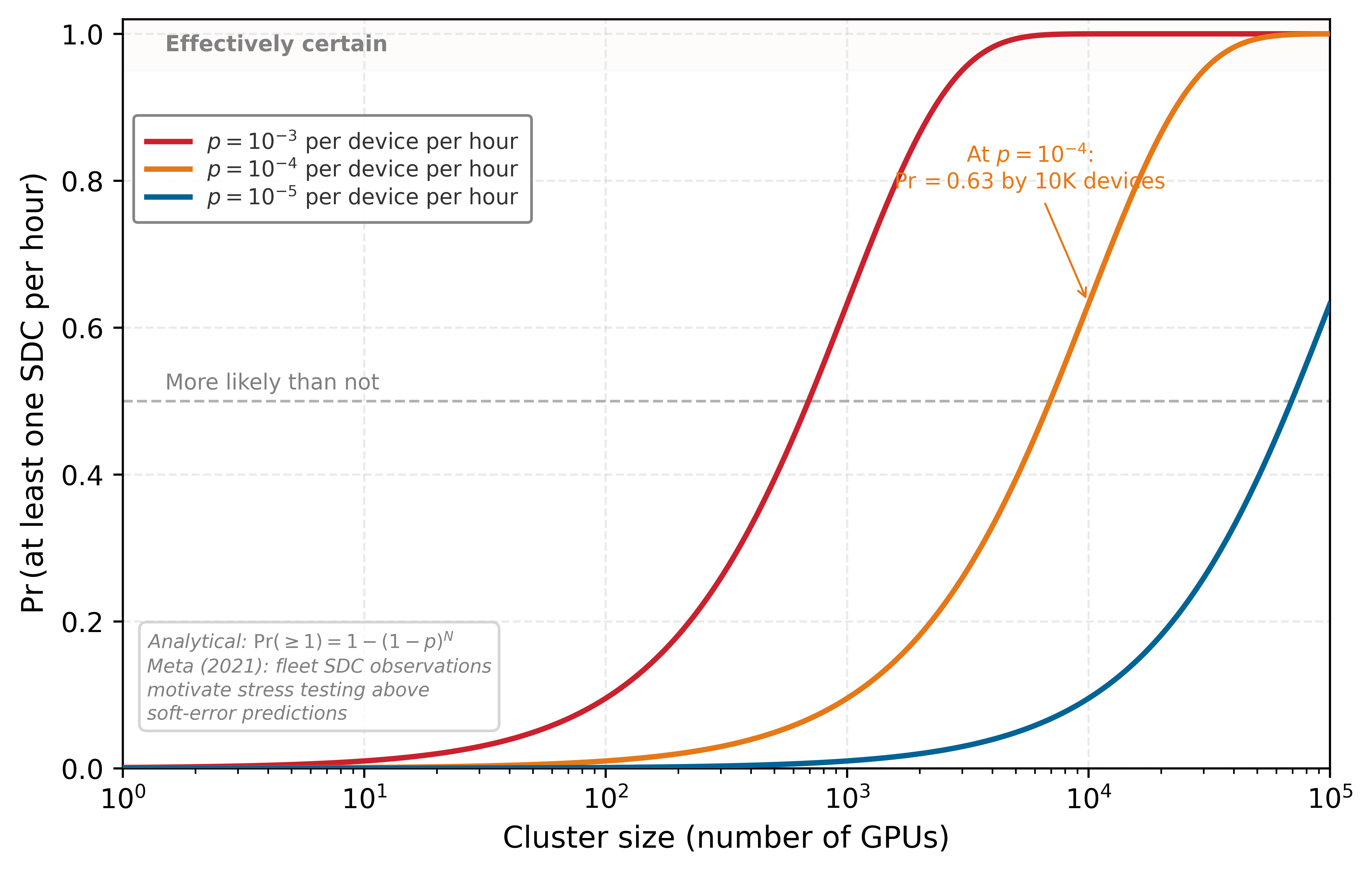
Fault Tolerance establishes that per-device silent corruption compounds across a fleet of \(N\) devices as \(\Pr(\geq 1) = 1 - (1 - p)^N\), the same arithmetic that makes a single bit flip a near-certain event at training scale. The robustness consequence is what figure 6 extends: sweeping the per-device rate shows how steeply the cluster-level probability climbs once a model is sharded across thousands of devices. The curve uses an illustrative stress-test rate of 0.01 percent per device-hour. At that rate, a 10,000-device cluster is more likely than not to see an hourly silent error (63.2 percent probability), and the probability crosses 95 percent at about 29,956 devices. Meta’s SDC report confirms corruption at observable fleet scale (Dixit et al. 2021).

Figure 6: Silent Error Probability at Scale: Probability of at least one silent data corruption event per hour as a function of cluster size, for three illustrative per-device error rates. The curves show how quickly cluster-scale probabilities compound as per-device rates increase.

The compounding effect at cluster scale motivates a unified framework for robustness that spans all dimensions of ML systems. Faults originating from hardware, adversarial inputs, and software defects share common characteristics and yield to systematic approaches.

The three pillars of robust AI

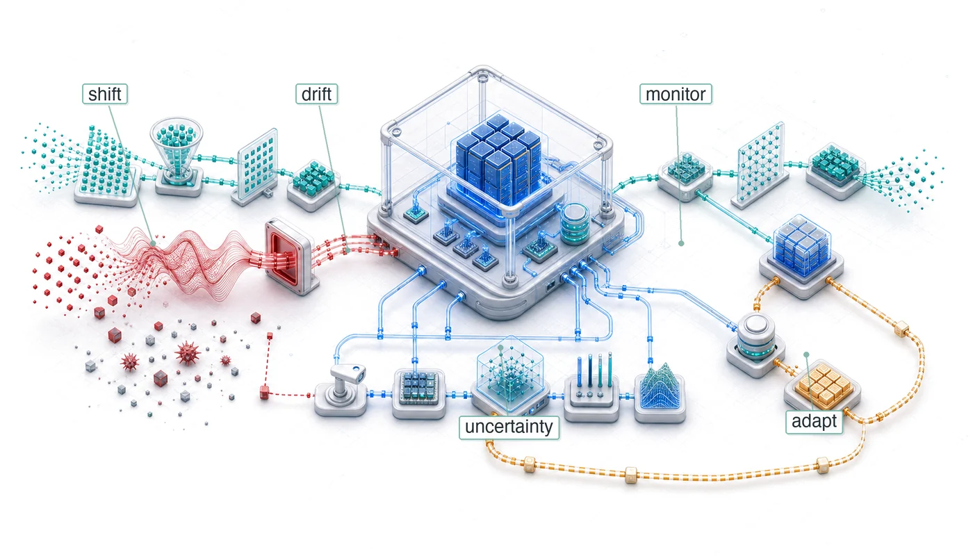
The unified framework helps engineers decide which failure signal they are seeing before they choose a defense. Environmental shifts, input-level attacks, and system-level faults produce different evidence and require different responses; software faults cut across all three because they can amplify or masquerade as any of them. The Three Pillars Framework in figure 7 organizes these threats as interconnected vulnerabilities that require complementary defense strategies.

Figure 7: Three Pillars Framework: The three core categories of robustness challenges that AI systems must address to ensure reliable operation in real-world deployments. A robust AI system is built upon effectively handling these three challenge areas.

What the figure adds to the three categories introduced earlier is the evidence each pillar produces and the defense family it demands. Environmental shifts produce a statistical signal: the input or label distribution moves continuously against a reference, so the evidence is distributional distance and the response family is monitoring, recalibration, and retraining.

Input-level attacks produce an adversarial signal: a crafted input or poisoned sample is engineered to maximize error, so the evidence is gradient-aligned perturbation or anomalous training samples, and the response family is adversarial training, certification, and input sanitization. Because the attacker operates within the model’s own input space, authentication and access control (Security & Privacy) do not reach this failure.

System-level faults encompass failures originating from the hardware, code, frameworks, and deployment infrastructure that support ML systems: numerical instability in gradient computations, data pipeline corruption from preprocessing bugs, race conditions in distributed training, memory leaks that degrade long-running services, dependency failures from version mismatches, and hardware faults such as bit flips or power events. The fault mechanics themselves, and their detection and recovery, belong to Fault Tolerance. What makes the third pillar a robustness problem rather than a pure reliability problem is that these faults rarely announce themselves as faults: they masquerade as the other two pillars, and an engineer who misreads the disguise spends the wrong defense budget.

Diagnosing the masquerade

Consider an operator who sees the same surface symptom from all three pillars: model accuracy is falling while latency and uptime hold steady. A preprocessing bug that silently rescales a feature looks exactly like covariate shift to a drift monitor, because the feature statistics have genuinely moved. A numerical overflow that corrupts a layer’s activations produces confident misclassifications that look exactly like an adversarial example, because the decision flipped without a visible input cause. The disguise is the whole difficulty: the cheap pillar-specific detectors fire on the symptom, not the cause.

Three signals separate the cases:

• Boundary of change: Genuine environmental shift moves continuously and affects whole populations of inputs as the world evolves; a pipeline fault appears as a step discontinuity synchronized with a deploy, a dependency bump, or a schema change, and it can move features that no real-world process would move together.
• Fixed-input reproducibility: Drift and adversarial perturbation are properties of the input distribution, so replaying a saved input through the current pipeline reproduces the correct historical output; a hardware or numerical fault is a property of the computation, so the same saved input now yields a different answer. Replaying a golden input set is the single most discriminating test, and it is why pipeline parity and preprocessing-version checks belong in the robustness toolkit alongside drift monitors.
• Cross-layer correlation: A real adversarial campaign correlates with input-space anomalies such as unusual query patterns or gradient-aligned perturbations; a masquerading software fault correlates instead with system-level signals, including a code release, an ECC counter, an SDC checker, or a memory-pressure alarm, that Fault Tolerance already instruments.

The diagnostic discipline is therefore to read the system-level evidence before accepting the drift or attack hypothesis the surface symptom suggests, because the response each pillar demands is different and only one of them is correct.

Common robustness principles

Across all three categories, the shared engineering problem is deciding which signal triggers which response. Robust systems need a detection threshold, a degradation path, and an adaptation mechanism, each with an explicit cost budget.

Detection and monitoring form the foundation of that strategy. Each pillar asks for a different signal. System-level monitoring samples hardware and runtime metrics to catch temperature anomalies, voltage fluctuations, memory errors, or silent data corruption before they corrupt model state. Input-level attack monitoring uses statistical or activation-space tests to flag adversarial inputs and poisoning attempts before they reach the decision boundary or training loop. Environmental-shift monitoring compares production traffic with reference distributions using tools such as Maximum Mean Discrepancy (MMD),¹³ Population Stability Index (PSI), or Kolmogorov-Smirnov (K-S) tests. The same quantitative discipline applies to defense cost: robustness mechanisms must be budgeted, not merely enabled, because every detector trades sensitivity against false positives, latency, and compute overhead.

¹³ Maximum Mean Discrepancy (MMD): A kernel-based statistical test measuring distance between two distributions in a reproducing kernel Hilbert space, without parametric assumptions. Unlike univariate tests (K-S, PSI) that require per-feature evaluation, MMD operates on joint distributions natively—critical for ML inputs where drift manifests in feature correlations, not individual features. The trade-off is compute: MMD scales \(\mathcal{O}(n^2)\) in sample size, making it impractical for real-time monitoring without subsampling or random feature approximations.

Napkin Math 1.1: The cost of defense

Problem: A team is training a robust classifier for an autonomous vehicle, using adversarial training with a seven-step projected-gradient descent attack (PGD-7) that searches for a worst-case perturbation for every training batch. How much does this extra attack-generation work slow down the training run?

Math: Generating an adversarial example requires \(K\) additional gradient steps per training sample.

1. Forward/backward passes: 1 (Standard) + 7 (Attack Generation) = 8 total passes.
2. Training Slowdown: 8× slower.
3. Utility Cost: Accuracy against the worst-case attack is 70 percent, compared with 95 percent clean-data accuracy for the standard model.

Systems insight: Robustness is an efficiency-utility trade-off. In this PGD-7 example, the team pays 8× the training cost and exposes a 25 percentage-point accuracy gap between standard clean-data accuracy and robust accuracy under the specified worst-case digital perturbation threat model. This notebook measures a training-cost scenario; the ResNet-50 robustness-tax example in section 1.6.1 measures the separate clean-accuracy tax of building adversarial robustness into the model weights. In the Machine Learning Fleet, “Robustness” is not a setting that can be flipped on; it is a budget the team spends. This budget pressure often makes detection attractive for lower-risk components, while certification and robust training are easier to justify for safety-critical paths.

Graceful degradation turns detection into a bounded operating mode instead of a crash. Robust systems exhibit predictable performance reduction that preserves critical capabilities. ECC memory systems recover from single-bit errors with 99.9 percent success rates while adding 12.5 percent bandwidth overhead. Model quantization from FP32 to INT8 reduces memory requirements by 75 percent and inference time by 2–4\(\times\), trading 1–3 percent accuracy for continued operation under resource constraints. Ensemble fallback systems trade peak accuracy for continuity, holding most of peak performance when a primary model fails and switching over fast enough to stay within a real-time serving budget.

Adaptive response completes the loop by changing system behavior when the signal persists. Adaptation might involve activating error correction mechanisms, applying input preprocessing techniques, or dynamically adjusting model parameters. The key principle is that robustness is not static but requires ongoing adjustment to maintain effectiveness.

Detection, degradation, and adaptation extend beyond fault recovery to form a systematic performance adaptation strategy that appears throughout ML system design. Figure 8 expands the same three pillars from figure 7 into concrete failure subtypes, then attaches the shared response pattern to each subtype: detection strategies form the foundation for monitoring systems, graceful degradation guides fallback mechanisms when components fail, and adaptive response enables systems to evolve with changing conditions.

Figure 8: The Robustness Taxonomy: Environmental shifts, input-level attacks, and system-level faults decomposed into concrete failure subtypes. Software faults can appear within or amplify all three categories.

The taxonomy in figure 8 reveals that no single defense covers all three pillars: environmental shifts, input-level attacks, and system-level faults each require distinct detection, degradation, and adaptation mechanisms, making defense-in-depth the core strategy for production systems.

Integration across the ML pipeline

Robustness cannot be bolted onto a trained model; it is a quality attribute enforced at every stage of the ML lifecycle, a principle often called defense in depth. In the data ingestion phase, sanitization filters must reject malformed or statistically anomalous records before they enter the training set, preventing data poisoning attacks at the source. During training, adversarial training directly exposes the model to worst-case perturbations, while randomized smoothing later turns noisy repeated predictions into a certifiable robustness bound. Both families try to limit how quickly outputs can change as inputs change, the intuition behind the model’s Lipschitz constant¹⁴. Validation extends beyond simple accuracy metrics to include stress testing on out-of-distribution (OOD) datasets, ensuring the model’s decision boundary is well-behaved in the open world.

¹⁴ Lipschitz Continuity: A mathematical property that bounds how much a function’s output changes relative to its input change (\(\lVert f(x) - f(x') \rVert \le K \lVert x - x' \rVert\)). In robust AI, minimizing the Lipschitz Constant \((K)\) ensures the model’s decision surface is “smooth” rather than “jagged,” making it physically impossible for small adversarial perturbations to flip the model’s prediction, though enforcing a low constant trades away clean-data accuracy and adds training cost.

Once deployed, the focus shifts to runtime defense. A robust inference server complements its serving architecture with the detection techniques in section 1.6.1.2, including input filtering that intercepts adversarial queries before they reach the accelerator. For a production fraud detection pipeline, this layered approach yields compound benefits: cheap statistical validation catches only the crudest poisoning attempts during data ingestion, while semantic input filtering at serving time blocks a much larger share of sophisticated evasion attacks. The monitoring layer acts as the safety net, detecting distribution drift—such as a sudden shift in transaction amounts or user geolocations—within days to weeks, triggering retraining workflows before performance degrades below the service level objective (SLO).

The holistic view integrates with hardware reality. Hardware faults (transient, permanent, and intermittent) are covered in detail in Hardware Fault Taxonomy, where they integrate with the broader fault detection and recovery mechanisms for distributed systems. A robust software pipeline treats silent data corruption in the ALU or a bit flip in HBM as another form of noise to be filtered or retried, not as an exceptional crash. With the lifecycle and hardware frame in place, the chapter now turns to the most common source of model degradation: the real world constantly evolves while training datasets remain frozen in time.

Checkpoint 1.1: Diagnosing the failure signal

The unified framework asks you to name which of the three pillars produced a silent failure before choosing a defense, and to recognize that software faults can masquerade as any of them.

Classifying the threat

• Pillar classification: Classify a model losing accuracy as customer behavior evolves, a crafted input that forces misclassification, and an accelerator HBM bit flip under the correct robustness pillars.
• Software-fault mimicry: Explain why a preprocessing bug that shifts every inference’s feature statistics is hard to distinguish from genuine environmental shift, then classify it under the appropriate pillar.

Choosing the response

• Response selection: Map an ECC-corrected single-bit memory error and a fired drift monitor to the shared responses of detection, graceful degradation, and adaptive response.
• Fleet-scale effects: Explain why a negligible per-device silent-corruption rate becomes an architectural constraint at a fleet scale of tens of thousands of accelerators.

Self-Check: Question

1. A production ML team is deciding how to organize its robustness engineering headcount across teams. Per the unified framework in this section, which division of concerns correctly reflects the taxonomy?

   1. One team each for training failures, validation failures, and deployment failures, treated as three fully independent pillars.
   2. One team each for environmental shifts and input-level attacks, with software faults staffed as a cross-cutting reliability function that interacts with both.
   3. One team each for model accuracy, inference latency, and model size, since those are the three axes of ML system performance.
   4. One team each for hardware faults, privacy attacks, and energy efficiency, because those are the only three robustness pillars this book recognizes.

2. Using the section’s illustrative silent-data-corruption stress-test rate of \(p = 10^{-4}\) per GPU per hour, what is the probability of at least one SDC event per hour in a 10,000-GPU cluster, and what is the operational implication?

   1. About \(10^{-8}\) per hour, so SDC can be ignored as a rare event that will statistically never occur during a training run.
   2. About 0.6-0.7 per hour, making SDC an expected-daily event that forces architectural defenses such as redundant recomputation and checksum gates.
   3. Exactly \(10^{-4}\) per hour because per-device rates do not compound across independent devices in a cluster.
   4. Exactly 1.0 per hour because with 10,000 devices at least one is guaranteed to fail every second regardless of the per-device rate.

3. Order the following three operational phases of the section’s robustness response cycle: (1) adaptive response tunes model or routing parameters, (2) detection and monitoring identifies that the system is operating under threat or shift, (3) graceful degradation preserves core functionality while the system absorbs the disturbance.

4. A team reports that switching from FP32 to INT8 quantization cut inference latency by 2–4\(\times\) and memory by 75 percent, at the cost of 1-3 percent clean accuracy. Explain why the chapter warns that the same optimization often reduces the model’s robustness margin, and why robustness evaluation cannot be decoupled from efficiency tuning.

5. The section argues for defense-in-depth across the ML pipeline. For a production fraud detection system, which layered design best reflects that guidance?

   1. Rely on a single strong runtime classifier and skip ingestion and monitoring logic so the serving path stays as simple as possible.
   2. Concentrate all defenses in the training loop, since inference-time mechanisms cannot help once the model weights are frozen.
   3. Combine data sanitization at ingestion, adversarial-aware training, OOD validation before deployment, runtime input filtering, and drift monitoring with retraining triggers.
   4. Focus only on hardware ECC since the section identifies hardware faults as the root cause of most robustness failures.

See Answers →

Environmental Shifts

Training data freezes a past world, while production traffic keeps changing. Environmental shifts are the robustness failures that follow from this mismatch: data distributions, user behavior, and operational contexts move after the model has learned its boundary. These shifts also interact with other vulnerability types: a model experiencing distribution shift becomes more susceptible to adversarial attacks, while software errors may manifest differently under changed environmental conditions.

Distribution shift and concept drift

A medical diagnosis model trained on X-ray images from a well-resourced hospital plummets in accuracy when deployed in a rural clinic with older equipment. The underlying medical conditions have not changed; the image characteristics differ. The world the model encounters differs from the world it learned from, and the result is distribution shift.

Napkin Math 1.2: Detecting a real distribution shift

Problem: A model monitors a critical input feature with a known standard deviation of 0.3. The baseline mean was 0.5. Over the last 1,000 requests, the mean has shifted to 0.55. The engineering question is whether this is a random fluctuation or a real distribution shift.

Math: Detection requires proving that the observed change is statistically unlikely under the baseline distribution.

1. Difference in means: 0.05.
2. Standard error: \(0.3/\sqrt{1,000} \approx 0.009\).
3. Statistical significance: The shift is approximately 5.3 standard errors away from the mean.
4. P-value: < 0.001.

Systems insight: Statistical significance is the signal-to-noise ratio of the monitoring system. A shift of 0.05 might seem “small,” but with 1,000 samples, the probability of it being random noise is less than 0.1 percent. In the machine learning fleet, this is a confirmed drift alert, not yet a confirmed model regression. The system should trigger investigation, increased monitoring, and correlation with precision, recall, latency, and business metrics; model fallback or retraining is warranted only when the shifted feature is high importance, the drift crosses severe thresholds, or service-level metrics degrade.

The taxonomy in figure 9 separates the three failure modes that a drift detector can surface: the inputs can move, the label prior can move, or the input-label relationship itself can change.

Figure 9: Types of Distribution Shift: Comparison of covariate shift (\(p(x)\) changes), label shift (\(p(y)\) changes), and concept drift (\(p(y \mid x)\) changes). Understanding the specific type of shift is crucial for selecting the correct adaptation strategy (for example, importance re-weighting vs. model retraining).

These shifts occur naturally as environments evolve. User preferences change seasonally, language evolves with new slang, and economic patterns shift with market conditions. Unlike adversarial attacks that require malicious intent, these shifts emerge organically from the dynamic nature of real-world systems.

Technical categories

Covariate shift occurs when the input distribution changes while the relationship between inputs and outputs remains constant (Quiñonero-Candela et al. 2009). Autonomous vehicle perception models trained on daytime images can experience accuracy degradation on the order of 15–30 percent when deployed in nighttime conditions despite the underlying object recognition task being unchanged, with the magnitude depending on luminance shift and sensor characteristics. Weather conditions introduce additional covariate shift: rain, snow, and fog are widely reported to drop object detection mAP by roughly 10–25 percent compared to clear-weather baselines in autonomous-driving evaluations. These numbers should be read as representative magnitudes from autonomous-vehicle perception benchmarks rather than a single cited result. These environmental changes effectively shift data points relative to the learned decision boundary (figure 10), causing misclassification without any change to the model itself.

Quiñonero-Candela, Joaquin, Masashi Sugiyama, Anton Schwaighofer, and Neil D. Lawrence, eds. 2009. Dataset Shift in Machine Learning. Neural Information Processing Series. The MIT Press.

Figure 10: Decision Boundary Under Distribution Shift: Environmental changes (for example, daytime to nighttime, clear to foggy) shift data points in the input space. When the shift moves points across the learned decision boundary, the model misclassifies inputs that it would have handled correctly under training conditions. Unlike adversarial perturbations, these shifts arise naturally and affect entire populations of inputs rather than individual examples.

Figure 10 illustrates the case where input distributions move while the true mapping \(p(y \mid x)\) stays fixed. A more insidious variant occurs when the mapping itself changes: the correct label for a given input today is different from what it was during training.

Definition 1.2: Concept drift

Concept Drift is the deployed-model subtype of distribution shift (see section 1.4.1) in which the statistical relationship \(p(y \mid x)\) changes over time, meaning the decision boundary itself becomes incorrect rather than merely the input distribution. Its sibling is data drift (see Monitoring at Scale), in which \(p(x)\) changes while \(p(y \mid x)\) remains stable.

1. Significance: It causes silent model degradation because the historical mapping learned by the model is no longer representative of current reality. Within the iron law, it compresses the effective deployment window before retraining is required: fraud-detection models, recommender systems, and other behavior-dependent models may need periodic retraining or recalibration as adversaries, users, and policies change. Each forced retraining cycle incurs the full \(O/(R_{\text{peak}} \cdot \eta_{\text{hw}})\) cost of the original training run, making the amortized per-prediction cost a direct function of drift velocity.
2. Distinction: Unlike data drift (where fresh \(p(x)\) data with unchanged labels fully restores performance), concept drift requires relabeling under the new \(p(y \mid x)\), because the same ground-truth labeling procedure that cures data drift is insufficient when the correct answer for the same input has changed. This makes concept drift structurally more expensive to remediate: it demands human annotation of recent examples, not merely resampling of the existing labeled distribution.
3. Common pitfall: A frequent misconception is that concept drift is detectable by monitoring input feature statistics. Because \(p(x)\) may be entirely unchanged, input-level monitoring (PSI, KL divergence on features) will show no signal. Concept drift can only be confirmed by comparing predictions to ground-truth outcomes, making it significantly harder to detect in real time and requiring a ground-truth feedback loop before remediation can begin.

Concept drift represents changes in the underlying relationship between inputs and outputs over time (Widmer and Kubat 1996). In production, this often appears in domains such as fraud detection or recommendation, where adversaries, seasonal patterns, and user preferences change the label relationship and force periodic recalibration or retraining.

Widmer, Gerhard, and Miroslav Kubat. 1996. “Learning in the Presence of Concept Drift and Hidden Contexts.” Machine Learning 23 (1): 69–101. https://doi.org/10.1023/a:1018046501280.

Lipton, Zachary, Yu-Xiang Wang, and Alexander Smola. 2018. “Detecting and Correcting for Label Shift with Black Box Predictors.” International Conference on Machine Learning, 3122–30.

Label shift affects the distribution of output classes without changing the input-output relationship (Lipton et al. 2018). During COVID-19, for example, hospital case mix and disease prevalence changed rapidly, so diagnostic models could require threshold recalibration even when image features carried the same clinical meaning. Similar class-prevalence shifts can occur as seasons, policies, or user populations change, requiring recalibration or reweighting rather than assuming that the feature-label relationship itself has changed.

Models can also fail because they learned the wrong lessons from the training data, not because the world changed. A classic example is a model that learns to identify “cow” by detecting “grass” background. When presented with a cow on a sandy beach, the model fails. The underlying cause is a spurious correlation: a feature that is predictive in the training set but not causally related to the label.

Standard training by empirical risk minimization (ERM) encourages these shortcuts because they are often statistically easier to learn than the robust features (shape, texture). Techniques like Group Distributionally Robust Optimization (Group DRO) explicitly mitigate this by minimizing the worst-case group loss (for example, cows on sand) rather than the average loss. The method requires groups to be known or inferred in advance, but when those groups are available, it forces the model to learn features that work across all contexts.

Monitoring and adaptation strategies

Drift monitoring earns its place only when it turns a distribution signal into an operating decision: investigate, adapt, retrain, or continue watching.

Statistical distance metrics quantify the degree of distribution shift by measuring differences between training and deployment data distributions. In this illustrative H100-class monitoring scenario, Maximum Mean Discrepancy (MMD) with RBF kernels (\(\gamma = 1.0\)) processes 10,000 samples in 150 ms; its sensitivity depends on the shift model and kernel choice. Kolmogorov-Smirnov tests can detect univariate shifts with 1,000+ samples, but scale poorly to high-dimensional data and miss joint changes that preserve marginals. Population Stability Index (PSI)¹⁵ thresholds of 0.1–0.25 indicate significant shift requiring model investigation.

¹⁵ Population Stability Index (PSI): Originally developed in the 1980s for credit scoring to detect whether the demographic of current loan applicants shifted from the historical baseline. In ML monitoring, PSI’s symmetric log-ratio formulation makes it a common industry tool for identifying data drift in categorical features, providing a single scalar trigger for retraining workflows.

Shalev-Shwartz, S. 2012. “Online Learning and Online Convex Optimization.” Foundations and Trends in Machine Learning 4 (2): 107–94. https://doi.org/10.1561/2200000018.

Kirkpatrick, J., R. Pascanu, N. Rabinowitz, J. Veness, G. Desjardins, A. A. Rusu, K. Milan, et al. 2017. “Overcoming Catastrophic Forgetting in Neural Networks.” Proceedings of the National Academy of Sciences 114 (13): 3521–26. https://doi.org/10.1073/pnas.1611835114.

Once a monitor fires, adaptation becomes a budgeted response instead of an automatic retraining command. Online learning enables models to continuously adapt to new data while maintaining performance on previously learned patterns (Shalev-Shwartz 2012). The adaptation budget depends on model size, drift rate, and feedback latency: updating too aggressively can chase noise, while updating too slowly lets performance drift. In production, online-learning systems usually bound update frequency, state size, and serving latency explicitly rather than assuming adaptation is free. Techniques like Elastic Weight Consolidation reduce catastrophic forgetting by penalizing changes to parameters important for previous tasks (Kirkpatrick et al. 2017).

Adaptive ensemble methods maintain multiple models or hypotheses and weight or select among them using recent performance, making them useful under gradual concept drift (Gama et al. 2014). This approach trades extra serving and monitoring complexity for the ability to respond when a single static model no longer matches the deployment distribution.

Federated learning enables distributed adaptation when the data cannot be centralized for privacy, regulatory, or bandwidth reasons. The adaptation then has to travel to the data instead, which makes the communication budget, not compute, the binding constraint: each round ships model parameters across many participants, so the design question is how many rounds and how much per-round transmission the deployment can afford. The federated mechanics belong to Edge Intelligence; the robustness-relevant point is that any privacy noise added to protect participants (for example, through differential privacy) carries a utility cost that must be measured for the application rather than assumed away.

Quantitative drift detection

Quantitative drift detection must answer an operational question: whether the model should keep serving, be monitored more closely, or be retrained. PSI supplies the cheap fleet-wide alert that starts that decision, while the mathematical foundations and operational thresholds below transform drift detection from a subjective judgment into an engineering discipline.

Population stability index (PSI)

Drift detection introduced the Population Stability Index as a cheap fleet-wide alerting signal, with its credit-scoring origin and the standard threshold bands. This section develops the full statistical machinery behind that signal: how PSI is computed, what binning and smoothing choices govern its sensitivity, and how it combines with KL divergence and significance tests into a retraining decision. PSI measures the divergence between an expected (baseline) distribution \(p_{\text{base}}\) and an actual (current) distribution \(p_{\text{curr}}\) by computing a symmetric log-ratio difference across discretized bins.

For a feature discretized into \(k\) bins, PSI is defined as:

\[ \text{PSI} = \sum_{i=1}^{k} (p_i - q_i) \times \ln\left(\frac{p_i}{q_i}\right) \]

where \(p_i\) represents the proportion of observations in bin \(i\) for the baseline distribution and \(q_i\) represents the corresponding proportion in the current distribution. The logarithmic term penalizes large relative changes, while the \((p_i - q_i)\) term weights by absolute magnitude. Established threshold bands translate these PSI values into actionable decisions.

Table 1 collects common PSI ranges and the recommended monitoring action at each tier. These threshold bands are monitoring conventions, especially common in credit-scoring practice, rather than universal statistical guarantees; PSI should be interpreted together with feature importance and downstream model-performance metrics (Yurdakul and Naranjo 2020).

Yurdakul, Bilal, and Joshua Naranjo. 2020. “Statistical Properties of the Population Stability Index.” The Journal of Risk Model Validation 52. https://doi.org/10.21314/jrmv.2020.227.

Table 1: PSI Interpretation Thresholds: Common Population Stability Index ranges and the recommended monitoring action at each tier.

PSI Value	Interpretation	Recommended Action
\(\text{PSI} < 0.1\)	Negligible shift	Continue monitoring
\(0.1 \le \text{PSI} < 0.2\)	Minor shift	Investigate root cause
\(0.2 \le \text{PSI} < 0.25\)	Moderate shift	Consider retraining
\(\text{PSI} \ge 0.25\)	Major shift	Retrain required

Several implementation choices determine whether PSI is sensitive enough to be useful. Bin selection significantly affects PSI sensitivity. For categorical features, each category forms a natural bin. For continuous features, equal-width bins (10–20 bins typical) or quantile-based bins provide different trade-offs: equal-width bins preserve the absolute scale of the feature space, while quantile bins ensure adequate sample sizes in each bin but may mask shifts in the tails. Production systems often use ten bins with a minimum of 5 percent of observations per bin to ensure statistical stability.

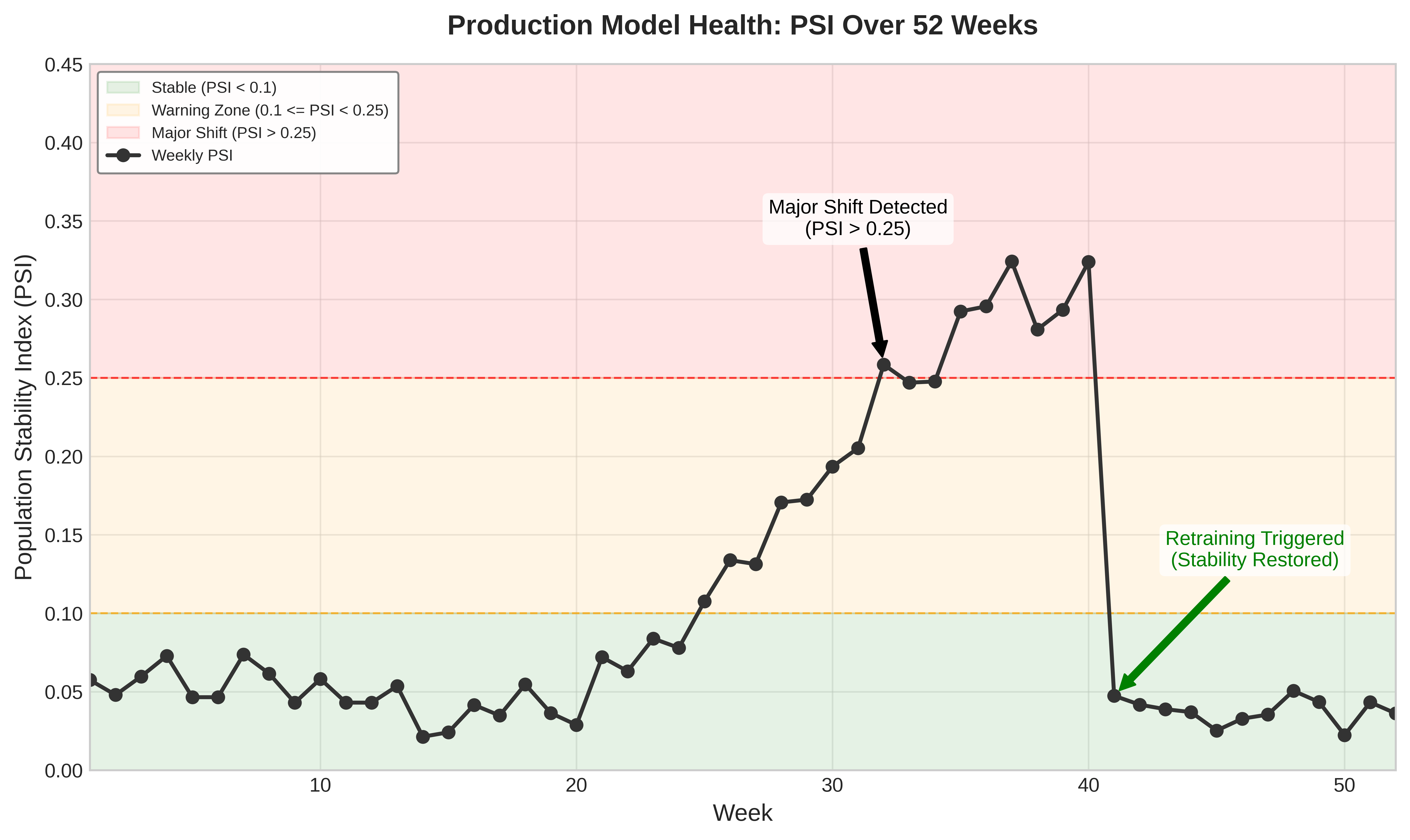
When a bin has zero observations in either distribution, adding a small smoothing constant (typically \(\epsilon = 10^{-8}\)) prevents undefined logarithms while minimally affecting the PSI value. As figure 11 shows, monitoring PSI over time reveals when a model drifts from stable (Green Zone) into warning (Orange) and critical (Red Zone) regions, triggering an escalation path that may lead to retraining after performance correlation.

Figure 11: The Distribution Shift Detector: Monitoring Population Stability Index (PSI) over a year. The model remains stable through week 24, enters the orange warning zone at week 25 as user behavior shifts, and breaches the red critical threshold at week 32. Automated retraining restores model stability at week 41.

Kullback-Leibler divergence

For continuous features where binning may lose information, Kullback-Leibler (KL) divergence provides a more direct measure of distributional difference. The KL divergence from baseline distribution \(p_{\text{base}}\) to current distribution \(p_{\text{curr}}\) is defined as:

\[ \mathcal{D}_{\text{KL}}(p_{\text{base}} \lVert p_{\text{curr}}) = \int_{-\infty}^{\infty} p_{\text{base}}(x) \ln\left(\frac{p_{\text{base}}(x)}{p_{\text{curr}}(x)}\right) dx \]

where \(p_{\text{base}}(x)\) and \(p_{\text{curr}}(x)\) are the probability density functions of the baseline and current distributions, respectively. Unlike PSI, KL divergence is asymmetric: \(\mathcal{D}_{\text{KL}}(p_{\text{base}} \lVert p_{\text{curr}}) \neq \mathcal{D}_{\text{KL}}(p_{\text{curr}} \lVert p_{\text{base}})\). For drift detection, we typically compute \(\mathcal{D}_{\text{KL}}(\text{baseline} \lVert \text{current})\), measuring how much information is lost when using the current distribution to approximate the baseline.

To address asymmetry, practitioners often use the Jensen-Shannon divergence:

\[ \mathcal{D}_{\text{JS}}(p_{\text{base}} \lVert p_{\text{curr}}) = \frac{1}{2} \mathcal{D}_{\text{KL}}(p_{\text{base}} \lVert p_{\text{mix}}) + \frac{1}{2} \mathcal{D}_{\text{KL}}(p_{\text{curr}} \lVert p_{\text{mix}}) \]

where \(p_{\text{mix}} = \frac{1}{2}(p_{\text{base}} + p_{\text{curr}})\) is the mixture distribution. Jensen-Shannon divergence is bounded between 0 and \(\ln(2)\) (approximately 0.693), making threshold selection more intuitive than unbounded KL divergence.

For drift monitoring in production, table 2 gives practical thresholds for interpreting KL divergence values.

Table 2: KL Divergence Threshold Reference: Practical thresholds for interpreting KL divergence values during drift monitoring. Values below 0.05 indicate minimal divergence; 0.05 to 0.1 indicates moderate divergence that warrants investigation; values at or above 0.1 indicate significant divergence that typically triggers retraining workflows.

\(\mathcal{D}_{\text{KL}}\) Value	Interpretation
\(\mathcal{D}_{\text{KL}} < 0.05\)	Minimal divergence
\(0.05 \le \mathcal{D}_{\text{KL}} < 0.1\)	Moderate divergence
\(\mathcal{D}_{\text{KL}} \ge 0.1\)	Significant divergence

For practical computation, kernel density estimation (KDE) with Gaussian kernels provides smooth density approximations suitable for integration, though computational cost scales as \(\mathcal{O}(n^2)\) for \(n\) samples, making sampling necessary for large datasets.

Statistical significance testing

PSI and KL divergence quantify how large a distributional change appears to be; statistical hypothesis tests ask the complementary question of whether the observed difference is larger than sampling noise. The two-sample Kolmogorov-Smirnov (KS) test (Berger and Zhou 2014) compares the empirical cumulative distribution functions (CDFs) of two samples without assuming any specific parametric form. The test statistic is:

\[ D_{n,m} = \sup_x |F_n(x) - G_m(x)| \]

where \(F_n\) and \(G_m\) are the empirical CDFs of samples of size \(n\) and \(m\) respectively. The null hypothesis (no distributional difference) is rejected when:

\[ D_{n,m} > c(\alpha) \sqrt{\frac{n + m}{nm}} \]

where \(c(\alpha)\) depends on the significance level (for example, \(c(0.05) \approx 1.36\)). The KS test is particularly effective for detecting shifts in location (mean) and spread (variance) but less sensitive to changes in distribution shape.

For categorical features, the chi-square goodness-of-fit test compares observed frequencies to expected frequencies under the baseline distribution:

\[ \chi^2 = \sum_{i=1}^{k} \frac{(n_i^{\text{obs}} - n_i^{\text{exp}})^2}{n_i^{\text{exp}}} \]

where \(n_i^{\text{obs}}\) is the observed count in category \(i\) and \(n_i^{\text{exp}}\) is the expected count based on the baseline distribution. With \(k-1\) degrees of freedom, the null hypothesis is rejected when \(\chi^2\) exceeds the critical value for significance level \(\alpha\).

When monitoring many features simultaneously, the significance test must also account for repeated comparisons. Applying Bonferroni correction (dividing \(\alpha\) by the number of tests) or false discovery rate (FDR) control prevents excessive false alarms. For \(m\) features at significance level \(\alpha = 0.05\), Bonferroni requires each test to achieve \(p < 0.05/m\) for significance.

Worked example: Production fraud detection model

Consider a fraud detection model serving an e-commerce platform with two key input features: user country (categorical) and transaction amount (continuous). After six months in production, the operations team suspects distribution drift and must decide whether to retrain.

Step 1: Categorical feature analysis

Table 3 compares the baseline (training) distribution and current (production) distribution for four named countries plus the Other bucket.

Table 3: Country-Feature PSI Decomposition: Per-country contribution to the total PSI for the user country feature in a production fraud-detection model. The “Other” bucket drives most of the divergence (0.0470 of the 0.065 total), reflecting growth of non-USA/UK/Germany/France traffic over six months in production.

Country	Baseline (\(p_i\))	Current (\(q_i\))	\(p_i - q_i\)	\(\ln(p_i/q_i)\)	Contribution
USA	0.45	0.38	0.07	0.169	0.0118
UK	0.20	0.18	0.02	0.105	0.0021
Germany	0.15	0.14	0.01	0.069	0.0007
France	0.10	0.12	-0.02	-0.182	0.0036
Other	0.10	0.18	-0.08	-0.588	0.0470

Summing the per-country contributions gives \(\text{PSI}_{\text{country}} = 0.0118 + 0.0021 + 0.0007 + 0.0036 + 0.0470 = 0.065\).

The PSI of 0.065 indicates negligible drift in user country distribution, falling well below the 0.1 threshold. No action required for this feature.

Step 2: Continuous feature analysis

For the transaction amount feature (log-transformed for normality), compute KL divergence using kernel density estimation:

• Baseline distribution: \(\mu = 4.2\), \(\sigma = 1.1\) (log-dollars)
• Current distribution: \(\mu = 4.5\), \(\sigma = 1.3\) (log-dollars)

For approximately Gaussian distributions, KL divergence has a closed-form solution:

\[ \mathcal{D}_{\text{KL}} = \ln\frac{\sigma_{\text{curr}}}{\sigma_{\text{base}}} + \frac{\sigma_{\text{base}}^2 + (\mu_{\text{base}} - \mu_{\text{curr}})^2}{2\sigma_{\text{curr}}^2} - \frac{1}{2} \]

The closed-form solution evaluates to \(\mathcal{D}_{\text{KL}} = \ln\frac{1.3}{1.1} + \frac{1.30}{3.38} - 0.5 = 0.167 + 0.385 - 0.5 = 0.052\). The KL divergence of 0.052 indicates moderate drift, warranting further investigation but not immediate retraining.

Step 3: Statistical significance via KS test

Using the KS test on 10,000 baseline samples and 10,000 current samples for transaction amount:

\[ D_{10000,10000} = 0.089 \]

Critical value at \(\alpha = 0.05\): \(c(0.05) \sqrt{\frac{20000}{10^8}} \approx 0.019\)

Since the observed statistic 0.089 exceeds the critical value 0.019, the difference is statistically significant \((p < 0.001)\). However, statistical significance alone does not mandate retraining; the practical significance (PSI, KL values) suggests monitoring rather than immediate action.

Step 4: Decision framework application

Table 4 combines the quantitative evidence.

Table 4: Retraining Decision Matrix: Combined quantitative evidence (PSI, KL divergence, KS test) compared against thresholds and the resulting action level. Drift signals below the practical threshold but with statistical significance call for monitoring at increased frequency rather than immediate retraining.

Metric	Value	Threshold	Action Level
PSI (country)	0.065	\(< 0.1\)	Monitor
\(\mathcal{D}_{\text{KL}}\) (amount)	0.052	\(< 0.1\)	Monitor
KS test	\(p < 0.001\)	\(\alpha = 0.05\)	Significant

Decision: Continue monitoring with increased frequency (weekly instead of monthly). If PSI or KL divergence exceeds 0.1 in the next monitoring cycle, or if model performance metrics (precision, recall) degrade by more than 5 percent, initiate retraining. The example stops at a monitoring decision; the general framework turns that same logic into a repeatable retraining gate.

Retraining decision framework

A systematic decision framework integrates drift metrics with performance monitoring to determine optimal retraining timing. The three levels below deliberately separate detection, correlation, and action so metric alerts do not become automatic retraining commands.

Level 1: Automated monitoring

Configure automated alerts for three drift thresholds:

• \(\text{PSI} > 0.1\) on any high-importance feature
• \(\mathcal{D}_{\text{KL}} > 0.05\) on continuous features
• KS test \(p\)-value \(< 0.01\) with Bonferroni correction

Level 2: Performance correlation

When drift alerts trigger, three performance correlations determine the response:

• If performance degradation exceeds 3 percent and coincides with drift: Initiate retraining
• If drift detected but performance stable: Continue monitoring, investigate drift source
• If performance degrades without detected drift: Investigate concept drift or label shift

Drift stays benign until the index crosses a threshold; past the knee, reliability degrades fast.

Level 3: Retraining vs. investigation

Not all drift requires retraining. Table 5 separates immediate remediation from investigation and continued monitoring.

Table 5: Retraining Decision Rules: Drift response depends on the strength of the statistical signal, observed performance change, and external evidence about whether the environment has truly changed.

Action	Trigger conditions	Response logic
Retrain immediately	• \(\text{PSI} > 0.25\) on critical features and performance degraded by more than 5% • Concept drift confirmed (\(p(y \mid x)\) changed) • Regulatory or compliance requirements mandate fresh models	The learned mapping, compliance baseline, or production population is no longer valid enough for monitoring alone
Investigate first	• \(0.1 \le \text{PSI} \le 0.25\) with stable performance • Drift localized to nonpredictive features • Drift may be temporary, such as seasonal effects or one-time events	The signal is real, but the remediation could be more expensive or riskier than the current degradation
Continue monitoring	• PSI < 0.1 across all features • Performance within acceptable bounds • No external signals suggesting environmental change	The evidence does not yet justify changing the model, but the baseline should remain under observation

The quantitative framework transforms drift detection from reactive troubleshooting into proactive model maintenance, enabling ML systems to maintain reliability as production environments evolve (Gama et al. 2014).

Gama, João, Indrė Žliobaitė, Albert Bifet, Mykola Pechenizkiy, and Abdelhamid Bouchachia. 2014. “A Survey on Concept Drift Adaptation.” ACM Computing Surveys 46 (4): 1–37. https://doi.org/10.1145/2523813.

Robustness in generative AI

Large language models (LLMs) shift the failure surface from incorrect classification to semantic reliability: a fluent answer can be factually baseless while the system still appears healthy. The earlier robustness question was whether a label changed under perturbation; the generative version is whether an open-ended output preserves factuality, policy constraints, and task intent under prompt variation. Evaluations in specialized domains such as legal or medical advice show that hallucination rates vary strongly with model, retrieval context, prompt design, and sampling temperature. Addressing this requires rigorous Uncertainty Quantification (UQ): a robust system must be self-aware enough to flag when it is guessing. One approach monitors the entropy of the output distribution; a “flat” probability distribution across the vocabulary indicates high uncertainty, which can trigger a fallback to a human operator or a refusal to answer. Log-probabilities at the token level reveal segments where the model transitions from confident generation to speculative completion.

More advanced UQ techniques involve Self-Consistency, where the model is prompted to generate multiple distinct reasoning paths for the same query. If five sampling runs produce five contradictory answers to a factual question, the system treats the output as unstable and suppresses it. This statistical approach transforms the nebulous concept of “truthfulness” into a measurable variance metric that integrates naturally with the MLOps monitoring pipeline (ML Operations at Scale). Predictive entropy—aggregating the Shannon entropy across the full output sequence—provides a scalar score that can be thresholded to route high-risk generations for human review.

In Retrieval-Augmented Generation (RAG) architectures (Inference at Scale), robustness depends heavily on the quality of the retrieved context. Retrieval Noise, the injection of irrelevant or conflicting documents into the prompt, can distract the model, causing it to ignore its internal parametric knowledge and propagate errors from the context. Robust RAG deployments can use re-ranking models and context verifiers to filter out noise before it reaches the generation step.

Generative models also face the unique threat of Prompt Injection, where an attacker embeds instructions within the input data to override the model’s system prompt. While often discussed as a security issue in Security & Privacy, prompt injection is equally a robustness failure: a model that can be easily manipulated into ignoring its behavioral constraints has failed to maintain its output invariants under adversarial input. A common deployment pattern is to add Output Guardrails—lightweight classification models that scan generated text for policy violations, toxicity, or logical errors before returning the response to the user. This final validation step helps keep the system as a whole reliable even if the core model enters a failure mode.

While prompt injection exploits the linguistic flexibility of generative models, it represents a bridge between natural environmental shifts and deliberate adversarial manipulation. The interaction runs both directions: distribution monitoring systems themselves can be exploited by adversaries who craft inputs that evade drift detection thresholds, turning a defensive tool into a blind spot. When an adversary stops relying on natural drift and actively begins reverse-engineering the model’s decision boundaries to force specific errors, we move from the domain of environmental robustness into the mathematically rigorous battleground of input-level attacks.

Checkpoint 1.2: Drift detection and the retraining decision

Environmental shifts split into distinct types, and the chapter’s drift framework deliberately separates a fired metric from a retraining command.

Distinguishing the shift type

• Shift taxonomy: Distinguish covariate shift, label shift, and concept drift by which probability the change touches, and explain why feature-statistics monitoring stays silent under pure concept drift.
• Shortcut failure: Identify the failure in a cow-on-a-beach misclassification where the world has not changed but the model learned the wrong lesson, and explain why standard empirical risk minimization encourages it.

Reasoning about thresholds and cost

• Threshold judgment: Select retraining, investigation, or continued monitoring for a high-importance feature whose population stability index is in the major-shift band while precision and recall stay flat.
• Cost asymmetry: Explain why concept drift is structurally more expensive to remediate than data drift, even when the same volume of fresh data is available.

Self-Check: Question

1. A fraud detection model’s input features continue to follow their training distribution — the same transaction amounts, same countries, same merchant-category frequencies — yet its precision falls from 88 percent to 64 percent over six months as criminal behavior adapts to the deployed detector. Using the section’s p(X), p(Y), p(Y|X) taxonomy, which form of environmental shift has occurred?

   1. Covariate shift, because the model is no longer seeing the inputs it was trained on.
   2. Concept drift, because the conditional p(Y|X) has changed while p(X) remains stable.
   3. Label smoothing, because the training labels have been regularized away from hard 0/1 values.
   4. Data augmentation drift, because the preprocessing pipeline has randomly perturbed the inputs.

2. A monitoring dashboard reports a Kolmogorov-Smirnov p-value of 0.003 on a single input feature after 500,000 samples, while PSI on that feature is 0.07 and downstream precision/recall are unchanged. The on-call engineer asks whether to retrain. Explain why the section’s decision framework does not treat a statistically significant p-value as sufficient evidence to retrain.

3. A production fraud detection team reviews four monitoring signals each week. Per the retraining decision framework in this section, which signal most strongly justifies immediate retraining rather than continued monitoring?

   1. PSI = 0.065 on the transaction-amount feature, KL divergence = 0.052, and precision holds at 0.88.
   2. PSI = 0.12 on a non-predictive metadata feature, with no measurable performance change.
   3. KS p-value < 0.01 on a single feature after Bonferroni correction, with PSI = 0.08 and performance unchanged.
   4. PSI = 0.28 on the transaction-amount feature together with precision dropping by 7 percent over the same window.

4. A monitoring system runs PSI and KS checks on every feature of a recommendation model and all tests stay green for eight consecutive weeks. Yet the embedding-space distribution has drifted in its correlation structure: feature pairs that were tightly coupled during training are now nearly independent. The metric that detects this correlation-only shift, because it compares joint distributions in a reproducing kernel Hilbert space rather than one feature at a time, is called ____.

5. True or False: For a credit-card fraud detection model, if PSI, KL divergence, and KS tests on every input feature stay green for three months, the production team can conclude that no concept drift has occurred without needing to compare predictions against labeled outcomes.

6. A customer-support chatbot built on a large language model is flagged for occasional confident fabrications (hallucinations) that never trigger classifier-style misclassification alarms. Explain how the section’s notion of semantic robustness in generative AI differs from classifier robustness, and what monitoring response follows.

See Answers →

Input-Level Attacks and Model Robustness

Adding a microscopic, mathematically calculated layer of noise to an image of a benign skin lesion, noise so subtle a human dermatologist cannot see it, causes a production diagnostic model to diagnose it as malignant with 99.9 percent confidence. The high-dimensional decision boundaries learned by deep neural networks possess counterintuitive blind spots that malicious actors can deliberately exploit. The practical question is what the attacker can see or control: gradients, queries, physical sensors, or training data. Adversarial attacks expose these blind spots.

Adversarial attacks

Definition 1.3: Adversarial attack

Adversarial Attack is a deliberate, mathematically crafted perturbation to model inputs designed to cause misclassification while remaining imperceptible to humans.

1. Significance: It reveals that high-dimensional decision boundaries have counterintuitive vulnerabilities. The per-feature perturbation magnitude required for misclassification scales inversely with input dimensionality, meaning models operating on high-dimensional inputs (for example, high-resolution images) are susceptible to attacks in which no single feature changes perceptibly.
2. Distinction: Unlike random noise (which the model can learn to ignore), adversarial perturbations are gradient-directed: they are specifically optimized to maximize the model’s prediction error.
3. Common pitfall: A frequent misconception is that adversarial vulnerability is a “bug” to be patched. In reality, it is a structural vulnerability of many standard neural networks trained by empirical risk minimization; robust defense typically requires fundamental changes to the objective function (for example, adversarial training).

Adversarial attack categories encode access and cost. A white-box attacker can use gradients directly, a black-box attacker relies on transfer, and a physical attacker must survive cameras, lighting, and distance. Figure 12 demonstrates the shared mechanism: small, carefully designed perturbations to input data can cause high-confidence misclassification, with perturbations invisible to the human eye but devastating to model accuracy.

Figure 12: Adversarial Perturbation: Subtle, intentionally crafted noise can cause neural networks to misclassify images with high confidence and expose vulnerabilities in model robustness. These perturbations, imperceptible to humans, alter the input in ways that maximize prediction error and highlight the need for defenses against adversarial attacks. Source: Sutanto (2019).

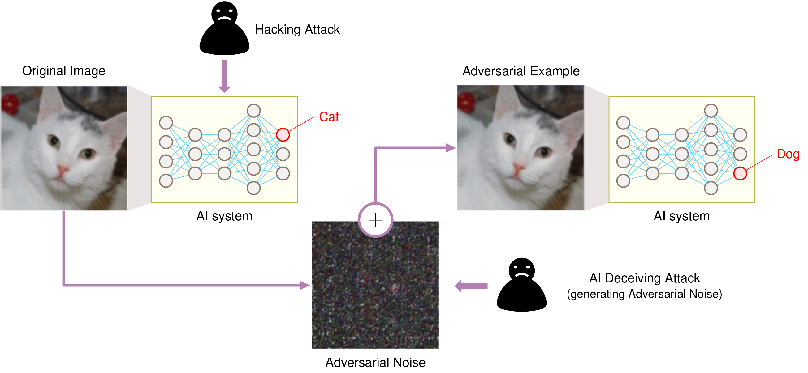
The effectiveness of these attacks traces to a fundamental mismatch between human and machine perception¹⁶. Neural networks draw nonlinear decision boundaries through a high-dimensional feature space, and adversarial perturbations exploit the geometry of those boundaries: the many input dimensions give an attacker many directions to push simultaneously, so a change too small to see in any one dimension can still cross the boundary.

¹⁶ Human vs. Machine Perception: First highlighted by Szegedy et al. (2013), neural networks learn statistical correlations in pixel space rather than the semantic invariances human vision enforces. This gap is not a bug to be patched but a structural consequence of gradient-based optimization on finite training data: the model finds decision boundaries that minimize empirical risk, and adversarial perturbations exploit the vast regions of input space those boundaries leave unguarded.

Szegedy, Christian, Wojciech Zaremba, Ilya Sutskever, Joan Bruna, Dumitru Erhan, Ian Goodfellow, and Rob Fergus. 2013. “Intriguing Properties of Neural Networks.” arXiv Preprint arXiv:1312.6199.

Attack categories and mechanisms

The useful axis is not the attack name by itself but the attacker’s access. Each mechanism reveals a different cost that the defense must raise: gradient access, optimization time, surrogate-model construction, or physical control over the sensor environment.

The most direct case is white-box gradient access. Neural networks compute gradients to learn how parameter changes reduce loss; an attacker with access to gradients can run that logic against the input instead. For an image classifier that correctly identifies a cat, the gradient with respect to the input image reveals which pixel-level changes would most increase prediction error. The Fast Gradient Sign Method¹⁷ turns that idea into a single-step attack by moving each input feature in the direction that increases loss fastest.

¹⁷ Fast Gradient Sign Method (FGSM): Proposed by Goodfellow et al. (2014) at ICLR, FGSM generates adversarial examples in a single gradient step, making it practical to use during training. This dual role is its lasting systems significance: the same attack that exposed neural network fragility became a simple adversarial-training primitive, where FGSM-generated perturbations augment clean batches with examples chosen to increase loss.

Goodfellow, I. J., J. Shlens, and C. Szegedy. 2014. “Explaining and Harnessing Adversarial Examples.” ICLR 3.

The underlying mathematical formulation captures this intuitive process:

\[ x_{\text{adv}} = x + \epsilon \cdot \text{sign}\big(\nabla_x \mathcal{L}(\theta, x, y)\big) \]

where:

• \(x\) is the original input
• \(x_{\text{adv}}\) is the adversarial example
• \(\mathcal{L}(\theta, x, y)\) is the prediction loss
• \(\nabla_x \mathcal{L}\) identifies the input changes that most increase that loss
• \(\text{sign}(\cdot)\) keeps only the direction of steepest ascent
• \(\epsilon\) controls how much perturbation the attacker is allowed to add

Figure 13 visualizes how this approach generates adversarial examples by taking a single step in the direction that increases the loss most rapidly, moving the input across the decision boundary with minimal perturbation.

Figure 13: Adversarial Perturbations: Gradient-based attacks generate subtle, intentionally crafted input noise with magnitude controlled by \(\epsilon\) that maximizes the loss function \(\mathcal{L}(\theta, x, y)\) and causes misclassification by the model. These perturbations, imperceptible to humans, exploit model vulnerabilities by moving the input \(x\) across the decision boundary. Source: adapted from a gradient-based-attacks tutorial at defence.AI.

FGSM is cheap because it takes one step. The Projected Gradient Descent (PGD) attack (Madry et al. 2018) spends more compute for a stronger attack: it repeatedly applies gradient updates and projects each step back into the allowed norm ball around the original input. That iterative refinement makes PGD a standard white-box robustness benchmark. The Jacobian-based Saliency Map Attack (JSMA) (N. Papernot et al. 2016) uses the Jacobian to identify the most influential input features and perturb a smaller set of dimensions toward a target class. These methods are most effective in white-box settings¹⁸, where the attacker knows the model architecture and gradients.

Papernot, N., P. McDaniel, S. Jha, M. Fredrikson, Z. Berkay Celik, and A. Swami. 2016. “The Limitations of Deep Learning in Adversarial Settings.” 2016 IEEE European Symposium on Security and Privacy (EuroS&amp;P), 372–87. https://doi.org/10.1109/eurosp.2016.36.

¹⁸ White-Box Attack: Adversarial attack with complete model knowledge (architecture, weights, gradients). Methods like PGD and Carlini-Wagner (C&W) are strong because they optimize directly against the model rather than probing it from the outside. Though less realistic than black-box scenarios for many deployed systems, white-box analysis establishes a demanding benchmark within a specified norm, perturbation budget, and attack procedure. Passing PGD is evidence for that threat model, not a universal guarantee against every weaker-looking attack.

¹⁹ Carlini and Wagner (C&W) Attack: Proposed in 2016 (IEEE S&P 2017), C&W formulates adversarial example generation as a constrained optimization problem that finds the minimal perturbation causing misclassification. Its significance is methodological: C&W broke defensive distillation (an early defense that masked gradients to blunt weaker attacks) and several other defenses that resisted FGSM and PGD, establishing the principle that robustness claims must be evaluated against optimization-based attacks, not just gradient-sign heuristics.

Carlini, Nicholas, and David Wagner. 2017. “Towards Evaluating the Robustness of Neural Networks.” 2017 IEEE Symposium on Security and Privacy (SP), 39–57. https://doi.org/10.1109/sp.2017.49.

When the attacker cares less about speed and more about stealth, the attack becomes an optimization problem. The Carlini and Wagner (C&W) attack¹⁹ (Carlini and Wagner 2017) searches for the smallest perturbation that causes misclassification while preserving perceptual similarity to the original input. Instead of merely following the sign of a gradient, C&W optimizes a custom objective that trades perturbation size against confidence in the wrong answer.

C&W attacks are difficult to detect because the perturbations are usually imperceptible to humans and can be optimized under different norm constraints, such as \(\ell_2\) or \(\ell_\infty\). The Elastic Net Attack to DNNs (EAD) adds elastic net regularization, combining \(\ell_1\) and \(\ell_2\) penalties to generate sparse, localized perturbations. These optimization-based methods are more computationally intensive than gradient-sign attacks, but they give the attacker finer control over the adversarial example’s geometry.

Black-box attackers lose direct gradient access, but they can still exploit transferability²⁰. Transferability is the phenomenon in which adversarial examples crafted for one model can fool other models, even when the architectures or training datasets differ. An attacker can train or obtain a surrogate model, craft attacks offline, and then submit the resulting examples to the target API without ever seeing its weights or gradients.

²⁰ Transferability: The property, analyzed in Nicolas Papernot, McDaniel, and Goodfellow (2016), that adversarial examples crafted for one model can fool different architectures. This transforms the threat model for deployed ML systems: attackers need not see the target model’s weights—they can train a substitute locally, craft attacks offline, and transfer them to production APIs. Ensemble adversarial training trains against perturbations from multiple models to improve transfer robustness, but the extra attack generation and model diversity make it a deliberate training-budget decision rather than a free mitigation (Tramèr et al. 2017).

Papernot, Nicolas, Patrick McDaniel, and Ian Goodfellow. 2016. “Transferability in Machine Learning: From Phenomena to Black-Box Attacks Using Adversarial Samples.” arXiv Preprint arXiv:1605.07277.

Tramèr, Florian, Alexey Kurakin, Nicolas Papernot, Ian Goodfellow, Dan Boneh, and Patrick McDaniel. 2017. “Ensemble Adversarial Training: Attacks and Defenses.” International Conference on Learning Representations abs/1705.07204.

Transfer success depends on model similarity, training-data overlap, and regularization. Attackers can improve transfer by using input diversity, such as random resizing or cropping, and momentum during optimization. This threat model is especially relevant for commercial APIs, where the attacker can observe inputs and outputs but not internal computation.

One surrogate-crafted adversarial example transfers across many models.

Physical-world attackers face the hardest constraint: the perturbation must survive sensors, distance, lighting, viewing angle, and ordinary deployment variation. Adversarial patches are printed patterns placed on objects so that cameras and detectors misread the scene. Modified road signs, clothing patches, and 3D-printed objects move the attack from the digital input tensor into the physical environment. That makes the robustness question operational rather than merely mathematical: a defense that works on a saved image may fail once the attack passes through a camera lens, compression, motion blur, and changing illumination. These threats matter most for AI systems deployed in physical spaces, such as autonomous vehicles, drones, and surveillance systems, where a model error becomes a safety, security, and accountability problem in the world.

Example 1.1: The stop sign attack

Context: The traffic-sign attack that Security & Privacy analyzes as a security threat is, from the robustness side, a physical adversarial example: black and white stickers fooled an object detector into reading a stop sign as a speed limit sign, with misclassification surviving distance (up to 30 feet), viewing angle, and lighting variation (Eykholt et al. 2018).

Systems lesson: The robustness obligation that case raises is mechanism, not classification. High-confidence predictions can be manipulated by physically realizable changes that are obvious to humans but catastrophic for the model’s feature extractors, so robustness must be evaluated against the deployed sensor loop, not just against digital test images.

Eykholt, K., I. Evtimov, E. Fernandes, B. Li, A. Rahmati, C. Xiao, A. Prakash, T. Kohno, and D. Song. 2018. “Robust Physical-World Attacks on Deep Learning Visual Classification.” 2018 IEEE/CVF Conference on Computer Vision and Pattern Recognition 1707.08945: 1625–34. https://doi.org/10.1109/cvpr.2018.00175.

The point of table 6 is defense selection, not vocabulary. A model that fails a white-box PGD test has no credible worst-case robustness claim; an API-facing model must budget for surrogate transfer and probing; a safety-critical vision system must test the full sensor loop rather than only saved images. The rows therefore identify what the attacker uses to cross the decision boundary: gradients, optimization, surrogate transfer, or physical sensor manipulation.

Table 6: Adversarial Attack Categories: Attack mechanisms determine defense selection: gradient and optimization attacks require robustness against explicit decision-boundary crossing, transfer attacks test black-box exposure, and physical attacks require evaluation through the deployed sensor loop.

Category	Method	Mechanism
Gradient	FGSM	Perturbs inputs along the loss gradient
	PGD	Iterative multi-step FGSM refinement
	JSMA	Targets the most influential features
Optimization	C&W	Minimizes perturbation size subject to misclassification
	DeepFool	Finds minimal perturbation to cross the decision boundary
	EAD	Elastic net regularization for sparse perturbations
Transfer	Transferability	Adversarial examples transfer across models (black-box)
Physical	Patches	Printed patches fool detectors in the real world
	3D Objects	Sculpted objects deceive sensors in deployment

The defense cannot be chosen generically. Adversarial training raises the cost of gradient-based attacks, input transformation disrupts some small perturbations before inference, ensembles make transfer less reliable, and physical evaluation exposes failures that digital tests miss. The reason this defense budget matters is that adversarial attacks extend far beyond the basic misclassification that figure 14 illustrates, where an imperceptible perturbation makes GoogLeNet relabel a panda as a gibbon on an otherwise unchanged image. That single-image failure is only the entry point; the same principle scales into physical, transferable, and systemic attacks that create risks across deployment domains.

Figure 14: Adversarial Perturbations: Subtle, intentionally crafted noise added to an image can cause a trained deep neural network (GoogLeNet) to misclassify it, even though the perturbed image remains visually indistinguishable to humans. This vulnerability underscores the lack of robustness in many machine learning models and motivates research into adversarial training and defense mechanisms. Source: (Goodfellow et al. 2014).

The physical sticker attack on stop signs (the canonical telling is the case study in Security & Privacy) misclassified stop signs as speed limit signs over 85 percent of the time, with the perturbation legible to humans yet decisive for the classifier. The implication for autonomous vehicles is direct: stickers deployed on actual roads could cause a self-driving car to misread a stop sign as a speed limit, leading to rolling stops or unintended acceleration into intersections (figure 15).

Figure 15: Adversarial Perturbation (Conspicuous Variant): Physically realizable modifications can cause machine learning models to make incorrect predictions. The image shown depicts a high-visibility variant (overt vandalism rather than imperceptible perturbation) to make the perturbation legible in print; in the literature, the more concerning attack class uses small, inconspicuous stickers that look like ordinary wear yet trigger the same misclassification — see (Eykholt et al. 2017).

Eykholt, Kevin, Ivan Evtimov, Earlence Fernandes, Bo Li, Amir Rahmati, Chaowei Xiao, Atul Prakash, Tadayoshi Kohno, and Dawn Song. 2017. “Robust Physical-World Attacks on Deep Learning Models.” ArXiv Preprint abs/1707.08945 (July).

Beyond performance degradation, adversarial vulnerabilities create cascading systemic risks. In healthcare, attacks on medical imaging could enable misdiagnosis (Tsai et al. 2023). Financial systems face analogous manipulation risk when sentiment, fraud, or trading models rely on brittle input patterns. Adversarial vulnerabilities undermine model trustworthiness by exposing reliance on features that are predictive on the training distribution but unstable under crafted perturbation (Goodfellow et al. 2014; Madry et al. 2018). Every defense against them, in turn, charges its own bill: adversarial training inflates training cost (Bai et al. 2021) and runtime detection such as feature squeezing (Xu et al. 2018) adds inference-time evaluations, so the defense itself becomes a budgeted line item rather than a free safeguard. Adversarial vulnerability therefore highlights the urgent need for the defense strategies examined in section 1.6.

Tsai, Min-Jen, Ping-Yi Lin, and Ming-En Lee. 2023. “Adversarial Attacks on Medical Image Classification.” Cancers 15 (17): 4228. https://doi.org/10.3390/cancers15174228.

Data poisoning

The attacks so far perturb a fixed model at inference time. Poisoning instead corrupts the model itself by reaching back into the data it learns from, and Microsoft’s Tay chatbot is the canonical illustration. Tay was an online learning loop in which adversarial users shaped the system’s future behavior rather than a norm-bounded image perturbation. Within 24 hours of launch, coordinated users manipulated its learning mechanisms to generate inappropriate and offensive content. The system lacked content filtering, user input validation, and behavioral monitoring, any one of which could have detected and prevented the exploitation. Systems that learn from user interactions require input validation, content filtering, and continuous behavioral monitoring as baseline safeguards.

Data poisoning runs a lifecycle: inject, learn, trigger.

Definition 1.4: Data poisoning

Data Poisoning is the corruption of training data to compromise model behavior at inference time, either by injecting malicious samples or modifying existing labels.

1. Significance: It undermines the foundational assumption of data integrity. Even a small fraction of poisoned samples (for example, <1 percent) can create backdoors or systematic biases that remain latent until triggered by specific inputs during serving.
2. Distinction: Unlike adversarial attacks (which occur at inference time), data poisoning occurs during data collection or training, contaminating the model’s learned mapping from the source.
3. Common pitfall: A frequent misconception is that poisoning can be “fixed” by more data. In reality, poisoning often exploits the aggregation property of training: adding more clean data may not “wash out” a carefully targeted backdoor that uses a unique trigger.

Data poisoning targets the training data itself, contaminating the model’s learned mapping before deployment begins. The distinction from adversarial attacks is fundamental: adversarial perturbations fool a trained model at inference time, but poisoning teaches the model wrong patterns from the start. As ML systems increasingly ingest data from automated pipelines, web scraping, and crowdsourced annotation, poisoning becomes a pipeline integrity problem as much as a model robustness problem: the system must detect corruption before the learner internalizes it.

A classic early formulation in ML security is Biggio et al.’s attack²¹ on support-vector machines (Biggio et al. 2012). More recent poisoning work broadens the target to web-scale and generative-model data pipelines (see also Shan et al. 2023). Poisoning attacks alter existing training samples, introduce malicious examples, or interfere with the data collection pipeline (figure 16). The consequences are especially severe in high-stakes domains like healthcare, where even small disruptions to training data can lead to dangerous misdiagnoses (Marulli et al. 2022).

²¹ Data Poisoning: In this classic formulation, the attacker injects malicious training samples to corrupt the learning process itself. Unlike adversarial examples that target inference and can sometimes be mitigated at serving time, poisoning embeds vulnerabilities into model weights during training. At web scale, that changes the systems problem from filtering individual inference requests to preserving data provenance, sanitizing suspicious batches, and auditing training samples before they become model behavior.

Biggio, Battista, Blaine Nelson, and Pavel Laskov. 2012. “Poisoning Attacks Against Support Vector Machines.” Proceedings of the 29th International Conference on Machine Learning, ICML 2012, Edinburgh, Scotland, UK, June 26 - July 1, 2012.

Marulli, Fiammetta, Stefano Marrone, and Laura Verde. 2022. “Sensitivity of Machine Learning Approaches to Fake and Untrusted Data in Healthcare Domain.” Journal of Sensor and Actuator Networks 11 (2): 21. https://doi.org/10.3390/jsan11020021.

Figure 16: Data Poisoning Examples: Mismatched image-text pairs represent a common data poisoning attack where manipulated training data causes models to misclassify inputs. These adversarial examples can compromise model integrity and introduce vulnerabilities in real-world applications.

Data poisoning typically unfolds in three stages. During injection, the attacker introduces poisoned samples into the training dataset—altered versions of existing data or entirely new instances designed to blend in with clean examples. The attacker may target specific classes, insert malicious triggers, or craft outliers intended to distort the decision boundary. During training, the model incorporates these samples and learns spurious or misleading patterns; because the poisoned data is often statistically similar to clean data, the corruption goes unnoticed during standard evaluation. Finally, during deployment, the attacker exploits the compromised model—triggering backdoor misclassifications, degrading overall accuracy, or manipulating predictions in targeted ways that are difficult to trace back to training data.

Poisoning categories differ by what the adversary wants the trained model to do (Oprea et al. 2022). In availability attacks, a substantial portion of the training data is poisoned with the aim of degrading overall model performance. A classic example involves flipping labels, for instance, systematically changing instances with true label \(y = 1\) to \(y = 0\) in a binary classification task. These attacks render the model unreliable across a wide range of inputs, effectively making it unusable.

Oprea, Alina, Anoop Singhal, and Apostol Vassilev. 2022. “Poisoning Attacks Against Machine Learning: Can Machine Learning Be Trustworthy?” Computer 55 (11): 94–99. https://doi.org/10.1109/mc.2022.3190787.

In contrast, targeted poisoning attacks aim to compromise only specific classes or instances. Here, the attacker modifies just enough data to cause a small set of inputs to be misclassified, while overall accuracy remains relatively stable. The subtlety of targeted attacks makes them especially hard to detect.

Backdoor poisoning²² introduces hidden triggers into training data, subtle patterns or features that the model learns to associate with a particular output. When the trigger appears at inference time, the model is manipulated into producing a predetermined response. These attacks are often effective even if the trigger pattern is imperceptible to human observers.

²² Backdoor Attack: Introduced by Gu et al. (2017), backdoor attacks embed hidden triggers in training data that activate malicious behavior at inference when a specific pattern appears. BadNets showed that trigger-based attacks can maintain clean-data accuracy while causing targeted misclassification, so ordinary test accuracy alone is a weak detector. The defense challenge is asymmetric: the attacker needs only a small trigger patch, while the defender must audit the training dataset or inspect high-dimensional activation space for spectral anomalies (Tran et al. 2018).

Gu, Tianyu, Brendan Dolan-Gavitt, and Siddharth Garg. 2017. “BadNets: Identifying Vulnerabilities in the Machine Learning Model Supply Chain.” arXiv Preprint arXiv:1708.06733.

Tran, Brandon, Jerry Li, and Aleksander Madry. 2018. “Spectral Signatures in Backdoor Attacks.” Advances in Neural Information Processing Systems.

Subpopulation poisoning compromises a specific subset of the data population. While similar in intent to targeted attacks, subpopulation poisoning applies availability-style degradation to a localized group, such as a particular demographic or feature cluster, while leaving the rest of the model’s performance intact. The localized nature of these attacks makes them both highly effective and especially dangerous in fairness-sensitive applications.

Lighthouse 1.1: Archetype B (DLRM at scale): fake profile injection

Archetype B (DLRM at Scale), the DLRM workload, is especially exposed to Fake Profile Injection. Because recommendation systems often use online learning to adapt to user trends in real time, an adversary can create a network of “sybil” accounts, fake identities controlled by the same attacker, that interact with specific items to artificially boost their popularity or associate them with high-value demographics. This poisoning bypasses traditional firewalls because the malicious interactions look like legitimate user behavior, requiring spectral-signature defenses, which search activation patterns for suspicious low-rank clusters, or other activation-space methods to detect.

A common thread across all four categories is their subtlety: manipulated samples are typically indistinguishable from clean data, making them difficult to identify through standard validation. Attacks may originate from internal actors with privileged pipeline access or from external adversaries who exploit weak points in data collection, particularly in crowdsourced environments or open data pipelines that lack integrity checks and lineage tracking.

Data poisoning attack methods

The four categories above describe an attacker’s objective; the attack mechanism depends on the attacker’s access to the system and knowledge of the data pipeline. All of them share a common shape: a poisoned record enters the training pipeline alongside clean data and corrupts the model that the pipeline produces (figure 17). The most direct mechanism is label modification, where an attacker selects a subset of training samples and alters their labels, flipping \(y = 1\) to \(y = 0\) or reassigning categories in multi-class settings. Even small-scale label corruption can shift decision boundaries significantly.

Figure 17: Data Poisoning Impact: A single poisoned record injected into the training set corrupts the model the pipeline produces, contrasting a normal learning pipeline (clean data, dataset, learning algorithm, model) against a poisoning attack where one malicious record carries through to the trained model. Even limited adversarial control over training data can disrupt model learning, highlighting the vulnerability of data-driven approaches to malicious manipulation.

After label modification, the attacker can keep the label intact and corrupt the features instead. Imperceptible image perturbations, subtle shifts in structured fields, and fixed trigger patterns all aim for the same outcome: the training example still appears legitimate, but it bends the learned decision boundary toward a future failure. Generative methods and data-synthesis tools raise the same risk at larger scale because they can create natural-looking examples whose only purpose is to distort what the model learns.

Whether those examples become poisoning depends on the data boundary. Web scraping, social media feeds, crowdsourced annotation, and untrusted user submissions all allow poisoned records to enter upstream and pass through weak cleaning checks in a “trusted” form. Physical systems add a second path: a sticker on a road sign is an inference-time adversarial attack when the car sees it, but it becomes training-time poisoning if a fleet-learning pipeline later harvests that image and folds it into the corpus. Online learning systems tighten the feedback loop further, allowing an attacker to introduce small increments of malicious data until model behavior drifts without a single obvious anomaly. Collaborative settings widen the boundary again: when many clients each contribute model updates to a central aggregator, a single malicious participant can poison the shared global model that aggregation produces (figure 18).

Figure 18: Collaborative Poisoning via Aggregation: In a collaborative learning setting, multiple clients each train on local data and contribute model updates to a central server that aggregates them into a shared global model. A single malicious participant can inject poisoned updates that the server folds into the aggregated model, so the corruption spreads to every client without any one obvious anomaly. This attack surface differs from adversarial examples because it targets the model during training rather than at inference.

Insider collaboration adds a final layer of complexity. Malicious actors with legitimate access to training data, such as annotators, researchers, or data vendors, can craft poisoning strategies that are more targeted and subtle than external attacks because they possess knowledge of the model architecture or training procedures. Whether the result is degraded accuracy, a hidden backdoor, or amplified bias against a demographic subgroup, data poisoning ultimately undermines the trustworthiness of the system itself: a model trained on poisoned data cannot be considered reliable, even if it performs well in benchmark evaluations.

Case study: Art protection via poisoning

Data poisoning is not always malicious. Researchers have begun exploring it as a defensive tool, particularly for protecting creative work from unauthorized use by generative AI models.

Nightshade, developed by researchers at the University of Chicago, helps artists prevent their work from being scraped and used to train image generation models without consent (Shan et al. 2023). Nightshade allows artists to apply subtle perturbations to their images before publishing them online. These changes are invisible to human viewers but cause serious degradation in generative models that incorporate them into training.

Shan, S., W. Ding, J. Passananti, S. Wu, H. Zheng, and B. Y. Zhao. 2023. “Nightshade: Prompt-Specific Poisoning Attacks on Text-to-Image Generative Models.” 2024 IEEE Symposium on Security and Privacy (SP) abs/2310.13828: 807–25. https://doi.org/10.1109/sp54263.2024.00207.

When Stable Diffusion was trained on just 300 poisoned images, the model began producing bizarre outputs, such as cows when prompted with “car,” or cat-like creatures in response to “dog” (figure 19). The experiment demonstrates concept poisoning: poisoned samples can distort a model’s semantic associations.

Figure 19: Concept Poisoning Dose-Response: Stable Diffusion XL outputs across four poison doses (clean, 50, 100, 300 samples) and eight source prompts (dog, car, handbag, hat, fantasy art, cubism, cartoon, concept art). As the dose grows, outputs morph from the intended source concept toward the attacker’s destination concept, demonstrating Nightshade-style concept poisoning of a pretrained model.

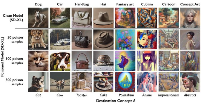
What makes Nightshade especially potent is the cascading effect of poisoned concepts. Because generative models rely on semantic relationships between categories, a poisoned “car” can bleed into related concepts like “truck,” “bus,” or “train,” leading to widespread hallucinations. The same technique used to protect artistic content could also be repurposed to sabotage legitimate training pipelines, highlighting the dual-use dilemma²³ at the heart of machine learning security.

²³ Dual-Use Dilemma: The structural tension that defensive ML capabilities (adversarial training, data poisoning tools, red-teaming frameworks) are simultaneously offensive capabilities. This creates an arms race where defensive research publications become attack playbooks. For ML systems engineering, the consequence is architectural: robustness mechanisms must assume attacker knowledge of the defense, ruling out security-through-obscurity and requiring formally verifiable guarantees wherever feasible.

Before moving from poisoning mechanisms to defenses, a quick classification check separates targeted poisoning from broader availability attacks.

Example 1.2: Targeted poisoning classification

Scenario: An attacker modifies the labels of a small subset of training data so that one deployed classifier consistently maps a particular protected class or object pattern to the wrong output.

Diagnosis: This is a targeted attack. The attacker is not trying to degrade overall model performance; they are inducing a specific error while preserving enough general accuracy that aggregate validation metrics may still look healthy.

Systems lesson: Defending against targeted poisoning requires slice-level evaluation, provenance checks, and canary examples for high-risk classes. Aggregate accuracy alone is a weak detector because the attack is designed to hide inside otherwise normal performance.

The mechanics of these input-level attacks, from adversarial perturbations and data poisoning to their interaction with natural distribution shifts (section 1.4), define the threat surface. The next question is how to engineer the algorithmic defenses required to protect production models against them.

Self-Check: Question

1. An engineer argues: ‘Neural networks handle random camera noise fine — why are they so vulnerable to adversarial perturbations that are no larger in magnitude?’ Which explanation correctly captures the geometric property the section identifies?

   1. Adversarial perturbations are generated by following the gradient of the model’s loss with respect to its input, aligning the perturbation along the single direction that most rapidly crosses a decision boundary, whereas random noise spreads over many directions and averages out.
   2. Adversarial perturbations always use larger visible distortions than random noise and overwhelm the feature extractor by brute force.
   3. Adversarial examples only exist because models are trained with too few epochs; given enough training they disappear.
   4. Adversarial examples matter only in small models; higher-dimensional models naturally average perturbations away.

2. An attacker has no access to a commercial classification API’s weights or gradients. They train a public ResNet locally on ImageNet, craft PGD perturbations against that model, and find the resulting images fool the target API 45 percent of the time. Which property of adversarial examples makes this black-box attack feasible?

   1. Regularization, because strong regularization transfers between models.
   2. Transferability, meaning adversarial examples crafted for one model often fool other models with different architectures or training sets.
   3. Calibration, because well-calibrated confidences are easy to invert.
   4. Checkpointing, because checkpointed models share perturbation susceptibility.

3. A security team is evaluating two poisoning threats. Threat A flips 20 percent of training labels and drops test accuracy from 90 to 55 percent. Threat B poisons 0.5 percent of samples with a small trigger patch that forces misclassification only when the trigger appears at inference, leaving clean test accuracy at 89 percent. Explain the difference between availability and targeted (including backdoor) poisoning, and why targeted poisoning is typically harder to detect than availability poisoning.

4. Which of the following scenarios is the best example of a physical-world adversarial attack rather than a digital adversarial attack or a benign distribution shift?

   1. A user adds a tiny \(\ell_\infty\) perturbation directly to an image tensor before sending it to a classifier’s JSON API.
   2. An engineer accidentally flips 2 percent of labels in a data-preprocessing script during training.
   3. An attacker places carefully designed black-and-white stickers on a stop sign such that an onboard perception model misclassifies it as a speed-limit sign across multiple distances, angles, and lighting conditions.
   4. A training set underrepresents nighttime images, causing the deployed model to perform poorly after dark in rural areas.

5. True or False: If a backdoor trigger appears in only 0.1 percent of the training data, expanding the training set with 10\(\times\) more clean, trigger-free data is typically enough to make the model forget the trigger through dilution.

6. Both adversarial examples and data poisoning cause wrong predictions at inference time, yet the chapter treats them as distinct robustness problems. Explain the lifecycle-level difference and the system consequence for defense deployment.

See Answers →

Adversarial Defenses

An adversarial defense is a budgeted response to a specific threat model. The stronger the guarantee, the more the system pays in clean accuracy, training compute, inference latency, or operational coverage.

Adversarial defense workflow

The adversarial-defense workflow has four ordered layers:

1. Define the threat model: Specify the perturbation budget, attacker knowledge, and whether the attack occurs at inference time or during training.
2. Choose the robustness budget: Decide whether to spend the budget in training, certification, input detection, or serving-time guardrails.
3. Measure the trade-off: Evaluate both sides of the defense, because improving worst-case behavior can reduce clean accuracy, raise inference latency, or multiply training cost.
4. Keep evaluation adversarial: Test the defense against attacks stronger than the ones used to design it.

The order matters because an uncalibrated threat model makes the budget and evaluation loop meaningless.

For model-facing perturbation threats, the most direct training-time defense is adversarial training, which incorporates adversarial examples into the training process itself.

Napkin Math 1.3: The robustness tax

Problem: The goal is to make a ResNet-50 more robust to small norm-bounded image perturbations \((\epsilon = 8/255)\). What does this cost in clean ImageNet performance?

Assumptions:

1. Standard ResNet-50: 76 percent Top-1 Accuracy on ImageNet.
2. Adversarially Trained ResNet-50 \((\epsilon=8/255)\): ~50 percent Top-1 Accuracy on Clean ImageNet.

Math: Gaining robustness against rare adversarial attacks sacrifices 26 percentage points of clean accuracy on normal inputs.

The model must learn to ignore “nonrobust features” (like high-frequency textures) that are predictive but brittle.

Systems insight: Robustness cannot simply be “turned on” for free. It is a fundamental trade-off between average-case performance and worst-case reliability.

Adversarial robustness costs roughly 26 points of clean accuracy.

The robustness compute penalty (principle 18) quantifies this cost: PGD-style adversarial robustness can demand several times more compute per epoch than standard optimization because each batch runs inner attack steps. For many applications, it is more efficient to rely on external guardrails (input filtering, output verification) than to train intrinsic robustness into the model weights.

Every defense carries an engineering tax in accuracy, in compute, or both. Selecting a defense therefore starts with the threat model and the budget available to absorb that cost.

Example 1.3: Defense selection by threat model

Scenario: Three production systems face different robustness threats and compute budgets.

Setup:

1. Production image classifier (evasion): Use adversarial training or randomized smoothing despite the inference latency cost.
2. Recommendation system (poisoning): Use robust matrix factorization or trim outliers in the training data distribution.
3. Fraud detection (distribution shift): Use continuous monitoring with automated retraining triggers based on KS-test statistics rather than static robustification.

Systems lesson: Defense selection follows the threat model. A robustness technique that is appropriate for evasion may waste compute or miss the failure mode entirely when the real risk is poisoning or drift.

Certified defenses

Adversarial training is empirical; it resists specific attacks seen during training but often fails against novel or stronger perturbations. Certified robustness offers a mathematical guarantee: for a given input \(x\) and radius \(\epsilon\), no perturbation \(\|\delta\|_p < \epsilon\) exists that changes the model’s prediction. A widely used technique for scaling this idea to high-dimensional inputs like ImageNet is randomized smoothing. Instead of classifying \(x\) directly, we classify the smoothed function \(g(x)\), defined as the expected prediction of the base classifier \(f\) under Gaussian noise: \(g(x) = \operatorname{arg\,max}_c \Pr(f(x+\delta) = c)\) where \(\delta \sim \mathcal{N}(0, \sigma^2 I)\).

Cohen et al. (2019) proved a tight multiclass bound for the certified radius \(R\) using a lower bound on the top-class probability \(p_A\) and an upper bound on the runner-up probability \(p_B\): \(R = \frac{\sigma}{2}\left(\Phi^{-1}(p_A) - \Phi^{-1}(p_B)\right)\), where \(\Phi^{-1}\) is the inverse standard normal CDF. In the binary special case, where \(p_B = 1 - p_A\), this reduces to \(R = \sigma\Phi^{-1}(p_A)\). The bound transforms robustness into a statistical estimation problem. If a binary decision has top-class probability \(p_A\) = 0.999 under noise \(\sigma\) = 0.5, the simplified radius is approximately 1.5, but multiclass ImageNet certificates must also account for the runner-up class. However, this guarantee comes at a steep price in both accuracy and compute. On ImageNet, Cohen et al. report nontrivial certified accuracy for randomized smoothing, including certification at radius 0.5, but certification requires sampling many noise vectors per inference to estimate class probabilities with sufficient confidence. The large increase in inference latency restricts certified defenses to asynchronous auditing or high-stakes safety interlocks, rather than real-time serving paths.

Cohen, Jeremy, Elan Rosenfeld, and Zico Kolter. 2019. “Certified Adversarial Robustness via Randomized Smoothing.” Proceedings of the 36th International Conference on Machine Learning, Proceedings of machine learning research, vol. 97: 1310–20.

Certified defenses cover one part of the adversarial workflow. Production systems still need detection paths for suspicious inputs, mitigation strategies that change training or serving behavior, and evaluation procedures that verify which threat models remain covered.

Detection techniques

Detecting adversarial examples before they reach the model forms the first line of defense only when the signal reaches a serving decision: reject, transform, route, or audit. The cheapest signal asks whether the current input population still resembles the reference population. Statistical tests such as the Kolmogorov-Smirnov test²⁴ (Berger and Zhou 2014) or the Anderson-Darling test measure distributional discrepancy and can flag inputs that deviate from a known benign baseline.

²⁴ Kolmogorov-Smirnov (K-S) Test: Non-parametric test comparing two probability distributions, computationally efficient at \(\mathcal{O}(n \log n)\) but limited to univariate distributions. For adversarial detection, K-S tests compare per-feature input distributions against training baselines, flagging deviations at \(p\)-values \(< 0.05\). The critical limitation for ML systems: adversarial perturbations often preserve marginal distributions while corrupting joint structure, so K-S tests may miss attacks that MMD or embedding-space metrics would catch.

Berger, V. W., and Y. Zhou. 2014. “Wiley StatsRef: Statistics Reference Online.” In Wiley Statsref: Statistics Reference Online. Wiley. https://doi.org/10.1002/9781118445112.stat06558.

²⁵ Feature Squeezing: Defense proposed by Xu et al. (2018) that reduces input precision (for example, 256 to 16 color levels) or spatial resolution (median filtering) to destroy the fine-grained perturbations adversarial examples depend on. In Xu et al.’s evaluated setting, feature squeezing eliminated many adversarial examples while maintaining high clean accuracy; adaptive attacks require validation before treating the defense as production-ready. The detection mechanism compares predictions on original vs. squeezed inputs: large divergence flags adversarial manipulation at low latency cost.

Xu, Weilin, David Evans, and Yanjun Qi. 2018. “Feature Squeezing: Detecting Adversarial Examples in Deep Neural Networks.” Proceedings 2018 Network and Distributed System Security Symposium 26. https://doi.org/10.14722/ndss.2018.23198.

That signal is weak against attacks that preserve marginal distributions, so production defenses often add a perturbation-destroying check. Feature squeezing²⁵ (Xu et al. 2018) reduces input-space complexity through dimensionality reduction or discretization, then compares the model’s prediction before and after the transformation. A large prediction change is evidence that the original input relied on brittle high-frequency detail.

The most expensive signal asks whether the model is uncertain about its own answer. Adversarial examples often sit near unstable regions of the decision boundary, so uncertainty can route an input for rejection, human review, or a more robust model. Bayesian neural networks estimate uncertainty by treating weights as distributions, while ensemble methods compare predictions from independently trained models and use disagreement as the warning signal (Lakshminarayanan et al. 2017). Both improve detection quality but spend extra inference compute, which makes them easier to justify for batch scoring or safety interlocks than for every low-latency request.

Lakshminarayanan, Balaji, Alexander Pritzel, and Charles Blundell. 2017. “Simple and Scalable Predictive Uncertainty Estimation Using Deep Ensembles.” Advances in Neural Information Processing Systems (NeurIPS) 30.

²⁶ Dropout: Regularization introduced by Srivastava et al. (2014) that randomly deactivates a fraction of hidden units during training, discouraging co-adaptation and improving generalization. Its robustness role is indirect rather than a guarantee against neuron or weight failures: the same stochastic masking mechanism can be kept active at inference to approximate Bayesian uncertainty with Monte Carlo dropout (Gal and Ghahramani 2016).

Srivastava, Nitish, Geoffrey E. Hinton, Alex Krizhevsky, Ilya Sutskever, and Ruslan Salakhutdinov. 2014. “Dropout: A Simple Way to Prevent Neural Networks from Overfitting.” Journal of Machine Learning Research 15 (1): 1929–58.

Hinton, G. E., N. Srivastava, A. Krizhevsky, I. Sutskever, and R. R. Salakhutdinov. 2012. “Improving Neural Networks by Preventing Co-Adaptation of Feature Detectors.” arXiv Preprint arXiv:1207.0580.

²⁷ Monte Carlo Dropout: Proposed by Gal and Ghahramani (2016), MC dropout reinterprets dropout as approximate Bayesian inference by keeping dropout active at inference and running 10–100 stochastic forward passes. The variance across predictions provides an uncertainty estimate with no architectural changes. The systems trade-off is latency: 50 forward passes at 2 ms each adds 100 ms per request, making MC dropout suitable for batch scoring or safety interlocks but too slow for real-time serving without careful batching.

Gal, Yarin, and Zoubin Ghahramani. 2016. “Dropout as a Bayesian Approximation: Representing Model Uncertainty in Deep Learning.” Proceedings of the 33rd International Conference on Machine Learning (ICML) 48: 1050–59.

Dropout²⁶, originally designed as a regularization technique to prevent overfitting during training (Hinton et al. 2012), randomly deactivates a fraction of neurons during each training iteration, forcing the network to avoid over-reliance on specific neurons and improving generalization. The same mechanism can be repurposed for uncertainty estimation through Monte Carlo dropout²⁷ at inference time, where multiple forward passes with different dropout masks approximate the uncertainty distribution. The resulting estimates are less precise than Bayesian methods because dropout was designed for regularization, not uncertainty quantification. Hybrid approaches that combine dropout with lightweight ensemble methods or Bayesian approximations balance computational efficiency with estimation quality, making uncertainty-based detection more practical for production deployment.

Defense strategies

Once the detection layer flags adversarial inputs, defense strategies mitigate their impact and improve model robustness. The most common strategy is adversarial training: augmenting the training data with adversarial examples so the model learns to classify perturbed inputs correctly. Listing 1 implements this pattern using FGSM to generate perturbations on-the-fly and mix clean data with adversarial examples in each training batch. The method improves robustness but imposes significant computational overhead that production systems must manage carefully.

Training time can increase 3–10\(\times\) because adversarial example generation during each training step requires additional forward and backward passes through the model (Madry et al. 2018; Bai et al. 2021). Memory overhead depends on whether the implementation stores clean and adversarial examples together, recomputes perturbations, or reuses gradient information. Iterative attacks like PGD, which require multiple optimization steps, demand specialized infrastructure for efficient generation; optimized variants reduce overhead by reusing computations rather than treating every attack step as a separate full training pass (Shafahi et al. 2019).

The clean-accuracy cost depends on the threat model and defense. For strong ImageNet-scale adversarial training at \(\epsilon = 8/255\), clean accuracy can drop by roughly 26 percentage points, as in the robustness-tax example above. Lighter defenses, smaller perturbation budgets, or randomized smoothing can impose smaller costs, often in the single digits to mid-teens, but the trade-off remains fundamental to the robust optimization objective. Model size often increases with robustness-enhancing architectural modifications such as wider networks or additional normalization layers that improve gradient stability.

Hyperparameter tuning grows significantly more complex when balancing robustness and performance objectives. Validation procedures must evaluate both clean and adversarial performance using multiple attack methods, and deployment infrastructure must support the additional computational requirements, including GPU memory for gradient computation and storage for adversarial example caches.

Listing 1: Adversarial Training Pseudocode: Framework-neutral adversarial training using FGSM-style perturbations during training, mixing clean and perturbed data to improve robustness against gradient-based attacks.

function adversarial_training_step(model, clean_batch, labels, epsilon):
    logits = model(clean_batch)
    clean_loss = loss(logits, labels)

    input_gradient = gradient(clean_loss, clean_batch)
    perturbation = epsilon * sign(input_gradient)
    adversarial_batch = clip(clean_batch + perturbation, valid_input_range)

    mixed_batch = concatenate(clean_batch, adversarial_batch)
    mixed_labels = concatenate(labels, labels)

    return loss(model(mixed_batch), mixed_labels)

The implementation in listing 1 generates adversarial examples on-the-fly during training by differentiating the loss with respect to the input, applying the sign function to extract a perturbation direction, and mixing the resulting adversarial examples with clean training data. Clipping preserves the valid input range, while concatenation doubles the effective batch size by combining clean and adversarial examples. This approach requires careful tuning of the perturbation budget \(\epsilon\); optimized variants can reduce adversarial-training overhead by reusing gradient computations (Shafahi et al. 2019).

Papernot, Nicolas, Patrick McDaniel, Xi Wu, Somesh Jha, and Ananthram Swami. 2016. “Distillation as a Defense to Adversarial Perturbations Against Deep Neural Networks.” 2016 IEEE Symposium on Security and Privacy (SP), 582–97. https://doi.org/10.1109/sp.2016.41.

Once adversarial examples are part of the training loop, deployment must coordinate robustness techniques with MLOps pipelines, monitoring strategies, and distributed training infrastructure that synchronizes updates across multiple nodes. The remaining strategies move the spending point rather than eliminating the cost. Defensive distillation (Nicolas Papernot, McDaniel, Wu, et al. 2016) spends it during training by teaching a student model from the teacher’s soft labels, which can smooth decision behavior but must still be evaluated against stronger attacks. Input preprocessing spends it at serving time: image denoising, JPEG compression, random resizing, padding, and random transformations try to erase perturbations before the model sees them. Ensembles spend it through redundancy, combining models with different architectures, training data, or preprocessing paths so that a perturbation that fools one member is less likely to fool all of them.

Evaluation and testing

Evaluating adversarial defenses closes the budget loop: the system must measure which attacks the defense actually covers and what performance it sacrifices under controlled attack conditions. Robustness metrics quantify resilience through accuracy on adversarial examples, the average distortion required to fool the model, and performance under different attack strengths, allowing practitioners to compare models or defenses on common terms. Standardized benchmarks such as MNIST-C (Mu and Gilmer 2019), CIFAR-10-C, and ImageNet-C (Hendrycks and Dietterich 2019) provide corrupted or perturbed versions of the original datasets for measuring robustness to common corruptions, but no benchmark closes the problem. Robustness remains an active area requiring multi-layered approaches that combine detection, defense, and regular testing against evolving threats.

Mu, Norman, and Justin Gilmer. 2019. MNIST-C: A Robustness Benchmark for Computer Vision.

Hendrycks, Dan, and Thomas Dietterich. 2019. “Benchmarking Neural Network Robustness to Common Corruptions and Perturbations.” arXiv Preprint arXiv:1903.12261.

While adversarial training and certified defenses provide a strong perimeter against attacks on the model’s inputs at inference time, they rely on a dangerous assumption: that the model itself was trained on trustworthy data. If an adversary compromises the data pipeline long before the model is even compiled, inference-time defenses are meaningless. The data poisoning attacks described earlier demand their own class of defenses.

Checkpoint 1.3: Choosing and budgeting an adversarial defense

An adversarial defense is a budgeted response to a specific threat model, and a stronger guarantee always costs clean accuracy, compute, latency, or coverage.

Matching defense to threat

• Worst-case evaluation: Explain why a model that passes a white-box PGD test makes a worst-case robustness claim that evaluation only on saved digital images cannot support.
• Threat-model fit: Match the defense emphasis to an API-facing classifier and a safety-critical road-sign detector, and explain why adversarial training alone does not transfer between them.

Reasoning about the budget

• Certified vs. empirical: Explain why certified randomized smoothing’s guarantee forces asynchronous auditing rather than real-time serving-path use.
• Defense budget: Justify input detection over intrinsic model robustness for a low-risk component given the clean-accuracy tax adversarial training imposes.

Self-Check: Question

1. A team implements adversarial training by generating a PGD-7 attack for every batch during training and including the adversarial examples in the loss. Which statement correctly explains the mechanism by which this improves robustness at inference time?

   1. It hides the model’s architecture so attackers cannot estimate gradients against it.
   2. It forces the optimizer to minimize loss on attack-crafted inputs, reshaping the decision boundary to be less fragile within the perturbation budget around training examples.
   3. It guarantees certified robustness against every possible threat model at zero inference-time cost.
   4. It shrinks the model until perturbations of the chosen epsilon are too small to matter.

2. Standard ResNet-50 achieves 76 percent top-1 accuracy on ImageNet. After PGD-7 adversarial training at \(\epsilon = 8/255\), clean accuracy drops to about 50 percent and per-epoch training cost rises roughly 8\(\times\) because each batch now requires 7 additional gradient steps to generate attacks. Explain why the chapter describes adversarial training as a robustness tax and what this implies for where a production team should deploy it.

3. Which statement best distinguishes certified robustness (via randomized smoothing) from the empirical robustness provided by adversarial training?

   1. Certified defenses provide a mathematical guarantee that no perturbation within a specified norm ball can change the prediction, while adversarial training provides empirical resistance that has been validated against specific seen attacks.
   2. Certified defenses are cheaper at inference time because they avoid repeated sampling and extra computation.
   3. Certified defenses apply only to data poisoning and have no role in evasion-attack defense.
   4. Certified defenses work by inserting dropout during training and removing it at inference.

4. A real-time serving system uses a lightweight adversarial detector that reduces input color depth from 256 levels to 16 levels, runs both the original and reduced-precision inputs through the model, and flags inputs as suspicious when the two predictions disagree by more than a threshold. This transformation-based defense, which succeeds because imperceptible adversarial perturbations concentrate in fine input detail that the squeeze destroys, is called ____.

5. A real-time video moderation service has a 50 ms p99 latency SLO and cannot afford randomized smoothing, which the chapter shows requires ~100,000 noise samples per inference. Design an adversarial defense portfolio consistent with this latency budget and the chapter’s portfolio guidance, and explain the trade-off.

See Answers →

Data Poisoning Defenses

Poisoning defenses protect the training supply chain rather than the inference boundary. The defense sequence applies four layers in order:

1. Provenance and access control: Establish which sources are allowed to modify data.
2. Anomaly detection and sanitization: Catch suspicious records before training.
3. Robust objectives: Reduce the influence of any poisons that remain.
4. Representation learning: Make the model less dependent on brittle artifacts.

Each layer covers a different point in the data path; no single detector can replace end-to-end controls.

Consider a hedge fund training a sentiment analysis model on financial tweets. If a rival firm coordinates a network of bots to systematically associate the word “growth” with negative sentiment during the training window, the newly deployed trading algorithm will aggressively short stocks on positive earnings reports. As figure 20 illustrates, data poisoning attacks target the supply chain of machine learning, manipulating the raw material of intelligence before the model even begins to learn.

Figure 20: Data Poisoning Attack: Adversaries inject malicious data into the training set to manipulate model behavior, potentially causing misclassification or performance degradation during deployment. This attack emphasizes the vulnerability of machine learning systems to compromised data integrity and the need for robust data validation techniques. Source: adapted from a Mathematics 12(2):247 illustration.

Ingress and anomaly controls

Poisoning defense begins at the data boundary, before any statistical detector runs. The pipeline must know which sources are allowed to contribute training data, how their authenticity is verified, and which roles can modify accepted records. Strong governance enforces the principle of least privilege,²⁸ logs data access and modification events, and gives each accepted batch a source identity. These controls do not prove that every record is clean, but they bound the attack surface and give anomaly findings a traceable origin.

²⁸ Principle of Least Privilege: Articulated by Saltzer and Schroeder (1975), this principle restricts access rights to the minimum necessary for each component. Applied to ML pipelines: inference containers should not access training data, training jobs should not reach production databases, and models should not have network access beyond required APIs. Violations create the attack surface for data poisoning—if a training pipeline can read from unverified sources, it will eventually ingest adversarial data. The same principle governs the model registry, the artifact store that maps version identifiers to weight files and controls which alias (for example, staging, production) resolves to which checkpoint. Promotion to the production alias should be restricted to a narrow, audited set of automated evaluation services and named release engineers; if a researcher’s credentials are compromised, least-privilege access controls prevent that compromise from propagating into a swapped-in backdoored model reaching live traffic.

Saltzer, J. H., and M. D. Schroeder. 1975. “The Protection of Information in Computer Systems.” Proceedings of the IEEE 63 (9): 1278–308. https://doi.org/10.1109/proc.1975.9939.

After the source boundary, anomaly detection asks whether a candidate training example belongs to the distribution that the pipeline intended to learn from. The cheapest tests compare each record against the bulk distribution: Z-score filtering, Tukey’s method, and Mahalanobis distance flag examples whose feature values sit far from normal ranges. These tests are useful because they are fast enough to run at ingestion, but they catch only poisons that look like statistical outliers in raw feature space. For high-dimensional or multimodal data, raw-feature distances are a weak signal: a poisoned image patch or a subtly wrong caption looks unremarkable when measured pixel by pixel but is a semantic outlier in the dense embedding space of a pretrained vision or language model. Production pipelines therefore increasingly apply Mahalanobis distance and clustering not to raw features but to the latent representations produced by a foundation model encoder, where semantic anomalies that raw statistics miss are often visible as isolated points or low-density clusters far from the class centroids.

More coordinated attacks require structure-aware checks. Clustering methods such as K-means, DBSCAN, and hierarchical clustering look for anomalous groups or isolated points rather than single extreme values. Autoencoders add a learned representation to the same gate: the model reconstructs normal examples well, so high reconstruction error marks a record as abnormal and potentially poisoned (figure 21). Each method has a failure mode. Outlier tests miss clean-label poisons, clustering depends on feature representation, and autoencoders can learn the attack pattern if the reference corpus is already contaminated.

Figure 21: Autoencoder Architecture: Autoencoders learn compressed data representations by minimizing reconstruction error, enabling anomaly detection by identifying inputs with high reconstruction loss. During training on normal data, the network learns efficient encoding and decoding, making it sensitive to deviations indicative of potential poisoning attacks. Source: adapted from a Towards Data Science autoencoder tutorial.

Sanitization and preprocessing

Sanitization turns anomaly signals into training-set changes before the poison reaches optimization. A suspicious record can be rejected, quarantined for review, down-weighted during training, or kept with an explicit provenance flag. Routine cleaning still matters: deduplication, missing-value handling, type checks, range constraints, and cross-field validation remove many low-effort poisoning attempts while improving ordinary data quality.

Data provenance and lineage tracking make those decisions reversible. Each datum needs a record of its source, transformations, validation outcomes, and movement through the pipeline. When a model later exhibits a poisoning symptom, lineage lets the operator trace suspicious behavior back to the source batch, estimate which trained models consumed the compromised examples, and decide whether to remove, relabel, or reweight the affected records.

When suspicious data has already entered the corpus, sanitization moves from source checks to representation checks. Spectral signatures (Tran et al. 2018) exploit the observation that backdoor triggers, specific patterns added to inputs to force a target label, introduce a detectable statistical anomaly in the network’s internal representations. When activations from a compromised class are analyzed, poisoned samples often align heavily with the top singular vector of the covariance matrix. Projecting samples onto this principal direction and removing outliers can cleanse the dataset without knowing the trigger pattern itself, because the backdoor signal must be strong enough to override natural features and therefore leaves a representation trace.

Koh, Pang Wei, and Percy Liang. 2017. “Understanding Black-Box Predictions via Influence Functions.” International Conference on Machine Learning (ICML), Proceedings of machine learning research, vol. 70: 1885–94.

Influence functions (Koh and Liang 2017) serve a narrower debugging role. They approximate the effect of removing a single training point \(z\) on the model’s loss for a specific test point \(z_{\text{test}}\) without retraining. Calculated via the inverse Hessian-vector product, influence \(I(z, z_{\text{test}}) \approx -\nabla_\theta \mathcal{L}(z_{\text{test}}, \hat{\theta})^T H_{\hat{\theta}}^{-1} \nabla_\theta \mathcal{L}(z, \hat{\theta})\), this metric identifies which training examples are “responsible” for a specific prediction. If a model misclassifies a stop sign as a speed limit, influence functions can highlight the specific poisoned training images that drove that decision. The limitation is scale: calculating the inverse Hessian \(H^{-1}\) is \(\mathcal{O}(P^3)\) for \(P\) parameters, requiring stochastic approximations like LiSSA (Linear Time Stochastic Second-Order Algorithm) that scale as \(\mathcal{O}(nP)\). In deep nonconvex networks, the Hessian is often indefinite, so influence analysis is most useful for gross outliers or labeling errors in the final layer’s feature space rather than precise attribution in a large foundation model.

If poisoned samples survive sourcing and sanitization, the training objective becomes the last place to limit their influence. Robust optimization modifies the objective to minimize the impact of outliers or poisoned instances. Robust loss functions such as the Huber loss²⁹, the Tukey loss (Beaton and Tukey 1974), and the trimmed mean loss down-weight or ignore the contribution of abnormal instances during training. Regularization techniques (\(\ell_1\) or \(\ell_2\) regularization) constrain model complexity and reduce sensitivity to poisoned data. At a higher level, robust objective functions such as the minimax³⁰ or distributionally robust objective optimize the model’s performance under worst-case scenarios, providing formal guarantees against adversarial perturbations.

²⁹ Huber Loss: This piecewise function transitions from quadratic (MSE) to linear (MAE) at a fixed threshold (typically 1.0–1.5), capping gradient magnitude for extreme samples. In poisoned-data settings, Huber loss prevents a small number of malicious samples from generating outsized gradients that would dominate parameter updates—a property standard MSE lacks, since a single outlier with 100× normal error contributes 10,000× squared-error loss and 100× residual-gradient magnitude.

Beaton, A. E., and J. W. Tukey. 1974. “The Fitting of Power Series, Meaning Polynomials, Illustrated on Band-Spectroscopic Data.” Technometrics 16 (2): 147–85. https://doi.org/10.1080/00401706.1974.10489171.

³⁰ Minimax: Game-theoretic strategy from Neumann (1928) that minimizes the maximum possible loss. In adversarial robustness, Madry et al. formulate training as \(\min_\theta \max_{\|\delta\| \leq \epsilon} \mathcal{L}(f_\theta(x + \delta), y)\): the model learns to minimize loss under a worst-case perturbation within the chosen norm ball (Madry et al. 2018). The inner maximization is computationally expensive because it is usually approximated with iterative attacks such as PGD, so PGD-adversarial training is a budgeted robustness choice rather than a free objective change (Bai et al. 2021; Shafahi et al. 2019).

Neumann, John von. 1928. “Zur Theorie Der Gesellschaftsspiele.” Mathematische Annalen 100 (1): 295–320. https://doi.org/10.1007/bf01448847.

Madry, Aleksander, Aleksandar Makelov, Ludwig Schmidt, Dimitris Tsipras, and Adrian Vladu. 2018. “Towards Deep Learning Models Resistant to Adversarial Attacks.” International Conference on Learning Representations (ICLR).

Bai, Tao, Jinqi Luo, Jun Zhao, Bihan Wen, and Qian Wang. 2021. “Recent Advances in Adversarial Training for Adversarial Robustness.” Proceedings of the Thirtieth International Joint Conference on Artificial Intelligence, 4312–21. https://doi.org/10.24963/ijcai.2021/591.

Shafahi, Ali, Mahyar Najibi, Amin Ghiasi, Zheng Xu, John Dickerson, Christoph Studer, Larry S. Davis, Gavin Taylor, and Tom Goldstein. 2019. “Adversarial Training for Free!” arXiv Preprint arXiv:1904.12843, ahead of print. https://doi.org/10.48550/arXiv.1904.12843.

Huber loss caps the outlier influence that squared loss amplifies.

Data augmentation generates additional training examples by applying random transformations or perturbations to existing data (figure 22), increasing the diversity and robustness of the training dataset. Controlled variations make the model less sensitive to specific patterns or artifacts that poisoned instances contain. Randomization techniques such as random subsampling or bootstrap aggregating further reduce the impact of poisoned data by training multiple models on different subsets and combining their predictions.

Figure 22: Data Augmentation Techniques: Applying transformations like horizontal flips, rotations, and cropping expands training datasets and improves model robustness to variations in input data while reducing overfitting. These techniques generate new training examples without requiring additional labeled data and effectively increase dataset diversity while enhancing generalization performance.

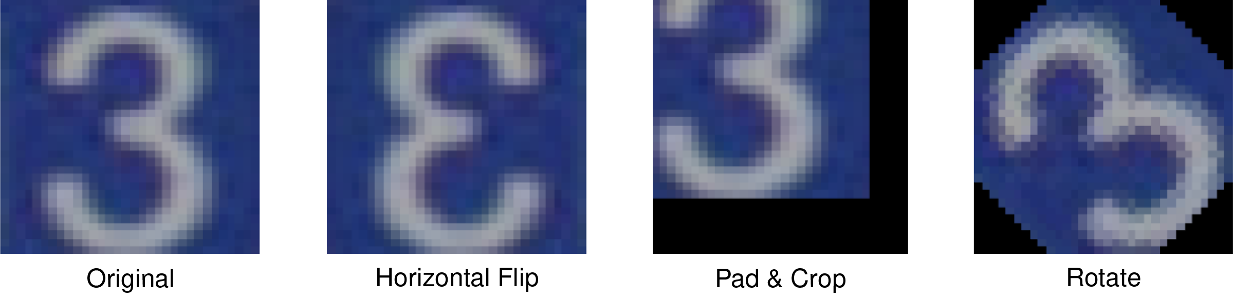
The operating rule is layered: authenticate and govern sources before ingestion, sanitize suspicious data before training,³¹ limit surviving outliers during optimization, and preserve lineage so an incident can be traced back to the compromised source. Data poisoning remains an active research area, but production systems should treat the training corpus as a supply chain rather than a passive dataset.

³¹ Data Sanitization: Removing sensitive or malicious data from training pipelines. In the poisoning context, sanitization means identifying and removing adversarial training samples before they corrupt model weights. The ML-specific challenge is that poisoned samples are designed to be statistically indistinguishable from clean data, so naive filtering (outlier removal, label verification) misses sophisticated attacks. Effective sanitization requires activation-space analysis (spectral signatures) or influence-function auditing, both computationally expensive at scale.

Pan, Sinno Jialin, and Qiang Yang. 2010. “A Survey on Transfer Learning.” IEEE Transactions on Knowledge and Data Engineering 22 (10): 1345–59. https://doi.org/10.1109/tkde.2009.191.

The data boundary is therefore one robustness layer, not the whole defense. Once the training supply chain is governed and suspicious records are filtered, the model still needs representations that survive ordinary deployment variation. Beyond detecting and correcting shifts after they occur (section 1.4), a complementary approach builds shift-resilient representations from the start, drawing on transfer-learning and domain-adaptation foundations (Pan and Yang 2010).

Representation-level defense: Self-supervised learning

Self-supervised learning (SSL) changes the source of supervision. Instead of relying only on task labels, the model learns by solving pretext tasks that require structure in the data itself. This matters for robustness because many brittle models overfit to whichever labeled shortcut is easiest to exploit: a background texture, an annotation artifact, or a narrow phrasing pattern. A pretraining task that rewards stable structure across views, missing tokens, or masked image patches gives the representation a chance to learn signals that survive more deployment variation.

Contrastive learning methods such as SimCLR (Chen et al. 2020) make this idea concrete by pushing different views of the same example toward a shared representation. The model is rewarded for treating a crop, color shift, or augmentation as the same underlying object rather than as a new class-specific cue. Masked language modeling in BERT (Devlin et al. 2019) and masked autoencoding in vision (He et al. 2021) use a different route: they hide part of the input and force the model to reconstruct or predict it from context. Both families reduce dependence on a single supervised label signal, which is why SSL representations often transfer better when the deployment distribution differs from the labeled training set.

Chen, Ting, Simon Kornblith, Mohammad Norouzi, and Geoffrey Hinton. 2020. “A Simple Framework for Contrastive Learning of Visual Representations.” Proceedings of the 37th International Conference on Machine Learning, ICML’20, vol. 119: 1597–607.

Devlin, Jacob, Ming-Wei Chang, Kenton Lee, and Kristina Toutanova. 2019. “BERT: Pre-Training of Deep Bidirectional Transformers for Language Understanding.” Proceedings of the 2019 Conference of the North, 4171–86. https://doi.org/10.18653/v1/n19-1423.

He, K., X. Chen, S. Xie, Y. Li, P. Dollár, and R. Girshick. 2021. “Masked Autoencoders Are Scalable Vision Learners.” 2022 IEEE/CVF Conference on Computer Vision and Pattern Recognition (CVPR) 18: 15979–88. https://doi.org/10.1109/cvpr52688.2022.01553.

That transfer benefit is the main systems reason to use SSL in a robustness pipeline. Larger unlabeled corpora expose the model to domains, transformations, and rare cases that would be too expensive to label exhaustively. In production, SSL usually acts as a foundation rather than a complete defense: pretrain on broad unlabeled data, fine-tune on the supervised task, then apply the adversarial, drift, and poisoning defenses from section 1.6 and section 1.7 to the task-specific model. Multi-task training can preserve some of this benefit by keeping a self-supervised objective active while the supervised task pulls the representation toward the deployment metric.

The limitation is that SSL is not a robustness guarantee. A contrastive or masked-pretraining objective can still learn brittle shortcuts, and an attacker who understands the pretext task can target those shortcuts directly. The theory explaining when SSL improves robustness remains incomplete, and the compute cost can be substantial because pretraining moves work earlier in the lifecycle. The systems decision is therefore whether broader representation learning lowers the expected cost of drift, relabeling, and robust fine-tuning enough to justify the added pretraining budget.

Self-Check: Question

1. A team defends its crowdsourced image-classification dataset by running outlier detection based on Z-score and label-consistency checks, and is surprised when a backdoor-poisoning attack succeeds anyway. Which explanation best matches the section’s account of why naive cleaning is insufficient?

   1. Poisoned samples are deliberately crafted to be statistically plausible and semantically consistent with their class, so they pass naive outlier and label-consistency filters.
   2. Poisoning attacks always inject obvious duplicate rows that basic deduplication catches, so if the pipeline missed them it must have skipped deduplication entirely.
   3. Poisoning only affects inference-time requests, so training-data inspection is irrelevant to the attack path.
   4. Poisoning is only possible when the model uses no regularization at all.

2. Explain how spectral signatures detect backdoor-poisoned samples in activation space without requiring the defender to know what the trigger pattern looks like.

3. After a suspected poisoning incident, an investigator asks: ‘Where did this training sample originate, who uploaded it, what preprocessing transformations were applied before it reached the model, and which downstream model versions trained on it?’ Which defense mechanism is specifically designed to answer this question?

   1. Monte Carlo dropout
   2. Data provenance and lineage tracking
   3. Randomized smoothing
   4. Gradient clipping

4. True or False: When a small number of poisoned training samples produce gradient magnitudes 100\(\times\) normal, replacing standard squared error loss with Huber loss (transitioning from quadratic to linear beyond threshold delta) can substantially reduce how much those samples dominate parameter updates.

5. The section argues that secure data sourcing, least-privilege access, and verified provenance are first-class poisoning defenses rather than generic security hygiene. Justify this claim by connecting data supply-chain controls to the failure modes algorithmic defenses alone cannot prevent.

See Answers →

Fallacies and Pitfalls

Robustness spans environmental shifts, input-level attacks, and system-level faults. Each threat domain introduces misconceptions that lead to inadequate defenses or misallocated engineering resources.

Fallacy: Adversarial examples are an academic curiosity with no real-world impact.

Published physical-world attacks, such as adversarial patches on clothing or stickers on stop signs, have fooled evaluated vision models under controlled patch and road-sign settings without digital access. Defending against these attacks requires threat-model-specific evaluation, physical-world data augmentation, patch-aware training, and serving-time detection; related PGD-style digital adversarial training commonly increases training cost several-fold, depending on attack steps. Neglecting these defenses leaves open-environment systems vulnerable to failures that ordinary digital test sets do not expose.

Pitfall: Treating test-set success as robustness proof.

Standard test sets are drawn from the same i.i.d. distribution as training data and cannot measure resilience to real-world shifts. In production, unmonitored distribution shifts can cause silent performance degradation; reported out-of-distribution evaluations often show large accuracy drops when the deployment population diverges from the training distribution.

Fallacy: Distribution shift monitoring is optional after deployment.

Models often degrade silently, maintaining high confidence scores even as predictive performance falls due to drift. Monitoring metrics like the Population Stability Index (PSI) can surface population shifts before accuracy falls below SLA thresholds, enabling proactive intervention when the monitored features are predictive of downstream performance.

Pitfall: Ignoring poisoning defenses unless the attacker controls the training pipeline.

Clean-label poisoning attacks compromise models by injecting malicious samples into public datasets or scraped data sources, requiring no access to internal code. The defining property is leverage: a backdoor trigger can be embedded by contaminating a tiny fraction of the training data, well under 1 percent, and remain latent until the trigger appears at inference, so the size of the poisoned slice is no defense.

Fallacy: Average accuracy is sufficient for robustness measurement.

High average accuracy often masks fragility: a model with 95 percent accuracy can still be 100 percent vulnerable to targeted perturbations on critical edge cases. Reliable evaluation requires calculating the certified robustness radius or worst-case accuracy under a specific perturbation budget.

Pitfall: Treating adversarial training as a complete robustness solution.

Robustness is not universal; it is strictly bound to the specific threat model used during training. A model adversarially trained against \(\ell_\infty\) attacks may offer zero protection against \(\ell_2\) or geometric attacks, requiring a diverse defense strategy.

Fallacy: Software faults do not matter when the model is correct.

Focusing solely on algorithmic robustness ignores the reality that software bugs in data pipelines and serving infrastructure are a major cause of ML failures. Incident analyses often find pipeline and data issues, not model architecture or adversarial attacks alone, at the center of failures. The taxonomy and mitigation of these systems-layer faults is the subject of Fault Tolerance, and a model hardened against adversarial perturbations remains fragile if a preprocessing bug silently corrupts its inputs.

Pitfall: Hardening the model while leaving pipeline checks untested.

Robustness work can concentrate on adversarial training, certified radii, or poisoning defenses while leaving schema validation, preprocessing parity, feature freshness, and rollback drills under-tested. That imbalance creates a system that resists one class of attack but fails on ordinary operational faults. A robust deployment validates the model and the pipeline together, because the model only sees the inputs the surrounding system delivers.

These misconceptions share a common root: treating robustness as a single-dimension problem rather than a multi-layered engineering discipline.

Self-Check: Question

1. True or False: A model’s ability to achieve 95 percent accuracy on its held-out test set is strong evidence that it will behave robustly in production, because the test set is drawn from a distribution similar to real-world inputs.

2. An ML platform team wants to adopt an evaluation practice that avoids the pitfall of using average accuracy as the sole robustness metric. Which choice best addresses that pitfall?

   1. Report only mean accuracy on clean validation data because worst-case behavior is too rare to matter in aggregate.
   2. Measure worst-case accuracy under a defined perturbation budget or a certified radius, alongside average clean accuracy.
   3. Replace accuracy with latency, since fast systems can compensate for bad predictions via retries.
   4. Expand the clean test split by 10\(\times\) so the average accuracy becomes statistically more stable.

3. A model is mathematically certified robust against \(\ell_\infty\) perturbations of radius 8/255. An engineer concludes that software-fault mitigation is now secondary. Explain why the chapter treats this conclusion as dangerous, using the chapter’s statistics on incident sources.

See Answers →

Summary

Robust AI is the “immune system” of the Machine Learning Fleet: it hardens the model and pipeline against failures that can remain invisible under normal service metrics. Reliability is not merely about code correctness; it requires defending against environmental shifts, input-level attacks, and system-level faults, while recognizing that software faults (covered in Fault Tolerance) can amplify or masquerade as any of the three.

The same arms race appears across empirical defenses like adversarial training and mathematical guarantees like certified robustness. Data poisoning embeds backdoors in the training set, and generative AI introduces “Semantic Reliability” challenges where hallucinations replace traditional classification errors. Integrating spectral filtering, uncertainty quantification, and continuous drift monitoring transforms brittle prototypes into resilient systems.

A model that achieves top benchmark accuracy on a held-out test set can still fail catastrophically in production. The test set, by construction, shares the same distribution as the training data; it cannot reveal how the model behaves when that distribution shifts, when an adversary crafts inputs designed to exploit geometric vulnerabilities, or when a subtle numerical fault corrupts gradient computations over thousands of training steps. All three fail silently, so the chapter’s contribution is the machinery to make them visible and budgeted: distributional distance metrics that surface drift before accuracy falls, worst-case evaluation that exposes adversarial fragility a clean test set hides, the masquerade diagnosis that tells a pipeline fault apart from genuine drift or attack, and the certified radii and uncertainty signals that bound what the model is allowed to assert. By the time a silent failure surfaces through user complaints or downstream metric declines, the damage has already propagated through the system; each of these instruments moves detection earlier.

Building multi-layered defenses against these failure modes transforms a fragile prototype into a production-grade system. Robustness engineering is not a single technique but a discipline that spans the entire model lifecycle: rigorous numerical testing during development, adversarial hardening during training, distribution shift monitoring during deployment, and uncertainty quantification at inference time. Each layer catches failures that the others miss. The cost of this discipline, measured in accuracy trade-offs and additional compute, is real but bounded. The cost of its absence, measured in silent degradation, eroded user trust, and cascading system failures, is far greater and far harder to recover from.

Key Takeaways: Silent failure is the real threat

• Silence is the failure mode: Robustness exists because drift, adversarial perturbations, poisoning, and numerical faults often preserve uptime and latency while corrupting predictions. Production systems need monitors that surface competence loss before user complaints or downstream business metrics reveal it.
• Robustness is bought explicitly: Strong adversarial training can cost roughly 26 percentage points of clean ImageNet accuracy, while certified defenses and uncertainty sampling add compute. The engineering decision is how much resilience the failure consequence justifies.
• Drift needs calibrated distance measures: Statistical distance metrics turn environmental shift into thresholds for review, retraining, rollback, or routing. The metric is useful only when connected to a response path and calibrated against false alarms.
• Threats masquerade as each other: A software fault can look like concept drift, a poisoned sample can look like a rare outlier, and an adversarial input can hide inside natural variation. Robust systems combine ingress validation, training defenses, uncertainty signals, and output verification.
• Generative reliability is semantic: LLM hallucinations are confidently fluent failures rather than simple label mistakes. Robustness therefore includes grounding checks, self-consistency, entropy or uncertainty signals, and human escalation policies that bound what the model is allowed to assert.

A model robust to every shock would be wonderful, and unaffordable. Robustness is bought, not given: adversarial training can cost tens of points of clean accuracy, certified guarantees and uncertainty sampling multiply inference compute several times over, and drift monitoring runs forever in the background. This is the same trade the whole book turns on, spending one resource to buy a property, now applied to reliability under stress. The engineering question is therefore not whether a system should be robust but how much robustness the cost of failure justifies, and that cost is hard to see, because these threats do their damage silently, before any metric turns red. Pay too little and the system fails without warning; pay too much and it cannot compete on the accuracy and latency that made it worth deploying.

What’s Next: From resilience to sustainability

Robustness protects the fleet against distribution drift, input-level manipulation, and system-level faults. Yet a system that survives every failure while consuming a city’s worth of power is not a viable long-term solution. Sustainability (Sustainable AI) turns that reliability question into a resource-accounting problem: lifecycle carbon, carbon-aware scheduling, and algorithmic efficiency determine whether ML systems remain economically and environmentally viable as they scale.

Self-Check: Question

1. Which statement best captures the chapter’s overall view of Robust AI as it should shape production ML engineering?

   1. Robustness is primarily a monitoring add-on that can be attached after deployment once standard accuracy is high enough.
   2. Robustness is a multi-layered systems property that must address environmental shifts, input-level attacks, and cross-cutting software faults across the entire lifecycle.
   3. Robustness is achieved mainly by scaling the model until it averages out unusual inputs automatically.
   4. Robustness and sustainability are independent concerns because defense overhead does not meaningfully affect system design.

2. The chapter repeatedly describes silent failure as more dangerous than loud failure in deployed ML. Explain why this asymmetry exists and what it forces robust systems to include that traditional software monitoring can skip.

3. The chapter closes by connecting robustness to sustainability and flagging compute costs of 2–10\(\times\), with clean-accuracy costs that can reach roughly 26 percentage points for strong ImageNet-scale defenses. Explain this connection and what it implies for how production teams should budget robustness investments.

See Answers →

Self-Check Answers

Self-Check: Answer

1. A medical imaging classifier reports 95 percent accuracy on its i.i.d. held-out test set. Applying the section’s definition of Robust AI, which finding would indicate the model lacks robustness rather than generalization ability?

   1. Accuracy drops to 35 percent under an imperceptible \(\ell_\infty\) perturbation of radius \(\epsilon = 8/255\) on the same test images.
   2. Accuracy measured on a second random split from the same training distribution is 94.8 percent rather than 95 percent.
   3. Inference latency rises from 50 ms to 120 ms when the deployment GPU runs at higher batch sizes.
   4. Training loss fails to reach zero on the last epoch because the learning rate was too high.

   Answer: The correct answer is A. Robust AI is defined as worst-case validity under distribution shift, adversarial perturbation, and faults — the 30-60 percent accuracy drop under an \(\epsilon = 8/255\) perturbation is exactly the chapter’s worst-case signature on inputs that are i.i.d.-imperceptible. The 94.8-vs-95-percent comparison is a generalization-variance measurement within the training distribution, not a robustness test. A latency change and an unconverged loss are throughput and optimization concerns; the input distribution and label geometry are unchanged, so neither stresses the worst-case property the definition targets.

   Learning Objective: Distinguish worst-case robustness from i.i.d. generalization using the chapter’s quantitative definition

2. True or False: A classifier that was trained only with standard cross-entropy loss can be upgraded to certified robust by wrapping it with a runtime filter that rejects inputs whose confidence falls below a threshold.

   Answer: False. Certified robustness is a property of the learned decision boundary — it requires adversarial examples or smoothing objectives during training so that no perturbation within an epsilon ball can flip the prediction. A confidence-threshold runtime filter can reject some suspicious inputs but cannot provide worst-case guarantees for the inputs it accepts, because the vulnerability lives in the weights themselves, not in which inputs reach the model.

   Learning Objective: Explain why runtime filtering cannot produce certified robustness for a model trained without robustness objectives

3. An engineering team must deploy the same perception model in two environments: a datacenter inference cluster with elastic capacity and a battery-powered industrial inspection drone with a fixed 10 W thermal budget. Per the section, the drone must add roughly 12-25 percent memory-bandwidth overhead and 2–3\(\times\) energy for full redundancy. Which deployment strategy best reflects the section’s guidance?

   1. Apply identical full-stack redundancy and continuous monitoring in both environments so robustness guarantees do not depend on hardware class.
   2. Give the datacenter broad redundancy and ensemble fallback while the drone selectively hardens its most critical inference paths and degrades gracefully elsewhere.
   3. Disable monitoring in the datacenter to reclaim throughput and push all monitoring onto the drone because the drone is closer to the failure surface.
   4. Route all drone inference requests to a cloud backup classifier and accept local silent degradation on the drone itself.

   Answer: The correct answer is B. The section explicitly contrasts cloud regimes — where 2–3\(\times\) energy overhead for redundancy is absorbable — with battery-constrained edge devices that cannot pay the full bill and must therefore harden critical paths and rely on graceful degradation on everything else. An identical-redundancy policy ignores that 2–3\(\times\) energy would exhaust a 10 W budget in minutes. Routing drone inference to a cloud backup contradicts the section’s point that edge devices exist precisely because the network round trip is unavailable under real-time constraints.

   Learning Objective: Select a deployment-specific robustness strategy given cloud vs edge resource envelopes

4. A preprocessing library’s unit conversion silently switches pixel values from 0-1 floats to 0-255 integers for 1 in 10,000 requests. Downstream monitoring shows occasional confidence drops and a pattern of predictions that looks statistically similar to adversarial attack. Explain why this fits the section’s description of software faults as a cross-cutting amplifier rather than a distinct fourth threat category.

   Answer: The bug produces inputs outside the model’s training distribution, which mathematically is an induced covariate shift, while simultaneously creating the kind of unexpected activation patterns that adversarial detectors would flag as attacks — a single software fault is therefore mimicking both environmental shift and adversarial manipulation at once. For the responding engineer, a defense that only monitors \(p(X)\) at ingest or only runs gradient-based attack detectors would partially catch the symptom without ever surfacing the root cause in the preprocessing code. The practical consequence is that robustness diagnosis must include systems-layer fault isolation (version pinning, schema checks, input-range assertions), because algorithmic defenses alone will mislabel the failure and direct engineering effort to the wrong layer.

   Learning Objective: Analyze how software faults can masquerade as both distribution shift and adversarial attack, and justify treating them as cross-cutting

5. When a battery-powered device’s full redundancy and adversarial-training budget exceed its thermal envelope, the section prescribes a controlled, predictable drop to a simpler model or a reduced-feature mode so core functionality continues rather than silently returning invalid predictions. This behavior is known as ____.

   Answer: graceful degradation. It is the predictable, bounded reduction in capability a robust system exhibits when conditions exceed its resources or competence, and it is why edge robustness engineering budgets for fallback behavior (smaller model, rejection threshold, human escalation) alongside the primary inference path rather than designing for uniform full-capacity operation.

   Learning Objective: Infer the graceful-degradation principle from a description of bounded capability reduction under resource stress

6. The section states that robustness measures add roughly 12-25 percent memory-bandwidth overhead, 2–3\(\times\) energy for redundant processing, and 5-15 percent compute overhead for continuous monitoring. Explain why these figures imply robustness must be treated as an architectural constraint budgeted from the start rather than a feature added after deployment.

   Answer: Each number represents a resource commitment that competes with accuracy, latency, and sustainability budgets at every layer of the stack, not a local change that can be toggled at one component. A 2–3\(\times\) energy increase alone reshapes cooling design, power-delivery sizing, and carbon accounting before anyone writes a line of defense code. If robustness is added after deployment, the team discovers mid-integration that the latency SLO is already consumed by serving, the thermal envelope is already saturated by training, or the carbon budget is already spent on scale — the defenses then get cut rather than the priorities rebalanced. The practical consequence is that robustness belongs in the same early-design conversation as model architecture, batch sizing, and accelerator selection, because it is a multi-dimensional tax that later-stage engineering cannot absorb without sacrificing one of the other constraints.

   Learning Objective: Justify why robustness overhead figures force its treatment as a lifecycle-wide architectural constraint rather than a late-stage feature

← Back to Questions

Self-Check: Answer

1. During the February 2017 AWS S3 outage, dependent services such as EC2 launches, EBS snapshot-dependent volumes, and Lambda experienced elevated errors or impaired functionality. Which design assumption does this failure most directly invalidate?

   1. That the inference model was too computationally heavy for the voice workload and needed further compression.
   2. That S3 availability could be treated as an invariant rather than a probabilistic guarantee in the serving pipeline’s dependency chain.
   3. That adversarial inputs were the dominant robustness threat to cloud-hosted conversational AI.
   4. That distributed training required Byzantine-tolerant gradient aggregation to prevent corrupted model updates.

   Answer: The correct answer is B. The outage propagated into EC2, EBS, and Lambda because these systems assumed regional S3 storage availability would be an invariant — when a single-region maintenance error removed that assumption, every dependent service failed in lockstep despite their application code remaining unchanged. An explanation based on model size misdiagnoses the failure as a compute problem when the failure was architectural dependence without a fallback. Adversarial inputs and Byzantine gradient attacks are unrelated categories of threat from the environmental-invariant violation this outage exposed.

   Learning Objective: Extract the architectural-dependency lesson from the AWS S3 outage case study

2. The chapter uses an illustrative silent-data-corruption rate of \(10^{-4}\) per device per hour, which makes a 10,000-GPU fleet more likely than not to see at least one SDC event in an hour. Explain why silent data corruption is qualitatively more dangerous in large-scale ML systems than crash failures that trigger a process restart.

   Answer: A crash is loud: it fires alerts, interrupts the scheduler, and triggers well-rehearsed recovery paths that bound the blast radius to the affected job. Silent data corruption produces plausible-looking outputs while quietly poisoning the computation — corrupted gradients infect the shared model state across all workers in an AllReduce, corrupted activations at inference return wrong predictions with normal confidence scores, and uptime-based health checks continue to report green. In Facebook’s production example, a zero-size read during decompression created missing rows without any exception being raised, so the downstream query results simply looked complete but were wrong. The practical consequence is that detecting SDC requires explicit checksums, redundant recomputation, or output-sanity validation in the data path, because the classic reliability tool (did anything crash?) never fires for this failure class.

   Learning Objective: Analyze why silent data corruption is uniquely severe in large-scale ML compared to loud failure modes

3. In the March 2018 Uber ATG pedestrian fatality in Tempe, the perception stack detected the victim 6 seconds before impact but did not predict a collision path until 1.3 seconds before impact. The case study attributes this to a specific robustness failure mode. Which one?

   1. The radar hardware had failed entirely and returned no signal, so the perception stack had no detection data to reason about.
   2. The deployment city had a fundamentally different road layout than the training city, causing a distribution-shift-induced generalization failure.
   3. The classifier kept reclassifying the same detected object among ‘unknown’, ‘vehicle’, and ‘bicycle’, which reset trajectory history each time and prevented stable collision forecasting.
   4. The cloud connection dropped so the vehicle could not query a remote backup classifier to verify the on-device prediction.

   Answer: The correct answer is C. The NTSB analysis and the case study both identify object-classification instability as the specific failure: the pedestrian was tracked, but the label flipped among three categories and each flip invalidated the prior trajectory, so the predicted collision path only converged inside the 1.3-second window. An explanation based on complete radar failure contradicts the evidence that sensor data was valid throughout. A cross-city distribution shift would be a slower-onset failure than 6 seconds of unstable classification on a single crossing, and the cloud-backup framing describes an architecture the vehicle did not use — onboard fusion, not cloud verification, is where the failure occurred.

   Learning Objective: Diagnose an edge ML safety-critical failure as a classification-stability problem rather than a sensing or connectivity problem

4. True or False: The Boeing 787 Dreamliner generator-control-unit bug that tripped after 248 days of continuous uptime, and the Mars Polar Lander engine-shutdown misread during landing, together illustrate that embedded systems typically face stricter robustness requirements than most cloud ML services because the recovery path is unavailable or prohibitively expensive once deployment is underway.

   Answer: True. A cloud service that misclassifies a query can retry on a healthy replica within milliseconds; the 787 in flight and the MPL mid-landing had no equivalent — a fault that would be a paged warning in a datacenter becomes a hull loss or mission loss in those environments. The section frames this as ‘low recoverability,’ and it is why embedded robustness demands pre-deployment validation, formal verification, and worst-case testing that cloud teams often defer to observe-and-iterate.

   Learning Objective: Explain why embedded ML deployments impose stricter upfront robustness validation than most cloud services

5. Across the AWS S3 outage, the Uber ATG fatality, and the Mars Polar Lander crash, each individual component reported its own state as nominal even as the system failed catastrophically. Explain the common structural pattern that justifies a single unified robustness framework across cloud, edge, and embedded deployments.

   Answer: In every case, the component layer was producing valid local outputs — S3 was responding to the servers still online, the Uber perception stack was detecting objects, the lander’s touchdown sensor was returning a ‘contact’ signal — while the cross-layer interpretation collapsed: the dependent service assumed S3 globally available, the fusion stage discarded a stable track, and the flight software treated deployment-leg vibration as touchdown. The failure propagated silently upward because no layer’s health check was asking the next layer’s question. The systems implication is that robustness cannot be the sum of independently verified components; it must include cross-layer invariants, end-to-end sanity checks, and explicit fault propagation models so a valid local signal cannot drive a catastrophic global action.

   Learning Objective: Synthesize the cross-layer silent-propagation pattern from three case studies and motivate a unified robustness framework

← Back to Questions

Self-Check: Answer

1. A production ML team is deciding how to organize its robustness engineering headcount across teams. Per the unified framework in this section, which division of concerns correctly reflects the taxonomy?

   1. One team each for training failures, validation failures, and deployment failures, treated as three fully independent pillars.
   2. One team each for environmental shifts and input-level attacks, with software faults staffed as a cross-cutting reliability function that interacts with both.
   3. One team each for model accuracy, inference latency, and model size, since those are the three axes of ML system performance.
   4. One team each for hardware faults, privacy attacks, and energy efficiency, because those are the only three robustness pillars this book recognizes.

   Answer: The correct answer is B. The framework names two primary categories — environmental shifts and input-level attacks — plus a cross-cutting software-faults concern that can amplify or mimic either. A taxonomy organized around lifecycle stages conflates threat category with pipeline stage, so the same adversarial attack would be fragmented across three teams. A taxonomy based on accuracy, latency, and size omits the threat concept entirely. The hardware-faults / privacy / energy split misallocates privacy (a confidentiality property covered in vol2/security_privacy) and energy (a sustainability concern) into the robustness frame and drops the environmental-shift category that dominates real incidents.

   Learning Objective: Apply the three-pillar framework to classify robustness concerns rather than recall the definitions

2. Using the section’s illustrative silent-data-corruption stress-test rate of \(p = 10^{-4}\) per GPU per hour, what is the probability of at least one SDC event per hour in a 10,000-GPU cluster, and what is the operational implication?

   1. About \(10^{-8}\) per hour, so SDC can be ignored as a rare event that will statistically never occur during a training run.
   2. About 0.6-0.7 per hour, making SDC an expected-daily event that forces architectural defenses such as redundant recomputation and checksum gates.
   3. Exactly \(10^{-4}\) per hour because per-device rates do not compound across independent devices in a cluster.
   4. Exactly 1.0 per hour because with 10,000 devices at least one is guaranteed to fail every second regardless of the per-device rate.

   Answer: The correct answer is B. Substituting \(p = 10^{-4}\) and \(N = 10,000\) into \(1 - (1-p)^N\) gives approximately \(1 - e^{-1} \approx 0.63\), so an hourly SDC event is more likely than not under this stress-test rate. The \(10^{-8}\) figure confuses \(\Pr(X=1)\) for a single device with the cluster-wide bound. Treating per-device rates as non-compounding contradicts the independence assumption the formula uses. A flat 1.0 ignores the actual arithmetic: even at 10,000 GPUs the per-hour probability is bounded below 1. The engineering consequence is that SDC must be designed for, not assumed away, which is why Meta and Google describe fleet-scale SDC as an architectural constraint rather than a rare anomaly.

   Learning Objective: Apply the cluster-scale SDC compounding formula to quantify why fault rates become architectural constraints

3. Order the following three operational phases of the section’s robustness response cycle: (1) adaptive response tunes model or routing parameters, (2) detection and monitoring identifies that the system is operating under threat or shift, (3) graceful degradation preserves core functionality while the system absorbs the disturbance.

   Answer: The correct order is: (2) detection and monitoring identifies that the system is operating under threat or shift, (3) graceful degradation preserves core functionality while the system absorbs the disturbance, (1) adaptive response tunes model or routing parameters. Detection must come first because both of the later phases need to know that something is wrong; graceful degradation must come before adaptive response because the system has to remain safely operating while any adaptation (retraining, re-routing, re-parameterizing) takes effect, which is slower than real-time. Swapping adaptation ahead of detection causes the system to react blindly to normal variation, generating oscillation and false alarms; skipping degradation and jumping straight from detection to adaptation risks catastrophic failure during the adaptation window because the inference path loses its floor.

   Learning Objective: Sequence the detection, graceful-degradation, and adaptive-response phases and explain why each step must precede the next

4. A team reports that switching from FP32 to INT8 quantization cut inference latency by 2–4\(\times\) and memory by 75 percent, at the cost of 1-3 percent clean accuracy. Explain why the chapter warns that the same optimization often reduces the model’s robustness margin, and why robustness evaluation cannot be decoupled from efficiency tuning.

   Answer: Quantization and aggressive pruning shrink the numerical and representational slack around decision boundaries — an activation that sat comfortably above a classification threshold at FP32 may sit barely above it at INT8, so smaller input perturbations or hardware bit flips can push it across. The chapter notes that this compresses the robustness margin, meaning that the same worst-case epsilon that a full-precision model absorbed can now flip predictions. Concretely, a ResNet-50 that lost 2 percent clean accuracy at INT8 can lose an additional 15-20 percent adversarial accuracy because it now lives closer to every boundary simultaneously. The practical consequence is that efficiency tuning and robustness evaluation have to run in the same loop: compressing a model without measuring its worst-case accuracy under the target threat model produces a system that looks production-ready on the average-case dashboard but fails silently on the exact inputs robustness is supposed to protect against.

   Learning Objective: Analyze the joint trade-off between compression-driven efficiency and robustness margin

5. The section argues for defense-in-depth across the ML pipeline. For a production fraud detection system, which layered design best reflects that guidance?

   1. Rely on a single strong runtime classifier and skip ingestion and monitoring logic so the serving path stays as simple as possible.
   2. Concentrate all defenses in the training loop, since inference-time mechanisms cannot help once the model weights are frozen.
   3. Combine data sanitization at ingestion, adversarial-aware training, OOD validation before deployment, runtime input filtering, and drift monitoring with retraining triggers.
   4. Focus only on hardware ECC since the section identifies hardware faults as the root cause of most robustness failures.

   Answer: The correct answer is C. The chapter’s defense-in-depth model places complementary defenses at every lifecycle stage because no single layer covers all three threat categories — ingestion filters catch crude poisoning, adversarial-aware training hardens the boundary, OOD validation exposes generalization gaps, input filtering intercepts serving-time attacks, and drift monitoring triggers retraining before performance drops. A single-classifier design ignores the ingestion and monitoring surface where 60 percent of real incidents originate. A training-only design contradicts the fact that software faults and runtime attacks emerge after weights freeze. A hardware-ECC-only design addresses bit-flip corruption but leaves environmental shift and adversarial evasion completely undefended.

   Learning Objective: Identify the pipeline-wide defense-in-depth pattern that integrates defenses across ingestion, training, serving, and monitoring

← Back to Questions

Self-Check: Answer

1. A fraud detection model’s input features continue to follow their training distribution — the same transaction amounts, same countries, same merchant-category frequencies — yet its precision falls from 88 percent to 64 percent over six months as criminal behavior adapts to the deployed detector. Using the section’s p(X), p(Y), p(Y|X) taxonomy, which form of environmental shift has occurred?

   1. Covariate shift, because the model is no longer seeing the inputs it was trained on.
   2. Concept drift, because the conditional p(Y|X) has changed while p(X) remains stable.
   3. Label smoothing, because the training labels have been regularized away from hard 0/1 values.
   4. Data augmentation drift, because the preprocessing pipeline has randomly perturbed the inputs.

   Answer: The correct answer is B. Concept drift is defined by a change in p(Y|X): the same transaction that was legitimate in training is now fraud or vice versa, so the decision boundary is stale even though input statistics look unchanged. A covariate-shift diagnosis contradicts the stated observation that p(X) is stable. Label smoothing is a training-time regularization choice, not a deployment-time shift, and data-augmentation drift is not a taxonomy category in this section — it would be a pipeline bug surfacing as covariate shift.

   Learning Objective: Distinguish concept drift from covariate shift by which probability distribution changes

2. A monitoring dashboard reports a Kolmogorov-Smirnov p-value of 0.003 on a single input feature after 500,000 samples, while PSI on that feature is 0.07 and downstream precision/recall are unchanged. The on-call engineer asks whether to retrain. Explain why the section’s decision framework does not treat a statistically significant p-value as sufficient evidence to retrain.

   Answer: With half a million samples, the KS test has so much power that shifts far below any operational concern produce tiny p-values — statistical significance detects that a change is real, not that it is large enough to hurt the model. The PSI of 0.07 is below the section’s 0.10 warning threshold, meaning the shift magnitude is negligible; performance metrics are unchanged, meaning the model continues to satisfy its SLO. A retraining run consumes the full \(O/(R_{\text{peak}} \cdot \eta_{\text{hw}})\) compute term of the original job, so triggering one on statistical significance alone wastes fleet resources without improving the user-facing metric. The operational framework instead requires drift magnitude (PSI >= 0.25), feature criticality (is this a predictive feature?), and measured performance degradation (>5 percent) before retraining — small p-values without those three signals should stay in the ‘continue monitoring’ bucket.

   Learning Objective: Evaluate drift alerts by separating statistical significance from operational significance for retraining decisions

3. A production fraud detection team reviews four monitoring signals each week. Per the retraining decision framework in this section, which signal most strongly justifies immediate retraining rather than continued monitoring?

   1. PSI = 0.065 on the transaction-amount feature, KL divergence = 0.052, and precision holds at 0.88.
   2. PSI = 0.12 on a non-predictive metadata feature, with no measurable performance change.
   3. KS p-value < 0.01 on a single feature after Bonferroni correction, with PSI = 0.08 and performance unchanged.
   4. PSI = 0.28 on the transaction-amount feature together with precision dropping by 7 percent over the same window.

   Answer: The correct answer is D. The framework escalates to retraining when a critical feature crosses PSI 0.25 and performance degrades above 5 percent — both triggers fire here. The 0.065-PSI / stable-performance case sits below the warning threshold. PSI 0.12 on a non-predictive feature is a magnitude signal without leverage; the model cannot have shifted in a way that matters because the drifting feature is not in its decision path. A KS p-value under 0.01 with PSI 0.08 and stable performance is the exact statistical-significance trap the section’s worked fraud example flags — large samples produce tiny p-values without operational consequence.

   Learning Objective: Apply the combined PSI, feature-criticality, and performance-degradation framework to decide when retraining is justified

4. A monitoring system runs PSI and KS checks on every feature of a recommendation model and all tests stay green for eight consecutive weeks. Yet the embedding-space distribution has drifted in its correlation structure: feature pairs that were tightly coupled during training are now nearly independent. The metric that detects this correlation-only shift, because it compares joint distributions in a reproducing kernel Hilbert space rather than one feature at a time, is called ____.

   Answer: Maximum Mean Discrepancy (MMD). MMD compares two distributions natively on joint structure through a kernel embedding, so it surfaces drifts that show up in feature correlations or in the geometry of the embedding space without changing any univariate marginal — exactly the failure mode where per-feature PSI and KS remain stable but the model’s decision surface is nonetheless misaligned with the current input manifold.

   Learning Objective: Infer that Maximum Mean Discrepancy is the metric required when shift appears in feature correlations rather than marginal distributions

5. True or False: For a credit-card fraud detection model, if PSI, KL divergence, and KS tests on every input feature stay green for three months, the production team can conclude that no concept drift has occurred without needing to compare predictions against labeled outcomes.

   Answer: False. Concept drift is a change in p(Y|X) while p(X) can remain entirely stable, so input-only monitoring is structurally blind to it — the shift is in the labels the model should be producing, not in the inputs it is receiving. The chapter’s fraud example makes this precise: credit-card fraud systems show 6-month correlation decay of 0.2-0.4 in p(Y|X) with no corresponding p(X) change, which is why confirming or ruling out concept drift requires a ground-truth feedback loop comparing predicted fraud labels against confirmed outcomes weeks later.

   Learning Objective: Explain why concept drift requires outcome-based validation and cannot be ruled out by input-distribution monitoring alone

6. A customer-support chatbot built on a large language model is flagged for occasional confident fabrications (hallucinations) that never trigger classifier-style misclassification alarms. Explain how the section’s notion of semantic robustness in generative AI differs from classifier robustness, and what monitoring response follows.

   Answer: For a classifier, a failure is a discrete wrong label that traditional accuracy metrics catch on a held-out set. For a generative model, a failure is a fluent, syntactically correct output that is factually wrong or ungrounded in the retrieval context — there is no discrete ground-truth label against which an accuracy score can fail, so classifier-style monitors stay silent. Semantic robustness therefore requires uncertainty-aware signals the chapter calls out: high predictive entropy, inconsistency across self-consistency samples, and low grounding score against a RAG context. The monitoring response is correspondingly different: instead of a binary misclassification alert, the system triggers refusal, human escalation, or retrieval-augmented verification when entropy or grounding crosses thresholds — a defense portfolio aimed at suppressing confident fabrication rather than at counting wrong labels.

   Learning Objective: Analyze how robustness objectives and monitoring signals change when moving from classification to generative AI

← Back to Questions

Self-Check: Answer

1. An engineer argues: ‘Neural networks handle random camera noise fine — why are they so vulnerable to adversarial perturbations that are no larger in magnitude?’ Which explanation correctly captures the geometric property the section identifies?

   1. Adversarial perturbations are generated by following the gradient of the model’s loss with respect to its input, aligning the perturbation along the single direction that most rapidly crosses a decision boundary, whereas random noise spreads over many directions and averages out.
   2. Adversarial perturbations always use larger visible distortions than random noise and overwhelm the feature extractor by brute force.
   3. Adversarial examples only exist because models are trained with too few epochs; given enough training they disappear.
   4. Adversarial examples matter only in small models; higher-dimensional models naturally average perturbations away.

   Answer: The correct answer is A. The section is explicit that adversarial perturbations are gradient-directed — they climb the loss surface along the most damaging direction at the input point, which is why a tiny \(\ell_\infty\) budget that random noise would dissipate across many dimensions instead concentrates in one that crosses the boundary. The ‘larger visible distortion’ framing contradicts the chapter’s imperceptibility emphasis and the section’s point about perturbations invisible to humans. Blaming training length reduces a geometric property to an optimization artifact. High-dimensional averaging is exactly backwards: higher dimensionality provides more directions for the attacker and typically increases vulnerability, not robustness.

   Learning Objective: Explain why gradient-directed adversarial perturbations are qualitatively more damaging than random noise of the same magnitude

2. An attacker has no access to a commercial classification API’s weights or gradients. They train a public ResNet locally on ImageNet, craft PGD perturbations against that model, and find the resulting images fool the target API 45 percent of the time. Which property of adversarial examples makes this black-box attack feasible?

   1. Regularization, because strong regularization transfers between models.
   2. Transferability, meaning adversarial examples crafted for one model often fool other models with different architectures or training sets.
   3. Calibration, because well-calibrated confidences are easy to invert.
   4. Checkpointing, because checkpointed models share perturbation susceptibility.

   Answer: The correct answer is B. Transferability is the specific property the section names: adversarial examples retain attack success across architectures and training sets, transforming a white-box attack on a surrogate into a black-box attack on a target. Calibration concerns confidence-probability alignment, a different property from gradient alignment across models. Regularization influences generalization, not cross-model attack portability. Checkpointing is a training-state artifact unrelated to inter-model attack transfer.

   Learning Objective: Identify transferability as the property that enables realistic black-box attacks via surrogate models

3. A security team is evaluating two poisoning threats. Threat A flips 20 percent of training labels and drops test accuracy from 90 to 55 percent. Threat B poisons 0.5 percent of samples with a small trigger patch that forces misclassification only when the trigger appears at inference, leaving clean test accuracy at 89 percent. Explain the difference between availability and targeted (including backdoor) poisoning, and why targeted poisoning is typically harder to detect than availability poisoning.

   Answer: Availability poisoning — Threat A — aims to make the model broadly unreliable, so standard held-out accuracy collapses and normal evaluation pipelines raise the alarm immediately. Targeted (and specifically backdoor) poisoning — Threat B — aims to induce misclassification on a narrow input set while preserving aggregate accuracy, so the model looks fine on benchmarks and on production dashboards until an adversary supplies the trigger. The detection asymmetry is structural: Threat A reveals itself in the same metrics the team already watches, while Threat B requires detection machinery that inspects specific regions of input or activation space (for example, spectral signatures on per-class activations) that a team unaware of the attack is unlikely to run. The system consequence is that production trust cannot rely on benchmark accuracy when the threat model includes targeted poisoning — auditing inputs, provenance, and activation structure becomes load-bearing.

   Learning Objective: Compare availability and targeted poisoning objectives and analyze why targeted poisoning evades standard accuracy metrics

4. Which of the following scenarios is the best example of a physical-world adversarial attack rather than a digital adversarial attack or a benign distribution shift?

   1. A user adds a tiny \(\ell_\infty\) perturbation directly to an image tensor before sending it to a classifier’s JSON API.
   2. An engineer accidentally flips 2 percent of labels in a data-preprocessing script during training.
   3. An attacker places carefully designed black-and-white stickers on a stop sign such that an onboard perception model misclassifies it as a speed-limit sign across multiple distances, angles, and lighting conditions.
   4. A training set underrepresents nighttime images, causing the deployed model to perform poorly after dark in rural areas.

   Answer: The correct answer is C. Physical-world attacks must survive camera capture, angle variation, and lighting change — the chapter’s stop-sign-sticker example is defined by robustness to exactly those environmental factors, which is what distinguishes it from a tensor-space attack. A digital tensor perturbation is a real adversarial attack but does not test the physical-pipeline survival requirement. A label-flip during preprocessing is data poisoning, not an input-level physical attack. Nighttime underrepresentation is natural covariate shift, not an attack of any kind.

   Learning Objective: Classify real-world attack scenarios by distinguishing physical adversarial attacks from digital attacks and from distribution shift

5. True or False: If a backdoor trigger appears in only 0.1 percent of the training data, expanding the training set with 10\(\times\) more clean, trigger-free data is typically enough to make the model forget the trigger through dilution.

   Answer: False. Backdoor attacks exploit the aggregation property of gradient-based training: a rare but distinctive trigger creates a sharp, reliable feature the model can still memorize even when surrounded by vastly more clean data, because the gradient signal for the trigger-label association remains consistent across those rare samples while clean samples point in many different directions. The chapter reports >99 percent attack success at <1 percent poisoning rate, and more clean data does not erase that mapping — it just fails to overwrite it. Defeating the backdoor requires inspecting training data (provenance, spectral signatures) or using robust training objectives, not scaling data volume.

   Learning Objective: Explain why backdoor poisoning is resistant to dilution by additional clean training data

6. Both adversarial examples and data poisoning cause wrong predictions at inference time, yet the chapter treats them as distinct robustness problems. Explain the lifecycle-level difference and the system consequence for defense deployment.

   Answer: Adversarial attacks target a fully trained model at inference time — the weights are correct, but the attacker manufactures inputs that exploit the decision boundary’s geometry. Data poisoning corrupts the training process itself, so the weights encode the attacker’s intended backdoor or skew, and the malicious behavior is already baked in before any inference happens. This difference drives where defenses must live: an adversarial defense (adversarial training, input filtering, detection) is a serving-path or training-objective change; a poisoning defense (provenance, spectral signatures, robust loss, least-privilege data access) is a data-supply-chain and training-data-integrity concern. The practical consequence is that an ML team hardened only at inference time leaves its pre-training pipeline as an untested attack surface — no amount of runtime filtering can clean poisoned weights once training has completed on compromised data.

   Learning Objective: Analyze the training-time vs inference-time distinction between poisoning and adversarial examples and connect it to defense deployment choices

← Back to Questions

Self-Check: Answer

1. A team implements adversarial training by generating a PGD-7 attack for every batch during training and including the adversarial examples in the loss. Which statement correctly explains the mechanism by which this improves robustness at inference time?

   1. It hides the model’s architecture so attackers cannot estimate gradients against it.
   2. It forces the optimizer to minimize loss on attack-crafted inputs, reshaping the decision boundary to be less fragile within the perturbation budget around training examples.
   3. It guarantees certified robustness against every possible threat model at zero inference-time cost.
   4. It shrinks the model until perturbations of the chosen epsilon are too small to matter.

   Answer: The correct answer is B. Adversarial training modifies the training objective — the model sees perturbed examples and must classify them correctly — which has the effect of hardening the learned decision surface within the epsilon ball the attacks explore. Hiding architecture is a security-through-obscurity argument unrelated to the boundary-geometry change. Universal certified guarantees are explicitly out of scope for adversarial training; the chapter calls out that adversarial training is empirical and threat-model-specific. Shrinking the model to make perturbations small is not the mechanism — epsilon is an input-space quantity, independent of parameter count.

   Learning Objective: Explain how adversarial training hardens the learned decision boundary rather than obscuring or shrinking the model

2. Standard ResNet-50 achieves 76 percent top-1 accuracy on ImageNet. After PGD-7 adversarial training at \(\epsilon = 8/255\), clean accuracy drops to about 50 percent and per-epoch training cost rises roughly 8\(\times\) because each batch now requires 7 additional gradient steps to generate attacks. Explain why the chapter describes adversarial training as a robustness tax and what this implies for where a production team should deploy it.

   Answer: Adversarial training is not free: every training step carries 7+ extra forward and backward passes for the inner attack optimization, and the hardened boundary sacrifices about 26 percentage points of clean accuracy because the model can no longer rely on non-robust features that would have been predictive in benign conditions. The tax is therefore paid in both fleet compute — roughly 8\(\times\) per-epoch wall clock for a ResNet-50 scale job — and user-facing accuracy. The practical consequence is that adversarial training should be reserved for components whose threat model and safety stakes justify both costs: safety-critical perception stacks, high-value fraud classifiers, or physical-world systems like stop-sign recognizers. For lower-stakes services the team should prefer cheaper portfolio defenses (feature squeezing, statistical detectors, confidence-based rejection) rather than paying 8\(\times\) training cost plus a 26-percentage-point accuracy hit to harden against an attack surface that may never be exercised.

   Learning Objective: Evaluate the compute-vs-clean-accuracy trade-off of adversarial training and decide where to deploy it

3. Which statement best distinguishes certified robustness (via randomized smoothing) from the empirical robustness provided by adversarial training?

   1. Certified defenses provide a mathematical guarantee that no perturbation within a specified norm ball can change the prediction, while adversarial training provides empirical resistance that has been validated against specific seen attacks.
   2. Certified defenses are cheaper at inference time because they avoid repeated sampling and extra computation.
   3. Certified defenses apply only to data poisoning and have no role in evasion-attack defense.
   4. Certified defenses work by inserting dropout during training and removing it at inference.

   Answer: The correct answer is A. Randomized smoothing yields a provable certified radius \(R = \sigma \Phi^{-1}(p_A)\), which means no perturbation inside that L2 ball can flip the smoothed classifier’s prediction — this is a mathematical guarantee, not an empirical observation. Adversarial training hardens against attacks the training loop generated but offers no such guarantee for novel or stronger attacks. The ‘cheaper at inference’ framing is the opposite of reality: randomized smoothing requires sampling 100,000 noise vectors per prediction to estimate \(p_A\) at 99.9 percent confidence, which is a five-order-of-magnitude inference-time cost increase. Certified robustness is aimed at evasion attacks, not poisoning, and has nothing to do with dropout schedules.

   Learning Objective: Compare certified robustness with empirical robustness by guarantee type and inference cost

4. A real-time serving system uses a lightweight adversarial detector that reduces input color depth from 256 levels to 16 levels, runs both the original and reduced-precision inputs through the model, and flags inputs as suspicious when the two predictions disagree by more than a threshold. This transformation-based defense, which succeeds because imperceptible adversarial perturbations concentrate in fine input detail that the squeeze destroys, is called ____.

   Answer: feature squeezing. It eliminates the fine-grained perturbations that gradient-directed attacks depend on (color-depth reduction and median-filter spatial squeezing are the canonical examples), and the disagreement between the squeezed-input and original-input predictions is the detection signal — which makes it practical for real-time serving because both forward passes are cheap compared to Monte Carlo smoothing.

   Learning Objective: Infer the feature-squeezing defense from its transformation-and-compare serving-time behavior

5. A real-time video moderation service has a 50 ms p99 latency SLO and cannot afford randomized smoothing, which the chapter shows requires ~100,000 noise samples per inference. Design an adversarial defense portfolio consistent with this latency budget and the chapter’s portfolio guidance, and explain the trade-off.

   Answer: A latency-aware portfolio should layer cheap detectors on the hot path and reserve strong guarantees for asynchronous or high-stakes subflows: in-line feature squeezing plus a Monte Carlo dropout check with a small sample budget (say 10 passes) for uncertainty-based rejection, input sanitization and statistical detectors on the ingest side, and selective adversarial training applied only to the subset of the model handling the highest-stakes categories. Randomized smoothing with 100,000 samples is pushed off-line, running on sampled traffic as an audit function rather than in the serving path. The trade-off is explicit: the portfolio will miss some strong adversarial attacks that a full smoothing certificate would have caught, but the alternative — certified defenses in-line — violates the 50 ms SLO by orders of magnitude, making the service unusable. Accepting weaker guarantees on most traffic while hardening a high-stakes subset is the chapter’s defense-in-depth answer to production latency budgets.

   Learning Objective: Design a latency-aware adversarial defense portfolio given a p99 SLO and the chapter’s smoothing-cost data

← Back to Questions

Self-Check: Answer

1. A team defends its crowdsourced image-classification dataset by running outlier detection based on Z-score and label-consistency checks, and is surprised when a backdoor-poisoning attack succeeds anyway. Which explanation best matches the section’s account of why naive cleaning is insufficient?

   1. Poisoned samples are deliberately crafted to be statistically plausible and semantically consistent with their class, so they pass naive outlier and label-consistency filters.
   2. Poisoning attacks always inject obvious duplicate rows that basic deduplication catches, so if the pipeline missed them it must have skipped deduplication entirely.
   3. Poisoning only affects inference-time requests, so training-data inspection is irrelevant to the attack path.
   4. Poisoning is only possible when the model uses no regularization at all.

   Answer: The correct answer is A. The section is explicit that sophisticated poisoning is designed to blend: clean-label attacks use correctly labeled images whose pixel-space perturbation shifts a learned feature in a targeted direction, and backdoor triggers are designed to look like legitimate artifacts. A Z-score filter on marginal feature statistics cannot distinguish a carefully constructed poisoned sample from natural variation. The ‘duplicate rows’ framing applies to accidental data-quality issues, not adversarial poisoning. Claiming poisoning is an inference-time problem inverts the lifecycle: poisoning corrupts training data before any inference occurs. Regularization shapes overfitting behavior but does not prevent a trigger-label association from forming.

   Learning Objective: Explain why sophisticated poisoning evades naive outlier and label-consistency checks

2. Explain how spectral signatures detect backdoor-poisoned samples in activation space without requiring the defender to know what the trigger pattern looks like.

   Answer: Backdoor triggers force the network to learn an unusually sharp feature that reliably produces the target label whenever the trigger appears. Because this feature must override natural class cues with a small number of samples, it ends up as a dominant anomalous direction in the activation-space covariance structure of the target class — the poisoned samples align strongly with the top singular vector of that covariance matrix. A defender computes activations for all samples of a suspected class, performs SVD, projects each sample onto the top singular vector, and removes outliers (typically beyond 1.5\(\times\) the interquartile range). The defense works without knowing the trigger because the trigger’s statistical footprint shows up in activation space even though the trigger itself may be a pixel-space pattern the defender has never seen. The practical implication is that sanitization can catch structural backdoors through a linear-algebra operation on representations the model already computes, rather than requiring explicit trigger signatures.

   Learning Objective: Analyze how spectral signatures expose backdoor triggers through activation-space statistics

3. After a suspected poisoning incident, an investigator asks: ‘Where did this training sample originate, who uploaded it, what preprocessing transformations were applied before it reached the model, and which downstream model versions trained on it?’ Which defense mechanism is specifically designed to answer this question?

   1. Monte Carlo dropout
   2. Data provenance and lineage tracking
   3. Randomized smoothing
   4. Gradient clipping

   Answer: The correct answer is B. Provenance and lineage tracking records origin, transformations, and propagation through the pipeline — exactly the supply-chain information a poisoning forensic investigation requires. Monte Carlo dropout produces an inference-time uncertainty estimate, not a data-origin trace. Randomized smoothing is an adversarial-evasion certification, unrelated to training-data provenance. Gradient clipping is an optimization hyperparameter that bounds update magnitude; it does not record who uploaded a sample or what transformations it saw before training.

   Learning Objective: Identify data provenance and lineage tracking as the pipeline mechanism that supports forensic analysis of poisoning

4. True or False: When a small number of poisoned training samples produce gradient magnitudes 100\(\times\) normal, replacing standard squared error loss with Huber loss (transitioning from quadratic to linear beyond threshold delta) can substantially reduce how much those samples dominate parameter updates.

   Answer: True. Squared-error loss grows quadratically with residual, so a residual 100\(\times\) normal produces a gradient 100\(\times\) normal that then drives the parameter update. Huber loss is quadratic only up to the threshold delta (typically 1.0-1.5) and becomes linear beyond it, which caps the gradient magnitude a single outlier can generate. That cap is why Huber and related robust losses reduce the influence of extreme outliers, including poisoned samples whose engineered residuals would otherwise dominate a batch’s gradient.

   Learning Objective: Explain how Huber loss bounds outlier gradient influence and reduces sensitivity to poisoned samples

5. The section argues that secure data sourcing, least-privilege access, and verified provenance are first-class poisoning defenses rather than generic security hygiene. Justify this claim by connecting data supply-chain controls to the failure modes algorithmic defenses alone cannot prevent.

   Answer: Algorithmic defenses — spectral signatures, robust loss, anomaly detection — operate after poisoned data has entered the training set, and they succeed only when the poison’s statistical footprint is large enough to see in activation space or residual distribution. A sufficiently clever clean-label attack, or a 0.01-percent poisoning rate targeted at a narrow decision region, may slip past all of them. Supply-chain controls move the defense earlier: restricting which principals can write to the training store, cryptographically signing data artifacts, logging every transformation in the pipeline, and verifying provenance from external sources reduce the rate at which poisoned samples reach the training job in the first place. The system consequence is that robust training cannot be the only line of defense when the adversary’s cost to corrupt a data source is low — the rate of compromise at ingest dominates the algorithmic detection rate downstream. Treating data sourcing as a robustness primitive, not a security afterthought, is what closes the supply-chain gap the algorithmic defenses leave open.

   Learning Objective: Justify data supply-chain controls as first-class poisoning defenses that complement algorithmic post-ingest sanitization

← Back to Questions

Self-Check: Answer

1. True or False: A model’s ability to achieve 95 percent accuracy on its held-out test set is strong evidence that it will behave robustly in production, because the test set is drawn from a distribution similar to real-world inputs.

   Answer: False. Standard held-out test sets are i.i.d. with training data by construction, which makes them a measure of generalization on the training distribution — not of behavior under distribution shift, adversarial perturbation, or silent degradation. The chapter’s example: a 95-percent-accurate model can still fail on \(\epsilon = 8/255\) perturbations or degrade 20-40 percent under out-of-distribution inputs. Production robustness requires explicit evaluation against worst-case, shifted, or adversarial inputs, not a larger i.i.d. split.

   Learning Objective: Reject the misconception that i.i.d. test accuracy is sufficient evidence of production robustness

2. An ML platform team wants to adopt an evaluation practice that avoids the pitfall of using average accuracy as the sole robustness metric. Which choice best addresses that pitfall?

   1. Report only mean accuracy on clean validation data because worst-case behavior is too rare to matter in aggregate.
   2. Measure worst-case accuracy under a defined perturbation budget or a certified radius, alongside average clean accuracy.
   3. Replace accuracy with latency, since fast systems can compensate for bad predictions via retries.
   4. Expand the clean test split by 10\(\times\) so the average accuracy becomes statistically more stable.

   Answer: The correct answer is B. The section’s evaluation principle is that high average accuracy can hide a high-probability vulnerability on critical edge cases — a 95-percent-accurate model can be 100-percent-fragile within an epsilon ball. Reporting worst-case accuracy or a certified radius makes that fragility visible. A larger clean split improves statistical precision on average accuracy but still samples from the benign distribution; it cannot surface worst-case failure. Replacing accuracy with latency swaps dimensions entirely and does not address robustness. Ignoring worst-case behavior is the exact pitfall the section warns against.

   Learning Objective: Evaluate robustness using worst-case or certified metrics rather than average accuracy alone

3. A model is mathematically certified robust against \(\ell_\infty\) perturbations of radius 8/255. An engineer concludes that software-fault mitigation is now secondary. Explain why the chapter treats this conclusion as dangerous, using the chapter’s statistics on incident sources.

   Answer: The chapter reports that roughly 60 percent of ML incidents originate in pipeline and data issues, not in model architecture or adversarial inputs — a certificate against input-space perturbations addresses the attack surface that accounts for the minority of real failures. Concretely, a preprocessing bug that shifts units from 0-1 to 0-255, a tokenizer that drops UTF-8 edge cases, or a distributed-training race that corrupts a shard all produce wrong predictions regardless of the robustness certificate, because the certificate assumes the input the model sees matches the input the system was supposed to deliver. The practical implication is that algorithmic robustness and systems-layer reliability are orthogonal: the certified model still needs version pinning, schema validation, redundant recomputation, and drift monitoring on the pipeline around it, or the certificate will be defending an input path the bug has already detoured.

   Learning Objective: Analyze why algorithmic robustness certificates do not eliminate the need for systems-layer fault mitigation

← Back to Questions

Self-Check: Answer

1. Which statement best captures the chapter’s overall view of Robust AI as it should shape production ML engineering?

   1. Robustness is primarily a monitoring add-on that can be attached after deployment once standard accuracy is high enough.
   2. Robustness is a multi-layered systems property that must address environmental shifts, input-level attacks, and cross-cutting software faults across the entire lifecycle.
   3. Robustness is achieved mainly by scaling the model until it averages out unusual inputs automatically.
   4. Robustness and sustainability are independent concerns because defense overhead does not meaningfully affect system design.

   Answer: The correct answer is B. The chapter’s central framing is defense-in-depth across the entire lifecycle — ingestion sanitization, robustness-aware training, OOD validation, runtime filtering, drift monitoring — not a single model tweak or dashboard. Framing robustness as a post-hoc monitoring add-on contradicts the chapter’s explicit argument that a model’s robustness is set at training time by its decision-boundary geometry. Scaling alone does not produce robustness: larger models are often more susceptible to gradient-directed attacks because higher-dimensional input spaces give attackers more perturbation directions. Treating robustness and sustainability as independent ignores the chapter’s 2–3\(\times\) energy cost and clean-accuracy trade-offs, which can reach roughly 26 percentage points for strong ImageNet-scale defenses.

   Learning Objective: Synthesize the chapter’s unified definition of Robust AI as a lifecycle-wide multi-layered systems property

2. The chapter repeatedly describes silent failure as more dangerous than loud failure in deployed ML. Explain why this asymmetry exists and what it forces robust systems to include that traditional software monitoring can skip.

   Answer: Silent failure evades the monitoring ecosystem production teams already run: a crashing process fires on-call pages, a timeout fills error dashboards, and the system’s own recovery machinery restarts the faulty component — none of which happens when a model produces a confident wrong answer. A drifting fraud classifier keeps returning fraud/not-fraud with the same p99 latency and the same HTTP 200 response codes while its precision collapses; a hallucinating language model produces fluent output that looks indistinguishable from correct output to uptime-based health checks. Because the classic reliability signal (‘did anything break?’) stays green, the damage accumulates for weeks before user complaints or downstream business metrics surface it. The practical consequence is that robust systems must add signals traditional software does not need — drift monitors, uncertainty quantification, ground-truth feedback loops, adversarial detectors — so hidden degradation becomes visible before it compounds into a business incident.

   Learning Objective: Explain the asymmetry between silent and loud failures and the additional monitoring primitives robust ML systems require

3. The chapter closes by connecting robustness to sustainability and flagging compute costs of 2–10\(\times\), with clean-accuracy costs that can reach roughly 26 percentage points for strong ImageNet-scale defenses. Explain this connection and what it implies for how production teams should budget robustness investments.

   Answer: Every robustness measure the chapter presents consumes resources: adversarial training at 8–10\(\times\) compute, randomized smoothing at roughly 100,000 forward passes per certified inference, continuous drift monitoring at 5-15 percent overhead, redundant processing at 2–3\(\times\) energy, and clean-accuracy costs that can reach roughly 26 percentage points for strong ImageNet-scale defenses. Those costs multiply across the fleet and compete directly with the carbon, cooling, and dollar budgets that constrain production ML. The implication is that robustness cannot be maximized in isolation — a team must jointly optimize accuracy, tail latency, resilience, and sustainability, choosing which threat models justify certified defenses, which tolerate lighter empirical methods, and which can be handled by monitoring alone. Robust AI design becomes a budgeting problem across four axes, not a single robustness-maximization objective — which sets up the sustainability chapter’s deeper treatment of the same trade-off.

   Learning Objective: Analyze the trade-off between robustness mechanisms and sustainability constraints and identify how teams should budget robustness investments

← Back to Questions