The Scheduling Problem

Fleet Orchestration

Purpose

Why does resource allocation become the primary bottleneck when hardware is plentiful?

A thousand accelerators sitting idle waiting for scheduling decisions cost the same as a thousand accelerators computing useful work. At scale, the limiting factor shifts from having enough hardware to using it efficiently: jobs waiting in queues while resources sit idle, fragmentation leaving gaps too small for any pending job, deadlocks where multiple jobs each hold partial resources while waiting for more. Orchestration is the discipline of extracting useful work from shared infrastructure, deciding which jobs run on which nodes, when preemption serves the greater good, how to balance fairness across teams against raw utilization, and how to prevent the coordination mechanisms themselves from becoming bottlenecks. Poor orchestration transforms expensive hardware into expensive waste; effective orchestration transforms a collection of machines into a coherent computing resource where capacity translates reliably into completed work. In C³ terms, orchestration is the coordination tax paid on purpose: theoretical peak utilization is traded away so that the fleet’s shared resources do not deadlock or fragment under load.

Learning Objectives

• Analyze scheduling objectives, fragmentation, and deadlock risks for distributed training jobs under shared fleet constraints
• Compare HPC, cloud-native, and hybrid orchestration paradigms for batch training and self-healing serving workloads
• Apply gang, bin-packing, and topology-aware placement policies across NVLink domains and switch hierarchies
• Design elastic training and preemption policies that trade throughput, recovery overhead, and spot-instance savings
• Evaluate ML-specific schedulers using job duration, iteration progress, fairness, and adaptive resource-allocation signals
• Design inference autoscaling, isolation, and routing policies using queue depth, tail latency, and GPU memory pressure
• Diagnose utilization losses from quota hoarding, noisy neighbors, fragmentation, topology mismatch, and data starvation

Imagine two research teams sharing a 1,000-GPU cluster: Team A submits a 512-GPU job that will run for a month, while Team B submits hundreds of 8-GPU experiments that each run for an hour. If the scheduler simply processes jobs as they arrive, Team B’s tiny experiments might indefinitely block Team A’s massive training run. The scheduling problem is the challenge of navigating this multi-dimensional conflict between throughput, fairness, and cluster utilization.

Partitioning computation, synchronizing it efficiently, and recovering from hardware failures solve the problem of running a single job across many machines. Orchestration solves the next problem: deciding which jobs run, where they run, and how resources are shared among competing demands.

In the fleet stack shown in The Fleet Stack, orchestration operates at the Distribution Layer, but its decisions are fundamentally constrained by the Infrastructure Layer. The scheduler must reason about physical realities: GPU heterogeneity, NVLink topology, rack power limits, and network bisection bandwidth. When scheduling goes wrong, debugging requires examining all four layers to identify whether the root cause is infrastructure (hardware constraints), distribution (algorithm limitations), serving (workload mismatch), or governance (policy misconfiguration). Orchestration is where physical infrastructure meets the demands of distributed algorithms, translating resource requests into placement decisions that respect both hardware topology and organizational policy.

To make the scheduling problem concrete, consider a research organization operating a 10,000-GPU cluster. Brown et al. (2020) report that training GPT-3 175B used \(3.14 \times 10^{23}\) floating-point operations on a V100 GPU cluster. Imagine 100 large-scale training jobs of that class queued, alongside thousands of smaller experiments and inference workloads all competing for the same resources. The system must decide which jobs run, when they run, and where they run. A naive first-come-first-served policy would let the first few large jobs monopolize the cluster for weeks, starving smaller experiments that researchers need to iterate quickly. A strict fair-share policy would fragment GPUs across many small allocations, preventing any large job from assembling the contiguous allocation it needs. Neither extreme works. The scheduler must navigate a multi-dimensional trade-off space where every decision affects throughput, fairness, cost, and researcher productivity simultaneously.

Brown, Tom B., Benjamin Mann, Nick Ryder, Melanie Subbiah, Jared Kaplan, Prafulla Dhariwal, Arvind Neelakantan, et al. 2020. “Language Models Are Few-Shot Learners.” Advances in Neural Information Processing Systems 33: 1877–901. https://doi.org/10.48550/arxiv.2005.14165.

The economic stakes make these decisions consequential at every scale. A 10,000-GPU cluster at $2/GPU-hour costs $480,000 per day to operate, whether the GPUs are computing useful work or sitting idle in a queue. If scheduling inefficiencies leave 30 percent of GPUs idle, that translates to $144,000 per day in wasted capacity, or about $52.6M annually. Conversely, improving utilization from 50 percent to 80 percent adds 3,000 fully utilized GPU-equivalents of productive capacity without purchasing additional hardware. That gain is equivalent to buying 6,000 raw GPUs if they ran at the old 50 percent utilization. At this scale, a 1 percentage-point improvement in utilization is worth more annually than the salary of the engineer who achieves it. Scheduling is not operational overhead; it is one of the highest-leverage engineering investments in ML infrastructure.

ML workloads present scheduling challenges that distinguish them from ordinary cloud service placement and from HPC workloads that can tolerate flexible resource counts. Gang scheduling¹ represents the most critical difference for synchronous distributed training: a job requiring 1,024 GPUs cannot make useful iteration progress with only 512. Many HPC jobs also need co-scheduled ranks, but synchronous data parallel training exposes the cost at every AllReduce. Every worker must participate in every collective, and a missing worker blocks all others. AllReduce develops the ring and tree AllReduce cost model that makes this constraint physical: the collective stalls until the last worker arrives, so allocating \(N\) GPUs but landing \(N-1\) leaves the missing rank’s peers burning fully idle on the synchronization barrier. A scheduler that partially allocates resources creates deadlocks where multiple jobs each hold some GPUs while waiting for more, with none able to proceed. This all-or-nothing requirement means the scheduler cannot simply “pack jobs tightly” as a traditional bin packer would; it must reason about atomic, multi-resource allocations across the entire cluster.

¹ Gang Scheduling: Formalized by Ousterhout (1982) for parallel systems, where the “Ousterhout matrix” co-schedules related threads across processors in synchronized time slices. In ML clusters, the constraint is stricter: synchronous AllReduce requires all workers simultaneously, so partial allocation wastes 100 percent of held resources rather than merely degrading throughput. Under the chapter’s cloud-equivalent $2/GPU-hour scenario, a 1,024-GPU job holding 900 idle GPUs while waiting for 124 more burns approximately $1,800/hour.

Ousterhout, John K. 1982. “Scheduling Techniques for Concurrent Systems.” Proceedings of the 3rd International Conference on Distributed Computing Systems (ICDCS), 22–30.

² Placement Group: A cloud-native abstraction (AWS, GCP) that requests instances be placed within a single high-bandwidth, low-latency network domain. For the ML Fleet, placement groups act as the topology contract that guarantees the bisection bandwidth \((\text{BW}_{\text{bisect}})\) required for AllReduce, preventing the “topology lottery” where nodes are scattered across different data center racks.

If gang scheduling is the first hard constraint, topology awareness via placement groups² is the second: to support tensor parallelism, the scheduler must ensure GPUs are placed within the same high-bandwidth NVLink domain rather than scattered across the data center.

GPU heterogeneity is the third dimension. Many clusters contain mixtures of A100 and H100 accelerators with different compute throughput, comparable HBM capacity (80 GB on A100 versus 80 GB on H100), and different interconnect bandwidth. An H100 provides roughly twice the training throughput of an A100 for transformer workloads but costs proportionally more. Some models fit in A100 memory with appropriate parallelism strategies; others require the larger H100 memory to avoid excessive model sharding. The scheduler must match workloads to appropriate hardware based on actual requirements, not user preferences, while maintaining high utilization across heterogeneous pools. When users request specific GPU types out of habit rather than necessity, the mismatch between requested and required resources can leave entire hardware pools idle while queues overflow on preferred hardware.

Job duration unpredictability compounds these challenges further. A training run may converge early and complete in days rather than weeks. Hardware failures may abort jobs unexpectedly, returning resources at unpredictable times. Hyperparameter searches may reveal early that certain configurations will not succeed, leading to voluntary termination. Traditional scientific computing workloads, such as weather simulations or molecular dynamics, have more predictable runtimes that enable better scheduling decisions: the scheduler can project when resources will become available and plan accordingly. ML workloads deny this luxury, forcing schedulers to operate with deep uncertainty about when current jobs will release resources.

The interaction between these challenges creates combinatorial complexity. A scheduler must simultaneously handle gang scheduling constraints (atomic allocation), heterogeneous resources (capability matching), topology requirements (NVLink locality for tensor parallelism), priority and fairness policies (organizational equity), preemption decisions (which running jobs to interrupt), and cost optimization (spot vs. on-demand placement). Each dimension constrains the others: a topology-optimal placement may violate fairness policies, a cost-optimal spot placement may violate reliability requirements, and a fairness-driven allocation may fragment resources in ways that prevent gang scheduling.

These constraints define the central problem of orchestration: the scheduler is not merely packing jobs onto GPUs, but maintaining a consistent, economically useful view of a failing, heterogeneous fleet. The first step is to see why cluster scheduling is fundamentally harder than single-machine process scheduling. At fleet scale, placement stops being only an optimization challenge and becomes a distributed systems problem of keeping state coherent across thousands of machines.

Distributed scheduling complexity

A single-machine scheduler enjoys luxuries that a cluster scheduler cannot: it has instantaneous, consistent visibility into all resource states; it can make atomic decisions that take effect immediately; and failures are binary (the machine is up or it is down). Cluster scheduling surrenders all three of these properties, and several fundamental distributed systems problems emerge as a result.

Partial failures pose the first challenge. A node can fail between allocation and job start, creating a gap between the scheduler’s decision and its effect. The scheduler may successfully allocate 32 GPUs across 4 nodes, only to have one node fail before the job launches. The remaining 24 GPUs sit idle while the scheduler detects the failure, updates its state, and re-plans the allocation. Meanwhile, other jobs that could have used those 24 GPUs have already been placed elsewhere, potentially on suboptimal hardware. The fault tolerance mechanisms from Fault Tolerance handle failures during execution; the scheduler must handle failures during placement, a fundamentally different problem because the job has not yet established any state to recover from.

Network partitions create a second problem that is unique to distributed scheduling. The scheduler may lose connectivity to a subset of nodes while those nodes continue operating normally. From the scheduler’s perspective, the nodes appear failed and their GPUs appear unavailable. From the nodes’ perspective, jobs may still be running and producing useful work. This ambiguity creates a dilemma with no universally correct resolution. Reallocating the GPUs to new jobs risks double-allocation if the partition heals; waiting for reconnection wastes capacity that may be perfectly functional. The duration of the partition is unknowable in advance, so any fixed timeout represents a guess about network behavior that may prove wrong.

State inconsistency emerges as a third challenge that compounds the first two. Resource state may differ between the scheduler’s view and reality on individual nodes. A GPU the scheduler believes is free may still be cleaning up from a previous job: flushing caches, deallocating device memory, running a zombie process from a failed container, or completing a CUDA driver reset after an error. Conversely, a GPU marked as “in use” may have been freed by a job that terminated between heartbeat intervals. This inconsistency means the scheduler operates on a model of cluster state that is always slightly stale, and the degree of staleness varies across nodes depending on heartbeat frequency, network latency, and the complexity of cleanup operations.

Ordering without global time presents the fourth fundamental issue. Without a global clock, determining whether allocation A happened before allocation B across different nodes requires careful protocol design using logical clocks or consensus algorithms. Two jobs may both believe they “own” the same GPU if the system does not enforce ordering through consensus protocols or centralized coordination. This scenario is not theoretical: during recovery from a network partition, allocation messages from before and after the partition may arrive in the wrong order at different nodes, creating conflicting resource assignments that must be detected and resolved.

These four challenges echo the consistency, availability, partition-tolerance trade-off described by the CAP theorem³. CAP is a theorem about distributed data systems, not a literal proof about every scheduler, but the analogy is useful: a control plane must choose how much stale or uncertain state it is willing to tolerate before making allocation decisions. Slurm-style centralized batch control emphasizes an authoritative allocation view before jobs start. Kubernetes-style reconciliation emphasizes continuously driving the actual cluster toward declared desired state. Custom ML schedulers often accept bounded inconsistency in exchange for scheduling throughput, using optimistic concurrency where conflicts are detected and resolved after the fact rather than prevented through locking.

³ CAP Theorem: Conjectured by Brewer (2000) and proven by Gilbert and Lynch (2002), CAP establishes that no distributed data system can simultaneously guarantee Consistency, Availability, and Partition tolerance. For ML schedulers, use CAP as a design analogy rather than a product claim: the concrete policy question is how much uncertainty the control plane accepts before it allocates, reclaims, or reschedules expensive accelerators.

Brewer, Eric A. 2000. “Towards Robust Distributed Systems (Abstract).” Proceedings of the Nineteenth Annual ACM Symposium on Principles of Distributed Computing, 7. https://doi.org/10.1145/343477.343502.

Gilbert, Seth, and Nancy Lynch. 2002. “Brewer’s Conjecture and the Feasibility of Consistent, Available, Partition-Tolerant Web Services.” ACM SIGACT News 33 (2): 51–59. https://doi.org/10.1145/564585.564601.

PyTorch Contributors. 2026b. Torchrun (Elastic Launch). PyTorch documentation.

PyTorch Contributors. 2026a. Torch Distributed Elastic Rendezvous. PyTorch documentation.

The control-plane tension becomes concrete when the scheduler interacts with the ML framework’s own distributed coordination plane during a partition. A scheduler may decide that a subset of nodes is unavailable while workers on those nodes are still blocked inside a collective operation. That creates a brief window of conflicting intent: the scheduler wants to recover the allocation, but the training job has not yet converged on a new membership view. Elastic launch and rendezvous mechanisms such as TorchElastic reduce this ambiguity by using heartbeats and re-rendezvous so the framework can either reform a viable worker group or terminate cleanly, giving the scheduler a clearer recovery signal than an opaque collective timeout (PyTorch Contributors 2026b, 2026a). This layered coordination—scheduler-level policy for coarse allocation, framework-level membership for workers—is the characteristic architecture of production distributed training clusters.

Failure rates at scale

At scale, failure is normal operation, not exceptional. This principle, established in the reliability analysis of Fault Tolerance, has direct consequences for scheduling: the scheduler must not merely tolerate failure but actively plan for it in every allocation decision. Component reliability does not change with cluster size, but aggregate system reliability degrades multiplicatively. Counting GPU hardware faults alone understates the rate; with 99.9 percent annual GPU reliability (typical for data center hardware), the hardware-only expectation for a 4,096-GPU cluster is modest:

Normal component failure rates make fleet failures routine.

\[ \text{Expected failures per day} = 4096 \times \frac{0.001}{365} \approx 0.01 \text{ GPU failures/day} \]

This calculation captures only GPU hardware failures. Including software failures (driver crashes, CUDA context corruption), thermal events (throttling, emergency shutdowns), network interface failures, host OS issues, and container runtime errors, large clusters can see 1 to 4 failures per day per 1,000 GPUs. A 10,000-GPU cluster would then experience 10 to 40 component failures daily. A multi-week training run on 4,096 GPUs is therefore very likely to encounter multiple failures. Component failure rates tabulates the FIT rates and MTTF figures behind the 99.9 percent annual reliability assumption, letting an operator substitute measured hardware rates and confirm whether the empirical 1-to-4 failures-per-day band still holds.

The scheduling implications are profound and shape nearly every design decision in the scheduler. The scheduler cannot treat the cluster as a static resource pool where resources, once allocated, remain available until voluntarily released. Instead, it must anticipate that allocated resources will disappear during job execution, maintain spare capacity or implement rapid rescheduling to keep jobs running through the constant churn of hardware entering and leaving operational status, and distinguish between transient failures (which may self-resolve within minutes and should not trigger expensive reallocation) and permanent failures (which require new resource allocation and checkpoint recovery) (Tiwari et al. 2015).

Tiwari, Devesh, Saurabh Gupta, James Rogers, Don Maxwell, Paolo Rech, Sudharshan Vazhkudai, Daniel Oliveira, et al. 2015. “Understanding GPU Errors on Large-Scale HPC Systems and the Implications for System Design and Operation.” 2015 IEEE 21st International Symposium on High Performance Computer Architecture (HPCA), 331–42. https://doi.org/10.1109/hpca.2015.7056044.

Consider the scheduler’s decision when a node heartbeat is missed. The scheduler has three options:

• Wait for recovery: The scheduler waits to see if the heartbeat resumes, risking wasted GPU time if the node is truly dead.
• Reallocate immediately: The scheduler assigns the node’s resources to other jobs, risking conflict if the node recovers and its original jobs are still running.
• Mark suspect: The scheduler marks the node as suspect and begins prepositioning replacement resources while waiting for confirmation, consuming spare capacity that could be used for other work.

Each option trades off between responsiveness and correctness, and the effective choice depends on the failure mode distribution for the specific hardware in the cluster, information the scheduler must learn from historical failure data. The anatomy of recovery time decomposes recovery time into its detect, reschedule, reload, and replay phases, which bound how long the scheduler can afford to wait on a missed heartbeat before committing to reallocation rather than betting on a transient self-resolution.

These requirements connect the scheduler directly to the checkpoint and recovery infrastructure from Fault Tolerance: scheduling decisions about spare capacity, preemption policies, and elastic training support determine how quickly the system recovers from statistically expected failures. A scheduler that reserves spare capacity or supports elastic recovery can restore throughput much faster than one that requires every failed job to wait for a full fresh allocation and reload, but the correct reserve fraction and recovery time are workload- and fleet-specific parameters rather than universal constants.

Scheduling objectives and their conflicts

Every scheduling decision represents a trade-off between four fundamental and often contradictory objectives:

• Throughput: The total useful work completed per unit time naturally favors large, long-running jobs that saturate hardware and minimize context-switching and data-movement overhead.
• Fairness: The equitable distribution of resources across users or teams prevents a single large team from monopolizing the fleet. Dominant resource fairness (Ghodsi et al. 2011) equalizes each user’s largest normalized share across resources such as GPUs, CPU, and memory.
• Latency: Rapid completion of short jobs maintains researcher velocity, but aggressive preemption can starve large training jobs.
• Cost efficiency: Interruptible spot instances, off-peak scheduling, and tight packing reduce budget burn, but often increase failure rates or completion time.

Ghodsi, Ali, Matei Zaharia, Benjamin Hindman, Andy Konwinski, Scott Shenker, and Ion Stoica. 2011. “Dominant Resource Fairness: Fair Allocation of Multiple Resource Types.” 8th USENIX Symposium on Networked Systems Design and Implementation (NSDI 11), 323–36.

The objectives conflict because each one rewards a different scheduling behavior. A throughput-maximal policy fills the cluster with massive training runs, achieving near-perfect utilization but forcing every other user to wait weeks for a slot. Fairness-driven allocation fragments resources, leaving small gaps that cannot be filled by large jobs and sacrificing aggregate throughput for social harmony. A latency-optimal scheduler, similar to Shortest Job First, aggressively preempts long-running training jobs to service interactive debugging sessions or small experiments. Cost optimization often means accepting higher failure rates and longer completion times, trading researcher productivity for budget preservation.

Optimizing all four simultaneously is impossible; every scheduling policy represents a specific point in this four-dimensional trade-off space. The most direct conflict exists between throughput and latency, a tension analogous to the throughput-latency trade-off in computer architecture. A throughput-optimal scheduler prioritizes the largest, most parallelizable jobs because they use the hardware most efficiently. However, this policy is latency-catastrophic for small jobs: a researcher submitting a 10-minute debugging task might wait days for the large job to finish. Conversely, a latency-optimal scheduler minimizes average wait time but potentially starves large jobs indefinitely, reducing aggregate cluster throughput by leaving large blocks of resources idle while waiting for “just one more” small job to finish.

Past about 70 percent utilization, queue wait time explodes.

Consider a 64-GPU fine-tuning run for our 175B model, a scheduling-demo workload distinct from the full 1,024-GPU pretraining run that recurs elsewhere in the fleet discussion. From a throughput perspective, this is an ideal job: it runs for days with high utilization and zero scheduling overhead once started. From a latency perspective, it is a boulder in the stream. To schedule it, the system might need to drain 64 GPUs of all other work, forcing hundreds of smaller jobs to wait. Once running, it occupies those resources immovably. If the scheduler prioritizes this run (throughput), the P99 latency for small jobs explodes. If it prioritizes small jobs (latency) by allowing them to preempt or fragmentation-fill the cluster, the 64-GPU job may never assemble the contiguous block it needs to start. This zero-sum game forces organizations to make explicit policy choices. In scheduler terminology, those choices often appear as Quality of Service classes: job-priority tiers that decide which objective wins when throughput, latency, fairness, and cost collide.

Napkin Math 1.1: The queuing theory of GPU clusters

A GPU cluster can be modeled as an M/G/1 queue, where jobs arrive according to a Poisson process \((\lambda_{\text{job}})\) and service times follow a general distribution \((G)\) with mean \(1/\mu\) and standard deviation \(\sigma\). The Pollaczek-Khinchine formula defines the expected waiting time in the queue \((W_q)\):

\[ \frac{W_q}{1/\mu} = \frac{\rho}{1-\rho} \cdot \frac{1+C_s^2}{2} \]

Here, \(\rho = \lambda_{\text{job}}/\mu\) represents cluster utilization, \(1/\mu\) is the average job duration, and \(C_s = \sigma \mu\) is the coefficient of variation of job duration. The right-hand side is therefore the waiting time expressed as a multiple of the average job duration.

In standard web serving, request service times are often approximated by an exponential distribution, yielding \(C_s \approx 1\). In ML clusters, job durations follow a heavy-tailed distribution: a vast number of short debugging jobs (minutes) mixed with a few massive training runs (weeks). The representative \(C_s=3\) calculation in this callout captures that variance without claiming a universal fleet constant. The impact on wait times is multiplicative. For the scheduling argument here, the single-server multiplier is sufficient; Queuing theory for batched inference generalizes the result to the M/G/c/K queue and validates it against Little’s Law for readers sizing a scheduler’s admission queue under heavy-tailed arrivals.

At 80 percent utilization \((\rho = 0.8)\): with an exponential workload \((C_s = 1)\), \(W_q =\) 4 \(\times\) the average job duration. With a typical ML workload \((C_s = 3)\), \(W_q =\) 20 \(\times\) the average job duration. This explains the “utilization wall” in ML infrastructure. A web server cluster feels responsive at 80 percent load, but an ML cluster at the same utilization feels broken, with jobs languishing in the queue for days. The heavy tail of the service distribution acts as a latency multiplier, forcing operators to run ML clusters at lower utilization (often 60 to 70 percent) to maintain acceptable responsiveness for interactive users.

Bin packing

The most fundamental scheduling algorithm is bin packing⁴: fitting jobs of varying sizes into fixed-capacity nodes. This problem is NP-hard in its general form, meaning no known algorithm finds optimal solutions in polynomial time. Fortunately, practical heuristics such as first-fit decreasing and best-fit decreasing achieve near-optimal results for the workload distributions typical of ML clusters, where job sizes follow a heavy-tailed distribution (many small jobs, few large ones).

⁴ Bin Packing: The one-dimensional version is NP-hard; ML scheduling adds four to five dimensions (GPU, CPU, memory, network, topology), making exact solutions intractable for clusters above a few hundred nodes. First-fit-decreasing heuristics achieve within 11/9 of optimal for typical workloads, but the real cost in ML clusters is not suboptimality in packing but fragmentation: stranded GPUs that individually satisfy no pending job yet collectively represent millions of dollars in idle capacity.

Consider a 64-node cluster with 8 GPUs per node, totaling 512 GPUs. If jobs request 6 GPUs each, each job occupies one full node but wastes 2 GPUs per node, reducing effective capacity to 75 percent. The remaining 2 GPUs per node cannot be combined across nodes because GPU workloads require local memory access. This fragmentation grows worse with heterogeneous job sizes: a mix of 1-GPU, 3-GPU, and 7-GPU jobs creates irregular gaps distributed across many nodes, where no single pending job can fit into any individual gap, yet the total free capacity would be sufficient if the gaps were contiguous.

ML workloads make bin packing multi-dimensional in ways that traditional scheduling rarely encounters. Each job requires GPUs together with CPU cores for data preprocessing, host memory for data loading and augmentation pipelines, local SSD storage for dataset caching, and network bandwidth for gradient synchronization. A job requesting 4 GPUs, 32 CPU cores, and 256 GB of RAM may not fit on a node that has 4 free GPUs but only 16 free CPU cores because other jobs have consumed the host CPU for preprocessing. The scheduler must simultaneously satisfy all resource dimensions, and the job fits only if every dimension has sufficient capacity on the selected node. This multi-dimensional constraint dramatically reduces the solution space compared to single-dimensional packing, because a bottleneck in any single resource dimension can strand capacity in all others.

Locality constraints further restrict placement beyond simple resource availability. A training job using tensor parallelism requires GPUs connected via NVLink within the same node, since cross-node communication over InfiniBand is an order of magnitude slower (450 GB/s per direction intra-node vs. 50 GB/s per port inter-node). A job requesting “4 GPUs with NVLink connectivity” cannot use 2 GPUs from node A and 2 from node B, even if all 4 GPUs are individually available and the total capacity is sufficient. These topology constraints transform a packing problem into a placement problem where which specific resources matter as much as how many resources are available. The placement problem is strictly harder than the packing problem because it adds spatial constraints to the existing capacity constraints.

Schedulers address fragmentation through several complementary strategies, each targeting a different aspect of the problem. Backfill scheduling allows smaller jobs to fill gaps while larger jobs wait for contiguous resources, improving utilization without violating priority ordering. The insight is that small jobs can execute and complete in the gaps, freeing those resources before the large job’s target start time. Backfill scheduling requires estimating when current jobs will complete (to determine whether a backfill candidate will finish before the large job can start), which is why accurate runtime estimates are so important.

Periodic defragmentation migrates or preempts low-priority jobs to consolidate free resources into contiguous blocks, analogous to memory compaction in operating systems. The scheduler identifies nodes where partial allocations leave stranded resources, preempts the jobs occupying those resources, and re-schedules them on nodes where they can be packed more efficiently. The cost of defragmentation (preempting running work, which wastes compute between the last checkpoint and the preemption event) must be weighed against the benefit (enabling large jobs to start sooner, improving overall throughput). Operators often schedule defragmentation during low-demand periods when the impact of preemption is lower.

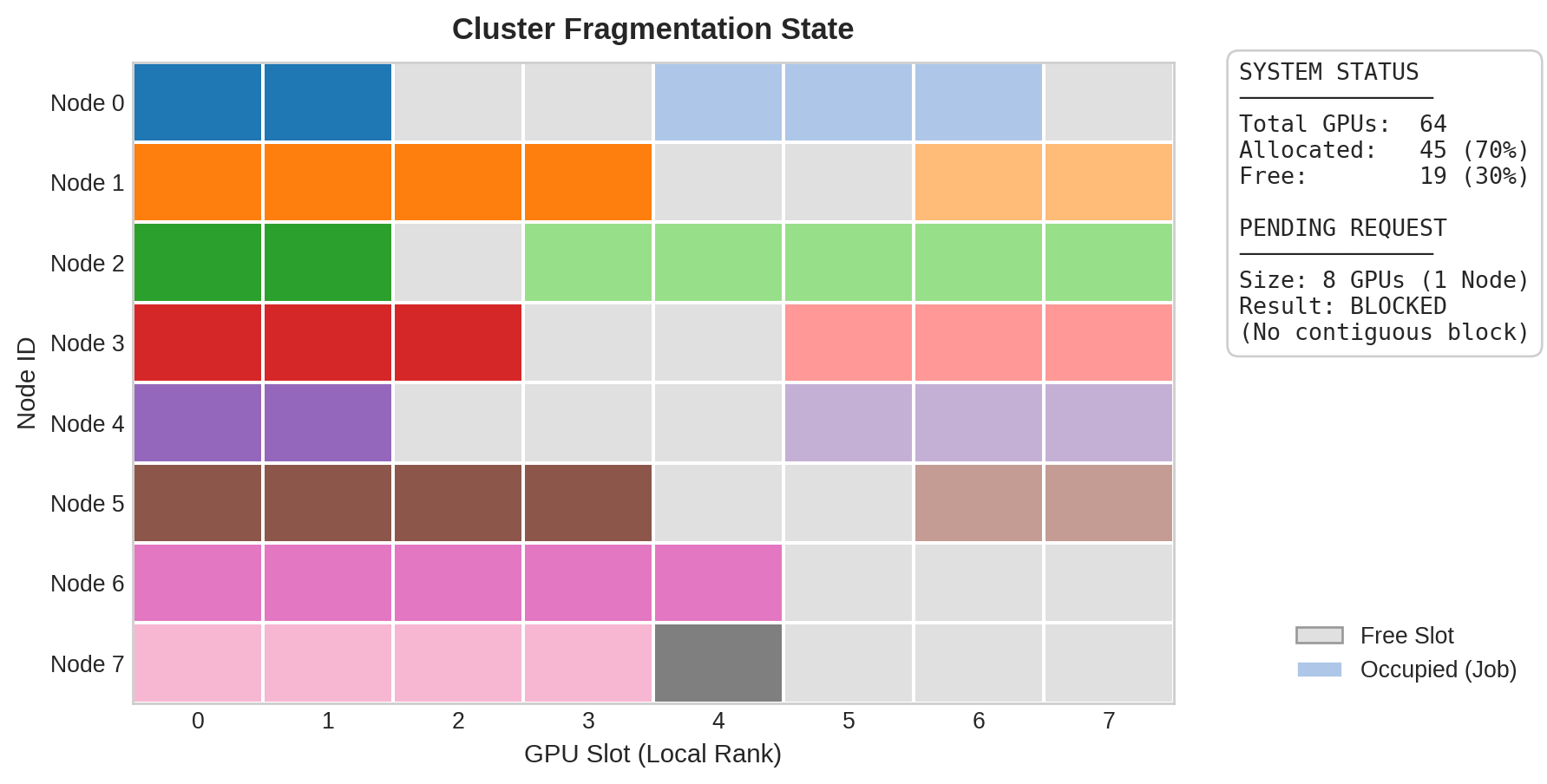
A third strategy, over-subscription, allows more jobs to be admitted than strictly fit, relying on statistical multiplexing to avoid simultaneous peak usage across all resource dimensions. If each job’s GPU utilization averages 70 percent (alternating between compute-intensive and data-loading phases), the cluster can support approximately 1.4\(\times\) as many jobs as the strict GPU count would allow. Over-subscription works well when resource utilization is genuinely bursty and jobs’ peak usage periods are uncorrelated, but can cause severe performance degradation (thrashing, memory pressure, network congestion) when multiple jobs peak simultaneously. The key to safe over-subscription is monitoring actual utilization in real time and throttling admission when contention is detected. Figure 1 shows the combined effect: although 19 GPUs (roughly 30 percent of the cluster) sit idle, no single node has a contiguous block of eight, so a full-node job cannot be placed.

Figure 1: The Fragmentation Problem: The heatmap shows a snapshot of an 8-node cluster (rows) with 8 GPUs each (columns). Different colors represent distinct active jobs, while gray slots represent free GPUs. Although 19 GPUs (~30 percent of capacity) are available globally, they are fragmented across nodes. A new job requiring 8 contiguous GPUs (a full node) cannot be scheduled because no single row is completely empty, illustrating how bin-packing inefficiencies reduce effective cluster capacity.

Gang scheduling

Partial allocation of multi-GPU jobs creates a failure mode unique to ML clusters: two jobs can each hold half the resources they need, blocking each other indefinitely while every allocated GPU sits idle. Figure 2 contrasts this deadlock scenario with the atomic allocation approach that eliminates it.

Figure 2: The Distributed Deadlock (Hold and Wait): In a non-gang scheduler (left), job J1 acquires half the cluster and waits for the rest, while job J2 acquires the other half and waits for J1 to release its GPUs. Neither can proceed, and 100 percent of the cluster sits idle. Gang scheduling (right) solves this by mandating atomic allocation: a job is either granted its entire \(N\)-GPU requirement simultaneously or it waits in the queue without holding any resources.

Definition 1.1: Gang scheduling

Gang Scheduling is the ML cluster scheduling policy that allocates all of a job’s accelerators atomically (all-or-nothing) because synchronous distributed training makes the marginal value of a partial allocation zero: every worker must reach every collective, so a job cannot trade fewer GPUs for proportionally slower progress.

1. Significance: A 1,024-GPU synchronous job holding 512 GPUs completes zero training steps, not half as many: each AllReduce stalls until every rank arrives, so the held GPUs burn power and capital at 0 percent useful output. Without atomic allocation, two such jobs can each acquire half the cluster and deadlock, both at zero progress while consuming the full cluster’s operating cost.
2. Distinction: Unlike cloud service placement (where a service granted half its requested replicas serves roughly half its traffic) and unlike flexible HPC workloads (which degrade gracefully with fewer ranks), synchronous training has step-function utility: full allocation or nothing, which forces the scheduler to reason about atomic multi-resource allocations rather than incremental bin packing.
3. Common pitfall: A frequent misconception is that priorities or quotas alone solve this. Atomicity must extend to every co-scheduled resource the job needs to make progress (accelerators, high-bandwidth interconnect domains, network capacity for collectives); enforcing it at GPU granularity alone recreates the deadlock one resource layer down.

Napkin Math 1.2: The physics of deadlock

Problem: A 1024-GPU cluster receives 2 large training jobs from separate teams, each requiring the full cluster. A naive non-gang scheduler allocates 512 GPUs to Team A and 512 GPUs to Team B, then waits for more GPUs to become available. What is the steady-state outcome?

Math:

1. Team A status: Holds 512 GPUs, Needs 1024 GPUs. Progress = 0 percent.
2. Team B status: Holds 512 GPUs, Needs 1024 GPUs. Progress = 0 percent.
3. Cluster status: 1024 GPUs allocated, 0 samples processed.
4. Waste: $2048 per hour in idle electricity and capital.

Systems insight: This is a circular dependency: Team A is waiting for Team B’s GPUs, and Team B is waiting for Team A’s. Without gang scheduling (all-or-nothing allocation), cluster efficiency drops to zero. In a large fleet, even a 5-minute deadlock can cost thousands of dollars. Batch schedulers and Kubernetes batch extensions address this by enforcing a job-level admission boundary: if the full gang cannot start, the job should remain queued rather than hold a partial allocation.

The partial-allocation pattern in figure 2 is a hold-and-wait deadlock⁵ in which two jobs each hold half the cluster and neither can proceed. The implementation guarantee is straightforward: for a job \(J\) requesting \(N\) GPUs, the scheduler must guarantee that either all \(N\) GPUs are allocated atomically, or the job remains in the queue without holding any resources. This binary outcome eliminates deadlock by construction, since a job that holds no resources cannot block other jobs. Implementing this guarantee efficiently, however, is the challenge that defines much of cluster scheduling algorithm design.

⁵ Hold-and-Wait Deadlock: One of the four classical conditions jointly sufficient for deadlock in resource-allocation systems. In GPU clusters, this condition is uniquely expensive: two jobs each holding 500 GPUs while waiting for 200 more strand 1,000 GPUs indefinitely, burning approximately $2,000/hour. Gang scheduling eliminates hold-and-wait by construction, requiring atomic all-or-nothing allocation at the cost of reduced packing flexibility.

Lifka, David A. 1995. “The ANL/IBM SP Scheduling System.” In Job Scheduling Strategies for Parallel Processing, edited by Dror G. Feitelson and Larry Rudolph, vol. 949. Lecture Notes in Computer Science. Springer. https://doi.org/10.1007/3-540-60153-8_35.

Naive gang scheduling is wasteful in predictable ways. If the cluster has 900 free GPUs and a job requests 1,024, the 900 GPUs sit idle until 124 more become available, potentially wasting thousands of GPU-hours. Backfill scheduling addresses this by identifying jobs in the queue that can fit within the 900 available GPUs without delaying the large job’s expected start time, an idea popularized in the ANL/IBM SP scheduling system (Lifka 1995). A 128-GPU job with estimated runtime of 2 hours can safely backfill if the 124 additional GPUs needed by the large job will become available within 2 hours anyway (from other completing jobs). The backfilled job uses resources that would otherwise be idle, improving utilization without violating the large job’s scheduling guarantee.

The accuracy of runtime estimates determines backfill effectiveness, and this creates a game-theoretic challenge. If users consistently overestimate runtimes, backfill slots are artificially narrow and fewer jobs fit, reducing utilization. If users underestimate, backfilled jobs may still be running when the large job’s resources become available, forcing preemption that wastes the backfilled job’s progress. In practice, users have strong incentives to overestimate (to avoid being killed before completion) and weak incentives to estimate accurately, leading to systematic inflation that degrades backfill performance. Research schedulers like Tiresias (Gu et al. 2019) address this fundamental problem by eliminating the requirement for runtime estimates entirely, instead using observed resource consumption to dynamically adjust priority. This approach, discussed in detail in section 1.5.1, turns the runtime estimation problem from a user-facing burden into a system-level observation.

A quick cost estimate shows why even modest improvements in this balance justify engineering effort.

Systems Perspective 1.1: The economics of idle GPUs

The cluster economics introduced in The Scheduling Problem set the stake; the gang-scheduling decision is where a scheduler first earns or burns it. Taking the same 10,000-GPU cluster:

• Operating cost: $480,000/day ($175.2M/year)
• Lower utilization (60 percent): 6,000 productive, 4,000 idle = $192,000/day wasted
• Higher utilization (80 percent): 8,000 productive, 2,000 idle = $96,000/day wasted
• Improvement value: Moving from 60 percent to 80 percent saves $96,000/day, or about $35.0M/year

The increment gang scheduling owns is the deadlock it prevents: a single hold-and-wait deadlock can strand the whole cluster, erasing more than a full day of this utilization gain in one event.

Gang scheduling removes the hold-and-wait deadlock from the utilization example, but another wait-for pattern remains: priority inversion can still strand reserved GPUs behind jobs that cannot finish their own exit path.

Priority inversion is a wait-for chain, not a root-failure tree.

Deadlock prevention and detection

Gang scheduling eliminates the hold-and-wait condition, one of the four formal Coffman conditions for deadlock, but it does not immunize the cluster against all forms of resource contention. Deadlocks can still emerge from the interaction of priority rules, preemption policies, and auxiliary resource dependencies. In a cluster with thousands of GPUs and petabytes of state, these edge cases transition from theoretical curiosities to daily operational incidents.

The most pernicious of these is priority inversion, a scenario borrowed from real-time systems where a high-priority job is indefinitely blocked by a low-priority job. Consider a 175B parameter training run (high priority) requesting a gang of 64 GPUs. The scheduler has reserved 60 available GPUs, but the remaining 4 are held by a low-priority data processing job. Normally, the scheduler would preempt the low-priority job to satisfy the high-priority request. However, if a stream of medium-priority development jobs saturates the cluster’s CPU or network bandwidth, starving the low-priority job of the resources it needs to checkpoint and exit, the low-priority job stalls. It cannot release the GPUs because it cannot complete its exit sequence. The high-priority job waits for the low-priority job, which is effectively blocked by the medium-priority jobs. The result is a 60-GPU idle block that persists until an operator manually intervenes.

Definition 1.2: Priority inversion

Priority Inversion is an ML cluster scheduling pathology in which a high-priority task is forced to wait for a lower-priority task to release a shared resource.

1. Significance: It reduces the progress rate of the entire fleet to that of the lowest-priority job. In ML clusters, this typically occurs when a low-priority job holding GPUs is starved of auxiliary resources (for example, \(\text{BW}\) for checkpointing), preventing it from finishing and releasing the accelerators needed by high-priority workloads.
2. Distinction: Unlike Standard Queuing (where tasks wait their turn), Priority Inversion involves an Active Blockage: the high-priority task is ready to run but is transitively dependent on a task that the scheduler does not prioritize.
3. Common pitfall: A frequent misconception is that strict priority levels solve this. In reality, without Holistic Preemption (reserving all resources needed for a task to exit), increasing priority levels can actually increase the likelihood of inversion by creating more complex dependency chains.

Solving this requires a choice between prevention and detection. Prevention mechanisms, like strict gang scheduling and aggressive timeouts, eliminate deadlock states by construction but often sacrifice utilization. Detection mechanisms allow the system to enter potentially unsafe states to maximize throughput, relying on monitoring to identify and resolve deadlocks when they occur.

For large-scale fleets, exact deadlock detection is computationally nontrivial. A cluster with 10,000 GPUs and 500 pending jobs has a state space exceeding \(10^{15}\) possible allocations, so constructing and traversing a global wait-for graph in real time is often intractable. Large-scale schedulers therefore approximate liveness rather than prove it. A lease-based resource gives every allocation a time-to-live (TTL), allowing the scheduler to reclaim GPUs when a job stops renewing its claim. Progress monitoring then checks whether the job is actually advancing, using signals such as GPU utilization, step counters, or heartbeat timestamps to identify zombie allocations. When the scheduler must preempt a lower-priority job, holistic preemption reserves the CPU, network, and storage bandwidth needed for that job to checkpoint and exit cleanly; otherwise, the victim can be too starved to release the accelerators. These strategies accept a nonzero rate of false positives to preserve cluster liveness.

Heterogeneous gang scheduling

The traditional gang scheduling model assumes a homogeneous Bulk Synchronous Parallel (BSP) workload: \(N\) identical workers executing the exact same compute graph. Some training workflows break this assumption because one logical job contains several roles with different resource profiles. In preference-training pipelines such as reinforcement learning from human feedback (RLHF), for example, one component may update the policy while another scores outputs or supplies reference behavior. The scheduler still sees one job, but the gang contains trainers, evaluators, and inference-style workers that need different GPU counts, memory footprints, and lifetimes.

Systems Perspective 1.2: Routing over synchrony

Heterogeneous gang scheduling reframes this allocation. The scheduler must atomically allocate a diverse constellation of resources: high-HBM nodes optimized for memory-bound inference generation, alongside high-compute nodes for compute-bound backpropagation. The orchestration challenge shifts from static topological bin-packing to dynamic data routing. Activations and gradients are no longer just reduced within a homogeneous ring; instead, data must stream continuously between inference nodes generating rollouts and training nodes computing policy updates. If the heterogeneous gang allocation is not perfectly balanced across these distinct workload profiles, the entire cluster falls out of sync, leaving expensive accelerators starved for data.

Heterogeneous RLHF gangs are the exception; for common homogeneous training jobs, the recurring tension is gang scheduling’s safety against backfill’s utilization. Gang scheduling prevents deadlock but wastes resources; backfill improves utilization but requires runtime estimates that users cannot accurately provide. Two common orchestration paradigms resolve this tension through fundamentally different architectural philosophies.

Orchestration Paradigms

The gang-scheduling/backfill tension does not have a tool-neutral answer: the orchestration paradigm determines which guarantee the platform protects first. Slurm, shaped by HPC batch systems, favors explicit resource requests and predictable allocation. Kubernetes, shaped by cloud-native service management, favors declared desired state and continuous reconciliation. The choice is therefore not Slurm vs. Kubernetes as products; it is which control model best matches the workload mix, failure behavior, and operational culture of the fleet.

The fundamental distinction is between imperative and declarative resource management. In an imperative system, users specify exactly what resources they need and the system allocates them directly. In a declarative system, users specify what they want running and the system converges toward that state. This distinction, familiar from programming language design, determines how ML workloads are scheduled, monitored, and recovered from failure.

Slurm: The HPC heritage

Slurm Workload Manager⁶ originated at Lawrence Livermore National Laboratory as a scalable, fault-tolerant resource manager for Linux clusters (Yoo et al. 2003). Its batch-oriented design fits the distinctive requirements of scientific computing: long-running jobs, expensive shared hardware, and users who can specify resource needs in advance. In ML infrastructure, the same model maps to GPU training through partitions for heterogeneous accelerator pools and predictable allocations for long-running distributed jobs.

⁶ Slurm Workload Manager: Originally “SLURM,” an acronym for Simple Linux Utility for Resource Management, the project dropped the acronym capitalization in 2012. Developed at Lawrence Livermore National Laboratory beginning in 2002, Slurm’s centralized controller (slurmctld) maintains a single authoritative view of resource allocations. At very large scale, operators may partition fleets or federate schedulers to keep scheduling latency, policy isolation, and failure domains manageable.

Yoo, A. B., M. A. Jette, and M. Grondona. 2003. “SLURM: Simple Linux Utility for Resource Management.” In Job Scheduling Strategies for Parallel Processing. Springer Berlin Heidelberg. https://doi.org/10.1007/10968987_3.

Slurm uses an imperative scheduling model: users submit job scripts specifying exact resource requirements, and the scheduler places jobs into partitions based on priority, fairness, and resource availability. This directness makes reasoning about allocation guarantees straightforward. When a user submits sbatch --gres=gpu:8 --nodes=4, Slurm guarantees that if the job starts, it will have exactly 32 GPUs across 4 nodes. The user knows precisely what they are getting, and the scheduler knows precisely what it must provide. The cost of this directness is that users must understand their resource needs precisely; requesting more than needed wastes resources, while requesting less causes out-of-memory errors or reduced performance.

Slurm’s architecture consists of a central controller daemon (slurmctld) that maintains the global view of cluster state and makes scheduling decisions, and per-node daemons (slurmd) that manage local resources and execute jobs. This centralized architecture provides the authoritative allocation model discussed in section 1.0.1: the controller is the source of truth for resource assignments, reducing the risk of conflicting allocations. The cost is a potential single point of failure (addressed through active-passive failover) and a scheduling-throughput limit. As fleets grow, organizations may partition the cluster or federate schedulers to bound scheduling latency and failure impact.

A typical ML cluster configuration defines Slurm partition configuration by accelerator type and interconnect, as table 1 shows:

Table 1: Slurm Partition Configuration: Partitions organize heterogeneous accelerators into logical pools matched to workload characteristics. NVLink-connected partitions support tensor parallelism, while PCIe partitions serve workloads that rely primarily on data parallelism. Separating inference and debug partitions prevents experimental workloads from impacting production serving.

Partition	GPUs/Node	Interconnect	Typical Use
dgx-a100	8\(\times\) A100	NVLink + IB NDR	Large LLM training
a100-pcie	4\(\times\) A100	PCIe + IB HDR	Medium training
inference	2\(\times\) A10G	Ethernet	Model serving
debug	1\(\times\) V100	Ethernet	Development

Those partitions make GPU allocation policy concrete, and Slurm provides several mechanisms for controlling placement. The --gres=gpu:N flag requests N GPUs per node, while --gpus=N requests a total GPU count for the job. Naive allocation can fragment nodes: if jobs request 6 GPUs on 8-GPU nodes, each job wastes 2 GPUs per node, reducing effective capacity to 75 percent. Slurm’s select/cons_tres plugin enables GPU-aware consumable-resource scheduling, tracking individual GPUs rather than treating nodes as indivisible units. The --gpus-per-node flag requests a fixed GPU count on each allocated node when NVLink communication patterns make partial-node allocation counterproductive, while --gpus-per-task distributes GPUs evenly across tasks for data-parallel workloads.

The interaction between GPU allocation and node selection creates subtleties that affect both performance and utilization. A job requesting --gpus=16 --gpus-per-node=8 will always receive exactly 2 complete nodes, ensuring all 8 GPUs within each node communicate via NVLink. The same job requesting --gpus=16 without the per-node constraint might receive GPUs spread across 3 or 4 partially occupied nodes, degrading intra-node communication performance. For training jobs using tensor parallelism, the per-node constraint is essential; for data-parallel jobs that communicate only through AllReduce, the flexibility of unconstrained placement improves the scheduler’s ability to find valid allocations and reduces fragmentation.

The fair-share scheduling mechanism prevents any single user or project from monopolizing resources over time. The core insight is that past usage should affect future priority: heavy users should yield to lighter users when the cluster is contended. The effective-priority heuristic combines base priority, the user’s target fair share (\(F_{\text{target}}\)), the user’s recent actual consumption (\(F_{\text{actual}}\)), and a small stabilizing constant (\(\epsilon\)):

\[\text{Priority}_{\text{effective}} = \text{Priority}_{\text{base}} \times \frac{F_{\text{target}}}{F_{\text{actual}} + \epsilon} \tag{1}\]

The fair-share formula in equation 1 naturally deprioritizes heavy users while allowing burst access when resources are idle. A researcher who has consumed twice their fair share sees their priority halved, pushing new submissions behind colleagues who have used less. Conversely, a researcher who has used no resources recently receives maximum priority, allowing rapid access when they return to active work.

The time decay of usage history determines how quickly the system “forgives” past heavy usage. A half-life of one week means that a researcher’s heavy usage from two weeks ago contributes only 25 percent to their current usage calculation. Short half-lives create rapid rebalancing but can lead to oscillatory behavior where users alternate between starving and gorging on resources. Long half-lives create stable priority ordering but may penalize researchers who completed a legitimate large project and now want resources for a smaller one. Most production clusters configure half-lives between 3 and 14 days, balancing responsiveness against stability.

Preemption policies enable high-priority jobs to reclaim resources from running workloads, and for ML training, this requires careful coordination with the checkpoint infrastructure. Slurm can notify selected jobs with SIGTERM and use GraceTime to delay final termination, typically giving 60 to 300 seconds for a checkpoint before the eventual SIGKILL. PreemptMode=REQUEUE requeues eligible batch jobs (for example, jobs submitted with --requeue or clusters with JobRequeue=1), and the job’s startup path must resume from the latest checkpoint. The checkpoint and recovery infrastructure developed in Fault Tolerance makes this preemption practical; without reliable checkpointing, preemption would lose all progress since the last manually triggered save, making preemption economically ruinous for long-running training jobs.

Preemption introduces a scheduling paradox: it improves the scheduler’s ability to serve high-priority work but can degrade overall cluster throughput. Every preemption wastes the compute between the last checkpoint and the preemption event, plus the time to restart and reload from checkpoint. If checkpoint intervals are long (for example, hourly) and preemptions are frequent, the wasted compute can be substantial. Production systems balance preemption frequency against checkpoint overhead, often configuring preemption cooldown periods that prevent the same job from being preempted more than once within a configurable interval.

Slurm’s strengths for ML training are clear: predictable allocation guarantees, mature fair-share policies, straightforward integration with MPI-based distributed training frameworks, and decades of operational experience in managing large-scale scientific computing. Its weaknesses emerge for inference workloads and mixed training-serving clusters, where the batch-oriented model struggles with the dynamic, latency-sensitive nature of serving traffic. Slurm has no native concept of “a service that should always be running,” making it awkward for inference endpoints that must respond to requests continuously. Adding or removing inference replicas requires submitting or canceling Slurm jobs, a much heavier operation than scaling a Kubernetes deployment.

Advanced Slurm configuration for ML

Once Slurm owns batch training, the remaining question is how much ML semantics the batch system can see. Standard partitions and fair-share policies schedule ordinary jobs; large-scale deep learning needs configuration that exposes sweep structure, asymmetric pipeline resources, hardware health at job boundaries, and the economic weight of different accelerator types.

Job arrays transform the chaotic submission of thousands of experimental hyperparameter sweep trials into a coherent, schedulable unit. Instead of flooding the controller with individual sbatch requests, a user submits a single array job: #SBATCH --array=0-99. Slurm treats this as a single object for parsing and queuing overhead but schedules each element as an independent task, allowing the scheduler to backfill small holes in the cluster with individual trials. Each task receives a unique SLURM_ARRAY_TASK_ID environment variable, which the training script uses to index into a hyperparameter configuration file (for example, selecting learning rate \(\eta = 10^{-4}\) for task 0 and \(\eta = 3 \times 10^{-4}\) for task 1). This mechanism is common for large-scale ablation studies, enabling researchers to launch 1,000 experiments with a single command while preserving scheduler throughput.

Heterogeneous jobs address the preprocessing bottleneck where expensive GPUs sit idle while CPUs prepare data. Traditional jobs allocate symmetric resources to every node, forcing users to reserve GPU nodes for the entire pipeline. Slurm heterogeneous job support lets a single submission span disparate resource types by separating components with : on the command line or #SBATCH hetjob inside a script. The 64-GPU fine-tuning run for our 175B model (the scheduling-demo workload, not the full 1,024-GPU pretraining run) uses this pattern: it requests a heterogeneous allocation of 8 GPU nodes (64 A100s) for the model and 2 CPU-only nodes for on-the-fly data tokenization. The srun --het-group=0 command launches the training process on the GPUs, while srun --het-group=1 launches the data workers, allowing the expensive accelerators to focus purely on gradient computation while cheaper CPU nodes feed them data.

Prolog and epilog scripts serve as the cluster’s immune system, running administrative code before a job starts and after it finishes. In ML clusters, a typical prolog script performs a preflight check on allocated hardware: it validates NVLink topology (using nvidia-smi topo -m), checks ECC error counters, and verifies InfiniBand link width. If a node fails these checks, the prolog returns a nonzero exit code, causing Slurm to drain the node and requeue the job elsewhere, preventing a silent hardware fault from corrupting a week-long training run. The epilog script ensures hygiene by killing orphaned Python processes, clearing shared memory segments (/dev/shm), and logging final GPU utilization metrics to the accounting database. For the 64-GPU fine-tuning run, the prolog script specifically validates that all 8 GPUs on each node have full P2P bandwidth access, preventing a single degraded NVLink lane from bottlenecking the entire tensor parallel group.

Finally, Trackable Resources (TRES) extend Slurm’s accounting beyond simple CPU/memory tracking to assets like GPU-hours, license tokens, or power budget. The capability that matters is economic-weight accounting per accelerator class: each tracked resource carries a billing weight, so fair-share can be driven by actual economic cost rather than raw core counts. This ensures that a team using 100 older GPUs does not deplete its budget as fast as a team using 100 flagship H100s, and it lets organizations implement project billing for expensive resources directly inside the scheduler’s fairness calculation.

These extensions make Slurm more ML-aware while preserving its batch-scheduler model. Kubernetes starts from a different contract: users declare the desired state of services and jobs, and controllers continuously reconcile the cluster toward that state.

Kubernetes: Declarative orchestration

Kubernetes is a common platform for ML infrastructure, particularly for organizations requiring unified management of training and serving workloads (Burns et al. 2016; Cloud Native Computing Foundation 2024). Where Slurm’s model is imperative (“run this job on these resources”), Kubernetes uses a declarative model (“ensure this state exists”), using control loops that continuously reconcile desired state with actual state. This fundamental difference shapes every aspect of ML workload management, from job submission to failure recovery.

Burns, Brendan, Brian Grant, David Oppenheimer, Eric Brewer, and John Wilkes. 2016. “Borg, Omega, and Kubernetes.” Communications of the ACM 59 (5): 50–57. https://doi.org/10.1145/2890784.

Cloud Native Computing Foundation. 2024. Kubernetes: Production-Grade Container Orchestration.

The declarative model’s power lies in its approach to failure handling. Slurm’s recovery is configuration-dependent and batch-oriented: slurmctld can detect node failures through slurmd heartbeats and requeue jobs when Requeue=1 is set, but the recovery semantics require explicit configuration to behave like a continuously-reconciling control loop. In Kubernetes, the control loop continuously reconciles desired state (“4 replicas of this serving worker should be running” for a Deployment, or the configured retry policy for a Job) against actual state, automatically creating a replacement pod on a healthy node when divergence is detected. For distributed training specifically, replica-replacement semantics typically come from a higher-level operator such as Kubeflow’s PyTorchJob or MPIJob rather than core Kubernetes primitives. This self-healing behavior reduces operational burden but introduces complexity: the system’s actions are emergent from control loop interactions rather than explicitly commanded, making debugging more challenging when things go wrong.

Kubernetes’ control loop architecture is built on the controller pattern⁷: a controller watches the cluster’s actual state (stored in etcd, Kubernetes’ distributed key-value store for API state), compares it to desired state (specified by users through API objects like Deployments, Jobs, and StatefulSets), and takes corrective action to close the gap. This pattern repeats at every level: the Deployment controller ensures the right number of pods exist, the scheduler assigns pods to nodes, the kubelet on each node ensures containers are running, and the node controller detects node failures. Each controller operates independently, communicating only through shared state in etcd, which makes the system resilient to individual controller failures but can create emergent behaviors when multiple controllers interact.

⁷ Controller Pattern (Reconciliation Loop): A “level-triggered” design where the controller continuously compares desired state to actual state, as opposed to “edge-triggered” systems that react to individual events. The distinction matters for ML clusters: if a controller crashes and restarts, it re-reads current state and self-heals without needing an event log. The trade-off is that emergent interactions between multiple independent controllers can create unexpected scheduling behaviors that are difficult to debug sequentially.

Native Kubernetes lacks ML-aware scheduling, but extensions address this gap. GPU scheduling relies on device plugins that expose accelerators as schedulable extended resources. The NVIDIA device plugin registers GPUs with the kubelet (the node-level agent), enabling pod specifications that request GPU resources declaratively through the standard Kubernetes resource model. Listing 1 shows the resulting pod fragment.

Listing 1: Kubernetes GPU Allocation: Pod resource specification requesting GPUs through the NVIDIA device plugin. The nvidia.com/gpu resource name follows Kubernetes extended resource conventions, where the domain prefix identifies the device plugin vendor. This declarative syntax enables portable GPU workload definitions across any Kubernetes cluster with the NVIDIA device plugin installed.

# Kubernetes pod resource specification for GPU allocation
resources:
  limits:
    nvidia.com/gpu: 4  # Request exactly 4 GPUs for this pod
  requests:
    cpu: "32"
    memory: "256Gi"

This binary allocation model creates a significant inefficiency for inference workloads. A small model serving occasional requests might need only a fraction of a GPU’s compute and memory capacity, yet Kubernetes allocates an entire GPU, wasting the remaining capacity. For training workloads that saturate GPU compute, full-device allocation is appropriate. For inference workloads with variable and often modest resource needs, it creates the same kind of fragmentation that partial-node allocation creates in Slurm.

Multi-Instance GPU (MIG)⁸ technology addresses this inefficiency by partitioning A100 (80 GB) and H100 (80 GB) GPUs into hardware-isolated instances. Unlike software-based GPU sharing, MIG dedicates memory, cache, and compute resources to each instance, preventing one workload from interfering with another and eliminating the noisy neighbor⁹ effect. The A100 MIG profiles in table 2 show the scheduling consequence: a single physical A100 becomes several fixed-size resources that the device plugin can expose as independently schedulable accelerators.

⁸ Multi-Instance GPU (MIG): Introduced with the A100 (2020), MIG partitions a single GPU into up to 7 hardware-isolated instances with dedicated memory controllers, L2 cache slices, and compute units (NVIDIA Corporation 2020). The isolation is enforced at the hardware level, not by time-slicing, reducing noisy-neighbor interference relative to software-only sharing. The trade-off is rigidity: partition profiles cannot change without draining all workloads, making MIG poorly suited for clusters with rapidly shifting workload mixes.

NVIDIA Corporation. 2020. NVIDIA A100 Tensor Core GPU Architecture. NVIDIA Whitepaper, V1.0.

⁹ Noisy Neighbor: A metaphor from multi-tenant housing where one resident’s activity (loud music) disturbs another’s peace. In GPU clusters, this occurs when one job’s bursty network traffic or memory bus utilization slows down a co-located job on the same node. For distributed training, noisy neighbors are fatal to efficiency because the slowest flow dictates the global AllReduce time.

Table 2: A100 MIG Profiles: Multi-Instance GPU configurations trade GPU memory and compute resources for increased sharing density. Each profile provides hardware-isolated resources, making MIG suitable for multi-tenant inference clusters where workloads from different teams or customers must not interfere. The SM (Streaming Multiprocessor) count determines compute throughput within each instance.

MIG Profile	GPU Memory	SM Count	Typical Workload
1g.10gb	10 GB	14 SMs	Small inference
2g.20gb	20 GB	28 SMs	Medium inference
3g.40gb	40 GB	42 SMs	Large inference
7g.80gb	80 GB	98 SMs	Training

As section 1.0.5 explains, default Kubernetes pod scheduling is independent, so ML platforms add admission or gang semantics when all-or-nothing startup matters. The default scheduler evaluates pods one at a time, placing each on the best available node. For a distributed training job with 64 pods, this means 64 independent scheduling decisions, with no guarantee that all 64 will succeed. If the cluster has resources for 60 pods but not 64, the default scheduler may place 60 pods and leave the remaining 4 pending, creating exactly the partial-allocation waste that gang scheduling prevents. PodGroup-style abstractions, whether implemented by scheduler plugins or higher-level batch controllers, give the platform a unit of admission that matches the training job rather than the individual pod.

The Volcano¹⁰ batch scheduler and Coscheduling scheduler plugin address this gap by implementing gang semantics through PodGroup abstractions. A PodGroup declares that a set of pods must be scheduled together, specifying a minimum member count that must be satisfiable before any pod in the group starts. The scheduler evaluates the entire group atomically: either all minimum members can be placed, and they are placed simultaneously, or none are placed and the group waits in the queue. This transforms Kubernetes’ pod-level scheduling into job-level scheduling that respects the all-or-nothing requirements of distributed training.

¹⁰ Volcano: Open-sourced by Huawei and now a CNCF incubating project, Volcano replaces the Kubernetes default scheduler entirely to add gang scheduling via its PodGroup CRD. The replacement approach provides strong atomicity guarantees for multi-pod ML training jobs but carries operational risk: a bug in Volcano affects all scheduling decisions on the cluster, not just batch workloads.

Priority classes control preemption behavior in Kubernetes, establishing a hierarchy that determines which workloads yield resources to which others. A typical production configuration assigns inference workloads high priority (ensuring serving SLOs are met), training workloads medium priority, and development jobs low priority. The default PriorityClass behavior, preemptionPolicy: PreemptLowerPriority, allows a higher-priority pending pod to evict lower-priority pods when that would make room for it. A PriorityClass with preemptionPolicy: Never is non-preempting: its pods can sit ahead of lower-priority pods in the scheduling queue, but they do not evict running pods and can still be preempted by still-higher-priority pods. Organizations must carefully balance the priority hierarchy: overly aggressive inference preemption can thrash training jobs (repeatedly preempting and restarting them), while overly permissive training priorities can starve inference during demand spikes. The Kubernetes priority and preemption system integrates with checkpoint-aware preemption patterns developed later in Fault Tolerance, where preempted training jobs save state before yielding resources, minimizing wasted computation.

Kueue¹¹, a newer Kubernetes-native job queueing system, represents an emerging approach that separates admission control from scheduling. Rather than replacing the Kubernetes scheduler entirely (as Volcano does), Kueue manages when jobs enter the cluster, while the default scheduler (or any compatible scheduler) handles where pods are placed. This separation of concerns has practical advantages: Kueue can be deployed alongside existing Kubernetes infrastructure without disrupting running workloads, and it integrates naturally with the ecosystem of scheduler plugins for topology-aware placement and other features.

¹¹ Kueue: Developed by Google, Kueue separates admission control (when jobs enter the cluster) from scheduling (where pods are placed), unlike Volcano which replaces the scheduler entirely. This less-invasive design can be deployed alongside existing Kubernetes infrastructure without disrupting running workloads, but it lacks Volcano’s strong gang scheduling guarantees, forcing teams to choose between deployment safety and scheduling atomicity.

Kueue provides fair-share scheduling through ClusterQueues that represent organizational teams or projects. Each queue has resource quotas, borrowing policies that allow queues to use idle capacity from other queues, and preemption policies that reclaim borrowed resources when the owning queue needs them. A research team queue might borrow idle capacity from a production team queue during off-peak hours, automatically returning resources through preemption when the production team submits urgent work. This borrowing mechanism mirrors the hierarchical fair-share approaches in Slurm but expressed through Kubernetes’ declarative model rather than Slurm’s imperative configuration.

Kubernetes ecosystem for ML training

Kubernetes provides the orchestration primitives, but a specialized ecosystem of operators and plugins is required to bridge the gap between microservice orchestration and high-performance training. Each extension makes one hidden operational constraint visible to the platform: job atomicity, network bypass, checkpoint storage, or telemetry. This ecosystem augments Kubernetes with the batch processing, hardware acceleration, and observability capabilities found in HPC environments.

The Training Operator ecosystem simplifies distributed training by extending Kubernetes with job-specific Custom Resource Definitions (CRDs). The Kubeflow Training Operator provides controllers for PyTorchJob, TFJob, and MPIJob resources, automating the complex lifecycle of distributed workloads. A PyTorchJob specification defines the number of workers, the container image, and resource requirements; the operator then creates the necessary pods and configures distributed environment variables such as MASTER_ADDR, MASTER_PORT, WORLD_SIZE, and RANK. If a worker pod fails, the operator can detect the deviation and create a replacement pod to restore the desired replica count, but training-state recovery still depends on the framework’s checkpoint and rendezvous logic.

Achieving high network performance in Kubernetes often requires bypassing networking layers that were designed for ordinary microservices rather than tightly synchronized collectives. CNI configuration, overlay networking, and CPU switching can add latency or reduce effective bandwidth when they sit on the critical gradient-synchronization path. For bandwidth-sensitive training, host networking (hostNetwork: true) allows pods to bypass the CNI entirely, granting direct access to the host’s network namespace and RDMA devices. The NVIDIA Network Operator automates the low-level plumbing required for this performance, managing RDMA device plugins, SR-IOV virtual function assignment, and GPUDirect RDMA configuration. This bypass capability allows containerized workloads to approach bare-metal interconnect performance when the remaining stack is configured correctly.

Storage integration addresses the “checkpoint storm” problem where thousands of GPUs simultaneously write terabytes of state. Kubernetes PersistentVolumeClaims (PVCs) abstract the underlying storage fabric, which may be a parallel file system like Lustre or GPFS, or high-performance object storage via CSI drivers. The critical architectural challenge is preventing these synchronized writes from saturating the storage backend. Storage classes with Quality of Service (QoS) policies and client-side throttling are essential to ensure that a 1,024-GPU training job writing a 2 TB checkpoint does not starve other workloads or crash the storage metadata server.

The observability stack for training clusters combines general-purpose cluster monitoring with specialized hardware telemetry. Prometheus and Grafana provide the collection and visualization layer, while the DCGM (Data Center GPU Manager) exporter exposes granular GPU metrics: utilization, memory bandwidth, temperature, and ECC errors. This stack enables the utilization dashboards essential for multi-tenant efficiency, allowing operators to distinguish between true compute saturation and I/O-bound idleness.

The 1,024-GPU pretraining run for our 175B model uses this full Kubernetes stack. The workload is defined as a PyTorchJob with 128 worker pods, each requesting 8 GPUs. Host networking is enabled to allow direct InfiniBand access for the NVLink-connected nodes. A PVC backed by a high-throughput Lustre file system provides access to the 100 TB training dataset and absorbs periodic checkpoints. DCGM metrics stream to Prometheus, triggering alerts if any GPU reports uncorrectable ECC errors or if NVLink bandwidth drops below the expected baseline.

Choosing between paradigms

The choice between Slurm and Kubernetes is rarely binary; it depends on workload composition, organizational context, and the relative importance of different system qualities. Understanding where each paradigm excels guides the architectural decision.

Slurm excels for pure training clusters where predictability and bare-metal performance matter most. Its direct resource management avoids the container overhead that Kubernetes introduces (container networking adds microseconds of latency and reduces effective network bandwidth by 1 to 5 percent), and its batch scheduling model aligns naturally with long-running training jobs that require guaranteed, uninterrupted access to specific hardware. Slurm’s centralized scheduler has global visibility into cluster state, enabling sophisticated multi-factor priority decisions that account for fair-share, job size, queue depth, and resource availability simultaneously. National laboratories, university research clusters, and dedicated training infrastructure typically favor Slurm because these environments prioritize maximum hardware utilization and minimal overhead for a relatively homogeneous set of batch workloads.

Kubernetes excels for mixed training-serving clusters where unified management, rolling updates, and service mesh integration reduce operational complexity. Organizations running both training pipelines and production inference endpoints benefit from a single control plane that manages both workload types through a consistent API. Kubernetes’ declarative model simplifies operational workflows: deploying a new model version means updating a Deployment specification, and Kubernetes handles rolling updates, health checks, and rollback automatically. Cloud-native organizations, teams deploying ML as microservices, and organizations with existing Kubernetes expertise typically favor Kubernetes because the marginal cost of adding ML workloads to an existing platform is lower than operating a separate scheduling system.

Many production environments recognize that neither paradigm alone satisfies all requirements, and they deploy both systems in complementary roles. A common architecture uses Slurm for dedicated training clusters where raw performance and scheduling sophistication matter, and Kubernetes for inference serving, pipeline orchestration, and lighter training workloads (fine-tuning, small-scale experimentation). The emerging pattern is to use Kubernetes as the outer orchestration layer, submitting Slurm jobs for large training runs through Kubernetes operators. This hybrid architecture achieves unified management and observability without sacrificing Slurm’s batch scheduling capabilities for the workloads that need them most.

The Slurm vs. Kubernetes trade-off organizes around the dimensions most relevant to ML workloads in table 3:

Table 3: Slurm vs. Kubernetes for ML Workloads: The two paradigms reflect different design philosophies optimized for different workload characteristics. Most production ML platforms use elements of both, with Slurm managing dedicated training clusters and Kubernetes managing inference serving and pipeline orchestration.

Dimension	Slurm	Kubernetes
Scheduling model	Imperative: user specifies exact resources and scheduler allocates them	Declarative: user specifies desired state, system reconciles continuously
Failure handling	Configuration-dependent requeue and checkpoint workflows	Self-healing through control loops
Gang/atomic multi-node start	Atomic job allocation plus backfill; Slurm “gang scheduling” specifically refers to time-slicing/preemption	Production clusters commonly use PodGroup-based support such as Volcano, Coscheduling, Kueue, or upstream alpha gang scheduling
Fair-share	Mature multi-factor priority with configurable decay	Kueue provides basic fair-share with ClusterQueue borrowing
Container overhead	None from a container runtime when jobs run directly on nodes	Configuration-dependent networking overhead and container startup time
Service management	No native support for long-running services	Native Deployment, rolling updates, health checks
Ecosystem	MPI, OpenMP, scientific computing libraries	Cloud-native, microservices mesh, observability stack

As table 3 illustrates, the choice also reflects organizational trajectory. Teams starting with HPC-focused training infrastructure may begin with Slurm and add Kubernetes for serving. Teams starting from cloud-native application infrastructure may begin with Kubernetes and add HPC-oriented extensions (Volcano, Kueue) for training. Either path can reach a functional hybrid architecture, but the starting point determines which capabilities are strongest and which require the most investment to develop.

Hybrid architectures in practice

While the choice between Slurm and Kubernetes often appears binary, sophisticated engineering organizations increasingly deploy hybrid architectures that use the strengths of both systems. These architectures acknowledge a fundamental reality: training workloads behave like HPC applications (batch, synchronous, monolithic), while serving workloads behave like microservices (continuous, asynchronous, elastic). Forcing both into a single paradigm often results in a “lowest common denominator” system that serves neither well.

The Kubernetes-over-Slurm pattern wraps the HPC scheduler within a cloud-native control plane. In this architecture, Kubernetes acts as the outer orchestration layer, managing the lifecycle of training jobs through custom operators while delegating the actual pod placement to Slurm. A developer submits a TrainingJob Custom Resource Definition (CRD) to Kubernetes, which the operator translates into a Slurm sbatch script. The operator then monitors the job status via Slurm’s REST API, streaming logs and metrics back to the Kubernetes control plane. This approach provides the best of both worlds: the unified observability, CI/CD integration, and access control of Kubernetes, combined with the gang scheduling sophistication, topology awareness, and bare-metal performance of Slurm.

The Slurm-alongside-Kubernetes pattern takes a coarser-grained approach, maintaining separate clusters for training and serving that draw from a shared pool of physical nodes. A meta-scheduler or capacity broker acts as an arbitrator, dynamically reassigning nodes between the Slurm partition and the Kubernetes cluster based on demand signals. During intensive training campaigns, nodes are drained from Kubernetes and joined to Slurm; during product launches or traffic spikes, the flow reverses. The primary challenge is the mode-switching cost: draining a Kubernetes node, re-imaging or reconfiguring it, and joining it to Slurm (or vice versa) typically requires 5 to 15 minutes. This latency limits the granularity of sharing: the system can adapt to diurnal patterns or weekly cycles but cannot use Slurm capacity to absorb second-by-second inference bursts.

Emerging unified platforms like Ray attempt to eliminate the dichotomy entirely by providing a single runtime for both training and serving. Ray implements its own distributed scheduler that handles actor placement, task scheduling, and resource management natively. This eliminates the impedance mismatch between training (stateful actors) and serving (stateless replicas), allowing a single Python script to define a training loop that seamlessly transitions into a deployment pipeline. The trade-off is maturity: while Ray excels at orchestration flexibility, its scheduling logic lacks the decades of hardening found in Slurm and the massive ecosystem support of Kubernetes, effectively requiring the platform team to assume more responsibility for reliability and isolation.

Threading these patterns together, consider the lifecycle of our 175B parameter model. The training phase runs on Slurm to maximize NVLink topology efficiency and gang scheduling reliability for the multi-month run. Once trained, the model artifacts are handed off to Kubernetes for serving, where rolling updates and autoscaling ensure high availability for end users. The bridge between them is a Kubernetes operator that monitors training progress; when validation loss stabilizes, it automatically triggers a quantization pipeline and deploys the resulting model to the inference cluster.

The operational impact of these choices is quantifiable, but the numbers depend on workload mix and local platform maturity. A pure Slurm-only environment minimizes batch-job overhead and can keep dedicated training clusters highly utilized, but it requires extra engineering to build production serving infrastructure. A Kubernetes-only environment reduces operational fragmentation by using standard cloud-native tools, but distributed training may need batch extensions to avoid scheduling fragmentation. The hybrid approach targets the efficient frontier: preserving strong batch-training placement guarantees while keeping a unified management surface for serving and pipeline workloads, at the cost of increased architectural complexity.

Systems Perspective 1.3: The convergence of HPC and cloud

The sharp distinction between HPC and cloud-native scheduling is rapidly blurring as both communities adopt features from the other. Kubernetes is evolving batch capabilities through the Volcano and Kueue projects, introducing concepts like queues, priorities, and gang scheduling that were previously unique to HPC. Conversely, Slurm is adopting cloud features like REST APIs, container runtime support, and elasticity. The industry is converging toward a unified fleet operating system: a system that offers the declarative API and fault tolerance of the cloud with the strict placement guarantees and performance of the supercomputer.

This convergence turns the paradigm choice into a workload-specific design decision: teams must decide which scheduling guarantees matter before layering on topology constraints.

Checkpoint 1.1: Scheduling paradigm trade-offs

Before the chapter turns to topology-aware scheduling, review the core trade-offs:

• Gang scheduling: Explain why gang scheduling is essential for distributed training but not for inference workloads, including the property of synchronous data parallelism that creates the all-or-nothing requirement.
• Slurm vs. Kubernetes: Identify the CAP theorem trade-off Slurm makes differently from Kubernetes, and describe how this difference appears during a network partition between the scheduler and a subset of nodes.
• MIG partitioning: Determine when MIG partitioning improves cluster utilization through concurrent inference workloads on fewer GPUs and when it reduces utilization for training jobs that need full GPU memory.
• Backfill incentives: Explain why backfill scheduling depends on accurate job runtime estimates and why users have game-theoretic incentives to provide inaccurate estimates.

The orchestration paradigms treat GPUs as interchangeable units within a partition, but physical location matters as much as count: the same 64 GPUs run far slower scattered across racks than packed into one. Topology-aware scheduling exploits that structure.

Self-Check: Question

1. One team submits sbatch --gres=gpu:8 --nodes=4 and waits for the scheduler to hand them exactly 32 GPUs; another team declares a deployment of 4 training-worker replicas and lets a controller keep that count alive through pod restarts. Which distinction does this pairing illustrate most directly?

   1. Slurm uses imperative resource requests executed once at submission, while Kubernetes expresses a declarative desired state that control loops continuously reconcile against actual state
   2. Slurm is optimized for Ethernet clusters while Kubernetes is optimized for InfiniBand fabrics
   3. Slurm is only used for training and Kubernetes is only used for inference, with no legitimate overlap
   4. Slurm schedules at pod granularity while Kubernetes schedules only at whole-node granularity

2. During a 90-second network partition between the control plane and a subset of worker nodes, which behavior best matches the chapter’s CAP-theorem characterization of Slurm and Kubernetes?

   1. Both systems prefer immediate reallocation to maximize availability, even if GPUs end up double-booked once the partition heals
   2. Kubernetes blocks all new scheduling until an administrator manually resolves the partition, while Slurm keeps scheduling with eventual consistency
   3. Slurm blocks new allocations during the partition to preserve consistency and avoid double-booking GPUs, while Kubernetes stays responsive and reconciles inconsistencies asynchronously once the partition heals
   4. Neither system is affected because node-local agents can always make globally consistent placement decisions without the control plane

3. A team submits a distributed training job to vanilla Kubernetes, which creates the 32 required pods one at a time as nodes become free. Two hours in, only 24 pods are running, holding their GPUs but making no progress because AllReduce cannot begin. Which scheduling failure mode is this, and which Kubernetes abstraction resolves it?

   1. Priority inversion; resolved by raising the job’s pod-level priority class
   2. Image pull back-off; resolved by pre-pulling container images to every node
   3. Node affinity mismatch; resolved by adding topology spread constraints
   4. Partial gang allocation stranding resources; resolved by a PodGroup (or equivalent gang abstraction) that requires the minimum set to be schedulable before any pod starts

4. An inference team reports that MIG partitioning raised GPU utilization dramatically, but a training team on the same cluster complains that MIG has made their job wait times worse. Explain, in terms of partition rigidity, why both can be true on the same hardware.

5. An organization already runs Kubernetes for their microservices, enjoying its CI/CD, RBAC, and observability tooling, but their largest pretraining runs want topology-aware gang scheduling and bare-metal performance. Which architecture best matches this goal?

   1. A pure Kubernetes cluster with no batch extensions, relying on vanilla pod scheduling for multi-node training
   2. A pure Slurm cluster, with custom in-house tooling built to replicate the organization’s existing CI/CD, RBAC, and observability
   3. A hybrid design where Kubernetes owns the operational control plane and orchestrates inference, while large training runs are submitted via operators into a Slurm-managed partition
   4. A design that partitions every node into MIG slices and runs training, inference, and microservices uniformly on those slices

See Answers →

Topology-Aware Scheduling

Randomly assigning 64 GPUs across a massive data center cripples a synchronous training job, causing it to run 15 to 30 percent slower than if those same 64 GPUs were packed into a single rack. The scheduling algorithms discussed so far treat GPUs as interchangeable units, but topology-aware scheduling recognizes that physical proximity in the network fabric is as critical as raw compute.

The topology hierarchy

Modern GPU clusters exhibit a multi-level communication hierarchy, where bandwidth decreases and latency increases at each level. This hierarchy is not an implementation detail that the scheduler can ignore; it is a physical constraint that directly determines training throughput for communication-intensive workloads. Understanding the hierarchy is essential for making placement decisions that translate allocated resources into useful work.

Bandwidth cliffs from NVLink to spine across the fabric.

Within a single node, GPUs communicate via NVLink, providing 600 GB/s per GPU on A100 systems and 900 GB/s on H100 systems. This high-bandwidth, low-latency interconnect enables efficient tensor parallelism, where matrix operations are split across GPUs that must exchange intermediate results (activations and gradients) at every transformer layer. The NVLink bandwidth is sufficient to overlap communication with computation for most model architectures, meaning tensor parallel operations can proceed at near-ideal throughput when confined to a single node.

Between nodes within the same rack or leaf switch domain, communication traverses InfiniBand or RoCE at 400 Gb/s (NDR InfiniBand), roughly 50 GB/s per link. This represents an order of magnitude reduction from NVLink bandwidth. Data parallelism, which requires AllReduce of gradients after each training step, operates efficiently at this level because the gradient synchronization pattern allows overlap between communication and the next iteration’s forward pass. The latency penalty is modest (microseconds vs. nanoseconds), and the aggregate bandwidth is sufficient for gradient tensors that are typically smaller than the activation tensors exchanged in tensor parallelism.

Between racks connected through spine switches, communication crosses additional switch hops, introducing both higher latency and potentially reduced effective bandwidth due to network congestion. The fat-tree topologies analyzed in Fat-tree (Clos) networks provide full bisection bandwidth in theory, but in practice, congestion from concurrent flows, routing inefficiencies, and switch buffer limitations reduce effective cross-rack bandwidth by 10 to 30 percent compared to intra-rack communication. Cross-rack communication also adds tail latency variability: while median latency may be only slightly higher, P99 latency can spike during congestion events, creating straggler effects in synchronous training where the slowest communicator determines the pace for all workers.

This hierarchy means that a 64-GPU job allocated entirely within a single rack (8 nodes, all under one leaf switch) will outperform the same job spread across 8 racks (1 node per rack, crossing spine switches for every AllReduce). The performance difference stems directly from the communication analysis in Collective Communication: ring AllReduce latency scales with the slowest link in the ring, and cross-rack hops introduce both higher latency and increased contention risk. For synchronous training, every iteration waits for the slowest worker to complete its AllReduce, so even occasional cross-rack congestion events create persistent throughput degradation.

The scheduler must therefore model the cluster not as a flat list of compute slots, but as a hierarchical graph with distinct bandwidth cliffs at each level (GPU, Node, Rack, and Pod) corresponding to NVLink, InfiniBand, and spine-switch boundaries. Each boundary crossing introduces an order-of-magnitude bandwidth reduction, and at the rack and pod levels, network oversubscription (often 2:1 or 4:1 at the spine switches) further restricts bisection bandwidth beyond what the raw link speed suggests. A topology-aware scheduler explicitly optimizes for these constraints, treating “locality” as a first-class resource. For a distributed training job requiring 1,024 GPUs, a fragmented placement that scatters workers across random racks can degrade end-to-end training throughput by 15 to 30 percent compared to a compact placement within a single pod.

Figure 3 contrasts optimal and scattered placement for a 4-GPU tensor parallel group, showing how the communication path determines whether GPUs use a single leaf switch or must traverse slower leaf-spine-leaf hops.

Figure 3: Topology-Unaware vs. Topology-Aware Placement: A 4-GPU job placed across two racks (left, topology-unaware) must traverse leaf-spine-leaf hops: 3 switch hops per AllReduce message at about 12 GB/s effective bandwidth. The same 4-GPU job packed within one rack (right, topology-aware) uses a single leaf switch: 1 hop at about 50 GB/s, roughly 4\(\times\) faster. A quantitative summary beneath the figure reports switch-hop counts and effective bandwidth.

Placement algorithms

The bandwidth gap shown in figure 3 is the key constraint: the roughly 4\(\times\) reduction from intra-rack leaf paths to cross-rack leaf-spine-leaf paths means that scattered placement forces tensor parallel groups to spend more time communicating than computing, a penalty that compounds at every transformer layer in the model. Topology-aware placement algorithms assign jobs to nodes that minimize communication cost, transforming the abstract bin packing problem into a graph optimization problem on the cluster’s physical topology. The simplest approach uses a locality cost, defined in equation 2, that penalizes allocations spanning multiple topology domains:

\[ \text{Cost}_{\text{locality}} = \sum_{i < j} w(d(g_i, g_j)) \tag{2}\]

where \(g_i\) and \(g_j\) are GPUs assigned to the job, \(d(g_i, g_j)\) is their topological distance (0 for same node, 1 for same rack, 2 for different racks), and \(w(\cdot)\) is a weighting function that increases with distance. The scheduler minimizes this score when selecting an allocation from the set of feasible placements. The weighting function encodes the performance impact of each topology level: \(w(0) = 0\) (same node, NVLink, no penalty), \(w(1) = 1\) (same rack, one switch hop), \(w(2) = 10\) (different racks, multiple switch hops). The tenfold weight difference between same-rack and cross-rack placements reflects the disproportionate performance impact of crossing spine switches.

More sophisticated algorithms distinguish between parallelism strategies, recognizing that different communication patterns have different bandwidth and latency requirements. Tensor parallelism requires the highest bandwidth and lowest latency because it exchanges activation tensors at every layer; it should be confined to NVLink domains within a single node. Pipeline parallelism tolerates moderate latency because it sends activations between stages less frequently (once per microbatch per stage boundary rather than at every layer); it can span nodes within a rack where InfiniBand provides sufficient bandwidth. Data parallelism, with its bulk gradient synchronization that can overlap with computation, operates efficiently across racks because the communication is less latency-sensitive and can use the available bandwidth effectively.

Algorithm 1 combines these pieces into a single decision: the all-or-nothing gang constraint of section 1.0.5, the locality cost of equation 2, and the parallelism-to-topology mapping just described. The scheduler enumerates the allocations that fit, scores each by communication cost, and takes the cheapest, leaving the job queued rather than stranding accelerators when none does.

\begin{algorithm} \caption{Topology-aware placement} \begin{algorithmic} \Require job requesting $N$ accelerators with tensor-, pipeline-, and data-parallel groups; cluster topology with per-level link costs $w(\cdot)$ \Ensure an all-or-nothing placement of least communication cost, or the job stays queued \State enumerate the feasible slots: sets of $N$ free accelerators that satisfy every resource dimension \Comment{gang: all or nothing} \If{no feasible slot exists} \State leave the job queued without holding any accelerators \Comment{prevents hold-and-wait deadlock} \EndIf \For{each feasible slot} \State map tensor-parallel ranks within an NVLink domain, pipeline stages within a rack, data-parallel replicas across racks \State score the slot by $\text{Cost}_{\text{locality}} = \sum_{i < j} w(d(g_i, g_j))$ \EndFor \State \Return the feasible slot of least $\text{Cost}_{\text{locality}}$ \Comment{topology-optimal, atomic} \end{algorithmic} \end{algorithm}

Scattered placement runs AllReduce 4.8\(\times\) slower than a topology-aware slot, a gap figure 4 breaks out across four placement strategies from random to topology-optimal.

Figure 4: Topology Placement Impact: Reducing AllReduce latency by 4.8\(\times\) through topology-aware scheduling (rack/rail optimization) compared to random placement for a 1 GB gradient sync on 64 GPUs.

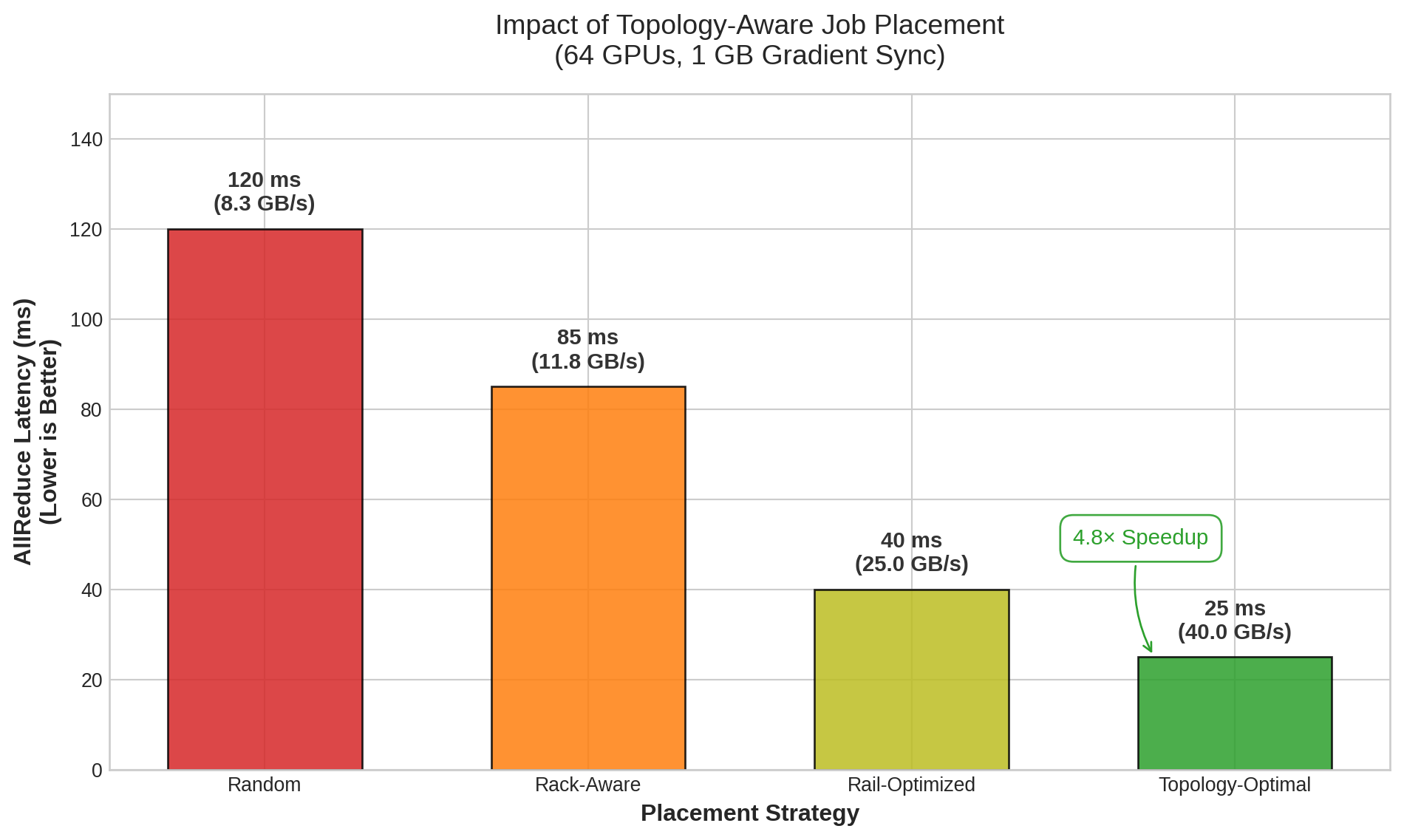
A hierarchical placement algorithm assigns resources in layers that match this parallelism hierarchy. First, it assigns tensor parallel groups to individual nodes, ensuring that all GPUs in a tensor parallel group share NVLink connectivity. Second, it groups those nodes into pipeline stages within racks, placing consecutive pipeline stages on nodes connected through the same leaf switch. Third, it distributes data parallel replicas across racks, ensuring that each data parallel group has access to the cluster’s full bisection bandwidth for AllReduce operations. This three-level placement mirrors the three-level topology and the three-level parallelism strategy, creating a natural alignment between logical and physical structure.

Napkin Math 1.3: The topology placement impact

The physical location of GPUs on the network switch fabric dramatically impacts collective performance. Consider an AllReduce operation across 64 GPUs:

• Random placement: Spread across many racks \(\rightarrow\) Traffic traverses core switches \(\rightarrow\) 120 ms latency.
• Rack-aware: Confined to a single rack (Top-of-Rack switch) \(\rightarrow\) 85 ms.
• Rail-optimized: Aligned to specialized “rails” (dedicated standard IB switches) \(\rightarrow\) 40 ms.
• Topology-optimal: All GPUs on the same leaf switch \(\rightarrow\) 25 ms. Proper scheduling yields a 4.8× speedup purely by respecting the network topology, with zero changes to the model code.

The computational cost of topology-aware placement is nontrivial. Evaluating all possible placements for a 256-GPU job across a 10,000-GPU cluster is combinatorially intractable. Production schedulers use heuristic approaches: greedy algorithms that build placements bottom-up (first fill NVLink domains, then fill racks, then spread across racks), tree-search algorithms with pruning that explore the most promising placements first, or scoring-based approaches that evaluate a sample of feasible placements and select the best. The scheduling latency introduced by topology-aware algorithms (milliseconds to seconds, depending on cluster size and algorithm complexity) is negligible compared to job runtimes of hours to weeks, making the throughput improvement worth the scheduling overhead.

Napkin Math 1.4: Placement impact on 3D-parallel training

Scenario: Consider a 256-GPU training job using 3D parallelism: 8-way tensor parallel, 4-way pipeline parallel, 8-way data parallel.

Good placement (topology-aware):

• Tensor parallel groups: 32 groups of 8 GPUs, each confined to one 8-GPU node (NVLink: 900 GB/s)
• Pipeline stages: 4 consecutive nodes within the same rack (1 switch hop, InfiniBand: 50 GB/s)
• Data parallel replicas: 8 racks (2 switch hops for cross-rack AllReduce)

Bad placement (topology-unaware):

• Tensor parallel groups split across 2 nodes (InfiniBand instead of NVLink)
• Pipeline stages scattered across racks (2 switch hops instead of 1)
• Data parallel replicas randomly distributed

Math: The tensor parallel communication alone illustrates the impact. With NVLink delivering 450 GB/s per direction, a 1 GB activation transfer takes approximately 2.2 ms. Over InfiniBand at 50 GB/s, the same transfer takes approximately 20 ms, a 9× slowdown.

Systems insight: The 4.8× AllReduce-latency gap in figure 4 is a communication-only measurement; it does not become a 4.8× end-to-end penalty because synchronous training overlaps much of that communication with the next iteration’s compute. Since tensor parallelism communicates at every transformer layer (typically 80+ layers for large models), the residual exposed communication compounds to 15 to 30 percent total training throughput degradation, the figure to carry forward for 3D-parallel jobs.

Rail-optimized scheduling

Large GPU clusters increasingly use rail-optimized topologies where each GPU in a node connects to a different network switch, creating parallel “rails” through the network fabric. This design, analyzed in Rail-optimized topology, provides balanced bandwidth across all GPUs by distributing traffic across independent switch hierarchies. However, it also creates a scheduling constraint: AllReduce operations are most efficient when communicating GPUs are on the same rail (connected to the same switch chain), because same-rail communication avoids cross-rail traffic that could create congestion at shared switch ports.

Rail-aware scheduling assigns data parallel replicas such that corresponding GPUs across nodes share the same rail. For an 8-GPU-per-node cluster with 8 rails, GPU 0 on every node connects to rail 0, GPU 1 to rail 1, and so on. The scheduler places data parallel rank \(r\) on GPU \(r \bmod 8\) across selected nodes, ensuring that AllReduce for each data parallel group traverses only a single rail switch hierarchy rather than crossing between rails. This alignment means that AllReduce traffic is confined to independent switch trees, eliminating contention between data parallel groups and providing each group with the full bandwidth of its dedicated rail.

The interaction between rail-aware scheduling and topology-aware placement creates a multi-dimensional optimization problem. The scheduler must simultaneously optimize for intra-node NVLink locality (tensor parallelism requires GPUs on the same node), intra-rack switch locality (pipeline parallelism benefits from minimal switch hops between stages), and rail alignment (data parallelism benefits from same-rail communication). These three objectives are partially conflicting: constraining data parallel replicas to specific GPU positions within each node (for rail alignment) reduces the scheduler’s flexibility to choose nodes based on rack locality, and requiring full-node allocations for NVLink locality prevents sharing nodes between jobs that could improve packing efficiency.

Production schedulers resolve these conflicts using weighted scoring functions that prioritize constraints based on workload characteristics. For large training jobs using 3D parallelism, tensor parallel locality receives the highest weight (because NVLink-to-InfiniBand performance degradation is the largest), followed by rail alignment (because it eliminates congestion for the most frequent communication pattern), followed by rack locality (because the performance benefit is smaller and can be partially compensated by compute-communication overlap). For pure data parallel jobs, rail alignment receives the highest weight. For single-node jobs, topology constraints are irrelevant and the scheduler optimizes purely for packing efficiency.

Topology discovery and dynamic adaptation

Static configuration files like Slurm’s topology.conf or Kubernetes node labels provide a baseline map of the cluster, but they represent the intended state, not the effective state. True topology discovery requires runtime introspection to validate that the physical hardware matches the architectural diagram. Libraries like NCCL bypass static configurations entirely, parsing the Linux virtual filesystem at /sys/class/infiniband to map the PCIe bus hierarchy, enumerate NVLink connections, and verify NIC proximity. This creates a ground-truth graph where edges represent verified, operational links rather than theoretical cables.

Cluster topology is an operating state, not a fixed schematic. Hardware failures, maintenance windows, and thermal throttling constantly reshape the effective topology available to the scheduler. A single spine switch failure in a Clos network does not sever connectivity entirely, but it drastically reduces the bisection bandwidth available to jobs spanning the affected racks. If a spine switch serving our 175B parameter model’s data-parallel AllReduce group fails, cross-rack bandwidth might drop by 50 percent. The scheduler faces a critical optimization decision: continue training at reduced throughput, effectively wasting 25 percent of the expensive GPU cycles waiting for straggling gradients, or initiate a topology-aware migration.

Migration is not free; it requires a coordinated checkpoint, a job kill, a rescheduling event on healthy nodes, and a warmup phase. This process typically consumes 5 to 15 minutes of idle time. However, for a multi-week training run, the math often favors migration. If the network degradation creates a 20 percent throughput penalty, the break-even point for a 10-minute migration is less than an hour of training. Sophisticated orchestrators continuously monitor effective bandwidth metrics reported by the collective communication library. When the delta between the assigned topology score and the realized throughput exceeds a threshold, the scheduler triggers a drain-and-migrate workflow, treating network degradation with the same severity as a GPU hardware fault.

Example 1.1: The limping switch

Scenario: A foundation-model training job shows a large throughput regression. The GPUs are healthy, the code is unchanged, and the static topology map says the job has full bisection bandwidth.

Failure mode: A single switch or transceiver can remain technically “up” while producing high CRC error rates, packet drops, or retransmissions. Binary health checks report green; collective communication performance reports red.

Consequence: If the scheduler relies on a static topology map, it continues to schedule communication-intensive jobs onto a degraded rack, assuming full bandwidth that no longer exists.

Systems insight: Binary health checks (up/down) are insufficient. Schedulers need performance-aware topology monitoring that incorporates switch counters, retransmission rates, and collective bandwidth tests. Nodes connected to a “limping” switch should be dynamically marked ineligible for communication-intensive jobs until the hardware is repaired.

The general scheduling idea is quarantine: when runtime evidence says a node, rack, or link is degraded, the scheduler should stop placing sensitive work there even if the nominal resource count still looks available. Kubernetes implements this pattern through taints and tolerations¹², while Slurm clusters commonly use drain states, node features, or partition rules. The complementary problem is how jobs adapt when available resources change dynamically. Rather than treating resource allocation as fixed for a job’s lifetime, elastic training allows jobs to grow, shrink, and recover without full restarts.

¹² Taints and Tolerations: Kubernetes primitives for restricting pod placement. A taint on a node repels all pods that do not explicitly tolerate it. For ML fleets, this is the primary mechanism for isolating specialized hardware: by tainting A100 nodes, the orchestrator prevents general-purpose web services from “stealing” expensive GPU capacity, ensuring those nodes are reserved for training jobs that tolerate the taint.

Self-Check: Question

1. An 8-way tensor-parallel group runs at near-ideal step time when it is placed inside a single NVLink-connected node but slows sharply when the same 8 GPUs are split across two nodes connected by NDR InfiniBand. Which explanation is correct?

   1. Tensor parallelism exchanges activation and gradient slices at every layer; NVLink’s order-of-magnitude-higher bandwidth and lower latency let these exchanges overlap with compute, whereas inter-node InfiniBand exposes the transfer cost on the critical path
   2. Aggregate InfiniBand bandwidth across two nodes exceeds a single node’s NVLink, so cross-node placement should actually be faster and any slowdown must be a driver bug
   3. AllReduce traffic dominates tensor-parallel communication, so both placements should perform identically once AllReduce is tuned
   4. Two nodes in the same rack share an NVLink domain, so the observed slowdown must come from the scheduler binding ranks to the wrong NUMA node
   5. The step-time slowdown is a GPU firmware throttle that activates when links cross a leaf switch boundary

2. A job uses 8-way tensor parallelism, 4-way pipeline parallelism, and 8-way data parallelism. Explain the placement logic a topology-aware scheduler should use across these three levels, matching each level to its appropriate tier of the communication hierarchy.

3. The section compares AllReduce latency for 64 GPUs under four placement strategies and reports 120 ms for random placement versus 25 ms for a topology-optimal placement. What is the main conclusion the reader should draw from this 4.8\(\times\) gap?

   1. AllReduce performance is largely insensitive to placement once the GPU count is fixed, so any difference must be measurement noise
   2. Rail optimization helps only serving workloads, not training
   3. Placement alone, without touching model code or hyperparameters, can produce a large collective-communication speedup because it changes the bandwidth and hop count the ring walks across
   4. The speedup comes entirely from raising the effective batch size until communication disappears from the critical path

4. True or False: A scheduler can rely on static topology files alone because any link or switch problem serious enough to matter will always surface as a hard failure.

5. In a rail-optimized cluster, which placement rule best supports data-parallel AllReduce efficiency?

   1. Assign each replica to arbitrary GPU indices so long as all replicas sit in the same rack
   2. Co-locate every data-parallel worker on one node to avoid every switch hop
   3. Alternate ranks across rails to maximize path diversity for each collective
   4. Place corresponding data-parallel ranks on the same GPU index across nodes so their AllReduce traffic stays on a single rail’s switch hierarchy and does not contend with other rails

6. A spine-switch failure halves cross-rack bandwidth for a training run that still has three weeks of compute ahead. Explain the calculation a scheduler should perform to decide whether to migrate the job to a healthy pod versus letting it ride out the degradation.

See Answers →

Elastic Scheduling

When cluster demand fluctuates, rigid allocation creates two categories of waste. During off-peak hours, a job running on 256 GPUs cannot absorb idle resources to speed up training. During peak demand, the same job cannot release excess resources to accommodate higher-priority work without being fully preempted. The scheduler’s only options are “let it keep all its resources” or “kill it entirely,” with nothing in between.

Elastic scheduling eliminates this binary choice. The recovery mechanics of elastic training developed in Elastic Recovery show how a distributed job can adjust its worker count, recalibrate batch size and learning rate, and reconstruct its communication group after a failure. From the scheduler’s perspective, the same capability solves a resource-allocation problem under fluctuating demand. A training job might start with 128 GPUs (the minimum needed for reasonable throughput), scale up to 256 when resources become available, and scale back to 192 when higher-priority work arrives, all while maintaining continuous training progress. This flexibility transforms the scheduler’s action space from a binary {continue, preempt} to a continuous spectrum of resource allocation levels.

The scheduler-framework contract

Elastic scheduling requires a well-defined contract between the scheduler and the training framework. The scheduler guarantees that resource changes are communicated through defined signals, with sufficient advance notice for graceful adaptation. The framework guarantees that it can handle resource changes without corrupting model state, using the batch size adjustment, learning rate recalibration, and communication group reconstruction mechanisms developed in Recovery adaptation mechanisms.

From the scheduler’s side, the contract has three parameters:

• Elastic range: \([N_{\text{min}}, N_{\text{max}}]\) specifies the worker counts between which the job can operate.
• Transition cost: The rendezvous cycle, typically 10 to 60 seconds, determines how frequently the scheduler can resize without the overhead negating the throughput gain.
• Scaling efficiency curve: The throughput gained from each added worker determines whether assigning idle GPUs to this job is more productive than holding them for a pending gang-scheduled job.

The contract gives the scheduler enough information to resize a job without treating elasticity as free capacity.

The scheduler must also account for the constraint that elastic scaling changes the effective batch size (\(B_{\text{effective}} = B_{\text{per-worker}} \times N\)). The two strategies for handling this (constant global batch size vs. adaptive learning rate) impose different limits on how aggressively the scheduler can resize: constant global batch size preserves convergence but may violate per-GPU memory limits at low worker counts, while adaptive learning rate simplifies worker management but introduces convergence risk during rapid scaling.

The scheduler interface to frameworks like TorchElastic exposes these parameters directly, as listing 2 illustrates.

Listing 2: TorchElastic Launch Configuration: The --nnodes=4:16 range tells the scheduler that this job can operate with 32 to 128 GPUs. The scheduler places the job at any point within this range based on current cluster load and resizes it as demand changes.

# Launch elastic training with min 32 to max 128 workers
torchrun \
  --nnodes=4:16 \
  --nproc_per_node=8 \
  --rdzv_backend=c10d \
  --rdzv_endpoint=head-node:29500 \
  --max_restarts=3 \
  train.py

The --nnodes=4:16 specification declares that the job can operate with anywhere from 4 to 16 nodes (32 to 128 GPUs with 8 GPUs per node). This range is the scheduler’s action space: it can place the job at any point within this range based on current cluster load, and resize it as demand changes.

Systems Perspective 1.4: Elastic vs. rigid scheduling

Consider a congested cluster where a 128-GPU job waits 8 hours for a full gang allocation.

Rigid scheduling: Wait 8 hours, then train for 24 hours at full throughput. Total wall-clock: 32 hours.

Elastic scheduling (min 32, max 128):

• Start immediately with 32 GPUs (throughput = 25 percent of full)
• After 2 hours, scale to 64 (throughput = 50 percent)
• After 4 hours, scale to 128 (throughput = 100 percent)
• Training progresses during the entire wait period

Approximate work completed during the 8-hour “queue wait”:

• Hours 0 to 2: 25 percent throughput \(\times\) 2 hours = 0.5 hours equivalent
• Hours 2 to 4: 50 percent throughput \(\times\) 2 hours = 1.0 hours equivalent
• Hours 4 to 8: 100 percent throughput \(\times\) 4 hours = 4.0 hours equivalent
• Total: 5.5 hours of equivalent full-scale work

The elastic job completes in approximately 26.5 hours (8 hours of scaled-up training plus 18.5 hours at full scale), saving 5.5 hours compared to rigid scheduling. This 17 percent improvement comes entirely from using resources productively during what would otherwise be idle queue time.

The scheduler cannot treat every job as elastic. The most significant constraint is incompatibility with model parallelism. Elastic scaling is fundamentally a data-parallel operation: the scheduler adds or removes replicas of the model, changing the global batch size but keeping the model architecture constant. For a 175B-parameter job that relies on 8-way tensor parallelism within each node, elasticity operates strictly at the node level. The job can scale between 128 nodes (1,024 GPUs) and 32 nodes (256 GPUs) in whole-node steps, changing the data-parallel degree. It cannot elastically remove a single GPU from a tensor-parallel group; doing so would require re-sharding the model weights, equivalent to a full checkpoint-and-restart cycle. Pipeline parallelism permits limited elasticity in principle, but adding or removing stages forces a recalculation of the pipeline schedule that often negates the benefit.

The transition cost also constrains the scheduler’s resize frequency. Each scaling event incurs 10 to 60 seconds of reduced throughput while the framework reconstructs its communication group. The scheduler must amortize this cost over the subsequent run duration, so small resize increments are only worthwhile if the job will run at the new scale for significantly longer than the transition window; section 1.3.3 works through the thrashing regime this rule rules out.

Scheduler integration

Elastic training’s value depends critically on scheduler integration. Without scheduler awareness, elastic training is merely a fault tolerance mechanism (replacing failed workers). With scheduler integration, it becomes a scheduling optimization that fundamentally changes the economics of cluster utilization. The scheduler must understand that elastic jobs can operate within a range of resource allocations, specified as \([N_{\text{min}}, N_{\text{max}}]\) workers, enabling three key scheduling optimizations.

The most immediately valuable benefit is faster job start. An elastic job requesting 32 to 128 GPUs can start as soon as 32 GPUs are available, rather than waiting in the gang scheduling queue for 128 contiguous GPUs. In congested clusters where large-job queue times can be hours to days, starting immediately at reduced scale often completes the job sooner than waiting for full-scale allocation, a trade-off the elastic scaling decision below works through quantitatively. The scheduler can compute it dynamically, choosing the start time and initial scale that minimizes expected total time (wait time plus execution time).

Opportunistic scaling enables the scheduler to use elastic jobs as flexible capacity absorbers. When resources become available (other jobs complete, spot instances are provisioned, preempted jobs release resources), the scheduler can expand running elastic jobs to improve their throughput. When resources are needed (higher-priority job arrives, reserved capacity is reclaimed), the scheduler can shrink elastic jobs without preempting them entirely. This bidirectional flexibility converts elastic jobs into a buffer that absorbs utilization variance, smoothing the gap between allocated and productive capacity.

Graceful preemption transforms the scheduler’s response to resource pressure. Instead of killing a training job outright to reclaim resources, the scheduler can request a scale-down, reducing the job’s resource allocation to release capacity for higher-priority work. The job continues with fewer workers, maintaining progress at reduced throughput rather than losing all progress since the last checkpoint and incurring restart overhead. This provides the scheduler with a continuous spectrum between “full resources” and “fully preempted,” rather than the binary choice of traditional scheduling. Graceful preemption composes well with checkpoint-based preemption: if the scheduler needs to reclaim all resources, it first scales the job down to its minimum size, then initiates a checkpoint-and-preempt sequence, minimizing the amount of lost work.

The trade-off for all of these benefits is complexity. Elastic training requires framework support (not all training frameworks support it), introduces potential convergence concerns from batch size changes (requiring validation that elastic scaling does not degrade model quality), and complicates performance modeling (a job’s throughput is no longer constant, making capacity planning harder). Not all workloads benefit equally from elastic scaling: jobs with high communication-to-computation ratios see diminishing returns from additional workers (because communication overhead grows with worker count) and thus benefit less from scale-up, while compute-bound jobs with low communication overhead scale more linearly and benefit more from opportunistic scaling. The scheduler must model these scaling characteristics per-job to make optimal elastic scaling decisions.

Elastic scaling policies

Adding resources to a running job does not always accelerate time-to-convergence. The naive assumption that throughput scales linearly with worker count collapses under the weight of communication overhead, requiring the scheduler to enforce elastic scaling policies based on empirical efficiency curves rather than resource availability alone. A job’s scaling efficiency \(\eta_{\text{scaling}}(k)\), defined as the ratio of observed throughput at \(k\) workers to the ideal linear speedup, typically exhibits three distinct phases: a linear phase where compute dominates communication, a sublinear phase where gradient synchronization latency begins to mask compute, and a saturation phase where the AllReduce ring becomes the bottleneck. A scheduler that blindly assigns available GPUs to a job in the saturation phase wastes cluster capacity that could have cleared the queue; conversely, running a job below its minimum viable scale forces it to hold onto memory and network leases for disproportionately low progress.

Elastic scaling’s benefit flattens into saturation.

The decision to scale is therefore a function of marginal utility, not vacancy alone. For our 175B parameter model, the efficiency curve is derived from profiling: it scales linearly from 64 to 512 GPUs, becomes sublinear between 512 and 1,024, and hits diminishing returns beyond 1,024. Consequently, the scheduler enforces an elastic range of \([256, 1024]\). If the cluster has free resources but the job is already at 1,024 GPUs, the scheduler withholds the extra nodes, predicting that the 5 percent marginal throughput gain does not justify the re-sharding overhead or the opportunity cost of starving a pending job. Similarly, if only 128 GPUs are available, the scheduler may choose to queue the job rather than run it, as the training intensity per GPU would be too low to hide the communication latency.

This logic extends to the temporal dimension, where the scheduler must weigh the immediate progress of a smaller allocation against the deferred gratification of waiting for a larger one. If a 512-GPU job can start immediately with 128 GPUs, or wait two hours for the full request, the optimal choice depends on the integration of throughput over time. The preemption overhead (the cost of stopping, checkpointing, and restarting to resize) must be amortized over the subsequent run duration. A policy of “opportunistic scaling” that resizes a job every time a single node becomes free often yields net negative progress due to the constant thrashing of the distributed process group.

Napkin Math 1.5: The elastic scaling decision

Consider a large language model training job with a target batch size that requires 512 A100s for peak efficiency. Three scheduling strategies are evaluated over a window of 24 hours.

Given: Throughput at 128 GPUs is 1 epoch/hour (baseline). Throughput at 256 GPUs is 1.8 epochs/hour (90 percent scaling efficiency). Throughput at 512 GPUs is 3.2 epochs/hour (80 percent scaling efficiency). Re-scaling cost is 10 minutes (0.17 hours) to checkpoint, re-shard, and restart.

Strategy 1 – immediate start (no scaling): The job starts immediately with 128 GPUs and runs for the full 24 hours. Total work: \(24 \times 1.0 = 24\) epochs.

Strategy 2 – wait for capacity (gang scheduling): The job waits in the queue for 4 hours until 512 GPUs become available, then runs for 20 hours. Total work: \(20 \times 3.2 = 64\) epochs.

Strategy 3 – elastic scaling (step-up): The job starts immediately with 128 GPUs. After 4 hours, 256 GPUs become available. The job pauses, scales up, and resumes. Phase 1: \(4 \times 1.0 = 4\) epochs. Phase 2: \((24 - 4 - 0.17) \times 1.8 \approx 35.7\) epochs. Total work: 4 + 35.7 = 39.7 epochs.

The elastic strategy completes nearly 1.7× the epoch-equivalent work of the immediate small-scale run, but still trails gang scheduling by about 38 percent. That gap shrinks when queue waits grow or peak capacity stays scarce; re-scaling overhead is only 10 minutes, and if that tax exceeded 2 hours (due to slow checkpoint transfer or compilation), Strategy 3 would fall further behind Strategy 2.

The placement and elasticity mechanisms discussed so far address individual job efficiency, optimizing how each job uses its allocated resources. Fleet economics shifts the objective to the collective level: an allocation policy must maximize useful work across all jobs when every placement, preemption, and reservation creates opportunity cost.

Self-Check: Question

1. What is the main scheduling advantage of submitting an elastic job as a range (32 to 128 GPUs) instead of a rigid 128-GPU request?

   1. The job can start as soon as the minimum viable allocation is available and grow later as capacity frees up, instead of waiting for the full gang
   2. Elastic jobs no longer require distributed coordination during failures because any worker can recover independently
   3. It guarantees linear speedup at every intermediate worker count, eliminating the scaling-efficiency curve
   4. It removes the need for checkpointing because live worker replacement always preserves training state

2. Explain the scheduler-framework contract required for safe elastic scale-up and scale-down, naming the responsibilities on each side.

3. Why is elastic training far easier to apply to data parallelism than to tensor parallelism?

   1. Tensor parallelism uses only CPUs for coordination, so schedulers cannot observe it
   2. Tensor parallelism is always asynchronous, so elasticity provides no value
   3. Data parallelism scales by adding or removing full replicas while the model structure is unchanged, whereas tensor parallelism partitions the model itself, so changing the group size requires re-sharding weights and rebuilding every matmul boundary
   4. Data parallelism never changes effective batch size when replicas change, so no hyperparameter adjustment is needed

4. An elastic training job is scaled down from 256 to 64 GPUs. Which trade-off must the framework navigate regarding batch size and memory limits?

   1. Holding the global batch size constant preserves convergence mathematics but risks out-of-memory errors because each remaining GPU must process more samples per step.
   2. Scaling the global batch size down proportionally guarantees both memory safety and identical convergence behavior without learning rate adjustments.
   3. Using an adaptive learning rate allows the global batch size to remain constant, automatically bypassing per-GPU memory limits.
   4. Holding the per-GPU batch size constant preserves memory limits and automatically maintains the original convergence trajectory.

5. Order the following scheduler decisions for an elastic job from first to last: (1) decide whether the marginal throughput gain justifies a resize, (2) perform the rescaling transition and group reconfiguration, (3) profile or estimate the job’s current scaling-efficiency curve.

6. Explain why an elastic policy that resizes a job every time a single node becomes free can reduce overall training throughput rather than improve it.

See Answers →

Cost Optimization

The utilization-to-dollars relationship established in The Scheduling Problem now becomes the orchestrator’s objective function. A 10,000-GPU cluster represents a capital investment of roughly $300 million and consumes millions more in monthly power and cooling. If poor scheduling leaves 20 percent of those GPUs idling in fragmentation gaps or waiting for data, roughly $60 million in deployed capital sits unused, and at cloud-equivalent rates the same idleness burns approximately $35 million per year in operating cost. Cost optimization forces the fleet orchestrator to treat the cluster as a massive financial asset whose return on investment (ROI) must be maximized.

Figure 5 makes this waste concrete by plotting annual wasted cost as a function of cluster size and utilization level. At 10,000 GPUs with 50 percent utilization, the annual waste exceeds $87 million under the chapter’s $2/GPU-hour accounting scenario. Published measurements from production clusters show that underutilization is a real operational problem: Microsoft’s Philly cluster study (Jeon et al. 2019) measured mean GPU utilization of approximately 52 percent, and Li et al. (2023) found that 50 percent of jobs on NERSC’s Perlmutter supercomputer used less than 25 percent of allocated GPU memory. The 30 to 70 percent shaded band in the figure is an illustrative operating range for the cost model, not a universal empirical claim about all production clusters. Moving from 50 percent to 70 percent utilization on a 10,000-GPU cluster saves over $35 million annually in this scenario without purchasing a single additional GPU.

Figure 5: The Cost of Idle GPUs: Annual wasted cost as a function of cluster size for different GPU utilization levels, assuming $2/GPU-hour (cloud equivalent). The shaded region between 30 percent and 70 percent is an illustrative operating range for the scenario analysis. At 10,000 GPUs with 50 percent utilization, the model yields $87.6M in annual wasted capacity. The Microsoft Philly data point marks the published mean GPU utilization of 52 percent. Data sources: (Jeon et al. 2019; Li et al. 2023).

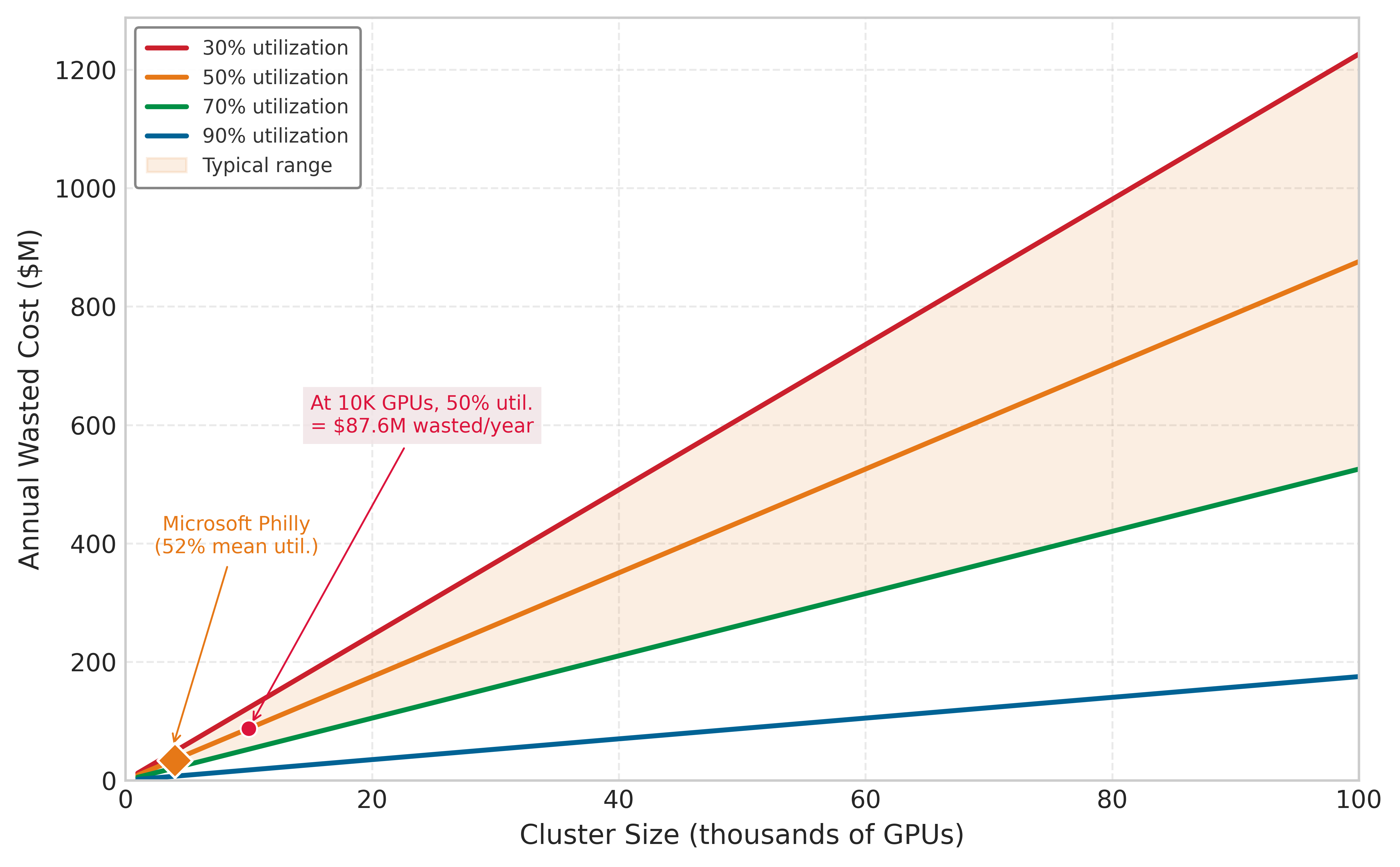
Jeon, Myeongjae, Shivaram Venkataraman, Amar Phanishayee, Junjie Qian, Wencong Xiao, and Fan Yang. 2019. “Analysis of Large-Scale Multi-Tenant GPU Clusters for DNN Training Workloads.” 2019 USENIX Annual Technical Conference (USENIX ATC 19), 947–60.

Li, Jie, George Michelogiannakis, Brandon Cook, Dulanya Cooray, and Yong Chen. 2023. “Analyzing Resource Utilization in an HPC System: A Case Study of NERSC’s Perlmutter.” Lect. Notes Comput. Sci., Lecture notes in computer science, vol. 13948: 297–316. https://doi.org/10.1007/978-3-031-32041-5_16.

The idle-capacity figure establishes the economic target; the remaining cost controls explain how the scheduler moves toward it. Interruptible capacity lowers the price of tolerant work, reservation and quota policy decide which jobs deserve scarce guaranteed capacity, and accountability mechanisms make idle GPUs visible to the teams that create demand.

Spot instances and preemptible VMs

Cloud providers offer spot instances¹³ (AWS) or preemptible VMs (GCP) at 60 to 90 percent discounts compared to on-demand pricing, with the caveat that instances can be reclaimed with as little as 30 seconds to 2 minutes notice when the provider needs the capacity for on-demand customers. At $0.70/GPU-hour instead of $2/GPU-hour, spot instances transform the economics of large-scale training, potentially reducing the cost of a multi-week pretraining run from hundreds of thousands of dollars to under one hundred thousand.

¹³ Spot Instances: Named after commodity trading’s “spot price” (the current market price for immediate delivery), spot instances sell spare cloud capacity at 60 to 90 percent discounts with the provider retaining reclamation rights. The critical asymmetry for ML training is the interruption notice window: AWS provides 2 minutes, GCP provides 30 seconds. A 175B-parameter model requires 3 to 5 minutes to checkpoint, so GCP’s 30-second notice forces either continuous checkpointing overhead or acceptance of lost work on every interruption.

The viability of spot instances for ML training depends on two factors that determine whether the discount translates into actual savings: the cost of each interruption (checkpoint overhead plus restart time plus lost work since the last checkpoint) and the frequency of interruption (which varies by instance type, region, time of day, and overall cloud demand). Equation 3 gives the effective cost of spot training:

\[ C_{\text{effective}} = C_{\text{spot}} \times \frac{T_{\text{total}}}{T_{\text{productive}}} \tag{3}\]

where \(T_{\text{total}}\) includes productive training time plus checkpoint overhead plus restart overhead after interruptions, and \(T_{\text{productive}}\) is the time spent advancing training. If interruptions are rare (less than once per day) and checkpointing is efficient (less than 5 percent overhead), effective cost remains close to the spot price and the savings are nearly the full discount. If interruptions are frequent (every few hours) and restarts are expensive (large model, slow checkpoint loading, cold GPU cache), effective cost can approach or even exceed on-demand pricing, turning the apparent discount into a hidden premium.

The relationship between spot savings and fault tolerance infrastructure is circular in an important way. The fault tolerance mechanisms from Fault Tolerance (frequent asynchronous checkpointing, fast checkpoint loading, elastic recovery) directly enable spot instance usage by minimizing the cost of each interruption. Elastic training allows jobs to continue with reduced worker count when some spot instances are reclaimed, avoiding full restart entirely. Organizations that invested in fault tolerance for reliability reasons discover that the same infrastructure unlocks significant cost savings through spot instance utilization, providing a return on their fault tolerance investment that goes far beyond avoiding lost work from hardware failures.

The strategic insight is that fault tolerance infrastructure has a double return: it both protects against involuntary losses (hardware failure) and enables voluntary cost savings (spot instances). This double return often justifies fault tolerance investments that would be hard to justify on reliability grounds alone, because the cost savings from spot utilization are concrete and measurable while the cost avoidance from hardware failure protection is statistical and harder to quantify.

Spot instance strategies for ML training

To maximize spot instance utility while minimizing disruption, sophisticated schedulers employ diversification and predictive strategies that go beyond simple “retry on failure” logic. Availability zone diversification reduces the probability of simultaneous fleet-wide reclamation. Cloud providers typically manage spot pools independently per availability zone (AZ). If a training job requires 1,024 GPUs, allocating them as a single block in one zone exposes the job to a complete stop if that specific zone’s spot pool is reclaimed. Spreading the job across multiple AZs ensures that a reclamation event in one zone affects only a fraction of the fleet. The scheduler still must model correlation carefully: independent per-instance interruptions make large simultaneous losses unlikely, but pool-level or AZ-level reclamations can remove hundreds of GPUs at once and must be treated as elastic-shrink or failover events rather than ordinary isolated failures.

Instance type diversification exploits independent spot markets across GPU SKUs. A job that strictly requests one instance type competes in a single, crowded market. A job that accepts multiple equivalent instance types dramatically increases its scheduling probability. The scheduler should maintain a priority-ordered list of acceptable instance types, falling back to larger-memory instances when the primary type is unavailable. While this mix requires careful peer-to-peer bandwidth management, it effectively uses the “upgrade” to maintain progress at a blended cost still far below on-demand rates.

Spot interruption prediction uses the data that cloud providers expose about reclamation likelihood, such as the AWS Spot Placement Score or GCP preemptibility data. Advanced schedulers ingest this feed to estimate the expected interruptions per day for a given instance type and region. If the expected interruption rate rises above a threshold where the overhead of restarts exceeds the cost savings (typically more than 4 interruptions per day for large models), the scheduler should automatically migrate the job to on-demand capacity or a different region, preventing thrashing where a job spends more time recovering than training.

Checkpoint frequency optimization for spot instances differs from the standard reliability logic. The Young-Daly formula developed in The Young-Daly law: Optimal checkpointing optimizes for unpredicted hardware failures. Spot interruptions, however, come with a warning: 2 minutes on AWS, 30 seconds on GCP. The optimal strategy is a two-tier checkpointing approach: a periodic checkpoint at the Young-Daly interval to protect against hard crashes, combined with an immediate checkpoint triggered by the termination notice. This “panic checkpoint” captures the exact state of training seconds before the node vanishes, reducing lost work to near zero and transforming preemption from a rollback event into a pause-and-resume event.

The same need for contingency planning becomes acute when spot interruptions are correlated rather than isolated.

Systems Perspective 1.5: Correlated spot risk

Context: Spot capacity is cheap because it is reclaimable. That risk is not independent across instances: cloud regions, instance types, product launches, and deadline cycles can create correlated demand.

Failure mode: A fleet that concentrates all interruptible training in one region and one instance type can lose a large fraction of workers at once, even if each individual worker appears restartable.

Consequence: Checkpointing handles isolated interruptions; it does not solve fleet-wide preemption when every retry targets the same exhausted pool.

Systems insight: A robust scheduler must diversify across regions and instance types, monitor interruption risk, and maintain a “break glass” path to on-demand capacity when the spot market becomes toxic.

Capacity reservation strategies

Organizations that rely on cloud infrastructure (or that think about on-premise infrastructure in economic terms) balance three tiers of compute capacity, each offering a different trade-off between cost, availability, and commitment. Table 4 compares those tiers across cost, availability, interruption risk, and workload fit.

Table 4: Cloud Capacity Reservation Tiers: Capacity tiers trade cost and commitment against availability guarantees and interruption risk, giving the scheduler a price ladder for routing workloads by urgency and restart tolerance.

Capacity tier	Cost and commitment	Availability and interruption risk	Best-fit workloads
Reserved capacity	One- to three-year commitments, with 30–60% discounts versus on-demand.	Guaranteed availability for the committed baseline.	Predictable continuous workloads: 24/7 inference, scheduled training, CI and regression testing, SLA-bound jobs.
On-demand capacity	Full price with no long-term commitment.	Immediate provisioning when queuing or interruption is unacceptable.	Urgent retraining, interactive debugging, and short-lived jobs that do not justify spot management.
Spot capacity	Discounted interruptible capacity.	Availability varies with cloud demand, and workers can be reclaimed.	Restart-tolerant jobs: hyperparameter sweeps, ablations, checkpointed pretraining, and exploratory research.

The optimal mix depends on workload characteristics and organizational priorities. An organization with 60 percent steady-state utilization and 40 percent burst demand might reserve capacity for 60 percent of peak need, use on-demand for latency-sensitive bursts that require immediate provisioning, and use spot for the remainder. The scheduling system must understand these capacity tiers and route workloads accordingly: inference workloads to reserved capacity for guaranteed availability, large training jobs to a mix of reserved (for the base allocation) and spot (for additional workers via elastic scaling), and exploratory work to spot exclusively where the cost savings are maximized and the interruption tolerance is highest.

Systems Perspective 1.6: Spot vs. on-demand training

Consider training a 70B parameter model requiring 512 GPUs for 14 days.

On-demand: 512 GPUs \(\times\) 336 hours \(\times\) $2/GPU-hour = $344,064

Spot (65 percent discount, 5 percent checkpoint overhead, 14 interruptions/day with 30 minutes restart):

• Base cost: 512 GPUs \(\times\) 336 hours \(\times\) $0.70/GPU-hour = $120,422
• Checkpoint overhead: 5 percent \(\times\) 336 hours = 16.8 hours
• Restart overhead: 196 interruptions \(\times\) 0.5 hours = 98 hours
• Total time: 336 hours + 16.8 hours + 98 hours = 450.8 hours
• Total cost: 512 GPUs \(\times\) 450.8 hours \(\times\) $0.70/GPU-hour = $161,567

Savings: $182,497 (53.0 percent), at the cost of approximately 34.2 percent longer wall-clock time.

The economics are compelling when fault tolerance infrastructure is already in place. Without checkpointing, a single interruption forces restart from scratch, potentially wasting days of compute and negating all savings.

Scheduling for cost efficiency

Cost-aware scheduling extends the scheduler’s optimization objective beyond utilization and fairness to include financial efficiency. Traditional schedulers minimize a single objective (for example, average job completion time or maximum wait time), but cost-aware schedulers must navigate multi-objective trade-offs where time, money, and reliability are all decision variables. The scheduler must routinely choose among three decision classes:

• Wait vs. run now: Run a job on reserved A100s now, or wait 2 hours for spot H100s that would complete the job 3\(\times\) faster at half the cost.
• Preempt vs. pay more: Preempt a low-priority hyperparameter sweep to make room for a high-priority training run on reserved capacity, or place the training run on more expensive on-demand instances.
• Fallback vs. elastic shrink: When spot capacity is reclaimed, migrate the job to on-demand to maintain throughput at higher cost, or scale down elastically to maintain low cost at reduced throughput.

Each decision prices time, money, and reliability differently, so cost-aware scheduling is policy design rather than simple bin packing.

These decisions require the scheduler to model both the time-value of computation (the organizational cost of a 2-hour delay in researcher productivity, product launch schedules, or competitive position) and the financial cost of different resource allocations. The time-value varies enormously by workload type: delaying a production model retrain by 2 hours might violate a service level agreement (SLA) and cost thousands in penalty fees, while delaying an exploratory experiment by 2 hours costs nothing but researcher patience.

Production systems typically define cost policies per workload class that encode these trade-offs as configuration rather than requiring per-decision human judgment. Inference workloads are pinned to reserved capacity for guaranteed availability and predictable latency, since the cost of an inference outage (lost revenue, degraded user experience) far exceeds the premium of reserved pricing. Large training runs use a mix of reserved capacity (for the minimum viable allocation) and spot capacity (for elastic expansion), with automatic fallback to on-demand if spot is reclaimed and the job is within a configurable deadline. Exploratory workloads are restricted to spot to minimize cost, with the understanding that they may be interrupted and must tolerate variable completion times.

Technical optimization must be paired with financial accountability through ML FinOps. In many organizations, GPU costs are pooled into a generic “infrastructure” bucket, creating a tragedy of the commons where teams lack visibility into their resource consumption and have no incentive to optimize. Effective governance requires granular tagging to implement showback (reporting costs to teams) or chargeback (billing teams’ budgets). Metrics must evolve from “GPU hours” to business-aligned units: “Cost per Model Version,” “Cost per Experiment,” and “Cost per 1M Predictions.” This shift transforms cost from an opaque infrastructure expense into a measurable input to product decisions, enabling teams to make informed trade-offs between model quality, training speed, and infrastructure cost. Cost visibility and attribution develops the platform machinery that makes these costs visible and attributable; the concern here is narrower, namely how that price signal reshapes the scheduling and quota behavior of the teams competing for the fleet.

The total cost of ownership

Optimizing for spot instance availability or scheduling density addresses only the visible tip of the infrastructure iceberg. The full cost of a machine learning fleet extends far beyond GPU-hours: in high-performance clusters the compute silicon typically accounts for only 40 to 60 percent of total system cost. The remainder is consumed by the supporting infrastructure required to keep that silicon fed and cool: high-bandwidth networking (InfiniBand switches, optics, and cabling), parallel file systems for checkpointing, and specialized power and cooling delivery. A single rack of H100 nodes can draw upwards of 40 kW, ten times the density of a standard web server rack, forcing facilities to deploy liquid cooling or rear-door heat exchangers that reshape the facility’s capital requirements. A scheduler that optimizes GPU-hours alone is therefore blind to most of what the fleet actually costs.

Whether that fixed capacity is worth owning is a question of utilization. Fleet Economics and Utilization develops the full build-versus-buy analysis, amortizing three years of capital and operational expenditure against cloud rental to find the break-even utilization that decides between them. The consequence for the scheduler is direct: owned hardware only amortizes when it stays busy, so every point of utilization the scheduler reclaims moves the fleet toward the break-even point that justifies its capital, while a cluster left idle by poor packing or fragmentation makes owned infrastructure more expensive than the cloud it was meant to undercut.

Checkpoint 1.2: Cost-aware scheduling trade-offs

Before moving to ML-specific schedulers, review how the cost-optimization mechanisms interact:

• Spot break-even: Determine the checkpoint frequency under which spot training becomes more expensive than on-demand for a 512-GPU, 14-day training job with a 65 percent spot discount, 1 interruption per day, and 30-minute restart overhead.
• Double return: Explain why fault tolerance infrastructure has a “double return” for reliability and cost savings, and identify the minimum fault tolerance investment needed to make spot instances viable.
• Reservation sizing: Determine whether increasing reserved capacity from 40 percent to 60 percent would save or waste money for an organization.

Spot pricing and reservation strategy squeeze the cost of running a job, but they leave a second source of efficiency untouched: the learning dynamics inside the training loop. The cost models so far optimize time-to-completion, yet the metric that matters to a research organization is time-to-accuracy, the wall-clock time until a run reaches a target validation metric. A scheduler blind to convergence cannot tell whether a run is in its steep early phase or its diminishing-returns tail, so it cannot redirect resources to where they buy the most progress. Closing that gap is the job of the ML-aware schedulers examined next.

Self-Check: Question

1. Why does the chapter treat utilization improvement as one of the highest-leverage cost optimizations in fleet orchestration?

   1. Because higher utilization mainly reduces software licensing fees rather than hardware waste
   2. Because utilization only matters in cloud settings where pricing is metered
   3. Because utilization improvements eliminate the need for quota systems
   4. Because a utilization gain converts existing hardware into additional productive GPU-hours, substituting for capital expenditure on new accelerators without changing the power and cooling bill

2. Spot instances advertise 60 to 70 percent discounts relative to on-demand pricing. Explain, using the chapter’s argument, why this discount does not automatically translate into lower effective training cost, and what property of the fault-tolerance stack determines whether it does.

3. Which workload is the best fit for reserved capacity rather than spot-only or purely on-demand placement?

   1. A hyperparameter sweep where each trial is disposable and tolerates interruption
   2. A one-off debugging task where startup speed matters far more than long-term cost
   3. A 24/7 production inference service with predictable baseline demand and strict availability requirements
   4. A weekend experiment that can wait for whichever capacity pool becomes cheapest

4. The chapter says fault-tolerance infrastructure has a ‘double return.’ Which interpretation is correct?

   1. It both raises researcher productivity and eliminates all hardware failures
   2. It reduces losses from routine hardware and software failures AND makes discounted but interruptible spot capacity economically viable, so the same checkpoint-and-recovery stack pays back through both reliability and cost channels
   3. It guarantees that cloud prices will eventually match on-premise costs
   4. It lets teams bypass quota governance by restarting interrupted jobs on different accounts

5. An organization is deciding between building an on-premise cluster and renting cloud GPUs. Explain why utilization is the key break-even variable in that decision.

See Answers →

Custom ML Schedulers

General-purpose schedulers treat training jobs as opaque boxes, so they cannot tell whether a model is in the steep early phase of learning or the final diminishing-returns phase. Custom ML schedulers trade implementation complexity for that visibility: they peer inside the training loop to optimize time-to-accuracy rather than only time-to-completion. The selection question is which internal signal addresses the fleet’s binding bottleneck, and the four systems differ less by scheduler sophistication than by the signal they ask the platform to trust: consumed service, iteration boundaries, completion value, or measured goodput.

Tiresias: Duration-agnostic scheduling

Tiresias (Gu et al. 2019) addresses the fundamental problem identified in section 1.0.5: ML job durations are unpredictable, and scheduling policies that rely on exact duration estimates can make poor decisions when those estimates are unavailable or unreliable. Rather than fighting this information asymmetry, Tiresias eliminates the requirement for duration estimates entirely. It uses a two-dimensional attained service¹⁴ scheduler that makes priority decisions based on what a job has already consumed, not what it claims it will consume. Jobs accumulate “service” based on GPU-time consumed, with priority decreasing as service increases. The two dimensions are time (how long the job has been running) and resources (how many GPUs the job uses), capturing both elapsed duration and resource intensity.

Gu, J., M. Chowdhury, K. G. Shin, Y. Zhu, M. Jeon, J. Qian, H. H. Liu, and C. Guo. 2019. “Tiresias: A GPU Cluster Manager for Distributed Deep Learning.” Proceedings of the 16th USENIX Symposium on Networked Systems Design and Implementation (NSDI ’19), 485–500.

¹⁴ Attained Service Scheduling: A discipline from OS queuing theory where priority decreases with cumulative resource consumption, approximating the theoretically optimal Shortest Remaining Processing Time (SRPT) policy without requiring the future knowledge that SRPT demands. In ML clusters, this approximation is particularly effective because job durations are heavy-tailed: the majority of submitted jobs are short experiments, so deprioritizing high-service jobs correctly identifies the long-running outliers without requiring users to provide runtime estimates they cannot accurately compute.

A discretized version groups jobs into service bins (for example, less than 1 GPU-hour, 1 to 10 GPU-hours, 10 to 100 GPU-hours, greater than 100 GPU-hours), promoting jobs in lower bins to the front of the queue. This bin structure means that all short jobs (the majority of submitted work) receive high priority and run quickly, while the few long jobs that consume most cluster resources gradually lose priority and are deprioritized relative to new arrivals. The key insight is that this behavior approximates the theoretically optimal Shortest Remaining Processing Time (SRPT) policy without requiring the future knowledge that SRPT demands: jobs that have consumed little service are statistically likely to be short jobs, so prioritizing them is a good heuristic for minimizing average completion time.

Experiments on production cluster traces from Microsoft and Alibaba show 40 to 60 percent reduction in average job completion time compared to FIFO scheduling, with the largest improvements for short jobs that previously waited behind long-running training runs. The improvement is not free: long-running training jobs experience increased completion times because they are systematically deprioritized. However, the aggregate benefit is positive because there are many more short jobs than long ones, and the short-job improvement exceeds the long-job penalty in total.

Gandiva: Iteration-aware scheduling

Gandiva (Xiao et al. 2018) exploits a characteristic that general-purpose schedulers completely ignore: the iterative nature of deep learning training. Each training iteration follows a predictable, repeating pattern: a GPU-intensive forward pass, a GPU-intensive backward pass, a communication-intensive gradient synchronization, and then a CPU-intensive data loading and preprocessing phase before the next iteration. During the data loading phase, the GPU sits partially idle, computing at less than full utilization while waiting for the next batch of data to be prepared.

Xiao, Wencong, Romil Bhardwaj, Ramachandran Ramjee, Muthian Sivathanu, Nipun Kwatra, Zhenhua Han, Prabal Patel, et al. 2018. “Gandiva: Introspective Cluster Scheduling for Deep Learning.” 13th USENIX Symposium on Operating Systems Design and Implementation (OSDI 18), 595–610.

Gandiva uses iteration-boundary time slicing, enabling higher utilization through controlled oversubscription. A cluster with 100 GPUs might support 120 concurrent jobs if each spends 20 percent of its iteration time waiting for data, because the scheduler can interleave data loading from one job with GPU computation from another on the same device. The critical insight that makes this practical is that iteration boundaries provide natural preemption points where GPU state is minimal. Between iterations, only model weights and optimizer state reside on the GPU; the intermediate activations from forward and backward passes have been freed. This minimal state makes context switching cheap (seconds rather than minutes), unlike preempting mid-iteration when the full activation memory is in use.

Gandiva also implements grow-shrink elasticity at a finer granularity than the framework-level elastic training discussed in section 1.3. Gandiva automatically adjusts data parallelism degree based on real-time resource availability, using profiled iteration times to predict the throughput impact of adding or removing workers. When a high-priority job arrives, Gandiva shrinks lower-priority jobs by reducing their worker count rather than killing them entirely, preserving their progress while freeing resources. When resources become available again, it grows jobs back to their preferred parallelism degree. This fine-grained elasticity, informed by actual iteration-level profiling data, enables scheduling decisions that general-purpose systems cannot make because they lack visibility into job internals.

Themis: Finish-time fairness

Traditional fair-share scheduling treats all GPU-seconds equally: a job consuming 100 GPU-hours is treated the same whether those hours represent the first 10 percent of a long training run or the last 10 percent of a nearly complete one. From a resource accounting perspective, 100 GPU-hours is 100 GPU-hours regardless of context. Themis (Mahajan et al. 2020) argues this resource-centric view is fundamentally unfair because it ignores the sunk cost of work already performed.

Mahajan, Kshiteej, Arjun Balasubramanian, Arjun Singhvi, Shivaram Venkataraman, Aditya Akella, Amar Phanishayee, and Shuchi Chawla. 2020. “Themis: Fair and Efficient GPU Cluster Scheduling.” 17th USENIX Symposium on Networked Systems Design and Implementation (NSDI 20), 289–304.

Themis defines a finish-time fairness metric that allocates resources to minimize the maximum slowdown any job experiences relative to exclusive access (the hypothetical scenario where the job has the entire cluster to itself). Under this metric, a job that is 90 percent complete and needs only 10 more GPU-hours to finish receives higher priority than a job that is 10 percent complete and needs 90 more GPU-hours. The reasoning is economic: delaying the nearly-complete job by an hour wastes the 900 GPU-hours already invested (because those hours only produce value when the job completes), while delaying the early-stage job by an hour has a proportionally smaller impact on the total investment’s return.

This approach benefits shorter jobs and nearly-complete jobs without excessive penalty to longer ones, and it aligns scheduling decisions with the economic value of completing work rather than the simple accounting of resource consumption. Themis implements this metric through an auction mechanism where jobs bid for resources based on their current marginal value (how much their completion time improves per GPU-hour allocated), creating a market-like dynamic that naturally directs resources to their highest-value use.

Pollux: Adaptive resource allocation

Pollux (Qiao et al. 2021) takes the most aggressive approach of the four research schedulers by jointly optimizing resource allocation and training hyperparameters. Where Tiresias, Gandiva, and Themis make scheduling decisions about jobs (when to run, how to share), Pollux makes decisions within jobs (how many GPUs and what batch size). The key observation is that the optimal number of GPUs for a training job depends on the current batch size, learning rate, and gradient noise level, all of which change during training as the model moves through different phases of convergence.

Qiao, Aurick, Sang Keun Choe, Suhas Jayaram Subramanya, Willie Neiswanger, Qirong Ho, Hao Zhang, Gregory R. Ganger, and Eric P. Xing. 2021. “Pollux: Co-Adaptive Cluster Scheduling for Goodput-Optimized Deep Learning.” 15th USENIX Symposium on Operating Systems Design and Implementation (OSDI 21), 1–18.

Pollux dynamically adjusts each job’s GPU allocation and batch size to maximize cluster-wide goodput, defined as the rate of useful training progress across all jobs simultaneously. The goodput metric folds both sides of the trade-off into one number: statistical efficiency (how much each gradient step advances convergence, which depends on batch size) and system throughput (how many gradient steps per second, which depends on GPU count and communication overhead). A job experiencing diminishing returns from its current GPU count (because communication overhead is growing superlinearly) may have GPUs reassigned to a job that would benefit more (because it is in a phase of training where larger batches improve statistical efficiency).

This co-optimization of scheduling and hyperparameters achieves 37 to 50 percent improvement in average job completion time compared to scheduling with fixed resource allocations. The improvement comes from two sources: better resource allocation (GPUs go to jobs where they produce the most progress) and better batch size tuning (each job runs at a batch size that balances statistical and computational efficiency for its current training phase). The combined effect is greater than either optimization alone.

Scheduler comparison framework

Custom ML schedulers represent a progressive trade-off between implementation complexity and scheduling precision, so the comparison in table 5 matters as a deployment filter rather than a ranking. General-purpose schedulers see declared resources and coarse runtime metadata; these research systems add ML-specific signals such as iteration structure, elasticity, convergence phase, and measured goodput.

Table 5: Custom ML Scheduler Comparison: A taxonomy of research schedulers based on the specific workload characteristic they exploit. Tiresias and Themis optimize for queuing metrics (JCT, fairness) using external signals, while Gandiva and Pollux optimize for efficiency using internal profiling data.

Scheduler	Key Insight	Scheduling Signal	Optimization Target	Overhead	Production Readiness
Tiresias	Attained service predicts remaining time	GPU-hours consumed	Minimize avg JCT	Low (no profiling)	Medium
Gandiva	Iteration boundaries are preemption points	Iteration timing	Maximize utilization	Medium (profiling)	Medium
Themis	Sunk cost matters for fairness	Completion percentage	Minimize max slowdown	Low (job metadata)	Low (auction complexity)
Pollux	Batch size and allocation are coupled	Goodput (stat + sys)	Maximize cluster goodput	High (continuous profiling)	Low (framework integration)

As table 5 summarizes, this design space reveals a fundamental tension: scheduler complexity vs. scheduling quality. Tiresias operates with the least information, essentially guessing that “young” jobs will finish soon, yet achieves significant gains simply by preventing large jobs from blocking small ones. It is robust because it requires no cooperation from the user or the training framework. At the other extreme, Pollux requires deep bidirectional integration: the scheduler must know the job’s scaling curve and gradient noise scale, and the job must accept commands to change its batch size and learning rate on the fly. When this integration works, it produces the highest cluster-wide throughput; when the assumptions are violated (for example, a model with unstable convergence dynamics that cannot tolerate batch size changes), the optimization collapses.

Failure modes generally track this complexity gradient. Tiresias fails gracefully: if its assumption (that past usage predicts future usage) is wrong, it simply degrades to a standard fair-share policy. Gandiva’s failure mode is performance jitter: if the profiling phase misestimates iteration variance, it may pack incompatible jobs onto the same node, causing interference. Pollux has the most brittle failure mode because it modifies the training semantics themselves; an incorrect goodput model could theoretically harm model convergence, a risk that most production teams are unwilling to take for a 15 percent efficiency gain.

For our 175B parameter model, these trade-offs dictate a hybrid lifecycle. Pollux offers the highest potential improvement during the early, unstable phase of training where batch sizes are small and the job is elastic; it could dynamically resize the job to fit available holes in the cluster. However, effectively using Pollux requires modifying the training loop to be elasticity-aware. Tiresias offers the simplest deployment path: it would treat the 175B model as a “heavy” job and deprioritize it relative to small experiments, ensuring the cluster remains responsive to researchers without requiring any changes to the 175B model’s code. In practice, most infrastructure teams start with Tiresias-like policies to solve the “blocked queue” problem before attempting the deep integration required by Pollux.

The consistent theme across all four systems is that exploiting domain-specific knowledge about ML workloads (predictable iteration times, diminishing returns from parallel scaling, and inherent checkpoint-restart capability) enables dramatically better scheduling outcomes than static resource requests alone. A generic scheduler sees a job requesting 64 GPUs for 3 days; an ML-aware scheduler sees a stochastic gradient descent process that converges nonlinearly, releases resources if performance plateaus, and can be preempted with minimal loss. The decision framework for selecting among these schedulers depends on the primary bottleneck: for exploratory clusters with high churn, Gandiva’s time-slicing minimizes queuing delay; for production training where job completion time is the primary SLA, Tiresias’s age-based prioritization prevents starvation; for large-scale training where resource efficiency is paramount, Pollux’s adaptive scaling reclaims the “elasticity gap” that static allocation leaves on the table.

The challenge for production systems is incorporating these insights while maintaining the operational reliability, policy flexibility, and organizational governance that production environments require. Production platforms usually adopt scheduler ideas selectively because reliability, governance, heterogeneous hardware, and user policy constrain pure research designs.

From research to production

Research schedulers become useful in production only when their core signal survives contact with a heterogeneous data center. In research, the cluster is often assumed to be a homogeneous pool of accelerators with uniform interconnect topology, and jobs are well-behaved entities that declare their resource needs accurately. In production, the “cluster” is a geological formation of hardware generations: V100s alongside A100s and H100s, connected by a patchwork of InfiniBand and Ethernet, running jobs that frequently crash, hang, or misrepresent their memory requirements. Consequently, no major hyperscaler simply “installs” a research scheduler; instead, they selectively transplant specific algorithms into standard orchestrators via Kubernetes operators or Slurm plugins.

Consider our 175B-parameter model training run. A pure implementation of Pollux might aggressively resize the job based on global cluster load, scaling the number of GPUs up and down to maximize goodput. However, changing the worker count for a synchronous training job requires a checkpoint-restart cycle, which for a model of this size involves writing terabytes of optimizer state to persistent storage. If the re-scaling interval is too short, the I/O overhead of checkpointing negates the throughput gains. In practice, production teams adopt a hybrid approach: they use Pollux-style adaptive allocation primarily during the volatile early phase of training or for hyperparameter sweeps, but lock the 175B model into a static, topology-aware allocation once the learning rate warmup completes and the job enters its months-long steady state.

The build-vs.-buy decision for a custom scheduler is a substantial capital investment. Developing a robust, fault-tolerant scheduler that outperforms the default bin-packing behavior of Kubernetes requires a specialized team of 3 to 5 systems engineers working for 6 to 12 months. The ROI math is what justifies the effort: if the team can improve overall cluster utilization by 10 percent on a fleet of 10,000 H100 GPUs (approximately $25,000 per hour in capital depreciation and power), the savings amount to roughly $22 million per year. This stark return on investment drives the development of internal scheduling platforms at every major AI lab, transforming the scheduler from a mere utility into a primary lever for operational efficiency.

The risk is not only implementation cost; scheduler behavior can also fail to match the execution semantics of distributed training.

War Story 1.1: OpenAI's gang-scheduling deadlock (2021)

Context: OpenAI scaled Kubernetes clusters to 7,500 nodes for workloads including GPT-3, CLIP, and DALL-E. Their large training jobs used MPI-style execution, where all workers in a group had to be scheduled simultaneously before training could make progress (Sigler 2021).

Failure mode: Default Kubernetes scheduling did not guarantee that all of one job’s workers would be placed before scheduling started filling another job. If two experiments each requested the whole cluster, Kubernetes could schedule half of each job instead of all of one job, leaving both jobs unable to run.

Consequence: The cluster could appear busy while no experiment made useful training progress: a classic gang-scheduling deadlock caused by partial allocation.

Systems lesson: Distributed ML scheduling must encode the job’s execution semantics. For MPI-style training, “some pods scheduled” is not partial progress; it is wasted allocation. Production schedulers need gang scheduling, quota controls, and workload-aware policies rather than generic pod placement alone.

Sigler, Eric. 2021. Scaling Kubernetes to 7,500 Nodes. OpenAI Blog.

A scheduler designed for general-purpose pod placement will mishandle workloads that require gang semantics, and adding gang awareness alone does not resolve priority conflicts among competing training jobs. Each of the four research schedulers examined above addresses one facet of this problem (runtime estimation, iteration-boundary preemption, fairness across finish times, or joint resource-hyperparameter tuning), but none addresses all facets simultaneously. The design space is therefore a set of explicit trade-offs rather than a single optimal policy.

Checkpoint 1.3: Custom scheduler design space

Consider the trade-offs between the four research schedulers:

• Estimate-free scheduling: Identify the information Tiresias sacrifices by eliminating runtime estimates, and describe when that sacrifice hurts scheduling quality.
• Time-slicing limits: Identify workloads for which Gandiva’s iteration-boundary time-slicing fails, and explain why.
• Job starvation: Assess whether Themis’s preference for nearly complete jobs can starve long-running pretraining jobs indefinitely.
• Goodput-model risk: Describe the failure mode when Pollux’s goodput model is wrong.

Custom schedulers maximize throughput for long-running training jobs, but the operational reality changes drastically when models are deployed for inference. The objective function flips from maximizing cluster utilization to guaranteeing millisecond-level responsiveness. Serving resource management must handle bursty, unpredictable traffic patterns while adhering to strict Service Level Objectives.

Self-Check: Question

1. What is the central limitation of general-purpose schedulers that motivates custom ML schedulers such as Tiresias and Pollux?

   1. They cannot run on clusters with more than a few hundred GPUs
   2. They treat training jobs as opaque resource consumers and ignore ML-specific signals such as iteration timing, learning-curve position, and convergence trajectory
   3. They can schedule only inference services, not training jobs
   4. They require every user to submit Kubernetes YAML rather than shell scripts

2. Which scheduler specifically addresses poor user runtime estimates by prioritizing jobs according to attained service rather than predicted duration?

   1. Tiresias
   2. Gandiva
   3. Themis
   4. Pollux

3. Explain why Gandiva uses iteration boundaries as a practical time-slicing point for GPU sharing, and why preempting at an arbitrary cycle inside an iteration would be strictly worse.

4. What makes Pollux more powerful but also more operationally risky than Tiresias?

   1. Pollux requires a centralized filesystem while Tiresias does not
   2. Pollux works only for inference while Tiresias works only for training
   3. Pollux avoids all profiling overhead by assigning every job to a fixed static class
   4. Pollux jointly tunes GPU allocation AND training hyperparameters (batch size, effective learning rate) based on its model of useful training progress per GPU-hour, so a mistake in that model can hurt convergence, not just queue order; Tiresias changes only scheduling priority, so a mistake there only shifts wait times

5. True or False: Minimizing average job completion time is a safe universal objective for a shared ML cluster, because a lower average automatically implies better outcomes for every workload class.

6. A platform team wants to adopt ideas from ML research schedulers but is wary of deep framework integration. Which scheduler family is the most plausible starting point, and why?

See Answers →

Serving Resource Management

Training jobs are predictable, batch-oriented workloads that run for weeks; serving workloads are volatile, user-facing services that must respond in milliseconds to unpredictable traffic spikes. When an e-commerce platform launches a major sale, the serving fleet must instantly autoscale to handle thousands of requests per second. Serving resource management forces the orchestrator to balance these aggressive latency constraints against raw hardware utilization.

For orchestration, the important serving fact is that inference capacity is a live envelope around user traffic rather than a batch allocation around a training job. The fleet orchestrator manages that envelope by scaling replica counts up and down with demand, isolating serving workloads from interference, and balancing inference resource needs against training’s claims on the same shared infrastructure.

Autoscaling for inference

Kubernetes Horizontal Pod Autoscaling (HPA) adjusts replica counts based on observed metrics, adding instances when load increases and removing them when load decreases. The default autoscaling metric for general cloud workloads is CPU utilization, with targets of 50 to 70 percent. This default poorly reflects GPU inference workloads for two reasons. First, GPU utilization is a noisy metric that can be high even when the system is not processing user requests (background maintenance, model warmup). Second, the relationship between GPU utilization and inference latency is highly nonlinear: latency can spike dramatically when utilization crosses a threshold (typically 70 to 80 percent for GPU inference), making utilization-based scaling reactive rather than predictive. The metric choice is therefore the first scheduling decision for serving: table 6 lists custom inference metrics that predict user-facing degradation before it occurs.

Table 6: Inference Autoscaling Metrics: Custom metrics for GPU inference workloads capture the relationship between load and user-facing performance more accurately than default CPU utilization. Queue depth provides a leading indicator of latency degradation, while pending tokens captures outstanding autoregressive decode work; KV-cache residency and context-length distribution then determine whether that work is also memory-pressure risk.

Metric	Target Range	Considerations
GPU utilization	60 to 80%	Varies by model batch efficiency
Request queue depth	10 to 50 requests	Prevents latency spikes before they manifest in P99 metrics
P99 latency	Below SLO target	Reactive metric that lags demand changes by seconds to minutes
Pending tokens	Model-specific	Tokens queued or currently being decoded across active requests

Beyond the HPA-oriented metrics in table 6, Vertical Pod Autoscaling (VPA) operates on a different axis, adjusting resource requests and limits for individual pods. Where HPA changes how many instances run, VPA changes how much resource each instance receives. For inference, VPA can right-size memory allocations based on observed usage patterns, preventing over-provisioning of CPU memory and host resources that reduces the number of inference pods that fit on each node. GPU resources cannot be vertically scaled without pod restart (the CUDA context must be reinitialized), limiting VPA’s utility for accelerated workloads where model loading takes minutes. However, VPA is valuable for the CPU components of inference pipelines, such as preprocessing, postprocessing, and tokenization, where resource requirements may differ significantly from initial estimates and can be adjusted with a brief pod restart.

Large language model (LLM) inference requires specialized scaling considerations that neither HPA nor VPA fully address, due to the key-value (KV) cache¹⁵ memory growth pattern. A 70B parameter model serving long-context requests may require more than 80 GB of GPU memory for KV cache alone, even when the serving engine stores that cache in paged, noncontiguous blocks. The GPU memory bottleneck for LLM serving is therefore not the model weights (which are fixed) but the KV cache (which grows with request count and context length). Scaling decisions must account for both request rate and context length distribution, not just computational load. A sudden increase in requests with long contexts (for example, a shift from short chatbot queries to document summarization workloads) can exhaust GPU memory even at moderate request rates, requiring scale-out despite low GPU compute utilization. Conversely, a burst of many short-context requests may stress compute without threatening memory limits.

¹⁵ Key-Value (KV) Cache: Stores precomputed attention key and value tensors to avoid recomputing attention over the entire sequence for each new token. KV cache grows linearly with sequence length and batch size; for a 70B model with 128K context, the cache can exceed the model weights in memory consumption. This growth pattern creates a scheduling failure mode invisible to compute-based autoscalers: GPU memory exhaustion at low compute utilization, causing requests to stall even when the GPU appears idle.

This dual resource dimension (compute and memory) suggests that effective LLM autoscaling should monitor both GPU compute utilization and GPU memory pressure, scaling out when either approaches critical thresholds. Some production systems define a composite scaling metric that combines these dimensions, triggering scale-out when the maximum of normalized compute utilization and normalized memory pressure exceeds a threshold. This composite approach prevents the system from being surprised by either type of resource exhaustion.

Autoscaling for inference must also handle cold start latency, which creates a tension between cost efficiency and responsiveness that has no simple resolution. The cold-start problem in serving is quantitatively more severe than in standard web services due to the sheer mass of model weights. A 70B-parameter model in FP16 occupies approximately 140 GB, and all of it must reach GPU memory before the first request can be served, a transfer bound by PCIe or NVLink bandwidth. Even at the per-direction PCIe Gen4 x16 speed of 32 GB/s, the raw transfer takes over 4 seconds, and in practice model initialization, graph compilation, and safety checks extend this to 60–120 seconds. Loading from Non-Volatile Memory Express (NVMe) SSDs at 7 GB/s read bandwidth takes roughly 20 seconds; from network storage, it can exceed 2 minutes.

Aggressive scale-down policies that terminate replicas during brief traffic lulls create painful cold starts when traffic returns minutes later, producing latency spikes that violate SLOs and degrade user experience. The fundamental problem is that inference traffic exhibits burstiness at multiple timescales (seconds, minutes, hours), and short-term lulls do not reliably predict sustained low demand. A five-minute quiet period might be followed by a traffic spike, and the cost of a cold start during that spike (degraded latency for all requests while the model loads) can exceed the cost savings from the few minutes of freed GPU capacity.

Production systems address cold start through three complementary strategies:

• Minimum replica count: Keeping at least one warm replica above zero eliminates cold starts for the first burst of traffic but incurs a baseline cost even during truly idle periods.
• Predictive scaling: Scaling from historical traffic patterns, such as diurnal cycles, day-of-week patterns, and known events, adds capacity before expected peaks rather than reacting after load arrives.
• Prewarming: Loading model replicas into GPU memory on standby GPUs reduces activation from minutes of model loading to seconds of process initialization, but standby replicas consume GPU memory that cannot serve other workloads.

Organizations with multiple models competing for the same GPU pool must balance the prewarming overhead against the cold-start penalty, choosing which models to keep warm based on their traffic patterns and latency requirements.

Predictive autoscaling and SLO management

Reactive autoscaling (like Kubernetes HPA) is inherently backward-looking: it observes a metric breach (for example, GPU utilization exceeding 80 percent), waits for a stabilization window, and then triggers a scale-up event. For a container that starts in milliseconds, this lag is negligible. For a 175B parameter model that takes 3 minutes to load weights from disk to GPU memory, this lag is fatal to SLOs. If traffic doubles in 30 seconds, a realistic scenario during a product launch or viral event, the reactive scaler will provision new replicas only after the surge has already saturated the existing fleet, causing a 3-minute window of degraded latency and dropped requests.

During this cold-start gap, continuous batching (also called in-flight batching) functions as a shock absorber. Serving engines that implement continuous batching, such as vLLM or TensorRT-LLM, do not wait for a fixed batch to fill before beginning generation; instead, they interleave new incoming requests into ongoing decode steps whenever a sequence slot becomes free. When load spikes and new replicas are still loading, the engine responds by increasing the live batch size toward the KV-cache memory limit, accepting more concurrent sequences per iteration. This absorbs additional requests without rejecting them, sustaining acceptable latency at the cost of higher per-request memory pressure. The relief is bounded: once the KV cache is fully saturated—meaning active sequences occupy every available memory page—the engine must begin queuing or shedding load regardless of batch elasticity. The scheduler therefore has a narrow window, typically from the moment the autoscaler fires until KV-cache saturation, in which continuous batching buys time. Tuning minimum replica counts and scale-up thresholds to keep that window open is the principal lever for preventing SLO violations during traffic ramps that exceed cold-start duration.

Reactive autoscaling opens an SLO gap during cold start.

Predictive autoscaling decouples scaling actions from current load. By analyzing historical traffic patterns (diurnal cycles, day-of-week seasonality) and incorporating real-time leading indicators (for example, a surge in login requests often precedes a surge in inference queries), the scheduler can preprovision capacity before the demand arrives. Serving our 175B model with a 500 ms P99 SLO requires this anticipation. If the model takes 3 minutes to become ready, the predictive scaler must issue the scale-up command at least 4 minutes before the expected traffic ramp. This transforms the scaling problem from a control theory problem (reacting to error) to a forecasting problem (predicting the future).

Effective scaling policies must be SLO-driven rather than utilization-driven. Targeting a fixed utilization (for example, “keep GPU at 70 percent”) is a proxy that often fails: a model might hit its latency SLO at 60 percent utilization due to memory bandwidth contention, or it might safely run at 90 percent utilization if the requests are compute-bound and uniform. An SLO-driven policy explicitly targets the metric that matters: “Scale up when P99 latency exceeds 400 ms (80 percent of the 500 ms target).” This approach automatically adapts to changes in workload characteristics. If a new model version is less efficient, the latency metric will rise faster, and the scaler will provision more replicas to maintain the SLO, without requiring manual tuning of utilization thresholds.

To prevent oscillation, where the scaler rapidly adds and removes replicas during noisy traffic, production systems implement hysteresis and cooldown periods. A typical policy scales up aggressively (no stabilization window) to protect the SLO, but scales down conservatively (15-minute cooldown) to avoid thrashing. This asymmetry acknowledges that the cost of an unnecessary scale-up (wasted compute for 15 minutes) is far lower than the cost of a missed scale-up (SLO violation and user churn).

Napkin Math 1.6: The autoscaling lag

Consider a serving fleet with 10 replicas, each capable of 5 QPS while meeting the 500 ms SLO. Total capacity: 50 QPS.

Scenario: Traffic ramps from 40 QPS to 80 QPS linearly over 60 seconds. Model load time: 3 minutes (180 seconds).

Reactive scaling: HPA detects overload at \(t =\) 15 s (when traffic hits 50 QPS). It requests 10 new replicas. These replicas become ready at \(t =\) 195 s (15 + 180 seconds). From \(t =\) 15 s to \(t =\) 195 s, demand exceeds capacity. During the ramp, excess demand grows linearly from 0 to 30 QPS; after the ramp reaches 80 QPS, the full 30 QPS overload persists until the new replicas are ready. The area above capacity is approximately 4,725 requests, all of which are queued or dropped and violate the SLO.

Predictive scaling: The scaler forecasts the ramp and triggers scale-up at \(t =\) -180 s. The 10 new replicas come online at \(t = 0\) s, pushing capacity to 100 QPS just as the ramp begins. Zero SLO violations.

Resource isolation

When multiple inference workloads share the same physical hardware, noisy neighbor problems arise when one workload’s resource consumption degrades another’s performance. On GPUs, interference manifests through four shared resource channels:

• Memory bandwidth: One workload’s data movement can saturate the HBM interface.
• L2 cache contention: One workload’s working set can evict another’s cached data.
• PCIe bottlenecks: Concurrent host-device transfers can compete for bus bandwidth.
• Thermal effects: One workload’s heat generation can cause thermal throttling that affects all workloads on the same GPU.

For latency-sensitive inference, even minor interference can push P99 latency above SLO thresholds, turning a seemingly well-provisioned system into an SLO-violating one.

MIG sits at the strong-isolation end of this design space. Table 2 already showed the fixed profiles; the operational implication is that hardware isolation removes most cross-tenant interference but turns partition choice into a placement constraint. MIG is available only on A100 and later GPUs, profiles cannot change without draining all workloads from the GPU, and fixed partition sizes may not match workload requirements. A workload that needs 15 GB of GPU memory wastes 5 GB on a 20 GB MIG instance or cannot fit on a 10 GB instance.

Software approaches to isolation provide more flexibility at the cost of weaker guarantees. Efficiently sharing GPUs for inference requires navigating a hierarchy of isolation mechanisms, each trading performance for security. At the simplest level, CUDA time-slicing allows multiple processes to share a GPU by context-switching the compute resources. While flexible, this incurs high latency penalties (often 10–20 ms) and offers no memory isolation. NVIDIA’s Multi-Process Service (MPS)¹⁶ improves this by allowing kernels from different processes to run concurrently on the same GPU, improving throughput for small batch inference while providing weaker isolation than MIG (Volta and newer give each client a separate GPU address space, but compute and memory bandwidth remain shared).

¹⁶ CUDA MPS (Multi-Process Service): Enables concurrent kernel execution from multiple processes on a single GPU, eliminating the 10 to 20 ms context-switch penalty of time-slicing. MPS adds approximately 5 to 10 microseconds of overhead per kernel launch but provides no memory isolation: a process that exhausts GPU memory crashes all colocated workloads. This makes MPS suitable for trusted, same-team inference workloads but dangerous for multi-tenant environments where a single misbehaving model can take down its neighbors.

GPU memory isolation prevents one model from consuming memory needed by another through explicit memory limits enforced by the container runtime. Without such limits, a memory leak, an unexpectedly large batch (triggered by a request with unusually long context), or a misbehaving custom kernel can consume all available GPU memory and crash colocated workloads. MPS improves utilization for small workloads by eliminating the context-switching overhead of time-slicing, but it adds latency overhead of approximately 5 to 10 microseconds per kernel launch and provides limited protection against memory bandwidth interference.

Furthermore, long-running serving instances suffer from dynamic memory fragmentation. The key culprit is the KV cache in transformer inference, which grows and shrinks with request sequence length. Standard allocators struggle with these highly variable lifetimes, leaving holes in GPU memory too small for new requests but collectively wasting gigabytes. Serving engines increasingly use paged memory management to allocate KV cache in noncontiguous blocks, reducing fragmentation-induced out-of-memory failures; Inference at Scale develops the paged-allocation mechanism in full.

At the CPU level, core pinning assigns specific CPU cores to inference pods, preventing the Linux scheduler from migrating processes between cores in ways that invalidate processor caches. For latency-sensitive workloads, isolating cores using isolcpus kernel parameters and taskset affinity removes OS scheduling jitter that manifests as random latency spikes. Combined with NUMA-aware¹⁷ placement that ensures inference pods access memory through the nearest memory controller (avoiding remote NUMA access that adds 50 to 100 ns per access), this reduces P99 latency by 10 to 30 percent for sub-millisecond inference tasks. The principle is straightforward: inference latency is dominated by memory access patterns, and any source of memory access unpredictability, whether cache eviction from core migration, remote NUMA access, or TLB misses from address space switching, directly degrades tail latency.

¹⁷ NUMA (Non-Uniform Memory Access): Local memory access takes approximately 100 ns vs. 150 to 200 ns for remote-socket access, a 50 to 100 percent penalty. For ML inference preprocessing, placing CPU cores on the wrong NUMA domain relative to the GPU’s PCIe connection adds this penalty to every host-device transfer, inflating P99 latency by 10 to 30 percent for sub-millisecond inference tasks. The fix is straightforward (CPU pinning and NUMA-aware pod scheduling) but often overlooked in Kubernetes deployments where the default scheduler ignores NUMA topology entirely.

The isolation techniques discussed here represent a spectrum from strong (MIG, hardware isolation) to flexible (MPS, software sharing), and the choice depends on the trust boundary between colocated workloads. Multi-tenant inference platforms serving different external customers typically require MIG for security isolation. Single-tenant platforms serving different internal models on the same GPU can use MPS or time-slicing where the isolation requirements are weaker.

GPU sharing economics

The decision to co-locate multiple models on a single GPU defines the efficiency frontier of an inference fleet. This choice operates on a spectrum: at one end, exclusive access guarantees isolation but strands capacity; at the other, aggressive sharing (via MPS or time-slicing) maximizes utilization but risks latency interference. The physics of this trade-off are dictated by memory fragmentation and compute contention.

Sharing packs two tenants, cutting wasted memory from 67 percent to 35 percent.

Consider an 80 GB A100 GPU serving a 7B parameter model. The model weights in FP16 consume approximately 14 GB. With a typical KV cache and activation overhead, the total runtime footprint is roughly 26 GB. Under an exclusive access policy, this single model leaves 54 GB (67 percent) of the GPU’s high-bandwidth memory dark, a waste of silicon capital. Partitioning the GPU with MIG (for example, a 3g.40gb profile) tightens the container, reducing the waste to roughly 35 percent within the partition, but still leaves the remainder of the GPU strictly segmented. Enabling MPS to pack two such models onto the same 80 GB device consumes 52 GB, dropping the aggregate memory waste to just 35 percent. For fleets running hundreds of small models, shifting from exclusive to shared hosting can reduce the required GPU count by a factor of 2–3\(\times\).

This density comes at the cost of interference. When two workloads share a GPU via MPS, they compete for Streaming Multiprocessors (SMs) and memory bandwidth. The degradation is workload-dependent: two compute-bound models (for example, large batch processing) fighting for ALUs often see 15 to 20 percent throughput degradation each. However, a compute-bound model co-located with a memory-bound model (for example, decoding-heavy generation) often coexist peacefully, seeing only 5 percent degradation because they bottleneck on different hardware resources. The scheduler’s job thus becomes a multi-dimensional bin packing problem: finding complementary workloads that maximize density while respecting latency SLOs.

For a heterogeneous fleet, this logic dictates a bifurcated strategy. Our 175B parameter model requires about 350 GB just for FP16 weights; on 80 GB A100s that means at least five GPUs before KV cache, activation buffers, runtime workspace, and tensor-parallel granularity are included. In practice, an 8-GPU tensor-parallel replica is the cleaner scheduling unit and is a candidate for exclusive access. Conversely, the dozens of 1B to 7B parameter support models, such as toxicity classifiers, query embedding encoders, and auxiliary generation models, are prime candidates for sharing. By packing these smaller models onto shared “utility nodes,” the orchestrator liberates high-performance clusters for the heavy lifting of foundation model inference.

Napkin Math 1.7: GPU sharing ROI

Consider a fleet serving 100 distinct 7B models (26 GB footprint each) and 10 distinct 175B models (350 GB footprint each).

Strategy A – exclusive access (one model per GPU): The 7B models require 100 A100 GPUs (80 GB each), achieving only 32.5 percent memory utilization (100 \(\times\) 26 GB used out of 8000 GB total). The 175B models require 80 GPUs (10 models \(\times\) 8 GPUs each for tensor parallelism). Total fleet: 180 GPUs.

Strategy B – mixed sharing (MPS for small, exclusive for large): Pack 2 models per A100 for the 7B models (2 \(\times\) 26 GB = 52 GB, well within 80 GB), requiring only 50 GPUs at 65 percent memory utilization. The 175B models remain unchanged at 80 GPUs. Total fleet: 130 GPUs.

Sharing reduces the fleet size by 27.8 percent (50 fewer GPUs). At $2/GPU-hour, this saves approximately $876,000 annually in compute costs, purely through scheduling policy.

Model routing and traffic management

Once resources are isolated, the orchestrator faces the challenge of directing inference queries to the correct model replicas. For a monolithic web service, simple round-robin load balancing suffices. For a 175B parameter language model served across thousands of GPUs, routing becomes a complex distributed systems problem where the “unit of serving” is no longer a single container but a tensor parallel group, a collection of 8 GPUs that must function as a single logical entity. The load balancer cannot simply route a request to “GPU 12”; it must route to “TP Group 3,” ensuring the request arrives at the exact moment the group is ready to process it.

Request routing strategies determine cluster-wide throughput. Naive round-robin distribution fails for generative workloads because request processing times vary by orders of magnitude based on output token length. A round-robin scheduler inevitably sends new requests to replicas backed up with long-generation tasks, causing tail latency to spike. Least-outstanding-requests (LOR) routing improves this by directing traffic to the idlest replicas. However, for large language models, memory-aware routing is superior. By tracking the KV cache occupancy of each replica, the router can send long-context requests to replicas with ample free memory and short requests to those near capacity, preventing fragmentation-induced out-of-memory errors and increasing effective batch sizes by 30 to 40 percent compared to blind routing.

Traffic shifting mechanisms like canary deployments and A/B testing are essential for safe model updates. When deploying Model v2, the orchestrator does not simply replace Model v1. Instead, it spins up v2 replicas alongside v1, creating a shadow fleet. The traffic manager routes 1 percent of live requests to v2 (often in “shadow mode,” where the response is computed but discarded) to validate latency and error rates against v1. Only after statistical verification does the orchestrator gradually shift weights (5 percent, 25 percent, 100 percent), draining v1 replicas only as v2 proves stable.

Multi-model serving complicates this further. A single cluster often hosts diverse models: a product recommendation model (10 ms P99 SLO, high throughput) alongside a coding assistant model (2,000 ms P99 SLO, bursty usage). Placing these on the same node invites interference; placing them on separate clusters strands capacity. The optimal strategy uses latency-aware bin packing: the orchestrator co-locates latency-critical models with batch-processing jobs (like embedding generation) that can be throttled instantly, ensuring high utilization without violating strict SLOs.

The training-serving resource boundary

The deepest utilization divide in the ML fleet is the wall between training and serving. Most organizations manage these as separate fiefdoms: a “Production Serving” cluster that must handle peak traffic (and sits 50 percent idle at night) and a “Research Training” cluster that is perpetually backlogged. This static partitioning is safe but economically inefficient. Dynamic sharing unifies these pools, but it introduces a fundamental friction: the mode-switching cost.

Repurposing a GPU from training to serving is not instantaneous. The orchestrator must checkpoint the training job (1 to 5 minutes), kill the container, launch the inference server, load the model weights from storage (2 to 10 minutes), and run warmup queries (1 to 5 minutes) to populate compilation caches. This 5-to-20-minute switching latency means GPUs cannot react to second-by-second traffic bursts. Instead, they must follow diurnal patterns.

Inference traffic typically follows a “human curve”: low at 3 AM, ramping up at 8 AM, peaking at 2 PM, and tapering off at 10 PM. A smart orchestrator forecasts this curve 30 minutes in advance. At 7:30 AM, it preempts low-priority training jobs (like hyperparameter sweeps) to warm up inference replicas. At 10:30 PM, as traffic drops, it drains inference replicas and releases GPUs back to the training scheduler.

Napkin Math 1.8: The diurnal GPU shift

Consider a fleet of 1,024 GPUs managed under two regimes:

Scenario A – static partitioning: The serving pool reserves 400 GPUs to handle peak demand, but average usage is only 150 GPUs (37.5 percent utilization). The training pool reserves 618 GPUs, and backlog ensures 100 percent utilization. Result: 150 GPUs + 618 GPUs = 768 active GPUs. Fleet utilization: 75 percent.

Scenario B – dynamic sharing: Serving claims GPUs strictly as needed (average 150 GPUs). Training reclaims unused serving GPUs (average 250 GPUs), minus a 117-GPU safety buffer. The orchestrator shifts approximately 133 GPUs between roles twice daily based on diurnal forecasts. Result: serving (150 GPUs) + training (618 GPUs + 133 GPUs) = 901 active GPUs (the second training term is reclaimed serving capacity). Fleet utilization: 88 percent.

Dynamic sharing recovers 133 GPUs of effective capacity. At $2/GPU-hour, this creates approximately $2.3M per year in value without purchasing a single additional accelerator.

Optimizing isolation for a single deployment is straightforward, but maintaining strict guarantees becomes volatile when thousands of training and serving workloads coexist on the same infrastructure. The collision of high-priority inference SLAs with resource-hungry training jobs creates a noisy neighbor problem that simple containerization cannot solve. Multi-tenancy and quotas become the governance layer that arbitrates fair access and prevents tragedy-of-the-commons scenarios in shared fleets.

Self-Check: Question

1. Why is raw GPU utilization often a poor primary autoscaling signal for LLM inference services?

   1. GPU utilization is relevant only to training, so serving should ignore it entirely
   2. Queue depth and KV-cache memory pressure can predict SLO violations well before GPU utilization alone reflects the stress, so a utilization-only policy tends to scale too late
   3. GPU utilization cannot be measured accurately under Kubernetes
   4. Latency always decreases as GPU utilization increases, so utilization is actively misleading

2. Explain why predictive autoscaling is especially important for large-model serving compared with ordinary web services.

3. Which GPU-sharing mechanism provides the strongest hardware-level isolation against noisy-neighbor interference in multi-tenant inference?

   1. CUDA time-slicing
   2. MPS
   3. MIG
   4. Round-robin request routing at the load balancer

4. A fleet serves many 7B models and a few 175B models. According to the section, which resource-management strategy is usually most economical?

   1. Give every model exclusive access to a full GPU or full tensor-parallel group
   2. Force the 175B models onto MIG slices so every model uses the same scheduling primitive
   3. Run all models on CPUs during low-traffic periods to avoid any GPU interference
   4. Pack the small 7B models onto shared utility GPUs (via MIG or MPS) and keep the 175B models on exclusive multi-GPU tensor-parallel groups

5. Least-outstanding-requests routing is adequate for many web services but not for LLM serving. Explain the gap and what additional signal closes it.

6. Why does dynamic sharing between training and serving capacity usually follow diurnal forecasts rather than reacting second-by-second to current traffic?

   1. Because preemption of training jobs is strictly forbidden in mixed clusters
   2. Because inference traffic is perfectly predictable at every timescale
   3. Because extra serving replicas never help latency once a model is deployed
   4. Because flipping a GPU between training and serving modes incurs minutes of checkpointing, weight loading, and warmup, so the mode switch cannot absorb sub-minute traffic bursts; forecasts let the switch happen before demand arrives

See Answers →

Multi-Tenancy and Quotas

When the computer vision team hoards 500 GPUs for a week while the natural language processing (NLP) team sits blocked trying to push a critical bug fix to production, shared clusters devolve into a tragedy of the commons. Teams with the most aggressive job submission rates, the largest jobs, or the most persistent resubmission scripts consume disproportionate resources, while teams with more modest or intermittent needs find the cluster perpetually occupied. This creates organizational friction, political escalation to management, and underinvestment in slower-moving but potentially higher-value projects whose teams lack the engineering effort to compete for resources.

Multi-tenancy and quotas provide the organizational and technical firewalls needed to prevent this degradation. The quota systems discussed in this section establish formal policies for resource allocation, borrowing, and reclamation, so fair access and high overall utilization become enforceable scheduler properties rather than managerial negotiation.

Hierarchical fair-share

GPU quota allocation typically operates at the namespace or project level, defining how much of the cluster each team is entitled to use. The simplest approach allocates fixed GPU counts per team: Team A gets 500 GPUs, Team B gets 300 GPUs, Team C gets 200 GPUs. This approach is easy to understand and implement but leads to systematic underutilization when teams have variable workloads. If Team A’s 500-GPU allocation sits 50 percent idle during a quiet period while Team B’s queue overflows with urgent work, the cluster wastes 250 GPUs of capacity that rigid quotas forbid Team B from using. The alternative, allocating less quota to each team, creates a different problem: teams are blocked from running legitimate work during peak periods even when the cluster has overall spare capacity.

Hierarchical quotas resolve this tension by enabling departmental limits with sub-team flexibility and cross-team borrowing. Equation 4 bounds the effective quota for any team by both its own allocation and the parent department’s capacity that sibling teams have not already claimed, where \(U_{\text{allocated}}\) is the resources currently committed to each of the other teams in the department:

\[ Q_{\text{effective}} = \min\left(Q_{\text{team}},\ Q_{\text{department}} - \sum_{\text{other teams}} U_{\text{allocated}}\right) \tag{4}\]

When aggregate demand exceeds capacity, each team receives resources proportional to its share allocation, ensuring that no team is systematically disadvantaged. Unused capacity borrows down the hierarchy: if Team A uses only 60 percent of its 500-GPU allocation, the remaining 200 GPUs become available to other teams within the same department. These borrowed resources carry lower preemption priority than owned resources: when Team A later submits jobs that need its full allocation, the scheduler reclaims borrowed capacity by preempting jobs running on those resources, returning capacity to its rightful owner.

This borrowing mechanism is essential for achieving high utilization in multi-tenant clusters. Without borrowing, organizations face a painful choice between allocating enough quota to handle each team’s peak demand (guaranteeing low utilization when demand is uneven, since peaks rarely coincide across all teams) or allocating less (guaranteeing that some team is always quota-blocked during their peak periods). Borrowing resolves this dilemma by allowing peak-level allocations as guarantees while permitting idle capacity to flow to where it is needed. A team that is guaranteed 500 GPUs can always get 500 GPUs when needed (through preemption of borrowed jobs), but it does not waste the cluster’s capacity when its actual demand is lower.

The preemption dynamics of borrowing require careful integration with the checkpoint infrastructure from Fault Tolerance. Jobs running on borrowed capacity must checkpoint frequently enough that preemption (when the owning team reclaims resources) does not waste significant work. Shared clusters often distinguish between “guaranteed” and “opportunistic” scheduling tiers: guaranteed jobs run on the team’s owned quota and face preemption only from higher-priority work, while opportunistic jobs run on borrowed capacity and accept that they may be preempted when the owning team needs its resources back. Training frameworks that support elastic scaling can respond to borrowed-capacity reclamation by shrinking rather than terminating, further reducing the cost of the borrowing mechanism.

Burst capacity and over-subscription

In a shared GPU cluster, static quotas inevitably lead to the “burst capacity” paradox: Team A has a quota of 64 GPUs but needs 256 for a weekend-long training run, while Team B’s allocated 64 GPUs sit idle. The solution requires decoupling “guaranteed quota” from “limit quota.” A team is guaranteed 64 GPUs, which they can access instantly, but can burst up to 512 GPUs if the cluster has slack capacity. This “over-subscription” model relies on preemption: if Team B wakes up and reclaims their guaranteed share, the scheduler must immediately terminate Team A’s burst jobs.

Burst capacity handling enables teams to temporarily exceed their quotas when cluster-wide resources are available, providing a more aggressive sharing mechanism than quota borrowing. Where borrowing reassigns idle capacity from one team to another, burst capacity allows teams to exceed the total allocated capacity by exploiting the gap between requested resources and actual utilization. Over-commitment ratios such as 1.2–1.5\(\times\) are plausible when admission controllers track actual vs. requested resources and intervene when contention materializes. When contention occurs, jobs using burst capacity face preemption first, protecting guaranteed allocations within each team’s owned quota.

To manage this safely, clusters must implement strict priority classes:

• Production serving: Priority 0 workloads are nonpreemptible.
• Production training: Priority 1 workloads handle core model updates and are only preemptible by serving outages.
• Interactive/debug: Priority 2 workloads get high scheduling precedence but short time limits.
• Batch/research: Priority 3 workloads are fully preemptible and fault-tolerant.

This hierarchy ensures that a massive hyperparameter sweep fills the cluster’s cracks but evaporates instantly when a critical retraining job arrives.

The appropriate over-commitment ratio depends on workload characteristics and requires careful observation of actual resource utilization patterns. If most jobs request 100 percent GPU utilization but actually achieve 70 percent (due to data loading phases, communication overhead, memory allocation gaps, or suboptimal kernel scheduling), a 1.3\(\times\) over-commitment ratio improves cluster-wide utilization without significant contention because the total actual demand (70 percent \(\times\) 1.3 = 91 percent) remains below physical capacity. If jobs are genuinely compute-bound and sustain near-100 percent GPU utilization, over-commitment leads to resource contention and performance degradation for all colocated workloads. The over-commitment ratio should therefore be calibrated empirically based on cluster-wide utilization telemetry, not set based on theoretical assumptions about workload behavior.

Resource accounting and observability

The 64 GPUs that sat idle for a weekend because a researcher forgot to cancel a reservation represent invisible waste in a multi-tenant cloud fleet. In a dedicated cluster, such waste is at least visible: the lights are on, but the fans are quiet. In a shared environment, the cost is hidden and compounds across thousands of jobs. Effective governance requires moving beyond simple “allocation” metrics to a tiered accounting model that distinguishes between what was requested, what was used, and what was useful.

Three tiers of measurement expose this gap:

• Allocated capacity: The resources the scheduler has reserved for a job are unavailable to others.
• Compute utilization: The percentage of time GPU kernels are active measures hardware busyness.
• Productive utilization: The fraction of time the GPU advances model state excludes data loading pauses, communication overhead, and checkpointing.

The distinction is financial, not merely technical. A team might be “allocated” 500 GPUs but only using 350 (70 percent compute utilization) and only “productively using” 280 (56 percent of allocation). If the organization pays for allocation but measures success by training progress, this 44 percent gap represents pure burn.

Allocated, active, and productive utilization drift far apart.

Attribution in a shared fleet presents a forensic challenge. A single “training” job might be a shared experiment between three teams, or a platform test run by an SRE. Without granular tagging at the job level, costs default to the “infrastructure” bucket, creating a tragedy of the commons where no one owns the bill. Kubernetes labels and Slurm accounts provide the mechanism for attribution, but the organizational discipline to apply them consistently is the harder problem. Mature organizations enforce “no tag, no schedule” policies, rejecting untagged jobs at the admission controller level.

This data feeds the utilization dashboard, the cluster operator’s primary instrument for fleet health. This view must synthesize per-team utilization against quotas, queue depth by priority class, and the fragmentation index, a measure of free GPUs that cannot be allocated due to topology constraints. Crucially, it must track the “cost of chaos”: preemption rates, spot instance interruption frequencies, and the recovery overhead they induce. When these metrics are visible, they drive behavior. A 64-GPU fine-tuning run for our 175B model held for 816 h consumes about $130,560 of capacity (64 GPUs \(\times\) 816 h \(\times\) $2.50/GPU-hour). Without proper accounting, this cost is invisible to the team that requested it. With chargeback, the team must justify this expenditure against the model’s expected business value.

Automated anomaly detection turns these metrics into actionable signals. A sudden spike in a team’s consumption to 3\(\times\) their historical norm might indicate a runaway script spawning infinite jobs. A queue that grows faster than it drains signals a capacity shortfall that auto-scaling must address. Conversely, a sudden drop in cluster-wide power consumption typically precedes a mass job failure event, often due to a shared dependency like a storage outage. These alerts allow operators to intervene before the budget is drained or the queue becomes unmanageable.

Systems Perspective 1.7: The three utilization metrics

To debug cluster efficiency, measure utilization at three distinct layers. Allocated utilization is the percentage of physical GPUs reserved by the scheduler; low values indicate a lack of demand or overly restrictive quotas. Compute utilization is the percentage of time allocated GPUs are executing kernels (reported by nvidia-smi); low values indicate inefficient code, I/O bottlenecks, or communication stalls. Productive utilization is the percentage of allocated time spent effectively training (excluding overhead); low values indicate poor distributed scaling, excessive checkpointing, or frequent restarts.

Security and namespace isolation

Multi-tenancy requires not only fair resource allocation but also security isolation that prevents teams from interfering with or observing each other’s workloads. The stakes are real: ML models represent significant intellectual property, training data may contain sensitive information subject to privacy regulations, and the models themselves may encode proprietary business logic. Without proper isolation, a compromised or misconfigured workload in one team’s namespace could access another team’s model weights, training data, or inference traffic.

In Kubernetes environments, namespace separation provides the fundamental isolation boundary. Each team operates within dedicated namespaces with role-based access control (RBAC) limiting visibility to their own resources. RBAC policies control who can submit jobs, view logs, access model artifacts, and modify scheduling policies within each namespace, providing organizational governance over cluster usage.

Network policies extend isolation to the network layer, preventing cross-namespace communication except through explicitly permitted services. Network policies for ML workloads must balance isolation against the communication requirements of distributed training. A practical policy might allow unrestricted all-to-all communication within a namespace (necessary for ring AllReduce as analyzed in Collective Communication, where every worker must communicate with every other worker) while blocking all ingress from other namespaces (preventing external workloads from intercepting gradient traffic or model updates). Egress policies can prevent training jobs from accessing external networks, reducing data exfiltration risk from compromised training code or poisoned dependencies.

Table 7 compares GPU virtualization options across isolation strength, resource efficiency, and workload fit.

Table 7: GPU Virtualization Isolation Spectrum: GPU sharing mechanisms trade isolation against packing efficiency, so the right mechanism depends on both the trust boundary and the workload’s tolerance for interference.

Option	Isolation strength	Efficiency and flexibility	Suitable workload or trust boundary
Time-slicing	Low; workloads share a GPU through software scheduling.	High flexibility and packing efficiency.	Trusted workloads from the same team sharing a GPU for cost efficiency.
MIG	Strong hardware partitioning with fixed GPU slices.	Predictable isolation but less flexible placement.	Multi-tenant inference where different customers share the same physical GPU.
Full device passthrough	Complete isolation through exclusive access to one or more GPUs.	Lowest packing efficiency.	Training jobs that saturate resources or cannot tolerate interference from colocated work.

The choice depends on the trust boundary between colocated workloads and the performance sensitivity of each workload type. Security in multi-tenant environments extends beyond simple resource fairness. Side-channel attacks on shared GPUs are a documented vulnerability; by monitoring contention on shared caches or memory controllers, a malicious tenant can infer the architecture or even data properties of a co-resident model. In highly sensitive environments, hardware isolation mechanisms like MIG or strictly dedicating entire GPU nodes to single tenants become mandatory requirements.

Priority preemption cascades

One eviction ripples to many: the preemption cascade.

When a high-priority job enters a saturated cluster, the scheduler must decide which running workloads to terminate to free up resources. This decision is rarely isolated. In tightly packed clusters, evicting a medium-priority job to accommodate a high-priority request often triggers a preemption cascade, where the evicted job immediately attempts to reschedule itself by displacing lower-priority workloads. Without dampening controls, a single urgent inference service deployment can ripple through the queue, destabilizing dozens of training jobs and forcing a storm of checkpoint reloads that saturate storage bandwidth.

The engineering cost of preemption extends far beyond the scheduling latency. The preemption tax is the sum of lost computation since the last checkpoint, the overhead of persisting state, and the cold-start penalty upon resumption. For large-scale distributed training, this tax is nonlinear. Consider the 64-GPU fine-tuning run for our 175B parameter model. If preempted, the job loses the work performed since the last snapshot (average 15 minutes). Upon restarting, it requires 20 minutes to reload the massive optimizer state from distributed storage and another 10 minutes of warmup time as data pipelines refill prefetch buffers, just-in-time (JIT) compilers re-optimize kernels, and GPU caches re-populate.

A further hidden cost compounds this tax: reconstructing the state of the distributed data pipeline. Preempting a large-scale training job does not merely interrupt gradient computation—it discards the deterministic state of the data loader, including the random seed used for shuffling, the shuffle order applied to the epoch, and the byte offset into the dataset shards that records exactly which samples have been consumed. Without restoring this state precisely, the restarted job either re-reads samples already processed (poisoning gradient statistics by amplifying certain examples) or uses a different shuffle order (disrupting the statistical independence between epochs). Restoring a petabyte-scale distributed data pipeline to its pre-preemption state typically requires replaying metadata logs across all data loader workers, a process that can extend the effective warmup window well beyond the time consumed by optimizer state reloading alone. Frameworks that store a compact data loader checkpoint—recording the seed, the sampled permutation index, and the current shard offset—reduce this cost significantly, but the majority of production training pipelines require a manual warmup period to approximate the original data ordering before gradient quality returns to baseline.

During this 45-minute recovery window, the GPUs are active but effectively unproductive. At $2/GPU-hour, a single preemption event costs $96 in wasted compute capital. If the scheduler allows unlimited preemption, 12 preemptions per day waste 9 hours per day of that job’s allocation, or 576 GPU-hours per day for this 64-GPU run. To mitigate this, schedulers enforce preemption budgets. These rate limits constrain disruption frequency, such as preventing a job from being preempted more than once per hour or capping total cluster preemption churn to 5 percent of capacity in any 10-minute window. This forces the scheduler to wait for natural job completions rather than triggering a cascade, trading slightly higher pending times for significantly higher aggregate throughput.

Quota governance and organizational dynamics

Schedulers manage the second-by-second allocation of silicon, but quota governance manages the month-by-month allocation of organizational intent. Quotas are the interface between engineering constraints and business priorities. In mature ML organizations, these are rarely static; they are adjusted through periodic quota review cycles where allocations are recalibrated based on realized utilization rather than forecasted demand. A team that consistently uses only 40 percent of their 128-GPU allocation is effectively blocking other teams from launching experiments, creating a phantom scarcity that drives up queue times despite ample physical capacity.

The central tension in quota management is the hoarding problem. Engineering teams, rational in their desire to minimize wait times, often request maximum capacity “just in case” a project accelerates. This leads to low average utilization and high burst demand. Two ML-specific patterns amplify this behavior beyond generic resource anxiety. The first is the reinforcement learning from human feedback (RLHF) evaluation phase, in which the GPU nodes allocated to the policy model sit largely idle while the team awaits scores from human annotators. The team retains the reservation to avoid queuing again once annotation batches arrive, but the actual GPU occupancy during the annotation window can fall below 10 percent. The second pattern occurs when a team reserves a GPU block for a training run whose preprocessing pipeline has not yet completed. CPU-heavy data tokenization and vocabulary normalization for large corpora routinely takes longer than the team estimated; the GPUs sit reserved and idle while the tokenizer processes the dataset, because releasing the reservation risks losing it to a competing team. Both scenarios are rational from the team’s perspective but represent systematic waste at the cluster level. To counter this, platform teams implement utilization-based reclamation: if a quota pool remains underutilized for a set period, the system automatically reduces the allocation, returning resources to the general pool. This technical enforcement shifts the burden of proof back to the team to justify their reservation.

Financial accountability further aligns incentives. Organizations typically begin with showback, a reporting mechanism that exposes the dollar cost of GPU usage to engineering managers without directly impacting their budgets. This fosters awareness but lacks teeth. As spending scales, organizations transition to chargeback, where compute costs are deducted from team budgets. Chargeback creates immediate pressure to optimize code and release unused quota, though it risks discouraging speculative research if the internal pricing model is too aggressive.

A concrete quota scenario shows how quickly idle reservations become expensive.

Example 1.2: Quota hoarding

Scenario: A team reserves a block of 500 GPUs for a “critical” urgent model refresh.

Failure mode: Upstream data delays postpone the training jobs, but the team retains the reservation to ensure availability “when the data arrives.”

Consequence: The GPUs sit idle for three weeks, a capital waste of roughly $504,000, while other teams’ queues grow.

Systems insight: The infrastructure team implemented a “use it or lose it” policy. Any reserved quota group operating below 20 percent utilization for 72 consecutive hours is automatically reclaimed and converted to spot capacity for the general pool. Reclaiming the quota requires VP-level approval, effectively eliminating “parking” on idle hardware.

The “use it or lose it” reclamation policy addresses the most visible symptom of quota hoarding, but it raises a second-order question: when idle capacity is lent to another team, the system must distinguish borrowed capacity (preemptible on short notice) from guaranteed reservations (protected by SLOs). Defining borrowing, preemption, and guaranteed tiers as first-class policy primitives is the core multi-tenancy design decision.

Checkpoint 1.4: Multi-tenancy design decisions

Consider a 2,000-GPU cluster shared between a research team (60 percent allocation) and a production team (40 percent allocation):

• Idle reclamation: Decide whether the production team can use the idle 30 percent of the cluster, and describe the preemption behavior when the research team submits a large job.
• Priority classes: Configure priority classes for a production inference workload that needs 100 GPUs with guaranteed latency SLOs and a research training job that can tolerate preemption.
• Over-commitment ratio: Determine the appropriate over-commitment ratio when research jobs average 65 percent GPU utilization and production jobs average 85 percent.

Even with sophisticated multi-tenancy and quota policies in place, the cluster can still fall victim to complex, systemic bottlenecks that defy simple monitoring. When utilization drops inexplicably despite full queues, operators must move from dashboards to systematic utilization debugging.

Self-Check: Question

1. Why are hierarchical fair-share systems with borrowing usually preferred over rigid fixed per-team GPU quotas in shared ML fleets?

   1. They let teams permanently exceed their allocations without any reclamation logic
   2. They keep idle capacity locked inside the owning team so fairness is never disturbed
   3. They allow idle capacity to flow to other teams while preserving the owning team’s guaranteed entitlement via reclamation when its own demand returns
   4. They eliminate the need for preemption and checkpointing support entirely

2. Explain why jobs running on borrowed capacity should checkpoint more aggressively than jobs running on their team’s owned quota, using the reclamation mechanism to justify the answer.

3. A cluster over-commits resources by 1.4\(\times\). Under what workload condition is this most likely to be safe and beneficial?

   1. When most jobs sustain near-100 percent real GPU utilization continuously
   2. When every team requests exactly the same GPU count
   3. When actual per-job utilization is bursty and peaks across jobs are not strongly synchronized, so statistical multiplexing smooths aggregate demand below the committed total
   4. When the cluster has no priority classes, so all pressure is treated uniformly

4. Explain why a mature cluster enforces a policy that rejects submissions lacking team or project metadata at admission time, and what breaks if that policy is not enforced.

5. What is the main danger of a preemption cascade in a saturated multi-tenant cluster?

   1. It triggers waves of checkpointing, restart, and rescheduling overhead across many jobs, burning a large fraction of cluster capacity on churn rather than on useful work
   2. It permanently breaks fair-share accounting by deleting prior usage history
   3. It prevents any high-priority workload from ever entering the cluster
   4. It eliminates all queueing delay for interactive jobs

6. Why is quota governance not just a technical scheduling problem but also an organizational one?

See Answers →

Debugging Cluster Utilization

A cluster dashboard shows average GPU utilization stuck at 60 percent, yet developers complain about three-day queue times for small debugging jobs. Hundreds of GPUs sit idle, but no jobs are starting. Bridging this gap between theoretical capacity and production reality requires methodical forensic analysis to untangle the interactions between hardware topology, scheduler policies, and user behavior. As figure 6 illustrates, the relationship between utilization and wait time is highly nonlinear: operating above 80 percent causes wait times to explode.

Figure 6: The Utilization Paradox: As cluster utilization approaches saturation (100 percent), job wait times increase hyperbolically and diverge near saturation, not linearly. Operating above 80 percent utilization (the Danger Zone) causes unpredictable scheduling delays, especially for large jobs, illustrating why 100 percent utilization is an anti-pattern for interactive research clusters. A dashed line shows target utilization at 75 percent.

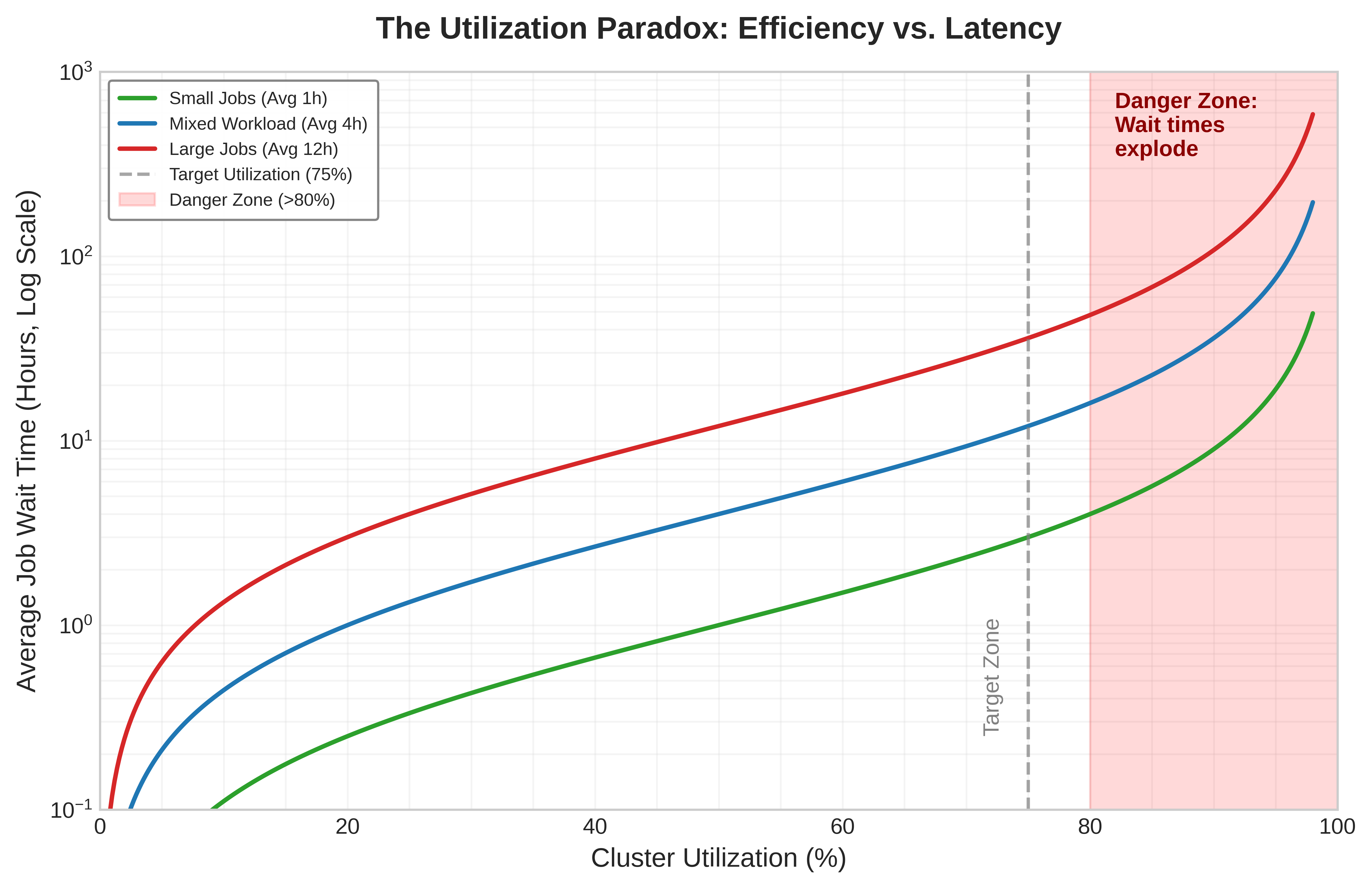
The debugging method is to compare scheduler state with physical capability, inspect job requests against the actual hardware pools, and then test for a policy-infrastructure mismatch. A full queue and idle accelerators can coexist when the scheduler is honoring constraints that the dashboard has aggregated away. The cluster at the center of the worked example below runs the heterogeneous hardware in table 8, accumulated across three procurement cycles.

Table 8: Cluster hardware inventory: Three procurement generations create distinct resource pools with different capabilities. A100 nodes support tensor parallelism via NVLink, while V100 nodes are limited to data parallelism.

GPU Type	Count	Memory	Interconnect	Nodes
A100-80 GB	400 GPUs	80 GB HBM2e	NVLink (600 GB/s)	50 nodes \(\times\) 8 GPUs
A100-40 GB	424 GPUs	40 GB HBM2e	NVLink (600 GB/s)	53 nodes \(\times\) 8 GPUs
V100-32 GB	200 GPUs	32 GB HBM2	PCIe Gen3 (15.8 GB/s)	50 nodes \(\times\) 4 GPUs

Example 1.3: Debugging low GPU utilization

Problem: A 1,024-GPU cluster reports 60 percent average utilization, below the 80 percent operating target, despite a full queue with over 50 pending jobs. Dashboards show idle GPUs, but users still wait. Identify the binding constraint and the diagnostic path.

The fleet stack framework in The Fleet Stack structures the diagnosis: inspect hardware capability first, then scheduling policy, then the mismatch between them.

The first diagnostic step is infrastructure-layer analysis. The hardware inventory in table 8 separates physical capability before the scheduler policy is examined: A100 nodes can run tensor-parallel jobs over NVLink, while the V100 pool is confined to data parallelism over PCIe.

The second diagnostic step is distribution-layer analysis. The Slurm scheduler implements gang scheduling with strict resource type matching. Examining the job specifications reveals the demand pattern:

• 15 large training jobs requesting at least 64 GPUs of A100-80 GB capacity, with aggregate demand of 1,200 GPUs.
• 8 medium jobs requesting 32 GPUs of A100-40 GB capacity, with aggregate demand of 256 GPUs.
• 0 jobs explicitly request V100 resources.

The scheduler’s allocation log shows A100-80 GB GPUs nearly saturated by a few running jobs, while the remaining large jobs stay pending because no full 64 GPUs A100-80 GB allocation can be formed. The result is not a standard Slurm partial-allocation deadlock; it is a policy-induced utilization gap where strict resource requests leave A100-40 GB and V100 pools idle while A100-80 GB jobs wait.

Analysis: Multiple pathologies compound to create low utilization:

1. Over-specification: Model memory analysis reveals that most large jobs actually require only 35 GB peak memory per GPU, well within A100-40 GB capacity. Users copied job templates specifying A100-80 GB without recalculating requirements.
2. Pool fragmentation: The strict homogeneity requirement means a 64 GPUs job requesting “A100-80 GB” cannot use any A100-40 GB GPUs, even when 300 GPUs sit idle.
3. Stranded resources: No jobs target V100 hardware because researchers perceive it as “legacy.” The 200 GPUs contribute zero productive work despite consuming power and cooling.
4. Atomic-allocation starvation: Large jobs remain pending until a full compatible allocation appears, while other resource pools sit idle because policy prevents compatible substitutions or backfill.

Diagnosis: Job templates and organizational practices evolved for a homogeneous A100-80 GB cluster. When infrastructure expanded with heterogeneous hardware, the Distribution Layer policies were never updated. The scheduler correctly implements its configured policy; the policy itself creates the utilization gap.

Solution: Implement tiered resource matching with topology awareness. The policy changes are durable: express capability requirements instead of exact GPU SKUs, reserve NVLink-connected nodes for jobs that need tensor parallelism, backfill compatible smaller jobs into otherwise idle pools, seed appropriate workloads onto older accelerators with lower cost accounting, and make the correct resource request easier than the over-specified template.

Impact: After implementing tiered matching and backfill scheduling, a two-week validation run recovered idle capacity across every pool, with the per-pool before-and-after allocation reported in table 9.

Systems lesson: Surface-level diagnosis suggested a scheduling algorithm problem. Deeper analysis showed a policy-infrastructure mismatch: the scheduler correctly implemented policies written for a homogeneous A100-80 GB cluster, but the infrastructure had become heterogeneous. Many utilization problems have this shape. The fix is not always a new scheduler; often it is updating the operational policy so it matches the fleet that actually exists.

Table 9: Utilization recovery results: The distinction between “allocated” and “effective” utilization captures the policy-induced utilization gap: before the fix, A100-80 GB GPUs showed high allocation in Slurm but lower actual compute utilization, while strict job templates stranded other capable hardware pools.

Pool	Before	After	Change
A100-80 GB	95% allocated, 72% effective	89% allocated, 94% effective	+22 pp
A100-40 GB	64% allocated	88% allocated	+24 pp
V100	0% allocated	71% allocated	+71 pp
Cluster-wide	60%	84%	+24 pp

As table 9 shows, this utilization gain adds approximately 246 fully utilized GPUs of productive work. That is equivalent to buying 410 additional raw GPUs if those GPUs ran at the old 60 percent utilization. At $2/GPU-hour, the equivalent raw capacity represents approximately $7M in annual recovered value, achieved through policy changes requiring zero additional hardware investment.

Common utilization anti-patterns

High-level metrics often mask deep inefficiencies. A cluster dashboard may report 85 percent allocation, but productive utilization, the share of cycles actually advancing model state, can be significantly lower. Debugging these gaps requires identifying specific signatures in the GPU telemetry that reveal the underlying bottleneck.

The zombie job represents the most egregious waste: a training process that has crashed or deadlocked but continues to hold GPU resources. In a distributed run training a 175B parameter model, a single rank failure can leave 128 GPUs allocated but idling if the process cleanup fails. The signature is high memory allocation (greater than 300 GB) paired with near-zero SM utilization (less than 5 percent) persisting for longer than a heartbeat timeout (typically 10 minutes). This state often results from CUDA context corruption or a driver-level deadlock that prevents the container runtime from successfully reaping the process, requiring forceful node-level remediation to reclaim the device.

The data starvation pattern manifests as a high-frequency sawtooth wave in GPU utilization, where the device oscillates between 100 percent load (forward/backward pass) and 0 percent load (waiting for the next batch). While the average utilization might appear acceptable at 60 to 70 percent, the GPU is effectively idling for a third of its life. This occurs when the CPU-bound data pipeline cannot sustain the throughput required by the GPU, a common scenario in computer vision where JPEG decoding and augmentation saturate host CPUs. A utilization variance exceeding 30 percent standard deviation is the primary diagnostic indicator, signaling the need for active prefetching, increased loader parallelism, or local NVMe caching to saturate the accelerator.

The communication bottleneck reveals itself through periodic, synchronized drops in SM utilization across all ranks in a distributed group. For the 175B model, synchronizing gradients for 350 GB of parameters requires massive bandwidth; if the network is undersized or congested, the GPUs spend more time waiting for AllReduce to complete than performing computation. The diagnostic metric is the step time ratio: if the total iteration time exceeds 1.5\(\times\) the compute-only time (forward plus backward passes in isolation), the network has become the dominant constraint. Remediation requires topology-aware placement to keep traffic on high-bandwidth switch tiers or algorithmic changes like gradient accumulation to increase the compute-to-communication ratio.

The memory fragmentation trap is an insidious failure mode in long-running inference servers. A 175B model serving diverse request lengths can end up with 80 percent of its HBM allocated to the KV cache, yet be unable to accept a new request because the free memory is scattered in small, noncontiguous blocks. The GPU appears full to the scheduler but underutilized in terms of throughput. This resembles the classic heap fragmentation problem but with higher stakes: a single restart to defragment dumps hundreds of gigabytes of state. Monitoring the ratio of requested token slots to allocated memory bytes often exposes this gap, which paged cache allocators address by decoupling logical sequence contiguity from physical memory layout, recovering usable memory and boosting serving throughput by 2–4\(\times\) without adding hardware.

The debugging example illustrates a broader principle that applies to every system discussed in this chapter: scheduling systems are only as effective as the policies they implement, and policies must evolve alongside infrastructure. When infrastructure changes (new hardware generations are added, network topologies are upgraded, workload mixes shift from training-dominant to serving-dominant), the policies encoded in scheduler configuration, job templates, and organizational practices must be re-evaluated and updated. The most expensive scheduling bug is often not a software defect but a policy that was correct for the old infrastructure and was never updated for the new one.

This principle connects scheduling mechanics to fleet governance. Technical policies (GPU type matching, gang scheduling timeouts, preemption grace periods) interact with organizational policies (team quotas, priority hierarchies, cost allocation) and human behavior (job template reuse, resource request habits, queue submission patterns). Effective fleet orchestration requires attending to all three layers simultaneously.

Self-Check: Question

1. Why can a cluster with very high utilization still be poorly serving researchers?

   1. Because high utilization always means too many GPUs are idle
   2. Because utilization measures only serving latency, not training performance
   3. Because queueing delay rises nonlinearly as utilization approaches saturation, so a highly utilized cluster can become effectively unusable for large or mixed ML workloads even though every GPU is busy
   4. Because clusters above 80 percent utilization automatically enter deadlock

2. In the chapter’s debugging case study, explain why the root cause was described as a policy-infrastructure mismatch rather than a scheduler-algorithm failure.

3. Which change most directly addressed the case study’s over-specification problem?

   1. Replacing every V100 node with A100-80GB nodes
   2. Forcing every data-parallel job to request NVLink-connected GPUs
   3. Rewriting templates so jobs request capabilities (minimum GPU memory, required topology) rather than specific GPU models, letting the scheduler match against any hardware that meets the need
   4. Disabling gang scheduling entirely for all distributed jobs

4. A telemetry pipeline reports that a training job’s GPU memory allocation is near 100 percent but its streaming-multiprocessor utilization has been at roughly 0 percent for longer than the heartbeat timeout. Which anti-pattern best matches this signature?

   1. A hung collective, where ranks are mid-AllReduce and waiting on one another but SM activity would still show periodic spikes
   2. A stalled checkpoint exit path, where the job is writing a large checkpoint but would show sustained host-to-device transfer and moderate SM activity
   3. A partially allocated gang waiting on missing ranks, which would leave GPU memory nearly empty rather than nearly full
   4. A zombie job: a crashed or deadlocked process that never released its GPU memory, so the allocation persists while no kernels execute

5. True or False: If a scheduler reports high GPU allocation, then the fleet is necessarily delivering high productive utilization.

6. A cluster-wide trace shows synchronized dips in SM utilization across all ranks of a distributed job, and total step time is substantially longer than compute-only time would predict. What does this pattern suggest, and what scheduling response is most appropriate?

See Answers →

Fallacies and Pitfalls

Those policy-infrastructure mismatches recur as a small set of misconceptions that can make an apparently healthy scheduler waste expensive fleet capacity. It is tempting to look at a cluster running at 98 percent utilization and declare victory, only to discover that researchers have stopped submitting jobs entirely because wait times have stretched into weeks. Cluster orchestration is riddled with counterintuitive traps like this, where optimizing a single metric destroys overall system value.

Fallacy: More sophisticated scheduling algorithms always improve utilization.

Engineers facing low utilization often reach for more advanced schedulers, assuming the algorithm is the bottleneck. As the debugging example in section 1.8 demonstrates, the root cause is frequently policy misconfiguration, not algorithmic limitation. A simple FIFO scheduler with correct policies (capability-based matching, backfill with timeouts, appropriate gang scheduling constraints) often outperforms a sophisticated scheduler with incorrect policies. Before upgrading the scheduler, audit the policies: confirm that users are not requesting resources they do not need, that heterogeneous resources are properly exposed, and that gang-scheduling timeouts are configured.

Pitfall: Treating all GPU-hours as equal when measuring utilization.

Cluster dashboards commonly report “GPU utilization” as a single percentage, averaging across all GPUs and all workloads. This metric hides critical information. A cluster might report 80 percent utilization where 60 percent is productive training, 15 percent is idle GPUs allocated to jobs waiting for gang completion, and 5 percent is GPUs running data loading with no active computation. Effective monitoring distinguishes between allocated utilization (GPUs assigned to jobs), compute utilization (GPUs executing kernels), and productive utilization (GPUs advancing useful training or serving requests). Only the last metric correlates with actual value delivered.

Fallacy: Gang scheduling is always necessary for distributed training.

Gang scheduling prevents deadlock for synchronous training, but not all distributed training is synchronous. Asynchronous training methods tolerate worker arrivals and departures, and elastic training frameworks handle variable worker counts. For workloads that can operate asynchronously or elastically, relaxing the gang scheduling requirement dramatically improves scheduling flexibility and reduces queue wait times. The trade-off is potential convergence degradation from stale gradients or batch size variability, but for many practical workloads (hyperparameter sweeps, fine-tuning, pretraining with adaptive batch size), this trade-off is favorable.

Pitfall: Setting static quotas based on peak demand.

Organizations commonly set team quotas to handle worst-case demand, reasoning that teams need guaranteed access during crunch periods. If Team A’s peak demand is 500 GPUs and Team B’s is 300 GPUs, the cluster needs 800 GPUs with static quotas. In practice, peaks rarely coincide. Hierarchical fair-share with borrowing can serve both teams’ peak demands with a 600-GPU cluster, because when Team A peaks, Team B is typically at moderate demand and can yield borrowed capacity. Static quotas at peak levels waste 25 to 40 percent of cluster capacity on guaranteed-but-unused allocations.

Fallacy: Spot instances are always cheaper for training.

The 60 to 90 percent discount on spot instances creates the impression of automatic savings. The effective cost depends on interruption frequency, checkpoint overhead, and restart time. For a large model with 15-minute checkpoint times and 30-minute restart times, a spot interruption costs 45 minutes of productive time. If interruptions occur every 2 hours, the effective cost rises enough that the nominal 65 percent discount shrinks to about 52 percent savings. For 100B+ parameter models with slow checkpointing on clusters with frequent spot interruptions, on-demand instances can actually be cheaper when accounting for all overhead. The decision requires quantitative analysis of the specific workload and spot market conditions, not blanket assumptions about cost savings.

Pitfall: Ignoring topology when scheduling distributed training.

Schedulers that treat GPUs as interchangeable units create allocations where tensor parallel groups span nodes (forcing NVLink-speed operations over InfiniBand) or AllReduce groups cross spine switches (adding latency and congestion). The 15 to 30 percent throughput penalty from poor topology placement accumulates over multi-week training runs, potentially wasting more resources than would be lost by waiting for a topology-aware allocation. Topology-aware scheduling increases scheduling complexity and may reduce packing efficiency, but for large distributed training jobs, the throughput improvement often justifies the trade-off.

Fallacy: GPU utilization alone is a sufficient autoscaling signal.

GPU utilization is a poor proxy for inference health. A GPU can be 90 percent utilized but still violating latency SLOs because the utilization comes from processing a backlog of queued requests. Conversely, a GPU at 40 percent utilization might be perfectly healthy if it is serving low-latency requests with headroom for bursts. The right metrics are queue depth, P99 latency relative to SLO, and KV cache memory pressure for LLM workloads. Relying on utilization creates a lagging indicator that only triggers scaling after performance has already degraded, whereas queue depth and SLO margin provide leading indicators that allow the fleet to scale before the user experience suffers. Furthermore, for LLMs, memory exhaustion from KV cache growth can occur at low compute utilization, causing requests to stall or fail. An autoscaler watching only compute utilization will miss this failure mode entirely, leaving the service degraded despite apparent capacity.

Pitfall: Using elastic training to avoid gang-scheduling decisions.

Elastic training complements but does not replace gang scheduling. While it allows jobs to resize, the resizing steps themselves often have atomic requirements. Elastic training works for data parallelism but not tensor parallelism (which requires a fixed number of GPUs per group). A 175B model using 8-way tensor parallelism needs exactly 8 GPUs per tensor-parallel group to function; this is a gang constraint that elastic training cannot relax. Elastic training adjusts the number of data-parallel replicas, not the intra-replica parallelism configuration, meaning the scheduler must still enforce gang constraints for the base unit of the model. If a scheduler naively places these 8 GPUs across different racks or fails to allocate them atomically, the tensor parallel group will either fail to initialize or suffer catastrophic performance degradation.

Fallacy: The scheduler needs no workload-specific validation.

Scheduler configuration requires continuous tuning as workloads evolve. Default configurations in Slurm or Kubernetes are optimized for generic workloads, often prioritizing simple fairness over throughput. ML-specific tuning (gang scheduling timeouts, topology-aware placement weights, preemption grace periods, and fair-share decay rates) can improve utilization by 15 to 25 percent. Organizations that deploy a scheduler and never revisit its configuration leave significant value on the table. A default preemption grace period might be too short for a large model to checkpoint, causing wasted work, while an untuned topology weight might fragment the cluster unnecessarily. As the cluster grows and the workload mix shifts (for example, from training-heavy to inference-heavy), the effective scheduling parameters shift with it. Treating the scheduler as a set-and-forget appliance lets the fleet drift into inefficiency.

Pitfall: Treating high utilization as proof of cluster health.

A cluster running at 95 percent utilization sounds efficient but may indicate a problem: insufficient capacity that is choking experimentation velocity. When utilization consistently exceeds 85 to 90 percent, queue times grow rapidly following the well-known M/M/1 queuing result from stochastic process theory. In this model, average wait time is proportional to \(\rho/(1-\rho)\) where \(\rho\) is utilization; at 90 percent utilization, average wait is 9\(\times\) the service time, and at 95 percent, it is 19\(\times\). Researchers waiting hours or days for resources conduct fewer experiments, test fewer hypotheses, and iterate more slowly on model designs. This reduced experimentation velocity has real costs that are harder to quantify than GPU-hours but may be larger in aggregate. The effective utilization target balances resource efficiency against researcher productivity, often landing between 70 and 85 percent for training clusters where queue responsiveness directly affects research output. Inference clusters, where requests are served immediately or not at all, often target even lower utilization (50 to 70 percent) to maintain latency headroom for traffic spikes.

Recognizing these fallacies prevents platform teams from chasing false optimizations that look good on dashboards but degrade developer velocity. The core orchestration principles that successfully navigate these trade-offs share a common thread: they treat scheduling as an engineering discipline, not an administrative function.

Self-Check: Question

1. Which metric best reflects whether a fleet is actually delivering useful ML work rather than merely reserving hardware?

   1. Allocated utilization alone
   2. Productive utilization, which excludes time lost to gang waits, checkpointing, communication stalls, and non-progress overhead
   3. Nameplate GPU count per cluster
   4. Average queue length without regard to job type

2. True or False: Once a training framework supports elasticity, the scheduler can safely drop all atomic placement requirements for that job, including tensor-parallel group boundaries and intra-group NVLink locality, because elasticity guarantees the job can run at any worker count.

3. Why is treating the scheduler as a black box that ‘just works’ a recurring pitfall in ML infrastructure?

See Answers →

Summary

Fleet orchestration transforms raw data center capacity into productive ML infrastructure. The scheduling algorithms, placement strategies, and resource management policies examined in this chapter determine whether thousands of isolated GPUs function as one coherent computing platform or as a fragmented collection of expensive servers. The difference between those outcomes is not hardware capability alone, but the scheduler’s ability to maintain useful state under partial failures, network partitions, stale resource views, and competing consistency and availability requirements. Slurm and Kubernetes embody different trade-offs along that spectrum, and large fleets may use both because batch training and self-healing service deployment stress the scheduler in different ways.

The chapter’s central technical lesson is that placement is performance. Topology-aware scheduling exploits the communication hierarchy of GPU clusters, improving training throughput by 15 to 30 percent when tensor-parallel, pipeline-parallel, and data-parallel groups are placed on the fabric tiers that match their traffic. Elastic training, preemption-aware checkpointing, and spot-instance policies add economic flexibility, but only when the job can survive changing worker counts or interruptions. Research schedulers such as Tiresias, Gandiva, Themis, and Pollux make the same point algorithmically: ML jobs have observable structure, including iterative progress, heavy-tailed durations, sunk-cost economics, and convergence-dependent scaling, so schedulers that exploit that structure can improve average completion time by 40 to 60 percent over generic policies.

The objective function changes again at serving time. Training clusters can trade queue wait against utilization, but inference fleets must protect tail latency under bursty demand. Autoscaling therefore needs queue depth, P99 latency, and KV-cache pressure rather than GPU utilization alone; multi-tenancy needs MIG, MPS, temporal slicing, quotas, borrowing, and chargeback policies that balance isolation against fleet-wide efficiency. The same scheduler that looks efficient on a utilization dashboard can still be mismanaging the fleet if researchers wait days for experiments, inference SLOs degrade under burst load, or fragmented GPUs cannot form the gang allocations that training jobs require.

Mastery of fleet orchestration is therefore diagnostic and economic as much as algorithmic. Zombie jobs, data starvation, topology mismatch, and resource fragmentation are symptoms of scheduler policy failing to match infrastructure reality; adding more nodes often hides the symptom without fixing the cause. With compute nodes defined, networks connected, storage configured, fault tolerance in place, and schedulers running, the infrastructure layers of the fleet stack now form a coherent platform rather than a rack of independent machines.

Key Takeaways: Scheduling is systems engineering

• Distributed scheduling is fundamentally hard: Cluster scheduling faces challenges (partial failures, network partitions, state inconsistency) that single-machine schedulers never encounter. The CAP theorem forces trade-offs between consistency and availability that shape every scheduling system’s design.
• Gang scheduling prevents deadlock but reduces flexibility: Gang scheduling gives distributed training atomic resource allocation to prevent hold-and-wait deadlocks, but rigid gang scheduling wastes resources when combined with backfill timeouts and elastic training alternatives.
• Topology determines performance: Where GPUs are placed within the cluster hierarchy matters as much as how many GPUs a job receives. NVLink vs. InfiniBand placement decisions can create 15 to 30 percent throughput differences for the same job on the same hardware.
• ML-specific scheduling outperforms generic approaches: Exploiting workload characteristics (predictable resource needs, iterative computation, diminishing returns) enables 40 to 60 percent improvements in job completion time compared to general-purpose FIFO or fair-share policies.
• Utilization is a first-order economic driver: Improving cluster utilization from 50 percent to 80 percent on a large cluster effectively adds thousands of GPUs worth of capacity. Closing this gap through policy and algorithm work pays back faster than buying additional accelerators.
• Policies must evolve with infrastructure: Scheduling algorithms are only as effective as the policies they implement. When infrastructure changes (heterogeneous hardware additions, topology upgrades, workload mix shifts), policies must be re-evaluated and updated.

The fleet now has every physical part it needs: compute, communication, storage, and the resilience to keep them running. None of it produces anything until something decides what runs where, and that decision is pure coordination. A scheduler that chases peak utilization will deadlock the first time two large jobs need the same nodes, so a scheduler that guarantees progress must leave some capacity deliberately unused. That gap, between the throughput a fleet could reach and the throughput it can safely sustain, is the price of coordination, and orchestration is the discipline of spending it where it buys the most finished work. At fleet scale the binding constraint moves up the stack again, from the speed of the hardware to the quality of the policy that hands it out.

What’s Next: From orchestration to optimization

We have organized the operational layer of the Machine Learning Fleet, the “who gets what, when, and where” of resource management. Yet the fleet’s purpose is not to run training jobs; it is to produce models that serve users. The next challenge is extracting maximum throughput from the hardware once it has been orchestrated. Performance Engineering examines the techniques that do so: operator fusion, precision engineering, graph compilation, and execution scheduling. These optimizations determine whether the fleet’s expensive silicon delivers its theoretical potential or wastes cycles on inefficient execution. The orchestration layer ensures the right resources are allocated; performance engineering ensures those resources are used effectively.

Self-Check: Question

1. Which statement best captures the chapter’s overall argument about fleet orchestration?

   1. Scheduling is mostly an administrative wrapper around hardware procurement decisions
   2. Fleet orchestration converts raw hardware capacity into useful ML work by aligning placement, policy, and workload structure against physical topology and organizational constraints
   3. Topology matters only for benchmark results, not for production systems
   4. Inference and training can usually be managed with identical objectives and metrics

2. Explain why the chapter treats scheduling sophistication as an economic lever rather than merely an operational convenience.

3. Across the chapter, a recurring lesson is that policies must evolve with infrastructure. Explain why this principle matters for both training clusters and serving fleets.

See Answers →

Self-Check Answers

Self-Check: Answer

1. One team submits sbatch --gres=gpu:8 --nodes=4 and waits for the scheduler to hand them exactly 32 GPUs; another team declares a deployment of 4 training-worker replicas and lets a controller keep that count alive through pod restarts. Which distinction does this pairing illustrate most directly?

   1. Slurm uses imperative resource requests executed once at submission, while Kubernetes expresses a declarative desired state that control loops continuously reconcile against actual state
   2. Slurm is optimized for Ethernet clusters while Kubernetes is optimized for InfiniBand fabrics
   3. Slurm is only used for training and Kubernetes is only used for inference, with no legitimate overlap
   4. Slurm schedules at pod granularity while Kubernetes schedules only at whole-node granularity

   Answer: The correct answer is A. The Slurm command performs an imperative, one-shot allocation; the Kubernetes deployment describes a steady-state invariant that a reconciliation loop enforces against the current cluster. The fabric-based claim confuses typical deployment patterns with the control-plane semantics, the training-versus-inference split is not a property of either system, and both systems can schedule at either pod or node granularity depending on configuration.

   Learning Objective: Differentiate imperative and declarative orchestration by the control-plane mechanism each system uses to express and enforce ML workload state

2. During a 90-second network partition between the control plane and a subset of worker nodes, which behavior best matches the chapter’s CAP-theorem characterization of Slurm and Kubernetes?

   1. Both systems prefer immediate reallocation to maximize availability, even if GPUs end up double-booked once the partition heals
   2. Kubernetes blocks all new scheduling until an administrator manually resolves the partition, while Slurm keeps scheduling with eventual consistency
   3. Slurm blocks new allocations during the partition to preserve consistency and avoid double-booking GPUs, while Kubernetes stays responsive and reconciles inconsistencies asynchronously once the partition heals
   4. Neither system is affected because node-local agents can always make globally consistent placement decisions without the control plane

   Answer: The correct answer is C. Slurm sits on the CP side of CAP: it blocks rather than risk conflicting allocations on GPUs worth thousands of dollars per hour. Kubernetes sits on the AP side: it keeps accepting requests and lets reconciliation loops heal divergence later. The symmetric-availability framing ignores the CAP trade-off entirely, the role of the administrator is reversed from how Kubernetes actually behaves, and independent node-local agents cannot preserve global consistency because they do not see each other’s allocations during a partition.

   Learning Objective: Compare how Slurm and Kubernetes trade off consistency and availability during partial control-plane failures

3. A team submits a distributed training job to vanilla Kubernetes, which creates the 32 required pods one at a time as nodes become free. Two hours in, only 24 pods are running, holding their GPUs but making no progress because AllReduce cannot begin. Which scheduling failure mode is this, and which Kubernetes abstraction resolves it?

   1. Priority inversion; resolved by raising the job’s pod-level priority class
   2. Image pull back-off; resolved by pre-pulling container images to every node
   3. Node affinity mismatch; resolved by adding topology spread constraints
   4. Partial gang allocation stranding resources; resolved by a PodGroup (or equivalent gang abstraction) that requires the minimum set to be schedulable before any pod starts

   Answer: The correct answer is D. Vanilla Kubernetes schedules pods one at a time, so a synchronous training job can accumulate workers that hold GPUs without ever forming a complete gang; this is exactly the partial-allocation deadlock the chapter introduced in section one. A PodGroup abstraction (used by Volcano and similar schedulers) requires the configured minimum to be schedulable atomically before any pod binds, which restores gang semantics. Priority tuning does not change the one-at-a-time binding behavior, image pulls are a startup latency concern rather than an allocation-semantics concern, and affinity rules steer placement but do not make it atomic.

   Learning Objective: Diagnose Kubernetes’ default partial-allocation failure mode for distributed training and identify the gang-scheduling abstraction that fixes it

4. An inference team reports that MIG partitioning raised GPU utilization dramatically, but a training team on the same cluster complains that MIG has made their job wait times worse. Explain, in terms of partition rigidity, why both can be true on the same hardware.

   Answer: MIG partitions an accelerator into fixed hardware slices at configuration time, which is ideal for many small inference pods that each consume a slice predictably. The cost is that the slice profiles cannot be reshaped without draining the workloads on the card first. When the workload mix shifts toward large training jobs, the cluster ends up with many MIG slices that no training job can use, even though the aggregate free compute would be sufficient if the slices were repartitioned. The scheduler therefore sees simultaneous high utilization on the inference side and long queues on the training side, with the rigidity of the partition profile as the binding constraint.

   Learning Objective: Evaluate the MIG utilization-versus-flexibility trade-off in mixed training-and-inference fleets

5. An organization already runs Kubernetes for their microservices, enjoying its CI/CD, RBAC, and observability tooling, but their largest pretraining runs want topology-aware gang scheduling and bare-metal performance. Which architecture best matches this goal?

   1. A pure Kubernetes cluster with no batch extensions, relying on vanilla pod scheduling for multi-node training
   2. A pure Slurm cluster, with custom in-house tooling built to replicate the organization’s existing CI/CD, RBAC, and observability
   3. A hybrid design where Kubernetes owns the operational control plane and orchestrates inference, while large training runs are submitted via operators into a Slurm-managed partition
   4. A design that partitions every node into MIG slices and runs training, inference, and microservices uniformly on those slices

   Answer: The correct answer is C. The hybrid pattern keeps Kubernetes’s lifecycle, identity, and observability story intact for the 95 percent of workloads that already fit it, while delegating the narrow, performance-critical training slice to Slurm where gang-scheduling and topology guarantees are mature. A pure Kubernetes answer ignores the explicit ask for topology-aware batch scheduling, a pure Slurm answer throws away significant working infrastructure, and forcing everything onto MIG slices confuses fine-grained inference partitioning with large-training placement.

   Learning Objective: Evaluate when a hybrid Kubernetes-plus-Slurm architecture is preferable to a single-platform design

← Back to Questions

Self-Check: Answer

1. An 8-way tensor-parallel group runs at near-ideal step time when it is placed inside a single NVLink-connected node but slows sharply when the same 8 GPUs are split across two nodes connected by NDR InfiniBand. Which explanation is correct?

   1. Tensor parallelism exchanges activation and gradient slices at every layer; NVLink’s order-of-magnitude-higher bandwidth and lower latency let these exchanges overlap with compute, whereas inter-node InfiniBand exposes the transfer cost on the critical path
   2. Aggregate InfiniBand bandwidth across two nodes exceeds a single node’s NVLink, so cross-node placement should actually be faster and any slowdown must be a driver bug
   3. AllReduce traffic dominates tensor-parallel communication, so both placements should perform identically once AllReduce is tuned
   4. Two nodes in the same rack share an NVLink domain, so the observed slowdown must come from the scheduler binding ranks to the wrong NUMA node
   5. The step-time slowdown is a GPU firmware throttle that activates when links cross a leaf switch boundary

   Answer: The correct answer is A. Tensor parallelism moves intermediate activations at every transformer layer, so the ratio of communication bandwidth to compute bandwidth directly sets iteration time; NVLink is on the order of 600 to 900 GB/s per GPU while NDR InfiniBand delivers about 50 GB/s, and that gap translates into visible step-time regression. The aggregate-bandwidth argument ignores that a single layer’s transfer is bounded by per-link bandwidth, not the sum across nodes. AllReduce dominates data parallelism, not tensor parallelism. Two nodes in the same rack do not share an NVLink domain (NVLink is intra-node), and no firmware throttle keys on leaf-switch crossings.

   Learning Objective: Identify why tensor-parallel workloads are especially sensitive to intra-node NVLink locality versus inter-node InfiniBand

2. A job uses 8-way tensor parallelism, 4-way pipeline parallelism, and 8-way data parallelism. Explain the placement logic a topology-aware scheduler should use across these three levels, matching each level to its appropriate tier of the communication hierarchy.

   Answer: The scheduler should keep each 8-GPU tensor-parallel group inside one NVLink domain because tensor parallelism exchanges activations every layer and is the most bandwidth-sensitive tier. Pipeline-adjacent groups should be placed within the same rack under a shared leaf switch, where InfiniBand latency and bandwidth are high enough to hide the point-to-point activation transfers between pipeline stages. Data-parallel replicas can be spread across racks through the spine, because gradient AllReduce happens once per step and the collective can overlap with the next forward pass. The result is that each logical parallelism dimension lives at the physical tier whose bandwidth and latency it can actually tolerate.

   Learning Objective: Apply topology-aware placement principles to a three-dimensional parallelism configuration

3. The section compares AllReduce latency for 64 GPUs under four placement strategies and reports 120 ms for random placement versus 25 ms for a topology-optimal placement. What is the main conclusion the reader should draw from this 4.8\(\times\) gap?

   1. AllReduce performance is largely insensitive to placement once the GPU count is fixed, so any difference must be measurement noise
   2. Rail optimization helps only serving workloads, not training
   3. Placement alone, without touching model code or hyperparameters, can produce a large collective-communication speedup because it changes the bandwidth and hop count the ring walks across
   4. The speedup comes entirely from raising the effective batch size until communication disappears from the critical path

   Answer: The correct answer is C. The 120-to-25 ms drop is a direct consequence of placing the ring so it walks shorter, higher-bandwidth links: hop count falls, tail-latency variance falls, and the slowest edge of the ring becomes much faster. The placement-insensitive framing contradicts the experiment outright, the rail-optimization comment misattributes the section’s scope, and batch size manipulates the ratio of compute to communication but does not explain why the same collective ran 4.8\(\times\) faster on the same hardware.

   Learning Objective: Quantify the impact of topology-aware placement on collective-communication performance

4. True or False: A scheduler can rely on static topology files alone because any link or switch problem serious enough to matter will always surface as a hard failure.

   Answer: False. The section emphasizes runtime topology discovery and performance-aware adaptation because links and switches can stay technically up while delivering much less bandwidth than nameplate (brownout from congestion, lane degradation, switch buffer pressure). Static maps capture intended structure; effective scheduling must track the topology that jobs can actually use.

   Learning Objective: Evaluate why production scheduling must track effective topology, not just intended topology

5. In a rail-optimized cluster, which placement rule best supports data-parallel AllReduce efficiency?

   1. Assign each replica to arbitrary GPU indices so long as all replicas sit in the same rack
   2. Co-locate every data-parallel worker on one node to avoid every switch hop
   3. Alternate ranks across rails to maximize path diversity for each collective
   4. Place corresponding data-parallel ranks on the same GPU index across nodes so their AllReduce traffic stays on a single rail’s switch hierarchy and does not contend with other rails

   Answer: The correct answer is D. Rail alignment pins rank i on every node to the same physical rail, so each data-parallel group’s AllReduce walks one dedicated switch hierarchy and never collides with another group’s traffic. Arbitrary indices may land in the same rack but still cross rails, single-node placement defeats the point of a multi-node data-parallel group, and alternating rails mixes traffic from different collectives onto shared switches, producing contention instead of avoiding it.

   Learning Objective: Identify the rail-alignment rule that exploits rail-optimized topologies for data-parallel AllReduce

6. A spine-switch failure halves cross-rack bandwidth for a training run that still has three weeks of compute ahead. Explain the calculation a scheduler should perform to decide whether to migrate the job to a healthy pod versus letting it ride out the degradation.

   Answer: The scheduler should compare the one-time migration cost (a 5 to 15 minute checkpoint-and-restart plus warmup) against the cumulative throughput loss from running on the degraded topology. If the halved cross-rack bandwidth translates to, say, a 20 percent step-time regression, then over three weeks the lost work vastly exceeds 15 minutes of migration overhead, so migration is the right call. For jobs that are only days from completion the arithmetic may flip: a moderate slowdown on a short remaining runtime can finish before the migration-plus-warmup overhead would have amortized.

   Learning Objective: Evaluate topology-aware migration decisions as a quantitative trade-off between migration overhead and degraded-bandwidth throughput loss

← Back to Questions

Self-Check: Answer

1. What is the main scheduling advantage of submitting an elastic job as a range (32 to 128 GPUs) instead of a rigid 128-GPU request?

   1. The job can start as soon as the minimum viable allocation is available and grow later as capacity frees up, instead of waiting for the full gang
   2. Elastic jobs no longer require distributed coordination during failures because any worker can recover independently
   3. It guarantees linear speedup at every intermediate worker count, eliminating the scaling-efficiency curve
   4. It removes the need for checkpointing because live worker replacement always preserves training state

   Answer: The correct answer is A. Elasticity widens the scheduler’s placement options: it can admit the job at 32 GPUs, do useful work immediately, and scale up as fragments free up, which compresses queue waiting time. The other options overstate what elasticity provides: the framework still has to rebuild communication groups and redistribute data (coordination is not eliminated), linear speedup is a convergence property of the model and optimizer rather than a scheduling guarantee, and elasticity explicitly assumes checkpoint-driven restart as the mechanism for rescaling.

   Learning Objective: Identify how elastic resource ranges reduce queueing delay for distributed training without removing the underlying coordination requirements

2. Explain the scheduler-framework contract required for safe elastic scale-up and scale-down, naming the responsibilities on each side.

   Answer: The scheduler guarantees that resource changes are communicated through defined signals with sufficient advance notice for graceful adaptation, rather than abruptly terminating processes. The framework guarantees it can handle these changes without corrupting model state by reconstructing communication groups, adjusting the effective batch size, and recalibrating the learning rate. If either side violates this contract, the job either crashes from unexpected preemption or resumes with an invalid distributed state.

   Learning Objective: Explain the coordination contract between orchestration and training frameworks in elastic training

3. Why is elastic training far easier to apply to data parallelism than to tensor parallelism?

   1. Tensor parallelism uses only CPUs for coordination, so schedulers cannot observe it
   2. Tensor parallelism is always asynchronous, so elasticity provides no value
   3. Data parallelism scales by adding or removing full replicas while the model structure is unchanged, whereas tensor parallelism partitions the model itself, so changing the group size requires re-sharding weights and rebuilding every matmul boundary
   4. Data parallelism never changes effective batch size when replicas change, so no hyperparameter adjustment is needed

   Answer: The correct answer is C. Data parallelism treats each replica as an independent copy of the model, so adding or removing replicas only changes the effective batch and the AllReduce ring size; tensor parallelism splits each weight tensor across workers, so removing even one GPU forces a re-shard of every affected weight and a rebuild of the per-layer collectives, which is effectively a restart. The CPU-only framing is incorrect, tensor parallelism is synchronous inside a layer, and the batch-size claim contradicts the section’s emphasis on recalibrating learning-rate schedules when the effective batch changes.

   Learning Objective: Compare the elasticity constraints of data-parallel versus tensor-parallel training

4. An elastic training job is scaled down from 256 to 64 GPUs. Which trade-off must the framework navigate regarding batch size and memory limits?

   1. Holding the global batch size constant preserves convergence mathematics but risks out-of-memory errors because each remaining GPU must process more samples per step.
   2. Scaling the global batch size down proportionally guarantees both memory safety and identical convergence behavior without learning rate adjustments.
   3. Using an adaptive learning rate allows the global batch size to remain constant, automatically bypassing per-GPU memory limits.
   4. Holding the per-GPU batch size constant preserves memory limits and automatically maintains the original convergence trajectory.

   Answer: The correct answer is A. To keep the global batch size constant across fewer workers, each remaining GPU must hold a larger per-worker batch of activations, which can easily violate per-GPU memory limits. Keeping the per-GPU batch size constant avoids memory limits but shrinks the global batch size, which introduces convergence risk unless the learning rate is adaptively recalibrated. The adaptive-learning-rate option conflates learning-rate scaling with memory footprint reduction.

   Learning Objective: Analyze the trade-off between constant global batch size and adaptive learning rate when scaling an elastic job down.

5. Order the following scheduler decisions for an elastic job from first to last: (1) decide whether the marginal throughput gain justifies a resize, (2) perform the rescaling transition and group reconfiguration, (3) profile or estimate the job’s current scaling-efficiency curve.

   Answer: The correct order is: (3) profile or estimate the job’s current scaling-efficiency curve, (1) decide whether the marginal throughput gain justifies a resize, (2) perform the rescaling transition and group reconfiguration. The scheduler first needs evidence about where the job sits on its efficiency curve, because a job already past the knee will gain little from more workers. Only with that signal in hand does the cost-benefit comparison against resize overhead become meaningful. The actual rescaling is the last and most expensive step, so it only fires once the first two decisions have cleared.

   Learning Objective: Order the policy steps required to make a well-reasoned elastic-scaling decision

6. Explain why an elastic policy that resizes a job every time a single node becomes free can reduce overall training throughput rather than improve it.

   Answer: Every resize pays checkpoint, pause, group reconfiguration, state transfer, and post-restart warmup overhead. If those transitions happen every few minutes, the job spends a non-trivial fraction of its wall-clock time reshaping itself rather than training. Production elastic policies therefore gate rescaling on marginal-utility thresholds plus a cooldown window, so small, short-lived capacity fluctuations do not trigger thrashing.

   Learning Objective: Evaluate why elastic-scaling policies must account for transition overhead and thrashing risk

← Back to Questions

Self-Check: Answer

1. Why does the chapter treat utilization improvement as one of the highest-leverage cost optimizations in fleet orchestration?

   1. Because higher utilization mainly reduces software licensing fees rather than hardware waste
   2. Because utilization only matters in cloud settings where pricing is metered
   3. Because utilization improvements eliminate the need for quota systems
   4. Because a utilization gain converts existing hardware into additional productive GPU-hours, substituting for capital expenditure on new accelerators without changing the power and cooling bill

   Answer: The correct answer is D. On a 10,000-GPU fleet, moving sustained productive utilization from 50 to 80 percent recovers roughly 6,000 GPUs of useful output while capex, power, and cooling stay constant; that makes utilization a direct substitute for procurement. Licensing is a small share of TCO at this scale, on-premise clusters have the same idle-dollars problem as cloud, and quotas enforce fairness rather than efficiency.

   Learning Objective: Evaluate how utilization improvements substitute for hardware procurement by converting existing capacity into additional productive GPU-hours

2. Spot instances advertise 60 to 70 percent discounts relative to on-demand pricing. Explain, using the chapter’s argument, why this discount does not automatically translate into lower effective training cost, and what property of the fault-tolerance stack determines whether it does.

   Answer: Effective spot cost is the list price divided by the fraction of wall-clock time spent doing useful work, so it is dominated by the interruption rate and the cost of each interruption. A large model with slow checkpointing may lose tens of minutes of training per preemption and may preempt every few hours, so its effective cost can climb back up to or past on-demand pricing. Spot economics therefore depend directly on checkpoint cadence, restart speed, and the framework’s ability to resume from the last save: cheap spot capacity is only actually cheap when the fault-tolerance stack keeps lost-work per preemption small.

   Learning Objective: Analyze when interruption overhead erases the headline discount of spot capacity and identify the fault-tolerance properties that preserve it

3. Which workload is the best fit for reserved capacity rather than spot-only or purely on-demand placement?

   1. A hyperparameter sweep where each trial is disposable and tolerates interruption
   2. A one-off debugging task where startup speed matters far more than long-term cost
   3. A 24/7 production inference service with predictable baseline demand and strict availability requirements
   4. A weekend experiment that can wait for whichever capacity pool becomes cheapest

   Answer: The correct answer is C. Reserved capacity is priced as a long-term commitment in exchange for guaranteed availability, which is exactly what a continuous production service needs. Disposable sweeps belong on spot because the discount matters and interruption is cheap, a one-off debugging task is matched to on-demand because flexibility and instant start beat a reservation commitment, and a flexible weekend experiment should ride the cheapest available pool rather than commit to reserved.

   Learning Objective: Classify workloads by the most economically appropriate capacity tier

4. The chapter says fault-tolerance infrastructure has a ‘double return.’ Which interpretation is correct?

   1. It both raises researcher productivity and eliminates all hardware failures
   2. It reduces losses from routine hardware and software failures AND makes discounted but interruptible spot capacity economically viable, so the same checkpoint-and-recovery stack pays back through both reliability and cost channels
   3. It guarantees that cloud prices will eventually match on-premise costs
   4. It lets teams bypass quota governance by restarting interrupted jobs on different accounts

   Answer: The correct answer is B. Fast checkpointing, elastic rendezvous, and automatic restart were originally justified by reliability alone, but they also shrink the per-interruption cost that determines whether spot capacity is actually cheaper than on-demand, so one investment pays in two places. The other options overstate the scope (no mechanism eliminates hardware failure), confuse resilience with pricing convergence, or describe a governance abuse rather than a cost mechanism.

   Learning Objective: Explain why investments in ML fault tolerance improve both reliability and cost efficiency

5. An organization is deciding between building an on-premise cluster and renting cloud GPUs. Explain why utilization is the key break-even variable in that decision.

   Answer: On-premise infrastructure converts compute into a high fixed cost through capital spending, facilities, and operations, so idle hardware is financially punishing; the per-GPU-hour TCO scales inversely with utilization. Cloud pricing charges a premium per GPU-hour in exchange for elastic, pay-for-use consumption that scales with actual demand. The break-even point is the utilization level at which the amortized on-premise TCO falls below the cloud rate; below that utilization, cloud wins on cost despite the higher per-hour price, and above it, owned hardware wins.

   Learning Objective: Explain how utilization determines the TCO break-even point between cloud and owned infrastructure

← Back to Questions

Self-Check: Answer

1. What is the central limitation of general-purpose schedulers that motivates custom ML schedulers such as Tiresias and Pollux?

   1. They cannot run on clusters with more than a few hundred GPUs
   2. They treat training jobs as opaque resource consumers and ignore ML-specific signals such as iteration timing, learning-curve position, and convergence trajectory
   3. They can schedule only inference services, not training jobs
   4. They require every user to submit Kubernetes YAML rather than shell scripts

   Answer: The correct answer is B. The four custom schedulers all exploit information that the training loop emits for free (iteration boundaries, gradient statistics, loss curves, attained service) but that generic schedulers throw away by treating a job as a black-box reservation. The other options confuse unrelated properties: generic schedulers do scale past a few hundred GPUs, they do schedule training jobs, and submission syntax is irrelevant to the information-asymmetry argument.

   Learning Objective: Identify why ML-specific workload signals can improve scheduling beyond generic resource allocation

2. Which scheduler specifically addresses poor user runtime estimates by prioritizing jobs according to attained service rather than predicted duration?

   1. Tiresias
   2. Gandiva
   3. Themis
   4. Pollux

   Answer: The correct answer is A. Tiresias sidesteps inaccurate user runtime estimates by using the amount of GPU-time a job has already consumed as its scheduling signal, demoting long-running jobs in favor of newer arrivals without ever asking the user how long the job will run. Gandiva keys on iteration boundaries for cheap preemption, Themis optimizes finish-time fairness across heterogeneous workloads, and Pollux adapts allocations to maximize goodput (useful training progress per GPU-hour, combining throughput with statistical efficiency).

   Learning Objective: Identify the ML scheduler designed to avoid dependence on user-supplied runtime estimates

3. Explain why Gandiva uses iteration boundaries as a practical time-slicing point for GPU sharing, and why preempting at an arbitrary cycle inside an iteration would be strictly worse.

   Answer: At an iteration boundary the forward-and-backward pass has finished, so the expensive intermediate activation tensors have already been freed by the normal training loop; pausing there means saving only parameters and optimizer state, and resuming means replaying the next mini-batch. Preempting mid-iteration would force the scheduler to save the full activation stack, which can be gigabytes per layer, and then restore all of it before the next backward pass. Using iteration boundaries therefore unlocks cheap interleaving of jobs during naturally idle windows (data loading, evaluation) without paying the full cost of arbitrary preemption.

   Learning Objective: Explain why iteration boundaries are the natural preemption point for deep learning workloads

4. What makes Pollux more powerful but also more operationally risky than Tiresias?

   1. Pollux requires a centralized filesystem while Tiresias does not
   2. Pollux works only for inference while Tiresias works only for training
   3. Pollux avoids all profiling overhead by assigning every job to a fixed static class
   4. Pollux jointly tunes GPU allocation AND training hyperparameters (batch size, effective learning rate) based on its model of useful training progress per GPU-hour, so a mistake in that model can hurt convergence, not just queue order; Tiresias changes only scheduling priority, so a mistake there only shifts wait times

   Answer: The correct answer is D. Pollux’s optimization target (useful training progress per GPU-hour, which combines raw throughput with statistical efficiency) requires it to change both how many GPUs a job has and how the training loop is configured, so model errors can damage the model itself; Tiresias only reorders jobs in the queue, so a bad decision costs wait time and nothing more. The filesystem, workload-scope, and profiling claims all contradict the section’s description of both systems.

   Learning Objective: Compare the optimization scope and risk profile of Pollux against simpler ML-aware schedulers

5. True or False: Minimizing average job completion time is a safe universal objective for a shared ML cluster, because a lower average automatically implies better outcomes for every workload class.

   Answer: False. The chapter’s production example shows that average-JCT optimization can repeatedly preempt or deprioritize long, high-value training runs to clear many tiny experiments, which improves the aggregate metric while degrading the critical-path work. Production schedulers therefore need QoS classes or per-class metrics; a single aggregate target hides the trade-off across workload types.

   Learning Objective: Evaluate why a single aggregate scheduling metric can conflict with production workload priorities

6. A platform team wants to adopt ideas from ML research schedulers but is wary of deep framework integration. Which scheduler family is the most plausible starting point, and why?

   Answer: A Tiresias-style approach is the most plausible starting point because it reorders jobs using external signals (attained GPU-service per job) without touching the training loop; the worst-case failure is a sub-optimal queue ordering, which is cheap to revert. By contrast, Pollux-style gains require the scheduler to co-tune GPU count, batch size, and the framework’s view of useful-training-progress-per-GPU-hour (Pollux’s goodput signal), which demands invasive coordination with the training framework and can regress convergence if the model is wrong. Tiresias therefore gives most of the ML-aware benefit with a much gentler blast radius.

   Learning Objective: Justify a production adoption path for ML-aware scheduling based on operational risk

← Back to Questions

Self-Check: Answer

1. Why is raw GPU utilization often a poor primary autoscaling signal for LLM inference services?

   1. GPU utilization is relevant only to training, so serving should ignore it entirely
   2. Queue depth and KV-cache memory pressure can predict SLO violations well before GPU utilization alone reflects the stress, so a utilization-only policy tends to scale too late
   3. GPU utilization cannot be measured accurately under Kubernetes
   4. Latency always decreases as GPU utilization increases, so utilization is actively misleading

   Answer: The correct answer is B. LLM serving can have modest average utilization while the queue has already grown and the KV cache is nearing saturation; p99 latency breaks at that moment, not when utilization hits 100 percent. The utilization-is-irrelevant framing goes too far (it remains a useful secondary signal), measurement is fine in modern Kubernetes, and the latency-versus-utilization curve is convex, not monotonically decreasing.

   Learning Objective: Identify why custom inference metrics outperform raw GPU utilization for LLM autoscaling decisions

2. Explain why predictive autoscaling is especially important for large-model serving compared with ordinary web services.

   Answer: Large models have minutes-scale cold-start times: weights must load into GPU memory, compiled kernels must warm up, and the serving stack must reach steady state before the replica can take traffic. Purely reactive autoscaling fires the scale-up only after queue depth or latency already exceeds threshold, by which time the SLO has been breached for the entire cold-start window. Predictive autoscaling uses a demand forecast so new replicas are warm and ready before the traffic arrives, turning a reactive SLO breach into a pre-positioned capacity change.

   Learning Objective: Explain why cold-start latency makes predictive autoscaling valuable for large-model inference

3. Which GPU-sharing mechanism provides the strongest hardware-level isolation against noisy-neighbor interference in multi-tenant inference?

   1. CUDA time-slicing
   2. MPS
   3. MIG
   4. Round-robin request routing at the load balancer

   Answer: The correct answer is C. MIG partitions the accelerator’s memory, L2 cache, and streaming multiprocessors at the hardware level, so one tenant cannot starve another through cache pressure or bandwidth contention. MPS and time-slicing share the same underlying resources and only multiplex access, so they reduce average latency but still leak interference across tenants. Request routing operates above the accelerator and provides no hardware isolation whatsoever.

   Learning Objective: Compare GPU-sharing mechanisms by the strength of their hardware-level isolation guarantees

4. A fleet serves many 7B models and a few 175B models. According to the section, which resource-management strategy is usually most economical?

   1. Give every model exclusive access to a full GPU or full tensor-parallel group
   2. Force the 175B models onto MIG slices so every model uses the same scheduling primitive
   3. Run all models on CPUs during low-traffic periods to avoid any GPU interference
   4. Pack the small 7B models onto shared utility GPUs (via MIG or MPS) and keep the 175B models on exclusive multi-GPU tensor-parallel groups

   Answer: The correct answer is D. Small models typically underfill a single accelerator and benefit from sharing; large models already saturate multiple GPUs and need dedicated placement with tensor-parallel-aware locality. Exclusive placement for every model wastes capacity on underfilled 7B replicas, MIG on the 175B side fights the model’s sharded communication pattern, and CPUs cannot meet LLM latency targets at any traffic level.

   Learning Objective: Evaluate when GPU sharing is economically attractive versus when exclusive placement is warranted

5. Least-outstanding-requests routing is adequate for many web services but not for LLM serving. Explain the gap and what additional signal closes it.

   Answer: LLM requests have hugely different computational cost: two replicas with the same outstanding-request count can be in very different states because one replica may be serving several 32K-context prompts while the other serves short-reply requests. Request count is blind to this because it ignores KV-cache occupancy and expected completion length. Memory-aware routing adds KV-cache utilization (and, where available, context-length estimates) into the decision, which steers long-context traffic away from already-loaded replicas and reduces both OOM kills and p99 latency spikes.

   Learning Objective: Analyze why LLM request routing must account for memory state in addition to request counts

6. Why does dynamic sharing between training and serving capacity usually follow diurnal forecasts rather than reacting second-by-second to current traffic?

   1. Because preemption of training jobs is strictly forbidden in mixed clusters
   2. Because inference traffic is perfectly predictable at every timescale
   3. Because extra serving replicas never help latency once a model is deployed
   4. Because flipping a GPU between training and serving modes incurs minutes of checkpointing, weight loading, and warmup, so the mode switch cannot absorb sub-minute traffic bursts; forecasts let the switch happen before demand arrives

   Answer: The correct answer is D. The training-serving boundary crossing is a minutes-scale operation, so any reactive controller that tries to move a GPU after the spike arrives will be late by definition. Diurnal forecasting shifts the decision earlier in time, when the mode switch can complete before the surge. Preemption is allowed with appropriate policy, inference traffic is not perfectly predictable, and replica count demonstrably affects latency.

   Learning Objective: Evaluate why the training-serving boundary is governed by mode-switching latency rather than instantaneous demand

← Back to Questions

Self-Check: Answer

1. Why are hierarchical fair-share systems with borrowing usually preferred over rigid fixed per-team GPU quotas in shared ML fleets?

   1. They let teams permanently exceed their allocations without any reclamation logic
   2. They keep idle capacity locked inside the owning team so fairness is never disturbed
   3. They allow idle capacity to flow to other teams while preserving the owning team’s guaranteed entitlement via reclamation when its own demand returns
   4. They eliminate the need for preemption and checkpointing support entirely

   Answer: The correct answer is C. Borrowing raises overall utilization by lending unused slots to teams with pending work, but the guarantee structure is preserved because the scheduler can reclaim those slots (via preemption of the borrower) the moment the owner’s demand returns. Permanent overuse breaks guarantees, locking idle capacity inside the owning team is the failure mode borrowing exists to solve, and borrowing specifically requires preemption and checkpointing to work.

   Learning Objective: Explain why borrowing improves utilization without abandoning quota guarantees

2. Explain why jobs running on borrowed capacity should checkpoint more aggressively than jobs running on their team’s owned quota, using the reclamation mechanism to justify the answer.

   Answer: Borrowed capacity can be reclaimed at any time when the owning team’s demand returns, so a borrower’s expected preemption rate is strictly higher than an owner’s. Under the reclamation mechanism, the borrower loses all work since its last checkpoint when the owner reclaims the slot, so the optimal checkpoint interval shrinks with preemption probability. Aggressive checkpointing caps the expected lost-work-per-preemption, which is what makes opportunistic borrowing economically positive rather than a source of wasted compute.

   Learning Objective: Analyze how reclamation risk changes checkpoint policy for opportunistic jobs

3. A cluster over-commits resources by 1.4\(\times\). Under what workload condition is this most likely to be safe and beneficial?

   1. When most jobs sustain near-100 percent real GPU utilization continuously
   2. When every team requests exactly the same GPU count
   3. When actual per-job utilization is bursty and peaks across jobs are not strongly synchronized, so statistical multiplexing smooths aggregate demand below the committed total
   4. When the cluster has no priority classes, so all pressure is treated uniformly

   Answer: The correct answer is C. Over-subscription is a bet that requested capacity overstates actual concurrent use, which pays off when peaks are uncorrelated. If every job runs compute-saturated all the time, 1.4\(\times\) over-commitment produces direct contention instead of statistical slack. Identical request sizes do not imply uncorrelated peaks, and flattening priority classes removes the tool the scheduler needs to resolve the contention when the bet goes wrong.

   Learning Objective: Evaluate when over-subscription can safely increase effective cluster utilization

4. Explain why a mature cluster enforces a policy that rejects submissions lacking team or project metadata at admission time, and what breaks if that policy is not enforced.

   Answer: Mandatory team or project metadata at admission time is the hinge that makes every downstream governance mechanism work: chargeback/showback can attribute GPU-hours to a cost center, quota systems can count usage against the right entitlement, anomaly detection can flag a team whose consumption suddenly spikes, and preemption policy can identify whose jobs to reclaim. Without enforced attribution, GPU consumption disappears into an unowned infrastructure bucket, quota accounting drifts, cost allocation becomes guesswork, and even simple audits (who ran the job that crashed the rack?) become impossible.

   Learning Objective: Explain why mandatory admission-time attribution is the precondition that makes quota enforcement, chargeback, and anomaly detection possible

5. What is the main danger of a preemption cascade in a saturated multi-tenant cluster?

   1. It triggers waves of checkpointing, restart, and rescheduling overhead across many jobs, burning a large fraction of cluster capacity on churn rather than on useful work
   2. It permanently breaks fair-share accounting by deleting prior usage history
   3. It prevents any high-priority workload from ever entering the cluster
   4. It eliminates all queueing delay for interactive jobs

   Answer: The correct answer is A. A cascade happens when evicting one job to make room for a higher-priority request in turn evicts another, which in turn evicts another; each eviction costs checkpoint, restart, and warmup time, so a single urgent request can destabilize the whole fleet. The section’s prescription is preemption budgets (rate-limits on evictions per window), not deleting accounting state, which would remove the ability to make the decision in the first place. High-priority jobs do enter the cluster, and queueing delay does not vanish during a cascade.

   Learning Objective: Analyze why preemption must be rate-limited in shared ML clusters

6. Why is quota governance not just a technical scheduling problem but also an organizational one?

   Answer: Quotas encode business priorities and team behavior as much as hardware limits. Teams respond to the incentives the system creates: if holding unused reservations is costless, they will hoard; if untagged jobs get scheduled anyway, they will skip metadata; if peak-case requests carry no accountability, they will request ‘just in case’ headroom. Chargeback or showback, periodic quota review, and admission-time attribution tilt those incentives toward honest requests. The practical consequence is that even a technically sound scheduler can waste large fractions of a fleet when the surrounding governance rewards hoarding or opacity.

   Learning Objective: Explain how organizational incentives shape the effective utilization of quota systems

← Back to Questions

Self-Check: Answer

1. Why can a cluster with very high utilization still be poorly serving researchers?

   1. Because high utilization always means too many GPUs are idle
   2. Because utilization measures only serving latency, not training performance
   3. Because queueing delay rises nonlinearly as utilization approaches saturation, so a highly utilized cluster can become effectively unusable for large or mixed ML workloads even though every GPU is busy
   4. Because clusters above 80 percent utilization automatically enter deadlock

   Answer: The correct answer is C. The utilization paradox in the section shows that wait time climbs superlinearly near saturation, so a 98-percent-utilized cluster can produce multi-day queues even though nothing is idle. Interpreting high utilization as idleness inverts the definition, tying utilization to serving latency alone ignores the training case the section focuses on, and no hard 80-percent deadlock threshold exists in the section.

   Learning Objective: Explain why high average utilization does not imply a healthy ML cluster

2. In the chapter’s debugging case study, explain why the root cause was described as a policy-infrastructure mismatch rather than a scheduler-algorithm failure.

   Answer: The scheduler was correctly enforcing the configured rules; the rules themselves had been written when the cluster was homogeneous A100-80GB and encouraged users to request that specific SKU in their job templates. When A100-40GB and V100 nodes were added, exact-SKU matching stranded large pools while A100-80GB queues ballooned. The fix was to rewrite the policy layer (capability-based requests, topology rules, gang timeouts), not to replace the scheduler; the algorithm was fine, it was being asked to optimize against a policy that no longer matched the hardware.

   Learning Objective: Diagnose when poor utilization comes from policy mismatch rather than scheduler algorithm failure

3. Which change most directly addressed the case study’s over-specification problem?

   1. Replacing every V100 node with A100-80GB nodes
   2. Forcing every data-parallel job to request NVLink-connected GPUs
   3. Rewriting templates so jobs request capabilities (minimum GPU memory, required topology) rather than specific GPU models, letting the scheduler match against any hardware that meets the need
   4. Disabling gang scheduling entirely for all distributed jobs

   Answer: The correct answer is C. Capability-based scheduling lets the template say ‘I need at least 40 GB of GPU memory and intra-node NVLink’ rather than ‘I need A100-80GB,’ which immediately makes A100-40GB and even V100 hardware usable for workloads whose real constraints were looser than the SKU name suggested. Replacing V100s with A100-80GBs is a hardware procurement, not a policy change. Forcing NVLink requests would over-constrain placement further. Disabling gang scheduling would reintroduce the partial-allocation deadlock.

   Learning Objective: Identify how capability-based scheduling mitigates resource over-specification in heterogeneous fleets

4. A telemetry pipeline reports that a training job’s GPU memory allocation is near 100 percent but its streaming-multiprocessor utilization has been at roughly 0 percent for longer than the heartbeat timeout. Which anti-pattern best matches this signature?

   1. A hung collective, where ranks are mid-AllReduce and waiting on one another but SM activity would still show periodic spikes
   2. A stalled checkpoint exit path, where the job is writing a large checkpoint but would show sustained host-to-device transfer and moderate SM activity
   3. A partially allocated gang waiting on missing ranks, which would leave GPU memory nearly empty rather than nearly full
   4. A zombie job: a crashed or deadlocked process that never released its GPU memory, so the allocation persists while no kernels execute

   Answer: The correct answer is D. A zombie job holds its memory allocation because the parent process died without going through the clean shutdown path, so the NVIDIA runtime still thinks the device is in use while no kernels are being dispatched; SM utilization sits at zero. A hung collective would still show SM activity during spin-wait or periodic retries, a stalled checkpoint write would show host-to-device traffic and non-zero SM activity, and a partial gang leaves memory near empty rather than near full because the training loop has not started.

   Learning Objective: Classify a utilization telemetry signature as a specific cluster anti-pattern by matching it against closely-related failure modes

5. True or False: If a scheduler reports high GPU allocation, then the fleet is necessarily delivering high productive utilization.

   Answer: False. The chapter explicitly separates allocated utilization, compute utilization, and productive utilization because GPUs can be reserved yet blocked on gang completion, waiting on data, stalled on collective communication, or held by a zombie job. Allocation measures reservation pressure, which is not the same as delivered work.

   Learning Objective: Distinguish reserved capacity from actual productive work when diagnosing cluster efficiency

6. A cluster-wide trace shows synchronized dips in SM utilization across all ranks of a distributed job, and total step time is substantially longer than compute-only time would predict. What does this pattern suggest, and what scheduling response is most appropriate?

   Answer: Synchronized dips across all ranks indicate a communication bottleneck: every worker is stalled on the same collective at the same moment, which is the signature of cross-rank synchronization rather than a local compute issue. The right response is to act on placement and topology, either by recompacting the job into a tighter locality (same rack, same rail) or, if the job is already compact, by raising the compute-to-communication ratio through larger micro-batches or gradient accumulation. Tuning a single node’s data loader would address a symptom that points at one worker, not a symptom that appears across all of them.

   Learning Objective: Analyze telemetry to distinguish communication bottlenecks from local compute bottlenecks

← Back to Questions

Self-Check: Answer

1. Which metric best reflects whether a fleet is actually delivering useful ML work rather than merely reserving hardware?

   1. Allocated utilization alone
   2. Productive utilization, which excludes time lost to gang waits, checkpointing, communication stalls, and non-progress overhead
   3. Nameplate GPU count per cluster
   4. Average queue length without regard to job type

   Answer: The correct answer is B. The section warns that allocated or even compute utilization can look healthy while real training or serving progress is poor; productive utilization is the only metric that tracks delivered ML work. Hardware counts and raw queue lengths are useful context but do not, by themselves, distinguish a busy cluster from an effective one.

   Learning Objective: Identify the utilization metric that most directly captures delivered ML value

2. True or False: Once a training framework supports elasticity, the scheduler can safely drop all atomic placement requirements for that job, including tensor-parallel group boundaries and intra-group NVLink locality, because elasticity guarantees the job can run at any worker count.

   Answer: False. Elasticity lets the scheduler change the number of data-parallel replicas, but a tensor-parallel group is still an atomic, NVLink-bound unit: the scheduler cannot drop one rank from an 8-way tensor-parallel shard without re-sharding the model. Elasticity widens the feasible scaling range; it does not remove the gang boundaries inside the model’s base communication structure, and treating it as if it did produces the same partial-allocation deadlock the chapter opened with.

   Learning Objective: Evaluate the precise boundary between elastic scaling and persistent gang-scheduling requirements

3. Why is treating the scheduler as a black box that ‘just works’ a recurring pitfall in ML infrastructure?

   Answer: Scheduler defaults are generic, but ML fleets drift continuously: hardware mixes change, workload archetypes shift between training and inference, rack and rail topologies expand, and latency or throughput targets evolve. If the operations team never revisits preemption budgets, topology weights, quota policies, capability rules, or autoscaling signals, the system accumulates invisible misalignment. The chapter’s case study and anti-pattern taxonomy both show that correctly-functioning scheduler software running an outdated policy produces exactly the symptoms teams mistakenly blame on the scheduler itself.

   Learning Objective: Explain why scheduling policy requires ongoing tuning as infrastructure and workloads evolve

← Back to Questions

Self-Check: Answer

1. Which statement best captures the chapter’s overall argument about fleet orchestration?

   1. Scheduling is mostly an administrative wrapper around hardware procurement decisions
   2. Fleet orchestration converts raw hardware capacity into useful ML work by aligning placement, policy, and workload structure against physical topology and organizational constraints
   3. Topology matters only for benchmark results, not for production systems
   4. Inference and training can usually be managed with identical objectives and metrics

   Answer: The correct answer is B. The chapter’s thesis is that orchestration is the binding that turns thousands of servers into a coherent computing resource: it aligns scheduler policy with workload needs and infrastructure constraints. The other options deny the chapter’s core themes (topology sensitivity, training-versus-serving divergence, and the primacy of scheduling over procurement).

   Learning Objective: Synthesize how placement, policy, and workload structure jointly determine effective fleet capacity

2. Explain why the chapter treats scheduling sophistication as an economic lever rather than merely an operational convenience.

   Answer: At fleet scale, scheduling directly controls what fraction of existing hardware is doing useful work: improvements in placement, quotas, elasticity, or autoscaling translate immediately into additional productive GPU-hours without capital spend. A few utilization points on a 10,000-GPU fleet, or one better cost tier on the capacity mix, can shift millions of dollars per year, which puts orchestration in the same budget conversation as procurement rather than in operations overhead.

   Learning Objective: Explain why scheduling quality has direct economic consequences for large ML fleets

3. Across the chapter, a recurring lesson is that policies must evolve with infrastructure. Explain why this principle matters for both training clusters and serving fleets.

   Answer: As clusters become heterogeneous, acquire new network topologies, or shift their training-to-inference mix, assumptions embedded in templates and scheduler settings stop matching reality. On the training side, that produces fragmentation, wrong-SKU requests, and poor topology placement; on the serving side, it produces weak autoscaling signals, stale cold-start estimates, and broken sharing boundaries. In both cases the scheduler software keeps ‘working’ while the outcomes degrade, so only continuous policy-infrastructure co-evolution prevents the drift.

   Learning Objective: Synthesize why policy-infrastructure alignment is a recurring requirement across training and serving orchestration

← Back to Questions