Collective Communication
Purpose
Why does communication between machines become the fundamental constraint that governs large-scale machine learning systems?
Computation scales by adding processors; communication scales by moving data between them. These scale differently: adding a processor increases aggregate compute linearly, but coordinating that processor with all others moves more total data and, for the most general synchronization patterns, multiplies the logical connections among workers quadratically. At sufficient scale, the time spent exchanging gradients, activations, and parameters exceeds the time spent computing them. This crossover point is not a bug to be fixed but a fundamental property of distributed systems that determines which parallelization strategies work, which model sizes are trainable, and which organizations can operate at the largest scales. The physics of light-speed delays, bandwidth limits, and energy costs of data movement constrains communication as firmly as transistor physics constrains computation, yet communication is far less intuitive to reason about, making it the hidden bottleneck that undermines systems designed by those who understand only the compute side. In C³ terms, collective communication forms the instruction set of the fleet: the physical operations that govern how compute is penalized by communication.
Learning Objectives
- Apply communication cost models to bound collective latency, bandwidth, and message-size crossover points
- Match collective communication primitives to parallelism strategies and model archetypes
- Compare ring, tree, butterfly, double-tree, and hierarchical reduction algorithms using scale-dependent cost models
- Analyze communication-library reality gaps by comparing theoretical costs with measured latency, bandwidth, and topology mapping
- Design topology-aware collective schedules for NVLink, InfiniBand, rail-optimized, torus, and in-network reduction fabrics
- Evaluate compression, sparsification, and error feedback by balancing communication savings against convergence risk
- Implement overlap strategies with bucket fusion, asynchronous operations, and layer-by-layer gradient scheduling
From Parallelism to Communication Patterns
When 10,000 GPUs need to apply one weight update, the splits created by data, tensor, pipeline, and expert parallelism have to be made consistent again. The workers are not sending arbitrary messages; they are executing choreographed collective operations. In the fleet stack shown in The Fleet Stack, those operations sit in the Distribution Layer, where logical parallelism becomes physical traffic.
The 3D Parallelism Cube assumes that replicas, shards, stages, and experts can exchange gradients, activations, parameters, and tokens quickly enough for the optimizer to see one coherent training run. That assumption is the handoff from parallelism to communication: every way of splitting the model relocates work onto the network.
The gap between that assumption and the wire reveals a fundamental asymmetry in how computation and communication scale. Computation is local: each GPU works on its own data, so aggregate compute grows with the number of GPUs. Communication is global: keeping the fleet synchronized requires information to cross physical links with finite latency, bandwidth, topology, and energy. The central case is gradient synchronization; from there the mechanics become concrete through alpha-beta cost models, collective primitives, AllReduce schedules, topology-aware routing, compression, and overlap.
Definition 1.1: Gradient synchronization
Gradient Synchronization is the collective communication step in synchronous data-parallel training in which every worker contributes its locally computed gradient tensor to an aggregate reduction, then receives the same reduced result so all model replicas apply an identical update.
- Significance: A 70B-parameter model in BF16 generates 140 GB of gradient data per worker per step. Synchronizing across 1,000 GPUs via ring AllReduce at 50 GB/s per link requires approximately \(2 \times 140/50\) \(\approx\) 5.6 s of communication per step, making the bandwidth (data-movement) term large enough to dominate the iron law unless overlap, hierarchy, or compression reduces the exposed transfer.
- Distinction: Unlike parameter-server approaches (where all workers send gradients to a centralized aggregator whose bandwidth scales as \(\mathcal{O}(N)\)), ring AllReduce distributes the communication across all workers so that each worker’s per-step communication cost stays constant at \(2 \times (N-1)/N \times M\) regardless of cluster size.
- Common pitfall: A frequent misconception is that ring AllReduce behaves like an all-to-all exchange. In ring AllReduce, each worker communicates with neighbors according to a schedule, and the per-node communication volume is approximately constant as the cluster grows. The scaling pressure comes from latency steps, topology, and the gradient volume per step, not from every worker opening a distinct stream to every other worker.
For standard synchronous data-parallel SGD, gradient synchronization is not a design convenience; it is the mechanism that preserves one shared optimization trajectory. If different GPUs apply different gradient updates to their local copies of the model, the copies diverge. After enough steps, the models on different GPUs represent entirely different functions, and the training process no longer approximates stochastic gradient descent on the global loss. Synchronization ensures that all copies remain identical (within floating-point precision) at every step, preserving the theoretical convergence guarantees of the optimization algorithm via the AllReduce1 primitive.2
1 AllReduce: A compound term from MPI (Message Passing Interface) indicating a Reduce operation (summing data from all nodes to one) followed by a Broadcast (sending the sum to all nodes). Ring-based AllReduce optimizes this by performing both phases simultaneously in \(2(N-1)\) steps, ensuring that every GPU ends with the global sum without any single node becoming a bottleneck.
2 Parameter Server (PS): Google’s DistBelief used a parameter-server architecture for large-scale neural-network training, and later parameter-server systems made the server-side bandwidth and consistency trade-offs explicit as worker counts grew (Dean et al. 2012; Li et al. 2014). The collective-communication lesson is that star-like aggregation concentrates traffic in the server tier, whereas peer-to-peer collectives such as Ring AllReduce distribute that traffic so each worker’s bandwidth cost can remain bounded.
Dean, Jeffrey, Greg Corrado, Rajat Monga, Kai Chen 0010, Matthieu Devin, Quoc V. Le, Mark Z. Mao, et al. 2012. “Large Scale Distributed Deep Networks.” In Advances in Neural Information Processing Systems (NeurIPS), edited by Peter L. Bartlett, Fernando C. N. Pereira, Christopher J. C. Burges, Léon Bottou, and Kilian Q. Weinberger, vol. 25. Curran Associates.
Li, M., D. G. Andersen, J. W. Park, A. J. Smola, A. Ahmed, V. Josifovski, J. Long, E. J. Shekita, and B.-Y. Su. 2014. “Scaling Distributed Machine Learning with the Parameter Server.” Proceedings of the 2014 International Conference on Big Data Science and Computing, 583–98. https://doi.org/10.1145/2640087.2644155.
3 Ring AllReduce: The algorithm dates to the HPC collective-communication literature; Patarasuk and Yuan analyzed bandwidth-optimal AllReduce algorithms for workstation clusters, Baidu’s Andrew Gibiansky popularized ring AllReduce for deep learning in February 2017, and Horovod plus NVIDIA NCCL helped make it a common distributed-training primitive (Patarasuk and Yuan 2009; Gibiansky 2017; Sergeev and Balso 2018; Jeaugey 2017).
Patarasuk, Pitch, and Xin Yuan. 2009. “Bandwidth Optimal All-Reduce Algorithms for Clusters of Workstations.” Journal of Parallel and Distributed Computing 69 (2): 117–24. https://doi.org/10.1016/j.jpdc.2008.09.002.
Gibiansky, A. 2017. Bringing HPC Techniques to Deep Learning. Baidu Research Technical Blog.
Sergeev, Alexander, and Mike Del Balso. 2018. “Horovod: Fast and Easy Distributed Deep Learning in TensorFlow.” CoRR abs/1802.05799.
The volume of data that must be synchronized is proportional to the model size. A model with \(P\) parameters stored in BF16 (2 bytes per parameter) generates \(2P\) bytes of gradient data per training step per GPU. For a 70 billion parameter model, this is 140 GB of gradients that every GPU must send and receive.3
At large scale (hundreds of billions of parameters across thousands of GPUs), gradient synchronization can dominate training step time unless aggressive optimization techniques are applied. The next step is to model that data movement as physics rather than as an API call.
The physics of data movement
Before designing algorithms, we must understand the physical constraints governing data movement. Level 1: Wire and Link establishes the wire-level physics behind these algorithms: the speed of light sets a latency floor4 (roughly 5 \(\mu\text{s}\) per kilometer in fiber), the bandwidth-distance product limits how far a fast link can reach before it needs optics (PAM4 signaling and copper-vs-optics reach are developed in Signal integrity and PAM4), and kernel-bypass transports such as RDMA and GPUDirect RDMA strip the per-message software tax down to a few microseconds (RDMA and GPUDirect). Collective communication adds the energy cost of moving a bit, which the algorithms must respect as firmly as latency and bandwidth.
4 The Speed of Light Constraint: Light travels through optical fiber at approximately 200,000 km/s, or 200 meters per microsecond. In a massive data center where cables between racks span 100 meters, the “wire delay” alone contributes 500 ns to every message—a physical limit that no amount of better networking hardware can reduce.
Moving data costs energy that scales with distance, as figure 1 illustrates. Concrete reference values are: local SRAM at roughly 0.5 pJ/bit, NVLink (on-package PCB) at the tens of pJ/bit, and inter-node InfiniBand at the hundreds-to-thousand-plus pJ/bit. The figure uses the higher published estimates that include link-, switch-, and transceiver-side power; chapter prose elsewhere uses the lower bound of each range. Both views agree on the central point: the energy cost climbs by two-to-three orders of magnitude between SRAM and inter-node fabric.

At the exascale (tens of thousands of GPUs), the power budget for communication rivals the power budget for computation itself. A 10,000-GPU cluster exchanging 1 GB of gradients per step at 30 pJ/bit consumes approximately 4.8 kJ per AllReduce (accounting for the factor of 2 in data movement), a nontrivial fraction of the total per-step energy budget.
These three constraints interact multiplicatively. Latency sets the floor for every message regardless of size. Bandwidth caps the throughput for large transfers. Protocol overhead adds a per-message tax that penalizes fine-grained communication, which is why the kernel-bypass transports recalled above5 matter for collective performance. A quick AllReduce estimate makes their combined cost concrete for a realistic training scenario.
5 Zero-Copy Communication: RDMA (Remote Direct Memory Access) allows the NIC to transfer data directly from the application’s memory on one node to the application’s memory on another, bypassing the operating system’s kernel buffers. For a 140 GB gradient exchange, zero-copy avoids moving 280 GB of data between the CPU and main memory, reclaiming significant memory bandwidth (\(\text{BW}\)).
Napkin Math 1.1: AllReduce cost for a 70B model
Problem: A 70B parameter model trains with data parallelism across 64 GPUs connected by InfiniBand NDR (50 GB/s per port). Each GPU computes gradients in BF16 (2 bytes per parameter, common for Llama-class training). How long does one AllReduce take?
Step 1: Size the gradient payload. Each GPU produces a full gradient tensor: \(7 \times 10^{10} \times 2\ \text{bytes}\) \(=\) 140 GB.
Step 2: Apply the Ring AllReduce bandwidth formula. \[T_{\text{bandwidth}} = 2 \cdot \frac{N-1}{N} \cdot \frac{n}{\beta}\]
Substituting: \(T_{\text{bandwidth}}\) = 1.96875 \(\times\) 140 GB / 50 GB/s \(\approx\) 5,512.5 ms.
Step 3: Add the latency term. \[T_{\text{latency}} = 2(N-1) \cdot \alpha\]
Substituting: \(T_{\text{latency}} =\) 126 \(\times\) 1.5 μs = 0.2 ms.
Step 4: Total communication time. Total: \(T_{\text{AllReduce}} \approx\) 5,512.5 ms + 0.2 ms \(\approx\) 5,512.7 ms.
Systems insight: The gradient AllReduce alone takes over five seconds. This is pure communication overhead added to every training step. At this scale, communication dominates the step time unless overlapped with backward pass computation. This is why large-scale training systems pipeline AllReduce with the backward pass, launching communication for early layers while later layers are still computing.

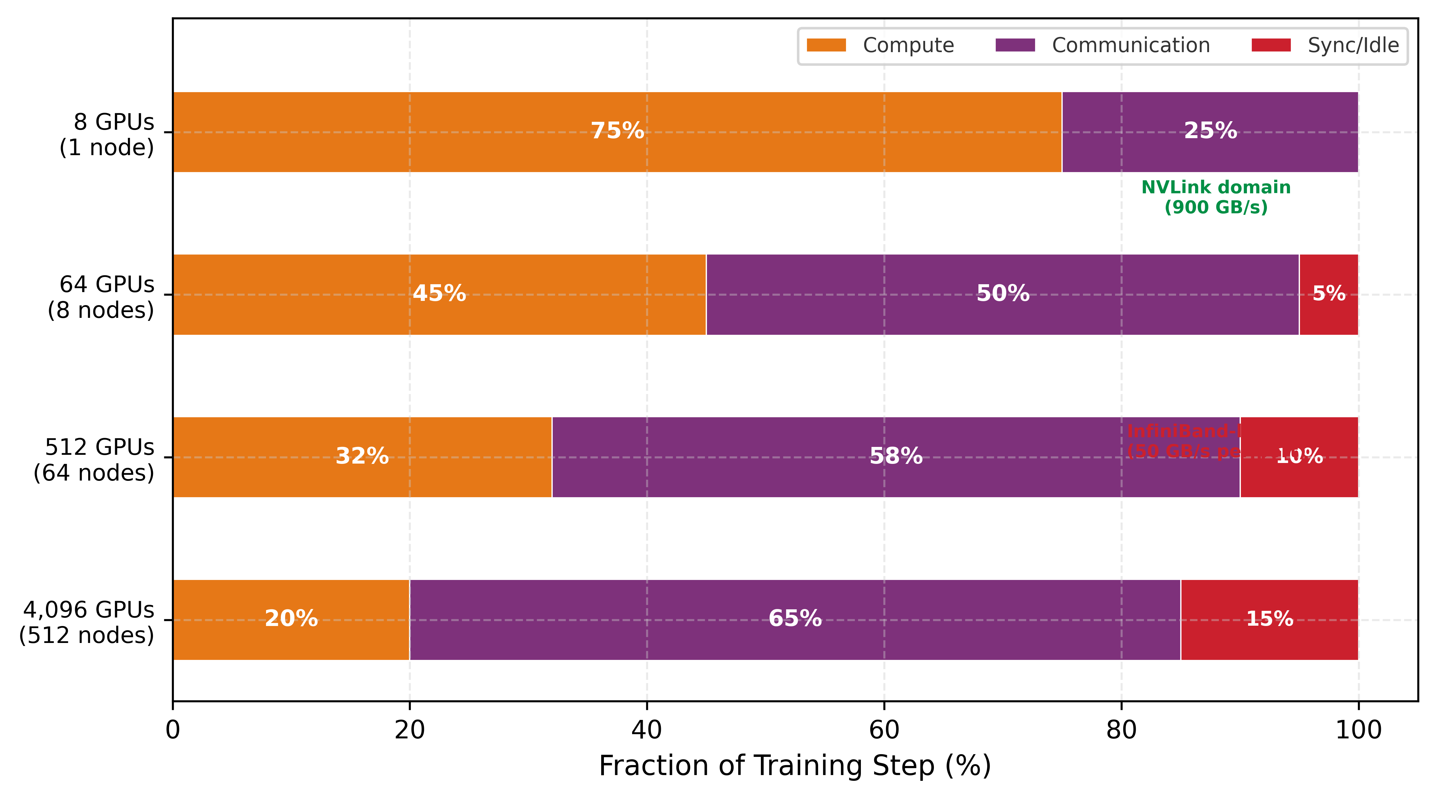
Gradient synchronization devours 30 to 70 percent of each step at scale.
The calculation reveals why data movement, not computation, becomes the governing constraint at scale. A single AllReduce on a 70B model’s gradients consumes seconds of wall-clock time, during which all GPUs would otherwise sit idle. This asymmetry between local computation (which parallelizes perfectly) and global coordination (which requires physical data movement) motivates every collective algorithm that follows. Halving that multi-second AllReduce would save thousands of GPU-hours over a typical training campaign, translating directly to reduced cost and faster time to deployment.
The cost analysis also explains why the choice of collective algorithm matters far more than most practitioners realize. Using a suboptimal algorithm that achieves only 60 percent of theoretical bandwidth (a common outcome with poor topology mapping) would inflate the five-second AllReduce to over nine seconds, adding several seconds of pure waste to every training step. Because this waste propagates through the entire fleet, communication algorithms occupy the Distribution Layer of the fleet stack: the Infrastructure Layer below provides raw bandwidth through NVLink, InfiniBand, and network topologies (covered in Network Fabrics), while the Serving Layer above depends on efficient gradient synchronization to complete training runs that produce deployable models. When communication algorithms fail to saturate the available bandwidth, training takes longer, serving models are delivered later, and the entire fleet operates below its economic potential.
Figure 2 quantifies how this communication overhead compounds as the fleet grows. At 8 GPUs within a single NVLink-connected node, communication consumes roughly 25 percent of each training step because the 900 GB/s interconnect bandwidth keeps pace with gradient volume. As the cluster expands to 64 GPUs across 8 nodes, the transition to InfiniBand (50 GB/s per port) shifts the balance: communication dominates at approximately 50 percent of step time, with an additional 5 percent lost to synchronization barriers. At a 4,096-GPU scale, communication and synchronization overhead together consume 80 percent of the training step, leaving only 20 percent for useful computation. This progression explains why collective algorithms matter: without hierarchical collectives, gradient compression, and communication-computation overlap, large-scale training would spend the vast majority of its multi-million-dollar compute budget waiting for data to arrive.
The gradient’s travel manifest
The journey begins at the moment the backward pass completes. On a single machine, that was the end of the story: the weights were updated, and the neuron learned. At production scale, however, the gradient is born into isolation. It exists on one GPU, while the “truth” of the model is distributed across thousands. To achieve global convergence, the gradient must find its peers.
The specific “travel manifest” for this journey is dictated by the parallelism strategy chosen in Distributed Training. The choice of how the math is split determines how the data moves. For our Lighthouse Archetypes (Three systems archetypes), these manifests differ fundamentally. For Archetype A (GPT-4/Llama-3), our gradient is part of a massive, dense tensor that must meet every other gradient in the fleet to compute a global average, so its primary vehicle is the AllReduce. For Archetype B (DLRM at Scale), the DLRM workload6, our gradient or activation is sparse and targeted: it does not need to meet everyone, only the specific GPU that holds its embedding shard. Mixture-of-experts (MoE) routing creates the same targeted pattern, sending each token to the GPU that hosts its assigned expert, so both rely on the AllToAll.
6 DLRM: Meta’s 2019 architecture for click-through rate prediction, where embedding tables can exceed 100 GB and must be sharded across workers. Each forward pass triggers AllToAll to exchange sparse embedding lookups, creating a communication pattern where message sizes are small (hundreds of KB) but fan-out is \(\mathcal{O}(N)\), making DLRM one of the most latency-sensitive distributed workloads in production.
Understanding this mapping is essential: the what of parallelism directly determines the how of communication. At large scale, these strategies are not mutually exclusive. A single training run for a large language model typically employs 3D parallelism (combining data parallelism, tensor parallelism, and pipeline parallelism simultaneously), which means multiple collective primitives execute concurrently on overlapping subsets of GPUs. Tensor parallelism drives AllReduce operations within each node (over NVLink), pipeline parallelism drives point-to-point sends between pipeline stages (often between nodes), and data parallelism drives AllReduce operations across groups of nodes (over InfiniBand).
Each primitive operates on a different process group, a subset of the total GPU population that participates in that particular collective. Classical MPI uses a communicator as the object that names such a participating set; its communicator size is the number of ranks in that set. MPI libraries already selected collective algorithms based on communicator size and message size (Thakur et al. 2005). GPU communication libraries inherit that algorithm-selection problem and add the further challenge of coordinating overlapping process groups without creating contention between concurrent collectives.
Table 1 previews the mapping from parallelism strategy to collective primitive. The primitive names are introduced formally in the next section; for now, read the table as a traffic map that says who must exchange data with whom.
| Parallelism Strategy | The Gradient’s Goal | Primary Primitive | Primary Constraint |
|---|---|---|---|
| Data Parallelism | Meet everyone, compute global average | AllReduce | Bandwidth (Large payloads) |
| FSDP/ZeRO | Find shards, reconstruct the whole | AllGather + ReduceScatter | Bandwidth (High frequency) |
| Tensor Parallelism | Quick handshake within the node | AllReduce | Latency (Speed is life) |
| Pipeline Parallelism | Handoff to the next neighbor | Point-to-Point (Send/Recv) | Latency (Sequential dependencies) |
| Expert Parallelism (MoE) | Targeted routing to a specialist | AllToAll | Latency + Contention |
In this table, Expert Parallelism refers to the mixture-of-experts (MoE)7 architecture pattern. The mapping shows that different parallelism strategies impose fundamentally different communication patterns. Data parallelism and FSDP generate large, bandwidth-bound messages that benefit from ring-based algorithms and hierarchical decomposition. Tensor and pipeline parallelism generate small, latency-bound messages that benefit from tree-based algorithms and low-overhead software stacks. Expert parallelism generates all-to-all traffic patterns that stress the network’s bisection bandwidth. To reason quantitatively about these differences, we need a model of network performance.
7 Mixture-of-Experts (MoE): An architecture where each token activates only a subset of specialized subnetworks (experts), reducing per-token FLOPs while maintaining total model capacity. The systems trade-off is stark: MoE replaces the bandwidth-bound AllReduce of dense models with latency-bound AllToAll, shifting the communication bottleneck from \(\beta\) to \(\alpha\) and creating \(\mathcal{O}(N^2)\) contention that limits practical cluster size.
Self-Check: Question
A team triples the GPU count on a dense training run expecting near-linear wall-clock speedup, but step time drops only 30 percent. Per-GPU compute utilization falls from 65 percent to 34 percent. What does the section’s local-versus-global asymmetry predict as the root cause?
- Each added GPU roughly triples local arithmetic throughput, while gradient synchronization must traverse physical space and scale with participant count, so coordination cost grows while per-GPU compute share shrinks.
- Backpropagation stops working correctly when distributed across multiple nodes because gradients cannot be computed in parallel.
- Floating-point accumulation becomes numerically unstable as more GPUs participate in the reduction.
- Optimizer state must be shuffled through host DRAM whenever the cluster exceeds one node.
A team scales a 70B-parameter model’s gradient synchronization from 8 GPUs to 1,000 GPUs under ring AllReduce and expects per-node bytes transferred to grow roughly linearly with participant count. Explain why that expectation is wrong, and identify what actually dominates synchronization time at scale.
A mixture-of-experts layer routes each token to a specific remote expert GPU based on a gating function, then gathers the expert outputs back for the next layer. Which collective primitive does this routing pattern most naturally induce, and why?
- Broadcast, because every GPU needs the same gating weights.
- AllToAll, because each worker must send distinct payloads to specific remote destinations rather than compute one global aggregate.
- AllReduce, because the per-expert outputs must be summed across all workers.
- ReduceScatter, because tokens are divided evenly across experts.
True or False: Deploying RDMA on a cluster eliminates the distance-dependent latency and bandwidth-over-distance costs that physically constrain collective communication.
Order the following stages of one data-parallel training step: (1) synchronize gradients across all workers, (2) perform the optimizer step on each replica using synchronized gradients, (3) run the forward pass and compute loss on each local batch, (4) run the backward pass to compute local gradients.
Mapping the Terrain: Network Performance Modeling
A data center engineer cannot predict how long it takes to send ten megabytes across a cluster without knowing two distinct variables: the fixed startup tax and the per-byte transit fee. As the gradient begins its journey, it immediately encounters the physical reality of the data center network.
The alpha-beta cost model: Startup tax and transit fee
Every message our gradient sends obeys the linear cost model \(T(n) = \alpha + n/\beta\)—a fixed startup tax plus a per-byte transit fee. Those two terms decide every algorithm choice in this chapter.
Definition 1.2: α-β model (Hockney model)
α-β Model (Hockney Model) is the linear communication cost model \(T(n) = \alpha + n/\beta\) that decomposes message transfer time into a fixed startup latency (\(\alpha\), the per-message overhead) and a message-size-dependent bandwidth term (\(n/\beta\), proportional to bytes transferred), enabling algorithm designers to predict when message fusion or gradient compression will improve throughput (Hockney 1994).
- Significance: For InfiniBand NDR at \(\alpha \approx 2\,\mu\text{s}\) and \(\beta \approx 50\,\text{GB/s}\), the crossover size \(n^* = \alpha \cdot \beta \approx 100\,\text{KB}\). A 4 KB routing message is far below \(n^*\), so the startup tax dominates; fusing 100 such messages into one 400 KB message reduces communication cost from \(100\alpha = 200\,\mu\text{s}\) to one \(\alpha + n/\beta \approx 10\,\mu\text{s}\), a 20\(\times\) improvement. A 140 GB gradient tensor is far above \(n^*\), so bandwidth dominates and reducing payload bytes is the effective lever.
- Distinction: Unlike idealized throughput models that treat bandwidth as the sole communication cost, the α-β model reveals that \(N\) small messages of size \(n/N\) cost up to \(N\times\) more than one large message of size \(n\) when \(n/N \ll n^*\), explaining why NCCL fuses small AllReduce calls and why MoE routing algorithms buffer tokens before launching collectives.
- Common pitfall: A frequent misconception is that gradient compression always helps. If the compressed gradient size remains well above \(n^*\), compression reduces the bandwidth term but leaves the latency term unchanged. Even shrinking a 70B model’s gradient payload from 140 GB to 1.4 GB leaves the message firmly bandwidth-bound; it does not turn the operation into a low-latency exchange.
Hockney, Roger W. 1994. “The Communication Challenge for MPP: Intel Paragon and Meiko CS-2.” Parallel Computing 20 (3): 389–98. https://doi.org/10.1016/s0167-8191(06)80021-9.
The two parameters have distinct physical meanings. Latency (\(\alpha\)) is the fixed start-up cost to send a message regardless of size, covering software overhead (kernel launch, NCCL initialization), PCIe traversal, and network switching time. Bandwidth (\(\beta\)) is the sustained data transfer rate in bytes per second. The critical message size \(n^* = \alpha \cdot \beta\) marks the crossover point: messages smaller than \(n^*\) are latency-bound; messages larger are bandwidth-bound. The α-β Communication Model works this model through concrete message-size regimes and roofline analysis, so a reader who wants the full derivation behind the crossover can follow it there; here we establish the parameters and apply them directly.
Table 2 shows typical values for data center interconnects, and the critical-size column carries the load-bearing pattern: intra-node NVLink stays latency-bound up to several hundred kilobytes, whereas the inter-node fabrics cross over near 100 KB, so a message large enough to be bandwidth-bound inside a node can still be latency-bound once it travels between nodes.
| Interconnect | Latency (\(\alpha\)) | Bandwidth (\(\beta\)) | Critical Size (\(n^*\)) |
|---|---|---|---|
| NVLink 4.0 (intra-node) | 1–2 μs | 450 GB/s | ~0.7 MB |
| InfiniBand NDR 400 Gbps | 1–3 μs | 50 GB/s (per port) | ~100 KB |
| InfiniBand HDR 200 Gbps | 2–5 μs | 25 GB/s | ~87.5 KB |
| PCIe Gen5 (GPU↔︎CPU) | 2–5 μs | 64 GB/s | ~224 KB |
| Ethernet 100 Gbps (RoCE) | 5–10 μs | 12.5 GB/s | ~93.7 KB |
Applying the critical message size formula to a concrete workload reveals which optimization strategy matters most:
Napkin Math 1.2: The critical message size
Problem: Consider a cluster using InfiniBand NDR 400 Gbps with \(\alpha =\) 2 μs and \(\beta =\) 50 GB/s. At what message size does optimizing for bandwidth start to matter more than optimizing for latency?
Math:
\(n^* = \alpha \cdot \beta =\) \(2 \times 10^{-6}\) s \(\times\) \(5 \times 10^{10}\) B/s \(=\) 100 KB
Systems insight: Messages under 100 KB (like MoE tokens, pipeline activations) are latency-bound: buy lower-latency switches and reduce software overhead. Messages over 100 KB, such as large language model (LLM) gradients, are bandwidth-bound: buy more bandwidth and compress the data. Applying the wrong optimization wastes money without improving performance.

Small messages are latency-bound, large ones bandwidth-bound; the cost reverses.
The critical message size separates two distinct operating regimes. Below it, small messages such as MoE routing tokens or scalar reductions are latency-bound \((n < n^*)\), where time is dominated by \(\alpha\) and optimization focuses on fusion (batching small messages), topology (reducing hop count), and software-stack tuning (kernel bypass via RDMA). Above it, large messages such as LLM gradients or optimizer states are bandwidth-bound \((n \gg n^*)\), where time is dominated by \(n/\beta\) and optimization shifts to compression (lower precision or sparsity), algorithm choice (Ring vs. Tree), and link aggregation (multi-rail NICs). The distinction between latency-bound and bandwidth-bound communication is the diagnostic skill to practice.
Checkpoint 1.1: Alpha-beta diagnostics
Verify your understanding of network performance regimes:
The LogP model
The α-β model assumes the processor is idle during communication. For pipelined systems where we overlap communication with computation, this assumption fails. The LogP model (Culler et al. 1993) extends α-β with four parameters:
Culler, David, Richard Karp, David Patterson, Abhijit Sahay, Klaus Erik Schauser, Eunice Santos, Ramesh Subramonian, and Thorsten von Eicken. 1993. “LogP: Towards a Realistic Model of Parallel Computation.” ACM SIGPLAN Notices 28 (7): 1–12. https://doi.org/10.1145/173284.155333.
- \(L_{\text{lat}}\) (Latency): The time for a message to traverse the network (similar to \(\alpha\)).
- \(o\) (Overhead): The CPU/GPU time spent initiating or receiving a transfer. During this time, the processor cannot compute, making this the nonoverlappable cost. In a distributed training context, \(o\) is the aggregate of PyTorch or JAX dispatch overhead, CUDA kernel launch time, tensor memory registration with the RDMA stack, and occasionally Python Global Interpreter Lock (GIL) contention when the communication thread competes with the training loop. These software layers account for why measured NCCL overhead is 25–50 \(\mu\text{s}\) per collective even when the wire-level \(\alpha\) is only 1–3 \(\mu\text{s}\); the NCCL comparison later in this section makes the gap concrete.
- \(g\) (Gap): The minimum time interval between consecutive message injections (inverse of message rate). This models link contention.
- \(N_{\text{rank}}\) (Rank count): The number of ranks in the communication group.
LogP distinguishes network latency (\(L_{\text{lat}}\), which can be hidden) from processor overhead (\(o\), which cannot). A system can overlap communication with computation only if the compute kernel runs longer than the overhead. A small overlap calculation makes this distinction concrete:
Napkin Math 1.3: Hiding communication behind computation
Problem: A training pipeline attempts to overlap gradient AllReduce with the next layer’s backward pass. The backward pass takes 500 μs. The AllReduce has network latency 100 μs but processor overhead \(o =\) 50 μs to initiate and \(o =\) 50 μs to receive. Can the communication be hidden?
Math:
- Overlappable portion: Network latency \(L_{\text{lat}}\) = 100 μs (data in flight while GPU computes).
- Non-overlappable portion: \(2o\) = 100 μs (GPU busy initiating/receiving).
- Compute available: 500 μs.
- Hidden: All 100 μs of \(L_{\text{lat}}\) can overlap with compute.
- Exposed: The 100 μs of \(2o\) overhead cannot overlap.
Result: Effective time is 100 μs + max(500 μs, 100 μs) = 600 μs. The network latency is hidden, but the processor overhead remains exposed. Figure 3 shows this overlap visually.
Systems insight: The α-β model captures the total communication time. The LogP model reveals how much of it can be hidden. When designing pipelined training, optimize for low \(o\) (kernel bypass, GPUDirect) rather than high \(\beta\) alone.

The choice between models depends on the analysis context. The \(\alpha\)-\(\beta\) model is the right tool for back-of-envelope calculations, algorithm selection (Ring vs. Tree), and cases where communication is blocking (synchronous barriers). Its strength is simplicity, since the two parameters can be measured directly with a point-to-point bandwidth test and a zero-byte message latency test. Its weakness is the assumption that the processor is idle during communication, which makes it overly pessimistic when overlap is possible. The LogP model earns its extra parameters when the analysis turns to pipelined execution, compute-communication overlap, or debugging why a theoretically fast algorithm underperforms (often high \(o\)). Its distinction between network latency \(L_{\text{lat}}\) (which can be hidden) and processor overhead \(o\) (which cannot) determines whether a given overlap strategy will actually hide communication. The cost is that measuring \(o\) accurately requires profiling tools such as NVIDIA Nsight Systems, because \(o\) depends on the specific communication library and GPU driver stack.
In practice, most engineering calculations start with the \(\alpha\)-\(\beta\) model for initial sizing and algorithm selection, then refine with LogP analysis when communication-computation overlap is the target optimization. Both models share a common limitation: they assume a single flow on a single link. Real communication patterns involve multiple simultaneous flows competing for shared bandwidth, which can cause congestion that neither model captures. For congestion-sensitive workloads (particularly AllToAll for MoE), empirical benchmarking on the target cluster remains the necessary validation step.
Putting the model to work: Llama 70B communication budget
The alpha-beta model becomes most valuable when applied to real training configurations. Consider a concrete scenario: training a Llama-class 70B parameter model using data parallelism across 128 GPUs spanning 16 nodes of 8 GPUs each. The gradient tensor is 140 GB in BF16 (70 billion parameters at 2 bytes each, common for Llama-class training). During each training step, this entire gradient must be synchronized across all workers.
The calculation uses the bandwidth hierarchy before the chapter formalizes it: reduce as much data as possible over the fast NVLink tier inside each node, send only the reduced shard over the slower InfiniBand tier, then reconstruct the result locally. The primitive names become precise in the hierarchy section; the engineering idea is already visible in the bandwidth budget.
Using BF16 gradients (a common practice that halves communication volume to 140 GB), the contrast is stark. Routing the full gradient over the slow inter-node fabric, as a flat Ring AllReduce does, costs roughly 5,557 ms. Confining most of the traffic to NVLink and sending only the reduced shard over InfiniBand cuts that to approximately 1200.8 ms. The difference is not marginal; it determines whether communication can be hidden behind computation or whether it becomes the critical path.
The per-phase breakdown behind these numbers (the intra-node reduction, the reduced inter-node exchange, and the intra-node redistribution) requires the collective primitives this section has not yet introduced. Section 1.5.1 names those primitives and works the full three-phase derivation; the budget here establishes only that the bandwidth hierarchy is worth respecting, and by how much.
Theory vs. practice: The NCCL reality gap
The bandwidth-latency trade-off (principle 11) provides useful first-order predictions, but real communication libraries introduce overheads that the idealized \(\alpha\)-\(\beta\) model does not capture. NCCL, a widely used GPU communication library, adds protocol negotiation, memory registration, and internal pipelining that modify the effective \(\alpha\) and \(\beta\) values (Jeaugey 2017; NVIDIA 2026). Table 3 compares one-message \(\alpha\)-\(\beta\) payload predictions against measured NCCL performance for common message sizes on an 8-node DGX H100 cluster (64 GPUs, InfiniBand NDR 400G).
| Message Size | \(\alpha\)-\(\beta\) Prediction | Measured NCCL | Ratio (Measured/Predicted) | Explanation |
|---|---|---|---|---|
| 1 KB | ~3.1 μs | ~25 μs | ~8.1× | NCCL protocol setup dominates |
| 64 KB | ~4.4 μs | ~30 μs | ~6.9× | Still latency-bound; NCCL overhead |
| 1 MB | ~23.1 μs | ~40 μs | ~1.7× | Transitioning to bandwidth-bound |
| 64 MB | ~1.3 ms | ~1.6 ms | ~1.2× | NCCL approaches theoretical bandwidth |
| 1 GB | ~20 ms | ~23 ms | ~1.15× | Bandwidth-dominant; NCCL nearly optimal |
| 10 GB | ~200 ms | ~215 ms | ~1.07× | Large payloads saturate the wire |
The table reveals two critical lessons. First, the \(\alpha\)-\(\beta\) model underestimates small-message latency by 7–8\(\times\) because it accounts only for wire-level propagation, not the software stack overhead. For latency-sensitive operations (tensor parallelism AllReduce, MoE token routing), the effective \(\alpha\) is 5–10\(\times\) higher than the physical wire latency. Second, for large messages the model is accurate to within 8–15 percent, confirming that bandwidth is the binding constraint and that NCCL’s internal optimizations (channel pipelining, kernel fusion) successfully saturate the available links.
This reality gap has practical consequences for algorithm selection. The crossover point between Ring and Tree AllReduce shifts upward in practice because the effective \(\alpha\) is larger than the wire-level value. Engineers who use textbook \(\alpha\) values will underestimate latency costs and may choose Ring when Tree would perform better. A robust practice is to measure the effective \(\alpha\) on the specific cluster by benchmarking small-message AllReduce latency, then use that measured value in all subsequent calculations.
Self-Check: Question
On InfiniBand NDR with \(\alpha = 2\) microseconds and \(\beta = 50\) GB/s, an MoE routing workload sends 4 KB token messages and a dense data-parallel workload sends 1 GB gradient buffers. Which optimization family should each workload prioritize?
- Both workloads should prioritize reducing \(\alpha\), since \(\alpha\) dominates on modern fabrics regardless of message size.
- The 4 KB messages sit well below the ~100 KB critical size so MoE should fuse messages and reduce startup cost, while 1 GB buffers sit three orders above the critical size so dense training should compress payload and add bandwidth.
- Both workloads should prioritize switching from RDMA to TCP to simplify the stack.
- The 1 GB buffers are latency-bound because longer messages take longer, so dense training should optimize \(\alpha\).
A training engineer has tuned an AllReduce algorithm using the alpha-beta model and predicted that it should finish in 5 ms on her cluster, but profiling shows the backward pass running in parallel is never fully hidden behind the AllReduce. Explain why the LogP model is better suited than alpha-beta for diagnosing this overlap failure.
The chapter’s Llama 70B budget on 128 GPUs across 16 nodes shows hierarchical AllReduce completing about six times faster than flat ring AllReduce. Which mechanism most directly explains the speedup?
- Hierarchical AllReduce eliminates inter-node communication entirely by keeping all traffic on NVLink.
- Hierarchical AllReduce first reduces within each node over fast NVLink so only a reduced shard, not the full gradient, traverses the slower InfiniBand fabric between nodes.
- Hierarchical AllReduce switches the optimizer to require fewer synchronization steps per training iteration.
- Flat ring AllReduce cannot operate on BF16 gradients and must promote every value to FP32.
On a link with \(\alpha = 2\) microseconds and \(\beta = 50\) GB/s, a 4 KB MoE routing message takes roughly 2.08 microseconds of which 96 percent is startup cost; because this message sits 25 times below the ____ message size, fusing many tokens into one large transfer delivers a far larger speedup than adding raw bandwidth.
True or False: Alpha-beta model predictions are accurate for 1 GB AllReduce messages on a real cluster but can be off by 5 to 10 times for 64 KB messages, because measured NCCL small-message latency is inflated by protocol setup and memory registration overhead that alpha-beta does not model.
Choosing the Vehicle: Collective Operation Primitives
If a GPU simply opens a socket and sends a massive gradient to another GPU, the entire cluster will rapidly collapse into an unmanageable web of deadlocks and congestion. With the terrain mapped, the gradient must now choose its vehicle: strictly choreographed group exchanges known as collective operations, a vocabulary standardized by MPI and inherited by modern ML communication libraries (Message Passing Interface Forum 2015). Figure 4 illustrates four of the central primitives in this vocabulary: AllReduce, AllGather, ReduceScatter, and AllToAll. Each panel reads as a before-and-after across the process group, with one row per rank: blue cells mark the input each rank starts with, green cells mark the result it ends with, and orange marks the AllToAll routing that shuffles unique data between every pair of ranks. Two further primitives, Broadcast (rank 0 sends to all) and Reduce (all aggregate to rank 0), are foundational building blocks defined in the prose below and used implicitly in the figure’s compound patterns. Collective Operation Complexity formalizes the semantics and latency and bandwidth complexity of each primitive; the prose here introduces them through their workload use cases, and the reader who wants the formal complexity bounds before proceeding can establish them there first.
Definition 1.3: Collective operation
Collective Operation is a distributed communication pattern in which all processes in a group participate simultaneously to aggregate, broadcast, or redistribute data, with the correctness guarantee that each participant receives the result prescribed by the collective’s semantics regardless of message ordering or arrival time.
- Significance: The right collective algorithm determines whether communication scales with cluster size or remains constant. Ring AllReduce achieves bandwidth-optimal \(2(N-1)/N \times M / \beta\) per node (constant in \(N\)), while a naive reduce-then-broadcast approach costs \(\mathcal{O}(N \times M / \beta)\), making it 500\(\times\) worse for \(N=1024\). Algorithm selection thus directly determines whether the \(\text{BW}\) term in the iron law is the training bottleneck.
- Distinction: Unlike point-to-point communication (where one sender and one receiver exchange data independently), a collective operation coordinates the entire process group—every participant must invoke the collective before any can complete it, and the library guarantees a consistent result even when different processes contribute different data.
- Common pitfall: A frequent misconception is that one collective algorithm suits all message sizes. Ring AllReduce achieves near-optimal bandwidth for large gradient tensors but has \(\mathcal{O}(N)\) latency—for small messages like MoE routing decisions (~4 KB), a tree-based algorithm reduces latency to \(\mathcal{O}(\log N)\) steps at the cost of suboptimal bandwidth utilization (the bandwidth-optimal recursive halving-doubling alternative is covered in section 1.4.5), requiring workload-specific algorithm selection rather than a single default.

The primitive choice is the first scaling decision because it fixes which ranks must coordinate, which data must move, and which communication term will dominate. Different model architectures stress different operations, and selecting the wrong primitive for a workload creates unnecessary bottlenecks.
The six core primitives
The six primitives in table 4 form a decision ladder: use the narrowest operation that preserves the model’s mathematics, because every broader pattern adds participants, barriers, or contention.
| Primitive | What it does | Primary use case | Communication cost |
|---|---|---|---|
| Broadcast | One sender transmits data to all receivers. | Distribute initial model weights from rank 0 at startup, across all parallelism strategies. | \(\mathcal{O}(\log N)\) latency (tree); \(\mathcal{O}(M)\) bandwidth. |
| Reduce | Aggregate data from all workers (sum, min, max) to a single root. | Aggregate validation metrics such as loss and accuracy to a logging process. | \(\mathcal{O}(\log N)\) latency (tree); \(\mathcal{O}(M)\) bandwidth. |
| AllReduce | Aggregate from all workers, then distribute the result to all (\(y_i = \sum_{j=0}^{N-1} x_j\) for all \(i\)). | Data parallelism (Data Parallelism): synchronize gradients so every GPU computes the same update. | Ring is bandwidth-optimal at \(2\frac{N-1}{N}\frac{M}{\beta}\) but \(\mathcal{O}(N)\) latency; Tree gives \(\mathcal{O}(\log N)\) latency with worse bandwidth. |
| AllGather | Each worker’s data goes to all; the result concatenates every input (\(x_i \rightarrow [x_0, \dots, x_{N-1}]\)). | Sharded data parallelism (FSDP/ZeRO): collect sharded parameters before a forward or backward pass. | Ring \(\frac{N-1}{N}\frac{M}{\beta}\); resident data grows from an \(M/N\) shard to the full \(M\). |
| ReduceScatter | Reduce across workers, but scatter so each keeps a distinct chunk (worker \(i\) receives the \(i\)-th block of \(\sum x_j\)). | Sharded data parallelism: reduce gradients while keeping them sharded to save memory. | Ring \(\frac{N-1}{N}\frac{M}{\beta}\); the inverse of AllGather. |
| AllToAll | The most general pattern: worker \(i\) sends a distinct chunk to each worker \(j\), a distributed matrix transpose. | MoE routing tokens to experts; DLRM exchanging embedding lookups across workers. | \(\frac{N-1}{N}M\) per worker, but \(\mathcal{O}(N^2)\) logical connections make contention the scaling limit. |
Ring achieves AllReduce’s bandwidth-optimal cost while Tree trades bandwidth for logarithmic latency; AllReduce develops the formal definition and a worked example comparing the two, so a reader who wants that derivation can take the full treatment there (Patarasuk and Yuan 2009; Thakur et al. 2005).
8 FSDP (Fully Sharded Data Parallel): PyTorch’s fully sharded implementation follows the ZeRO-3 idea of sharding parameters, gradients, and optimizer states across \(N\) accelerators (Rajbhandari et al. 2020). The trade-off is communication frequency: full sharding adds layer-level AllGather and ReduceScatter operations instead of relying only on data parallelism’s step-level AllReduce, making it more sensitive to the \(\alpha\) overhead.
Rajbhandari, Samyam, Jeff Rasley, Olatunji Ruwase, and Yuxiong He. 2020. “ZeRO: Memory Optimizations Toward Training Trillion Parameter Models.” SC20: International Conference for High Performance Computing, Networking, Storage and Analysis, 1–16. https://doi.org/10.1109/sc41405.2020.00024.
A key insight is that AllReduce can be decomposed into ReduceScatter followed by AllGather. This is not merely a mathematical equivalence; it is precisely how Ring AllReduce works internally (the Scatter-Reduce phase is a ReduceScatter, the AllGather phase is an AllGather). ZeRO-style sharding, realized in PyTorch as FSDP8, exploits this decomposition by AllGathering parameter shards before a module needs them and ReduceScattering gradients after backward so each rank retains only its shard for the optimizer step (Rajbhandari et al. 2020). This shards parameters, gradients, and optimizer state across workers, reducing persistent model-state memory roughly by \(N \times\), while temporary full-parameter buffers and prefetching determine peak memory.
The same AllGather/ReduceScatter pair also appears in sequence parallelism: an AllGather reconstructs the activation view needed for a local operation, and a later ReduceScatter redistributes the result along the sequence dimension. That example will matter later because it shows that a primitive’s semantics stay fixed even when the tensor dimension being sharded changes.
This ladder matters because the primitive determines the synchronization shape before any algorithmic optimization begins. AllReduce creates global agreement, AllGather and ReduceScatter trade memory for repeated shard movement, and AllToAll replaces a bandwidth problem with fan-out and contention.
The contrast between AllToAll and AllReduce highlights a fundamental difference in how collective operations scale with cluster size.
Systems Perspective 1.1: AllToAll vs. AllReduce: Why scale differs
While AllReduce scales efficiently because it can be pipelined in a ring (where each node only talks to its neighbor), AllToAll is fundamentally harder to scale.
In an AllToAll, every process has a unique piece of data for every other process. This creates \(\mathcal{O}(N^2)\) logical connections. At the hardware level, this leads to network contention: if 1024 GPUs all try to send data to different targets simultaneously, the “Fat-Tree” or “Spine” switches in the data center become the bottleneck.
This is why Expert Parallelism (MoE) and large-scale recommendation systems often hit a “communication wall” much earlier than standard data-parallel models. The algorithm choice (AllReduce vs. AllToAll) determines the scaling ceiling.

All-to-All traffic scales worse than AllReduce.
To make the AllToAll pattern concrete, consider a Mixture of Experts model with 64 experts distributed across 8 GPUs (8 experts per GPU). During each forward pass, a gating network assigns each input token to one or more experts. The tokens assigned to experts on remote GPUs must be physically moved to those GPUs before computation can proceed, and the results must be moved back afterward.
Napkin Math 1.4: AllToAll for MoE token routing
Problem: A MoE model processes a batch of 4096 tokens across 8 GPUs (512 tokens per GPU). Each token is a 2048-dimensional hidden state in BF16 (4.096 KB per token). The gating network assigns each token to exactly 1 of 64 experts (8 experts per GPU). Assuming uniform routing (each expert receives 64 tokens), how much data does each GPU send and receive?
Math:
Each GPU holds 512 tokens that need to reach 64 different experts across 8 GPUs. With uniform routing, each GPU sends 64 tokens to each of the other 7 GPUs (keeping 64 tokens local).
- Data per GPU-to-GPU transfer: 64 tokens \(\times\) 4.096 KB/token = 262.144 KB
- Total data sent per GPU: 7 \(\times\) 262.144 KB = 1.84 MB
- Total data received per GPU: 1.84 MB (symmetric)
Latency Analysis (InfiniBand NDR, \(\alpha =\) 3 μs, \(\beta =\) 50 GB/s):
Each of the 7 transfers is a 262.144 KB message. From the \(\alpha\)-\(\beta\) model: \(T_{\text{transfer}}\) = 3 μs + 5 μs = 8 μs per transfer.
If serialized: 7 \(\times\) 8 μs = 56 μs. If all 7 transfers run in parallel (full-duplex, non-blocking): \(\approx\) 8 μs.
Systems insight: The per-transfer sizes in this MoE example sit near the critical-message-size boundary, so startup overhead remains comparable to serialization time. This is why MoE scaling is often constrained by \(\alpha\) (latency), fan-out, and contention rather than raw \(\beta\) (bandwidth) alone, and why MoE systems benefit from low-latency switches, RDMA, message fusion, and topology-aware routing. The AllToAll also runs twice per layer (once for token dispatch, once for result collection), doubling the startup tax.
In practice, MoE routing is rarely perfectly uniform. Popular experts receive more tokens than unpopular ones, creating load imbalance that translates to communication imbalance. If one expert receives 3\(\times\) more tokens than average, the GPU hosting that expert receives 3\(\times\) more incoming data, creating a hotspot that can stall the entire collective (since AllToAll is a barrier operation). Large MoE systems address this through auxiliary load-balancing losses that penalize the gating network for routing too many tokens to any single expert, and through capacity factors that cap the maximum number of tokens an expert can accept (dropping overflow tokens). These techniques trade a small amount of model quality for communication balance, which is the right trade-off at scale.
Table 5 maps these primitives to the parallelism strategies introduced in Distributed Training and the lighthouse archetypes introduced in Three systems archetypes.
| Training Strategy | Primary Collective | Bottleneck Characteristic |
|---|---|---|
| Data Parallelism | AllReduce | Bandwidth-bound (large gradients) |
| FSDP/ZeRO-3 | AllGather, ReduceScatter | Bandwidth-bound, high frequency |
| Tensor Parallelism | AllReduce, AllGather | Latency-bound (requires NVLink) |
| Pipeline Parallelism | Point-to-Point (Send/Recv) | Latency-bound (microbatch handoffs) |
| Sequence Parallelism | AllGather, ReduceScatter | Bandwidth-bound (activation exchange) |
| MoE (Experts) | AllToAll | Latency-sensitive + contention |
| DLRM (RecSys) | AllToAll | Latency & Bandwidth (sparse lookups) |
FSDP communication patterns

FSDP trades one step-level collective for two per-layer collectives.
The FSDP/ZeRO strategy deserves special attention because its communication pattern differs fundamentally from standard data parallelism (Rajbhandari et al. 2020). In standard data parallelism, each GPU holds a complete copy of the model, computes gradients locally, and synchronizes via a single AllReduce at the end of the backward pass. Full sharding eliminates this redundancy by partitioning the model parameters across GPUs, so each GPU holds only its local shard outside the moments when a layer must be reconstructed.
Because each GPU now holds only \(1/N\) of the parameters, it must reconstruct the full tensor before it can use a layer, and that reconstruction is what transforms the communication pattern. Before each layer’s forward pass, the GPU calls AllGather to collect the shards from all other GPUs. After the backward pass, the gradients are reduced and redistributed via ReduceScatter, so each GPU holds gradients only for its own parameter shard. The sharded parameters can then be discarded (freed from memory) until the next forward pass needs them.
The consequence is a displacement of overhead: sharding relieves the memory bottleneck but raises communication frequency. Standard data parallelism communicates once per training step (a single AllReduce of the full gradient). FSDP communicates twice per layer per step (AllGather in forward, ReduceScatter in backward), but each communication is smaller (only that layer’s parameters, sharded across ranks). For a model with \(N_L\) layers, FSDP issues \(2N_L\) collective operations per step instead of 1; across all those operations, the total communication volume can be comparable to the single full-gradient AllReduce, but it is spread across many smaller operations.
The higher operation count makes FSDP more sensitive to latency (\(\alpha\)) than standard data parallelism. If each of the \(2N_L\) collectives pays the full NCCL startup overhead (25–50 \(\mu\text{s}\) per operation from table 3), the aggregate overhead for a 100-layer model is 5–10 ms, which can represent a meaningful fraction of step time. FSDP implementations mitigate this through prefetching (launching the next layer’s AllGather while the current layer is computing) and communication stream pipelining (using dedicated CUDA streams for communication that overlap with compute streams).
Selecting the right collective algorithm at each invocation requires understanding these asymmetric patterns. The AllGather operations in FSDP are medium-sized (one layer’s parameters, typically 10–100 MB for transformer models) and latency-sensitive (because computation blocks until the full parameters are available). The ReduceScatter operations are of similar size but can overlap with the next layer’s backward computation. This asymmetry means the AllGather operations benefit more from low-latency algorithms (Tree or hybrid) while the ReduceScatter operations can use bandwidth-optimal algorithms (Ring) because their latency is hidden behind computation.
The collective primitives catalog above defines what must be communicated; the question now becomes how to execute these primitives efficiently on real networks. The most performance-critical primitive, AllReduce, admits multiple algorithmic implementations whose latency and bandwidth characteristics differ by orders of magnitude. The choice of algorithm can change AllReduce time by an order of magnitude, making this the single most consequential implementation decision in distributed training.
Self-Check: Question
In FSDP, each worker holds a parameter shard and must reconstruct the full parameter tensor immediately before that layer’s forward pass, then release it. Which collective primitive matches this reconstruction semantic?
- AllReduce, which aggregates values numerically across all workers into one summed tensor.
- AllGather, which concatenates shards from all participants so every worker ends with the full tensor.
- Broadcast, which sends a single worker’s copy to all other workers.
- ReduceScatter, which computes a reduction and then distributes non-overlapping chunks to each worker.
Viewing AllReduce as ReduceScatter followed by AllGather is operationally important for FSDP because it:
- proves that Tree AllReduce is always faster than Ring AllReduce for any cluster size.
- allows FSDP to perform the ReduceScatter after backward and defer the AllGather until the next forward pass needs the parameters, keeping tensors sharded for most of the step instead of materializing full tensors at all times.
- means AllReduce can be skipped whenever gradients are sparse.
- eliminates the need for any inter-node communication across training steps.
A team migrates a 7B-parameter training run from standard data parallelism to FSDP to fit a larger model on the same hardware and observes that memory pressure drops as expected but throughput worsens. Explain why FSDP can preserve total communication volume yet degrade throughput, and identify the system property that changed.
A mixture-of-experts layer uses AllToAll to route tokens to remote experts. The workload scales poorly from 128 to 1,024 GPUs even though the gradient AllReduce on the same hardware continues to scale well. What fundamental property of AllToAll explains this divergence?
- AllToAll cannot use RDMA, so every transfer must pass through CPU memory and bottlenecks on host DRAM.
- AllToAll creates roughly \(N^2\) distinct source-to-destination transfers that stress bisection bandwidth and produce contention patterns that AllReduce’s structured reduction avoids.
- AllToAll is only valid within one node, so multi-node MoE must emulate it with repeated Broadcast operations.
- AllToAll always moves more total bytes per worker than the model’s hidden dimension, regardless of batch size.
True or False: Because FSDP’s per-operation message size is much smaller than standard data parallelism’s single fused AllReduce, FSDP is automatically less sensitive to per-collective startup latency.
Engineering the Flow: AllReduce Algorithms
A correct AllReduce must give all 1,000 GPUs the exact sum of all 1,000 one-gigabyte gradients, and the algorithm that delivers it sets the cluster’s scaling ceiling. The naive answer—every GPU sends to one central server, whose network card instantly saturates—fails first, which makes it the right place to start.
Naive approaches vs. the bandwidth bottleneck
Consider a naive implementation using a Parameter Server (Star topology). All \(N\) workers send their gradients to rank 0; rank 0 sums them and sends the result back. The constraint is rank 0’s bandwidth: it must receive \(N \times M\) bytes and send \(N \times M\) bytes, so the time grows as \(T \propto N \times M / \beta\). At 1,000 GPUs, this makes the central rank the scaling bottleneck rather than the arithmetic.
This naive approach captures the pressure that early distributed ML frameworks had to manage: parameter-server systems receive, aggregate, and redistribute model updates through a server tier, while practical implementations shard the parameter space to spread that load (Dean et al. 2012; Li et al. 2014). Sharding reduces the per-server traffic from \(N \times M\) to \(N \times M/K_{\text{srv}}\) (where \(K_{\text{srv}}\) is the number of servers), but the server tier still grows as workers and model state grow, and it introduces additional complexity in parameter partitioning and consistency management.
The fundamental limitation is that any star-topology approach concentrates traffic at a central point. Regardless of how many servers participate, the aggregate traffic through the central tier scales as \(\mathcal{O}(N \times M)\). To achieve true scalability, we need algorithms where the communication volume per node is constant regardless of \(N\). This property, known as bandwidth optimality, is the design target for scalable collective algorithms.
War Story 1.1: When the parameter server became the bottleneck
Context: In 2017, Alexander Sergeev and Mike Del Balso’s team at Uber open-sourced Horovod as part of Uber’s Michelangelo ML platform, where TensorFlow training jobs needed to scale across many GPUs without forcing every model author to rewrite large portions of training code (Sergeev and Balso 2018).
Failure mode: TensorFlow’s stock distributed training relied on a parameter-server pattern that concentrated gradient traffic through a central tier and imposed non-negligible communication overhead. Scaling beyond a single node required heavy code modification, and the star-topology aggregation degraded as worker counts grew.
Consequence: Horovod adopted Baidu’s draft ring-allreduce implementation and wrapped efficient ring reduction behind a small API surface—just a few lines added to existing TensorFlow code (Gibiansky 2017; Sergeev and Balso 2018). The bandwidth bottleneck moved off the central server and onto bandwidth-optimal collective communication, and distributed training became practical for teams without distributed-systems expertise.
Systems lesson: A collective algorithm is also a developer interface. Scaling improves when the communication primitive is both bandwidth efficient and easy enough that teams actually use it correctly.
The bandwidth-optimal lower bound
Before examining specific algorithms, it is useful to establish a theoretical lower bound. In any correct AllReduce, every GPU starts with \(M\) bytes of local data and ends with \(M\) bytes of globally reduced data. Each byte of the final result incorporates information from all \(N\) GPUs, which means every GPU must receive at least \(M \cdot (N-1)/N\) bytes of “new” information (the contributions from all other GPUs). Symmetrically, each GPU must send at least \(M \cdot (N-1)/N\) bytes (its own contribution to the other GPUs’ results).
The minimum total transfer per GPU is therefore \(2 \cdot M \cdot (N-1)/N\) bytes (send plus receive). Dividing by the link bandwidth \(\beta\) gives the bandwidth lower bound:
\[T_{\text{bandwidth}}^{\text{min}} = \frac{2(N-1)}{N} \cdot \frac{M}{\beta}\]
As \(N\) grows large, this approaches \(2M/\beta\), which is independent of \(N\). An algorithm that achieves this bound is bandwidth-optimal. Ring AllReduce achieves this bound exactly; simple tree variants do not (Patarasuk and Yuan 2009; Thakur et al. 2005). This distinction has practical consequences: on a 64-GPU cluster synchronizing a 1 GB gradient, the bandwidth difference between an optimal and a merely logarithmic algorithm amounts to several milliseconds per step, which accumulates to hours over a multi-day training run.
Ring AllReduce
Ring AllReduce9 arranges nodes in a logical ring (\(0 \to 1 \to \dots \to N-1 \to 0\)). It achieves bandwidth optimality by pipelining: every node sends and receives simultaneously on every link (Patarasuk and Yuan 2009).
9 Bandwidth-Optimal: Ring AllReduce achieves the information-theoretic lower bound of \(2(N-1)/N \cdot M/\beta\) bytes per node, meaning no correct AllReduce algorithm can move fewer bytes per node regardless of topology or strategy. This optimality holds because every GPU must receive \(M(N-1)/N\) bytes of “new” information from other GPUs and contribute the same amount, and Ring saturates every link in every step.
The algorithm splits the vector of size \(M\) into \(N\) chunks and then alternates communication and local reduction in two named phases: Scatter-Reduce followed by AllGather. Algorithm 1 states the mechanics before the figure and trace make the same dataflow concrete.
\begin{algorithm} \caption{Ring AllReduce} \begin{algorithmic} \Require $N$ ranks in a logical ring; each rank $i$ starts with tensor $G_i$ of $M$ bytes, split into $N$ chunks \Ensure every rank holds $G = \sum_{i=0}^{N-1} G_i$ \State assign the ring order $0\to 1\to\dots\to N{-}1\to 0$ \For{$N-1$ scatter-reduce steps} \State each rank sends one chunk (or partial sum) right, receives one from the left, and adds it into the matching local sum \EndFor \State each rank now owns one fully reduced chunk of $G$ \For{$N-1$ all-gather steps} \State each rank forwards a reduced chunk around the ring and stores the chunks it receives \EndFor \State \Return the complete reduced tensor $G$, held on every rank \end{algorithmic} \end{algorithm}
Across the \(2(N-1)\) send/receive rounds each rank moves \(M/N\) bytes per round, for \(2(N-1)M/N\) bytes sent and the same received: the bandwidth term reaches the information-theoretic lower bound, while the latency term grows as \(2(N-1)\alpha\). The data flow during the Scatter-Reduce phase is illustrated in figure 5.

The key property visible in figure 5 is that every link carries data simultaneously in every step, leaving no link idle. This uniform link utilization is what makes Ring AllReduce bandwidth-optimal: each node sends exactly \(2(N-1)/N \cdot M\) bytes total across both phases, matching the information-theoretic lower bound. Ring vs. tree vs. recursive halving-doubling works through side-by-side examples that compare Ring, tree, and recursive halving-doubling and show how the best algorithm shifts with message size, giving the reader concrete crossover numbers to weigh against the per-algorithm derivations developed here.
To make the ring algorithm concrete, consider a step-by-step trace with 4 GPUs reducing a vector of 4 elements by summation. Each GPU \(i\) starts with a local gradient vector \(g_i = [a_i, b_i, c_i, d_i]\). The vector is split into 4 chunks (one per GPU), and the algorithm proceeds through two phases.
Example 1.1: Ring AllReduce: Step-by-step trace (4 GPUs)
Setup: 4 GPUs in a ring \((0 \to 1 \to 2 \to 3 \to 0)\). Each GPU holds a vector of 4 values. We use concrete numbers for clarity:
Table 6: Ring AllReduce Scatter-Reduce trace: Three sequential steps across 4 GPUs.
Table 7: Ring AllReduce AllGather trace: Three sequential steps in which each GPU forwards its fully-reduced chunk around the ring.
- GPU 0: \([1, 5, 3, 7]\)
- GPU 1: \([2, 6, 4, 8]\)
- GPU 2: \([3, 7, 5, 9]\)
- GPU 3: \([4, 8, 6, 10]\)
Expected result (element-wise sum): \([10, 26, 18, 34]\).
Each GPU “owns” one chunk: GPU 0 owns chunk A (element 0), GPU 1 owns chunk B (element 1), and so on.
Phase 1: Scatter-Reduce (3 steps)
Each GPU sends one chunk or partial sum to its right neighbor, which adds the received value to its local copy. Table 6 traces the three sequential steps across all four GPUs:
| Step | GPU 0 sends | GPU 1 sends | GPU 2 sends | GPU 3 sends | After receive and add: |
|---|---|---|---|---|---|
| 1 | chunk A \((1) \to\) GPU 1 | chunk B \((6) \to\) GPU 2 | chunk C \((5) \to\) GPU 3 | chunk D \((10) \to\) GPU 0 | GPU 0: D=\(17\), GPU 1: A=\(3\), GPU 2: B=\(13\), GPU 3: C=\(11\) |
| 2 | chunk D \((17) \to\) GPU 1 | chunk A \((3) \to\) GPU 2 | chunk B \((13) \to\) GPU 3 | chunk C \((11) \to\) GPU 0 | GPU 0: C=\(14\), GPU 1: D=\(25\), GPU 2: A=\(6\), GPU 3: B=\(21\) |
| 3 | chunk C \((14) \to\) GPU 1 | chunk D \((25) \to\) GPU 2 | chunk A \((6) \to\) GPU 3 | chunk B \((21) \to\) GPU 0 | GPU 0: B=\(\mathbf{26}\), GPU 1: C=\(\mathbf{18}\), GPU 2: D=\(\mathbf{34}\), GPU 3: A=\(\mathbf{10}\) |
After Phase 1, each GPU holds the complete sum for exactly one chunk: GPU 0 has the global sum for element B (26), GPU 1 for C (18), GPU 2 for D (34), GPU 3 for A (10).
Phase 2: AllGather (3 steps)
Each GPU sends its fully reduced chunk around the ring so all GPUs receive all results. Table 7 shows the three forwarding steps that complete the collective:
| Step | Action | Result |
|---|---|---|
| 4 | Each sends its complete chunk to right neighbor | Each GPU now has 2 of 4 final chunks |
| 5 | Continue forwarding | Each GPU now has 3 of 4 final chunks |
| 6 | Final forwarding | All GPUs hold \([10, 26, 18, 34]\) |
The total data movement per GPU is fixed by the ring schedule: in each of the \(2(N-1)\) = 6 steps, each GPU sends exactly \(M/N\) = 1 element. Total per GPU: 6 \(\times\) 1 = 6 elements sent, 6 received.
The trace leaves two mechanics to verify before moving on: the \(2(N-1)\) step count, and that every rank sends and receives in each step.

Ring latency grows with N; tree stays logarithmic.
Checkpoint 1.2: Ring AllReduce mechanics
Verify your understanding of bandwidth-optimal reduction:
The trace above illustrates the key property of Ring AllReduce: at every step, every link in the ring is active, with data flowing in the same direction. No GPU ever sits idle, and no link is underutilized. This uniform link utilization is what makes Ring bandwidth-optimal.
The performance follows directly from the algorithm structure. Each node sends and receives \(\frac{M}{N}\) bytes in each of the \(2(N-1)\) steps. \[ T_{\text{ring}} = \underbrace{2(N-1)\alpha}_{\text{Latency Term}} + \underbrace{2\frac{N-1}{N} \frac{M}{\beta}}_{\text{Bandwidth Term}} \]
- Bandwidth: As \(N \to \infty\), the term approaches \(2M/\beta\). This is theoretically optimal (each byte must be sent once and received once).
- Latency: The latency scales linearly with \(N\). For 10,000 nodes, 20,000 sequential hops creates massive latency. This is why Ring is bad for small messages.
Tree AllReduce
Ring AllReduce pays a high price in latency for its bandwidth optimality. When a cluster grows to thousands of GPUs and the message size is moderate (a few megabytes), the \(2(N-1)\alpha\) latency term dwarfs the bandwidth term, and the algorithm spends most of its time in sequential hops rather than in useful data transfer. To address this linear latency, Tree AllReduce uses a binary tree structure that works in two phases. In the reduce phase, leaves send to their parents, which sum the incoming values and pass them up, reaching the root in \(\log_2 N\) steps. In the broadcast phase, the root sends the result back down to the leaves in another \(\log_2 N\) steps.
Tree AllReduce has worse bandwidth efficiency because of link underutilization. In Ring AllReduce, every node sends and receives simultaneously, so all \(N\) links are active at every step. In Tree AllReduce, only a fraction of links are active at any time, and that fraction shrinks at every level. At the leaves, \(N/2\) nodes send to \(N/2\) parents, leaving half the nodes as idle receivers; at the next level up, \(N/4\) nodes send to \(N/4\) parents, leaving three-quarters idle; at the root, only two nodes communicate while the remaining \((N-2)\) sit idle. The result is that while Ring achieves near-100 percent link utilization for large messages on a balanced ring, a simple tree can leave many links idle and concentrate traffic near the root or interior links.
The resulting time complexity depends on the specific tree variant. A simple reduce-then-broadcast tree has logarithmic latency but nonuniform traffic and root/interior bottlenecks; recursive-doubling-style variants can incur \(\mathcal{O}(\log N)\) full-message bandwidth per rank. The simplified model below captures the latency advantage and the potential bandwidth penalty of tree-like collectives: \[ T_{\text{tree-like}} \approx \underbrace{2\log_2 N \cdot \alpha}_{\text{Latency}} + \underbrace{2 \log_2 N \frac{M}{\beta}}_{\text{Bandwidth penalty in full-message exchange variants}} \]
The latency term is logarithmic (\(\mathcal{O}(\log N)\)): for 1024 nodes, Ring needs 2046 steps while Tree needs only 20, and that 100\(\times\) reduction in steps makes Tree the preferred algorithm for latency-sensitive collectives such as tensor parallelism’s per-layer AllReduce, where message sizes are small but frequency is high. The bandwidth term carries the penalty, because tree-like algorithms can underutilize links or concentrate traffic on interior links, and recursive-doubling-style full-message exchanges add a \(\log_2 N\) bandwidth factor; these penalties make naive tree variants a poor choice for data parallelism’s large gradient AllReduce, where bandwidth efficiency determines whether the network is saturated or partially idle.
This bandwidth penalty is catastrophic for large-scale data parallelism when the implementation repeatedly exchanges full messages or creates root/interior bottlenecks. For a 70B-parameter model’s 140 GB gradient AllReduce across 1,000 GPUs, a bandwidth-inefficient tree-like variant can erase the latency advantage that motivated it. Optimized double-tree algorithms exist precisely to keep logarithmic latency without imposing that naive bandwidth penalty.
Tree AllReduce is, however, the correct choice when latency is the primary bottleneck, typically for smaller collectives with small message sizes. The canonical use case is a latency-sensitive AllReduce required by tensor parallelism, which operates on activations or weight gradients within a single layer. For an 8-GPU group inside a node communicating a small 1 MB tensor, the latency drops from Ring’s \(2(8-1)\alpha = 14\alpha\) to Tree’s \(2\log_2(8)\alpha = 6\alpha\). The bandwidth penalty is modest at that size, so reducing sequential startup steps can win.
Recursive halving-doubling (butterfly)
Ring and Tree represent two extremes of the latency-bandwidth trade-off: Ring is bandwidth-optimal but latency-poor, while Tree is latency-optimal but bandwidth-poor. A third approach combines the logarithmic latency of Tree with better bandwidth utilization. The Recursive Halving-Doubling algorithm (sometimes called the Butterfly algorithm) operates in \(\log_2 N\) rounds. In each round \(k\), every GPU exchanges data with a partner at distance \(2^k\) in the logical numbering, and the message size halves (in the ReduceScatter phase) or doubles (in the AllGather phase).
In the ReduceScatter phase (first \(\log_2 N\) rounds), GPU \(i\) partners with GPU \(i \oplus 2^k\) (XOR of indices), and they exchange half of their current data. After receiving, each GPU sums its half with the received half, then discards the other half. After \(\log_2 N\) rounds, each GPU holds \(M/N\) bytes of the fully reduced result. The AllGather phase reverses the process: in each round, partners exchange their reduced chunks, doubling the data each GPU holds until all GPUs have the complete result.
The performance of Recursive Halving-Doubling is: \[ T_{\text{butterfly}} = 2\log_2 N \cdot \alpha + 2\frac{N-1}{N} \cdot \frac{M}{\beta} \]
This achieves the best of both worlds: logarithmic latency (\(\mathcal{O}(\log N)\), like Tree) and bandwidth-optimal data movement (\(2(N-1)/N \cdot M/\beta\), like Ring). The catch is that it requires nonneighbor communication (GPU \(i\) must communicate with GPU \(i \oplus 2^k\), which may be physically distant), and it requires \(N\) to be a power of two. For clusters where \(N\) is not a power of two, additional complexity is needed to handle the irregular cases.
Recursive halving-doubling is used in MPI-style collective implementations and is useful as a theoretical point in the latency-bandwidth trade-off (Thakur et al. 2005). NCCL’s implementation families include ring, tree-derived, hierarchical, NVLink/NVSwitch-aware, and pattern-aware choices, with exact names and availability changing by version and topology (Jeaugey 2017; NVIDIA 2026). The durable point is not the label on a particular release: practical communication libraries select algorithms through a topology-aware cost model because nonlocal communication patterns can create contention on shared network links that erodes theoretical advantages.
Thakur, Rajeev, Rolf Rabenseifner, and William Gropp. 2005. “Optimization of Collective Communication Operations in MPICH.” The International Journal of High Performance Computing Applications 19 (1): 49–66. https://doi.org/10.1177/1094342005051521.
Sequence parallelism and Mixture of Experts routing expose the topology sensitivity of recursive halving-doubling most sharply. In sequence parallelism, AllGather reconstructs activation shards and ReduceScatter redistributes them along the sequence dimension—the inter-rank exchange schedule follows the same distance-doubling logic as the butterfly algorithm. In MoE routing, each token must reach any of \(N\) expert GPUs, creating the same fan-out pattern: a butterfly-style schedule produces cross-boundary pairings in the final round because token dispatch must traverse the full cluster diameter. The following eight-GPU ReduceScatter trace shows exactly how those long-distance crossings emerge.
To make this concrete, consider the ReduceScatter phase for 8 GPUs, which proceeds in \(\log_2(8) = 3\) rounds. In round \(k=0\), each GPU \(i\) partners with GPU \(i \oplus 1\), pairing neighbors: (0,1), (2,3), (4,5), (6,7). They exchange half their data and reduce. In round \(k=1\), the distance doubles: GPU \(i\) partners with GPU \(i \oplus 2\), creating pairs (0,2), (1,3), (4,6), (5,7). In round \(k=2\), the distance doubles again: GPU \(i\) partners with GPU \(i \oplus 4\), creating pairs (0,4), (1,5), (2,6), (3,7).
The problem with this pattern becomes clear on real hardware. The round \(k=2\) pairings force communication across physical boundaries. If GPUs 0–3 are on one node and 4–7 are on another, this final round creates cross-node traffic between the two nodes. For our 1,000-GPU cluster (approximated as 1,024 for the algorithm), the final round pairs GPU \(i\) with GPU \(i \oplus 512\), forcing GPUs in the first half of the cluster to communicate with partners in the second half and potentially flooding the high-level network fabric that connects server racks. This topology-oblivious communication pattern is why Butterfly’s theoretical optimality does not translate to practical superiority on large hierarchical clusters.
Double binary tree
NCCL can use a Double Binary Tree for many message sizes and topologies, which addresses the bandwidth inefficiency of a standard binary tree without requiring the nonlocal communication of Butterfly (Jeaugey 2017; NVIDIA 2026). The idea is to construct two independent binary trees that together cover all links, then run both trees simultaneously, each carrying half the data.
In a standard binary tree, at each level only half the links are active (the other half are idle because those nodes are receiving, not sending). By constructing a second, complementary tree (rooted at a different node, with edges that cover the links unused by the first tree), both trees can operate in parallel. Each tree carries \(M/2\) bytes, and since their link utilization is complementary, the aggregate link utilization approaches 100 percent, matching Ring’s bandwidth efficiency while retaining Tree’s \(\mathcal{O}(\log N)\) latency.
The combined performance is approximately: \[ T_{\text{double-tree}} \approx 2\log_2 N \cdot \alpha + \frac{2M}{\beta} \]
In practice, the bandwidth term approaches \(2M/\beta\) (optimal) while maintaining logarithmic latency. This makes Double Binary Tree a strong choice across a wide range of message sizes and cluster counts, which is why communication libraries select it in many configurations. The algorithm requires careful construction of the two complementary trees to ensure they do not create link contention, a problem that NCCL’s topology-aware graph search addresses during initialization.
The double binary tree’s broad competitiveness across message sizes explains why PyTorch DDP and FSDP bucket sizes (typically 25–100 MB) frequently fall into exactly the crossover territory where neither Ring nor pure Tree is clearly optimal. A bucket at 25 MB sits near the Ring-Tree crossover for medium-scale clusters, and a bucket at 100 MB begins to favor Ring on slow networks. Double binary tree handles this middle ground well, which is one reason NCCL dynamically selects it for many DDP/FSDP gradient synchronization calls rather than committing unconditionally to Ring.
Table 8 summarizes the AllReduce algorithm comparison and the performance characteristics of the four algorithms. As figure 6 illustrates, the choice between algorithms depends on message size: Tree dominates for small messages while Ring wins for large ones.
| Algorithm | Latency | Bandwidth | Bandwidth Optimal? | Constraint |
|---|---|---|---|---|
| Ring | \(\mathcal{O}(N)\alpha\) | \(2\frac{N-1}{N}\frac{M}{\beta}\) | Yes | None |
| Tree | \(\mathcal{O}(\log N)\alpha\) | \(\mathcal{O}(\log N)\frac{M}{\beta}\) | No | None |
| Butterfly | \(\mathcal{O}(\log N)\alpha\) | \(2\frac{N-1}{N}\frac{M}{\beta}\) | Yes | \(N = 2^k\) |
| Double Tree | \(\mathcal{O}(\log N)\alpha\) | \(\approx\frac{2M}{\beta}\) | Near-optimal | Complementary tree construction |
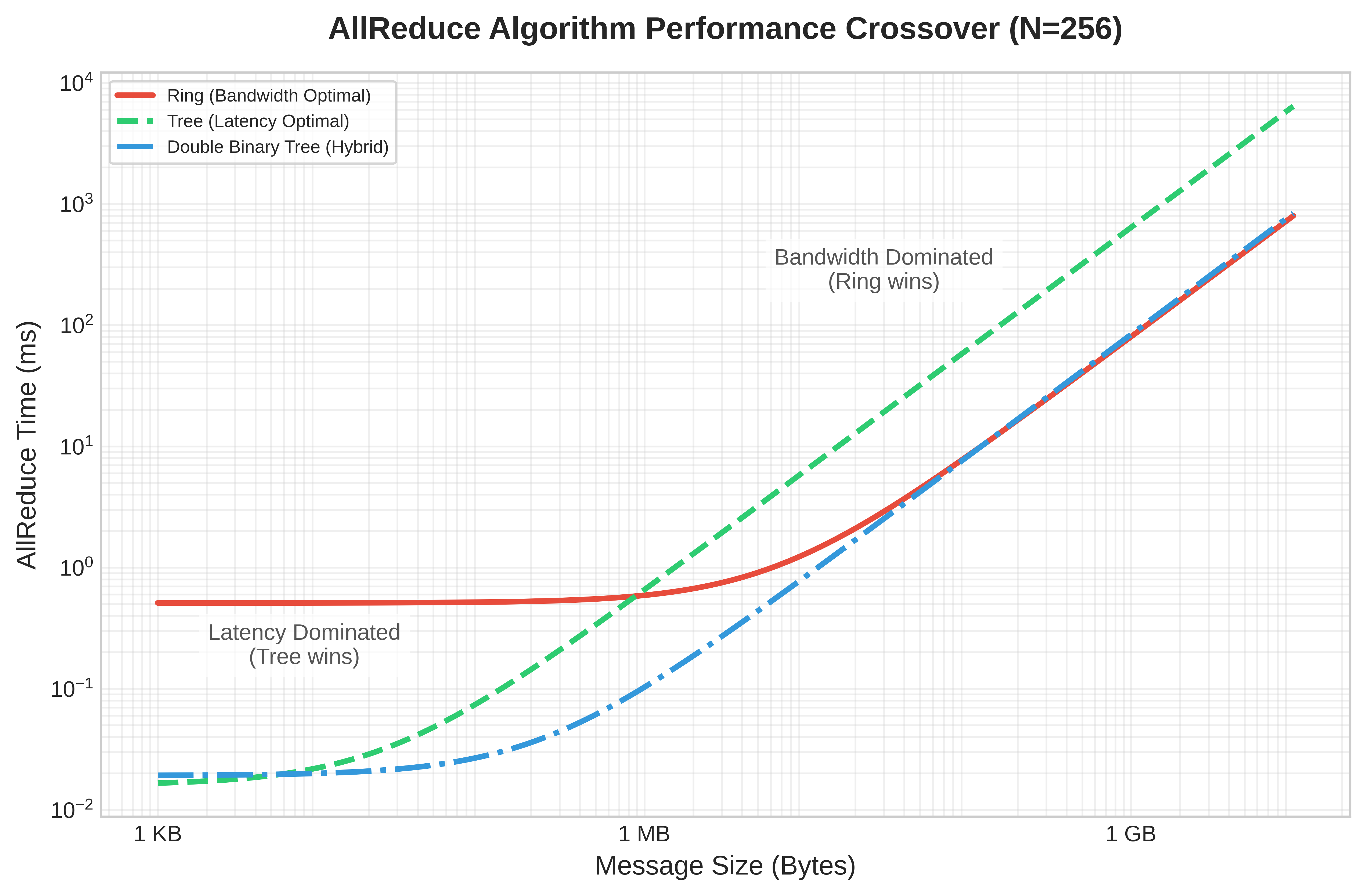
The algorithm crossover point
The crossover point in figure 6, where Ring overtakes Tree, follows from setting \(T_{\text{ring}} = T_{\text{tree}}\) and solving for \(M\). The full time equations make the trade-off explicit:
\[ T_{\text{ring}} = 2(N-1)\alpha + 2\frac{N-1}{N}\frac{M}{\beta} \] \[ T_{\text{tree}} = 2\log_2 N \cdot \alpha + 2\log_2 N \cdot \frac{M}{\beta} \]
For large \(N\), \((N-1) \approx N\) and \(\frac{N-1}{N} \approx 1\), so the ring pays a latency term proportional to \(N\) while moving each byte close to the bandwidth limit:
\[ T_{\text{ring}} \approx 2N\alpha + \frac{2M}{\beta}, \quad T_{\text{tree}} \approx 2\log_2 N \cdot \alpha + \frac{2\log_2 N \cdot M}{\beta} \]
The tree has the opposite shape: logarithmic startup cost, but each message byte moves through more stages. Setting the estimates equal isolates the message size where the cheaper latency path stops compensating for the extra bandwidth work:
\[ 2N\alpha + \frac{2M}{\beta} = 2\log_2 N \cdot \alpha + \frac{2\log_2 N \cdot M}{\beta} \] \[ \frac{2M}{\beta} - \frac{2\log_2 N \cdot M}{\beta} = 2\log_2 N \cdot \alpha - 2N\alpha \] \[ \frac{2M}{\beta}(1 - \log_2 N) = 2\alpha(\log_2 N - N) \]
Since \(N \gg \log_2 N\) for large clusters, \((\log_2 N - N) \approx -N\) and \((1 - \log_2 N) \approx -\log_2 N\), yielding:
\[ \frac{2M}{\beta}(-\log_2 N) \approx 2\alpha(-N) \] \[ M_{\text{crossover}} \approx \frac{N \cdot \alpha \cdot \beta}{\log_2 N} \]
For a rough upper-scale mental model, engineers sometimes drop the logarithmic factor: \[ \boxed{M_{\text{crossover}} \approx N \cdot \alpha \cdot \beta} \]
The log-aware crossover formula yields a useful intuition, not a hard selection rule. Above the crossover, message size dominates and Ring’s bandwidth efficiency wins; below it, startup latency dominates and Tree’s logarithmic depth wins.
For a cluster with \(\alpha=5\ \mu\text{s}\), \(\beta=50\ \text{GB/s}\), and \(N=100\), the direct approximation gives: \[M_{\text{crossover}} \approx \frac{100 \times 5\cdot 10^{-6} \times 50\cdot 10^9}{\log_2 100} \approx 3.8 \text{ MB}\]
In practice, NCCL’s algorithm selection is more nuanced than a simple two-way split. The Double Binary Tree algorithm offers logarithmic latency with near-optimal bandwidth, making it competitive with both Ring and Tree across a broad range of message sizes. NCCL also considers the number of channels (parallel communication streams), the network topology, and whether inter-node or intra-node links are being used. The effective selection logic resembles a multi-way decision tree indexed by (message size, GPU count, topology type) rather than a single crossover point.
Nevertheless, the crossover formula remains the essential mental model for understanding why libraries make the choices they do. When a library selects an unexpected algorithm, the crossover analysis provides the reasoning framework to evaluate whether the choice is correct or whether manual override is warranted. A concrete buffer-size calculation applies this framework to a realistic decision:
Napkin Math 1.5: The ring vs. tree crossover
Problem: A cluster synchronizes a 1 MB buffer across 64 GPUs. The network has latency \(\alpha =\) 10 μs and bandwidth \(\beta =\) 10 GB/s. Which algorithm performs better: Ring or Tree?
Table 9: Ring vs. tree AllReduce timing for a 1 MB buffer on 64 GPUs: Latency, bandwidth, and total-time terms with \(\alpha = 10\ \mu\text{s}\) and \(\beta = 10\ \text{GB/s}\).
Math:
Latency:
- Ring Latency: \(2(N-1)\alpha =\) \(2 \times 63 \times 10\ \mu\text{s}\) = 1260 μs.
- Tree Latency: \(2(\log_2 N)\alpha =\) \(2 \times 6 \times 10\ \mu\text{s}\) = 120 μs.
Bandwidth (note the difference):
- Ring Bandwidth: \(2\frac{N-1}{N}\frac{M}{\beta} \approx\) \(2 \times \frac{1\text{ MB}}{10\text{ GB/s}}\) = 196.9 μs (optimal: each byte sent once).
- Tree Bandwidth: \(2\log_2 N \cdot \frac{M}{\beta} =\) \(12 \times \frac{1\text{ MB}}{10\text{ GB/s}}\) = 1200 μs (each level sends full message).
Table 9 sums the latency and bandwidth contributions into a head-to-head comparison:
| Algorithm | Latency | Bandwidth | Total |
|---|---|---|---|
| Ring | 1260 μs | 196.9 μs | 1456.9 μs |
| Tree | 120 μs | 1200 μs | 1320 μs |
Tree wins, but only by 9 percent. For this 1 MB message, we are near the crossover point.
Systems insight: Ring’s latency penalty (10\(\times\) worse than Tree) nearly balances Tree’s bandwidth penalty (6\(\times\) worse than Ring). The log-aware crossover estimate predicts \(M_{\text{crossover}} \approx N \alpha \beta / \log_2 N = 64 \times 10\ \mu\text{s} \times 10\ \text{GB/s} / 6 \approx\) 1.1 MB. At 1 MB, we are just below crossover, so Tree wins. At 10 MB, Ring would dominate.
The crossover point sits inside the range that DDP and FSDP workloads traverse during normal training. A 1 MB message corresponds to gradients from a single feed-forward layer in a smaller transformer, or an MoE token-routing payload—Tree territory. A 10 MB DDP gradient bucket from a mid-size transformer layer sits near the crossover. A fused DDP bucket covering multiple layers reaches 50–300 MB; a full BF16 gradient tensor for a 70B parameters model reaches 1120 GB—both firmly in Ring territory. Most real training workloads sweep through this entire range as bucket sizes are tuned, and the crossover analysis sets the algorithmic boundary that separates bucket-level Tree operations from full-model Ring synchronizations.
The crossover analysis demonstrates that algorithm selection is not a static choice but depends on the specific combination of message size, cluster scale, and network parameters. In practice, communication libraries like NCCL maintain internal lookup tables that map message size, GPU count, topology, and protocol settings to selected algorithms such as Ring, Tree, or hybrid approaches. Understanding the underlying crossover math allows engineers to predict when the library’s built-in choices may be suboptimal and to override them when necessary.
Checkpoint 1.3: AllReduce algorithm selection
Verify your understanding of Ring vs. Tree AllReduce trade-offs:
Self-Check: Question
A naive parameter-server AllReduce gathers all gradients at a central server, sums them, and broadcasts the result back. Why does this approach become unscalable as GPU count grows?
- Because the central aggregator’s NIC must carry traffic proportional to \(N \times M\), creating a bandwidth hotspot whose saturation point is independent of how many workers exist.
- Because reduction is only mathematically valid when every worker communicates with exactly two neighbors.
- Because tree-based broadcast cannot be implemented on InfiniBand fabrics.
- Because modern optimizers require gradients to remain permanently sharded across workers.
Order the following stages of Ring AllReduce for \(N\) GPUs and a tensor split into \(N\) chunks: (1) every GPU holds a copy of the fully reduced tensor, (2) each GPU owns one fully reduced chunk after the scatter-reduce phase, (3) the initial tensor is partitioned into \(N\) chunks and circulates around the ring while workers accumulate partial sums.
A library must choose an AllReduce algorithm for 256-byte control-message synchronization across 256 GPUs on a datacenter fabric with \(\alpha = 5\) microseconds and \(\beta = 25\) GB/s. Which algorithm should it pick, and why?
- Ring AllReduce, because its bandwidth term is always smaller than tree’s regardless of message size.
- Tree AllReduce, because 256 bytes sits far below even the log-aware crossover, so the \(\mathcal{O}(\log N)\) step count dominates total time over bandwidth efficiency.
- Parameter-server aggregation, because small messages are below the threshold where decentralized collectives matter.
- Any algorithm will perform identically because 256 bytes fits inside a single network packet.
Recursive halving-doubling (butterfly) AllReduce has bandwidth-optimal data motion and \(\mathcal{O}(\log N)\) latency in its cost equation, yet it can underperform ring AllReduce on large hierarchical clusters. Explain the mismatch between its theoretical strength and its real-world weakness.
True or False: In a synchronous Ring AllReduce, if one GPU in the ring runs 20 percent slower than the others on a given iteration, total collective completion time is also roughly 20 percent slower for every participant in the ring.
Hierarchical Communication
The algorithms above assume a flat network where every link has the same bandwidth. Real data centers violate this assumption by an order of magnitude or more. Not all wires are created equal.
Hierarchical communication is the response to that inequality. Intra-node links are abundant and fast, inter-node links are scarce and expensive, and the algorithm must shrink payloads before they cross the scarce tier whenever possible. This is why the same AllReduce can be implemented as a local ReduceScatter, a cross-node reduction, and a local AllGather rather than as one flat exchange across every rank.
A GPU node delivers an order of magnitude more intra-node bandwidth (NVLink at 900 GB/s) than inter-node bandwidth (InfiniBand at 50 GB/s).
Hierarchical AllReduce
The algorithms above (Ring, Tree, Butterfly, Double Binary Tree) all assume a flat network where every link has the same bandwidth. This assumption holds within a single node (where all GPUs are connected by NVLink at equal bandwidth) but fails by 9× in multi-node clusters. Real clusters are hierarchical networks, with fundamentally different bandwidths at each tier, as table 10 quantifies.
| Tier | Interconnect | Bandwidth | Relative Speed |
|---|---|---|---|
| Intra-Node | NVLink 4.0 | ~900 GB/s | 9× faster |
| Inter-Node | InfiniBand NDR 400G | ~50 GB/s | 1\(\times\) (baseline) |
A naive flat Ring AllReduce ignores this structure, potentially routing data across InfiniBand when NVLink would suffice and wasting the scarce inter-node bandwidth. Hierarchical AllReduce decomposes the global operation into three phases that respect the bandwidth hierarchy, as shown in figure 7.

Hierarchical collectives shrink payload before it crosses slow tiers.

The three-phase decomposition in figure 7 confines the expensive inter-node traffic to Phase 2, where each GPU transmits only \(M/G\) bytes instead of \(M\). With \(G = 8\) GPUs per node (a typical DGX configuration), this reduces inter-node traffic by 8\(\times\), effectively multiplying the scarce InfiniBand bandwidth by the number of GPUs per node.
The phases form one causal chain:
- Intra-node ReduceScatter over NVLink: A local reduction among the \(G\) GPUs in each node leaves each GPU with \(1/G\) of the partially reduced data, using only abundant intra-node bandwidth.
- Inter-node AllReduce over InfiniBand: Each GPU sends its node shard across corresponding GPU positions, transmitting \(M/G\) bytes instead of \(M\).
- Intra-node AllGather over NVLink: Each node redistributes the final shards internally, completing the result without consuming additional inter-node bandwidth.
A simple 8-node budget makes this bandwidth multiplication concrete:
Napkin Math 1.6: The hierarchical bandwidth multiplier
Problem: A cluster has 8 nodes, each with 8 GPUs (64 total). The system must AllReduce a 1 GB gradient buffer. Compare flat Ring AllReduce vs. Hierarchical AllReduce.
Flat ring AllReduce (ignoring hierarchy):
- Each GPU sends ~2 GB total (the bandwidth-optimal Ring AllReduce formula).
- The ring crosses node boundaries multiple times.
- Effective bandwidth: Limited by the slowest link = 50 GB/s (InfiniBand).
- Time: \(\approx\) \(2 \times 1\ \text{GB} / 50\ \text{GB/s}\) = 40 ms (bandwidth term dominates).
Hierarchical AllReduce (3-step decomposition):
Intra-node ReduceScatter: Each GPU sends 875 MB at 450 GB/s per direction → ~1.94 ms
Inter-Node AllReduce: Each GPU AllReduces a \(1\ \text{GB}/8\) = 125 MB shard over InfiniBand; Ring moves roughly \(2(N-1)/N\) times that payload, and after adding the small latency term the phase takes ~4.42 ms at 50 GB/s
(Only 1/8 of the data crosses InfiniBand!)
Intra-node AllGather: Each GPU receives 875 MB at 450 GB/s per direction → ~1.94 ms
Total time: \(\approx\) 1.94 ms + 4.42 ms + 1.94 ms = 8.3 ms
Systems insight: Hierarchical AllReduce achieves a 4.8× speedup by reducing the inter-node payload from 1 GB to 125 MB per GPU before the Ring traffic multiplier. With 8 GPUs per node, we effectively get 8\(\times\) the apparent inter-node bandwidth. This is why NVIDIA’s NCCL and similar libraries often select hierarchical algorithms on multi-node clusters when the topology supports them.
These three phases confine most traffic within each node before crossing the slower inter-node fabric, and the same idea generalizes beyond two levels. Large clusters with multiple racks connected through spine switches introduce a third bandwidth tier (rack-to-rack at reduced bisection bandwidth). At 128 GPUs arranged as 4 racks of 4 nodes of 8 GPUs with 2:1 cross-rack oversubscription, applying the same decomposition at each tier shrinks the cross-rack payload per GPU by 32\(\times\) compared to the original gradient—roughly 15 ms total versus 160 ms for flat AllReduce. The hierarchical decomposition concentrates traffic where bandwidth is abundant and minimizes traffic where bandwidth is scarce.
In-network reduction: SHARP and beyond
The contrast in figure 8 shows the next step: move the reduction work from endpoint GPUs into the switch ASIC so packets are aggregated while they traverse the fabric.

Hierarchical AllReduce reduces the volume of cross-node traffic, but the aggregation still requires multiple network round-trips. NVIDIA’s Scalable Hierarchical Aggregation and Reduction Protocol (SHARP)10 implements this idea: instead of gradients traveling to a destination GPU for summation, the InfiniBand switch aggregates partial sums as data packets pass through it.
10 SHARP (Scalable Hierarchical Aggregation and Reduction Protocol): In-network computing on Quantum InfiniBand switches that performs reduction operations (such as sum, min, and max) as packets traverse an aggregation tree (Graham et al. 2020). Graham et al. report substantially higher reduction bandwidth than host-based algorithms and describe switch-resource limits on outstanding aggregation groups and trees, which can create contention when many collectives compete for the same in-network resources.
Graham, R. L., D. Bureddy, P. Lui, H. Rober, G. Bloch, G. Shainer, J. Poole, et al. 2020. “Scalable Hierarchical Aggregation and Reduction Protocol (SHARP) Streaming-Aggregation Hardware Design and Evaluation.” International Conference on High Performance Computing, 41–59. https://doi.org/10.1007/978-3-030-50743-5_3.
The benefit is twofold. First, SHARP reduces endpoint memory traffic and can reduce pressure on upper-level links by aggregating packets before they leave a switch tier. In a software-based tree reduction, data arrives at a GPU, is written to memory, summed with local data, and then transmitted to the next level. With SHARP, the switch combines incoming packets in flight and forwards the aggregate for the reduction tree. Second, SHARP eliminates the store-and-forward path through intermediate GPUs. Each software hop adds the full \(\alpha\)-\(\beta\) cost; with in-switch aggregation, the reduction happens inside the switch ASIC rather than in endpoint memory.
The practical impact is most pronounced for message sizes where aggregation latency contributes meaningfully to total AllReduce time. For very large messages, bandwidth dominates regardless of algorithm, and SHARP’s latency reduction becomes proportionally smaller. For very small messages, fixed switch-processing overhead can limit the benefit. Graham et al. (2020) report multi-fold reduction-bandwidth improvements and smaller application-level gains for PyTorch workloads when SHARP Streaming-Aggregation is enabled on HDR/Quantum InfiniBand switches.
Strong scaling campaigns—training a fixed model across more accelerators without proportionally growing batch size—are precisely the workloads where SHARP’s latency reduction translates into step-time reduction. As the per-accelerator batch shrinks, each gradient tensor stays large (proportional to model size) but the backward pass per accelerator shortens, so communication dominates an increasing fraction of step time and the latency term \(\alpha\) in the ring formula hits the bottleneck. In-switch aggregation cuts directly into that latency cost. Switch ASIC vendors have explicitly extended InfiniBand ASICs to support ML-native datatypes, including FP16 and BF16, confirming that SHARP is co-evolving with ML workload requirements rather than serving only the legacy HPC floating-point operations that motivated its original design. An ML system team choosing SHARP infrastructure for a scaling campaign should verify FP16/BF16 aggregation support in the specific switch generation, since earlier ASICs supported only FP32 and INT32.
SHARP does impose constraints. The switch must support the specific reduction operation (typically limited to sum, min, and max on floating-point and integer types). The number of concurrent SHARP aggregation trees is limited by switch resources, so large clusters with many simultaneous training jobs may exhaust SHARP capacity. Additionally, SHARP requires InfiniBand infrastructure; it is not available on Ethernet-based fabrics.
Topology-aware routing
Hierarchical AllReduce reduces inter-node traffic, and SHARP eliminates some of it entirely, but neither technique addresses a subtler problem: how the logical communication pattern maps to the physical network topology. A Ring AllReduce among 64 GPUs creates a logical ring, but which physical links carry each hop determines whether the ring achieves peak bandwidth or creates congestion. Two runs of the same training job on the same hardware can differ by 2\(\times\) in communication throughput depending on how ranks are assigned to GPUs and how the resulting traffic pattern interacts with the network’s physical structure.
Communication libraries like NCCL perform topology detection at initialization, running graph search algorithms to discover the physical network structure and find high-bandwidth communication paths (NVIDIA 2026). The library must determine, for each pair of ranks, whether the peer sits on a local NVLink switch or 100 meters away across an InfiniBand fabric, because the same collective algorithm can differ by 2\(\times\) or more in throughput depending on how logical ranks map to physical hardware.
The topology detection process begins with hardware enumeration. NCCL queries the PCIe bus to discover GPU placement, NVLink connectivity between GPUs, and NIC-to-PCIe-switch affinity. From this information, it constructs an internal graph where nodes represent GPUs and edges represent physical links with annotated bandwidth and latency. A graph search algorithm then finds communication paths that maximize aggregate bandwidth while minimizing the number of cross-domain hops (transitions between NVLink, PCIe, and InfiniBand domains). This topology-aware path selection is what allows NCCL to approach theoretical peak bandwidth on well-configured systems, while topology-unaware implementations can leave a large fraction of bandwidth unused.
Torus topology (TPU pods)
The dimension-ordered reduction in figure 9 shows why torus fabrics use the physical mesh directly instead of pretending the pod is a flat all-to-all network.

Google’s Tensor Processing Unit (TPU) pods use a 3D torus topology where each TPU connects directly to 6 neighbors \((\pm X, \pm Y, \pm Z)\); figure 9 depicts the same dimension-ordered idea as a 2D simplification. Unlike the hierarchical fat-tree topology of InfiniBand clusters, the torus provides uniform, direct connectivity: every TPU chip has the same number of links (6) and the same per-link bandwidth, regardless of its position in the mesh. The optimal AllReduce strategy for this topology is dimension-ordered reduction:
- Reduce along X for each fixed \((Y,Z)\) line, producing partial sums over the X dimension
- Reduce those partials along Y for each fixed \((X,Z)\) line, producing partial sums over the \(X \times Y\) plane
- Reduce those partials along Z for each fixed \((X,Y)\) line to complete the global result
Each dimension-ordered reduction is itself a Ring AllReduce along one axis-aligned torus ring. For a pod with \(X{\times}Y{\times}Z\) TPUs, the first step runs independent X-dimension rings, one for each fixed \((Y,Z)\) coordinate, so each participant receives a partial sum over that X line. The second step runs Y-dimension rings to combine those X partials across Y, and the third step runs Z-dimension rings to complete the global reduction. This cascading reduction achieves total bandwidth cost \(2M/\beta\) (same as a single Ring) but with latency proportional to \(2(X + Y + Z)\) rather than \(2(X \times Y \times Z)\), because each dimension’s ring is shorter than a global ring.
Dimension-ordered reduction minimizes network diameter and ensures each link carries traffic in only one direction at a time, avoiding congestion. The torus topology also provides natural fault tolerance through alternate routing paths: if one link in the X-dimension fails, traffic can detour through the Y or Z dimensions (at the cost of increased latency). Google’s Accelerated Linear Algebra (XLA) compiler generates dimension-ordered collectives automatically when targeting TPU pods, abstracting the topology details from the user.
Rail-optimized routing (NVIDIA DGX)
In NVIDIA DGX systems, each GPU has its own dedicated NIC (network interface card). Rail-optimized routing exploits this by ensuring that GPUs at the same position within their respective nodes communicate only with each other:
- GPU 0 on Node A talks only to GPU 0 on Node B, Node C, and so on.
- GPU 1 on Node A talks only to GPU 1 on other nodes.
- And so on for GPUs 2–7.
This creates 8 independent “rails” of communication that operate in parallel without contention, as table 11 illustrates.
| Rail | Participants | Traffic |
|---|---|---|
| Rail 0 | Node0-GPU0 ↔︎ Node1-GPU0 ↔︎ Node2-GPU0 ↔︎ … | \(M/8\) each |
| Rail 1 | Node0-GPU1 ↔︎ Node1-GPU1 ↔︎ Node2-GPU1 ↔︎ … | \(M/8\) each |
| … | … | … |
| Rail 7 | Node0-GPU7 ↔︎ Node1-GPU7 ↔︎ Node2-GPU7 ↔︎ … | \(M/8\) each |
Rail alignment is critical because without it, all 8 GPUs on a node might try to send to the same remote GPU simultaneously, creating 8\(\times\) contention on a single NIC. Rail-aligned routing ensures each NIC handles exactly 1/8 of the traffic, achieving full bisection bandwidth utilization.
Rail-optimized routing and hierarchical AllReduce reinforce each other. In the hierarchical decomposition described earlier, Step 2 (inter-node AllReduce) naturally aligns with rail topology. GPU \(i\) on each node communicates only with GPU \(i\) on other nodes, which is precisely the rail pattern. This alignment is not coincidental; NVIDIA designed the DGX hardware with rail-optimized communication in mind, and NCCL’s hierarchical algorithms can exploit this structure when the topology is detected and ranks are mapped correctly. When the logical communication pattern matches the physical topology, each NIC carries its intended share of traffic and the cluster can approach its theoretical peak bisection bandwidth.
Misalignment between logical and physical topology is a common source of performance degradation that is difficult to diagnose without careful profiling. If process ranks are assigned arbitrarily (for example, by the job scheduler without topology awareness), the hierarchical AllReduce may route cross-node traffic through the wrong NICs, creating hotspots that reduce effective bandwidth by 2–4\(\times\). Large deployments use topology-aware rank assignment (configured through NCCL’s CUDA_VISIBLE_DEVICES and the scheduler’s GPU binding policies) to ensure alignment.
The hierarchical approach, combined with topology-aware routing, represents the culmination of the algorithms explored in this section: the \(\alpha\)-\(\beta\) model identifies the bottleneck (inter-node bandwidth), hierarchical decomposition reduces traffic across that bottleneck, and rail optimization ensures the reduced traffic flows without contention. Together, these techniques close the gap between theoretical peak bandwidth and achieved bandwidth on well-configured clusters.
Self-Check: Question
Why is a flat (single-tier) AllReduce model a poor fit for a typical GPU training cluster?
- Because collective operations are only mathematically defined on equal-bandwidth links.
- Because real clusters have roughly 10-to-20-times bandwidth differences between intra-node NVLink and inter-node InfiniBand, so treating all links as equal both wastes the fast local tier and saturates the slow global tier.
- Because flat models require CPU intervention for every reduction step.
- Because only hierarchical models can operate on BF16 gradients.
Order the phases of hierarchical AllReduce on a cluster of \(H\) nodes times \(G\) GPUs per node, with \(N = H G\) devices: (1) perform cross-node reduction among corresponding GPU indices across nodes, (2) perform intra-node reduction within each node’s \(G\) GPUs over NVLink, (3) perform intra-node AllGather within each node so every GPU in the node receives the final result.
What is the main systems benefit of SHARP-style in-network reduction?
- It converts AllReduce into AlltoAll so that traffic can use more physical links simultaneously.
- It offloads reduction arithmetic into the network switch ASIC, so partial sums are aggregated as they traverse the fabric rather than bouncing between GPU memories, which reduces both round-trips and HBM bandwidth pressure.
- It removes the need for any topology detection during library initialization.
- It benefits only very small messages because large messages do not traverse switches at all.
Compare topology-aware collective execution on TPU torus systems with rail-optimized routing on NVIDIA DGX-style GPU clusters, and identify the shared design principle.
A training job achieves significantly less bandwidth than nccl-tests on the same cluster even though the algorithm choice and message sizes look reasonable. Which topology-related issue from this section is the most plausible culprit?
- The model uses BF16 gradients, which disables hierarchical AllReduce inside NCCL.
- Ranks were assigned to GPUs without respecting physical topology, so rails are misaligned or NVLink groups are split across ring segments, creating hotspots and forcing traffic onto congested links.
- The cluster has too many GPUs per node for any ring-based collective to operate correctly.
- NCCL requires identical latency on every link before it will discover cluster topology.
Gradient Compression Under Bandwidth Scarcity
Even after topology tuning and algorithm selection, a system may remain bandwidth-bound because the physical fabric cannot move gradient payloads fast enough. In that regime, sending fewer bits becomes a deliberate design choice rather than a universal last resort. The previous section attacked the communication bottleneck from the scheduling and topology side; payload compression attacks the same bottleneck by changing what crosses the fabric.
The bandwidth wall arises most acutely in two scenarios: training across data centers connected by wide-area networks (where bandwidth is 10–100\(\times\) lower than InfiniBand), and training on cloud instances with commodity Ethernet networking where RDMA is unavailable or constrained. In these bandwidth-constrained settings, gradient compression techniques can reduce communication volume by 4–1000\(\times\), at the cost of introducing noise into the optimization process. The central tension is between bandwidth reduction and the noise tolerance of the optimization process—how much compression the optimizer can absorb before convergence is compromised.
Quantization: Reducing precision
Quantization is the least disruptive compression lever when bandwidth is binding because it keeps every gradient element but reduces the bits used to represent it. Most gradients are computed in FP32 (32-bit floating point) or BF16 (16-bit brain float), so reducing bit-width directly reduces communication volume. The useful question is how much gradient fidelity the optimizer can absorb, and the progression from mild to aggressive quantization illustrates the trade-off between compression ratio and gradient fidelity:
- FP16 (16-bit): A common baseline for accelerator training. Half the bits of FP32, with minimal impact on convergence for many models. Provides 2\(\times\) compression over FP32.
- INT8 (8-bit): Quantize each gradient vector to 256 discrete levels. This requires computing a scaling factor per tensor: \(g_{\text{int8}} = \text{round}(g/s)\) where \(s = \max(|g|) / 127\). The receiver reconstructs \(\hat{g} = g_{\text{int8}} \times s\). Provides 4\(\times\) compression over FP32 but introduces quantization noise proportional to the gradient magnitude.
- 1-bit SGD: The extreme case: transmit only the sign of each gradient element (+1 or -1). The receiver reconstructs using a learned or adaptive scaling factor. This achieves 32\(\times\) compression over FP32 but introduces substantial noise that can degrade convergence without additional mechanisms (Seide et al. 2014; Karimireddy et al. 2019).
Block quantization for gradient communication
The quantization progression above uses a single scaling factor per entire tensor, which implicitly assumes the gradient distribution is uniform across the tensor. In practice, gradient distributions are highly nonuniform: attention layers produce gradients with heavy tails, embedding layers produce extremely sparse gradients, and normalization layers produce gradients concentrated near zero. A single scaling factor per tensor is suboptimal when gradient distributions vary across the tensor. Regions with small gradients lose most of their information when quantized with a scaling factor dominated by the tensor’s maximum value. Block quantization addresses this by dividing the gradient tensor into blocks of \(b_{\text{block}}\) elements (typically \(b_{\text{block}} = 64\) or \(128\)) and computing an independent scaling factor per block. Each block’s scaling factor adapts to the local gradient distribution, reducing quantization error at the cost of transmitting \(d_{\text{grad}}/b_{\text{block}}\) additional scaling factors.
For a gradient vector of dimension \(d_{\text{grad}}\) quantized to INT8 with block size \(b_{\text{block}}\), the message size is \(d_{\text{grad}} \times 1\ \text{byte}\) for the quantized values plus \((d_{\text{grad}}/b_{\text{block}}) \times 4\ \text{bytes}\) for the FP32 scaling factors, or \(d_{\text{grad}} + 4d_{\text{grad}}/b_{\text{block}}\) bytes in total. The effective compression is therefore \(4d_{\text{grad}} / (d_{\text{grad}} + 4d_{\text{grad}}/b_{\text{block}}) = 4b_{\text{block}} / (b_{\text{block}} + 4)\), which for \(b_{\text{block}} = 128\) reaches 3.88\(\times\), close to the theoretical 4\(\times\). The quality gain comes from replacing the global error bound: block quantization reduces the maximum quantization error from \(s \cdot 0.5\), where \(s\) is the global scaling factor, to \(s_b \cdot 0.5\), where \(s_b\) is the block-local scaling factor, which for the heavy-tailed gradient distributions common in attention layers can cut quantization error by 2–5\(\times\) compared to per-tensor quantization.
Interfaces that fuse quantize-reduce operations make block quantization practical in communication compression, but each reduction in bit-width introduces quantization noise. This noise acts as a biased perturbation to the true gradient direction. For aggressive quantization (INT8 and especially 1-bit), the systematic bias can prevent convergence unless the system carries an error-feedback correction across steps. Quantization should therefore move only as far down the precision ladder as the convergence budget permits.
Sparsification: Transmitting only important gradients
Quantization attacks communication volume by reducing the number of bits per gradient element while transmitting every element. An orthogonal approach, sparsification, attacks the problem from the other direction: keep full precision but transmit only a subset of gradient elements, setting the rest to zero.
Top-k sparsification
The most common method is Top-k compression: for a gradient vector \(g \in \mathbb{R}^{d_{\text{grad}}}\), transmit only the \(K_{\text{top}}\) elements with the largest absolute magnitude, setting the rest to zero (Aji and Heafield 2017; Lin et al. 2018):
\[\text{TopK}(g) = g \odot \mathbf{1}_{|g| \geq |g|_{(K_{\text{top}})}}\]
where \(|g|_{(K_{\text{top}})}\) is the \(K_{\text{top}}\)-th largest element by magnitude. With \(K_{\text{top}} = 0.001 \times d_{\text{grad}}\) (keeping only 0.1 percent of elements), this achieves 1000\(\times\) compression.
The compression headline must be discounted by the cost of encoding the sparse representation. Transmitting a sparse gradient requires sending both the nonzero values and their indices. For a gradient vector of dimension \(d_{\text{grad}}\) with \(K_{\text{top}}\) nonzero elements, the encoded message contains \(K_{\text{top}}\) values (each in FP32 or FP16) plus \(K_{\text{top}}\) indices (typically INT32). The total message size is \(K_{\text{top}} \times (4 + 4) = 8 K_{\text{top}}\) bytes for FP32 values with INT32 indices. The effective compression ratio is therefore \(4d_{\text{grad}} / (8 K_{\text{top}}) = d_{\text{grad}} / (2 K_{\text{top}})\).
For \(K_{\text{top}} = 0.001 d_{\text{grad}}\), the encoded message yields a compression ratio of 500\(\times\), not the 1000\(\times\) suggested by the kept-element fraction alone, because the index overhead is significant. Reducing the index size to INT16 (for \(d_{\text{grad}} < 65536\)) or using run-length encoding for structured sparsity patterns can improve the effective ratio.
Top-k is not the only sparsification rule. Random-k sparsification selects \(K_{\text{rand}}\) elements uniformly at random and scales them by \(d_{\text{grad}}/K_{\text{rand}}\) to maintain an unbiased gradient estimate. Random-k has the advantage of being an unbiased compressor even without error feedback, because \(\mathbb{E}[\text{RandomK}(g)] = g\). However, it introduces higher variance than Top-k because it discards large gradients with the same probability as small ones. In practice, Top-k with error feedback converges faster than Random-k for the same compression ratio, because Top-k preserves the most informative gradient components at each step.
The convergence problem
Naively discarding small gradients creates a systematic bias. If a parameter consistently receives small gradients (e.g., 0.01 per step), it will not be updated because 0.01 is always below the Top-k threshold. Over thousands of steps, these “lost” gradients accumulate to a significant error that prevents the model from converging to the true optimum.
The problem is not merely practical; it is a fundamental mathematical obstacle. Without correction, sparsified SGD is a biased estimator of the true gradient, and biased gradient descent can converge to arbitrarily wrong solutions. The same problem afflicts aggressive quantization: rounding gradients to INT8 or 1-bit introduces a systematic rounding error that accumulates across training steps. Error feedback addresses this accumulation for quantized gradients (Seide et al. 2014) and for sparsified gradients (Stich et al. 2018; Karimireddy et al. 2019).
Error feedback: The memory of the journey
We solve the conflict between compression and convergence with error feedback. The system applies the compressor immediately to recover bandwidth, then stores the discarded residual in a local accumulator and re-injects it into the next gradient. The error is deferred, not destroyed. We maintain a local error accumulator \(e_t\) that stores the compression residual.

Error feedback carries the residual into the next compressed step.
Definition 1.4: Error feedback mechanism
Error Feedback is a distributed-training technique for gradient compression that maintains a per-worker residual accumulator \(e_t\), re-injecting the compression error back into the next gradient update so that information deferred by the compressor is never permanently discarded.
- Significance: Top-k sparsification at 1 percent keeps only the largest 1 percent of gradient values by magnitude, reducing AllReduce data volume from 140 GB to 1.4 GB for a 70B model—a 100\(\times\) payload reduction before sparse-index overhead. Without error feedback, the discarded 99 percent of gradient values create a biased update that can harm convergence; with error feedback, the residual accumulates until deferred components cross the compression threshold in later steps, recovering the convergence guarantees analyzed for memory/error-feedback variants under their assumptions (Stich et al. 2018; Karimireddy et al. 2019).
- Distinction: Unlike lossy compression (which permanently discards sub-threshold gradient components), error feedback is a delayed transmission strategy: the residual \(e_t\) telescopes across steps so that \(\frac{1}{K}\sum_{t=1}^{K} v_t \to \frac{1}{K}\sum_{t=1}^{K} g_t\) as \(K \to \infty\), making the long-run average of transmitted gradients equal to the true gradient average.
- Common pitfall: A frequent misconception is that error feedback is automatic whenever a compressor is used. It is not: the training system must explicitly preserve and reinject the residual. Without that residual path, Top-k and 1-bit quantization introduce systematic bias that can accumulate across steps (Karimireddy et al. 2019).
Error feedback preserves cumulative gradient information over time. Consider what happens over \(K\) steps:
\[\sum_{t=1}^{K} v_t = \sum_{t=1}^{K} \left[(g_t + e_t) - e_{t+1}\right] = \sum_{t=1}^{K} g_t + e_1 - e_{K+1}\]
If the error accumulator remains bounded (which it does for reasonable compression schemes), then as \(K \to \infty\):
\[\frac{1}{K}\sum_{t=1}^{K} v_t \to \frac{1}{K}\sum_{t=1}^{K} g_t\]
The long-run average of transmitted gradients equals the long-run average of true gradients. No gradient information is permanently lost; it is merely delayed. Small gradients that are repeatedly dropped eventually accumulate in \(e_t\) until they exceed the compression threshold and get transmitted.
The telescoping property of compression error across time is why error feedback can transform a biased compressor into a convergent training method. Theoretical analyses show convergence guarantees for sparsified SGD with memory and for EF-SGD with broad compression operators under their stated assumptions (Stich et al. 2018; Karimireddy et al. 2019). A short trace shows how error feedback preserves gradient information that naive compression would lose. Table 12 runs the trace for a greedy compressor with no residual path, transmitting only values \(\geq 0.5\):
| Step | True Gradient \(g_t\) | Transmitted \(v_t\) | Cumulative Transmitted | Cumulative True |
|---|---|---|---|---|
| 1 | 0.4 | 0 | 0 | 0.4 |
| 2 | 0.3 | 0 | 0 | 0.7 |
| 3 | 0.2 | 0 | 0 | 0.9 |
| 4 | 0.4 | 0 | 0 | 1.3 |
| 5 | 0.3 | 0 | 0 | 1.6 |
The error-feedback trace in table 13 runs the same sequence with a residual accumulator \(e_t\) that re-injects the discarded remainder into the next step. The example below works through both traces to show that the deferred information is conserved rather than lost.
Example 1.2: Error feedback mechanism
Problem: A single parameter receives small gradients (all below 0.5) over five training steps. A greedy compressor transmits only values \(\geq 0.5\) (rounding to nearest integer: values in \([0, 0.5) \to 0\), values in \([0.5, 1.5) \to 1\), etc.). After five steps, how much gradient information does naive compression lose, and how does an error-feedback accumulator recover it?
Naive compression outcome: In table 12, after 5 steps the system has transmitted 0 but the true cumulative gradient is 1.6. The parameter never updates, and 100 percent of gradient information is lost.
Error-feedback outcome: In table 13, the accumulator \(e_t\) telescopes the residual across steps. After 5 steps, the system has transmitted 2 with a remaining error of −0.4. The true cumulative is 1.6, so transmitted \(+\) error = 2 + (−0.4) = 1.6 ✓
Systems insight:
- No information is lost: The sum (transmitted + error buffer) always equals the cumulative true gradient.
- Small gradients accumulate: Individual gradients of 0.3–0.4 were too small to transmit alone, but they accumulated until crossing the threshold.
- Error oscillates around zero: The error buffer \(e_t\) does not grow unboundedly; it oscillates as gradients are “paid back” through transmission.
- Convergence preserved: Over time, the model receives approximately the correct total gradient, with some delay.
| Step | \(g_t\) | \(e_t\) | \(g_t + e_t\) | \(v_t\) | \(e_{t+1} = (g_t + e_t) - v_t\) | Cumulative \(v\) |
|---|---|---|---|---|---|---|
| 1 | 0.4 | 0 | 0.4 | 0 | 0.4 | 0 |
| 2 | 0.3 | 0.4 | 0.7 | 1 | −0.3 | 1 |
| 3 | 0.2 | −0.3 | −0.1 | 0 | −0.1 | 1 |
| 4 | 0.4 | −0.1 | 0.3 | 0 | 0.3 | 1 |
| 5 | 0.3 | 0.3 | 0.6 | 1 | −0.4 | 2 |
1-bit Adam: Compression-aware optimization
Error feedback restores convergence guarantees for any compression scheme, but it treats the optimizer as a black box. The gradient is compressed, transmitted, decompressed, and then fed to the optimizer as if nothing happened. This separation leaves performance on the table: the optimizer maintains internal state (momentum, variance estimates) that contains information about the gradient distribution, yet compression ignores this state entirely. The decision is whether compression should operate on raw gradients or on the optimizer state that already summarizes them.
A more integrated approach, pioneered by Microsoft’s DeepSpeed team, compresses the optimizer’s communication rather than the raw gradients. 1-bit Adam (Tang et al. 2021) observes that the Adam optimizer maintains two momentum states (\(m_t\) and \(v_t\)) that change slowly between steps. Rather than communicating the full gradient and reconstructing Adam states independently on each worker, 1-bit Adam communicates only the sign of the momentum (1 bit per parameter) plus a per-tensor scaling factor.
The algorithm proceeds in two phases. During a warmup phase (typically 15–20 percent of training), standard Adam runs with full-precision communication to establish stable momentum estimates. Once the momentum variance stabilizes (indicated by the ratio \(\text{Var}(m_t) / \text{E}[|m_t|]^2\) falling below a threshold), the algorithm switches to compressed mode. In compressed mode, each worker computes its local Adam update, extracts the sign of the momentum difference since the last communication, and transmits 1 bit per parameter plus a single FP32 scaling factor per tensor.
The theoretical justification rests on the observation that Adam’s adaptive learning rates concentrate gradient information into the magnitude of the momentum terms. Once these magnitudes stabilize, the direction (sign) carries most of the information, while the magnitude can be approximated by a single scaling factor. Error feedback is applied to the sign compression to ensure no directional information is permanently lost.
The 1-bit Adam paper reports up to 5\(\times\) communication-volume reduction while matching the convergence speed of uncompressed Adam, with experiments up to 256 GPUs showing up to 3.3\(\times\) higher throughput for BERT-Large pretraining and up to 2.9\(\times\) higher throughput for SQuAD fine-tuning (Tang et al. 2021). The practical lesson is narrower than “compression always wins”: the compression overhead must remain small compared with the communication time saved.
The success of 1-bit Adam illustrates a broader principle: compression is most effective when it is co-designed with the optimization algorithm. Compressing raw gradients discards information indiscriminately. Compressing optimizer states exploits the structure of the optimization trajectory, achieving higher compression ratios with less convergence impact.
Napkin Math 1.7: The payback of compression
Problem: A training job takes 40 ms to synchronize a gradient buffer. The system implements 1-bit Adam, which reduces communication volume by 32\(\times\) but adds 2 ms of CPU/GPU overhead for the compression logic. Scaling factors, optimizer-state coordination, and protocol overhead reduce the realized network gain to 8× effective throughput. What is the actual communication speedup?
Math:
- Compressed communication time: 40 ms divided by 8 = 5 ms.
- Total new time: 5 ms (comm) + 2 ms (overhead) = 7 ms.
- Effective speedup: 40 ms divided by 7 ms \(\approx\) 5.7×.
Systems insight: Compression is a trade of compute for bandwidth. It pays off only when \(T_{\text{overhead}} < T_{\text{comm}}(N) \times (1 - 1/\text{Ratio})\). In this case, spending 2 ms to save 35 ms of network time is an exceptional trade. However, on a high-speed NVLink network where \(T_{\text{comm}}(N)\) is only 1 ms, this same compression logic would slow down training. Always profile the network before adding compression.
The payoff calculation makes compression a conditional optimization: it must save enough communication time to cover both encoding overhead and convergence risk.
Checkpoint 1.4: Gradient compression decisions
Verify your understanding of when and how to apply gradient compression:
Compression trade-offs: Bandwidth vs. convergence
Gradient compression is not free; it trades reduced communication for increased variance or bias in the optimization process. The comparison in table 14 summarizes the source-backed patterns from quantization, sparsification, error-feedback, and optimizer-aware compression work (Seide et al. 2014; Aji and Heafield 2017; Lin et al. 2018; Stich et al. 2018; Karimireddy et al. 2019; Tang et al. 2021).
Seide, Frank, Hao Fu, Jasha Droppo, Gang Li, and Dong Yu. 2014. “1-Bit Stochastic Gradient Descent and Its Application to Data-Parallel Distributed Training of Speech DNNs.” Interspeech 2014, 1058–62. https://doi.org/10.21437/interspeech.2014-274.
Aji, Alham Fikri, and Kenneth Heafield. 2017. “Sparse Communication for Distributed Gradient Descent.” Proceedings of the 2017 Conference on Empirical Methods in Natural Language Processing, 440–45. https://doi.org/10.18653/v1/d17-1045.
Lin, Yujun, Song Han, Huizi Mao, Yu Wang, and William J Dally. 2018. “Deep Gradient Compression: Reducing the Communication Bandwidth for Distributed Training.” International Conference on Learning Representations.
Stich, S. U., J.-B. Cordonnier, and M. Jaggi. 2018. “Sparsified SGD with Memory.” Advances in Neural Information Processing Systems 31.
Karimireddy, Sai Praneeth, Quentin Rebjock, Sebastian U. Stich, and Martin Jaggi. 2019. “Error Feedback Fixes SignSGD and Other Gradient Compression Schemes.” Proceedings of the 36th International Conference on Machine Learning (ICML), Proceedings of machine learning research, vol. 97: 3252–61.
Tang, Hanlin, Shaoduo Gan, Ammar Ahmad Awan, Samyam Rajbhandari, Conglong Li, Xiangru Lian, Ji Liu, Ce Zhang, and Yuxiong He. 2021. “1-Bit Adam: Communication Efficient Large-Scale Training with Adam’s Convergence Speed.” Proceedings of the 38th International Conference on Machine Learning (ICML), Proceedings of machine learning research, vol. 139: 10118–29.
| Method | Compression Ratio | Convergence Impact | Best Use Case |
|---|---|---|---|
| FP16 | 2\(\times\) | Negligible | Common accelerator baseline |
| INT8 + Error FB | 4\(\times\) | Minor slowdown (~5–10%) | Bandwidth-constrained clusters |
| Top-k (1%) + Error FB | 100\(\times\) | Moderate slowdown (~10–20%) | Cross-data center training |
| 1-bit + Error FB | 32\(\times\) | Significant slowdown (~20–30%) | Extreme bandwidth constraints |
When to use compression
The decision rule is not the compression ratio alone. Compression is worthwhile only when the wall-clock time saved per step exceeds the encoding overhead and the extra steps caused by slower convergence. Aggressive compression pays off when communication time dominates compute time (a high \(T_{\text{comm}}(N)/(T_{\text{compute}}/N)\) ratio), which typically occurs with smaller models on large clusters; when compute time dominates instead, the convergence slowdown is not worth the savings because the system is not bottlenecked on communication. Independently of that ratio, any lossy compression beyond FP16 should carry error feedback unless the optimizer analysis and convergence tests justify omitting it, since without correction convergence can fail.
The \(\alpha\)-\(\beta\) analysis from section 1.2 helps determine when compression pays off: if the gradients are large enough to be bandwidth-bound (\(M > n^*\)), compression directly reduces wall-clock time. If they are latency-bound (\(M < n^*\)), compression will not help because the latency term dominates regardless of message size.
The decision of whether compression is worthwhile requires comparing the communication time savings against the convergence penalty. Consider a concrete scenario: a training run requires 100,000 steps to converge without compression, with each step taking 500 ms (300 ms compute, 200 ms communication). The total training time is 50,000 seconds. Applying INT8 compression with error feedback reduces communication time by 4\(\times\) (from 200 ms to 50 ms per step) but increases the required steps by 10 percent (from 100,000 to 110,000). The new total time is \(110{,}000 \times 0.35 = 38{,}500\) seconds, a 23 percent improvement. The compression is worthwhile because the per-step communication savings (150 ms) outweigh the additional steps required.
Now consider the same model on a faster network where communication takes only 30 ms per step. Compression reduces this to 7.5 ms (saving 22.5 ms per step) but still adds 10 percent more steps. The new total time is \(110{,}000 \times 0.3075 = 33{,}825\) seconds vs. \(100{,}000 \times 0.33 = 33{,}000\) seconds without compression. The compression increases total training time by 2.5 percent, because the per-step savings (22.5 ms) are too small relative to the convergence penalty (10,000 extra steps at 307.5 ms each). This example illustrates why compression should only be applied when the communication-to-computation ratio (\(T_{\text{comm}}(N)/(T_{\text{compute}}/N)\)) exceeds a threshold that depends on the specific convergence penalty of the chosen method.
Self-Check: Question
A production training run reports that communication occupies 55 percent of step time and the gradient is well above the critical message size. When is aggressive gradient compression most likely to improve total step time?
- When communication already occupies a tiny fraction of step time, so any saved bandwidth is pure upside.
- When communication is bandwidth-bound and a large share of each step, so reducing payload yields a real step-time win that outweighs the compression compute cost and any slight convergence penalty.
- Whenever the optimizer is Adam rather than SGD, independent of the communication regime.
- Only when messages are latency-bound, because compression reduces the startup term directly.
Top-K sparsification selects the top-K largest-magnitude gradient entries per worker, promising a compression ratio of roughly \(d_{\text{grad}}/K_{\text{top}}\) on a \(d_{\text{grad}}\)-dimensional gradient. Why does the effective compression ratio rarely reach this theoretical value in practice?
- Because sparse encoding must transmit both values and indices, and for a typical \(10^8\)-parameter model, 32-bit indices for each kept entry often cost more than the 16-bit values themselves, roughly halving effective compression.
- Because sparse gradients require the full dense tensor to be materialized at the receiver before any computation proceeds.
- Because only gradients with positive sign can be transmitted sparsely.
- Because AllReduce cannot be applied to sparse representations.
Explain how error feedback turns a lossy gradient compressor from a convergence hazard into a practical training mechanism, and identify the invariant it preserves over many steps.
The chapter describes 1-bit Adam as “compression-aware optimization” rather than simply aggressive quantization. Which feature of Adam does 1-bit Adam exploit that naive 1-bit gradient compression does not?
- 1-bit Adam compresses communication only after a warm-up phase in which Adam’s momentum and variance estimates stabilize, so the quantized signal is a structured slowly-changing moment rather than a raw noisy gradient.
- 1-bit Adam eliminates the need for error feedback because Adam’s adaptive step sizes automatically cancel quantization bias.
- 1-bit Adam works by increasing the total number of messages while shrinking each one below the critical size.
- 1-bit Adam depends on SHARP switches to perform the dequantization step inside the network fabric.
True or False: If a compressed gradient remains far above the critical message size \(n^*\), the main benefit of compression is reducing the bandwidth term rather than the latency term.
Block quantization assigns a separate scaling factor to each small region of a gradient tensor rather than one tensor-wide scale. Explain why this improves quantization accuracy on gradient tensors that are heavy-tailed in some regions and near-zero in others.
The Communication Library Landscape
Writing a highly optimized, topology-aware, hierarchical Ring AllReduce from scratch in C++ would take a dedicated team of engineers months of effort. The engineering decision is which library preserves the chapter’s model, topology, and overlap assumptions on the target hardware. The preceding sections developed three complementary strategies for taming communication cost; production libraries realize those strategies through four decision axes: the device memory path, topology awareness, portability, and observability.
NCCL: Why it is central to NVIDIA GPU workloads
NVIDIA Collective Communications Library (NCCL)11 is central to many NVIDIA multi-GPU training deployments because it turns the collective algorithms above into GPU-resident data movement (Jeaugey 2017; NVIDIA 2026). Its adoption stems from three GPU-specific optimizations that MPI and Gloo cannot replicate without hardware vendor support. Kernel fusion folds the reduction operator (sum, average) directly into the memory-copy kernel, so instead of copying data to a buffer, reducing, then copying the results back, NCCL reduces during the transfer and eliminates the intermediate memory traffic that would otherwise cap HBM bandwidth utilization. Channel pipelining opens multiple parallel communication channels to saturate every network interface at once, so a DGX node with 8 NICs reaches 8\(\times\) the bandwidth of a single-channel implementation. GPUDirect RDMA lets the network card read directly from GPU memory over PCIe, bypassing the CPU entirely; without it, data would traverse GPU → CPU memory → NIC → network, adding microseconds of latency and consuming CPU cycles. Together these explain why NCCL is usually the first backend to benchmark for NVIDIA GPU collectives before falling back to generic MPI implementations.
11 NCCL (NVIDIA Collective Communications Library): NCCL can approach theoretical peak bandwidth on well-configured NVIDIA clusters by combining GPU-resident collectives, GPUDirect RDMA, and topology-aware path selection (Jeaugey 2017; NVIDIA 2026). Its NVIDIA-specific design creates a vendor lock-in trade-off: organizations can gain a tuned collective backend for NVIDIA GPU fabrics but lose portability to AMD (RCCL) or Intel (oneCCL) hardware.
Jeaugey, Sylvain. 2017. NCCL 2.0. GPU Technology Conference presentation.
NVIDIA. 2026. NCCL User Guide.
Beyond raw performance, NCCL’s topology auto-discovery is a critical differentiator. The topology-detection phase from section 1.5.3 is, in NCCL, driven by NVIDIA Management Library (NVML) queries and PCI bus enumeration of NVLink connectivity and NIC placement. The library-specific payoff is hardware-aware algorithm selection: on a DGX H100 with NVSwitch, NCCL recognizes that all 8 GPUs are fully connected and selects NVSwitch-based algorithms that differ from the ring algorithms used on systems with point-to-point NVLink connections.
NCCL also implements automatic algorithm selection based on message size and GPU count. Internally, it maintains tuning logic that maps message size, GPU count, and topology to a selected algorithm or protocol family. Users can override or inspect some built-in choices through documented environment variables such as NCCL_ALGO, NCCL_PROTO, and NCCL_DEBUG when benchmarking reveals suboptimal choices for specific workloads (NVIDIA 2026). The debug output provides essential visibility for performance debugging.
A newer NCCL capability is limited support for user-defined reduction operators, such as the documented premultiplied-sum reduction for a communicator and datatype (NVIDIA 2026). This support is narrower than MPI-style arbitrary reductions and custom datatypes, so application-specific aggregation such as outlier clipping usually still requires separate kernels or framework-level logic.
Despite its adoption, NCCL is not without limitations. It is open source but tightly coupled to NVIDIA GPUs and networking, and cannot be used as the native collective library on AMD or Intel accelerators. For organizations building multi-vendor infrastructure or requiring full control over the communication stack, these limitations motivate the use of alternative libraries.
MPI: The HPC foundation
The Message Passing Interface (MPI)12 standardized collective operations decades before deep learning existed. The MPI Forum’s standards history records Version 1.0 in May 1994, defining a vendor-neutral API for point-to-point messaging, collective operations, and process management that became the lingua franca of high-performance computing (Message Passing Interface Forum 2015, 1993). MPI remains relevant for ML systems when portability, CPU-side coordination, or HPC integration is the binding requirement.
12 MPI (Message Passing Interface): Standardized in June 1994 after a three-year community effort, MPI defined the collective operations (AllReduce, Broadcast, Scatter) that ML frameworks later adopted wholesale. For GPU training, standard MPI requires explicit device-to-host copies that negate GPUDirect benefits, which is why NCCL displaced it for GPU collectives while MPI persists for job launch (mpirun) and CPU-side coordination.
Message Passing Interface Forum. 2015. MPI: A Message-Passing Interface Standard, Version 3.1.
Message Passing Interface Forum. 1993. “MPI: A Message Passing Interface.” Proceedings of the 1993 ACM/IEEE Conference on Supercomputing - Supercomputing ’93, 878–83. https://doi.org/10.1145/169627.169855.
For CPU-based distributed computing, MPI implementations (OpenMPI, MPICH, Intel MPI) are mature and well-optimized, with decades of performance tuning across diverse network fabrics. HPC facilities that predate the GPU training era often have MPI deeply integrated into their job schedulers and resource managers, making MPI the path of least resistance for deploying ML workloads on these systems.
MPI’s specification includes features that NCCL lacks, most notably persistent collectives and non-blocking collective operations with fine-grained completion semantics. Persistent collectives (introduced in MPI 4.0) allow applications to “preregister” a collective operation, amortizing the setup overhead across thousands of invocations. This is valuable for training loops where the same AllReduce shape repeats at every step. Non-blocking collectives (MPI_Iallreduce) provide explicit request handles that can be tested for completion, enabling more flexible overlap patterns than NCCL’s asynchronous operations.
MPI also provides one-sided communication (MPI_Put, MPI_Get, MPI_Accumulate) that maps naturally to RDMA hardware. These operations allow a process to read from or write to another process’s memory without the remote process explicitly participating, enabling communication patterns that are difficult to express with collective operations alone. Parameter server architectures and certain asynchronous training algorithms benefit from one-sided semantics.
The primary limitation for ML practitioners is GPU-awareness. Standard MPI implementations assume host memory buffers. Calling MPI_Allreduce on GPU memory typically requires explicit device-to-host copies, which negate the performance advantage of keeping data on the GPU. CUDA-aware MPI extensions (available in OpenMPI and MVAPICH2) can accept GPU pointers directly, but their internal implementations rarely match NCCL’s kernel fusion and channel pipelining optimizations. The practical guidance is hardware-specific: use NCCL for NVIDIA GPU-to-GPU collective operations when the hardware stack supports it, and use MPI for CPU collective operations, process management (mpirun, mpiexec), or cross-platform portability across non-NVIDIA hardware.
Gloo: Cross-platform flexibility
Gloo is Meta’s open-source collective communication library, integrated into PyTorch as a backend option alongside NCCL. While NCCL is often the primary choice for performance-critical NVIDIA GPU training, Gloo fills a complementary role in the PyTorch ecosystem: it preserves distributed semantics when portability matters more than saturating GPU interconnects.
Gloo’s primary strength is its portability. It supports Linux, macOS, and Windows without requiring CUDA or any vendor-specific runtime. This makes Gloo the natural choice for development and debugging workflows where engineers prototype distributed training logic on laptops or CI servers before deploying to GPU clusters. Gloo’s TCP/IP transport works over any network stack, including the loopback interface for single-machine multi-process testing, eliminating the infrastructure requirements that NCCL imposes.
For CPU-only training (data preprocessing pipelines, feature engineering, CPU-based model architectures), Gloo’s implementations are competitive with MPI for small-to-medium cluster sizes. Gloo optimizes for the common case in PyTorch distributed training: process groups that perform AllReduce and Broadcast on tensors stored in CPU memory. Its shared-memory transport enables high-bandwidth intra-node communication without network overhead, achieving near-memcpy throughput for local process groups.
Gloo also serves as a fallback backend in PyTorch’s torch.distributed module. When NCCL is unavailable or inappropriate (non-NVIDIA hardware, missing drivers, unsupported platforms), PyTorch configurations can use Gloo for collective operations. This fallback behavior is valuable for mixed-vendor environments and for ensuring that distributed training code remains portable across hardware configurations.
The primary limitation is performance on GPU clusters. Gloo lacks kernel fusion, GPUDirect RDMA, and NVLink-aware routing, so GPU tensor collectives require explicit device-to-host copies. On NVIDIA GPU clusters, Gloo can achieve far less bandwidth than NCCL for large-message AllReduce operations. For latency-sensitive small-message operations, the gap widens further because Gloo cannot bypass the OS kernel for GPU memory access. The guidance for practitioners is straightforward: use Gloo for development, CPU workloads, and portability; switch to a hardware-optimized backend for performance-critical GPU training.
Library selection guide
The selection matrix in table 15 summarizes those axes. The point is not to memorize library names; it is to choose the backend whose memory path, topology model, portability constraints, and debugging visibility match the job.
| Scenario | Recommended Library | Rationale |
|---|---|---|
| Multi-GPU training (NVIDIA) | NCCL | GPUDirect, kernel fusion, NVLink-aware |
| CPU-only distributed training | Gloo or MPI | Mature CPU optimizations |
| Development/debugging | Gloo | Cross-platform, no CUDA dependency |
| Mixed vendor GPUs | Gloo (fallback) | NCCL is NVIDIA-specific |
| HPC integration | MPI + NCCL | MPI for job launch, NCCL for GPU collectives |
The table follows directly from the chapter’s cost model. A backend is not faster in the abstract; it is faster when its memory path avoids host copies, its topology model matches the fabric, and its failure signals expose the part of \(\alpha\), \(\beta\), or processor overhead that limits the job.
Vendor-specific libraries
The three libraries above do not exhaust the communication landscape because the same collective algorithm has different effective \(\alpha\), \(\beta\), and topology constraints on different accelerator platforms. The pattern is consistent: use the backend that understands the device memory path and interconnect on the hardware actually running the job. AMD’s RCCL (ROCm Communication Collectives Library) mirrors NCCL’s API for AMD GPUs and optimizes collectives for the ROCm stack and Infinity Fabric, but benchmarked RCCL deployments may achieve only 70–85 percent of comparable NCCL bandwidth when intra-node fabric maturity or software tuning lags the NVIDIA stack. Intel’s oneCCL (oneAPI Collective Communications Library) targets Intel accelerator and CPU deployments with its own topology-aware collectives.
The broader pattern is a standardized front-end API with hardware-specific backends underneath it. PyTorch’s torch.distributed module routes collective calls to NCCL, RCCL, oneCCL, or Gloo based on the configured process group and available backend. In practice, teams often mix backends rather than choosing one globally: a GPU process group may use NCCL for gradient AllReduce while a CPU-side coordination group uses Gloo for barriers, scalar broadcasts, or sampler state. The chapter’s algorithms remain universal, but the efficient execution plan is hardware-specific. When that plan underperforms, the communication backend also becomes the diagnostic starting point.
Systems Perspective 1.2: Debugging communication bottlenecks
When a distributed training job runs slower than expected, the communication library provides the first diagnostic signals because it exposes the selected algorithm, measured bandwidth, rank mapping, and overlap behavior. A systematic workflow isolates whether the bottleneck is in computation, communication, or their interaction:
- Profile with NCCL debug logging: Set
NCCL_DEBUG=INFOto see which algorithm (Ring, Tree) and protocol (Simple for bulk bandwidth, LL/LL128 as lower-latency protocols for small messages) NCCL selects for each collective. Unexpected algorithm choices often indicate topology mis-detection. - Measure bare collective performance: Run NCCL’s built-in benchmarks (
nccl-tests) with the cluster’s exact topology to establish the achievable bandwidth baseline. Ifnccl-testsachieves 90 percent of theoretical bandwidth but the training job achieves only 50 percent, the bottleneck is in how the training framework invokes collectives, not in the communication library itself. - Check for stragglers: Use
torch.cuda.synchronize()before and after each collective to measure per-operation time. A collective that takes 2\(\times\) longer than expected often indicates one GPU is delayed (thermal throttling, ECC error recovery, or unbalanced data loading), which stalls the entire barrier. - Verify overlap effectiveness: Use NVIDIA Nsight Systems to visualize the timeline of compute kernels and communication operations on the same axis. Effective overlap shows communication operations running in parallel with backward pass kernels. Poor overlap shows gaps where the GPU is idle during communication.
- Isolate network vs. host overhead: If
nccl-testsshows low bandwidth, the issue is network-level (bad cables, congestion, misconfigured routing). Ifnccl-testsshows full bandwidth but training is slow, the issue is host-level (insufficient overlap, small bucket sizes, CPU bottlenecks in data loading).
Once the backend is correctly matched to the hardware and measured against a bare collective baseline, the remaining exposed communication time must be hidden behind computation.
Self-Check: Question
Why does NCCL typically outperform generic communication libraries on NVIDIA GPU clusters?
- It combines GPU-specific optimizations including kernel fusion, channel pipelining, GPUDirect RDMA, and topology-aware path selection that generic libraries cannot perform without matching hardware integration.
- It avoids all collective algorithms and relies exclusively on point-to-point sends to guarantee simplicity.
- It achieves lower wire-level latency than the underlying InfiniBand or NVLink hardware.
- It stores gradients persistently inside network switch memory to avoid HBM traffic on every step.
A developer needs to debug distributed training logic on a laptop or a CI server that does not have a CUDA GPU. Which library is most appropriate for this environment, and why?
- NCCL, because it is the default backend for all PyTorch distributed jobs.
- MPI, because its HPC heritage and portable binaries mean it is the natural choice for CPU-only debugging.
- Gloo, because it is cross-platform, runs on CPU and GPU without vendor-specific dependencies, and supports the same distributed APIs used in production.
- SHARP, because in-network reduction is the easiest collective to emulate in software.
A production training stack uses NCCL for GPU tensor collectives and Gloo for CPU-side coordination such as barriers and scalar broadcasts. Explain why splitting backends across process groups can be better than standardizing on a single library for all communication.
Communication-Computation Overlap
A 20-millisecond network delay can effectively disappear—not by upgrading the physical network, but by hiding the communication behind arithmetic. The preceding sections reduced communication cost through algorithm choice, topology awareness, and payload compression. Overlap attacks the residual by changing when communication happens.
Layer-by-layer overlap
Gradient computation during the backward pass proceeds layer by layer, from the output layer back to the input layer. The gradient for layer \(\ell\) is available as soon as that layer’s backward pass completes, even while layers \(\ell-1, \ell-2, \ldots\) are still computing. This creates an opportunity: begin communicating the gradient for layer \(\ell\) immediately, while the GPU computes the gradient for layer \(\ell-1\).
In PyTorch’s DistributedDataParallel (DDP), this overlap is implemented through gradient hooks. Each parameter registers a hook that fires when its gradient is ready. The hook triggers an asynchronous AllReduce for that parameter’s gradient bucket. Meanwhile, the backward pass continues computing gradients for earlier layers. If the backward computation for the remaining layers takes longer than the AllReduce (the common case for large models), the communication is completely hidden.
The effectiveness of this overlap depends on the relative sizes of computation and communication at each layer. For transformer models, the largest gradient tensors belong to the attention and feed-forward weight matrices, which are also the most computationally expensive layers. This favorable correlation means that the layers with the most data to communicate are also the layers with the most computation behind which to hide that communication.
The overlap strategy interacts with the algorithm choice from the previous sections. Ring AllReduce, with its higher latency but optimal bandwidth, benefits more from overlap than Tree AllReduce, because Ring’s latency penalty (which would otherwise dominate for medium-sized messages) can be hidden behind computation. This is one reason why NCCL may select Ring even below the theoretical crossover point when it detects that the framework supports asynchronous operation: the latency disadvantage of Ring is neutralized by overlap, while its bandwidth advantage remains.
A critical synchronization barrier limits this overlap: the optimizer step cannot begin until all gradients are reduced. The gradients for the final layers processed (closest to the input) expose their communication latency because no subsequent backward computation remains to mask them.
Bucket fusion
The layer-by-layer overlap described earlier assumes that each layer’s gradient is communicated as a single message. In reality, a transformer layer contains dozens of individual parameter tensors (query, key, value projection matrices, output projection, layer norm parameters, feed-forward weights, and biases). Launching a separate AllReduce for every individual parameter would create thousands of small-message collectives, each paying the full \(\alpha\) overhead. To avoid this, DDP uses bucket fusion to group parameters into buckets (often configured around tens of megabytes, with 25 MB a common PyTorch reference point) and launches one AllReduce per bucket. The bucket size represents a trade-off: larger buckets amortize \(\alpha\) overhead but delay the start of communication (because the bucket cannot be sent until all its parameters have computed gradients). Smaller buckets start communication earlier but pay more \(\alpha\) overhead.
The optimal bucket size depends on the model architecture and network characteristics. For models with many small layers (such as deep residual networks), smaller buckets (5–10 MB) improve overlap by starting communication sooner. For models with a few large layers (such as large language models with multi-gigabyte embedding tables), larger buckets (50–100 MB) are preferable because the large layers dominate both computation and communication time. PyTorch’s bucket_cap_mb parameter in DDP allows tuning this trade-off.
The order in which parameters are added to buckets determines overlap effectiveness. DDP assigns parameters to buckets in reverse order of their use in the forward pass, which corresponds to the order in which gradients become available during the backward pass. This reverse-order assignment ensures that the first bucket to fill (and thus the first AllReduce to launch) contains the parameters from the last layers of the forward pass, which are the first layers of the backward pass. This ordering maximizes the overlap window: the earliest buckets have the most subsequent computation behind which to hide their communication.
Overlap limits: When hiding fails
Communication-computation overlap has fundamental limits. The LogP model’s overhead parameter \(o\) represents the irreducible GPU time consumed by initiating and completing transfers. Even with perfect overlap, the GPU must spend at least \(2o\) per AllReduce operation on initiation and completion. If the model has many layers but each layer’s backward pass is short (less than \(o\)), the GPU spends more time on communication overhead than on computation, and overlap provides no benefit.
Additionally, the first and last layers of the backward pass cannot overlap. The first layer to complete (the output layer) has no prior communication to overlap with. The last layer to communicate (the input layer) has no subsequent computation to overlap with. For shallow models (2–3 layers), these boundary effects consume a significant fraction of the total time, limiting the achievable overlap to 50–60 percent. For deep models (dozens of layers or more), the boundary effects are negligible, and overlap can hide 90–95 percent of communication time.
A third limitation arises from memory pressure. Overlapping communication with computation requires maintaining additional GPU memory buffers: the gradient being communicated must remain in memory while the backward pass continues producing new gradients for earlier layers. For FSDP workloads, where memory optimization is the primary motivation, this additional buffer requirement can conflict with the memory savings that FSDP provides. The engineering challenge is to find the sweet spot where overlap is aggressive enough to hide communication but not so aggressive that it pushes the GPU into out-of-memory territory. PyTorch FSDP settings such as limit_all_gathers, backward_prefetch, forward_prefetch, and resharding or prefetch choices provide knobs for this trade-off.
A realistic training configuration shows how much communication remains exposed after overlap.
Napkin Math 1.8: Overlap budget for a 7B transformer
Problem: A 32-layer transformer model (7B parameters) is trained on 64 GPUs. Each layer’s backward pass takes 15 ms. For this overlap budget, the communication bucket uses conservative FP32-gradient accounting, so the hierarchical AllReduce for each layer’s gradients (~880 MB per layer) takes 26.4 ms using 100 MB buckets. What is the step time with and without overlap?
Without overlap (sequential):
\(T_{\text{sequential}} = T_{\text{backward}} + T_{\text{comm}}(N)\) = 480 ms + 32 \(\times\) 26.4 ms = 1324.8 ms.
With overlap (pipelined):
Each layer’s AllReduce (26.4 ms) runs in parallel with the next layer’s backward pass (15 ms). Since 26.4 ms > 15 ms, there is 11.4 ms of exposed communication per layer that cannot be hidden.
\(T_{\text{pipelined}} = T_{\text{backward}} + T_{\text{first layer comm}} + (N_L - 1) \times T_{\text{exposed}}\) = 859.8 ms.
Systems insight: Overlap reduces total step time by 35.1 percent. The remaining exposed communication comes from the AllReduce being slower than the per-layer backward pass. To eliminate this residual, either increase the backward pass computation (larger batch size) or reduce AllReduce time (more aggressive compression, better topology). The overlap is most effective when \(T_{\text{backward per layer}} > T_{\text{AllReduce per layer}}\).
The combination of hierarchical AllReduce (reducing the volume of data to communicate), rail-optimized routing (maximizing the throughput of each communication operation), and layer-by-layer overlap (hiding the remaining communication behind computation) forms a common communication optimization stack for distributed training. Each technique addresses a different term in the performance equation: hierarchical algorithms reduce \(M\), topology-aware routing maximizes effective \(\beta\), and overlap amortizes \(\alpha\) by running communication concurrently with computation. When all three are applied together, the communication overhead for a well-configured system can fall to 5–15 percent of total step time, down from the 50–80 percent that a naive flat, synchronous approach would impose.
Even the intra-node base case shows this stack succeeding before any of the multi-node machinery is needed: a 70B-parameter model on a single node of 8 NVLink-connected GPUs must AllReduce 140 GB of FP16 gradients per step, which Ring AllReduce on NVLink completes in roughly 0.3 seconds against a 2.1-second per-step compute budget, comfortably overlapped at about 15 percent of compute time. That quantitative success sets up the pitfalls below, because each one begins by optimizing the wrong term, choosing the wrong primitive, or trusting a topology assumption that no longer matches the workload.
Self-Check: Question
What is the core mechanism behind layer-by-layer communication-computation overlap in data-parallel training?
- Delay all gradient communication until after the optimizer step so that backward kernels run without interruption.
- Launch asynchronous gradient communication for layer k’s gradients as soon as backward finishes at layer k, while backward for layer k-1 and earlier continues in parallel on the GPU.
- Replace AllReduce with Broadcast because Broadcast overlaps with computation more naturally.
- Move the backward pass onto CPUs so GPUs are free to run communication exclusively.
Bucket fusion groups multiple small gradient AllReduce calls into one larger call. Why is bucket size a tuning decision rather than a “larger is always better” choice?
- Large buckets amortize \(\alpha\) startup costs across more payload but delay when communication can start, shrinking the compute window available for overlap; the optimum balances startup amortization against overlap exposure.
- Large buckets are mathematically incompatible with ring-based collectives, so only small buckets work.
- Small buckets always maximize both bandwidth and overlap, so tuning only affects memory usage.
- Bucket size matters only for CPU training, because GPUs ignore collective launch overhead entirely.
Explain why switching from blocking to asynchronous collective APIs does not automatically guarantee that communication is hidden behind computation, and identify the quantitative condition under which some communication still lands on the critical path.
True or False: Deeper models (more layers) can typically hide a larger fraction of their communication time than shallower models at comparable batch sizes, because the boundary effects at the first and last layers become a smaller proportion of total backward time.
A training run has per-layer AllReduce time of 25 ms and per-layer backward compute time of 15 ms. Per-layer overlap is implemented correctly. What is the residual problem per layer, and why?
- No residual problem exists; properly implemented overlap always hides the slower operation.
- The optimizer step becomes unnecessary because the AllReduce already produces the update.
- Roughly 10 ms of communication per layer remains exposed on the critical path, because overlap can hide only the portion of communication that fits under concurrent computation.
- The framework automatically switches to Tree AllReduce, which eliminates the exposed communication.
Fallacies and Pitfalls
Communication optimization attracts persistent misconceptions because the interaction between latency, bandwidth, topology, and compression creates nonobvious failure modes that simple mental models miss.
Fallacy: Bandwidth is the only metric that matters.
For small messages (pipeline parallelism activations, MoE tokens), latency (\(\alpha\)) dominates. Buying 400G networking will not help if the message takes 5 μs to serialize in software. The critical message size \(n^* = \alpha \cdot \beta\) determines which metric to optimize: below \(n^*\), reduce latency; above it, increase bandwidth.
Pitfall: Assuming AllReduce works for everything.
AllReduce creates a global barrier and assumes all participants contribute identical data shapes. In Expert Parallelism (MoE) and Recommendation Systems, where each worker needs to send distinct data to every other worker, AllReduce is fundamentally wrong. These workloads require AllToAll, which has \(\mathcal{O}(N^2)\) logical connections and hits network contention limits at much smaller cluster sizes.
Fallacy: Pipeline parallelism eliminates communication overhead.
Pipeline parallelism replaces AllReduce with point-to-point activation transfers between adjacent stages, and the per-message cost is genuinely cheaper. Pipeline introduces a different overhead: bubble idleness. With \(p\) pipeline stages, at least \((p-1)/(p-1+m)\) of GPU-time is idle while the pipeline fills and drains, where \(m\) is the number of microbatches. For deep pipelines (\(p \geq 8\)), this requires \(m \geq 32\) microbatches to keep the bubble below 20 percent, which constrains batch size, activation memory, and convergence. The choice between data parallelism and pipeline parallelism is not “communication vs. no communication” but a trade between bandwidth-bound AllReduce and time-bound bubble overhead.
Pitfall: Using Ring AllReduce by default without checking message size and topology.
Ring achieves bandwidth-optimal \(2\frac{N-1}{N}\frac{M}{\beta}\) but pays \(\mathcal{O}(N)\) latency. For a 1 MB gradient across 64 GPUs with \(\alpha = 10\ \mu\text{s}\), Tree AllReduce wins because Ring’s 1,260 μs latency penalty exceeds Tree’s 1,000 μs bandwidth penalty. The log-aware crossover estimate \(M_{\text{crossover}} \approx N \alpha \beta / \log_2 N\) determines when to switch algorithms; \(N\alpha\beta\) is only a coarse upper-scale heuristic.
Fallacy: Gradient compression is safe without error feedback.
Top-k sparsification can achieve 99 percent compression, but naively discarding small gradients causes divergence. Without error feedback (\(e_{t+1} = (g_t + e_t) - v_t\)), gradients below the threshold are lost forever, accumulating systematic bias that eventually destabilizes training.
Pitfall: Evaluating gradient compression by communication speedup alone.
A compression scheme that achieves 100\(\times\) communication speedup is worthless if it degrades model quality enough to require 2\(\times\) more training iterations to reach the target accuracy. The right metric is time-to-accuracy, not time-per-iteration. Communication microbenchmarks measure time-per-iteration, while the engineering decision depends on time-to-accuracy, and the two diverge whenever compression introduces gradient bias or variance that slows convergence. Validate compression on the target convergence benchmark with the deployment training schedule, not on a synthetic AllReduce microbenchmark alone.
Fallacy: Async collectives always hide latency.
Python’s dist.all_reduce(..., async_op=True) only returns control to the CPU. The LogP model distinguishes network latency \(L_{\text{lat}}\) (overlappable) from processor overhead \(o\) (nonoverlappable). If the GPU compute kernel is shorter than the communication overhead, the GPU still stalls. Communication can only be hidden when \(T_{\text{compute}} > o\).
Pitfall: Silent data corruption in the network.
Networks are not perfect. A bad cable, faulty NIC, or firmware bug can corrupt data below the level where the training framework sees an explicit error. At 10,000 nodes running 24/7, even very rare bit errors can appear often enough to matter. The communication-specific lesson is that bandwidth tuning is incomplete without end-to-end validation: checksums, collective result checks, gradient-norm sanity tests, and fault-tolerance mechanisms must catch corrupted gradients before they become model updates.
Fallacy: Flat AllReduce is good enough for multi-node training.
A flat Ring AllReduce treats all links as equal, routing data across 50 GB/s InfiniBand when 900 GB/s NVLink is available within the node. For an 8-node cluster with 8 GPUs per node, hierarchical AllReduce reduces inter-node traffic by 8\(\times\) compared to flat Ring, achieving about 4.8× in the worked example above. Ignoring the bandwidth hierarchy leaves the majority of intra-node bandwidth unused while overloading the scarce inter-node bandwidth.
Pitfall: Using the ring AllReduce formula for intra-node communication.
The ring AllReduce cost model assumes a logical ring topology, which matches the inter-node communication pattern across InfiniBand. It does not match intra-node communication. Within a DGX-class node, GPUs talk through NVLink and NVSwitch, which provides all-to-all connectivity rather than a ring. The actual intra-node AllReduce often uses a single-step reduce through the NVSwitch crossbar, with latency closer to a single hop than to the \(\mathcal{O}(N)\) ring cost. Capacity planning that applies the ring formula uniformly overstates intra-node communication time by an order of magnitude and pushes the parallelism boundary outward unnecessarily. Use the crossbar model inside the node, the ring or tree model across nodes, and the hierarchical sum for global AllReduce.
Fallacy: Rank-to-GPU mapping does not affect collective performance.
If the job scheduler assigns ranks to GPUs without considering the physical topology, hierarchical AllReduce and rail-optimized routing may route traffic suboptimally. A common symptom is that nccl-tests achieves full bandwidth on the cluster, but the actual training job achieves only 50–60 percent because ranks are assigned across nodes in a way that prevents rail alignment. Verify that rank assignment matches the expected topology (e.g., ranks 0–7 on Node 0, ranks 8–15 on Node 1) before benchmarking communication performance.
Pitfall: Benchmarking collectives without recording placement context.
A collective benchmark is not reusable evidence unless it records rank order, NIC rail binding, NCCL topology configuration, and node allocation. Without that context, teams compare results from different physical layouts and mistake placement differences for library or hardware regressions.
Self-Check: Question
True or False: Upgrading a cluster’s inter-node fabric from 100G to 400G Ethernet will typically accelerate MoE token routing as much as it accelerates dense LLM gradient synchronization on the same cluster.
A team sees degraded throughput on an MoE workload and proposes replacing its AllToAll-based token routing with an AllReduce-based aggregation, arguing that AllReduce’s better asymptotic bandwidth should fix the problem. Why is this a misdiagnosis?
- Because AllReduce has better asymptotic bandwidth than AllToAll and should always replace AllToAll in expert routing.
- Because AllReduce computes a global aggregate (one value per position, summed across workers), while MoE routing requires distinct worker-to-worker payloads, so the two primitives have incompatible semantics regardless of bandwidth asymptotics.
- Because AllToAll is slower purely because it cannot use topology-aware routing.
- Because AllReduce eliminates all synchronization barriers, making it safer for sparse models.
A distributed training job on an 8-node DGX cluster achieves only 50 to 60 percent of the bandwidth that nccl-tests reports for the same machines, and profiling shows similar per-layer timings but lower AllReduce throughput than the microbenchmark. Give the most likely chapter-based diagnosis and the concrete remediation step.
Summary
Communication is the friction of scale. Computation is local, but learning is global, and the \(\alpha\)-\(\beta\) and LogP models transform communication bottleneck analysis from guesswork into quantitative engineering. The critical message size \(n^* = \alpha \cdot \beta\) separates latency-bound from bandwidth-bound regimes, and the gap between theoretical predictions and measured NCCL performance reveals that software stack overhead inflates small-message latency by 5–10\(\times\), shifting algorithm crossover points in practice.
The Collective Primitives (AllReduce, AllGather/ReduceScatter, AllToAll) map directly to parallelism strategies, and each primitive determines a distinct scaling ceiling. AllReduce workloads are bandwidth-bound and scale gracefully, while AllToAll workloads are contention-bound and hit practical limits at smaller cluster sizes.
The Ring and Tree AllReduce algorithms occupy opposite ends of the latency-bandwidth trade-off, with the log-aware crossover estimate \(M_{\text{crossover}} \approx N \alpha \beta / \log_2 N\) determining which is optimal for a given configuration. Hierarchical AllReduce and Rail-Optimized Routing exploit the bandwidth hierarchy of GPU clusters to multiply effective inter-node bandwidth, while in-network reduction (SHARP) reduces host-visible communication by performing part of the aggregation inside network switches.
When even the fastest wires are not enough, gradient compression provides the final squeeze. Quantization, sparsification, and compression-aware optimizers like 1-bit Adam reduce communication volume by 4–1000\(\times\). Error feedback ensures that while the journey may be compressed or delayed, no vital information is permanently lost, preserving the mathematical truth of the model’s convergence. Finally, communication-computation overlap through layer-by-layer pipelining and bucket fusion hides the remaining communication time behind useful computation, reducing the effective communication overhead to 5–15 percent of total step time in well-configured systems.
The communication traffic patterns differ fundamentally across the Lighthouse Archetypes.
Lighthouse 1.1: Communication archetype patterns
The “Travel Manifest” for a gradient depends on the system’s objective function and constraint regime. Each lighthouse archetype faces a distinct communication challenge, and the techniques developed in this chapter map to those challenges differently, as table 16 summarizes.
Table 16: Archetype-to-collective mapping: Each lighthouse archetype’s communication pattern is determined by its dominant bottleneck.
| Archetype | Primary Collective | Dominant Friction | Optimization Strategy |
|---|---|---|---|
| Archetype A (GPT-4/Llama-3) | AllReduce | Bandwidth (\(\beta\)) | Hierarchical AllReduce; Rail-optimization |
| Archetype B (DLRM at Scale) | AllToAll | Latency (\(\alpha\)) & Contention | Topology-aware routing; token load-balancing |
| Archetype C (Federated MobileNet) | P2P/Async | Connectivity & Latency | Aggressive quantization; Error Feedback |
The key insight is that the archetypes face different communication bottlenecks even when they all train neural networks. Archetype A (GPT-4/Llama-3) is bandwidth-bound and benefits from hierarchical AllReduce combined with communication-computation overlap. Archetype B (DLRM at Scale) is latency-bound and benefits from low-latency switches and topology-aware AllToAll routing. Archetype C (Federated MobileNet) is constrained by intermittent connectivity and small devices, so aggressive quantization and error feedback matter more than data-center topology. Applying the wrong optimization to the wrong archetype wastes engineering effort without improving performance.
The compression and error-feedback mechanisms developed in this chapter also matter outside data centers: for Archetype C and similar intermittent or bandwidth-poor settings, the dominant cost may be the ability to send any useful update at all rather than saturating a high-speed fabric.
The communication patterns established in this chapter reveal that distributed training is fundamentally a network engineering problem disguised as a machine learning problem. The \(\alpha\)-\(\beta\) model provides the analytical framework for reasoning about this problem: every communication design decision, from algorithm selection to compression to overlap, can be evaluated in terms of its effect on the latency and bandwidth terms. Understanding these models and techniques transforms practitioners from users of distributed frameworks into engineers who can diagnose bottlenecks, optimize topology configurations, and achieve the scaling efficiency that determines whether trillion-parameter training runs complete in weeks or months.
Key Takeaways: Every byte has a travel cost
- The \(\alpha\)-\(\beta\) model reveals the bottleneck: The critical message size \(n^* = \alpha \cdot \beta\) determines whether to optimize software latency (small messages) or hardware bandwidth (large payloads). In practice, NCCL’s effective \(\alpha\) is 5–10\(\times\) higher than wire-level latency.
- Algorithm choice is scale-dependent: Ring AllReduce is bandwidth-optimal but pays \(\mathcal{O}(N)\) latency; Tree AllReduce is latency-optimal (\(\mathcal{O}(\log N)\)) but bandwidth-inefficient. Use the log-aware crossover estimate \(M_{\text{crossover}} \approx N \alpha \beta / \log_2 N\) to reason about the switch point, and treat \(N\alpha\beta\) only as a coarse upper-scale heuristic.
- Hierarchical algorithms multiply bandwidth: By performing local reductions over fast NVLink before crossing the slow InfiniBand bridge, hierarchical collectives effectively multiply inter-node bandwidth by the number of GPUs per node.
- AllToAll is the contention king: Unlike AllReduce, AllToAll creates \(\mathcal{O}(N^2)\) logical connections. This makes Expert Parallelism (MoE) and Recommendation Systems fundamentally harder to scale than dense LLMs.
- Error feedback makes lossy compression safe: Sparsification can discard 99 percent of gradients, provided the “error” is accumulated locally and added to the next step. This turns biased estimators into unbiased ones over time.
- Overlap is the final multiplier: Communication-computation pipelining through gradient hooks and bucket fusion can hide 90–95 percent of communication time behind backward pass computation for deep models.
- Topology discovery is not optional: High-performance libraries like NCCL dynamically map logical rings to physical wires to avoid “hot spots” and maximize bisection bandwidth. Misaligned rank-to-GPU mapping can degrade performance by 2–4\(\times\).
If parallelism decides what must be communicated, this chapter is about what that communication actually costs. Every collective (AllReduce, AllGather, AllToAll) is an instruction in the fleet’s real instruction set, and its price is set by the α-β model: a fixed latency to begin and a per-byte bandwidth to finish. The engineering is in lowering both, choosing a ring where bandwidth binds and a tree where latency does, collapsing the slow inter-node hop into a fast local one, and above all overlapping the transfer with computation so the fleet pays for it in time it would have spent anyway. Communication is the penalty compute pays to act as one machine, and this chapter is how that penalty is kept small enough to be worth paying.
What’s Next: From logic to resilience
The fleet now has its logic (Parallelism) and its traffic patterns (Communication). The map is drawn and the vehicles are built. In production, however, hardware fails as a statistical certainty: GPUs overheat, networks drop packets, and nodes fail mid-calculation. In fault tolerance (Fault Tolerance), we examine how to maintain the illusion of a perfect supercomputer on imperfect hardware. We move from the logic of movement to the mechanics of survival, exploring checkpointing, recovery, and elastic training.
Self-Check: Question
A dense LLM training job is bandwidth-bound on inter-node gradient synchronization across 16 nodes of 8 GPUs, while an MoE job on the same cluster is latency- and contention-bound on token routing. Which primary optimization strategy best pairs the workload with its dominant bottleneck?
- Dense LLM: hierarchical AllReduce plus rail-aligned rank placement to multiply inter-node bandwidth; MoE: low-latency topology-aware AlltoAll routing plus token load balancing to cut \(\alpha\) and contention.
- Dense LLM: switch every collective to AlltoAll for higher asymptotic throughput; MoE: switch to parameter-server aggregation to simplify scheduling.
- Dense LLM: use Tree AllReduce for all message sizes regardless of payload; MoE: buy more inter-node bandwidth per link without touching routing.
- Dense LLM: disable communication-computation overlap to simplify execution; MoE: increase bucket size until messages cross the critical size.
Explain how the chapter’s three major levers (algorithm choice, topology-aware execution, and the overlap-plus-compression residual-cost layer) act on different parts of the total communication problem, and describe the order in which an engineer should apply them when tuning a distributed training job.
Self-Check Answers
Self-Check: Answer
A team triples the GPU count on a dense training run expecting near-linear wall-clock speedup, but step time drops only 30 percent. Per-GPU compute utilization falls from 65 percent to 34 percent. What does the section’s local-versus-global asymmetry predict as the root cause?
- Each added GPU roughly triples local arithmetic throughput, while gradient synchronization must traverse physical space and scale with participant count, so coordination cost grows while per-GPU compute share shrinks.
- Backpropagation stops working correctly when distributed across multiple nodes because gradients cannot be computed in parallel.
- Floating-point accumulation becomes numerically unstable as more GPUs participate in the reduction.
- Optimizer state must be shuffled through host DRAM whenever the cluster exceeds one node.
Answer: The correct answer is A. The asymmetry is the governing frame of the section: computation is local and scales with silicon, but synchronization is a physical data-movement problem whose cost grows with distance and participant count. A naive “backprop no longer parallelizes” explanation confuses algorithm structure with the real bottleneck, and the claim that reductions become numerically unstable conflates FP precision with scaling mechanics.
Learning Objective: Diagnose why per-GPU compute utilization falls as distributed training scales, using the local-compute versus global-communication asymmetry.
A team scales a 70B-parameter model’s gradient synchronization from 8 GPUs to 1,000 GPUs under ring AllReduce and expects per-node bytes transferred to grow roughly linearly with participant count. Explain why that expectation is wrong, and identify what actually dominates synchronization time at scale.
Answer: In ring AllReduce, each participant transfers 2(N-1)/N times the full gradient per collective, which approaches 2 times the gradient size as N grows rather than scaling with N. Per-node bytes are therefore nearly constant: 1,000 GPUs move essentially the same volume per node as 8 GPUs. What dominates at scale is the aggregate payload (hundreds of gigabytes for a 70B model’s gradient) divided by inter-node bandwidth, plus the \(\mathcal{O}(N)\) step-count latency of the ring. The practical consequence is that bandwidth per link and the algorithm’s step count become the knobs to tune, not per-node message volume.
Learning Objective: Analyze how ring AllReduce’s per-node communication volume scales with participant count and identify the dominant cost at large N.
A mixture-of-experts layer routes each token to a specific remote expert GPU based on a gating function, then gathers the expert outputs back for the next layer. Which collective primitive does this routing pattern most naturally induce, and why?
- Broadcast, because every GPU needs the same gating weights.
- AllToAll, because each worker must send distinct payloads to specific remote destinations rather than compute one global aggregate.
- AllReduce, because the per-expert outputs must be summed across all workers.
- ReduceScatter, because tokens are divided evenly across experts.
Answer: The correct answer is B. Expert routing is a targeted many-to-many exchange: worker i has a distinct chunk destined for every other worker j, which is precisely AllToAll’s semantic. An AllReduce-based interpretation misreads the workload, since the outputs are not being summed across workers but routed to destinations; a broadcast-based answer misses that each worker sends different data to each peer.
Learning Objective: Classify a distributed workload by the collective primitive its communication pattern induces.
True or False: Deploying RDMA on a cluster eliminates the distance-dependent latency and bandwidth-over-distance costs that physically constrain collective communication.
Answer: False. RDMA removes kernel-path software overhead and enables zero-copy transfers, but signals still propagate at roughly 200 meters per microsecond through fiber, and energy-per-bit still rises with distance. A 100-meter cable contributes 500 ns of wire delay regardless of NIC sophistication, and inter-rack paths remain slower than intra-node NVLink by orders of magnitude.
Learning Objective: Distinguish software-stack overhead reductions from the physical propagation and bandwidth-over-distance limits that persist across any communication stack.
Order the following stages of one data-parallel training step: (1) synchronize gradients across all workers, (2) perform the optimizer step on each replica using synchronized gradients, (3) run the forward pass and compute loss on each local batch, (4) run the backward pass to compute local gradients.
Answer: The correct order is: (3) run the forward pass and compute loss on each local batch, (4) run the backward pass to compute local gradients, (1) synchronize gradients across all workers, (2) perform the optimizer step on each replica using synchronized gradients. Gradients are defined only after a loss is computed, so the forward pass must precede backward; local gradients must exist before synchronization can aggregate them; and replicas must agree on the synchronized gradient before applying an update, otherwise each replica would diverge on stale per-worker information.
Learning Objective: Sequence the four stages of a data-parallel training step and justify why the ordering preserves replica consistency.
Self-Check: Answer
On InfiniBand NDR with \(\alpha = 2\) microseconds and \(\beta = 50\) GB/s, an MoE routing workload sends 4 KB token messages and a dense data-parallel workload sends 1 GB gradient buffers. Which optimization family should each workload prioritize?
- Both workloads should prioritize reducing \(\alpha\), since \(\alpha\) dominates on modern fabrics regardless of message size.
- The 4 KB messages sit well below the ~100 KB critical size so MoE should fuse messages and reduce startup cost, while 1 GB buffers sit three orders above the critical size so dense training should compress payload and add bandwidth.
- Both workloads should prioritize switching from RDMA to TCP to simplify the stack.
- The 1 GB buffers are latency-bound because longer messages take longer, so dense training should optimize \(\alpha\).
Answer: The correct answer is B. The critical message size \(n^* = \alpha \cdot \beta = 2\) microseconds \(\times 50\) GB/s \(= 100\) KB separates regimes: messages much smaller than \(n^*\) are \(\alpha\)-dominated and benefit from fusion, while messages much larger than \(n^*\) are \(\beta\)-dominated and benefit from compression and added bandwidth. A “both should optimize \(\alpha\)” answer ignores that 1 GB at 50 GB/s takes 20,000 microseconds of transfer time versus 2 microseconds of startup, making \(\alpha\) effectively invisible. The claim that longer messages are latency-bound reverses the regime relationship entirely.
Learning Objective: Apply the critical message size \(n^* = \alpha \cdot \beta\) to classify a workload and select the correct optimization family.
A training engineer has tuned an AllReduce algorithm using the alpha-beta model and predicted that it should finish in 5 ms on her cluster, but profiling shows the backward pass running in parallel is never fully hidden behind the AllReduce. Explain why the LogP model is better suited than alpha-beta for diagnosing this overlap failure.
Answer: The alpha-beta model predicts the total communication time but treats the processor as idle throughout the transfer, which hides the distinction between what can overlap with computation and what cannot. LogP separates network latency \(L_{\text{lat}}\), which can run in parallel with compute, from processor overhead \(o\), which consumes the GPU during initiation and completion of every transfer. If the backward pass has 500 microseconds of compute but each AllReduce has 50 microseconds of non-overlappable \(o\) on each end, 100 microseconds of every collective sits on the critical path regardless of how much \(L_{\text{lat}}\) is hidden. Diagnosing overlap therefore requires measuring \(o\) separately, not just the \(\alpha\) and \(\beta\) the alpha-beta model exposes.
Learning Objective: Compare alpha-beta and LogP for analyzing whether a collective can be hidden behind concurrent computation.
The chapter’s Llama 70B budget on 128 GPUs across 16 nodes shows hierarchical AllReduce completing about six times faster than flat ring AllReduce. Which mechanism most directly explains the speedup?
- Hierarchical AllReduce eliminates inter-node communication entirely by keeping all traffic on NVLink.
- Hierarchical AllReduce first reduces within each node over fast NVLink so only a reduced shard, not the full gradient, traverses the slower InfiniBand fabric between nodes.
- Hierarchical AllReduce switches the optimizer to require fewer synchronization steps per training iteration.
- Flat ring AllReduce cannot operate on BF16 gradients and must promote every value to FP32.
Answer: The correct answer is B. The win comes from exploiting the NVLink-to-InfiniBand bandwidth hierarchy: intra-node ReduceScatter shrinks the payload by the GPUs-per-node factor before it crosses the scarce inter-node fabric. An “eliminates inter-node traffic” interpretation overstates the mechanism, since the inter-node AllReduce still runs. An “optimizer change” answer invents a mechanism that hierarchical routing does not perform, and a “BF16 incompatibility” claim is a datatype myth unrelated to the bandwidth-tiering insight.
Learning Objective: Analyze why respecting the NVLink-to-InfiniBand bandwidth hierarchy multiplies effective inter-node bandwidth for large-model gradient synchronization.
On a link with \(\alpha = 2\) microseconds and \(\beta = 50\) GB/s, a 4 KB MoE routing message takes roughly 2.08 microseconds of which 96 percent is startup cost; because this message sits 25 times below the ____ message size, fusing many tokens into one large transfer delivers a far larger speedup than adding raw bandwidth.
Answer: critical. The critical message size \(n^* = \alpha \cdot \beta\) marks the crossover between latency-bound and bandwidth-bound regimes; messages far below \(n^*\) are dominated by per-message startup, so amortizing \(\alpha\) through fusion reduces total transfer time more than any feasible bandwidth upgrade.
Learning Objective: Infer the critical-message-size concept from a described workload and connect it to the correct optimization family.
True or False: Alpha-beta model predictions are accurate for 1 GB AllReduce messages on a real cluster but can be off by 5 to 10 times for 64 KB messages, because measured NCCL small-message latency is inflated by protocol setup and memory registration overhead that alpha-beta does not model.
Answer: True. The section documents that NCCL’s effective small-message \(\alpha\) includes protocol negotiation, CUDA kernel launch, and memory registration costs that dwarf wire-level startup, so a 64 KB collective predicted at roughly 4 microseconds can measure 20 to 40 microseconds. For 1 GB messages, transfer time dominates at 20,000 microseconds, so any software overhead is a negligible fraction of total time, and alpha-beta predictions closely match measurements.
Learning Objective: Evaluate when alpha-beta predictions are reliable versus when library-level overhead dominates, based on message-size regime.
Self-Check: Answer
In FSDP, each worker holds a parameter shard and must reconstruct the full parameter tensor immediately before that layer’s forward pass, then release it. Which collective primitive matches this reconstruction semantic?
- AllReduce, which aggregates values numerically across all workers into one summed tensor.
- AllGather, which concatenates shards from all participants so every worker ends with the full tensor.
- Broadcast, which sends a single worker’s copy to all other workers.
- ReduceScatter, which computes a reduction and then distributes non-overlapping chunks to each worker.
Answer: The correct answer is B. AllGather’s semantic is precisely “each worker contributes a shard, every worker ends with the full concatenation,” which matches the FSDP parameter-reconstruction step. An AllReduce-based answer confuses numerical aggregation with structural concatenation: summing shards would corrupt the parameter tensor. A broadcast-based answer fails because no single worker holds the full tensor to broadcast. ReduceScatter is the reverse-direction primitive, appropriate for gradient distribution, not parameter reconstruction.
Learning Objective: Select the collective primitive whose semantic matches sharded-parameter reconstruction in FSDP-style training.
Viewing AllReduce as ReduceScatter followed by AllGather is operationally important for FSDP because it:
- proves that Tree AllReduce is always faster than Ring AllReduce for any cluster size.
- allows FSDP to perform the ReduceScatter after backward and defer the AllGather until the next forward pass needs the parameters, keeping tensors sharded for most of the step instead of materializing full tensors at all times.
- means AllReduce can be skipped whenever gradients are sparse.
- eliminates the need for any inter-node communication across training steps.
Answer: The correct answer is B. The decomposition exposes a scheduling boundary: the ReduceScatter output (one shard per worker) is a legitimate stopping point that can persist while the forward pass for the next microbatch begins, deferring the AllGather until it is strictly required. This is what lets FSDP keep the working set sharded and trade compute-time reconstruction for memory savings. A “Tree beats Ring” answer confuses algorithm comparison with composition, and a “skip AllReduce under sparsity” answer conflates communication structure with compression strategy.
Learning Objective: Explain how decomposing AllReduce into ReduceScatter plus AllGather enables memory-efficient training schedules.
A team migrates a 7B-parameter training run from standard data parallelism to FSDP to fit a larger model on the same hardware and observes that memory pressure drops as expected but throughput worsens. Explain why FSDP can preserve total communication volume yet degrade throughput, and identify the system property that changed.
Answer: FSDP replaces one AllReduce per step with roughly one AllGather per forward layer plus one ReduceScatter per backward layer, so a 32-layer network issues around 64 collectives per step instead of one fused gradient synchronization. Total bytes across the step may be comparable, but each collective now pays \(\alpha\)-dominated startup cost, making the workload far more sensitive to per-operation latency and library-level overhead. The system property that changed is the balance between bandwidth cost and startup-frequency cost: FSDP is latency-sensitive in a way standard data parallelism is not. The consequence is that FSDP throughput depends heavily on prefetching quality, communication-stream overlap, and the effective \(\alpha\) of the library.
Learning Objective: Analyze the frequency-versus-volume trade-off that makes FSDP more latency-sensitive than standard data parallelism.
A mixture-of-experts layer uses AllToAll to route tokens to remote experts. The workload scales poorly from 128 to 1,024 GPUs even though the gradient AllReduce on the same hardware continues to scale well. What fundamental property of AllToAll explains this divergence?
- AllToAll cannot use RDMA, so every transfer must pass through CPU memory and bottlenecks on host DRAM.
- AllToAll creates roughly \(N^2\) distinct source-to-destination transfers that stress bisection bandwidth and produce contention patterns that AllReduce’s structured reduction avoids.
- AllToAll is only valid within one node, so multi-node MoE must emulate it with repeated Broadcast operations.
- AllToAll always moves more total bytes per worker than the model’s hidden dimension, regardless of batch size.
Answer: The correct answer is B. AllToAll’s logical connectivity is \(\mathcal{O}(N^2)\): every worker has a distinct payload for every other worker, which hits bisection bandwidth and produces in-network contention that grows superlinearly with cluster size. AllReduce’s ring or tree structure avoids this by amortizing traffic along a fixed topology. Claims that AllToAll cannot use RDMA or only works within one node are implementation myths, and the assertion about byte volumes misrepresents how AllToAll scales with workload parameters.
Learning Objective: Compare AllToAll and AllReduce scaling behavior to explain why expert-parallel workloads hit contention ceilings at smaller cluster sizes than dense workloads.
True or False: Because FSDP’s per-operation message size is much smaller than standard data parallelism’s single fused AllReduce, FSDP is automatically less sensitive to per-collective startup latency.
Answer: False. Smaller messages issued many more times per step amplify sensitivity to \(\alpha\) because every collective pays the startup cost. Standard data parallelism fuses the entire gradient into roughly one AllReduce per step, so \(\alpha\) is amortized over the whole payload. FSDP pays roughly \(2N_{\text{layers}}\) collectives per step for an \(N_{\text{layers}}\)-layer network, making startup frequency rather than message size the dominant latency concern unless prefetching and overlap hide it.
Learning Objective: Evaluate how message frequency versus message size determines the latency sensitivity of sharded training schemes.
Self-Check: Answer
A naive parameter-server AllReduce gathers all gradients at a central server, sums them, and broadcasts the result back. Why does this approach become unscalable as GPU count grows?
- Because the central aggregator’s NIC must carry traffic proportional to \(N \times M\), creating a bandwidth hotspot whose saturation point is independent of how many workers exist.
- Because reduction is only mathematically valid when every worker communicates with exactly two neighbors.
- Because tree-based broadcast cannot be implemented on InfiniBand fabrics.
- Because modern optimizers require gradients to remain permanently sharded across workers.
Answer: The correct answer is A. A star topology concentrates aggregate traffic at the center: doubling worker count doubles the central NIC’s load while leaving individual worker NICs underutilized, so one link saturates regardless of how much peer bandwidth remains. The “neighbor-only” requirement is a ring implementation detail, not a mathematical constraint on reduction. Tree-based broadcasts are standard on InfiniBand, and the sharded-gradient claim reverses causality since sharding is a response to, not a cause of, the scaling failure.
Learning Objective: Explain why centralized aggregation topologies hit a bandwidth hotspot that prevents scaling beyond a small worker count.
Order the following stages of Ring AllReduce for \(N\) GPUs and a tensor split into \(N\) chunks: (1) every GPU holds a copy of the fully reduced tensor, (2) each GPU owns one fully reduced chunk after the scatter-reduce phase, (3) the initial tensor is partitioned into \(N\) chunks and circulates around the ring while workers accumulate partial sums.
Answer: The correct order is: (3) the initial tensor is partitioned into \(N\) chunks and circulates around the ring while workers accumulate partial sums, (2) each GPU owns one fully reduced chunk after the scatter-reduce phase, (1) every GPU holds a copy of the fully reduced tensor. Ring AllReduce runs scatter-reduce first to produce one fully reduced chunk per GPU (the intermediate state), then runs all-gather to replicate those chunks to every participant. Reversing the phases would attempt to replicate chunks before the reductions were complete, leaving each GPU with only partial sums rather than the global aggregate.
Learning Objective: Sequence the two phases of Ring AllReduce and identify the intermediate state after scatter-reduce.
A library must choose an AllReduce algorithm for 256-byte control-message synchronization across 256 GPUs on a datacenter fabric with \(\alpha = 5\) microseconds and \(\beta = 25\) GB/s. Which algorithm should it pick, and why?
- Ring AllReduce, because its bandwidth term is always smaller than tree’s regardless of message size.
- Tree AllReduce, because 256 bytes sits far below even the log-aware crossover, so the \(\mathcal{O}(\log N)\) step count dominates total time over bandwidth efficiency.
- Parameter-server aggregation, because small messages are below the threshold where decentralized collectives matter.
- Any algorithm will perform identically because 256 bytes fits inside a single network packet.
Answer: The correct answer is B. The coarse crossover point \(M \sim N\alpha\beta = 256 \times 5\) microseconds \(\times 25\) GB/s \(\approx 32\) MB, while the log-aware estimate is about 4 MB. A 256-byte message sits many orders of magnitude below either threshold, deep in the latency-bound regime where the algorithm with fewer sequential steps wins. Ring’s \(2(N-1)\) startup steps are roughly \(510\alpha\), while tree’s \(2\log_2 N\) steps are \(16\alpha\). Returning to a parameter server would reintroduce the hotspot problem at even modest scales, and the packet-size argument ignores that the competition is between sequential step counts, not within-packet efficiency.
Learning Objective: Apply the tree-versus-ring crossover rule, including the log-aware estimate, to a concrete cluster scenario that differs from the worked example.
Recursive halving-doubling (butterfly) AllReduce has bandwidth-optimal data motion and \(\mathcal{O}(\log N)\) latency in its cost equation, yet it can underperform ring AllReduce on large hierarchical clusters. Explain the mismatch between its theoretical strength and its real-world weakness.
Answer: Halving-doubling is topology-oblivious: its partner exchanges in later rounds pair GPUs that may be physically distant, forcing traffic across slow inter-node fabric even though the partnership is arbitrary. On a two-tier cluster where NVLink is an order of magnitude faster than InfiniBand, round \(\log_2(\text{GPUs-per-node})\) and later pair workers across the InfiniBand boundary. This contention on the scarce tier erases the theoretical advantage that assumed uniform link cost. Ring AllReduce, though it has \(\mathcal{O}(N)\) latency terms, can be mapped to match the physical topology (intra-node segments on NVLink, inter-node segments on InfiniBand) through hierarchical execution, letting the implementation extract the bandwidth the topology actually offers. The lesson is that an algorithm’s cost formula is only as accurate as its link-uniformity assumption.
Learning Objective: Analyze why a collective with favorable theoretical asymptotics may lose on hierarchical physical networks.
True or False: In a synchronous Ring AllReduce, if one GPU in the ring runs 20 percent slower than the others on a given iteration, total collective completion time is also roughly 20 percent slower for every participant in the ring.
Answer: True. Ring AllReduce proceeds in synchronized steps where every participant must send to its next-hop neighbor and receive from its previous-hop neighbor in each round. A slow GPU stalls the entire ring because every other worker waits at the synchronization barrier of each step, so the ring’s end-to-end time is bounded by the slowest participant at each round.
Learning Objective: Evaluate how synchronization barriers in Ring AllReduce cause straggler propagation across all participants.
Self-Check: Answer
Why is a flat (single-tier) AllReduce model a poor fit for a typical GPU training cluster?
- Because collective operations are only mathematically defined on equal-bandwidth links.
- Because real clusters have roughly 10-to-20-times bandwidth differences between intra-node NVLink and inter-node InfiniBand, so treating all links as equal both wastes the fast local tier and saturates the slow global tier.
- Because flat models require CPU intervention for every reduction step.
- Because only hierarchical models can operate on BF16 gradients.
Answer: The correct answer is B. Modern clusters are deeply hierarchical, with NVLink reaching 900 GB/s intra-node and InfiniBand reaching 50 GB/s per port inter-node. A flat algorithm sends the same bytes through both tiers, wasting NVLink headroom and overloading the scarce inter-node fabric. The equal-bandwidth claim confuses an analysis simplification with a correctness requirement, the CPU-intervention claim is false for modern GPU-to-GPU reductions, and the BF16 claim is a datatype myth.
Learning Objective: Explain how physical bandwidth hierarchy invalidates the flat-collective assumption on multi-node GPU clusters.
Order the phases of hierarchical AllReduce on a cluster of \(H\) nodes times \(G\) GPUs per node, with \(N = H G\) devices: (1) perform cross-node reduction among corresponding GPU indices across nodes, (2) perform intra-node reduction within each node’s \(G\) GPUs over NVLink, (3) perform intra-node AllGather within each node so every GPU in the node receives the final result.
Answer: The correct order is: (2) perform intra-node reduction within each node’s G GPUs over NVLink, (1) perform cross-node reduction among corresponding GPU indices across nodes, (3) perform intra-node AllGather within each node so every GPU in the node receives the final result. Local NVLink-based ReduceScatter shrinks each node’s payload by factor G before it crosses the inter-node fabric; only the reduced shard then traverses InfiniBand; and only after that global reduction completes can the intra-node AllGather reconstruct the full tensor on every GPU. Doing the inter-node phase first would move a G-times larger payload across the slow tier; doing the final AllGather before the cross-node reduction would replicate incomplete sums.
Learning Objective: Sequence the three phases of hierarchical AllReduce and explain why the ordering minimizes traffic on the slowest tier.
What is the main systems benefit of SHARP-style in-network reduction?
- It converts AllReduce into AlltoAll so that traffic can use more physical links simultaneously.
- It offloads reduction arithmetic into the network switch ASIC, so partial sums are aggregated as they traverse the fabric rather than bouncing between GPU memories, which reduces both round-trips and HBM bandwidth pressure.
- It removes the need for any topology detection during library initialization.
- It benefits only very small messages because large messages do not traverse switches at all.
Answer: The correct answer is B. SHARP changes the execution path: instead of each intermediate GPU receiving a partial sum, writing it to HBM, reducing, and forwarding, the switch performs the addition as packets traverse it. This both cuts the number of network hops a full sum must make and frees GPU HBM bandwidth for other work. The AllToAll conversion claim is a misreading of the mechanism, the topology-detection claim is unrelated to what SHARP offloads, and the “large messages bypass switches” claim is backwards: large messages always traverse switches, though SHARP’s proportional benefit varies by size and fabric.
Learning Objective: Analyze how in-network reduction changes the execution path of a collective operation and which resources it frees.
Compare topology-aware collective execution on TPU torus systems with rail-optimized routing on NVIDIA DGX-style GPU clusters, and identify the shared design principle.
Answer: TPU torus systems use uniform neighbor connectivity along each mesh dimension, so collectives reduce dimension-by-dimension to minimize traversal diameter and avoid contention across the grid. DGX clusters instead expose multiple rails (independent NIC-aligned paths), so GPU i on each node communicates with GPU i on other nodes over a dedicated rail, keeping flows from different rank-positions on physically separate paths. Despite the very different hardware layouts, the shared principle is the same: align logical collective communication with the hardware’s natural high-bandwidth paths rather than fight the topology. Fighting the topology (for example, mapping a ring arbitrarily across rails, or reducing a torus without respecting dimensions) creates hotspots and contention that undo the bandwidth the fabric provides.
Learning Objective: Compare topology-aware communication strategies across torus and rail-optimized architectures and identify the shared alignment principle.
A training job achieves significantly less bandwidth than nccl-tests on the same cluster even though the algorithm choice and message sizes look reasonable. Which topology-related issue from this section is the most plausible culprit?
- The model uses BF16 gradients, which disables hierarchical AllReduce inside NCCL.
- Ranks were assigned to GPUs without respecting physical topology, so rails are misaligned or NVLink groups are split across ring segments, creating hotspots and forcing traffic onto congested links.
- The cluster has too many GPUs per node for any ring-based collective to operate correctly.
- NCCL requires identical latency on every link before it will discover cluster topology.
Answer: The correct answer is B. When a microbenchmark reaches high bandwidth but the application does not, the gap typically lies in how ranks are laid onto the physical fabric. Poor rank-to-GPU mapping can split an NVLink-reachable group across rings or force rails to cross boundaries the fabric does not optimize for, causing contention even when algorithm and payload look right. The BF16 and GPUs-per-node claims are not real constraints on NCCL, and the identical-latency requirement misdescribes how topology discovery works.
Learning Objective: Diagnose how rank-to-GPU mapping and topology alignment affect achieved collective bandwidth in production jobs.
Self-Check: Answer
A production training run reports that communication occupies 55 percent of step time and the gradient is well above the critical message size. When is aggressive gradient compression most likely to improve total step time?
- When communication already occupies a tiny fraction of step time, so any saved bandwidth is pure upside.
- When communication is bandwidth-bound and a large share of each step, so reducing payload yields a real step-time win that outweighs the compression compute cost and any slight convergence penalty.
- Whenever the optimizer is Adam rather than SGD, independent of the communication regime.
- Only when messages are latency-bound, because compression reduces the startup term directly.
Answer: The correct answer is B. Compression pays off when the bandwidth term is the dominant step-time cost and the compute overhead plus any convergence penalty is small relative to the bandwidth savings. A “communication is already tiny” answer is exactly the regime where compression hurts, because there is no bandwidth to save but compute cost is paid every step. The Adam-versus-SGD answer confuses optimizer choice with communication regime, and the latency-bound claim gets the mechanism backwards: compression shrinks \(n/\beta\), which is invisible when \(\alpha\) dominates.
Learning Objective: Evaluate when gradient compression improves end-to-end training time based on communication regime and compression cost.
Top-K sparsification selects the top-K largest-magnitude gradient entries per worker, promising a compression ratio of roughly \(d_{\text{grad}}/K_{\text{top}}\) on a \(d_{\text{grad}}\)-dimensional gradient. Why does the effective compression ratio rarely reach this theoretical value in practice?
- Because sparse encoding must transmit both values and indices, and for a typical \(10^8\)-parameter model, 32-bit indices for each kept entry often cost more than the 16-bit values themselves, roughly halving effective compression.
- Because sparse gradients require the full dense tensor to be materialized at the receiver before any computation proceeds.
- Because only gradients with positive sign can be transmitted sparsely.
- Because AllReduce cannot be applied to sparse representations.
Answer: The correct answer is A. Sparse encoding is not just numbers; it must carry position information so the receiver knows where each value belongs in the dense tensor. When index width (log2 of the dimension, rounded up to 32 bits in most implementations) exceeds value width (16 bits for BF16, 8 or less for quantized), metadata eats most of the savings. The dense-materialization claim is false (sparse AllReduce schemes exist), the positive-sign claim is wrong, and the AllReduce-incompatibility claim ignores that sparse AllReduce variants are implementable.
Learning Objective: Analyze how sparse encoding overhead changes the effective compression ratio of Top-K methods.
Explain how error feedback turns a lossy gradient compressor from a convergence hazard into a practical training mechanism, and identify the invariant it preserves over many steps.
Answer: Error feedback stores the compression residual locally after each send and adds it back into the next step’s gradient before recompressing, so information the compressor discarded today rejoins the signal tomorrow. Small components that miss this step’s sparsification threshold or quantization bucket accumulate in the local residual until they eventually cross the threshold and are transmitted. The invariant preserved is the long-run average gradient: over many steps, the sum of transmitted gradients plus the current residual equals the sum of the true gradients, so the optimizer’s trajectory converges to the same fixed point as the uncompressed run. Without error feedback, the compressor introduces a systematic bias (the same small components are always dropped) that makes the trajectory drift away from the dense baseline.
Learning Objective: Explain how error feedback preserves long-run gradient information and prevents systematic bias under lossy communication compression.
The chapter describes 1-bit Adam as “compression-aware optimization” rather than simply aggressive quantization. Which feature of Adam does 1-bit Adam exploit that naive 1-bit gradient compression does not?
- 1-bit Adam compresses communication only after a warm-up phase in which Adam’s momentum and variance estimates stabilize, so the quantized signal is a structured slowly-changing moment rather than a raw noisy gradient.
- 1-bit Adam eliminates the need for error feedback because Adam’s adaptive step sizes automatically cancel quantization bias.
- 1-bit Adam works by increasing the total number of messages while shrinking each one below the critical size.
- 1-bit Adam depends on SHARP switches to perform the dequantization step inside the network fabric.
Answer: The correct answer is A. 1-bit Adam’s design recognizes that Adam’s moment estimates change slowly once the optimizer is warm, so the signal being quantized has far less dynamic range than a raw gradient. Compressing after warm-up therefore loses less information than compressing from step zero. The error-feedback-eliminated claim is wrong (1-bit Adam still uses error feedback), the message-count claim inverts the mechanism (it reduces volume, not message count), and the SHARP dependence misattributes the method to a hardware feature it does not require.
Learning Objective: Compare optimizer-aware communication compression with naive low-bit gradient compression and explain why co-design reduces quantization error.
True or False: If a compressed gradient remains far above the critical message size \(n^*\), the main benefit of compression is reducing the bandwidth term rather than the latency term.
Answer: True. In the bandwidth-bound regime (\(n \gg n^*\)), total time is dominated by \(n/\beta\), so shrinking \(n\) by compression reduces total time proportionally. \(\alpha\) is essentially a constant addendum that compression cannot affect. Only when compression drops \(n\) below \(n^*\) does the workload shift into the \(\alpha\)-dominated regime, where further compression stops helping.
Learning Objective: Apply the alpha-beta model to predict what kind of benefit compression delivers in the bandwidth-bound regime.
Block quantization assigns a separate scaling factor to each small region of a gradient tensor rather than one tensor-wide scale. Explain why this improves quantization accuracy on gradient tensors that are heavy-tailed in some regions and near-zero in others.
Answer: A single tensor-wide scale must accommodate the largest magnitude anywhere in the tensor; if one region contains outliers of magnitude \(10^3\) while another contains values near \(10^{-4}\), the shared scale is set by the outliers, so quantization buckets in the small-magnitude region span values the region never actually uses, wasting bit budget. Block-local scales adapt to each region’s statistics independently: the block containing outliers uses a coarse scale, the block containing near-zero values uses a fine scale, and neither is penalized by the other. The practical consequence is significantly lower quantization error on tensors with non-uniform magnitude distributions, which describes almost every real gradient tensor after some training progress.
Learning Objective: Analyze why per-block scaling reduces quantization error on gradient tensors with non-uniform magnitude distributions.
Self-Check: Answer
Why does NCCL typically outperform generic communication libraries on NVIDIA GPU clusters?
- It combines GPU-specific optimizations including kernel fusion, channel pipelining, GPUDirect RDMA, and topology-aware path selection that generic libraries cannot perform without matching hardware integration.
- It avoids all collective algorithms and relies exclusively on point-to-point sends to guarantee simplicity.
- It achieves lower wire-level latency than the underlying InfiniBand or NVLink hardware.
- It stores gradients persistently inside network switch memory to avoid HBM traffic on every step.
Answer: The correct answer is A. NCCL’s advantage is vertical integration with the NVIDIA stack: kernels that run directly on the GPU, channel-level pipelining that overlaps sends and receives, GPUDirect RDMA that bypasses host memory, and topology discovery that maps rings to physical links. It does not improve wire-level physics, and it does not abandon collective algorithms; that would be the opposite of its purpose. The switch-memory claim invents a capability that standard NCCL does not have.
Learning Objective: Identify the GPU-specific mechanisms that explain NCCL’s advantage on NVIDIA training clusters.
A developer needs to debug distributed training logic on a laptop or a CI server that does not have a CUDA GPU. Which library is most appropriate for this environment, and why?
- NCCL, because it is the default backend for all PyTorch distributed jobs.
- MPI, because its HPC heritage and portable binaries mean it is the natural choice for CPU-only debugging.
- Gloo, because it is cross-platform, runs on CPU and GPU without vendor-specific dependencies, and supports the same distributed APIs used in production.
- SHARP, because in-network reduction is the easiest collective to emulate in software.
Answer: The correct answer is C. Gloo was specifically designed to be a portable, dependency-light backend for development and debugging: it runs on commodity CPU systems, requires no NVIDIA hardware or drivers, and exposes the same process-group interface used in production. MPI is a reasonable alternative in HPC-native environments but has heavier installation and configuration requirements and uneven support for the PyTorch distributed API on macOS and Windows laptops, which is why Gloo, not MPI, became the CI and developer-laptop default. NCCL fails immediately without CUDA, and SHARP is a switch feature, not a user-space library.
Learning Objective: Select an appropriate communication backend for portable development and debugging environments.
A production training stack uses NCCL for GPU tensor collectives and Gloo for CPU-side coordination such as barriers and scalar broadcasts. Explain why splitting backends across process groups can be better than standardizing on a single library for all communication.
Answer: Different process groups face different bottlenecks, so matching each to its optimal backend is a per-traffic-class decision rather than a global one. GPU tensor collectives benefit from NCCL’s GPUDirect paths, fused kernels, and topology awareness; these require GPU-resident tensors and CUDA context, and they deliver orders of magnitude more bandwidth on the workloads that dominate step time. CPU-side coordination such as checkpoint barriers or control-plane scalars moves a few bytes a few times per step and does not benefit from GPU-optimized paths; forcing these flows through NCCL would add CUDA-context overhead without any bandwidth gain, and forcing GPU tensor traffic through Gloo would throw away the 10–100\(\times\) speedup NCCL provides. The practical consequence is that a two-backend design serves both paths at their peak, while a single-backend design pessimizes one of them.
Learning Objective: Justify multi-backend communication designs by matching each backend to the memory location and traffic class it optimizes.
Self-Check: Answer
What is the core mechanism behind layer-by-layer communication-computation overlap in data-parallel training?
- Delay all gradient communication until after the optimizer step so that backward kernels run without interruption.
- Launch asynchronous gradient communication for layer k’s gradients as soon as backward finishes at layer k, while backward for layer k-1 and earlier continues in parallel on the GPU.
- Replace AllReduce with Broadcast because Broadcast overlaps with computation more naturally.
- Move the backward pass onto CPUs so GPUs are free to run communication exclusively.
Answer: The correct answer is B. Backward produces gradients layer-by-layer from output back to input, so each layer’s gradients become ready before the full pass finishes; launching async collectives at each ready point creates a window in which communication for one layer runs in parallel with computation for the next. Delaying all communication until the optimizer step destroys exactly this window. The Broadcast substitution misses that AllReduce is required for data-parallel correctness, and the CPU-backward claim inverts the performance hierarchy.
Learning Objective: Explain how incremental gradient readiness during backward enables communication-computation overlap.
Bucket fusion groups multiple small gradient AllReduce calls into one larger call. Why is bucket size a tuning decision rather than a “larger is always better” choice?
- Large buckets amortize \(\alpha\) startup costs across more payload but delay when communication can start, shrinking the compute window available for overlap; the optimum balances startup amortization against overlap exposure.
- Large buckets are mathematically incompatible with ring-based collectives, so only small buckets work.
- Small buckets always maximize both bandwidth and overlap, so tuning only affects memory usage.
- Bucket size matters only for CPU training, because GPUs ignore collective launch overhead entirely.
Answer: The correct answer is A. Bucket sizing is a two-sided trade-off: smaller buckets launch sooner (more overlap opportunity) but pay \(\alpha\) more times; larger buckets launch later (less overlap) but amortize \(\alpha\) more efficiently. The optimum depends on the ratio of \(\alpha\) to backward-pass length. The mathematical-incompatibility claim invents a constraint that does not exist, the “small always wins” claim ignores \(\alpha\) entirely, and the CPU-only claim contradicts the whole motivation for bucket fusion.
Learning Objective: Analyze the two-sided trade-off between \(\alpha\) amortization and overlap opportunity in bucketed gradient communication.
Explain why switching from blocking to asynchronous collective APIs does not automatically guarantee that communication is hidden behind computation, and identify the quantitative condition under which some communication still lands on the critical path.
Answer: Async APIs only mean the host thread regains control after issuing the collective; they do not eliminate the GPU-side initiation and completion overhead the LogP model calls \(o\). Under LogP, only the in-flight network latency \(L_{\text{lat}}\) can overlap with concurrent compute; the \(2o\) of non-overlappable processor overhead remains on the critical path regardless of async semantics. The condition for hidden communication is \(T_{\text{compute}} > L_{\text{lat}} + 2o\). If a layer’s backward work is only 100 microseconds but the collective has \(L_{\text{lat}} = 50\) microseconds and \(o = 30\) microseconds, then \(L_{\text{lat}} + 2o = 110\) microseconds > 100 microseconds, and the extra 10 microseconds is exposed on the critical path even with a perfectly implemented async launch.
Learning Objective: Evaluate overlap limits using the LogP distinction between overlappable latency and non-overlappable overhead.
True or False: Deeper models (more layers) can typically hide a larger fraction of their communication time than shallower models at comparable batch sizes, because the boundary effects at the first and last layers become a smaller proportion of total backward time.
Answer: True. Overlap works continuously through the middle of the backward pass but fails at the edges: the last layer’s gradients have no subsequent layer to hide behind, and the first layer’s gradient synchronization finishes too late to overlap with anything. With more layers, the middle dominates total time, so the unavoidable boundary fraction shrinks and the achievable hidden-communication fraction approaches 1.
Learning Objective: Compare how model depth affects the achievable fraction of hidden communication in layer-by-layer overlap.
A training run has per-layer AllReduce time of 25 ms and per-layer backward compute time of 15 ms. Per-layer overlap is implemented correctly. What is the residual problem per layer, and why?
- No residual problem exists; properly implemented overlap always hides the slower operation.
- The optimizer step becomes unnecessary because the AllReduce already produces the update.
- Roughly 10 ms of communication per layer remains exposed on the critical path, because overlap can hide only the portion of communication that fits under concurrent computation.
- The framework automatically switches to Tree AllReduce, which eliminates the exposed communication.
Answer: The correct answer is C. Overlap hides min(transfer, compute) per layer; when transfer (25 ms) exceeds compute (15 ms), the difference of 10 ms sits on the critical path regardless of how well the overlap is implemented. The “always hides the slower operation” answer is precisely the misconception this section rejects. The optimizer-unnecessary claim misunderstands what AllReduce produces, and the Tree-substitution claim invents an automatic framework behavior that does not exist.
Learning Objective: Calculate the exposed communication time that remains when per-layer transfer exceeds the per-layer compute window.
Self-Check: Answer
True or False: Upgrading a cluster’s inter-node fabric from 100G to 400G Ethernet will typically accelerate MoE token routing as much as it accelerates dense LLM gradient synchronization on the same cluster.
Answer: False. Dense LLM gradient synchronization moves hundreds of gigabytes per step and is bandwidth-bound, so a 4\(\times\) bandwidth upgrade translates nearly linearly to step-time reduction. MoE token routing sends many small messages that sit deep in the latency-bound regime below the critical size, where \(\alpha\) dominates and adding bandwidth barely changes the per-message cost. The same upgrade therefore produces very different speedups for the two workloads, and an MoE team would see far more benefit from reducing \(\alpha\) (switch latency, kernel bypass) than from adding \(\beta\).
Learning Objective: Evaluate why bandwidth upgrades deliver regime-dependent speedups across different distributed workload classes.
A team sees degraded throughput on an MoE workload and proposes replacing its AllToAll-based token routing with an AllReduce-based aggregation, arguing that AllReduce’s better asymptotic bandwidth should fix the problem. Why is this a misdiagnosis?
- Because AllReduce has better asymptotic bandwidth than AllToAll and should always replace AllToAll in expert routing.
- Because AllReduce computes a global aggregate (one value per position, summed across workers), while MoE routing requires distinct worker-to-worker payloads, so the two primitives have incompatible semantics regardless of bandwidth asymptotics.
- Because AllToAll is slower purely because it cannot use topology-aware routing.
- Because AllReduce eliminates all synchronization barriers, making it safer for sparse models.
Answer: The correct answer is B. AllToAll and AllReduce solve different problems: AllReduce sums position-wise values to a globally consistent result, whereas MoE needs to move different tokens to different experts. Substituting AllReduce would produce summed expert inputs rather than routed tokens, which is the wrong function. The bandwidth-asymptotics answer is the actual misconception the section rejects; the topology-routing and barrier-elimination claims invent properties that AllReduce does not have.
Learning Objective: Diagnose why collective choice must match workload semantics, not just raw throughput intuition.
A distributed training job on an 8-node DGX cluster achieves only 50 to 60 percent of the bandwidth that nccl-tests reports for the same machines, and profiling shows similar per-layer timings but lower AllReduce throughput than the microbenchmark. Give the most likely chapter-based diagnosis and the concrete remediation step.
Answer: The most likely cause is topology-unaware rank placement: PyTorch or the job launcher has assigned ranks to GPUs in a way that splits NVLink-reachable groups across the logical ring or sends flows through the wrong rails on the inter-node fabric. The hardware is capable (nccl-tests confirms it), but the application’s ring layout forces traffic onto congested paths that the microbenchmark avoided because it allocates ranks optimally by default. The remediation is to align rank assignment with physical topology: set CUDA_VISIBLE_DEVICES and the distributed launcher so that local ranks within a node map to GPUs reachable over NVLink, and so that global rank stride matches the fabric’s rail structure. The practical consequence is that scheduler binding and rank layout must be fixed before any further algorithmic tuning, because no amount of algorithm work can recover bandwidth the rank map is forbidding.
Learning Objective: Diagnose a realistic collective-performance discrepancy using topology-aware rank-placement concepts from the chapter.
Self-Check: Answer
A dense LLM training job is bandwidth-bound on inter-node gradient synchronization across 16 nodes of 8 GPUs, while an MoE job on the same cluster is latency- and contention-bound on token routing. Which primary optimization strategy best pairs the workload with its dominant bottleneck?
- Dense LLM: hierarchical AllReduce plus rail-aligned rank placement to multiply inter-node bandwidth; MoE: low-latency topology-aware AlltoAll routing plus token load balancing to cut \(\alpha\) and contention.
- Dense LLM: switch every collective to AlltoAll for higher asymptotic throughput; MoE: switch to parameter-server aggregation to simplify scheduling.
- Dense LLM: use Tree AllReduce for all message sizes regardless of payload; MoE: buy more inter-node bandwidth per link without touching routing.
- Dense LLM: disable communication-computation overlap to simplify execution; MoE: increase bucket size until messages cross the critical size.
Answer: The correct answer is A. Dense LLM gradient traffic is bandwidth-bound, so the primary levers are hierarchical decomposition (to move the reduced shard across the slow tier) and topology alignment (to use every rail). MoE routing is latency-bound and contention-bound, so the primary levers are lowering \(\alpha\) through switch selection and topology-aware paths, plus load balancing to keep experts from becoming hotspots. The AlltoAll-everywhere answer misapplies a primitive to a workload whose semantics do not match; the Tree-everywhere answer ignores that Ring wins on large payloads; the disable-overlap answer throws away the largest lever on dense workloads.
Learning Objective: Select workload-appropriate primitive-plus-topology strategy pairs for bandwidth-bound dense training versus latency-and-contention-bound sparse routing.
Explain how the chapter’s three major levers (algorithm choice, topology-aware execution, and the overlap-plus-compression residual-cost layer) act on different parts of the total communication problem, and describe the order in which an engineer should apply them when tuning a distributed training job.
Answer: Algorithm choice decides the latency-versus-bandwidth trade-off of the collective itself: Ring when the payload is above the log-aware crossover estimate \(N\alpha\beta / \log_2 N\) (bandwidth-optimal); Tree or butterfly when the payload is below that threshold (latency-optimal). Topology-aware execution then maps the chosen algorithm onto real links so that payload traverses fast tiers first (hierarchical AllReduce) and traffic respects rail boundaries (rail-optimized routing), reclaiming bandwidth the flat model would waste. Overlap and compression attack whatever cost remains: overlap hides some of the transfer behind concurrent compute (bounded by LogP’s \(o\)), and compression reduces \(n/\beta\) when bandwidth still binds. The engineering order is to select the right algorithm first (wrong algorithm cannot be fixed by topology), align the topology next (wrong placement cannot be fixed by overlap), and apply overlap and compression last to attack residual cost. Reversing this order wastes effort on lower levers while higher-impact choices remain suboptimal.
Learning Objective: Synthesize how algorithm choice, topology-aware execution, and residual-cost reduction address distinct parts of the communication problem and justify the order in which they should be applied.