The Economics and Architecture of Inference

Inference at Scale

Purpose

Why does inference cost eventually dwarf training cost, and what does this mean for system design?

Training a model is a one-time expense; serving it is perpetual. A model trained once for millions of dollars may serve billions of requests over its lifetime, and every request consumes compute, memory, network, and energy budget. The serving cost dominance law captures this economic reality: for a successful production model, ongoing inference operating expense can exceed the one-time training capital expenditure by orders of magnitude. That cost structure changes the architecture: optimizations that shave milliseconds from inference latency or percentage points from accelerator utilization compound across billions of requests into substantial savings or costs. Performance engineering supplied the local toolkit—fusion, precision, compilation, and algorithmic changes such as speculative decoding—and this chapter applies those tools at serving scale, where batching, sharding, routing, autoscaling, and isolation must preserve strict latency budgets under live traffic. Reliability requirements intensify as well, because downtime during serving means lost revenue and broken user experiences, not merely delayed experiments. Inference at scale is where ML systems succeed or fail economically. Serving the fleet is a continuous exercise in C³ management: batching compute for throughput while holding coordination overhead within strict tail-latency budgets.

Learning Objectives

• Quantify lifetime serving cost from request volume, token mix, accelerator price, utilization, and latency targets
• Select batching and scheduling policies for vision, LLM, recommender, and streaming workloads
• Analyze attention-cache capacity, fragmentation, and decode-time policies for memory-bound language-model serving
• Compare sharding, disaggregation, and quantized serving designs using communication, memory, and quality constraints
• Evaluate routing, load balancing, and isolation controls against tail latency and noisy-neighbor risks
• Design autoscaling and multi-region failover policies that balance cold starts, cost, and SLO compliance
• Synthesize serving architectures that manage C³ trade-offs across request, replica, service, and platform layers

Imagine a language model that costs $5 million to train over two months. Once deployed to a global user base serving thousands of queries per second, that same model burns through $5 million in inference compute every single week. The economics of inference force a radical architectural shift: we are no longer optimizing a temporary batch job; we are operating a perpetual, latency-sensitive factory.

Operator fusion, precision engineering, and graph compilation can maximize throughput on individual forward passes. The next challenge emerges when a single optimized model must serve thousands of concurrent users across a globally distributed fleet. Single-machine inference optimization, including batching, caching, model optimization, and hardware acceleration, provides the building blocks. Distributed approaches become necessary when those techniques reach their limits.

Distributed inference systems must solve problems that do not exist at single-machine scale. Load balancing¹ becomes critical when requests must be distributed across hundreds of GPU instances while maintaining latency guarantees. Request routing must account for model-specific characteristics: recommendation systems with trillion-parameter embedding tables require different placement strategies than large language models that generate responses token by token. Autoscaling must anticipate demand fluctuations that can change request volume by orders of magnitude within minutes while maintaining latency bounds users expect.

¹ Load Balancing (Inference): GPU inference requests range from 10 ms to 30+ seconds with high variance, unlike web requests that complete in uniform milliseconds. This variance invalidates round-robin and random assignment, forcing queue-depth-aware routing strategies that add monitoring overhead but prevent tail-latency blowups across heterogeneous GPU fleets.

The economics of inference at scale differ fundamentally from training economics. Training costs are dominated by compute time and can be amortized over the lifetime of the resulting model. Inference costs are directly tied to user traffic and revenue. An e-commerce recommendation system might serve millions of requests per second during peak shopping periods, with each request contributing directly to potential revenue. The cost of overprovisioning during quiet periods or underprovisioning during peaks translates immediately to business impact. Inference efficiency becomes a first-order concern in ways that training efficiency rarely achieves. Building such a service requires three linked decisions: when distribution becomes necessary, how the architecture preserves latency bounds under varying load, and how resource utilization stays high enough that serving cost does not erode the value the model creates.

When single-machine serving is insufficient

Three distinct signals indicate when distributed inference becomes necessary rather than merely optional. Table 1 categorizes these triggers by constraint type and corresponding strategy.

The first signal is memory exhaustion, which occurs when model parameters, key-value caches, or embedding tables exceed single-device capacity. A single NVIDIA H100 GPU provides 80 GB of HBM3² memory; Assumption Provenance records the provenance of this capacity figure and the other canonical hardware constants used throughout the analysis that follows. GPT-4-class models dwarf that capacity: the public ~1.8T-parameter mixture-of-experts estimate implies ~3.5 TB just for weights in FP16 precision, forcing distribution across multiple GPUs regardless of throughput requirements. Recommendation systems with trillion-parameter embedding tables face similar constraints: Meta’s DLRM architecture³ stores embedding tables that require multiple terabytes of memory.

² HBM3 (High Bandwidth Memory 3): 3D-stacked DRAM delivering 3.35 TB/s on the H100 vs. 2.04 TB/s for HBM2e on the A100. Because large language model (LLM) decode is memory-bandwidth-bound, this improvement translates directly into higher tokens-per-second and larger feasible batch sizes, making HBM generation one major variable in inference cost-per-token.

³ DLRM: Meta’s 2019 reference architecture separates dense features – GPU-bound multilayer perceptrons (MLPs) – from sparse features (CPU-bound embedding lookups), creating a hybrid serving topology (Naumov et al. 2019). Production recommendation characterizations show why this structure matters for serving: embedding-heavy recommendation models create memory-access and capacity constraints that differ from dense CNN, RNN, or LLM inference (Gupta et al. 2020).

Naumov, Maxim, Dheevatsa Mudigere, Hao-Jun Michael Shi, Jianyu Huang, Narayanan Sundaraman, Jongsoo Park, Xiaodong Wang, et al. 2019. “Deep Learning Recommendation Model for Personalization and Recommendation Systems.” arXiv Preprint arXiv:1906.00091.

Gupta, Udit, Carole-Jean Wu, Xiaodong Wang, Maxim Naumov, Brandon Reagen, David Brooks, Bradford Cottel, et al. 2020. “The Architectural Implications of Facebook’s DNN-Based Personalized Recommendation.” 2020 IEEE International Symposium on High Performance Computer Architecture (HPCA), 488–501. https://doi.org/10.1109/HPCA47549.2020.00047.

Beyond memory constraints, throughput limitations emerge when request volume exceeds single-machine capacity even with optimal batching. Consider a recommendation system serving 100,000 queries per second with a 10 ms latency budget. If single-machine throughput peaks at 10,000 QPS, no amount of optimization on that machine can satisfy demand. Horizontal scaling across multiple replicas becomes mandatory.

Finally, strict latency requirements drive distribution when model execution time exceeds latency budgets even at batch size one. Large language models generating responses token by token face this constraint acutely. A 70-billion parameter model requires approximately 140 GB of memory in FP16, exceeding a single 80 GB H100-class GPU before KV cache is considered. Even when quantization or larger-memory hardware makes a single-replica configuration possible, decode throughput is often limited by memory bandwidth. Sharding the model across multiple GPUs enables parallel computation that reduces time-to-first-token below acceptable thresholds.

Table 1: Triggers for Distributed Inference: Each constraint type indicates different distribution strategies. Memory constraints require model sharding; throughput constraints require replication; latency constraints may require either depending on whether the bottleneck is compute or memory bandwidth.

Constraint	Single-Machine Limit	Example Workload	Distribution Strategy
Memory	80 GB (H100)	GPT-4 (~3.5 TB FP16)	Tensor/pipeline parallelism
Throughput	~10K QPS (vision)	100K QPS RecSys	Horizontal replication
Latency	Model execution time	500 ms LLM TTFT	Model sharding

Memory, throughput, and latency triggers all become user-visible once an interactive endpoint starts streaming. Time to First Token (TTFT)⁴ determines when the user sees a response begin, while Time Per Output Token (TPOT) determines whether the rest of the response arrives at a readable pace; this is why inference reverses many of the optimization priorities from training.

⁴ TTFT vs. TPOT: Time to First Token (prefill) determines the perceived responsiveness; Time Per Output Token (decode) determines the perceived reading speed. Humans read at roughly 5–10 tokens/sec; TPOT above roughly 100–200 ms can begin to feel slower than natural reading, while many products target lower TPOT for smooth streaming. This dual service level agreement (SLA) requirement forces schedulers to prioritize decode tokens over new prefill prompts.

Checkpoint 1.1: Distribution strategy selection

Verify your understanding of when to move from single-machine to distributed inference:

• Shard vs. replicate: For a 13B model (26 GB weights) that fits on a single A100, select model sharding or horizontal replication when throughput requirements double.
• Latency floor: For a real-time speech-to-text service where inter-token latency is the primary bottleneck, determine whether data-parallel replication reduces this latency.
• Mandatory sharding: Explain why model sharding is mandatory for a 175B model on 80 GB GPUs, regardless of the request volume.
• Latency trigger: Identify when a latency target forces distribution and when added network, serialization, coordination, or queuing overhead can erase the benefit.

The fundamental inversion: Training vs. inference

The contrast between training and inference optimization extends beyond the basic throughput-vs.-latency distinction. Training optimizes for samples processed per hour and tolerates latency variations. Inference optimizes for response time and must meet strict latency bounds. At scale, this inversion manifests in system architecture, resource allocation, and operational priorities. Table 2 details six key system aspects where these differences emerge.

Table 2: Training vs. Inference System Requirements: The fundamental inversion from throughput to latency optimization ripples through every aspect of system design.

Aspect	Distributed Training	Distributed Inference
Primary metric	Throughput (samples/hour)	Latency (P99 ms)
Acceptable variance	Hours	Milliseconds
State management	Checkpoints (periodic)	Session state (continuous)
Batch formation	Large, controlled	Request-driven, variable
Failure tolerance	Restart from checkpoint	Redirect without user impact
Cost structure	Fixed duration, variable rate	Variable duration, fixed SLO

Training tolerates substantial latency variance because the optimization target is aggregate progress over hours or days. A training iteration that takes 2 seconds instead of the usual 1 second represents acceptable variation. An inference request that takes 2 seconds instead of 100 milliseconds represents catastrophic failure, potentially causing user abandonment or cascading timeouts in dependent services.

State management differs fundamentally. Training maintains model state (parameters, optimizer states) that evolves gradually and can be captured in periodic checkpoints. Inference often maintains session state (conversation history, key-value caches, user context) that must be preserved across requests and cannot tolerate the staleness that checkpoint-based recovery would introduce.

Failure handling diverges correspondingly. Training failures trigger checkpoint restoration and continuation, with minutes of lost progress being acceptable. Inference failures must be invisible to users. Requests redirect to healthy replicas, degraded results substitute for unavailable models, and SLOs must be maintained despite infrastructure instability.

The serving tax: Overhead of distribution

Distributing inference across multiple machines introduces overhead absent from single-machine serving. This “serving tax” must be understood and budgeted within latency constraints.

Network communication adds latency for every cross-machine interaction. Within a data center, network round-trip times range from 50–500 microseconds depending on topology and congestion. For model sharding that requires synchronization between GPUs on different machines, each synchronization point adds this overhead. A model sharded across 8 machines with 4 synchronization points per inference adds 200 microseconds to 2 milliseconds of network latency. The α-β Communication Model develops the \(\alpha\)-\(\beta\) model that decomposes each such transfer into a fixed startup latency plus a bandwidth-dependent term, giving the quantitative framework for budgeting these synchronization costs against a latency SLO.

Serialization overhead compounds the problem by converting in-memory tensors to network-transmittable formats. Traditional serializers like Protocol Buffers, JSON, and Python’s pickle perform a parse-allocate-copy cycle on every transfer, and a 1 GB activation tensor takes approximately 100 milliseconds to serialize and deserialize through such formats. Zero-copy alternatives like FlatBuffers and Cap’n Proto⁵ sidestep most of this cost by accessing wire-format data in place, but they impose stricter schema layout requirements that not every production stack adopts.

⁵ Zero-Copy Serialization: FlatBuffers and Cap’n Proto access wire-format data in place, eliminating the parse-allocate-copy cycle of Protocol Buffers or JavaScript Object Notation (JSON). For distributed inference with large activation tensors, this drops per-hop serialization overhead from milliseconds to microseconds, reclaiming latency budget that would otherwise consume 5–10 percent of a tight SLO.

Load balancer latency adds another layer. Requests must be routed to appropriate replicas, which requires examining request metadata, consulting routing tables, and forwarding to selected backends. Well-optimized load balancers add 100–500 microseconds; poorly configured ones can add milliseconds.

Coordination overhead emerges when requests require fan-out to multiple services. A recommendation system that queries a user model, item model, and ranking model in parallel must coordinate these queries and aggregate results. The coordination logic itself consumes CPU cycles and introduces latency variation.

The total serving tax often consumes 10–30 percent of the latency budget in distributed systems, as equation 1 shows:

\[T_{\text{total}} = T_{\text{compute}} + T_{\text{network}} + T_{\text{serialization}} + T_{\text{coordination}} + T_{\text{queuing}} \tag{1}\]

Minimizing this tax requires co-locating communicating components, using high-bandwidth interconnects, and designing communication patterns that minimize round trips.

Serving cost can dominate training cost

Lifetime serving cost dwarfs one-time training.

The serving tax quantified above consumes a fraction of the latency budget per request. The true economic impact of inference emerges when we consider cost over a model’s entire operational lifetime. The serving cost dominance law (principle 15) states that serving cost can dominate training cost by orders of magnitude because training is a one-time capital expenditure (CapEx) while serving is a continuous operational expenditure (OpEx) that scales with user growth. A quick cost calculation makes the multiplier concrete.

Napkin Math 1.1: The serving cost multiplier

Problem: A team has spent $2,000,000 training a 70B parameter model and now serves it to 1,000,000 daily active users (DAU), each making 50 requests/day. Is training or serving the dominant cost over 1 year?

Math:

1. Training Cost: $2,000,000 (One-time).
2. Metric: Annual inference volume is \(10^{6}\,\text{users} \times 50\,\text{reqs} \times 365\,\text{days} \approx\) 18.25B requests/year.
3. Cost per Request: Assume a 70B model on H100 costs \(\approx\) $0.001/request (input + output).
4. Annual Serving Cost: 18.25B requests \(\times\) $0.001/request = $18,250,000.

Systems insight: Serving costs 9.1× more than training in just the first year. A 10 percent serving-cost or latency-linked efficiency improvement saves about $1.8M in the first year, nearly paying for the original training run.

The total cost of operating a model comprises training cost (a one-time expense) and serving cost (an ongoing expense), as equation 2 shows:

\[C_{\text{total}} = C_{\text{training}} + C_{\text{serving}} \times T_{\text{deployment}} \times Q_{\text{rate}} \tag{2}\]

where \(C_{\text{training}}\) is the one-time cost to train the model, \(C_{\text{serving}}\) is the cost per query served, \(T_{\text{deployment}}\) is the deployment duration in appropriate time units, and \(Q_{\text{rate}}\) is the query rate.

The same leverage holds across application categories with different cost structures. A recommendation model (DLRM) trained for $12,000 ($3000 hardware for 1,000 GPU-hours at $3/GPU-hour, plus 3× additional engineering cost for data and experimentation) and served at 10,000 QPS for 730 days accumulates \(6.31 \times 10^{11}\) lifetime queries, which at $10/million queries costs $6,307,200 to serve—a 525.6× leverage on serving optimization over training optimization. The cost dominance ratio varies by application. Table 3 quantifies this disparity:

Table 3: Training vs. Serving Cost Ratios: High-QPS applications like recommendation systems show the most extreme cost dominance of serving over training.

Application	Training Cost	Annual Serving Cost	Ratio
Recommendation (high QPS)	$10K–$100K	$1M–$10M	100–1000\(\times\)
Search ranking	$100K–$1M	$10M–$100M	100–1000\(\times\)
LLM API	$1M–$100M	$10M–$1B	10–100\(\times\)
Internal analytics	$1K–$10K	$10K–$100K	10–100\(\times\)

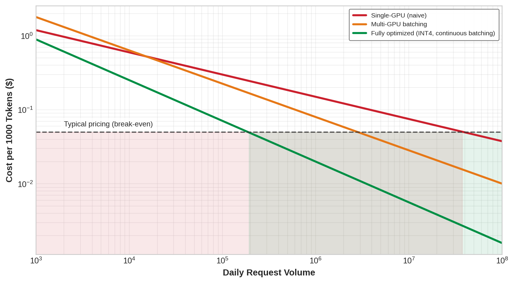
The cost structure motivates serving optimization: every percentage point of efficiency improvement yields ongoing cost reduction over the model’s operational lifetime. Figure 1 illustrates why optimization matters by showing how the gap between naive and optimized serving determines whether an inference service is profitable or hemorrhaging money.

Figure 1: The Serving Cost Curve: Cost per 1000 tokens decreases with scale and optimization. Single-GPU serving reaches break-even only at very high volume. Multi-GPU batching breaks even at moderate volume. Fully optimized serving (INT4, continuous batching, speculative decoding) achieves profitability at much lower volumes, fundamentally changing the economics of inference.

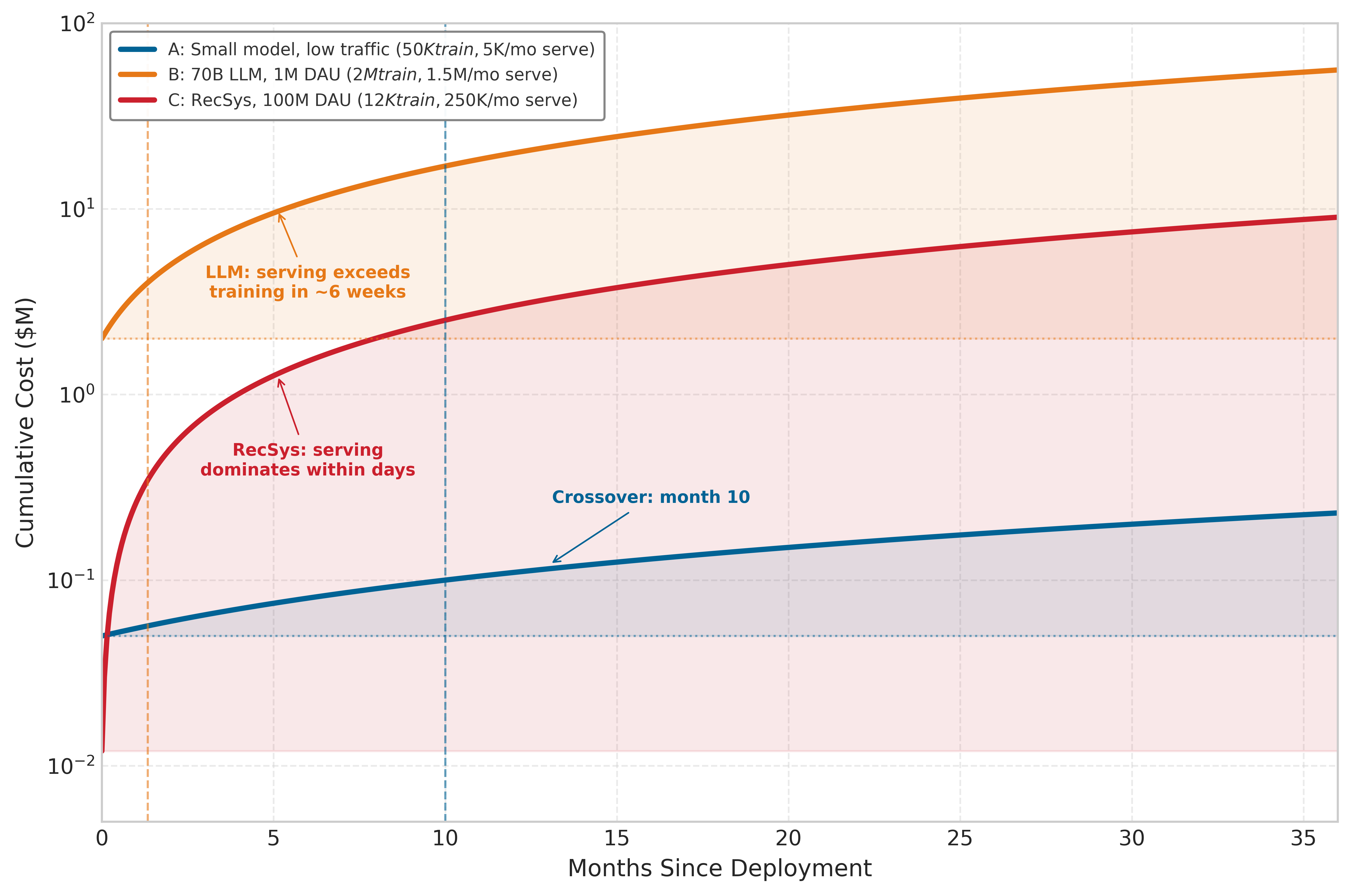
The cost ratios in table 3 tell a static story, but the dynamics of cost accumulation reveal an even more striking pattern. Figure 2 plots cumulative total deployment cost over a 36-month window for three representative scenarios: a small model with low traffic, a 70B LLM serving one million daily active users, and a recommendation system serving 100 million users. The vertical crossover markers show when cumulative serving spend equals the original training cost; because the plotted curves include both training and serving, the total-cost curve is at roughly twice the training baseline at that marker. For recommendation systems, serving dominates within days; for high-traffic LLMs, within roughly six weeks. Only small models with expensive training and low traffic see training cost dominate for extended periods. This temporal view reinforces why inference optimization deserves early engineering attention at production scale. For generative LLM services, serving-specific designs can translate directly into throughput, cost, and power gains (Patel et al. 2024).

Patel, Pratyush, Esha Choukse, Chaojie Zhang, Aashaka Shah, Íñigo Goiri, Saeed Maleki, and Ricardo Bianchini. 2024. “Splitwise: Efficient Generative LLM Inference Using Phase Splitting.” 2024 ACM/IEEE 51st Annual International Symposium on Computer Architecture (ISCA), 118–32. https://doi.org/10.1109/isca59077.2024.00019.

Figure 2: The Serving Cost Crossover: Cumulative total deployment cost (initial training plus ongoing serving) for three scenarios. Vertical markers indicate when the serving portion equals the one-time training cost. For high-traffic LLMs, serving cost matches training cost within weeks. For recommendation systems at 100M daily active users, serving dominates within days. Only low-traffic, expensive-to-train models see training cost dominate for extended periods.

The inference landscape: Beyond LLMs

A common misconception frames inference at scale as synonymous with LLM serving. Large language models present distinctive challenges and attract attention, but they are only one part of production inference. Appropriate technique selection requires understanding the full inference landscape. In large consumer platforms, recommendation and ranking workloads can dominate AI inference cycles and capacity, even though they are not the only user-visible model class (Gupta et al. 2020; Hazelwood et al. 2018). Vision and image processing, NLP and LLM workloads, fraud detection, ads, and other classification tasks fill out the remainder. Table 4 breaks down these model types qualitatively by serving pressure and optimization challenge, and the comparison shows that each class binds on a different constraint: recommendation on embedding lookup, vision on batch efficiency, LLMs on memory bandwidth, and speech on sequential decode. No single optimization serves all four.

Recommendation systems often dominate high-volume consumer inference because they serve predictions for many user interactions. Every page load, scroll, or click can trigger ranking or retrieval inference. A user browsing an e-commerce site might generate many recommendation requests in a single session. In contrast, LLM queries typically require explicit user action and occur less frequently.

The distribution has direct implications for technique selection. Recommendation systems have driven important production inference innovations: dynamic batching, embedding sharding, feature store architectures, and low-latency serving were all developed primarily for recommendation workloads (Naumov et al. 2019; Gupta et al. 2020). LLM-specific techniques like continuous batching and KV cache management address a different slice of production inference. Text-to-image systems such as DALL-E provide one multimodal model example (Ramesh et al. 2021), but multimodal serving volume and latency targets remain product-specific.

Ramesh, A., M. Pavlov, G. Goh, S. Gray, C. Voss, A. Radford, M. Chen, and I. Sutskever. 2021. “Zero-Shot Text-to-Image Generation.” In Proceedings of the 38th International Conference on Machine Learning, ICML 2021, 18-24 July 2021, Virtual Event, edited by Marina Meila and Tong Zhang, vol. 139. Proceedings of Machine Learning Research. PMLR.

Table 4: Production Inference Landscape: Different model types create different serving pressure, latency requirements, and optimization challenges. The table is a qualitative workload map rather than a universal traffic-share distribution. Technique selection must match the specific workload.

Model Type	Serving Pressure	Latency Target	Key Challenge
Recommendation/ranking	Very high in consumer platforms	<10 ms P99	Embedding lookup
Vision (CNN)	Workload-dependent	20–100 ms	Batch efficiency
LLM	High cost per request	100 ms–10s	Memory bandwidth
Speech/Audio	Stream-driven	Real-time	Sequential decode
Multimodal/text-to-image	Emerging and product-specific	Varies	Cross-modal coordination

The serving hierarchy

The optimization techniques organize into a serving hierarchy, analogous to the memory hierarchy in computer architecture. Each level owns a different bottleneck, so an optimization that helps one level can leave another unchanged. The request level follows one request through preprocessing, batching, caching, and model execution, where the target is the latency a user sees. The replica level looks inside one model instance, where GPU utilization, memory management, kernel efficiency, and model optimization determine how much useful throughput that replica can deliver before it saturates. The service level then works across many replicas of the same model, using load balancing, request routing, and autoscaling to turn individual replicas into aggregate capacity. The platform level works across services and tenants, where resource allocation, multi-tenancy, scheduling, and placement decide whether a shared serving fleet remains efficient without allowing one workload to degrade another.

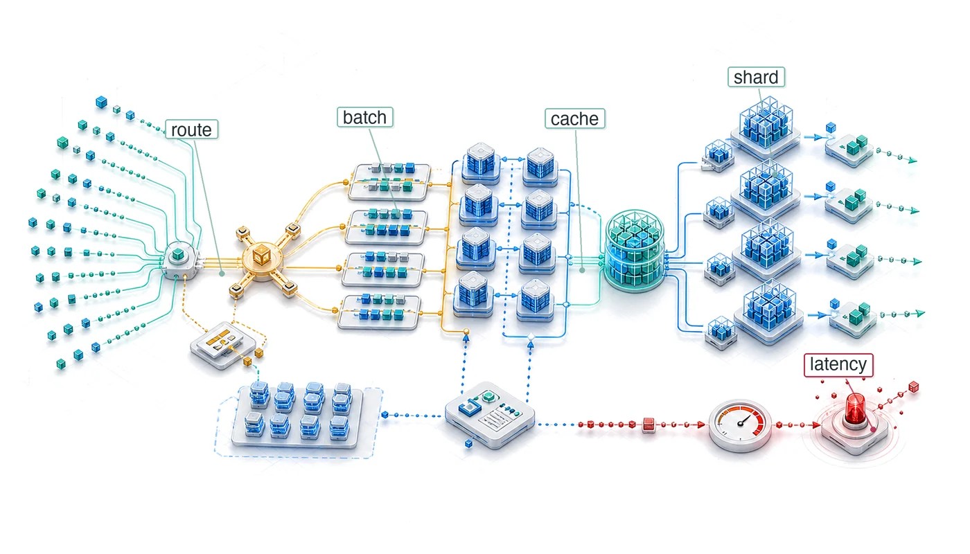
The hierarchy matters because each level changes a different metric and fails at a different boundary. A related deployment stack appears in figure 3, showing how requests pass through edge, routing, and model-serving infrastructure in production.

Figure 3: Serving Deployment Stack: A three-tier serving stack with cumulative latency budget from top to bottom. Tier 1 (CDN/Edge Cache) handles geographic distribution and cached static responses (SLA <10 ms). Tier 2 (Gateway/Router) handles request routing, rate limiting, and authentication (SLA <50 ms). Tier 3 (Model Serving Cluster) runs GPU workers with autoscaling and continuous batching (SLA <2 s).

Each level has distinct optimization levers, and table 5 shows why the lever is level-specific: request-level changes reduce per-request latency, replica-level changes raise utilization, service-level changes add aggregate capacity, and platform-level changes improve fleet efficiency across tenants. Optimizing the wrong level moves the wrong metric.

Table 5: Serving Hierarchy Optimization Targets: Each level of the hierarchy addresses different metrics with different techniques.

Level	Optimization Target	Key Techniques
Request	Per-request latency	Dynamic batching, caching, prefetching
Replica	Throughput, utilization	Memory optimization, kernel fusion
Service	Aggregate capacity	Load balancing, routing, autoscaling
Platform	Resource efficiency	Multi-tenancy, scheduling, placement

Checkpoint 1.2: The serving hierarchy

Verify your understanding of where specific optimizations sit within the serving hierarchy:

• Memory level: Identify the hierarchy level responsible for managing GPU memory waste to increase concurrent request capacity.
• Caching level: Identify the hierarchy level responsible for reducing KV-cache waste when request lengths vary.
• Load balancing: Identify the primary optimization target of Service-level load-balancing algorithms like Power-of-Two-Choices.
• Isolation level: Evaluate the claim that multi-tenancy and resource isolation are primarily Request-level concerns.

The hierarchy guides the rest of the design while allowing a few techniques to cross levels. Batching, KV-cache layout, and decode-time optimizations start at the request level. Quantization, adapter state, and model sharding change the replica’s memory and compute budget. Disaggregated serving, load balancing, and autoscaling coordinate replicas into a service, while multi-tenancy and resource isolation govern the platform. Quantization appears across the hierarchy because it is a representation-level lever that changes memory, bandwidth, and cost budgets wherever model state or KV state resides.

Serving Architecture Dimensions

A recommendation system that processes 100,000 embedding lookups per second across a sharded feature store requires a fundamentally different serving architecture than a 70-billion parameter language model generating tokens one at a time. The difference is not merely one of framework choice; it reflects distinct constraints in batching strategy, memory management, scheduling policy, and deployment topology. Rather than catalog specific tools, this section identifies the architectural dimensions that distinguish serving systems and the constraints that drive each design decision. Specific frameworks serve as examples of these principles, not as the subject of study.

Batching strategy: The throughput-latency trade-off

The most consequential architectural decision in a serving system is how it forms batches from incoming requests. This choice determines the fundamental throughput-latency operating point.

Static batching collects a fixed number of requests before dispatching them to the accelerator. For vision models processing fixed-size inputs, this approach maximizes GPU utilization because all requests in the batch execute identical computation graphs with predictable memory access patterns. A ResNet-50 inference server can batch 32 or 64 images with near-linear throughput scaling because the batch amortizes fixed launch overhead and reuses resident weights across many inputs.

Autoregressive language models break this assumption. Each request generates a different number of output tokens, so static batching forces all requests to wait for the longest generation in the batch and can leave accelerator capacity idle after shorter requests finish. Continuous batching⁶ solves this by allowing requests to enter and exit the batch at each decoding step, an iteration-level scheduling approach introduced by Orca (Yu et al. 2022). When one request finishes generation, a new request immediately fills its slot. Systems like vLLM combine this scheduling style with PagedAttention-based KV-cache management, achieving 2–4\(\times\) throughput gains over prior LLM serving systems by reducing memory waste (Kwon et al. 2023).

⁶ vLLM (Virtual LLM): The name signals its core design: applying OS-style virtual memory to KV cache management, decoupling logical sequence addresses from physical GPU memory. Developed at UC Berkeley (2023), vLLM achieved 2–4\(\times\) throughput over FasterTransformer and up to 24\(\times\) over HuggingFace Transformers by eliminating the 60–80 percent memory fragmentation that capped batch sizes in prior serving systems (Kwon et al. 2023).

Kwon, Woosuk, Zhuohan Li, Siyuan Zhuang, Ying Sheng, Lianmin Zheng, Cody Hao Yu, Joseph Gonzalez, Hao Zhang, and Ion Stoica. 2023. “Efficient Memory Management for Large Language Model Serving with PagedAttention.” Proceedings of the 29th Symposium on Operating Systems Principles, 611–26. https://doi.org/10.1145/3600006.3613165.

Recommendation systems introduce a third pattern: feature-parallel batching. Because the bottleneck is distributed embedding lookup rather than dense matrix multiplication, these systems batch requests by feature type and shard the batch across embedding servers. The dense MLP computation that follows can then operate on prefetched, prebatched feature vectors. The batching strategies section (section 1.2) develops these approaches in full quantitative detail.

Memory management: From preallocation to paging

Serving systems differ fundamentally in how they manage accelerator memory, and this difference determines the maximum concurrent request capacity.

Definition 1.1: KV cache

KV Cache is a per-request LLM inference memory buffer that stores the Key and Value attention tensors of all previously generated tokens so the next token can be produced without recomputing the full attention over the prefix.

1. Significance: It reduces per-token attention compute from \(O(n^2)\) to \(O(n)\) in the sequence length, but its footprint grows linearly with both context length and batch size, often consuming more HBM than the model weights themselves and becoming the binding constraint on serving capacity. KV cache fundamentals derives the fundamental sizing math.
2. Distinction: Unlike model weights (which are shared across all requests and statically allocated), the KV cache is request-private and dynamically sized; each concurrent user pays a separate, sequence-length-proportional memory tax that the scheduler must budget for.
3. Common pitfall: A frequent misconception is that reducing model size proportionally reduces serving memory. In practice, the KV cache dominates HBM at long contexts, so a quantized 70B model can still be capacity-bound at batch sizes the weights alone would easily admit.

Preallocated memory management reserves a fixed memory budget per request at admission time based on the maximum possible output length. For a model supporting 4,096-token outputs, every request reserves memory for 4,096 tokens regardless of whether it generates 50 or 4,000. This approach is simple and predictable but wastes memory proportional to the gap between maximum and actual output lengths. In practice, 60–80 percent of reserved KV cache memory goes unused.

Paged memory management, inspired by operating system virtual memory, allocates memory in fixed-size blocks (pages) and maps logical sequence positions to physical memory locations through a block table. As a request generates tokens, new physical blocks are allocated on demand. When generation completes, blocks return to the free pool immediately. This approach, exemplified by PagedAttention (covered in section 1.3.3), achieves near-100 percent memory utilization by eliminating both internal fragmentation (partially filled preallocations) and external fragmentation (unusable gaps between allocations).

The memory management strategy directly determines batch capacity: paged systems can serve 2–4\(\times\) more concurrent requests than preallocated systems on the same hardware, because they reclaim memory that preallocation wastes. For a service with a fixed GPU budget, this translates directly to 2–4\(\times\) lower cost per request.

Scheduling policy: FCFS, preemptive, and priority-aware

The scheduling policy determines which requests receive GPU time and in what order. This decision becomes critical when request mix is heterogeneous, with some requests requiring 50 tokens of output and others requiring 4,000. First-come-first-served (FCFS) scheduling processes requests in arrival order. FCFS is fair and simple but suffers from head-of-line blocking: a single long-generation request delays all subsequent requests. For workloads with high output-length variance, FCFS produces poor tail latency.

Preemptive scheduling allows the system to pause a long-running request and swap its KV cache to CPU memory (or discard it for later recomputation) to make room for shorter, higher-priority requests. The cost of preemption is the swap overhead (transferring KV cache between GPU and CPU memory) or the recomputation cost (re-running the prefill phase when the preempted request resumes). Production systems typically preempt when a request has consumed more than 2\(\times\) the median generation length.

Priority-aware scheduling assigns different service classes to requests and guarantees that high-priority requests receive GPU slots before lower-priority ones. A production API might classify revenue-generating customer requests as critical, internal batch processing as standard, and free-tier traffic as best-effort. The scheduling policy then ensures that critical requests never wait behind best-effort traffic, even during load spikes.

Deployment topology: Single-GPU to disaggregated

The deployment topology determines how model computation maps to physical hardware, and this mapping is driven by the ratio of model size to single-device memory capacity. Single-GPU deployment is the simplest topology: the entire model fits in one device’s memory, and all inference computation occurs locally. For models under 15–20 billion parameters (30–40 GB in FP16), this topology provides the lowest latency because it eliminates all inter-device communication.

Multi-GPU tensor parallelism shards each layer’s weight matrices across multiple GPUs connected by high-bandwidth interconnect (NVLink at 900 GB/s on H100). Each GPU computes a partial result for every layer, and an all-reduce operation synchronizes the partial results before the next layer. This topology is necessary when model weights exceed single-device memory and provides latency reduction proportional to the parallelism degree, at the cost of communication overhead per layer. The model sharding section (section 1.4) analyzes the communication overhead quantitatively.

Disaggregated serving separates the prefill phase (processing the input prompt, which is compute-bound) from the decode phase (generating tokens one at a time, which is memory-bandwidth-bound) onto different hardware pools optimized for each workload profile. Prefill nodes use high-FLOP/s accelerators; decode nodes use high-bandwidth-memory configurations. This separation allows each phase to operate at its hardware’s optimal operating point rather than compromising between the two regimes on shared hardware. The disaggregated serving section (section 1.3.9) develops this architecture in detail.

Stateful vs. stateless: The scaling divide

A serving system’s statefulness determines whether horizontal scaling is trivial or requires careful engineering. Vision models and embedding lookups are typically stateless: any replica can serve any request because no per-session state persists between requests. Horizontal scaling is straightforward – add replicas behind a load balancer – and failure recovery is instant because the load balancer simply routes to a healthy replica.

LLM serving with KV cache is inherently stateful: the cache accumulated during a conversation creates replica-specific state that cannot be reconstructed without re-running the entire conversation history through prefill. This statefulness has cascading implications for system design. Load balancing requires sticky routing to direct subsequent requests in a conversation to the same replica. Autoscaling down requires draining active sessions, which can take minutes for long conversations. Failure recovery is expensive: when a stateful replica crashes, users either experience the latency of regenerating context (seconds) or lose conversation state entirely.

The choice between stateless and stateful serving is not a framework feature but a consequence of the model architecture. Systems that serve autoregressive models must engineer for statefulness; systems that serve fixed-computation models can treat scaling as a simpler capacity-planning exercise.

Architectural comparison

Table 6 summarizes how the batching, memory, scheduling, topology, and state dimensions interact across the major workload types. The table reveals that no single serving architecture is optimal for all workloads; the constraint profile of each workload type determines the appropriate design point along each dimension.

Table 6: Serving Architecture Dimensions by Workload Type: Each workload’s constraint profile determines the optimal design point along five architectural dimensions. Selecting a serving system amounts to choosing the combination that matches the workload’s constraints.

Dimension	Vision/Embedding	LLM (Autoregressive)	Recommendation
Batching	Static/dynamic (uniform inputs)	Continuous (variable outputs)	Feature-parallel (sharded embeddings)
Memory	Preallocated (predictable)	Paged (variable KV cache)	Distributed (embedding tables)
Scheduling	FCFS (uniform cost)	Preemptive (high variance)	Priority-aware (SLO tiers)
Topology	Single-GPU replicas	Tensor/pipeline parallel	Hybrid CPU-GPU sharding
State	Stateless	Stateful (KV cache)	Stateless (feature store)

Checkpoint 1.3: Serving dimensions

Verify your understanding of how workload constraints drive architectural choices:

• LLM vs. vision: Explain why preemptive scheduling is more critical for LLMs than for vision models.
• Stateful workloads: Identify the workload type for which stateful serving (requiring sticky routing) is a fundamental requirement.
• RecSys standard: Explain why feature-parallel batching is the standard for recommendation systems but not for LLMs.
• Memory pressure: Identify which dimension (batching, memory, scheduling, topology, state) is primarily affected when quantization reduces model or KV-cache size.

The architectural dimensions determine which serving system to select for a given workload. Rather than comparing frameworks feature by feature, an engineer identifies the workload’s position along each dimension (batching pattern, memory profile, scheduling requirements, deployment topology, and statefulness) and selects the system that matches. The optimization techniques in this chapter operate within this architectural framework, each addressing a specific dimension.

Self-Check: Question

1. A product team is choosing an architecture for an autoregressive LLM service where output lengths range from 30 tokens to 3,000 tokens and conversations persist across multiple turns. Which combination of the five dimensions matches this workload’s constraint profile?

   1. Static batching, pre-allocated KV memory, FCFS scheduling, single-GPU replicas, stateless routing
   2. Continuous batching, paged KV memory, preemptive or priority-aware scheduling, tensor-parallel topology, stateful sticky routing
   3. Feature-parallel batching, distributed embedding storage, priority-only scheduling, hybrid CPU-GPU topology, stateless routing
   4. No batching with single-frame processing, pre-allocated memory, FCFS scheduling, edge deployment, stateless routing

2. Once each LLM conversation accumulates replica-specific KV-cache state that survives across turns, horizontal scale-out can no longer add capacity by routing the next turn to any idle replica; autoscaling-down must drain active sessions for minutes, and a replica crash forces users to either wait for seconds of prefill recomputation or lose context entirely. The service has become ____ rather than stateless.

3. Explain why preemptive scheduling is essential for an LLM service whose output lengths range from 50 to 4,000 tokens, while a ResNet-50 image service with fixed 224x224 inputs is well served by FCFS. Reference the head-of-line blocking mechanism quantitatively.

4. A serving system admits each request by reserving KV-cache memory for the model’s 4,096-token maximum context, even though typical generations complete in 200-500 tokens. What is the primary concurrency consequence?

   1. Pre-allocation wastes roughly 88-95 percent of each reservation for typical requests, so fewer concurrent requests fit on the same GPU; paged memory recovers this and supports 2–4\(\times\) higher concurrency
   2. Pre-allocation guarantees near-100 percent memory utilization because every admitted request has a reserved slot before execution starts
   3. Pre-allocation makes horizontal scaling easier because fixed reservations remove replica-local state that would otherwise bind requests to specific GPUs
   4. Pre-allocation shifts the decode phase from memory-bandwidth-bound to compute-bound by making allocation patterns deterministic across the batch

5. Meta’s DLRM serves requests whose dominant cost is embedding-table lookup across tables totaling over 100 TB of sparse features, followed by a much smaller dense ranking MLP. Which combination of architectural dimensions is the matched design point?

   1. Static batching on dense inputs, pre-allocated GPU memory, FCFS, single-GPU replicas, stateless routing
   2. Continuous batching with paged memory, preemptive scheduling, tensor-parallel topology, stateful routing
   3. Feature-parallel batching with sharded embedding storage, priority-aware SLO-tiered scheduling, hybrid CPU-GPU topology, stateless routing to the feature store
   4. No batching, single-GPU replicas, FCFS, stateful sticky routing to preserve embedding affinity

See Answers →

Batching Strategies at Scale

A stream of hundreds of disparate chat requests arrives at an inference server every second. Processing them one by one leaves much of the GPU idle, starved for work between small decode steps. Waiting to gather a large static batch forces the first request in line to endure unacceptable latency. Batching strategies at scale demand dynamic algorithms that fuse requests on the fly without violating strict tail-latency deadlines.

Processing multiple requests together amortizes fixed costs (model loading, kernel launch overhead, and memory transfer latency) across more useful work, trading higher per-request latency for dramatically improved throughput. Single-machine serving applies this insight through dynamic batching, which collects requests within a time window before processing them together.

At scale, batching becomes more complex because different model architectures have distinct batching requirements. A strategy optimal for vision models may be catastrophic for LLMs, and techniques developed for recommendation systems may not apply to either.

In large consumer platforms, recommendation systems can constitute the majority of AI inference cycles or capacity pressure, with vision, language, ranking, fraud, ads, and other classification workloads sharing the remainder (Gupta et al. 2020; Hazelwood et al. 2018). Despite this distribution, we present batching strategies in order of conceptual complexity: vision (straightforward batching), LLMs (continuous batching with KV cache), and recommendation (feature-parallel batching with distributed embedding). This pedagogical ordering builds understanding progressively, even though practitioners may frequently encounter recommendation workloads first. The taxonomy that follows matches batching strategies to model characteristics, providing quantitative analysis of when each approach applies and what performance to expect.

Why batching differs across model types

Batching efficiency depends on how computation scales with batch size relative to how memory and communication scale. Different model architectures exhibit different scaling relationships, requiring different batching strategies, as figure 4 summarizes.

Figure 4: Batching Strategies Compared: Three timelines show how batching policies trade wait time for GPU utilization. (a) No batching: requests processed sequentially, GPU idle between them (around 40 percent utilization). (b) Static batching: requests wait until a full batch is assembled before dispatch, with padding for short requests (around 70 percent utilization). (c) Dynamic batching: assembles a batch within a short time window with adaptive size, reducing wait and lifting utilization (around 85 percent).

For vision models, including convolutional neural networks (CNNs) and vision transformers (ViTs) processing fixed-size images, computation scales linearly with batch size while memory scales sub-linearly due to weight sharing. Larger batches improve GPU utilization with minimal overhead, making static or dynamic batching with large batch sizes optimal.

For LLMs in the decode phase, computation per token is small relative to memory bandwidth requirements for loading model weights. The bottleneck is memory bandwidth, not compute. Larger batches amortize weight loading across more tokens, dramatically improving throughput but with diminishing returns as batch size grows.

For recommendation systems, the bottleneck is often embedding lookup rather than dense computation. Batching strategies must optimize for parallel embedding access patterns rather than matrix multiplication throughput.

The physics of batching: The efficiency curve

Batching is not merely a heuristic; it is a trade-off governed by the physics of hardware utilization. We can model the relationship between batch size \((B)\), request latency \((T_{\text{lat}})\), and throughput \((X)\) to identify the optimal operating point for any inference system.

Here \(T_{\text{lat}}\) follows standard queuing notation for request time in system. Elsewhere in the book, \(L_{\text{lat}}\) denotes fixed latency overheads or latency components; this section keeps \(T_{\text{lat}}\) for the end-to-end request-time variable used in Little’s Law and batching equations.

The latency equation decomposes per-request latency into fixed overheads (kernel launch, memory loading) and variable costs (compute per sample):

\[T_{\text{lat}}(B) = T_{\text{fixed}} + B \times T_{\text{variable}}\]

• \(T_{\text{fixed}}\): Costs paid once per batch (for example, loading weights from HBM, kernel launch latency).
• \(T_{\text{variable}}\): Marginal cost of adding one request (for example, compute time for that sample).

The throughput equation describes the system’s capacity:

\[X(B) = \frac{B}{T_{\text{lat}}(B)} = \frac{B}{T_{\text{fixed}} + B \times T_{\text{variable}}}\]

The resulting Batching Efficiency Curve shows three distinct regimes. For small batch sizes (\(B\)), throughput is dominated by \(T_{\text{fixed}}\), making the system latency-bound (or overhead-bound) where increasing \(B\) yields super-linear throughput gains. As \(B\) becomes large, the \(T_{\text{fixed}}\) term becomes negligible, and throughput asymptotically approaches the hardware limit \(1/T_{\text{variable}}\), leaving the system compute-bound (or bandwidth-bound for LLMs). The optimal batch size sits at the knee of the curve, the point where throughput gains diminish while latency continues to grow linearly.

Throughput saturates at the batch size where latency hits the SLO.

The engineering goal is to find the maximum \(B\) such that \(T_{\text{lat}}(B) \le \text{SLO}\). This formulation explains why vision models (high \(T_{\text{variable}}\)) saturate at smaller batches than LLMs (high \(T_{\text{fixed}}\) due to weight loading), requiring different tuning strategies.

Napkin Math 1.2: The batching efficiency curve

Problem: An engineer optimizes two services: a Vision model (ResNet) and an LLM (70B). At what batch size does each hit the “Knee” of its efficiency curve?

Math: The knee occurs where the variable compute cost \((B \times T_{\text{var}})\) starts to exceed the fixed overhead \((T_{\text{fixed}})\).

1. Vision Model \((T_{\text{fixed}} = 2\text{ ms}, T_{\text{var}} = 1\text{ ms})\):
   • Knee: \(B \approx 2\text{ ms}/1\text{ ms} =\) 2.
   • Result: This simplified latency model reaches its first overhead-amortization knee at a very small batch. Production CNNs often continue gaining throughput until batches of 32–64+ before hardware saturation.
2. LLM Decode \((T_{\text{fixed}} = 40\text{ ms}, T_{\text{var}} = 0.5\text{ ms})\):
   • Knee: \(B \approx 40\text{ ms}/0.5\text{ ms} =\) 80.
   • Result: LLMs require massive batches to amortize the expensive weight-loading overhead.

Systems insight: Because the LLM’s “Fixed Overhead” (loading 140 GB of weights from HBM) is so large, the system has not reached the efficiency knee until batch size 80. LLM serving therefore requires continuous batching and paged memory: the system must pack hundreds of concurrent users into a single batch just to overcome the memory bandwidth bottleneck.

Translating these batch-level equations into system-wide capacity planning requires a classical result from queuing theory: Little’s Law⁷, which relates concurrency, throughput, and latency in any stable system. Across model architectures, table 7 shows that batching choice follows the binding bottleneck: compute for vision models, memory capacity or bandwidth for LLM prefill and decode, embedding lookup for recommendation systems, and real-time latency for speech.

⁷ Little’s Law: From queuing theory, \(Q_{\text{req}} = \lambda_{\text{arr}} T_{\text{lat}}\), so concurrency equals arrival rate times latency. For a serving fleet, this defines the capacity envelope: if a GPU can handle 32 concurrent requests and each takes 100 ms, the maximum arrival rate is 320 req/s. Beyond this, queues grow rapidly as utilization approaches 1, and tail latency \((L_{\text{lat}})\) explodes.

Table 7: Batching Strategy by Model Type: Each model type has characteristic batching behavior determined by its computational bottleneck.

Model Type	Batching Strategy	Typical Batch Size	Key Constraint	Throughput Scaling
Vision (CNN)	Static/Dynamic	32–256	GPU compute	Near-linear to 64+
LLM (prefill)	Dynamic	1–64	Memory capacity	Sub-linear
LLM (decode)	Continuous	100–1000s	Memory bandwidth	Log-linear
RecSys	Feature-parallel	1000–10000s	Embedding lookup	Depends on sharding
Speech	Streaming	1	Real-time	N/A (latency-bound)

Theorem 1.1: Little's Law for inference

Concept: In any stable queuing system, the average number of requests in the system \((Q_{\text{req}})\) equals the arrival rate \((\lambda_{\text{arr}})\) multiplied by the average time a request spends in the system \((T_{\text{lat}})\).

\[ Q_{\text{req}} = \lambda_{\text{arr}} \cdot T_{\text{lat}} \]

Application: Concurrency Planning

• Target Throughput \((\lambda_{\text{arr}})\): 1,000 requests/sec
• Latency SLO \((T_{\text{lat}})\): 100 ms (0.1 s)

Required Concurrency \((Q_{\text{req}})\): \(Q_{\text{req}} = 1000 \times 0.1 =\) 100 concurrent requests

Capacity Planning: If a single GPU replica handles batch size 8 with 80 ms latency:

1. Replica Throughput \(=\) \(8/0.08 =\) 100 req/s
2. Replicas Needed = 1,000 divided by 100 = 10 replicas

Verification: Total system concurrency \(=\) \(10\text{ replicas} \times 8\text{ batch} =\) 80, short of the 100 required. The shortfall is the queue: with 10 replicas actively processing 80 requests, the remaining 20 wait in queues, and that queue wait must fit inside the SLO.

The 20-request queue depth and the unresolved question of whether queue wait time fits inside the SLO are exactly what queuing theory formalizes; Queuing theory for batched inference derives the M/D/1 wait-time distribution that determines whether queue delay fits inside a serving SLO.

Static and dynamic batching for vision models

Vision models represent the simplest batching case because inputs have uniform size (after preprocessing) and computation follows a predictable pattern. Single-machine batching principles apply directly, with scale introducing considerations of batch formation across multiple replicas.

Static batching collects exactly \(B\) requests before processing. This maximizes GPU utilization when request arrival is predictable but causes unbounded latency during low-traffic periods.

Dynamic batching collects requests for a maximum time window \(T_{\text{window}}\) or until reaching maximum batch size \(B_{\text{max}}\), whichever occurs first. The expected latency under Poisson arrivals with rate \(\lambda_{\text{arr}}\) follows equation 3:

\[E[T_{\text{total}}] = E[T_{\text{queue}}] + T_{\text{batch}} + T_{\text{inference}}(B) \tag{3}\]

where \(E[T_{\text{queue}}]\) is the expected queuing delay, \(T_{\text{batch}}\) is the batch formation delay (up to \(T_{\text{window}}\)), and \(T_{\text{inference}}(B)\) is the inference time for batch size \(B\). The arrival rate enters through the queuing and formation terms: under Poisson arrivals the mean inter-arrival gap is \(1/\lambda_{\text{arr}}\), so a higher \(\lambda_{\text{arr}}\) fills the batch faster and shrinks both \(E[T_{\text{queue}}]\) and \(T_{\text{batch}}\), while a lower rate pushes them toward the \(T_{\text{window}}\) ceiling. The worked example that follows makes these interactions concrete.

Example 1.1: Dynamic batching for ResNet-50

Consider a vision classification service with the following requirements:

• Arrival rate: 5,000 QPS
• Latency SLO: 50 ms P99
• Per-image inference time: 5 ms at batch=1, 25 ms at batch=32
• Number of replicas: 10 (each handling 500 QPS)

For a single replica with Poisson arrivals at \(\lambda_{\text{arr}} =\) 500 QPS:

The three choices in table 8 differ only in how much latency budget they convert into batch size:

Table 8: Dynamic batching policy comparison: Option C achieves about 33 percent higher per-replica capacity, or 25 percent lower utilization, at the cost of higher average latency. Both dynamic batching policies meet the 50 ms P99 SLO.

Policy	Batching window	Expected batch	Per-request compute	Utilization	Latency outcome
No batching	0 ms	1 request	5 ms	\(\rho_{\text{serv}} = \lambda_{\text{arr}} \times T_{\text{svc}} = 500 \times 0.005 = 2.5\)	Overloaded; cannot meet demand
Dynamic B	10 ms	5 requests	1.6 ms	\(\rho_{\text{serv}} = 500 \times 0.0016 = 0.8\)	~15 ms mean, ~30 ms P99
Dynamic C	20 ms	10 requests	1.2 ms	\(\rho_{\text{serv}} = 500 \times 0.0012 = 0.6\)	~22 ms mean, ~42 ms P99

Systems insight: Dynamic batching is useful only when the latency budget has slack. The serving policy converts unused latency headroom into higher throughput, but the same window would violate an already tight SLO.

At scale with multiple replicas, batch formation can occur either at individual replicas or at a centralized batching layer. Replica-local batching has each replica independently form batches from its assigned traffic. This approach is simpler to implement but may result in uneven batch sizes across replicas when load is imbalanced. Centralized batching uses a batching service to collect requests and dispatch formed batches to replicas. This achieves more uniform batch sizes but adds a centralization bottleneck and additional network hop. Production systems typically use replica-local batching with load balancing that ensures roughly equal traffic distribution, achieving the benefits of centralized batching without the complexity.

Continuous batching for LLM inference

The autoregressive bottleneck (principle 14) governs this regime: in generative models, the decode phase is strictly memory-bandwidth bound because the entire model weight set must be loaded for every single token generated. Throughput scales with batch size, sharing weight loads across multiple requests, not compute power.

Definition 1.2: Continuous batching

Continuous Batching is a serving strategy that decouples batch membership from iteration boundaries, allowing new requests to enter and completed ones to exit at every decode step.

1. Significance: It maximizes system throughput \((X)\) by eliminating the padding waste and head-of-line blocking inherent in static batching. It ensures the GPU remains saturated even when requests have widely varying sequence lengths.
2. Distinction: Unlike static or dynamic batching (which group requests at the request level), continuous batching operates at the Iteration Level, dynamically reshaping the compute tensor at each clock cycle.
3. Common pitfall: A frequent misconception is that continuous batching is “purely a scheduler change.” In reality, it requires a Dynamic Memory Manager (like PagedAttention) because the KV caches for different requests grow and shrink at different rates, preventing static memory preallocation.

Decoupling batch membership from iteration boundaries is slot reuse: when one request reaches its stop token, the scheduler hands its KV-cache slot to a waiting request on the next decode step instead of leaving capacity idle until the longest sequence finishes.

Autoregressive language models present a unique batching challenge that static and dynamic approaches handle poorly. The key insight comes from the Orca system⁸ (Yu et al. 2022): traditional batching forces all sequences in a batch to complete before any new sequences can join, wasting compute when sequences finish at different times.

⁸ Orca (Iteration-Level Scheduling): Introduced by Yu et al. (2022), Orca demonstrated that scheduling at iteration granularity rather than request granularity allows sequences to enter and exit batches at each decode step. This eliminated the head-of-line blocking that wasted 50 percent+ of GPU compute in static batching and established the scheduling paradigm adopted by LLM serving systems such as vLLM.

Yu, Gyeong-In, Joo Seong Jeong, Geon-Woo Kim, Soojeong Kim, and Byung-Gon Chun. 2022. “Orca: A Distributed Serving System for Transformer-Based Generative Models.” 16th USENIX Symposium on Operating Systems Design and Implementation (OSDI 22), 521–38.

Consider a batch of 8 sequences. If one sequence completes after 10 tokens while others require 100 tokens, the completed sequence’s GPU resources sit idle for 90 iterations. With traditional batching:

\[\text{Wasted compute} = \frac{(100 - 10) \times 1}{100 \times 8} = 11.25\%\]

For realistic output length distributions with high variance, wasted compute can exceed 50 percent. Continuous batching (also called iteration-level batching) decouples batch membership from iteration boundaries. Algorithm 1 states the scheduler as a decode loop: completed requests release KV-cache pages, waiting requests enter freed slots, and the next batched kernel runs over the reorganized active set. This technique is central to the throughput-latency trade-off that defines large-scale LLM serving—Archetype A workloads (GPT-4/Llama-3, Three systems archetypes) would be economically unviable without it, because their memory-bandwidth-bound decode phase leaves compute cores idle waiting for weights to load, and only by interleaving unrelated requests can the bandwidth be saturated.

\begin{algorithm} \caption{Continuous batching decode scheduler} \begin{algorithmic} \Require waiting queue $Q$; active set $A$; KV-cache page allocator; active-token capacity $C_{\text{tok}}$; batched decode kernel \Ensure generated tokens for completed requests; a continually refreshed active batch \While{the service is running} \State admit requests from $Q$ while capacity and free KV-cache pages remain; allocate state, append to $A$ \State run one batched decode kernel over all sequences in $A$ \State append each sampled token; extend its KV-cache pages \State remove completed or length-limited sequences from $A$; return their pages to the allocator \If{HBM pressure exceeds the policy threshold} \State preempt low-priority sequences by paging their KV-cache to CPU DRAM \EndIf \State fill freed capacity from $Q$, or resume paused sequences whose pages now fit \EndWhile \end{algorithmic} \end{algorithm}

Admitting, completing, and refilling slots on every iteration keeps active-token capacity from idling behind the longest sequence in the batch, while the preemption path adds HBM-to-CPU-DRAM transfer latency under memory pressure. The throughput gain therefore scales with output-length variance and must be balanced against KV-cache movement. As figure 5 illustrates, static batching leaves the GPU idle while waiting for the longest request, whereas continuous batching keeps it saturated.

Figure 5: Static vs. Continuous Batching: In static batching (A), all requests in a batch must wait for the longest request to complete before the GPU can begin the next batch, leading to significant idle compute time (shaded gray). Continuous batching (B) allows new requests to enter the batch as soon as any request finishes, keeping the GPU saturated and dramatically improving throughput.

Continuous batching throughput analysis

The contrast in figure 5 motivates the throughput analysis: static batching leaves GPUs idle for the duration of the longest sequence in each batch, while continuous batching eliminates these idle gaps by inserting new requests at every iteration boundary. Continuous batching’s dynamic batch management maintains high GPU utilization regardless of sequence length variance. The throughput improvement depends on sequence length distribution. For a distribution with coefficient of variation \(\text{CV} = \sigma / \mu\), the gain is approximately equation 4:

\[\text{Throughput gain} \approx 1 + \frac{\text{CV}^2}{2} \tag{4}\]

With typical LLM output lengths having \(\text{CV} \approx 1.0\), continuous batching achieves approximately 1.5\(\times\) throughput improvement. For highly variable outputs (conversational vs. code generation), gains can reach 2–4\(\times\). This \(1 + \text{CV}^2/2\) form estimates the average gain across the output-length distribution; section 1.2.6.3 develops a complementary \(1 + k \cdot \text{CV}\) upper bound that compares the single longest sequence against the mean. The distributional estimate predicts typical throughput; the max-over-mean bound caps the best case a workload can reach.

The analytical gains translate directly into production systems. The following implementation study examines how vLLM realizes continuous batching through iteration-level scheduling, paged memory management, preemption, throughput, and GPU utilization.

Example 1.2: Continuous batching in vLLM

vLLM implements continuous batching with several key mechanisms. Iteration-level scheduling evaluates at each decode step which sequences have generated end-of-sequence tokens (remove from batch), which waiting sequences can fit in available KV cache slots (add to batch), and which sequences should be preempted if memory pressure exists (swap to CPU). Memory management uses PagedAttention (detailed in section 1.3), which enables dynamic allocation without fragmentation. When a sequence completes, its KV cache pages are immediately available for new sequences. The batched decode kernel processes all active sequences in a single batched operation despite dynamic batch composition. Sequences at different generation lengths are padded to a common shape within the kernel.

Preemption and swapping. A critical challenge in continuous batching is memory contention. As sequences grow during generation, they consume more KV cache pages. If the GPU memory fills up, the system cannot simply crash; it must preempt running requests.

vLLM implements a virtual memory mechanism similar to an operating system’s swap. When memory is exhausted, the scheduler identifies low-priority requests (for example, those most recently started) and swaps their KV cache blocks from GPU HBM to CPU DRAM. These requests are paused until memory becomes available, at which point they are swapped back in and resumed. This mechanism ensures system stability under heavy load at the cost of increased latency for preempted requests.

Typical performance: Table 9 reports the throughput and utilization improvement for Llama-2 70B on 8\(\times\) A100:

Table 9: Continuous batching throughput on Llama-2 70B (8\(\times\) A100): Tokens-per-second and GPU utilization for static, dynamic, and continuous batching of a Llama-2 70B serving workload on an 8\(\times\) A100 node.

Batching Strategy	Throughput (tokens/s)	GPU Utilization
Static (batch=8)	400	45%
Dynamic (timeout=50 ms)	580	65%
Continuous	1,200	92%

Systems insight: As table 9 shows, the 3\(\times\) throughput improvement from continuous batching comes from eliminating idle GPU cycles during sequence length variation.

The throughput numbers establish that continuous batching wins when output lengths vary, but they do not show where the gain comes from or how large it can grow. Quantifying the waste that traditional batching leaves on the table turns that intuition into a number a scheduler can act on.

Quantitative analysis: Traditional vs. continuous batching

The first baseline is traditional LLM batching, where unequal output lengths turn request heterogeneity into wasted decode cycles. The mathematics of batching waste reveals exactly how much throughput is lost and under what conditions continuous batching delivers the greatest improvement.

The waste function for traditional batching

Traditional batching (also called static batching) processes all requests in a batch through all decode iterations until the longest sequence completes. For batch size \(B\) with output lengths \(\{S_1, S_2, ..., S_B\}\), the total compute performed is:

\[O_{\text{traditional}} = B \times S_{\text{max}} \times c_{\text{decode}}\]

where \(S_{\text{max}} = \max_i(S_i)\) and \(c_{\text{decode}}\) is the compute cost per decode iteration per sequence. However, the useful compute is only:

\[O_{\text{useful}} = \sum_{i=1}^{B} S_i \times c_{\text{decode}}\]

Equation 5 defines the waste ratio that quantifies the inefficiency:

\[W = 1 - \frac{O_{\text{useful}}}{O_{\text{traditional}}} = 1 - \frac{\sum_{i=1}^{B} S_i}{B \times S_{\text{max}}} = 1 - \frac{\bar{S}}{S_{\text{max}}} \tag{5}\]

where \(\bar{S}\) is the mean output sequence length. This reveals that waste depends entirely on the ratio of mean to maximum output length within the batch. For uniform output lengths \((\bar{S} = S_{\text{max}})\), waste is zero. For highly variable lengths, waste can exceed 50 percent.

Worked example: LLM serving with variable-length outputs

Consider a GPT-class model serving four concurrent requests with the generation lengths shown in table 10 (in tokens):

Table 10: Concurrent Request Generation Lengths: Four concurrent requests on a GPT-class model with varying prompt and output lengths. The 4\(\times\) spread in output length (50 to 200 tokens) drives the batching waste analyzed in this section: a static batch of four pads every request to the longest, wasting compute on the three shorter requests until the longest finishes generating.

Request	Prompt Length	Output Length	Total Tokens
R1	100	50	150
R2	80	200	280
R3	120	100	220
R4	90	150	240

Napkin Math 1.3: Continuous batching waste calculation

Problem: Given four LLM requests with unequal output lengths, quantify how much average latency traditional batching wastes and how continuous batching recovers that idle slot time.

Variables:

• Decode time per iteration (batch of 4): 20 ms
• Maximum output length in batch: 200 tokens (R2)
• Mean output length: \((50 + 200 + 100 + 150) / 4 =\) 125 tokens

Traditional batching: All four requests must wait for R2 to complete its 200 tokens.

• Total decode iterations: 200
• Total batch time: \(200 \times 20\text{ ms} =\) 4,000 ms
• Request completion times:
  • R1 completes useful work at iteration 50, but waits until iteration 200 → latency = 4,000 ms
  • R2 completes at iteration 200 → latency = 4,000 ms
  • R3 completes useful work at iteration 100, but waits until iteration 200 → latency = 4,000 ms
  • R4 completes useful work at iteration 150, but waits until iteration 200 → latency = 4,000 ms

Waste calculation using equation 5:

\(W = 1 - \frac{125}{200} = 1 - 0.625 = 37.5\%\)

The GPU performs \(4 \times 200 =\) 800 “sequence-iterations” but only 500 are useful.

Continuous batching: Sequences depart the batch upon completion, and new requests can join.

• Iteration 50: R1 completes → slot freed, new request R5 can join
• Iteration 100: R3 completes → slot freed, new request R6 can join
• Iteration 150: R4 completes → slot freed, new request R7 can join
• Iteration 200: R2 completes

Request latencies with continuous batching (assuming no queuing delay):

• R1: \(50 \times 20\text{ ms} =\) 1,000 ms (4× improvement over traditional)
• R3: \(100 \times 20\text{ ms} =\) 2,000 (2× improvement)
• R4: \(150 \times 20\text{ ms} =\) 3,000 (1.33× improvement)
• R2: \(200 \times 20\text{ ms} =\) 4,000 (no improvement for longest request)

Average latency comparison

• Traditional: 4,000 ms (all requests)
• Continuous: (1,000 ms + 2,000 + 3,000 + 4,000) / 4 = 2,500

Result: Continuous batching reduces average latency by 37.5 percent, exactly matching the waste ratio.

Systems insight: Continuous batching does not make the longest request faster; it prevents shorter requests from occupying finished slots while they wait for that longest request. The gain comes from reusing slots at iteration boundaries, which is the slot-reuse pattern shown in figure 5.

When continuous batching provides maximum benefit

The continuous-batching analysis reveals that benefit scales with output length variance. A useful upper-bound intuition comes from comparing the longest sequence in a traditional batch with the average sequence length. Let \(\text{CV} = \sigma / \mu\) be the coefficient of variation of output lengths. If the longest request in a batch is roughly \(k\) standard deviations above the mean, then:

\[\text{Improvement} \approx \frac{S_{\text{max}}}{\bar{S}} = \frac{\mu + k\sigma}{\mu} = 1 + k \cdot \text{CV}\]

where \(k\) is the number of standard deviations the maximum output exceeds the mean. Real systems realize less than this upper bound because scheduler overhead, KV-cache pressure, and refill gaps consume part of the theoretical gain. The table therefore reports effective waste and speedup, where \(\text{speedup} \approx 1/(1 - W_{\text{effective}})\).

Table 11 quantifies this relationship across different workload types, including Retrieval-Augmented Generation (RAG) (Lewis et al. 2020):

Lewis, Patrick, Ethan Perez, Aleksandra Piktus, Fabio Petroni, Vladimir Karpukhin, Naman Goyal, Heinrich Küttler, et al. 2020. “Retrieval-Augmented Generation for Knowledge-Intensive NLP Tasks.” Advances in Neural Information Processing Systems 33: 9459–74.

Table 11: Continuous Batching Benefit by Workload Type: Higher output length variance (CV) yields greater improvement from continuous batching. Workloads with predictable output lengths (code completion) see modest gains, while highly variable workloads (RAG with documents of varying length) see dramatic improvement.

Workload Type	CV	k	Waste (Trad.)	Speedup (Continuous)
Code completion	0.3	2.5K	16.7%	1.2×
Chat (short responses)	0.6	2K	33.3%	1.5×
General text generation	1	2.5K	50%	2×
Creative writing	1.5	3K	64.3%	2.8×
RAG with variable docs	2	2.5K	71.4%	3.5×

The systems pattern is straightforward: continuous batching is most valuable when output lengths are unpredictable, mixed workload types share the same cluster, request volume is high enough to refill vacated slots, and latency SLOs make early completion valuable. It provides minimal benefit when output lengths are uniform, as in classification or embedding generation, when batch sizes are too small for slot reuse to matter, or when request volume is too low to refill vacated slots.

Implementation complexity trade-offs

The same variability that makes continuous batching valuable also makes it harder to operate. Its performance benefits come with implementation complexity that systems engineers must weigh.

Memory management complexity increases substantially. Traditional batching allocates a fixed KV cache region per sequence at batch formation, deallocating only when the entire batch completes. Continuous batching requires dynamic allocation as sequences grow and immediate deallocation upon completion, necessitating sophisticated memory management akin to operating system virtual memory.

Scheduler complexity rises correspondingly. Traditional batching uses simple FIFO scheduling: collect requests until the batch is full or the timeout expires, then execute. Continuous batching requires per-iteration decision-making about which sequences to admit, which to preempt if memory pressure exists, and how to handle priority classes. This increases scheduler overhead from \(\mathcal{O}(1)\) per batch to \(\mathcal{O}(B)\) per iteration.

Kernel design must also adapt. Batched GPU kernels traditionally assume fixed batch composition. Continuous batching requires kernels that handle variable-length sequences efficiently, often through techniques like packing multiple short sequences into shared attention masks or using specialized memory layouts that support dynamic batch membership.

Table 12 summarizes these trade-offs:

Table 12: Traditional vs. Continuous Batching Trade-Offs: Continuous batching provides significant throughput gains for variable-length workloads at the cost of implementation complexity. For uniform-length workloads, the complexity overhead may not justify adoption.

Dimension	Traditional Batching	Continuous Batching
Implementation effort	Low (standard frameworks)	High (custom scheduler, kernels)
Memory overhead	Fixed allocation	Dynamic + fragmentation mgmt
Scheduler latency	~0.1 ms per batch	~0.5-1 ms per iteration
Debugging complexity	Deterministic behavior	State-dependent, harder to trace
Throughput (variable)	Baseline	1.5–3.5\(\times\) improvement
Throughput (uniform)	Baseline	~1.0\(\times\) (no improvement)

For new LLM serving deployments, continuous batching frameworks like vLLM, TensorRT-LLM, or TGI provide mature implementation paths. The decision becomes whether to adopt these frameworks or build custom serving infrastructure. For organizations with existing traditional batching systems, the migration cost must be weighed against the workload’s output length variance using table 11.

Even with mature serving frameworks, diagnosing tail latency anomalies requires systematic investigation across the system stack. A representative P99 latency regression shows how the fleet stack methodology applies across infrastructure, execution, and serving layers.

Example 1.3: Debugging high P99 latency

Scenario: An LLM serving system exhibits unexpectedly high tail latency. P50 latency is 100 ms and P95 is 180 ms, both within SLO, but P99 spikes to 500 ms against a 200 ms target. GPU utilization appears healthy at 85 percent.

Setup: The system runs on 4 A100-80 GB GPUs connected via PCIe Gen4 (32 GB/s per GPU) rather than NVLink. Memory bandwidth per GPU is 2.04 TB/s (HBM2e), adequate for decode operations, but PCIe limits tensor-parallel communication. For a batch requiring 100 MB activation transfers between GPUs, raw bandwidth math gives approximately 3.1 ms per synchronization point over PCIe versus 0.17 ms over NVLink. The scheduling policy is the real problem: dynamic request-level batching uses max batch size 32 and timeout 50 ms, and the largest 5 percent of batches experience head-of-line blocking because FIFO batching holds short requests behind long-sequence requests.

Systems lesson: The root cause is not the hardware layer but the scheduling policy. Implement priority-aware scheduling with separate batch size limits by request type:

1. Request classification: Tag requests by expected output length (short: under 50 tokens, medium: 50 to 200 tokens, long: over 200 tokens) based on prompt patterns or user-provided hints
2. Differentiated batching: Limit short-request batches to 8, medium to 16, long to 32
3. Priority preemption: Allow short requests to preempt long-running sequences when P99 approaches SLO

After implementing these changes, P99 dropped to 185 ms. High average GPU utilization can mask head-of-line blocking that affects only a small percentage of requests but drives P99; section 1.6 develops the full isolation framework for keeping one workload’s tail from degrading another.

The batching strategies examined so far divide along a fundamental constraint boundary. Vision workloads are compute-bound with fixed-shape tensors: every image in a batch undergoes identical arithmetic, so the batch formation problem reduces to packing a GPU’s compute pipeline as tightly as possible. LLM workloads are memory-bound with variable-length sequences: the KV cache grows per-request and per-token, so the batch formation problem shifts to memory accounting, eviction policies, and iteration-level scheduling that continuous batching provides. Each regime produced a different dominant strategy because the scarce resource differs: compute throughput for vision, memory capacity for language.

Recommendation systems present a third constraint regime that resembles neither. Sparse embedding lookups, not dense matrix multiplications, dominate both compute time and memory traffic. A single recommendation request may touch millions of embedding table entries scattered across shards, while the dense ranking head that follows is comparatively small. This access pattern demands a batching strategy organized around feature types and embedding locality rather than around request shape or sequence length.

Feature-parallel batching for recommendation systems

Recommendation batching starts by grouping work around embedding locality rather than request shape. Figure 6 shows how the request is split into feature-specific paths before the dense ranking head recombines the retrieved representations.

Figure 6: Feature-Parallel Batching Pipeline: Requests are batched by feature type (Users, Items, Context) and dispatched to specialized embedding servers in parallel. The retrieved embeddings are then concatenated and processed by the dense ranking head. This architecture enables scaling to trillions of parameters by decoupling embedding storage from dense compute.

Recommendation systems expose the same scheduling principle under a different bottleneck. Their computation pattern involves four stages:

1. Sparse feature lookup: Retrieve embeddings for user, item, and context features

2. Dense feature processing: Transform and normalize dense features

3. Feature interaction: Compute interactions between features (often via attention or factorization)

4. Ranking head: Produce final scores

The sparse embedding lookup often dominates latency and determines batching strategy. Feature-parallel batching processes different feature types in parallel rather than batching entire requests:

Request 1: [user_id_1, item_ids_1, context_1]
Request 2: [user_id_2, item_ids_2, context_2]
Request 3: [user_id_3, item_ids_3, context_3]

Feature-parallel view:
User embeddings:  [lookup(user_1), lookup(user_2), lookup(user_3)]  → parallel
Item embeddings:  [lookup(items_1), lookup(items_2), lookup(items_3)]  → parallel
Context features: [process(ctx_1), process(ctx_2), process(ctx_3)]  → parallel

Then: Combine features per request for ranking

Feature-parallel batching is natural when embeddings are sharded across servers: each embedding server handles lookups for its shard across all requests in the batch. At Meta-scale request volumes, this turns feature sharding into a serving strategy rather than a storage detail.

Example 1.4: RecSys batching at Meta scale

Consider Meta’s recommendation infrastructure serving 10 million QPS across the platform:

Request characteristics:

• Each request queries approximately 100 items (candidate ranking)
• Each item requires 50 embedding lookups (user features, item features, cross features)
• Total per request: 5,000 embedding lookups
• Embedding table size: 100 TB across 1,000 shards

Batching strategy:

With 10 million QPS and 1,000 shards, each shard receives:

\[\text{Lookups per shard} = \frac{\text{QPS} \times \text{lookups/request}}{\text{shards}}\]

In this scenario, the rate is 50 million lookups per second per shard.

Single-threaded processing cannot sustain that rate. Instead, the system uses a batch accumulation window of 1 ms, which yields batches of 10,000 requests at 10 million QPS and about 50K lookups per shard per batch.

Each embedding shard processes 50K lookups in a batched operation, achieving high memory bandwidth utilization through sequential memory access patterns.

As table 13 shows, the per-phase latency composition includes request routing, batch accumulation, embedding lookup, feature processing, and ranking:

Table 13: Latency breakdown for a recommender request: Per-phase contribution to end-to-end latency for a single recommender request at the request volume and shard count in the batching example.

Phase	Duration	Notes
Request routing	0.2 ms	Consistent hashing to shard
Batch accumulation	0.5 ms (avg)	1 ms window
Embedding lookup	2 ms	Batched, SSD-backed
Feature processing	1 ms	Dense computation
Ranking model	1.5 ms	Final scoring
Total	5.2 ms	Within 10 ms SLO

Systems insight: Recommendation batching is organized around sparse feature access, not around identical request tensors. The system wins by batching embedding lookups at the shard where memory bandwidth is consumed.

Streaming inference for real-time applications

Streaming workloads define the boundary where batching itself becomes the wrong response. Real-time speech recognition, video analysis, and robotics require processing inputs as they arrive with minimal latency.

Streaming inference processes inputs incrementally without waiting for batch formation. In speech recognition, it processes audio frames (10–20 ms chunks) as they arrive from the microphone. In video analysis, it processes frames at the capture rate (30–60 FPS) without buffering. In robotics, it processes sensor readings at the control loop frequency (100–1000 Hz).

For streaming applications, the relevant metric is not throughput but time to process each input:

\[T_{\text{streaming}} = T_{\text{capture}} + T_{\text{transfer}} + T_{\text{inference}} + T_{\text{action}}\]

where all components must complete within the inter-frame interval. A streaming speech-to-text pipeline shows how these latency components compose under tight real-time constraints.

Example 1.5: Streaming speech recognition pipeline

Consider a streaming speech-to-text system with 20 ms audio frames:

Latency budget: 100 ms end-to-end (5 frames of delay)

Table 14 traces the per-stage latency, including feature extraction, that the pipeline must hit to stay within the 100 ms budget:

Table 14: Streaming speech recognition pipeline latency: Per-stage latency for a streaming speech-to-text pipeline operating on 20 ms audio frames against a 100 ms end-to-end budget.

Stage	Duration	Notes
Audio capture	0 ms (continuous)	Microphone buffer
Network to server	20 ms	Including jitter buffer
Feature extraction	5 ms	MFCC computation
Encoder inference	30 ms	Streaming Conformer
Decoder step	15 ms	CTC or transducer decoding
Text formatting	5 ms	Capitalization, punctuation
Network to client	15 ms	Response transmission
Total	90 ms	Within 100 ms budget

Here, a Streaming Conformer is the low-latency speech encoder, while CTC and transducer decoding are incremental decoders that emit text from frame-level acoustic states without waiting for the full utterance.

Key constraints:

• No batching: Each frame processes individually
• Stateful model: Encoder maintains context across frames
• Pipeline parallelism: While frame N is in decoder, frame N+1 is in encoder

GPU utilization is typically 30–50 percent for streaming workloads, traded for latency guarantee.

Systems insight: Streaming inference deliberately sacrifices accelerator utilization to preserve end-to-end latency. The binding constraint is the inter-frame deadline, not average throughput.

Adaptive batching strategies

Once batching is workload-specific, fixed parameters become fragile. Production systems adapt batching behavior based on current conditions:

Traffic-adaptive batching adjusts the batch window based on arrival rate:

\[T_{\text{window}} = \min\left(T_{\text{max}}, \frac{B_{\text{target}}}{\lambda_{\text{current}}}\right)\]

When traffic is high, the window shrinks because the target batch size fills quickly. When traffic is low, the window extends but is capped to bound maximum latency.

SLO-adaptive batching takes a complementary approach, monitoring latency percentiles and adjusting parameters aggressively:

if P99_latency > 0.9 * SLO:
    reduce B_max by 20%
    reduce T_window by 20%
elif P99_latency < 0.5 * SLO:
    increase B_max by 10%
    increase T_window by 10%

The feedback loop maintains latency headroom while maximizing throughput during normal operation. Request-aware batching adds a third dimension by considering request characteristics when forming batches. For LLMs, this means grouping requests by expected output length (inferred from prompt type), grouping them by prompt length to minimize padding, and prioritizing latency-sensitive requests in smaller batches.

Production serving infrastructure embodies these adaptive principles. The NVIDIA Triton Inference Server implements a configurable adaptive batching system that illustrates how SLO-aware and request-aware strategies operate in practice. Triton exposes three knobs: max_batch_size (the upper bound on batch size), batching_timeout_ms (the maximum time to wait for batch formation), and preferred_batch_size (target batch sizes that align with kernel efficiency). Internally, the scheduler maintains separate queues for each preferred batch size and routes requests to minimize total latency:

\[\text{Queue selection} = \operatorname{arg\,min}_{q} \left( \text{wait}_q + \text{exec}(|q| + 1) \right)\]

This optimization weighs both the current queue length and the kernel-efficiency of the resulting batch size. Table 15 shows the result for ResNet-50 on V100: the scheduler automatically increases batch size to maintain throughput as traffic grows, with measured throughput tracking offered load until saturation near 2,000 QPS.

Table 15: Triton Adaptive Batching: ResNet-50 on V100: Observed batch size, average latency, and sustained throughput for the Triton inference server’s adaptive batcher under increasing traffic on ResNet-50 (V100).

Traffic Level	Avg Batch Size	Avg Latency	Throughput
100 QPS	2.1	8 ms	100 QPS
500 QPS	6.3	12 ms	500 QPS
1000 QPS	12.4	18 ms	1000 QPS
2000 QPS	24.1	28 ms	1980 QPS

Every batching strategy to this point assumes the work per request is fixed once a request is admitted: continuous batching and adaptive windows tune when requests join a batch and how long the system waits, but the number of decode steps each request needs is treated as given. Reasoning-heavy inference breaks that assumption. When a model can spend more tokens thinking before it answers, the work per request becomes a variable the scheduler must set, not a property it can only observe.

Reasoning expands latency about 128 times over fast pattern-matching.

The logic wall: Test-time compute scaling

Test-time scaling turns reasoning into a serving resource. A request may issue more generated tokens, internal chain-of-thought (CoT) tokens, or search steps before producing the answer. Large-model capability work describes emergent behaviors (Wei et al. 2022), while later analysis cautions that some apparent emergence can be an artifact of metric choice (Schaeffer et al. 2023).

Wei, Jason, Yi Tay, Rishi Bommasani, Colin Raffel, Barret Zoph, Sebastian Borgeaud, Dani Yogatama, et al. 2022. “Emergent Abilities of Large Language Models.” Transactions on Machine Learning Research 4. https://doi.org/10.48550/arXiv.2206.07682.

Schaeffer, Rylan, Brando Miranda, and Sanmi Koyejo. 2023. “Are Emergent Abilities of Large Language Models a Mirage?” Advances in Neural Information Processing Systems 36, 55565–81. https://doi.org/10.52202/075280-2425.

From a serving-systems perspective, the relevant shift is the work issued per request. Extra reasoning consumes latency budget, KV-cache residency, and accelerator time. Models that move from “fast thinking” (instant pattern matching) to “slow thinking” (deliberative reasoning) push pressure from HBM bandwidth toward Test-Time Compute: the scheduler must decide how many search steps or CoT tokens a request may consume. The Logic Wall is the resulting serving constraint: for complex problems, compute per request grows with task difficulty, and a fleet optimized for tokens per second also needs a policy for allocating thinking time. This is a different control than the batch-window tuning of the previous section: adaptive batching decides when requests run together, while test-time compute decides how much work each request is allowed to do.

Napkin Math 1.4: Scaling reasoning depth

Problem: Calculate the latency impact of a model that uses 128 “Thinking Tokens” to solve a complex math proof vs. a standard answer.

1. Standard response: 1 token answer = 100 ms.
2. Reasoning response: 128 of internal search/CoT before the answer.
3. The latency: 128 \(\times\) 100 ms = 12.8 seconds.

Systems insight: Test-time scaling transforms the serving architecture from a throughput factory to a search engine. While standard serving optimizes for tokens per second, reasoning-heavy models are constrained by steps per second. This creates a “reasoning SLO”: users may tolerate 12 seconds for a correct proof, but not for a simple greeting. In the Machine Learning Fleet, this motivates dynamic compute allocation, where the scheduler grants more thinking time to harder prompts.

Variable work per request closes the batching story: continuous and adaptive batching handle variation the system observes, while test-time compute is variation the system chooses. Dynamic compute allocation assigns per-request compute budgets based on task difficulty, latency tolerance, and fleet load rather than applying a fixed decode budget to every prompt. With both the batching mechanism and the per-request compute budget now on the table, the remaining task is to decide which combination a given workload should run.

Quantitative summary: Batching strategy selection

The selection problem is to match the batching mechanism to model shape, traffic variance, and latency budget. That match depends on where in the request path the latency budget is actually spent.

Checkpoint 1.4: Batching strategy trade-offs

Verify your understanding of different batching mechanics:

• Static vs. continuous: For a vision service with highly uniform input sizes and predictable traffic, select static batching or continuous batching.
• Waste ratio: Explain why the “Waste Ratio” (\(1 - \bar{S}/S_{\text{max}}\)) collapses to zero when an LLM serving chat requests moves from static to continuous batching.
• Adaptive batching: Explain why adaptive batching (shrinking the window when traffic is high) reduces P99 latency without sacrificing throughput.
• RecSys bottleneck: In feature-parallel batching for RecSys, identify whether the primary fleet-stack bottleneck is the GPU’s Tensor Cores or the distributed Embedding Store’s memory bandwidth.
• Batching limit: Explain why free HBM, not Tensor Core compute, often caps the achievable batch size for long-context LLM serving.

Before selecting a batching strategy, it is essential to understand where latency accumulates across the full request lifecycle. Figure 7 maps each stage from client to response, revealing the “serving tax” that serialization, routing, and coordination impose outside of GPU compute.

Figure 7: End-to-End Inference Pipeline: A detailed view of the request lifecycle: client requests arrive at a load balancer, then undergo preprocessing (tokenization) on the CPU. The data moves to the GPU for the compute-bound prefill stage and the memory-bound decode stage, which uses the KV cache. Finally, the response is postprocessed on the CPU (detokenization) and sent back. This visualization highlights the critical “Serving Tax” components (serialization, routing, coordination) that consume latency budget outside of the actual GPU compute time.

As figure 7 shows, noncompute stages (serialization, queuing, routing) can consume a substantial fraction of the latency budget, meaning batching strategy selection must account for the full pipeline, not GPU execution time alone. A decision tree guides strategy selection.

Is it autoregressive text generation?
├─ Yes → Continuous batching with chunked prefill
└─ No → Is it real-time streaming speech/video/robotics?
        ├─ Yes → Streaming pipeline with minimal or no batching
        └─ No → Do embedding lookups dominate latency?
                ├─ Yes → Feature-parallel batching (RecSys)
                └─ No → Dynamic batching with adaptive parameters

Table 16 shows that each strategy tunes toward a different objective, so the parameter worth tuning follows from the binding goal: throughput for static, the latency-throughput balance for dynamic, decode-variance for continuous, shard capacity for feature-parallel, and the real-time deadline for streaming.

Table 16: Batching Strategy Parameters: Each strategy has distinct parameters requiring tuning for the specific deployment.

Strategy	Key Parameters	Tuning Goal
Static	Batch size	Maximize throughput
Dynamic	Window, max batch	Balance latency vs. throughput
Continuous	Chunk size, max batch	Minimize decode latency variance
Feature-parallel	Accumulation window	Match embedding shard capacity
Streaming	Pipeline depth	Meet real-time deadline

Even a well-tuned continuous batching strategy cannot eliminate a deeper, architecture-specific bottleneck for large language models. The context window of every active request must be stored in GPU memory, making KV cache management the next binding constraint on serving throughput.

Self-Check: Question

1. LLM decode workloads typically benefit from much larger effective batch sizes than vision-inference workloads running the same model weights on the same hardware. Which mechanism best explains this asymmetry?

   1. LLM decode is memory-bandwidth-bound on weight loading, so each additional request in the batch reuses weights already streamed from HBM and amortizes the fixed bandwidth cost across more work
   2. Vision workloads stop benefiting from batching as soon as their requests are distributed across multiple replicas by a load balancer
   3. LLM decode is compute-bound while vision inference is memory-bandwidth-bound, so larger LLM batches reduce the compute backlog faster
   4. Larger LLM batches shrink the per-request KV cache because tokens can be shared across sequences, removing the main memory constraint on batch size

2. An inference service faces 1,000 requests per second with a 100 ms end-to-end latency SLO. Apply Little’s Law to derive the steady-state concurrency requirement, and explain why matching replica throughput to the arrival rate alone is insufficient.

3. True or False: In dynamic batching, configuring a larger maximum batch size to lower the system’s hardware utilization will reliably decrease total end-to-end latency.

4. A continuous-batching LLM server is processing four active requests with output lengths 50, 200, 100, and 150 tokens at 20 ms per decode iteration. Compared with traditional batching, what is the mechanism by which continuous batching reduces average latency for the short requests (R1 at 50 tokens)?

   1. Continuous batching makes the longest request finish earlier by parallelizing its token dependencies across the remaining slots
   2. Continuous batching stops running attention for shorter requests as soon as the batch contains a longer response, reducing their compute cost
   3. Continuous batching lets each finished request depart immediately (R1 finishes at iteration 50) and admits a new request into the freed slot, so short requests no longer wait for the 200-iteration maximum to elapse
   4. Continuous batching removes the need for KV-cache state, so scheduling no longer depends on sequence length

5. A real-time speech recognizer must process 20 ms audio frames under a strict 100 ms end-to-end budget, with new frames arriving every 20 ms. Which batching strategy matches the workload’s deadline structure?

   1. Streaming inference with minimal or no batching, because any batch-formation wait consumes the 80 ms remaining budget and would force frames to miss their inter-frame deadline
   2. Static batching at size 32, because uniform 20 ms frame size guarantees the best GPU utilization regardless of arrival cadence
   3. Feature-parallel batching, because audio frames are dominated by distributed embedding lookups similar to recommendation systems
   4. Continuous batching, because 20 ms audio frames behave like variable-length LLM decode steps

6. Order the following phases of a feature-parallel recommendation request: (1) Batch accumulation gathers requests over a short time window, (2) Request routing distributes the query to the correct embedding shards, (3) Dense feature processing transforms the retrieved representations, (4) The ranking model computes the final score, (5) Sparse embedding lookup retrieves the features from storage.

See Answers →

Memory and Decode-Time Management

As an LLM generates a 2,000-word essay, it must constantly recall every word it has previously written. It does this by storing intermediate attention states in a rapidly expanding memory buffer known as the KV Cache. Unmanaged, this cache will aggressively fragment GPU memory, causing out-of-memory crashes even when 40 percent of the VRAM is technically free.

Two classes of techniques meet at this boundary. KV-state capacity techniques, such as PagedAttention and prefix caching, decide where attention state lives and how much fragmentation the memory manager tolerates. Decode-time latency techniques, such as speculative decoding, change how much target-model work is needed per emitted token. Speculative decoding is not KV-cache compression; it trades extra draft-model state, target-model verification, and scheduler complexity for lower time per output token under the same memory budget.

The KV cache wall: Memory-bound capacity

Increasing the batch size to maximize throughput in LLM serving is bounded by the KV cache wall. As figure 8 shows, model weights represent a fixed “static tax” on GPU memory, while the KV cache grows linearly with both batch size and sequence length.

Figure 8: The KV Cache Wall: Total GPU memory usage for a 4-bit quantized 70B model (35 GB weights) on an 80 GB H100. While the model fits easily at small context lengths, the KV cache (sloped lines) eventually consumes all remaining HBM. At 128K context, a batch size of 2 is physically impossible on a single GPU (35 GB + 84 GB > 80 GB), forcing the system to either reduce batch size (killing throughput) or shard the model.

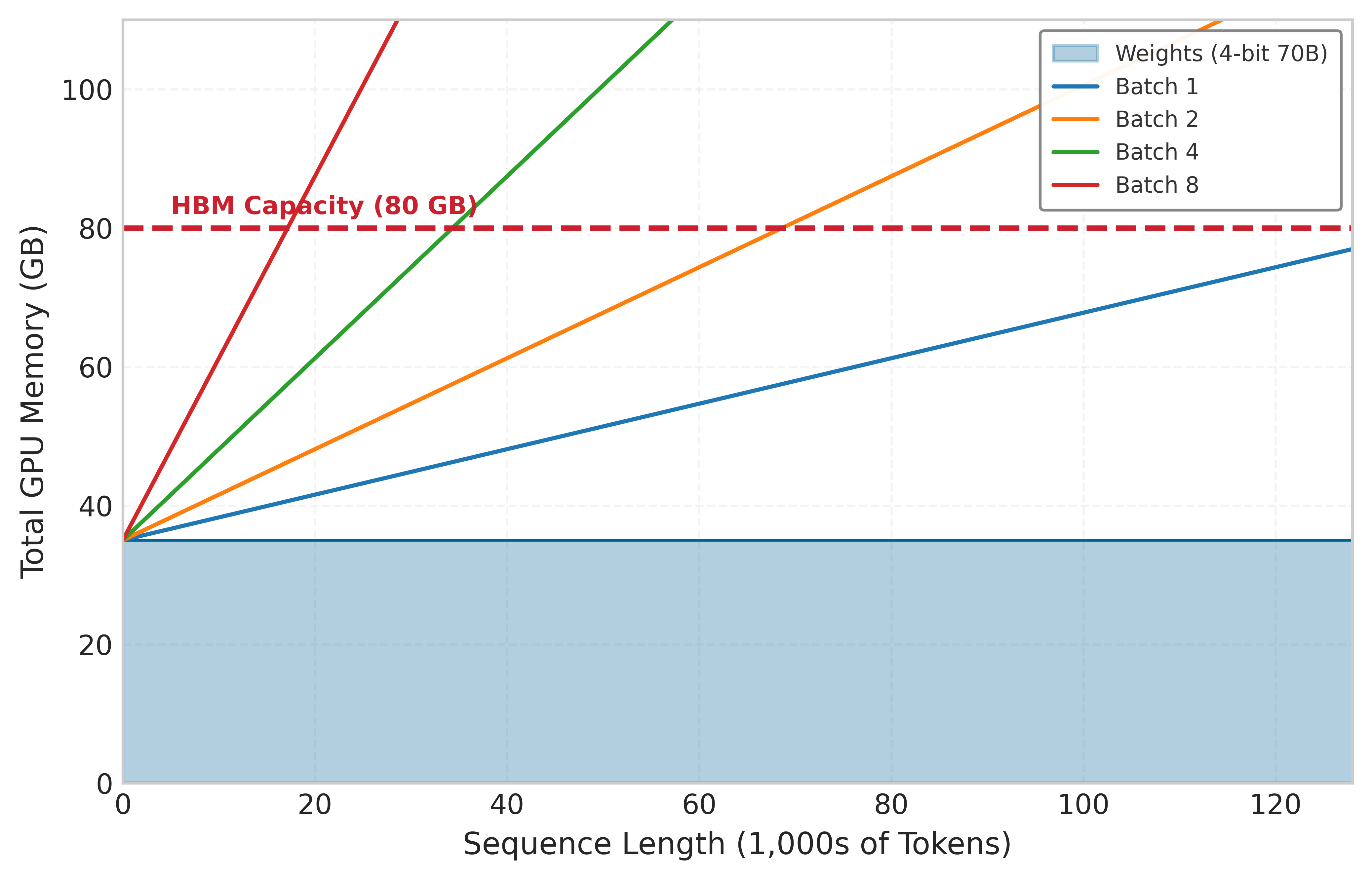
The visualization reveals why the replica level must sometimes shard models that would otherwise fit on a single GPU. Sharding provides the memory headroom needed to maintain high batch sizes for long-context requests. Without sharding, a 128K context request effectively “evicts” all other users from the GPU.

The same formula can be turned into an explicit batch-size limit for production hardware.

Example 1.6: KV-cache capacity estimator

Problem: A deployment serves Llama-3-70B (FP16 weights \(\approx\) 141.2 GB) on an 8\(\times\) H100 node (640 GB total HBM). The goal is to determine the maximum batch size for a context length of 128K tokens.

Formula: \[ M_{\text{KV}} = 2 \times N_L \times H_{\text{KV}} \times d_{\text{head}} \times s_{\text{elem}} \] \[ \text{Total Memory} = M_{\text{weights}} + (\text{Batch} \times \text{Context} \times M_{\text{KV}}) \]

Parameters:

• \(N_L = 80\), \(H_{\text{KV}} = 8\) for Llama-3-70B GQA, \(d_{\text{head}} = 128\).
• \(s_{\text{elem}} = 2\) bytes (FP16).
• Context \(= 131,072\) tokens.

Step 1: Calculate memory per token. \[ M_{\text{KV}} = 2 \times 80 \times 8 \times 128 \times 2 = 327,680 \text{ bytes} \approx 0.33 \text{ MB/token} \]

Step 2: Calculate cache per request. \[ 131,072 \text{ tokens} \times 0.33 \text{ MB/token} \approx 42.9 \text{ GB/request} \]

Step 3: Determine max batch size. Available Memory for KV = 640 GB (Total) - 141.2 GB (Weights) - 20 GB (System) = 478.8 GB. \[ \text{Max Batch} = \left\lfloor \frac{478.8}{42.9} \right\rfloor = 11 \]

Systems insight: Even with GQA, the shared-KV-head attention variant from Weight-only vs. weight-activation quantization that the 8-head count above already reflects, 128K-context requests consume tens of gigabytes of KV cache, so the system serves only a small number of concurrent long-context requests before memory becomes the binding constraint. Addressing this requires PagedAttention (to reduce fragmentation) and KV-cache quantization or sharding.

The fragmentation problem

Traditional memory allocation for KV cache preallocates contiguous memory for each sequence based on maximum expected length. This creates two forms of waste.

Internal fragmentation wastes memory within each allocation. Sequences shorter than the maximum allocation leave the unused portion idle. If maximum length is 4,096 but average output is 100 tokens, 97.5 percent of allocated memory is wasted.

External fragmentation compounds this problem across allocations. As sequences complete and new ones start, memory becomes fragmented into noncontiguous free blocks. Even with sufficient total free memory, no single block may be large enough for a new maximum-length allocation.

Consider a simplified example with 8 memory slots and maximum sequence length of 4. Fixed-size reservations first create internal fragmentation:

Time 0: Allocate Seq A (slots 0-3), Seq B (slots 4-7)
        [A][A][a][a][B][B][B][b]
        lowercase = reserved but unused

External fragmentation appears after sequences complete and new sequences start:

Time 1: Active Seq C and Seq D leave two 2-slot gaps
        [ ][ ][C][C][ ][ ][D][D]

Time 2: Try to allocate Seq E (needs 4 contiguous slots)
        [ ][ ][C][C][ ][ ][D][D]  <- Total free slots = 4, largest block = 2

Result: enough total free capacity exists, but no contiguous block is large enough.

Production systems report 60–80 percent memory waste from fragmentation under realistic workloads, severely limiting batch sizes and throughput.

PagedAttention

The fragmentation example exposes the allocator failure: enough KV-cache capacity can exist in aggregate while no contiguous block is available for the next sequence. PagedAttention fixes that serving problem by treating KV-cache storage like virtual memory rather than a single preallocated slab.

Definition 1.3: PagedAttention

PagedAttention is an LLM serving memory management technique that applies virtual memory principles to KV Cache allocation, storing attention states in noncontiguous, fixed-size physical blocks.

1. Significance: It eliminates Internal and External Fragmentation, which can waste 60–80 percent of the memory allocated to the KV cache under contiguous preallocation. By allowing sequences to grow dynamically, it enables 2–4\(\times\) higher Concurrent Throughput \((X)\) on the same hardware.
2. Distinction: Unlike Contiguous Allocation (which requires prereserving the maximum context length), PagedAttention uses a Block Table to map logical sequence indices to physical memory pages, allocating only what is currently used.
3. Common pitfall: A frequent misconception is that PagedAttention speeds up individual token math. In reality, it is a Capacity Optimization: it improves system-level efficiency by allowing larger batch sizes, though it adds a small Indirection Overhead \((L_{\text{lat}})\) for the pointer lookups.

The virtual-memory shift changes the allocation problem: capacity no longer has to be reserved as one contiguous block before the request starts.

Systems Perspective 1.1: Analogy: The inefficient hotel

Imagine a hotel where every guest might stay anywhere from 1 to 10 days, but they do not know in advance.

Under contiguous allocation, the hotel manager blocks out a 10-day suite for every guest just in case. A 100-room hotel becomes “fully booked” with only 10 guests, wasting 90 percent of its capacity (Internal Fragmentation).

Under PagedAttention (Virtual Memory), the manager assigns a guest just 1 room. If the guest stays another day, they are given whatever room is available next, even if it is on a different floor. The front desk maintains a “Block Table” to keep track of which rooms belong to which guest. The hotel can now accommodate 100 guests simultaneously, recovering the 90 percent wasted capacity.

PagedAttention (Kwon et al. 2023), introduced in vLLM, applies virtual memory concepts to KV cache management. Instead of contiguous allocation, the KV cache is divided into fixed-size pages, using 16-token blocks in the default vLLM configuration, and sequences are allocated pages on demand. Figure 9 illustrates the key concepts including page tables that map logical sequence positions to physical memory pages, block size that defines the number of tokens per page (typically 16 tokens), and physical blocks that provide fixed-size memory allocations assignable to any sequence.

Figure 9: KV Cache Fragmentation and the PagedAttention Solution: Top left: internal fragmentation wastes memory by preallocating for the maximum sequence length. Top right: external fragmentation leaves unusable memory gaps. Bottom: PagedAttention solves this by mapping contiguous logical pages of a sequence to noncontiguous physical memory blocks via a block table, allowing the system to fill fragmentation gaps with small blocks from any sequence.

PagedAttention provides four capacity benefits:

• Internal fragmentation: It allocates only the pages needed for actual tokens.
• External fragmentation: Any free page can be used by any sequence.
• Dynamic growth: Sequences can grow without preallocation.
• Prefix sharing: Common prefixes can share physical pages.

Together, these properties turn KV cache capacity into a schedulable resource rather than a fixed per-request reservation.

Example 1.7: PagedAttention implementation details

Memory layout:

Physical blocks (16 tokens by hidden_dim by 2 by precision):
Block 0:  [K₀...K₁₅, V₀...V₁₅]
Block 1:  [K₀...K₁₅, V₀...V₁₅]
...
Block N:  [K₀...K₁₅, V₀...V₁₅]

Page table per sequence:

class PageTable:
    def __init__(self, max_blocks):
        self.block_map = {}  # logical_block -> physical_block

    def allocate_block(self, logical_idx, physical_block):
        self.block_map[logical_idx] = physical_block

    def get_physical(self, logical_idx):
        return self.block_map[logical_idx]

Attention kernel modification:

Standard attention: output = softmax(Q @ K.T/sqrt(d)) @ V

PagedAttention:

def paged_attention(Q, page_table, physical_blocks, block_size):
    # Gather K, V from noncontiguous physical blocks
    for logical_idx in range(num_logical_blocks):
        physical_idx = page_table[logical_idx]
        K_block = physical_blocks[physical_idx].K
        V_block = physical_blocks[physical_idx].V
        # Compute attention for this block
        attention_scores = Q @ K_block.T / sqrt(d)
        output += softmax(attention_scores) @ V_block
    return output

Systems insight: The throughput impact of gather operations is small compared to the memory savings; table 17 shows the 2.5–4\(\times\) throughput improvement coming from fitting more concurrent sequences in the same memory.

Table 17: PagedAttention vs. Contiguous KV Cache: KV cache pool utilization and relative serving throughput for contiguous allocation against PagedAttention.

Approach	KV Cache Pool Utilization	Throughput (relative)
Contiguous	30-40%	1.0\(\times\) (baseline)
PagedAttention	95%+	2.5–4\(\times\)

Prefix caching

Many LLM workloads share common prefixes across requests. System prompts like “You are a helpful assistant…” are prepended to every request. Few-shot examples use the same examples for many queries. Document context involves multiple questions about the same document. Recomputing these shared prefixes wastes both compute (prefill) and memory (duplicate KV cache entries).

Prefix caching shares KV cache entries across requests with common prefixes. Figure 10 demonstrates how shared system prompts avoid redundant computation.

Figure 10: Prefix Caching via Block Sharing: PagedAttention enables efficient prefix caching by allowing multiple sequences’ block tables to point to the same physical blocks for shared content. In this example, the System Prompt is stored in blocks 0-5. Request A and Request B maps their first 6 logical pages to these same physical blocks, storing only their unique suffixes in new blocks. This dramatically reduces memory usage and prefill computation for workloads with shared context.

With PagedAttention, prefix caching integrates naturally through copy-on-write semantics:

System prompt → Physical blocks [0, 1, 2, 3, 4, 5]

Request A page table: [0, 1, 2, 3, 4, 5, 10, 11]  <- shares prefix blocks
Request B page table: [0, 1, 2, 3, 4, 5, 12, 13, 14]  <- shares prefix blocks
Request C page table: [0, 1, 2, 3, 4, 5, 15]  <- shares prefix blocks

All three requests reference the same physical blocks for the system prompt. Only when generating unique tokens do they allocate new blocks. The savings can be substantial when many concurrent requests share the same system prompt; the following example quantifies them for a typical chatbot deployment.

Example 1.8: Prefix caching at scale

Scenario: A chatbot service uses a 2,000-token system prompt and serves 1,000 concurrent users.

Without prefix caching:

• KV cache per user: \(2000 + 500\text{ (avg response)} =\) 2,500 tokens
• Total KV cache: 2,500 tokens \(\times 1000 \times 2 \times 80 \times 8192 \times 2 =\) 6.6 TB

With prefix caching:

• Shared prefix: 2,000 tokens (once)
• Unique per user: 500 tokens
• Total: \((2000 \times 1) + (500 \times 1000) =\) 502,000
• Memory: 502,000 \(\times 2 \times 80 \times 8192 \times 2 =\) 1.3 TB

Result: Prefix caching yields a 79.9 percent memory reduction in KV cache, enabling 5× more concurrent users.

Systems insight: Prefix caching pays off when the prefix hit rate is high because many requests share a long prefix. Table 18 contrasts hit rates and memory savings across workloads, showing where the technique changes serving capacity and where it does not.

Table 18: Prefix Caching Effectiveness by Workload: Typical prefix hit rates and resulting KV-cache memory savings for chatbot, document-QA, and general API workloads, showing where prefix caching pays off and where it does not.

Workload	Prefix Hit Rate	Memory Savings
Chatbot (same system prompt)	95%+	70-80%
Document QA (same doc)	80-90%	50-70%
General API (diverse)	20–40%	10–30%

KV cache compression and architectural optimization

The capacity techniques above tolerate the cache; compression shrinks it. The calculation here uses a 64-KV-head multi-head attention baseline so the grouped query attention subsection can isolate the head-count reduction as a separate architectural lever. For a 70B parameter model with 80 layers, 64 heads, head dimension 128, and sequence length 4096 in FP16, the KV cache requires:

\[ \text{KV cache} = 2 \times 80 \times 64 \times 128 \times 4096 \times 2 \approx 10.7 \text{ GB (FP16)} \]

A single request’s KV cache alone consumes a substantial fraction of the H100’s 80 GB of HBM. For a batch of 8 concurrent requests, the KV cache would require 85.9 GB, exceeding single-GPU capacity. Reducing this footprint requires two complementary strategies: quantization and architectural optimization.

KV cache quantization

Reducing the size of cached values through lower precision provides direct memory savings. Weight-only quantization (GPTQ, AWQ) reduces weight precision while keeping activations in high precision. While effective for storage, this does not reduce the KV cache. KV cache quantization explicitly targets the activations, storing cached keys and values in INT8, FP8, or even INT4.

Compressing the KV cache to INT4 reduces it to approximately 2.7 GB per request, a 4× reduction. This freed memory directly translates into larger batch sizes and higher serving throughput. KV cache values exhibit different distributions than model weights: KIVI observes channel-wise outliers in keys and uses per-channel key quantization, while values lack the same channel-wise pattern and are quantized per-token.

Grouped query attention (GQA)

Grouped query attention (Ainslie et al. 2023), the shared-KV-head architecture established in Weight-only vs. weight-activation quantization, is the second lever on cache size, complementary to quantization: where quantization shrinks the bytes per cached element, GQA shrinks how many key-value heads are cached per layer. The serving consequence is the head-count arithmetic. For our earlier 70B model, switching from the multi-head attention (MHA) baseline of 64 KV heads to GQA with 8 KV heads shrinks the KV cache by 8\(\times\):

Ainslie, Joshua, James Lee-Thorp, Michiel de Jong, Yury Zemlyanskiy, Federico Lebron, and Sumit Sanghai. 2023. “GQA: Training Generalized Multi-Query Transformer Models from Multi-Head Checkpoints.” Proceedings of the 2023 Conference on Empirical Methods in Natural Language Processing, 4895–901. https://doi.org/10.18653/v1/2023.emnlp-main.298.

\[ \text{KV cache (GQA)} = 2 \times 80 \times 8 \times 128 \times 4096 \times 2 \approx 1.3 \text{ GB (FP16)} \]

At 1.3 GB, the GQA cache is dramatically more manageable than the 10.7 GB required by MHA. Combining GQA with INT8 KV cache quantization yields sub-gigabyte per-request cache sizes, often enabling substantially larger batches on a single GPU. GQA has become a common architectural choice for inference-optimized LLMs because it reduces KV-cache bandwidth and capacity pressure with comparatively small quality impact in many deployments.

Napkin Math 1.5: The precision dividend

Problem: A team serves a 70B model on 4\(\times\) H100 GPUs. Weights in FP16 consume 140 GB (35 GB/GPU). KV cache at FP16 consumes 10.7 GB per request. How does quantizing weights to INT4 and KV cache to INT8 change the maximum batch size?

Before optimization (all FP16):

• Weights: 35 GB/GPU
• Available for KV cache: 80 GB \(-\) 35 GB = 45 GB/GPU
• KV cache per request: 10.7 GB \(\div\) 4 \(\approx\) 2.7 GB/GPU
• Maximum batch size: \(\lfloor\) 45 GB divided by 2.7 GB \(\rfloor\) \(\approx\) 16 requests

After optimization (INT4 weights, INT8 KV cache):

• Weights: 35 GB \(\times (4/16) =\) 8.75 GB/GPU (INT4)
• Available for KV cache: 80 GB \(-\) 8.75 GB = 71.25 GB/GPU
• KV cache per request (INT8): 5.4 GB \(\div\) 4 \(\approx\) 1.3 GB/GPU
• Maximum batch size: \(\lfloor\) 71.25 GB divided by 1.3 GB \(\rfloor\) \(\approx\) 53 requests

Systems insight: Precision engineering fundamentally changes serving economics by enabling larger batch sizes. Larger batches amortize the fixed cost of weight loading, shifting operations from memory-bound toward compute-bound.

Speculative decoding as a serving policy

Speculative decoding established speculative decoding as an algorithmic optimization: a small draft model proposes \(K\) tokens, the target model verifies them in one parallel forward pass, and rejection sampling guarantees the emitted tokens follow the target model’s distribution exactly, so the technique is lossless and bounded by the draft acceptance rate \(\alpha_{\text{acc}}\). The serving question is different. Speculation becomes a resource-admission policy under SLA pressure: the scheduler must decide when to enable it, how its memory cost interacts with KV-cache admission, and what it does to the SLA the endpoint is bound by.

Decode is memory-bound; parallel verification moves work toward the ridge.

The latency win is real but conditional, and the condition is the acceptance rate. The expected number of tokens emitted per round, including the correction token, is \(\frac{1 - \alpha_{\text{acc}}^{K+1}}{1 - \alpha_{\text{acc}}}\), which collapses toward 1 as acceptance falls. For \(K = 5\) draft tokens and a draft model 20\(\times\) faster than the target, that sensitivity is steep:

• High acceptance \((\alpha_{\text{acc}} = 0.9)\): Expected 4.69 tokens per round, speedup of 3.7×.
• Medium acceptance \((\alpha_{\text{acc}} = 0.7)\): Expected 2.94 tokens per round, speedup of 2.4×.
• Low acceptance \((\alpha_{\text{acc}} = 0.5)\): Expected 1.97 tokens per round, speedup of 1.6×.

Predictable text achieves \(\alpha_{\text{acc}} > 0.9\), while creative reasoning or code generation may fall below 0.5; well-aligned model pairs that share training data and architecture commonly land at 0.6–0.8. Because acceptance is a property of the workload, not of the hardware, a single global setting is wrong for a mixed fleet: the same speculation that halves time per token on a chat endpoint can slow a code-generation endpoint that sits below the break-even acceptance rate. The serving system must therefore decide per endpoint, and three serving concerns govern that decision.

The speculation tax and KV-cache admission

The first concern is memory. The draft model is not free state: it requires its own GPU allocation for weights, and each in-flight request that uses speculation reserves a small additional KV cache for the draft model alongside the target’s. Pairing a 7B draft model with a 70B target adds roughly 14 GB of weights per replica plus per-request draft cache. This speculation tax competes directly with the KV-cache admission budget developed in section 1.3.1: every gigabyte the draft model holds is a gigabyte the admission controller cannot allocate to a concurrent request. Speculation therefore shrinks the maximum batch size the node can admit, trading aggregate throughput for the latency of individual requests. The admission controller and the speculation policy cannot be tuned independently; enabling speculation lowers the concurrency ceiling that the KV-cache wall already imposes.

The latency-throughput tension under an SLA

The second concern is which service-level objective the endpoint is bound by. Speculation improves time per output token but, by lowering the concurrency ceiling, reduces the requests per second a replica can sustain. An endpoint with a tight time-to-first-token or per-token latency SLA, such as interactive chat, benefits: the speculation tax buys headroom against the latency target that matters. An endpoint bound by a throughput SLA, such as bulk document processing or batch summarization, is harmed: speculation spends batch capacity to improve a latency metric no one is measuring, and the lost concurrency directly threatens the throughput target. The decision is therefore an SLA question. The scheduler enables speculation on latency-bound endpoints and disables it on throughput-bound ones, and on a shared replica serving both it must account for the draft model’s resident cost against the stricter of the two budgets.

Per-endpoint scheduling

The third concern is that these decisions are dynamic, not static configuration. Acceptance rate drifts with the traffic mix, and the value of speculation collapses at high load: when a replica is already near its concurrency ceiling, the decode phase is closer to compute-bound and the marginal latency benefit of speculation shrinks even as its memory tax stays fixed. Production schedulers therefore treat speculation as a runtime knob gated on observed load and acceptance. They enable it for latency-sensitive endpoints during normal operation, disable it under traffic spikes to reclaim KV-cache pages for admission, and may switch draft strategies per endpoint. Self-speculative decoding uses early exit from the target model itself as the draft, eliminating the separate-model memory tax at the cost of lower acceptance; Medusa (Cai et al. 2024) adds lightweight prediction heads to the target backbone; Lookahead decoding uses Jacobi iteration to avoid a draft model entirely. Each variant trades a different slice of the speculation tax against acceptance, and the scheduler chooses among them per endpoint based on which SLA binds and how much KV-cache budget remains.

Cai, Tianle, Yuhong Li, Zhengyang Geng, Hongwu Peng, Jason D. Lee, Deming Chen, and Tri Dao. 2024. “Medusa: Simple LLM Inference Acceleration Framework with Multiple Decoding Heads.” Proceedings of the 41st International Conference on Machine Learning (ICML).

KV cache in distributed settings

When a conversation is moved, rebalanced, or split across devices, its KV state must either move with it or be rebuilt token by token. Section 1.4 develops the tensor and pipeline parallelism strategies that distribute a model across devices; each strategy carries a different consequence for KV-cache management:

Under tensor parallelism, the KV cache is sharded across devices along with attention heads. Each device stores cache for its subset of heads.

8-way tensor parallelism:
Device 0: KV cache for heads 0-7
Device 1: KV cache for heads 8-15
...
Device 7: KV cache for heads 56-63

Cross-device sharing adds a constraint: prefix caching across tensor-parallel devices requires cache to be sharded identically on all devices. This is automatic when prefixes are processed with the same tensor-parallel configuration.

KV cache migration presents a further challenge. When the router moves a conversation to a different replica because of failure or rebalancing (routing keyed on a hash of the session ID, the consistent-hashing scheme developed in section 1.5.6), the KV cache must be migrated:

Migration options:
1. Rebuild: Re-run prefill on new replica (500 ms+ for long context)
2. Transfer: Send KV cache over network (100 MB at 100Gbps = 8 ms)
3. Hybrid: Transfer if small, rebuild if large

Decision threshold:
if cache_size_bytes/network_bandwidth < prefill_time:
    transfer()
else:
    rebuild()

For Llama-70B GQA with 4K context, KV cache is about 1.3 GB total per sequence, or about 168 MB per device under 8-way tensor parallelism. At 100 Gbps (12.5 GB/s), transferring one shard takes roughly 13 ms, while transferring the full cache would take about 100 ms. Both are often preferable to a ~500 ms prefill rebuild, so transfer remains the better choice when bandwidth is available.

Memory management best practices

Effective KV-cache management begins with capacity accounting rather than an eviction policy. The serving process first reserves memory for weights, activations, runtime overhead, and safety headroom, then treats the remaining HBM as a managed pool for active sequences:

Available GPU memory = Total - Weights - Activations - Overhead
KV pool size = 0.9 * Available  # Leave 10% headroom

Max concurrent sequences = KV pool size / (avg_seq_length * per_token_cache)

That budget determines how many sequences can coexist before the scheduler must choose between rejection, preemption, or paging. When the cache is full, LRU eviction removes the sequence with the oldest access, size-based eviction frees the longest sequence first, and priority-based eviction protects paid-tier or latency-critical requests. Continuous batching then turns eviction into a scheduling decision: a high-priority request that cannot fit triggers victim selection, swaps the victim’s KV cache to CPU memory, allocates GPU memory to the new request, and restores the victim later if its service-level objective still permits the delay.

Example 1.9: KV cache memory hierarchy

Production systems manage KV-cache memory pressure across the three-tier hierarchy in table 19, paging from GPU HBM down to CPU DRAM and NVMe SSD as the active working set exceeds each tier’s capacity:

Table 19: KV cache memory hierarchy: Capacity, swap-in latency, and intended use case for the three tiers production inference servers use to manage KV-cache memory pressure.

Tier	Capacity	Latency	Use Case
GPU HBM	80 GB	0 ms	Active sequences
CPU DRAM	1 TB	1–5 ms	Swapped sequences
NVMe SSD	10 TB	10–50 ms	Long-term cache

Swap implementation:

async def swap_to_cpu(sequence_id):
    kv_cache = gpu_cache[sequence_id]
    cpu_cache[sequence_id] = kv_cache.cpu()  # Async transfer
    gpu_cache.free(sequence_id)


async def swap_to_gpu(sequence_id):
    cpu_kv = cpu_cache[sequence_id]
    gpu_cache[sequence_id] = cpu_kv.cuda()  # Async transfer
    cpu_cache.free(sequence_id)

Observed performance:

• GPU-only (no swapping): 50 concurrent sequences
• GPU+CPU swapping: 500 concurrent sequences (10\(\times\))
• Average swap latency: 3 ms (acceptable for nonurgent requests)

Systems insight: Treating CPU DRAM and NVMe as overflow tiers behind HBM raises concurrency by an order of magnitude at the cost of millisecond swap latency, so paging is a throughput lever for non-urgent traffic but not a substitute for HBM capacity on the latency-critical path.

The mismatch swapping papers over remains structural: a single GPU must handle both the compute-heavy prompt processing and the bandwidth-heavy token generation. Separating those phases onto different hardware pools eliminates this mismatch entirely.

Disaggregated serving: Splitting the workload

LLM inference consists of two distinct phases with different computational characteristics, requiring different batching strategies within the same request. Figure 11 illustrates how this architectural split separates the two phases onto dedicated hardware pools, and table 20 contrasts their resource profiles.

Figure 11: Disaggregated Serving Architecture: Separating the compute-bound prefill phase from the bandwidth-bound decode phase. Requests enter the Prefill Pool for prompt processing, and the resulting KV cache is migrated to the Decode Pool for token generation. This allows each phase to run on hardware optimized for its specific bottleneck, improving overall fleet efficiency.

Definition 1.4: Prefill and decode phases

Prefill and Decode Phases are the two distinct computational regimes of transformer-based LLM inference.

1. Significance: The Prefill Phase (processing the prompt) is compute bound \((R_{\text{peak}})\) with high arithmetic intensity, while the Decode Phase (generating tokens) is bandwidth bound \((\text{BW})\) with extremely low arithmetic intensity. This mismatch means a single request’s efficiency \((\eta_{\text{hw}})\) varies wildly during its lifecycle.
2. Distinction: Unlike Single-Pass Inference (for example, ImageNet), where the resource bottleneck is constant, LLM inference switches between these regimes at every request, requiring Iteration-Level Scheduling to maintain utilization.
3. Common pitfall: A frequent misconception is that both phases should be batched together naively. In reality, because they have opposing hardware requirements, mixing them in the same batch without Chunked Prefill or similar techniques can lead to significant queuing delays \((L_{\text{lat}})\) for decoding tokens.

The prefill phase processes the entire input prompt in parallel. Computation scales with prompt length, and the memory access pattern is compute-bound with high arithmetic intensity⁹.

⁹ Arithmetic Intensity (Prefill vs. Decode): Measured in FLOP/byte of memory accessed, this ratio determines whether a workload is compute-bound or bandwidth-bound. Prefill achieves 100+ FLOP/byte (compute-bound); decode achieves 1–10 FLOP/byte (bandwidth-bound). This 10–100\(\times\) gap is why mixing the two phases in a single batch wastes either compute or bandwidth, motivating disaggregated serving architectures.

The decode phase, by contrast, generates output tokens one at a time. Each token requires loading the entire model weights, making the memory access pattern bandwidth-bound with low arithmetic intensity. The single-accelerator roofline places these two phases on the roofline: decode sits far below the ridge point of equation, where throughput is set by HBM bandwidth rather than peak FLOP/s, while prefill’s high arithmetic intensity (equation) pushes it past the ridge into the compute-bound regime.

Table 20: Prefill vs. Decode Characteristics: The two phases have opposite optimization requirements.

Phase	Computation	Memory Access	Bottleneck	Optimal Batch
Prefill	\(\mathcal{O}(\text{prompt length}^2)\)	Activation and attention tiles	Compute	Moderate request batches or large chunks
Decode	\(\mathcal{O}(1)\) dense weight work plus \(\mathcal{O}(\text{context length})\) attention over KV cache per token	Weight and KV-cache reads	Bandwidth	Large continuous batches of active tokens

Because decode is bandwidth-bound, hardware that shrinks the bytes moved per token attacks that phase’s binding constraint directly.

Systems Perspective 1.2: FP4 as a bandwidth lever for decode

The durable point is that decode is bandwidth-bound, so any technique that shrinks the bytes moved per token attacks the binding constraint; native hardware support for narrow formats is the current manifestation of that lever. The Blackwell (B200) architecture introduces native FP4 support, making 4-bit inference a first-class hardware target rather than a framework-specific workaround. Halving weight and KV-cache bytes relative to FP8 raises token throughput and concurrent-sequence capacity without increasing clock speed, which is what loosens the decode-pool sizing in a disaggregated deployment. The product is point-in-time, and the exact cost-per-token gain depends on model architecture, kernel maturity, batch shape, and the fraction of time spent in prefill versus decode, so production systems should validate FP4 with workload-specific benchmarks rather than assuming a fixed multiplier.

The dichotomy creates a scheduling challenge: prefill operations are long-running and compute-intensive, while decode operations are short and bandwidth-limited. Mixing them in the same batch can cause interference. The GPU remains powered and allocated even when decode steps expose little useful compute, so low-utilization decode traffic can dominate energy cost unless the scheduler keeps the hardware busy with compatible work.

Chunked prefill¹⁰ addresses this by breaking long prompts into fixed-size chunks that interleave with decode operations:

¹⁰ Chunked Prefill: Without chunking, a long prompt can block decode while prefill completes, violating inter-token latency SLOs for concurrent users. Chunking divides the prompt into smaller work units processed between decode iterations, bounding decode stalls at the cost of slightly longer total prefill time. The trade-off is a classic latency-vs.-throughput decision: interactive applications favor smaller chunks; batch workloads can favor larger ones.

\[\text{Chunk latency} = \frac{\text{Chunk size}}{\text{Prefill throughput}}\]

With chunk size chosen to match decode iteration time, prefill and decode can share GPU resources without decode latency spikes.

Prefill-decode disaggregation takes this separation further by running prefill and decode on separate GPU pools. The prefill pool is optimized for compute intensity, using nodes with high TFLOP/s, moderate request batches, or large token chunks to maximize throughput without blocking decode. The decode pool is optimized for memory bandwidth, using nodes with maximum HBM capacity, the Tier 0 storage resource discussed in Tier 0: GPU HBM, to handle thousands of concurrent autoregressive streams.

Independent scaling follows directly: prefill capacity scales with input volume while decode capacity scales with output volume. Crucially, this architecture relies on the high-speed, RDMA-enabled networking fabric established in Network Fabrics. When a prefill finishes, the resulting KV cache (often megabytes of data) must be migrated to a decode node within the inter-token latency budget, typically under 10 ms. InfiniBand’s low-microsecond latency and high bisection bandwidth are the physical enablers of this logical disaggregation, a displacement of overhead that trades communication bandwidth for specialized prefill and decode hardware.

The Sarathi-Serve system formalizes chunked prefill into a practical scheduling algorithm that limits decode stalls from long prompts.

Example 1.10: Sarathi: Chunked prefill implementation

The Sarathi-Serve system (Agrawal et al. 2024) implements chunked prefills with stall-free scheduling:

Chunk sizing: Chunks are sized so prefill work can be interleaved with decode iterations. For example, if a deployment targets a 20 ms scheduling quantum and observes 10,000 prefill tokens/second, one chunk would process about 200 tokens. The right chunk size is workload- and hardware-dependent.

Interleaving schedule: Each GPU iteration processes either:

• One prefill chunk for a new request, OR
• One decode step for all active sequences

The schedule reduces decode stalls caused by long incoming prompts.

KV-cache handoff: When a prefill chunk completes, the scheduler has enough KV state to continue the request through later decode work. In disaggregated prefill/decode systems, any physical KV-cache transfer is a separate networking and placement budget rather than a guarantee supplied by Sarathi-Serve itself.

Performance impact:

• Without chunking: long prompts can create decode latency spikes for other active requests.
• With chunking: prefill work is broken into bounded units, so decode iterations can continue to make progress while long prompts enter the system.

Systems insight: Chunked prefill turns a long prompt from one blocking request into bounded work units that can coexist with decode traffic.

Agrawal, Amey, Nitin Kedia, Ashish Panwar, Jayashree Mohan, Nipun Kwatra, Bhargav S. Gulavani, Alexey Tumanov, and Ramachandran Ramjee. 2024. “Taming Throughput-Latency Tradeoff in LLM Inference with Sarathi-Serve.” 18th USENIX Symposium on Operating Systems Design and Implementation (OSDI 24), 117–34.

Adapter state and locality

KV-cache management makes one GPU safe for many concurrent requests; multi-tenant adapter serving asks the same serving process to manage another kind of resident state. The KV cache is per-token attention state. A LoRA adapter is per-tenant weight delta. Both must be available at the moment a decode step runs, and both can erase batching gains if the scheduler ignores locality. As serving platforms scale to support thousands of concurrent users on a single foundation model, personalization introduces a new memory bottleneck. Low-Rank Adaptation (LoRA) stores a small set of user- or task-specific adapter weights that modify a shared base model without copying the full model. When 10,000 users each have a unique LoRA adapter applied to the same 140 GB base model, replicating the base weights for each user is physically impossible. Instead, the base model remains pinned in HBM, while user-specific adapters are brought into the fast on-chip working set as needed.

Systems Perspective 1.3: The context switch of machine learning

This multi-tenant serving pattern shifts the fundamental performance constraint from compute throughput to adapter locality. As the continuous batching scheduler interleaves requests from different users, adapter weights may have to move repeatedly from HBM into SRAM or registers before each generation step. The effect is similar to an operating-system context switch: the accelerator has work to do, but it first waits for the state belonging to the next tenant. If the adapter swap latency exceeds the compute time of the generation step, the GPU compute cores stall. Efficient multi-tenancy therefore batches requests by active adapter when possible and coordinates adapter placement with KV-cache paging so personalization does not erase the benefit of sharing the base model.

The same locality problem reappears at a larger scale when the model itself exceeds single-GPU capacity. For a 175-billion-parameter foundation model, even the weights must be split across multiple devices, so inference becomes a sharding problem before it becomes a scheduling problem.

Self-Check: Question

1. A 13B model’s FP16 weights occupy 26 GB on an 80 GB H100, leaving 54 GB for KV cache and activations. With a grouped-query-attention configuration of 40 layers, 8 KV heads, head dimension 128, FP16 KV elements, 64 concurrent requests, and 8K context, the KV cache consumes roughly 86 GB. What does this arithmetic reveal about the operating bottleneck?

   1. KV cache grows linearly in sequence length and batch size, so even when weights fit the serving capacity hits a memory wall driven by decode concurrency, not by the weights themselves
   2. KV cache eliminates the need to reload model weights each step, so decode becomes compute-bound rather than memory-bound
   3. KV cache lives on CPU memory and transfers back over PCIe per token, so the constraint is host-device bandwidth rather than HBM capacity
   4. KV cache affects only the prefill phase and has no consequence for decode throughput or sustainable concurrency

2. A baseline serving system pre-allocates one contiguous KV-cache region per request at the model’s 4,096-token maximum. Under a realistic workload where most requests finish in 200-500 tokens, what mechanism allows PagedAttention to roughly 2–4\(\times\) concurrent request capacity?

   1. It reduces the arithmetic FLOPs of attention itself, so each token’s compute cost falls and more tokens fit in the time budget
   2. It lets the system skip batching entirely and process every request independently on its own dedicated page
   3. It maps logical sequence positions to fixed-size physical blocks allocated on demand, eliminating internal fragmentation (partially filled pre-allocations) and external fragmentation (unusable gaps between contiguous reservations), which recovers the 60-80 percent memory waste inherent in pre-allocation
   4. It moves all sequence state to host memory via zero-copy transfer, so GPU memory no longer limits concurrent batch size

3. A production chatbot uses a 2,000-token shared system prompt across 10,000 concurrent conversations. Apply prefix caching to quantify the compute and memory savings, and explain the time-to-first-token (TTFT) consequence.

4. True or False: Deploying speculative decoding with a draft model guarantees lower serving latency because verifying K draft tokens in one target-model pass strictly dominates K separate decode steps.

5. Order the stages of one speculative decoding step: (1) Target model accepts or rejects each draft token based on the verification probabilities, (2) The draft model proposes K future tokens autoregressively, (3) The target model computes verification probabilities for all K draft tokens in a single parallel pass.

6. Why does disaggregated serving deploy prefill and decode phases on separately optimized hardware pools rather than running both on the same GPUs?

   1. Prefill and decode share the same bottleneck profile, so splitting them only improves software modularity and operational boundaries
   2. Prefill is compute-bound on large matrix multiplications while decode is memory-bandwidth-bound on weight streaming, so matching each phase to hardware optimized for its bottleneck lets both operate near their roofline instead of sharing a compromise operating point
   3. Decode no longer needs the KV cache after prefill completes, so state can be discarded at the phase boundary and each pool runs stateless
   4. Splitting the phases avoids any need to transfer KV-cache state between machines because it is regenerated from scratch at each phase

See Answers →

Model Sharding for Inference

A 70-billion-parameter model requires over 140 GB of VRAM to hold its weights in FP16, exceeding a single 80 GB GPU’s capacity. To serve this model, we must slice its architecture across multiple GPUs that act together as a single logical replica. Adapting distributed training parallelism techniques, specifically tensor and pipeline parallelism, for low-latency inference introduces a distinct set of constraints.

When sharding becomes necessary

Model sharding for inference is driven by two distinct requirements. Table 21 identifies the memory and latency constraints that necessitate sharding:

The first driver is memory capacity. A model that cannot fit in single-GPU memory must be sharded regardless of performance considerations. For a model with \(P\) parameters at precision \(b\) bits, the weight memory is calculated by equation 6:

\[\text{Memory}_{\text{weights}} = P \times \frac{b}{8} \text{ bytes} \tag{6}\]

A 70-billion-parameter model in FP16 (16 bits) requires:

\[\text{Memory} = 70 \times 10^9 \times \frac{16}{8} = 140 \text{ GB}\]

The result exceeds the 80 GB capacity of an H100 GPU, requiring at minimum 2-way sharding.

The second driver is latency. Even when a model fits in memory, sharding can reduce latency by parallelizing computation. Equation 7 formalizes the potential speedup as a function of parallelization efficiency:

\[T_{\text{parallel}} = \frac{T_{\text{compute}}}{N} + T_{\text{comm}}(N) + T_{\text{sync}}(N) - T_{\text{overlap}} \tag{7}\]

where \(N\) is the number of devices in the sharding group, \(T_{\text{comm}}(N)\) is the communication overhead, \(T_{\text{sync}}(N)\) is synchronization overhead, and \(T_{\text{overlap}}\) is communication hidden behind useful compute. In the common no-overlap simplification with negligible extra synchronization, this reduces to \(T_{\text{compute}}/N + T_{\text{comm}}(N)\). Sharding provides latency benefit only when the nonoverlapped overhead is smaller than the time saved through parallelization.

Table 21: Sharding Triggers: Different constraints lead to different sharding requirements and strategies.

Sharding Trigger	Model Examples	Minimum Sharding	Strategy
Memory (weights)	Llama-70B (140 GB)	2-way	Tensor or pipeline
Memory (KV cache)	GPT-4 (long context)	4–8 way	Tensor (for cache)
Memory (embeddings)	DLRM (100 TB)	1000+ way	Embedding sharding
Latency	Any large model	Varies	Tensor parallelism

Tensor parallelism

Tensor parallelism (Shoeybi et al. 2019) distributes individual layers across multiple devices, enabling parallel computation within each layer. The column-row partitioning scheme introduced for training in Distributed Training applies here: splitting the first linear layer by columns and the second by rows requires only one AllReduce per transformer block. For transformer models, the primary target is the attention mechanism and feed-forward layers, which contain the majority of computation.

Shoeybi, Mohammad, Mostofa Patwary, Raul Puri, Patrick LeGresley, Jared Casper, and Bryan Catanzaro. 2019. “Megatron-LM: Training Multi-Billion Parameter Language Models Using Model Parallelism.” arXiv Preprint arXiv:1909.08053.

The multi-head attention computation naturally partitions across attention heads. For a model with \(N_{\text{heads}}\) attention heads distributed across tensor-parallel degree \(t\), each device computes \(N_{\text{heads}}/t\) heads:

\[\text{Attention}_i = \text{softmax}\left(\frac{Q_i K_i^T}{\sqrt{d_k}}\right) V_i \text{ for heads } i \in \{1, ..., N_{\text{heads}}/t\}\]

After computing local attention, an AllReduce operation (covered in Collective Communication) combines results across devices, adding communication overhead proportional to the activation size divided by the interconnect bandwidth.

The feed-forward layer (typically two linear transformations with activation) partitions along the hidden dimension. For the first linear layer, columns are distributed; for the second, rows are distributed. This column-row partitioning requires only one all-reduce per feed-forward block.

The communication pattern for tensor-parallel inference follows a two-phase synchronization per layer. Figure 12 illustrates this flow:

Figure 12: Tensor Parallelism for Inference: Computation is distributed across devices by splitting tensor operations. Attention heads are partitioned across GPUs, requiring an AllReduce operation to synchronize results. Feed-forward networks use a column-row splitting strategy that requires only one AllReduce synchronization per block. This approach reduces latency for large models but introduces communication overhead that demands high-bandwidth interconnects like NVLink.

The inference time with tensor parallelism follows equation 8:

\[T_{\text{inference}} = \frac{T_{\text{compute}}}{t} + 2 \times T_{\text{allreduce}}\left(\frac{A}{t}\right) \tag{8}\]

where \(T_{\text{compute}}\) is the sequential compute time, \(t\) is the tensor-parallel degree, and \(A\) is the activation size being reduced. The factor of 2 accounts for the two all-reduce operations per transformer layer (attention and feed-forward).

Example 1.11: Tensor parallelism for Llama-70B

Consider serving Llama-70B with the following configuration: (Touvron et al. 2023)

Model specifications:

• Parameters: 70B
• Hidden dimension: 8,192
• Attention heads: 64
• Layers: 80

Memory per GPU (weight only, FP16):

\(\text{Memory}_{\text{70B}} = 70 \times 10^9 \times 2 = 140\text{ GB}\)

Minimum sharding: 2-way (140 GB/80 GB per H100)

Recommended sharding: 8-way for optimal latency

Table 22 decomposes the per-layer cost of 8-way tensor parallelism on 8\(\times\) H100 (NVLink interconnect) into compute and AllReduce phases, exposing the realized 6.9\(\times\) speedup as compute scaling minus a small communication tax.

Table 22: 8-Way Tensor Parallelism Per-Layer Breakdown: Sequential vs. 8-way tensor-parallel timings for attention, feed-forward, and AllReduce phases of one Llama-70B transformer layer, decomposing the realized 6.9\(\times\) speedup into compute scaling and communication tax.

Component	Sequential (1 GPU)	8-way TP	Speedup
Attention compute	12 ms	1.5 ms	8×
AllReduce (attention)	0 ms	0.3 ms	N/A
Feed-forward compute	18 ms	2.25 ms	8×
AllReduce (FF)	0 ms	0.3 ms	N/A
Total per layer	30 ms	4.35 ms	6.9×

Layer-stack estimate (80 layers on the same prefill workload):

• Sequential: 2,400 ms for the full prefill pass
• 8-way TP: 348 ms for the full prefill pass

The 6.9× speedup (vs. theoretical 8×) reflects communication overhead. At 900 GB/s, moving a 8 MB activation payload would take only about 0.01 ms by raw bandwidth math; the 0.3 ms budget shown here includes collective launch, synchronization, ring protocol, and framework overheads.

Time-to-first-token (1024-token prompt):

• Prefill compute: ~348 ms on 8-way TP (compute-bound, near-linear scaling minus communication overhead)
• Total TTFT: ~400 ms with preprocessing and serving overhead

Systems insight: Tensor parallelism buys latency by spending communication. It works for Llama-70B only because the interconnect keeps the collective tax small relative to the compute saved by sharding.

Touvron, Hugo, Louis Martin, Kevin Stone, Peter Albert, Amjad Almahairi, Yasmine Babaei, Nikolay Bashlykov, et al. 2023. “Llama 2: Open Foundation and Fine-Tuned Chat Models.” arXiv Preprint arXiv:2307.09288.

Pipeline parallelism for inference

Pipeline parallelism distributes layers across devices sequentially, with each device handling a subset of layers. Unlike tensor parallelism, there is no synchronization within a layer, only between pipeline stages.

For inference, pipeline parallelism creates bubbles differently than in training. Figure 13 contrasts single-request latency (bubble-dominated) with pipelined throughput (bubble-amortized):

Figure 13: Pipeline Parallelism Bubbles: For a single inference request (top), pipeline parallelism offers no latency benefit as the request must traverse all four stages sequentially. When processing multiple concurrent requests (bottom), the pipeline fills and throughput scales with the number of stages. This makes pipeline parallelism ideal for high-throughput batch processing but less suitable for latency-critical interactive serving.

For a single request, pipeline parallelism provides no latency benefit: the request must traverse all stages sequentially. The pipeline fill time equals the sequential execution time.

However, pipeline parallelism enables throughput scaling through pipelining multiple requests:

Time →
Device 0: [Req1] [Req2] [Req3] [Req4] ...
Device 1:        [Req1] [Req2] [Req3] [Req4] ...
Device 2:               [Req1] [Req2] [Req3] [Req4] ...
Device 3:                      [Req1] [Req2] [Req3] [Req4] ...

Once the pipeline is full, throughput equals \(p\) times single-stage throughput, where \(p\) is the number of pipeline stages. The steady-state latency remains approximately the single-device latency (sum of all stage times), but throughput scales with parallelism.

Pipeline parallelism is appropriate for inference in three scenarios:

• Memory constraints require sharding but latency requirements are relaxed
• Throughput matters more than individual request latency
• Network bandwidth between devices is limited (only point-to-point communication)

Table 23 captures the trade-offs between these two sharding approaches:

Table 23: Pipeline vs. Tensor Parallelism: Each strategy has distinct trade-offs in latency, throughput, and implementation complexity.

Aspect	Tensor Parallelism	Pipeline Parallelism
Single-request latency	Reduced by ~\(t\times\)	No improvement
Throughput	\(t\times\)	\(p\times\) (when pipelined)
Communication pattern	AllReduce (bandwidth-intensive)	Point-to-point (latency-sensitive)
Memory efficiency	Activations replicated	Activations passed along
Complexity	Higher (requires custom kernels)	Lower (layer-level partitioning)

The decision rule is latency first, topology second. Tensor parallelism is the right default when single-request latency matters and NVLink-class bandwidth is available; pipeline parallelism is a throughput tool for relaxed-latency workloads or placements where only point-to-point stage communication is affordable.

Expert parallelism for MoE models

Mixture-of-experts (MoE) models, such as DeepSeek-V3 or Mixtral, introduce unique serving challenges beyond those of dense models. In an MoE transformer layer, the feed-forward network (FFN) is replaced by multiple parallel “expert” sub-networks and a lightweight router that selects a subset of experts for each token.

The MoE architecture enables scaling the total parameter count while keeping the per-token compute constant. However, serving such models at scale requires expert parallelism (EP), where different experts are hosted on different GPUs.

MoE economics and capacity planning

The economics of MoE serving create a paradox: total parameter count determines the minimum hardware count (for memory), while active parameter count determines the compute cost per token. This makes MoE models efficient in compute but expensive in terms of VRAM “rent.”

The performance advantages are striking. During autoregressive decode at batch size 1, the dominant cost is reading weights from HBM. A dense 400B model in FP16 reads 800 GB per step. DeepSeek-V3, despite having more total parameters, reads only the 37B active parameters per step (approximately 74 GB in FP16), a 10.8× reduction in per-token bandwidth. The compute savings are proportional: 10.8× fewer FLOPs per token.

MoE keeps every expert resident but activates few per token.

The trade-off is memory capacity: all experts must reside in memory even though only a fraction are active at any time. DeepSeek-V3’s full model in FP16 requires approximately 1342 GB, necessitating distribution across many GPUs.

Napkin Math 1.6: MoE capacity planning

Problem: A team deploys DeepSeek-V3 (671B total parameters, 37B active per token) for a chatbot application. The model uses FP8 weights (1 byte per parameter). The cluster has 8-GPU nodes, each with 8\(\times\) H100 GPUs (80 GB HBM per GPU, 640 GB per node). How many nodes are needed, and what is the per-token decode latency?

Math:

1. Memory: Total weight memory = 671 GB. A single node (640 GB) is insufficient. 2 provide 1,280 GB, leaving enough room for KV caches.
2. Latency: Each decode step reads 37B active parameters (37 GB). Distributed across 16 GPUs, each reads about 2.3 GB. At 3.35 TB/s HBM bandwidth, \(t_{\text{read}} \approx\) 0.69 ms. AllToAll routing adds about 0.3 ms.
3. Floor: Estimated decode latency \(\approx\) 1.0 ms/token, or 1,000 tokens/s at batch size 1.

Systems insight: MoE allows a 671B model to approach the per-token bandwidth cost of a much smaller dense model, but capacity planning is still driven by the full parameter set that must remain resident.

Expert parallelism and load balancing

Distributing MoE models across GPUs introduces expert parallelism: each GPU holds a subset of experts, and tokens are routed to the GPU holding their assigned expert. In an MoE layer, a gating network selects \(k\) experts (out of \(E\) total) for each token:

\[\text{Output} = \sum_{i \in \text{top-}k} g_i \cdot \text{Expert}_i(\text{input})\]

Expert parallelism distributes experts across devices, with each device hosting \(E/N\) experts, where \(N\) is the number of expert-parallel devices. Figure 14 traces the routing, dispatch, and gather operations:

Figure 14: Mixture-of-Experts (MoE) Routing: Expert parallelism distributes “experts” across different devices. For each token, a gating mechanism selects the top-\(k\) experts. An AllToAll communication step dispatches tokens to the devices hosting their selected experts (1). Experts process the tokens in parallel (2). A second AllToAll step gathers the results back to the original device (3). This pattern enables massive model capacity but introduces all-to-all communication overhead.

The communication pattern differs from tensor parallelism: instead of all-reduce (same data to all devices), expert parallelism uses all-to-all (different data to different devices based on routing). This AllToAll pattern creates a critical system challenge: load balancing. If the router consistently sends more tokens to certain experts than others, those experts’ GPUs become bottlenecks while other GPUs sit idle. Three mechanisms address load imbalance:

• Auxiliary loss: An additional term in the training loss penalizes uneven expert utilization by rewarding uniform routing probabilities.
• Capacity factor: Each expert has a maximum number of tokens it will accept per batch (typically 1.25\(\times\) the fair share). Tokens exceeding this are dropped or rerouted.
• Expert buffering: Tokens are buffered and processed in subsequent iterations if experts are at capacity, smoothing out load spikes at the cost of latency variance.

These mechanisms keep expert utilization balanced enough that routing remains a throughput advantage instead of a new straggler source.

Routing failure modes

Router behavior directly impacts both system performance and model quality. Expert collapse is a training-time router failure in which the router converges to a small subset of experts, leaving others undertrained; the served model then behaves like a small dense model with a massive memory footprint. Routing instability is another training-time failure: assignments oscillate, preventing experts from specializing. Serving introduces runtime overload conditions as well. Distribution shift can make a router trained on formal text overload specific “grammar experts” when served colloquial chat data, creating hotspots. Token dropping occurs when capacity-limited experts drop tokens, skip their computation, and rely only on the residual connection, degrading output quality.

These failure modes follow from the basic MoE serving trade-off¹¹: computation is dynamically routed to different experts based on input, so the routing pattern becomes a systems workload rather than only a model-internal choice. Popular models like Mixtral (Jiang et al. 2024) use MoE to achieve high capacity with lower inference cost.

¹¹ MoE (Mixture-of-Experts) Serving Trade-Off: Only a subset of experts activate per token (typically 2 of 8–16), keeping per-token FLOPs low while total parameter count reaches hundreds of billions. The serving constraint: all expert weights must reside in memory even though most are idle on any given token, inflating memory footprint 4–8\(\times\) relative to the active compute. This forces expert parallelism across devices with AllToAll communication at every MoE layer.

Jiang, A. Q., A. Sablayrolles, A. Roux, A. Mensch, B. Savary, C. Bamford, D. S. Chaplot, et al. 2024. “Mixtral of Experts.” arXiv Preprint arXiv:2401.04088.

Example 1.12: Expert parallelism for Mixtral-8x7B

Mixtral-8x7B uses 8 experts per MoE layer with top-2 routing:

Model characteristics:

• Total parameters: 46.7B (but only ~12.9B active per token)
• Experts per layer: 8
• Active experts per token: 2 (top-\(k\) = 2)
• MoE layers: Every feed-forward layer (each FFN replaced by a 8-expert MoE block)

Sharding strategy (4-way expert parallelism):

• Experts 0-1 on Device 0
• Experts 2-3 on Device 1
• Experts 4-5 on Device 2
• Experts 6-7 on Device 3

Mechanism: The per-token communication pattern has four steps:

1. Gating: Determine which 2 experts to use (~0.1 ms)
2. AllToAll dispatch: Send token to devices hosting selected experts (~0.2 ms)
3. Expert compute: Process token through selected experts (~1 ms each, parallel)
4. AllToAll gather: Collect results back (~0.2 ms)

Total MoE layer time: ~1.5 ms (vs. ~4 ms for equivalent dense layer)

Systems insight: Routing imbalance directly erodes GPU utilization and throughput across the eight experts; table 24 quantifies the degradation. Production systems monitor routing statistics and may retrain or fine-tune gating to improve balance.

Table 24: MoE Routing Load Balance vs. Throughput: GPU utilization and throughput impact as routing imbalance grows across the eight experts of a Mixtral-8x7B MoE layer with 4-way expert parallelism.

Routing Distribution	GPU Utilization	Throughput Impact
Perfectly balanced	100%	Baseline
Moderate imbalance (20%)	83%	-17%
Severe imbalance (50%)	67%	-33%

Expert parallelism represents the peak of model sharding complexity, requiring tight integration between the model architecture, the routing algorithm, and the physical interconnect topology. The next section examines how recommendation systems use similar sharding techniques for massive embedding tables.

Embedding sharding for recommendation systems

Recommendation systems typically contain embedding tables that dwarf dense model weights in size. Meta’s DLRM reference architecture uses model parallelism over embedding tables to mitigate memory constraints while scaling dense layers separately (Naumov et al. 2019). At production scale, this embedding-heavy structure requires sharding strategies distinct from tensor or pipeline parallelism.

Row-wise sharding partitions embedding tables by row (entity ID):

\[\text{Shard}_i = \{e_j : \text{hash}(j) \bmod N_{\text{shards}} = i\}\]

Each shard contains approximately \(N_{\text{entities}}/N_{\text{shards}}\) embeddings, where \(N_{\text{entities}}\) is the total number of entities and \(N_{\text{shards}}\) is the shard count.

Column-wise sharding partitions each embedding vector across devices:

\[e_j = [e_j^{(0)}, e_j^{(1)}, ..., e_j^{(N_{\text{shards}}-1)}]\]

Each device stores a slice of every embedding. Hybrid sharding combines both approaches: frequently accessed embeddings are column-sharded for faster access, while the long tail uses row sharding. The choice of embedding sharding strategy depends on lookup patterns and communication overhead. Table 25 compares row-wise, column-wise, and hybrid approaches:

Table 25: Embedding Sharding Strategies: Different strategies trade off lookup locality against load balance.

Sharding Strategy	Lookup Pattern	Communication	Best For
Row-wise	Single device per lookup	AllToAll gather	Uniform access patterns
Column-wise	All devices per lookup	AllGather	Hot embeddings
Hybrid	Varies by embedding	Mixed	Production RecSys

The trade-off is locality against load balance. Row-wise sharding keeps each embedding vector whole on one device, which localizes the lookup but needs an AllToAll gather to collect vectors scattered by entity ID; column-wise sharding parallelizes every lookup across devices at the cost of an AllGather; and hybrid sharding splits the difference, replicating hot embeddings column-wise while row-sharding the cold tail. Figure 15 shows the three layouts, where the row-wise “network gather” is the AllToAll collective named in table 25.

Figure 15: Embedding Sharding Strategies: Row-wise sharding places complete embedding vectors on specific servers based on entity ID, requiring a network gather for lookup. Column-wise sharding splits each vector across all servers, allowing parallel local lookups followed by an AllGather, which is efficient for popular “hot” embeddings. Hybrid sharding combines these approaches, using column sharding for hot items and row sharding for the “cold” long tail to balance load and memory.

All three sharding strategies operate at massive scale in production. Meta’s recommendation infrastructure provides a concrete example of how row-wise, column-wise, and hybrid approaches combine to serve trillion-entity embedding tables.

Lighthouse 1.1: Archetype B (DLRM at Scale): Embedding sharding at Meta

For the Archetype B recommendation workload, Meta’s infrastructure demonstrates embedding sharding at extreme scale:

Scale:

• Embedding tables: 100+ TB total
• Unique entities: 10+ trillion
• Embedding dimension: 128–256
• Shards: 1,000+ servers

These scale bullets describe infrastructure-level totals, not one dense resident table in which every unique entity has a 128–256-dimensional vector. A dense INT8 table with 10 trillion entities and 128 dimensions would require at least 1,280 TB, while 100 TB across the same entity count averages only 10 bytes per entity. The production system therefore relies on compression, tiering, cold storage, and uneven entity coverage rather than a single fully materialized dense matrix.

Sharding strategy:

• Hot embeddings (top 1 percent by access frequency): Replicated across all shards
• Warm embeddings (next 10 percent): Column-sharded with 8-way parallelism
• Cold embeddings (remaining 89 percent): Row-sharded with consistent hashing

Each inference request requires approximately 5,000 embedding lookups. Without optimization, this would require 5,000 network round trips. Instead, the system applies several optimizations. Batch accumulation collects lookups for 1 ms. Lookup deduplication removes duplicate entities across requests. Shard-aware batching groups lookups by destination shard. Parallel dispatch sends batched requests to all shards simultaneously. Streaming assembly reconstructs embeddings as responses arrive.

The order-of-magnitude effect of these optimizations on round-trip count, lookup latency, and bandwidth appears in table 26:

Table 26: Meta embedding sharding lookup performance: Network round-trip, lookup-latency, and bandwidth measurements for the recommendation lookup path before and after batching plus shard-aware dispatch, showing the order-of-magnitude effect of these optimizations.

Metric	Without Optimization	With Optimization
Network round trips	5,000	1 (batched)
Lookup latency	50 ms	2 ms
Network bandwidth	10 Gbps	40 Gbps (burst)

The lighthouse lesson is that DLRM-scale serving is dominated by sparse embedding placement and lookup coordination, not by dense accelerator FLOP/s.

Hybrid sharding strategies

Production systems often combine multiple sharding strategies because no single axis satisfies every inference constraint. Hybrid sharding composes memory capacity, latency, and communication requirements: one axis may keep weights resident, another may reduce per-token latency, and a third may route sparse components without forcing dense layers onto the wrong device. Three recurring combinations illustrate the pattern:

Tensor and pipeline parallelism combine when models require both memory distribution and latency reduction:

8 GPUs organized as 2 by 4 (pipeline stages by tensor parallel):

Stage 0 (Layers 1-40):  TP across GPUs 0,1,2,3
Stage 1 (Layers 41-80): TP across GPUs 4,5,6,7

The combination achieves 4\(\times\) latency reduction (from TP) while handling models requiring 8-way sharding for memory.

Expert and tensor parallelism combine for MoE models where individual experts are large:

Mixtral with large experts:

- Expert parallelism: Distribute 8 experts across 8 GPU groups
- Tensor parallelism: Each expert spread across 2 GPUs
- Total GPUs: 16

Embedding and dense parallelism serve recommendation models with both large embeddings and large dense components:

DLRM-scale model:

- Embedding sharding: 1,000 shards across CPU servers
- Dense model: 8-way tensor parallel across GPUs
- Communication: Embeddings gathered to GPU, processed, returned

Hybrid sharding buys fit or latency by adding new communication patterns at every boundary between shards. The next question is whether the communication tax stays inside the latency and throughput budget.

Communication overhead analysis

The practical speedup from sharding depends critically on communication efficiency. Each sharding strategy has characteristic communication patterns with different bandwidth and latency requirements.

Equation 9 quantifies AllReduce communication time for tensor parallelism, where data is combined from all devices with the result available on all devices.

\[T_{\text{allreduce}} \approx 2(N-1)\alpha + \frac{2(N-1)}{N} \times \frac{M}{\beta} \tag{9}\]

where \(N\) is the number of devices, \(M\) is the collective payload size, \(\alpha\) is startup latency, and \(\beta\) is the interconnect bandwidth. The factor of 2 accounts for the reduce-scatter and all-gather phases. AllReduce derives this ring-AllReduce cost and its bandwidth-optimal \(2(N-1)/N\) scaling, establishing why the per-layer communication tax stays bounded as the tensor-parallel degree grows.

Equation 10 expresses the simpler point-to-point communication for pipeline parallelism, where data flows from one device to the next.

\[T_{\text{p2p}}(n) = \alpha + \frac{n}{\beta} \tag{10}\]

where \(n\) is the point-to-point payload size, \(\alpha\) is the network latency, and \(n/\beta\) is the transfer time. Equation 11 captures the more complex AllToAll communication for expert parallelism, where each device exchanges distinct data with every other device.

\[T_{\text{alltoall}} = (N-1) \times \left(\alpha + \frac{M/N}{\beta}\right) \tag{11}\]

Both equations make clear that the achievable bandwidth \(\beta\) and latency \(\alpha\) of the underlying interconnect determine real-world sharding performance. Production hardware differs enough on both axes that the interconnect choice can determine whether a sharding plan is viable.

Communication overhead depends heavily on the interconnect technology. Table 27 records the physical bandwidth, latency, and intended scope of each candidate interconnect:

Table 27: Datacenter interconnect specs: Bandwidth, latency, and intended scope for NVLink, PCIe Gen5, InfiniBand HDR, and 100G Ethernet, establishing the physical limits that bound achievable sharding speedups.

Interconnect	Bandwidth	Latency	Use Case
NVLink (H100)	900 GB/s	500 ns	Intra-node TP
PCIe Gen5	64 GB/s	1 μs	Intra-node (no NVLink)
InfiniBand HDR	200 Gb/s (25 GB/s)	7 μs	Inter-node
Ethernet 100G	100 Gb/s (12.5 GB/s)	50 μs	Inter-node (commodity)

Table 28 translates those bandwidths into AllReduce time for an 8-way tensor-parallel layer (activation 8 MB per all-reduce; batch=1, hidden=8,192) as a fraction of a 30 ms transformer-layer budget:

Table 28: AllReduce cost by interconnect: AllReduce time for an 8 MB activation across NVLink, InfiniBand, and 100G Ethernet, with each as a fraction of a 30 ms transformer-layer budget, showing why intra-node TP requires NVLink-class bandwidth.

Interconnect	AllReduce Time	Share of 30 ms Layer
NVLink	0.03 ms	0.10%
InfiniBand	0.56 ms	1.9%
100G Ethernet	1.12 ms	3.7%

The engineering boundary is local: NVLink makes tensor parallelism efficient within a node, InfiniBand can make cross-node tensor parallelism acceptable for carefully chosen workloads, and commodity Ethernet is usually too slow for latency-sensitive inference.

NVLink bandwidth¹² has evolved significantly over GPU generations.

¹² NVLink Bandwidth Evolution: From 160 GB/s bidirectional on early NVLink implementations to 900 GB/s on Hopper-class GPUs to 1.8 TB/s on Blackwell-class GPUs—roughly a 10\(\times\) improvement across three hardware generations. This bandwidth growth is what made intra-node tensor parallelism across 8 GPUs practical with less than 5 percent communication overhead, directly determining the maximum model size servable without crossing the slower cross-node interconnect.

Sharding strategy selection

The choice of sharding strategy depends on model architecture and deployment priorities. Table 29 evaluates each approach across four critical factors:

Table 29: Sharding Strategy Selection Guide: Match strategy to deployment priorities and constraints.

Factor	Tensor Parallel	Pipeline Parallel	Expert Parallel	Embedding Shard
Latency priority	Best	Worst	Moderate	N/A
Throughput priority	Good	Best (pipelined)	Good	Best
Interconnect limited	Poor fit	Good fit	Moderate	Good fit
Implementation effort	High	Low	Moderate	High

Strategy selection starts from the deployment bottleneck. Use tensor parallelism when latency dominates and the interconnect can sustain frequent collectives, pipeline parallelism when throughput matters more than per-request latency, expert parallelism when MoE routing defines the model structure, and embedding sharding when large sparse tables dominate capacity.

Once we have constructed these massively sharded, multi-GPU replicas, dozens of them must run in parallel to handle global traffic. The challenge shifts from the internal mechanics of a single replica to the traffic control layer that routes millions of user queries across the fleet.

Self-Check: Question

1. A team plans to serve a 70B-parameter model in FP16. Using \(\text{Memory}_{\text{weights}} = P \times (b/8)\) bytes, compute the weight footprint, then determine the minimum sharding strategy on 80 GB H100s assuming KV cache and activations add another 40 GB per replica.

   1. No sharding is needed because a 70B FP16 model fits on one 80 GB H100 after quantization is applied transparently at load time
   2. At least 2-way sharding, because weights alone are \(70 \times 10^9 \times 16/8 = 140\text{ GB}\), already 1.75\(\times\) the 80 GB capacity, and adding 40 GB of KV and activations forces partition across a minimum of two devices with substantial headroom
   3. Pipeline parallelism must be 4-way because latency-critical inference always requires four stages to achieve acceptable TTFT for a 70B model
   4. Tensor parallelism must be used across 8 GPUs because cross-device communication always wins over single-device compute for large models

2. A service must serve one user request as quickly as possible (low time-to-first-token is the dominant metric, not aggregate QPS). Which statement best distinguishes tensor parallelism from pipeline parallelism for this objective?

   1. Tensor parallelism reduces single-request latency by splitting each layer’s matrix multiplies across devices with one AllReduce per transformer block, while pipeline parallelism’s main benefit is throughput via micro-batching once the pipeline is full, and it offers little single-request latency benefit because one request still traverses all stages sequentially
   2. Pipeline parallelism reduces single-request latency more than tensor parallelism because splitting across stages avoids the synchronization cost of AllReduce
   3. Tensor parallelism is mainly for recommendation systems while pipeline parallelism is mainly for LLMs, regardless of latency objective
   4. Pipeline parallelism eliminates all inter-device communication because each stage executes independently once startup has completed

3. A 671B-parameter mixture-of-experts (MoE) model activates only 37B parameters per token through top-2 expert routing. Explain why decode-time latency resembles a 37B dense model while hardware provisioning must still hold the full 671B weights, and describe the resulting fleet-sizing consequence.

4. Which communication pattern is the defining signature of expert parallelism for MoE inference?

   1. AllReduce, because every device computes the same tensor slice and then sums identical partial outputs across the fleet
   2. Point-to-point only, because each token traverses a fixed sequence of pipeline stages in a predetermined order
   3. AllToAll, because tokens must be dispatched to whichever devices host their data-dependent chosen experts, and the computed outputs must then be gathered back to the tokens’ original positions for the next layer
   4. No communication, because expert routing is local to each GPU once the expert weights are loaded at startup

5. A recommendation system has embedding tables totaling 8 TB across hundreds of features, while its dense ranking MLP is only 12 GB. Which sharding strategy most directly targets the actual bottleneck?

   1. Embedding sharding (row-wise, column-wise, or hybrid) because storage and lookup cost are dominated by sparse tables, not by the dense ranking head
   2. Pipeline parallelism across the dense model, because staged execution of the ranking head is the primary performance concern
   3. Tensor parallelism applied to every embedding lookup so every GPU processes every embedding vector at every layer
   4. Speculative decoding adapted to embedding retrieval, because lookup behaves autoregressively

6. True or False: Cross-node tensor parallelism is worthwhile only when interconnect bandwidth makes the AllReduce overhead smaller than the compute time saved by parallelizing each layer across more devices.

See Answers →

Load Balancing and Request Routing

If ten model replicas are actively serving traffic, and a new request arrives asking for a 5,000-word document summarization, sending it to a replica that is already overloaded will trigger a massive latency spike for every user assigned to that node. Simple round-robin load balancing fails catastrophically for generative ML. We must employ intelligent request routing that understands the internal memory and queue states of every replica in the fleet.

Lighthouse 1.2: Archetype B (DLRM at Scale): The tail at scale

Archetype B (DLRM at Scale) is the canonical victim of tail latency (Dean and Barroso 2013). Processing 10 million QPS means that a 1-in-10,000 latency spike happens 1,000 times every second. For Archetype B (DLRM at Scale), sophisticated load balancing, such as routing each request to the less-loaded of two sampled replicas, is mandatory to suppress these outliers; simple Round-Robin would allow queues to build up, causing the 99th percentile latency to collapse into unacceptable slowness.

Dean, Jeffrey, and Luiz André Barroso. 2013. “The Tail at Scale.” Communications of the ACM 56 (2): 74–80. https://doi.org/10.1145/2408776.2408794.

Load balancing principles

Two-choice routing flattens the tail imbalance of random placement.

Load balancing serves two primary goals that sometimes conflict: latency minimization and utilization maximization. Latency minimization routes requests to the replicas that can serve them fastest, considering current queue depth and processing time; utilization maximization spreads load evenly to avoid both idle replicas and overloaded replicas. The tension arises because latency-optimal routing may concentrate load on fast replicas, reducing their performance and leaving other replicas underutilized.

Evaluation therefore needs four signals that cover both tail latency and load balance:

• Maximum queue length: This determines worst-case latency.
• Load variance: This measures how evenly work is distributed.
• Utilization spread: This shows whether some replicas are idle while others are saturated.
• Decision overhead: This captures the cost of making the routing choice.

A policy that optimizes only one of these signals can look healthy in aggregate while sending unlucky requests into the tail.

Round-robin and random assignment

The simplest load-balancing strategies assign requests without considering server state. Round-robin sends request 1 to server 1, request 2 to server 2, and so on, which gives perfect distribution only when servers are homogeneous and request processing times are identical. Random assignment selects a server uniformly at random for each request; with many requests it converges to an even mean distribution, but its variance is higher than round-robin. Both strategies are reasonable baselines for identical servers, yet production serving rarely satisfies that assumption. Heterogeneous GPU generations, different memory configurations, variable request sizes, warmup behavior, and replicas nearing memory limits all make the state of the server fleet matter.

Under these realistic conditions, uninformed strategies perform poorly because unlucky assignments accumulate in the tail. The maximum queue length under random assignment follows the classical balls-into-bins result (Mitzenmacher 2001), shown in equation 12:

\[E[\text{max queue}] = \Theta\left(\frac{\log R}{\log \log R}\right) \tag{12}\]

where \(R\) is the number of servers or replicas. Evaluating the ratio at \(R = 1{,}000\) gives \(\log R/\log\log R \approx 6.9/1.9 \approx 3.6\), which the leading constant lifts to roughly 4–5 requests in the worst-case queue. This seems small, but the unlucky requests in long queues experience significantly higher latency. The power of two choices (principle 16) provides the theoretical response: one extra queue-length probe changes the tail behavior from \(\mathcal{O}(\log R / \log \log R)\) to \(\mathcal{O}(\log \log R)\).

The power of two choices

A foundational result in load balancing theory (Mitzenmacher 2001) shows that querying just two random servers before making a routing decision provides exponentially better load distribution than random assignment.¹³

Mitzenmacher, M. 2001. “The Power of Two Choices in Randomized Load Balancing.” IEEE Transactions on Parallel and Distributed Systems 12 (10): 1094–104. https://doi.org/10.1109/71.963420.

¹³ Balls-into-Bins (Power of Two Choices): With random placement, maximum bin load is \(\Theta(\log R / \log \log R)\); with two random choices and greedy selection, it drops to \(\Theta(\log \log R)\). For a 1,000-server inference fleet, this reduces worst-case queue depth from roughly 5 to roughly 2, cutting P99 tail latency by nearly half while adding only the overhead of a single extra queue-length probe per request.

The procedure is deliberately small, but the load signal must match the serving workload. For a homogeneous vision fleet, current queue length may be enough. For an LLM fleet, active tokens, estimated remaining decode work, and KV-cache pressure better approximate the work a replica has already accepted. Algorithm 2 states a representative routing loop: probe two replicas, compare normalized work, and route without polling the whole fleet.

\begin{algorithm} \caption{Power-of-two choices request routing} \begin{algorithmic} \Require replica set $\mathcal{S}$; request $r$; capacity weights $w_s$; per-replica work signal $W_s$ (queue length, active tokens, predicted work, or KV-cache occupancy) \Ensure a selected replica for $r$ \State sample two candidate replicas $s_a, s_b$ from $\mathcal{S}$ \Comment{capacity-weighted} \State query $W_{s_a}, W_{s_b}$; estimate incremental work $\hat{c}(r)$ (expected output tokens or KV pages) \State $u_s \gets (W_s + \hat{c}(r)) / w_s$ for $s \in \{s_a, s_b\}$ \Comment{post-admission load} \State route $r$ to the candidate with smaller $u_s$ \Comment{ties: cache affinity} \State update the chosen replica's local admission state \end{algorithmic} \end{algorithm}

The two probes and the one state update per request are \(\mathcal{O}(1)\) coordination rather than an all-replica scan, and the tail-latency win materializes only when the load signal reflects true work: in LLM serving, request count alone can hide a 10-token request behind a 500-token one, while active-token and KV-cache signals expose the risk. The queue-length bound in equation 13 formalizes why this small change matters, reducing maximum queue length from \(\mathcal{O}(\log R / \log \log R)\) to \(\mathcal{O}(\log \log R)\):

\[E[\text{max queue}]_{\text{two choices}} = \Theta(\log \log R) \tag{13}\]

For 1,000 servers, random assignment produces a maximum queue of roughly 4–5 requests, while two choices reduces the maximum to roughly 2. The improvement is exponential: two choices with 1,000 servers achieves better balance than random assignment with just 10 servers.

Theorem 1.2: Power-of-two choices load-balancing bound

For \(R\) servers receiving independent requests, random assignment produces a maximum queue length of \(\mathcal{O}(\log R / \log \log R)\) with high probability, while routing each request to the shorter of two randomly sampled queues reduces the maximum queue length to \(\mathcal{O}(\log \log R)\).

The practical implication is that near-optimal load balancing does not require polling the whole fleet. Two probes avoid the \(R\)-probe cost of exact least-loaded routing, the improvement grows with system size, and the method remains simple enough to implement inside ordinary load balancers. Variants of power-of-two-choices appear in large-scale systems because they offer strong tail behavior without global polling.

The mechanism is intuitive: random assignment occasionally makes poor choices by routing to an already-busy server, and these mistakes compound. With two choices, the algorithm almost never makes the worst choice, avoiding the tail behavior that creates long queues. Mathematically, when \(m\) servers have queue length \(k\), random assignment grows queue length \(k+1\) with probability proportional to \(m/R\). With two choices, that probability drops to \((m/R)^2\), creating a super-exponential decay in queue length distribution.

Weighted and adaptive load balancing

When servers have different capacities, naive load balancing creates imbalance. A mix of A100 GPUs and lower-capacity T4 GPUs receiving equal request rates will overload the T4 servers while leaving A100 capacity idle. Weighted round-robin corrects the mean assignment rate by routing requests proportional to server capacity:

\[\Pr(\text{route to server } i) = \frac{w_i}{\sum_j w_j}\]

where \(w_i\) is the weight, or capacity, of server \(i\). Weighted two-choices applies the same idea to tail control: sample two servers with probability proportional to their weights, compare current load relative to capacity, and route to the lower relative load. The weighted-routing example makes this policy concrete for mixed GPU hardware.

Example 1.13: Heterogeneous GPU cluster

Scenario: A serving cluster mixes two GPU tiers and must route requests without overloading the slower tier.

Given:

• 10 NVIDIA H100 GPUs at 1000 QPS each.
• 20 NVIDIA A100 GPUs at 600 QPS each.
• Total capacity is 22,000 QPS; target traffic is 15,000 QPS.

At target traffic of 15,000 QPS, weighted assignment gives each H100 a weight of 4.5 percent and each A100 a weight of 2.7 percent. The expected per-server load becomes 681.8 QPS for H100s and 409.1 QPS for A100s, leaving the two server types at 68.2 percent and 68.2 percent utilization.

Without weighting: Equal distribution would send 500 QPS to every server, leaving H100s underutilized at 50 percent and A100s with reduced latency headroom at 83.3 percent.

Systems insight: Heterogeneous clusters need capacity-weighted routing. Equal request counts are not equal load when each hardware tier has a different service rate.

Static weights handle known capacity differences, but production replicas also change over time. Adaptive load balancing adjusts weights dynamically based on observed performance:

For each server i:
    latency[i] = exponential_moving_average(observed_latency)
    weight[i] = 1 / latency[i]  # Inverse latency weighting

Inverse latency weighting lowers the probability of routing to servers whose observed latency has risen, whether the cause is memory pressure, thermal throttling, request mix, or background work consuming resources.

Least-connections load balancing

An alternative to random selection is routing to the server with the fewest active connections or shortest queue. Least-connections maintains an active-request count for each server, routes a new request to the minimum count, increments on dispatch, and decrements on completion. For long-running requests, common in LLM serving, this outperforms round-robin because it accounts for work still in progress rather than only historical assignment order.

The challenge is maintaining accurate connection counts in a distributed system. A centralized counter gives a single source of truth but can become a bottleneck. Distributed counters with gossip scale better but may route using stale information. Sampled least-connections combines the idea with two choices by probing only a subset of servers and choosing the minimum.

Example 1.14: Least-connections for LLM serving

LLM inference has highly variable request durations because output length changes service time. A short 10-token response might take 500 ms, while a 500-token response might take 25 seconds, a 50\(\times\) difference. With round-robin at 100 QPS across 10 servers, each server receives 10 requests per second regardless of whether it is already handling long responses. A server that receives several long requests falls behind while other servers sit idle. Least-connections routes new work away from those busy servers, so replicas that finish short requests receive new work immediately and load balances around actual work remaining.

Table 30 reports the observed improvement in production LLM serving across routing algorithms:

Table 30: LLM routing algorithm comparison: Observed p99 latency and load variance under round-robin, least-connections, and least-connections-plus-two-choices routing for highly variable LLM workloads, quantifying how routing choices reshape tail latency.

Algorithm	P99 Latency	Load Variance
Round-robin	45s	3.2 requests
Least-connections	28s	0.8 requests
Two-choices + LC	26s	0.5 requests

Systems insight: Least-connections reduces P99 by 38 percent; combining with two-choices provides additional improvement because routing follows current work rather than request count alone.

Consistent hashing for stateful routing

Many inference workloads maintain state that benefits from routing affinity. LLM conversations reuse KV cache from previous turns, recommendation sessions carry user context and recent interactions, and streaming inference may depend on model state from previous frames. For these workloads, routing the same user or session to the same server improves performance by avoiding cache misses and state reconstruction.

Consistent hashing¹⁴ (Karger et al. 1997) maps requests to servers based on a hash of the routing key (user ID, session ID):

¹⁴ Consistent Hashing: A ring-based load distribution algorithm originally deployed at Akamai for CDN routing. Servers are mapped onto a virtual ring so that adding or removing a node remaps only \(K/N_{\text{servers}}\) keys on average. For LLM serving, this minimal-disruption property preserves KV cache locality during autoscaling events: without it, every scale-up would invalidate cached conversation state across the fleet, forcing expensive recomputation.

Karger, D., E. Lehman, T. Leighton, R. Panigrahy, M. Levine, and D. Lewin. 1997. “Consistent Hashing and Random Trees: Distributed Caching Protocols for Relieving Hot Spots on the World Wide Web.” Proceedings of the Twenty-Ninth Annual ACM Symposium on Theory of Computing - STOC ’97, 654–63. https://doi.org/10.1145/258533.258660.

\[\text{server}(request) = \operatorname{arg\,min}_{s \in \mathcal{S}_{\text{srv}}} \text{distance}(\text{hash}(key), \text{hash}(s))\]

where \(\mathcal{S}_{\text{srv}}\) is the set of servers mapped onto the ring, and each request routes to the nearest server clockwise.

The important properties are determinism, minimal disruption, and balance. The same key always routes to the same server, adding or removing servers remaps only \(K/N_{\text{servers}}\) keys on average, and virtual nodes distribute load evenly enough to prevent one physical server from owning a disproportionate key range. For LLM serving, the most direct payoff is avoiding unnecessary KV-cache rebuilds across conversation turns.

Example 1.15: Consistent hashing for KV cache affinity

Scenario: An LLM serving system maintains user-specific KV cache state across conversation turns.

Without affinity:

• User sends message, routed to Server A, KV cache built
• Next message routes to Server B (random)
• KV cache rebuilt from scratch, 500 ms penalty
• Average conversation: 10 turns, 4.5 seconds wasted on cache rebuilds

With consistent hashing:

• User ID hashed to Server A
• All messages from this user route to Server A
• KV cache reused across turns
• Rebuild only on server changes or cache eviction

Implementation with virtual nodes:

Each physical server has 100 virtual nodes on the hash ring, ensuring even distribution despite server heterogeneity.

Hash ring positions:
Server A: [0.01, 0.03, 0.07, 0.12, ...]  (100 positions)
Server B: [0.02, 0.05, 0.09, 0.15, ...]  (100 positions)
...

Request for user "alice":
hash("alice") = 0.0834
Nearest server clockwise: Server A (at 0.09)

Handling server failures: When Server A fails, its 100 virtual nodes drop from the ring and the affected requests reroute to the next server clockwise, so only \(\sim 1/N_{\text{servers}}\) of all requests are touched.

Systems insight: Stateful serving turns load balancing into a cache-locality problem. The routing layer must preserve affinity without making failure recovery disruptive.

The same stateful routing machinery becomes a correctness boundary when cached state is user-specific.

War Story 1.1: When cache state crossed users

Context: ChatGPT used Redis Cluster through the redis-py client to cache user information and reduce database lookups in a high-volume serving system (OpenAI 2023).

Failure mode: Under a specific Asyncio connection-reuse bug, a request could receive cached data associated with another active user because a connection was recycled with unexpected response state.

Consequence: On March 20, 2023, OpenAI took ChatGPT offline while fixing the issue, and reported that some users could see another user’s conversation title data and limited payment-related information.

Systems lesson: Stateful inference infrastructure needs isolation guarantees around caches, connection pools, and routing keys. A cache is part of the serving correctness boundary, not merely an optimization.

OpenAI. 2023. March 20 ChatGPT Outage: Here’s What Happened. OpenAI incident report.

Request routing for sharded models

The sharding strategies examined in section 1.4 introduce routing complexity: a single inference request may require computation on multiple devices, necessitating coordination. The routing pattern depends on the sharding strategy.

Under tensor parallelism, each request is broadcast to all devices in the shard group. Each device processes its portion of each layer, and results are synchronized via AllReduce. Figure 16 shows this fan-out, compute, and gather pattern.

Figure 16: Tensor Parallelism Request Routing: A request is broadcast from the load balancer to all devices in the shard group. Each GPU computes its assigned attention head partition, then a single AllReduce synchronizes results before the response is returned. Interconnect bandwidth—not model size—determines latency.

The key constraint visible in figure 16 is that every request requires an AllReduce synchronization across all devices in the shard group, making interconnect bandwidth the latency-determining factor rather than model size.

Under pipeline parallelism, each request traverses stages sequentially, with each stage forwarding activations to the next. Figure 17 illustrates how pipelining multiple requests achieves throughput scaling even though single-request latency equals the sum of all stage times.

Figure 17: Pipeline Parallelism Request Flow: (a) A single request flows sequentially through four stages—no latency benefit from parallelism. (b) Multiple requests fill the pipeline: once steady state is reached, throughput scales with the number of pipeline stages, while per-request latency remains approximately constant.

The critical insight from figure 17 is that pipeline parallelism offers no single-request latency benefit: one request still traverses all stages sequentially. Throughput scales only when multiple concurrent requests fill the pipeline, reaching steady-state throughput proportional to the number of stages.

Under expert parallelism, each request is dispatched to the devices hosting its selected experts based on the gating decision. Two AllToAll communication steps bookend the expert compute, as shown in figure 18. Load imbalance is the critical challenge: when the gating function routes disproportionately to some experts, communication overhead becomes a bottleneck.

Figure 18: Expert Parallelism (MoE) Request Flow: Gating selects the top-\(k\) experts; an AllToAll dispatch sends tokens to the GPUs hosting those experts; experts compute in parallel; a second AllToAll gathers results. The lower panel contrasts unbalanced routing (one expert bottlenecks) against balanced routing (uniform utilization via auxiliary loss).

As figure 18 illustrates, the two AllToAll communication steps make expert parallelism uniquely sensitive to load imbalance: if the gating function concentrates tokens on a few experts, those devices become bottlenecks while others sit idle.

When multiple shard groups provide horizontal scaling, the load balancer routes to groups rather than individual devices. Figure 19 shows this two-level hierarchy: standard load-balancing algorithms (round-robin, two-choices, consistent hashing) operate at the group level, while each group handles its own internal AllReduce locally.

Figure 19: Horizontal Scaling with Shard Groups: The load balancer treats each shard group as a single logical inference server. Within each group, 8 GPUs coordinate via tensor parallelism. Adding groups scales throughput linearly; adding GPUs per group reduces per-request latency.

The two-level hierarchy in figure 19 separates concerns: the load balancer treats each shard group as a single logical server using standard algorithms, while internal AllReduce coordination remains local to each group. Adding shard groups scales throughput linearly; adding GPUs per group reduces per-request latency.

Health checking and failover

Load balancers can route around failure only if the health signal matches the failure mode. For ML serving, a process that is alive may still be unusable because weights are not loaded, the GPU memory pool is exhausted, or the first request will trigger a long warm-up. Production systems therefore layer health checks from cheapest to most realistic.

Liveness probes verify that the server process is running:

GET /health/live
Response: 200 OK (process alive) or timeout (process dead)

Readiness probes go further, verifying the server can handle requests (model loaded, GPU initialized):

GET /health/ready
Response: 200 OK (ready to serve) or 503 (not ready)

Deep health checks verify that actual inference works by running a test request:

POST /health/inference
Body: {"prompt": "test"}
Response: 200 OK with valid output, or error

Deep health checks are the primary defense against a failure mode that does not exist in traditional web servers: silent hardware degradation. A GPU with degraded HBM modules may continue to respond to process-level probes while producing output corrupted by NaN propagation or silent bit errors in activation tensors. The replica returns HTTP 200 and passes every liveness and readiness probe, yet every generated sequence is nonsense. Deep health checks catch this by validating the tensor output of a known probe input against expected bounds—checking, for example, that logit distributions stay within a plausible entropy range and that no NaN or Inf values appear in the output. Standard health checks are necessary but insufficient for GPU-accelerated servers, which face these hardware-specific failure modes.

Example 1.16: Health checks for GPU inference

Scenario: GPU inference servers can pass ordinary process health checks while still being unable to serve real requests.

GPU memory pressure: Server may be alive but unable to allocate memory for new requests.

def readiness_check():
    free_memory = (
        torch.cuda.memory_reserved() - torch.cuda.memory_allocated()
    )
    if free_memory < MIN_REQUEST_MEMORY:
        return {
            "status": "not_ready",
            "reason": "insufficient GPU memory",
        }
    return {"status": "ready"}

Model warm-up: First inference after load is slower. Mark ready only after warm-up.

async def startup():
    model = load_model()
    # Warm up with dummy requests
    for _ in range(10):
        model.generate(dummy_input)
    # Now mark as ready
    global ready
    ready = True

The three probe tiers each balance fast outage detection against GPU-resident probing cost; table 31 fixes interval, timeout, and failure-threshold values for liveness, readiness, and deep-health probes. The cadences form a gradient: readiness probes run fastest because routing decisions depend on them, liveness probes run slower because they only catch a dead process, and deep health checks run rarest because they consume GPU resources to validate model output.

Table 31: GPU Inference Health-Check Cadences: Liveness, readiness, and deep-health probe intervals, timeouts, and failure thresholds for GPU inference servers, balancing fast outage detection against the cost of GPU-resident probes.

Check Type	Interval	Timeout	Failure Threshold
Liveness	10s	5s	3 failures
Readiness	5s	3s	2 failures
Deep health	30s	10s	1 failure

Systems lesson: A serving process being alive is not the same as a model replica being ready. GPU memory, warm-up state, and model-output validity must be part of the health contract.

Quantitative analysis: Load balancing impact

The choice of load balancing algorithm has quantitative impact on system performance. Consider a system with 100 servers, 10,000 QPS, and variable request sizes (CV = 0.5). Table 32 quantifies the latency and overhead trade-offs:

Table 32: Load Balancing Algorithm Comparison: More sophisticated algorithms reduce queue lengths and latency at the cost of increased overhead.

Algorithm	Max Queue	P99 Latency	CPU Overhead
Random	4.2 requests	45 ms	Minimal
Round-robin	2.8 requests	32 ms	Minimal
Two-choices	1.9 requests	24 ms	2 probes/request
Least-connections	1.4 requests	19 ms	Global state
Two-choices + LC	1.2 requests	17 ms	2 probes + state

Table 32 shows the familiar serving trade-off: random and round-robin routing keep CPU overhead near zero but leave longer queues and higher latency variance; two-choices roughly halves p99 latency with only two probes per request; least-connections improves further when request cost varies but requires global state; and combining two-choices with least-connections produces the shortest queues at the highest implementation complexity.

For many serving systems, two-choices provides a strong trade-off between performance improvement and implementation complexity. Least-connections adds value for workloads with high request size variance (LLM serving, recommendation ranking).

Circuit breakers and backpressure

When a GPU inference server slows down, routing more requests to it can turn a local slowdown into a fleet-wide failure. Thermal throttling is a typical trigger: a replica that normally serves a request in 50 ms begins taking 500 ms, queues fill behind it, client timeouts generate retries, and those retries push load onto neighboring replicas. The load balancer needs a way to stop treating that replica as merely slow and start treating it as unavailable.

The circuit breaker pattern¹⁵ (Nygard 2007) provides that control. In the closed state, the server receives normal traffic. When error rate, timeout rate, or latency exceeds a threshold, the breaker opens and requests fail fast or route elsewhere instead of waiting behind a saturated queue. After a recovery interval, the breaker becomes half-open: it admits a small number of probe requests, closes if they succeed, and reopens if they fail. The important systems property is bounded blast radius. The failed replica loses traffic quickly enough that its queue cannot export overload to the rest of the fleet.

¹⁵ Circuit Breaker: Named after the electrical safety device that cuts current before wires overheat. In inference serving, the three-state machine (closed, open, half-open) prevents a single overloaded GPU replica from cascading failure to the entire fleet: once error rate exceeds threshold, the breaker opens and fails requests fast (microseconds) rather than waiting for timeout (seconds), protecting upstream callers and preserving capacity for healthy replicas.

Backpressure propagation complements the breaker by making overload visible upstream. When queue depth crosses a threshold, the server returns a signal such as 503 Service Unavailable; the load balancer marks the replica as degraded and routes fewer requests to it. If all replicas become degraded, the system shifts from routing control to admission control, rejecting some requests at the edge rather than accepting work it cannot serve within the latency SLO. Circuit breakers isolate unhealthy replicas; backpressure tells the rest of the system to slow down before retries amplify the failure.

A saturated LLM fleet under KV cache pressure has three relief valves that generic backpressure cannot provide:

• Context eviction: Evict older conversational turns from the KV cache to reduce context window and free memory.
• Speculative decoding: Disable speculative decoding to reclaim the GPU memory its draft model occupies.
• Fallback routing: Route new requests to a smaller quantized fallback model until the primary queue drains.

Each response trades output quality or latency for continued availability, which is often preferable to rejection from the user’s perspective. The system designer must specify which degradation modes are acceptable at each pressure tier, because the correct trade-off depends on the application—a real-time assistant tolerates context truncation better than silent quality degradation.

Example 1.17: Cascading failure prevention

Consider a scenario where one server becomes slow (thermal throttling):

Without circuit breaker:

1. Server A slows down (processing 500 ms instead of 50 ms)
2. Load balancer continues routing to Server A
3. Requests queue on Server A, timeouts begin
4. Retry logic sends failed requests to other servers
5. Other servers overload from retry traffic
6. System-wide failure

With circuit breaker:

1. Server A slows down
2. Error rate on Server A rises above 50 percent
3. Circuit breaker opens for Server A
4. All requests route to Servers B, C, D
5. System operates at reduced capacity but remains stable
6. After 30 s, the breaker admits probe requests and closes if they succeed

Systems lesson: For GPU inference, the canonical thresholds and recovery settings appear in table 33. Circuit breakers preserve partial capacity by stopping retries from amplifying one slow replica into a system-wide overload.

Table 33: Circuit-Breaker Settings for GPU Inference: Error and latency thresholds, open duration, and half-open probe count chosen so that a single throttling GPU is isolated quickly without prematurely failing healthy nodes.

Parameter	Value	Rationale
Error threshold	50%	GPU OOM failures are serious
Latency threshold	2× baseline	Detect throttling early
Open duration	30 s	Probe only after the queue drains
Half-open requests	5 requests	Careful testing before full reopening

Efficient routing assumes that our inference servers own the underlying hardware. In enterprise environments, however, our critical production models are often running on the exact same physical clusters as experimental models and developer endpoints. To prevent a rogue developer query from crashing our flagship service, we must enforce strict multi-tenancy and resource isolation.

Self-Check: Question

1. Why does power-of-two-choices outperform uniform random routing for a large inference fleet, despite making only one extra probe per request?

   1. Sampling two candidates and routing to the shorter queue reduces the maximum queue length from \(\mathcal{O}(\log R / \log \log R)\) under random to \(\mathcal{O}(\log \log R)\), an exponential improvement in tail behavior at negligible extra probe cost
   2. It guarantees perfectly balanced queues by probing every server in the fleet before each routing decision
   3. It is used only because round-robin cannot interact with GPU-based servers
   4. It removes the need for any queue-depth monitoring or routing state, simplifying the data plane

2. Explain why least-connections routing is especially well matched to LLM serving, using the contrast with round-robin and the variance in LLM request durations.

3. A conversational LLM service must route successive turns of the same conversation to the replica that already holds that conversation’s KV cache, while still tolerating replica additions and removals without remapping every session. Which routing scheme best fits?

   1. Round-robin, because guaranteed equal distribution across replicas is the dominant concern for session-state systems
   2. Consistent hashing, because it provides stable affinity for session IDs with only \(K/N_{\text{servers}}\) session remaps when a replica is added or removed (not a full redistribution)
   3. Random assignment, because cache reuse is secondary to statistical fairness in conversational workloads
   4. Weighted round-robin, because capacity weighting automatically induces session-sticky behavior

4. When a single replica’s error rate crosses a threshold or its observed latency exceeds the fleet p99 by a configured factor, the serving infrastructure should open a ____ so new requests to that replica fail fast or reroute to healthy peers; without this mechanism, retrying clients pile more work onto an already-degraded node and convert one replica’s local failure into fleet-wide cascade.

5. A serving cluster contains a mix of H100 (peak throughput roughly 2\(\times\) A100) and A100 servers. Why is weighted load balancing superior to equal per-server assignment for this heterogeneous fleet?

   1. It equalizes relative utilization by assigning more traffic proportional to each server’s capacity, so an H100 sees roughly twice the QPS of a co-located A100 and both run at similar occupancy
   2. It forces all requests onto the fastest GPU type, eliminating heterogeneity by retiring the A100s from service
   3. It is only needed when servers are stateful; heterogeneous stateless fleets can use equal assignment without consequence
   4. It makes request latency identical across all servers regardless of prompt length or current queue depth

See Answers →

Multi-Tenancy and Isolation

Consider a critical customer-support chatbot running on the same GPU server as an experimental computer vision script. If the experimental workload accidentally monopolizes the PCIe bus or memory bandwidth, the customer-facing chatbot begins timing out, violating SLAs. Multi-tenancy and isolation ensure that co-located workloads save money without sacrificing the predictability of flagship services.

The multi-tenancy challenge

Multi-tenancy saves cost through cost efficiency, operational simplicity, and statistical multiplexing. Sharing infrastructure raises resource utilization, reduces the number of clusters to manage, and makes aggregate traffic more predictable than any one tenant’s traffic.

One tenant’s burst can degrade every workload sharing the pool.

The same sharing creates the isolation problem and multi-tenancy trade-offs that table 34 frames: noisy neighbors can make one tenant’s burst degrade others, resource contention spans GPU memory, network bandwidth, and CPU cycles, security boundaries must protect tenant data, and SLO complexity increases when tenants have different requirements.

Table 34: Single vs. Multi-Tenant Tradeoffs: Multi-tenancy reduces cost but requires careful isolation engineering.

Aspect	Single-Tenant	Multi-Tenant
Resource utilization	30–50%	70-90%
Cost per request	Higher	Lower
SLO guarantees	Simple	Complex
Isolation	Complete	Requires engineering
Operational overhead	Higher (many clusters)	Lower (fewer clusters)

Noisy neighbor problems

The noisy neighbor problem occurs when one tenant’s workload degrades performance for others sharing the same infrastructure. The interference manifests across three resource dimensions simultaneously.

GPU memory contention is the most severe: a tenant with unexpectedly long sequences can consume a disproportionate share of the KV cache pool. Consider three tenants sharing a 60 GB KV cache pool with equal 20 GB allocations. When one tenant begins issuing long-context requests, its allocation can swell to 45 GB, forcing evictions that reduce the other tenants from 200 concurrent sequences each to 75 – a 62 percent batch size reduction that directly degrades their throughput. Network bandwidth saturation compounds this effect when a tenant streaming many large responses consumes the available egress capacity. GPU time-sharing between tenants introduces context-switching overhead and unpredictable latency variance. Measuring noisy-neighbor impact requires capturing all three interference dimensions simultaneously.

Napkin Math 1.7: Quantifying noisy neighbor impact

Problem: Quantify how one tenant’s burst changes latency for every tenant in an unprotected shared pool.

Consider an inference platform serving 10 tenants on shared H100 GPUs:

Baseline (even load):

• Each tenant: 100 QPS, 10 ms P99 latency
• GPU utilization: 70 percent
• All SLOs met

Tenant 3 bursts to 500 QPS (5\(\times\) baseline). Without per-tenant quotas, the burst cascades into SLO violations for all ten tenants on the shared pool (table 35):

Table 35: Noisy neighbor without isolation (unprotected pool): All tenants violate their latency SLO when one tenant bursts.

Tenant	QPS	P99 Latency	SLO Status
Tenant 1	100	25 ms	Violated
Tenant 2	100	28 ms	Violated
Tenant 3	500	45 ms	Violated
Tenants 4-10	100 each	22-30 ms	Violated

Systems insight: Shared capacity raises utilization only if the serving system also enforces isolation. Without quotas, the effective SLO becomes the worst burst any tenant can generate.

Example 1.18: Noisy neighbor with per-tenant quotas

Enabling per-tenant quotas contains the impact to the offending tenant alone (table 36):

Table 36: Noisy neighbor with per-tenant quotas: Per-tenant QPS, p99 latency, and SLO status after enabling per-tenant resource quotas in the same workload.

Tenant	QPS (actual)	P99 Latency	SLO Status
Tenant 1	100	10 ms	Met
Tenant 2	100	10 ms	Met
Tenant 3	120 QPS (throttled)	50 ms	Violated (only for them)
Tenants 4-10	100 each	10 ms	Met

Systems insight: Quotas turn a platform-wide failure into a local admission-control decision: the bursting tenant is throttled, while protected tenants keep their latency contract.

Resource quotas and fair sharing

Resource quotas limit what each tenant can consume, preventing any single tenant from monopolizing shared resources. Hard quotas turn shared serving into admission control: the system checks concurrency, KV-cache memory, and request rate before admitting each request. Listing 1 uses those three gates so a tenant can be throttled at the scarce resource boundary instead of degrading the whole batch.

Listing 1: Resource Quotas: Admission control that enforces per-tenant limits on concurrency, KV cache memory, and request rate.

class TenantQuota:
    max_concurrent_requests: int  # e.g., 100
    max_kv_cache_mb: int  # e.g., 20,000
    max_qps: int  # e.g., 1,000
    max_batch_tokens: int  # e.g., 50,000


def admit_request(tenant_id, request):
    quota = get_quota(tenant_id)
    usage = get_usage(tenant_id)

    if usage.concurrent >= quota.max_concurrent:
        return RateLimitError("concurrent request limit")
    if usage.kv_cache_mb >= quota.max_kv_cache_mb:
        return RateLimitError("memory limit")
    if usage.qps >= quota.max_qps:
        return RateLimitError("rate limit")

    return admit(request)

The invariant is deny before interference. A request that would exceed any tenant quota never enters the scheduler, which keeps protected tenants from paying for another tenant’s burst with higher queueing delay or KV-cache pressure.

Soft quotas with fair sharing provide a more flexible alternative. Each tenant has a nominal token generation quota (for example, 10,000 tokens/sec), but when the cluster is underutilized (50 percent capacity), tenants can burst to 2\(\times\) their quota. When the cluster saturates (90 percent capacity), quotas are enforced. This approach maximizes utilization during low-traffic periods while protecting tenants during contention.

When total demand exceeds capacity, max-min fairness allocates resources to maximize the minimum allocation across tenants. The algorithm first gives each tenant an equal share, then redistributes unused capacity from tenants whose demand falls below their equal share. Raw request counts are an inadequate unit for this calculation because, as section 1.6 establishes, equal request counts are not equal load—a tenant issuing long-context summarization requests consumes far more KV cache and decode compute than a tenant issuing short classification queries. Token generation rate (tokens/sec) serves as the appropriate bounding metric, capturing both throughput and memory pressure. For three tenants with demands of 30,000, 20,000, and 80,000 tokens/sec competing for a GPU pool capable of 100,000 tokens/sec, max-min fairness yields allocations of 30,000, 20,000, and 50,000—each tenant receives up to its demand or its fair share, whichever is less, with excess capacity redistributed proportionally.

Priority scheduling

When tenants have different SLO requirements, priority scheduling ensures that high-priority requests receive resources first. Table 37 shows that preemption rights and resource guarantees move together down the three classes: critical traffic both preempts any lower class and reserves capacity, while best-effort never preempts and gets no guarantee, so an SLO tier maps directly onto a position in the preemption ladder.

Table 37: Priority Scheduling Classes: Three-tier priority hierarchy for multi-tenant inference. Critical traffic gets 100 percent reserved capacity and can preempt any lower class; standard traffic shares capacity proportionally and can preempt best-effort; best-effort runs on leftover capacity with no guarantees.

Class	Use Case	Preemption	Resource Guarantee
Critical	Revenue-generating	Can preempt lower	100% reserved
Standard	General traffic	Can preempt best-effort	Weighted share
Best-effort	Background, batch	Cannot preempt	No guarantee

The scheduler sorts incoming requests by priority class, then by arrival time within each class. When a new critical request arrives, it jumps ahead of all standard and best-effort requests in the queue, ensuring that revenue-generating traffic never waits behind background batch jobs.

Preemption extends this principle to requests already in flight. When a critical request arrives and all GPU slots are occupied by lower-priority work, the scheduler selects a victim from the lowest priority class, saves its KV cache state to CPU memory, and yields the GPU slot. Once the critical request completes, the preempted request resumes from its saved state rather than restarting from scratch. This checkpoint-and-resume mechanism makes preemption practical for autoregressive generation, where discarding partial output would waste all tokens generated so far.

Bulkhead pattern

The bulkhead pattern¹⁶ (Nygard 2007) physically isolates tenant workloads, preventing failures from propagating across tenants. The pattern is named after ship compartments that contain flooding to isolated sections.

¹⁶ [offset=-30mm] Bulkhead Pattern: Named after ship compartments that contain flooding to isolated sections. The Titanic’s bulkheads failed because they did not extend to the top of the hull, allowing water to cascade over as the ship tilted. The lesson for multi-tenant inference: shared GPU pools with soft quotas provide only partial isolation, and a single tenant’s burst can exhaust memory or saturate bandwidth for all others. Effective bulkheads require dedicated hardware resources per critical tenant.

Nygard, Michael T. 2007. Release It!: Design and Deploy Production-Ready Software. Pragmatic Bookshelf.

The strongest form of bulkhead dedicates entire replicas to specific tenants or tenant groups. Figure 20 illustrates this deployment-level isolation between gold and standard tiers:

Figure 20: Bulkhead Isolation Patterns: To prevent cascading failures in multi-tenant systems, bulkheads isolate resources. Deployment-level bulkheads (shown) assign dedicated physical replicas to high-priority tenants, ensuring complete isolation. Request-level bulkheads enforce strict concurrency limits within shared processes. Like ship compartments, these boundaries ensure that a failure or resource exhaustion in one segment cannot sink the entire platform.

Deployment-level bulkheads provide complete isolation for premium tenants, ensuring that their performance is never affected by other workloads. The trade-off is lower overall resource utilization and increased operational overhead from managing dedicated infrastructure.

Request-level bulkheads complement this physical separation by limiting what any single request can consume within a shared process. Capping input length (for example, 8,000 tokens), output length (2,000 tokens), and execution time (30 seconds) prevents a single pathological request from monopolizing a GPU for minutes while other requests queue behind it.

Failure isolation follows naturally from bulkhead boundaries. When a tenant submits malformed input that triggers a model error, the bulkhead confines the failure to that tenant’s request; other tenants continue processing normally rather than sharing a crashed inference worker. In multi-tenant deployments, these boundaries typically align with service tiers, each with distinct resource guarantees.

Example 1.19: Bulkhead configuration for API tiers

Scenario: A typical LLM API has enterprise, professional, and free service tiers.

Setup: The enterprise tier runs on a dedicated GPU pool with hardware isolation and a 99.9 percent availability SLO – no other tenant’s traffic can affect it. The professional tier shares a GPU pool but receives 70 percent of that pool’s capacity through resource quotas and can preempt the free tier when contention arises. The free tier receives the remaining 30 percent on a best-effort basis with rate limiting (for example, 10 QPS) and no SLO guarantee.

Systems lesson: Bulkheads concentrate isolation cost where the business requirement justifies it while still allowing shared infrastructure to run at high utilization.

Model isolation

When multiple models run on shared infrastructure, isolation must span memory, compute, and model loading. Memory isolation partitions GPU memory so that one model’s allocation cannot encroach on another’s. On an 80 GB H100, for example, reserving 40 GB for one model and 30 GB for a second leaves a 10 GB shared pool for transient needs – each model’s KV cache growth is bounded regardless of the other’s request pattern.

Compute isolation addresses the latency variance that GPU time-sharing introduces. MIG (Multi-Instance GPU)¹⁷ provides the strongest guarantee by spatially partitioning the GPU into hardware-isolated instances, each with dedicated SMs, memory bandwidth, and L2 cache. Time-slicing offers a softer alternative with higher overhead, while dedicating entire GPUs per model trades utilization for complete isolation.

¹⁷ MIG (Multi-Instance GPU): Introduced with NVIDIA’s A100 (NVIDIA Corporation 2020), MIG spatially partitions a single GPU into up to 7 isolated instances, each with dedicated compute SMs, memory bandwidth, and L2 cache. Unlike time-slicing, which shares resources and introduces latency variance of 2–5\(\times\), MIG provides hardware-enforced isolation with predictable performance, making it a strong mechanism for serving multiple small models on a single expensive data center GPU when partition sizes match model requirements.

NVIDIA Corporation. 2020. NVIDIA A100 Tensor Core GPU Architecture. NVIDIA Whitepaper, V1.0.

Model loading presents a subtler isolation challenge: loading a new model should not evict a running model from GPU memory. Listing 2 implements that policy as a fail-closed memory check: evict only lower-priority, evictable models, and reject the load when the remaining memory is protected.

Listing 2: Model Loading Isolation: Priority-aware memory management that prevents model eviction from violating tenant isolation constraints.

class ModelManager:
    def load_model(self, model_id, priority):
        required_memory = get_model_size(model_id)
        available = get_free_gpu_memory()

        if required_memory > available:
            # Check if eviction would violate isolation
            evictable = get_evictable_memory(priority)
            if required_memory > evictable:
                raise InsufficientMemoryError(
                    "Cannot load without violating isolation constraints"
                )
            evict_lower_priority_models(priority, required_memory)

        load_to_gpu(model_id)

That rejection path is the isolation guarantee. It may lower utilization in the moment, but it prevents a control-plane load request from turning into an unplanned model eviction or a tenant-visible outage.

Observability for multi-tenancy

Effective multi-tenancy requires per-tenant visibility into resource consumption and performance. The essential metrics span four dimensions: request volume and latency distribution (P50, P95, P99), GPU memory and KV cache utilization, throttling and preemption event counts, and error rates broken down by error type. Together, these metrics reveal whether each tenant is receiving its contracted quality of service.

Three alerting thresholds transform these metrics into actionable signals:

• SLO violation: An alert fires when a tenant’s P99 latency exceeds its target by more than 10 percent for five consecutive minutes.
• Quota exhaustion: An alert triggers when usage reaches 90 percent of the tenant’s allocation, providing advance warning before hard limits cause request rejection.
• Noisy neighbor detection: An alert identifies tenants consuming more than twice their fair share for five minutes, flagging interference before it cascades to other tenants.

Chargeback and attribution close the operational loop by mapping resource consumption – GPU-seconds, KV cache GB-hours, network egress – to individual tenants for billing and capacity planning. Without per-tenant attribution, organizations cannot distinguish between tenants that need more capacity and tenants that are simply inefficient, making informed provisioning decisions impossible.

Proper isolation allows us to securely pack workloads onto a fixed set of servers. Traffic on the internet, however, is rarely fixed. To handle viral product launches or deep nocturnal lulls without burning cash, our isolated inference services must dynamically grow and shrink across global data centers through intelligent autoscaling.

Self-Check: Question

1. A shared inference fleet hosts tenants A, B, and C on common GPUs. Tenant A launches a burst of long-context LLM queries that saturate HBM bandwidth and allocate most available KV-cache pages. What does the noisy-neighbor framing predict will happen to tenants B and C?

   1. B and C experience degraded latency and reduced concurrent capacity because shared GPU time, memory bandwidth, and KV-cache pool are contested resources that A’s burst has consumed
   2. A shared cluster always has strictly lower total utilization than dedicated single-tenant clusters, so B and C actually benefit from A’s burst via aggregate smoothing
   3. Multi-tenancy eliminates the need for load balancing because traffic becomes statistically smoother when multiple tenants co-exist
   4. Only security isolation between tenants matters in multi-tenancy; performance isolation is provided automatically by the scheduler

2. Explain why soft quotas with fair sharing are typically preferable to hard quotas alone in a shared inference platform, and identify the single regime where hard quotas still win.

3. True or False: Priority scheduling only affects requests still waiting in the queue; once a lower-priority request has begun executing on the GPU, priority information has no further role.

4. Which isolation mechanism provides the strongest guarantee that a failure in one tenant’s workload (memory exhaustion, runaway cost, OOM crash) cannot consume another tenant’s serving capacity?

   1. Soft quotas applied within a single shared process, because configurable limits are sufficient for failure containment
   2. Weighted fair sharing across all tenants, because proportional allocation prevents runaway consumption
   3. Deployment-level bulkheads with dedicated replica pools per tenant tier, because physical replica separation contains failures at the infrastructure layer rather than relying on per-process enforcement
   4. Round-robin routing over a common fleet, because equal distribution dampens any single tenant’s failure impact

5. Platform operators notice that one anonymous tenant is exhausting the shared KV-cache pool and triggering throttling events that harm other tenants. Which capability is the direct prerequisite for diagnosing and responding?

   1. Per-tenant observability that attributes latency, memory usage, throttling events, error rates, and cache occupancy to individual tenant IDs
   2. Only global cluster-level aggregate metrics (fleet utilization, overall p99), because tenant-level data is unnecessary
   3. A larger warm pool of spare replicas, because autoscaling provides implicit diagnosis of shared-fleet issues
   4. Consistent hashing for routing, because routing affinity reveals the cause of any resource hotspot

See Answers →

Autoscaling and Global Infrastructure

A viral social media post drives a 10\(\times\) spike in traffic to a generative AI application in under five minutes. If the infrastructure team relies on manual scaling or slow, CPU-based metrics to spin up new GPU instances, the service collapses before new replicas even finish downloading the model weights. Autoscaling for ML inference requires predictive, custom-metric strategies to handle these massive load dynamics.

That response has four coupled dimensions: how capacity is added, how long new replicas take to become useful, how predictive signals avoid cold-start lag, and how global routing moves traffic when capacity or regions fail. Treating autoscaling as a replica-count knob misses the interaction between model loading, cache warmup, spot capacity, and user geography.

Scaling dimensions

Inference systems can scale along three dimensions, each with distinct cost, latency, and speed characteristics. Table 38 contrasts these approaches.

A common approach is horizontal scaling: adding or removing model replicas to adjust aggregate throughput. Total capacity scales linearly as \(\text{Capacity} = \text{Replicas} \times \text{Per-replica throughput}\), but each new replica requires provisioning time measured in minutes.

When replica count is fixed, vertical scaling replaces existing GPUs with more powerful ones to increase per-replica throughput. Cost efficiency is \(\text{Throughput} / \text{GPU cost}\), but vertical scaling requires redeployment and is the slowest scaling response.

The fastest response comes from batch size scaling, which adjusts how many requests the system processes simultaneously. Increasing batch size trades higher per-request latency for greater throughput, with no provisioning delay. This makes batch size the first knob to turn during a traffic spike, buying time for horizontal scaling to take effect. These scaling dimension trade-offs are summarized in table 38.

Table 38: Scaling Dimension Tradeoffs: Horizontal scaling preserves per-request latency but waits on provisioning, batch-size scaling reacts immediately by trading latency for throughput, and vertical scaling changes the hardware envelope but requires redeployment.

Scaling Type	Latency	Cost	Speed
Horizontal (add replicas)	Unchanged	Linear	Slow (minutes)
Batch size	Increases	Unchanged	Instant
Vertical (better GPU)	Unchanged	Nonlinear	Very slow (redeployment)

The cold start problem

Cold start latency represents a significant challenge for serverless inference because model loading often dominates the total startup time. Unlike stateless web services that start in seconds, inference services must provision hardware, load weights, and warm runtime kernels before serving traffic, as equation 14 defines:

\[T_{\text{cold start}} = T_{\text{provision}} + T_{\text{load}} + T_{\text{warmup}} \tag{14}\]

The provisioning phase (\(T_{\text{provision}}\)) acquires a GPU instance, which takes 30 seconds to several minutes depending on cloud provider and GPU type.¹⁸ This delay alone exceeds the total cold start time of a stateless web service.

¹⁸ Cold Start (GPU vs. Serverless): Serverless functions cold-start in 100 ms–1 s; GPU inference cold-starts in 1–10 minutes due to GPU allocation, model weight transfer, and CUDA context initialization. This 100\(\times\) gap means reactive autoscaling alone cannot absorb traffic spikes, making predictive scaling and warm pools essential design requirements for any GPU serving fleet with latency SLOs.

Once the instance is available, model loading (\(T_{\text{load}}\)) transfers weights from storage to GPU memory. Loading time scales with model size and depends heavily on storage tier, as table 39 shows:

Table 39: Model Load Time by Storage Tier: Local SSD loads weights at roughly 6 GB/s; remote object storage (S3) loads at roughly 0.5 GB/s before additional validation and runtime overhead. The 12\(\times\) gap matters most for the largest models: a 175B model takes about 1 minute from SSD (350 GB at 6 GB/s) vs. 12 minutes from S3, dominating the cold-start budget for any serving deployment that has to pull weights from object storage on each scale-up.

Model Size	Load Time (SSD)	Load Time (S3)
7B (14 GB)	5s	30s
70B (140 GB)	25s	5min
175B (350 GB)	1min	12min

Even after weights reside in GPU memory, the first inference runs slower than steady state because just-in-time (JIT) kernel compilation, CUDA context initialization, memory pool allocation, and cache population must complete. This warmup phase (\(T_{\text{warmup}}\)) typically requires 10–30 dummy inferences, adding 5–30 seconds. The phase-by-phase timeline for Llama-70B shows how these delays accumulate in practice.

Napkin Math 1.8: Cold start timeline for Llama-70B

Table 40 traces the per-phase and cumulative duration of bringing up a new replica for Llama-70B on H100:

Table 40: Cold-start timeline for a Llama-70B replica (H100): Per-phase and cumulative duration for bringing up a fresh Llama-70B serving replica on an H100 instance.

Phase	Duration	Cumulative
Cloud API request	5s	5s
GPU instance provisioning	60s	65s
Container startup	10s	75s
Model download (S3)	300s	375s
Model load to GPU	25s	400s
CUDA warmup	15s	415s
Readiness probe pass	5s	420s
Total cold start	7 min

Systems insight: Scaling decisions must anticipate demand several minutes in advance. Reactive scaling alone cannot handle sudden traffic spikes.

Figure 21 visualizes the cumulative timeline:

Figure 21: Anatomy of a Cold Start: Bringing up a new GPU inference replica is a multi-step process taking minutes. While container startup is fast, provisioning the specialized instance and downloading massive model weights (100 GB+) dominate the timeline. CUDA context initialization and “warmup” inference passes add further delay. This roughly 7-minute lag makes purely reactive scaling dangerous for handling sudden traffic spikes.

Reactive scaling

Reactive scaling adjusts capacity after the system observes pressure. It is useful for gradual demand changes, but it cannot solve the cold-start problem by itself because the signal arrives after traffic has already reached the fleet.

Metric-based scaling is a thresholded control loop. Listing 3 separates the target operating point from the scale-up and scale-down thresholds, while the cooldown period prevents the controller from undoing its own last decision before the new replicas affect the metric.

Listing 3: Metric-Based Scaling: Autoscaling policy driven by utilization thresholds with a cooldown period to prevent oscillation.

autoscaling:
  metric: cpu_utilization  # or gpu_utilization, queue_depth
  target_value: 70%
  scale_up_threshold: 80%
  scale_down_threshold: 50%
  cooldown_period: 300s

Those fields encode the responsiveness-stability trade-off. Tighter thresholds react sooner but can oscillate under noisy utilization; longer cooldowns dampen oscillation but leave the fleet overloaded longer after a real spike.

A more responsive alternative scales on queue depth rather than utilization, targeting a maximum queue length per replica:

\[\text{Desired replicas} = \left\lceil \frac{\text{Queue depth}}{\text{Queue target}} \times \text{Current replicas} \right\rceil\]

When the primary concern is SLO compliance rather than utilization, latency-based scaling adjusts replicas to maintain a target P99 latency:

\[\text{Desired replicas} = \left\lceil \frac{\text{P99}_{\text{observed}}}{\text{P99}_{\text{target}}} \times \text{Current replicas} \right\rceil\]

All reactive approaches share three fundamental limitations:

• Cold start vulnerability: Cold start time prevents rapid response to sudden spikes.
• Oscillation risk: Metric-based triggers can create oscillation between scale-up and scale-down cycles.
• Over-provisioning requirement: The system must over-provision during the cold start window to absorb load that new replicas cannot yet handle.

These limits show up most sharply during a traffic spike, where replicas must exist before cold-started capacity becomes usable.

Napkin Math 1.9: Reactive scaling response analysis

Consider traffic spike from 1000 to 3000 QPS:

Current state: 10 replicas, 100 QPS each, 70 percent utilization

Target state: 30 replicas for 3000 QPS

Without prewarming:

• T=0: Spike detected, scale-up triggered
• T=0 to T=5min: Cold start for 20 new replicas
• T=0 to T=5min: Existing 10 replicas handle 3000 QPS (300 QPS each)
• Utilization: 210 percent (overloaded)
• P99 latency: 500 ms+ (SLO violated)

With sufficient warm spares (20 replicas):

• T=0: Spike detected, warm spares activated immediately
• T=0: 30 replicas handle 3000 QPS (100 QPS each)
• T=0 to T=5min: Replenish 20 warm spares in the background
• Utilization: 70 percent (headroom preserved)
• P99 latency: 80 ms (SLO maintained)

Warm spares convert cold-start delay into idle-capacity cost: the system pays for extra replicas before the spike so the user does not pay for provisioning latency during the spike.

At internet-launch scale, the same cold-start window turns from a capacity-planning nuisance into an infrastructure survival problem.

Example 1.20: The ChatGPT traffic spike

Context: When ChatGPT scaled from zero to 100 million users in two months, the engineering challenge shifted from model quality to survival.

Failure mode: The service faced an unprecedented cold-start problem: provisioning thousands of GPUs while managing a KV cache memory footprint that grew linearly with context length and request concurrency. Early serving infrastructure had to evolve rapidly toward optimized serving layers, aggressive batching and quantization, and geographic load balancing to keep per-token latency acceptable despite the deluge.

Systems lesson: Successful model launch can create an infrastructure failure mode. At serving scale, demand growth, state memory, and provisioning latency become part of the product architecture.

Predictive scaling

Predictive scaling anticipates demand before it occurs, initiating scaling ahead of traffic changes. The simplest and most effective approach uses time-series forecasting on historical traffic patterns. Listing 4 shows a simplified forecasting function combining daily and weekly seasonality with trend estimation. For generative LLM services, however, forecasting request volume alone is insufficient: a volume spike of long-context summarization requests exhausts KV cache far faster than the same volume of short-context chat completions, because each long-context request can hold tens of thousands of tokens in active KV cache while decode completes. Accurate predictive scaling for LLM fleets must therefore forecast the mix of request types alongside total volume, treating a shift toward long-context requests as a memory-bound demand increase even when request count is unchanged.

Listing 4: Predictive Scaling: Time-series demand forecasting combining daily seasonality, weekly seasonality, and trend estimation.

def predict_demand(current_time, history):
    # Seasonal decomposition
    daily_pattern = extract_daily_seasonality(history)
    weekly_pattern = extract_weekly_seasonality(history)

    # Trend estimation
    trend = estimate_trend(history)

    # Forecast
    predicted = (
        daily_pattern[current_time.hour]
        * weekly_pattern[current_time.weekday()]
        * trend
    )
    return predicted

Event-driven scaling is useful when demand has an external clock the platform can trust. Listing 5 schedules capacity before a product launch or recurring batch window, using the ramp-up field to hide cold start and the duration field to release extra replicas after the event.

Listing 5: Event-Driven Scaling: Scheduled scaling rules that preprovision capacity for product launches and recurring traffic spikes.

scheduled_scaling:
  - event: "product_launch"
    time: "2024-03-15 09:00 UTC"
    target_replicas: 50  # 5x normal
    ramp_up: 30min  # Start scaling 30min before

  - event: "nightly_rag_embedding_refresh"
    cron: "0 2 * * *"  # Every night at 2am
    target_replicas: 20  # 2x normal; batch embedding workload exhausts KV-cache headroom
    duration: 2h

This pattern works for launches, batch refreshes, and calendar-driven traffic; it does not replace reactive control for unplanned demand because the schedule is only as good as the event model.

In practice, neither forecasting nor event schedules alone suffice. Production systems combine a predictive baseline with reactive adjustment to handle both anticipated patterns and unexpected deviations:

\[\text{Target replicas} = \max(\text{Predicted}, \text{Reactive}) + \text{Buffer}\]

Daily patterns make the proactive side of this rule concrete.

Example 1.21: Predictive scaling for traffic

Table 41 shows a chatbot service’s predictable diurnal traffic:

Table 41: Daily traffic pattern for a chatbot service: Hourly QPS bands and the number of replicas required to absorb each band for a chatbot with predictable diurnal traffic.

Time (UTC)	Typical QPS	Replicas Needed
00:00-06:00	500	5
06:00-09:00	1500	15 (ramp up)
09:00-17:00	3000	30 (peak)
17:00-20:00	2000	20 (ramp down)
20:00-00:00	1000	10

A predictive autoscaler converts that demand curve into the schedule in table 42, where each scale-up action leads its ramp by roughly 30 minutes (10 replicas warming at 05:30 for the 06:00 ramp, 15 more at 08:30 for the 09:00 peak). That deliberate lead time is what absorbs the cold-start delay the reactive knob cannot anticipate.

Table 42: Predictive scaling schedule: Per-time-bucket scaling actions, active replicas, and replicas in cold-start warming for the same chatbot service.

Time	Action	Replicas Active	Replicas Starting
05:30	Scale up	5	+10 warming
06:00	Traffic ramp	15	-
08:30	Scale up	15	+15 warming
09:00	Peak traffic	30	-
17:00	Scale down	20	-10 terminating
20:00	Scale down	10	-10 terminating
00:00	Scale down	5	-5 terminating

Systems insight: A reactive-only autoscaler must over-provision during each ramp (about 45 replicas at peak) because it cannot anticipate the curve. Predictive scaling sizes the fleet to the actual peak (30 replicas), recovering roughly 33 percent of GPU spend without sacrificing latency headroom.

The cost savings above depend on anticipating traffic before it arrives. As figure 22 shows, proactive provisioning avoids the SLO violations that reactive-only systems suffer during ramp-up periods.

Figure 22: Predictive vs. Reactive Scaling: Reactive scaling (red line) responds to traffic spikes after they occur, leading to periods of under-provisioning where SLOs are violated due to cold start latency. Predictive scaling (blue line) anticipates traffic and begins provisioning capacity before the spike arrives, ensuring consistent performance.

Warm pool management

Maintaining a pool of prewarmed replicas reduces effective cold start time by buying idle readiness before demand arrives. Warm pool sizing starts from the expected spike and per-replica throughput:

\[\text{Warm pool size} = \frac{\text{Max expected spike}}{\text{Per-replica throughput}} \times \text{Headroom factor}\]

For example, if the maximum expected spike is 2\(\times\) normal and the headroom factor is 1.5, the fleet needs three times the minimum pool capacity available before the spike arrives:

\[\text{Warm pool} = 2 \times 1.5 = 3 \times \text{minimum pool capacity}\]

The cost of maintaining warm replicas is \(\text{Pool size} \times \text{GPU cost/hour} \times \text{Idle fraction}\), creating a direct trade-off between response speed and idle-capacity expense. Tiered warm pools, summarized in table 43, resolve this trade-off by maintaining replicas at different readiness levels, each with different activation latency and cost:

Table 43: Tiered Warm Pool Readiness Levels: Three readiness tiers trade activation latency against idle-capacity cost. Hot replicas absorb bursts instantly at full cost; warm replicas activate in 30 seconds at 60 percent cost; cold replicas cost nothing but take five minutes to come online. Production deployments combine a small hot pool, a larger warm pool, and unlimited cold capacity.

Tier	State	Response Time	Cost (relative)
Hot	GPU loaded, running	Instant	100%
Warm	GPU allocated, model loaded	30s	60%
Cold	GPU not allocated	5+ min	0%

When a traffic spike hits, the scaling sequence activates hot replicas immediately, promotes warm replicas within 30 seconds, and cold-starts new instances only if demand persists beyond the warm pool’s capacity. A typical configuration maintains 2 hot replicas for instant burst absorption and 5 warm replicas for sustained spikes, with unlimited cold capacity available from the cloud provider.

Scaling response time analysis

The scaling response budget is the sum of the control loop’s detection, decision, provisioning, and warmup delays. Equation 15 makes those phases explicit:

\[T_{\text{response}} = T_{\text{detect}} + T_{\text{decide}} + T_{\text{provision}} + T_{\text{warmup}} \tag{15}\]

Table 44 decomposes each term and identifies its primary optimization path:

Table 44: Scaling Response Time Components: The four phases of a scaling event with typical durations and their primary optimization lever. Provisioning dominates the budget by an order of magnitude, which is why warm pools are a high-leverage optimization for latency-sensitive serving fleets.

Component	Duration	Optimization
Detection	10–60s	Reduce metrics interval
Decision	1–5s	Faster autoscaler
Provisioning	30s–5min	Warm pools
Warmup	5–30s	Precompilation

Each component offers distinct optimization opportunities. Detection speed improves by collecting metrics at 1-second intervals rather than 60-second intervals, at the cost of noisier signals and higher metric volume. Decision speed improves by precomputing scaling plans for predicted scenarios so that when a trigger fires, the system executes a precomputed plan rather than computing one from scratch. Provisioning speed improves most dramatically through warm pools, which eliminate the provisioning phase entirely for anticipated demand. Warmup speed improves through precompiled inference engines that skip JIT compilation, reducing the final phase from 30 seconds to under 5 seconds.

Spot and preemptible instances

Cloud providers may offer discounted GPU instances¹⁹ that can be reclaimed with short notice, so the scheduling decision is whether the workload can drain, reroute, or recompute without violating its SLO. Table 45 lays out the three GPU instance classes and the workloads each suits best:

¹⁹ Spot Instance Economics: Cloud providers have sold unused GPU capacity at large discounts, sometimes with 30-second to 2-minute termination notice. For inference, termination destroys in-flight requests and KV cache state, requiring graceful drain logic and rapid request re-routing. The savings can justify this complexity for burst and best-effort traffic tiers but are unsuitable for SLO-critical paths where termination would violate latency guarantees.

Table 45: GPU Instance Types by Pricing and Reliability: Three GPU instance classes trade discount against interruption risk. On-demand is the reference price with no interruption; reserved instances trade upfront commitment for moderate discount; spot instances trade preemption risk for large savings. Production fleets often run a baseline of reserved + on-demand instances and burst into spot capacity for best-effort traffic.

Instance Type	Discount	Interruption Notice	Use Case
On-demand	0%	Never	SLO-critical
Reserved	30-60%	Never	Steady baseline
Spot/Preemptible	60–90%	30s–2min	Burst capacity

Spot termination handling is a race against the provider’s warning window. Listing 6 orders the shutdown path so new work stops first, in-flight work drains while time remains, recoverable state is persisted, and the load balancer stops sending traffic before the instance disappears.

Listing 6: Spot Termination Handling: Graceful shutdown sequence that drains in-flight requests, persists KV cache state, and deregisters from the load balancer.

def handle_spot_termination():
    # Received 2-minute warning
    # 1. Stop accepting new requests
    stop_accepting_requests()

    # 2. Complete in-flight requests (if possible)
    await complete_inflight(timeout=90)

    # 3. Save state for resumption elsewhere
    save_kv_cache_to_storage()

    # 4. Signal load balancer to redirect traffic
    deregister_from_loadbalancer()

    # 5. Terminate gracefully
    shutdown()

The sequence matters because the steps are not interchangeable. Deregistering too early strands useful capacity, but saving state after shutdown loses the KV cache; the handler preserves availability by draining first and routing away only after the replica can no longer accept work safely.

A spot-aware architecture splits traffic between on-demand and spot replicas by SLO class, as shown in figure 23. SLO-critical requests always route to on-demand capacity, while best-effort requests absorb the cost savings and interruption risk of spot instances.

Figure 23: Spot-Aware Traffic Distribution: The load balancer routes 70 percent of traffic to on-demand replicas (guaranteed availability) and 30 percent to spot replicas (cost savings, preemption risk). SLO-critical requests always use on-demand; best-effort requests tolerate occasional retries on eviction. In the representative discount scenario, the mixed fleet achieves roughly 18–27 percent cost reduction vs. 100 percent on-demand.

The split architecture in figure 23 achieves approximately 18–27 percent cost reduction compared to a fully on-demand fleet in the representative discount scenario, while absorbing preemption risk only for best-effort traffic and keeping SLO-critical requests on guaranteed capacity.

Global inference infrastructure

Global serving becomes necessary when distance, failure domains, or data-residency constraints exceed what one region can hide. A user in Tokyo expects low-latency responses regardless of where models were trained or where the company headquarters is located; the engineering choice is whether to replicate computation, cache repeated work, or centralize the model and pay the network penalty. The architectural patterns are useful only when tied to that choice.

Why multi-region matters

Single-region deployment creates three fundamental limitations. The most immediate is the latency floor imposed by network round-trip time (RTT) to distant users, quantified in table 46:

Table 46: Network RTT by User Location: A single US-East deployment imposes a 75 to 200 ms RTT on European, Asian, and Australian users—an order of magnitude above the local-region floor. For interactive workloads where each request makes several model calls, this latency floor compounds quickly, motivating multi-region deployment for any globally distributed user base.

User Location	RTT to US-East	RTT to Local Region
New York	10 ms	10 ms
London	75 ms	10 ms
Tokyo	150 ms	10 ms
Sydney	200 ms	10 ms

For interactive applications (chatbots, autocomplete), these delays compound across multiple model calls per request. Beyond latency, single-region deployment creates a single point of failure: cloud region outages, while rare, affect all users simultaneously. Regulatory constraints add a third dimension, as data residency requirements (the General Data Protection Regulation (GDPR) and data sovereignty laws) may require processing user data within specific geographic boundaries. The resulting patterns form a decision ladder: regional replicas pay the highest deployment cost but minimize RTT and isolate regional failures; edge caching pays operational complexity only when queries repeat; and cross-region sharding is a last resort for capacity shortages because inter-region latency overwhelms per-stage compute.

Pattern 1: Global load balancing with regional replicas

Each region runs independent inference replicas with identical models. A global load balancer routes each user to the nearest region based on measured round-trip latency, as shown in figure 24. A shared model registry synchronizes weights across regions during rollouts.

Figure 24: Multi-Region Inference: Global Load Balancing: A global load balancer routes requests to three independent regional deployments (US-East, EU-West, Asia-Pacific) based on latency. Each region operates independently; a shared model registry synchronizes weights. During regional failure, the LB reroutes to the next nearest healthy region.

As figure 24 shows, independent regional replicas reduce RTT from 150–200 ms to under 10 ms for distant users, while the shared model registry ensures consistency across deployments. Model synchronization is the first architectural concern: updates must propagate to all regions. Push-based synchronization lets a central registry push to every region, which is simple but creates a possible inconsistency window; pull-based synchronization lets regions poll for updates, trading higher rollout latency for stronger consistency; hybrid synchronization combines push notification with pull verification. Version consistency is the second concern. During rollouts, different regions may briefly serve different versions. For most applications this is acceptable, but applications requiring strict consistency need version pinning in request routing.

Pattern 2: Edge caching with central inference

For models too large to replicate globally, caching responses at the edge eliminates redundant inference for repeated queries. Figure 25 shows the two paths: a cache hit returns in under 10 ms from the nearest edge node; a cache miss traverses the full backend and populates the cache on return.

Figure 25: Edge Caching: Cache Hit vs. Cache Miss Paths: A cache hit returns immediately from the CDN edge node (<10 ms). A cache miss flows through to central inference and populates the cache on return. Hit rate determines the effective cost saving; open-ended generative workloads have low repeatability and benefit little from this pattern.

The two paths in figure 25 highlight the order-of-magnitude latency difference: cache hits return in under 10 ms, while cache misses incur the full backend round-trip. Effectiveness depends on request repeatability across workloads such as autocomplete, FAQ chatbots, open-ended chat, and code generation, as table 47 quantifies:

Table 47: Edge Cache Hit Rates by Workload: Cache effectiveness depends almost entirely on request repeatability. Autocomplete and FAQ workloads have high prefix overlap and benefit dramatically; open-ended chat has near-unique inputs and barely benefits. The hit-rate range determines whether edge caching is worth the operational complexity for a given workload.

Workload	Cache Hit Rate	Suitability
Autocomplete	60–80%	Excellent
FAQ chatbot	40-60%	Good
Open-ended chat	5-15%	Poor
Code generation	20–40%	Moderate

Semantic caching²⁰ (caching based on embedding similarity rather than exact match) can improve hit rates for open-ended workloads.

²⁰ [offset=-10mm] Semantic Caching: Returns cached responses for queries that are embedding-similar rather than string-identical, requiring a vector database lookup per request. The trade-off: higher hit rates (potentially 2–3\(\times\) for open-ended workloads) at the cost of added lookup latency (1–5 ms) and the risk of incorrect cache hits when semantically similar queries require different answers. Setting the similarity threshold is a precision-recall trade-off with direct impact on response correctness.

Pattern 3: Cross-region model sharding

Cross-region model sharding is a last-resort capacity strategy rather than a normal latency optimization. For the largest models, pipeline parallelism can theoretically span regions: a router assigns early layers to one region and later layers to another. This pattern is rarely practical because inter-region network latency (75–150 ms) dominates compute time per stage (1–5 ms), making cross-region pipeline parallelism 10–100\(\times\) slower than co-located deployment. It applies only when no single region has sufficient GPU capacity for the full model.

Because cross-region sharding is so costly on the steady-state path, most production designs keep inference co-located and use other regions for resilience. The cross-region question therefore shifts from splitting one request across regions to deciding how quickly traffic can move when a region fails.

Cross-region failover

When a region becomes unavailable, traffic must reroute to healthy regions. Listing 7 shows active-active failover routing logic that falls back to the next healthy region after timeout or unavailability.

Listing 7: Active-Active Failover: Global routing that falls back to the second-nearest healthy region on timeout or unavailability.

# Simplified global routing logic
def route_request(user_region, request):
    primary = get_nearest_healthy_region(user_region)
    secondary = get_second_nearest_healthy_region(user_region)

    try:
        return call_region(primary, request, timeout=2.0)
    except (Timeout, RegionUnavailable):
        # Failover with increased latency
        return call_region(secondary, request, timeout=5.0)

Stateful LLM serving makes failover harder than ordinary HTTP routing because the receiving region must absorb both traffic and lost session state. Session affinity loss means users mid-conversation lose KV cache state, so the fallback region must regenerate context from conversation history. The receiving region also sees a sudden capacity spike, requiring preprovisioned headroom, typically 30–50 percent over steady state, or accepted degraded latency during failover. When the failed region recovers, gradual recovery shifts traffic back slowly enough to avoid oscillation.

Global model deployment

Deploying model updates across regions requires careful coordination. A phased rollout begins with a canary deployment to a single region (typically 1 percent of traffic), monitors for 1–4 hours, then progressively expands to additional regions. Each expansion point is a gate: if error rates exceed 0.1 percent or P99 latency exceeds the target, the rollout halts. Rollback switches the affected region back to the previous model version while preserving the new version for debugging. The key invariant is that no region proceeds to a new version until the prior region has demonstrated healthy metrics for a sufficient monitoring window.

Global deployment health requires monitoring four metrics both per-region and globally, as table 48 specifies:

Table 48: Global Deployment Health Metrics: Four metrics monitored at both per-region and global granularity during phased rollouts. Per-region thresholds catch localized regressions; global thresholds catch cross-region effects (such as a P99 inflation greater than 2\(\times\) the single-region target) that no per-region check would surface.

Metric	Per-Region	Global
Error rate	< 0.1%	< 0.1%
P99 latency	< target	< 2\(\times\) single-region
Throughput	Stable	Stable
Model quality	Within bounds	Consistent across regions

Cost optimization across regions

GPU pricing varies by region. Table 49 shows representative H100 prices so placement can balance cost against latency requirements:

Table 49: H100 Pricing and Latency by Region: Representative spot and on-demand H100 prices alongside RTT to US users. The 20 percent price spread across regions is modest compared to the latency spread, so cost-aware routing typically sends only latency-tolerant workloads (batch inference, background processing) to the cheapest region while keeping interactive traffic local.

Region	H100 Spot Price	On-Demand	Latency to US Users
US-East	$2.50/hr	$4.00/hr	10–50 ms
US-West	$2.30/hr	$3.80/hr	30–70 ms
EU-West	$2.80/hr	$4.20/hr	75–100 ms

Cost-aware routing directs latency-tolerant workloads (batch inference, background processing) to the cheapest available region, as shown in listing 8.

Listing 8: Cost-Aware Routing: Priority-based routing that sends low-priority batch requests to the cheapest region while keeping interactive traffic local.

def route_batch_request(request):
    if request.priority == "low":
        # Route to cheapest region with capacity
        return get_cheapest_region_with_capacity()
    else:
        # Route to nearest region
        return get_nearest_region(request.user_location)

Time-of-day routing can reduce costs by 20–40 percent for batch workloads while maintaining SLOs for interactive traffic.

Scaling global infrastructure aggressively is highly effective, but it is also exceptionally expensive. To further bend the cost curve of our deployments, we must look inward again at the model itself, altering its fundamental mathematical representation to run faster and cheaper through weight quantization.

Self-Check: Question

1. A web service scales out in 5 seconds after CPU utilization crosses 80 percent, but the same policy applied to a GPU inference service allows p99 latency to blow past the SLO for 3 minutes after a traffic spike. What is the mechanism behind this asymmetry?

   1. GPU inference replicas take multiple minutes to become serving-ready because provisioning a GPU instance, loading 140 GB of weights from storage, and warming up CUDA contexts cannot complete in seconds, so reactive scaling-up arrives long after the burst has already violated the SLO
   2. GPU inference cannot be horizontally scaled at all, so reactive policies are fundamentally inapplicable regardless of cold-start time
   3. Queue depth is never a meaningful signal for inference services, so the triggering signal never fires during real bursts
   4. Predictive scaling is cheaper only when models are small enough to fit on CPUs, and this service uses a GPU model

2. Explain how warm pools preserve latency SLOs during traffic spikes, and explain why they do not eliminate the need for predictive scaling.

3. A service has predictable daily peaks (a reliable 3\(\times\) traffic rise at 09:00) plus occasional unexpected bursts from external events (product launches, news cycles). Which scaling policy matches the chapter’s guidance?

   1. Use only reactive scaling, because predictive models are too inaccurate in practice to justify the cost of forecasting
   2. Use only scheduled scaling for the daily pattern, because unexpected bursts are rare and can be allowed to breach SLOs
   3. Combine predictive scaling ahead of known patterns (so capacity arrives before 09:00) with reactive adjustment and a warm-pool buffer to absorb the sub-minute bursts the forecast cannot anticipate
   4. Disable autoscaling entirely and rely on batch-size increases as the only safe mechanism to handle load variation

4. True or False: Spot (preemptible) GPU instances, which cost 60-80 percent less than on-demand, are especially appropriate for the most latency-critical stateful production endpoints because cost reduction is the dominant concern at scale.

5. Why does deploying independent model replicas across multiple geographic regions materially improve a global inference service compared with a single-region deployment?

   1. It makes model updates unnecessary because each region can safely diverge in its weight version
   2. It reduces user-perceived latency by cutting round-trip time for distant users (typically 50-200 ms per region hop saved) and removes the single-region failure as a fleet-wide outage point
   3. It eliminates the need for any cache or routing layer above the model servers because regional replicas are self-contained
   4. It enables cross-region pipeline parallelism as the default mechanism for serving frontier models

See Answers →

Weight Quantization for Serving

INT4 turns a two-GPU model into a one-GPU candidate.

Weight quantization for serving is a bottleneck-selection decision: reducing weights from 16-bit floats to 8-bit or 4-bit integers can turn a 140 GB FP16 language model that requires two A100 GPUs into a 35 GB INT4 representation that fits on a single GPU. The trade-off is a small accuracy loss in exchange for a 4\(\times\) reduction in memory bandwidth and capacity demand.

Systems Perspective 1.4: Quantization as a serving constraint

In serving systems, quantization is not merely a model-compression technique; it changes the binding resource. Post-training quantization (PTQ) can shrink a deployed model without retraining, while quantization-aware training (QAT) spends training effort to preserve accuracy at lower precision. The systems question is which constraint the lower-precision representation relaxes: GPU memory capacity, HBM bandwidth during decode, accelerator instruction support, or cost per served token. The precision foundations appear in Precision Engineering and Post-training vs. quantization-aware training.

Quantization reduces numerical precision of model weights and activations, decreasing memory footprint by 2–4\(\times\) while increasing decode throughput, which is memory-bandwidth limited rather than compute limited. The serving decision is which quantity should shrink: resident weights for fit, bytes moved per decode step for bandwidth, activations for prefill throughput, or the precision path supported by target hardware. Serving at scale also introduces distinct challenges: models must be quantized after training without access to training data, quality must be preserved across diverse inputs, and hardware deployment targets vary from data center GPUs to edge accelerators. Production inference therefore needs a decision model, not a method roster. The decision model in table 50 keeps the method choice tied to the serving constraint that actually binds the system.

Table 50: Serving Quantization Decision Model: Quantization methods are useful only when they relax the resource that actually binds the serving system. The method family follows from the bottleneck: fit, bandwidth, prefill compute, or outlier robustness.

Binding serving constraint	Representation change	Method family	Risk to test before rollout
Model does not fit in memory	Quantize weights only	GPTQ, AWQ	Calibration mismatch and quality regression
Decode is bandwidth-bound	Reduce bytes read per token	W4A16 weight-only paths	Kernel support and KV-cache headroom
Prefill is compute-bound	Quantize weights and activations	SmoothQuant W8A8	Activation outliers and INT8 hardware path
Outliers block low precision	Change the coordinate basis before quantization	Rotation-based methods	Transform overhead and limited runtime path

LLM-specific quantization challenges

Large language models present unique quantization challenges distinct from vision or recommendation models. The outlier activation problem occurs because certain attention heads produce activation magnitudes orders of magnitude larger than typical values. Naive quantization clips these outliers, causing significant quality degradation.

Consider a large language-model layer where most activation values are modest but specific channels produce much larger outliers (Xiao et al. 2023). Symmetric INT8 quantization with range [-127, 127] has no painless scale choice: a wide range preserves outliers but collapses typical values into too few bins, while a narrow range preserves resolution for typical values but clips outliers and introduces large errors.

The outlier distribution explains why the specialized methods that follow differ: each one protects a different part of the serving contract.

GPTQ: Layer-by-layer weight quantization

GPTQ (Frantar et al. 2023) is the weight-only choice when deployment needs 4-bit compression after training and can afford calibration data. Its serving value is that the model gets smaller without a full retraining run. The risk is that rounding one weight changes the layer output in a way later weights must absorb. GPTQ addresses that risk by using calibration activations to estimate which weight errors matter most,²¹ then compensating the remaining unquantized weights as each column is rounded.

Frantar, Elias, Saleh Ashkboos, Torsten Hoefler, and Dan Alistarh. 2023. “GPTQ: Accurate Post-Training Quantization for Generative Pre-Trained Transformers.” In CoRR, abs/2210.17323. https://doi.org/10.48550/ARXIV.2210.17323.

²¹ Hessian Matrix in Quantization: The Hessian \(H = X^T X\) captures second-order sensitivity: weights with large diagonal entries have outsized impact on model outputs. GPTQ exploits this to quantize insensitive weights aggressively while preserving sensitive ones, achieving 3–4-bit quantization with less than 1 percent perplexity degradation. Without Hessian guidance, naive uniform quantization below 8-bit typically destroys model quality.

²² GPTQ column-wise update: GPTQ factors the inverse Hessian \(H^{-1}\) via Cholesky decomposition so the compensation becomes a stable triangular update: after rounding column \(q\), the residual error is propagated to columns \(q{+}1{:}\) weighted by \([H^{-1}][:,q{+}1{:}] / [H^{-1}]_{qq}\). The factorization avoids recomputing a full inverse per column, giving \(\mathcal{O}(d_{\text{row}} \cdot d_{\text{col}}^2)\) work instead of the naive \(\mathcal{O}(d_{\text{row}} \cdot d_{\text{col}}^3)\). Per-group scaling (group size 128) gives outlier channels a finer step than a single per-matrix scale.

GPTQ processes the model one layer at a time, quantizing each weight matrix column by column²² and compensating the still-unquantized columns so the layer’s output drifts as little as possible. The serving consequence is a two-part deploy-time cost: a calibration pass over 128–256 representative samples that must match production traffic, and a per-layer second-order update that makes quantization minutes-to-hours of offline work rather than a one-shot cast. Both are paid once before deployment, so they do not touch serving latency, but a calibration set that misrepresents the deployed traffic mix is the failure mode to test for before rollout.

Table 51 summarizes GPTQ performance across Llama model sizes:

Table 51: GPTQ Performance Across Llama Sizes: Quantization quality holds remarkably steady as model size scales: the 70B model loses less perplexity than the 7B model despite the same 4-bit target. Memory reduction is uniformly 4\(\times\). Quantization time scales near-linearly with model size, dominated by the per-layer second-order updates.

Model	Bits	Perplexity Increase	Memory Reduction	Quantization Time
Llama-7B	4	+0.3	4\(\times\)	15 min
Llama-13B	4	+0.2	4\(\times\)	30 min
Llama-70B	4	+0.15	4\(\times\)	3 hours

GPTQ’s strengths include fast quantization without retraining, minimal quality loss for 4-bit weights, and broad hardware compatibility. Its limitations include requiring calibration data, sensitivity to calibration set selection, and per-layer processing that cannot use cross-layer information.

AWQ: Activation-aware weight quantization

AWQ (Lin et al. 2024) attacks the same weight-only serving goal from the activation side. A calibration pass measures per-channel activation magnitudes, and the weights feeding the few high-magnitude channels are scaled up before quantization (with a matching scale folded into the next layer), so those salient weights keep their resolution while the rest are quantized aggressively. Its serving advantage over GPTQ is that protecting salient channels avoids the per-column error-feedback pass, so calibration is lighter and data-free of any reference output; the risk to test is that the salient-channel scaling must fuse into the deployed graph without a separate runtime op, or the memory win is eaten by an extra kernel.

Lin, Ji, Jiaming Tang, Haotian Tang, Shang Yang, Guangxuan Xiao, and Song Han. 2024. “AWQ: Activation-Aware Weight Quantization for on-Device LLM Compression and Acceleration.” GetMobile: Mobile Computing and Communications 28 (4): 12–17. https://doi.org/10.1145/3714983.3714987.

Table 52 summarizes how AWQ compares to GPTQ across error compensation, calibration cost, quality, speed, and hardware compatibility.

Table 52: AWQ vs. GPTQ: AWQ scales salient channels rather than compensating residual error, achieves higher 4-bit quality at marginally slower calibration speed, and matches GPTQ on hardware compatibility.

Aspect	GPTQ	AWQ
Error compensation	Adjusts remaining weights	Scales salient channels
Calibration data	128–256 samples	128 samples
Quality (4-bit)	Very good	Excellent
Speed	Faster	Slightly slower
Hardware compatibility	Broad	Broad

AWQ can achieve 0.5-1 percent lower perplexity degradation than GPTQ at the same bit-width in the representative setting here, making it a plausible choice when the quality budget is tight.

SmoothQuant: Migrating quantization difficulty

SmoothQuant (Xiao et al. 2023) is the serving path for W8A8 deployments where activation quantization matters, especially compute-bound prefill. Activations carry unpredictable outliers that defeat INT8; weights do not. SmoothQuant divides activations by a per-channel scale and multiplies the corresponding weights by the same scale, an algebraically identical transform that leaves the layer output unchanged while moving the hard-to-quantize range out of the activations and into the more forgiving weights. Its serving consequence is that the scales fold into the existing weights and a cheap activation division, so the smoothed model runs on a standard INT8 path at near-zero runtime overhead; the risk to test is that the migration only shifts outliers rather than removing them, so a calibration set whose activation extremes differ from production can still clip.

Xiao, Guangxuan, Ji Lin, Mickaël Seznec, Hao Wu, Julien Demouth, and Song Han. 2023. “SmoothQuant: Accurate and Efficient Post-Training Quantization for Large Language Models.” Proceedings of the 40th International Conference on Machine Learning, 38087–99.

In the W8A8 deployment regime, SmoothQuant enables INT8 quantization for both weights and activations. Table 53 shows how W8A8 compares to FP16 baseline and weight-only quantization:

Table 53: W8A8 SmoothQuant vs. Weight-Only Quantization: W8A8 quantizes both weights and activations to INT8, doubling memory savings and unlocking compute-bound prefill speedup, but its decode speedup is lower than W8A16’s because decode is memory-bound and W8A8’s smaller weights are already captured by the simpler weight-only scheme.

Configuration	Memory	Prefill Speedup	Decode Speedup	Quality
FP16 (baseline)	1\(\times\)	1\(\times\)	1\(\times\)	Baseline
W8A16 (weights only)	2\(\times\)	1.3\(\times\)	1.8\(\times\)	<0.5% loss
W8A8 (SmoothQuant)	2\(\times\)	1.8–2\(\times\)	1.3–1.5\(\times\)	<1% loss

The critical distinction is that W8A8 provides near 2\(\times\) speedup for compute-bound prefill (large batch processing initial prompt) but only 1.3–1.5\(\times\) speedup for memory-bound decode (generating tokens one at a time). LLM serving is typically decode-heavy, so real-world throughput improvements from W8A8 are often 1.3–1.7\(\times\) rather than the theoretical 2\(\times\) compute throughput of INT8 Tensor Cores.

Rotation-based quantization

Traditional quantization methods (GPTQ, AWQ, SmoothQuant) address outliers through compensation or migration. Rotation-based quantization (Ashkboos et al. 2024) is the aggressive path when activation outliers block lower precision: it mathematically transforms the weight and activation space to eliminate outliers entirely.

Ashkboos, Saleh, Amirkeivan Mohtashami, Maximilian L. Croci, Bo Li, Pashmina Cameron, Martin Jaggi, Dan Alistarh, Torsten Hoefler, and James Hensman. 2024. “QuaRot: Outlier-Free 4-Bit Inference in Rotated LLMs.” Advances in Neural Information Processing Systems (NeurIPS), 100213–40. https://doi.org/10.52202/079017-3180.

The crucial realization is that outliers are artifacts of the coordinate basis representation. Rotating to a different basis spreads extreme values uniformly, making all values quantization-friendly.

QuaRot (quantization with rotation)

QuaRot rotates the weight and activation spaces with an orthogonal Hadamard transform²³ so that any single outlier is spread evenly across all dimensions, leaving a distribution with no dominant value that uniform low-bit quantization can capture. Because the rotation is orthogonal, the layer output is unchanged and the transform needs no calibration data, which is what lets QuaRot reach W4A4 where the compensation and migration methods stop at higher precision. The serving consequence is a runtime cost the other methods do not pay: the rotation runs inline on every forward pass, adding roughly 3 percent overhead, so the test before rollout is whether the W4A4 memory-and-bandwidth win clears that standing tax on the target hardware.

²³ Hadamard rotation in QuaRot: QuaRot transforms activations as \(X' = X \cdot H\) and weights as \(W' = H^T \cdot W\), where \(H\) is an orthogonal Hadamard matrix, computed structurally without being stored. Orthogonality preserves \(X W = X' W'^{\,T}\), so the layer output is unchanged. The outlier-spreading effect is concrete: a vector \([1000, 1, 1, 1]\) with one extreme value becomes roughly \([502, 500, 500, 500]\) after the transform, so no single coordinate dominates the quantization range.

Table 54 contrasts QuaRot’s rotation-based approach with SmoothQuant’s migration. The operating trade-off is calibration and runtime cost: SmoothQuant avoids runtime overhead after calibration but stops at W8A8, while QuaRot reaches W4A4 by paying an inline rotation cost.

Table 54: QuaRot vs. SmoothQuant: SmoothQuant migrates outliers from activations into weights and runs at zero runtime overhead but requires calibration data and stops at W8A8. QuaRot eliminates outliers through Hadamard rotation, runs data-free, reaches W4A4, and pays a ~3 percent runtime cost for the inline transforms.

Aspect	SmoothQuant	QuaRot
Calibration data	Required	Not required (data-free)
Minimum precision	W8A8	W4A4
Runtime overhead	~0%	~3% (Hadamard transforms)
Outlier handling	Migration	Elimination

Table 55 compares perplexity across quantization methods and precision choices on LLaMA-2-70B:

Table 55: Quantization Perplexity on LLaMA-2-70B: Perplexity degradation across four quantization methods on a 70B model. QuaRot’s W4A4 lands within 0.2 perplexity of FP16 baseline while delivering roughly 4\(\times\) memory reduction for quantized tensors, demonstrating that rotation-based methods make 4-bit activation quantization viable for production inference.

Method	Precision	LLaMA-2-70B Perplexity	vs. Baseline
FP16	W16A16	3.12	Baseline
SmoothQuant	W8A8	3.18	+0.06
GPTQ	W4A16	3.24	+0.12
QuaRot	W4A4	3.31	+0.19

QuaRot achieves 4-bit weights and 4-bit activations with quality competitive to GPTQ’s 4-bit weights only, enabling approximately 4\(\times\) memory reduction vs. FP16 for quantized weights and activations. SpinQuant extends QuaRot by learning optimal rotation matrices during a short fine-tuning phase, improving quality at the cost of training compute. Rotation methods therefore extend low-precision reach, but whether the trade-off pays depends on the deployment hardware’s support for the target precision.

Hardware-deployment co-design

The quantization method only pays off when the deployment hardware accelerates the chosen precision. Different accelerators support formats such as BF16, INT8, and INT4 with varying performance multipliers.

Table 56 summarizes NVIDIA Tensor Core precision support across Ampere and Hopper:

Table 56: Tensor Core Precision Support and Speedup: Native precision support across NVIDIA Ampere and Hopper Tensor Cores. The 2\(\times\) speedup at INT8 and FP8 reflects the doubled throughput of those native paths; INT4 remains framework-dependent on Ampere and Hopper, with native FP4 first appearing in Blackwell.

Format	Ampere (A100)	Hopper (H100)	Speedup vs. FP16
FP16	Yes	Yes	1\(\times\)
BF16	Yes	Yes	1\(\times\)
INT8	Yes	Yes	2\(\times\)
FP8 (E4M3)	No	Yes	2\(\times\)
INT4	Software/CUTLASS or framework-dependent	Software/framework-dependent on H100; native FP4 is a Blackwell feature	workload-dependent

Memory bandwidth dominates autoregressive LLM decode throughput because each token reads the entire model:

\[\text{Decode throughput} \propto \frac{\text{Memory bandwidth}}{\text{Model size in bytes}}\]

In the ideal memory-bound case, reducing FP16 weights to 4-bit values cuts weight traffic by 4\(\times\), but realized decode throughput depends on kernel support, dequantization overhead, KV-cache precision, batch shape, and whether HBM bandwidth is truly the bottleneck. The value of 4-bit serving is therefore strongest when it increases model residency or batch capacity, and throughput gains should be validated on the target serving workload.

Table 57 shows that the configuration follows two things the deployment fixes in advance: the precision path the target hardware supports and whether the goal is memory residency or throughput. Memory-constrained consumer GPUs take W4A16, INT8 accelerators take W8A8 for Tensor Core throughput, and H100-class hardware takes its native FP8 path.

Table 57: Quantization Deployment Configurations: Mapping from quantization scheme to deployment target and supporting frameworks. W4A16 is common for consumer and memory-constrained deployments; W8A8 unlocks INT8 Tensor Core throughput; FP8 is the native low-precision path on H100/H200-class deployments; W4A4 is an aggressive compression target with more limited framework support.

Quantization	Best For	Framework Support
W4A16 (GPTQ/AWQ)	Consumer GPUs, memory-constrained	vLLM, TensorRT-LLM, llama.cpp
W8A8 (SmoothQuant)	INT8 accelerators, high throughput	TensorRT-LLM, ONNX Runtime
FP8	H100/H200 deployments	TensorRT-LLM
W4A4	Research, extreme compression	Limited

Runtime contract for quantized serving

Production serving frameworks matter because quantized weights reduce cost only when the runtime preserves the theoretical savings. The durable contract is framework-independent: the serving stack must load the quantized artifact without silently dequantizing it, choose kernels that execute the intended low-precision path, allocate KV cache around the smaller weight footprint, and expose enough telemetry to detect quality or latency regressions. Table 58 lists these responsibilities alongside the way each one silently leaks the theoretical saving when the runtime fails it, which is why all four together form the minimum contract a framework must satisfy before quantization becomes a production-serving win.

Table 58: Quantized Serving Runtime Contract: Framework-specific APIs differ, but every production path has to preserve representation, choose supported kernels, plan memory, and validate quality under the deployed traffic mix.

Runtime responsibility	Why it matters
Preserve the quantized artifact	Silent dequantization restores the FP16 memory and bandwidth cost.
Select compatible low-precision kernels	Unsupported operators fall back to slower or higher-precision execution.
Plan memory around weights and KV cache	The capacity gain matters only if the freed memory becomes useful batch headroom.
Validate quality and latency together	A lower-bit path that meets latency but fails task quality is not a serving win.

Quantized models combine with PagedAttention for maximum memory efficiency:

\[\text{Max batch} = \frac{\text{GPU Memory} - \text{Quantized Weights}}{\text{KV Cache per Sequence}}\]

A 70B model with 4-bit weights requires approximately 35 GB, leaving 45 GB on an 80 GB A100 for KV cache. With FP16 KV cache at about 2.6 GB per 1K-token sequence for the MHA baseline, this supports about 17 concurrent 1K-token sequences before other runtime overheads. With FP16 weights, the same 70B model would not fit on one A100 at all, so weight-only quantization changes both feasibility and batch capacity.

Quantization selection guidelines

The final selection matches the method to the binding constraint. Latency-sensitive paths should prefer FP16 or BF16 when quantization overhead would dominate, while throughput-oriented paths are more likely to benefit from quantization. Hardware support narrows the viable choices: H100 and H200 deployments can consider FP8 because the hardware provides native support with minimal quality loss; A100 and A10G deployments usually choose between W8A8 and W4A16 depending on the workload; consumer GPUs often require W4A16 simply to fit the model. The quality budget then sets the lower precision bound. If less than 0.5 percent degradation is acceptable, AWQ 4-bit is a plausible target; if less than 1 percent degradation is acceptable, GPTQ 4-bit or SmoothQuant W8A8 may be viable; if no degradation is acceptable, FP16 or BF16 remains the safest choice. The binding resource makes the final distinction: compute-bound prefill favors W8A8 because it can provide a 2\(\times\) speedup, whereas memory-bound decode favors W4A16 because it can provide a 4\(\times\) effective bandwidth increase.

Table 59 shows how quantization reshapes serving cost per million tokens:

Table 59: Quantization Impact on Serving Cost: Estimated cost per million tokens at three configurations. Halving the GPU count via 4-bit quantization halves the cost; halving it again brings the per-million-token cost to one quarter of the FP16 baseline. The cost savings come almost entirely from fewer GPUs rather than from per-GPU throughput gains.

Configuration	Cost per 1M tokens (estimated)
FP16 on 8\(\times\) A100	$2.40
AWQ 4-bit on 4\(\times\) A100	$1.20
AWQ 4-bit on 2\(\times\) A100	$0.60

Quantization can reduce serving costs by 2–4\(\times\) while maintaining acceptable quality, making it an important lever for cost-effective LLM deployment.

These serving optimizations span continuous batching, PagedAttention, global load balancing, and extreme quantization. The case studies that follow show how production systems at global scale combine these techniques to meet specific cost and latency targets.

Self-Check: Question

1. Why do production LLMs typically require specialized quantization methods (AWQ, SmoothQuant, GPTQ) rather than naive uniform INT8 quantization that works acceptably on ResNet?

   1. LLMs do not use matrix multiplication, so ordinary quantization math cannot apply and custom methods are required from first principles
   2. Transformer activations contain small numbers of channels with magnitudes 10–100\(\times\) the typical range; naive symmetric fixed-range quantization either clips those channels (destroying important signal) or wastes the entire representable range accommodating the outliers, degrading accuracy by several percentage points
   3. Quantization only helps during training and has no role in inference, so serving-specific methods are required to retrofit post-training
   4. Decode is compute-bound, so lower precision affects only FLOPs and not memory traffic; specialized methods are needed to unlock the compute saving

2. What is the core mechanism of Activation-Aware Weight Quantization (AWQ)?

   1. It identifies the weight columns connected to activation channels with large magnitudes, multiplies those weights by a per-channel scale before quantization, and applies the inverse scale at inference time; this protects the high-impact pathways while quantizing the bulk of weights aggressively
   2. It quantizes every layer with the same fixed scale and uses no calibration data, prioritizing deployment simplicity over accuracy
   3. It shifts the quantization difficulty out of activations and into the KV cache, which is quantized separately
   4. It avoids hardware-specific trade-offs by keeping both weights and activations in FP16 during execution and compressing only for storage

3. A team deploys a 70B-parameter model quantized from FP16 (140 GB) to INT4 (35 GB). Explain why this 4\(\times\) storage reduction typically yields more than a 4\(\times\) serving-cost improvement, using the decode bottleneck explicitly.

4. True or False: SmoothQuant enables W8A8 deployment by applying a mathematically equivalent per-channel rescaling that migrates quantization difficulty from hard-to-quantize activation channels into weight channels, which tolerate the shift more gracefully.

5. A team deploying a 70B model on H100s wants minimal accuracy loss with meaningful throughput gain over FP16. Which precision choice best matches the section’s hardware co-design guidance?

   1. FP8 (E4M3 or E5M2), because Hopper-generation Tensor Cores natively support FP8 at 2\(\times\) FP16 throughput with roughly 1 percent accuracy loss, and production kernels are mature
   2. W4A4 universally, because all production frameworks and accelerators now support symmetric 4-bit weights and activations equally well
   3. The lowest bit-width reported in any recent research paper, regardless of whether production kernels or framework support exist on the target hardware
   4. Keep FP16 weights unchanged, because memory-bandwidth-bound decode cannot benefit from lower-precision weights in any case

See Answers →

Case Studies

Production-scale serving systems force the chapter’s techniques to meet real workload variance, latency budgets, and operational constraints. The cases bind on different constraints: embedding scale, variable-length generation, cascade cost, or multimodal freshness. The examples show how systems combine batching, sharding, caching, routing, and quantization to meet specific cost and latency targets. The Orca and vLLM mechanisms developed earlier provide the LLM-serving primitives; the cases below broaden the view to recommendation serving, global request routing, ranking cascades, and multimodal freshness.

Meta recommendation serving

Meta’s recommendation infrastructure binds on embedding scale rather than dense forward-pass compute. It serves predictions for feeds, ads, and content ranking across Facebook, Instagram, WhatsApp, and Messenger, making it one of the largest production inference deployments in the world.

The scale numbers explain why embedding locality dominates the design:

• Request volume: Billions of requests per day
• Latency target: <10 ms P99
• Model diversity: Hundreds of model variants
• Feature cardinality: Trillions of unique entities

The serving stack separates sparse lookup from dense ranking:

User request → Feature collection → Embedding lookup → Model inference → Response

                    │                     │                  │
                    ▼                     ▼                  ▼
             Feature Store        Embedding Servers      GPU Inference
             (CPU, DRAM)         (CPU + SSD, 1000s)     (GPU, 100s)

In Meta’s architecture, the binding design constraint is embedding scale: tables total over 100 TB, requiring 1,000+ shards. Meta uses a hybrid sharding strategy:

• Hot embeddings (top 1 percent): Replicated across memory on all inference servers
• Warm embeddings (next 10 percent): Column-sharded with 8-way parallelism
• Cold embeddings (remaining 89 percent): Row-sharded with consistent hashing, SSD-backed

Hybrid sharding reduces embedding lookup latency from 50 ms (naive) to 2 ms through batching and locality optimization.

Instead of batching entire requests, Meta batches at the feature level. Each inference request triggers 5,000+ embedding lookups, but these lookups are batched across requests within a 1 ms window. This achieves 90 percent+ memory bandwidth utilization on embedding servers.

The resulting GPU-CPU hybrid architecture runs dense model computation (ranking towers) on GPUs, while sparse embedding lookups run on CPU servers with large memory and SSD storage. Table 60 places each component on the hardware whose strength matches its bottleneck: the memory-bound sparse lookups land on SSD-backed CPU servers, the low-intensity feature processing stays on CPU, and only the compute-dense ranking pass uses the GPU.

Table 60: Meta DLRM Hybrid CPU/GPU Architecture: Hardware-workload mapping for Meta’s recommendation serving stack. CPU + SSD handles the bandwidth-bound sparse path; CPU handles low-arithmetic-intensity feature processing; GPU handles the compute-dense ranking forward pass. The three latency budgets sum to ~5 ms, well within typical recommendation SLOs.

Component	Hardware	Latency	Throughput
Embedding lookup	CPU + SSD	2 ms	50M lookups/s
Feature processing	CPU	1 ms	10M ops/s
Dense ranking	GPU	1.5 ms	100K infs/s

The serving lesson is that recommendation latency is often dominated by embedding lookup rather than dense model inference. Feature-parallel batching and a hybrid CPU-GPU architecture match the hardware to the sparse and dense halves of the workload, which sets up a contrast with GPT-style API serving where request variance and autoregressive state dominate.

OpenAI API infrastructure

OpenAI-style API infrastructure binds on request variance: short prompts, long-context requests, and different model sizes share capacity while users expect predictable TTFT. The infrastructure serves GPT-class models to large developer and application workloads while maintaining quality of service across diverse workloads.

The scale numbers explain why continuous batching and admission control dominate:

• Request volume: Millions of requests per hour
• Latency target: Time-to-first-token (TTFT) <2s, throughput varies by model
• Model sizes: Billions to hundreds of billions of parameters
• Context lengths: Up to 128K tokens

The serving stack separates routing, scheduling, cache management, and shard groups:

API Gateway → Rate Limiting → Request Router → Model Cluster → Response Streaming

                                     │
                                     ▼
                              ┌─────────────┐
                              │ Model Pool  │
                              │ ┌─────────┐ │
                              │ │ Large   │ │
                              │ │ 8×H100  │ │
                              │ └─────────┘ │
                              │ ┌─────────┐ │
                              │ │ Smaller │ │
                              │ │ 4×A100  │ │
                              │ └─────────┘ │
                              └─────────────┘

The main design decision is to prevent long prompts from blocking decode service for everyone else.

An Orca-style long-context serving design uses continuous batching to maintain high GPU utilization despite variable output lengths. Chunked prefill bounds decode latency by processing long prompts in chunks that interleave with ongoing generation. Table 61 contrasts the three approaches:

Table 61: Batching Strategy Comparison: Three batching approaches with the resulting GPU utilization and 128K-prompt behavior. Static batching lets the longest request idle the whole batch; continuous batching lifts utilization to 75 percent but still stalls decode behind long prefills; chunked prefill interleaves prefill chunks with decode, capping decode stalls at a few seconds while reaching 85 percent utilization.

Batching Strategy	GPU Utilization	128K Prompt Behavior
Static batching	45%	30s TTFT; decode blocked
Continuous batching	75%	30s TTFT; decode still blocked by prefill
Continuous + chunked	85%	30s TTFT; decode stalls bounded to ~3s

Large GPT-class models often require 8-way or greater tensor parallelism for memory capacity and latency:

• 8\(\times\) H100 per large-model shard group
• NVLink for intra-node communication
• Consistent hashing for session affinity (KV cache reuse)

OpenAI implements rate limiting at multiple levels to prevent noisy neighbors:

• Per-API-key request rate limits
• Per-API-key token-per-minute limits
• Organization-level capacity quotas
• Global model capacity limits

During peak demand, OpenAI shifts capacity between models based on queue depth:

if large_model_queue_depth > threshold:
    # Migrate some smaller-model capacity to the larger model
    reallocate_cluster_capacity(from="smaller-model", to="large-model", fraction=0.2)

The serving lesson is that LLM APIs are governed by variance control: continuous batching, prefix caching, and multi-tier rate limiting keep long prompts, repeated conversational context, and traffic spikes from turning one user’s request into everyone else’s latency. Search ranking faces a different shape of the same problem: many cheaper models must cooperate under one strict deadline.

Google search ranking

Google Search binds on cascade cost: each query coordinates many smaller models under one end-to-end latency budget rather than serving one large model. The ensemble combines specialized models for query understanding, document relevance, and result ranking.

The scale numbers explain why a cascade is mandatory:

• Request volume: Billions of searches per day
• Latency target: <200 ms end-to-end
• Model count: Dozens of models per query
• Result processing: Thousands of documents per query

To meet this latency budget while evaluating thousands of documents, the system employs a ranking cascade (figure 26) that progressively narrows the candidate set through increasingly expensive models.

Figure 26: Ranking Cascade Architecture: To optimize latency and cost, search and recommendation systems use a cascade of increasingly complex models. Early stages (Retrieval) filter millions of candidates down to thousands using fast, cheap heuristics. Later stages use expensive, high-precision models only on the most promising candidates.

The central design decision is progressive refinement: rather than running one expensive model on all candidates, Google uses a ranking cascade. Table 62 shows the trade the cascade makes: each stage spends a larger latency budget on a smaller candidate set, so the expensive L3 ensemble is affordable only because L0 through L2 have already cut the candidates by four orders of magnitude.

Table 62: Google Ranking Cascade: Four-stage cascade that filters a million candidates down to ten while spending compute proportional to depth. Each stage uses a more expensive model on fewer candidates, so total cost is dominated by the cheap early stages rather than the expensive final ensemble.

Stage	Model Complexity	Candidates	Latency Budget
L0 (Retrieval)	Embedding lookup	1,000,000 → 10,000	10 ms
L1 (First pass)	Linear model	10,000 → 1,000	20 ms
L2 (Second pass)	Small transformer	1,000 → 100	50 ms
L3 (Final rank)	Large ensemble	100 → 10	100 ms

The cascade reduces final L3 evaluations by 10,000× compared to running L3 on all candidates. Under this simplified request-budget model, the L3 stage costs 1 ms per candidate. Applying L3 to the full million-candidate set would therefore consume about 1000 s of model work, while the cascade budget sums to 180 ms. The resulting model-work reduction is roughly 5,600×.

Given tight latency budgets, Google uses speculative execution for model ensembles. Here, speculation means launching candidate ranking work in parallel under a deadline, not draft-token verification for LLM decoding:

# Instead of sequential:
#   q1 = model1(query)
#   q2 = model2(query)
#   q3 = model3(query, q1, q2)

# Speculative parallel:
async_q1 = async model1(query)
async_q2 = async model2(query)
async_q3 = async model3(query, predicted_q1, predicted_q2)

# Use actual results if they arrive in time, otherwise use speculative

Search ranking deployments can run ranking models on Tensor Processing Units (TPUs)²⁴ optimized for transformer inference. TPU pods provide:

²⁴ [offset=-10mm] TPU for Inference: TPU systolic arrays provide deterministic, low-variance matrix execution for ranking-style inference. GPU latency can vary with batch composition, while TPU-style execution can deliver consistent per-request timing for strict search SLOs where P99 latency directly affects revenue.

• 2D mesh topology for efficient AllReduce
• High memory bandwidth for attention operations
• Custom quantization for serving efficiency

Each sub-request carries a deadline, and workers prioritize by deadline proximity:

Worker queue: [Doc1: 50 ms left] [Doc2: 30 ms left] [Doc3: 80 ms left]
                                      ↑ Process first

If deadline will be missed:
  Return cached/default result rather than timing out

The serving lesson is that ranking cascades reduce cost by spending expensive models only on a shrinking candidate set, while deadline propagation and priority scheduling keep the ensemble inside a strict latency budget. Custom hardware can improve predictability when the workload matches the accelerator, but the next case adds a freshness constraint that hardware alone cannot solve.

TikTok multimodal recommendation

TikTok’s recommendation system binds on freshness under a tight ranking SLO: video understanding is expensive, new content arrives continuously, and user modeling remains online. It combines video understanding (vision) with user modeling (recommendation) for personalized content ranking, creating a multimodal inference challenge where different model types must coordinate.

The scale numbers explain why online/offline separation matters:

• Request volume: Millions of video rankings per second
• Latency target: <50 ms P99
• Content volume: Millions of new videos daily
• Modalities: Video, audio, text, user signals

The serving stack separates content and user paths:

User request → User embedding → Candidate videos → Video understanding → Ranking

                    │                  │                    │
                    ▼                  ▼                    ▼
             User Tower          Video Cache          Vision Models
           (Transformer)        (Pre-computed)        (On-demand)

TikTok’s architecture separates user understanding (online) from content understanding (offline) through a two-tower architecture with caching²⁵. Table 63 contrasts the online and offline tower update cadences:

²⁵ Two-Tower Architecture: Encodes user features and item features through separate neural networks (“towers”) into embeddings, then scores via dot product. The serving advantage: item embeddings can be precomputed offline and cached, reducing online inference to the user tower forward pass plus a sub-millisecond vector similarity lookup. The trade-off is reduced model expressiveness from late interaction, since the towers cannot attend to each other’s features during encoding.

Table 63: TikTok Two-Tower Update Cadence: User and video towers run on different cadences: user features change second-to-second and must run inference online; video features change much more slowly and are precomputed in hourly batches. This asymmetric scheduling is the design that takes vision inference out of the critical path for almost every request.

Tower	Update Frequency	Latency	Compute
User tower	Real-time	5 ms	GPU (online)
Video tower	Hourly	N/A	GPU (batch)

Video embeddings are precomputed and cached, eliminating vision inference from the critical path for most requests. Only new videos (uploaded within the hour) require online vision inference.

Like Meta, TikTok uses CPU for embedding operations and GPU for dense model computation:

User features → CPU preprocessing (1 ms)
             → Embedding lookup (2 ms, CPU+DRAM)
             → Dense ranking (10 ms, GPU)
             → Response formatting (1 ms)

New video content is processed with different priorities, as table 64 shows:

Table 64: TikTok Video Ingestion Priority Tiers: Three-tier SLA for video ingestion. High-follower-count creators get a five-minute SLA to maximize content freshness for their audience; standard uploads get 30 minutes; bulk imports get two hours of slack so the system can absorb them during quiet periods.

Priority	SLA	Use Case
Critical	5 min	Creator with large following
Standard	30 min	Normal uploads
Background	2 hours	Bulk/imported content

The priority scheme ensures popular creators’ content reaches recommendations quickly while managing compute costs.

TikTok combines multiple understanding modalities through late fusion, which combines independently computed modality embeddings or scores near the end of ranking rather than running one joint model over all raw modalities:

Video embedding (512d) ─┐
Audio embedding (256d) ─┼─ Concat → Fusion MLP → Final embedding (256d)
Text embedding (256d)  ─┘

Late fusion allows independent updates to each modality’s model without retraining the full system.

The serving lesson is that freshness requires separating online and offline work. Two-tower architectures make aggressive caching possible because item embeddings can be refreshed asynchronously, while priority-based processing spends the freshest compute where it has the largest user impact.

Cross-cutting observations

Across these cases, the common pattern is specialization instead of a universal serving stack. Systems separate embedding and retrieval from ranking and generation, use hybrid CPU-GPU architectures to match hardware to workload characteristics, cache at multiple levels while accepting staleness, progressively refine candidate sets to avoid expensive work on unlikely items, and propagate deadlines so quality/latency trade-offs stay explicit under pressure. Table 65 identifies the primary technique and key innovation from each system. The four differ precisely because each is specialized to its own workload; that specialization is the shared pattern, not a contradiction of it.

Table 65: Case Study Summary: Each system innovates on a core technique matched to its workload characteristics.

System	Primary Technique	Key Innovation
Meta	Embedding sharding	Feature-parallel batching
OpenAI	Continuous batching	Chunked prefill
Google	Ranking cascade	Speculative execution
TikTok	Two-tower caching	Multimodal fusion

The case studies reveal how deeply custom engineering is required to serve ML at scale. Engineers attempting to replicate these architectures often fall victim to conventional wisdom that does not translate to GPU-bound workloads, leading us to the field’s most common fallacies and pitfalls.

Self-Check: Question

1. Which case study most directly exemplifies feature-parallel batching, multi-terabyte embedding sharding across a hybrid CPU-GPU topology, and stateless routing to a distributed feature store as its dominant serving design?

   1. Meta’s recommendation serving (DLRM-class) workload
   2. OpenAI’s API infrastructure for GPT-class autoregressive models
   3. Google Search’s ranking cascade across candidate retrieval and reranking
   4. TikTok’s multimodal video recommendation pipeline

2. Compare why OpenAI’s API infrastructure centers on continuous batching and chunked prefill, while Google Search’s serving centers on ranking cascades and deadline-aware ensemble coordination. Ground each in the workload’s dominant bottleneck.

3. True or False: The case studies collectively show that production-scale serving systems converge on a single homogeneous GPU-only architecture because uniform hardware simplifies operations and minimizes cost at scale.

See Answers →

Fallacies and Pitfalls

A DevOps team applies their standard web-server load balancing rules to a new fleet of GPU inference nodes, only to watch tail latency explode because they ignored the extreme variance of autoregressive token generation. Inference at scale breaks the rules of traditional microservices, creating dangerous fallacies for engineers transitioning from standard web development to machine learning systems.

Fallacy: Inference at scale is synonymous with LLM serving.

The misconception, reinforced by LLM-centric discourse, leads to over-focus on LLM-specific techniques while ignoring the broader inference landscape. In large consumer platforms, recommendation systems can constitute the majority of AI inference cycles or capacity pressure, with vision, language, fraud, ads, and other models comprising the remainder (Gupta et al. 2020; Hazelwood et al. 2018). A practitioner who only understands continuous batching and KV cache management is unprepared for the feature-parallel batching and embedding sharding that dominate high-volume recommendation inference. Technique selection must match the actual workload.

Hazelwood, Kim, Sarah Bird, David Brooks, Soumith Chintala, Utku Diril, Dmytro Dzhulgakov, Mohamed Fawzy, et al. 2018. “Applied Machine Learning at Facebook: A Datacenter Infrastructure Perspective.” 2018 IEEE International Symposium on High Performance Computer Architecture (HPCA), 620–29. https://doi.org/10.1109/hpca.2018.00059.

Pitfall: Using training infrastructure for production serving.

Training and serving have different requirements. Training optimizes for aggregate throughput over hours or days; serving optimizes for per-request latency under strict SLOs. Training tolerates batch sizes of thousands; serving often requires batch sizes in single digits. Training accepts checkpoint-based recovery; serving requires graceful failover without user impact. Teams that deploy training clusters for serving often discover unacceptable latency variance, poor resource utilization, and difficulty meeting SLOs. Purpose-built serving infrastructure with appropriate batching, load balancing, and autoscaling is essential.

Fallacy: Continuous batching solves the whole LLM serving problem.

Continuous batching dramatically improves GPU utilization for LLM serving, but it addresses only one dimension of the problem. Prefill remains a bottleneck for long contexts, as the quadratic attention computation cannot be avoided regardless of how subsequent decode iterations are batched. As discussed in section 1.3, KV cache memory, not compute, often limits batch size. Network bandwidth between sharded model components can dominate latency for large models. Continuous batching is necessary but not sufficient for efficient LLM serving.

Pitfall: Sizing the fleet by average throughput.

Queuing theory establishes that systems provisioned for average load violate SLOs during traffic peaks. At 80 percent average utilization, a modest 25 percent traffic spike pushes utilization above 100 percent, causing unbounded queue growth. As discussed in section 1.7, the cold start problem exacerbates this: by the time new capacity is available, which can take multiple minutes for GPU instances, SLO violations have already occurred. Capacity planning must account for peak load plus headroom, not average load.

Fallacy: Load balancing does not matter much for inference.

Simple load balancing strategies like round-robin seem adequate until examined quantitatively. As shown in section 1.5, random assignment produces maximum queue lengths of \(\mathcal{O}(\log R / \log \log R)\) across \(R\) servers. Power-of-two-choices reduces this to \(\mathcal{O}(\log \log R)\), an exponential improvement. For a 1,000-server cluster, this translates from ~4-5 requests maximum queue to ~2 requests. At the tail latencies that determine SLO compliance, this difference is substantial. The choice of load balancing algorithm has first-order impact on system performance.

Pitfall: Ignoring the serving tax.

Distributed inference introduces overhead absent from single-machine serving: network round-trips, serialization, load balancer decisions, and coordination for sharded models. This “serving tax” often consumes 10–30 percent of the latency budget. A team that achieves 70 ms model inference on a single GPU may be surprised when end-to-end latency reaches 100 ms in production due to these overheads. Latency budgets must explicitly account for distribution overhead, not just compute time.

Fallacy: More GPU memory always means larger batch size and higher throughput.

Larger GPU memory enables larger batches only for models whose throughput is capacity-bound. The binding constraint in LLM decode is memory bandwidth, not capacity: once HBM bandwidth saturates, adding memory does not increase tokens per second. The bottleneck hierarchy makes the mistake visible.

While larger GPU memory enables larger batches for models that fit in memory, the bottleneck often shifts before memory is exhausted. Memory bandwidth limits throughput for bandwidth-bound operations (LLM decode). Compute limits throughput for compute-bound operations (prefill, vision inference). A bandwidth-bound decode workload on an H100 with 80 GB memory eventually plateaus when HBM3 bandwidth (3.35 TB/s) saturates; adding memory alone does not raise token throughput once that point is reached. Understanding whether the workload is compute-bound, memory-bandwidth-bound, or capacity-bound guides appropriate resource allocation.

Pitfall: Neglecting multi-tenancy isolation until production.

In development and staging, single-tenant deployments work well. In production, noisy neighbors cause sudden, unpredictable performance degradation that is difficult to diagnose and resolve. A tenant bursting to 5\(\times\) normal traffic can degrade latency for all other tenants on shared infrastructure. As emphasized in section 1.6, resource quotas, priority scheduling, and bulkhead isolation must be designed into the system from the start, not retrofitted after production incidents.

Avoiding these pitfalls keeps serving infrastructure resilient to traffic variance, cost-efficient under fixed SLOs, and consistently responsive across tenants.

Self-Check: Question

1. Which of the following statements is flagged by the section as a fallacy the reader should actively reject?

   1. Load balancing has a first-order effect on tail latency in large inference fleets, so routing policy choice materially affects p99
   2. Serving infrastructure must budget explicitly for network, serialization, coordination, and queueing overheads on top of model compute time
   3. Continuous batching by itself solves all major LLM serving problems and makes prefill scheduling, KV-cache management, and cross-node communication optimization unnecessary
   4. Recommendation-system traffic accounts for the majority of inference requests at major technology companies

2. A capacity planner sizes an inference fleet at 80 percent average utilization based on historical mean traffic, reasoning that 20 percent headroom is generous. Explain why this planning approach is dangerous under real traffic patterns and GPU cold-start constraints, grounded in queueing theory.

3. True or False: Once a model comfortably fits in GPU memory, adding more GPU memory capacity will continue to raise batch size and throughput proportionally for any inference workload.

See Answers →

Summary

Inference at scale is the service layer that turns trained models and distributed infrastructure into low-latency global predictions. It is where throughput, tail latency, memory residency, and tenant isolation become user-visible system behavior.

The serving hierarchy organizes the optimization problem from request-level batching and caching to replica-level GPU memory management, service-level load balancing, and platform-level multi-tenancy. The inversion from training to inference changes the dominant metric: aggregate throughput remains important, but P99 latency determines whether the service feels usable and whether downstream systems can depend on it.

Different model architectures require different batching strategies. Vision models benefit from static or dynamic batches because inputs have predictable shapes. Recommendation systems batch and shard sparse features because embedding lookup dominates. LLMs need continuous batching and KV-cache management because every active request carries private sequence state. Model sharding techniques such as tensor and expert parallelism reduce latency for very large models only when the networking fabric discussed in Collective Communication can sustain the synchronization overhead.

Understanding inference at scale matters because serving cost, not training cost, can dominate the total economics of machine learning in production. A very large model may require tens of millions of dollars and several months to train, but that investment is amortized once. Serving that same model to millions of users over its operational lifetime can exceed the original training expenditure by large factors when request volume is high and the model stays in service for years. This asymmetry means that every optimization discussed in this chapter, from continuous batching to PagedAttention to power-of-two-choices load balancing, translates directly into sustained cost savings that compound over the model’s deployment period.

The engineer who internalizes the prefill/decode split, who understands why wasted KV-cache memory destroys throughput, and who can reason about the interaction between batching strategy and tail latency can make serving economically viable under fixed SLOs. Choosing continuous batching over static batching can raise utilization when output lengths vary; implementing PagedAttention can recover memory otherwise lost to KV-cache fragmentation; and disaggregating prefill from decode can lower per-token cost when the workload mix justifies separate hardware pools. In aggregate, the techniques presented in this chapter represent the difference between inference infrastructure that scales economically and one whose serving bill grows faster than useful demand.

Key Takeaways: Serving inverts every assumption

• Serving cost compounds forever: Training is paid once, but inference OpEx accrues on every request; for high-traffic production systems it can dominate by 100\(\times\) or more over a model’s lifetime. Milliseconds, memory fragments, and utilization points are financial levers, not local optimizations.
• Tail latency governs architecture: Inference systems optimize under P99 SLOs, so batching, sharding, caching, and autoscaling must raise utilization without spending the user-visible deadline. Aggregate throughput is necessary but insufficient when a slow request can break downstream services.
• Decode turns memory into capacity: LLM prefill is compute-bound, while autoregressive decode rereads weights and expands private KV state token by token. Continuous batching, PagedAttention, prefix reuse, and KV compression matter because they convert scarce HBM bandwidth and memory into admitted requests.
• Model class sets the primitive: Vision models benefit from predictable static or dynamic batches, recommenders from feature-parallel embedding sharding, and LLMs from iteration-level scheduling. A fleet scheduler must match the workload shape instead of applying one universal batch-size rule.
• Distribution always sends a bill: Tensor parallelism, expert routing, global load balancing, multi-tenancy, and failover all buy capacity or isolation by adding communication and coordination. Production serving works only when that tax is explicitly budgeted inside latency, cost, and reliability envelopes.

The cost that decides an inference system is usually serving OpEx, not the one-time training bill. A frontier model’s training run is paid once, while serving is paid on every request for as long as the model remains in production; a small utilization gain can therefore outweigh a large training expense. The difficulty is physical: autoregressive generation produces one token at a time, and each decode step rereads model weights from memory, so bandwidth rather than arithmetic often limits throughput. The techniques in this chapter improve utilization under that constraint, and at serving scale each saved millisecond, memory page, or idle accelerator slot is collected across the full request stream.

What’s Next: From data center to edge

The architectural foundations for inference at scale developed here, continuous batching, PagedAttention, model sharding, and load balancing, all assume data center-grade hardware: H100 GPUs, NVLink interconnects, terabytes of HBM. Many applications, however, require inference closer to the user: on smartphones, IoT devices, or local gateways where power budgets are measured in milliwatts, memory in megabytes, and connectivity is intermittent. Edge Intelligence examines how serving principles change when intelligence moves to the edge and every data center assumption is inverted.

Self-Check: Question

1. The chapter frames inference serving as the ‘interface to reality’ for ML systems rather than a final packaging step. Explain this framing by connecting earlier design decisions to user-visible consequences through a concrete example.

2. Which statement best captures the chapter’s core takeaway about matching workloads to serving strategies?

   1. Use continuous batching for all major model classes because it is the universal throughput optimum regardless of workload shape
   2. Use static or dynamic batching for fixed-shape vision workloads, feature-parallel batching with distributed embeddings for recommendation systems, and continuous batching with paged KV cache for autoregressive LLMs; each is matched to its workload’s dominant bottleneck
   3. Use pipeline parallelism first and choose batching and routing later because memory and routing are secondary details at scale
   4. Use a single stateless serving architecture whenever possible because stateful systems are always a design mistake that should be engineered away

3. True or False: The chapter’s notion of a ‘distribution tax’ means that network, serialization, coordination, and queueing overhead must be explicitly budgeted inside the user-facing latency target, not treated as free infrastructure overhead.

See Answers →

Self-Check Answers

Self-Check: Answer

1. A product team is choosing an architecture for an autoregressive LLM service where output lengths range from 30 tokens to 3,000 tokens and conversations persist across multiple turns. Which combination of the five dimensions matches this workload’s constraint profile?

   1. Static batching, pre-allocated KV memory, FCFS scheduling, single-GPU replicas, stateless routing
   2. Continuous batching, paged KV memory, preemptive or priority-aware scheduling, tensor-parallel topology, stateful sticky routing
   3. Feature-parallel batching, distributed embedding storage, priority-only scheduling, hybrid CPU-GPU topology, stateless routing
   4. No batching with single-frame processing, pre-allocated memory, FCFS scheduling, edge deployment, stateless routing

   Answer: The correct answer is B. LLM serving has a 100\(\times\) output-length range in this scenario, so continuous batching reuses slots the moment short requests finish; paged memory prevents the 60-80 percent fragmentation that pre-allocation for max-length would waste; preemption contains head-of-line blocking from rare multi-thousand-token generations; tensor parallelism is typical because 70B-class models exceed single-device memory; and persistent KV state across turns forces sticky routing. The static/pre-allocated/stateless profile matches fixed-shape vision workloads. Feature-parallel batching with distributed embeddings fits recommendation systems whose bottleneck is sparse lookup. Single-frame streaming is a real-time audio pattern with no batch-formation budget.

   Learning Objective: Classify an LLM workload across all five architectural dimensions simultaneously and justify each choice against the workload’s constraint shape.

2. Once each LLM conversation accumulates replica-specific KV-cache state that survives across turns, horizontal scale-out can no longer add capacity by routing the next turn to any idle replica; autoscaling-down must drain active sessions for minutes, and a replica crash forces users to either wait for seconds of prefill recomputation or lose context entirely. The service has become ____ rather than stateless.

   Answer: stateful. The term names a property whose consequences cascade into every scaling and recovery decision: sticky routing to preserve cache locality, slow drain on scale-down because sessions cannot be yanked mid-conversation, and expensive failure recovery because the KV cache is not reconstructible without re-running prefill on the full history.

   Learning Objective: Infer statefulness from observed scaling and recovery behavior and connect it to sticky routing, graceful draining, and prefill recomputation cost.

3. Explain why preemptive scheduling is essential for an LLM service whose output lengths range from 50 to 4,000 tokens, while a ResNet-50 image service with fixed 224x224 inputs is well served by FCFS. Reference the head-of-line blocking mechanism quantitatively.

   Answer: Under FCFS with an 80\(\times\) output-length spread, a single 4,000-token generation occupying a batch slot can force a 50-token request behind it to wait roughly 3,950 extra decode iterations beyond its own service time; tail latency for short replies becomes dominated by the longest concurrent request rather than their own service time. Preemptive scheduling can swap the long request’s KV cache to host memory (or discard it for later recomputation) when it exceeds roughly 2\(\times\) median length, freeing the slot for shorter, higher-priority work. ResNet-50 requests have essentially constant service time across the batch, so the head-of-line mechanism never fires, and the simpler FCFS policy avoids preemption’s swap and recompute overhead. The practical takeaway is that scheduling-policy choice is dictated by output-cost variance, not by framework features.

   Learning Objective: Analyze how request-duration variance determines whether FCFS produces head-of-line blocking and justify preemption as the remediation.

4. A serving system admits each request by reserving KV-cache memory for the model’s 4,096-token maximum context, even though typical generations complete in 200-500 tokens. What is the primary concurrency consequence?

   1. Pre-allocation wastes roughly 88-95 percent of each reservation for typical requests, so fewer concurrent requests fit on the same GPU; paged memory recovers this and supports 2–4\(\times\) higher concurrency
   2. Pre-allocation guarantees near-100 percent memory utilization because every admitted request has a reserved slot before execution starts
   3. Pre-allocation makes horizontal scaling easier because fixed reservations remove replica-local state that would otherwise bind requests to specific GPUs
   4. Pre-allocation shifts the decode phase from memory-bandwidth-bound to compute-bound by making allocation patterns deterministic across the batch

   Answer: The correct answer is A. The section states that 60-80 percent of reserved KV memory goes unused under pre-allocation; with typical generations at 200-500 of 4,096 tokens, waste exceeds 88 percent and directly caps concurrent batch size. The section credits paged memory (exemplified by PagedAttention) with 2–4\(\times\) concurrent-request capacity on the same hardware. The utilization-guarantee answer confuses predictability of allocation with efficient use of allocated bytes. The stateless-scaling claim is wrong in both directions: reservations do not remove KV state, and statefulness is driven by conversation persistence, not allocator choice. The compute-bound claim misattributes the decode bottleneck, which is weight-loading bandwidth, not allocator determinism.

   Learning Objective: Compare pre-allocated versus paged KV-cache memory management and calculate the concurrency multiplier from waste-ratio reasoning.

5. Meta’s DLRM serves requests whose dominant cost is embedding-table lookup across tables totaling over 100 TB of sparse features, followed by a much smaller dense ranking MLP. Which combination of architectural dimensions is the matched design point?

   1. Static batching on dense inputs, pre-allocated GPU memory, FCFS, single-GPU replicas, stateless routing
   2. Continuous batching with paged memory, preemptive scheduling, tensor-parallel topology, stateful routing
   3. Feature-parallel batching with sharded embedding storage, priority-aware SLO-tiered scheduling, hybrid CPU-GPU topology, stateless routing to the feature store
   4. No batching, single-GPU replicas, FCFS, stateful sticky routing to preserve embedding affinity

   Answer: The correct answer is C. Recommendation workloads are embedding-lookup-dominated: batching must be organized by feature type so sparse lookups can be sharded across many embedding servers, the feature store typically runs CPU-side while dense MLPs run on GPU (hybrid topology), and service-tier prioritization is needed because latency SLOs differ across product surfaces; the feature store itself is stateless per request. A continuous-batching/paged-memory profile is matched to autoregressive LLM decode, not to embedding-dominated sparse lookup. A single-GPU static-batching setup cannot hold 100 TB of tables. The no-batching answer throws away the amortization that makes DLRM serving affordable.

   Learning Objective: Match an embedding-dominated recommendation workload to the feature-parallel, hybrid-topology design point across all five architectural dimensions.

← Back to Questions

Self-Check: Answer

1. LLM decode workloads typically benefit from much larger effective batch sizes than vision-inference workloads running the same model weights on the same hardware. Which mechanism best explains this asymmetry?

   1. LLM decode is memory-bandwidth-bound on weight loading, so each additional request in the batch reuses weights already streamed from HBM and amortizes the fixed bandwidth cost across more work
   2. Vision workloads stop benefiting from batching as soon as their requests are distributed across multiple replicas by a load balancer
   3. LLM decode is compute-bound while vision inference is memory-bandwidth-bound, so larger LLM batches reduce the compute backlog faster
   4. Larger LLM batches shrink the per-request KV cache because tokens can be shared across sequences, removing the main memory constraint on batch size

   Answer: The correct answer is A. The section frames LLM decode as weight-streaming-limited: each decode step loads tens of gigabytes of weights once and then applies them to every sequence in the batch, so bandwidth cost amortizes across batch size until KV-cache memory pressure caps further growth. The compute-bound framing inverts the chapter’s bottleneck diagnosis; decode is routinely far below roofline on FLOPs. The cross-request-KV claim is physically wrong: each sequence keeps its own keys and values because attention depends on the sequence’s own history. The horizontal-replication answer is orthogonal to the batching-efficiency curve.

   Learning Objective: Explain why the batching efficiency curve differs between memory-bandwidth-bound LLM decode and compute-bound vision inference.

2. An inference service faces 1,000 requests per second with a 100 ms end-to-end latency SLO. Apply Little’s Law to derive the steady-state concurrency requirement, and explain why matching replica throughput to the arrival rate alone is insufficient.

   Answer: Little’s Law gives \(Q_{\text{req}} = \lambda_{\text{arr}} T_{\text{lat}} = 1{,}000\,\text{req/s} \times 0.1\,\text{s} = 100\) requests in flight at steady state. Even if the replica fleet’s aggregate throughput nominally matches 1,000 req/s, that is the mean service rate; part of those 100 in-flight requests will be queued rather than actively served, so provisioning capacity at exactly the mean arrival rate leaves zero headroom. When a burst arrives, queue wait grows unboundedly as the service approaches 100 percent utilization (the queueing cliff), and p99 latency collapses. The practical consequence is that planners must size for both processing capacity AND queueing headroom, typically running the fleet at 70-80 percent utilization so bursts decay within the SLO rather than pile up.

   Learning Objective: Apply Little’s Law to compute required concurrency from arrival rate and SLO, and justify queueing headroom above nominal throughput.

3. True or False: In dynamic batching, configuring a larger maximum batch size to lower the system’s hardware utilization will reliably decrease total end-to-end latency.

   Answer: False. End-to-end latency includes batch formation delay, which often grows when targeting larger batches. The ResNet-50 worked example shows exactly this trade-off: doubling the batch window drops utilization from 80 percent to 60 percent but raises average latency from 15 ms to 22 ms, converting unused latency headroom into higher per-replica capacity rather than faster responses.

   Learning Objective: Analyze how dynamic batching trades latency headroom for lower utilization and higher capacity, and recognize that larger batches do not automatically reduce end-to-end latency.

4. A continuous-batching LLM server is processing four active requests with output lengths 50, 200, 100, and 150 tokens at 20 ms per decode iteration. Compared with traditional batching, what is the mechanism by which continuous batching reduces average latency for the short requests (R1 at 50 tokens)?

   1. Continuous batching makes the longest request finish earlier by parallelizing its token dependencies across the remaining slots
   2. Continuous batching stops running attention for shorter requests as soon as the batch contains a longer response, reducing their compute cost
   3. Continuous batching lets each finished request depart immediately (R1 finishes at iteration 50) and admits a new request into the freed slot, so short requests no longer wait for the 200-iteration maximum to elapse
   4. Continuous batching removes the need for KV-cache state, so scheduling no longer depends on sequence length

   Answer: The correct answer is C. The waste ratio \(W = 1 - \bar{S}/S_{\text{max}}\) applies to traditional batching because every request pays \(S_{\text{max}}\) iterations regardless of its own length. Under continuous batching, R1 exits the batch at iteration 50 (1,000 ms) instead of iteration 200 (4,000 ms), a 4\(\times\) latency improvement; the freed slot immediately admits new work. The long-sequence parallelization answer is physically impossible for autoregressive decode because each token depends on the prior token. The stop-attention answer contradicts the chapter: short sequences finish their own attention normally; they simply leave the batch afterward. The KV-cache-free answer inverts the mechanism: continuous batching requires more sophisticated KV management (paging), not its removal.

   Learning Objective: Analyze how continuous batching’s slot-reclamation mechanism reduces latency for short requests in a variable-length batch.

5. A real-time speech recognizer must process 20 ms audio frames under a strict 100 ms end-to-end budget, with new frames arriving every 20 ms. Which batching strategy matches the workload’s deadline structure?

   1. Streaming inference with minimal or no batching, because any batch-formation wait consumes the 80 ms remaining budget and would force frames to miss their inter-frame deadline
   2. Static batching at size 32, because uniform 20 ms frame size guarantees the best GPU utilization regardless of arrival cadence
   3. Feature-parallel batching, because audio frames are dominated by distributed embedding lookups similar to recommendation systems
   4. Continuous batching, because 20 ms audio frames behave like variable-length LLM decode steps

   Answer: The correct answer is A. The streaming-inference subsection makes the deadline argument explicit: under a hard inter-frame budget, any amortization-motivated wait for batch formation directly competes with the SLO margin; at 20 ms inter-arrival and 100 ms budget, a 64 ms batch-formation wait already leaves only 36 ms for compute, serialization, and return. Static batching’s GPU-utilization win is irrelevant when the dominant constraint is that each frame must complete within its own deadline. Audio frames are dense signal data, not sparse embedding lookups. Speech frames are fixed size and roughly uniform service time, so the LLM-style continuous-batching mechanism does not fit either.

   Learning Objective: Select a batching strategy from a hard real-time deadline and arrival cadence, rejecting utilization-motivated batching when deadline slack is insufficient.

6. Order the following phases of a feature-parallel recommendation request: (1) Batch accumulation gathers requests over a short time window, (2) Request routing distributes the query to the correct embedding shards, (3) Dense feature processing transforms the retrieved representations, (4) The ranking model computes the final score, (5) Sparse embedding lookup retrieves the features from storage.

   Answer: The correct order is: (2) Request routing distributes the query to the correct embedding shards, (1) Batch accumulation gathers requests over a short time window, (5) Sparse embedding lookup retrieves the features from storage, (3) Dense feature processing transforms the retrieved representations, (4) The ranking model computes the final score. Routing must happen first to send the request to the appropriate embedding shard; the shard then accumulates a batch to amortize the memory-bound lookup; only after the sparse embeddings are retrieved can they be processed as dense features; and the ranking head requires all processed features to output the final score. Swapping accumulation and routing would mean attempting to batch requests before knowing which shard they belong to.

   Learning Objective: Sequence the phases of a feature-parallel recommendation request and justify the ordering based on data dependencies.

← Back to Questions

Self-Check: Answer

1. A 13B model’s FP16 weights occupy 26 GB on an 80 GB H100, leaving 54 GB for KV cache and activations. With a grouped-query-attention configuration of 40 layers, 8 KV heads, head dimension 128, FP16 KV elements, 64 concurrent requests, and 8K context, the KV cache consumes roughly 86 GB. What does this arithmetic reveal about the operating bottleneck?

   1. KV cache grows linearly in sequence length and batch size, so even when weights fit the serving capacity hits a memory wall driven by decode concurrency, not by the weights themselves
   2. KV cache eliminates the need to reload model weights each step, so decode becomes compute-bound rather than memory-bound
   3. KV cache lives on CPU memory and transfers back over PCIe per token, so the constraint is host-device bandwidth rather than HBM capacity
   4. KV cache affects only the prefill phase and has no consequence for decode throughput or sustainable concurrency

   Answer: The correct answer is A. The section frames KV-cache scaling as a second memory wall: because cache grows with both sequence length and batch size, a weights-fit model can still exhaust GPU memory at realistic concurrency (about 86 GB > 54 GB here requires reducing batch, shortening context, or paging). The decode-becomes-compute-bound claim inverts the bottleneck: decode still reloads weights every step. The CPU-memory claim describes a pathological setup, not the standard case (which keeps KV GPU-resident for bandwidth). The prefill-only claim contradicts the chapter, which makes concurrent decode the primary victim of KV pressure.

   Learning Objective: Recognize KV-cache linear growth as the primary capacity limit for concurrent decode on a weights-fit model.

2. A baseline serving system pre-allocates one contiguous KV-cache region per request at the model’s 4,096-token maximum. Under a realistic workload where most requests finish in 200-500 tokens, what mechanism allows PagedAttention to roughly 2–4\(\times\) concurrent request capacity?

   1. It reduces the arithmetic FLOPs of attention itself, so each token’s compute cost falls and more tokens fit in the time budget
   2. It lets the system skip batching entirely and process every request independently on its own dedicated page
   3. It maps logical sequence positions to fixed-size physical blocks allocated on demand, eliminating internal fragmentation (partially filled pre-allocations) and external fragmentation (unusable gaps between contiguous reservations), which recovers the 60-80 percent memory waste inherent in pre-allocation
   4. It moves all sequence state to host memory via zero-copy transfer, so GPU memory no longer limits concurrent batch size

   Answer: The correct answer is C. PagedAttention treats KV memory like OS virtual memory: each sequence writes into fixed-size blocks (pages) as generation progresses, with a block table mapping logical positions to physical pages. Requests that finish early release their pages to the free pool immediately. The FLOPs-reduction claim is wrong because arithmetic per token is unchanged; only allocation efficiency changes. The skip-batching answer misreads the mechanism: PagedAttention complements continuous batching, it does not replace it. The host-memory claim describes offloading, which is a different latency-cost technique with its own penalties.

   Learning Objective: Explain how PagedAttention’s paged block mapping eliminates internal and external fragmentation and converts recovered memory into concurrent capacity.

3. A production chatbot uses a 2,000-token shared system prompt across 10,000 concurrent conversations. Apply prefix caching to quantify the compute and memory savings, and explain the time-to-first-token (TTFT) consequence.

   Answer: Without prefix caching, each new conversation runs its own prefill over the 2,000-token system prompt at roughly \(2{,}000 \times c_{\text{prefill}}\) compute and allocates 2,000 tokens of KV cache per replica; across 10,000 conversations this duplicates 20 million tokens of prefill work and roughly 20 million tokens of KV state. Prefix caching computes the system-prompt KV once and lets every conversation reference those blocks, so prefill for each new request skips directly to the user-specific tail (typically 50-200 tokens), and memory occupancy for the shared prefix drops by roughly 10,000\(\times\) on that replica. The TTFT consequence is decisive: prefill for the shared prefix is eliminated from the latency path, dropping first-token latency from seconds (full prefill) to hundreds of milliseconds (tail prefill only). The practical takeaway is that common-prefix workloads turn prefix caching from a nice-to-have into a latency and cost lever that gates product viability.

   Learning Objective: Quantify prefill and KV-memory savings from prefix caching in a shared-prompt chatbot and connect the savings to TTFT.

4. True or False: Deploying speculative decoding with a draft model guarantees lower serving latency because verifying K draft tokens in one target-model pass strictly dominates K separate decode steps.

   Answer: False. Speculative decoding is a probabilistic bet on draft acceptance: when acceptance is high (roughly 75 percent or more), one target pass verifies 4 candidates for the cost of 1, delivering 2–3\(\times\) throughput. At low acceptance (25 percent), only 1 of 4 drafts is kept, but the draft-model run and verification overhead are paid on every attempt, so the team burns bandwidth running both models for each kept token. Below roughly 50 percent acceptance on the production workload, speculative decoding should be disabled.

   Learning Objective: Evaluate speculative decoding against the acceptance-rate threshold that determines whether it helps or hurts.

5. Order the stages of one speculative decoding step: (1) Target model accepts or rejects each draft token based on the verification probabilities, (2) The draft model proposes K future tokens autoregressively, (3) The target model computes verification probabilities for all K draft tokens in a single parallel pass.

   Answer: The correct order is: (2) The draft model proposes K future tokens autoregressively, (3) The target model computes verification probabilities for all K draft tokens in a single parallel pass, (1) Target model accepts or rejects each draft token based on the verification probabilities. The target model cannot verify tokens that do not yet exist, so proposal must precede verification; acceptance decisions consume the verification probabilities, so they must follow the parallel pass. Reversing verification and acceptance would break the lossless-correction property that makes speculative decoding preserve the target model’s output distribution exactly: acceptance compares the target’s probability to the draft’s per-token, and that comparison requires the target probabilities to be computed first.

   Learning Objective: Sequence the three phases of speculative decoding and explain why the ordering preserves the target model’s exact output distribution.

6. Why does disaggregated serving deploy prefill and decode phases on separately optimized hardware pools rather than running both on the same GPUs?

   1. Prefill and decode share the same bottleneck profile, so splitting them only improves software modularity and operational boundaries
   2. Prefill is compute-bound on large matrix multiplications while decode is memory-bandwidth-bound on weight streaming, so matching each phase to hardware optimized for its bottleneck lets both operate near their roofline instead of sharing a compromise operating point
   3. Decode no longer needs the KV cache after prefill completes, so state can be discarded at the phase boundary and each pool runs stateless
   4. Splitting the phases avoids any need to transfer KV-cache state between machines because it is regenerated from scratch at each phase

   Answer: The correct answer is B. The section contrasts prefill’s dense matrix operations over the full prompt (compute-bound, benefits from high-FLOP/s parts) with decode’s one-token-at-a-time weight streaming (memory-bandwidth-bound, benefits from high-HBM-bandwidth parts); running both on the same hardware forces a compromise on both. The same-bottleneck claim contradicts the section’s central motivation. The discard-KV claim is wrong: decode depends on the prefill-computed KV for every generated token. The no-transfer claim reverses reality: disaggregation creates a real KV-handoff problem that production systems solve with high-bandwidth interconnects (NVLink or InfiniBand), not eliminates it.

   Learning Objective: Compare prefill and decode bottleneck profiles and justify disaggregated serving by hardware-to-bottleneck matching.

← Back to Questions

Self-Check: Answer

1. A team plans to serve a 70B-parameter model in FP16. Using \(\text{Memory}_{\text{weights}} = P \times (b/8)\) bytes, compute the weight footprint, then determine the minimum sharding strategy on 80 GB H100s assuming KV cache and activations add another 40 GB per replica.

   1. No sharding is needed because a 70B FP16 model fits on one 80 GB H100 after quantization is applied transparently at load time
   2. At least 2-way sharding, because weights alone are \(70 \times 10^9 \times 16/8 = 140\text{ GB}\), already 1.75\(\times\) the 80 GB capacity, and adding 40 GB of KV and activations forces partition across a minimum of two devices with substantial headroom
   3. Pipeline parallelism must be 4-way because latency-critical inference always requires four stages to achieve acceptable TTFT for a 70B model
   4. Tensor parallelism must be used across 8 GPUs because cross-device communication always wins over single-device compute for large models

   Answer: The correct answer is B. \(70 \times 10^9 \times 2\text{ bytes} = 140\text{ GB}\) for weights alone; the 40 GB of KV and activations bring the footprint to 180 GB, forcing at minimum a 3-way split in practice and 2-way as a ceiling-hugging minimum for weights alone. The transparent-quantization answer invents a mechanism the section does not describe and would change the arithmetic only under explicit quantization planning. The fixed-4-way pipeline answer prescribes a topology unconnected to the memory-fit calculation. The always-use-8-GPU-tensor-parallel answer ignores the cost-of-communication trade-off the section makes central.

   Learning Objective: Apply the weight-memory formula to compute minimum sharding degree for a given model size and device capacity.

2. A service must serve one user request as quickly as possible (low time-to-first-token is the dominant metric, not aggregate QPS). Which statement best distinguishes tensor parallelism from pipeline parallelism for this objective?

   1. Tensor parallelism reduces single-request latency by splitting each layer’s matrix multiplies across devices with one AllReduce per transformer block, while pipeline parallelism’s main benefit is throughput via micro-batching once the pipeline is full, and it offers little single-request latency benefit because one request still traverses all stages sequentially
   2. Pipeline parallelism reduces single-request latency more than tensor parallelism because splitting across stages avoids the synchronization cost of AllReduce
   3. Tensor parallelism is mainly for recommendation systems while pipeline parallelism is mainly for LLMs, regardless of latency objective
   4. Pipeline parallelism eliminates all inter-device communication because each stage executes independently once startup has completed

   Answer: The correct answer is A. Tensor parallelism partitions attention heads and feed-forward matrices across devices so one request’s layer computation runs in parallel; the one AllReduce per transformer block is the cost of that parallelism. Pipeline parallelism splits the model along its depth, so each request still traverses every stage one after the other; throughput rises when many requests fill the pipeline simultaneously, but a single request sees roughly the same latency as sequential execution plus inter-stage transfers. The claim that pipeline parallelism avoids synchronization is wrong: stages still exchange activations and gradients at boundaries. The workload-assignment answer invents a mapping not supported by the section. The no-communication answer contradicts the stage-boundary transfers that define pipelines.

   Learning Objective: Compare tensor and pipeline parallelism for single-request latency and explain why pipeline parallelism’s benefit is throughput-oriented.

3. A 671B-parameter mixture-of-experts (MoE) model activates only 37B parameters per token through top-2 expert routing. Explain why decode-time latency resembles a 37B dense model while hardware provisioning must still hold the full 671B weights, and describe the resulting fleet-sizing consequence.

   Answer: Per-token decode reads and computes on only the activated experts (37B parameters), so memory bandwidth per token resembles a much smaller dense model; this is why MoE decode can match dense 37B latency at near the accuracy of a 671B dense model. However, every token’s routing decision is data-dependent, and different tokens activate different experts, so every weight in the 671B total must be resident somewhere in the serving fleet or the system cannot guarantee the chosen expert is reachable. The fleet-sizing consequence is that hardware count is driven by total parameters (capacity) while per-token cost is driven by active parameters (bandwidth); a single-device fit is impossible even though single-device decode speed looks manageable. The system move is expert parallelism: each device holds a subset of experts, and tokens are dispatched to wherever their chosen experts live.

   Learning Objective: Distinguish active from total parameter counts in MoE inference and analyze how the gap drives hardware provisioning separately from decode latency.

4. Which communication pattern is the defining signature of expert parallelism for MoE inference?

   1. AllReduce, because every device computes the same tensor slice and then sums identical partial outputs across the fleet
   2. Point-to-point only, because each token traverses a fixed sequence of pipeline stages in a predetermined order
   3. AllToAll, because tokens must be dispatched to whichever devices host their data-dependent chosen experts, and the computed outputs must then be gathered back to the tokens’ original positions for the next layer
   4. No communication, because expert routing is local to each GPU once the expert weights are loaded at startup

   Answer: The correct answer is C. MoE routing is data-dependent: every token’s gating network picks the expert set dynamically, so device i’s tokens must be shipped to device j wherever the chosen expert lives and returned after computation; the collective that implements this is AllToAll. AllReduce fits tensor parallelism where every device computes an identical-shape partial output that is summed. Pipeline-style point-to-point traffic assumes a fixed route per request, which MoE violates by construction. The no-communication answer contradicts the dynamic routing that defines MoE.

   Learning Objective: Identify AllToAll as the defining communication pattern of expert-parallel MoE serving.

5. A recommendation system has embedding tables totaling 8 TB across hundreds of features, while its dense ranking MLP is only 12 GB. Which sharding strategy most directly targets the actual bottleneck?

   1. Embedding sharding (row-wise, column-wise, or hybrid) because storage and lookup cost are dominated by sparse tables, not by the dense ranking head
   2. Pipeline parallelism across the dense model, because staged execution of the ranking head is the primary performance concern
   3. Tensor parallelism applied to every embedding lookup so every GPU processes every embedding vector at every layer
   4. Speculative decoding adapted to embedding retrieval, because lookup behaves autoregressively

   Answer: The correct answer is A. The section identifies embedding tables as the memory and bandwidth bottleneck in recommendation serving; sharding them row-wise (hash on ID), column-wise (partition by feature dimension), or hybrid spreads both the footprint and the lookup traffic across many servers. Pipeline parallelism over the dense head targets a tiny fraction of total cost (12 GB vs. 8 TB). Tensor parallelism across all embedding lookups misreads embedding as dense computation; sparse lookup does not benefit from the all-to-all dense partitioning pattern. Speculative decoding is an autoregressive-generation technique unrelated to sparse table retrieval.

   Learning Objective: Select a sharding strategy that targets the dominant bottleneck in recommendation serving, not a secondary component.

6. True or False: Cross-node tensor parallelism is worthwhile only when interconnect bandwidth makes the AllReduce overhead smaller than the compute time saved by parallelizing each layer across more devices.

   Answer: True. The section’s simplified no-overlap latency model \(T_{\text{parallel}} = T_{\text{sequential}}/N + T_{\text{comm}}(N)\) makes the break-even explicit: if \(T_{\text{comm}}(N) > T_{\text{sequential}}(1 - 1/N)\), the strategy produces net slowdown. In the full Volume 2 step-time notation, this simplified model corresponds to negligible \(T_{\text{sync}}(N)\) and \(T_{\text{overlap}}=0\). This is why NVLink (900 GB/s on H100) within a node often makes tensor parallelism profitable while cross-node tensor parallelism over 200 Gbps Ethernet frequently does not.

   Learning Objective: Evaluate when interconnect bandwidth preserves or destroys the benefit of tensor-parallel inference.

← Back to Questions

Self-Check: Answer

1. Why does power-of-two-choices outperform uniform random routing for a large inference fleet, despite making only one extra probe per request?

   1. Sampling two candidates and routing to the shorter queue reduces the maximum queue length from \(\mathcal{O}(\log R / \log \log R)\) under random to \(\mathcal{O}(\log \log R)\), an exponential improvement in tail behavior at negligible extra probe cost
   2. It guarantees perfectly balanced queues by probing every server in the fleet before each routing decision
   3. It is used only because round-robin cannot interact with GPU-based servers
   4. It removes the need for any queue-depth monitoring or routing state, simplifying the data plane

   Answer: The correct answer is A. The classical result on two-choice load balancing shows that picking the shorter of two random samples exponentially tightens the worst-case queue length, translating directly into better p99 latency for the routed fleet. Probing every server is \(\mathcal{O}(R)\) per request and defeats the algorithm’s purpose. The round-robin-cannot-work claim is false: round-robin works fine but is blind to current load. The no-state claim contradicts the method, which depends on lightweight queue-depth information from each probed candidate.

   Learning Objective: Analyze why two-probe sampling produces exponential improvement in maximum queue length over uniform random routing.

2. Explain why least-connections routing is especially well matched to LLM serving, using the contrast with round-robin and the variance in LLM request durations.

   Answer: LLM request durations span 10\(\times\) to 100\(\times\) depending on output length (50 tokens vs. 4,000 tokens), so round-robin’s equal-arrivals policy routinely assigns a new 4,000-token request to a server already midway through another 4,000-token request, while a peer server sits finishing a 50-token reply; the fast server clears and idles while the slow server accumulates work. Least-connections routes based on in-flight request count, so the newly-freed server receives the next request and load tracks actual pressure rather than historical arrival order. The practical result is substantially lower load variance across the fleet and a materially better p99 latency on variable-duration workloads, especially under bursty traffic.

   Learning Objective: Explain how duration variance changes which routing policy minimizes fleet load variance and p99 latency.

3. A conversational LLM service must route successive turns of the same conversation to the replica that already holds that conversation’s KV cache, while still tolerating replica additions and removals without remapping every session. Which routing scheme best fits?

   1. Round-robin, because guaranteed equal distribution across replicas is the dominant concern for session-state systems
   2. Consistent hashing, because it provides stable affinity for session IDs with only \(K/N_{\text{servers}}\) session remaps when a replica is added or removed (not a full redistribution)
   3. Random assignment, because cache reuse is secondary to statistical fairness in conversational workloads
   4. Weighted round-robin, because capacity weighting automatically induces session-sticky behavior

   Answer: The correct answer is B. Consistent hashing places replicas on a ring and routes a session to the first replica clockwise from the session’s hash; adding or removing one replica remaps only roughly \(1/N_{\text{servers}}\) of sessions rather than all of them, preserving cache locality at minimal churn. Round-robin and random ignore session identity entirely and would repeatedly spray a single conversation across replicas, forcing KV-cache rebuilds every turn. Weighted round-robin adjusts capacity shares but is still session-blind and does not produce sticky affinity.

   Learning Objective: Select a routing scheme that preserves session-state locality while tolerating fleet membership changes with minimal remapping.

4. When a single replica’s error rate crosses a threshold or its observed latency exceeds the fleet p99 by a configured factor, the serving infrastructure should open a ____ so new requests to that replica fail fast or reroute to healthy peers; without this mechanism, retrying clients pile more work onto an already-degraded node and convert one replica’s local failure into fleet-wide cascade.

   Answer: circuit breaker. The pattern matters because cascading failure is the dominant mode by which a single slow replica takes down a healthy fleet: retries amplify the load, slow responses block upstream threads, and queue depths grow until every caller times out. Opening the breaker contains the damage by routing away until the replica recovers, at which point a half-open probe verifies recovery before restoring normal traffic.

   Learning Objective: Identify the circuit-breaker failure-containment pattern from its described cascading-failure mechanism and name its role in the recovery loop.

5. A serving cluster contains a mix of H100 (peak throughput roughly 2\(\times\) A100) and A100 servers. Why is weighted load balancing superior to equal per-server assignment for this heterogeneous fleet?

   1. It equalizes relative utilization by assigning more traffic proportional to each server’s capacity, so an H100 sees roughly twice the QPS of a co-located A100 and both run at similar occupancy
   2. It forces all requests onto the fastest GPU type, eliminating heterogeneity by retiring the A100s from service
   3. It is only needed when servers are stateful; heterogeneous stateless fleets can use equal assignment without consequence
   4. It makes request latency identical across all servers regardless of prompt length or current queue depth

   Answer: The correct answer is A. Weighted routing assigns traffic shares proportional to capacity (typically expressed as a weight), so the H100 gets approximately 2\(\times\) the A100’s request rate and both run at similar relative load; without weighting, either the A100s saturate first while H100s sit half-idle, or the H100s must be artificially capped to match the A100 ceiling. Retiring A100s wastes capacity the team already paid for. The stateful-only claim is wrong; heterogeneity affects throughput, which matters regardless of statefulness. The identical-latency claim misunderstands what weighting does: it balances occupancy, not per-request latency.

   Learning Objective: Apply capacity-weighted routing to equalize relative utilization across heterogeneous hardware.

← Back to Questions

Self-Check: Answer

1. A shared inference fleet hosts tenants A, B, and C on common GPUs. Tenant A launches a burst of long-context LLM queries that saturate HBM bandwidth and allocate most available KV-cache pages. What does the noisy-neighbor framing predict will happen to tenants B and C?

   1. B and C experience degraded latency and reduced concurrent capacity because shared GPU time, memory bandwidth, and KV-cache pool are contested resources that A’s burst has consumed
   2. A shared cluster always has strictly lower total utilization than dedicated single-tenant clusters, so B and C actually benefit from A’s burst via aggregate smoothing
   3. Multi-tenancy eliminates the need for load balancing because traffic becomes statistically smoother when multiple tenants co-exist
   4. Only security isolation between tenants matters in multi-tenancy; performance isolation is provided automatically by the scheduler

   Answer: The correct answer is A. Noisy neighbor is the canonical failure: one tenant’s resource pressure (GPU time, HBM bandwidth, KV-cache memory, or network) degrades unrelated tenants on the same fleet. The aggregate-smoothing claim inverts the mechanism; multi-tenant fleets can increase utilization only when interference is explicitly mitigated, not as a free side effect. The load-balancing-unnecessary claim is wrong because variance across tenants is typically larger, not smaller. The security-only claim is the exact misconception the section is written to refute: performance isolation requires explicit quotas, bulkheads, and priority scheduling.

   Learning Objective: Recognize cross-tenant resource contention as the root of noisy-neighbor effects and reject the misconception that isolation is automatic.

2. Explain why soft quotas with fair sharing are typically preferable to hard quotas alone in a shared inference platform, and identify the single regime where hard quotas still win.

   Answer: Hard quotas cap every tenant at a fixed share even when the cluster is lightly loaded, leaving expensive GPUs idle while tenants with legitimate bursts are throttled; this is a clear utilization loss against a fleet that is paid for 24/7. Soft quotas let tenants burst above their baseline share when spare capacity exists, then fall back to fair-sharing allocation when aggregate demand approaches saturation, so isolation activates only when it is actually needed. The regime where hard quotas still win is strict contractual isolation (a regulated tenant with a guaranteed share, or a safety-critical workload whose SLO must be provable), where the benefit of predictable capacity exceeds the cost of occasional underutilization. The practical consequence is that most production platforms default to soft quotas plus a reserved hard floor for SLO-critical tenants.

   Learning Objective: Analyze the isolation-versus-utilization trade-off between soft and hard quotas and identify the contractual regime where strict hard quotas remain appropriate.

3. True or False: Priority scheduling only affects requests still waiting in the queue; once a lower-priority request has begun executing on the GPU, priority information has no further role.

   Answer: False. The section explicitly covers preemption, which suspends a lower-priority in-flight request by swapping its KV cache to host memory (or discarding it for later recomputation) and reassigns the freed slot to a higher-priority request. Priority therefore shapes both queue ordering and active execution; the in-flight-is-immutable assumption is a common misconception the section refutes.

   Learning Objective: Distinguish priority scheduling’s role on queued requests from its additional role on in-flight work via preemption.

4. Which isolation mechanism provides the strongest guarantee that a failure in one tenant’s workload (memory exhaustion, runaway cost, OOM crash) cannot consume another tenant’s serving capacity?

   1. Soft quotas applied within a single shared process, because configurable limits are sufficient for failure containment
   2. Weighted fair sharing across all tenants, because proportional allocation prevents runaway consumption
   3. Deployment-level bulkheads with dedicated replica pools per tenant tier, because physical replica separation contains failures at the infrastructure layer rather than relying on per-process enforcement
   4. Round-robin routing over a common fleet, because equal distribution dampens any single tenant’s failure impact

   Answer: The correct answer is C. Bulkheads (the naval engineering analogy) partition the fleet physically: tenant A’s replicas cannot exhaust tenant B’s replicas because they are separate capacity pools. Soft quotas and fair sharing still rely on a shared substrate where a kernel panic, host failure, or resource exhaustion can bleed across tenants. Round-robin routing is orthogonal: it distributes incoming traffic but does not contain failure; a failing replica still drops its share of requests.

   Learning Objective: Compare isolation mechanisms by failure-containment strength and identify bulkheads as the strongest physical-partition option.

5. Platform operators notice that one anonymous tenant is exhausting the shared KV-cache pool and triggering throttling events that harm other tenants. Which capability is the direct prerequisite for diagnosing and responding?

   1. Per-tenant observability that attributes latency, memory usage, throttling events, error rates, and cache occupancy to individual tenant IDs
   2. Only global cluster-level aggregate metrics (fleet utilization, overall p99), because tenant-level data is unnecessary
   3. A larger warm pool of spare replicas, because autoscaling provides implicit diagnosis of shared-fleet issues
   4. Consistent hashing for routing, because routing affinity reveals the cause of any resource hotspot

   Answer: The correct answer is A. Tenant attribution is the prerequisite for any diagnosis: global averages hide the specific tenant responsible, so throttling events appear as noise rather than signal. Only aggregate metrics is exactly the anti-pattern the section argues against. Warm pools address capacity response, not root-cause identification. Consistent hashing preserves session locality; it does not report which tenant is consuming which resource.

   Learning Objective: Identify per-tenant observability and attribution as the diagnostic prerequisite for managing multi-tenant interference.

← Back to Questions

Self-Check: Answer

1. A web service scales out in 5 seconds after CPU utilization crosses 80 percent, but the same policy applied to a GPU inference service allows p99 latency to blow past the SLO for 3 minutes after a traffic spike. What is the mechanism behind this asymmetry?

   1. GPU inference replicas take multiple minutes to become serving-ready because provisioning a GPU instance, loading 140 GB of weights from storage, and warming up CUDA contexts cannot complete in seconds, so reactive scaling-up arrives long after the burst has already violated the SLO
   2. GPU inference cannot be horizontally scaled at all, so reactive policies are fundamentally inapplicable regardless of cold-start time
   3. Queue depth is never a meaningful signal for inference services, so the triggering signal never fires during real bursts
   4. Predictive scaling is cheaper only when models are small enough to fit on CPUs, and this service uses a GPU model

   Answer: The correct answer is A. GPU cold-start has three staged costs: instance provisioning (30-90 seconds depending on cloud), large-model weight load from object storage to HBM (60-180 seconds for tens-of-GB weights), and CUDA kernel and runtime warmup (10-30 seconds); by the time the new replica takes traffic, the burst has peaked and the SLO is already breached. GPU inference scales horizontally perfectly well once replicas are ready; the issue is the startup delay, not horizontal scalability. Queue depth is a perfectly valid signal; the gap is between signal and response. The CPU-versus-GPU cost comparison is orthogonal.

   Learning Objective: Explain why GPU cold-start latency makes purely reactive autoscaling insufficient for inference SLOs.

2. Explain how warm pools preserve latency SLOs during traffic spikes, and explain why they do not eliminate the need for predictive scaling.

   Answer: Warm pools keep partially or fully prepared replicas ready to take traffic in seconds: instance is already provisioned, model weights are already loaded into HBM, and CUDA context is warm. During a burst, warm replicas absorb the first wave while cold replicas are being started, so SLO violations are contained to the brief window before warm capacity is depleted. The cost is that warm GPUs are paid for even when idle, and at production GPU prices of tens of dollars per hour, a large warm pool sized for worst-case burst is a material ongoing expense. Predictive scaling remains necessary for sustained demand shifts: the warm pool handles sub-minute surprises, but daily or weekly trends require scaling the base capacity ahead of known demand rather than keeping a massive standby pool forever. The practical pattern is predictive scaling for the curve plus a smaller warm pool for the noise on top.

   Learning Objective: Analyze how warm pools trade idle cost for response time and why they complement rather than replace predictive scaling.

3. A service has predictable daily peaks (a reliable 3\(\times\) traffic rise at 09:00) plus occasional unexpected bursts from external events (product launches, news cycles). Which scaling policy matches the chapter’s guidance?

   1. Use only reactive scaling, because predictive models are too inaccurate in practice to justify the cost of forecasting
   2. Use only scheduled scaling for the daily pattern, because unexpected bursts are rare and can be allowed to breach SLOs
   3. Combine predictive scaling ahead of known patterns (so capacity arrives before 09:00) with reactive adjustment and a warm-pool buffer to absorb the sub-minute bursts the forecast cannot anticipate
   4. Disable autoscaling entirely and rely on batch-size increases as the only safe mechanism to handle load variation

   Answer: The correct answer is C. The section recommends combining methods because no single approach handles both seasonality and surprise: predictive scaling is accurate for recurring patterns but blind to novelty, reactive scaling responds to novelty but lags cold-start, and a warm pool bridges the reactive lag. Reactive-only ignores cold-start reality. Scheduled-only accepts SLO violations on unexpected bursts. Batch-size-only ignores that batching has its own latency ceiling and cannot compensate for capacity shortfalls.

   Learning Objective: Design an autoscaling policy that combines predictive forecasting, reactive response, and warm-pool buffering for mixed traffic patterns.

4. True or False: Spot (preemptible) GPU instances, which cost 60-80 percent less than on-demand, are especially appropriate for the most latency-critical stateful production endpoints because cost reduction is the dominant concern at scale.

   Answer: False. Spot capacity can be reclaimed by the cloud provider with seconds to minutes of notice, which destroys in-flight requests and any stateful KV cache on those replicas; for SLO-critical paths, a single preemption event during a burst can cascade into session losses and p99 breaches. The section recommends spot for burst-absorbing best-effort traffic or batch inference, where graceful drain and reroute are feasible, and reserves on-demand or reserved capacity for SLO-critical and stateful endpoints.

   Learning Objective: Evaluate spot capacity suitability by workload tier and identify the interruption-cost mechanism that disqualifies it for SLO-critical traffic.

5. Why does deploying independent model replicas across multiple geographic regions materially improve a global inference service compared with a single-region deployment?

   1. It makes model updates unnecessary because each region can safely diverge in its weight version
   2. It reduces user-perceived latency by cutting round-trip time for distant users (typically 50-200 ms per region hop saved) and removes the single-region failure as a fleet-wide outage point
   3. It eliminates the need for any cache or routing layer above the model servers because regional replicas are self-contained
   4. It enables cross-region pipeline parallelism as the default mechanism for serving frontier models

   Answer: The correct answer is B. Light-speed RTT from Sydney to us-east-1 is fundamental physics (over 160 ms RTT minimum); serving from a Sydney region replica drops the floor to single-digit milliseconds, and region isolation means one region’s cloud incident cannot take the global service down. Divergent region weights are a bug, not a feature, and require deliberate cross-region coordination. Caches and routing remain essential for session affinity and cost. Cross-region pipeline parallelism is explicitly described as impractical because inter-region latency dwarfs per-stage compute time.

   Learning Objective: Analyze multi-region deployment for latency reduction and availability, and reject cross-region pipeline parallelism as a viable default.

← Back to Questions

Self-Check: Answer

1. Why do production LLMs typically require specialized quantization methods (AWQ, SmoothQuant, GPTQ) rather than naive uniform INT8 quantization that works acceptably on ResNet?

   1. LLMs do not use matrix multiplication, so ordinary quantization math cannot apply and custom methods are required from first principles
   2. Transformer activations contain small numbers of channels with magnitudes 10–100\(\times\) the typical range; naive symmetric fixed-range quantization either clips those channels (destroying important signal) or wastes the entire representable range accommodating the outliers, degrading accuracy by several percentage points
   3. Quantization only helps during training and has no role in inference, so serving-specific methods are required to retrofit post-training
   4. Decode is compute-bound, so lower precision affects only FLOPs and not memory traffic; specialized methods are needed to unlock the compute saving

   Answer: The correct answer is B. The outlier-channel phenomenon is the central technical difference: a handful of dimensions in attention and MLP activations carry disproportionate information and have tail magnitudes that blow up the quantization scale for every other channel. AWQ, SmoothQuant, and GPTQ each address this differently (selective protection, scaling migration, error compensation). The no-matmul claim is false. The training-only claim inverts the section’s motivation. The compute-bound claim contradicts the chapter’s decode bottleneck analysis, which is memory-bandwidth.

   Learning Objective: Explain why activation-outlier channels make LLM quantization qualitatively harder than quantizing vision CNNs.

2. What is the core mechanism of Activation-Aware Weight Quantization (AWQ)?

   1. It identifies the weight columns connected to activation channels with large magnitudes, multiplies those weights by a per-channel scale before quantization, and applies the inverse scale at inference time; this protects the high-impact pathways while quantizing the bulk of weights aggressively
   2. It quantizes every layer with the same fixed scale and uses no calibration data, prioritizing deployment simplicity over accuracy
   3. It shifts the quantization difficulty out of activations and into the KV cache, which is quantized separately
   4. It avoids hardware-specific trade-offs by keeping both weights and activations in FP16 during execution and compressing only for storage

   Answer: The correct answer is A. AWQ uses a small calibration dataset to measure activation magnitudes per channel, identifies the salient channels (typically 1-3 percent of channels hold disproportionate signal), and applies a per-channel scale that keeps their effective dynamic range wide after quantization. The uniform-no-calibration description misses the whole point: AWQ is activation-aware, hence the name. Shifting to the KV cache confuses AWQ with W-only-by-KV strategies. Keeping everything FP16 at inference eliminates the technique’s benefit entirely.

   Learning Objective: Compare AWQ’s activation-aware per-channel scaling with uniform quantization and explain why salient-channel protection preserves accuracy.

3. A team deploys a 70B-parameter model quantized from FP16 (140 GB) to INT4 (35 GB). Explain why this 4\(\times\) storage reduction typically yields more than a 4\(\times\) serving-cost improvement, using the decode bottleneck explicitly.

   Answer: Decode is memory-bandwidth-bound: each decoded token streams the full weight set through HBM, so weight size maps directly to HBM bytes per token and therefore to tokens-per-second at fixed bandwidth. Dropping weights from 140 GB to 35 GB cuts per-token HBM traffic by 4\(\times\), which roughly 4\(\times\) the tokens-per-second and 4\(\times\) the throughput per GPU. The additional gain comes from the 105 GB of HBM now free for KV cache, which allows a larger batch size; at 2\(\times\) batch, another roughly 2\(\times\) throughput multiplier stacks on top for memory-bandwidth-bound workloads because weight loading is now amortized across more sequences. The combined effect of faster decode and higher concurrency is commonly a 6–10\(\times\) cost-per-token reduction, larger than the storage saving alone would suggest. The practical takeaway is that quantization’s serving win is a bandwidth-and-concurrency compound, not a storage rebate.

   Learning Objective: Explain why quantization’s cost-per-token improvement compounds from bandwidth savings and KV-headroom-driven concurrency gains in memory-bound decode.

4. True or False: SmoothQuant enables W8A8 deployment by applying a mathematically equivalent per-channel rescaling that migrates quantization difficulty from hard-to-quantize activation channels into weight channels, which tolerate the shift more gracefully.

   Answer: True. SmoothQuant’s core insight is that \(y = xW\) is identical to \(y = (x/s)(sW)\) for any positive diagonal s, so scaling down activation outliers by s and scaling up the corresponding weight columns by s produces an equivalent function that is easier to quantize on the activation side. W8A8 becomes practical because activations fit in INT8 cleanly once the outlier magnitudes are transferred to weights, which tolerate wider ranges under per-channel quantization.

   Learning Objective: Summarize SmoothQuant’s equivalent-rescaling mechanism and explain why it makes W8A8 deployment viable.

5. A team deploying a 70B model on H100s wants minimal accuracy loss with meaningful throughput gain over FP16. Which precision choice best matches the section’s hardware co-design guidance?

   1. FP8 (E4M3 or E5M2), because Hopper-generation Tensor Cores natively support FP8 at 2\(\times\) FP16 throughput with roughly 1 percent accuracy loss, and production kernels are mature
   2. W4A4 universally, because all production frameworks and accelerators now support symmetric 4-bit weights and activations equally well
   3. The lowest bit-width reported in any recent research paper, regardless of whether production kernels or framework support exist on the target hardware
   4. Keep FP16 weights unchanged, because memory-bandwidth-bound decode cannot benefit from lower-precision weights in any case

   Answer: The correct answer is A. The hardware co-design subsection highlights FP8 on Hopper and later NVIDIA hardware because native Tensor Core support translates directly into throughput without the kernel-quality gap that plagues W4A4 in practice, and the accuracy loss against FP16 is typically bounded at roughly 1 percent on mainstream workloads. W4A4 is still uneven across frameworks and kernels. Chasing research-paper bit widths without kernel and framework support yields a paper-but-not-product advantage. Keeping FP16 ignores the bandwidth-binding argument the chapter develops for decode.

   Learning Objective: Select a quantization precision that matches both hardware capability and framework maturity on the deployment target.

← Back to Questions

Self-Check: Answer

1. Which case study most directly exemplifies feature-parallel batching, multi-terabyte embedding sharding across a hybrid CPU-GPU topology, and stateless routing to a distributed feature store as its dominant serving design?

   1. Meta’s recommendation serving (DLRM-class) workload
   2. OpenAI’s API infrastructure for GPT-class autoregressive models
   3. Google Search’s ranking cascade across candidate retrieval and reranking
   4. TikTok’s multimodal video recommendation pipeline

   Answer: The correct answer is A. Meta’s DLRM-class architecture is defined by multi-TB embedding tables (up to 100 TB in some deployments), feature-parallel batching across those tables, CPU-side sparse lookup paired with GPU-side dense ranking, and stateless routing to the feature store. OpenAI’s serving is dominated by continuous batching, KV-cache management, and prefill/decode trade-offs for autoregressive LLMs, not embedding-dominated retrieval. Google Search focuses on ranking cascades (retrieve, rerank, finalize) with deadline-aware ensembles across many smaller models. TikTok blends multimodal encoders with recommendation ranking but is not the canonical embedding-sharding example.

   Learning Objective: Match the feature-parallel, embedding-sharded, hybrid-topology architecture to the production case study that exemplifies it.

2. Compare why OpenAI’s API infrastructure centers on continuous batching and chunked prefill, while Google Search’s serving centers on ranking cascades and deadline-aware ensemble coordination. Ground each in the workload’s dominant bottleneck.

   Answer: OpenAI serves autoregressive LLMs where output lengths vary 10\(\times\) or more and state persists in KV cache; the dominant bottlenecks are per-token weight bandwidth and KV-memory-driven concurrency, so continuous batching fills slots immediately as requests finish and chunked prefill splits long prompt processing so prefill does not monopolize decoding resources. Google Search serves query workloads where candidate retrieval can surface thousands of documents that must be scored by progressively more expensive models under a strict whole-query deadline (often 200-300 ms total); the dominant bottleneck is aggregate compute across many small-model evaluations against a hard budget, so ranking cascades filter aggressively at early stages (cheap retrieval), narrow the candidate set, and reserve the expensive final reranker for the survivors, with deadline-aware coordination dropping sub-models if the budget will otherwise be exceeded. The system consequence is that each company’s serving architecture is dictated by the shape of its bottleneck, not by a universal optimum.

   Learning Objective: Compare OpenAI’s LLM-decode-driven architecture with Google Search’s deadline-cascaded architecture and explain each by its dominant bottleneck.

3. True or False: The case studies collectively show that production-scale serving systems converge on a single homogeneous GPU-only architecture because uniform hardware simplifies operations and minimizes cost at scale.

   Answer: False. The case studies repeatedly show specialized and hybrid designs: CPU plus GPU splits for sparse-dense recommendation (Meta), cached offline components plus deadline-aware online coordination (Google), LLM-specific prefill and decode pools with continuous batching (OpenAI), and multimodal encoders with recommendation ranking (TikTok). The cross-cutting lesson is that architecture matches the dominant bottleneck shape of the workload; homogeneity is a design anti-pattern at scale.

   Learning Objective: Synthesize the cross-cutting lesson that successful production serving architectures are workload-specific rather than uniformly GPU-only.

← Back to Questions

Self-Check: Answer

1. Which of the following statements is flagged by the section as a fallacy the reader should actively reject?

   1. Load balancing has a first-order effect on tail latency in large inference fleets, so routing policy choice materially affects p99
   2. Serving infrastructure must budget explicitly for network, serialization, coordination, and queueing overheads on top of model compute time
   3. Continuous batching by itself solves all major LLM serving problems and makes prefill scheduling, KV-cache management, and cross-node communication optimization unnecessary
   4. Recommendation-system traffic accounts for the majority of inference requests at major technology companies

   Answer: The correct answer is C. The section explicitly warns that continuous batching is necessary but not sufficient: prefill/decode interference, KV-cache memory pressure, distributed communication cost, and tail-latency outliers remain active constraints after continuous batching is in place; treating it as a silver bullet is a named fallacy. The load-balancing and serving-tax statements are the chapter’s teaching points, not misconceptions. The recommendation-volume statement is presented as an empirical fact about production workload mix, not a fallacy.

   Learning Objective: Identify the continuous-batching-as-silver-bullet overgeneralization as a named fallacy.

2. A capacity planner sizes an inference fleet at 80 percent average utilization based on historical mean traffic, reasoning that 20 percent headroom is generous. Explain why this planning approach is dangerous under real traffic patterns and GPU cold-start constraints, grounded in queueing theory.

   Answer: Queueing theory shows that as utilization approaches 1, waiting time grows as 1/(1 - rho), so a jump from 80 to 95 percent utilization during a burst increases mean wait by roughly 4\(\times\), and p99 far more. Real traffic is bursty rather than smooth at the mean, so the 20 percent headroom evaporates during any reasonable-scale event; once the queue starts growing, GPU cold-start (2-5 minutes to stand up new replicas) guarantees that by the time reactive scaling completes, the SLO has collapsed and many requests have timed out. The practical consequence is that average-based sizing is an anti-pattern: planners must provision for p99-arrival peaks and maintain enough warm headroom (typically sizing at 50-70 percent average utilization plus a warm pool) for bursts to decay before cold-start can arrive. Skipping this gives a fleet that looks fine on dashboards but breaks during every real burst.

   Learning Objective: Analyze why average-utilization capacity planning interacts catastrophically with queueing non-linearity and GPU cold-start lag.

3. True or False: Once a model comfortably fits in GPU memory, adding more GPU memory capacity will continue to raise batch size and throughput proportionally for any inference workload.

   Answer: False. Once the memory-capacity constraint is relieved, the bottleneck shifts to the next binding constraint (typically memory bandwidth for decode, or compute for prefill), and adding more memory does nothing for either. Throughput plateaus at whatever the new binding constraint allows, so capacity additions past the fit threshold produce diminishing or zero returns without corresponding bandwidth or compute upgrades.

   Learning Objective: Distinguish memory-capacity, memory-bandwidth, and compute bottlenecks and predict how the binding constraint shifts as one is relaxed.

← Back to Questions

Self-Check: Answer

1. The chapter frames inference serving as the ‘interface to reality’ for ML systems rather than a final packaging step. Explain this framing by connecting earlier design decisions to user-visible consequences through a concrete example.

   Answer: Every algorithmic and hardware decision made before deployment (model size, precision, architecture, training data coverage) becomes economically and experientially visible only at inference time, where real users face real latency SLOs and the fleet burns real money. A 175B-parameter model that fits the training budget may require 8-way tensor parallelism at inference, where the 2-millisecond NVLink AllReduce per layer now lives inside a 100 ms user-facing budget; a quantization choice that looked like a throughput rebate in benchmarks becomes the difference between 10,000 and 30,000 concurrent users a single replica can serve. The system consequence is that serving architecture is a primary design surface: earlier chapters produce the artifact, but this chapter determines whether that artifact is responsive, reliable, and affordable under production load.

   Learning Objective: Explain how inference serving operationalizes prior ML systems design decisions and makes them user-visible and economically consequential.

2. Which statement best captures the chapter’s core takeaway about matching workloads to serving strategies?

   1. Use continuous batching for all major model classes because it is the universal throughput optimum regardless of workload shape
   2. Use static or dynamic batching for fixed-shape vision workloads, feature-parallel batching with distributed embeddings for recommendation systems, and continuous batching with paged KV cache for autoregressive LLMs; each is matched to its workload’s dominant bottleneck
   3. Use pipeline parallelism first and choose batching and routing later because memory and routing are secondary details at scale
   4. Use a single stateless serving architecture whenever possible because stateful systems are always a design mistake that should be engineered away

   Answer: The correct answer is B. The summary explicitly rejects universal solutions: batching strategy must match the shape of the workload’s heterogeneity and bottleneck, so vision gets static or dynamic batching, recommendation gets feature-parallel batching, and LLMs get continuous batching. The universal-continuous-batching answer is the continuous-batching-as-silver-bullet fallacy from the pitfalls section. The pipeline-first answer inverts the chapter’s priority (bottleneck first, topology second). The statelessness-is-always-right answer misreads the chapter: statefulness is a consequence of autoregressive models, not an avoidable defect.

   Learning Objective: Synthesize the chapter’s guidance that batching strategy must match workload shape rather than defaulting to one universal technique.

3. True or False: The chapter’s notion of a ‘distribution tax’ means that network, serialization, coordination, and queueing overhead must be explicitly budgeted inside the user-facing latency target, not treated as free infrastructure overhead.

   Answer: True. The summary reiterates that distributed serving contributes non-compute latency that typically consumes 10-30 percent of the end-to-end budget; planning a 100 ms SLO around 100 ms of model compute leaves zero budget for the distribution tax and guarantees SLO violations. End-to-end design must decompose the budget across compute, network, serialization, coordination, and queueing from the start.

   Learning Objective: Recognize that distributed-serving overheads must be explicitly budgeted within the user-facing latency target rather than ignored.

← Back to Questions