AI Moment
Introduction
Purpose
Why does building machine learning systems require engineering principles so different from those governing traditional computing systems?
Machine learning systems have a physics: data moves through memory hierarchies governed by bandwidth, arithmetic runs on silicon governed by power, and predictions must arrive within latency windows. These constraints are not implementation details; they shape decisions from model architecture to deployment target. ML systems also differ from traditional computing systems because behavior is defined by data, not only by explicit logic or hardware state. When a conventional program misbehaves, engineers can often trace source or inspect hardware state; when an ML system misbehaves, the code may execute correctly while learned behavior fails because the data was incomplete, biased, stale, or no longer representative. ML engineers therefore manage statistical uncertainty and physical execution constraints together. A model that fits in a data center may be useless on a phone; a training pipeline that converges in a week on one accelerator may take a month on another; an accurate model trained on last year’s data may silently degrade. Traditional practices such as testing, modularity, version control, and performance analysis remain necessary, but they are not sufficient. This volume builds a discipline grounded in computation’s physical limits: algorithmic choices affect the stack down to the machine, and hardware constraints flow back up to model design. Each part of this book opens by naming the principles active at that stage: foundations, development, optimization, and deployment. Later chapters return to those principles only after the reader has the context to use them, so new techniques arrive as instances of a growing constraint set rather than as isolated tools.
Learning Objectives
- Explain why data-defined behavior and physical constraints distinguish ML systems from traditional software
- Apply a data-algorithm-machine lens to diagnose bottlenecks across data movement, arithmetic, and machine limits
- Analyze AI’s shift from symbolic rules to deep learning through the bitter lesson
- Calculate iron-law performance terms to reason about throughput, latency, and return on compute
- Synthesize lifecycle, deployment, degradation, and five-pillar perspectives into ML systems engineering judgments
Machine learning systems enter daily life not as ordinary programs but as data-shaped behavior running under physical constraint. When a user asks a smartphone a question, an AI system converts speech to text, interprets intent, and generates a response. Scrolling through social media, AI systems decide which posts appear and in what order. Applying for a loan, AI systems assess creditworthiness. Driving a modern car, AI systems monitor lane position, detect pedestrians, and adjust cruise control. In each case, the system is not merely retrieving information but making decisions under uncertainty, often controlling physical outcomes that affect safety, finances, or access to opportunity. These are not future possibilities; they are present realities affecting billions of people daily.
Building these systems becomes an engineering challenge distinct from traditional software because of a dual mandate. Every ML system must simultaneously manage statistical uncertainty, because the model’s predictions are probabilistic, and physical constraints, because executing those predictions requires moving terabytes of data and performing quintillions of arithmetic operations, often within milliseconds. The difference becomes clearest at failure boundaries: a code bug causes a crash, a loud failure, whereas a data bug causes a wrong prediction, a silent one. When an ML system’s accuracy drops by 5 percentage points, the training data may have shifted, the hardware may have run out of memory mid-training, or the model may not have converged. Debugging, testing, and architectural design all change when a system’s behavior is defined by data rather than by code.
This dual mandate is visible in every large-scale AI deployment. Conversational AI services coordinate large pools of GPUs1 across data centers, executing enormous numbers of operations per query while managing memory, network bandwidth, and thermal constraints. Modern driver-assistance and autonomous-driving systems process high-rate sensor streams, often combining cameras with radar, LiDAR, or other sensors depending on the vehicle platform, and fuse perception into control decisions within milliseconds. Google processes 8.5B searches per day, each one triggering multiple AI systems for ranking, knowledge extraction, and spell-checking, all while meeting strict latency targets on globally distributed infrastructure. These systems do not merely run algorithms. They orchestrate data, computation, and hardware under tight physical constraints to deliver statistically reliable results at scale. Beneath all of them lies the dual mandate’s deeper implication: when data rather than code defines behavior, the very nature of software changes.
1 GPU (Graphics Processing Unit): Originally designed for rendering video game graphics, a workload requiring thousands of simple, parallel pixel calculations. This hardware-algorithm alignment proved decisive for neural networks, where the same massively parallel arithmetic structure maps directly onto matrix multiplication, making GPUs the primary physical enabler of modern training scale (see Hardware Acceleration).
Data-Centric Paradigm Shift
When a traditional program fails, the engineer can often trace a branch, inspect a stack frame, and patch the code path. When an ML system’s accuracy falls without a code change, the debugging target may be a shifted data distribution, a changed label process, or a model that no longer represents production behavior. Andrej Karpathy2 formalized this distinction as the shift from Software 1.0 to Software 2.0 (Karpathy 2017), a framing for the programming-model shift from hand-written logic to learned weights. Table 1 maps the shift term by term, and the row that drives the rest of this chapter is the systems consequence: Software 1.0 fails loudly with a crash, while Software 2.0 can degrade silently through metric degradation, so the failure stays invisible until a monitoring system catches it.
2 Andrej Karpathy: A founding member of OpenAI and former Director of AI at Tesla who pioneered the application of deep learning to autonomous vehicle fleets. His “Software 2.0” thesis (2017) crystallized the insight that neural network weights are the new “source code,” forcing a new engineering reality: instead of debugging explicit logic, engineers must curate and version the data that defines program behavior, since a model with millions of parameters cannot be patched or reasoned about directly.
Karpathy, Andrej. 2017. “Software 2.0.” Medium unknown.
| Feature | Software 1.0 (Traditional) | Software 2.0 (Machine Learning) |
|---|---|---|
| Source Code | C++, Python, Java | Training Data + Labels |
| Compiler | GCC, LLVM | Training loop (stochastic gradient descent) |
| Logic | Explicit (Hand-coded) | Implicit (Learned) |
| Failure Mode | Loud (Crash, Exception) | Silent (Metric Degradation) |
| Debugging | Trace execution path | Inspect data distribution |
The data-centered workflow creates a systems cost that does not appear in ordinary software projects: model behavior depends on pipelines, labels, monitoring, and feedback loops that surround the learned code. Google researchers quantified that hidden technical debt in a landmark 2015 paper.

Production ML work is mostly the surrounding system, not the model code alone.
The infrastructure burden is a structural property of the system, but it carries a subtler consequence: when 95 percent of the engineering surface sits outside the model, the data pipeline itself becomes a source of failure that no amount of model tuning can address.
War Story 1.1: When search logs mistook attention for illness
Context: Google Flu Trends (GFT) estimated influenza activity from aggregated search-query patterns, and was held up as the canonical example of a data-rich predictive system built on behavioral traces rather than direct measurement (Ginsberg et al. 2009). In a 2014 Science paper, David Lazer and colleagues at Northeastern, Harvard, and the University of Houston audited GFT against CDC ground truth across its 2011–2013 operating window (Lazer et al. 2014).
Failure mode: The proxy drifted. Search behavior responded to media attention, to Google’s own product changes (autocomplete, related-search suggestions), and to evolving user habits—so a model that had looked powerful against historical flu data was effectively chasing a signal whose meaning kept shifting. Lazer and colleagues coined the phrase “big data hubris” to describe the implicit assumption that volume substituted for measurement validity. During the 2012–2013 season, GFT predicted roughly twice the CDC-reported proportion of doctor visits for influenza-like illness, and overestimated for nearly every week of the period examined.
Systems lesson: Data volume is not ground truth. ML systems built on behavioral proxies need feedback loops to trusted measurements, ongoing checks that the proxy still tracks the quantity it claims to measure, and skepticism about signals whose meaning changes under the system that consumes them.
Lazer, David, Ryan Kennedy, Gary King, and Alessandro Vespignani. 2014. “The Parable of Google Flu: Traps in Big Data Analysis.” Science 343 (6176): 1203–5. https://doi.org/10.1126/science.1248506.
Ginsberg, Jeremy, Matthew H. Mohebbi, Rajan S. Patel, Lynnette Brammer, Mark S. Smolinski, and Larry Brilliant. 2009. “Detecting Influenza Epidemics Using Search Engine Query Data.” Nature 457 (7232): 1012–14. https://doi.org/10.1038/nature07634.
3 Stochastic Gradient Descent (SGD): The algorithm implements the “compilation” of logic from data by processing one small, random data sample (a “batch”) at a time, instead of the entire dataset. This trade-off, statistical noise for computational speed, is the core engine of the training “compiler.” The choice of batch size becomes a critical compilation flag; a batch that is too small may fail to saturate the parallel processors of an accelerator, wasting much of its potential computation.
4 Model Weights: The learned numerical parameters of a neural network, one value per connection between units. A GPT-3-scale model stores 175B such values, consuming 350 GB in FP16 precision, a 16-bit floating-point format that uses two bytes per value (Brown et al. 2020). Because every inference request must load these weights through the memory hierarchy, weight count is the single largest determinant of both memory footprint and serving cost (see Neural Computation).
Brown, Tom B., Benjamin Mann, Nick Ryder, Melanie Subbiah, Jared Kaplan, Prafulla Dhariwal, Arvind Neelakantan, et al. 2020. “Language Models Are Few-Shot Learners.” Advances in Neural Information Processing Systems 33: 1877–901. https://doi.org/10.48550/arxiv.2005.14165.
That failure lived not in the model but in the data, and it reflects how ML systems are built: the data, not the code, defines what the system does. This is the Data as Code Invariant. In traditional software, a programmer writes explicit logic (if x > 0 then y). In machine learning, the programmer writes the optimization meta-logic (the training algorithm), but the actual operational logic is “compiled” from the training dataset through stochastic gradient descent3 and related optimization methods. The dataset serves as source code, the training pipeline as compiler, and the model weights4 as binary executable.
From a systems perspective, this represents a transition from instruction-centric to data-centric computing (Ng 2021) . In the traditional instruction-centric model, systems are optimized for the efficient execution of hand-crafted logic, and the programmer’s job is to write correct instructions. In the data-centric model of machine learning, systems are optimized instead for the efficient ingestion of data and the iterative refinement of model parameters, and the programmer’s job is to curate correct data.
Ng, Andrew. 2021. MLOps: From Model-Centric to Data-Centric AI. DeepLearning.AI.
Debugging an ML system therefore means debugging the data, not the Python scripts. Version control must track datasets, not just git commits. Testing must validate data distributions, not just code paths. Yet even thorough testing cannot close what amounts to a structural verification gap between finite test sets and the vast continuous input spaces that ML systems encounter in production.
Systems Perspective 1.1: The verification gap
In Software 1.0, logic is discrete. We can write unit tests that cover edge cases because the input space is often enumerable or partitionable.
In Software 2.0, the input space is high-dimensional (for example, all possible images). Although technically discrete, it is so vast that it is practically unsamplable. Consider an image classifier: a \(224{\times}224\) RGB image has \(256^{150{,}528}\) possible pixel configurations, a number with 362,508 digits. The ImageNet Large Scale Visual Recognition Challenge (ILSVRC) test set covers only 50,000 of them (Russakovsky et al. 2015). Let Total Input Space denote the number of possible inputs and Test Set Coverage denote the number of inputs a test suite actually evaluates. No test suite can sample this space meaningfully. Equation 1 captures this disparity: \[ \text{Verification Gap} = \text{Total Input Space} - \text{Test Set Coverage} \approx \text{Total Input Space} \tag{1}\]
This gap means we must rely on statistical monitoring in production (ML Operations develops the monitoring infrastructure that makes this feasible) rather than predeployment verification alone. Guaranteed correctness is traded for statistical reliability.

Test coverage is a vanishing fraction of the input space.
Russakovsky, Olga, Jia Deng, Hao Su, Jonathan Krause, Sanjeev Satheesh, Sean Ma, Zhiheng Huang, et al. 2015. “ImageNet Large Scale Visual Recognition Challenge.” International Journal of Computer Vision 115 (3): 211–52. https://doi.org/10.1007/s11263-015-0816-y.
The verification gap is symptomatic of a deeper shift: from deterministic systems where correctness can be proven to probabilistic systems where it can only be bounded. In classic systems engineering, success is defined by determinism: the same input always yields the same output. In AI engineering, variance is inherent; the “squishiness” of data (its noise, its drift, its hidden patterns) is the source of the system’s intelligence but also its unpredictability. Traditional systems achieve robustness through resistance to change, while ML systems achieve robustness through adaptation to change. True robustness in AI therefore comes from engineering observability and adaptation rather than rigidity.
Rethinking the stack also requires historical context. The shift from instruction-centric to data-centric computing did not happen overnight; it emerged through seven decades of paradigm transitions, each overcoming the bottlenecks of its predecessor. Each era of AI faced a characteristic bottleneck, and understanding those bottlenecks reveals why systems engineering became central to progress.
Checkpoint 1.1: The paradigm shift
Before tracing the history of AI, verify your understanding of the paradigm shift in how we build software:
Self-Check: Question
In Karpathy’s Software 2.0 framing used here, which component plays the role that hand-written source code plays in Software 1.0?
- The training dataset and labels, which SGD compiles into model weights
- The GPU driver stack that dispatches work to the accelerator
- The serving endpoints that expose model predictions to clients
- The evaluation dashboards that track offline benchmark scores
A 224×224 RGB image with 8-bit color has \(256^{224 \times 224 \times 3}\) possible configurations—roughly \(10^{362{,}000}\)—so even ImageNet’s 50,000 test images cover an astronomically small slice of the input space. This structural mismatch between benchmark coverage and the true input space is what the chapter calls the ____.
A team adds 50,000 new labeled edge cases to a spam classifier’s training set. The Python training script, model architecture, and hyperparameters are unchanged, yet the deployed model begins labeling different messages as spam. Explain why this behavior change is expected under the data-centric paradigm shift and name two engineering practices that must change to accommodate it.
An engineering team argues that because images are discrete 8-bit pixel arrays, building a sufficiently large test set should eventually certify a classifier’s correctness. Given the astronomical size of the 224×224 RGB input space, which conclusion is the most important engineering consequence?
- Image inputs should be treated as continuous rather than discrete for modeling purposes
- Benchmark datasets should be shrunk to simplify reliability analysis
- Guaranteed correctness must be replaced by statistical monitoring and reliability bounds in production
- Stochastic training methods should be replaced with deterministic compilers
True or False: Because image pixels are discrete integers, a 224×224 RGB classifier’s input space is small enough that a sufficiently well-funded test-set construction project could, in principle, provide exhaustive coverage.
AI Paradigm Evolution
AI’s evolution reveals a progression of bottlenecks, each overcome by systems innovations that expanded what was computationally possible. The field traces its origin to Turing’s5 paper “Computing Machinery and Intelligence” (Turing 1950), which posed the foundational question: Can machines think? Early systems that attempted to answer this question, such as the Perceptron (1958) (Rosenblatt 1958) and ELIZA6 (Weizenbaum 1966), ran into the limits of manual logic and mainframe-era hardware, resulting in brittleness. Subsequent eras hit the knowledge acquisition bottleneck: manual knowledge entry could not scale. Modern systems face a different constraint: computational throughput.
5 Alan Turing: His 1950 “Imitation Game” reframed intelligence as an output-measurement problem: judge a system by what it does, not by what it is. This engineering-first stance persists in every ML systems metric we use today: accuracy, latency, throughput, and FLOP/s per watt are all output measurements. The iron law (section 1.6) decomposes performance into observable, measurable terms rather than internal architectural properties for exactly this reason.
6 ELIZA: A 1966 natural language program that ran on 256 KB mainframes using pattern-matching rules with no learned state—its brittleness was a direct systems consequence of zero memory across turns. Every new input variation required a new hand-written rule, making maintenance cost grow faster than capability and foreshadowing the knowledge bottleneck that killed expert systems a decade later.
7 AI Winters as Systems Failures: The first AI winter (1974–1980) is commonly linked to funding cuts after the 1973 Lighthill Report, which criticized the gap between AI promises and delivered results (Lighthill 1973). The second winter (1987–1993) involved a market and funding collapse around expert systems and specialized Lisp machines as general-purpose workstations undercut their economics (Hendler 2008). From this book’s systems perspective, both episodes expose algorithm ambition outrunning available infrastructure, market support, and engineering maturity, not merely a shortage of clever algorithms.
Lighthill, James. 1973. “Artificial Intelligence: A General Survey.” In Artificial Intelligence: A Paper Symposium. Science Research Council.
Hendler, James A. 2008. “Avoiding Another AI Winter.” IEEE Intelligent Systems 23 (2): 2–4. https://doi.org/10.1109/MIS.2008.20.
The timeline in figure 1 traces how often artificial intelligence is mentioned in published books, a proxy for attention rather than a direct measure of research output, and it reveals a recurring pattern: periods of intense optimism followed by “AI winters”7 when funding collapsed, each triggered by systems limitations that algorithms alone could not overcome. The boom-and-bust rhythm spanning seven decades follows a consistent pattern: each winter arrives precisely when the dominant paradigm hits its systems ceiling, and each resurgence follows a breakthrough in engineering infrastructure rather than in algorithms alone. Each era represents a paradigm shift attempting to overcome the limitations of the previous approach.

Michel, Jean-Baptiste, Yuan Kui Shen, Aviva Presser Aiden, Adrian Veres, Matthew K. Gray, William Brockman, Joseph P. Pickett, et al. 2011. “Quantitative Analysis of Culture Using Millions of Digitized Books.” Science 331 (6014): 176–82. https://doi.org/10.1126/science.1199644.
Turing, Alan M. 1950. “I.—Computing Machinery and Intelligence.” Mind LIX (236): 433–60. https://doi.org/10.1093/mind/lix.236.433.
Rosenblatt, Frank. 1958. “The Perceptron: A Probabilistic Model for Information Storage and Organization in the Brain.” Psychological Review 65 (6): 386–408. https://doi.org/10.1037/h0042519.
Weizenbaum, Joseph. 1966. “ELIZA–a Computer Program for the Study of Natural Language Communication Between Man and Machine.” Communications of the ACM 9 (1): 36–45. https://doi.org/10.1145/365153.365168.
The prelearning era: Logic and knowledge bottlenecks
Before machine learning existed as a discipline, engineers attempted to build intelligent systems through two successive paradigms, each of which hit a fundamental scaling barrier. Symbolic AI encoded intelligence as logical rules and hit the logic bottleneck: rules could not capture real-world ambiguity. Expert systems encoded intelligence as domain knowledge and hit the knowledge bottleneck: acquiring and maintaining that knowledge became more expensive than the systems were worth. Together, these two eras reveal a pattern that motivates everything that follows: hand-crafted representations do not scale.
Symbolic AI era: The logic bottleneck
The first era of AI engineering (1950s–1970s) attempted to reduce intelligence to Symbolic AI manipulation, an approach later crystallized in the physical-symbol-system hypothesis (Newell and Simon 1976). Researchers at the 1956 Dartmouth Conference8 (McCarthy et al. 1955) hypothesized that aspects of intelligence could be precisely described and simulated by machines. Even then, some saw a different path: Arthur Samuel at IBM demonstrated in 1959 that a checkers program could improve through self-play, coining the very term “machine learning” (Samuel 1959), though the dominant paradigm remained symbolic. Daniel Bobrow’s STUDENT9 system exemplifies this approach (Bobrow 1964).
Newell, Allen, and Herbert A. Simon. 1976. “Computer Science as Empirical Inquiry: Symbols and Search.” Communications of the ACM 19 (3): 113–26. https://doi.org/10.1145/360018.360022.
8 Dartmouth Conference (1956): The workshop where John McCarthy coined “artificial intelligence.” Its participants framed intelligence in terms of language, abstraction, problem solving, and self-improvement, with little attention to the physical constraints of storage and compute that later became central. The same compute-agnostic assumption, that a better algorithm could always overcome a hardware limit, is precisely what this book exists to correct: every chapter that follows argues that systems constraints are first-class design variables, not afterthoughts.
McCarthy, John, Marvin L. Minsky, Nathaniel Rochester, and Claude E. Shannon. 1955. A Proposal for the Dartmouth Summer Research Project on Artificial Intelligence, August 31, 1955. No. 4. Vol. 27. Dartmouth College. https://doi.org/10.1609/aimag.v27i4.1904.
Samuel, A. L. 1959. “Some Studies in Machine Learning Using the Game of Checkers.” IBM Journal of Research and Development 3 (3): 210–29. https://doi.org/10.1147/rd.33.0210.
9 STUDENT: Daniel Bobrow’s 1964 MIT system exposed the core failure mode of symbolic AI: complexity grows faster than capability. Every new problem type required new hand-written parsing rules, so the system’s maintenance burden scaled superlinearly with coverage. Data-driven approaches break this trap by learning the mapping from examples rather than encoding it as rules, which is why the shift to statistical ML in the 1980s–90s was fundamentally a scaling breakthrough, not merely an accuracy improvement.
Bobrow, Daniel G. 1964. “Natural Language Input for a Computer Problem Solving System.” PhD thesis, Massachusetts Institute of Technology.
10 Moravec’s Paradox: Carnegie Mellon roboticist Hans Moravec observed that high-level reasoning (chess) requires little compute while low-level perception (walking) requires massive parallelism (Moravec 1988). This paradox explains a central fact of ML systems engineering: the tasks that seem “easy” to humans (vision, speech, motor control) are the ones that demand the highest FLOP/s, memory bandwidth, and specialized hardware, driving the accelerator revolution that defines modern ML infrastructure.
Moravec, Hans. 1988. Mind Children: The Future of Robot and Human Intelligence. Harvard University Press.
While impressive in demonstrations, these systems were operationally brittle. They relied on manually coded rules for every possible state. A minor variation in input phrasing (for example, “Tom’s client count”) would cause system failure. The engineering lesson: explicit logic cannot scale to handle real-world ambiguity. The complexity of the “rule base” grows exponentially until it becomes unmaintainable. This limitation extended beyond language: Hans Moravec’s10 work on autonomous navigation at Stanford revealed that tasks humans find trivial (seeing, walking, grasping) were far harder to engineer than tasks humans find difficult, like chess or algebra.
Example 1.2: STUDENT (1964)
Scenario: STUDENT demonstrated how symbolic AI could solve a narrow class of algebra word problems by translating language into hand-coded logical structure.
Mechanism:
Problem: "If the number of customers Tom gets is twice the square of 20%
of the number of advertisements he runs, and the number of advertisements
is 45, what is the number of customers Tom gets?"
STUDENT would:
1. Parse the English text
2. Convert it to algebraic equations
3. Solve the equation: n = 2(0.2 × 45)^2
4. Provide the answer: 162 customersSystems lesson: The demonstration works because the problem matches the rules the system already knows. As phrasing, domain, or problem structure varies, the engineering burden shifts back to manually maintaining the parser and rule base.
Expert systems era: The knowledge bottleneck
In the expert-systems era, engineers pivoted from general logic to capturing deep domain expertise. MYCIN, designed to diagnose blood infections, included rule-acquisition capabilities that let domain experts add knowledge directly (Shortliffe et al. 1975).
Shortliffe, Edward H., Randall Davis, Stanton G. Axline, Bruce G. Buchanan, C.Cordell Green, and Stanley N. Cohen. 1975. “Computer-Based Consultations in Clinical Therapeutics: Explanation and Rule Acquisition Capabilities of the MYCIN System.” Computers and Biomedical Research 8 (4): 303–20. https://doi.org/10.1016/0010-4809(75)90009-9.
Example 1.3: MYCIN (1976)
Context: MYCIN encoded medical expertise as explicit production rules with uncertainty weights.
Mechanism:
Rule Example from MYCIN:
IF
    The infection is primary-bacteremia
    The site of the culture is one of the sterile sites
    The suspected portal of entry is the gastrointestinal tract
THEN
    Found suggestive evidence (0.7) that infection is bacteroid
Systems lesson: Expert systems could capture specialist logic, but every new disease, evidence source, and exception expanded the knowledge-acquisition and maintenance burden.
MYCIN outperformed junior doctors in specific tests but revealed the knowledge acquisition bottleneck11. Extracting implicit intuition from human experts and formalizing it into IF-THEN rules proved slow, error prone, and contradictory.
11 Knowledge Acquisition Bottleneck: Feigenbaum’s knowledge-engineering work framed applied AI around the practical difficulty of extracting, representing, and maintaining expert knowledge (Feigenbaum 1984). In systems terms, this bottleneck was a throughput problem: knowledge elicitation and rule maintenance were bound by the serial bandwidth of human experts. Unlike computational bottlenecks that yield to faster hardware, this one was the original “does not scale” constraint in AI and a direct motivation for the data-driven paradigm that followed.
Feigenbaum, Edward A. 1984. “Knowledge Engineering: The Applied Side of Artificial Intelligence.” Annals of the New York Academy of Sciences 426: 91–107. https://doi.org/10.1111/j.1749-6632.1984.tb16513.x.
Maintaining a system with thousands of conflicting rules became an intractable systems engineering problem. This failure demonstrated that scalable AI required systems to learn rules from data, rather than having them manually injected by engineers.
Statistical learning era: The feature engineering bottleneck
The 1990s marked the shift to statistical learning and probabilistic systems. Instead of hard-coded logic, systems estimated probabilities from data (\(p(y \mid x)\)). This transition was driven by the availability of digital data and the “unreasonable effectiveness”12 of large datasets.
12 Unreasonable Effectiveness of Data: The principle that a simple statistical model fed with massive amounts of data often outperforms a more sophisticated model with less data (Halevy et al. 2009). This validated the pivot from brittle, hand-crafted expert systems to probabilistic models by showing that engineering investment in data scaling yielded more accuracy than investment in algorithmic complexity alone. For language tasks of that era, increasing a training dataset by 10\(\times\) often reduced error rates more than switching to a completely new, more complex algorithm.
Halevy, Alon, Peter Norvig, and Fernando Pereira. 2009. “The Unreasonable Effectiveness of Data.” IEEE Intelligent Systems 24 (2): 8–12. https://doi.org/10.1109/mis.2009.36.
Spam filtering illustrates this shift. Rather than maintaining lists of forbidden words, statistical filters learned the probability that a word implies spam based on millions of examples.
Example 1.4: Early spam detection systems
Rule-based (1980s):
IF contains("viagra") OR contains("winner") THEN spam
Statistical (1990s): \[ p(\text{spam} \mid \text{word}) = \frac{\text{frequency in spam emails}}{\text{total frequency}} \]
Combined using Naive Bayes: \[ p(\text{spam} \mid \text{email}) \propto p(\text{spam}) \prod_i p(\text{word}_i \mid \text{spam}) \]
Systems lesson: Statistical learning shifted the bottleneck from writing rules to collecting representative data and choosing features. The system became easier to extend because new evidence could update probabilities instead of forcing engineers to enumerate every spam rule by hand.
This era faced the feature engineering bottleneck. Algorithms like Support Vector Machines (SVMs) could learn robustly, but only after humans converted raw data into structured “features.” The system’s performance was bounded by human ingenuity in preprocessing, not by the data itself. The bottleneck was not purely algorithmic. Scaling to a new problem meant rebuilding the preprocessing stack from scratch, turning what appeared to be an algorithm limitation into a systems engineering cost that grew linearly with the number of applications. The traditional pipeline illustrates the depth of this manual effort, where multiple hand-crafted stages preceded any learning at all.
This hybrid approach combined human-engineered features with statistical learning. The Viola-Jones algorithm13 (Viola and Jones 2001) exemplifies this era, achieving real-time frontal-face detection using simple rectangular features and cascaded classifiers. It showed that well-engineered features could enable practical low-latency applications, but only within narrow domains where experts could hand-craft the right representations.
13 Viola-Jones Algorithm: The algorithm’s real-time speed came from a classifier cascade that used simple, hand-engineered rectangular features to immediately reject nonface regions. The method was designed and evaluated for frontal-face detection, illustrating the era’s trade-off: expert feature design could be fast and effective, but the representation was task-specific. The first two layers alone could discard over 80 percent of negative sub-windows while using just eleven of the 6,000+ total features (Viola and Jones 2001).
Viola, Paul, and Michael J. Jones. 2001. “Rapid Object Detection Using a Boosted Cascade of Simple Features.” Proceedings of the 2001 IEEE Computer Society Conference on Computer Vision and Pattern Recognition. CVPR 2001 1: I-511-I-518. https://doi.org/10.1109/cvpr.2001.990517.
Example 1.5: Traditional computer vision pipeline
Scenario: Before representation learning became practical, computer vision systems depended on handcrafted feature pipelines.
Mechanism:
- Manual Feature Extraction
- SIFT (Scale-Invariant Feature Transform)
- HOG (Histogram of Oriented Gradients)
- Gabor filters
- Feature Selection/Engineering
- “Shallow” Learning Model (for example, SVM)
- Postprocessing
Systems lesson: The pipeline made model accuracy depend on domain-specific preprocessing logic. Each new task required new feature engineering, so the system scaled by adding human design work rather than by learning representations from data.
Deep learning era: The infrastructure bottleneck
Deep learning removed the human feature engineering requirement. Neural networks learn representations directly from raw data (pixels, audio waveforms), enabling “end-to-end” learning. This shift was not simply a new-algorithm story: CNNs existed in earlier forms (LeCun et al. 1998, 2015), while AlexNet combined architectural and training choices with systems co-design: choosing model structure, training procedure, and hardware mapping together rather than treating hardware as an afterthought. The AlexNet breakthrough (Krizhevsky et al. 2012) occurred because algorithmic structure (parallel matrix operations) matched hardware capabilities (GPUs). With 60 million parameters distributed across two GTX 580 GPUs, AlexNet achieved 15.3 percent top-5 error, a 41.6 percent relative improvement over the next-best entry that year, through both model choices and hardware-algorithm alignment. Figure 2 makes this co-design visible. The labeled boxes are the network’s successive processing stages, the convolution and pooling layers that extract image features and the fully connected layers that produce the final classification, all developed in later chapters; what matters here is that the architecture splits into two parallel processing streams. That split reflected the memory limits of a single GTX 580 GPU, making part of the network’s structure a product of its hardware constraints.
LeCun, Yann, Léon Bottou, Yoshua Bengio, and Patrick Haffner. 1998. “Gradient-Based Learning Applied to Document Recognition.” Proceedings of the IEEE 86 (11): 2278–324. https://doi.org/10.1109/5.726791.
LeCun, Yann, Yoshua Bengio, and Geoffrey Hinton. 2015. “Deep Learning.” Nature 521 (7553): 436–44. https://doi.org/10.1038/nature14539.

Krizhevsky, Alex, Ilya Sutskever, and Geoffrey E. Hinton. 2012. “ImageNet Classification with Deep Convolutional Neural Networks.” Advances in Neural Information Processing Systems 25.
Deep learning effectively traded the feature engineering bottleneck for a new compute bottleneck. Models like GPT-3 (Brown et al. 2020) (175 billion parameters) illustrate the scale of this new challenge. Brown et al. report training on about 300 billion tokens from filtered web text, books, and Wikipedia. Using the book’s dense-training approximation, that parameter-token scale implies roughly 314 zettaFLOPs of compute; because the GPT-3 paper does not specify the exact hardware configuration, any V100 GPU-year conversion is an illustrative internal estimate rather than a reported fact. (One zettaFLOP equals \(10^{21}\) floating-point operations; the training corpus comprised roughly 420 GB of text.) The primary engineering challenge shifted from “how do we describe a cat’s ear?” to “how do we coordinate large-scale distributed training without failure?”
With these four paradigm shifts traced, the pattern becomes visible in table 2: each era’s breakthrough came not from cleverer algorithms but from removing a systems bottleneck that prevented existing algorithms from using more data and computation. Symbolic AI had the algorithms for logic but lacked the data; expert systems had domain knowledge but could not scale it; statistical learning had the data but required human feature engineering; deep learning automated feature learning but demanded infrastructure that did not yet exist. The recurring theme is that systems innovations, not algorithmic innovations, enabled each transition, and it raises a practical dilemma: given limited resources, organizations must decide whether to invest in better algorithms, larger datasets, or higher-throughput hardware. One of AI’s leading researchers examined the historical record systematically and reached a conclusion that challenges our deepest intuitions about how intelligence should be built.
| Aspect | Symbolic AI | Expert Systems | Statistical Learning | Deep Learning |
|---|---|---|---|---|
| Key Strength | Logical reasoning | Domain expertise | Versatility | Pattern recognition |
| Bottleneck | Brittleness (Rules break) | Knowledge Entry (Experts are scarce) | Feature Engineering (Manual preprocessing) | Compute & Data Scale (Infrastructure cost) |
| Data Handling | Minimal data needed | Domain knowledge-based | Moderate data required | Massive data processing |
Self-Check: Question
Order the following AI paradigms from earliest to latest as the section presents them: (1) Statistical learning, (2) Deep learning, (3) Symbolic AI, (4) Expert systems.
Which pairing between AI era and its characteristic bottleneck is correct?
- Symbolic AI → compute bottleneck (rules ran too slowly on contemporary hardware)
- Expert systems → knowledge acquisition bottleneck (extracting and maintaining human expertise as rules did not scale)
- Statistical learning → memory-capacity bottleneck (storing probability tables exceeded available RAM)
- Deep learning → logic bottleneck (neural networks could not express enough formal rules)
The section describes both AI winters (1974–1980 and 1987–1993) as systems failures rather than purely algorithmic failures. Explain what this characterization means by referring to the Lisp Machine collapse and the compute-mismatch pattern.
AlexNet’s 2012 breakthrough reduced ImageNet top-5 error from 26.2 to 15.3 percent, yet Krizhevsky’s team had to split the convolutional layers across two GTX 580 GPUs because a single GPU’s memory could not hold the full model. What engineering point does this split architecture make most forcefully?
- Deep convolutional networks still depended primarily on hand-engineered visual features to work
- The 2012 breakthrough was an example of systems co-design, where model structure was explicitly shaped by hardware memory limits
- Expert systems became practical again once consumer GPUs were available
- Deep learning succeeded because training finally became deterministic
A modern team has a well-understood statistical model, but engineers spend three months designing preprocessing stages (SIFT-style descriptors, histograms, and hand-tuned normalizations) before the model can be trained at all. Which historical bottleneck does this most closely resemble?
- The feature engineering bottleneck of the statistical learning era
- The knowledge acquisition bottleneck of expert systems
- The infrastructure bottleneck that enabled deep learning
- The logic bottleneck of symbolic AI
Across the four paradigms—symbolic AI, expert systems, statistical learning, and deep learning—identify the recurring pattern that supports the claim that systems innovation rather than algorithmic novelty alone drove progress. Use GPT-3’s scale (roughly 175 billion parameters trained on about 300 billion tokens) to illustrate where the bottleneck has moved next.
Bitter Lesson
Expert systems invested engineering effort in encoding domain knowledge; deep learning systems invest that effort in absorbing more data and computation. The Bitter Lesson captures this historical pattern: general methods that use increasing computation consistently outperform approaches that encode human expertise. Richard Sutton14 crystallized this insight in his 2019 essay “The Bitter Lesson” (Sutton 2019), writing: “The biggest lesson that can be read from 70 years of AI research is that general methods that leverage computation are ultimately the most effective, and by a large margin.”
14 Richard Sutton: A reinforcement learning pioneer whose 2019 essay crystallized the pattern traced in the preceding sections: from symbolic AI through expert systems to deep learning, general methods using computation consistently outperformed hand-engineered expertise. The lesson is “bitter” because it implies that domain-specific logic is a depreciating asset, while the durable advantage belongs to systems engineering that can absorb the billion-fold increase in raw compute since the 1970s.
Sutton, Richard S. 2019. “The Bitter Lesson.” Incompleteideas.net 43.
Table 3 quantifies the shift from expert systems to statistical learning to deep learning: representative task performance improved as each transition unlocked more computational scale rather than more elaborate encodings of human knowledge. The rightmost column shows the systems pattern: as computational resources grew from rule evaluation to CPU-era feature pipelines, multi-GPU training, and eventually large-scale distributed training, performance improved from amateur-level to superhuman. GPT-4’s exact training configuration was not disclosed, so the table uses an illustrative mlsysim reference anchor rather than an official training disclosure: 2.5 million reference GPU-days, the same order of magnitude as 25,000 reference GPUs for roughly 90 days (SemiAnalysis 2023).
| Era | Approach | Representative Task | Performance | Computational Resources |
|---|---|---|---|---|
| Expert Systems (1980s) | Hand-crafted rules | Chess (Elo rating) | ~2000 Elo (amateur) | Minimal (rule evaluation) |
| Statistical ML (1990s–2000s) | Feature engineering + learning | Handwritten digit recognition | about 98–99% on MNIST-era benchmarks | CPU-era feature pipelines; resources varied by implementation |
| Deep Learning (2012) | End-to-end neural networks | ImageNet top-5 accuracy | 84.7% (AlexNet) | 6 days on 2 GPUs |
| Modern Deep Learning (2020+) | Large-scale transformers | ImageNet top-5 accuracy | 90%+ (ViT) (Dosovitskiy et al. 2021) | Hours on distributed systems |
| Modern Deep Learning (2023) | Foundation models | MMLU benchmark | 86.4% (GPT-4) (OpenAI et al. 2023) | Not disclosed; illustrative mlsysim reference anchor of about 2.5 million reference GPU-days (same scale as 25,000 reference GPUs for 90 days) (SemiAnalysis 2023) |
OpenAI, Josh Achiam, Steven Adler, Sandhini Agarwal, Lama Ahmad, Ilge Akkaya, Florencia Leoni Aleman, et al. 2023. “GPT-4 Technical Report.” arXiv Preprint arXiv:2303.08774, ahead of print. https://doi.org/10.48550/arXiv.2303.08774.
SemiAnalysis. 2023. GPT-4 Architecture, Infrastructure, Training Dataset, Costs, Vision, MoE. SemiAnalysis Blog.
The table reveals two additional insights. MMLU (Massive Multitask Language Understanding), a standard benchmark for broad knowledge across many subjects, anchors the foundation-model row; Benchmarking formalizes how to interpret such benchmarks. For fixed benchmark tasks such as ImageNet, distributed training pushed training time from multi-day AlexNet runs back toward hours; frontier foundation-model runs still take days to months because teams reinvest parallelism into larger scale. The most dramatic improvements occurred at paradigm transitions (expert systems to statistical learning, statistical learning to deep learning) when new approaches unlocked the ability to use more computation effectively. The pattern validates Sutton’s observation: progress comes from finding ways to use more compute, not from encoding more human knowledge.
The principle finds further validation across AI breakthroughs. In chess, IBM’s Deep Blue defeated world champion Garry Kasparov15 in 1997 by combining custom chess hardware, large-scale search, and chess-specific evaluation knowledge. Its evaluation function encoded human chess heuristics, but the scale of search enabled by custom silicon was central to turning that knowledge into championship-level play. In Go, DeepMind’s AlphaGo16 (Silver et al. 2016) achieved superhuman performance by combining supervised learning from expert games with reinforcement learning through self-play and neural-network-guided tree search, rather than relying on hand-coded Go strategy.
15 Deep Blue: IBM’s chess system (Campbell et al. 2002) defeated World Champion Garry Kasparov in 1997 through a systems combination: search at roughly 200 million positions per second on 480 custom chess processors, plus chess-specific evaluation and knowledge. Deep Blue was an early public demonstration that purpose-built silicon could amplify search and encoded domain knowledge, foreshadowing the domain-specific accelerator strategy that defines modern ML hardware.
Campbell, Murray, Jr. Hoane A.Joseph, and Feng-hsiung Hsu. 2002. “Deep Blue.” Artificial Intelligence 134 (1-2): 57–83. https://doi.org/10.1016/s0004-3702(01)00129-1.
16 AlphaGo: AlphaGo first learned from human expert games, then improved through reinforcement learning from self-play, trading hand-coded Go strategy for a data-and-compute pipeline that could explore the problem space at massive computational scale. The successor system, AlphaGo Zero, used this principle exclusively: it surpassed the original after just 3 days on 4 TPUs, winning 100 games to 0. That stated accelerator allocation corresponds to 288 TPU-hours, making infrastructure budget rather than hand-coded expertise the binding constraint.
Silver, David, Aja Huang, Chris J. Maddison, Arthur Guez, Laurent Sifre, George van den Driessche, Julian Schrittwieser, et al. 2016. “Mastering the Game of Go with Deep Neural Networks and Tree Search.” Nature 529 (7587): 484–89. https://doi.org/10.1038/nature16961.
The lesson is “bitter” because our intuition misleads us. We naturally assume that encoding human expertise should be the path to artificial intelligence. Yet repeatedly, systems that use computation to learn from data outperform systems that rely on human knowledge given sufficient scale. The pattern has held across symbolic AI, statistical learning, and deep learning eras.
Modern language models like GPT-4 and image generation systems like DALL-E illustrate this principle directly. Their capabilities emerge not from linguistic or artistic theories encoded by humans but from training general-purpose neural networks on vast amounts of data using substantial computational resources. Estimates for models at GPT-3’s scale suggest roughly 1.3 GWh of energy17 (Patterson et al. 2021), and serving these models to millions of users turns inference into a continuous data-center power, cooling, and capacity-planning problem.
17 GPT-3 Training Energy: Patterson et al. (2021) estimated GPT-3’s single training run consumed approximately 1,287 MWh and emitted 552 tonnes of CO2-equivalent, roughly the annual electricity of 120 average US households using a 10.7 MWh/household-year baseline. The energy cost is shaped not only by arithmetic but also by data movement through the memory hierarchy; moving data across memory levels can cost orders of magnitude more energy than local arithmetic (Horowitz 2014).
Patterson, David, Joseph Gonzalez, Quoc Le, Chen Liang, Lluis-Miquel Munguia, Daniel Rothchild, David So, Maud Texier, and Jeff Dean. 2021. “Carbon Emissions and Large Neural Network Training.” arXiv Preprint arXiv:2104.10350.
Horowitz, Mark. 2014. “1.1 Computing’s Energy Problem (and What We Can Do about It).” 2014 IEEE International Solid-State Circuits Conference Digest of Technical Papers (ISSCC), 10–14. https://doi.org/10.1109/isscc.2014.6757323.
18 Memory Bandwidth: The rate at which a model’s parameters move from memory to the processor. The gigawatt-hour-scale energy consumed by GPT-scale training is shaped not only by computation but also by the physically expensive process of fetching billions of weights through the memory hierarchy. Moving data from off-chip memory can cost one to several orders of magnitude more energy than local arithmetic, depending on precision and memory level, making bandwidth, not processor speed alone, a direct driver of the data center’s massive power draw.
The implication is that realizing the bitter lesson’s promise requires expertise in data engineering, hardware optimization, and systems coordination18 that goes far beyond algorithmic innovation. We explore these hardware constraints quantitatively in Hardware Acceleration, where students will have the prerequisite background to analyze memory bandwidth limitations and their implications for system design.
Sutton’s bitter lesson explains the motivation for ML systems engineering. If AI progress depends on our ability to scale computation effectively, then understanding how to build, deploy, and maintain these computational systems is essential for AI practitioners. Yet this understanding demands more than familiarity with any single technical domain. Computer Science advances ML algorithms, and Electrical Engineering develops specialized AI hardware, but neither discipline alone provides the engineering principles needed to deploy, optimize, and sustain ML systems at scale. The convergence of data management, algorithmic design, and infrastructure optimization into a single engineering challenge has given rise to a new discipline, one we define formally later in this chapter and develop across the entire book.
The bitter lesson tells us why scale matters. The natural next question is what kind of systems make that scale practical. A precise characterization begins with a concrete example.
Self-Check: Question
What is the core claim of Sutton’s bitter lesson as presented in this section?
- Encoded human domain knowledge scales better than general-purpose learning methods over seven decades of AI research
- General methods that can absorb more computation eventually outperform approaches built around hand-crafted human expertise
- The best AI systems avoid large datasets because computation is too expensive
- Distributed systems matter only after a model has already achieved superhuman accuracy
True or False: The section argues that the improvements from expert systems (roughly 2,000 Elo on chess) to modern foundation models (86.4 percent on MMLU) came mainly from encoding more detailed human strategies.
Why is the lesson described as “bitter” for researchers or engineers who prefer domain-specific insight? Use AlphaGo Zero’s 4-TPU, three-day run that beat the expert-seeded AlphaGo 100–0 to anchor your answer.
Which example most directly supports the section’s claim that raw computational scale can substitute for hand-crafted expertise?
- Deep Blue evaluating 200 million chess positions per second on 480 custom chess processors in 1997
- A rule-based medical diagnosis system adding more expert-written IF-THEN rules to improve coverage
- The Viola-Jones face detector depending on hand-engineered rectangular features and a classifier cascade
- A team choosing a smaller benchmark dataset to simplify testing and analysis
A lab can spend its next budget cycle on (a) hiring domain experts to encode more handcrafted rules into its existing pipeline or (b) expanding GPU capacity and data pipelines to train a larger general model. Using the bitter lesson, explain how the lab should think about the choice and what the estimated 1,287 MWh training energy of GPT-3 implies about hidden costs of option (b).
Defining ML Systems
Rather than beginning with an abstract definition, consider a system most people interact with daily: email spam filtering. A spam filter protecting a typical inbox operates against global email traffic measured in hundreds of billions of sent and received messages per day (Statista Research Department 2024), and large providers must decide in milliseconds which messages deserve attention and which should be quarantined.
Statista Research Department. 2024. Number of Sent and Received e-Mails Per Day Worldwide from 2017 to 2027. Statista.
This deceptively simple task reveals what distinguishes machine learning systems from traditional software. The challenge begins with data: the filter trains on millions of labeled examples and must keep adapting as spammers evolve their tactics, rather than relying on programmers to encode every spam pattern manually. It then becomes an algorithmic problem, because the model must generalize from those examples to messages it has never seen before while balancing precision against recall so legitimate email is not hidden. Finally, the same decision becomes an infrastructure problem: providers must process billions of emails daily, store and update models as spam evolves, and serve predictions with sub-100 ms latency across horizontally scaled data centers.
These three interconnected concerns, obtaining and managing training data at scale, implementing algorithms that learn and generalize effectively, and building infrastructure that supports both training and real-time prediction, appear in every machine learning system. No traditional software system exhibits all three simultaneously.
Definition 1.1: Machine learning systems
Machine Learning Systems are software systems whose core behavior is determined by parameters learned from data rather than explicitly programmed rules, making performance a function of data quality, algorithm choice, and hardware capacity simultaneously.
- Significance: Every performance budget traces back to three physical costs: bytes moved, arithmetic work performed, and fixed latency overhead. In a production recommendation system serving 10 million requests per day, reducing the bytes moved per request cuts total data movement proportionally, while upgrading the processor only helps the computation portion of the request. The binding constraint must be identified before any optimization investment yields returns.
- Distinction: Unlike traditional software, whose correctness degrades only when code changes, an ML system’s accuracy degrades when the world changes. Model weights are fixed after deployment, but the distribution of inputs relative to what the model learned shifts continuously, eroding accuracy silently without any error or exception.
- Common pitfall: A frequent misconception is that an ML system is the model. Google’s analysis of technical debt in production ML systems used a schematic where the model code is a small central box, roughly 5 percent of the diagram, surrounded by much larger support infrastructure; data pipelines, serving infrastructure, monitoring, and other support code often dominate the engineering burden (Sculley et al. 2015).
This definition motivates the Data · Algorithm · Machine (D·A·M) taxonomy, which we now formalize as a diagnostic tool: when performance stalls or behavior degrades, the first diagnostic step is to identify the binding axis.
Definition 1.2: The D·A·M taxonomy
D·A·M Taxonomy is a diagnostic framework that classifies any machine learning system performance bottleneck along three axes: Data, which determines what examples and bytes the system must process; Algorithm, which determines the model structure and work required to learn or predict; and Machine, which determines the hardware capacity available to execute that work. The goal is to identify which axis is the binding constraint.
- Significance: The diagnostic power is concrete even before detailed hardware arithmetic enters the story. If the spam filter misses a new phishing campaign because the training set never contained that tactic, the binding axis is Data. If the training examples are adequate but the model cannot express the pattern, the binding axis is Algorithm. If both are adequate but the service cannot classify messages quickly enough during a traffic spike, the binding axis is Machine. Quantitative diagnosis begins by asking which axis is limiting the system.
- Distinction: Unlike traditional software performance analysis, which treats code and data as separate concerns, the D·A·M taxonomy recognizes that algorithm choice directly determines both the training dataset size required (a transformer needs orders of magnitude more data than a linear model to generalize) and the machine required to run it.
- Common pitfall: A frequent misconception is that the three axes are independent. Changing from a simple classifier to a larger model can require more memory, different serving infrastructure, and a broader data distribution. The axes move together.
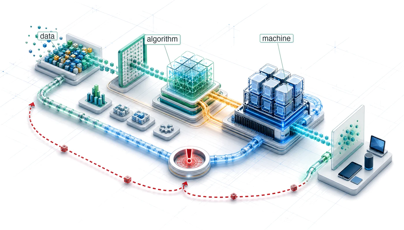
The three components can be conceptualized as Data (the fuel), Algorithm (the blueprint), and Machine (the engine). Without any one component, the others remain theoretical. The D·A·M taxonomy captures this interdependence directly; figure 3 shows why the three elements cannot be designed, or even reasoned about, in isolation.

The bidirectional arrows between Data, Algorithm, and Machine emphasize that no axis can be optimized in isolation. Each element shapes the possibilities of the others. The algorithm dictates both the computational demands for training and inference and the volume and structure of data required for effective learning. The data’s scale and complexity influence what machines are needed for storage and processing while determining which algorithms are feasible. The machine’s capabilities establish practical limits on both model scale and data processing capacity, creating a boundary within which the other axes must operate.
ML systems engineering is the discipline of keeping all three axes in balance. Table 4 formalizes each axis’s role.
| Axis | Definition | Role in System |
|---|---|---|
| Data | Information that guides behavior | The Fuel: Defines what the system learns |
| Algorithm | Mathematical structures that learn | The Blueprint: Defines how patterns are captured |
| Machine | Hardware and software infrastructure | The Engine: Defines computation speed and location |
The D·A·M taxonomy provides the diagnostic lens, but to build systems, we must organize these axes into a reproducible hierarchy: a four-layer stack that transforms raw physical constraints into functional user applications.
From silicon to mission: A four-layer hierarchy
Every machine learning system analyzed in this text is constructed from four hierarchical layers, ensuring that a decision made at the silicon level is traceable to its impact on the final mission.
- Hardware (The Silicon): The physical foundation (The Engine). This layer defines the raw capabilities: peak compute throughput \((R_{\text{peak}})\), memory bandwidth \((\text{BW})\), and memory capacity; concrete hardware twins instantiate those quantities when deployment scenarios need numeric constraints.
- Systems (The Platforms): The integrated deployment unit (The Car). This layer defines the “Envelope” in which hardware operates: power budget, thermal limits, and node-level interconnects. Examples include the Training Cluster Node or the Sub-Watt Sensor Node.
- Workloads (The Models): The algorithmic demand (The Route). This layer defines the mathematical workload: operation count \((O)\), data volume moved \((D_{\text{vol}})\), and data layout. Scenario-specific workloads, such as GPT-4 and Wake Vision, instantiate these demands for particular missions.
- Missions (The Scenarios): The application context (The Destination). This is the top of the stack, where a system is deployed to solve a specific problem. A mission introduces high-level requirements, such as battery life, safety latency, or cloud cost ceilings, that dictate the configuration of every layer below.
This hierarchy ensures that when we build a lab or a case study, engineers are not starting from scratch, but rather inheriting the constraints of a deployment paradigm and applying a scenario workload to a specific mission. The lifecycle discussion later in this chapter pairs each recurring mission with its workload and binding constraint. This structured approach allows us to reason about the “Physics of ML” across any application domain.
The D·A·M taxonomy serves as a diagnostic lens throughout this text. Scale in ML systems is the relentless pursuit of the moving bottleneck. Alleviating a constraint along one axis often shifts the limitation to another. Upgrading to faster GPUs (Machine) might reveal that storage cannot feed data fast enough (Data). Collecting a massive dataset (Data) might reveal that the model lacks capacity to learn from it (Algorithm). Switching to a larger model (Algorithm) might exceed available memory (Machine). Understanding these dynamics is central to ML systems engineering. Part III formalizes this diagnostic approach, and Diagnostic Summary maps each axis to its binding physical constraint and high-leverage optimization pathway, giving the reader a reference point for where to intervene once the dominant axis is identified.
Systems Perspective 1.2: The ML systems landscape: Four deployment paradigms
The machine learning systems landscape spans roughly \(10^{6}\) in computational power and \(10^{5}\) in memory capacity. Table 5 contrasts the memory, compute, and power envelopes across the four Deployment Paradigms that define the constraints for every subsequent chapter.
Table 5: Four Deployment Paradigms: Representative memory, compute, and power envelopes for cloud, edge, mobile, and TinyML systems, exposing the multi-order-of-magnitude span that prevents simple model reuse across tiers. Exact hardware twins and peak-rate calculations appear in the hardware chapters.
| Paradigm | Representative System | Memory Envelope | Compute Envelope | Power Envelope |
|---|---|---|---|---|
| Cloud | Data-center accelerator node | Large device memory plus storage (\(\approx 10^{11}\,\text{B}\)) | Highest-throughput tier (\(\approx 10^{15}\,\text{ops/s}\)) | Facility-managed power |
| Edge | Robotics or industrial gateway | Local memory under deployment limits (\(\approx 10^{11}\,\text{B}\)) | Local accelerator or CPU budget (\(\approx 10^{14}\,\text{ops/s}\)) | Wall, vehicle, or site power |
| Mobile | Smartphone or wearable-class SoC | Shared application memory (\(\approx 10^{10}\,\text{B}\)) | Phone-class neural, GPU, and CPU engines (\(\approx 10^{13}\,\text{ops/s}\)) | Battery and thermal cap |
| TinyML | Microcontroller node | Kilobyte-scale memory (\(\approx 10^{6}\,\text{B}\)) | Always-on sensor compute (\(\approx 10^{9}\,\text{ops/s}\)) | Milliwatt-class battery budget |
Observation: Reading the memory and compute columns from Cloud to TinyML, the endpoints differ by \(10^{5}\) in memory and \(10^{6}\) in compute. This divergence is precisely why we cannot simply “shrink” a cloud model to run at the edge; each tier requires a fundamental redesign of the D·A·M axes.
The multi-order-of-magnitude span across these four paradigms is not merely a technical curiosity; it translates directly into cost. A model that fits comfortably in a data-center accelerator’s memory cannot run unchanged on a microcontroller-class device, and bridging that gap requires engineering trade-offs at every tier of the D·A·M taxonomy. Data quality, algorithmic efficiency, and hardware capability interact through a single economic constraint: samples per dollar.
Systems Perspective 1.3: Samples per dollar
Systems insight: While researchers optimize for accuracy, systems engineers optimize for samples per dollar. Let model size be the parameter count, dataset size the number of training samples, and hardware efficiency the compute throughput per dollar (FLOP/s per dollar, with FLOP/s formalized in the iron law below). This metric unifies the three axes of the D·A·M taxonomy into a single constraint equation, shown in equation 2: \[ \text{Cost} \propto \frac{\text{Model Size} \times \text{Dataset Size}}{\text{Hardware Efficiency}} \tag{2}\]
- Data (Information): Improving data quality (cleaning, filtering) increases the “learning value” of each sample, effectively reducing the numerator.
- Algorithm (Logic): More efficient model structures reduce the compute per sample, lowering the numerator.
- Machine (Physics): Specialized hardware increases the denominator, allowing more compute per dollar.
Systems engineering is the art of balancing this equation. A 10 percent gain in hardware efficiency can fund about 10 percent more data or a larger model at the same budget, but the accuracy return depends on the workload’s learning-curve elasticity. If error scales approximately as \(D^{-\alpha}\) for dataset size \(D\), the gain from more data is governed by \(\alpha \log(1.1)\) rather than by a universal percentage. The engineer’s job is to estimate that elasticity for the system at hand and decide whether the trade-off is economically viable.
This economic view explains why ML failures rarely belong to one component: a data shortcut, model change, or hardware bottleneck can all surface as degraded behavior after deployment.
Self-Check: Question
Which description best matches the chapter’s definition of a machine learning system?
- A software artifact whose behavior is fixed once programmers finish writing explicit rules
- A software system whose core behavior is determined by parameters learned from data, making performance jointly dependent on data quality, algorithm choice, and hardware capacity
- Any distributed application that serves responses in under 100 ms
- Any statistical model trained on a labeled dataset, regardless of deployment
When a team asks which of Data, Algorithm, or Machine is the binding constraint on performance before choosing what to optimize, they are applying the three-axis diagnostic framework the chapter formalizes as the ____ taxonomy.
A production spam filter starts missing a new phishing campaign even though its serving latency stays normal; separately, during a traffic spike the same service falls behind and cannot classify messages quickly enough. Using the D·A·M taxonomy, diagnose which axis is binding in each situation and name one intervention per situation that attacks that axis directly.
In the four-layer engineering crux hierarchy (Hardware, Systems, Workloads, Missions), which layer introduces application-specific end-use requirements such as “one-year battery life on a coin-cell” for a smart doorbell?
- Hardware, because battery life is ultimately determined by silicon power characteristics
- Systems, because deployment envelopes set the thermal and power budgets
- Workloads, because a longer-running model necessarily implies a larger operation count
- Missions, because this is where application-level requirements enter and propagate downward
Order the layers of the engineering crux from the lowest physical layer to the highest application layer: (1) Missions, (2) Hardware, (3) Workloads, (4) Systems.
ML vs. Traditional Software
The D·A·M taxonomy reveals what ML systems comprise: data that guides behavior, algorithms that extract patterns, and machines that enable learning and inference19. The critical distinction between ML systems engineering and traditional software engineering lies not in these components themselves but in how the resulting systems fail.
19 Inference: From Latin inferre (“to bring in” or “to conclude”). In ML engineering, inference refers to the deployment phase where a trained model applies learned patterns to novel inputs. The systems distinction matters: training is throughput-optimized (maximize samples/second), while inference is latency-optimized (minimize milliseconds/prediction), and these opposing objectives demand fundamentally different hardware configurations and software stacks (see Model Serving).
Traditional software exhibits explicit failure modes. When code breaks, applications crash, error messages propagate, and monitoring systems trigger alerts. This immediate feedback enables rapid diagnosis and remediation: the system operates correctly or fails observably. Machine learning systems operate under silent degradation: they can continue functioning while their performance degrades silently, without triggering conventional error detection mechanisms. The algorithms continue executing and the machines maintain prediction serving, yet the learned behavior becomes progressively less accurate or contextually relevant.
An autonomous vehicle’s perception system illustrates this distinction concretely. Traditional automotive software exhibits binary operational states: the engine control unit either manages fuel injection correctly or triggers diagnostic warnings. The failure mode remains observable through standard monitoring. An ML-based perception system presents a different challenge. The system’s accuracy in detecting pedestrians might decline from 95 percent to 85 percent over several months due to seasonal changes, as different lighting conditions, clothing patterns, or weather phenomena underrepresented in training data affect model performance. The vehicle continues operating, successfully detecting most pedestrians, yet the degraded performance creates safety risks that become apparent only through systematic monitoring of edge cases and comprehensive evaluation. Conventional error logging and alerting mechanisms remain silent while the system becomes measurably less safe.
The magnitude of this degradation matters in safety-critical contexts. A perception model running at 10 Hz processes 36,000 frames in one hour. Even a 0.1 percent false-negative rate would produce dozens of missed detections before temporal filtering, sensor fusion, and operational-design-domain limits reduce the risk. The 10-percentage-point degradation from 95 percent to 85 percent is therefore not merely an accuracy change; it changes the exposure rate of downstream control logic in precisely the edge cases where detection was already marginal.
This silent degradation manifests across all three D·A·M axes. The data distribution shifts as the world changes: user behavior evolves, seasonal patterns emerge, and new edge cases appear (Gama et al. 2014; Quiñonero-Candela et al. 2009). Meanwhile, the algorithms continue making predictions based on outdated learned patterns, unaware that their training distribution no longer matches operational reality. The machines faithfully serve these increasingly inaccurate predictions at scale, amplifying the problem across every user and every query.
Because this failure mode is silent, crash logs cannot be relied upon for detection; mathematical approaches must be used. When failures do not announce themselves, quantitative signals are needed that connect measurable distribution shift to expected performance loss. By analogy with the processor-performance decomposition introduced below, we can decompose ML system degradation into constituent factors. The degradation equation in equation 3 is a first-order diagnostic approximation, not a universal prediction law: it captures the common case where greater distribution shift increases expected performance loss over time. \[ \text{Accuracy}(t) \approx \text{Accuracy}_0 - \lambda \cdot \mathcal{D}(P_t \lVert P_0) \tag{3}\] where:
- \(\text{Accuracy}_0\): Initial accuracy at deployment
- \(\mathcal{D}(P_t \lVert P_0)\): Statistical divergence between current data distribution \(P_t\) and training distribution \(P_0\)
- \(\lambda\): Model sensitivity to distribution shift (architecture-dependent)

Accuracy decays silently under drift.
This first-order linearization captures the dominant trend: accuracy erodes roughly in proportion to how far the current data distribution has drifted from the training distribution. That gradual divergence is Data Drift: the production distribution moves away from the distribution the model learned, so predictions can become unreliable even when the code has not changed. The model breaks down for large shifts (where the relationship becomes nonlinear) and the specific divergence measure \(\mathcal{D}(\cdot \lVert \cdot)\) is left deliberately general (common choices include KL divergence, total variation distance, or Wasserstein distance, each with different sensitivity profiles). Despite these simplifications, the equation reveals three engineering levers for managing degradation:
- Improve initial accuracy \((\text{Accuracy}_0)\): Better training, more data, superior architectures. This shifts the curve but not its slope.
- Reduce distribution sensitivity \((\lambda)\): Robust training techniques, domain adaptation, broader training distributions. These flatten the degradation curve.
- Monitor and respond to drift (\(\mathcal{D}(P_t \lVert P_0)\)): Continuous measurement of distribution divergence enables proactive retraining before accuracy falls below acceptable thresholds.
The practical implication: knowing when to retrain is as important as knowing how to train. A system that retrains when \(\mathcal{D}(P_t \lVert P_0) > \tau\) for some threshold \(\tau\) maintains accuracy within bounds. A system without drift monitoring operates blind to its own degradation. We develop the monitoring infrastructure and alerting strategies that implement this principle in ML Operations.
This framework distinguishes ML systems engineering from traditional software engineering at the deepest level. Traditional systems have no equivalent equation because they do not drift: a function that computed correctly yesterday computes correctly today. ML systems require continuous investment in monitoring infrastructure that traditional software never needed, and the degradation equation quantifies why. It is the engineering response to the verification gap identified in equation 1: since we cannot test exhaustively, we must monitor continuously.
A recommendation system illustrates the pattern: it might lose several percentage points under mild seasonal drift or tens of points under a severe training-serving skew, with the rate depending on the measured distribution shift and the model’s sensitivity to that shift. This degradation often stems from training-serving skew, where features computed differently between training and serving pipelines cause model performance to degrade despite unchanged code. This is a machine issue that manifests as algorithmic failure.
The difference in failure modes demands new engineering practices. Traditional software development focuses on eliminating bugs and ensuring deterministic behavior, but ML systems engineering must additionally address probabilistic behaviors, evolving data distributions, and performance degradation that occurs without code changes. Monitoring systems must track infrastructure health, model performance, data quality, and prediction distributions simultaneously. Deployment practices must enable continuous model updates as data distributions shift. The entire system lifecycle, from data collection through model training to inference serving, must be designed with silent degradation in mind.
The degradation equation reveals what goes wrong with ML systems: silent reliability decay absent from traditional software. Knowing that a system will degrade is not the same as knowing why it degrades or where to intervene. For that, we need to decompose performance itself into its physical constituents. The bitter lesson established that computational scale drives AI progress; the question now becomes how to reason quantitatively about the data movement, computation, and overhead that constitute that scale.
Self-Check: Question
The section illustrates the ML vs. traditional software distinction with an autonomous-vehicle perception system whose pedestrian-detection accuracy drifts from 95 percent to 85 percent over several months while conventional error logging stays silent. Which statement best captures the distinction this example highlights?
- ML systems are usually written in Python while traditional software is not
- Traditional software has no performance constraints while ML systems do
- ML systems can continue operating while prediction quality silently degrades as data distributions shift, whereas traditional software failures are typically explicit and observable
- Traditional software cannot be monitored in production
The degradation equation \(\text{Accuracy}(t) \approx \text{Accuracy}_0 - \lambda \cdot \mathcal{D}(P_t \lVert P_0)\) identifies three control levers. Name each lever, describe how an engineering team would act on it, and explain how the levers together convert silent degradation into a manageable operational problem.
True or False: If no code has changed and the hardware is healthy, a deployed ML system’s accuracy should remain stable.
A deployed recommendation model still returns responses on time, but over three months click-through quality falls steadily as user tastes shift. In the degradation equation \(\text{Accuracy}(t) \approx \text{Accuracy}_0 - \lambda \cdot \mathcal{D}(P_t \lVert P_0)\), which term most directly captures the cause?
- The divergence \(\mathcal{D}(P_t \lVert P_0)\) between the current input distribution and the training distribution
- The initial accuracy \(\text{Accuracy}_0\) at deployment time
- The model’s floating-point precision
- The accelerator’s peak hardware throughput \(R_{\text{peak}}\)
Why does the chapter argue that knowing when to retrain is as important as knowing how to train? Illustrate with a fraud-detection scenario where the deployed code is flawless.
Iron Law of ML Systems
A training job stalls when storage cannot feed an accelerator; an inference path misses its deadline when model state moves too slowly through memory or across the network. These failures look different, but they share a single performance structure. Machine learning system performance is governed by the Iron Law of ML Systems, formalized in equation 4: \[T = \underbrace{\frac{D_{\text{vol}}}{\text{BW}}}_{\text{The Data Term}} + \underbrace{\frac{O}{R_{\text{peak}} \cdot \eta_{\text{hw}}}}_{\text{The Compute Term}} + \underbrace{L_{\text{lat}}}_{\text{The Latency Term}} \tag{4}\]
This equation is the mathematical spine of this book. It decomposes the total time required for any ML task, whether training a model for weeks or serving an inference in milliseconds, into three terms that correspond directly to the physical constraints of the Dual Mandate introduced earlier:
- The data term \((D_{\text{vol}}/\text{BW})\): The physical cost of moving bits. \(D_{\text{vol}}\) is the volume of data moved (bytes), and \(\text{BW}\) is the memory or network bandwidth (bytes/s). Whether loading terabytes from cloud storage or fetching weights from high-bandwidth memory, performance is often limited by I/O physics. This is addressed in Part I: Foundations.
- The compute term \((O/(R_{\text{peak}} \cdot \eta_{\text{hw}}))\): The cost of arithmetic. \(O\) is the number of floating-point operations. \(R_{\text{peak}}\) is the hardware’s theoretical peak throughput (FLOP/s). \(\eta_{\text{hw}}\) is the hardware utilization factor \((0 \le \eta_{\text{hw}} \le 1)\), representing realized efficiency. We address this in Part II: Build and Part III: Optimize.
- The latency term \((L_{\text{lat}})\): The irreducible “tax” of system orchestration, networking, and serialization. This fixed latency dominates in real-time deployment. We address this in Part IV: Deploy.
Systems Perspective 1.4: The iron law analogy
We call this the “iron law” by analogy to Patterson & Hennessy’s Iron Law of Processor Performance (Patterson and Hennessy 2017). However, there are important differences. P&H’s law is a multiplicative decomposition (a tautology factoring CPU time), whereas our equation is an additive first-order model that approximates performance under simplifying assumptions.
The additive form assumes sequential execution; in practice, systems can overlap these terms, transforming the sum into a max as equation 5 shows: \[T_{\text{pipelined}} = \max\left(\frac{D_{\text{vol}}}{\text{BW}}, \frac{O}{R_{\text{peak}} \cdot \eta_{\text{hw}}}\right) + L_{\text{lat}} \tag{5}\]
We retain “iron law” because, like Amdahl’s Law (Amdahl 1967), its value lies in diagnostic power: identifying which physical constraint dominates before optimizing. The iron law is useful precisely because it simplifies the complexity of the full stack into three manageable terms. The D·A·M Taxonomy presents the refined treatment, including pipelining and overlap techniques that transform the additive model into the max-based formulation used in practice.
Amdahl, Gene M. 1967. “Validity of the Single Processor Approach to Achieving Large Scale Computing Capabilities.” Proceedings of the April 18-20, 1967, Spring Joint Computer Conference on - AFIPS ’67 (Spring), AFIPS ’67 (spring), 483–85. https://doi.org/10.1145/1465482.1465560.
Patterson, David A., and John L. Hennessy. 2017. Computer Architecture: A Quantitative Approach. 6th ed. Morgan Kaufmann.
Box, George E. P. 1976. “Science and Statistics.” Journal of the American Statistical Association 71 (356): 791–99. https://doi.org/10.1080/01621459.1976.10480949.
20 “All Models Are Wrong, but Some Are Useful”: Statistician George Box’s aphorism applies directly to the iron law: the additive decomposition ignores pipelining, memory hierarchy effects, and communication overhead. Yet this deliberate simplification is precisely what makes it diagnostic. Engineers who try to model every interaction before profiling never ship; engineers who identify which of three terms dominates ship systems that work.
As George Box famously said, “All models are wrong, but some are useful” (Box 1976).20
The roofline model develops the deeper mathematical treatment, including the ridge point that makes the data/compute trade-off measurable: below the ridge, data movement dominates; above it, arithmetic throughput dominates. Throughout this book, every optimization technique we study is a method for manipulating one of these variables: moving less data, doing less work, using the machine more effectively, or reducing orchestration delay. A GPT-3-class training estimate makes that manipulation concrete by showing how an efficiency change propagates through the iron law.
Napkin Math 1.1: Training GPT-3
Problem: What is the training time for a GPT-3 class model on a cluster of 1024 accelerators built from reference accelerators?
Given:
- Ops \((O)\): \(\approx 3.14 \times 10^{23}\ \text{FLOPs}\)
- Peak \((R_{\text{peak}})\): 312 TFLOP/s
- Efficiency \((\eta_{\text{hw}})\): ≈ 45 percent (typical for large-scale distributed training)
- Scale \((N_{\text{accel}})\): 1024 accelerators
Math:
- \(T_{\text{train}} \approx \frac{O}{N_{\text{accel}} \cdot R_{\text{peak}} \cdot \eta_{\text{hw}}}\) \(\approx \frac{3.14 \times 10^{23}}{1024 \times 312 \times 10^{12} \times 0.45}\) \(\approx 25\ \text{days}\)
Result: 25 days.
Systems insight: If we improve hardware utilization \((\eta_{\text{hw}})\) from 45 percent to 60 percent through better scheduling and more efficient execution, training time drops to 19 days, saving nearly 6 days of expensive compute time.
The equation is dimensionally consistent: each term resolves to seconds. One cannot add FLOPs to bytes any more than one can add meters to kilograms; the iron law adds time to time to time. Dimensional analysis provides a formal dimensional analysis verifying this consistency and demonstrates how unit tracking prevents common modeling errors.
The iron law governs time, but time is not the only constraint. For mobile devices, edge systems, and large-scale training clusters, energy often matters more than raw speed.

Moving a byte costs about 145 times an FP16 op, the data-movement tax.
Just as time is governed by physics, so is energy. We must add a fourth term to our mental model: the energy tax. In many modern systems (mobile, edge, and large-scale training), energy, not time, is the hard constraint. Let \(D_{\text{vol}}\) be the total data volume moved (bytes), \(E_{\text{move}}\) the energy per byte moved, \(O\) the total operation count, and \(E_{\text{compute}}\) the energy per operation. Equation 6 formalizes this relationship, following the hardware-energy observation that data movement can dominate arithmetic energy (Horowitz 2014): \[ E_{\text{total}} \approx \underbrace{ D_{\text{vol}} \times E_{\text{move}} }_{\text{Dominant Term}} + \underbrace{ O \times E_{\text{compute}} }_{\text{Secondary Term}} \tag{6}\]
The dominant term is data movement: \(E_{\text{move}} \gg E_{\text{compute}}\). Under the energy constants used in this text, moving one byte from off-chip DRAM costs about 145.5× one FP16 operation and about 800× one INT8 operation (Horowitz 2014). The exact ratio depends on precision and memory level, but the conclusion is stable: moving data through the memory hierarchy costs orders of magnitude more energy than arithmetic. The physical reason is that data movement requires charging and discharging wires over macroscopic distances, while arithmetic is performed locally within a processing unit’s circuits. Therefore, minimizing data movement \((D_{\text{vol}})\) is the primary lever for both speed and energy efficiency.
Checkpoint 1.2: The iron law
The iron law \((T \approx \frac{D_{\text{vol}}}{\text{BW}} + \frac{O}{R_{\text{peak}} \cdot \eta_{\text{hw}}} + L_{\text{lat}})\) is the analytical backbone of this book. Before proceeding, verify you can manipulate its terms:
Self-test: If you double the processor speed \((R_{\text{peak}})\), which term does it improve?
The same terms that determine time and energy also determine cost: every byte moved, operation executed, and millisecond of latency consumes infrastructure budget. The next test is therefore economic, asking whether added compute buys enough model improvement to justify the resources it consumes.
The economic invariant: Return on compute (RoC)
The decomposition of time is also an economic constraint. In the Hennessy & Patterson tradition of quantitative reasoning, the return on compute (RoC) is defined as the marginal accuracy gain per dollar of infrastructure investment. \[ \text{RoC} = \frac{\Delta \text{Accuracy}}{\Delta \text{Compute Cost}} \]
This invariant exposes an economic boundary: a 1 percent gain in accuracy may fail the RoC test if it requires a 10\(\times\) increase in \(O\) (Total Operations). Every optimization in the following chapters targets either the numerator (extracting more signal from the same data) or the denominator (reducing the cost of executing the math). If the RoC is negative or negligible, the system is over-engineered, regardless of its technical sophistication. This economic lens transforms “accuracy” from a research target into an engineering budget.
If scale is the ultimate lever for performance, it is also the ultimate consumer of resources. The bitter lesson teaches that scale works, but the iron law teaches us how to afford it. This tension between scaling and sustainability shapes the engineering principles that follow.
Lighthouse models: The iron law in practice
The iron law does more than diagnose bottlenecks; it organizes the entire discipline. Each term in the equation corresponds to a core engineering imperative. The data term demands that we build robust data pipelines and infrastructure (Data Engineering). The compute term requires that we optimize algorithms and hardware utilization for efficiency (Part III). The latency term necessitates that we deploy and operate systems reliably in production (Model Serving, ML Operations). These three imperatives structure this textbook: Parts I and II address building, Part III addresses optimization, and Part IV addresses deployment and operations.
Abstract equations become concrete through concrete workloads. This textbook employs five recurring Lighthouse Models as diagnostic tools for the iron law. These canonical workloads reappear across chapters to test how the same physical constraints affect different architectural patterns.
Each lighthouse model represents a distinct stress case for the iron law. For instance, ResNet-50 lets us investigate compute throughput when a system repeatedly reuses the same learned parameters, while GPT-2/Llama acts as our primary probe for memory bandwidth pressure during language generation. For language models, autoregressive decode means generating one token at a time; the KV cache is the saved attention state from previous tokens (Network Architectures introduces the attention mechanism in full), and prefill is the initial pass that processes the prompt before token-by-token generation begins. That diagnosis is regime-specific: small-batch decode often streams weights and KV-cache state fast enough to expose memory bandwidth, while prefill and high-batch serving can shift the bottleneck toward arithmetic or communication. By following these same workloads from data engineering through to edge deployment, each chapter demonstrates how a single architectural choice propagates physical and economic constraints across the entire system.
The iron law makes these differences precise. ResNet-50 applies the same small weight filters across many spatial positions and, under batching, across many inputs; that reuse can make \(O/(R_{\text{peak}} \cdot \eta_{\text{hw}})\) the dominant term because the processor must sustain enormous arithmetic throughput while the data footprint remains modest. GPT-2, by contrast, loads billions of unique weight parameters for every token it generates, and each weight is used only once before the next must be fetched; its \(D_{\text{vol}}/\text{BW}\) term dominates because memory bandwidth, not arithmetic, is the binding constraint. The same equation, applied to two different workloads, yields different diagnoses and therefore different optimization strategies: doubling \(R_{\text{peak}}\) helps batched ResNet-50 once reuse increases computation per byte moved, but barely affects GPT-2 decode; doubling \(\text{BW}\) has the reverse effect for bandwidth-bound decode. Table 6 summarizes why each lighthouse model serves as a diagnostic tool for a specific bottleneck.
| Lighthouse Model | System Bottleneck | What It Reveals | Key Engineering Questions |
|---|---|---|---|
| ResNet-50 | Compute throughput under reuse | GPU utilization, batching | Is my hardware doing math or waiting for data? |
| GPT-2/Llama | Memory bandwidth | Weight and sequence-state movement | How fast can I move model state to compute? |
| Deep Learning Recommendation Model (DLRM) | Memory capacity | Embedding tables, scale-out | How do I fit terabyte-scale models in memory? |
| MobileNetV2 | Latency and power | Efficient operator design | Can I meet real-time constraints on battery? |
| Keyword Spotting | Power envelope | Tiny memory and energy budgets | Can I run always-on inference on milliwatts? |

GPT-2 decode is bandwidth-bound: the data term dominates.
Each lighthouse model manifests different constraints along the D·A·M axes, ensuring that the principles developed throughout this text are tested against the diversity of real-world systems engineering challenges. The division of labor among the book’s recurring examples is deliberate: the four deployment paradigms fix the envelope a system must operate within, the five Lighthouse Models supply the workloads that stress it, and later in this chapter four engineering missions and three production case studies (Waymo, FarmBeats, and AlphaFold) pair envelope with workload under real-world constraints.
The same diagnostic reading applies retrospectively to the breakthrough that launched the deep learning era. The AlexNet victory traced in section 1.2.3 was a D·A·M alignment: the error reduction came not from algorithmic novelty alone but from convolutional networks’ parallel matrix operations matching GPU capabilities, trained on ImageNet’s21 (Deng et al. 2009) unprecedented labeled corpus.
21 ImageNet: The 2009 dataset that proved data scale was the missing ingredient in computer vision. Fei-Fei Li marshaled 49,000 Mechanical Turk workers to label 14.2 million images across 21,841 categories; the 2012 challenge training split used by AlexNet contained about 1.3M labeled images. This data engineering operation dwarfed the algorithmic novelty of everything it subsequently enabled, including AlexNet’s 2012 breakthrough (see Data Engineering).
Deng, Jia, Wei Dong, Richard Socher, Li-Jia Li, Kai Li, and Li Fei-Fei. 2009. “ImageNet: A Large-Scale Hierarchical Image Database.” 2009 IEEE Conference on Computer Vision and Pattern Recognition, 248–55. https://doi.org/10.1109/cvpr.2009.5206848.
This interdependence means that optimizing one component often shifts pressure to another. AlexNet’s co-design success came at a cost affordable in 2012 (two consumer GPUs for a week), but modern models demand resources roughly 7 orders of magnitude larger. If the iron law governs how fast a system runs, we still need a framework for reasoning about how efficiently it uses those resources.
Self-Check: Question
An engineer doubles an accelerator’s peak FP16 throughput \(R_{\text{peak}}\) while memory bandwidth \(\text{BW}\) and fixed overhead \(L_{\text{lat}}\) stay the same. In the iron law \(T = D_{\text{vol}}/\text{BW} + O/(R_{\text{peak}} \cdot \eta_{\text{hw}}) + L_{\text{lat}}\), which term is most directly improved?
- The data term \(D_{\text{vol}}/\text{BW}\) only
- The compute term \(O/(R_{\text{peak}} \cdot \eta_{\text{hw}})\) only
- The latency term \(L_{\text{lat}}\) only
- All three terms equally
A team is weighing whether a 1-percentage-point accuracy gain that requires a 10× increase in operation count \(O\) and 10× larger training clusters is worth the infrastructure bill. The economic invariant that formalizes whether that marginal accuracy gain per dollar of added compute is acceptable is called ____.
GPT-2/Llama-style decode is presented as memory-bandwidth-bound, while batched ResNet-50 convolution is presented as compute-throughput-heavy once weight reuse is high. For a team considering a hardware upgrade with either 2× bandwidth OR 2× peak TFLOP/s, explain which upgrade wins for each workload and why, using the iron law to ground your reasoning.
Among the five Lighthouse Models presented in the chapter (ResNet-50, GPT-2/Llama, DLRM, MobileNetV2, Keyword Spotting), which is the clearest probe for compute-throughput bottlenecks in the iron law’s compute term?
- GPT-2/Llama, because autoregressive decoding stresses arithmetic throughput
- DLRM, because embedding-table lookups dominate recommendation workloads
- Keyword Spotting, because always-on inference is constrained by peak FLOP/s
- ResNet-50, because its convolutional filters are reused thousands of times per forward pass
True or False: The iron law is a physical law in the same strict sense as Patterson & Hennessy’s iron law of processor performance, so its additive form \(T = D_{\text{vol}}/\text{BW} + O/(R_{\text{peak}} \cdot \eta_{\text{hw}}) + L_{\text{lat}}\) always matches measured execution exactly.
A new architecture improves MMLU accuracy by 1 percentage point over the previous generation but requires 10× the operation count \(O\) and a 10× larger training cluster. Using the RoC invariant, walk through how an engineer should evaluate whether to ship this improvement, and explain what RoC reveals that a pure accuracy comparison hides.
Efficiency Framework
The bitter lesson establishes that scale drives AI progress, but it also creates a paradox: if advancing AI requires ever-larger datasets and compute budgets, participation narrows to only the most resource-rich organizations. Even those organizations face physical limits in data center power constraints, memory bandwidth bottlenecks, and the diminishing returns of adding more parameters.
Common public estimates for GPT-4-class training place the compute budget around 2.5 million accelerator-days, representing millions of dollars in compute costs and substantial environmental impact. Many research institutions and companies cannot afford to compete through brute-force scaling. The reality motivates a complementary approach: rather than focusing solely on applying more compute, the field must also address how efficiently existing compute is used.
Efficiency is a bottleneck diagnosis, not a single technique. Three complementary dimensions map directly to our D·A·M taxonomy (table 4), and each changes a different term in the resource budget. Algorithmic efficiency, the earliest frontier, reduces computational requirements through better model design and training procedures. Its goal is to produce more useful behavior per operation, so capability rises without scaling every resource in lockstep. As algorithms demanded ever more computation, compute efficiency became the second critical dimension. It maximizes hardware utilization by aligning algorithmic logic with machine physics, turning theoretical processor capability into useful work. Most recently, data selection emerged as the third dimension, extracting more learning signal from limited examples and thereby reducing the total operations term \(O\) of the iron law. The timeline in figure 4 places these three dimensions on the same axis so the historical sequence of bottlenecks is visible before the chapter sequence presents them in build order. Together, these three dimensions provide the engineering tools to overcome the data, algorithm, and machine walls that pure scaling alone cannot address.

These three dimensions did not emerge simultaneously; each progressed through distinct eras at different rates. Algorithmic efficiency led the way, compute efficiency followed as demand grew, and data-centric methods matured most recently. While history progressed from algorithmic breakthroughs to hardware acceleration to data-centric methods, Part III of this book reverses that sequence: we begin with data selection, then model compression, then hardware acceleration. This pedagogical order reflects how practitioners actually build systems: quality data is prerequisite to effective model optimization, and understanding the model is prerequisite to mapping it efficiently onto hardware.
The architecture-level trajectory in figure 5 makes the algorithmic side of this gap visible model by model, rather than only as an aggregate scaling claim.
The magnitude of efficiency improvements is measurable. Between 2012 and 2019, computational resources needed to train a neural network to achieve AlexNet-level performance on ImageNet classification decreased by approximately 44.5× (Hernandez and Brown 2020). This improvement, which halved about every 15 months, outpaced hardware efficiency gains predicted by Moore’s Law22, demonstrating that algorithmic innovation drives efficiency as much as hardware advances.
Hernandez, Danny, and Tom B. Brown. 2020. “Measuring the Algorithmic Efficiency of Neural Networks.” arXiv Preprint arXiv:2005.04305, ahead of print. https://doi.org/10.48550/arxiv.2005.04305.
22 Moore’s Law: Gordon Moore’s 1965 observation described rapid growth in the number of components that could be economically integrated on a chip (Moore 1998); later industry summaries often expressed the cadence as roughly a two-year doubling. Over the same 2012–2019 window, a two-year doubling cadence yields roughly 11.3× in transistor scaling, meaning algorithmic innovation closed more of the efficiency gap than hardware alone. Simultaneously, demand for training compute doubled every 3.4 months, about 7.1× faster than the two-year hardware cadence, forcing the shift to domain-specific accelerators.
Moore, G. E. 1998. “Cramming More Components onto Integrated Circuits.” Proceedings of the IEEE 86 (1): 82–85. https://doi.org/10.1109/jproc.1998.658762.
Simultaneously, aggregate training compute in published frontier runs followed a much steeper cadence than Moore’s Law, with a fitted doubling time of approximately 3.4 months (Amodei and Hernandez 2018). That aggregate publication trend is not the same quantity as an endpoint ratio between two landmark models, but it explains why efficiency optimization is not optional. Without it, only the most resource-rich organizations could participate in AI development.
These measurements emerge from rigorous empirical methodology that tracked training compute across hundreds of published models; Benchmarking develops the measurement frameworks that enable such systematic analysis of ML system performance. The two cadences just compared define the systems gap: the widening distance between what models demand (compute doubling every 3.4 months) and what hardware supplies (transistor density doubling roughly every two years). Closing that gap is the primary objective of this textbook, requiring integrated expertise across the software and hardware stack; Hardware Acceleration quantifies it directly.
Figure 5 traces this trajectory architecture by architecture: VGG, ResNet, MobileNet, and EfficientNet each reach comparable accuracy with progressively fewer computational resources. Later ImageNet architectures are shown to give visual context for the mature benchmark, but the cited empirical efficiency claim is the 2012–2019 trajectory.
Efficiency gains tell only half the story. Figure 6 compares illustrative endpoint estimates for AlexNet-era and GPT-4-class training—one visualization of scale, distinct from the aggregate 3.4-month doubling trend cited above—yet the span still grows exponentially, making efficiency optimization not a luxury but a necessity for continued progress.
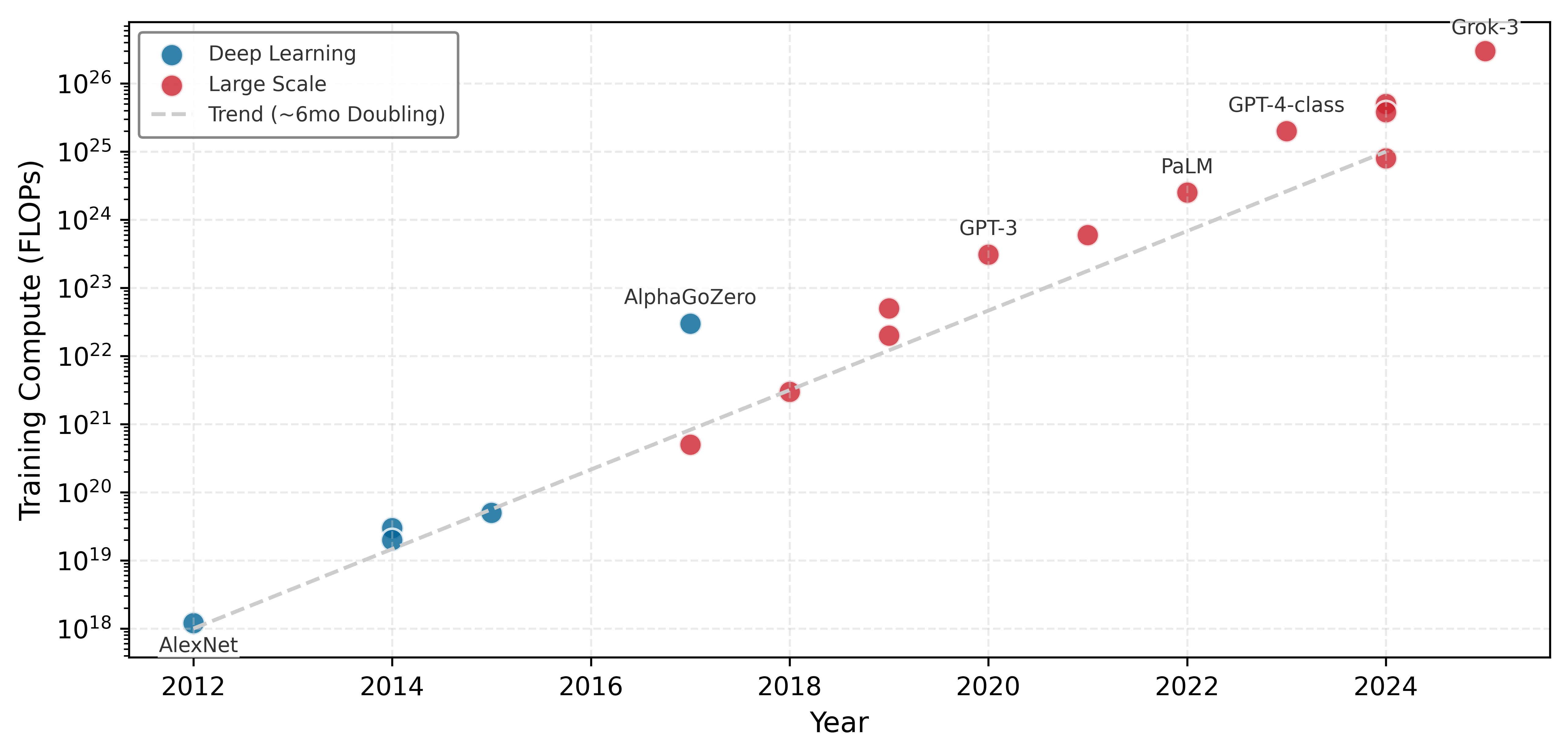
Amodei, Dario, and Danny Hernandez. 2018. “AI and Compute.” OpenAI Blog 6.
Sevilla, Jaime, Lennart Heim, Anson Ho, Tamay Besiroglu, Marius Hobbhahn, and Pablo Villalobos. 2022. “Compute Trends Across Three Eras of Machine Learning.” 2022 International Joint Conference on Neural Networks (IJCNN), 1–8. https://doi.org/10.1109/ijcnn55064.2022.9891914.
Taken together, these two figures reveal a seeming contradiction that defines the economics of modern AI development: figure 5 shows efficiency improving 44.5× while figure 6 shows compute demand growing by roughly 7 orders of magnitude. The resolution lies in understanding how efficiency and scale co-evolve.
Systems Perspective 1.5: The efficiency paradox
This efficiency paradox defines the economics of ML systems engineering. Efficiency gains enabled larger experiments, which demanded more compute, which motivated further efficiency research. Consider: if EfficientNet needs 44.5× less compute than AlexNet to reach the same accuracy, organizations invest the savings not into cost reduction but into training larger models on more data, which is precisely how GPT-3 came to require orders of magnitude more compute than AlexNet despite enormous per-FLOP efficiency gains. This feedback loop, where efficiency enables scale and scale demands efficiency, defines the modern AI engineering landscape. Understanding this dynamic is essential for making informed decisions about where to invest optimization effort.
The specific methods for achieving these gains are developed systematically in Model Compression (algorithmic techniques) and Hardware Acceleration (hardware foundations). Data Selection addresses data selection as an efficiency technique, while Data Engineering covers the pipeline design and quality infrastructure that make selected data usable.
Deployment context determines which efficiency dimensions to prioritize: cloud systems optimize for throughput while edge devices optimize for power. Notice what the last several sections have demanded of the engineer: the iron law requires reasoning about data movement and computation simultaneously, the degradation equation requires monitoring statistical drift in production, and the efficiency framework requires balancing algorithmic, compute, and data improvements against each other. No single existing discipline teaches all of these skills. Computer science addresses algorithms; electrical engineering addresses hardware. Neither addresses the integrated challenge of building ML systems that are simultaneously efficient, reliable, and scalable. This gap motivates a formal definition of the discipline that spans them: AI Engineering.
Self-Check: Question
Which set correctly lists the three efficiency dimensions the chapter defines, mapped onto the D·A·M taxonomy?
- Algorithmic efficiency (Algorithm axis), compute efficiency (Machine axis), and data selection (Data axis)
- Accuracy, fairness, and interpretability
- Bandwidth, latency, and thermal throttling
- Training, validation, and testing
A team is deploying an always-on keyword spotter on a microcontroller with kilobyte-scale memory and a milliwatt-scale active power budget. Which efficiency focus matters most in this deployment context?
- Distributed-training efficiency across large GPU clusters
- Batching to reduce cloud serving cost per query
- Extreme model compression and specialized architectures designed for microcontroller constraints
- Larger training sets to maximize raw throughput
Between 2012 and 2019 algorithmic efficiency improved about 44.5× (AlexNet to EfficientNet), yet over the larger AlexNet-to-GPT-4-class window total AI training compute grew by roughly seven orders of magnitude and demand was doubling every 3.4 months during the scale-up era. Explain why these trends are not contradictory and what they imply about where an engineering team should invest.
True or False: Because algorithmic efficiency improved 44× between 2012 and 2019 while Moore’s Law delivered roughly 11× in transistor scaling, hardware efficiency is no longer an important systems concern.
A medical-imaging team has severely limited access to labeled data (a few thousand radiographs per class) but adequate GPU capacity. According to the efficiency framework, which dimension should they prioritize first?
- Data selection, because it extracts more learning value from each scarce labeled sample
- Compute efficiency, because better accelerator utilization indirectly produces more labels
- Latency optimization, because lower inference latency reduces distribution drift
- Serving optimization, because efficient serving removes the need for more training data
Defining AI Engineering
Definition 1.3: AI engineering
AI Engineering is the engineering discipline of designing, deploying, and maintaining systems whose outputs are inherently probabilistic (stochastic) to meet deterministic reliability targets by simultaneously satisfying constraints on all three D·A·M axes (Data quality, Algorithm correctness, Machine efficiency) in production.
- Significance: ML research typically optimizes only the algorithm axis (\(O\) and convergence). AI engineering jointly optimizes all three: it bounds \(D_{\text{vol}}\) by data governance requirements, bounds \(O/(R_{\text{peak}} \cdot \eta_{\text{hw}})\) by production latency requirements, and bounds total power draw by energy and cost budgets. A production system that achieves 95 percent accuracy in research but violates a 100 ms latency requirement in production is a failed system, regardless of its algorithm score.
- Distinction: Unlike machine learning research, which targets a single objective (validation loss) on a static dataset, AI engineering targets a multi-objective constraint surface (latency, throughput, accuracy, cost, fairness, and robustness) on a distribution that shifts continuously after deployment.
- Common pitfall: A frequent misconception is that AI engineering is just “software engineering for ML.” The critical difference is that the system specification is probabilistic: an ML system’s output is statistically valid or invalid relative to a shifting distribution, not correct or incorrect relative to a fixed deterministic contract. This makes continuous monitoring a structural requirement, not an operational choice.
The phrase “stochastic systems with deterministic reliability” captures a deep lineage. The emergence of AI engineering as a distinct discipline mirrors how computer engineering emerged in the late 1960s and early 1970s.23 As computing systems grew more complex, neither electrical engineering nor computer science alone could address the integrated challenges of building reliable computers. Computer engineering emerged as a discipline bridging both fields. Today, AI engineering faces similar challenges at the intersection of algorithms, infrastructure, and operational practices.
23 Computer Engineering: Formalized as an academic discipline when Case Western Reserve launched the first accredited program in 1971, recognizing that neither electrical engineering nor computer science alone could address building reliable computers from unreliable components. ML systems engineering recapitulates this convergence: the binding constraint is not algorithmic or hardware in isolation but the integration of both under latency, power, and data-quality budgets that neither discipline’s curriculum addresses.
AI engineering encompasses the complete lifecycle of production intelligent systems. A breakthrough algorithm requires efficient data collection and processing, distributed computation across hundreds or thousands of machines, reliable service to users with strict latency requirements, and continuous monitoring and updating based on real-world performance. Throughout this text, we use “ML systems engineering” to describe the practice: the work of designing, deploying, and maintaining the machine learning systems that constitute modern AI.
Defining a discipline is one thing; practicing it is another. The definition tells us what AI engineering is, but engineers need to know how it unfolds in practice. Traditional software follows a well-understood lifecycle: design, implement, test, deploy, maintain. ML systems follow a different pattern, one shaped by the data-dependent behavior and silent degradation modes we have identified. Understanding this lifecycle, and how deployment context reshapes it, is the bridge between abstract principles and daily engineering work.
Self-Check: Question
Which statement best captures the chapter’s definition of AI Engineering?
- The discipline of proving that stochastic models become deterministic after sufficient training
- The discipline of designing, deploying, and maintaining probabilistic systems so they meet deterministic reliability targets while simultaneously satisfying Data, Algorithm, and Machine constraints in production
- Traditional software engineering with accelerators added to the stack
- Machine learning research conducted on static benchmark datasets
A research team reports a new vision model achieving 95 percent accuracy on a standard image-classification benchmark, but when the production team deploys it the p99 latency is 160 ms against a 100 ms SLO and the model draws 320 W on the inference fleet’s 200 W sockets. Explain why AI Engineering treats this as a failed system and what has to be specified at the start to prevent the outcome.
True or False: Continuous monitoring is optional in AI Engineering because sufficiently rigorous preflight validation can establish a stochastic model’s reliability before deployment.
ML System Lifecycle
The lifecycle matters because the engineering object is no longer only code; it is code, data, model behavior, deployment context, and monitoring evidence evolving together. Production feedback loops can force a deployed system back into data collection and training, bending the familiar linear arc into a cycle.
The ML development lifecycle
The structural difference shows up first in tooling. Decades of established practice support code-defined behavior: version control maintains precise histories, continuous integration pipelines automate testing, and static analysis tools measure quality. Behavior learned from data slips through this tooling, because the artifact that changes is no longer a diff a developer wrote. We address these challenges and the specialized workflows they demand in ML Workflow.
The deeper difference is the shape of the process itself: ML systems operate in continuous cycles rather than a linear progression from design through deployment. The feedback loops in figure 7 show why: when monitoring detects performance degradation, the system does not simply receive a patch. It cycles back through data collection, preparation, training, and evaluation before redeployment, creating a never-ending loop that has no counterpart in traditional software engineering.

The data-dependent nature of ML systems creates dynamic lifecycles requiring continuous monitoring and adaptation. Unlike source code that changes only through developer modifications, data reflects real-world dynamics: distribution shifts can silently alter system behavior without any code changes. The tooling gap identified above follows the system into production: version control built for discrete code changes struggles with large, evolving datasets, and testing frameworks built for deterministic outputs require adaptation for probabilistic predictions. We address data versioning and quality management in Data Engineering and monitoring approaches that handle probabilistic behaviors in ML Operations.
What each lifecycle stage demands is not uniform; it depends on the mission the system is built to serve.
Systems Perspective 1.6: From paradigms to missions
The top of the hierarchy transforms abstract systems into concrete engineering missions. Each mission inherits one of the four deployment paradigms introduced in section 1.4.1 and pairs it with a scenario-specific workload. Table 7 makes the pairing concrete for the four application scenarios that recur throughout the book and its associated labs. These missions act as the end-to-end verification for our engineering decisions. A 2\(\times\) increase in memory bandwidth is an academic result until it is proven to extend the battery life of the Smart Doorbell or enable the safety-critical latency required for Autonomous Perception.
| Mission | Deployment Paradigm | Scenario Workload | Critical Constraint |
|---|---|---|---|
| Frontier Training | Cloud Cluster | GPT-4 | Target: 500 ms/step |
| Autonomous Perception | Edge Robotics | YOLOv8-nano | SLA: 10 ms latency |
| Mobile Assistant | Smartphone | Mobile-optimized small LLM | Thermal Throttling/RAM |
| Smart Doorbell | TinyML (MCU) | Wake Vision | Power: 100 mW |
Each mission runs this lifecycle continuously, and because the stages feed one another, the loop compounds in whichever direction it is pushed: high-quality data improves the model, which improves the product, which collects better data, while a single weak stage drags every downstream stage with it. The wake-word failure chain examined in section 1.11.1 traces one such vicious cycle stage by stage.
The deployment spectrum
Deployment context determines which lifecycle pressures dominate. The same stages apply across ML systems, but a megawatt-scale data center and a milliwatt-scale embedded device impose different bottlenecks on data collection, model updates, monitoring, and serving.
At one end of the spectrum, cloud-based ML systems run in massive data centers. These systems, including large language models and recommendation engines, process petabytes of data while serving millions of users simultaneously. They draw on virtually unlimited computing resources but manage enormous operational complexity and costs. ML Systems examines the architectural patterns for building such large-scale systems, while Hardware Acceleration explores the hardware foundations that make this scale economically viable.
At the other end, TinyML systems run on microcontrollers24 and embedded devices, performing ML tasks with severe memory, computing power, and energy consumption constraints. Smart home devices like Alexa or Google Assistant must recognize voice commands using less power than LED bulbs, while sensors must detect anomalies on battery power for months or years. The efficiency framework developed earlier in this chapter (section 1.7) introduces the principles underlying constrained deployment, while Model Compression develops the model-reduction techniques that make TinyML feasible.
24 [offset=-42mm] Microcontrollers: Single-chip computers with kilobytes of memory and milliwatts of power budget. For TinyML, memory and energy determine feasibility before model quality.
25 [offset=-42mm] Latency: From Latin latere (“to lie hidden”), delay is invisible until it causes failure. In autonomous braking, every millisecond adds roughly 3 cm of stopping distance, making \(L_{\text{lat}}\) the edge constraint.
Between these poles, placement becomes a constraint-allocation problem. Edge ML systems bring computation closer to data sources, reducing latency25 and bandwidth requirements while managing local computing resources. Mobile ML systems must balance sophisticated capabilities against memory shared with every other application, processors throttled by thermal limits, and a battery budget the whole device must ration; an on-device model operates orders of magnitude below a data-center server’s power draw, trading raw speed for locality and privacy (ML Systems quantifies the per-tier envelopes). Enterprise ML systems often operate within specific business constraints, focusing on particular tasks while integrating with existing infrastructure. Some organizations employ hybrid approaches, distributing ML capabilities across multiple tiers to balance latency, privacy, bandwidth, and update control.
Each position on this deployment spectrum creates distinct bottlenecks that determine which efficiency dimensions matter most, as summarized in table 8:
| Environment | Primary Constraint | Efficiency Focus |
|---|---|---|
| Cloud training | Cost, throughput | Distributed efficiency, hardware utilization |
| Cloud inference | Latency, cost per query | Batching, model serving optimization |
| Edge devices | Memory, power | Smaller models and lower data movement |
| Mobile | Battery, thermal | Energy-efficient inference |
| TinyML | kilobyte-scale memory, mW power | Extreme compression, specialized architectures |
How deployment shapes the lifecycle
The deployment spectrum represents more than different hardware configurations. Each deployment environment reshapes every stage of the ML lifecycle, from initial data collection through continuous operation and evolution, creating an interplay of constraints that traditional software rarely encounters.
Consider how a single deployment decision cascades through the entire system. Latency-sensitive applications like autonomous vehicles or real-time fraud detection require edge or embedded architectures despite their resource constraints, while large language models naturally gravitate toward centralized cloud infrastructure. This initial architectural choice, however, determines far more than where computation happens. Cloud systems must optimize for cost efficiency at scale, balancing expensive GPU clusters, storage, and network bandwidth, which in turn shapes how often models are retrained, what historical data is retained, and how inference load is distributed. Edge and mobile systems face fixed resource limits that constrain model complexity and update frequency, forcing aggressive model compression26 and careful scheduling. The strictest constraints arise in embedded and TinyML environments, where every byte of memory and milliwatt of power matters.
26 Model Compression: A required consequence of the architectural choice to deploy on the edge, directly trading a model’s predictive accuracy to satisfy a device’s fixed resource budget. This allows a model originally designed for a data center to run within the kilobyte-scale memory and milliwatt power envelope of an embedded system, often reducing its size by over 90 percent.
Operational complexity increases as systems become more distributed. Centralized cloud architectures benefit from mature deployment tools and managed services, while edge and hybrid systems must coordinate data collection across sensors with varying connectivity, track models deployed across thousands of devices, handle staged rollouts with rollback capabilities, and aggregate monitoring signals from geographically distributed endpoints (ML Operations). Data considerations introduce competing pressures: privacy requirements or data sovereignty regulations may push computation toward the edge, while the need for large-scale training data pulls toward centralized cloud aggregation. Even model updates behave differently across the spectrum: cloud architectures enable rapid iteration through centralized traffic control, while edge deployments require remote updates with careful bandwidth management and rollback capabilities.
In practice, these trade-offs are rarely simple binary choices. Modern ML systems often adopt hybrid approaches that span the deployment spectrum. An autonomous vehicle performs real-time perception and control at the edge for latency reasons, uploads driving data to the cloud for model improvement, and periodically downloads updated models. A voice assistant runs wake-word detection on-device to preserve privacy and reduce latency but sends full speech to the cloud for complex natural language processing. The key insight is that a choice to deploy on embedded devices does not just constrain model size; it affects data collection strategies, training approaches, evaluation metrics, deployment mechanisms, and monitoring capabilities. These interconnected decisions demonstrate the D·A·M taxonomy in practice, where constraints along one axis create cascading effects throughout the system.
To make these abstract trade-offs concrete, we examine three production systems that represent the extremes of the deployment spectrum. Each system faces the same core challenges (data quality, model complexity, and machine scale), but the constraints of their deployment environments force radically different engineering solutions.
Self-Check: Question
Order the six stages of the ML system lifecycle as the section presents them: (1) Deployment, (2) Monitoring, (3) Data collection, (4) Evaluation, (5) Data preparation, (6) Model training.
What most clearly distinguishes the ML lifecycle from the traditional software lifecycle as the chapter characterizes them?
- ML systems avoid evaluation because benchmark testing is misleading
- ML systems operate in continuous feedback loops where evaluation and monitoring can force returns to earlier data and training stages
- ML systems are deployed only once after training finishes
- ML systems do not require version control once they enter production
Across the chapter’s deployment spectrum—cloud training, cloud inference, edge devices, mobile, TinyML—which environment is most constrained by kilobyte-scale memory and milliwatt-scale power budgets?
- Cloud training, because GPU cluster utilization dominates cost
- Enterprise ML running in a data center, because cost ceilings apply
- TinyML on microcontrollers, because KB-scale memory and mW-scale power force aggressive compression
- General mobile inference, because battery life is the primary concern
Why does the chapter claim that choosing edge deployment changes more than just where inference runs? Walk through how the decision cascades through at least three lifecycle stages, using the remote-update constraint as an anchor.
A voice assistant runs wake-word detection on-device to preserve privacy and meet a sub-100 ms latency floor but sends full natural language processing to cloud GPUs. What does this partitioning illustrate about ML system design?
- That cloud deployment eliminates the need for any edge inference
- That the best ML systems choose a single deployment tier and avoid mixing tiers
- That hybrid architectures distribute tasks across the spectrum to balance latency, privacy, and compute constraints per subtask
- That mobile systems cannot benefit from cloud-based monitoring
Deployment Case Studies
A deployment case study becomes an engineering tool when it exposes the binding constraint behind a design. The three production systems below sit at different extremes of the deployment spectrum, so the same D·A·M questions force different engineering responses:
- Waymo27 (Sun et al. 2020) binds on safety-critical latency and data freshness. Its autonomous-driving perception stack illustrates a high-stakes hybrid deployment pattern: on-vehicle perception models run at the edge under strict latency requirements, while cloud infrastructure supports training and evaluation on large-scale multimodal driving data.
- FarmBeats28 (Vasisht et al. 2017) binds on connectivity and model freshness. Microsoft’s precision agriculture platform deploys ML models to farms with limited connectivity. FarmBeats represents the resource-constrained edge deployment pattern: compact models run inference on low-power devices while network links constrain how quickly data and updates can move.
- AlphaFold (Jumper et al. 2021) binds on compute-intensive search and curated scientific data. DeepMind’s protein structure prediction system solved a 50-year grand challenge in biology. AlphaFold represents the compute-intensive cloud deployment pattern: training required 128 TPUv3 cores for weeks and drew on the Protein Data Bank’s experimentally determined structures.
27 Waymo: A high-stakes hybrid autonomous-driving workflow forces a synchronization challenge absent from pure cloud or pure edge systems: the on-vehicle model must be controlled and regression-tested before deployment, while cloud infrastructure can train and evaluate improved versions on newly collected driving data. This creates a version-management gap between deployed and newly trained models, requiring rigorous validation before any remote model update can be pushed to safety-critical vehicles.
28 FarmBeats: The system demonstrates that the binding constraint for edge ML is often network \(\text{BW}\) rather than compute or model quality. By using TV white-space networking and edge processing, FarmBeats makes model freshness and data synchronization first-class engineering problems in connectivity-constrained deployments (Vasisht et al. 2017).
Vasisht, Deepak, Zerina Kapetanovic, Jongho Won, Xinxin Jin, Ranveer Chandra, Sudipta N. Sinha, Ashish Kapoor, Madhusudhan Sudarshan, and Sean Stratman. 2017. “FarmBeats: An IoT Platform for Data-Driven Agriculture.” 14th USENIX Symposium on Networked Systems Design and Implementation (NSDI 17), 515–29.
Jumper, John, Richard Evans, Alexander Pritzel, Tim Green, Michael Figurnov, Olaf Ronneberger, Kathryn Tunyasuvunakool, et al. 2021. “Highly Accurate Protein Structure Prediction with AlphaFold.” Nature 596 (7873): 583–89. https://doi.org/10.1038/s41586-021-03819-2.
These systems complement the Lighthouse Models by illustrating how the same core challenges (data quality, model complexity, and infrastructure scale) manifest under radically different constraints. Rather than examining each system in isolation, they are analyzed through the lens of the D·A·M taxonomy. The same data drift phenomenon that affects Waymo’s perception models in changing weather also affects FarmBeats’ crop disease detection across growing seasons, though the engineering responses differ based on machine constraints.
The interdependencies across the D·A·M axes create specific challenge categories that define the daily work of an ML systems engineer. By examining our deployment extremes, we can see these challenges in their most rigorous forms.
Real-world data is often noisy and inconsistent, presenting the first category of challenges. Waymo’s autonomous vehicles serve as roving data centers, processing large multimodal sensor streams across LiDAR29, radar30, and cameras (Sun et al. 2020). Engineers must solve for sensor interference, such as rain obscuring cameras, and temporal misalignment across asynchronous data streams. Scale compounds these quality issues: FarmBeats sits at one extreme, its sub-megabyte models squeezed through the kilobit-class links described earlier, while AlphaFold occupies the opposite, requiring access to the Protein Data Bank’s experimentally determined structures during training.
29 LiDAR (Light Detection and Ranging): This sensor is a primary reason the vehicle is a “roving data center,” as its pulsed lasers generate a dense 3D point cloud of the environment. The raw data stream from a single unit can exceed 100 megabytes per second, creating both the terabyte-scale volume challenge and the quality challenge mentioned, as the signal is easily degraded by sensor interference from rain or fog.
30 Radar (Radio Detection and Ranging): Radar emits radio waves that are largely unaffected by the rain and fog that blind optical sensors like cameras. This physical property provides the critical robustness layer in a sensor fusion system like Waymo’s, allowing it to compensate for the known failure mode of its cameras in bad weather. Automotive radar’s all-weather reliability stems from its high-frequency operation (~77 GHz), which provides continuous object detection even when higher-resolution sensors are degraded.
Sun, Pei, Henrik Kretzschmar, Xerxes Dotiwalla, Aurelien Chouard, Vijaysai Patnaik, Paul Tsui, James Guo, et al. 2020. “Scalability in Perception for Autonomous Driving: Waymo Open Dataset.” Proceedings of the IEEE/CVF Conference on Computer Vision and Pattern Recognition, 2446–54. https://doi.org/10.1109/CVPR42600.2020.00252.
Gama, João, Indrė Žliobaitė, Albert Bifet, Mykola Pechenizkiy, and Abdelhamid Bouchachia. 2014. “A Survey on Concept Drift Adaptation.” ACM Computing Surveys 46 (4): 1–37. https://doi.org/10.1145/2523813.
Quiñonero-Candela, Joaquin, Masashi Sugiyama, Anton Schwaighofer, and Neil D. Lawrence, eds. 2009. Dataset Shift in Machine Learning. Neural Information Processing Series. The MIT Press.
Koh, Pang Wei, Shiori Sagawa, Henrik Marklund, Sang Michael Xie, Marvin Zhang, Akshay Balsubramani, Weihua Hu, et al. 2021. “WILDS: A Benchmark of in-the-Wild Distribution Shifts.” In Proceedings of the 38th International Conference on Machine Learning, ICML 2021, 18-24 July 2021, Virtual Event, edited by Marina Meila and Tong Zhang, vol. 139. Proceedings of Machine Learning Research. PMLR.
31 Data Drift: The gradual divergence between the training data distribution (\(P_0\)) and the real-world production distribution (\(P_t\)). Drift is the “entropy” of ML systems: accuracy decays silently over time as the environment shifts, and without continuous monitoring the degradation is invisible until it manifests as a system failure (see ML Operations).
Data drift creates an ongoing operational burden atop both quality and scale. The statistical properties of input data change over time, and models are only as reliable as their alignment with the current distribution (Gama et al. 2014; Quiñonero-Candela et al. 2009; Koh et al. 2021). Waymo models trained on Phoenix’s sun-drenched roads may fail in New York’s snowstorms due to distribution shift31; detecting these shifts requires continuous monitoring of input statistics before they manifest as system failures.
Beyond data, model complexity and generalization form the second challenge category. Computational intensity defines the upper bound of capability: foundation models at GPT-3 scale (section 1.2.3) demand zettaFLOPs of compute, and even smaller scientific models like AlphaFold required weeks of specialized accelerator training. Systems engineers must optimize for “FLOP/s per watt” to make these models economically and environmentally viable. Yet raw scale is not enough. The generalization gap remains the central algorithmic risk: a model might achieve 99 percent accuracy on benchmarks but only 75 percent in the real world. For Waymo’s safety-critical autonomous driving systems, minimizing this gap is a life-or-death requirement, demanding robustness methods that cover the long tail of edge cases.
The third category encompasses the system-level challenges of getting models to work reliably in production. The training-serving divide describes the gap between the flexible environment where models are born and the rigid environment where they operate. Latency-throughput trade-offs dictate architecture: Waymo-style perception systems require low-latency safety decisions at the edge, while AlphaFold prioritizes throughput, running for days in the cloud to explore vast protein configuration spaces. Hybrid coordination adds further complexity, as modern systems increasingly adopt tiered architectures. A voice assistant, for example, performs wake-word detection locally (TinyML) to preserve privacy and reduce latency, but offloads complex natural language processing to massive GPU clusters in the cloud.
Finally, as systems scale, their impact on society becomes a first-class engineering concern that cuts across all three D·A·M axes. Fairness and bias must be managed proactively, since models can unintentionally learn societal biases present in their training data. Responsible engineering requires systematic auditing of performance across demographic subgroups to ensure equitable outcomes. Transparency and privacy requirements further constrain design: many deep networks function as “black boxes,” yet in domains like healthcare or finance, stakeholders require interpretability. Systems must also be resilient against inference attacks32 that attempt to extract sensitive training data from model predictions.
32 Inference Attack: A security threat where an adversary queries a model to deduce sensitive information about the training set. These attacks exploit the tendency of overparameterized models to memorize unique patterns in their training data, creating a direct trade-off between model capacity and privacy risk that motivates defensive techniques such as differential privacy and output perturbation.
These four challenge categories, data, model, system, and ethical, do not exist in isolation. Data drift degrades model accuracy, which strains infrastructure, which can amplify ethical risks. The unresolved problem is ownership: each category demands specialized engineering, but the failure chain crosses all of them.
Self-Check: Question
Which of the three case studies (Waymo, FarmBeats, AlphaFold) exemplifies the high-stakes hybrid deployment pattern, where on-vehicle models serve safety-critical inference while cloud infrastructure trains improved versions on fleet-collected data?
- Waymo, which runs perception under <10 ms latency on the vehicle while training improved models in the cloud on petabytes of collected driving data
- FarmBeats, which trains models exclusively on-device in the field
- AlphaFold, which runs under milliwatt power budgets on embedded sensors
- None of the three, because hybrid deployment is not used in production ML
FarmBeats runs models under 500 KB over TV white-space bandwidth measured in kilobits per second. Explain why model freshness can become a more serious problem than raw model accuracy in this deployment, and identify what the binding constraint actually is.
Waymo models trained in Phoenix’s sun-drenched roads fail in New York snowstorms despite passing all pre-deployment benchmarks. Which of the chapter’s four challenge categories (data, model, system, ethical) does this most directly illustrate?
- Ethical governance only
- Data-related challenges, specifically distribution shift and the operational burden of drift monitoring
- Purely hardware procurement challenges
- Only benchmark design
True or False: The chapter argues that the four challenge categories (data, model, system, ethical) can be treated independently because each is owned by a separate specialist team.
Using Waymo (1–19 TB/hr sensor data, <10 ms latency), FarmBeats (500 KB models, kilobit-per-second links), and AlphaFold (128 TPUv3 cores for weeks, curated Protein Data Bank structures), explain how the three case studies together support the claim that ML systems engineering is shaped by deployment context rather than by a universal best architecture.
Five-Pillar Framework
The gap between model development and deployment is not only algorithmic: it spans data quality, model behavior, operational infrastructure, and organizational workflow (Paleyes et al. 2022). Silent performance degradation, data drift, model complexity, and ethical concerns each demand specialized engineering, yet they interact: a data quality failure degrades the model, which strains the serving infrastructure, which can amplify ethical risks. Traditional software engineering practices cannot address systems that degrade quietly rather than failing visibly, so the framework must assign clear responsibility for each challenge category while preserving coordination across the whole system.
This work organizes ML systems engineering around five interconnected disciplines that directly address the challenge categories we have identified. Figure 8 presents this organizational structure: five engineering pillars, each targeting a distinct challenge category, resting on a shared foundation that reflects the physical and economic constraints every pillar must respect. Together, they represent the core engineering capabilities required to bridge the gap between research prototypes and production systems capable of operating reliably at scale. While these pillars organize the practice of ML engineering, they are supported by the foundational technical imperatives of Performance Optimization and Hardware Acceleration (covered in Part III), which provide the efficiency required to make large-scale training and deployment economically and physically viable.
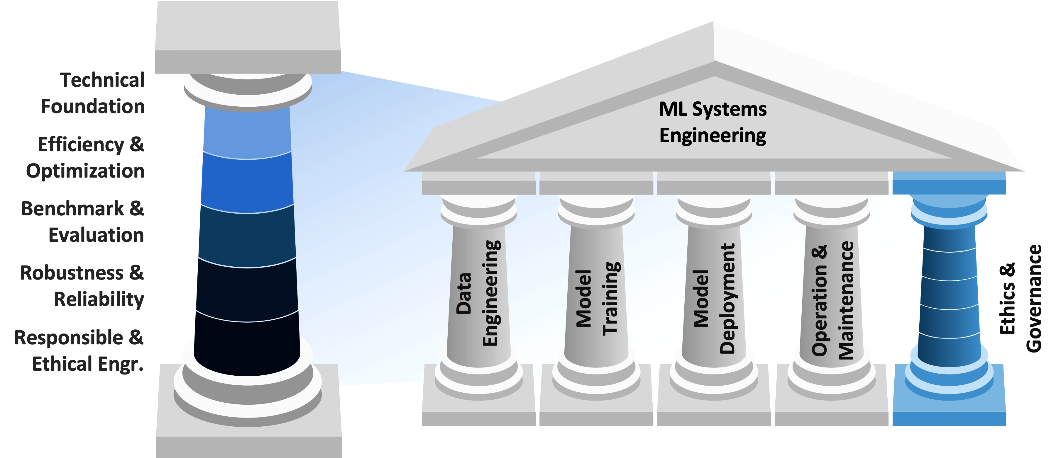
The five engineering disciplines
The pillars are easiest to understand through a failure chain. Suppose a wake-word model stops working reliably for users in a noisy apartment building after a model update. The first question is whether the training data captured that acoustic environment, whether labels were reliable, and whether the pipeline can trace which examples reached the model. That is the Data Engineering pillar (Data Engineering): it owns the data-quality, scale, privacy, drift, and lineage problems that determine what the model can learn.
If the data is sound, the next question is whether the training process converted it into a model that fits the task and budget. The Training Systems pillar (Model Training) owns that boundary: coordinating datasets, frameworks, optimization algorithms, hyperparameters, distributed jobs, restarts, and the cost-quality trade-offs created by model scale. A model that trains successfully is still not a system. The Deployment Infrastructure pillar owns the training-serving divide: model packaging, inference performance, latency, throughput, device constraints, and the benchmarking methods that reveal whether the deployed artifact still meets the requirement.
Once the model is serving, failure becomes temporal. The Operations and Monitoring pillar owns the question of whether behavior remains acceptable after launch, when data distributions shift, traffic changes, and model quality can degrade while infrastructure dashboards stay green. It connects monitoring, alerting, rollout strategy, incident response, and continuous evaluation. Finally, the wake-word failure may not affect all users equally, and the audio pipeline may raise consent or privacy obligations. The Ethics and Governance pillar (Responsible Engineering) owns those constraints: fairness, transparency, privacy, safety, documentation, and accountability throughout the lifecycle.
Alternative organizational frameworks could group these concerns by component or lifecycle phase. The five-pillar structure was chosen because it matches the ownership boundaries that appear in real engineering teams while still making their interdependence explicit. Data choices shape training outcomes; training choices constrain deployment; deployment choices determine what operations can observe; and governance requirements can change all four. Treating responsible engineering as its own pillar prevents it from becoming an implicit afterthought under deadline pressure.
The five pillars do not operate in isolation; they emerge from the D·A·M taxonomy and lifecycle stages established earlier, with each pillar responsible for specific axes and their interactions across the system lifecycle. This structure reflects how AI evolved from algorithm-centric research to systems-centric engineering, shifting focus from making individual algorithms work to building systems that reliably deploy, operate, and maintain those algorithms at scale. The five pillars represent the engineering capabilities required for that transition.
These pillars also provide the organizational backbone for this textbook. Each part of the book develops the knowledge and skills needed for one or more pillars, following a progression that mirrors how engineers build systems in practice: foundations first, then model construction, then optimization, and finally production deployment.
Self-Check: Question
Production ML failures chain across data quality, model behavior, serving infrastructure, and governance, so the framework assigns each challenge category to a named engineering discipline. Which of the following is one of the five pillars the framework names?
- Kernel Scheduling
- Compiler Construction
- Operations and Monitoring
- Symbolic Reasoning
Why does the framework make Ethics and Governance its own explicit pillar rather than expecting the other four pillars to absorb fairness, privacy, and accountability work implicitly? Use a concrete example to ground your answer.
A team is designing drift-detection alarms on production input distributions, writing incident-response procedures for subgroup accuracy drops, and building dashboards that combine infrastructure health, model performance, data quality, and prediction distributions. Which pillar is primarily responsible for this work?
- Data Engineering
- Training Systems
- Deployment Infrastructure
- Operations and Monitoring
Book Organization
The five pillars map directly onto this textbook’s four-part structure, which progresses from foundational concepts through model development to production deployment. The organizing principle is context before theory: the landscape and vocabulary are established (Part I) before building models (Part II), optimizing those models (Part III), and deploying them reliably (Part IV). Table 9 outlines this organization.`
Part I establishes the constraint vocabulary before model machinery appears. Section 1 develops the engineering revolution in AI and the frameworks that organize this discipline. ML Systems explores the deployment spectrum from Cloud to TinyML, examining how physical constraints (power envelopes, memory hierarchies, and latency budgets) govern each tier. ML Workflow presents the end-to-end process from problem formulation through deployment, providing the conceptual map that guides subsequent learning. Data Engineering addresses data collection, processing, and management, establishing that data infrastructure precedes and enables model development.
| Part | Theme | Key Chapters |
|---|---|---|
| I: Foundations | Context: ML systems landscape | section 1, ML Systems, ML Workflow, Data Engineering |
| II: Build | Theory: Model fundamentals | Neural Computation, Network Architectures, ML Frameworks, Model Training |
| III: Optimize | Efficiency: Performance tuning | Data Selection, Model Compression, Hardware Acceleration, Benchmarking |
| IV: Deploy | Production: Real-world systems | Model Serving, ML Operations, Responsible Engineering, Conclusion |
Part II turns that vocabulary into model construction skills. Neural Computation provides algorithmic foundations, while Network Architectures extends these to specific network designs. Both chapters reference the five Lighthouse Models introduced earlier (ResNet-50, GPT-2/Llama, MobileNetV2, DLRM, and Keyword Spotting) to anchor abstract concepts in concrete workloads. ML Frameworks examines the software infrastructure from TensorFlow and PyTorch to specialized tools. Model Training develops training systems for complex models and large datasets.
Part III asks how to change the terms of the iron law without losing quality. Data Selection introduces techniques for reducing computational requirements while maintaining quality. Model Compression covers model-reduction techniques that make deployment cheaper. Hardware Acceleration examines specialized hardware from GPUs to custom ASICs. Benchmarking establishes methodologies for measuring and comparing system performance.
Part IV returns optimized systems to production, where degradation and deployment context dominate. Model Serving covers infrastructure for delivering predictions with low latency. ML Operations encompasses practices from monitoring and deployment to incident response. Responsible Engineering addresses ethical considerations and governance. Conclusion synthesizes the complete methodology and prepares the reader for the transition from single-node mastery to fleet-scale orchestration.
This book covers the single-node regime: 1–8 accelerators connected by shared memory, where the binding constraint is the memory wall, the rate at which data moves from HBM (accelerator-local high-bandwidth memory) to compute units. At fleet scale, thousands of nodes coordinate across network fabrics and the bottleneck shifts toward bisection bandwidth, the aggregate capacity across a cut through the cluster network. For detailed guidance on reading paths, learning outcomes, prerequisites, and how to get the most from this textbook, the front-of-book About This Book chapter provides the orientation.
Before moving forward, we examine the assumptions that trip up practitioners new to ML systems. The preceding frameworks provide the right mental models, but only if we also shed the wrong ones carried over from adjacent fields. Every discipline accumulates intuitions that work within its boundaries but fail when applied elsewhere. ML systems engineering is particularly vulnerable to such imported assumptions because it draws from software engineering, statistics, and hardware design simultaneously, each of which cultivates subtly different intuitions about how systems should behave.
Self-Check: Question
Order the book’s four parts as the chapter presents them: (1) Deploy, (2) Foundations, (3) Optimize, (4) Build.
Why does the chapter argue for teaching context before theory in this textbook, and how does the single-node scope of this foundation set up the distributed-fleet regime? Use one concrete example of a Part III technique whose meaning depends on Part I context.
Fallacies and Pitfalls
Assumptions that hold in traditional software, academic research, or pure mathematics fail when applied to systems whose behavior emerges from data. The following fallacies and pitfalls capture errors that waste engineering effort, delay deployments, and cause silent production failures.
Fallacy: Better algorithms automatically produce better systems.
Engineers assume algorithmic sophistication drives system performance, but this ignores the iron law (section 1.6). Vision transformers demonstrate that architecture and large-scale pretraining can produce strong image-recognition results (Dosovitskiy et al. 2021), but production utility still depends on compute, memory movement, and latency budgets. In production, a model that is 1 percent more accurate but violates latency requirements has effectively zero utility. The hidden-technical-debt example earlier in this chapter shows why model code is only the visible center of a much larger production system. A well-engineered system with a simpler model can outperform a more sophisticated architecture lacking robust infrastructure.
Dosovitskiy, Alexey, Lucas Beyer, Alexander Kolesnikov, Dirk Weissenborn, Xiaohua Zhai, Thomas Unterthiner, Mostafa Dehghani, et al. 2021. “An Image Is Worth 16x16 Words: Transformers for Image Recognition at Scale.” International Conference on Learning Representations.
Pitfall: Treating ML systems as traditional software that happens to include a model.
Engineers apply traditional testing and deployment practices to ML systems, but these systems fail in qualitatively different ways (section 1.5). Traditional bugs often produce immediate failures; ML systems can silently degrade over weeks or months before anyone notices. A/B tests in conventional software may show clear signals quickly, while ML comparisons can require longer observation windows to detect small accuracy differences across subpopulations. Unit tests verify deterministic paths; ML systems require monitoring infrastructure to catch unreliable predictions, data drift, and calibration failures. Teams deploying ML with only CI/CD pipelines risk silent failures that surface only after user-facing behavior has already degraded.
Fallacy: High accuracy on benchmark datasets indicates production readiness.
Engineers assume benchmark performance predicts production accuracy, but distribution shift and operational differences can cause substantial degradation in deployment. A sentiment analysis model that performs well on curated test data may fall sharply in production as users employ slang, emojis, and context absent from benchmarks. The deployment spectrum (section 1.9.2) shows that cloud, edge, and mobile environments each introduce distinct constraints: network latency adds overhead, mobile devices’ limited numerical precision can alter accuracy, and edge devices may lack the memory for multi-model strategies that boosted benchmark scores. Production systems require failure mode analysis across demographic subgroups, monitoring infrastructure to detect drift, and validation protocols that match actual operating conditions rather than idealized test sets.
Pitfall: Optimizing individual components without considering system interactions.
Engineers optimize inference latency in isolation, but Amdahl’s Law governs end-to-end performance. A team reduces model inference from 45 ms to 15 ms, expecting proportional improvement. Yet preprocessing consumes 60 ms and postprocessing adds 25 ms, so total latency drops only from 130 ms to 100 ms: 23 percent improvement rather than the expected 67 percent. The D·A·M taxonomy (table 4) shows that the Data, Algorithm, and Machine axes form an interdependent system where optimizing one component shifts bottlenecks rather than eliminating them. A model requiring 3\(\times\) more preprocessing can increase total cost 40 percent while improving accuracy only 2 percent. Teams optimizing components independently often find 50–70 percent of their engineering effort fails to improve end-to-end metrics.

Optimizing only inference leaves end-to-end latency mostly intact.
Fallacy: ML systems can be deployed once and left to run indefinitely.
Engineers assume deployed systems maintain performance indefinitely, but the degradation equation in equation 3 quantifies why ML systems decay. A recommendation system deployed at 85 percent accuracy drops to 80.2 percent within 6 months as purchasing patterns shift, losing 4.8 percentage points without any code changes. The ML development lifecycle (section 1.9.1) shows continuous monitoring and retraining as operational requirements. Fraud-detection and NLP systems face the same pattern: attackers adapt, vocabulary shifts, and user behavior changes while the code remains unchanged. Without monitoring, systems can appear healthy while prediction quality erodes. Organizations treating deployment as one-time often discover failures only after customer complaints or downstream metrics reveal the degradation.
Pitfall: Assuming that ML expertise alone is sufficient for ML systems engineering.
Organizations hire ML researchers expecting production-ready systems, but the five engineering disciplines (section 1.11.1) require integrated expertise across algorithms, software, systems, and operations. Teams with strong ML skills but limited systems experience can miss throughput targets because API design, storage layout, and serving infrastructure shape realized performance. Conversely, software infrastructure built without ML awareness can introduce preprocessing or feature bugs that degrade model behavior without obvious system failures. Deployment case studies show that production ML requires coordinated attention to data, models, infrastructure, and organizational workflow, not algorithmic quality alone (Paleyes et al. 2022). Effective teams integrate ML researchers, software engineers, and operations specialists rather than expecting one role to master all skills. The summary pulls these failures back to the chapter’s central claim: ML systems engineering exists because learned behavior, physical infrastructure, and organizational workflow must be designed together.
Paleyes, Andrei, Raoul-Gabriel Urma, and Neil D. Lawrence. 2022. “Challenges in Deploying Machine Learning: A Survey of Case Studies.” ACM Computing Surveys 55 (6): 1–29. https://doi.org/10.1145/3533378.
Self-Check: Question
True or False: A model that is state-of-the-art on an ImageNet benchmark is usually production-ready unless major bugs remain in the serving code.
A team cuts model inference from 45 ms to 15 ms (a 3× local speedup), but preprocessing consumes 60 ms and postprocessing adds 25 ms. Total latency drops from 130 ms to 100 ms—a 23 percent end-to-end improvement rather than the naive 67 percent the 3× speedup suggested. Which principle explains this gap?
- The bitter lesson, because compute-scaling always dominates
- Amdahl’s Law applied to the full inference pipeline
- The verification invariant, because test sets cannot certify production latency
- Data-centric computing, because preprocessing is part of the data pipeline
Why is it a mistake to assume ML expertise alone is sufficient for ML systems engineering? Ground your answer in two concrete failure modes the chapter describes.
Which scenario most directly illustrates the fallacy that ML systems can be deployed once and left alone indefinitely?
- A recommendation model keeps serving responses, but its accuracy falls steadily from 85 percent to about 80 percent over six months as user purchasing patterns shift
- A server crashes immediately after a faulty release and the on-call engineer rolls back within minutes
- A compiler emits a syntax error during build and the CI pipeline blocks the merge
- A database replica lags during a failover drill and the team extends the replication window
How does the D·A·M perspective help prevent the pitfall of optimizing individual components in isolation? Use the 45 ms→15 ms inference example to illustrate where effort should go instead.
Summary
This introduction has established the conceptual foundation for everything that follows. The chapter began with the AI moment and the Software 2.0 shift: ML systems differ from traditional software because their behavior is learned from data and can fail silently as distributions change. It then traced AI’s paradigm history and the bitter lesson, showing why progress repeatedly came from systems that could exploit more computation rather than from hand-coded expertise. The chapter formalized ML systems through the D·A·M taxonomy, then introduced the degradation equation, the iron law, and the energy and efficiency frameworks as quantitative lenses for diagnosis.
With those tools in place, the chapter defined AI engineering as the discipline of engineering stochastic systems to deterministic reliability targets, jointly satisfying the three D·A·M constraints across computational platforms. It then mapped the ML development lifecycle, deployment spectrum, and production case studies from cloud training to TinyML, showing why continuous iteration and context-aware design are mandatory rather than optional. The five Lighthouse Models introduced here (ResNet-50, GPT-2/Llama, MobileNetV2, DLRM, and Keyword Spotting, detailed in Network Architectures) serve as recurring touchstones throughout subsequent chapters, grounding abstract principles in the concrete engineering challenges of real workloads.
The principles and frameworks established in this introduction provide the conceptual vocabulary for everything that follows. They also answer the question posed at the outset: building machine learning systems demands different engineering principles because these systems derive their behavior from data rather than code, degrade silently rather than fail explicitly, and require co-design across algorithms, software, and hardware at every stage. This is the mandate of AI engineering: to tame this stochastic behavior with deterministic reliability. The D·A·M taxonomy offers a systematic lens for analyzing any ML system challenge, while the five Lighthouse Models ground these abstract concepts in concrete engineering problems encountered throughout a practitioner’s career.
Key Takeaways: Constraints drive architecture
- D·A·M bottlenecks migrate, not disappear: Data, Algorithm, and Machine constraints interact, so improving one axis often exposes another. The systems habit is to ask which axis now binds, then choose the intervention that relieves that constraint without creating a larger downstream failure.
- Learned behavior decays silently: Traditional software usually fails when code changes; ML systems can degrade while code and infrastructure stay fixed because the world shifts under the training distribution. The degradation equation turns that drift into retraining triggers rather than surprise accuracy loss.
- The iron law makes latency diagnostic: Data movement, computation, and overhead all spend from the same time budget. Cutting inference from 45 ms to 15 ms gives only 23 percent improvement when preprocessing (60 ms) and postprocessing (25 ms) dominate, so optimize the term that binds end-to-end behavior.
- Scale wins inside physical limits: The bitter lesson explains why general methods with more compute displaced hand-crafted systems, but scale only helps when data, architecture, and machine can support it. Efficiency gains of 44.5× coexisted with roughly 7 orders of compute growth.
- AI engineering is continuous co-design: Deployment context, lifecycle monitoring, and the five engineering pillars are not later add-ons; they are how stochastic learned behavior is held to deterministic reliability targets from cloud training through TinyML operation.
Everything this chapter has introduced points to one claim the rest of the book will not let go of: a machine learning system is governed by physics, not by intention. Traditional software does what it is written to do; a machine learning system does what its data, its arithmetic, and its hardware permit, and those three rarely agree with the programmer’s hopes. The bitter lesson, the iron law, the degradation equation, and the D·A·M taxonomy are not separate facts to memorize but a single vocabulary for that shift, a way to reason about behavior that is grown rather than coded and that decays unless it is maintained. To engineer such a system is to treat its constraints as the real specification, and that is what turns a collection of techniques into a discipline.
What’s Next: From vision to architecture
Where should an ML model actually run? Physical laws dictate what is possible. The speed of light makes distant cloud servers useless for emergency braking. Thermodynamics prevents data-center-class models from running on a mobile device. Memory physics creates bandwidth ceilings that faster chips cannot overcome. The four deployment paradigms are where those laws land: ML Systems derives each paradigm’s operating envelope from the physics and develops the decision framework for choosing among them when requirements conflict.
Self-Check: Question
Which pair of quantitative frameworks does the chapter identify as the main tools for reasoning about ML systems performance and reliability over time?
- The iron law of ML systems and the degradation equation
- A/B testing and static type checking
- Backpropagation and gradient descent
- The Turing test and the Lighthill report
A deployed GPT-2-style chat model misses its 200 ms p99 latency target, its live input distribution is drifting, and the team is debating whether to (a) buy faster accelerators or (b) retrain on fresher data. Using D·A·M, the iron law, and the degradation equation together, walk through how the team should approach the decision.
Self-Check Answers
Self-Check: Answer
In Karpathy’s Software 2.0 framing used here, which component plays the role that hand-written source code plays in Software 1.0?
- The training dataset and labels, which SGD compiles into model weights
- The GPU driver stack that dispatches work to the accelerator
- The serving endpoints that expose model predictions to clients
- The evaluation dashboards that track offline benchmark scores
Answer: The correct answer is A. In the Software 2.0 framing the dataset defines the behavior that the training loop (the compiler) translates into weights (the binary executable); the programmer’s job shifts from writing logic to curating the data that encodes it. The driver-stack answer confuses low-level dispatch plumbing with the artifact that defines behavior—swapping drivers leaves the learned logic unchanged. The serving-endpoint and dashboard answers describe delivery and observability layers: they matter operationally but do not encode the model’s learned behavior.
Learning Objective: Map Software 1.0 components onto their Software 2.0 counterparts by identifying which artifact encodes system behavior.
A 224×224 RGB image with 8-bit color has \(256^{224 \times 224 \times 3}\) possible configurations—roughly \(10^{362{,}000}\)—so even ImageNet’s 50,000 test images cover an astronomically small slice of the input space. This structural mismatch between benchmark coverage and the true input space is what the chapter calls the ____.
Answer: verification invariant. It denotes the provable impossibility of certifying ML behavior by exhaustive testing: because the input space is orders of magnitude larger than any benchmark can sample, guaranteed correctness must be replaced by statistical monitoring and reliability bounds in production.
Learning Objective: Infer the chapter’s term for the structural mismatch between benchmark coverage and the astronomically large ML input space, and connect it to the shift from predeployment certification to continuous monitoring.
A team adds 50,000 new labeled edge cases to a spam classifier’s training set. The Python training script, model architecture, and hyperparameters are unchanged, yet the deployed model begins labeling different messages as spam. Explain why this behavior change is expected under the data-centric paradigm shift and name two engineering practices that must change to accommodate it.
Answer: In Software 2.0 the dataset is the source code, and the training loop compiles data into weights; changing the corpus changes the compiled artifact even when the Python script is byte-identical. Adding 50,000 labeled edge cases shifts the optimizer’s loss surface and therefore the decision boundary, so different borderline messages land on different sides of it. Two practices must change: (1) version control must treat datasets as first-class artifacts with reproducible snapshots and hashes, not just git commits; and (2) regression testing must validate data distributions and model-behavior deltas on frozen eval sets, since unit tests of Python code can all pass while the learned boundary moves. The practical consequence is that dataset changes are deployments.
Learning Objective: Explain why dataset changes produce behavior changes under Software 2.0 and identify the engineering practices (versioning and regression testing of data) that must be adopted in response.
An engineering team argues that because images are discrete 8-bit pixel arrays, building a sufficiently large test set should eventually certify a classifier’s correctness. Given the astronomical size of the 224×224 RGB input space, which conclusion is the most important engineering consequence?
- Image inputs should be treated as continuous rather than discrete for modeling purposes
- Benchmark datasets should be shrunk to simplify reliability analysis
- Guaranteed correctness must be replaced by statistical monitoring and reliability bounds in production
- Stochastic training methods should be replaced with deterministic compilers
Answer: The correct answer is C. The \(256^{224 \times 224 \times 3}\) input space is finite but orders of magnitude beyond any reachable test set, so no benchmark can certify behavior the way unit tests certify deterministic code—continuous monitoring of live distributions and reliability bounds replaces exhaustive verification. The continuous-vs-discrete reframing does not change the sampling math. Shrinking the benchmark makes coverage worse, not better. Swapping stochastic training for a deterministic compiler does not shrink the input space that must be certified, so it does not address the verification invariant.
Learning Objective: Analyze why ML deployment requires observability and reliability bounds instead of exhaustive predeployment verification.
True or False: Because image pixels are discrete integers, a 224×224 RGB classifier’s input space is small enough that a sufficiently well-funded test-set construction project could, in principle, provide exhaustive coverage.
Answer: False. Discreteness does not tame the combinatorics: \(256^{224 \times 224 \times 3} \approx 10^{362{,}000}\) possible images dwarfs the number of atoms in the observable universe (\(\sim 10^{80}\)), so no physically realizable test set can exhaustively cover even this single input modality.
Learning Objective: Reject the misconception that discreteness implies tractable exhaustive testing for high-dimensional ML input spaces.
Self-Check: Answer
Order the following AI paradigms from earliest to latest as the section presents them: (1) Statistical learning, (2) Deep learning, (3) Symbolic AI, (4) Expert systems.
Answer: The correct order is: (3) Symbolic AI, (4) Expert systems, (1) Statistical learning, (2) Deep learning. Symbolic AI came first (1950s–1970s) with hand-written logic like STUDENT; expert systems followed (1980s) by encoding domain rules like MYCIN; statistical learning (1990s) replaced explicit rules with probability estimates learned from data but still required manual feature engineering; deep learning (2012+) automated feature learning. Swapping the last two would erase the section’s key point that deep learning’s breakthrough was specifically the removal of the feature-engineering bottleneck introduced by statistical methods.
Learning Objective: Sequence the four AI paradigms in their historical order and identify the bottleneck each successor removed.
Which pairing between AI era and its characteristic bottleneck is correct?
- Symbolic AI → compute bottleneck (rules ran too slowly on contemporary hardware)
- Expert systems → knowledge acquisition bottleneck (extracting and maintaining human expertise as rules did not scale)
- Statistical learning → memory-capacity bottleneck (storing probability tables exceeded available RAM)
- Deep learning → logic bottleneck (neural networks could not express enough formal rules)
Answer: The correct answer is B. Expert systems like MYCIN hit the knowledge acquisition bottleneck: knowledge elicitation consumed 70–80 percent of project time, roughly 60 percent of projects failed outright, and the bandwidth of human experts—not hardware—was the binding constraint. A compute-bottleneck framing for symbolic AI misses that the limit was representational: rules could not capture real-world ambiguity regardless of speed. A memory-capacity framing for statistical learning mislabels the era whose limit was human ingenuity in feature design, not RAM. A logic-bottleneck framing for deep learning inverts the section’s claim that deep learning succeeded precisely because it abandoned formal logic for representation learning.
Learning Objective: Match each AI paradigm to the specific bottleneck that constrained it.
The section describes both AI winters (1974–1980 and 1987–1993) as systems failures rather than purely algorithmic failures. Explain what this characterization means by referring to the Lisp Machine collapse and the compute-mismatch pattern.
Answer: AI winters are systems failures because the dominant paradigms hit hardware, economic, or scaling limits before their underlying ideas were exhausted—the mathematics was often sound, but the infrastructure could not support the algorithms’ ambitions. The second winter’s trigger, the collapse of the Lisp Machine market around 1987, illustrates this directly: cheaper general-purpose workstations undercut specialized AI hardware, so algorithms with workable ideas became economically and operationally untenable. The same compute-mismatch pattern drove neural networks underground from 1969 to 1986, when backpropagation revival awaited hardware that could train non-trivial networks in reasonable time. The engineering lesson is that AI progress depends on matching algorithmic demands to feasible compute platforms, not on algorithms alone.
Learning Objective: Explain how infrastructure and hardware-economics constraints contributed to historical reversals in AI progress.
AlexNet’s 2012 breakthrough reduced ImageNet top-5 error from 26.2 to 15.3 percent, yet Krizhevsky’s team had to split the convolutional layers across two GTX 580 GPUs because a single GPU’s memory could not hold the full model. What engineering point does this split architecture make most forcefully?
- Deep convolutional networks still depended primarily on hand-engineered visual features to work
- The 2012 breakthrough was an example of systems co-design, where model structure was explicitly shaped by hardware memory limits
- Expert systems became practical again once consumer GPUs were available
- Deep learning succeeded because training finally became deterministic
Answer: The correct answer is B. The two-GPU split was not a modeling choice but a hardware-imposed constraint: AlexNet’s architecture was directly shaped by the memory ceiling of a single GTX 580, making the model a textbook case of co-designing algorithm and machine. A hand-engineered-features reading points backward to the statistical-learning era that deep learning superseded. An expert-systems-revival claim contradicts the section’s timeline. A determinism claim misidentifies the mechanism: stochastic gradient descent remained stochastic, but GPU throughput and hardware-algorithm alignment made it practical at scale.
Learning Objective: Analyze how hardware memory constraints shaped a landmark deep learning architecture.
A modern team has a well-understood statistical model, but engineers spend three months designing preprocessing stages (SIFT-style descriptors, histograms, and hand-tuned normalizations) before the model can be trained at all. Which historical bottleneck does this most closely resemble?
- The feature engineering bottleneck of the statistical learning era
- The knowledge acquisition bottleneck of expert systems
- The infrastructure bottleneck that enabled deep learning
- The logic bottleneck of symbolic AI
Answer: The correct answer is A. The signature of the statistical-learning era was that learning algorithms worked robustly, but only after humans manually transformed raw inputs into usable features—the Viola-Jones cascade and SIFT/HOG pipelines are the canonical examples, and the team’s three months of manual pipeline design recapitulates them exactly. A knowledge-acquisition framing would match the MYCIN pattern of extracting IF-THEN rules from domain experts, which is a different failure mode. The infrastructure-bottleneck answer describes what deep learning overcame, not what the team is experiencing. A logic-bottleneck framing would apply to systems that failed on ambiguous inputs, not to a pipeline being slowed by feature design.
Learning Objective: Classify a modern engineering problem using the historical bottleneck framework.
Across the four paradigms—symbolic AI, expert systems, statistical learning, and deep learning—identify the recurring pattern that supports the claim that systems innovation rather than algorithmic novelty alone drove progress. Use GPT-3’s scale (roughly 175 billion parameters trained on about 300 billion tokens) to illustrate where the bottleneck has moved next.
Answer: Each paradigm advanced specifically when a binding scaling bottleneck was removed: explicit rules gave way to learned statistics when data volume made it viable, manual features gave way to representation learning when GPUs made it tractable, and deep models became useful when infrastructure could feed and train them. GPT-3 then pushed the bottleneck further into infrastructure: training on a 300-billion-token corpus required an estimated zettaFLOPs of compute, corresponding to hundreds of GPU-years, so the binding challenge became coordinating large-scale distributed training without failure rather than inventing new learning rules. The engineering consequence is that investment should target the current binding constraint—whether that is memory bandwidth, the network capacity between machines, or dataset curation—rather than assuming better algorithms alone will unlock the next jump.
Learning Objective: Synthesize how historical AI progress repeatedly followed bottleneck removal rather than isolated algorithmic cleverness, and identify where the binding constraint has moved in the foundation-model era.
Self-Check: Answer
What is the core claim of Sutton’s bitter lesson as presented in this section?
- Encoded human domain knowledge scales better than general-purpose learning methods over seven decades of AI research
- General methods that can absorb more computation eventually outperform approaches built around hand-crafted human expertise
- The best AI systems avoid large datasets because computation is too expensive
- Distributed systems matter only after a model has already achieved superhuman accuracy
Answer: The correct answer is B. Sutton’s 70-year bitter-lesson thesis is that methods that exploit increasing computation win over hand-crafted expertise in the long run—the “bitter” framing expresses that this is what the evidence shows, not what researchers hoped for. A human-knowledge-scales-better claim exactly inverts the thesis, which is why it is the strongest distractor. A compute-avoidance framing contradicts the energy and infrastructure story the section tells. A “distributed systems matter only after” claim misstates causality: distributed systems are the mechanism that makes scale possible, not an afterthought.
Learning Objective: Identify the central claim of Sutton’s bitter lesson and distinguish it from its opposite.
True or False: The section argues that the improvements from expert systems (roughly 2,000 Elo on chess) to modern foundation models (86.4 percent on MMLU) came mainly from encoding more detailed human strategies.
Answer: False. The section’s table shows that as approaches shifted from hand-crafted rules to end-to-end neural networks to transformers, computational resources grew from “minimal rule evaluation” to a public-estimate regime of millions of A100 GPU-days—Sutton’s point is that gains came from scaling compute and data, not from richer expert encodings.
Learning Objective: Distinguish computation-driven progress from expertise-encoding explanations of AI improvement.
Why is the lesson described as “bitter” for researchers or engineers who prefer domain-specific insight? Use AlphaGo Zero’s 4-TPU, three-day run that beat the expert-seeded AlphaGo 100–0 to anchor your answer.
Answer: It is bitter because it implies that carefully encoded human theories and heuristics are a depreciating asset: decades of Go opening theory lost to a system that learned purely from self-play using four TPUs for three days, then beat its own expert-seeded predecessor 100–0. The same pattern appeared with Deep Blue winning through 200 million positions per second on 480 custom chess processors rather than by reproducing grandmaster strategy. The engineering consequence is that durable advantage shifts toward infrastructure that can support larger-scale general methods—data pipelines, accelerators, and the software stack that feeds them—rather than toward encoded expertise that will be overtaken by the next generation of scaled compute.
Learning Objective: Explain why the bitter lesson challenges human-centered intuitions about AI design and identify the assets whose value rises in its place.
Which example most directly supports the section’s claim that raw computational scale can substitute for hand-crafted expertise?
- Deep Blue evaluating 200 million chess positions per second on 480 custom chess processors in 1997
- A rule-based medical diagnosis system adding more expert-written IF-THEN rules to improve coverage
- The Viola-Jones face detector depending on hand-engineered rectangular features and a classifier cascade
- A team choosing a smaller benchmark dataset to simplify testing and analysis
Answer: The correct answer is A. Deep Blue won precisely by applying massive search on purpose-built silicon rather than by encoding human chess understanding—the 480-processor, 200-million-positions-per-second architecture is the canonical example of computation substituting for expertise. A rule-adding medical system and the Viola-Jones hand-engineered-features example belong to exactly the expertise-driven paradigms the bitter lesson says general compute-scaling surpasses. Shrinking a benchmark has no relationship to the scaling thesis.
Learning Objective: Map a historical AI success to the computation-scaling principle in the bitter lesson.
A lab can spend its next budget cycle on (a) hiring domain experts to encode more handcrafted rules into its existing pipeline or (b) expanding GPU capacity and data pipelines to train a larger general model. Using the bitter lesson, explain how the lab should think about the choice and what the estimated 1,287 MWh training energy of GPT-3 implies about hidden costs of option (b).
Answer: The bitter lesson favors investments that let general methods absorb more compute: seven decades of evidence, from Deep Blue through AlphaGo to GPT-scale systems, show that scaling beats encoded expertise over time, so option (b) is the one with longer-term compounding returns. However, the hidden cost is that at GPT-3 scale a single training run consumes roughly 1,287 MWh—the annual electricity of about 120 US households—and that energy is dominated by data movement through the memory hierarchy rather than by arithmetic. Under the chapter’s energy constants, moving one off-chip DRAM byte costs about 145× one FP16 operation and about 800× one INT8 operation. The practical implication is that infrastructure investment should target data-movement efficiency (memory hierarchy, bandwidth, interconnects) alongside peak FLOP/s, because scaling without that discipline makes the energy and cost curves unaffordable.
Learning Objective: Apply the bitter lesson to evaluate competing investments in expertise encoding versus scalable infrastructure, and reason about the energy-cost structure of scaled training.
Self-Check: Answer
Which description best matches the chapter’s definition of a machine learning system?
- A software artifact whose behavior is fixed once programmers finish writing explicit rules
- A software system whose core behavior is determined by parameters learned from data, making performance jointly dependent on data quality, algorithm choice, and hardware capacity
- Any distributed application that serves responses in under 100 ms
- Any statistical model trained on a labeled dataset, regardless of deployment
Answer: The correct answer is B. The definition foregrounds learned parameters as the source of behavior and the simultaneous dependence on Data, Algorithm, and Machine axes—the D·A·M triad. A rule-based framing describes Software 1.0, not ML. A latency-threshold definition is arbitrary: a spam filter hitting 50 ms and a batch training job running for days are both ML systems. A bare-trained-model framing is too narrow because the chapter explicitly distinguishes the full system (data pipelines, serving infrastructure, monitoring) from the model alone—Google found model code is roughly 5 percent of production ML code.
Learning Objective: Distinguish a full ML system from rule-based software, from a latency threshold, and from an isolated trained model.
When a team asks which of Data, Algorithm, or Machine is the binding constraint on performance before choosing what to optimize, they are applying the three-axis diagnostic framework the chapter formalizes as the ____ taxonomy.
Answer: D·A·M. Its diagnostic power comes from forcing the engineer to identify the binding axis before investing: Data bottlenecks (volume, bandwidth) yield to pipeline and storage fixes, Algorithm bottlenecks (operation count, architecture) yield to model changes, and Machine bottlenecks (peak throughput, memory capacity) yield to hardware or utilization work—and picking the wrong axis wastes effort while the real bottleneck persists.
Learning Objective: Infer the named three-axis framework used to classify ML system bottlenecks and explain why identifying the binding axis precedes optimization.
A production spam filter starts missing a new phishing campaign even though its serving latency stays normal; separately, during a traffic spike the same service falls behind and cannot classify messages quickly enough. Using the D·A·M taxonomy, diagnose which axis is binding in each situation and name one intervention per situation that attacks that axis directly.
Answer: The missed phishing campaign is a Data-axis bottleneck: the training set never contained the new tactic, so no algorithm or hardware change can supply the missing signal. The direct intervention is collecting and labeling examples of the new campaign and retraining. The traffic-spike failure is a Machine-axis bottleneck: the data and model are adequate, but serving capacity cannot keep up with demand. The direct intervention is adding serving capacity or making each prediction cheaper to execute. If instead the examples were adequate but the model could not express the pattern, the binding axis would be Algorithm, and the intervention would be a more expressive model structure. The D·A·M lens matters because the three fixes are completely different investments: applying the wrong one (for example, buying hardware to fix a missing-data problem) leaves the real bottleneck untouched while consuming budget.
Learning Objective: Apply the D·A·M taxonomy to diagnose which axis binds in concrete production failures and match each axis to the intervention that addresses it.
In the four-layer engineering crux hierarchy (Hardware, Systems, Workloads, Missions), which layer introduces application-specific end-use requirements such as “one-year battery life on a coin-cell” for a smart doorbell?
- Hardware, because battery life is ultimately determined by silicon power characteristics
- Systems, because deployment envelopes set the thermal and power budgets
- Workloads, because a longer-running model necessarily implies a larger operation count
- Missions, because this is where application-level requirements enter and propagate downward
Answer: The correct answer is D. Missions sit at the top of the hierarchy and carry end-use constraints—battery life, safety, latency, cost—that flow downward and reshape every layer below them: the Smart Doorbell’s one-year-battery mission forces Wake Vision as the workload, the Sub-Watt Sensor Node as the system archetype, and a microcontroller-class hardware twin underneath. A Hardware-starting framing reverses the section’s explicit claim that missions drive the stack. A Systems-level answer confuses the envelope that implements the requirement with the requirement itself. A Workloads-level answer conflates the model’s operation count with the application-level battery-life goal.
Learning Objective: Identify where application-level requirements enter the four-layer engineering crux and propagate through the stack.
Order the layers of the engineering crux from the lowest physical layer to the highest application layer: (1) Missions, (2) Hardware, (3) Workloads, (4) Systems.
Answer: The correct order is: (2) Hardware, (4) Systems, (3) Workloads, (1) Missions. Hardware defines raw physical capability (\(R_{\text{peak}}\), \(\text{BW}\), memory capacity); Systems wrap that silicon into deployable platforms with power and thermal envelopes; Workloads impose algorithmic demand (\(O\), \(D_{\text{vol}}\), data layout) on those platforms; Missions at the top supply end-use requirements that flow downward. Reversing Systems and Hardware would imply that deployment envelopes exist independently of the silicon they inherit—but the Sub-Watt Sensor Node cannot exist without the microcontroller underneath it. Reversing Workloads and Missions would put algorithms above application requirements, inverting the book’s mission-driven design philosophy.
Learning Objective: Sequence the four layers that connect silicon constraints upward to end-user ML missions and justify why each layer inherits from the one below.
Self-Check: Answer
The section illustrates the ML vs. traditional software distinction with an autonomous-vehicle perception system whose pedestrian-detection accuracy drifts from 95 percent to 85 percent over several months while conventional error logging stays silent. Which statement best captures the distinction this example highlights?
- ML systems are usually written in Python while traditional software is not
- Traditional software has no performance constraints while ML systems do
- ML systems can continue operating while prediction quality silently degrades as data distributions shift, whereas traditional software failures are typically explicit and observable
- Traditional software cannot be monitored in production
Answer: The correct answer is C. The pedestrian-detection drift is silent: code executes, logs stay green, alerts stay off—yet the system becomes measurably less safe as seasonal distribution shift accumulates. This failure-mode asymmetry is the defining distinction. A programming-language framing confuses implementation detail with behavior; Python is used in both modalities. A performance-constraint framing is false for both sides: traditional software has SLAs too. A monitoring-impossibility framing is trivially incorrect and would make production ML inconceivable.
Learning Objective: Distinguish the dominant failure mode of ML systems (silent distribution-shift-driven degradation) from that of traditional software (explicit, observable failure).
The degradation equation \(\text{Accuracy}(t) \approx \text{Accuracy}_0 - \lambda \cdot \mathcal{D}(P_t \lVert P_0)\) identifies three control levers. Name each lever, describe how an engineering team would act on it, and explain how the levers together convert silent degradation into a manageable operational problem.
Answer: Lever 1 is initial accuracy \(\text{Accuracy}_0\): act on it with better training procedures, richer datasets, and stronger architectures; this shifts the whole accuracy curve upward but does not change its slope. Lever 2 is sensitivity to distribution shift \(\lambda\): act on it with robust training, domain adaptation, data augmentation, and broader training distributions; this flattens the slope so the same amount of drift causes less accuracy loss. Lever 3 is measured drift \(\mathcal{D}(P_t \lVert P_0)\): act on it with continuous distribution-divergence monitoring (KL divergence, total variation distance, Wasserstein distance) and retraining triggered when \(\mathcal{D} > \tau\). Together the levers turn silent decay into three measurable engineering surfaces: the starting point, the slope, and the trigger—so operations can set retraining policies, service-level objectives on model quality, and alerting that catches failure before users do.
Learning Objective: Explain the three control levers in the degradation equation and how combining them operationalizes silent degradation into monitored engineering behavior.
True or False: If no code has changed and the hardware is healthy, a deployed ML system’s accuracy should remain stable.
Answer: False. The degradation equation shows that accuracy tracks \(\mathcal{D}(P_t \lVert P_0)\), the divergence between the live distribution and the training distribution; both can shift with no code change and no hardware fault—the chapter’s worked example shows a recommendation system falling from 85 percent to about 80.2 percent accuracy over six months, a 4.8 percentage-point loss from user-behavior drift alone.
Learning Objective: Reject the misconception that unchanged code and healthy hardware imply unchanged ML behavior.
A deployed recommendation model still returns responses on time, but over three months click-through quality falls steadily as user tastes shift. In the degradation equation \(\text{Accuracy}(t) \approx \text{Accuracy}_0 - \lambda \cdot \mathcal{D}(P_t \lVert P_0)\), which term most directly captures the cause?
- The divergence \(\mathcal{D}(P_t \lVert P_0)\) between the current input distribution and the training distribution
- The initial accuracy \(\text{Accuracy}_0\) at deployment time
- The model’s floating-point precision
- The accelerator’s peak hardware throughput \(R_{\text{peak}}\)
Answer: The correct answer is A. Steady accuracy decay with unchanged code, unchanged weights, and healthy latency points directly at \(\mathcal{D}(P_t \lVert P_0)\)—the world has moved while the model has not. A starting-accuracy term cannot explain time-varying decline because \(\text{Accuracy}_0\) is a constant. A floating-point-precision term appears nowhere in this equation and would affect accuracy uniformly, not as a trend. A peak-throughput term affects \(R_{\text{peak}}\) in the iron law, not the degradation equation, and throughput problems manifest as latency issues, not accuracy decay.
Learning Objective: Apply the degradation equation to identify distribution drift as the direct source of steady accuracy decay in a deployed model.
Why does the chapter argue that knowing when to retrain is as important as knowing how to train? Illustrate with a fraud-detection scenario where the deployed code is flawless.
Answer: Because correctness in ML is not a property of code alone: as the input distribution moves, even a perfectly trained, bug-free model silently drops below operational safety. A fraud-detection model trained on six-month-old attack patterns can keep issuing correctly formatted predictions while attackers mutate their tactics weekly, so false-negative rates climb from 2 percent to 10 percent without a single exception thrown. Uptime dashboards stay green while dollar losses compound. The practical consequence is that retraining triggers based on measured drift (\(\mathcal{D}(P_t \lVert P_0) > \tau\)), subgroup performance monitoring, and rollback-capable deployment pipelines are part of the product—not optional maintenance—because without them the system is blind to its own degradation.
Learning Objective: Justify why retraining policy and drift-driven monitoring are core engineering responsibilities, not operational afterthoughts.
Self-Check: Answer
An engineer doubles an accelerator’s peak FP16 throughput \(R_{\text{peak}}\) while memory bandwidth \(\text{BW}\) and fixed overhead \(L_{\text{lat}}\) stay the same. In the iron law \(T = D_{\text{vol}}/\text{BW} + O/(R_{\text{peak}} \cdot \eta_{\text{hw}}) + L_{\text{lat}}\), which term is most directly improved?
- The data term \(D_{\text{vol}}/\text{BW}\) only
- The compute term \(O/(R_{\text{peak}} \cdot \eta_{\text{hw}})\) only
- The latency term \(L_{\text{lat}}\) only
- All three terms equally
Answer: The correct answer is B. \(R_{\text{peak}}\) sits only in the compute term’s denominator, so doubling it directly halves that term’s contribution when utilization \(\eta_{\text{hw}}\) holds (in practice \(\eta_{\text{hw}}\) may drop if software cannot feed the faster compute, which only deepens the point that \(R_{\text{peak}}\) and realized throughput are different quantities). A data-term answer would require changing bytes moved or bandwidth, neither of which happens here. A latency-term answer misidentifies \(L_{\text{lat}}\) as a function of arithmetic throughput; it is a fixed orchestration overhead. An all-three-equally answer contradicts the iron law’s additive decomposition, whose whole purpose is to let engineers target one term at a time.
Learning Objective: Identify which term of the iron law changes when peak arithmetic throughput increases and distinguish the compute term’s ceiling from the data and latency terms.
A team is weighing whether a 1-percentage-point accuracy gain that requires a 10× increase in operation count \(O\) and 10× larger training clusters is worth the infrastructure bill. The economic invariant that formalizes whether that marginal accuracy gain per dollar of added compute is acceptable is called ____.
Answer: return on compute (RoC). RoC = ΔAccuracy / ΔCompute Cost forces the engineer to ask whether a technical improvement is also economically viable: a tiny accuracy gain that requires orders of magnitude more infrastructure may fail the RoC test even if the benchmark improves, so optimization targets are chosen by impact per dollar rather than by accuracy in isolation.
Learning Objective: Infer the economic invariant used to judge whether extra compute spending is justified and connect it to the ΔAccuracy / ΔCost ratio.
GPT-2/Llama-style decode is presented as memory-bandwidth-bound, while batched ResNet-50 convolution is presented as compute-throughput-heavy once weight reuse is high. For a team considering a hardware upgrade with either 2× bandwidth OR 2× peak TFLOP/s, explain which upgrade wins for each workload and why, using the iron law to ground your reasoning.
Answer: For GPT-2/Llama decode, doubling bandwidth \(\text{BW}\) wins. Each decoded token must load the full weight matrix through HBM, and each weight is used once per token before the next fetch, so the data term \(D_{\text{vol}}/\text{BW}\) dominates total time; doubling \(\text{BW}\) roughly halves that term while doubling \(R_{\text{peak}}\) leaves the processor waiting. For batched ResNet-50 convolution, doubling peak TFLOP/s can win once batching and spatial reuse raise the computation done per byte moved above the ridge point. The filters are reused across many spatial positions and batch elements, so the compute term \(O/(R_{\text{peak}} \cdot \eta_{\text{hw}})\) becomes the dominant ceiling. At batch size one, however, reuse is low, so data movement and utilization can still bind, and batching itself is the first optimization. The practical implication is that the same iron law applied to two workloads yields different purchasing decisions, and even the same model can change regimes with batch size.
Learning Objective: Analyze why bandwidth-focused optimizations matter more for memory-bound workloads (GPT-2/Llama) while compute-focused upgrades matter more for compute-bound workloads (ResNet-50), using the iron law’s term-by-term decomposition.
Among the five Lighthouse Models presented in the chapter (ResNet-50, GPT-2/Llama, DLRM, MobileNetV2, Keyword Spotting), which is the clearest probe for compute-throughput bottlenecks in the iron law’s compute term?
- GPT-2/Llama, because autoregressive decoding stresses arithmetic throughput
- DLRM, because embedding-table lookups dominate recommendation workloads
- Keyword Spotting, because always-on inference is constrained by peak FLOP/s
- ResNet-50, because its convolutional filters are reused thousands of times per forward pass
Answer: The correct answer is D. ResNet-50 is the compute-term detective precisely because each filter is applied across many spatial positions and, under batching, across many examples, so arithmetic throughput and utilization dominate the iron law’s compute term. Its weight footprint is modest compared with LLM-scale decode, and it is exactly this reuse under batching that must be confirmed before calling any workload compute-bound. A GPT-2/Llama answer reverses the contrast the chapter builds: GPT loads billions of weights once per token and is the canonical bandwidth-bound case. A DLRM answer points at memory capacity (terabyte-scale embedding tables), not compute throughput. A Keyword Spotting answer identifies the power-envelope probe, not the compute-throughput probe.
Learning Objective: Match a Lighthouse Model to the iron-law term it most clearly exposes and justify the pairing using the model’s weight-reuse pattern.
True or False: The iron law is a physical law in the same strict sense as Patterson & Hennessy’s iron law of processor performance, so its additive form \(T = D_{\text{vol}}/\text{BW} + O/(R_{\text{peak}} \cdot \eta_{\text{hw}}) + L_{\text{lat}}\) always matches measured execution exactly.
Answer: False. The chapter explicitly calls the ML iron law an additive first-order model—useful for diagnosis, not a multiplicative tautology like P&H’s CPU-time factoring. When stages overlap through pipelining, the additive sum becomes a max: \(T_{\text{pipelined}} = \max(D_{\text{vol}}/\text{BW}, O/(R_{\text{peak}} \cdot \eta_{\text{hw}})) + L_{\text{lat}}\). George Box’s “all models are wrong, but some are useful” is cited precisely to mark this status.
Learning Objective: Recognize the iron law as a first-order diagnostic model rather than an exact execution simulator, and identify when overlap transforms the additive form into a max form.
A new architecture improves MMLU accuracy by 1 percentage point over the previous generation but requires 10× the operation count \(O\) and a 10× larger training cluster. Using the RoC invariant, walk through how an engineer should evaluate whether to ship this improvement, and explain what RoC reveals that a pure accuracy comparison hides.
Answer: RoC = ΔAccuracy / ΔCompute Cost, so the engineer divides the 1-point gain by the 10× cost increase: the marginal accuracy per added compute dollar has fallen by roughly an order of magnitude compared with the previous generation. Shipping the new model might still make sense if downstream revenue scales superlinearly with accuracy (for example in high-value query categories) or if the cost curve will bend with future hardware, but RoC forces the question rather than letting benchmark-accuracy improvements auto-justify themselves. A pure accuracy comparison would silently accept the change; RoC reveals that the return on the added compute has collapsed and that the same accuracy gain might be obtainable more cheaply via data selection, better model design, or improved hardware utilization. The practical implication is that optimization targets are chosen by impact per cost, not by accuracy in isolation.
Learning Objective: Apply return on compute to judge whether a model improvement is worth its added infrastructure cost and articulate what the economic lens exposes that benchmark accuracy hides.
Self-Check: Answer
Which set correctly lists the three efficiency dimensions the chapter defines, mapped onto the D·A·M taxonomy?
- Algorithmic efficiency (Algorithm axis), compute efficiency (Machine axis), and data selection (Data axis)
- Accuracy, fairness, and interpretability
- Bandwidth, latency, and thermal throttling
- Training, validation, and testing
Answer: The correct answer is A. Algorithmic efficiency attacks the Algorithm axis through better model design and training procedures (the AlexNet-to-EfficientNet trajectory); compute efficiency attacks the Machine axis by maximizing hardware utilization, aligning algorithmic logic with machine physics; data selection attacks the Data axis by extracting more learning signal from limited examples, reducing the iron law’s total operations term. The accuracy/fairness/interpretability answer names model-quality metrics, not efficiency levers. The bandwidth/latency/throttling answer names symptoms the iron law diagnoses rather than the optimization dimensions. The training/validation/testing answer names lifecycle stages, not efficiency axes.
Learning Objective: Identify the three efficiency dimensions that organize optimization work and map each to its D·A·M axis.
A team is deploying an always-on keyword spotter on a microcontroller with kilobyte-scale memory and a milliwatt-scale active power budget. Which efficiency focus matters most in this deployment context?
- Distributed-training efficiency across large GPU clusters
- Batching to reduce cloud serving cost per query
- Extreme model compression and specialized architectures designed for microcontroller constraints
- Larger training sets to maximize raw throughput
Answer: The correct answer is C. TinyML deployment with KB-scale memory and mW-scale power is the regime where neither the model nor its working data fits without extreme compression and architectures specifically designed for microcontroller constraints. A distributed-training answer targets cloud-side cost, not the device’s binding constraint. A cloud-batching answer optimizes serving cost per query for a cloud tier that this device never touches. A larger-training-set answer would make the problem worse: the device cannot run or store the resulting model regardless of training-data size.
Learning Objective: Choose the efficiency strategy that matches an ultra-constrained TinyML deployment and explain why cloud-oriented strategies do not transfer.
Between 2012 and 2019 algorithmic efficiency improved about 44.5× (AlexNet to EfficientNet), yet over the larger AlexNet-to-GPT-4-class window total AI training compute grew by roughly seven orders of magnitude and demand was doubling every 3.4 months during the scale-up era. Explain why these trends are not contradictory and what they imply about where an engineering team should invest.
Answer: The trends co-evolve rather than compete. Algorithmic efficiency made larger experiments affordable per unit of progress, and organizations predictably reinvested the savings into bigger models and more data rather than into cost reduction—EfficientNet needing 44× less compute than AlexNet did not stop teams from building GPT-3-scale systems; it lowered the cost of each capability step in a race where everyone could now step further. The implication is that efficiency research is not a substitute for systems scaling; it is an enabler of it. Teams should treat algorithmic efficiency, compute efficiency, and data selection as interacting levers: gains in any dimension fund investments along the others, and the binding constraint changes as scale shifts (from peak FLOP/s to memory bandwidth to bisection bandwidth across the cluster network).
Learning Objective: Explain the efficiency paradox—that per-FLOP efficiency gains coexist with exponential compute-demand growth—and interpret what it means for engineering investment.
True or False: Because algorithmic efficiency improved 44× between 2012 and 2019 while Moore’s Law delivered roughly 11× in transistor scaling, hardware efficiency is no longer an important systems concern.
Answer: False. Over the same window AI training-compute demand doubled every 3.4 months—far outpacing both algorithmic efficiency and hardware scaling—so hardware utilization, domain-specific accelerators, and data-movement efficiency remain essential; the shift to domain-specific accelerators such as TPUs happened precisely because neither algorithmic nor transistor scaling alone could keep up.
Learning Objective: Reject the misconception that algorithmic progress obviates hardware-aware optimization, using the comparative growth rates of demand versus supply.
A medical-imaging team has severely limited access to labeled data (a few thousand radiographs per class) but adequate GPU capacity. According to the efficiency framework, which dimension should they prioritize first?
- Data selection, because it extracts more learning value from each scarce labeled sample
- Compute efficiency, because better accelerator utilization indirectly produces more labels
- Latency optimization, because lower inference latency reduces distribution drift
- Serving optimization, because efficient serving removes the need for more training data
Answer: The correct answer is A. Data selection is the dimension explicitly aimed at extracting more learning signal from limited examples, which directly attacks the team’s binding constraint of scarce labeled radiographs. A compute-efficiency answer confuses throughput with information: no amount of GPU utilization creates labeled radiographs. A latency-reduces-drift claim is false—latency and drift are independent phenomena. A serving-optimization answer mislocates the bottleneck: efficient serving does not train a model that never saw enough labels.
Learning Objective: Apply the efficiency framework to prioritize improvements under data scarcity and distinguish data-selection techniques from compute-side levers.
Self-Check: Answer
Which statement best captures the chapter’s definition of AI Engineering?
- The discipline of proving that stochastic models become deterministic after sufficient training
- The discipline of designing, deploying, and maintaining probabilistic systems so they meet deterministic reliability targets while simultaneously satisfying Data, Algorithm, and Machine constraints in production
- Traditional software engineering with accelerators added to the stack
- Machine learning research conducted on static benchmark datasets
Answer: The correct answer is B. The definition combines three load-bearing elements: outputs are inherently stochastic, reliability targets are deterministic (latency SLOs, availability, safety bounds), and all three D·A·M axes must be satisfied simultaneously in production. A determinism-via-training claim contradicts the entire premise; ML outputs remain probabilistic regardless of training compute. A software-engineering-plus-accelerators framing misses the central point that probabilistic specifications and shifting distributions make monitoring and trade-off management structural requirements. An ML-research-on-static-datasets framing describes exactly what AI Engineering is not: research optimizes a single objective on a fixed distribution, engineering operates a multi-objective system on a distribution that drifts.
Learning Objective: Distinguish AI Engineering from benchmark-focused ML research and from conventional software engineering by identifying its distinctive stochastic-deterministic contract.
A research team reports a new vision model achieving 95 percent accuracy on a standard image-classification benchmark, but when the production team deploys it the p99 latency is 160 ms against a 100 ms SLO and the model draws 320 W on the inference fleet’s 200 W sockets. Explain why AI Engineering treats this as a failed system and what has to be specified at the start to prevent the outcome.
Answer: AI Engineering evaluates systems against a multi-objective constraint surface—latency, throughput, cost, power, robustness, fairness—not validation accuracy alone. A 95-percent-accurate model that misses a 100 ms p99 target by 60 percent cannot serve its mission, and a 320 W draw on 200 W sockets is not a tuning issue; it is a physical impossibility on the deployed hardware. What has to be specified at the start is the full constraint surface as first-class success criteria: accuracy floor, p99 latency ceiling, per-inference energy budget, fairness metrics across demographic subgroups, and robustness to distribution shift. With those fixed, the team can make principled trade-offs during training (model compression and other efficiency techniques) rather than discovering infeasibility at deployment time. The practical consequence is that “deployment mission” is an input to the research agenda, not a post hoc check on a trained model.
Learning Objective: Explain why production latency, power, and subgroup constraints can invalidate a model that looks successful in research, and articulate what specifying the constraint surface up front prevents.
True or False: Continuous monitoring is optional in AI Engineering because sufficiently rigorous preflight validation can establish a stochastic model’s reliability before deployment.
Answer: False. The probabilistic specification is the point: an ML system’s output is statistically valid or invalid relative to a distribution that shifts continuously after deployment, so no finite preflight validation covers the runtime distribution. Continuous monitoring of drift, subgroup performance, and production metrics is therefore a structural requirement of the discipline, not an operational add-on.
Learning Objective: Recognize continuous monitoring as intrinsic to AI Engineering and reject the claim that preflight validation can substitute for it.
Self-Check: Answer
Order the six stages of the ML system lifecycle as the section presents them: (1) Deployment, (2) Monitoring, (3) Data collection, (4) Evaluation, (5) Data preparation, (6) Model training.
Answer: The correct order is: (3) Data collection, (5) Data preparation, (6) Model training, (4) Evaluation, (1) Deployment, (2) Monitoring. Collection feeds preparation, prepared data feeds training, the trained model must be evaluated before it is deployed, and monitoring follows deployment to detect real-world degradation. Two feedback loops cross this chain: evaluation returns to preparation when results are insufficient, and monitoring triggers new data collection when production performance degrades. Swapping monitoring ahead of deployment would break the feedback logic because there is nothing in production to monitor until the model is serving.
Learning Objective: Sequence the six stages of the cyclical ML lifecycle and identify the two feedback loops that distinguish it from the linear software lifecycle.
What most clearly distinguishes the ML lifecycle from the traditional software lifecycle as the chapter characterizes them?
- ML systems avoid evaluation because benchmark testing is misleading
- ML systems operate in continuous feedback loops where evaluation and monitoring can force returns to earlier data and training stages
- ML systems are deployed only once after training finishes
- ML systems do not require version control once they enter production
Answer: The correct answer is B. The ML lifecycle is cyclical: insufficient evaluation sends the team back to data preparation, and production monitoring can detect drift that triggers new collection, retraining, and redeployment. A benchmark-avoidance framing contradicts the evaluation stage’s central role in the cycle. A one-shot-deployment framing is exactly what the chapter rejects with the Degradation Equation. A no-version-control framing would disable both reproducibility and rollback, which are prerequisites for the feedback loops the cycle depends on.
Learning Objective: Explain how feedback loops between evaluation/monitoring and earlier stages reshape the ML lifecycle relative to traditional linear software development.
Across the chapter’s deployment spectrum—cloud training, cloud inference, edge devices, mobile, TinyML—which environment is most constrained by kilobyte-scale memory and milliwatt-scale power budgets?
- Cloud training, because GPU cluster utilization dominates cost
- Enterprise ML running in a data center, because cost ceilings apply
- TinyML on microcontrollers, because KB-scale memory and mW-scale power force aggressive compression
- General mobile inference, because battery life is the primary concern
Answer: The correct answer is C. TinyML is the endpoint of the spectrum where memory measured in kilobytes and active power measured in low milliwatts force extreme compression and specialized microcontroller-aware architectures. A cloud-training answer describes the opposite extreme (hundreds of watts per accelerator, gigabytes to terabytes of RAM). A data-center-enterprise answer describes a cost regime, not the severe physical constraint the question targets. A mobile-inference answer describes a middle tier (4–12 GB RAM, 2–5 W budgets), which is significantly less constrained than TinyML.
Learning Objective: Identify the deployment tier associated with the most severe on-device resource limits and distinguish it from adjacent tiers on the spectrum.
Why does the chapter claim that choosing edge deployment changes more than just where inference runs? Walk through how the decision cascades through at least three lifecycle stages, using the remote-update constraint as an anchor.
Answer: Edge deployment is an architectural commitment that reshapes every subsequent stage. At the training stage it constrains model size and architecture to fit KB–MB memory budgets and mW–W power envelopes, which forces model compression and efficient architectures into the training pipeline itself. At the deployment stage remote-update mechanics become the binding constraint: intermittent low-bandwidth networks cannot deliver multi-gigabyte packages, so update cadence drops from minutes (cloud A/B tests) to weeks or months, and on-device storage must hold both current and new model for rollback. At the monitoring stage, centralized log aggregation becomes infeasible; the team must design sampled telemetry with privacy and bandwidth budgets in mind, so drift detection becomes lossy. Data collection is affected too: privacy and connectivity may keep raw data local, pushing teams toward collaborative on-device approaches rather than centralized aggregation. The practical implication is that deployment location is an input to the research and operations plan, not a late-stage packaging choice.
Learning Objective: Analyze how an edge-deployment decision cascades through training, deployment, and monitoring stages and identify the specific engineering practices each stage must adopt.
A voice assistant runs wake-word detection on-device to preserve privacy and meet a sub-100 ms latency floor but sends full natural language processing to cloud GPUs. What does this partitioning illustrate about ML system design?
- That cloud deployment eliminates the need for any edge inference
- That the best ML systems choose a single deployment tier and avoid mixing tiers
- That hybrid architectures distribute tasks across the spectrum to balance latency, privacy, and compute constraints per subtask
- That mobile systems cannot benefit from cloud-based monitoring
Answer: The correct answer is C. Different subtasks have different binding constraints—wake-word detection is latency- and privacy-bound, full language processing is compute-bound—so placing each on the tier that minimizes its binding constraint produces a hybrid that outperforms any single-tier design. A cloud-eliminates-edge claim contradicts the latency and privacy reasons for keeping wake-word on-device. A single-tier-is-best claim contradicts the example itself. A monitoring-impossibility claim is false: mobile systems routinely report telemetry to cloud analytics pipelines.
Learning Objective: Classify a partitioned voice-assistant design using the deployment-spectrum framework and articulate why different subtasks may live on different tiers.
Self-Check: Answer
Which of the three case studies (Waymo, FarmBeats, AlphaFold) exemplifies the high-stakes hybrid deployment pattern, where on-vehicle models serve safety-critical inference while cloud infrastructure trains improved versions on fleet-collected data?
- Waymo, which runs perception under <10 ms latency on the vehicle while training improved models in the cloud on petabytes of collected driving data
- FarmBeats, which trains models exclusively on-device in the field
- AlphaFold, which runs under milliwatt power budgets on embedded sensors
- None of the three, because hybrid deployment is not used in production ML
Answer: The correct answer is A. Waymo is the explicit hybrid case: latency-critical perception stays on the vehicle because a 3,600 km round trip to cloud would exceed the 10 ms budget many times over, while cloud GPUs train on the 1–19 TB per hour per vehicle range of collected sensor data, and remote updates deliver improved models back to the fleet behind safety-certification gates. A FarmBeats on-device-only training framing inverts the system’s actual bandwidth-constrained edge profile. An AlphaFold milliwatt-sensor framing contradicts its 128-TPUv3 cloud-training setup. A no-hybrid-exists claim contradicts the section’s thesis.
Learning Objective: Match a production ML system to the deployment pattern it exemplifies and distinguish the hybrid pattern from pure-edge and pure-cloud extremes.
FarmBeats runs models under 500 KB over TV white-space bandwidth measured in kilobits per second. Explain why model freshness can become a more serious problem than raw model accuracy in this deployment, and identify what the binding constraint actually is.
Answer: At kilobit-per-second links, a 500 KB model update takes minutes or more to deliver to a single field device, and large fleets amplify that into long staged rollouts. A slightly better cloud-trained model is not useful when connectivity cannot deliver it before the next growing season’s drift has already shifted the distribution. The binding constraint is therefore network bandwidth, not compute or model capacity: the system’s effective accuracy is limited by how recently the deployed model can be refreshed, not by the best accuracy the team can train offline. The engineering consequence is that FarmBeats must optimize for smaller, incremental updates and aggressive model compression to shrink the payload, rather than chasing cloud-side accuracy that cannot reach the field in time.
Learning Objective: Explain how kilobit-per-second connectivity limits make update latency rather than model quality the binding constraint in edge deployments.
Waymo models trained in Phoenix’s sun-drenched roads fail in New York snowstorms despite passing all pre-deployment benchmarks. Which of the chapter’s four challenge categories (data, model, system, ethical) does this most directly illustrate?
- Ethical governance only
- Data-related challenges, specifically distribution shift and the operational burden of drift monitoring
- Purely hardware procurement challenges
- Only benchmark design
Answer: The correct answer is B. The failure signature—different weather, different geography, different visual distribution—is a textbook distribution-shift problem: the training distribution \(P_0\) (Phoenix sun) diverges from the production distribution \(P_t\) (New York snow), so the degradation equation predicts exactly the accuracy collapse observed. An ethics-only framing misses the data mechanism, though fairness across weather conditions is a downstream consequence. A hardware-procurement framing misidentifies the cause entirely. A benchmark-design framing confuses symptom (benchmarks did not surface the shift) with root cause (the data distribution moved).
Learning Objective: Classify a weather-driven Waymo failure using the chapter’s four challenge categories and identify distribution shift as the root cause.
True or False: The chapter argues that the four challenge categories (data, model, system, ethical) can be treated independently because each is owned by a separate specialist team.
Answer: False. The chapter explicitly states the categories interact: data drift degrades model accuracy, which strains serving infrastructure, which amplifies ethical risk (degradation concentrates on underrepresented subgroups). The five-pillar framework exists precisely to assign clear ownership while forcing coordination across categories.
Learning Objective: Recognize the interdependence of data, model, system, and ethical challenges in production ML and reject siloed treatment.
Using Waymo (1–19 TB/hr sensor data, <10 ms latency), FarmBeats (500 KB models, kilobit-per-second links), and AlphaFold (128 TPUv3 cores for weeks, curated Protein Data Bank structures), explain how the three case studies together support the claim that ML systems engineering is shaped by deployment context rather than by a universal best architecture.
Answer: All three systems face the same core engineering concerns—data quality, model capability, and infrastructure scale—but the binding constraints differ by orders of magnitude, forcing radically different designs. Waymo is dominated by safety and latency (<10 ms budget forces edge inference) combined with massive data ingestion (1–19 TB/hr/vehicle forces cloud-scale storage and training). FarmBeats is dominated by connectivity (kilobit-per-second links force sub-500 KB models and update-latency engineering). AlphaFold is dominated by centralized compute (128 TPUv3 cores for weeks, drawing on the Protein Data Bank’s experimentally determined structures) and has no real-time latency budget. The practical consequence is that there is no context-free best architecture; the right design follows from naming the mission (safety-critical, precision-agriculture, scientific-throughput) and identifying which D·A·M axis is binding at that scale.
Learning Objective: Synthesize how three deployment contexts with shared ML concerns produce different engineering solutions and articulate why deployment context determines architecture.
Self-Check: Answer
Production ML failures chain across data quality, model behavior, serving infrastructure, and governance, so the framework assigns each challenge category to a named engineering discipline. Which of the following is one of the five pillars the framework names?
- Kernel Scheduling
- Compiler Construction
- Operations and Monitoring
- Symbolic Reasoning
Answer: The correct answer is C. Operations and Monitoring is one of the five named disciplines precisely because ML systems degrade silently after deployment and need drift detection, alerting, and incident response that traditional software monitoring cannot supply. A Kernel Scheduling pillar would collapse into the OS/systems layer that underlies (but does not constitute) ML engineering. A Compiler Construction pillar is a software-engineering subfield, not one of the five organizational disciplines the framework identifies. A Symbolic Reasoning pillar would be an AI paradigm, not an engineering discipline for production ML systems.
Learning Objective: Identify Operations and Monitoring as one of the five pillars and distinguish the framework’s engineering disciplines from adjacent CS subfields.
Why does the framework make Ethics and Governance its own explicit pillar rather than expecting the other four pillars to absorb fairness, privacy, and accountability work implicitly? Use a concrete example to ground your answer.
Answer: Because teams under deadline pressure systematically deprioritize work that does not have a named owner—and fairness, transparency, and privacy risks are precisely the concerns that get deferred when every pillar’s owner can plausibly claim “not my pillar.” A concrete example: a loan-approval model whose subgroup accuracy gap goes unmeasured ships without anyone having explicitly refused to measure it, because the data engineer optimizes pipeline quality, the training engineer optimizes loss, the deployment engineer optimizes latency, and the operations engineer optimizes uptime. Making Ethics and Governance a first-class pillar assigns responsibility (fairness, privacy review, documentation, accountability) to a named team whose incentives are aligned with those risks, so responsible engineering becomes an enforced discipline rather than an implicit afterthought under deadline pressure.
Learning Objective: Justify why explicit organizational ownership of Ethics and Governance shapes whether responsible engineering is enforced or postponed under production pressure.
A team is designing drift-detection alarms on production input distributions, writing incident-response procedures for subgroup accuracy drops, and building dashboards that combine infrastructure health, model performance, data quality, and prediction distributions. Which pillar is primarily responsible for this work?
- Data Engineering
- Training Systems
- Deployment Infrastructure
- Operations and Monitoring
Answer: The correct answer is D. Operations and Monitoring is explicitly the pillar that handles multi-dimensional production observation (infrastructure, model, data, prediction distributions), degradation detection, and incident response—the exact activities the team is doing. A Data Engineering answer is adjacent because data-quality monitoring overlaps the drift-detection input, but incident response and multi-dimensional production alerting live in Operations. A Training Systems answer mislocates production-runtime work to a training-time pillar. A Deployment Infrastructure answer conflates the rollout and serving mechanics (which Deployment owns) with the ongoing observation that catches post-deployment failure (which Operations owns).
Learning Objective: Map a concrete production responsibility (drift detection, incident response, multi-dimensional monitoring) to the correct engineering pillar.
Self-Check: Answer
Order the book’s four parts as the chapter presents them: (1) Deploy, (2) Foundations, (3) Optimize, (4) Build.
Answer: The correct order is: (2) Foundations, (4) Build, (3) Optimize, (1) Deploy. Foundations (Part I) establishes context, vocabulary, and the D·A·M/iron-law machinery. Build (Part II) develops neural-computation, architectures, frameworks, and training systems on top of that context. Optimize (Part III) tunes those models via data selection, compression, hardware acceleration, and benchmarking. Deploy (Part IV) covers serving, ML operations, responsible engineering, and the transition to fleet scale. Swapping Optimize ahead of Build would make readers tune systems before understanding the workloads being tuned; swapping Deploy before Optimize would ship un-optimized systems to production.
Learning Objective: Sequence the book’s four parts in the intended pedagogical order and justify why each builds on its predecessors.
Why does the chapter argue for teaching context before theory in this textbook, and how does the single-node scope of this foundation set up the distributed-fleet regime? Use one concrete example of a Part III technique whose meaning depends on Part I context.
Answer: Context before theory means Part I first establishes the deployment spectrum, the D·A·M taxonomy, the iron law, and the degradation equation so that later model and optimization material has a systems frame rather than arriving as isolated techniques. For example, Part III’s model compression is pedagogically meaningless without Part I’s memory-bandwidth framing: choosing INT8 instead of FP16 only makes sense once the reader understands that bytes moved dominate time in bandwidth-bound workloads (the iron law’s data term) and that mobile and TinyML tiers enforce byte budgets the cloud does not (the deployment spectrum). The single-node scope—1–8 accelerators sharing memory within one node, with the memory wall as the binding constraint—gives students mastery of the simplest regime where the iron law’s three terms can be diagnosed directly. Advanced fleet-scale training then extends the same machinery to fleets of thousands of nodes, where bisection bandwidth and cross-machine coordination become first-class concerns, building on rather than replacing the single-node vocabulary.
Learning Objective: Explain how the context-first curriculum supports later technical decisions and how the single-node scope prepares the reader for the fleet-scale regime.
Self-Check: Answer
True or False: A model that is state-of-the-art on an ImageNet benchmark is usually production-ready unless major bugs remain in the serving code.
Answer: False. The chapter cites concrete gaps: sentiment models dropping from 94 percent on curated test data to 78–82 percent in production under slang and emoji drift, subgroup performance varying by 10–15 percentage points across demographic splits, network-latency overhead of 50–200 ms, and 2–5 percent accuracy loss from mobile numerical precision. Benchmark accuracy measures one slice of one distribution; production readiness requires drift monitoring, subgroup validation, deployment-environment precision testing, and operating-condition evaluation.
Learning Objective: Reject the misconception that benchmark accuracy alone demonstrates production readiness and identify the specific validation gaps the chapter names.
A team cuts model inference from 45 ms to 15 ms (a 3× local speedup), but preprocessing consumes 60 ms and postprocessing adds 25 ms. Total latency drops from 130 ms to 100 ms—a 23 percent end-to-end improvement rather than the naive 67 percent the 3× speedup suggested. Which principle explains this gap?
- The bitter lesson, because compute-scaling always dominates
- Amdahl’s Law applied to the full inference pipeline
- The verification invariant, because test sets cannot certify production latency
- Data-centric computing, because preprocessing is part of the data pipeline
Answer: The correct answer is B. Amdahl’s Law governs end-to-end speedup when only part of a pipeline is accelerated: inference was 45/130 ≈ 35 percent of total time, so a 3× local speedup yields overall speedup = 1/((1−0.35) + 0.35/3) ≈ 1.30×, exactly matching the observed 23 percent end-to-end improvement. A bitter-lesson framing addresses scaling compute vs. expertise, which is an unrelated argument. A verification-invariant framing addresses testability, not pipeline speedup math. A data-centric-computing framing names an architectural paradigm, not a quantitative law about the limits of local optimization.
Learning Objective: Apply Amdahl-style end-to-end reasoning to evaluate local optimizations in an ML pipeline and compute the expected overall speedup given a local speedup and its serial fraction.
Why is it a mistake to assume ML expertise alone is sufficient for ML systems engineering? Ground your answer in two concrete failure modes the chapter describes.
Answer: Production ML requires integrated expertise across algorithms, software, systems, and operations, and the chapter attributes most deployment failures to systems-engineering gaps rather than algorithmic limitations. Two concrete failure modes illustrate why ML expertise alone is insufficient: (1) Teams with strong ML skills but limited systems experience can miss throughput targets because API design, storage layout, and serving infrastructure shape realized performance—the model trains fine but the serving path cannot feed it. (2) Software infrastructure built without ML awareness can introduce preprocessing or feature bugs that quietly degrade model behavior without obvious system failures, because the pipeline does not know which transformations must match between training and serving (training-serving skew). The practical implication is that production ML requires integrated competence across data pipelines, software systems, deployment infrastructure, monitoring, and responsible engineering—which is why the five-pillar framework exists.
Learning Objective: Explain why production ML systems require multidisciplinary competence beyond modeling expertise and identify the systems-engineering gaps that cause deployment failures.
Which scenario most directly illustrates the fallacy that ML systems can be deployed once and left alone indefinitely?
- A recommendation model keeps serving responses, but its accuracy falls steadily from 85 percent to about 80 percent over six months as user purchasing patterns shift
- A server crashes immediately after a faulty release and the on-call engineer rolls back within minutes
- A compiler emits a syntax error during build and the CI pipeline blocks the merge
- A database replica lags during a failover drill and the team extends the replication window
Answer: The correct answer is A. Silent six-month accuracy decay with no crash, no exception, and no code change is exactly the deployment-and-forget failure the chapter warns against: the degradation equation quantifies the decay as proportional to \(\mathcal{D}(P_t \lVert P_0)\), and without drift monitoring the team discovers the 5-percentage-point loss through customer complaints rather than telemetry. A crash-and-rollback scenario describes a loud traditional-software failure, which is precisely what makes conventional systems easier to diagnose. A syntax-error scenario is a build-time failure detected by the compiler. A replica-lag scenario is a database-consistency drill, unrelated to learned-model drift.
Learning Objective: Identify a realistic case of silent post-deployment degradation and distinguish it from the loud failure modes that characterize traditional software.
How does the D·A·M perspective help prevent the pitfall of optimizing individual components in isolation? Use the 45 ms→15 ms inference example to illustrate where effort should go instead.
Answer: The D·A·M lens forces engineers to ask whether the binding constraint lies in Data (volume, bandwidth, preprocessing), Algorithm (operation count, architecture), or Machine (peak throughput, memory capacity) before committing optimization effort. In the 45 ms→15 ms example, tripling inference speed shifted the bottleneck to the 60 ms preprocessing stage—a Data-axis problem—so the next 3× inference speedup would yield even less end-to-end improvement, and the team would discover that tokenization pipelines, I/O, or feature computation are now the limiter. The systems consequence is that optimization should be driven by end-to-end diagnosis (profile the full pipeline, identify the slowest D·A·M term, attack it) rather than by whichever component is easiest to speed up. Teams optimizing components independently often find 50–70 percent of their engineering effort fails to improve end-to-end metrics because they accelerated the wrong term.
Learning Objective: Use the D·A·M lens to justify end-to-end rather than component-local optimization and apply it to a concrete inference-pipeline scenario.
Self-Check: Answer
Which pair of quantitative frameworks does the chapter identify as the main tools for reasoning about ML systems performance and reliability over time?
- The iron law of ML systems and the degradation equation
- A/B testing and static type checking
- Backpropagation and gradient descent
- The Turing test and the Lighthill report
Answer: The correct answer is A. The summary names the iron law (\(T = D_{\text{vol}}/\text{BW} + O/(R_{\text{peak}} \cdot \eta_{\text{hw}}) + L_{\text{lat}}\)) for decomposing execution time into data, compute, and latency terms and the degradation equation (\(\text{Accuracy}(t) \approx \text{Accuracy}_0 - \lambda \cdot \mathcal{D}(P_t \lVert P_0)\)) for modeling silent performance decay under drift—together they span the chapter’s performance and reliability axes. An A/B-testing-plus-static-typing pair names operational and language-design tools unrelated to the chapter’s physics-of-AI framing. A backprop-plus-SGD pair names the optimization mechanism, not the analytical lenses for systems reasoning. A Turing-test-plus-Lighthill-report pair names historical touchstones rather than quantitative frameworks.
Learning Objective: Identify the chapter’s two main quantitative frameworks (iron law and degradation equation) and distinguish them from adjacent-but-unrelated tools.
A deployed GPT-2-style chat model misses its 200 ms p99 latency target, its live input distribution is drifting, and the team is debating whether to (a) buy faster accelerators or (b) retrain on fresher data. Using D·A·M, the iron law, and the degradation equation together, walk through how the team should approach the decision.
Answer: First, diagnose the bottleneck with D·A·M and the iron law before spending money. GPT-2 inference is typically bandwidth-bound (Machine axis, data term dominates), so if profiling confirms that weight transfer through HBM is saturating at 90+ percent bandwidth utilization while arithmetic throughput sits near 10 percent, faster accelerators with more peak FLOP/s but the same bandwidth will barely help—the team should target bandwidth (upgrade to higher-bandwidth HBM, store weights at lower precision such as INT8 instead of FP16 to halve bytes moved, or batch more aggressively) rather than compute. Second, use the degradation equation to determine whether drift is the driver of quality loss: measure \(\mathcal{D}(P_t \lVert P_0)\) on input distributions; if divergence has crossed the retraining threshold and accuracy has fallen by several percentage points, retraining is required regardless of the hardware decision. The two decisions are orthogonal and both may be needed: bandwidth-targeted hardware to fix latency, retraining on fresher data to fix quality. The practical implication is that reliable ML engineering combines performance diagnosis, drift monitoring, and deployment-aware trade-offs rather than one-dimensional fixes.
Learning Objective: Integrate the chapter’s three core frameworks (D·A·M, iron law, degradation equation) to evaluate a production trade-off involving simultaneous latency and drift problems.