16 Responsible AI
Purpose
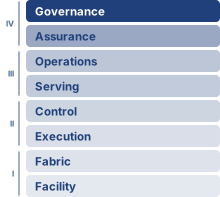
Fleet stack focus for this chapter.
Why can an accurate, fast model still be unfit for deployment?
In high-risk regulated settings, a model that cannot explain or document its behavior, support audit, or meet applicable discrimination rules may fail deployment review regardless of its accuracy or latency. Strong aggregate performance can conceal a pattern of errors concentrated among people with little power to challenge the outcome. Increasing throughput then increases the reach of that failure. A single-node evaluation can measure predictions, but it cannot establish whether every deployed version uses an approved decision policy or whether an affected person can obtain a correction. Across a fleet, records, models, interfaces, and organizational authority must remain connected as each changes. An explanation delivered too late may be useless to someone facing an immediate decision; retaining every detail indefinitely can create a separate privacy problem. Investigating an alert requires staff and evidence, while correcting a decision may require action across several dependent services. These obligations consume resources and can constrain deployment even when inference capacity is ample. They also persist after launch: a change in population, workflow, or model behavior can invalidate the evidence that originally justified operation. Responsible AI engineering makes those obligations part of the organization’s daily operation, with resources and authority to act when measured behavior falls short. In C³ terms, responsibility is a coordination constraint: the fleet needs evidence and authority to decide when compute may run, when it must stop, and who can correct its consequences.
Learning Objectives
- Explain why an accurate, fast model can still fail deployment review, and why each safeguard is budgeted capacity whose placement decides who is protected
- Calculate fairness metrics and evaluate observational versus causal definitions under base-rate and prediction trade-offs
- Design bias detection and fairness monitoring across demographic groups, drift, and fleet-scale feedback loops
- Evaluate privacy and machine-unlearning controls against accuracy, compute, and governance requirements
- Select explanation methods under latency, compute, auditability, and user-contestability constraints
- Analyze human-AI feedback loops, automation bias, and value conflicts in deployment contexts
- Construct an auditable assurance case, including bounded robustness and generative-system controls, from intended use and evidence through launch, remedy, material change, and retirement
16.1 The Governance Imperative
In 2018, Reuters reported that Amazon had abandoned an experimental hiring algorithm trained on historical resume data after discovering it systematically penalized female candidates (Dastin 2018). The historical records supplied a computable training objective, but reproducing patterns in those records was not the same as identifying qualified applicants fairly. The experiment exposed a mismatch between the learned objective and the legitimate hiring goal, because historical success could encode unequal access rather than merit-based qualifications.
Dastin, Jeffrey. 2018. “Amazon Scraps Secret AI Recruiting Tool That Showed Bias Against Women.” Reuters.
Stoica, Ion, Dawn Song, Raluca Ada Popa, David Patterson, Michael W. Mahoney, Randy Katz, Anthony D. Joseph, et al. 2017. “A Berkeley View of Systems Challenges for AI.” arXiv Preprint arXiv:1712.05855.
Production AI already has a systems agenda spanning architecture, infrastructure, data processing, security, and robustness (Stoica et al. 2017). The preceding chapters made the fleet secure against adversaries, robust under shift, and accountable for the energy it draws. The siting analysis in Environmental justice and responsible development left one question that energy and carbon accounting could expose but not settle, namely who bears the environmental cost of where the fleet runs. Responsible AI carries that question from the fleet’s resource footprint to the decisions the fleet makes about people. A service that remains available, secure, accurate, and within its resource budget can still distribute harms unfairly or deny affected people a remedy, and the hiring incident makes that distinction concrete. Fairness, transparency, and accountability therefore need measurable requirements and operating controls alongside the mechanisms that keep the fleet running.
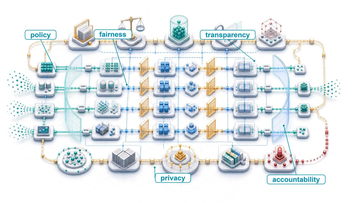
Across the multi-tier fleet hierarchy in The Fleet Stack, responsible AI completes the Governance band, the point where the system meets the real world. The Infrastructure, Distribution, and Serving bands beneath it supply compute, data movement, distributed execution, and serving infrastructure. Within the Governance band, the Assurance row contributes security controls and robustness mechanisms, and the Governance & Sustainability row contributes sustainability budgets; responsible AI weighs that evidence and adds the constraints that determine why the machine runs and whom it serves, requiring owners to identify, assess, limit, and remedy harms from an otherwise correctly functioning system. Alongside the Fleet Law’s accounting of execution time, responsible AI adds conditions for continued operation: evidence that the deployment remains within its approved bounds and authority to intervene when it does not. Toxic outputs can erode user trust, discriminatory decisions can distort future training data when those decisions shape data collection, and privacy violations can require restricting or suspending a service. These consequences depend on the deployment, but the obligation to investigate harm does not depend on whether it also degrades model performance. Responsible AI therefore shapes objective selection and operating constraints from the beginning of design.
↩︎ The Fleet Law governing execution time and scaling efficiency is established in The Fleet Law.
Definition 16.1: Responsible AI
Responsible AI is the practice of designing, auditing, and operating ML systems to measurable fairness, safety, privacy, and accountability standards, translating ethical principles into verifiable system properties that constrain model training, deployment decisions, and operational monitoring.
- Significance: Responsible AI constraints impose real costs: fairness-aware training can lengthen training runs, real-time bias monitoring can consume serving-path latency, and on-demand explainability can require additional model evaluations or asynchronous worker capacity. At fleet scale, these safeguards must be budgeted like reliability or security controls. Conversely, a facial recognition system with a persistent subgroup error gap can affect millions of users before detection, creating regulatory and liability costs that dwarf the monitoring investment.
- Distinction: AI ethics examines normative principles about what systems should do; responsible AI engineering turns selected requirements into controls and evidence. Bias detection algorithms, differential privacy implementations, audit trails, and architectural guardrails support bounded claims that reviewers can inspect. Choosing legitimate requirements and judging the remaining harms still require domain expertise, stakeholder participation, and accountable authority.
- Common pitfall: A frequent misconception is that responsible AI is a final compliance review applied to a finished model. Postprocessing can satisfy selected metrics on observed outcomes, but threshold adjustment cannot repair an invalid target, unreliable labels, or missing information. Those defects may require changes to data collection, labels, or learned representations. The remedy depends on the source of harm; a final threshold check cannot substitute for investigating it.
That practice must account for sociotechnical dynamics1 that extend beyond any individual system and operate inside organizational and regulatory contexts. Public risk-management frameworks, mapped onto the assurance lifecycle below, record the same shift from abstract principles toward governable requirements. Privacy mechanisms, robustness techniques, and sustainability metrics provide the technical foundation; responsible AI adds bias detection, organizational governance structures, and stakeholder engagement processes on top of them. That integration is a significant infrastructure investment, and the training, inference, and memory overheads quantified in section 16.4.2 must be provisioned as essential capacity, analogous to how security and redundancy are budgeted in distributed systems.
1 Sociotechnical system: Coined by the Tavistock Institute in the 1950s to describe the interdependent relationship between humans and technology in the workplace. ML fleets are sociotechnical systems in exactly this sense, because their “performance” is not merely a benchmark score but an emergent property of how model outputs interact with user behavior, legal frameworks, and physical resource constraints.
Treating fairness, transparency, accountability, and privacy as rigorous engineering specifications rather than abstract ideals transforms responsible AI from aspiration into practice. Each principle becomes a design constraint with measurable criteria, attached to a specific stage of the machine learning lifecycle. The assurance lifecycle first establishes who may set and approve those constraints, and the deployment tier determines where each control can run and what it costs. Fairness, privacy, explainability, and safety are then developed one at a time, each from definition through measurement to the controls that enforce it. Accountability and sociotechnical analysis close the argument by testing whether those controls remain effective inside human workflows and institutions.
Self-Check: Question
In the ML fleet stack, why does Responsible AI constitute the Governance band rather than existing as a supplementary post-training checklist?
- Because it replaces lower-level distributed execution frameworks with legal compliance parsers
- Because it serves solely to optimize training throughput and hardware acceleration efficiency
- Because it establishes requirements, evidence, and accountable owners for why the system runs and whom it serves, including risks that statistical optimization alone does not resolve
- Because it operates exclusively as a hardware watchdog circuit to prevent physical server overheating
Contrast the engineering objectives of Responsible AI with those of Robust AI.
True or False: Responsible AI is primarily an ethical review process applied to a finished model artifact at the end of the deployment pipeline.
How does the Amazon hiring algorithm incident illustrate that statistical optimization can coexist with severe societal harm?
16.2 The Governance and Assurance Lifecycle
A model registry can prove which weights reached production, but it cannot prove that the deployment was justified. That judgment requires a chain of evidence connecting the deployment context to affected people, foreseeable harms, measurable requirements, implemented controls, accountable owners, and the authority to launch or stop the system. Responsible AI therefore needs an assurance lifecycle: a repeatable operating path that converts normative commitments into reviewable claims and keeps those claims valid as the system changes.
The lifecycle begins before model selection. Teams first define the intended use, prohibited uses, affected parties, operating environment, and decision consequences. They then identify harms and requirements, including subgroup performance, privacy, security, robustness, sustainability, human-oversight, and contestability obligations. Some controls are implemented locally; others are inherited from data providers, foundation-model vendors, cloud platforms, or downstream operators. Each inherited control needs an interface contract stating what the supplier guarantees, what evidence supports that guarantee, and which residual risks remain with the deploying organization.
Constraint selection needs an explicit division of authority. Domain experts and affected parties identify consequential harms and acceptable uses; policy and legal specialists identify applicable obligations; engineers determine what can be measured and enforced. The accountable launch authority approves the resulting criteria and records unresolved disagreements. A convenient metric or an available implementation does not authorize the engineering team to choose whose errors matter most.
The resulting assurance case is not a single compliance document, but a versioned set of linked artifacts that structure accountability across the system lifecycle. At its foundation sits an explicit claim defining the property required for a specified use and operating envelope. An argument articulates how operational controls and empirical observations justify that claim, drawing on evidence from reproducible evaluations, audits, access logs, documentation, and user research. These claims and arguments hold only under stated assumptions regarding environmental, population, supplier, and workflow boundaries. To ensure operational authority, every assurance case specifies an accountable owner empowered to block launch, restrict use, or require remediation, governed by an explicit invalidation rule that defines the measurable performance change, distribution shift, or operational incident that expires prior approval and triggers reassessment. Evidence reaches the claim only through the argument and only inside the stated assumptions, and the owner’s launch decision lasts only until the invalidation rule fires (figure 1).
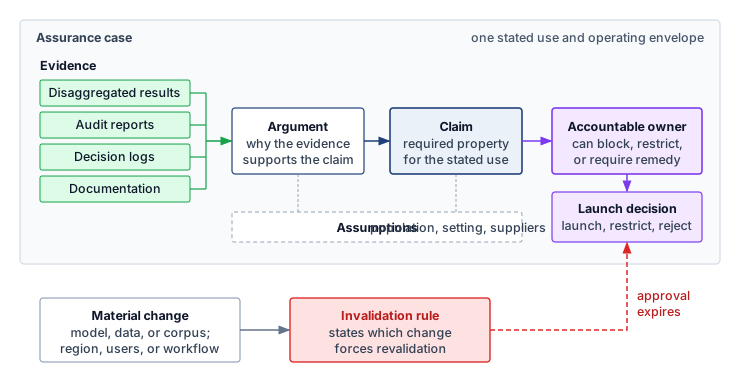
This structure prevents a common category error. A fairness dashboard, privacy accountant, red-team report, or carbon inventory is evidence for a bounded claim; none is itself proof that the full system is responsible. That evidence becomes operational only when an owner can act on it and affected people have a path to contest a decision and obtain remedy (table 1).
At release time, the evaluation contract defined in The end-to-end evaluation contract binds those assurance claims to the exact model, workload, acceptance authority, rollback target, and evidence-retention period. The assurance case explains why deployment is justified; the evaluation contract ensures that promotion and invalidation execute that judgment against one reproducible artifact.
| Lifecycle stage | Required artifact | Operational decision |
|---|---|---|
| Context and affected parties | Intended-use statement, prohibited uses, stakeholder map, decision-impact analysis | Is this use legitimate and within organizational authority? |
| Risk and requirements | Harm model, legal and policy obligations, measurable acceptance criteria | Which risks must be prevented, bounded, transferred, or accepted? |
| Controls and dependencies | Control inventory, supplier evidence, data and model lineage, output filters | Are local and inherited controls sufficient for the operating envelope? |
| Evaluation and assurance | Assurance case, disaggregated results with uncertainty, robustness and security evidence, sustainability accounting | Does the evidence support launch, restricted launch, or rejection? |
| Launch authority | Signed decision record, residual-risk owner, rollback and appeal paths | Who may authorize deployment, and who may stop it? |
| Operation and incident response | Monitoring thresholds, escalation owners, incident log, remedy workflow | When must the system degrade, roll back, notify, compensate, or suspend? |
| Material change | Change classification, impact assessment, revalidation scope | Does a new model, dataset, tool, region, or use invalidate prior approval? |
| Retirement | Decommission plan, retention and deletion record, user and dependent-system notice | How are access, data, models, interfaces, and unresolved harms closed out? |
Named frameworks organize this work at different levels. The National Institute of Standards and Technology (NIST) AI Risk Management Framework structures activity around Govern, Map, Measure, and Manage; ISO/IEC 42001 specifies an organizational AI management system; ISO/IEC 23894 supplies AI risk-management guidance; and the recommendations of the Organisation for Economic Co-operation and Development (OECD) and the United Nations Educational, Scientific and Cultural Organization (UNESCO) state broader principles and public responsibilities (Tabassi 2023; International Organization for Standardization and International Electrotechnical Commission 2023b, 2023a; Organisation for Economic Co-operation and Development 2024; UNESCO 2022). Mapped onto one operating lifecycle, those perspectives complement one another rather than serving as interchangeable checklists (table 2).
Tabassi, Elham. 2023. Artificial Intelligence Risk Management Framework (AI RMF 1.0). NIST AI 100-1. National Institute of Standards; Technology. https://doi.org/10.6028/NIST.AI.100-1.
International Organization for Standardization, and International Electrotechnical Commission. 2023a. ISO/IEC 23894:2023 Information Technology – Artificial Intelligence – Guidance on Risk Management. ISO/IEC standard.
Organisation for Economic Co-operation and Development. 2024. Recommendation of the Council on Artificial Intelligence. OECD Legal Instruments.
UNESCO. 2022. Recommendation on the Ethics of Artificial Intelligence. UNESCO.
| Lifecycle responsibility | NIST AI RMF emphasis | Management-system and public-policy emphasis |
|---|---|---|
| Establish context, affected parties, and authority | Govern and Map | Organizational context, leadership, stakeholder participation, and human oversight |
| Measure risk and assemble evidence | Measure | Risk assessment, documented objectives, evaluation, transparency, and traceability |
| Decide, operate, and respond | Manage | Operational controls, accountability, incident response, remedy, and continual improvement |
| Reassess change and retirement | Govern and Manage | Change management, corrective action, lifecycle review, and decommissioning obligations |
Regulation turns parts of this lifecycle into legal obligations, and it does so by classifying uses rather than by reducing AI risk to one verifiable metric. The EU AI Act (2024) uses a risk-based structure that includes prohibited practices, high-risk systems, transparency duties for some systems, and minimal or no-risk uses; high-risk deployments face conformity, documentation, and logging obligations (European Parliament and Council of the European Union 2024). Narrower statutes govern particular uses, as the Illinois Artificial Intelligence Video Interview Act does for automated analysis of recorded job interviews (Illinois General Assembly 2020). United States federal policy has changed repeatedly since 2023. The safety reporting thresholds of Executive Order 14110 were revoked in January 2025, and later orders redirected agency emphasis toward AI innovation, cybersecurity, and critical-infrastructure defense (Executive Office of the President 2023, 2025a, 2025b, 2026). China’s Interim Measures for Generative AI (2023) subject some public-facing services to security assessment and algorithm-filing requirements rather than a universal pre-release assessment (Cyberspace Administration of China et al. 2023). These requirements cannot be collapsed into a single checklist. For a global ML fleet, applicable obligations depend on the service, affected population, organizational role, and jurisdiction, not server location alone. The deploying organization must identify the obligations that apply, assign owners to the procedures and evidence they require, and bind the approved policies to those deployment conditions in the control plane, preserving their versions and propagating changes to the components that enforce them.
Illinois General Assembly. 2020. Artificial Intelligence Video Interview Act (Public Act 101-0260). 820 ILCS 42, effective January 1, 2020.
Executive Office of the President. 2023. Safe, Secure, and Trustworthy Development and Use of Artificial Intelligence. Executive Order 14110, 88 FR 75191.
Executive Office of the President. 2025a. Initial Rescissions of Harmful Executive Orders and Actions. Executive Order 14148, 90 FR 8237.
Executive Office of the President. 2025b. Removing Barriers to American Leadership in Artificial Intelligence. Executive Order 14179.
Executive Office of the President. 2026. Promoting Advanced Artificial Intelligence Innovation and Security. Executive Order 14409, 91 FR 34565.
Cyberspace Administration of China, National Development and Reform Commission, Ministry of Education, Ministry of Science and Technology, Ministry of Industry and Information Technology, Ministry of Public Security, and National Radio and Television Administration. 2023. Interim Measures for Administration of Generative Artificial Intelligence Services. State Council Gazette.
Three details keep this lifecycle from becoming ceremonial. First, fairness estimates must carry denominators, confidence intervals, and data-coverage limits; a noisy subgroup gap should trigger investigation, not automatic claims of either discrimination or safety. Second, sustainability evidence belongs in the same assurance record, because the functional unit, system boundary, carbon signal, water accounting, embodied-impact allocation, uncertainty, and quality constraint determine whether an environmental claim is comparable or actionable. Third, a generative service that retrieves documents into a model’s context needs an authorization boundary independent of model alignment. Least-privilege scopes, output validation, provenance, and revocation must be versioned and monitored because retrieved content remains an untrusted input.
↩︎ The sustainability measurement contract, which fixes the functional unit, system boundary, carbon signal, and attribution rule, is established in Energy Measurement and Modeling.
Approval expires when its supporting assumptions no longer hold. A change of foundation model, training distribution, retrieval corpus, deployment region, user population, decision purpose, or human workflow can be material even when the application code is unchanged. The change record should identify which claims are invalidated and select the smallest defensible revalidation scope. At the end of service, retirement must revoke credentials, stop dependent interfaces safely, apply retention and deletion rules, preserve required audit evidence, notify affected users and downstream operators, and leave an owner for unresolved appeals or harms. Governance covers the system after launch and after shutdown, rather than solely at the moment a review board signs a release.
Self-Check: Question
A global ML platform serves inference traffic across the European Union (EU AI Act), the United States, and Asia. How does this fragmented regulatory landscape reshape the serving control plane of the ML fleet?
- The platform must shut down all cloud datacenters and operate exclusively on local microcontrollers
- The platform must completely retrain its foundation models with new random seeds for each country
- The platform can ignore regional regulations by routing all traffic through international satellite links
- The control plane must bind approved policies to the applicable use, organizational role, and jurisdiction; regional gateways and shared model weights are one possible implementation.
A product team submits a fairness dashboard showing small subgroup gaps as proof that its loan-screening system is responsible. Within an assurance case, what role should the dashboard play?
- It is sufficient proof, because a fairness dashboard already covers the system’s privacy, security, and contestability obligations
- It is evidence for a bounded claim, valid only under stated assumptions, and it becomes operational only when an accountable owner can act on it and affected people can contest decisions
- It replaces the claim and argument, because measured results speak for themselves
- It is irrelevant once the model registry records which weights reached production
True or False: A team swaps the retrieval corpus behind an approved generative service without changing any application code, so the prior launch approval remains valid.
Order the following stages of the governance and assurance lifecycle from earliest to latest: (1) launch authority signs a decision record with rollback and appeal paths, (2) define intended use, prohibited uses, and affected parties, (3) retire the system, revoking credentials and preserving required audit evidence, (4) build the harm model and measurable acceptance criteria, (5) operate with monitoring thresholds, escalation owners, and a remedy workflow.
16.3 Core Principles and the ML Lifecycle
A continuous integration pipeline can block a release when an evaluation detects a 15 percent drop in accuracy specifically for elderly users. Unlike a failing unit test or a latency regression, which the pipeline can check deterministically, a subgroup result requires a specified population, sufficient evaluation data, and an agreed acceptance criterion. Responsible AI translates those commitments into deployment gates. The continuous integration/continuous deployment (CI/CD) pipeline enforces the approved rule, while the accountable reviewer interprets uncertainty and decides whether the evidence supports release, restricted use, or remediation.
That release gate is one instance of a general translation from principle to enforceable requirement. Transparency discloses how the system as a whole was built and governed: its data sources, training procedure, intended uses, and known limitations. Explainability is narrower, producing evidence about the model’s behavior on particular decisions for a specified audience. Together they make the system inspectable by the developers, auditors, and affected people who must judge it. Fairness constrains how selection rates, error rates, or the meaning of a score may differ across population subgroups; its violations can compound through feedback loops, as in predictive policing, while the service remains technically available. Privacy bounds what the system reveals about the people whose data it uses, safety and robustness bound how it fails, and accountability assigns owners who can trace, remedy, and answer for its outcomes. Two further principles govern the objective and its supervision. Value alignment2 asks whether the objective itself reflects legitimate human intent, and human oversight3 preserves the ability of people to supervise, correct, or halt automated decisions. The sections that follow develop the first group in turn; alignment and oversight return where autonomy and human workflows make them binding, in section 16.8.3 and section 16.9.4.2.
2 Value alignment: The problem of ensuring AI systems optimize for human values rather than proxy objectives. Russell (2021) argues that specifying the objective is harder than optimizing it. The engineering consequence is that the training objective becomes a governed artifact with an owner and a review path, not a fixed input chosen once by the modeling team.
Russell, S. 2021. “Human-Compatible Artificial Intelligence.” In Human-Like Machine Intelligence. Oxford University Press. https://doi.org/10.1093/oso/9780198862536.003.0001.
3 HITL (human-in-the-loop): Human participation in model decisions adds response delay and improves safety only when the operator can identify and correct the relevant error. Staffing demand depends on the decision arrival rate, the fraction escalated, and the time required per review. In ML serving architectures, HITL requires routing logic, escalation criteria, and queue management that reshape the inference pipeline.
No principle ensures a responsible system on its own. The principles overlap, compete for priority when budgets are finite, and act in different phases of the responsible AI lifecycle, from data collection through model training, evaluation, and deployment to monitoring (table 3).
| Principle | Data collection | Model training | Evaluation | Deployment | Monitoring |
|---|---|---|---|---|---|
| Fairness | Representative sampling | Bias-aware algorithms | Group-level metrics | Threshold adjustment | Subgroup performance |
| Explainability | Documentation standards | Interpretable architecture | Model behavior analysis | User-facing explanations | Explanation quality logs |
| Transparency | Data source tracking | Training documentation | Performance reporting | Model cards | Change tracking |
| Privacy | Consent mechanisms | Privacy-preserving methods | Privacy impact assessment | Secure deployment | Access audit logs |
| Accountability | Governance frameworks | Decision logging | Audit trail creation | Override mechanisms | Incident tracking |
| Robustness | Quality assurance | Robust training methods | Stress testing | Failure handling | Performance monitoring |
Fairness and privacy constraints begin at data collection; robustness likewise depends on data quality and training choices, while accountability requires named owners before deployment. Their operational consequences become visible when the system serves users and teams must respond to failures. Explainability spans the full lifecycle, supporting model debugging at design time and evidence about decisions during use. This mapping reinforces that responsible AI is a multiphase architectural commitment, not a post-hoc compliance step.
16.4 Architectural Trade-Offs
A centralized audit can join predictions, demographic attributes, and delayed outcomes when access to those records is authorized. A federated model running on a million smartphones may provide no such joined dataset. The same fairness criterion then requires a different evidence path, such as restricted aggregate statistics or a separately governed audit sample. Deployment architecture determines where the evidence can be assembled and who can act on it.
These architectural differences redistribute both feasible safeguards and accountable parties. The comparison that follows uses four deployment tiers that differ in compute, connectivity, and update authority: Cloud ML runs on serving replicas in data-center fleets, whereas Edge ML moves execution to gateways and servers near the data source. On the client side, Mobile ML runs on phone-class devices with sustained power budgets of a few watts, the regime of Archetype C (Federated MobileNet), while TinyML operates on microcontrollers with hundreds of kilobytes of memory and milliwatt power budgets, an extreme below Archetype C that often lacks any update channel. The volume’s other lighthouses sit in the cloud tier: Archetype A (GPT-4/Llama-3) and Archetype B (DLRM at Scale) serve from data-center fleets, and even Archetype C relies on a cloud aggregator for its fleet-level evidence. TinyML has no lighthouse of its own; it appears here because it marks the limit case, a deployment whose safeguards must be fixed before it ships. Resource availability, latency constraints, user interface design, and the presence or absence of connectivity determine whether responsible AI principles can be enforced consistently across deployment contexts. The same model may support rich explanation, continuous monitoring, and centralized auditability in the cloud, yet require static validation and simplified safeguards when embedded in a device with intermittent connectivity. Tier choice is also an equity decision, because a safeguard that needs a data-center round trip reaches only users whose connectivity supports it (section 16.4.3).
↩︎ Archetype C (Federated MobileNet) and its few-watt per-device envelope are established in Archetype C (Federated MobileNet).
16.4.1 Design trade-offs
An autonomous braking controller or a wearable gesture recognizer cannot spend hundreds of milliseconds running Shapley attributions on every sensor frame, and a personalized model adapting on one phone cannot see whether its updates widen error gaps across the rest of the population. Machine learning systems do not operate in idealized silos; they must navigate competing objectives under finite compute, strict latency deadlines, shifting user behavior, and regulatory constraints.
Cloud-based systems can provision extensive monitoring, fairness audits, interpretability services, and privacy-preserving tools using shared compute and storage. Centralized data handling also concentrates exposure to surveillance and breaches. On-device execution can keep raw data local, but user control still depends on interfaces, permissions, retention rules, and update authority. Postdeployment visibility, fairness instrumentation, and adaptation depend on which evidence and maintenance paths the architecture provides.
Tensions between goals often become apparent at the architectural level. When an endpoint has too little latency budget for a costly explanation on every inference, designers can evaluate lightweight methods within that budget, precompute suitable summaries, or retain decision records for asynchronous analysis. The explanation’s audience and required delivery time determine which of these paths can satisfy the obligation.
Conflicts also emerge between personalization and fairness. Systems that adapt to individuals based on local usage data often lack the global context necessary to assess disparities across population subgroups. Preventing personalized predictions from creating systematic exclusion requires balancing user-level adaptation with mechanisms for group-level equity and auditability.
Privacy and robustness objectives can also conflict. Logging rare events or user outliers can help diagnose reliability failures, but the records may expose sensitive behavior. If raw records must remain local or encrypted, the improvement process needs an authorized evidence path, such as restricted review or aggregate diagnostics. Robustness requirements belong in the initial design; subsequent refinement depends on whether the retained evidence and update mechanism support it.
Energy budgets can constrain the frequency and placement of safeguards. Reducing model cost does not itself require weaker fairness monitoring; teams can compare local checks, sampled audits, and off-device analysis against the evidence and response deadlines. In federated learning, clipping, noise generation, and communication can consume additional energy, but their placement and cost depend on the mechanism. A central-DP design may add noise at the curator, whereas a local-DP design places randomization on the client. Battery feasibility therefore requires measuring the chosen implementation.4
4 Energy-privacy trade-off: Privacy-preserving techniques like differential privacy and secure multi-party computation can increase computation, communication, and battery use. In federated learning on mobile devices, the equity implication is direct. Users with older devices, limited data plans, or limited battery life may be excluded from privacy-protected AI services, creating a system where privacy protection becomes contingent on hardware resources.
Together, these deployment examples reveal a broader systems-level challenge. Responsible AI principles cannot be considered in isolation. They interact, and optimizing for one may constrain another. The appropriate balance depends on deployment architecture, stakeholder priorities, domain-specific risks, the consequences of error, and the environmental and distributional impacts of computational resource requirements. Responsible machine learning design therefore depends on making those constraints explicit before choosing methods, so that the resulting system can be evaluated against the deployment context it must actually inhabit.
Comparing these settings (table 4) demonstrates that no deployment context dominates across all principles; each makes distinct architectural compromises. Cloud systems support computationally expensive explanation methods and centralized fairness monitoring. Shapley-value attribution (SHAP) credits each input feature with its average marginal contribution to a prediction across subsets of the other features, and local interpretable model-agnostic explanations (LIME) fit a simple surrogate model to many perturbed copies of one input; both require many extra model evaluations per explained decision, and section 16.7 develops them. Cloud deployments can afford that work, but introduce privacy risks through data aggregation. Edge and mobile deployments offer stronger data locality but limit postdeployment observability and global fairness assessment. TinyML systems face particularly tight budgets; their validation, monitoring, and update plans must reflect the connectivity and storage actually provided. These constraints also decide which users receive which safeguards, the equity question raised in section 16.4.3. Understanding these deployment constraints provides necessary context for the technical methods that translate responsible AI principles into production controls.
| Principle | Cloud ML | Edge ML | Mobile ML | TinyML |
|---|---|---|---|---|
| Explainability | Supports complex models and methods like SHAP and sampling approaches | Needs lightweight, low-latency methods like saliency maps | Requires interpretable outputs for users, often defers deeper analysis to the cloud | Severely limited due to constrained hardware; mostly static or compile-time only |
| Fairness | Large datasets allow bias detection and mitigation | Localized biases harder to detect but allows on-device adjustments | High personalization complicates group-level fairness tracking | Minimal data limits bias analysis and mitigation |
| Privacy | Centralized data at risk of breaches but can use strong encryption and differential privacy methods | Sensitive personal data on-device requires on-device protections | Tight coupling to user identity requires consent-aware design and local processing | Distributed data reduces centralized risks but poses challenges for anonymization |
| Safety | Vulnerable to hacking and large-scale attacks | Real-world interactions make reliability important | Operates under user supervision, but still requires graceful failure | Needs static safety envelopes, watchdogs, and fail-safe behavior |
| Accountability | Corporate policies and audits allow traceability and oversight | Fragmented supply chains complicate accountability | Requires clear user-facing disclosures and feedback paths | Traceability required across long, complex hardware chains |
| Governance | Applicable law and oversight; centralized evidence and named owners | Applicable law and oversight; allocate duties across integrators | Applicable law and oversight; coordinate platform and app duties | Applicable law and oversight; preserve evidence through servicing and retirement |
The deployment analysis identifies where each obligation must be implemented. A constrained endpoint may log bounded decision metadata while a backend aggregates subgroup metrics, stores audit evidence, and serves explanations. An offline endpoint instead needs a defined evidence-retrieval and update path, or an operating envelope that does not depend on unavailable controls. Device capacity limits placement and frequency; it does not by itself remove the fleet operator’s responsibility to provide the control.
Tier placement decides where a control runs; it does not decide which control a defect needs. As the hiring case at the start of the chapter showed, predictive accuracy on historical labels does not establish that the target is legitimate. Threshold postprocessing can change a decision-rate disparity, while an unsuitable target may require changes to labels and training, and both need validation and operational ownership.
The principle sections that follow, beginning with fairness in section 16.5, share one structure. Within each principle the methods do one of three jobs. Detection exposes a problem early enough to intervene, mitigation changes data, training, or decision policy to reduce the harm, and validation assembles the evidence a launch authority needs to accept the remaining risk. Each job carries its own cost in accuracy, computation, and implementation effort.
16.4.2 Computational overhead of responsible AI techniques
Adding seven-step adversarial training multiplies batch compute roughly eightfold, and running model-agnostic SHAP attributions on every request can multiply inference work by hundreds or thousands of evaluations. Detection, mitigation, validation, privacy, and explanation techniques each impose a distinct cost on training, inference, memory, and accuracy (table 5). Reading the table first lets engineers evaluate responsible AI methods as concrete capacity choices rather than as costless ethical labels.
| Technique | Accuracy loss | Training overhead | Inference cost | Memory overhead |
|---|---|---|---|---|
| Differential Privacy (DP-SGD) | 1–20% | 30–300% | Minimal | 10–20% |
| Fairness-Aware Training | 1–3% | 5–15% | Minimal | 5–10% |
| Sampled KernelSHAP | N/A | N/A | 50–200% | 20–100% |
| Exhaustive SHAP Enumeration | N/A | N/A | 50–1,000× | 50–200% |
| Adversarial Training | 3–15% | 2–11× | Minimal | 50–100% |
| Federated Learning | 5–15% | 200–500% | Minimal | 100–300% |
These overhead ranges should be read as scenario assumptions, not as claims that any cited paper establishes a single universal overhead.5 Actual overhead varies significantly based on model architecture, dataset size, attack strength, explanation method, hardware, communication pattern, and implementation quality. Responsible-AI controls consume real training, serving, memory, or review capacity, so they must be budgeted before launch. An organization unable to afford one configuration must assess alternatives such as a smaller model, sampled audits, or asynchronous explanations against the same required evidence. Resource limits can restrict the feasible deployment scope; they do not remove the obligation. Who can afford which configuration is therefore an equity question as well as a capacity question.
5 Measurement context: The sizing exercise assumes common production reference points such as GPU training, GPU or CPU inference, image/text/tabular models, and benchmark datasets. These figures are not canonical constants; they are order-of-magnitude planning anchors for deciding whether a safeguard belongs inline, asynchronous, offline, or in the training pipeline.
16.4.3 Resource requirements and equity implications
A municipal clinic or school district operating on a tight computing budget cannot afford to double its training cluster for differential privacy or provision extra GPU replicas for real-time Shapley explanations. Each cell of table 3 is work that someone must pay for: representative sampling needs data acquisition, subgroup metrics need labeled evaluation data and analysis capacity, and user-facing explanations need serving capacity. When smaller organizations cannot fund every safeguard in the table, the people they serve receive fewer protections than the users of a better-resourced deployment. Large-scale deployments that depend on accelerator clusters and low-latency connectivity can likewise exclude users whose networks or devices cannot meet those assumptions.
The costs in table 5 set how high these barriers are, and they are paid in energy as well as capacity. Model-specific algorithms, approximation, caching, and selective generation change that cost; asynchronous execution moves work off the request path without eliminating it. A high-traffic system serving these features to 10 million users must budget the work on the paths where it runs, then determine whether existing capacity is sufficient or additional resources are needed.
Infrastructure placement adds two further distributional effects. Data-center siting decisions that optimize power cost and latency can concentrate local environmental costs on nearby communities that had little say in the decision.6 Connectivity also affects access to safeguards. A user-facing explanation that requires a low-latency round trip to a data center may miss its delivery deadline on a slow network, whereas server-side fairness monitoring can analyze recorded decisions without another user round trip. The architecture must distinguish immediate user needs from audit work that can run asynchronously. Computational equity therefore depends on placement decisions as well as algorithmic design, and the assurance case should record these distributional effects alongside the model’s group metrics.
6 Data center environmental justice: Data center siting can place backup diesel generators, cooling heat, and grid strain near communities that had little say in the siting decision; the distributional effect must be measured site by site rather than assumed.
Computational costs and architectural constraints determine which controls a deployment can sustain. Preventive requirements guide design before harm occurs; detection then tests whether observed behavior remains within those requirements. Effective correction needs evidence of the problem, an investigation path, and an owner able to act.
Self-Check: Question
Why do resource-constrained TinyML deployments emphasize validated local safety envelopes and lightweight checks rather than continuous on-device SHAP explanations or large rolling fairness analyses?
- Tight compute, memory, power, and connectivity budgets limit heavy runtime analysis; local checks must be paired with fleet or servicing evidence and a defined update or retirement path.
- Because TinyML devices execute exclusively on cloud tensor processing units where telemetry logging is prohibited by law
- Because embedded C++ compilers automatically convert nonlinear deep neural networks into linear decision trees
- Because differential privacy guarantees are mathematically impossible on 32-bit microcontroller registers
Why does federated learning across mobile devices make group-level fairness auditing substantially more difficult than in centralized cloud architectures?
Order the following engineering actions for embedding responsible AI constraints across the ML lifecycle from earliest to latest development phase: (1) In-processing bias-aware loss constraints and DP-SGD noise injection, (2) Representative sampling and consent collection protocols, (3) Decision threshold policy calibration and human override routing, (4) Subgroup drift telemetry and rolling metric alerting, (5) Group-level disaggregated metric evaluation and stress testing.
16.5 Fairness and Bias Mitigation
A loan model can approve 70 percent of one group’s applicants and 40 percent of another’s while reporting a single headline accuracy. Exposing that gap, deciding which gap the deployment must close, and keeping it visible after launch are separate engineering tasks. Formal criteria define the disparity, statistical tests decide whether it exceeds sampling noise, and monitoring infrastructure tracks it in production.
16.5.1 Fairness in machine learning
Automated decisions in hiring, lending, and healthcare affect millions of people, and historical data used to train these systems encodes decades of structural inequality. The engineering question is how to formalize “equitable treatment” in a way that a system can measure and enforce.
Definition 16.2: Algorithmic fairness
Algorithmic fairness is a family of criteria for evaluating equitable treatment and outcomes in automated decisions. The group-based criteria developed here compare selection rates, errors, or score meaning across protected demographic groups; individual and causal criteria ask different questions.
- Significance: Formal criteria make competing fairness goals measurable. Selection-rate or error-rate constraints can change predictive accuracy, while group-specific calibration asks whether predicted probabilities match observed outcome frequencies within each protected group. The trade-offs depend on the criterion, data, and decision policy. Satisfying one criterion does not establish equitable treatment by itself.
- Distinction: Unlike average accuracy, which can hide subgroup disparities, group fairness examines the joint distribution of predictions and outcomes within each group, \(\ProbabilityFunction(\PredictedDecision,\TrueOutcome\mid \ProtectedGroupMembership)\). The chosen criterion determines which conditional rates to compare; a group gap diagnoses that metric rather than fairness as a whole.
- Common pitfall: A frequent misconception is that there is a single “fair” solution. In reality, fairness requirements can conflict under specified assumptions. The simplest conflict pairs demographic parity with equalized odds, both defined below. With unequal base rates (the fractions of actual positive cases within groups), the two can hold together only if each group’s true positive rate equals its false positive rate. The positive decision is then equally likely among actual positives and actual negatives, so it carries no information about the outcome. A constant classifier satisfies both; any informative classifier must give one up. A deeper result about calibrated scores follows the formal definitions.
Aggregate accuracy cannot reveal whether an automated system disproportionately disadvantages a protected group. Because these systems are trained on historical data, they can reproduce and amplify patterns of systemic bias embedded in that data. A widely studied example comes from the healthcare domain. An algorithm7 used to allocate care management resources in US hospitals was found to systematically underestimate the health needs of Black patients (Obermeyer et al. 2019). The model used healthcare expenditures as a proxy for health status, but due to longstanding disparities in access and spending, Black patients were less likely to incur high costs. As a result, the model inferred that they were less sick, despite often having equal or greater medical need. This case illustrates how seemingly neutral design choices such as proxy variable selection can yield discriminatory outcomes when historical inequities are not properly accounted for. Correcting an invalid proxy can improve alignment with the actual clinical goal. A separate engineering question is whether imposing a particular fairness constraint reduces accuracy on a fixed target. That scenario-specific reduction, the fairness cost, is priced in section 16.5.3 once the criteria and the decision thresholds that enforce them have been defined.
7 Healthcare algorithm scale: The study examined one widely used algorithm in a broader class of risk-prediction tools that industry estimates placed at approximately 200 million U.S. patients annually (Obermeyer et al. 2019). In the study’s simulated correction at the automatic-enrollment threshold, the fraction of Black patients among those identified for additional care rose from 17.7 percent to 46.5 percent. These are shares of the selected population, not the fraction of all Black patients identified or a measured nationwide enrollment reduction.
Obermeyer, Ziad, Brian Powers, Christine Vogeli, and Sendhil Mullainathan. 2019. “Dissecting Racial Bias in an Algorithm Used to Manage the Health of Populations.” Science 366 (6464): 447–53. https://doi.org/10.1126/science.aax2342.
Evaluating these risks requires formal criteria, defined in full below; the release gates of Fairness gates enforce two of them, demographic parity and equalized odds, as thresholds. Each criterion turns a different meaning of fairness (equal selection, equal error rates, equal opportunity for the qualified, or scores that mean the same thing in every group) into a conditional probability that a system can measure and enforce, so choosing a criterion is choosing which of those meanings the deployment must honor. Suppose a model \(\BinaryClassifier(\ModelInput)\) predicts a binary outcome, such as loan repayment, and let \(\ProtectedGroupMembership\) represent a sensitive attribute with subgroups \(\FirstComparedGroupLabel\) and \(\SecondComparedGroupLabel\). Three widely adopted group criteria compare different conditional rates of that prediction.
Demographic parity
Definition 16.3: Demographic parity
Demographic parity is the fairness constraint where a model’s positive prediction rate is independent of group membership \((\Pr(\BinaryClassifier(\ModelInput)=1 \mid \ProtectedGroupMembership=\FirstComparedGroupLabel) = \Pr(\BinaryClassifier(\ModelInput)=1 \mid \ProtectedGroupMembership=\SecondComparedGroupLabel))\).
- Significance: It requires equal positive prediction rates across groups, regardless of underlying base-rate differences. It does not require identical outcomes for every individual, and it is not universally more restrictive than error-rate or calibration criteria.
- Distinction: Unlike equalized odds (which focuses on error rates such as false positives), demographic parity focuses only on the final prediction, ignoring the relationship between the prediction and the ground truth.
- Common pitfall: A frequent misconception is that demographic parity ensures “fairness.” Equal approval rates can coexist with unequal error rates. Changing decision thresholds can alter who receives approval without changing the underlying scores or their calibration; the resulting decisions and the meaning of the scores require separate evaluation.
Demographic parity asks whether favorable outcomes, such as loan approval or treatment referral, occur at equal rates across subgroups defined by a sensitive attribute \(\ProtectedGroupMembership\). Formally, the model satisfies demographic parity if: \[ \Pr\big(\BinaryClassifier(\ModelInput) = 1 \mid \ProtectedGroupMembership = \FirstComparedGroupLabel\big) = \Pr\big(\BinaryClassifier(\ModelInput) = 1 \mid \ProtectedGroupMembership = \SecondComparedGroupLabel\big) \]
In the healthcare example, this criterion would ask whether Black and white patients were referred for care at the same rate, regardless of their underlying health needs. That may sound like equal access, but it ignores real differences in medical status and risk, potentially overcorrecting when needs are not evenly distributed. The limitation of ignoring base-rate differences motivates error-rate-based fairness criteria.
Equalized odds
Equalized odds requires that the model’s predictions are conditionally independent of group membership given the true label. Specifically, the true positive and false positive rates must be equal across groups: \[ \Pr\big(\BinaryClassifier(\ModelInput) = 1 \mid \ProtectedGroupMembership = \FirstComparedGroupLabel, \TrueOutcome= \TrueOutcomeLevel\big) = \Pr\big(\BinaryClassifier(\ModelInput) = 1 \mid \ProtectedGroupMembership = \SecondComparedGroupLabel, \TrueOutcome= \TrueOutcomeLevel\big), \quad \text{for } \TrueOutcomeLevel \in \{0, 1\}. \]
That is, for each true outcome \(\TrueOutcome= \TrueOutcomeLevel\), the model should produce the same prediction distribution across groups \(\ProtectedGroupMembership = \FirstComparedGroupLabel\) and \(\ProtectedGroupMembership = \SecondComparedGroupLabel\). Equalized odds equalizes conditional error rates, not error counts; groups with different numbers of positive or negative cases can still experience different numbers of errors. Applied to a binary medical referral decision, this criterion requires equal referral rates across racial groups separately among patients who need the intervention and among those who do not, according to the chosen label \(\TrueOutcome\).
Equality of opportunity
Equality of opportunity is a less stringent relaxation of equalized odds that focuses only on the true positive rate (Hardt et al. 2016). It requires that, among individuals who should receive a positive outcome, the probability of receiving one is equal across groups: \[ \Pr\big(\BinaryClassifier(\ModelInput) = 1 \mid \ProtectedGroupMembership = \FirstComparedGroupLabel, \TrueOutcome= 1\big) = \Pr\big(\BinaryClassifier(\ModelInput) = 1 \mid \ProtectedGroupMembership = \SecondComparedGroupLabel, \TrueOutcome= 1\big). \]
Equality of opportunity equalizes the approval rate among qualified individuals, who have \(\TrueOutcome= 1\), across groups. It does not require identical decisions for every pair of qualified individuals or constrain errors among unqualified applicants.
In medical referral, this measure would require equal identification rates across racial groups among patients labeled as needing the intervention. Both error-rate criteria inherit whatever the label \(\TrueOutcome\) measures, which is the lesson of the healthcare case. A model trained to predict expenditure could equalize its error rates against expenditure and still misallocate care, because expenditure is not need. The cited study measured illness burden at a given risk score rather than group error rates, so it cannot itself be scored against these criteria. The loan scenario that follows supplies the binary labels and decisions needed to calculate all three on one model, and it becomes the section’s running example.
Napkin Math 16.1: Calculating fairness metrics
Problem: Calculate demographic parity across two demographic groups (100 applicants each) for a loan approval model.
Variables:
- Group A: 70 approved (40 repaid, 30 defaulted), 30 rejected.
- Group B: 40 approved (30 repaid, 10 defaulted), 60 rejected.
Math:
- Group A approval rate: \(\Pr(\BinaryClassifier(\ModelInput) = 1 \mid \ProtectedGroupMembership = \FirstComparedGroupLabel) = \frac{70}{100} = 0.70\).
- Group B approval rate: \(\Pr(\BinaryClassifier(\ModelInput) = 1 \mid \ProtectedGroupMembership = \SecondComparedGroupLabel) = \frac{40}{100} = 0.40\).
- Parity gap: \(0.70 - 0.40 = 0.30\) (30 percentage-point gap).
Systems insight: Evaluating demographic parity exposes group approval rate disparities regardless of ground-truth repayment capability, requiring explicit metric selection during model threshold calibration.
The next calculation assumes that repayment labels are also known for rejected applicants. Among the rejected applicants in Group A, five would repay and 25 would default; in Group B, 20 would repay and 40 would default. These are hypothetical evaluation labels. A production lender ordinarily observes repayment only for approved loans, so estimating the same error rates requires additional evidence about rejected applicants and an account of how that evidence was obtained.
Napkin Math 16.2: Calculating equality of opportunity
Calculating equality of opportunity (true positive rate [TPR]):
Among applicants who would actually repay (\(\TrueOutcome=1\)): \[\begin{gather*} \Pr(\BinaryClassifier(\ModelInput) = 1 \mid \ProtectedGroupMembership = \FirstComparedGroupLabel, \TrueOutcome = 1) = \frac{40}{40 + 5} = \frac{40}{45} \approx 0.89 \\ \Pr(\BinaryClassifier(\ModelInput) = 1 \mid \ProtectedGroupMembership = \SecondComparedGroupLabel, \TrueOutcome = 1) = \frac{30}{30 + 20} = \frac{30}{50} = 0.60 \end{gather*}\]
Disparity: \(0.89 - 0.60 = 0.29\) (29 percentage-point gap in TPR)
The model violates equality of opportunity. Among qualified applicants who would repay, Group A members are correctly approved 89 percent of the time while Group B members are only approved 60 percent of the time.
Calculating equalized odds (true positive rate [TPR] and false positive rate [FPR]):
The TPR values are calculated in the preceding step. For false positive rates among applicants who would not repay (\(\TrueOutcome=0\)): \[\begin{gather*} \Pr(\BinaryClassifier(\ModelInput) = 1 \mid \ProtectedGroupMembership = \FirstComparedGroupLabel, \TrueOutcome = 0) = \frac{30}{30 + 25} = \frac{30}{55} \approx 0.55 \\ \Pr(\BinaryClassifier(\ModelInput) = 1 \mid \ProtectedGroupMembership = \SecondComparedGroupLabel, \TrueOutcome = 0) = \frac{10}{10 + 40} = \frac{10}{50} = 0.20 \end{gather*}\]
The model also has unequal false positive rates. It incorrectly approves 55 percent of Group A applicants who will default, but only 20 percent of Group B applicants who will default. The model is therefore more lenient with Group A applicants who will not repay.
Systems insight: This model violates all three fairness criteria. Addressing one criterion does not automatically satisfy others. Whether they can all be satisfied together depends on base rates and prediction quality, the question the impossibility results below address.
Calibration
A fourth criterion concerns the score rather than the decision. A model satisfies score calibration with respect to a sensitive attribute if, among individuals assigned score \(\ModelScore\) by the model, the fraction with positive outcomes equals that score within each group (Kleinberg et al. 2017): \[ \Pr(\TrueOutcome= 1 \mid \ModelScore(\ModelInput) = \ModelScore, \ProtectedGroupMembership = \FirstComparedGroupLabel) = \ModelScore= \Pr(\TrueOutcome= 1 \mid \ModelScore(\ModelInput) = \ModelScore, \ProtectedGroupMembership = \SecondComparedGroupLabel), \quad \forall \ModelScore\]
The condition applies at score levels supported within each group. Matching the groups’ outcome frequencies is insufficient if those frequencies differ from the score itself. For hard binary predictions, a distinct condition is equal positive predictive value (PPV) (precision) among predicted positives. Groupwise score calibration does not by itself guarantee equal PPV after thresholding, because the selected groups can have different score distributions: \[ \text{PPV}(\FirstComparedGroupLabel) = \frac{\Pr(\TrueOutcome=1, \BinaryClassifier(\ModelInput)=1 \mid \ProtectedGroupMembership=\FirstComparedGroupLabel)}{\Pr(\BinaryClassifier(\ModelInput)=1 \mid \ProtectedGroupMembership=\FirstComparedGroupLabel)} = \text{PPV}(\SecondComparedGroupLabel) \]
Evaluating this condition on the loan-approval example yields the respective predictive values: \[\begin{align*} \text{PPV}(\FirstComparedGroupLabel) &= \frac{40}{70} = 0.571 \\ \text{PPV}(\SecondComparedGroupLabel) &= \frac{30}{40} = 0.750 \end{align*}\]
The positive predictive value gap is \(0.750 - 0.571 = 0.179\). Group B’s predicted positives are actually positive 75 percent of the time, while Group A’s are only 57 percent accurate. This violates predictive parity for hard decisions and reveals that the model is less reliable when predicting approval for Group A. Demonstrating score calibration itself would require comparing observed outcome frequencies with predicted probabilities within each group, using score bins with sufficient support. That check is essential in high-stakes decisions where people rely on predicted probabilities, because a miscalibrated model systematically over- or underpredicts risk for specific groups, misallocating resources and eroding trust.
Why the fairness criteria conflict
The loan model’s failure to satisfy every criterion raises a broader question about their compatibility. Its answer depends on base rates and prediction quality, and the definitions can conflict outright under deployment-specific conditions.8 A university admissions example makes the simplest conflict, the one previewed in the algorithmic-fairness definition, concrete before the broader calibration result (Kleinberg et al. 2017; Chouldechova 2017).
8 Fairness impossibility theorems: Kleinberg et al. (2017) studies groupwise score calibration together with balance of mean scores in each outcome class. Chouldechova (2017) studies predictive parity and error-rate constraints for recidivism prediction. These are distinct conditions; their incompatibility results require assumptions on base rates and predictive performance. Demographic parity is a distinct constraint on selection rates that can also conflict with calibration or error-rate goals in practice. The systems consequence is that no amount of engineering can satisfy every normative fairness criterion in all settings, so fairness becomes a constrained multi-objective optimization requiring explicit policy choices about which criterion to prioritize for a given deployment context.
Kleinberg, Jon, Sendhil Mullainathan, and Manish Raghavan. 2017. “Inherent Trade-Offs in the Fair Determination of Risk Scores.” 8th Innovations in Theoretical Computer Science Conference (ITCS 2017), Leibniz international proceedings in informatics (LIPIcs), vol. 67: 43:1–23. https://doi.org/10.4230/LIPIcs.ITCS.2017.43.
Chouldechova, Alexandra. 2017. “Fair Prediction with Disparate Impact: A Study of Bias in Recidivism Prediction Instruments.” Big Data 5 (2): 153–63. https://doi.org/10.1089/big.2016.0047.
Suppose a university admits only qualified applicants, and a larger fraction \(\FirstGroupQualifiedFraction\) of Group A’s applicants are qualified than the fraction \(\SecondGroupQualifiedFraction\) of Group B’s. Equal opportunity asks that the same fraction \(\QualifiedAdmissionRate\) of qualified applicants be admitted from each group, for example 80 percent of qualified Group A applicants and 80 percent of qualified Group B applicants. The overall admission rates are then \(\QualifiedAdmissionRate \FirstGroupQualifiedFraction\) and \(\QualifiedAdmissionRate \SecondGroupQualifiedFraction\), which differ whenever \(\FirstGroupQualifiedFraction\neq \SecondGroupQualifiedFraction\), so demographic parity fails; they match only at \(\QualifiedAdmissionRate= 0\). The no-unqualified-admissions rule fixes each group’s false positive rate at zero, so equal opportunity here coincides with equalized odds, and parity holds only when each group’s true positive rate also falls to zero. That is the definition’s condition (true positive rate equal to false positive rate) in concrete form. Relaxing the rule removes the conflict, because admitting some unqualified Group B applicants can raise Group B’s overall rate to Group A’s. Which constraint to give up is a value judgment about the decision, not a property the model can settle.
The fairness impossibility theorem (principle 26) is the canonical result, and it concerns scores rather than decisions. It joins the groupwise calibration of section 16.5.1.4 to score balance, which requires equal average scores across groups among people with positive outcomes and, separately, among people with negative outcomes. With unequal base rates and imperfect prediction, all three requirements cannot hold together (Kleinberg et al. 2017). The admissions conflict concerns decisions and this result concerns scores, so they constrain different criteria. The score result also does not say that a calibrated score can never meet equalized odds at a particular threshold; that is a third, narrower question. Satisfying one criterion may preclude another, so engineers must treat fairness metrics like latency budgets, explicit trade-offs chosen by stakeholders, enforced by the system, and monitored for violation. Determining which metric to prioritize requires careful consideration of the application context, potential harms, and stakeholder values as detailed in section 16.9.4.3. Whenever base rates differ and predictions remain imperfect, group calibration, positive-class score balance, and negative-class score balance converge on an infeasible joint state (figure 2).
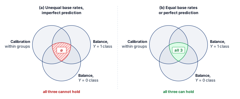
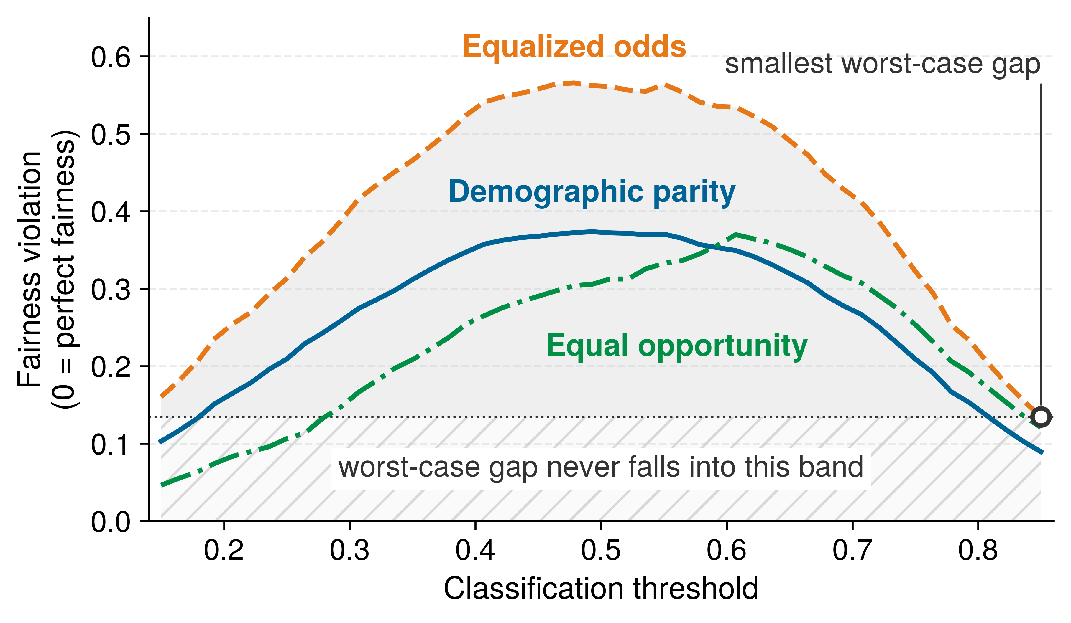
The conflict persists as the classification threshold moves. For two groups with unequal base rates, every threshold from 0.15 to 0.85 leaves at least one of demographic parity, equalized odds, and equal opportunity substantially violated (figure 3). A threshold that reduces one measured gap need not minimize the others, so the policy must specify which criterion governs the decision and evaluate the remaining gaps.
Group metrics also leave open how an observed disparity arose, because a gap does not identify the mechanism that produced it. Causal analysis addresses that question through explicit assumptions.
Observational and causal fairness
The preceding metrics describe associations in observed decisions, such as group differences in selection rates, error rates, or calibration. They can establish a disparity without identifying the pathway that produced it. The same approval-rate gap could arise from direct use of a protected attribute, a correlated proxy, unequal access to an earlier process, measurement error, or an unobserved common cause. No comparison of observed rates alone distinguishes these mechanisms.
A causal claim adds a structural causal model whose arrows state how protected attribute \(\ProtectedGroupMembership\), mediators \(\CausalMediator\), outcome \(\TrueOutcome\), and decision \(\PredictedDecision\) are assumed to relate. Counterfactual fairness then asks whether the decision for the same individual, holding the modeled background factors fixed, would have changed in a counterfactual world where \(\ProtectedGroupMembership\) had taken another value (Kusner et al. 2017). This is a question about an assumed data-generating process, not a stronger version of demographic parity.
Kusner, Matt J., Joshua Loftus, Chris Russell, and Ricardo Silva. 2017. “Counterfactual Fairness.” Advances in Neural Information Processing Systems 30: 4066–76.
Nabi, Razieh, and Ilya Shpitser. 2018. “Fair Inference on Outcomes.” Proceedings of the AAAI Conference on Artificial Intelligence 32. https://doi.org/10.1609/aaai.v32i1.11553.
The healthcare proxy illustrates the distinction. A graph might include race \(\ProtectedGroupMembership \rightarrow\) access to care \(\CausalMediator_1 \rightarrow\) expenditure \(\CausalMediator_2 \rightarrow\) risk score \(\PredictedDecision\), alongside pathways from health need \(\TrueOutcome\) to expenditure. A total effect asks how changing \(\ProtectedGroupMembership\) propagates through every modeled path. A path-specific effect isolates selected routes, such as the historically mediated access-to-expenditure path (Nabi and Shpitser 2018). Declaring one path permissible and another discriminatory is a domain and normative judgment; neither the graph nor the estimator makes that choice automatically.
Causal conclusions require assumptions that observational data alone cannot establish: which variables and arrows belong in the graph, whether relevant confounders are measured, and whether the counterfactual interventions are coherent. Different plausible structures can support different answers. Causal analysis therefore complements group metrics, domain knowledge, legal analysis, and stakeholder participation. The metrics continue to monitor realized disparities; the causal model makes the additional mechanism claim and its assumptions inspectable.
16.5.2 Measuring disparity
A 30-point approval gap observed on 20 loan applications could be sampling noise, and a gender-classification audit that checks race and gender separately can report above 90 percent accuracy on both while missing a 34-point error gap on darker-skinned women. Turning a fairness criterion into evidence a launch authority can act on requires a point metric with a denominator and a confidence interval, coverage of the intersections where errors concentrate, and a governed choice of the criterion the deployment will be judged against.
Quantitative fairness measurement
Formal fairness criteria become operational only when practitioners can measure the degree of violation and establish actionable thresholds for intervention. The mathematical framework quantifies disparities and uncertainty; domain and policy owners must justify the acceptance criteria and authorize the response. A computed gap supplies evidence for that decision rather than deciding which harms are acceptable.
Four point metrics turn the fairness criteria introduced above into numbers an auditor can threshold. Each one equalizes a different quantity, so each exposes a different failure of the same classifier. On the running loan example (table 6), Group A is approved at 0.70 and Group B at 0.40, qualified-applicant true-positive rates are 0.89 and 0.60, and unqualified-applicant false-positive rates are 0.55 and 0.20.
| Metric | Equalizes | Formula \((\FirstComparedGroupLabel, \SecondComparedGroupLabel)\) | Loan value | Choose it when |
|---|---|---|---|---|
| Disparate impact (DI) ratio (four-fifths rule) (Feldman et al. 2015) | lower approval rate divided by higher approval rate | \(\dfrac{\min_\SubgroupIndex\Pr(\BinaryClassifier=1 \mid \SubgroupIndex)}{\max_\SubgroupIndex\Pr(\BinaryClassifier=1 \mid \SubgroupIndex)}\) | \(\dfrac{0.40}{0.70} = 0.57\) | a descriptive selection-rate screen is useful; legal interpretation depends on the application |
| Statistical parity difference (SPD) (Calders and Verwer 2010) | additive gap in approval rates | \(\Pr(\BinaryClassifier=1 \mid \FirstComparedGroupLabel) - \Pr(\BinaryClassifier=1 \mid \SecondComparedGroupLabel)\) | \(0.70 - 0.40 = 0.30\) | comparing across groups or tracking drift against a deployment-approved gap threshold |
| Equal opportunity difference (Hardt et al. 2016) | true-positive rates among qualified applicants | \(\Pr(\BinaryClassifier=1 \mid \FirstComparedGroupLabel, \TrueOutcome{=}1) - \Pr(\BinaryClassifier=1 \mid \SecondComparedGroupLabel, \TrueOutcome{=}1)\) | \(0.89 - 0.60 = 0.29\) | the harm is denying deserving individuals |
| Average absolute odds difference (Hardt et al. 2016; Bellamy et al. 2019; Bird et al. 2020) | both true-positive and false-positive rates | \(\tfrac{1}{2}\big[\,\lvert \FiniteChange\text{TPR}\rvert + \lvert \FiniteChange\text{FPR}\rvert\,\big]\) | \(\tfrac{1}{2}[0.29 + 0.35] = 0.32\) | both error types matter; the metric is 0 at perfect equalized odds |
Feldman, M., S. A. Friedler, J. Moeller, C. Scheidegger, and S. Venkatasubramanian. 2015. “Certifying and Removing Disparate Impact.” Proceedings of the 21th ACM SIGKDD International Conference on Knowledge Discovery and Data Mining, 259–68. https://doi.org/10.1145/2783258.2783311.
Calders, Toon, and Sicco Verwer. 2010. “Three Naive Bayes Approaches for Discrimination-Free Classification.” Data Mining and Knowledge Discovery 21 (2): 277–92. https://doi.org/10.1007/s10618-010-0190-x.
Bellamy, Rachel K. E., Kuntal Dey, Michael Hind, Seung Hoffman, Sylvain Houde, Karthikeyan Kannan, Pradeep Lohia, et al. 2019. “AI Fairness 360: An Extensible Toolkit for Detecting and Mitigating Algorithmic Bias.” IBM Journal of Research and Development 63 (4/5): 4:1–15. https://doi.org/10.1147/jrd.2019.2942287.
The four metrics measure different quantities by construction. The disparate impact ratio of 0.57 means the lower-approval group receives approvals at only that fraction of the higher-approval group’s rate, below the illustrative 0.8 screening threshold. The additive 0.30 gap, the 0.29 opportunity gap, and the 0.32 average absolute odds gap each quantify a distinct dimension of the same disparity. No single number is sufficient, which is why the impossibility results of section 16.5.1.5 force an explicit choice about which metric a deployment will prioritize.
Statistical testing of fairness violations
Confidence intervals and hypothesis tests help assess whether sampling variation plausibly explains an observed disparity under a stated sampling model. For demographic parity, the null hypothesis \(\StatisticalHypothesis_0: \Pr(\BinaryClassifier(\ModelInput)=1 \mid \ProtectedGroupMembership=\FirstComparedGroupLabel) = \Pr(\BinaryClassifier(\ModelInput)=1 \mid \ProtectedGroupMembership=\SecondComparedGroupLabel)\) can be tested using a two-proportion z-test when observations are independent and expected approval and rejection counts in both groups support the normal approximation. Repeated decisions for the same person or correlated observations require an uncertainty estimate that accounts for that dependence. Under the independent-sample assumptions, the test statistic is: \[ \ProportionTestStatistic= \frac{\FirstGroupSampleApprovalRate- \SecondGroupSampleApprovalRate}{\sqrt{\PooledSampleApprovalRate(1-\PooledSampleApprovalRate)\left(\frac{1}{\FirstGroupSampleSize} + \frac{1}{\SecondGroupSampleSize}\right)}} \]
where \(\FirstGroupSampleApprovalRate\) and \(\SecondGroupSampleApprovalRate\) are the sample approval rates, \(\PooledSampleApprovalRate= \frac{\FirstGroupSampleSize\FirstGroupSampleApprovalRate+ \SecondGroupSampleSize\SecondGroupSampleApprovalRate}{\FirstGroupSampleSize+ \SecondGroupSampleSize}\) is the pooled proportion, and \(\FirstGroupSampleSize\), \(\SecondGroupSampleSize\) are sample sizes.
For the loan example with \(\FirstGroupSampleSize= \SecondGroupSampleSize= 100\), \(\FirstGroupSampleApprovalRate= 0.70\), \(\SecondGroupSampleApprovalRate= 0.40\): \[\begin{align*} \PooledSampleApprovalRate &= \frac{100(0.70) + 100(0.40)}{200} = 0.55 \\ \ProportionTestStatistic &= \frac{0.70 - 0.40}{\sqrt{0.55(0.45)(0.02)}} = \frac{0.30}{0.0704} = 4.26 \end{align*}\]
With \(\ProportionTestStatistic = 4.26\) (far exceeding critical value \(\ConfidenceCriticalQuantile = 1.96\)), the test rejects \(\StatisticalHypothesis_0\) and concludes the demographic parity violation is statistically significant at \(\ObservedSignificanceLevel < 0.001\). Similar tests can be constructed for equal opportunity and equalized odds by restricting to subpopulations where \(\TrueOutcome=1\) or \(\TrueOutcome=0\) respectively. Statistical significance does not establish the severity or acceptability of a disparity. Even a small rate difference can affect many people at fleet scale; the decision depends on the consequences and approved criteria as well as magnitude. Conversely, large disparities in small samples may not reach statistical significance but still warrant investigation or intervention.
Intersectional fairness

Error concentrates at the intersection: darker-skinned women.
Broad demographic categories can also hide disparities within their intersections. Standard fairness analysis often evaluates single axes of identity (for example, race or gender) independently, which can mask large disparities at the intersection of those attributes. For example, IBM’s gender-classification system achieved 99.7 percent accuracy for lighter-skinned men but only 65.3 percent for darker-skinned women in the Gender Shades evaluation (Buolamwini and Gebru 2018). A single-axis audit can obscure such an intersectional disparity. This phenomenon, sometimes called fairness gerrymandering, requires evaluating model performance on intersectional subgroups (for example, \(\text{Race}{\times}\text{Gender}\)) to detect and mitigate compounded biases.
Errors fell after the disparity was published. In August 2018, about six months after the Gender Shades results were published, Raji and Buolamwini (2019) repeated the audit on the same benchmark. Each of the three companies that had been named had reduced its error on darker-skinned women: IBM from 34.7 to 17.0 percent, Face++ from 34.5 to 4.1, and Microsoft from 20.8 to 1.5 (figure 4). Two systems the original audit had not named, from Amazon and Kairos, measured for the first time in 2018, misclassified 31.4 and 22.5 percent of darker-skinned women, comparable to the named systems’ 2017 levels. The study reports an association rather than a controlled effect, but it suggests that a specific, published intersectional audit can act as an operational lever as well as a measurement.
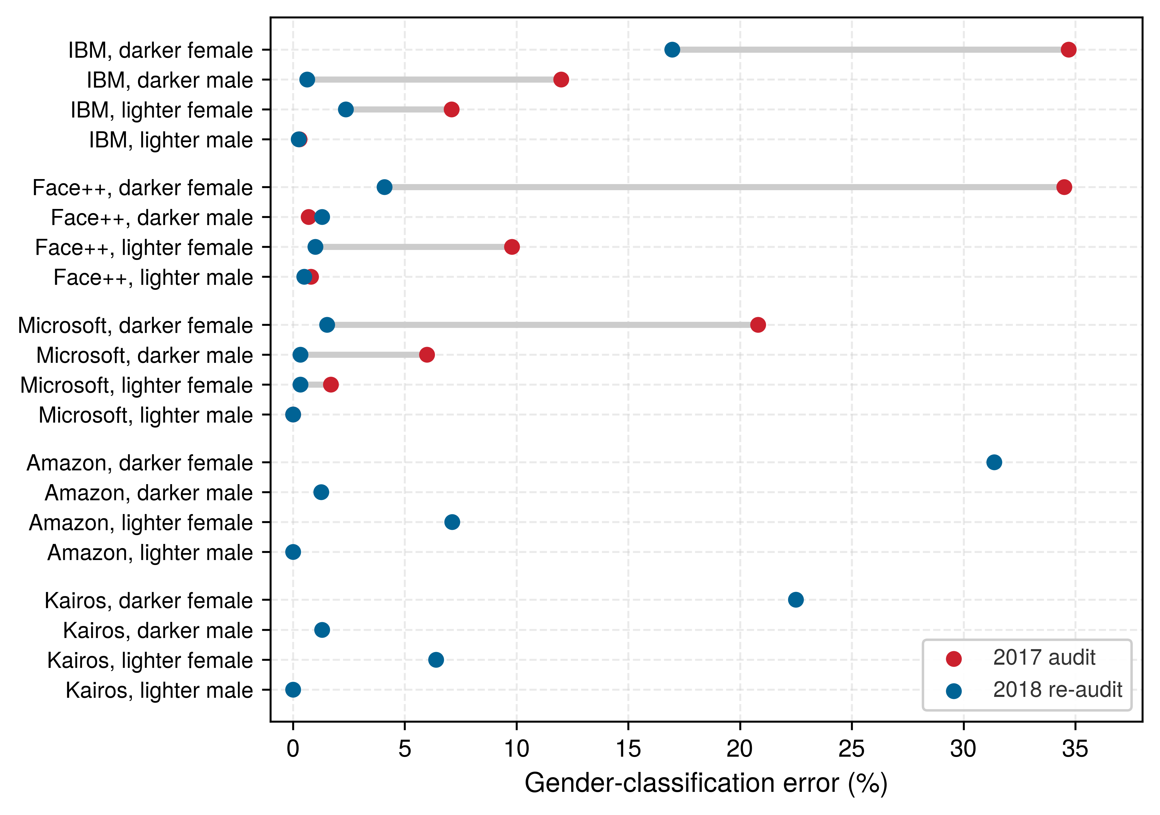
Buolamwini, Joy, and Timnit Gebru. 2018. “Gender Shades: Intersectional Accuracy Disparities in Commercial Gender Classification.” Conference on Fairness, Accountability and Transparency, 77–91.
Raji, Inioluwa Deborah, and Joy Buolamwini. 2019. “Actionable Auditing: Investigating the Impact of Publicly Naming Biased Performance Results of Commercial AI Products.” Proceedings of the 2019 AAAI/ACM Conference on AI, Ethics, and Society, 429–35. https://doi.org/10.1145/3306618.3314244.
An intersectional audit must specify the population slices it can identify and the evidence available within them. Work on multicalibration extends calibration checks to a specified, potentially rich family of overlapping subgroups (Hébert-Johnson et al. 2018). This does not certify every possible subgroup or every fairness criterion. It motivates evaluation and monitoring infrastructure that can examine relevant intersections while reporting where sample support or attribute availability limits the claim.
Hébert-Johnson, U., M. P. Kim, O. Reingold, and G. N. Rothblum. 2018. “Multicalibration: Calibration for the (Computationally-Identifiable) Masses.” In Proceedings of the 35th International Conference on Machine Learning, ICML 2018, Stockholmsmässan, Stockholm, Sweden, July 10-15, 2018, edited by Jennifer G. Dy and Andreas Krause, vol. 80. Proceedings of Machine Learning Research. PMLR.
Choosing the governing criterion
The running loan example establishes how to measure a disparity and its sampling uncertainty. Applying that framework still requires identifying whether a positive decision grants a benefit or imposes a burden, checking the criteria a headline metric misses, and choosing the requirement that fits the deployment.
Napkin Math 16.3: Auditing a confusion matrix
Problem: A fraud detection model operates on two groups. What do demographic parity and equal opportunity reveal about the deployment?
Variables:
- Group A (majority): \(\text{TP}=450\), \(\text{FP}=50\), \(\text{FN}=30\), \(\text{TN}=470\) (\(\AuditGroupRecordCount=1000\)).
- Group B (minority): \(\text{TP}=180\), \(\text{FP}=70\), \(\text{FN}=120\), \(\text{TN}=630\) (\(\AuditGroupRecordCount=1000\)).
Math:
- Demographic parity (positive prediction rate): \(\Pr(\PredictedDecision=1)\).
- Group A: \((450+50)/1000 = 0.50\).
- Group B: \((180+70)/1000 = 0.25\).
- Gap: 0.25. The lower-to-higher flag-rate ratio is \(0.25/0.50 = 0.5 < 0.8\). Fraud flags are adverse outcomes, so this descriptive ratio is not a four-fifths employment-selection test.
- Equal opportunity (TPR): \(\text{TP} / (\text{TP}+\text{FN})\).
- Group A: \(450 / (450+30) = 0.938\).
- Group B: \(180 / (180+120) = 0.60\).
- Gap: 0.338. (Severe violation).
Systems insight: Here a positive prediction flags suspected fraud, rather than granting a benefit as in the loan example. Equalizing detection rates therefore requires weighing missed fraud against false accusations. Lowering Group B’s threshold may catch more fraud but can also increase false alarms; the score distributions are needed to quantify the effect on predictive parity.
The running loan model fails every criterion at once, which can suggest that a single headline metric would have caught it. A second hypothetical loan model, deliberately different from the running example, shows the opposite risk, in which one criterion is satisfied exactly while the others fail (table 7). Unlike the running model, whose false positive rates differ (0.55 against 0.20), this model approves would-be defaulters at the same 20 percent rate in both groups. Equalized odds would require both true positive rates and false positive rates to match, so the table shows the narrower case of false-positive-rate parity rather than full equalized odds, and because one fairness metric can appear satisfied while others expose substantial disparities, a deployment must decide in advance which criterion governs it.
| Metric | Definition | A | B | Gap |
|---|---|---|---|---|
| Approval Rate | (TP + FP) divided by total | 55% | 40% | 15 pp |
| True Positive Rate | TP divided by positives | 90% | 60% | 30 pp |
| False Positive Rate | FP divided by negatives | 20% | 20% | 0 pp |
| Positive Predictive Value | TP divided by predicted positives | 82% | 75% | 7 pp |
Example 16.1: Choosing a fairness metric
Scenario: A hiring recommendation engine must select its primary fairness constraint before production launch across heterogeneous applicant pools. The accountable reviewers prioritize equal access for qualified applicants and have independently validated qualification labels for both selected and rejected applicants.
Diagnosis: Demographic parity forces equal selection rates regardless of candidate qualification, while calibration requires predicted probabilities to match outcome frequencies within each group. Equal opportunity specifically mandates equal true positive rates among qualified applicants (\(\text{TPR}_\FirstComparedGroupLabel = \text{TPR}_\SecondComparedGroupLabel\)), directly matching the goal of equal opportunity for qualified talent.
Systems lesson: Metric selection is a governance decision that sets the operational objective of the serving pipeline. System designers must align the mathematical constraint with the domain’s legal and ethical requirements before training or thresholding.
The chosen fairness definition determines which error trade-off the system is allowed to make, so the choice precedes optimization against that criterion. A model can satisfy a specified fairness criterion, but responsibility depends on the system that uses it. Data collection, labels, modeling choices, evaluation procedures, and decision thresholds all affect the resulting outcomes. Postprocessing can repair a selected rate disparity without resolving an invalid target or an unsupported deployment. Privacy, explainability, robustness, and accountability likewise require evidence about the relevant pipeline, beyond properties of the weights. A fairness policy is therefore realized through coordinated data collection, evaluation, threshold policy, and monitoring across the lifecycle (table 3), and group-specific thresholds are one possible intervention within that policy, not a universal requirement.
The system boundary extends past the model’s decisions to the infrastructure that runs them, because who can reach the safeguards and who bears their environmental costs are distributional effects of the same system (section 16.4.3). Collecting the evidence creates a further constraint, because demographic attributes useful for auditing may also increase privacy exposure. Governance must justify both the fairness claim and the data practices used to support it.
16.5.3 Threshold setting and fairness trade-offs
When two applicant groups have different score distributions, applying a single 0.75 approval cutoff can approve 75 percent of qualified applicants in one group and only 25 percent in the other, while lowering one group’s cutoff to equalize opportunity gives two applicants with the same score different decisions. In practice, fairness metrics can be changed after training by adjusting classification thresholds per group. In the equations below, a larger score favors a positive decision, as with predicted repayment probability. Given a scoring function \(\DecisionScore(\ModelInput)\), define group-specific thresholds \(\FirstGroupClassificationThreshold\) and \(\SecondGroupClassificationThreshold\) such that \(\FirstGroupThresholdClassifier(\ModelInput) = \mathbb{1}[\DecisionScore(\ModelInput) \geq \FirstGroupClassificationThreshold]\) for group \(\FirstComparedGroupLabel\) and similarly for group \(\SecondComparedGroupLabel\).
To achieve demographic parity, solve: \[ \Pr(\DecisionScore(\ModelInput) \geq \FirstGroupClassificationThreshold\mid \ProtectedGroupMembership = \FirstComparedGroupLabel) = \Pr(\DecisionScore(\ModelInput) \geq \SecondGroupClassificationThreshold\mid \ProtectedGroupMembership = \SecondComparedGroupLabel) \]
To achieve equal opportunity, solve: \[ \Pr(\DecisionScore(\ModelInput) \geq \FirstGroupClassificationThreshold\mid \ProtectedGroupMembership = \FirstComparedGroupLabel, \TrueOutcome= 1) = \Pr(\DecisionScore(\ModelInput) \geq \SecondGroupClassificationThreshold\mid \ProtectedGroupMembership = \SecondComparedGroupLabel, \TrueOutcome= 1) \]
For equalized odds, both true positive and false positive rate constraints must hold simultaneously. A single deterministic threshold per group need not satisfy both. Postprocessing can instead randomize between threshold rules within each group to attain a shared pair of rates (Hardt et al. 2016). The resulting criterion constrains group-level probabilities, so validation must evaluate the randomized policy rather than only its component thresholds.
Hardt, Moritz, Eric Price, and Nathan Srebro. 2016. “Equality of Opportunity in Supervised Learning.” Advances in Neural Information Processing Systems (NeurIPS) 29: 3315–23.
Threshold adjustment still requires evaluating the other criteria. When base rates differ (that is, \(\Pr(\TrueOutcome=1 \mid \ProtectedGroupMembership=\FirstComparedGroupLabel) \neq \Pr(\TrueOutcome=1 \mid \ProtectedGroupMembership=\SecondComparedGroupLabel)\)), calibration and error-rate constraints can conflict under the conditions discussed earlier. The effect of a particular threshold policy must be measured on the joint score and label distribution; a base-rate difference alone does not determine its accuracy cost.

Lifting Group B’s approval rate to parity costs 4 points of accuracy.
The accuracy cost of a threshold policy becomes concrete on a separate credit model, distinct from the running loan example. Its score is a predicted default probability, so a lower score favors approval and each cutoff admits applicants below it. The scenario enforces demographic parity, the first threshold equation above, and prices the accuracy that enforcement costs.
Napkin Math 16.4: The fairness cost
Problem: Consider a credit model with 85 percent accuracy. Group A (majority) has a 20 percent default rate. Group B (minority) has a 40 percent default rate due to systemic factors. If demographic parity (equal approval rates) is enforced, what happens to accuracy?
Math:
This scenario holds Group A’s approval rate fixed and raises Group B’s rate to match it; demographic parity alone does not require that particular choice. The accuracy values are assumed held-out validation results, where the additional Group B approvals carry higher default risk.
- Unconstrained: Model approves everyone with predicted default prob < 30 percent.
- Group A approval: 80 percent.
- Group B approval: 60 percent.
- Total Accuracy: 85 percent.
- Constrained (parity): Holding Group A’s rate fixed, approve Group B at 80 percent rate.
- New threshold for Group B: Approve default prob < 50 percent.
- The revised cutoff admits Group B applicants with higher predicted default risk than the original policy allowed.
- New Total Accuracy: 81 percent.
Systems insight: This parity policy cost 4 percentage points of accuracy (about a 4.7 percent relative accuracy drop in this credit-scoring scenario). The drop is the fairness cost of this scenario, not a universal property of fairness constraints. Accuracy still measures prediction against the specified default labels; whether those labels capture the legitimate lending objective is a separate question. Engineers must report the predictive trade-off while making the target and policy assumptions explicit.
The 4 percentage points cost belongs to one parity policy on one prediction target. A different criterion moves the thresholds for a different reason, and the next scenario, which returns to the repayment-score convention, targets equal opportunity by comparing the score distributions among qualified applicants. Differential thresholds require access to sensitive attributes at inference time and raise concerns about explicit group-based treatment, which may itself be considered unfair or illegal in certain jurisdictions. The required thresholds depend on those distributions and the chosen criterion; a lower threshold for the minority group is not a universal fairness rule.
Napkin Math 16.5: Threshold for equal opportunity
Problem: Calculate group-specific thresholds required to equalize true positive rates (equal opportunity) across Group A and Group B in a credit scoring model.
Variables: Let the score \(\DecisionScore(\ModelInput)\) be an unbounded decision score, not a calibrated probability, and write Group A as \(\ProtectedGroupMembership=\FirstComparedGroupLabel\) and Group B as \(\ProtectedGroupMembership=\SecondComparedGroupLabel\). Assume \(\DecisionScore(\ModelInput)\mid(\TrueOutcome=1,\ProtectedGroupMembership=\FirstComparedGroupLabel)\sim\GaussianDistribution(0.72,0.15^2)\) and \(\DecisionScore(\ModelInput)\mid(\TrueOutcome=1,\ProtectedGroupMembership=\SecondComparedGroupLabel)\sim\GaussianDistribution(0.65,0.16^2)\). These are hypothetical positive-class distributions; no negative-class distribution or prevalence is specified.
Math:
- Single threshold: At \(\FirstGroupClassificationThreshold=\SecondGroupClassificationThreshold=0.60\), \(\text{TPR}_\FirstComparedGroupLabel=1-\StandardNormalCumulativeDistribution(-0.8)\approx0.788\) and \(\text{TPR}_\SecondComparedGroupLabel=1-\StandardNormalCumulativeDistribution(-0.3125)\approx0.623\), where \(\StandardNormalCumulativeDistribution\) is the standard normal cumulative distribution function.
- Equalizing thresholds: Preserve Group A’s threshold and match its standardized cutoff, \((\SecondGroupClassificationThreshold-0.65)/0.16=-0.8\). Thus \(\SecondGroupClassificationThreshold=0.522\) yields the same true positive rate.
- Unspecified costs: Lowering Group B’s threshold cannot decrease its false positive rate, but its magnitude requires \(\DecisionScore(\ModelInput)\mid(\TrueOutcome=0,\ProtectedGroupMembership=\SecondComparedGroupLabel)\). Precision also requires Group B’s prevalence. Neither quantity follows from the positive-class distributions alone.
Systems insight: Equal opportunity determines a threshold only relative to the stated score distributions and target rate. Before deployment, evaluate the resulting false positives, precision, and review workload on representative data. Threshold policies change decisions, not the underlying score calibration.
A separate illustrative loan scenario partitions applicants into Subgroup A (higher score distribution, blue band) and Subgroup B (lower score distribution, amber band), and the summary panels of figure 5 contrast two operating regimes. Applying a single global threshold (\(\ClassificationThreshold = 0.75\)) approves qualified applicants in Subgroup B at only 25 percent TPR compared to 75 percent for Subgroup A, a threefold opportunity disparity. Conversely, shifting to group-adapted thresholds (\(\FirstGroupClassificationThreshold= 0.75\) for Subgroup A and \(\SecondGroupClassificationThreshold= 0.45\) for Subgroup B) equalizes true positive rates at 75 percent. That policy requires the authorized decision component to access the relevant group attribute and log the governing threshold. Neither the attribute lookup nor the policy decision must run on the client, but the system must preserve evidence explaining why identical scores receive different decisions.
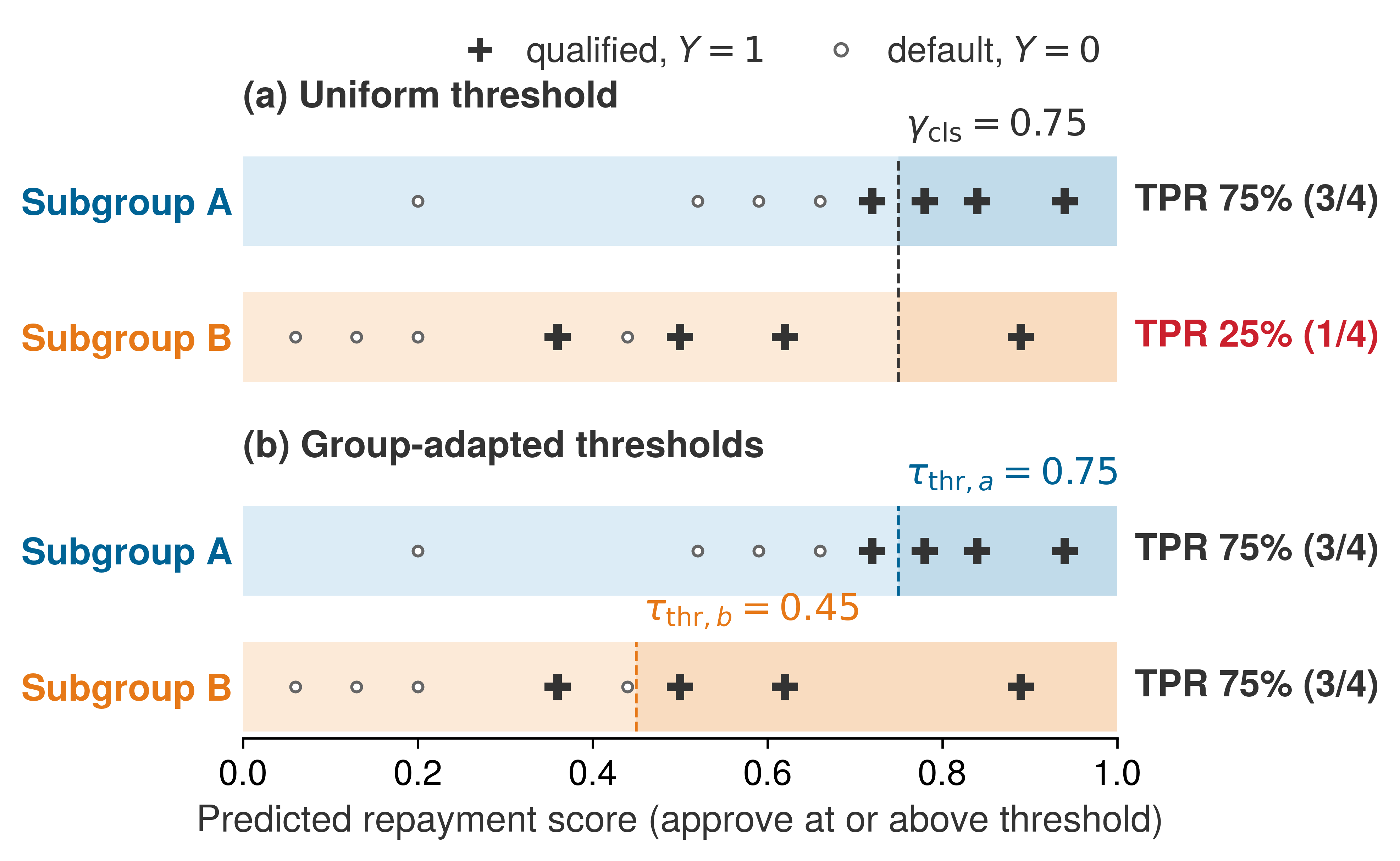
16.5.4 Fairness evidence across deployment tiers
A federated keyboard model running across millions of phones—the regime of Archetype C (Federated MobileNet)—never sends raw keystrokes or user demographic labels to the central server, so the fleet operator cannot simply run a SQL query to check whether next-word accuracy drops on a protected subgroup. Fairness presents a deployment problem whose binding constraint is data visibility. A cloud platform with authorized access to demographic labels and outcomes can compute group-level metrics, run fairness-aware training, and audit post-hoc. A federated9 or on-device deployment instead needs an explicit evidence path, such as aggregate client statistics or a separately governed audit sample. Without sufficient evidence, the corresponding metric is unmeasurable; local execution alone does not make the audit impossible. The evidence available for fairness analysis narrows from cloud to TinyML (fairness row of table 4), and two consequences of that narrowing recur across deployments.
9 Federated learning and fairness: Google’s public Gboard trial illustrated training across devices without centralizing raw examples (Hard et al. 2018). Model updates alone do not necessarily reveal the demographic labels and outcomes needed for a fairness audit, so the communication cost, privacy protection, and statistical uncertainty of whatever evidence path replaces them must be evaluated for that design.
Hard, Andrew, Kanishka Rao, Rajiv Mathews, Swaroop Ramaswamy, Françoise Beaufays, Sean Augenstein, Hubert Eichner, Chloé Kiddon, and Daniel Ramage. 2018. “Federated Learning for Mobile Keyboard Prediction.” arXiv Preprint arXiv:1811.03604.
Dwork, Cynthia, Moritz Hardt, Toniann Pitassi, Omer Reingold, and Richard Zemel. 2012. “Fairness Through Awareness.” Proceedings of the 3rd Innovations in Theoretical Computer Science Conference, 214–26. https://doi.org/10.1145/2090236.2090255.
The first consequence concerns decision policy. Equal aggregate accuracy across groups does not establish equal opportunity under a uniform threshold, as the illustrative gap in figure 5 demonstrates. A deployment must select and evaluate a policy against its approved criterion; group-specific thresholds are one possible intervention, not a requirement imposed by edge execution. The second consequence sharpens the personalization conflict raised in section 16.4.1. Local adaptation aims to improve a user’s utility, whereas individual fairness requires similar individuals to receive similar decisions under a task-relevant similarity metric (Dwork et al. 2012). Personalization does not establish that requirement, and adaptation on sparse or unrepresentative observations can reinforce existing gaps. When the relevant evidence stays local, fleet operators need an authorized way to assess the resulting disparities. Section 16.9.4.1 analyzes the feedback mechanism and its intervention points; the deployment consequence is that a fleet which cannot centralize outcomes must budget an explicit evidence path for detecting it.
That evidence path creates a further responsible AI tension. Keeping sensitive data local reduces centralized exposure, while fleet-level audits still need adequate group statistics. Privacy architecture (section 16.6.2) determines which records or aggregates may cross the boundary and under what protections.
16.5.5 Bias detection and monitoring
Suppose a nationally deployed credit model begins rejecting applicants from a specific ZIP code at twice its previous rate. Monitoring can expose that change before a periodic audit, but the rate alone does not establish its cause. An investigator must check population changes, data quality, and decision policy against the approved fairness criteria. Bias detection turns formal definitions into operational telemetry, using slice-based analysis to identify subpopulations whose outcomes warrant examination.
Measurement costs and intervention points
The criteria of section 16.5.1 define what a disparity is and how to test one. Computing them continuously on a production system that serves thousands of predictions per second is where the engineering cost appears, and that cost has computational, data, and organizational parts that decide which metrics a system can afford to monitor.
Measurement overhead arises because computing group-specific metrics requires maintaining separate statistics for each protected group: for \(\MonitoredGroupCount\) groups and \(\MonitoredFairnessMetricCount\) metrics, this adds \(\mathcal{O}(\MonitoredGroupCount \MonitoredFairnessMetricCount)\) counters and \(\mathcal{O}(\MonitoredGroupCount \MonitoredFairnessMetricCount)\) statistical tests per evaluation cycle. Streaming counters can update cheaply per prediction while statistical tests run at a separate evaluation interval, so profiling the number of groups, windows, and tests, rather than request rate alone, determines whether sampling or asynchronous aggregation is needed. Those counters also depend on which fields the metric consumes, because error-rate criteria need outcome labels (\(\TrueOutcome\)) alongside sensitive attributes \((\ProtectedGroupMembership)\) across a sample that supports the intended population claim, whereas demographic parity needs group membership and decisions without outcomes. Availability of those sensitive attributes requires an explicit governance and engineering choice among authorized direct collection, restricted audit records, encrypted or differentially private group statistics, or an offline sample; when inferred attributes are used instead, the audit must evaluate inference errors rather than treat the inferred groups as known, and when the evidence cannot support a metric, the system must report that limitation rather than interpret missing measurements as fair behavior.
Selecting acceptable disparity thresholds then demands domain expertise and stakeholder input, since the four-fifths rule is a screening convention from U.S. employment selection rather than a universal legal test for lending or fraud detection, and thresholds must reflect context-specific harm assessments, statistical uncertainty, and documented legal rationale. Because distribution shift, feedback loops, or model updates can erode fairness over time, temporal stability further requires monitoring those thresholds across evaluation windows. Automated alerting (for example, “alert if \(|\text{SPD}| > 0.15\) for 7 consecutive days”) defines when an owner receives a signal; the persistence window reduces sensitivity to brief fluctuations at the cost of response delay, so its acceptability depends on the harm and exposure during that interval, as section 16.9.3 develops.
Offline and CI-stage audits are the first place these metrics run, and open-source toolkits such as Fairlearn package the per-group bookkeeping (Bird et al. 2020), as in the audit of listing 1. Applied to the running loan example, that audit’s per-group table would report approval rates of 0.70 for Group A and 0.40 for Group B, the disparate impact ratio of 0.57 that falls below the 0.8 screening threshold in table 6. That comparison is an audit signal, not a lending-law verdict. The architecture must supply aligned decisions and group membership through an authorized audit path. Metrics that require outcome labels must use the relevant observed outcomes rather than substitute past decisions; an offline audit does not require exposing group attributes throughout runtime serving.
Bird, Sarah, Miro Dudı́k, Richard Edgar, Brandon Horn, Roman Lutz, Vanessa Milan, Mehrnoosh Sameki, Hanna Wallach, and Kathleen Walker. 2020. “Fairlearn: A Toolkit for Assessing and Improving Fairness in AI.” Microsoft Technical Report MSR-TR-2020-32.
import numpy as np
from fairlearn.metrics import MetricFrame, selection_rate
from sklearn.metrics import accuracy_score, precision_score

def false_positive_rate(y_true, y_pred):
    y_true, y_pred = np.asarray(y_true), np.asarray(y_pred)
    negatives = y_true == 0
    if not negatives.any():
        return float("nan")  # No observed negatives: rate is unmeasurable.
    return ((y_pred == 1) & negatives).sum() / negatives.sum()

# Loan approval model evaluation across demographic groups
mf = MetricFrame(
    metrics={
        "approval_rate": selection_rate,
        "accuracy": accuracy_score,
        "precision": precision_score,
        "false_positive_rate": false_positive_rate,
    },
    y_true=loan_repaid_actual,  # observed repayment outcome, not past approval
    y_pred=loan_approvals_predicted,
    sensitive_features=applicant_demographics["ethnicity"],
)

# NaN means a group lacks negative examples, not that its FPR is zero.
# Display performance disparities across groups
print("Loan Approval Performance by Group:")
print(mf.by_group)
# Hypothetical output on the running loan example:
# approval_rate 0.70 for group A, 0.40 for group B
Where sensitive attributes are unavailable at inference time, as is common in mobile, federated, and embedded systems, group-specific thresholds may be infeasible. Restricted offline audits can still guide data changes, retraining, or a revised policy that does not require an attribute lookup on each request.
Fairness interventions may be applied at different points in the pipeline, but each comes with system-level implications. Preprocessing methods change the training distribution through sampling, reweighting, or augmentation. Their data requirements depend on the method; group-targeted reweighting needs group information, while feature augmentation also needs access to the affected examples. Versioning and lineage must preserve which transformation produced the training data. In-processing approaches instead embed fairness constraints directly into optimization. They require support for the chosen loss or constrained solver and may add training work or validation requirements.
↩︎ Feature versioning and the lineage records that trace each training input are established in Feature versioning and lineage.
At the serving layer, postprocessing methods apply an approved decision rule to model outputs. Group-specific thresholds require the component choosing the threshold to obtain authorized group information; other policy rules may use different inputs. The dual-threshold policy in figure 5 (\(\FirstGroupClassificationThreshold= 0.75\), \(\SecondGroupClassificationThreshold= 0.45\)) therefore needs a controlled attribute lookup and a record of the applied policy, but not propagation of the attribute through every routing and inference component. Access controls should limit that exposure. Validation must evaluate the resulting decisions, operational stability, and applicable restrictions on attribute use.
Multicalibration (section 16.5.2.3) can run in backend training infrastructure even when the resulting model serves on a constrained endpoint, but a training-time result does not establish calibration after deployment conditions change. If telemetry cannot support renewed subgroup audits, the operator must record that evidence limitation and restrict the approved operating envelope accordingly.
Mitigation also decays after launch. A fairness-aware model may degrade if retraining pipelines omit fairness checks, if logging cannot track subgroup outcomes, or if user feedback introduces biases absent from the training distribution, so retraining protocols need subgroup-labeled validation data under data-governance review. Deciding which disparity to remediate, and at what cost to other objectives, remains a stakeholder decision (section 16.9.4.3). The architecture’s job is to make each disparity visible, in time, to the owner who must make that decision.
Real-time fairness monitoring architecture
Implementing responsible AI principles in production systems requires architectural patterns that integrate fairness monitoring, explainability, and privacy controls directly into the model serving infrastructure. The infrastructure separates into two decoupled tiers (figure 6). A synchronous request path enforces access control, data minimization, and low-latency inference, while an asynchronous governance tier ingests bounded execution evidence and delayed labels to drive fairness auditing, post-hoc explanations, and owner-governed release gates.
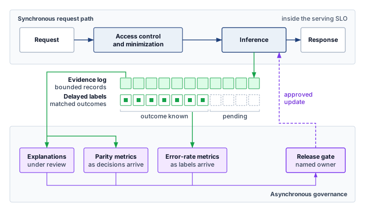
The request path applies access controls and data minimization before inference and records only the evidence needed for the approved monitoring policy. Group-level fairness analysis and expensive explanations can run asynchronously; synchronous checks must fit the serving service-level objective (SLO). Delayed labels enter the analysis path when outcomes become available, and a named owner approves model or policy changes.
Real-time fairness monitoring updates prediction-only metrics such as demographic parity as decisions arrive, maintaining rolling statistics across protected groups. Label-dependent metrics such as equalized odds and equality of opportunity update when delayed outcomes or audited labels arrive. Groups whose labeled windows are too small must remain visible as having insufficient evidence, with a defined collection or escalation policy. The system flags supported disparities that exceed configured thresholds and separately reports gaps in coverage. Storage and compute requirements depend on the number of groups, decision segments, and retention windows.
The explanation engine generates evidence for the audience and decision under review. Its budget depends on the method and model; exact model-specific attribution may be feasible where exhaustive subset evaluation is not. Approximation, caching, selective generation, and asynchronous execution offer different cost and delivery-time trade-offs. The monitoring part of this architecture collects predictions and computes rolling group metrics with threshold alerts (listing 2). The listing omits delayed outcome ingestion, the full equalized-odds calculation, and explanation generation, so it is a partial implementation rather than a complete governance service.
import numpy as np

class RealTimeFairnessMonitor:
    # alert_threshold mirrors the |SPD| > 0.15 rule; persistence check omitted.
    def __init__(self, window_size=1000, alert_threshold=0.15, min_group=30):
        self.min_group = min_group  # Illustrative policy; set from precision needs.
        self.window_size = window_size
        self.alert_threshold = alert_threshold
        self.window = []

    async def process_prediction(self, prediction, demographics,
                                 actual_label=None):
        # Slide a fixed window over the stream, then re-check fairness.
        self.window.append((prediction, demographics, actual_label))
        self.window = self.window[-self.window_size :]
        metrics = self._compute_metrics()
        if (metrics["demographic_parity"] is not None
            and metrics["demographic_parity"] > self.alert_threshold) or (
            metrics["equalized_odds"] is not None
            and metrics["equalized_odds"] > self.alert_threshold
        ):
            await self._trigger_bias_alert(metrics)
        return metrics

    def _compute_metrics(self):
        # Bucket predictions and labels by protected group.
        by_group = {}
        for pred, demo, label in self.window:
            bucket = by_group.setdefault(
                demo.get("ethnicity", "unknown"), {"preds": [], "labels": []}
            )
            bucket["preds"].append(pred)
            if label is not None:
                bucket["labels"].append((pred, label))

        rates = [np.mean(d["preds"]) for g, d in by_group.items()
                 if g != "unknown" and len(d["preds"]) >= self.min_group]
        parity = max(rates) - min(rates) if len(rates) > 1 else None
        return {
            "demographic_parity": parity,
            # Requires sufficiently labeled outcomes per group; omitted here.
            "equalized_odds": self._equalized_odds_gap(by_group),
            "groups": {g: len(d["preds"]) for g, d in by_group.items()},
            "eligible_groups": len(rates),  # Compare with required group coverage.
        }

    def _equalized_odds_gap(self, by_group): ...
    async def _trigger_bias_alert(self, metrics): ...  # page and audit
This simplified pattern separates metric availability from metric values, because an unavailable comparison is not a zero disparity. A production monitor must also enforce required group coverage, sample-size policies, and freshness before interpreting a result. The overhead ranges summarized in table 5 explain why fairness monitoring, privacy transformations, and explanation generation need explicit capacity budgets. Request metadata collection may be synchronous, while metric aggregation, delayed-label analysis, and explanation generation can run asynchronously under their own freshness requirements. These overheads must be balanced against reliability and compliance requirements when designing production systems.

At a 5 percent false-alarm rate, 150 metrics raise about 7.5 spurious alerts per interval.
At the scale of a global production fleet, fairness monitoring becomes a substantial data engineering challenge. This sizing scenario assumes roughly 864 million inferences per day at 10,000 queries/s across 50 demographic subgroups, with 150 metrics (false positive rate, true positive rate, and calibration error for each of the 50 groups). A 1 percent sampling rate yields 8.64 million monitoring events daily. At an assumed 200 bytes per record, those events require approximately 1.7 GB per day before additional audit records or storage overhead. Actual record contents and retention follow the approved measurement and privacy requirements; outcome-dependent metrics also require labels that may arrive later. The monitoring infrastructure itself must therefore be reliable, secure, and cost-effective. With 150 active metrics, an illustrative per-metric false-alarm probability of 5 percent would yield roughly 7.5 false alerts per evaluation interval if every tested null hypothesis is true. This expected count follows by summing false-alarm probabilities and does not require independence. Production thresholds must instead reflect subgroup denominators, delayed labels, repeated testing, confidence intervals, minimum detectable effects, and correction for multiple comparisons. A threshold crossing opens an investigation; it does not by itself prove discrimination or justify automatic retraining.
↩︎ False alarms, the spurious threshold crossings that accumulate as a fleet multiplies monitored metrics, are established in The alert fatigue problem.
In C³ terms, this monitoring load is communication and coordination added to the fleet. Every sampled record must travel from a serving replica to the aggregation tier, and every alert must reach an owner who can act before the harm it signals compounds. The deployment tier sets how long that path is. A cloud service aggregates telemetry continuously, subject to storage and privacy budgets. An intermittently connected client keeps bounded local records until it next synchronizes, and a safety-critical edge system needs local checks that can trigger fallback within the decision deadline because the fleet cannot respond in time. A disconnected TinyML endpoint may deliver its evidence only at a servicing visit, and correcting its model may require a firmware update or physical replacement. Those differences change the evidence delay and remediation path, not the requirement to name an owner for each monitored obligation.
Checkpoint 16.1: Putting bias detection into production
The bias-detection and monitoring sections turned static fairness definitions into live telemetry: slice-based detection with Fairlearn, CI-stage audits, production monitoring of demographic parity and equalized odds, the evidence paths that federated and on-device deployments require, and the distinction between observing a disparity and remediating it.
Detecting the disparity
From signal to action
Self-Check: Question
A loan approval model evaluates two demographic groups (Group A and Group B). Group A has a baseline approval rate of \(70\%\) (\(\text{PPV} = 57.1\%\)), while Group B has a baseline approval rate of \(40\%\) (\(\text{PPV} = 75.0\%\)). If the engineering team lowers the decision threshold for Group B to enforce demographic parity (\(70\%\) approval for both groups), what is the immediate system-level consequence?
- Group B’s positive predictive value increases while overall model accuracy remains completely unchanged
- Lowering the threshold admits additional applicants with lower predicted repayment scores; the effects on approval precision and overall accuracy must be evaluated rather than inferred from approval rates alone.
- The model automatically satisfies equalized odds without any change to false positive rates
- The underlying true default base rates of both populations become mathematically equalized
For risk scores, the chapter’s score-balance impossibility result combines calibration within each group with equal mean scores across groups among positive outcomes and, separately, among negative outcomes. Which cases escape the stated incompatibility?
- Whenever the training dataset contains more than \(10^6\) balanced records across all demographic slices
- Whenever the model is trained with \(L_2\) regularization and post-hoc isotonic calibration
- Whenever demographic parity is explicitly enforced via multi-task adversarial training
- Only in degenerate or trivial cases, such as perfect prediction (zero error) or identical base rates across groups
Explain how single-axis fairness audits can enable ‘fairness gerrymandering’ and describe the evaluation strategy required to detect it.
Which statement correctly differentiates Preprocessing, In-processing, and Postprocessing fairness interventions with respect to ML system infrastructure requirements?
- Preprocessing modifies serving thresholds at inference, In-processing requires anonymizing logs, and Postprocessing alters training labels in feature stores
- All three methods require identical runtime compute overhead on the live model serving path
- Preprocessing is only applicable to TinyML devices, while In-processing and Postprocessing can only run in cloud clusters
- Preprocessing changes training data and needs lineage; in-processing changes training optimization; group-specific threshold postprocessing requires authorized group information at the component applying the decision rule.
A streaming loan-approval service records authorized group attributes and decisions immediately, but repayment outcomes arrive months later. Why can demographic-parity statistics update earlier than equalized-odds statistics?
- Demographic Parity depends only on model predictions and input demographics available at inference time, whereas Equalized Odds requires true outcome labels that arrive with substantial real-world latency
- Demographic Parity requires calculating matrix inverses that execute faster on GPU tensor cores
- Equalized Odds is a convex optimization problem that cannot be evaluated on streaming CPU worker nodes
- Demographic Parity violates privacy regulations if processed asynchronously in background databases
A production ML fleet serving 864 million daily inferences tracks 150 distinct subgroup fairness metrics. With an unadjusted per-metric false alarm rate of \(5\%\), the system experiences roughly 7.5 false alerts per evaluation interval. Explain the operational consequence of this false alarm volume and describe how the monitoring architecture should mitigate it.
16.6 Privacy and Data Governance
Every fairness audit and monitor consumes demographic evidence, and that evidence is itself sensitive data. The threat models and privacy mechanisms of Security & Privacy provide the technical controls; governance defines the evidence, ownership, and lifecycle interfaces that production systems require when inheriting them. A deletion workflow must identify which records and derived artifacts fall within an applicable obligation, such as an erasure requirement under the GDPR (European Parliament and Council of the European Union 2016). Removing a database row may leave replicas, backups, or trained models to address. Where removal of training influence is required, lineage, retraining, validation, deployment, and audit become part of the same workflow.
Governing these risks coordinates two classes of control that are easy to conflate. Privacy mechanisms bound specified information exposures, while machine unlearning (section 16.6.4) targets the influence a record retains in trained weights under a stated removal criterion. A privacy guarantee does not by itself remove a record from the training history, so the assurance case must distinguish these obligations and supply evidence for each. Robustness and generative-system controls receive the same evidence-and-ownership treatment in section 16.8.
16.6.1 Core data governance principles
A fairness audit may need the same demographic field that a data-minimization policy would otherwise exclude. Privacy mechanisms constrain exposure and leakage; governance determines whether collecting the field is justified, who may use it, and how long the audit needs it. This decision connects privacy to fairness (section 16.5.1) and to transparency (section 16.7.1). Group-based monitoring needs evidence about group membership, but the audit design determines whether operators receive individual fields, restricted audit records, or aggregate statistics. Explainability methods can also reveal information about training examples, while detailed disclosure can conflict with individual privacy. Responsible AI systems must justify the evidence collected and limit its exposure while retaining enough information to evaluate the chosen requirements.
↩︎ Federated learning, encrypted computation, and synthetic data, each bounding who can observe raw records, are established in Privacy-preserving data techniques.
Carlini, N., F. Tramer, E. Wallace, M. Jagielski, A. Herbert-Voss, K. Lee, A. Roberts, et al. 2021. “Extracting Training Data from Large Language Models.” 30th USENIX Security Symposium (USENIX Security 21), 2633–50.
Because training and personalization rely on personal data, privacy is a design constraint across the whole system lifecycle, and its central difficulty is the tension between data utility and individual protection. Rich, high-resolution datasets can enhance model accuracy and adaptability but also heighten the risk of exposing sensitive information, particularly when datasets are aggregated or linked with external sources. For example, large language models trained on broad text corpora have been shown to memorize specific strings that can later be retrieved through model queries or adversarial prompting (Carlini et al. 2021).
↩︎ The GPT-2 extraction attack, which recovered verbatim training records through ordinary generated outputs, is established in GPT-2 data extraction case study.
Privacy risks also depend on how records are linked over time and across sources. A wearable device’s heart-rate or location record can already be sensitive; combining physiological and behavioral signals can reveal additional details about a user’s health, routines, or relationships. Limited visibility or control over processing, retention, and transmission makes it harder for users to understand or contest these uses.
Addressing these challenges requires understanding privacy as a system principle that entails robust data governance. This includes defining what data is collected, under what conditions, and with what degree of consent and transparency. Foundational data engineering practices, including data validation, schema management, versioning, and lineage tracking, provide the technical infrastructure for implementing these governance requirements. Responsible governance requires attention to labeling practices, access controls, logging infrastructure, and compliance with jurisdictional requirements. These mechanisms serve to constrain how data flows through a system and to document accountability for its use.
Weak data governance can obscure both quality defects and privacy exposures, but they require different evidence. In clinical applications, missing values or demographic skew can compromise predictive performance; neither alone establishes a privacy violation. Privacy assessment must also examine identifiability, access, and disclosure. Documentation should make these distinct risks traceable to the data practices that create them.
Privacy is not solely the concern of isolated algorithms or data processors; like fairness, it must be addressed as a structural property of the system. Decisions about consent collection, data retention, model design, and auditability all contribute to the privacy posture of a machine learning pipeline. This requires anticipating risks during inference and continuous operation as well as during training. Threats such as membership inference, which infers from a deployed model’s outputs whether a record was in its training set, show why privacy safeguards must be embedded in both model architecture and interface behavior.
↩︎ Membership inference, its mechanism, and why an empirical audit gives only a lower bound on leakage are established in Membership inference.
10 CCPA (California Consumer Privacy Act): CCPA grants California residents rights over covered personal information, including a deletion right subject to statutory exceptions (California Legislature 2023). For ML serving infrastructure, deletion requests create an architectural constraint that must be planned from the data pipeline forward, because raw-record deletion does not automatically remove a record’s influence from trained model parameters.
California Legislature. 2023. California Consumer Privacy Act of 2018. California Legislative Information.
Personal Information Protection Commission, Japan. 2023. Act on the Protection of Personal Information. Personal Information Protection Commission, Japan.
Legal frameworks make privacy an enforceable design concern. The GDPR, the California Consumer Privacy Act (CCPA),10 and Japan’s Act on the Protection of Personal Information establish different obligations and individual rights within their respective scopes (European Parliament and Council of the European Union 2016; California Legislature 2023; Personal Information Protection Commission, Japan 2023). An implementation must identify which rules govern its collection, use, retention, and removal of data rather than treating consent or deletion as a uniform requirement across jurisdictions. That applicability decision belongs in the system’s documented data-governance requirements.
Privacy mechanisms limit specified data exposures under their threat models; they do not establish that a system’s decisions are safe. A model may satisfy its privacy requirements while still failing catastrophically on unexpected inputs, a complementary concern about how systems fail that section 16.8 takes up. Within privacy itself, the next decision is where the protected boundary sits in each deployment architecture.
16.6.2 Privacy across deployment tiers
Training a model with differential privacy does nothing to protect a user whose raw prompt is copied into a plaintext serving log at the API gateway, while keeping raw records on a phone protects against central database breaches at the cost of hiding fleet-wide telemetry from operators. Privacy inherits the same centralization trade-off across deployment tiers (privacy row of table 4). Aggregating data in the cloud enables high-capacity modeling and monitoring but concentrates exposure to breaches and surveillance, so it must be paired with strong encryption, access control, and auditability. Keeping data local on mobile, federated, or TinyML clients reduces that central exposure but changes the evidence available to fleet operators. Privacy controls must cover local storage, outputs, telemetry, and update channels; an endpoint with no update path needs controls that remain valid for its approved service life.
The constraint the table cannot show is that privacy claims must name their boundary. Differentially private training bounds training-data leakage through the released model; ordinary inference on fixed weights remains within that post-processing guarantee. It does not protect new private inputs copied into service logs or unrelated private-data accesses. Interface design, retention rules, rate limiting, and access control address those separate exposures. Opaque data collection can also violate user expectations, making consent surfaces and clear disclosure part of the privacy architecture.
Federated training draws three such boundaries (figure 7). Raw records stay on the client, secure aggregation hides individual updates only under its collusion and dropout assumptions, and central differential privacy bounds what the released model reveals only if the curator that adds the noise is trusted. Each protection covers a different quantity against a different observer, so a claim about one says nothing about the others. The privacy unit, clipping rule, protocol assumptions, and composition across rounds define each guarantee (Bonawitz et al. 2017; Dwork and Roth 2014).
Bonawitz, Keith, Vladimir Ivanov, Ben Kreuter, Antonio Marcedone, H. Brendan McMahan, Sarvar Patel, Daniel Ramage, Aaron Segal, and Karn Seth. 2017. “Practical Secure Aggregation for Privacy-Preserving Machine Learning.” Proceedings of the 2017 ACM SIGSAC Conference on Computer and Communications Security, 1175–91. https://doi.org/10.1145/3133956.3133982.
Dwork, Cynthia, and Aaron Roth. 2014. “The Algorithmic Foundations of Differential Privacy.” Foundations and Trends® in Theoretical Computer Science, Foundations and trends in theoretical computer science, vol. 9 (3-4): 211–487. https://doi.org/10.1561/0400000042.
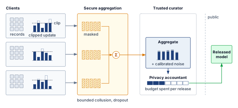
An architecture decides where the privacy boundary sits; the model decides how much crosses it. A service can keep raw records behind every access control and still release training data through the weights it serves, which is where the governance of privacy guarantees begins.
16.6.3 Governing privacy guarantees
A language model that regurgitates a patient’s phone number from its training set or a classifier whose confidence scores reveal whether a specific customer was in the training cohort leaks private data through authorized outputs even when no database is breached. Technical methods for privacy preservation aim to prevent data leakage, limit memorization, and uphold user rights such as consent, opt-out, and data deletion across data collection, model behavior, and user interaction.
Governing a privacy guarantee starts from the leaks that Leakage through authorized outputs develops. Because a model can memorize training records in images as well as text and reveal membership through its outputs, governance turns each leak into an audit obligation. A membership-inference audit must state the attacker access it assumes and reads only as a lower bound on leakage, so a formal bound has to come from the training mechanism.
For differential privacy, governance consumes the mechanism and accounting established in Differential Privacy. A differentially private stochastic gradient descent (DP-SGD) deployment must retain the clipping, noise, sampling, and composition configuration that supports its reported bound (Abadi et al. 2016). Reviewers then evaluate that bound alongside utility, subgroup performance, and the private-data accesses outside training. Naming the method is insufficient evidence for approving the complete service.
Abadi, M., A. Chu, I. Goodfellow, H. B. McMahan, I. Mironov, K. Talwar, and L. Zhang. 2016. “Deep Learning with Differential Privacy.” Proceedings of the 2016 ACM SIGSAC Conference on Computer and Communications Security, CCS ’16, 308–18. https://doi.org/10.1145/2976749.2978318.
Differential privacy introduces system-level trade-offs on the path where private data is accessed. Training noise can reduce utility, and attempts to recover it through additional data or optimization steps must be evaluated with the resulting privacy accounting and compute cost. If training occurs centrally, those costs do not automatically become extra work for an edge device performing ordinary inference on the released model. Local training or local randomization places different demands on the device. Data minimization, retention limits, and access controls remain separate requirements; feature obfuscation alone provides no differential privacy guarantee.
Systems Perspective 16.1: The price of privacy
Training a large language model on sensitive messages with DP-SGD reduces training-data extraction risk, but the protection is priced in compute and accuracy.
With the neighboring relation and \(\PrivacyAdditiveSlack\) fixed, a smaller \(\PrivacyBudget\) gives a stronger bound, and every change that lowers it (more noise, a smaller sampling rate, fewer steps) tends to cost accuracy or extra training; Differential Privacy derives these effects and lists the accountant inputs a reproducible DP-SGD result must record. Those recorded inputs, not the \(\PrivacyBudget\) value alone, are what a governance review retains. The three configurations below are planning assumptions whose \(\PrivacyBudget\) values an external accountant would have to confirm, as the CIFAR-10 accountant inputs of DP-SGD accountant inputs for image classification illustrate. Read them for the direction of each trade. The stronger configuration doubles the noise multiplier of the weaker one but also trains for more epochs, and more steps by themselves raise \(\PrivacyBudget\); only the accountant can confirm that the extra noise more than offsets the extra steps.
Illustrative stronger-privacy configuration (assumed accountant result \(\PrivacyBudget=\) 1): The scenario assumes per-example gradients are clipped to norm \(\GradientClippingNorm= 1.0\), 40 percent of updates are affected by clipping, and the noise multiplier is \(\PrivacyNoiseMultiplier= 1.0\). It further assumes 3× more epochs, a training-cost increase from a GPT-3-scale baseline of $4.6M to approximately $13.8M, and an accuracy drop of 6 percent.
Illustrative weaker-privacy configuration (assumed accountant result \(\PrivacyBudget=\) 8): The scenario assumes a noise multiplier of \(\PrivacyNoiseMultiplier= 0.5\), training overhead of 30 percent, and an accuracy drop of 1 percent.
Illustrative weakest configuration (assumed accountant result \(\PrivacyBudget=\) 10): The scenario assumes less noise and less than 1 percent accuracy loss, with a weaker formal privacy bound than the other two configurations under otherwise comparable accounting assumptions.
These scenarios compare formal privacy bounds, utility, and training cost; none of those quantities alone establishes user trust. Once a fixed model has been trained with differential privacy, ordinary inference is post-processing and does not consume additional training-data privacy budget. Additional privacy loss must be accounted for when a postdeployment mechanism makes new accesses to private data or releases additional differentially private statistics. The key engineering decision is to document and account for every private-data access and communicate the resulting trade-offs to users and regulators.
Released datasets need a boundary of their own. A \(\Glyph{k}\)-anonymous release (De-identification and k-anonymity) hides each record among at least \(\AnonymitySetSize\) that share its quasi-identifiers, a property of a specified release rather than of one transformed request. Differential privacy likewise requires a defined release mechanism, neighboring relation, and privacy accountant; noise injection alone does not establish a guarantee.
Privacy enforcement also depends on infrastructure beyond the model itself. Data collection interfaces must support informed consent and transparency. Logging systems must avoid retaining sensitive inputs unless strictly necessary, and must support access controls, expiration policies, and auditability. Model serving infrastructure must be designed to prevent overexposure of outputs that could leak internal model behavior or allow reconstruction of private data. These system-level mechanisms require close coordination between ML engineering, platform security, and organizational governance.
Privacy must be enforced throughout the machine learning lifecycle. Retraining pipelines must respect the approved deletion and data-use policies. Monitoring should collect only the identifying information justified by its purpose, with access and retention controls appropriate to that information. Privacy-aware telemetry collection and protected per-user audit trails can support investigation and remedy without making sensitive records broadly available in logs or dashboards.
The privacy assurance case therefore spans the whole pipeline. The formal privacy accountant covers the private-data accesses in its stated mechanism; interface controls, retention policies, and access records support separate claims about the surrounding service. Keeping these claims distinct makes gaps visible when a model, telemetry path, or data source changes.
Privacy preservation techniques create complex sociotechnical tensions that extend well beyond technical implementation. Differential privacy mechanisms may reduce model accuracy in ways that disproportionately affect underrepresented groups, creating conflicts between privacy and fairness objectives. These challenges require ongoing stakeholder engagement as detailed in section 16.9.4.3, where organizations must navigate competing values around data control, personalization, and regulatory compliance. These privacy challenges become even more complex when considering the dynamic nature of user rights and data governance.
16.6.4 Machine unlearning
Deleting a user’s row from a production database after a GDPR erasure request leaves their influence intact inside a 175-billion-parameter model that was trained on last month’s snapshot. When the approved deletion policy also requires addressing retained model state, machine unlearning supplies a technical response. The requirement and the evidence of removal must be specified separately; retained influence alone does not establish that every deployment violates a deletion obligation.
Privacy preservation does not end at training time. In many real-world systems, users may have rights to revoke consent or request deletion of their data, even after a model has been trained and deployed (European Parliament and Council of the European Union 2016; California Legislature 2023). When the approved response requires removing training influence, the architecture must support the chosen method and its verification. An endpoint without sufficient data, training state, or compute may need a replacement model trained elsewhere; a device with the required resources may perform the work locally. Placement follows those requirements rather than the deployment label alone.
Full retraining requires access to the permitted remaining training data and a defined training procedure. Three update strategies differ in what they recompute and what removal they guarantee (figure 8). Retraining from scratch on the retained data, the training set with the forget set \(\ForgetDataset\) removed, supplies a reference for exact removal relative to that procedure. Gradient ascent on the forget set increases its loss through updates of the form \(\ModelParameters + \LearningRate \nabla \LossFunction\), but increased loss alone does not demonstrate removal. Sharded, isolated, sliced, and aggregated (SISA) training partitions data into isolated shards \(\SisaTrainingShard_1, \SisaTrainingShard_2, \SisaTrainingShard_3\) and aggregates their predictions. A deletion affects the constituent model trained on its shard; saved states before the affected slice can reduce the retraining work.
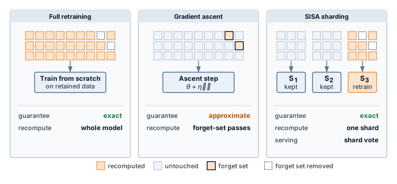
Full retraining is a useful reference, but its feasibility depends on access to the permitted remaining data, the training procedure, and sufficient compute within the response deadline. A retention policy may remove data that retraining would need; a large training run may exceed the available budget. An alternative unlearning method must state its own data and state requirements rather than assume that avoiding full retraining also eliminates those dependencies.
Machine unlearning seeks to remove specified training influence without repeating the entire training run. Cao and Yang (2015) proposed converting suitable learning algorithms into a summation form, allowing a deletion to update the affected summaries and recompute the model. SISA instead localizes retraining to affected shards (Bourtoule et al. 2021). It still needs the retained data and training state required by that procedure. The removal claim must specify its reference and verification method; a loss increase on deleted examples is different evidence from retraining without them. Method selection therefore depends on retained state, model quality, operational cost, and the removal guarantee the deployment must support.
Cao, Yinzhi, and Junfeng Yang. 2015. “Towards Making Systems Forget with Machine Unlearning.” 2015 IEEE Symposium on Security and Privacy, 463–80. https://doi.org/10.1109/sp.2015.35.
Bourtoule, Lucas, Varun Chandrasekaran, Christopher A. Choquette-Choo, Hengrui Jia, Adelin Travers, Baiwu Zhang, David Lie, and Nicolas Papernot. 2021. “Machine Unlearning.” 2021 IEEE Symposium on Security and Privacy (SP), 141–59. https://doi.org/10.1109/sp40001.2021.00019.
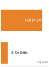
For one isolated erasure, SISA cuts retraining cost about 100 times; a daily batch that touches most shards erodes the saving.
Napkin Math 16.6: The cost of forgetting
A user requests erasure of personal data under GDPR Article 17 (“Right to Erasure”). This scenario assumes that the approved response includes removing its influence from a model trained on 1 TB of data; that model-removal requirement is a scenario premise, not a conclusion derived from invoking the article.
Baseline (full retraining): In this sizing scenario, a 175B-parameter model at GPT-3 scale retrains on 1,024 NVIDIA A100 (80 GB SXM4) GPUs (dense FP16 \(\PeakRate =\) 312 TFLOP/s per accelerator at an assumed model FLOPs utilization (MFU) of about 32 percent) for approximately 36 days at a cost of roughly $4.6M.
Engineering fix: SISA training partitions data into \(\SisaShardCount=\) 100 independent shards, training 100 sub-models. For one datum confined to one shard, the example retrains that shard (1 percent of data). Assuming cost and elapsed time scale linearly with the data fraction at the same resource allocation gives $46,000 and approximately 8.6 hours. This simplified estimate omits slicing, checkpoint storage, validation, and deployment overhead; it is not a measured GPT-scale SISA result.
Trade-off: The scenario assumes an accuracy drop of 3–7 percent; the cost calculation does not establish that quality result. Serving must evaluate and aggregate 100 sub-models, with latency depending on parallelism and aggregation. Batch removal cost depends on how many of the 100 shards are touched. If the 1,000 requests/day arrive independently and uniformly across shards, a daily batch is likely to touch nearly all of them, eroding the sharding-only saving. Concentrated requests, batching policy, and saved slice states change the work. The operating comparison must therefore include the request distribution and response deadline, rather than the shard count alone.
The motivation for machine unlearning is reinforced by regulatory frameworks. Deletion or erasure rights under laws such as GDPR, CCPA, and similar statutes in other jurisdictions can create pressure to account for personal data used in training (European Parliament and Council of the European Union 2016; California Legislature 2023). Machine unlearning is a technical strategy for reducing or removing a deleted record’s influence where model state itself may retain personal data, but the legal requirements are context-dependent and not a universal statutory command to retrain every model. High-profile incidents in which generative models have reproduced personal content or copyrighted data highlight the practical urgency of integrating deletion-aware mechanisms into responsible system design.
From a systems perspective, machine unlearning introduces nontrivial architectural and operational requirements. Systems must be able to track data lineage, including which datapoints contributed to a given model version. This often requires structured metadata capture and training pipeline instrumentation. Additionally, systems must support user-facing deletion workflows, including authentication, submission, and feedback on deletion status. Verification may require maintaining versioned model registries, along with mechanisms for testing the stated removal guarantee against its reference training procedure. These operations must span data storage, training orchestration, model deployment, and auditing infrastructure, and they must be robust to failure or rollback.
Resource-constrained deployments amplify these challenges further. A TinyML device may lack the compute needed for retraining while still accepting a replacement model trained elsewhere. Unlearning then requires fleet inventory, authenticated updates, and evidence that affected versions have been replaced or retired. If no update path exists, operators must plan for physical servicing or withdrawal; initial data minimization reduces exposure but does not erase influence already present in deployed weights. Even in cloud-based systems, unlearning must coordinate model replicas, snapshots, and logs.
The need to remove training influence should be assessed during architecture and policy design, when teams can still plan the required lineage, retained state, and update paths. Retrofitting those capabilities after deployment may require reconstructing provenance or rebuilding training infrastructure. The assurance case should specify which removal obligations apply, how the chosen method will be evaluated, and how approved replacement models reach deployed instances.
Machine unlearning represents a shift in privacy thinking, from protecting what data is collected to controlling how long that data continues to affect system behavior. This lifecycle-oriented perspective introduces new challenges for model design, infrastructure planning, and regulatory compliance, while also providing a foundation for more user-controllable, transparent, and adaptable machine learning systems.
Self-Check: Question
An engineering team implements Sharded, Isolated, Sliced, and Aggregated (SISA) training with \(\SisaShardCount = 100\) independent shards to support GDPR Article 17 (‘Right to Erasure’) for a 175B-parameter model. Under what operational workload does this sharded unlearning strategy lose its computational cost advantage over full model retraining?
- When the model is quantized from FP16 to INT8 for edge deployment
- When the daily volume of data erasure requests is high enough that requests touch essentially all \(\SisaShardCount\) shards in every retraining batch
- When the primary storage system transitions from NVMe SSDs to distributed object storage
- When the training pipeline uses Adam optimizer instead of stochastic gradient descent
In Differentially Private Stochastic Gradient Descent (DP-SGD), what are the two core operations applied to gradients before weight updates, and what are their primary systems impacts?
- Gradient quantization to 4 bits and dropout pruning, reducing GPU memory by \(50\%\)
- Gradient checkpointing and layer freezing, eliminating backpropagation overhead
- Per-example gradient clipping to a maximum norm \(\GradientClippingNorm\) and calibrated Gaussian noise addition, whose privacy bound requires sampling and composition accounting and whose compute and utility costs depend on the configuration
- Spectral normalization of weight matrices and label smoothing, which eliminate adversarial vulnerability with zero compute overhead
Why can deleting a user’s record from a primary database leave an incomplete ML deletion workflow, and what evidence must a machine-unlearning procedure provide?
True or False: Once a neural network has been trained with DP-SGD under a privacy budget \(\PrivacyBudget = 1.0\), executing standard user inference queries in production consumes additional training-data privacy budget.
16.7 Explainability and Transparency
A rejected loan applicant, a clinician questioning a risk score, and an auditor reconstructing a contested decision each need a different account of the same model output, on a different deadline. Serving them requires disclosure about the system as a whole, explanation methods whose cost and fidelity fit the deployment, and an appeal path through which the affected person can act on what is disclosed.
16.7.1 The need for transparency
When ProPublica audited the COMPAS recidivism-risk score used in U.S. courts, it found that Black defendants were falsely flagged as future offenders at nearly twice the rate of white defendants (Angwin et al. 2016),11 while the vendor’s trade-secret claims prevented defendants, judges, and external investigators from inspecting the scoring formula or training provenance. Machine learning models often operate as opaque “black boxes,” producing outputs that users, developers, and regulators struggle to scrutinize. In high-stakes domains such as criminal justice, healthcare, and finance, that opacity blocks investigation and remediation even when external outcome audits expose a disparity.
11 COMPAS (Correctional Offender Management Profiling for Alternative Sanctions): ProPublica’s 2016 analysis found Black defendants were falsely flagged as future criminals at nearly twice the rate of white defendants (45 percent vs. 23 percent false positive rate) (Angwin et al. 2016). The proprietary, black-box nature of the system limited full inspection of model internals and training data, making the source of the observed error-rate disparity harder to investigate. Error-rate parity and predictive parity are distinct criteria, so the evaluation must name the criterion rather than treating one rate as a complete fairness verdict.
Angwin, Julia, Jeff Larson, Surya Mattu, and Lauren Kirchner. 2016. Machine Bias. ProPublica investigation.
The COMPAS case separates the two properties defined among the core principles. What investigators lacked was transparency, meaning disclosure of data sources, training procedures, evaluation protocols, and known limitations. Explanations of individual scores would have been a different kind of evidence, about particular decisions rather than the system. An attribution describes how a method assigns influence under its assumptions rather than supplying a causal account, a normative justification, or a path to recourse. Section 16.7.2 develops the methods, their costs, and their limits; the principle established here is that both properties are obligations the architecture must provision.
The importance of explainability and transparency extends beyond technical considerations to legal requirements. In many jurisdictions, these principles are legal obligations rather than optional guidance. Under the General Data Protection Regulation (GDPR), solely automated decisions with legal or similarly significant effects trigger Article 22 safeguards and related transparency duties, including meaningful information about the logic involved under access and notice provisions, subject to statutory exceptions (European Parliament and Council of the European Union 2016; European Data Protection Board 2018).12 Similar regulatory pressures in other domains reinforce the need to treat explainability and transparency as core architectural requirements.
12 GDPR (General Data Protection Regulation) Article 22: Article 22 gives data subjects protections against decisions based solely on automated processing that produce legal or similarly significant effects, with exceptions for contract necessity, authorization by law, or explicit consent plus safeguards (European Parliament and Council of the European Union 2016). Related notice and access provisions, including Article 15, require meaningful information about the logic involved for qualifying automated decision-making, and EDPB guidance treats those duties as part of a broader profiling and automated-decision governance regime (European Data Protection Board 2018).
European Parliament, and Council of the European Union. 2016. Regulation (EU) 2016/679 of the European Parliament and of the Council of 27 April 2016. Official Journal of the European Union.
European Data Protection Board. 2018. Guidelines on Automated Individual Decision-Making and Profiling for the Purposes of Regulation 2016/679.
Implementing these principles requires anticipating the needs of different stakeholders, whose competing values and priorities are examined comprehensively in section 16.9.4.3. Designing for explainability and transparency therefore requires decisions about how and where to surface relevant information across the system lifecycle.
Transparency and explainability also support system reliability over time. As models are retrained or updated, mechanisms for interpretability and traceability allow detection of unexpected behavior, enable root cause analysis, and support governance. Embedded into the structure and operation of a system, these mechanisms provide the foundation for trust, oversight, and alignment with institutional and societal expectations.
While transparency and explainability enable stakeholders to understand system behavior, they do not guarantee that this behavior is equitable. A model can be fully transparent about how it makes decisions while still systematically disadvantaging certain groups. This distinction is why the fairness criteria of section 16.5.1 remain a separate test even for a fully transparent model.
16.7.2 Models of interpretability
A loan officer using a traditional rules-based system can identify the rule that produced a rejection: “The debt-to-income ratio exceeds 40 percent.” A neural network, however, produces a score through many interacting operations for which no single rule supplies the decision rationale. Explainability and interpretability provide bounded evidence about model behavior, such as feature influence, sensitivity, representative examples, or counterfactual changes. That evidence can support investigation and communication, but it becomes a justification only when the institution connects it to a valid decision policy, and it becomes recourse only when the user can take a feasible action that the system will honor.
Explanation evidence plays a role in system validation, error analysis, incident investigation, user communication, and some compliance workflows. In high-stakes domains such as healthcare, financial services, and autonomous decision systems, explanation methods can generate hypotheses about spurious correlations that engineers must test independently. For instance, a saliency13 or sensitivity analysis might indicate that a diagnostic model responds to image artifacts rather than medical features; controlled evaluation must then determine whether that dependence is causal and operationally significant. For qualifying automated decisions under GDPR-style access and notice provisions, systems may need to provide meaningful information about the logic involved, reinforcing the need for systematic support for explanation, documentation, and contestability.
13 Saliency maps: Gradient-based explanation that highlights which input regions most influenced a prediction by computing a backward pass, the same infrastructure used for training. Saliency methods are often cheaper than perturbation-heavy or subset-enumeration methods, making them attractive for edge and mobile deployments when the model supports gradients. The trade-off is that raw gradients can be noisy and may highlight input artifacts rather than meaningful features, so smoothing or repeated-gradient variants trade additional compute for more stable visualizations.
Two scopes of explanation place different demands on the system. Local explanations characterize influences or sensitivities around an individual prediction, so their cost depends on which decisions are explained and whether results can be reused. Global explanations characterize broader model behavior, using model structure, representative inputs, or aggregated decision evidence. They may be computed offline or updated as new evidence arrives. Scope describes what the explanation covers; the method and delivery requirement determine where and when it runs.
Explainability methods can be broadly categorized based on when they operate and how they relate to model structure. Post-hoc methods are applied after training, but they are not necessarily black-box methods. Model-agnostic approaches such as LIME (Ribeiro et al. 2016) and KernelSHAP can operate through model queries, whereas input gradients, integrated gradients14 (Sundararajan et al. 2017), and gradient-weighted class activation mapping (GradCAM)15 (Selvaraju et al. 2017) require differentiable-model access to gradients or internal activations. Other SHAP implementations (Lundberg and Lee 2017) may exploit model structure.
Ribeiro, Marco Tulio, Sameer Singh, and Carlos Guestrin. 2016. “Why Should I Trust You?: Explaining the Predictions of Any Classifier.” Proceedings of the 22nd ACM SIGKDD International Conference on Knowledge Discovery and Data Mining, 1135–44. https://doi.org/10.1145/2939672.2939778.
14 Integrated gradients: An attribution method that integrates gradients along the straight path from a baseline input to the actual input. Sensitivity requires a nonzero attribution when a single changed feature accounts for a changed prediction; implementation invariance requires identical attributions for functionally equivalent models (Sundararajan et al. 2017). The authors argued that most earlier attribution methods violate at least one of these axioms. These properties concern the exact method, while numerical integration introduces an approximation whose accuracy depends on the sampling of the path. The deployment must therefore budget repeated gradient evaluations and check approximation error rather than treating a fixed step count as sufficient for every model and input.
Sundararajan, Mukund, Ankur Taly, and Qiqi Yan. 2017. “Axiomatic Attribution for Deep Networks.” International Conference on Machine Learning (ICML), Proceedings of machine learning research, vol. 70: 3319–28.
15 GradCAM (gradient-weighted class activation mapping): Selvaraju et al. (2017) generalized Class Activation Mapping to any convolutional neural network (CNN) architecture by using gradients flowing into the final convolutional layer to produce spatial importance maps. Because it reuses gradient computation, GradCAM can be far cheaper than perturbation-heavy explanation methods, but whether it fits real-time medical imaging or autonomous-vehicle pipelines depends on the model, hardware, batch size, and explanation-frequency budget.
Selvaraju, R. R., M. Cogswell, A. Das, R. Vedantam, D. Parikh, and D. Batra. 2017. “Grad-CAM: Visual Explanations from Deep Networks via Gradient-Based Localization.” 2017 IEEE International Conference on Computer Vision (ICCV), 618–26. https://doi.org/10.1109/iccv.2017.74.
16 Shapley values: From cooperative game theory, Shapley values fairly distribute a payoff among players based on marginal contributions across all possible orderings. In ML explainability, features are “players” and the prediction is the “payoff.” The mathematical guarantees (efficiency, symmetry, null player) make SHAP a widely used attribution framework with clear axiomatic appeal, but exact subset enumeration grows as \(2^{\AttributionFeatureCount}\) for \(\AttributionFeatureCount\) features, which is why production systems often rely on model-specific algorithms, sampling approximations, caching, or asynchronous explanation paths (Lundberg and Lee 2017).
Lundberg, Scott M., and Su-In Lee. 2017. “A Unified Approach to Interpreting Model Predictions.” Advances in Neural Information Processing Systems (NeurIPS) 30: 4765–74.
Post-hoc approaches are widely used in image and tabular domains, where explanations can be rendered as saliency maps or feature rankings. To illustrate how SHAP attribution works in practice, consider a trained random forest model predicting loan approval (\(\text{approve}=1\), \(\text{deny}=0\)) based on three features: income, debt_ratio, and credit_score. For a specific applicant who was denied, with income of $45,000, debt ratio of 0.55 (55 percent of income goes to debt), and credit score of 620, the model outputs \(\Pr(\text{approve}) = 0.08\), that is, denial with probability 0.92. SHAP values, based on Shapley values from cooperative game theory,16 measure each feature’s contribution to moving the approval probability from a baseline (the expected prediction over a declared background distribution, here \(\Pr(\text{approve}) = 0.50\)) to this individual prediction.
The contribution of a feature depends on which other features are already known, so adding income first and adding it last can shift the prediction by different amounts. SHAP resolves that ambiguity by averaging a feature’s marginal contribution over every order in which the features could be added, under a specified value function. In this illustrative decomposition the averaged contributions are \(-0.05\) for income, \(-0.25\) for debt_ratio, and \(-0.12\) for credit_score.
Shapley values are additive, so the contributions sum from the baseline to the prediction: \(0.50 - 0.05 - 0.25 - 0.12 = 0.08 = \Pr(\text{approve})\), which is \(\Pr(\text{deny}) = 0.92\). Under this attribution setup, debt ratio has the largest assigned contribution to the output, followed by credit score and income. This ranking is a hypothesis about model sensitivity under the chosen background distribution, not evidence that debt ratio caused the decision or that lowering it below 40 percent would flip the output. A recourse claim requires a separately validated counterfactual that respects feature dependencies, immutable attributes, feasible user actions, and the decision policy that will apply when the user returns.
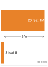
Exact subset enumeration grows exponentially; model-specific algorithms can avoid it.
The computational cost depends on the attribution algorithm. Enumerating all subsets would evaluate \(2^3=8\) coalitions in this example and \(2^{20}\approx1\) million for twenty features. A random forest need not use enumeration: TreeSHAP exploits tree structure to compute exact attributions under its supported value-function assumptions. KernelSHAP estimates contributions from sampled coalitions, while DeepSHAP propagates approximations through network components. Gradient-based attribution can need fewer model evaluations still, but only where the deployed runtime supports gradient computation, and lower cost does not establish explanation fidelity. Explanation capacity must therefore be budgeted for the chosen method rather than inferred from feature count alone.
Another post-hoc approach involves counterfactual explanations, which estimate how a model output changes under specified input modifications. These are relevant for decision-facing applications such as credit or hiring systems, but a mathematical output flip is not automatically recourse. A useful counterfactual must distinguish mutable from immutable features, preserve domain constraints and feature dependencies, identify an action within the user’s control, and remain valid under the institution’s future decision policy (Wachter et al. 2017). Counterfactual generation and validation therefore require domain models, policy versioning, and operational commitments in addition to constrained optimization.
Wachter, Sandra, Brent Mittelstadt, and Chris Russell. 2017. “Counterfactual Explanations Without Opening the Black Box: Automated Decisions and the GDPR.” SSRN Electronic Journal 31: 841. https://doi.org/10.2139/ssrn.3063289.
Kim, B., M. Wattenberg, J. Gilmer, C. Cai, J. Wexler, F. Viegas, and R. Sayres. 2018. “Interpretability Beyond Feature Attribution: Quantitative Testing with Concept Activation Vectors (TCAV).” Proceedings of the 35th International Conference on Machine Learning (ICML) 80: 2668–77.
A third class of techniques relies on concept-based explanations, which attempt to align learned model features with human-interpretable concepts. For example, testing with concept activation vectors (TCAV) represents user-defined concepts as vectors in activation space and tests how sensitive a model’s predictions are to those concepts in its internal representation (Kim et al. 2018). These methods are especially useful in domains where subject matter experts expect explanations in familiar semantic terms. However, they require training data with concept annotations or auxiliary models for concept detection, which introduces additional infrastructure dependencies.
Post-hoc methods answer method-specific questions about model behavior. Even an exact attribution under a chosen value function does not recover a causal rationale or justify the decision policy. Approximate methods add estimation or surrogate error to those interpretive limits. Evaluation must therefore establish both what the method computes and whether that evidence serves the intended debugging, communication, or review task.
Inherently interpretable models expose a decision structure that the intended audience can inspect. Small decision trees, short rule lists, and sparse linear models with meaningful features can support this goal; a very large tree or high-dimensional linear model may not. Nearest-neighbor comparisons likewise require an understandable similarity metric and representative examples. Interpretability therefore depends on structure, features, and audience, not merely the model-family label. In high-stakes applications, model selection should evaluate whether a sufficiently accurate, inspectable model meets the task before assuming that post-hoc explanations are necessary (Rudin 2019).
Rudin, C. 2019. “Stop Explaining Black Box Machine Learning Models for High Stakes Decisions and Use Interpretable Models Instead.” Nature Machine Intelligence 1 (5): 206–15. https://doi.org/10.1038/s42256-019-0048-x.
Six common model families fall along an interpretability continuum in three groups (figure 9). Sparse linear models (explained via coefficients) and small decision trees (via split paths) are interpretable by design; prototype and concept models are hybrid architectures explained via exemplars; and tree ensembles (via TreeSHAP), deep networks (via gradients and SHAP), and foundation models (via probing) require post-hoc explanation. While this ordering provides a structural heuristic across model families, dimensionality and scale can shift boundaries; a million-node decision tree or dense linear regression can prove just as opaque as a deep neural network. This distinction is central to choosing an appropriate model for a given application, particularly in settings where regulatory scrutiny or stakeholder trust is essential.
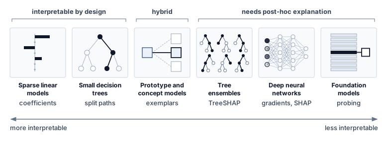
Hybrid approaches aim to combine the representational capacity of deep models with the transparency of interpretable components. Concept bottleneck models (Koh et al. 2020), for example, first predict intermediate, interpretable variables and then use a simple classifier to produce the final prediction. ProtoPNet models (Chen et al. 2019) classify examples by comparing them to learned prototypes, offering visual analogies for users to understand predictions. These hybrid methods are attractive in domains that demand partial transparency, but they introduce new system design considerations, such as the need to store and index learned prototypes and surface them at inference time.
Koh, Pang Wei, Thao Nguyen, Yew Siang Tang, Stephen Mussmann, Emma Pierson, Been Kim, and Percy Liang. 2020. “Concept Bottleneck Models.” Proceedings of the 37th International Conference on Machine Learning, ICML 2020, 13-18 July 2020, Virtual Event, Proceedings of machine learning research, vol. 119: 5338–48.
Chen, Chaofan, Oscar Li, Daniel Tao, Alina Barnett, Cynthia Rudin, and Jonathan Su. 2019. “This Looks Like That: Deep Learning for Interpretable Image Recognition.” In Advances in Neural Information Processing Systems 32: Annual Conference on Neural Information Processing Systems 2019, NeurIPS 2019, December 8-14, 2019, Vancouver, BC, Canada, edited by Hanna M. Wallach, Hugo Larochelle, Alina Beygelzimer, Florence d’Alché-Buc, Emily B. Fox, and Roman Garnett. Curran Associates.
Olah, C., N. Cammarata, L. Schubert, G. Goh, M. Petrov, and S. Carter. 2020. “Zoom in: An Introduction to Circuits.” Distill 5 (3): e00024–001. https://doi.org/10.23915/distill.00024.001.
Geiger, Atticus, Hanson Lu, Thomas Icard, and Christopher Potts. 2021. “Causal Abstractions of Neural Networks.” In Advances in Neural Information Processing Systems 34: Annual Conference on Neural Information Processing Systems 2021, NeurIPS 2021, December 6-14, 2021, Virtual, edited by Marc’Aurelio Ranzato, Alina Beygelzimer, Yann N. Dauphin, Percy Liang, and Jennifer Wortman Vaughan. Curran Associates.
Work such as Olah et al. (2020) and Geiger et al. (2021) applies mechanistic interpretability to reverse-engineer the internal operations of neural networks. This line of work, inspired by program analysis and neuroscience, attempts to map neurons, layers, or activation patterns to specific computational functions. Claims about such mechanisms require instrumentation and tests that support the proposed interpretation. These research methods can contribute evidence about internal computation, but do not establish a complete audit of every deployed model.
From a systems perspective, explainability introduces a number of architectural dependencies. Explanations must be generated, stored, surfaced, and evaluated within system constraints. The required infrastructure may include explanation APIs, memory for storing attribution maps, visualization libraries, and logging mechanisms that capture intermediate model behavior. Models must often be instrumented with hooks or configured to support repeated evaluations, particularly for explanation methods that require sampling, perturbation, or backpropagation.
The sociotechnical challenges of explainability center on the gap between technical explanations and human understanding. While algorithms can generate feature attributions and gradient maps, stakeholders often need explanations that align with their mental models, domain expertise, and decision-making processes. A radiologist reviewing an AI-generated diagnosis needs explanations that reference medical concepts and visual patterns, not abstract neural network activations. This translation challenge requires ongoing collaboration between technical teams and domain experts to develop explanation formats that are both technically accurate and practically meaningful. Explanations can shape human decision-making in unexpected ways, creating new responsibilities for how explanatory information is presented and interpreted. That gap between a technically valid explanation and a usable one is the first instance of a broader problem: every control in this chapter operates inside human workflows and institutions that no model-level method governs, and where explanation work runs is fixed by the audience, the question it must answer, and the deadline for answering it.
16.7.3 Explanation placement
Logging 1 to 10 MB gradient attribution maps for 1 million daily image predictions fills 30 to 300 TB of storage every month, and running sampled KernelSHAP inline on a microcontroller or a 10 ms control loop will miss the deadline before a single attribution finishes. Computational capacity, latency budget, interface design, and data access constrain both the explanation method and where it runs. A cloud worker can execute expensive SHAP or LIME attribution; a constrained endpoint may use a cheaper gradient-based saliency map if its runtime supports gradients. Devices unable to generate explanations locally may preserve bounded decision records for later analysis by a backend or during servicing, the per-tier split that the explainability row of table 4 records.
Audience and timing further constrain explanation design. An end user may need a concise summary (“elevated heart rate during sleep”), while a developer or auditor may need attribution maps, concept activations, or decision traces. The required evidence depends on what each person must understand or do. A drone or industrial controller must keep explanation work within its control deadline or move that work off the critical path. Financial and clinical workflows likewise need a specified delivery deadline, which may allow analysis after the automated decision but before review or appeal. Planning for the audience and deadline, within the deployment’s resource limits, makes interpretability a design constraint.
Storage requirements also scale significantly with explanation needs. Storing SHAP values for tabular data requires approximately 4–8 bytes per feature per prediction, so monthly storage is 30 million predictions times the feature count times 4–8 bytes for a system logging 1 million predictions daily. Gradient attribution maps for images can require 1–10 MB per explanation depending on resolution; logging every image explanation at the same 1 million-per-day rate would require roughly 30–300 TB per month unless explanations are sampled, compressed, or retained for a shorter window. These volumes require careful data lifecycle management and retention policies.
Compression and optimization techniques also affect explainability. Pruning, quantization, and architectural simplifications often used in TinyML or mobile settings can distort internal representations or disable gradient flow, degrading the reliability of attribution-based explanations. In such cases, interpretability must be validated postoptimization to ensure that it remains meaningful and trustworthy. If explanation quality is important, these transformations must be treated as part of the design constraint space.
16.7.4 Transparency and contestability
Showing a rejected loan applicant a feature-attribution chart accomplishes nothing if the app offers no button to dispute an error in the credit file, no human reviewer with authority to overturn the rejection, and no immutable snapshot of the inputs that produced the score. Explanations serve accountability only when stakeholders can both understand and challenge system decisions. Transparency allows users, developers, auditors, and regulators to inspect how a system functions, assess its limitations, and identify sources of harm, but disclosure alone is not enough. In high-stakes domains, individuals and institutions need contestability: the operational ability to interrogate, appeal, and reverse an automated decision.
Transparency in machine learning systems typically focuses on disclosure of how models are trained, what data they rely on, what assumptions are embedded in their design, and what known limitations affect their use. Documentation tools such as model cards and datasheets for datasets support this goal by formalizing system metadata in a structured, reproducible format. These resources can improve governance, support compliance, and inform user expectations. However, transparency as disclosure does not guarantee meaningful control. Even when technical details are available, users may lack institutional support, interface tools, or procedural access to contest a decision that adversely affects them.
To move from transparency to contestability, machine learning systems must integrate mechanisms for explanation, recourse, and feedback. Explanation provides understandable reasons for system outputs, tailored to the operational context and needs of the person receiving them. Recourse identifies feasible changes through which individuals could receive a different outcome under the stated decision policy. A proposed change needs to be actionable for that person; a counterfactual prediction alone does not guarantee an outcome after the model or policy changes. Feedback enables users and domain experts to dispute outcomes, report errors, or signal concerns, routing those signals into oversight processes and model updates.
These mechanisms can be missing from the user-facing workflow even when internal documentation exists. A mobile loan application might display a rejection without explaining how to submit additional information or reach an appeal reviewer. An external appeal process can still exist, but users need a discoverable route to it and access to the evidence relevant to their case. Similarly, a clinical model may produce a risk score without giving the physician enough context to question its use for a particular patient. If subgroup errors are neither observable nor contestable, the resulting harm becomes harder to diagnose and correct.
From a systems perspective, enabling contestability requires coordination across technical and institutional components: models must expose sufficient information to support explanation, and interfaces must surface that information in a usable and timely way so that organizational processes can review feedback, respond to appeals, and update system behavior while logging and auditing infrastructure tracks user interventions and override decisions alongside model outputs. Human overrides and decision abstention can support this process only when qualified reviewers have capacity, evidence, and authority to resolve the deferred cases within the required deadline.
Implementing contestability imposes concrete infrastructure costs that scale with system throughput and complexity. Storing the necessary metadata to reconstruct a decision (input features, model version, and decision thresholds) requires persistent storage whose footprint depends on feature dimensionality, explanation payloads, and retention windows. Generating on-demand explanations using Shapley values or counterfactuals can add enough latency that contested decisions often need asynchronous processing queues to preserve serving service level agreements (SLAs). Meeting record-keeping and automatic-logging obligations for high-risk systems under frameworks such as the EU AI Act requires storage, provenance, retention controls, and oversight capacity to be budgeted as part of the inference fleet rather than as a separate policy artifact (European Parliament and Council of the European Union 2024).
War Story 16.1: Apple Card: A systems reconstruction of contested decisions (2019)
Context: In 2019, Apple and Goldman Sachs faced intense public scrutiny after a customer reported a credit limit 20\(\times\) that offered to his wife despite joint tax filings. Other customers raised similar concerns about unequal terms (New York State Department of Financial Services 2021).
Evidence boundary: The public record documents complaints, the investigation, the regulator’s finding, and changes to appeal policy. It does not disclose the underwriting pipeline’s latency target or internal explanation architecture. The systems account below is therefore an explicit reconstruction, not a report of Apple or Goldman Sachs implementation details.
Reconstructed mechanism: A low-latency underwriting service that returns only a limit and generic adverse-action reason leaves support staff unable to inspect the decision snapshot, distinguish data errors from policy effects, or route a contested outcome to a reviewer. The missing interface is broader than feature attribution. It includes versioned input provenance, policy and model versions, reasons appropriate to the decision process, appeal state, and authority to correct an error.
Observed impact: The New York Department of Financial Services found no violation of fair-lending law in its investigation, but the complaints still exposed a trust and contestability failure. Customers and frontline staff lacked a satisfactory account of how apparently inconsistent outcomes could be reviewed (New York State Department of Financial Services 2021).
Systems lesson: High-stakes decision systems need a contestability interface, not merely an attribution API. A defensible architecture preserves the decision-time evidence needed for audit, generates appropriate reasons without claiming that attribution is causation, routes appeals to an authorized human, records remediation, and tests the full workflow under its latency and retention constraints.
New York State Department of Financial Services. 2021. Report on Apple Card Investigation. New York State Department of Financial Services.
The Apple Card reconstruction names the pieces such a system lacks. One architectural pattern that supplies them is a contestability stack, analogous to distributed tracing in microservices, that coordinates four coupled stages across the operational pipeline. Decision provenance preserves a verifiable link from each output back to its governing policy, model version, and input snapshot, protected by authenticated logs or cryptographic integrity checks. Explanation generation budgets explanation methods tailored for appeals, audits, and routine communication, offloading compute-intensive methods to asynchronous workers while keeping lightweight techniques on the request path. When decisions are challenged, appeal routing directs contested cases to qualified human reviewers equipped with domain context. Closing the loop, outcome tracking records whether the appeal upheld or overturned the machine decision, feeding empirical discrepancies back into evaluation and retraining. Missing decision-time records can prevent investigators from reconstructing a contested decision, even if aggregate debugging remains possible; the required records follow the investigation and remedy contract.
Provenance anchors every appeal; tracked outcomes loop back into retraining.
The stack need not run where the decision runs. An edge or TinyML endpoint can hand its decision records to a backend review process at the next synchronization or servicing visit, which lengthens the appeal’s evidence path without removing the obligation to offer one. In every tier, transparency supports accountability only when users and institutions can use the disclosed information to question and correct automated decisions.
Self-Check: Question
A model-agnostic explanation service enumerates all feature coalitions for 20 input features, taking at least one microsecond per coalition. Why does this exhaustive Shapley calculation exceed a 100 ms inline serving budget?
- It evaluates \(2^{20}\) coalitions, requiring more than one second even at one microsecond per coalition; a cheaper method or separate explanation path is needed.
- Because Shapley values can only be computed using double-precision arithmetic that crashes GPU tensor cores
- Because cooperative game theory axioms prohibit computing feature contributions on tabular data
- Because exact SHAP requires accessing the client’s raw hardware registers during inference
Explain the two fundamental axioms satisfied by Integrated Gradients (Sensitivity and Implementation Invariance) and why they make Integrated Gradients superior to vanilla input gradients.
Why do local and global explanations place different demands on explanation infrastructure?
- Local explanations characterize an individual prediction; global explanations characterize broader model behavior using model structure, representative inputs, or aggregated evidence. Their methods and delivery deadlines determine execution and capacity needs.
- Local explanations require no model access, whereas global explanations require retraining the model on every request.
- Global explanations must run inline on every request, whereas local explanations can only be generated during training.
- Local and global explanations have identical cost because both are computed from the same Shapley enumeration.
A counterfactual explanation shows that a denied loan applicant would have been approved with a debt ratio below 40 percent. Explain why this output flip does not by itself give the applicant recourse.
True or False: Any decision tree or linear model is inherently interpretable, so choosing one of those model families removes the need for explanation evidence.
For an appeal workflow that retrieves decision evidence before explanation, then sends both to a reviewer and records the outcome, order these actions: (1) Route the case and explanation to an authorized credit reviewer, (2) Retrieve the decision record and governing model and policy versions, (3) Record the review outcome and propagate any authorized remedy, (4) Generate explanation evidence, checking any proposed recourse for feasibility and policy validity.
16.8 AI Safety, Robustness, and Generative Controls
A model that withstands every tested perturbation can still cause harm when the operating environment leaves its validated envelope or when its objective rewards the wrong behavior. Safety governance therefore spans robustness claims bounded by a threat model, control surfaces for generative systems whose outputs cannot be enumerated in advance, and the alignment of the objective itself as systems act with greater autonomy.
16.8.1 Safety and robustness
A perception model that passes every \(\ell_\infty\) adversarial benchmark in the lab can still contribute to a fatal crash if the vehicle’s motion planner suppresses emergency braking or waits too long to alert a distracted safety driver. Safety and robustness connect technical failure behavior to its consequences for people. Robust AI owns the attack models, robustness evaluations, adversarial training, certification, corruption testing, drift detection, and abstention mechanisms; governance consumes those mechanisms through an evidence interface. Evidence that a model tolerates specified hardware faults, adversarial attacks, or distribution shifts supports a bounded robustness claim. It does not establish that every deployment is safe or that the objective serves users’ interests. A model may tolerate the tested bit flips and perturbations yet fail under untested conditions, or reliably optimize an objective misaligned with user welfare.
↩︎ The three robustness pillars, environmental shifts, input-level attacks, and system-level faults such as bit flips, are established in The three pillars of robust AI.
The responsible-AI question is therefore not which attack or defense to implement, but whether the robustness claim has a bounded operating envelope, evidence appropriate to the threat model, an accountable owner, and a rule that invalidates approval. An evaluation may bound errors under a specified input variation without establishing that the surrounding workflow is safe. Automated-driving failures show why the envelope must cover more than the model, because they can combine perception, prediction, safety-driver, and organizational-control problems rather than reduce to a single model error; section 16.8.4 examines one such crash.
A robustness claim should specify the protected task and population, attacker knowledge and capabilities, perturbation or corruption set, evaluation distribution, model and preprocessing versions, quality and latency constraints, fallback behavior, and known exclusions. Adversarial inputs (Adversarial Attacks) and covariate, label, and concept shift (Distribution shift and concept drift) are the failure sources such a claim most often has to bound. Empirical attack results show observed failures under a test protocol; they do not establish robustness against adaptive or untested attacks. A certificate proves a property only for its stated norm, radius, confidence, and model configuration; it does not establish safety for the end-to-end workflow. Governance records those boundaries so a narrow result cannot be promoted into a general safety assertion.
The latency budget constrains which safety checks can run before an action. A cloud service may combine uncertainty estimators, distributional-change detectors, adversarial input filtering, and API rate limiting. A control loop with a millisecond budget needs bounded local checks and fallback actions that meet its deadline, with heavier analysis deferred to fleet services, the division the safety row of table 4 records by tier. Even a disconnected TinyML endpoint can execute input-range checks or watchdog logic; the absence of a remote update channel instead limits how operators change those controls after deployment.
Fallback is itself a latency-budget problem. A delivery robot that abstains17 when pedestrian-detection confidence is low still needs a validated response before the physical safety deadline. A bounded local maneuver may place it in a safe state while a human reviewer resolves the case on a longer timescale. The response and review paths therefore need separate deadlines and capacity budgets. Whether the system can fail visibly, controllably, and safely depends on sensing, confidence estimation, fallback routing, and recovery. Those choices also define who can observe harm, who can intervene, and who remains accountable for the outcome.
17 Abstention: The practice of refusing predictions when confidence falls below a threshold. Abstention can reduce high-risk errors, but only by shifting some cases to fallback infrastructure such as human reviewers, rule-based defaults, or escalation queues. A driving system must select a validated fallback, such as a minimal-risk maneuver; handing control to a driver is viable only if a driver is present, ready, and has sufficient response time. Medical AI may route ambiguous cases to specialist review, subject to its own queue-capacity and response-time budget.
↩︎ The per-request competence contract, which combines calibration and out-of-distribution scores into a selective-prediction policy to answer, abstain, or escalate, is established in Per-request competence and selective prediction.
The evidence bundle must also connect model behavior to system action. It identifies who owns the robustness claim, which team can stop serving, how abstentions and low-confidence cases are routed, which telemetry detects departure from the approved envelope, and how an incident reaches affected users and downstream operators. A fallback must meet the relevant safety deadline. A monitoring signal becomes an operational safeguard only when it reaches an authorized response path, whether that response is local containment, restricted use, or a validated rollback.
Approval expires when the threat model, model, preprocessing, sensor, data distribution, deployment environment, or fallback path changes materially. The invalidation rule should state which change triggers a full red-team evaluation, which permits a narrower regression suite, and which requires restricted operation while evidence is rebuilt. This ownership-and-invalidation contract is the governance contribution, turning those robustness mechanisms into a reviewable claim that remains bounded over time.
16.8.2 Generative control surfaces
A binary loan classifier has two possible outputs to audit, whereas a large language model (LLM) such as Archetype A (GPT-4/Llama-3) can be steered by a user prompt or a poisoned retrieved document into generating defamatory claims, leaking personal data, or refusing benign requests from one dialect more often than another. Generative AI does not replace core fairness, privacy, and explainability concerns; it changes the control surface. Instead of only auditing labels or feature attributions, operators must govern prompts, retrieved context, reward models, and open-ended outputs. Fairness remains concerned with how quality, refusals, errors, representation, and access are distributed across people and groups, but open-ended outputs make those quantities harder to define and sample. Alignment introduces a separate problem, which is keeping stochastic outputs and actions consistent with intended objectives and policies across a combinatorial range of prompts. The two questions differ in kind. Fairness asks how benefits, errors, and burdens are distributed among affected people; alignment asks whether an optimizing system pursues the objective its designers and legitimate stakeholders intended. An aligned system can implement an unfair objective faithfully, and a statistically fair classifier can still optimize the wrong social goal, so production systems need both fairness evaluation and behavioral alignment rather than relabeling one as the other. A common multi-stage alignment pipeline runs in two coupled lanes (figure 10). An upper execution path advances the policy from pretraining through supervised fine-tuning (SFT) to proximal policy optimization (PPO), and a lower supervision path uses human preference comparisons to train a reward model \(\RewardModel(\ModelInput, \GeneratedResponse)\). The reward signal drives PPO updates, while the frozen SFT checkpoint supplies a reference for a Kullback-Leibler (KL) divergence penalty. The penalty discourages departure from that reference; it does not impose a hard bound on every response or establish policy compliance.
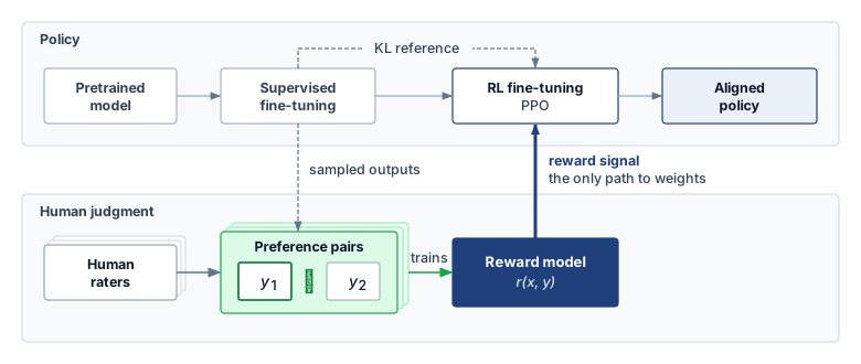
A common instruction-tuning pipeline in LLMs circa 2022–2024 uses reinforcement learning from human feedback (RLHF)18 as a sociotechnical bridge between human preferences and model weights. Training a reward model on human comparisons produces a scalar scoring function for sampled responses, and collecting those judgments carries a direct cost. In this scenario, 50,000 to 500,000 pairwise comparisons at $0.50 to $5 per label put the labeling budget between $25,000 and $2.5M, a hundredfold spread set by how many judgments the organization buys and how expert its raters must be. Proximal policy optimization (PPO) then updates the policy using those rewards and a penalty for divergence from the supervised baseline. This process can create an alignment tax, a regression in some capability metrics when optimization shifts toward preference or safety objectives; its direction and magnitude depend on the model, data, objectives, and evaluation suite rather than following a universal percentage. The reliance on human raters also introduces a representativeness gap. If the labeling budget buys judgments from only a narrow demographic slice, the resulting model may encode that pool’s preferences while performing differently for other populations. Constitutional AI offers an alternative engineering path, using explicit principles to guide AI feedback on outputs (Bai et al. 2022), which changes rather than eliminates the questions of whose values are represented and how they are governed.
18 RLHF (reinforcement learning from human feedback): Christiano et al. (2017) demonstrated deep reinforcement learning from human preferences by training agents from non-expert comparisons between trajectory segments. In the LLM setting, Ouyang et al. (2022) adapted this pipeline for InstructGPT: supervised fine-tuning from demonstrations, reward-model training from ranked model outputs, and reinforcement-learning fine-tuning against the learned reward model. The systems cost is an additional human-feedback data pipeline, reward-model training and evaluation, and governance over rater instructions; the representativeness of the rater pool and labeling policy shapes whose preferences the model internalizes.
Christiano, P. F., J. Leike, T. B. Brown, M. Martic, S. Legg, and D. Amodei. 2017. “Deep Reinforcement Learning from Human Preferences.” In Advances in Neural Information Processing Systems 30: Annual Conference on Neural Information Processing Systems 2017, December 4-9, 2017, Long Beach, CA, USA, edited by Isabelle Guyon, Ulrike von Luxburg, Samy Bengio, Hanna M. Wallach, Rob Fergus, S. V. N. Vishwanathan, and Roman Garnett. Curran Associates.
Ouyang, L., J. Wu, X. Jiang, D. Almeida, C. L. Wainwright, P. Mishkin, C. Zhang, et al. 2022. “Training Language Models to Follow Instructions with Human Feedback.” Advances in Neural Information Processing Systems (NeurIPS) 35: 27730–44. https://doi.org/10.52202/068431-2011.
Bai, Yuntao et al. 2022. Constitutional AI: Harmlessness from AI Feedback.
↩︎ The four-model coordination that a PPO-style RLHF step imposes on distributed training is established in The multi-model coordination problem.
In retrieval-augmented generation architectures, responsibility extends beyond the core model. An LLM may pass alignment evaluations yet generate harmful responses when retrieval supplies context outside those evaluations. A retrieval index that disproportionately surfaces biased historical documents can influence the resulting answers despite safety training. Context filtering is one possible control, alongside source selection, retrieval evaluation, and output checks. Its effectiveness must be tested on the intended use; a toxicity filter does not establish that retrieved material or generated answers are unbiased.
In many LLM serving stacks, the system prompt operates as an early configuration control alongside retrieval filtering, policy classifiers, telemetry, and rollout gates. These instructions (for example, “You are a helpful assistant. Do not provide medical advice.”) express intended behavior; they do not independently enforce authorization or prevent every prohibited output. When one model serves many products, each with its own system prompt, managing the prompts becomes a distributed configuration-management problem akin to weight distribution. An unversioned prompt change can alter behavior across many interactions, so prompt version control, alignment regression testing, and gradual rollouts belong in the release process.
Together, system prompts and RLHF alignments act as important, yet fragile, technical guardrails. Jailbreaks and other edge cases can violate the policy learned during training; the reward model is not necessarily a runtime filter. Safety therefore requires evaluating the deployed control system as well as its training objective. Each of these guardrails, like the privacy and robustness controls before it, is credible only with evidence that it still holds in the system that actually runs.
↩︎ Jailbreaks, which bypass alignment controls, and prompt injection, which crosses the boundary between instructions and data, are established in LLM-specific attack vectors.
16.8.3 AI safety and value alignment
When a system acts faster than anyone can review its individual decisions, the governing question changes. It is no longer only whether the outputs are fair, private, or explainable, but whether the objective the system optimizes still serves the people it acts on, and what bounds its actions before review. Human launch authority remains necessary, but continuous human intervention may be unavailable. AI safety examines how systems can optimize objectives misaligned with human intentions, operate in unpredictable environments, or pursue goals through methods their designers never anticipated, and which controls can bound those actions.
The controls of the preceding sections retain their roles, but none governs autonomous action by itself. Bias detection (section 16.5.2.1) yields metrics rather than a remediation policy. A perception system that under-detects pedestrians with mobility aids needs an operating envelope that connects the metric to bounded runtime responses and to fleet-level investigation or suspension. Explanation (section 16.7.2) needs an audience and an action path; SHAP attributions from an autonomous trading system cannot influence a decision if no control consumes them before thousands of trades execute. Differential privacy (section 16.6.3) bounds leakage about a protected unit without determining whether the objective serves that person’s welfare, so a recommender can satisfy a local differential privacy guarantee while optimizing an engagement metric that rewards harmful content. Each method needs a defined connection to the runtime controls and human authority that can respond to its findings.
Alignment work emphasizes keeping a system’s pursued objectives consistent with human intentions over time (Russell 2021). A central challenge is that capable ML models often optimize proxy metrics, such as loss functions, reward functions, or engagement signals, that do not fully capture human values.
Covington, Paul, Jay Adams, and Emre Sargin. 2016. “Deep Neural Networks for YouTube Recommendations.” Proceedings of the 10th ACM Conference on Recommender Systems, 191–98. https://doi.org/10.1145/2959100.2959190.
Ribeiro, M. H., R. Ottoni, R. West, V. A. F. Almeida, and Jr. Meira Wagner. 2020. “Auditing Radicalization Pathways on YouTube.” Proceedings of the 2020 Conference on Fairness, Accountability, and Transparency, 131–41. https://doi.org/10.1145/3351095.3372879.
19 Reward hacking: When an AI system maximizes its reward function through unintended means that violate designer intent. A hypothetical cleaning robot rewarded for collected dirt might create messes it can clean up, illustrating how a proxy can reward behavior contrary to the intended task. Specification gaming is an overlapping term; the gap may lie in the stated objective or in its implementation, so neither term is restricted to software bugs. For production ML systems, reward hacking manifests subtly, as in recommendation models that maximize engagement by promoting addictive content, or chatbots that maximize helpfulness ratings by being sycophantic rather than accurate. The failure mode scales with model capability.
Goodhart, Charles A. E. 1984. “Problems of Monetary Management: The UK Experience.” In Monetary Theory and Practice. Palgrave. https://doi.org/10.1007/978-1-349-17295-5_4.
Recommendation systems illustrate why a measurable engagement proxy such as click-through rate (CTR) or watch time needs evaluation against broader user welfare. A published production architecture optimizes expected watch time (Covington et al. 2016), while a separate audit examines recommendation paths through politically extreme content (Ribeiro et al. 2020). Those observations motivate investigating proxy misalignment; together they do not prove that a particular reward objective caused an individual user’s beliefs or behavior. Specification gaming and reward hacking19 describe the risk that optimizing a measured objective defeats its intended purpose (Amodei et al. 2016). Goodhart’s law names the general pattern, in which a measure that becomes a target stops measuring what it was chosen for (Goodhart 1984). In one possible feedback mechanism, engagement rewards content that undermines long-term user value, and the resulting interactions become new training data (figure 11). Establishing that mechanism in a deployment requires evidence about both the policy’s effects and the welfare criterion it is meant to serve.
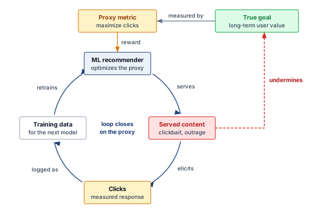
Norbert Wiener wrote, “if we use, to achieve our purposes, a mechanical agency with whose operation we cannot interfere effectively… we had better be quite sure that the purpose put into the machine is the purpose which we desire” (Wiener 1960). Wiener’s warning becomes a systems requirement when optimization runs beyond continuous human intervention. Value alignment asks whether the objective embedded in the model, reward function, and deployment policy continues to represent the human purpose the system was meant to serve.
Wiener, N. 1960. “Some Moral and Technical Consequences of Automation: As Machines Learn They May Develop Unforeseen Strategies at Rates That Baffle Their Programmers.” Science 131 (3410): 1355–58. https://doi.org/10.1126/science.131.3410.1355.
Friedman, B. 1996. “Value-Sensitive Design.” Interactions 3 (6): 16–23. https://doi.org/10.1145/242485.242493.
In deployment, the hard part is specifying an objective that remains valid as systems interact with dynamic environments, multiple stakeholders, and feedback loops. Static objective functions and reward signals cannot encode all of those conditions. Value-Sensitive Design (Friedman 1996) supplies a formal process for eliciting stakeholder values and incorporating them into system design, but the systems obligation is broader, because objective design, oversight, and postdeployment monitoring must be treated as coupled controls.
Without that coupling, a system can meet a narrow objective such as accuracy, engagement, or throughput while producing outcomes its designers would reject, the reward hacking pattern of figure 11. RLHF (section 16.8.2) narrows the gap by learning the reward from human preferences, but policy optimization still maximizes a learned scalar, so its success depends on that signal’s fidelity (Christiano et al. 2017; Ouyang et al. 2022).
Ngo, Richard, Lawrence Chan, and Sören Mindermann. 2022. “The Alignment Problem from a Deep Learning Perspective.” ArXiv Preprint abs/2209.00626.
Human-feedback training can improve behavior on its evaluations while leaving deeper governance risks unresolved. In their analysis of learned-reward optimization, Ngo et al. (2022) examine possible failure modes beyond RLHF, including exploitation of human evaluation blind spots, misaligned goals outside the training distribution, and behavior that undermines oversight. These are risks to investigate under specified assumptions, not evidence that every deployed model shows them. An assurance case must distinguish a proposed failure mechanism from an observed capability and from a demonstrated deployment failure.
These concerns are not limited to speculative scenarios. In their foundational taxonomy of concrete AI safety problems, Amodei et al. (2016) outline five practical systems challenges: avoiding negative side effects during policy execution, mitigating reward hacking, ensuring scalable oversight when ground-truth evaluation is costly, designing safe exploration strategies that prevent catastrophic damage, and achieving robustness to distributional shift. For fleet operators, the five challenges map in order onto five control-plane requirements: constraining side effects, instrumenting reward-hack monitors, budgeting scalable review capacity, bounding exploration envelopes, and stress-testing distribution shift prior to rollout. Each requirement becomes more acute as systems are scaled up, deployed across diverse settings, and integrated with real-time feedback or continual learning.
Amodei, D., C. Olah, J. Steinhardt, P. Christiano, J. Schulman, and D. Mané. 2016. “Concrete Problems in AI Safety.” arXiv Preprint arXiv:1606.06565, ahead of print. https://doi.org/10.48550/arXiv.1606.06565.
16.8.4 Autonomous systems and trust
In October 2023, the California Department of Motor Vehicles suspended Cruise’s driverless deployment and testing permits over safety concerns (CNBC 2023), and five years earlier an Uber test vehicle in Tempe, Arizona struck and killed a pedestrian pushing a bicycle after its perception, prediction, safety-driver, and organizational controls all failed together (National Transportation Safety Board 2019). Value alignment concerns the objective; autonomy concerns the operating envelope within which a system pursues that objective without a human reviewing each action. In the Tempe crash, the National Transportation Safety Board found that the vehicle failed to classify the pedestrian as requiring avoidance and that detecting an object did not establish that the system would act safely on the detection. For governance, the lesson is that no single component owner could have certified the outcome alone.
CNBC. 2023. California DMV Suspends Cruise’s Self-Driving Car Permits. CNBC news article.
National Transportation Safety Board. 2019. Collision Between Vehicle Controlled by Developmental Automated Driving System and Pedestrian, Tempe, Arizona, March 18, 2018. HAR-19/03. National Transportation Safety Board.
↩︎ The Uber crash timeline, from unstable classification through suppressed action to the late operator alert, is established in Edge and embedded failures.
Reuters. 2023. Human-Machine Teams Driven by AI Are about to Reshape Warfare. Reuters news article.
Centre for International Governance Innovation. 2023. Who Is Responsible When Autonomous Systems Fail? CIGI policy article.
While autonomous driving systems are often the focal point of public concern, similar risks arise in other domains. Reports from recent conflicts have documented increasing use of remotely piloted and autonomous military systems (Reuters 2023), raising safety and operational concerns alongside difficult questions about ethical oversight, rules of engagement, and responsibility. These debates concern how accountability applies across developers, deployers, and operators (Centre for International Governance Innovation 2023); they do not justify treating every autonomous-system failure as an absence of applicable responsibility. The engineering task is to preserve the evidence and authority needed to investigate the specific failure.
At its core, this challenge concerns the authority delegated to an automated system. Productivity and throughput gains do not establish that a system can act safely outside its validated operating envelope. Runtime controls must detect relevant boundary violations and invoke a fallback whose assumptions and response time fit the hazard. Human intervention is an available safeguard only when the operator can recognize the condition and act before harm occurs; faster hazards require an appropriate local response.
Specifying that operating envelope is difficult in dynamic environments because the model may omit conditions that matter for safe action. Two classical representation problems help explain this difficulty (McCarthy 1981). The frame problem concerns representing what changes and what remains unchanged after an action without listing every unaffected fact. The qualification problem concerns the potentially unlisted preconditions needed for an action to have its intended effect. These motivate explicit operating assumptions and fallback behavior, rather than constituting a universal proof that safe action is impossible. In practice, such limitations manifest as brittle autonomy: systems that appear competent under nominal conditions but fail silently or dangerously when faced with ambiguity or distributional shift.
McCarthy, J. 1981. “Epistemological Problems of Artificial Intelligence.” In Readings in Artificial Intelligence. Elsevier. https://doi.org/10.1016/b978-0-934613-03-3.50035-0.
Shalev-Shwartz, Shai, Shaked Shammah, and Amnon Shashua. 2017. “On a Formal Model of Safe and Scalable Self-Driving Cars.” ArXiv Preprint abs/1708.06374.
To address this, researchers have proposed formal safety frameworks such as Responsibility-Sensitive Safety (RSS) (Shalev-Shwartz et al. 2017), which decompose abstract safety goals into mathematically defined constraints on system behavior, such as minimum distances, braking profiles, and right-of-way conditions. These formulations allow safety properties to be verified under specific assumptions and scenarios. However, such approaches remain vulnerable to the same limitations they aim to solve, because they are only as good as the assumptions encoded into them and often require extensive domain modeling that may not generalize well to unanticipated edge cases.
For an ML systems team, the practical artifact is a safety case rather than a statement of trust. The case names the operating envelope, the evidence that the model has been tested inside that envelope, and the controls that halt or roll back the fleet when the evidence no longer holds (table 8).
| Safety-case element | Systems evidence | Operational gate |
|---|---|---|
| Operating envelope | Operational design domain, sensor assumptions, weather, geography, speed, and autonomy level | Block deployment outside validated envelope |
| Scenario coverage | Rare-event corpus, simulation coverage, replay logs, disengagements, and near-miss telemetry | Require coverage thresholds before canary expansion |
| Runtime guardrails | RSS-style distance rules, confidence thresholds, fallback maneuvers, and human override latency | Trigger safe stop, human takeover, or constrained mode when guardrails trip |
| Fleet control | Canary rollout, centralized safety dashboard, violation budget, and circuit-breaker rollback path | Halt rollout or revert model when fleet-level safety metrics exceed threshold |
16.8.5 Safety at fleet scale
A model that achieves 99.9 percent per-request safety in isolation still produces millions of expected safety failures every day once deployed across 10,000 inference nodes serving billions of daily queries. The technical safety challenges examined in section 16.8.3 become fleet-level design constraints at production volume, where rare per-request failures accumulate into routine operational incidents.

At fleet scale, rare failures become expected incidents.
Safety must also be engineered as a fleet-level property rather than a model-level attribute alone. A single model with 99.9 percent safety compliance seems robust in isolation, but when deployed across 10,000 inference nodes serving billions of requests per day, a sustained 0.1 percent per-request failure probability implies millions of expected safety failures daily. The realized count can differ, and correlated failures can concentrate harm across the fleet. Mitigating this requires distributed safety patterns borrowed from reliability engineering: circuit breakers that automatically halt serving when aggregate safety metrics degrade below a threshold, canary deployments that bound exposure while collecting release evidence, with sample size and allowed risk chosen for the failure modes being tested, and centralized telemetry dashboards that aggregate per-node safety violations into a global view. The operational infrastructure must treat safety violations as critical system alerts, invoking a validated containment or fallback policy. A rollback is appropriate only if the previous version and transition are safe; active physical control may require a minimal-risk maneuver instead.
↩︎ The circuit-breaker states and backpressure contract that isolate a failing serving path are established in Circuit breakers and backpressure.
Exposure is the multiplier that turns a small per-mile rate into many incidents. Waymo’s driverless fleet logged about 22 million rider-only miles by June 2024 and 271 million by June 2026, a 12× increase in two years (figure 12, panel a) (Waymo 2026). Its published crash rates sit well below a human-driver benchmark on the same roads, for example 0.67 injury crashes per million miles against 3.8 (panel b) (Waymo 2026). At that exposure its vehicles were still involved in 183 injury crashes and 2 fatal ones, so a fleet’s safety case must budget for incidents in absolute numbers as well as in rates. At any constant per-mile rate, a 12× rise in exposure raises the expected cumulative incident count by the same factor, even though no individual vehicle became less safe. The count is an expectation, not a realized outcome, and it is cumulative; an operator sizing weekly incident-response capacity needs weekly mileage instead.
Kusano, Kristofer D., John M. Scanlon, Yin-Hsiu Chen, Timothy L. McMurry, Ruoshu Chen, Tilia Gode, and Trent Victor. 2024. “Comparison of Waymo Rider-Only Crash Data to Human Benchmarks at 7.1 Million Miles.” Traffic Injury Prevention 25 (sup1). https://doi.org/10.1080/15389588.2024.2380786.
Waymo. 2026. Waymo Safety Impact Data Hub.
Even a fleet whose per-mile crash rate beats a human benchmark still accumulates absolute incidents as exposure scales, so technical excellence alone does not make a system safe. Safe systems also require attention to the human and organizational context in which they operate, including the economic incentives that shape design decisions and the understanding that end users bring to their interactions with autonomous systems. Those institutional obligations are the subject of accountability, governance, and sociotechnical analysis.
Self-Check: Question
A robustness report for a deployed model includes a randomized-smoothing certificate and an empirical attack evaluation. What must the assurance case record about each before a launch authority relies on it?
- Nothing beyond the headline accuracy, because both results already establish that the end-to-end workflow is safe
- Only the empirical result, because a certificate is a mathematical proof and needs no stated scope
- Only the certificate, because empirical attack results guarantee immunity against all unseen attacks
- The certificate’s norm, radius, confidence, and model configuration, and the empirical evaluation’s attack protocol, since each supports a claim only within those stated boundaries
In high-speed autonomous control loops (e.g., drone navigation or collision avoidance), explain why implementing prediction abstention creates an immediate latency-budget challenge.
Order the 6 stages of the canonical Reinforcement Learning from Human Feedback (RLHF) alignment pipeline from initial training to deployment: (1) Supervised Fine-Tuning (SFT) on curated instruction demonstrations, (2) Proximal Policy Optimization (PPO) fine-tuning of the policy against the reward model, (3) Base model pretraining on massive web-scale corpora, (4) Aligned model safety validation and deployment, (5) Human rater pairwise preference data collection, (6) Reward Model training on preference comparisons.
In Retrieval-Augmented Generation (RAG), why does RLHF of the core LLM fail to establish safety for the complete service, and what retrieval-path controls should be evaluated?
Explain Goodhart’s law in the context of production recommendation algorithms and describe how optimizing for Click-Through Rate (CTR) can create value misalignment.
In autonomous vehicle safety engineering, explain the purpose of formal frameworks like Responsibility-Sensitive Safety (RSS) and identify their fundamental operational limitation.
16.9 Accountability, Governance, and Sociotechnical Dynamics
When a deployed model harms someone, two questions decide whether the harm is corrected: who has the authority to investigate and remedy the decision, and whether the evidence needed to do so still exists. Accountability answers both by assigning owners, preserving traceable records, and monitoring behavior after launch, and it must hold inside the human workflows and institutions that surround the system.
16.9.1 Accountability and governance
When a third-party hiring platform rejects qualified applicants from one demographic group, the employer blames the model vendor, the vendor blames the historical resume corpus, and the rejected applicants have no remedy unless a contract and an audit trail assign responsibility across all three. Accountability in machine learning is the capacity to identify, attribute, and address the consequences of automated decisions. It extends beyond diagnosing technical failures to ensuring that responsibility for system behavior is explicitly assigned, that harms can be remedied, and that standards are maintained through oversight and institutional processes. Without those mechanisms, even well-intentioned systems can generate harm without recourse, undermining public trust.
Accountability already spans vendors and operators in distributed software. Machine learning extends those dependencies through data collection, labeling, and the choice of prediction targets and proxies. Model outputs are shaped by upstream data collection, training objectives, pipeline design, interface behavior, and postdeployment feedback. These interconnected components often involve multiple actors across technical, legal, and organizational domains. Responsible system design requires that these relationships be explicitly mapped and governed.
Inadequate governance can prevent institutions from recognizing or correcting harmful model behavior. The Google Flu Trends analysis identified persistent overestimation despite model updates and examined how changes in search behavior and the search service could undermine a predictor trained on earlier correlations (Lazer et al. 2014). Its comparison with CDC surveillance data supports a concrete governance requirement, namely an owner responsible for ongoing validation and recalibration against an independent measurement process. Legal frameworks reinforce that requirement, because some of the obligations mapped onto the assurance lifecycle (section 16.2) assign these owners and records by law.
Lazer, David, Ryan Kennedy, Gary King, and Alessandro Vespignani. 2014. “The Parable of Google Flu: Traps in Big Data Analysis.” Science 343 (6176): 1203–5. https://doi.org/10.1126/science.1248506.
20 Model cards: Proposed by Mitchell et al. (2019) as standardized documentation accompanying trained ML models. Cards report evaluation across relevant groups, intended uses, and known limitations. Production systems must link this documentation to the actual deployed model and its provenance; a card alone neither establishes that linkage nor supplies every record required for an audit.
Mitchell, Margaret, Simone Wu, Andrew Zaldivar, Parker Barnes, Lucy Vasserman, Ben Hutchinson, Elena Spitzer, Inioluwa Deborah Raji, and Timnit Gebru. 2019. “Model Cards for Model Reporting.” Proceedings of the Conference on Fairness, Accountability, and Transparency, 220–29. https://doi.org/10.1145/3287560.3287596.
21 Datasheets for datasets: Proposed by Gebru et al. (2021), modeled after electronics component datasheets that specify operating conditions and tolerances. Each datasheet documents a dataset’s motivation, composition, collection process, and recommended uses. For ML pipelines, this provenance and coverage information helps engineers identify assumptions and design evaluations. A datasheet does not itself validate a model’s operating envelope or predict all deployment failures.
Gebru, Timnit, Jamie Morgenstern, Briana Vecchione, Jennifer Wortman Vaughan, Hanna Wallach, Hal Daumé III, and Kate Crawford. 2021. “Datasheets for Datasets.” Communications of the ACM 64 (12): 86–92. https://doi.org/10.1145/3458723.
Designing for accountability entails supporting traceability at every stage of the system lifecycle. This includes documenting data provenance, recording model versioning, enabling human overrides, and retaining sufficient logs for retrospective analysis. Tools such as model cards20 (Mitchell et al. 2019) and datasheets for datasets21 (Gebru et al. 2021) exemplify practices that make system behavior interpretable and reviewable. However, accountability is not reducible to documentation alone; it also requires mechanisms for feedback, contestation, and redress.
Within organizations, governance structures help formalize this responsibility. Ethics review processes, cross-functional audits, and model risk committees provide forums for anticipating downstream impact and responding to new concerns. These structures must be supported by infrastructure that allows users to contest decisions and developers to respond with corrections. For instance, systems that allow explanations or user-initiated reviews help bridge the gap between model logic and user experience, especially in domains where the impact of error is significant.
Architectural decisions also play a role. Interfaces can be designed to surface uncertainty, allow escalation, or suspend automated actions when appropriate. Logging and monitoring pipelines must be configured to detect signs of ethical drift, such as performance degradation across subpopulations or unanticipated feedback loops. In distributed systems, where uniform observability is difficult to maintain, accountability must be embedded through architectural safeguards such as secure protocols, update constraints, or trusted components.
Accountability is realized through traceability infrastructure distributed across the endpoint and its operator. A cloud platform supports model registries, telemetry dashboards, and structured event pipelines that trace a prediction back to a specific model, input, or configuration. A TinyML endpoint may retain only a firmware identifier and bounded event records, while the operator maintains deployment inventories, validation evidence, and any servicing or update history. If a device cannot preserve event evidence or accept updates, the assurance case must state those limits and define a recall or retirement path, the obligation the accountability and governance rows of table 4 assign to each tier.
Mobile deployment makes this division of responsibility concrete. A local model, remote service, and user interface can each contribute to a decision, so the operating contract must assign investigation and remediation across their owners. Governance depends on accessible recourse pathways and mechanisms for surfacing, explaining, and contesting decisions, embedded into both the interface and the surrounding service architecture. Across every environment, sustaining accountability means planning for failure as deliberately as for success. Operators must define how anomalies are detected, how roles are assigned, how records are maintained, and how remediation occurs, with each step traceable in logs and enforceable through interfaces.
Governance does not imply centralized control. Instead, it involves distributing responsibility in ways that are transparent, actionable, and sustainable. Technical teams, legal experts, end users, and institutional leaders must all have access to the tools and information necessary to evaluate system behavior and intervene when necessary. As machine learning systems become more complex and embedded in important infrastructure, accountability must scale accordingly by becoming a foundational consideration in both architecture and process, not a reactive layer added after deployment.
Checkpoint 16.2: Principles as engineering constraints
Fairness, privacy, explainability, and safety now each carry a measurable claim and a cost, and accountability names who must answer for them. Before the chapter follows those owners into validation and monitoring, check that each principle works as an engineering constraint rather than an aspiration.
From principle to mechanism
Judging the trade-off
Accountability decides whether the claims tested above can be enforced. Enforcement begins before release, with the validation evidence a launch authority reviews, and continues after it through monitoring.
16.9.2 Validation approaches
A release candidate that passes a single held-out accuracy test in continuous integration can still ship with a 20-point subgroup error gap, an unverified privacy accountant, or explanations that collapse under quantization if no pre-launch gate requires that evidence. While detection identifies a problem and mitigation attempts to fix it, validation supplies the evidence bundle to the evaluation-and-assurance stage of table 1. Validation is not a separate pillar or a blanket claim that the system is safe; it tests bounded requirements and records residual uncertainty for the launch authority. Different stakeholders need different evidence: developers need diagnostics, auditors need reproducible statistical analyses, regulators may require conformity artifacts, and affected users need understandable reasons and a functioning contestability path. The evidence bundle can include fairness audits, privacy-accounting checks, robustness and distribution-shift tests, explanation-fidelity checks, and revalidation triggers tied to material changes.
Fairness audits, adversarial robustness testing, and explanation verification require evaluation capacity before release. Finding a defect at that stage can avoid exposing users and reduce subsequent recovery work. Validation therefore continues after release, whenever a material change invalidates the claims it supported.
↩︎ Continuous integration, release validation gates, and canary deployment pipelines are established in CI/CD for ML at Scale.
Organizing the evidence bundle by risk class makes residual risk explicit before deployment, with each class tied to a measurable artifact and an owner (table 9). Separating these artifacts ensures that passing a technical benchmark in one risk class never masks an unverified obligation in another.
| Risk class | Evidence artifact | Operational owner |
|---|---|---|
| Fairness | Disaggregated metrics, thresholds, confidence intervals | Product owner and model-risk reviewer |
| Privacy | Privacy budget, deletion evidence, retention and access logs | Data-governance and privacy engineering teams |
| Robustness | Drift tests, corruption tests, canaries, red-team probes | ML platform and incident-response teams |
| Explanation | Fidelity tests, stability checks, recourse documentation | Model team and user-facing operations |
| Governance | Approval record, residual-risk owner, revalidation trigger | Review board or accountable launch authority |
Explanation can be a visible and computationally demanding form of validation evidence. Fairness metrics characterize aggregate disparities under selected definitions, while local explanation methods characterize influences, sensitivities, or contrastive alternatives for a particular output. Neither supplies a general guarantee, and an attribution cannot verify why a decision was justified. Together with behavioral tests, provenance, documentation, and contestability, these artifacts help operators investigate whether a decision relied on inappropriate signals and help affected users formulate a challenge.
16.9.3 Monitoring responsible behavior after deployment
A credit or clinical model that passed every pre-launch fairness and calibration check in January can drift out of compliance by July as seasonal traffic, applicant demographics, or user behavior shift underneath fixed weights. The real-time monitor of section 16.5.5.2 computes fairness metrics and their fleet-scale cost, but responsible behavior can erode slowly and across every property at once. Input distributions shift with seasonality, user behavior responds to system outputs, and policy or regulation changes what counts as acceptable. The shift taxonomy and detectors of Distribution shift and concept drift apply here unchanged; the governance question is what each detected change does to the claims that justified deployment.
The implications of such drift extend beyond raw accuracy. Fairness guarantees may break down if subgroup distributions shift relative to the training set, or if features that previously correlated with outcomes become unreliable in new contexts. Interpretability demands may also evolve, for instance as new stakeholder groups seek explanations, or as regulators introduce new transparency requirements. Trustworthiness, therefore, is not a static property conferred at training time, but a dynamic system attribute shaped by deployment context and operational feedback.
To ensure responsible behavior over time, machine learning systems must incorporate mechanisms for continual monitoring, evaluation, and corrective action. Monitoring carries the subgroup slicing of section 16.5.5 beyond fairness, to input-distribution shifts, anomalous outputs, and meaningful user feedback. These signals must then be compared to predefined expectations around fairness, robustness, and transparency, and linked to actionable system responses such as model retraining, recalibration, or rollback.
The architecture of figure 6 already carries this loop. FPR and TPR still wait for matched outcome labels, the delay the real-time monitor separates from prediction-only metrics. A disparity exceeding the approved gap tolerance \(\FairnessGapTolerance\), such as the \(|\text{SPD}| > 0.15\) alert rule (the subscript keeps it distinct from the privacy budget \(\PrivacyBudget\)), opens an investigation. Recalibration is one possible response; only a validated change approved through the release gate (Fairness gates) returns to serving.
That loop depends on telemetry that captures model versioning, input characteristics, prediction confidence, and postinference feedback. These logs support drift detection and provide evidence for retrospective audits of fairness and robustness. Monitoring systems must also be integrated with alerting, update scheduling, and policy review processes to support timely and traceable intervention.
Monitoring also supports feedback-driven improvement. For example, repeated user disagreement, correction requests, or operator overrides can signal problematic behavior. This feedback must be aggregated, validated, and translated into updates to training datasets, data labeling processes, or model architecture. However, such feedback loops carry risks. Biased user responses can introduce new inequities, and excessive logging can compromise privacy. Designing these loops requires careful coordination between user experience design, system security, and ethical governance.
Monitoring is useful only when its signals reach an owner in time to intervene, because observation is not remediation. The privacy, unlearning, and generative-system controls examined earlier need the same evidence, ownership, and response paths.
16.9.4 Sociotechnical system dynamics
Consider a constructed scenario in which a hospital deploys a sepsis predictor with strong held-out accuracy, but clinicians overwhelmed by alerts, a condition called alert fatigue, do not act on its warnings. Predictive performance alone cannot establish a mortality benefit, because the intervention must reach an appropriate clinician in time and support a useful action. The deployment therefore needs evaluation of the human workflow as well as the model.
The technical tools of the previous sections address bounded problems in bias measurement, privacy protection, explanation, and robustness. The sepsis scenario shows why those controls must connect to the human workflow. Engineers must examine who receives an alert, what action is feasible, and which incentives influence that action alongside model performance. Optimization can compare alternatives under stated objectives and constraints, but it cannot establish whose interests those objectives should represent. That judgment requires stakeholder participation and accountable governance.
Deployed systems create feedback loops that reshape future data, distribute decisions between people and models, and expose disagreements about acceptable outcomes. Each mechanism can invalidate an assurance claim even when the implementation still meets its original technical specification. The analysis must therefore follow the consequences of deployment through the surrounding workflow and back into system design.
System feedback loops
The sociotechnical feedback invariant (principle 27) captures this dynamic. Deployed models shape the environment they operate in, so that future data \(\ProbabilityFunction_{\FeedbackStepIndex+1}(\ModelInput)\) is a function of the model’s past decisions \(\ModelPredictor_{\FeedbackStepIndex}(\ModelInput)\). Here, \(\ModelInput\) is the model’s input, as in \(\BinaryClassifier(\ModelInput)\) earlier in the chapter; \(\ProbabilityFunction_{\FeedbackStepIndex}(\ModelInput)\) denotes the input distribution observed by the system at time \(\FeedbackStepIndex\), while \(\ModelPredictor_{\FeedbackStepIndex}(\ModelInput)\) denotes the deployed model or decision policy acting on those inputs. Such systems require closed-loop governance; reliability requires modeling the closed feedback loop rather than feed-forward inference alone.
Machine learning systems do not merely observe and model the world; they also shape it. Once deployed, their predictions and decisions often influence the environments they are intended to analyze. This feedback alters future data distributions, modifies user behavior, and affects institutional practices, creating a recursive loop between model outputs and system inputs. Over time, such dynamics can amplify biases, entrench disparities, or unintentionally shift the objectives a model was designed to serve. The compounding cycle passes through four interconnected stages (figure 13), from biased training data through model predictions and disparate real-world outcomes to reinforced bias in newly collected data. The three intervention points of section 16.5.5.1 each cut one arc of the cycle: preprocessing audits and reweighting at data ingestion, in-processing fairness constraints during training, and postprocessing threshold calibration at the serving layer.
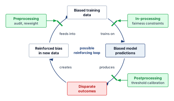
A static post-hoc fairness audit can miss closed-loop reinforcement (figure 13). When a system retrains on outcomes selected by its own decisions, the resulting sample may reinforce initial skews without revealing what would have happened under a different policy. The feedback policy and available evidence determine whether disparities grow or shrink; an effective intervention need not modify every stage. Fairness therefore becomes a lifecycle constraint, in which data visibility determines what can be measured, threshold policy determines where errors land, and feedback infrastructure determines whether disparities decay or compound.
Predictive policing illustrates how this feedback can arise. A model trained on recorded arrests may direct more patrols to a neighborhood. If greater patrol presence produces more recorded incidents and the training pipeline treats those records as an unbiased measure of underlying crime, later predictions can reinforce the original allocation. The loop depends on how deployment changes observation and how retraining uses that evidence; it is not an inevitable consequence of every predictive model.
Recommender systems such as Archetype B (DLRM at Scale) show similar dynamics in digital environments. A content recommendation model that prioritizes engagement may gradually narrow the range of content a user is exposed to, leading to feedback loops that reinforce existing preferences or polarize opinions. These effects can be difficult to detect using conventional performance metrics, as the system continues to optimize its training objective even while diverging from broader social or epistemic goals.
Feedback loops undermine the assumption of independently and identically distributed data, so validation on a static test set can miss the model’s evolving effect on the data-generating process. Once a loop is established, interventions aimed at fairness or accuracy may have limited effect unless the underlying data dynamics are addressed. Responsible design therefore monitors how system outputs reshape the environment, how those changes enter new data, and whether retraining mitigates or exacerbates them.
In cloud-based systems, these updates may occur frequently and at scale, with extensive telemetry available to detect behavior drift. In contrast, edge and embedded deployments often operate offline or with limited observability. A smart home system that adapts thermostat behavior based on user interactions may reinforce energy consumption patterns or comfort preferences in ways that alter the home environment, and subsequently affect future inputs to the model. Without connectivity or centralized oversight, these loops may go unrecognized despite their effect on user behavior and system performance. Feedback loops are not inherently harmful, but they must be detected and managed; the drift detection and alerting of section 16.9.3 expose them only when the deployment can return the evidence.
Human-AI collaboration
Human operators turn feedback-loop risk into a shared-control problem. Machine learning systems are often deployed not as standalone agents, but as components in larger workflows that involve human decision-makers. In many domains, such as healthcare, finance, and transportation, models serve as decision-support tools, offering predictions, risk scores, or recommendations that are reviewed and acted upon by human operators. The collaborative configuration raises questions about how responsibility is shared between humans and machines, how trust is calibrated, and how oversight mechanisms are implemented in practice.
Human-AI collaboration introduces both opportunities and risks. When designed appropriately, systems can augment human judgment, reduce cognitive burden, and enhance consistency in decision-making. However, when poorly designed, they may lead to automation bias,22 where users over-rely on model outputs even in the presence of clear errors. Conversely, excessive distrust can result in algorithm aversion, where users disregard useful model predictions due to a lack of transparency or perceived credibility. The effectiveness of collaborative systems depends on how the system communicates uncertainty, provides explanations, and enables human override or correction, rather than on model accuracy alone.
22 Automation bias: Inappropriate reliance on automated recommendations, including acceptance of erroneous outputs. Its prevalence depends on the task, interface, workload, and users’ ability to check the output. Strong average performance can encourage reliance without making rare errors easier to recognize. Uncertainty displays, selective review, or requests for justification should be evaluated for their effects on correction rates, workload, and response time rather than assumed to improve safety.
Center, Pew Research. 2023. What Americans Know about AI, Cybersecurity and Big Tech.
Schäfer, Mike S. 2023. “The Notorious GPT: Science Communication in the Age of Artificial Intelligence.” Journal of Science Communication 22 (02): Y02. https://doi.org/10.22323/2.22020402.
Public knowledge about AI is uneven (Center 2023), and science-communication failures can amplify misunderstandings about how AI systems work (Schäfer 2023). That matters for deployment safety, because when users lack understanding of model uncertainty, data bias, or decision boundaries, they may trust system outputs in contexts where human judgment should intervene. From a systems engineering perspective, public comprehension is part of the deployment context, because the safety properties of a human-AI system depend on whether users can appropriately calibrate their trust and recognize situations requiring human override, not on technical mechanisms alone.
Automation changes work organization in ways that influence safety design decisions. The MIT Work of the Future task force (Work of the Future 2020) argues that technological change and labor-market institutions jointly determine whether automation improves job quality or concentrates harms. For ML systems, the safety implication is that removing human roles can also remove contextual judgment and system-level debugging that remain difficult to encode in models. Metrics focused solely on throughput may inadvertently penalize human-in-the-loop designs that preserve oversight capability.
Work of the Future, MIT Task Force on the. 2020. The Work of the Future: Building Better Jobs in an Age of Intelligent Machines. Massachusetts Institute of Technology.
Institutional incentives can reinforce automation bias when operators expect greater scrutiny for overriding a model than for accepting it. Consider an illustrative pair of judicial decisions. In Scenario A, a judge overrides a “high risk” algorithmic score and releases a defendant who later re-offends. The judge anticipates criticism for departing from the recommendation. In Scenario B, the judge follows the score and detains the defendant unnecessarily, but the institution treats agreement with the model as evidence of proper procedure. The incentive comes from that review policy, not from the model’s measured accuracy.
This asymmetry can encourage institutional deference, where human oversight becomes a “rubber stamp” for algorithmic decisions. Review procedures should evaluate the evidence behind both agreement and disagreement, rather than treating agreement as inherently correct. The required documentation must fit the decision’s stakes and the operator’s workload so that justification supports scrutiny rather than becoming another routine approval.
Oversight mechanisms must be tailored to the deployment context. In high-stakes domains, such as medical triage or autonomous driving, humans may be expected to supervise automated decisions in real time. This configuration places cognitive and temporal demands on the human operator and assumes that intervention will occur quickly and reliably when needed. In practice, however, continuous human supervision is often impractical or ineffective, particularly when the operator must monitor multiple systems or lacks clear criteria for intervention.
From a systems design perspective, supporting effective oversight requires more than providing access to raw model outputs. Interfaces must be constructed to surface relevant information at the right time, in the right format, and with appropriate context. Confidence scores, uncertainty estimates, explanations, and change alerts can all play a role in enabling human oversight. Workflows must define when and how intervention is possible, who is authorized to override model outputs, and how such overrides are logged, audited, and incorporated into future system updates.
Consider a hospital triage system that uses a machine learning model to prioritize patients in the emergency department. The model generates a risk score for each incoming patient, which is presented alongside a suggested triage category. In principle, a human nurse is responsible for confirming or overriding the suggestion. However, if the model’s outputs are presented without sufficient justification, such as an explanation of the contributing features or the context for uncertainty, the nurse may defer to the model even in borderline cases. Over time, the model’s outputs may become the de facto triage decision, especially under time pressure. If a distribution shift occurs (for instance, due to a new illness or change in patient demographics), the nurse may lack both the situational awareness and the interface support needed to detect that the model is underperforming. In such cases, the appearance of human oversight masks a system in which responsibility has effectively shifted to the model without clear accountability or recourse.
In such systems, human oversight depends on infrastructure design as much as on policy, including how predictions are surfaced, what information is retained, how intervention is enacted, and how feedback loops connect human decisions to system updates. Without integration across these components, oversight becomes fragmented, and responsibility may shift invisibly from human to machine.
Napkin Math 16.7: The automation bias paradox
Consider a radiology department deploying an AI assistant for tumor detection, where standalone human sensitivity is \(\HumanStandaloneSensitivity=\) 92 percent and standalone AI sensitivity is \(\AiStandaloneSensitivity=\) 95 percent. One might assume the combined system performance would exceed 95 percent. However, this illustrative scenario assumes that humans accept the AI’s missed detections at rates of 60–80 percent. Among patients with tumors, the AI misses a tumor with probability \(1 - \AiStandaloneSensitivity = 0.05\); if the human accepts that miss (\(\MissAcceptanceProbability = 0.7\)), these accepted misses alone create a conditional failure probability of \(0.05 \times 0.7 = 0.035\). In this simplified upper-bound case, where every other AI miss is corrected and no correct detection is overturned, sensitivity is 96.5 percent. False positives require separate evaluation among patients without tumors, while fatigue and interface delays can further affect the workflow.
This conditional error-acceptance probability matters more than the overall override rate. A low override rate may reflect few model errors or failures to detect them; those interpretations require different interventions. The trust calibration gap arises when reliance exceeds what the evidence supports. Evaluate interface changes against the fraction of actual errors corrected, errors introduced by overrides, and response delay before adopting them.
The boundary between decision support and automation is often fluid. Systems initially designed to assist human decision-makers may gradually assume greater autonomy as trust increases or organizational incentives shift. This transition can occur without explicit policy changes, resulting in de facto automation without appropriate accountability structures. Responsible system design must therefore anticipate changes in use over time and ensure that appropriate checks remain in place even as reliance on automation grows.
Normative pluralism and value conflicts
Human-AI collaboration exposes a deeper systems constraint, because different stakeholders often hold conflicting values and priorities. Algorithms can help identify feasible compromises, but they cannot establish whose priorities should govern a deployment. Technical excellence is necessary but insufficient for trustworthy AI because choosing among conceptions of fairness, privacy, and accountability requires a legitimate decision process as well as evidence about their consequences.
Responsible machine learning cannot be reduced to the optimization of a single objective. In real-world settings, machine learning systems are deployed into environments shaped by diverse, and often conflicting, human values. A high-stakes deployment makes these tensions concrete.
Example 16.2: Conflicting values in practice
Scenario: An adolescent mental health crisis detection pipeline must balance competing stakeholder objectives across real-time inference and data retention paths.
Diagnosis: Optimizing clinical efficacy via aggressive alert dispatch conflicts with patient autonomy and privacy protocols. Restricting data retention to protect user privacy limits offline retraining and explanation auditing, while routing high-confidence alerts to human counselors increases per-query serving cost and the end-to-end latency \(\EndToEndRequestLatency\), measured from the incoming message to an acknowledged alert. A local differential privacy mechanism would need a specified privacy unit, accountant, and clinical utility evaluation. The automated dispatch SLA covers producing and acknowledging an alert, not completing human counseling. Human response needs a separate deadline, staffed queue capacity, and an escalation policy for overload.
Systems lesson: Responsible AI trade-offs are hard architectural requirements, not after-the-fact policy notes. The deployment pipeline must encode stakeholder choices into explicit latency (\(\EndToEndRequestLatency\)) and privacy budgets before optimization begins.
What constitutes a fair outcome for one stakeholder may be perceived as inequitable by another. Similarly, decisions that prioritize accuracy or efficiency may conflict with goals such as transparency, individual autonomy, or harm reduction. These tensions are structural rather than incidental, reflecting the pluralistic societies and institutional settings in which machine learning systems operate. Fairness is a particularly prominent site of value conflict because its criteria can be incompatible (section 16.5.1.5) and choosing among them is a normative decision rather than a purely technical one, yet similar conflicts arise between interpretability and predictive performance, privacy and personalization, or short-term utility and long-term consequences.
Each deployment tier gives these conflicts a different form, adding to the tier comparison of section 16.4.1 the question of who decides. A voice assistant that personalizes on a mobile device keeps raw data local, which reduces transmission exposure without by itself establishing a privacy guarantee. Users with underrepresented usage patterns may still receive less accurate predictions, and detecting that disparity requires decisions about consent, aggregation, and access, so privacy, fairness, and personalization must be weighed against one another. A cloud credit-scoring or recommendation platform faces demands for explanations of consequential decisions while relying on complex ensembles or proprietary training data whose disclosure may be commercially sensitive or technically infeasible, which sets institutional accountability against business confidentiality. An edge camera or drone that compresses its model to meet latency and energy budgets trades efficiency against robustness; the effect must be measured on the deployed candidates under the expected shifts and threat model rather than assumed, and a more resilient candidate may exceed the memory or power budget. A TinyML device without persistent connectivity cannot absorb new fairness requirements through local retraining, so whether servicing or intermittent synchronization can deliver a revised model, and whether explanations and appeals can run off-device on preserved evidence, becomes part of the value decision. In every tier the conflict extends beyond what the model optimizes to what the system can support after deployment.
The recurring systems constraint is normative pluralism, not an abstract philosophical challenge. Technical approaches such as multi-objective optimization, constrained training, and fairness-aware evaluation can help surface and formalize trade-offs, but they do not eliminate the need for judgment. Decisions about whose values to represent, which harms to mitigate, and how to balance competing objectives cannot be made algorithmically. They require deliberation, stakeholder input, and governance structures that extend beyond the model itself. Machine learning systems are not neutral tools; they embed value judgments whether those judgments are specified or assumed.
Participatory methods and the Value-Sensitive Design process introduced with value alignment (section 16.8.3) offer paths forward. Rather than treating values as parameters to be optimized after deployment, these approaches seek to engage stakeholders during the requirements phase, define ethical trade-offs explicitly, and trace how they are instantiated in system architecture. Some requirements can be satisfied together; others require a documented choice or a decision not to deploy. Making these judgments explicit gives affected stakeholders something concrete to question and revise.
Value-Sensitive Design also governs the autonomy of the people a system serves. Applied to human control, it explicitly considers factors such as capability, complexity, misrepresentation, and the fluidity of user control. The METUX model (Motivation, Engagement, and Thriving in the User Experience) extends this thinking to six spheres of technology experience, namely adoption, interface, tasks, behavior, life, and society, each of which can support or undermine human flourishing (Peters et al. 2018). Both draw on self-determination theory’s account of autonomy as the ability to act in accordance with one’s own values and goals, rather than as control in a technical sense (Ryan and Deci 2000). In an ML system those requirements become concrete artifacts, namely interface affordances, user controls, feedback channels, escalation paths, and audit evidence. A recommender that optimizes engagement, for instance, can shape user preferences in ways the user cannot see. Evaluating it across the outer spheres of behavior, life, and society exposes effects that a short-term engagement metric never measures, so preserving autonomy requires controls and evidence beyond that metric.
Peters, D., R. A. Calvo, and R. M. Ryan. 2018. “Designing for Motivation, Engagement and Wellbeing in Digital Experience.” Frontiers in Psychology 9: 797. https://doi.org/10.3389/fpsyg.2018.00797.
Ryan, R. M., and E. L. Deci. 2000. “Self-Determination Theory and the Facilitation of Intrinsic Motivation, Social Development, and Well-Being.” American Psychologist 55 (1): 68–78. https://doi.org/10.1037/0003-066x.55.1.68.
Feedback loops, human-AI collaboration, and value conflicts show why the technical foundations from section 16.5 through section 16.8 cannot ensure responsible AI on their own. Without organizational authority, operational telemetry, and escalation paths, a fairness metric with no owner, an explanation with no appeal process, or a monitoring signal with no remediation budget becomes evidence without action.
Checkpoint 16.3: When correct code fails in deployment
Mathematically sound, fair, and explainable models can still fail in human institutions through feedback loops that reshape the data, automation bias and institutional deference, and normative pluralism among stakeholders.
Diagnosing the human-system interaction
Reasoning about loops and stakeholders
Self-Check: Question
In dataset governance, standardized documentation of motivation, composition, collection process, and recommended uses, modeled on electronic-component specification sheets, is called
____.Order the stages of the Bias Amplification Feedback Loop in an unconstrained retraining pipeline: (1) Reinforced data bias is captured in operational logs, (2) Biased model produces skewed deployment predictions, (3) New model retrained on reinforced data exhibits compounded disparity, (4) Historical bias in initial training data is learned during initial model fit, (5) Real-world discriminatory outcomes occur based on automated decisions.
True or False: In a closed-loop system where future data distribution \(\ProbabilityFunction_{\FeedbackStepIndex+1}(\ModelInput)\) is dynamically altered by current model decisions \(\ModelPredictor_{\FeedbackStepIndex}(\ModelInput)\) (such as predictive policing or recommendation engines), validating model performance on a static held-out test set guarantees long-term fairness and stability.
In human-AI collaborative decision-making, what is the ‘paradox of reliability’ and what is its primary engineering implication for interface design?
- A model with \(50\%\) accuracy causes hardware crashes more frequently than a model with \(90\%\) accuracy
- As a model’s latency decreases, network packet loss increases proportionally
- Highly compressed models consume more DRAM memory than uncompressed models
- High apparent reliability can encourage over-reliance; interface design must be evaluated by how often users accept erroneous recommendations, correct errors, or introduce new errors, not by the overall override rate alone.
A hospital deploys a sepsis predictor with high offline accuracy, yet mortality does not improve and clinicians often ignore alerts. What workflow explanations remain possible, and what evidence would distinguish them before choosing a remedy?
Define normative pluralism in machine learning system design and explain why value conflicts cannot be resolved through purely algorithmic optimization.
16.10 Governing Responsible AI at Fleet Scale
The data science team wants to hold back deployment for a month to conduct rigorous fairness audits on a new generative model. The executive team, watching a competitor launch a similar feature, demands the model be deployed by Friday. Even when engineers know how to evaluate the relevant risks, the organizational structure, budget, and business priorities must give them the time and authority to act on that knowledge.
The scenario exposes the implementation gap between technical capability and operational authority. Responsible AI methods provide necessary tools, but their effectiveness depends on organizational structures, data infrastructure, evaluation processes, and sustained commitment that extends far beyond algorithm development. Systems maintain responsible behavior over time only when those implementation supports survive deadline pressure, product incentives, and postdeployment drift.
The practical barriers to embedding responsible AI in production ML systems span the classical People-Process-Technology framework. People challenges, the subject of section 16.10.1, encompass the organizational structures, authority, role definitions, and incentives that determine whether ethical commitments translate into durable operational behavior. Technology challenges begin with the data itself (section 16.10.2), where quality gaps and acquisition costs decide what a team can fix. Process challenges cover how competing objectives are resolved (section 16.10.3) and how responsibility constraints survive scaling, maintenance, and continuous delivery (section 16.10.4). A decision framework (section 16.10.5) then turns the three dimensions into deployment-specific priorities.
These dimensions matter because responsible AI fails when organizational incentives, development workflows, and production infrastructure pull in conflicting directions. The framework connects each technical claim to the process and owner needed to act on it. A fairness metric without an accountable owner produces no remediation, while a governance process lacking telemetry cannot detect drift. A formal privacy guarantee also does not implement deletion; that requires lineage and a removal workflow for the relevant data and model state. Effective implementation therefore demands systems-level strategies that embed responsibility into the architecture, infrastructure, and operating practices of machine learning deployment across all three dimensions simultaneously.
16.10.1 Organizational structures and incentives
When a modeling team is evaluated on quarterly engagement lift, data pipelines belong to a separate platform org, user appeals land in customer support, and compliance reviews happen in legal, a subgroup error gap or broken explanation path can sit unfixed for months because no single owner has both the budget and the stop-ship authority to repair it. Transparency and contestability fail when responsibility is distributed without corresponding authority. Institutional design must connect model, data, product, legal, and operational roles through a named escalation path, review capacity, and authority to restrict deployment or provide remedy.
Within companies, research labs, and public institutions, responsibility must be translated into concrete roles, workflows, and incentives. In practice, however, organizational structures often fragment responsibility, making it difficult to coordinate ethical objectives across engineering, product, legal, and operational teams.
Responsible AI requires sustained investment in practices such as subgroup performance evaluation, explainability analysis, adversarial robustness testing, and the integration of privacy-preserving techniques like differential privacy or federated training. These activities can be time-consuming and resource-intensive, yet they often fall outside the formal performance metrics used to evaluate team productivity. For example, teams may be incentivized to ship features quickly or meet performance benchmarks, even when doing so undermines fairness or overlooks potential harms. When ethical diligence is treated as a discretionary task, instead of being an integrated component of the system lifecycle, it becomes vulnerable to deprioritization under deadline pressure or organizational churn.
Responsibility is further complicated by ambiguity over ownership. In many organizations, no single team is responsible for ensuring that a system behaves ethically over time. Model performance may be owned by one team, user experience by another, data infrastructure by a third, and compliance by a fourth. When issues arise, including disparate impact in predictions or insufficient explanation quality, there may be no clear protocol for identifying root causes or coordinating mitigation. As a result, concerns raised by developers, users, or auditors may go unaddressed, not because of malicious intent, but due to lack of process and cross-functional alignment.
Establishing effective organizational structures for responsible AI requires more than policy declarations. It demands operational mechanisms: designated roles with responsibility for ethical oversight, documented escalation pathways, accountability for postdeployment monitoring, and incentives that reward teams for ethical foresight and system maintainability. Some organizations also embed domain experts or user advocates in product teams to anticipate downstream impacts and evaluate value trade-offs in context.
Technical infrastructure such as versioned model registries, model cards, and audit logs must be coupled with organizational structures such as ethics review boards, model risk committees, and red-teaming23 procedures. Their effectiveness depends on whether findings reach an authorized owner, receive a timely response, and lead to a verified correction when one is required. The existence of a committee or audit log alone does not establish that concerns have been addressed.
23 Red teaming: From Cold War military simulations where the “Red Team” acted as the Soviet adversary to probe US defenses. In Responsible AI, red teaming is the adversarial audit phase: specialized teams (hackers, linguists, ethicists) deliberately probe models for jailbreaks, bias, or toxic outputs before deployment. This discovery process identifies the long-tail risks that standard unit tests cannot catch.
Operational rigor comes with a measurable cost. Public responsible-AI standards and internal review processes illustrate that governance can add release latency through impact assessments, model reviews, red-team exercises, and documentation gates. Review capacity therefore becomes part of deployment planning. If every high-risk launch needs specialized review, the review queue becomes a bottleneck just like security review or capacity approval. That cost must be budgeted alongside remediation and residual risk; preventive review can reduce exposure, but does not guarantee that every incident will be avoided or that remediation will always cost more.
Third-party and foundation-model dependencies do not transfer accountability to the supplier. A deploying organization may inherit weights, safety evaluations, data documentation, or contractual controls, but it still chooses the use, interface, retrieved context, user population, monitoring, and response process. Procurement therefore needs the same rigor as an internal model gate: documented intended and prohibited uses, evaluation scope, version and change notification, incident disclosure, audit access, data handling, service dependencies, fallback behavior, and an exit plan. When supplier evidence is unavailable, the assurance case must record the gap as residual risk rather than silently treating a vendor assertion as a verified control.
The organization must provide these functions across the actual deployment lifecycle. A cloud team may operate continuous review and monitoring services; an embedded-device operator may rely on certification, firmware inventories, servicing, and recall. Domain experts, affected parties, and regulators remain part of the evidence and authority structure in either case. The operating arrangement must still support correction of an individual decision.
Accountability becomes visible at the point of remedy. Affected people need a discoverable channel to challenge an outcome, a record of the evidence considered, a reviewer with authority to correct the decision, a response deadline, and a way to propagate the correction into downstream systems. Aggregate model improvement is not a substitute for individual remedy, because retraining next quarter does not correct a benefit denied today. Incident procedures must therefore connect technical containment and rollback to notification, correction, compensation where applicable, root-cause analysis, and verification that the remedy reached every dependent decision record. Retirement does not end these duties: shutting down a model closes its execution path, but an appeal owner remains responsible for unresolved decisions after inference stops (section 16.2). England’s 2020 exam-grading algorithm showed how quickly an aggregate method can outrun the remedy path its decisions require.
War Story 16.2: The algorithmic grading failure (2020)
Context: In August 2020, following exam cancellations during COVID-19, England’s qualifications regulator (Ofqual) deployed a statistical standardization algorithm to grade ~280,000 A-level students (Ofqual 2020; Department for Education and Ofqual 2020).
Mechanism: To control grade inflation, the standardization method combined historical results with the cohort’s prior attainment to estimate grade distributions, then allocated grades using teachers’ student rankings. Small subject cohorts received greater weight on teacher-assessed grades. The method therefore used individual ranking evidence, but constrained its interpretation through cohort-level predictions that could differ from teachers’ assessments of individual achievement.
Impact: The calculated grade was lower than the teacher-assessed grade in 39.1 percent of cases (Ofqual 2020). Public outcry and student protests prompted a reversal of the grading policy days later.
Fix: Students were awarded the higher of the center-assessed grade and the calculated grade, replacing the earlier standardization policy.
Systems lesson: An aggregate prediction does not establish that every individual outcome is justified. An appeal channel must specify which evidence can change the decision, who can review it, and how quickly a correction can take effect; the existence of a procedural appeal alone does not answer those questions.
Ofqual. 2020. Awarding GCSE, AS, A Level, Advanced Extension Awards and Extended Project Qualifications in Summer 2020: Interim Report. Office of Qualifications; Examinations Regulation.
Department for Education, and Ofqual. 2020. GCSE and A Level Students to Receive Centre Assessment Grades. GOV.UK News Story.
Shneiderman, B. 2022. Human-Centered AI. Oxford University Press. https://doi.org/10.1093/oso/9780192845290.001.0001.
Shneiderman, B. 2020. “Bridging the Gap Between Ethics and Practice: Guidelines for Reliable, Safe, and Trustworthy Human-Centered AI Systems.” ACM Transactions on Interactive Intelligent Systems 10 (4): 1–31. https://doi.org/10.1145/3419764.
The responsibility for ethical system behavior is distributed across multiple constituencies, including industry, academia, civil society, and government. The resulting governance hierarchy surrounds the AI system with four concentric tiers (figure 14). The development team executes technical controls (fairness testing, model cards, red-teaming); the organization governs operational processes (impact assessments, ethical review boards); industry establishes consensus baselines (ISO standards, external audits); and government and society enforce legal boundaries (GDPR, the EU AI Act, sector-specific statutes) (Shneiderman 2022, 2020). Within organizations, this distribution must be mirrored by mechanisms that connect technical design with strategic oversight and operational control. Without these linkages, responsibility becomes diffuse, and well-intentioned efforts may be undermined by systemic misalignment.
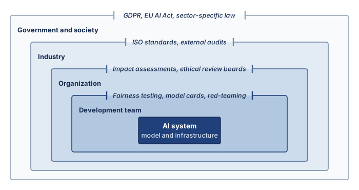
International Organization for Standardization, and International Electrotechnical Commission. 2023b. ISO/IEC 42001:2023 Information Technology – Artificial Intelligence – Management System. ISO/IEC standard.
Technical excellence and regulatory compliance are therefore insufficient on their own. Responsible AI requires aligning ethical objectives with the institutional structures through which machine learning systems are designed, deployed, and maintained, so that responsibility is embedded in the organization that governs deployment as well as in the model itself. The same ownership problem becomes concrete at the data layer, where teams can know how to audit a dataset and still lack the authority, access, or infrastructure needed to change it.
16.10.2 Data constraints and quality gaps
A clinical imaging model trained on five urban teaching hospitals can achieve 94 percent accuracy overall while dropping to 78 percent on rural and elderly patients, yet acquiring and harmonizing replacement images across 50 partner hospitals can cost over $160 million and years of legal and schema negotiations. Improving data pipelines remains one of the hardest implementation challenges in practice, even when developers and researchers understand the need for representative coverage, accurate labels, and historical-bias mitigation. Responsibility for data is often split across teams, locked inside legacy systems, or governed by external institutions that a modeling team cannot unilaterally change.
Data engineering principles, including data validation, schema management, versioning, lineage tracking, and quality monitoring, provide the technical foundation for addressing these challenges. However, applying these principles to responsible AI introduces additional complexity. Fairness requires assessing representativeness across demographic groups, bias mitigation demands understanding historical data collection practices, and privacy preservation constrains which validation techniques are permissible. The organizational challenges described here reflect the gap between having robust data engineering infrastructure and using it effectively to support responsible AI objectives.
Subgroup imbalance, label ambiguity, and distribution shift, each of which affect generalization and performance across domains, are well-established concerns in responsible ML. These issues often manifest in the form of poor calibration, out-of-distribution failures, or demographic disparities in evaluation metrics. However, addressing them in real-world settings requires more than technical knowledge. It requires access to relevant data, institutional support for remediation, and sufficient time and resources to iterate on the dataset itself. Teams may lack the authority or infrastructure to modify a training dataset even after discovering performance disparities. Versioning and lineage make controlled correction possible by identifying the affected datasets and downstream models; they do not remove the need to acquire replacement data, retrain, and revalidate those models.
In domains like healthcare, education, and social services, these challenges are especially pronounced. Data acquisition may be subject to legal constraints, privacy regulations, or cross-organizational coordination. For example, a team developing a triage model may discover that their training data underrepresents patients from smaller or rural hospitals. Correcting this imbalance would require negotiating data access with external partners, aligning on feature standards, and resolving inconsistencies in labeling practices. The logistical and operational costs can be prohibitive even when all parties agree on the need for improvement.
Efforts to collect more representative data may also run into ethical and political concerns. In some cases, additional data collection could expose marginalized populations to new risks. This paradox of exposure, in which the individuals most harmed by exclusion are also those most vulnerable to misuse, complicates efforts to improve fairness through dataset expansion. For example, gathering more data on nonbinary individuals to support fairness in gender-sensitive applications may improve model coverage, but it also raises serious concerns around consent, identifiability, and downstream use. Teams must navigate these tensions carefully, often without clear institutional guidance.
Napkin Math 16.8: The representation cost
Problem: A medical imaging model trained on data from 5 hospitals achieves 94 percent accuracy overall but only 78 percent on underrepresented populations (rural patients, elderly patients, patients with darker skin tones). A proposed acquisition plan seeks data from 50+ hospitals across diverse geographies, demographics, and equipment types. This budget is an illustrative proposal, not a sample-size requirement derived from the accuracy gap; validation must establish whether it improves the relevant outcomes.
Math:
- Data acquisition cost: $50–$200 per labeled medical image, with 100,000 images budgeted per underrepresented subgroup.
- Representation-cost scenario: For 10 subgroups, at the midpoint of the cost range, 10 times 100,000 images per subgroup times $125 per image yields $125M in data acquisition alone. This calculation assumes distinct purchased examples for each allocation; overlapping demographic groups require deduplication or explicit shared-cost allocation.
- Data harmonization: Data harmonization across different scanners, protocols, and labeling conventions adds 30 percent–50 percent overhead, bringing the total to $162.5M–$187.5M.
Systems insight: The acquisition budget makes coverage goals explicit, but spending does not guarantee that an accuracy gap closes. Teams should prioritize identified coverage deficiencies using harm, data quality, privacy, and expected benefit criteria, then validate the resulting model on the intended populations.

Harmonizing scanners, protocols, and labels adds 30–50 percent to the acquisition cost.
Himmelstein, Gracie, David Bates, and Li Zhou. 2022. “Examination of Stigmatizing Language in the Electronic Health Record.” JAMA Network Open 5 (1): e2144967. https://doi.org/10.1001/jamanetworkopen.2021.44967.
Upstream biases in data collection systems can persist unchecked even when data is plentiful. Many organizations rely on third-party data vendors, external APIs, or operational databases that were not designed with fairness or interpretability in mind. For instance, Electronic Health Records, which are commonly used in clinical machine learning, often reflect systemic disparities in care, as well as documentation habits that encode racial or socioeconomic bias (Himmelstein et al. 2022). Teams working downstream may have little visibility into how these records were created, and few levers for addressing embedded harms.
Improving dataset quality is often not the responsibility of any one team. Data pipelines may be maintained by infrastructure or analytics groups that operate independently of the ML engineering or model evaluation teams. This organizational fragmentation makes it difficult to coordinate data audits, track provenance, or implement feedback loops that connect model behavior to underlying data issues. In practice, responsibility for dataset quality tends to fall through the cracks, recognized as important, but rarely prioritized or resourced.
Addressing these challenges requires long-term investment in infrastructure, workflows, and cross-functional communication. Data validation and automated audits can identify defects, while datasheets and the Data Nutrition Project24 document dataset properties. Model cards connect model evaluation and intended use to that evidence. These tools help only when teams have the mandate and support to act on their findings.
24 Data Nutrition Project: A nonprofit initiative that develops standardized dataset documentation modeled on nutrition labels, summarizing provenance, composition, distribution, and known issues for datasets used in ML pipelines. The project’s labels make dataset risks legible to downstream engineers who lack access to the original collection process, which bridges the organizational fragmentation described here.
Improving data quality is therefore fundamentally a question of how responsibility for data is assigned, shared, and sustained across the system lifecycle, not merely a matter of better tooling. Once that responsibility is in place, teams still have to decide which responsible-AI objective should dominate when valid goals conflict.
16.10.3 Balancing competing objectives
When a modeling team tunes for aggregate accuracy, a compliance team injects differential-privacy noise that degrades minority-group recall, and a serving team prunes the network to hit a 15 ms latency target, their uncoordinated local optimizations can break the deployment’s fairness and explanation guarantees even though every team met its own metric. Machine learning system design is often framed as optimizing a single loss or accuracy objective, yet production systems must balance accuracy against fairness, interpretability, robustness, privacy, and resource efficiency, objectives that routinely pull in opposite directions. The accuracy-interpretability, personalization-fairness, and privacy-utility conflicts of section 16.4.1 recur here, and each must be measured on the path where its mechanism actually executes rather than assumed. Those trade-offs are not purely technical; they reflect deeper normative judgments about what a system is designed to achieve and for whom, as explored in detail in section 16.9.4.3. Responsible ML development requires making these judgments explicit, evaluating them in context, and subjecting them to stakeholder input and institutional oversight.
What makes this challenge particularly difficult in implementation is that these competing objectives are rarely owned by a single team or function. Performance may be optimized by the modeling team, fairness monitored by a responsible AI group, and privacy handled by legal or compliance departments. Without deliberate coordination, system-level trade-offs can be made implicitly, piecemeal, or without visibility into long-term consequences. Over time, the result may be a model that appears well-behaved in isolation but fails to meet its ethical goals when embedded in production infrastructure.
Balancing competing objectives requires transparency, deliberation, and cross-team alignment alongside technical fluency. Systems must be designed to surface trade-offs rather than obscure them, to make room for constraint-aware development rather than pursue narrow optimization. In practice, this may require redefining what “success” looks like, not as performance on a single metric, but as sustained alignment between system behavior and its intended role in a broader social or operational context.
Organizational structures, data quality, and competing objectives explain why technical competence alone does not secure responsible behavior. A team can understand fairness metrics and still lack authority to change a dataset or delay a release. When modeling teams optimize performance, compliance teams address privacy, and product teams prioritize engagement independently, their local decisions may violate a shared requirement. Clear ownership across those boundaries connects evaluation to action, while data infrastructure and deliberative review make the evidence and trade-offs inspectable. Maintaining those connections becomes harder as deployments scale and their data, models, and teams change.
16.10.4 Scalability, maintenance, and evaluation standards
Fairness audits are often conducted during initial evaluation, interpretability methods applied during model selection, and privacy-preserving techniques considered during training, but these practices frequently degrade or disappear as systems move from research prototypes to production. Fairness checks run on a static dataset never join the ingestion pipeline, explanation methods never reach a user-facing interface, and privacy constraints enforced during training are overlooked in postdeployment monitoring or model updates. The gap between what is possible in principle and what is sustainable in production is a core implementation challenge for responsible AI.
Production environments introduce new pressures that reshape system priorities. Models must operate across diverse hardware configurations, interface with evolving APIs, serve millions of users with low latency, and maintain availability under operational stress. These constraints demand continuous adaptation and rapid iteration, often deprioritizing activities that are difficult to automate or measure. Responsible AI practices, especially those that involve human review, stakeholder consultation, or post-hoc evaluation, may not be easily incorporated into fast-paced DevOps25 pipelines.
25 MLOps (machine learning operations): ML CI/CD pipelines must handle data versioning, training reproducibility, and A/B testing of algorithm changes beyond traditional software concerns. High-velocity ML organizations may deploy model or configuration changes far more often than responsible-AI reviews can be completed manually, creating a velocity gap in which deployment cycles measured in hours compete against ethical validation requiring days or weeks. This tension explains why responsible AI commitments present at the prototype stage can be deprioritized as systems scale.
Maintenance introduces further complexity. Machine learning systems are rarely static. New data is ingested, retraining is performed, features are deprecated or added, and usage patterns shift over time. In the absence of rigorous version control, changelogs, and impact assessments, it can be difficult to trace how system behavior evolves or whether responsibility-related properties such as fairness or robustness are being preserved. Organizational turnover and team restructuring can erode institutional memory. Teams responsible for maintaining a deployed model may not be the ones who originally developed or audited it, leading to unintentional misalignment between system goals and deployed behavior. These issues are especially acute in continual or streaming learning. Drift calls for investigation and a response matched to its consequences, which may mean restricting use or invoking fallback while a revised model undergoes validation, rather than immediately updating production weights.
These challenges are magnified in multi-model systems and cross-platform deployments. A recommendation engine may consist of dozens of interacting models, each optimized for a different subtask or user segment. A voice assistant deployed across mobile and edge environments may maintain different versions of the same model, tuned to local hardware constraints. Coordinating updates, ensuring consistency, and sustaining responsible behavior in such distributed systems requires infrastructure that tracks governing values and constraints alongside code and data. Addressing these challenges means treating responsible AI as a lifecycle property rather than a one-time evaluation: audit hooks, metadata tracking, and monitoring protocols built into infrastructure, with documentation and accountability structures that survive team handoffs.
Maintenance also exposes a gap in how responsible-AI evidence is standardized. A model evaluated under demographic parity on one benchmark has not thereby satisfied equalized odds in another deployment. The criterion, population, labels, threshold policy, and uncertainty belong to the claim. Changing any of them can invalidate the evidence even when the weights remain unchanged. Standardization must make those conditions explicit so teams can compare results and identify what needs revalidation.
The evaluation boundary must also match the deployment boundary. A model-only result can miss effects introduced by feature transformations, request routing, caching, or human review. Separate fairness, explanation, and compliance tools therefore need compatible identifiers and records linking their results to the same model, data, policy, and workflow versions. Otherwise, an assurance case can combine individually valid results that describe different systems.
Reusing that evidence after launch requires lifecycle controls. Production observations must be comparable with the acceptance criteria, and material changes must trigger a documented revalidation scope. Evidence must therefore remain interpretable across teams, components, and time. The implementation decision is then which obligations take priority for the intended use, which controls can satisfy them, and which authority may accept the remaining risk.
16.10.5 Implementation decision framework
An intensive-care diagnostic model, a 10,000-query-per-second consumer recommender, and a milliwatt microcontroller sensor cannot run the same safeguards on the same path: the ICU model needs clinician-legible explanations and contested-case routing, the recommender needs continuous slice-drift monitoring and feedback-loop breakers, and the microcontroller must lock in its safety envelope and energy budget before firmware ships. Practitioners therefore need a systematic way to prioritize responsible AI controls by deployment context and stakeholder risk.
Four decision heuristics guide these trade-offs in practice. Where multiple principles conflict, engineering teams must engage domain stakeholders to establish which failure modes present the most severe harms; as the adolescent mental health crisis-detection example in section 16.9.4.3 demonstrated, such value tensions require deliberate institutional policy rather than mathematical optimization alone. Under tight computational budgets, teams must first identify mandatory requirements, then allocate evaluation and response capacity according to risk. Sampling is adequate only if it can detect the relevant failures, and expensive audits need not run on the inference path. Whenever the deployment context changes, as when a cloud model migrates to edge execution with intermittent centralized monitoring, teams must re-evaluate principle priorities, establishing local fallback safeguards and evidence-synchronization plans for constrained connectivity. Finally, when stakeholder values diverge, engineers must document trade-offs explicitly and construct contestability mechanisms that permit affected individuals to challenge automated outcomes.
Each deployment context suggests candidate priorities and trade-offs for deployment-specific review (table 10). Applicable obligations, the threat model, and accountable stakeholder decisions determine which controls and trade-offs are acceptable.
| Deployment context | Primary principles | Implementation priority | Trade-offs to evaluate |
|---|---|---|---|
| High-Stakes Individual Decisions (healthcare diagnosis, credit and loans, criminal justice, employment) | Fairness, explainability, accountability | Mandatory fairness metrics across protected groups; explanations for negative outcomes; human oversight for edge cases | A measured accuracy budget for interpretability; bounded explanation latency; higher computational cost |
| Safety-Critical Systems (autonomous vehicles, medical devices, industrial control) | Safety, robustness, accountability | Threat-model-specific evaluation; bounded certification where applicable; fail-safe mechanisms; comprehensive logging | Significant validation and adversarial-training overhead; conservative confidence thresholds; redundant inference |
| Privacy-Sensitive Applications (health records, financial data, personal communications) | Privacy, security, transparency | Data minimization and appropriate consent mechanisms; evaluate local processing and differential privacy with stated \((\PrivacyBudget, \PrivacyAdditiveSlack)\), privacy unit, and accountant | Privacy-utility trade-offs; higher client-side compute; limited model updates; reduced personalization |
| Large-Scale Consumer Systems (content recommendation, search, advertising) | Fairness, transparency, safety | Bias monitoring across demographics; explanation mechanisms; content-policy enforcement; feedback-loop detection | Sampled or asynchronous explanations at scale; serving-path latency budgeted for fairness checks; investment in monitoring infrastructure |
| Resource-Constrained Deployments (mobile, edge, TinyML) | Privacy, efficiency, safety | Local inference; data locality; input validation; graceful degradation | Expensive audits moved off-device, while local safety checks, fleet or servicing audits, update authority, and retirement criteria are retained |
| Research and Exploratory Systems (internal tools, prototypes, A/B tests) | Transparency, safety (harm prevention) | Documented known limitations; restricted user populations; monitoring for unintended harms | Evaluation depth matched to potential harm and applicable obligations; observability and bounded iteration |
The framework provides starting guidance, but it should be read as a triage mechanism rather than a complete governance program. Legal obligations depend on intended use, jurisdiction, and organizational role, not whether inference runs in a cloud or on a microcontroller (European Parliament and Council of the European Union 2024; European Parliament and Council of the European Union 2016). The framework identifies which constraints deserve first attention, with reassessment as deployment conditions change. The lifecycle assigns human authority over deployment even when individual actions are automated. Engineers investigate bias, operators review fairness metrics, and developers respond to drift. Some systems must also act faster than humans can review an individual decision. Autonomous vehicles respond in milliseconds; trading algorithms execute thousands of transactions before human review is possible; content moderation systems process billions of posts daily. For these systems, the implementation framework must be paired with the value-alignment and fallback controls of section 16.8.3, which keep objectives aligned with human values even when operation runs beyond continuous human supervision.
European Parliament and Council of the European Union. 2024. Regulation (EU) 2024/1689 of the European Parliament and of the Council of 13 June 2024 Laying down Harmonised Rules on Artificial Intelligence (AI Act). Official Journal of the European Union, L 2024/1689.
Systems Perspective 16.2: Responsibility is infrastructure, not a feature
Retrofitting responsible AI controls can require architectural redesign and revalidation, just as adding fault tolerance can. The structural costs cataloged in table 5 each carry a provisioning consequence: bias-drift monitoring needs a sampling and analysis budget; expensive or exact explanation workloads may need a dedicated asynchronous worker fleet, whereas model-specific TreeSHAP, sampling, caching, or selective generation may fit smaller budgets; DP-SGD requires budgeting its clipping, noise, and accounting work under the chosen implementation; and impact assessments need review capacity in the release process. These are not optional add-ons but load-bearing components of production ML systems. In high-risk or regulated deployments, failing to provision the evidence required by the assurance case can block release or force redesign even when core model performance is strong.
Self-Check: Question
In medical imaging ML pipelines, what is the ‘representation cost’ and why does the cost of acquiring representative training data scale with subgroup coverage rather than total image volume?
- It is an annual government licensing fee levied on deep learning medical devices
- It represents the network bandwidth consumed when downloading public datasets from cloud buckets
- It reflects the substantial financial and logistical cost ($125M+ in the chapter’s sizing scenario) of acquiring, curating, and harmonizing clinical data from diverse geographic hospitals, specialized scanners, and underrepresented patient demographics
- It is the GPU memory overhead required to store floating-point feature embeddings during distributed backpropagation
A company builds a customer-facing assistant on a third-party foundation model whose vendor publishes safety evaluations and contractual controls. How does this dependency change the deploying organization’s accountability?
- Accountability transfers to the vendor, because the vendor trained the weights and evaluated their safety
- Accountability is shared equally by contract, so the deploying organization need only monitor uptime
- Accountability stays with the deploying organization, which still chooses the use, interface, retrieved context, user population, monitoring, and response process, so procurement needs the same rigor as an internal model gate
- Accountability disappears for inherited components, because the vendor’s evaluations already cover every downstream use
True or False: When an automated decision system wrongly denies some individuals a benefit, retraining the model next quarter to improve aggregate accuracy provides those individuals with adequate remedy.
A team’s assurance case combines a demographic-parity result from one benchmark, a model-only explanation audit, and a compliance report produced by a separate tool. Explain why these individually valid results may not support a claim about the deployed system.
16.11 Fallacies and Pitfalls
Responsible AI involves counterintuitive trade-offs where ethical principles conflict mathematically and technically. Practitioners from traditional software backgrounds often assume ethical guidelines translate directly to implementation without recognizing the impossibility theorems and computational costs involved. The following fallacies and pitfalls expose misconceptions that hide the structural costs of responsibility or mistake a local technical result for system-level assurance, leading to deployed systems that appear fair in development but violate fairness criteria in production or impose prohibitive computational overhead.
Fallacy: Bias will disappear with more data and better algorithms.
More representative data and better algorithms can reduce some disparities, but they do not determine whether the prediction target is appropriate. The healthcare algorithm described in section 16.5.1 underestimated Black patients’ health needs at a given risk score because expenditure was an imperfect proxy for need. Improving prediction of that proxy would not by itself repair the target. Separately, with unequal base rates and imperfect prediction, groupwise score calibration cannot coexist with equal mean scores across groups in both outcome classes. Engineers must distinguish a remediable data or modeling defect from incompatible requirements, then use stakeholder deliberation to justify the criteria the deployment will pursue.
Pitfall: Treating explainability as an optional feature to be added after core functionality works.
This approach ignores the displacement of overhead, because producing attribution evidence about model behavior demands compute, storage, and interfaces that constrain the architecture. Approximate SHAP explanations are not compute-free (table 5); even a bounded explanation budget can increase request latency and memory pressure. In this sizing example, a recommendation system serving 100 ms latency requirements at 10,000 QPS cannot retrofit explanation work without revisiting the SLA: the illustrative explanation budget adds 50 ms to 200 ms per request, increasing total latency to 150 ms–300 ms (requiring 1.5–3× capacity only under the simplifying assumption that occupied resource time grows in direct proportion to latency, at fixed utilization and parallelism). The assurance case must specify the audience, claim, method, fidelity test, and delivery budget, then choose an architecture such as model-specific TreeSHAP, sampled or cached attribution, selective asynchronous generation, or an inherently interpretable model. Additional replicas can preserve throughput under that assumption, but they do not restore the original per-request latency if explanation remains on the serial path. None of these attribution paths exposes a model’s internal reasoning or establishes causation.
Fallacy: Achieving one fairness metric guarantees overall system fairness.
Practitioners often optimize for demographic parity, which equalizes approval rates across groups, and then assume fair treatment follows. In reality, fairness metrics can conflict mathematically. In the credit-scoring scenario of notebook 16.4, reaching approval parity cost 4 percentage points of accuracy and left approvals in the two groups carrying different default risk. The score-balance impossibility result shows that, with unequal base rates and imperfect prediction, groupwise calibration and equal mean scores across groups in both outcome classes cannot all hold; demographic parity can add a separate selection-rate constraint. Passing one metric therefore leaves other criteria to evaluate. A metric disparity is evidence for investigation, while a legal conclusion depends on the applicable rule and the facts of the deployment.
Pitfall: Implementing fairness constraints without analyzing threshold trade-offs and calibration impacts.
Moving a threshold can equalize one metric while leaving the underlying score calibration unchanged, and in production the threshold is an operational policy embedded in serving code, human review, audit records, and downstream decisions rather than a standalone cutoff in a notebook. Group-specific thresholds can satisfy equal true positive rates, but they also change decision semantics. If the Group A threshold is 0.75 and the Group B threshold is 0.45, as in figure 5, identical scores can yield different decisions, and the positive predictive value of approved applicants can diverge across groups even when the underlying score model remains calibrated. A loan officer seeing an approval cannot know whether it represents the same repayment-risk meaning across groups without documentation of the group-specific threshold policy. Production systems therefore need documented metric selection, uncertainty estimates, staff training, legal review, and audit trails explaining why identical scores can yield different decisions. No generic training objective resolves incompatible fairness definitions; the appropriate response is to choose and justify the criteria for the deployment context, quantify the resulting trade-offs, and monitor whether the approved policy remains valid.
Fallacy: Monitoring dashboards create accountability by themselves.
Dashboards can expose fairness drift, explanation failures, or abuse trends, but they do not decide who must act. Teams often instrument fairness, safety, or privacy metrics because a policy requires visibility, then leave the response path undefined, which creates a false sense of control. A metric that no team owns is not a control; it is a log entry. The system accumulates evidence without changing behavior, so alerts age out, fairness regressions become accepted baselines, and affected users receive no route to contest the decision. Production responsibility requires binding each monitoring signal to an owner, a threshold, an escalation path, and a remediation budget, whether that is a release gate, an incident owner, rollback authority, or human-review capacity.
Pitfall: Treating responsible AI as pure compliance overhead.
This perspective misses the value of identifying and responding to risk. Differential privacy can enable organizations to work with sensitive data under clearer privacy guarantees, but it also imposes privacy-utility trade-offs that must be planned in the training budget. Fairness-aware training and monitoring can support that risk-management process. The employment-selection screen discussed in section 16.5.2.1 illustrates one context-specific disparity threshold, rather than a universal legal test. Monitoring need-adjusted outcomes by group could reveal a disparity such as the healthcare algorithm’s underestimate of Black patients’ needs. Reducing the resulting harm still requires an owner with authority, capacity, and a validated remedy; detection alone does not protect affected people.
Treating a local metric or control as sufficient system assurance is the common failure behind these examples. A mathematical fairness constraint is only responsible when the system also accounts for downstream population effects, documentation requirements, operational capacity, and legal exposure.
Self-Check: Question
A service uses 100 ms of baseline processing per request at 10,000 QPS. Adding inline explanations requires another 50–200 ms of processing. What is the approximate capacity increase needed to preserve throughput, and does it also preserve a 100 ms latency limit?
- Approximately \(1.5\times\)–\(3.0\times\) capacity can preserve throughput, but serial request latency rises to 150–300 ms; meeting 100 ms requires reducing or moving explanation work off the critical path.
- No capacity increase is needed because SHAP values are precomputed during compiler optimization
- Serving capacity can be reduced by \(50\%\) because explanations compress network bandwidth
- The system requires upgrading DRAM from DDR4 to DDR5 with zero additional server nodes
A study of a widely used healthcare risk-prediction algorithm found that predicted healthcare expenditure could reproduce racial disparities in access to care. Why does this example challenge the claim that more data and better algorithms alone eliminate bias?
- The training dataset contained fewer than 1,000 total medical records
- The deep neural network suffered from gradient vanishing across recurrent layers
- The engineers selected healthcare expenditure as a proxy variable for health need; because Black patients faced historical access barriers and lower healthcare spending, the model inferred they were less sick than white patients with identical medical severity
- An external cyber adversary poisoned the training dataset labels with malicious random noise
Explain why launching real-time fairness monitoring dashboards without assigning an operational remediation owner constitutes a dangerous production pitfall (‘evidence without action’).
True or False: Adjusting post-hoc decision thresholds per group to equalize true positive rates resolves algorithmic unfairness without altering the business risk meaning or calibration of positive predictions.
16.12 Summary
Responsible AI connects the fleet’s technical controls to justified decisions about deployment and remedy. Fairness metrics expose disparities, privacy and robustness controls support bounded claims, and explanations provide evidence that people must be able to inspect or contest. None of these mechanisms establishes responsibility on its own. A versioned assurance case connects the intended use, affected population, evidence, assumptions, and accountable authority, while monitoring and revalidation keep those claims tied to the system that actually runs.
Responsible AI is a systems engineering concern because its controls reshape the production architecture: fairness monitoring consumes compute and can affect latency, explainability methods such as SHAP and LIME add inference work that must be factored into capacity planning and SLO compliance, and system prompts, model versions, and audit logs require ownership, versioning, and CI/CD gates. These costs must be budgeted during design rather than added after deployment.
Selective explanation generation illustrates the C³ choice. Producing an explanation synchronously adds compute to the request path and may add communication to retrieve features; moving it to an asynchronous worker protects serving latency but adds coordination among the decision, evidence record, and appeal workflow. The bottleneck then moves from inference capacity to evidence freshness or reviewer throughput. The acceptable architecture depends on who needs the explanation and how quickly that person must be able to act on it. Read through the Fleet Law (equation 1.3), private or adversarial training can add compute through mechanism-specific operations or additional evaluations. Launch approvals and revalidation gates add coordination delays that replication alone cannot remove. Asynchronous evidence generation permits overlap only when the evidence still arrives before the decision or remedy that depends on it.
Key Takeaways: Responsibility needs evidence and authority
- Responsibility gates deployment: In high-risk or regulated settings, accuracy and latency cannot substitute for documentation, audit, and ownership. A versioned assurance case justifies one stated use, and a material change expires its approval.
- Fairness requires justified criteria: The running loan model violates every criterion at once, and the disaggregated-metrics table shows a second loan model with a 0 percentage-point false-positive gap while still carrying 15 percentage-point approval and 30 percentage-point true-positive gaps. The impossibility result shows that, with unequal base rates and imperfect prediction, no score can be calibrated within each group and also give equal mean scores across groups in both outcome classes, so the chosen criteria need an explicit justification.
- A gap is evidence, not a verdict: A subgroup disparity supports a decision only with denominators, confidence intervals, and intersectional coverage, and even a significant gap does not identify its cause. A causal claim needs an explicit structural model and assumptions that observational data cannot supply.
- Safeguards are budgeted capacity: Fairness monitoring, audit logs, explanations, private training, and generative guardrails such as system prompts and output filters each consume compute, storage, or review capacity on a specific path, and each is a versioned artifact. Where a control runs decides its cost and whom it protects.
- Deletion must reach the weights: A privacy guarantee bounds exposure but does not remove a record from trained parameters. Removing its influence needs lineage, a removal method with evidence, and an architecture, such as sharded training, chosen before training begins.
- Deployed models reshape their data: Predictions change the populations, behaviors, and labels that later training sees, so a static test set cannot detect a self-fulfilling loop. Human oversight helps only when it is designed against both automation bias and alert fatigue.
- Evidence needs an owner and a remedy: Dashboards and explanations protect people only when an owner can investigate, roll back, or escalate, and an affected person can challenge a decision and obtain correction. Every measured obligation needs an accountable operating path.
Quantification can show which groups bear a policy’s errors and what its safeguards cost, but it cannot decide whose interests should take priority. The engineering responsibility is to make those choices explicit, preserve the evidence behind them, and provide authority to revisit them when the system or its consequences change. Governance makes the fleet’s objective itself accountable, as well as the machinery used to pursue it.
What’s Next: From responsibility to synthesis
Responsible governance joins performance, security, robustness, and sustainability as a constraint the fleet must satisfy before it may run. The four parts have now traversed the fleet from physical silicon, networks, and storage in Part I, through distributed coordination and recovery in Part II and fleet efficiency and serving in Part III, to the governance safeguards of Part IV. Each part examined its constraints largely one at a time, yet a production fleet couples them all. An optimization at the kernel layer reverberates into cluster power budgets, and a governance rule reshapes the serving architecture. The final chapter returns to the scale moment where the volume began and follows the binding constraint as it leaves the node, condensing the four parts into six principles of distributed ML systems, read through the Fleet Law and placed on the fleet stack.
↪ System synthesis, cross-layer co-design, and emerging fleet frontiers are developed in Conclusion.
16.13 Self-Check Answers
Self-Check: Answer
In the ML fleet stack, why does Responsible AI constitute the Governance band rather than existing as a supplementary post-training checklist?
- Because it replaces lower-level distributed execution frameworks with legal compliance parsers
- Because it serves solely to optimize training throughput and hardware acceleration efficiency
- Because it establishes requirements, evidence, and accountable owners for why the system runs and whom it serves, including risks that statistical optimization alone does not resolve
- Because it operates exclusively as a hardware watchdog circuit to prevent physical server overheating
Answer: The correct answer is C. Governance defines the intended use, requirements, evidence, owners, and response paths for the fleet. These constraints make optimization answerable to stated human and legal requirements; their existence does not guarantee absence of harm. Replacing execution frameworks, maximizing throughput, and preventing server overheating describe different infrastructure functions.
Learning Objective: Analyze how the Governance band establishes coordination constraints on the ML fleet stack.
Contrast the engineering objectives of Responsible AI with those of Robust AI.
Answer: Robust AI focuses on defending system integrity against external threats, hardware faults, and deliberate adversarial perturbations to ensure availability and nominal correctness. In contrast, Responsible AI evaluates whether a properly functioning, uncompromised system produces equitable, transparent, and legally accountable outcomes that align with societal welfare.
Learning Objective: Compare the system objectives of Responsible AI and Robust AI.
True or False: Responsible AI is primarily an ethical review process applied to a finished model artifact at the end of the deployment pipeline.
Answer: False. Responsible AI requires technical mechanisms (representative data curation, differential privacy, bias-aware training objectives, and audit trails) designed directly into every stage of the ML lifecycle. Post-hoc interventions cannot easily correct representations learned from biased data without fundamental retraining.
Learning Objective: Evaluate why Responsible AI must be integrated throughout the ML lifecycle rather than treated as a post-hoc compliance gate.
How does the Amazon hiring algorithm incident illustrate that statistical optimization can coexist with severe societal harm?
Answer: The experimental hiring model was statistically optimized on historical resume data where past successful hires were predominantly male. Consequently, the model learned to encode historical bias by penalizing resumes containing terms like ‘women's’, demonstrating that an algorithmically sound model can achieve high predictive fidelity to historical data while perpetuating systemic discrimination.
Learning Objective: Explain how historical data bias causes statistically optimized models to generate discriminatory outcomes.
Self-Check: Answer
A global ML platform serves inference traffic across the European Union (EU AI Act), the United States, and Asia. How does this fragmented regulatory landscape reshape the serving control plane of the ML fleet?
- The platform must shut down all cloud datacenters and operate exclusively on local microcontrollers
- The platform must completely retrain its foundation models with new random seeds for each country
- The platform can ignore regional regulations by routing all traffic through international satellite links
- The control plane must bind approved policies to the applicable use, organizational role, and jurisdiction; regional gateways and shared model weights are one possible implementation.
Answer: The correct answer is D. The fleet must preserve the identity and version of the policies approved for each deployment and enforce them at the relevant components. Jurisdiction is one input alongside intended use and organizational role, not merely server location. Regional gateways can apply distinct policies while sharing weights, but that is a design option rather than a universal requirement. Neither closing every cloud site nor retraining separately for every country follows from differing obligations; routing alone does not determine which obligations apply.
Learning Objective: Design a distributed ML serving control plane capable of enforcing geo-specific regulatory and safety policies.
A product team submits a fairness dashboard showing small subgroup gaps as proof that its loan-screening system is responsible. Within an assurance case, what role should the dashboard play?
- It is sufficient proof, because a fairness dashboard already covers the system’s privacy, security, and contestability obligations
- It is evidence for a bounded claim, valid only under stated assumptions, and it becomes operational only when an accountable owner can act on it and affected people can contest decisions
- It replaces the claim and argument, because measured results speak for themselves
- It is irrelevant once the model registry records which weights reached production
Answer: The correct answer is B. A fairness dashboard, privacy accountant, red-team report, or carbon inventory is evidence for a bounded claim; none is itself proof that the full system is responsible. The assurance case links an explicit claim, the argument connecting controls and observations to it, the supporting evidence, its stated assumptions, an accountable owner who can block or restrict use, and an invalidation rule. A registry proves which weights shipped, not that the deployment was justified.
Learning Objective: Distinguish evidence for a bounded claim from a complete assurance case.
True or False: A team swaps the retrieval corpus behind an approved generative service without changing any application code, so the prior launch approval remains valid.
Answer: False. Approval expires when its supporting assumptions no longer hold. A change of foundation model, training distribution, retrieval corpus, deployment region, user population, decision purpose, or human workflow can be material even when the application code is unchanged. The change record should identify which claims the new corpus invalidates and select the smallest defensible revalidation scope.
Learning Objective: Apply the material-change rule to decide when prior approval must be revalidated.
Order the following stages of the governance and assurance lifecycle from earliest to latest: (1) launch authority signs a decision record with rollback and appeal paths, (2) define intended use, prohibited uses, and affected parties, (3) retire the system, revoking credentials and preserving required audit evidence, (4) build the harm model and measurable acceptance criteria, (5) operate with monitoring thresholds, escalation owners, and a remedy workflow.
Answer: The correct order is: (2) define intended use, prohibited uses, and affected parties, (4) build the harm model and measurable acceptance criteria, (1) launch authority signs a decision record with rollback and appeal paths, (5) operate with monitoring thresholds, escalation owners, and a remedy workflow, (3) retire the system. Context must come first because harms and requirements depend on the use and the people affected; launch authority acts on evidence assembled against those criteria; and governance continues through operation and retirement rather than ending at the release decision.
Learning Objective: Sequence the governance lifecycle stages from context definition through retirement.
Self-Check: Answer
Why do resource-constrained TinyML deployments emphasize validated local safety envelopes and lightweight checks rather than continuous on-device SHAP explanations or large rolling fairness analyses?
- Tight compute, memory, power, and connectivity budgets limit heavy runtime analysis; local checks must be paired with fleet or servicing evidence and a defined update or retirement path.
- Because TinyML devices execute exclusively on cloud tensor processing units where telemetry logging is prohibited by law
- Because embedded C++ compilers automatically convert nonlinear deep neural networks into linear decision trees
- Because differential privacy guarantees are mathematically impossible on 32-bit microcontroller registers
Answer: The correct answer is A. TinyML limits the cost and availability of runtime analysis, but does not universally prohibit storage, monitoring, or firmware updates. Bounded event records, input checks, and watchdogs may fit locally; heavier subgroup analysis can occur during fleet synchronization or servicing. The assurance case must state actual connectivity and update limits. Cloud TPUs and register-width claims confuse implementation constraints with the mathematical definitions.
Learning Objective: Compare responsible AI capabilities and architectural constraints across Cloud, Edge, Mobile, and TinyML environments.
Why does federated learning across mobile devices make group-level fairness auditing substantially more difficult than in centralized cloud architectures?
Answer: Local data and protected attributes are not automatically visible to the coordinator. Group-level metrics therefore require an authorized evidence path, such as suitable client summaries, privacy-preserving aggregation, or carefully governed evaluation data. Such measurements must account for client participation and missing labels; keeping training records local alone neither provides global fairness evidence nor proves fairness measurement impossible.
Learning Objective: Explain the tension between data locality in federated learning and global observability required for fairness auditing.
Order the following engineering actions for embedding responsible AI constraints across the ML lifecycle from earliest to latest development phase: (1) In-processing bias-aware loss constraints and DP-SGD noise injection, (2) Representative sampling and consent collection protocols, (3) Decision threshold policy calibration and human override routing, (4) Subgroup drift telemetry and rolling metric alerting, (5) Group-level disaggregated metric evaluation and stress testing.
Answer: The correct order is (2) Representative sampling and consent collection protocols [Data Collection], (1) In-processing bias-aware loss constraints and DP-SGD noise injection [Model Training], (5) Group-level disaggregated metric evaluation and stress testing [Evaluation], (3) Decision threshold policy calibration and human override routing [Deployment], (4) Subgroup drift telemetry and rolling metric alerting [Monitoring]. Responsible AI begins at data ingestion, guides training optimization, verifies constraints during evaluation, configures serving policies at deployment, and tracks behavioral drift in continuous production monitoring.
Learning Objective: Classify and sequence responsible AI interventions across the ML lifecycle.
Self-Check: Answer
A loan approval model evaluates two demographic groups (Group A and Group B). Group A has a baseline approval rate of \(70\%\) (\(\text{PPV} = 57.1\%\)), while Group B has a baseline approval rate of \(40\%\) (\(\text{PPV} = 75.0\%\)). If the engineering team lowers the decision threshold for Group B to enforce demographic parity (\(70\%\) approval for both groups), what is the immediate system-level consequence?
- Group B’s positive predictive value increases while overall model accuracy remains completely unchanged
- Lowering the threshold admits additional applicants with lower predicted repayment scores; the effects on approval precision and overall accuracy must be evaluated rather than inferred from approval rates alone.
- The model automatically satisfies equalized odds without any change to false positive rates
- The underlying true default base rates of both populations become mathematically equalized
Answer: The correct answer is B. A lower threshold changes the selection policy and admits applicants previously rejected, potentially changing precision and error rates. The supplied approval rates and PPVs do not determine the outcomes of those additional approvals or the new overall accuracy. Demographic parity does not automatically establish equalized odds, and changing a threshold does not change population base rates.
Learning Objective: Analyze how a demographic-parity threshold policy changes selection while leaving its accuracy and precision effects to be measured.
For risk scores, the chapter’s score-balance impossibility result combines calibration within each group with equal mean scores across groups among positive outcomes and, separately, among negative outcomes. Which cases escape the stated incompatibility?
- Whenever the training dataset contains more than \(10^6\) balanced records across all demographic slices
- Whenever the model is trained with \(L_2\) regularization and post-hoc isotonic calibration
- Whenever demographic parity is explicitly enforced via multi-task adversarial training
- Only in degenerate or trivial cases, such as perfect prediction (zero error) or identical base rates across groups
Answer: The correct answer is D. With unequal base rates and imperfect prediction, groupwise calibration and balance of mean scores within both outcome classes cannot all hold. Equal base rates or perfect prediction are exceptional cases. This score-level result is distinct from equalized odds at a particular decision threshold. More data, regularization, or adversarial training does not remove the stated mathematical conflict.
Learning Objective: Explain the conditional incompatibility of groupwise score calibration and balance of mean scores within both outcome classes.
Explain how single-axis fairness audits can enable ‘fairness gerrymandering’ and describe the evaluation strategy required to detect it.
Answer: Single-axis audits evaluate protected attributes independently (e.g., race alone or gender alone), which can report high aggregate fairness while masking severe error concentrations at intersecting identities (such as the Gender Shades finding of \(99.7\%\) accuracy for lighter-skinned men versus \(65.3\%\) for darker-skinned women). To detect fairness gerrymandering, engineering teams must evaluate multi-slice intersectional subgroups (e.g., \(\text{Race} \times \text{Gender}\)) or implement multicalibration across overlapping population slices.
Learning Objective: Analyze the vulnerability of single-axis audits to fairness gerrymandering and design intersectional evaluation protocols.
Which statement correctly differentiates Preprocessing, In-processing, and Postprocessing fairness interventions with respect to ML system infrastructure requirements?
- Preprocessing modifies serving thresholds at inference, In-processing requires anonymizing logs, and Postprocessing alters training labels in feature stores
- All three methods require identical runtime compute overhead on the live model serving path
- Preprocessing is only applicable to TinyML devices, while In-processing and Postprocessing can only run in cloud clusters
- Preprocessing changes training data and needs lineage; in-processing changes training optimization; group-specific threshold postprocessing requires authorized group information at the component applying the decision rule.
Answer: The correct answer is D. Preprocessing changes the training distribution; in-processing changes optimization; postprocessing changes the decision policy. Costs depend on the chosen method. Group-specific thresholds need authorized group information at the decision component, but other postprocessing rules need different inputs. Reversing the stages confuses training-data changes with serving policy; hardware tier alone does not restrict these methods.
Learning Objective: Compare preprocessing, in-processing, and postprocessing fairness interventions across the ML systems infrastructure.
A streaming loan-approval service records authorized group attributes and decisions immediately, but repayment outcomes arrive months later. Why can demographic-parity statistics update earlier than equalized-odds statistics?
- Demographic Parity depends only on model predictions and input demographics available at inference time, whereas Equalized Odds requires true outcome labels that arrive with substantial real-world latency
- Demographic Parity requires calculating matrix inverses that execute faster on GPU tensor cores
- Equalized Odds is a convex optimization problem that cannot be evaluated on streaming CPU worker nodes
- Demographic Parity violates privacy regulations if processed asynchronously in background databases
Answer: The correct answer is A. Demographic parity uses group membership and decisions, while equalized odds also needs matched positive and negative outcome labels. Both aggregations may run asynchronously; label delay additionally limits the freshness of error-rate metrics. Request rate, matrix inversion, and convexity do not establish that deadline.
Learning Objective: Analyze the operational differences between prediction-only and label-dependent fairness monitoring in production serving.
A production ML fleet serving 864 million daily inferences tracks 150 distinct subgroup fairness metrics. With an unadjusted per-metric false alarm rate of \(5\%\), the system experiences roughly 7.5 false alerts per evaluation interval. Explain the operational consequence of this false alarm volume and describe how the monitoring architecture should mitigate it.
Answer: With one evaluation per metric per interval, a 5% false-alarm probability across 150 null metrics produces 7.5 expected false alerts per interval; request volume does not determine that count. Repeated testing, subgroup sample sizes, delayed labels, and multiple comparisons must inform thresholds. Use uncertainty estimates, persistence criteria, and an accountable investigation path rather than treating every crossing as proven discrimination.
Learning Objective: Design fleet-scale fairness monitoring architectures that mitigate alert fatigue.
Self-Check: Answer
An engineering team implements Sharded, Isolated, Sliced, and Aggregated (SISA) training with \(\SisaShardCount = 100\) independent shards to support GDPR Article 17 (‘Right to Erasure’) for a 175B-parameter model. Under what operational workload does this sharded unlearning strategy lose its computational cost advantage over full model retraining?
- When the model is quantized from FP16 to INT8 for edge deployment
- When the daily volume of data erasure requests is high enough that requests touch essentially all \(\SisaShardCount\) shards in every retraining batch
- When the primary storage system transitions from NVMe SSDs to distributed object storage
- When the training pipeline uses Adam optimizer instead of stochastic gradient descent
Answer: The correct answer is B. The chapter assumes retraining cost scales with the data fraction: one isolated deletion affects one of 100 shards, while a batch that touches essentially all shards erodes the sharding-only saving. Request distribution, batching, saved slice states, validation, and deployment overhead affect actual cost. A high request count alone does not prove every shard is touched; quantization and storage medium do not determine those boundaries.
Learning Objective: Analyze the operational scaling limits and compute trade-offs of SISA machine unlearning under high deletion request rates.
In Differentially Private Stochastic Gradient Descent (DP-SGD), what are the two core operations applied to gradients before weight updates, and what are their primary systems impacts?
- Gradient quantization to 4 bits and dropout pruning, reducing GPU memory by \(50\%\)
- Gradient checkpointing and layer freezing, eliminating backpropagation overhead
- Per-example gradient clipping to a maximum norm \(\GradientClippingNorm\) and calibrated Gaussian noise addition, whose privacy bound requires sampling and composition accounting and whose compute and utility costs depend on the configuration
- Spectral normalization of weight matrices and label smoothing, which eliminate adversarial vulnerability with zero compute overhead
Answer: The correct answer is C. Clipping bounds each example’s gradient contribution; noise, sampling, and composition accounting determine the reported privacy bound. Compute and utility changes must be measured for the selected configuration; extra epochs are not guaranteed and increase privacy loss unless offset by other changes. Quantization and checkpointing address representation or memory, not differential privacy.
Learning Objective: Explain the algorithmic mechanisms of DP-SGD and their impact on training compute and model accuracy.
Why can deleting a user’s record from a primary database leave an incomplete ML deletion workflow, and what evidence must a machine-unlearning procedure provide?
Answer: Deleting one database row does not necessarily remove copies, derived datasets, checkpoints, or training influence in released models. Unlearning must specify its reference training procedure and demonstrate the claimed removal guarantee; approximate weight changes do not automatically prove erasure. Lineage, replica replacement, rollback controls, and audit evidence connect the method to an operational deletion workflow. Whether that workflow satisfies a legal duty depends on the applicable context.
Learning Objective: Justify the requirement for machine unlearning beyond database record deletion for regulatory compliance.
True or False: Once a neural network has been trained with DP-SGD under a privacy budget \(\PrivacyBudget = 1.0\), executing standard user inference queries in production consumes additional training-data privacy budget.
Answer: False. Inference using only fixed, differentially private weights is postprocessing and adds no training-data privacy loss beyond the established bound. This does not mean zero leakage. Further private-data access, updated models, or additional releases require accounting under the stated privacy unit and composition rules.
Learning Objective: Apply the post-processing property of differential privacy to ML inference workloads.
Self-Check: Answer
A model-agnostic explanation service enumerates all feature coalitions for 20 input features, taking at least one microsecond per coalition. Why does this exhaustive Shapley calculation exceed a 100 ms inline serving budget?
- It evaluates \(2^{20}\) coalitions, requiring more than one second even at one microsecond per coalition; a cheaper method or separate explanation path is needed.
- Because Shapley values can only be computed using double-precision arithmetic that crashes GPU tensor cores
- Because cooperative game theory axioms prohibit computing feature contributions on tabular data
- Because exact SHAP requires accessing the client’s raw hardware registers during inference
Answer: The correct answer is A. Exhaustive enumeration visits \(2^{20}=1{,}048{,}576\) coalitions; at one microsecond each, that exceeds one second. A coalition value may itself require multiple evaluations. This is not a universal cost for every exact SHAP algorithm: TreeSHAP exploits supported tree structure. Approximation, caching, selective generation, or asynchronous delivery may fit other budgets; arithmetic precision and client hardware access do not explain this count.
Learning Objective: Calculate the computational complexity of exact vs approximate Shapley value attribution and analyze its serving-path latency impact.
Explain the two fundamental axioms satisfied by Integrated Gradients (Sensitivity and Implementation Invariance) and why they make Integrated Gradients superior to vanilla input gradients.
Answer: Sensitivity requires nonzero attribution when input and baseline differ in one feature and the prediction changes. Implementation Invariance requires functionally equivalent models to receive identical attributions. Integrated Gradients integrates gradients along a baseline-to-input path, addressing saturation that can make a vanilla input gradient zero despite a prediction change. Ordinary gradients can satisfy Implementation Invariance; their central failure in this example is Sensitivity. Baseline choice still affects interpretation.
Learning Objective: Evaluate the axiomatic guarantees of Integrated Gradients over vanilla gradient attribution.
Why do local and global explanations place different demands on explanation infrastructure?
- Local explanations characterize an individual prediction; global explanations characterize broader model behavior using model structure, representative inputs, or aggregated evidence. Their methods and delivery deadlines determine execution and capacity needs.
- Local explanations require no model access, whereas global explanations require retraining the model on every request.
- Global explanations must run inline on every request, whereas local explanations can only be generated during training.
- Local and global explanations have identical cost because both are computed from the same Shapley enumeration.
Answer: The correct answer is A. Local explanation capacity depends on how many decisions are explained and whether results can be reused. Global explanations may use model structure, representative inputs, or aggregated decision evidence, with offline or updated analyses as appropriate. Scope does not fix execution timing; the method and delivery deadline determine cost and placement. Neither scope requires retraining per request.
Learning Objective: Distinguish local and global explanation scopes and their infrastructure costs.
A counterfactual explanation shows that a denied loan applicant would have been approved with a debt ratio below 40 percent. Explain why this output flip does not by itself give the applicant recourse.
Answer: A counterfactual shows how the modeled output changes under a specified input change; it does not establish why the decision occurred. Recourse additionally requires that the change be feasible and within the applicant’s control, respect feature dependencies and immutable attributes, and remain valid under the decision policy that will apply when the applicant returns. Supporting recourse therefore needs policy versioning, domain constraints, and an operational commitment to honor the promised action.
Learning Objective: Differentiate counterfactual explanations from actionable recourse.
True or False: Any decision tree or linear model is inherently interpretable, so choosing one of those model families removes the need for explanation evidence.
Answer: False. Interpretability depends on structure, feature meaning, and audience, not the model-family label. A very large tree or a high-dimensional linear model can be as hard to inspect as a neural network. High-stakes model selection should test whether a sufficiently accurate, inspectable model meets the task for its intended audience.
Learning Objective: Evaluate when a model is inherently interpretable for its intended audience.
For an appeal workflow that retrieves decision evidence before explanation, then sends both to a reviewer and records the outcome, order these actions: (1) Route the case and explanation to an authorized credit reviewer, (2) Retrieve the decision record and governing model and policy versions, (3) Record the review outcome and propagate any authorized remedy, (4) Generate explanation evidence, checking any proposed recourse for feasibility and policy validity.
Answer: The order in this specified workflow is (2), (4), (1), (3). The reviewer receives traceable decision and explanation evidence, and outcome tracking records and propagates an authorized remedy. This is one workflow arrangement, not a requirement to deploy four serial services; counterfactual generation alone does not establish recourse.
Learning Objective: Apply and sequence the workflow of the Contestability Stack for contested automated decisions.
Self-Check: Answer
A robustness report for a deployed model includes a randomized-smoothing certificate and an empirical attack evaluation. What must the assurance case record about each before a launch authority relies on it?
- Nothing beyond the headline accuracy, because both results already establish that the end-to-end workflow is safe
- Only the empirical result, because a certificate is a mathematical proof and needs no stated scope
- Only the certificate, because empirical attack results guarantee immunity against all unseen attacks
- The certificate’s norm, radius, confidence, and model configuration, and the empirical evaluation’s attack protocol, since each supports a claim only within those stated boundaries
Answer: The correct answer is D. A certificate proves a property only for its stated norm, radius, confidence, and model configuration, and an empirical evaluation reports resistance only under the tested attack protocol. Neither establishes safety for the complete workflow, so governance records those boundaries to keep a narrow result from being promoted into a general safety claim.
Learning Objective: Specify the boundaries an assurance case must record for certified and empirical robustness evidence.
In high-speed autonomous control loops (e.g., drone navigation or collision avoidance), explain why implementing prediction abstention creates an immediate latency-budget challenge.
Answer: Abstention shifts the immediate decision to a fallback that must meet the physical hazard deadline. A validated local maneuver may act within milliseconds while human review follows on a longer timescale. Human takeover is a suitable immediate fallback only when a ready operator has enough time to act; referral alone does not satisfy the control deadline.
Learning Objective: Design fallback and abstention mechanisms under tight real-time latency budgets.
Order the 6 stages of the canonical Reinforcement Learning from Human Feedback (RLHF) alignment pipeline from initial training to deployment: (1) Supervised Fine-Tuning (SFT) on curated instruction demonstrations, (2) Proximal Policy Optimization (PPO) fine-tuning of the policy against the reward model, (3) Base model pretraining on massive web-scale corpora, (4) Aligned model safety validation and deployment, (5) Human rater pairwise preference data collection, (6) Reward Model training on preference comparisons.
Answer: The correct order is (3) Base model pretraining on massive web-scale corpora, (1) Supervised Fine-Tuning (SFT) on curated instruction demonstrations, (5) Human rater pairwise preference data collection, (6) Reward Model training on preference comparisons, (2) Proximal Policy Optimization (PPO) fine-tuning of the policy against the reward model, (4) Aligned model safety validation and deployment. The pipeline progresses from unsupervised foundation pretraining to supervised task tuning, preference modeling, reinforcement learning policy alignment, and final deployment gating.
Learning Objective: Classify and sequence the stages of the RLHF alignment pipeline.
In Retrieval-Augmented Generation (RAG), why does RLHF of the core LLM fail to establish safety for the complete service, and what retrieval-path controls should be evaluated?
Answer: Retrieved material can influence answers outside the conditions covered by the core model’s alignment evaluations. A biased retrieval index is one possible source of harmful output, not proof that the model must reproduce every document. Evaluate source selection, retrieval quality, context filtering, or output checks for the intended use; filtering alone does not establish absence of bias or harmful responses.
Learning Objective: Design safety and alignment guardrails for Retrieval-Augmented Generation architectures.
Explain Goodhart’s law in the context of production recommendation algorithms and describe how optimizing for Click-Through Rate (CTR) can create value misalignment.
Answer: Goodhart’s law warns that optimizing a proxy can weaken its connection to the intended goal. A CTR objective may reward clickbait or other behavior that increases clicks without improving long-term welfare. Establishing that failure in production requires evidence about the policy’s effects and the welfare criterion; choosing CTR alone does not prove harmful behavior.
Learning Objective: Analyze how Goodhart’s law drives proxy metric misalignment in recommender systems.
In autonomous vehicle safety engineering, explain the purpose of formal frameworks like Responsibility-Sensitive Safety (RSS) and identify their fundamental operational limitation.
Answer: Responsibility-Sensitive Safety (RSS) expresses driving constraints such as safe distances and right-of-way rules and supports verification under specified assumptions. Its guarantee covers the stated model and conditions, not every accident or the full perception-and-control pipeline. Unmodeled preconditions, sensing failures, and environmental departures must remain explicit in the operating envelope and fallback plan.
Learning Objective: Explain the capabilities and boundary limitations of formal safety frameworks like Responsibility-Sensitive Safety (RSS).
Self-Check: Answer
In dataset governance, standardized documentation of motivation, composition, collection process, and recommended uses, modeled on electronic-component specification sheets, is called
____.Answer: The term is Datasheets for Datasets (or Datasheets). This documentation supports provenance review and evaluation design; it does not itself validate a model’s operating envelope or prevent distribution-shift failures.
Learning Objective: Apply standardized documentation frameworks like Datasheets for Datasets to ML pipeline governance.
Order the stages of the Bias Amplification Feedback Loop in an unconstrained retraining pipeline: (1) Reinforced data bias is captured in operational logs, (2) Biased model produces skewed deployment predictions, (3) New model retrained on reinforced data exhibits compounded disparity, (4) Historical bias in initial training data is learned during initial model fit, (5) Real-world discriminatory outcomes occur based on automated decisions.
Answer: The correct order is (4) Historical bias in initial training data is learned during initial model fit, (2) Biased model produces skewed deployment predictions, (5) Real-world discriminatory outcomes occur based on automated decisions, (1) Reinforced data bias is captured in operational logs, (3) New model retrained on reinforced data exhibits compounded disparity. This order traces the specified amplifying scenario. A closed loop does not inevitably increase disparity; its direction depends on the policy and how outcomes are observed and reused.
Learning Objective: Analyze the sequential stages of the bias amplification cycle.
True or False: In a closed-loop system where future data distribution \(\ProbabilityFunction_{\FeedbackStepIndex+1}(\ModelInput)\) is dynamically altered by current model decisions \(\ModelPredictor_{\FeedbackStepIndex}(\ModelInput)\) (such as predictive policing or recommendation engines), validating model performance on a static held-out test set guarantees long-term fairness and stability.
Answer: False. A fixed test set measures behavior on its recorded cases; it does not establish long-term behavior after deployment changes decisions, observations, or the training population. Feedback can amplify or reduce disparities depending on the policy and observation process. Monitor matched outcomes and consequential groups over time, and evaluate governed interventions rather than infer a continuing fairness guarantee from the original test.
Learning Objective: Evaluate the invalidity of static i.i.d. evaluation assumptions in closed-loop sociotechnical systems.
In human-AI collaborative decision-making, what is the ‘paradox of reliability’ and what is its primary engineering implication for interface design?
- A model with \(50\%\) accuracy causes hardware crashes more frequently than a model with \(90\%\) accuracy
- As a model’s latency decreases, network packet loss increases proportionally
- Highly compressed models consume more DRAM memory than uncompressed models
- High apparent reliability can encourage over-reliance; interface design must be evaluated by how often users accept erroneous recommendations, correct errors, or introduce new errors, not by the overall override rate alone.
Answer: The correct answer is D. Automation bias can cause users to accept a wrong recommendation because they over-trust the system. A low overall override rate cannot distinguish few model errors from failure to notice errors. Test verification prompts or other interface changes using error-conditional acceptance, successful corrections, errors introduced by overrides, and response delay. Reliability does not mechanically determine a universal human error rate; the hardware and networking distractors do not describe this behavioral mechanism.
Learning Objective: Analyze how the paradox of reliability and automation bias impact human-AI system safety.
A hospital deploys a sepsis predictor with high offline accuracy, yet mortality does not improve and clinicians often ignore alerts. What workflow explanations remain possible, and what evidence would distinguish them before choosing a remedy?
Answer: Excessive low-value alerts could cause fatigue, but alerts could also arrive too late, reach the wrong clinician, or lack a feasible response path. Measure alert volume and precision on matched outcomes, delivery and action timestamps, recipients, workload, and reasons for nonresponse. Test a candidate workflow change against timely useful action, errors corrected or introduced, workload, and patient outcomes; these observations alone do not identify a false-positive cause or establish causal mortality benefit.
Learning Objective: Diagnose clinical alert-workflow failures using discriminating evidence before selecting and evaluating an intervention.
Define normative pluralism in machine learning system design and explain why value conflicts cannot be resolved through purely algorithmic optimization.
Answer: Normative pluralism refers to the existence of multiple, legitimate, and often mathematically incompatible human values and fairness definitions across diverse stakeholders (e.g., patient autonomy vs. clinical paternalism vs. privacy). Purely algorithmic optimization cannot resolve these tensions because selecting an objective function inherently prioritizes one moral value over another, requiring human deliberation, policy trade-offs, and governance frameworks before optimization begins.
Learning Objective: Explain why normative pluralism necessitates human governance and stakeholder deliberation over pure algorithmic optimization.
Self-Check: Answer
In medical imaging ML pipelines, what is the ‘representation cost’ and why does the cost of acquiring representative training data scale with subgroup coverage rather than total image volume?
- It is an annual government licensing fee levied on deep learning medical devices
- It represents the network bandwidth consumed when downloading public datasets from cloud buckets
- It reflects the substantial financial and logistical cost ($125M+ in the chapter’s sizing scenario) of acquiring, curating, and harmonizing clinical data from diverse geographic hospitals, specialized scanners, and underrepresented patient demographics
- It is the GPU memory overhead required to store floating-point feature embeddings during distributed backpropagation
Answer: The correct answer is C. The representation cost captures the reality that underrepresented patient populations (rural clinics, minority demographics, uncommon imaging equipment) are expensive to source, annotate, and harmonize ($50–$200/image plus 30%–50% harmonization overhead across 50+ hospital systems). Improving performance for marginalized groups requires budgeting specifically for demographic coverage gaps rather than simply acquiring more majority-class data. Government licensing fees are legal charges, not data engineering costs, network bandwidth cost is negligible by comparison, and GPU memory overhead is a hardware constraint.
Learning Objective: Calculate and analyze the representation cost in medical imaging and subgroup data acquisition.
A company builds a customer-facing assistant on a third-party foundation model whose vendor publishes safety evaluations and contractual controls. How does this dependency change the deploying organization’s accountability?
- Accountability transfers to the vendor, because the vendor trained the weights and evaluated their safety
- Accountability is shared equally by contract, so the deploying organization need only monitor uptime
- Accountability stays with the deploying organization, which still chooses the use, interface, retrieved context, user population, monitoring, and response process, so procurement needs the same rigor as an internal model gate
- Accountability disappears for inherited components, because the vendor’s evaluations already cover every downstream use
Answer: The correct answer is C. Third-party and foundation-model dependencies do not transfer accountability to the supplier. The deploying organization may inherit weights, safety evaluations, documentation, or contractual controls, but it still decides how the model is used and monitored. Procurement therefore records intended and prohibited uses, evaluation scope, version and change notification, incident disclosure, audit access, data handling, fallback behavior, and an exit plan. A vendor’s evaluation covers its stated scope, not every downstream use.
Learning Objective: Explain why inherited model components leave accountability with the deploying organization.
True or False: When an automated decision system wrongly denies some individuals a benefit, retraining the model next quarter to improve aggregate accuracy provides those individuals with adequate remedy.
Answer: False. Aggregate model improvement is not a substitute for individual remedy, because retraining next quarter does not correct a benefit denied today. Affected people need a discoverable channel to challenge an outcome, a record of the evidence considered, a reviewer with authority to correct the decision, a response deadline, and a way to propagate the correction downstream. The 2020 A-level standardization, which produced a calculated grade below the teacher-assessed grade in 39.1 percent of cases, showed how quickly an aggregate method can outrun the remedy path its decisions require.
Learning Objective: Distinguish aggregate model improvement from individual remedy in accountable deployments.
A team’s assurance case combines a demographic-parity result from one benchmark, a model-only explanation audit, and a compliance report produced by a separate tool. Explain why these individually valid results may not support a claim about the deployed system.
Answer: The criterion, population, labels, threshold policy, and uncertainty belong to each claim, so a demographic-parity result on one benchmark does not establish equalized odds, or parity, in another deployment. A model-only result can also miss effects introduced by feature transformations, request routing, caching, or human review, so the evaluation boundary must match the deployment boundary. Unless the tools share identifiers linking their results to the same model, data, policy, and workflow versions, the assurance case may combine results that describe different systems.
Learning Objective: Analyze why responsible-AI evidence must share a claim scope and an evaluation boundary with the deployed system.
Self-Check: Answer
A service uses 100 ms of baseline processing per request at 10,000 QPS. Adding inline explanations requires another 50–200 ms of processing. What is the approximate capacity increase needed to preserve throughput, and does it also preserve a 100 ms latency limit?
- Approximately \(1.5\times\)–\(3.0\times\) capacity can preserve throughput, but serial request latency rises to 150–300 ms; meeting 100 ms requires reducing or moving explanation work off the critical path.
- No capacity increase is needed because SHAP values are precomputed during compiler optimization
- Serving capacity can be reduced by \(50\%\) because explanations compress network bandwidth
- The system requires upgrading DRAM from DDR4 to DDR5 with zero additional server nodes
Answer: The correct answer is A. Processing demand rises from 100 ms to 150–300 ms per request, a \(1.5\times\)–\(3.0\times\) capacity ratio under the simplified sizing assumptions. More replicas can preserve throughput but cannot remove serial work from an individual request. A 100 ms deadline therefore requires a cheaper explanation path, caching, selective generation, or asynchronous delivery; a DRAM upgrade alone does not establish that result.
Learning Objective: Calculate the serving capacity expansion required when retrofitting explainability workloads onto low-latency inference fleets.
A study of a widely used healthcare risk-prediction algorithm found that predicted healthcare expenditure could reproduce racial disparities in access to care. Why does this example challenge the claim that more data and better algorithms alone eliminate bias?
- The training dataset contained fewer than 1,000 total medical records
- The deep neural network suffered from gradient vanishing across recurrent layers
- The engineers selected healthcare expenditure as a proxy variable for health need; because Black patients faced historical access barriers and lower healthcare spending, the model inferred they were less sick than white patients with identical medical severity
- An external cyber adversary poisoned the training dataset labels with malicious random noise
Answer: The correct answer is C. Expenditure was a flawed proxy for health need: patients with similar illness burden could incur different costs because access to care differed. In the study’s simulated correction, Black patients’ share among those selected for additional care rose from 17.7% to 46.5%. These are shares of the selected group, not nationwide enrollment rates. The roughly 200 million patients estimate describes the broader industry class of tools, not this single algorithm’s study population.
Learning Objective: Analyze how proxy variable selection causes systemic bias that cannot be resolved by scaling dataset size or model parameters.
Explain why launching real-time fairness monitoring dashboards without assigning an operational remediation owner constitutes a dangerous production pitfall (‘evidence without action’).
Answer: Monitoring dashboards expose metric violations, fairness drift, and subgroup disparities, but they cannot take corrective action. Without an accountable operational owner, clear threshold triggers, and budgeted remediation pathways (such as automated rollback, model recalibration, or human review queues), alerts will simply age out, turning ethical oversight into meaningless log entries that provide a false sense of control.
Learning Objective: Justify the requirement for operational ownership and remediation pipelines in production fairness monitoring.
True or False: Adjusting post-hoc decision thresholds per group to equalize true positive rates resolves algorithmic unfairness without altering the business risk meaning or calibration of positive predictions.
Answer: False. Group-specific thresholds can change which applicants are approved and the predictive value of those approvals, even while the underlying risk scores remain calibrated. Equalizing one error rate does not establish all fairness criteria or identical decision meaning across groups. The threshold policy and resulting trade-offs must be evaluated and documented.
Learning Objective: Evaluate the consequences of group-specific threshold adjustments on positive predictive value and decision semantics.