$$ \newcommand{\AbsoluteConicImageEntry}{B} \newcommand{\AbsoluteConicImageMatrix}{\mathbf{B}} \newcommand{\AbsoluteConicVector}{\mathbf{b}} \newcommand{\AcceleratedEpisodeTime}{T'} \newcommand{\AcceleratedFractionSpeedup}{G} \newcommand{\AccelerationNoiseDensityMatrix}{\mathbf{Q}_c} \newcommand{\AccelerationNoiseSpectralDensity}{q_c} \newcommand{\AccelerationWhiteNoise}{w} \newcommand{\AcceleratorBatchTime}{T_{\text{GPU}}} \newcommand{\AcceleratorConsumptionRate}{R_{\text{accel}}} \newcommand{\AcceleratorCount}{N_{\text{GPU}}} \newcommand{\AcceleratorDataConsumptionRate}{R_{\text{consumption}}} \newcommand{\AcceleratorGain}{G_{\text{accel}}} \newcommand{\AcceleratorHourlyPrice}{R_{\text{GPU/hr}}} \newcommand{\AcceleratorMemoryBandwidth}{\text{BW}_{\text{accelerator}}} \newcommand{\AcceleratorRailVoltage}{V_{\text{rail}}} \newcommand{\AcceleratorSecondsPerQuery}{S_{\text{GPU/query}}} \newcommand{\AcceleratorSupplyCurrent}{i} \newcommand{\AcceleratorTargetQueryRate}{R_{\text{GPU,target}}} \newcommand{\AcceleratorsPerNode}{G_{\text{node}}} \newcommand{\AccelerometerBias}{b_a} \newcommand{\AcceptanceFraction}{\alpha} \newcommand{\AcceptanceIntervalLowerLimit}{L} \newcommand{\AcceptanceIntervalUpperLimit}{U} \newcommand{\AcceptanceProbability}{p_{\text{acc}}} \newcommand{\AcceptedInfluences}{\text{Inf}} \newcommand{\AcceptedInputSet}{\mathcal{A}_{\tau}} \newcommand{\AcceptedLabelCount}{d} \newcommand{\AcceptedOutcomePayoff}{V} \newcommand{\AcceptedSampleCount}{X} \newcommand{\AcceptedTaskMeanCost}{C_{\text{succ}}} \newcommand{\AcceptedTasks}{N_{\text{acc}}} \newcommand{\AcceptingStateSet}{F} \newcommand{\AccessAttemptTime}{t} \newcommand{\AccountQueryDistribution}{p_{\text{user}}} \newcommand{\AccumulatedProcessNoiseCovariance}{\mathbf{Q}_d} \newcommand{\AccumulatedSyncTime}{T_{\text{sync}}} \newcommand{\AccumulatedUpdateTime}{T_{\text{effective}}} \newcommand{\AccumulationStepCount}{k} \newcommand{\AccuracyAfterDeployment}{\text{Accuracy}} \newcommand{\AccuracyDecayRate}{\gamma} \newcommand{\AccuracyPayoffPerQuery}{V} \newcommand{\AchievedBrakingDeceleration}{a} \newcommand{\AchievedKernelBandwidth}{\text{BW}_{\text{effective}}} \newcommand{\AcquisitionEpoch}{t_{\text{acq}}} \newcommand{\ActVariationalObjective}{\mathcal{L}_{\text{ACT}}} \newcommand{\ActionBinCount}{B} \newcommand{\ActionChunk}{\mathbf{A}} \newcommand{\ActionChunkHorizon}{H} \newcommand{\ActionChunkIndex}{k} \newcommand{\ActionDimension}{d_a} \newcommand{\ActionExecutionRate}{f_{\text{exec}}} \newcommand{\ActionFilterCutoffFrequency}{f_{\text{cutoff}}} \newcommand{\ActionLowerBound}{\mathbf{a}_{\min}} \newcommand{\ActionMagnitudeBound}{a_{\max}} \newcommand{\ActionRangeMaximum}{a_{\max}} \newcommand{\ActionRangeMinimum}{a_{\min}} \newcommand{\ActionRecoverableFraction}{\rho_{a}} \newcommand{\ActionResidualVector}{\mathbf{r}} \newcommand{\ActionSpace}{\mathcal{A}} \newcommand{\ActionTokenPrefix}{a_{<j}} \newcommand{\ActionUpperBound}{\mathbf{a}_{\max}} \newcommand{\ActivationCheckpointCount}{n_{\text{ckpt}}} \newcommand{\ActivationFunction}{f} \newcommand{\ActivationInput}{x} \newcommand{\ActivationLipschitzBound}{L_{\phi}} \newcommand{\ActivationMatrix}{\mathbf{A}} \newcommand{\ActivationMemory}{M_{\text{activations}}} \newcommand{\ActivationPayloadSize}{M_{\text{act}}} \newcommand{\ActivationStagingTime}{t_{\text{activate}}} \newcommand{\ActivationVector}{\mathbf{a}} \newcommand{\ActiveContactIndex}{k} \newcommand{\ActiveControlTorque}{\mathbf{u}_{\text{active}}} \newcommand{\ActiveInferencePower}{P_{\text{active}}} \newcommand{\ActiveLeaseCount}{N_{\text{active}}} \newcommand{\ActiveMotionDuration}{T_{\text{motion}}} \newcommand{\ActiveParameterCount}{P_{\text{model}}} \newcommand{\ActivePrefillRequestSet}{\mathcal{P}_{\text{active}}} \newcommand{\ActiveSchemaSet}{\mathcal{S}} \newcommand{\ActiveTargetTokenCount}{N_{\text{active}}} \newcommand{\ActorAccelerationBound}{a_{k,\max}} \newcommand{\ActorBodyRadius}{r} \newcommand{\ActorUpdateDelayCount}{d} \newcommand{\ActuatedJointAccelerations}{\ddot{\mathbf{q}}_j} \newcommand{\ActuatedJointBiasForces}{\mathbf{h}_j} \newcommand{\ActuatedJointCoordinates}{\mathbf{q}_j} \newcommand{\ActuationSelectionBaseBlock}{\mathbf{S}_b} \newcommand{\ActuationSelectionMatrix}{\mathbf{S}} \newcommand{\ActuatorAxisCount}{N_{\text{axes}}} \newcommand{\ActuatorBiasEffort}{u_{\text{bias}}} \newcommand{\ActuatorCyclePeriod}{t_{\text{cycle}}} \newcommand{\ActuatorDutyCycle}{D_{\text{cycle}}} \newcommand{\ActuatorEffort}{u} \newcommand{\ActuatorOffTime}{t_{\text{off}}} \newcommand{\ActuatorOnTime}{t_{\text{on}}} \newcommand{\ActuatorResponseTime}{T_{\text{act}}} \newcommand{\ActuatorTorqueLowerBound}{\mathbf{u}_{\min}} \newcommand{\ActuatorTorqueUpperBound}{\mathbf{u}_{\max}} \newcommand{\AdamFirstMoment}{m} \newcommand{\AdamMomentDecayRate}{\beta} \newcommand{\AdamSecondMoment}{v} \newcommand{\AdaptationEnergyAllowance}{E_{\text{slack}}} \newcommand{\AdaptationInvestmentCost}{C_{\text{invest}}} \newcommand{\AdaptationLatencyIncrease}{\Delta L_{\text{lat,fg}}^{\text{wc}}} \newcommand{\AdaptationModule}{g_{\psi}} \newcommand{\AdaptationPeakMemory}{M_{\text{peak}}} \newcommand{\AdaptationPowerIncrement}{P_{\text{update}}} \newcommand{\AdaptationWindowEnergy}{E_{\text{update}}} \newcommand{\AdaptedHiddenActivation}{\mathbf{h}'} \newcommand{\AdaptedTaskCost}{C_{\text{task, adapt}}} \newcommand{\AdaptedWeightMatrix}{\mathbf{W}_{\text{adapted}}} \newcommand{\AdapterActivationFunction}{\sigma} \newcommand{\AdapterAssignmentVector}{\mathbf{m}} \newcommand{\AdapterDownProjectionMatrix}{\mathbf{A}} \newcommand{\AdapterIndex}{k} \newcommand{\AdapterInitializationStandardDeviation}{\sigma} \newcommand{\AdapterRank}{r} \newcommand{\AdapterScalingFactor}{\gamma} \newcommand{\AdapterUpProjectionMatrix}{\mathbf{B}} \newcommand{\AdjacentNeighboringDataset}{X'} \newcommand{\AdjacentQueryResult}{v'} \newcommand{\AdminLeaseTime}{T_{\text{admin}}} \newcommand{\AdmissibleBacklogCount}{n} \newcommand{\AdmissibleControlSet}{\mathcal{U}_{\text{adm}}} \newcommand{\AdmissibleDisturbanceSet}{\mathcal{W}} \newcommand{\AdmissionCheckCount}{n_{\text{chk}}} \newcommand{\AdmissionCheckIndex}{i} \newcommand{\AdmissionDecisionEvent}{e_{\text{auth}}} \newcommand{\AdmissionInclusivePrebrakeDelay}{T_{\text{true}}} \newcommand{\AdmissionRouteYield}{Y} \newcommand{\AdmittedAttemptCap}{N} \newcommand{\AdmittedCommand}{u} \newcommand{\AdmittedContactForce}{F^*} \newcommand{\AdmittedControlCommand}{\mathbf{u}} \newcommand{\AdmittedSpeedCommand}{v^*} \newcommand{\AdmittedTargetPosition}{\hat{\mathbf{p}}_{\text{target}}} \newcommand{\AdmittedWorkUnitCount}{m} \newcommand{\AdvantageStabilizer}{\epsilon_{\text{stab}}} \newcommand{\AdversarialDisturbance}{\mathbf{d}} \newcommand{\AdversarialExample}{x_{\text{adv}}} \newcommand{\AdversarialInputLength}{n} \newcommand{\AdversarialPenaltyWeight}{\lambda_{\text{adv}}} \newcommand{\AdversarialPerturbation}{\boldsymbol{\delta}_{\text{adv}}} \newcommand{\AdversarialPerturbationBudget}{\epsilon_{\text{adv}}} \newcommand{\AdversaryLoss}{\mathcal{L}_{\text{adv}}} \newcommand{\AffordanceFrame}{\mathcal{F}_{\text{affordance}}} \newcommand{\AffordanceSuccessEstimate}{V_{\text{policy}}} \newcommand{\AgeBlindTravel}{\Delta x_{\text{blind}}} \newcommand{\AgeCheckInstant}{t_{\text{curr}}} \newcommand{\AggregateServerPower}{P_{\text{servers}}} \newcommand{\AggregateSlotWork}{W} \newcommand{\AggregatedRecoveryDataset}{\mathcal{D}} \newcommand{\AggregatedSurrogateLoss}{\epsilon_N} \newcommand{\AggregationLearnedPolicy}{\hat{\pi}} \newcommand{\AggregationLearnerStateDistribution}{d_{\hat{\pi}_i}} \newcommand{\AggregationRoundCount}{N} \newcommand{\AggregationRoundIndex}{i} \newcommand{\AggregationRoundTrajectorySet}{\mathcal{T}} \newcommand{\AiStandaloneSensitivity}{S_{\text{AI}}} \newcommand{\AisleTravelSpeed}{v_{\text{aisle}}} \newcommand{\AisleWidth}{w} \newcommand{\AlertCheckCount}{N_{\text{tests}}} \newcommand{\AlertFalsePositiveRate}{\alpha_{\text{fp}}} \newcommand{\AlgorithmTaxonomyAxis}{\mathsf{Algorithm}} \newcommand{\AliasedVibrationFrequency}{f_{\text{alias}}} \newcommand{\AliasingHarmonicIndex}{k} \newcommand{\AllGatherCompletionTime}{T_{\text{allgather}}} \newcommand{\AllOnesVector}{\mathbf{1}} \newcommand{\AllReduceCompletionTime}{T_{\text{allreduce}}} \newcommand{\AllReduceMinimumBandwidthTime}{T_{\text{bandwidth}}^{\text{min}}} \newcommand{\AllRunsPassEstimate}{\widehat{r}} \newcommand{\AllToAllCompletionTime}{T_{\text{alltoall}}} \newcommand{\AllToAllExchangeTime}{T} \newcommand{\AllocatedBlockCount}{N_{\text{blocks}}} \newcommand{\AllocatedHazardRate}{\lambda_{\text{alloc}}} \newcommand{\AllocatedWallTime}{T_{\text{wall}}} \newcommand{\AllowableCollisionEnergy}{E_{k, \text{allow}}} \newcommand{\AllowableRailDroop}{\Delta V_{\text{droop, max}}} \newcommand{\AllowableRailExcursion}{\Delta V_{\max}} \newcommand{\AllowableWindingTemperatureRise}{\Delta T_{\max}} \newcommand{\AllowedTokenSet}{\mathcal{V}_{\text{allow}}} \newcommand{\AllowedViolationFraction}{V^{\text{allow}}} \newcommand{\AlphabetByte}{b} \newcommand{\AlternateModelInput}{x'} \newcommand{\AmbientDimension}{D} \newcommand{\AmbientTemperature}{T_{\text{amb}}} \newcommand{\AmortizedTurnCost}{\bar{C}_{\text{turn}}} \newcommand{\AngularAcceleration}{\boldsymbol{\alpha}} \newcommand{\AngularClearance}{\theta_{\text{clear}}} \newcommand{\AngularClearanceRate}{\dot{\theta}_{\text{clear}}} \newcommand{\AngularFrequency}{\omega} \newcommand{\AngularSpeed}{\omega} \newcommand{\AngularVelocity}{\boldsymbol{\omega}} \newcommand{\AngularVelocityDerivative}{\dot{\boldsymbol{\omega}}} \newcommand{\AnnualQueryVolume}{Q_{\text{annual}}} \newcommand{\AnonymitySetSize}{k_{\text{anon}}} \newcommand{\AntiWindupTrackingTimeConstant}{T_t} \newcommand{\AntialiasingFilterVariance}{s} \newcommand{\ApiAccount}{u} \newcommand{\ApparentContrast}{C} \newcommand{\AppearanceRealityGap}{\Delta_{\text{vis}}} \newcommand{\AppliedForce}{F} \newcommand{\AppliedLoadCycleCount}{n} \newcommand{\ApproachChannelCount}{K_a} \newcommand{\ApproachDirection}{\hat{\mathbf{a}}_{\text{approach}}} \newcommand{\ApproachPosition}{x} \newcommand{\ApproachPredicate}{P_{\text{approach}}} \newcommand{\ApproachSpeed}{v_{\text{app}}} \newcommand{\ApprovalCatchFraction}{q} \newcommand{\ApprovalHeldTrajectories}{N_{\text{held}}} \newcommand{\ApproximatingDistribution}{q} \newcommand{\ArbitrationFieldBitCount}{B_{\text{arb},i}} \newcommand{\ArcObstacleDistance}{d_{\text{arc}}} \newcommand{\ArchitectureResourceCost}{C} \newcommand{\ArchitectureSearchSpace}{\mathcal{A}} \newcommand{\ArcsineEffectSize}{h} \newcommand{\ArgumentLegConfidence}{r} \newcommand{\ArgumentLegCount}{m} \newcommand{\ArithmeticIntensity}{I} \newcommand{\ArmStoppingDeceleration}{a_{\text{arm}}} \newcommand{\ArmSuccessProbability}{p} \newcommand{\ArmingSettleDuration}{t_{\text{settle}}} \newcommand{\ArrivalOffsetTravel}{\Delta x} \newcommand{\ArrivalRate}{\lambda_{\text{arr}}} \newcommand{\ArrivalStampOffset}{\Delta t_{\text{recv}}} \newcommand{\ArrivalTimestamp}{t_{\text{recv}}} \newcommand{\ArtifactVersion}{v} \newcommand{\AssessedContactForceLimit}{F_{\text{limit}}} \newcommand{\AssignedJobGpu}{g} \newcommand{\AssociationCostEntry}{c} \newcommand{\AssuranceClaim}{C} \newcommand{\AsymptoticTightBound}{\Theta} \newcommand{\AtmosphericExtinctionCoefficient}{\beta_{\text{atm}}} \newcommand{\AttackStepsPgd}{K_{\text{PGD}}} \newcommand{\AttackedTrialCount}{n} \newcommand{\AttainableComputeRate}{R_{\text{attain}}} \newcommand{\AttemptCleanupCost}{C_{\text{cleanup}}} \newcommand{\AttemptCost}{C_{\text{attempt}}} \newcommand{\AttemptCycleDuration}{t_{\text{cyc}}} \newcommand{\AttemptDuration}{t_{\text{att}}} \newcommand{\AttemptGenerationTime}{T_{\text{gen}}} \newcommand{\AttemptPassProbability}{p} \newcommand{\AttemptRuntimeOverheadCost}{C_{\text{runtime}}} \newcommand{\AttemptVerificationCost}{C_{\text{verify}}} \newcommand{\AttentionHeadCount}{N_{\text{heads}}} \newcommand{\AttentionHeadDimension}{d_{\text{head}}} \newcommand{\AttentionHeadIndex}{i} \newcommand{\AttentionHeadOutput}{\mathbf{O}} \newcommand{\AttentionKeyMatrix}{\mathbf{K}} \newcommand{\AttentionOutputMatrix}{\mathbf{O}} \newcommand{\AttentionOutputProjectionMatrix}{\mathbf{W}_{O}} \newcommand{\AttentionQueryMatrix}{\mathbf{Q}} \newcommand{\AttentionScoreEntry}{S_{ij}} \newcommand{\AttentionScoreMatrix}{\mathbf{S}} \newcommand{\AttentionScoreRow}{\mathbf{S}_{i, \cdot}} \newcommand{\AttentionScoreSummand}{S_{ik}} \newcommand{\AttentionScoreTile}{\mathbf{S}_{ij}} \newcommand{\AttentionValuesMatrix}{\mathbf{V}} \newcommand{\AttentionValuesProjectionMatrix}{\mathbf{W}_{V}} \newcommand{\AttentionValuesSourceMatrix}{\mathbf{X}_{V}} \newcommand{\AttentionValuesVector}{\mathbf{v}} \newcommand{\AttentionWeightEntry}{A_{ij}} \newcommand{\AttentionWeightMatrix}{\mathbf{A}} \newcommand{\AttentionWeightVector}{\mathbf{a}} \newcommand{\AttitudeError}{\theta_{\text{att}}} \newcommand{\AttributionFeatureCount}{n_{\text{feat}}} \newcommand{\AuditGroupRecordCount}{n_{\text{records}}} \newcommand{\AuthorityExposureLevel}{A} \newcommand{\AutocorrelationLagIndex}{k} \newcommand{\AutoencoderReconstructionError}{\mathcal{L}_{\text{rec}}} \newcommand{\AutomatedResetTime}{t_{\text{reset,auto}}} \newcommand{\AutomatonStateSet}{Q} \newcommand{\AutomatonTransitionFunction}{\delta} \newcommand{\AutonomousExecutionComputeCost}{C_{\text{compute}}} \newcommand{\AutoscalingDecisionTime}{T_{\text{decide}}} \newcommand{\AutoscalingDetectionTime}{T_{\text{detect}}} \newcommand{\AutoscalingResponseTime}{T_{\text{response}}} \newcommand{\AvailabilityObjective}{S_{\text{availability}}} \newcommand{\AvailableBrakingDistance}{D_{\text{avail}}} \newcommand{\AvailableDeceleration}{a} \newcommand{\AvailableObservations}{\mathcal{O}_{\text{avail}}} \newcommand{\AverageCopperLossPower}{\bar{P}_{\text{loss}}} \newcommand{\AverageOnlineRegret}{\gamma_N} \newcommand{\AveragePower}{P_{\text{avg}}} \newcommand{\AverageStateVisitationDistribution}{\bar{d}} \newcommand{\AxiBurstLength}{A_{\text{len}}} \newcommand{\AxisGridPointCount}{N} \newcommand{\AzimuthAngle}{\theta_{\text{az}}} \newcommand{\BackEmfVoltage}{e_{\text{bemf}}} \newcommand{\BacklashAngle}{\theta_{\text{backlash}}} \newcommand{\BackwardEulerEigenvalue}{\lambda_{\text{BE}}} \newcommand{\BackwardEulerTransitionMatrix}{\mathbf{A}_{\text{BE}}} \newcommand{\BackwardPassTime}{T_{\text{backward}}} \newcommand{\BackwardReachableTube}{\mathcal{R}} \newcommand{\BalanceDivergenceTime}{\tau_{\text{fall}}} \newcommand{\BallRadius}{r} \newcommand{\BallVolume}{V_D} \newcommand{\Bandwidth}{\text{BW}} \newcommand{\BankConflictPenalty}{\Delta t_{\text{conflict}}} \newcommand{\BarrierConstraintBound}{b_{\text{cbf}}} \newcommand{\BarrierConstraintCount}{K_b} \newcommand{\BarrierConstraintNormal}{\mathbf{a}_{\text{cbf}}} \newcommand{\BarrierFunction}{h} \newcommand{\BarrierFunctionRate}{\dot{h}} \newcommand{\BarrierHalfSpaceControlSet}{\mathcal{U}_{\text{safe}}} \newcommand{\BarrierMargin}{\delta} \newcommand{\BarrierNormalizationScale}{h_{\text{scale}}} \newcommand{\BarrierProjectionLagrangian}{L_{\text{Lag}}} \newcommand{\BarrierProjectionMultiplier}{\lambda} \newcommand{\BarrierRelativeDegree}{r} \newcommand{\BaseAbscissaVelocity}{\dot{x}} \newcommand{\BaseAccelerationCommand}{a} \newcommand{\BaseBatchSize}{B_{\text{base}}} \newcommand{\BaseCameraRotation}{\mathbf{R}_{\text{base}}^{\text{cam}}} \newcommand{\BaseCameraTransform}{\mathbf{T}_{\text{base}}^{\text{cam}}} \newcommand{\BaseCameraTranslation}{\mathbf{t}_{\text{base}}^{\text{cam}}} \newcommand{\BaseFlangeTransform}{\mathbf{T}_{\text{base}}^{\text{flange}}} \newcommand{\BaseForwardSpeed}{v} \newcommand{\BaseFramePoint}{\mathbf{p}_{\text{base}}} \newcommand{\BaseHeadingRate}{\dot{\theta}_{\text{head}}} \newcommand{\BaseJointInertiaCoupling}{\mathbf{M}_{bj}} \newcommand{\BaseLateralPosition}{y_{\text{base}}} \newcommand{\BaseLateralVelocity}{\dot{y}} \newcommand{\BaseLayerCount}{N_{L,0}} \newcommand{\BaseLearningRate}{\eta_{\text{base}}} \newcommand{\BaseLongitudinalPosition}{x_{\text{base}}} \newcommand{\BaseLongitudinalVelocity}{\dot{x}} \newcommand{\BaseOdometrySpeed}{v} \newcommand{\BaseOrdinateVelocity}{\dot{y}} \newcommand{\BasePosition}{\mathbf{p}_{\text{base}}} \newcommand{\BasePromptLength}{S_{\text{base}}} \newcommand{\BaseStoppingDistance}{d_{\text{base}}} \newcommand{\BaseToCameraTransform}{\mathbf{T}_{\text{cam} \leftarrow \text{base}}} \newcommand{\BaseTrainingComputeCost}{C_{\text{compute}}} \newcommand{\BaseTrajectoryTokenCount}{N_{\text{base}}} \newcommand{\BaseTravelDistance}{d} \newcommand{\BaseTravelSpeed}{v_{\text{base}}} \newcommand{\BaseWidthMultiplier}{w_{\text{mult},0}} \newcommand{\BaseWorkerCount}{N_{\text{base}}} \newcommand{\BaseWristTransform}{\mathbf{T}_{\text{base} \leftarrow \text{wrist}}} \newcommand{\BaseYawRateBias}{\omega_{\text{bias}}} \newcommand{\BaselineAcceptanceEstimate}{\hat{p}_{\text{base}}} \newcommand{\BaselineAnnualOperationsCost}{C_{\text{current}}} \newcommand{\BaselineControllerAction}{\mathbf{a}_t^{\text{base}}} \newcommand{\BaselineConversionRate}{p_0} \newcommand{\BaselineFeatureMean}{\mu_{\text{base}}} \newcommand{\BaselineFeatureStandardDeviation}{\sigma_{\text{base}}} \newcommand{\BaselineIntervalLowerLimit}{l_{\text{base}}} \newcommand{\BaselineIntervalUpperLimit}{u_{\text{base}}} \newcommand{\BaselineLowerLimitDistance}{\delta^-_{\text{base}}} \newcommand{\BaselineOnlyAcceptedTaskCount}{b} \newcommand{\BaselineOnlyCorrectCount}{n_{\text{base}}} \newcommand{\BaselinePolicyAcceptanceProbability}{p_{X}} \newcommand{\BaselinePolicyCost}{C_{X}} \newcommand{\BaselineStateDistribution}{d^{\pi_{\text{base}}}} \newcommand{\BaselineTaskCost}{C_{\text{task, base}}} \newcommand{\BaselineToolCallDistribution}{p_{b}} \newcommand{\BaselineTrackingError}{e_{\text{track}}} \newcommand{\BaselineTrainingDuration}{T_{\text{hours}}} \newcommand{\BaselineTrajectoryGoodput}{\mathcal{G}_{b}} \newcommand{\BaselineUpperLimitDistance}{\delta^+_{\text{base}}} \newcommand{\BatchArrivalRate}{\lambda_{\text{batch}}} \newcommand{\BatchAxisLabel}{b} \newcommand{\BatchBufferMemory}{M_{\text{batch}}} \newcommand{\BatchCostPerAcceptedTask}{C_{\text{eff,batch}}} \newcommand{\BatchDataVolume}{D_{\text{vol}}^{(\text{batch})}} \newcommand{\BatchExampleIndex}{n} \newcommand{\BatchFetchTime}{T_{\text{fetch}}} \newcommand{\BatchFillArrivalCount}{k} \newcommand{\BatchFixedOverheadTime}{T_{\text{fixed}}} \newcommand{\BatchFlushStartTime}{t_{\text{start}}} \newcommand{\BatchFormationDelay}{L_{\text{lat,form}}} \newcommand{\BatchIndex}{k} \newcommand{\BatchLabelComponent}{y_{ij}} \newcommand{\BatchLatencyEnvelope}{L_{\text{lat,envelope}}} \newcommand{\BatchLoss}{\mathcal{L}_{\text{batch}}} \newcommand{\BatchMaxOutputLength}{S_{\text{max}}} \newcommand{\BatchMaximumDeviationMultiple}{k} \newcommand{\BatchMeanOutputLength}{\bar{S}} \newcommand{\BatchNormMean}{\mu_{\mathcal{B}}} \newcommand{\BatchNormOutput}{y} \newcommand{\BatchNormRunningMean}{\boldsymbol{\mu}_{\mathcal{B}}} \newcommand{\BatchNormRunningStandardDeviation}{\boldsymbol{\sigma}_{\mathcal{B}}} \newcommand{\BatchNormStandardDeviation}{\sigma_{\mathcal{B}}} \newcommand{\BatchOperations}{O_{\text{batch}}} \newcommand{\BatchPredictedProbability}{\hat{y}_{ij}} \newcommand{\BatchProcessingTime}{T_{\text{process}}} \newcommand{\BatchRolloutCount}{N_{\text{batch}}} \newcommand{\BatchScalingFactor}{k} \newcommand{\BatchServiceTime}{T_{\text{svc}}} \newcommand{\BatchSize}{B} \newcommand{\BatchTransferTime}{T_{\text{transfer}}} \newcommand{\BatchedDecodeStepTime}{t_{\text{step}}} \newcommand{\BatchedEventIndex}{i} \newcommand{\BatchedRequestLatency}{L_{\text{lat,batch}}} \newcommand{\BatchingLatencyBudget}{L_{\text{lat,budget}}} \newcommand{\BatchingQueueWait}{L_{\text{lat,wait}}} \newcommand{\BatchingWindow}{T_{\text{window}}} \newcommand{\BatteryCellResistance}{R_{\text{cell}}} \newcommand{\BeamDivergenceAngle}{\delta\theta_{\text{div}}} \newcommand{\BeamWidth}{W} \newcommand{\BearingRay}{\mathbf{r}} \newcommand{\BeatFrequency}{f_b} \newcommand{\BehaviorCloningHorizon}{S} \newcommand{\BehaviorCloningLoss}{\mathcal{L}_{\text{BC}}} \newcommand{\BehaviorDistribution}{b} \newcommand{\BehaviorPolicyVersion}{\text{ver}_b} \newcommand{\BeliefErrorBound}{E} \newcommand{\BeliefInvalidationHorizon}{T_{\text{inv}}} \newcommand{\BeliefState}{b} \newcommand{\BellmanBackupTarget}{y} \newcommand{\BellmanErrorLoss}{\mathcal{L}_{\text{Bellman}}} \newcommand{\BelowThresholdIndicator}{\mathbf{1}_{\{|(\mathbf{W}_{\text{sparse}})_{ij}| \leq \delta_{\text{prune}}\}}} \newcommand{\BestEffortWireBitCount}{B_{\text{BE,wire}}} \newcommand{\BetterArmSuccessProbability}{p_{\text{high}}} \newcommand{\BetweenTaskStandardDeviation}{\sigma_{\text{task}}} \newcommand{\BevPillarFeature}{\mathbf{V}_{\text{BEV}}} \newcommand{\BevPillarXIndex}{X} \newcommand{\BevPillarYIndex}{Y} \newcommand{\BiasFeedbackFactor}{\alpha_{\text{fb}}} \newcommand{\BiasVector}{\mathbf{b}} \newcommand{\BilledAllocationTime}{T_{\text{total}}} \newcommand{\BinaryActivationVector}{\mathbf{a}} \newcommand{\BinaryClassifier}{h} \newcommand{\BinaryWeightVector}{\mathbf{w}} \newcommand{\BinomialSuccessCount}{X} \newcommand{\BipedTiltAcceleration}{\ddot{\theta}_{\text{tilt}}} \newcommand{\BisectionBandwidth}{\text{BW}_{\text{bisect}}} \newcommand{\BitFlippedFloatNumber}{x_{\text{corrupt}}} \newcommand{\BitTime}{T_{\text{bit}}} \newcommand{\BlackoutClockConversionError}{\Delta t_{\text{one-sigma scenario}}} \newcommand{\BlendDeadline}{t_{\text{blend}}} \newcommand{\BlendedCommandJerk}{j_{\text{cmd}}} \newcommand{\BlendedControlCommand}{\mathbf{u}_{\text{blend}}} \newcommand{\BlendedInputTokenPrice}{c_{\text{in}}} \newcommand{\BlendingTransitionWindow}{\tau_{\text{blend}}} \newcommand{\BlindTravelDistance}{d_{\text{blind}}} \newcommand{\BlockCheckTime}{T_{\text{ver}}} \newcommand{\BlockCoordinateX}{b_x} \newcommand{\BlockCoordinateY}{b_y} \newcommand{\BlockCoordinateZ}{b_z} \newcommand{\BlockEdgeVoxelCount}{n_{\text{blk}}} \newcommand{\BlockMaximum}{M} \newcommand{\BlockMaximumLevel}{z} \newcommand{\BlockMaximumLimitDistribution}{G} \newcommand{\BlockMaximumNormalizingScale}{a} \newcommand{\BlockMaximumNormalizingShift}{b} \newcommand{\BlockMetadataSize}{s_{\text{meta}}} \newcommand{\BlockQuantizationScale}{s_b} \newcommand{\BlockRangeMaximum}{x_{\max,i}} \newcommand{\BlockRangeMinimum}{x_{\min,i}} \newcommand{\BlockSampleCount}{n} \newcommand{\BlockedWorkerCount}{N_{\text{blocked}}} \newcommand{\BlockingCallTimeout}{T_{\text{out}}} \newcommand{\BlockingTaskIndex}{k} \newcommand{\BodyAcceleration}{\dot{v}} \newcommand{\BodyDisplacement}{x} \newcommand{\BodyEndEffectorTransform}{\mathbf{T}_{BE}} \newcommand{\BodyFramePoint}{\mathbf{p}_{\text{body}}} \newcommand{\BodyFramePointCovariance}{\boldsymbol{\Sigma}_{\text{body}}} \newcommand{\BodyLidarTransform}{\mathbf{T}_{bl}} \newcommand{\BodyReferenceFrame}{\mathcal{F}_B} \newcommand{\BodyRegionMass}{m_H} \newcommand{\BodySpeed}{v} \newcommand{\BoltzmannConstant}{k_B} \newcommand{\BoltzmannStateEnergy}{E} \newcommand{\BoltzmannTemperature}{T} \newcommand{\BootstrapQuantileFunction}{Q} \newcommand{\BootstrapReplicateCount}{B_{\text{boot}}} \newcommand{\BootstrapReplicateIndex}{r} \newcommand{\BottomedOutContactStiffness}{k_{\infty}} \newcommand{\BouligandContingentCone}{T_{\mathcal{C}}} \newcommand{\BoundaryConditionVector}{\mathbf{b}} \newcommand{\BoundaryLayerTime}{t_{\text{fast}}} \newcommand{\BoundedRegimeTimestamp}{t_{\text{bounded}}} \newcommand{\BoxMaximumHorizontalCoordinate}{x_{\text{max}}} \newcommand{\BoxMaximumVerticalCoordinate}{y_{\text{max}}} \newcommand{\BoxMinimumHorizontalCoordinate}{x_{\text{min}}} \newcommand{\BoxMinimumVerticalCoordinate}{y_{\text{min}}} \newcommand{\BrakeChopperResistance}{R_{\text{brake}}} \newcommand{\BrakeCommandForce}{F_{\text{cmd}}} \newcommand{\BrakeResistorPulseEnergy}{E_{\text{pulse}}} \newcommand{\BrakingDistance}{d_{\text{brake}}} \newcommand{\BrakingForce}{F_{\text{brake}}} \newcommand{\BrakingOnsetContactForce}{F_{\text{cmd}}} \newcommand{\BrakingWork}{W_{\text{brake}}} \newcommand{\BreadthCriticalPathLatency}{T^{\text{breadth}}} \newcommand{\BreadthPeakKvCacheMemory}{M_{\text{KV}}^{\text{breadth}}} \newcommand{\BreakEvenAcceptanceProbability}{p'} \newcommand{\BreakEvenBrakingDeceleration}{a} \newcommand{\BreakEvenParseFailureRate}{p_{\text{break}}} \newcommand{\BreakEvenTaskCount}{N^*} \newcommand{\BreakEvenUtilization}{u^*} \newcommand{\BreakerCooldownInterval}{T_{\text{cool}}} \newcommand{\BreakerFailureFraction}{r} \newcommand{\BreakerMinimumSampleCount}{n_{\min}} \newcommand{\BreakerOutcomeIndex}{i} \newcommand{\BreakerOutcomeWindow}{W} \newcommand{\BreakerTripThreshold}{r_{\text{trip}}} \newcommand{\BridgeTraceResistance}{R_{\text{trace}}} \newcommand{\BroadcastColumnElement}{A} \newcommand{\BroadcastColumnTensor}{\mathbf{A}} \newcommand{\BroadcastCompletionTime}{T_{\text{broadcast}}} \newcommand{\BroadcastRowElement}{b} \newcommand{\BroadcastRowTensor}{\mathbf{B}} \newcommand{\BroadcastTableSize}{s_{\text{table}}} \newcommand{\BspLearningRate}{\eta_{\text{BSP}}} \newcommand{\BsplineBasisFunction}{B} \newcommand{\BudgetEvaluationTime}{\tau} \newcommand{\BudgetFreeBalance}{F} \newcommand{\BudgetNodeIndex}{k} \newcommand{\BudgetReservedFunds}{R} \newcommand{\BudgetSettledCharges}{E} \newcommand{\BudgetedAcceptanceProbability}{q_{\pi}} \newcommand{\BufferDependencyEdgeSet}{E} \newcommand{\BufferDependencyGraph}{G} \newcommand{\BufferDependencyVertexSet}{V} \newcommand{\BufferIndex}{i} \newcommand{\BulkDecouplingCapacitance}{C_{\text{bulk}}} \newcommand{\BumplessTransferBlend}{\alpha} \newcommand{\BumplessTransferBlendAcceleration}{\ddot{\alpha}} \newcommand{\BumplessTransferBlendRate}{\dot{\alpha}} \newcommand{\BumplessTransferBlendSlope}{\alpha'} \newcommand{\BumplessTransferProgress}{\hat{t}} \newcommand{\BumplessTransferStartInstant}{t_{\text{start}}} \newcommand{\BurstArrivalCount}{N_{\text{burst}}} \newcommand{\BurstSurvivalTime}{t_{\text{limit}}} \newcommand{\BusBitRate}{R_{\text{bit}}} \newcommand{\BusCapacitorEnergy}{E_C} \newcommand{\BusCapacitorVoltage}{V_C} \newcommand{\BusSerializationTime}{t_{\text{bus}}} \newcommand{\ButterflyAllReduceTime}{T_{\text{butterfly}}} \newcommand{\ByteAlphabet}{\Sigma} \newcommand{\ByteString}{u} \newcommand{\ByzantineClientCount}{f} \newcommand{\ByzantineFaultCount}{f} \newcommand{\CableFlexCycleCount}{n_{\text{cable}}} \newcommand{\CableRatedFatigueLife}{L_{\text{cable}}} \newcommand{\CacheMissStallFraction}{f} \newcommand{\CachedInputTokenCount}{n_{\text{cache}}} \newcommand{\CachedInputTokenPrice}{c_{\text{cache}}} \newcommand{\CalibratedAcceptanceEstimate}{\hat{p}} \newcommand{\CalibrationBinCount}{N_{\text{bins}}} \newcommand{\CalibrationBinExampleSet}{B_m} \newcommand{\CalibrationBinIndex}{m} \newcommand{\CalibrationConstraintMatrix}{\mathbf{V}} \newcommand{\CalibrationDataDistribution}{p_{\text{cal}}} \newcommand{\CalibrationDataset}{\mathcal{C}_{\text{cal}}} \newcommand{\CalibrationExampleCount}{n_{\text{cal}}} \newcommand{\CalibrationModelPoint}{\mathbf{M}} \newcommand{\CalibrationPoseIndex}{k} \newcommand{\CalibrationRotationAxisCount}{N} \newcommand{\CalibrationSceneIndex}{j} \newcommand{\CalibrationTemperature}{T_{\text{cal}}} \newcommand{\CalibrationViewCount}{N} \newcommand{\CallLatency}{T_{\text{call}}} \newcommand{\CallPostprocessingTime}{T_{\text{post}}} \newcommand{\CallPreparationTime}{T_{\text{prep}}} \newcommand{\CallTailProbability}{p_{\text{tail}}} \newcommand{\CallUsefulWorkTime}{W} \newcommand{\CameraCenterArcPosition}{x_{\text{rot}}} \newcommand{\CameraExtrinsicRotation}{\mathbf{R}_{bc}} \newcommand{\CameraExtrinsicTransform}{\mathbf{T}_{bc}} \newcommand{\CameraExtrinsicTranslation}{\mathbf{p}_{bc}} \newcommand{\CameraFrameDepth}{Z_c} \newcommand{\CameraFrameHorizontalCoordinate}{X_c} \newcommand{\CameraFramePeriod}{T_{\text{sample}}} \newcommand{\CameraFramePoint}{\mathbf{p}_c} \newcommand{\CameraFramePointCovariance}{\boldsymbol{\Sigma}_c} \newcommand{\CameraFrameVerticalCoordinate}{Y_c} \newcommand{\CameraIdentifierEmbedding}{\mathbf{e}_{\text{cam}}} \newcommand{\CameraImage}{\mathbf{I}} \newcommand{\CameraImuTimeOffset}{\Delta t_{\text{imu}}} \newcommand{\CameraIntrinsicCalibrationMatrix}{\mathbf{K}} \newcommand{\CameraIntrinsicInverseTranspose}{\mathbf{K}^{-\top}} \newcommand{\CameraLateralStandardDeviation}{\sigma_{x_c}} \newcommand{\CameraMountTiltAngle}{\theta_{\text{ext}}} \newcommand{\CameraObjectTransform}{\mathbf{T}_{\text{camera}}^{\text{object}}} \newcommand{\CameraOpticalCenter}{\mathbf{o}} \newcommand{\CameraReferenceFrame}{\mathcal{F}_{\text{cam}}} \newcommand{\CameraRotationColumn}{\mathbf{r}} \newcommand{\CameraSampleTimestamp}{t_{\text{cam}}} \newcommand{\CameraSkewCoefficient}{\gamma} \newcommand{\CameraTargetTransform}{\mathbf{T}_{\text{cam}}^{\text{target}}} \newcommand{\CameraToWorldRotation}{\mathbf{R}_{WC}} \newcommand{\CameraToWorldTransform}{\mathbf{T}_{WC}} \newcommand{\CameraToWorldTranslation}{\mathbf{t}_{WC}} \newcommand{\CampaignActiveTime}{T_{\text{active}}} \newcommand{\CanHighLineVoltage}{V_{\text{CANH}}} \newcommand{\CanLowLineVoltage}{V_{\text{CANL}}} \newcommand{\CanaryAllocationFraction}{\rho} \newcommand{\CanaryInterventionRate}{\lambda_{\text{canary}}} \newcommand{\CanaryLabelDelay}{t_{\text{label}}} \newcommand{\CanarySpeedBound}{v_{\text{canary}}} \newcommand{\CanaryStageDuration}{T_{\text{stage}}} \newcommand{\CanaryTrafficFraction}{p_{\text{stage}}} \newcommand{\CandidateAcceptanceEstimate}{\hat{p}_{\text{cand}}} \newcommand{\CandidateActionVector}{\hat{\mathbf{a}}} \newcommand{\CandidateArchitecture}{a} \newcommand{\CandidateAvailabilityEstimate}{\widehat{q}} \newcommand{\CandidateAvailabilityProbability}{q} \newcommand{\CandidateCheckingCost}{v} \newcommand{\CandidateClientCount}{K_{\text{candidates}}} \newcommand{\CandidateControlCommand}{\mathbf{u}^{\text{cand}}} \newcommand{\CandidateControlCommandDerivative}{\dot{\mathbf{u}}^{\text{cand}}} \newcommand{\CandidateDefectRate}{\epsilon} \newcommand{\CandidateGenerationCost}{g} \newcommand{\CandidateIndex}{i} \newcommand{\CandidateIntervalLowerLimit}{l_{\text{cand}}} \newcommand{\CandidateIntervalUpperLimit}{u_{\text{cand}}} \newcommand{\CandidateLowerLimitDistance}{\delta^-_{\text{cand}}} \newcommand{\CandidateOnlyAcceptedTaskCount}{c} \newcommand{\CandidatePolicyAcceptanceProbability}{p_{Y}} \newcommand{\CandidatePolicyAction}{\mathbf{a}_t^{\text{cand}}} \newcommand{\CandidatePolicyCost}{C_{Y}} \newcommand{\CandidatePoolSize}{N} \newcommand{\CandidateProposal}{p} \newcommand{\CandidateRoutingPolicy}{Y} \newcommand{\CandidateScoreVector}{\mathbf{c}} \newcommand{\CandidateScoringCost}{c_{\text{infer}}} \newcommand{\CandidateScoringError}{\epsilon} \newcommand{\CandidateSkill}{a} \newcommand{\CandidateSpeedCommand}{v_{\text{cand}}} \newcommand{\CandidateTailCompletionTime}{\widehat{T}_{c,0.99}} \newcommand{\CandidateToolCallDistribution}{p_{c}} \newcommand{\CandidateTrackingErrorStandardDeviation}{\sigma_{\text{track}}} \newcommand{\CandidateTrajectoryGoodput}{\mathcal{G}_{c}} \newcommand{\CandidateUpperLimitDistance}{\delta^+_{\text{cand}}} \newcommand{\CandidateUtility}{U} \newcommand{\CandidateUtilityMean}{\mu} \newcommand{\CandidateUtilityStandardDeviation}{\sigma_{U}} \newcommand{\CandidateViolationCount}{V_{c}} \newcommand{\CandidateWinCount}{j} \newcommand{\CapabilityGrant}{\Gamma} \newcommand{\CaptureAgeEmbedding}{\mathbf{e}_{\Delta t}} \newcommand{\CaptureSampleIndex}{t_0} \newcommand{\CaptureSampleKalmanGain}{\mathbf{G}_{t_0}} \newcommand{\CaptureSampleMeasurementMatrix}{\mathbf{H}_{t_0}} \newcommand{\CaptureSamplePredictedCovariance}{\mathbf{P}_{t_0|t_0-1}} \newcommand{\CaptureSamplePredictedEstimate}{\hat{\mathbf{x}}_{t_0|t_0-1}} \newcommand{\CaptureSampleUpdatedCovariance}{\mathbf{P}_{t_0|t_0}} \newcommand{\CaptureSampleUpdatedEstimate}{\hat{\mathbf{x}}_{t_0|t_0}} \newcommand{\CaptureTimestamp}{t_{\text{capture}}} \newcommand{\CapturedSensorObservation}{\mathbf{z}_{t_0}} \newcommand{\CartesianAcceleration}{\ddot{\mathbf{p}}} \newcommand{\CartesianPosition}{\mathbf{p}} \newcommand{\CartesianXCoordinate}{x} \newcommand{\CartesianYCoordinate}{y} \newcommand{\CartesianZCoordinate}{z} \newcommand{\CascadeEscalationProbability}{p_{\text{escalate}}} \newcommand{\CascadeGateCost}{g} \newcommand{\CascadeGateDuration}{v} \newcommand{\CascadeInferenceEnergy}{E_{\text{cascade}}} \newcommand{\CascadeTaskCost}{C_{\text{cascade}}} \newcommand{\CascadeTaskDuration}{T_{\text{cascade}}} \newcommand{\CascadeTierCost}{c^{\text{tier}}} \newcommand{\CascadeTierDuration}{t} \newcommand{\CascadeTierIndex}{j} \newcommand{\CascadedBarrierCertificate}{\psi} \newcommand{\CascadedBarrierClassKFunction}{\alpha} \newcommand{\CascadedBarrierDerivative}{\dot{\psi}} \newcommand{\CaseAmbientThermalResistance}{R_{\text{th,case-amb}}} \newcommand{\CaseTemperature}{T_{\text{case}}} \newcommand{\CaseThermalCapacitance}{C_{\text{case}}} \newcommand{\CaseThermalTimeConstant}{\tau_{\text{th,case}}} \newcommand{\CatalogDefinitionTokens}{S_{\text{catalog}}} \newcommand{\CatalogStagingCallCount}{N} \newcommand{\CategoryRecordCount}{n} \newcommand{\CausalInterventionMask}{\mathcal{M}} \newcommand{\CausalMediator}{M} \newcommand{\CausalTokenPosition}{s} \newcommand{\CbsRuntimeBudget}{Q} \newcommand{\CellOccupancyProbability}{p} \newcommand{\CenterCount}{k} \newcommand{\CentralizedTrainingEnergy}{E_{\text{centralized}}} \newcommand{\CentroidalAngularMomentum}{\mathbf{h}_{\text{ang}}} \newcommand{\CentroidalAngularMomentumDerivative}{\dot{\mathbf{h}}_{\text{ang}}} \newcommand{\CentroidalLinearMomentum}{\mathbf{h}_{\text{lin}}} \newcommand{\CentroidalLinearMomentumDerivative}{\dot{\mathbf{h}}_{\text{lin}}} \newcommand{\CentroidalMomentum}{\mathbf{h}_G} \newcommand{\CentroidalMomentumMatrix}{\mathbf{A}_G} \newcommand{\CentroidalMomentumMatrixDerivative}{\dot{\mathbf{A}}_G} \newcommand{\CentroidalMomentumRate}{\dot{\mathbf{h}}_G} \newcommand{\CertifiedCommandWindow}{\mathbf{u}^*_{t:t+H-1}} \newcommand{\CertifiedControlAction}{\mathbf{u}^*} \newcommand{\CertifiedJointTorque}{u^*} \newcommand{\CertifiedRadius}{R} \newcommand{\ChainRuleInput}{x} \newcommand{\ChainRuleIntermediate}{u} \newcommand{\ChainRuleOutput}{v} \newcommand{\ChainedOperationCount}{n_{\text{ops}}} \newcommand{\ChanceAnnotatorAgreement}{p_e} \newcommand{\ChannelAuthorityState}{S} \newcommand{\ChannelCommand}{u} \newcommand{\ChannelStoredEnergy}{E_{\text{channel}}} \newcommand{\CharacteristicPolynomial}{p} \newcommand{\CharacteristicPolynomialCoefficient}{c} \newcommand{\ChassisThermalResistance}{R_{\text{th,chassis}}} \newcommand{\CheapConfigurationAttemptCost}{c_{\text{small}}} \newcommand{\CheapConfigurationPassProbability}{p_{\text{small}}} \newcommand{\CheckIntervalStepCount}{m} \newcommand{\CheckPassProbability}{p^{\text{chk}}} \newcommand{\CheckSlotTime}{T} \newcommand{\CheckWindowTurnCount}{w} \newcommand{\CheckedSignal}{x} \newcommand{\CheckedSignalLimit}{L_{\text{limit}}} \newcommand{\CheckpointAttemptDuration}{T_{\text{att}}} \newcommand{\CheckpointExtraPauseTime}{T_{\text{pause}}} \newcommand{\CheckpointInterval}{T_{\text{ckpt}}} \newcommand{\CheckpointLoadTime}{T_{\text{load}}} \newcommand{\CheckpointLogPosition}{j_{\text{ckpt}}} \newcommand{\CheckpointOrdinalIndex}{m} \newcommand{\CheckpointOverheadFraction}{f_{\text{ckpt}}} \newcommand{\CheckpointOverheadRatio}{w} \newcommand{\CheckpointRecoveryOverheadTime}{T_{\text{overhead}}} \newcommand{\CheckpointRestoreTime}{T_{\text{restore}}} \newcommand{\CheckpointStride}{k} \newcommand{\CheckpointSuffixReadTime}{T_{\text{read}}} \newcommand{\CheckpointWasteFraction}{W} \newcommand{\CheckpointWriteTime}{T_{\text{write}}} \newcommand{\ChildBatchSize}{n_{\text{batch}}} \newcommand{\ChildBudgetAllocation}{C_{\max,C}} \newcommand{\ChildCapabilityGrant}{\Gamma_{\text{child}}} \newcommand{\ChildFreeBalance}{F_{C}} \newcommand{\ChildPruningProbability}{p_{\text{prune}}} \newcommand{\ChildReservedFunds}{R_{C}} \newcommand{\ChildSettledCharges}{E_{C}} \newcommand{\ChinchillaIrreducibleLoss}{E} \newcommand{\ChirpDuration}{T_c} \newcommand{\ChirpSlope}{S} \newcommand{\ChopperClampVoltage}{V_{\text{clamp}}} \newcommand{\ChopperTurnOffVoltage}{V_{\text{clamp,off}}} \newcommand{\ChopperTurnOnVoltage}{V_{\text{clamp,on}}} \newcommand{\ChunkActionDimension}{d_{\text{chunk}}} \newcommand{\ChunkEnsemblingWeight}{w} \newcommand{\ChunkExecutionHorizon}{H_{\text{exec}}} \newcommand{\ChunkImitationLoss}{\mathcal{L}_{\text{chunk}}} \newcommand{\ChunkLease}{T_{\text{lease}}} \newcommand{\ChunkLeaseTime}{T_{\text{lease}}} \newcommand{\ChunkReactionLatency}{T_{\text{reaction}}} \newcommand{\ChunkRenewalPeriod}{T_{\text{chunk}}} \newcommand{\ChunkRenewalRate}{f_{\text{replan}}} \newcommand{\ChunkStepIndex}{i} \newcommand{\ClampedControlCommand}{\mathbf{u}_{\text{clip}}} \newcommand{\ClassCount}{K} \newcommand{\ClassIndex}{j} \newcommand{\ClassKFunction}{\kappa} \newcommand{\ClassKFunctionSet}{\mathcal{K}} \newcommand{\ClassProbabilityVector}{\mathbf{p}} \newcommand{\ClassificationThreshold}{\gamma_{\text{cls}}} \newcommand{\CleanLabelSampleCount}{D_{\text{clean}}} \newcommand{\CleanTrainingDataset}{\mathcal{S}} \newcommand{\CleanupGraphEdgeSet}{E} \newcommand{\CleanupGraphVertexSet}{V} \newcommand{\ClearDistance}{D_{\text{clear}}} \newcommand{\ClearanceAcceleration}{\ddot{D}_{\text{clear}}} \newcommand{\ClearanceAllowance}{C} \newcommand{\ClearanceExhaustionTime}{t_{\text{impact}}} \newcommand{\ClearanceInset}{C_{\text{inset}}} \newcommand{\ClearanceQueryTime}{t_{\text{query}}} \newcommand{\ClearanceRate}{\dot{D}_{\text{clear}}} \newcommand{\ClearanceSpeedClamp}{v_{\text{clamp}}} \newcommand{\ClearanceTimeBudget}{T_{\text{total}}} \newcommand{\ClfClassKFunction}{\alpha_V} \newcommand{\ClfDescentControlSet}{\mathcal{U}_{\text{CLF}}} \newcommand{\ClientGradientVector}{\mathbf{g}} \newcommand{\ClientIndex}{k} \newcommand{\ClientLocalDataset}{\mathcal{D}} \newcommand{\ClientLocalTrainingEnergy}{E_{\text{client}}} \newcommand{\ClientMaskVector}{\mathbf{r}} \newcommand{\ClientObjectiveWeight}{w} \newcommand{\ClientSampleCount}{n} \newcommand{\ClientUpdateUploadEnergy}{E_{\text{upload}}} \newcommand{\ClippedSurrogateObjective}{\mathcal{M}} \newcommand{\ClippingRangeLowerBound}{\alpha} \newcommand{\ClippingRangeUpperBound}{\beta} \newcommand{\ClockConversionBound}{\epsilon_{\text{sync}}} \newcommand{\ClockConversionIntercept}{b_{\text{clk}}} \newcommand{\ClockConversionSlope}{a} \newcommand{\ClockFrequency}{f} \newcommand{\ClockOffset}{\theta_{\text{offset}}} \newcommand{\ClockPeriod}{T_{\text{clk}}} \newcommand{\ClockSynchronizationSkew}{\delta_{\text{skew}}} \newcommand{\ClosedLoopTrajectoryDensity}{p_{\text{cl}}} \newcommand{\ClosingSpeedBound}{v_{\text{close}}} \newcommand{\CloudInferenceEnergy}{E_{\text{cloud}}} \newcommand{\CloudOffloadEnergy}{E_{\text{transmit}}} \newcommand{\CloudTrainingRunEnergy}{E_{\text{cloud,train}}} \newcommand{\ClusterAvailability}{A_{\text{cluster}}} \newcommand{\ClusterCount}{k} \newcommand{\ClusterHeadroom}{N} \newcommand{\ClusterNodeCount}{N_{\text{nodes}}} \newcommand{\ClusterPower}{P_{\text{cluster}}} \newcommand{\CoarseCellCount}{C} \newcommand{\CodecDecodeTime}{T_{\text{decode}}} \newcommand{\CodecEncodeTime}{T_{\text{encode}}} \newcommand{\CodecOverheadTime}{T_{\text{overhead}}} \newcommand{\CognitivePolicyAction}{\mathbf{a}} \newcommand{\CoherencyCoefficient}{\kappa_{\text{coh}}} \newcommand{\ColdCopperLossPower}{P_0} \newcommand{\ColdResetCycleTime}{T_{\text{cycle,cold}}} \newcommand{\CollaborativeContactForce}{F_{\text{contact}}} \newcommand{\CollectedPhotocharge}{Q} \newcommand{\CollectionCohortCost}{C_{\text{cohort}}} \newcommand{\CollectionStateVisitationDistribution}{p^{\pi_{\text{col}}}} \newcommand{\CollectiveCallStartupLatency}{\alpha_{\text{eff}}} \newcommand{\CollectiveInputTensor}{\mathbf{X}} \newcommand{\CollectivePayloadSize}{M} \newcommand{\CollectiveTensorSize}{M_{\text{coll}}} \newcommand{\CollisionHullCount}{N_{\text{hulls}}} \newcommand{\CollocationDefect}{\Delta} \newcommand{\ColumnAccessLatency}{t_{\text{CL}}} \newcommand{\ColumnModeComponentVector}{\mathbf{b}_s} \newcommand{\ColumnModeFactorMatrix}{\mathbf{B}} \newcommand{\ColumnModeFactorSlice}{\mathbf{b}} \newcommand{\ColumnParallelWeightMatrix}{\mathbf{A}} \newcommand{\CombinedBatch}{B_{\text{total}}} \newcommand{\CombinedPlanValidationAllowance}{t_{\text{validate}}} \newcommand{\CommandComponentCount}{N_c} \newcommand{\CommandRateCeiling}{r} \newcommand{\CommandTransportTime}{T_{\text{bus}}} \newcommand{\CommandedActuatorEffort}{u_{\text{cmd}}} \newcommand{\CommandedApproachAcceleration}{a_{\text{cmd}}} \newcommand{\CommandedJointConfiguration}{\mathbf{q}_{\text{cmd}}} \newcommand{\CommandedJointCount}{N_j} \newcommand{\CommandedJointTorque}{\tau} \newcommand{\CommandedJointTorqueSlew}{\dot{\tau}} \newcommand{\CommandedTrackedPosition}{r_{\text{cmd}}} \newcommand{\CommandedTractiveForce}{F_{\text{cmd}}} \newcommand{\CommitBatchRecordCount}{N_{\text{batch}}} \newcommand{\CommitmentInstant}{t_{\text{commit}}} \newcommand{\CommitmentPathPosition}{q_{c}} \newcommand{\CommonPositionShift}{\Delta} \newcommand{\CommunicationComputeRatio}{\rho} \newcommand{\CommunicationIntensity}{\text{CI}} \newcommand{\CommunicationSlowdownFactor}{r} \newcommand{\CommunicationTime}{T_{\text{comm}}} \newcommand{\CommunicationTimeFraction}{f} \newcommand{\CompactedContextLength}{S_{\text{comp}}} \newcommand{\CompactionBoundaryCount}{k} \newcommand{\CompactionBoundaryIndex}{i} \newcommand{\CompactionCycleTurnCount}{n_{\text{cycle}}} \newcommand{\CompactionCycleTurnIndex}{i} \newcommand{\CompactionLossProbability}{\rho} \newcommand{\CompactionPassCost}{C_{\text{comp}}} \newcommand{\CompactionPathCost}{C_{\text{compact}}} \newcommand{\CompactionPaybackCallCount}{N_{\min}} \newcommand{\CompactionPerCallSaving}{s} \newcommand{\CompactionTargetLength}{S_{\text{low}}} \newcommand{\CompactionTriggerLength}{S_{\text{high}}} \newcommand{\CompactionUpfrontCost}{U} \newcommand{\ComparedPeriodAccuracy}{a} \newcommand{\ComparisonArmTrialCount}{n_{\text{arm}}} \newcommand{\ComparisonContext}{c} \newcommand{\ComparisonSampleEmpiricalCdf}{G_{m}} \newcommand{\ComparisonSampleSize}{m} \newcommand{\ComparisonTrajectory}{z} \newcommand{\ComparisonTrajectoryDerivative}{\dot{z}} \newcommand{\CompensatedEnvironmentState}{\sigma_0'} \newcommand{\CompensationPostcondition}{\phi} \newcommand{\CompensationPostconditionSet}{\Phi} \newcommand{\CompetingKeyCount}{n} \newcommand{\CompetingKeyLogit}{z} \newcommand{\CompilationBreakevenCount}{N_{\text{breakeven}}} \newcommand{\CompilationTime}{T_{\text{compile}}} \newcommand{\CompiledExecutionTime}{T_{\text{compiled}}} \newcommand{\CompilerBackendCount}{N_{\text{backend}}} \newcommand{\CompilerFrontendCount}{M} \newcommand{\ComplementarityNormalForce}{\lambda_n} \newcommand{\CompletedRequestCount}{N} \newcommand{\CompletedRoundIndex}{r} \newcommand{\CompletionCriteria}{\mathcal{K}_{\text{comp}}} \newcommand{\CompletionDeadline}{T_{\text{deadline}}} \newcommand{\CompletionOffset}{c} \newcommand{\CompliantElementPreload}{F_{\text{preload}}} \newcommand{\CompliantElementStiffness}{k_{\text{spring}}} \newcommand{\ComponentAvailability}{A_{\text{component}}} \newcommand{\ComponentFailureRate}{\lambda} \newcommand{\ComponentHazardRate}{h} \newcommand{\ComponentMttf}{\text{MTTF}_{\text{component}}} \newcommand{\ComponentReliability}{R_{\text{single}}} \newcommand{\ComposedChainTransform}{\mathbf{T}_{AC}} \newcommand{\ComposedFunctionInput}{x} \newcommand{\ComposedFunctionOutput}{y} \newcommand{\ComposedMechanismCount}{k} \newcommand{\CompoundScalingCoefficient}{\phi} \newcommand{\CompressedCommunicationTime}{T_{\text{compressed}}} \newcommand{\CompressedGradientUpdate}{\mathbf{v}} \newcommand{\CompressedGradientUpdateElement}{v} \newcommand{\CompressedOnlyCorrectCount}{n_{\text{comp}}} \newcommand{\CompressionRatio}{r_{\text{comp}}} \newcommand{\ComputationalDimensionCount}{N_{\text{comp}}} \newcommand{\ComputationalGraph}{G} \newcommand{\ComputeBudgetConstraint}{g} \newcommand{\ComputeChipPower}{P_{\text{chip}}} \newcommand{\ComputeConstrainedLagrangian}{\mathcal{L}_{\text{Lagrange}}} \newcommand{\ComputeConstraintMultiplier}{\lambda} \newcommand{\ComputeDemandVolume}{Q} \newcommand{\ComputeLimitedSampleRate}{R_{\text{compute}}} \newcommand{\ComputeOptimalTokenCount}{D_{\text{opt}}} \newcommand{\ComputeUnitCost}{P} \newcommand{\ConcordantTaskCount}{n} \newcommand{\ConcurrentTrajectories}{N_{\text{traj}}} \newcommand{\ConditionalDamageProbability}{p} \newcommand{\ConditionalDistribution}{p(y \mid x)} \newcommand{\ConditionalFlowMap}{\psi} \newcommand{\ConditionalVelocityField}{v} \newcommand{\ConditioningTokenPrefix}{x} \newcommand{\ConductorCurrent}{I} \newcommand{\ConeLimitStepSize}{\tau} \newcommand{\ConfidenceCalibrationDataset}{\mathcal{D}_{\text{cal}}} \newcommand{\ConfidenceCriticalQuantile}{z_{\alpha/2}} \newcommand{\ConfidenceLevel}{C} \newcommand{\ConfidentialityLabel}{\kappa} \newcommand{\ConfigurationSpace}{\mathcal{C}} \newcommand{\ConfirmationHitCount}{M} \newcommand{\ConfirmationWindowCount}{N_{\text{conf}}} \newcommand{\ConfluentVandermondeMatrix}{\mathbf{M}} \newcommand{\ConformalMiscoverageRate}{\epsilon} \newcommand{\ConformalPredictionSet}{\mathcal{C}} \newcommand{\ConformalQuantileRank}{k_{\epsilon}} \newcommand{\ConformalScoreQuantile}{\widehat{q}_{1-\epsilon}} \newcommand{\ConservativePenaltyWeight}{\alpha_{\text{CQL}}} \newcommand{\ConservativeSamplingDistribution}{\mu} \newcommand{\ConsoleCommunicationTime}{T_{\text{comm}}} \newcommand{\ConsolidationOverheadTime}{T_{\text{overhead}}} \newcommand{\ConsolidationStride}{c} \newcommand{\ConstantDivisorGrpoObjective}{\widehat{\mathcal{J}}_{\text{const}}} \newcommand{\ConstantHazardRate}{\lambda} \newcommand{\ConstrainedCallLatency}{T_{\text{constrained}}} \newcommand{\ConstrainedDecodingAutomaton}{\mathcal{D}} \newcommand{\ConstrainedParameterVector}{\mathbf{w}} \newcommand{\ConstrainedTestEnvelope}{\mathcal{S}} \newcommand{\ConstraintLagrangeMultiplier}{\lambda} \newcommand{\ConstraintRetentionFraction}{\eta_{\mathcal{C}}} \newcommand{\ContactApproachSpeed}{v_{\text{approach}}} \newcommand{\ContactCount}{N_c} \newcommand{\ContactDeformationDuration}{\Delta t_{\text{def}}} \newcommand{\ContactDirectionSpeed}{v_c} \newcommand{\ContactDirectionVelocity}{\dot{x}} \newcommand{\ContactDriftAcceleration}{a_{\text{drift}}} \newcommand{\ContactForce}{F_{\text{contact}}} \newcommand{\ContactForceBarrierFunction}{h_{\text{force}}} \newcommand{\ContactForceCap}{F_{\text{cap}}} \newcommand{\ContactForceCeiling}{F_{\max}} \newcommand{\ContactForceLimit}{F_{\text{limit}}} \newcommand{\ContactForceMagnitude}{F} \newcommand{\ContactForceRegularizationWeight}{w_f} \newcommand{\ContactForceRiseTime}{t_{\text{rise}}} \newcommand{\ContactGapAcceleration}{\ddot{\phi}} \newcommand{\ContactGapFunction}{\phi} \newcommand{\ContactGapVelocity}{\dot{\phi}} \newcommand{\ContactImpulse}{I} \newcommand{\ContactJacobianBaseBlock}{\mathbf{J}_{k,b}} \newcommand{\ContactJacobianJointBlock}{\mathbf{J}_{k,j}} \newcommand{\ContactLoopResponseTime}{T_c} \newcommand{\ContactNaturalTimescale}{T_{\text{contact}}} \newcommand{\ContactNormal}{\hat{\mathbf{n}}} \newcommand{\ContactNormalDeflection}{x} \newcommand{\ContactNormalJacobian}{\mathbf{J}_n} \newcommand{\ContactNormalJacobianDerivative}{\dot{\mathbf{J}}_n} \newcommand{\ContactNormalPosition}{x} \newcommand{\ContactNormalVelocity}{v_n} \newcommand{\ContactPatchRegion}{\mathcal{A}} \newcommand{\ContactPointForce}{\mathbf{f}} \newcommand{\ContactPointIndex}{i} \newcommand{\ContactPointJacobian}{\mathbf{J}_{\text{c}}} \newcommand{\ContactPointJacobianDerivative}{\dot{\mathbf{J}}_{\text{c}}} \newcommand{\ContactPointOffset}{\mathbf{r}} \newcommand{\ContactPointPosition}{x} \newcommand{\ContactPointTorque}{\boldsymbol{\tau}} \newcommand{\ContactReactionForce}{F} \newcommand{\ContactResponseLatency}{t_{\text{resp}}} \newcommand{\ContactStiffness}{k_{\text{contact}}} \newcommand{\ContactTorqueCeiling}{\tau_{\max}} \newcommand{\ContactTripwireForce}{F_{\text{trip}}} \newcommand{\ContactWrench}{\mathbf{w}} \newcommand{\ContactWrenchCeiling}{\mathbf{w}_{\max}} \newcommand{\ContactWrenchEnvelope}{\mathbf{w}_{\text{contact}}} \newcommand{\ContactWrenchTransform}{\mathbf{X}_k^*} \newcommand{\ContactYieldDeadline}{t_{\text{yield}}} \newcommand{\ContainerInnerRadius}{R} \newcommand{\ContainmentForceCeiling}{F_{\max}} \newcommand{\ContendingApplicationCount}{N} \newcommand{\ContentionCoefficient}{\sigma_{\text{cont}}} \newcommand{\ContextChunkTokenCount}{n} \newcommand{\ContextHiddenRepresentation}{\mathbf{h}_{\text{context}}} \newcommand{\ContextParallelDegree}{c} \newcommand{\ContextParallelRankIndex}{i} \newcommand{\ContextSaveTime}{t_{\text{context\_save}}} \newcommand{\ContextWindow}{S_{\max}} \newcommand{\ContinuationCount}{K} \newcommand{\ContinuationIndex}{i} \newcommand{\ContinuationReturnStandardDeviation}{\sigma} \newcommand{\ContinuityCorrectedCrossProduct}{A} \newcommand{\ContinuousActionComponent}{a} \newcommand{\ContinuousActionSpace}{\mathcal{A}} \newcommand{\ContinuousActionVector}{\mathbf{a}} \newcommand{\ContinuousCurrent}{I_{\text{cont}}} \newcommand{\ContinuousFactorialFunction}{\Gamma} \newcommand{\ContinuousMeasurementNoiseIntensity}{\mathbf{R}_{\text{cont}}} \newcommand{\ContinuousMotionModel}{\mathbf{f}} \newcommand{\ContinuousOutcome}{\mathbf{x}} \newcommand{\ContinuousRandomVariable}{\mathbf{X}} \newcommand{\ContinuousStateTransitionMatrix}{\boldsymbol{\Phi}} \newcommand{\ContinuousTorque}{\tau_{\text{cont}}} \newcommand{\ContractedBarrierFunction}{h_{\text{contracted}}} \newcommand{\ControlAffineDriftField}{\mathbf{f}} \newcommand{\ControlAffineInputField}{\mathbf{g}} \newcommand{\ControlCommand}{\mathbf{u}} \newcommand{\ControlCommandDerivative}{\dot{\mathbf{u}}} \newcommand{\ControlCommandSpace}{\mathcal{U}} \newcommand{\ControlConversionRate}{\hat{p}_A} \newcommand{\ControlCycleIndex}{i} \newcommand{\ControlInput}{\mathbf{u}} \newcommand{\ControlInputDimension}{m} \newcommand{\ControlInputLowerLimit}{\mathbf{u}_{\min}} \newcommand{\ControlInputSet}{\mathcal{U}} \newcommand{\ControlInputUpperLimit}{\mathbf{u}_{\max}} \newcommand{\ControlInputWindow}{\mathbf{u}_{[t, t+\Delta t]}} \newcommand{\ControlSampleIndex}{k} \newcommand{\ControlSampleSize}{m_A} \newcommand{\ControlSetpointJerk}{\mathbf{j}} \newcommand{\ControlSetpointPeriod}{\Delta t_{\text{ctrl}}} \newcommand{\ControlStepIndex}{t} \newcommand{\ControlTaskIndex}{i} \newcommand{\ControllabilityMatrix}{\mathbf{C}_{\text{ctrb}}} \newcommand{\ControlledStopCommand}{\mathbf{u}_{\text{stop}}} \newcommand{\ControllerReactionDelay}{T_{\text{react}}} \newcommand{\ConversationTurnIndex}{i} \newcommand{\ConverterLockoutVoltage}{V_{\text{uvlo}}} \newcommand{\ConveyorSpeed}{v_{\text{conv}}} \newcommand{\ConveyorSpeedBound}{v_{\text{conv}}} \newcommand{\ConvolutionActivation}{H} \newcommand{\ConvolutionTimeInstant}{t'} \newcommand{\CookedTokenKeyVector}{\mathbf{k}_{\text{cooked}}} \newcommand{\CookedTokenQueryVector}{\mathbf{q}_{\text{cooked}}} \newcommand{\CoolantHeatLoad}{P_{\text{thermal}}} \newcommand{\CoolantMassFlowRate}{\dot{m}} \newcommand{\CoolantTemperature}{T} \newcommand{\CoolingEnergy}{E_{\text{cooling}}} \newcommand{\CoordinateFrameEmbedding}{\mathbf{e}_{\text{frame}}} \newcommand{\CoordinationLatency}{L_{\text{lat,coordination}}} \newcommand{\CoordinationOverhead}{h} \newcommand{\CopperIronThermalResistance}{R_{\text{th,cu-iron}}} \newcommand{\CopperReferenceTemperature}{T_0} \newcommand{\CopperTemperatureCoefficient}{\alpha_{\text{Cu}}} \newcommand{\CopperThermalCapacitance}{C_{\text{cu}}} \newcommand{\CopperThermalTimeConstant}{\tau_{\text{th,cu}}} \newcommand{\CoreAmbientThermalResistance}{R_{\text{th,ca}}} \newcommand{\CoreRailVoltageDroop}{\Delta V_{\text{droop}}} \newcommand{\CoreThermalCapacitance}{C_{\text{core}}} \newcommand{\CoresetBudget}{K} \newcommand{\CoriolisCentrifugalMatrix}{\mathbf{C}} \newcommand{\CorrectCandidateTrialPassProbability}{p_{g}} \newcommand{\CorrectClassIndex}{c} \newcommand{\CorrectClassLogit}{z_{c}} \newcommand{\CorrectClassProbability}{\hat{y}_{c}} \newcommand{\CorrectnessReward}{R_{\text{corr}}} \newcommand{\CorrelationCoefficient}{\rho} \newcommand{\CorruptedAttentionScoreMatrix}{\mathbf{S}_{\text{corrupt}}} \newcommand{\CorruptedModelWeight}{w'} \newcommand{\CostAnomalyScore}{Z} \newcommand{\CostBudgetUsedFraction}{\rho_C} \newcommand{\CostCeiling}{C_{\max}} \newcommand{\CostPerAcceptedTask}{C_{\text{eff}}} \newcommand{\CostPerEmittedArtifact}{C_{\text{emit}}} \newcommand{\CostToGo}{C} \newcommand{\CoulombFrictionCoefficient}{\mu} \newcommand{\CoulombFrictionForce}{F_{\text{friction}}} \newcommand{\CountedFailureIndicator}{e} \newcommand{\CovariateDriftBound}{\mathcal{O}(S^2 \epsilon)} \newcommand{\CoverageFactor}{k} \newcommand{\CpuEnergy}{E_{\text{CPU}}} \newcommand{\CredibleBrakingDeceleration}{a_{\text{brake}}} \newcommand{\CreditWindowCapacity}{N_{\text{win}}} \newcommand{\CriticActionReturnEstimate}{Q_{\phi}} \newcommand{\CriticApproximationError}{\epsilon} \newcommand{\CriticModel}{M_{\text{value}}} \newcommand{\CriticParameters}{\phi} \newcommand{\CriticReturnEstimate}{V_{\phi}} \newcommand{\CriticalBatchSize}{B^{*}} \newcommand{\CriticalConstraint}{c} \newcommand{\CriticalPathDuration}{T_{\text{crit}}} \newcommand{\CriticalSectionIndex}{s} \newcommand{\CriticalSectionWcet}{C^{\text{cs}}} \newcommand{\CriticalTrackingErrorBound}{\epsilon_{\text{crit}}} \newcommand{\CriticalTransitDistance}{d_{\text{crit}}} \newcommand{\CrossEntropyLevelThreshold}{\gamma} \newcommand{\CrossEntropyLoss}{\mathcal{L}_{\text{CE}}} \newcommand{\CrossoverFrequency}{\omega_c} \newcommand{\CruiseSpeed}{v_{c}} \newcommand{\CumulativeArrivals}{A} \newcommand{\CumulativeCompletions}{C} \newcommand{\CumulativeIncidentCount}{N} \newcommand{\CumulativeLogLikelihoodRatio}{\Lambda} \newcommand{\CumulativeScheduleStepIndex}{s} \newcommand{\CumulativeTransmittance}{T} \newcommand{\CumulativeWorkCost}{C} \newcommand{\CurrentBinProportion}{A} \newcommand{\CurrentDistribution}{P_t} \newcommand{\CurrentFeatureMean}{\mu_{\text{curr}}} \newcommand{\CurrentFeatureStandardDeviation}{\sigma_{\text{curr}}} \newcommand{\CurrentLayerWidth}{n_{\ell}} \newcommand{\CurrentModelParameters}{\theta_{\text{old}}} \newcommand{\CurrentMonotonicTime}{t_{\text{now,mono}}} \newcommand{\CurrentNodeIndex}{j} \newcommand{\CurrentPeriodCost}{C_{\text{current}}} \newcommand{\CurrentStateDigest}{h_{\text{state},t}} \newcommand{\CurrentStateEstimate}{\hat{\mathbf{x}}_{t_{\text{current}}}} \newcommand{\CurrentTime}{t_{\text{now}}} \newcommand{\CurrentWallClockTime}{t_{\text{current}}} \newcommand{\CutCrossingDataVolume}{V_{\text{cut}}} \newcommand{\CvaeEncoderParameters}{\phi} \newcommand{\CvaeRecognitionEncoder}{q_\phi} \newcommand{\CycleAveragePowerCeiling}{\bar{P}_{\max}} \newcommand{\CycleGuardTime}{t_{\text{guard}}} \newcommand{\CylinderForce}{F_{\text{cyl}}} \newcommand{\DailyAccountQueryCount}{q_{\text{daily}}} \newcommand{\DailyQueryVolume}{Q_{\text{day}}} \newcommand{\DamageEventCount}{N_{\text{damage}}} \newcommand{\DamageProbabilityTolerance}{\epsilon} \newcommand{\DamageProbabilityUpperBound}{p_U} \newcommand{\DamagingOutcomeIndicator}{Y} \newcommand{\DampedLeastSquaresPseudoinverse}{\mathbf{J}_{\lambda}^\dagger} \newcommand{\DampedStepConfiguration}{\mathbf{q}_\lambda} \newcommand{\DampingRatio}{\zeta} \newcommand{\DataAcquisitionCost}{C_{\text{acquire}}} \newcommand{\DataDebtGrowthRate}{r} \newcommand{\DataEgressCost}{C_{\text{egress}}} \newcommand{\DataFieldBitCount}{B_{\text{data},i}} \newcommand{\DataInformationContent}{\mathcal{I}} \newcommand{\DataLabelingCost}{C_{\text{label}}} \newcommand{\DataLoaderWorkerCount}{W} \newcommand{\DataMovementEnergyFraction}{q} \newcommand{\DataParallelDegree}{N_{\text{DP}}} \newcommand{\DataPhaseBitRate}{R_{\text{data}}} \newcommand{\DataPipelineProcessingCost}{C_{\text{process}}} \newcommand{\DataProcessingCost}{C_{\text{process}}} \newcommand{\DataScaleCoefficient}{B} \newcommand{\DataScalingExponent}{\beta} \newcommand{\DataScalingLossFactor}{D^{-\beta}} \newcommand{\DataStallFraction}{f_{\text{stall}}} \newcommand{\DataStorageCost}{C_{\text{store}}} \newcommand{\DataSupplyRate}{R_{\text{data}}} \newcommand{\DataTaxonomyAxis}{\mathsf{Data}} \newcommand{\DataVolume}{D_{\text{vol}}} \newcommand{\DatasetQuery}{f} \newcommand{\DatasetQueryResult}{v} \newcommand{\DatasetShardCount}{K_{\text{shards}}} \newcommand{\DatasetSize}{D} \newcommand{\DatasetTransferTime}{T} \newcommand{\DcBusBulkCapacitance}{C_{\text{bus}}} \newcommand{\DcBusOvervoltageThreshold}{V_{\text{max\_safe}}} \newcommand{\DcBusVoltage}{V_{\text{bus}}} \newcommand{\DcRailVoltage}{V_{\text{rail}}} \newcommand{\DeadTimeCycleCount}{N_{\text{dtg}}} \newcommand{\DeadTimeDqVoltageError}{\Delta V_{d,q}} \newcommand{\DeadTimeSafetyMargin}{t_{\text{margin}}} \newcommand{\DeadTimeTickPeriod}{T_{\text{dtg}}} \newcommand{\DeadTimeVoltageError}{\Delta V_{\text{phase}}} \newcommand{\DeadlineInstant}{t_{\text{deadline}}} \newcommand{\DebiasingTotalLoss}{\mathcal{L}_{\text{total}}} \newcommand{\DebounceFrameCount}{N} \newcommand{\DecisionProcessState}{s} \newcommand{\DecisionScore}{s_{\text{dec}}} \newcommand{\DecisionStepIndex}{k} \newcommand{\DecodeArithmeticIntensity}{I_{\text{decode}}} \newcommand{\DecodeBatchSize}{B_{\text{dec}}} \newcommand{\DecodeInterval}{T_{\text{decode}}} \newcommand{\DecodeRequestSet}{\mathcal{D}} \newcommand{\DecodeTokenTimeFloor}{T_{\text{token}}} \newcommand{\DecoderEvaluationCount}{N_{\text{eval}}} \newcommand{\DecoderPassTime}{t_{\text{pass}}} \newcommand{\DecodingConstraintState}{q} \newcommand{\DecomposedTensor}{\mathcal{Y}} \newcommand{\DecomposedTensorEntry}{y_{ijt}} \newcommand{\DecouplingCapacitance}{C} \newcommand{\DecouplingDriftVector}{\mathbf{b}} \newcommand{\DecouplingMatrix}{\mathbf{E}} \newcommand{\DecouplingMatrixElement}{E} \newcommand{\DedicatedHourlyFixedCost}{C_{\text{fixed}}} \newcommand{\DedicatedVariableTokenCost}{c_{\text{ded}}} \newcommand{\DefectiveActionProbability}{p_{\text{bad}}} \newcommand{\DefinitionSerializedSize}{S} \newcommand{\DeflectionComplianceAllowance}{\delta_{\text{deflect}}} \newcommand{\DegradedFrictionCoefficient}{\mu_{\text{fault}}} \newcommand{\DegradedStepTime}{T_{\text{slow}}} \newcommand{\DelassusOperator}{\mathbf{A}_{\text{Delassus}}} \newcommand{\DelayPhaseLag}{\Delta \phi} \newcommand{\DelayTravelDistance}{d_{\text{delay}}} \newcommand{\DelayWindowIntegrationTime}{\sigma} \newcommand{\DelayedObservation}{\mathbf{y}_{t_0}} \newcommand{\DelegatedAllocationAmount}{b} \newcommand{\DelegationTokenMultiple}{r} \newcommand{\DeliveredActuatorTorque}{\tau_{\text{act}}} \newcommand{\DeliveredCapacityFraction}{u} \newcommand{\DemandCap}{x_{\max}} \newcommand{\DemandPriceElasticity}{\epsilon_{\text{elast}}} \newcommand{\DemandThreshold}{x} \newcommand{\DemonstratedTargetA}{\mathbf{y}_A} \newcommand{\DemonstratedTargetB}{\mathbf{y}_B} \newcommand{\DemonstrationActionDistribution}{p} \newcommand{\DemonstrationActionLabel}{\mathbf{a}} \newcommand{\DemonstrationArchiveActionDistribution}{p_{\text{demo}}} \newcommand{\DemonstrationChunkDistribution}{p_{\text{data}}} \newcommand{\DemonstrationDataset}{\mathcal{D}_{\text{demo}}} \newcommand{\DemonstrationRetentionRate}{R} \newcommand{\DemonstratorAction}{\mathbf{a}^{*}} \newcommand{\DemonstratorActionComponent}{a} \newcommand{\DenseEvaluationEnergy}{E_{\text{eval}}} \newcommand{\DenseEvaluationRate}{f_{\text{eval}}} \newcommand{\DenseVoxelGridMemory}{M_{\text{dense}}} \newcommand{\DepartmentQuotaLimit}{Q_{\text{department}}} \newcommand{\DependencyGraphEdgeSet}{E} \newcommand{\DependencyGraphVertex}{v} \newcommand{\DependencyGraphVertexSet}{V} \newcommand{\DepletedBusVoltage}{V_{\text{low}}} \newcommand{\DeploymentAge}{t} \newcommand{\DeploymentDistribution}{p_{\text{deploy}}} \newcommand{\DeploymentDuration}{T_{\text{deployment}}} \newcommand{\DepthBinCount}{D} \newcommand{\DepthBinDistribution}{\boldsymbol{\alpha}_{u, v}} \newcommand{\DepthBinIndex}{k} \newcommand{\DepthBinLogits}{\mathbf{d}_{u, v}} \newcommand{\DepthBinProbability}{\alpha_{u, v}} \newcommand{\DepthCalibrationScale}{s} \newcommand{\DepthCalibrationShift}{t} \newcommand{\DepthCriticalPathLatency}{T^{\text{depth}}} \newcommand{\DepthFrameRate}{f_{\text{cam}}} \newcommand{\DepthHypothesis}{d} \newcommand{\DepthModeComponentVector}{\mathbf{c}_s} \newcommand{\DepthModeFactorMatrix}{\mathbf{C}} \newcommand{\DepthModeFactorSlice}{\mathbf{c}} \newcommand{\DepthRayCount}{N_{\text{rays}}} \newcommand{\DepthScalingRatio}{\alpha} \newcommand{\DepthStandardDeviation}{\sigma_z} \newcommand{\DerivativeControlEffort}{\mathbf{u}_{d}} \newcommand{\DerivativeFilterTimeConstant}{T_{f}} \newcommand{\DerivativeGainMatrix}{\mathbf{K}_{d}} \newcommand{\DerivativeOperator}{d} \newcommand{\DerivativeSplineControlPoint}{\mathbf{v}} \newcommand{\DerivedMemoryEntry}{c} \newcommand{\DerivedRecord}{y} \newcommand{\DesignLatencyQuantile}{Q_{1-\epsilon}} \newcommand{\DesiredContactPosition}{x_{\text{des}}} \newcommand{\DesiredContactVelocity}{\dot{x}_{\text{des}}} \newcommand{\DesiredTaskAcceleration}{\ddot{\mathbf{x}}_d} \newcommand{\DesiredTaskPosition}{\mathbf{x}_d} \newcommand{\DesiredTaskSpaceAcceleration}{\ddot{\mathbf{x}}^{\text{des}}} \newcommand{\DesiredTaskVelocity}{\dot{\mathbf{x}}_d} \newcommand{\DestinationRankIndex}{j} \newcommand{\DetectionCount}{n_{\text{det}}} \newcommand{\DetectionInterval}{t_{\text{detect}}} \newcommand{\DetectionMeasurementNoiseCovariance}{\boldsymbol{\Sigma}_{\text{meas},j}} \newcommand{\DetectionRangeShortfall}{\Delta d_{\text{detect}}} \newcommand{\DetectionTimestamp}{t_{\text{det}}} \newcommand{\DetectorMissProbability}{p_{\text{miss}}} \newcommand{\DeterministicPolicy}{\mu_{\theta}} \newcommand{\DevelopmentIterationCount}{N_{\text{dev}}} \newcommand{\DeviationDisadvantage}{u} \newcommand{\DeviceCount}{N} \newcommand{\DeviceEnergy}{E_{\text{device}}} \newcommand{\DeviceHardwareTime}{T_{\text{hw}}} \newcommand{\DeviceMemoryCapacity}{M_{\text{device}}} \newcommand{\DevicePower}{P_{\text{device}}} \newcommand{\DeviceRequestCapacity}{Q_{\text{req,max}}} \newcommand{\DeviceSilentCorruptionProbability}{p} \newcommand{\DiagnosticCoverage}{C_{\text{diag}}} \newcommand{\DictionaryCoefficientMatrix}{\mathbf{C}} \newcommand{\DifferentiabilityClass}{C} \newcommand{\DifferentialEntropy}{h} \newcommand{\DiffusionCumulativeSchedule}{\bar{\alpha}} \newcommand{\DiffusionGaussianNoise}{\boldsymbol{\epsilon}} \newcommand{\DiffusionMatchingLoss}{\mathcal{L}_{\text{diff}}} \newcommand{\DiffusionNoiseVariance}{\beta} \newcommand{\DiffusionStepCount}{N} \newcommand{\DiffusionStepIndex}{k} \newcommand{\DiffusionStepRetention}{\alpha} \newcommand{\DiffusionTimeCoordinate}{t_{\text{diff}}} \newcommand{\DirectAxisCurrent}{i_d} \newcommand{\DirectAxisInductance}{L_d} \newcommand{\DirectAxisVoltage}{v_d} \newcommand{\DirectionalCosineMatrix}{\mathbf{R}} \newcommand{\DirectionalDerivativeStep}{\epsilon} \newcommand{\DisadvantagedGroupClassificationThreshold}{\gamma_{\text{cls},g=\text{B}}} \newcommand{\DiscordantPairCount}{n_{\text{disc}}} \newcommand{\DiscordantPairFraction}{\psi} \newcommand{\DiscountFactor}{\gamma} \newcommand{\DiscountedReturn}{G} \newcommand{\DiscountedReturnStepOffset}{j} \newcommand{\DiscountedStateVisitationDistribution}{d} \newcommand{\DiscreteLqrFeedbackGain}{\mathbf{K}_{\text{lqr},d}} \newcommand{\DiscreteLqrQuadraticObjective}{J_d} \newcommand{\DiscreteOutcome}{x} \newcommand{\DiscretePlantDynamics}{f} \newcommand{\DiscreteRandomVariable}{X} \newcommand{\DiscreteSampleIndex}{k} \newcommand{\DiscreteStateSpaceInputMatrix}{\mathbf{B}_{d}} \newcommand{\DiscreteStateSpaceSystemMatrix}{\mathbf{A}_{d}} \newcommand{\DiscretizationBinCount}{n_{\text{bin}}} \newcommand{\DisengagedTakeoverResponseTime}{T_{\Sigma,2}} \newcommand{\DiskBandwidth}{\text{BW}_{\text{disk}}} \newcommand{\DisparityStandardDeviation}{\sigma_d} \newcommand{\DispatchAdmissionCeiling}{\Delta_{\text{da,max}}} \newcommand{\DispatchAdmissionInterval}{\Delta_{\text{da}}} \newcommand{\DispatchObservationAge}{t_{\text{age}}} \newcommand{\DispatchedOperationCount}{N_{\text{ops}}} \newcommand{\DisplayPipelineLatency}{t_{\text{disp}}} \newcommand{\DispreferredReferenceRelativeScore}{\Delta_l} \newcommand{\DispreferredTrajectory}{\tau_l} \newcommand{\DistanceEstimateStandardDeviation}{\sigma} \newcommand{\DistanceMeasurement}{z} \newcommand{\DistanceNormOrder}{p} \newcommand{\DistanceQueryPoint}{\mathbf{y}} \newcommand{\DistillationClassProbability}{p^{(T_{\text{distill}})}} \newcommand{\DistillationLoss}{\mathcal{L}_{\text{distill}}} \newcommand{\DistillationLossWeight}{\gamma_{\text{KD}}} \newcommand{\DistillationTemperature}{T_{\text{distill}}} \newcommand{\DistortedImageAbscissa}{x_d} \newcommand{\DistortedImageOrdinate}{y_d} \newcommand{\DistributedStepTime}{T_{\text{step}}} \newcommand{\DisturbanceAccelerationBound}{a_{\text{dist}}} \newcommand{\DisturbanceBasisCoefficient}{\psi} \newcommand{\DisturbanceBasisCount}{K} \newcommand{\DisturbanceBasisFunction}{B} \newcommand{\DisturbanceBudget}{\Delta_{w}} \newcommand{\DisturbanceDimension}{p} \newcommand{\DisturbanceForceBound}{d_{\max}} \newcommand{\DisturbanceParameterSet}{\Psi} \newcommand{\DisturbanceParameterVector}{\boldsymbol{\psi}} \newcommand{\DisturbanceTrajectory}{w_{\text{dist}}} \newcommand{\DivergenceInstant}{t_{\text{div}}} \newcommand{\DivergenceMeasure}{\mathcal{D}} \newcommand{\DivergenceTolerance}{\delta_{\text{tol}}} \newcommand{\DmaBurstPeriod}{T_{\text{dma}}} \newcommand{\DmaBurstStallTime}{C_{\text{dma}}} \newcommand{\DmaQueueTime}{t_{\text{DMA}}} \newcommand{\DocumentPayloadFraction}{q} \newcommand{\DomainRandomizationDistribution}{\mathcal{D}_{\text{DR}}} \newcommand{\DomainRandomizationObjective}{J_{\text{DR}}} \newcommand{\DominantComponentEnergy}{E_{\text{dominant}}} \newcommand{\DominantShare}{d} \newcommand{\DoorOpenReward}{r_{\text{open}}} \newcommand{\DoubleIntegratorPosition}{p} \newcommand{\DoubleIntegratorPositionDerivative}{\dot{p}} \newcommand{\DoubleIntegratorVelocity}{v} \newcommand{\DoubleIntegratorVelocityDerivative}{\dot{v}} \newcommand{\DoubleTreeAllReduceTime}{T_{\text{double-tree}}} \newcommand{\DownstreamStageLatency}{Y} \newcommand{\DpoLoss}{\mathcal{L}_{\text{DPO}}} \newcommand{\DraftAcceptanceRate}{\alpha} \newcommand{\DraftCandidateToken}{\tilde{x}} \newcommand{\DraftModelDistribution}{q_{\phi}} \newcommand{\DraftPositionAcceptanceProbability}{\alpha_{\text{spec}, j}} \newcommand{\DraftPositionIndex}{i} \newcommand{\DraftSamplingDistribution}{q} \newcommand{\DraftTokenAcceptanceProbability}{\alpha_{\text{acc}}} \newcommand{\DraftTokenCostRatio}{\beta} \newcommand{\DraftTokenCount}{\gamma} \newcommand{\DraftedToken}{T} \newcommand{\DragonflyGlobalChannelCount}{h} \newcommand{\DragonflyGroupRouterCount}{a} \newcommand{\DragonflyTerminalPortCount}{p} \newcommand{\DrainSourceVoltage}{V_{\text{ds}}} \newcommand{\DriftElapsedTime}{t_{\text{drift}}} \newcommand{\DriftImpactTime}{t_{\text{impact}}} \newcommand{\DriftLieDerivativeOperator}{L_{\mathbf{f}}} \newcommand{\DriftSpeedBound}{v_{\text{drift}}} \newcommand{\DriftTestSampleSize}{n} \newcommand{\DriftVelocityBound}{v_{\text{drift}}} \newcommand{\DriveBrakingForceCeiling}{F} \newcommand{\DriveBrakingTorqueCeiling}{\tau} \newcommand{\DrivenWheelLoadFraction}{\phi_{\text{drive}}} \newcommand{\DriverInterruptLatency}{t_{\text{driver\_irq}}} \newcommand{\DrivetrainAntiresonanceFrequency}{f_{\text{anti}}} \newcommand{\DrivetrainResonanceFrequency}{f_{\text{res}}} \newcommand{\DroopedSupplyVoltage}{V_{\text{droop}}} \newcommand{\DropletDiameter}{d_{\text{droplet}}} \newcommand{\DropoutProbability}{p_{\text{drop}}} \newcommand{\DualNumberInfinitesimal}{\epsilon} \newcommand{\DuplicateEffectProbability}{p_{\text{dup}}} \newcommand{\DurableAcknowledgmentTime}{t_{\text{ack}}} \newcommand{\DurableStoreWriteBandwidth}{\text{BW}_{\text{store}}} \newcommand{\DutyCyclePeriod}{T_{\text{period}}} \newcommand{\DynamicPower}{P_{\text{dynamic}}} \newcommand{\DynamicReachableSet}{\mathcal{R}} \newcommand{\DynamicsRealityGap}{\Delta_{\text{dyn}}} \newcommand{\EagerExecutionTime}{T_{\text{eager}}} \newcommand{\EarlierBaseFlangeTransform}{\mathbf{T}_{\text{base}, k}^{\text{flange}}} \newcommand{\EarlierCameraTargetTransform}{\mathbf{T}_{\text{cam}, k}^{\text{target}}} \newcommand{\EarlierControlStepIndex}{t'} \newcommand{\EarlierWorkerCount}{k} \newcommand{\EarliestConflictTime}{t_{\text{conflict}}} \newcommand{\EarthReferenceFrame}{\mathcal{F}_{\text{earth}}} \newcommand{\EchoFactor}{e} \newcommand{\EchoRoundTripTime}{t_{\text{rt}}} \newcommand{\EditGrantRights}{\mathcal{R}_{\Gamma_{\text{edit}}}} \newcommand{\EditPhaseCapabilityGrant}{\Gamma_{\text{edit}}} \newcommand{\EffectiveAdmissionCeiling}{Q_{\text{effective}}} \newcommand{\EffectiveApiOutputTokenPrice}{c_{\text{API}}} \newcommand{\EffectiveBrakingDelay}{T_{\text{eff}}} \newcommand{\EffectiveBranchingFactor}{b_{\text{eff}}} \newcommand{\EffectiveConfidentialityLabel}{\kappa_{\text{eff}}} \newcommand{\EffectiveFleetThroughput}{R_{\text{eff}}} \newcommand{\EffectiveImpactMass}{m_{\text{eff}}} \newcommand{\EffectiveIntegrityProvenance}{\iota_{\text{eff}}} \newcommand{\EffectiveJointInertia}{J_{\text{eff}}} \newcommand{\EffectiveLossResistance}{R_{\text{eff}}} \newcommand{\EffectiveSampleSize}{N_{\text{eff}}} \newcommand{\EffectiveSeriesStiffness}{k_{\text{eff}}} \newcommand{\EffectiveServiceRate}{\mu_{\text{eff}}} \newcommand{\EffectiveSpotTrainingCost}{C_{\text{effective}}} \newcommand{\EffectiveStorageThroughput}{R_{\text{storage,eff}}} \newcommand{\EffectiveWasteFraction}{W_{\text{effective}}} \newcommand{\EfficiencyHw}{\eta_{\text{hw}}} \newcommand{\EgressArrivalRate}{\lambda_{\text{arr}}} \newcommand{\EgressBufferCapacity}{Q_{\text{max}}} \newcommand{\EgressPortUtilization}{\rho_{\text{egress}}} \newcommand{\EgressPrice}{R_{\text{egress/GB}}} \newcommand{\EgressQueueOccupancy}{Q} \newcommand{\EgressServiceRate}{\mu} \newcommand{\ElapsedPlanningPeriods}{n} \newcommand{\ElasticJointTorque}{\mathbf{z}} \newcommand{\ElasticMaximumWorkerCount}{N_{\text{max}}} \newcommand{\ElasticMinimumWorkerCount}{N_{\text{min}}} \newcommand{\ElasticModalFrequencyMatrix}{\boldsymbol{\Omega}} \newcommand{\ElasticPotentialEnergy}{E} \newcommand{\ElasticStrainEnergy}{U_{\text{elastic}}} \newcommand{\ElasticTorqueSecondDerivative}{\ddot{\mathbf{z}}} \newcommand{\ElbowSwivelAngle}{\psi} \newcommand{\ElectricalAngularSpeed}{\omega_e} \newcommand{\ElectricalResistance}{R} \newcommand{\ElectricalRotorAngle}{\theta_e} \newcommand{\ElectricalTimeConstant}{\tau_e} \newcommand{\ElectricityPrice}{R_{\$/\text{kWh}}} \newcommand{\ElementStorageSize}{s_{\text{elem}}} \newcommand{\ElementaryCharge}{q} \newcommand{\ElementaryOperationCount}{W} \newcommand{\ElevationAngle}{\phi} \newcommand{\EligibleCachedPrefixLength}{S_{\text{hit}}} \newcommand{\EligibleTargetPositionSet}{\mathcal{P}_{\text{elig}}} \newcommand{\EligibleVectorCount}{N} \newcommand{\EliteSampleFraction}{\beta} \newcommand{\EmbeddingDimension}{d} \newcommand{\EmbeddingShardCount}{N_{\text{shards}}} \newcommand{\EmergencyStopContact}{S} \newcommand{\EmergencyStopCount}{n_{\text{estop}}} \newcommand{\EmittedArtifactCount}{N_{\text{emit}}} \newcommand{\EmittedTokenCount}{S_{\text{out}}} \newcommand{\EmpiricalBellmanOperator}{\mathcal{B}} \newcommand{\EmpiricalExceedanceFraction}{\hat{\zeta}_{u}} \newcommand{\EmpiricalTimestepAverage}{\hat{\mathbb{E}}} \newcommand{\EmpiricalTransferDiscrepancy}{\hat{\epsilon}_{\text{gap}}} \newcommand{\EmptyByteString}{\epsilon} \newcommand{\EncodedLatentState}{\hat{\mathbf{z}}} \newcommand{\EncoderAngle}{\theta_{\text{enc}}} \newcommand{\EncoderBitCount}{n} \newcommand{\EncoderLatentRepresentation}{\mathbf{z}} \newcommand{\EncoderVelocityEstimate}{\dot{\theta}_{\text{enc}}} \newcommand{\EncoderVelocityNoise}{\sigma_{\dot{\theta}_{\text{enc}}}} \newcommand{\EndEffectorCameraTransform}{\mathbf{T}_{EC}} \newcommand{\EndEffectorFirstAxisPosition}{x} \newcommand{\EndEffectorPitchAngle}{\phi_{\text{pitch}}} \newcommand{\EndEffectorPose}{\mathbf{T}_{WE}} \newcommand{\EndEffectorRollAngle}{\phi_{\text{roll}}} \newcommand{\EndEffectorSecondAxisPosition}{y} \newcommand{\EndEffectorTaskAcceleration}{\ddot{\mathbf{x}}} \newcommand{\EndEffectorTaskPosition}{\mathbf{x}} \newcommand{\EndEffectorTaskVelocity}{\dot{\mathbf{x}}} \newcommand{\EndEffectorThirdAxisPosition}{z} \newcommand{\EndEffectorTwist}{\mathbf{V}_E} \newcommand{\EndEffectorVelocity}{\mathbf{v}_e} \newcommand{\EndEffectorYawAngle}{\phi_{\text{yaw}}} \newcommand{\EndToEndRequestLatency}{L_{\text{lat,total}}} \newcommand{\EnergyCrossoverIntensity}{I_{\text{crossover}}} \newcommand{\EnergyLimitedContactForce}{F_E} \newcommand{\EnergyPerByteMoved}{E_{\text{move}}} \newcommand{\EnergyPerOperation}{E_{\text{compute}}} \newcommand{\EnergyTankBarrierFunction}{h_{\text{energy}}} \newcommand{\EnergyTankLevel}{E_{\text{tank}}} \newcommand{\EnergyTankPower}{\dot{E}_{\text{tank}}} \newcommand{\EnergyTankReserve}{E_{\text{min}}} \newcommand{\EnforcedCommandLabel}{\mathbf{a}_{\text{enf}, t}} \newcommand{\EnforcedCommandTap}{a_{\text{enf}}} \newcommand{\EnforcerComputeTime}{T_{\text{comp}}} \newcommand{\EnforcerDeadline}{T_{\text{deadline,enf}}} \newcommand{\EngineerHourlyCost}{C_{\text{engineer}}} \newcommand{\EngineeringTeamSize}{n} \newcommand{\EngineeringTemperatureCeiling}{T_{\text{ceil}}} \newcommand{\EnsembleSpreadThreshold}{\sigma_{\text{thresh}}} \newcommand{\EnsemblingDecayRate}{m} \newcommand{\EnsemblingWindowLength}{K} \newcommand{\EntityCount}{N_{\text{entities}}} \newcommand{\EntityEmbedding}{\mathbf{e}} \newcommand{\EntityIndex}{j} \newcommand{\EntropyTemperature}{\alpha} \newcommand{\EnvelopeCallCount}{N} \newcommand{\EnvelopeSetupTime}{T_{\text{setup}}} \newcommand{\EnvironmentCycleTime}{T_{\text{cycle}}} \newcommand{\EnvironmentFixture}{f} \newcommand{\EnvironmentLatentDimension}{d_z} \newcommand{\EnvironmentLatentVector}{\mathbf{z}} \newcommand{\EnvironmentParameters}{e} \newcommand{\EnvironmentResetTime}{T_{r}} \newcommand{\EnvironmentResponseFunction}{g} \newcommand{\EnvironmentRolloutStepCount}{h} \newcommand{\EnvironmentTransitionDistribution}{p} \newcommand{\EpipolarLine}{\mathbf{l}} \newcommand{\EpochCount}{N_{\text{epochs}}} \newcommand{\EpochIndex}{n_{\text{epoch}}} \newcommand{\EquilibriumWindingTemperature}{T_\infty} \newcommand{\EquivalentSeriesStiffness}{k_{\text{eq}}} \newcommand{\ErasureDataFragmentCount}{d} \newcommand{\ErasureParityFragmentCount}{m} \newcommand{\ErroneousPredictionCost}{C_{\text{error}}} \newcommand{\ErrorBudgetConsumption}{B} \newcommand{\ErrorCovarianceDerivative}{\dot{\mathbf{P}}} \newcommand{\ErrorFeedbackResidual}{\mathbf{e}} \newcommand{\ErrorFeedbackResidualElement}{e} \newcommand{\ErrorGrowthRate}{r} \newcommand{\ErrorRecoveryCost}{C_{\text{recovery}}} \newcommand{\EscalationDecision}{d} \newcommand{\EscalationLossMatrix}{\mathbf{L}} \newcommand{\EscalationThresholdProbability}{p_{\text{threshold}}} \newcommand{\EssentialMatrix}{\mathbf{E}} \newcommand{\EstimateEpoch}{t_{\text{est}}} \newcommand{\EstimatedAcceptanceProbability}{\hat{p}} \newcommand{\EstimatedAccuracy}{\hat{p}} \newcommand{\EstimatedCandidateUtility}{\hat{U}} \newcommand{\EstimatedCleanActionChunk}{\hat{\mathbf{A}}} \newcommand{\EstimatedCoriolisMatrix}{\hat{\mathbf{C}}} \newcommand{\EstimatedDamageProbability}{\hat{p}} \newcommand{\EstimatedDivergenceInstant}{\hat{t}_{\text{div}}} \newcommand{\EstimatedForceSensorBias}{\hat{b}} \newcommand{\EstimatedGravitationalTorque}{\hat{\mathbf{g}}} \newcommand{\EstimatedGripContactForce}{\hat{x}} \newcommand{\EstimatedHistoryAdvantage}{\hat{A}} \newcommand{\EstimatedInertiaMatrix}{\hat{\mathbf{M}}} \newcommand{\EstimatedPairedAcceptanceDifference}{\hat{\Delta}} \newcommand{\EstimatedPlantState}{\hat{\mathbf{x}}} \newcommand{\EstimatedPosition}{\hat{\mathbf{p}}} \newcommand{\EstimatedRemainingReturn}{\hat{V}} \newcommand{\EstimatedUtilityStandardDeviation}{s} \newcommand{\EstimatedVelocity}{\hat{\mathbf{v}}} \newcommand{\EstimatedWindingTemperature}{\hat{T}_{\text{wind}}} \newcommand{\EstimationErrorCovariance}{\mathbf{P}} \newcommand{\EstimatorDrawCount}{N} \newcommand{\EstimatorDrawStandardDeviation}{\sigma} \newcommand{\EstimatorState}{\mathbf{x}} \newcommand{\EstimatorStateVector}{\mathbf{x}} \newcommand{\EstimatorStepIndex}{k} \newcommand{\EulerIntegralFirstShape}{a} \newcommand{\EulerIntegralSecondShape}{b} \newcommand{\EulerIntegralVariable}{t} \newcommand{\EvaluatedExceedance}{y} \newcommand{\EvaluationPredicate}{\phi} \newcommand{\EvaluationSampleCount}{N} \newcommand{\EvaluationTrialCount}{N} \newcommand{\EvaluationTrialIndex}{i} \newcommand{\EventContrastThreshold}{C_{\text{th}}} \newcommand{\EventDetectionPower}{P_{\text{detect}}} \newcommand{\EventIndicator}{\mathbf{1}} \newcommand{\EventPacket}{e} \newcommand{\EventPolarity}{p} \newcommand{\EventProcessingEnergy}{E_{\text{event}}} \newcommand{\EvidenceCaptureInstant}{t_{\text{capture}}} \newcommand{\EvidenceEpoch}{t_0} \newcommand{\EvidenceHorizon}{\tau_{\text{ev}}} \newcommand{\EvidenceLowerBound}{\mathcal{L}_{\text{ELBO}}} \newcommand{\EvidenceRecordEvent}{e_{\text{obs}}} \newcommand{\ExactFailureLowerLimit}{p_{L}} \newcommand{\ExactFailureUpperLimit}{p_{U}} \newcommand{\ExampleAveragedBatchLoss}{\mathcal{L}_{\text{example}}} \newcommand{\ExampleIndex}{i} \newcommand{\ExampleLabel}{y} \newcommand{\ExceedanceReturnLevel}{z_\epsilon} \newcommand{\ExceedanceSampleSet}{\mathcal{Y}_u} \newcommand{\ExceedanceThreshold}{u} \newcommand{\ExcessDistributionFunction}{F_{u}} \newcommand{\ExcessForcePenaltyWeight}{\lambda_f} \newcommand{\ExcessSupportUpperEndpoint}{y_{\max}} \newcommand{\ExecutedActionStepCount}{T_a} \newcommand{\ExecutedToolCall}{a} \newcommand{\ExecutedTrialCount}{N_{\text{trial}}} \newcommand{\ExecutionHorizon}{H_{\text{exec}}} \newcommand{\ExecutionNondeterminism}{\xi} \newcommand{\ExecutionSwitchTime}{T_{\text{switch}}} \newcommand{\ExogenousDataDistribution}{\mathcal{D}} \newcommand{\ExpectedCategoryFrequency}{n_i^{\text{exp}}} \newcommand{\ExpectedCheckingTime}{T_{\text{check}}} \newcommand{\ExpectedCostLimit}{\delta} \newcommand{\ExpectedDecisionRisk}{\mathcal{R}} \newcommand{\ExpectedHistoryActionReturn}{Q} \newcommand{\ExpectedIrreversibleLoss}{L_A} \newcommand{\ExpectedNormalMaximum}{m_{N}} \newcommand{\ExpectedQueryDistribution}{p_{\text{expected}}} \newcommand{\ExpectedRemainingReturn}{V} \newcommand{\ExpectedReturnObjective}{J} \newcommand{\ExpectedRunCompletionTime}{T} \newcommand{\ExpectedTaskCostSum}{J} \newcommand{\ExperienceReplayBuffer}{\mathcal{D}} \newcommand{\ExperimentCount}{N_{\text{exp}}} \newcommand{\ExperimentUserIndex}{i} \newcommand{\ExpertCapacityFactor}{C_{\text{cap}}} \newcommand{\ExpertCount}{N_{\text{experts}}} \newcommand{\ExpertDiscountedStateVisitationDistribution}{d^{\pi^*}} \newcommand{\ExpertIndex}{e} \newcommand{\ExpertSelectionProbability}{p_e} \newcommand{\ExpertStateVisitationDistribution}{p^{\pi^*}} \newcommand{\ExpertTokenCount}{B_e} \newcommand{\ExploitCandidateFraction}{p_{\text{exp}}} \newcommand{\ExploitTrajectory}{\tau_{\text{hack}}} \newcommand{\ExploratoryStateVisitationDistribution}{p^{\pi_{\text{expl}}}} \newcommand{\ExponentBitIndex}{k} \newcommand{\ExponentialSeriesArgument}{u} \newcommand{\ExponentialStabilityConstant}{k} \newcommand{\ExposedCommunicationTime}{T_{\text{comm,exposed}}} \newcommand{\ExposedUnitCount}{E_{\text{exposure}}} \newcommand{\ExposureDuration}{t_{\text{exp}}} \newcommand{\ExposureMidpointTime}{t_{\text{mid}}} \newcommand{\ExposureMotionDisplacement}{\Delta x_{\text{motion}}} \newcommand{\ExposureStartTime}{t_{\text{start}}} \newcommand{\ExposureTravelDistance}{\Delta x} \newcommand{\ExtendedClassKInfinityFamily}{\mathcal{K}_\infty} \newcommand{\ExtendedDepthLength}{K_{\text{ext}}} \newcommand{\ExternalContactTorque}{\boldsymbol{\tau}_{\text{ext}}} \newcommand{\ExternalDispatchAction}{a_{\text{ext}}} \newcommand{\ExternalDisturbanceForce}{d} \newcommand{\ExternalDisturbanceLoad}{\mathbf{d}_{\text{ext}}} \newcommand{\ExternalJointTorque}{\tau_{\text{ext}}} \newcommand{\ExternalObjectWrench}{\mathbf{w}_{\text{ext}}} \newcommand{\ExternalWait}{T_{\text{wait}}} \newcommand{\ExternalWrench}{\mathbf{F}_{\text{ext}}} \newcommand{\ExtractionAnomalyClassifier}{f_{\theta}} \newcommand{\ExtractionQueryCount}{n_{\text{queries}}} \newcommand{\ExtrinsicCalibrationCovariance}{\boldsymbol{\Sigma}_{\text{ext}}} \newcommand{\ExtrinsicCovarianceJacobian}{\mathbf{J}_{\text{ext}}} \newcommand{\ExtrinsicLateralError}{\Delta y} \newcommand{\ExtrinsicMisalignmentAngle}{\theta_{\text{ext}}} \newcommand{\EyeInHandCameraMotion}{\mathbf{B}} \newcommand{\EyeInHandFlangeMotion}{\mathbf{A}} \newcommand{\EyeInHandUnknownTransform}{\mathbf{X}} \newcommand{\EyeToHandCameraPose}{\mathbf{B}'} \newcommand{\EyeToHandFlangePose}{\mathbf{A}'} \newcommand{\EyeToHandTargetTransform}{\mathbf{Z}} \newcommand{\EyeToHandUnknownTransform}{\mathbf{X}'} \newcommand{\FacilityEnergy}{E_{\text{facility}}} \newcommand{\FacilityHeatRemovalCapacity}{\dot{Q}_{\text{remove,max}}} \newcommand{\FacilityPower}{P_{\text{facility}}} \newcommand{\FacilityWaterConsumption}{W_{\text{water}}} \newcommand{\FactoredIntermediateActivation}{\mathbf{z}} \newcommand{\FactorizationRank}{k} \newcommand{\FailureDetectionTime}{T_{\text{detect}}} \newcommand{\FailureEventCost}{C_{\text{per-failure}}} \newcommand{\FailureFlagLatency}{\delta_{\text{flag}}} \newcommand{\FailureMarginFunction}{l} \newcommand{\FailureModeOccurrenceCount}{n_{f}} \newcommand{\FailureObservationInterval}{T} \newcommand{\FailureOverheadFraction}{F_{\text{fail}}} \newcommand{\FailureRecoveryTime}{T_{\text{recovery}}} \newcommand{\FailureRegion}{F} \newcommand{\FailureSet}{\mathcal{F}_{\text{fail}}} \newcommand{\FailureUpperConfidenceLimit}{p_{\text{fail, upper}}} \newcommand{\FairShareStabilizingConstant}{\epsilon_{\text{stab}}} \newcommand{\FairnessGapTolerance}{\epsilon_{\text{fair}}} \newcommand{\FakeQuantizedOutput}{x_{\text{fake}}} \newcommand{\FallbackCost}{C_{\text{fallback}}} \newcommand{\FallbackDeadline}{T_{\text{deadline,fallback}}} \newcommand{\FallbackHold}{T_{\text{hold}}} \newcommand{\FalseAcceptHarmCost}{C_{\text{harm}}} \newcommand{\FalseApprovalCount}{N_{\text{fa}}} \newcommand{\FalseApprovalOutcomeCount}{k} \newcommand{\FalseApprovalPropensity}{Q} \newcommand{\FalseApprovalPropensityLevel}{q} \newcommand{\FalseDiscoveryRateTarget}{q} \newcommand{\FalsificationInitialStateSet}{\mathcal{X}_0} \newcommand{\FanoutBackendCount}{m} \newcommand{\FarthestCandidateDistance}{D_{\max}} \newcommand{\FatTreeHostCount}{N_{\text{hosts}}} \newcommand{\FatigueLifeCycleCount}{N} \newcommand{\FaultContainmentLatency}{\Delta t_{\text{bounded}}} \newcommand{\FaultDetectionLatency}{\Delta t_{\text{det}}} \newcommand{\FaultDomainIsolation}{\mathcal{F}} \newcommand{\FaultInjectionDuration}{\Delta t_{\text{duration}}} \newcommand{\FaultStartTimestamp}{t_{\text{fault\_start}}} \newcommand{\FaultTakeoverLatency}{\Delta t_{\text{takeover}}} \newcommand{\FaultTakeoverTimestamp}{t_{\text{takeover}}} \newcommand{\FaultToleranceCost}{C_{\text{ft}}} \newcommand{\FaultToleranceInvestment}{x} \newcommand{\FeasibleOutputTokenRate}{\mu_{\text{out}}} \newcommand{\FeasibleTrajectoryProjection}{\Pi_{\mathcal{K}}} \newcommand{\FeasibleTrajectorySet}{\mathcal{K}} \newcommand{\FeatureCategoryCount}{k} \newcommand{\FeatureCategoryIndex}{i} \newcommand{\FeatureCellVector}{\mathbf{f}_{u, v}} \newcommand{\FeatureChannelCount}{C} \newcommand{\FeatureCount}{N_{\text{features}}} \newcommand{\FeatureFreshnessLatency}{T_{\text{freshness}}} \newcommand{\FeatureMapColumnCoordinate}{x} \newcommand{\FeatureMapGrowthRate}{g} \newcommand{\FeatureMapHeight}{H_{\text{img}}} \newcommand{\FeatureMapRowCoordinate}{y} \newcommand{\FeatureMapWidth}{W_{\text{img}}} \newcommand{\FeatureRecordTime}{t} \newcommand{\FeatureRetentionWindow}{T_{\text{retention}}} \newcommand{\FeatureUpdateInterval}{T_{\text{update}}} \newcommand{\FeatureUpdateLag}{T_{\text{staleness}}} \newcommand{\FeatureUpdateTimestamp}{t_{\text{feat}}} \newcommand{\FeatureViewingDistance}{r} \newcommand{\FederatedRoundCount}{R} \newcommand{\FederatedRoundIndex}{t} \newcommand{\FederatedTrainingEnergy}{E_{\text{federated}}} \newcommand{\FeedForwardOperations}{O_{\text{FFN}}} \newcommand{\FeedForwardWidth}{d_{\text{ff}}} \newcommand{\FeedbackCheckDuration}{t_{\text{check}}} \newcommand{\FeedbackCriticalPathLatency}{T^{\text{feedback}}} \newcommand{\FeedbackIntervalCount}{k} \newcommand{\FeedbackStepIndex}{t} \newcommand{\FeedforwardJointTorque}{\boldsymbol{\tau}_{\text{ff}}} \newcommand{\FeedthroughMatrix}{\mathbf{D}} \newcommand{\FewShotStepCount}{n_{\text{steps}}} \newcommand{\FewShotSupportSet}{\mathcal{D}_{\text{shot}}} \newcommand{\FiberPropagationSpeed}{c_{\text{fiber}}} \newcommand{\FieldbusCycleTime}{T_{\text{cycle}}} \newcommand{\FilmEncounterRate}{\lambda_{\text{film}}} \newcommand{\FilterSolveBudget}{T_{\text{budget}}} \newcommand{\FilterSolveTime}{T_{\text{solve}}} \newcommand{\FilterTapCount}{N} \newcommand{\FilterWeight}{w} \newcommand{\FilteredScreenSpaceCovariance}{\boldsymbol{\Sigma}_{2D}'} \newcommand{\FinalBusVoltage}{V_{\text{final}}} \newcommand{\FinalGeneratorLatentVector}{\mathbf{z}_{m}} \newcommand{\FinalLayerFunction}{f_{N_L}} \newcommand{\FinalLayerWidth}{n_{N_L}} \newcommand{\FinalMiniBatchActivation}{a_{B}} \newcommand{\FinalRecurrentHiddenState}{\mathbf{h}_{S}} \newcommand{\FinalWatchdogToken}{T_{\text{final}}} \newcommand{\FingerNormalForce}{f_n} \newcommand{\FingerTangentialForce}{\mathbf{f}_t} \newcommand{\FinishedWorkerCount}{j} \newcommand{\FiniteChange}{\Delta} \newcommand{\FiniteSampleGeneralizationBound}{\delta_N} \newcommand{\FiniteTimeHorizon}{T} \newcommand{\FirstAdjacentCheckIndex}{a} \newcommand{\FirstAdjacentCheckPassProbability}{p_{a}} \newcommand{\FirstAdjacentCheckSlotTime}{T_{a}} \newcommand{\FirstAtomicGradientUpdate}{A} \newcommand{\FirstCatalogDefinitionCount}{n_{\text{def},A}} \newcommand{\FirstCatalogDefinitionSize}{S_{A}} \newcommand{\FirstClassCoverageFloor}{a} \newcommand{\FirstClientMaskedUpdate}{\mathbf{y}_A} \newcommand{\FirstClientModelParameters}{\theta_A} \newcommand{\FirstComparedGroupLabel}{a} \newcommand{\FirstComparedItem}{i} \newcommand{\FirstDiscardedSingularNumber}{\sigma_{r+1}} \newcommand{\FirstErrorStepIndex}{k} \newcommand{\FirstFloatingPointAddend}{a} \newcommand{\FirstGroupClassificationThreshold}{\tau_{\text{thr},a}} \newcommand{\FirstGroupQualifiedFraction}{q_a} \newcommand{\FirstGroupSampleApprovalRate}{\hat{p}_a} \newcommand{\FirstGroupSampleSize}{n_a} \newcommand{\FirstGroupThresholdClassifier}{h_a} \newcommand{\FirstIncidentTime}{t_1} \newcommand{\FirstInputNodePrimal}{v_{1-N}} \newcommand{\FirstJaccardSet}{\mathcal{A}} \newcommand{\FirstMistakeEvent}{\mathcal{E}} \newcommand{\FirstRankComputeTime}{T_{\text{rank}_0}} \newcommand{\FirstRaterCategoryFraction}{p_{y,1}} \newcommand{\FirstRingTraceElement}{a} \newcommand{\FirstSummandStandardDeviation}{\sigma_a} \newcommand{\FirstTwinCriticReturnEstimate}{Q_{\phi_1}} \newcommand{\FittedSensitivity}{\lambda} \newcommand{\FixedClearanceAllowance}{\delta} \newcommand{\FlangeCameraTransform}{\mathbf{T}_{\text{flange}}^{\text{cam}}} \newcommand{\FlangePose}{\mathbf{T}_{\text{flange}}} \newcommand{\FlangeReferenceFrame}{\mathcal{F}_{\text{flange}}} \newcommand{\FlangeTargetTransform}{\mathbf{T}_{\text{flange}}^{\text{target}}} \newcommand{\FlattenedFilterWeights}{\mathbf{w}_{\text{col}}} \newcommand{\FleetAcceleratorCount}{N_{\text{fleet}}} \newcommand{\FleetCommunicationTaxonomyAxis}{C_2} \newcommand{\FleetComputeTaxonomyAxis}{C_1} \newcommand{\FleetCoordinationTaxonomyAxis}{C_3} \newcommand{\FleetEnergyProductivity}{\rho_{\text{energy}}} \newcommand{\FleetManufacturingDistribution}{\mathcal{M}} \newcommand{\FleetResourceCapacity}{C_{r}} \newcommand{\FleetRobotCount}{N_{\text{fleet}}} \newcommand{\FlippedFloatExponentField}{e'} \newcommand{\FloatEncodedNumber}{x} \newcommand{\FloatExponentField}{e} \newcommand{\FloatMantissaField}{m} \newcommand{\FloatSignBit}{s} \newcommand{\FloatingBaseAccelerations}{\ddot{\mathbf{q}}_b} \newcommand{\FloatingBaseBiasForces}{\mathbf{h}_b} \newcommand{\FloatingBaseInertiaBlock}{\mathbf{M}_{bb}} \newcommand{\FloatingBasePose}{\mathbf{q}_b} \newcommand{\FlopPrice}{c_{\text{FLOP}}} \newcommand{\FlowMatchingLoss}{\mathcal{L}_{\text{FM}}} \newcommand{\FlowProbabilityPath}{\rho} \newcommand{\FlowSampleVector}{\mathbf{y}} \newcommand{\FlowTimeCoordinate}{t} \newcommand{\FocalLength}{f} \newcommand{\FollowerForwardWave}{\mathbf{u}_s} \newcommand{\FollowerJointPositions}{\mathbf{q}_{\text{follower}}} \newcommand{\FollowerMechanicalLatency}{t_{\text{mech}}} \newcommand{\FollowerReturnWave}{\mathbf{w}_s} \newcommand{\ForceGuidedRelay}{K} \newcommand{\ForceReadingInnovation}{\nu} \newcommand{\ForceSensorBias}{b} \newcommand{\ForceSensorReading}{y} \newcommand{\ForegroundLatency}{L_{\text{lat,fg}}} \newcommand{\ForgetDataset}{D_{\text{forget}}} \newcommand{\ForkBoundarySet}{\mathcal{B}_{\text{fork}}} \newcommand{\ForkedTrajectoryTokenCount}{N_{\text{total}}} \newcommand{\FormatComplianceScore}{\Phi} \newcommand{\FormatEfficiency}{\eta_{\text{format}}} \newcommand{\FormatRewardWeight}{\lambda_{\text{fmt}}} \newcommand{\ForwardDiffusionDistribution}{q} \newcommand{\ForwardEulerEigenvalue}{\lambda_{\text{FE}}} \newcommand{\ForwardEulerTransitionMatrix}{\mathbf{A}_{\text{FE}}} \newcommand{\ForwardInvariantSafeSet}{\mathcal{C}} \newcommand{\ForwardKinematicsMap}{\mathbf{FK}} \newcommand{\ForwardOccupancySet}{\mathcal{R}} \newcommand{\ForwardPassTokenCount}{n} \newcommand{\ForwardPosteriorMean}{\tilde{\boldsymbol{\mu}}} \newcommand{\ForwardPosteriorVariance}{\tilde{\beta}} \newcommand{\FourthRingTraceElement}{d} \newcommand{\FrameBitCount}{B_{\text{frame}}} \newcommand{\FrameBlockingTime}{B} \newcommand{\FrameExposureStartTime}{t_{\text{start}}} \newcommand{\FrameIndex}{i} \newcommand{\FramePayloadSize}{B_{\text{payload}}} \newcommand{\FramePeriod}{T} \newcommand{\FrameReadoutTime}{t_{\text{readout}}} \newcommand{\FrameReleaseJitter}{J} \newcommand{\FrameResponseTime}{R} \newcommand{\FrameSerializationTime}{t_{\text{frame},i}} \newcommand{\FrameTransmissionTime}{C} \newcommand{\FrameWireBitCount}{B_{\text{wire},i}} \newcommand{\FreeConfigurationSpace}{\mathcal{C}_{\text{free}}} \newcommand{\FreeCreditCount}{N_{\text{free}}} \newcommand{\FreeSpaceDepth}{d_{\text{free}}} \newcommand{\FreeSpaceLogOddsIncrement}{L_{\text{free}}} \newcommand{\FreeSurfaceTiltAngle}{\theta_{\text{tilt}}} \newcommand{\FreeboardHeight}{h_{f}} \newcommand{\FreshEvidenceTime}{t_{\text{fresh}}} \newcommand{\FreshInputTokenCount}{S_{\text{fresh}}} \newcommand{\FreshnessObjective}{S_{\text{freshness}}} \newcommand{\FrictionCoefficientFloor}{\mu_{\min}} \newcommand{\FrictionPyramidMatrix}{\mathbf{F}} \newcommand{\FrobeniusNorm}{F} \newcommand{\FrozenBackboneFunction}{f} \newcommand{\FrozenFeatureEncoder}{f} \newcommand{\FrozenWeightMatrix}{\mathbf{W}_{\text{frozen}}} \newcommand{\FrustumFeature}{\mathbf{c}_{u, v, k}} \newcommand{\FullBatchLoss}{\mathcal{L}_B} \newcommand{\FullDatasetSize}{D_{\text{total}}} \newcommand{\FullPrecisionWeight}{w} \newcommand{\FullSnapshotWriteVolume}{D_{\text{vol,full}}} \newcommand{\FullSpeedTravelTime}{b} \newcommand{\FunctionInputAdjoint}{\bar{x}} \newcommand{\FunctionInputDimension}{N} \newcommand{\FunctionInputElement}{x} \newcommand{\FunctionInputTangent}{\dot{x}} \newcommand{\FunctionInputVariable}{x} \newcommand{\FunctionInputVector}{\mathbf{x}} \newcommand{\FunctionJacobian}{\mathbf{J}} \newcommand{\FunctionOutputDimension}{M} \newcommand{\FunctionOutputElement}{y} \newcommand{\FunctionOutputVariable}{z} \newcommand{\FunctionOutputVector}{\mathbf{y}} \newcommand{\FunctionSecondInputVariable}{y} \newcommand{\FundamentalMatrix}{\mathbf{F}} \newcommand{\FusedConvolutionBias}{\mathbf{b}_{\text{fused}}} \newcommand{\FusedConvolutionWeight}{\mathbf{W}_{\text{fused}}} \newcommand{\FusedTokenCount}{N_{\text{total}}} \newcommand{\FusionCandidate}{x_{\text{cand}}} \newcommand{\FusionInputList}{\mathcal{L}} \newcommand{\FusionInputRank}{r} \newcommand{\FusionInputTensor}{\mathbf{X}} \newcommand{\FusionIntermediateTensor}{\mathbf{Z}} \newcommand{\FusionOutputTensor}{\mathbf{Y}} \newcommand{\FutureControlTrajectory}{\mathbf{u}_{[t, \infty)}} \newcommand{\FutureTimeInstant}{t'} \newcommand{\GaeAdvantageEstimate}{\widehat{A}^{\text{GAE}}} \newcommand{\GateCurrent}{I_g} \newcommand{\GateDriverSkew}{t_{\text{prop, skew}}} \newcommand{\GatePropagationDelay}{t_{\text{prop}}} \newcommand{\GateSourceCapacitance}{C_{\text{gs}}} \newcommand{\GateSourceCharge}{Q_{\text{gs}}} \newcommand{\GateSourceVoltage}{V_{\text{gs}}} \newcommand{\GaussianCovarianceMatrix}{\boldsymbol{\Sigma}} \newcommand{\GaussianDistribution}{\mathcal{N}} \newcommand{\GaussianFirstAxisScale}{s_{x}} \newcommand{\GaussianMeanVector}{\boldsymbol{\mu}} \newcommand{\GaussianMechanismNoiseVector}{\mathbf{z}} \newcommand{\GaussianMechanismStandardDeviation}{\sigma_{\text{mech}}} \newcommand{\GaussianOpacityLogit}{o} \newcommand{\GaussianPrimitiveCovariance}{\boldsymbol{\Sigma}} \newcommand{\GaussianPrimitiveDensity}{G} \newcommand{\GaussianPrimitiveIndex}{i} \newcommand{\GaussianPrimitiveMean}{\boldsymbol{\mu}} \newcommand{\GaussianPrimitiveOpacity}{\alpha} \newcommand{\GaussianPrimitiveScaleMatrix}{\mathbf{S}} \newcommand{\GaussianSecondAxisScale}{s_{y}} \newcommand{\GaussianStandardDeviation}{\sigma} \newcommand{\GaussianThirdAxisScale}{s_{z}} \newcommand{\GaussianViewDependentColor}{c} \newcommand{\GearFaceWidth}{b} \newcommand{\GearModule}{m} \newcommand{\GearRatedFatigueLife}{L_{\text{gear}}} \newcommand{\GearReductionRatio}{N_{\text{gear}}} \newcommand{\GearTangentialLoad}{W_t} \newcommand{\GearToothBendingStress}{\sigma_b} \newcommand{\GearTorqueReversalCount}{n_{\text{gear}}} \newcommand{\GearboxTransmissionEfficiency}{\eta_{\text{gear}}} \newcommand{\GemmAccumulatorScale}{\beta} \newcommand{\GemmColumnDimension}{N} \newcommand{\GemmInnerDimension}{K} \newcommand{\GemmLeftOperand}{\mathbf{A}} \newcommand{\GemmLeftOperandElement}{A} \newcommand{\GemmLeftOperandEntry}{A_{ik}} \newcommand{\GemmOutputElement}{C} \newcommand{\GemmOutputEntry}{C_{ij}} \newcommand{\GemmOutputMatrix}{\mathbf{C}} \newcommand{\GemmProductScale}{\alpha} \newcommand{\GemmReductionIndex}{k} \newcommand{\GemmRightOperand}{\mathbf{B}} \newcommand{\GemmRightOperandElement}{B} \newcommand{\GemmRightOperandEntry}{B_{kj}} \newcommand{\GemmRowDimension}{M} \newcommand{\GemmTileColumnDimension}{N_{\text{tile}}} \newcommand{\GemmTileInnerDimension}{K_{\text{tile}}} \newcommand{\GemmTileRowDimension}{M_{\text{tile}}} \newcommand{\GemvArithmeticIntensity}{I_{\text{GEMV}}} \newcommand{\GeneralPurposeEnergyProductivity}{\rho_{\text{energy,general}}} \newcommand{\GeneralizedAccelerationLowerBound}{\ddot{\mathbf{q}}_{\min}} \newcommand{\GeneralizedAccelerationUpperBound}{\ddot{\mathbf{q}}_{\max}} \newcommand{\GeneralizedAccelerations}{\ddot{\mathbf{q}}} \newcommand{\GeneralizedBiasForces}{\mathbf{h}} \newcommand{\GeneralizedCoordinateCount}{n} \newcommand{\GeneralizedCoordinates}{\mathbf{q}} \newcommand{\GeneralizedInertiaMatrix}{\mathbf{M}} \newcommand{\GeneralizedParetoDistribution}{H} \newcommand{\GeneralizedParetoLikelihood}{L} \newcommand{\GeneralizedVelocities}{\dot{\mathbf{q}}} \newcommand{\GeneratedResponse}{y} \newcommand{\GeneratedSampleCount}{n} \newcommand{\GeneratedTokenCap}{N_{\text{cap}}} \newcommand{\GenerationStepErrorRate}{\lambda_{\text{error}}} \newcommand{\GenerativeActionModelDistribution}{p_\theta} \newcommand{\GeneratorLatentVector}{\mathbf{z}} \newcommand{\GenericRandomVariable}{X} \newcommand{\GeometricStateRepresentation}{\mathbf{Z}_{\text{geom}}} \newcommand{\GevLocationParameter}{\mu} \newcommand{\GevScaleParameter}{\sigma} \newcommand{\GlobalBatchGradient}{\mathbf{g}_{\text{global}}} \newcommand{\GlobalBatchSize}{B_{\text{global}}} \newcommand{\GlobalDeviationPenalty}{\mathcal{R}} \newcommand{\GlobalModelParameters}{\theta_{\text{global}}} \newcommand{\GoalConfiguration}{\mathbf{q}_{\text{goal}}} \newcommand{\GoalSet}{\mathcal{G}_{\text{goal}}} \newcommand{\GoodputRelativeTolerance}{\epsilon_{\mathcal{G}}} \newcommand{\GpdCumulativeDistribution}{F_{\text{GPD}}} \newcommand{\GpdScaleParameter}{\tilde{\sigma}} \newcommand{\GpuAvailability}{A_{\text{GPU}}} \newcommand{\GpuEnergy}{E_{\text{GPU}}} \newcommand{\GpuFailureRate}{\lambda_{\text{GPU}}} \newcommand{\GpuMttf}{\text{MTTF}_{\text{GPU}}} \newcommand{\GpuTopologicalDistance}{d} \newcommand{\GradientClippingNorm}{C} \newcommand{\GradientCovarianceMatrix}{\Sigma} \newcommand{\GradientElementCount}{d_{\text{grad}}} \newcommand{\GradientMemory}{M_{\text{gradients}}} \newcommand{\GradientPayload}{M_{\text{grad}}} \newcommand{\GradientStaleness}{\tau_{\text{stale}}} \newcommand{\GrantAllowedAccesses}{\mathcal{A}} \newcommand{\GrantCondition}{\phi_{\Gamma}} \newcommand{\GrantExpiryTime}{t_{\text{exp}}} \newcommand{\GrantIssueTime}{T} \newcommand{\GrantRights}{\mathcal{R}_{\Gamma}} \newcommand{\GraphEdgeSet}{E} \newcommand{\GraphNodeIndex}{i} \newcommand{\GraphNodeSet}{V} \newcommand{\GraspContactDisplacement}{\mathbf{d}} \newcommand{\GraspForceCeiling}{f_{\max}} \newcommand{\GraspForceFloor}{f_{\min}} \newcommand{\GraspMap}{\mathbf{G}} \newcommand{\GraspOrientation}{\mathbf{R}_{\text{grasp}}} \newcommand{\GraspPose}{\mathbf{T}_{\text{grasp}}} \newcommand{\GraspPosition}{\mathbf{p}_{\text{grasp}}} \newcommand{\GraspVerticalAcceleration}{a_z} \newcommand{\GravitationalTorqueVector}{\mathbf{g}} \newcommand{\Gravity}{g} \newcommand{\GravityCenterHeight}{h_{\text{cg}}} \newcommand{\GravityVector}{\mathbf{g}_0} \newcommand{\GridFeedCapacity}{P_{\text{grid}}} \newcommand{\GridSideCellCount}{N} \newcommand{\GripContactForce}{x} \newcommand{\GripperContactAngle}{\theta_{\text{contact}}} \newcommand{\GripperOpeningCommand}{a_{\text{gripper}}} \newcommand{\GroundPlaneAbscissa}{x} \newcommand{\GroundPlaneOrdinate}{y} \newcommand{\GroupCommitWaitTime}{L_{\text{lat}, i}} \newcommand{\GroupContrastProbability}{p_{\text{contrast}}} \newcommand{\GroupDisparity}{\Delta_g} \newcommand{\GroupMeanReward}{\mu_{R}} \newcommand{\GroupRelativeAdvantage}{\hat{A}} \newcommand{\GroupRewardStandardDeviation}{\sigma_{R}} \newcommand{\GroupRolloutIndex}{i} \newcommand{\GroupSize}{G} \newcommand{\GrpoSampledObjective}{\widehat{\mathcal{J}}_{\text{GRPO}}} \newcommand{\GuardBandDuration}{t_{\text{guard}}} \newcommand{\GuardedContactPredicate}{P_{\text{contact}}} \newcommand{\GuestImageMemory}{M_{\text{guest}}} \newcommand{\GuestKernelBootTime}{T_{\text{kernel}}} \newcommand{\HadamardRotationMatrix}{\mathbf{H}} \newcommand{\HalfPrecisionGemvIntensity}{I_{\text{GEMV, 16-bit}}} \newcommand{\HammingDataBitCount}{n} \newcommand{\HandForceCriterion}{F_h} \newcommand{\HandleAffordanceFrame}{\mathcal{F}_{\text{handle}}} \newcommand{\HandoffExceedanceProbability}{\epsilon} \newcommand{\HandoverTimeout}{T_{\text{timeout}}} \newcommand{\HandoverTimeoutCeiling}{T_{\text{config}}} \newcommand{\HandshakeProtocolLatency}{T_{\text{handshake}}} \newcommand{\HardwareCommonCauseRate}{\lambda_{\text{other}}} \newcommand{\HardwareParameterVector}{\boldsymbol{\xi}_{\text{real}}} \newcommand{\HardwareServiceLife}{T_{\text{lifetime}}} \newcommand{\HarmInclusiveTaskCost}{C_{\text{with\ harm}}} \newcommand{\HarmInstant}{t_{\text{harm}}} \newcommand{\HarmLeadTime}{t_{\text{harm}}} \newcommand{\HarmonicDriveTorsionalStiffness}{k_c} \newcommand{\HarmonicPeriodMultiple}{m} \newcommand{\HarnessConnectorResistance}{R_{\text{harness}}} \newcommand{\HashBucketCount}{N_{\text{buckets}}} \newcommand{\HashEntrySize}{s_{\text{entry}}} \newcommand{\HashRingServer}{s} \newcommand{\HashRingServerCount}{N} \newcommand{\HashRingServerSet}{\mathcal{S}_{\text{srv}}} \newcommand{\HashedGridMemory}{M_{\text{hashed}}} \newcommand{\HazardClassIndex}{h} \newcommand{\HazardOnset}{t_{\text{onset}}} \newcommand{\HazardOnsetBound}{t_{\text{bound}}} \newcommand{\HazardousProposalRate}{\lambda_{\text{proposal}, h}} \newcommand{\HazardousWorldState}{s_B} \newcommand{\HeadAxisLabel}{h} \newcommand{\HeadByteAllocation}{M_{\text{head}}} \newcommand{\HeadComponentIndex}{m} \newcommand{\HeadDimensionAxisLabel}{d} \newcommand{\HeadKeyProjectionMatrix}{\mathbf{W}_{K,i}} \newcommand{\HeadQueryProjectionMatrix}{\mathbf{W}_{Q,i}} \newcommand{\HeadSamplingProbability}{\theta} \newcommand{\HeadValuesProjectionMatrix}{\mathbf{W}_{V,i}} \newcommand{\HeadingAngle}{\theta_{\text{head}}} \newcommand{\HeadingCurvature}{\kappa} \newcommand{\HealthyStepTime}{T_{\text{healthy}}} \newcommand{\HeartbeatAge}{\Delta t_{\text{heartbeat}}} \newcommand{\HeartbeatInterval}{H} \newcommand{\HeartbeatReceiptTime}{t_{\text{local}}} \newcommand{\HeartbeatSequenceCounter}{k} \newcommand{\HeartbeatTimestamp}{t^{\text{hb}}} \newcommand{\HeatDissipationPower}{P_{\text{heat}}} \newcommand{\HermiteBasisFunction}{h} \newcommand{\HermiteInterpolationFraction}{\lambda} \newcommand{\HermiteSegmentProgress}{s} \newcommand{\HertzianContactCoefficient}{k_{c}} \newcommand{\HertzianContactStiffness}{k_H} \newcommand{\HiddenActivation}{\mathbf{h}} \newcommand{\HiddenActivationMatrix}{\mathbf{H}} \newcommand{\HiddenDimension}{d} \newcommand{\HiddenUnitOutput}{h} \newcommand{\HighOccupancyBinCount}{m} \newcommand{\HigherPriorityFrames}{hp} \newcommand{\HigherPriorityTasks}{hp} \newcommand{\HighestSignalFrequency}{f_{\max}} \newcommand{\HnswLayerIndex}{L} \newcommand{\HnswLevelDraw}{U} \newcommand{\HnswLevelNormalization}{m_\ell} \newcommand{\HnswMaximumConnectionCount}{M} \newcommand{\HnswSearchBeamWidth}{ef_{\text{search}}} \newcommand{\HoldingTorque}{\tau_{\text{hold}}} \newcommand{\HomogeneousCameraFramePoint}{\tilde{\mathbf{p}}_C} \newcommand{\HomogeneousPixelCoordinates}{\tilde{\mathbf{m}}} \newcommand{\HomogeneousPointCoordinates}{\tilde{\mathbf{p}}} \newcommand{\HomogeneousTransform}{\mathbf{T}_{AB}} \newcommand{\HomogeneousWorldFramePoint}{\tilde{\mathbf{p}}_W} \newcommand{\HomographyColumn}{\mathbf{h}} \newcommand{\HomographyColumnEntry}{h} \newcommand{\HomographyConstraintVector}{\mathbf{v}} \newcommand{\HomographyScaleFactor}{\lambda} \newcommand{\HomomorphicCiphertext}{c} \newcommand{\HomomorphicFunction}{f} \newcommand{\HomomorphicPublicKey}{pk} \newcommand{\HomomorphicSecretKey}{sk} \newcommand{\HorizonStepIndex}{k} \newcommand{\HorizontalFocalLength}{f_x} \newcommand{\HostArrivalTimestamp}{t_{\text{host}}} \newcommand{\HostHeartbeatRate}{f_{\text{heartbeat}}} \newcommand{\HostLinkBandwidth}{\text{BW}_{\text{link}}} \newcommand{\HostPower}{P_{\text{host}}} \newcommand{\HostPreparationTime}{T_{\text{prep}}} \newcommand{\HostRuntimeCount}{N_{\text{host}}} \newcommand{\HostSoftwareTime}{T_{\text{sw}}} \newcommand{\HostTransferBandwidth}{\text{BW}_{\text{host}}} \newcommand{\HotTierHitProbability}{h} \newcommand{\HotTierServiceTime}{T_{\text{hot}}} \newcommand{\HourlyAccountQueryCount}{q_{\text{hourly}}} \newcommand{\HourlyComponentFailureRate}{\lambda_{\text{hour}}} \newcommand{\HuberLossThreshold}{\delta} \newcommand{\HullQueryTime}{t_{\text{query}}} \newcommand{\HullSphereRadius}{r_{\text{hull}}} \newcommand{\HumanCommandRate}{\dot{\mathbf{u}}_{\text{human}}} \newcommand{\HumanControlCommand}{\mathbf{u}_{\text{human}}} \newcommand{\HumanFallbackCost}{C_{h}} \newcommand{\HumanReactionTime}{T_{\text{human}}} \newcommand{\HumanResolutionProbability}{h} \newcommand{\HumanReviewCost}{C_{\text{human}}} \newcommand{\HumanStandaloneSensitivity}{S_{\text{human}}} \newcommand{\HumanWalkingSpeedBound}{v_h} \newcommand{\HybridIterationTime}{T_{\text{step}}} \newcommand{\HydraulicSupplyPressure}{p} \newcommand{\HypothesisIndex}{h} \newcommand{\HypothesisTestFalseNegativeRate}{\beta_{\text{stat}}} \newcommand{\HypothesisTestSignificanceLevel}{\alpha_{\text{sig}}} \newcommand{\HypothesizedAcceptanceProbability}{p} \newcommand{\HypothesizedTrialFailureProbability}{p} \newcommand{\IdealAcceleratorTime}{T_{\text{ideal}}} \newcommand{\IdealMemoryQueueDelay}{t_{\text{queue,ideal}}} \newcommand{\IdempotentAlgebraElement}{x} \newcommand{\IdentityMatrix}{\mathbf{I}} \newcommand{\IllustrativeFunction}{f} \newcommand{\ImageChannelCount}{C} \newcommand{\ImageChannelIndex}{c} \newcommand{\ImageColumnIndex}{w} \newcommand{\ImageEpipole}{\mathbf{e}} \newcommand{\ImageHeight}{H} \newcommand{\ImagePlanePixelCoordinates}{\mathbf{u}_{\text{px}}} \newcommand{\ImageRowIndex}{h} \newcommand{\ImageTensorElement}{X} \newcommand{\ImageWidth}{W} \newcommand{\ImaginaryUnit}{j} \newcommand{\ImitationLearnedPolicy}{\hat{\pi}} \newcommand{\ImitationTargetCommand}{\mathbf{u}_{\text{target}}} \newcommand{\ImmediateTaskCostScore}{C} \newcommand{\ImpactInstant}{T} \newcommand{\ImpactRiseTime}{t_{\text{rise}}} \newcommand{\ImpactSpeed}{v_{\text{impact}}} \newcommand{\ImpedanceControlledPosition}{x} \newcommand{\ImpedanceControlledVelocity}{\dot{x}} \newcommand{\ImpedanceEquilibriumPosition}{x_{\text{des}}} \newcommand{\ImpedanceEquilibriumVelocity}{\dot{x}_{\text{des}}} \newcommand{\ImpedanceRestoringForce}{F} \newcommand{\ImplicitPolicyEnergyFunction}{E_\theta} \newcommand{\ImportanceProposalDistribution}{q} \newcommand{\ImportanceSampledFailureProbability}{\hat{p}_F} \newcommand{\ImuSampleTime}{t_{\text{IMU}}} \newcommand{\InContactViableSet}{\mathcal{C}_{\text{contact}}} \newcommand{\IncidenceAngle}{\theta_{\text{inc}}} \newcommand{\IncidentOpticalPower}{P_{\text{opt}}} \newcommand{\IncomingChannelCommand}{u_{\text{new}}} \newcommand{\IncomingCommandDerivative}{\dot{u}_{\text{new}}} \newcommand{\IncorrectCandidateTrialPassProbability}{p_{b}} \newcommand{\IncrementalSnapshotWriteVolume}{D_{\text{vol,delta}}} \newcommand{\IncumbentControlCommand}{\mathbf{u}^{\text{incumbent}}} \newcommand{\IncumbentInterventionRate}{\lambda_{\text{incumbent}}} \newcommand{\IncumbentTrackingErrorStandardDeviation}{\sigma_{\text{incumbent}}} \newcommand{\IndependentAttemptCount}{k} \newcommand{\IndependentEventProbability}{p} \newcommand{\IndependentSampleRate}{f} \newcommand{\IndexGraphNodeSet}{V} \newcommand{\IndexedDocumentCount}{N} \newcommand{\IndicatorFunction}{\mathbb{I}} \newcommand{\InducedGateVoltage}{V_{\text{gs,induced}}} \newcommand{\InductiveVoltage}{v} \newcommand{\InequalityConstraintFunction}{g} \newcommand{\InertiaMatchingRatio}{N^*} \newcommand{\InertiaMatrixDerivative}{\dot{\mathbf{M}}} \newcommand{\InertialIntegrationTime}{T} \newcommand{\InferenceActiveTime}{t_{\text{inference}}} \newcommand{\InferenceCost}{C_{\text{infer}}} \newcommand{\InferenceDutyCycle}{\alpha_{\text{duty}}} \newcommand{\InferenceEnergy}{E_{\text{inf}}} \newcommand{\InferenceLatency}{L_{\text{lat,infer}}} \newcommand{\InferenceLoadSocPower}{P_{\text{load}}} \newcommand{\InflatedHullRadius}{r_{\text{inflated}}} \newcommand{\InflightRolloutReservation}{M_{\text{inflight}}} \newcommand{\InfluenceFunction}{I} \newcommand{\InformationTechnologyEnergy}{E_{\text{IT}}} \newcommand{\InformationTechnologyHeatLoad}{\dot{Q}_{\text{IT}}} \newcommand{\InformationTechnologyPower}{P_{\text{IT}}} \newcommand{\InformativeTaskFraction}{p_{\text{inform}}} \newcommand{\IngestionPricePerSample}{C_{\text{ingest/sample}}} \newcommand{\InitialAccuracy}{\text{Accuracy}_0} \newcommand{\InitialBusVoltage}{V_{\text{initial}}} \newcommand{\InitialPositionStandardDeviation}{\sigma_{p,0}} \newcommand{\InitialPositionVelocityCovariance}{\sigma_{pv,0}} \newcommand{\InitialProposalDistribution}{q_{\boldsymbol{\psi}_0}} \newcommand{\InitialStateDistribution}{\rho_0} \newcommand{\InitialTrackingError}{e_0} \newcommand{\InitialVelocityStandardDeviation}{\sigma_{v,0}} \newcommand{\InitiatedTasks}{N} \newcommand{\InjectionBandwidth}{\text{BW}_{\text{inject}}} \newcommand{\InjectionTriggerEpoch}{t_{\text{inject}}} \newcommand{\InnerChainTransform}{\mathbf{T}_{BC}} \newcommand{\InnerLayerFunction}{g} \newcommand{\InnerProductLeftComponent}{a} \newcommand{\InnerProductLeftVector}{\mathbf{a}} \newcommand{\InnerProductRightComponent}{v} \newcommand{\InnerProductRightVector}{\mathbf{b}} \newcommand{\InnovationBias}{b} \newcommand{\InnovationCovariance}{\mathbf{S}} \newcommand{\InnovationVariance}{S} \newcommand{\InputCaptureTime}{T_{\text{capture}}} \newcommand{\InputChannelCount}{C_{\text{in}}} \newcommand{\InputChannelIndex}{c} \newcommand{\InputColumnLieDerivativeOperator}{L_{\mathbf{g}_j}} \newcommand{\InputConsumerAcceleratorCount}{N_{\text{GPU}}} \newcommand{\InputCoordinateCount}{d} \newcommand{\InputDistribution}{p(x)} \newcommand{\InputEventRate}{r_{\text{event}}} \newcommand{\InputFeatureIndex}{i} \newcommand{\InputFeatureVector}{\mathbf{x}} \newcommand{\InputLieDerivativeOperator}{L_{\mathbf{g}}} \newcommand{\InputNodePrimal}{v_{i-N}} \newcommand{\InputPipelineRate}{R_{\text{pipeline}}} \newcommand{\InputPipelineRatio}{r_{\text{pipe}}} \newcommand{\InputPipelineServiceRate}{r_{\text{pipeline}}} \newcommand{\InputPipelineStageIndex}{j} \newcommand{\InputQuantizationScale}{s_X} \newcommand{\InputResolution}{r} \newcommand{\InputStageServiceRate}{r} \newcommand{\InputTokenPrice}{c_{\text{in}}} \newcommand{\InputTokenSequence}{x_{1:S}} \newcommand{\InputVariableIndex}{m} \newcommand{\InsetAvailableBrakingDistance}{D_{\text{avail}}} \newcommand{\InstanceReplenishTime}{T_{\text{init}}} \newcommand{\InstantaneousPhaseCurrent}{i_{\text{phase}}} \newcommand{\InstantaneousRequestOccupancy}{Q} \newcommand{\IntegerWeightCode}{q} \newcommand{\IntegralControlEffort}{\mathbf{u}_{\text{int}}} \newcommand{\IntegralGainMatrix}{\mathbf{K}_{i}} \newcommand{\IntegratedPixelResponse}{I_{\text{pixel}}} \newcommand{\IntegrationCandidateCommitHash}{h_{\text{candidate}}} \newcommand{\IntegrationDummyTime}{t'} \newcommand{\IntegrationHeadCommitHash}{h_{\text{head}}} \newcommand{\IntegrationPoint}{\mathbf{y}} \newcommand{\IntegrationPointCoordinate}{y} \newcommand{\IntegrationTimeInstant}{s} \newcommand{\IntegratorState}{\mathbf{z}} \newcommand{\IntegratorStateRate}{\dot{\mathbf{z}}} \newcommand{\IntegratorUnwindDelay}{T_{\text{unwind}}} \newcommand{\IntegrityProvenance}{\iota} \newcommand{\IntegrityTrustLabel}{\iota} \newcommand{\IntentAcknowledgmentEvent}{e_{\text{flush}}} \newcommand{\IntentAdministrativeLease}{T_{\text{admin}}} \newcommand{\IntentDemonstrationDataset}{\mathcal{D}_{\text{intent}}} \newcommand{\IntentLease}{\mathcal{I}_{\text{intent}}} \newcommand{\IntentLeaseExpiry}{t_{\text{intent\_exp}}} \newcommand{\IntentProposalPeriod}{T_{\text{period}}} \newcommand{\InterAnnotatorAgreement}{\kappa} \newcommand{\InterFeedInterval}{T_{\text{feed}}} \newcommand{\InterGroupColumnDelay}{t_{\text{CCD\_S}}} \newcommand{\InterKernelGapTime}{T_{\text{gap}}} \newcommand{\InterNodeContextParallelDegree}{c_{\text{inter}}} \newcommand{\InterQueryIntervalDeviation}{\sigma_{\text{inter-query}}} \newcommand{\InterSensorClockSkew}{\Delta t_{\text{skew}}} \newcommand{\InteractionHistory}{h} \newcommand{\InteractionPortForce}{F} \newcommand{\InteractionPortVelocity}{v} \newcommand{\InterarrivalVariationCoefficient}{c_{a}} \newcommand{\InterfaceMaterialThermalResistance}{R_{\text{th,TIM}}} \newcommand{\InterferenceSlowdownFactor}{r_{\text{slow}}} \newcommand{\InterframeSpacingTime}{t_{\text{interframe},i}} \newcommand{\InterleavedPipelineBubbleFraction}{b_{\text{interleaved}}} \newcommand{\IntermediateTensorSize}{M_{\text{tensor}}} \newcommand{\InternalDissipationPower}{g} \newcommand{\IntervalCompletionTime}{T_{\text{total}}} \newcommand{\IntervalMean}{\bar{T}} \newcommand{\IntervalMeanOccupancy}{\bar{Q}} \newcommand{\IntervalNormalQuantile}{z} \newcommand{\IntervalStandardDeviation}{\sigma} \newcommand{\IntervalTransitionMatrix}{\boldsymbol{\Phi}} \newcommand{\IntervalVariationCoefficient}{c} \newcommand{\InterventionDensity}{D_{\text{int}}} \newcommand{\InterventionRate}{\lambda_{\text{int}}} \newcommand{\InterventionWindowDuration}{W} \newcommand{\IntraClusterCorrelation}{\rho_{\text{ICC}}} \newcommand{\IntraGroupColumnDelay}{t_{\text{CCD\_L}}} \newcommand{\IntraNodeContextParallelDegree}{c_{\text{intra}}} \newcommand{\IntrusionDistance}{C} \newcommand{\IntrusionDistanceAllowance}{C} \newcommand{\InvalidatedArtifactNode}{v} \newcommand{\InverseDepth}{\rho} \newcommand{\InverseDepthLandmarkParameters}{\mathbf{y}} \newcommand{\InverseKinematicsDamping}{\lambda} \newcommand{\InverseSensorLogOdds}{L_{\text{sensor}}} \newcommand{\InverterCurrentLimit}{I_{\max}} \newcommand{\InverterDeadTime}{t_{\text{dead}}} \newcommand{\IoTransferTime}{T_{\text{IO}}} \newcommand{\IronCaseThermalResistance}{R_{\text{th,iron-case}}} \newcommand{\IronLawComputeTime}{T_{\text{compute}}} \newcommand{\IronLawMemoryTime}{T_{\text{memory}}} \newcommand{\IronLossPower}{P_{\text{iron}}} \newcommand{\IronThermalCapacitance}{C_{\text{iron}}} \newcommand{\IrreducibleLoss}{C_{\mathcal{L}}} \newcommand{\IsolatedEnforcerExecutionTime}{t_{\text{iso}}} \newcommand{\IsolatedJobRunTime}{T} \newcommand{\IspProcessingTime}{t_{\text{ISP}}} \newcommand{\IsrExecutionTime}{t_{\text{ISR}}} \newcommand{\IterationCost}{C_{\text{iter}}} \newcommand{\IterationTokenBudget}{N_{\text{budget}}} \newcommand{\JaccardSimilarity}{J} \newcommand{\JacobianLeftSingularMatrix}{\mathbf{U}} \newcommand{\JacobianLeftSingularVector}{\mathbf{u}} \newcommand{\JacobianPseudoinverse}{\mathbf{J}^\dagger} \newcommand{\JacobianRightSingularMatrix}{\mathbf{V}} \newcommand{\JacobianRightSingularVector}{\mathbf{v}} \newcommand{\JacobianSingularNumber}{\sigma} \newcommand{\JacobianSingularNumberMatrix}{\boldsymbol{\Sigma}} \newcommand{\JawAperture}{w_{\text{aperture}}} \newcommand{\JensenShannonDivergence}{\mathcal{D}_{\text{JS}}} \newcommand{\JensenShannonMixtureDistribution}{\bar{P}} \newcommand{\JerkLimit}{j_{\max}} \newcommand{\JerkWeightMatrix}{\mathbf{W}_j} \newcommand{\JitterBufferPlayoutDelay}{T_{\text{buf}}} \newcommand{\JobAbsoluteDeadline}{d} \newcommand{\JobAvailability}{A_{\text{all}}} \newcommand{\JobDuration}{T_{\text{job}}} \newcommand{\JobIndex}{j} \newcommand{\JobQueueWaitTime}{W} \newcommand{\JobReleaseTime}{r} \newcommand{\JobRestartTime}{T_{\text{restart}}} \newcommand{\JobSlowdown}{S} \newcommand{\JobStartupTime}{T_{\text{startup}}} \newcommand{\JointAcceleration}{\ddot{q}} \newcommand{\JointAngle}{\theta_{\text{joint}}} \newcommand{\JointAngleLowerLimit}{q_{\min}} \newcommand{\JointAngleUpperLimit}{q_{\max}} \newcommand{\JointAngularAcceleration}{\dot{\omega}} \newcommand{\JointAngularRate}{\omega} \newcommand{\JointAngularSpeed}{\omega} \newcommand{\JointBaseInertiaCoupling}{\mathbf{M}_{jb}} \newcommand{\JointBiasTorque}{\tau_{\text{bias}}} \newcommand{\JointCoordinate}{q} \newcommand{\JointCount}{n} \newcommand{\JointFrictionTorque}{\tau_{\text{fric}}} \newcommand{\JointIndex}{i} \newcommand{\JointJerk}{j_{\text{joint}}} \newcommand{\JointLoadTorque}{\tau_{\text{load}}} \newcommand{\JointOutputImpedance}{Z_{\text{out}}} \newcommand{\JointOutputTorque}{\tau_{\text{out}}} \newcommand{\JointPathCurvature}{\mathbf{q}''} \newcommand{\JointPathTangent}{\mathbf{q}'} \newcommand{\JointPosition}{q} \newcommand{\JointPositionLowerLimit}{\mathbf{q}_{\min}} \newcommand{\JointPositionSetpoint}{\mathbf{q}^*} \newcommand{\JointPositionTarget}{q_{\text{des}}} \newcommand{\JointPositionUpperLimit}{\mathbf{q}_{\max}} \newcommand{\JointReflectedRotorInertia}{J_{m}} \newcommand{\JointSampleTimestamp}{t_{\text{joint}}} \newcommand{\JointTorque}{\boldsymbol{\tau}} \newcommand{\JointTorqueConstant}{K_t} \newcommand{\JointTorqueLimit}{\tau_{\max}} \newcommand{\JointTorqueLimits}{\boldsymbol{\tau}_{\max}} \newcommand{\JointTorqueLowerLimit}{\boldsymbol{\tau}_{\min}} \newcommand{\JointTorqueSlew}{\dot{\boldsymbol{\tau}}} \newcommand{\JointTorqueSlewLimit}{\dot{\boldsymbol{\tau}}_{\max}} \newcommand{\JointTorqueTarget}{\tau_{\text{des}}} \newcommand{\JointTorqueUpperLimit}{\boldsymbol{\tau}_{\max}} \newcommand{\JointTorsionalStiffnessMatrix}{\mathbf{K}} \newcommand{\JointTrackingError}{\mathbf{e}} \newcommand{\JointVelocity}{\dot{q}} \newcommand{\JointVelocityCeiling}{\dot{q}_{\max}} \newcommand{\JointVelocityLimit}{\dot{\mathbf{q}}_{\max}} \newcommand{\JointVelocitySetpoint}{\dot{\mathbf{q}}^*} \newcommand{\JointVelocityTarget}{\dot{q}_{\text{des}}} \newcommand{\JouleanTemperatureRise}{\Delta T} \newcommand{\JunctionAmbientThermalResistance}{R_{\text{th,JA}}} \newcommand{\JunctionCaseThermalResistance}{R_{\text{th,JC}}} \newcommand{\JunctionTemperature}{T_{\text{j}}} \newcommand{\KalmanBucyObserverGain}{\mathbf{L}} \newcommand{\KalmanGain}{\mathbf{G}} \newcommand{\KeepContextPathCost}{C_{\text{keep}}} \newcommand{\KendallMarkovianCode}{M} \newcommand{\KernelActiveTime}{T_{\text{compute}}} \newcommand{\KernelColumnOffset}{n} \newcommand{\KernelExecutionTime}{T_{\text{kernel}}} \newcommand{\KernelHeight}{K_h} \newcommand{\KernelHorizontalLoopOffset}{k_{x}} \newcommand{\KernelRowOffset}{m} \newcommand{\KernelSize}{K} \newcommand{\KernelVerticalLoopOffset}{k_{y}} \newcommand{\KernelWeight}{W} \newcommand{\KernelWidth}{K_w} \newcommand{\KeyAxisLabel}{j} \newcommand{\KeyBufferPosition}{j} \newcommand{\KeyComponent}{k_{jm}} \newcommand{\KeyLeftSingularMatrix}{\mathbf{U}} \newcommand{\KeyLeftSingularVector}{\mathbf{u}} \newcommand{\KeyProjectionMatrix}{\mathbf{W}_{K}} \newcommand{\KeyRightSingularMatrix}{\mathbf{V}} \newcommand{\KeyRightSingularVector}{\mathbf{v}} \newcommand{\KeySingularNumber}{\sigma} \newcommand{\KeySingularSpectrumMatrix}{\mathbf{\Sigma}} \newcommand{\KeySourceMatrix}{\mathbf{X}_{K}} \newcommand{\KeySpectrumLength}{q} \newcommand{\KeyVector}{\mathbf{k}} \newcommand{\KineticEnergy}{E_k} \newcommand{\KineticEnergyCeiling}{E_{\max}} \newcommand{\KineticInsetBarrierFunction}{h_{\text{kinetic}}} \newcommand{\KineticInsetBarrierRate}{\dot{h}_{\text{kinetic}}} \newcommand{\KlDivergence}{\mathcal{D}_{\text{KL}}} \newcommand{\KlPenaltyCoefficient}{\beta_{\text{KL}}} \newcommand{\KlSampleStatistic}{d} \newcommand{\KnownComponentStopDistance}{d_{\text{budget}}} \newcommand{\KolmogorovSmirnovCriticalThreshold}{c_{\text{crit}}} \newcommand{\KolmogorovSmirnovStatistic}{\mathcal{D}_{\text{KS}}} \newcommand{\KroneckerIndicator}{\delta} \newcommand{\KrumClientCount}{n} \newcommand{\KrylovSubspace}{\mathcal{K}} \newcommand{\KsCriticalCoefficient}{c} \newcommand{\KvBlockSize}{S_{\text{blk}}} \newcommand{\KvBlockTailWaste}{\Delta_{\text{tail}}} \newcommand{\KvCacheBytesPerToken}{m_{\text{token}}} \newcommand{\KvCacheHandoffTime}{T_{\text{handoff}}} \newcommand{\KvCacheMemory}{M_{\text{KV}}} \newcommand{\KvElementStorageSize}{s_{\text{elem,KV}}} \newcommand{\KvHeadCount}{H_{\text{KV}}} \newcommand{\KvPoolHeadroomFraction}{f_{\text{head}}} \newcommand{\KvPoolMemory}{M_{\text{pool}}} \newcommand{\KvRecomputeTime}{T_{\text{recompute}}} \newcommand{\KvReloadTime}{T_{\text{reload}}} \newcommand{\KvTileCount}{T_c} \newcommand{\KvTileIndex}{j} \newcommand{\KvTileSize}{B_c} \newcommand{\LaSalleInvariantSet}{\Omega} \newcommand{\LabelCategoryIndex}{i} \newcommand{\LabelVector}{\mathbf{y}} \newcommand{\LabeledRecord}{x} \newcommand{\LabeledSampleCount}{D_{\text{labeled}}} \newcommand{\LabelingRoundIndex}{k} \newcommand{\LaggedModelInput}{x_{t-\Delta}} \newcommand{\LaggedStateDigest}{h_{\text{state},t-k}} \newcommand{\LandmarkDepth}{d} \newcommand{\LanguageInstruction}{c_{\text{instr}}} \newcommand{\LanguageSkillPrior}{p_{\text{LLM}}} \newcommand{\LaplaceLikelihoodScale}{b} \newcommand{\LaplaceNoiseSample}{x} \newcommand{\LaplaceNoiseScale}{b} \newcommand{\LaplaceVariable}{s} \newcommand{\LargestDrivenWheelLoadShare}{\varphi} \newcommand{\LargestEigenvalue}{\lambda_{\max}} \newcommand{\LargestInvariantSet}{\mathcal{M}} \newcommand{\LargestSingularNumber}{\sigma_{\max}} \newcommand{\LarsGlobalLearningRate}{\eta_{\text{global}}} \newcommand{\LastCandidateEmbeddingVector}{\mathbf{x}_N} \newcommand{\LastFunctionInputComponent}{x_N} \newcommand{\LastMeasurementTime}{t_{\text{last}}} \newcommand{\LastRankComputeTime}{T_{\text{rank}_{N-1}}} \newcommand{\LatchApproachSpeed}{v_{\text{latch}}} \newcommand{\LatchClearance}{c} \newcommand{\LatchContactForce}{f} \newcommand{\LatchForceLimit}{F_{\text{lim}}} \newcommand{\LatchPlateStiffness}{k_{\text{latch}}} \newcommand{\LatchStallForce}{F} \newcommand{\LatchStrengthFloor}{F_{\text{floor}}} \newcommand{\LateHandoffProbability}{p} \newcommand{\Latency}{L_{\text{lat}}} \newcommand{\LatencyBandwidthCrossoverSize}{n^*} \newcommand{\LatencyBoundedBatchSize}{B_{\text{SLO}}} \newcommand{\LatencyObjective}{S_{\text{latency}}} \newcommand{\LatencyQuantileFunction}{Q_p} \newcommand{\LatencyRewardExponent}{\beta_{\text{lat}}} \newcommand{\LatencySlo}{L_{\text{lat,SLO}}} \newcommand{\LatentActionComponent}{u} \newcommand{\LatentComponentMean}{\mu_{\phi, j}} \newcommand{\LatentComponentStandardDeviation}{\sigma_{\phi, j}} \newcommand{\LatentDimension}{d_z} \newcommand{\LatentGaussianPolicyDensity}{\mu} \newcommand{\LatentKlWeight}{\beta} \newcommand{\LatentPosteriorDistribution}{q} \newcommand{\LatentPosteriorMean}{\boldsymbol{\mu}_\phi} \newcommand{\LatentPosteriorStandardDeviation}{\boldsymbol{\sigma}_\phi} \newcommand{\LatentStateEncoder}{q_\phi} \newcommand{\LatentStyleVariable}{\mathbf{z}} \newcommand{\LatentVariableSpace}{\mathcal{Z}} \newcommand{\LaterBaseFlangeTransform}{\mathbf{T}_{\text{base}, k+1}^{\text{flange}}} \newcommand{\LaterCameraTargetTransform}{\mathbf{T}_{\text{cam}, k+1}^{\text{target}}} \newcommand{\LaterRolloutTurnIndex}{j} \newcommand{\LaterStepIndex}{j} \newcommand{\LateralClearance}{W_{\text{clear}}} \newcommand{\LatestSequentialObservation}{X_m} \newcommand{\LayerAllReduceTime}{T_{\text{layer comm}}} \newcommand{\LayerBackwardTime}{T_{\text{layer backward}}} \newcommand{\LayerCount}{N_L} \newcommand{\LayerExposedCommunicationTime}{T_{\text{exposed}}} \newcommand{\LayerFunction}{f} \newcommand{\LayerIndex}{\ell} \newcommand{\LayerInputComponent}{x} \newcommand{\LayerInputMatrix}{\mathbf{X}} \newcommand{\LayerInputVector}{\mathbf{x}} \newcommand{\LayerInputWidth}{d_{\text{in}}} \newcommand{\LayerIntermediateStateMemory}{s_{\ell}} \newcommand{\LayerNonlinearity}{\phi} \newcommand{\LayerNormMean}{\mu_{\text{LN}}} \newcommand{\LayerNormStandardDeviation}{\sigma_{\text{LN}}} \newcommand{\LayerOutputMatrix}{\mathbf{Y}} \newcommand{\LayerOutputVector}{\mathbf{y}} \newcommand{\LayerOutputWidth}{d_{\text{out}}} \newcommand{\LayerParameterPayload}{M_{\text{layer}}} \newcommand{\LayerSavedTensorCount}{n_{\text{saved}}} \newcommand{\LayerSelectionIndex}{i} \newcommand{\LayerWeightEntry}{W} \newcommand{\LayerWeights}{\mathbf{w}} \newcommand{\LayerWidth}{n} \newcommand{\LcResonantFrequency}{f_0} \newcommand{\LeaderForwardWave}{\mathbf{u}_m} \newcommand{\LeaderJointPositions}{\mathbf{q}_{\text{leader}}} \newcommand{\LeaderPortEffort}{\mathbf{F}_m} \newcommand{\LeaderPortFlow}{\dot{\mathbf{x}}_m} \newcommand{\LeaderPortPower}{P_m} \newcommand{\LeaderReturnWave}{\mathbf{w}_m} \newcommand{\LeaderWristRollAngle}{\theta_{\text{roll}}} \newcommand{\LeadingSupportDistance}{d_{\text{lead}}} \newcommand{\LeakageCurrent}{I_{\text{leak}}} \newcommand{\LeakagePower}{P_{\text{leakage}}} \newcommand{\LearnedActionProposal}{\hat{\mathbf{a}}_{\text{learned}}} \newcommand{\LearnedNominalTrajectory}{\hat{\mathbf{q}}_{\text{learned}}} \newcommand{\LearnedRemainingReturnEstimate}{\widehat{V}} \newcommand{\LearnedVelocityField}{v_\theta} \newcommand{\LearnerStateDisagreementRate}{\epsilon_\pi} \newcommand{\LearnerStateVisitationDistribution}{p^{\pi}} \newcommand{\LearningCurveSampleCount}{n} \newcommand{\LearningRate}{\eta} \newcommand{\LeaseAdmissionInstant}{t_{\text{adm}}} \newcommand{\LeaseDirtyMemory}{M_{\text{dirty}}} \newcommand{\LeaseExpiryDelaySubtotal}{\tau_{\text{delay,sub}}} \newcommand{\LeaseHoldTime}{T_{\text{hold}}} \newcommand{\LeasePathTravel}{d_{\text{lease}}} \newcommand{\LeaseRefreshInstant}{t_{\text{refresh}}} \newcommand{\LeftEvasionAction}{\mathbf{a}_{\text{left}}} \newcommand{\LeftSingularVectorMatrix}{\mathbf{P}} \newcommand{\LengthPenaltyWeight}{\lambda_{\text{len}}} \newcommand{\LeverArmLength}{r_{\text{arm}}} \newcommand{\LeverArmSweepError}{e_{\text{rot}}} \newcommand{\LewisFormFactor}{Y} \newcommand{\LexicalDocument}{x} \newcommand{\LexicalFrequencySaturation}{k_1} \newcommand{\LexicalLengthNormalization}{b} \newcommand{\LexicalQuery}{Q} \newcommand{\LidarAzimuthAngle}{\theta_{\text{az}}} \newcommand{\LidarBeamDirection}{\mathbf{d}} \newcommand{\LidarElevationAngle}{\phi} \newcommand{\LidarFramePoint}{\mathbf{p}_{\text{lidar}}} \newcommand{\LidarReferenceFrame}{\mathcal{F}_{\text{lidar}}} \newcommand{\LidarScanRate}{f_{\text{scan}}} \newcommand{\LidarSweepPeriod}{T_{\text{sweep}}} \newcommand{\LidarSweepStartTime}{t_{\text{sweep}}} \newcommand{\LieDerivativeAlongControl}{L_{\mathbf{g}} h} \newcommand{\LieDerivativeAlongDrift}{L_{\mathbf{f}} h} \newcommand{\LieDerivativeOrder}{k} \newcommand{\LikelihoodRatioWeight}{w} \newcommand{\LimitMarginFunction}{M} \newcommand{\LinearAcceleration}{\mathbf{a}} \newcommand{\LinearBarrierDecayRate}{\gamma_{\text{cbf}}} \newcommand{\LinearMomentum}{p} \newcommand{\LinearizedVirtualInput}{\mathbf{v}} \newcommand{\LinkAngularAcceleration}{\ddot{\theta}_{\text{link}}} \newcommand{\LinkBandwidth}{\beta} \newcommand{\LinkBitRate}{R_{\text{link}}} \newcommand{\LinkLength}{l} \newcommand{\LinkOutputPosition}{q_{\text{out}}} \newcommand{\LintFalseAcceptFraction}{\phi} \newcommand{\LipschitzConstant}{K} \newcommand{\LiveAutomatonStateSet}{Q_{\text{live}}} \newcommand{\LoadCurrent}{I_{\text{load}}} \newcommand{\LoadInertia}{J_{\text{load}}} \newcommand{\LoadStepCurrentDeficit}{\Delta I_{\text{step}}} \newcommand{\LoadStepDeficitDuration}{\Delta t_{\text{step}}} \newcommand{\LoadedEnforcerExecutionTime}{t_{\text{enf}}} \newcommand{\LoadedJunctionTemperature}{T_{\text{load}}} \newcommand{\LocalBatchSize}{B_{\text{local}}} \newcommand{\LocalEpochCount}{E} \newcommand{\LocalGradient}{\mathbf{g}} \newcommand{\LocalInferenceEnergy}{E_{\text{local}}} \newcommand{\LocalPathTime}{T_{\text{local}}} \newcommand{\LocalRankIndex}{i} \newcommand{\LocalTokenCount}{B_{\text{tok}}} \newcommand{\LocalUpdateCount}{H_{\text{local}}} \newcommand{\LocalityPenaltyFunction}{w} \newcommand{\LocalizationBound}{\delta_{\text{loc}}} \newcommand{\LogFailureRatio}{s_{\text{fail}}} \newcommand{\LogOddsLowerClamp}{L_{\min}} \newcommand{\LogOddsUpperClamp}{L_{\max}} \newcommand{\LogPositionIndex}{j} \newcommand{\LoggedEvent}{e} \newcommand{\LoggedEventPrefix}{\mathbf{e}_{1:j}} \newcommand{\LoggpLongMessageTime}{T_{\text{long}}} \newcommand{\LogisticProbability}{p_{\text{sig}}} \newcommand{\LogitMask}{\mathbf{M}} \newcommand{\LogitMaskEntry}{M} \newcommand{\LogitStorageSize}{s_{\text{logit}}} \newcommand{\LogitVector}{\mathbf{z}} \newcommand{\LogpNetworkLatency}{L_{\text{LogGP}}} \newcommand{\LonePassAdvantage}{\hat{A}_{\text{pass}}} \newcommand{\LongMessageGapPerByte}{G} \newcommand{\LongestInterruptMaskTime}{t_{\text{irq\_disabled,max}}} \newcommand{\LongitudinalFrictionCoefficient}{\mu_x} \newcommand{\LongitudinalSlipRatio}{\lambda} \newcommand{\LongitudinalTractionStiffness}{C_x} \newcommand{\LongitudinalVehicleSpeed}{v_x} \newcommand{\LookaheadStepIndex}{l} \newcommand{\LoopAcceptanceProbability}{p_{\text{loop}}} \newcommand{\LoopGainScalingFactor}{\kappa} \newcommand{\LoopNestDepth}{n_{\text{loops}}} \newcommand{\LoopOrderCount}{N_{\text{order}}} \newcommand{\LoopParallelizationChoiceCount}{\mathcal{P}_{\text{parallel}}} \newcommand{\LoopTurnCost}{C} \newcommand{\Loss}{L} \newcommand{\LossAdjointSeed}{\bar{\mathcal{L}}} \newcommand{\LossFunction}{\mathcal{L}} \newcommand{\LossGradient}{g} \newcommand{\LossGradientVector}{\mathbf{g}} \newcommand{\LossHessian}{\mathbf{H}} \newcommand{\LossLowerBound}{\mathcal{L}_{\inf}} \newcommand{\LossScaleFactor}{s_{\text{loss}}} \newcommand{\LossTimeDerivative}{\dot{\mathcal{L}}} \newcommand{\LostMotionDeflection}{\delta_{\text{lost}}} \newcommand{\LostSuffixTurnCount}{H_{\text{suffix},i}} \newcommand{\LostWorkReplayTime}{T_{\text{replay}}} \newcommand{\LotSamplingProbability}{q} \newcommand{\LowRankLeftFactor}{\mathbf{U}} \newcommand{\LowRankRightFactor}{\mathbf{V}} \newcommand{\LowerPriorityFrames}{lp} \newcommand{\LowerPriorityTasks}{lp} \newcommand{\LowerRatioClippingWidth}{\epsilon_{\text{low}}} \newcommand{\LqrControlWeightMatrix}{\mathbf{R}_u} \newcommand{\LqrCostToGoMatrix}{\mathbf{P}} \newcommand{\LqrFeedbackGain}{\mathbf{K}_{\text{lqr}}} \newcommand{\LqrQuadraticObjective}{J} \newcommand{\LqrStateWeightMatrix}{\mathbf{Q}_x} \newcommand{\LshBandCount}{L} \newcommand{\LshCandidateProbability}{p_{\text{candidate}}} \newcommand{\LshRowsPerBand}{r} \newcommand{\LyapunovAnalysisDomain}{\mathcal{D}} \newcommand{\LyapunovFunction}{V} \newcommand{\LyapunovFunctionDerivative}{\dot{V}} \newcommand{\LyapunovPositivityMargin}{\epsilon_{\text{pos}}} \newcommand{\LyapunovSublevelSet}{\Omega_c} \newcommand{\MacAccumulator}{\text{acc}} \newcommand{\MachineTaxonomyAxis}{\mathsf{Machine}} \newcommand{\MahalanobisDistance}{d_M} \newcommand{\ManifestTrackIndex}{k} \newcommand{\ManipulatorBaseFrame}{\mathcal{F}_{\text{base}}} \newcommand{\ManipulatorJacobian}{\mathbf{J}} \newcommand{\ManualLease}{T_{\text{lease,man}}} \newcommand{\ManualResetTime}{t_{\text{reset,manual}}} \newcommand{\ManualReviewCost}{C_{\text{manual}}} \newcommand{\ManualReviewFraction}{r_{\text{manual}}} \newcommand{\MapCovarianceJacobian}{\mathbf{J}_{\text{map}}} \newcommand{\MapOdometryTransform}{\mathbf{T}_{\text{map}}^{\text{odom}}} \newcommand{\MapParameterEstimate}{\theta_{\text{MAP}}} \newcommand{\MapPoseCovariance}{\boldsymbol{\Sigma}_{\text{map}}} \newcommand{\MapReferenceFrame}{\mathcal{F}_{\text{map}}} \newcommand{\MappedCommandTap}{a_{\text{cmd}}} \newcommand{\MappingSearchSpaceSize}{\mathcal{S}_{\text{mapping}}} \newcommand{\MarginalFalseApprovalProbability}{p} \newcommand{\MarginalRequestServiceTime}{t_{\text{req}}} \newcommand{\MarginalStoppingThreshold}{\epsilon_{\text{stop}}} \newcommand{\MarginalVelocityField}{u} \newcommand{\MarginalizedModelParameters}{\theta'} \newcommand{\MarkovDecisionProcess}{\mathcal{M}} \newcommand{\MaskTokenIndex}{i} \newcommand{\MaskedClientUpdate}{\mathbf{y}} \newcommand{\MaskedFinetuningLoss}{\mathcal{L}_{\text{SFT}}} \newcommand{\MaskedImitationDataset}{\mathcal{D}_{\text{train}}} \newcommand{\MaskedImitationLoss}{\mathcal{L}_{\text{imitation}}} \newcommand{\MaskedLogitVector}{\mathbf{z}'} \newcommand{\MaskedTokenLogit}{z'} \newcommand{\Mass}{m} \newcommand{\MassCenterAcceleration}{\ddot{\mathbf{c}}} \newcommand{\MassCenterHeight}{z_c} \newcommand{\MassCenterPosition}{\mathbf{c}} \newcommand{\MasterProcessingTime}{t_{\text{master}}} \newcommand{\MatchingRowCount}{K} \newcommand{\MatrixColumnIndex}{j} \newcommand{\MatrixEigenvalue}{\lambda} \newcommand{\MatrixMultiplyDestination}{\mathbf{D}} \newcommand{\MatrixRowIndex}{i} \newcommand{\MaxBatchSize}{B_{\text{max}}} \newcommand{\MaxBatchingWindow}{T_{\text{max}}} \newcommand{\MaxReceivedTokenCount}{B_{\text{max}}} \newcommand{\MaxResidentContextCount}{B_{\max}} \newcommand{\MaximumActuatorEffort}{u_{\max}} \newcommand{\MaximumBreakerCooldownInterval}{T_{\text{cool}}^{\max}} \newcommand{\MaximumCompletionOffset}{c_{\max}} \newcommand{\MaximumDepthHypothesis}{d_{\max}} \newcommand{\MaximumEntropyObjective}{J} \newcommand{\MaximumLoadCurrentStep}{\Delta I_{\max}} \newcommand{\MaximumLogit}{z_{\max}} \newcommand{\MaximumObservationAge}{t_{\text{age},\max}} \newcommand{\MaximumPlateIndentation}{x_{\max}} \newcommand{\MaximumRetryBackoffInterval}{b_{\max}} \newcommand{\MaximumTurnOffDelay}{t_{\text{off, max}}} \newcommand{\McnemarTestStatistic}{\chi^2} \newcommand{\McuCaptureTime}{t_{\text{MCU,capture}}} \newcommand{\McuDispatchTime}{t_{\text{MCU,dispatch}}} \newcommand{\MealTokenKeyVector}{\mathbf{k}_{\text{meal}}} \newcommand{\MealTokenQueryVector}{\mathbf{q}_{\text{meal}}} \newcommand{\MeanAcceptedDraftLength}{\bar{m}} \newcommand{\MeanAttemptCost}{c} \newcommand{\MeanClusterSize}{m} \newcommand{\MeanContextLength}{\bar{S}} \newcommand{\MeanDeliveryPayloadLength}{L} \newcommand{\MeanDocumentLength}{\overline{|x|}} \newcommand{\MeanHoldTime}{\bar{T}_{\text{hold}}} \newcommand{\MeanLatchContactForce}{\bar{F}} \newcommand{\MeanMessageQueueDelay}{\bar{T}_q} \newcommand{\MeanNeesStatistic}{\bar{\epsilon}} \newcommand{\MeanQueryDistance}{\mu_D} \newcommand{\MeanRolloutLength}{\bar{N}} \newcommand{\MeanSlotOccupancy}{\bar{N}_{\text{slot}}} \newcommand{\MeanSquaredErrorCloningLoss}{\mathcal{L}_{\text{MSE}}} \newcommand{\MeanStoredTokensPerRecord}{\bar{S}} \newcommand{\MeanTargetTokensPerRecord}{\bar{w}} \newcommand{\MeanTimeBetweenFailures}{\text{MTBF}} \newcommand{\MeanTimeToFailure}{\text{MTTF}} \newcommand{\MeanTimeToRepair}{\text{MTTR}} \newcommand{\MeanVerifierServiceTime}{\bar{T}_{\text{svc}}} \newcommand{\MeasuredAxisPosition}{x_{\text{meas}}} \newcommand{\MeasuredContactForce}{\mathbf{F}_{\text{contact}}} \newcommand{\MeasuredJointVelocities}{\dot{\mathbf{q}}_{\text{meas}}} \newcommand{\MeasuredPixelDepth}{Z_{\text{meas}}} \newcommand{\MeasuredResponseTap}{a_{\text{meas}}} \newcommand{\MeasuredSeamAccelerations}{\ddot{\mathbf{q}}_{\text{meas}}} \newcommand{\MeasuredSeamConfiguration}{\mathbf{q}_{\text{meas}}} \newcommand{\MeasuredSeamVelocities}{\dot{\mathbf{q}}_{\text{meas}}} \newcommand{\MeasuredTrackedPosition}{\mathbf{p}_{\text{meas}}} \newcommand{\MeasurementCovariance}{\boldsymbol{\Sigma}_z} \newcommand{\MeasurementDimension}{m} \newcommand{\MeasurementErrorStandardDeviation}{\sigma} \newcommand{\MeasurementFunction}{h} \newcommand{\MeasurementHistory}{\mathbf{y}_{1:k}} \newcommand{\MeasurementInnovation}{\boldsymbol{\nu}} \newcommand{\MeasurementMatrix}{\mathbf{H}} \newcommand{\MeasurementNoiseCovariance}{\boldsymbol{\Sigma}_{\text{meas}}} \newcommand{\MeasurementNoiseVector}{\mathbf{v}_{\text{meas}}} \newcommand{\MeasurementVector}{\mathbf{y}} \newcommand{\MeasurementVectorDerivative}{\dot{\mathbf{y}}} \newcommand{\MeasurementWindowEnd}{t_{\text{end}}} \newcommand{\MechanicalEnergy}{E} \newcommand{\MechanicalEnergyDerivative}{\dot{E}} \newcommand{\MechanicalImpedanceMap}{Z} \newcommand{\MechanicalPlantState}{\mathbf{x}} \newcommand{\MechanicalWork}{W} \newcommand{\MechanismAcceptanceProbability}{p'_{\text{acc}}} \newcommand{\MechanismAttemptCost}{C'_{\text{attempt}}} \newcommand{\MechanismLogMoment}{\alpha_{\mathcal{M}}} \newcommand{\MechanismOutcome}{o} \newcommand{\MechanismOutputSet}{\mathcal{S}} \newcommand{\MechanismOutputVector}{\mathbf{y}} \newcommand{\MechanismRenyiPrivacyBudget}{\epsilon_{\text{R},i}} \newcommand{\MemoryBusQueueDelay}{t_{\text{queue}}} \newcommand{\MemoryEntryBirthGeneration}{g_{\text{birth}}} \newcommand{\MemoryEntryDeathGeneration}{g_{\text{death}}} \newcommand{\MemoryHierarchyLevelCount}{N_{\text{mem}}} \newcommand{\MemoryHoldDuringWait}{O_{\text{mem}}} \newcommand{\MemoryPlacementCount}{\mathcal{M}_{\text{placement}}} \newcommand{\MemorySubsystemEnergy}{E_{\text{memory}}} \newcommand{\MergedAttentionOutput}{\mathbf{O}^{\text{new}}} \newcommand{\MergedSoftmaxMaximum}{m^{\text{new}}} \newcommand{\MergedSoftmaxNormalizer}{z^{\text{new}}} \newcommand{\MergedWeightMatrix}{\mathbf{W}_{\text{final}}} \newcommand{\MessageInjectionGap}{g} \newcommand{\MessageQueueDelay}{T_q} \newcommand{\MessageStartupLatency}{\alpha} \newcommand{\MessageTimestamp}{t_{\text{msg}}} \newcommand{\MetricDepth}{z_{\text{metric}}} \newcommand{\MicroUnitPrefix}{\text{µ}} \newcommand{\MicrobatchCount}{m} \newcommand{\MicrobatchGradient}{\mathbf{g}} \newcommand{\MicrobatchIndex}{j} \newcommand{\MicrobatchPassTime}{T_{\text{micro},j}} \newcommand{\MicrobatchSize}{B_{\text{micro}}} \newcommand{\MicrocontrollerClockTime}{t_{\text{MCU}}} \newcommand{\MillerCapacitance}{C_{\text{gd}}} \newcommand{\MillerCharge}{Q_{\text{gd}}} \newcommand{\MillerDisplacementCurrent}{I_{\text{miller}}} \newcommand{\MillerPlateauDuration}{t_{\text{plateau}}} \newcommand{\MillerPlateauVoltage}{V_{\text{plateau}}} \newcommand{\MinHashPermutation}{\sigma} \newcommand{\MinHashPermutationCount}{n_{\sigma}} \newcommand{\MinHashSketchSize}{s} \newcommand{\MiniBatchActivation}{a} \newcommand{\MiniBatchSet}{\mathcal{B}} \newcommand{\MinibatchGradient}{\mathbf{g}} \newcommand{\MinimumActuatorEffort}{u_{\min}} \newcommand{\MinimumCellSupportCount}{N_{\min}} \newcommand{\MinimumChunkSetpointCount}{h_{\min}} \newcommand{\MinimumCompletionOffset}{c_{\min}} \newcommand{\MinimumDepthHypothesis}{d_{\min}} \newcommand{\MinimumDetectableEffect}{\delta_{\text{MDE}}} \newcommand{\MinimumPrefetchBufferCount}{Q_{\text{prefetch,min}}} \newcommand{\MinimumRailVoltage}{V_{\text{rail,min}}} \newcommand{\MinimumRoundTripLatency}{L_{\text{lat,min}}} \newcommand{\MinimumStableBatchSize}{B_{\text{min}}} \newcommand{\MinimumTransitTime}{t_{\min}} \newcommand{\MinimumTurnOnDelay}{t_{\text{on, min}}} \newcommand{\MisclassifiedFraction}{r_{\text{error}}} \newcommand{\MisroutedQueryFraction}{m} \newcommand{\MissAcceptanceProbability}{\alpha} \newcommand{\MissPathServiceTime}{T_{\text{cold}}} \newcommand{\MissionDuration}{T_{\text{mission}}} \newcommand{\MissionEnergy}{E_{\text{mission}}} \newcommand{\MissionExceedanceBudget}{\epsilon_{\text{mission}}} \newcommand{\MissionHandoffCount}{K} \newcommand{\MixtureComponentCount}{M} \newcommand{\MixtureComponentCovariance}{\boldsymbol{\Sigma}_m} \newcommand{\MixtureComponentIndex}{m} \newcommand{\MixtureComponentMean}{\boldsymbol{\mu}_m} \newcommand{\MixtureComponentWeight}{w_m} \newcommand{\MixupSample}{\tilde{x}} \newcommand{\MixupWeight}{\lambda_{\text{mix}}} \newcommand{\MlProductivityGoodput}{\text{MPG}} \newcommand{\MlpWeightArithmeticIntensity}{I_{\text{MLP}}} \newcommand{\MobileBaseBarrierFunction}{h_{\text{base}}} \newcommand{\MobilenetWidthMultiplier}{\alpha_{\text{width}}} \newcommand{\ModelBandwidthUtilization}{\text{MBU}} \newcommand{\ModelCallIndex}{i} \newcommand{\ModelCallRequest}{\mathcal{R}} \newcommand{\ModelDownloadEnergy}{E_{\text{download}}} \newcommand{\ModelFlopsUtilization}{\text{MFU}} \newcommand{\ModelGenerationIndex}{n} \newcommand{\ModelInput}{x} \newcommand{\ModelLifetimeCost}{C_{\text{total}}} \newcommand{\ModelParameters}{\theta} \newcommand{\ModelPointAbscissa}{X} \newcommand{\ModelPointHeight}{Z} \newcommand{\ModelPointOrdinate}{Y} \newcommand{\ModelPrediction}{\hat{y}} \newcommand{\ModelPredictor}{f} \newcommand{\ModelScore}{s} \newcommand{\ModelStepOperations}{O_{\text{model}}} \newcommand{\ModelTime}{T_{\text{model}}} \newcommand{\ModelTimeFraction}{f} \newcommand{\ModelWeight}{w} \newcommand{\MomentOrder}{\lambda_{\text{mom}}} \newcommand{\MonitorStartupTime}{T_{\text{vmm}}} \newcommand{\MonitoredFairnessMetricCount}{m} \newcommand{\MonitoredFeatureLevel}{x_{\text{feat}}} \newcommand{\MonitoredGroupCount}{k} \newcommand{\MonitoredMetric}{X} \newcommand{\MonitoredMetricMean}{\mu} \newcommand{\MonitoredMetricStandardDeviation}{\sigma} \newcommand{\MonitoringAlertCost}{C_{\text{alert}}} \newcommand{\MonitoringComputeCost}{C_{\text{compute}}} \newcommand{\MonitoringCostComponent}{C_*} \newcommand{\MonitoringIngestionCost}{C_{\text{ingest}}} \newcommand{\MonitoringStorageCost}{C_{\text{storage}}} \newcommand{\MonotonicClockInstant}{t} \newcommand{\MonthlyOptimizationSavings}{C_{\text{save,monthly}}} \newcommand{\MotionBlurLength}{L} \newcommand{\MotionCyclePeriod}{T_{\text{cycle}}} \newcommand{\MotionModelInput}{\mathbf{u}} \newcommand{\MotorBackEmfConstant}{K_e} \newcommand{\MotorConstant}{K_m} \newcommand{\MotorPhaseRmsCurrent}{I_{\text{phase}}} \newcommand{\MotorRotorAccelerations}{\ddot{\boldsymbol{\theta}}_{\text{motor}}} \newcommand{\MotorRotorCoordinates}{\boldsymbol{\theta}_{\text{motor}}} \newcommand{\MotorRotorVelocities}{\dot{\boldsymbol{\theta}}_{\text{motor}}} \newcommand{\MotorShaftDamping}{D_{\text{motor}}} \newcommand{\MotorShaftPosition}{q_{\text{motor}}} \newcommand{\MotorTorque}{\tau_{\text{motor}}} \newcommand{\MotorTorqueConstant}{K_t} \newcommand{\MotorViscousDamping}{B_{m}} \newcommand{\MotorViscousDampingMatrix}{\mathbf{B}_m} \newcommand{\MpcControlSequence}{\mathbf{u}_{0:N_{\text{mpc}}-1}} \newcommand{\MpcControlSequenceTail}{\mathbf{u}_{1:N_{\text{mpc}}-1}} \newcommand{\MpcHorizonObjective}{J} \newcommand{\MpcPredictionHorizon}{N_{\text{mpc}}} \newcommand{\MpcTerminalCost}{\ell_f} \newcommand{\MpcTerminalCostMatrix}{\mathbf{P}_{N_{\text{mpc}}}} \newcommand{\MultiAgentAcceptanceProbability}{p_{\text{multi}}} \newcommand{\MultiDeviceRunTime}{T_N} \newcommand{\MultimodalFusedTokenStream}{\mathbf{Z}} \newcommand{\MultimodalObservation}{\mathbf{o}} \newcommand{\MutatingToolAction}{a} \newcommand{\MutualInformation}{I} \newcommand{\NaturalLogarithmBase}{e} \newcommand{\NearestCandidateDistance}{D_{\min}} \newcommand{\NeesStatistic}{\epsilon} \newcommand{\NegativeGateSupplyVoltage}{V_{\text{ee}}} \newcommand{\NeighborCount}{k} \newcommand{\NeighborUserIndex}{j} \newcommand{\NeighboringDataset}{X} \newcommand{\NetAngularBrakingDeceleration}{\alpha_{\text{net}}} \newcommand{\NetBrakingDeceleration}{a_{\text{net}}} \newcommand{\NetworkBandwidth}{\text{BW}_{\text{network}}} \newcommand{\NetworkDelayStandardDeviation}{\sigma_d} \newcommand{\NetworkEnergy}{E_{\text{network}}} \newcommand{\NetworkEquipmentPower}{P_{\text{network}}} \newcommand{\NetworkFunction}{f_{\text{net}}} \newcommand{\NetworkLatency}{L_{\text{lat,network}}} \newcommand{\NetworkOutput}{y} \newcommand{\NetworkTrafficVolume}{M} \newcommand{\NeuralLyapunovFactor}{\mathbf{L}_{\phi}} \newcommand{\NeuronActivation}{a} \newcommand{\NeuronBias}{b} \newcommand{\NeuronConnectionWeight}{w_{ij}} \newcommand{\NeuronIndex}{j} \newcommand{\NeuronPreactivation}{z} \newcommand{\NewSoftmaxRunningMaximum}{m_{\text{new}}} \newcommand{\NextDecisionProcessState}{s'} \newcommand{\NextFailureTime}{F} \newcommand{\NextLayerActivationMemory}{M_{\text{activations}}^{(\ell+1)}} \newcommand{\NextProprioceptiveObservation}{\mathbf{o}_{\text{proprio}, t+1}} \newcommand{\NextRobotAction}{\mathbf{a}'} \newcommand{\NextTokenDistribution}{p} \newcommand{\NextTokenEntropy}{\mathcal{H}} \newcommand{\NextTokenLogitFunction}{\mathbf{f}_\theta} \newcommand{\NgramLength}{n} \newcommand{\NicMttf}{\text{MTTF}_{\text{nic}}} \newcommand{\NicsPerNode}{n_{\text{nic}}} \newcommand{\NodeAcceleratorCount}{n_{\text{acc}}} \newcommand{\NodeHbmCapacity}{M_{\text{HBM}}} \newcommand{\NodeMtbf}{\text{MTBF}_{\text{node}}} \newcommand{\NodeStragglerProbability}{p_{\text{straggle}}} \newcommand{\NoisePredictionNetwork}{\boldsymbol{\epsilon}_\theta} \newcommand{\NoisedActionChunk}{\mathbf{A}^k} \newcommand{\NoisyClassProbability}{\tilde{p}} \newcommand{\NoisyClassProbabilityVector}{\tilde{\mathbf{p}}} \newcommand{\NoisyLabelSampleCount}{D_{\text{noisy}}} \newcommand{\NominalBitRate}{R_{\text{nom}}} \newcommand{\NominalBitTime}{T_{\text{bit,nom}}} \newcommand{\NominalBrakingDeceleration}{a_{\text{nominal}}} \newcommand{\NominalClearance}{C_{\text{nominal}}} \newcommand{\NominalClockFrequency}{f_{\text{nom}}} \newcommand{\NominalCommandWindow}{\mathbf{u}_{\text{nom}, t:t+H-1}} \newcommand{\NominalContactForces}{\mathbf{f}_{\text{nom}}} \newcommand{\NominalControlCommand}{\mathbf{u}_{\text{nom}}} \newcommand{\NominalFrameInterval}{T_{\text{nominal}}} \newcommand{\NominalFrictionCoefficient}{\mu_{\text{nom}}} \newcommand{\NominalOscillatorFrequency}{f_{\text{nom}}} \newcommand{\NominalPlanExpiry}{t_{\text{plan\_exp}}} \newcommand{\NominalRatedSpeed}{v_{\text{nominal}}} \newcommand{\NominalReferenceClearance}{c} \newcommand{\NominalSupplyVoltage}{V_{\text{nom}}} \newcommand{\NominalTickPeriod}{T_{\text{period}}} \newcommand{\NominalTrackingTolerance}{\epsilon_{\text{nom}}} \newcommand{\NonconformityScore}{s} \newcommand{\NoninferiorityRatioMargin}{\delta} \newcommand{\NoninferiorityTolerance}{\delta_{\text{tol}}} \newcommand{\NonlinearBiasTorque}{\mathbf{h}} \newcommand{\NonlinearObservationSpace}{\mathbf{O}_{\text{NL}}} \newcommand{\NonlinearOutputFunction}{\mathbf{h}} \newcommand{\NonzeroCount}{n_{\text{nz}}} \newcommand{\NonzeroParameterBudget}{k_{\text{nz}}} \newcommand{\NormWeightMatrix}{\mathbf{W}} \newcommand{\NormalContactForce}{f_{k, \perp}} \newcommand{\NormalContactImpulse}{P_n} \newcommand{\NormalizationScale}{\gamma} \newcommand{\NormalizationScaleVector}{\boldsymbol{\gamma}} \newcommand{\NormalizationShift}{\beta} \newcommand{\NormalizationShiftVector}{\boldsymbol{\beta}} \newcommand{\NormalizedActionCommand}{\tilde{a}} \newcommand{\NormalizedActionResidual}{e} \newcommand{\NormalizedActivation}{\hat{a}} \newcommand{\NormalizedCandidateScore}{c} \newcommand{\NormalizedElapsedTimeRatio}{D} \newcommand{\NormalizedGearRatio}{\tilde{N}} \newcommand{\NormalizedImageAbscissa}{x_n} \newcommand{\NormalizedImageOrdinate}{y_n} \newcommand{\NormalizedMetricBaseline}{v} \newcommand{\NormalizedPredicateMargin}{\bar{f}} \newcommand{\NormalizedRadialDistance}{r} \newcommand{\NormalizedStatusEnvelope}{\mathcal{N}} \newcommand{\NormalizerTokenIndex}{w} \newcommand{\NormalizingClassIndex}{k} \newcommand{\NormalizingKeyIndex}{m} \newcommand{\NormalizingNextState}{\tilde{s}} \newcommand{\NoticeByteAllocation}{M_{\text{notice}}} \newcommand{\NucleusProbabilityMass}{p} \newcommand{\NullSpaceProjector}{\mathbf{N}} \newcommand{\NullSpaceVelocityBias}{\dot{\mathbf{q}}_0} \newcommand{\NumericBitWidth}{b} \newcommand{\NumericalStabilityConstant}{\epsilon} \newcommand{\ObjectHandle}{h} \newcommand{\ObjectWrench}{\mathbf{w}_{\text{obj}}} \newcommand{\ObservabilityMatrix}{\mathbf{O}_{\text{obs}}} \newcommand{\ObservableModelOutput}{O} \newcommand{\ObservationAge}{t_{\text{age}}} \newcommand{\ObservationAgeBudget}{t_{\text{age},\max}} \newcommand{\ObservationAgeDisplacement}{\Delta \mathbf{p}} \newcommand{\ObservationBinding}{\lambda} \newcommand{\ObservationByteBudget}{M_{\text{obs},\max}} \newcommand{\ObservationCount}{N} \newcommand{\ObservationDataset}{\mathcal{D}} \newcommand{\ObservationEncodingTime}{t_{\text{enc}}} \newcommand{\ObservationFunction}{h} \newcommand{\ObservationHistory}{\mathbf{O}} \newcommand{\ObservationHistoryLength}{H_{\text{hist}}} \newcommand{\ObservationHistorySequence}{\mathbf{o}_{0:t}} \newcommand{\ObservationHistoryWindow}{\mathbf{o}_{t-H_{\text{hist}}:t}} \newcommand{\ObservationIntervalEnd}{t_{b}} \newcommand{\ObservationIntervalLength}{T_{\text{obs}}} \newcommand{\ObservationIntervalStart}{t_{a}} \newcommand{\ObservationPairingLag}{\Delta t_{\text{lag}}} \newcommand{\ObservationPayload}{\mathbf{T}_{\text{payload}}} \newcommand{\ObservationResponseLatency}{T_{\text{total}}} \newcommand{\ObservationTimestamp}{t_{\text{obs}}} \newcommand{\ObservationTokenCount}{S_{\text{obs}}} \newcommand{\ObservationTokenSequence}{\mathbf{z}_{\text{token}}} \newcommand{\ObservedAnnotatorAgreement}{p_o} \newcommand{\ObservedCategoryCount}{n_i^{\text{obs}}} \newcommand{\ObservedCycleCount}{N} \newcommand{\ObservedDataPoint}{\mathbf{x}} \newcommand{\ObservedFailureCount}{k} \newcommand{\ObservedFailureFraction}{\hat{p}} \newcommand{\ObservedFreeSpace}{\mathcal{M}_{\text{free}}} \newcommand{\ObservedLabelCount}{n} \newcommand{\ObservedOccupiedSpace}{\mathcal{M}_{\text{occ}}} \newcommand{\ObservedPixelCoordinates}{\tilde{\mathbf{m}}_{\text{observed}}} \newcommand{\ObservedPlantState}{\mathbf{x}_{\text{obs}}} \newcommand{\ObservedPointRange}{r} \newcommand{\ObservedRelativeSpeed}{v_{\text{rel}}} \newcommand{\ObservedSignificanceLevel}{p_{\text{val}}} \newcommand{\ObservedSuccessFraction}{\hat{p}} \newcommand{\ObservedTrialFailureCount}{k} \newcommand{\ObservedViolationFraction}{V} \newcommand{\ObservedVolume}{V_{\text{obs}}} \newcommand{\ObstacleConfigurationSet}{\mathcal{C}_{\text{obs}}} \newcommand{\ObstacleCostWeight}{\lambda_{\text{obs}}} \newcommand{\ObstaclePoint}{\mathbf{o}} \newcommand{\ObstaclePosition}{x_{\text{obstacle}}} \newcommand{\ObstacleProximityCost}{c_{\text{obs}}} \newcommand{\ObstacleRiskRadius}{r_{\text{risk}}} \newcommand{\ObstacleSeparationDistance}{d} \newcommand{\ObstacleStateSet}{\mathcal{X}_{\text{obs}}} \newcommand{\ObstacleSurfaceArea}{A_{\text{surface}}} \newcommand{\OccupancyCoverageMultiplier}{k_\sigma} \newcommand{\OccupancyLogOdds}{L} \newcommand{\OccupancyThreshold}{k} \newcommand{\OccupiedLogOddsIncrement}{L_{\text{occ}}} \newcommand{\OccupiedScenarioCellCount}{N_{\text{supported}}} \newcommand{\OdometryBaseTransform}{\mathbf{T}_{\text{odom}}^{\text{base}}} \newcommand{\OdometryCovarianceJacobian}{\mathbf{J}_{\text{odom}}} \newcommand{\OdometryNoiseStandardDeviation}{\sigma_{w}} \newcommand{\OdometryPoseCovariance}{\boldsymbol{\Sigma}_{\text{odom}}} \newcommand{\OdometryReferenceFrame}{\mathcal{F}_{\text{odom}}} \newcommand{\OfflineTransitionDataset}{\mathcal{D}_{\text{offline}}} \newcommand{\OffloadTailNetworkTime}{t_{\text{net}}^{\text{tail}}} \newcommand{\OffloadTailProcessingTime}{t_{\text{proc}}^{\text{tail}}} \newcommand{\OffloadTransactionWindow}{W} \newcommand{\OhmUnit}{\Omega} \newcommand{\OilBulkModulus}{\beta} \newcommand{\OldSoftmaxRunningMaximum}{m_{\text{old}}} \newcommand{\OnDieDecouplingCapacitance}{C_{\text{die}}} \newcommand{\OnlineSoftmaxKeyTile}{\mathbf{K}_{\text{tile}}} \newcommand{\OnlineSoftmaxQueryBlock}{\mathbf{Q}_{\text{block}}} \newcommand{\OnlineSoftmaxScoreBlock}{\mathbf{A}_{\text{block}}} \newcommand{\OpenLoopTransferFunction}{L} \newcommand{\OpenLoopTransferMatrix}{\mathbf{L}} \newcommand{\OperationChargeBound}{\bar{c}} \newcommand{\OperationDispatchOverhead}{t_{\text{dispatch}}} \newcommand{\OperationRecipient}{r} \newcommand{\OperationReconciliationTime}{T_{\text{rec}}} \newcommand{\OperationalFailureProbability}{p_F} \newcommand{\OperationalOverheadFraction}{f_{\text{overhead}}} \newcommand{\OperationalScenarioDistribution}{p} \newcommand{\OperationalTaxonomyDimension}{C} \newcommand{\OperationalTestDistribution}{\mathcal{D}} \newcommand{\Operations}{O} \newcommand{\OperationsPerSample}{O_{\text{sample}}} \newcommand{\OperatorCognitiveTime}{T_{\text{cognitive}}} \newcommand{\OperatorMotorTime}{T_{\text{motor}}} \newcommand{\OperatorResponseLatency}{t_{\text{hum}}} \newcommand{\OperatorSensoryTime}{T_{\text{sensory}}} \newcommand{\OperatorStabilizationInstant}{t_{\text{stabilize}}} \newcommand{\OperatorWindowTime}{t'} \newcommand{\OperatorWorkspaceMemory}{M_{\text{workspace}}} \newcommand{\OpticalFrequency}{\nu} \newcommand{\OpticalWavelength}{\lambda_{\text{wl}}} \newcommand{\OptimalCheckpointInterval}{T^\ast_{\text{ckpt}}} \newcommand{\OptimalCostToGoDerivative}{\dot{V}} \newcommand{\OptimalCostToGoFunction}{V} \newcommand{\OptimalModelParameters}{\theta^*} \newcommand{\OptimalStateReturn}{V_{\text{RL}}} \newcommand{\OptimizationBreakevenTime}{T_{\text{breakeven}}} \newcommand{\OptimizationImplementationCost}{C_{\text{optimization}}} \newcommand{\OptimizationIterate}{x} \newcommand{\OptimizerStateMemory}{M_{\text{optimizer}}} \newcommand{\OptimizerStepIndex}{t} \newcommand{\OptimizerStepTime}{T_{\text{update}}} \newcommand{\OptimizerUpdateCount}{T} \newcommand{\OptimumMissFactor}{x} \newcommand{\OrderedTestRank}{r} \newcommand{\OrientationTolerance}{\theta_{\text{tol}}} \newcommand{\OrphanSweepInterval}{T} \newcommand{\OscillationPriorStateDigest}{h_{\text{state},t-2}} \newcommand{\OscillatorAcceleration}{\ddot{q}} \newcommand{\OscillatorNaturalFrequency}{\omega} \newcommand{\OscillatorPosition}{q} \newcommand{\OscillatorStepVelocity}{v} \newcommand{\OscillatorVelocity}{\dot{q}} \newcommand{\OutcomeAlphabet}{\mathcal{X}} \newcommand{\OutcomeCheckPassProbability}{p_{\text{out}}} \newcommand{\OutcomeCheckSlotTime}{T_{\text{out}}} \newcommand{\OutcomePairPrivacyLoss}{\mathcal{L}_{\text{priv},(X,X')}^{(o)}} \newcommand{\OutcomeStandardDeviation}{\sigma} \newcommand{\OutgoingChannelCommand}{u_{\text{prior}}} \newcommand{\OutgoingCommandDerivative}{\dot{u}_{\text{prior}}} \newcommand{\OutputBearingDamping}{D_{\text{joint}}} \newcommand{\OutputChannel}{y} \newcommand{\OutputChannelCount}{C_{\text{out}}} \newcommand{\OutputChannelIndex}{k} \newcommand{\OutputComponentFunction}{h} \newcommand{\OutputDimension}{p} \newcommand{\OutputFeatureMapHeight}{H_{\text{out}}} \newcommand{\OutputFeatureMapWidth}{W_{\text{out}}} \newcommand{\OutputIndex}{\ell} \newcommand{\OutputLayerBiasVector}{\mathbf{b}_{\text{out}}} \newcommand{\OutputLayerWeightMatrix}{\mathbf{W}_{\text{out}}} \newcommand{\OutputLength}{K} \newcommand{\OutputLengthStandardDeviation}{\sigma} \newcommand{\OutputLimit}{K_{\max}} \newcommand{\OutputLogit}{z} \newcommand{\OutputNodeAdjoint}{\bar{v}_W} \newcommand{\OutputNodePrimal}{v_W} \newcommand{\OutputProjectionOperations}{O_{\text{out}}} \newcommand{\OutputQuantizationScale}{s_Y} \newcommand{\OutputRelativeDegree}{r} \newcommand{\OutputToken}{y} \newcommand{\OutputTokenPrefix}{y_{<t}} \newcommand{\OutputTokenPrice}{c_{\text{out}}} \newcommand{\OutputTokenSequence}{y_{1:K}} \newcommand{\OutputTorqueCeiling}{\tau_{\text{out,max}}} \newcommand{\OutstandingItemCount}{N_{\text{out}}} \newcommand{\OverheadCameraEmbedding}{\mathbf{e}_{\text{overhead}}} \newcommand{\OverlappedBackwardCommunicationTime}{T_{\text{pipelined}}} \newcommand{\OverlappedTime}{T_{\text{overlap}}} \newcommand{\OverlappingGaussianSet}{\mathcal{N}} \newcommand{\OversubscriptionRatio}{R} \newcommand{\OwnershipAcquisitionTime}{T_{\text{own}}} \newcommand{\PackageDecouplingCapacitance}{C_{\text{pkg}}} \newcommand{\PackageInductance}{L_{\text{pkg}}} \newcommand{\PackageResistance}{R_{\text{pkg}}} \newcommand{\PackageThermalCapacitance}{C_{\text{th}}} \newcommand{\PackageThermalTimeConstant}{\tau_{\text{th}}} \newcommand{\PackedExampleIndex}{k} \newcommand{\PackedExampleLength}{s} \newcommand{\PackedExampleOffset}{b} \newcommand{\PacketBuffer}{b} \newcommand{\PaddingWasteFraction}{W} \newcommand{\PageRankDampingFactor}{d} \newcommand{\PageRankScoreVector}{\mathbf{r}} \newcommand{\PairedAcceptanceDifference}{\Delta} \newcommand{\PairedDifferenceLowerLimit}{L_{\Delta}} \newcommand{\PairedDifferenceUpperLimit}{U_{\Delta}} \newcommand{\PairedOutcomeCellCount}{n} \newcommand{\PairedRandomVariable}{Y} \newcommand{\PairedTaskIndex}{j} \newcommand{\PairedTimeInstant}{s} \newcommand{\PairedVerdictCorrelation}{\hat{\phi}} \newcommand{\PairingLagCeiling}{\Delta t_{\text{lag,max}}} \newcommand{\PairwiseCoordinationCoefficient}{\beta_{\text{pair}}} \newcommand{\PairwiseMaskSecret}{\mathbf{s}} \newcommand{\ParallelEnvironmentCount}{n_{\text{env}}} \newcommand{\ParallelFraction}{f_{\text{parallel}}} \newcommand{\ParallelLoopCount}{k_{\text{parallel}}} \newcommand{\ParallelRigCount}{N_{\text{rig}}} \newcommand{\ParameterPayload}{M_{\text{param}}} \newcommand{\ParameterRandomizationRanges}{\mathcal{P}} \newcommand{\ParameterScaleCoefficient}{A} \newcommand{\ParameterScalingExponent}{\alpha} \newcommand{\ParameterServerCount}{K_{\text{srv}}} \newcommand{\ParameterSpace}{\Theta} \newcommand{\ParameterSpaceDirection}{u} \newcommand{\ParameterStreamingTime}{t_{\text{stream}}} \newcommand{\ParameterVelocity}{\dot{\theta}} \newcommand{\ParameterizedPredictor}{f_{\theta}} \newcommand{\Parameters}{P} \newcommand{\ParametricProposalDistribution}{q_{\boldsymbol{\psi}}} \newcommand{\ParasiticLoopInductance}{L_{\text{parasitic}}} \newcommand{\ParentCapabilityGrant}{\Gamma_{\text{parent}}} \newcommand{\ParentFreeBalance}{F_{P}} \newcommand{\ParentNodeIndex}{k} \newcommand{\ParentReservedFunds}{R_{P}} \newcommand{\ParentSettledCharges}{E_{P}} \newcommand{\ParetoMinimumDemand}{x_{\min}} \newcommand{\ParetoTailExponent}{\alpha_{\text{tail}}} \newcommand{\ParetoTaskDemand}{X} \newcommand{\ParticipatingClientCount}{N_{\text{clients}}} \newcommand{\PartnerBitIndex}{k} \newcommand{\PassAtKEstimate}{\widehat{\operatorname{pass@}k}} \newcommand{\PassedTrialCount}{N_{\text{pass}}} \newcommand{\PassingRunCount}{s} \newcommand{\PassingSampleCount}{c} \newcommand{\PassiveModelPrediction}{\hat{Y}} \newcommand{\PastSynchronizationStepIndex}{j} \newcommand{\PatchColumnIndex}{w} \newcommand{\PatchRowIndex}{h} \newcommand{\PatchTokenCount}{N} \newcommand{\PathAcceleration}{\ddot{s}} \newcommand{\PathAccelerationInput}{u} \newcommand{\PathAccelerationLowerBound}{\ddot{s}_{\min}} \newcommand{\PathAccelerationTorqueCoefficient}{\mathbf{a}_{\tau}} \newcommand{\PathAccelerationUpperBound}{\ddot{s}_{\max}} \newcommand{\PathCoordinate}{s} \newcommand{\PathDelayAsymmetry}{\Delta t_{\text{asym}}} \newcommand{\PathGridPointCount}{N_{\text{grid}}} \newcommand{\PathVelocity}{\dot{s}} \newcommand{\PathVelocityField}{v} \newcommand{\PathVelocitySquaredTorqueCoefficient}{\mathbf{b}_{\tau}} \newcommand{\PayloadGravityTorque}{\tau_{g}} \newcommand{\PayloadLeverArm}{r} \newcommand{\PcieLinkFailureRate}{\lambda_{\text{PCIe}}} \newcommand{\PdnBranchCurrent}{I_{\text{branch}}} \newcommand{\PdnBranchResistance}{R_{\text{PDN}}} \newcommand{\PdnTargetImpedance}{Z_{\text{target}}} \newcommand{\PeakBridgeJerk}{j_{\text{peak}}} \newcommand{\PeakContactForce}{F_{\text{peak}}} \newcommand{\PeakCopperLossPower}{P_{\text{peak}}} \newcommand{\PeakCurrent}{I_{\text{peak}}} \newcommand{\PeakMemoryBandwidth}{\text{BW}_{\text{peak}}} \newcommand{\PeakPenetrationDepth}{\delta_{\max}} \newcommand{\PeakRate}{R_{\text{peak}}} \newcommand{\PeakRegenerativePower}{P_{\text{regen, peak}}} \newcommand{\PeakRotorAngularSpeed}{\omega_{\max}} \newcommand{\PeakSlipRatio}{\lambda_{\text{peak}}} \newcommand{\PeakStopDeceleration}{a_{\text{peak}}} \newcommand{\PeakTorque}{\tau_{\text{peak}}} \newcommand{\PeakTractionCoefficient}{\mu_{\text{peak}}} \newcommand{\PearsonFitStatistic}{\chi^2} \newcommand{\PeerReviewerIndex}{i} \newcommand{\PeerToolCallIndex}{j} \newcommand{\PenaltyContactDamping}{c} \newcommand{\PenaltyContactStiffness}{k_{\text{pen}}} \newcommand{\PenaltyPenetrationDepth}{\delta_{\text{pen}}} \newcommand{\PenaltyRestitutionDuration}{\Delta t_{\text{res}}} \newcommand{\PendulumNaturalFrequency}{\omega_0} \newcommand{\PenetrationDepth}{\delta} \newcommand{\PenetrationRate}{\dot{\delta}} \newcommand{\PenultimateLayerWidth}{n_{N_L-1}} \newcommand{\PerDeviceComputeTime}{T_{\text{compute,local}}} \newcommand{\PerDeviceWeightReadTime}{T_{\text{read}}} \newcommand{\PerExperimentComputeCost}{C_{\text{compute,per-exp}}} \newcommand{\PerExperimentEngineeringCost}{C_{\text{engineer,per-exp}}} \newcommand{\PerFrameDetectionProbability}{p_{\text{frame}}} \newcommand{\PerGpuNetworkFailureRate}{\lambda_{\text{network/GPU}}} \newcommand{\PerGpuPowerFailureRate}{\lambda_{\text{power/GPU}}} \newcommand{\PerGpuTotalFailureRate}{\lambda_{\text{total/GPU}}} \newcommand{\PerStepCostBound}{C_{\max}} \newcommand{\PerStepErrorRate}{\epsilon} \newcommand{\PerStreamTokenRate}{R} \newcommand{\PerTaskRunCount}{R} \newcommand{\PerTestSignificanceLevel}{\alpha_{\text{sig}}'} \newcommand{\PerTokenDecodeTime}{t_{\text{decode}}} \newcommand{\PerTokenKlEstimate}{\hat{\mathcal{D}}} \newcommand{\PerTokenMaskingTime}{t_{\text{mask}}} \newcommand{\PerTokenPrefillTime}{t_{\text{prefill}}} \newcommand{\PerWorkerBatchSize}{B_{\text{per-worker}}} \newcommand{\PerceptionDepthCovariance}{\boldsymbol{\Sigma}_{\text{depth}}} \newcommand{\PerceptionDispatchTime}{t_{\text{IPC}}} \newcommand{\PerceptionErrorScale}{\epsilon_{\text{scale}}} \newcommand{\PeriodicPeakWindingTemperature}{T_{\text{peak}}} \newcommand{\PeriodicTaskCount}{n} \newcommand{\PermanentMagnetFluxLinkage}{\lambda_{\text{pm}}} \newcommand{\PermissionLoopPeriod}{T_{\text{tick}}} \newcommand{\PermissionPathKernel}{G_\kappa} \newcommand{\PermissionPathParameters}{\kappa} \newcommand{\PermissionTickWaitTime}{t_{\text{wait}}} \newcommand{\PermissionTickWcet}{T_{\text{wcet}}} \newcommand{\PermittedActions}{\mathcal{A}_{\text{perm}}} \newcommand{\PermittedUsePassProbability}{p_{\text{use}}} \newcommand{\PersonApproachTravel}{S_h} \newcommand{\PersonPositionUncertainty}{Z_d} \newcommand{\PersonalizationPenaltyWeight}{\lambda_{\text{reg}}} \newcommand{\PersonalizationVector}{\mathbf{p}} \newcommand{\PerturbationNoiseStandardDeviation}{\sigma} \newcommand{\PerturbationNormOrder}{p} \newcommand{\PerturbedPose}{\mathbf{T}'} \newcommand{\PerturbedSignalDimension}{D} \newcommand{\PerturbedSignalVector}{\mathbf{x}} \newcommand{\PfcWatchdogTimeout}{T_{\text{watchdog}}} \newcommand{\PhaseInductance}{L_{\text{phase}}} \newcommand{\PhaseJoulePower}{P_{\text{phase}}} \newcommand{\PhaseMargin}{\Phi_m} \newcommand{\PhaseResistance}{R_{\text{phase}}} \newcommand{\PhotodiodeQuantumEfficiency}{\eta_{\text{QE}}} \newcommand{\PhysicalPlantDynamics}{f_{\text{real}}} \newcommand{\PhysicalRestoreTime}{t_{\text{physical\_restore}}} \newcommand{\PhysicalReturnLevel}{z_{T, \text{real}}} \newcommand{\PhysicalStateTrajectory}{s_{\text{real}}} \newcommand{\PhysicalStlRobustness}{\rho_{\text{real}}} \newcommand{\PhysicalTrajectorySet}{\mathcal{S}_{\text{real}}} \newcommand{\PhysicalWorldState}{s} \newcommand{\PidDerivativeGain}{K_d} \newcommand{\PidIntegralGain}{K_i} \newcommand{\PidProportionalGain}{K_p} \newcommand{\PidProportionalGainMatrix}{\mathbf{K}_p} \newcommand{\PipelineBubbleFraction}{b_{\text{pipe}}} \newcommand{\PipelineBufferMemory}{M_{\text{required}}} \newcommand{\PipelineClockSkew}{t_{\text{skew}}} \newcommand{\PipelineFlushDelay}{t_{\text{hw\_pipe}}} \newcommand{\PipelineIterationTime}{T_{\text{iteration}}} \newcommand{\PipelineParallelDegree}{N_{\text{PP}}} \newcommand{\PipelineTimeSlot}{t} \newcommand{\PipelinedExecutionTime}{T_{\text{pipelined}}} \newcommand{\PistonArea}{A} \newcommand{\PixelColumnCoordinate}{u} \newcommand{\PixelLastEventTime}{t_{\text{last}}} \newcommand{\PixelOpacityContribution}{\alpha'} \newcommand{\PixelRowCoordinate}{v} \newcommand{\PixelRowStandardDeviation}{\sigma_v} \newcommand{\PixelStandardDeviation}{\sigma_u} \newcommand{\PlacementChoiceCount}{n} \newcommand{\PlaintextInput}{m} \newcommand{\PlanAction}{a} \newcommand{\PlanarHomographyMatrix}{\mathbf{H}} \newcommand{\PlanarPositionEmbedding}{\mathbf{E}_{\text{pos}}^{2D}} \newcommand{\PlanarSpecialEuclideanGroup}{SE(2)} \newcommand{\PlanckConstant}{h} \newcommand{\PlanningOperator}{o} \newcommand{\PlanningStageLatency}{T_{\text{plan}}} \newcommand{\PlanningStartInstant}{t_{\text{plan}}} \newcommand{\PlantDynamicsFunction}{\mathbf{f}} \newcommand{\PlantDynamicsParameters}{\theta_{\text{plant}}} \newcommand{\PlantOutcomeFunction}{g} \newcommand{\PlantParameters}{m} \newcommand{\PlantStateAcceleration}{\ddot{\mathbf{x}}} \newcommand{\PlantStateComponentCount}{N_s} \newcommand{\PlantStateDimension}{n} \newcommand{\PlantStateRate}{\dot{\mathbf{x}}} \newcommand{\PlantStateSpace}{\mathcal{X}} \newcommand{\PlantTransitionDensity}{p_m} \newcommand{\PlantTransitionKernel}{\mathcal{T}} \newcommand{\PlatformAnnualOperationsCost}{C_{\text{after}}} \newcommand{\PlatformResourceCapacity}{\text{Cap}} \newcommand{\PlatformResourceIndex}{i} \newcommand{\PlatformTotalCost}{C_{\text{platform}}} \newcommand{\PlatformUtilization}{U_{\text{platform}}} \newcommand{\PointClearanceMargin}{d_{\text{margin}}} \newcommand{\PointToPointMessageSize}{n} \newcommand{\PointToPointTransferTime}{T} \newcommand{\PoisonedModel}{f_{\mathcal{S} \cup \mathcal{S}_{\text{poison}}}} \newcommand{\PoisoningDataset}{\mathcal{S}_{\text{poison}}} \newcommand{\PoisoningTargetDataset}{\mathcal{S}_{\text{test}}} \newcommand{\PoissonSubintervalCount}{n} \newcommand{\Policy}{\pi_\theta} \newcommand{\PolicyAction}{a} \newcommand{\PolicyActionStandardDeviation}{\sigma^{\pi}} \newcommand{\PolicyActionWindow}{\mathbf{A}_{t:t+H-1}} \newcommand{\PolicyCheckpoint}{v} \newcommand{\PolicyEnsembleCovariance}{\boldsymbol{\Sigma}_{\pi}} \newcommand{\PolicyEntropy}{\mathcal{H}} \newcommand{\PolicyGaussianMean}{\boldsymbol{\mu}_{\theta}} \newcommand{\PolicyGaussianMeanComponent}{\mu^{\pi}} \newcommand{\PolicyGaussianStandardDeviation}{\boldsymbol{\sigma}_{\theta}} \newcommand{\PolicyGradientBaseline}{b} \newcommand{\PolicyGradientEstimate}{\widehat{g}} \newcommand{\PolicyHistoryActionReturn}{Q^{\pi}} \newcommand{\PolicyHistoryAdvantage}{A^{\pi}} \newcommand{\PolicyImitationLoss}{\mathcal{L}_{\text{policy}}} \newcommand{\PolicyLipschitzBound}{L_{\text{lip}}} \newcommand{\PolicyObservedState}{s} \newcommand{\PolicyPassRate}{f} \newcommand{\PolicyProbabilityRatio}{\rho} \newcommand{\PolicyRemainingReturn}{V^{\pi}} \newcommand{\PolicyRequestLength}{S_{\pi}} \newcommand{\PolicyStateActionDistribution}{\rho_{\pi_\theta}} \newcommand{\PolicyTrajectoryDistribution}{p_\theta} \newcommand{\PolicyTti}{T_{\text{TTI}}} \newcommand{\PolicyUpdateStepTime}{T_{\text{step}}} \newcommand{\PolyakAveragingCoefficient}{\tau} \newcommand{\PolynomialCoefficientVector}{\mathbf{a}} \newcommand{\PolynomialTrajectoryCoefficient}{a} \newcommand{\PomdpActionSet}{\mathsf{A}} \newcommand{\PomdpObservationFunction}{\mathsf{O}} \newcommand{\PomdpObservationSet}{\Omega} \newcommand{\PomdpRewardFunction}{\mathsf{R}} \newcommand{\PomdpStateSpace}{\mathsf{S}} \newcommand{\PomdpTransitionFunction}{\mathsf{T}} \newcommand{\PoolResidentMemory}{M_{\text{pool}}} \newcommand{\PooledAcceptanceProbability}{\bar{p}} \newcommand{\PooledConversionRate}{\hat{p}} \newcommand{\PooledSampleApprovalRate}{\hat{p}} \newcommand{\PopulationStabilityBinCount}{n_{\text{bins}}} \newcommand{\PopulationStabilitySmoothingConstant}{\epsilon_{\text{smooth}}} \newcommand{\PortCycleNetEnergy}{\Delta E} \newcommand{\PortEffort}{\mathbf{F}} \newcommand{\PortFlow}{\dot{\mathbf{x}}} \newcommand{\PortInput}{\mathbf{u}} \newcommand{\PortOutput}{\mathbf{y}} \newcommand{\PortStoredEnergy}{E} \newcommand{\PortVelocity}{v} \newcommand{\Pose}{\mathbf{T}} \newcommand{\PoseTwistPerturbation}{\boldsymbol{\epsilon}} \newcommand{\PoseTwistPerturbationMatrix}{\hat{\boldsymbol{\epsilon}}} \newcommand{\PositionComponent}{p} \newcommand{\PositionConfidenceEllipsoidRadius}{\chi_{3,0.95}} \newcommand{\PositionErrorBound}{E} \newcommand{\PositionErrorCeiling}{e_{\max}} \newcommand{\PositionErrorCovariance}{\mathbf{P}_{pp}} \newcommand{\PositionErrorEnvelope}{e} \newcommand{\PositionLossMask}{m} \newcommand{\PositionUncertaintyRadius}{r} \newcommand{\PositionalTaskTolerance}{r_{\text{tol}}} \newcommand{\PositiveClassInput}{x_{+}} \newcommand{\PositiveIntegerExponent}{n} \newcommand{\PostContactDrivenStroke}{\Delta x_{\text{driven}}} \newcommand{\PostImpactNormalVelocity}{v_n^+} \newcommand{\PostRevocationDelay}{\tau_{\text{rev}}} \newcommand{\PosteriorCovarianceMatrix}{\boldsymbol{\Sigma}_{\text{post}}} \newcommand{\PosteriorDifferentialEntropy}{h_{\text{post}}} \newcommand{\PostprocessingLatency}{L_{\text{lat,post}}} \newcommand{\PotentialOutcome}{Y^{\text{pot}}} \newcommand{\PowerCriticalQuantile}{z_{\beta}} \newcommand{\PowerLimitBase}{a} \newcommand{\PowerRailInductance}{L_{\text{bus}}} \newcommand{\PowerRailResistance}{R_{\text{bus}}} \newcommand{\PoweredHoldCommand}{\mathbf{u}_{\text{hold}}} \newcommand{\PoweredHoldState}{\mathbf{x}_{\text{hold}}} \newcommand{\PoweredServerCount}{N} \newcommand{\PpoClippedSurrogateObjective}{\mathcal{L}^{\text{CLIP}}} \newcommand{\PqApproximateDistance}{\tilde{d}} \newcommand{\PqCentroidCode}{c^{\text{pq}}} \newcommand{\PqSubspaceIndex}{j} \newcommand{\PqSubvectorCount}{m} \newcommand{\PreForwardEnvironmentState}{\sigma_0} \newcommand{\PreImpactNormalVelocity}{v_n^-} \newcommand{\PreImpactSeparationDistance}{d_{\text{sep}}} \newcommand{\PrePivotCatchRate}{v} \newcommand{\PreTriggerWindowDuration}{T_{\text{pre}}} \newcommand{\PreactivationMatrix}{\mathbf{Z}} \newcommand{\PreactivationVector}{\mathbf{z}} \newcommand{\PrebrakeDelay}{\tau_{\text{delay}}} \newcommand{\PrebrakeDelayCeiling}{\tau_{\text{delay},\max}} \newcommand{\PredecessorGraphVertex}{u} \newcommand{\PredicateLipschitzConstant}{L_{\phi}} \newcommand{\PredicateNormalizationScale}{c} \newcommand{\PredictedActionComponent}{\hat{a}} \newcommand{\PredictedClassProbability}{p} \newcommand{\PredictedConfidence}{\hat{p}} \newcommand{\PredictedDecision}{\hat{Y}} \newcommand{\PredictedEnvironmentLatent}{\hat{\mathbf{z}}} \newcommand{\PredictedErrorCovariance}{\mathbf{P}_{k|k-1}} \newcommand{\PredictedForceReading}{\hat{y}} \newcommand{\PredictedOutput}{\hat{\mathbf{y}}} \newcommand{\PredictedOutputComponent}{\hat{y}} \newcommand{\PredictedPolicyAction}{\hat{\mathbf{a}}} \newcommand{\PredictedProtectedAttribute}{\hat{a}} \newcommand{\PredictedRelativeDepth}{z_{\text{pred}}} \newcommand{\PredictedStateEmbedding}{\mathbf{e}_{\text{state}}} \newcommand{\PredictedStateEstimate}{\hat{\mathbf{x}}_{k|k-1}} \newcommand{\PredictionHeadFunction}{g} \newcommand{\PredictionStepIndex}{i} \newcommand{\PredictiveEntropy}{H_{\text{pred}}} \newcommand{\PreemptionFanoutCount}{k} \newcommand{\PreemptionRate}{\lambda_{\text{preempt}}} \newcommand{\PreemptionTaxTime}{T_{\text{preempt}}} \newcommand{\PreferenceMargin}{z} \newcommand{\PreferencePairDataset}{\mathcal{D}} \newcommand{\PreferenceScale}{\beta} \newcommand{\PreferenceScoredPositionSet}{\mathcal{A}} \newcommand{\PreferredReferenceRelativeScore}{\Delta_w} \newcommand{\PreferredTrajectory}{\tau_w} \newcommand{\PrefetchBufferCount}{N_{\text{prefetch}}} \newcommand{\PrefillAllocatedTokenCount}{C} \newcommand{\PrefillArithmeticIntensity}{I_{\text{prefill}}} \newcommand{\PrefillChunkSize}{C_{\text{chunk}}} \newcommand{\PrefillOperations}{O_{\text{prefill}}} \newcommand{\PrefillRequestIndex}{i} \newcommand{\PrefillTime}{T_{\text{prefill}}} \newcommand{\PrefixHitRate}{\rho_{\text{prefix}}} \newcommand{\PregraspPosition}{\mathbf{p}_{\text{pre}}} \newcommand{\PreprocessingLatency}{L_{\text{lat,pre}}} \newcommand{\PreprocessingServiceTime}{T_{\text{preprocessing}}} \newcommand{\PreprocessingThroughput}{R_{\text{preprocessing}}} \newcommand{\PresaturationTorqueCommand}{\boldsymbol{\tau}_{\text{cmd}}} \newcommand{\PreviousLayerWidth}{n_{\ell-1}} \newcommand{\PreviousPeriodCost}{C_{\text{previous}}} \newcommand{\PreviousRangeObservationHistory}{z_{1:t-1}} \newcommand{\PreviousUpdatedErrorCovariance}{\mathbf{P}_{k-1|k-1}} \newcommand{\PreviousUpdatedStateEstimate}{\hat{\mathbf{x}}_{k-1|k-1}} \newcommand{\PrimitiveOperation}{\phi} \newcommand{\PrincipalPointColumn}{c_x} \newcommand{\PrincipalPointRow}{c_y} \newcommand{\PriorCovarianceMatrix}{\boldsymbol{\Sigma}_{\text{prior}}} \newcommand{\PriorDifferentialEntropy}{h_{\text{prior}}} \newcommand{\PriorStandardDeviation}{\sigma_0} \newcommand{\PriorTurnCount}{j} \newcommand{\PrivacyAdditiveSlack}{\delta} \newcommand{\PrivacyBudget}{\epsilon} \newcommand{\PrivacyLossVariable}{\mathcal{L}_{\text{priv}}} \newcommand{\PrivacyNoiseMultiplier}{\sigma} \newcommand{\PrivatizedQuery}{\tilde{f}} \newcommand{\PrivilegeTrapTime}{T_{\text{trap}}} \newcommand{\PrivilegedSimulatorState}{s_{\text{priv}}} \newcommand{\PrivilegedStateDimension}{d_{\text{priv}}} \newcommand{\PrivilegedStateEncoder}{E} \newcommand{\ProbabilityFunction}{p} \newcommand{\ProbabilitySimplex}{\Delta} \newcommand{\ProbedCellCount}{n_{\text{probe}}} \newcommand{\ProcessConditionCheckTime}{T_{\text{proc}}} \newcommand{\ProcessConditionPassProbability}{p_{\text{proc}}} \newcommand{\ProcessNoiseCovariance}{\mathbf{Q}} \newcommand{\ProcessNoiseIntensity}{\mathbf{Q}} \newcommand{\ProcessNoiseVector}{\mathbf{w}} \newcommand{\ProcessedDataVolume}{D_{\text{vol,processed}}} \newcommand{\ProcessedKeyTileIndex}{t} \newcommand{\ProcessedSampleCount}{N_{\text{samples}}} \newcommand{\ProcessingBufferCount}{N_{\text{processing}}} \newcommand{\ProcessingPrice}{R_{\text{process/GB}}} \newcommand{\ProductFactorIndex}{j} \newcommand{\ProductionExecutionCount}{N_{\text{prod}}} \newcommand{\ProductionModelCount}{N_{\text{models}}} \newcommand{\ProductionOnlyFailureCount}{n_{\text{prod}}} \newcommand{\ProfileAccelerationBound}{a_{\max}} \newcommand{\ProfileJerk}{\dot{a}} \newcommand{\ProgramGoodput}{\eta_{\text{program}}} \newcommand{\ProgramInvariantPredicate}{P} \newcommand{\ProgramState}{s} \newcommand{\ProgramStateSpace}{\Sigma} \newcommand{\ProjectedSeamState}{\hat{\mathbf{x}}_{\text{seam}}} \newcommand{\ProjectedTrajectoryRecord}{R} \newcommand{\ProjectedTurnGradientContribution}{Z} \newcommand{\ProjectionBallRadius}{\epsilon} \newcommand{\ProjectionConstraintSet}{\mathcal{C}} \newcommand{\ProjectiveDistanceSample}{s} \newcommand{\ProjectiveRayScale}{\lambda} \newcommand{\ProjectiveScaleFactor}{s} \newcommand{\PromotedFusionInputRank}{r'} \newcommand{\PromptLength}{S_{\text{prompt}}} \newcommand{\PromptToken}{x} \newcommand{\PromptTokensSent}{S_{\text{sent}}} \newcommand{\PropagatedPositionStandardDeviation}{\sigma_p} \newcommand{\PropensityPriorApprovalShape}{a} \newcommand{\PropensityPriorRejectionShape}{b} \newcommand{\ProportionTestStatistic}{z} \newcommand{\ProportionalGainMatrix}{\mathbf{K}_{p}} \newcommand{\ProportionalPotentialEnergy}{\mathcal{L}_{\text{pos}}} \newcommand{\ProposalDeserializationTime}{t_{\text{deser}}} \newcommand{\ProposalExpiryInstant}{t_{\text{valid}}} \newcommand{\ProposalFirstWaypoint}{\mathbf{a}_0} \newcommand{\ProposalLinkTransportTime}{t_{\text{link}}} \newcommand{\ProposalParameterVector}{\boldsymbol{\psi}} \newcommand{\ProposalPayload}{\mathcal{P}} \newcommand{\ProposedAccess}{r} \newcommand{\ProposedContactForce}{F_{\text{nom}}} \newcommand{\ProposedEndEffectorPoseSequence}{\mathbf{X}_{1:H}} \newcommand{\ProposedGripperCommandSequence}{\mathbf{g}_{1:H}} \newcommand{\ProposedJointPositionSequence}{\mathbf{Q}_{1:H}} \newcommand{\ProposedJointVelocitySequence}{\dot{\mathbf{Q}}_{1:H}} \newcommand{\ProposedOperation}{o} \newcommand{\ProposerConfidenceScore}{\hat{p}} \newcommand{\ProposerEvaluationRate}{f} \newcommand{\ProposerInferenceTime}{t_{\text{infer}}} \newcommand{\ProprioceptiveInputSpace}{\mathcal{X}} \newcommand{\ProprioceptiveInputVector}{\mathbf{x}} \newcommand{\ProprioceptiveTokenEmbeddings}{\mathbf{z}_{\text{proprio}}} \newcommand{\ProtectedAttribute}{a} \newcommand{\ProtectedGroupMembership}{G} \newcommand{\ProtectedTrainingRecord}{R} \newcommand{\ProtectionSwitchResistance}{R_{\text{switch}}} \newcommand{\ProtectiveClearanceMargin}{\delta_{\text{margin}}} \newcommand{\ProtectiveSeparationDistance}{S_p} \newcommand{\ProtectiveSpringStiffness}{k_{\text{spring}}} \newcommand{\ProtectiveSpringTravel}{\delta} \newcommand{\ProxyTrajectoryReward}{\hat{R}} \newcommand{\PrunedWeightMatrix}{\hat{\mathbf{W}}} \newcommand{\PruningMask}{\mathbf{M}} \newcommand{\PruningMaskEntry}{M_{i,j}} \newcommand{\PruningThreshold}{\delta_{\text{prune}}} \newcommand{\PsuMttf}{\text{MTTF}_{\text{psu}}} \newcommand{\PtpExchangeTimestamp}{t} \newcommand{\PtpForwardPathDelay}{T_{\text{prop}, M \to S}} \newcommand{\PtpHardwareTimestamp}{t_{\text{PTP}}} \newcommand{\PtpPropagationDelay}{T_{\text{prop}}} \newcommand{\PtpReversePathDelay}{T_{\text{prop}, S \to M}} \newcommand{\PublicationEpoch}{t_{\text{pub}}} \newcommand{\PufChallenge}{C} \newcommand{\PufResponse}{R} \newcommand{\PufResponseBit}{r} \newcommand{\PulseRoundTripTime}{\Delta t} \newcommand{\PureNoiseActionChunk}{\mathbf{A}^N} \newcommand{\PureTransportDelay}{T_d} \newcommand{\PwmPeriod}{T_{\text{pwm}}} \newcommand{\QuadratureAxisInductance}{L_q} \newcommand{\QuadratureAxisVoltage}{v_q} \newcommand{\QualifiedAdmissionRate}{r} \newcommand{\QualityObjective}{S_{\text{quality}}} \newcommand{\QuantileLevel}{u} \newcommand{\QuantileProbabilityLevel}{q} \newcommand{\QuantileThresholdCandidate}{x} \newcommand{\QuantizationBitWidth}{b} \newcommand{\QuantizationBlockSize}{b_{\text{block}}} \newcommand{\QuantizationScale}{s} \newcommand{\QuantizationStep}{\delta} \newcommand{\QuantizationZeroPoint}{z} \newcommand{\QuantizedGradient}{\mathbf{g}_{\text{int8}}} \newcommand{\QuantizedIntegerCode}{x_q} \newcommand{\QuantizedWeightEntry}{W_{ik}} \newcommand{\QuantizerInput}{x} \newcommand{\QuarterCycleCompressionTime}{t_{\text{peak}}} \newcommand{\QueryAxisLabel}{i} \newcommand{\QueryBlockCount}{T_r} \newcommand{\QueryBlockIndex}{i} \newcommand{\QueryBlockSize}{B_r} \newcommand{\QueryBoundaryCount}{S_{\text{eff}}} \newcommand{\QueryBufferPosition}{i} \newcommand{\QueryComponent}{q_{im}} \newcommand{\QueryPrice}{p_{\text{query}}} \newcommand{\QueryProjectionMatrix}{\mathbf{W}_{Q}} \newcommand{\QuerySensitivity}{\Delta} \newcommand{\QuerySourceMatrix}{\mathbf{X}_{Q}} \newcommand{\QueryVector}{\mathbf{q}} \newcommand{\QueryWord}{q} \newcommand{\QueryWordDocumentFrequency}{n} \newcommand{\QueryWordFrequency}{f} \newcommand{\QueryWorkspaceGeneration}{g_q} \newcommand{\QueueArrivalTime}{t_{\text{arr}, i}} \newcommand{\QueueServerCount}{c} \newcommand{\QueueServiceVariationCoefficient}{c_{s}} \newcommand{\QueueSystemCapacity}{K} \newcommand{\QueueWaitTime}{W_{q}} \newcommand{\QueuedJobCount}{N_{\text{queue}}} \newcommand{\QueuedTransactionBytes}{D_{\text{vol}}} \newcommand{\QueuedTransactionCount}{K} \newcommand{\QueuedTransactionSet}{\mathcal{Q}} \newcommand{\QueueingLatency}{L_{\text{lat,queue}}} \newcommand{\QuiescentJunctionTemperature}{T_{\text{j},\text{target}}} \newcommand{\QuiescentSocPower}{P_{\text{base}}} \newcommand{\QuinticBlendCoefficient}{\mathbf{a}} \newcommand{\QuotaReductionSensitivity}{\gamma_{\text{rate}}} \newcommand{\RadarRangeResolution}{\Delta R} \newcommand{\RadialBasisKernelCoefficient}{\gamma} \newcommand{\RadialDistortionCoefficient}{k} \newcommand{\RadialRange}{R} \newcommand{\RadialRangeStandardDeviation}{\sigma_R} \newcommand{\RadiationWavelength}{\lambda} \newcommand{\RailVoltageTolerance}{\delta_{\text{tol}}} \newcommand{\RandomEnvironmentState}{S} \newcommand{\RandomRetainedElementCount}{K_{\text{rand}}} \newcommand{\RandomSampleCollectionSize}{D_{\text{eval,total}}} \newcommand{\RandomVectorDimension}{d} \newcommand{\RandomizationClusterCount}{K} \newcommand{\RandomizedMechanism}{\mathcal{M}} \newcommand{\RandomizedSmoothingNoise}{\boldsymbol{\delta}} \newcommand{\RangeObservation}{z} \newcommand{\RangeObservationHistory}{z_{1:t}} \newcommand{\RankComponentIndex}{s} \newcommand{\RankConstrainedMatrix}{\mathbf{A}} \newcommand{\RankContribution}{x} \newcommand{\RankCountBinaryExponent}{m} \newcommand{\RankFusionSmoothingConstant}{k_{\text{rrf}}} \newcommand{\RankIndex}{i} \newcommand{\RankReductionResult}{y} \newcommand{\RankingFunction}{V} \newcommand{\RatedActuatorTorque}{\tau_{\text{rated}}} \newcommand{\RatedCurrentEquilibriumTemperature}{T_{\text{eq}}} \newcommand{\RatedFatigueLife}{L_{10}} \newcommand{\RatedJointTorque}{\boldsymbol{\tau}_{\text{rated}}} \newcommand{\RatingCategory}{y} \newcommand{\RatioClippingWidth}{\epsilon_{\text{clip}}} \newcommand{\RationaleTokens}{z} \newcommand{\RawClearanceBarrierFunction}{h_{\text{raw}}} \newcommand{\RawDataUploadEnergy}{E_{\text{raw}}} \newcommand{\RawHardwareFaultRate}{\lambda_{\text{raw}}} \newcommand{\RawPipelineInput}{x} \newcommand{\RawRecordCount}{N} \newcommand{\RawSensoryData}{\mathbf{S}} \newcommand{\RayReturnRange}{r_{\text{hit}}} \newcommand{\RayStepCount}{N_{\text{steps}}} \newcommand{\RayTraversalLength}{d_{\text{ray}}} \newcommand{\RayVoxelRange}{r_{\text{voxel}}} \newcommand{\RayleighDissipationFunction}{\mathcal{D}} \newcommand{\ReachabilityCostate}{\mathbf{p}} \newcommand{\ReachabilityHamiltonian}{\mathcal{H}} \newcommand{\ReachabilityHorizonInstant}{t'} \newcommand{\ReachabilityLevelFunction}{V} \newcommand{\ReachabilityTerminalTime}{T} \newcommand{\ReachableArtifactNode}{u} \newcommand{\ReachableDistance}{d_{\text{reach}}} \newcommand{\ReachableWorkspace}{\mathcal{W}} \newcommand{\ReadEndSequenceCount}{c_{\text{end}}} \newcommand{\ReadStartSequenceCount}{c_{\text{start}}} \newcommand{\ReadTimeCeiling}{R} \newcommand{\RealDataset}{\mathcal{S}_{\text{real}}} \newcommand{\RealTimeTaskIndex}{i} \newcommand{\RealityGapVector}{\boldsymbol{\Delta}_{\text{sim2real}}} \newcommand{\RealizedActuatorEffort}{u_{\text{act}}} \newcommand{\RealizedArrivalCount}{n} \newcommand{\RealizedDamageOutcome}{y} \newcommand{\RealizedDampingPower}{P_d} \newcommand{\RealizedDeviceComputeRate}{R} \newcommand{\RealizedFalseAlarmProbability}{\alpha_{*}} \newcommand{\RealizedMissedDegradationProbability}{\beta_{*}} \newcommand{\RealizedServiceTime}{s} \newcommand{\ReceiptSampleIndex}{t_{\text{recv}}} \newcommand{\ReceiveBandwidth}{\text{BW}_{\text{rx}}} \newcommand{\ReceiverOverhead}{o_{\text{recv}}} \newcommand{\ReceiverTimingJitter}{\sigma_{\Delta t}} \newcommand{\RecentUsageShare}{F_{\text{actual}}} \newcommand{\RecommenderItemCount}{N_{\text{items}}} \newcommand{\RecommenderUserCount}{N_{\text{users}}} \newcommand{\ReconcilableToolInterface}{\mathbb{T}_{a}} \newcommand{\ReconstructedGradient}{\hat{\mathbf{g}}} \newcommand{\ReconstructedWeight}{\hat{w}} \newcommand{\RecordAdequacyPassProbability}{p_{\text{record}}} \newcommand{\RecordSizeCeiling}{s_{\max}} \newcommand{\RecordedAuthorityState}{S_{\text{auth}}} \newcommand{\RecoveryCompletionInstant}{t_{\text{rec}}} \newcommand{\RecoveryPoseTolerance}{\epsilon_{\text{sync}}} \newcommand{\RecoveryTargetLogPosition}{j_{\text{target}}} \newcommand{\RecoveryWarmupTime}{T_{\text{warmup}}} \newcommand{\RecurrentHiddenBias}{\mathbf{b}_{\text{h}}} \newcommand{\RecurrentHiddenState}{\mathbf{h}} \newcommand{\RecurrentInputWeights}{\mathbf{W}_{\text{hx}}} \newcommand{\RecurrentOutputWeights}{\mathbf{W}_{\text{yh}}} \newcommand{\RecurrentStateWeights}{\mathbf{W}_{\text{hh}}} \newcommand{\ReduceScatterCompletionTime}{T_{\text{reducescatter}}} \newcommand{\ReducedBoundaryConditionVector}{\mathbf{b}_{\text{red}}} \newcommand{\ReducedImpactMass}{m_{\text{red}}} \newcommand{\ReducibleLoss}{\hat{\mathcal{L}}} \newcommand{\ReductionInputCount}{n} \newcommand{\RedundantComponentCount}{N_{\text{red}}} \newcommand{\RedundantReplicaCount}{k} \newcommand{\RedundantServiceAvailability}{A_{\text{system}}} \newcommand{\ReferenceActionDisadvantage}{A_t^{\pi^*}} \newcommand{\ReferenceAssessedFailure}{F} \newcommand{\ReferenceBinIndex}{b} \newcommand{\ReferenceBinProportion}{E} \newcommand{\ReferenceCostToGo}{Q_t^{\pi^*}} \newcommand{\ReferenceDisagreementProbability}{\mathcal{L}} \newcommand{\ReferenceDistribution}{p} \newcommand{\ReferenceJointAccelerations}{\ddot{\mathbf{q}}^{\text{ref}}} \newcommand{\ReferenceJointPosition}{q_{\text{reference}}} \newcommand{\ReferenceJointPositions}{\mathbf{q}^{\text{ref}}} \newcommand{\ReferenceJointVelocities}{\dot{\mathbf{q}}^{\text{ref}}} \newcommand{\ReferenceLogProbabilitySum}{\Delta_{\text{ref}}} \newcommand{\ReferenceMixingProbability}{\lambda} \newcommand{\ReferenceNextTokenDistribution}{q} \newcommand{\ReferencePosition}{\mathbf{r}} \newcommand{\ReferenceProbabilityRatio}{z} \newcommand{\ReferenceRelativeScore}{\Delta_\theta} \newcommand{\ReferenceRequestLength}{S_{\text{ref}}} \newcommand{\ReferenceSampleEmpiricalCdf}{F} \newcommand{\ReferenceStateDisagreementRate}{\epsilon_E} \newcommand{\ReferenceStateDistribution}{d_{\pi^*}} \newcommand{\ReferenceStepDisagreementRate}{\epsilon} \newcommand{\ReferenceWindingResistance}{R_0} \newcommand{\ReflectedContactForce}{F_{\text{contact}}} \newcommand{\ReflectedRotorInertia}{J_{\text{ref}}} \newcommand{\ReflectedRotorInertiaMatrix}{\mathbf{J}_m} \newcommand{\ReflectedTransmissionInputInertia}{J_{\text{ref,in}}} \newcommand{\ReflectionAngle}{\theta_{\text{refl}}} \newcommand{\ReflexCollisionBudget}{T_{\text{reflex\_budget}}} \newcommand{\RegeneratedBrakingEnergy}{E_{\text{regen}}} \newcommand{\RegenerativeBrakingTorque}{\tau_{\text{brake}}} \newcommand{\RegenerativeRecoveryEfficiency}{\eta_{\text{regen}}} \newcommand{\RegisterSetupTime}{t_{\text{setup}}} \newcommand{\RegisteredDescriptorCount}{n_{\text{reg}}} \newcommand{\RegularizedEulerIntegral}{I} \newcommand{\RejectionDecodeStep}{t_{\text{cut}}} \newcommand{\RelationalSelection}{\sigma} \newcommand{\RelativeContrastTolerance}{\epsilon_{\text{contrast}}} \newcommand{\RelativeDeviationBound}{\delta} \newcommand{\RelativeImprovementFraction}{\delta} \newcommand{\RelativeStandardError}{r} \newcommand{\RelevantRecordSet}{\mathcal{D}^*} \newcommand{\ReliabilityTargetIndex}{i} \newcommand{\ReliableDetectionFrameCount}{N_{\text{frames}}} \newcommand{\RemainingCallCount}{N_{\text{rem}}} \newcommand{\RemainingDistanceEstimate}{\hat{s}} \newcommand{\RemainingExecutionLease}{T_{\text{lease,rem}}} \newcommand{\RemainingHarmDistance}{d_{\text{rem}}} \newcommand{\RemainingIntentTime}{T_{\text{rem}}} \newcommand{\RemainingReturn}{R_{\geq k}} \newcommand{\RemainingUprightDistance}{s} \newcommand{\RemoteHardwareEfficiency}{\eta_{\text{hw,remote}}} \newcommand{\RemotePathTime}{T_{\text{remote}}} \newcommand{\RemotePeakRate}{R_{\text{peak,remote}}} \newcommand{\RenderedPixelColor}{C} \newcommand{\RenewalJitterAllowance}{T_{\text{jitter}}} \newcommand{\RenyiDivergence}{\mathcal{D}_{\alpha_{\text{R}}}} \newcommand{\RenyiOrder}{\alpha_{\text{R}}} \newcommand{\RenyiPrivacyBudget}{\epsilon_{\text{R}}} \newcommand{\RepairAttemptCost}{C_{\text{repair}}} \newcommand{\RepairCap}{K_{\text{repair}}} \newcommand{\RepairCapabilityGrant}{\Gamma_{\text{repair}}} \newcommand{\RepairFirstCost}{C_{\text{repair\ first}}} \newcommand{\RepairPatchArtifact}{P} \newcommand{\RepairSuccessProbability}{p} \newcommand{\RepairTurnLatency}{T_{\text{repair}}} \newcommand{\ReparameterizationNoise}{\boldsymbol{\epsilon}} \newcommand{\RepeatedRunCount}{k} \newcommand{\RepeatedRunMean}{\mu_{\text{run}}} \newcommand{\RepeatedRunStandardDeviation}{\sigma_{\text{run}}} \newcommand{\ReplacementLatency}{L} \newcommand{\ReplacementTimingReserve}{T_{\text{reserve}}} \newcommand{\ReplanRequestOffset}{T_{\text{request}}} \newcommand{\ReplayBuffer}{\mathcal{M}} \newcommand{\ReplayBufferTransitionCount}{n_{\text{replay}}} \newcommand{\ReplayedErrorCovariance}{\mathbf{P}_{t_{\text{recv}}}} \newcommand{\ReplayedStateEstimate}{\hat{\mathbf{x}}_{t_{\text{recv}}}} \newcommand{\ReplicaAvailability}{A_{\text{single}}} \newcommand{\ReplicaColdStartTime}{T_{\text{cold-start}}} \newcommand{\ReplicaCount}{R} \newcommand{\ReplicaModelLoadTime}{T_{\text{load}}} \newcommand{\ReplicaProvisioningTime}{T_{\text{provision}}} \newcommand{\ReplicaWarmupTime}{T_{\text{warmup}}} \newcommand{\ReplyLossProbability}{q_{\text{rep}}} \newcommand{\RepositoryEdgeSourceIndex}{i} \newcommand{\RepositoryEdgeTargetIndex}{j} \newcommand{\RepositoryEdgeWeight}{A} \newcommand{\RepositoryEdgeWeightMatrix}{\mathbf{A}} \newcommand{\RepositoryFileCount}{n} \newcommand{\RepositoryGraphEdgeSet}{E} \newcommand{\RepositoryGraphVertexSet}{V} \newcommand{\RepositoryTransitionMatrix}{\mathbf{P}_{\text{graph}}} \newcommand{\ReprojectionResidual}{\epsilon_{\text{reproj}}} \newcommand{\RepublicationIndex}{k} \newcommand{\RepublicationPeriod}{T_{\text{rep}}} \newcommand{\RequantizationScale}{s_{\text{eff}}} \newcommand{\RequestCompressionRatio}{\gamma_{\text{req}}} \newcommand{\RequestConcurrency}{Q_{\text{req}}} \newcommand{\RequestLossProbability}{q_{\text{req}}} \newcommand{\RequestOutputLength}{S} \newcommand{\RequestPromptTokens}{\mathbf{x}} \newcommand{\RequestQueueTime}{T_{\text{queue}}} \newcommand{\RequestResidenceTime}{W} \newcommand{\RequestResponseTime}{t} \newcommand{\RequestSeenBatchSize}{B_{\text{req}}} \newcommand{\RequestServiceTime}{T_{\text{svc}}} \newcommand{\RequestTimeInSystem}{T_{\text{lat}}} \newcommand{\RequestedActionTap}{a_{\text{req}}} \newcommand{\RequiredClearance}{C_{\text{safe}}} \newcommand{\RequiredComponentCount}{N} \newcommand{\RequiredDetectionRange}{d_{\text{detect}}} \newcommand{\RequiredInputBandwidth}{\text{BW}_{\text{required}}} \newcommand{\RequiredMemoryBandwidth}{\text{BW}_{\text{req}}} \newcommand{\RequiredPremiseClaim}{P} \newcommand{\RequiredPremiseConfidence}{p} \newcommand{\RequiredPremiseCount}{n} \newcommand{\RequiredResultCount}{k} \newcommand{\RequiredScenarioCellCount}{N_{\text{req}}} \newcommand{\RequiredScenarioSet}{\mathcal{S}_{\text{req}}} \newcommand{\RequiredServiceRate}{\mu_{\text{required}}} \newcommand{\RequiredTaskPairCount}{N'} \newcommand{\RequiredUsersPerVariant}{n} \newcommand{\ResampledReplacementToken}{T_4'} \newcommand{\ReservedDeviceMemory}{M_{\text{reserve}}} \newcommand{\ResetCalibrationTime}{t_{\text{calibration}}} \newcommand{\ResetDuration}{t_{\text{rst}}} \newcommand{\ResetLatency}{T_{\text{reset}}} \newcommand{\ResidentStopDistance}{d_{\text{suffix}}} \newcommand{\ResidentWeightMemory}{M_{\text{weights,resident}}} \newcommand{\ResidualAdapterFunction}{A} \newcommand{\ResidualBlockOutput}{\mathbf{y}} \newcommand{\ResidualCorrectionCeiling}{\Delta_{\max}} \newcommand{\ResidualDynamicsPerturbation}{\Delta \mathbf{f}} \newcommand{\ResidualFrequencyError}{\Delta f_{\text{res}}} \newcommand{\ResidualFunction}{\mathcal{F}} \newcommand{\ResidualGate}{g} \newcommand{\ResidualPolicyTorque}{\boldsymbol{\tau}_{\text{res},\theta}} \newcommand{\ResidualSamplingDistribution}{p_{\text{res}}} \newcommand{\ResizedWorkerCount}{N_{\text{new}}} \newcommand{\ResolutionScalingRatio}{\gamma} \newcommand{\ResourceChangeRate}{r_{\text{chg}}} \newcommand{\ResourceCostBudget}{C_{\text{max}}} \newcommand{\ResourceTypeIndex}{r} \newcommand{\ResourceUtilization}{U} \newcommand{\ResponseActionTokens}{a} \newcommand{\ResponseMetadata}{\mathbf{m}} \newcommand{\ResponsePayload}{\mathbf{y}} \newcommand{\ResponseReward}{r} \newcommand{\ResponseThreshold}{\tau} \newcommand{\ResponseTimeDistributionFunction}{F} \newcommand{\ResponseTimeIterationIndex}{\ell} \newcommand{\ResponseTimeStandardDeviation}{\sigma_t} \newcommand{\RestConfiguration}{\mathbf{q}_{\text{rest}}} \newcommand{\RestitutionCoefficient}{e} \newcommand{\RestoreWorkerCount}{w} \newcommand{\RestrictedAccelerationBound}{a_{\text{restricted}}} \newcommand{\RestrictedSpeedBound}{v_{\text{restricted}}} \newcommand{\ResultActionTime}{T_{\text{action}}} \newcommand{\ResumeTime}{T_{\text{resume}}} \newcommand{\RetainedDigestCount}{m} \newcommand{\RetainedGradientElementCount}{K_{\text{top}}} \newcommand{\RetainedProductiveTime}{T_{\text{productive}}} \newcommand{\RetainedSpectralEnergyFraction}{\eta_r} \newcommand{\RetainingCallCount}{H_{\text{rem}}} \newcommand{\RetiringChunkJointVelocity}{\dot{q}_A} \newcommand{\RetiringChunkReferenceState}{\mathbf{x}_A} \newcommand{\RetrainingComputeCost}{C_{\text{compute}}} \newcommand{\RetrainingDeploymentCost}{C_{\text{deployment}}} \newcommand{\RetrainingInterval}{T} \newcommand{\RetrainingRiskCost}{C_{\text{risk}}} \newcommand{\RetrainingRunCost}{C} \newcommand{\RetrainingValidationCost}{C_{\text{validation}}} \newcommand{\RetrievalCollectionSize}{N} \newcommand{\RetrievalCutoffCount}{k} \newcommand{\RetrievalMethodIndex}{i} \newcommand{\RetrievedRecordSet}{\mathcal{R}} \newcommand{\RetryAttemptIndex}{j} \newcommand{\RetryBackoffInterval}{b} \newcommand{\RetryJitterDelay}{d} \newcommand{\ReturnLevel}{z} \newcommand{\ReturnPeriodTrialCount}{T} \newcommand{\ReturnStepOffset}{k} \newcommand{\ReturnedClassLabel}{c} \newcommand{\ReusedPrefixLength}{S_{\text{match}}} \newcommand{\ReverseModeWorkConstant}{C} \newcommand{\ReverseTransitionCovariance}{\boldsymbol{\Sigma}} \newcommand{\ReverseTransitionMean}{\boldsymbol{\mu}_\theta} \newcommand{\RevertFidelity}{\rho_{\text{revert}}} \newcommand{\ReviewerFalseApprovalIndicator}{X} \newcommand{\ReviewerIndex}{j} \newcommand{\RevisionPassProbability}{p_{\text{rev}}} \newcommand{\Reward}{r} \newcommand{\RewardFunction}{r} \newcommand{\RewardModel}{r} \newcommand{\RightEvasionAction}{\mathbf{a}_{\text{right}}} \newcommand{\RightSingularVectorMatrix}{\mathbf{Q}} \newcommand{\RigidGangJob}{J} \newcommand{\RigidImpactInstant}{t_{\text{impact}}} \newcommand{\RigidTransformTranslation}{\mathbf{t}} \newcommand{\RingAllReduceBandwidthTime}{T_{\text{bandwidth}}} \newcommand{\RingAllReduceCompletionTime}{T_{\text{ring}}} \newcommand{\RingAllReduceStartupTime}{T_{\text{latency}}} \newcommand{\RingBufferHorizon}{T_{\text{buffer}}} \newcommand{\RingBufferSlotCount}{N_{\text{buffer}}} \newcommand{\RingStepIndex}{s} \newcommand{\RingTreeCrossoverPayload}{M_{\text{crossover}}} \newcommand{\RmsMotorTorque}{\tau_{\text{rms}}} \newcommand{\RmspropSquaredGradientAverage}{s} \newcommand{\RobotAction}{\mathbf{a}} \newcommand{\RobotApproachSpeed}{v_r} \newcommand{\RobotApproachVelocity}{v_{\text{robot}}} \newcommand{\RobotObservation}{\mathbf{o}} \newcommand{\RobotPosition}{x_{\text{robot}}} \newcommand{\RobotPositionUncertainty}{Z_r} \newcommand{\RobotReactionTime}{T_r} \newcommand{\RobotReactionTravel}{S_r} \newcommand{\RobotStoppingTravel}{S_s} \newcommand{\RobotStructuralStiffness}{k_{\text{robot}}} \newcommand{\RobotTransitVolume}{\mathcal{T}_{\text{robot}}} \newcommand{\RollingShutterDistortion}{\Delta \mathbf{x}} \newcommand{\RollingShutterFrameSkew}{\Delta t_{\text{skew}}} \newcommand{\RollingShutterRowReadout}{t_{\text{row}}} \newcommand{\RolloutAction}{a} \newcommand{\RolloutActionSequence}{\mathbf{a}_{0:T}} \newcommand{\RolloutAdmissionAge}{\Delta T_{\text{rollout}}} \newcommand{\RolloutAssessmentTime}{T_{v}} \newcommand{\RolloutDuration}{T_{\text{rollout}}} \newcommand{\RolloutEnvironmentState}{s} \newcommand{\RolloutHorizon}{T} \newcommand{\RolloutLoss}{\mathcal{L}} \newcommand{\RolloutPolicyParameters}{\theta_{\text{old}}} \newcommand{\RolloutPolicyTokenCount}{N} \newcommand{\RolloutStateSequence}{s_{0:T}} \newcommand{\RolloutStepCount}{N} \newcommand{\RolloutStepIndex}{k} \newcommand{\RolloutSurrogateObjective}{\mathcal{L}} \newcommand{\RolloutTurnIndex}{k} \newcommand{\RooflineRidgePoint}{I_{\text{ridge}}} \newcommand{\RotaryRotationMatrix}{\mathbf{R}} \newcommand{\RotatedActivationMatrix}{\mathbf{X}'} \newcommand{\RotatedWeightMatrix}{\mathbf{W}'} \newcommand{\RotatingBodyAngularSpeed}{\omega} \newcommand{\RotatingBodyInertia}{J} \newcommand{\RotationOriginAcceleration}{\mathbf{a}_O} \newcommand{\RotationOriginVelocity}{\mathbf{v}_O} \newcommand{\RotationalKineticEnergy}{E_{k,\text{rot}}} \newcommand{\RotationalSpringStiffness}{K} \newcommand{\RotorAngularSpeed}{\omega_m} \newcommand{\RotorInertia}{J_{\text{rotor}}} \newcommand{\RotorPolePairCount}{N_{\text{poles}}} \newcommand{\RoundCommunicationVolume}{M_r} \newcommand{\RoundDownloadVolume}{M_{\text{download},r}} \newcommand{\RoundDuration}{t_r} \newcommand{\RoundEmittedTokenCount}{N_{\text{emit}}} \newcommand{\RoundProtocolVolume}{M_{\text{protocol},r}} \newcommand{\RoundRetryVolume}{M_{\text{retry},r}} \newcommand{\RoundSampleCount}{n_{\text{round}}} \newcommand{\RoundUploadVolume}{M_{\text{upload},r}} \newcommand{\RoundedClassProbability}{p^{\text{rnd}}} \newcommand{\RoundingDecimalCount}{d_{\text{dec}}} \newcommand{\RoutedExpertCount}{k_{\text{experts}}} \newcommand{\RouterGateProbability}{p_{\text{gate}}} \newcommand{\RowActivationDelay}{t_{\text{RCD}}} \newcommand{\RowActiveTime}{t_{\text{RAS}}} \newcommand{\RowAttitudeIncrement}{\Delta \boldsymbol{\theta}_{\text{att}}} \newcommand{\RowConflictCount}{N_{\text{conflict}}} \newcommand{\RowCycleTime}{t_{\text{RC}}} \newcommand{\RowExposureStartTime}{t_{\text{scan}}} \newcommand{\RowModeComponentVector}{\mathbf{a}_s} \newcommand{\RowModeFactorMatrix}{\mathbf{A}} \newcommand{\RowModeFactorSlice}{\mathbf{a}} \newcommand{\RowParallelOutputMatrix}{\mathbf{Z}} \newcommand{\RowParallelWeightMatrix}{\mathbf{B}} \newcommand{\RowPrechargeTime}{t_{\text{RP}}} \newcommand{\RunIndexSubset}{J} \newcommand{\RuntimeGoodput}{\eta_{\text{runtime}}} \newcommand{\RuntimeReserveMemory}{M_{\text{runtime}}} \newcommand{\SCurveAccelerationPhaseTime}{T_{\text{acc}}} \newcommand{\SafeApproachSpeedEnvelope}{v_{\text{safe}}} \newcommand{\SafeControlSet}{\mathcal{U}_{\text{safe}}} \newcommand{\SafeOverrideCommand}{\mathbf{u}_{\text{safe}}} \newcommand{\SafeSeparationDistance}{d_{\text{safe}}} \newcommand{\SafeSetProjection}{\mathcal{P}_{\mathcal{C}}} \newcommand{\SafeStateConstraintSet}{\mathcal{X}_{\text{safe}}} \newcommand{\SafeStateSet}{\mathcal{X}_{\text{safe}}} \newcommand{\SafeWorldState}{s_A} \newcommand{\SafeguardSeparationDistance}{S} \newcommand{\SafeguardStoppingTime}{T} \newcommand{\SafetyBoundaryManifold}{\partial \mathcal{C}} \newcommand{\SagaCompensatingStep}{C} \newcommand{\SagaFailedForwardStep}{F_k^{\text{fail}}} \newcommand{\SagaForwardStep}{F} \newcommand{\SagaStepIndex}{k} \newcommand{\SampleAcquisitionPrice}{c_{\text{sample}}} \newcommand{\SampleGradientStandardDeviation}{\sigma} \newcommand{\SampleLabelingPrice}{c_{\text{label}}} \newcommand{\SampleStatistic}{\widehat{\theta}} \newcommand{\SampleStorageSize}{s_{\text{sample}}} \newcommand{\SampledPolicyToken}{w} \newcommand{\SampledSimulationParameterVector}{\tilde{\boldsymbol{\xi}}} \newcommand{\SampledUnit}{y} \newcommand{\SampledUnitCount}{m} \newcommand{\SamplingParameters}{\mathbf{\Theta}_{\text{sample}}} \newcommand{\SamplingPeriod}{T_s} \newcommand{\SamplingRate}{f_s} \newcommand{\SamplingTemperature}{\tau_{\text{temp}}} \newcommand{\SandboxColdBootTime}{T_{\text{cold}}} \newcommand{\SaturatedJointTorque}{\boldsymbol{\tau}_{\text{act}}} \newcommand{\SavedEngineeringTime}{T_{\text{saved}}} \newcommand{\ScalarFieldSize}{k} \newcommand{\ScalarGraphFunction}{f} \newcommand{\ScalarKalmanGain}{g} \newcommand{\ScalarTrackingError}{e} \newcommand{\ScalarTrackingErrorAcceleration}{\ddot{e}} \newcommand{\ScalarTrackingErrorRate}{\dot{e}} \newcommand{\ScaleCoefficient}{A_{\mathcal{L}}} \newcommand{\ScaledBatchSize}{B_{\text{new}}} \newcommand{\ScaledJointStiffnessMatrix}{\tilde{\mathbf{K}}} \newcommand{\ScaledLearningRate}{\eta_{\text{new}}} \newcommand{\ScaledResource}{X} \newcommand{\ScaledSerialFraction}{s} \newcommand{\ScalingCurveWorkerCount}{k} \newcommand{\ScalingEfficiency}{\eta_{\text{scaling}}} \newcommand{\ScalingExponent}{\alpha_{\text{scale}}} \newcommand{\ScalingLawLoss}{\mathcal{L}} \newcommand{\ScanCapabilityGrant}{\Gamma_{\text{scan}}} \newcommand{\ScatteringCrossSection}{\sigma_s} \newcommand{\ScenarioCellRecordCount}{N_{\text{cell}}} \newcommand{\SceneRadiance}{I} \newcommand{\ScheduleFinishTime}{T_{\text{finish}}} \newcommand{\ScheduledSessionDuration}{T_{\text{sched}}} \newcommand{\SchedulingClassWeight}{w} \newcommand{\SchedulingGoodput}{\eta_{\text{scheduling}}} \newcommand{\SchedulingIntervalLength}{t} \newcommand{\ScoreNoiseStandardDeviation}{\sigma} \newcommand{\ScoreNoiseVector}{\mathbf{z}} \newcommand{\ScoreRefreshInterval}{k_{\text{refresh}}} \newcommand{\ScoredPrefixLength}{S_{\text{step}}} \newcommand{\ScoredStepCount}{J} \newcommand{\ScoredStepIndex}{j} \newcommand{\ScoredToolCall}{a} \newcommand{\ScoredToolCallCount}{N} \newcommand{\ScoringErrorStandardDeviation}{\sigma} \newcommand{\ScreenSpaceCovariance}{\boldsymbol{\Sigma}_{2D}} \newcommand{\ScreenedFeature}{x} \newcommand{\ScreenedFeatureSet}{X} \newcommand{\ScreeningMissRate}{m} \newcommand{\SeamActualAccelerations}{\ddot{\mathbf{q}}_{\text{actual}}} \newcommand{\SeamActualConfiguration}{\mathbf{q}_{\text{actual}}} \newcommand{\SeamActualVelocities}{\dot{\mathbf{q}}_{\text{actual}}} \newcommand{\SeamBlendReference}{\mathbf{s}} \newcommand{\SeamBridgeDuration}{T_{\text{blend}}} \newcommand{\SeamBridgePosition}{q_{\text{blend}}} \newcommand{\SeamInstant}{t_{\text{seam}}} \newcommand{\SeamStepTorque}{\tau_{\text{request}}} \newcommand{\SearchBranchingFactor}{b} \newcommand{\SearchDepth}{d_{\max}} \newcommand{\SearchDepthIndex}{d} \newcommand{\SearchQueryEmbedding}{\mathbf{q}} \newcommand{\SecondAdjacentCheckIndex}{b} \newcommand{\SecondAdjacentCheckPassProbability}{p_{b}} \newcommand{\SecondAdjacentCheckSlotTime}{T_{b}} \newcommand{\SecondAtomicGradientUpdate}{B} \newcommand{\SecondCatalogDefinitionCount}{n_{\text{def},B}} \newcommand{\SecondCatalogDefinitionSize}{S_{B}} \newcommand{\SecondClassCoverageFloor}{b} \newcommand{\SecondClientMaskedUpdate}{\mathbf{y}_B} \newcommand{\SecondClientModelParameters}{\theta_B} \newcommand{\SecondComparedGroupLabel}{b} \newcommand{\SecondComparedItem}{j} \newcommand{\SecondFloatingPointAddend}{b} \newcommand{\SecondGroupClassificationThreshold}{\tau_{\text{thr},b}} \newcommand{\SecondGroupQualifiedFraction}{q_b} \newcommand{\SecondGroupSampleApprovalRate}{\hat{p}_b} \newcommand{\SecondGroupSampleSize}{n_b} \newcommand{\SecondJaccardSet}{\mathcal{B}} \newcommand{\SecondRankComputeTime}{T_{\text{rank}_1}} \newcommand{\SecondRaterCategoryFraction}{p_{y,2}} \newcommand{\SecondRingTraceElement}{b} \newcommand{\SecondSummandStandardDeviation}{\sigma_b} \newcommand{\SecondTwinCriticReturnEstimate}{Q_{\phi_2}} \newcommand{\SecurityLabelLattice}{\mathbb{L}} \newcommand{\SecurityLabelSet}{\mathcal{S}_{\text{lab}}} \newcommand{\SelectedActuationCommand}{\mathbf{u}_{\text{act}}} \newcommand{\SelectedDescriptorCount}{n_{\text{sel}}} \newcommand{\SelectedLayerSet}{\mathcal{S}} \newcommand{\SelectionOverheadSize}{S_{\text{sel}}} \newcommand{\SelectionScoreFunction}{f} \newcommand{\SelectionTime}{T_{\text{selection}}} \newcommand{\SelectiveAcceptanceScore}{\kappa} \newcommand{\SelfConsistencySampleCount}{k} \newcommand{\SelfWatchdogTimeout}{T_{\text{self}}} \newcommand{\SenderOverhead}{o_{\text{send}}} \newcommand{\SensingRealityGap}{\Delta_{\text{sens}}} \newcommand{\SensingStageLatency}{T_{\text{sense}}} \newcommand{\SensorErrorBound}{\epsilon} \newcommand{\SensorFeatureTokens}{\mathbf{z}_{\text{sensor}}} \newcommand{\SensorLeverArm}{\mathbf{r}_{P/O}} \newcommand{\SensorLeverArmLength}{r} \newcommand{\SensorLinkTransportTime}{t_{\text{transport}}} \newcommand{\SensorNoiseBound}{\epsilon} \newcommand{\SensorNoiseDensity}{N_{\text{IMU}}} \newcommand{\SensorNoiseStandardDeviation}{\sigma} \newcommand{\SensorObservationFunction}{g} \newcommand{\SensorPatternDictionary}{\mathbf{\Phi}_{\text{dict}}} \newcommand{\SensorPitchAngle}{\theta_{\text{pitch}}} \newcommand{\SensorPointAcceleration}{\mathbf{a}_P} \newcommand{\SensorPointVelocity}{\mathbf{v}_P} \newcommand{\SensorReadoutTime}{t_{\text{readout}}} \newcommand{\SensorReferenceFrame}{\mathcal{F}_{\text{sensor}}} \newcommand{\SensorRowIndex}{y} \newcommand{\SensorTraceMatrix}{\mathbf{X}} \newcommand{\SequenceCounterReading}{S} \newcommand{\SequenceIterationOperations}{c_{\text{decode}}} \newcommand{\SequenceLength}{S} \newcommand{\SequenceToken}{x} \newcommand{\SequentialAttemptIndex}{j} \newcommand{\SequentialBackwardCommunicationTime}{T_{\text{sequential}}} \newcommand{\SequentialCandidateCount}{M} \newcommand{\SequentialCostPerAcceptedTask}{C_{\text{eff,seq}}} \newcommand{\SequentialExecutionTime}{T_{\text{sequential}}} \newcommand{\SequentialLikelihoodRatio}{\Lambda_m} \newcommand{\SequentialLogLikelihoodRatio}{\Lambda_m} \newcommand{\SequentialTestObservation}{X} \newcommand{\SequentialTrialCount}{m} \newcommand{\SerialAutocorrelation}{\rho} \newcommand{\SerialCallCount}{n} \newcommand{\SerialFraction}{r} \newcommand{\SerialLinkClockFrequency}{f_{\text{link}}} \newcommand{\SerialReferenceTime}{T_{\text{serial}}} \newcommand{\SerializationLatency}{L_{\text{lat,serialization}}} \newcommand{\SerializedChunkVolume}{D_{\text{vol,chunk}}} \newcommand{\SerializedTrainingExample}{X} \newcommand{\SeriesComponentCount}{N_{\text{series}}} \newcommand{\SeriesElasticStiffness}{k} \newcommand{\SeriesPsuCount}{n_{\text{psu}}} \newcommand{\ServerAggregationEnergy}{E_{\text{aggregation}}} \newcommand{\ServerIndex}{i} \newcommand{\ServerPower}{P_{\text{server}}} \newcommand{\ServerRoutingWeight}{w} \newcommand{\ServiceRate}{\mu} \newcommand{\ServiceTimeStandardDeviation}{\sigma} \newcommand{\ServiceTimeVariationCoefficient}{c_{s}} \newcommand{\ServingCostPerQuery}{C_{\text{serving}}} \newcommand{\ServingEmpiricalCdf}{F_{P_t}} \newcommand{\ServingPathPredictor}{f_{\text{serve}}} \newcommand{\ServingTransformFunction}{f_{\text{serve}}} \newcommand{\ServingUtilization}{\rho_{\text{serv}}} \newcommand{\ServoFrequencyCorrection}{\Delta f} \newcommand{\SessionAttemptCount}{N_{\text{att}}} \newcommand{\SessionRequestCount}{N_{\text{session}}} \newcommand{\SetMemberPoint}{\mathbf{z}} \newcommand{\SetpointSampleIndex}{k} \newcommand{\SetpointStepInterval}{\Delta t_{\text{step}}} \newcommand{\SettledOperationCharge}{c} \newcommand{\SettledTrajectoryCost}{C} \newcommand{\SetupShareCap}{\phi} \newcommand{\ShadowOnlyFailureCount}{n_{\text{shadow}}} \newcommand{\ShannonEntropy}{H} \newcommand{\ShapedObservationSize}{S_{\text{shaped}}} \newcommand{\ShapedTotalReward}{r_{\text{total}}} \newcommand{\ShapingPotential}{\Phi} \newcommand{\ShardIndex}{s} \newcommand{\ShardReaderCount}{n_{\text{workers}}} \newcommand{\SharedBusBandwidth}{\text{BW}_{\text{bus}}} \newcommand{\SharedHardwareInterferenceDelay}{T_{\text{interf,shared}}} \newcommand{\SharedPoolWorkerCount}{N_{\text{pool}}} \newcommand{\SharedPrefixFraction}{f} \newcommand{\SharedPrefixLength}{S_{\text{prefix}}} \newcommand{\SharedPrefixRequestCount}{n_{\text{req}}} \newcommand{\ShellRelativeThickness}{\epsilon} \newcommand{\ShieldInterceptionCoverage}{c_h} \newcommand{\ShiftedMpcControlSequence}{\tilde{\mathbf{u}}_{0:N_{\text{mpc}}-1}} \newcommand{\ShiftedTestDistribution}{\mathcal{D}'} \newcommand{\ShingleLength}{w} \newcommand{\ShipDecision}{\mathbf{1}_{\text{ship}}} \newcommand{\ShootThroughCurrent}{I_{\text{shoot-through}}} \newcommand{\SiblingPolicyAction}{a'} \newcommand{\SiblingTeamAllocation}{U_{\text{allocated}}} \newcommand{\SightlineRange}{d} \newcommand{\SigmoidFunction}{\sigma} \newcommand{\SignalDimension}{n} \newcommand{\SignalHandoff}{\mathcal{H}} \newcommand{\SignalPropagationDelay}{t_{\text{prop}}} \newcommand{\SignalTrajectory}{s} \newcommand{\SignatureBandCount}{b} \newcommand{\SignificanceCriticalQuantile}{z_{1-\alpha_{\text{sig}}/2}} \newcommand{\SignificanceLevel}{\alpha} \newcommand{\SiliconThermalTimeConstant}{\tau_{\text{th,silicon}}} \newcommand{\SimplexProjection}{\Pi_{\Delta^{K-1}}} \newcommand{\SimulatedPlantDynamics}{f_{\text{sim}}} \newcommand{\SimulatedReturnLevel}{z_{T, \text{sim}}} \newcommand{\SimulatedStateTrajectory}{s_{\text{sim}}} \newcommand{\SimulatedStlRobustness}{\rho_{\text{sim}}} \newcommand{\SimulatedTrajectorySet}{\mathcal{S}_{\text{sim}}} \newcommand{\SimulatedTransportDelay}{T_{d,\text{sim}}} \newcommand{\SimulatedUnbrakedImpactForce}{F_{\text{unbraked,sim}}} \newcommand{\SimulationParameterSet}{\Xi} \newcommand{\SimulationParameterVector}{\boldsymbol{\xi}} \newcommand{\SimulatorStepFunction}{\mathbf{F}} \newcommand{\SingleAgentAcceptanceProbability}{p_{\text{single}}} \newcommand{\SingleDeviceContextLength}{S_{\text{single}}} \newcommand{\SingleDeviceRunTime}{T_1} \newcommand{\SingleJointAccelerationLimit}{\ddot{q}_{i,\max}} \newcommand{\SingleJointInertia}{M} \newcommand{\SingleJointVelocityLimit}{\dot{q}_{i,\max}} \newcommand{\SingleLinkBandwidth}{\text{BW}_{\text{link}}} \newcommand{\SinglePrecisionGemvIntensity}{I_{\text{GEMV, 32-bit}}} \newcommand{\SingleStepImitationError}{\epsilon} \newcommand{\SingularSpectrumMatrix}{\mathbf{\Sigma}} \newcommand{\SisaShardCount}{K} \newcommand{\SisaTrainingShard}{S} \newcommand{\SixthHarmonicTorqueRipple}{\tau_{\text{ripple}}} \newcommand{\SkewDisplacementEnvelope}{d_{\text{skew}}} \newcommand{\SkillSelectionDistribution}{p} \newcommand{\SlaveDriveCount}{S} \newcommand{\SlaveDriveIndex}{s} \newcommand{\SlaveForwardingDelay}{t_{\text{slave},s}} \newcommand{\SlipAccelerationBound}{a_{\text{slip}}} \newcommand{\SlipRegularizationSpeed}{\epsilon_{\text{reg}}} \newcommand{\SloVector}{\mathbf{S}} \newcommand{\SlowdownPersistenceUpdateCount}{K} \newcommand{\SmallChange}{\delta} \newcommand{\SmallPerturbation}{\delta} \newcommand{\SmallestJacobianSingularNumber}{\sigma_{\min}} \newcommand{\SmallestKeySingularNumber}{\sigma_{\min(S, d_{\text{head}})}} \newcommand{\SmoothedClassifier}{g} \newcommand{\SmoothedRunnerUpProbability}{p_{B}} \newcommand{\SmoothedTargetAction}{\tilde{\mathbf{a}}'} \newcommand{\SmoothedTopClassProbability}{p_{A}} \newcommand{\SmoothingNoiseClipBound}{c} \newcommand{\SmoothingNoiseStandardDeviation}{\sigma} \newcommand{\SmoothnessConstant}{L_s} \newcommand{\SnapshotReadTime}{t_{\text{own}}} \newcommand{\SnapshotResetCycleTime}{T_{\text{cycle,snap}}} \newcommand{\SnapshotStepIndex}{s} \newcommand{\SoftExpectedActionReturn}{Q} \newcommand{\SoftExpectedRemainingReturn}{V} \newcommand{\SoftenedStudentProbabilityVector}{\mathbf{p}_{\text{student}}^{(T_{\text{distill}})}} \newcommand{\SoftenedTeacherProbabilityVector}{\mathbf{p}_{\text{teacher}}^{(T_{\text{distill}})}} \newcommand{\SoftmaxFunction}{\sigma} \newcommand{\SoftmaxInputScore}{x} \newcommand{\SoftmaxInputVector}{\mathbf{x}} \newcommand{\SoftmaxNormalizer}{z} \newcommand{\SoftmaxOutputProbability}{p} \newcommand{\SoftmaxRowMaximum}{m} \newcommand{\SoftmaxRowScore}{s} \newcommand{\SoftmaxRunningMaximum}{m} \newcommand{\SoftmaxVectorLength}{n} \newcommand{\SontagStabilizingControl}{\mathbf{u}_{\text{Sontag}}} \newcommand{\SourceCurrent}{I_{\text{source}}} \newcommand{\SourceEventTime}{T_{\text{event}}} \newcommand{\SourceFramePoint}{\mathbf{p}_B} \newcommand{\SourceSinkPathSet}{\Pi} \newcommand{\SourceVoltage}{V_{\text{source}}} \newcommand{\SourceWriteShardGrant}{\Gamma_{c}} \newcommand{\SpareStoppingClearance}{d_{\text{spare}}} \newcommand{\SparseMatrixEntryCount}{n_{\text{elem}}} \newcommand{\SparseMatrixRowCount}{n_{\text{rows}}} \newcommand{\SparseProductInputComponent}{v} \newcommand{\SparseWeightMatrix}{\mathbf{W}_{\text{sparse}}} \newcommand{\SparsityPenaltyWeight}{\lambda_{\text{L1}}} \newcommand{\SparsityRatio}{\rho_{\text{sparse}}} \newcommand{\SpatialClearancePredicate}{P_{\text{clear}}} \newcommand{\SpatialColumnIndex}{j} \newcommand{\SpatialCovarianceEmbedding}{\mathbf{e}_{\Sigma}} \newcommand{\SpatialErrorVector}{\boldsymbol{\epsilon}_{\text{spatial}}} \newcommand{\SpatialHashFunction}{h} \newcommand{\SpatialMemoryMap}{\mathcal{M}} \newcommand{\SpatialPositionCount}{N_{\text{pix}}} \newcommand{\SpatialRowIndex}{i} \newcommand{\SpatialTransformation}{\mathcal{T}} \newcommand{\SpecialEuclideanAlgebra}{\mathfrak{se}(3)} \newcommand{\SpecialEuclideanGroup}{SE(3)} \newcommand{\SpecialOrthogonalGroup}{SO(3)} \newcommand{\SpecializedEnergyProductivity}{\rho_{\text{energy,specific}}} \newcommand{\SpecificHeatCapacity}{c_p} \newcommand{\SpectrallyNormalizedWeightMatrix}{\overline{\mathbf{W}}} \newcommand{\SpeculativeDecodingSpeedup}{S_{\text{spec}}} \newcommand{\SpeculativeDraftLength}{K} \newcommand{\SpeculativeDraftTokenCount}{k} \newcommand{\SpeedAtDetection}{v} \newcommand{\SpeedBound}{v_{\max}} \newcommand{\SpendingWindowDuration}{T_{\text{win}}} \newcommand{\SphereSurfaceArea}{S_{D-1}} \newcommand{\SplineControlPoint}{\mathbf{p}} \newcommand{\SplineDegree}{p} \newcommand{\SplineFinalControlIndex}{L} \newcommand{\SplineKnotTime}{\xi} \newcommand{\SplitAssignmentMap}{s} \newcommand{\SplitMessageCount}{N_{\text{msg}}} \newcommand{\SpotHourlyPrice}{C_{\text{spot}}} \newcommand{\SpringBrakeEngagementTime}{t_{\text{engage}}} \newcommand{\SpringCompressionForce}{F} \newcommand{\SprtExpectedLogIncrement}{m} \newcommand{\SprtLowerBoundary}{\Lambda_{\text{lo}}} \newcommand{\SprtLowerLogBoundary}{b_{\text{low}}} \newcommand{\SprtStoppingSampleCount}{N_{\text{stop}}} \newcommand{\SprtUpperBoundary}{\Lambda_{\text{up}}} \newcommand{\SprtUpperLogBoundary}{u} \newcommand{\SquareGemmDimension}{N} \newcommand{\SquaredGaussianSumQuantile}{\chi} \newcommand{\SquaredPathVelocity}{x} \newcommand{\SquaredRadiusSubstitution}{u} \newcommand{\SquashedActionComponent}{a} \newcommand{\SramCapacity}{M_{\text{SRAM}}} \newcommand{\StabilizationErrorThreshold}{\epsilon_{\text{stable}}} \newcommand{\StabilizationSlewCeiling}{j_{\text{stable}}} \newcommand{\StackedContactForces}{\mathbf{f}_{\text{c}}} \newcommand{\StageConditionalAcceptanceProbability}{q} \newcommand{\StageEpisodeCount}{N_{\text{episodes}}} \newcommand{\StageReachProbability}{r} \newcommand{\StagedDefinitionCount}{n_{\text{def}}} \newcommand{\StagingExhaustionTime}{T_{\text{exhaust}}} \newcommand{\StagingStoreCapacity}{M_{\text{stage}}} \newcommand{\StaleSupportRate}{\epsilon_{\text{stale}}} \newcommand{\StalenessAdjustedLearningRate}{\eta'} \newcommand{\StalenessBound}{s} \newcommand{\StallCounterTorque}{\tau_{\text{stall}}} \newcommand{\StallTravelBound}{d_{\text{F1}}} \newcommand{\StandardDeviationMultiple}{k} \newcommand{\StandardNormalCumulativeDistribution}{\Phi} \newcommand{\StandardNormalQuantile}{z_q} \newcommand{\StandbyInstanceMemory}{M_{\text{standby}}} \newcommand{\StandbyPower}{P_{\text{idle}}} \newcommand{\StandbyReserveCount}{N_{\text{reserve}}} \newcommand{\StandstillSpeedThreshold}{\epsilon_{\text{vel}}} \newcommand{\StateConstraintMatrix}{\mathbf{H}_x} \newcommand{\StateConstraintVector}{\mathbf{b}_x} \newcommand{\StateCotangentSpace}{T_{\mathbf{x}}^*} \newcommand{\StateDimension}{n} \newcommand{\StateDistribution}{d_\pi} \newcommand{\StateEstimate}{\hat{\mathbf{x}}} \newcommand{\StateEstimateDerivative}{\dot{\hat{\mathbf{x}}}} \newcommand{\StateEstimationError}{\mathbf{e}} \newcommand{\StateExposureLevel}{S} \newcommand{\StateNormWeighting}{W} \newcommand{\StateOperation}{f} \newcommand{\StateParameterSensitivity}{\mathbf{S}} \newcommand{\StateRecurrencePeriod}{\ell} \newcommand{\StateScalarFunction}{\phi} \newcommand{\StateSpaceDimension}{d_s} \newcommand{\StateSpaceInputMatrix}{\mathbf{B}} \newcommand{\StateSpaceSystemMatrix}{\mathbf{A}_{\text{sys}}} \newcommand{\StateTokenCount}{K_s} \newcommand{\StateTrackingWeightMatrix}{\mathbf{W}_q} \newcommand{\StateTransitionMatrix}{\mathbf{F}} \newcommand{\StatelessCursorPayload}{d} \newcommand{\StaticBatchingOperations}{O_{\text{traditional}}} \newcommand{\StaticChassisPower}{P_{\text{chassis\_static}}} \newcommand{\StaticDataDistribution}{p_{\text{data}}} \newcommand{\StationaryConditionPolynomial}{P} \newcommand{\StatisticalDivergence}{\mathcal{D}(P_t \| P_0)} \newcommand{\StatisticalFalseNegativeRate}{\beta} \newcommand{\StatisticalHypothesis}{H} \newcommand{\StatisticalPowerQuantile}{z_{1-\beta}} \newcommand{\StatisticalSignificanceLevel}{\alpha_{\text{sig}}} \newcommand{\StatorCoreTemperature}{T_{\text{core}}} \newcommand{\StatorIronTemperature}{T_{\text{iron}}} \newcommand{\StatorThermalCapacitance}{C_{\text{th}}} \newcommand{\StatusPollCount}{N_{\text{poll}}} \newcommand{\SteadyDeceleration}{a} \newcommand{\SteadyStateAvailability}{A} \newcommand{\SteadyStateCurrent}{I_{\text{final}}} \newcommand{\SteadyStateErrorCovariance}{\mathbf{P}_{\text{est}}} \newcommand{\SteadyStateIntegratorState}{\mathbf{z}_{\text{ss}}} \newcommand{\SteadyStateTemperatureRise}{\Delta T_{\max}} \newcommand{\SteadyStateTrackingError}{\mathbf{e}_{\text{ss}}} \newcommand{\SteeringTransferTime}{T} \newcommand{\StepFailureHazard}{a} \newcommand{\StepGenerationCost}{C_{\text{gen}}} \newcommand{\StepGenerationTime}{T_{\text{step}}} \newcommand{\StepIoTime}{T_{\text{IO}}} \newcommand{\StepResponsePhaseLag}{\Delta \phi} \newcommand{\StepSettlingTime}{t_{\text{settle}}} \newcommand{\StepSuccessProbability}{p} \newcommand{\StepTestVoltage}{V_{\text{step}}} \newcommand{\StepTimePenalty}{c_{\text{time}}} \newcommand{\StepTokenLogit}{z_{t,v}} \newcommand{\StereoBaseline}{b} \newcommand{\StereoDisparity}{d} \newcommand{\StlEventuallyDeadline}{\tau} \newcommand{\StlFormula}{\phi} \newcommand{\StlIntervalEnd}{b} \newcommand{\StlIntervalStart}{a} \newcommand{\StlPredicateFunction}{f} \newcommand{\StlRobustness}{\rho} \newcommand{\StlUntilOperator}{\mathcal{U}_{[a, b]}} \newcommand{\StockoutNormalQuantile}{z_{1-\epsilon}} \newcommand{\StockoutProbabilityTarget}{\epsilon} \newcommand{\StopAxisAcceleration}{\ddot{q}_{\text{stop}}} \newcommand{\StopAxisPosition}{q_{\text{stop}}} \newcommand{\StopCompletionInstant}{t_{\text{stop\_end}}} \newcommand{\StopDecisionComputeBound}{T_{\text{compute}}} \newcommand{\StopProgress}{u} \newcommand{\StopSequenceSet}{\mathcal{S}_{\text{stop}}} \newcommand{\StoppingBoundaryClearance}{z} \newcommand{\StoppingCrossoverSpeed}{v^{*}} \newcommand{\StoppingDeadline}{t_{\text{deadline,stop}}} \newcommand{\StoppingDistance}{d_{\text{stop}}} \newcommand{\StoppingDistanceBudget}{d_{\text{budget}}} \newcommand{\StoppingDuration}{T_{\text{stop}}} \newcommand{\StorageAccessFactor}{F_{\text{access}}} \newcommand{\StorageBandwidth}{\text{BW}_{\text{storage}}} \newcommand{\StorageCapacityPrice}{C_{\text{storage/byte-time}}} \newcommand{\StorageEquipmentPower}{P_{\text{storage}}} \newcommand{\StorageFunction}{V} \newcommand{\StorageFunctionDerivative}{\dot{V}} \newcommand{\StorageIngestBandwidth}{\text{BW}_{\text{ingest}}} \newcommand{\StoragePrice}{c_{\text{storage}}} \newcommand{\StorageReadTime}{T_{\text{read}}} \newcommand{\StorageRetentionTime}{T_{\text{months}}} \newcommand{\StorageThroughput}{R_{\text{storage}}} \newcommand{\StoredDataVolume}{D_{\text{vol,store}}} \newcommand{\StoredEmbedding}{\mathbf{z}} \newcommand{\StoredIndexVector}{\mathbf{x}} \newcommand{\StoredSystemState}{s} \newcommand{\StoredTokenVolume}{V} \newcommand{\StragglerStepTime}{T_{\text{step,straggler}}} \newcommand{\StreamAcceptanceProbability}{p} \newcommand{\StreamingEndToEndLatency}{T_{\text{streaming}}} \newcommand{\StrideCheckpointCount}{N} \newcommand{\StrongConfigurationAttemptCost}{c_{\text{big}}} \newcommand{\StrongConfigurationPassProbability}{p_{\text{big}}} \newcommand{\StruckObjectMass}{m_{\text{obj}}} \newcommand{\StructuredSparsityGroupSize}{m_{\text{group}}} \newcommand{\StructuredSparsityNonzeroCount}{n_{\text{keep}}} \newcommand{\StudentProbabilityVector}{\mathbf{p}_{\text{student}}} \newcommand{\StuffBitTime}{t_{\text{stuff},i}} \newcommand{\SubgroupIndex}{g} \newcommand{\SubgroupSampleSize}{n} \newcommand{\SubintervalFailureProbability}{p} \newcommand{\SublevelSetThreshold}{c} \newcommand{\SubsequentArrivalTime}{\tau} \newcommand{\SubsetAllPassIndicator}{I_J^{\text{all}}} \newcommand{\SubsetAnyPassIndicator}{I_J} \newcommand{\SubsetDatasetSize}{D_{\text{subset}}} \newcommand{\SuccessCountIndex}{j} \newcommand{\SuccessLowerConfidenceLimit}{p_{\text{lower}}} \newcommand{\SuccessfulTrialCount}{k} \newcommand{\SuccessorActionVector}{\mathbf{a}'} \newcommand{\SuccessorPlanningState}{s'} \newcommand{\SuffixFoldTime}{T_{\text{fold}}} \newcommand{\SummaryOutputLength}{K_{\text{sum}}} \newcommand{\SummaryTokenEmbedding}{\mathbf{x}_{\text{class}}} \newcommand{\SupervisoryMtbi}{T_{\text{MTBI}}} \newcommand{\SupervisoryTakeoverLatency}{T_{\Sigma}} \newcommand{\SupplyVoltage}{V} \newcommand{\SupportPolygon}{\mathcal{P}_{\text{support}}} \newcommand{\SupportSetSize}{n_{\text{shot}}} \newcommand{\SustainableAttemptRate}{R_{\text{attempt}}} \newcommand{\SustainableCopperLossPower}{P_{\text{loss,ss}}} \newcommand{\SustainableHoldingTorque}{\tau_{\text{hold,max}}} \newcommand{\SustainedComputeRate}{R_{\text{sustained}}} \newcommand{\SustainedDropoutFrameCount}{N_{\text{drop}}} \newcommand{\SustainedMemoryBandwidth}{\text{BW}_{\text{mem}}} \newcommand{\SweepCandidateCostFraction}{f} \newcommand{\SweepCandidateCount}{k} \newcommand{\SwitchBreakdownVoltage}{V_{\text{breakdown}}} \newcommand{\SwitchInputCapacitance}{C_{\text{iss}}} \newcommand{\SwitchOnResistance}{R_{\text{ds(on)}}} \newcommand{\SwitchRadix}{k} \newcommand{\SwitchedCapacitance}{C} \newcommand{\SwitchingActivityFactor}{\alpha} \newcommand{\SwitchingEnergy}{E} \newcommand{\SwitchingTransitionTime}{t_{\text{sw}}} \newcommand{\SymbolicPlanningState}{s} \newcommand{\SymmetricClippingThreshold}{\alpha_{\text{sym}}} \newcommand{\SymmetricMessageOverhead}{o} \newcommand{\SymplecticEulerTransitionMatrix}{\mathbf{A}_{\text{symp}}} \newcommand{\SyncMessageInterval}{\Delta t_{\text{interval}}} \newcommand{\SyncPairingDisplacement}{\Delta \mathbf{x}_{\text{sync}}} \newcommand{\SynchronizationBlackout}{T_{\text{blackout}}} \newcommand{\SynchronizationClearanceMargin}{d_{\text{sync}}} \newcommand{\SynchronizationErrorBound}{\epsilon_{\text{sync}}} \newcommand{\SynchronizationStepIndex}{k} \newcommand{\SynchronizationTime}{T_{\text{sync}}} \newcommand{\SyntheticDataGenerator}{G_{\theta}} \newcommand{\SyntheticDataset}{\mathcal{S}_{\text{synthetic}}} \newcommand{\SystemCallFilterTime}{T_{\text{filter}}} \newcommand{\SystemCallOverheadTime}{T_{\text{syscall}}} \newcommand{\SystemFailureRate}{\lambda_{\text{system}}} \newcommand{\SystemHazardRate}{\lambda_{\text{system}, h}} \newcommand{\SystemInstructionTokenCount}{S_{\text{system}}} \newcommand{\SystemMatrixPowerIndex}{k} \newcommand{\SystemMemoryBandwidth}{\text{BW}_{\text{system}}} \newcommand{\SystemMtbf}{\text{MTBF}_{\text{system}}} \newcommand{\SystemReliability}{R_{\text{system}}} \newcommand{\TableRowCount}{N} \newcommand{\TailByteAllocation}{M_{\text{tail}}} \newcommand{\TailMomentOrder}{k} \newcommand{\TailPerformanceMetric}{X} \newcommand{\TailRequestLatency}{T_{\text{lat},\text{p99}}} \newcommand{\TailRequestSeenBatchSize}{B_{\text{req,p99}}} \newcommand{\TailRiskDistributionFunction}{F} \newcommand{\TailRiskObservation}{X} \newcommand{\TailRiskObservationLevel}{x} \newcommand{\TailShapeParameter}{\xi} \newcommand{\TailStepIoTime}{T_{\text{IO,p99}}} \newcommand{\TailSupportUpperEndpoint}{x_F} \newcommand{\TakeoverInstant}{t_{\text{takeover}}} \newcommand{\TakeoverResponseTime}{T_{\Sigma, 1}} \newcommand{\TakeoverStateVisitationDistribution}{p^{\text{takeover}}} \newcommand{\TakeoverTrackingError}{\mathbf{e}_{\text{track}}} \newcommand{\TangentDirection}{\mathbf{v}} \newcommand{\TangentSeedVector}{\dot{\mathbf{x}}} \newcommand{\TangentialContactShear}{\mathbf{f}_{k, \parallel}} \newcommand{\TangentialSpeed}{v_{\text{tangential}}} \newcommand{\TapeIntermediateResult}{y_{\text{tape}}} \newcommand{\TargetAcceptanceDifference}{\Delta} \newcommand{\TargetActionReturnEstimate}{\hat{Q}} \newcommand{\TargetActorParameters}{\theta'} \newcommand{\TargetBatchSize}{B_{\text{target}}} \newcommand{\TargetCompletionQuantile}{q} \newcommand{\TargetComputeRate}{R_{\text{ops}}} \newcommand{\TargetComputeTimeFraction}{\eta_{\text{target}}} \newcommand{\TargetCriticParameters}{\phi'} \newcommand{\TargetCriticReturnEstimate}{Q_{\phi'}} \newcommand{\TargetDeterministicPolicy}{\mu_{\theta'}} \newcommand{\TargetError}{\epsilon} \newcommand{\TargetExceedanceProbability}{\epsilon} \newcommand{\TargetFairShare}{F_{\text{target}}} \newcommand{\TargetFramePoint}{\mathbf{p}_A} \newcommand{\TargetHazardRate}{\lambda_{\text{target}}} \newcommand{\TargetImpedanceDampingMatrix}{\mathbf{D}_d} \newcommand{\TargetImpedanceInertiaMatrix}{\mathbf{M}_d} \newcommand{\TargetImpedanceStiffnessMatrix}{\mathbf{K}_d} \newcommand{\TargetInferenceLatency}{L_{\text{lat,target}}} \newcommand{\TargetKeyAttentionWeight}{\alpha_{\text{target}}} \newcommand{\TargetKeyLogit}{z_{\text{target}}} \newcommand{\TargetModelDistribution}{p_{\theta}} \newcommand{\TargetOrientation}{\mathbf{R}_{\text{target}}} \newcommand{\TargetPlantState}{\mathbf{x}_{f}} \newcommand{\TargetPolicyEntropy}{\overline{\mathcal{H}}} \newcommand{\TargetPose}{\mathbf{T}_{\text{target}}} \newcommand{\TargetPosition}{\mathbf{p}_{\text{target}}} \newcommand{\TargetPositionComponent}{p_{\text{target},i}} \newcommand{\TargetRange}{z} \newcommand{\TargetRepeatedRunConsistency}{p_{\text{target}}} \newcommand{\TargetSamplingDistribution}{p} \newcommand{\TargetServingUtilization}{\rho_{\text{target}}} \newcommand{\TargetSmoothingNoise}{\boldsymbol{\epsilon}} \newcommand{\TargetSmoothingNoiseStandardDeviation}{\sigma} \newcommand{\TargetTokenVolume}{W} \newcommand{\TargetTravelDistance}{d} \newcommand{\TargetTrialFailureProbability}{p_{*}} \newcommand{\TargetTrialSuccessProbability}{p_{\text{target}}} \newcommand{\TargetTwinCriticReturnEstimate}{Q_{\phi'_i}} \newcommand{\TargetUnitQuaternion}{\mathbf{q}_{\text{quat,target}}} \newcommand{\TargetUpdateCount}{K_{\text{target}}} \newcommand{\TargetUtilizationBatchSize}{B_{\text{util}}} \newcommand{\TargetXPosition}{x} \newcommand{\TargetYPosition}{p_y} \newcommand{\TargetZPosition}{z} \newcommand{\TaskAcceptanceLabel}{x} \newcommand{\TaskBlockingTime}{B} \newcommand{\TaskContract}{\mathcal{C}} \newcommand{\TaskContractGoal}{G} \newcommand{\TaskCost}{C_{\text{task}}} \newcommand{\TaskCount}{K} \newcommand{\TaskCoverageProbability}{Q} \newcommand{\TaskCriticalSections}{cs} \newcommand{\TaskDerivativeGain}{\mathbf{K}_{d,i}} \newcommand{\TaskDistance}{d_{\text{task}}} \newcommand{\TaskEnvironment}{\mathcal{E}_{\text{env}}} \newcommand{\TaskErrorTolerance}{\tau_{\text{tol}}} \newcommand{\TaskGroupMap}{g} \newcommand{\TaskIndex}{i} \newcommand{\TaskInterferenceTime}{I} \newcommand{\TaskJacobian}{\mathbf{J}} \newcommand{\TaskJacobianDerivative}{\dot{\mathbf{J}}} \newcommand{\TaskJacobianPseudoinverse}{\mathbf{J}^\dagger} \newcommand{\TaskKinematicMap}{f} \newcommand{\TaskLoss}{\mathcal{L}_{\text{task}}} \newcommand{\TaskLossGradient}{\nabla \mathcal{L}} \newcommand{\TaskPeriod}{T} \newcommand{\TaskProportionalGain}{\mathbf{K}_{p,i}} \newcommand{\TaskReadCount}{n_{\text{read}}} \newcommand{\TaskRelativeDeadline}{D} \newcommand{\TaskRelevantOutcome}{\mathbf{Y}_{\text{task}}} \newcommand{\TaskReward}{r_{\text{task}}} \newcommand{\TaskSetUtilization}{U} \newcommand{\TaskSpaceAcceleration}{\ddot{\mathbf{x}}} \newcommand{\TaskSpaceCoordinates}{\mathbf{x}} \newcommand{\TaskSpaceDimension}{m} \newcommand{\TaskSpaceReference}{\mathbf{x}_i^{\text{ref}}} \newcommand{\TaskSpaceReferenceAcceleration}{\ddot{\mathbf{x}}^{\text{ref}}} \newcommand{\TaskSpaceReferenceVelocity}{\dot{\mathbf{x}}^{\text{ref}}} \newcommand{\TaskSpaceVelocity}{\dot{\mathbf{x}}} \newcommand{\TaskSpecificLoss}{\mathcal{L}} \newcommand{\TaskStateTokenCount}{S_{\text{state}}} \newcommand{\TaskToleranceSemiAxes}{\mathbf{r}} \newcommand{\TaskToleranceSemiAxis}{r} \newcommand{\TaskTurnCost}{C_{\text{call}}} \newcommand{\TaskWeight}{w} \newcommand{\TasksPerComparisonArm}{N_{\text{arm}}} \newcommand{\TeacherProbabilityVector}{\mathbf{p}_{\text{teacher}}} \newcommand{\TeamQuotaCap}{Q_{\text{team}}} \newcommand{\TelemetryFlushTime}{t_{\text{telemetry\_flush}}} \newcommand{\TelemetryFreshnessBound}{\Delta t_{\text{fresh}}} \newcommand{\TelemetryRetentionDuration}{T_{\text{retention}}} \newcommand{\TelemetrySamplingFrequency}{f_{\text{sample}}} \newcommand{\TelemetrySeriesCount}{N_{\text{series}}} \newcommand{\TelemetryTickInterval}{\Delta t_s} \newcommand{\TeleoperationCommandLatency}{t_{\text{cmd}}} \newcommand{\TeleoperationDownlinkTime}{T_{\text{downlink}}} \newcommand{\TeleoperationRoundTripLatency}{t_{\text{loop}}} \newcommand{\TeleoperationRoundTripTime}{T_{\text{RTT}}} \newcommand{\TeleoperationStateVisitationDistribution}{p^{\pi_{\text{teleop}}}} \newcommand{\TeleoperationUplinkTime}{T_{\text{uplink}}} \newcommand{\TeleoperationVideoLatency}{T_{\text{video}}} \newcommand{\TemperatureDualObjective}{\mathcal{L}} \newcommand{\TemperatureStepSize}{\lambda_{\alpha}} \newcommand{\TemplateSharedMemory}{M_{\text{template}}} \newcommand{\TemporalDifferenceResidual}{\delta} \newcommand{\TemporalEnsemblingWeight}{w_i} \newcommand{\TenantIndex}{i} \newcommand{\TenantResourceAllocation}{a_{i,r}} \newcommand{\TensorAxisCount}{n} \newcommand{\TensorColumnModeSize}{J} \newcommand{\TensorCoreAccumulatorMatrix}{\mathbf{C}_{\text{acc}}} \newcommand{\TensorCoreLeftInput}{\mathbf{A}_{\text{tc}}} \newcommand{\TensorCoreOutputMatrix}{\mathbf{D}_{\text{tc}}} \newcommand{\TensorCoreRightInput}{\mathbf{B}_{\text{tc}}} \newcommand{\TensorDepthModeSize}{T} \newcommand{\TensorElementCount}{N} \newcommand{\TensorModeIndex}{n_{\text{mode}}} \newcommand{\TensorParallelDegree}{N_{\text{TP}}} \newcommand{\TensorParallelLayerTime}{T_{\text{inference}}} \newcommand{\TensorRowModeSize}{I} \newcommand{\TerminalFeedbackGain}{\mathbf{K}_f} \newcommand{\TerminalInvariantSet}{\mathcal{X}_{f}} \newcommand{\TerminalPlantState}{\mathbf{x}_N} \newcommand{\TerminalTransitTime}{t_{\text{transit}}} \newcommand{\TerminalVoltageLimit}{V_{\max}} \newcommand{\TerminationProtocol}{\kappa} \newcommand{\TestExample}{z_{\text{test}}} \newcommand{\TestFamilySize}{k} \newcommand{\TestPhaseCapabilityGrant}{\Gamma_{\text{test}}} \newcommand{\TestsDirectoryShardGrant}{\Gamma_{a}} \newcommand{\TextTokenCount}{S_{\text{text}}} \newcommand{\TextTokenEmbeddings}{\mathbf{z}_{\text{text}}} \newcommand{\ThermalExpansionCoefficient}{\alpha} \newcommand{\ThermalPenaltyWeight}{\lambda_T} \newcommand{\ThermalPowerLimit}{P_{\text{thermal}}} \newcommand{\ThermalResistance}{R_{\text{th}}} \newcommand{\ThermalTimeConstant}{\tau_{\text{th}}} \newcommand{\ThirdAtomicGradientUpdate}{C} \newcommand{\ThirdFloatingPointAddend}{c} \newcommand{\ThirdRingTraceElement}{c} \newcommand{\ThresholdExceedanceCount}{N_u} \newcommand{\ThresholdExceedanceRate}{\zeta_u} \newcommand{\ThresholdExcess}{y} \newcommand{\ThresholdExcessVariable}{Y} \newcommand{\ThresholdedSparsityRatio}{\rho_{\text{sparse},\delta}} \newcommand{\ThrottleClearTemperature}{T_{\text{clear}}} \newcommand{\ThrottleOnsetJunctionTemperature}{T_{\text{j},\text{start}}} \newcommand{\ThrottleRecoveryTime}{t_{\text{recov}}} \newcommand{\ThrottleTripTemperature}{T_{\text{trip}}} \newcommand{\ThrottledClockFrequency}{f_{\text{throt}}} \newcommand{\TickCycleCount}{N} \newcommand{\TickIndex}{n} \newcommand{\TickPeriodJitterBound}{J_{\text{phase}}} \newcommand{\TieredRequestServiceTime}{T} \newcommand{\TightenedDiscreteSafeSet}{\mathcal{C}_{\text{discrete}}} \newcommand{\TileRowIndex}{m} \newcommand{\TiltAngle}{\theta_{\text{tilt}}} \newcommand{\Time}{T} \newcommand{\TimeBudgetUsedFraction}{\rho_T} \newcommand{\TimeInstant}{t} \newcommand{\TimeScaleSeparationRatio}{\epsilon} \newcommand{\TimeStepIndex}{t} \newcommand{\TimeToResult}{T_{\text{result}}} \newcommand{\TimeToTarget}{T_{\text{target}}} \newcommand{\TimeoutSafetyMultiplier}{k} \newcommand{\TimeoutTrialCount}{n_{\text{timeout}}} \newcommand{\TimerClockPeriod}{T_{\text{timer\_clk}}} \newcommand{\TimestampJitterDelay}{\delta_{\text{jitter}}} \newcommand{\TimestampQuantizationBound}{T_{\text{quant}}} \newcommand{\TimestampSkew}{t_{\text{skew}}} \newcommand{\TimingJitter}{\sigma_{\text{jitter}}} \newcommand{\TimingRealityGap}{\Delta_{\text{lat}}} \newcommand{\TokenAuthenticationCode}{\sigma} \newcommand{\TokenAveragedBatchLoss}{\mathcal{L}_{\text{token}}} \newcommand{\TokenBucketDepth}{b} \newcommand{\TokenBucketRefillRate}{r} \newcommand{\TokenBudgetUsedFraction}{\rho_N} \newcommand{\TokenByteDecoding}{s} \newcommand{\TokenCaveat}{c} \newcommand{\TokenDispatchTime}{T_{\text{dispatch}}} \newcommand{\TokenIdentifierSize}{s_{\text{id}}} \newcommand{\TokenIndex}{t} \newcommand{\TokenPrefix}{x_{<t}} \newcommand{\TokenVocabulary}{\mathcal{V}} \newcommand{\TokenizationTime}{T_{\text{tokenize}}} \newcommand{\ToleranceEllipsoidMatrix}{\mathbf{E}} \newcommand{\ToleratedFailureProbability}{\epsilon} \newcommand{\ToleratedPositionError}{\epsilon_{\text{pos}}} \newcommand{\TombstonedNodeSet}{V_{\text{tomb}}} \newcommand{\TombstonedRecordFraction}{\rho_{\text{dead}}} \newcommand{\ToolArgumentKey}{p} \newcommand{\ToolCallCategory}{y} \newcommand{\ToolCallCost}{c_{\text{tool}}} \newcommand{\ToolCallIndex}{i} \newcommand{\ToolCallReadSet}{R} \newcommand{\ToolCallWriteSet}{W} \newcommand{\ToolCartesianPose}{\mathbf{x}} \newcommand{\ToolCartesianVelocity}{\dot{\mathbf{x}}} \newcommand{\ToolCenterPointAxis}{\hat{\mathbf{z}}_{\text{TCP}}} \newcommand{\ToolCenterPointFrame}{\mathcal{F}_{\text{TCP}}} \newcommand{\ToolCenterPointPose}{\mathbf{T}_{\text{TCP}}} \newcommand{\ToolCenterPointPosition}{\mathbf{p}_{\text{TCP}}} \newcommand{\ToolClearanceDistance}{d_{\text{tool}}} \newcommand{\ToolDeclarationTokenCount}{S_{\text{tools}}} \newcommand{\ToolDescriptorSize}{S_{\text{desc}}} \newcommand{\ToolPlanarAbscissa}{x} \newcommand{\ToolPlanarOrdinate}{y} \newcommand{\ToolPositionError}{e_{\text{tool}}} \newcommand{\ToolServiceCount}{N_{\text{tool}}} \newcommand{\ToolSpeedLimit}{v_{\text{TCP}}} \newcommand{\ToolTargetState}{s} \newcommand{\ToolTime}{T_{\text{tool}}} \newcommand{\ToolTipPose}{\mathbf{T}_{\text{tool}}} \newcommand{\TopClassCount}{k} \newcommand{\TopMagnitudeIndicator}{\mathbf{1}_{|\mathbf{g}| \geq |\mathbf{g}|_{(K_{\text{top}})}}} \newcommand{\TopTokenSampleCount}{k} \newcommand{\TopologicalPlaceNode}{p^{\text{place}}} \newcommand{\TopologyEndpointCount}{N} \newcommand{\TorqueCutoffCommand}{\mathbf{u}_{\text{cutoff}}} \newcommand{\TorqueEffortPenaltyWeight}{\lambda_{\tau}} \newcommand{\TorqueProducingCurrent}{i_q} \newcommand{\TorqueRateLimit}{\dot{\tau}_{\max}} \newcommand{\TorqueRegularizationWeight}{w_\tau} \newcommand{\TorqueSlewPenaltyWeight}{\lambda_{\dot{\tau}}} \newcommand{\TorusFirstAxisChipCount}{X} \newcommand{\TorusSecondAxisChipCount}{Y} \newcommand{\TorusThirdAxisChipCount}{Z} \newcommand{\TotalChipPower}{P_{\text{total}}} \newcommand{\TotalCollisionQueryTime}{T_{\text{query\_total}}} \newcommand{\TotalDataCost}{C_{\text{total}}} \newcommand{\TotalDelayPhaseShift}{\phi_{\text{total}}} \newcommand{\TotalEnergy}{E_{\text{total}}} \newcommand{\TotalExecutedTrialCount}{N_{\text{total}}} \newcommand{\TotalFailureRecoveryTime}{T_{\text{recovery}}} \newcommand{\TotalGateCharge}{Q_g} \newcommand{\TotalInterventionCount}{N_{\text{int}}} \newcommand{\TotalKineticEnergy}{E_{k,\text{total}}} \newcommand{\TotalMemoryFootprint}{M_{\text{total}}} \newcommand{\TotalPipelineLatency}{L_{\text{lat,total}}} \newcommand{\TotalTrainingRunCost}{C_{\text{total}}} \newcommand{\TraceCrashCount}{N_{\text{crash}}} \newcommand{\TraceCrashIndex}{i} \newcommand{\TraceDecay}{\lambda} \newcommand{\TraceIntermediateAdjoint}{\bar{v}} \newcommand{\TraceIntermediateTangent}{\dot{v}} \newcommand{\TraceIntermediateVariable}{v} \newcommand{\TrackIndex}{i} \newcommand{\TrackLastUpdateTime}{t_{\text{last}}} \newcommand{\TrackLossTimeout}{T_{\text{lost}}} \newcommand{\TrackPositionDeviation}{\sigma_{\text{track}}} \newcommand{\TrackPredictedErrorCovariance}{\mathbf{P}_{t|t-1}} \newcommand{\TrackPredictedStateEstimate}{\hat{\mathbf{x}}_{t|t-1}} \newcommand{\TrackedEvidenceHorizon}{\tau_{\text{ev,tracked}}} \newcommand{\TrackerFrameIndex}{t} \newcommand{\TrackingErrorAcceleration}{\ddot{\mathbf{e}}} \newcommand{\TrackingErrorAllowance}{\epsilon_{\text{pos}}} \newcommand{\TrackingErrorBound}{\epsilon_{\text{track}}} \newcommand{\TrackingErrorDistance}{e} \newcommand{\TrackingErrorRate}{\dot{\mathbf{e}}} \newcommand{\TrackingErrorVector}{\mathbf{e}} \newcommand{\TrackingRelaxationSlack}{\delta} \newcommand{\TrackingSlackPenaltyWeight}{p} \newcommand{\TrackingStartInstant}{t_{\text{start}}} \newcommand{\TractionLimitedDeceleration}{a} \newcommand{\TractiveForce}{F_x} \newcommand{\TrainableStateMemory}{M_{\text{train}}} \newcommand{\TrainerUpdateTime}{T_{\text{train}}} \newcommand{\TrainingCompute}{O_{\text{train}}} \newcommand{\TrainingCost}{C_{\text{train}}} \newcommand{\TrainingDataset}{D} \newcommand{\TrainingDistribution}{P_0} \newcommand{\TrainingEmpiricalCdf}{F_{P_0}} \newcommand{\TrainingExample}{z} \newcommand{\TrainingFailureCount}{N_{\text{failures}}} \newcommand{\TrainingFeatureMean}{\mu} \newcommand{\TrainingFeatureStandardDeviation}{\sigma} \newcommand{\TrainingLabelMask}{\mathcal{M}_{\text{train}}} \newcommand{\TrainingLoss}{\mathcal{L}_{\text{train}}} \newcommand{\TrainingPathPredictor}{f_{\text{train}}} \newcommand{\TrainingPipelineFunction}{f} \newcommand{\TrainingRunCount}{N_{\text{runs}}} \newcommand{\TrainingSampleThroughput}{R_{\text{train}}} \newcommand{\TrainingSchemaKeySet}{\mathcal{K}_{\text{train}}} \newcommand{\TrainingServingSkew}{S_{\text{skew}}} \newcommand{\TrainingSplitFraction}{f_{\text{train}}} \newcommand{\TrainingStepCount}{K} \newcommand{\TrainingStepEnergy}{E_{\text{step}}} \newcommand{\TrainingStepOperations}{O_{\text{step}}} \newcommand{\TrainingStepTime}{T_{\text{step}}} \newcommand{\TrainingThroughput}{R_{\text{training}}} \newcommand{\TrainingTime}{T_{\text{train}}} \newcommand{\TrainingTransformFunction}{f_{\text{train}}} \newcommand{\Trajectory}{\tau} \newcommand{\TrajectoryAction}{a} \newcommand{\TrajectoryAdmissionRate}{\lambda_{\text{traj}}} \newcommand{\TrajectoryBudget}{\mathbf{B}} \newcommand{\TrajectoryCallCount}{N_{\text{call}}} \newcommand{\TrajectoryCategoryIndex}{j} \newcommand{\TrajectoryCheckpointCount}{N_{\text{ckpt}}} \newcommand{\TrajectoryDivergenceResidual}{e_{\text{div}}} \newcommand{\TrajectoryDuration}{T_{\text{traj}}} \newcommand{\TrajectoryGoodput}{\mathcal{G}} \newcommand{\TrajectoryObservation}{o} \newcommand{\TrajectoryOptimizationObjective}{\mathcal{U}} \newcommand{\TrajectoryRecordDuration}{T_{\text{record}}} \newcommand{\TrajectoryRecordFrame}{\mathcal{F}} \newcommand{\TrajectoryReturn}{R} \newcommand{\TrajectoryReward}{R} \newcommand{\TrajectorySampleCount}{N} \newcommand{\TrajectoryState}{s} \newcommand{\TrajectoryStateSpace}{\mathcal{S}} \newcommand{\TrajectoryTimeLimit}{T_{\max}} \newcommand{\TrajectoryTokenCost}{C_{\text{session}}} \newcommand{\TrajectoryTokenLimit}{N_{\max}} \newcommand{\TrajectoryTurnLimit}{H_{\max}} \newcommand{\TransceiverDelay}{t_{\text{transceiver}}} \newcommand{\TransductionInstant}{t_{\text{transduction}}} \newcommand{\TransferBufferCount}{N_{\text{transfer}}} \newcommand{\TransferDiscrepancyBound}{\epsilon_{\text{gap}}} \newcommand{\TransferTimeForPayload}{T_{\text{transfer}}} \newcommand{\TransferredDataVolume}{D_{\text{vol,transfer}}} \newcommand{\TransformGraph}{\mathcal{G}} \newcommand{\TransformGraphEdgeSet}{\mathcal{E}} \newcommand{\TransformGraphFrame}{\mathcal{F}} \newcommand{\TransformGraphVertexSet}{\mathcal{V}} \newcommand{\TransformRotationBlock}{\mathbf{R}_{AB}} \newcommand{\TransformTranslationBlock}{\mathbf{t}_{AB}} \newcommand{\TransformationInputCount}{k} \newcommand{\TransformedCartesianPosition}{\mathbf{p}'} \newcommand{\TransformedHomogeneousPointCoordinates}{\tilde{\mathbf{p}}'} \newcommand{\TransistorThresholdVoltage}{V_{\text{th}}} \newcommand{\TransitionStorageSize}{b_{\text{tr}}} \newcommand{\TranslationComponent}{v} \newcommand{\TranslationVector}{\mathbf{v}} \newcommand{\TranslationalDriftError}{e_{\text{trans}}} \newcommand{\TranslationalJerk}{j} \newcommand{\TranslationalKineticEnergy}{E_{k,\text{trans}}} \newcommand{\TransmissionEnergyPerByte}{E_{\text{tx}}} \newcommand{\TransmissionInputInertia}{J_{\text{in}}} \newcommand{\TransmissionTorsionalStiffness}{K_{\text{joint}}} \newcommand{\TransverseStandardDeviation}{\sigma_\perp} \newcommand{\TravelPosition}{x} \newcommand{\TraverseDistance}{d} \newcommand{\TreatedNeighborFraction}{e} \newcommand{\TreatmentAssignment}{w} \newcommand{\TreatmentConversionRate}{\hat{p}_B} \newcommand{\TreatmentSampleSize}{m_B} \newcommand{\TreeAllReduceCompletionTime}{T_{\text{tree}}} \newcommand{\TreeLikeAllReduceTime}{T_{\text{tree-like}}} \newcommand{\TreeSearchExplorationWeight}{c_{\text{explore}}} \newcommand{\TreeSearchLeafScore}{V} \newcommand{\TreeSearchMeanReturn}{Q} \newcommand{\TreeSearchPriorDistribution}{p_{\text{prior}}} \newcommand{\TreeSearchVisitCount}{N_{\text{visit}}} \newcommand{\TrialCampaignWallTime}{T_{\text{wall}}} \newcommand{\TrialCompletionIndicator}{Y} \newcommand{\TrialCondition}{c} \newcommand{\TrialControlStepCount}{N_{\text{steps}, i}} \newcommand{\TrialCount}{N} \newcommand{\TrialFailureIndicator}{x} \newcommand{\TrialFailureProbability}{p_{\text{fail}}} \newcommand{\TrialIndex}{n} \newcommand{\TrialInterventionCount}{n_{\text{int}}} \newcommand{\TrialLoadReversalCount}{n_{\text{rev}}} \newcommand{\TrialPassProbability}{p_{\text{trial}}} \newcommand{\TrialPathDistance}{d} \newcommand{\TrialResetLatency}{T_{\text{reset}}} \newcommand{\TrialResetTime}{t_{\text{reset}}} \newcommand{\TrialRolloutTime}{t_{\text{rollout}}} \newcommand{\TrialRunTime}{t_{\text{run}}} \newcommand{\TrialSuccessProbability}{p} \newcommand{\TriggeredWindowArrivalCount}{Q_{\text{arr}}} \newcommand{\TrueClearance}{C_{\text{true}}} \newcommand{\TrueLabelComponent}{y} \newcommand{\TrueOutcome}{Y} \newcommand{\TrueOutcomeLevel}{v} \newcommand{\TrueReferentScore}{c_{y_j}} \newcommand{\TruncatedDistanceSample}{d_{\mu}} \newcommand{\TruncatedKeyApproximation}{\hat{\mathbf{K}}_r} \newcommand{\TruncatedKeyLeftSingularMatrix}{\mathbf{U}_r} \newcommand{\TruncatedKeyRightSingularMatrix}{\mathbf{V}_r} \newcommand{\TruncatedKeySpectrumMatrix}{\mathbf{\Sigma}_r} \newcommand{\TruncationBandVolume}{V_{\text{band}}} \newcommand{\TruncationRank}{r} \newcommand{\TruthInstrumentSet}{\mathcal{I}_{\text{truth}}} \newcommand{\TsdfAccumulatedDistance}{D} \newcommand{\TsdfAccumulatedWeight}{W} \newcommand{\TsdfObservationWeight}{w} \newcommand{\TsdfTruncationBand}{\mu_{\text{tsdf}}} \newcommand{\TsdfWeightCap}{W_{\max}} \newcommand{\TuckerCoreTensor}{\mathcal{G}} \newcommand{\TurnAppendLength}{\Delta S_{\text{turn}}} \newcommand{\TurnBoundaryDelay}{t_{\text{boundary}}} \newcommand{\TurnBudgetUsedFraction}{\rho_H} \newcommand{\TurnContext}{c} \newcommand{\TurnContributionDeviationBound}{\sigma} \newcommand{\TurnCovarianceBoundScale}{C} \newcommand{\TurnCovarianceDecayRatio}{\alpha_{\text{corr}}} \newcommand{\TurnFailureRate}{\lambda_{\text{fail}}} \newcommand{\TurnGeneratedTokenCount}{n_{\text{gen}}} \newcommand{\TurnHorizon}{H} \newcommand{\TurnIndex}{t} \newcommand{\TurnInputTokenCost}{C_{\text{in}}} \newcommand{\TurnOffGateCurrent}{I_{g,\text{off}}} \newcommand{\TurnOffGateResistance}{R_{g,\text{off}}} \newcommand{\TurnOnGateResistance}{R_{g,\text{on}}} \newcommand{\TurnOutputTokenCost}{C_{\text{out}}} \newcommand{\TurnPayloadProbability}{q_{\text{turn}}} \newcommand{\TurnReadCount}{r} \newcommand{\TurnReconstructionTime}{T_{\text{recon}}} \newcommand{\TurnReexecutionTime}{T_{\text{exec}}} \newcommand{\TurnReward}{r} \newcommand{\TurnSandboxCost}{C_{\text{sandbox}}} \newcommand{\TurnStateGrowth}{s_{\text{turn}}} \newcommand{\TurnToolFeeCost}{C_{\text{tools}}} \newcommand{\TustinEigenvalue}{\lambda_{\text{Tustin}}} \newcommand{\TustinTransitionMatrix}{\mathbf{A}_{\text{Tustin}}} \newcommand{\TwinCriticReturnEstimate}{Q_{\phi_i}} \newcommand{\TwistCoordinates}{\boldsymbol{\xi}} \newcommand{\TwistCovarianceMatrix}{\boldsymbol{\Sigma}_{\boldsymbol{\xi}}} \newcommand{\TwistMatrix}{\hat{\boldsymbol{\xi}}} \newcommand{\TwistRotationAngle}{\theta_{\text{rot}}} \newcommand{\TwistRotationCoordinates}{\boldsymbol{\omega}} \newcommand{\TwistTranslationMatrix}{\mathbf{V}} \newcommand{\TwistWedgeOperator}{\wedge} \newcommand{\UnacceptedTaskMeanCost}{C_{\text{fail}}} \newcommand{\UnassistedCompletionCount}{N_{\text{unassisted}}} \newcommand{\UnassistedSuccessIndicator}{A} \newcommand{\UnbiasedAngularBrakingDeceleration}{\alpha_{\text{nom}}} \newcommand{\UnbrakedImpactForce}{F_{\text{unbraked}}} \newcommand{\UncachedInputTokenCount}{n_{\text{in}}} \newcommand{\UncachedPromptLength}{S_{\text{new}}} \newcommand{\UncertainScenarioParameters}{x} \newcommand{\UnconstrainedCallLatency}{T_{\text{free}}} \newcommand{\UnconstrainedParseFailureRate}{p_{\text{err}}} \newcommand{\UndampedNaturalFrequency}{\omega_n} \newcommand{\UnfoldedConvolutionOutput}{\mathbf{Y}_{\text{col}}} \newcommand{\UnfoldedPatchMatrix}{\mathbf{X}_{\text{col}}} \newcommand{\UniformDistribution}{\mathcal{U}} \newcommand{\UniformLoopTurnCost}{C_{\text{turn}}} \newcommand{\UnitAliasMultiplier}{k} \newcommand{\UnitImpulseFunction}{\delta} \newcommand{\UnitQuaternion}{\mathbf{q}_{\text{quat}}} \newcommand{\UnitQuaternionScalarComponent}{q_w} \newcommand{\UnitQuaternionSphere}{S^3} \newcommand{\UnitQuaternionXComponent}{q_x} \newcommand{\UnitQuaternionYComponent}{q_y} \newcommand{\UnitQuaternionZComponent}{q_z} \newcommand{\UnitTemperatureProbabilityVector}{\mathbf{p}_{\tau_{\text{temp}}=1}} \newcommand{\UnlabeledPool}{U} \newcommand{\UnloadedTickExecutionTime}{t_{\text{unloaded}}} \newcommand{\UnmitigatedHardwareFaultRate}{\lambda_{\text{unmitigated}}} \newcommand{\UnmodeledCommandPathDelay}{\Delta t_{\text{bus}}} \newcommand{\UnobservableForceOffset}{\Delta} \newcommand{\UnobservedUnknownSpace}{\mathcal{M}_{\text{unknown}}} \newcommand{\UnprojectionJacobian}{\mathbf{J}_{\text{unproj}}} \newcommand{\UnrecoverableDamageCost}{C_{\text{blast}}} \newcommand{\UnreservedStopDelay}{\delta} \newcommand{\UnscaledAttentionScoreMatrix}{\mathbf{A}} \newcommand{\UnshardedLocalExecutionTime}{T_{\text{compute}}} \newcommand{\UnsquashedLatentAction}{\mathbf{u}} \newcommand{\UntilPrefixTime}{t''} \newcommand{\UntrackedEvidenceHorizon}{\tau_{\text{ev,untracked}}} \newcommand{\UpdatedErrorCovariance}{\mathbf{P}_{k|k}} \newcommand{\UpdatedModelParameters}{\theta_{\text{new}}} \newcommand{\UpdatedParameterSubset}{\theta_{\text{updated}}} \newcommand{\UpdatedSoftmaxRunningMaximum}{m'} \newcommand{\UpdatedStateEstimate}{\hat{\mathbf{x}}_{k|k}} \newcommand{\UpperRatioClippingWidth}{\epsilon_{\text{high}}} \newcommand{\UprightPosition}{\mathbf{p}_{\text{upright}}} \newcommand{\UprightRange}{r} \newcommand{\UpstreamGradientElement}{\bar{y}} \newcommand{\UpstreamGradientVector}{\mathbf{v}} \newcommand{\UpstreamStageLatency}{X} \newcommand{\UsableDemonstrationYield}{Y_{\text{usable}}} \newcommand{\UsefulAcceleratorHourCost}{C_{\text{useful}}} \newcommand{\UsefulComputeFraction}{f_{\text{compute}}} \newcommand{\UsefulModelFlops}{O_{\text{useful}}} \newcommand{\UsefulStepCount}{N} \newcommand{\UsefulTrainingTime}{T_{\text{useful}}} \newcommand{\UserConnectionSet}{\mathcal{N}} \newcommand{\UserSpaceSetupTime}{T_{\text{user}}} \newcommand{\UvloThresholdVoltage}{V_{\text{UVLO}}} \newcommand{\VacuumLightSpeed}{c} \newcommand{\ValidCandidateRate}{p_{\text{valid}}} \newcommand{\ValidTokenSet}{\mathcal{V}_{\text{valid}}} \newcommand{\ValidatedMotionDuration}{T_{\text{yield}}} \newcommand{\ValidatedProposalEvent}{e_{\text{prop}}} \newcommand{\ValidationDataset}{\mathcal{D}_{\text{val}}} \newcommand{\ValidationGateThreshold}{\gamma_{\text{gate}}} \newcommand{\ValidationLoss}{\mathcal{L}_{\text{val}}} \newcommand{\VanishingTimeOffset}{\epsilon} \newcommand{\VariationalDistribution}{q_\phi} \newcommand{\VariationalParameters}{\phi} \newcommand{\VectorAngle}{\phi} \newcommand{\VectorElementCount}{N_{\text{vec}}} \newcommand{\Velocity}{\mathbf{v}} \newcommand{\VelocitySaturationExponent}{\alpha} \newcommand{\VerificationCheckCost}{C_{\text{ver}}} \newcommand{\VerificationCheckCount}{K} \newcommand{\VerificationPoolCapacity}{\mu_{\text{verify}}} \newcommand{\VerificationScheduleCost}{C} \newcommand{\VerificationTrialCount}{n_{\text{trial}}} \newcommand{\VerificationTrialIndex}{j} \newcommand{\VerificationTrialTime}{T_{\text{trial}}} \newcommand{\VerifiedDemonstrationDataset}{\mathcal{D}_{\text{verified}}} \newcommand{\VerifierFalseAcceptanceRate}{\epsilon_{\text{FA}}} \newcommand{\VerifierFalseRejectionRate}{\epsilon_{\text{FR}}} \newcommand{\VerifierPassProbability}{q} \newcommand{\VerifierPrecision}{\Pi_{V}} \newcommand{\VerifierTimeout}{T_{\text{out}}} \newcommand{\VerifierTrueAcceptanceRate}{u} \newcommand{\VerifierVerdict}{V} \newcommand{\VersionSkewBound}{k_{\text{skew}}} \newcommand{\VertexSlotTime}{d} \newcommand{\VerticalFocalLength}{f_y} \newcommand{\VibrationFrequency}{f_{\text{vib}}} \newcommand{\VirtualAccelerationCommand}{\ddot{\mathbf{q}}^*} \newcommand{\VirtualDampingMatrix}{\mathbf{D}_{\text{virt}}} \newcommand{\VirtualPipelineStagesPerDevice}{V} \newcommand{\ViscousDampingMatrix}{\mathbf{D}} \newcommand{\VisionBackboneTime}{t_{\text{backbone}}} \newcommand{\VisionTokenEmbeddings}{\mathbf{z}_{\text{vision}}} \newcommand{\VisualConditioningEmbedding}{\mathbf{E}} \newcommand{\VisualEncodingTime}{t_{\text{vis}}} \newcommand{\VitImagePatch}{\mathbf{x}_p} \newcommand{\VitPatchProjectionWeights}{\mathbf{W}_{\text{patch}}} \newcommand{\VitPatchSize}{p_{\text{patch}}} \newcommand{\VitPatchTokenEmbedding}{\mathbf{z}} \newcommand{\VocabularyToken}{v} \newcommand{\VocabularyTokenLogit}{o} \newcommand{\VolumetricFlowRate}{\dot{V}} \newcommand{\VoxelBlockCoordinate}{\mathbf{b}} \newcommand{\VoxelBlockEdgeLength}{L_{\text{blk}}} \newcommand{\VoxelCenterPosition}{\mathbf{p}_{\text{vox}}} \newcommand{\VoxelIndex}{i} \newcommand{\VoxelOccupancyState}{m} \newcommand{\VoxelPitch}{r} \newcommand{\VoxelStorageSize}{s_{\text{voxel}}} \newcommand{\VoxelUpdateTraffic}{s_{\text{rw}}} \newcommand{\WarmupEpochCount}{N_{\text{warmup}}} \newcommand{\WarmupStepCount}{W} \newcommand{\WatchdogClockFrequency}{f_{\text{wdg}}} \newcommand{\WatchdogCounterReading}{W} \newcommand{\WatchdogEarliestServiceTime}{T_{\text{lower}}} \newcommand{\WatchdogLatestServiceTime}{T_{\text{upper}}} \newcommand{\WatchdogLowerWindowCount}{W_{\text{lower}}} \newcommand{\WatchdogReloadCount}{W_{\text{init}}} \newcommand{\WatchdogServiceTime}{t_{\text{service}}} \newcommand{\WatchdogToken}{T} \newcommand{\WatchdogUpperWindowCount}{W_{\text{upper}}} \newcommand{\WaveImpedance}{b} \newcommand{\WeightElementStorageSize}{s_{\text{elem,W}}} \newcommand{\WeightMatrix}{\mathbf{W}} \newcommand{\WeightMatrixColumnCount}{n} \newcommand{\WeightMatrixEntry}{W_{ij}} \newcommand{\WeightMatrixRowCount}{m} \newcommand{\WeightMemory}{M_{\text{weights}}} \newcommand{\WeightOnlyStepTime}{t} \newcommand{\WeightPenaltyStrength}{\lambda_{\text{reg}}} \newcommand{\WeightQuantizationScale}{s_W} \newcommand{\WeightRangeBound}{W_{\text{max}}} \newcommand{\WeightStreamingDecodeTime}{T_{\text{decode}}} \newcommand{\WeightVector}{\mathbf{w}} \newcommand{\WeightedNormArgument}{\mathbf{z}} \newcommand{\WheelAngularSpeed}{\omega} \newcommand{\WheelDiameter}{D_{\text{wheel}}} \newcommand{\WheelInertia}{J_{\text{wheel}}} \newcommand{\WheelNormalLoad}{F_z} \newcommand{\WheelRadius}{r} \newcommand{\WheelRevolutionCount}{N_{\text{rev}}} \newcommand{\WheelTrackWidth}{b} \newcommand{\WhiteNoiseProcess}{\mathcal{WN}} \newcommand{\WholeBodyDecisionVariables}{\mathbf{z}} \newcommand{\WholeRepositoryShardGrant}{\Gamma_{b}} \newcommand{\WidthMultiplier}{w_{\text{mult}}} \newcommand{\WidthScalingRatio}{\beta} \newcommand{\WilsonIntervalCenter}{\tilde{p}} \newcommand{\WindingCoreThermalResistance}{R_{\text{th,wc}}} \newcommand{\WindingCurrent}{I} \newcommand{\WindingJouleHeat}{E_{\text{thermal}}} \newcommand{\WindingLossPower}{P_{\text{loss}}} \newcommand{\WindingTemperature}{T_{\text{winding}}} \newcommand{\WindingTemperatureLimit}{T_{\text{limit}}} \newcommand{\WindingTerminalVoltage}{V_{\text{terminal}}} \newcommand{\WindingThermalCapacitance}{C_{\text{wind}}} \newcommand{\WindowArrivalCount}{k} \newcommand{\WindowArrivalOffset}{t} \newcommand{\WindowSpendingLimit}{C_{\text{win}}} \newcommand{\WithinTaskRunStandardDeviation}{\sigma_{\text{run}}} \newcommand{\WorkedTraceProduct}{c} \newcommand{\WorkedTraceProductAdjoint}{\bar{c}} \newcommand{\WorkedTraceSine}{b} \newcommand{\WorkedTraceSineAdjoint}{\bar{b}} \newcommand{\WorkedTraceSquare}{a} \newcommand{\WorkedTraceSquareAdjoint}{\bar{a}} \newcommand{\WorkerBaseCommitHash}{h_{\text{base}}} \newcommand{\WorkerCandidateCommitHash}{h_{\text{worker}}} \newcommand{\WorkerCompletionDistribution}{F} \newcommand{\WorkerCompletionTime}{T} \newcommand{\WorkerCount}{N_{\text{workers}}} \newcommand{\WorkerDelayProbability}{p} \newcommand{\WorkerIndex}{k} \newcommand{\WorkerMinibatch}{B} \newcommand{\WorkerOverheadSlope}{\gamma} \newcommand{\WorkerTransformTime}{T_{\text{transform}}} \newcommand{\WorkerWrittenFileCount}{w} \newcommand{\WorkloadMeanOutputLength}{\mu} \newcommand{\WorkloadRequestIndex}{i} \newcommand{\WorkspaceExtentX}{L_x} \newcommand{\WorkspaceExtentY}{L_y} \newcommand{\WorkspaceExtentZ}{L_z} \newcommand{\WorkspaceRestoreTime}{T_{\text{ws}}} \newcommand{\WorkspaceVolume}{V_{\text{ws}}} \newcommand{\WorldBaseTransform}{\mathbf{T}_{WB}} \newcommand{\WorldBodyTransform}{\mathbf{T}_{wb}} \newcommand{\WorldFramePoint}{\mathbf{p}_{\text{world}}} \newcommand{\WorldLidarTransform}{\mathbf{T}_{wl}} \newcommand{\WorldMapTransform}{\mathbf{T}_{\text{world}}^{\text{map}}} \newcommand{\WorldPointCovariance}{\boldsymbol{\Sigma}_{\text{world}}} \newcommand{\WorldReferenceFrame}{\mathcal{F}_W} \newcommand{\WorldStateSpace}{\mathcal{S}} \newcommand{\WorldToCameraRotation}{\mathbf{R}_{CW}} \newcommand{\WorldToCameraTransform}{\mathbf{T}_{CW}} \newcommand{\WorldToCameraTranslation}{\mathbf{t}_{CW}} \newcommand{\WornPlantTransitionDistribution}{p_{n \gg 1}} \newcommand{\WorseArmSuccessProbability}{p_{\text{low}}} \newcommand{\WorstCaseExecutionTime}{C} \newcommand{\WorstCaseInterruptLatency}{t_{\text{irq,lat}}} \newcommand{\WorstCasePermissionCycleTime}{T_{\text{exec}}} \newcommand{\WorstCaseResponseTime}{R} \newcommand{\WristAngularVelocity}{\boldsymbol{\omega}_{\text{wrist}}} \newcommand{\WristCameraEmbedding}{\mathbf{e}_{\text{wrist}}} \newcommand{\WristLinearVelocity}{\mathbf{v}_{\text{wrist}}} \newcommand{\WristObjectTransform}{\mathbf{T}_{\text{wrist} \leftarrow \text{object}}} \newcommand{\WristSkewDisplacement}{\Delta \mathbf{p}_{\text{skew}}} \newcommand{\XAxisAngularRate}{\omega_x} \newcommand{\XAxisRotationCoordinate}{\omega_x} \newcommand{\XForceCeiling}{F_x} \newcommand{\XPositionErrorEnvelope}{e_x} \newcommand{\XTaskToleranceSemiAxis}{r_x} \newcommand{\XTorqueCeiling}{\tau_x} \newcommand{\YAxisAngularRate}{\omega_y} \newcommand{\YAxisRotationCoordinate}{\omega_y} \newcommand{\YForceCeiling}{F_y} \newcommand{\YPositionErrorEnvelope}{e_y} \newcommand{\YTaskToleranceSemiAxis}{r_y} \newcommand{\YTorqueCeiling}{\tau_y} \newcommand{\YawRate}{\omega_z} \newcommand{\YoshikawaManipulability}{w} \newcommand{\ZAxisRotationCoordinate}{\omega_z} \newcommand{\ZForceCeiling}{F_z} \newcommand{\ZPositionErrorEnvelope}{e_z} \newcommand{\ZTaskToleranceSemiAxis}{r_z} \newcommand{\ZTorqueCeiling}{\tau_z} \newcommand{\ZTransformVariable}{z} \newcommand{\ZeroEntryIndicator}{\mathbf{1}_{\{(\mathbf{W}_{\text{sparse}})_{ij} = 0\}}} \newcommand{\ZeroFailureTrialCount}{n} \newcommand{\ZeroFailureUpperConfidenceLimit}{p_{\text{fail, upper}}^{95\%}} \newcommand{\ZeroMatrix}{\mathbf{0}} \newcommand{\ZeroMomentPoint}{\mathbf{p}_{\text{ZMP}}} \newcommand{\ZeroVector}{\mathbf{0}} \newcommand{\ZohHoldTravel}{d_{\text{ZOH}}} \newcommand{\ZohPhaseShift}{\phi_{\text{ZOH}}} \newcommand{\ZohTransportDelay}{\tau_{\text{ZOH}}} \newcommand{\AuthorityLevels}{\AuthorityExposureLevel} \newcommand{\BreakEvenTaskVolume}{\BreakEvenTaskCount} \newcommand{\PertokenPricesCache}{\CachedInputTokenPrice} \newcommand{\ContentionAndCoherencyCoefficientsTwo}{\CoherencyCoefficient} \newcommand{\CoherencyContentionCoefficient}{\CoherencyCoefficient} \newcommand{\TaskDeadline}{\CompletionDeadline} \newcommand{\Deadline}{\CompletionDeadline} \newcommand{\Confidentiality}{\ConfidentialityLabel} \newcommand{\ContentionAndCoherencyCoefficients}{\ContentionCoefficient} \newcommand{\CostPerAcceptedTaskEff}{\CostPerAcceptedTask} \newcommand{\DuplicateeffectProbability}{\DuplicateEffectProbability} \newcommand{\EstimatedAdvantageK}{\EstimatedHistoryAdvantage} \newcommand{\EstimatedValueK}{\EstimatedRemainingReturn} \newcommand{\ExpectedIrreversibleLossA}{\ExpectedIrreversibleLoss} \newcommand{\PertokenPricesIn}{\InputTokenPrice} \newcommand{\CohensKappa}{\InterAnnotatorAgreement} \newcommand{\KvBlockSizeBlk}{\KvBlockSize} \newcommand{\MaskedFinetuningLossSft}{\MaskedFinetuningLoss} \newcommand{\ValidityIntervalOfAMemoryEntryBirth}{\MemoryEntryBirthGeneration} \newcommand{\ValidityIntervalOfAMemoryEntryDeath}{\MemoryEntryDeathGeneration} \newcommand{\MemoryHeldDuringAWait}{\MemoryHoldDuringWait} \newcommand{\OptimalCheckpointIntervalCkpt}{\OptimalCheckpointInterval} \newcommand{\PertokenPricesOut}{\OutputTokenPrice} \newcommand{\PertokenDecodeTime}{\PerTokenDecodeTime} \newcommand{\TokenLossMask}{\PositionLossMask} \newcommand{\LossMaskT}{\PositionLossMask} \newcommand{\ValidityIntervalOfAMemoryEntryQ}{\QueryWorkspaceGeneration} \newcommand{\RequestAndReplylossProbabilitiesTwo}{\ReplyLossProbability} \newcommand{\RequestAndReplylossProbabilities}{\RequestLossProbability} \newcommand{\EnvironmentStateK}{\RolloutEnvironmentState} \newcommand{\StalesupportRate}{\StaleSupportRate} \newcommand{\StateLevels}{\StateExposureLevel} \newcommand{\GoalContract}{\TaskContractGoal} \newcommand{\Environment}{\TaskEnvironment} \newcommand{\Vocabulary}{\TokenVocabulary} \newcommand{\ActionProposal}{\TrajectoryAction} \newcommand{\ConcurrentTrajectoriesTwo}{\TrajectoryAdmissionRate} \newcommand{\ActionObservation}{\TrajectoryObservation} \newcommand{\Observation}{\TrajectoryObservation} \newcommand{\StateAtTurn}{\TrajectoryState} \newcommand{\PerturnAppend}{\TurnAppendLength} \newcommand{\Context}{\TurnContext} \newcommand{\Horizon}{\TurnHorizon} \newcommand{\VerifierFalseacceptance}{\VerifierFalseAcceptanceRate} \newcommand{\VerifierFalseacceptanceFr}{\VerifierFalseRejectionRate} \newcommand{\WorkerCountWorkers}{\WorkerCount} \newcommand{\AllocationHoldTime}{\AllocatedWallTime} \newcommand{\CheckpointIntervalCkpt}{\CheckpointInterval} \newcommand{\AcceleratorsPerNodeNodes}{\ClusterNodeCount} \newcommand{\CommunicationcomputationRatio}{\CommunicationComputeRatio} \newcommand{\PercomponentFailureRate}{\ComponentFailureRate} \newcommand{\Correlation}{\CorrelationCoefficient} \newcommand{\DataparallelDegreeDp}{\DataParallelDegree} \newcommand{\NumberOfDevices}{\DeviceCount} \newcommand{\TypeIAndTypeIiErrorRatesStat}{\HypothesisTestFalseNegativeRate} \newcommand{\TypeIAndTypeIiErrorRatesSig}{\HypothesisTestSignificanceLevel} \newcommand{\DollarCostInfer}{\InferenceCost} \newcommand{\KvcacheBytesPerToken}{\KvCacheBytesPerToken} \newcommand{\KvcacheMemory}{\KvCacheMemory} \newcommand{\CrossoverPoint}{\LatencyBandwidthCrossoverSize} \newcommand{\LoggpLongmessageTime}{\LoggpLongMessageTime} \newcommand{\LogploggpNetworkLatency}{\LogpNetworkLatency} \newcommand{\LongmessageGapPerByte}{\LongMessageGapPerByte} \newcommand{\MeanTimeBetweenFailuresThree}{\MeanTimeBetweenFailures} \newcommand{\PermessageLatency}{\MessageStartupLatency} \newcommand{\NdeviceTime}{\MultiDeviceRunTime} \newcommand{\PipelineparallelDegreePp}{\PipelineParallelDegree} \newcommand{\MlProductivityGoodputFactorsProgram}{\ProgramGoodput} \newcommand{\ReceiverOverheadRecv}{\ReceiverOverhead} \newcommand{\CollectiveCompletionTimeRing}{\RingAllReduceCompletionTime} \newcommand{\RingtreeCrossoverPayload}{\RingTreeCrossoverPayload} \newcommand{\MlProductivityGoodputFactorsRuntime}{\RuntimeGoodput} \newcommand{\GoodputRatio}{\RuntimeGoodput} \newcommand{\ScalingExponentScale}{\ScalingExponent} \newcommand{\MlProductivityGoodputFactorsScheduling}{\SchedulingGoodput} \newcommand{\SingledeviceTimeOne}{\SingleDeviceRunTime} \newcommand{\ReliabilityFunctionSystem}{\SystemReliability} \newcommand{\TensorparallelDegreeTp}{\TensorParallelDegree} \newcommand{\SmallConstant}{\ToleratedFailureProbability} \newcommand{\DollarCostTrain}{\TrainingCost} \newcommand{\CollectiveCompletionTimeTree}{\TreeAllReduceCompletionTime} \newcommand{\UsefulComputetimeFraction}{\UsefulComputeFraction} \newcommand{\AccuracyAtTime}{\AccuracyAfterDeployment} \newcommand{\NumberOfAttentionHeads}{\AttentionHeadCount} \newcommand{\Distribution}{\InputDistribution} \newcommand{\NumberOfKeyValueHeads}{\KvHeadCount} \newcommand{\NumberOfKeyvalueHeadsKv}{\KvHeadCount} \newcommand{\NumberOfLayers}{\LayerCount} \newcommand{\LayerInputAndOutputWidths}{\LayerInputWidth} \newcommand{\LayerInputAndOutputWidthsTwo}{\LayerOutputWidth} \newcommand{\Gradient}{\LossGradient} \newcommand{\TrainingDistributionZero}{\TrainingDistribution} \newcommand{\AcceleratorCountGpu}{\AcceleratorCount} \newcommand{\ActivationMemoryActivations}{\ActivationMemory} \newcommand{\BatchServiceTimeSvc}{\BatchServiceTime} \newcommand{\EnergyPerOperationCompute}{\EnergyPerOperation} \newcommand{\GradientMemoryGradients}{\GradientMemory} \newcommand{\IronlawTermTimesCompute}{\IronLawComputeTime} \newcommand{\SingleDeviceComputeTime}{\IronLawComputeTime} \newcommand{\IronlawTermTimesMemory}{\IronLawMemoryTime} \newcommand{\LossscaleFactor}{\LossScaleFactor} \newcommand{\OptimizerstateMemory}{\OptimizerStateMemory} \newcommand{\RequestTimeInSystemLat}{\RequestTimeInSystem} \newcommand{\StoragePricePerByteTime}{\StorageCapacityPrice} \newcommand{\WeightMemoryWeights}{\WeightMemory} \newcommand{\WindingAndAmbientTemperatureTwo}{\AmbientTemperature} \newcommand{\BackemfVoltageBemf}{\BackEmfVoltage} \newcommand{\CoordinateReferenceFramesB}{\BodyReferenceFrame} \newcommand{\CameraframeThreedCoordinate}{\CameraFramePoint} \newcommand{\CartesianThreedPosition}{\CartesianPosition} \newcommand{\CommandTransportTimeBus}{\CommandTransportTime} \newcommand{\ContactForceVectorK}{\ContactPointForce} \newcommand{\ContactPointJacobianK}{\ContactPointJacobian} \newcommand{\ContinuousPeakCurrent}{\ContinuousCurrent} \newcommand{\CredibleDecelerationBrake}{\CredibleBrakingDeceleration} \newcommand{\OpenloopCrossoverFrequency}{\CrossoverFrequency} \newcommand{\PhaseLagDegradation}{\DelayPhaseLag} \newcommand{\DiffusionScheduleParameterK}{\DiffusionCumulativeSchedule} \newcommand{\DispatchtoadmissionIntervalDa}{\DispatchAdmissionInterval} \newcommand{\EmittedTokenCountOut}{\EmittedTokenCount} \newcommand{\FundamentalAndEssentialMatricesTwo}{\EssentialMatrix} \newcommand{\ForwardinvariantSafeSet}{\ForwardInvariantSafeSet} \newcommand{\FreespaceDepth}{\FreeSpaceDepth} \newcommand{\FundamentalAndEssentialMatrices}{\FundamentalMatrix} \newcommand{\TransmissionEfficiencyGear}{\GearboxTransmissionEfficiency} \newcommand{\HardwareAndCommoncauseRateOther}{\HardwareCommonCauseRate} \newcommand{\ContinuousPeakTorqueHold}{\HoldingTorque} \newcommand{\OptimalInertiamatchingRatio}{\InertiaMatchingRatio} \newcommand{\IntentleaseExpiryIntentexp}{\IntentLeaseExpiry} \newcommand{\LatentStyleStateEmbedding}{\LatentStyleVariable} \newcommand{\LinearBarrierDecayRateCbf}{\LinearBarrierDecayRate} \newcommand{\Momentum}{\LinearMomentum} \newcommand{\RotorAndLoadInertiaTwo}{\LoadInertia} \newcommand{\LqrGainAndWeights}{\LqrFeedbackGain} \newcommand{\CenterOfMass}{\MassCenterPosition} \newcommand{\TorqueAndBackemfConstants}{\MotorTorqueConstant} \newcommand{\NoisePredictionNetworkTwo}{\NoisedActionChunk} \newcommand{\ObservabilityMatricesNl}{\NonlinearObservationSpace} \newcommand{\ObservabilityMatrices}{\ObservabilityMatrix} \newcommand{\ContinuousPeakCurrentTwo}{\PeakCurrent} \newcommand{\ContinuousPeakTorque}{\PeakTorque} \newcommand{\PermissionloopPeriodTick}{\PermissionLoopPeriod} \newcommand{\PhaseInductanceAndResistance}{\PhaseInductance} \newcommand{\PhaseInductanceAndResistanceTwo}{\PhaseResistance} \newcommand{\InitialAndCeilingError}{\PositionErrorCeiling} \newcommand{\RenewaljitterAllowance}{\RenewalJitterAllowance} \newcommand{\ResidentStopDistanceSuffix}{\ResidentStopDistance} \newcommand{\CoefficientOfRestitution}{\RestitutionCoefficient} \newcommand{\RigidtransformTranslation}{\RigidTransformTranslation} \newcommand{\RotorAndLoadInertia}{\RotorInertia} \newcommand{\SamplingPeriodAndRate}{\SamplingPeriod} \newcommand{\SensorLeverarmVector}{\SensorLeverArm} \newcommand{\SequentialLoglikelihoodRatioM}{\SequentialLogLikelihoodRatio} \newcommand{\SinglestepImitationError}{\SingleStepImitationError} \newcommand{\SprtBoundariesLo}{\SprtLowerBoundary} \newcommand{\SprtBoundariesUp}{\SprtUpperBoundary} \newcommand{\LinearStatespaceMatrices}{\StateSpaceInputMatrix} \newcommand{\LinearStatespaceMatricesSys}{\StateSpaceSystemMatrix} \newcommand{\PertrialProbabilitiesTarget}{\TargetTrialSuccessProbability} \newcommand{\TorqueproducingCurrent}{\TorqueProducingCurrent} \newcommand{\TrackingerrorBound}{\TrackingErrorBound} \newcommand{\PertrialProbabilitiesFail}{\TrialFailureProbability} \newcommand{\TsdfAccumulatedVolumeVox}{\TsdfAccumulatedWeight} \newcommand{\VirtualDampingAndStiffness}{\VirtualDampingMatrix} \newcommand{\Radius}{\WheelRadius} \newcommand{\WindingAndAmbientTemperature}{\WindingTemperature} \newcommand{\CoordinateReferenceFramesW}{\WorldReferenceFrame} \newcommand{\ZerofailureTrialCount}{\ZeroFailureTrialCount} \newcommand{\ZeroMomentPointZmp}{\ZeroMomentPoint} \newcommand{\Glyph}[1]{#1} $$

5 Collective Communication
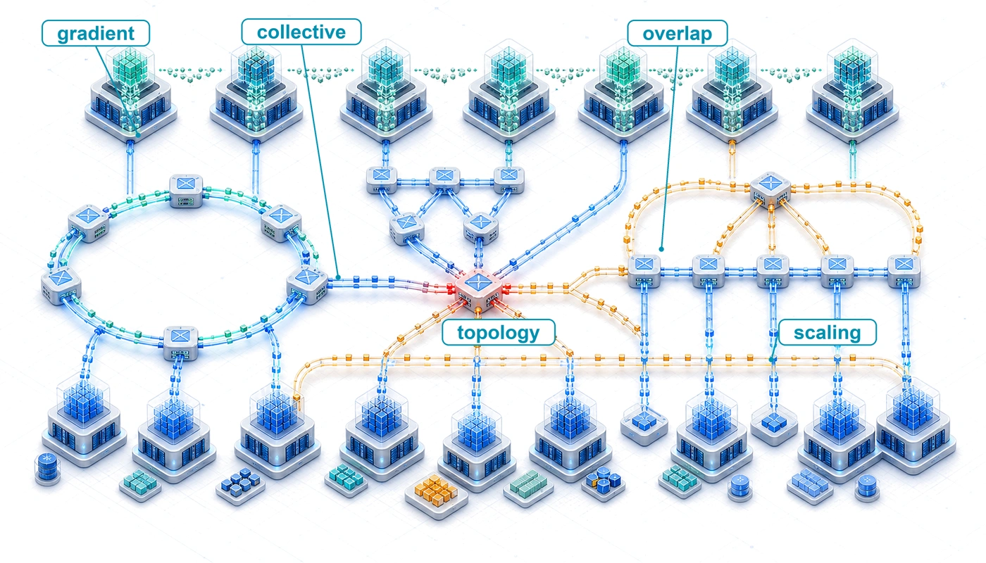
Collective communication topology map where gradient fragments circulate through ring and tree reduction paths before broadcasting synchronized state.

Purpose

Fleet Machine Learning Systems Stack

Fleet stack focus for this chapter.

Why does communication between machines constrain large-scale machine learning systems?

Computation scales by adding processors; communication scales by moving data between them. These scale differently. Adding processors increases available arithmetic capacity, but useful work stalls when the required data does not arrive in time. Exchanging gradients, activations, and parameters can then consume more time than computing them. On one machine, shortening the dominant calculation often shortens the job. Across a fleet, that same improvement may simply make each processor reach its next dependency sooner and wait longer for the others. The cost of that wait includes every reserved accelerator, so a small delay repeated throughout training can consume a substantial budget without advancing the model. Faster links help when transfer capacity is the constraint, but the benefit depends on which physical paths the traffic shares. More bandwidth cannot remove a dependency. Sending less data introduces its own choices about numerical accuracy, memory use, and when the next computation can begin. An exchange must also deliver the correct result to every participant that needs it. A fast transfer that combines the wrong contributions does not preserve a valid training run. The engineering decision is therefore how to organize communication so that its cost remains compatible with the work it enables. Light-speed delays, bandwidth limits, and the energy cost of movement make that decision as physical as processor design. In C³ terms, collective communication connects distributed compute through coordinated exchanges whose correctness and exposed cost determine whether the fleet delivers useful scale.

Learning Objectives
  • Apply communication cost models to estimate collective duration and message-size crossover points
  • Match collective communication primitives and AllToAll schedules to parallelism strategies, topology, message granularity, and skew
  • Compare ring, tree, butterfly, double-tree, and hierarchical reduction algorithms using scale-dependent cost models
  • Evaluate topology-aware collective schedules under link-bandwidth, rank-placement, and shared-capacity constraints
  • Evaluate compression, sparsification, and error feedback by balancing communication savings against convergence risk
  • Design overlap strategies with bucket fusion, asynchronous operations, and layer-by-layer gradient scheduling
  • Specify matched measurements for calibrating collective cost models across algorithms, process groups, and topologies

5.1 From Parallelism to Communication Patterns

When 10,000 GPUs cooperate on one training update, the splits created by data, tensor, pipeline, and expert parallelism determine which results must cross device boundaries. Workers execute collective operations within participating groups and point-to-point transfers between pipeline stages. In the multi-tier fleet stack of The Fleet Stack, these exchanges occupy the Distributed Execution row of the Distribution band, where logical parallelism becomes physical traffic.

Every such split assumes that replicas, shards, stages, and experts can exchange gradients, activations, parameters, and tokens quickly enough for the optimizer to see one coherent training run. In data parallelism, each worker holds a full copy of the model and processes its own slice of the batch, so the copies must agree on one combined gradient before every update; tensor, pipeline, and expert parallelism divide the model itself, so partial results must cross device boundaries within each step. Each of these exchanges is charged to the Fleet Law’s communication term \(\CommunicationTime(\DeviceCount)\), and the part of it not hidden behind computation counts against program goodput, the ratio of a step’s ideal execution time to its actual time (The iron law and the Fleet Law terms). Every way of splitting the model relocates work onto the network, and this chapter turns those exchanges into schedules whose latency, bandwidth, and topology costs can be computed.

↪ The partitioning strategies themselves, and the 3D parallelism cube that composes data, pipeline, and tensor parallelism into one configuration space, are developed in The Parallelism Design Space.

1 AllReduce: The name comes from MPI and describes the result, not the schedule: a Reduce (combining every rank’s data at one root) followed by a Broadcast (returning the combined value to all ranks). A direct gather to the root concentrates raw input traffic there, but a tree can aggregate contributions along the way. The algorithms in section 5.6.3 distribute the reduction without a root.

The first distinction is between an operation’s result and the schedule that produces it. The Synchronization Backbone named AllReduce, AllGather, and AllToAll as the traffic the fabric must carry; here they become contracts on results. AllReduce1 combines corresponding tensor elements across participating workers and returns the reduced tensor to every worker. AllGather instead concatenates their shards, ReduceScatter combines contributions but leaves each worker with only a shard of the result, and AllToAll sends different data to different destinations. The parallel decomposition determines which contract each exchange needs; ring, tree, and hierarchical algorithms are alternative schedules for carrying that contract out.

The gap between that assumption and the wire reveals an asymmetry in how computation and communication scale. Computation is local because each GPU works on its own data, so aggregate compute grows with the number of GPUs. Communication is global because keeping the fleet synchronized requires information to cross physical links with finite latency, bandwidth, interconnect topology, and energy. Gradient synchronization is the central case, because every synchronous data-parallel step repeats it on the full gradient. Scaling laws (principle 9) make that case harder over time, because the capability they reward comes from more parameters trained on more accelerators, so the gradient to be reduced and the group that must agree on it grow together.

For the initial gradient budget, consider a ring schedule: each worker passes tensor chunks to a neighbor, first accumulating their sums and then circulating the completed chunks. Each phase moves nearly one tensor’s worth of data per worker, so the bandwidth budget is approximately twice the gradient size divided by link bandwidth. The detailed round count follows once the transfer model is established.

Definition 5.1: Gradient synchronization

Gradient synchronization is the collective communication step in synchronous data-parallel training in which every worker contributes its locally computed gradient tensor to an aggregate reduction, then receives the same reduced result so all model replicas apply an identical update.

  1. Significance: Communicating all gradients of a 70B-parameter model in BF16 gives a 140 GB logical payload per replica per step. As a communication-only baseline, suppose every rank reduces that complete buffer. A ring across 1,000 GPUs at 50 GB/s per link has a bandwidth budget of approximately \(2 \times 140/50\) \(\approx\) 5.6 s of transfer per step. Model partitioning shrinks each rank’s share of that buffer, and only the portion of \(\CommunicationTime(\DeviceCount)\) left exposed after overlap adds to step time in the Fleet Law (equation 1.3).
  2. Distinction: Unlike a parameter server, which concentrates every worker’s gradient at a central aggregator, ring AllReduce spreads the exchange so that each worker sends \(2 \times (\DeviceCount-1)/\DeviceCount\times \CollectivePayloadSize\) bytes per step, approaching \(2\CollectivePayloadSize\) however large the cluster grows (section 5.6.1 develops the comparison).
  3. Common pitfall: A frequent misconception is that ring AllReduce makes every worker exchange data with every other worker. In ring AllReduce, each worker communicates with neighbors according to a schedule, and the per-node communication volume is approximately constant as the cluster grows. The scaling pressure comes from latency steps, topology, and the gradient volume per step, not from every worker opening a distinct stream to every other worker.

For standard synchronous data-parallel stochastic gradient descent (SGD), gradient synchronization supplies the shared gradient needed for one optimization trajectory. Replicas that apply different local gradients can diverge. To reproduce the intended global-batch update, they must also start from matching parameters and optimizer state, weight local contributions correctly, and apply the same update rule. The AllReduce primitive provides the reduction; convergence follows from the optimization assumptions, not from communication alone. Floating-point reduction order can still change low-order bits.

The gradient payload depends on parameter count and the representation transmitted. A model with \(\Parameters\) parameters contributes \(2\Parameters\) bytes per data-parallel replica when all gradients are communicated in BF16 (2 bytes per parameter); stored weight precision alone does not determine that choice. For a 70-billion-parameter model, a mid-sized dense model smaller than the 175B-parameter running instance of Archetype A (GPT-4/Llama-3), this gives 140 GB for the complete logical gradient. A ring moves nearly twice its input buffer size per rank.2 If a replica spans multiple ranks through model parallelism, each corresponding-shard group reduces its own portion rather than this full buffer.

2 Ring AllReduce: The algorithm dates to the HPC collective-communication literature; Patarasuk and Yuan analyzed bandwidth-optimal AllReduce algorithms for workstation clusters, Baidu’s Andrew Gibiansky popularized ring AllReduce for deep learning in February 2017, and Horovod plus NVIDIA NCCL helped make it a common distributed-training primitive (Patarasuk and Yuan 2009; Gibiansky 2017; Sergeev and Balso 2018; Jeaugey 2017).

Patarasuk, Pitch, and Xin Yuan. 2009. “Bandwidth Optimal All-Reduce Algorithms for Clusters of Workstations.” Journal of Parallel and Distributed Computing 69 (2): 117–24. https://doi.org/10.1016/j.jpdc.2008.09.002.
Gibiansky, A. 2017. Bringing HPC Techniques to Deep Learning. Baidu Research Technical Blog.
Sergeev, Alexander, and Mike Del Balso. 2018. “Horovod: Fast and Easy Distributed Deep Learning in TensorFlow.” CoRR abs/1802.05799.
Jeaugey, Sylvain. 2017. NCCL 2.0. GPU Technology Conference presentation.

The worked examples vary the volume’s reference configuration in two stated ways. The headline payload is this 70B gradient rather than the 175B instance’s, which keeps the worked arithmetic compact; every bandwidth term in the chapter is linear in payload, so each result scales directly to the larger model, and section 5.7.1 prices the 175B instance on the volume’s reference cluster itself. The cluster size changes from example to example, because each algorithm’s behavior depends on rank count and the point of an example is often to isolate one term. Each worked example states its rank count. A second recurring payload, the chapter’s reference gradient buffer, first appears in the energy estimate of section 5.2.

At large scale (hundreds of billions of parameters across thousands of GPUs), gradient synchronization can dominate training step time unless collective communication is systematically optimized. Understanding how to manage that overhead requires modeling data movement as physics rather than as an abstract API call.
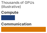
Two horizontal bars on a common scale under the header thousands of GPUs, illustrative, showing one large-scale training step. A short blue bar labeled compute is less than a third the length of a long amber bar labeled communication, so communication takes about three times as long as compute.

Exposed gradient synchronization can dominate step time at scale.

Self-Check: Question
  1. A dense-model training run triples its GPU count from 64 to 192 while holding the global work per update fixed. Step time drops by only 30%, and per-GPU compute utilization falls. Which scaling mechanism should the team investigate, without treating these aggregates as proof of the cause?

    1. Backpropagation stops functioning correctly across multiple nodes because gradients cannot be computed concurrently across independent data batches.
    2. Floating-point accumulation during gradient reduction becomes numerically unstable when more than 64 GPUs participate in the collective.
    3. Host CPU memory bandwidth saturates because all optimizer states must be shuffled through host DRAM on every multi-node step.
    4. Local compute can shrink while global synchronization and shared-link transfers remain exposed; rank-aligned traces are needed to determine whether communication actually limits the step.
  2. A logical Ring AllReduce cost model uses a 140 GB input per rank, corresponding to the model-wide BF16 gradient size of a 70B-parameter model. Holding that input fixed, a team expects per-rank sent volume to grow over 100 times when the group grows from 8 to 1,000 ranks. Explain why the expectation is false and why time can still increase. Treat this as transfer arithmetic, not a claim that a full replicated training state fits on one GPU.

  3. True or False: In synchronous data-parallel distributed training, using Ring AllReduce causes each GPU network bandwidth requirement to scale quadratically with the number of GPUs \(N\) because every worker must open a direct communication socket to every other worker in the cluster.

See Answers →

5.2 The Physics of Data Movement

Whenever a gradient shard leaves an accelerator, three hardware limits bound its trip before any collective algorithm runs: the speed of light sets a propagation floor3 of roughly 5 \(\MicroUnitPrefix\text{s}\) per kilometer in fiber, high-frequency signal loss limits how far copper traces can reach before the link must convert to optics (the bandwidth-distance product of Reach and medium for copper and optics), and host-kernel networking stacks add tens of microseconds of software copy overhead unless kernel-bypass transports such as remote direct memory access (RDMA) and GPUDirect RDMA strip per-message initiation down to a few microseconds. Collective communication also pays an energy price for every bit moved across those links, which the schedule must respect as firmly as latency and bandwidth.

3 The speed-of-light constraint: Light travels through optical fiber at approximately 200,000 km/s, or 200 meters per microsecond. For a rack-to-rack fiber path of 100 meters, propagation alone contributes approximately 500 ns in one direction. Faster switches can reduce other latency components, but reducing this propagation delay requires a shorter path or a different propagation medium.

↩︎ Kernel-bypass RDMA, which strips the per-message software overhead, and GPUDirect RDMA, which removes the host-memory bounce, are established in RDMA and GPUDirect.

Moving data consumes energy across storage arrays, interfaces, serializers, transceivers, and switches. A transfer that starts in local SRAM can stay on-package in high-bandwidth memory (HBM), cross to an intra-node peer GPU, or traverse intermediate switches to a remote node, and each step widens the physical accounting boundary that an energy estimate must include (figure 1). Each boundary activates distinct physical components: on-package links, intra-node crossbars, serializers, optical transceivers, and switch fabrics. Distance alone does not determine energy per bit, and an endpoint-only estimate cannot be compared directly with a complete fabric-path estimate. Locality remains useful because it can avoid transfers and active interfaces; the energy saving must be evaluated under the same workload, utilization, and accounting boundary.
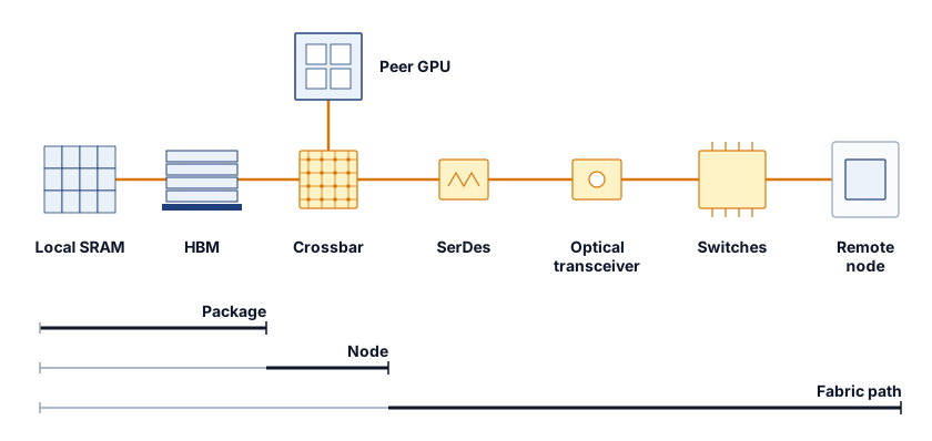
Figure 1: Data-Movement Accounting Boundaries: Successively broader paths involve different storage and communication components. The schematic identifies what an energy estimate must include; it assigns no universal distance law or fixed energy multiplier. Compare energy per transferred byte only after specifying endpoints, interfaces, switches, and utilization.

The chapter’s reference gradient buffer of 1 GB stands for one large fused reduction, far smaller than a full model gradient but large enough that per-byte transfer, not per-message startup, governs its cost; later examples return to it by name. Reducing it around an illustrative 10,000-rank ring sends approximately twice the payload from every rank. At a fabric-path transfer cost of 35 pJ/bit, a representative midpoint of the range typical of switched fabrics rather than a measurement of any particular one, this gives about 5.6 kJ per reduction, paid again at every synchronous step. The usable rule is that communication energy is the bytes an algorithm sends multiplied by the energy per bit of every boundary those bytes cross. An algorithm that moves fewer bytes, or a placement that keeps more of them inside the node, therefore saves energy as directly as it saves time, while the share of the step’s total energy that communication represents must be measured at the same accounting boundary as the compute it accompanies. The fabric-path figure charges the serializers, transceivers, and switches between two endpoints; a whole-system estimate that also charges endpoint memory reads, host software, and idle network power assigns each byte crossing the network a much larger cost, so two per-byte figures can be compared only after their boundaries match.

↪ The energy cost of moving a byte across memory, storage, and network boundaries, and why movement can outweigh arithmetic, is developed in Energy per byte.

4 Zero-copy communication: GPUDirect RDMA lets the NIC read gradients directly from accelerator memory, so a 140 GB gradient never passes through host DRAM, whereas a staged path writes and then rereads it there (280 GB of host-memory traffic per send).

These constraints govern different parts of a communication budget: propagation latency sets a floor for every message regardless of size, link bandwidth caps throughput once a transfer is large enough to fill the pipe, and protocol overhead adds a fixed per-message cost that penalizes fine-grained exchanges unless a kernel-bypass transport removes it. RDMA’s zero-copy path4 avoids staging each transfer through host memory and the kernel’s socket buffers, keeping that per-message cost low. Because the physical fabric fixes these limits, the collective schedule determines how many times the job pays them.

The opening ring budget is one instance of the network wall that Communication dominance and the network wall established, in which exposed communication takes a growing share of each step as a fixed workload spreads across more devices. How large that share becomes depends on gradient size, local batch size, partitioning, and overlap, so the critical path must be measured at each scale.

Self-Check: Question
  1. On the same fabric, one collective exchanges thousands of 4 KB messages per step while another moves a single 1 GB fused buffer. Which term governs each cost, and which lever addresses it?

    1. Both are bandwidth-bound, so a faster link shortens both by the same factor.
    2. The small messages pay per-message latency and protocol overhead on every send, so fusing messages or using a kernel-bypass transport helps; the 1 GB buffer is governed by per-byte transfer, so moving fewer bytes or adding bandwidth helps.
    3. The small messages are bandwidth-bound because there are many of them, while the 1 GB buffer is latency-bound because a large transfer takes the longest path.
    4. Both are latency-bound, because the speed of light sets a floor on every message regardless of its size.
  2. A 10,000-rank ring AllReduce reduces a 1 GB gradient buffer over a fabric path that costs about 35 pJ per bit. Set up the energy of one reduction and explain what the result implies for algorithm and placement choices.

  3. True or False: Energy per transferred bit grows in proportion to physical distance, so a transfer that travels twice as far costs about twice the energy.

See Answers →

5.3 Parallelism Strategies and Their Traffic

Once a training job splits its batch, layers, or parameters across devices, no rank holds all the state needed to finish a step on its own. A synchronous data-parallel worker computes gradients from its local batch slice, but its optimizer cannot update the weights until every replica’s gradients have been combined; some of those reductions can start as backward layers finish, while earlier layers are still computing. Tensor ownership determines where each tensor must go, and gradient or activation readiness determines when each transfer can start.

How the model is partitioned dictates which tensors cross device boundaries and which ranks must exchange them. For Archetype A (GPT-4/Llama-3), dense gradient contributions are combined within each data-parallel group; in a hybrid layout, that group contains the matching parameter shard from each replica. AllReduce serves the replicated-gradient baseline. For Archetype B (DLRM at Scale),5 lookup requests travel to embedding-shard owners and the resulting vectors return to the workers that need them. Mixture-of-experts (MoE) routing similarly sends activations to the ranks hosting selected experts and returns their outputs. These destination-specific exchanges motivate AllToAll.

5 DLRM (Deep Learning Recommendation Model): Meta’s 2019 architecture for click-through rate prediction uses sharded embedding tables and exchanges the resulting sparse lookups across workers, an AllToAll whose limiting term section 5.8 develops.

↩︎ The three lighthouse archetypes and the C³ regimes each one stresses are established in Three systems archetypes.

At large scale, these parallelism strategies can be combined. A 3D parallelism layout combines data parallelism, tensor parallelism, and pipeline parallelism, creating distinct communication groups whose exchanges may overlap in time. In a node-local tensor-parallel example, layer reductions use NVLink, pipeline stages exchange activations and their gradients point-to-point across nodes, and data-parallel groups reduce matching parameter shards over InfiniBand. Other placements change those physical paths while retaining the logical communication requirements.

Each primitive operates on a different process group, a subset of the total GPU population that participates in that particular collective. Classical Message Passing Interface (MPI) uses a communicator as the object that names such a participating set; its communicator size is the number of ranks in that set. MPI libraries already selected collective algorithms based on communicator size and message size (Thakur et al. 2005). GPU communication libraries inherit that algorithm-selection problem and add the further challenge of coordinating overlapping process groups without creating contention between concurrent collectives.

Each parallelism strategy fixes the data it must move, the collective primitive that moves it, and the term most likely to bind (table 1), and with them which participants must exchange data. The collective primitives that follow make each exchange’s contract precise, the pricing model then charges it per round, and the collective algorithms provide its execution schedule.

Table 1: Parallelism-to-Collective Mapping: How each parallelism strategy becomes a traffic pattern. Pipeline parallelism alone relies on point-to-point transfers rather than a collective.
Parallelism strategy What must move Primary primitive Primary constraint
Data Parallelism Full gradient, averaged across replicas AllReduce Bandwidth (large payloads)
FSDP/ZeRO-3 Parameter shards in, gradient shards out AllGather + ReduceScatter Bandwidth, high frequency
Tensor Parallelism Partial layer activations within the node AllReduce, AllGather Critical path (NVLink bandwidth and latency)
Sequence Parallelism Activations sharded along the sequence AllGather + ReduceScatter Bandwidth (activation exchange)
Pipeline Parallelism Activations to the next stage Point-to-Point (Send/Recv) Latency (microbatch dependencies)
Expert Parallelism (MoE) Tokens to the ranks hosting their experts AllToAll Startup, injection/bisection, or skew
Embedding Sharding (DLRM) Embedding lookups to and from shard owners AllToAll Granularity, fabric capacity, or skew

In this table, expert parallelism refers to the mixture-of-experts architecture pattern, in which each token activates only a few experts. Data parallelism and fully sharded data parallel (FSDP), which divides each replica’s parameters, gradients, and optimizer state across the data-parallel ranks, generate large reductions and gathers that reward byte-efficient rings and hierarchical schedules. Tensor and pipeline parallelism, by contrast, generate smaller, more frequent messages directly on the critical path, so low software overhead and fast node-local links dominate their cost, whereas expert parallelism and sharded embedding tables produce destination-specific traffic whose bottleneck shifts among message granularity, endpoint injection and reception, fabric bisection, oversubscription, routing, and skew.

The table’s rows describe data center parallelism, so they leave out the federated Archetype C. Across all three lighthouse archetypes, the dominant exchange and its bottleneck differ.

Lighthouse 5.1: Communication archetype patterns
A gradient’s communication pattern depends on the system’s objective function and constraint regime. Each lighthouse archetype faces a distinct communication challenge, and the techniques developed in this chapter map to those challenges differently, as table 2 summarizes.

Table 2: Archetype-to-Collective Mapping: Each lighthouse archetype produces a characteristic traffic pattern, but the limiting term depends on message shape, placement, and the physical fabric.
Archetype Primary collective Candidate limiter Optimization strategy
Archetype A (GPT-4/Llama-3) AllReduce Bandwidth (\(\LinkBandwidth\)) Hierarchical AllReduce; rail-optimized placement
Archetype B (DLRM at Scale) AllToAll Granularity, fabric capacity, or skew Message coalescing; topology-aware routing; shard balancing
Archetype C (Federated MobileNet) Client uploads to an aggregator (asynchronous) Uplink bandwidth and availability Aggressive quantization; error feedback

The table separates traffic pattern from limiting resource. A dense reduction, a destination-specific exchange, and an intermittent device update require different interventions even though all three serve a training workload. Hierarchical AllReduce, AllToAll schedule selection, and compression with error feedback each receive their own treatment later in the chapter.

A traffic map names which pattern a workload generates, but it does not specify what each rank must hold when the call completes. Before any of those interventions can be priced, each exchange needs a precise contract that states which ranks contribute and what each holds afterward.

Self-Check: Question
  1. A machine learning engineer evaluates the communication traffic induced by different model parallelism strategies. According to the chapter’s parallelism-to-collective mapping, which mapping correctly pairs a parallelism strategy with its primary collective primitive and primary physical constraint?

    1. Fully Sharded Data Parallel (FSDP) -> Broadcast primitive -> Memory capacity constraint.
    2. Mixture-of-Experts (MoE) Routing -> AllToAll primitive -> Latency and bisection network contention constraint.
    3. Tensor Parallelism within a node -> Point-to-Point Send/Recv -> Inter-node bisection bandwidth constraint.
    4. Data Parallelism -> Reduce primitive -> Host-to-device PCIe bandwidth constraint.
  2. On a supported hardware and transport path, the mechanism that lets a NIC read and write GPU memory without staging payloads through host DRAM is known as ____ RDMA.

See Answers →

5.4 Collective Operation Primitives

Sending a gradient tensor to a peer does not specify which workers must contribute or where the final result belongs. Collective operations supply that group-level contract, using a vocabulary standardized by MPI and inherited by modern ML communication libraries (Message Passing Interface Forum 2015). The four contracts sketched at the start of the chapter differ in what each rank holds afterward (figure 2). AllReduce leaves an identical sum (\(\Glyph{\Sigma}\)) on every rank, AllGather leaves every rank with the concatenation of all shards, ReduceScatter sums across ranks but leaves each rank one reduced shard (\(\Glyph{\Sigma}_i\)), and AllToAll performs a distributed matrix transpose, routing each rank’s \(\DestinationRankIndex\)-th chunk to rank \(\DestinationRankIndex\). Two further primitives complete the set and serve as building blocks for these four: Broadcast, in which rank 0 sends its data to all ranks, and Reduce, in which all ranks aggregate into rank 0.

↪ The bandwidth and latency cost terms of AllReduce, AllGather, ReduceScatter, AllToAll, and Broadcast, under ring, tree, and pairwise-exchange algorithms, are developed in Collective Operation Complexity.

Definition 5.2: Collective operation

Collective operation is a distributed communication pattern in which every rank in a process group invokes a matching operation to aggregate, broadcast, or redistribute data. The operation’s contract specifies the output at each rank; it does not require simultaneous entry and does not, by itself, impose a general-purpose barrier before or after the call (Message Passing Interface Forum 2015).

  1. Significance: Because the contract names only each rank’s result, the schedule that carries it decides how communication demand spreads as the group grows. A schedule that funnels every contribution through one endpoint makes the communication term \(\CommunicationTime(\DeviceCount)\) of the Fleet Law (equation 1.3) grow with \(\DeviceCount\), while a balanced schedule keeps each rank’s bytes nearly constant; section 5.6.1 quantifies the gap.
  2. Distinction: Unlike point-to-point communication, a collective defines one operation over a process group. Ranks may enter at different times, and some algorithms allow one rank to complete before another has entered; correctness depends on matching the operation sequence and argument contract across ranks, not on barrier semantics.
  3. Common pitfall: Treating a non-blocking collective as complete when its initiation call returns. The returned request or stream event represents work in flight. A dependent consumer must wait for completion, and a late rank can extend that dependency even though the collective is not a barrier.
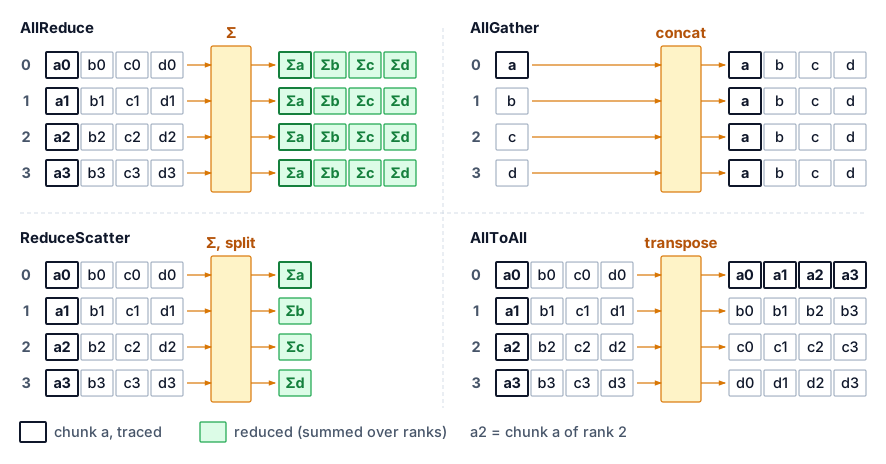
Figure 2: Four Central Collective Primitives: Standardized patterns for group communication in distributed systems. In each panel the four rows are ranks 0 to 3, read left to right from each rank’s input, through the collective, to what each rank holds afterward. (1) AllReduce: all aggregate and all receive the result. (2) AllGather: all send to all and concatenate. (3) ReduceScatter: all aggregate and results are distributed in shards. (4) AllToAll: every process sends unique data to every other process. The two foundational primitives Broadcast (rank 0 sends to all) and Reduce (all aggregate to rank 0) compose the patterns shown here and are defined in the surrounding prose.

The primitive choice is the first scaling decision because it fixes which ranks must coordinate and which result each must obtain. Once that contract is chosen, the algorithm and placement determine how the resulting traffic crosses the fabric.

5.4.1 The six core primitives

Calling a full AllReduce when each rank’s optimizer updates only a \(1/\DeviceCount\) parameter shard moves twice as many bytes as the step needs, because half the work goes into assembling full tensors that every rank immediately discards. Choosing the right primitive therefore means matching the contract in table 3 to the exact slice the next computation consumes. The table’s rows run from the root-centered patterns (Broadcast and Reduce), through the three in which every rank contributes to and receives part or all of one shared tensor (AllReduce, AllGather, and ReduceScatter), to AllToAll, in which every pair of ranks exchanges distinct data. That order describes routing rather than cost: ReduceScatter and AllGather each move half of AllReduce’s bytes because each is one phase of it. The cost column previews the algorithms derived in section 5.6, using \(\DeviceCount\) for the participating rank count, \(\CollectiveTensorSize\) for the full tensor, and \(\CollectivePayloadSize\) for the per-rank AllToAll input payload. For AllReduce, the full tensor has the same byte size as each rank’s input payload, the convention used in the following algorithm models. Two schedules appear there: a ring passes chunks between neighbors, whereas a simple full-message tree reduces up a binary tree and broadcasts back down it, forwarding the whole tensor at each of its \(2\log_2 \DeviceCount\) levels. For Broadcast and Reduce, the table counts startup rounds and bytes per tree edge separately; each traverses one tree depth, so the elapsed transfer cost accumulates across its levels, and the Tree AllReduce derivation combines those two traversals.

Table 3: The Six Collective Primitives: What each primitive computes, its primary use, and its communication cost, ordered from root-centered patterns (Broadcast, Reduce) to the fully destination-specific AllToAll. The order describes routing, not cost.
Primitive What it does Primary use case Communication cost
Broadcast One sender transmits data to all receivers. Distribute initial model weights from rank 0 at startup, across all parallelism strategies. \(\mathcal{O}(\log \DeviceCount)\) startup rounds; \(\mathcal{O}(\CollectiveTensorSize)\) bytes per tree edge. Elapsed byte-transfer time also grows with tree depth.
Reduce Aggregate data from all workers (sum, min, max) to a single root. Aggregate validation metrics such as loss and accuracy to a logging process. \(\mathcal{O}(\log \DeviceCount)\) startup rounds; \(\mathcal{O}(\CollectiveTensorSize)\) bytes per tree edge. Elapsed byte-transfer time also grows with tree depth.
AllReduce Aggregate from all workers, then distribute the result to all (\(\RankReductionResult_i = \sum_{j=0}^{\DeviceCount-1} \RankContribution_j\) for all \(\RankIndex\)). Data parallelism: synchronize gradients so every GPU computes the same update. Ring is bandwidth-optimal at \(2\frac{\DeviceCount-1}{\DeviceCount}\frac{\CollectiveTensorSize}{\LinkBandwidth}\) but \(\mathcal{O}(\DeviceCount)\) latency; the simple full-message Tree model gives \(\mathcal{O}(\log \DeviceCount)\) latency with more byte-transfer work.
AllGather Each worker’s data goes to all; the result concatenates every input (\(\RankContribution_i \rightarrow [\RankContribution_0, \dots, \RankContribution_{\DeviceCount-1}]\)). Sharded data parallelism (FSDP/ZeRO): collect sharded parameters before a forward or backward pass. Ring \(\frac{\DeviceCount-1}{\DeviceCount}\frac{\CollectiveTensorSize}{\LinkBandwidth}\); resident data grows from an \(\CollectiveTensorSize/\DeviceCount\) shard to the full \(\CollectiveTensorSize\).
ReduceScatter Reduce across workers, but scatter so each keeps a distinct chunk (worker \(\RankIndex\) receives the \(\RankIndex\)-th block of \(\sum \RankContribution_j\)). Sharded data parallelism: reduce gradients while keeping them sharded to save memory. Ring \(\frac{\DeviceCount-1}{\DeviceCount}\frac{\CollectiveTensorSize}{\LinkBandwidth}\); the same ring byte-transfer term as AllGather, with reduction.
AllToAll The most general pattern: worker \(\RankIndex\) sends a distinct chunk to each worker \(\DestinationRankIndex\), a distributed matrix transpose. MoE routing tokens to experts; DLRM exchanging embedding lookups across workers. Per-worker payload \(\frac{\DeviceCount-1}{\DeviceCount}\CollectivePayloadSize\); the limiter can arise from startup, injection/reception, bisection, oversubscription, routing, granularity, or skew.

Ring achieves AllReduce’s bandwidth-optimal cost while the simple full-message Tree model trades bandwidth for logarithmic latency (Patarasuk and Yuan 2009; Thakur et al. 2005), and AllReduce itself decomposes into ReduceScatter followed by AllGather. The decomposition is operational as well as mathematical, since Ring AllReduce’s first phase is a ReduceScatter and its second phase is an AllGather. ReduceScatter performs arithmetic, so it does not invert AllGather despite reversing the direction of shard expansion. Full ZeRO-style sharding and PyTorch FSDP use the pair the same way, gathering parameter shards with AllGather before a module needs them and reducing gradients with ReduceScatter after backward so each rank retains only its shard for the optimizer step (Rajbhandari et al. 2020). Sharding parameters, gradients, and optimizer state across workers reduces persistent model-state memory roughly by \(\DeviceCount\times\), while temporary full-parameter buffers and prefetching determine peak memory. That memory saving is developed in Memory-efficient data parallelism with ZeRO and FSDP; the communication it adds is priced in section 5.4.2.

The same AllGather/ReduceScatter pair also appears in sequence parallelism, where an AllGather reconstructs the activation view needed for a local operation and a later ReduceScatter redistributes the result along the sequence dimension. A primitive’s semantics stay fixed even when the tensor dimension being sharded changes, so every schedule developed for the pair applies to both uses.

Beyond defining data-movement dependencies, collective operations carry explicit interface and numerical contracts. At the interface level, every rank in a process group must issue collectives in a compatible sequence; mismatched operation orders can deadlock or pair unrelated buffers. Operations also enforce shape and type contracts. AllReduce requires matching element counts and datatypes across all ranks, whereas variable-size exchanges require explicit per-destination counts and displacements. These invariants form the contract between the parallel decomposition and the communication runtime: the model decides which tensor slices each rank owns, and the collective contract guarantees that those slices can be recombined deterministically.

Reduction order introduces a second, numerical contract. Floating-point addition is not associative, so ring, tree, and switch-assisted reductions may accumulate the same values in different orders and produce different low-order bits (Goldberg 1991). A correct AllReduce therefore guarantees the specified reduction over all contributions, not bitwise identity across algorithms, rank counts, or hardware. Reproducibility-sensitive workloads must fix the algorithm and process-group configuration or use a reproducible accumulation scheme; ordinary training should treat small order-dependent differences as numerical behavior while still checking for larger rank disagreement.

Goldberg, David. 1991. “What Every Computer Scientist Should Know about Floating-Point Arithmetic.” ACM Computing Surveys 23 (1): 5–48. https://doi.org/10.1145/103162.103163.

AllToAll scales differently from AllReduce with cluster size, and section 5.8 develops the bound that governs it. With the six contracts defined, every row of table 1 now names a primitive whose output and traffic pattern are precise, and the sharded data-parallel row repays closer study because sharding changes how often those primitives run rather than which ones run.

5.4.2 FSDP communication patterns

Sharding every parameter, gradient, and optimizer-state tensor across \(\DeviceCount\) data-parallel ranks saves memory, but it replaces one end-of-step reduction with a stream of collective calls inside the forward and backward passes. Under fully sharded data parallelism (Rajbhandari et al. 2020), each rank holds only \(1/\DeviceCount\) of a layer’s weights, so it must call AllGather before the layer’s forward pass to assemble the full weights, call ReduceScatter after the backward pass to leave each rank the gradient for its own shard, and then free the temporary full weights.

Rajbhandari, Samyam, Jeff Rasley, Olatunji Ruwase, and Yuxiong He. 2020. “ZeRO: Memory Optimizations Toward Training Trillion Parameter Models.” SC20: International Conference for High Performance Computing, Networking, Storage and Analysis, 1–16. https://doi.org/10.1109/sc41405.2020.00024.

Trading resident memory for on-demand assembly multiplies the collective call count. With one communication group per layer, a model with \(\LayerCount\) layers issues \(2\LayerCount\) collective calls per step where unbucketed data parallelism issues one AllReduce, or about \(3\LayerCount\) when parameters are resharded after forward and gathered again for backward. The byte volume changes far less. When parameters and gradients travel at the same width and the group is large, each rank sends roughly the AllReduce’s \(2\CollectiveTensorSize\), or about \(3\CollectiveTensorSize\) (\(1.5\times\)) with resharding, where \(\CollectiveTensorSize\) is the model-sized payload without optimizer state; different parameter and reduction datatypes shift that ratio. The call count carries its own price, because every call pays a startup cost. An effective startup cost \(\CollectiveCallStartupLatency\) contributes approximately \(2\LayerCount\CollectiveCallStartupLatency\) per step before overlap, or \(3\LayerCount\CollectiveCallStartupLatency\) with resharding, so FSDP is more sensitive to \(\CollectiveCallStartupLatency\) than an unbucketed data-parallel reduction even though its bytes barely change. The counts describe one grouping policy, since FSDP units need not coincide with layers and bucketed data parallelism also splits its reduction to enable overlap. FSDP implementations mitigate the startup cost through prefetching and communication-stream pipelining, but the relevant \(\CollectiveCallStartupLatency\) must come from a matched collective benchmark rather than a wire-latency specification.

↪ The ZeRO stages and the reshard-after-forward FSDP schedule, with the memory each saves and the communication each adds, are developed in Memory-efficient data parallelism with ZeRO and FSDP.

Selecting the right collective algorithm at each invocation requires distinguishing transfer cost from dependency exposure. An FSDP AllGather is latency-sensitive in the scheduling sense, because a layer cannot compute until its full parameters arrive. Its transfer can nevertheless be bandwidth-bound when the parameter tensor is large. Prefetching can hide part of that gather, while a ReduceScatter can overlap with the remaining backward computation. Neither dependency alone selects Ring or Tree; message size, group size, topology, and the available overlap window jointly determine the useful schedule.

The primitives specify what must be communicated, and sharding shows how often a training step invokes them. Choosing a schedule for each invocation first requires a price for every round of an exchange.

Self-Check: Question
  1. How does the communication pattern of Fully Sharded Data Parallel (FSDP / ZeRO-3) differ structurally and operationally from standard Distributed Data Parallelism (DDP)?

    1. DDP communicates twice per transformer layer using Point-to-Point Send/Recv, whereas FSDP communicates only once at the end of the step using Broadcast.
    2. FSDP replaces all network communication with CPU host memory paging, eliminating collective communication entirely.
    3. DDP reduces ready gradient buckets, whereas layer-wrapped full-shard FSDP with resharding typically issues \(3N_L\) collectives: forward and backward AllGathers plus backward ReduceScatters, increasing launch-latency sensitivity.
    4. FSDP eliminates AllGather operations by permanently keeping full model parameters in every GPU high-bandwidth memory.
  2. In Fully Sharded Data Parallel (FSDP), when does a parameter AllGather or gradient ReduceScatter add exposed delay to a training step? Explain why the primitive name alone does not identify a latency-bound or bandwidth-bound transfer.

  3. The mathematical identity that an AllReduce can be decomposed into an intra-group ____ phase (where each worker retains a reduced chunk) followed by an ____ phase (where workers circulate and concatenate the reduced chunks) forms the foundational communication mechanism behind both Ring AllReduce and ZeRO-3/FSDP memory sharding.

See Answers →

5.5 Pricing Collectives by Rounds and Chunks

A gradient bucket of tens of megabytes is large enough to saturate a single network link, yet when a thousand-GPU ring divides that bucket into a thousand shards, each hop moves only tens of kilobytes and can spend more time starting the transfer than sending its bytes. Pricing a collective therefore requires separating the fixed time to initiate each message from the rate at which bytes move once in transit.

The \(\MessageStartupLatency\)-\(\LinkBandwidth\) model \(\PointToPointTransferTime(\PointToPointMessageSize) = \MessageStartupLatency+ \PointToPointMessageSize/\LinkBandwidth\) prices a transfer over a single link (principle 5), separating a fixed startup cost (\(\MessageStartupLatency\)) from a per-byte transfer cost (\(\PointToPointMessageSize/\LinkBandwidth\)) (Hockney 1994). A collective pays that price at every step of its schedule, so the two terms, multiplied by the schedule’s round count and traffic factor, determine algorithm selection across the fleet.

Hockney, Roger W. 1994. “The Communication Challenge for MPP: Intel Paragon and Meiko CS-2.” Parallel Computing 20 (3): 389–98. https://doi.org/10.1016/s0167-8191(06)80021-9.

↩︎ The \(\MessageStartupLatency\)-\(\LinkBandwidth\) model for a single link and its latency-dominated and bandwidth-dominated regimes are established in The \MessageStartupLatency-\LinkBandwidth performance model.

↪ Worked message-size regimes and crossover calculations for this model are developed in The \MessageStartupLatency-\LinkBandwidth Communication Model.

For collectives, the parameters must describe the effective path. Latency (\(\MessageStartupLatency\)) is the startup cost paid at every step of a schedule, so it includes recurring software overhead, PCIe traversal, and network switching time; one-time communicator initialization is a separate setup cost. Bandwidth (\(\LinkBandwidth\)) is the sustained per-direction transfer rate. The critical message size \(\LatencyBandwidthCrossoverSize = \MessageStartupLatency\cdot \LinkBandwidth\), where the two terms are equal, carries over unchanged, but it must be compared against each step’s chunk (\(\CollectivePayloadSize/\DeviceCount\) in an \(\DeviceCount\)-rank ring) rather than the whole tensor \(\CollectivePayloadSize\), which is why a large bucket can still fall below the inter-node crossovers in table 4. Below \(\LatencyBandwidthCrossoverSize\), a step is latency-bound; above it, bandwidth-bound.

The crossover explains two recurring optimizations. For InfiniBand NDR at \(\MessageStartupLatency\approx\) 1.5 μs and \(\LinkBandwidth\approx\) 50 GB/s, the knee sits at \(\LatencyBandwidthCrossoverSize \approx\) 75 KB, the value The \MessageStartupLatency-\LinkBandwidth performance model computed for a single transfer. A 4 KB routing message is far below \(\LatencyBandwidthCrossoverSize\), so the startup cost dominates. If 100 ready messages have compatible destinations and can share one transfer, fusing them into a 400 KB message reduces the modeled cost from approximately \(100\MessageStartupLatency=\) 150 μs to \(\MessageStartupLatency+ \PointToPointMessageSize/\LinkBandwidth\approx\) 9.5 μs, roughly a 16× improvement before packing costs. More generally, \(\SplitMessageCount\) serialized messages of size \(\PointToPointMessageSize/\SplitMessageCount\) can cost up to \(\SplitMessageCount\times\) as much as one message of size \(\PointToPointMessageSize\) when \(\PointToPointMessageSize/\SplitMessageCount\ll \LatencyBandwidthCrossoverSize\). Fusion is the first optimization, and it motivates framework gradient buckets and destination-aware token coalescing.

Compression is the second, and the crossover tells where it pays. A 140 GB gradient tensor sits far above \(\LatencyBandwidthCrossoverSize\), so shrinking its bytes shrinks the dominant \(\PointToPointMessageSize/\LinkBandwidth\) term directly, provided encoding and aggregation costs are counted. Even keeping only the largest 1 percent of values (Top-k sparsification, developed in section 5.9) leaves 1.4 GB of values before their indices are added, still far above \(\LatencyBandwidthCrossoverSize\), so the saving remains a byte saving. Compressing a 4 KB routing message, by contrast, offers little, because its unchanged \(\MessageStartupLatency\) term already dominates.

Across the typical data center interconnects tabulated in table 4, the critical-size column carries the load-bearing pattern: intra-node NVLink stays latency-bound up to several hundred kilobytes, whereas the inter-node fabrics cross over below roughly 100 KB. A message between those crossover sizes can therefore be latency-bound inside a node but bandwidth-bound once it travels between nodes.

Table 4: Interconnect Performance Parameters: Effective per-message launch latency (\(\MessageStartupLatency\), including the software stack), per-direction link bandwidth (\(\LinkBandwidth\), the one-way deliverable rate that enters \(\PointToPointTransferTime(\PointToPointMessageSize) = \MessageStartupLatency+ \PointToPointMessageSize/\LinkBandwidth\); NVLink’s datasheet 900 GB/s is the bidirectional total, so its \(\LinkBandwidth\) is the 450 GB/s one-way rate), and the computed crossover size \(\LatencyBandwidthCrossoverSize = \MessageStartupLatency\cdot \LinkBandwidth\) at each row’s \(\MessageStartupLatency\) midpoint (for InfiniBand NDR, at the representative 1.5 μs used throughout this chapter), where communication transitions from latency-bound to bandwidth-bound.
Interconnect Latency (\(\MessageStartupLatency\)) Bandwidth (\(\LinkBandwidth\)) Critical size (\(\LatencyBandwidthCrossoverSize\))
NVLink 4.0 (intra-node) 1–2 μs 450 GB/s ~0.7 MB
InfiniBand NDR 400 Gbps 1–3 μs 50 GB/s (per port) ~75 KB
InfiniBand HDR 200 Gbps 2–5 μs 25 GB/s ~87.5 KB
PCIe Gen5 (GPU\(\leftrightarrow\)CPU) 2–5 μs 64 GB/s ~224 KB
Ethernet 100 Gbps (RoCE) 5–10 μs 12.5 GB/s ~93.7 KB

The NVLink and NDR rows show the roughly ninefold per-direction cliff of Bandwidth hierarchy, which The Synchronization Backbone traces across a decade of interconnect generations. Even on the lower-crossover inter-node fabric, a bucket far above \(\LatencyBandwidthCrossoverSize\) can still travel in chunks below it because a ring divides the bucket among its \(\DeviceCount\) ranks. Pricing one bucket at two group sizes shows when that happens and what it costs.

Napkin Math 5.1: The critical message size
Problem: A data-parallel job reduces a 25 MB gradient bucket with Ring AllReduce over InfiniBand NDR, with \(\MessageStartupLatency=\) 1.5 μs and \(\LinkBandwidth=\) 50 GB/s. The bucket is hundreds of times larger than the single-transfer knee. Does each step of the ring run in the bandwidth-bound regime on 64 GPUs, and on the 1,024-GPU reference cluster?

Math:

  1. Knee: \(\LatencyBandwidthCrossoverSize = \MessageStartupLatency\cdot \LinkBandwidth=\) \(1.5 \times 10^{-6}\) s \(\times\) \(5 \times 10^{10}\) B/s \(=\) 75 KB.
  2. Chunk per step: A ring sends \(\CollectivePayloadSize/\DeviceCount\) per step, 390.6 KB on 64 ranks (above the knee) but only 24.4 KB on 1,024 ranks (below it).
  3. Ring time \(2(\DeviceCount-1)\left(\MessageStartupLatency+ \frac{\CollectivePayloadSize}{\DeviceCount\LinkBandwidth}\right)\): about 1.2 ms on 64 ranks, of which the byte term is 1.0 ms; about 4.1 ms on 1,024 ranks, where the byte term is still only 1.0 ms.

Systems insight: The regime belongs to the chunk, not to the tensor. The byte term barely moves as the group grows, but at 1,024 ranks each step carries a chunk below \(\LatencyBandwidthCrossoverSize\), so startup dominates and the same bucket takes several times longer. Large language model (LLM) gradients are bandwidth-bound as tensors, yet a flat ring over a large group can still carry them in latency-bound steps. The levers then shift to larger buckets, fewer rounds, and hierarchy, which is why the algorithms of section 5.6 compete on round count as well as bytes.

For collectives, the two regimes map onto different levers. In the latency-bound regime \((\PointToPointMessageSize< \LatencyBandwidthCrossoverSize)\), where MoE routing tokens, scalar reductions, and the small chunks of a large-group schedule sit, the levers are fusion, fewer schedule rounds, fewer hops, and a leaner software stack. In the bandwidth-bound regime \((\PointToPointMessageSize\gg \LatencyBandwidthCrossoverSize)\), where LLM gradients and optimizer states sit, they are compression, a byte-efficient algorithm, and link aggregation across multiple network interface cards (NICs). Classifying each exchange, and each chunk within it, into one regime is the diagnostic skill the rest of the chapter applies.

Checkpoint 5.1: Per-chunk pricing diagnostics

Verify your understanding of per-chunk pricing regimes:

The pricing model charges a schedule per round and per chunk, but it does not choose the schedule. AllReduce, the most performance-critical primitive, admits several schedules whose round counts and byte volumes differ sharply, and for a large gradient the choice can decide whether gradient synchronization can be hidden at all.

Self-Check: Question
  1. A single-transfer model uses effective startup cost \(\alpha=1.5\,\mu\text{s}\) and per-direction bandwidth \(\beta=50\text{ GB/s}\). Which conclusion follows for a 4 KB transfer, and what must be added before classifying a complete gradient AllReduce?

    1. The single-transfer knee is 75 KB, so startup dominates the 4 KB transfer. A complete AllReduce additionally requires the schedule’s round count and chunk size, then calibration for its placement.
    2. The 4 KB transfer is bandwidth-bound because adding ranks makes every individual transfer saturate its port.
    3. The 75 KB knee is a maximum buffer size, so larger messages cannot be sent over this link.
    4. The critical message size defines the maximum possible buffer size that can be transferred in a single CUDA stream without host CPU intervention.
  2. Explain why small-message collective timings can exceed a bare-wire prediction by a much larger relative factor than large-message timings. Which measurements are needed before using this difference in a cluster capacity plan?

See Answers →

5.6 AllReduce Algorithms and Topologies

A correct AllReduce must give each of 1,000 GPUs the reduced sum of all 1,000 gradient contributions, subject to the floating-point reduction contract, and the algorithm that delivers it sets the cluster’s scaling ceiling. The naive answer, in which every GPU sends to one central server whose single network link must carry every worker’s gradient, fails first, which makes it the right place to start.

5.6.1 Naive approaches vs. the bandwidth bottleneck

Consider a naive implementation using a parameter server (a star topology), with a dedicated server in addition to the workers. All \(\DeviceCount\) workers send their gradients to that server; it sums them and sends the result back. The server must receive \(\DeviceCount\times \CollectivePayloadSize\) bytes and send \(\DeviceCount\times \CollectivePayloadSize\) bytes, so its bandwidth budget grows as \(\CommunicationTime \propto \DeviceCount\times \CollectivePayloadSize/ \LinkBandwidth\). At 1,000 GPUs, concentrating those transfers at one server creates a scaling bottleneck even if the arithmetic is fast.

This naive approach captures the pressure that early distributed ML frameworks had to manage: parameter-server systems receive, aggregate, and redistribute model updates through a server tier, while practical implementations shard the parameter space to spread that load (Dean et al. 2012; Li et al. 2014). Sharding reduces the per-server traffic from \(\DeviceCount\times \CollectivePayloadSize\) to \(\DeviceCount\times \CollectivePayloadSize/\ParameterServerCount\) (where \(\ParameterServerCount\) is the number of servers), but the server tier still grows as workers and model state grow, and it introduces additional complexity in parameter partitioning and consistency management.

Dean, Jeffrey, Greg Corrado, Rajat Monga, Kai Chen, Matthieu Devin, Quoc V. Le, Mark Z. Mao, et al. 2012. “Large Scale Distributed Deep Networks.” In Advances in Neural Information Processing Systems (NeurIPS), edited by Peter L. Bartlett, Fernando C. N. Pereira, Christopher J. C. Burges, Léon Bottou, and Kilian Q. Weinberger, vol. 25. Curran Associates.
Li, M., D. G. Andersen, J. W. Park, A. J. Smola, A. Ahmed, V. Josifovski, J. Long, E. J. Shekita, and B.-Y. Su. 2014. “Scaling Distributed Machine Learning with the Parameter Server.” Proceedings of the 2014 International Conference on Big Data Science and Computing, 583–98. https://doi.org/10.1145/2640087.2644155.

The bottleneck comes from concentration, not from total traffic. Every AllReduce algorithm moves more total data as workers are added, because every worker’s contribution must be combined and every worker must receive the result. A star, however, routes all of that traffic through one endpoint, so the server’s time grows as \(\DeviceCount\times \CollectivePayloadSize/\LinkBandwidth\), while a ring spreads the same work so that each rank sends about \(2\CollectivePayloadSize\) and its time stays near \(2\CollectivePayloadSize/\LinkBandwidth\) however large \(\DeviceCount\) becomes. The ratio of the two is about \(\DeviceCount/2\), so at 1,024 workers the server’s byte time is roughly 500× the ring’s, before startup, arithmetic, or contention are counted. Bandwidth optimality makes that comparison precise by measuring an algorithm’s required byte movement against a lower bound under a stated communication model, which the next derivation supplies for AllReduce.

War Story 5.1: When the parameter server became the bottleneck (2017)
Context: In 2017, Alexander Sergeev and Mike Del Balso’s team at Uber open-sourced Horovod as part of Uber’s Michelangelo ML platform, where TensorFlow training jobs needed to scale across many GPUs without forcing every model author to rewrite large portions of training code (Sergeev and Balso 2018).

Mechanism: TensorFlow’s stock distributed training relied on a parameter-server pattern that concentrated gradient traffic through a central tier. As worker count \(\DeviceCount\) grew, the central server link saturated, degrading scaling efficiency.

Impact: Scaling training beyond a single node resulted in severe throughput bottlenecks and required complex, model-specific parameter partitioning.

Fix: Uber adopted Baidu’s ring AllReduce algorithm (Gibiansky 2017), wrapping bandwidth-optimal collective reduction behind a lightweight API that replaced parameter servers with ring communication.

Systems lesson: A collective algorithm is also a developer interface. Scaling improves when the communication primitive is both bandwidth efficient and easy enough that teams actually use it correctly.

5.6.2 The bandwidth-optimal lower bound

Before choosing a schedule to replace the parameter server, we need to know the minimum byte volume any point-to-point AllReduce must move when \(\DeviceCount\) ranks each start with an \(\CollectivePayloadSize\)-byte gradient and neither compression nor in-network switch reduction is used. Reducing one independent data item across \(\DeviceCount\) ranks and distributing its result requires at least \(2(\DeviceCount-1)\) item transfers in aggregate (Patarasuk and Yuan 2009). The count has two halves. Combining \(\DeviceCount\) contributions that start on \(\DeviceCount\) different ranks takes at least \(\DeviceCount-1\) transfers, because each transfer combines at most two partial sums and so reduces the number of separate partial sums by at most one. Delivering the finished value to the other \(\DeviceCount-1\) ranks then takes at least one transfer each. For an \(\CollectivePayloadSize\)-byte tensor, the minimum aggregate sent volume is therefore \(2(\DeviceCount-1)\CollectivePayloadSize\) bytes. At least one rank must send the average share, \(2(\DeviceCount-1)\CollectivePayloadSize/\DeviceCount\) bytes; a balanced algorithm assigns that share to every rank.

Take \(\LinkBandwidth\) as each rank’s available send bandwidth, with equal receive bandwidth that can operate simultaneously. Dividing the required sent volume by \(\LinkBandwidth\) gives the full-duplex bandwidth lower bound:

\[\AllReduceMinimumBandwidthTime= \frac{2(\DeviceCount-1)}{\DeviceCount} \cdot \frac{\CollectivePayloadSize}{\LinkBandwidth}\]

As \(\DeviceCount\) grows large, the bandwidth lower bound approaches \(2\CollectivePayloadSize/\LinkBandwidth\), independent of \(\DeviceCount\) (principle 11). Ring AllReduce matches the required byte volume under this model; startup and local reduction still add time (Patarasuk and Yuan 2009; Thakur et al. 2005). On a 64-GPU cluster synchronizing the chapter’s 1 GB reference buffer over 50 GB/s links, the ring’s byte term is about 39.4 ms.

5.6.3 Ring AllReduce

To hit that \(2(\DeviceCount-1)\CollectivePayloadSize/\DeviceCount\) byte floor without funneling traffic through a central server, Ring AllReduce arranges nodes in a logical loop (\(0 \to 1 \to \dots \to \DeviceCount-1 \to 0\)) where each node sends to its successor while receiving from its predecessor at the same time. That even chunk schedule spreads the required byte volume across every rank and reaches the bandwidth lower bound in the ideal endpoint model (Patarasuk and Yuan 2009).

The algorithm splits the vector of size \(\CollectivePayloadSize\) into \(\DeviceCount\) chunks and then alternates communication and local reduction in two phases, a ReduceScatter phase (often called scatter-reduce) followed by an AllGather phase. Algorithm 1 states the mechanics before the figure and trace make the same dataflow concrete.

Across the \(2(\DeviceCount-1)\) send/receive rounds each rank moves \(\CollectivePayloadSize/\DeviceCount\) bytes per round, for \(2(\DeviceCount-1)\CollectivePayloadSize/\DeviceCount\) bytes sent and the same received. The bandwidth term therefore reaches the information-theoretic lower bound, while the latency term grows as \(2(\DeviceCount-1)\MessageStartupLatency\). On a four-GPU ring with wrap-around links, the state progresses in two phases (figure 3). In row (a), \(\DeviceCount-1 = 3\) ReduceScatter steps circulate gradient chunks A through D until each GPU holds exactly one fully reduced partition (green \(\Glyph{\Sigma} \Glyph{A}\) through \(\Glyph{\Sigma} \Glyph{D}\)). In row (b), \(\DeviceCount-1 = 3\) subsequent AllGather steps forward those finished shards around the ring until every device holds the complete sum.
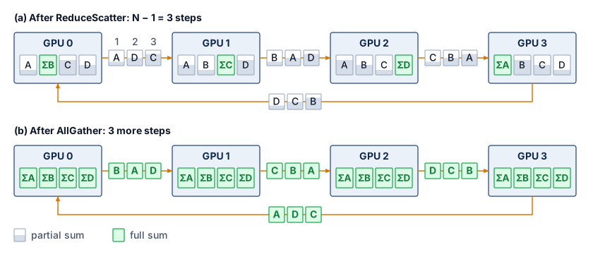
Figure 3: Ring AllReduce Data Flow: Four GPUs in a logical ring, each gradient split into chunks A to D; the wrap-around link closes the ring from GPU 3 back to GPU 0. (a) After the \(\DeviceCount-1\) ReduceScatter steps, in which every GPU sends one chunk to its neighbor and adds the chunk it receives, each GPU holds one fully reduced chunk. (b) After \(\DeviceCount-1\) AllGather steps that forward those finished chunks around the same ring, every GPU holds the full sum. Every link carries data in every step, so each GPU sends \(2\frac{\DeviceCount-1}{\DeviceCount}\CollectivePayloadSize\) bytes in total, while the \(2(\DeviceCount-1)\) steps each pay one startup latency \(\MessageStartupLatency\).

Logical ring edges may share physical links, and startup, local reduction, or contention can leave transfer capacity unused, so byte optimality does not guarantee peak physical-link utilization. To see how the logical schedule itself reaches that byte lower bound, consider 4 GPUs reducing a vector of 4 elements by summation. Each GPU \(\RankIndex\) starts with a local gradient vector \(\LocalGradient_i = [\FirstRingTraceElement_i, \SecondRingTraceElement_i, \ThirdRingTraceElement_i, \FourthRingTraceElement_i]\) split into 4 chunks (one per GPU), and the algorithm proceeds through two phases.

Example 5.1: Ring AllReduce: Two-phase example (4 GPUs)
Scenario: Four GPUs (\(0 \to 1 \to 2 \to 3 \to 0\)) perform a Ring AllReduce on local vectors \([1, 5, 3, 7]\), \([2, 6, 4, 8]\), \([3, 7, 5, 9]\), and \([4, 8, 6, 10]\) to compute the element-wise sum \([10, 26, 18, 34]\).

Diagnosis: The trace has to show three properties of the schedule, namely that it takes \(2(\DeviceCount-1) = 6\) steps, that every GPU sends and receives in every step, and that each step moves only one chunk. Ring AllReduce splits each vector into \(\DeviceCount=4\) chunks \(\FirstRingTraceElement\), \(\SecondRingTraceElement\), \(\ThirdRingTraceElement\), \(\FourthRingTraceElement\). In ReduceScatter step \(\RingStepIndex\) (\(\RingStepIndex= 1, 2, 3\)), GPU \(\RankIndex\) sends its running copy of chunk \((\RankIndex-\RingStepIndex+1) \bmod 4\) to GPU \((\RankIndex+1) \bmod 4\), which adds it to its own copy. After the third step, each GPU owns one fully reduced chunk. In AllGather step \(\RingStepIndex\), GPU \(\RankIndex\) forwards the finished chunk it completed or received most recently to GPU \((\RankIndex+1) \bmod 4\), which stores it without arithmetic. In each of the six steps, every GPU receives one chunk and updates the value it holds (table 5).

Table 5: Ring AllReduce Trace: The chunk each of four GPUs receives in each of the six steps. In the three ReduceScatter steps the GPU adds the incoming chunk to its running partial sum; in the three AllGather steps it stores an already finished sum.
Step GPU 0 GPU 1 GPU 2 GPU 3
ReduceScatter 1 d: 17 a: 3 b: 13 c: 11
ReduceScatter 2 c: 14 d: 25 a: 6 b: 21
ReduceScatter 3 b: 26 c: 18 d: 34 a: 10
AllGather 1 a: 10 b: 26 c: 18 d: 34
AllGather 2 d: 34 a: 10 b: 26 c: 18
AllGather 3 c: 18 d: 34 a: 10 b: 26

Every cell in every row is filled, so every GPU receives (and, symmetrically, sends) one chunk in every step, and after the sixth step every GPU holds [10, 26, 18, 34].

Systems lesson: Ring AllReduce achieves the optimal byte volume under the stated model: each GPU sends \(2\frac{\DeviceCount-1}{\DeviceCount}\CollectivePayloadSize\) total bytes, approaching \(2\CollectivePayloadSize\) as \(\DeviceCount\) grows, while the startup-round count continues to grow. Physical-link utilization also depends on placement and runtime overhead.

Checkpoint 5.2: Ring AllReduce mechanics

Verify your understanding of bandwidth-optimal reduction:

The performance follows directly from the two-phase schedule in example 5.1. Each node sends and receives \(\frac{\CollectivePayloadSize}{\DeviceCount}\) bytes in each of the \(2(\DeviceCount-1)\) steps. \[ \RingAllReduceCompletionTime = \underbrace{2(\DeviceCount-1)\MessageStartupLatency}_{\text{Latency Term}} + \underbrace{2\frac{\DeviceCount-1}{\DeviceCount} \frac{\CollectivePayloadSize}{\LinkBandwidth}}_{\text{Bandwidth Term}} \]

The bandwidth term approaches \(2\CollectivePayloadSize/\LinkBandwidth\) as \(\DeviceCount\to \infty\), reaching the full-duplex lower bound: each rank sends nearly \(2\CollectivePayloadSize\) bytes across the two phases and receives the same amount concurrently. In contrast, the latency term scales linearly with \(\DeviceCount\). Across 10,000 nodes, 19,998 sequential startup rounds accumulate substantial latency, which explains why Ring AllReduce becomes uncompetitive for small payloads.

Napkin Math 5.2: AllReduce cost for a 70B model
Problem: Consider a communication-only baseline for a 70B parameter model across 64 GPUs connected by InfiniBand NDR (50 GB/s per port). The bandwidth term barely depends on rank count, so this smaller group reproduces the bandwidth-only estimate from the opening definition while keeping the latency term visible. Each rank contributes a complete logical gradient buffer communicated in BF16 (2 bytes per parameter). This calculation isolates collective cost without establishing that the training state fits on each GPU. How long does one AllReduce take?

Step 1: Size the gradient payload. Each rank in this baseline contributes the complete logical gradient tensor of \(7 \times 10^{10} \times 2\ \text{bytes}\) \(=\) 140 GB. A hybrid layout that partitions the model would instead reduce corresponding gradient shards within smaller groups and requires its own calculation.

Step 2: Apply the Ring AllReduce bandwidth formula. \[\RingAllReduceBandwidthTime= 2 \cdot \frac{\DeviceCount-1}{\DeviceCount} \cdot \frac{\CollectivePayloadSize}{\LinkBandwidth}\]

Substituting: \(\RingAllReduceBandwidthTime\) = 1.96875 \(\times\) 140 GB / 50 GB/s \(\approx\) 5,512.5 ms.

Step 3: Add the latency term. \[\RingAllReduceStartupTime= 2(\DeviceCount-1) \cdot \MessageStartupLatency\]

Substituting: \(\RingAllReduceStartupTime=\) 126 \(\times\) 1.5 μs = 0.2 ms.

Step 4: Total communication time. Total: \(\RingAllReduceCompletionTime \approx\) 5,512.5 ms + 0.2 ms \(\approx\) 5,512.7 ms.

Systems insight: The modeled full-buffer AllReduce takes over five seconds under the stated link and rank assumptions, and almost all of it is the bandwidth term. Its effect on step time depends on how much remains exposed relative to useful computation. When it is fully exposed, halving it saves about 2.8 s per step; across a 100,000-step campaign on these 64 GPUs, that is roughly 4,900 GPU-hours of reserved accelerator time. Large-scale training systems can launch reductions for output-side gradients while input-side layers are still computing. Partitioned training also changes each rank’s payload and participating group, so this complete-gradient budget must be recomputed for the actual layout.

5.6.4 Tree AllReduce

Ring AllReduce’s byte efficiency comes with many startup rounds. As the group grows, the \(2(\DeviceCount-1)\MessageStartupLatency\) term can exceed the byte-transfer term for a fixed payload; the crossover depends on the measured path parameters. Tree AllReduce reduces the number of dependent rounds. In the simple reduce phase, pairs combine contributions and forward partial sums toward a root, taking \(\log_2 \DeviceCount\) steps for a balanced power-of-two group. The broadcast phase distributes the result in another \(\log_2 \DeviceCount\) steps. This shorter dependency chain motivates the comparison before bandwidth costs are counted.
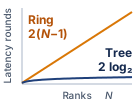
Latency rounds against rank count N on linear axes. An amber straight line labeled ring, 2 times N minus 1, climbs steadily; a blue curve labeled tree, 2 log base 2 of N, bends over and stays near the bottom.

Ring latency grows with N; tree stays logarithmic.

The simple full-message tree loses parallel activity as contributions converge. A ring activates all \(\DeviceCount\) logical edges in each round. In a pairwise tree reduction, the first round has \(\DeviceCount/2\) senders and \(\DeviceCount/2\) receivers; receiving is useful work, not idleness. The next round has \(\DeviceCount/4\) senders and \(\DeviceCount/4\) receivers, and the final reduction exchange involves two ranks while the remaining \((\DeviceCount-2)\) have completed their upstream contribution. Sending the full message through successive levels adds byte-transfer time along the dependency path. This is a limitation of the illustrated schedule, not every tree-based implementation or every physical link mapping.

The resulting time complexity depends on the specific tree variant. A simple reduce-then-broadcast tree has logarithmic latency but nonuniform traffic and root/interior bottlenecks. Recursive doubling, in which partners at doubling distances exchange the entire tensor in each of \(\log_2 \DeviceCount\) rounds, has the same logarithmic round count and incurs \(\mathcal{O}(\log \DeviceCount)\) full-message bandwidth per rank. The following simplified model captures the latency advantage and the potential bandwidth penalty of tree-like collectives: \[ \TreeLikeAllReduceTime\approx \underbrace{2\log_2 \DeviceCount\cdot \MessageStartupLatency}_{\text{Latency}} + \underbrace{2 \log_2 \DeviceCount\frac{\CollectivePayloadSize}{\LinkBandwidth}}_{\text{Bandwidth penalty in full-message exchange variants}} \]

The latency term is logarithmic (\(\mathcal{O}(\log \DeviceCount)\)): for 1,024 nodes, Ring needs 2,046 steps while Tree needs only 20, and that roughly 100× reduction in steps makes Tree attractive for small, frequent collectives across large process groups, such as scalar reductions, control messages, or small-batch activation reductions. The bandwidth term carries the penalty, because tree-like algorithms can underutilize links or concentrate traffic on interior links, and recursive-doubling-style full-message exchanges add a \(\log_2 \DeviceCount\) bandwidth factor; these penalties make naive tree variants a poor choice for data parallelism’s large gradient AllReduce, where bandwidth efficiency determines whether the network is saturated or partially idle.

For large-scale data parallelism, this bandwidth penalty decides the comparison whenever the implementation repeatedly exchanges full messages or creates root/interior bottlenecks. On the 64-GPU cluster of section 5.6.2, the simple tree forwards the whole tensor once per level on the way up and once per level on the way down, \(2\log_2 64 = 12\) full-message transfers, about 240 ms against the ring’s 39.4 ms, or 6.1× the ring’s byte time. The difference of roughly 200 ms per step would accumulate to about 5.6 hours over a 100,000-step run if fully exposed, although actual wall-clock savings also depend on startup, placement, and overlap. For a 70B-parameter model’s 140 GB gradient AllReduce across 1,000 GPUs, a bandwidth-inefficient tree-like variant can erase the latency advantage that motivated it. Optimized double-tree algorithms exist precisely to keep logarithmic latency without imposing that naive bandwidth penalty.

Small activation reductions provide a useful case for fewer startup rounds. For an eight-GPU group communicating a 1 MB tensor, the simple model reduces Ring’s \(2(8-1)\MessageStartupLatency= 14\MessageStartupLatency\) to Tree’s \(2\log_2(8)\MessageStartupLatency= 6\MessageStartupLatency\), but Tree’s byte term remains about 3.4× Ring’s. Whether the saved startups outweigh those extra byte transfers depends on the measured latency and bandwidth. Tensor-parallel collectives also have a scheduling constraint independent of this comparison: a layer that needs the reduced activation must wait for it. A critical-path dependency does not by itself imply a latency-dominated transfer or select a tree algorithm.

5.6.5 Recursive halving-doubling (butterfly)

The simple full-message Tree reduces startup rounds but repeats more byte-transfer work than Ring. Recursive halving-doubling, sometimes called the Butterfly algorithm, combines logarithmic rounds with the optimal byte volume under the flat-network model. It pairs ranks exactly as recursive doubling does, but where recursive doubling exchanges the whole tensor in every round, halving-doubling halves the exchanged region in each ReduceScatter round and doubles it in each AllGather round, and that difference removes the \(\log_2 \DeviceCount\) byte penalty. For a power-of-two group, it uses \(2\log_2 \DeviceCount\) rounds: \(\log_2 \DeviceCount\) ReduceScatter rounds followed by \(\log_2 \DeviceCount\) AllGather rounds. A partner-bit index \(\PartnerBitIndex\) selects the XOR pairing with mask \(2^\PartnerBitIndex\). The ReduceScatter trace below visits those bits in increasing order as messages shrink; the matching AllGather reverses that order as the assembled result grows.

In the ReduceScatter phase (first \(\log_2 \DeviceCount\) rounds), GPU \(\RankIndex\) partners with GPU \(\RankIndex\oplus 2^\PartnerBitIndex\) (XOR of indices). The partners retain complementary halves of the current tensor region and send the other half. Each adds the received contribution to the matching half it retained. After \(\log_2 \DeviceCount\) rounds, each GPU owns \(\CollectivePayloadSize/\DeviceCount\) bytes of the fully reduced result. AllGather traverses the partner bits in reverse, exchanging completed regions and doubling the data held at each rank until every rank has the full result.

Recursive halving-doubling costs \[ \ButterflyAllReduceTime= 2\log_2 \DeviceCount\cdot \MessageStartupLatency+ 2\frac{\DeviceCount-1}{\DeviceCount} \cdot \frac{\CollectivePayloadSize}{\LinkBandwidth} \]

The schedule combines logarithmic latency (\(\mathcal{O}(\log \DeviceCount)\), like Tree) with bandwidth-optimal data movement (\(2(\DeviceCount-1)/\DeviceCount\cdot \CollectivePayloadSize/\LinkBandwidth\), like Ring). The catch is that it requires nonneighbor communication (GPU \(\RankIndex\) must communicate with GPU \(\RankIndex\oplus 2^\PartnerBitIndex\), which may be physically distant), and it requires \(\DeviceCount\) to be a power of two. For clusters where \(\DeviceCount\) is not a power of two, additional complexity is needed to handle the irregular cases.

Recursive halving-doubling is used in MPI-style collective implementations and is useful as a theoretical point in the latency-bandwidth trade-off (Thakur et al. 2005). NVIDIA’s GPU collective backend, the NVIDIA Collective Communications Library (NCCL), offers implementation families that include ring, tree-derived, hierarchical, NVLink/NVSwitch-aware, and pattern-aware choices, with exact names and availability changing by version and topology (Jeaugey 2017; NVIDIA 2026). Whatever a particular release calls them, practical communication libraries select algorithms through a topology-aware cost model because nonlocal communication patterns can create contention on shared network links that erodes theoretical advantages.

Thakur, Rajeev, Rolf Rabenseifner, and William Gropp. 2005. “Optimization of Collective Communication Operations in MPICH.” The International Journal of High Performance Computing Applications 19 (1): 49–66. https://doi.org/10.1177/1094342005051521.

The partner distance is where topology enters. Consider the ReduceScatter phase for 8 GPUs placed four per node on two nodes, GPUs 0–3 on the first and GPUs 4–7 on the second, which proceeds in \(\log_2(8) = 3\) rounds. In round \(\PartnerBitIndex=0\), each GPU \(\RankIndex\) partners with GPU \(\RankIndex\oplus 1\), pairing neighbors: (0,1), (2,3), (4,5), (6,7). They exchange half their data and reduce. In round \(\PartnerBitIndex=1\), the distance doubles: GPU \(\RankIndex\) partners with GPU \(\RankIndex\oplus 2\), creating pairs (0,2), (1,3), (4,6), (5,7). In round \(\PartnerBitIndex=2\), the distance doubles again: GPU \(\RankIndex\) partners with GPU \(\RankIndex\oplus 4\), creating pairs (0,4), (1,5), (2,6), (3,7).

Physical placement determines the cost of these logical pairings (figure 4). Rounds \(\PartnerBitIndex=0\) and \(\PartnerBitIndex=1\) pair GPUs within a node, but in round \(\PartnerBitIndex=2\) every GPU on the first node exchanges with one on the second, so that round crosses the node boundary. On eight-GPU nodes the same crossing would appear one round later, at \(\PartnerBitIndex=3\) in a 16-rank group. In a separate 1,024-rank example, the final ReduceScatter round pairs GPU \(\RankIndex\) with GPU \(\RankIndex\oplus 512\). If the two rank halves occupy different racks, those exchanges share the inter-rack fabric. The algorithm’s logarithmic rounds and optimal byte volume therefore do not establish its runtime advantage; placement, shared paths, and the changing chunk size in each round must enter the comparison.
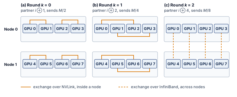
Figure 4: Halving-Doubling Partners across a Node Boundary: The ReduceScatter phase of recursive halving-doubling on 8 GPUs placed four per node. In round \(\PartnerBitIndex\), GPU \(\RankIndex\) exchanges with GPU \(\RankIndex \oplus 2^{\PartnerBitIndex}\) and sends half of the region it still holds, so the exchanged volume halves each round. (a) and (b) The first two rounds pair GPUs inside a node and use NVLink. (c) The last round pairs every GPU with one on the other node, so the round with the smallest message is the only one that crosses the slower fabric. Which round crosses depends on how many ranks each node holds.

5.6.6 Double binary tree

NCCL can use a double binary tree for many message sizes and topologies, which addresses the bandwidth inefficiency of a standard binary tree while allowing topology-aware tree placement (Jeaugey 2017; NVIDIA 2026). The idea is to construct two independent binary trees with complementary interior-node roles, then run both trees simultaneously, each carrying half the data.

The complementary-tree construction balances endpoint work by making ranks that act as interior nodes in one tree act as leaves in the other. With eight ranks, build the first tree by labeling the nodes of a binary tree in the order of an in-order traversal (left subtree, then node, then right subtree). In a balanced seven-node tree labeled from 0, in-order traversal puts the leaves at the even ranks 0, 2, 4, and 6 and the interior nodes at 1, 3, and 5; in one simple construction the eighth rank, 7, joins as one more interior node above that tree. The odd ranks 1, 3, 5, and 7 thus form the first tree’s interior and the even ranks are its leaves; the second tree shifts every rank by one position, so the even ranks become its interior and the odd ranks its leaves (figure 5). Each tree carries half the tensor, \(\CollectivePayloadSize/2\), and the two halves never meet.
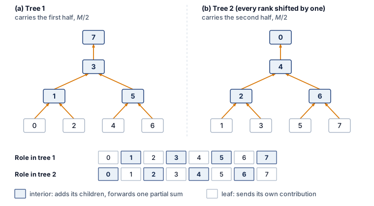
Figure 5: Complementary Roles in a Double Binary Tree: Two reduction trees over eight ranks, each carrying half of the tensor toward its root. (a) The first tree places the odd ranks at its interior and the even ranks at its leaves. (b) The second tree shifts every rank by one, which swaps the roles. The strip below shows the result: every rank is an interior node in exactly one tree and a leaf in the other, so it forwards one combined half and sends one half of its own, about \(\CollectivePayloadSize\) in the reduce phase. The broadcast phase runs the same trees in the opposite direction.

Two further steps bring the byte term down from the simple tree’s \(2\log_2 \DeviceCount\cdot \CollectivePayloadSize/\LinkBandwidth\) to about \(2\CollectivePayloadSize/\LinkBandwidth\). First, each tree pipelines its half in small chunks, so while one chunk moves up from the leaves, the next is already leaving them and every level works at once; tree depth then adds startup rounds and a short pipeline fill, not repeated full-message transfers. Second, count what one rank sends during the reduce phase. As an interior node of one tree it combines the inputs of its (at most two) children and forwards one \(\CollectivePayloadSize/2\) stream to its parent, and as a leaf of the other tree it sends its own \(\CollectivePayloadSize/2\) contribution, so it sends about \(\CollectivePayloadSize\) in total. The broadcast phase mirrors that traffic, for about \(2\CollectivePayloadSize\) per rank across both phases, the same per-rank volume as the ring. This logical balance does not guarantee that every physical link stays busy or that both trees avoid shared fabric bottlenecks; rank placement and routing still matter.

The combined performance is approximately: \[ \DoubleTreeAllReduceTime\approx 2\log_2 \DeviceCount\cdot \MessageStartupLatency+ \frac{2\CollectivePayloadSize}{\LinkBandwidth} \]

The ideal bandwidth term approaches \(2\CollectivePayloadSize/\LinkBandwidth\) while the startup-round count remains logarithmic. This combination makes the double binary tree a useful candidate across message sizes that penalize either the ring’s many rounds or the simple tree’s repeated full-message transfers. Complementary endpoint roles do not ensure disjoint physical paths, so topology-aware tree construction seeks a good placement, and measurements must establish the achieved rate under contention.

5.6.7 The algorithm crossover point

Plotting the three cost models for a 256-GPU group on a 200 Gbps fabric, over message sizes from 1 KB to 10 GB, shows the simple Tree and Ring curves intersecting near 1 MB (figure 6). At small sizes, fewer startup rounds favor the tree schedules; at large sizes, the simple full-message Tree pays more byte-transfer time. The Double Binary Tree curve includes illustrative overhead factors, so it approaches a comparable bandwidth-dominated regime without representing a measured library result. The candidate schedules differ in their latency and bandwidth terms, in whether they reach the bandwidth lower bound, and in the constraint each one places on the group (table 6).

Table 6: AllReduce Algorithm Comparison: Each algorithm occupies a different point in the latency-bandwidth trade-off space. Ring and Butterfly achieve bandwidth optimality with different latency characteristics, while Double Binary Tree combines logarithmic depth with a near-optimal byte term. The Tree row refers to the simple full-message model, not every tree implementation.
Algorithm Latency Bandwidth Bandwidth optimal? Constraint
Ring \(\mathcal{O}(\DeviceCount)\MessageStartupLatency\) \(2\frac{\DeviceCount-1}{\DeviceCount}\frac{\CollectivePayloadSize}{\LinkBandwidth}\) Yes None
Simple Tree \(\mathcal{O}(\log \DeviceCount)\MessageStartupLatency\) \(\mathcal{O}(\log \DeviceCount)\frac{\CollectivePayloadSize}{\LinkBandwidth}\) No None
Butterfly \(\mathcal{O}(\log \DeviceCount)\MessageStartupLatency\) \(2\frac{\DeviceCount-1}{\DeviceCount}\frac{\CollectivePayloadSize}{\LinkBandwidth}\) Yes \(\DeviceCount= 2^\RankCountBinaryExponent\)
Double Tree \(\mathcal{O}(\log \DeviceCount)\MessageStartupLatency\) \(\approx\frac{2\CollectivePayloadSize}{\LinkBandwidth}\) Near-optimal Complementary tree construction

Figure 6: Algorithm Crossover in Collective Communication: Below about 1 MB the simple tree’s fewer startup rounds make it faster than the ring; above that size the ring’s smaller byte volume wins, and the double binary tree tracks the faster of the two across most sizes. The curves are modeled AllReduce times for a 256-GPU group on a 200 Gbps interconnect with \(\MessageStartupLatency = 1\ \MicroUnitPrefix\text{s}\), over messages from 1 KB to 10 GB. The double binary tree curve applies modest latency and bandwidth overhead factors (1.2\(\times\) and 1.05\(\times\)) to its ideal cost, so it illustrates the model rather than a measured library result.

The intersection near 1 MB in figure 6 marks where the modeled Ring and simple Tree have equal total cost. It is an algorithm crossover, distinct from the startup-versus-transfer crossover for one message. Setting \(\RingAllReduceCompletionTime = \TreeAllReduceCompletionTime\) and solving for payload \(\CollectivePayloadSize\) identifies the point where Ring’s lower byte cost compensates for its additional startup rounds:

\[ \RingAllReduceCompletionTime = 2(\DeviceCount-1)\MessageStartupLatency+ 2\frac{\DeviceCount-1}{\DeviceCount}\frac{\CollectivePayloadSize}{\LinkBandwidth} \] \[ \TreeAllReduceCompletionTime = 2\log_2 \DeviceCount\cdot \MessageStartupLatency+ 2\log_2 \DeviceCount\cdot \frac{\CollectivePayloadSize}{\LinkBandwidth} \]

For large \(\DeviceCount\), \((\DeviceCount-1) \approx \DeviceCount\) and \(\frac{\DeviceCount-1}{\DeviceCount} \approx 1\), so the ring pays a latency term proportional to \(\DeviceCount\) while moving each byte close to the bandwidth limit:

\[ \RingAllReduceCompletionTime \approx 2\DeviceCount\MessageStartupLatency+ \frac{2\CollectivePayloadSize}{\LinkBandwidth}, \quad \TreeAllReduceCompletionTime \approx 2\log_2 \DeviceCount\cdot \MessageStartupLatency+ \frac{2\log_2 \DeviceCount\cdot \CollectivePayloadSize}{\LinkBandwidth} \]

The tree has the opposite shape: logarithmic startup cost, but each message byte moves through more stages. Setting the estimates equal isolates the message size where the cheaper latency path stops compensating for the extra bandwidth work:

\[ 2\DeviceCount\MessageStartupLatency+ \frac{2\CollectivePayloadSize}{\LinkBandwidth} = 2\log_2 \DeviceCount\cdot \MessageStartupLatency+ \frac{2\log_2 \DeviceCount\cdot \CollectivePayloadSize}{\LinkBandwidth} \] \[ \frac{2\CollectivePayloadSize}{\LinkBandwidth} - \frac{2\log_2 \DeviceCount\cdot \CollectivePayloadSize}{\LinkBandwidth} = 2\log_2 \DeviceCount\cdot \MessageStartupLatency- 2\DeviceCount\MessageStartupLatency\] \[ \frac{2\CollectivePayloadSize}{\LinkBandwidth}(1 - \log_2 \DeviceCount) = 2\MessageStartupLatency(\log_2 \DeviceCount- \DeviceCount) \]

Since \(\DeviceCount\gg \log_2 \DeviceCount\) for large clusters, \((\log_2 \DeviceCount- \DeviceCount) \approx -\DeviceCount\) and \((1 - \log_2 \DeviceCount) \approx -\log_2 \DeviceCount\), yielding:

\[ \frac{2\CollectivePayloadSize}{\LinkBandwidth}(-\log_2 \DeviceCount) \approx 2\MessageStartupLatency(-\DeviceCount) \] \[ \boxed{\RingTreeCrossoverPayload \approx \frac{\DeviceCount\cdot \MessageStartupLatency\cdot \LinkBandwidth}{\log_2 \DeviceCount}} \]

The log-aware crossover formula is the large-\(\DeviceCount\) approximation to the exact crossover \(\RingTreeCrossoverPayload(\DeviceCount)\) derived in Ring vs. tree vs. recursive halving-doubling. Within this two-algorithm model, Ring wins above the crossover because its byte savings exceed its extra startup cost; the simple Tree wins below it because the startup saving is larger. Optimized trees and topology-dependent rates require separate comparisons.

On the reference cluster, with the chapter’s effective NDR \(\MessageStartupLatency=\) 1.5 μs and \(\LinkBandwidth=\) 50 GB/s across all 1,024 GPUs, the estimate gives \(\RingTreeCrossoverPayload \approx\) \(\frac{1{,}024 \times 1.5\ \MicroUnitPrefix\text{s} \times 50\ \text{GB/s}}{\log_2 1{,}024} = \frac{1{,}024 \times 1.5\ \MicroUnitPrefix\text{s} \times 50\ \text{GB/s}}{10}\) \(\approx\) 7.7 MB. A gradient bucket of tens of megabytes or the full model gradient therefore sits on the ring side of the crossover, while a reduction of a few hundred kilobytes sits on the tree side. The two other configurations in this section depart from that anchor in stated ways. A smaller 256-GPU group on a slower 200 Gbps fabric with \(\MessageStartupLatency= 1\ \MicroUnitPrefix\text{s}\) moves the curves’ intersection down to about 1 MB (figure 6), and a 64-GPU group on a still slower, higher-latency fabric places a 1 MB buffer almost exactly on the crossover (notebook 5.3).

NCCL’s algorithm selection is more nuanced than a two-way split. The double binary tree offers logarithmic latency with near-optimal bandwidth, so it competes with both Ring and Tree across a broad range of message sizes, and the library also weighs the number of channels (parallel communication streams), the network topology, and whether a hop is inter-node or intra-node. The effective selection logic resembles a multi-way decision indexed by message size, GPU count, and topology type rather than a single crossover point. The crossover formula nevertheless explains the shape of those choices, because every candidate trades startup rounds against bytes moved. The model therefore names a candidate worth benchmarking rather than proving the library wrong, and an override is retained only after measured collective duration and exposed training-step time confirm it.

Training frameworks decide which payloads reach that analysis. PyTorch DistributedDataParallel (DDP) groups gradient tensors into buckets (section 5.10.3), while FSDP groups parameter gathers and gradient reductions according to its sharding units. A bucket size alone does not locate a crossover, because rank count, effective startup cost, and available bandwidth also enter the comparison, so NCCL’s algorithm selection must be evaluated for the actual invocation and topology rather than inferred from a nominal bucket-size range. A single 1 MB buffer on a slower fabric shows how close to the crossover a real bucket can sit.

Napkin Math 5.3: The ring vs. tree crossover
Problem: A cluster synchronizes a 1 MB buffer across 64 GPUs. The network has latency \(\MessageStartupLatency=\) 10 μs and bandwidth \(\LinkBandwidth=\) 10 GB/s. Which algorithm performs better: Ring or Tree?

Math:

Latency:

  1. Ring Latency: \(2(\DeviceCount-1)\MessageStartupLatency=\) \(2 \times 63 \times 10\ \MicroUnitPrefix\text{s}\) = 1260 μs.
  2. Tree Latency: \(2(\log_2 \DeviceCount)\MessageStartupLatency=\) \(2 \times 6 \times 10\ \MicroUnitPrefix\text{s}\) = 120 μs.

Bandwidth (note the difference):

  1. Ring Bandwidth: \(2\frac{\DeviceCount-1}{\DeviceCount}\frac{\CollectivePayloadSize}{\LinkBandwidth} \approx\) \(2 \times \frac{1\text{ MB}}{10\text{ GB/s}}\) = 196.9 μs (optimal: each rank sends about \(2\CollectivePayloadSize\) in total, the lower bound).
  2. Tree Bandwidth: \(2\log_2 \DeviceCount\cdot \frac{\CollectivePayloadSize}{\LinkBandwidth} =\) \(12 \times \frac{1\text{ MB}}{10\text{ GB/s}}\) = 1200 μs (each level sends full message).

Summing the latency and bandwidth terms gives each algorithm’s total time (table 7).

Table 7: Ring vs. Tree AllReduce Timing for a 1 MB Buffer on 64 GPUs: Latency, bandwidth, and total-time terms with \(\MessageStartupLatency=\) 10 μs and \(\LinkBandwidth=\) 10 GB/s.
Algorithm Latency Bandwidth Total
Ring 1260 μs 196.9 μs 1456.9 μs
Tree 120 μs 1200 μs 1320 μs

Tree wins, but only by 9 percent. For this 1 MB message, the payload is near the crossover point.

Systems insight: Ring’s latency term (10.5× Tree’s) nearly balances Tree’s bandwidth term (6.1× Ring’s). The log-aware crossover estimate predicts \(\RingTreeCrossoverPayload \approx \DeviceCount\MessageStartupLatency\LinkBandwidth/ \log_2 \DeviceCount=\) \(64 \times 10\ \MicroUnitPrefix\text{s} \times 10\ \text{GB/s} / 6\) \(\approx\) 1.1 MB. At 1 MB, the payload is just below crossover, so Tree wins. At 10 MB, Ring would dominate.

The crossover point sits inside the range that gradient reductions can traverse as bucket sizes change. In this example, the 1 MB AllReduce lies near crossover, whereas a 10 MB DDP bucket is already above it. A fused bucket of 50–300 MB or the full 140 GB BF16 gradient of a 70B parameters model favors Ring over the simple Tree model even more strongly. These conclusions apply to the stated AllReduce configuration. An MoE token-routing payload of the same size still requires an AllToAll schedule, and optimized tree or hierarchical implementations require their own cost comparison.

Checkpoint 5.3: AllReduce algorithm selection

Verify your understanding of Ring vs. Tree AllReduce trade-offs:

Self-Check: Question
  1. Why does Ring AllReduce achieve the information-theoretic lower bound for bandwidth (\(2 \frac{N-1}{N} \frac{M}{\beta}\)) while a simple unsegmented binary Tree AllReduce incurs a bandwidth penalty of \(\mathcal{O}(\log N \cdot \frac{M}{\beta})\)?

    1. Ring AllReduce distributes uniform chunks (\(M/N\)) across all logical ring edges in each round, whereas the simple unsegmented tree sends full messages through successive levels of a reduction and broadcast.
    2. Ring AllReduce compresses floating-point gradients to 1-bit representations during ring circulation, whereas Tree AllReduce always uses uncompressed FP64 precision.
    3. Tree AllReduce requires an external parameter server node to perform floating-point additions, whereas Ring AllReduce computes sums purely in network switch ASICs.
    4. Ring AllReduce eliminates the latency term \(\alpha\) entirely by using asynchronous token rings, whereas Tree AllReduce scales latency quadratically with cluster size.
  2. An infrastructure engineer evaluates AllReduce algorithm selection for synchronizing gradients across a 256-GPU cluster with per-node launch latency \(\alpha = 5\,\mu\text{s}\) and link bandwidth \(\beta = 50\text{ GB/s}\). Using the log-aware crossover model \(M_{\text{crossover}} \approx \frac{N \alpha \beta}{\log_2 N}\), within the simple full-message Tree versus Ring comparison, what is the crossover message size, and which modeled candidate has lower cost for a 500 KB activation tensor versus a 100 MB gradient bucket?

    1. The crossover is \(M_{\text{crossover}} \approx 1.25\text{ GB}\); Tree AllReduce should be selected for both tensors because \(\log_2(256) = 8\) is always smaller than 256.
    2. The crossover is \(M_{\text{crossover}} \approx 800\text{ KB}\); Ring AllReduce should be selected for 500 KB, and Tree AllReduce for 100 MB.
    3. The crossover is \(M_{\text{crossover}} \approx 16\text{ GB}\); Butterfly AllReduce should be selected for both tensors regardless of network topology.
    4. The crossover is \(M_{\text{crossover}} \approx \frac{256 \times (5 \times 10^{-6}\text{ s}) \times (50 \times 10^9\text{ B/s})}{8} = 8\text{ MB}\); Tree AllReduce wins for the 500 KB tensor (latency-dominated), while Ring AllReduce wins for the 100 MB bucket (bandwidth-dominated).
  3. Recursive halving-doubling (Butterfly AllReduce) combines logarithmic startup rounds with bandwidth-optimal byte volume in a flat-network model. What physical placement condition can defeat that modeled advantage, and why do double-tree or hierarchical alternatives still require measurement?

  4. Explain the structural mechanism of the Double Binary Tree AllReduce algorithm that allows it to achieve near-optimal bandwidth (\(\approx 2M/\beta\)) while preserving logarithmic latency (\(\mathcal{O}(\log N)\alpha\)).

  5. Sequence the execution steps of a 4-GPU Ring AllReduce (\(0 \to 1 \to 2 \to 3 \to 0\)) reducing a 4-chunk vector \([A, B, C, D]\): (1) each GPU forwards its fully reduced chunk around the ring for \(N-1\) steps until all ranks possess the complete array, (2) rank \(i\) owns a single fully aggregated chunk of the global sum, (3) each GPU partitions its local vector into \(N=4\) equal chunks, (4) each GPU simultaneously sends chunk \(k\) to its right neighbor and receives from its left neighbor, accumulating partial sums over \(N-1\) steps.

  6. Under the standard balanced point-to-point model, an AllReduce with \(M\) bytes per rank has a per-rank sent-volume lower bound of \(2(N-1)M/N\) bytes. Meeting this bound is known as ____ optimality, which Ring AllReduce achieves.

See Answers →

5.7 Hierarchical Communication

The AllReduce cost models in section 5.6 assume a flat network with uniform endpoint bandwidth. A multi-node GPU cluster instead has distinct local and cross-node communication paths. The DGX H100 nodes of the reference cluster show the gap at its starkest, with each GPU’s NVLink capacity roughly nine times its one InfiniBand port, the bandwidth hierarchy that Bandwidth hierarchy established.

Hierarchical communication is the response to that inequality. Intra-node links are abundant and fast, inter-node links are scarce and expensive, and the algorithm must shrink payloads before they cross the scarce tier whenever possible. This is why the same AllReduce can be implemented as a local ReduceScatter, a cross-node reduction, and a local AllGather rather than as one flat exchange across every rank.

5.7.1 Hierarchical AllReduce

On a DGX H100 node, each GPU’s local NVLink capacity is 450 GB/s per direction (the 900 GB/s datasheet figure is the bidirectional total), while its one inter-node port provides 50 GB/s over InfiniBand. These are endpoint capacity budgets, not a promise of uniform achieved rate to every peer. Intra-node connectivity and simultaneous traffic still matter. That hierarchical network motivates a schedule that assigns work to each tier according to its usable capacity.

A flat ring whose ordering repeatedly crosses node boundaries can leave local NVLink capacity unused while loading scarce inter-node links. Hierarchical AllReduce explicitly partitions the global operation into three stages that align communication volume with the fabric tiers (figure 7).
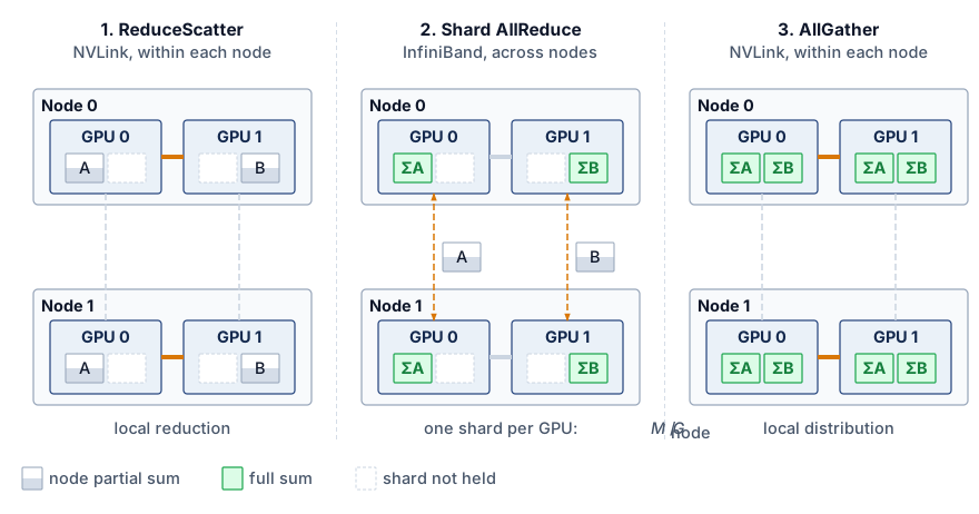
Figure 7: Hierarchical AllReduce: Three-phase decomposition that exploits the intra-node/inter-node bandwidth gap. Phase 1 performs intra-node aggregation over NVLink (an NVLink ring acting as a ReduceScatter that leaves each GPU holding a node-shard partial sum), leaving a payload of \(\CollectivePayloadSize/\AcceleratorsPerNode\) on each of the \(\AcceleratorsPerNode\) GPUs per node. Phase 2 runs an AllReduce across corresponding GPUs using InfiniBand. Phase 3 completes intra-node distribution over NVLink (the AllGather that returns each GPU to the full result). The schematic shows two representative ranks per node; the same decomposition applies to \(\AcceleratorsPerNode\) ranks.

With \(\AcceleratorsPerNode\) GPUs in each of \(\ClusterNodeCount\) nodes, the three phases form a single causal pipeline. First, an intra-node ReduceScatter over NVLink performs a local reduction among the \(\AcceleratorsPerNode\) GPUs in each node, leaving each GPU with a \(1/\AcceleratorsPerNode\) shard of partially reduced data while consuming only abundant intra-node bandwidth. Next, each corresponding-rank group applies an inter-node AllReduce over InfiniBand to its \(\CollectivePayloadSize/\AcceleratorsPerNode\)-byte input shard, where the chosen collective algorithm dictates the bytes transmitted across the network fabric. Finally, an intra-node AllGather over NVLink redistributes the globally reduced shards within each node, completing the collective without consuming additional inter-node bandwidth.

Only Phase 2 (Shard AllReduce) loads the slower inter-node InfiniBand links (figure 7). In this middle phase, each corresponding-rank group reduces an \(\CollectivePayloadSize/\AcceleratorsPerNode\)-byte shard across \(\ClusterNodeCount\) nodes. A ring in that group sends \(2(\ClusterNodeCount-1)\CollectivePayloadSize/(\ClusterNodeCount\AcceleratorsPerNode)\) bytes per participating GPU and receives the same amount. Summing across the node’s \(\AcceleratorsPerNode\) GPUs gives \(2(\ClusterNodeCount-1)\CollectivePayloadSize/\ClusterNodeCount\) bytes sent per node. Smaller per-port payloads improve elapsed time when the node has independent ports and sufficient fabric capacity; sharding does not create bandwidth on a shared uplink. An 8-node budget quantifies the bandwidth multiplier this decomposition provides when those ports operate in parallel.

Napkin Math 5.4: The hierarchical bandwidth multiplier
Problem: A cluster has 8 nodes, each with 8 GPUs (64 total). The system must AllReduce the chapter’s 1 GB reference buffer. Assume each GPU has its own full-rate inter-node port, one rail per GPU as on a DGX H100 (rails are the subject of section 5.7.4.1), with no oversubscription. The flat baseline is a single ring over all 64 ranks. How much faster is Hierarchical AllReduce than that flat ring?

Flat ring AllReduce (ignoring hierarchy):

  • Each GPU sends ~2 GB total (the bandwidth-optimal Ring AllReduce formula).
  • Every edge of a ring carries the same traffic in every step, so the whole ring advances at the rate of its slowest edge. Every ordering puts at least one fabric-crossing edge on each node, even the node-contiguous ordering that crosses the fabric only once per node.
  • Effective Bandwidth: Limited by the slowest link = 50 GB/s (InfiniBand).
  • Time: \(\approx\) \(2 \times 1\ \text{GB} / 50\ \text{GB/s}\) = 40 ms (bandwidth term dominates).

Hierarchical AllReduce (3-step decomposition):

  1. Intra-node ReduceScatter: Each GPU sends 875 MB at 450 GB/s per direction → ~1.94 ms

  2. Inter-Node AllReduce: Each GPU AllReduces a \(1\ \text{GB}/8\) = 125 MB shard over InfiniBand; Ring moves roughly \(2(\ClusterNodeCount-1)/\ClusterNodeCount\) times that payload, and after adding the small latency term the phase takes ~4.40 ms at 50 GB/s

    (The eight shard groups run concurrently, each on its own GPU’s port, so the node’s eight ports together carry the full payload in parallel.)

  3. Intra-node AllGather: Each GPU receives 875 MB at 450 GB/s per direction → ~1.94 ms

  4. Total time: \(\approx\) 1.94 ms + 4.40 ms + 1.94 ms = 8.3 ms

Systems insight: Hierarchical AllReduce achieves a 4.8× speedup by reducing the inter-node payload from 1 GB to 125 MB per GPU before the Ring traffic multiplier. The flat ring used one port’s worth of fabric bandwidth because a single ring runs at its slowest edge; the hierarchical schedule uses all eight ports at once. That is also its precondition, since a node whose GPUs shared one uplink would carry the eight shard streams one after another and lose most of the speedup. This is why NVIDIA’s NCCL and similar libraries often select hierarchical algorithms on multi-node clusters when the topology supports them.

The volume’s running instance makes the same comparison on the cluster it was defined for. Archetype A’s 175B-parameter model produces a 350 GB BF16 gradient, and the reference cluster holds 1,024 GPUs as 128 nodes of 8. A single flat ring over every GPU would spend about 14.0 s per full-gradient reduction. The hierarchical schedule sends one-eighth of the gradient through each GPU’s port in a shard ring that spans every node and completes in about 3.1 s, a 4.5× improvement, of which the cross-node phase still accounts for about 1.7 s. Seconds per step remain a large exposed cost even after hierarchy, which is why the production layout for this instance shards the model so that each data-parallel group reduces a fraction of this payload, and why the overlap and compression techniques later in the chapter still matter at this scale.

These three phases also generalize to additional fabric tiers. For example, 4 racks of 4 nodes with 8 GPUs per node contain 128 GPUs. A rack-local ReduceScatter over 32 GPUs can leave each GPU with \(1/32\) of the original payload for the cross-rack phase. The total elapsed time still includes both local phases, the cross-rack collective’s traffic factor, startup, and contention. A cross-rack oversubscription ratio alone cannot determine a speedup over a flat ring.

5.7.2 Multidimensional reduction on a torus

Hierarchy fits a fabric whose tiers differ in speed. A torus, the direct-connect topology of Google’s Tensor Processing Unit (TPU) pods, has uniform links instead, and its collectives reduce along one dimension at a time. TPU v4 pods support a 3D torus topology, unlike the 2D torus used by TPU v2 and v3. In the regular 3D torus model, each chip links directly to six neighbors \((\pm \Glyph{X}, \pm \Glyph{Y}, \pm \Glyph{Z})\) with equal per-link bandwidth. For collectives, the torus invites dimension-ordered reduction, which decomposes the AllReduce into sequential Ring AllReduces along axis-aligned torus rings. For a pod with \(\TorusFirstAxisChipCount{\times}\TorusSecondAxisChipCount{\times}\TorusThirdAxisChipCount\) chips, ranks first execute independent X-dimension rings for each fixed \((\Glyph{Y},\Glyph{Z})\) coordinate, producing partial sums along each X line. A second phase runs Y-dimension rings to combine those partials across the \(\Glyph{X} \times \Glyph{Y}\) plane, and a third executes Z-dimension rings across fixed \((\Glyph{X},\Glyph{Y})\) coordinates to complete the global reduction.

↩︎ The torus topology and its bisection and path-length trade-offs against the fat-tree are established in Dragonfly and torus alternatives.

On a \(4{\times}4\) 2D torus grid of 16 ranks, the dimension-ordered schedule runs in two phases (figure 8). In Phase 1 (orange solid paths), each row executes an independent 4-rank Ring AllReduce across the horizontal X dimension using dashed wrap-around boundary links to close the ring (\(2(\TorusFirstAxisChipCount-1) = 6\) steps). Once row partial sums are established, Phase 2 (slate solid paths) executes orthogonal 4-rank vertical Ring AllReduces down the Y dimension (\(2(\TorusSecondAxisChipCount-1) = 6\) steps). These phases use direct nearest-neighbor links without multi-hop routing within a logical ring edge. They reduce the startup count from \(2(\DeviceCount-1) = 30\) rounds on a flat 16-rank ring to \(2(\TorusFirstAxisChipCount-1) + 2(\TorusSecondAxisChipCount-1) = 12\) rounds, a 2.5× reduction in the modeled startup term. In this simple form each axis still processes the full message, so the round-count saving comes at a byte cost that the partitioned dimension-wise schedule removes.
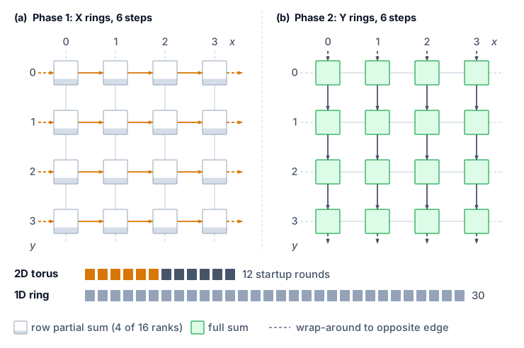
Figure 8: Dimension-Ordered Reduction on a Torus Topology: In a 2D torus mesh (\(4 \times 4\) node grid representing a simplified TPU pod slice), AllReduce proceeds sequentially along orthogonal dimensions. Phase 1 (orange) executes four parallel horizontal rings across the X dimension (\(2(\TorusFirstAxisChipCount-1) = 6\) steps). Phase 2 (slate) then executes four parallel vertical rings across the Y dimension (\(2(\TorusSecondAxisChipCount-1) = 6\) steps) on the row-aggregated partial sums. Dashed stubs mark the torus wrap-around links, each leaving one edge of the grid and re-entering at the opposite edge. This dimension-ordered decomposition needs 12 startup rounds against 30 for a 16-rank 1D global ring, a \(2.5\times\) reduction, but each axis processes the full message, so its bandwidth time is \(3\CollectivePayloadSize/\LinkBandwidth\) for this grid.

The byte term does not shrink with the rings. Because every axis processes the full \(\CollectivePayloadSize\)-byte tensor, the bandwidth time is \(2\CollectivePayloadSize[(\TorusFirstAxisChipCount-1)/\TorusFirstAxisChipCount+ (\TorusSecondAxisChipCount-1)/\TorusSecondAxisChipCount+ (\TorusThirdAxisChipCount-1)/\TorusThirdAxisChipCount]/\LinkBandwidth\) for equal per-axis bandwidth \(\LinkBandwidth\), while the startup term is \(2[(\TorusFirstAxisChipCount-1)+(\TorusSecondAxisChipCount-1)+(\TorusThirdAxisChipCount-1)]\MessageStartupLatency\). Shorter rings reduce startup cost, but these sequential full-message AllReduces do not retain the bandwidth cost of one global ring. A bandwidth-efficient multidimensional implementation instead partitions the work with dimension-wise ReduceScatter followed by reverse-order AllGather. The X-dimension ReduceScatter sends \(\CollectivePayloadSize(\TorusFirstAxisChipCount-1)/\TorusFirstAxisChipCount\) bytes per rank and leaves each rank an \(\CollectivePayloadSize/\TorusFirstAxisChipCount\) shard; the Y-dimension ReduceScatter then operates only on that shard and sends \((\CollectivePayloadSize/\TorusFirstAxisChipCount)(\TorusSecondAxisChipCount-1)/\TorusSecondAxisChipCount\), and the Z dimension continues the pattern. The three terms telescope to \(\CollectivePayloadSize(\DeviceCount-1)/\DeviceCount\) for \(\DeviceCount= \TorusFirstAxisChipCount \TorusSecondAxisChipCount \TorusThirdAxisChipCount\), and the mirrored AllGather doubles that to \(2(\DeviceCount-1)\CollectivePayloadSize/\DeviceCount\), the ring’s optimal byte term, while keeping the short rings’ startup count. The torus thus teaches the same lesson as hierarchy, which is to shrink the payload before each successive stage rather than send the full tensor through every one.

Dimension-ordered reduction follows direct neighbor links and separates axis traffic in time; it does not change the network diameter or eliminate contention with other workloads. The torus topology also provides natural fault tolerance through alternate routing paths. If one link in the X-dimension fails, traffic can detour through the Y or Z dimensions (at the cost of increased latency). The compiler and collective runtime must choose a schedule for the actual topology, message size, and available links.

5.7.3 In-network reduction with SHARP

Hierarchical and dimension-ordered schedules redistribute work across links, but their software reduction stages still require endpoint GPUs to receive and combine contributions. NVIDIA’s Scalable Hierarchical Aggregation and Reduction Protocol (SHARP)6 moves that intermediate aggregation into the network. Instead of routing each partial sum through a GPU for arithmetic, an aggregation-capable InfiniBand switch combines contributions as packets pass through it.

6 SHARP (Scalable Hierarchical Aggregation and Reduction Protocol): In-network computing on Quantum InfiniBand switches that performs reduction operations (such as sum, min, and max) as packets traverse an aggregation tree (Graham et al. 2020). The same work reports substantially higher reduction bandwidth than host-based algorithms and describes switch-resource limits on outstanding aggregation groups and trees, which can create contention when many collectives compete for the same in-network resources.

Graham, R. L., D. Bureddy, P. Lui, H. Rober, G. Bloch, G. Shainer, J. Poole, et al. 2020. “Scalable Hierarchical Aggregation and Reduction Protocol (SHARP) Streaming-Aggregation Hardware Design and Evaluation.” International Conference on High Performance Computing, 41–59. https://doi.org/10.1007/978-3-030-50743-5_3.

A centralized endpoint reduction and in-switch aggregation send different data up the switch tree (figure 9). In the endpoint tree of panel (a), intermediate switches merely forward raw packets, forcing all four full gradient tensors (\(\LocalGradient_0\) through \(\LocalGradient_3\)) across the upper links into a single Reducer GPU that executes every addition. In panel (b), SHARP offloads arithmetic to aggregation-capable switch application-specific integrated circuits (ASICs): each intermediate switch computes partial sums (\(\LocalGradient_0+\LocalGradient_1\) and \(\LocalGradient_2+\LocalGradient_3\)) in-flight, leaving only the combined shards for the root switch to finalize. Moving reduction into the network fabric halves the upper link traffic and relieves accelerator endpoints from coordinating arithmetic steps.
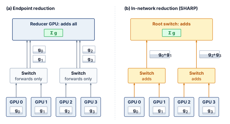
Figure 9: Endpoint and In-Network Reduction: The upstream half of a reduction over four GPUs. (a) Switches only forward packets, so every full gradient tensor crosses the upper links and converges on one reducer GPU, which does all the arithmetic. (b) Aggregation-capable switches add their inputs, so each upper link carries one partial sum and the root switch finishes the reduction; the result then travels back down the same tree. A software reduction tree also aggregates along its path, but performs arithmetic at endpoints rather than switches. The diagram compares where arithmetic happens, not measured speedup.

SHARP changes both terms of the cost model. On the startup side, it shortens the dependency chain. In a software-based tree reduction, each level waits for an intermediate GPU to receive, reduce, and forward its inputs; with SHARP the switch performs that step in the packet path, so no GPU execution stage or extra endpoint round trip sits between levels. On the byte side, each upper-tier link carries one partial sum rather than every contribution beneath it (figure 9), and in the idealized aggregation tree each GPU sends its contribution up once and receives the result once, where a ring rank sends nearly \(2\CollectivePayloadSize\). Endpoint memory traffic falls for the same reason. Switch processing and contention for aggregation resources add costs of their own, so moving arithmetic into the network changes the \(\MessageStartupLatency\)-\(\LinkBandwidth\) terms rather than eliminating them.

Which benefit matters follows the regimes of section 5.5. For small and medium messages, where startup rounds dominate, the shorter dependency chain is the main gain, although for very small messages fixed switch-processing overhead can limit it. For large messages the startup saving becomes proportionally small, and what remains is the byte saving at the endpoints and on the upper tier, which shortens the collective only when those links are the binding resource. Graham et al. (2020) report multi-fold reduction-bandwidth improvements and smaller application-level gains for PyTorch workloads when SHARP Streaming-Aggregation is enabled on HDR/Quantum InfiniBand switches.

Strong scaling campaigns (training a fixed model across more accelerators without proportionally growing batch size) expose the importance of this distinction between collective speed and step time. As the per-accelerator batch shrinks, each gradient tensor stays large (proportional to model size) but the backward pass per accelerator shortens, exposing more of the communication budget. The limiting term can still be bandwidth; strong scaling alone does not establish that startup latency dominates. In-switch aggregation helps when its reduction in endpoint work or fabric traffic shortens the exposed critical path.

In-switch reduction also brings hardware and capacity constraints of its own. The switch ASIC must support the exact reduction operator and numerical format the job uses, such as FP16 or BF16 gradients, which vary across switch generations, and its finite internal memory limits how many aggregation trees can remain active at once, so a large cluster running many concurrent jobs or process groups can exhaust switch-tree capacity and fall back to host-based reductions. Moreover, the HDR and Quantum SHARP implementations examined here depend on InfiniBand switch support, so their gains do not carry over to Ethernet fabrics unless an equivalent in-network aggregation path is present.

5.7.4 Topology-aware routing

Two runs of the same 64-GPU Ring AllReduce on identical hardware can differ by a multiple in throughput depending on whether consecutive logical ranks sit on the same NVLink domain or across shared inter-node uplinks. Hierarchy and in-network aggregation change where bytes move and where sums are computed, but their benefit still depends on mapping the logical communication pattern onto physical links.

Communication libraries like NCCL perform topology detection at initialization and use graph search to choose paths through the hardware topology available to them (NVIDIA 2026). For each pair of ranks, the library must determine whether the peer sits behind a local NVLink switch or 100 meters away across an InfiniBand fabric, because that mapping decides which physical links each logical hop occupies. Local GPU, NVLink, PCIe, and NIC connectivity informs those choices, but local discovery does not reveal every remote switch, route, or competing flow. Fabric configuration and placement information must complement the library’s view when diagnosing cross-node contention.

The topology detection process begins with hardware enumeration. NCCL queries the PCIe bus to discover GPU placement, NVLink connectivity between GPUs, and NIC-to-PCIe-switch affinity. From this information, it constructs an internal graph where nodes represent GPUs and edges represent physical links with annotated bandwidth and latency. A graph search algorithm then finds communication paths that maximize aggregate bandwidth while minimizing the number of cross-domain hops (transitions between NVLink, PCIe, and InfiniBand domains). This topology-aware path selection is what allows NCCL to approach theoretical peak bandwidth on well-configured systems, while topology-unaware implementations can leave a large fraction of bandwidth unused.

Rail-optimized routing (NVIDIA DGX)

In the eight-GPU DGX layout considered here, each GPU has a dedicated inter-node NIC, and the fabric connects matching NIC positions to rail switches. Rail-optimized routing fits the corresponding-shard phase of hierarchical AllReduce: GPU 0 on Node A exchanges its shard with GPU 0 on Nodes B and C, GPU 1 exchanges with peer GPU 1s, and so on. The eight rails can carry these groups concurrently (table 8), subject to their physical capacity and competing traffic. Other collectives may require cross-rail paths.

↩︎ Rail-optimized cabling, which connects each GPU slot position to its own rail switch, is established in Rail-optimized topology.

Table 8: Rail-Optimized Traffic Distribution: Each rail carries 1/8 of the total traffic independently.
Rail Participants Traffic
Rail 0 Node0-GPU0 \(\leftrightarrow\) Node1-GPU0 \(\leftrightarrow\) Node2-GPU0 \(\leftrightarrow\) … \(\CollectivePayloadSize/8\) each
Rail 1 Node0-GPU1 \(\leftrightarrow\) Node1-GPU1 \(\leftrightarrow\) Node2-GPU1 \(\leftrightarrow\) … \(\CollectivePayloadSize/8\) each
… … …
Rail 7 Node0-GPU7 \(\leftrightarrow\) Node1-GPU7 \(\leftrightarrow\) Node2-GPU7 \(\leftrightarrow\) … \(\CollectivePayloadSize/8\) each

If all eight shard streams converge on one remote NIC, that endpoint faces 8\(\times\) the balanced receive demand. In the equal-shard layout, matching each shard group to its intended rail distributes one-eighth of the payload to each NIC. This removes that particular concentration; achieving the predicted rate still requires sufficient switch, uplink, and bisection capacity for concurrent traffic.

NVIDIA designed the DGX node and rail layout together so that Step 2 of hierarchical AllReduce (section 5.7.1) maps each corresponding-rank shard group onto its own rail, and NCCL exploits that structure whenever its topology detection finds aligned ranks. When the job scheduler assigns process ranks without topology awareness, however, logical shards and physical rails drift apart, routing cross-node traffic through the wrong NICs or across spine switches and cutting a node’s usable injection bandwidth to as little as one-eighth of the rail-aligned value when all eight shard exchanges converge on one NIC. Large deployments therefore enforce topology-aware rank assignment through device ordering (CUDA_VISIBLE_DEVICES), NIC binding, and scheduler placement policies so that logical rank \(\LocalRankIndex\) on every node stays bound to rail \(\LocalRankIndex\).

↪ How the scheduler places a job’s gangs on the topology hierarchy so that its collectives stay on fast links is developed in Topology-Aware Scheduling.

Hierarchical execution and topology-aware routing connect the cost model to a physical placement. The \(\MessageStartupLatency\)-\(\LinkBandwidth\) terms estimate the service required by each scheduled exchange; hierarchy redistributes work across fabric tiers, and rail alignment can balance corresponding-shard traffic across independent ports. None removes shared-capacity limits. Measured collective duration must confirm that the intended placement shortens the dependency path before the design is accepted.

Self-Check: Question
  1. On an 8-node cluster with 8 GPUs per node, fast local NVLink, and eight independent 50 GB/s network ports per node, how can hierarchical AllReduce improve on a flat ring whose inter-node traffic is serialized through one port?

    1. Hierarchical AllReduce converts the floating-point values to 8-bit integers during the intra-node phase to save inter-node bandwidth.
    2. Flat Ring AllReduce requires every GPU to establish an optical fiber connection directly to all 63 other GPUs in the cluster.
    3. Local ReduceScatter creates one 125 MB shard per GPU from a 1 GB tensor; corresponding-rank AllReduces can distribute these shards across the eight ports, followed by local AllGather.
    4. Hierarchical AllReduce executes without any inter-node network synchronization barriers.
  2. How does dimension-ordered reduction on a 3D torus network (such as Google TPU pods) optimize communication latency and link utilization compared to running a single global logical ring?

    1. It skips communication along the Z-axis by projecting all activations onto a 2D plane.
    2. It executes axis-aligned rings in sequence, reducing startup rounds to \(2[(X-1)+(Y-1)+(Z-1)]\) while trading extra full-message transfers for shorter rings.
    3. It broadcasts full gradient tensors directly to all pod nodes simultaneously over optical circuit switches.
    4. It routes all collective packets through a single central root TPU in the pod to minimize total wire length.
  3. Describe the architectural principle of rail-optimized routing in multi-GPU DGX clusters, and explain the performance pathology that occurs if a job scheduler assigns process ranks without topology awareness.

  4. True or False: On a supported aggregation path, SHARP can move intermediate reduction arithmetic from endpoints into switches, but the resulting latency and training-step benefit still depend on message size, placement, switch resources, and exposed dependencies.

  5. Sequence the three phases of Hierarchical AllReduce executed across a multi-node cluster with \(G\) GPUs per node: (1) intra-node AllGather across local GPUs over NVLink to reconstruct the full globally reduced tensor, (2) inter-node AllReduce across corresponding GPU positions over InfiniBand on the \(M/G\) node shards, (3) intra-node ReduceScatter across local GPUs over NVLink leaving each GPU holding \(1/G\) of the partially reduced tensor.

See Answers →

5.8 AllToAll Exchanges at Scale

Hierarchy, in-network reduction, and rail alignment were all developed for AllReduce, whose uniform payload lets every rank follow the same schedule. The AllToAll rows of table 1, expert parallelism and sharded embedding tables, break that uniformity, because each rank sends different data to each destination and the exchange finishes only when its slowest term finishes.

Systems Perspective 5.1: AllToAll vs. AllReduce: Why scale differs
Ring AllReduce can pipeline a uniform payload through neighbor exchanges. AllToAll presents a different scaling problem because every rank has destination-specific traffic, but the logical peer count alone does not determine its cost.

An AllToAll over \(\DeviceCount\) ranks creates \(\DeviceCount(\DeviceCount-1)\) logical source-destination transfers, yet each rank’s aggregate payload can remain fixed under weak scaling. Its lower bound is governed by the largest of four terms: source injection time, destination reception time, traffic crossing the fabric bisection, and per-message startup or scheduling overhead. Oversubscription and routing determine how much physical capacity those flows share. Message granularity determines how often they pay \(\MessageStartupLatency\). Routing skew determines whether one destination or link becomes the critical path. A full-bisection network carrying balanced, coarse-grained traffic can therefore scale well despite the quadratic logical connection count, whereas an oversubscribed fabric or skewed expert assignment can stall at much smaller \(\DeviceCount\).

Expert parallelism and large-scale recommendation systems can reach a communication wall earlier than standard data parallelism when their traffic exhausts injection, reception, or bisection capacity, or when routing and destination skew create hotspots. The primitive determines the traffic matrix; the physical fabric and routing distribution determine the scaling ceiling.
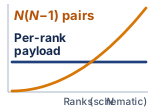
Schematic against rank count N: a curve labeled N(N−1) pairs starts near zero and rises quadratically, crossing a flat line labeled per-rank payload that stays at a fixed nonzero level.

Logical pairs grow quadratically while per-rank payload can stay flat.

A mixture-of-experts model with 64 experts distributed across 8 GPUs (8 experts per GPU) shows the AllToAll pattern at small scale. During each forward pass, a gating network assigns each input token to one or more experts. The tokens assigned to experts on remote GPUs must be physically moved to those GPUs before computation can proceed, and the results must be moved back afterward.

Napkin Math 5.5: AllToAll for MoE token routing
Problem: An MoE model processes a batch of 4096 tokens across 8 GPUs (512 tokens per GPU). Each token is a 2048-dimensional hidden state in BF16 (4.096 KB per token). The gating network assigns each token to exactly 1 of 64 experts (8 experts per GPU). Assuming uniform routing (each expert receives 64 tokens), how much data does each GPU send and receive?

Math:

Each GPU holds 512 tokens that need to reach 64 different experts across 8 GPUs. With uniform routing, each GPU sends 64 tokens to each of the other 7 GPUs (keeping 64 tokens local).

  • Data per GPU-to-GPU transfer: 64 tokens \(\times\) 4.096 KB/token = 262.144 KB
  • Total data sent per GPU: 7 \(\times\) 262.144 KB = 1.84 MB
  • Total data received per GPU: 1.84 MB (symmetric)

Latency Analysis (InfiniBand NDR, \(\MessageStartupLatency=\) 1.5 μs, \(\LinkBandwidth=\) 50 GB/s):

Each of the 7 transfers is a 262.144 KB message. From the \(\MessageStartupLatency\)-\(\LinkBandwidth\) model: \(\TransferTimeForPayload\) = 1.5 μs + 5 μs = 6.5 μs per transfer.

If serialized: 7 \(\times\) 6.5 μs = 45.5 μs. If all 7 transfers are issued concurrently, they still share the GPU’s 50 GB/s injection port. The aggregate injection lower bound is therefore \(\MessageStartupLatency+ \text{total bytes sent}/\LinkBandwidth=\) 38.2 μs, before contention and additional collective overhead. Full duplex permits simultaneous sending and receiving; it does not provide one full-bandwidth outgoing port per peer.

Systems insight: The injection result is only a lower bound. If the topology’s usable bisection bandwidth is \(\BisectionBandwidth\) and \(\CutCrossingDataVolume\) bytes must cross its minimum cut, the exchange also obeys \(\AllToAllExchangeTime\geq \CutCrossingDataVolume/\BisectionBandwidth\). Oversubscription reduces \(\BisectionBandwidth\), fine-grained peer messages add startup cost, and expert skew raises the maximum receive volume above the uniform estimate. The forward pass runs the AllToAll twice per layer, once for token dispatch and once for result collection; training also communicates gradients during backward.

5.8.1 Dynamic routing and expert imbalance in MoE AllToAll

The worked trace in notebook 5.5 assumes uniform token routing, in which every expert receives an identical share of tokens. In production MoE models, routing decisions are dynamic and data-dependent. The exchange keeps its two-phase shape, but its buffer sizes, its slowest receiver, and its load on the fabric all become functions of the routing distribution, and the hierarchy just developed for AllReduce reappears as one of the schedules that can contain them.

Each MoE layer performs two exchanges. In an MoE transformer layer with \(\ExpertCount\) experts distributed across \(\DeviceCount\) ranks (\(\ExpertCount/\DeviceCount\) experts per rank), each rank holds a local batch of \(\LocalTokenCount\) tokens. A gating router computes top-\(\RoutedExpertCount\) routing probabilities over all \(\ExpertCount\) experts for each token, inducing two collective communication phases separated by expert computation. During token dispatch, each rank partitions its \(\LocalTokenCount\) local token activation vectors (\(\LayerInputVector\in \mathbb{R}^\HiddenDimension\), where \(\HiddenDimension\) is the model’s hidden dimension) according to the destination ranks hosting the selected experts, executing an AllToAll collective (or variable-size AllToAllv) to route tokens across the fabric according to the routing matrix. After each rank computes forward passes through its assigned local expert feed-forward networks (FFNs), the token combine phase executes a second AllToAll collective to route output vectors back to their originating ranks. Each rank then computes the weighted combination of expert outputs: \[\LayerOutputVector_i = \sum_{j \in \text{top-}\RoutedExpertCount} {\RouterGateProbability}_{i,j} \cdot \text{Expert}_j(\LayerInputVector_i)\]

Because routing is data-dependent, so are the required buffer sizes, even when the input tensor shape is fixed. One simplified model treats assignments of different tokens independently: the count for expert \(\ExpertIndex\) is then \(\ExpertTokenCount\sim \text{Binomial}(\DeviceCount \LocalTokenCount, \ExpertSelectionProbability)\), where \(\ExpertSelectionProbability\) is the fixed probability that a token selects expert \(\ExpertIndex\). Correlated tokens or changing router probabilities require a different count model. To avoid reallocating buffers for every routing decision, a capacity-limited implementation can reserve space using an expert capacity factor \(\ExpertCapacityFactor\ge 1.0\), a multiplier on each expert’s average share of token assignments (Lepikhin et al. 2021; Fedus et al. 2022): \[\text{Capacity}_\ExpertIndex= \left\lceil \frac{\DeviceCount\times \LocalTokenCount\times \RoutedExpertCount}{\ExpertCount} \times \ExpertCapacityFactor\right\rceil\]

Lepikhin, Dmitry, HyoukJoong Lee, Yuanzhong Xu, Dehao Chen, Orhan Firat, Yanping Huang, Maxim Krikun, Noam Shazeer, and Zhifeng Chen. 2021. “GShard: Scaling Giant Models with Conditional Computation and Automatic Sharding.” International Conference on Learning Representations (ICLR).
Fedus, William, Barret Zoph, and Noam Shazeer. 2022. “Switch Transformers: Scaling to Trillion Parameter Models with Simple and Efficient Sparsity.” Journal of Machine Learning Research 23 (120): 1–39.

The capacity factor exposes a trade-off between reserved space and retained expert assignments. At uniform expected capacity (\(\ExpertCapacityFactor= 1.0\)), some experts can still overflow while others have unused slots. A dropping implementation bypasses excess assignments through the residual connection, changing the computation and potentially harming training quality. Increasing headroom (\(\ExpertCapacityFactor> 1.0\), for example \(1.25\)–\(1.5\)) can reduce overflow. If the implementation transmits every reserved slot, its padded payload grows by approximately a factor of \(\ExpertCapacityFactor\) relative to the uniform capacity-one budget; kernels that skip unused slots need not perform the corresponding dummy computation. A dropless implementation retains every assignment and can use variable-size AllToAllv to avoid sending unused slots. It still needs enough memory for the realized counts and remains exposed to routing skew.

Skew turns the most heavily loaded rank into a straggler. Because token routing is determined by input semantics, some experts inevitably receive disproportionate token volumes. An expert that receives several times the average load raises its host GPU’s receive traffic by the same excess. The host’s total receive volume depends on the combined load of all experts assigned to it, which is the rank-level quantity in the bound that follows.

Routing skew can create stragglers in both communication and expert computation. An inbound reception bottleneck bounds dispatch completion by the most heavily loaded receiver. Other ranks may finish their transfers earlier, but work that needs the delayed expert outputs must wait. The receive budget gives a lower bound before expert computation and the return exchange are counted: \[\TokenDispatchTime\ge \frac{\MaxReceivedTokenCount\times \HiddenDimension\times \ElementStorageSize}{\ReceiveBandwidth}\] where \(\MaxReceivedTokenCount= \max_\RankIndex \sum_{\ExpertIndex\in \text{rank } \RankIndex} \ExpertTokenCount\) counts the largest remotely received token batch at any rank \(\RankIndex\), restricting \(\ExpertTokenCount\) in this sum to assignments arriving from other ranks; \(\ElementStorageSize\) is the bytes per activation element, and \(\ReceiveBandwidth\) is that rank’s receive bandwidth. Bisection capacity provides a separate limit. Ring AllReduce exchanges data with logical ring neighbors, whereas AllToAll permits a complete bipartite exchange. Under uniform destination assignment, a fraction \((\DeviceCount-1)/\DeviceCount\approx 1\) of tokens leaves its source rank; the fraction crossing nodes or a particular fabric cut depends on placement. In the simplified symmetric fabric model with oversubscription ratio \(\OversubscriptionRatio:1\), usable bisection bandwidth \(\BisectionBandwidth = (\DeviceCount\cdot \InjectionBandwidth) / (2\OversubscriptionRatio)\) bounds the time needed to carry traffic across that cut: \[\TokenDispatchTime\ge \frac{\CutCrossingDataVolume}{\BisectionBandwidth}\]

Napkin Math 5.6: The cost of a hot expert rank
Problem: Return to the uniform routing of notebook 5.5: 8 GPUs, 64 experts, 4.096 KB per token, and one 50 GB/s port per GPU. Suppose skew sends one rank’s experts 1.5 times the average remote load. This is an assumed realized routing skew; the per-expert capacity factor reserves total-assignment headroom and does not determine remote arrivals. How does the receive bound on dispatch change?

Math:

  1. Uniform receiver: Each GPU receives 448 remote tokens, or 1.84 MB, so \(\TokenDispatchTime\ge\) 1.84 MB / 50 GB/s \(\approx\) 36.7 μs.
  2. Hot receiver: \(\MaxReceivedTokenCount\) rises to 672 remote tokens, or 2.75 MB, so \(\TokenDispatchTime\ge\) 2.75 MB / 50 GB/s \(\approx\) 55.1 μs.

Systems insight: The exchange cannot finish before its hottest receiver, so a 1.5× load on one rank raises the dispatch bound for the whole layer by the same factor. Transmitting unused capacity slots can add padding bytes; the amount depends on the packing layout rather than on this receive-skew factor alone. A variable-size exchange removes unused-slot traffic but not the receive bound. Expert computation processes local as well as remote assignments, so its work grows by the same factor only if the hot rank’s total local-plus-remote assignment count also grows by that factor, with unchanged work per assignment.

Scale compounds both problems. To amortize small-message overhead across thousands of GPUs, hierarchical MoE runtimes decompose the flat AllToAll into a two-level collective (Hwang et al. 2023). Intra-node NVLink first coalesces tokens destined for experts on the same remote server node. Participating nodes then exchange aggregated payloads over InfiniBand or RoCE, and receiving GPUs use NVLink to distribute tokens to the GPUs hosting the targeted experts. At the logical level, this replaces \(\DeviceCount(\DeviceCount-1)\) directed rank pairs with \(\ClusterNodeCount(\ClusterNodeCount-1)\) directed node pairs; actual transport connections depend on the implementation. Coalescing can improve link utilization and reduce startup overhead, but the token bytes still have to cross the required fabric cuts, and skew can still overload a destination.

5.8.2 AllToAll schedule selection

A flat, fixed-size AllToAll schedule that works well for balanced, megabyte-scale peer transfers on eight GPUs can stall across thousands of GPUs when per-peer chunks shrink to a few kilobytes or when expert skew forces every rank to pad its buffers to the hottest receiver’s count. Because AllToAll names only the destination-specific contract, the runtime must match its schedule to the traffic matrix and physical hierarchy rather than treating every exchange as one flat pattern. Three schedules cover the common regimes (table 9). Direct pairwise exchange suits balanced, coarse per-peer chunks; hierarchical exchange coalesces many small remote chunks before they cross scarce inter-node links; and variable-size exchange avoids padding when token or embedding counts differ by destination. Hierarchical designs such as Tutel’s two-dimensional exchange demonstrate why the best schedule changes with message size, scale, and topology (Hwang et al. 2023).

Hwang, Changho, Wei Cui, Yifan Xiong, Ziyue Yang, Ze Liu, Han Hu, Zilong Wang, et al. 2023. “Tutel: Adaptive Mixture-of-Experts at Scale.” Proceedings of Machine Learning and Systems (MLSys) 5.
Table 9: AllToAll Schedule Selection: The right schedule minimizes the active bound rather than the logical peer count. Direct exchange preserves simplicity, hierarchy coalesces traffic before scarce links, and variable-size exchange removes padding without removing skew.
Schedule When it fits Cost exposed
Direct pairwise exchange Balanced, coarse per-peer chunks on a small or full-bisection process group Each rank injects directly to its peers; fine granularity repeats startup and scheduling cost, while oversubscription can bind the bisection
Hierarchical/coalesced exchange Many small remote chunks across multi-GPU nodes or rails; pack by remote node, exchange aggregates, then redistribute locally Coalescing amortizes inter-node startups and respects fast local links, but adds packing, local copies, synchronization, and temporary buffers
Variable-size exchange Token or embedding counts differ by destination and padding to the maximum count would waste substantial bandwidth Explicit counts and displacements avoid padding, but count exchange and irregular transfers add control overhead; the hottest receiver still sets completion time

The selection test follows the four-term lower bound from perspective 5.1 and section 5.8.1. When per-peer chunks are already coarse and source injection or fabric bisection dominates, coalescing cannot shrink the byte term and only adds local copies; when each remote destination receives a small chunk so that \(\DeviceCount\MessageStartupLatency\) dominates instead, a hierarchical schedule replaces those many inter-node startups with a single aggregated exchange per remote node. Under routing skew, a variable-size interface keeps padding from inflating \(\CutCrossingDataVolume\), though the runtime must still provision memory and time for the hottest receiver’s load. Because these bounds depend on live routing behavior, a runtime must benchmark candidate schedules under the observed token-count distribution, rank placement, and fabric topology rather than relying on a balanced, fixed-size microbenchmark. Even the best schedule, however, must still transmit the full activation or gradient payload unless the system reduces the bytes themselves.

Self-Check: Question
  1. Why can MoE token routing with AllToAll encounter contention and tail-latency limits even when its per-worker payload is smaller than that of a dense AllReduce?

    1. AllToAll transfers more total bytes per GPU than AllReduce, requiring each GPU to send \(2(N-1)M\) bytes instead of \(2 \frac{N-1}{N} M\) bytes.
    2. AllToAll exchanges distinct payloads among many peers; routing skew and concurrent cross-fabric transfers can concentrate traffic on shared links and destinations.
    3. AllToAll cannot execute over InfiniBand fabrics and must fall back to host CPU TCP/IP socket emulation.
    4. AllToAll mandates single-precision FP32 representation, preventing BF16 or FP16 tensor transfers across remote experts.
  2. True or False: In a mixture-of-experts (MoE) model where tokens are routed across 8 GPUs using full-duplex InfiniBand NDR (50 GB/s per port), issuing 7 concurrent peer transfers allows the GPU to achieve an aggregate outgoing transmission rate of \(7 \times 50\text{ GB/s} = 350\text{ GB/s}\).

See Answers →

5.9 Gradient Compression Under Bandwidth Scarcity

Training across data centers over wide-area links or on cloud instances with commodity Ethernet can leave each worker with 10–100\(\times\) less network bandwidth than the reference InfiniBand fabric, and federated training on phone-class devices, the Archetype C (Federated MobileNet) regime, faces cellular or Wi-Fi uplinks that are both slower and intermittently available. Even after hierarchical routing and schedule tuning extract all usable capacity from such links, moving a full-precision gradient or a multi-step client update can still dominate step time. Gradient compression attacks the payload size directly by trading numerical representation fidelity for fewer transmitted bits, offering nominal value-payload reductions of 4–1000\(\times\) before metadata and aggregation costs reduce the realized savings. Because noisy or biased updates can slow or stall optimization, the central engineering question is how much communication volume a compressor can remove while preserving progress toward the training quality target.

↪ The per-round uplink budget of federated training, and the update compression that fits it to cellular and Wi-Fi links, are developed in Bandwidth-aware update compression.

5.9.1 Precision reduction via quantization

Quantization is the least disruptive compression lever when bandwidth is binding because it keeps every gradient element but reduces the bits used to represent it. Most gradients are computed in FP32 (32-bit floating point) or BF16 (16-bit brain float), so reducing bit-width directly reduces communication volume. The useful question is how much gradient fidelity the optimizer can absorb across the progression from mild to aggressive quantization. The compression ratios discussed in this section follow the compression literature and are quoted against FP32 values. The chapter’s 70B payload is already BF16, so against it every ratio halves; INT8 saves 2\(\times\) rather than 4\(\times\), and 1-bit encoding 16\(\times\) rather than 32\(\times\).

FP16 halves FP32’s value bytes when its range supports the workload, and INT8 stores each quantized value in one byte, a \(4\times\) reduction relative to FP32 before scale metadata. A symmetric INT8 scheme uses 255 levels from negative 127 through positive 127; for a nonzero gradient vector, it computes a tensor-wide scaling factor \(\QuantizationScale= \max(\lvert \LocalGradient\rvert) / 127\), quantizes via \(\QuantizedGradient= \text{round}(\LocalGradient/\QuantizationScale)\), and has the receiver reconstruct \(\ReconstructedGradient= \QuantizedGradient\times \QuantizationScale\); an all-zero vector requires a separate zero case. Gradients differ from other quantized tensors in the reduction. Each rank computes its scale from its own gradient, so independently scaled integer vectors cannot be added directly to recover the sum of their reconstructed gradients. The collective must carry every rank’s scale through the reduction and use sufficient accumulator precision, or reconstruct values before reducing them. At the extreme, 1-bit SGD transmits only the sign of each gradient element (\(+1\) or \(-1\)), yielding a \(32\times\) reduction in value bits over FP32. The receiver reconstructs values using a learned or adaptive scaling factor, though the substantial noise introduced by 1-bit quantization can severely degrade convergence without error-feedback mechanisms (Seide et al. 2014; Karimireddy et al. 2019).

↪ Byte widths for every format named here are collected for reference in Numeric Precision and Training Memory.

Block quantization for gradient communication

Using a single scaling factor for an entire tensor makes every element’s quantization resolution depend on the largest magnitude. When magnitudes vary substantially across the tensor, small gradients may round to zero even in regions whose values could be represented accurately with a smaller scale. Block quantization addresses this by dividing the gradient tensor into blocks of \(\QuantizationBlockSize\) elements (for example, \(\QuantizationBlockSize= 64\) or \(128\)) and computing an independent scaling factor per block. Each block’s scaling factor adapts to its local range, improving resolution where that range is smaller at the cost of transmitting \(\GradientElementCount/\QuantizationBlockSize\) additional scaling factors for evenly divided blocks.

For a gradient vector of dimension \(\GradientElementCount\) quantized to INT8 with block size \(\QuantizationBlockSize\), the message size is \(\GradientElementCount\times 1\ \text{byte}\) for the quantized values plus \((\GradientElementCount/\QuantizationBlockSize) \times 4\ \text{bytes}\) for the FP32 scaling factors, or \(\GradientElementCount+ 4\GradientElementCount/\QuantizationBlockSize\) bytes in total. The effective compression is therefore \(4\GradientElementCount/ (\GradientElementCount+ 4\GradientElementCount/\QuantizationBlockSize) = 4\QuantizationBlockSize/ (\QuantizationBlockSize+ 4)\), which for \(\QuantizationBlockSize= 128\) reaches 3.88\(\times\), close to the theoretical 4\(\times\). For rounding to the nearest level without clipping, the absolute error bound changes from \(\QuantizationScale\cdot 0.5\), where \(\QuantizationScale\) is the global scaling factor, to \(\BlockQuantizationScale\cdot 0.5\), where \(\BlockQuantizationScale\) is the block-local scaling factor. Blocks with smaller ranges obtain tighter bounds; the improvement depends on how magnitudes are distributed among blocks.

Interfaces that fuse quantization and reduction must preserve the meaning of each block’s scale throughout aggregation. They must also control the resulting numerical error. Deterministic rounding generally introduces bias, whereas suitable randomized quantizers preserve the input in expectation while adding variance. Error feedback addresses accumulated compression error, but the need for it depends on the compressor and optimizer rather than on bit-width alone. Quantization should therefore move only as far down the precision ladder as the convergence budget permits.

5.9.2 Gradient sparsification methods

Quantization attacks communication volume by reducing the number of bits per gradient element while transmitting every element. An orthogonal approach, sparsification, attacks the problem from the other direction: keep full precision but transmit only a subset of gradient elements, setting the rest to zero.

Top-k sparsification

The most common method is Top-k compression: for a gradient vector \(\LocalGradient\in \mathbb{R}^{\GradientElementCount}\), transmit only the \(\RetainedGradientElementCount\) elements with the largest absolute magnitude, setting the rest to zero (Aji and Heafield 2017; Lin et al. 2018):

\[\text{TopK}(\LocalGradient) = \LocalGradient\odot \TopMagnitudeIndicator\]

where \(|\LocalGradient|_{(\RetainedGradientElementCount)}\) is the \(\RetainedGradientElementCount\)-th largest element by magnitude. The threshold expression retains all ties; an implementation targeting an exact count must break ties at the boundary. With \(\RetainedGradientElementCount= 0.001 \times \GradientElementCount\) (keeping only 0.1 percent of elements), the retained values occupy 1000\(\times\) less space before index overhead.

The compression headline must be discounted by the cost of encoding the sparse representation. Transmitting a sparse gradient requires sending both the nonzero values and their indices. For a gradient vector of dimension \(\GradientElementCount\) with \(\RetainedGradientElementCount\) nonzero elements, the encoded message contains \(\RetainedGradientElementCount\) values (each in FP32 or FP16) plus \(\RetainedGradientElementCount\) indices (typically INT32). The total message size is \(\RetainedGradientElementCount\times (4 + 4) = 8 \RetainedGradientElementCount\) bytes for FP32 values with INT32 indices. The effective compression ratio is therefore \(4\GradientElementCount/ (8 \RetainedGradientElementCount) = \GradientElementCount/ (2 \RetainedGradientElementCount)\).

For \(\RetainedGradientElementCount= 0.001 \GradientElementCount\), the encoded message yields a compression ratio of 500\(\times\), not the 1000\(\times\) suggested by the kept-element fraction alone, because the index overhead is significant. Using a 16-bit unsigned index representation (for \(\GradientElementCount< 65536\)) or run-length encoding for suitable sparsity patterns can improve the effective ratio. Aggregation imposes a separate cost. Workers may retain different coordinates, so summing their packed value arrays would combine unrelated parameters. A sparse collective must match indices and sum contributions to each coordinate; the union of selected coordinates can be much larger than any one worker’s selection. Local compression ratios therefore do not directly specify collective traffic or runtime.

Top-k is not the only sparsification rule. Random-k sparsification selects \(\RandomRetainedElementCount\) elements uniformly at random and scales them by \(\GradientElementCount/\RandomRetainedElementCount\) to maintain an unbiased gradient estimate. Random-k has the advantage of being an unbiased compressor even without error feedback, because \(\mathbb{E}[\text{RandomK}(\LocalGradient)] = \LocalGradient\). Its random selection can discard large components, and rescaling the retained values introduces variance. Top-k retains the largest components but introduces bias. Their convergence behavior therefore depends on the optimizer, residual correction, and gradient distribution; unbiasedness alone does not determine which reaches a quality target sooner.

The convergence problem

Naively discarding small gradients with Top-k creates a systematic bias. If a parameter’s gradient remains below the selection threshold, even a consistent contribution of 0.01 per step is repeatedly omitted. Over thousands of steps, those omissions can materially change the optimization trajectory. The problem is persistent exclusion, which can occur even when each discarded component looks negligible in isolation.

The bias of uncorrected Top-k means that the usual argument for SGD with an unbiased gradient estimate no longer applies directly. Biased compression can cause convergence failure even when the uncompressed method converges. Deterministic quantization can also repeatedly omit small contributions; randomized quantization and rescaled Random-k instead require accounting for their added variance. Error feedback addresses accumulated compression error for quantized gradients (Seide et al. 2014) and for sparsified gradients (Stich et al. 2018; Karimireddy et al. 2019).

5.9.3 Error feedback and residual accumulation

Error feedback controls the accumulated error introduced by compression. At step \(\OptimizerStepIndex\), the system adds the local residual \(\ErrorFeedbackResidual_t\) to the new gradient \(\LocalGradient_t\), compresses that corrected vector, and transmits the compressed update \(\CompressedGradientUpdate_t\). The next local accumulator stores the difference between the corrected vector and the transmitted update. This residual path defers information so that later updates can recover it under the compressor’s convergence assumptions.
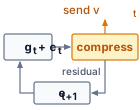
Error-feedback loop: a box g t plus e t feeds an amber compress box, which sends v t upward; the residual e t plus 1 returns to the first box for the next step.

Error feedback carries the residual into the next compressed step.

Definition 5.3: Error feedback mechanism

Error feedback is a distributed-training technique for gradient compression that maintains a per-worker residual accumulator \(\ErrorFeedbackResidual_t\), re-injecting the compression error back into the next gradient update so that information omitted from the transmitted update remains in the residual. A finite run can end with an untransmitted residual.

  1. Significance: Top-k sparsification at 1 percent keeps only the largest 1 percent of gradient values by magnitude, reducing each worker’s retained value payload from 140 GB to 1.4 GB for a full 70B gradient, a 100\(\times\) reduction before sparse-index and aggregation overhead. Without error feedback, the discarded 99 percent of gradient values create a biased update that can harm convergence. With error feedback, omitted information remains in the residual and can influence later selections, supporting the convergence guarantees analyzed for memory/error-feedback variants under their assumptions (Stich et al. 2018; Karimireddy et al. 2019).
  2. Distinction: Unlike plain lossy compression, which permanently discards sub-threshold gradient components, error feedback delays their transmission. A component too small to send in one step stays in the residual and can influence later transmitted updates as it accumulates; a finite run may still end with an untransmitted residual.
  3. Common pitfall: A frequent misconception is that error feedback is automatic whenever a compressor is used. It is not: the training system must explicitly preserve and reinject the residual. Without that residual path, Top-k and 1-bit quantization introduce systematic bias that can accumulate across steps (Karimireddy et al. 2019).

Error feedback preserves cumulative gradient information over time. Consider what happens over \(\TrainingStepCount\) steps:

\[\sum_{t=1}^{\TrainingStepCount} \CompressedGradientUpdate_t = \sum_{t=1}^{\TrainingStepCount} \left[(\LocalGradient_t + \ErrorFeedbackResidual_t) - \ErrorFeedbackResidual_{t+1}\right] = \sum_{t=1}^{\TrainingStepCount} \LocalGradient_t + \ErrorFeedbackResidual_1 - \ErrorFeedbackResidual_{\TrainingStepCount+1}\]

If the error accumulator remains bounded under the chosen compressor and training assumptions, then as \(\TrainingStepCount\to \infty\):

\[\frac{1}{\TrainingStepCount}\sum_{t=1}^{\TrainingStepCount} \CompressedGradientUpdate_t \to \frac{1}{\TrainingStepCount}\sum_{t=1}^{\TrainingStepCount} \LocalGradient_t\]

Under that bounded-residual condition, the difference between the two averages vanishes. At a finite stopping point, untransmitted information remains in the residual. Repeated small gradients can accumulate in \(\ErrorFeedbackResidual_t\) until they exceed the compression threshold, as the worked trace illustrates.

The telescoping property of compression error across time is why error feedback can transform a biased compressor into a convergent training method. Theoretical analyses show convergence guarantees for sparsified SGD with memory and for EF-SGD with broad compression operators under their stated assumptions (Stich et al. 2018; Karimireddy et al. 2019). A rounding compressor with no residual path shows what is lost without that memory (table 10). It transmits each value rounded to the nearest whole unit, so any value below 0.5 is sent as zero.

Table 10: Naive Compression Trace (No Error Feedback): Five-step worked trace showing how a rounding compressor transmits zero whenever an individual gradient falls below 0.5.
Step True gradient \(\LossGradient_t\) Transmitted \(\CompressedGradientUpdateElement_t\) Cumulative transmitted Cumulative true
1 0.4 0 0 0.4
2 0.3 0 0 0.7
3 0.2 0 0 0.9
4 0.4 0 0 1.3
5 0.3 0 0 1.6

A residual accumulator \(\ErrorFeedbackResidual_t\) that re-injects the discarded remainder into the next step changes the outcome of the same sequence (table 11). Instead of vanishing at each rounding step, the fractional updates accumulate locally until they cross the transmission threshold.

Table 11: Error-Feedback Compression Trace: Same five-step sequence under error-feedback compression.
Step \(\LossGradient_t\) \(\ErrorFeedbackResidualElement_t\) \(\LossGradient_t + \ErrorFeedbackResidualElement_t\) \(\CompressedGradientUpdateElement_t\) \(\ErrorFeedbackResidualElement_{t+1} = (\LossGradient_t + \ErrorFeedbackResidualElement_t) - \CompressedGradientUpdateElement_t\) Cumulative \(\CompressedGradientUpdateElement\)
1 0.4 0 0.4 0 0.4 0
2 0.3 0.4 0.7 1 −0.3 1
3 0.2 −0.3 −0.1 0 −0.1 1
4 0.4 −0.1 0.3 0 0.3 1
5 0.3 0.3 0.6 1 −0.4 2

Example 5.2: Error feedback mechanism
Scenario: A gradient compression pipeline rounds each gradient value to the nearest whole unit before transmission, so values below 0.5 are sent as zero, over 5 training steps of distributed data-parallel training.

Diagnosis: Naive rounding (table 10) discards every value below 0.5, transmitting 0 when the true cumulative gradient is 1.6 (100 percent gradient loss). With error feedback (table 11), the residual grows until it crosses 0.5 and is sent, so the run transmits 2 and ends holding −0.4 in the residual. Transmitted plus residual, 2 + (−0.4), equals the true total of 1.6.

Systems lesson: The trace illustrates how error feedback carries omitted information into later updates. By storing untransmitted residual vectors in local accelerator memory (\(\ErrorFeedbackResidual_{t+1} = \LocalGradient_t + \ErrorFeedbackResidual_t - \CompressedGradientUpdate_t\)), repeated small contributions can accumulate until they cross the transmission threshold. The trace demonstrates the residual mechanism; convergence still depends on the compressor and optimizer assumptions.

5.9.4 1-bit Adam compression-aware optimization

Compressing raw gradients works cleanly for stochastic gradient descent, where the parameter update is linear in the gradient, but adaptive optimizers such as Adaptive Moment Estimation (Adam) divide the first moment (momentum) by the square root of a running second-moment (variance) estimate, so compression noise in the raw gradient distorts that nonlinear denominator and can destabilize training. Microsoft’s DeepSpeed team observed that Adam’s second-moment estimate stabilizes early in training even while momentum continues to evolve (Tang et al. 2021). Rather than compressing raw gradients on every step, 1-bit Adam runs standard full-precision Adam during an initial warmup phase until the variance estimate settles, freezes that variance tensor as a fixed adaptive preconditioner, and then switches to a communication-efficient phase in which workers communicate only the momentum using 1-bit compression (sign plus a scaling factor) while retaining each compression residual locally for the next step.

Because the frozen preconditioner is no longer perturbed by quantization noise and the local residual feeds omitted momentum back into subsequent messages, the method controls accumulated compression error and preserves Adam’s convergence trajectory without requiring each 1-bit message to be an unbiased estimator. Across experiments up to 256 GPUs, Tang et al. (2021) report up to 5\(\times\) end-to-end communication-volume reduction—smaller than the raw 32\(\times\) ratio of 1-bit values to FP32 momentum because the uncompressed warmup and other communication costs are included—while matching the convergence speed of uncompressed Adam and achieving up to 3.3\(\times\) higher throughput for BERT-Large pretraining and up to 2.9\(\times\) higher throughput for Stanford Question Answering Dataset (SQuAD) fine-tuning. Designing the compressor around the optimizer’s internal state thus succeeds where replacing every raw gradient with its sign would fail, provided the compression overhead remains small compared with the communication time saved.

5.9.5 Bandwidth versus convergence trade-offs in compression

Gradient compression is not free; it trades reduced communication for increased variance or bias in the optimization process. The comparison in table 12 summarizes the source-backed patterns from quantization, sparsification, error-feedback, and optimizer-aware compression work (Seide et al. 2014; Aji and Heafield 2017; Lin et al. 2018; Stich et al. 2018; Karimireddy et al. 2019; Tang et al. 2021).

Seide, Frank, Hao Fu, Jasha Droppo, Gang Li, and Dong Yu. 2014. “1-Bit Stochastic Gradient Descent and Its Application to Data-Parallel Distributed Training of Speech DNNs.” Interspeech 2014, 1058–62. https://doi.org/10.21437/interspeech.2014-274.
Aji, Alham Fikri, and Kenneth Heafield. 2017. “Sparse Communication for Distributed Gradient Descent.” Proceedings of the 2017 Conference on Empirical Methods in Natural Language Processing, 440–45. https://doi.org/10.18653/v1/d17-1045.
Lin, Yujun, Song Han, Huizi Mao, Yu Wang, and William J Dally. 2018. “Deep Gradient Compression: Reducing the Communication Bandwidth for Distributed Training.” International Conference on Learning Representations (ICLR).
Stich, S. U., J.-B. Cordonnier, and M. Jaggi. 2018. “Sparsified SGD with Memory.” Advances in Neural Information Processing Systems 31.
Karimireddy, Sai Praneeth, Quentin Rebjock, Sebastian U. Stich, and Martin Jaggi. 2019. “Error Feedback Fixes SignSGD and Other Gradient Compression Schemes.” Proceedings of the 36th International Conference on Machine Learning (ICML), Proceedings of machine learning research, vol. 97: 3252–61.
Tang, Hanlin, Shaoduo Gan, Ammar Ahmad Awan, Samyam Rajbhandari, Conglong Li, Xiangru Lian, Ji Liu, Ce Zhang, and Yuxiong He. 2021. “1-Bit Adam: Communication Efficient Large-Scale Training with Adam’s Convergence Speed.” Proceedings of the 38th International Conference on Machine Learning (ICML), Proceedings of machine learning research, vol. 139: 10118–29.
Table 12: Gradient Compression Methods: Encoded-payload ratios relative to an FP32 payload, as the literature quotes them, and relative to the BF16 payload this chapter’s examples use. Top-k assumes FP32 values and 32-bit indices in both columns; quantization scales and other metadata reduce the stated upper bounds. No method has a fixed convergence penalty across workloads. The right choice depends on whether bandwidth or convergence speed is the binding constraint; evaluate the complete time to the same quality target, including encoding and any additional training steps.
Method Ratio vs. FP32 Ratio vs. BF16 Convergence impact Best use case
FP16 2\(\times\) 1\(\times\) (none) Check range and numerical stability Common accelerator baseline
INT8 + Error FB At most 4\(\times\) At most 2\(\times\) Workload- and scaling-dependent Bandwidth-constrained clusters
Top-k (1%) + Error FB At most 50\(\times\) At most 25\(\times\) Depends on sparsity and residual control Cross-data-center training
1-bit + Error FB At most 32\(\times\) At most 16\(\times\) Requires compression-aware optimization Extreme bandwidth constraints

Decision criteria for gradient compression

The decision rule is not the compression ratio alone. Compression is worthwhile only when the wall-clock time it saves across the run exceeds its encoding overhead plus the cost of any extra steps that slower convergence requires, so the comparison must be made in time to the same quality target. A high communication-computation ratio \(\CommunicationComputeRatio= \CommunicationTime(\DeviceCount)/(\IronLawComputeTime/\DeviceCount)\), which compares communication time with ideally partitioned compute time and separates compute-bound from communication-bound clusters (The communication-computation ratio), creates an opportunity when that communication is exposed on the critical path. The compressor and optimizer analysis must establish how bias or variance is controlled, including whether error feedback is required; convergence tests then check that the chosen configuration reaches the target.

The first test is per synchronization. Compression shrinks only the byte term, so it helps a payload above \(\LatencyBandwidthCrossoverSize\), such as a full gradient or a large bucket, and does little for one below it, whose startup term remains (section 5.5). Even above \(\LatencyBandwidthCrossoverSize\), encoding must cost less than the transfer time it removes.

Napkin Math 5.7: The payback of compression
Problem: A training job takes 40 ms to synchronize a gradient buffer. A compression scheme shrinks the payload, but after scale factors, metadata, and protocol overhead its assumed effective throughput gain is 8×, and encoding and decoding add 2 ms of accelerator time per synchronization. Does compression shorten the synchronization, and by how much?

Math:

  1. Compressed communication time: 40 ms divided by the effective factor 8 = 5 ms.
  2. Total new time: 5 ms (comm) + 2 ms (overhead) = 7 ms.
  3. Effective speedup: 40 ms divided by 7 ms \(\approx\) 5.7×.

Systems insight: Compression is a trade of compute for bandwidth. With compression ratio \(\CompressionRatio\) and encoding cost \(\CodecOverheadTime\), it pays off only when \(\CodecOverheadTime< \CommunicationTime(\DeviceCount) \times (1 - 1/\CompressionRatio)\), that is, when encoding costs less than the communication time it removes. In this case, spending 2 ms to save 35 ms of network time is a clear win. On a high-speed NVLink network where \(\CommunicationTime(\DeviceCount)\) is only 1 ms, the same compression logic would cost more than it saves and slow down training. Always profile the network before adding compression.

The second test spans the full training run, because a compressor that passes the per-step test can still lose once slower convergence adds iterations. Comparing total wall-clock time to the same quality target on a slow and a fast network shows how a modest step-count penalty can reverse the verdict.

Suppose a training run requires 100,000 steps to reach its quality target without compression, with each step taking 500 ms (300 ms compute and 200 ms communication), for a total of 50,000 s. INT8 compression with error feedback of an FP32 payload reduces communication by 4× (from 200 ms to 50 ms per step), but suppose it raises the required steps by 10 percent, to 110,000. The new total is 110,000 steps at 350 ms each, or 38,500 s, a 23 percent improvement. Compression wins here because the per-step saving of 150 ms outweighs the additional steps.

The same model on a faster network, where communication takes only 30 ms per step, reverses the verdict. Compression cuts that to 7.5 ms, saving 22.5 ms per step, but still adds 10,000 steps at 307.5 ms each. The run now takes 33,825 s instead of 33,000 s, 2.5 percent longer. In this serial compute-plus-communication model, the break-even value of \(\CommunicationComputeRatio\) depends on the assumed compression ratio and extra steps, with no separate encoding cost included. A training schedule with overlap must instead compare the exposed time saved against encoding and convergence costs. Scheduling transfers during independent computation offers another way to reduce that exposed time.

Checkpoint 5.4: Gradient compression decisions

Verify your understanding of when and how to apply gradient compression:

Self-Check: Question
  1. A distributed training team applies Top-k sparsification with \(K_{\text{top}} = 0.001 \times d_{\text{grad}}\) (retaining 0.1% of elements) to FP32 gradients (\(d_{\text{grad}}\) elements at 4 bytes each). Transmitting the sparse gradient requires sending both FP32 values (4 bytes) and INT32 index locations (4 bytes) for each surviving element. What is the realized compression ratio compared to the dense FP32 gradient baseline?

    1. \(500\times\), because each kept element requires 8 bytes (value plus index), yielding an encoded payload of \(8 \times 0.001 d_{\text{grad}} = 0.008 d_{\text{grad}}\) bytes compared to the \(4 d_{\text{grad}}\) dense baseline.
    2. \(1000\times\), because index encoding overhead is completely eliminated by the network interface hardware.
    3. \(100\times\), because the error-feedback accumulator doubles the size of the transmitted index buffer.
    4. \(32\times\), because sparse tensors automatically conform to 1-bit quantization limits.
  2. Why is the Error Feedback mechanism (\(e_{t+1} = g_t + e_t - v_t\)) mathematically essential when applying aggressive lossy compression (such as 1-bit SGD or Top-k sparsification) in distributed training?

    1. It dynamically recompiles CUDA backward kernels to eliminate all register spills during gradient calculation.
    2. It converts AllReduce operations into asynchronous point-to-point transfers to bypass network switch buffers.
    3. It forces all model weights to remain strictly positive throughout optimization.
    4. It preserves deferred residuals, so average transmitted and original updates differ by \((e_1-e_{K+1})/K\), which vanishes if the residual grows sublinearly.
  3. How does 1-bit Adam achieve high compression ratios on optimizer state communication without suffering the severe convergence degradation of naive 1-bit SGD?

  4. True or False: Applying \(4\times\) gradient quantization will always decrease end-to-end training step time because reducing communication payload bytes is unconditionally beneficial regardless of whether the cluster is in a compute-bound or communication-bound regime.

  5. Describe the two phases of 1-bit Adam and the dependency that connects each compressed momentum message to the next residual-corrected update. Does residual storage have to wait for network transmission to finish?

See Answers →

5.10 Communication-Computation Overlap

Even with hierarchical routing and gradient compression, waiting until the entire backward pass finishes before launching AllReduce leaves every GPU idle across the full transfer window before the optimizer can update the weights. Communication-computation overlap hides that stall by running transfers concurrently with independent backward-pass computation, attacking the communication time that algorithm selection and compression leave exposed. How much of a transfer can be hidden depends on which parts of that transfer occupy the processor and which occupy only the network.

5.10.1 The LogP model of what overlap can hide

The α-β model estimates transfer duration without specifying how much independent computation can proceed during that transfer. Adding the entire estimate to compute time therefore overstates step time when overlap is possible. The LogP model (Culler et al. 1993) separates network transit from processor involvement with four parameters:

Culler, David, Richard Karp, David Patterson, Abhijit Sahay, Klaus Erik Schauser, Eunice Santos, Ramesh Subramonian, and Thorsten von Eicken. 1993. “LogP: Towards a Realistic Model of Parallel Computation.” ACM SIGPLAN Notices 28 (7): 1–12. https://doi.org/10.1145/173284.155333.
  • \(\LogpNetworkLatency\) (latency): The time for a message to traverse the network (similar to \(\MessageStartupLatency\)).
  • \(\SymmetricMessageOverhead\) (overhead): The processor time spent initiating or completing a transfer. During this work, the same execution resource cannot compute, making \(\SymmetricMessageOverhead\) the nonoverlappable cost. In a distributed training context, dispatch, device-kernel launch, memory registration, and runtime progress can all contribute. The value is an effective parameter of a particular software and hardware path, so it must be measured with the same collective, process group, and topology used by the workload.
  • \(\MessageInjectionGap\) (gap): The minimum spacing between consecutive sends or consecutive receives at a processor. It limits endpoint message rate but does not describe every source of link contention in a routed fabric.
  • \(\DeviceCount\) (rank count): The number of ranks in the communication group. The original model names this processor count with its final letter, P; this chapter writes it \(\DeviceCount\) to match its other collective cost formulas.

LogP distinguishes network latency (\(\LogpNetworkLatency\), which can be hidden) from processor overhead (\(\SymmetricMessageOverhead\), which cannot). Independent computation can overlap the network transit interval, while initiation and completion overhead remain exposed on the execution resource that performs them.

Napkin Math 5.8: Hiding communication behind computation
Problem: A training pipeline attempts to overlap gradient AllReduce with the next layer’s backward pass. The backward pass takes 500 μs. Represent the complete transfer by a toy budget with network time 100 μs, processor overhead \(\SymmetricMessageOverhead=\) 50 μs to initiate, and \(\SymmetricMessageOverhead=\) 50 μs to receive. Assume both overhead intervals occupy the same execution resource as backward computation, with independent network progress and no contention. Can the communication be hidden under these assumptions?

Math:

  1. Overlappable portion: Network latency \(\LogpNetworkLatency\) = 100 μs (data in flight while GPU computes).
  2. Non-overlappable portion: \(2\SymmetricMessageOverhead\) = 100 μs (GPU busy initiating/receiving).
  3. Compute available: 500 μs.
  4. Hidden: All 100 μs of \(\LogpNetworkLatency\) can overlap with compute.
  5. Exposed: The 100 μs of \(2\SymmetricMessageOverhead\) overhead cannot overlap.

Result: Effective time is 100 μs + max(500 μs, 100 μs) = 600 μs. The network latency is hidden, but the processor overhead remains exposed. Applied to every layer of a backward pass, the same split determines which gradient transfers a training step can hide.

Systems insight: The α-β model captures the total communication time. The LogP model reveals how much of it can be hidden. When designing pipelined training, optimize for low \(\SymmetricMessageOverhead\) (kernel bypass, GPUDirect) rather than high \(\LinkBandwidth\) alone.

The \(\MessageStartupLatency\)-\(\LinkBandwidth\) model estimates transfer duration from latency and bandwidth measurements. LogP adds the processor/network distinction needed to estimate exposed delay in pipelined execution. Choosing a communication schedule therefore requires both a transfer budget and the independent computation available to overlap it.

When messages are large and pipelined across the network, the LogGP model (Alexandrov et al. 1995) extends LogP with a gap-per-byte parameter \(\LongMessageGapPerByte\), modeling the streaming cost of long messages. These models describe multiprocessor communication with endpoint rate and capacity limits; they are not restricted to one flow on one link. Their compact parameters do not explicitly represent every shared path, oversubscribed cut, or routing hotspot. For congestion-sensitive workloads, particularly AllToAll for MoE, measurements on the target placement must test whether the model captures the active bottleneck.

Alexandrov, Albert D., Mihai F. Ionescu, Klaus E. Schauser, and Chris J. Scheiman. 1995. “LogGP: Incorporating Long Messages into the LogP Model—One Step Closer Towards a Realistic Model for Parallel Computation.” Proceedings of the Seventh Annual ACM Symposium on Parallel Algorithms and Architectures - SPAA ’95 30: 95–105. https://doi.org/10.1145/215399.215427.

↪ The LogGP long-message cost model and its gap parameters are developed in The LogGP model extension.

5.10.2 Layer-by-layer overlap

Gradient computation during the backward pass proceeds layer by layer, from the output layer back to the input layer. The gradient for layer \(\ell\) is available as soon as that layer’s backward pass completes, even while layers \(\ell-1, \ell-2, \ldots\) are still computing. That ordering lets the gradient for layer \(\ell\) start communicating immediately while the GPU computes the gradient for layer \(\ell-1\). Over a four-layer backward pass, the transfers for layers 4 through 2 run beneath later backward work, and only the transfer for layer 1, which becomes ready last, is left exposed before the optimizer step (figure 10).

In PyTorch’s DistributedDataParallel, this overlap is implemented through gradient hooks. Each parameter registers a hook that marks its gradient ready. Once all required gradients in a bucket are ready, the reducer can launch an asynchronous AllReduce, preserving the same collective order across ranks. Meanwhile, the backward pass continues computing gradients for earlier layers. A transfer is hidden only if it completes before its result is needed; queued communication can consume part of that window, and the last bucket’s transfer remains exposed (section 5.10.4).
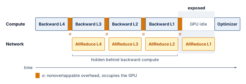
Figure 10: Communication-Computation Overlap: The backward pass runs from the last layer to the first, and each layer’s gradient AllReduce launches as soon as that layer finishes, so it runs on the network while the GPU computes the next layer’s gradients. The first layer finishes last and has no computation left to hide behind, so its AllReduce is exposed before the optimizer step. Overlap succeeds only when the nonoverlappable overhead (\(\SymmetricMessageOverhead\)) is small, leaving the bulk transfer free to proceed concurrently. Durations are schematic.

The effectiveness of this overlap depends on the relative sizes of computation and communication at each layer. For transformer models, the largest gradient tensors belong to the attention and feed-forward weight matrices, which are also the most computationally expensive layers. That computation cannot hide the same layer’s gradient transfer, because the gradient is ready only afterward. It can hide a previously launched transfer; the ordering and cost of the remaining layers determine each gradient’s overlap window.

The overlap strategy interacts with algorithm choice from section 5.6 and section 5.7. An isolated-collective crossover need not predict the best training-step schedule, because the dependency schedule determines how much of each candidate’s transfer time is exposed. Overlap with the backward pass can reduce Ring’s exposed latency penalty, but the benefit must be measured with the actual gradient-ready times and runtime progress behavior. The optimizer step still cannot begin until every required reduction completes, so the transfers of the last layers processed, those closest to the input, stay exposed.

5.10.3 Bucket fusion

The layer-by-layer overlap described in section 5.10.2 assumes that each layer’s gradient is communicated as a single message. In reality, a transformer layer contains dozens of individual parameter tensors (query, key, value projection matrices, output projection, layer norm parameters, feed-forward weights, and biases). Launching a separate AllReduce for every individual parameter would create thousands of small-message collectives, each paying the full \(\CollectiveCallStartupLatency\) overhead. To avoid this, DDP uses bucket fusion to group parameters into buckets (often configured around tens of megabytes, with 25 MB a common PyTorch reference point) and launches one AllReduce per bucket. The bucket size represents a trade-off: larger buckets amortize \(\CollectiveCallStartupLatency\) overhead but delay the start of communication (because the bucket cannot be sent until all its parameters have computed gradients). Smaller buckets start communication earlier but pay more \(\CollectiveCallStartupLatency\) overhead.

The optimal bucket size depends on gradient-ready times, tensor sizes, and network characteristics. Smaller buckets can start communication sooner when waiting for more gradients would consume the overlap window. Larger buckets can amortize startup when repeated small transfers dominate. Neither choice follows from the model family alone; the useful measure is the resulting training-step time, including the exposed final transfer. PyTorch’s bucket_cap_mb parameter in DDP allows tuning this trade-off.

Bucket membership also determines how early communication can begin. A bucket containing one late gradient must wait even if its other gradients are ready. DDP can use reverse parameter registration order as an approximation to backward readiness and, depending on configuration, rebuild buckets from the observed backward order. Registration order need not match forward execution order, especially in models with branches or reused parameters. Grouping gradients that become ready together helps preserve the overlap window while maintaining a consistent collective sequence across ranks.

5.10.4 Overlap limits and exposed communication

Communication-computation overlap has fundamental limits. The LogP model’s overhead parameter \(\SymmetricMessageOverhead\) represents processor time consumed by initiating or completing transfers. In the simplified LogP budget, initiation and completion consume \(2\SymmetricMessageOverhead\) per operation on the participating execution resource. When backward compute intervals are short relative to that overhead, hiding network transit may save time while leaving processor overhead as the dominant cost.

The pipeline also has boundary effects. During the first backward computation, no gradient from this pass is ready to communicate. Once the output-side gradient is ready, however, its communication can overlap with the remaining backward work. At the other end, the input-side gradient has no subsequent backward computation to hide its transfer. More layers create a longer overlap window, but depth alone does not guarantee high coverage: if communication takes longer than each compute interval, a backlog remains even in a deep model.

A third limitation arises from memory pressure. Buffers used by an in-flight transfer must remain valid while independent computation produces or consumes other tensors. Their overlapping lifetimes can increase peak GPU memory use, although views and buffer reuse can avoid separate copies. For FSDP workloads, prefetching parameters can keep multiple materialized groups resident at once, trading memory savings for communication overlap. The engineering challenge is to hide transfers within the available memory budget, and FSDP’s prefetch and resharding policies are the controls that set this trade-off.

Together, processor overhead, boundary stalls, and per-layer transfer time determine how much of a collective schedule can hide behind backward computation. Pricing a realistic 32-layer transformer backward pass shows how much communication remains exposed when each layer’s reduction outlasts its compute window.

Napkin Math 5.9: Overlap budget for a 7B transformer
Problem: A 32-layer transformer model (7B parameters) is trained on 64 GPUs. Assume the data-parallel reducer communicates FP32 gradients, about 875 MB per layer, in 100 MB buckets, four times the common 25 MB default. Each layer’s backward pass takes 15 ms. Assume the cluster achieves 3 ms per bucket under its contention and protocol overheads, so each layer’s gradients take 27 ms, and assume equal layers and the same charge for the final partial bucket. What is the backward-plus-communication time with and without overlap?

Without overlap (sequential):

\(\SequentialBackwardCommunicationTime= \BackwardPassTime+ \CommunicationTime(\DeviceCount)\) = 480 ms + 32 \(\times\) 27 ms = 1344 ms.

With overlap (pipelined):

Each layer’s AllReduce (27 ms) runs in parallel with the next layer’s backward pass (15 ms). Since 27 ms > 15 ms, there is 12 ms of exposed communication per layer that cannot be hidden.

Communication runs back to back from the moment the output layer’s gradients are ready. Each later reduction overruns its backward window by the exposed amount, so the backlog grows by that much per layer, and the last reduction adds its full duration after the backward pass ends:

\(\OverlappedBackwardCommunicationTime= \BackwardPassTime+ \LayerAllReduceTime+ (\LayerCount - 1) \times \LayerExposedCommunicationTime\) = 879 ms.

Systems insight: Overlap reduces backward-plus-communication time by 34.6 percent. The remaining exposed communication comes from the AllReduce being slower than the per-layer backward pass. To reduce the backlog, either lengthen the independent compute window (for example, with a larger batch) or reduce AllReduce time. The final gradient still has an exposed transfer tail, and any change must preserve the intended training workload and quality target. The overlap is most effective when per-layer backward compute exceeds the reduction time (\(\LayerBackwardTime > \LayerAllReduceTime\)).

The verdict turns on the assumed per-bucket charge. The hierarchical model of notebook 5.4 prices one uncontended 100 MB bucket on these eight nodes at about 0.85 ms, or 7.6 ms per layer, inside the 15 ms backward window, so at that rate every transfer except the last would hide. An overlap budget is therefore only as good as its achieved per-bucket time, which the calibration of section 5.11.2 measures rather than assumes.

An overlap budget joins the collective’s transfer cost to the model’s dependency schedule. Realizing that budget requires a runtime whose asynchronous progress and device-memory path preserve the independent work available between gradient production and consumption.

Self-Check: Question
  1. In a toy overlap budget, independent computation takes \(600\,\mu\text{s}\) and the complete network interval takes \(200\,\mu\text{s}\). Initiation and completion each cost \(50\,\mu\text{s}\) on the same execution resource as that computation. Assume independent network progress and no contention. What is the effective elapsed time, and which component remains exposed?

    1. Effective time is \(600\,\mu\text{s}\), and communication is 100% hidden because \(L_{\text{lat}} < T_{\text{compute}}\).
    2. Effective time is \(800\,\mu\text{s}\), because network latency and processor overhead must both be added directly to compute time.
    3. Effective time is \(750\,\mu\text{s}\), because the gap parameter \(g\) adds an irreducible stall to the compute pipeline.
    4. Effective time is \(700\,\mu\text{s}\) (\(2o + \max(T_{\text{compute}}, L_{\text{lat}})\)), where the \(200\,\mu\text{s}\) network latency is completely hidden behind the \(600\,\mu\text{s}\) compute, but the \(100\,\mu\text{s}\) of processor overhead (\(2o\)) remains exposed.
  2. True or False: In the stated toy LogP budget with independent work, network progress, and no contention, upgrading a network fabric to achieve lower physical wire latency (\(L_{\text{lat}}\)) will not reduce step time if the overlapped computation window \(T_{\text{compute}}\) already exceeds \(L_{\text{lat}}\) and the nonoverlappable processor overhead \(o\) remains unchanged.

  3. In PyTorch DistributedDataParallel (DDP), how does bucket fusion balance the trade-off between communication startup latency (\(\alpha\)) and the compute-communication overlap window?

    1. Grouping multiple parameter gradients into a bucket amortizes per-collective startup overhead, but the bucket must wait until all required gradients are ready, reducing the available overlap window.
    2. Bucket fusion compresses all gradient tensors into 8-bit integers before allocating them to ring communication buffers.
    3. Bucket fusion permanently disables all gradient hooks and forces all communication to occur after optimizer step completion.
    4. Bucket fusion ensures that all layers in the transformer model have mathematically identical parameter counts.
  4. In the illustrative 32-layer, 7B-parameter FP32 gradient budget, each equal layer has 875 MB of gradients. Charging nine 100 MB buckets at 3 ms each gives 27 ms of communication per layer, while backward compute takes 15 ms. Under a single serialized communication stream, calculate total backward-plus-communication time with and without overlap and explain the exposed tail.

  5. Explain the startup and drain boundaries of bucketed backpropagation that limit communication-computation overlap even when intermediate layers hide communication successfully.

  6. Why can one late gradient delay a DDP bucket whose other gradients are ready? Explain how parameter registration order and observed backward readiness can guide bucket membership without guaranteeing an optimal overlap schedule.

See Answers →

5.11 Communication Libraries and Runtimes

An overlap schedule only works if the communication backend can move the required tensors while independent computation proceeds. Production libraries realize the same algorithms and schedules, so the engineering decision is which one preserves the chapter’s model, topology, and overlap assumptions on the target hardware.

5.11.1 Backend selection

A collective runtime that bounces GPU tensors through host DRAM over PCIe or ignores NVLink and rail topology can cut effective reduction bandwidth by an order of magnitude even when it implements the right ring or tree schedule. Four properties therefore separate communication backends in practice: the device memory path, topology awareness, portability, and observability. NCCL leads on the first two for NVIDIA GPUs because it executes the collective algorithms of section 5.6 and section 5.7 directly on GPU-resident buffers (Jeaugey 2017; NVIDIA 2026): its kernel fusion combines reduction arithmetic with data movement so intermediate results do not bounce back to HBM, while GPUDirect RDMA lets the network card read and write GPU memory directly over PCIe without staging payloads through host DRAM. To keep multiple links busy at once, channel pipelining splits each collective across parallel communication channels, though realized throughput still depends on NIC placement, routing, and contention because extra channels cannot create port capacity. Documented environment variables then expose these choices for observability, with NCCL_ALGO and NCCL_PROTO inspecting or overriding the selected algorithm and protocol and NCCL_DEBUG reporting the active topology, channels, and schedule (NVIDIA 2026).

Message Passing Interface Forum. 2015. MPI: A Message-Passing Interface Standard, Version 3.1.

MPI matters when portability, CPU-side coordination, or HPC integration is the binding requirement (Message Passing Interface Forum 2015), and two of its features bear directly on overlap. Non-blocking collectives such as MPI_Iallreduce return a request handle that the application tests or waits on, a completion model different from NCCL’s ordering on CUDA streams. Persistent collectives, introduced in MPI 4.0, initialize an operation once and activate it at every step, amortizing setup for a training loop that repeats the same AllReduce shape. Either model hides a transfer only when independent work exists and the runtime makes progress. MPI’s one-sided communication (MPI_Put, MPI_Get, MPI_Accumulate) maps onto RDMA hardware and suits asynchronous designs in which one process writes another’s memory without its participation. CUDA-aware MPI implementations accept GPU pointers, but the selected transport decides whether data still passes through host memory, so that path must be benchmarked against NCCL.

Portability is the strength of Gloo, a PyTorch backend for CPU tensors, development, and testing whose TCP transport exercises collective semantics on one machine before a job reaches an accelerator cluster. Whether a faster shared-memory transport is active must be measured rather than assumed. Other accelerators have their own backends, AMD’s RCCL for the ROCm stack and Intel’s oneCCL, because the same algorithm has different effective \(\MessageStartupLatency\), \(\LinkBandwidth\), and topology constraints on each platform. PyTorch’s torch.distributed routes each call to the backend its process group names, so teams often mix them, with NCCL reducing gradients in a GPU group while a CPU group uses Gloo for barriers, scalar broadcasts, or sampler state. Applied to common scenarios, the four properties select a library, or a pairing of libraries, for each (table 13).

Table 13: Communication Library Selection: Choose based on hardware and workload requirements. Many NVIDIA GPU training deployments use NCCL; Gloo serves as a portable fallback.
Scenario Recommended library Rationale
Multi-GPU training (NVIDIA) NCCL GPUDirect, kernel fusion, NVLink-aware
CPU-only distributed training Gloo or MPI Mature CPU optimizations
Development/debugging Gloo Cross-platform, no CUDA dependency
Mixed vendor GPUs Vendor-specific groups; validate cross-group path NCCL, RCCL, and oneCCL are vendor-specific
HPC integration MPI + NCCL MPI for job launch, NCCL for GPU collectives

The table follows from the chapter’s cost model. A backend’s memory path and topology choices determine how it uses the fabric, and its diagnostic signals help identify whether \(\MessageStartupLatency\), \(\LinkBandwidth\), or processor overhead limits the job, but the resulting performance must still be measured with the workload’s collective and placement.

5.11.2 Calibrating collective communication models

The bandwidth-latency trade-off (principle 5) provides useful first-order predictions, but a valid comparison must model the same collective that the benchmark executes. For a ring AllReduce over \(\DeviceCount\) ranks and an \(\CollectivePayloadSize\)-byte tensor, the first-order cost is \(2(\DeviceCount-1)\MessageStartupLatency+ 2(\DeviceCount-1)\CollectivePayloadSize/(\DeviceCount\LinkBandwidth)\), not the point-to-point expression \(\MessageStartupLatency+\CollectivePayloadSize/\LinkBandwidth\). A tree, a hierarchical schedule, and a switch-assisted reduction have different step counts and traffic factors. NCCL also selects protocols, channels, and algorithms according to message size and detected topology, so those choices become part of the experimental condition (Jeaugey 2017; NVIDIA 2026).

NVIDIA. 2026. NCCL User Guide.

A calibrated collective model therefore records the operation, reduction datatype, rank count, tensor size, algorithm and protocol, topology, rank placement, and achieved bus bandwidth. It then fits effective \(\MessageStartupLatency\) and \(\LinkBandwidth\) to measurements from that same configuration, as The \MessageStartupLatency-\LinkBandwidth performance model does for one measured NCCL AllReduce. Comparing predicted and observed time under this contract reveals software overhead or topology loss without mistaking a collective’s algorithmic traffic factor for library inefficiency. The resulting parameters apply only to the measured regime; changing the collective, process group, topology, or library version requires recalibration. A calibrated model selects a collective schedule and sizes its overlap window; attributing an observed training-step regression to kernels, memory, communication, or contention is a broader measurement task, which the program goodput analysis of Program Goodput develops.

Communication diagnosis begins by comparing the workload against a matched bare-collective baseline and recording the selected algorithm, protocol, rank placement, and achieved bandwidth. A healthy baseline with a slow training step points to invocation granularity, contention, stragglers, or insufficient overlap rather than the fabric alone. Profiler traces and the attribution workflow separate those causes; the output needed here is the calibrated \(\MessageStartupLatency\), \(\LinkBandwidth\), and overlap window that select a collective schedule.

The backend must satisfy both the collective contract and the measured execution budget. A fast isolated collective is insufficient when its placement, invocation order, or progress behavior leaves the training step waiting.

Self-Check: Question
  1. Which mechanisms make NCCL a useful candidate for GPU-resident collective communication on NVIDIA clusters?

    1. NCCL runs all collective communication on host CPU threads using OpenMP parallel loops.
    2. NCCL combines supported GPUDirect paths, fused reduction and data movement, and parallel channels with topology-aware placement.
    3. NCCL eliminates all network synchronization barriers by approximating gradient additions as stochastic random walks.
    4. NCCL replaces InfiniBand hardware with standard TCP/IP operating system sockets.
  2. An ML engineering team is setting up distributed training across three environments: (1) local developer laptops running macOS for unit testing, (2) an HPC cluster using Slurm where legacy CPU nodes perform data preprocessing, and (3) an 8-node NVIDIA H100 cluster for large-scale model pretraining. According to the chapter library selection guide, which backend mapping is recommended?

    1. NCCL for macOS development, NCCL for CPU preprocessing, and Gloo for H100 training.
    2. MPI for macOS development, NCCL for CPU preprocessing, and Gloo for H100 training.
    3. Gloo for macOS development (cross-platform portability without CUDA), MPI for CPU preprocessing (mature CPU optimizations), and NCCL for H100 multi-GPU training (GPUDirect RDMA and NVLink awareness).
    4. Gloo for all three environments because a single unified backend always outperforms specialized hardware libraries.
  3. When debugging a multi-node distributed training job that runs at 50% of expected throughput, what diagnostic information does running nccl-tests provide compared to profiling the PyTorch training loop directly?

  4. True or False: Setting the environment variable NCCL_DEBUG=INFO modifies the mathematical reduction operator in NCCL from floating-point summation to exact integer bitwise addition to guarantee deterministic gradient aggregation across runs.

  5. Sequence the hierarchy of communication cost models and diagnostic analyses in order from the simplest zero-overlap first-order sizing to real-world cluster validation: (1) empirically benchmark bare collectives with nccl-tests to capture cluster-specific reality gaps and contention, (2) compute critical message size \(n^* = \alpha \cdot \beta\) using the \(\alpha\)-\(\beta\) model to classify latency vs bandwidth regimes, (3) profile processor overhead \(o\) and overlappable latency \(L_{\text{lat}}\) using the LogP model to assess overlap feasibility with the backward pass.

See Answers →

5.12 Fallacies and Pitfalls

Communication optimization attracts persistent misconceptions because the interaction between latency, bandwidth, topology, and compression creates nonobvious failure modes that simple mental models miss. Each of the following pitfalls traces a common rule of thumb to the physical or algorithmic boundary where it breaks down.

Fallacy: Bandwidth is the only metric that matters.

For small control messages or sufficiently small token exchanges, latency (\(\MessageStartupLatency\)) dominates, and buying 400G networking will not help a message that takes 5 μs to serialize in software; The \MessageStartupLatency-\LinkBandwidth performance model draws that point-to-point split at the critical message size \(\LatencyBandwidthCrossoverSize = \MessageStartupLatency\cdot \LinkBandwidth\). A collective hides a less obvious case. The regime belongs to each schedule step’s chunk rather than to the tensor, so a gradient bucket far above \(\LatencyBandwidthCrossoverSize\) can still travel in latency-bound steps on a large ring, where fewer rounds or larger buckets help and added bandwidth helps little.

Pitfall: Assuming AllReduce works for everything.

AllReduce computes one reduction over compatible element counts and datatypes; it does not implement destination-specific routing. In expert parallelism and recommendation systems, each worker instead sends distinct data to different peers. These workloads require AllToAll or its variable-count form, whose performance depends on injection bandwidth, bisection bandwidth, oversubscription, message granularity, routing, and skew rather than logical connection count alone.

Fallacy: Pipeline parallelism eliminates communication overhead.

Pipeline parallelism exchanges activations and their backward gradients between adjacent stages. It can coexist with data-parallel AllReduce, and transfer cost still depends on tensor size and placement. Each stage boundary is a point-to-point dependency on the critical path, so a stage cannot start a microbatch until its activations arrive. The pipeline bubble, the time stages sit idle while the pipeline fills and drains, adds to whatever transfer time remains exposed, and the bubble analysis of Pipeline parallelism shows that shrinking it requires many more microbatches than stages, a constraint on batch size and activation memory that no faster link removes. Parallelism choices must therefore account for both communication dependencies and schedule-induced idleness.

Pitfall: Using Ring AllReduce by default without checking message size and topology.

Ring achieves the bandwidth-optimal term \(2\frac{\DeviceCount-1}{\DeviceCount}\frac{\CollectivePayloadSize}{\LinkBandwidth}\) in the endpoint model but pays \(\mathcal{O}(\DeviceCount)\) latency. For a 1 MB gradient across 64 GPUs with \(\MessageStartupLatency=\) 10 μs and \(\LinkBandwidth=\) 10 GB/s, the simple Tree model wins because Ring’s extra startup cost (about 1140 μs beyond Tree’s) exceeds Tree’s extra byte-transfer cost (about 1000 μs beyond Ring’s). The log-aware crossover estimate \(\RingTreeCrossoverPayload \approx \DeviceCount\MessageStartupLatency\LinkBandwidth/ \log_2 \DeviceCount\) guides this two-model comparison. Runtime selection should be evaluated with the actual algorithm variants and placement.

Fallacy: Gradient compression is safe without error feedback.

Top-k sparsification can achieve 99 percent compression, but naively discarding small gradients can prevent convergence. Without error feedback (\(\ErrorFeedbackResidual_{t+1} = (\LocalGradient_t + \ErrorFeedbackResidual_t) - \CompressedGradientUpdate_t\)), gradients below the threshold are lost forever, accumulating systematic bias that can destabilize training or leave a persistent optimization error.

Pitfall: Evaluating gradient compression by communication speedup alone.

Even a 100\(\times\) communication speedup must be evaluated against the complete training budget when reaching the target quality requires 2\(\times\) more iterations. It helps only if the reduction in total step time outweighs the extra iterations. The right metric is time to target quality, not time per iteration. Communication microbenchmarks measure collective time, while the engineering decision depends on time to target quality, and the two diverge whenever compression introduces gradient bias or variance that slows convergence. Validate compression on the target convergence benchmark with the deployment training schedule, not on a synthetic AllReduce microbenchmark alone.

Fallacy: Async collectives always hide latency.

Python’s dist.all_reduce(..., async_op=True) only returns control to the CPU. The LogP model distinguishes network latency \(\LogpNetworkLatency\) (overlappable) from processor overhead \(\SymmetricMessageOverhead\) (nonoverlappable). The condition \(\IronLawComputeTime > \SymmetricMessageOverhead\) alone does not guarantee that a transfer is hidden. The remaining independent work must cover the transfer interval, the runtime must make progress, and dependent consumers must wait for completion.

Pitfall: Silent data corruption in the network.

Networks are not perfect. A bad cable, faulty NIC, or firmware bug can corrupt data below the level where the training framework sees an explicit error. At 10,000 nodes running 24/7, even rare bit errors can appear often enough to matter. The communication-specific lesson is that bandwidth tuning is incomplete without end-to-end validation: checksums, collective result checks, gradient-norm sanity tests, and the fault-tolerance mechanisms of Fault Tolerance must catch silent data corruption before corrupted gradients become model updates.

Fallacy: Flat AllReduce is good enough for multi-node training.

A single flat Ring AllReduce runs at the rate of its slowest edge, and on a multi-node cluster that edge is one cross-node port at 50 GB/s over InfiniBand rather than the 450 GB/s per direction available within the node, however carefully the ranks are ordered. For an 8-node cluster with 8 GPUs per node, the worked hierarchical schedule assigns one-eighth of the payload to each inter-node shard group and runs the eight groups on eight ports at once, an 8\(\times\) reduction per group rather than a reduction in aggregate cross-node bytes. The modeled gain of about 4.8× in section 5.7.1 therefore depends on independent port capacity. A multichannel flat schedule that also occupies several ports at once requires its own traffic accounting.

Pitfall: Assuming one cost formula fits every intra-node algorithm.

NVSwitch provides high-radix, nonblocking connectivity within supported DGX generations, but it does not turn an arbitrary AllReduce into a one-step reduction. Unless the switch generation and software path provide in-network reduction, endpoints still execute a ring, tree, or other scheduled algorithm over NVLink paths; newer switch-assisted designs require their own documented cost model. Capacity planning should therefore use the algorithm and hardware generation that the runtime actually selects. Apply the corresponding intra-node traffic factor, the inter-node ring or tree factor, and their hierarchical composition rather than substituting a generic crossbar hop for reduction work.

Fallacy: Rank-to-GPU mapping does not affect collective performance.

If the job scheduler assigns ranks to GPUs without considering the physical topology, hierarchical AllReduce and rail-optimized routing may route traffic suboptimally. A common symptom is that nccl-tests reaches full bandwidth on the cluster while the training job achieves only a fraction of it, because the job’s ranks were placed so that corresponding shards cannot stay on one rail; message sizes, overlap, and competing traffic can produce a similar gap. Before benchmarking, record each rank’s GPU, NIC binding, node, and rail and confirm the intended layout (for example, ranks 0–7 on node 0 and ranks 8–15 on node 1, with local rank \(\LocalRankIndex\) on each node bound to rail \(\LocalRankIndex\)). Contiguous rank numbers on a node alone do not establish that corresponding shards use the intended physical rails. A benchmark that omits this record and the NCCL topology configuration is not reusable evidence, because a placement difference then reads as a library or hardware regression.

Self-Check: Question
  1. A machine learning engineer claims: ‘Setting async_op=True on PyTorch collective calls guarantees that communication will be 100% hidden behind computation, eliminating communication overhead entirely.’ Based on the chapter discussion of asynchronous collectives and the LogP model, why is this claim a fallacy?

    1. async_op=True is an invalid argument that causes PyTorch to raise a runtime exception on GPU clusters.
    2. Asynchronous operations automatically disable GPUDirect RDMA and route all traffic through host CPU RAM.
    3. A nonblocking call does not guarantee independent work, effective runtime progress, or completion before a dependent consumer needs the result; overhead, contention, and unfinished transfers can remain exposed.
    4. Asynchronous collectives are mathematically restricted to Broadcast operations and cannot execute gradient AllReduces.
  2. An infrastructure team applies \(T_{\mathrm{lat}}=2(N-1)\alpha\) to every intra-node AllReduce on an 8-GPU NVSwitch system without checking the selected collective algorithm. Why can that model be misleading?

    1. DGX nodes do not contain high-bandwidth interconnects and rely solely on 1 GbE management cables.
    2. The formula describes a logical ring. NVSwitch supports other collective schedules, so the selected algorithm and message size must be checked before assuming sequential ring rounds.
    3. Intra-node AllReduce is forbidden by the CUDA driver, which mandates that all gradient reductions take place across inter-node InfiniBand links.
    4. Ring AllReduce cannot operate on power-of-two GPU counts.
  3. Explain why evaluating a new gradient compression algorithm using only ‘communication time per step’ or ‘network compression ratio’ is an engineering pitfall, and describe the metric that should be used instead.

  4. True or False: Topology-unaware placement can concentrate collective traffic on a subset of network interfaces, reducing realized bandwidth even when nominal aggregate port capacity is unchanged.

See Answers →

5.13 Summary

Every mechanism in this chapter works on the communication term \(\CommunicationTime(\DeviceCount)\) of the Fleet Law (equation 1.3), either shrinking it through better schedules, placement, and smaller payloads or enlarging \(\OverlappedTime\) so that less of it is exposed, and each spends effort on the Communication axis of C³ so that added compute does not sit waiting. The mechanisms compose into one ordered judgment that starts with the collective contract, because the primitive whose output the next computation consumes fixes which ranks exchange data and what each holds afterward, and no faster schedule can recover bytes spent delivering a broader result than the model needs. Once the contract is fixed, the \(\MessageStartupLatency\)-\(\LinkBandwidth\) model, the critical size \(\LatencyBandwidthCrossoverSize = \MessageStartupLatency\cdot \LinkBandwidth\), and the ring-tree crossover \(\RingTreeCrossoverPayload\) price each candidate schedule round by round on its per-step chunk rather than on the whole tensor.

A schedule priced on a flat network realizes that cost only when hierarchy, rail alignment, and rank order map the logical exchange onto the physical links. Compression and overlap then determine how much of the remaining transfer reaches the critical path, with LogP separating the network transit time that overlap can hide from the processor overhead it cannot, and with every candidate judged by time to the same quality target rather than isolated collective speed. A model calibrated against the same collective, process group, and topology closes the loop by separating a schedule’s inherent traffic from library or placement loss.

Key Takeaways: Every byte has a travel cost
  • Contract first, then price per round: Choose the narrowest primitive whose output the next computation consumes, then price its schedule round by round. Each round pays the startup cost on a chunk, so the critical size \(\LatencyBandwidthCrossoverSize = \MessageStartupLatency\cdot \LinkBandwidth\) (principle 5) classifies the chunk rather than the tensor. Collective duration also depends on round count and traffic volume; fit parameters with a benchmark that matches the workload’s collective and topology.
  • Algorithm choice is scale-dependent: Ring AllReduce is bandwidth-optimal but pays \(\mathcal{O}(\DeviceCount)\) latency; the simple full-message Tree model uses fewer rounds (\(\mathcal{O}(\log \DeviceCount)\)) but more bandwidth work. Use the log-aware crossover estimate \(\RingTreeCrossoverPayload \approx \DeviceCount\MessageStartupLatency\LinkBandwidth/ \log_2 \DeviceCount\) to reason about the switch point.
  • Hierarchy exposes parallel network capacity: Local reductions over fast NVLink leave smaller shards for the slow InfiniBand tier. The effective bandwidth gain requires independent port capacity for concurrent shard exchanges; splitting a payload cannot multiply the capacity of a shared uplink.
  • AllToAll schedule selection follows the active bound: Direct exchange preserves simplicity for balanced coarse chunks, hierarchy amortizes startup across scarce inter-node links, and variable-size exchange removes padding under skew. Injection bandwidth, bisection capacity, oversubscription, message granularity, and the hottest receiver determine which schedule wins.
  • Error feedback controls lossy compression error: Sparsification can discard 99 percent of each transmitted update while accumulating the compression residual locally and adding it before the next compression step. Under the analyzed assumptions, this bounds accumulated compression error and restores convergence guarantees even though individual compressed updates can remain biased.
  • Overlap is limited by remaining independent work: Gradient hooks and bucket fusion let communication run during later backward computations, but the final transfer and any communication backlog remain exposed. Evaluate the resulting step time, not model depth alone (principle 10).
  • Placement determines usable bandwidth: Logical collective schedules share physical links according to rank placement and routing (principle 6). A matched benchmark must record that placement; changing the mapping can change the bottleneck even when the algorithm and hardware stay fixed.

If parallelism decides what must be communicated, collective communication measures what that communication costs. Every collective, whatever its contract, is priced first by the same two terms, a startup latency paid once per round and a transfer time paid per byte. The useful optimization is the one that shortens the training dependency path while preserving the required result.

What’s Next: From traffic to partitioning
The fleet now has its traffic patterns and a price for each of them: a startup latency per round, a transfer time per byte, and a placement that decides which links carry the load. Which exchanges a training step actually issues, how large they are, and how often they run all follow from how the model and its data are divided among accelerators. The next chapter makes that division explicit. It partitions training across data, tensor, pipeline, and expert dimensions and uses the costs derived here to judge when each partition repays the communication it creates.

↪ Data, tensor, pipeline, and expert parallelism, and the hybrid configurations that combine them, are developed in Distributed Training.

5.14 Self-Check Answers

Self-Check: Answer
  1. A dense-model training run triples its GPU count from 64 to 192 while holding the global work per update fixed. Step time drops by only 30%, and per-GPU compute utilization falls. Which scaling mechanism should the team investigate, without treating these aggregates as proof of the cause?

    1. Backpropagation stops functioning correctly across multiple nodes because gradients cannot be computed concurrently across independent data batches.
    2. Floating-point accumulation during gradient reduction becomes numerically unstable when more than 64 GPUs participate in the collective.
    3. Host CPU memory bandwidth saturates because all optimizer states must be shuffled through host DRAM on every multi-node step.
    4. Local compute can shrink while global synchronization and shared-link transfers remain exposed; rank-aligned traces are needed to determine whether communication actually limits the step.

    Answer: The correct answer is D. Under fixed global work, added workers can reduce local computation while required exchanges retain startup, byte-transfer, and coordination costs. Those costs may then occupy more of the critical path. Step time and utilization alone do not identify communication as the cause: input stalls, placement, kernel efficiency, or stragglers can produce similar symptoms. Compare rank-aligned readiness and transfer traces with matched collective measurements before selecting an intervention.

    Learning Objective: Analyze why per-GPU compute utilization drops as distributed training scales using the local-compute versus global-communication asymmetry.

  2. A logical Ring AllReduce cost model uses a 140 GB input per rank, corresponding to the model-wide BF16 gradient size of a 70B-parameter model. Holding that input fixed, a team expects per-rank sent volume to grow over 100 times when the group grows from 8 to 1,000 ranks. Explain why the expectation is false and why time can still increase. Treat this as transfer arithmetic, not a claim that a full replicated training state fits on one GPU.

    Answer: The expectation is false because Ring AllReduce decouples per-node byte volume from cluster size: each participant transfers exactly \(2 \cdot \frac{N-1}{N} \cdot M\) bytes sent, and the same volume received, across the scatter-reduce and all-gather phases. For \(N=8\), each GPU transfers \(2 \cdot (7/8) \cdot 140\text{ GB} = 245\text{ GB}\); for \(N=1{,}000\), each GPU transfers \(2 \cdot (999/1000) \cdot 140\text{ GB} = 279.72\text{ GB}\), an increase of only 14%, approaching the asymptotic \(2M = 280\text{ GB}\) ceiling. What actually causes synchronization time to increase at large scale is not per-node volume, but: (1) the linear growth in sequential latency hops (\(2(N-1)\alpha\)), which adds barrier overhead; (2) the physical transition from high-bandwidth intra-node NVLink (450 GB/s one-way) to lower-bandwidth inter-node InfiniBand (50 GB/s per port); and (3) network switch hops and straggler delays that amplify across thousands of participants.

    Learning Objective: Calculate per-node Ring AllReduce communication volume and identify the physical mechanisms that increase synchronization overhead at large scale.

  3. True or False: In synchronous data-parallel distributed training, using Ring AllReduce causes each GPU network bandwidth requirement to scale quadratically with the number of GPUs \(N\) because every worker must open a direct communication socket to every other worker in the cluster.

    Answer: False. A ring exchanges chunks with neighbors. Each rank sends \(2(N-1)M/N\) bytes and receives the same amount; this approaches \(2M\) in each direction. AllToAll has \(N(N-1)\) directed peer relationships, but quadratic peer count does not imply quadratic bytes or bisection demand when the total per-rank payload is fixed.

    Learning Objective: Distinguish the linear ring neighbor topology of Ring AllReduce from the quadratic connection pattern of AllToAll.

← Back to Questions

Self-Check: Answer
  1. On the same fabric, one collective exchanges thousands of 4 KB messages per step while another moves a single 1 GB fused buffer. Which term governs each cost, and which lever addresses it?

    1. Both are bandwidth-bound, so a faster link shortens both by the same factor.
    2. The small messages pay per-message latency and protocol overhead on every send, so fusing messages or using a kernel-bypass transport helps; the 1 GB buffer is governed by per-byte transfer, so moving fewer bytes or adding bandwidth helps.
    3. The small messages are bandwidth-bound because there are many of them, while the 1 GB buffer is latency-bound because a large transfer takes the longest path.
    4. Both are latency-bound, because the speed of light sets a floor on every message regardless of its size.

    Answer: The correct answer is B. Latency and protocol overhead are paid once per message, so thousands of small sends accumulate fixed costs that fusion and kernel-bypass transports such as RDMA reduce, while a 1 GB buffer spends nearly all its time on per-byte transfer. Treating both as bandwidth-bound misses the fixed per-message cost that a faster link cannot remove, and treating both as latency-bound ignores that the propagation floor is microseconds while the large transfer takes far longer.

    Learning Objective: Classify a collective’s cost as dominated by per-message overhead or per-byte transfer and select the lever that addresses it.

  2. A 10,000-rank ring AllReduce reduces a 1 GB gradient buffer over a fabric path that costs about 35 pJ per bit. Set up the energy of one reduction and explain what the result implies for algorithm and placement choices.

    Answer: Each rank sends about twice the payload, so the ring moves roughly 20 TB, or about \(1.6 \times 10^{14}\) bits, and at 35 pJ per bit one reduction costs about 5.6 kJ, paid again at every synchronous step. Communication energy is the bytes an algorithm sends multiplied by the energy per bit of every boundary those bytes cross, so an algorithm that sends fewer bytes, or a placement that keeps more traffic inside the node, saves energy as directly as it saves time. The 35 pJ figure charges only the fabric path, so it must not be compared with a whole-system estimate until both use the same boundary.

    Learning Objective: Calculate the transfer energy of a collective from bytes sent and energy per bit, and explain why fewer bytes or more local placement reduces it.

  3. True or False: Energy per transferred bit grows in proportion to physical distance, so a transfer that travels twice as far costs about twice the energy.

    Answer: False. Each broader path activates different components, such as on-package links, intra-node crossbars, serializers, optical transceivers, and switches, so distance alone does not set energy per bit. Two energy estimates can be compared only after their endpoints, interfaces, switches, and utilization match.

    Learning Objective: Explain why energy per bit depends on the components inside an accounting boundary rather than on distance alone.

← Back to Questions

Self-Check: Answer
  1. A machine learning engineer evaluates the communication traffic induced by different model parallelism strategies. According to the chapter’s parallelism-to-collective mapping, which mapping correctly pairs a parallelism strategy with its primary collective primitive and primary physical constraint?

    1. Fully Sharded Data Parallel (FSDP) -> Broadcast primitive -> Memory capacity constraint.
    2. Mixture-of-Experts (MoE) Routing -> AllToAll primitive -> Latency and bisection network contention constraint.
    3. Tensor Parallelism within a node -> Point-to-Point Send/Recv -> Inter-node bisection bandwidth constraint.
    4. Data Parallelism -> Reduce primitive -> Host-to-device PCIe bandwidth constraint.

    Answer: The correct answer is B. MoE routing exchanges token payloads with the ranks hosting selected experts. Its AllToAll pattern can create many peer messages, skewed destinations, and bisection contention. The \(N(N-1)\) potential directed peer relationships do not imply quadratic bytes at fixed per-rank payload. FSDP uses AllGather and ReduceScatter, while dense data-parallel training uses AllReduce rather than root-only Reduce.

    Learning Objective: Classify distributed parallelism strategies by their corresponding collective communication primitives and governing physical constraints.

  2. On a supported hardware and transport path, the mechanism that lets a NIC read and write GPU memory without staging payloads through host DRAM is known as ____ RDMA.

    Answer: GPUDirect. A supported GPUDirect RDMA path lets the NIC access GPU memory without staging the payload through host DRAM. This removes that staging traffic, but does not guarantee a particular launch latency, eliminate CPU coordination, or prevent every source of host-memory contention. Measure the configured device, PCIe, NIC, and transport path.

    Learning Objective: Identify GPUDirect RDMA as a mechanism for avoiding host-memory payload staging.

← Back to Questions

Self-Check: Answer
  1. How does the communication pattern of Fully Sharded Data Parallel (FSDP / ZeRO-3) differ structurally and operationally from standard Distributed Data Parallelism (DDP)?

    1. DDP communicates twice per transformer layer using Point-to-Point Send/Recv, whereas FSDP communicates only once at the end of the step using Broadcast.
    2. FSDP replaces all network communication with CPU host memory paging, eliminating collective communication entirely.
    3. DDP reduces ready gradient buckets, whereas layer-wrapped full-shard FSDP with resharding typically issues \(3N_L\) collectives: forward and backward AllGathers plus backward ReduceScatters, increasing launch-latency sensitivity.
    4. FSDP eliminates AllGather operations by permanently keeping full model parameters in every GPU high-bandwidth memory.

    Answer: The correct answer is C. DDP keeps replicated state and launches AllReduce as gradient buckets become ready. With one FSDP unit per layer and resharding after forward, two AllGathers and one ReduceScatter produce approximately \(3N_L\) calls per step. Wrapping and resharding policy can change that count. FSDP saves resident state through communication, not by eliminating networking or permanently retaining full parameters.

    Learning Objective: Contrast the communication frequency, message granularity, and latency sensitivity of FSDP with standard Data Parallelism.

  2. In Fully Sharded Data Parallel (FSDP), when does a parameter AllGather or gradient ReduceScatter add exposed delay to a training step? Explain why the primitive name alone does not identify a latency-bound or bandwidth-bound transfer.

    Answer: A layer waits when its parameter AllGather has not completed by the time computation needs those parameters. Prefetching can hide the gather within independent work, at the cost of additional resident parameters. ReduceScatter starts after the required gradients are ready and can overlap remaining backward computation, but its final transfer or backlog can remain exposed before the optimizer step. Message size, group size, topology, achieved transfer duration, and the available overlap window determine the cost; a consumer dependency does not establish startup dominance.

    Learning Objective: Analyze FSDP communication exposure using parameter dependencies, gradient readiness, prefetch memory, and available overlap windows.

  3. The mathematical identity that an AllReduce can be decomposed into an intra-group ____ phase (where each worker retains a reduced chunk) followed by an ____ phase (where workers circulate and concatenate the reduced chunks) forms the foundational communication mechanism behind both Ring AllReduce and ZeRO-3/FSDP memory sharding.

    Answer: ReduceScatter, AllGather (or Reduce-Scatter and All-Gather). In Ring AllReduce, this decomposition executes in two \(N-1\) step phases; in FSDP, the AllGather is invoked per layer during the forward pass to reconstruct parameters, and the ReduceScatter is invoked during the backward pass to shard the accumulated gradients.

    Learning Objective: Identify the fundamental two-phase decomposition of AllReduce into ReduceScatter and AllGather.

← Back to Questions

Self-Check: Answer
  1. A single-transfer model uses effective startup cost \(\alpha=1.5\,\mu\text{s}\) and per-direction bandwidth \(\beta=50\text{ GB/s}\). Which conclusion follows for a 4 KB transfer, and what must be added before classifying a complete gradient AllReduce?

    1. The single-transfer knee is 75 KB, so startup dominates the 4 KB transfer. A complete AllReduce additionally requires the schedule’s round count and chunk size, then calibration for its placement.
    2. The 4 KB transfer is bandwidth-bound because adding ranks makes every individual transfer saturate its port.
    3. The 75 KB knee is a maximum buffer size, so larger messages cannot be sent over this link.
    4. The critical message size defines the maximum possible buffer size that can be transferred in a single CUDA stream without host CPU intervention.

    Answer: The correct answer is A. The single-transfer terms are equal at \(\alpha\beta=75\text{ KB}\). A 4 KB transfer therefore spends more modeled time in startup than in byte transfer. Fusion of compatible ready messages or a lower-overhead path are candidates, with packing and readiness costs included. For a ring AllReduce of an \(M\)-byte tensor over \(N\) ranks, compare each \(M/N\) chunk with the knee and count \(2(N-1)\) rounds; the full tensor’s size alone does not classify the schedule. Compression only removes byte-transfer work and must also win against encoding, aggregation, and quality costs.

    Learning Objective: Apply the critical message size \(n^* = \alpha \cdot \beta\) to classify communication workloads into latency-bound and bandwidth-bound regimes.

  2. Explain why small-message collective timings can exceed a bare-wire prediction by a much larger relative factor than large-message timings. Which measurements are needed before using this difference in a cluster capacity plan?

    Answer: Small transfers can spend most of their time in launch, descriptor preparation, registration, proxy processing, and synchronization rather than serialization. For large transfers, the payload-over-bandwidth term can dominate those fixed costs. Benchmark effective startup latency and sustained bandwidth for the intended message sizes, placement, and concurrent traffic. The discrepancy is configuration-dependent, so an illustrative overhead ratio is not a measured hardware guarantee.

    Learning Objective: Explain the NCCL reality gap by contrasting software stack launch overheads in small messages with wire saturation in large payloads.

← Back to Questions

Self-Check: Answer
  1. Why does Ring AllReduce achieve the information-theoretic lower bound for bandwidth (\(2 \frac{N-1}{N} \frac{M}{\beta}\)) while a simple unsegmented binary Tree AllReduce incurs a bandwidth penalty of \(\mathcal{O}(\log N \cdot \frac{M}{\beta})\)?

    1. Ring AllReduce distributes uniform chunks (\(M/N\)) across all logical ring edges in each round, whereas the simple unsegmented tree sends full messages through successive levels of a reduction and broadcast.
    2. Ring AllReduce compresses floating-point gradients to 1-bit representations during ring circulation, whereas Tree AllReduce always uses uncompressed FP64 precision.
    3. Tree AllReduce requires an external parameter server node to perform floating-point additions, whereas Ring AllReduce computes sums purely in network switch ASICs.
    4. Ring AllReduce eliminates the latency term \(\alpha\) entirely by using asynchronous token rings, whereas Tree AllReduce scales latency quadratically with cluster size.

    Answer: The correct answer is A. Each ring rank sends a uniform chunk in every round, yielding the balanced byte-volume lower bound. The simple unsegmented tree instead forwards full messages along successive levels, adding byte-transfer time to the dependency path. Logical ring edges may share physical links, so byte optimality does not guarantee peak link utilization. The ring needs neither gradient compression nor switch arithmetic and retains a startup cost that grows with rank count.

    Learning Objective: Compare Ring AllReduce and a simple unsegmented Tree AllReduce in terms of balanced byte volume and elapsed transfer cost.

  2. An infrastructure engineer evaluates AllReduce algorithm selection for synchronizing gradients across a 256-GPU cluster with per-node launch latency \(\alpha = 5\,\mu\text{s}\) and link bandwidth \(\beta = 50\text{ GB/s}\). Using the log-aware crossover model \(M_{\text{crossover}} \approx \frac{N \alpha \beta}{\log_2 N}\), within the simple full-message Tree versus Ring comparison, what is the crossover message size, and which modeled candidate has lower cost for a 500 KB activation tensor versus a 100 MB gradient bucket?

    1. The crossover is \(M_{\text{crossover}} \approx 1.25\text{ GB}\); Tree AllReduce should be selected for both tensors because \(\log_2(256) = 8\) is always smaller than 256.
    2. The crossover is \(M_{\text{crossover}} \approx 800\text{ KB}\); Ring AllReduce should be selected for 500 KB, and Tree AllReduce for 100 MB.
    3. The crossover is \(M_{\text{crossover}} \approx 16\text{ GB}\); Butterfly AllReduce should be selected for both tensors regardless of network topology.
    4. The crossover is \(M_{\text{crossover}} \approx \frac{256 \times (5 \times 10^{-6}\text{ s}) \times (50 \times 10^9\text{ B/s})}{8} = 8\text{ MB}\); Tree AllReduce wins for the 500 KB tensor (latency-dominated), while Ring AllReduce wins for the 100 MB bucket (bandwidth-dominated).

    Answer: The correct answer is D. The crossover is \(M_{\text{crossover}} \approx \frac{256 \times (5 \times 10^{-6}\text{ s}) \times (50 \times 10^9\text{ B/s})}{8} = 8\text{ MB}\); Tree AllReduce wins for the 500 KB tensor (latency-dominated), while Ring AllReduce wins for the 100 MB bucket (bandwidth-dominated). Equating \(T_{\text{ring}} = 2(N-1)\alpha + 2\frac{N-1}{N}\frac{M}{\beta}\) and \(T_{\text{tree}} = 2\log_2 N \cdot \alpha + 2\log_2 N \cdot \frac{M}{\beta}\) yields the crossover threshold \(M_{\text{crossover}} \approx \frac{N \alpha \beta}{\log_2 N}\). For \(N=256\), \(\log_2(256) = 8\), so \(M_{\text{crossover}} \approx \frac{256 \times 5\,\mu\text{s} \times 50\text{ GB/s}}{8} = \frac{64\text{ MB}}{8} = 8\text{ MB}\). For the 500 KB tensor (\(M < 8\text{ MB}\)), latency dominates, and Tree AllReduce wins by avoiding Ring’s \(2(255) \times 5\,\mu\text{s} = 2.55\text{ ms}\) startup delay. For the 100 MB bucket (\(M > 8\text{ MB}\)), bandwidth dominates, and Ring AllReduce wins by avoiding Tree’s \(8\times\) bandwidth penalty. The \(1.25\text{ GB}\) crossover miscalculates the formula, the \(800\text{ KB}\) choice inverts algorithm assignments, and the \(16\text{ GB}\) choice ignores message-size regime transitions. These are predictions for the stated two-model comparison, not a selection guarantee over optimized trees, hierarchy, or a contended runtime. Benchmark candidate collective duration and exposed step time.

    Learning Objective: Calculate the approximate Ring-versus-simple-Tree crossover and identify lower modeled cost under stated assumptions.

  3. Recursive halving-doubling (Butterfly AllReduce) combines logarithmic startup rounds with bandwidth-optimal byte volume in a flat-network model. What physical placement condition can defeat that modeled advantage, and why do double-tree or hierarchical alternatives still require measurement?

    Answer: XOR partner pairs can share a constrained fabric cut if the rank placement sends their concurrent exchanges across it. For example, pairing the two logical rank halves crosses racks only when those halves occupy different racks. Shared paths and changing chunk sizes can then erode the flat-network advantage. Complementary trees balance logical endpoint work, and hierarchy distributes work across tiers, but neither construction guarantees disjoint physical paths or sufficient port capacity. Compare achieved collective duration and exposed step time under the actual placement.

    Learning Objective: Explain how rank placement and shared physical paths can limit Butterfly AllReduce and its alternatives.

  4. Explain the structural mechanism of the Double Binary Tree AllReduce algorithm that allows it to achieve near-optimal bandwidth (\(\approx 2M/\beta\)) while preserving logarithmic latency (\(\mathcal{O}(\log N)\alpha\)).

    Answer: Double Binary Tree divides the payload between complementary logical trees so that ranks serving as interior nodes in one tree can be leaves in the other. This balances forwarding and reduction work while retaining logarithmic depth. Pipelining the halves can approach bandwidth-efficient transfer, but complementary logical roles do not guarantee that every physical link is saturated or that the mapping avoids network contention.

    Learning Objective: Describe how Double Binary Tree AllReduce combines complementary binary trees to achieve near-optimal bandwidth with logarithmic latency.

  5. Sequence the execution steps of a 4-GPU Ring AllReduce (\(0 \to 1 \to 2 \to 3 \to 0\)) reducing a 4-chunk vector \([A, B, C, D]\): (1) each GPU forwards its fully reduced chunk around the ring for \(N-1\) steps until all ranks possess the complete array, (2) rank \(i\) owns a single fully aggregated chunk of the global sum, (3) each GPU partitions its local vector into \(N=4\) equal chunks, (4) each GPU simultaneously sends chunk \(k\) to its right neighbor and receives from its left neighbor, accumulating partial sums over \(N-1\) steps.

    Answer: The correct order is: (3) each GPU partitions its local vector into \(N=4\) equal chunks, (4) each GPU simultaneously sends chunk \(k\) to its right neighbor and receives from its left neighbor, accumulating partial sums over \(N-1\) steps, (2) rank \(i\) owns a single fully aggregated chunk of the global sum, (1) each GPU forwards its fully reduced chunk around the ring for \(N-1\) steps until all ranks possess the complete array. The algorithm first partitions the tensor into \(N\) equal chunks; executes \(N-1\) Scatter-Reduce steps where partial sums are accumulated; establishes that each rank holds one fully reduced chunk; and finishes with \(N-1\) AllGather steps circulating the reduced chunks so every rank ends with the full result.

    Learning Objective: Order the operational phases and dataflow transitions of a Ring AllReduce collective execution.

  6. Under the standard balanced point-to-point model, an AllReduce with \(M\) bytes per rank has a per-rank sent-volume lower bound of \(2(N-1)M/N\) bytes. Meeting this bound is known as ____ optimality, which Ring AllReduce achieves.

    Answer: bandwidth. The ring ReduceScatter and AllGather phases each send \((N-1)M/N\) bytes per rank. The rank also receives the same total volume; adding sent and received bytes would double the one-direction accounting used with link bandwidth \(\beta\).

    Learning Objective: Identify the definition and formula for bandwidth optimality in collective reductions.

← Back to Questions

Self-Check: Answer
  1. On an 8-node cluster with 8 GPUs per node, fast local NVLink, and eight independent 50 GB/s network ports per node, how can hierarchical AllReduce improve on a flat ring whose inter-node traffic is serialized through one port?

    1. Hierarchical AllReduce converts the floating-point values to 8-bit integers during the intra-node phase to save inter-node bandwidth.
    2. Flat Ring AllReduce requires every GPU to establish an optical fiber connection directly to all 63 other GPUs in the cluster.
    3. Local ReduceScatter creates one 125 MB shard per GPU from a 1 GB tensor; corresponding-rank AllReduces can distribute these shards across the eight ports, followed by local AllGather.
    4. Hierarchical AllReduce executes without any inter-node network synchronization barriers.

    Answer: The correct answer is C. Each inter-node rank receives an input shard of \(M/8\), then sends \(2(7/8)(M/8)\) bytes in its eight-node ring and receives the same volume. Summing over eight local ranks gives \(2(7/8)M\) sent per node, not an eightfold reduction in aggregate optical bytes. Speedup comes from the declared local aggregation and independent-port mapping; a topology-aware flat implementation can change the comparison.

    Learning Objective: Analyze hierarchical AllReduce by separating input shard size, sent volume, aggregate node traffic, and available port capacity.

  2. How does dimension-ordered reduction on a 3D torus network (such as Google TPU pods) optimize communication latency and link utilization compared to running a single global logical ring?

    1. It skips communication along the Z-axis by projecting all activations onto a 2D plane.
    2. It executes axis-aligned rings in sequence, reducing startup rounds to \(2[(X-1)+(Y-1)+(Z-1)]\) while trading extra full-message transfers for shorter rings.
    3. It broadcasts full gradient tensors directly to all pod nodes simultaneously over optical circuit switches.
    4. It routes all collective packets through a single central root TPU in the pod to minimize total wire length.

    Answer: The correct answer is B. Sequential full-message rings along X, Y, and Z reduce startup rounds from \(2(XYZ-1)\) to \(2[(X-1)+(Y-1)+(Z-1)]\). Their bandwidth time is \(2M[(X-1)/X+(Y-1)/Y+(Z-1)/Z]/\beta\), not the cost of one global ring. Direct-neighbor routing avoids arbitrary paths but does not eliminate other workloads’ contention. Skipping an axis omits contributions; a central root recreates a bottleneck.

    Learning Objective: Analyze how dimension-ordered reduction on torus topologies reduces latency hop complexity from multiplicative volume to additive perimeter.

  3. Describe the architectural principle of rail-optimized routing in multi-GPU DGX clusters, and explain the performance pathology that occurs if a job scheduler assigns process ranks without topology awareness.

    Answer: Rail-aware placement keeps the same model shard at the same local GPU index across replicas, aligning corresponding-rank communication with GPU-to-NIC affinities. Distinct shard groups can then use distinct rails when the topology provides them. A poor mapping may concentrate traffic on a subset of NICs or cross additional fabric tiers. Alignment does not reserve bandwidth, eliminate contention, or imply a universal slowdown factor; measure the actual placement.

    Learning Objective: Explain the mechanics of rail-optimized routing and diagnose the performance penalties caused by topology-unaware rank placement.

  4. True or False: On a supported aggregation path, SHARP can move intermediate reduction arithmetic from endpoints into switches, but the resulting latency and training-step benefit still depend on message size, placement, switch resources, and exposed dependencies.

    Answer: True. Aggregation-capable switches combine contributions in the packet path, avoiding some intermediate endpoint receive-reduce-forward work. Startup, switch processing, data movement, and contention remain. The supported operation and datatype, aggregation-resource availability, and binding links determine collective benefit; independent computation and consumer readiness determine how much reaches step time. In-network reduction does not guarantee a fixed speedup for every tensor.

    Learning Objective: Identify how in-network reduction (SHARP) offloads collective arithmetic to switch ASICs to eliminate store-and-forward GPU memory traffic.

  5. Sequence the three phases of Hierarchical AllReduce executed across a multi-node cluster with \(G\) GPUs per node: (1) intra-node AllGather across local GPUs over NVLink to reconstruct the full globally reduced tensor, (2) inter-node AllReduce across corresponding GPU positions over InfiniBand on the \(M/G\) node shards, (3) intra-node ReduceScatter across local GPUs over NVLink leaving each GPU holding \(1/G\) of the partially reduced tensor.

    Answer: The correct order is: (3) intra-node ReduceScatter across local GPUs over NVLink leaving each GPU holding \(1/G\) of the partially reduced tensor, (2) inter-node AllReduce across corresponding GPU positions over InfiniBand on the \(M/G\) node shards, (1) intra-node AllGather across local GPUs over NVLink to reconstruct the full globally reduced tensor. The hierarchy first exploits high-speed intra-node NVLink to reduce local data into shards; then performs the expensive inter-node exchange only on the reduced \(M/G\) payload over InfiniBand; and finally redistributes the global results locally over NVLink.

    Learning Objective: Order the three causal phases of Hierarchical AllReduce across intra-node and inter-node network tiers.

← Back to Questions

Self-Check: Answer
  1. Why can MoE token routing with AllToAll encounter contention and tail-latency limits even when its per-worker payload is smaller than that of a dense AllReduce?

    1. AllToAll transfers more total bytes per GPU than AllReduce, requiring each GPU to send \(2(N-1)M\) bytes instead of \(2 \frac{N-1}{N} M\) bytes.
    2. AllToAll exchanges distinct payloads among many peers; routing skew and concurrent cross-fabric transfers can concentrate traffic on shared links and destinations.
    3. AllToAll cannot execute over InfiniBand fabrics and must fall back to host CPU TCP/IP socket emulation.
    4. AllToAll mandates single-precision FP32 representation, preventing BF16 or FP16 tensor transfers across remote experts.

    Answer: The correct answer is B. AllToAll has \(N(N-1)\) potential directed peer relationships, so placement, routing, and load imbalance matter as well as total bytes. With a fixed total \(M\)-byte input per rank, uniform AllToAll sends \((N-1)M/N\) bytes per rank, not a quadratic volume. Traffic can still contend on a limited bisection or overloaded expert. The operation does not inherently require TCP or FP32.

    Learning Objective: Compare the scaling constraints of AllToAll and AllReduce by analyzing logical connection density and network bisection contention.

  2. True or False: In a mixture-of-experts (MoE) model where tokens are routed across 8 GPUs using full-duplex InfiniBand NDR (50 GB/s per port), issuing 7 concurrent peer transfers allows the GPU to achieve an aggregate outgoing transmission rate of \(7 \times 50\text{ GB/s} = 350\text{ GB/s}\).

    Answer: False. Full-duplex communication allows a network interface card (NIC) to send and receive simultaneously at line rate (50 GB/s in each direction), but it does not multiply the physical injection bandwidth of a single port across multiple concurrent destinations. All concurrent outgoing peer streams share the same physical 50 GB/s injection link, meaning total outgoing data must serialize through that single port. The aggregate outgoing transmission rate remains bounded by the 50 GB/s link capacity.

    Learning Objective: Distinguish full-duplex bidirectional link capability from multi-destination injection bandwidth limits.

← Back to Questions

Self-Check: Answer
  1. A distributed training team applies Top-k sparsification with \(K_{\text{top}} = 0.001 \times d_{\text{grad}}\) (retaining 0.1% of elements) to FP32 gradients (\(d_{\text{grad}}\) elements at 4 bytes each). Transmitting the sparse gradient requires sending both FP32 values (4 bytes) and INT32 index locations (4 bytes) for each surviving element. What is the realized compression ratio compared to the dense FP32 gradient baseline?

    1. \(500\times\), because each kept element requires 8 bytes (value plus index), yielding an encoded payload of \(8 \times 0.001 d_{\text{grad}} = 0.008 d_{\text{grad}}\) bytes compared to the \(4 d_{\text{grad}}\) dense baseline.
    2. \(1000\times\), because index encoding overhead is completely eliminated by the network interface hardware.
    3. \(100\times\), because the error-feedback accumulator doubles the size of the transmitted index buffer.
    4. \(32\times\), because sparse tensors automatically conform to 1-bit quantization limits.

    Answer: The correct answer is A. \(500\times\), because each kept element requires 8 bytes (value plus index), yielding an encoded payload of \(8 \times 0.001 d_{\text{grad}} = 0.008 d_{\text{grad}}\) bytes compared to the \(4 d_{\text{grad}}\) dense baseline. While retaining 0.1% of elements suggests a \(1000\times\) reduction based on element count alone, transmitting a sparse tensor across a network requires sending both the non-zero values and their coordinate indices so the receiver can reconstruct the tensor. For \(K_{\text{top}}\) elements in FP32 with INT32 indices, the message size is \(K_{\text{top}} \times (4 + 4) = 8 K_{\text{top}}\) bytes. The effective compression ratio is \(\frac{4 d_{\text{grad}}}{8 K_{\text{top}}} = \frac{4 d_{\text{grad}}}{8 \times 0.001 d_{\text{grad}}} = \frac{4}{0.008} = 500\times\). The \(1000\times\) claim ignores mandatory index metadata, the \(100\times\) claim confuses local memory storage with transmitted payload, and the \(32\times\) choice confuses sparsification with 1-bit quantization.

    Learning Objective: Calculate the realized compression ratio of Top-k gradient sparsification by accounting for coordinate index encoding overhead.

  2. Why is the Error Feedback mechanism (\(e_{t+1} = g_t + e_t - v_t\)) mathematically essential when applying aggressive lossy compression (such as 1-bit SGD or Top-k sparsification) in distributed training?

    1. It dynamically recompiles CUDA backward kernels to eliminate all register spills during gradient calculation.
    2. It converts AllReduce operations into asynchronous point-to-point transfers to bypass network switch buffers.
    3. It forces all model weights to remain strictly positive throughout optimization.
    4. It preserves deferred residuals, so average transmitted and original updates differ by \((e_1-e_{K+1})/K\), which vanishes if the residual grows sublinearly.

    Answer: The correct answer is D. Error feedback carries discarded information into later updates. Summing the recurrence gives \(\sum v_t=\sum g_t+e_1-e_{K+1}\). The average difference vanishes only when the residual divided by the step count tends to zero. This identity supports convergence analysis under further assumptions; it does not guarantee convergence for any compressor or workload.

    Learning Objective: Explain the conditional cumulative-update conservation established by the error-feedback recurrence.

  3. How does 1-bit Adam achieve high compression ratios on optimizer state communication without suffering the severe convergence degradation of naive 1-bit SGD?

    Answer: 1-bit Adam first runs uncompressed Adam until the second-moment estimate stabilizes, then freezes that estimate as a preconditioner and communicates compressed momentum with residual correction. This optimizer-aware design supports the method’s convergence analysis under its assumptions. The paper reports up to fivefold end-to-end communication-volume reduction while matching uncompressed Adam’s convergence speed on its evaluated workloads; that result is not a guarantee for every workload or a fivefold training speedup. Warmup, scale metadata, encoding cost, and exposed communication determine the realized benefit.

    Learning Objective: Analyze the two-phase architecture of 1-bit Adam that separates variance stabilization from error-compensated momentum compression.

  4. True or False: Applying \(4\times\) gradient quantization will always decrease end-to-end training step time because reducing communication payload bytes is unconditionally beneficial regardless of whether the cluster is in a compute-bound or communication-bound regime.

    Answer: False. Reducing payload bytes can save transfer time, but encoding and decoding consume execution resources, startup costs remain, and communication already hidden behind computation offers little exposed time to remove. In a serial synchronization budget, encoding must cost less than the transfer time saved; with overlap, compare the exposed critical-path saving. Compression can also change the number of steps needed to reach the same quality target. That penalty is workload-dependent, so evaluate complete time to quality rather than assuming a fixed extra-iteration percentage.

    Learning Objective: Evaluate why gradient compression fails to improve wall-clock time in compute-bound or low-latency communication regimes.

  5. Describe the two phases of 1-bit Adam and the dependency that connects each compressed momentum message to the next residual-corrected update. Does residual storage have to wait for network transmission to finish?

    Answer: Uncompressed Adam first stabilizes the second-moment estimate, which is then frozen as a preconditioner. In the compressed phase, the current momentum and carried residual determine the compressed message and next residual. The message is communicated through the supported compressed aggregation path, and the residual must be preserved before the next update that uses it. Computing or storing that residual need not wait for transmission to finish when buffer ownership and runtime dependencies permit; the essential order is warmup before freezing and residual production before its next use.

    Learning Objective: Explain the two phases and residual dependencies of 1-bit Adam without imposing an unnecessary transport order.

← Back to Questions

Self-Check: Answer
  1. In a toy overlap budget, independent computation takes \(600\,\mu\text{s}\) and the complete network interval takes \(200\,\mu\text{s}\). Initiation and completion each cost \(50\,\mu\text{s}\) on the same execution resource as that computation. Assume independent network progress and no contention. What is the effective elapsed time, and which component remains exposed?

    1. Effective time is \(600\,\mu\text{s}\), and communication is 100% hidden because \(L_{\text{lat}} < T_{\text{compute}}\).
    2. Effective time is \(800\,\mu\text{s}\), because network latency and processor overhead must both be added directly to compute time.
    3. Effective time is \(750\,\mu\text{s}\), because the gap parameter \(g\) adds an irreducible stall to the compute pipeline.
    4. Effective time is \(700\,\mu\text{s}\) (\(2o + \max(T_{\text{compute}}, L_{\text{lat}})\)), where the \(200\,\mu\text{s}\) network latency is completely hidden behind the \(600\,\mu\text{s}\) compute, but the \(100\,\mu\text{s}\) of processor overhead (\(2o\)) remains exposed.

    Answer: The correct answer is D. Under the stated shared-resource assumptions, initiation and completion add \(2o=100\,\mu\text{s}\). Independent computation hides the 200-microsecond network interval, giving \(2o+\max(600,200)=700\,\mu\text{s}\). This is a scoped overlap budget, not a claim that all CPU coordination blocks every GPU execution resource. Other processor placement, dependencies, progress, or contention require a different schedule.

    Learning Objective: Calculate effective overlapped step time using the LogP model by separating overlappable wire latency from nonoverlappable processor overhead.

  2. True or False: In the stated toy LogP budget with independent work, network progress, and no contention, upgrading a network fabric to achieve lower physical wire latency (\(L_{\text{lat}}\)) will not reduce step time if the overlapped computation window \(T_{\text{compute}}\) already exceeds \(L_{\text{lat}}\) and the nonoverlappable processor overhead \(o\) remains unchanged.

    Answer: True under those assumptions. The budget is \(2o+\max(T_{\text{compute}},L_{\text{lat}})\). When independent compute already covers the complete network interval, reducing that interval alone leaves the maximum and elapsed time unchanged. This does not establish the same result for a different dependency schedule, processor placement, or contended transfer.

    Learning Objective: Evaluate how computation-latency overlap renders further wire latency reductions ineffective when processor overhead dominates.

  3. In PyTorch DistributedDataParallel (DDP), how does bucket fusion balance the trade-off between communication startup latency (\(\alpha\)) and the compute-communication overlap window?

    1. Grouping multiple parameter gradients into a bucket amortizes per-collective startup overhead, but the bucket must wait until all required gradients are ready, reducing the available overlap window.
    2. Bucket fusion compresses all gradient tensors into 8-bit integers before allocating them to ring communication buffers.
    3. Bucket fusion permanently disables all gradient hooks and forces all communication to occur after optimizer step completion.
    4. Bucket fusion ensures that all layers in the transformer model have mathematically identical parameter counts.

    Answer: The correct answer is A. Fusion replaces many small reductions with fewer larger ones, amortizing startup cost. Each bucket waits for its last required gradient, so a larger bucket can delay launch enough to expose communication that smaller buckets could hide. The useful size depends on readiness, tensor sizes, achieved transfer duration, and collective ordering. Measure training-step time, including the final transfer and any backlog; larger buckets do not guarantee bandwidth saturation or only a slight delay. Fusion does not itself quantize gradients or change layer dimensions.

    Learning Objective: Analyze the trade-off between startup latency amortization and communication launch delay in DDP bucket fusion.

  4. In the illustrative 32-layer, 7B-parameter FP32 gradient budget, each equal layer has 875 MB of gradients. Charging nine 100 MB buckets at 3 ms each gives 27 ms of communication per layer, while backward compute takes 15 ms. Under a single serialized communication stream, calculate total backward-plus-communication time with and without overlap and explain the exposed tail.

    Answer: Sequential execution takes \(32(15+27)=1344\) ms. With overlap, the first gradient becomes ready at 15 ms, then 32 communication stages take 27 ms each: \(15+32\times27=879\) ms, a 34.6 percent saving. Compute alone takes 480 ms, leaving 399 ms exposed: a 27 ms drain plus \(31(27-15)=372\) ms of backlog. These values include the stated full-bucket charge for the final partial bucket.

    Learning Objective: Calculate exposed communication residuals in pipelined training when collective transfer time exceeds layer backward computation.

  5. Explain the startup and drain boundaries of bucketed backpropagation that limit communication-computation overlap even when intermediate layers hide communication successfully.

    Answer: Communication cannot start until the first backward bucket is ready, leaving an initial compute-only startup interval. That first bucket can then overlap with later backward work; its communication is not inherently exposed. At the other end, the final bucket has no later backward computation to hide behind, so the optimizer must wait for its reduction and any accumulated communication backlog.

    Learning Objective: Identify the output-layer and input-layer boundary conditions that prevent complete communication hiding in backward pass overlap.

  6. Why can one late gradient delay a DDP bucket whose other gradients are ready? Explain how parameter registration order and observed backward readiness can guide bucket membership without guaranteeing an optimal overlap schedule.

    Answer: A bucket cannot launch its reduction until all required gradients are ready, so one late gradient consumes the overlap window of the others. Reverse parameter registration order can approximate backward readiness, and some configurations rebuild buckets using observed readiness. Registration order need not match forward execution order in branched models or models with reused parameters. Grouping gradients that become ready together can help, while the runtime must preserve compatible collective order across ranks and measure the resulting step time.

    Learning Objective: Analyze how gradient readiness and bucket membership affect DDP communication overlap.

← Back to Questions

Self-Check: Answer
  1. Which mechanisms make NCCL a useful candidate for GPU-resident collective communication on NVIDIA clusters?

    1. NCCL runs all collective communication on host CPU threads using OpenMP parallel loops.
    2. NCCL combines supported GPUDirect paths, fused reduction and data movement, and parallel channels with topology-aware placement.
    3. NCCL eliminates all network synchronization barriers by approximating gradient additions as stochastic random walks.
    4. NCCL replaces InfiniBand hardware with standard TCP/IP operating system sockets.

    Answer: The correct answer is B. NCCL optimizes GPU-resident collectives through topology-aware transfers, fused reduction kernels, and parallel channels. GPUDirect paths avoid unnecessary host-memory staging when the hardware and configuration support them. CPU-centric paths can incur extra copies; CUDA-aware MPI can also communicate GPU buffers directly, so the advantage must be evaluated against the actual backend rather than assuming all MPI stages through host memory.

    Learning Objective: Identify NCCL mechanisms that support GPU-resident collectives and explain why achieved performance requires measurement.

  2. An ML engineering team is setting up distributed training across three environments: (1) local developer laptops running macOS for unit testing, (2) an HPC cluster using Slurm where legacy CPU nodes perform data preprocessing, and (3) an 8-node NVIDIA H100 cluster for large-scale model pretraining. According to the chapter library selection guide, which backend mapping is recommended?

    1. NCCL for macOS development, NCCL for CPU preprocessing, and Gloo for H100 training.
    2. MPI for macOS development, NCCL for CPU preprocessing, and Gloo for H100 training.
    3. Gloo for macOS development (cross-platform portability without CUDA), MPI for CPU preprocessing (mature CPU optimizations), and NCCL for H100 multi-GPU training (GPUDirect RDMA and NVLink awareness).
    4. Gloo for all three environments because a single unified backend always outperforms specialized hardware libraries.

    Answer: The correct answer is C. Gloo for macOS development (cross-platform portability without CUDA), MPI for CPU preprocessing (mature CPU optimizations), and NCCL for H100 multi-GPU training (GPUDirect RDMA and NVLink awareness). Gloo requires no CUDA runtime or specialized networking, making it ideal for local laptop development and CI testing across macOS, Linux, and Windows. MPI provides decades of mature CPU-level communication optimizations and native Slurm integration for CPU-only data preprocessing pipelines. NCCL is the standard specialized backend for multi-GPU NVIDIA clusters to exploit NVLink, NVSwitch, and GPUDirect RDMA. Assigning NCCL to macOS or CPU nodes is impossible because NCCL is strictly NVIDIA GPU-dependent, and using Gloo on H100 nodes sacrifices GPUDirect and NVLink saturation.

    Learning Objective: Design a multi-environment communication runtime configuration by selecting among NCCL, Gloo, and MPI based on hardware platform and workload constraints.

  3. When debugging a multi-node distributed training job that runs at 50% of expected throughput, what diagnostic information does running nccl-tests provide compared to profiling the PyTorch training loop directly?

    Answer: Running nccl-tests measures bare collective performance for the tested message sizes, rank placement, and network conditions. Healthy isolated results shift investigation toward training-specific overlap, bucket sizes, input stalls, and shared-resource contention. They do not rule out intermittent faults or congestion that occurs only during training. Reproduce the application placement and traffic pattern before excluding the fabric.

    Learning Objective: Explain how bare collective benchmarking (nccl-tests) isolates physical network fabric performance from framework-level software bottlenecks.

  4. True or False: Setting the environment variable NCCL_DEBUG=INFO modifies the mathematical reduction operator in NCCL from floating-point summation to exact integer bitwise addition to guarantee deterministic gradient aggregation across runs.

    Answer: False. NCCL_DEBUG=INFO is strictly an observability and diagnostic logging flag. It outputs runtime metadata to standard error, including detected physical hardware topology, GPU-to-NIC affinities, selected collective algorithms (e.g., Ring vs. Tree), channel counts, and communication protocols (e.g., Simple vs. LL/LL128). It does not alter the mathematical semantics, reduction operators, or numerical precision of collective operations.

    Learning Objective: Identify the diagnostic and logging purpose of the NCCL_DEBUG environment variable.

  5. Sequence the hierarchy of communication cost models and diagnostic analyses in order from the simplest zero-overlap first-order sizing to real-world cluster validation: (1) empirically benchmark bare collectives with nccl-tests to capture cluster-specific reality gaps and contention, (2) compute critical message size \(n^* = \alpha \cdot \beta\) using the \(\alpha\)-\(\beta\) model to classify latency vs bandwidth regimes, (3) profile processor overhead \(o\) and overlappable latency \(L_{\text{lat}}\) using the LogP model to assess overlap feasibility with the backward pass.

    Answer: The correct order is: (2) compute critical message size \(n^* = \alpha \cdot \beta\) using the \(\alpha\)-\(\beta\) model to classify latency vs bandwidth regimes, (3) profile processor overhead \(o\) and overlappable latency \(L_{\text{lat}}\) using the LogP model to assess overlap feasibility with the backward pass, (1) empirically benchmark bare collectives with nccl-tests to capture cluster-specific reality gaps and contention. Engineers start with the analytical \(\alpha\)-\(\beta\) model for initial sizing and regime classification; refine with the LogP model when designing compute-communication overlap to distinguish nonoverlappable processor overhead from overlappable wire transit; and finally validate against actual cluster behavior using bare collective benchmarks (nccl-tests) to expose hardware topology, network contention, and software runtime overheads.

    Learning Objective: Order the progression of communication modeling techniques from analytical sizing to empirical cluster benchmarking.

← Back to Questions

Self-Check: Answer
  1. A machine learning engineer claims: ‘Setting async_op=True on PyTorch collective calls guarantees that communication will be 100% hidden behind computation, eliminating communication overhead entirely.’ Based on the chapter discussion of asynchronous collectives and the LogP model, why is this claim a fallacy?

    1. async_op=True is an invalid argument that causes PyTorch to raise a runtime exception on GPU clusters.
    2. Asynchronous operations automatically disable GPUDirect RDMA and route all traffic through host CPU RAM.
    3. A nonblocking call does not guarantee independent work, effective runtime progress, or completion before a dependent consumer needs the result; overhead, contention, and unfinished transfers can remain exposed.
    4. Asynchronous collectives are mathematically restricted to Broadcast operations and cannot execute gradient AllReduces.

    Answer: The correct answer is C. Returning a work handle lets the host continue, but it does not make the transfer instantaneous or guarantee overlap. Independent computation must cover the transfer interval, the runtime must make progress, and dependent consumers must wait for completion using the backend’s synchronization contract. Launch and completion overhead or shared-resource contention can reduce the benefit. A waiting consumer does not imply that every GPU resource stalls, and nonblocking execution does not inherently disable GPUDirect or restrict collectives to Broadcast.

    Learning Objective: Analyze the fallacy that asynchronous collectives guarantee complete latency hiding using the LogP model and stream barrier semantics.

  2. An infrastructure team applies \(T_{\mathrm{lat}}=2(N-1)\alpha\) to every intra-node AllReduce on an 8-GPU NVSwitch system without checking the selected collective algorithm. Why can that model be misleading?

    1. DGX nodes do not contain high-bandwidth interconnects and rely solely on 1 GbE management cables.
    2. The formula describes a logical ring. NVSwitch supports other collective schedules, so the selected algorithm and message size must be checked before assuming sequential ring rounds.
    3. Intra-node AllReduce is forbidden by the CUDA driver, which mandates that all gradient reductions take place across inter-node InfiniBand links.
    4. Ring AllReduce cannot operate on power-of-two GPU counts.

    Answer: The correct answer is B. A ring can run over a switched fabric, and its round-count model still applies when that algorithm is used. NVSwitch connectivity also permits other schedules and supported reduction offloads. Physical connectivity alone does not identify the runtime algorithm or guarantee constant latency; benchmark the selected collective for the intended message size.

    Learning Objective: Identify the modeling pitfall of applying 1D Ring AllReduce formulas to full-crossbar NVSwitch intra-node fabrics.

  3. Explain why evaluating a new gradient compression algorithm using only ‘communication time per step’ or ‘network compression ratio’ is an engineering pitfall, and describe the metric that should be used instead.

    Answer: Evaluating gradient compression solely by per-step communication speedup or compression ratio (e.g., \(100\times\)) is a pitfall because lossy compression introduces gradient noise, variance, or systematic bias into the stochastic optimization process. If compression degrades gradient quality enough that the model requires \(2\times\) more training iterations or smaller learning rates to reach the target validation loss, total wall-clock training time will increase even if individual network steps are \(50\%\) faster. The true engineering evaluation metric must be ‘time-to-accuracy’ (total wall-clock time required to reach target convergence/validation perplexity on a realistic training schedule), not time-per-step or network payload reduction alone.

    Learning Objective: Explain why gradient compression algorithms must be evaluated on time-to-accuracy rather than microbenchmark time-per-step.

  4. True or False: Topology-unaware placement can concentrate collective traffic on a subset of network interfaces, reducing realized bandwidth even when nominal aggregate port capacity is unchanged.

    Answer: True. GPU-to-NIC affinity and the mapping of corresponding model shards determine which ports and paths carry a collective. Concentrating traffic on a few interfaces can leave others underused. The penalty depends on workload and topology; rail alignment alone neither reserves bandwidth nor removes contention.

    Learning Objective: Evaluate how topology-unaware rank assignment causes NIC contention and degrades multi-rail collective bandwidth.

← Back to Questions

Back to top