10 Serving at Scale

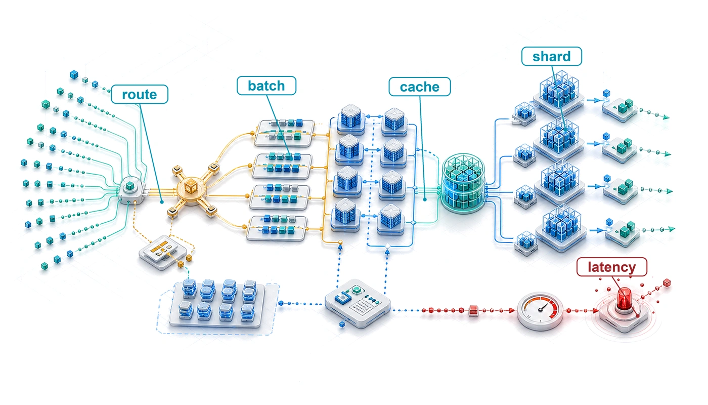
Purpose

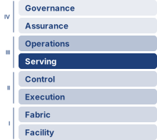
Fleet stack focus for this chapter.

Why can lifetime inference cost dwarf training cost?

Training is paid for each model version; serving continues throughout that version’s operational lifetime. A model trained for millions of dollars may serve billions of requests, each consuming compute, memory, network, and energy. At high traffic, recurring inference expense can exceed the original training cost by orders of magnitude. Milliseconds of latency and small differences in accelerator utilization then compound across the service’s lifetime. A fast prediction measured on an otherwise idle machine does not reveal how the same model behaves when requests arrive together, vary in length, and compete for memory. Work can spend longer waiting than executing, while an apparently busy fleet produces responses that arrive too late to be useful. Keeping extra machines ready protects response time but incurs cost during quiet periods; admitting more work improves utilization only while the service can still meet its promises. Failures sharpen this tension because displaced requests consume the spare capacity intended to absorb demand changes. Continuing to accept work during overload can worsen the shortage when delayed requests trigger retries that compete for capacity. The engineering decision is therefore how much useful work the fleet can sustain at an acceptable cost while preserving response quality and timeliness. The answer depends on the request mix and service requirements, so a gain for one workload may become a loss for another. In C³ terms, compute reuse must pay for communication and coordination without exhausting the user’s latency budget.

Learning Objectives

Estimate lifetime serving cost from traffic volume, deployment duration, and measured cost per SLO-compliant request
Select batching, scheduling, and per-request compute-budget policies for vision, LLM, recommender, and streaming workloads
Analyze attention-cache capacity, fragmentation, and prefill-decode interference under workload-dependent serving constraints
Compare sharding, disaggregation, and quantized serving designs using communication, memory, and quality constraints
Evaluate routing, overload-control, and isolation policies against tail latency, retry amplification, and noisy-neighbor risks
Design autoscaling and multi-region routing policies that balance cold starts, cost, and SLO compliance
Synthesize serving architectures that manage C³ trade-offs across request, replica, service, and platform layers

10.1 Inference Cost and Serving Architecture

A language model that costs millions of dollars to train over two months can, once deployed to a global user base at thousands of queries per second, consume a comparable sum in inference compute every week. Inference is then no longer a temporary batch job. It is a continuous, latency-sensitive service.

Fleet efficiency characterizes a replica in steady state by how close its decode steps come to the bandwidth floor, how long it takes to become ready, and how much of its held time runs at the ideal rate, each averaged over windows of hours to weeks. Serving policy determines how that capacity is shared when requests arrive unevenly and each carries a latency target. A faster decode step supplies a better service rate, but it does not determine how long requests wait to join a batch, which replica receives them, which requests receive scarce cache space, or when the fleet needs another replica. These decisions connect the local execution toolkit to user-visible performance under load.

↩︎ The serving replica’s program and runtime goodput, its bandwidth floor, and the fusion, graph replay, and compilation levers that shape it are established in Fleet Efficiency.

The service contract makes that distinction measurable. Offered load is the work arriving at the endpoint, including requests the service may reject; admitted load is the work it accepts. A service-level objective (SLO) specifies the required outcome over a measurement window, such as a latency percentile or successful-request fraction. For language models, request rate alone is insufficient because prompt and output lengths determine different amounts of work. Capacity comparisons must therefore hold the request mix and SLO fixed while measuring how much offered work completes successfully within the targets.

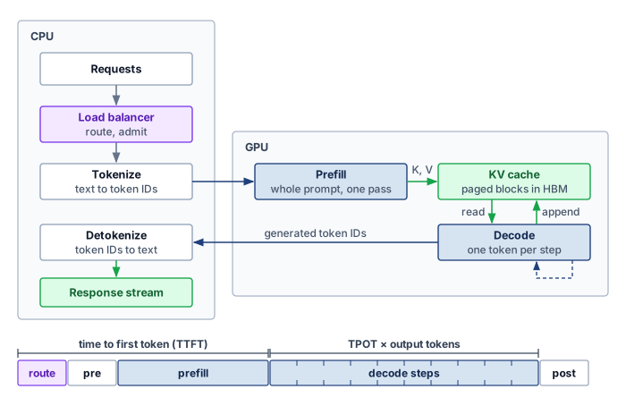
An admitted request passes through routing, preprocessing, queueing, batch formation, model execution, and response delivery, crossing between the host CPU and the accelerator twice on the way (figure 1). The host manages admission, tokenization, and detokenization, while the GPU executes the prompt prefill pass and iterative KV-cache decode loop; the figure maps noncompute serving overhead against the time-to-first-token (TTFT) and time-per-output-token (TPOT, the average gap between streamed tokens) latency budgets. For an autoregressive model, prefill processes the prompt and builds cached attention keys and values; decode extends that KV cache as it generates subsequent tokens. Waiting before prefill delays the first token, while competition during decode delays the stream. The scheduler must budget both delays alongside execution time. Batching and cache management govern work within a replica, sharding changes the replica’s capacity, and routing and autoscaling distribute demand across replicas.

↩︎ Prefill’s arithmetic-bound regime and decode’s bandwidth floor, measured as MBU, are established in Program goodput and its measure.

Figure 1: **End-to-End Inference Pipeline**: One language-model request crosses between CPU and GPU twice. The load balancer routes and admits it and the CPU tokenizes it; prefill then processes the whole prompt in one pass and writes its keys and values to the KV cache, and decode reads and appends that cache one token per step before the CPU detokenizes the stream. The strip orders one request’s latency, with illustrative segment widths. Everything up to the end of prefill counts against time to first token, and the routing and CPU segments are serving-tax work that spends latency budget outside GPU compute.

Distribution adds placement and coordination decisions to the local serving problem. Load balancing¹ must distribute requests across replicas with different amounts of unfinished work and available memory. Request routing must also account for model-specific characteristics: recommendation systems with large sharded embedding tables require different placement strategies than language models that generate responses token by token. When demand changes faster than new replicas can become ready, routing alone cannot restore capacity. Autoscaling, spare capacity, and admission limits must work together to protect the service’s latency targets.

¹ Load balancing for inference: Request service times can span milliseconds to tens of seconds as models, prompt lengths, and generated outputs vary. Queue-aware routing exposes that remaining work more directly than assignment counts alone.

Training and serving place costs on different timelines. A model version’s training expense can be amortized over its deployment, while serving capacity must follow recurring demand. An e-commerce recommendation service, for example, must accommodate peak shopping traffic without paying for an unnecessarily large idle fleet during quiet periods. Both training efficiency and serving efficiency matter, but the serving decision must also account for when requests arrive and how long they can wait. Building such a service requires three linked decisions: when distribution becomes necessary, how the architecture meets latency targets under varying load, and how resource utilization stays high enough that serving cost does not erode the value the model creates. The worked scenarios that follow size these decisions with stated inputs: registry values for real hardware and models, and labeled scenario assumptions for traffic, prices, and latency budgets. They show how a mechanism scales, not what any named deployment measured.

Self-Check: Question

True or False: A service that meets its latency SLO on every admitted request is serving all of its offered load.
Configuration X reports 900 requests per second on a benchmark of short prompts, and configuration Y reports 700 requests per second on the production prompt and output mix, both at the same TTFT and TPOT targets. Which conclusion is justified?
1. X has more capacity, because request rate is the capacity metric for a serving system.
2. Neither can be ranked yet, because prompt and output lengths change the work per request, so capacity must be compared at the same request mix and SLO by counting offered work that completes within the targets.
3. Y has more capacity, because production traffic always contains longer requests than a benchmark.
4. The two are equivalent, because both meet the same latency targets.
In a streaming language-model service, explain which latency budget is consumed by waiting before prefill and which by contention during decode, and why a faster decode kernel alone cannot settle either problem.

See Answers →

10.2 Limits of Single-Machine Serving

A single accelerator fails a production endpoint in three ways: its memory fills before the model weights or caches fit, its throughput saturates below the arriving query rate, or its forward pass runs longer than a request’s latency budget. Overcoming those limits requires distributing work across several devices within one machine or across machines over the network. Table 1 categorizes these three triggers and their matching distribution strategies, whose necessity depends on the permitted precision, placement, and service contract.

The first signal is memory exhaustion, which occurs when model parameters, key-value caches, or embedding tables exceed single-device capacity. A single NVIDIA H100 GPU provides 80 GB of HBM3² memory; Assumption Provenance records the provenance of this capacity figure and the other canonical hardware constants used throughout the analysis that follows. For an illustrative mixture-of-experts model with ~1.8T parameters, FP16 weights alone require ~3.5 TB. Keeping all those weights resident on accelerators requires multiple devices regardless of request volume; quantization and offloading change that placement constraint. Recommendation systems with trillion-parameter embedding tables face similar constraints. Meta’s DLRM architecture³ stores embedding tables that require multiple terabytes of memory.

² HBM3 capacity and bandwidth: The H100 combines 80 GB of 3D-stacked DRAM with 3.35 TB/s of bandwidth, compared with 2.04 TB/s for HBM2e on the A100. Capacity determines whether model and cache state fit; bandwidth bounds memory-bound decode throughput.

³ DLRM (Deep Learning Recommendation Model): Meta’s 2019 reference architecture combines dense features processed by multilayer perceptrons (MLPs) with sparse features represented by embedding lookups (Naumov et al. 2019). This separation permits different placement strategies; it does not require embeddings on CPUs and MLPs on GPUs. Production recommendation characterizations show why this structure matters for serving: embedding-heavy recommendation models create memory-access and capacity constraints that differ from dense convolutional neural network (CNN), recurrent neural network (RNN), or large language model (LLM) inference (Gupta et al. 2020).

Naumov, Maxim, Dheevatsa Mudigere, Hao-Jun Michael Shi, Jianyu Huang, Narayanan Sundaraman, Jongsoo Park, Xiaodong Wang, et al. 2019. “Deep Learning Recommendation Model for Personalization and Recommendation Systems.” arXiv Preprint arXiv:1906.00091.

Gupta, Udit, Carole-Jean Wu, Xiaodong Wang, Maxim Naumov, Brandon Reagen, David Brooks, Bradford Cottel, et al. 2020. “The Architectural Implications of Facebook’s DNN-Based Personalized Recommendation.” 2020 IEEE International Symposium on High Performance Computer Architecture (HPCA), 488–501. https://doi.org/10.1109/HPCA47549.2020.00047.

Beyond memory constraints, throughput limitations emerge when request volume exceeds single-machine capacity even with optimal batching. Consider a recommendation system serving 100,000 queries per second with a 10 ms latency budget. If single-machine throughput peaks at 10,000 QPS, no amount of optimization on that machine can satisfy demand. Horizontal scaling across multiple replicas becomes mandatory.

Finally, latency requirements can motivate distribution even when memory is sufficient. A 70-billion parameter model requires approximately 140 GB of weight memory in FP16, exceeding a single 80 GB H100-class GPU before KV cache is considered. Quantization or larger-memory hardware can make a single-device configuration feasible, yet its execution time may still exceed the request budget. Sharding the model across multiple GPUs can divide computation and weight traffic, but it adds communication and synchronization. Because sharding shortens compute-bound prefill and bandwidth-bound decode by different amounts, the latency benefit must be measured for each phase against its own target.

Table 1: Triggers for Distributed Inference: Each constraint type indicates different distribution strategies. Memory constraints require model sharding; throughput constraints require replication; latency constraints may require either depending on whether the bottleneck is compute or memory bandwidth.

Constraint	Single-machine limit	Example workload	Distribution strategy
Memory	80 GB (H100)	Illustrative MoE (~3.5 TB FP16)	Tensor/pipeline parallelism
Throughput	~10K QPS (vision)	100K QPS RecSys	Horizontal replication
Latency	Forward pass $> \text{SLO}$	500 ms LLM TTFT	Model sharding

Memory, throughput, and latency triggers all become user-visible once an interactive endpoint starts streaming. Time to first token (TTFT) determines when the user sees a response begin, while time per output token (TPOT) determines whether the rest of the response arrives at a readable pace. TPOT is the average of the time between tokens (TBT), the gap between successive streamed tokens, which many serving systems report as inter-token latency (ITL). A stream can meet its TPOT target while a single long TBT gap still stalls the reader, so average cadence is stated here as TPOT and per-gap tail targets as TBT. Protecting both first-token delay and stream cadence is why inference reverses many of the optimization priorities from training.

Checkpoint 10.1: Distribution strategy selection

Verify your understanding of when to move from single-machine to distributed inference:

Shard vs. replicate: for a 13B model (26 GB weights) that fits on a single A100, select model sharding or horizontal replication when throughput requirements double.
Latency floor: for a real-time speech-to-text service where TBT is the primary bottleneck, determine whether data-parallel replication reduces this latency.
Mandatory sharding: explain why a 175B model requires multiple 80 GB GPUs when all FP16 weights must remain accelerator-resident, regardless of request volume.
Latency trigger: identify when a latency target forces distribution and when added network, serialization, coordination, or queuing overhead can erase the benefit.

Self-Check: Question

A recommendation service must answer 100,000 queries per second within 10 ms. Its model fits comfortably on one machine, which peaks at 10,000 queries per second with optimal batching. Which strategy addresses the binding constraint?
1. Shard the model with tensor parallelism across machines, because sharding is the general remedy whenever one machine is insufficient.
2. Quantize the weights so a single machine runs ten times faster.
3. Replicate the full model across at least ten machines and route requests among them, because the binding constraint is throughput rather than memory or per-request latency.
4. Raise the batch size on one machine until it reaches 100,000 queries per second.
A 70B-parameter model needs roughly 140 GB of FP16 weights, more than one 80 GB accelerator holds, and quantization can make it fit on one device. Explain why the team might still shard it, and how they should decide.
True or False: A stream that meets its TPOT target cannot stall the reader, because TPOT bounds the gap between successive tokens.

See Answers →

10.3 SLO Goodput and the Serving Tax

A replica that runs near its hardware limit still wastes its capacity if requests wait so long in queues, network hops, and host processing that responses arrive after the user’s deadline. Because a served request counts as useful work only when it meets its latency and quality targets, every stage it crosses spends part of that contract’s budget.

10.3.1 The inversion from training to inference

A training iteration that takes 2 seconds instead of the usual 1 second slows a run slightly, and faster steps later can still keep the job on schedule; an interactive request that takes 2 seconds against a 100 ms target fails its contract immediately, even if every subsequent request finishes on time. This contrast between training and inference centers on the unit of useful progress. Training evaluates throughput together with convergence over a run; interactive serving evaluates completed requests against quality and latency targets. Offline inference can also prioritize throughput, while training still loses progress to stragglers and stalls. The distinction is therefore which delays violate the workload’s contract, not whether one activity cares about time and the other does not. That difference reorders priorities across six system aspects, from the primary metric onward (table 2).

Table 2: Training vs. Inference System Requirements: The fundamental inversion from throughput to latency optimization ripples through system design, state management, batch formation, and failure recovery.

Aspect	Distributed training	Distributed inference
Primary metric	Throughput (samples/hour)	Latency (p99 ms)
Acceptable variance	Hours	Milliseconds
State management	Checkpoints (periodic)	Session state (continuous)
Batch formation	Large, controlled	Request-driven, variable
Failure tolerance	Restart from checkpoint	Redirect if capacity and state allow
Cost structure	Fixed duration, variable rate	Variable duration, fixed SLO

Failure handling follows those different contracts. Training restores a checkpoint and repeats lost work, charging recovery time to the run. Interactive serving has far less time per request, so redirecting work needs spare capacity and recoverable request state, and substituting a smaller model needs an acceptable quality fallback. SLOs define which failures and delays the service may tolerate, and a recovery mechanism helps only when its added work fits within that contract.

The same targets also define the serving system’s capacity metric. SLO goodput is the rate of completed requests that meet the stated TTFT and TPOT targets for a fixed request mix. It is the serving counterpart of the useful-progress goodput that coordination protects in training (Orchestration coordination layer), and it applies after ML goodput, which measures how much of a replica’s held capacity runs at its ideal rate; SLO goodput then counts how much of that capacity completes requests within their targets. A request that misses its contract counts for nothing, however busy the accelerators were while serving it, so increasing arrivals without completing more requests within those targets does not increase useful capacity.

↩︎ ML goodput, the fraction of fleet capacity that becomes useful work at the ideal rate, and its three factors are established in ML Goodput.

10.3.2 The serving tax

If an interactive request carries a 100 ms latency target and model execution takes 70 ms on an idle replica, routing, network transfers, serialization, coordination, and queueing must all fit inside the remaining 30 ms. Distributing inference adds transfers and coordination to a request that already spends time in host processing and queues. This “serving tax” is the exposed work outside model execution that consumes the request’s latency budget, and its size depends on which components the request crosses and which costs can overlap.

Network communication contributes setup and transfer time at each cross-machine dependency. Synchronization between GPUs can expose that cost when the next operation needs a remote result. For an illustrative path with four sequential exchanges taking 50–500 microseconds each, the exposed contribution is 200 microseconds to 2 milliseconds. Actual collective time also depends on payload, topology, contention, and the number of communication rounds; a generic network round-trip time cannot be charged once per collective without checking its implementation.

↩︎ The $\MessageStartupLatency$-$\LinkBandwidth$ model, which splits each transfer into a fixed startup latency plus a bandwidth-dependent term, is established in The \MessageStartupLatency-\LinkBandwidth performance model.

Before and after those network hops, serialization adds host work whenever a service converts structured data into a wire representation and reconstructs it at the receiver. Protocol Buffers, JSON, and Python’s pickle provide different representations and implementation paths, so their cost must be measured for the actual payload and runtime. Tensor transfers within a sharded model need not pass through the same object-serialization path as a service request. Formats such as FlatBuffers and Cap’n Proto permit access to wire-format data in place, avoiding a separate unpacking step when the consumer supports that representation, though they do not eliminate network transfer or every downstream copy.

Once the payload is on the wire, load balancing adds a routing decision and sometimes another forwarding hop: examining request metadata, consulting replica state, and forwarding to the selected backend all consume time before execution begins. The measurement must separate decision time from waiting and transport so that a slow routing path is not mistaken for a slow model.

When a request fans out across several backend services—such as feature stores, retrieval indexes, and ranking models—coordination overhead emerges as the gateway joins their results. Independent feature or model calls can run concurrently, but a dependent ranking stage must wait for the inputs it needs, so the critical path includes exposed coordination and the slowest required branch rather than the sum of every branch’s runtime. Finally, queuing delay ($\QueueingLatency$) adds waiting time whenever work arrives while the required resources are busy, even when the average arrival rate remains below average service capacity.

The serving tax must be measured on the same request boundary as model execution. Equation 1 decomposes that latency, with each term counting an exposed contribution so concurrent work is not counted twice:

\[\EndToEndRequestLatency= \InferenceLatency+ \NetworkLatency+ \SerializationLatency+ \CoordinationLatency+ \QueueingLatency \tag{1}\]

In the 100 ms request budget above, the four sequential exchanges alone can claim up to 2 ms of the 30 ms non-compute slack before any request waits for a busy replica. The measured contribution determines the intervention: co-location removes a network hop, fewer dependent exchanges reduce startup costs, and a faster link shortens large transfers, whereas queueing requires controlling admitted work or increasing usable capacity. Each choice spends resources to recover latency budget, connecting the request-level diagnosis to lifetime serving cost.

Self-Check: Question

Two configurations serve the same request mix under the same TTFT and TPOT targets. Configuration X completes 1,200 requests per second, of which 70 percent meet both targets; configuration Y completes 1,000 requests per second, of which 95 percent meet both. Which has more serving capacity?
1. X, because it completes more requests per second and keeps its accelerators busier.
2. The two are equal, because both process the same request mix.
3. X, because requests that miss their targets still return results to users.
4. Y, because SLO goodput counts only requests that meet their targets, about 950 per second against about 840 for X.
Explain the composition of the distributed ‘serving tax’ ($\EndToEndRequestLatency = \InferenceLatency + \NetworkLatency + \SerializationLatency + \CoordinationLatency + \QueueingLatency$) and describe how zero-copy serialization formats mitigate serialization overhead.
True or False: Interactive inference recovery is judged against request latency and availability objectives, whereas long-running training recovery is usually judged against lost progress and time to completion.

See Answers →

10.4 Serving Cost Dominance in Production

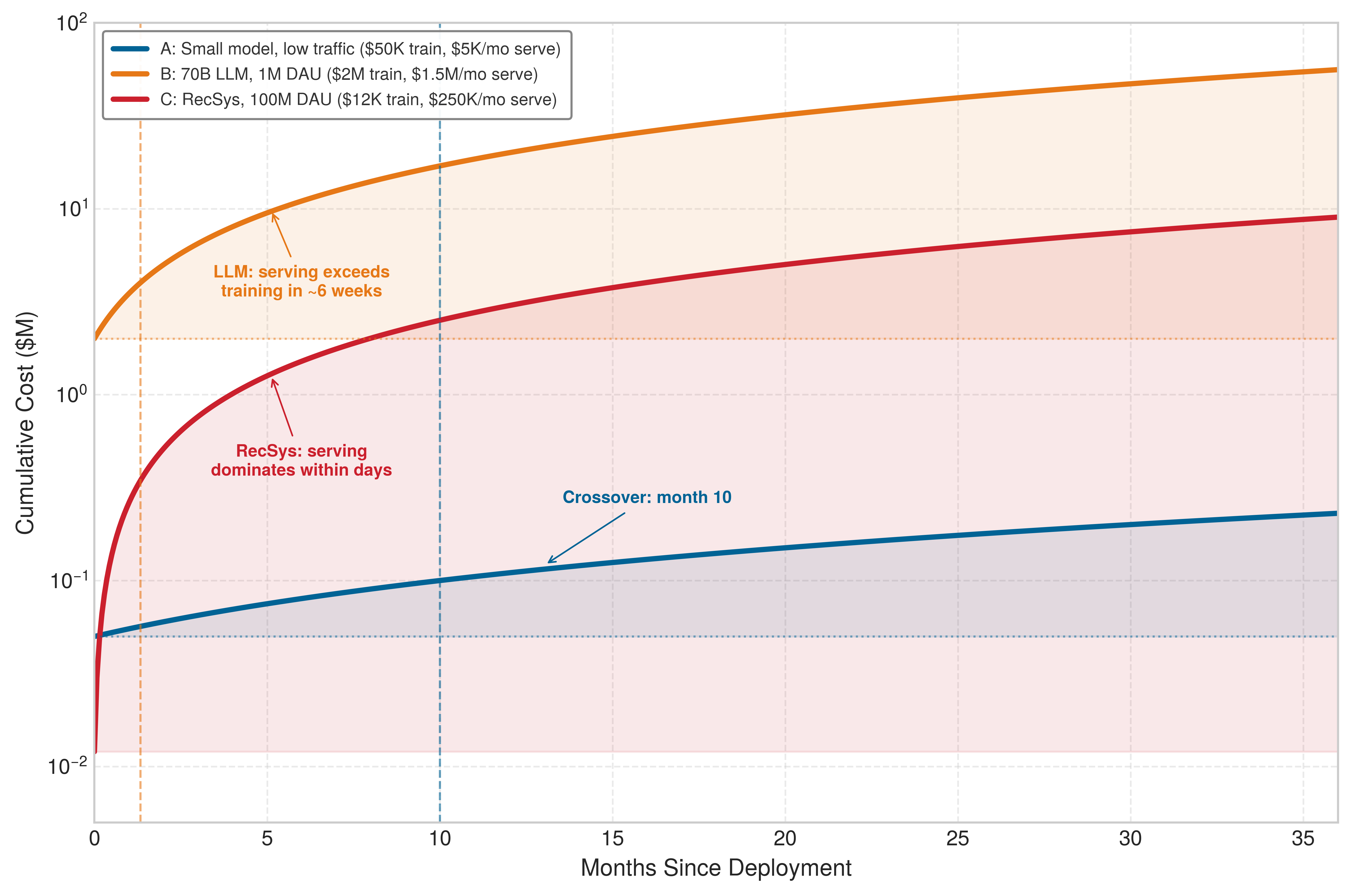
At this traffic, one year of serving costs about nine times the training run.

A team that budgets millions of dollars to train a model can find within weeks of launch that serving traffic is spending more compute per month than the entire training run cost. While the serving tax in equation 1 consumes a fraction of each request’s latency budget, those per-request costs compound across every query over the model’s operational lifetime. By the serving cost dominance principle (17), recurring serving expense can dwarf upfront training expense by orders of magnitude because a model version incurs training cost once before deployment while serving cost recurs with traffic. Both activities can consume purchased or rented infrastructure; the distinction here is expense timing, not financial capitalization. In a high-volume deployment, that recurring traffic bill rapidly overtakes the one-time training investment (notebook 10.1).

Napkin Math 10.1: The serving cost multiplier

Problem: A team has spent $2,000,000 training a 70B parameter model and now serves it to 1,000,000 daily active users, each making 50 requests/day. Is training or serving the dominant cost over 1 year?

Math:

Training cost: $2,000,000 (one-time).
Metric: Annual inference volume is $10^{6}\,\text{users} \times 50\,\text{reqs} \times 365\,\text{days} \approx$ 18.25B requests/year.
Cost per request: Assume a 70B model on H100 costs $\approx$ $0.001/request (input + output).
Annual serving cost: 18.25B requests $\times$ $0.001/request = $18,250,000.

Systems insight: Serving costs 9.1× more than training in the first year alone. A 10 percent reduction in cost per request, at unchanged request volume and service quality, saves about $1.8M in the first year, nearly paying for the original training run.

For one model version at a fixed query rate and average cost per served query, equation 2 combines training expense with recurring serving expense:

\[\ModelLifetimeCost= \TrainingCost + \ServingCostPerQuery\times \DeploymentDuration\times \ArrivalRate \tag{2}\]

where $\TrainingCost$ is the one-time cost to train the model, $\ServingCostPerQuery$ is the cost per query served, $\DeploymentDuration$ is the deployment duration in appropriate time units, and $\ArrivalRate$ is the query rate. The rate must count the same served queries used to estimate unit cost. That cost must include the chosen serving boundary, including idle or reserved capacity when it is billed. Changing traffic mix, fleet size, or price requires evaluating separate intervals rather than treating one unit cost as constant throughout deployment.

The same leverage can hold across application categories with different cost structures. In the chapter’s illustrative recommendation scenario, a DLRM trained for $8,000 ($2,000 hardware for 1,000 GPU-hours at $2/GPU-hour, plus 3× additional engineering cost for data and experimentation) and served at 10,000 QPS for 730 days accumulates $6.31 \times 10^{11}$ lifetime queries. At the assumed $10/million queries, those queries cost $6,307,200 to serve, producing a 788.4× ratio in this scenario. Other workload envelopes span orders of magnitude in both terms, and the sensitivity ranges in table 3 are illustrative envelopes rather than market-price estimates.

Table 3: Illustrative Training and Serving Cost Ranges: Independent sensitivity ranges for training a model version and serving it for a year. A cost ratio requires a paired training-and-serving scenario; it cannot be inferred from matching endpoints of independent ranges. A deployment must substitute measured traffic and a consistent accounting boundary.

Application	Training cost	Annual serving cost
Recommendation (high QPS)	$10K–$100K	$1M–$10M
Search ranking	$100K–$1M	$10M–$100M
LLM API	$1M–$100M	$10M–$1B
Internal analytics	$1K–$10K	$10K–$100K

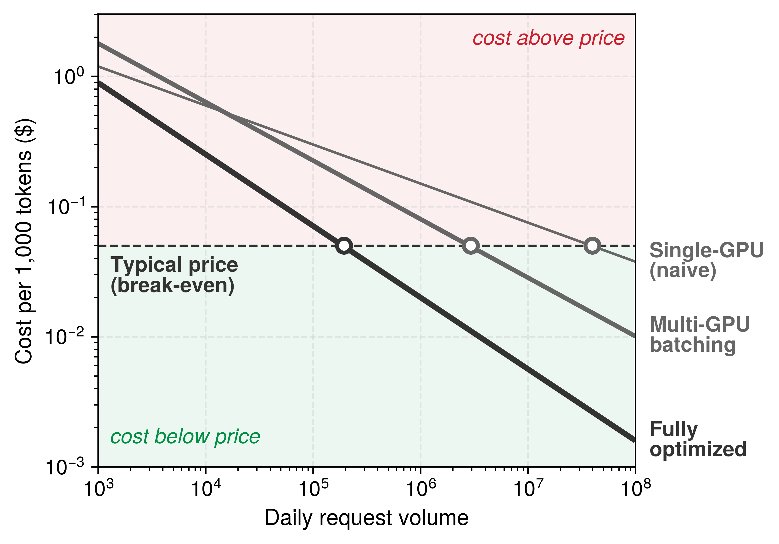
A reduction in cost per completed request yields recurring savings only if workload volume and service quality stay fixed; lower latency alone does not reduce billed capacity. Unit cost also changes with daily request volume, as the constructed cost curves of figure 2 illustrate. Against its assumed price of $0.05 per 1,000 tokens, the optimized curve crosses near $2 \times 10^{5}$ requests per day and the unbatched single-GPU curve near $4 \times 10^{7}$ requests. These crossings follow from the assumed curves, not measured profitability, so a deployment needs its own token mix, occupied capacity, and cost boundary to locate its break-even point.

Figure 2: **The Serving Cost Curve**: Constructed unit-cost curves cross an assumed price line at different request volumes. The optimized curve crosses earlier under these assumptions; the crossings do not establish measured profitability or guaranteed savings from quantization and batching.

The cost ranges in table 3 give a static comparison; figure 3 instead accumulates assumed monthly serving expense over a 36-month deployment and marks when the serving portion equals the initial training expense, within days in the plotted recommendation scenario and roughly six weeks in the 70B LLM scenario. These timings follow from the specified expenses, not from model size or user count, and a larger training expense, lower traffic, or shorter deployment can reverse which activity dominates. For generative LLM services, serving-specific designs can improve throughput, cost, and power use (Patel et al. 2024).

Patel, Pratyush, Esha Choukse, Chaojie Zhang, Aashaka Shah, Íñigo Goiri, Saeed Maleki, and Ricardo Bianchini. 2024. “Splitwise: Efficient Generative LLM Inference Using Phase Splitting.” 2024 ACM/IEEE 51st Annual International Symposium on Computer Architecture (ISCA), 118–32. https://doi.org/10.1109/isca59077.2024.00019.

Figure 3: **The Serving Cost Crossover**: Cumulative total deployment cost (initial training plus ongoing serving) for three illustrative scenarios. Vertical markers (scenarios A and B) indicate when the serving portion equals the one-time training cost. In the two high-traffic scenarios, serving expense matches training expense within weeks or days. In the low-traffic scenario, training expense remains larger over the plotted period. These differences follow from the specified training costs, traffic, and unit serving prices.

Self-Check: Question

A production recommendation model costs $50,000 to train (a one-time expense) and serves 10,000 QPS continuously for 2 years (730 days) at an operational cost of $10 per million queries. What is the ratio of lifetime serving cost to training cost?
1. Approximately $1.3\times$
2. Approximately $126.1\times$
3. Approximately $12.6\times$
4. Approximately $630.7\times$
True or False: Serving cost always exceeds training cost once a model is large enough, because larger models cost more per query.
A team estimates its cost per query from GPU time on fully loaded replicas, but its fleet also bills for reserved replicas that sit idle overnight to absorb the daytime peak. What does the lifetime cost model require?
1. Nothing more, because idle replicas do no work and therefore add no cost per query.
2. Doubling the query rate to account for the peak, because peaks set the cost.
3. Replacing cost per query with training cost, because idle capacity is a one-time expense.
4. Charging the billed idle and reserved capacity inside the unit cost, and counting the same served queries in the rate that was used to estimate that cost.
A model costs $2M to train, and its first year of serving costs about $18M. Explain why a 10 percent reduction in cost per request can be worth nearly as much as the original training run, and state the conditions under which that saving is real.

See Answers →

10.5 Serving Workloads and the Serving Hierarchy

An optimization tuned for one model family or one layer of the stack can miss the active bottleneck when applied to another: paging a key-value cache does nothing for an embedding-heavy recommendation model, and fusing a GPU kernel cannot rescue a service whose requests stall in a load balancer. Controlling serving cost therefore requires separating the workload mix from the system layer that owns each bottleneck.

10.5.1 Inference beyond LLMs

Designing a serving platform around autoregressive token generation alone leaves a fleet unprepared for the workloads that dominate consumer request volume. In large consumer platforms, recommendation and ranking workloads can consume the majority of AI inference cycles and capacity (Gupta et al. 2020; Hazelwood et al. 2018), stalling on terabyte-scale sparse embedding lookups under sub-10 ms deadlines rather than sequential weight reads. Vision and image processing, NLP and LLM workloads, fraud detection, ads, and other classification tasks create additional serving demands. Table 4 compares representative pressures: sparse lookup for recommendation, batch efficiency for fixed-shape vision, weight and cache traffic for LLM decode, and incremental deadlines for speech. These are starting points for diagnosis; the active bottleneck still depends on the model, input shape, and deployment.

Recommendation traffic illustrates why request volume must be derived from application behavior. A page load, scroll, or click can trigger ranking or retrieval, so one browsing session can produce many inference requests. A language-model application may likewise issue several model calls for one user action or run background tasks without an explicit query. Capacity planning therefore counts the model work triggered by each interaction rather than treating user count as request rate.

Workload structure also determines which techniques can help. Embedding sharding and lookup locality address large recommendation models (Naumov et al. 2019; Gupta et al. 2020), and feature store architectures must deliver the inputs a model expects within its latency budget, while continuous batching and KV cache management address variable-length autoregressive work. Text-to-image systems such as DALL-E add multimodal serving demands (Ramesh et al. 2021) whose volume and latency targets remain product-specific.

Ramesh, A., M. Pavlov, G. Goh, S. Gray, C. Voss, A. Radford, M. Chen, and I. Sutskever. 2021. “Zero-Shot Text-to-Image Generation.” In Proceedings of the 38th International Conference on Machine Learning, ICML 2021, 18-24 July 2021, Virtual Event, edited by Marina Meila and Tong Zhang, vol. 139. Proceedings of Machine Learning Research. PMLR.

Table 4: Production Inference Landscape: Different model types create different serving pressure, latency requirements, and optimization challenges. The table is a qualitative workload map rather than a universal traffic-share distribution. Technique selection must match the specific workload.

Model type	Serving pressure	Latency target	Key challenge
Recommendation/ranking	High volume in consumer platforms	$<10\text{ ms}$ p99	Embedding lookup
Vision (CNN)	Workload-dependent	20–100 ms	Batch efficiency
LLM	High cost per request	100 ms–10s	Memory bandwidth
Speech/Audio	Stream-driven	Real-time	Sequential decode
Multimodal/text-to-image	Emerging and product-specific	Varies	Cross-modal coordination

10.5.2 The serving hierarchy

Tuning a replica’s kernels or cache allocator cannot fix tail latency when requests are waiting inside a router or starving behind a noisy neighbor on a shared cluster. To locate the right control, serving optimizations organize into a four-level serving hierarchy ordered by scope, where each level owns a distinct bottleneck and measurement boundary. The request level follows one request through preprocessing, batch-formation waiting, response caching, and model execution, where the target is the latency a user sees. The replica level looks inside one model instance, where utilization, KV-cache memory management, and kernel efficiency set the throughput it can deliver before it saturates. The service level turns many replicas of the same model into aggregate capacity through load balancing, request routing, and autoscaling, and the platform level decides, across services and tenants, whether a shared serving fleet stays efficient without allowing one workload to degrade another.

Each level supplies a different measurement boundary. Table 5 associates request latency, replica throughput, aggregate service capacity, and cross-tenant efficiency with the controls most directly responsible for them. Their effects still cross boundaries: batching can increase replica throughput while adding request delay, and replica placement can change both communication cost and service capacity. The hierarchy helps locate the decision without treating its metric in isolation. In C³ terms, batching and cache management improve compute reuse, sharding introduces communication, and routing, isolation, and autoscaling coordinate the resources that make those gains usable.

Table 5: Serving Hierarchy Optimization Targets: Each level of the serving hierarchy targets distinct performance metrics, from per-request latency at the request tier to aggregate resource efficiency at the platform tier.

Level	Optimization target	Key techniques
Request	Per-request latency	Dynamic batching, response caching
Replica	Throughput, utilization	KV-cache paging, kernel fusion
Service	Aggregate capacity	Load balancing, routing, autoscaling
Platform	Resource efficiency	Multi-tenancy, scheduling, placement

Checkpoint 10.2: The serving hierarchy

Verify your understanding of where specific optimizations sit within the serving hierarchy:

Replica level: identify the hierarchy level at which KV-cache paging reduces GPU memory waste, and explain why that raises concurrent request capacity rather than single-request latency.
Caching level: distinguish response caching, which shortens one request’s path, from KV-cache paging, which raises a replica’s capacity, and place each in the hierarchy.
Load balancing: identify why load balancing belongs at the service level and explain how its choice of replica can affect both aggregate goodput and a request’s queueing delay.
Isolation level: evaluate the claim that multi-tenancy and resource isolation are primarily request-level concerns.

The serving decisions that follow climb the hierarchy from the request level to the platform level. Batching sets how long each request waits to share execution; KV-cache layout, decode-time policies, and adapter state decide how many requests a replica can hold; the split between prefill and decode decides whether a new prompt and the streams already decoding share a worker or separate pools; weight quantization and model sharding change the replica’s memory and compute budget; routing, isolation, autoscaling, and global placement then turn replicas into a service and a platform. Precision enters every capacity calculation that follows through two separate budgets: reducing weight precision frees resident memory, whereas reducing KV precision lowers the memory required per active sequence. Section 10.9 compares the serving trade-offs of these representation choices before sharding divides a replica across devices.

Self-Check: Question

In the four-level Serving Hierarchy (Request, Replica, Service, Platform), which level and primary optimization lever are correctly matched to their target bottleneck?
1. Platform level: Minimizing single-forward-pass latency via kernel fusion and memory layout
2. Request level: Ensuring fair-share GPU quotas and tenant isolation across organizations
3. Service level: Managing aggregate capacity across multiple replicas via load balancing and autoscaling
4. Replica level: Reducing client-side network RTT via edge caching and CDN routing
Order the four levels of the Serving Hierarchy from the most granular execution tier to the highest fleet-wide governance tier:

Service level (fleet routing, load balancing, autoscaling)
Request level (per-request latency, tokenization, dynamic batching)
Platform level (multi-tenancy, cross-workload scheduling, placement)
Replica level (intra-instance utilization, GPU memory allocation, kernel fusion)

See Answers →

10.6 Batching Strategies at Scale

A stream of hundreds of disparate chat requests arrives at an inference server every second. Processing them one by one leaves much of the GPU idle, starved for work between small decode steps. Waiting to gather a large static batch forces the first request in line to endure unacceptable latency. Batching at scale therefore needs policies that group requests as they arrive without violating tail-latency deadlines.

Processing multiple requests together shares weight reads and kernel launch overhead across more useful work. The resulting service-rate gain can reduce queueing, but waiting to form a batch adds delay; the net effect on request latency depends on load. Single-machine serving applies this insight through dynamic batching, which collects requests within a time window before processing them together.

At scale, batching must also account for workload structure. A policy suited to uniform vision inputs can leave slots unused during variable-length generation, while grouping sparse embedding lookups solves a different problem from batching dense execution. The unit of reusable work determines which policy is worth evaluating. The strategies below proceed in order of mechanism rather than traffic share: vision (request batching), LLMs (iteration-level batching with KV state), and recommendation (feature-parallel batching over distributed embeddings), even though recommendation often dominates consumer inference volume (section 10.5.1).

10.6.1 Batching across model architectures

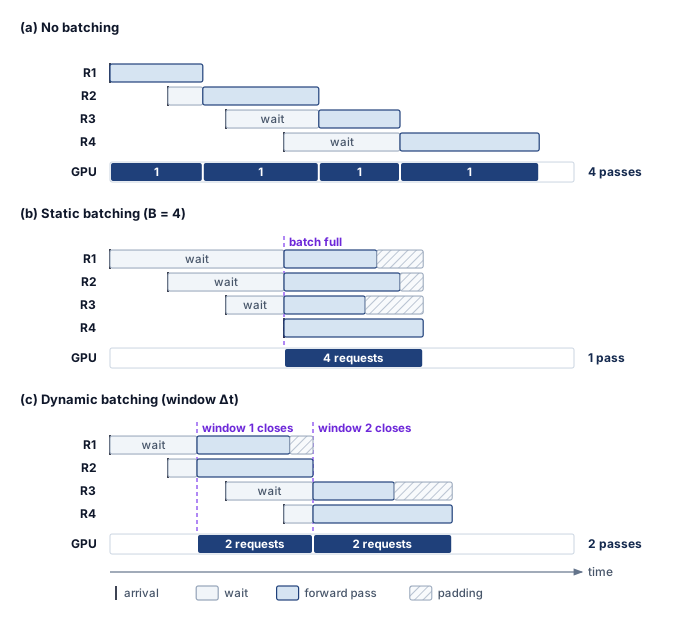
Holding arriving requests until a fixed batch fills forces early arrivals to wait and pads shorter inputs with wasted work, whereas running every request immediately leaves later arrivals queued behind one-request passes that underuse the GPU. Batching efficiency depends on how computation scales with batch size relative to memory and communication constraints, and the execution timeline in figure 4 separates waiting to form a batch from waiting for the accelerator to become available. Unbatched serving adds no batch-formation delay, but later requests can still queue behind earlier forward passes. Static batching consolidates all four illustrated requests into one pass, adding formation delay and padding to accommodate different input lengths. Dynamic batching closes formation windows at fixed time intervals ($\FiniteChange \TimeInstant$), producing two passes with two requests each in this example. The window limits intentional formation delay; it does not bound total queueing when ready batches arrive faster than the server can execute them.

Figure 4: **Batching Strategies Compared**: Four requests of different lengths arrive one time unit apart under three policies; the timings are illustrative. (a) Without batching, each request receives its own forward pass, so later arrivals queue behind earlier ones and the GPU runs four passes. (b) Static batching holds every request until the batch of four is full, then runs one pass padded to the longest request; early arrivals pay the longest wait. (c) Dynamic batching dispatches whatever has arrived when a short window closes, limiting intentional formation delay in this timeline while sharing each pass between two requests. Waiting for an occupied worker remains a separate source of delay.

In vision models processing fixed-size images, arithmetic work grows roughly in proportion to batch size while requests share the weights, so larger batches improve weight reuse until compute, memory, or the latency budget binds; the largest feasible batch is not necessarily the best interactive operating point. By contrast, in LLMs during the decode phase, small batches perform little computation per byte of active weights loaded, so memory bandwidth binds, and larger batches raise arithmetic intensity until compute, KV-cache traffic, or the latency budget limits further gains. Small-batch decode therefore does not inherit a new accelerator generation’s headline compute improvement. From Volta to Blackwell, peak compute climbs 18× while memory bandwidth expands by only 8.9×, and figure 5 shows generation throughput tracking the slower curve whenever weight streaming dominates at small batch sizes.

↩︎ The accelerator trajectory behind this divergence, with compute outpacing memory bandwidth from one generation to the next, is established in Evolution of GPU architectures.

Recommendation systems shift the bottleneck again: sparse embedding lookup can limit throughput before dense computation does. Grouping sparse accesses improves locality and distributes lookup work across shards, while batching the dense stages improves matrix multiplication throughput. The serving policy must therefore account for both stages and the communication between them rather than infer the bottleneck from the model category alone.

Figure 5: **Decode Inherits the Bandwidth Deficit**: Peak compute and memory bandwidth for four accelerator generations, normalized to the V100. Compute rises 18× against bandwidth’s 8.9×. In weight-bandwidth-bound decode, each iteration loads the active weights and reuses them across its output tokens; at fixed batch size, bandwidth growth constrains the gain. These hardware ratios are not measured workload speedups. Specifications are dense peak rates and bandwidths from the vendor datasheets recorded in the chapter’s data file.

10.6.2 Batching physics and efficiency curves

Cranking up batch size to maximize a replica’s throughput stretches each batch’s execution time and holds arriving requests in a formation queue until the service violates its latency SLO. Batch size is the single-replica control knob that moves a workload along the roofline, raising arithmetic intensity by reusing each weight read across more requests, yet at fleet scale the same knob sets how long arriving work waits and how much request state the replica must hold. A model relating batch size $(\BatchSize)$, batch service time $(\BatchServiceTime(\BatchSize))$, and batched service rate $(\EffectiveServiceRate(\BatchSize))$ exposes that trade-off; selecting an operating point also requires the arrival pattern, memory budget, and latency target.

↪ The roofline bound, and why batch-one decode sits far below the ridge point, are collected for reference in The roofline bound.

The first model isolates batch execution. Here $\BatchServiceTime(\BatchSize)$ is the service time once a batch begins execution; it excludes queueing and batch formation. Keeping the measurement boundary explicit prevents an execution-time improvement from being mistaken for an end-to-end SLO guarantee.

The service-time equation decomposes batch execution time into fixed overheads (kernel launch, memory loading) and variable costs (compute per sample):

\[\BatchServiceTime(\BatchSize) = \BatchFixedOverheadTime+ \BatchSize\times \MarginalRequestServiceTime\]

In this formulation, $\BatchFixedOverheadTime$ captures costs paid once per batch, such as loading weights from high-bandwidth memory (HBM) and kernel launch latency, while $\MarginalRequestServiceTime$ denotes the marginal cost of adding one request, such as the compute time for that sample. Treating these terms as constants is a local approximation for a fixed workload and execution regime. Kernel changes, cache traffic, and resource saturation can alter the measured curve as batch size grows.

The throughput equation describes the system’s capacity:

\[\EffectiveServiceRate(\BatchSize) = \frac{\BatchSize}{\BatchServiceTime(\BatchSize)} = \frac{\BatchSize}{\BatchFixedOverheadTime+ \BatchSize\times \MarginalRequestServiceTime}\]

The resulting batching efficiency curve shows diminishing returns from amortizing overhead. For small batch sizes ($\BatchSize$), $\BatchFixedOverheadTime$ dominates service time, so increasing $\BatchSize$ shares that cost and raises throughput substantially. As $\BatchSize$ grows, the relative contribution of $\BatchFixedOverheadTime$ shrinks and the model approaches its asymptotic rate $1/\MarginalRequestServiceTime$. This limit alone does not identify whether compute or bandwidth binds on the actual device. The knee of the curve, where fixed and variable costs become comparable, is a useful candidate operating point. It is not an optimum independent of the service contract; a tight latency budget may require a smaller batch, while a throughput-oriented workload may benefit from a larger one.

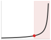
Throughput saturates toward $1/\MarginalRequestServiceTime$; past the knee, each larger batch buys less.

The execution-only feasibility condition is $\BatchServiceTime(\BatchSize) \le \text{SLO}$. In a live service, execution receives only the budget remaining after routing, queueing, batch formation, and response delivery. The batch-size decision must therefore use that remaining budget rather than consume the full SLO. Comparing a vision workload with a relatively high $\MarginalRequestServiceTime$ against an LLM decode workload with a high $\BatchFixedOverheadTime$ from weight loading shows how those measured costs shift the efficiency knee (notebook 10.2).

Napkin Math 10.2: The batching efficiency curve

Problem: An engineer optimizes two services: a vision model (ResNet) and an LLM (70B). At what batch size does each hit the “knee” of its efficiency curve?

Math: The knee occurs where the variable compute cost $(\BatchSize\times \MarginalRequestServiceTime)$ starts to exceed the fixed overhead $(\BatchFixedOverheadTime)$.

Vision Model $(\BatchFixedOverheadTime= 2\text{ ms}, \MarginalRequestServiceTime= 1\text{ ms})$:
- Knee: $\BatchSize\approx 2\text{ ms}/1\text{ ms} =$ 2.
- Result: This simplified latency model reaches its first overhead-amortization knee at a small batch. It does not locate hardware saturation; measuring throughput at larger batches tests whether additional concurrency still helps.
LLM Decode $(\BatchFixedOverheadTime= 40\text{ ms}, \MarginalRequestServiceTime= 0.5\text{ ms})$:
- Knee: $\BatchSize\approx 40\text{ ms}/0.5\text{ ms} =$ 80.
- Result: The larger fixed cost in this decode example moves the overhead-amortization knee to a larger batch.
- Where 0.5 ms comes from: It is an assumed marginal cost per added sequence, dominated by reading that sequence’s own KV state at a moderate context length. Unlike the weight stream, that read is private to each sequence, so it grows with batch size instead of being shared.
- Where 40 ms comes from: It is roughly the time to stream the model’s 140 GB of FP16 weights through one H100’s 3.35 TB/s of HBM bandwidth, the aggregate weight traffic of one decode step expressed in single-device time. No single H100 holds those weights. The reference replica of Where Fleet Capacity Goes spreads them over eight GPUs, which divides both $\BatchFixedOverheadTime$ and $\MarginalRequestServiceTime$ by the tensor-parallel degree and leaves their ratio, and therefore the knee, unchanged.

Systems insight: Because streaming the weights is the dominant per-step cost of decode, the system has not reached the efficiency knee until batch size 80. The knee depends on the ratio of fixed to per-request cost, not on how many devices share them, which is why sharing weight reads across concurrent requests matters at every replica size. The batch a service actually runs also depends on context length, cache capacity, kernel efficiency, and the latency target; continuous batching and paged allocation are the mechanisms that let a replica reach it.

While the analytical batching model locates the knee from each model class’s ratio of fixed to per-request cost (table 9), production serving stacks measure the resulting throughput-latency frontier directly. The open InferenceX benchmark serves DeepSeek-R1, a mixture-of-experts reasoning model, with 1,024-token prompts and 1,024-token responses on each accelerator across many combinations of serving framework, parallelism, and concurrency (SemiAnalysis 2026). For every configuration it records the output tokens per second each user receives, called interactivity (the reciprocal of TPOT), and the output tokens per second each GPU delivers across all users. Figure 6 plots 325 such configurations at FP8 precision and traces, for each accelerator, the frontier of configurations that no other configuration beats on both rates. Every frontier falls as interactivity rises, because a faster stream per user permits fewer concurrent sequences per decode step. The best B200 configuration delivers about 6,300 output tokens per second per GPU when each user receives about 13 tokens per second, and about 210 when each user must receive at least 100, a 30× difference in per-GPU output paid for faster streams. The interactivity target alone moves per-GPU output by that much, so it must be fixed before any two throughput figures can be compared.

The same frontiers separate hardware generations by more than their datasheets do. At 50 tokens per second per user, the best measured H100 configuration delivers about 80 output tokens per second per GPU and the best GB200 NVL72 configuration about 3,650, a 44× difference, although the peak dense FP8 rate of a GB200 GPU is only about 2.3× that of an H100. The benchmark does not apportion the gap, but the candidates lie mostly beyond peak arithmetic, in memory bandwidth and capacity per GPU, a 72-GPU NVLink domain that keeps experts and KV state off slower networks, and platform-tuned serving software. A throughput figure quoted without its latency target therefore says little about either system.

Figure 6: **Throughput versus Interactivity in Measured LLM Serving**: Output tokens per second per GPU against output tokens per second per user for DeepSeek-R1 at FP8 with 1,024-token prompts and responses. Faint points are individual serving configurations (framework, parallelism, and concurrency); each line is the frontier of configurations that no other configuration on the same accelerator beats on both axes. The dashed line marks 50 tokens per second per user. Data from SemiAnalysis (2026), latest published result per configuration as of October 2026.

Translating the batch-level equations into system-wide capacity planning requires Little’s law,⁴ a classical result from queuing theory that relates concurrency, throughput, and latency in any stable system. Whereas $\BatchServiceTime(\BatchSize)$ prices one replica’s execution batch, Little’s law connects the external arrival rate and mean request time in system to the total number of requests concurrently in flight across the fleet.

⁴ Little’s law: The identity holds for any stable system regardless of the arrival or service distribution, which is why it survives the bursty, variable-length traffic of inference. Because it relates averages, it bounds neither maximum service capacity nor tail latency.

↩︎ The M/G/1 waiting-time model, in which utilization and service-time variability multiply queueing delay, is established in Scheduling Objectives and Their Conflicts.

Theorem 10.1: Little's law for inference

Concept: In any stable queuing system, the average number of requests in the system $(\RequestConcurrency)$ equals the arrival rate $(\ArrivalRate)$ multiplied by the average time a request spends in the system $(\RequestTimeInSystem)$.

\[ \RequestConcurrency = \ArrivalRate \cdot \RequestTimeInSystem \]

Application: Concurrency planning. This idealized service counts only batch formation, queueing, and execution in its end-to-end latency; routing and response delivery add no delay. Assume the mean latency given below and full execution batches of the stated size. A percentile SLO cannot generally be substituted for the mean in Little’s law.

Target Throughput $(\ArrivalRate)$: 1,000 requests/sec
Assumed mean latency $(\RequestTimeInSystem)$: 100 ms (0.1 s)

Mean in-flight work $(\RequestConcurrency)$: $1000 \times 0.1 =$ 100 concurrent requests

Capacity planning: If a single GPU replica executes batches of 8 in 80 ms, and the fleet targets at most 80 percent mean service utilization:

Replica throughput $=$ $8/0.08 =$ 100 req/s
Throughput-only lower bound $=$ $\lceil 1000/100\rceil =$ 10 replicas
Illustrative headroom-sized replica count $=$ $\lceil 1000/(0.8 \times 100)\rceil =$ 13 replicas

Verification: Maximum executing positions $=$ $13\text{ replicas} \times 8\text{ batch positions} =$ 104. These positions do not include requests waiting for execution or batch formation. Under the assumed fixed batch service time, Little’s law on the execution boundary gives 80 requests executing on average; the remaining 20 of the assumed mean in-flight population are waiting or accumulating. The throughput-only lower bound would run at the stability boundary; the utilization-sized candidate runs at about 76.9 percent service utilization. The assumed mean latency still needs validation, and this arithmetic does not prove a percentile latency SLO; that requires an arrival/service model or a measured load test.

This stability boundary can be measured faithfully only when the load generator preserves the workload claim. The measurement contract of The measurement contract guards against load that eases off while the replica stalls, so a serving measurement holds a fixed external arrival process rather than a fixed concurrency, because response-paced generation can reduce arrivals during a stall and make the system appear to have more headroom than it does. The distinction between throughput capacity and latency capacity is exactly what queuing theory formalizes.

↪ The mean queuing delay under a batched M/G/1 surrogate, and how utilization headroom and batch size trade against latency, is developed in Queuing theory for batched inference.

10.6.3 Static and dynamic batching for vision models

Static batching, which waits until exactly $\BatchSize$ requests arrive before launching a forward pass, leaves early requests stranded during traffic lulls until their latency budgets expire. Vision models otherwise present the simplest batching case: preprocessed inputs share a fixed tensor shape and execute in a predictable time, so single-machine batching applies directly and fleet scale adds only the question of where batches form.

Dynamic batching collects requests for a maximum time window $\BatchingWindow$ or until reaching maximum batch size $\MaxBatchSize$, whichever occurs first. For Poisson arrivals with rate $\ArrivalRate$, equation 3 organizes expected request latency into queueing, formation, and execution contributions:

\[\mathbb{E}[\RequestTimeInSystem] = \mathbb{E}[\QueueingLatency] + \BatchFormationDelay + \BatchServiceTime(\BatchSize) \tag{3}\]

where $\mathbb{E}[\QueueingLatency]$ is the expected queuing delay, $\BatchFormationDelay$ represents mean batch formation delay (up to $\BatchingWindow$), and $\BatchServiceTime(\BatchSize)$ represents mean inference time over the realized batch sizes $\BatchSize$. Queueing here excludes time already counted as batch formation. The two waiting terms respond differently to load. Under Poisson arrivals the mean inter-arrival gap is $1/\ArrivalRate$, so a higher arrival rate fills a batch faster and reduces formation delay. Queueing for a busy replica can nevertheless grow as arrival rate approaches service capacity; the batching timeout does not cap that queueing delay. Spending a small slice of the latency budget on batch formation can multiply per-GPU capacity while keeping end-to-end latency within target (example 10.1).

Example 10.1: Dynamic batching for ResNet-50

Scenario: A vision classification service receives requests at 5,000 QPS with a 50 ms p99 latency SLO across 10 replicas, so each replica sees 500 QPS. One image served alone takes 5 ms. The scenario assumes that a batch of about 5 images executes in 8 ms and a batch of about 10 in 12 ms, because a batch shares weight reads and kernel launches across its images.

Diagnosis: Each utilization below is the per-replica arrival rate multiplied by the service time one request consumes. Option A serves every image alone, which overloads the replica ($\ServingUtilization = \ArrivalRate \times \BatchServiceTime = 500 \times 0.005 = 2.5$ utilization). Option B holds a 10 ms batching window, which collects about 5 requests (arrival rate $\times$ window). Their batch runs in 8 ms, so each request consumes 1.6 ms of execution, and utilization falls to $\ServingUtilization = 500 \times 0.0016 = 0.8$. The wider 20 ms window of Option C collects about 10 requests whose batch runs in 12 ms, or 1.2 ms each, reaching $\ServingUtilization = 500 \times 0.0012 = 0.6$ and a further 33 percent of per-replica capacity. Both options leave service headroom. Whether they also meet the p99 SLO depends on the window plus the queueing delay each utilization implies under the service’s real arrival pattern, which utilization alone does not determine.

Systems lesson: Dynamic batching is effective when the latency budget has unused slack. The serving policy converts latency headroom into throughput, but requires careful tuning to prevent SLO violations.

↪ A procedure for this tuning, from fitting the service-time model to checking the p99 target, is developed in Batch size selection framework given an SLO.

At scale with multiple replicas, batch formation can occur either at individual replicas or at a centralized batching layer. Replica-local batching has each replica independently form batches from its assigned traffic. This avoids a shared batching stage, but splitting a light arrival stream among many replicas can leave each waiting to fill its batch. Centralized batching pools arrivals before dispatching formed batches, potentially shortening formation waits, at the cost of an additional network hop and a shared scheduling bottleneck. Load balancing helps local batching, but equal request counts do not guarantee equal work or reproduce the formation benefit of pooling arrivals. The choice depends on arrival density, request compatibility, and replica service times.

10.6.4 Continuous batching for large language model (LLM) inference

When a request-level batch locks its membership until the longest sequence finishes, a short reply that ends after 10 tokens leaves its slot stranded for the remaining 90 steps of a 100-token neighbor, starving queued requests while the GPU still streams the full model weights on every step. The autoregressive bottleneck (principle 18) makes that wasted slot expensive: at small batch sizes, decode is typically bandwidth-bound because each iteration streams active model weights while generating only one token per sequence. Batching shares those weight reads across concurrent requests, and as the batch grows, compute or KV-cache traffic can become the binding constraint, so bandwidth-bound decode is an operating regime rather than a property of every serving configuration.

Definition 10.1: Continuous batching

Continuous batching is a serving strategy that updates batch membership at iteration boundaries, allowing new requests to enter without waiting for every request in the original batch to finish.

Significance: It reduces padding waste by refilling completed slots at iteration boundaries. Throughput gains require waiting requests, available KV-cache capacity, and scheduling overhead small enough to preserve the benefit.
Distinction: Unlike static or dynamic batching (which group requests at the request level), continuous batching operates at the iteration level, reshaping the active batch between decode iterations.
Common pitfall: Continuous admission must coordinate scheduling with KV-state ownership and lifetime. A Dynamic Memory Manager such as PagedAttention improves space utilization, but paging is not required: an implementation can recycle fixed-capacity request slots, at the cost of unused reserved space.

The Orca system (Yu et al. 2022) removed the request-level barrier by updating membership at iteration boundaries to enable slot reuse. Once a request completes, another can enter if its prompt has been processed and sufficient cache capacity is available. The scheduler must account for that preparation rather than treat every replacement as a decode-only operation.

Yu, Gyeong-In, Joo Seong Jeong, Geon-Woo Kim, Soojeong Kim, and Byung-Gon Chun. 2022. “Orca: A Distributed Serving System for Transformer-Based Generative Models.” 16th USENIX Symposium on Operating Systems Design and Implementation (OSDI 22), 521–38.

Consider a fixed-width batch of 8 sequences. If one sequence completes after 10 tokens while others require 100 tokens, its slot contributes no useful output for 90 iterations. If the kernel continues executing padded work for that slot, the fraction of wasted compute attributable to it is:

\[\text{Wasted compute} = \frac{(100 - 10) \times 1}{100 \times 8} = 11.25\%\]

The waste grows with the spread of output lengths, a dependence that section 10.6.5 turns into a formula. A kernel that skips completed sequences avoids their padded arithmetic, but a fixed-membership policy still prevents waiting requests from using the vacated capacity. Algorithm 1 states the continuous-batching scheduler as a decode loop with a prefilled waiting queue. Completed requests release their pages in this simplified policy, eligible waiting requests enter freed slots, and the next kernel runs over the updated active set. For Archetype A workloads (GPT-4/Llama-3), refilling slots lets more useful tokens share each weight read. The gain comes from reusing transferred weights, not merely from saturating bandwidth, which a smaller batch may already do.

↩︎ Archetype A (GPT-4/Llama-3), the autoregressive transformer whose serving must stream billions of weights for every generated token, is established in Archetype A (GPT-4/Llama-3).

\begin{algorithm}
\caption{Continuous batching decode scheduler}
\begin{algorithmic}
\Require prefilled waiting queue $Q$; active set $A$; KV-cache page allocator; active-token capacity $C_{\text{tok}}$; batched decode kernel
\Ensure generated tokens for completed requests; a continually refreshed active batch
\While{the service is running}
    \State admit requests from $Q$ while capacity and free KV-cache pages remain; allocate state, append to $A$
    \State reserve pages for the next decode step; preempt requests that do not fit
    \State run one batched decode kernel over the remaining sequences in $A$
    \State append each sampled token; extend its KV-cache pages
    \State remove completed or length-limited sequences from $A$; return their pages to the allocator
    \If{HBM pressure exceeds the policy threshold}
        \State move low-priority sequences from $A$ to the paused set; page their KV-cache to CPU DRAM
    \EndIf
    \State fill freed capacity from $Q$, or resume paused sequences whose pages now fit
\EndWhile
\end{algorithmic}
\end{algorithm}

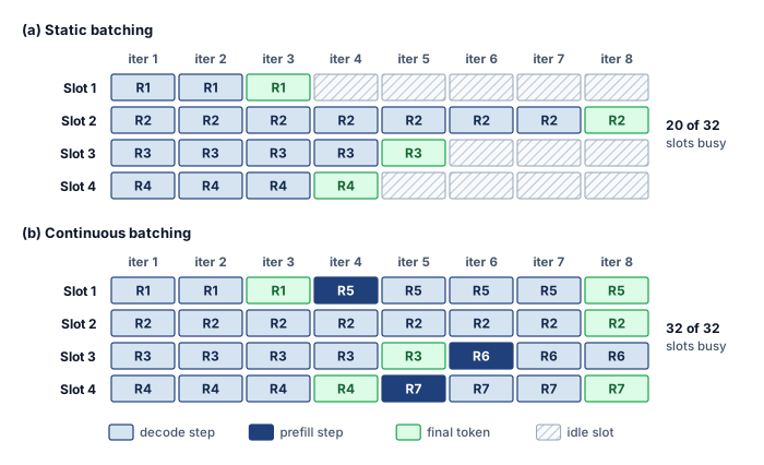
Admitting, completing, and refilling slots on every iteration lets waiting work use capacity released before the longest sequence finishes. The illustrated preemption path adds HBM-to-CPU-DRAM transfers under memory pressure, so recovered capacity must repay both scheduling and state-movement costs. Counted in slot-iterations (figure 7), fixed membership leaves only 20 of 32 productive, while continuous admission fills all 32 under the illustrated arrival and capacity assumptions. Prefill and decode cells do not necessarily take equal time. Slot occupancy therefore measures the opportunity; the realized throughput gain depends on how much longer the inserted prefill cells take than the decode steps they share an iteration with.

Figure 7: **Static vs. Continuous Batching**: In static batching (a), completed slots cannot be reused until the longest request finishes, although completed responses may already be released. Continuous batching (b) admits waiting requests into freed slots at iteration boundaries, starting each with a prefill step. Over the eight iterations shown, 20 of 32 slot-iterations do useful work under static batching and all 32 under continuous batching; the hatched idle slots are the capacity recovered when arrivals and cache capacity permit.

10.6.5 Quantifying continuous batching

In a static batch whose output lengths vary widely, a single long response holds every completed slot idle until its final token, wasting a growing share of the batch’s sequence-iterations as length variance rises. Continuous batching recovers that stranded capacity by refilling vacated slots at iteration boundaries (figure 7). Counting useful and unused sequence-iterations in a fixed batch bounds the recoverable opportunity; arrivals, KV-cache admission, prefill scheduling, and scheduler overhead determine how much of that ceiling a live replica actually captures.

The waste function for traditional batching

The 11.25 percent example of one early-finishing sequence generalizes to any mix of output lengths. For this waste model, traditional batching (also called static batching) retains a fixed batch width through all decode iterations until the longest sequence completes. Assume equal compute cost per sequence-iteration, including padded work for completed requests. For batch size $\BatchSize$ with output lengths $\{\RequestOutputLength_1, \RequestOutputLength_2, ..., \RequestOutputLength_{\BatchSize}\}$, the total compute performed under those assumptions is:

\[\StaticBatchingOperations= \BatchSize\times \BatchMaxOutputLength\times \SequenceIterationOperations\]

where $\BatchMaxOutputLength= \max_i(\RequestOutputLength_i)$ and $\SequenceIterationOperations$ is the compute cost per decode iteration per sequence. However, the useful compute is only:

\[\UsefulModelFlops = \sum_{i=1}^{\BatchSize} \RequestOutputLength_i \times \SequenceIterationOperations\]

Equation 4 defines the waste ratio that quantifies the inefficiency:

\[\PaddingWasteFraction= 1 - \frac{\UsefulModelFlops}{\StaticBatchingOperations} = 1 - \frac{\sum_{i=1}^{\BatchSize} \RequestOutputLength_i}{\BatchSize\times \BatchMaxOutputLength} = 1 - \frac{\BatchMeanOutputLength}{\BatchMaxOutputLength} \tag{4}\]

where $\BatchMeanOutputLength$ is the mean output sequence length. Waste therefore depends entirely on the ratio of mean to maximum output length within the batch. For uniform output lengths $(\BatchMeanOutputLength= \BatchMaxOutputLength)$, waste is zero. For highly variable lengths, waste can exceed 50 percent.

Serving variable-length outputs in LLMs

Consider a GPT-class model serving four concurrent requests whose prompt and output lengths vary fourfold across the batch. Table 6 lists the token counts for each request:

Table 6: Concurrent Request Generation Lengths: Four concurrent requests on a GPT-class model with varying prompt and output lengths. The 4$\times$ spread in output length (50 to 200 tokens) drives batching waste, because a static batch of four pads every request to the longest, wasting compute on the three shorter requests until the longest finishes generating. Prompt length sets each request’s prefill work, and the total is the number of tokens its KV cache holds when it finishes; both matter for admission, while the decode-slot accounting below uses only the output lengths.

Request	Prompt length	Output length	Total tokens
R1	100	50	150
R2	80	200	280
R3	120	100	220
R4	90	150	240

Napkin Math 10.3: Continuous batching waste calculation

Problem: Four LLM requests with unequal output lengths share a four-slot batch. Assume fixed decode-iteration time and no queueing. How much of the batch’s slot time does fixed membership leave unused, how much of it can continuous admission hand to new requests, and what happens to the original requests’ latencies?

Variables:

Decode time per iteration (batch of 4): 20 ms
Maximum output length in batch: 200 tokens (R2)
Mean output length: $(50 + 200 + 100 + 150) / 4 =$ 125 tokens

Slot accounting under fixed membership: The batch keeps all four slots until R2, the longest request, finishes.

Total decode iterations: 200
Total batch time: $200 \times 20\text{ ms} =$ 4,000 ms

The waste ratio in equation 4, one minus the ratio of mean to maximum output length, measures the slot time that finished requests leave idle:

$\PaddingWasteFraction = 1 - \frac{125}{200} = 1 - 0.625 = 37.5\%$

The fixed-width schedule contains $4 \times 200 =$ 800 “sequence-iterations” but only 500 are useful. These counts measure executed work only if the kernel continues processing completed slots; otherwise they measure useful work relative to the schedule’s available slots.

Continuous admission: Sequences depart at the iteration where they complete, and eligible new requests take their slots without delaying the original requests under the fixed-iteration-time assumption.

Iteration 50: R1 completes → slot freed, new request R5 can join
Iteration 100: R3 completes → slot freed, new request R6 can join
Iteration 150: R4 completes → slot freed, new request R7 can join
Iteration 200: R2 completes

Response latency, a separate effect: The fixed-membership schedule in this comparison deliberately withholds all four responses until R2 completes its 200 tokens. Static batch membership alone does not require that barrier.

Completion times with the barrier:
- R1 completes useful work at iteration 50, but waits until iteration 200 → latency = 4,000 ms
- R2 completes at iteration 200 → latency = 4,000 ms
- R3 completes useful work at iteration 100, but waits until iteration 200 → latency = 4,000 ms
- R4 completes useful work at iteration 150, but waits until iteration 200 → latency = 4,000 ms

Latencies with immediate release under continuous admission (assuming no queuing delay):

R1: $50 \times 20\text{ ms} =$ 1,000 ms (4× improvement over traditional)
R3: $100 \times 20\text{ ms} =$ 2,000 (2× improvement)
R4: $150 \times 20\text{ ms} =$ 3,000 (1.33× improvement)
R2: $200 \times 20\text{ ms} =$ 4,000 (no improvement for longest request)

Average latency comparison

Traditional: 4,000 ms (all requests)
Continuous: (1,000 ms + 2,000 + 3,000 + 4,000) / 4 = 2,500

Result: Under fixed membership, only 500 of the 800 sequence-iterations do useful work. Continuous admission hands the rest to R5, R6, and R7, which start generating at iterations 50, 100, and 150 instead of waiting for a new batch, so the same 200 iterations now advance seven requests rather than four. Releasing each response on completion separately reduces the original requests’ average latency by 37.5 percent, numerically matching the unused-slot ratio, and static batching that released responses on completion would obtain the same original-request latencies.

Systems insight: Response release and slot reuse are separate decisions. Removing a response barrier helps the requests already in the batch; only continuous admission recovers the stranded iteration capacity shown in figure 7, and that recovered capacity is what raises a replica’s throughput.

Efficiency regimes for continuous batching

The continuous-batching analysis relates recoverable slot capacity to the gap between a batch’s longest and average output lengths. Let $\text{CV} = \OutputLengthStandardDeviation/ \WorkloadMeanOutputLength$ be the coefficient of variation of output lengths. For the idealized fixed-width schedule, suppose the longest request in a batch is roughly $\BatchMaximumDeviationMultiple$ standard deviations above the mean. The factor $\BatchMaximumDeviationMultiple$ is an assumption about the batch rather than a property of the workload, because a larger batch draws more samples and pushes its maximum further into the tail. With immediate refill and unchanged iteration time, the corresponding capacity ratio is:

\[\text{Improvement} \approx \frac{\BatchMaxOutputLength}{\BatchMeanOutputLength} = \frac{\WorkloadMeanOutputLength+ \BatchMaximumDeviationMultiple\OutputLengthStandardDeviation}{\WorkloadMeanOutputLength} = 1 + \BatchMaximumDeviationMultiple\cdot \text{CV}\]

where $\BatchMaximumDeviationMultiple$ specifies how far the batch maximum lies above the mean, so the expression is a scenario ceiling on the opportunity from filling otherwise unused slots; scheduler overhead, KV-cache pressure, and refill gaps reduce the recovered fraction. In the table that follows, the CV and $\BatchMaximumDeviationMultiple$ columns are inputs, the speedup column is an assumed realized fraction held below the $1 + \BatchMaximumDeviationMultiple\cdot \text{CV}$ ceiling, and the waste column restates that speedup through $\text{speedup} \approx 1/(1 - \EffectiveWasteFraction)$. Neither column is a measurement. Together they show how much of the ceiling a scheduler must recover to reach a given gain, which is the quantity a load test should measure. Across workload types, including retrieval-augmented generation (RAG) (Lewis et al. 2020), this accounting yields the scenario rows of table 7.

Lewis, Patrick, Ethan Perez, Aleksandra Piktus, Fabio Petroni, Vladimir Karpukhin, Naman Goyal, Heinrich Küttler, et al. 2020. “Retrieval-Augmented Generation for Knowledge-Intensive NLP Tasks.” Advances in Neural Information Processing Systems 33: 9459–74.

Table 7: Continuous Batching Benefit by Workload Type: Higher output-length variance (CV) raises the ceiling on improvement from continuous batching. The $\BatchMaximumDeviationMultiple$ values are assumed, so each $1 + \BatchMaximumDeviationMultiple\cdot \text{CV}$ ceiling is a scenario value, and the speedups are assumed values held below it rather than measurements; the waste column is the effective waste those speedups imply. Workloads with predictable output lengths (code completion) have little to recover, while highly variable workloads (RAG with documents of varying length) have the most.

Workload type	CV	k	Waste (trad.)	Speedup (continuous)
Code completion	0.3	2.5	16.7%	1.2×
Chat (short responses)	0.6	2	33.3%	1.5×
General text generation	1	2.5	50%	2×
Creative writing	1.5	3	64.3%	2.8×
RAG with variable docs	2	2.5	71.4%	3.5×

Continuous batching is most valuable when output lengths are unpredictable, mixed workload types share the same cluster, request volume is high enough to refill vacated slots, and latency SLOs make early completion valuable. It provides minimal benefit when output lengths are uniform, as in classification or embedding generation, when batch sizes are too small for slot reuse to matter, or when request volume is too low to refill vacated slots.

Because arrivals, KV-cache admission, prefill scheduling, and scheduler overhead decide how much vacated capacity is actually recovered, serving teams must compare policies under the same arrival trace, latency objective, and memory budget. The published vLLM system, which pairs iteration-level admission with paged KV allocation, reports 2–4$\times$ higher throughput at comparable latency than FasterTransformer and Orca on its evaluated workloads (Kwon et al. 2023); that figure compares whole systems rather than isolating slot reuse, because paged allocation also permits larger active batches.

Implementation complexity trade-offs

The same variability that makes continuous batching valuable also makes it harder to operate. Memory management must support overlapping request lifetimes. Fixed-membership batching can reserve cache regions when a batch forms and release them together, whereas continuous admission must track which request owns each region and when it becomes reusable, either through fixed-capacity slots that retain unused reservations or through paging with its block tables. Kernels must also handle variable-length sequences and changing batch membership, often by packing short sequences under shared attention masks.

Scheduler work moves into the decode loop as well. A fixed-membership policy checks once per batch whether it is full or its timeout has expired, while continuous admission tracks completions, free cache capacity, and eligible waiting requests at every iteration boundary. That work must stay small relative to a decode step or it erodes the throughput that slot reuse recovers, so engines keep the per-iteration path short and prepare the next iteration’s batch on the host while the accelerator executes the current one. Continuous batching therefore buys its throughput gain with implementation and operating cost, weighed dimension by dimension in table 8.

Table 8: Traditional vs. Continuous Batching Trade-Offs: Continuous batching provides significant throughput gains for variable-length workloads at the cost of implementation complexity. For uniform-length workloads, the complexity overhead may not justify adoption.

Dimension	Traditional batching	Continuous batching
Implementation effort	Low (standard frameworks)	High (custom scheduler, kernels)
Memory overhead	Fixed allocation	Dynamic + fragmentation mgmt
Scheduler work	Once per batch	Every decode iteration
Debugging complexity	Deterministic behavior	State-dependent, harder to trace
Throughput (variable)	Baseline	Up to $1 + \BatchMaximumDeviationMultiple\cdot \text{CV}$
Throughput (uniform)	Baseline	~1.0$\times$ (no improvement)

Even with continuous batching available, diagnosing tail latency anomalies requires systematic investigation across the system stack. The following constructed p99 regression illustrates how to investigate infrastructure, execution, and serving layers. Its latency observations and mitigation outcome are scenario assumptions; only the transfer-time estimates are computed from payload and bandwidth.

Example 10.2: Debugging high p99 latency

Scenario: An LLM serving system shows high tail latency: p50 = 100 ms and p95 = 180 ms maintain SLO, but p99 spikes to $\TailRequestLatency =$ 500 ms against a 200 ms target despite a monitored GPU utilization of 85 percent.

Diagnosis: The system runs across 4 A100 GPUs linked via PCIe Gen4 (32 GB/s per GPU) rather than NVLink. For a 100 MB payload, the bandwidth-only transfer estimate is $\CommunicationTime(\DeviceCount) \approx$ 3.1 ms over PCIe versus 0.17 ms over NVLink. Collective startup, topology, and contention can add time. The service still runs an older request-level batching server rather than an iteration-level engine, with max batch size 32 and timeout 50 ms, so a batch holds its members until its longest generation finishes. The scenario assumes that 5 percent of batches experience head-of-line queuing delay $\QueueingLatency$ as short requests wait behind long generations.

Systems lesson: The latency distribution motivates tracing both candidates, because a transfer paid by every request also amplifies tail queueing near saturation. In this scenario, traces showing stable transfer times too small to explain the additional delay, together with short requests waiting behind long generations, identify the fixed-membership barrier as the immediate cause. Continuous admission removes that barrier; prefill scheduling, cache capacity, and other waits still require measurement. Until the server can be replaced, the following policy reduces output-length variation within request-level batches:

Request classification: Classify requests by expected output length (short: under 50 tokens, medium: 50 to 200 tokens, long: over 200 tokens)
Differentiated batching: Limit short batches to 8, medium to 16, long to 32

Grouping requests by expected length shrinks the spread of output lengths inside each batch, which is the quantity equation 4 says drives both waste and waiting. The scenario assumes a post-mitigation p99 latency of $\TailRequestLatency =$ 185 ms; a real service confirms it by replaying the same arrival workload and measuring the tail.

10.6.6 Feature-parallel batching for recommendation systems

A single recommendation request may issue thousands of sparse lookups across embedding tables holding billions of entries before the dense ranking head can score a candidate, so grouping requests solely at the dense MLP leaves the service bottlenecked on scattered memory reads and cross-server transfers. While fixed-shape vision inputs allow simple request grouping and autoregressive generation pairs iteration-level admission with KV-cache management (and with prefill-decode scheduling in section 10.8), recommendation systems must also batch around the placement of sparse state. Sparse embedding lookups can dominate memory access and communication in an embedding-heavy workload even when dense matrix multiplications account for much of the arithmetic. Grouping those accesses by feature type and destination—feature-parallel batching—improves lookup locality at each shard, complementing request batching in the dense stages.

Recommendation batching starts by grouping work around embedding locality rather than request shape. An incoming request splits across user, item, and context feature types to query sharded embedding tables concurrently, after which a gather barrier concatenates the retrieved representations for the dense MLP ranking head (figure 8).

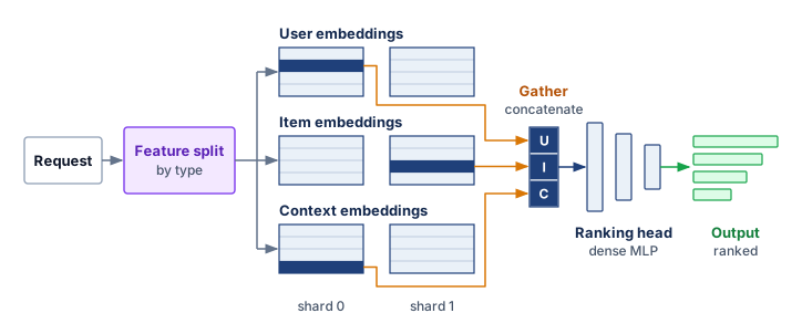
Figure 8: Feature-Parallel Batching Pipeline: Requests are batched by feature type (Users, Items, Context) and dispatched to specialized embedding servers in parallel. The retrieved embeddings are then concatenated and processed by the dense ranking head. This architecture enables scaling to trillions of parameters by decoupling embedding storage from dense compute.

The sparse lookup path and the dense feature path can execute concurrently before feature interaction combines their representations and a ranking head produces final scores. The interaction stage must wait for its required inputs, which puts the slowest embedding shard on the request’s critical path.

When sparse embedding access dominates latency, feature-parallel batching groups lookups by feature type and destination across requests so that each embedding server handles the lookups for its shard across the whole batch, turning feature sharding into a serving strategy rather than a storage detail while preserving the association needed to reconstruct each request for ranking:

Request 1: [user_id_1, item_ids_1, context_1]
Request 2: [user_id_2, item_ids_2, context_2]
Request 3: [user_id_3, item_ids_3, context_3]

Feature-parallel view:
User embeddings:  [lookup(user_1), lookup(user_2), lookup(user_3)]  → parallel
Item embeddings:  [lookup(items_1), lookup(items_2), lookup(items_3)]  → parallel
Context features: [process(ctx_1), process(ctx_2), process(ctx_3)]  → parallel

Then: Combine features per request for ranking

Example 10.3: RecSys batching at hyperscale

Scenario: A hyperscale recommendation service handles 10 million QPS, querying 5,000 embedding lookups per request across 1,000 shards.

Diagnosis: The assumed distribution of requests requires 50 million lookups/sec per shard. That rate is the capacity target each shard’s lookup service must sustain. Accumulating requests over a 1 ms window forms batches of 50K lookups per shard, creating an opportunity to deduplicate, reorder, or coalesce lookups. Batching alone does not make random addresses sequential.

Systems lesson: Shard-level batching exploits sparse feature locality, but its benefit depends on cache hits, access distribution, and the amount of work each shard receives. The formation window spends part of the 5.2 ms end-to-end latency budget; measured lookup and communication times must fit in what remains alongside the dense stages.

10.6.7 Streaming inference for real-time applications

Holding a live audio chunk or robot control frame in a batching queue until a large batch fills stalls transcription and breaks closed-loop control. Speech recognition, video analysis, and robotics process an ongoing sequence of observations under tight per-frame deadlines, so batching across ready streams helps only while the added waiting time fits each frame’s slack.

Streaming inference processes inputs incrementally rather than waiting for the complete recording or interaction. Illustrative input cadences include 10–20 ms audio chunks for speech recognition, 30–60 FPS video, and 100–1000 Hz sensor or control updates in robotics. These rates specify how often work arrives, not a universal inference deadline. Buffering, frame selection, and batching must follow the application’s latency and freshness requirements.

A streaming service must sustain the arrival rate while meeting the latency budget for each accepted input. The end-to-end processing path includes:

\[\StreamingEndToEndLatency= \InputCaptureTime+ \TransferTimeForPayload+ \InferenceLatency + \ResultActionTime\]

where the sum must fit the end-to-end latency budget. A pipelined implementation must also sustain the input arrival rate; its slowest stage must process frames at least as quickly as they arrive. The end-to-end budget may span several frame intervals. A speech pipeline with 20 ms frames and a 100 ms budget can hold at most five frames of delay, so batching ready frames from independent streams helps only while the added waiting and service time fit that slack.

10.6.8 Adaptive batching strategies

A batching window and maximum batch size tuned for daytime peak traffic either hold requests waiting too long when traffic drops at night or cap throughput too early when a flash crowd arrives. Because fixed batching parameters break as arrival rates and request mixes shift, production systems adapt their batching windows and size limits to live conditions.

Traffic-adaptive batching adjusts the batch window based on arrival rate:

\[\BatchingWindow= \min\left(\MaxBatchingWindow, \frac{\TargetBatchSize}{\ArrivalRate}\right)\]

When traffic is high, the window shrinks because the target batch size fills quickly. When traffic is low, the window extends but is capped to bound batch-formation delay. This cap does not bound the separate wait for a busy replica.

SLO-adaptive batching takes a complementary approach, monitoring latency percentiles and adjusting parameters aggressively:

if P99_latency > 0.9 * SLO:
    reduce B_max by 20%
    reduce T_window by 20%
elif P99_latency < 0.5 * SLO:
    increase B_max by 10%
    increase T_window by 10%

The feedback loop is a tuning heuristic, not a guarantee of latency headroom. Reducing batch size can shorten execution while also reducing service capacity and increasing queueing under heavy load. Feedback delay and noisy percentile estimates can cause oscillation, so the controller must be evaluated with the intended arrival trace and overload policy. Request-aware batching adds another dimension by considering request characteristics. For LLMs, prompt length can guide padding and prefill budgets, while estimated output length can guide grouping. Prediction errors and priority choices must be included when evaluating tail latency.

Production runtimes expose these controls directly. NVIDIA Triton Inference Server, for example, caps batches with max_batch_size, bounds formation waiting with max_queue_delay_microseconds, and accepts preferred_batch_size values for particularly efficient execution profiles; priority queues and overload policy remain separate controls. Under a load test, larger batches absorb rising traffic until offered load approaches execution capacity, after which completions fall below arrivals and the growing queue needs an admission or scaling response rather than a larger batch.

The batching strategies to this point focus on scheduling work under a chosen request budget. Output length remains uncertain, but the service can already cap generation. Reasoning-heavy inference makes that budget an explicit quality-cost decision. The service may allocate additional tokens or candidate evaluations when the expected benefit justifies their latency and capacity costs. This extends the scheduling question from when requests run to how much work they may consume.

10.6.9 Test-time compute and the per-request budget

Reasoning through 128 serial tokens turns a 100 ms answer into 12.8 s.

Wei, Jason, Yi Tay, Rishi Bommasani, Colin Raffel, Barret Zoph, Sebastian Borgeaud, Dani Yogatama, et al. 2022. “Emergent Abilities of Large Language Models.” Transactions on Machine Learning Research 4. https://doi.org/10.48550/arXiv.2206.07682.

Schaeffer, Rylan, Brando Miranda, and Sanmi Koyejo. 2023. “Are Emergent Abilities of Large Language Models a Mirage?” Advances in Neural Information Processing Systems (NeurIPS), 55565–81. https://doi.org/10.52202/075280-2425.

Letting a model emit hundreds of serial chain-of-thought (CoT) tokens or sample dozens of candidate solutions per query can turn a 100 ms interactive reply into a multi-second job that pins KV-cache memory and drains replica capacity. Test-time scaling buys answer quality by spending more compute on each query at inference time, which moves the scaling curve out of the training cluster and into the request path. Every increment of quality bought this way is paid on every request for the lifetime of the deployment, the recurring cost that the serving cost dominance principle (17) already prices. Whether extra generated tokens, internal CoT steps, or search branches actually improve quality on a given task is an empirical question: capability studies describe abilities that appear abruptly with scale (Wei et al. 2022), while later analysis finds some apparent jumps to be artifacts of the metric chosen (Schaeffer et al. 2023), so a serving budget should rest on measured quality gains for the workload.

From a serving-systems perspective, the relevant shift is the work issued per request. Additional reasoning consumes accelerator time and can extend both latency and KV-cache residency. Increasing test-time work does not necessarily change the bottleneck of each decode step. It instead requires a per-request compute budget, a limit on the generated tokens, candidate solutions, or search steps a request may consume, stated in both latency and capacity. The budget binds when serial reasoning tokens exhaust a request’s latency target, or its share of fleet capacity, before additional reasoning stops improving the answer. A harder task may justify more work, but additional work does not guarantee a correct answer. Adaptive batching decides when requests run together; test-time compute allocation decides how much work each request is allowed to issue.

↩︎ Test-time scaling, the lifecycle regime that spends compute per request rather than per training run, is established alongside the empirical scaling laws in Resource-constrained scaling regimes.

Napkin Math 10.4: Scaling reasoning depth

Problem: Calculate the latency impact of a model that uses 128 “Thinking Tokens” to solve a complex math proof vs. a standard answer.

Standard response: 1 token answer = 100 ms.
Reasoning response: 128 of internal search/CoT before the answer.
The latency: 128 $\times$ 100 ms = 12.8 seconds.

Systems insight: The per-token time is a round figure chosen for easy arithmetic, more than ten times the batch-one decode step of the reference 70B replica in Drilling into the step. What the calculation teaches does not depend on it. Serial reasoning tokens multiply latency by the ratio of reasoning tokens to answer tokens, whatever each token costs, so a faster replica shortens both responses in proportion and leaves the 128-fold expansion intact. Against a direct answer of many tokens rather than one, the ratio shrinks accordingly; against a one-token answer it is largest. A search step that evaluates several candidates in parallel adds compute and KV residency without adding the same serial latency, which is why reasoning budgets must be stated in both time and capacity. At fleet scale, compute allocation weighs the measured quality gain against both the request deadline and the capacity the additional work consumes.

Variable work per request closes the batching story: continuous and adaptive batching handle variation the system observes, while test-time compute is variation the system chooses. A serving policy therefore sets each request’s budget from task difficulty, latency tolerance, and fleet load rather than applying a fixed decode budget to every prompt. With the batching mechanism and the per-request compute budget both defined, the remaining decision is which combination a given workload should run.

10.6.10 Selecting a batching strategy

Each batching mechanism trades scheduler overhead against slot utilization, so a fixed-shape vision classifier needs a different policy than an autoregressive chat endpoint or a sparse recommendation ranker. Selecting a batching strategy starts by matching the mechanism to the model’s work shape, traffic variance, and where the request path spends its latency budget.

Checkpoint 10.3: Batching strategy trade-offs

Verify your understanding of different batching mechanics:

Static vs. continuous: for a vision service with highly uniform input sizes and predictable traffic, select static batching or continuous batching.
Waste ratio: explain when refilling completed slots can eliminate the static-batch padding waste ($1 - \BatchMeanOutputLength/\BatchMaxOutputLength$), and why low arrivals or KV-cache pressure prevent perfect slot reuse.
Adaptive batching: explain when shrinking the formation window reduces waiting without sacrificing throughput, and why it cannot resolve overload when arrivals exceed service capacity.
RecSys bottleneck: in feature-parallel batching for RecSys, identify whether the primary fleet-stack bottleneck is the GPU’s Tensor Cores or the distributed Embedding Store’s memory bandwidth.
Batching limit: explain why free HBM, not Tensor Core compute, often caps the achievable batch size for long-context LLM serving.

The end-to-end traversal in figure 1 provides the final operational check on batching selection. Noncompute stages such as host serialization, queuing, and network routing consume a substantial fraction of the latency budget, so batch formation and execution must be budgeted across the full pipeline rather than against accelerator runtime alone. The following questions identify candidate policies; memory admission, arrivals, and the remaining latency budget determine their usable settings:

Is it autoregressive text generation?
|- Yes → Continuous batching with chunked prefill
`- No → Is it real-time streaming speech/video/robotics?
        |- Yes → Streaming pipeline with minimal or no batching
        `- No → Do embedding lookups dominate latency?
                |- Yes → Feature-parallel batching (RecSys)
                `- No → Dynamic batching with adaptive parameters

Each resulting strategy has a typical batch range, a constraint that binds it, and a parameter it tunes (table 9). Vision and long-prompt prefill can emphasize compute utilization, small-batch decode can emphasize weight bandwidth, and sharded recommendation can emphasize embedding access, while speech introduces deadlines tied to the input stream. Each row is a starting point for measurement against both useful throughput and the latency budget, not a fixed bottleneck or batch-size requirement for every model in a category.

Table 9: Batching Strategy by Model Type: Each model class pairs a batching policy (from static or dynamic batching in vision to continuous batching in LLM decode and feature-parallel batching in recommendation) with its dominant constraint and the parameter that tunes it. Typical batch sizes are operating ranges set by latency budgets and KV-cache capacity; they may fall below or above the overhead-amortization knees of notebook 10.2, which mark where fixed costs stop dominating rather than where batching stops paying.

Model type	Strategy	Typical batch size	Key constraint	Key parameters	Tuning goal
Vision (CNN)	Static/Dynamic	32–256	GPU compute	Batch size; window and max batch	Balance latency vs. throughput
LLM (prefill)	Dynamic	1–64	GPU compute	Window, max batch	Balance latency vs. throughput
LLM (decode)	Continuous	Tens–hundreds (KV-limited)	Memory bandwidth	Chunk size, max batch	Minimize decode latency variance
RecSys	Feature-parallel	1000–10000s	Embedding lookup	Accumulation window	Match embedding shard capacity
Speech	Streaming	1	Real-time	Pipeline depth	Meet real-time deadline

Batching policy and memory admission are coupled. In a full-attention deployment that retains active KV state on the GPU, every admitted sequence consumes cache capacity as its context grows. A schedule with room for more decode work can therefore run out of memory before it reaches its execution limit. Managing that state is the next step in determining useful concurrency.

Self-Check: Question

A vision model has fixed latency overhead $\BatchFixedOverheadTime = 2\text{ ms}$ and variable compute time $\MarginalRequestServiceTime = 1\text{ ms/item}$. An LLM decode step has $\BatchFixedOverheadTime = 40\text{ ms}$ (loading 140 GB weights from HBM) and $\MarginalRequestServiceTime = 0.5\text{ ms/token}$. At what approximate batch size $\BatchSize$ does each workload reach the ‘knee’ of its batching efficiency curve ($\BatchSize \approx \BatchFixedOverheadTime / \MarginalRequestServiceTime$)?
1. Vision knee at $\BatchSize \approx 10$; LLM decode knee at $\BatchSize \approx 20$
2. Vision knee at $\BatchSize \approx 80$; LLM decode knee at $\BatchSize \approx 2$
3. Vision knee at $\BatchSize \approx 4$; LLM decode knee at $\BatchSize \approx 40$
4. Vision knee at $\BatchSize \approx 2$; LLM decode knee at $\BatchSize \approx 80$
For a static LLM batch that retains all slots and pads completed sequences until the longest sequence finishes, define the waste ratio $W=1-\bar{S}/S_{\max}$. How can continuous batching reduce this waste?
For a recommendation pipeline that first retrieves sparse features and then processes dense features before combining them, order: (1) Feature Interaction, (2) Dense Feature Processing, (3) Sparse Feature Lookup, (4) Ranking Head.
A stable inference service completes 1,000 requests/sec with an assumed mean end-to-end latency of 100 ms. Each replica executes full batches of eight in 80 ms, giving 100 requests/sec of service capacity. With a separate target of at most 80% mean service utilization, what mean in-flight work and candidate fleet size follow, without claiming a P99 guarantee?
1. Mean in-flight work is 100 requests; sizing service capacity at the 80% utilization target gives 13 replicas
2. Required concurrency $Q_{\text{req}} = 1{,}000$; minimum SLO-sized fleet $= 125$ replicas
3. Required concurrency $Q_{\text{req}} = 80$; minimum SLO-sized fleet $= 10$ replicas
4. Required concurrency $Q_{\text{req}} = 100$; minimum SLO-sized fleet $= 10$ replicas
What is a per-request compute budget for test-time compute, and how does additional reasoning change the serving cost of a request?
True or False: Increasing the batching timeout window during a high-traffic spike is always the optimal policy for reducing tail latency.

See Answers →

10.7 Memory and Decode-Time Management

As a full-attention LLM generates a 2,000-word essay, each new token attends to representations of earlier tokens. The KV cache retains the keys and values needed for that attention, with a per-request footprint that grows as generation proceeds. Large contiguous reservations can leave HBM reserved but unused or create gaps too small for another reservation. Admission can then fail even though the stored attention state occupies less than the available capacity.

Definition 10.2: KV cache

KV cache is a per-request LLM inference memory buffer that stores key and value attention tensors for processed prompt and generated tokens. It avoids recomputing those tensors for the prefix; each new query still performs attention against the cached state.

Significance: Compared with recomputing full-prefix attention for each new token, caching changes the attention work from $\mathcal{O}(\SequenceLength^2)$ to $\mathcal{O}(\SequenceLength)$ in sequence length for full attention with fixed model dimensions. Retaining that state costs memory proportional to context length and the number of active sequences, potentially exceeding the weight footprint. Section 10.7.1 sizes it per token and per replica.
Distinction: Model weights are shared across requests using the same model, while each sequence has its own logical KV state. Physical storage can still be shared for compatible common prefixes. The scheduler must budget for distinct retained state and its growth, rather than assume every request needs a wholly separate copy or that sharing removes the capacity limit.
Common pitfall: A frequent misconception is that reducing model size proportionally reduces serving memory. In practice, the KV cache dominates HBM at long contexts, so a quantized 70B model can still be capacity-bound at batch sizes the weights alone would easily admit.

Two classes of techniques meet at this boundary. KV-state capacity techniques, such as PagedAttention and prefix caching, decide where attention state lives and how much fragmentation the memory manager tolerates. Decode-time latency techniques, such as speculative decoding, change how much target-model work is needed per emitted token. Speculative decoding is not KV-cache compression; it trades extra draft-model state, target-model verification, and scheduler complexity for lower TPOT under the same memory budget. Capacity accounting and adapter locality then determine how retained KV state and task-specific weights share the remaining memory budget.

Wherever they can, the calculations that follow share one reference replica, the 70B model on one eight-GPU H100 node that fleet efficiency measured as its serving replica, with FP16 weights split eight ways; a few leave it on purpose and say so. The attention layout matters even more, because it sets the bytes cached per token. Grouped-query attention (GQA) with eight KV heads, the layout of the Llama-family 70B models, caches one eighth the state of a 64-head multi-head attention baseline, so each calculation names its hardware and attention layout, and numbers from different calculations compare only after conversion to the same configuration.

↩︎ The reference serving replica, a 70B model on one eight-GPU H100 node, is established in Where Fleet Capacity Goes.

10.7.1 The KV cache wall and memory capacity

Even when a 4-bit quantized 70B model occupies only 35 GB of an 80 GB H100, admitting a second 128K-token request pushes the combined weight and KV-cache footprint past 80 GB and exhausts HBM before execution resources saturate. Increasing batch size in LLM serving therefore hits the KV cache wall long before compute binds. Figure 9 leaves the reference replica to show the wall on a single H100, combining an idealized 35 GB weight payload for a quantized 70B model with its full-attention, eight-KV-head GQA state under a conservative decimal budget matching the nameplate label, unlike the registered byte capacity of the node estimator below. A batch of 8 reaches the memory boundary at roughly 17K tokens per sequence; quantization metadata, runtime buffers, and other allocations make the plotted boundary an optimistic sizing limit.

Figure 9: **The KV Cache Wall**: Total GPU memory usage for a 4-bit quantized 70B model (35 GB weights) on an 80 GB H100. While the model fits easily at small context lengths, the KV cache (sloped lines) eventually consumes all remaining HBM. At 128K context, a batch size of 2 is physically impossible on a single GPU (35 GB + 84 GB exceeds 80 GB), forcing the system to either reduce batch size, change the state representation, or distribute the state across devices.

The visualization explains why weight fit alone does not establish serving capacity. A long-context request can consume nearly all remaining memory in the illustrated configuration, leaving little space for other active sequences. Sharding can add headroom, but its communication cost must be weighed against alternatives such as lower concurrency or a smaller cache representation. The effect of a 128K context depends on the model’s cache dimensions and precision, not on context length alone.

The capacity model behind the figure starts from the cost of one cached token. Every layer stores a key vector and a value vector for each KV head, so with $\LayerCount$ layers, $\KvHeadCount$ KV heads, head dimension $\AttentionHeadDimension$, and $\ElementStorageSize$ bytes per element, equation 5 gives the bytes cached per token:

\[\KvCacheBytesPerToken = 2 \times \LayerCount \times \KvHeadCount \times \AttentionHeadDimension \times \ElementStorageSize \tag{5}\]

A replica’s KV footprint is that cost multiplied by every token it holds, $\KvCacheMemory = \BatchSize \times \SequenceLength \times \KvCacheBytesPerToken$, so the largest admissible batch at context $\SequenceLength$ is the HBM left after weights and runtime allocations divided by $\SequenceLength \times \KvCacheBytesPerToken$. Each serving lever acts on a different factor. Grouped-query attention lowers $\KvHeadCount$, KV quantization lowers $\ElementStorageSize$, a shorter admitted context lowers $\SequenceLength$, and paging returns HBM lost to fragmentation without changing the per-token cost. The notebook below turns this budget into an explicit batch-size limit for a production node.

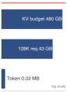
A dozen 128K-token requests exhaust the whole KV budget.

Napkin Math 10.5: KV-cache capacity estimator

Unlike the conservative decimal budgets used in the illustrative comparisons, this estimator retains the registered byte capacity when summing the node’s HBM. Converting its display units does not change that byte count.

Problem: A deployment serves an illustrative 70B-class GQA model with 128K context support (FP16 weights $\approx$ 141.2 GB) on an 8$\times$ H100 node (640 GB total HBM). The goal is to determine the maximum batch size for a context length of 128K tokens.

Formula: Bytes per token come from equation 5, and \[ \TotalMemoryFootprint = \WeightMemory + \KvCacheMemory, \qquad \KvCacheMemory = \BatchSize\times \SequenceLength\times \KvCacheBytesPerToken \]

Parameters:

$\LayerCount = 80$, $\KvHeadCount = 8$ for the assumed GQA architecture, $\AttentionHeadDimension = 128$.
$\ElementStorageSize = 2$ bytes (FP16).
Context $= 131{,}072$ tokens.

Step 1: Calculate memory per token. \[ m_{\text{token}} = 2 \times 80 \times 8 \times 128 \times 2 = 327,680 \text{ bytes} \approx 0.33 \text{ MB/token} \]

Step 2: Calculate cache per request. \[ 131,072 \text{ tokens} \times 0.33 \text{ MB/token} \approx 42.9 \text{ GB/request} \]

Step 3: Determine max batch size. Available Memory for KV = 687.2 GB (Total) - 141.2 GB (Weights) - 20 GB (System) = 526.0 GB. \[ \text{Max Batch} = \left\lfloor \frac{526.0}{42.9} \right\rfloor = 12 \]

Systems insight: Even with grouped query attention (GQA), whose shared key-value heads the 8-head count in this calculation already reflects, each 128K-context request consumes tens of gigabytes of KV state. This configuration therefore admits only a limited number of concurrent long-context requests. PagedAttention can recover allocation waste, but cannot shrink the attention tensors counted here. Increasing concurrency beyond that limit requires changing the memory budget, cache representation, or placement of state.

10.7.2 The fragmentation problem

Preallocating a contiguous HBM slab for every sequence’s maximum permitted length—such as reserving 4,096 tokens for a reply that finishes after 100—strands 60 to 80 percent of KV-cache memory in unused reservations and noncontiguous gaps (Kwon et al. 2023). Traditional contiguous allocation creates two distinct forms of this waste.

Internal fragmentation wastes memory within each allocation. Preallocated memory management reserves room at admission for the prompt plus the permitted output, so a request allowed 4,096 output tokens holds that room even if generation stops after 50, and the unused reservation cannot serve another request until it is released. If the output reservation holds 4,096 tokens but the average output uses 100 tokens, 97.6 percent of that output reservation goes unused. Prompt state consumes additional space; this calculation does not give the unused fraction of the combined prompt-and-output allocation.

External fragmentation compounds this problem across allocations. As sequences complete and new ones start, memory becomes fragmented into noncontiguous free blocks. Even with sufficient total free memory, no single block may be large enough for a new maximum-length allocation.

Consider a simplified example with 8 memory slots and maximum sequence length of 4. Fixed-size reservations first create internal fragmentation:

Time 0: Allocate Seq A (slots 0-3), Seq B (slots 4-7)
        [A][A][a][a][B][B][B][b]
        lowercase = reserved but unused

External fragmentation can arise when the allocator also permits smaller contiguous reservations. In a later state, two sequences occupy two slots each, leaving separated gaps:

Time 1: Active Seq C and Seq D leave two 2-slot gaps
        [ ][ ][C][C][ ][ ][D][D]

Time 2: Try to allocate Seq E (needs 4 contiguous slots)
        [ ][ ][C][C][ ][ ][D][D]  <- Total free slots = 4, largest block = 2

Result: enough total free capacity exists, but no contiguous block is large enough.

Under variable sequence lengths, the two effects compound. The vLLM authors measured roughly 60 to 80 percent of reserved KV-cache memory going unused in the prior serving systems they studied, capacity that could otherwise have admitted more sequences (Kwon et al. 2023).

10.7.3 PagedAttention

The fragmentation example exposes the allocator failure: enough KV-cache capacity can exist in aggregate while no contiguous block is available for the next sequence. PagedAttention fixes that serving problem by treating KV-cache storage like virtual memory rather than a single preallocated slab.

Systems Perspective 10.1: Analogy: The inefficient hotel

Consider a hotel storage room with 100 lockers. Each guest may bring up to 10 suitcases, but currently every guest has only one suitcase.

Under maximum-size reservation, the manager reserves 10 lockers for each guest. Ten guests exhaust the 100-locker budget while occupying only 10 lockers; the other 90 remain reserved but unused.

With on-demand allocation, each suitcase receives any free locker, and a directory records which lockers belong to each guest. At the current one-suitcase occupancy, the room can accommodate 100 guests. Additional suitcases still consume real capacity; allocation does not remove the storage limit.

Definition 10.3: PagedAttention

PagedAttention is an LLM serving memory management technique that applies virtual memory principles to KV cache allocation, storing attention states in noncontiguous, fixed-size physical blocks.

Significance: It eliminates external fragmentation within the fixed-block pool and bounds internal waste to the unused portion of each sequence’s final block. Recovering capacity from contiguous preallocation permits larger concurrent batches; the throughput gain depends on sequence lengths, demand, and the serving bottleneck.
Distinction: A contiguous allocation must find a sufficiently large free region; supporting later growth may require reserving extra space or relocating the allocation. PagedAttention uses a block table to map logical sequence indices to physical memory pages, allocating blocks as the sequence grows without requiring adjacent free space.
Common pitfall: A frequent misconception is that PagedAttention speeds up individual token math. In reality, it is a capacity optimization: it improves system-level efficiency by allowing larger batch sizes, though it adds a small indirection overhead for the block-table lookups.

PagedAttention (Kwon et al. 2023), introduced in vLLM, applies virtual memory concepts to KV cache management. Instead of contiguous allocation, the KV cache is divided into fixed-size pages, using 16-token blocks in the original paper’s default configuration, and sequences are allocated pages on demand. Whereas contiguous reservation strands non-adjacent free slots when earlier sequences finish, PagedAttention uses a per-sequence block table to map logical token pages to scattered physical HBM slots on demand (figure 10). The block size fixes how many tokens each page holds, so a sequence’s pages need not form one contiguous allocation run.

Kwon, Woosuk, Zhuohan Li, Siyuan Zhuang, Ying Sheng, Lianmin Zheng, Cody Hao Yu, Joseph Gonzalez, Hao Zhang, and Ion Stoica. 2023. “Efficient Memory Management for Large Language Model Serving with PagedAttention.” Proceedings of the 29th Symposium on Operating Systems Principles, 611–26. https://doi.org/10.1145/3600006.3613165.

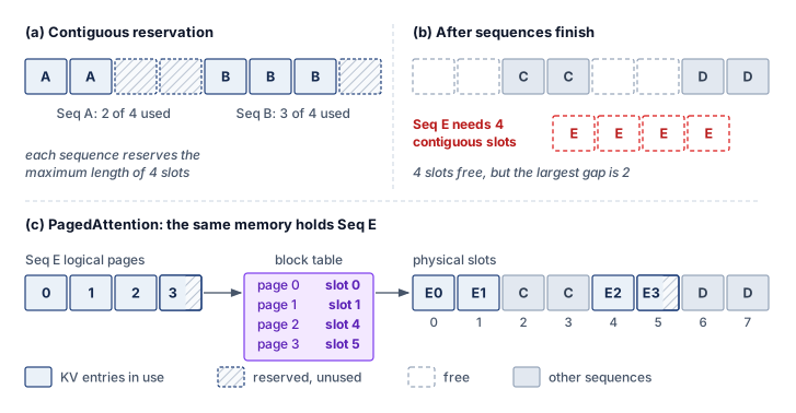
Figure 10: **KV Cache Fragmentation and the PagedAttention Solution**: The panels replay the eight-slot example from the text. (a) Contiguous reservation holds the maximum length of four slots per sequence, so the slots Seq A and Seq B never fill sit idle (internal fragmentation). (b) After sequences finish, four slots are free but the largest contiguous gap is two, so Seq E, which needs four contiguous slots, cannot be admitted (external fragmentation). (c) PagedAttention maps Seq E’s logical pages through a block table onto any free physical blocks, so the same memory now holds it; only the unfilled tail of its final block remains unused.

Beyond the fragmentation bounds in the definition, paging gives two further capacity advantages. Sequences grow page by page without worst-case preallocation, and common prefixes across requests can share physical pages directly in memory. Together, these properties turn KV cache capacity into a schedulable resource rather than a fixed per-request reservation. The price is indirection, because custom attention kernels must gather keys and values from noncontiguous blocks through each sequence’s block table. Recovered capacity also raises throughput only when demand fills it. Allocator occupancy is not a throughput measurement, since throughput still depends on decode work, prefill interference, and the latency budget.

10.7.4 Prefix caching

Recomputing the same 2,000-token system prompt, few-shot example block, or shared document on every arriving request burns prefill compute and fills HBM with identical copies of the same key-value tensors. Because many LLM workloads prepend those shared prefixes across thousands of concurrent queries, prefix caching stores the prefix’s KV-cache blocks once and shares them across compatible requests. Reuse requires the same token prefix and the same model computation, including any task-specific weight adapter and other inputs that affect the cached state. The cache key must distinguish those conditions, and the service must restrict sharing to the permitted users or tenants; matching visible text alone is insufficient. In valid block-level sharing (figure 11), logical tables for independent requests map common prefix tokens to physical blocks B0–B5, skipping their repeated prefill work while storing request-specific suffix state separately.

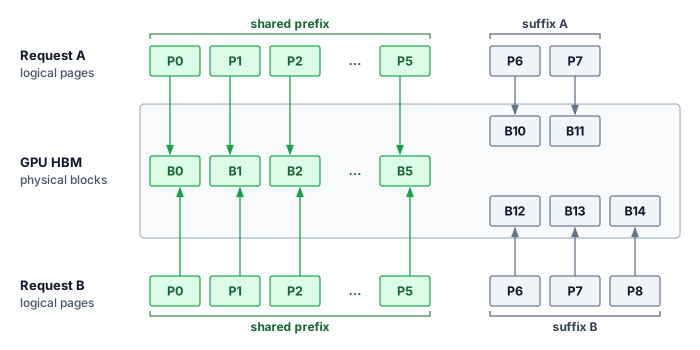
Figure 11: **Prefix Caching via Block Sharing**: PagedAttention enables efficient prefix caching by allowing multiple sequences’ block tables to point to the same physical blocks for shared content. In this example, the system prompt is stored in blocks 0–5. Request A and Request B map their first six logical pages to these same physical blocks, storing only their unique suffixes in new blocks. Sharing reduces KV memory and repeated prefill computation for workloads with a common context.

With PagedAttention, prefix caching uses copy-on-write semantics, in which shared blocks stay shared until a request must write into one, and that request then receives a private copy. Three requests that share a system prompt map their first six logical pages to the same physical blocks:

System prompt → Physical blocks [0, 1, 2, 3, 4, 5]

Request A page table: [0, 1, 2, 3, 4, 5, 10, 11]  <- shares prefix blocks
Request B page table: [0, 1, 2, 3, 4, 5, 12, 13, 14]  <- shares prefix blocks
Request C page table: [0, 1, 2, 3, 4, 5, 15]  <- shares prefix blocks

All three requests reference the same physical blocks for the system prompt, and their distinct suffixes occupy new blocks. If a shared prefix ends partway through a block, appending a different suffix writes into a shared block, which is the copy-on-write case. In a chatbot deployment where thousands of concurrent users share a long system prompt, sharing those prefix blocks cuts total KV-cache memory by roughly four-fifths (notebook 10.6).

Napkin Math 10.6: Prefix caching at scale

Scenario: A chatbot service uses a 2,000-token system prompt and serves 1,000 concurrent users. The illustrative model uses multi-head attention with 80 layers, 64 KV heads of dimension 128, and FP16 state. These full-width KV assumptions differ from the grouped-query attention of Llama-70B.

Without prefix caching:

KV cache per user: $2000 + 500\text{ (avg response)} =$ 2,500 tokens
Total KV cache: 2,500 tokens $\times 1000 \times 2 \times 80 \times 8192 \times 2 =$ 6.6 TB

With prefix caching:

Shared prefix: 2,000 tokens (once)
Unique per user: 500 tokens
Total: $(2000 \times 1) + (500 \times 1000) =$ 502,000
Memory: 502,000 $\times 2 \times 80 \times 8192 \times 2 =$ 1.3 TB

Result: Prefix caching yields a 79.9 percent memory reduction in KV cache, a roughly 5× capacity ratio for this fixed request population. Actual admitted concurrency also depends on other memory use, generation lengths, and latency limits.

Systems insight: Prefix caching pays off when the prefix hit rate is high because many requests share a long prefix. Table 10 uses illustrative hit-rate envelopes to show where the technique changes serving capacity and where it does not; production sizing must derive the distribution from a request trace.

Table 10: Illustrative Prefix-Caching Sensitivity: Assumed prefix hit rates and resulting KV-cache memory savings for three workload shapes. The values demonstrate sensitivity rather than population-wide norms; a serving team must measure exact-prefix reuse and prefix length on its own traffic.

Workload	Prefix hit rate	Memory savings
Chatbot (same system prompt)	95%+	70–80%
Document QA (same doc)	80–90%	50–70%
General API (diverse)	20–40%	10–30%

10.7.5 KV cache compression and attention layout

Even after paged allocation (section 10.7.3) eliminates unused reservations and prefix sharing (section 10.7.4) deduplicates shared prompts, unique active tokens still consume enough HBM per token to cap concurrency at small batch sizes. Shrinking that per-token footprint requires reducing either the bytes stored per element or the number of key-value heads cached per layer. The calculation here starts from a 64-KV-head multi-head attention (MHA) baseline so the grouped query attention subsection can isolate the head-count reduction as a separate architectural lever. For a 70B parameter model with 80 layers, 64 heads, head dimension 128, and sequence length 4096 in FP16, the KV cache requires:

\[\text{KV cache} = 2 \times 80 \times 64 \times 128 \times 4096 \times 2 \approx 10.7\text{ GB (FP16)}\]

A single request’s KV cache alone consumes a substantial fraction of the H100’s 80 GB of HBM. For a batch of 8 concurrent requests, the KV cache would require 85.9 GB, leaving no room for model weights or runtime state. Quantization reduces bytes per cached element, while architectural optimization can reduce the number of cached elements. These complementary levers change different factors in the capacity calculation.

KV cache quantization

Weight-only quantization leaves the KV cache untouched. KV cache quantization instead stores cached keys and values in INT8, FP8, or even INT4. Storing the cache payload in INT4 reduces it to approximately 2.7 GB per request, a 4× reduction before quantization metadata and any higher-precision residual state. Recovered memory can admit more sequences, but throughput depends on kernel support, conversion costs, and the latency target. Quality must also be evaluated for the intended contexts. Cached keys and values also have different distributions from the model weights and from each other. Keys tend to carry channel-wise outliers, which favors quantizing them per channel, while values lack that channel pattern and can be quantized per token.

Grouped query attention (GQA)

Grouped query attention (Ainslie et al. 2023) changes the number of key-value heads cached per layer, while quantization changes bytes per cached element. GQA is a model architecture choice established through training or checkpoint adaptation, not a serving switch that discards heads from an unchanged model. Holding the other cache dimensions fixed, the representative comparison of 64 KV heads under MHA with 8 under GQA gives an 8$\times$ reduction:

Ainslie, Joshua, James Lee-Thorp, Michiel de Jong, Yury Zemlyanskiy, Federico Lebron, and Sumit Sanghai. 2023. “GQA: Training Generalized Multi-Query Transformer Models from Multi-Head Checkpoints.” Proceedings of the 2023 Conference on Empirical Methods in Natural Language Processing, 4895–901. https://doi.org/10.18653/v1/2023.emnlp-main.298.

\[\text{KV cache (GQA)} = 2 \times 80 \times 8 \times 128 \times 4096 \times 2 \approx 1.3\text{ GB (FP16)}\]

At 1.3 GB, the GQA cache occupies less memory than the 10.7 GB required by MHA in this comparison. Combining GQA with INT8 KV cache quantization reduces the payload further, but per-request size still grows with context length. The architectural and numerical changes each require quality evaluation; recovered capacity permits additional sequences only while their execution remains within the service budget.

Napkin Math 10.7: The precision dividend

The precision dividend is the gain in maximum batch when lower precision frees memory for KV cache. Computing it first with the 64-head MHA baseline, whose requests carry eight times more KV state than the reference replica’s eight-head GQA cache, and then with the replica’s own GQA cache separates what the attention layout changes from what precision changes.

This comparison uses a conservative decimal HBM budget of 80 GB per GPU, matching the nameplate label rather than the registered byte capacity used by the node estimator.

Problem: A team serves a 70B model on 8$\times$ H100 GPUs. Weights in FP16 consume 140 GB (17.5 GB/GPU). KV cache at FP16 consumes 10.7 GB per request. How does quantizing weights to INT4 and KV cache to INT8 change the maximum batch size?

Before optimization (all FP16):

Weights: 17.5 GB/GPU
Available for KV cache: 80 GB $-$ 17.5 GB = 62.5 GB/GPU
KV cache per request: 10.7 GB $\div$ 8 $\approx$ 1.34 GB/GPU
Maximum batch size: $\lfloor$ 62.5 GB divided by 1.34 GB $\rfloor$ $\approx$ 46 requests

After optimization (INT4 weights, INT8 KV cache):

Weights: 17.5 GB $\times (4/16) =$ 4.38 GB/GPU (INT4)
Available for KV cache: 80 GB $-$ 4.38 GB = 75.62 GB/GPU
KV cache per request (INT8): 5.4 GB $\div$ 8 $\approx$ 0.67 GB/GPU
Maximum batch size: $\lfloor$ 75.62 GB divided by 0.67 GB $\rfloor$ $\approx$ 112 requests

The reference replica’s GQA cache (same budgets, eight KV heads):

KV cache per request at FP16: 1.34 GB, or 0.17 GB/GPU, giving a maximum batch of about 372 requests with FP16 weights
KV cache per request at INT8: 0.08 GB/GPU, giving about 901 requests with INT4 weights, a dividend of 2.4×

Systems insight: The two layouts yield the same multiplicative dividend, because each maximum batch is free memory divided by per-request cache, and precision changes both quantities by the same factors whatever the head count. The layout sets the absolute count, and at either precision the MHA replica admits roughly an eighth as many requests. In both layouts, compressing the cache does more for admission than compressing the weights, since halving per-request state doubles the count while INT4 weights free only the weight share of each GPU. At serving scale the recovered headroom is an admission budget, not yet throughput. The scheduler converts it into completed requests only while the larger batch still meets TPOT, and the counts here omit runtime allocations and headroom, so they are optimistic upper bounds on what admission control should allow.

10.7.6 Speculative decoding

When a lightly loaded replica serves one or a few interactive streams, batching has no other requests to share each weight read with, so every generated token pays the full latency of streaming the target model’s weights from HBM. While KV compression and GQA shrink the state each decode step reads, speculative decoding raises the useful work each step performs within a single request. A small draft model proposes $\SpeculativeDraftLength$ tokens, and the target model verifies all of them in one parallel forward pass (Leviathan et al. 2023; Chen et al. 2023). That pass streams the target’s weights once, as a single decode step does, so it processes $\SpeculativeDraftLength$ candidate positions for roughly the weight traffic of one token. This is the reuse that batching buys, drawn from one request’s future tokens instead of from other requests, and it moves the decode operating point up the bandwidth slope toward the ridge.

Leviathan, Yaniv, Matan Kalman, and Yossi Matias. 2023. “Fast Inference from Transformers via Speculative Decoding.” International Conference on Machine Learning (ICML), 19274–86.

Chen, C., S. Borgeaud, G. Irving, J.-B. Lespiau, L. Sifre, and J. Jumper. 2023. “Accelerating Large Language Model Decoding with Speculative Sampling.” arXiv Preprint arXiv:2302.01318.

On a shared time axis (figure 12), standard decoding uses four target passes to emit four tokens. In the speculative round, the draft model proposes $\DraftedToken_1$ through $\DraftedToken_4$ sequentially and the target evaluates those positions in one pass; three drafts are accepted, and the first rejected token, $\DraftedToken_4$, is replaced by $\ResampledReplacementToken$ sampled from the target. The shorter timeline holds only when drafting, verification, and correction together cost less than the target passes they replace. If too many drafts are rejected, the target streams its weights and keeps little of the work; if the draft model is too expensive, its own sequential passes consume the time that one-pass verification saved.

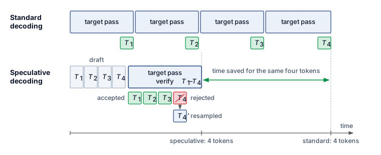
Figure 12: **Speculative Decoding Process**: Instead of generating tokens sequentially with the large target model, a small draft model proposes a sequence of $\SpeculativeDraftLength$ tokens. The target model verifies all $\SpeculativeDraftLength$ tokens in a single parallel forward pass. Drafted tokens that pass the acceptance test are emitted together; the first rejected token triggers a corrected sample and discards the remaining draft.

Algorithm 2 makes the acceptance test precise. After the single target pass, each drafted token is accepted with probability $\min(1, \TargetModelDistribution/\DraftModelDistribution)$, and a rejection resamples from the normalized positive residual $(\TargetModelDistribution- \DraftModelDistribution)_+$, so the emitted sequence is distributed exactly as the target model would have produced it unaided. That exactness is what lets a serving system trade draft-model compute for latency without changing the output distribution. Approximate verification rules, which accept drafts the target merely ranks highly, do not inherit the guarantee.

\begin{algorithm}
\caption{Speculative decoding}
\begin{algorithmic}
\Require target distribution $p_\theta(\cdot \mid \cdot)$; draft distribution $q_\phi(\cdot \mid \cdot)$; prefix $y_{1:t}$; draft length $K$
\Ensure one or more new tokens distributed as $p_\theta$
\For{$i = 1$ to $K$}
    \State draft $\hat{y}_{t+i}$ from $q_\phi(\cdot \mid y_{1:t}, \hat{y}_{t+1:t+i-1})$
\EndFor
\State run $p_\theta$ once on the prefix plus all $K$ drafts to obtain target distributions for the drafted positions and final next-token position
\For{$i = 1$ to $K$}
    \State $a_i \gets \min\!\left(1,\frac{p_\theta(\hat{y}_{t+i}\mid y_{1:t},\hat{y}_{t+1:t+i-1})}{q_\phi(\hat{y}_{t+i}\mid y_{1:t},\hat{y}_{t+1:t+i-1})}\right)$
    \State accept $\hat{y}_{t+i}$ with probability $a_i$
    \If{$\hat{y}_{t+i}$ is rejected}
        \State sample one corrected token from the normalized positive residual $(p_\theta-q_\phi)_+$
        \State emit accepted draft tokens and the corrected token; discard the remaining draft; start a new round
    \EndIf
\EndFor
\State if all $K$ drafts were accepted, emit them and sample one extra token from the target distribution
\end{algorithmic}
\end{algorithm}

The draft acceptance rate $\DraftTokenAcceptanceProbability$ determines how much proposed work survives. Under a simplified model in which each drafted position is accepted independently with that probability, a round emits its accepted prefix plus one target-sampled token, either the correction at the first rejection or the extra token after full acceptance. Each draft position contributes a token only if every earlier draft was accepted, so each successive position adds one more factor of $\DraftTokenAcceptanceProbability$ and the expectation is a geometric series over the $\SpeculativeDraftLength+1$ possible emissions. Equation 6 gives its closed form, the expected output of one verification round with $\SpeculativeDraftLength$ drafted tokens:

\[ \mathbb{E}[\RoundEmittedTokenCount] = \frac{1-\DraftTokenAcceptanceProbability^{\SpeculativeDraftLength+1}}{1-\DraftTokenAcceptanceProbability} \tag{6}\]

The target streams its weights once per round whatever the acceptance, so the weight traffic amortized per emitted token falls in proportion to equation 6, and low acceptance can make generation slower than ordinary decoding because rejected drafts still cost drafting and verification time. That mechanism belongs to one replica. A serving fleet must decide when to enable speculation, how its memory cost interacts with admission, and whether it improves the endpoint’s SLO-compliant capacity.

Those decisions start from how steeply the benefit falls with acceptance. The following calculation assumes $\SpeculativeDraftLength= 5$ draft tokens, a draft step 20$\times$ faster than a target decode step, and a verification pass costing one target decode step, which isolates sensitivity to acceptance:

High acceptance ($\DraftTokenAcceptanceProbability= 0.9$) yields an expected 4.69 tokens per verification round for a 3.7× speedup, medium acceptance ($\DraftTokenAcceptanceProbability= 0.7$) delivers 2.94 tokens per round for a 2.4× speedup, and low acceptance ($\DraftTokenAcceptanceProbability= 0.5$) drops progress to 1.97 tokens per round, yielding a modest speedup of 1.6×.

Speedup shrinks quickly as draft acceptance falls.

Acceptance depends on the draft-target pair, sampling policy, and request distribution. The preceding calculations are sensitivity cases, not fixed acceptance rates for chat, reasoning, or code generation. A serving fleet must measure acceptance and useful token throughput for its actual traffic before selecting a speculation policy, and that policy must answer three serving concerns: memory, the SLO, and change over time.

The first concern is memory. The draft model is not free state. It requires memory for weights, and each in-flight request that uses it reserves additional draft KV state. Pairing a 7B draft model with a 70B target adds roughly 14 GB of FP16 weights per replica plus per-request draft cache. When colocated with the target, this memory overhead competes directly with the KV-cache admission budget developed in section 10.7.1; every gigabyte reserved for the draft is unavailable to target requests. Under a binding memory limit, that reservation lowers maximum concurrency. Placing the draft on separate devices preserves target memory at the cost of additional hardware and communication. The admission controller and the speculation policy therefore require a joint capacity and latency evaluation.

The second concern is which service-level objective the endpoint must meet. At sufficient acceptance, speculation can reduce TPOT, while draft execution and cache residency reduce admission capacity, so the scheduler should compare SLO-compliant goodput with and without speculation under the intended load. TTFT needs separate measurement because draft setup and prefill can add work before the first response token.

The third concern is that acceptance and load change over time. Batch size moves the payoff as well as acceptance does: verification is cheap only while decode leaves compute idle, and a larger batch consumes that headroom, so the same draft configuration can cross from a gain to a loss as concurrency rises, while variable accepted lengths add scheduler work. The crossover batch must be measured for each draft-target pair and machine rather than inferred from a batch-one result. A scheduler can enable speculation when measured TPOT or goodput improves and disable it when verification cost outweighs accepted progress, but disabling draft execution frees neither the resident draft weights nor the draft KV pages; recovering that capacity requires unloading the weights and ending or migrating the speculative state. Self-speculative decoding, Medusa prediction heads (Cai et al. 2024), and lookahead decoding change this budget, and each needs its own quality, acceptance, and resource evaluation.

Cai, Tianle, Yuhong Li, Zhengyang Geng, Hongwu Peng, Jason D. Lee, Deming Chen, and Tri Dao. 2024. “Medusa: Simple LLM Inference Acceleration Framework with Multiple Decoding Heads.” Proceedings of the 41st International Conference on Machine Learning (ICML).

10.7.7 Preemption and the victim policy

When active sequences grow their contexts until every free KV-cache page is claimed, the replica can neither advance those sequences nor admit a higher-priority arrival without evicting a sequence that is already running. Iteration-level admission can take requests in first-come-first-served (FCFS) order while still advancing many sequences together, so head-of-line blocking arises only in a serial or full-batch-barrier implementation; once the KV pool fills, however, admitting a waiting request or extending an active one means taking capacity from a running sequence.

Preemptive scheduling allows the system to stop allocating decode iterations to one request so that another can run. Preemption is practical at token boundaries, but it is not free. The scheduler must retain the request’s KV pages in HBM, swap them to host memory, or discard them and repeat prefill when the request resumes. A useful victim policy compares those three costs with the waiting request’s remaining deadline rather than preempting at a fixed generation length. Retaining state consumes scarce capacity, swapping consumes interconnect bandwidth, and recomputation consumes prefill compute; under heavy load, rejecting low-priority work can cost less than repeatedly moving or rebuilding its state.

10.7.8 KV-cache budgeting and eviction

Admitting sequences up to a naive average-length estimate without reserving headroom for context growth forces the replica into constant mid-generation preemptions or out-of-memory crashes. Effective KV-cache management therefore begins with capacity accounting rather than an eviction policy. The serving process first reserves memory for weights, activations, runtime overhead, and safety headroom, then treats the remaining HBM as a managed pool for active sequences:

Available GPU memory = Total - Weights - Activations - Overhead
KV pool size = 0.9 * Available  # Leave 10% headroom

Max concurrent sequences = KV pool size / (avg_seq_length * KV bytes per token)

That budget estimates how many sequences can coexist, but an average length does not reserve space for future growth. Admission must account for the admitted requests’ remaining budgets. LRU eviction can reclaim retained prefix blocks that no active request references. Reclaiming an active sequence’s state instead requires a preemption decision, made with the victim policy of section 10.7.7. What capacity accounting adds is the observation that freeing the most bytes is not necessarily the cheapest recovery, because the largest sequence is also the most expensive to swap or rebuild.

Example 10.4: KV cache memory hierarchy

Scenario: A multi-tenant LLM serving system experiences KV-cache HBM exhaustion (80 GB limit) during peak concurrency.

Diagnosis: Pure HBM allocation limits node concurrency to 50 active sequences in this scenario. Implementing a 3-tier memory hierarchy (HBM $\to$ CPU DRAM $\to$ Non-Volatile Memory Express (NVMe) SSD) allows swapping inactive sequence pages to CPU DRAM or NVMe. The illustrative swap budgets of 1–5 ms and 10–50 ms, respectively, require validation for the bytes transferred, effective bandwidth, and contention; they are not fixed properties of the storage tiers.

Systems lesson: In this scenario, multi-tier paging raises retained sequence capacity from 50 to 500, while the active HBM-resident set remains limited to 50. Suspended sequences must be restored before execution resumes under this policy. The extra retention does not establish a throughput gain; restoration costs must fit the affected requests’ deadlines. Streaming active state from another tier would be a different execution policy with transfer costs on the decode path.

10.7.9 Adapter state and locality

Deploying a separate copy of a 140 GB base model for each of 10,000 fine-tuned tenants is prohibitive in HBM, yet fetching a tenant’s weight delta from host memory on the critical path stalls every decode step. Alongside the KV-cache attention state of concurrent sequences, adapter serving therefore adds a second claim on the replica’s memory and bandwidth budget. A low-rank adaptation (LoRA) adapter is a user- or task-specific weight delta that must be available when its request executes. LoRA modifies a shared base model without copying all of its weights: the serving process keeps the 140 GB base resident once while loading the adapters needed by active requests. Whether adapter storage or transfer becomes limiting depends on the active adapter mix, ranks, and reuse.

Systems Perspective 10.2: The context switch of machine learning

Adapter locality becomes a performance constraint when a scheduled request needs weights that are not resident. Loading those weights from host memory resembles part of an operating-system context switch, because execution must wait for the required state unless transfer overlaps other useful work. An adapter already in HBM need not be transferred from the host on every generation step. Coordinating admission with adapter placement can reduce these stalls, while grouping requests by adapter can improve reuse at the cost of waiting for compatible work. The policy must balance locality against the latency and fairness of less frequent adapters.

Multi-LoRA serving and batched adapter execution

In multi-tenant environments, thousands of fine-tuned adapters share a single base foundation model. For a linear projection layer with base weights $\WeightMatrix_0 \in \mathbb{R}^{\LayerOutputWidth \times \LayerInputWidth}$, an adapter $\AdapterIndex$ parameterizes the forward transformation using low-rank decomposition matrices $\AdapterDownProjectionMatrix_k \in \mathbb{R}^{\AdapterRank_k \times \LayerInputWidth}$ and $\AdapterUpProjectionMatrix_k \in \mathbb{R}^{\LayerOutputWidth \times \AdapterRank_k}$ with rank $\AdapterRank_k \ll \min(\LayerInputWidth, \LayerOutputWidth)$ (typically $\AdapterRank\in \{8, 16, 64\}$), as formulated in equation 7:

\[\LayerOutputVector= \LayerInputVector\WeightMatrix_0^T + \frac{\AdapterScalingFactor_k}{\AdapterRank_k} \LayerInputVector\AdapterDownProjectionMatrix_k^T \AdapterUpProjectionMatrix_k^T \tag{7}\]

where $\LayerInputVector\in \mathbb{R}^{1 \times \LayerInputWidth}$ is a row vector, $\LayerOutputVector\in \mathbb{R}^{1 \times \LayerOutputWidth}$, and $\AdapterScalingFactor_k$ is a fixed scaling factor, the hyperparameter usually written $\Glyph{\alpha}$ in LoRA papers and renamed here because $\Glyph{\alpha}$ already denotes startup latency and draft acceptance in this chapter. Each adapted projection adds $\AdapterRank_k(\LayerInputWidth + \LayerOutputWidth)$ parameters instead of a full $\LayerInputWidth\LayerOutputWidth$ weight matrix. The resident adapter budget therefore depends on which layers are adapted, their dimensions and ranks, precision, and the number of simultaneously loaded tenants.

↪ How low-rank adapters are trained, and how their rank is chosen under a device’s memory and energy budget, is developed in Low-rank techniques.

Packing requests with different adapters into one batch lets the base projection $\LayerInputMatrix\WeightMatrix_0^T$ execute as one shared dense general matrix multiply (GEMM), but a naive implementation then launches a separate small kernel for each request’s adapter $(\AdapterDownProjectionMatrix, \AdapterUpProjectionMatrix)$. Hundreds of such launches per layer make host dispatch and launch latency significant even when each adapter performs little arithmetic, and the small kernels leave GPU streaming multiprocessors (SMs) underused. The following batched operation removes the need for one launch per request.

Definition 10.4: Batched gather-matrix-vector multiplication (BGMV)

Batched gather-matrix-vector multiplication (BGMV) is a GPU kernel operation that batches matrix-vector products across distinct adapters, dynamically gathering adapter weights from a memory pool according to a per-token adapter index vector.

Significance: It reduces per-request kernel launch overhead in multi-adapter serving, allowing different adapters to share kernel launches. The remaining overhead depends on adapter ranks, batch composition, and memory locality.
Distinction: A single dense GEMM applies one weight matrix across its input rows. BGMV gathers the adapter-specific weight slice for each element, combining distinct matrix-vector products in one kernel operation.
Common pitfall: Batched execution does not itself solve allocation waste. Loading and unloading differently sized adapters can fragment a contiguous allocator. Paged adapter storage addresses that separate problem, provided the execution kernels support its layout.

Systems such as Punica (Chen et al. 2024) and S-LoRA (Sheng et al. 2024) address launch overhead and adapter memory through two architectural mechanisms (definition 10.4):

Batched gather-matrix-vector (BGMV) kernels

Instead of launching separate kernels for every request, batched or segmented gather-matrix-vector operations group different adapters within each projection. Down-projection and up-projection can use separate kernels; Punica distinguishes shrink and expand operators (Chen et al. 2024). The scheduler builds a per-request adapter index, and each kernel uses it to gather a request’s activation row and its adapter’s matrices, apply the rank-$\AdapterRank$ down- and up-projections of equation 7, and add the resulting delta to the shared base projection’s output.

Chen, Liyuan, Zihao Ye, Yonghao Wu, Danyang Zhuo, Luis Ceze, and Arvind Krishnamurthy. 2024. “Punica: Multi-Tenant LoRA Serving.” Proceedings of the 7th Conference on Machine Learning and Systems (MLSys).

By gathering adapter weights within batched kernels, BGMV avoids dispatching a separate kernel for each request’s adapter. The gain must be measured against the actual adapter mix; irregular access and small ranks can still limit achieved bandwidth.

Unified paged adapter memory management

S-LoRA (Sheng et al. 2024) jointly manages adapter weights and KV state in a unified GPU memory pool. Its page holds a vector along the shared hidden dimension, rather than a fixed operating-system-sized byte allocation. Adapter matrices $\AdapterDownProjectionMatrix_k$ and $\AdapterUpProjectionMatrix_k$ occupy noncontiguous pages, allowing adapters of varying ranks ($\AdapterRank\in \{8, 16, 32, 64\}$) to share capacity with growing KV caches. Paging reduces fragmentation; both kinds of state still consume the same finite pool.

The published design keeps adapters in host memory and uses the waiting queue to predict which weights the next batch will need. Prefetching overlaps adapter transfers with current execution when sufficient time and free GPU memory are available. A cache miss whose transfer cannot be hidden still delays the affected request.

Across a tensor-parallel group, S-LoRA aligns each adapter with the base layer’s column- or row-parallel split and communicates only the $\AdapterRank_k$-dimensional intermediates. An AllGather assembles the intermediate after a column-parallel down-projection, and an AllReduce sums partial intermediates after a row-parallel one (Sheng et al. 2024). The layout reduces adapter replication at the price of extra synchronization on those small intermediates, while the final output assembly shares the base layer’s own collective.

Sheng, Ying, Shiyi Cao, Dacheng Li, Coleman Hooper, Shuo Chen, Daxin Jiang, Christopher Rodriguez, et al. 2024. “S-LoRA: Serving Thousands of Concurrent LoRA Adapters.” Proceedings of the 7th Conference on Machine Learning and Systems (MLSys).

KV pages and adapter deltas share HBM with the base weights, so every byte freed in one allocation can admit work in another. When a request claims that memory, and how fast it then uses it, depends on the phase it is in: prefill builds a request’s cache in one pass, while decode extends it one token at a time.

Self-Check: Question

How does PagedAttention reduce memory waste in LLM KV cache management, and what system-level benefit can follow?
1. It compresses KV cache tensors using lossless entropy coding to reduce arithmetic intensity in attention kernels.
2. It replaces standard multi-head attention with grouped query attention by dynamically merging key-value heads.
3. It maps logical tokens to non-contiguous fixed-size physical blocks, reclaiming unused reservations so that more requests may fit
4. It offloads 100% of KV cache data to host CPU DRAM, eliminating GPU HBM usage entirely for active sequences.
What cost does a colocated draft model impose on a speculative decoding replica, and how does it influence whether speculative decoding should be enabled for a specific serving endpoint?
1. The latency penalty paid when draft models fail to generate valid UTF-8 token encodings.
2. The GPU memory allocated to draft model weights and draft KV cache, which reduces available HBM for batch concurrency.
3. The serialization overhead incurred when transmitting draft tokens across InfiniBand interconnects.
4. The loss in model generation accuracy caused by greedy sampling during draft token verification.
Why does speculative decoding accelerate autoregressive generation on modern GPUs without altering the target model’s output probability distribution?
1. It lets the draft model’s tokens through whenever the draft model’s own confidence exceeds a fixed threshold, so the target pass can be skipped for confident tokens
2. It runs the target model at lower precision during verification, so each verification pass streams fewer weight bytes than an ordinary decode step
3. It accepts each draft token with probability equal to the smaller of one and the ratio of the target model’s probability to the draft model’s probability, resamples a rejected position from the normalized positive difference between the two distributions, and verifies all drafts in one target pass for roughly the weight traffic of one token
4. It verifies only the first draft token and emits the remaining drafts unchecked, relying on the draft model’s training to match the target
A chatbot has 1,000 concurrent users sharing a 2,000-token prefix and retaining 500 private response tokens each. For a hypothetical MHA model with 80 layers, 64 KV heads, head width 128, and FP16 cache, explain the reduction from about 6.6 TB to 1.3 TB with prefix sharing.
True or False: When measured acceptance falls and the scheduler stops running the draft model, the memory that speculative decoding consumed returns immediately to the target model’s KV-cache admission budget.
In the precision dividend for the reference 70B replica, FP16 weights use 17.5 GB per GPU on eight 80 GB GPUs. Ignoring runtime reserves and quantization metadata, INT4 weights use about 4.4 GB per GPU and INT8 KV cache halves the per-request cache footprint. Why is the gain in maximum batch about 2.4 times rather than the fourfold weight reduction?
1. Because INT4 weights must be dequantized into a resident FP16 copy, so only part of the weight saving survives in HBM
2. Because the gain applies only to the eight-head GQA cache; the 64-head MHA baseline gains nothing from INT8 KV storage
3. Because the freed weight memory raises the KV budget from 62.5 GB to about 75.6 GB per GPU, a factor of about 1.21, and halving bytes per cached request doubles the count again, so the two effects multiply to about 2.4
4. Because quantizing the KV cache lengthens each decode step enough to cancel most of the extra capacity

See Answers →

10.8 Prefill and Decode

Admitting a 4,096-token prompt onto a worker that is already streaming replies to thirty users saturates the GPU’s Tensor Cores for hundreds of milliseconds and freezes every active token stream until the prompt finishes. A language-model request is two workloads in sequence: prefill reads the whole prompt in one forward pass and writes its keys and values into the cache sized in section 10.7.1, while decode extends that cache one token per step until the response ends. Because the two phases run the same weights on opposite sides of the roofline ridge, their asymmetry decides which optimization helps which phase, how a replica schedules them when they share a worker, and whether they should share one at all.

10.8.1 The phase asymmetry

That roofline split comes directly from how many tokens each phase feeds through a linear projection at once. During the prefill phase, the engine computes key-value representations across all prompt tokens ($\PromptLength$) concurrently. Because all prompt tokens are processed in parallel, the linear projection GEMM operations operate on large sequence dimensions ($\GemmRowDimension= \PromptLength$). For a projection layer with hidden dimension $\HiddenDimension$, arithmetic intensity scales with prompt length: \[\PrefillArithmeticIntensity\approx \frac{2 \cdot \PromptLength\cdot \HiddenDimension^2}{2 \cdot \HiddenDimension^2} = \PromptLength\quad \left[\frac{\text{FLOPs}}{\text{byte of weights loaded}}\right]\] A 1,024-token prompt therefore performs about 1,024 FLOPs per byte of FP16 weights, well past an H100’s FP16 ridge. Under this weight-traffic-only approximation, increasing $\PromptLength$ beyond the accelerator’s ridge point moves the projection’s roofline ceiling to the compute limit. Reaching that ceiling still depends on kernel efficiency; short prompts, attention, other memory traffic, and communication can limit the complete prefill phase, so prefill as a whole still requires profiling.

↩︎ The ridge point that separates compute-bound from bandwidth-bound execution is established in Roofline model.

In contrast, the subsequent decode phase generates a single token per sequence sequentially, so the GEMM’s row dimension is the number of sequences decoding together, not the prompt length. At batch one the intensity is about 1 FLOP per byte of FP16 weights. At the decode batch sizes this chapter considers, from tens of sequences up to the knee near 80 in notebook 10.2, the arithmetic intensity $\DecodeArithmeticIntensity\approx \DecodeBatchSize$ stays below the ridge point, placing the weight projections in a memory-bandwidth-bound regime under this approximation. Each decode iteration streams the active weights from HBM and reuses them across the batch, which is why batch size is the decode phase’s control knob. The approximation omits KV-cache reads, which grow with every sequence’s context, so larger batches and longer contexts add bytes to every step and hold decode on the bandwidth slope short of the ridge.

Long-prompt prefill reaches the compute ceiling; decode stays on the bandwidth slope.

The asymmetry also sorts the optimizations by phase. Tiled, IO-aware attention reduces attention’s memory traffic mainly during prefill, because only prefill forms the full prompt-by-prompt score matrix that a tiled kernel avoids writing to HBM (Tiling and IO-aware attention). A decode step has a single query row and no quadratic intermediate; it benefits instead from a fused kernel that reads each cached key and value once and computes scores, softmax, and the weighted sum in one pass. Speculative decoding (section 10.7.6) targets decode alone, and KV-cache quantization reduces decode’s storage and read traffic while its encoding cost begins when prefill writes the cache. Precision helps both phases through different mechanisms: a weight-activation format raises the compute ceiling that long-prompt prefill reaches, while low-bit weights shrink the bytes that weight-dominated decode streams (section 10.9). Each gain depends on format and kernel support, conversion overhead, and the costs the change leaves untouched, and each must preserve output quality.

These are properties of each phase in isolation. Once continuous batching admits new prompts onto a worker that is decoding other streams, the asymmetry becomes a scheduling conflict between them, and a replica has two ways to resolve it: interleave the phases on one worker, or give each phase its own pool.

10.8.2 Chunked prefill and prompt-decode interleaving

Continuous batching admits work at iteration boundaries, yet production requests arrive with widely disparate prompt lengths. Admitting a long prompt in one piece holds the worker for its entire compute-bound prefill while the bandwidth-bound decode streams beside it wait.

Definition 10.5: Chunked prefill

Chunked prefill is an LLM serving mechanism that divides long prompt evaluations into discrete token chunks of size at most $\PrefillChunkSize$, interleaving prefill computation with ongoing decode iterations within a shared token budget.

Significance: It limits the prompt-decode interference problem where monolithic prefills stall active decode streams for hundreds of milliseconds, giving the scheduler control over how much prefill work can lengthen the TBT of active streams. Meeting interactive streaming service-level objectives (SLOs) still requires measuring the resulting tail latency.
Distinction: Unlike continuous batching with monolithic prefill (which prefills each prompt in one uninterrupted pass before the worker returns to decoding), chunked prefill treats prefill as a multi-step iterative process co-scheduled alongside memory-bound decode tokens.
Common pitfall: Sizing the chunk budget $\PrefillChunkSize$ too small incurs kernel launch and attention mask overheads, degrading overall prefill throughput. Sizing it too large allows prefill compute to monopolize execution time, causing TBT tail spikes.

With an unchunked prefill policy, the scheduler runs an incoming prompt through the whole model before returning to decode work. The interference comes from scheduling that whole operation without interleaving other requests’ decode steps, and the delay lands in the TBT of requests already decoding on the same worker. A long response can dilute an isolated stall in its average TPOT even though the user sees a conspicuous gap, so prioritizing the new prompt’s time to first token can consume the streaming-latency budget of requests already decoding. The measured prefill duration and the endpoint’s TBT target determine whether interleaving is necessary.

The chunked prefill scheduling mechanism

To limit this interference, chunked prefill (definition 10.5, used by Sarathi-Serve (Agrawal et al. 2024)) partitions prompts into chunks of at most $\PrefillChunkSize$ tokens. A candidate range such as $256\text{--}512$ tokens must be tested against the model, hardware, and streaming deadline rather than treated as a universal setting. A prompt of length $\PromptLength$ requires at least $\lceil \PromptLength/ \PrefillChunkSize\rceil$ scheduling iterations; a smaller residual token budget can require more.

The two schedules in figure 13 hand the same long prompt to the same worker. Run whole, its prefill sits between two decode steps of every active stream, so each stream’s token gap stretches to the full prefill time. Split into chunks, the prompt advances one chunk per hybrid iteration beside the streams’ decode tokens, so each stream waits at most one hybrid iteration, while the prompt’s own first token arrives later than it would have under the monolithic schedule.

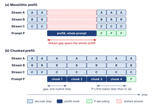
Figure 13: **Chunked Prefill Trades One Prompt’s TTFT for Every Stream’s TBT**: Three streams decode while a long prompt P arrives; the timing is illustrative. (a) A monolithic prefill runs P’s whole prompt in one pass, and every active stream stalls for its full duration. (b) Chunked prefill gives P one chunk per hybrid iteration beside the streams’ decode tokens, so each stream’s gap shrinks to one hybrid iteration, and P’s first token arrives later. Chunking changes when the prefill work runs, not how much of it there is.

In each iteration, the scheduler constructs a hybrid batch combining active decode requests with prefill chunks under a global iteration token budget $\IterationTokenBudget$, a count of tokens rather than a time, as formulated in equation 8:

\[\DecodeBatchSize+ \sum_{\PrefillRequestIndex \in \ActivePrefillRequestSet} \PrefillAllocatedTokenCount_{\PrefillRequestIndex} \le \IterationTokenBudget \tag{8}\]

where $\DecodeBatchSize$ is the number of active decode tokens and $\PrefillAllocatedTokenCount_{\PrefillRequestIndex}$ is the number of prompt tokens allocated to waiting prefill request $\PrefillRequestIndex$, so every term counts tokens. The simplified loop assumes admission control reserves sufficient KV-cache capacity and a future decode slot for each admitted request, keeping the decode count within the iteration budget even after prefills are promoted. Each waiting request contributes at most one chunk per iteration, with its committed prompt offset unchanged until execution completes. Algorithm 3 formalizes this iteration-level hybrid scheduling loop.

\begin{algorithm}
\caption{Chunked prefill and hybrid batch scheduler}
\begin{algorithmic}
\Require waiting prefill queue $\mathcal{Q}_{\text{prefill}}$; active decode set $\mathcal{D}$; iteration token budget $N_{\text{budget}}$; maximum chunk size $C_{\text{chunk}}$
\Ensure generated tokens for decode requests; incremental KV-cache construction for prefills
\While{serving engine is active}
    \State $B_{\text{dec}} \gets |\mathcal{D}|$
    \State $N_{\text{rem}} \gets N_{\text{budget}} - B_{\text{dec}}$
    \State $\mathcal{B}_{\text{prefill}} \gets \emptyset$
    \For{each $R_i$ in a snapshot of $\mathcal{Q}_{\text{prefill}}$, in queue order}
        \If{$N_{\text{rem}} > 0$}
            \State $o_i \gets R_i.\text{offset}$
            \State $C_i \gets \min(C_{\text{chunk}}, N_{\text{rem}}, R_i.\text{prompt\_length} - o_i)$
            \State $\mathcal{B}_{\text{prefill}} \gets \mathcal{B}_{\text{prefill}} \cup \{(R_i, o_i, C_i)\}$
            \State $N_{\text{rem}} \gets N_{\text{rem}} - C_i$
        \EndIf
    \EndFor
    \State run hybrid forward pass using each prefill slice $R_i[o_i:o_i+C_i]$ and the decode set $\mathcal{D}$
    \State append newly generated tokens for all $R \in \mathcal{D}$
    \State remove completed decode requests from $\mathcal{D}$ and release their KV blocks
    \For{$(R_i, o_i, C_i) \in \mathcal{B}_{\text{prefill}}$}
        \State update prompt offset: $R_i.\text{offset} \gets o_i + C_i$
        \If{$R_i.\text{offset} = R_i.\text{prompt\_length}$}
            \State promote $R_i$ from $\mathcal{Q}_{\text{prefill}}$ to $\mathcal{D}$
        \EndIf
    \EndFor
\EndWhile
\end{algorithmic}
\end{algorithm}

Weight-loading amortization via decode piggybacking

Executing prefill and decode tokens together in shared projection operations amortizes weight loading across both phases, an effect termed decode piggybacking. Alternating separate prefill and decode operations limits scheduling interference but does not by itself establish this weight reuse.

In a small-batch isolated decode step, streaming the model parameters ($\WeightMemory$ bytes) from HBM to registers achieves low arithmetic intensity because only $\DecodeBatchSize$ tokens share the weight reads. Memory bandwidth then limits how much work the compute units can sustain, leaving arithmetic capacity available for a larger shared projection.

In a hybrid iteration, the model weights loaded from HBM into on-chip cache and registers are simultaneously reused for both the compute-dense prefill chunks ($\sum_{\PrefillRequestIndex} \PrefillAllocatedTokenCount_{\PrefillRequestIndex}$ tokens in total) and the memory-bound decode tokens ($\DecodeBatchSize$ tokens). Ignoring attention-state traffic, communication, and scheduling overhead gives the projection-only lower-bound estimate in equation 9:

\[\HybridIterationTime\gtrsim \max\left(\frac{\WeightMemory}{\SustainedMemoryBandwidth}, \frac{2 \cdot (\DecodeBatchSize+ \sum_{\PrefillRequestIndex} \PrefillAllocatedTokenCount_{\PrefillRequestIndex}) \cdot \ActiveParameterCount}{\PeakRate}\right) \tag{9}\]

where $\ActiveParameterCount$ is the active parameter count, $\SustainedMemoryBandwidth$ is HBM memory bandwidth, and $\PeakRate$ is peak accelerator compute throughput. These quantities must describe the same device or shard. Balancing the total prefill token allocation against weight streaming can amortize weight-loading cost across both phases, but this lower bound cannot guarantee $\HybridIterationTime\le \text{SLO}_{\text{TBT}}$. Chunk sizing must leave room for the omitted costs and be validated against measured tail latency under the intended workload.

Example 10.5: Sarathi: Chunked prefill implementation

Scenario: An LLM inference server receives a mix of long input prompts ($10{,}000+$ tokens) and interactive short decode requests (Agrawal et al. 2024).

Diagnosis: When the worker schedules a full long-prompt prefill before returning to decode, that prefill can occupy execution for hundreds of milliseconds and create a TBT spike for active streams.

Systems lesson: Chunking moves the cost of a long prompt rather than removing it. At $512$ tokens per chunk, a $10{,}000$-token prompt needs at least $\lceil 10{,}000/512 \rceil = 20$ iterations to finish its prefill. With this prompt as the only prefill request, active streams share each decode iteration with at most one of its chunks, while the prompt’s own time to first token stretches across those 20 iterations. Multiple waiting prompts can contribute additional chunks within the total iteration budget. The chunk budget sets that exchange between other streams’ TBT and the long prompt’s TTFT, so it must be tuned against both measured tails.

Agrawal, Amey, Nitin Kedia, Ashish Panwar, Jayashree Mohan, Nipun Kwatra, Bhargav S. Gulavani, Alexey Tumanov, and Ramachandran Ramjee. 2024. “Taming Throughput-Latency Tradeoff in LLM Inference with Sarathi-Serve.” 18th USENIX Symposium on Operating Systems Design and Implementation (OSDI 24), 117–34.

10.8.3 Prefill-decode disaggregation

Even with chunked prefill, every hybrid step still forces active decode streams to wait while prompt chunks execute on the same GPU, and a single worker pool must compromise between prefill’s compute-heavy parallelism and decode’s bandwidth- and capacity-heavy layout. Disaggregation removes that compromise by giving each phase its own hardware pool, while the KV-cache sizing of section 10.7.1 sets the price of separating them: the cache that prefill builds is the exact payload that the network must hand off to the decode pool.

Disaggregation partitions the serving pipeline into specialized physical tiers (figure 14). In the illustrated long-prompt, small-decode-batch regime, the compute-bound prefill pool and the bandwidth-bound decode pool are joined by a remote direct memory access (RDMA) KV-cache transfer (Zhong et al. 2024), which keeps the phases from competing on one accelerator and permits independent parallelism and capacity plans. The phase asymmetry tells each pool what to buy: the prefill pool wants arithmetic throughput for its compute-bound GEMMs, while the decode pool wants memory bandwidth and capacity for weight streaming and KV cache, which also makes it the natural home for aggressive weight quantization. The transfer and queueing at each pool still add to request latency, and other batch or context sizes can change which resources bind.

Zhong, Yinmin, Shengyu Liu, Junda Chen, Jianbo Hu, Yibo Zhu, Xuanzhe Liu, Xin Jin, and Hao Zhang. 2024. “DistServe: Disaggregating Prefill and Decoding for Goodput-Optimized Large Language Model Serving.” 18th USENIX Symposium on Operating Systems Design and Implementation (OSDI 24), July, 193–210.

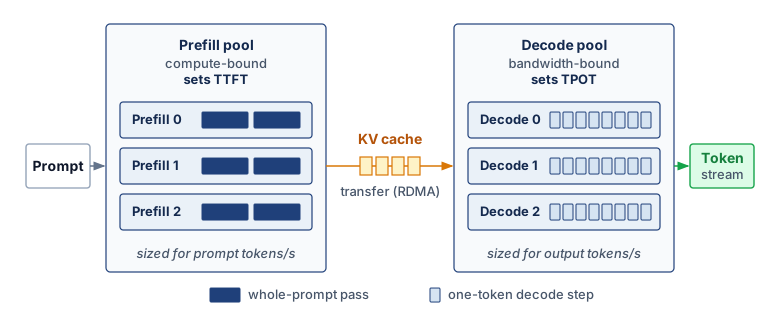
Figure 14: **Disaggregated Serving Architecture**: A long-prompt, small-decode-batch regime separates compute-bound prefill instances from memory-bandwidth-bound decode instances, mediated by RDMA KV-cache transfer. Because prefill sets time to first token and decode sets time per output token, each pool is sized for its own token rate. Other batch and context sizes can change the binding resources.

The disaggregation decision therefore depends on a quantitative contract, not on the phase labels alone. If prefill produces $\KvCacheMemory$ bytes of attention state and the usable inter-pool bandwidth is $\LinkBandwidth$, then the handoff consumes at least

\[\KvCacheHandoffTime= \MessageStartupLatency+ \frac{\KvCacheMemory}{\LinkBandwidth}, \tag{10}\]

where $\MessageStartupLatency$ includes transfer setup and queueing for the operating point being evaluated; it is not a fixed network latency once load changes. The payload term sets the scale. A 128K-token request on the GQA model of notebook 10.5 carries tens of gigabytes of KV state, so moving it over a single 450 GB/s NVLink direction takes on the order of a hundred milliseconds, and an inter-node link takes longer still. Spreading the transfer across a tensor-parallel group divides that time only when each device has its own path to its counterpart in the decode pool. Because $\KvCacheMemory$ grows linearly with prompt length, the long prompts that make disaggregation attractive are also the prompts whose handoff costs most, and that cost lands on TTFT.

Equation 10 therefore makes placement part of the service contract. The prefill pool must sustain the admitted prompt-token rate, the decode pool must sustain the admitted output-token rate, and both pools need headroom for the request-length distribution. Disaggregation justifies its KV-cache transfer cost only when eliminating phase interference and balancing the two pools raises SLO goodput. Otherwise, colocated chunked prefill avoids the additional handoff and pool coordination.

Whether the phases share a worker or split into pools, the base weights remain the largest fixed claim on each device’s memory and, for decode, the largest share of the bytes streamed per step. Weight quantization addresses that part of the budget, with numerical quality and execution cost determining how much of the storage saving becomes useful serving capacity.

Self-Check: Question

Why do the prompt prefill phase and the token decode phase of LLM serving exhibit different performance bottlenecks on the same accelerator?
1. Prefill generates tokens sequentially one by one, making it memory-bound by weight reads, whereas decode processes all prompt tokens in parallel, making it compute-bound by Tensor Cores
2. Prefill relies exclusively on integer arithmetic units, whereas decode requires floating-point matrix multiplication units
3. Long-prompt prefill GEMMs reuse weights across prompt tokens and can have a compute ceiling, whereas weight-dominated single-request decode has low intensity and a bandwidth ceiling
4. Prefill requires continuous network AllToAll collective exchanges between GPUs, whereas decode requires no inter-GPU communication
How can an un-chunked long prompt prefill delay active decode streams on the same worker, and what trade-off does chunked prefill introduce?
The architectural pattern that decouples LLM inference by executing the compute-bound prompt prefill phase and the bandwidth-bound autoregressive token decode phase on separate, specialized hardware pools is known as ____ serving.
True or False: Because disaggregation removes prefill-decode interference, moving a deployment to separate prefill and decode pools lowers time to first token most for the longest prompts.

See Answers →

10.9 Weight Quantization for Serving

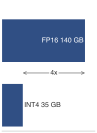
INT4 turns a two-GPU model into a one-GPU candidate.

Keeping a 70B model’s 140 GB of FP16 weights intact forces every replica across at least two 80 GB GPUs and makes every decode step wait on streaming 140 GB from HBM. Weight quantization for serving is therefore a bottleneck-selection decision: reducing precision turns that 140 GB FP16 weight payload into a 35 GB INT4 payload, allowing a model that previously required multiple GPUs to fit on one. The ideal payload reduction is 4$\times$, although metadata, runtime buffers, and KV state still enter the deployment’s memory budget. Because neither quality loss nor speedup is fixed by nominal bit width, both must be measured for the deployed representation and workload.

Systems Perspective 10.3: Quantization as a serving constraint

In serving systems, quantization changes the binding resource as well as the model’s size. Post-training quantization (PTQ) can shrink a deployed model without retraining, while quantization-aware training (QAT) spends training effort to preserve accuracy at lower precision. QAT simulates low-precision rounding in the forward pass and passes gradients through the rounding step as if it were absent, the straight-through estimator (Bengio et al. 2013), so the weights adapt to the error they will carry. It earns that cost only after a PTQ recipe misses the quality budget at the target precision, and a recipe that passes at INT8 says nothing about INT4. The practical order is to deploy with PTQ when it meets quality and reach for QAT, or adapter-based fine-tuning of a quantized base, when it does not, rechecking quality after the final deployment conversion. The systems question is which constraint the lower-precision representation relaxes: GPU memory capacity, HBM bandwidth during decode, accelerator instruction support, or cost per served token.

Bengio, Yoshua, Nicholas Léonard, and Aaron Courville. 2013. “Estimating or Propagating Gradients Through Stochastic Neurons for Conditional Computation.” arXiv Preprint arXiv:1308.3432.

Quantization reduces numerical precision of model weights and activations, decreasing their memory footprint by 2–4$\times$. Reducing weight traffic can improve bandwidth-bound decode, provided kernel support and dequantization overhead preserve the saving. The serving decision is which quantity should shrink: resident weights for fit, bytes moved per decode step for bandwidth, activations for prefill throughput, or the precision path supported by target hardware. Serving at scale also introduces distinct challenges: a deployment team may need post-training quantization without the original training corpus, quality must be preserved across diverse inputs, and hardware deployment targets vary from data center GPUs to edge accelerators. Lack of the original corpus does not imply data-free calibration; the methods that follow may still require representative deployment inputs. Production inference therefore starts from a decision model rather than from the methods. Table 11 ties each method family to the serving constraint it relaxes; what changes for each when it is deployed is its calibration cost, kernel path, and the evaluation a serving team must run.

Table 11: Serving Quantization Decision Model: Quantization methods are useful only when they relax the resource that binds the serving system. The method family follows from the bottleneck: fit, bandwidth, prefill compute, or outlier robustness.

Binding serving constraint	Representation change	Method family	Risk to test before rollout
Model does not fit in memory	Quantize weights only	GPTQ, AWQ	Calibration mismatch and quality regression
Decode is bandwidth-bound	Reduce bytes read per token	W4A16 weight-only paths	Kernel support and KV-cache headroom
Prefill is compute-bound	Quantize weights and activations	SmoothQuant W8A8	Activation outliers and INT8 hardware path
Outliers block low precision	Change the coordinate basis before quantization	Rotation-based methods	Transform overhead and limited runtime path

10.9.1 Outliers and block-wise scaling

When a single weight or activation channel is ten times larger than its neighbors, uniform per-tensor quantization must either clip that extreme value or stretch its step size across the entire range, collapsing the surrounding small values to zero. Large language models produce such outlier features routinely: in the models studied by Dettmers et al. (2022), about 0.1 percent of hidden dimensions carried activation magnitudes roughly 3–20$\times$ larger than the rest. Weight tensors face the same damage when a few large weights set the scale for the whole matrix. Block-wise quantization contains that weight-side damage inside the stored format.

Definition 10.6: Block-wise quantization

Block-wise quantization is an ML quantization scheme that partitions a weight tensor into nonoverlapping groups of $\QuantizationBlockSize$ elements and assigns each group its own scale. An affine scheme uses $\QuantizationScale_i = (\BlockRangeMaximum- \BlockRangeMinimum) / (2^\NumericBitWidth- 1)$ together with an offset or zero point; a symmetric scheme centers the range at zero and needs only scale metadata. The metadata examples below assume symmetric scale-only quantization.

Significance: With block size $\QuantizationBlockSize = 64$ and $\NumericBitWidth= 4$ bits, weights compress from 16 bits to 4 bits (a 4$\times$ memory reduction) while each FP16 scale adds $16/64 = 0.25$ bits per weight. This yields an effective bit-width of $4.25$ bits per weight: 6.25 percent overhead relative to the INT4 payload, or about 1.6 percent of the original FP16 weight size.
Distinction: Unlike per-tensor quantization, which applies a single scale across the entire weight matrix and forces that scale to accommodate outlier values at the cost of wasting precision on the majority of near-zero weights, block-wise quantization contains outlier damage within individual blocks, preventing a single extreme value from degrading quantization fidelity for the whole tensor.
Common pitfall: A frequent misconception is that block size is a free hyperparameter. Smaller blocks ($\QuantizationBlockSize = 32$) can improve local range resolution but double the scale metadata overhead vs. $\QuantizationBlockSize = 64$. At $\QuantizationBlockSize = 16$, the scale adds 1 bit per weight: 25 percent overhead relative to the INT4 payload, or 6.25 percent of the original FP16 weight size. The effect on model quality and kernel speed must be evaluated rather than inferred from block size alone.

The metadata price stays small across formats. An INT8 scheme with one FP32 scale per 128 weights adds $32/128 = 0.25$ bits per weight, about 3 percent of its payload, so block-wise scaling isolates outliers without the bandwidth penalty of a higher-precision format, which is what keeps the decode traffic saving of a low-bit format intact. Figure 15 isolates this dynamic-range protection across an eight-weight sample containing a single outlier ($58.7$). Under per-tensor scaling (left), the outlier dictates a coarse scale factor ($\QuantizationScale\approx 0.462$) that forces six of the seven small weights to round to zero. Partitioning the tensor into four-element blocks (right) confines that coarse scale to the second block, allowing the uncorrupted first block to adopt a fine scale ($\QuantizationScale_1 \approx 0.00165$) that preserves full INT8 resolution.

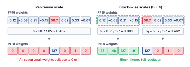
Figure 15: **Block-Wise versus Per-Tensor Quantization**: Under per-tensor scaling (left), one outlier weight sets the scale for the whole tensor, so six of the seven small weights round to zero and the seventh rounds to one. Under block-wise quantization (right), each group of weights gets its own scale: the block without the outlier keeps full INT8 resolution, while the small weights that share the outlier’s block are still crushed. Smaller blocks confine the damage further at the cost of more scale metadata.

10.9.2 LLM-specific quantization challenges

Block-wise scaling handles weight outliers inside the stored format. The outlier activation problem is harder, because activations arrive at run time and their extreme channels cannot be rescaled offline block by block. A coarse scale loses resolution for smaller values, while a narrow range clips large ones. This trade-off is not unique to language models, but its channel structure motivates the methods below.

For a serving deployment the consequence is that no single INT8 scale suits both the outlier channels and the typical values, so the method families differ in which part of the serving contract they protect, at which stage they pay for it, and what they cost to deploy. LLM.int8() (Dettmers et al. 2022) pays at run time: it detects outlier dimensions against a magnitude threshold, multiplies them in FP16 and the rest in INT8, and sums the two products, preserving quality at the cost of outlier detection and a second execution path on every step. GPTQ (Frantar et al. 2023) and AWQ (Lin et al. 2024) pay offline and both produce 4-bit weight-only artifacts. GPTQ quantizes a layer’s weights in sequence and adjusts the still-unquantized weights to compensate for the error already introduced, guided by a second-order estimate from calibration activations of how sensitive the layer’s output is to each weight. AWQ instead protects the salient weights, those that multiply large activations, by scaling their channels before group quantization. Both need representative calibration inputs and supported packing kernels, a reconstruction objective that is only a proxy for task quality, and a comparison at the same model, bit budget, and held-out evaluation; AWQ also needs its scales fused into the deployed graph or it spends part of the latency saving on an extra runtime operation. SmoothQuant (Xiao et al. 2023) pays in a preprocessing transform: it divides each activation channel by a smoothing factor and multiplies the matching weights by the same factor, which leaves the product unchanged before rounding and migrates part of the activation range into the weights so that both can run in INT8. That matters for compute-bound prefill, but a smaller activation range makes the weights harder to quantize, so the smoothing factor balances the two errors, and production activation extremes can still differ from the calibration ranges. Rotation-based methods such as QuaRot (Ashkboos et al. 2024) apply orthogonal Hadamard transforms that spread large coordinates across channels, which makes W4A4 a serving candidate at the price of some online rotation work.

Dettmers, Tim, Mike Lewis, Younes Belkada, and Luke Zettlemoyer. 2022. “LLM.int8(): 8-Bit Matrix Multiplication for Transformers at Scale.” Advances in Neural Information Processing Systems (NeurIPS), 30318–32. https://doi.org/10.52202/068431-2198.

Frantar, Elias, Saleh Ashkboos, Torsten Hoefler, and Dan Alistarh. 2023. “GPTQ: Accurate Post-Training Quantization for Generative Pre-Trained Transformers.” In CoRR, abs/2210.17323. https://doi.org/10.48550/ARXIV.2210.17323.

Lin, Ji, Jiaming Tang, Haotian Tang, Shang Yang, Wei-Ming Chen, Wei-Chen Wang, Guangxuan Xiao, Xingyu Dang, Chuang Gan, and Song Han. 2024. “AWQ: Activation-Aware Weight Quantization for on-Device LLM Compression and Acceleration.” Proceedings of Machine Learning and Systems 6: 87–100.

Xiao, Guangxuan, Ji Lin, Mickaël Seznec, Hao Wu, Julien Demouth, and Song Han. 2023. “SmoothQuant: Accurate and Efficient Post-Training Quantization for Large Language Models.” International Conference on Machine Learning (ICML), 38087–99.

Ashkboos, Saleh, Amirkeivan Mohtashami, Maximilian L. Croci, Bo Li, Pashmina Cameron, Martin Jaggi, Dan Alistarh, Torsten Hoefler, and James Hensman. 2024. “QuaRot: Outlier-Free 4-Bit Inference in Rotated LLMs.” Advances in Neural Information Processing Systems (NeurIPS), 100213–40. https://doi.org/10.52202/079017-3180.

None of these properties fixes quality. Each artifact must be compared with the FP16 baseline on the same model, evaluation data, and runtime, reporting its calibration set, group size, kernel path, and any online-transform overhead, and its serving benefit must be measured as SLO-compliant throughput on the target workload rather than inferred from nominal bit width.

10.9.3 W8A8 versus weight-only ceilings

Quantizing only the weights (W8A16 or W4A16) cuts weight traffic during decode but leaves compute-bound prefill executing on FP16 Tensor Cores at unchanged arithmetic speed, whereas quantizing both weights and activations (W8A8) risks accuracy loss from activation outliers without further shrinking weight bytes. The prefill-decode split therefore decides which path can pay: both schemes shrink the weights, but only W8A8 changes the arithmetic ceiling. Table 12 bounds what each 8-bit path can buy relative to the FP16 baseline.

Table 12: W8A8 SmoothQuant vs. Weight-Only Quantization: Ceilings derived from bytes per weight and the H100’s INT8-to-FP16 peak ratio, not measured speedups. Both schemes halve weight bytes, so both can at most halve weight traffic in bandwidth-bound decode. Only W8A8 moves prefill onto INT8 Tensor Cores. Realized gains and quality loss depend on kernels, calibration, and the request mix.

Configuration	Weight bytes	Prefill compute ceiling	Decode weight-traffic ceiling	Quality
FP16 (baseline)	1$\times$	1$\times$	1$\times$	Baseline
W8A16 (weights only)	Reduced 2×	1$\times$ (FP16 math)	Up to 2×	Measure vs. FP16
W8A8 (SmoothQuant)	Reduced 2×	Up to 2× (INT8 Tensor Cores)	Up to 2×	Measure vs. FP16

The critical distinction is which ceiling binds. Among these configurations, W8A8 enables INT8 matrix multiplication, with the illustrated 2× peak ratio providing a compute ceiling rather than a measured prefill speedup. Both quantized schemes halve the weight payload. If weight reads dominate decode, activation quantization does not further reduce that traffic, although it can change other memory and compute costs. Quantization and dequantization also add work. The end-to-end benefit therefore depends on the prompt/output mix, batch sizes, and measured execution path.

Hardware and software support decide which of these savings reach the serving workload, because the arithmetic format and the resident storage format need not be identical. A common INT4 weight-only kernel reads packed weights and dequantizes them to FP16 on chip during the GEMM, so it cuts weight capacity and read traffic without any INT4 arithmetic. For batch-one decode dominated by weight reads, throughput then scales roughly as memory bandwidth divided by the model’s weight bytes, omitting KV-cache traffic and execution overhead, and leaving the arithmetic in FP16 costs little because arithmetic is not the binding term. At large batch or in prefill, where execution approaches the compute ceiling, the gain comes instead from a weight-activation format, W8A8 or FP8 on hardware with FP8 Tensor Cores, which raises the ceiling that weight-only formats cannot move. In the ideal memory-bound case, 4-bit weights cut weight traffic by 4$\times$, but realized decode throughput depends on kernel support, dequantization overhead, KV-cache precision, batch shape, and whether HBM bandwidth is truly the bottleneck. A serving system can therefore run different formats at different operating points, with each configuration evaluated against the same quality criterion and its own latency targets, and the value of 4-bit serving is strongest when it increases model residency or batch capacity.

10.9.4 Runtime contract for quantized serving

Loading a 4-bit checkpoint into a serving runtime that expands the weights back into resident FP16 tensors at startup or falls back to unoptimized kernels forfeits both the memory capacity and the HBM bandwidth savings before a single request arrives. Production serving frameworks determine whether a quantized artifact retains its intended advantages by converting packed weights inside the execution kernel rather than in HBM. The serving stack must therefore report the resident representation and kernel path, budget KV state around actual allocations, and expose quality and latency regressions (table 13).

Table 13: Quantized Serving Runtime Contract: Framework-specific APIs differ, but every production path has to preserve representation, choose supported kernels, plan memory, and validate quality under the deployed traffic mix.

Runtime responsibility	Why it matters
Preserve the quantized artifact	Full-model expansion into resident FP16 forfeits the reduced weight storage and traffic.
Select compatible low-precision kernels	Unsupported operators fall back to slower or higher-precision execution.
Plan memory around weights and KV cache	The capacity gain matters only if the freed memory becomes useful batch headroom.
Validate quality and latency together	A lower-bit path that meets latency but fails task quality is not a serving win.

Weight quantization reduces the weight allocation, while PagedAttention reduces waste in allocating KV state. Both feed the same admission budget as the capacity estimator of notebook 10.5, with quantized weights in place of FP16 ones. That estimate is optimistic, because a usable integer limit must round down after reserving runtime buffers, quantization metadata, and safety headroom, and sharded deployments must satisfy the budget on every device.

This comparison uses a conservative decimal HBM budget matching the A100 nameplate label, rather than the registered byte capacity used by the node estimator. A 70B model with 4-bit weights requires approximately 35 GB, leaving 45 GB on an 80 GB A100 for KV cache. With FP16 KV cache at about 2.6 GB per 1K-token sequence for the MHA baseline, this supports about 17 concurrent 1K-token sequences before other runtime overheads. With FP16 weights, the same 70B model would not fit on one A100 at all, so weight-only quantization changes both feasibility and batch capacity.

10.9.5 Selecting a quantization format

Choosing a quantization format from datasheet TFLOPS or nominal bit width alone fails when a 4-bit checkpoint degrades task accuracy on production prompts or when a smaller replica completes fewer SLO-compliant tokens per GPU. The final selection must satisfy memory, quality, and latency requirements together. Native support makes a precision path a candidate without establishing the model’s quality at that precision, and no universal quality ordering separates 4-bit weight-only from 8-bit weight-and-activation quantization, so both are evaluated against the same task baseline. For compute-bound prefill, W8A8 offers the illustrated 2× INT8 compute ceiling; for decode dominated by weight reads, W4A16 can cut the weight payload by up to 4$\times$, provided conversion and other costs leave a useful saving.

These precision choices affect cost per million useful tokens. The A100 residency calculation explains why fewer GPUs become possible at all, because INT4 weights shrink the resident payload enough for a 70B replica to fit on fewer devices. Table 14 isolates the effect of GPU count by assuming equal per-GPU prices and the same completed token rate across three configurations. Under that contract, reducing the number of billed GPUs reduces cost proportionally. The calculation does not establish that the smaller replicas sustain the same rate or meet the same quality and latency targets.

Table 14: Quantization Impact on Serving Cost: Estimated cost per million tokens at three configurations. At equal unit prices and unchanged useful token throughput, halving the GPU count halves the cost; halving it again brings the per-million-token cost to one quarter of the FP16 baseline. The cost savings come almost entirely from fewer GPUs rather than from per-GPU throughput gains.

Configuration	Cost per 1M tokens (estimated)
FP16 on 8$\times$ A100	$2.40
AWQ 4-bit on 4$\times$ A100	$1.20
AWQ 4-bit on 2$\times$ A100	$0.60

The illustrated 2–4$\times$ cost reduction follows from the assumed device-count reduction at unchanged useful throughput. If the smaller replica completes fewer qualifying tokens per second, cost per token falls by less and can increase. A deployment comparison must therefore combine billed replica cost with measured SLO-compliant output under the same quality contract.

Precision moves the capacity wall without removing it. A 175-billion-parameter model still needs about 87.5 GB for its 4-bit weight payload alone, more than one 80 GB H100 holds before KV state and runtime allocations. Keeping that representation accelerator-resident requires distributing it across devices. Offloading to host memory is another placement choice, but introduces transfers that must fit the latency budget. Sharding addresses the capacity problem while adding communication and coordination to each replica.

Self-Check: Question

How does SmoothQuant enable efficient 8-bit weight and 8-bit activation (W8A8) inference, and why is its speedup significantly higher during prefill than during decode?
1. It prunes 50% of model weights using structured sparsity, accelerating decode but having no effect on prefill.
2. It divides activations by a per-channel scale $s$ and multiplies weights by $s$, moving quantization difficulty toward weights; compute-bound prefill can benefit from native INT8 arithmetic while decode remains sensitive to memory traffic
3. It rotates the coordinate basis using randomized Walsh-Hadamard matrices, eliminating memory bandwidth bottlenecks during decode.
4. It converts floating-point weights into binary spikes, enabling single-cycle bitwise operations during token generation.
True or False: In block-wise INT4 quantization with one FP16 scale per block, reducing the block size from 64 to 16 weights can improve local range resolution but quadruples the scale metadata, from 0.25 bits per weight (6.25 percent overhead on the INT4 payload) to 1.0 bit per weight (25 percent overhead).
GPTQ and AWQ both produce 4-bit weight-only artifacts offline. How do they differ, and what extra deployment step does AWQ need?
1. GPTQ quantizes activations while AWQ quantizes weights; AWQ needs no calibration data.
2. GPTQ compensates rounding error with approximate second-order information, while AWQ scales salient channels chosen from activation statistics; AWQ’s scales must be fused into the deployed graph or they cost an extra runtime operation.
3. GPTQ requires full retraining while AWQ is applied at runtime; AWQ needs a second GPU to hold its scales.
4. Both methods are identical except for bit width; AWQ needs its weights stored in FP32.
Explain what a rotation-based method such as QuaRot changes before quantization, what that makes possible for serving, and what it costs at run time.
Order the steps for choosing and rolling out a quantization method for a serving system:

Test the method family’s specific risk (calibration mismatch, kernel support, activation outliers, or transform overhead) before rollout
Identify which resource binds the serving system: memory fit, decode bandwidth, prefill compute, or outlier robustness
Choose the method family that makes that change
Choose the representation change that relaxes that resource

A serving team’s INT8 post-training quantization (PTQ) recipe meets its quality budget, and it now wants INT4 weights. When does quantization-aware training (QAT) earn its cost, and what must be checked after the model is converted for deployment?

See Answers →

10.10 Model Sharding for Inference

When a deployment must retain a 70B model’s 140 GB of FP16 weights in accelerator memory, or when a 175B model’s 87.5 GB INT4 weight payload still exceeds a single 80 GB GPU, no single accelerator can hold the replica. Where quantization shrinks the representation, sharding keeps it intact and divides it across multiple GPUs that execute together as one logical replica. The resulting design adapts tensor and pipeline parallelism from training, but must evaluate their communication and scheduling costs against per-request inference deadlines.

10.10.1 Memory and latency triggers for model sharding

A single-GPU replica fails when model weights overflow its HBM capacity or when its serial forward pass takes too long to meet the endpoint’s TTFT and TPOT targets. Model sharding addresses the memory and latency rows of table 1 through different mechanisms, and the timing analysis below determines whether parallel execution repays its communication cost.

The first driver is memory capacity. If the selected representation must remain in accelerator memory but does not fit on one device, the replica needs multiple devices. For a model with $\Parameters$ parameters at precision $\NumericBitWidth$ bits, equation 11 gives the weight payload before metadata and runtime state:

\[\WeightMemory = \Parameters\times \frac{\NumericBitWidth}{8} \text{ bytes} \tag{11}\]

Applied to the 70B model in FP16 (16 bits), equation 11 recovers the payload quoted since section 10.2. Each parameter occupies two bytes, so the unquantized checkpoint alone requires:

\[M_{\text{weights}} = 7 \times 10^{10} \times \frac{16}{8} = 140 \text{ GB}\]

The result exceeds the 80 GB capacity of an H100 GPU, establishing a weight-only lower bound of 2 shards for an accelerator-resident replica. KV state, buffers, replication within the chosen partition, and uneven placement can require a larger degree.

The second driver is latency. Even when a model fits in memory, sharding can reduce latency by parallelizing computation. Equation 12 is the Fleet Law (equation 1.3) applied to a single inference request, separating the compute term that sharding divides from the communication and synchronization terms it adds:

\[\DistributedStepTime(\DeviceCount) = \frac{\IronLawComputeTime}{\DeviceCount} + \CommunicationTime(\DeviceCount) + \SynchronizationTime(\DeviceCount) - \OverlappedTime \tag{12}\]

where $\DeviceCount$ is the number of devices in the sharding group, $\CommunicationTime(\DeviceCount)$ is the communication overhead, $\SynchronizationTime(\DeviceCount)$ is synchronization overhead, and $\OverlappedTime$ is communication hidden behind useful compute. In the common no-overlap simplification with negligible extra synchronization, this reduces to $\IronLawComputeTime/\DeviceCount+ \CommunicationTime(\DeviceCount)$. Sharding provides latency benefit only when the nonoverlapped overhead is smaller than the time saved through parallelization.

10.10.2 Tensor parallelism

Splitting every linear projection independently across GPUs would force an AllReduce synchronization after every matrix multiplication, stalling decode on interconnect latency. Tensor parallelism (Shoeybi et al. 2019) avoids half of those collectives by splitting each layer with the column-row partitioning developed for training, which keeps the activation between paired linear layers local and costs two AllReduce operations per transformer block, one after attention and one after the feed-forward sublayer.

Shoeybi, Mohammad, Mostofa Patwary, Raul Puri, Patrick LeGresley, Jared Casper, and Bryan Catanzaro. 2019. “Megatron-LM: Training Multi-Billion Parameter Language Models Using Model Parallelism.” arXiv Preprint arXiv:1909.08053.

↩︎ Column-row tensor partitioning and its two AllReduce operations per transformer block are established in Tensor parallelism.

The attention computation partitions across heads, so with $\AttentionHeadCount$ heads and tensor-parallel degree $\TensorParallelDegree$ each device computes attention for $\AttentionHeadCount/\TensorParallelDegree$ of them when the head count divides evenly. The KV cache is sharded with the heads, so each device stores cache only for its own heads. A multi-head attention layout spreads many KV heads across the group, while grouped-query attention with eight KV heads leaves one per device in an eight-way group.

8-way tensor parallelism, 64 KV heads (MHA):
Device 0: KV cache for heads 0-7
Device 1: KV cache for heads 8-15
...
Device 7: KV cache for heads 56-63

Cross-device reuse requires compatible cache content and placement. Matching tensor-parallel configurations can align the head partitions, but the receiver must also use the same model state, prefix inputs, cache representation, and logical token positions. A different partition requires redistribution rather than direct shard reuse. Equal parallelism degree alone does not establish cache validity.

Each device applies its shard of the attention output projection to its local heads, and an AllReduce sums the projected partial outputs; its latency includes collective startup and coordination as well as payload transfer. Figure 16 traces the resulting two synchronization points per layer across two GPU ranks.

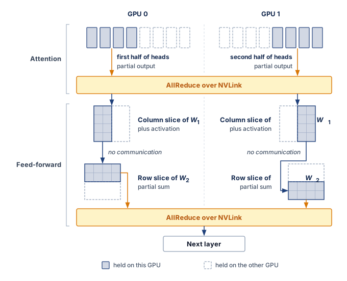
Figure 16: **Tensor Parallelism for Inference**: Computation is distributed across devices by splitting tensor operations. Attention heads are partitioned across GPUs, requiring an AllReduce operation to synchronize results. Feed-forward networks use a column-row splitting strategy that requires only one AllReduce synchronization per block. This partition can reduce latency when saved compute exceeds communication cost, which is why the two collectives run over a fast local interconnect.

The inference time with tensor parallelism follows equation 13:

\[\TensorParallelLayerTime= \frac{\IronLawComputeTime}{\TensorParallelDegree} + 2 \times \AllReduceCompletionTime(\CollectivePayloadSize) \tag{13}\]

Equation 13 is the per-layer instance of equation 12, with $\IronLawComputeTime$ now the sequential compute time of one layer and $\CollectivePayloadSize$ the full activation payload each rank contributes to each AllReduce, priced by the ring cost model of Ring AllReduce. Compute divides ideally across ranks, but the reduced activation keeps its full shape, (tokens in the step) $\times$ (hidden width) $\times$ (bytes per element), and the factor of 2 counts the attention and feed-forward collectives.

↩︎ Hiding tensor-parallel collectives behind compute on one node, and what that overlap can and cannot recover, is established in Tensor-parallel collectives under contention.

Example 10.6: Tensor parallelism for Llama-70B

Scenario: An engineering team deploys Llama-70B (70B parameters, FP16 footprint 140 GB) across an 8-GPU H100 node with NVLink (Touvron et al. 2023).

Diagnosis: The calculation assumes 30 ms of serial layer compute as a reference, independent of the devices required to hold the weights: 12 ms for attention and 18 ms for the feed-forward block. That reference describes a long-prompt prefill, in which every prompt token passes through the layer in one step, so it is far larger than one layer’s share of a decode step on the reference replica. Ideal eight-way division gives 1.5 ms and 2.25 ms, and the two AllReduce operations of equation 13 add an assumed 0.3 ms each, for 4.35 ms per layer.

Systems lesson: The illustrative eight-way model gives a 6.9× reduction relative to its serial-compute reference (prefill time reduced from 2,400 ms to 348 ms). The entire shortfall from the ideal 8$\times$ is the two collectives, a fixed cost per layer that dividing compute cannot shrink. Their share of the layer therefore grows as per-device compute falls, which is why a decode step, with far less compute per layer than this prefill reference, feels the collective cost most.

Touvron, Hugo, Louis Martin, Kevin Stone, Peter Albert, Amjad Almahairi, Yasmine Babaei, Nikolay Bashlykov, et al. 2023. “Llama 2: Open Foundation and Fine-Tuned Chat Models.” arXiv Preprint arXiv:2307.09288.

10.10.3 Pipeline parallelism for inference

Splitting an 80-layer model sequentially across four GPU stages leaves three accelerators idle during an isolated request and does nothing to shorten its forward pass. Pipeline parallelism distributes layers across devices so each stage runs a contiguous subset of layers and passes activations to the next stage without intra-layer synchronization.

For inference, pipeline parallelism creates bubbles differently than in training. Executing an isolated request serially across four GPU stages leaves three accelerators idle at every step, whereas maintaining multiple in-flight requests fills the pipeline and amortizes the initial bubble across steady-state token delivery (figure 17).

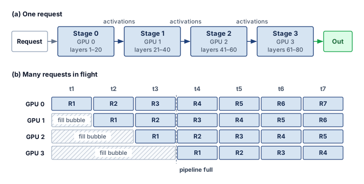
Figure 17: **Pipeline Parallelism Bubbles**: (a) An 80-layer model split into four stages passes one request’s activations from stage to stage, so splitting the layers alone does not shorten its sequential computation; it must still traverse all four stages. (b) With many requests in flight, later stages idle during the fill bubble, and from slot t4 onward every stage is busy and one request leaves the pipeline per slot. Pipeline parallelism therefore suits throughput-oriented serving better than latency-critical interactive serving.

For a single request, pipeline staging does not parallelize the dependent layers. If stage execution times are unchanged, the request still pays their sum plus transfers, so staging alone provides no execution-latency reduction. A comparison against a memory-constrained implementation that offloads weights can differ because keeping stages resident changes those execution costs.

Pipeline parallelism instead scales throughput by sustaining multiple concurrent requests across execution stages, as tracked in the steady-state schedule of figure 17(b). Once the pipeline reaches saturation, throughput is limited by the slowest stage. For $\PipelineParallelDegree$ balanced stages with negligible transfer overhead, this is $\PipelineParallelDegree$ times the throughput of executing the whole model sequentially on one device, not $\PipelineParallelDegree$ times a single stage’s throughput. An individual request still traverses every stage, so its execution latency remains approximately the sum of the stage times.

Pipeline parallelism therefore suits inference when memory forces sharding but latency targets are relaxed, when aggregate throughput matters more than individual request latency, or when the interconnect handles point-to-point transfers better than fast AllReduce. The two sharding approaches differ in single-request latency, throughput, communication pattern, activation memory, and implementation complexity (table 15).

Table 15: Pipeline vs. Tensor Parallelism: Key trade-offs between layer-internal tensor splitting (can reduce single-request latency when compute savings exceed collective cost) and inter-layer pipeline staging (overlaps concurrent requests but introduces pipeline bubbles). Throughput is relative to sequential execution of the whole model on one device; per-layer AllReduces keep tensor parallelism below the $\TensorParallelDegree\times$ ideal, and balanced, full pipelines approach $\PipelineParallelDegree\times$.

Aspect	Tensor parallelism	Pipeline parallelism
Single-request latency	Compute term reduced up to $\TensorParallelDegree\times$	No reduction from overlapping this request alone
Throughput	Below $\TensorParallelDegree\times$ (AllReduce cost)	Up to $\PipelineParallelDegree\times$ (pipelined)
Communication pattern	AllReduce (bandwidth-intensive)	Point-to-point (latency-sensitive)
Memory efficiency	Activations replicated	Activations passed along
Complexity	Higher (requires custom kernels)	Lower (layer-level partitioning)

The decision starts with capacity feasibility and then compares latency and throughput on the available topology. Neither a fast interconnect nor a relaxed deadline alone establishes the best choice; the request mix and measured execution costs determine the useful partition.

10.10.4 Expert parallelism for MoE models

An MoE model activates only a small fraction of its parameters per token, yet replicating the entire expert pool on every GPU quickly exhausts device memory. Mixture-of-experts (MoE) models such as DeepSeek-V3 (DeepSeek-AI 2025) and Mixtral (Jiang et al. 2024) replace each feed-forward network with parallel expert sub-networks and a lightweight router that selects a few experts per token, growing parameter capacity without proportionally growing expert arithmetic per token. Routing, shared layers, and communication still add work. Expert parallelism places different experts on different GPUs to distribute their storage and execution when the model and workload exceed a single device.

DeepSeek-AI. 2025. “Insights into DeepSeek-V3: Scaling Challenges and Reflections on Hardware for AI Architectures.” Proceedings of the 52nd Annual International Symposium on Computer Architecture, 1731–45. https://doi.org/10.1145/3695053.3731412.

Jiang, A. Q., A. Sablayrolles, A. Roux, A. Mensch, B. Savary, C. Bamford, D. S. Chaplot, et al. 2024. “Mixtral of Experts.” arXiv Preprint arXiv:2401.04088.

MoE economics and capacity planning

MoE serving separates two capacity measures. The total parameter count sets the weight-storage requirement at the chosen precision, while the active parameter count estimates the weight-related arithmetic and traffic for each token. Neither count includes all runtime costs. An accelerator-resident deployment must accommodate inactive experts as well as active ones, even though each token uses only a subset.

The following comparison isolates weight-related costs at batch size 1. Streaming all weights of a dense 400B FP16 model moves 800 GB per step. Counting only DeepSeek-V3’s 37B active parameters gives approximately 74 GB in FP16, a 10.8× reduction in weight bytes per token. The proportional estimate of weight-related arithmetic is 10.8× lower. These are payload and arithmetic comparisons, not equivalent-quality model comparisons or measured speedups; cache traffic, expert placement, routing, and communication affect realized latency.

MoE keeps every expert resident but activates few per token.

The trade-off is resident capacity: keeping all experts on accelerators avoids fetching inactive experts when routing changes. Offloading can reduce that resident footprint but adds transfer and scheduling costs. DeepSeek-V3’s full model in FP16 requires approximately 1342 GB, requiring many devices if the entire FP16 weight set remains accelerator-resident.

Napkin Math 10.8: MoE capacity planning

This comparison uses a conservative decimal budget of 80 GB per GPU, matching the H100 nameplate label rather than the registered byte capacity used by the node estimator.

Problem: A team deploys DeepSeek-V3 (671B total parameters, 37B active per token) for a chatbot application. The model uses FP8 weights (1 byte per parameter). The cluster has 8-GPU nodes, each with 8$\times$ H100 GPUs (80 GB HBM per GPU, 640 GB per node). How many nodes are needed, and what is the per-token decode latency?

Math:

Memory: Total weight memory = 671 GB. A single node (640 GB) is insufficient. 2 provide 1,280 GB in aggregate. The remaining capacity must still accommodate KV state, metadata, buffers, and any replicated weights on each device.
Latency: Count 37B active parameters (37 GB) per decode step. If their reads were evenly distributed across 16 GPUs, each would read about 2.3 GB. At the stated 3.35 TB/s HBM bandwidth, $\PerDeviceWeightReadTime\approx$ 0.69 ms. The scenario adds 0.3 ms for routing. Expert placement and token routing do not guarantee this balance, especially at batch size 1.
Floor: The simplified sum is $\approx$ 1.0 ms/token, corresponding to 1,000 tokens/s at batch size 1 under these assumptions. It is an optimistic estimate, not a measured rate or a rigorous latency bound; compute, KV traffic, synchronization, and imbalance remain unmodeled.

Systems insight: Sparse activation separates resident parameter capacity from the work selected for one token. Planning an accelerator-resident 671B model therefore requires both a per-device memory budget and a timing model for the actual expert placement. Dividing total active bytes by device count does not establish that every device can contribute bandwidth equally.

Expert parallelism and load balancing

Expert parallelism carries over from training unchanged in mechanism. Each GPU holds a subset of experts, and each token travels to the devices holding the experts its gate selects. What changes in serving is who pays for imbalance, because an overloaded expert now delays live requests rather than a training step. In an MoE layer, a gating network selects $\RoutedExpertCount$ of the $\ExpertCount$ experts for each token and sums their outputs weighted by its gate probabilities. An even expert placement assigns each device $\ExpertCount/\DeviceCount$ experts, where $\DeviceCount$ is the number of expert-parallel devices, and each token then makes the round trip of Mixture-of-Experts (MoE) AllToAll Routing: one AllToAll dispatches its representation to the ranks hosting its experts, and a second returns their outputs for the weighted sum.

The communication pattern differs from tensor parallelism. AllReduce delivers one combined result to every device, so per-link traffic is fixed by the message size. Expert parallelism uses AllToAll to deliver different routed tokens to different devices, so link and receiver load depend on the router’s choices, and the host of a popular expert becomes an incast point whose completion time the other hosts wait on. Balancing the number of stored experts does not balance token traffic.

Serving inherits training’s balance controls without their guarantees. The auxiliary balancing loss shapes routing on training data, not on future traffic. The expert capacity factor caps accepted tokens per expert (1.25$\times$ is an illustrative setting), leaving the server to decide what happens to the excess. Dropping or rerouting it changes the model computation and needs quality validation, while expert buffering retains it at the cost of latency and queue capacity.

↩︎ The capacity factor, the auxiliary load-balancing loss, and the hot-expert skew they bound during training are established in Expert parallelism (mixture of experts).

Routing failure modes

Router behavior affects both system performance and model quality. Expert collapse during training concentrates traffic on a few experts, and at serving time a shifted input distribution can create hotspots without any change to the stored model. Token dropping under a capacity limit makes the computation differ from the uncapped model, so its quality impact must be evaluated together with any throughput gain. Because routing selects experts dynamically,⁵ the routing pattern becomes a systems workload rather than only a model-internal choice.

⁵ MoE (mixture-of-experts) serving trade-off: Only a subset of experts activates per token (2 of 8 in Mixtral, 8 of 256 routed experts in DeepSeek-V3). Keeping all weights accelerator-resident gives a total-to-active weight ratio of roughly 3.6× (Mixtral) to 18× (DeepSeek-V3). Expert parallelism distributes that storage while adding token-routing communication; offloading is an alternative that trades resident capacity for weight transfers.

Example 10.7: Expert parallelism for Mixtral-8x7B

Scenario: Mixtral-8x7B (46.7B total parameters, ~12.9B active per token) is served across a 4-GPU group using top-2 routing.

Diagnosis: Replicating all 8 experts on every GPU requires the full 93.4 GB FP16 weight set per device, more than one 80 GB H100 holds. Placing 2 experts on each GPU (4-way expert parallelism) cuts each device’s share to about 25.8 GB, the shared attention layers plus its local experts, but every MoE layer now needs an AllToAll dispatch and gather to move tokens to the devices that hold their selected experts.

Systems lesson: Expert parallelism trades AllToAll communication for per-GPU parameter memory. The trade pays only when the collective, repeated at every MoE layer, fits inside the decode budget that the smaller resident footprint makes possible.

Expert parallelism couples state placement to input-dependent access. Embedding-heavy recommendation models face a related problem: entity popularity determines which stored vectors receive traffic. Their sharding strategy must therefore balance storage and lookup load, just as expert placement must account for both resident weights and routed tokens.

10.10.5 Embedding sharding for recommendation systems

Production recommendation models carry multi-terabyte embedding tables that cannot fit on any single server and would stall every ranking query if fetched over thousands of serial network hops. Meta’s DLRM reference architecture applies model parallelism to those tables while scaling dense layers separately (Naumov et al. 2019), and serving inherits the row-wise, column-wise, and hybrid layouts that training uses to shard them (Sparse embedding sharding).

What changes at serving time is the constraint the layout answers to. Training shards tables for sparse update throughput, while serving must finish every lookup within a per-request deadline. Popularity skew concentrates lookups on the shards that own hot keys, and under a latency SLO the slowest of those shards sets the tail of every request that touches it. Serving layouts therefore replicate or column-partition hot entries even at extra storage cost, keep the cold tail row-sharded, and batch lookups by destination shard so that one request does not wait on thousands of sequential round trips.

The following Archetype B scenario combines row-wise, column-wise, and hybrid sharding. The 100 TB platform-wide resident budget deliberately sits well above the 10 TB-plus embedding tables of a single Archetype B model, so that the sharding arithmetic is stressed at the upper end of the regime.

Lighthouse 10.1: Archetype B (DLRM at Scale): Embedding sharding budget

Consider an Archetype B recommendation workload with a large entity catalog and a smaller resident embedding tier:

Scale:

Resident embedding budget (platform-wide): 100 TB
Entity catalog: 10 trillion identifiers
Embedding dimension: 128–256
Shards: 1,000+ servers

The arithmetic of these bullets is the design constraint. A dense INT8 table with 10 trillion entities and 128 dimensions would require at least 1,280 TB, while 100 TB across the same entity count averages only 10 bytes per entity, a fraction of one 128-byte vector. Most entities therefore cannot hold a resident vector at all. The resident tier keeps the frequently accessed subset, and the long tail lives in another tier or a compressed representation, which is exactly the split the sharding strategy below is built around.

Sharding strategy:

The tier percentages below describe the admitted resident population, not the full entity catalog. Replica bytes count against the platform-wide resident budget, so the admitted population and replication scope must be chosen together.

Hot embeddings (top 1 percent by access frequency): Replicated within selected shard groups
Warm embeddings (next 10 percent): Column-sharded with 8-way parallelism
Cold embeddings (remaining 89 percent): Row-sharded with consistent hashing

Each inference request requires approximately 5,000 embedding lookups. Instead of one RPC per lookup, the batched design accumulates lookups for 1 ms, deduplicates entities across requests, groups lookups by destination shard, dispatches to all shards in parallel, and assembles embeddings as responses arrive.

Illustrative before-and-after assumptions for sequential dispatch versus parallel shard batching appear in table 16.

Table 16: Illustrative Embedding Lookup Comparison: Assumed latency and bandwidth compare sequential per-lookup RPCs with shard-batched parallel dispatch. One dispatch wave still contains multiple network requests; it does not mean one RPC to the entire fleet.

Metric	Without optimization	With optimization
Sequential dispatch waves	5,000 individual RPCs	One parallel wave; multiple shard RPCs
Lookup latency	50 ms	2 ms
Network bandwidth	10 Gbps	40 Gbps (burst)

The lighthouse lesson is that sparse embedding placement and lookup coordination can dominate DLRM-scale serving even when dense arithmetic has spare capacity. The illustrated workload motivates measuring shard traffic and lookup latency before adding dense compute.

10.10.6 Hybrid sharding strategies

Extending tensor parallelism across node boundaries stalls decode on slow inter-node AllReduces, while using pipeline parallelism alone leaves single-request latency untouched. Production systems therefore combine sharding strategies into hybrid sharding, using one axis to cut per-token latency inside a node, another to fit weights across nodes, and a third to route sparse components without forcing dense layers onto the wrong device. Joint placement across these axes is established in Hybrid Parallelism, so the serving question is which axis buys latency. Tensor and pipeline parallelism combine when a model needs both memory distribution and latency reduction:

8 GPUs organized as 2 by 4 (pipeline stages by tensor parallel):

Stage 0 (Layers 1-40):  TP across GPUs 0,1,2,3
Stage 1 (Layers 41-80): TP across GPUs 4,5,6,7

The four-way tensor split can cut per-layer compute time by up to 4$\times$, while the two pipeline stages complete the eight-way memory distribution; pipelining adds no per-request latency benefit of its own. Expert-parallel MoE layers and recommendation models that keep embeddings on CPU servers beside a tensor-parallel dense model follow the same rule, and the recommendation split reappears in the case study of section 10.15.2.

Hybrid sharding buys fit or latency by adding new communication patterns at every boundary between shards. The next question is whether that added communication time stays inside the latency and throughput budget.

10.10.7 Interconnect latency and communication overhead

Sharding a model across more GPUs can make inference slower rather than faster when collective synchronization takes longer than the compute time it saves. Each sharding strategy has a characteristic communication pattern, and each pattern carries a cost model developed earlier in the volume. Pipeline parallelism passes activations point to point between stages and pays one startup latency plus a bandwidth term per transfer (The \MessageStartupLatency-\LinkBandwidth performance model). Tensor parallelism pays a ring AllReduce per collective, whose startup term grows linearly with the number of devices while its bandwidth term approaches twice the payload divided by link bandwidth (Ring AllReduce). Expert parallelism pays an AllToAll, whose completion time is set by the largest of per-message startup, endpoint injection or reception, and traffic across the fabric bisection (AllToAll Exchanges at Scale).

These models give an initial communication budget, not a complete prediction of request latency. Skewed expert traffic, network contention, or a different collective algorithm can change the realized timing, so the chosen topology and collective implementation must sustain that budget under the intended concurrent load.

Communication overhead depends heavily on the interconnect technology, because each candidate link fixes the physical bandwidth, latency, and scope available to the sharded model (table 17).

Table 17: Data-Center Interconnect Specifications: Bandwidth, latency, and intended scope for NVLink, PCIe Gen5, InfiniBand HDR, and 100G Ethernet, establishing the physical limits that bound achievable sharding speedups.

Interconnect	Bandwidth	Latency	Use case
NVLink (H100)	900 GB/s	500 ns	Intra-node TP
PCIe Gen5	64 GB/s	1 μs	Intra-node (no NVLink)
InfiniBand HDR	200 Gb/s (25 GB/s)	7 μs	Inter-node
Ethernet 100G	100 Gb/s (12.5 GB/s)	50 μs	Inter-node (commodity)

For tensor parallelism the latency column, not the bandwidth column, decides placement. Decode divides a small per-layer compute time across the group while still paying two collectives per layer for every generated token, so the fixed per-collective latency in table 17 sets the overhead share. The 0.3 ms per collective assumed in example 10.6 already lies an order of magnitude above the bandwidth-only transfer time on NVLink, so startup, synchronization, and launch costs dominate it, and an inter-node link with higher per-message latency would multiply that cost on every token. That decode regime is why tensor-parallel groups are normally kept inside one NVLink domain.

10.10.8 Selecting a sharding strategy

Choosing the wrong sharding axis either burns interconnect bandwidth on per-layer collectives that the link cannot support or leaves single-request latency above the SLO. No approach wins on latency priority, throughput priority, interconnect limits, and implementation effort at once (table 18).

Table 18: Sharding Strategy Selection Guide: Evaluation of tensor, pipeline, expert, and embedding sharding across latency targets, throughput priorities, interconnect constraints, and implementation complexity.

Factor	Tensor parallel	Pipeline parallel	Expert parallel	Embedding shard
Latency priority	Compute savings exceed collectives	No staging-only reduction	Routing-dependent	Lookup-dependent
Throughput priority	Collective-limited	Full, balanced pipeline	Balanced expert traffic	Balanced lookup load
Interconnect limited	Poor fit	Good fit	Moderate	Good fit
Implementation effort	High	Low	Moderate	High

Strategy selection starts from the deployment bottleneck. Tensor parallelism is a candidate when reduced layer execution can repay frequent collectives; pipeline parallelism distributes layers and can sustain throughput when enough concurrent work fills the stages. Expert and embedding sharding distribute sparse state while adding routed communication. These choices can be combined, but each must fit the per-device memory budget and the measured latency contract.

Once a replica’s memory footprint and execution capacity are established, demand determines how many replicas the service needs. The next decision is where to send each arriving request. Routing must account for work already in progress and reusable state, so that replica capacity becomes useful fleet capacity.

Self-Check: Question

Why can tensor parallelism shorten a single forward pass, while pipeline parallelism alone does not provide the same intra-layer acceleration for one request?
1. TP eliminates the need for activation storage, while PP doubles activation sizes across stages.
2. TP uses point-to-point transfers over Ethernet, while PP requires NVLink broadcast collectives.
3. TP relies on asynchronous CPU offloading, whereas PP executes purely on GPU Tensor Cores.
4. TP partitions intra-layer matrix multiplications across devices with per-layer AllReduce, whereas PP requires a single request to traverse all sequential stages in series.
Explain why a 671B-parameter MoE model with 37B active parameters per token needs much more resident weight capacity than its per-token arithmetic suggests, and why sparse activation does not guarantee small-dense-model latency.
True or False: In model sharding, Tensor Parallelism relies on AllToAll collective communication to route tokens between layers, whereas Expert Parallelism relies strictly on AllReduce to synchronize partial attention head outputs.
An illustrative recommendation service has a resident embedding tier smaller than its full entity catalog. Within that admitted resident population, 1% of embeddings are hot, 10% warm, and 89% cold. Which hybrid placement matches the chapter’s scenario while counting replicas against the resident memory budget?
1. Hot (1%) embeddings are replicated within selected shard groups; warm (10%) are column-sharded; cold (89%) are row-sharded by entity hash, with transport chosen for the runtime.
2. Hot embeddings are stored exclusively on remote cold storage; cold embeddings are replicated in HBM across all GPUs.
3. All embeddings are strictly column-sharded across all GPUs regardless of popularity to eliminate network communication.
4. Hot embeddings are sharded row-wise across CPUs; cold embeddings are broadcast via AllReduce to all GPU Tensor Cores.
Order the sequence of operations that occurs during token execution in an Expert-Parallel (MoE) transformer layer:

AllToAll dispatch transmits token activation vectors to the specific GPUs hosting the selected experts
Gating network evaluates input representations and computes top-$k$ routing probabilities
AllToAll gather routes expert output activations back to the originating host devices
Selected expert sub-networks compute local feed-forward transformations on assigned tokens
Weighted sum combines expert outputs with gating coefficients and adds residual connections

Using the $\alpha$-$\beta$ communication model, explain why Tensor Parallelism across nodes linked via standard 100G Ethernet introduces prohibitive latency overhead compared to intra-node NVLink.

See Answers →

10.11 Load Balancing and Request Routing

Suppose ten model replicas are serving traffic when a request for a 5,000-word document summary arrives. Assigning it to an overloaded replica adds waiting and can increase interference for work already admitted there. The effect depends on admission, batching, and priority policies. Round-robin assignment does not inspect those differences in remaining work. A state-aware router uses memory and queue information to choose a feasible destination, while limiting the cost and staleness of its observations.

Lighthouse 10.2: Archetype B (DLRM at Scale): The tail at scale

Archetype B (DLRM at Scale) uses $\text{p99} \le 100\text{ ms}$ as its illustrative latency target. At $10^{7}$ QPS, an event probability of $10^{-4}$ implies an expected 1,000 such events per second. This count motivates examining the tail, but does not identify its cause. Two-choice routing can reduce imbalanced queuing delay $\QueueingLatency$; traces must establish whether queueing, inference time $\InferenceLatency$, or another component drives the misses.

Load balancing serves two goals that can conflict: sending each request to the replica that can serve it fastest, and spreading load so that no replica idles or saturates. Latency-optimal routing can concentrate load on fast replicas until they slow down. Evaluation therefore needs signals for both goals, queue length and estimated remaining work per replica for latency and utilization spread for balance, together with the decision overhead of the routing choice, all judged against completed-request tail latency and admission outcomes rather than balanced request counts.

10.11.1 Tail latency under fan-out

When a serving request fans out to 100 backend shards that each meet their own p99 latency target independently, the assembled response misses that threshold about 63 percent of the time. Many serving requests are not one call but a set of parallel sub-requests whose results must all return before the response can be assembled: a ranking query that scores candidates on many shards, a recommendation that looks up embeddings across tables, or a sharded model whose replicas must all finish a step. Because the request completes only when its slowest leaf returns, it inherits the tail of every leaf it touches, the way a series system fails when any one component fails. If each of $\SeriesComponentCount$ leaves independently exceeds its own latency threshold with probability $\IndependentEventProbability$, the request exceeds it with probability $1 - (1 - \IndependentEventProbability)^{\SeriesComponentCount}$.

Reading the same expression backward turns it into a budgeting rule. To keep the whole request within its p99 target, each of the 100 leaves may be slow only about 0.01 percent of the time, so the leaf target moves from p99 to roughly p99.99. Fan-out width is therefore a tail-latency cost that the service pays per request, and the levers act on different terms. Fewer, larger shards lower $\SeriesComponentCount$; queue-aware routing and isolation lower $\IndependentEventProbability$ by keeping leaves out of their own queueing tails; and a deadline with a partial or default result, as in the search cascade of section 10.15.4, caps the damage when a leaf still misses. Hedged requests lower $\IndependentEventProbability$ further at the price of duplicated work. The independence assumption is optimistic, because a shared switch, host, or hot key slows many leaves together, so the measured composed tail is the quantity to budget, not the formula alone.

↩︎ The same independence model applied to storage reads, and hedged reads with their failure-domain placement, are established in Tier 3 parallel file systems.

10.11.2 Round-robin and random assignment

Routing requests in a fixed cycle or at random works when every call costs the same, but in an inference fleet where one request generates 10 tokens and the next generates 2,000, stateless assignment piles long queues onto unlucky replicas while others sit idle. Round-robin cycles through the servers in order, which distributes work evenly only when servers are homogeneous and processing times identical, while random assignment picks a server uniformly, converging to an even mean with higher variance. Both are reasonable baselines for identical servers, but heterogeneous GPU generations, variable request sizes, warmup behavior, and replicas nearing memory limits make the state of the server fleet matter in production.

A static placement model isolates the imbalance caused by random choice: place $\ReplicaCount$ equal-size jobs sequentially into $\ReplicaCount$ initially empty bins, without departures. With uniform independent choices, the expected maximum bin occupancy follows the classical balls-into-bins result (Mitzenmacher 2001) in equation 14:

Two-choice routing flattens the tail imbalance of random placement.

\[\mathbb{E}[\text{max bin occupancy}] =\AsymptoticTightBound\left(\frac{\log \ReplicaCount}{\log \log \ReplicaCount}\right) \tag{14}\]

Here $\ReplicaCount$ counts both jobs and bins. The asymptotic expression does not predict a finite serving queue at a given fleet size, because arrivals, departures, job sizes, and service rates are absent from this model. The power of two choices (principle 19) changes the occupancy tail using one additional probe.

10.11.3 The power of two choices

Polling every replica in a large fleet on every arrival turns the load balancer into a coordination bottleneck, yet picking one replica blindly leaves hot queues unchecked. A foundational result in load-balancing theory (Mitzenmacher 2001) shows that querying only two random servers before making a routing decision provides exponentially better load distribution than random assignment in the static balls-into-bins model. The procedure is deliberately small, but the load signal must match the serving workload. The destination must atomically admit or reject the request because probe results can become stale; a rejection requires bounded retry or overload handling. For a homogeneous vision fleet, current queue length may be enough. For an LLM fleet, active tokens, estimated remaining decode work, and KV-cache pressure better approximate the work a replica has already accepted. Algorithm 4 states a representative routing loop: probe two replicas, compare normalized work, and route without polling the whole fleet.

Mitzenmacher, M. 2001. “The Power of Two Choices in Randomized Load Balancing.” IEEE Transactions on Parallel and Distributed Systems 12 (10): 1094–104. https://doi.org/10.1109/71.963420.

\begin{algorithm}
\caption{Power-of-two choices request routing}
\begin{algorithmic}
\Require eligible replica set $\mathcal{S}$; request $r$; positive capacity weights $w_s$; per-replica work signal $W_s$ (queue length, active tokens, predicted work, or KV-cache occupancy); finite attempt budget
\Ensure an admitting replica for $r$, or an overload rejection
\For{each allowed attempt}
    \If{$\mathcal{S}$ is empty}
        \State \Return overload rejection
    \EndIf
    \State sample two candidate replicas $s_a, s_b$ from $\mathcal{S}$ with replacement \Comment{capacity-weighted}
    \State query $W_{s_a}, W_{s_b}$; estimate incremental work $\hat{c}(r)$ (expected output tokens or KV pages)
    \State $u_s \gets (W_s + \hat{c}(r)) / w_s$ for $s \in \{s_a, s_b\}$ \Comment{post-admission load}
    \State $s^\star \gets$ candidate with smaller $u_s$ \Comment{ties: cache affinity}
    \If{$s^\star$ atomically admits $r$ and reserves its local capacity}
        \State \Return $s^\star$
    \EndIf
\EndFor
\State \Return overload rejection
\end{algorithmic}
\end{algorithm}

Two probes avoid an all-replica scan. The practical algorithm uses predicted work and capacity weights; it is a serving heuristic, not the uniform static placement process. For the latter process, choosing the less occupied of two independently sampled bins gives equation 15:

\[\mathbb{E}[\text{max bin occupancy}]_{\text{two choices}} = \AsymptoticTightBound(\log \log \ReplicaCount) \tag{15}\]

Theorem 10.2: Power-of-two choices load-balancing bound

For $\ReplicaCount$ equal-size jobs placed sequentially into $\ReplicaCount$ initially empty bins, without departures, uniform random placement has maximum occupancy $\mathcal{O}(\log \ReplicaCount/ \log \log \ReplicaCount)$ with high probability. Choosing the less occupied of two independent uniform candidates reduces this to $\mathcal{O}(\log \log \ReplicaCount)$.

The bound shows that limited probing substantially improves maximum occupancy in this static model. Two probes avoid the $\ReplicaCount$-probe cost of examining every bin. Applying the idea to serving requires a load signal that reflects remaining work and available capacity; the theorem does not establish near-optimal latency for changing queues, heterogeneous replicas, or stale measurements.

The mechanism is the suppression of repeated unlucky placement. If $\HighOccupancyBinCount$ of $\ReplicaCount$ bins have occupancy at least $\OccupancyThreshold$, one uniform probe hits that set with probability $\HighOccupancyBinCount/\ReplicaCount$, whereas two independent probes both hit it with probability $(\HighOccupancyBinCount/\ReplicaCount)^2$.

10.11.4 Weighted and adaptive load balancing

Sending equal request rates to replicas with different hardware capacities saturates the slower tier while leaving the faster tier underutilized. In a mixed A100 and T4 fleet, the lower-capacity replicas reach saturation first as demand increases; equal routing does not imply overload at every arrival rate. Weighted assignment accounts for measured capacity by allocating the following long-run request share to each server:

\[\Pr(\text{route to server } \ServerIndex) = \frac{\ServerRoutingWeight_i}{\sum_j \ServerRoutingWeight_j}\]

where $\ServerRoutingWeight_i$ is the weight, or capacity, of server $\ServerIndex$. Weighted two-choices applies the same idea to tail control: sample two servers with probability proportional to their weights, compare current load relative to capacity, and route to the lower relative load. The weighted-routing example makes this policy concrete for mixed GPU hardware.

Example 10.8: Heterogeneous GPU cluster

Scenario: A serving cluster mixes 10 H100 GPUs (1000 QPS each) and 20 A100 GPUs (600 QPS each), processing 15,000 QPS target traffic.

Diagnosis: Unweighted round-robin routes equal request counts (500 QPS) to all nodes, leaving H100s underutilized (50 percent) while leaving less latency headroom on A100s (83.3 percent). Weighted routing assigns H100s a weight of 4.5 percent and A100s a weight of 2.7 percent, balancing utilization across tiers (68.2 percent vs. 68.2 percent).

Systems lesson: Heterogeneous inference clusters require capacity-weighted routing. Equal request volumes produce unbalanced load when hardware tiers have different service rates.

Static weights handle known capacity differences, but production replicas also change over time. Adaptive load balancing adjusts weights dynamically based on observed performance:

For each server i:
    latency[i] = exponential_moving_average(observed_latency)
    weight[i] = 1 / latency[i]  # Inverse latency weighting

Inverse latency weighting reduces traffic to replicas whose observed latency rises. That observation mixes server condition with request cost: a replica receiving longer generations can appear slow even when its hardware is healthy. Delayed measurements can also make weights oscillate as traffic shifts. The heuristic therefore needs evaluation against comparable request classes, measurement lag, and overload behavior before its weights can be treated as capacity estimates.

10.11.5 Least-connections load balancing

Even capacity-weighted routing can overload a replica that draws several long-running generations in a row while neighboring servers finish short replies. Least-connections routes to the server with the fewest active requests, incrementing a counter on dispatch and decrementing it on completion. This accounts for unfinished requests that round-robin does not inspect, though a connection carrying multiple requests needs different bookkeeping. The policy improves routing only to the extent that the count represents the work and capacity competing at each replica.

The challenge is maintaining accurate connection counts in a distributed system. A centralized counter gives a single source of truth but can become a bottleneck. Distributed counters with gossip scale better but may route using stale information. Sampled least-connections combines the idea with two choices by probing only a subset of servers and choosing the minimum. Connection counts are themselves a proxy. Two in-flight LLM requests can differ fiftyfold in remaining decode work, from a 10-token reply to a 500-token essay, so active tokens or estimated remaining work track load more faithfully than the count of open requests.

No routing policy wins on every axis. Random and round-robin assignment have low decision overhead but ignore work in progress. Two-choice routing samples load state, while least-connections tracks outstanding requests at the cost of maintaining current counts. Neither counts nor limited probes fully describe remaining work when request costs vary widely. Which policy meets a tail target is an empirical question, evaluated with the same arrival trace, request-length mix, and replica capacities.

10.11.6 Consistent hashing for stateful routing

Routing each turn of a multi-turn conversation to a different replica forces the receiving server to recompute or fetch the entire conversation’s KV cache before generating a single new token. How much state a serving system retains across requests determines what must be preserved when traffic moves between replicas. Vision inference and individual embedding lookups can expose stateless interfaces because they need no session history from an earlier request. A ready replica with the required model and data can then accept a rerouted request. Adding replicas still requires loading that state, distributing traffic, and checking downstream capacity; failure recovery also requires spare capacity and a policy for retrying interrupted work. Statelessness removes session-state migration from these operations, but does not remove their resource costs.

↩︎ Stateless and stateful failure recovery mechanics are established in Stateless vs. stateful serving.

An autoregressive request is stateful while it is generating because its KV cache belongs to that in-flight sequence. Cross-request statefulness is optional. An API may send the full conversation history with every turn and rebuild KV state during prefill, making any replica eligible for the next request. A serving platform may instead retain a completed turn’s KV state as a session cache, reducing repeated prefill at the cost of replica affinity, cache lifetime management, and recovery complexity. Sticky routing is an optimization for that retained cache, not a correctness requirement of autoregressive models.

The scaling divide is therefore an interface and cache-policy decision. Every live generation needs request-scoped state, but the service decides whether state survives the request boundary. Session-cached service saves prefill work but must drain, migrate, or rebuild cached state during scaling and failure, so affinity earns its place only when measured cache-reuse value exceeds the resulting imbalance and recovery costs. Recommendation sessions that carry user context and streaming inference that depends on state from earlier frames benefit from the same routing affinity, while a stateless LLM API may still use prefix-aware routing when a reusable prefix happens to be cached.

Consistent hashing⁶ (Karger et al. 1997) maps requests to servers based on a hash of the routing key (user ID, session ID):

⁶ Consistent hashing: The ring-based algorithm was introduced for distributed caching (Karger et al. 1997) and then used in large-scale content delivery. Its limited-remapping property made it useful wherever membership changes should preserve cache locality.

Karger, D., E. Lehman, T. Leighton, R. Panigrahy, M. Levine, and D. Lewin. 1997. “Consistent Hashing and Random Trees: Distributed Caching Protocols for Relieving Hot Spots on the World Wide Web.” Proceedings of the Twenty-Ninth Annual ACM Symposium on Theory of Computing - STOC ’97, 654–63. https://doi.org/10.1145/258533.258660.

\[\text{server}(\text{request}) = \operatorname{arg\,min}_{\HashRingServer\in \HashRingServerSet} \text{distance}(\text{hash}(\text{key}), \text{hash}(\HashRingServer))\]

where $\HashRingServerSet$ is the set of servers mapped onto the ring, and each request routes to the nearest server clockwise.

For fixed ring membership, consistent hashing sends the same key to the same server. Membership changes affect only part of the ring. With balanced equal-capacity assignments and uniformly distributed keys, adding a server moves an expected $1/(\HashRingServerCount+1)$ fraction of keys, while removing one affects its expected $1/\HashRingServerCount$ share. Virtual nodes help smooth uneven ranges, but popular keys can still concentrate traffic even when key counts are balanced. For session-cached LLM serving, affinity increases the chance of reaching reusable state. That benefit must outweigh additional waiting; overload routing, failure, eviction, and remapping can still require repeated prefill. The same stateful routing machinery becomes a correctness boundary when cached state is user-specific.

War Story 10.1: When cache state crossed users (2023)

Context: ChatGPT used Redis Cluster through the redis-py client to cache user information and conversation titles in a high-volume serving system (OpenAI 2023).

Mechanism: Under an Asyncio connection-pooling race condition, canceled requests left unread responses in recycled connection buffers, causing subsequent requests to receive cache data belonging to previous users.

Impact: On March 20, 2023, OpenAI took ChatGPT offline after a bug allowed some users to see another active user’s conversation titles. Further investigation found possible exposure of payment-related information for a subset of active Plus subscribers during a nine-hour window; full credit card numbers were not exposed.

Fix: OpenAI sent the Redis maintainers a patch for the redis-py cancellation path and added redundant checks that the data returned from the cache belongs to the requesting user.

Systems lesson: Stateful inference infrastructure needs isolation guarantees around caches, connection pools, and routing keys. A cache is part of the serving correctness boundary, not merely an optimization.

OpenAI. 2023. March 20 ChatGPT Outage: Here’s What Happened. OpenAI incident report.

↪ Shared prefix caches as a cross-tenant leakage channel, and the tenant-scoped caches that close it, are developed in Shared accelerators and caches.

10.11.7 Request routing for sharded models

Treating individual GPUs inside a sharded model as independent routing targets breaks execution: a tensor-parallel group must run every layer in lockstep across all its ranks, and a pipeline group can admit new requests only at its first stage. A sharded replica is therefore one routing destination even though several devices execute the request. A tensor-parallel group presents one destination whose latency already includes its per-layer collectives (figure 16). A pipeline group admits requests at its first stage (figure 17), so the router must account for the group’s service capacity rather than treat each stage as a replica. In expert-parallel architectures, the gating network (section 10.10.4.2) routes tokens across internal expert destinations after the external router has chosen the replica, so expert imbalance and replica imbalance require different controls. The result is a two-tier topology (figure 18) in which the external load balancer sees each shard group as one destination and the group’s NVLink collectives stay inside it.

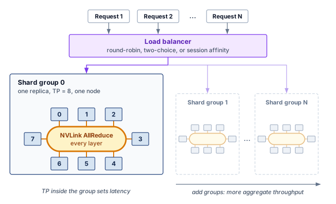
Figure 18: **Horizontal Scaling with Shard Groups**: The load balancer treats each shard group as a single logical inference server and chooses among groups by round-robin, two-choice, or session-affinity routing. Within a group, eight GPUs hold the tensor-parallel weight shards and join partial results with an NVLink AllReduce inside every layer, which the router never sees. Adding ready groups raises aggregate capacity; the group’s internal parallelism affects per-request latency.

10.11.8 KV cache migration between replicas

When a replica fails or consistent hashing remaps a session to a new shard group, the new group cannot generate the next token until it either receives the conversation’s gigabyte-scale KV cache over the network or reruns prefill across the entire history. Routing a request to a shard group fixes where its KV state lives (section 10.10.2), so moving an active session between groups forces a choice between network transfer and recomputation (section 10.11.6). Transfer requires a reachable source or a saved copy; after an unrecoverable replica failure, the service rebuilds from authoritative conversation history:

Migration options:
1. Rebuild: Re-run prefill on new replica (cost grows with context length)
2. Transfer: Send KV cache over network (cache bytes / link bandwidth)
3. Hybrid: Transfer if small, rebuild if large

Decision threshold:
if cache_size_bytes/network_bandwidth < prefill_time:
    transfer()
else:
    rebuild()

For Llama 3 70B with GQA and a 4,096-token context, KV cache is about 1.3 GB total per sequence, or about 168 MB per device under 8-way tensor parallelism. At 100 Gb/s (12.5 GB/s), the bandwidth-only estimate for one shard is roughly 13 ms, while sending the full cache over one such link takes about 107 ms. The prefill approximation counts $5.8 \times 10^{14}$ FLOPs ($2 \times 7.1 \times 10^{10}$ parameters $\times$ 4,096 tokens), giving roughly 180 ms on the tensor-parallel group at the assumed 40 percent utilization. Transfer is faster in this comparison, but achieving the per-shard time for the whole group requires concurrent links with sufficient aggregate bandwidth. Shared network bottlenecks, source availability, cache conversion, and destination queueing can change the decision. Long-context attention adds rebuild work omitted from this approximation, so measured transfer and prefill times should determine the policy.

The shard group boundary also defines readiness. A group can accept work only when the devices, model state, and cache capacity required for its execution plan are available, so the load balancer needs a health signal for the serving replica as a whole.

10.11.9 Health checking and failover

An inference worker whose HTTP server responds 200 OK to a shallow ping can still time out every real query if its weights are still loading, its KV pool is exhausted, or its CUDA context is wedged. Load balancers can route around failure only if the health signal matches the failure mode across three probe tiers (liveness, readiness, and inference correctness) that escalate from cheapest to most realistic. On an accelerator replica, each tier must test a different part of the serving state: readiness includes admission capacity as well as loaded weights and completed warmup, while an inference probe compares a fixed prompt’s output or logits against expected bounds. Passing that probe does not establish correctness or capacity for every request shape, so production errors and latency remain necessary health signals. Failover then depends on the detected failure, available replacement capacity, and whether affected KV state can be transferred or must be reconstructed.

↩︎ Liveness, readiness, and inference-correctness probes, the failover time their settings bound, and stateful failover are established in Failover mechanisms.

10.11.10 Circuit breakers and backpressure

When a GPU inference server slows down, routing more requests to it can turn a local problem into a fleet-wide failure. Consider an illustrative rise in service time from 50 ms to 500 ms. Queues accumulate, client timeouts generate retries, and rerouted work consumes neighboring replicas’ headroom. The cause might be a stalled dependency, device degradation, or resource contention. The load balancer needs a policy for withdrawing an unhealthy replica while controlling the displaced load.

The circuit breaker pattern (Nygard 2007) limits repeated work sent to an unhealthy destination. In the closed state, the server receives normal traffic. When the configured error, timeout, or latency threshold is exceeded, the breaker opens and requests fail fast or become candidates for rerouting. After a recovery interval, a half-open state admits limited probes, closing on recovery or reopening on failure (figure 19). Opening a breaker does not create replacement capacity, so rerouting must respect admission limits and retry budgets or it can overload the surviving replicas.

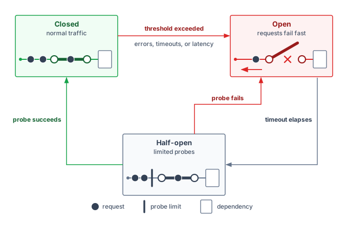
Figure 19: **Circuit Breaker States**: The circuit breaker protects the system from cascading failure. Closed: normal operation. Open: error threshold exceeded; all requests fail fast to prevent resource exhaustion. Half-open: after a timeout, a limited number of requests are allowed through to probe the dependency’s health. Success resets to closed; failure returns to open.

Backpressure propagation complements the breaker by making overload visible upstream. When queue depth crosses a threshold, the server returns a signal such as 503 Service Unavailable; the load balancer marks the replica as degraded and routes fewer requests to it. If all replicas become degraded, the system shifts from routing control to admission control, rejecting some requests at the edge rather than accepting work it cannot serve within the latency SLO; load-shedding policies decide which requests to reject first. Circuit breakers isolate unhealthy replicas; backpressure tells the rest of the system to slow down before retries amplify the failure.

↩︎ Load shedding, model fallback, and the other strategies that trade quality for availability are established in Graceful degradation strategies.

Backpressure works only when the request contract propagates through the whole serving graph. The gateway converts the client timeout into an absolute deadline and every downstream stage subtracts elapsed time before admitting more work. If the client disconnects or the deadline expires, cancellation must reach queued CPU work, accelerator batches, retrieval calls, and streamed output. A canceled request that remains in a continuous batch is zombie work: it consumes KV pages and decode bandwidth while producing no useful response. Some kernels cannot be interrupted mid-launch, so cancellation commonly takes effect at the next batch or token boundary; the scheduler must measure that cancellation lag rather than promise instantaneous preemption.

The same request identifier must connect routing, queueing, prefill, decode, cache allocation, and response streaming. A useful serving trace records admitted and rejected requests, queue delay, TTFT, TPOT, input and output tokens, cache pages, batch membership, preemptions, cancellations, and fallback decisions. Aggregate accelerator utilization cannot distinguish useful work from late or canceled work. SLO goodput and the wasted-token rate close that gap. SLO goodput reports how much completed work met its contract. The wasted-token rate is the fraction of generated tokens spent on requests that were canceled, timed out, or delivered after their deadline, the execution the system performed after the result had lost value.

A saturated LLM fleet operating under severe KV cache pressure has three workload-specific relief options. Engines can apply context eviction through an explicitly supported sliding-window or approximate policy with a quality check, or truncate retained history and recompute its state. Silently dropping old KV entries is not equivalent to recomputing a shorter conversation, because later cached states already depend on the earlier context. Disabling speculative execution reduces draft work, but reclaiming its memory also requires unloading draft weights and releasing the associated cache state. Finally, fallback routing can send eligible requests to a smaller model with available capacity, provided that model meets the application’s fallback quality contract.

These options change latency, resource use, or model behavior in different ways. The application must specify which changes are acceptable at each pressure tier. Context truncation can remove information essential to an answer, and a smaller model can fail the task’s quality requirement. In those cases, an explicit rejection can be preferable to an apparently successful but unacceptable response.

Routing relies on estimates of replica capacity, but shared hardware can make that capacity change when another workload becomes active. Critical production models may share a cluster or device with experimental models and developer endpoints. Protecting the serving contract under that interference requires multi-tenant isolation in addition to routing.

Self-Check: Question

Why does the power-of-two-choices result motivate probing two replicas, and what limitation applies when using the classical balls-into-bins bounds to predict a 1,000-server serving fleet?
1. It eliminates all network packet headers by broadcasting requests to all 1,000 servers simultaneously.
2. Two probes improve static occupancy scaling from $\Theta(\log R/\log\log R)$ to $\Theta(\log\log R)$, but do not determine production queue depths or P99 latency
3. It guarantees zero queuing delay by dynamically compiling new CUDA kernels on the fly for each request.
4. It forces all requests to execute on CPU fallback nodes whenever GPU utilization exceeds 50%.
Explain why Consistent Hashing is critical for routing multi-turn LLM conversations, and describe what happens to KV cache state when an autoscaling event adds a new replica.
True or False: Standard HTTP 200 process liveness checks are sufficient to detect GPU inference degradation caused by thermal throttling or silent HBM memory pool exhaustion.
A heterogeneous inference cluster contains 10 H100 servers (delivering 1,000 QPS capacity each) and 20 A100 servers (delivering 600 QPS capacity each), serving a total target load of 15,000 QPS. What weighted routing ratio should be applied to achieve equal utilization across all hardware tiers?
1. Route 500 QPS equally to every server regardless of type, producing 50% utilization on H100 and 83.3% on A100.
2. Assign weight 1.0 to H100 and 1.0 to A100 so all servers receive equal traffic shares.
3. Assign capacity-proportional weights (H100 weight $= 1000/22000 \approx 4.55\%$ per server; A100 weight $= 600/22000 \approx 2.73\%$ per server), achieving uniform 68.2% utilization across all nodes.
4. Route 100% of traffic to A100 servers first and overflow remaining traffic to H100 servers.
The three-state resilience pattern that fails fast and stops routing traffic to a degraded or thermally throttled GPU replica before retries cascade across the fleet is called a ____.
True or False: An autoregressive LLM must retain state during active decoding, but a serving API can still be stateless across completed requests if each new request supplies the required conversation history.

See Answers →

10.12 Multi-Tenancy and Isolation

Consider a critical customer-support chatbot running on the same GPU server as an experimental computer vision script. If the experimental workload monopolizes the PCIe bus or memory bandwidth, the chatbot can miss its latency target. Sharing saves capacity only when the resulting interference remains within each service’s contract. Fleet quotas, fair-share hierarchies, and priority preemption decide how much of the cluster a serving system receives; the problem here is controlling contention among the tenants who share that allocation, request by request.

↩︎ Fleet quotas, hierarchical fair-share, and the priority classes that govern preemption are established in Multi-Tenancy and Quotas.

Sharing a serving pool can raise utilization and reduce separately provisioned capacity when tenant demand peaks occur at different times. This statistical-multiplexing gain weakens when bursts are correlated, and shared resources introduce interference even when aggregate demand fits. Pooling therefore needs both a demand model and enforceable isolation.

One tenant’s burst can degrade every workload sharing the pool.

A burst from one tenant can delay others through shared KV-cache capacity, network bandwidth, and accelerator time. The pool must preserve each tenant’s data boundary and service contract; different SLOs can require different admission limits, reservations, or placements. Noisy-neighbor interference comes first because it connects shared-resource contention directly to those latency contracts.

10.12.1 Noisy neighbor problems

A noisy neighbor, the tenant whose consumption of a shared resource slows the others on the same hardware, interferes inside a serving pool through three resources at once, and each is denominated in units a request-level scheduler can meter. Unchecked demand for KV-cache capacity, network egress bandwidth, or accelerator execution time lets one bursty workload erode the headroom of every co-located tenant.

GPU memory contention can limit admission before compute capacity is exhausted. Consider three tenants sharing a 60 GB KV pool with nominal 20 GB shares. Without enforced limits, one tenant’s long-context requests can raise its allocation to 45 GB. In the scenario, the others lose capacity from 200 concurrent sequences each to 75, a 62.5 percent reduction. That is a concurrency loss, not a proportional throughput prediction; the effect depends on their execution regime and preemption costs. Egress bandwidth and accelerator time are additional shared resources whose contention must be measured alongside memory occupancy.

↩︎ Noisy-neighbor contention and the device-level interference channels of shared accelerators (memory bandwidth, cache hierarchy, host-device interconnect, and thermal dissipation) are established in Resource isolation.

Example 10.9: Quantifying noisy neighbor impact

Scenario: An inference platform serves 10 tenants on shared H100 GPUs at 100 QPS each under a 50 ms p99 SLO. Tenant 3 bursts to 500 QPS, 5× its baseline.

Diagnosis: Without quotas, contention raises pool-wide p99 into the 22 ms to 45 ms range in this scenario, eroding every tenant’s headroom while remaining within the stated target. With quotas, Tenant 3 is limited to 120 QPS and the other tenants retain 15 ms p99. Throttling turns Tenant 3’s excess into rejected or delayed requests, which are judged against Tenant 3’s own contract rather than spread across the pool.

Systems lesson: Shared capacity raises utilization only when it is coupled with isolation. Quotas turn pool-wide erosion of latency headroom into an admission decision confined to the tenant that caused it; without them, a larger burst or a tighter SLO turns the same erosion into violations across the pool.

10.12.2 Resource quotas and fair sharing

Limiting tenants by request count alone fails when one request carries a 20-token query and the next submits a 100,000-token document that monopolizes KV-cache pages and prefill compute. Resource quotas limit what each tenant can consume across every scarce resource, preventing any single tenant from monopolizing shared hardware. Hard quotas turn shared serving into admission control: request rate and concurrency bound arrival pressure, while input tokens, output tokens, KV-cache pages, accelerator time, and egress bytes bound the work performed after admission. Listing 1 shows representative gates so a tenant can be throttled at the scarce resource boundary instead of degrading the whole batch.

Listing 1: Multidimensional Resource Quotas: A snapshot check compares prospective resource use with tenant limits. Atomic reservation and scheduler enforcement are separate requirements.

class TenantQuota:
    max_concurrent_requests: int  # e.g., 100
    max_kv_cache_mb: int  # e.g., 20,000
    max_qps: int  # e.g., 1,000
    max_input_tokens_per_minute: int
    max_output_tokens_per_minute: int
    max_batch_tokens: int  # e.g., 50,000


def check_quota_snapshot(tenant_id, request):
    quota = get_quota(tenant_id)
    usage = get_usage(tenant_id)

    if usage.concurrent + 1 > quota.max_concurrent_requests:
        return RateLimitError("concurrent request limit")
    if usage.kv_cache_mb + request.reserved_kv_mb > quota.max_kv_cache_mb:
        return RateLimitError("memory limit")
    if usage.requests_last_second + 1 > quota.max_qps:
        return RateLimitError("rate limit")
    if usage.input_tokens + request.input_tokens > quota.max_input_tokens_per_minute:
        return RateLimitError("input-token limit")
    if usage.output_tokens + request.max_output_tokens > quota.max_output_tokens_per_minute:
        return RateLimitError("output-token limit")

    if request.prefill_chunk_tokens > quota.max_batch_tokens:
        return RateLimitError("prefill chunk exceeds batch-token limit")

    return None  # Snapshot is eligible; no resources have been reserved.

This listing assumes that reserved_kv_mb includes the requested prompt and output-token budget, and that usage counters include outstanding reservations in their stated time windows. A passing snapshot is not an admission guarantee: simultaneous callers can observe the same free capacity. Production admission must check and reserve resources atomically, roll back failed admissions, and release reservations on completion or cancellation. The batch scheduler separately enforces the aggregate batch-token limit. Quotas protect the resources they account for; shared compute, networking, and control-plane contention still require isolation and measurement.

Soft quotas permit borrowing unused capacity while preserving an enforceable share when demand rises. The unit of account matters: equal request counts can hide large differences in prefill work, output length, and retained state. Input and output tokens therefore need separate accounting, with memory and concurrency limits alongside them. The progressive-filling approach in Dominant-resource fairness allocation reduces to max-min fairness when only one divisible resource constrains the allocation. For three tenants demanding 30,000, 20,000, and 80,000 output tokens/sec from an idealized 100,000-token/sec pool with equal token costs, the allocation is 30,000, 20,000, and 50,000. Coupled prefill, decode, and memory constraints require joint feasibility checks; independent fair allocations do not automatically compose into a feasible service.

10.12.3 Priority scheduling

First-come, first-served scheduling treats a paid interactive query and a background batch job identically, letting a surge of free-tier or offline traffic delay revenue-critical requests past their SLO. Priority-aware scheduling gives eligible high-priority requests precedence at scheduling boundaries: a production API might classify revenue-generating customer requests as critical, internal batch processing as standard, and free-tier traffic as best-effort. Already-running kernels and shared resources can still delay critical work, so admission limits and reserved capacity must complement priority ordering. Priority becomes an isolation tool once its classes map to tenants and service tiers. Fleet priority classes govern preemption across allocations; request priority applies inside a serving allocation. Table 19 illustrates a policy that combines precedence with reservations. Those reservations must be provisioned and enforced separately: priority alone cannot create capacity, interrupt every running kernel, or guarantee a deadline under unbounded critical traffic.

Table 19: Priority Scheduling Classes: Three-tier priority hierarchy for multi-tenant inference. Critical traffic gets 100 percent reserved capacity and can preempt any lower class; standard traffic shares capacity proportionally and can preempt best-effort; best-effort runs on leftover capacity with no guarantees.

Class	Use case	Preemption	Resource guarantee
Critical	Revenue-generating	Can preempt lower	100% reserved
Standard	General traffic	Can preempt best-effort	Weighted share
Best-effort	Background, batch	Cannot preempt	No guarantee

Preemption extends priority to requests already in flight, but priority does not make state movement free. The retain, swap, recompute, or reject choice of section 10.7.7 still decides how a displaced request’s KV state is handled; priority adds an input to that choice rather than replacing it. A priority class determines who may be displaced, while remaining service time, state size, and deadline slack determine which victim is cheapest. Ignoring those costs lets aggressive preemption consume more capacity than it releases.

10.12.4 Bulkhead pattern

Quotas and priority queues inside a single shared serving process cannot stop a malformed request or out-of-memory fault from crashing the worker and dropping every tenant’s in-flight generations at once. The bulkhead pattern⁷ (Nygard 2007), named after ship compartments intended to contain flooding, partitions resources across separate concurrency pools, processes, or dedicated hardware so exhaustion or failure in one allocation stays contained.

⁷ Bulkhead limits: A divider isolates failure only if it closes the relevant boundary. The Titanic’s incomplete bulkheads allowed water to cascade between compartments; similarly, a soft quota cannot isolate shared memory or bandwidth that remains globally exhaustible.

Nygard, Michael T. 2007. Release It!: Design and Deploy Production-Ready Software. Pragmatic Bookshelf.

Dedicated replicas separate more resources than request limits inside one process. Figure 20 assigns distinct compute and memory pools to tenant groups, so an engine crash or exhausted local allocation in the standard tier need not stop the gold-tier engines. Shared networking, storage, and control-plane services can still carry interference across that boundary.

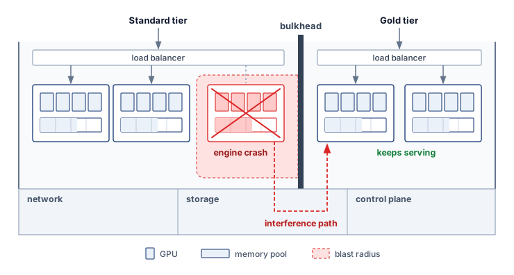
Figure 20: **Bulkhead Isolation Patterns**: To prevent cascading failures in multi-tenant systems, bulkheads isolate resources. Deployment-level bulkheads (shown) assign dedicated physical replicas to high-priority tenants, separating their compute and memory pools. Request-level bulkheads enforce strict concurrency limits within shared processes. Shared networking, storage, and control-plane dependencies remain possible paths for interference.

Deployment-level bulkheads cost pooling efficiency and the operational overhead of dedicated infrastructure. Request-level bulkheads are cheaper but weaker. Caps such as 8,000 input tokens, 2,000 output tokens, and 30 seconds of execution bound request size and duration when the scheduler enforces them, but they still need concurrency limits, reservations, and cancellation handling, and they cannot contain a crash. A malformed request that crashes a shared worker interrupts every tenant on that worker, so service tiers that require stronger fault isolation need placement boundaries to match.

Example 10.10: Bulkhead configuration for API tiers

Scenario: An LLM API platform serves Enterprise, Professional, and Free service tiers across shared and dedicated hardware.

Diagnosis: Unpartitioned pools allow Free-tier bursts or shared-worker failures to affect Enterprise requests. The example assigns Enterprise to dedicated GPU pools with a 99.9 percent availability target, allocates 70 percent of the remaining shared capacity to Professional, and caps Free at 30 percent best-effort capacity. Meeting that target still requires reliability evidence for the dedicated pools themselves.

Systems lesson: Bulkheads concentrate isolation overhead where business requirements dictate. Hardware partitioning reduces cross-tenant compute and memory contention. SLO compliance still depends on sufficient capacity, admission policy, shared dependencies, and failure handling.

Multi-tenant isolation limits the blast radius of excess demand, but it does not create capacity. Once protected queues approach their latency budgets, the service needs a control loop that can add replicas before admission begins to fail.

Self-Check: Question

Which statement best distinguishes deployment-level bulkheads from request-level bulkheads in a multi-tenant inference platform?
1. Deployment-level bulkheads enforce rate limits using software counters; request-level bulkheads isolate GPU power supplies.
2. Deployment-level bulkheads apply only to batch inference; request-level bulkheads apply only to interactive chat.
3. Deployment-level bulkheads dynamically quantize weights to INT4; request-level bulkheads dynamically compile CUDA graphs.
4. Deployment-level bulkheads physically isolate tenant tiers onto dedicated GPU replicas, while request-level bulkheads cap input/output token lengths and execution time within shared processes.
Why is pure First-Come-First-Served (FCFS) scheduling problematic for multi-tenant LLM serving, and what mechanism does preemptive scheduling use to resolve it?
1. FCFS requires excessive GPU memory for block tables; preemptive scheduling replaces block tables with static pointers.
2. FCFS causes extreme AllReduce communication overhead; preemptive scheduling converts tensor parallelism to pipeline parallelism.
3. FCFS forces all requests to run at INT4 precision; preemptive scheduling dynamically promotes high-priority requests to FP16.
4. FCFS can let long requests occupy scarce slots while short requests wait; preemption pauses selected requests and manages their KV state to admit other work
When multiple tenants with unequal demand compete for a shared GPU pool, the fair-allocation algorithm that maximizes the minimum allocation by bounding per-tenant consumption using token generation rate (tokens/sec) is called ____ fairness.

See Answers →

10.13 Autoscaling and Capacity Control

A serving autoscaler that reacts only to average accelerator utilization can scale in the wrong direction. Decode can saturate memory bandwidth while arithmetic units appear idle, long prompts can consume prefill capacity before request count rises, and queued work can violate an SLO while fleet-wide utilization remains moderate. The control signal must represent outstanding work relative to phase-specific service capacity. Every replica the controller adds is also a claim on accelerators that training jobs may hold, so fleet-level arbitration with training bounds how quickly and how far serving can grow.

↩︎ The arbitration between serving replicas and training jobs for shared accelerators, including the minutes-long cost of switching a device between them, is established in The training-serving resource boundary.

For a conventional fixed-cost model, queueing delay and request rate per ready replica can guide scaling. Autoregressive serving also needs prompt-token and output-token rates, KV occupancy, and measured phase service rates. A colocated replica must satisfy all phase requirements; disaggregated prefill and decode pools need separate counts and a feasible transfer budget. SLO goodput measures useful supply, but rejected work and backlog must remain visible as unmet demand. A latency threshold can detect deterioration after a model change, yet controller timing and headroom still need validation. Adding replicas also depends on their startup delay. Changing an existing accelerator allocation may require a restart or state migration, depending on the runtime and execution plan.

Scale-up and scale-down require asymmetric evidence. Scale-up acts on sustained queue growth, forecast demand, or declining deadline slack because cold-start delay makes late reactions expensive. Scale-down requires low demand over a longer window, enough spare capacity to survive one replica failure, and a drain plan for in-flight requests and any optional session cache. This hysteresis prevents oscillation in which replicas repeatedly load large weights, accept work, and terminate before amortizing startup cost.

The controller also needs observability that distinguishes demand from impaired supply: the per-request serving trace of section 10.11.10, plus ready replicas, model-load failures, and per-phase service rate. Without readiness and service-rate measurements, an autoscaler can respond to a sick replica by adding cold replicas indefinitely while the original failure remains hidden.

10.13.1 Scaling response time

If a traffic spike hits a serving pool in 10 seconds but acquiring a GPU node and loading 140 GB of weights takes five minutes, the autoscaler cannot prevent the queue from overflowing during the gap. The scaling response budget is the sum of the control loop’s detection, decision, provisioning, and warmup delays, as equation 16 makes explicit:

\[\AutoscalingResponseTime= \AutoscalingDetectionTime+ \AutoscalingDecisionTime+ \ReplicaProvisioningTime+ \ReplicaWarmupTime \tag{16}\]

Each term has its own typical duration and its own primary lever, from a shorter metrics interval for detection to warm pools for provisioning and precompilation for warmup (table 20).

Table 20: Scaling Response Time Components: The four phases of a scaling event with illustrative durations and their primary optimization lever. Provisioning dominates this example; a deployment must measure its own critical path, which may instead be dominated by artifact loading.

Component	Duration	Optimization
Detection	10–60s	Reduce metrics interval
Decision	1–5s	Faster autoscaler
Provisioning	30s–5min	Warm pools
Warmup	5–30s	Precompilation

Provisioning can dominate the illustrated budget, making already allocated capacity valuable. The large-model example that follows shows that artifact loading can instead dominate startup; the relevant term is the one measured on the deployment’s critical path. Finer-grained metrics can reduce detection delay but increase noise, while prepared scaling decisions and precompiled engines reduce other costs. A warm pool removes only the phases already completed at its stated readiness level.

10.13.2 Cold start and predictive scaling

When a 70B replica takes nearly seven minutes to boot and stream its weights from object storage, waiting for a morning traffic ramp to appear in queue metrics guarantees several minutes of overloaded replicas. A cold start for a 70B replica shows the scale of that delay, and a demand forecast shows how a controller can begin the wait before the traffic arrives.

Example 10.11: Cold start timeline for Llama-70B

Scenario: An autoscaling engine provisions a Llama-70B replica during a traffic surge, using an H100-based allocation large enough for its FP16 weights, cache, and runtime state.

Diagnosis: The scenario’s sequential startup estimate is 6.7 minutes ($\ReplicaColdStartTime= \ReplicaProvisioningTime+ \ReplicaModelLoadTime+ \ReplicaWarmupTime$): 1 minute for provisioning, 4.7 minutes to fetch 140 GB of artifacts at the assumed 0.5 GB/s, and 1 minute for device loading and warmup. Cached artifacts or overlapping phases can shorten this path; scarce capacity and shared storage can lengthen it. If existing headroom cannot absorb the surge, newly requested replicas arrive too late to protect short deadlines.

Systems lesson: Cold-start latency depends on artifact size, effective storage bandwidth, provisioning delay, compilation, and warmup. The controller must measure this distribution and begin provisioning far enough ahead that its high percentile fits inside the forecast horizon.

Example 10.12: Predictive scaling for traffic

Scenario: A commercial chatbot service faces predictable diurnal traffic patterns, ramping from 500 QPS at night to 3,000 QPS at peak.

Diagnosis: A controller that waits for the morning ramps at 06:00 and 09:00 UTC before requesting capacity must cover the assumed 7-minute startup interval with existing headroom or admission limits. Without enough ready capacity, queues grow while replicas start. Forecasting can shift that wait ahead of the expected demand.

Systems lesson: Predictive autoscaling converts demand forecasts into planned pre-warming windows (table 21). Starting 30 minutes ahead of the expected ramps exceeds the modeled startup time. Readiness still depends on actual provisioning and warmup, and forecast errors can leave the fleet short or idle. Reactive correction and an overload policy remain necessary.

Table 21: Predictive Scaling Schedule: Per-time-bucket scaling actions, active replicas, and replicas in cold-start warming for the chatbot workload.

Time	Action	Replicas active	Replicas starting
05:30	Scale up	5	+10 warming
06:00	Traffic ramp	15	-
08:30	Scale up	15	+15 warming
09:00	Peak traffic	30	-
17:00	Scale down	20	-10 terminating
20:00	Scale down	10	-10 terminating
00:00	Scale down	5	-5 terminating

Systems insight: Against an assumed reactive peak of 45 replicas, the forecast-based peak of 30 is a 33 percent reduction in peak replica count at equal unit cost. The reactive controller over-provisions because it reacts to a queue that has already formed and must add capacity for the backlog as well as the demand. Peak count is only part of the bill. Total spending counts replica-hours, including the pre-warming window, so the forecast pays only when the replica-hours spent warming ahead of demand are fewer than those the reactive overshoot would consume.

Example 10.12 illustrates the opportunity to prepare capacity before demand arrives. Figure 21 depicts a forecast that anticipates the surge, while the reactive curve starts later and temporarily lacks capacity. Whether that deficit produces queueing, rejection, or missed deadlines depends on admission and existing headroom. The predictive curve illustrates a successful forecast, not a guarantee that future demand or startup time will match it.

Figure 21: **Predictive vs. Reactive Scaling**: Reactive scaling (gray line) responds to traffic spikes after they occur, leaving a capacity deficit (red region) during cold start in this scenario. Predictive scaling (green line) anticipates traffic and begins provisioning before the spike peaks, shrinking that deficit to a brief, small shortfall at onset in the illustrated forecast. Its early ramp does not eliminate every interval when demand exceeds capacity.

10.13.3 Warm pool management

Demand forecasts still miss unscheduled traffic spikes, and cold-starting a large model from scratch takes minutes that an interactive SLO cannot spare. Maintaining prewarmed replicas in a warm pool buys readiness before unexpected demand arrives. Sizing that pool begins with the total capacity needed during the provisioning delay, then subtracts capacity already ready to serve. If peak demand doubles and the chosen headroom factor is 1.5, the target is three times baseline capacity, assuming unchanged per-replica throughput. Partly prepared replicas count only if they can become ready before that capacity is needed. The expression $\text{Pool size} \times \text{GPU cost/hour} \times \text{Idle fraction}$ estimates the hourly cost attributed to idle GPU capacity; it excludes busy capacity and non-GPU resources. Readiness comes in tiers, each trading activation delay against the cost of waiting (table 22).

Table 22: Tiered Warm Pool Readiness Levels: Readiness trades activation delay against idle resource cost. Actual delay and billing depend on the deployment. Cold capacity is subject to quotas and physical availability.

Tier	State	Activation requirement	Cost while waiting
Hot	Model running on allocated GPU	Route admitted work	Allocated GPU and service resources
Warm	Capacity allocated; runtime partly prepared	Finish initialization and validation	Allocated resources remain billable
Cold	GPU not allocated	Acquire capacity, load, and warm up	Artifact storage; no allocated GPU

When a traffic spike hits, the controller routes work to ready replicas, activates prepared capacity, and requests additional instances if needed. Pool sizing must cover the measured provisioning delay and include an overload policy for capacity that cannot be acquired in time.

10.13.4 Spot and preemptible instances

Revoking a spot GPU replica mid-generation destroys every in-flight sequence’s KV cache unless the worker can drain or migrate its active requests inside the cloud provider’s two-minute warning window. Discounted interruptible capacity enters serving through the same purchasing tiers that fleet capacity planning uses (Cloud Capacity Reservation Tiers): reserved capacity for the steady baseline, on-demand capacity for bursts, and spot capacity for work that tolerates revocation. equation 8.3 derives the effective cost of preemptible capacity from its productive fraction, and serving adds a loss that training checkpoints do not cover: the productive fraction must also pay for draining, rerouting, and rebuilding in-flight KV state without violating the affected requests’ SLO. Listing 2 orders the shutdown path so new work stops first, in-flight work drains while time remains, recoverable state is persisted, and the load balancer stops sending traffic before the instance disappears.

↩︎ Capacity purchasing tiers and the effective cost of interruptible capacity are established in Cost Optimization.

Listing 2: Spot Termination Handling: Graceful shutdown sequence that stops admission, deregisters from the load balancer, drains in-flight requests, and persists recoverable state.

async def handle_spot_termination():
    # Received 2-minute warning
    # 1. Stop admission and remove the replica from routing
    stop_accepting_requests()
    deregister_from_loadbalancer()

    # 2. Complete in-flight requests (if possible)
    await complete_inflight(timeout=90)

    # 3. Save state for resumption elsewhere
    save_kv_cache_to_storage()

    # 4. Terminate gracefully
    shutdown()

Replica-level draining protects in-flight requests only if the upstream router avoids placing strict-SLO traffic on interruptible capacity in the first place. The gateway in figure 22 separates traffic by its tolerance for capacity revocation, and an eviction notice triggers draining when time permits; requests that cannot finish need a permitted retry, reconstruction, or rejection path.

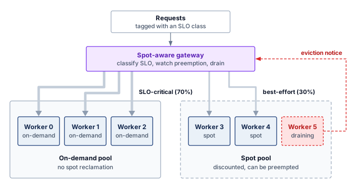
Figure 22: **Spot-Aware Traffic Distribution**: The gateway classifies requests by SLO and routes 70 percent of traffic, the SLO-critical share, to on-demand replicas that face no spot reclamation, and 30 percent, the best-effort share, to discounted spot replicas that can be preempted. When a spot worker receives an eviction notice, the gateway stops routing to it while it drains, and best-effort requests tolerate occasional retries. The traffic split is illustrative; cost savings depend on provisioned capacity, discounts, retries, and idle headroom.

Savings under this split depend on provisioned GPU-hours, discounts, retries, and reserve capacity rather than on the traffic share, and spot capacity changes none of the fault-tolerance requirements of the SLO-critical path. Even a well-scaled single-region fleet, however, remains bounded by wide-area network latency to distant users and by the blast radius of a regional outage.

Self-Check: Question

In an illustrative fresh-replica startup, fetching 140 GB of model artifacts takes five minutes while detection and controller decisions take seconds. Why are pre-warmed pools or predictive scaling useful?
1. Artifact loading dominates this scenario, so pre-warmed pools or advance provisioning can make capacity ready before the surge
2. $\AutoscalingDecisionTime$ dominates (10–15 minutes evaluating autoscaling PID loops); mitigated by switching to manual scaling.
3. $\AutoscalingDetectionTime$ dominates (30 minutes gathering Prometheus metrics); mitigated by removing metric telemetry entirely.
4. $\ReplicaWarmupTime$ dominates (1–2 hours running CUDA kernel JIT compilation); mitigated by disabling Tensor Cores.
When a cloud provider issues a 2-minute termination warning for a spot/preemptible GPU inference instance, describe a four-step shutdown sequence that reduces disruption within the remaining time budget.

See Answers →

10.14 Global Inference Infrastructure

A fleet confined to one region can batch, shard, route, isolate, and autoscale well, yet a user in Sydney still pays roughly a 200 ms round trip to a US-East deployment before any of that machinery acts, and a regional outage removes every replica at once. Extending resource isolation and failure boundaries beyond one data center introduces placement decisions at geographic scale. Distance, regional failures, and data-placement requirements can motivate regional replicas, caches, or a centralized service with an explicit network budget. Figure 23 illustrates three tiers: edge points of presence for reusable responses, regional gateways for authentication and routing, and GPU clusters for model execution. Its 10 ms, 50 ms, and 2 s budgets are scenario targets, not measured performance or universal deadlines. The application must define whether its execution budget governs first response, individual tokens, or completion of the entire request.

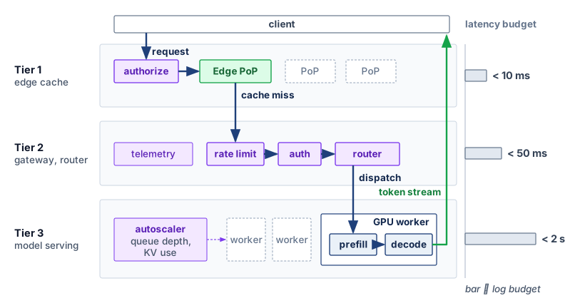
Figure 23: **Serving Deployment Stack**: A cache miss crosses three tiers before reaching a model replica. Tier 1 edge points of presence (PoPs) enforce authorization and reuse eligibility before answering repeated requests from cache; a miss passes to Tier 2, where the gateway applies rate limits and authentication and the router picks a destination; Tier 3 GPU workers run prefill and decode while an autoscaler sizes the fleet from queue depth and KV cache use. Tokens stream back up through the tiers to the client. The per-tier latency budgets on the right, drawn on a log scale, are illustrative.

10.14.1 Drivers for multi-region deployment

Serving all global traffic from a single US-East cluster forces European, Asian, and Australian users to pay a 75 to 200 ms wide-area network round trip on every request and leaves the entire service vulnerable to a single regional outage. Single-region deployment couples every user to the same geographic site and regional failure domain. Network round-trip time (RTT) adds a latency floor for distant users, and illustrative regional timings show that floor rising with distance from the serving region (table 23). Actual paths, access networks, and congestion require measurement.

Table 23: Network RTT by User Location: A single US-East deployment imposes a 75 to 200 ms RTT on European, Asian, and Australian users, an order of magnitude above the local-region floor. Sequential calls that cross this boundary can add repeated wide-area delay. Regional replicas can reduce that exposed delay when placement policy, workload volume, and available capacity justify them.

User location	RTT to US-East	RTT to local region
New York	10 ms	10 ms
London	75 ms	10 ms
Tokyo	150 ms	10 ms
Sydney	200 ms	10 ms

Network delays compound when a request makes sequential calls across the distant boundary; multiple model calls inside one backend region do not each pay another client-to-region RTT. Regional replication can shorten that path and separate failure domains. Data-placement policies also constrain eligible destinations. The General Data Protection Regulation permits international transfers under specified conditions rather than requiring blanket EU-only processing; applicable law and contractual commitments must be translated into explicit placement rules. Regional replicas, edge caches, and cross-region sharding then trade capacity, communication, and coordination within those rules.

10.14.2 Global load balancing with regional replicas

Deploying replicas in multiple regions cuts wide-area latency only if the global router avoids sending users to a nearby region whose GPU queues are already saturated or whose data-residency rules forbid the request. In figure 24, a global load balancer selects among regions that satisfy placement policy, readiness, and capacity requirements. Measured network latency helps choose among those eligible destinations, because geographic proximity alone does not determine completion time, while a shared registry supplies versioned artifacts to the independent regional replicas.

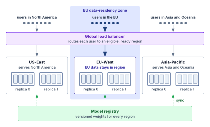
Figure 24: **Global Load Balancing across Inference Regions**: A global load balancer routes each user to an eligible region with suitable latency and ready capacity (table 23 gives the round-trip times this avoids). Each region (US-East, EU-West, Asia-Pacific) runs independent replicas of the same model, and EU requests can stay in the EU to meet data-residency rules. A shared model registry supplies versioned weights to every region. If a region fails, the load balancer reroutes its users only to destinations that still satisfy placement, readiness, and capacity requirements.

Replication also creates a version-management obligation. Push-based synchronization sends artifacts to each region, while pull-based synchronization lets regions fetch them after notification or polling. Neither mechanism alone guarantees consistent serving versions. Artifact verification, readiness gates, and coordinated activation determine when a region may serve the new version; hybrid synchronization combines push notification with pull verification.

During a rollout, regions may serve different versions. The application must decide whether that is acceptable and whether a request or session needs version pinning. A region-by-region canary deployment exposes the new version to one region’s traffic share at a time, and each expansion passes its own error-rate, latency, and quality gate with compatible prior artifacts retained for rollback.

↪ Staged rollout and the canary observation window, sized from the required sample count and the canary’s traffic share, are developed in Canary deployment (equation 12.7).

10.14.3 Edge caching with central inference

Standing up a full GPU cluster in every continent is an expensive way to reduce round-trip latency when a large fraction of distant requests ask repeated FAQ or autocomplete questions. Caching responses at the edge avoids both the wide-area round trip and repeated central inference whenever a stored response remains valid for the incoming request. Before returning a hit, the edge must enforce authorization and match the relevant model version, conversation or retrieval context, generation policy, and freshness requirements. Identical visible queries do not necessarily permit the same answer, and fresh-sample semantics may prohibit reuse. A hit returns within an illustrative 10 ms budget, while a miss reaches the central cluster (figure 25); only responses eligible for reuse should enter the edge store.

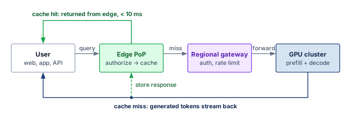
Figure 25: **Cache Hit and Cache Miss Paths at the Edge**: A query first reaches the nearest edge point of presence (PoP). After enforcing authorization and reuse eligibility, the edge targets a cache-hit response in under 10 ms without touching a GPU. On a miss, the request passes through the regional gateway to the central GPU cluster, which runs prefill and decode. Generated tokens stream back to the user, and a response eligible for reuse can be stored at the edge for later queries. The saving depends on the rate of requests eligible for reuse; open-ended generation may offer few such requests.

On the two paths of figure 25, cache hits avoid the backend round trip, while misses incur it. Effectiveness depends on request repeatability across workloads such as autocomplete, FAQ chatbots, open-ended chat, and code generation. Table 24 supplies illustrative hit-rate envelopes for sensitivity analysis; an actual design must derive hit rate and correctness from production traces.

Table 24: Illustrative Edge-Cache Hit-Rate Envelopes: Assumed cache-hit ranges for four workload shapes. These values are scenario inputs, not universal workload statistics. Trace-derived repeatability, response validity, and latency saved determine whether caching is worthwhile.

Workload	Cache hit rate	Suitability
Autocomplete	60–80%	Excellent
FAQ chatbot	40–60%	Good
Open-ended chat	5–15%	Poor
Code generation	20–40%	Moderate

Semantic caching⁸ (caching based on embedding similarity rather than exact match) can improve hit rates for open-ended workloads. Any cache miss still requires full model execution, raising the question of whether a large model can be split across regions or must run inside a single data center.

⁸ Semantic caching: A similarity lookup can reuse responses beyond exact string matches, but it adds retrieval work and can return an invalid answer when superficially similar queries require different responses. The similarity threshold therefore trades cache coverage against correctness.

10.14.4 Cross-region model sharding

Splitting a single model replica across data centers puts wide-area network latency directly on the request’s execution path: when pipeline stages reside in separate regions, every stage crossing pays a 75–150 ms inter-region transfer against only 1–5 ms of local stage computation. That illustrative gap can slow inference by 10–100$\times$, though the exact penalty depends on the model’s stage layout. Such placement needs a reason strong enough to justify that cost, such as unavailable colocated capacity, and must be evaluated against the actual stage layout and deadline. Because cross-region sharding is so costly on the steady-state path, most production designs keep inference co-located and use other regions for resilience. The cross-region question therefore shifts from splitting one request across regions to deciding how quickly traffic can move when a region fails.

10.14.5 Cross-region failover

When a region becomes unavailable, failover must choose a healthy destination permitted to process the request and able to absorb its work. A simplified fallback tries the nearest eligible region first and, on timeout or rejection, the next one (listing 3). A production policy must also preserve the request’s remaining deadline, version requirements, and data-placement constraints when selecting the secondary region.

Listing 3: Active-Active Failover: A bounded retry policy selects eligible regions and limits each attempt to the remaining request deadline.

# Eligibility includes placement, version, readiness, and capacity.
def route_request(user_region, request):
    attempted = set()
    for attempt_budget in (2.0, 5.0):
        remaining = request.deadline - monotonic_time()
        regions = eligible_regions(request, excluding=attempted)
        if remaining <= 0 or not regions:
            break
        region = nearest_region(user_region, regions)
        attempted.add(region)
        try:
            # The endpoint atomically admits work and enforces the deadline.
            return call_region(region, request,
                               timeout=min(attempt_budget, remaining))
        except (Timeout, RegionUnavailable, AdmissionRejected):
            # Cancel abandoned work; retries require replay-safe semantics.
            cancel_attempt(region, request)
    return unavailable_or_deadline_exceeded(request)

Rerouting is only part of regional failover. The destination needs accessible, authoritative conversation history to reconstruct lost KV state and enough headroom for both reconstruction and continuing traffic. If the required history is unavailable or cannot be processed there under the placement policy, a healthy replica alone cannot restore the session.

↩︎ Regional headroom, session rebuilding, and the gradual return of traffic to a recovered region are established in Replication strategies.

10.14.6 Cost optimization across regions

Running every batch job and latency-tolerant query in the primary interactive region overpays whenever another compliant region has cheaper spot or off-peak GPU capacity. Because GPU pricing varies by provider, contract, region, and time, table 25 uses a hypothetical price snapshot to show how placement can balance cost against latency requirements; it must not be used for procurement.

Table 25: Hypothetical Regional Price and Latency Snapshot: Scenario prices and RTTs illustrate a placement calculation. Both inputs are time- and provider-specific; a deployment must refresh them from its contract and measured network paths before making a routing decision.

Region	H100 spot price	On-demand	Latency to US users
US-East	$2.50/hr	$4.00/hr	10–50 ms
US-West	$2.30/hr	$3.80/hr	30–70 ms
EU-West	$2.80/hr	$4.20/hr	75–100 ms

Cost-aware routing compares eligible regions for latency-tolerant work (listing 4). GPU price alone is insufficient: transfer charges, startup and idle capacity, retries, and achieved useful throughput determine the cost of completing the workload. Deadline and data-placement constraints must filter destinations before that comparison.

Listing 4: Cost-Aware Routing: The router filters eligible destinations before comparing completion cost for low-priority work or proximity for interactive work.

def route_batch_request(request):
    # Filter by placement, version, readiness, capacity, and deadline.
    regions = eligible_regions(request)
    if not regions:
        return no_feasible_destination(request)
    if request.priority == "low":
        return lowest_completion_cost_region(request, regions)
    return nearest_region(request.user_location, regions)

Time-of-day routing can reduce batch cost when regional price differences exceed data-transfer and coordination costs. Savings require a workload-specific calculation, and interactive traffic must retain its own latency budget. Regional placement completes the serving hierarchy, from one request’s batch slot to a fleet that spans continents. The design cases that follow show how these techniques combine when a service must meet specific cost and latency targets.

Self-Check: Question

True or False: Cross-region model sharding (spanning pipeline stages between US-East and Asia-Pacific) is an effective strategy for minimizing single-request P99 latency.
An edge point of presence receives a query whose visible text exactly matches a cached response. Which condition must hold before the edge may return that cached response as a hit?
1. The cached response is younger than the 10 ms edge latency budget, so it cannot be stale
2. The request passes authorization, and the cached response matches its model version, conversation or retrieval context, generation policy, and freshness requirements
3. The query text matches exactly, which by itself guarantees that the same answer is valid for every user
4. The regional gateway has confirmed that the central GPU cluster is overloaded
Region A fails and the global load balancer reroutes an ongoing conversation to a healthy replica in Region B. Explain why rerouting alone may not restore the session, and what Region B needs for the failover to succeed.
True or False: In the chapter’s hypothetical price snapshot, US-West H100 spot capacity costs 2.30 dollars per hour versus 2.50 dollars per hour in US-East, so routing low-priority batch work to US-West always lowers the cost of completing that work.

See Answers →

10.15 Case Studies

Individual serving optimizations—quantization, continuous batching, sharding, or caching—can look decisive in isolation yet still leave a production endpoint missing its latency, memory, or cost contract when combined under real traffic. The five design cases below are illustrative composites rather than descriptions of named companies’ internal deployments, and their request rates, latency budgets, hardware allocations, and update cadences follow the chapter’s scenario convention. Each case binds on a different constraint: one replica’s decode step, embedding scale, variable-length generation, cascade cost, or multimodal freshness. Orca and vLLM supply the previously cited scheduling and memory-management mechanisms; the scenarios combine those ideas with precision, routing, sharding, and admission control.

10.15.1 One replica against its token-latency target

Even before a serving cluster worries about routing or multi-region failover, a single replica can fail its per-token latency target on a batch of one—leaving zero headroom to batch additional requests. The first case stays inside one replica, the reference 70B model on eight NVLink-connected H100s with FP16 weights split eight ways, serving an interactive endpoint whose illustrative TPOT target is 50 ms. A batching policy can only spend the headroom that a batch-one decode step leaves, because every admitted sequence lengthens the step (section 10.6.2), so the first question is whether one batch-one step fits inside the target at all. This constructed example illustrates budget accounting, not benchmark results. Every interval is an exposed, nonoverlapping contribution to the same request’s critical path, and time to first token, output quality, and throughput under load each need their own measurements.

The deployment’s FP16 weights occupy 140 GB, about 17.5 GB per GPU. The assumed baseline decode step is 85 ms, about 16× the 5.2 ms that streaming each shard at full HBM bandwidth would take, so the replica runs at an MBU of about 6.1 percent (Program goodput and its measure). That gap, not the weight-streaming floor, is what eager dispatch, unfused kernels, and exposed synchronization must explain, and table 26 apportions the whole step among those causes on one absolute-time boundary. In an actual trace, overlapping work must not be counted twice when constructing such a budget.

Table 26: Constructed Decode Budget for the Reference Replica: Assumed nonoverlapping critical-path intervals for one batch-one decode step. Each column sums to its step duration; none is an empirical performance claim.

Exposed interval (ms)	Baseline	After precision	After fusion and replay
GEMM	34	18.7	18.7
Attention	20.4	20.4	15.3
Element-wise operations	10.2	10.2	3.4
AllReduce	10.2	10.2	10.2
Launch and runtime overhead	10.2	10.2	2
Total	85	69.7	49.6

The first experiment targets weight-read traffic with INT4 weight-only quantization, the bandwidth-bound decode row of table 11. Assume that quality validation succeeds and that exposed GEMM time falls by 45 percent, with every other interval unchanged. The step takes 69.7 ms, still above the 50 ms target, because a large cut to one interval removes only that interval’s share of the step. INT8 KV-cache compression is a separate candidate whose benefit is capacity, as notebook 10.7 computes; it needs its own quality check and a new profile, so this column grants it no latency benefit.

The second experiment targets exposed attention, element-wise work, and launch gaps, using the single-replica levers of Kernel-level levers. Assume a validated fused decode-attention kernel, the single-pass kernel over the KV cache of section 10.8.1, reduces attention by 25 percent, fusion reduces element-wise work to 3.4 ms, and graph replay reduces launch and runtime overhead to 2 ms. These are scenario assumptions, and each intervention would be tested separately before the combination is retained. The step becomes 49.6 ms, inside the target with almost no slack and still about 9× above the bandwidth floor. Communication remains 10.2 ms, unchanged in absolute time even as its share of the shorter step grows. Spread across the 160 AllReduces of an 80-layer step, that interval implies about 64 μs per collective, against roughly 5 μs of launch and transfer, or about 0.8 ms per step. The difference is the protocol and synchronization cost of small collectives that Tensor-parallel collectives under contention flags for measurement, and a trace that attributed it would make communication the next experiment.

The third experiment changes how much output each step yields. Assume a draft model proposes $\SpeculativeDraftLength=$ 5 tokens in 4 ms, verification costs one round-two step, and each candidate is accepted independently with probability $\DraftTokenAcceptanceProbability=$ 0.78. Equation 6 gives 3.52 tokens per round, so a 53.6 ms round yields 15.2 ms per emitted token, an amortized 3.26-fold improvement in TPOT. The tokens, however, arrive in blocks. The gap between blocks is a whole round, 53.6 ms, which exceeds the same 50 ms if the endpoint also states it as a per-gap TBT target. Speculation thus meets an average-cadence contract with room to spare while missing a per-gap one on every round, which is why the TPOT and TBT targets of section 10.2 are stated separately. The gain also belongs to batch one; as the speculative-decoding policy in section 10.7.6 warns, larger batches consume the spare compute that made verification cheap.

The budget exposes bottleneck displacement without crediting a system improvement to an isolated kernel speedup. Precision changes one interval, fusion and replay change others, and speculation changes the output per round; their benefits compose only on a shared accounting boundary, with quality preserved. What the sequence produces is a set of candidate replica configurations, not a serving result. Accepting one for production means replacing the illustrative intervals with measurements, preserving the request-length distribution and offered load, and measuring SLO goodput (section 10.3) at the batch the scheduler will actually admit. Memory freed by INT4 weights can permit that larger batch, but neither the freed capacity nor a faster batch-one step shows that the service meets every target at once.

10.15.2 Embedding-heavy recommendation serving

An embedding-heavy recommendation service binds on sparse lookup rather than dense forward-pass compute. Modeled on feeds, advertising, and content ranking, it processes billions of requests per day under a p99 budget below $10\text{ ms}$ for the ranking service, nested inside the roughly 100 ms end-to-end tail target of Archetype B (DLRM at Scale), across hundreds of model variants and trillions of unique sparse features. The serving stack separates sparse lookup from dense ranking:

User request → Feature collection → Embedding lookup → Model inference → Response

                    |                     |                  |
                    v                     v                  v
             Feature Store        Embedding Servers      GPU Inference
             (CPU, DRAM)         (CPU + SSD, 1000s)     (GPU, 100s)

The hybrid sharding strategy in lighthouse 10.1 supplies the sparse path: replication protects hot entries, column sharding spreads warm-entry access, and row sharding places the cold tail. Feature-level batching then combines lookups across requests. The remaining design decision is where each stage runs. In the GPU-CPU hybrid architecture, memory-rich CPU servers serve sparse embeddings while GPUs execute dense ranking. Table 27 connects that placement to the end-to-end latency budget.

Table 27: Illustrative Hybrid CPU/GPU Architecture: Illustrative hardware-workload mapping for the recommendation scenario. CPU + SSD handles the bandwidth-bound sparse path; CPU handles low-arithmetic-intensity feature processing; GPU handles the compute-dense ranking forward pass. The component budgets exclude queueing and response delivery; their sum alone does not establish the p99 target.

Component	Hardware	Latency	Throughput
Embedding lookup	CPU + SSD	2 ms	50M lookups/s
Feature processing	CPU	1 ms	10M ops/s
Dense ranking	GPU	1.5 ms	100K infs/s

The serving lesson is that recommendation latency is often dominated by embedding lookup rather than dense model inference. Feature-parallel batching and a hybrid CPU-GPU architecture match the hardware to the sparse and dense halves of the workload, which sets up a contrast with GPT-style API serving where request variance and autoregressive state dominate.

10.15.3 A multi-model generation API

A multi-model generation API binds on request variance, because short prompts, long-context requests, and different model sizes share capacity while users expect predictable TTFT. The platform serves millions of requests per hour under a time-to-first-token target below $2\text{ s}$, with models from billions to hundreds of billions of parameters and contexts up to 128K tokens. The serving stack separates routing, scheduling, cache management, and shard groups:

API Gateway → Rate Limiting → Request Router → Model Cluster → Response Streaming

                                     |
                                     v
                              +-------------+
                              | Model Pool  |
                              | +---------+ |
                              | | Large   | |
                              | | 8×H100  | |
                              | +---------+ |
                              | +---------+ |
                              | | Smaller | |
                              | | 4×A100  | |
                              | +---------+ |
                              +-------------+

The main design decision is to prevent long prompts from blocking decode service for everyone else. An Orca-style design uses continuous batching to refill completed slots. Chunked prefill limits interference from long prompts by interleaving prompt chunks with ongoing generation. The TTFT target must be validated across prompt lengths; admitting a 128K-token prompt does not imply that it meets the short-request latency target. Slot reuse and long-prompt interference are separate concerns. Continuous batching addresses the first and chunking bounds the second, so neither mechanism alone establishes the utilization or tail latency the API will see.

The tensor-parallel degree must satisfy weight and KV-cache capacity while leaving enough latency budget for communication. This scenario allocates eight H100 GPUs per large-model shard group connected via high-speed NVLink for intra-node communication, with consistent hashing at the gateway to maintain session affinity and enable compatible cross-turn KV cache reuse. The eight-device allocation is a design choice to validate against the model, precision, and admitted context lengths, not a requirement of GPT-class models in general.

To prevent noisy neighbors from exhausting capacity, the illustrative API applies hierarchical rate limiting across multiple granularities: per-API-key request arrival limits, per-API-key token-per-minute consumption limits, organization-level capacity quotas, and global model capacity ceilings. Within those ceilings, capacity can also shift between models on queue depth, subject to model-loading delay and each service’s minimum allocation, using the autoscaling signals of section 10.13.

LLM APIs are governed by variance control. Continuous batching reuses execution slots, prefix caching avoids compatible repeated work, and multi-tier rate limiting bounds admitted demand. Their combined effect on latency still depends on prompt scheduling and available capacity. Search ranking faces a different shape of the same problem. Many cheaper models must cooperate under one strict deadline.

10.15.4 Search ranking under a deadline

The search-ranking scenario binds on cascade cost, because each query coordinates many smaller models for query understanding, document relevance, and result ranking under one end-to-end budget rather than serving one large model. The system processes billions of searches per day under a target below $200\text{ ms}$ while evaluating thousands of candidate documents per query, so screening candidates with cheaper models reserves the expensive ranking budget for a smaller set.

To meet this latency budget while evaluating thousands of documents, the ranking cascade in figure 26 screens candidate pools across four progressively expressive tiers. Early lexical and approximate-nearest-neighbor (ANN) embedding retrievers discard 99 percent of candidates within a 10 ms budget, reserving compute-intensive cross-attention transformers for the final top 100 items. This saving creates a recall constraint. A relevant document discarded upstream cannot be recovered by a more accurate downstream ranker, so each stage’s candidate budget must be evaluated for retained relevant items as well as latency.

↩︎ The vector indexes behind the L0 retrieval stage, and the storage cost of keeping them fast enough for a serving deadline, are established in Retrieval indexes.

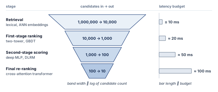
Figure 26: Ranking Cascade Architecture: To optimize latency and cost, search and recommendation systems use a cascade of increasingly complex models. Early stages (Retrieval) filter millions of candidates down to thousands using fast, cheap heuristics. Later stages use expensive, high-precision models only on the most promising candidates.

The central design decision is progressive refinement through a ranking cascade rather than one expensive model applied to every candidate. Each stage of the cascade spends a larger latency budget on a smaller candidate set (table 28), so the expensive L3 transformer is affordable only because L0 through L2 have already cut the candidates by four orders of magnitude.

Table 28: Illustrative Ranking Cascade: Each stage evaluates fewer candidates with a more expensive model. The final stage has the largest latency allocation in this scenario; candidate reduction makes that expense affordable.

Stage	Model complexity	Candidates	Latency budget
L0 (Retrieval)	Lexical and ANN embeddings	1,000,000 → 10,000	10 ms
L1 (First pass)	Two-tower or GBDT	10,000 → 1,000	20 ms
L2 (Second pass)	Deep MLP (DLRM)	1,000 → 100	50 ms
L3 (Final rank)	Cross-attention transformer	100 → 10	100 ms

The cascade reduces final L3 evaluations by 10,000× compared to running L3 on all candidates. If the stage budgets are treated as additive model work and L3 cost scales linearly with candidate count, the L3 allocation implies 1 ms per candidate. Applying L3 to the full million-candidate set would then consume about 1000 s of model work, while the cascade budget sums to 180 ms. The resulting reduction is roughly 5,600× under these assumptions. This accounting estimate is not a measured latency speedup; batching and parallel execution can change elapsed time without changing the candidate count.

A deadline-constrained ranking ensemble can use speculative execution when it has a validated fallback-quality policy. Here, speculation means launching candidate ranking work in parallel under a deadline, not draft-token verification for LLM decoding:

# Instead of sequential:
#   q1 = model1(query)
#   q2 = model2(query)
#   q3 = model3(query, q1, q2)

# Speculative parallel:
async_q1 = async model1(query)
async_q2 = async model2(query)
async_q3 = async model3(query, predicted_q1, predicted_q2)

# Use actual results if they arrive in time, otherwise use speculative

Each sub-request carries an explicit remaining-time budget, and workers order their local queues by deadline proximity rather than arrival order. When a queued sub-request cannot complete before its budget expires, the worker returns a cached or default score immediately instead of timing out the parent query:

Worker queue: [Doc1: 50 ms left] [Doc2: 30 ms left] [Doc3: 80 ms left]
                                      ↑ Process first

If deadline will be missed:
  Return cached/default result rather than timing out

The serving lesson is that ranking cascades reduce cost by spending expensive models only on a shrinking candidate set, at the risk of losing relevant items upstream. Deadline propagation and priority scheduling expose the remaining time budget; meeting it also requires sufficient capacity and a validated fallback when work cannot finish. The next case adds a freshness constraint that deadline scheduling alone cannot solve.

10.15.5 Multimodal recommendation and freshness

The multimodal recommendation scenario binds on freshness under a tight ranking SLO: video understanding is expensive, new content arrives continuously, and user modeling remains online. The system ranks millions of videos per second under a p99 target below $50\text{ ms}$ while ingesting millions of new videos daily across video, audio, text, and interaction signals, which is why online and offline work must separate. The serving stack separates content and user paths:

User request → User embedding → Candidate videos → Video understanding → Ranking

                    |                  |                    |
                    v                  v                    v
             User Tower          Video Cache          Vision Models
           (Transformer)        (Pre-computed)        (On-demand)

The scenario separates user understanding (online) from content understanding (offline) through a two-tower architecture with caching.⁹ The user tower runs online on every request, while the video tower refreshes in hourly offline batches (table 29).

⁹ Two-tower architecture: Encodes user features and item features through separate neural networks (“towers”) into embeddings, then scores via dot product. Its serving advantage is that item embeddings can be precomputed offline and cached, reducing online candidate generation to the user tower forward pass and vector similarity search. Search latency depends on index size, placement, and the required recall. The trade-off is reduced model expressiveness from late interaction, since the towers cannot attend to each other’s features during encoding.

Table 29: Illustrative Two-Tower Update Cadence: User and video towers run on different cadences: user features change second-to-second and must run inference online; video features change much more slowly and are precomputed in hourly batches. This asymmetric scheduling is the design that takes vision inference out of the critical path for almost every request.

Tower	Update frequency	Latency	Compute
User tower	Real-time	5 ms	GPU (online)
Video tower	Hourly	N/A	GPU (batch)

Video embeddings are precomputed and cached, eliminating vision inference from the critical path for most requests. A newly uploaded video without a cached embedding needs an explicit policy: process it before admitting it to recommendations, serve a validated fallback, or run vision inference on demand if the request budget permits. The hourly refresh cadence alone does not meet the shorter ingestion targets below; those targets require a separate path for new content.

The online path below separates candidate generation from a later dense reranker. Its user-tower budget is distinct from the reranker budget:

User features → CPU preprocessing (1 ms)
             → Embedding lookup (2 ms, CPU+DRAM)
             → User tower (5 ms, GPU)
             → Dense reranking (10 ms, GPU)
             → Response formatting (1 ms)

New uploads enter an ingestion queue with priority tiers, so time-sensitive content is embedded within minutes and bulk imports absorb hours of slack, although priority only changes who waits when ingestion capacity falls short. The modality embeddings (video, audio, text) are combined late by a small fusion model, so updating one modality’s encoder requires a compatibility check and, when its embedding contract changes, regeneration of the cached embeddings.

The serving lesson is that freshness requires separating online and offline work. Two-tower architectures make aggressive caching possible because item embeddings can be refreshed asynchronously, while priority-based processing spends the freshest compute where it has the largest user impact.

10.15.6 Cross-cutting observations

Trying to serve LLM token generation, sparse recommendation ranking, and multimodal retrieval through one generic model server forces every workload to pay for scheduling and memory abstractions it does not need. Across these cases, the common pattern is specialization rather than a universal serving stack: embedding and retrieval separate from ranking and generation, hardware matched to each stage, caches that accept bounded staleness, candidate sets that shrink before expensive work, and deadlines that propagate so quality-latency trade-offs stay explicit under pressure. Table 30 distills the same choices along five design axes for the three workload families the cases cover. Its entries are candidate combinations for the illustrated constraint regimes, not prescriptions, because a model class alone does not fix a scheduler or topology, which also depend on model size, request mix, available hardware, and service targets.

Table 30: Serving Architecture Dimensions by Workload Type: The rows identify candidate design choices along five architectural dimensions. The workload’s state, scheduling, and hardware constraints guide selection; the service contract determines whether a combination supplies useful capacity.

Dimension	Vision/embedding	LLM (autoregressive)	Recommendation
Batching	Static/dynamic (uniform inputs)	Continuous (variable outputs)	Feature-parallel (sharded embeddings)
Memory	Preallocated (predictable)	Paged (variable KV cache)	Distributed (embedding tables)
Scheduling	FCFS (uniform cost)	Preemptive (high variance)	Priority-aware (SLO tiers)
Topology	Single-GPU replicas	Tensor/pipeline parallel	Hybrid CPU-GPU sharding
State	Stateless	Request state; optional session cache	Stateless or session features

The case studies show why serving architectures must be adapted to their workloads. Applying conventional web-service assumptions to GPU-bound systems creates the fallacies and pitfalls examined next.

Self-Check: Question

The reference 70B replica’s constructed batch-one decode step is 85 ms: 34 ms GEMM, 20.4 ms attention, 10.2 ms element-wise work, 10.2 ms AllReduce, and 10.2 ms launch and runtime overhead. INT4 weights cut only the GEMM interval, by 45 percent, leaving 69.7 ms. Why does this still miss a 50 ms TPOT target?
1. INT4 weights halve memory bandwidth, so the other intervals lengthen to absorb the saving
2. The bandwidth-only floor of about 5.2 ms already exceeds what INT4 can recover, so no precision change can help
3. The unchanged non-GEMM intervals still total 51 ms, so reducing GEMM alone by the assumed amount cannot reach the target
4. The TPOT target applies to prefill, and INT4 weights do not change prefill time
After fusion and graph replay, the reference replica’s decode step is 49.6 ms. Adding speculative decoding with a 4 ms draft and about 3.5 emitted tokens per round brings the average time per output token to about 15 ms. Why can the endpoint still miss a 50 ms time-between-tokens (TBT) target?
In an illustrative search-ranking cascade (L0: 1M to 10k in 10 ms; L1: 10k to 1k in 20 ms; L2: 1k to 100 in 50 ms; L3: 100 to 10 in 100 ms), what follows under a simplified additive candidate-work model?
1. It runs L3 on all 1,000,000 candidates using asynchronous DMA transfers without CPU involvement.
2. It replaces neural networks entirely with BM25 keyword matching across all stages.
3. It dynamically recompiles transformer weights at each stage using TensorRT-LLM.
4. It cuts final expensive L3 evaluations by $10{,}000\times$ (from 1,000,000 to 100), reducing total candidate-scoring compute by $\approx 5{,}600\times$ within a 180 ms budget.
Compare the binding bottlenecks and serving topologies of the illustrative embedding-heavy recommendation scenario and autoregressive LLM API scenario.
True or False: In the illustrative two-tower video recommendation scenario, both the user tower and the content tower must execute synchronously for every swipe.
Which combination of architectural design choices addresses variable-length autoregressive generation and reusable session context in the chapter’s LLM serving scenario?
1. Continuous batching, paged memory management, preemptive scheduling, and stateful routing
2. Static batching, preallocated memory management, first-come-first-served (FCFS) scheduling, and stateless routing
3. Feature-parallel batching, distributed memory tables, priority-aware scheduling, and stateless routing
4. Streaming frame batching, pinned buffer allocation, non-preemptive scheduling, and edge-only topology

See Answers →

10.16 Fallacies and Pitfalls

A DevOps team that applies its standard web-server load-balancing rules to a new fleet of GPU inference nodes can see tail latency climb sharply, because those rules ignore the extreme variance of autoregressive token generation. Web services also face variable work and queueing, but an inference fleet adds model residency, accelerator scheduling, and per-sequence state to those familiar concerns. The fallacies below arise when a serving design ignores these constraints or treats one optimization as a complete solution.

Fallacy: Serving at scale is synonymous with LLM serving.

The misconception leads to over-focus on LLM-specific techniques. As section 10.5.1 showed, recommendation and ranking models can consume most AI inference cycles on large consumer platforms (Gupta et al. 2020; Hazelwood et al. 2018), and a practitioner who knows only continuous batching and KV cache management is unprepared for the feature-parallel batching and embedding sharding that dominate that traffic. Technique selection must match the actual workload.

Hazelwood, Kim, Sarah Bird, David Brooks, Soumith Chintala, Utku Diril, Dmytro Dzhulgakov, Mohamed Fawzy, et al. 2018. “Applied Machine Learning at Facebook: A Datacenter Infrastructure Perspective.” 2018 IEEE International Symposium on High Performance Computer Architecture (HPCA), 620–29. https://doi.org/10.1109/hpca.2018.00059.

Pitfall: Using training infrastructure for production serving.

Training and serving have different requirements, as table 2 summarized. Interactive serving must satisfy per-request latency targets under external arrivals, so its batch size depends on the workload and waiting budget, and its recovery policy must account for in-flight requests, retries, and the availability target rather than a checkpoint. Hardware can be shared or repurposed, but a training configuration does not establish serving readiness.

Fallacy: Continuous batching solves the whole LLM serving problem.

Continuous batching reuses slots released by completed requests, but it addresses only one dimension of the problem. Prefill can remain a bottleneck for long contexts because scheduling subsequent decode iterations does not remove the quadratic attention work of full-attention prefill. Section 10.7 demonstrates that KV cache memory, not compute, often limits batch size. Network bandwidth between sharded model components can dominate latency for large models. The value of continuous batching depends on the workload; slot reuse alone does not resolve these other constraints.

Pitfall: Sizing the fleet by average throughput.

Average throughput alone does not establish capacity for bursts. With unchanged work per request and service capacity, a 25 percent traffic increase from 80 percent utilization reaches 100 percent utilization, leaving no spare capacity to absorb variance. Whether the resulting queue violates an SLO depends on burst duration, the waiting budget, and admission policy. Cluster-level cold starts can delay relief for multiple minutes. Capacity planning must therefore account for peak load, burst duration, ready headroom, and the work the service can defer or reject.

Fallacy: Load balancing does not matter much for inference.

Simple load balancing strategies like round-robin can distribute request counts while leaving work uneven. The static placement analysis in section 10.11 motivates two probes, but its occupancy bounds do not predict production queue lengths. Serving comparisons must preserve arrivals, request lengths, cache affinity, and replica capacity. Work-aware routing earns its place when it improves measured tail latency without excessive coordination cost.

Pitfall: Ignoring the serving tax.

Distributed inference adds network round-trips and shard coordination to the serialization, routing, and queueing costs that can already surround a single-machine model. This serving tax depends on deployment topology and load. In the illustrative budget of section 10.3, 70 ms of model execution leaves only 30 ms for every other stage of a 100 ms request target, and queueing alone can consume that remainder as load rises. A kernel benchmark measures only the first term of equation 1; the serving latency is the measured sum along the complete request path.

Fallacy: More GPU memory always means larger batch size and higher throughput.

Larger GPU memory raises throughput only when the extra capacity supports useful work within the latency budget. Even when memory bandwidth is saturated, a larger decode batch can increase tokens per second by sharing weight reads across more sequences. That gain stops when compute, per-sequence KV-cache traffic, or the SLO becomes binding. The bottleneck hierarchy distinguishes these limits.

For an H100 with 80 GB memory and 3.35 TB/s HBM3 bandwidth, capacity and transfer rate are separate limits. More capacity may admit additional sequences, but the resulting batch must still meet compute, bandwidth, and latency budgets. Once extra sequences no longer improve useful throughput within those budgets, adding memory alone cannot help. Capacity planning therefore measures the bottleneck at the intended batch size and context length rather than assigning one permanent bottleneck to the model.

Pitfall: Neglecting multi-tenancy isolation until production.

In development and staging, single-tenant deployments work well. In production, noisy neighbors cause sudden, unpredictable performance degradation that is difficult to diagnose and resolve. A tenant bursting to 5$\times$ normal traffic can degrade latency for all other tenants on shared infrastructure. As emphasized in section 10.12, resource quotas, priority scheduling, and bulkhead isolation must be designed into the system from the start, not retrofitted after production incidents.

Fallacy: The lowest supported precision is always the best precision.

Aggressive quantization (INT4 weights, INT4 KV cache, FP8 activations) can degrade model quality in ways that standard benchmarks miss but users see. Perplexity on a held-out dataset may change by less than 1 percent while responses degrade for edge cases, rare languages, or complex reasoning. A serving system that doubles its tokens per second with a format that lowers answer quality has not doubled its useful capacity, because throughput and quality form a frontier and a precision choice is a point on it. The disciplined approach is targeted quantization: measure per-layer sensitivity under representative workloads, restrict lower bit widths to the tensors that tolerate them, and evaluate KV caches, endpoint layers, and attention logits empirically rather than by a presumed sensitivity ranking. Calibration on representative data, followed by evaluation on diverse quality benchmarks reported beside the latency and throughput results, comes before any quantized model reaches production (section 10.9).

Pitfall: Treating MoE expert count as a free scaling knob.

Adding experts to an MoE model raises total parameters without proportionally raising active per-token arithmetic, which makes expert count look free. Every expert still occupies memory whether or not a token selects it, as section 10.10.4.1 prices for resident versus active parameters, so more experts mean more devices or less KV headroom, and a distributed placement adds dispatch and combine communication to every layer. The realized cost depends on experts selected per token, token-to-expert skew, expert capacity, topology, and batching, and no universal expert count marks where the design starts to lose. The change is justified only when a matched-quality comparison shows that active-compute savings exceed routing, imbalance, memory, and communication costs over the intended workload envelope.

These fallacies and pitfalls identify what a serving evaluation must test: traffic variance, cost per completed request within the SLO, output quality beside throughput, and interference across tenants. Correct technique selection must be followed by measurement under the intended load and failure conditions.

Self-Check: Question

A team upgrades a cluster serving a 13B LLM from 80 GB GPUs to 140 GB GPUs with identical HBM3 memory bandwidth (3.35 TB/s). At an unchanged small batch and context length, with resident weights and weight-read-dominated decode, why does extra capacity alone not raise the bandwidth-limited throughput ceiling?
1. Autoregressive decode is strictly compute-bound; increasing memory without adding Tensor Cores leaves execution time unchanged.
2. Autoregressive decode is memory-bandwidth bound ($D_{\text{vol}} / \text{BW}$); once model weights fit resident in memory, token generation speed is constrained by memory bandwidth, not total memory capacity.
3. 140 GB GPUs automatically disable CUDA graph compilation, adding driver launch latency to every iteration.
4. The larger memory capacity forces PagedAttention block sizes to shrink from 16 tokens to 2 tokens.
A capacity planner provisions an inference serving fleet for 80% average utilization based on mean daily traffic. Why can traffic spikes exhaust headroom before reactive scaling helps, and what determines whether the P99 SLO is missed?
True or False: Deploying continuous batching alone completely solves all throughput and latency bottlenecks in LLM serving.
True or False: Because each token activates only a small fixed number of experts, raising an MoE model’s expert count from 8 to 256 adds serving capacity at essentially no cost.
A team moves its endpoint from INT8 to INT4 weights and INT4 KV cache, doubling tokens per second while held-out perplexity changes by less than 1 percent. What should it conclude before rollout?
1. The change doubles useful capacity, because perplexity confirms quality is unchanged
2. The change is safe only if the KV cache returns to FP16, because weight precision never affects quality
3. Useful capacity has not been established: low-bit formats can degrade rare languages, edge cases, or reasoning while perplexity barely moves, so quality must be evaluated per layer and per task and reported beside throughput
4. The change should be rejected, because INT4 always reduces quality below an acceptable level

See Answers →

10.17 Summary

Serving at scale turns trained models and distributed hardware into a service under continuously arriving work. Training optimizes aggregate progress over a run; serving must also meet user-visible latency targets while paying recurring operating costs. The useful capacity of the fleet is the work it completes within its service contract, not the work its accelerators execute in isolation. Test-time compute sharpens the point. When quality is bought by spending more compute per query, the scaling curve that drove the fleet’s growth moves into the request path, and every increment of quality is paid again on every request.

Serving performance depends on the balance between compute and memory bandwidth. In the terms of the single-machine iron law recalled in The Fleet Law, long-prompt prefill can be compute-bound ($\Operations/\PeakRate$), while small-batch decode is often bandwidth-bound ($\DataVolume/\Bandwidth$). Each decode iteration reads active weights and the sequences’ KV state; batching shares weight reads across more tokens, whereas longer contexts increase KV traffic. Single-replica efficiency ($\EfficiencyHw$) therefore depends on phase, batch size, and context length. Variable output lengths make fixed batch membership waste capacity after shorter requests finish.

To maximize throughput under memory-bandwidth constraints, modern serving architectures co-design the memory hierarchy and the iteration scheduler. Continuous batching recovers idle slots by inserting new requests at token boundaries; PagedAttention reduces physical memory fragmentation through fixed-block allocation while retaining partial-page waste; and prefill/decode disaggregation assigns prompt processing and token generation to separate hardware pools sized around their measured compute, memory, and communication costs.

When model state exceeds device memory, sharding spreads a replica across accelerators; when demand exceeds a replica’s service capacity, additional replicas supply aggregate throughput. In Fleet Law terms, sharding divides the compute term $\IronLawComputeTime/\DeviceCount$ of equation 12 but adds communication and synchronization $(\CommunicationTime(\DeviceCount), \SynchronizationTime(\DeviceCount))$ governed by interconnect latency floors ($\MessageStartupLatency$) and transfer bandwidth ($\LinkBandwidth$). Replication, routing, isolation, autoscaling, and multi-region placement add coordination costs and wide-area round trips to the same budget, and their tail control requires headroom. Across the serving hierarchy, the engineering objective is to increase useful completed work while preserving the latency and reliability contract under load.

Key Takeaways: Serving capacity is constrained by its contract

Serving cost recurs throughout deployment: Training is paid per model version, while inference expense accrues with traffic (principle 17). In the chapter’s high-volume recommendation scenario, lifetime serving cost reaches 788.4× the training cost, making efficiency a recurring economic lever.
SLO goodput is the capacity measure: A serving fleet’s capacity is the rate of completed requests that meet their TTFT and per-token targets for a fixed request mix, so batching, sharding, caching, and autoscaling help only when they raise that rate. Aggregate throughput overstates capacity whenever queueing, first-token delay, or slow token delivery makes completed work miss its contract.
Decode turns memory into capacity: Long-prompt prefill often binds on compute, while small-batch decode rereads active weights and expands private KV state token by token (principle 18). Continuous batching, PagedAttention, prefix reuse, and KV compression matter because they convert scarce HBM bandwidth and memory into admitted requests.
Prefill and decode compete for a shared worker: A monolithic long-prompt prefill lands in every active stream’s token gap. Chunked prefill bounds that gap by moving the cost into the long prompt’s own time to first token, while separate prefill and decode pools remove the interference only when their KV-cache transfer is repaid in SLO goodput.
Model class sets the primitive: Vision models benefit from predictable static or dynamic batches, recommenders from feature-parallel embedding sharding, and LLMs from iteration-level scheduling. A fleet scheduler must match the workload shape instead of applying one universal batch-size rule.
Distribution always sends a bill: Sharding, routing, isolation, and failover buy capacity or resilience while consuming communication and coordination budgets. Power-of-two choices (principle 19) illustrates the value of limiting coordination: routing can use a small number of probes rather than polling every replica.

The serving cost dominance principle (17) makes local efficiency valuable only when the service can turn it into useful capacity. Memory released by quantization may admit more sequences, but those sequences still compete for execution time and can push the endpoint beyond its latency budget. The economic comparison therefore holds the request mix, quality requirement, and service targets fixed before asking whether a change lowers the cost of completed work.

What’s Next: From data center to edge

The serving designs developed here coordinate accelerator replicas under data-center memory, network, and availability assumptions; even the global stack’s edge points of presence only answer from cache and leave model execution in the clusters. Many applications also run models on smartphones and other personal devices, where sustained power is a few watts, memory is shared with foreground work, and connectivity is intermittent. When those devices must also adapt to local data, the fleet has to decide where learning happens, which device updates it accepts, and how a population improves a shared model without collecting raw examples.

↪ On-device adaptation under device resource budgets and federated learning across device populations are developed in Edge Intelligence.

10.18 Self-Check Answers

Self-Check: Answer

True or False: A service that meets its latency SLO on every admitted request is serving all of its offered load.

Answer: False. Offered load counts all arriving work, including requests the service rejects or sheds, while admitted load counts only the work it accepts. A service can meet its latency target on admitted requests by refusing others, so capacity must be judged by how much offered work completes within the targets.

Learning Objective: Distinguish offered load from admitted load when judging whether a service meets its contract.
Configuration X reports 900 requests per second on a benchmark of short prompts, and configuration Y reports 700 requests per second on the production prompt and output mix, both at the same TTFT and TPOT targets. Which conclusion is justified?
1. X has more capacity, because request rate is the capacity metric for a serving system.
2. Neither can be ranked yet, because prompt and output lengths change the work per request, so capacity must be compared at the same request mix and SLO by counting offered work that completes within the targets.
3. Y has more capacity, because production traffic always contains longer requests than a benchmark.
4. The two are equivalent, because both meet the same latency targets.
Answer: The correct answer is B. For language models, request rate alone is insufficient because prompt and output lengths determine how much work each request carries, so a benchmark of short prompts inflates the rate. Ranking by raw rate repeats that error, and assuming production traffic is always longer replaces measurement with a guess. Meeting the same targets on different mixes does not make the configurations equivalent.

Learning Objective: Justify why serving capacity must be compared at a fixed request mix and SLO rather than by raw request rate.
In a streaming language-model service, explain which latency budget is consumed by waiting before prefill and which by contention during decode, and why a faster decode kernel alone cannot settle either problem.

Answer: Everything up to the end of prefill, including routing, admission, tokenization, queueing, and the prefill pass, counts against time to first token, while contention among sequences sharing decode steps stretches the gaps between streamed tokens and so consumes the TPOT budget. A faster decode step raises the service rate, but it does not decide how long a request waits to join a batch, which replica receives it, which requests get scarce KV-cache space, or when the fleet adds a replica. A request queued 400 ms behind a burst misses a 300 ms TTFT target however fast decode runs, so the scheduler must budget waiting and contention alongside execution time.

Learning Objective: Analyze how queueing before prefill and contention during decode consume the TTFT and TPOT budgets independently of kernel speed.

← Back to Questions

Self-Check: Answer

A recommendation service must answer 100,000 queries per second within 10 ms. Its model fits comfortably on one machine, which peaks at 10,000 queries per second with optimal batching. Which strategy addresses the binding constraint?
1. Shard the model with tensor parallelism across machines, because sharding is the general remedy whenever one machine is insufficient.
2. Quantize the weights so a single machine runs ten times faster.
3. Replicate the full model across at least ten machines and route requests among them, because the binding constraint is throughput rather than memory or per-request latency.
4. Raise the batch size on one machine until it reaches 100,000 queries per second.
Answer: The correct answer is C. The model fits and a single request meets its budget, so the shortfall is aggregate throughput, which horizontal replication solves by multiplying independent replicas. Sharding addresses memory or per-request latency and adds communication without multiplying throughput. Larger batches cannot help because the 10,000-query peak already assumes optimal batching, and quantization does not reliably deliver a tenfold gain.

Learning Objective: Classify a serving shortfall as a memory, throughput, or latency trigger and select replication or sharding accordingly.
A 70B-parameter model needs roughly 140 GB of FP16 weights, more than one 80 GB accelerator holds, and quantization can make it fit on one device. Explain why the team might still shard it, and how they should decide.

Answer: Fitting in memory removes the memory trigger, but the single-device execution time may still exceed the request latency budget. Sharding across several GPUs divides computation and weight traffic, yet it adds communication and synchronization, and it shortens compute-bound prefill and bandwidth-bound decode by different amounts. The team should measure the sharded configuration’s prefill latency against the TTFT target and its decode latency against the TPOT target separately, and shard only if both phases gain more than the added communication costs.

Learning Objective: Evaluate when a latency target justifies sharding a model that already fits on one device, measuring each phase against its own target.
True or False: A stream that meets its TPOT target cannot stall the reader, because TPOT bounds the gap between successive tokens.

Answer: False. TPOT is the average of the gaps between tokens, so one long gap can stall the reader while the average still meets its target. Per-gap tail targets are stated as time between tokens (TBT), which must be monitored separately from average cadence.

Learning Objective: Distinguish average token cadence (TPOT) from per-gap time between tokens (TBT) when setting streaming latency targets.

← Back to Questions

Self-Check: Answer

Two configurations serve the same request mix under the same TTFT and TPOT targets. Configuration X completes 1,200 requests per second, of which 70 percent meet both targets; configuration Y completes 1,000 requests per second, of which 95 percent meet both. Which has more serving capacity?
1. X, because it completes more requests per second and keeps its accelerators busier.
2. The two are equal, because both process the same request mix.
3. X, because requests that miss their targets still return results to users.
4. Y, because SLO goodput counts only requests that meet their targets, about 950 per second against about 840 for X.
Answer: The correct answer is D. SLO goodput is the rate of completed requests that meet the stated TTFT and TPOT targets for a fixed request mix, so X delivers about 840 useful requests per second and Y about 950. A request that misses its contract counts for nothing however busy the accelerators were, so higher raw throughput or a returned result does not add useful capacity.

Learning Objective: Calculate SLO goodput from completion rate and target attainment, and use it to compare serving configurations.
Explain the composition of the distributed ‘serving tax’ ($\EndToEndRequestLatency = \InferenceLatency + \NetworkLatency + \SerializationLatency + \CoordinationLatency + \QueueingLatency$) and describe how zero-copy serialization formats mitigate serialization overhead.

Answer: The serving tax comprises exposed network, serialization, coordination, and queueing delays beyond model execution. Zero-copy formats can expose compatible wire-format data without a separate parse-and-copy pass. They do not remove network transmission, all validation, or every memory copy: layout, ownership, device placement, and transport determine what can be avoided. Measure each contribution on the request critical path rather than adding overlapping intervals.

Learning Objective: Analyze the components of the distributed serving tax and the mechanism by which zero-copy serialization reduces latency.
True or False: Interactive inference recovery is judged against request latency and availability objectives, whereas long-running training recovery is usually judged against lost progress and time to completion.

Answer: True. Interactive serving may need rerouting, bounded retries, or a fallback before a request deadline. Training often restores a checkpoint and repeats lost work. Neither mode guarantees invisible recovery; the acceptable interruption follows the workload contract.

Learning Objective: Compare operational fault tolerance and state management requirements between distributed training and distributed inference.

← Back to Questions

Self-Check: Answer

A production recommendation model costs $50,000 to train (a one-time expense) and serves 10,000 QPS continuously for 2 years (730 days) at an operational cost of $10 per million queries. What is the ratio of lifetime serving cost to training cost?
1. Approximately $1.3\times$
2. Approximately $126.1\times$
3. Approximately $12.6\times$
4. Approximately $630.7\times$
Answer: The correct answer is B. The model serves $10{,}000 \times 86{,}400 \times 730 = 6.3072 \times 10^{11}$ queries. At $10^{-5}$ dollars per query, serving costs 6,307,200 dollars, or approximately 126.1 times the 50,000-dollar training cost. The other ratios miscount accumulated queries or unit cost. This result depends on the specified sustained traffic, lifetime, and price rather than a universal cost ratio.

Learning Objective: Calculate the lifetime economic leverage of recurring inference expense relative to one-time training expense.
True or False: Serving cost always exceeds training cost once a model is large enough, because larger models cost more per query.

Answer: False. Whether serving dominates depends on traffic, unit serving cost, deployment duration, and the training expense, not on model size alone. A low-traffic deployment or a short lifetime can leave training as the larger cost over the whole deployment.

Learning Objective: Identify the inputs that decide whether serving or training dominates a model’s lifetime cost.
A team estimates its cost per query from GPU time on fully loaded replicas, but its fleet also bills for reserved replicas that sit idle overnight to absorb the daytime peak. What does the lifetime cost model require?
1. Nothing more, because idle replicas do no work and therefore add no cost per query.
2. Doubling the query rate to account for the peak, because peaks set the cost.
3. Replacing cost per query with training cost, because idle capacity is a one-time expense.
4. Charging the billed idle and reserved capacity inside the unit cost, and counting the same served queries in the rate that was used to estimate that cost.
Answer: The correct answer is D. Unit serving cost must include the chosen serving boundary, including idle or reserved capacity whenever it is billed, and the query rate must count the same served queries. Treating idle replicas as free understates the bill, and inflating the query rate double-counts traffic rather than fixing the cost boundary. Reserved capacity recurs with every billing period, so it is not a one-time expense.

Learning Objective: Apply a consistent accounting boundary when estimating unit serving cost for the lifetime cost model.
A model costs $2M to train, and its first year of serving costs about $18M. Explain why a 10 percent reduction in cost per request can be worth nearly as much as the original training run, and state the conditions under which that saving is real.

Answer: Serving expense recurs with traffic, so a 10 percent reduction in cost per request saves about $1.8M in the first year alone and keeps saving every year after, while training was paid once. The saving is real only if request volume and service quality stay fixed, because the reduction must lower billed capacity for the same useful work. A change that only lowers latency does not reduce billed capacity, so engineering effort on a deployed model should target cost per completed request at the SLO.

Learning Objective: Justify why recurring serving savings can rival training cost, and identify the conditions under which a unit-cost reduction yields real savings.

← Back to Questions

Self-Check: Answer

In the four-level Serving Hierarchy (Request, Replica, Service, Platform), which level and primary optimization lever are correctly matched to their target bottleneck?
1. Platform level: Minimizing single-forward-pass latency via kernel fusion and memory layout
2. Request level: Ensuring fair-share GPU quotas and tenant isolation across organizations
3. Service level: Managing aggregate capacity across multiple replicas via load balancing and autoscaling
4. Replica level: Reducing client-side network RTT via edge caching and CDN routing
Answer: The correct answer is C. The Service level coordinates multiple replicas of the same model to deliver aggregate capacity through load balancing, request routing, and autoscaling. The proposal linking the Platform level to kernel fusion confuses fleet-wide multi-tenancy with intra-device execution; the proposal placing fair-share tenant quotas at the Request level incorrectly attributes platform governance to per-request transformations; and the proposal placing edge CDN caching at the Replica level confuses single-device execution with edge routing infrastructure.

Learning Objective: Classify inference optimization levers according to their respective tiers in the Serving Hierarchy.
**Order the four levels of the Serving Hierarchy from the most granular execution tier to the highest fleet-wide governance tier:

Service level (fleet routing, load balancing, autoscaling)
Request level (per-request latency, tokenization, dynamic batching)
Platform level (multi-tenancy, cross-workload scheduling, placement)
Replica level (intra-instance utilization, GPU memory allocation, kernel fusion)**

Answer: The correct sequence is (2) -> (4) -> (1) -> (3). - (2) Request level operates on individual input tensors, handling preprocessing, dynamic batching, and per-request latency. - (4) Replica level optimizes single-instance execution, managing GPU memory, KV cache allocation, and fused kernels. - (1) Service level coordinates multiple identical replicas into aggregate capacity via load balancers and autoscaling. - (3) Platform level manages the global fleet across multiple models and tenants, enforcing fair sharing, resource quotas, and physical placement.

Learning Objective: Structure the hierarchy of inference optimization tiers from individual request processing to global platform management.

← Back to Questions

Self-Check: Answer

A vision model has fixed latency overhead $\BatchFixedOverheadTime = 2\text{ ms}$ and variable compute time $\MarginalRequestServiceTime = 1\text{ ms/item}$. An LLM decode step has $\BatchFixedOverheadTime = 40\text{ ms}$ (loading 140 GB weights from HBM) and $\MarginalRequestServiceTime = 0.5\text{ ms/token}$. At what approximate batch size $\BatchSize$ does each workload reach the ‘knee’ of its batching efficiency curve ($\BatchSize \approx \BatchFixedOverheadTime / \MarginalRequestServiceTime$)?
1. Vision knee at $\BatchSize \approx 10$; LLM decode knee at $\BatchSize \approx 20$
2. Vision knee at $\BatchSize \approx 80$; LLM decode knee at $\BatchSize \approx 2$
3. Vision knee at $\BatchSize \approx 4$; LLM decode knee at $\BatchSize \approx 40$
4. Vision knee at $\BatchSize \approx 2$; LLM decode knee at $\BatchSize \approx 80$
Answer: The correct answer is D. The knee of the batching efficiency curve occurs where the variable compute cost ($\BatchSize \times \MarginalRequestServiceTime$) begins to exceed fixed overhead ($\BatchFixedOverheadTime$). For the vision model, $\BatchSize \approx 2\text{ ms} / 1\text{ ms} = 2$. For LLM decode, $\BatchSize \approx 40\text{ ms} / 0.5\text{ ms} = 80$. The larger LLM knee illustrates a stronger incentive to amortize weight reads across concurrent requests. The chosen batch can remain below that knee when arrivals, KV-cache capacity, or the latency budget limit useful concurrency; the knee is not a universal batch requirement. The inverted result swaps the two workloads; the intermediate configurations miscalculate the quotient of fixed and variable parameters.

Learning Objective: Calculate the knee point on the batching efficiency curve for compute-bound versus memory-bandwidth-bound inference workloads.
For a static LLM batch that retains all slots and pads completed sequences until the longest sequence finishes, define the waste ratio $W=1-\bar{S}/S_{\max}$. How can continuous batching reduce this waste?

Answer: The stated implementation allocates $B S_{\max}$ token-step slots but performs only $B\bar{S}$ useful token steps, leaving a waste fraction $1-\bar{S}/S_{\max}$. Continuous batching can replace completed sequences with waiting requests at each iteration. This reduces padded-slot waste when enough admissible work is queued; it does not guarantee a full batch under light arrivals or memory pressure. Holding responses until the batch finishes is a separate response-barrier policy, not an inherent consequence of fixed membership.

Learning Objective: Analyze the mathematical formulation of batching waste in static LLM execution and the mechanism of continuous batching.
For a recommendation pipeline that first retrieves sparse features and then processes dense features before combining them, order: (1) Feature Interaction, (2) Dense Feature Processing, (3) Sparse Feature Lookup, (4) Ranking Head.

Answer: The correct sequence is (3) Sparse Feature Lookup -> (2) Dense Feature Processing -> (1) Feature Interaction -> (4) Ranking Head for the stated pipeline. Interaction consumes both sparse and dense representations; ranking consumes their combined features. Sparse lookup and dense processing can run concurrently in other implementations when neither depends on the other, so their serial order is an explicit scenario assumption.

Learning Objective: Structure the sequential execution stages of a feature-parallel recommendation model pipeline.
A stable inference service completes 1,000 requests/sec with an assumed mean end-to-end latency of 100 ms. Each replica executes full batches of eight in 80 ms, giving 100 requests/sec of service capacity. With a separate target of at most 80% mean service utilization, what mean in-flight work and candidate fleet size follow, without claiming a P99 guarantee?
1. Mean in-flight work is 100 requests; sizing service capacity at the 80% utilization target gives 13 replicas
2. Required concurrency $Q_{\text{req}} = 1{,}000$; minimum SLO-sized fleet $= 125$ replicas
3. Required concurrency $Q_{\text{req}} = 80$; minimum SLO-sized fleet $= 10$ replicas
4. Required concurrency $Q_{\text{req}} = 100$; minimum SLO-sized fleet $= 10$ replicas
Answer: The correct answer is A. Little’s law gives 1,000 × 0.1 = 100 requests in flight on average, including waiting work. Fleet sizing instead uses the separate utilization target: ceil(1,000/(0.8 × 100)) = 13 replicas, running at about 76.9% utilization. Their 104 executing positions exclude queues. Under the idealized assumption that all other latency is waiting or batch formation, the fixed 80 ms service time gives 80 requests executing on average and leaves 20 waiting or accumulating. Ten replicas are the throughput-only saturation boundary. The assumed mean and tail SLO both require validation; dividing in-flight work by batch slots does not establish the fleet size.

Learning Objective: Separate mean in-flight occupancy from executing capacity and size a candidate fleet with an explicit service-utilization target.
What is a per-request compute budget for test-time compute, and how does additional reasoning change the serving cost of a request?

Answer: A per-request compute budget limits the generated tokens, candidate evaluations, or search steps a request may consume, stated in both latency and capacity. It binds when serial reasoning tokens exhaust a request’s latency budget or its share of fleet capacity before further reasoning stops improving the answer. Additional generated tokens, candidate evaluations, or search steps increase work per request and can extend KV-cache residency without changing the bottleneck of each decode step. A serving policy sets that budget from measured quality gains, request deadlines, and fleet load. Parallel candidate evaluations consume capacity without necessarily adding the same serial latency.

Learning Objective: Explain the serving cost of test-time compute and why a per-request compute budget is stated in both latency and capacity.
True or False: Increasing the batching timeout window during a high-traffic spike is always the optimal policy for reducing tail latency.

Answer: False. In the chapter’s traffic-adaptive rule, a fixed target batch fills sooner as arrival rate rises, permitting a shorter formation window. This reduces intentional formation delay, not the separate wait for a busy replica. Shrinking the maximum batch can also reduce service capacity and worsen queueing. The policy must be evaluated against arrival patterns, measured service rates, tail latency, and overload handling; neither a longer nor a shorter window is universally optimal.

Learning Objective: Evaluate adaptive batching control policies under varying traffic arrival intensities.

← Back to Questions

Self-Check: Answer

How does PagedAttention reduce memory waste in LLM KV cache management, and what system-level benefit can follow?
1. It compresses KV cache tensors using lossless entropy coding to reduce arithmetic intensity in attention kernels.
2. It replaces standard multi-head attention with grouped query attention by dynamically merging key-value heads.
3. It maps logical tokens to non-contiguous fixed-size physical blocks, reclaiming unused reservations so that more requests may fit
4. It offloads 100% of KV cache data to host CPU DRAM, eliminating GPU HBM usage entirely for active sequences.
Answer: The correct answer is C. Any free block can extend a sequence, removing external fragmentation within the fixed-block pool. Only the final partly filled block retains internal waste. Reclaimed capacity can support larger batches, but the gain depends on request lengths, available memory, and the latency contract. Paging changes allocation; it neither compresses tensor values nor changes the number of KV heads.

Learning Objective: Analyze the virtual memory mapping mechanism of PagedAttention and its impact on KV cache fragmentation and serving throughput.
What cost does a colocated draft model impose on a speculative decoding replica, and how does it influence whether speculative decoding should be enabled for a specific serving endpoint?
1. The latency penalty paid when draft models fail to generate valid UTF-8 token encodings.
2. The GPU memory allocated to draft model weights and draft KV cache, which reduces available HBM for batch concurrency.
3. The serialization overhead incurred when transmitting draft tokens across InfiniBand interconnects.
4. The loss in model generation accuracy caused by greedy sampling during draft token verification.
Answer: The correct answer is B. Draft weights and draft KV cache consume memory that could otherwise support target-model concurrency. Speculation is useful when lower latency or more accepted output per target pass outweighs that capacity cost and draft execution. The result depends on load, acceptance, and both models; a latency-oriented endpoint does not automatically benefit, nor is every throughput-oriented endpoint harmed.

Learning Objective: Evaluate the memory and throughput trade-offs of speculative decoding as an admission and scheduling policy under service-level agreements.
Why does speculative decoding accelerate autoregressive generation on modern GPUs without altering the target model’s output probability distribution?
1. It lets the draft model’s tokens through whenever the draft model’s own confidence exceeds a fixed threshold, so the target pass can be skipped for confident tokens
2. It runs the target model at lower precision during verification, so each verification pass streams fewer weight bytes than an ordinary decode step
3. It accepts each draft token with probability equal to the smaller of one and the ratio of the target model’s probability to the draft model’s probability, resamples a rejected position from the normalized positive difference between the two distributions, and verifies all drafts in one target pass for roughly the weight traffic of one token
4. It verifies only the first draft token and emits the remaining drafts unchecked, relying on the draft model’s training to match the target
Answer: The correct answer is C. The acceptance-and-resampling rule makes the emitted sequence follow the target model’s distribution exactly, and verifying every drafted position in one target pass streams the target’s weights once, the same reuse batching buys but drawn from one request’s future tokens. Confidence thresholds or partial verification are approximate rules that do not inherit the guarantee, and verification runs at the target’s own precision.

Learning Objective: Analyze how speculative decoding achieves latency speedups while preserving exact target model output distributions
A chatbot has 1,000 concurrent users sharing a 2,000-token prefix and retaining 500 private response tokens each. For a hypothetical MHA model with 80 layers, 64 KV heads, head width 128, and FP16 cache, explain the reduction from about 6.6 TB to 1.3 TB with prefix sharing.

Answer: Each cached token uses 2 × 80 × 64 × 128 × 2 = 2,621,440 bytes. Without sharing, 2,500,000 token positions consume 6.5536 TB; storing the shared prefix once leaves 2,000 + 1,000 × 500 = 502,000 positions, or 1.316 TB. The reduction is 79.92%. This is an MHA scenario, not the smaller eight-KV-head GQA cache of Llama-2-70B; saved memory alone does not prove a fivefold throughput gain.

Learning Objective: Calculate KV cache memory savings achieved through prefix caching in shared-context multi-tenant workloads.
True or False: When measured acceptance falls and the scheduler stops running the draft model, the memory that speculative decoding consumed returns immediately to the target model’s KV-cache admission budget.

Answer: False. Disabling draft execution stops the drafting and verification work, but the resident draft weights and any draft KV pages remain allocated. Recovering that memory for target requests requires unloading the draft weights and ending or migrating the speculative state, so the speculation policy and the admission controller must be evaluated together.

Learning Objective: Evaluate speculative decoding as a serving policy whose memory cost persists until the draft state is released.
In the precision dividend for the reference 70B replica, FP16 weights use 17.5 GB per GPU on eight 80 GB GPUs. Ignoring runtime reserves and quantization metadata, INT4 weights use about 4.4 GB per GPU and INT8 KV cache halves the per-request cache footprint. Why is the gain in maximum batch about 2.4 times rather than the fourfold weight reduction?
1. Because INT4 weights must be dequantized into a resident FP16 copy, so only part of the weight saving survives in HBM
2. Because the gain applies only to the eight-head GQA cache; the 64-head MHA baseline gains nothing from INT8 KV storage
3. Because the freed weight memory raises the KV budget from 62.5 GB to about 75.6 GB per GPU, a factor of about 1.21, and halving bytes per cached request doubles the count again, so the two effects multiply to about 2.4
4. Because quantizing the KV cache lengthens each decode step enough to cancel most of the extra capacity
Answer: The correct answer is C. Maximum batch is free memory divided by per-request cache. INT4 weights raise free memory by 75.6/62.5 ≈ 1.21, and INT8 cache halves per-request state, a factor of two, giving about 2.4 for either attention layout. The weight reduction is fourfold, but weights are only part of each GPU’s budget. Runtime reserves, metadata, and the latency target lower the deployable batch below this bound.

Learning Objective: Synthesize how weight and KV-cache quantization interact multiplicatively to expand serving batch capacity

← Back to Questions

Self-Check: Answer

Why do the prompt prefill phase and the token decode phase of LLM serving exhibit different performance bottlenecks on the same accelerator?
1. Prefill generates tokens sequentially one by one, making it memory-bound by weight reads, whereas decode processes all prompt tokens in parallel, making it compute-bound by Tensor Cores
2. Prefill relies exclusively on integer arithmetic units, whereas decode requires floating-point matrix multiplication units
3. Long-prompt prefill GEMMs reuse weights across prompt tokens and can have a compute ceiling, whereas weight-dominated single-request decode has low intensity and a bandwidth ceiling
4. Prefill requires continuous network AllToAll collective exchanges between GPUs, whereas decode requires no inter-GPU communication
Answer: The correct answer is C. Long-prompt prefill GEMMs can reuse weights across many prompt tokens, while single-request decode streams weights for one token. The simplified FP16 estimates place those components above and below the ridge, respectively. Neither estimate proves saturation or classifies every operator: actual traffic, kernel shapes, cache reads, dispatch, and communication require profiling. The phases use compatible arithmetic rather than exclusively different number types.

Learning Objective: Compare the computational characteristics and primary hardware bottlenecks of the prefill and decode serving phases
How can an un-chunked long prompt prefill delay active decode streams on the same worker, and what trade-off does chunked prefill introduce?

Answer: A policy that schedules a full long-prompt prefill before returning to decode can create a conspicuous gap in active streams’ time between tokens (TBT). An isolated stall can be diluted in a long response’s average time per output token (TPOT). Chunked prefill interleaves bounded prompt-token chunks with decode work, controlling how much prefill work enters each iteration. Smaller chunks can reduce interference while adding overhead and extending the incoming prompt’s TTFT. A token budget alone does not guarantee a time bound; both TTFT and TBT tails require measurement.

Learning Objective: Explain the operational mechanism of chunked prefill in preventing decode stalls and mitigating tail latency.
The architectural pattern that decouples LLM inference by executing the compute-bound prompt prefill phase and the bandwidth-bound autoregressive token decode phase on separate, specialized hardware pools is known as ____ serving.

Answer: disaggregated. Separate pools specialize for prompt processing and token generation; transferring the KV cache between them adds a communication cost that the specialization must repay.

Learning Objective: Identify the architectural term for separating prefill and decode workloads across specialized hardware pools
True or False: Because disaggregation removes prefill-decode interference, moving a deployment to separate prefill and decode pools lowers time to first token most for the longest prompts.

Answer: False. The prefill pool must hand each request’s KV cache to the decode pool, and that handoff costs at least a startup term plus KV bytes divided by link bandwidth. KV bytes grow linearly with prompt length, so the longest prompts pay the largest transfer, and it lands on time to first token. Disaggregation earns its transfer cost only when removing interference and balancing the two pools raises measured SLO goodput.

Learning Objective: Evaluate the KV-cache handoff cost that disaggregated serving adds to time to first token

← Back to Questions

Self-Check: Answer

How does SmoothQuant enable efficient 8-bit weight and 8-bit activation (W8A8) inference, and why is its speedup significantly higher during prefill than during decode?
1. It prunes 50% of model weights using structured sparsity, accelerating decode but having no effect on prefill.
2. It divides activations by a per-channel scale $s$ and multiplies weights by $s$, moving quantization difficulty toward weights; compute-bound prefill can benefit from native INT8 arithmetic while decode remains sensitive to memory traffic
3. It rotates the coordinate basis using randomized Walsh-Hadamard matrices, eliminating memory bandwidth bottlenecks during decode.
4. It converts floating-point weights into binary spikes, enabling single-cycle bitwise operations during token generation.
Answer: The correct answer is B. The equivalent transform is $XW=(X\operatorname{diag}(s)^{-1})(\operatorname{diag}(s)W)$. It smooths activation outliers while increasing weight range, enabling an INT8 path when calibration preserves quality. Compute-bound prefill can benefit from higher arithmetic throughput; memory-bound decode depends on bytes moved and conversion costs. Speedup is workload-dependent, not guaranteed by the transform alone.

Learning Objective: Analyze the mathematical mechanism of SmoothQuant W8A8 quantization and contrast its performance gains during prefill versus decode phases.
True or False: In block-wise INT4 quantization with one FP16 scale per block, reducing the block size from 64 to 16 weights can improve local range resolution but quadruples the scale metadata, from 0.25 bits per weight (6.25 percent overhead on the INT4 payload) to 1.0 bit per weight (25 percent overhead).

Answer: True. Each block shares one 16-bit scale, so the metadata per weight is 16 bits divided by the block size: 16/64 = 0.25 bits (0.25/4 = 6.25 percent of the 4-bit payload) and 16/16 = 1.0 bit (25 percent), an effective 5.0 bits per weight. Whether the finer blocks improve quality or slow the kernel must be measured, not inferred from block size.

Learning Objective: Calculate the metadata overhead and effective bit-width scaling of block-wise quantization group sizes
GPTQ and AWQ both produce 4-bit weight-only artifacts offline. How do they differ, and what extra deployment step does AWQ need?
1. GPTQ quantizes activations while AWQ quantizes weights; AWQ needs no calibration data.
2. GPTQ compensates rounding error with approximate second-order information, while AWQ scales salient channels chosen from activation statistics; AWQ’s scales must be fused into the deployed graph or they cost an extra runtime operation.
3. GPTQ requires full retraining while AWQ is applied at runtime; AWQ needs a second GPU to hold its scales.
4. Both methods are identical except for bit width; AWQ needs its weights stored in FP32.
Answer: The correct answer is B. Both are offline, weight-only methods that need representative calibration inputs and supported packing kernels. GPTQ corrects the error left by rounding using approximate second-order information; AWQ protects the channels that activation statistics mark as salient by scaling them. If AWQ’s scales are not fused into the deployed graph, the serving path pays for an extra operation that eats part of the latency saving.

Learning Objective: Contrast how GPTQ and AWQ preserve quality in 4-bit weight-only quantization and what each requires at deployment.
Explain what a rotation-based method such as QuaRot changes before quantization, what that makes possible for serving, and what it costs at run time.

Answer: It applies an orthogonal (Hadamard) transform that changes the coordinate basis, spreading large activation coordinates across many channels so that no single channel carries an extreme value. With the outliers spread out, a single low-precision scale fits the values better, which makes W4A4 (4-bit weights and activations) a serving candidate. The price is some rotation work performed online during inference and a narrower set of runtimes that support the transformed path, so the transform overhead must be measured before rollout.

Learning Objective: Explain how rotation-based quantization addresses activation outliers and the serving cost it introduces.
**Order the steps for choosing and rolling out a quantization method for a serving system:

Test the method family’s specific risk (calibration mismatch, kernel support, activation outliers, or transform overhead) before rollout
Identify which resource binds the serving system: memory fit, decode bandwidth, prefill compute, or outlier robustness
Choose the method family that makes that change
Choose the representation change that relaxes that resource**

Answer: The correct sequence is (2) -> (4) -> (3) -> (1). - (2) A quantization method helps only if it relaxes the resource that actually binds, so the bottleneck comes first. - (4) The bottleneck determines the representation change: weights only, fewer bytes per token, weights and activations, or a change of coordinate basis. - (3) The method family follows from that change (for example GPTQ or AWQ for fit, SmoothQuant W8A8 for prefill compute). - (1) Each family carries its own rollout risk, which must be tested on the deployment before traffic moves to it.

Learning Objective: Apply the serving quantization decision model from bottleneck to rollout test.

A serving team’s INT8 post-training quantization (PTQ) recipe meets its quality budget, and it now wants INT4 weights. When does quantization-aware training (QAT) earn its cost, and what must be checked after the model is converted for deployment?

Answer: An INT8 result says nothing about INT4, so the team first tries a PTQ recipe at INT4 and evaluates it on held-out task data, not the calibration set. QAT earns its training cost only if that PTQ model misses the quality budget: it simulates rounding in the forward pass and passes gradients through it with the straight-through estimator so the weights adapt to the error. Because merging adapters or requantizing can change the numerical path, quality must be rechecked on the final deployed representation.

Learning Objective: Decide when quantization-aware training is justified over post-training quantization for a serving deployment

← Back to Questions

Self-Check: Answer

Why can tensor parallelism shorten a single forward pass, while pipeline parallelism alone does not provide the same intra-layer acceleration for one request?
1. TP eliminates the need for activation storage, while PP doubles activation sizes across stages.
2. TP uses point-to-point transfers over Ethernet, while PP requires NVLink broadcast collectives.
3. TP relies on asynchronous CPU offloading, whereas PP executes purely on GPU Tensor Cores.
4. TP partitions intra-layer matrix multiplications across devices with per-layer AllReduce, whereas PP requires a single request to traverse all sequential stages in series.
Answer: The correct answer is D. TP divides each layer’s computation across devices but adds collective costs, so its latency gain depends on the workload and interconnect. PP places successive layers on different devices; one request still traverses them in order. PP primarily supplies capacity and concurrent-request throughput. It can alter memory placement or eliminate offload costs, so zero latency improvement is not a universal claim.

Learning Objective: Compare the latency and throughput mechanics of Tensor Parallelism versus Pipeline Parallelism during inference.
Explain why a 671B-parameter MoE model with 37B active parameters per token needs much more resident weight capacity than its per-token arithmetic suggests, and why sparse activation does not guarantee small-dense-model latency.

Answer: All 671B parameters need about 1,342 GB in FP16 or 671 GB in FP8 before caches and runtime reserves. Only 37B active parameters contribute roughly 74 GB of FP16 weight reads per token under the simplified model. Two eight-GPU 80 GB nodes supply 1,280 GB, insufficient even for FP16 weights alone. Routing, expert imbalance, and network transfers further separate achieved latency from a small dense model’s behavior.

Learning Objective: Analyze the memory capacity versus memory bandwidth trade-offs in serving large Mixture-of-Experts models.
True or False: In model sharding, Tensor Parallelism relies on AllToAll collective communication to route tokens between layers, whereas Expert Parallelism relies strictly on AllReduce to synchronize partial attention head outputs.

Answer: False. The communication collectives are inverted. Tensor Parallelism relies on AllReduce collectives (two per transformer block: one after attention, one after MLP row-split) to sum partial activation results across all devices. Expert Parallelism (MoE) relies on AllToAll collectives (dispatch to route token activations to expert-hosting devices, and gather to retrieve expert outputs) because different tokens are dynamically routed to different target GPUs based on gating scores.

Learning Objective: Classify the specific communication collective patterns required by Tensor Parallelism versus Expert Parallelism.
An illustrative recommendation service has a resident embedding tier smaller than its full entity catalog. Within that admitted resident population, 1% of embeddings are hot, 10% warm, and 89% cold. Which hybrid placement matches the chapter’s scenario while counting replicas against the resident memory budget?
1. Hot (1%) embeddings are replicated within selected shard groups; warm (10%) are column-sharded; cold (89%) are row-sharded by entity hash, with transport chosen for the runtime.
2. Hot embeddings are stored exclusively on remote cold storage; cold embeddings are replicated in HBM across all GPUs.
3. All embeddings are strictly column-sharded across all GPUs regardless of popularity to eliminate network communication.
4. Hot embeddings are sharded row-wise across CPUs; cold embeddings are broadcast via AllReduce to all GPU Tensor Cores.
Answer: The correct answer is A. The supplied hot/warm/cold split describes the admitted resident population, not every entity in the catalog or a verified named-company deployment. Selected-group replication spends memory to reduce hot-entry lookup traffic; column sharding spreads warm-entry access; row sharding places the cold tail. Replicated bytes remain part of the resident budget. The layouts do not uniquely prescribe AllGather, AllToAll, or shard RPCs; the runtime and input/output placement determine transport.

Learning Objective: Design a hybrid embedding sharding topology that balances access locality, network collectives, and memory tiering for trillion-parameter recommendation systems.
**Order the sequence of operations that occurs during token execution in an Expert-Parallel (MoE) transformer layer:

AllToAll dispatch transmits token activation vectors to the specific GPUs hosting the selected experts
Gating network evaluates input representations and computes top-$k$ routing probabilities
AllToAll gather routes expert output activations back to the originating host devices
Selected expert sub-networks compute local feed-forward transformations on assigned tokens
Weighted sum combines expert outputs with gating coefficients and adds residual connections**

Answer: The correct sequence is (2) -> (1) -> (4) -> (3) -> (5). - (2) The gating network evaluates token embeddings to select the top-$k$ experts per token. - (1) An AllToAll dispatch collective routes token representations to the devices hosting their assigned experts. - (4) Expert devices execute feed-forward matrix multiplications in parallel on received tokens. - (3) A second AllToAll gather collective transmits computed expert outputs back to originating devices. - (5) The host device performs a weighted summation of expert outputs using routing probabilities and adds residual connections.

Learning Objective: Structure the sequence of computation and communication steps in Expert-Parallel MoE token execution.

Using the $\alpha$-$\beta$ communication model, explain why Tensor Parallelism across nodes linked via standard 100G Ethernet introduces prohibitive latency overhead compared to intra-node NVLink.

Answer: TP invokes collectives repeatedly along the forward-pass critical path. In a ring model, both startup steps and transferred bytes matter: slower Ethernet links can expose far more time than intra-node NVLink. Use per-direction bandwidth consistently, specify message size and rank count, and include both collectives per layer where required. A bandwidth-only 8 MB comparison is an illustrative component cost, not a complete 80-layer latency prediction.

Learning Objective: Analyze the quantitative impact of interconnect bandwidth and latency on Tensor Parallelism communication overhead.

← Back to Questions

Self-Check: Answer

Why does the power-of-two-choices result motivate probing two replicas, and what limitation applies when using the classical balls-into-bins bounds to predict a 1,000-server serving fleet?
1. It eliminates all network packet headers by broadcasting requests to all 1,000 servers simultaneously.
2. Two probes improve static occupancy scaling from $\Theta(\log R/\log\log R)$ to $\Theta(\log\log R)$, but do not determine production queue depths or P99 latency
3. It guarantees zero queuing delay by dynamically compiling new CUDA kernels on the fly for each request.
4. It forces all requests to execute on CPU fallback nodes whenever GPU utilization exceeds 50%.
Answer: The correct answer is B. The cited asymptotic bounds describe equal jobs placed into initially empty bins without departures. They motivate the low coordination cost of two choices, but cannot predict a two-request production queue. Serving also depends on arrivals, service times, hardware capacity, and cached state; probes should compare normalized remaining work and be validated under the actual workload.

Learning Objective: Explain the static occupancy bounds behind two-choice routing and their limits for dynamic serving queues.
Explain why Consistent Hashing is critical for routing multi-turn LLM conversations, and describe what happens to KV cache state when an autoscaling event adds a new replica.

Answer: When a service retains session KV state across turns, routing affinity avoids rebuilding that context. Adding a node to a balanced consistent-hash ring remaps roughly 1/(N+1) of keys from N existing nodes. Their old cache state does not move automatically: affected sessions need transfer or reconstruction, while other mappings stay stable. A stateless API supplying full history can operate without this affinity.

Learning Objective: Explain the role of consistent hashing in maintaining KV cache session affinity and minimizing cache invalidation during fleet scaling.
True or False: Standard HTTP 200 process liveness checks are sufficient to detect GPU inference degradation caused by thermal throttling or silent HBM memory pool exhaustion.

Answer: False. Process-level HTTP liveness checks only confirm that the web server daemon is running. A GPU experiencing thermal throttling, corrupted memory modules, unallocated KV pools, or un-warmed model weights will continue returning HTTP 200 while failing or stalling on real inference queries. Production fleets require Tiered Probing, specifically Deep Health checks that execute lightweight test inference requests and validate logit output distributions.

Learning Objective: Differentiate between process liveness probes, readiness checks, and deep inference health checks in GPU serving fleets.
A heterogeneous inference cluster contains 10 H100 servers (delivering 1,000 QPS capacity each) and 20 A100 servers (delivering 600 QPS capacity each), serving a total target load of 15,000 QPS. What weighted routing ratio should be applied to achieve equal utilization across all hardware tiers?
1. Route 500 QPS equally to every server regardless of type, producing 50% utilization on H100 and 83.3% on A100.
2. Assign weight 1.0 to H100 and 1.0 to A100 so all servers receive equal traffic shares.
3. Assign capacity-proportional weights (H100 weight $= 1000/22000 \approx 4.55\%$ per server; A100 weight $= 600/22000 \approx 2.73\%$ per server), achieving uniform 68.2% utilization across all nodes.
4. Route 100% of traffic to A100 servers first and overflow remaining traffic to H100 servers.
Answer: The correct answer is C. Total cluster capacity is $(10 \times 1{,}000) + (20 \times 600) = 10{,}000 + 12{,}000 = 22{,}000\text{ QPS}$. Capacity-proportional routing assigns each H100 server a weight of $1{,}000 / 22{,}000 \approx 4.55\%$ ($681.8\text{ QPS}$ load, $68.2\%$ utilization) and each A100 server a weight of $600 / 22{,}000 \approx 2.73\%$ ($409.1\text{ QPS}$ load, $68.2\%$ utilization). Equal routing leaves less latency headroom on the A100s ($83.3\%$ utilization) than on H100s ($50\%$ utilization). Both remain below their stated service capacities; these utilization values alone establish neither overload nor a tail-SLO violation.

Learning Objective: Calculate capacity-proportional routing weights to balance resource utilization across heterogeneous accelerator fleets.
The three-state resilience pattern that fails fast and stops routing traffic to a degraded or thermally throttled GPU replica before retries cascade across the fleet is called a ____.

Answer: circuit breaker (or Circuit Breaker / circuit breaker pattern). A circuit breaker transitions from closed to open when error rates or latencies exceed a threshold, isolating the degraded replica and protecting the rest of the fleet.

Learning Objective: Identify the circuit breaker pattern as the primary mechanism for preventing cascading failures in inference clusters.
True or False: An autoregressive LLM must retain state during active decoding, but a serving API can still be stateless across completed requests if each new request supplies the required conversation history.

Answer: True. The active decode loop uses per-request KV state. Retaining that state across turns is a serving choice that can save prefill work and favor routing affinity; a full-history request can instead rebuild it on another replica.

Learning Objective: Distinguish active autoregressive state from optional session-cache retention across requests.

← Back to Questions

Self-Check: Answer

Which statement best distinguishes deployment-level bulkheads from request-level bulkheads in a multi-tenant inference platform?
1. Deployment-level bulkheads enforce rate limits using software counters; request-level bulkheads isolate GPU power supplies.
2. Deployment-level bulkheads apply only to batch inference; request-level bulkheads apply only to interactive chat.
3. Deployment-level bulkheads dynamically quantize weights to INT4; request-level bulkheads dynamically compile CUDA graphs.
4. Deployment-level bulkheads physically isolate tenant tiers onto dedicated GPU replicas, while request-level bulkheads cap input/output token lengths and execution time within shared processes.
Answer: The correct answer is D. Dedicated replicas reduce direct contention between tenant tiers, while request-level caps bound individual work within shared processes. Dedicated replicas do not guarantee complete failure isolation: power, networks, storage, and control planes can still be shared. Rate limits and deadlines complement placement, rather than replacing hardware capacity planning.

Learning Objective: Compare the architectural mechanisms and isolation guarantees of deployment-level versus request-level bulkheads.
Why is pure First-Come-First-Served (FCFS) scheduling problematic for multi-tenant LLM serving, and what mechanism does preemptive scheduling use to resolve it?
1. FCFS requires excessive GPU memory for block tables; preemptive scheduling replaces block tables with static pointers.
2. FCFS causes extreme AllReduce communication overhead; preemptive scheduling converts tensor parallelism to pipeline parallelism.
3. FCFS forces all requests to run at INT4 precision; preemptive scheduling dynamically promotes high-priority requests to FP16.
4. FCFS can let long requests occupy scarce slots while short requests wait; preemption pauses selected requests and manages their KV state to admit other work
Answer: The correct answer is D. Preemption can run at token boundaries, but the victim state must remain in HBM, move to host memory, or be rebuilt on resumption. These alternatives consume capacity, transfer bandwidth, or prefill compute. The policy must compare those costs with deadlines; preemption does not change model precision or replace tensor-parallel collectives.

Learning Objective: Analyze the causes of head-of-line blocking in FCFS LLM scheduling and the operational trade-offs of KV-cache preemption.
When multiple tenants with unequal demand compete for a shared GPU pool, the fair-allocation algorithm that maximizes the minimum allocation by bounding per-tenant consumption using token generation rate (tokens/sec) is called ____ fairness.

Answer: max-min (or Max-Min / max-min fairness). Max-min fairness allocates equal capacity up to each tenant’s demand, redistributing unused headroom from low-demand tenants to high-demand tenants.

Learning Objective: Identify the max-min fairness principle applied to multi-tenant inference resource allocation.

← Back to Questions

Self-Check: Answer

In an illustrative fresh-replica startup, fetching 140 GB of model artifacts takes five minutes while detection and controller decisions take seconds. Why are pre-warmed pools or predictive scaling useful?
1. Artifact loading dominates this scenario, so pre-warmed pools or advance provisioning can make capacity ready before the surge
2. $\AutoscalingDecisionTime$ dominates (10–15 minutes evaluating autoscaling PID loops); mitigated by switching to manual scaling.
3. $\AutoscalingDetectionTime$ dominates (30 minutes gathering Prometheus metrics); mitigated by removing metric telemetry entirely.
4. $\ReplicaWarmupTime$ dominates (1–2 hours running CUDA kernel JIT compilation); mitigated by disabling Tensor Cores.
Answer: The correct answer is A. Reactive decisions cannot supply ready capacity faster than provisioning, artifact loading, and warmup complete. A pre-warmed pool avoids much of that delay; forecasting starts the work before expected demand. Five minutes is a scenario assumption governed by effective storage bandwidth and cache state, not a universal cold-start duration or a reason to disable telemetry.

Learning Objective: Analyze the components of autoscaling response latency and evaluate strategies for mitigating cold-start delays.
When a cloud provider issues a 2-minute termination warning for a spot/preemptible GPU inference instance, describe a four-step shutdown sequence that reduces disruption within the remaining time budget.

Answer: First stop admission and deregister the replica. Then drain admitted requests within the remaining deadline. Preserve recoverable session history or transferable state where the service supports it; otherwise plan bounded retries or reconstruction on healthy replicas. Finally terminate workers before reclamation. This sequence reduces disruption but cannot guarantee every long request finishes or that all KV state can be copied within two minutes.

Learning Objective: Structure the graceful termination and state-preservation workflow for preemptible/spot inference instances.

← Back to Questions

Self-Check: Answer

True or False: Cross-region model sharding (spanning pipeline stages between US-East and Asia-Pacific) is an effective strategy for minimizing single-request P99 latency.

Answer: False for the stated interactive scenario. Exposed inter-region transfers add wide-area delay to the request critical path and can exceed the stage-compute budget. Compare actual transfer times, message sizes, and the request deadline rather than treating RTT as the cost of every stage. Independent regional replicas avoid these per-request cross-region stage transfers when the model fits within each eligible region; placement must also satisfy policy and available-capacity constraints.

Learning Objective: Evaluate the latency implications and feasibility constraints of cross-region distributed model sharding.
An edge point of presence receives a query whose visible text exactly matches a cached response. Which condition must hold before the edge may return that cached response as a hit?
1. The cached response is younger than the 10 ms edge latency budget, so it cannot be stale
2. The request passes authorization, and the cached response matches its model version, conversation or retrieval context, generation policy, and freshness requirements
3. The query text matches exactly, which by itself guarantees that the same answer is valid for every user
4. The regional gateway has confirmed that the central GPU cluster is overloaded
Answer: The correct answer is B. Identical visible queries do not necessarily permit the same answer: the edge must enforce authorization and match the model version, the conversation or retrieval context, the generation policy, and freshness before reuse, and fresh-sample semantics may prohibit reuse entirely. The 10 ms figure is an illustrative hit-latency budget, not a validity window, and cluster load does not make a stored response valid for a different request.

Learning Objective: Identify the validity conditions an edge cache must check before reusing a generated response.
Region A fails and the global load balancer reroutes an ongoing conversation to a healthy replica in Region B. Explain why rerouting alone may not restore the session, and what Region B needs for the failover to succeed.

Answer: The KV state built in Region A is lost, so Region B must reconstruct it from accessible, authoritative conversation history. Region B therefore needs that history to be available and permitted for processing there under the data-placement policy, plus enough headroom to absorb both the reconstruction work and its continuing traffic. If the history is unavailable or cannot be processed in Region B, a healthy replica cannot restore the session; the failover policy must also respect the request’s remaining deadline and version requirements.

Learning Objective: Explain the state, placement, and capacity requirements that cross-region failover must satisfy beyond rerouting.
True or False: In the chapter’s hypothetical price snapshot, US-West H100 spot capacity costs 2.30 dollars per hour versus 2.50 dollars per hour in US-East, so routing low-priority batch work to US-West always lowers the cost of completing that work.

Answer: False. GPU price alone is insufficient. Transfer charges, startup and idle capacity, retries, and achieved useful throughput determine the cost of completing the workload, and deadline and data-placement constraints must filter eligible destinations before any cost comparison. The snapshot is hypothetical and time- and provider-specific, so a router must refresh prices and measured paths before deciding.

Learning Objective: Evaluate cost-aware regional routing using completion cost rather than hourly GPU price.

← Back to Questions

Self-Check: Answer

The reference 70B replica’s constructed batch-one decode step is 85 ms: 34 ms GEMM, 20.4 ms attention, 10.2 ms element-wise work, 10.2 ms AllReduce, and 10.2 ms launch and runtime overhead. INT4 weights cut only the GEMM interval, by 45 percent, leaving 69.7 ms. Why does this still miss a 50 ms TPOT target?
1. INT4 weights halve memory bandwidth, so the other intervals lengthen to absorb the saving
2. The bandwidth-only floor of about 5.2 ms already exceeds what INT4 can recover, so no precision change can help
3. The unchanged non-GEMM intervals still total 51 ms, so reducing GEMM alone by the assumed amount cannot reach the target
4. The TPOT target applies to prefill, and INT4 weights do not change prefill time
Answer: The correct answer is C. GEMM becomes 34 × 0.55 = 18.7 ms, while the other exposed intervals remain 51 ms, so the step is 69.7 ms. The next experiment must attack other critical-path intervals: with attention at 15.3 ms, element-wise work at 3.4 ms, and launch and runtime overhead at 2 ms, the constructed budget reaches 49.6 ms. These are scenario assumptions, not benchmark claims, and the batch-one step says nothing yet about SLO goodput under load.

Learning Objective: Analyze bottleneck displacement across iterative optimization rounds using timeline breakdown data
After fusion and graph replay, the reference replica’s decode step is 49.6 ms. Adding speculative decoding with a 4 ms draft and about 3.5 emitted tokens per round brings the average time per output token to about 15 ms. Why can the endpoint still miss a 50 ms time-between-tokens (TBT) target?

Answer: Speculation emits tokens in blocks, one block per draft-and-verify round. Each round takes 4 + 49.6 = 53.6 ms, so the gap between blocks exceeds 50 ms even though the average per token is about 15 ms. A TPOT target, which averages the cadence, is met easily; a per-gap TBT target is missed on every round. The gain also shrinks at larger batch, where verification no longer finds idle compute, so the policy must be measured at the admitted batch.

Learning Objective: Distinguish average token cadence from per-gap latency when evaluating speculative decoding against serving targets
In an illustrative search-ranking cascade (L0: 1M to 10k in 10 ms; L1: 10k to 1k in 20 ms; L2: 1k to 100 in 50 ms; L3: 100 to 10 in 100 ms), what follows under a simplified additive candidate-work model?
1. It runs L3 on all 1,000,000 candidates using asynchronous DMA transfers without CPU involvement.
2. It replaces neural networks entirely with BM25 keyword matching across all stages.
3. It dynamically recompiles transformer weights at each stage using TensorRT-LLM.
4. It cuts final expensive L3 evaluations by $10{,}000\times$ (from 1,000,000 to 100), reducing total candidate-scoring compute by $\approx 5{,}600\times$ within a 180 ms budget.
Answer: The correct answer is D. Under the stated simplified model, L3 evaluates 100 rather than 1,000,000 candidates, a 10,000-fold reduction. If its 100 ms budget represents one ms of additive work per candidate, applying it to every candidate costs 1,000 seconds versus the assumed 0.18-second cascade budget, about 5,556-fold more. Parallel service latency is not generally interchangeable with aggregate compute; this is an illustrative accounting assumption, not a verified production benchmark.

Learning Objective: Calculate candidate reduction factors and compute savings achieved by multi-stage ranking cascades.
Compare the binding bottlenecks and serving topologies of the illustrative embedding-heavy recommendation scenario and autoregressive LLM API scenario.

Answer: The recommendation scenario prioritizes sparse embedding locality and memory capacity, placing large tables on memory-rich CPU/SSD servers and dense ranking on GPUs. The LLM scenario prioritizes growing KV state, variable request lengths, and decode bandwidth, using sharded replicas and iteration scheduling. These are workload design cases, not verified inventories of a named company’s private infrastructure; the topology follows the measured limiting resource.

Learning Objective: Compare the hardware topologies and bottleneck constraints of large-scale recommendation systems versus LLM serving APIs.
True or False: In the illustrative two-tower video recommendation scenario, both the user tower and the content tower must execute synchronously for every swipe.

Answer: False. The scenario computes changing user representations online but precomputes slower-changing content embeddings and caches them. Online work then combines the user representation with stored candidates. Refresh cadence must satisfy the application’s freshness contract rather than a universal hourly schedule.

Learning Objective: Analyze the asynchronous online-versus-offline execution cadence of two-tower recommendation architectures.
Which combination of architectural design choices addresses variable-length autoregressive generation and reusable session context in the chapter’s LLM serving scenario?
1. Continuous batching, paged memory management, preemptive scheduling, and stateful routing
2. Static batching, preallocated memory management, first-come-first-served (FCFS) scheduling, and stateless routing
3. Feature-parallel batching, distributed memory tables, priority-aware scheduling, and stateless routing
4. Streaming frame batching, pinned buffer allocation, non-preemptive scheduling, and edge-only topology
Answer: The correct answer is A. These mechanisms address variable-length generation, growing KV state, scheduling interference, and reusable session context. They are useful architectural choices rather than mandatory properties of every LLM endpoint: a stateless API can reconstruct context, and a scheduler can use different preemption policies. Uniform static batches are a better fit for predictable fixed-work requests.

Learning Objective: Evaluate how the computational characteristics of autoregressive LLMs dictate their specific profile across the five serving architecture dimensions.

← Back to Questions

Self-Check: Answer

A team upgrades a cluster serving a 13B LLM from 80 GB GPUs to 140 GB GPUs with identical HBM3 memory bandwidth (3.35 TB/s). At an unchanged small batch and context length, with resident weights and weight-read-dominated decode, why does extra capacity alone not raise the bandwidth-limited throughput ceiling?
1. Autoregressive decode is strictly compute-bound; increasing memory without adding Tensor Cores leaves execution time unchanged.
2. Autoregressive decode is memory-bandwidth bound ($D_{\text{vol}} / \text{BW}$); once model weights fit resident in memory, token generation speed is constrained by memory bandwidth, not total memory capacity.
3. 140 GB GPUs automatically disable CUDA graph compilation, adding driver launch latency to every iteration.
4. The larger memory capacity forces PagedAttention block sizes to shrink from 16 tokens to 2 tokens.
Answer: The correct answer is B. At the same small batch and context length, when weight reads dominate decode and the resident model already fits, extra memory capacity does not increase the bandwidth ceiling. A larger admitted batch can nevertheless raise aggregate token throughput by sharing weight reads across more sequences while execution remains bandwidth-bound. The gain stops when KV traffic, compute, or the latency budget binds; crossing into a compute-bound regime is not required for batching to help.

Learning Objective: Analyze why memory bandwidth, rather than memory capacity, bounds autoregressive decode throughput.
A capacity planner provisions an inference serving fleet for 80% average utilization based on mean daily traffic. Why can traffic spikes exhaust headroom before reactive scaling helps, and what determines whether the P99 SLO is missed?

Answer: Waiting grows sharply as utilization approaches one. At an 80% baseline, a 25% traffic increase reaches exactly 100% utilization, leaving no spare capacity to absorb arrival or service-time variation; a larger sustained increase exceeds capacity. Cold starts can take minutes, so reactive scaling may arrive after latency failures begin. Whether a spike misses the P99 SLO depends on its duration, the arrival and service-time distributions, the waiting budget, and admission policy. Capacity planning therefore needs measured peak behavior and ready headroom alongside average traffic.

Learning Objective: Explain the queuing theory and autoscaling risks of provisioning inference fleets based on average rather than peak-plus-headroom demand.
True or False: Deploying continuous batching alone completely solves all throughput and latency bottlenecks in LLM serving.

Answer: False. Continuous batching reuses slots at iteration boundaries. It does not remove the quadratic attention work of long full-attention prefills, shrink the KV tensors needed by admitted requests, or eliminate communication within sharded replicas. Additional mechanisms are selected for the binding constraint: chunking can limit prefill interference, paging can recover allocation waste, compatible prefix reuse can avoid repeated work, and sharding or replication can supply needed capacity. No fixed combination establishes the service contract without workload measurements.

Learning Objective: Evaluate the scope and limitations of continuous batching within the end-to-end LLM serving pipeline.
True or False: Because each token activates only a small fixed number of experts, raising an MoE model’s expert count from 8 to 256 adds serving capacity at essentially no cost.

Answer: False. Every expert occupies memory whether or not a token selects it, so more experts mean more devices or less KV headroom, and a distributed placement adds dispatch, combine, and imbalance costs. The design is justified only when a matched-quality comparison shows active-compute savings exceeding routing, imbalance, memory, and communication costs.

Learning Objective: Analyze the system-level memory, communication, and load balancing costs of scaling expert counts in MoE models
A team moves its endpoint from INT8 to INT4 weights and INT4 KV cache, doubling tokens per second while held-out perplexity changes by less than 1 percent. What should it conclude before rollout?
1. The change doubles useful capacity, because perplexity confirms quality is unchanged
2. The change is safe only if the KV cache returns to FP16, because weight precision never affects quality
3. Useful capacity has not been established: low-bit formats can degrade rare languages, edge cases, or reasoning while perplexity barely moves, so quality must be evaluated per layer and per task and reported beside throughput
4. The change should be rejected, because INT4 always reduces quality below an acceptable level
Answer: The correct answer is C. Throughput and quality form a frontier, and a precision choice is a point on it. Perplexity can stay nearly flat while users see worse answers on hard or rare inputs, so targeted quantization measures per-layer sensitivity, keeps sensitive tensors at higher precision, and evaluates diverse quality benchmarks alongside latency and throughput. Neither blanket acceptance nor blanket rejection follows from bit width alone.

Learning Objective: Evaluate quantized serving changes on the throughput-quality frontier rather than throughput alone

← Back to Questions