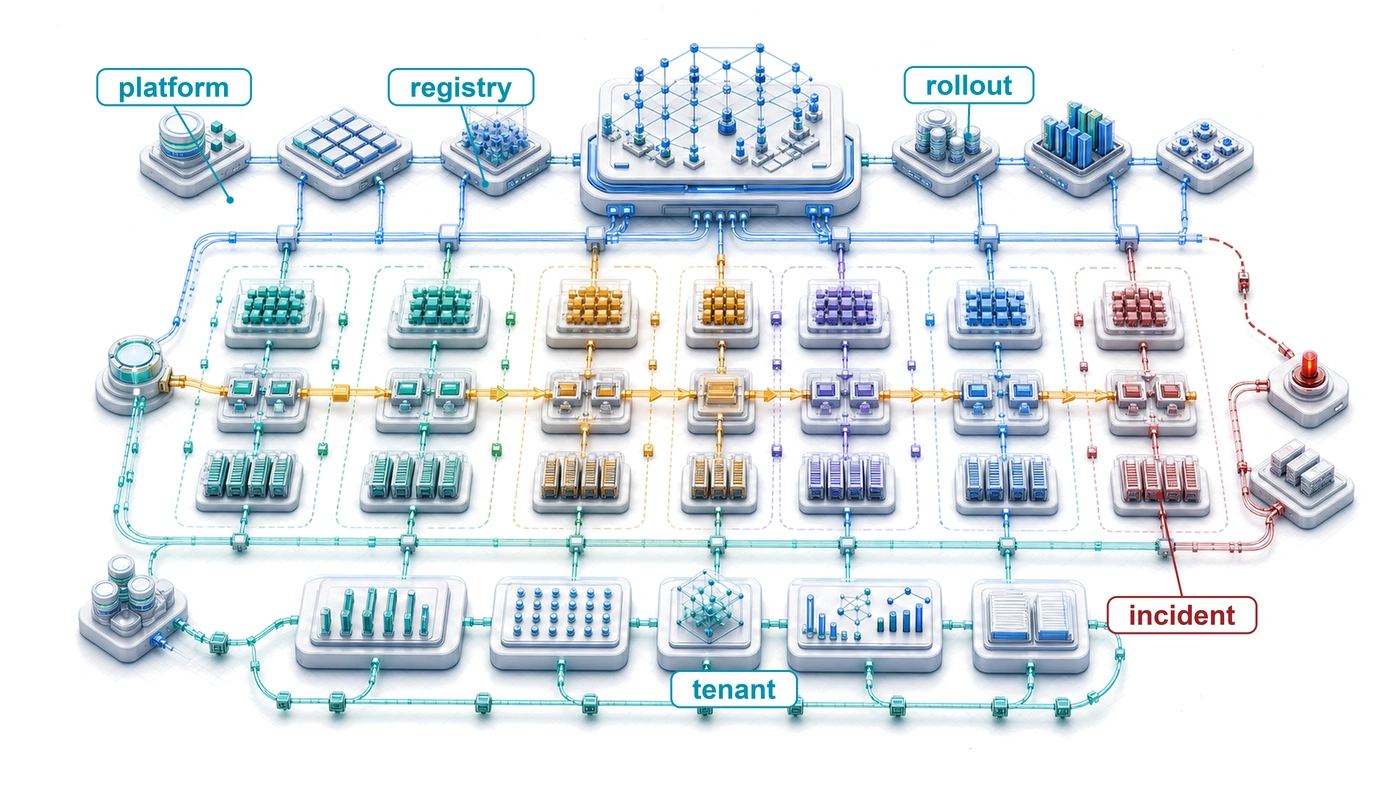
12 ML Operations at Scale

Purpose

Fleet stack focus for this chapter.

Why do practices that work for managing one model collapse when organizations deploy hundreds?

One model is a project. A hundred models form a system of systems whose dependencies and failures cannot be managed one model at a time. A data-pipeline change may affect models built by several teams, while a deployment failure may require coordinated rollbacks across interconnected services. The team making a change may not know every consumer, and the team seeing a regression may not control its cause. Practices that work when one engineer knows the entire system become unreliable when ownership, data, and release schedules are distributed. Adding faster machines does not resolve that uncertainty. A fleet can have spare compute capacity and still be unable to ship safely because nobody can establish which models depend on a changed input or who may authorize recovery. Shared infrastructure can reduce this repeated coordination, but it also concentrates dependencies and introduces its own operating cost. Centralizing every decision can turn the platform team into a bottleneck; leaving every team to improvise makes compatibility and accountability difficult to sustain. The engineering task is to make routine changes repeatable while preserving evidence about their effects and clear authority over their consequences. Growth becomes manageable when adding a model does not require rebuilding the surrounding operational process, yet its owners remain responsible for acceptable behavior. In C³ terms, fleet operations makes coordination a designed system constraint alongside the compute and communication resources that models consume.

Learning Objectives

Explain why operational load grows with coupling through shared features, pipelines, and capacity rather than with model count
Design registries, release gates, and evaluation contracts that preserve lineage, dependency safety, and rollback confidence
Design feature-store operations that manage freshness, ownership, compatibility, and training-serving skew
Size staged rollouts and production experiments whose sample size, stopping rule, and interference assumptions bound user exposure
Diagnose production incidents using monitoring hierarchies and multidimensional reliability budgets across the fleet
Calculate platform return, utilization break-even, and lifecycle total cost, then attribute fleet spend to accountable owners
Evaluate platform organization and lifecycle choices using adoption, versioning, and retirement evidence

12.1 Why a Model Fleet Needs a Control Plane

Consider a team of five engineers maintaining a single recommendation model. When the model drifts, they manually retrain it. When the API latency spikes, they manually scale the instances. Now, scale that same team to support five hundred models across dozens of product surfaces. The same engineering team cannot sustain that growth by performing machine learning operations (MLOps), the practices that version, deploy, monitor, and roll back production models, by hand for every model. Shared controls must preserve human accountability while automating routine coordination. The fleet becomes the unit of capacity planning and investment; versioned model and feature state makes changes reviewable, release gates bound their exposure, and monitoring and incident review feed production evidence back into those controls.

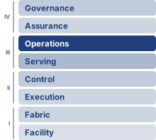
In the fleet stack of The Fleet Stack, the Operations row sits directly above Runtime and Serving and directly below Assurance, the first row of the Governance band. It belongs to the Serving band because it operates models that are already deployed, whereas the Reliability and Control row two rows lower schedules and recovers individual jobs. The Operations row acts as the fleet’s control plane, the dashboard, steering, and maintenance system that keeps physical infrastructure, training systems, serving paths, edge deployments, and governance rules from drifting apart. Once models span data centers, serving platforms, and heterogeneous edge fleets of adaptive devices, reliability depends less on any single model and more on the operational machinery that keeps the whole fleet observable, coordinated, and recoverable. Adaptive edge fleets sharpen the requirement, because there the operator ships a versioned adaptation policy rather than fixed weights, and that policy stays safe only while telemetry keeps it observable and rollback keeps it recoverable. Those controls must operate as shared infrastructure for every model the fleet runs.

↩︎ Adaptive edge device populations and the constraints that shape them are established in Edge Intelligence.

Shared dependencies make local operational choices fleet-wide concerns. An upstream data change can affect several models, concurrent deployments can contend for the same capacity, and independent alerts can obscure a common failure. Training and serving also compete for expensive infrastructure whose idle capacity still incurs cost. The platform must coordinate those interactions while preserving each team’s responsibility for model behavior.

The organizational response is platform thinking. Rather than treating each model as an independent system with its own infrastructure, platforms provide shared services that amortize operational costs across the entire model portfolio. Feature stores¹ share feature definitions and values across models. Their contract is that training and serving use compatible feature meanings, with historical training values restricted to information available at the prediction time. Unified deployment pipelines ensure consistent rollout practices. Centralized monitoring aggregates signals across models to detect system-wide issues and enable capacity planning. The challenge is designing, implementing, and operating these platforms so they scale with the portfolio rather than against it. This is the C³ coordination axis at its widest. The Fleet Law charges synchronization within one distributed step, while fleet operations pays the coordination cost of every release, rollback, and shared dependency across the whole portfolio.

¹ Feature store: A centralized repository that manages the computation, storage, and serving of ML features. The core systems problem it solves is training-serving skew; section 12.4 develops that failure mode and the platform invariant that contains it.

Self-Check: Question

Why can manual, per-model operational maintenance become difficult to sustain as an organization expands to hundreds of models that share features, resources, and release dependencies?
1. Shared data dependencies, contested resources, and independent alert streams add coordination work that can exceed the capacity of manual per-model processes.
2. Modern deep learning framework compilers prohibit deploying more than one model graph per physical datacenter.
3. Single-model architectures run on asynchronous virtual memory subnets that cannot route traffic through standard TCP/IP gateways.
4. Network switches automatically drop telemetry packets when concurrent endpoint connections exceed ten.
What is the primary architectural purpose of the Control Plane in an enterprise ML platform spanning datacenters, cloud clusters, and edge fleets?
Treating each model in an enterprise as an isolated, independent entity with bespoke pipelines remains an economically sound strategy as long as each individual model achieves high predictive accuracy.

See Answers →

12.2 The N-Models Problem

An organization’s first homepage recommender, search ranker, and fraud detector can each run on a bespoke pipeline built by its own team, yet as the fleet grows those independent pipelines begin sharing features, embeddings, and GPU pools until one uncoordinated upstream change breaks five downstream models at once. The five engineers of the opening example do not acquire five hundred models overnight, and the path from one model to many explains where a control plane becomes necessary. With few models, team-local pipelines for data processing, training, validation, and deployment let each group optimize for its immediate requirements.

As the number of models grows, shared dependencies create operational complexity faster than model count alone suggests. Dense interactions produce superlinear coordination work unless strong ownership and interface boundaries contain them. Between one model and a hundred, deployment coordination moves from a team-local task to the critical path and shared data dependencies grow from a single pipeline into a dense graph, while monitoring, on-call scope, utilization, debugging, and governance change with them (table 1).

Table 1: Operational Complexity Growth at Scale: Illustrative challenges across 1, 10, and 100 models. Even one model requires deployment coordination and depends on its data pipeline. Shared dependencies can make releases a fleet-wide critical path, dashboards require aggregation, and debugging span team boundaries; actual complexity depends on coupling and ownership.

Operational aspect	Single model	10 models	100 models
Deployment coordination	Team-local	Ad hoc	Critical path
Shared data dependencies	Within pipeline	Some overlap	Dense graph
Monitoring dashboards	1	10	Unmanageable
On-call rotation scope	Single team	Multiple teams	Organization-wide
Infrastructure utilization	Often idle	Moderate sharing	Efficiency critical
Debugging complexity	Local	Cross-team	Distributed tracing required
Governance	Team policy	Diverging policy	Organization-wide automation

One upstream embedding update can degrade every dependent model.

Per-model validation does not establish compatibility across a dependency chain. When Model A depends on features computed by Pipeline B, which uses embeddings from Model C, a change to one component can affect its downstream consumers. A seemingly innocuous update to Model C’s embedding layer might shift the feature distributions that Model A depends upon, degrading its performance even though Model A itself has not changed. This cascading interdependence makes the interfaces between models part of the operational contract.

Systems Perspective 12.1: The complexity explosion

As a fleet accumulates shared dependencies, system-level coordination can become the binding problem. A new model adds its own operating cost, but it can also change feature pipelines, release schedules, and contention for infrastructure used by existing models. The marginal cost therefore depends on how the new model couples to the portfolio rather than simply on how many models the fleet already contains.

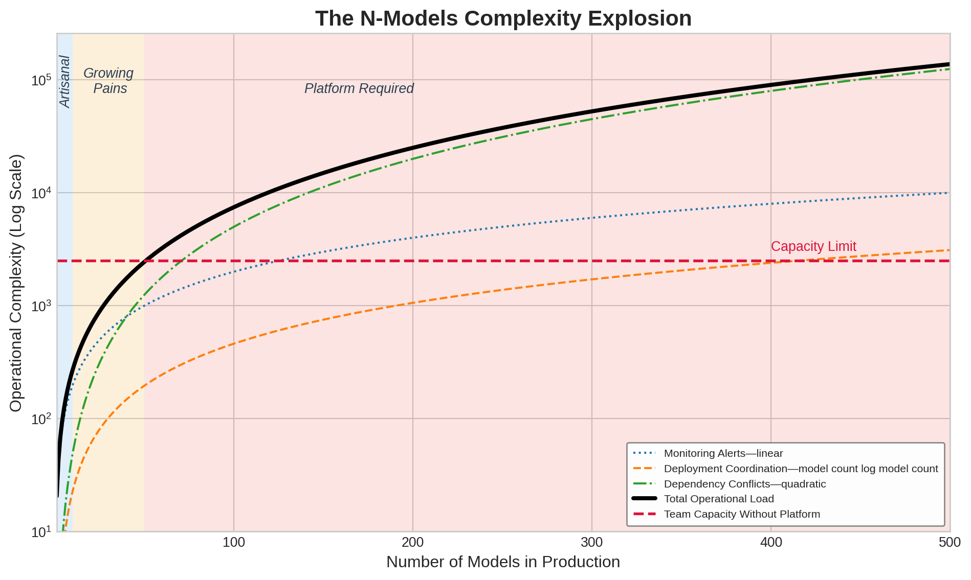
A sketch of operational load across production model counts, drawn on logarithmic axes with one assumed growth shape per source of work, shows how coupling outruns a fixed team (figure 1). Alerts grow linearly because each model brings its own fixed set of monitored metrics. The sketch assigns deployment coordination an intermediate $\ProductionModelCount \log \ProductionModelCount$ growth shape; this is an illustrative assumption rather than a release-scheduling complexity bound. A dense dependency graph motivates the quadratic conflict curve because $\ProductionModelCount$ models form roughly $\ProductionModelCount^2/2$ possible pairs; the recorded dependencies determine which pairs can actually conflict. Under these shapes the total crosses the team-capacity ceiling near 50 models. The shapes are a sketch, not measurements, so the crossing marks where repeated work outgrows a team rather than a threshold a real organization can read off the plot; measured dependency density, engineering effort, and remediation cost decide when platform engineering pays.

Figure 1: **The N-Models Complexity Explosion**: The curves show monitoring alerts growing linearly with model count, deployment coordination growing as $\mathcal{O}(\ProductionModelCount \log \ProductionModelCount)$, and dependency conflicts growing quadratically as models share features and data sources. Under these assumed shapes, the total operational load crosses team capacity around 50 models, sketching the transition from artisanal model management to platform-required operations.

Once operational load exceeds team capacity, continued portfolio growth requires reducing repeated work, simplifying dependencies, or expanding the team’s capacity. Shared platform engineering addresses the repeated work of deploying, monitoring, and debugging models. Its economic case begins with identifying which of those responsibilities can be shared and which must remain with model owners.

12.2.1 Single-model vs. platform operations at scale

A single-model team can promote a release through a canary (a small slice of live traffic served by the candidate) and roll back in isolation, whereas pushing an updated upstream model in a shared fleet can silently shift inputs for downstream rankers, exhaust shared GPU headroom during concurrent rollouts, or leave dependent services broken if one model rolls back alone. Platform-scale deployment must preserve compatibility with dependent models at every intermediate state. Compatible interfaces can permit independent updates; a changed feature representation may instead require a coordinated migration. Rollback follows the same dependency contract, because reverting one model may require restoring compatible features or dependent models. Concurrent deployments also compete for GPU memory and network bandwidth, making resource headroom part of the release decision.

For recommendation systems, this complexity appears along the request path. Candidate retrieval and ranking models execute alongside diversity filters and business rule layers, sometimes in sequence and sometimes in parallel. Updating a component requires identifying which consumers depend on its outputs and testing whether the complete path still meets its quality and latency targets.

Monitoring requirements evolve similarly. Model-specific metrics such as prediction accuracy, inference latency, and data drift remain necessary, but separate dashboards do not expose shared causes by themselves. When many models depend on the same feature pipeline, a single upstream failure can appear as many unrelated model alerts. Responders need a portfolio view that connects those symptoms before investigating individual models.

Platform monitoring must therefore aggregate across models while maintaining the ability to drill down into specifics. This requires hierarchical metrics that run from business outcomes through portfolio and model signals down to infrastructure health, the structure section 12.6.3 develops. The same contrast between one model and a portfolio also changes what each release must prove, because workloads differ in how fast they change and how much harm a bad version can do.

12.2.2 Release policies across model archetypes

Applying a single release policy across a fleet either starves a fraud detector that needs hourly updates and second-scale rollback as attackers adapt, or rushes a $70\text{B}\text{--}405\text{B}$ generalist large language model (LLM) into production before multi-domain evaluation catches a capability regression. Different deployment contexts impose different operational contracts, and the archetype taxonomy in Three systems archetypes helps interpret the illustrative policies in table 2. Release frequency follows data change and validation cost; rollback targets follow the harm and reversibility of a bad release. Model family alone determines neither: LLMs may need long observation windows while still requiring rapid traffic rollback, and fraud detection needs fast containment even when a new model takes longer to validate.

Table 2: Illustrative Release Policies: Example cadences and rollback targets for several deployment contexts. These are planning assumptions, not requirements implied by architecture. Rollback means routing to a validated version; the observation period needed to approve a new version can be much longer.

Model type	Example update cadence	Deployment pattern	Primary risk	Rollback speed
Archetype A (GPT-4/Llama-3)	Monthly to quarterly	Staged, careful	Quality regression, safety	Minutes with standby capacity
Archetype B (DLRM at Scale)	Daily to weekly	Shadow, interleaving	Engagement drop	Minutes
Fraud Detection	Hourly to daily	Rapid with instant rollback	False negatives	Seconds
Vision (Classification)	Weekly to monthly	Canary	Accuracy regression	Minutes
Search Ranking	Daily	A/B with holdout	Relevance degradation	Minutes

The table mixes two lighthouse archetypes with ordinary model families because release policy follows the workload, not the label. Archetype C (Federated MobileNet) is absent because its edge fleet follows release controls of its own (Fleet release controls). The deployment patterns name release controls developed later in the chapter. Shadow deployment runs the candidate on copied traffic without returning its outputs to users, and interleaving merges two rankers’ results into one list so each user compares them directly (section 12.5.3). The table separates release cadence from containment speed. Large-model evaluation can require extended shadow deployment, human review, and staged exposure because a quality regression may be subtle. Keeping the previous model warm can nevertheless permit fast traffic rollback. The cost of that standby capacity belongs in the release policy rather than being hidden behind an hours-long rollback assumption, and the cost of regression becomes concrete when one model must preserve every capability at once.

Lighthouse 12.1: Archetype A (GPT-4/Llama-3): Cost of regression

Context: Archetype A (GPT-4/Llama-3) represents ultra-large generalist models ($70\text{B}\text{--}405\text{B}$ parameters) serving millions of concurrent requests across diverse tasks. Released models span that whole range; where this chapter needs one concrete instance, as in the fleet cost examples of section 12.9, it uses the volume’s reference instance, the GPT-3-class dense model of Archetype A (GPT-4/Llama-3).

Mechanism: The “Generalist’s Dilemma” occurs when targeted fine-tuning (e.g., optimizing Python code generation) causes catastrophic forgetting in unmonitored domains (e.g., creative writing or reasoning). Evaluating candidate weights across 10,000+ benchmark prompts adds the iron law’s compute time, $\Operations/(\PeakRate \cdot \EfficiencyHw)$ for the evaluation’s total operations $\Operations$, to every release. Prompt count alone does not determine that time or its GPU-hours; input and output lengths and model size set $\Operations$, and achieved throughput sets $\EfficiencyHw$.

Impact: A silent degradation in secondary metrics forces a costly emergency rollback, and the warm standby held for that rollback competes with the serving capacity needed to hold the per-request latency target $\LatencySlo$.

Systems lesson: Release gates for large generalist LLMs must combine broad capability benchmarks (such as Massive Multitask Language Understanding (MMLU) and HumanEval) with policy-based safety checks. Their evaluation time and accelerator-hours belong in the deployment schedule and budget rather than being treated as a zero-cost pre-flight check.

Recommendation systems face continuously changing user preferences and content inventories (Steck et al. 2021; Gomez-Uribe and Hunt 2015), so their operational urgency includes feature freshness, the delay between a user action and its reflection in the model’s inputs, which section 12.4.2 measures and budgets. Recommendation ensembles must also preserve compatible behavior as their components update. Fraud detection adds an adaptive adversary that probes the model and shifts tactics once detected, increasing the value of prompt containment and monitoring for sudden feature shifts. Shadow scoring and outcome evidence still have to establish whether an update reduces fraud without unacceptable false positives; urgency alone does not validate a new model. LLM releases face a broad set of capability and safety risks that require evaluation before exposure (Bender et al. 2021). These differences determine the evidence, update cadence, and recovery policy each workload needs. A shared platform is valuable when it enforces those distinct contracts without making every team rebuild the operational machinery.

Steck, Harald, Linas Baltrunas, Ehtsham Elahi, Dawen Liang, Yves Raimond, and Justin Basilico. 2021. “Deep Learning for Recommender Systems: A Netflix Case Study.” AI Magazine 42 (3): 7–18. https://doi.org/10.1609/aimag.v42i3.18140.

Bender, E. M., T. Gebru, A. McMillan-Major, and S. Shmitchell. 2021. “On the Dangers of Stochastic Parrots: Can Language Models Be Too Big?” Proceedings of the 2021 ACM Conference on Fairness, Accountability, and Transparency, 610–23. https://doi.org/10.1145/3442188.3445922.

12.2.3 Quantifying platform economics

Enforcing those workload-specific release policies without forcing every team to rebuild the machinery requires a shared platform, which raises an immediate budget question: standing up a dedicated ML platform team for a five-model organization can cost twice as much as the manual toil it replaces, whereas delaying that investment past fifty models leaves product teams buried in repetitive deployment and pipeline maintenance. The economic case for platform operations rests on comparing the cost of fragmented approaches against the returns from shared infrastructure. Equation 1 defines the platform benefit-cost ratio (BCR) as the ratio of engineering time savings across all models to total platform cost:

\[\text{BCR}_{\text{platform}} = \frac{\ProductionModelCount\times \SavedEngineeringTime\times \EngineerHourlyCost}{\PlatformTotalCost} \tag{1}\]

where $\ProductionModelCount$ represents the number of models benefiting from the platform, $\SavedEngineeringTime$ is the engineering time saved per model per period, $\EngineerHourlyCost$ is the fully-loaded cost per engineer hour, and $\PlatformTotalCost$ is the total platform cost including development, infrastructure, and maintenance.

A ratio of one is break-even; net return on investment is this ratio minus one. Engineering hours valued at their loaded cost measure recovered capacity, not automatic payroll savings. Costs and benefits must cover the same period and include ongoing platform operation.

The equation makes the investment boundary explicit. For an organization with five models, platform cost may exceed the value of recovered effort; unusually costly recurring work could reverse that comparison even at a small model count. Holding per-model savings constant makes the numerator grow linearly with $\ProductionModelCount$. Whether the ratio improves depends on how development, support, and infrastructure costs grow as additional models adopt the platform.

Napkin Math 12.2: Platform benefit-cost ratio

Problem: An organization manages 50 models. A centralized ML Platform team costs $120,000/month. If the platform saves each model team 20 hours of manual toil per month, is the platform investment profitable?

Math:

Gross Monthly Capacity Value: 50 models $\times$ 20 hours/model $\times$ $150/hr = $150,000.
Net Monthly Benefit: $150,000 (Savings) - $120,000/month (Cost) = $30,000.
Benefit-Cost Ratio: $150,000 / $120,000/month = 1.25.

Systems insight: Platforms cross a scaling threshold under a declared cost model. At 50 models, this platform earns a 25 percent return on its modeled cost. However, if the organization only had 20 models, the capacity value would be only $60,000, a 50 percent loss relative to the platform team’s salary. This comparison holds the team cost and per-model savings fixed. An investment decision must also include migration, infrastructure, and ongoing support costs, then establish how the recovered engineering time will create value.

From artisanal to industrial operations

The notebook prices one portfolio at one model count. The investment decision also needs to know where break-even falls and which inputs move it.

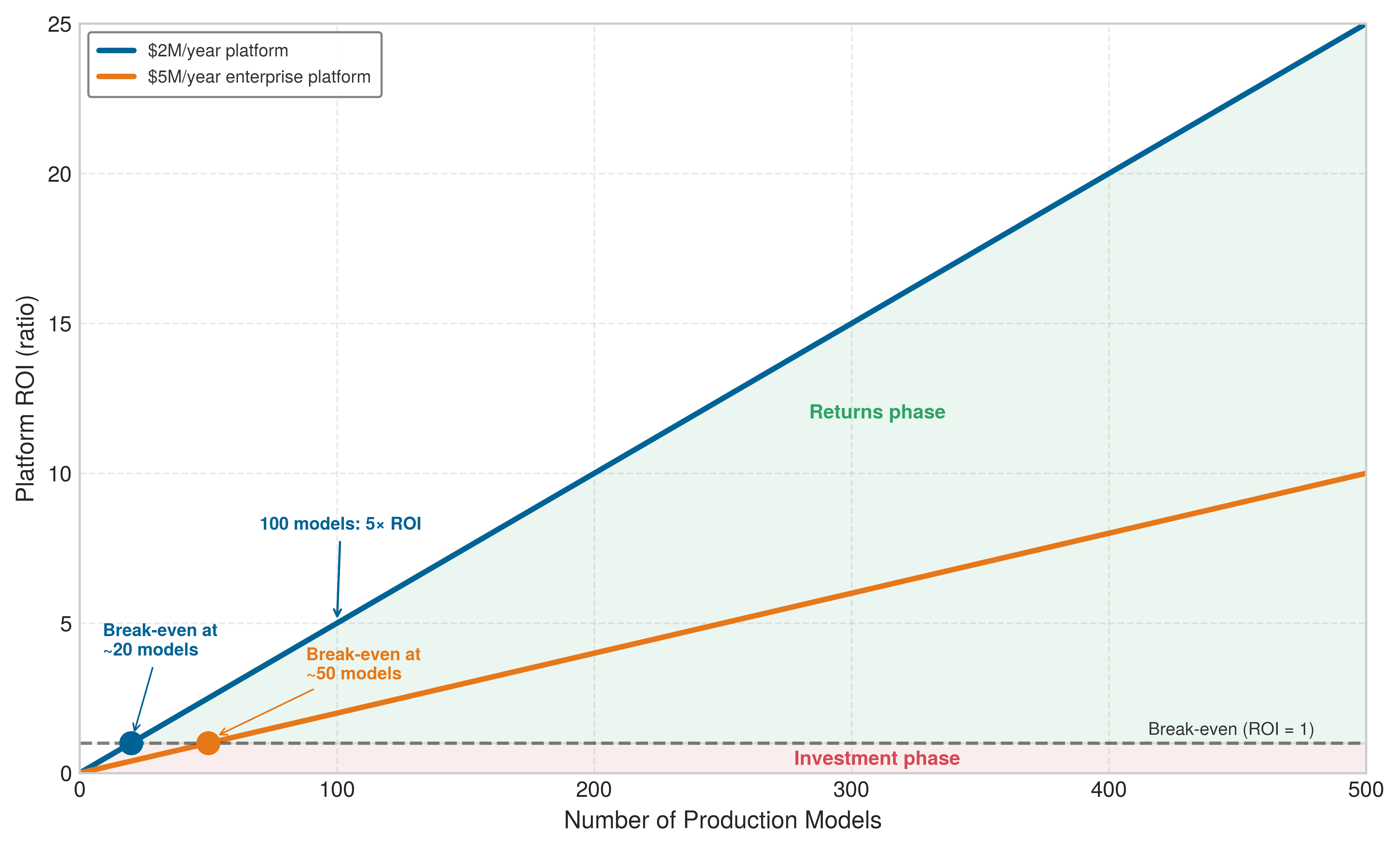
Plotting the benefit-cost ratio against production model count for two annual platform budgets locates the break-even crossing, where each linear benefit ray climbs out of the shaded investment phase into the net-positive returns phase (figure 2). With a fixed $100K benefit per model per year, a $2M/year platform achieves parity at the 20-model marker, whereas a $5M/year enterprise platform requires 50 models to reach the break-even line. At 100 models, the $2M platform ascends to a benefit-cost ratio of 5, equivalent to a net ROI of 400 percent. The linear curves assume constant marginal benefit and fixed platform costs; dependency growth, diminishing savings, or higher operating costs change the result. The $5M platform’s 50-model crossing is also a different quantity from the 50-model crossing in figure 1: that one marks where repeated work outgrows a team, whereas this one marks where a budget pays back. The figure’s budgets are annual running costs, while a one-time build amortized over three years charges only a third of its cost to each year; in either form the break-even count moves with the two inputs a platform team controls, shifting left as savings per model rise and right as platform cost rises.

Figure 2: **The Platform Benefit-Cost Threshold**: Assumed annual benefit divided by annual cost for two platform budgets. Break-even occurs at a ratio of one. With fixed per-model benefit, the ratio grows linearly; a ratio of five corresponds to a net ROI of 400 percent, not 500 percent.

Checkpoint 12.1: Platform ROI break-even

Equation 1 expresses the platform benefit-cost ratio as $\ProductionModelCount\times \SavedEngineeringTime\times \EngineerHourlyCost/ \PlatformTotalCost$. In figure 2, the dual benefit-cost rays illustrate this linear growth under fixed savings assumptions, isolating where each platform budget intersects the break-even parity threshold. Apply the formula to two concrete decisions.

Platform ROI: for an organization with 30 models, each saving 200 engineer-hours per year at $150/hour, calculate the benefit-cost ratio and net ROI of a $2M/year platform and a $5M/year enterprise platform.
Break-even count: using the same per-model savings ($30K/year, which is 200 hours at $150/hour), determine the model count where each platform breaks even, compare it to the 20- and 50-model parity markers plotted in figure 2, and explain how the figure’s stated $100K per-model benefit moves those thresholds.
Build now vs. wait: for an organization with 8 models debating whether to build a $2M/year platform, use the linear ROI structure of equation 1 past break-even to state the strongest argument for building now and the future-growth assumption required for that argument.

The benefit-cost ratio takes the per-model savings $\SavedEngineeringTime$ as an input. In practice those hours come from specific recurring work, such as unversioned data, brittle pipelines, and manual deployment toil, that a shared platform can retire. Measuring that work is the job of technical-debt accounting. The hardware side of the cost accounting, where utilization decides whether shared capacity earns its cost, returns in section 12.9 after the operational machinery that consumes that capacity is in place.

12.2.4 Quantifying and managing ML technical debt

Those recurring hours accumulate whenever unvalidated 800-line configuration files, duplicated preprocessing scripts, and ad-hoc monitoring setups spread across dozens of models, stretching a two-day training run into a six-week release. Technical debt at fleet scale becomes a prioritization problem when recurring maintenance competes with new development: the platform must identify dependencies that slow deployments, raise incident rates, or consume engineering time, then compare the expected benefit and cost of repairing them. ML debt falls into four categories according to where the recurring work originates: data debt begins upstream in inputs that are unversioned or weakly validated, whereas configuration debt accumulates in duplicated, unvalidated settings that every release must review by hand; closer to the artifact, model debt arises from the coupling around a model—including undeclared consumers and glue code, the supporting code written to move data into and out of general-purpose libraries and between pipeline stages, which binds a model to one pipeline’s formats—while infrastructure debt surfaces in brittle pipelines, manual deployment, and drifting environments. The categories locate where the work originates; common effort and risk measures make candidate repairs comparable across the fleet.

Napkin Math 12.3: Payback of a debt cleanup

Problem: A team spends 40 hours/month manually fixing “broken plumbing” (stale data, failed scripts, manual monitoring). A one-month intensive cleanup (160 hours) is projected to reduce this to 8 hours/month. Is the cleanup worth it over 3 years of model lifecycle?

Math:

Status quo (3 years): 36 months $\times$ 40 hours/month $\times$ $150/hr = $216000.
Proactive Path: (160 hours investment + 36 months $\times$ 8 hours/month) $\times$ $150/hr = $67200.
Net Savings: $216000 - $67200 = $148800.
Cost ratio: 3.2×.

Systems insight: Under the projected toil reduction, proactive maintenance reduces the modeled cost by a factor of 3.2× over the model lifecycle. The benefit comes from avoiding repeated work long enough to recover the initial repair effort. A shorter remaining lifetime, lower recurrence, or additional upkeep can change the decision, so refactoring earns priority through measured recurring cost and a credible remediation plan.

The cleanup calculation becomes actionable only when the platform can compare unlike debts on a common operational scale. ML technical debt manifests in measurable symptoms that directly affect platform velocity and reliability (Sculley et al. 2015; Amershi et al. 2019).

Amershi, Saleema, Andrew Begel, Christian Bird, Robert DeLine, Harald Gall, Ece Kamar, Nachiappan Nagappan, Besmira Nushi, and Thomas Zimmermann. 2019. “Software Engineering for Machine Learning: A Case Study.” 2019 IEEE/ACM 41st International Conference on Software Engineering: Software Engineering in Practice (ICSE-SEIP), 291–300. https://doi.org/10.1109/icse-seip.2019.00042.

Debt categories and measurement

The debt category matters because each failure mode leaves a different operational trace. Table 3 turns the taxonomy into a measurement map: data debt appears as incidents and manual pipeline intervention, configuration debt as unvalidated release surface, model debt as glue-code drag, and infrastructure debt as toil that consumes platform capacity.

Table 3: Technical Debt Measurement Map: Different debt types require different observable signals. Numerical thresholds are illustrative platform policies, not empirical laws. A shared scoring process can compare them only after each category has been tied to the symptom and threshold that make the debt operationally visible.

Debt type	Operational symptom	Measurement signal	Warning threshold
Data debt	Unstable dependencies, missing versioning, weak validation	Data incidents per month and manual pipeline intervention	More than 10 data incidents/month or 30% manual runs.
Configuration debt	Ad-hoc files, duplicated parameters, absent validation	Deployment failures, lines of config, unvalidated parameters	More than 500 lines of unvalidated configuration per model.
Model debt	Glue code, undeclared consumers, tangled serving paths	Coupling score, undocumented consumers, trace time	More than 20% engineering time maintaining glue code.
Infrastructure debt	Brittle pipelines, manual deployment, environment drift	Toil hours, automation coverage, drift incidents	More than 50% platform capacity spent on toil.

Four fleet-level indicators show when that debt is accumulating, whatever its category: deployment velocity from commit to production, incidents per thousand deployments, the share of team capacity spent on toil, and the share of dependencies behind supported versions. Each needs a baseline and an escalation threshold calibrated to the platform’s workload risk and release cadence. The worked example applies that threshold logic to rank debt by the capacity each fix returns to the platform team.

ML debt audit and prioritization

An ML platform team supporting 40 production models with 15 engineers faces deployment velocity problems. New models require 6 weeks to reach production, frustrating both platform and model teams. The audit estimates how much capacity each repair could release and compares that benefit with implementation effort and operational risk. A highly visible symptom is a starting point for measurement, not sufficient evidence of priority.

The audit applies the measurement map of table 3 to the deployment-velocity complaint, so it records in table 4 the three categories that the team’s release and incident symptoms point to before scoring them: configuration debt, model debt in the form of pipeline glue code, and infrastructure debt in the form of fragmented monitoring. Data debt can also delay releases, but this audit has not attributed the observed delay to data incidents and leaves that category outside its scope. Each row pairs an operational symptom with the impact measure that makes the debt comparable across teams.

Table 4: ML Debt Audit Inputs: Initial observations for configuration debt, model debt (pipeline glue code), and infrastructure debt (monitoring) before priority scoring. The table preserves the symptom, impact metric, technical measure, and estimated annual cost for each debt category.

Debt category	Symptom	Impact metric	Technical measure	Estimated annual cost
Configuration debt	Each model has custom YAML configuration files averaging 847 lines with no validation schema	35% of deployment delays result from late config errors	Manual config review required for every deployment	12 engineer-hours per deployment $\times$ 80 deployments/year = 960 hours
Model debt (pipeline glue code)	Data preprocessing uses 23 different scripts with 62% code duplication	12 engineer-hours per week debugging pipeline breaks	No shared preprocessing library; each team implements custom logic	12 hours/week $\times$ 52 weeks = 624 hours
Infrastructure debt (monitoring)	Each model uses ad-hoc monitoring, with no unified observability platform	Mean time to detect incidents is 4.2 hours	23 monitoring approaches across 40 models	Extended incident duration costs $50K per incident $\times$ 15 incidents/year = $750K

The scoring approach uses three criteria: impact severity, frequency, and resolution cost, each scored 1 to 3. Higher impact and frequency raise priority; higher resolution cost lowers it. Applied to the three debt categories observed earlier, these scores produce the ranking in table 5.

Table 5: Debt Prioritization Scoring: Three-criterion scoring (impact severity, frequency, and resolution cost) applied to three observed debt categories. Scores use $\text{Impact} \times \text{Frequency} / \text{Resolution Cost}$, so slower or more expensive fixes are penalized. Configuration debt scores highest, justifying first-priority remediation.

Debt category	Impact	Frequency	Resolution cost	Total score	Priority
Configuration	3 (High)	3 (Daily)	2 (Medium: 6 weeks)	4.5	1st
Monitoring	3 (High)	2 (Weekly)	2 (Medium: 8 weeks)	3	2nd
Pipeline Glue	2 (Medium)	2 (Weekly)	3 (High: 16 weeks)	1.3	3rd

The score makes configuration debt the first paydown target: build configuration schema validation and a templating system before addressing lower-scoring pipeline glue. The investment requires 6 weeks of engineering effort to build the configuration system. The savings estimate needs one more input, the share of each deployment’s manual configuration review that schema validation eliminates. Take it as 35 percent. That planning assumption happens to equal the share of deployment delays the audit attributes to configuration, but delays and review hours are different quantities, and only a pilot of the schema system can measure the second. With that input, released capacity is: 12 engineer-hours per deployment $\times$ 80 deployments per year $\times$ 35 percent = 336 engineer-hours saved per year. At $150/hour, that is $50K in annual savings, so the investment pays back in about 8.6 months.

Decision framework

The table score generalizes by adding a Benefit term that rates what the repair returns, such as released hours or avoided incidents. The result remains a ranking heuristic rather than a monetary return. Impact and Frequency are ordinal weights, Benefit is a separate score, and Resolution Cost is effort on a consistent internal scale. Because Frequency already appears as its own factor, Benefit must be scored per occurrence; an annual dollar benefit already includes frequency and would count it twice:

\[\text{Paydown Priority} = \frac{\text{Impact} \times \text{Frequency} \times \text{Benefit}}{\text{Resolution Cost}} \tag{2}\]

The paydown-priority formula in equation 2 keeps automation work tied to operational value: high-impact, frequent, high-benefit fixes outrank expensive work whose payoff is speculative. The score only ranks candidates. The payback calculation in the deployment-automation notebook below is a separate tool that keeps the terms with measurable units (deployments per week, toil hours saved per deployment, and setup hours), so any severity that saved hours cannot express, such as outage or compliance exposure, must be argued alongside the payback period rather than folded into it.

Napkin Math 12.4: ROI of automation

Problem: A team spends 10 hours of manual toil per model deployment. Investing 120 hours in a CI/CD pipeline is projected to reduce deployment toil to 0.5 hours. At 3 deploys/week, how long until the automation pays for itself?

Math:

Automation Cost: 120 hours $\times$ $150/hr = $18000.
Weekly Savings: 9.5 hours/deploy $\times$ 3 deploys/week $\times$ $150/hr = $4275/week.
Payback Period: $18000 / $4275/week $\approx$ 4.2 weeks.

Systems insight: The projected payback period of 4.2 weeks makes this recurring deployment task a strong automation candidate. The calculation assumes that deployment frequency and time savings persist, and it excludes additional maintenance of the automation. Comparing that upkeep with the recurring effort avoided determines whether the initial payback becomes a lasting reduction in toil.

The score ranks candidates for investigation; comparing debt paydown with feature development then requires costs, expected benefits, uncertainty, and time horizons in common units. The configuration example scores highly under its stated assumptions; it is not automatically preferable to an unrelated project with a different scoring scale. A planned system retirement or a small affected population can reduce its practical value.

The same prioritization logic must become organizational habit, or the measured debt will reaccumulate between audits. Quantified debt enters a backlog with its affected systems, impact, resolution cost, and score, and a quarterly review re-ranks it against current deployment velocity, incident rates, and toil. A debt budget reserves an explicit, revisable share of engineering time for remediation, and design review applies the same reasoning upstream by catching new configuration complexity and hard-to-maintain dependencies before they become recurring toil.

12.2.5 When to form a dedicated platform team

Auditing and paying down cross-model debt eventually requires an owner with a charter wider than any single product team, because product teams rarely fund shared infrastructure on their own until an outage exposes undocumented dependencies, missing rollback paths, and idle GPU silos. A dedicated ML platform team is justified when fragmentation costs more than the shared infrastructure needed to replace it, combining quantitative factors (cost savings, velocity improvements) with qualitative factors (consistency, governance, talent retention).

The savings of shared capacity and the benefit-cost ratio point to three potential benefits of shared ownership: infrastructure efficiency, faster releases, and fewer incidents. Only the first is computed so far, in notebook 12.1, and it holds only while peak demand and reliability headroom permit the smaller pool. Faster delivery and fewer incidents are additional hypotheses to measure; neither a guaranteed engagement gain nor a fixed incident-reduction percentage follows from introducing a platform. The business case combines observed capacity savings with independently valued release and reliability improvements.

The qualitative case follows from the same fragmentation cost. Shared ownership gives telemetry, rollback capability, and runbook documentation a common acceptance process, but those standards protect the fleet only when deployment gates enforce them. A centralized platform team also gives product teams access to operational expertise and provides dedicated roles for engineers focused on machine learning systems and reliability. Platform-level lineage and policy controls support governance review by preserving evidence of which versions ran, what checks passed, and who authorized the release.

The decision to establish a platform team typically occurs when organizations recognize that allowing fragmentation to continue imposes coordination costs exceeding the platform investment. This recognition often follows a significant production incident that revealed cross-model dependencies or operational gaps. The resulting economics show why platform operations become more valuable as the model fleet grows.

While the economic justification for platform operations becomes clear at scale, the technical implementation begins with a harder problem, preventing independent models from colliding through shared state. Multi-model management requires untangling the hidden dependencies that emerge when hundreds of models share the same data, infrastructure, and user experiences.

Self-Check: Question

An organization operates 50 models. A platform team costs $120,000 per month and recovers 20 engineering hours per model monthly, valued at $150 per hour. What are the benefit-cost ratio and net ROI based on this recovered-capacity value?
1. Benefit-cost ratio 0.80 and net ROI of -20%.
2. Benefit-cost ratio 1.25 and net ROI of 25%, with $30,000 in net monthly capacity value above platform cost.
3. Benefit-cost ratio 2.50 and net ROI of 150%, with $180,000 in net monthly capacity value above platform cost.
4. Benefit-cost ratio 0.50 and net ROI of -50%.
According to the ML technical debt taxonomy (Sculley et al.), which operational symptom specifically indicates dangerous Configuration Debt rather than Data Debt or Model Debt?
1. Upstream database schema changes that silently alter categorical feature encodings.
2. Extensive glue code written to convert data between disparate third-party machine learning libraries.
3. Large, unvalidated configuration parameter files (e.g., exceeding 500 lines of ad-hoc YAML per model) causing frequent deployment failures.
4. Tangled feedback loops where a fraud detection model’s historical outputs bias incoming training labels.
How does the debt-cleanup payback calculation quantitatively justify investing 160 engineering hours upfront to refactor and automate brittle pipeline plumbing over a 3-year model lifecycle?
Contrast the deployment frequency and rollback latency requirements of an adversarial fraud detection model with those of a frontier large language model (LLM).
ML platform engineering is a variable cost that delivers immediate positive economic return regardless of the number of deployed models in an organization.
A portfolio has shared embeddings, cross-team feature pipelines, and cascading latency regressions. Which coordination and diagnostic controls become necessary, and why does model count alone not determine when to introduce them?

See Answers →

12.3 Governance of State and Change

Imagine an e-commerce platform where the search ranking model uses outputs from a user embedding model. An unannounced dimensionality change can break the consumer’s input interface; a change in scale or meaning can pass shape checks while degrading ranking quality. Governing this dependency requires both an artifact record and a data contract. Registries identify the model versions and consumers involved; feature operations preserve the meaning and timing of the inputs those consumers expect. Release gates can then evaluate a complete dependency state rather than an isolated model binary.

Managing multiple machine learning models in production extends dependency governance across model and team boundaries. When models share features, feed predictions into one another, or compete for shared infrastructure resources, their individual behaviors become interdependent. Effective portfolio management therefore starts with registries, dependency tracking, and ensemble-aware deployment practices that make those relationships explicit.

12.3.1 Model registries at scale

Storing model weights in ad-hoc cloud buckets or team-local folders leaves operators unable to tell which commit or dataset produced a deployed checkpoint—or which downstream rankers will break when an upstream embedding model is updated. Effective multi-model management begins by turning artifacts into governed interfaces. A model registry serves as the central catalog for all machine learning artifacts in an organization, and at enterprise scale it also exposes the dependency graph that determines which downstream systems an update can break.

Core registry requirements

The registry can enforce dependency control only if four ordinary catalog capabilities are reliable (table 6). Version identifiers let downstream consumers pin the exact artifact they validated; metadata exposes the training and deployment context needed for review; artifact storage turns registry entries into durable deployable assets; and access control keeps ownership boundaries explicit.

Table 6: Core Registry Requirements: Enterprise model registries need versioning, metadata, artifact storage, and access control before dependency-aware validation can be reliable. These catalog capabilities make model artifacts behave like governed production interfaces rather than files on shared storage.

Requirement	What it stores or enforces	Why it matters at scale
Version management	Unique artifact identifiers plus lineage for training data, hyperparameters, code commits, and evaluation metrics.	Downstream consumers can pin the exact artifact they validated.
Metadata storage	Training configuration, evaluation results, hardware requirements, serving configuration, and ownership.	Deployment and review decisions can be made without reverse-engineering the artifact.
Artifact storage	Durable model binaries with efficient retrieval and caching near serving locations.	Large models such as LLMs can exceed 100 GB and cannot rely on ad-hoc file distribution.
Access control	Read-write, administrative, and read-only permissions at team and dependency boundaries.	Model developers, platform operators, and dependent teams interact through governed APIs.

Dependency tracking

Beyond these core requirements, the distinguishing feature of enterprise registries is explicit dependency tracking. When Model A consumes features computed by Model B, that relationship must be recorded and enforced, because the recorded edges are what bound the work an upstream change creates. A version bump on embedding model $\Glyph{E}$ propagates along those edges to an impact set of candidate retrieval, parallel rankers, and an ensemble, all of which must be re-evaluated before release (figure 3).

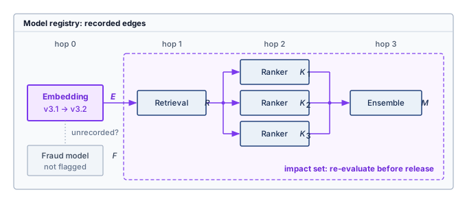
Figure 3: **Dependency-Aware Model Registry**: A version bump on embedding model $\Glyph{E}$ starts a traversal of the registry’s recorded downstream edges: retrieval $\Glyph{R}$, rankers $\Glyph{K}_1$ to $\Glyph{K}_3$, and ensemble $\Glyph{M}$ form the impact set (dashed region) that must be re-evaluated before $\Glyph{E}$ v3.2 ships. A model with no recorded edge from $\Glyph{E}$, such as fraud model $\Glyph{F}$, is not flagged, which is why an unrecorded dependency is a silent risk. The rankers also consume features derived from $\Glyph{E}$ directly; only the retrieval path is drawn.

The impact boundary in figure 3 identifies consumers that require evaluation after an upstream change. Fraud model $\Glyph{F}$ has no recorded dependency, so the traversal does not flag it; an omitted edge would leave that conclusion incomplete. Within the recorded graph, upstream embedding model $\Glyph{E}$ produces representations consumed by retrieval model $\Glyph{R}$, three parallel rankers ($\Glyph{K}_1$, $\Glyph{K}_2$, $\Glyph{K}_3$) score those candidates using features derived from $\Glyph{E}$, and ensemble model $\Glyph{M}$ combines the scores into a final ranking. Recording these relationships tells the release controller where to test, and the tests on those consumers decide whether the new representations remain compatible.

Update approval begins with graph traversal and then requires behavioral and interface evidence. When embedding model $\Glyph{E}$ is updated, the registry and release controller coordinate four steps:

Traverse downstream edges to identify every dependent model ($\Glyph{R}$, $\Glyph{K}_1$, $\Glyph{K}_2$, $\Glyph{K}_3$, and $\Glyph{M}$).
Re-evaluate each dependent model against the proposed embeddings.
Block deployment of $\Glyph{E}$ until every consumer passes.
Roll out the approved version set through compatible intermediate states, retaining a validated rollback target. Topological ordering alone is insufficient if an existing consumer cannot accept the new producer’s outputs.

Without explicit dependency tracking, organizations discover architectural coupling through production outages when an upstream change silently corrupts downstream assumptions. A single YAML entry captures artifact location, training provenance, evaluation results, and declared dependencies (listing 1). The downstream entries seed impact analysis; following their registry records reveals transitive consumers. Release approval additionally requires confirming that the update preserves the input-output contract expected by those consumers, or scheduling a coordinated rollout while retaining a validated rollback target.

Listing 1: Model Registry Schema: A YAML entry capturing model metadata, artifact location, training provenance, and evaluation results for dependency tracking and reproducibility.

model:
  name: user_embedding_v3
  version: "3.2.1"
  type: embedding_model
  domain: recommendation

artifact:
  path: gs://models/user_embedding_v3/3.2.1/
  format: tensorflow_savedmodel
  size_bytes: 4294967296

training:
  data_version: user_interaction_2024_01
  code_commit: abc123def
  started_at: 2024-01-15T10:00:00Z
  duration_hours: 48
  hardware: 8xA100-80 GB

evaluation:
  metrics:
    recall_at_100: 0.342
    embedding_quality: 0.891
  evaluation_set: eval_2024_01

dependencies:
  upstream:
    - feature_store/user_features_v2
    - feature_store/interaction_features_v1
  downstream:
    - models/candidate_retrieval_v4
    - models/ranking_ensemble_v2

serving:
  min_replicas: 10
  max_replicas: 100
  latency_p99_target_ms: 5
  memory_gb: 16

ownership:
  team: recommendation-core
  oncall: recsys-oncall-team

12.3.2 Ensemble management

The downstream entries in listing 1—candidate retrieval and a ranking ensemble—point to a composition problem that registry edges alone cannot solve: when a recommendation pipeline chains retrieval, ranking, and filtering models owned by different teams, an upstream retrieval change that improves local recall can shift the candidate distribution enough to degrade final ranking. Recommendation systems exemplify this multi-model management challenge by composing stages and combining predictions from several models into an ensemble. The platform must validate the complete recommendation interface even when different teams own its components.

Architectural rationale for recommendation ensembles

Recommendation architectures separate work when evaluating every candidate with the richest model would exceed the latency or compute budget. Retrieval produces a manageable candidate set, ranking scores that set with richer features, and later re-ranking or business-rule stages produce the final ordering (Covington et al. 2016; Liu et al. 2022). Within this path, specialized models can address competing objectives such as engagement, diversity, and freshness, while ensemble stages combine their outputs. The decomposition trades a smaller amount of expensive scoring for additional interfaces whose behavior the platform must validate.

Covington, Paul, Jay Adams, and Emre Sargin. 2016. “Deep Neural Networks for YouTube Recommendations.” Proceedings of the 10th ACM Conference on Recommender Systems, 191–98. https://doi.org/10.1145/2959100.2959190.

Liu, W., Y. Xi, J. Qin, F. Sun, B. Chen, W. Zhang, R. Zhang, and R. Tang. 2022. “Neural Re-Ranking in Multi-Stage Recommender Systems: A Review.” Proceedings of the Thirty-First International Joint Conference on Artificial Intelligence, 5512–20. https://doi.org/10.24963/ijcai.2022/771.

The same decomposition improves experimentation velocity because teams can update individual components without retraining the entire recommendation stack, but that independence creates version-compatibility obligations for the platform. It also changes risk management. Other ensemble components can sometimes compensate when one model fails or produces poor results, yet the platform must detect when compensation hides a regression rather than resolving it.

Ensemble deployment patterns

Deploying an ensemble update requires evaluating its effect on the composed system. Consider updating the fine ranking model within a recommendation ensemble. An illustrative staged ensemble deployment moves the update through four phases (table 7): shadow deployment (24–48 hours logging without serving), canary (1 percent traffic for 4–8 hours), staged rollout (5 percent to 100 percent over 24–72 hours), and soak (7–14 days monitoring for delayed effects). These durations are planning assumptions; promotion requires enough eligible observations, mature outcomes, and acceptable guardrail metrics for the release decision.

Table 7: Staged Ensemble Deployment Pattern: Four-phase rollout for updating recommendation ensemble components. Shadow deployment (24–48 hours) compares behavior without serving candidate outputs; resource isolation and outcome evidence bound what it establishes. Canary (1 percent traffic, 4–8 hours) enables statistical regression detection, staged rollout progressively increases exposure, and soak period (7–14 days) catches delayed interaction effects.

Deployment stage	Actions	Duration	Rollback trigger
Shadow	New model scores alongside production, results logged but not served	24–48 hours	Quality metrics below threshold
Canary	1% traffic receives new model results	4–8 hours	Statistical significance of regression
Staged Rollout	5% → 25% → 50% → 100%	24–72 hours	Business metric degradation
Soak	Full traffic, extended monitoring	7–14 days	Delayed effects emerge

The extended timeline reflects the difficulty of detecting regressions in ensemble systems. A component change that improves its local metrics might degrade system-level performance through subtle interactions with other components.

Interaction effects

Ensemble components interact in ways that make local validation insufficient. If a ranking model is retrained on lower-quality retrieval candidates, it may learn greater reliance on auxiliary signals; restoring retrieval can then change the distribution that this adapted ranker expects. A fixed ranker can also respond differently to changed inputs without changing its learned weights. Distribution shift propagates whenever an upstream update alters representations consumed by downstream models trained on older versions. Over longer horizons, ranking decisions change which items users encounter, shaping the feedback used for future training. Intermediate outputs help locate these effects, while stable holdouts and observation windows support comparison of the complete system. Joint retraining is a candidate intervention when the evidence identifies incompatible learned behavior, rather than a required periodic reset.

12.3.3 Model lifecycle management

Governing those dependencies over time requires controls at both ends of a model’s life: promoting experimental notebooks straight to live traffic without staging gates causes avoidable outages, whereas retiring a model without migrating its consumers leaves behind “zombie models”² that silently drain GPU capacity and block platform upgrades. Lifecycle management keeps model dependencies from becoming permanent obligations: every promotion widens a model’s blast radius, and every retirement must migrate its consumers before the platform can reclaim resources. The lifecycle stages trace that progression from development to archive, each defined by the gates it imposes rather than by a status label.

² Zombie models: Production models that continue serving despite being obsolete or superseded. Even a low-traffic model consumes registry, monitoring, dependency-management, and on-call capacity until it is deliberately retired. The operational cost therefore extends beyond compute: zombie models enlarge the dependency graph, making platform-wide upgrades and security patches slower and riskier.

Development → Staging → Canary → Production → Deprecation → Archive

In development, models exist as experimental artifacts. Operations requirements are intentionally light, but they are not optional: successful experiments must preserve results, version history, and enough reproducibility metadata to be challenged later. The operational concern is therefore transition readiness. A promising model should not move to staging until it has clear production-readiness criteria, automated evaluation against production-equivalent data, and documentation sufficient for review.

Staging tests the candidate as a deployable service before it serves user-visible outputs. Production-equivalent data, feature interfaces, and hardware make latency, throughput, and behavioral checks relevant to deployment. Shadow traffic can add evidence about live request patterns when its coverage justifies its cost. The promotion gate combines the checks required by the release contract with human review where model behavior or risk demands judgment.

Production widens the blast radius from validation traffic to live traffic, so the model now requires continuous monitoring with alerting, capacity for traffic fluctuations, rollback procedures, and on-call support. Production is not a terminal state. Distribution shifts prompt investigation and evaluation; retraining is warranted when the resulting evidence supports an update. Feature and infrastructure changes likewise require compatibility checks, and periodic comparison with newer baselines tests whether the deployed model still earns its place.

The lifecycle closes only when a model can be retired without breaking its consumers. Deprecation identifies dependent systems, provides migration paths and timelines, maintains the old model until migration completes, and archives artifacts for reproducibility and audit. Organizations often underinvest in this final stage, allowing obsolete models to linger in production long after their replacements ship. Platform-level lifecycle enforcement closes that gap.

12.3.4 Deployment patterns by model count

How a model moves through those lifecycle stages depends on how many other models move with it. Rolling out a single isolated vision classifier once a month requires only a local canary, whereas pushing daily updates across a 50-model recommendation ensemble or hundreds of platform models without cross-model rate limits can trigger cascading regressions. The appropriate deployment pattern depends on the interdependence of the versions being updated, because a compatibility change can widen the rollback unit. Across the example deployment patterns in table 8, single model deployments update monthly for isolated vision classifiers, pipeline deployments weekly for 3–5 sequential NLP models, ensemble deployments daily for 10–50 recommendation components, and platform deployments continuously across hundreds of enterprise models. The cadences describe example operating contexts; model count does not determine release frequency or the evidence required for promotion.

Table 8: Deployment Patterns by Scale: Four patterns addressing different model counts and update frequencies. Single model deployments (1 model, monthly updates) use standard canary rollouts, while platform deployments (100+ models, continuous updates) require automated policy enforcement, cross-model impact analysis, and global rate limiting to prevent simultaneous high-risk deployments.

Pattern	Model count	Update frequency	Example
Single Model	1	Monthly	Vision classifier
Pipeline	3-5	Weekly	NLP processing pipeline
Ensemble	10-50	Daily	Recommendation system
Platform	100s	Continuous	Enterprise ML platform

For a model without downstream model consumers, the rollback unit can be smaller. Canary deployments, blue-green switches,³ and gradual rollouts still require a validated previous version together with compatible preprocessing, features, and serving configuration. Restoring the model artifact alone is sufficient only when those surrounding interfaces remain compatible.

³ Blue-green deployment: A release pattern that prepares the new version in a parallel environment before switching production traffic. Fast rollback requires the previous environment to remain ready and its dependencies to remain compatible. Holding both versions during the transition adds serving capacity and cost $(\InferenceCost)$; the duplication depends on which resources the environments can safely share.

Pipelines introduce ordering constraints because models execute in sequence and each model’s output feeds the next. Compatibility must hold at every intermediate deployment state. An upstream-first update is safe only if existing consumers accept its new outputs; otherwise the platform must prepare compatible consumers or stage both versions before switching traffic. The release record names the compatible version set and the rollback unit, which may span the entire pipeline.

Ensembles widen the coordination problem because multiple models may execute in parallel or in a graph. Different teams can update components on different schedules, partial updates may change only part of the ensemble, and the system behavior emerges from component interactions. Testing in isolation is therefore insufficient; integration testing becomes the deployment gate.

At platform scale, continuous deployment means some model is always being updated somewhere, so the platform must prevent individually safe changes from combining into an unsafe fleet state. Platform deployment requires automated rollout policies based on model risk classification, cross-model impact analysis before deployment approval, global rate limiting to prevent simultaneous high-risk deployments, and automated correlation of incidents with recent deployments.

12.3.5 E-commerce model ecosystem

Updating a single user-embedding model in an e-commerce stack alters the inputs to candidate retrieval, price sensitivity, ranking, and business rules simultaneously, turning a local model upgrade into a five-tier integration test. The registry, ensemble, and lifecycle mechanisms meet in this production graph. An e-commerce platform typically starts the graph with embedding models. A user embedding model generates user representations from behavior history, while a product embedding model represents products from attributes and interactions. Those embeddings are not final predictions; they are shared interfaces consumed by downstream services.

The next layer turns shared representations into candidate sets and business signals. A candidate retrieval model uses the embeddings to find relevant products, and a price sensitivity model estimates how strongly a user will respond to price changes. A ranking model then scores the candidate products using both embedding features and auxiliary signals, while a business rules model applies promotional and inventory constraints before results reach the user.

The resulting graph has five tiers, and its shape decides what a change costs. User and product representations travel over a shared bus into candidate retrieval and price sensitivity, which converge in ranking before business rules apply (figure 4).

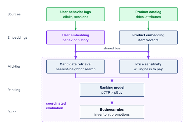
Figure 4: **E-Commerce Model Ecosystem**: Data sources feed a user embedding and a product embedding. A shared bus carries both embeddings into both mid-tier models, candidate retrieval and price sensitivity, whose outputs merge in the ranking model before business rules apply inventory and promotion constraints. Because every embedding reaches every downstream model, a change to the user embedding requires coordinated evaluation of all four consumers.

Because the embedding bus in figure 4 branches directly to both mid-tier consumers, a change can affect candidate retrieval and price sensitivity before propagating through ranking and business rules. The platform therefore evaluates both direct embedding compatibility and downstream recommendation quality. If old consumers cannot accept the new embeddings, the release can retain both versions and route each consumer to the version it validated while migration proceeds. The rollback plan must preserve that compatible state as well. While the dependency graph maps affected consumers, a model registry alone cannot preserve the feature values they ingest. Shared features demand versioned definitions, point-in-time correctness, and explicit freshness guarantees, contracts that complete the state a release pipeline must validate.

Self-Check: Question

When an upstream User Embedding Model is updated in an enterprise model registry, which automated sequence of graph-traversal actions must the registry execute to prevent silent production failures?
1. Hot-swap the model binary on serving pods and trigger immediate asynchronous retrains of downstream models without blocking traffic.
2. Identify all dependent downstream models (retrieval, ranking, ensembles), trigger compatibility re-evaluations, and block promotion of the upstream model until all dependents pass verification.
3. Overwrite the existing embedding schema in-place and invalidate all client-side prediction caches.
4. Recompile the entire datacenter Kubernetes cluster manifest and flush all feature store storage tables.
In high-throughput e-commerce recommendation systems, what is the primary systems rationale for deploying a multi-stage ensemble (retrieval $\rightarrow$ ranking $\rightarrow$ re-ranking) rather than a single end-to-end deep neural network?
1. Multi-stage ensembles eliminate all network communication between microservices.
2. Single deep learning models cannot process floating-point tensors larger than 32 bits.
3. Evaluating millions of catalog items with an expensive, feature-rich ranking model violates strict serving latency budgets ($<10\text{ ms}$), requiring fast candidate filtering before fine ranking.
4. Modern web browsers reject HTTP responses generated by single-model inference backends.
Why must an enterprise model registry record complete training provenance (code commit, dataset version, hyperparameters, hardware envelope) in addition to the binary model weights?
In a production multi-model recommendation ensemble, severe accuracy degradation in one component model will always trigger explicit application crashes and exception alerts in monitoring dashboards.
Arrange the four stages of this example Staged Ensemble Deployment Pattern in operational sequence. The durations and traffic shares are assumed release-contract settings, not universal requirements:

Soak monitoring (7–14 days observing delayed feedback and distribution shifts)
Canary deployment (1% live traffic for 4–8 hours)
Shadow deployment (24–48 hours logging outputs without serving them)
Staged rollout (expanding traffic from 5% to 100% over 24–72 hours)

See Answers →

12.4 Feature Store Operations

Consider a fraud detection system that needs to know a user’s transaction volume over the last ten minutes. Serving retrieves that feature within the prediction’s latency budget, while training reconstructs it for many historical transactions. These access paths differ, but the feature’s meaning must remain compatible. If training counts transactions that were unavailable at the historical prediction time, or serving applies a different aggregation rule, the model receives inputs that differ from those on which it was evaluated.

A common design separates the two access paths: online stores serve low-latency feature lookups, while offline stores generate reproducible training data. The two paths form a training-serving gap in computational context. Training computes features in batch over hours, while serving computes them in real time within milliseconds, yet each feature must mean the same thing on both paths. The gap is a design condition, not yet a failure. It becomes one as training-serving skew, the failure mode in which small differences in processing logic between the two paths give the deployed model inputs it never saw in training and degrade accuracy silently.

Systems Perspective 12.2: Training-serving skew

At fleet scale, the concern shifts from detecting training-serving skew in a single model to controlling it as a platform-level property. A feature store reduces skew by making training and serving pipelines read from shared feature definitions and materialized feature values where possible, turning $\TrainingTransformFunction(\RawPipelineInput) \equiv \ServingTransformFunction(\RawPipelineInput)$ into an architectural invariant that can be tested and monitored rather than a manual convention repeated by every team.

12.4.1 Feature store architecture

Training jobs scan terabytes of historical features across millions of examples, whereas live serving must fetch a single user’s latest feature vector in under 10 milliseconds without diverging in feature logic. The dual-store architecture resolves this conflict between high-throughput batch scans and low-latency point lookups by splitting storage while the platform enforces compatible definitions and temporal semantics across both paths. One materialization engine, governed by versioned feature definitions, writes ingested batch and stream data into an offline analytical store for historical joins and an online key-value store for point lookups (figure 5).

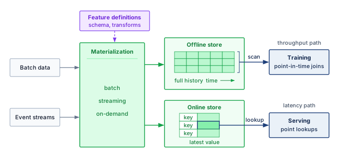
Figure 5: **Feature Store Architecture**: A dual-store architecture resolves the conflict between training (high-throughput batch scans) and serving (low-latency point lookups). One set of feature definitions drives materialization from batch and streaming sources into an offline store, which keeps full history for point-in-time training joins (the throughput path, top), and an online store, which keeps the latest value per entity for serving lookups (the latency path, bottom). Shared definitions support compatible feature meanings; materialization and historical-availability checks must verify that contract.

The offline store retains historical feature data for reproducible training examples, so its access path favors large scans and joins, where a single query might read terabytes to build a feature set for millions of examples. Throughput determines how quickly that dataset can be prepared within the training schedule.

The online store serves feature values within the prediction’s latency budget. At fleet scale its load depends on request rate, features fetched per request, batching, and cache reuse, rather than model count alone, and the storage choice must satisfy that access pattern at the required tail latency and peak load.

Materialization loads computed features into both stores: in batch on a daily or hourly schedule, from event streams in near real time, or on demand at request time when freshness requirements exceed batch frequency. The central architectural challenge is ensuring consistency between the two stores during materialization. If the offline store contains a feature value for training that was not identically available in the online store at the time of prediction, it creates a training-serving mismatch that can silently degrade model performance in production, the training-serving skew problem formalized in perspective 12.2.

For a platform serving hundreds of models, such as the five-hundred-model portfolio that opened this chapter, shared feature contracts prevent each consumer from reconstructing historical correctness and serving consistency independently. The dual-store pattern provides one implementation of that contract; the invariant is compatible feature meaning and temporal availability across both paths, rather than a requirement that every workload use the same storage system.

12.4.2 Freshness SLOs

Recommending products from a 24-hour batch feature table ignores everything a shopper clicked in the last ten minutes, whereas streaming every static demographic attribute at one-second latency wastes compute on values that rarely change. Feature freshness represents the delay between real-world events and their reflection in feature values. Example requirements range from days for static attributes such as demographics, which batch computation can serve, to seconds for features built on the last user action, which may require streaming or on-demand computation (table 9). The consuming decision determines the acceptable delay; the feature category alone does not establish a service-level objective (SLO).⁴ The categories in the table are a starting point for those SLOs; monitoring and alerting must use the timestamp and delay contract validated for the consuming workload.

⁴ SLO: A target for a declared service indicator and measurement window. Under a time-based definition, “three nines” (99.9 percent) annual availability allows about 8.8 hours of downtime; a request-based definition instead counts failed eligible requests. A p99 latency target of 200 ms requires at least 99 percent of eligible requests to complete within that bound over the specified window.

Table 9: Feature Freshness Requirements by Type: Four feature categories with SLO thresholds and computation patterns. Static features (user demographics) tolerate day-scale staleness with batch computation; real-time features (last user action) demand seconds-scale freshness through streaming or on-demand computation, directly impacting recommendation quality and engagement.

Feature type	Example	Freshness SLO	Computation pattern
Static	User demographics	Days	Batch
Slowly changing	User preferences	Hours	Batch
Session-level	Current session context	Minutes	Streaming
Real-time	Last action	Seconds	Streaming/On-demand

The table’s freshness classes are budgets on feature freshness latency, the event-to-availability delay between a user action and its arrival in the model’s inputs. Stale features can degrade relevance even when serving remains fast and available.

Streaming closes the freshness lag that batch leaves open.

Example 12.1: Feature freshness latency

Scenario: A real-time recommendation service processes user interaction logs to compute feature vectors during an active user session.

Diagnosis: Suppose the daily batch pipeline delivers relevant interactions with freshness latency $\FeatureFreshnessLatency\approx 12\text{--}24\text{ h}$. Those features cannot reflect activity from the current session, even if other recommendation inputs change. A streaming pipeline (Kafka/Flink) operating at $\FeatureFreshnessLatency\approx 1\text{--}5\text{ s}$ can incorporate that activity sooner; whether it updates the vector before the next user action depends on the session’s timing.

Systems lesson: Feature freshness latency is a physical system metric ($\FeatureFreshnessLatency= \FeatureRecordTime - \SourceEventTime$). Reducing freshness latency can improve decisions that depend on recent behavior, but engagement lift must be measured in an experiment. The business benefit must justify the additional streaming capacity and operational complexity.

Recommendation systems show how a missed freshness SLO reaches the user when a ranking decision depends on behavior from the current session. At platform scale, that session-level deadline must hold across multi-terabyte embedding tables and millions of queries per second while sharing ingestion capacity with offline training.

Lighthouse 12.2: Archetype B (DLRM at Scale): Feature staleness

Context: Archetype B (DLRM at Scale) recommendation workloads maintain sparse embedding tables of 10 TB+ across distributed memory and serve on the order of 10 million queries per second platform-wide, each within a p99 serving budget ($\LatencySlo$) of 100 ms, of which feature retrieval receives only a few milliseconds.

Mechanism: Ground truth user intent shifts continuously. If the feature materialization pipeline has a 10-minute update lag ($\FeatureUpdateLag= 600\text{ s}$), serving queries read feature values that omit the last 10 minutes of user behavior, so downstream rankers can recommend items the user has already moved past.

Impact: The lag is dominated by pipeline scheduling rather than transfer time, and it can make recent behavior unavailable to a ranking decision. The resulting click-through or revenue effect must be measured for the service; there is no universal staleness penalty.

Systems lesson: When recent behavior materially affects ranking quality, DLRM operations must provision ingestion and materialization to meet the feature’s freshness SLO. Scheduling must preserve that deadline alongside offline training needs. The measured value of fresher inputs determines whether the additional streaming capacity earns its cost.

Freshness becomes operational only when the SLO names its timestamp contract. Equation 3 measures time since the most recent feature update. This refresh-age proxy supports the thresholds in table 9 when updates certify that the source stream has been processed through the required time:

\[\text{Staleness} = \CurrentWallClockTime- \FeatureUpdateTimestamp \tag{3}\]

Refresh age differs from event-to-availability latency: rewriting an old source value can make its update timestamp recent without making the source information fresh. Streaming monitors therefore need source progress or watermarks as well as update timestamps, and must distinguish an idle entity from a stalled pipeline. Batch age increases between scheduled refreshes. Each path needs a threshold matched to its update contract rather than one global freshness rule.

Freshness impact on model quality

A recommendation system uses user interaction features with different freshness levels. Assume an online experiment yields the relative engagement lifts in table 10. These constructed values illustrate a planning calculation; replay of historical inputs alone does not establish a causal engagement gain:

Table 10: Assumed Engagement Lift by Feature Freshness: Constructed relative lifts measured against the same baseline engagement rate. The hourly-to-real-time gap is 2.1 percentage points of the relative-lift metric, not 2.1 percentage points of the raw engagement rate. The example translates that assumed gain into an infrastructure budget.

Feature freshness	Engagement lift vs. baseline
Real-time (< 1 min)	+12.3%
Near real-time (< 5 min)	+11.8%
Hourly	+10.2%
Daily	+8.1%

The difference in relative lift between hourly and real-time features is 2.1 percentage points of the shared baseline. If the organization values that incremental engagement at $10 million annually, the comparison must use the incremental cost of replacing the hourly path, including migration and ongoing operation over the same horizon. The engagement experiment supplies the quality difference; the business valuation and infrastructure cost determine whether it justifies investment.

Checkpoint 12.2: Pricing the streaming and batch freshness decision

Under the constructed lifts in table 10, moving from hourly to real-time features adds 2.1 percentage points of engagement lift. Treat that lift as $10 million in annual engagement value and apply it to the choice between streaming and batch infrastructure.

Freshness break-even: determine the maximum annual incremental cost of a real-time feature pipeline relative to the hourly path that still breaks even on the 2.1-point lift, holding the $10 million engagement value constant, and state the cost threshold under which streaming is a clear win.
Lift per point: compare the additional engagement lift for the daily-to-hourly, hourly-to-near-real-time, and near-real-time-to-real-time transitions, and identify the incremental pipeline-cost estimates needed to choose among them.
Scaling to users: if the $10 million annual engagement value scales linearly with platform user count, determine the break-even user count as a fraction of the current population for a streaming feature platform costing an additional $5 million per year relative to the hourly path, state the range where it does not pay off, and choose an alternative architecture from table 9.

12.4.3 Point-in-time correctness

Joining a noon training example against a midnight batch table leaks six afternoon clicks into the model’s training inputs, inflating total_clicks_today 2.5$\times$ and producing offline metrics that collapse in production. Training data must reconstruct features strictly as they existed at the timestamp of each historical event (figure 6). Using unaligned feature values as inputs for historical training examples creates data leakage⁵ that inflates offline evaluation while leaving the deployed model without the future signals it learned to rely on.

⁵ Data leakage: Future information can inflate offline metrics when a model learns signals unavailable at prediction time. Shared feature infrastructure should enforce historical availability boundaries, but model and data owners must still specify the prediction moment and verify how features were computed. A timestamped join cannot remove future information already embedded inside an incorrectly constructed feature.

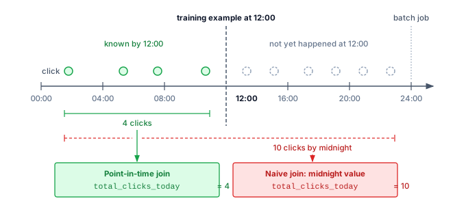
Figure 6: **Point-in-Time Correctness**: A training example at noon should see only the clicks already logged by noon (solid green, 4), not the clicks that arrive later (dashed gray). A naive join that reads the midnight batch value of `total_clicks_today` counts all 10 and leaks six future events into the example. A point-in-time join pairs each training event with feature values as they existed *at the event timestamp*, so the example contains only information that would have been available at inference time.

Comparing the aggregation brackets in figure 6 isolates the leakage mechanism. The point-in-time join uses the four clicks logged before noon, whereas the naive join reads the midnight total, inflating total_clicks_today by 2.5$\times$. This “time travel” failure uses a value that is valid in the database but invalid for the prediction moment: total_clicks_today is 10 at midnight, while the noon prediction can use only the 4 clicks already available. Training on the later value exposes information unavailable to the deployed predictor and can make offline evaluation overestimate production quality. Feature stores prevent that leakage by implementing point-in-time joins that retrieve feature values as of specific timestamps, as shown in listing 2.

Listing 2: Point-in-Time Join: A SQL lateral join that retrieves the most recent feature values available before each event, preventing future data leakage into training examples.

SELECT
    e.user_id,
    e.event_timestamp,
    e.label,
    f.feature_1,
    f.feature_2
FROM events e
LEFT JOIN LATERAL (
    SELECT feature_1, feature_2
    FROM features f
    WHERE f.user_id = e.user_id
      AND f.feature_timestamp <= e.event_timestamp
    ORDER BY f.feature_timestamp DESC
    LIMIT 1
) f ON TRUE

The query assumes that feature_timestamp records when the value became available to serving. If it records only the source event time, a late arrival or later backfill could pass the filter despite being unavailable at the historical prediction. The store must retain availability time as well as event time when those differ, and the training join must enforce the availability boundary.

Point-in-time correctness has a storage cost because the store must retain feature history rather than current values alone. The same guarantee that prevents leakage also multiplies retained state:

\[\text{Storage} = \EntityCount\times \FeatureCount\times \frac{\FeatureRetentionWindow}{\FeatureUpdateInterval} \times \text{bytes}_{\text{row}}\]

For 100 million users and 1,000 features, with a retention window of 1 year and an update interval of 1 hour, the history contains 876 trillion feature values. Each stored row carries more than the value itself. An 8-byte value needs an 8-byte entity key and, because a correct point-in-time join must filter on availability time as well as event time, two 8-byte timestamps, for 32 bytes per row. Full hourly snapshots then represent approximately 28 PB before compression, three quarters of it metadata that makes the history reproducible. Storing only changed values, compressing columns, and limiting retention can reduce this footprint. The reduction depends on change frequency and encoding, while retention must still cover the historical predictions the platform needs to reconstruct.

12.4.4 Feature versioning and lineage

Feature definitions are production interfaces, so changing one without versioning can break every dependent model. Versioning and lineage make this evolution governable rather than implicit.

A representative user_engagement_score incident makes the mechanics concrete. A platform team changes the feature from a 30-day z-score to a 7-day min-max scale. The output may still be a floating-point number, so schema validation alone can pass while the feature’s meaning changes completely. Versioning names the semantic change before it reaches production; lineage identifies every model trained or served with the old meaning; backfill recomputes historical values for the new meaning; and freshness and quality checks decide whether the rewritten history is safe to use. Without that chain, a feature migration becomes a silent multi-model regression.

A safe feature interface records both version dimensions and lineage fields, and each field supports a specific operation, such as blocking a silent formula change or reproducing a historical value for audit (table 11).

Table 11: Feature Version and Lineage Components: Feature versioning separates logic, data, and schema changes; lineage records the path needed to debug, audit, and reproduce feature values. Together, these fields turn a feature definition into a governed production interface.

Component	What it records	Operational use
Definition version	Computation logic for the feature	Blocks silent semantic changes when the formula changes but the type does not.
Data version	Source snapshot or stream contract	Distinguishes model changes from upstream data changes.
Schema version	Output type, shape, units, and nullability	Preserves API compatibility checks while still naming semantic shifts.
Consumer declaration	Exact feature versions each model consumes	Gives the platform a place to block unsafe updates before serving.
Source lineage	Source tables, streams, and their versions	Traces bad predictions back to the upstream data that produced them.
Transformation and runtime provenance	Transformation code, timestamp, and environment	Reproduces historical values for audit, debugging, and compliance.
Quality and freshness metrics	Validation results observed when the value was produced	Estimates blast radius and decides whether rewritten history is safe to use.

12.4.5 Backfill procedures

Once a new feature version is declared, dependent models cannot train on it until the platform populates its historical values—and recomputing a year of history without idempotent partition writes or event-time bounds can saturate cluster compute or stamp training rows with post-hoc availability times. A backfill is a production migration over history: changing a feature definition creates a new version of the training history for dependent models, so the platform must bound the compute cost, validate values against the intended definition, and preserve a path back. Treating the backfill as a migration changes the operational question from whether the computation can run once to whether history can be rewritten without corrupting future training data.

Feature replay requires a concrete execution safety contract. Each backfill partition needs a stable identity and an idempotent or transactional write path so retries cannot duplicate feature effects; event-time bounds and the late-data policy must also match the point-in-time join used for training. Otherwise, a mechanically successful replay can produce a history that is complete in processing time but incorrect at the prediction time the model is meant to reproduce.

↩︎ Exactly-once commit boundaries, event-time watermarks, and late-data policies for distributed transformations are established in Replay and commit boundaries in data pipelines.

At scale, historical data may have moved into cold storage, so recomputation first becomes a data-placement problem. The long historical window then competes with production workloads for compute. Even after the job finishes, the platform must compare overlapping periods against the intended new computation, explain differences from the old definition, and coordinate with dependent pipelines so training jobs do not mix old and new semantics mid-run, before it can trust the new values.

The practical pattern is incremental. Historical data is processed in bounded date partitions, and each partition is validated before consumers can use it. Independent partitions can run concurrently within the backfill’s resource budget. During a dual-write period, old and new computations run in parallel, giving the platform overlapping values for comparison before cutover. The previous feature version and its lineage remain available through the migration and rollback window so dependent models can return to a compatible state.

12.4.6 Scale challenges

Serving 1 billion daily recommendations that each fetch 100 features generates 100 billion feature lookups per day—roughly 1.16 million feature lookups per second before peak traffic—explaining why feature stores at recommendation scale are critical-path serving infrastructure rather than a metadata convenience. This count measures feature-value accesses rather than backend requests; batching and cache reuse determine how many requests reach the store. A planning envelope of 5–10× the mean raises the required capacity accordingly; observed request patterns must establish the appropriate peak allowance.

Feature retrieval must fit inside the overall latency budget because lookup time on the critical path leaves less time for ranking. If the recommendation budget is 50 ms, the feature store may receive only 5–10 ms. Network overhead can consume 1–2 ms of that allocation, leaving roughly 3–8 ms for the store lookup itself. In-memory storage or caching, bounded batching, and placement near the serving fleet are candidate mechanisms. The selected design must meet the remaining lookup budget under peak load.

Production feature stores also carry two time horizons at once. Online capacity depends on the number of populated entity-feature pairs, encoded bytes per value, metadata, and replication. Offline capacity additionally depends on update frequency and retained history, as the snapshot calculation above shows. Neither footprint follows from model count alone. Multi-region replication can improve availability and lookup latency, but it also requires an explicit contract for how quickly new feature values become visible in each region.

12.4.7 Data quality operations

Meeting the millisecond lookup budget and multi-region replication contract still does not guarantee usable predictions if an upstream pipeline drops 18 percent of daily user events or leaks sentinel values like -1 and 999 into an age feature while HTTP health checks stay green. Data quality issues are a major source of production ML problems (Polyzotis et al. 2017). Model metrics reveal downstream effects after users are exposed, whereas data checks can identify missing, stale, or invalid inputs earlier in the pipeline so validation gates can quarantine suspect data before consumers use it. At scale, these checks need explicit response policies so detecting an upstream problem leads to containment rather than merely another dashboard signal.

Polyzotis, Neoklis, Sudip Roy, Steven Euijong Whang, and Martin Zinkevich. 2017. “Data Management Challenges in Production Machine Learning.” Proceedings of the 2017 ACM International Conference on Management of Data, 1723–26. https://doi.org/10.1145/3035918.3054782.

The first step is to quantify data quality in dimensions that support release decisions. Completeness measures whether expected records and fields are present. A daily data pipeline expected to produce 10 million user events but delivering only 8.2 million user events is 82 percent complete relative to that expectation. Investigation must distinguish missing delivery from a legitimate change in source volume. Consistency captures schema compliance and referential integrity; an age field with an allowed range of 0 to 120 would reject values such as 999 or -1, which may represent leaked sentinels. A policy might quarantine a batch when more than 5 percent of its checks fail, but a single critical violation can warrant rejection. The policy must weigh the consequences of invalid inputs against delayed or unavailable data.

Timeliness measures freshness against the SLO of the consuming model. Fraud detection may need features less than 100 milliseconds old, while demographic features can tolerate staleness measured in days; the alert threshold should therefore be tied to the feature’s use, not a global constant. Accuracy asks whether values remain correct within expected distributions. Sensor drift after calibration lapses, for example, can leave values well-typed but wrong. Statistical tests such as Kolmogorov-Smirnov for continuous features, chi-square for categorical features, and maximum mean discrepancy for high-dimensional data detect distribution changes that warrant investigation; they do not establish that individual values are accurate.

Validation then turns those measurements into a layered defense. Schema validation enforces expected column names, types, and constraints at ingestion; tools such as Great Expectations, TensorFlow Data Validation, and Pandera provide declarative schemas with automated checks. Distribution monitoring tracks feature distributions over time, catching drift that may not violate a type constraint but still indicates an upstream change whose effect on model performance requires evaluation. Cross-field validation adds the business logic that neither schema nor marginal distributions can express: if country="USA", the zip_code should match US postal formats; if order_status="shipped", a shipping_date should exist; and age derived from birthdate should match any explicit age field.

Debugging data quality incidents

A recommendation model’s click-through rate (CTR) drops 8 percent over 5 days. The initial hypothesis focuses on model drift, but the constructed investigation reveals a feature computation defect.

The investigation starts with the model symptom and then works backward through the data path. Model metrics confirm that CTR declined from 4.2 percent to 3.87 percent, but freshness checks show that features still arrive within the 1-hour SLO. That weakens the stale-pipeline hypothesis only if source progress, event-time coverage, and the affected entities are also verified; refresh age alone cannot exclude stale inputs. The investigation therefore tests semantic change as well. Distribution analysis then shows the mean of user_engagement_score, the shared feature whose redefinition section 12.4.4 used to motivate versioning, shifting from 0.42 to 0.31, a 26 percent decline, and lineage tracking ties the shift to an upstream pipeline version deployed 5 days earlier.

The shift and deployment history make the new pipeline a candidate cause; a changed population could also move the mean. Replaying the same source records through both pipeline versions with identical event cutoffs isolates the computation. In this scenario, the new version uses a different aggregation window even though its declared feature definition is unchanged, while the previous version matches that definition. This same-record comparison establishes a feature computation defect. The defect is the same class of silent semantic change that feature versioning is meant to name before release; the marginal distribution alone would not establish it.

Assuming revenue falls in proportion to CTR and traffic is uniform over the interval, the modeled impact is 8 percent of $15M/week over 5 days, producing $857K in lost revenue. If automated alerts and effective containment shorten exposure to 4 hours, the modeled impact falls by 97 percent. The resolution restores the previous pipeline and compatible model-feature state. A distribution validation gate then blocks unexplained feature shifts exceeding the scenario’s 10 percent threshold; semantic tests remain necessary for bugs that do not cross that band.

Four-hour alerts shrink a five-day exposure window 30$\times$.

Operational integration

Data quality operations integrate into production systems by turning checks into enforceable contracts. Data contracts establish formal agreements between data producers and consumers, specifying schema requirements, freshness SLOs, quality thresholds for completeness and accuracy, and escalation procedures for violations. Release controls enforce those agreements by checking proposed schema or computation changes and requiring consumer review when compatibility cannot be established.

The contract becomes operational through continuous validation and incident response. Ingestion checks reject source data that violates declared constraints, transformation checks test computed values, and serving gates block features known to be invalid. When a check fails, alerts identify severity and affected systems, circuit breakers contain the bad path, and quarantined batches preserve evidence for investigation. A fallback may use cached or last-known-good features only while they remain acceptable under the consuming model’s freshness and compatibility contract. Root-cause analysis then repairs the pipeline rather than only clearing the current alert.

At enterprise scale with thousands of features, individual checks need a shared routing and grouping policy so that one upstream failure does not page every downstream consumer separately. Grouping by source system connects symptoms of a shared outage—such as a payment-processing failure that corrupts several features at once—while grouping by computation pipeline directs investigation toward shared transformation code or dependencies. Because streaming and daily batch features operate under different freshness contracts, update-frequency grouping separates their alert thresholds, and business-domain grouping routes the resulting evidence to the teams that understand the affected models. Together, these groupings cut duplicate notifications without removing feature-level checks or suppressing an urgent contract violation.

Freshness monitoring applies the same aggregation rule to time. For 10,000 features updated at different frequencies, checking every feature value can consume substantial capacity. Sampling 1 percent of representative entities reduces that work, but the sample still grows with the entity population and must cover the relevant sources and partitions. Pipeline-level aggregation can reduce checks further when one pipeline updates 500 features and its source-progress watermark covers the group. A recent successful update alone cannot rule out a stalled partition or missing entities. With a bounded number of checks per feature, monitoring can maintain $\mathcal{O}(\FeatureCount)$ overhead, but that bound trades exhaustive coverage for aggregate or sampled evidence. Critical features need checks whose coverage and detection delay match their failure consequences.

Feature definitions, historical availability, and freshness now belong to the same governed state as model artifacts. A release pipeline must validate that state as a unit, retain a compatible rollback target, and limit live exposure while evidence accumulates.

Self-Check: Question

Why does an enterprise feature store implement a dual-store architecture (separating an offline store from an online store) instead of relying on a single unified database system?
1. Online stores can store only integer IDs, whereas offline stores are required for floating-point feature values.
2. Training requires high-throughput sequential analytical batch scans over historical data, whereas serving requires sub-10 millisecond point lookups for individual entity keys.
3. Cloud providers legally mandate separating batch compute from streaming ingress databases.
4. Single database systems crash when table schemas exceed ten columns.
What failure mode occurs when a training pipeline constructs training examples using current feature values rather than historical values as of each event timestamp?
1. GPU kernel deadlocks during forward propagation.
2. Hardware bit errors in the offline data lake storage controller.
3. ‘Time travel’ data leakage, where future information contaminates training data, producing deceptively high offline metrics but disastrous performance in production.
4. Out-of-memory errors in distributed model serving sidecars.
In the context of Deep Learning Recommendation Models (DLRM), explain the cost of feature staleness that results from lagged streaming feature pipelines.
Calculate the raw uncompressed historical storage footprint for a recommendation feature store with $100\text{ million}$ users, $1,000$ features per user, $1\text{ year}$ retention ($8,760\text{ hours}$), hourly full snapshots, and a $32\text{-byte}$ stored row (an $8\text{-byte}$ value, an $8\text{-byte}$ entity key, and $8\text{-byte}$ event and availability timestamps).
In an enterprise feature store, modifying the feature transformation logic of a shared feature in-place (e.g., changing normalization from z-score to min-max) is safe as long as the feature name and output datatype remain unchanged.
The subtle difference in feature transformation logic between offline batch training pipelines and online real-time inference pipelines is known as ____.

See Answers →

12.5 CI/CD for ML at Scale

Versioned model dependencies and feature contracts define a candidate release, but they do not establish that it is safe to expose. Each model update must navigate the dependency web: an embedding model update might require re-evaluation of four transitive downstream components, including the business rules layer, before any component can safely reach production. This coordination challenge transforms CI/CD from a per-model concern into a platform orchestration problem. Software integration tests already validate interacting components. ML CI/CD adds learned behavior and changing data to that contract, requiring evidence that upstream changes preserve downstream quality and that each deployment state remains compatible.

Continuous integration and continuous deployment practices for machine learning differ from traditional software CI/CD in what they must validate. Software CI/CD focuses on code correctness and deployment reliability, whereas ML CI/CD must additionally validate data, verify model performance, and manage the interactions between code, data, and learned parameters. At platform scale, these challenges multiply as pipelines must coordinate across hundreds of models with varying requirements.

12.5.1 Training pipeline automation

When a training run is kicked off from an engineer’s laptop with unrecorded data paths and ad-hoc hyperparameters, no reviewer can reproduce the resulting checkpoint or verify what changed when it fails in staging. CI/CD for machine learning begins by making each training run an accountable producer of deployable artifacts. The pipeline records versioned inputs and execution conditions, defines recovery behavior, and preserves the results needed for deployment validation. Automation makes those obligations repeatable; reproducibility still depends on the recorded data, code, environment, and sources of nondeterminism.

Pipeline stages

Figure 7 stages the delivery lifecycle across continuous integration, training, and deployment, with an evaluation gate that blocks or registers a candidate. Monitoring returns drift signals to data validation. A confirmed population change may justify retraining, while a corrupted feature pipeline requires repair before it supplies another training run. The sequence matters because each stage establishes evidence for the next rather than treating every alert as permission to train and deploy.

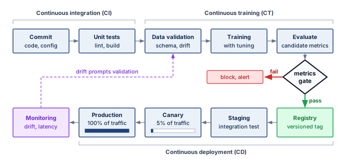
Figure 7: **ML CI/CD Pipeline**: Read the top row left to right and the bottom row right to left. Continuous integration checks each commit; continuous training validates data, trains, and evaluates against a metrics gate that either blocks the candidate and raises an alert or registers it. Continuous deployment then moves the registered version through staging, a canary slice of traffic, and full production. Monitoring closes the loop: detected drift returns to data validation and investigation before a decision to retrain.

Data validation pins the data version and rejects schema, freshness, or distribution failures before they consume training capacity.
Feature engineering preserves the feature contract between training and serving, so preprocessing changes do not become silent production regressions.
Training records code, data, hyperparameters, hardware envelope, and random seeds so a promising artifact can be reproduced or challenged later.
Evaluation compares the candidate with baselines, slice metrics, latency budgets, and task-specific gates before any user traffic is exposed.
Artifact generation packages the model with its serving configuration, dependency versions, and rollback target.
Registration records the artifact in the model registry with lineage, approvals, and deployment eligibility.

Each stage needs a defined retry boundary and durable outputs. If evaluation fails, the pipeline can reuse completed data-validation and feature-engineering results when their data, code, configuration, and relevant execution environment remain unchanged. Missing outputs or a changed dependency invalidate that reuse. Idempotent publication prevents a retry from registering duplicate artifacts or repeating external side effects.

Pipeline orchestration

Training pipelines require orchestration systems that make dependency order, resource allocation, and failure recovery explicit. The orchestrator represents the workflow as a directed acyclic graph (DAG), tracks dependencies between stages, retries transient failures without rerunning unaffected work, schedules scarce resources such as GPUs and memory, caches intermediate results when inputs are unchanged, and records logs and artifacts for later debugging.

Common orchestration choices include Kubeflow Pipelines⁶ (Bisong 2019), Airflow with ML extensions, and cloud-native solutions like Vertex AI Pipelines or SageMaker Pipelines. The choice depends on which dependency and resource contracts the platform must enforce, as well as existing infrastructure, team expertise, and scale requirements. Orchestration fixes the execution contract; parameterization fixes the variation contract, so the same graph can run against different data, models, and hardware envelopes without becoming a new program each time.

⁶ Kubeflow: Kubeflow Pipelines connects workflow dependencies to Kubernetes execution and resource requests. Declared requests let scheduling account for resources needed by a step, but do not eliminate contention on shared storage, networks, or other services. Platform policy must therefore combine admission and resource allocation with measurements of actual execution behavior.

Bisong, E. 2019. “Kubeflow and Kubeflow Pipelines.” Kubeflow and Kubeflow Pipelines in Building Machine Learning and Deep Learning Models on Google Cloud Platform. Apress. https://doi.org/10.1007/978-1-4842-4470-8_46.

Pipeline parameterization

Effective pipelines separate configuration from code (listing 3). The listing’s evaluation block names two standard ranking metrics: normalized discounted cumulative gain at rank 10 (NDCG@10), which rewards placing relevant items near the top of a list, and mean reciprocal rank (MRR), which averages the inverse position of the first relevant item.

Listing 3: Pipeline Parameterization: A YAML configuration separating data paths, feature sets, training hyperparameters, and evaluation criteria from pipeline code.

training_pipeline:
  model_type: transformer_ranking
  data:
    train_path: gs://data/train/2024-01-*
    eval_path: gs://data/eval/2024-01-15
    schema_version: v3.2
  features:
    user_features: [embedding, history, demographics]
    item_features: [embedding, attributes, popularity]
  training:
    epochs: 10
    batch_size: 4096
    learning_rate: 0.001
    optimizer: adam
    hardware: 4xA100
  evaluation:
    metrics: [ndcg_10, mrr, coverage]
    baseline_model: ranking_v2.1.0

The separation enables configuration-driven training because the platform can vary data versions, hyperparameters, and resource requests without rewriting pipeline code. A parameter file is also an audit input, but a path or version label alone does not prove which bytes a run consumed. The execution record must resolve those references to immutable data and artifacts and retain the actual environment, feature definitions, and evaluation policy. That record lets a release reviewer reconstruct the conditions behind the candidate’s evidence.

12.5.2 Validation gates

An immutable execution record tells a reviewer what a training run produced, whereas validation gates decide whether that candidate may advance toward production—because promoting a model solely for a 1 percent aggregate NDCG gain can still double p99 tail latency, degrade a protected subgroup, or rely on a corrupted upstream feature. A release gate consumes a versioned evidence bundle tying the candidate and its dependencies to metrics, thresholds, and accountable owners. Model performance, latency, policy and fairness constraints, data quality, and operational readiness each answer a different failure mode. Together they form an evaluation contract that remains attached to the release as it moves from offline validation to production experiments.

Performance gates

Performance validation combines minimum acceptable performance with comparisons against the production baseline and historical results. The release policy names the primary improvement sought and the regression bounds permitted on secondary metrics, rather than requiring every metric to improve simultaneously. A performance gate therefore checks three conditions: absolute thresholds, relative improvement over the production model, and regression bounds on secondary metrics (listing 4).

Listing 4: Performance Gate Evaluation: A validation function that checks absolute thresholds, relative improvement over the production model, and regression bounds on secondary metrics.

def evaluate_performance_gate(
    candidate_metrics, production_metrics, thresholds
):
    """
    Evaluate whether candidate model passes performance gates.

    Returns tuple of (passed: bool, reasons: list)
    """
    import math

    required_metrics = ("ndcg_10", "mrr", "coverage")
    required_thresholds = ("min_ndcg", "min_improvement", "max_regression")
    try:
        values = [candidate_metrics[k] for k in required_metrics]
        values += [production_metrics[k] for k in required_metrics]
        values += [thresholds[k] for k in required_thresholds]
        valid = all(math.isfinite(v) for v in values)
        valid = valid and production_metrics["ndcg_10"] > 0
        valid = valid and 0 <= thresholds["max_regression"] <= 1
    except (KeyError, TypeError, ValueError):
        valid = False
    if not valid:
        return False, ["Missing, nonfinite, or invalid gate inputs"]

    reasons = []

    # Absolute threshold check
    if candidate_metrics["ndcg_10"] < thresholds["min_ndcg"]:
        reasons.append(
            f"NDCG_10 {candidate_metrics['ndcg_10']:.4f} below minimum {thresholds['min_ndcg']}"
        )

    # Relative improvement check
    relative_improvement = (
        candidate_metrics["ndcg_10"] - production_metrics["ndcg_10"]
    ) / production_metrics["ndcg_10"]
    if relative_improvement < thresholds["min_improvement"]:
        reasons.append(
            f"Improvement {relative_improvement:.2%} below minimum {thresholds['min_improvement']:.2%}"
        )

    # Regression check on secondary metrics
    for metric in ["mrr", "coverage"]:
        if candidate_metrics[metric] < production_metrics[metric] * (
            1 - thresholds["max_regression"]
        ):
            reasons.append(
                f"{metric} regression exceeds {thresholds['max_regression']:.2%} tolerance"
            )

    return (len(reasons) == 0, reasons)

Latency gates

Production models must meet workload-specific latency requirements. Validation measures representative request shapes at expected load, batching, and hardware. Illustrative thresholds span two orders of magnitude, from a 5 ms median for fraud detection to a 500 ms median time to first token (TTFT) for an LLM, and they are policy choices rather than universal model-type requirements (table 12). The LLM row measures TTFT, reflecting the prefill phase of Prefill and Decode; completion latency requires a separate output-length contract for decode. The other rows measure request-to-response latency.

Table 12: Illustrative Latency Gates: Assumed p50 and p99 service targets under a declared request distribution and load. LLM targets refer to TTFT; other targets cover the complete response. Product risk and the service contract determine thresholds and exception authority.

Model type	p50 target	p99 target	Gate action if exceeded
LLM (TTFT)	500 ms	2000 ms	Block deployment, require optimization
Recommendation	10 ms	50 ms	Block deployment
Fraud Detection	5 ms	20 ms	Block deployment, high priority
Vision	50 ms	200 ms	Warning, conditional approval

Latency gates catch overt performance violations, but some regressions pass every gate and still degrade the product. The most dangerous failures are semantically silent: valid outputs built on corrupted inputs.

Example 12.2: Silent model regression

Scenario: A high-throughput product ranking model ($25{,}000\text{ QPS}$) passes offline validation and serving latency gates (per-request latency $\LatencySlo < 12\text{ ms}$), but causes a 3.2 percent conversion rate drop post-deployment.

Diagnosis: An upstream schema change caused a key user-affinity feature to return null for 8 percent of queries. The serving layer silently imputed null as 0.0, a valid float value, so HTTP error rates and latency remained normal while prediction quality degraded unalerted for 48 hours.

Systems lesson: Syntactically valid feature imputations cause semantically silent production failures. Automated release pipelines and monitoring systems must evaluate feature distribution shifts and null rates alongside system uptime and latency SLOs.

Fairness gates

Fairness concepts become operational at release time when policy choices are encoded as thresholds. For models affecting users, fairness validation turns a policy commitment into a release gate. A gate cannot test whether “the model is fair” in the abstract, because different contexts encode fairness differently and some definitions cannot hold at once. Each chosen definition becomes an executable bound on a measured gap between protected groups. A demographic-parity gate bounds the difference between groups in the rate of positive predictions; an equalized-odds gate bounds the difference in prediction rates between groups that share the same true outcome (Hardt et al. 2016). The operational point is not that every gate should enforce every definition. The gate must record which definition the organization chose, compare the measured value against historical baselines as well as absolute thresholds, and route borderline cases to human review because a near-threshold fairness result is also a governance decision.

Hardt, Moritz, Eric Price, and Nathan Srebro. 2016. “Equality of Opportunity in Supervised Learning.” Advances in Neural Information Processing Systems (NeurIPS) 29: 3315–23.

↪ The fairness criteria behind these gates, and why they cannot all hold at once, are developed in Fairness in machine learning.

Data quality gates

Before training or deployment, data quality validation reapplies the schema, distribution, freshness, and completeness checks of section 12.4.7 as a release gate (Caveness et al. 2020). Passing them establishes evidence for the properties tested; it does not rule out an untested semantic error.

Caveness, E., P. S. G. C., Z. Peng, N. Polyzotis, S. Roy, and M. Zinkevich. 2020. “TensorFlow Data Validation: Data Analysis and Validation in Continuous ML Pipelines.” Proceedings of the 2020 ACM SIGMOD International Conference on Management of Data, 2793–96. https://doi.org/10.1145/3318464.3384707.

These gates complete the offline evidence bundle. The next evidence must come from production traffic, gathered first without exposing users and then at a bounded share of live requests.

12.5.3 Production experimentation as a release gate

Offline validation on static holdouts cannot catch a candidate model that doubles tail latency under live concurrency or reduces user clicks when its predictions interact with real traffic. Once the offline gates pass, production experiments evaluate the candidate under a controlled exposure policy, starting from shadow traffic, which exposes no user to its outputs. Shadow traffic tests behavior without returning candidate outputs, interleaving compares rankers within a combined presentation, and A/B tests compare assigned variants. Network-effect checks determine whether interactions between experimental units undermine that comparison. These methods answer different questions; every release need not use all of them. Each supplies evidence for the online-experiment plane of the evaluation contract assembled in section 12.5.8, so the statistics that follow are tools for filling one row of the release record, not a separate discipline. Before exposure begins, the release record must name the invariant metrics, decision threshold, maximum user and infrastructure blast radius, stopping rule, rollback owner, and evidence required for promotion. A candidate that improves its primary metric but exhausts latency, reliability, fairness, or cost headroom fails the gate.

Shadow deployment and traffic replay

Shadow deployment runs the new model alongside production, receiving copied inputs and logging outputs without returning them to users. Figure 8 contrasts mirroring to an isolated candidate (Panel A) with canary deployment (Panel B), which exposes a controlled share of traffic to candidate responses. Shadow execution can reveal defects absent from offline tests, but its resource consumption and external side effects still require containment. It also cannot reveal how users would react to outputs they never receive.

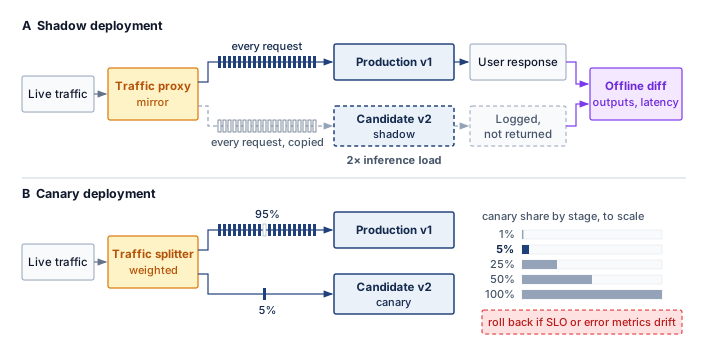
Figure 8: **Shadow and Canary Deployment**: In shadow deployment (A), the proxy mirrors all production traffic to the candidate; users receive only the production response, and both outputs are compared offline. No user sees the candidate’s output, but mirroring every request doubles inference load, so the shadow path needs its own capacity and must be isolated so it cannot slow production. In canary deployment (B), the splitter sends a small weighted slice of live traffic to the candidate (here the 5 percent stage) and widens it through the 1, 5, 25, 50, and 100 percent stages as evidence accumulates, rolling back if SLO or error metrics drift.

Shadow deployment earns its duplicate infrastructure cost when it answers validation questions offline tests cannot. A full-load shadow run measures errors, memory growth, and latency against the release SLOs, exposing leaks and resource contention that small offline datasets miss, and comparison under real traffic reveals output shifts such as changed confidence scores in a classifier or changed diversity in a recommender. That evidence holds only for the observed workload, duration, dependencies, and contention, and rare inputs may never arrive, so the shadow load profile and run length belong in the release record beside the result. Output differences require interpretation; they do not by themselves establish improvement or regression.

Shadow deployment requires capturing and replaying production traffic, and the replay choice determines the trade-off among fidelity, cost, and freshness. Three architectural patterns address different operational requirements.

Live mirroring duplicates every production request to the shadow model in real time. The production model serves the response while the shadow model processes the same input in parallel, providing immediate validation at full production scale but requiring shadow infrastructure capable of handling 100 percent traffic load. To keep this validation path from becoming a production dependency, the serving system must invoke shadow requests asynchronously, enforce timeouts, shed shadow load when it falls behind, and isolate resources so shadow work cannot affect production responses.

Sampled replay mirrors a configurable percentage of production traffic to shadow models. This reduces infrastructure costs, but the sampling rate and observation window must still supply enough eligible examples for the targeted failures. Uniform random sampling estimates the sampled traffic population, while stratification can ensure coverage of important segments. Adaptive sampling concentrates investigation on patterns where candidate and production outputs diverge. Such targeted samples need recorded inclusion probabilities and an appropriate estimator before their error rates can be interpreted as fleet-wide rates.

Batch replay captures production traffic logs and replays them asynchronously against shadow models. This decouples validation from the live request path and supports regression tests during available capacity windows. Fidelity depends on what the logs preserve. Replaying request contents without their historical feature state can change the task, while replaying them faster changes queueing and load. A load test must reproduce the relevant arrival pattern and serving conditions; historical replay still cannot observe user responses to candidate outputs.

Effective shadow deployment requires quantitative comparisons tied to the intended change. Output divergence locates differences from production: classification systems track disagreement rates, probability shifts, and class-specific concentration, while regression systems can compare prediction errors or differences between outputs. A changed prediction is not inherently a regression; outcome evidence or a validation oracle must establish its quality. Performance metrics assess latency, throughput, and resource consumption against the operating contract. A candidate with equivalent accuracy but 50 percent higher p99 latency needs review against that contract, even if both versions remain below the SLO.

The metric set must also separate operational failures from genuine model changes. Error-mode metrics count timeouts, exceptions, malformed outputs, and null predictions. A shadow model that times out on 0.1 percent of requests encounters 1,000 failures per day at 1M requests/day scale, and the request patterns that trigger those failures guide remediation. Statistical validation then determines whether observed differences represent genuine model changes or random variation. Because production and shadow models process the same requests, their outcomes are paired. Define a binary failure against a labeled outcome or validation oracle, let $\ProductionOnlyFailureCount$ count requests on which production fails and shadow succeeds, and let $\ShadowOnlyFailureCount$ count requests on which shadow fails and production succeeds. McNemar’s large-sample test uses the discordant pairs:

\[\McnemarTestStatistic= \frac{(\ProductionOnlyFailureCount-\ShadowOnlyFailureCount)^2}{\ProductionOnlyFailureCount+\ShadowOnlyFailureCount}\]

For a one-degree-of-freedom test at $\HypothesisTestSignificanceLevel = 0.05$, reject equal failure probabilities when $\McnemarTestStatistic> 3.84$. Marginal failure rates of 1 percent and 1.5 percent do not determine this statistic by themselves; the paired discordant counts $\ProductionOnlyFailureCount$ and $\ShadowOnlyFailureCount$ must be retained.

Shadow deployment workflow

Consider an illustrative fraud detection service processing 5 million transactions daily. A sampled shadow phase mirrors 10 percent of traffic for three days. Assume the eligible labeled subset yields recall of 94.2 percent for the shadow model versus 94.5 percent in production, and precision of 87.1 percent versus 82.3 percent. These point estimates alone establish neither improvement nor noninferiority. The gate also needs labeled counts, paired outcomes, label maturity, uncertainty intervals, and a prespecified recall tolerance. Assume shadow p99 latency is 45 ms versus 38 ms in production, both below the 50 ms SLO. The team proceeds to full shadow only after the statistical gate passes.

The full-shadow phase mirrors 100 percent of traffic for five days. In this scenario, the same labeled-data analysis supports the precision gain at full scale, but the run also exposes an edge case: the shadow model flags 0.02 percent of transactions as errors due to an unexpected feature distribution, which is 1,000 transactions per day. The root cause is heightened sensitivity to outliers in transaction amount. Adjusting feature clipping thresholds reduces the error rate to 0.001 percent in a new shadow run. Because clipping also changes model inputs, the revised candidate must pass the precision, recall, latency, and slice gates again before canary deployment.

Post-deployment validation then compares actual production metrics with the shadow predictions. Precision materializes at 87.3 percent in production vs. 87.1 percent in shadow, a nearby point estimate. Confirming agreement still requires uncertainty bounds and checks for label or traffic shifts; similarity between two percentages is insufficient.

Criteria for shadow deployment

Shadow deployment earns its cost when the additional evidence reduces expected deployment harm enough to justify duplicate execution, comparison logging, and analysis. That cost includes infrastructure that bounds the shadow path’s effect on production. The mirroring layer enforces sampling, timeouts, and load shedding, and separate compute pools, network allocation, and database capacity keep shadow work from stealing production capacity, because shared queues or dependencies can still transmit failures that asynchronous invocation alone does not prevent.

New architectures, consequential predictions, live feature dependencies, and tight latency budgets can make the evidence worth that cost, but only for failures shadow traffic can reveal; user responses to candidate outputs remain unobserved, and rare events may remain absent. A smaller shadow phase, or a direct move from offline validation to a bounded canary, can be appropriate when existing evidence covers the relevant failure modes and residual exposure is acceptable. Routine retraining does not establish low risk by itself, because changed data or parameters can alter behavior without an architecture change. The platform should compare the additional evidence shadow execution can provide with its resource cost, the harm a canary could cause before containment, and the time needed to observe that harm.

Interleaving experiments

Interleaving experiments⁷ were developed for ranking and search evaluation (Chapelle et al. 2012) and are also used in recommender personalization experiments (Netflix Technology Blog 2017). Rather than splitting users between variants, interleaving presents items from both variants to each user, then measures which items users engage with.

⁷ Interleaving experiments: Originally developed for search engine evaluation, interleaving merges results from two rankers into one list shown to each user, then credits clicks to the originating ranker (Chapelle et al. 2012). For fleet-scale recommendation systems iterating on many model variants, the sample efficiency of that within-user comparison translates directly into faster experiment cycles and lower opportunity cost from suboptimal models in production.

Chapelle, Olivier, Thorsten Joachims, Filip Radlinski, and Yisong Yue. 2012. “Large-Scale Validation and Analysis of Interleaved Search Evaluation.” ACM Transactions on Information Systems 30 (1): 1–41. https://doi.org/10.1145/2094072.2094078.

The advantage of interleaving is statistical efficiency. An interleaving experiment can require far fewer samples than A/B testing, and Netflix reports more than 100$\times$ fewer users for some ranking experiments (Netflix Technology Blog 2017), because each user provides direct comparison signals rather than contributing only to aggregate statistics.

In an interleaving workflow, the variants produce ranked lists that a method such as team draft or probabilistic interleaving combines into one presentation. The mixing and credit-assignment rules must control position effects and identify which ranker contributed each item. Engagement with those items supplies a relative preference signal. Figure 9 contrasts the between-cohort comparison of A/B testing (Panel A) with this within-user comparison (Panel B). The latter can screen candidates efficiently, but preference within a blended list does not directly measure the effect of deploying either complete ranking policy on long-term outcomes such as retention. Those outcomes still require an experiment designed to measure them.

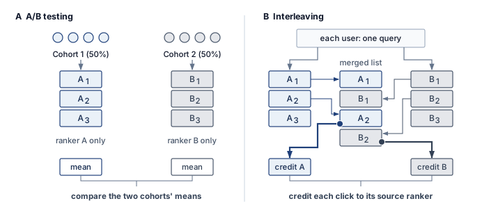
Figure 9: **Interleaving vs. A/B Testing**: (A) A/B testing splits users into cohorts, and each cohort sees only one ranker’s list, so the comparison is between cohort means and must overcome the variation between users. (B) Interleaving has both rankers rank the same query for each user and merges the results into one list (here by team draft); each click is credited to the ranker that contributed the item, so every user supplies a paired, within-user comparison. That pairing can make ranker-preference screening more sample-efficient; it does not measure the full deployment outcome assessed by an A/B test (Netflix Technology Blog 2017).

A/B test sizing and significance

At platform scale, experiment design determines how long a release occupies capacity and exposes users. A/B testing provides frameworks for comparing model variants (Kohavi et al. 2009, 2020), but its release decision depends on statistical power,⁸ significance thresholds, and multiple testing correction. The formulas below supply inputs to the operational contract: the number of eligible observations, the promotion rule, and the permitted stopping schedule. They do not establish that behavior remains reliable outside the evaluated population.

Kohavi, Ron, Roger Longbotham, Dan Sommerfield, and Randal M. Henne. 2009. “Controlled Experiments on the Web: Survey and Practical Guide.” Data Mining and Knowledge Discovery 18 (1): 140–81. https://doi.org/10.1007/s10618-008-0114-1.

Kohavi, Ron, Diane Tang, and Ya Xu. 2020. Trustworthy Online Controlled Experiments: A Practical Guide to A/B Testing. Cambridge University Press. https://doi.org/10.1017/9781108653985.

⁸ A/B testing power: The probability that an experiment correctly detects a true effect ($1-\HypothesisTestFalseNegativeRate$, typically set to 0.8). At fleet scale, the systems cost of power is exposure time. If the expected improvement is small (for example, 0.1 percent), the experiment may require millions of samples to reach statistical significance, consuming substantial serving resources $(\InferenceCost)$ for weeks.

For an equally allocated comparison of two proportions, the standard normal-approximation sample plan uses four parameters: significance level $(\HypothesisTestSignificanceLevel)$, statistical power $(1-\HypothesisTestFalseNegativeRate)$, baseline conversion rate $(\BaselineConversionRate)$, and minimum detectable effect $(\MinimumDetectableEffect)$. Equation 4 estimates observations per variant, assuming independent eligible outcomes and a small absolute difference near the baseline rate. Holding the other inputs fixed, the requirement scales inversely with the square of that difference:

Detecting smaller effects explodes the required sample size.

\[\RequiredUsersPerVariant = \frac{(\ConfidenceCriticalQuantile + \PowerCriticalQuantile)^2 \times 2\BaselineConversionRate(1-\BaselineConversionRate)}{\MinimumDetectableEffect^2} \tag{4}\]

where $\ConfidenceCriticalQuantile$ is the two-sided critical value for significance level $\HypothesisTestSignificanceLevel$ (typically 1.96 for $\HypothesisTestSignificanceLevel = 0.05$), $\PowerCriticalQuantile$ is the critical value for power (typically 0.84 for 80 percent power), $\BaselineConversionRate$ is the baseline rate, and $\MinimumDetectableEffect$ is the minimum detectable effect as an absolute difference. Both critical values use the positive upper-tail convention: the upper-tail areas are $\HypothesisTestSignificanceLevel/2$ and $\HypothesisTestFalseNegativeRate$, respectively.

Once data is collected, a two-proportion z-test determines if the observed difference is statistically significant. Equation 5 computes the test statistic as the difference in observed rates normalized by the pooled standard error:

\[\ProportionTestStatistic= \frac{\TreatmentConversionRate- \ControlConversionRate}{\sqrt{\PooledConversionRate(1-\PooledConversionRate)(\frac{1}{\ControlSampleSize} + \frac{1}{\TreatmentSampleSize})}} \tag{5}\]

where $\ControlConversionRate$ and $\TreatmentConversionRate$ are the observed conversion rates for control and treatment, $\ControlSampleSize$ and $\TreatmentSampleSize$ are sample sizes, and $\PooledConversionRate= \frac{\ControlSampleSize\ControlConversionRate+ \TreatmentSampleSize\TreatmentConversionRate}{\ControlSampleSize+ \TreatmentSampleSize}$ is the pooled proportion. For the two-sided test, if $|\ProportionTestStatistic| > \ConfidenceCriticalQuantile$, reject the null hypothesis and conclude the variants differ significantly.

Sample size for recommendation models

A recommendation system has baseline CTR of 5 percent. The team wants to detect a 10 percent relative improvement (0.5 percentage points absolute) with 95 percent confidence and 80 percent power.

Parameters:

$\ConfidenceCriticalQuantile = 1.96$ (95 percent confidence, two-tailed)
$\PowerCriticalQuantile = 0.84$ (80 percent power)
$\BaselineConversionRate= 0.05$ (baseline CTR)
$\MinimumDetectableEffect = 0.005$ (0.5 percentage point improvement)

Calculation:

\[\RequiredUsersPerVariant = \frac{(1.96 + 0.84)^2 \times 2 \times 0.05 \times 0.95}{0.005^2}\]

\[\RequiredUsersPerVariant = \frac{7.84 \times 0.095}{0.000025} = \frac{0.7448}{0.000025} = 29{,}792\]

Each variant requires approximately 30,000 samples, totaling 60,000 observations. If requests supply independent eligible observations with immediately available outcomes, 1 million requests per day split evenly between variants collects that sample in less than 2 hours. However, for a model with 1 percent baseline CTR detecting a 5 percent relative improvement (0.05 percentage points), the calculation yields:

\[\RequiredUsersPerVariant = \frac{7.84 \times 2 \times 0.01 \times 0.99}{0.0005^2} = \frac{0.1552}{0.00000025} = 620{,}800\]

Now each variant needs approximately 621K samples. Under the same independence and outcome-availability assumptions, 1M total requests/day split evenly between the two variants collects that sample in about 30 hours. Required observation windows can extend either experiment beyond its collection time. Here, the lower baseline and smaller relative improvement also imply a much smaller absolute effect. At a fixed relative improvement, rarer outcomes require more observations; a fixed absolute effect would give a different comparison.

Multiple testing correction

Running multiple A/B tests simultaneously or sequentially without correction inflates the familywise error rate. With 20 independent tests whose null hypotheses are all true, at $\HypothesisTestSignificanceLevel = 0.05$, the probability of at least one false positive is:

\[\Pr(\text{at least one false positive}) = 1 - (1-\HypothesisTestSignificanceLevel)^\TestFamilySize= 1 - 0.95^{20} = 0.642\]

The result is a 64 percent chance of at least one false rejection; a two-sided rejection can point in either direction. Two families of correction address this problem.

Bonferroni correction adjusts the significance threshold to $\PerTestSignificanceLevel = \frac{\HypothesisTestSignificanceLevel}{\TestFamilySize}$ for $\TestFamilySize$ tests. This is conservative but simple. For 20 tests with $\HypothesisTestSignificanceLevel = 0.05$, use $\PerTestSignificanceLevel = 0.0025$ for each test. This controls the familywise error rate but reduces statistical power; the Šidák variant, exact for independent tests, is only slightly more lenient (0.00256 per test for 20 tests).

False discovery rate (FDR) control using the Benjamini-Hochberg procedure bounds the expected false-discovery proportion under independence or suitable positive dependence. It is not a hard cap on the false discoveries in one experiment batch. This is appropriate when some false positives are acceptable. Order p-values from smallest to largest: ${\ObservedSignificanceLevel}_{(1)} \leq {\ObservedSignificanceLevel}_{(2)} \leq \ldots \leq {\ObservedSignificanceLevel}_{(\TestFamilySize)}$. Find the largest $\OrderedTestRank$ such that:

\[{\ObservedSignificanceLevel}_{(i)} \leq \frac{\OrderedTestRank}{\TestFamilySize} \times \HypothesisTestSignificanceLevel\]

Reject all hypotheses $\StatisticalHypothesis_{(1)}, \ldots, \StatisticalHypothesis_{(\OrderedTestRank)}$. This procedure yields higher statistical power than Bonferroni when running many tests.

Multiple testing scenario

A platform team runs 30 A/B tests per quarter comparing candidate models. Suppose every null hypothesis is true and each test has a calibrated false-positive probability of $\HypothesisTestSignificanceLevel = 0.05$. Without correction, the expected count is $30 \times 0.05 = 1.5$ false rejections per quarter, or approximately 6 models over a year. These are false claims of a difference, not necessarily improvements: a two-sided rejection can point toward either benefit or harm.

Applying Bonferroni correction: $\PerTestSignificanceLevel = \frac{0.05}{30} = 0.00167$ per test. This requires larger sample sizes. For the recommendation model example in section 12.5.3.6 (5 percent baseline, 0.5-percentage-point effect), the original requirement was 30K samples per variant. With a two-sided Bonferroni threshold, the critical value rises to about 3.14, increasing the requirement to roughly 60K samples per variant.

Using FDR control at $\FalseDiscoveryRateTarget= 0.05$, the Benjamini-Hochberg procedure bounds the expected false-discovery proportion across repeated experiment families under its dependence assumptions, counting the proportion as zero when there are no rejections. Observing 10 significant results out of 30 tests does not establish how many of those 10 are false or give a conditional guarantee for that quarter. The procedure accepts a different error criterion from familywise control and can gain power in exchange.

The choice begins with the error the decision must control. When even one false promotion among the planned comparisons has serious consequences, familywise control is appropriate; Bonferroni is one simple option. Exploratory screening may instead use FDR control when a bounded expected proportion of false discoveries is acceptable and later validation will assess candidates individually. The experiment family and error criterion belong in the release plan before results are inspected.

Checkpoint 12.3: Family-wise error rate under multiple testing

The correction methods are Bonferroni and Benjamini-Hochberg. Apply the family-wise reasoning to a smaller platform.

Family-wise error: for 20 simultaneous A/B tests per quarter at $\HypothesisTestSignificanceLevel = 0.05$ with no correction, calculate the expected number of false positives and the family-wise error rate under independence.
Bonferroni correction: apply Bonferroni correction, calculate the per-test threshold $\PerTestSignificanceLevel$, compute the family-wise error rate after correction, and compare it to the uncorrected rate.
Bonferroni vs. FDR: for 20 tests where the team expects most candidates to genuinely improve the metric, choose Bonferroni or Benjamini-Hochberg FDR control and justify the statistical-power trade-off.

Sequential testing and early stopping

Traditional A/B tests fix sample size in advance and evaluate once. Release teams rarely wait that long without looking, and looking is where the error rate leaks. A fixed-sample test checked after every batch of observations and stopped at the first $|\ProportionTestStatistic| > 1.96$ gets many chances to cross the threshold by chance, so its realized false-positive rate climbs well above the nominal 5 percent. Sequential testing budgets for those looks in advance, allowing monitoring during data collection with principled early stopping rules. Stopping can occur earlier when the evidence is strong, but the gain depends on the hypotheses, effect size, and stopping design.

The sequential probability ratio test, the classic design, updates a likelihood ratio after every observation and stops when it crosses Wald’s bounds, but it assumes two fully specified hypotheses, so release experiments more often use group sequential designs. Group sequential methods divide the experiment into planned analysis stages. At each stage, the test statistic is compared with adjusted thresholds that maintain the overall $\HypothesisTestSignificanceLevel$. The boundary family decides how that error budget is spent across the looks. An O’Brien-Fleming boundary spends almost none of it early, demanding overwhelming evidence to stop at the first looks and keeping the final threshold close to the fixed-sample value. A Pocock boundary spends it evenly, applying the same stricter threshold at every look. For a canary whose guardrail metric is checked every hour, the evaluation contract must prespecify a valid sequential stopping rule, such as one of these boundaries; comparing each hourly look against the single-look 1.96 reintroduces the inflation the design exists to prevent.

A valid stopping rule still rests on the independence and stationarity assumptions behind these formulas, and production tests can violate both. Carryover occurs when treatment changes behavior after exposure ends, so a design that reassigns users must account for that persistence. Novelty can make early responses differ from later behavior, and no fixed number of weeks guarantees that the effect has settled, so observation windows must cover the relevant behavioral cycles and outcome delays. Surrogate metrics such as clicks can also move in a different direction from long-term objectives such as retention and revenue, which is why a release gate pairs the short-term surrogate with guardrail metrics that may require longer observation. Interference between users is the most consequential violation for social and marketplace products, because it biases the estimated effect itself rather than only its variance.

12.5.4 SUTVA violations and network effects

When User A on a social platform receives better content recommendations from a treatment model and shares those posts with friends in the control group, User B’s engagement rises even though User B never received the new algorithm. The control condition becomes contaminated through the natural mechanics of a networked product, violating the assumption behind every sample-size and significance calculation above that one user’s treatment assignment does not change another user’s outcome.

The stable unit treatment value assumption (SUTVA) requires well-defined treatment versions and no interference between units (Rubin 1980). Its no-interference component says that user $\ExperimentUserIndex$’s outcome $\PotentialOutcome_{\ExperimentUserIndex}(\TreatmentAssignment)$ depends on their own assignment $\TreatmentAssignment$, not on other users’ assignments. Versioned releases address the treatment-definition requirement; network interactions challenge the second requirement. Ignoring those interactions can bias the effect estimate used for a deployment decision (Hudgens and Halloran 2008; Eckles et al. 2017).

Rubin, Donald B. 1980. “Randomization Analysis of Experimental Data: The Fisher Randomization Test Comment.” Journal of the American Statistical Association 75 (371): 591–93. https://doi.org/10.2307/2287650.

Hudgens, Michael G., and M. Elizabeth Halloran. 2008. “Toward Causal Inference with Interference.” Journal of the American Statistical Association 103 (482): 832–42. https://doi.org/10.1198/016214508000000292.

Eckles, Dean, Brian Karrer, and Johan Ugander. 2017. “Design and Analysis of Experiments in Networks: Reducing Bias from Interference.” Journal of Causal Inference 5 (1): 1–23. https://doi.org/10.1515/jci-2015-0021.

Interference can travel through direct connections, shared markets, or geographic and temporal spillovers. A treated user may share recommended content with control users, changing their outcomes even though they never receive the new ranker. A ridesharing incentive may change driver supply and wait times for both groups. Local merchant recommendations may redirect traffic from neighboring areas assigned to control. In these examples, independent user assignment remains possible, but each user’s assignment no longer describes all the treatment exposure affecting that user’s outcome. The direction and size of the resulting bias depend on the interaction and the effect being estimated.

Quantifying SUTVA violations

Grouping connected users into randomized clusters changes the precision calculation as well as the exposure pattern. For clusters of equal or similar size with a common within-cluster outcome correlation, equation 6 gives a planning approximation for variance inflation relative to independent observations:

\[\text{DEFF} \approx 1 + (\MeanClusterSize- 1)\IntraClusterCorrelation \tag{6}\]

where $\MeanClusterSize$ is the average cluster size and $\IntraClusterCorrelation$ is the intra-cluster correlation of outcomes (how similar outcomes are within connected user groups). Multiplying an independent-observation sample plan by this factor approximates the additional observations needed under those assumptions. Unequal cluster sizes and the chosen estimator require a more specific precision analysis. This variance adjustment does not identify or remove bias from interference across clusters.

Detection strategies

Network-exposure diagnostics test for evidence of interference. Ego-network analysis summarizes each control user’s treated neighbors as $\TreatedNeighborFraction_{\ExperimentUserIndex} = |\{\NeighborUserIndex\in \UserConnectionSet_{\ExperimentUserIndex} : \TreatmentAssignment_{\NeighborUserIndex} = 1\}| / |\UserConnectionSet_{\ExperimentUserIndex}|$, where $\UserConnectionSet_{\ExperimentUserIndex}$ is the recorded connection set for control user $\ExperimentUserIndex$ and $\TreatmentAssignment_{\NeighborUserIndex}$ is peer $\NeighborUserIndex$’s treatment assignment. Correlation between control outcomes and $\TreatedNeighborFraction_{\ExperimentUserIndex}$ motivates investigation, but graph structure and user differences can also explain it. Comparisons between high- and low-exposure control cohorts therefore require an assignment design and analysis that address those differences. Temporal analysis adds evidence about when effects appear, without by itself distinguishing contagion from a shared external trend. These diagnostics make the interference assumption testable within the observed graph and exposure definition; a null result does not prove that all spillover is absent.

Mitigation approaches

When SUTVA violations are detected, four experimental designs modify assignment to address distinct interference paths, each demanding an exposure model tailored to its randomization unit. In graph cluster randomization, treatment is assigned at the community level rather than to individual users. Graph partitioning algorithms like Louvain or spectral clustering seek groups with dense internal connections and sparse cross-cluster edges. Whether that grouping sufficiently limits cross-arm interaction must be measured on the resulting partition. Assignment now operates over $\RandomizationClusterCount$ clusters, so precision depends on the number of independent assignment units, cluster sizes, within-cluster correlation, and remaining spillovers.

Ego-exclusion designs instead filter the analyzed cohort by discarding users whose network exposure crosses a safety threshold. Restricting evaluation to control users with minimal treatment connections (such as $\TreatedNeighborFraction_{\ExperimentUserIndex} < 0.05$) reduces measured interference, but it cannot guarantee an uncontaminated baseline. Furthermore, pruning heavily connected users alters the effective sample population and can introduce severe selection bias.

For marketplace dynamics where network connections cannot be partitioned cleanly, switchback experiments alternate treatment and control over time blocks within the selected market or population. This reduces simultaneous cross-arm interaction within that unit, but outcomes can carry over between blocks; the analysis must account for persistence and time trends. Geo-based experiments instead randomize spatial units such as cities, while monitoring cross-boundary travel and shared supply. Choosing the unit trades interference control against the number of independent comparisons and the observation time needed for adequate precision.

The chosen design determines the infrastructure needed to support its claims. Graph-based assignment needs maintained topology and cluster records; a switchback needs an auditable schedule and outcome timing; an exposure-specific estimator needs the peer-assignment information its exposure model uses. Analysis must respect the randomization unit, and monitoring must track the spillovers that could invalidate the comparison. The sensitivity example shows why this work can matter: under its stated assumption, spillover halves the observed lift. The platform must estimate the relevant effect before treating that observed contrast as evidence for or against promotion.

12.5.5 Staged rollout strategies

Cutting 100 percent of live traffic over to a new ranking model all at once exposes every user to a latent bug until operators can roll back, whereas starting at a 5 percent canary cuts that initial blast radius twentyfold. Experiment design fixes how much evidence a release needs; staged rollout fixes how much live traffic may carry the candidate while that evidence accumulates, turning deployment risk into a controllable exposure budget. Traffic increases only after the model earns each larger blast radius through continued acceptable performance.

Napkin Math 12.5: The safety of staged rollouts

Problem: A team is deploying a new ranking model. A blue-green switch that moves all traffic at once (100 percent cutover) exposes all users to any potential bugs. A “Canary” deployment starts at 5 percent traffic. How much does the canary approach reduce the deployment’s “Risk Exposure”?

Math: Assume the same request rate, per-request harm, and time to effective rollback in both deployments. Under those assumptions, exposure is proportional to the affected traffic share; comparing shares alone would be insufficient if the smaller canary took longer to reveal the failure.

All-at-Once Blue-Green Exposure: 100 percent of users affected until rollback.
Canary Exposure: 5 percent of users affected until rollback.
Risk Mitigation: $100 / 5 = 20\times$.

Systems insight: Limiting initial exposure to 5 percent reduces affected traffic by 20× under the shared observation and rollback assumptions. This limits harm while the platform collects live evidence. It does not guarantee detection of rare failures or delayed quality effects, so the release policy must choose its observation window and containment triggers alongside the traffic share.

Blue-green deployment

Blue-green deployment keeps the current version (blue) serving while the new version (green) is readied in a parallel environment, then shifts traffic through the routing layer once readiness checks pass; switching time depends on routing propagation and treatment of in-flight requests. For a large model, keeping both releases ready can reserve substantial accelerator memory. Separate full-capacity fleets duplicate the weights and serving resources during the transition, while a smaller candidate fleet reduces that initial reservation. Fast rollback requires enough ready capacity for the previous version; otherwise model loading and replica startup become part of recovery time. Capacity planning must therefore account for the overlap between releases as well as the steady-state serving allocation.

The environment layout and the traffic policy are separate decisions. A blue-green deployment can switch all traffic at once (the policy notebook 12.5 assumed) or expose the green environment through canary stages. An all-at-once switch forgoes the evidence from limited live exposure, while staged routing retains parallel-environment costs for longer. The release contract determines whether that additional observation and rollback capacity justify their resource cost.

Canary deployment

Canary deployment⁹ routes a small percentage of traffic to the new version while monitoring for regressions. If metrics remain acceptable, traffic percentage increases until the new version serves all traffic.

⁹ Canary deployment: Named after the coal-mining practice of using canaries to detect toxic gases. In an ML release, a limited traffic cohort supplies early evidence while bounding initial exposure. Quality regressions can leave health checks green, so the canary needs model and product metrics as well as service-health signals; delayed outcomes can still postpone detection.

Each canary stage earns a larger share of live traffic.

A typical progression moves from 1 percent to 5 percent to 25 percent to 50 percent to 100 percent as evidence accumulates. The 5 percent canary in notebook 12.5 is the second of these stages; opening at 1 percent bounds initial exposure further. Determining the duration of each stage is critical. Equation 7 relates stage duration to sample requirements, request rate, and traffic percentage, giving a lower bound on the time needed to collect the planned sample:

\[\CanaryStageDuration= \frac{\RequiredUsersPerVariant}{\ArrivalRate \times \CanaryTrafficFraction} \tag{7}\]

where $\CanaryStageDuration$ is the time needed to collect the planned observations, $\RequiredUsersPerVariant$ is the sample requirement from the experiment design, $\ArrivalRate$ is the request rate, and $\CanaryTrafficFraction$ is the traffic share expressed as a fraction. This is a collection-time bound, not a complete stopping rule; delayed labels, correlated requests, and the required observation window can extend the stage.

Canary duration calculation

A model serves 1 million requests per hour. Suppose its canary plan specifies approximately 10,000 samples per variant. That is a guardrail sample, sized to catch a large regression quickly before exposure widens, not the sample needed to confirm a small improvement. The sample-size derivation of section 12.5.3.5 takes the baseline rate, effect size, confidence, and power as inputs, and its worked example needs about 30,000 samples per variant just to detect a 10 percent relative change at a 5 percent baseline click-through rate. Smaller effects need far more, so promotion evidence comes from the full experiment, while the canary stages below take their guardrail sample as an input.

At 1 percent canary traffic: $\CanaryStageDuration = \frac{10,000}{1,000,000 \times 0.01} = 1\text{ hour}$. At 5 percent canary traffic: $\CanaryStageDuration = \frac{10,000}{1,000,000 \times 0.05} = 0.2\text{ hours} = 12\text{ minutes}$.

The organization might configure five rollout stages:

1 percent for 2 hours (2$\times$ minimum for buffer)
5 percent for 30 minutes
25 percent for 30 minutes
50 percent for 1 hour
100 percent deployment

The schedule totals approximately 4 hours. Promotion still requires the planned statistical test and guardrail windows to pass; elapsed time alone does not establish confidence.

Four hours is far shorter than the ensemble soak of table 7 or the multi-region waves that section 12.5.7.2 develops later in this chapter, because each schedule answers a different question. A guardrail sample of fast outcomes, such as errors and clicks, fills in hours. An ensemble change whose effects surface through delayed outcomes needs days of soak. A multi-region rollout repeats evidence collection region by region. The slowest outcome the release must observe, not the traffic share, sets the length of the schedule.

12.5.6 Rollout risk management

A minor bug fix and a core architecture replacement should not share the same canary schedule, and a silent 0.5-percentage-point CTR regression at 5,000 QPS costs over $1 million in a single day if no automated rollback trigger stops it. Because deployments differ in risk, effective CI/CD systems estimate each change’s risk before deciding how quickly to expose it. Equation 8 formalizes deployment risk as the product of regression probability, impact severity, and exposure level, providing a quantitative foundation for risk-based rollout decisions:

\[\text{Risk}_{\text{rollout}} = \Pr(\text{regression}) \times \text{Impact}_{\text{regression}} \times \ExposedUnitCount \tag{8}\]

where $\Pr(\text{regression})$ is the probability that the change causes a regression, $\text{Impact}_{\text{regression}}$ is the conditional harm per exposure unit, and $\ExposedUnitCount$ is the number of those units exposed during the rollout period. For example, harm per affected request multiplied by exposed requests gives a total harm estimate. If impact already denotes total loss over the rollout, multiplying by exposure again would double-count it.

The rollout risk framework distinguishes three operational levers. Pre-release evaluation screens out known defects and provides evidence about regression probability ($\Pr(\text{regression})$). Validated fallbacks can reduce conditional harm ($\text{Impact}_{\text{regression}}$) when a defect occurs. Traffic limits, regional isolation, and prompt containment bound exposure ($\ExposedUnitCount$). Longer observation at a small traffic share can reveal delayed failures, but also exposes that cohort for longer. The release policy must balance evidence collection against accumulated harm rather than assuming that every longer hold reduces risk. Exposure accumulates in time as well as in traffic share. A regression that no alarm catches keeps charging its harm for every hour it stays live, and notebook 12.6 prices one such day.

Napkin Math 12.6: The cost of a delayed alert

Problem: A team deploys a recommendation model that has a silent bug: it reduces click-through rate (CTR) by 0.5 percentage points (10 percent relative), from 5 percent to 4.5 percent. If the service handles 5,000 requests/s and each click is worth $0.50/click, how much revenue is lost if detection and remediation take 24 hours?

Math:

Total Requests: 5,000 requests/s $\times$ 86,400 s/day = 432,000,000 requests.
Lost Clicks: 432,000,000 requests $\times$ 0.005 = 2,160,000 lost clicks.
Total Financial Loss: 2,160,000 lost clicks $\times$ $0.50/click = $1,080,000.

Systems insight: At the assumed traffic and value per click, a 0.5 percentage-point regression costs $1,080,000 per day. Earlier detection creates value when it enables effective containment sooner. Monitoring and rollback therefore share one operating objective: reducing the time users remain exposed to a harmful release. A drift alarm alone neither establishes the revenue loss nor stops it.

Risk categories

The risk equation becomes actionable when its estimates inform a rollout policy. Qualitative examples of that mapping range from a fast canary for a bounded change to additional validation and review for a consequential one (table 13). A change label alone does not supply a calibrated regression probability; the decision also needs dependency scope, available evidence, and the consequences of failed containment.

Table 13: Risk-Based Rollout Strategy Selection: Four qualitative risk categories mapped to deployment strategies. Teams compute numeric rollout risk as the product of regression probability, impact, and exposure in equation 8, then choose the rollout pattern that matches the resulting risk profile.

Category	Typical change (drives $\Pr(\text{regression})$)	Typical impact ($\text{Impact}_{\text{regression}}$)	Rollout strategy
Low	Minor code fix	Limited user impact	Fast canary
Medium	Retrained model	Engagement effects	Standard canary
High	New architecture	Revenue impact	Extended shadow + slow canary
Critical	Core model change	Safety implications	Shadow + human review + staged

Automated rollback triggers

Risk categories decide how cautiously traffic should expand, but rollback triggers decide when expansion must stop. The trigger configuration in listing 5 makes that stop condition executable by binding each monitored metric to a threshold, observation window, and minimum sample count.

Listing 5: Automated Rollback Configuration: Metric-specific thresholds, observation windows, and minimum sample sizes that balance sensitivity against false triggers.

rollback_config = {
    "metrics": {
        "engagement_rate": {
            "threshold": -0.02,  # 2% relative decline triggers rollback
            "window_minutes": 15,
            "min_samples": 1000,
        },
        "error_rate": {
            "threshold": 0.01,  # 1% absolute increase triggers rollback
            "window_minutes": 5,
            "min_samples": 500,
        },
        "latency_p99": {
            "threshold": 1.5,  # 50% relative increase triggers rollback
            "window_minutes": 5,
            "min_samples": 100,
        },
    },
    "rollback_action": "immediate",  # or 'gradual' for less severe issues
    "notification": ["oncall", "model-owner"],
}

Automated rollback must balance sensitivity against false triggers. Minimum sample counts and window durations limit unstable decisions, but they do not define a statistical test. The release contract must also specify the comparison, uncertainty rule, and repeated-monitoring policy. Immediate safety guardrails may require containment before statistical significance is available. These triggers assume a single serving domain. A fleet that spans regions must also keep its version boundary coherent while traffic expands or retracts, which turns rollout and rollback into a coordination protocol.

12.5.7 Multi-region deployment coordination

When Region B switches traffic to a new ranking model before its updated embedding tables finish replicating—or when a regional rollback leaves mobile users bouncing between incompatible model versions across regions—a rollout that passed every single-region check fails globally. Multi-region deployment carries the fault-tolerance concern for recoverable state into the inference plane. Where replicas live and how global traffic reaches them is the serving design of Global Inference Infrastructure; operations inherits that placement and must change versions across it safely. Geographic distribution therefore adds artifact propagation, routing, and regional recovery decisions to the release protocol. Multiple versions may coexist during a staged rollout, but their compatibility, traffic assignment, and rollback behavior must remain within the release contract.

↩︎ Geographic replication of serving replicas, with the spare regional capacity and gradual traffic return it requires, is established in Replication strategies.

Coordination challenges

Multi-region ML deployment couples artifact readiness with input readiness. Large model artifacts consume transfer and loading capacity before a region can serve the new version. For models that retrieve features, receiving the binary is not enough: the region must also provide the feature versions and freshness that the candidate validated. If Region B loads a new model before its required embeddings arrive, requests may fail or use incompatible inputs. The readiness check must therefore cover the model, its feature dependencies, and serving health as one versioned state.

Uncontrolled version mixing is the failure mode that binds multi-region deployment. Staged releases intentionally serve multiple versions, but the protocol must preserve compatibility and experiment assignment even when clocks, traffic volume, routing, and rollback behavior differ by region.

Clock skew and asynchronous progress make timestamps insufficient to establish rollout state. At a planned 2:00 PM UTC start, Region A may begin its 1 percent canary while Region B is still loading the candidate. The coordinator needs explicit readiness and phase acknowledgments to distinguish a permitted staggered release from a failed transition. Regional version differences are acceptable only when routing preserves the declared compatibility and assignment rules.

Regional traffic variation turns the same percentage into different amounts of evidence. A larger canary share in a low-volume region can still collect fewer eligible observations than a smaller share in a high-volume region. The platform must evaluate per-region sample counts, assignment units, and outcome delays against the experiment plan; traffic percentages alone do not establish statistical power.

Cross-region routing can expose version skew when requests move for latency, load balancing, or failover. If an experiment assigns treatment by user, routing must preserve that assignment across regions or record and handle any deviation according to the experiment plan. Mixed versions alone do not invalidate an experiment; unplanned changes in exposure violate the assumptions on which its interpretation depends.

Rollback is the final consistency test. Reverting one region changes the available version set and can violate assignment or dependency assumptions elsewhere. A regional rollback is valid when the release contract permits that state; otherwise the coordinator must contain exposure across the affected regions. Rollback therefore belongs in the rollout protocol rather than an ad hoc emergency procedure.

Deployment strategies

Multi-region coordination trades deployment duration against permitted regional skew. In a sequential regional rollout, each region completes its canary progression before the next begins, limiting early exposure while extending the schedule. A globally coordinated rollout instead requires regions to satisfy shared readiness and activation conditions. Logical ordering does not make network delivery simultaneous; routing must enforce the version boundary while activation propagates. A hybrid rollout permits regional progress within declared phase or version bounds, pausing regions when local evidence is insufficient or further progress would exceed the allowed skew. The appropriate policy follows the service’s compatibility, assignment, and availability requirements.

An illustrative rollout across 5 regions uses three waves followed by final validation:

Canary region (lowest traffic): Full canary cycle, 24 to 48 hours
Early adopter regions (2 regions, 20 percent global traffic): Parallel deployment, 24 to 48 hours
Majority regions (2 regions, 70 percent global traffic): Parallel deployment, 24 to 48 hours
Final validation: Cross-region consistency check, 12 to 24 hours

The assumed windows total 3.5 to 7 days. Actual promotion still depends on regional evidence and guardrails, so low traffic, delayed outcomes, or a failed check can extend the schedule.

Traffic management during transitions

Routing controls enforce different parts of the release contract. Region affinity keeps a user’s requests in one region, but does not by itself prevent version changes within that region. Version pinning directs requests to replicas serving the assigned release, including during permitted failover. Restricting cross-region fallback can simplify an experiment’s exposure boundary, but sacrifices availability when the selected region fails. The platform chooses and tests these controls together so assignment remains interpretable under both normal routing and recovery.

Consistency models for deployment

The choice of activation contract affects both coordination cost and the interpretation of deployment metrics. Multi-region systems choose among three consistency models, each trading coordination cost against permitted divergence (table 14). Globally ordered activation establishes a shared transition order, eventual convergence permits temporary regional divergence, and bounded staleness limits that divergence. The application must specify which guarantee its decisions require; a financial use case alone does not prohibit controlled experiments or staged versions.

Table 14: Consistency Models for Multi-Region Deployment: Version activation contracts trade coordination cost against permitted divergence. Financial or safety-related use does not by itself require identical versions everywhere: assignment consistency, compatible schemas, auditability, and explicitly authorized experiments may permit staged versions. The decision being served sets the required guarantee.

Model	Guarantee	Use case	Coordination overhead
Strong	Globally ordered version activation	One shared activation contract	High (global synchronization)
Eventual	Regions converge to same version	Content recommendations	Low (independent progression)
Bounded staleness	Regions within $\VersionSkewBound$ versions of each other	Real-time ranking	Medium (version monitoring)

For A/B testing, the serving system must implement the declared assignment and record actual exposure. A user assigned to the candidate should receive that candidate across permitted regional routes unless the experiment explicitly models another exposure policy. Unrecorded fallback to the old version changes the intervention being measured and can bias the comparison. Different versions across control and treatment groups are intentional; they are not a relaxation of the assignment contract.

Rollback coordination

Rolling back a multi-region deployment requires careful coordination to prevent oscillation and mixed-version serving. The rollback protocol executes across two ordered phases separated by an acknowledgment barrier (figure 10). First, the coordinator halts traffic to the new version globally by broadcasting rollback intent, waiting for every region to acknowledge that it has stopped routing new requests to the rejected version, and allowing in-flight requests to drain; any region failing to acknowledge before the timeout expires is marked unhealthy. Next, the coordinator restores the old version globally once it confirms that all healthy regions serve only the previous release, re-enabling normal traffic routing, clearing transient deployment state, and resetting the system for a future attempt.

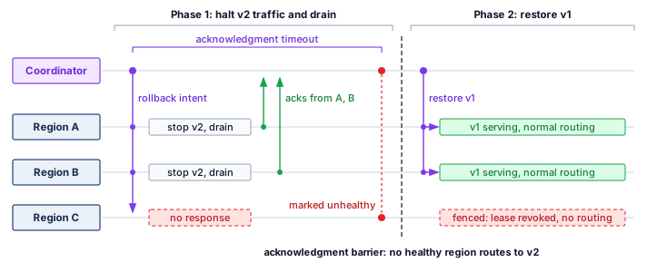
Figure 10: **Two-Phase Multi-Region Rollback**: Time runs left to right on one lane per participant. In phase 1 the coordinator broadcasts rollback intent; regions A and B stop routing new requests to the rejected version (v2), drain in-flight work, and acknowledge. Region C never answers, so when the acknowledgment timeout expires the coordinator marks it unhealthy and fences it. Only after the barrier, when no healthy region still routes to v2, does phase 2 restore the previous version (v1) on the healthy regions; the fenced region stays out of routing until it rejoins under the restored version.

The acknowledgment barrier prevents restoration from completing while reachable regions still route new requests to the rejected version. A timeout alone cannot stop an isolated region from serving; the serving path must enforce a lease, routing exclusion, or equivalent fencing rule. The release contract must specify what happens to in-flight requests and to availability during that interval.

Partial rollback allows rolling back individual regions while others continue. This is appropriate when issues are region-specific (infrastructure problems, regional traffic patterns) rather than model-inherent. The deployment coordinator tracks per-region state and prevents inconsistent global decisions based on partial information.

Multi-region coordination overhead

In an illustrative five-region deployment with an assumed 80 ms one-way delay per coordination leg, each phase transition needs four synchronous legs (announce intent, collect acknowledgments, confirm completion, collect confirmations), about 320 ms, so five canary phases add under two seconds to a rollout measured in hours. Latency is therefore not where coordination costs the release.

The coordination service nevertheless becomes a critical dependency. Its failure policy must specify whether regions may continue serving their last authorized state and whether any further promotion is permitted. A shared activation barrier can halt progress while existing traffic continues; a policy allowing regional independence can permit local progress within its compatibility limits. A bounded-skew contract must stop progress before the bound is exceeded, rather than merely alert afterward. Replicating coordinator state through a consensus protocol can preserve decisions across replica failures while a quorum remains available, but routing enforcement and regional readiness still determine whether those decisions hold in the serving path.

12.5.8 The end-to-end evaluation contract

Shadow runs, experiments, canary stages, and regional waves each produce release evidence, yet a candidate that passes offline accuracy on one dataset, passes latency benchmarks on a lighter synthetic load profile, and enters an online A/B test without a tested rollback target remains unverified as a whole because those checks never evaluated the same release state. Evidence from different stages is useful only when it refers to the same candidate and decision. An evaluation contract is the versioned release record that binds a model and its dependencies to the workload, metrics, statistical design, acceptance thresholds, rollback conditions, and accountable owners. This record is the subject of the evaluation contract principle (21), one of the fleet-in-production principles listed in the opener to this part of the book. It holds that a fleet release decision is valid only when all of its evidence refers to one versioned contract. The record therefore becomes the unit of validity for everything this chapter has built, from registry versions and feature contracts to rollout stages and experiment statistics. Table 15 assembles that record across five evidence planes.

Table 15: End-to-End Evaluation Contract: A model release is accepted against one versioned record spanning offline behavior, production-equivalent performance, specialist assurance, online experimentation, and recovery. Each plane has both an evidence owner and a condition that expires its claim.

Evidence plane	Contract must pin	Acceptance or invalidation rule	Accountable owner
Offline behavior	Evaluation-set version, primary metric, consequential slices, baseline, uncertainty evidence, and robustness tests (developed later, in Common robustness principles)	Promote only if prespecified aggregate and slice bounds hold; invalidate when the population, label definition, or intended use leaves the validated envelope	Model owner and domain reviewer
System performance	Hardware and software envelope, open- or closed-loop workload model, concurrency, request mix, warm-up, p50 and tail latency, throughput, errors, and resource cost	Promote only under the production-equivalent load contract; invalidate when capacity headroom or an SLO budget is exhausted	Serving and site-reliability owners
Responsibility and safety	Fairness slices, privacy and safety evidence, affected-party requirements, and assurance claims (developed later, in The Governance and Assurance Lifecycle)	Promote only when the named claims have sufficient evidence and review; invalidate on a material change, control failure, or unbounded harm signal	Risk owner and governance authority
Online experiment	Assignment unit, holdout, minimum detectable effect, power, sample size, confidence interval, multiple-testing correction, stopping rule, and guardrail metrics	Promote only after the planned decision rule passes; stop and roll back when any guardrail crosses its prespecified threshold	Experiment owner and product decision owner
Recovery and audit	Rollback artifact and dependencies, trigger windows, evidence-retention period, data and code versions, environment, seeds, raw aggregate counts, and approvals	Reject exposure without a tested rollback; reopen the decision when evidence cannot be reproduced or retained for the required review period	Release owner, platform owner, and audit custodian

Acceptance is deliberately distributed, but promotion authority is not ambiguous. The model and domain owners accept predictive utility; the serving owner accepts capacity and reliability; specialist risk owners accept bounded robustness, fairness, privacy, and safety claims. A named release authority promotes only when all required sign-offs refer to the same artifact. The platform automates gates and preserves evidence, but it cannot choose the product objective or waive a failed assurance claim.

Invalidation is the return path through the contract. Drift beyond the evaluated population, a feature or label-definition change, exhausted latency headroom, a statistically supported guardrail regression, or a material governance change sends the candidate back to the owning gate. Thresholds and rollback targets are fixed before exposure so an apparent primary-metric gain cannot redefine success after the result is known. Reproducibility requires retaining the inputs to that decision, not merely its verdict: the dataset and traffic snapshot, model and code versions, environment and hardware envelope, random seeds, assignment and sampling rules, sufficient statistics or permitted logs, approvals, and the exact rollback artifact.

12.5.9 CI/CD patterns by model type

Every workload family shares the five evidence planes of table 15, yet the intended use determines which plane gates promotion: releasing a general-purpose LLM with a two-hour automated check misses subtle safety regressions, whereas holding an emergency fraud-model patch in a two-week human review window lets an active attack drain funds. Table 16 returns to the workload families of table 2, whose cadence and rollback targets still apply, and adds the column that table lacked, what each family must validate before promotion. The listed durations are operating assumptions, not consequences of architecture; label maturity, traffic, and potential harm determine the actual validation and rollback policy.

Table 16: CI/CD Patterns by Model Type: The rows illustrate validation and response policies for different workloads. Their durations are planning assumptions; promotion depends on the required evidence, including outcome-label delay, and rollback depends on a ready compatible target.

Pattern	Model type	Validation focus	Rollout speed	Rollback speed
Quality-gated	LLM	Human eval, safety	Days to weeks	Minutes with warm standby
Metric-driven	Recommendation	Engagement metrics	Hours to days	Minutes
Threshold-gated	Fraud	Precision/recall	Hours	Seconds
Accuracy-focused	Vision	Classification metrics	Days	Minutes

For a broadly capable LLM, evaluation must cover consequential uses that aggregate benchmarks can miss. Automated tasks such as MMLU and HumanEval screen selected capabilities; human review and adversarial probes examine additional failure modes; shadow traffic tests operational behavior on live inputs. A planning window of 2–4 weeks may accommodate these activities and staged observation, but elapsed time is not the acceptance criterion. The required evidence depends on the changed capabilities and the service’s exposure policy.

Recommendation pipelines balance freshness with statistically defensible comparison. Offline NDCG and recall can screen candidates, interleaving can compare ranker preference, and A/B tests measure the selected product outcomes. A 24–48-hour rollout is feasible only when traffic and outcome timing supply the required evidence within that interval. Promotion and rollback follow the prespecified rules rather than a fixed refresh deadline.

Fraud models add adversarial urgency, but confirmed outcomes can arrive after the decision window. Historical labeled cases and shadow scoring provide evidence before exposure; neither makes fresh precision and recall immediately observable. The release policy must state what evidence supports an urgent change, what uncertainty remains, and who accepts its bounded exposure. Rapid routing to a validated fallback can contain harm while additional labels accumulate, provided that fallback remains suitable for the current threat.

Edge fleets, absent from the table, apply the same contract to weeks-long rollouts that leave many model versions active at once, to devices whose memory and thermal limits require hardware-in-the-loop validation, and to telemetry that privacy rules limit to federated aggregates. Fleet release controls develops these release controls, including why the devices that report health do not represent the deployed fleet.

Whether a model runs in a data center or on a phone, a CI/CD pipeline promotes candidates supported by evidence within a specified operating envelope. Production can move outside that envelope as data, traffic, and dependencies change. Monitoring must therefore preserve the release contract after promotion, detect when its evidence no longer applies, and return the affected model to evaluation or recovery.

Self-Check: Question

In the described social recommendation experiment, treatment users share boosted content with control users. Why does this violate the no-interference component of the Stable Unit Treatment Value Assumption (SUTVA)?
1. Individual user hashing causes GPU thread divergence on inference accelerators.
2. Social networks disallow collecting engagement metrics across control groups due to data privacy regulations.
3. User randomization forces feature stores to duplicate user embeddings across all regional caches.
4. Treatment users share boosted content with control users, making control outcomes depend on other users’ treatment assignments.
When an ML platform evaluates 20 simultaneous A/B experiments across a model portfolio, why might the team adopt the Benjamini-Hochberg False Discovery Rate (FDR) procedure instead of the Bonferroni correction?
1. Bonferroni correction divides alpha by the number of tests ($0.05 / 20 = 0.0025$), creating an overly conservative threshold that inflates Type II errors (false negatives) and discards real model gains.
2. The Benjamini-Hochberg procedure eliminates the requirement for computing statistical significance or p-values.
3. Bonferroni correction can only be applied to computer vision models running on mobile edge devices.
4. The Benjamini-Hochberg procedure mathematically guarantees that zero false discoveries occur across any number of tests.
What three criteria must be evaluated within an automated ‘performance gate’ function before a candidate model is approved for staging deployment?
A model serves 1 million requests per hour and its canary plan needs about 10,000 samples per variant. Why should each canary stage’s duration be computed from that planned sample rather than set by elapsed time, and what sets the length of the whole rollout schedule?
The formal statistical assumption that an experimental unit’s outcome is unaffected by the treatment assignments of other units is abbreviated as ____.
Arrange the standard stages of an end-to-end automated ML training and release pipeline in execution order:

Automated evaluation against baseline and slice performance gates
Artifact packaging with serving configuration and registration in model registry
Data validation and schema verification
Distributed training execution with lineage logging
Feature engineering and transformation

See Answers →

12.6 Monitoring at Scale

Application-layer drift detection depends on a healthy physical substrate. At fleet scale, a degraded NVLink connection or a thermally throttling GPU can masquerade as a software timeout. Monitoring therefore starts bottom-up with fleet telemetry, then climbs through alert aggregation, model-quality signals, and dashboards so that operators can route a symptom to the layer that can repair it.

12.6.1 Fleet telemetry and hardware observability

Under an illustrative independent-failure model, a 50,000-hour per-GPU planning interval gives a 10,000-GPU cluster a hardware failure roughly every five hours—and the full-system interval of Cluster MTBF calculation is shorter still. Because failure is routine at pod scale, fleet monitoring and hardware observability are prerequisites for productive training. Recovering in 10 minutes rather than hours depends on detection, usable recovery state, replacement capacity, and restart procedures, so the monitoring system is itself a distributed service collecting telemetry across devices, switches, and cooling components.

The telemetry spans three physical levels. At the GPU level, junction temperature tracks cooling degradation, error-correcting code (ECC) counts in high-bandwidth memory (HBM) and SRAM track memory health (a rising rate of correctable errors can precede an uncorrectable, job-ending error), and streaming multiprocessor (SM) utilization shows whether the device is doing work. None alone identifies the cause: low utilization can reflect input starvation, synchronization, or a device problem. At the network level, retry counters on individual ports can point to a failing cable or switch; at the facility level, coolant temperature deviations can trigger load shedding before thermal limits force throttling. Correlating these signals with workload and topology lets responders narrow the failure domain before deciding whether to reduce load, quarantine hardware, or investigate software.

Correlation analysis helps locate the scope of a shared disturbance. Elevated temperature on one GPU motivates local inspection; simultaneous changes across 8 GPUs in a node suggest checking shared cooling and workload changes. A rack-wide pattern adds the coolant distribution unit (CDU) and rack-level load to the investigation, while a multi-rack pattern raises facility-level hypotheses. These patterns guide diagnosis rather than prove a cause. Grouping related alerts preserves that context and avoids presenting one shared event as hundreds of unrelated failures.

Telemetry capacity follows the series count, sample rate, bytes per observation, retention, and indexing policy. Sampling one metric every second across 10,000 GPUs produces 864 million observations per day before other metrics or labels are added. A daily byte total or monitoring-budget share cannot be inferred without the encoding and retention assumptions. The platform therefore bounds label cardinality and provisions ingestion, storage, and queries as an explicit platform workload.

Before allocating a long training job, a scheduler can use automated preflight checks to screen its nodes. General matrix multiply (GEMM) benchmarks exercise arithmetic throughput, NCCL AllReduce tests exercise collective paths, and memory stress tests look for errors under load. Results must be compared with baselines for the same hardware and configuration before a node is quarantined. Preflight consumes startup time and cannot reveal every fault; its value depends on the failed work it avoids and the cost of unnecessary exclusions.

One slow accelerator stalls every peer at the barrier.

A gray failure leaves a component responsive while degrading its useful performance. In synchronous data-parallel training, a persistently slow participant can delay collective completion even when every device passes an availability check. Per-rank timing and hardware telemetry help localize the slowdown; controlled microbenchmarks can then compare suspected nodes with healthy peers. An illustrative policy flags GEMM throughput below 90 percent of a matched fleet median or NVLink bandwidth below 85 percent. Those thresholds require calibration for hardware generation, software, load, and measurement variability. A low result warrants investigation rather than proving a hardware defect, because configuration and contention can produce similar symptoms.

↩︎ Gray failures and the straggler detection that exposes them are established in Stragglers versus fail-stop failures.

In multi-tenant clusters, shared links can also couple otherwise separate workloads, so fabric telemetry must attribute congestion to the tenant that caused it. The isolation mechanisms that bound such interference, along with their limits, are established in Traffic isolation and quality of service.

Checkpoint cadence is the point where hardware telemetry becomes visible to ML operators rather than only to data-center technicians. A degraded node that forces frequent checkpoint recovery, or a storage path that lengthens checkpoint writes, turns directly into lost training throughput. The Young-Daly checkpoint interval derives the checkpoint-compute trade-off and the Young-Daly interval; the operations responsibility here is to expose the telemetry those formulas depend on: write time, failure rate, straggler behavior, and recovery duration. Without that visibility, a platform may report that a job is “running” while useful learning has quietly collapsed behind retries and slow checkpoints.

With the physical substrate accounted for, monitoring returns to the deployed model fleet. Validation and canary evidence cover a candidate under observed conditions; production can later change abruptly or drift over weeks and months. Monitoring must therefore retain acute-failure controls while detecting gradual loss of quality. Independently paging on every model metric can multiply notifications from a shared event and create alert fatigue. Fleet-level aggregation connects those symptoms while preserving urgent local signals that require immediate action.

12.6.2 The alert fatigue problem

When 100 models each expose 10 monitored metrics checked every five minutes, even a calibrated 3-sigma threshold with a 0.3 percent false-positive rate per check generates hundreds of false threshold crossings every day. Whether those crossings become pages depends on the alerting policy.

Napkin Math 12.7: False alarms across many checks

Problem: Consider a system monitoring 100 models. Each model has 10 metrics (latency, accuracy, drift, and others). Alert thresholds are set at 3-sigma (99.7 percent specificity), and a control script re-evaluates every metric on a fixed interval. Assume calibrated stable Gaussian null behavior and count raw threshold crossings before grouping or suppression; those crossings are not necessarily distinct incidents.

Math:

Total Monitors: 100 models $\times$ 10 metrics = 1,000 monitors.
False Positive Rate: $1 - 0.997 = 0.003$ (0.3 percent).
Checks per day: Assume checks every 5 minutes (288 checks/day).
Daily false threshold crossings: $1,000 \times 288 \times 0.003$ $\approx$ 864 alerts/day.

Systems insight: Even with high-specificity (3-sigma) alerts, scale becomes problematic. Aggregation, deduplication, persistence windows, and calibrated thresholds reduce repeated notifications. Specific safety or hardware-failure alerts must still trigger independently when their contracts require immediate action.

False alerts become near-certain as checks multiply.

The multiple-testing problem from concurrent experiments (section 12.5.3.7) also appears in monitoring. For independent checks under the null, each with false positive rate $\AlertFalsePositiveRate$, equation 9 shows that the probability of at least one false alert approaches certainty as the number of tests $\AlertCheckCount$ grows, because the probability of no false alert decays exponentially:

\[\Pr(\text{at least one false alert}) = 1 - (1 - \AlertFalsePositiveRate)^{\AlertCheckCount} \tag{9}\]

The equation holds at any per-check rate, and teams under pressure to catch regressions sooner often loosen thresholds. Loosening the notebook’s 3-sigma thresholds to 2 sigma raises the per-check rate from 0.3 percent to roughly $\AlertFalsePositiveRate= 0.05$. With that rate and $\AlertCheckCount= 1000$ (100 models $\times$ 10 metrics):

\[\Pr(\text{false alert}) = 1 - (1 - 0.05)^{1000} = 1 - 0.95^{1000} \approx 1.0\]

The probability is essentially 100 percent for this collection of independent checks. This result establishes the likelihood of at least one false crossing, not the fraction of alerts that are false. Repeated checks compound the operational burden when every crossing generates a page, and frequent nonactionable pages can train operators to discount the alert stream, making genuine incidents harder to recognize. For the notebook’s fleet of 100 models with 10 metrics checked every 5 minutes, the 5 percent rate raises the daily raw crossings far above the 3-sigma count.

Expected daily false alerts: $\text{Daily false alerts} = 100 \times 10 \times 0.05 \times \frac{24 \times 60}{5} = 14,400$.

Even if 99 percent of these crossings are deduplicated or auto-resolved, the remaining 144 alerts daily would impose a substantial interruption burden if each became a page. Comprehensive telemetry therefore needs a policy that separates diagnostic records from notifications requiring immediate action.

12.6.3 Hierarchical monitoring architecture

When a shared feature store stalls, paging twenty downstream model teams simultaneously floods on-call rotations without telling anyone that the root cause sits in shared infrastructure. To prevent uncoordinated alarm floods, hierarchical monitoring arranges telemetry as a four-tier triage pyramid that maps operational scope from component health at the base to fleet-wide business impact at the apex (figure 11). Broad signals reveal fleet impairment, portfolio signals route incidents to the owning model family, and granular model or infrastructure telemetry supports local diagnosis. Routine fluctuations remain diagnostic records, while urgent local failures still page their owners without waiting for a fleet-wide signal. The hierarchy provides context for routing and grouping alerts while preserving those immediate response paths.

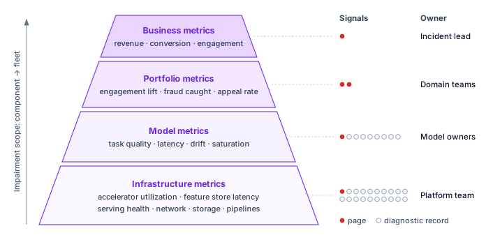
Figure 11: **Hierarchical Monitoring Architecture**: To prevent alert fatigue, monitoring operates at four levels, each with its own owner. Business and portfolio metrics raise the few alarms that indicate broad impairment and route each incident to the owning model family, while model and infrastructure metrics serve primarily for diagnosis and root-cause analysis.

The hierarchy works because each level answers a different routing question and has a different owner, from the incident lead who watches business impairment to the platform team that repairs capacity, networking, and storage failures (table 17).

Table 17: Hierarchical Monitoring Levels: Monitoring levels organize incident scope and ownership. Broad signals route shared incidents, while urgent local failures can page their owners directly; evidence at every level supports diagnosis of model, data, serving, or infrastructure causes.

Level	Representative signals	Primary owner	Operational role
Business	Revenue or conversion attributed to recommendations, engagement indicators, automation rate, and human-review volume.	Incident lead	Few high-confidence alerts that indicate product or business impairment.
Portfolio	Engagement lift and diversity for recommendation, fraud caught and false-positive rate, or violation detection and appeal rate.	Domain team	Routes investigation to the model family or product area that owns the shared objective.
Model	Task quality, latency distributions, throughput, error rates, resource utilization, serving saturation, and recent deployment state.	Model owner	Supports local diagnosis after business or portfolio signals move.
Infrastructure	GPU cluster utilization and availability, feature store latency, training pipeline time, serving health, networking, and storage.	Platform team	Routes failures that require capacity, placement, networking, storage, or control-plane repair.

Multidimensional reliability budgets

A fleet cannot summarize reliability with availability alone. An endpoint may return HTTP 200 while serving stale features, missing its latency target, or producing predictions below the quality floor. Each service therefore needs an SLO vector

\[ \SloVector= (\AvailabilityObjective, \LatencyObjective, \FreshnessObjective, \QualityObjective), \]

with one indicator, target, measurement window, and owner for every dimension. For dimension $\ReliabilityTargetIndex$, the normalized budget consumption over a window is

\[ \ErrorBudgetConsumption_{\ReliabilityTargetIndex} = \frac{\ObservedViolationFraction_{\ReliabilityTargetIndex}}{\AllowedViolationFraction_{\ReliabilityTargetIndex}}, \]

where $\ObservedViolationFraction_{\ReliabilityTargetIndex}$ is the fraction of eligible observations that violate target $\ReliabilityTargetIndex$ and $\AllowedViolationFraction_{\ReliabilityTargetIndex}$ is the allowed violating fraction for that same target and window. The numerator and denominator have identical units within each dimension: failed-request fraction for availability, late-request fraction for latency, stale-prediction fraction for freshness, and below-floor evaluation fraction for model quality. The quality contract must define its evaluation units, label delay, and coverage; unlabeled predictions cannot silently count as passing observations. A value $\ErrorBudgetConsumption_{\ReliabilityTargetIndex}=1$ exhausts that dimension’s budget; $\ErrorBudgetConsumption_{\ReliabilityTargetIndex}>1$ exceeds it. Ratios may be compared after this normalization, but raw latency, freshness, and quality magnitudes are not commensurable. The fleet remains inside its measured reliability envelope only when $\max_{\ReliabilityTargetIndex} \ErrorBudgetConsumption_{\ReliabilityTargetIndex} \leq 1$, the reliability half of the evaluation contract (principle 21). Averaging would hide a severe regression behind healthy dimensions. A service whose freshness budget is overspent can still report a comfortable mean consumption, yet the maximum stops its promotion (figure 12). Missing or stale evidence requires its own release policy rather than an assumed pass.

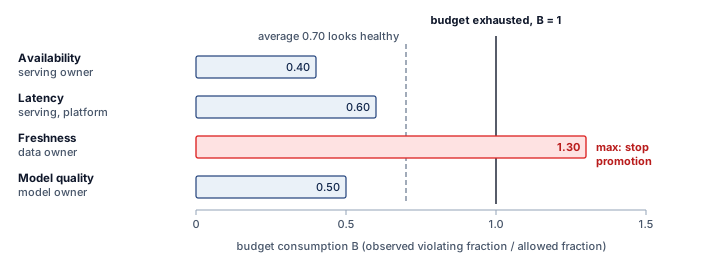
Figure 12: **Reliability as a Vector of Budgets**: Each bar is one dimension’s budget consumption, its observed violating fraction divided by the allowed fraction, with the owner of that dimension beside it. The values are illustrative. Availability, latency, and quality sit inside their budgets and the four-dimension average is 0.70, but freshness has spent 1.30 of its budget; because the maximum, not the average, governs, the service stops promotion until the data owner restores freshness.

Burn rate converts this vector into an operating control. For dimension $\ReliabilityTargetIndex$, the burn rate is the observed violating fraction over a short recent interval divided by the allowed fraction $\AllowedViolationFraction_{\ReliabilityTargetIndex}$, so it measures how fast the budget is being spent relative to the pace that would exhaust it exactly at the end of the window. A burn rate of 1 spends the budget on schedule; a burn rate of 10 would exhaust the whole window’s budget in a tenth of the window. A fast burn in any dimension pages the owning team and stops promotion; sustained moderate burn reduces rollout velocity and requires remediation; an exhausted budget freezes nonessential releases until the responsible indicator returns inside its recovery policy. The platform owns indicator computation, common windows, alert routing, and enforcement. Model teams own task-quality thresholds and remediation for model behavior; data owners own freshness and validity; serving owners own latency and availability. This division turns monitoring into an explicit contract between evidence and authority rather than a dashboard that everyone can see but no one must act on, and each exhausted dimension triggers a release consequence its own owner carries out (table 18).

Table 18: ML Reliability Budget Vector: Fleet reliability joins service health, data freshness, and model behavior. Any exhausted dimension can stop a release because success in one dimension cannot compensate for failure in another.

Budget dimension	Representative indicator	Primary owner	Release consequence
Availability	Successful eligible requests/total requests	Serving	Halt rollout or fail over when fast burn exceeds policy
Latency	Requests meeting the tail-latency objective	Serving/platform	Reduce traffic, capacity pressure, or candidate complexity
Freshness	Predictions using features inside freshness SLO	Data	Block promotion and fall back to a safe feature path
Model quality	Slice-aware task metric above its quality floor	Model/domain	Roll back, abstain, or route to a validated baseline

12.6.4 Anomaly detection across the fleet

When 60 of 100 models cross their control limits at the same timestamp because a shared feature pipeline broke—or when user input distributions shift days before ground-truth labels arrive—per-model static thresholds cannot distinguish a local bug from a fleet-wide event. Fleet-wide anomaly detection adds portfolio context to individual metric thresholds. The detection stack proceeds from local statistical process control, to correlation across model families, to drift scores that characterize changes in data distributions. Each stage narrows the investigation, but none establishes a cause by itself. Grouping related signals can reduce duplicate pages while retaining the evidence needed to route an incident to the right owner.

Statistical process control

Statistical process control originated in industrial quality control (Shewhart 1931). When adapted for ML monitoring, control charts¹⁰ track whether metric distributions remain stable over time and complement drift-detection methods that watch for changing data distributions (Gama et al. 2014). The core idea is distinguishing common cause variation (normal fluctuation) from special cause variation (genuine anomalies).

¹⁰ Statistical process control (SPC): Shewhart (1931) established the control-chart framework for manufacturing quality control. Under a normal approximation, a 3-sigma control limit produces a false-alarm probability of only 0.27 percent for a stable process. For ML fleet monitoring, even small per-test false-alarm rates compound across many models and metrics, making alert-fatigue management an inherent constraint of applying SPC at platform scale.

Shewhart, Walter A. 1931. Economic Control of Quality of Manufactured Product. D. Van Nostrand Company.

Gama, João, Indrė Žliobaitė, Albert Bifet, Mykola Pechenizkiy, and Abdelhamid Bouchachia. 2014. “A Survey on Concept Drift Adaptation.” ACM Computing Surveys 46 (4): 1–37. https://doi.org/10.1145/2523813.

For a metric $\MonitoredMetric$ with established mean $\MonitoredMetricMean$ and standard deviation $\MonitoredMetricStandardDeviation$, the upper control limit is $\text{UCL} = \MonitoredMetricMean+ 3\MonitoredMetricStandardDeviation$ and the lower control limit is $\text{LCL} = \MonitoredMetricMean- 3\MonitoredMetricStandardDeviation$. Points outside control limits or systematic patterns, such as 7 consecutive points above or below the mean, trigger investigation. Adding pattern rules changes the combined false-alarm rate; the single-check 3-sigma rate no longer describes the entire policy. Calibration must also account for seasonality and temporal dependence in the monitored metric.

Fleet-wide correlation

When multiple models show similar anomalies simultaneously, shared infrastructure or an upstream data pipeline becomes a candidate cause. Correlation analysis across the fleet supports three operational tasks: identifying shared dependencies to investigate, grouping related alerts into an incident, and prioritizing triage based on the breadth of downstream impact. As shown in listing 6, the fraction of anomalous models can guide escalation from model-by-model debugging to a coordinated investigation. Crossing that threshold does not establish a shared failure; dependency records, deployment timing, and component telemetry must support the attribution.

Listing 6: Fleet Anomaly Attribution: Detecting correlated anomalies across a model fleet and attributing them to shared infrastructure or data causes.

def detect_fleet_anomaly(model_metrics, threshold=0.6):
    """
    Detect correlated anomalies across model fleet.

    Returns list of (timestamp, affected_models, likely_cause) tuples.
    """
    anomalies = []

    for timestamp in model_metrics.timestamps:
        # Identify models with anomalous metrics at this time
        anomalous_models = []
        for model in model_metrics.models:
            if is_anomalous(model_metrics[model][timestamp]):
                anomalous_models.append(model)

        # Check if anomaly fraction exceeds correlation threshold
        if (
            len(anomalous_models) / len(model_metrics.models)
            > threshold
        ):
            # Many models affected -> likely shared cause
            cause = attribute_to_shared_cause(
                timestamp, anomalous_models
            )
            anomalies.append((timestamp, anomalous_models, cause))

    return anomalies

The threshold controls when the monitor escalates to a fleet-wide investigation. A low threshold increases sensitivity and investigation load; a high threshold can miss failures affecting a smaller but critical subset of models. Above the threshold, the incident coordinator uses shared dependencies to identify candidate owners, while affected model teams retain responsibility for local containment.

Drift detection

Distribution changes can invalidate the population assumptions behind a release even while service health remains normal. Monitoring must distinguish a change in inputs from a change in the input-output relationship; neither an input alarm nor a healthy input histogram alone establishes model quality.

Covariate shift moves the input distribution $\ProbabilityFunction(\ModelInput)$ while the input-output relationship holds, so label-free input monitoring can detect the move but cannot confirm that the relationship stayed fixed. Concept drift changes the relationship $\ProbabilityFunction(\ExampleLabel\mid \ModelInput)$ itself, so detecting it requires ground-truth labels that often arrive minutes, days, or weeks late.

↪ The full shift taxonomy, including label shift, and the evidence that distinguishes one kind of drift from another are developed in Distribution shift and concept drift.

Because labels are often delayed, most real-time monitoring systems use input drift as a leading indicator of possible performance degradation. A cheap drift score is valuable even when it is not a complete theory of robustness because it tells the operator where to investigate before outcome labels arrive.

For continuous features, the population stability index (PSI)¹¹ quantifies distribution shift (Yurdakul and Naranjo 2020). Equation 10 computes PSI as the sum of log-ratio weighted differences between actual and expected bucket proportions. In platform operations, PSI plays a narrow role as an inexpensive alerting signal.

¹¹ Population stability index (PSI): Bands such as $\text{PSI} < 0.1$ for routine monitoring and $\text{PSI} \geq 0.25$ for investigation are heuristics, not guarantees of stability or model failure. Once histograms are available, the comparison uses bucket proportions rather than individual records. Histogram construction, sample size, binning, and treatment of empty buckets still affect cost and interpretation, so the platform must calibrate the signal on its own data.

Yurdakul, Bilal, and Joshua Naranjo. 2020. “Statistical Properties of the Population Stability Index.” The Journal of Risk Model Validation 52. https://doi.org/10.21314/jrmv.2020.227.

\[\text{PSI} = \sum_{\ReferenceBinIndex=1}^{\PopulationStabilityBinCount} (\CurrentBinProportion_{\ReferenceBinIndex} - \ReferenceBinProportion_{\ReferenceBinIndex}) \times \ln\left(\frac{\CurrentBinProportion_{\ReferenceBinIndex}}{\ReferenceBinProportion_{\ReferenceBinIndex}}\right) \tag{10}\]

where $\CurrentBinProportion_{\ReferenceBinIndex}$ is the proportion in bucket $\ReferenceBinIndex$ of the actual (current) distribution, $\ReferenceBinProportion_{\ReferenceBinIndex}$ is the proportion in bucket $\ReferenceBinIndex$ of the expected (reference) distribution, and $\PopulationStabilityBinCount$ is the number of buckets.

An illustrative policy uses these coarse bands to route investigation. PSI below 0.1 leaves the model in the normal monitoring path; values between 0.1 and 0.25 create an investigation ticket; values at or above 0.25 escalate review of the shifted inputs and affected predictions. These actions depend on local calibration. A high PSI does not establish degraded model quality, and a low PSI does not establish that quality remains acceptable.

Napkin Math 12.8: Time-to-detection: Monitoring lag

Problem: A production model has a baseline accuracy of 95 percent. A data drift event causes accuracy to fall to 93 percent. If labeled outcomes arrive at 1000 samples/hour, what collection time supports the stated detection-power calculation, assuming an independent baseline sample of the same size and immediately available labels?

Math: Detection requires enough samples to distinguish the signal (the 2-percentage-point drop) from the noise (random variance). The sizing logic of equation 4 applies, in its unpooled form because the baseline and degraded accuracies ($\ComparedPeriodAccuracy_1$, $\ComparedPeriodAccuracy_2$) differ, with the same confidence and power targets ($\ConfidenceCriticalQuantile$, $\PowerCriticalQuantile$):

\[\DriftTestSampleSize\approx \frac{(\ConfidenceCriticalQuantile + \PowerCriticalQuantile)^2 \left[ \ComparedPeriodAccuracy_1(1 - \ComparedPeriodAccuracy_1) + \ComparedPeriodAccuracy_2(1 - \ComparedPeriodAccuracy_2) \right]}{(\ComparedPeriodAccuracy_1 - \ComparedPeriodAccuracy_2)^2}\]

Samples Required: At 95 percent confidence and 80 percent power, the standard normal quantiles are $\ConfidenceCriticalQuantile = 1.96,\ \PowerCriticalQuantile = 0.84$, and plugging in gives $\DriftTestSampleSize \approx (1.96 + 0.84)^2 \times \left[ 0.95(1 - 0.95) + 0.93(1 - 0.93) \right] / (0.95 - 0.93)^2 \approx 2,207$ samples.
Detection Latency: 2,207 samples / 1000 samples/hour $\approx$ 2.2 hours.

Systems insight: Monitoring is not instantaneous. The computed duration is a planned collection time at 80 percent power, not a guaranteed detection deadline. It assumes an independent baseline sample, the stated post-change rate, and immediately available labels. Delayed labels, dependence, and repeated testing change the detection contract. Input drift can provide an earlier investigation signal, but it does not establish a quality regression by itself.

Fleet-wide drift monitoring extends that signal across the portfolio. A PSI spike in one noncritical feature may be a local investigation, while simultaneous drift across shared features or dependent models warrants a broader investigation. A shared data pipeline failure is one candidate cause; a genuine change in the population served can produce the same pattern. Pipeline checks and outcome evidence distinguish a data defect from a change to which the models must adapt. Whether a confirmed shift calls for retraining, adaptation, or no change is a model decision developed in Retraining decision framework; the fleet monitor’s responsibility ends when calibrated evidence reaches the owner who makes that decision.

12.6.5 Model-type specific monitoring

A fraud detector watching for active card-testing attacks, a recommendation ranker watching real-time click-through rates, and an LLM assistant watching for toxic or hallucinated generations cannot share one monitoring metric or polling interval. Monitoring cadence follows failure cost, label delay, and traffic volume. The same workload families that set release cadence in table 2 and validation focus in table 16 now need a post-promotion counterpart: which metric each watches and how often. The illustrative parameters in table 19 must be calibrated to the service, because a frequently updated metric is useful only if enough observations support the alert decision.

Table 19: Illustrative Monitoring Policies: Example metrics, thresholds, and collection frequencies. None is a universal requirement of a model family. Label availability, sample size, failure cost, and the required detection delay determine the production policy.

Model type	Primary metrics	Alert thresholds	Monitoring frequency
Recommendation	CTR, engagement lift	5% relative drop	Real-time
Fraud Detection	Precision, recall, fraud rate	1% degradation	Real-time
LLM	Quality scores, safety metrics	Per-model calibration	Hourly
Vision	Accuracy by class	Dataset-specific	Daily
Search Ranking	NDCG, click position	2% degradation	Real-time

Recommendation monitoring must respond quickly to user impact, but each metric becomes informative on its own observation timescale. Click-through rate, dwell time, and conversion rate should be compared against time-matched historical baselines, control traffic when available, and the previous model version after a release. Conversions can arrive later than clicks, and sparse traffic can delay a reliable comparison. Engagement metrics alone also leave gaps; diversity, catalog coverage, and filter-bubble indicators track longer-term concerns, while revenue attribution and promotional-inventory metrics connect recommendation quality to business outcomes.

Fraud monitoring binds on adversarial urgency. Missed fraud creates immediate financial loss, but excessive false positives create customer friction and manual-review load. The monitoring surface therefore has to pair detection rate, prevented dollar amount, and detection latency with false-positive rate, blocked-legitimate-transaction events, manual-review volume, and adversarial indicators such as probing patterns or sudden shifts in fraudulent behavior.

LLM monitoring binds on semantic quality, which is difficult to measure from service metrics alone. Latency, token generation rate, error rate, and safety-classifier scores establish operational health; user satisfaction signals such as thumbs-up/thumbs-down rates, regeneration rate, and task-completion proxies add delayed quality evidence. Safety metrics such as toxicity detections, refusal rate, and hallucination indicators remain partial, so they should trigger review rather than claim complete coverage.

Service-health metrics alone cannot detect semantic safety failures such as persuasive misinformation or skilled manipulation. Here, red teaming supplies an additional monitoring channel: human evaluators or automated probes attempt jailbreaks before deployment, and a smaller continuous probe set checks production behavior against known failure cases. Sampling outputs for delayed human review adds evidence about failures that automated metrics miss. Neither a passing probe set nor a reviewed sample establishes complete safety coverage.

12.6.6 Observability architecture

When a single user request traverses ten inference services and suffers a 50 ms tail-latency spike or a silent accuracy regression, independent service counters cannot tell investigators which stage stalled, while unsampled logs from 10,000 nodes can flood the telemetry backend during the outage. Effective monitoring therefore requires observability infrastructure that preserves enough context to route an alert from symptom to owner. The metrics, logs, and traces that make up that infrastructure were introduced for debugging a single distributed job; at fleet scale the same channels must route evidence across many models and owners. Metrics show that a service property moved outside its envelope, traces show where a request spent time, logs identify which component emitted the abnormal event, and prediction logs connect system health back to model behavior. Distributed tracing,¹² exemplified by Google’s Dapper system (Sigelman et al. 2010), preserves a request’s path across inference services so investigators can locate latency contributions. Taken together, the channels form an evidence map rather than a set of disconnected telemetry tools, with each channel matched to the operational question it answers (table 20).

¹² Distributed tracing: Google’s 2010 Dapper paper describes propagating trace context across service boundaries while controlling collection overhead through sampling and instrumentation in common libraries. In a multi-model pipeline, the resulting trace connects stage timings to the same request rather than requiring investigators to infer the path from independent service summaries. Without it, a 50 ms tail-latency spike in a 10-model pipeline must be investigated in all 10 models separately. Sampling and instrumentation coverage determine which requests and stages remain visible.

Sigelman, Benjamin H, Luiz André Barroso, Mike Burrows, Pat Stephenson, Manoj Plakal, Donald Beaver, Saul Jaspan, and Chandan Shanbhag. 2010. Dapper, a Large-Scale Distributed Systems Tracing Infrastructure. Dapper-2010-1. Google.

Table 20: Observability Signals by Operational Question: Observability architecture is an evidence-routing system. Metrics trigger attention, traces localize the request path, logs explain component behavior, and prediction logs connect operational symptoms to model quality.

Evidence channel	Primary question	What it preserves	Typical failure revealed
Metrics	Which service property moved out of bounds?	Real-time streams for alerting and aggregated time series for trends	Drift, saturation, error-rate spikes, cost anomalies
Traces	Where did this request spend time?	Request IDs propagated across model invocations, timing, and resources	Cross-model latency, fan-out failures, hot stages
Logs	Which component emitted the abnormal event?	Structured events with consistent schemas and searchable indexes	New error classes, dependency failures, bad releases
Prediction logs	Did system health preserve model behavior?	Sampled inputs, outputs, features, and delayed labels	Accuracy regressions, bad cohorts, data gaps

↩︎ The observability pillars for a single distributed job are established in Observability pillars.

The channels also grow at different rates, which decides what the platform can afford to collect continuously. Metrics stay compact only while the number of distinct time series is bounded. Each label combination creates another series, so a request identifier or an unbounded user label can overwhelm monitoring even when each sample is small. Logs grow with recorded events and traces with spans, so both are sampled or aggregated at fleet scale; when 10,000 edge nodes or hundreds of microservices emit at once, unsampled telemetry can become a thundering herd that perturbs the production system it is meant to observe. Effective platforms therefore present high-level metric dashboards by default and open lower levels only when an anomaly warrants investigation.

Prediction logging can be expensive because it records model-facing data rather than compact service counters. Production systems therefore sample it deliberately, for example logging 1 percent of predictions or retaining additional examples from cohorts under investigation. The sample must serve the intended analysis; a debugging sample concentrated on failures does not directly estimate fleet-wide accuracy. Recording the selection policy alongside inputs, outputs, and eventual labels preserves the context needed to interpret the evidence without making every prediction a permanent storage record.

12.6.7 Dashboard design

Sampling metrics, logs, and traces keeps telemetry storage bounded, yet a single all-purpose dashboard still fails both ends of an outage: an executive checking whether the business is impaired gets lost in per-GPU trace spans, while an on-call responder diagnosing a tail-latency spike is stuck staring at a high-level portfolio summary. A dashboard is the human attention surface of the monitoring hierarchy, and it should answer routing questions without forcing every reader into the same debugging console. Executives need to know whether the business is impaired, domain owners need to know which portfolio is failing, model owners need the evidence for their model, and incident responders need the trace from symptom to root cause. Each view therefore answers one question at one level of detail (table 21).

Table 21: Dashboard Views by Operational Question: Dashboard hierarchy should route attention from business impact to root cause. Each view reveals the amount of detail needed for the decision at that level, preventing executive views from becoming debugging consoles and investigation views from becoming portfolio summaries.

View	Question answered	Signals to surface
Executive	Is the business impaired?	Platform health, business impact, active incidents, key trends
Portfolio	Which domain or model family is driving the impairment?	Model inventory, portfolio metrics, recent deployments, resource utilization and cost
Model	What changed for the responsible model?	Current metrics vs. baselines, deployment history, drift indicators, cost attribution
Investigation	Why did the change occur?	Cross-model correlations, time-series overlays, log search, request-level trace detail

The same views carry cost as one more monitored dimension: the portfolio and model views surface spend beside quality and latency, and section 12.9.7.3 develops the anomaly detection that watches that spend. Even a well-instrumented fleet does not prevent failures. The monitoring hierarchy detects them; what remains is the response, which must classify the symptom, contain its impact, and route it to an owner with the authority to act.

Self-Check: Question

Why are ‘gray failures’ (e.g., an accelerator whose GEMM arithmetic throughput drops by 20% or an NVLink connection suffering intermittent packet retries) exceptionally damaging in large synchronous distributed training runs?
1. Gray failures trigger automatic emergency power-off sequences across the entire datacenter hall.
2. A degraded rank or link on the communication critical path can delay collective completion and the next training step while ordinary availability checks remain healthy.
3. Gray failures cause the training loss optimizer to invert gradient signs during backpropagation.
4. The Kubernetes control plane immediately unmounts shared file systems when a GPU runs slowly.
If 8 GPUs in one server chassis show elevated junction temperatures while adjacent nodes remain normal, which local cooling hypothesis should the investigation prioritize?
1. Failure of the building’s central chiller cooling plant.
2. An optical transceiver failure on the top-of-rack InfiniBand switch.
3. A localized node-level failure, such as a chassis fan malfunction or a cold-plate coolant flow restriction.
4. A software bug in the Prometheus time-series database metric scraper.
In a fleet of 100 models with 10 metrics each, checked every 5 minutes at a threshold with false positive rate $\alpha = 0.003$, calculate expected raw false threshold crossings per day. How should monitoring distinguish these crossings from operator pages?
Describe the four levels of a hierarchical monitoring architecture for ML platforms and identify the primary owner and operational role of each level.
Automated hardware preflight checks necessarily reduce overall training productivity because they add job startup latency.
Hardware memory errors corrected automatically without crashing an application are called ____ errors; an elevated rate can warrant investigation before an uncorrectable failure.

See Answers →

12.7 Production Debugging and Incident Response

At 3:00 AM, PagerDuty alerts the on-call engineer that revenue from the core recommendation system has dropped 15 percent in the last hour. The servers are healthy, the latency is normal, and there are no exception logs. Conventional software can also return incorrect results silently, but machine learning adds failures rooted in data and statistical behavior while ordinary service-health signals remain normal. Debugging production ML systems therefore requires investigative frameworks that reach beyond code and infrastructure.

When production debugging consumes a large share of engineering attention, platform scale multiplies the complexity because failures may originate in data pipelines, model code, infrastructure, or emergent interactions between components that no single team owns end to end. Effective incident response therefore classifies the symptom and contains impact while attribution proceeds, then converts the incident into a stronger platform control. A known safe containment action need not wait for complete root-cause analysis.

War Story 12.1: The control plane that disappeared (2021)

Context: Meta’s global backbone connected its data centers and carried dependencies whose loss also made DNS and internal recovery tools unavailable (Janardhan 2021).

Mechanism: On October 4, 2021, a maintenance command intended to assess backbone capacity disconnected the data centers. A bug in the command-audit tool failed to stop it. DNS servers then withdrew their Border Gateway Protocol (BGP) advertisements, the routing announcements that tell other networks how to reach them, after losing data-center connectivity. DNS and network unavailability also disabled internal recovery tools and remote access.

Impact: The outage interrupted services worldwide and disabled internal tools needed to diagnose and resolve it, extending the consequences of the backbone failure into the recovery process itself.

Fix: Engineers went onsite to the data centers, completed secure access procedures, and restored backbone connectivity. They then brought services back under controlled load to avoid a second failure during recovery.

Systems lesson: Platform-scale operations must treat the control plane as a hard dependency with a defined blast radius. ML platforms present identical failure risks at fleet scale: training schedulers, model registries, feature stores, and inference routers share the underlying auth, DNS, and network planes. When network partitions occur, recovery requires bounded failure domains and an administrative path that remains usable when the normal control plane is unavailable. Physical separation is one possible mechanism, not a universal requirement.

Janardhan, Santosh. 2021. More Details about the October 4 Outage. Meta Engineering postmortem.

12.7.1 Incident classification

The first five minutes of an outage are wasted if the responder restarts GPU serving containers for what is actually a stalled feature pipeline or a seasonal drop in user traffic. Incident classification is the first routing decision after an alert fires: the category tells responders which telemetry to inspect first, which owner to page, and whether the likely control is a rollback, a data repair, or infrastructure isolation. The incident categories are organized around that first diagnostic signal.

Data incidents involve problems with input data: pipeline failures that prevent fresh data from reaching models, schema changes that break downstream consumers, data quality degradation from missing values or distribution shifts, and feature staleness exceeding SLO thresholds. These incidents often manifest as accuracy degradation across multiple models that share data sources, making data pipeline health the first diagnostic checkpoint.

Model incidents involve problems with model behavior, including accuracy degradation beyond acceptable thresholds, latency spikes indicating computational issues, memory exhaustion from growing state (KV cache, buffers), and prediction bias shifts detected by fairness monitoring. Model incidents typically affect individual models. When multiple unrelated models degrade simultaneously, a shared data or infrastructure issue becomes the leading hypothesis rather than independent model problems.

Infrastructure incidents involve problems with the serving platform: GPU failures causing request errors, network partitions between model shards, load balancer misconfigurations routing traffic poorly, and container orchestration issues affecting deployments. These incidents tend to produce error rate spikes and timeout patterns rather than gradual accuracy degradation.

Business metric incidents involve unexpected changes to downstream KPIs, such as engagement drops without clear model or data cause, revenue anomalies during normal model operation, and user behavior shifts that affect model efficacy. These incidents are the hardest to attribute because they may stem from external factors (competition, seasonality, marketing campaigns) rather than ML system problems.

12.7.2 Attribution analysis

Once an outage is classified, attribution analysis tests candidate causes in sequence while containment limits user impact: when recommendation engagement drops 5 percent in an hour with no recent model deployments, rolling back the ranker wastes time if a 95 percent-full Kafka broker disk is stalling feature ingestion three hours behind its freshness SLO. Responders can pause promotion, reduce exposure, or invoke a validated rollback before the root cause is certain, while preserving evidence for diagnosis. Temporal correlation traces the degradation backward through recent changes:

Symptom: Recommendation engagement dropped 5% in past hour

Step 1: Check recent deployments
        → No model deployments in past 4 hours
        → Lower the priority of a recent deployment; still check configuration and routing changes

Step 2: Check feature freshness SLOs
        → user_features: 3 hours stale (SLO: 1 hour)
        → Feature pipeline delayed

Step 3: Check feature pipeline status
        → Kafka consumer lag: 10M events (normal: 10K)
        → Data ingestion bottleneck

Step 4: Investigate Kafka cluster
        → Broker disk 95% full on partition 7
        → Storage pressure is a leading hypothesis, not yet a confirmed cause

Step 5: Test the storage-pressure hypothesis
        → Write stalls on the affected broker coincide with stalled ingestion
        → Bounded capacity recovery preserves committed data and consumer offsets
        → Consumer progress and feature freshness recover without a model change

The recovery evidence supports storage pressure as the ingestion bottleneck in this scenario. Responders still monitor engagement and delayed quality outcomes after freshness recovers; restoring pipeline progress does not by itself prove that all user impact has ended.

When measured accuracy drops, responders first verify the evaluation signal and then investigate changes in data, model behavior, and execution. Four recurring hypotheses within data and model incidents guide that investigation. Data drift is an input-distribution change, such as evolving demographics or seasonality, whose quality effect requires outcome evidence. Feature staleness arises when ingestion or pipeline delays leave predictions using outdated inputs. Model decay can reflect concept drift, where changed input-output relationships reduce the usefulness of learned parameters. Upstream model changes can invalidate representation assumptions across downstream consumers. These hypotheses are not exhaustive; label defects, configuration changes, and numerical faults can also alter measured accuracy.

The diagnostic sequence then tests the highest-probability shared causes before local model defects:

Compare current input distribution to training distribution
Check feature freshness across all input features
Examine performance on stable evaluation sets
Trace dependency graph for recent changes

Example 12.3: Feature pipeline cascade

Scenario: A variant of the user_engagement_score change from section 12.4.4 ships without versioning. A core platform team alters the shared feature’s transformation logic in place, changing its normalization from a 30-day z-score to a 7-day min-max scale.

Diagnosis: Fourteen downstream models across five engineering teams consumed the feature as an un-versioned interface. The in-place mutation invalidated feature distribution assumptions, causing a 12 percent drop in ranking accuracy and 18 hours of cross-team debugging toil.

Systems lesson: Shared feature definitions are production API contracts that require explicit, immutable versioning (user_engagement_score_v2) for incompatible changes. A transformation can preserve the field name and type while changing its meaning, so schema validation alone cannot protect downstream model assumptions.

At platform scale, the affected model set helps prioritize shared dependencies for investigation. Table 22 maps observed patterns to candidate causes; dependency records and component evidence must establish whether the suggested cause explains the incident. A single affected model can still depend on faulty shared infrastructure, while a broad pattern can reflect a common traffic change:

Table 22: Cross-Model Failure Patterns: At platform scale, the pattern of which models degrade simultaneously prioritizes shared dependencies to investigate. Correlated degradation across all recommender systems can motivate checking shared features; an all-vision degradation can motivate checking shared image preprocessing; a single-model degradation starts the investigation at that model and its dependencies.

Pattern	Likely cause
All RecSys models degraded	Feature store issue
All vision models degraded	Image preprocessing pipeline
Single model degraded	Model-specific issue
Geographic pattern	Regional infrastructure
Time-based pattern	Batch job scheduling

12.7.3 Runbook development

Because cross-model attribution requires checking shared dependencies before local model containers, a runbook that says “Investigate the issue” or “If BERT model fails, restart container” wastes the first half hour on healthy serving pods while a stalled feature pipeline keeps serving stale inputs. A runbook earns its place when it preserves diagnostic order under time pressure. If latency and error rates are nominal but business KPIs fall, responders inspect feature freshness, input distributions, and recent model or data changes before restarting infrastructure; if requests time out or a region becomes unreachable, serving and infrastructure health take priority. In either path, the runbook names a safe containment action, the evidence to retain, and the owner authorized to escalate.

The reusable structure is a diagnostic flow, not a document template. For a recommendation engagement drop, the responder should move through the same control loop every time: detect user impact, localize the shared dependency, bound the blast radius, escalate by evidence, and learn from the gap (table 23).

Table 23: Runbook Diagnostic Flow: Symptoms prioritize dependency checks, and safe containment proceeds whenever the evidence warrants it. Attribution and mitigation can proceed concurrently; the runbook records evidence, authority, and the rollback path.

Step	Question	Example evidence
Detect user impact	Which product or cohort is degraded?	CTR, conversion, retention, revenue, or complaint rate
Localize dependency	Did a shared service change for many models?	Feature freshness, model registry, regional health
Bound blast radius	Can traffic be reduced, routed to a fallback, or rolled back?	Canary metrics, rollback target, serving saturation
Escalate by evidence	Which team owns the failed control?	Data pipeline, platform, serving, or model owner
Learn from the gap	Which missing signal would have caught it sooner?	Freshness gate, slice alert, deployment guardrail

Runbook anti-patterns break diagnostic order in three common ways: encoding a single historical fix rather than a reusable investigation, transferring all judgment back to the responder with vague instructions at the worst possible time, or pointing responders toward deprecated systems, dead dashboards, and obsolete contacts. Avoiding these failure modes requires treating the runbook as a maintained operational artifact that is exercised and updated alongside the service itself.

12.7.4 Post-incident reviews

Once the runbook restores service, the operational question shifts from immediate containment to preventing recurrence: closing a feature-outage report with “the Kafka disk filled up” or blaming the engineer on call guarantees that the next stalled pipeline will reach production undetected because no freshness gate blocked the stale features before user engagement dropped. Post-incident reports (PIRs) transform incidents into organizational learning only when they turn one failure into a stronger platform control. The incident record connects duration and user impact to the timeline of detection, attribution, mitigation, and recovery. Root causes identify the control that failed or did not exist, and corrective actions name owners and deadlines so the review changes the platform rather than only documenting the outage.

The useful PIR fields are the ones that force a control decision. Duration and impact quantify severity; the timeline exposes detection and attribution latency; root causes name missing controls; and corrective actions assign ownership for the next platform change. The questions in table 24 turn that timeline into platform work.

Table 24: PIR Control Questions: A post-incident review is valuable when it converts an incident timeline into a stronger platform invariant.

PIR question	Control decision it should force
How long was user impact visible?	Whether detection latency or mitigation latency dominated the incident.
Which dependency failed first?	Whether the missing control belongs to data, platform, serving, or model code.
Which signal arrived too late?	Whether a new freshness, slice, saturation, or canary guard is needed.
What would have bounded impact?	Whether rollback, exposure limits, admission control, or fallback was absent.
Who owns the next control?	Whether the review changes the platform rather than only recording blame.

Effective PIRs require psychological safety and a systems frame rather than individual blame. The review should identify which systems allowed the incident, not which person caused it. It should ask which signal would have detected the failure earlier, not why an individual missed it. It should prevent the entire class of failure, rather than merely the exact failure that occurred.

12.7.5 Incident ownership for distributed failures

Assigning corrective actions after an outage works only when runtime, infrastructure, and modeling teams also have clear authority during the outage itself; otherwise, when a 1,024-GPU training job stalls at a collective barrier or diverges on step 4,000, unjoined logs without shared rank, host, switch, and data-shard identifiers leave those teams debating the cause while no one has authority to quarantine a node or halt the run. Distributed training and inference can fail at a rank, device, host, fabric link, data shard, or control-plane dependency, and the fleet telemetry of section 12.6.1 collects the raw signals that detect such failures. Because mechanism-level diagnosis and recovery semantics resolve individual faults, incident response adds a narrower contract on top of that telemetry: it joins the signals by stable identifiers so responders can identify the affected domain, assigns authority before an incident occurs, and preserves the evidence needed for escalation and postincident learning.

↩︎ Heartbeat failure detection and in-flight job recovery procedures are established in Failure Detection and Recovery.

The telemetry contract starts with stable identifiers. Every event must carry the job or service identifier, attempt and model version, rank and host, device identity, topology location, data-shard or request cohort, software build, a synchronized wall-clock or trace timestamp for cross-host correlation, and a host-local monotonic time or sequence number for local duration and ordering. Clock-domain and synchronization-uncertainty metadata bound how precisely events from different hosts can be ordered. Logs without these dimensions force responders to reconstruct joins during an outage; unbounded high-cardinality labels can overwhelm the monitoring system. The platform therefore stores low-cardinality health aggregates for alerting and retains sampled or event-scoped high-cardinality traces for diagnosis. Correlation, not raw log volume, determines whether telemetry is operationally useful. With events joined on these identifiers, each class of failure evidence has a first owner and a defined escalation record (table 25).

Table 25: Distributed Failure Telemetry and Ownership: The platform collects correlated evidence and routes the incident; the owning subsystem team performs mechanism-level diagnosis. Stable identity and topology fields let responders distinguish one defective rank from a fleet-wide software or fabric failure.

Failure evidence	Fleet-level signal	First owner	Escalation evidence
Collective progress stalls	Ranks entering and completing each collective by topology domain	Training runtime	Blocked rank set, last completed collective, fabric locality
One rank approaches its memory limit	Per-rank allocated, reserved, and peak memory distribution	Model/training team	Allocation phase, model state, comparison with peer ranks
Step time develops a long tail	Rank-level step-time distribution correlated with host and switch	Fleet infrastructure	Straggler persistence, thermal, network, and input evidence
Loss or gradients diverge across ranks	Rank-specific numerical summaries tied to artifact and data shard	Model/training team	First divergent step, shard, build, and checkpoint
Repeated attempts fail on one domain	Failure rate by host, rack, device generation, and software build	Fleet infrastructure	Quarantine history and reproduction on a known-good domain

Ownership must include the authority to contain impact. The training-runtime owner may cancel or restart a job when progress stalls; fleet infrastructure may quarantine a device, host, or topology domain; the data owner may stop a corrupted shard; and the model owner decides whether numerical divergence invalidates the resulting artifact. The incident commander coordinates these actions when more than one domain is implicated. A dashboard that identifies a likely cause without naming who may stop traffic, quarantine capacity, or invalidate an artifact leaves the most consequential decision unresolved.

Telemetry retention closes the control loop. Routine healthy runs need aggregate distributions and sampled traces, whereas failed attempts and release-gate violations require full event-scoped evidence through the postincident review and corrective-action window. The platform should measure attribution latency, percentage of incidents routed to the correct owner on first escalation, recurrence by failure class, and time from corrective action to deployed control. Those measures reveal whether observability is reducing fleet risk or merely generating more data.

12.7.6 On-call practices for ML teams

Even clear ownership tables and correlated identifiers fail if the human rotation carrying the pager is structured for traditional web uptime alone—where one responder is expected to diagnose a GPU scheduler, trace a stale feature pipeline, and interpret a statistical drop in prediction quality during a single shift. ML systems therefore require specialized on-call practices because prediction quality, data freshness, and dependency graphs join uptime as reliability concerns. The attribution analysis of section 12.7.2 shows why an incident can begin as a business metric anomaly and end in a feature pipeline, a model registry, or a stalled distributed operation. On-call design has to make that diagnostic burden sustainable, building on established site reliability engineering (SRE)¹³ principles (Beyer et al. 2016).

¹³ SRE: Founded by Ben Treynor Sloss at Google in 2003, SRE introduced error budgets and SLOs as quantitative reliability contracts. For ML systems, classical SRE must be extended. Traditional services can fail semantically as well as become unavailable, and models add statistical quality degradation that an uptime check cannot detect. This demands drift-aware SLOs that treat prediction quality alongside uptime as a reliability metric.

Beyer, Betsy, Chris Jones, Jennifer Petoff, and Niall Richard Murphy. 2016. Site Reliability Engineering: How Google Runs Production Systems. O’Reilly Media.

Because data and statistical failures expand the evidence responders must interpret across platform, data, and modeling domains, a tiered response assigns initial containment, triage, and escalation to a primary responder, with clear paths to domain specialists. A 15-to-30-minute routing target is an illustrative operational objective to calibrate against incident severity and coverage, not a universal deadline or a reason to delay an immediately available containment action.

Rotation design determines whether the team can sustain that diagnostic burden. A reasonable starting policy is a one-week primary rotation with a secondary backup and a 30-minute handoff overlap, adapted to page volume, staffing, time zones, and incident duration (table 26). Secondary coverage supplies backup expertise, while explicit handoffs preserve context. Rotation length alone cannot prevent burnout if interruptions and recovery work exceed the team’s capacity.

Table 26: On-Call Rotation Design: An illustrative starting policy for rotation length, backup coverage, and handoffs. Interruption burden, recovery work, staffing, and context-transfer quality determine whether the policy is sustainable; rotation length alone does not establish burnout risk.

Aspect	Recommendation
Rotation length	Start with 1 week; adapt to page load, staffing, and recovery work
Primary + secondary	Always have backup; ML incidents often require multiple experts
Handoff overlap	30 min overlap for incident context transfer
Follow-the-sun	Target 8-hour regional shifts, with explicit handoffs and backup

Alert fatigue, the cumulative false-alarm burden of section 12.6.2, shows up on call as discounted notifications, slower acknowledgment, and pages with no useful response. Teams therefore recalibrate thresholds against observed false alarms and missed incidents on a declared schedule, track the share of pages that lead to action, and require each page to name its owner, diagnostic evidence, and runbook.

Beyond general SRE skills, ML on-call requires interpreting model quality metrics, understanding data dependencies, and choosing safe containment while diagnosis continues. Toil reduction matters because recurring manual tasks consume the capacity needed to improve the platform, so teams track their share of on-call time over a declared measurement window. A target below 25 percent is one planning choice, to be assessed alongside page load, recovery work, and time available for engineering improvements.

Common ML toil accumulates at the model-platform boundary in tasks such as restarting failed runs, processing routine deployments, triaging repeated alert noise, and compiling reports. Automation can reduce this overhead when the action and its failure conditions are understood, and its payback follows the same calculation as notebook 12.4, extended by validation, maintenance, exception handling, and the risk of automating the wrong response.

The controls built so far, from release pipelines, registries, and feature contracts to hierarchical monitoring and incident response, are expensive to build, and building them separately for every product team would recreate the duplication that motivated them. Organizations therefore package these capabilities as a unified internal product, a discipline known as platform engineering.

Self-Check: Question

In an enterprise ML platform hosting dozens of services, on-call alerts report that all recommendation models across multiple teams have suffered a 15% drop in conversion over the past two hours, while vision models, NLP services, and raw server health metrics remain completely green. What is the most probable root cause?
1. A catastrophic failure in the data center’s primary 400 Gbps spine network switches.
2. Simultaneous random hardware bit-flips across all GPU Tensor Cores.
3. An unannounced git commit modifying the loss function in the vision model repository.
4. An upstream feature store pipeline delay causing user interaction features to become stale across all recommender models.
Why should an ML incident response runbook check feature freshness and input distributions when business KPIs drop even though server health and latency remain normal?
1. ML systems fail silently: when feature pipelines stall or input distributions drift, models continue returning HTTP 200 responses with normal latency, rendering infrastructure checks falsely reassuring.
2. Inspecting GPU hardware metrics immediately triggers automated container restarts.
3. Data pipelines are not connected to production networks and cannot cause outages.
4. Infrastructure monitoring tools require 24 hours of latency to register server crashes.
How does an operator diagnose a silent collective communication hang in a 1,024-GPU distributed training run using NCCL debug tooling?
Explain the primary objective of a Post-Incident Review (PIR) in an ML platform team and how it prevents recurrent operational failures.
The 2021 Meta global outage demonstrated that control plane dependencies (such as DNS, authentication, and routing) can be safely shared across both management and inference serving paths without physical isolation.
Arrange the stages of the depicted ML Runbook Diagnostic Flow in their presentation order; containment may begin during attribution rather than waiting for a confirmed cause:

Bound blast radius (rollback or apply safe fallback controls)
Detect user impact (identify affected products, cohorts, and metrics)
Learn from the gap (add missing gates or alerts)
Localize dependency (check releases, feature freshness, and pipeline lag)
Escalate by evidence (route diagnostics to the responsible owner)

See Answers →

12.8 Platform Engineering

Organizations where every data science team independently provisions GPU clusters, configures model registries, and wires up alerting dashboards duplicate infrastructure work. Platform engineering addresses this by treating the ML infrastructure itself as a product, providing supported paths that reduce repeated implementation and maintenance. Product teams still own model behavior and workload-specific decisions; the platform makes shared operational responsibilities explicit.

Platform engineering for machine learning creates shared infrastructure that absorbs recurring operational complexity while exposing the controls model teams need. Effective platforms balance self-service capabilities that accelerate development against governance requirements that enforce common release and reliability policies.

12.8.1 Abstraction levels

Handing ten model teams raw Kubernetes namespaces forces each team to rebuild its own training loop, serving stack, and monitoring dashboard, whereas locking every team into a rigid end-to-end wizard blocks the first workload that needs a custom distributed topology. The abstraction-level decision is how much operational judgment the platform should centralize on behalf of model teams. The four levels in table 27 sit on that flexibility-vs.-convenience curve, distinguished by which concerns the platform owns and which it leaves to the model team.

Table 27: Platform Abstraction Levels: Platform engineering centralizes different parts of the ML lifecycle at each abstraction level. The right level depends on whether an organization values workload-specific control or shared operational invariants more.

Level	Platform owns	Model team still owns	Best fit and risk
Level 1	GPU capacity, storage volumes, network connectivity, and basic orchestration such as Kubernetes namespaces	Training code, serving stack, monitoring, and deployment path	Fits unusual workloads with strong infrastructure teams; becomes costly when many teams repeat the same operational work
Level 2	Standardized containers, ML-aware Kubernetes integration, persistent volumes, and basic service-mesh support	Experiment structure, training jobs, serving releases, and monitoring workflows	Reduces packaging duplication; operational correctness still depends heavily on each team
Level 3	ML-specific control loops such as topology-aware scheduling, hyperparameter tuning, distributed training, serving	Modeling judgment and workload-specific trade-offs	Absorbs failure modes that recur across teams; systems such as Kubeflow and Ray often sit near this level
Level 4	Full lifecycle product: IDEs, feature stores, experiment tracking, registries, CI/CD, monitoring, cost, governance	Higher-level product and modeling intent, with less direct low-level control	Maximizes speed and consistency; the platform team accepts responsibility for policy, reliability, and economic visibility

Managed services such as Vertex AI and SageMaker, and lifecycle tooling such as TensorFlow Extended (TFX)¹⁴ at Google (Baylor et al. 2017) and MLflow (Zaharia et al. 2018), support different parts of this spectrum. A product name does not establish the organization’s abstraction level. The decisive boundary is which lifecycle responsibilities the assembled platform actually owns, which controls model teams retain, and who supplies policy, reliability, and economic visibility for the gaps.

¹⁴ TensorFlow Extended (TFX): Google’s production ML pipeline framework includes TensorFlow Data Validation (TFDV), which checks data against schema expectations and configured drift and skew comparisons. Connecting those checks to a release policy allows a pipeline to stop before spending training resources on detected data defects. The checks cover declared expectations; a passing result does not establish that every value is correct or that a distribution change is harmless.

Baylor, Denis, Eric Breck, Heng-Tze Cheng, Noah Fiedel, Chuan Yu Foo, Zakaria Haque, Salem Haykal, et al. 2017. “TFX: A TensorFlow-Based Production-Scale Machine Learning Platform.” Proceedings of the 23rd ACM SIGKDD International Conference on Knowledge Discovery and Data Mining, 1387–95. https://doi.org/10.1145/3097983.3098021.

Zaharia, Matei, Andrew Chen, Aaron Davidson, Ali Ghodsi, Sue Ann Hong, Andy Konwinski, Siddharth Murching, et al. 2018. “Accelerating the Machine Learning Lifecycle with MLflow.” IEEE Data Engineering Bulletin 41 (4): 39–45.

12.8.2 Platform lifecycle and adoption

When a platform team treats its internal stack as a one-time infrastructure build, every breaking upgrade forces product teams into a synchronized migration that stalls launches, or leaves behind “shelfware” with high signup counts where teams still maintain custom shadow pipelines. An internal ML platform is a versioned product whose interfaces, supported workflows, reliability targets, and ownership boundaries must evolve without halting model delivery. Each platform release therefore needs compatibility guarantees, a migration path, telemetry that distinguishes old and new paths, and a retirement date for deprecated behavior. The platform team also needs its own service-level objectives because a registry, feature service, or deployment controller outage can block every product team at once.

Adoption measures whether the platform removes work rather than merely centralizing it. Useful indicators include the share of production models on supported paths, time from validated artifact to bounded production traffic, exception rate, migration completion, support load, and repeated toil outside the paved road. A high signup count with persistent custom pipelines signals nominal adoption but weak product fit. Conversely, mandatory migration can raise the adoption percentage while increasing lead time and operational risk. The platform roadmap should therefore combine fleet outcomes with user evidence: incident reduction and cost attribution matter alongside time-to-first-deployment and the fraction of teams that can complete routine changes without platform intervention.

Lifecycle decisions must preserve an escape hatch for workloads whose constraints do not fit the shared path. Exceptions should be explicit, time-bounded contracts with named owners and integration obligations, not permanent forks. When exception volume grows around the same missing capability, the pattern becomes product evidence for the next platform version. When a capability no longer earns its maintenance and migration cost, the platform should deprecate it through measured dual-running, compatibility testing, and a final removal gate. This product discipline keeps the shared control plane from becoming the next source of technical debt.

12.8.3 Self-service model deployment

If every model release requires a ticket to the infrastructure team, deployments stall in a central queue; if model teams push directly to production without guardrails, a single unvalidated config can exhaust cluster GPU quotas or bypass canary gates. Self-service deployment works only when the platform lets model teams move quickly while keeping risky choices inside governed boundaries. The design question is therefore which deployment decisions remain team-owned and which invariants the platform enforces before a model receives production traffic.

A well-designed deployment API abstracts operational complexity by making the model team’s intent declarative. The platform lesson is not the shape of a particular YAML file; it is which invariants the platform must capture before it turns a model version into fleet traffic. The invariants in table 28 are the platform contract behind that declarative interface. Prometheus¹⁵ is one common operational sink for the telemetry side of that contract.

¹⁵ Prometheus: An open-source monitoring system that scrapes and stores labeled time series. A fleet can export operational metrics and computed drift scores through the same metrics interface while retaining detailed prediction records elsewhere for analysis. The distinction is between compact alerting signals and the evidence needed to investigate them; it does not require every platform to adopt the same two-tier implementation.

Table 28: Self-Service Deployment Invariants: A deployment API should encode the controls that keep local team autonomy from creating fleet-wide risk. The concrete syntax can vary, but the invariants must survive across platforms.

Declared intent	Platform invariant
Model artifact and version	The serving system loads exactly the validated model from the registry.
Resource envelope	GPU, memory, and replica requests stay inside quota and scheduling constraints.
Traffic policy	Canary, shadow, and rollback controls bound blast radius before full promotion.
Quality gates	Error, latency, drift, and task-quality thresholds block unsafe promotion.
Telemetry sink	Operational metrics flow into operational monitoring, while model-quality signals flow into drift and slice monitors.
Approval boundary	Sensitive data access, budget overruns, and high-risk release windows require review.

TensorFlow Serving provides model-serving lifecycle capabilities for loading, versioning, canarying, and rolling back models (Olston et al. 2017). A self-service platform adds the policy layer around those capabilities: model teams specify intent, and the platform translates it into scheduling, traffic routing, telemetry, and approval controls.

Olston, Christopher, Noah Fiedel, Kiril Gorovoy, Jeremiah Harmsen, Li Lao, Fangwei Li, Vinu Rajashekhar, Sukriti Ramesh, and Jordan Soyke. 2017. “TensorFlow-Serving: Flexible, High-Performance ML Serving.” CoRR abs/1712.06139. https://doi.org/10.48550/arXiv.1712.06139.

12.8.4 Resource management

Packing batch training jobs onto a shared cluster to hit 95 percent GPU utilization leaves co-located inference endpoints without headroom when user traffic spikes, while preempting a 72-hour training job that lacks a recent checkpoint wipes out days of compute. Training jobs can trade completion time for utilization within their deadlines; serving needs headroom to protect tail latency as requests arrive. A shared scheduler can manage both, provided its policy represents those distinct constraints rather than maximizing utilization alone.

Training resource policy must expose which jobs may wait or be preempted,¹⁶ which deadlines are binding, and who accepts the recovery cost. Scheduler mechanisms enforce those choices. The platform records checkpoint readiness, budget, priority, and accountable owner with each job so a utilization improvement does not silently transfer deadline or lost-work risk to a model team.

¹⁶ Job preemption: The ability to terminate lower-priority workloads to free resources for urgent work. Preemptible capacity is also how cloud providers sell deep discounts, which section 12.9.4 prices. Without a usable checkpoint, a preempted 72-hour run may need to restart from scratch, potentially erasing the discount. Checkpoint frequency trades I/O overhead against wasted-compute risk; the right policy depends on job duration, interruption frequency, and recovery cost.

↩︎ Scheduler mechanisms for queueing, priority preemption, and elastic resizing of training jobs are established in Fleet Orchestration.

Serving binds on latency rather than batch flexibility, because a live request cannot be preempted without user impact. Its control loop therefore starts from the latency SLO and the capacity that must be online before requests arrive. Autoscalers translate request load and queue pressure into capacity decisions; operations owns their policy envelope: the latency SLO, warm rollback capacity, tenant limits, budget, and authority to override normal scaling during an incident. Those commitments must remain visible in the release record so a cheaper allocation cannot silently remove the headroom on which validation relied.

↩︎ Autoscaling controllers that convert queue growth and token arrival rates into replica counts are established in Autoscaling and Capacity Control.

Platform utilization metrics

Once training and serving controls are separated, the shared platform still needs an aggregate measure of whether capacity is being converted into useful work. Equation 11 defines platform efficiency as the capacity-weighted average utilization across all resources:

\[\PlatformUtilization= \frac{\sum_{\PlatformResourceIndex} \ResourceUtilization_{\PlatformResourceIndex} \times \PlatformResourceCapacity_{\PlatformResourceIndex}}{\sum_{\PlatformResourceIndex} \PlatformResourceCapacity_{\PlatformResourceIndex}} \tag{11}\]

where $\ResourceUtilization_{\PlatformResourceIndex}$ is the utilization of resource $\PlatformResourceIndex$ and $\PlatformResourceCapacity_{\PlatformResourceIndex}$ is its capacity in a common unit over the same interval. Heterogeneous accelerators require a declared workload normalization; CPU cores, device counts, and bytes cannot be added directly. Weighting by capacity keeps the metric honest about where stranded work lives: an idle single GPU and an idle eight-GPU node are not equally wasteful, so a small underused resource should not drag the platform average down as hard as a large idle pool.

However, raw utilization is incomplete. The scheduler already separates allocated, compute, and productive utilization for a single cluster; the platform metric needs the same distinction. Effective utilization must also consider utilization quality to determine whether GPUs are doing productive work or waiting on data, utilization fairness to assess whether utilization is distributed appropriately across teams, and utilization cost to evaluate efficiency in terms of cost per unit of ML output.

↩︎ The allocated, compute, and productive utilization tiers are established in Allocated, active, and productive utilization.

GPU cluster efficiency

A platform operates a 100-GPU training cluster with average GPU utilization of 65 percent, memory utilization of 80 percent, four-hour average queue waits, and an internal chargeback rate of $2.50/GPU-hour. Memory occupancy and compute utilization alone do not identify the bottleneck. Profiling must separate input stalls, communication, kernel inefficiency, and scheduling gaps, and queue waits may reflect burst arrivals or placement constraints rather than insufficient aggregate capacity. Busy time is also not useful work. The cluster costs $100 \times 24 \times \$2.50 = \$6,000/\text{day}$ at the chargeback rate, and its busy share, $100 \times 24 \times 0.65 \times \$2.50 = \$3,900/\text{day}$, is only an upper bound on the value of its useful output, because busy accelerators can still run jobs that later fail, repeat work lost after a checkpoint, or stall inside a step. The goodput accounting of Accounting boundaries charges each of those losses to the layer that caused it. Suppose profiling attributes the gap to input stalls and a data-loading repair raises busy time to 80 percent, $100 \times 24 \times 0.80 \times \$2.50 = \$4,800/\text{day}$, with throughput validated at the same quality target. The fixed cluster bill does not change; whether the recovered capacity becomes cash, by avoiding a purchase, or value, by serving queued work, follows the utilization valuation of Cost Optimization. Scheduling and capacity planning then address the remaining queue pressure.

Checkpoint 12.4: The annual cost of GPU cluster underutilization

Use daily cluster spend ($6,000/day) and busy-capacity value, utilization times spend and an upper bound on useful work ($3,900/day at 65 percent utilization), to extend the analysis to annual scale and compare against the platform ROI argument.

Underutilization cost: calculate the annual cost of underutilization for the 100-GPU cluster at 65 percent utilization, the cost after optimization to 80 percent, and the annual value of recovered capacity. State when that value would become cash savings.
Queue dynamics: Little’s law (theorem 10.1) holds for any stable queue, rather than serving requests alone. Applied to the training-job queue, the average number of jobs waiting equals the job arrival rate times the average queue wait. Calculate the job arrival rate for a 4-hour average wait with 100 jobs in queue and explain what additional job-size, service-time, and arrival-pattern measurements are needed to choose expansion or utilization optimization.
Savings vs. platform: compare the annual recovered-capacity value from cluster optimization to the $2M/year platform investment scenario. Holding the utilization gain and chargeback rate fixed, determine the GPU count where annual recovered-capacity value equals that investment, and state what must happen for the capacity value to become cash savings.

12.8.5 ML productivity goodput across the portfolio

A GPU spinning at 100 percent utilization on a hyperparameter tuning job that eventually fails from a configuration error looks efficient on a hardware dashboard while producing zero engineering value. Raw utilization metrics capture device busyness, not useful progress; ML productivity goodput (MPG) turns that distinction into a fleet metric (Wongpanich et al. 2025).

Wongpanich, A., T. Oguntebi, J. Baiocchi Paredes, Y. E. Wang, P. M. Phothilimthana, R. Mitra, Z. Zhou, N. Kumar, and V. J. Reddi. 2025. Machine Learning Fleet Efficiency: Analyzing and Optimizing Large-Scale Google TPU Systems with ML Productivity Goodput.

↩︎ ML productivity goodput, its three factors, and the boundary at which each one counts a loss are established in ML Goodput.

MPG multiplies scheduling, runtime, and program goodput, which measure how much capacity survives each stage of a job’s life: holding a complete allocation, retaining progress while it holds one, and running its retained steps at the ideal rate. Each lost hour is charged to exactly one factor, so the product says which layer limits useful output as well as how much output was lost. The platform’s job is to compute the three factors per team and workload class from scheduler records, job timelines, and step traces, so that a portfolio dashboard shows which layer limits each team and which owner, orchestration, the runtime, or the program, must act.

12.8.6 Multi-tenancy and isolation

When a batch training job claims all free HBM on a shared node and starves co-located production inference, or when a shared cluster generates a monthly GPU bill that no team can attribute to its own workloads, multi-tenancy fails before its efficiency savings can materialize. The scheduler’s quotas and fair-share policies and the serving system’s isolation mechanisms, established in Multi-Tenancy and Isolation, already bound interference within one cluster or one inference service. What the platform adds is one namespace hierarchy across training and serving, plus cost isolation that follows each tenant’s spend, and neither the scheduler nor the serving system owns those alone. Multi-tenancy is therefore an isolation problem before it is an efficiency problem, and the platform must bound performance interference, data exposure, and cost spillover at the same time.

↩︎ Quotas, hierarchical fair-share, and burst borrowing are established in Multi-Tenancy and Quotas.

The platform’s added obligations are hierarchy and attribution. A typical design gives each team its own development, staging, and production namespaces with resource quotas, and places shared services such as the feature store, model registry, and monitoring in common namespaces with access controls, network segmentation, and encryption at the tenant boundary. Cost isolation then combines metering with declared allocation rules for shared services and reserved capacity, because not every shared cost can be assigned to an individual request. Without these boundaries, one team’s demanding workload can degrade performance for the others, the noisy neighbor problem, which on an ML platform crosses the boundary between training and serving whenever an unthrottled training job contends with co-located inference. The request limits, rate limits, priority classes, and burst budgets that enforce fairness in the data plane are the serving and scheduling mechanisms already cited; the platform’s job is to apply them consistently across every tenant’s namespaces.

↩︎ Noisy-neighbor interference and the device-sharing mechanisms that bound it are established in Resource isolation.

Isolation makes sharing safe, but it does not make sharing pay. Cost isolation meters each tenant’s consumption; whether the shared fleet is worth its capital, how its spend reaches the teams that caused it, and when a workload’s cost justifies optimization are economic questions that the platform must answer with the same rigor it applies to releases.

Self-Check: Question

A platform computes ML productivity goodput per team and workload class from scheduler records, job timelines, and step traces. What does charging each lost hour to exactly one goodput factor let a portfolio dashboard show?
1. The dollar value of every busy GPU-hour, independent of whether the job later fails
2. Which layer (orchestration, the runtime, or the program) limits each team’s useful output, and therefore which owner must act
3. The capacity-weighted average utilization across heterogeneous accelerators
4. The number of models a platform needs before its benefit-cost ratio passes one
Which shared-resource path can allow a training tenant to violate the latency SLO of a co-located inference tenant?
1. Competition for finite GPU High Bandwidth Memory (HBM) or shared RDMA fabric bandwidth can stall the inference tenant even when host CPU resources are isolated.
2. Linux kernel cgroups and container namespaces cannot be instantiated on systems containing GPU accelerators.
3. CPUs cannot run multi-tenant virtualization or container runtimes.
4. Multi-tenant GPU clusters require all tenant models to share the exact same weights in memory.
A platform reports utilization as the simple average across its resources. Why does the chapter weight each resource’s utilization by its capacity instead, and what must be true of the capacity units before the weighted average is meaningful?
In a 100-GPU training cluster operating at $65\%$ average compute utilization and $80\%$ memory utilization with 4-hour queue waits and a cost of $\$2.50$/GPU-hour, evaluate whether buying more GPUs or optimizing data-loading pipelines is the superior operational intervention.
Batch training workloads and live online serving workloads share the same operational constraints and should be managed under an identical cluster scheduling and preemption policy.
Arrange the four Platform Abstraction Levels in order from lowest level of abstraction (1) to highest level of abstraction (4):

Full Lifecycle Product (Managed IDEs, feature stores, experiment tracking, registries, automated governance, Vertex/SageMaker)
Standardized Containers (ML-aware Kubernetes integrations, standardized images, persistent volume claims)
Infrastructure as a Service (Raw GPU capacity, bare namespaces, raw block storage, manual script execution)
ML Control Loops (Topology-aware schedulers, distributed training orchestrators, Ray/Kubeflow)

See Answers →

12.9 Fleet Economics and Utilization

A provisioned GPU incurs capacity costs whether it serves predictions, waits between training bursts, or remains reserved for rollback. Those idle periods have different meanings: a scheduling bottleneck strands capacity, while a justified reserve buys recovery capability. The operational machinery developed so far decides how models change safely; it does not decide whether the capacity underneath them is worth what it costs. Fleet economics therefore distinguishes productive use, deliberate headroom, and avoidable waste before treating higher utilization as an improvement.

Three economic levels keep the cost analysis from collapsing unlike decisions into one number. Platform economics (section 12.2.3) asks whether common control-plane capabilities repay their fixed development and maintenance cost across the portfolio. Fleet economics asks whether shared hardware, facilities, and capacity commitments produce useful work at acceptable utilization and risk. Workload economics asks whether one training run, serving endpoint, or experiment earns its marginal compute, data, and engineering cost. A gain at one level does not establish value at the others. Faster jobs do not remove an existing capacity commitment, and high fleet utilization does not establish that a platform repays its adoption and maintenance costs. The placement and scheduling mechanisms in Fleet Orchestration operate within this capacity envelope. Operations owns the commitments around them: capital planning, portfolio return, lifecycle total cost of ownership (TCO), and cost attribution across teams.

Definition 12.1: ML systems TCO

Total cost of ownership (TCO) for ML systems is the complete economic accounting of developing, deploying, and operating machine learning capabilities across their full lifecycle.

Significance: It captures the cost inversion of scale: training incurs a cost per run, while inference accumulates with served work. The lifecycle example in section 12.9.2.2 prices that inversion for a high-traffic service, where cheaper serving repays additional training spend.
Distinction: This lifecycle view includes serving efficiency alongside hardware, data, development, and recurring training costs. The energy and compute cost of each prediction depends on achieved hardware efficiency $\EfficiencyHw$ as well as batching and model size.
Common pitfall: A frequent misconception is that the initial training bill is the primary financial risk. In reality, the data debt and maintenance overhead are the “silent interest rates” that can make an accurate model economically unsustainable in production.

Platform economics was priced earlier in the chapter, so the analysis here follows the remaining levels downward. It prices the fleet first, then the workload, and closes with financial operations (FinOps), the controls that attribute those costs to teams and assign the authority to act on them.

Engineering constraints shape the feasible economic choices. Infrastructure must first meet quality, latency, reliability, and capacity requirements; useful computation per dollar then helps compare feasible designs over the system’s lifetime. At an assumed $350,000 per 8-GPU DGX H100 node, a 10,000-GPU cluster represents about $437.5M in node hardware capital expenditure before networking, facility, staffing, and maintenance costs. The purchase price, however, is only the beginning. Over the three-year planning horizon used here, those operating and supporting costs determine the full commitment. TCO¹⁷ connects that commitment to useful output and provides the basis for the broader ML-lifecycle accounting developed in section 12.9.6.

¹⁷ TCO boundary: A fleet comparison must declare what its total cost of ownership counts. The boundary must include the supporting power, cooling, networking, facility, and staffing commitments. Moving from 20 percent to 80 percent useful utilization spreads fixed costs over more output, but whether that changes the ownership decision depends on the rental alternative, workload fit, and costs included in each option.

An accelerator fleet concentrates a large commitment in resources that stand idle whenever data, communication, or scheduling falls behind, so the economic target is useful output within the headroom that failures, rollbacks, and traffic spikes require, not maximum device busyness.

Two reference prices anchor the arithmetic that follows. The internal fleet rate of $2/GPU-hour approximates what an owned H100 fleet operated at high utilization costs its own teams, and the on-demand cloud rate of $4/GPU-hour is the rental reference for build-vs.-buy comparisons. Other rates in the chapter, such as the internal chargeback price in the GPU cluster efficiency example, the FinOps spending scenario, or the non-energy accelerator-hour rate in the training cost example, are scenario choices and are labeled as such where they occur. Cluster sizes follow the same rule. The running fleet is the Archetype A reference cluster of Archetype A (GPT-4/Llama-3), the H100 cluster that trains the GPT-3-class reference instance; every later analysis prices it unless it names a separate scenario.

12.9.1 Cost centers as operating constraints

Standing up the running 1,024-GPU H100 cluster (128 nodes) commits $44.80M in server hardware before a single job runs, plus $5 million for the InfiniBand fabric, $10 million for facility buildout, and $1.5 million each year in power and staffing. The total cost of an ML cluster decomposes into two broad categories. Capital expenditure (CapEx) covers the one-time costs of building the infrastructure: accelerators, servers, networking equipment, facility construction, and installation. Operational expenditure (OpEx) covers the recurring costs of running it: electricity, cooling, network bandwidth, staffing, maintenance, and software licenses. For a large on-premises cluster, table 29 separates the cost stack into capital and operating centers, each with different utilization implications.

Table 29: Frontier Training Cost Stack: Capital costs are dominated by accelerators, networking, and facilities, while operating costs are dominated by electricity and specialized staffing. The shares are broad planning ranges; in the running 1,024-GPU example, node hardware is about 75 percent of CapEx and electricity about 44 percent of OpEx.

Cost center	Cost class	Typical share	Included components and implications
Accelerators and servers	CapEx	50–60% of CapEx	GPUs or TPUs, host servers, baseboard management controllers, and local storage; this category dominates upfront purchase and depreciation.
Networking	CapEx	10–15% of CapEx	InfiniBand switches, HCAs, cables, and optical transceivers; the running example budgets about $5 million for a two-tier fat-tree serving 1,024 GPUs.
Facilities and cooling	CapEx	15–25% of CapEx	Building construction or retrofit, transformers, UPS systems, PDUs, and cooling plant; liquid cooling adds 10–15% to facility costs but reduces long-term OpEx.
Electricity	OpEx	60–70% of OpEx	At $0.07/kWh, a 1,024-GPU H100 cluster consuming about 1.1 MW including cooling at power usage effectiveness (PUE) 1.1 costs about $665,000 per year.
Staffing and maintenance	OpEx	20–30% of OpEx	System administrators, hardware technicians, replacement parts, and software license fees.

The running cost example is Archetype A’s reference instance, the 175B-parameter GPT-3-class model, trained on the reference cluster of 1,024 H100 GPUs spread across 128 nodes. For the illustrative training plan developed below, assume a 2–4-week run. Parameter count alone does not determine this duration; the later planning example states its token and throughput budget. Evaluating the TCO over a three-year lifecycle reveals a stark utilization dependency. The hardware CapEx of $44.80M ($350,000 per node), the $5 million two-tier InfiniBand fat-tree network, the $10 million facility allocation, and $1.5 million per year in electricity (at $0.07/kWh with a PUE of 1.1) and specialized staffing bring the three-year total to roughly $64 million. If this dedicated cluster only trains six large models per year, the effective cost per run is $3.6 million. Renting the same 1,024-GPU allocation in the public cloud at $4/GPU-hour costs about $1.4M–2.8M per run (1,024 GPUs $\times$ 336–672 hours $\times$ $4), or $25M–50M over three years for six runs per year. Cloud rental is cheaper for this bursty scenario when idle allocations can be released. At the opposite extreme, continuous utilization spreads the owned cluster’s stated costs over every available hour, reducing the cost to approximately $2.39/GPU-hour, below the cloud reference rate. Ownership need not require continuous use; the actual break-even lies where useful demand repays the fixed commitment under matched cost boundaries.

↪ Power usage effectiveness as a facility metric, and what it omits, is developed in Facility-level power metrics.

12.9.2 Utilization as the economic invariant

An organization that buys a dedicated cluster for six bursty training runs a year pays more per run than public cloud rental, whereas keeping that same cluster busy above its break-even utilization turns upfront capital into a substantial per-GPU-hour savings. The most consequential economic question is whether the fleet can sustain enough useful load to amortize fixed capacity. Build-vs.-buy is one expression of that question, but the same invariant appears inside a deployed platform: reserved capacity, fallback pools, regional replicas, and canary headroom all become economical only when their reliability value justifies their idle cost. Ownership pays a large CapEx step up front and then climbs a shallow operating slope, while cloud rental starts at zero and rises steadily; under sustained high utilization the rental line overtakes the owned cluster within a 30-month horizon (figure 13).

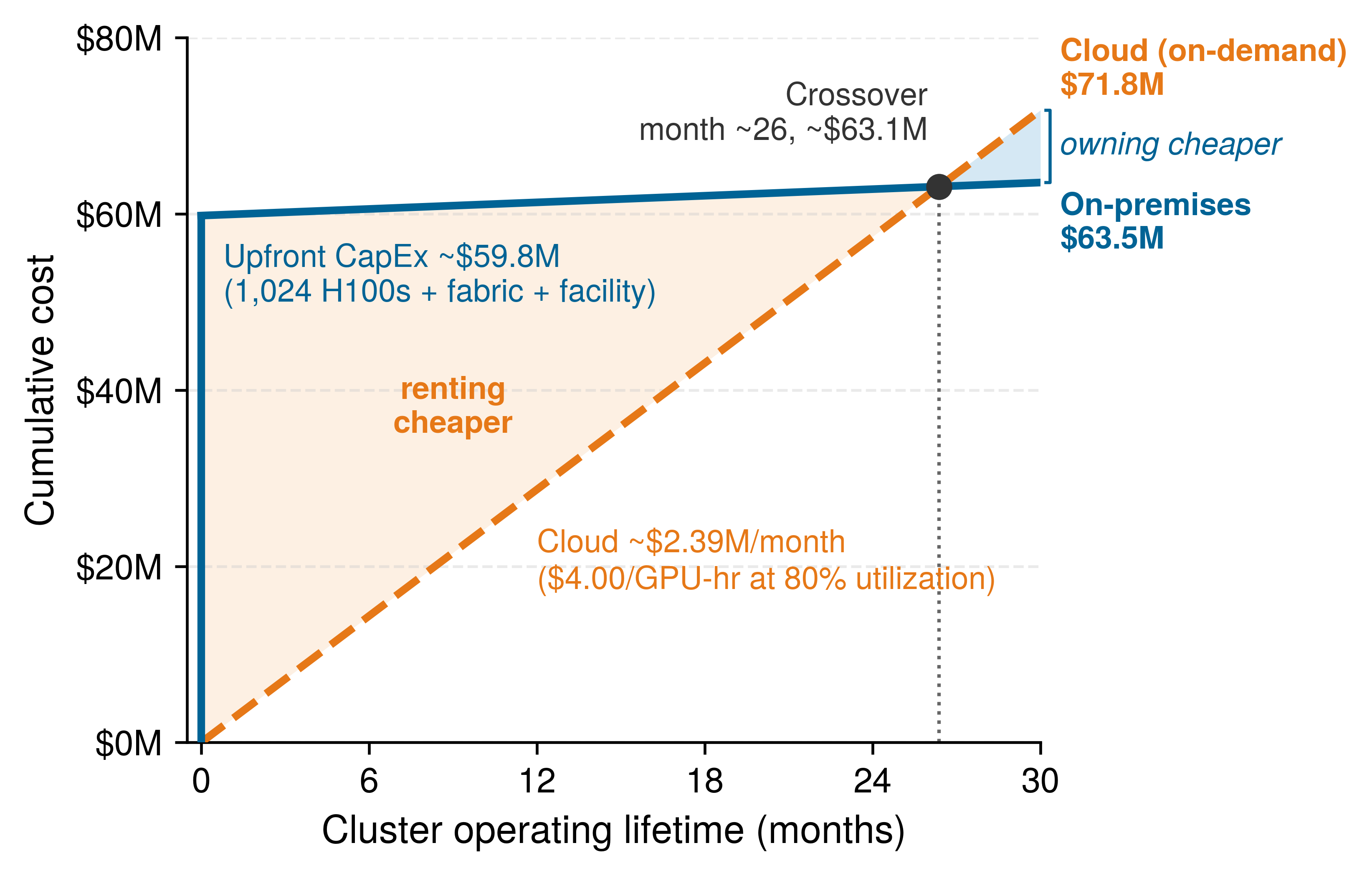
Figure 13: **Build vs. Buy TCO**: The curves compare cumulative cost over a 30-month horizon for a high-utilization H100 reference cluster. On-premises deployment begins with a CapEx step plus monthly OpEx, whereas cloud rental cost rises linearly with utilization. Over a 3-year service life, owning pays off only above 59.7 percent sustained utilization; below that, renting stays cheaper.

The plotted reference uses 1,024 H100 GPUs across 128 nodes at 80 percent sustained utilization. The on-premises curve starts at $59.80M in upfront CapEx and adds about $1.5M per year, while cloud rental at $4/GPU-hour grows by about $2.39M per month. Over 30 months, the cloud line reaches $71.8M, and the on-premises line crosses it around 26.4 months.

Cloud providers charge by the GPU-hour. At the on-demand reference rate of $4 per H100-hour, a single 8-GPU node rented only during 80 percent of the year costs $224,256 per year. An on-premises DGX H100 node costs approximately $350,000 to purchase. Amortized over three years and combined with electricity costs of $4,519 per node per year, the total annual on-premises cost is approximately $121,186 per node. This assumes idle rental periods can be released; an allocated but idle GPU still incurs a bill. Solving the break-even equation with electricity scaling at the same allocation fraction, on-premises infrastructure becomes favorable when sustained utilization exceeds roughly 42.5 percent. This narrow comparison includes node acquisition and utilization-proportional electricity; it excludes idle power, network and facility capital, staffing, maintenance, and financing. It does not use the wider owned-cost boundary of the cluster comparison in figure 13.

The same calculation explains why cloud pricing cannot be read as a simple price list. The scenario’s reserved discount of 40–60 percent converts optionality into commitment. Its spot or preemptible discount of 60–90 percent introduces interruption risk. The relevant comparison is cost per completed workload under the deadline or service contract. Checkpoint recovery, replacement capacity, and traffic fallback offer different ways to manage that risk; no single combination is required for every workload.

Owned capacity moves a different set of risks into the platform. Facility construction, networking, staffing, maintenance, and hardware obsolescence continue to accrue even when the GPUs are idle; their cost depends on site, power delivery, cooling design, and accounting boundary. A three-year-old GPU may be economically stranded if the next generation delivers 3$\times$ more performance per watt. The engineering question is therefore not whether one purchasing channel is universally cheaper; it is whether the workload mix can keep fixed capacity useful enough to compensate for its lifecycle and operating risks.

Hybrid designs follow from the same invariant. Owned infrastructure can carry predictable baseline work, while cloud allocations absorb peak demand, early hardware access, or bursty training campaigns. The hybrid split is not a compromise between two vendor categories; it is a scheduling policy over capital risk, utilization, and deadline risk.

For the 175B model, workload cadence changes the ownership decision. Consider a dedicated training fleet used only 15–20 percent of the time because its annual training campaign leaves long gaps. A portfolio of experiments, hyperparameter sweeps, fine-tuning jobs, and model variants could instead sustain 70–80 percent utilization on the same hardware, provided those jobs fit its capacity and scheduling constraints. Serving can also fill gaps when the hardware and isolation policy support it. These illustrative utilization levels describe workload mixes, not consequences of training a particular model. A hybrid design can keep predictable baseline work on owned capacity and rent the temporary expansion, such as the 5–10$\times$ baseline allocation assumed here for large training runs. The same invariant governs the comparison at a larger fleet scale, provided each estimate states which costs it includes.

Napkin Math 12.9: The 10,000-GPU cluster

Consider a cluster of 1,250 DGX H100 nodes (10,000 GPUs) for training the 175B model.

On-premises (3-year lifecycle):

Hardware CapEx: 1,250 $\times$ $350,000 = $437.5M
Network CapEx: ~$25M (InfiniBand fat-tree fabric)
Facility CapEx: ~$75M (liquid-cooled data center hall)
Annual Electricity: Simplified GPU-only estimate: 10,000 GPUs $\times$ 700 W $\times$ PUE 1.1 $\times$ 8,760 h/year $\times$ $0.07/kWh = $4.7M/year
Annual Staffing: ~$5M/year
3-year total: $537.5M + 3 years $\times$ $9.7M = ~$566.7M

Cloud rental (3-year rental at 80 percent utilization):

Annual Cost: 10,000 GPUs $\times$ $4/GPU-hour $\times$ 8,760 h/year $\times$ 0.80 = $280.3M/year
3-year total: ~$841.0M

Systems insight: With the stated prices and cost boundary, on-premises saves approximately $274.3M over three years at 80 percent utilization, but the savings disappear below roughly 53.9 percent. Owned hardware still incurs facility and staffing costs regardless of load. This is a scenario comparison, not a procurement quote: its GPU-only electricity estimate omits host and network power, and omitted maintenance or financing costs would also change the break-even point.

The three build-vs.-buy scenarios yield three different break-even utilizations because each draws a different cost boundary around owned capacity (table 30). All three use the same on-demand cloud reference rate, so the spread comes entirely from what each scenario charges to ownership, and the 10,000-GPU threshold shows how sustained demand, rather than fleet size, decides the ownership case.

Table 30: Build-vs.-Buy Break-Even by Cost Boundary: Three scenarios compare owned capacity with the same on-demand cloud rate. The single-node comparison omits network, facility, and staffing costs, so its threshold is lowest; the two cluster scenarios include them and differ by scale and by how each prices operating cost. A procurement decision needs the boundary of the cluster scenarios or wider.

Scenario	Scale	Owned cost included	Break-even utilization
Single-node comparison	One 8-GPU DGX H100 node	Node purchase amortized over three years; electricity proportional to use	42.5%
Build-vs.-buy figure (figure 13)	1,024 GPUs (the running cluster)	Nodes, network, and facility CapEx plus annual OpEx over the 3-year life	59.7%
10,000-GPU notebook	10,000 GPUs	Nodes, network, and facility CapEx; GPU-only electricity at full load; staffing; three years	53.9%

Systems Perspective 12.3: Sustained demand and unit cost

The 10,000-GPU scenario illustrates how sustained demand can support ownership. A portfolio that keeps compatible capacity usefully occupied at 70–90 percent utilization spreads fixed costs over more work than one operating at 20–30 percent. These are illustrative demand regimes, not utilization guarantees based on organizational size. Continuous training pipelines, model refreshes, and compatible inference workloads can support the higher regime; sporadic campaigns favor the option to release rented capacity. When a broad workload portfolio lowers unit cost enough to fund further investment, the advantage compounds, but it depends on useful demand and operating discipline, not fleet size alone.

Operational complexity

A TCO estimate must include the operational work that sustains the fleet. Hardware maintenance must diagnose failed GPUs, links, network adapters, and cooling components before a local fault becomes a fleet-wide slowdown. The five-hour fleet failure interval in the scenario of section 12.6.1 informs staffing, but does not determine headcount by itself. Staffing also depends on diagnosis and repair time, automation, concurrent incidents, and coverage requirements while the rest of the fleet keeps working.

The software side creates the same coupling. CUDA, GPU drivers, InfiniBand drivers, container runtimes, schedulers, monitoring systems, and training frameworks all participate in the achieved utilization number. A driver/toolkit incompatibility can silently degrade performance, while a scheduler or monitoring gap can strand accelerators behind failed jobs. Staffing depends on automation, service commitments, and operating scope because performance optimization is continuous: as models, frameworks, and hardware configurations change, communication patterns, memory pressure, and parallelism strategies change with them. Case 1 on the underutilized compute fleet works an underutilized fleet through the C³ diagnosis, ruling out communication before isolating the compute axis, which shows the performance engineer how to locate where the lost utilization goes rather than tuning blindly.

↪ The C³ telemetry diagnostic decision tree is developed in C^3 Infrastructure Diagnostic Decision Tree and Fleet Diagnostic Scorecard.

Cloud providers charge a margin above raw hardware and electricity partly because they absorb this operating burden. The point is not that cloud is simpler in every technical sense; it exposes a different interface. The platform either pays for internal expertise in GPU kernel behavior, InfiniBand operations, distributed-systems debugging, liquid cooling, and power infrastructure, or it pays a provider to hide some of that machinery behind a service contract. In both cases, the economics are still governed by useful work per dollar.

From TCO to total value of ownership

A more complete framework than TCO is total value of ownership, which includes the value generated by infrastructure rather than only its cost. Two clusters with identical TCO may create different outcomes if one reaches a result two weeks earlier, sustains higher scaling efficiency, starts jobs faster, checkpoints more cheaply, or serves the resulting model at lower cost per token. The value terms are hard to price exactly, but they are not optional in systems reasoning: time-to-result affects product deadlines, scaling efficiency affects final model quality under a fixed training window, experimentation velocity affects the number of hypotheses the team can test, and inference efficiency can dominate training cost over a multi-year deployment.

This value-oriented perspective changes the infrastructure decision from cost minimization to constraint management. A cheaper cluster that slows the research cycle or produces a model with higher serving cost may be more expensive over the model lifecycle. Conversely, a more expensive training platform can pay for itself if it enables a smaller or more efficient deployed model.

The inference dimension of total value of ownership (TVO) connects a training investment to the service it supports. Serving Cost Dominance in Production establishes why recurring serving cost overtakes a one-time training bill (principle 17); the fleet accounting asks the converse question, whether additional training spend repays itself through cheaper serving. Consider a service of the 175B model that handles 10 million queries per day, each generating an average of 500 tokens, for 5 billion tokens daily. At an assumed $2 per million tokens, serving costs approximately $3.6M per year, held constant over a three-year deployment. If an additional $2M training investment produces a validated 20 percent reduction in serving cost at matched quality and traffic, the three-year gross savings are $2.2M, enough to recover that investment before any additional maintenance costs. A lifecycle forecast must still add retraining and changing demand when they occur.

12.9.3 Depreciation and lifecycle

A three-year-old accelerator fleet that still passes every hardware diagnostic can become uneconomic for frontier pretraining when the next GPU generation delivers 3–4$\times$ the performance per watt, or lose tens of millions of dollars in hardware value while sitting idle between two annual training runs. ML accelerators depreciate as newer devices change the cost of useful work: a physically functioning accelerator can become uneconomic for a particular training workload while remaining useful for another. The peak arithmetic efficiencies in Power Efficiency across GPU Generations provide one screening measure, but depreciation and refresh decisions require sustained throughput at matched quality, memory capacity, energy consumption, and the cost of replacing otherwise usable equipment.

Resale value depends on supply, demand, memory capacity, software support, and the workload a buyer intends to run. A refresh budget should therefore test a range of resale assumptions rather than extrapolating a fixed historical depreciation rate across generations.

Refresh policy connects lifecycle planning to scheduling. The three-year horizon used in these examples is a planning assumption, not a universal accounting life or a required replacement date. Replacing the entire fleet at once creates a large CapEx spike, while staggered refresh spreads expenditure but leaves the scheduler with mixed-generation hardware. Placement must then account for different compute capabilities, memory capacities, and communication bandwidths. Keeping generations in separate job pools is one option; jobs that span generations need explicit support for their performance differences.

The same lifecycle logic determines where older accelerators remain useful. A GPU that is inefficient for the largest training runs may still serve smaller models, fine-tuning jobs, or memory-bound inference economically if its capacity, bandwidth, and energy cost meet those workloads’ requirements. A newer device’s peak arithmetic advantage alone does not settle that comparison. Resale, repurposing, and capacity-sharing arrangements preserve value only when the platform can route useful work to the appropriate generation without hiding performance cliffs from users.

Depreciation is most punitive for bursty workloads. If a team trains one large model per year, the GPUs lose value during the idle months even though they perform no useful computation. Cloud capacity amortizes the same depreciation across many customers, while owned capacity must amortize it across the owner’s own workload mix. That is why the utilization invariant appears again: the hardware must either stay busy or be cheap enough to strand.

Isolating hardware cost shows how much depreciation alone charges each run of the 175B model. Under the $350,000-per-8-GPU-node assumption, the 1,024-GPU (128-node) fleet costs $44.8M before network and facility costs. Assume a resale value of $7M–10M after three years in a market where newer accelerators offer 3–4$\times$ the performance per watt. That performance assumption does not determine resale value by itself. The assumed residual value yields net hardware depreciation of $34.8M–37.8M. Allocated to only two large training runs, it contributes $17.4M–18.9M per run before electricity, staffing, or facility costs. At 80 percent useful utilization over three years, it instead contributes approximately $1.62–1.76 per used GPU-hour. This is the hardware component of owned cost, not a complete rate directly comparable with cloud rental. Utilization spreads that commitment across output; the full cost accounting determines economic viability.

Refresh screening

Each accelerator generation has raised peak arithmetic per watt, more slowly than raw throughput because device power rose as well, but a refresh pays only when the workload realizes enough of the higher ceiling to lower energy and cost per completed run at the same quality target, so memory-bound serving and communication-bound training can justify different refresh choices for the same fleet.

↩︎ Accelerator generations, their peak rates, the power each draws, and their peak arithmetic per watt are established in Evolution of GPU architectures.

A refresh comparison can hold either the arithmetic ceiling or the accelerator power budget fixed, and the two framings answer different questions. Consider replacing a V100 fleet of the reference cluster’s size, 1,024 devices with a combined accelerator thermal design power (TDP) of 307.2 kW. On the dense FP16 basis of Power Efficiency across GPU Generations, 130 H100s match that fleet’s arithmetic ceiling at about 91 kW of combined TDP. Held at the same 307.2 kW, the budget instead accommodates 438 H100s with 3.4× the original ceiling. The first comparison screens for a lower power envelope at matched peak arithmetic; the second screens for more arithmetic capacity within a fixed power envelope. Neither establishes achieved throughput or measured power.

The fleet matched by arithmetic ceiling is not automatically usable. The original fleet has 7.9× as many devices, so, with the same port count per device, the replacement offers proportionally fewer network ports, and its aggregate HBM falls from 35.2 TB to 11.2 TB. A replacement plan must pass memory-fit, topology, and latency checks before the arithmetic equivalence counts as capacity, and both framings compare peak ceilings rather than energy per completed run at matched quality. The hybrid split described in section 12.9.2 also hedges refresh timing, because cloud bursts provide access to newer hardware before a large purchase commits the fleet to it.

The screening numbers bound the refresh decision for the 175B model without settling it. The H100’s 700 W TDP is more than twice the V100’s 300 W, yet run energy can still fall, because energy integrates measured power over elapsed time and the faster device finishes sooner. The dollar saving and payback period therefore come from a matched training configuration: measured or validated runtime, accelerator and host power, fabric and storage consumption, and the facility overhead applied to that IT total.

12.9.4 Cloud capacity as an operations constraint

Renting 1,024 cloud GPUs avoids upfront capital expenditure, but a synchronous training job whose tensor-parallel ranks straddle a cloud placement-group boundary stalls on inter-instance network latency at every layer, and a spot preemption without checkpoint discipline can erase a 70 percent price discount in a single lost afternoon. For organizations that choose the cloud path, the provider absorbs hardware ownership while exposing capacity, topology, and interruption risk as operating constraints. Instance types and pricing change frequently, so the durable distinction is not vendor branding; it is how the cloud allocation affects communication, scheduling, and fault tolerance.

Three properties of a cloud allocation matter most. The interconnect fabric decides whether distributed jobs keep the scaling assumptions used in design, through fixed-latency and per-byte terms that The \MessageStartupLatency-\LinkBandwidth Communication Model separates. Provisioning granularity decides how much topology the platform controls, from individual instances it must assemble itself to preconnected pods that limit composition. Custom accelerators repeat the generality tax (principle 1): supported operations get cheaper, but end-to-end savings depend on workload mapping, software support, and migration effort. The on-demand, reserved, and spot pricing compared in section 12.9.2 trade optionality, commitment, and interruption risk alongside those physical properties, so the purchasing choice is also a fault-tolerance decision.

Spot instances and preemptible VMs develops spot economics from the scheduler’s side, where equation 8.3 inflates the spot price by the ratio of total to productive time. The operations view applies that relation to a capacity budget. At a 70 percent discount, a scenario choice within the 60–90 percent range that section cites, spot H100 instances cost approximately $1.20/GPU-hour instead of $4. For the 175B model, the 1,024-GPU, 2–4 week workload consumes approximately 344,000–688,000 allocated GPU-hours. The on-demand cost is therefore about $1.4M–2.8M, while spot pricing would reduce the bill to roughly $0.4M–0.8M before interruptions. Interruptions, restarts, and lost work can erase that discount or push the job past its deadline, so completion cost and elapsed time both belong in the comparison. Checkpoint frequency, instance diversification, and on-demand fallback improve that comparison within the limits that Spot instance strategies for ML training sets out, and serving can use interruptible capacity only when remaining replicas, routing, and replacement readiness preserve its service contract.

Renting capacity for the 175B model also requires an allocation whose placement contract matches the parallelism plan. Cloud instances share the provider’s fabric with other tenants, and placement groups or dedicated fabrics reserve high-bandwidth connectivity only within a group, so a synchronous job whose ranks straddle a group boundary pays that boundary’s latency and bandwidth on every step. The working rule is to keep tensor- and pipeline-parallel groups, which exchange data within every layer or micro-batch, inside one placement group, and let only the less frequent data-parallel gradient traffic cross the boundary. Representative collectives must be benchmarked on the actual allocation before nominal GPU availability counts as usable training capacity.

Checkpoint 12.5: TCO decision framework

An organization needs to train 10 models/year, each requiring 1,000 GPU-hours on H100s, evaluating an on-premises cluster with 8 GPUs against cloud instances at $4/GPU-hour.

Cloud cost estimate: calculate the annual cloud cost from the training volume and hourly rate.
On-premises TCO: calculate the annualized on-premises cost, assuming $350,000 per 8-GPU node, $0.07/kWh electricity at PUE 1.1, and 700 W per GPU.
Break-even volume: solve for the number of annual training runs at which on-premises becomes cheaper.

12.9.5 Capacity planning as a reliability control

Sizing a training cluster from parameter count alone—or ordering 1,024 H100s that arrive six months before the substation and liquid-cooled racks can power them—either starves the job of memory and fabric bandwidth or leaves tens of millions of dollars of silicon sitting in crates while the launch window closes. Infrastructure planning begins when a workload requirement becomes a facility requirement. Model architecture, precision, optimizer state, and batch configuration establish memory needs; the training algorithm and token budget establish work; the deadline establishes required sustained throughput. Parallelization then determines the communication that the fabric must support. Accelerator TDP contributes to the node power envelope, which also includes hosts, memory, and networking, and that envelope constrains rack density and cooling. Planning follows this causal chain from useful work to physical capacity and total cost of ownership.

The first step is workload characterization. Memory sizing follows activations, optimizer state, temporary buffers, and the sharding or offload policy rather than parameter count alone, while the token budget, itself a compute-optimal choice under the scaling laws of AI Scaling Laws (principle 9) that holds only within the breakdown conditions of When scaling laws break down, fixes total work and the deadline fixes sustained throughput. Bottom-up sizing then works from the accelerator outward, using roofline analysis to tell whether each training or serving phase binds on computation or memory bandwidth and the parallelization plan to set the AllReduce, AllToAll, or point-to-point traffic the fabric must carry.

↩︎ The Roofline Model and its ridge point are established in Roofline model.

Each layer of physical sizing then applies a method taught in an earlier chapter. Per-device training state sets node memory and the sharding or offload policy (Node memory partitioning, Memory-efficient data parallelism with ZeRO and FSDP). The primary collective sets the fabric topology and its congestion-control requirements (Fat-tree (Clos) networks, End-to-end congestion control with DCQCN and HPCC). Node power sets rack density and cooling (Power and thermal envelopes). The four-node DGX H100 rack assumed for the 175B plan is roughly a 33.5 kW design point once host, network, conversion, and cooling overhead are included. TCO and schedule remain design variables because the cluster must arrive in time to matter, and GPU supply or electrical work often dominates lead time.

For the 175B training plan, the pod-sizing method of The Pod turns the run’s 3.15 × 10²³ FLOPs budget into a cluster. On a BF16/FP16 planning basis rather than the FP8 headline peak, each H100 sustains an assumed 445.1 TFLOP/s at 45 percent model FLOPs utilization (MFU), so 1,024 GPUs complete the work in about 8 days. That token budget is the GPT-3 operating point, which is undertrained relative to compute-optimal allocation (Compute-optimal resource allocation). A plan that followed the compute-optimal ratio of tokens to parameters at the same model size would multiply the token count, and with it the cluster-days, so the scaling-law choice moves the capacity plan before any hardware question arises. A 2–4-week calendar allowance and a 5–10 percent spares pool then cover delays and recovery outside the MFU measurement window; stalls already reflected in MFU must not be counted again.

The plan’s 32 racks draw approximately 1.1 MW under the rack accounting boundary of Power and thermal envelopes, and its three-year cost and cloud alternative are those of the running cluster in section 12.9.1, where ownership pays only if utilization stays high beyond the initial training run. Procurement and facility schedules must be confirmed against available capacity. A three-month initial deployment is feasible only if its hardware and facility resources are already available within that window; it cannot be inferred from a longer procurement lead time.

Checkpoint 12.6: Infrastructure planning exercise

A team needs to train a 70B-parameter model on 1T tokens within 4 weeks, with H100 GPUs at 1979 TFLOP/s FP8 peak (45 percent MFU), the headline basis that the worked plan above set aside, and a 2 MW facility power ceiling.

GPU sizing: determine the minimum number of GPUs needed to complete training within 4 weeks for a compute budget of $6 \times 70 \times 10^9 \times 10^{12} = 4.2 \times 10^{23}$ FLOPs.
Power headroom: evaluate sufficiency of the 2 MW power budget, assuming PUE 1.1, 700 W per GPU, and 50 percent overhead for non-GPU components.
Cost comparison: estimate the training-run cost at $4/GPU-hour in the cloud vs. $350,000 per 8-GPU node on premises.
Precision basis: repeat the GPU sizing on the BF16/FP16 planning peak of 989 TFLOP/s used in the worked plan, explain why the two GPU counts differ, and state which basis a procurement plan should use unless the training recipe has been validated in FP8.

Capacity lead time as operational risk

The economics of ML infrastructure are not purely about hardware specifications and electricity rates. Capacity lead time is itself an operational risk: a platform that cannot acquire, reserve, or free capacity quickly enough may miss model launches, delay rollback-safe migrations, or run without the headroom needed for incident response.

The GPU supply chain adds a correlated risk, because processors, memory, packaging, and network equipment that must arrive together can depend on the same upstream capacity, so orders placed with several vendors do not by themselves establish independent supply.

Capacity commitments can take much longer to change than model traffic. For planning, consider a large deployment (1,000+ GPUs) with a 6–12-month interval from purchase decision to usable capacity; the actual interval requires supplier and facility confirmation. That delay changes operations. The platform must forecast model growth, reserve refresh capacity, and maintain fallbacks before demand arrives rather than after dashboards turn red.

Facility readiness can lag silicon delivery. In a planning scenario, substation, building-shell, and facility schedules of 12–30 months run concurrently with 6–12-month GPU deliveries, and the longest prerequisite sets the critical path; site power, data-residency rules, and connection queues can also rule out an otherwise economical location before any accelerator is purchased. The physical design of power delivery and cooling belongs to Power and thermal envelopes; the operational point is that its schedule becomes the fleet’s schedule.

Mismatched schedules are expensive in both directions. Hardware delivered before the facility is ready ties up capital without producing useful work, as does a completed facility waiting for accelerators. Phased deployment can reduce the mismatch by commissioning usable capacity in waves while construction continues. An early phase lets the software team validate the distributed-training stack and tune collective kernels on the deployed topology while operators test power distribution and cooling; success at that scale does not establish readiness at full load. The economic value of making useful capacity available earlier can justify premiums for modular halls or temporary colocation when the expected benefit exceeds their additional cost. Projected monthly model value is an input to that comparison, not a guaranteed loss for every month of delay: the estimate must account for launch readiness, demand, operating costs, and whether delayed value can be recovered later.

Hardware access becomes part of the deployment schedule for the 175B model as well. An illustrative 1,024-H100 allocation represents approximately $45 million in node hardware under the $350,000-per-8-GPU-node assumption established in section 12.9.2, but the operational risk extends beyond the purchase price alone. If the allocation arrives a quarter late, the platform may lack capacity for fine-tuning, shadow traffic, canary expansion, or rollback-safe serving during the model launch window. Capacity planning is therefore a reliability control rather than a procurement function alone.

12.9.6 ML systems TCO framework

A budget that prices only visible GPU compute and object storage misses the engineering labor, pipeline maintenance, continuous retraining, monitoring, and incident response that routinely make up the other half of total cost. Fleet cost accounting prices physical capacity, but deciding which workloads deserve to consume that capacity requires a TCO framework covering the full ML lifecycle alongside the value each workload creates. The lifecycle definition of TCO that opened the fleet analysis (definition 12.1) now applies workload by workload, widening the hardware lens to training and inference costs, with data and iteration completing a four-component model. Their relative weights depend on workload, traffic, retraining cadence, and operating requirements rather than a fixed distinction between ML and traditional software.

The TCO equation

Equation 12 expresses the total cost of ownership as the sum of four distinct cost components, each with different scaling characteristics and optimization levers:

\[\text{TCO}_{\text{ML}} = \TrainingCost + \InferenceCost + \TotalDataCost + \IterationCost \tag{12}\]

Here, $\TrainingCost$ is the initial training and evaluation cost, $\InferenceCost$ is recurring serving cost, $\TotalDataCost$ covers data acquisition, storage, cleaning, and governance, and $\IterationCost$ captures subsequent experimentation and maintenance. The categories require a common accounting horizon and an explicit allocation rule. If retraining compute is charged to $\TrainingCost$, it must be excluded from $\IterationCost$; shared hardware depreciation and energy likewise enter these workload costs once rather than being added again as a separate fleet bill.

In the illustrative budget of figure 14, engineering labor (20 percent), pipeline maintenance (10 percent), continuous retraining, monitoring, incident response, and governance together equal the visible infrastructure spend. The example shows what an incomplete budget can miss; its proportions are not universal cost shares. Each organization must measure these obligations within the same accounting horizon as its infrastructure costs.

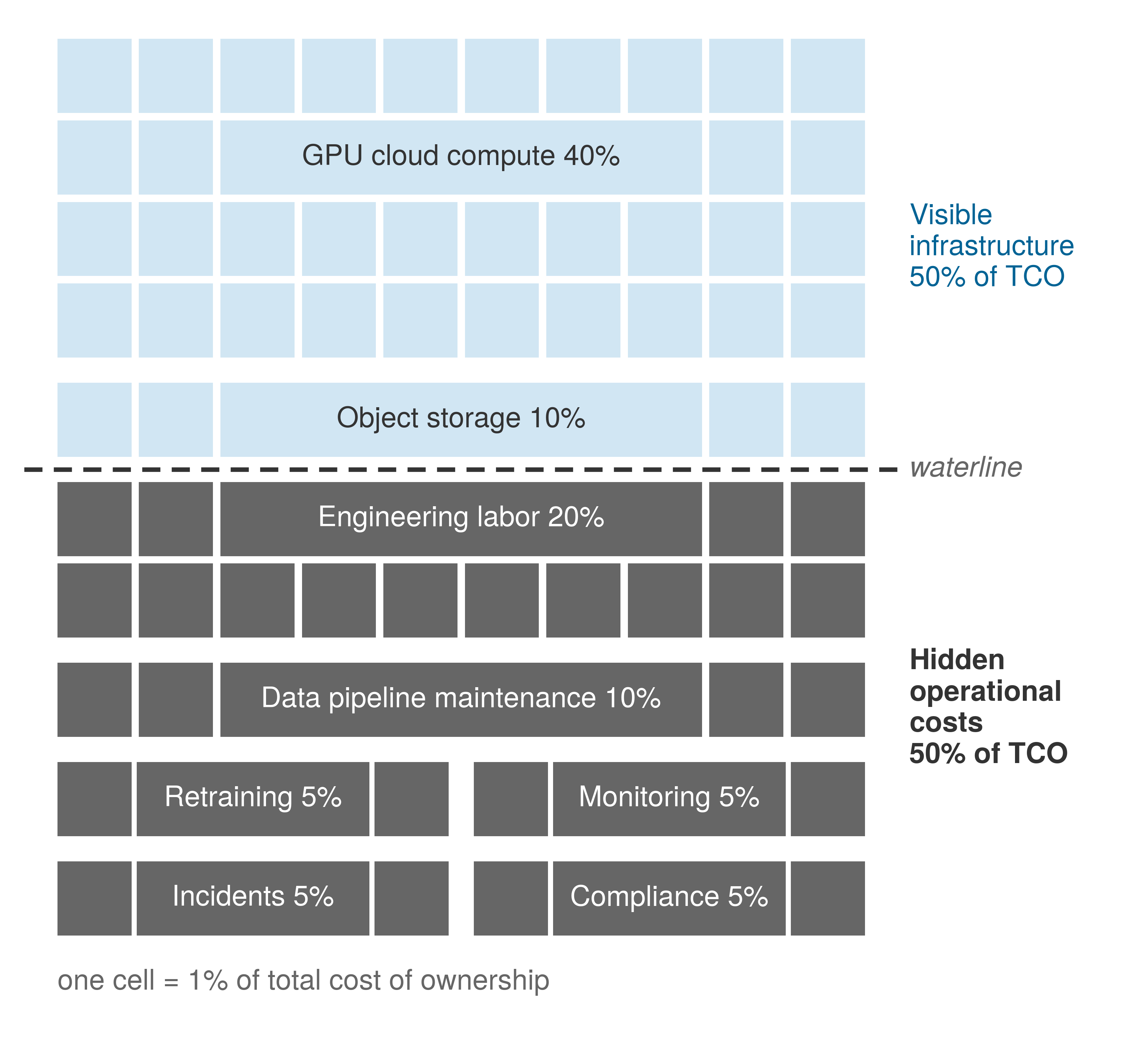
Figure 14: **The TCO Iceberg**: The analysis separates visible infrastructure costs from operational costs that are easier to omit. In this illustrative budget, the hidden operational costs (engineering labor, pipeline maintenance, retraining, monitoring, incident response, and compliance) together constitute half of total cost.

The decomposition shows why optimization must follow the measured cost structure. An effort centered on experimentation may spend most on $\IterationCost$, a training campaign on $\TrainingCost$, and a high-traffic deployment on $\InferenceCost$. These are workload regimes, not mandatory stages of organizational maturity. The cost breakdown identifies which component merits attention under the current workload mix.

Training cost model

Training cost begins with the price of the GPU-hour. A 30-day run on a 256-node H100 cluster (2,048 GPUs) at the internal fleet rate of $2/GPU-hour is a direct investment of roughly $2.95M. At this scale the cost per training run $(\TrainingCost)$ becomes a design lever that sizes the fleet. Faster time-to-market pushes the planner toward more GPUs, but larger jobs also suffer diminishing parallel efficiency and a higher probability of hardware interruption. Total cost is therefore not merely a function of compute time; it must account for data staging, checkpointing, and the cost of recovery from interruptions.

Organizations must decide when to buy additional permanent capacity and when to recover useful throughput through better orchestration or model optimization. The decision also has an energy dimension. Less electricity consumption reduces the energy bill at a fixed tariff, but emissions depend on the energy source and time of use; a lower price alone does not establish lower carbon impact. The cost model below accounts for purchased energy, while an emissions comparison requires the corresponding carbon intensity.

Equation 13 formalizes training cost as a function of GPU count, training duration, non-energy accelerator-hour rates, data center energy overhead, and failure overhead:

\[\TrainingCost = \AcceleratorCount \times \BaselineTrainingDuration\times \left(\AcceleratorHourlyPrice+ \DevicePower \times \ElectricityPrice\times \text{PUE}\right) \times (1 + \FailureOverheadFraction) \tag{13}\]

where:

$\AcceleratorCount$ is the number of GPUs allocated
$\BaselineTrainingDuration$ is the baseline training duration in hours before the additional failure overhead
$\AcceleratorHourlyPrice$ is the non-energy accelerator-hour cost
$\DevicePower$ is per-GPU power draw in kW
$\ElectricityPrice$ is the electricity price
$\text{PUE}$ is the power usage effectiveness multiplier applied to the energy term
$\FailureOverheadFraction$ is additional time from failures and recovery as a fraction of the baseline duration

The PUE factor captures facility energy overhead, the facility metric of Facility-level power metrics. A PUE of 1.1 means 10 percent additional energy relative to IT energy. It applies to energy consumption, not to the whole accelerator-hour rate. This equation uses GPU power as a simplified IT boundary; a full facility estimate must also include host, network, and storage power. The failure overhead $\FailureOverheadFraction$ adds recovery time beyond the baseline. Checkpointing or restart time already included in measured baseline duration must not be charged again through this factor.

↩︎ Cluster mean time between failures and the checkpoint interval it implies are established in Failure Analysis at Scale.

Training cost calculation

Consider training a large language model:

Configuration: 256 H100 GPUs for 14 days
Base non-energy accelerator-hour rate (scenario choice): $3.50/GPU-hour
Energy adder: 700 W at $0.07/kWh and PUE 1.1 adds $0.05/GPU-hour
Effective rate: $3.55/GPU-hour
Failure overhead: 10 percent (scenario assumption relative to baseline duration)

$\TrainingCost = 256 \times (14 \times 24) \times (\$3.50 + \$0.05) \times 1.1 \approx \$335,892$

If this model requires quarterly retraining, annual training cost reaches approximately $1.3M. However, training cost often represents a small fraction of total TCO for production systems serving millions of users.

Inference cost model

Serving can outgrow the training bill.

Inference costs can dominate when cumulative serving demand outweighs training and iteration costs. Equation 14 estimates continuously provisioned capacity from average daily demand and sustained per-GPU throughput measured under representative batching, the target latency SLO, and operating headroom. Daily volume alone does not size traffic peaks; the estimate requires a separate check against the arrival pattern, workload mix, and scaling response:

\[\AcceleratorCount = \left\lceil \frac{\DailyQueryVolume}{86{,}400 \times \AcceleratorTargetQueryRate} \right\rceil, \qquad \InferenceCost = \AcceleratorCount \times 24 \times 365 \times \AcceleratorHourlyPrice \tag{14}\]

where:

$\DailyQueryVolume$ is the daily query volume
$\AcceleratorTargetQueryRate$ is sustained queries per second per GPU at the target latency SLO, including batching and operating headroom
$\AcceleratorCount$ is the integer number of continuously provisioned GPUs
$\AcceleratorHourlyPrice$ is the hourly GPU cost

Inference cost therefore grows with query volume in discrete capacity steps. Utilization and batching reduce cost only when they improve measured throughput at the target latency SLO; they should not be applied again as independent divisors.

For capacity planning, the same cost can be expressed in terms of required GPU-seconds per query:

\[\InferenceCost = \AnnualQueryVolume\times \AcceleratorSecondsPerQuery\times \frac{\AcceleratorHourlyPrice}{3600}\]

where $\AcceleratorSecondsPerQuery$ is allocated GPU-seconds divided by completed queries over the same accounting period. Allocated time includes idle headroom and provisioned capacity, so this definition reproduces the continuous-provisioning bill above. Measuring only busy kernel time instead estimates service demand and excludes those costs; it is not an equivalent billing formula without an allocation policy.

Data cost model

Data costs can grow faster than the user base when per-user history, transfer volume, and feature processing all rise together, even though each term below is linear in its own volume. Equation 15 decomposes data cost into three components that scale differently: storage cost $\DataStorageCost$, egress cost $\DataEgressCost$ for moving data out over the network, and processing cost $\DataPipelineProcessingCost$:

\[\TotalDataCost = \DataStorageCost + \DataEgressCost+ \DataPipelineProcessingCost \tag{15}\]

Storage costs grow with data retention requirements: \[\DataStorageCost = \StoredDataVolume \times \StoragePrice \times \StorageRetentionTime\]

where $\StoredDataVolume$ is a fixed data volume in GB, $\StoragePrice$ is the monthly storage rate, and $\StorageRetentionTime$ is its retention period in months. This product prices one volume retained at a constant rate; a growing dataset requires accounting for each period’s stored volume rather than multiplying the final volume by the entire history.

Egress costs scale with data transfer volume: \[\DataEgressCost= \TransferredDataVolume\times \EgressPrice\]

At the scenario egress rate of $0.09/GB, repeated transfers can become a significant cost driver for multi-region deployments and training data distribution. The applicable rate depends on the source, destination, and service contract; the estimate must distinguish billable transfers from included traffic.

Processing costs scale with compute requirements for extract, transform, load, feature engineering, and data validation: \[\DataPipelineProcessingCost= \ProcessedDataVolume\times \ProcessingPrice\]

Data processing costs often surprise organizations: a feature engineering pipeline processing 10 TB daily at $0.02/GB costs $73,000 annually.

Iteration cost model

Development costs capture the engineering investment in experimentation and model improvement. Equation 16 formalizes this as the experiment count multiplied by the combined per-experiment engineering and compute costs:

\[\IterationCost= \ExperimentCount\times (\PerExperimentEngineeringCost+ \PerExperimentComputeCost) \tag{16}\]

where:

$\ExperimentCount$ is the number of experiments conducted
$\PerExperimentEngineeringCost$ is the engineering cost per experiment
$\PerExperimentComputeCost$ is the compute cost per experiment

Experiments that do not improve production metrics still incur costs. If 90 percent produce no improvement and every experiment has the same cost, expenditure per improving experiment is 10$\times$ the per-experiment cost. A negative result can nevertheless rule out an unproductive direction or expose a risk. Experiment infrastructure should reduce avoidable engineering and compute work while preserving that learning value, rather than optimize the fraction of positive results alone.

Startup versus production company TCO

Two constructed organizational scenarios price the same four cost components (table 31). The startup operates 1 production model serving 100,000 daily users with monthly retraining, a 2-engineer team, and cloud-native infrastructure. The production company operates 50 models serving 10 million daily users with weekly retraining for high-velocity models, a dedicated 15-engineer ML platform team, and hybrid cloud/on-premise infrastructure. Because traffic, model count, cadence, and staffing all change, the comparison illustrates different cost structures rather than isolating the effect of scale alone.

Table 31: TCO Comparison: Startup vs. Production Company: In these constructed budgets, iteration costs dominate the startup scenario, while inference is the largest component in the production scenario. The comparison changes traffic, model count, retraining cadence, and staffing together; it does not isolate the effect of scale. The 100$\times$ user increase yields only a 20.6× TCO increase because the startup baseline is mostly salaries, even though inference grows faster than users. Data costs grow 160×, faster than users, in a scenario that also stores features for 50 models and retrains weekly.

Cost component	Startup	Production company	Scaling factor
Training	$5,000/month	$150,000/month	30× (more models, larger)
Inference	$2,000/month	$400,000/month	200× (100$\times$ users, 50 models)
Data	$500/month	$80,000/month	160× (50 models, weekly retraining)
Iteration	$40,000/month	$350,000/month	8.75× (team size, experiments)
Total TCO	$47,500/month	$980,000/month	20.6×
Dominant Cost	Iteration (84%)	Inference (41%)

Two lessons survive the constructed budgets. The dominant term flips, from iteration (84 percent) for the startup to inference (41 percent) for the production company, so the optimization target flips with it. Data cost also grows faster than the user count, because the production scenario stores and processes features for 50 models and retrains weekly, so its storage, egress, and processing volumes (equation 15) grow with model count and cadence as well as with users. The budgets are assumed, so they show why measured cost structure matters without isolating model count, feature complexity, or automation as the cause of any ratio.

TCO sensitivity analysis

Sensitivity analysis starts with the dollar cost breakdown and changes one workload assumption at a time. Each change touches only some cost terms, and the platform must update specific measurements before it can estimate a new total; more daily users, for example, requires new figures for requests per user, peak concurrency, retained history, and SLO headroom (table 32). The same increase in user count can have different consequences for a cached recommendation service and a long-context language-model service.

Table 32: TCO Sensitivity Drivers: Each workload change maps to the cost terms it affects and the measurements needed to update them. Shared infrastructure, capacity steps, and changing engineering effort can make the response nonlinear; the complete cost breakdown determines the total.

Workload change	Cost terms affected	Measurements needed
More daily users	Inference, data, and capacity operations	Requests per user, peak concurrency, history retained per user, and headroom needed to meet the SLO
More models	Training, inference, data, and iteration	Refresh cadence, traffic per model, shared feature reuse, and engineering effort per release
More queries per user	Inference and request-related data processing	Request mix, batching, cache hit rate, bytes logged, and provisioned capacity at the target SLO
Larger models	Training, inference, and iteration	Live-state memory, sustained throughput, parallelism, and time spent validating each candidate
More frequent retraining	Training, data preparation, and iteration	Cost per run, incremental data processing, evaluation effort, and any measured serving benefit

User scaling changes requests and stored history; model size scaling changes arithmetic and memory demand. The analysis recomputes those components in dollars over the same period, retaining unchanged components and including iteration and platform overhead, then sums the revised components and compares the total with the baseline. The resulting change identifies where an optimization can create enough recurring savings to repay its implementation cost.

Decision framework for speed versus efficiency

TCO analysis enables principled decisions about when to optimize for development speed vs. operational efficiency. Equation 17 calculates the breakeven point for optimization investments:

\[\OptimizationBreakevenTime= \frac{\OptimizationImplementationCost}{\MonthlyOptimizationSavings} \tag{17}\]

where $\OptimizationImplementationCost$ is the one-time implementation and validation cost and $\MonthlyOptimizationSavings$ is positive monthly savings net of added operating and maintenance costs. This simple payback assumes savings remain constant over the interval; recovered capacity counts as cash savings only when it reduces expenditure or avoids a planned purchase.

The breakeven equation helps compare specific investments once their implementation costs and recurring savings are estimated. The dominant cost component suggests where to look first, but does not rule out a valuable smaller intervention elsewhere. Table 33 offers investigation starting points and illustrative policy thresholds; actual investment criteria also depend on service risk, expected workload lifetime, and available engineering capacity.

Table 33: Cost-Structure Decision Rules: Measured cost shares guide investigation and name the risk each posture must evaluate. Candidate savings, useful lifetime, and operational risk determine whether an investment satisfies the organization’s policy.

Dominant cost structure	Operating context	Optimization posture and risk to evaluate	Payback threshold
Iteration costs dominate ($\IterationCost > 50\%$ of TCO)	Experiment-heavy workload	Investigate experiment infrastructure and developer tooling that shorten iteration time. Risk: engineering effort that does not repay through faster iteration or realized savings.	Evaluate candidate value; iteration cost share alone does not set a payback bar.
Training costs dominate ($\TrainingCost > 40\%$ of TCO)	Repeated training campaigns	Investigate mixed precision, gradient checkpointing, checkpoint-and-resume on spot instances, and architecture changes. Risk: recovery overhead, completion risk, and useful investment lifetime.	An illustrative policy accepts 3–6 months only if the candidate remains useful beyond payback.
Inference costs dominate ($\InferenceCost > 40\%$ of TCO)	High-volume serving	Investigate quantization, batching, caching, and distillation where repeated queries can realize savings. Risk: quality loss, latency changes, and workload lifetime.	An illustrative policy requires 1–3 months; the actual bar depends on candidate lifetime and risk.
Data costs dominate ($\TotalDataCost > 30\%$ of TCO)	Feature- and history-heavy	Investigate storage tiering, egress reduction, and feature simplification. Risk: retention, freshness, and downstream quality requirements.	Evaluate against retention and freshness obligations; storage share alone does not set a bar.

The payback bars in the table represent an illustrative investment policy, not a consequence of training or serving alone. Repeated queries can make serving savings accumulate quickly, but a model refresh or request-mix change can retire the optimized path before payback. A reusable training pipeline may support a longer horizon, while a one-off training campaign may not. For either workload, the comparison sets net savings over the candidate’s expected useful lifetime against implementation cost and risk; a dominant cost category does not guarantee that its next optimization has the highest value.

Optimization investment decisions

A production company with an inference bill of $400K/month evaluates INT8 quantization:

Implementation cost: $80,000 (engineering time + validation)
Expected inference cost reduction: 40 percent
Monthly savings: $400,000 $\times$ 0.40 = $160,000

$\OptimizationBreakevenTime = \frac{\$80,000}{\$160,000/month} = 0.5 \text{ months}$

Breakeven in about 2 weeks makes this investment attractive if validation confirms acceptable quality and latency and the expected cost reduction can be realized. For comparison, the same company, with a training bill of $150K/month, evaluates a training optimization:

Implementation cost: $80,000
Expected training cost reduction: 30 percent
Monthly savings: $150,000 $\times$ 0.30 = $45,000

$\OptimizationBreakevenTime = \frac{\$80,000}{\$45,000/month} = 1.8 \text{ months}$

The training optimization has longer payback and smaller absolute savings in this scenario. Those results favor the inference investment if both satisfy their quality and reliability requirements and compete for the same engineering capacity.

TCO-driven architecture decisions

TCO analysis should inform architectural choices alongside operational optimization. The build-vs.-buy analysis in section 12.9.2 also applies to individual workloads, accounting for any capacity they share with the rest of the portfolio. Model architecture selection changes the cost breakdown because a model requiring 2$\times$ training cost but 0.5$\times$ inference cost may have lower lifecycle cost at sufficient serving volume. Retraining frequency adds to $\TrainingCost$ and $\TotalDataCost$; it can reduce emergency work charged to $\IterationCost$ only when evaluation and release controls produce timely, useful updates. Monitoring detects the need to investigate drift; retraining alone does not. Feature complexity can likewise increase $\TotalDataCost$ and $\TrainingCost$, while its effect on $\IterationCost$ depends on whether better predictions outweigh added integration and maintenance. Knowledge placement in language-model services illustrates the same trade-off.

Retrieval-augmented generation vs. fine-tuning

Domain knowledge can live in a retrievable index, in model weights, or in adapter weights, and each placement creates a different operating cost surface. Retrieval-augmented generation (RAG) retrieves documents at inference time and places them in the prompt (Lewis et al. 2020). Fine-tuning stores adaptation in model weights or adapter weights: supervised fine-tuning trains on curated input-output examples, while low-rank adaptation (LoRA) stores small adapter-weight deltas (Hu et al. 2021). Both approaches can improve task behavior, but they move cost and failure risk to different terms of equation 12. RAG charges knowledge to $\InferenceCost$, through retrieval and the extra prompt tokens every request must prefill, and to $\TotalDataCost$, through the index it must build and refresh. Fine-tuning charges it to $\TrainingCost$ and $\IterationCost$, through curation, training runs, and re-evaluation whenever the knowledge changes. Query volume therefore decides which cost grows faster.

Lewis, Patrick, Ethan Perez, Aleksandra Piktus, Fabio Petroni, Vladimir Karpukhin, Naman Goyal, Heinrich Küttler, et al. 2020. “Retrieval-Augmented Generation for Knowledge-Intensive NLP Tasks.” Advances in Neural Information Processing Systems 33: 9459–74.

Hu, Edward J., Yelong Shen, Phillip Wallis, Zeyuan Allen-Zhu, Yuanzhi Li, Shean Wang, Lu Wang, and Weizhu Chen. 2021. “LoRA: Low-Rank Adaptation of Large Language Models.” arXiv Preprint arXiv:2106.09685.

RAG makes knowledge updates possible through the document index without retraining the model. Retrieved passages provide evidence against which generated claims can be checked, but retrieval alone does not ensure that an answer uses or cites that evidence correctly. Retrieved context also consumes serving resources, through prefill work that grows faster than linearly with sequence length and KV-cache memory that grows with it (The KV cache wall and memory capacity). The cost comparison therefore depends on retrieval quality, context selection, and the serving configuration; excessive context can also make relevant evidence harder for the model to use.

Fine-tuning moves adaptation work before deployment. The platform pays for data curation, training, and evaluation; successful adaptation can shorten prompts when it replaces instructions or examples that would otherwise accompany each request. Lower serving cost is a benefit to measure, not an automatic consequence of changing weights. Adapter-based fine-tuning also creates a fleet-management obligation when many customer-specific LoRA adapters must be versioned, loaded, and isolated, while changing facts embedded in weights requires a different update process from replacing documents in an index.

The decision depends on knowledge volatility, attribution requirements, latency budget, and adapter-management complexity. RAG provides an update path for changing facts and a source trail for review, subject to retrieval and generation quality. Fine-tuning can adapt domain language or stable behavior, subject to training cost and validation. Neither method implies a fixed context length or query-volume limit. A combined design can fine-tune how the model uses tools and documents while retrieving facts that must remain fresh, and evaluation must establish whether those benefits justify the combined lifecycle cost. Because each of these architecture choices is a forecast of lifecycle cost, once a choice ships the fleet needs controls that measure whether spending follows the forecast and give someone the authority to act when it does not.

12.9.7 FinOps for ML platforms

A cost dashboard can identify a failed training sweep without giving anyone authority to stop it. FinOps closes that gap by connecting fleet cost accounting and anomaly signals to budgets, owners, and intervention policies. The platform, fleet, and workload analyses above decide whether capacity and platform investment are worthwhile; FinOps decides how teams spend that capacity and respond when cost or value departs from the plan.

Definition 12.2: FinOps for ML

FinOps for ML is the practice of treating compute cost as a first-class engineering constraint (measured in real-time per experiment and model, and optimized jointly with model accuracy and latency) rather than accounting for it retrospectively through annual budget reconciliation.

Significance: ML compute costs scale steeply with experimentation volume. A team running 1,000 GPU-hours/day at the fleet reference rate of $2/GPU-hour spends $2,000/day ($730K/year) on training alone. With per-experiment cost visibility, an engineer can identify that 30 percent of runs are terminated early due to divergence (a reason to investigate the training configuration and failure causes) and that the team’s fault-tolerant jobs could run on spot capacity at 60–90 percent discounts, provided recovery and interruption costs preserve the required quality and completion target.
Distinction: Unlike traditional IT budgeting (which allocates fixed annual compute budgets across departments), FinOps for ML operates at the per-run and per-model level with real-time feedback, enabling decisions like early stopping a $50K training run at step 1,000 when loss curves signal divergence, rather than discovering the waste after the full run completes.
Common pitfall: A frequent misconception is that FinOps means minimizing compute spend. The goal is useful value across the full lifecycle within quality, latency, and reliability requirements: a $500K training run producing a model serving 10B inferences at $0.0001/query may be far more cost-efficient than a $50K run producing a model that requires 10$\times$ the inference compute to achieve the same accuracy at scale.

Cost components

ML platform cost breakdown depends on the portfolio and accounting period. In an assumed training-heavy annual budget, training compute takes half of spending and serving a quarter, with storage, network, and platform overhead sharing the rest (table 34). A mature, high-traffic serving portfolio can instead be inference-dominated, as the earlier lifecycle example shows.

Table 34: Illustrative Training-Heavy Platform Budget: Assumed shares sum to 100 percent over one annual accounting period. Training dominates this portfolio; a serving-heavy portfolio can reverse the ordering. Optimization levers belong on the measured cost driver; these shares are not industry norms.

Cost category	Assumed share	Primary drivers	Optimization lever
Training compute	50%	GPU hours, experiment volume	Spot instances, early stopping
Serving compute	25%	Traffic volume, latency SLOs	Autoscaling, model optimization
Storage	12%	Dataset size, checkpoint frequency	Tiered storage, retention policies
Network	8%	Multi-region, data transfer	Caching, compression
Platform overhead	5%	Team size, tooling	Automation, self-service

Cost visibility and attribution

Cost optimization requires visibility into spending and ownership. Attribution policy also shapes incentives. Direct metering charges for measured consumption, but shared services and idle reserves still require allocation rules; measured activity does not uniquely determine every team’s cost. Charging only for consumption can encourage under-provisioning when teams optimize their bill instead of service health. Allocation-based attribution charges for reserved capacity, making commitments visible even when that capacity is idle. Hybrid attribution combines a base allocation charge with a variable charge for excess usage. Each policy must preserve the headroom and shared services on which the reliability contract depends, and attribution starts from metadata: tag-based allocation assigns each resource’s cost to a team, service, environment, and cost center, as listing 7 shows.

Listing 7: Cost Attribution Schema: Resource tagging dimensions and shared-cost distribution policies for allocating ML infrastructure expenses to teams and services.

# Resource tagging schema for cost attribution
cost_allocation:
  dimensions:
    - team: "recommendation"      # Organizational owner
    - service: "ranking-model"    # Specific service
    - environment: "production"   # prod/staging/dev
    - model_type: "inference"     # training/inference
    - cost_center: "CC-4521"      # Finance tracking

  shared_cost_distribution:
    # Platform infrastructure costs distributed by usage
    - resource: "shared-gpu-cluster"
      method: "proportional_gpu_hours"
    - resource: "feature-store"
      method: "proportional_query_volume"
    - resource: "monitoring-infrastructure"
      method: "equal_split"

Shared infrastructure needs its own accounting policy because no single team owns it. Platforms typically adopt one of three models: proportional allocation distributes shared cluster expenses according to measured consumption metrics such as GPU-hours, storage capacity, or API query volume; equal split divides common baseline expenses evenly across consuming teams, which is well suited for fixed foundational tooling; and marginal cost charges tenant teams strictly for the incremental compute and storage their workloads introduce. The choice of allocation policy ultimately determines whether operational dashboards can drive organizational action rather than merely describing past spend.

For serving workloads, cost per inference provides a unit economic metric. Equation 18 divides total serving cost by inference count over the same accounting period. Comparisons require matched request mix, quality and latency targets, and cost boundaries; a short classification request and a long generated response are not equivalent units of work:

\[\text{Cost per inference} = \frac{\text{Total serving cost}}{\text{Total inferences served}} \tag{18}\]

Cost per inference then becomes the bridge from infrastructure telemetry to product decisions. Teams can compare model versions by asking whether an accuracy gain justifies a 2$\times$ inference cost, evaluate optimization work by measuring whether quantization reduced cost per inference by 40 percent, and forecast monthly serving cost under projected traffic. Tracking the metric by model, customer segment, and request type reveals which workload deserves optimization effort.

Cost dashboards reuse the attention-routing hierarchy of the reliability views in table 21. At the top of the hierarchy, the executive view tracks total ML infrastructure cost, its month-over-month trend, budget against actual, and efficiency metrics such as cost per prediction and cost per active user. When that top-level spend shifts, the portfolio view breaks cost down by domain and model type so the platform team can see which domain is driving the change, while the service view exposes per-service cost, cost per inference, GPU utilization efficiency, and budget comparison for the responsible team. Finally, the investigation view adds deployment markers and attribution detail so responders can tie an anomaly to a specific change rather than dismissing it as accounting noise.

Chargeback becomes actionable only when fine-grained metering, the attribution rules above, budget forecasts, and anomaly detection feed continuous cost monitoring across four complementary signals. Cost per inference tracks unit spending under a declared request mix, whereas cost per active user relates spending to the population served—though cross-service comparisons still require comparable activity and product scope. To connect those unit metrics to hardware and calendar limits, GPU utilization efficiency measures how allocated accelerators are used (distinct from revenue or engagement per accelerator-hour, which also depends on product demand and model quality), while budget burn rate tracks spending velocity against the allocation so owners can investigate projected overruns before the budget is exhausted.

Cost anomaly detection

Cost anomaly detection must account for the fleet’s allocation and lifecycle behavior because several distinct operational events can masquerade as a simple spending spike. Adding a serving replica creates an immediate cost step when that replica occupies multiple accelerators, whereas training sweeps and repeated recovery attempts accumulate GPU-hours gradually without producing useful artifacts, and zombie models (section 12.3.3) hold onto serving capacity long after their traffic has disappeared. Because traffic spikes, shifting request mixes, and cloud price changes can also raise the bill, detection must connect any cost change to allocation, workload, and lifecycle evidence rather than inferring a cause from dollar magnitude alone. An undetected anomaly keeps accruing charges until someone reviews the bill, so cost anomaly detection must balance sensitivity against false positive rates as deliberately as reliability alerting does.

The foundation of cost monitoring is the statistical process control of section 12.6.4.1 applied to spend. For a cost time series with historical mean $\MonitoredMetricMean$ and standard deviation $\MonitoredMetricStandardDeviation$, the Z-score quantifies how unusual a current observation is:

\[\CostAnomalyScore= \frac{\CurrentPeriodCost- \MonitoredMetricMean}{\MonitoredMetricStandardDeviation}\]

where $\CurrentPeriodCost$ is the observed cost for the current period.

Complementing Z-score analysis, percentage change detection captures sudden shifts regardless of historical variance, which makes it useful for catching step-function increases such as a misconfigured autoscaler that doubles instance count overnight:

\[\FiniteChange\% = \frac{\CurrentPeriodCost- \PreviousPeriodCost}{\PreviousPeriodCost} \times 100\]

Effective alerting requires calibrating thresholds to balance detection sensitivity against operational burden. Two illustrative configurations are a Z-score threshold, which alerts when $|\CostAnomalyScore| > 3$, and a percentage change threshold, which alerts when $|\FiniteChange\%| > 50\%$ day over day. Seasonal demand and planned jobs must be represented in the baseline before ordinary variation can be interpreted as unusual spending. Under the calibrated Gaussian null of the statistical-process-control rule, a daily $|\CostAnomalyScore| > 3$ check raises about one raw false alert per year and a 2-sigma check about 16, and section 12.6.2 shows how such crossings compound across many monitored series. Choosing between thresholds requires measuring detection power and the cost of missed events as well as alert burden.

For percentage-based alerts, false positive rates depend on the underlying volatility of costs. Services with naturally variable demand may require higher thresholds (75 percent or 100 percent) to avoid excessive alerts, while stable baseline services can use tighter thresholds (25 percent or 30 percent).

A threshold crossing identifies an unusual observation under the monitoring baseline, not a confirmed defect or cause. Table 35 groups candidate cost anomaly root causes into five classes, each with a distinct investigation path.

Table 35: Cost Anomaly Root Cause Categories: Five primary categories of cost anomalies with their characteristic indicators and investigation approaches. Traffic increases show proportional QPS growth, while efficiency regressions pair rising latency with stable traffic.

Category	Indicators	Investigation path
Traffic increase	QPS proportional to cost	Check upstream services, marketing campaigns, viral events
Efficiency regression	Cost up, QPS unchanged, latency up	Review recent deployments, model updates, infrastructure changes
Resource leak	Gradual cost growth, utilization stable	Check for orphaned resources, failed cleanup jobs, zombie processes
Pricing change	Cost up, all metrics stable	Verify cloud provider pricing, reserved instance expiration
Configuration error	Step-function cost increase	Audit autoscaling rules, instance types, replica counts

Detecting an inference cost spike

A recommendation service typically costs $100 per day for inference compute. The operations team receives an alert: today’s cost has reached $250 by end of day.

Historical data shows mean daily cost $\MonitoredMetricMean= \$100$ with standard deviation $\MonitoredMetricStandardDeviation= \$15$, so the first check is whether the alert is statistically plausible under normal operations: $\CostAnomalyScore = \frac{\$250 - \$100}{\$15} = \frac{\$150}{\$15} = 10$. A Z-score of 10 is far outside the assumed Gaussian baseline, but the team first verifies billing completeness, duplicate records, and pipeline correctness. Query volume is unchanged; the investigation must also check request mix and arrival peaks before ruling out demand. In this scenario, those remain comparable while p99 latency rises from 50 ms to 125 ms. A larger ranking model deployed at 2:00 AM adds features, GPU utilization stays near 95 percent, and measured throughput per GPU falls 60 percent. At matched demand and operating targets, that throughput loss implies 2.5× the capacity requirement. The team confirms the allocation increase and unchanged rates before attributing the rise from $100/day to $250/day to the release. It then evaluates whether the measured quality benefit justifies the cost or calls for a leaner serving configuration.

Cost optimization strategies

Cost optimization is a risk-allocation decision, not a catalog of discounts. Interruptible compute pays off only when checkpointing bounds the work lost to preemption, serving autoscaling only within the latency budget, and instance right-sizing only against measured cost per step or per inference. Each optimization lever trades a specific risk for a specific saving.

Interruptible training capacity and its checkpoint discipline were priced in section 12.9.4. Serving allocates risk differently. Model load time, lumpy accelerator capacity steps, and the batching trade-off between throughput and latency budget all constrain how far autoscaling can cut serving cost, and Autoscaling and Capacity Control develops those controllers. FinOps asks a narrower question, whether the warm spare capacity and fallback paths that absorb demand while new replicas start are priced as deliberate headroom rather than flagged as waste.

Instance selection then starts from the binding constraint rather than the newest instance type. Memory-bound training with large embedding tables prioritizes GPU memory capacity and bandwidth, and compute-bound dense training maximizes sustained FLOP/s per dollar. Latency-sensitive serving minimizes cold start and single-request latency, while throughput-oriented serving maximizes requests per dollar through batching. Selection is therefore benchmark-driven, comparing cost per training step or cost per inference across instance types instead of assuming larger hardware is automatically more economical.

Budget-aware development

FinOps extends beyond infrastructure optimization because cost feedback changes which experiments teams run and which models they ship. Unconstrained experimentation leads to runaway costs, but budget controls should make trade-offs visible before they block useful work: per-experiment limits cap individual training runs at a cost threshold, team budgets allocate monthly compute budgets with visibility into consumption, and approval workflows require review for experiments that exceed cost thresholds. Controls should make the budget boundary and exception path explicit. An authorized owner may raise a limit for a valuable experiment; a job cannot silently exceed it.

Model selection should explicitly consider cost alongside accuracy, and a cost-quality trade-off analysis exposes diminishing returns (table 36). Moving from small to medium model yields a 3 percentage-point accuracy gain for 10$\times$ training cost increase, while medium to large yields only 1 additional percentage point for another 10$\times$ cost, a pattern that should inform deployment decisions.

Table 36: Cost-Quality Trade-Off Analysis: Diminishing returns in model scaling. Small-to-medium model transition yields a 3 percentage-point accuracy gain for 10$\times$ cost increase; medium-to-large yields only 1 additional percentage point for another 10$\times$ cost. This pattern demonstrates why explicit cost-quality analysis should inform model selection rather than defaulting to larger architectures.

Model	Accuracy	Training cost	Serving cost/1K	Value judgment
Small	92%	$500	$0.10	Baseline
Medium	95%	$5,000	$0.50	3 percentage points for 10× cost
Large	96%	$50,000	$2.00	Additional 1 percentage point for 10× more

The marginal accuracy gain must be valued in the application context. An additional percentage point can matter greatly if it reduces costly errors on an important population, but aggregate accuracy alone does not establish that value. Comparing error consequences, quality by slice, and lifecycle cost prevents defaulting to the largest available model.

Efficiency metrics should be reviewed alongside model quality to identify spending that warrants investigation. Low utilization can reflect required reserve capacity, and experiments without a deployed model can still resolve useful questions. Each efficiency metric therefore prompts an investigation rather than delivering an automatic verdict of waste (table 37).

Table 37: Efficiency Metric Action Map: Efficiency metrics are useful only when they identify a decision. The platform reviews these signals alongside quality metrics to find waste that accuracy alone hides.

Metric	Waste signal	Typical action
Cost per accuracy point	Accuracy gains are bought with disproportionate spend	Revisit model size, feature set, or serving target before scaling up.
Experiments per production model	Many runs produce little deployable value	Improve experiment design, stopping rules, and promotion criteria.
GPU utilization	Capacity is reserved but not doing useful work	Right-size instances, improve batching, or profile inefficient code.
Spot utilization rate	Eligible workloads use expensive on-demand capacity	Move fault-tolerant jobs to spot instances with checkpoint support.

Taken together, the three economic levels and the FinOps controls make platform investment accountable to measured lifecycle outcomes: platform return decides whether shared tooling pays, fleet utilization decides whether capacity pays, workload TCO decides where optimization pays, and attribution with anomaly detection keeps each team answerable for its share. A technically sound shared service still needs an owner for its budget, compatibility promises, and retirement decisions. Organizational design determines whether those responsibilities support model teams or leave every cross-team change waiting in a central queue.

Self-Check: Question

In the chapter’s illustrative on-premises AI cluster cost stack, which cost center represents the largest ongoing Operational Expenditure (OpEx) component over the 3-year lifecycle?
1. InfiniBand optical transceiver replacements and network switch warranty contracts.
2. Commercial software licenses and distributed file system support subscriptions.
3. Hardware technician salaries and baseboard management controller maintenance.
4. Electricity for powering compute accelerators, host servers, and facility cooling plants (60–70% of OpEx).
In a build-versus-buy TCO evaluation for a 1,024-GPU cluster comparing on-premises ownership against a cloud rental rate of $4.00 per GPU-hour, what operational invariant determines whether on-premises ownership achieves lower cumulative cost over a 30-month horizon?
1. Sustained useful demand relative to full ownership cost; under the plotted assumptions, an 80% cloud allocation crosses the owned-capacity cost near month 26.
2. Completely eliminating power usage effectiveness (PUE) overhead by operating servers without cooling.
3. Depreciating GPU accelerators over a 10-year accounting window instead of a standard 3-year window.
4. Restricting cluster execution exclusively to single-GPU batch inference jobs.
Why can a newer accelerator generation make an older fleet economically less attractive even while its hardware remains functional, and what evidence is needed before replacing it?
Analyze how adopting a ‘staggered refresh’ policy for an enterprise GPU cluster impacts cluster scheduling and distributed training workloads compared to a wholesale one-time replacement.
An organization with highly sporadic training needs (e.g., training a single frontier model once per year and idling the cluster otherwise) achieves lower total cost of ownership by building an on-premises GPU cluster.
In datacenter energy efficiency modeling, the ratio of total facility power to the power consumed by IT equipment is known as ____.

See Answers →

12.10 Organizational Operation and Learning

A shared feature change may pass platform checks yet still require approval from several model owners. The control plane becomes durable only when those technical interfaces align with organizational authority. Team structure determines who can approve the change, stop a rollout, or fund the repair when a shared dependency fails.

Organizational structure also decides whether platform capabilities become shared infrastructure or another bottleneck. The central question is where an organization places invariants. Deployment safety, observability, compliance, cost control, and feature consistency can either be enforced once by a platform team or rediscovered differently by every model team.

12.10.1 Centralized platform team

When eight product teams each build their own deployment scripts, feature pipelines, and alert dashboards, the same stale-feature or rollback outage repeats across the company. A centralized ML platform team eliminates that duplication by building and maintaining shared infrastructure while model teams own model development and behavior. Three organizational patterns trade consistency against local responsiveness (figure 15). A shared request queue (Panel A) centralizes prioritization but can become a bottleneck; uniform standards depend on enforced contracts, not the queue itself. Embedded tooling (Panel B) favors local responsiveness while risking duplication. The hybrid pattern (Panel C) places dedicated ML engineers near product teams while retaining a common platform. Self-service interfaces can preserve central standards without routing every routine action through a human queue.

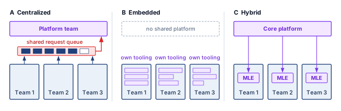
Figure 15: **Organizational Patterns for ML**: (A) A centralized platform team gives every model team the same infrastructure, but all requests pass through one shared queue, which can become the bottleneck. (B) Embedded teams each build their own tooling, which is fast locally but duplicates infrastructure and lets stacks diverge. (C) A hybrid keeps a core platform and places ML engineers (MLE) inside model teams as liaisons, balancing standardization with responsiveness.

Centralization works when the same operational mistakes would otherwise recur across the organization. A shared team can enforce consistent deployment, monitoring, and governance practices; invest once in training, serving, and observability infrastructure; and concentrate deep ML systems expertise that would be hard to replicate across many product teams. It also gives infrastructure engineers a visible career path rather than scattering them as one-person support functions.

The same structure can become a queue. If every platform request routes through one team, model teams wait on prioritization decisions they do not control. Distance from product context can also produce abstractions that are technically elegant but poorly matched to the consuming team’s constraints. Centralization is therefore strongest when common invariants dominate local variation, and weakest when model teams need rapid domain-specific changes.

12.10.2 Embedded ML engineers

When a fraud detection team needs a custom streaming feature adapter before tomorrow’s attack window, waiting two weeks in a central platform queue is unacceptable. The embedded pattern chooses proximity over uniformity by placing ML infrastructure expertise directly inside model teams, with coordination through communities of practice rather than a single reporting line. The benefit is responsiveness: the infrastructure engineer sees the team’s data, model behavior, release pressure, and incident history firsthand, so local changes do not wait for cross-team scheduling.

The cost appears later, when each team has solved deployment, monitoring, and feature management slightly differently. Fragmentation wastes engineering effort, complicates integration, and makes platform quality depend on the skill and bandwidth of whoever happens to be embedded with a given team. Embedded teams therefore work best when local speed matters more than cross-team consistency, and worst when every team is reimplementing the same platform substrate.

12.10.3 Hybrid models

An organization running 80 production models across recommendation, search, fraud, and ads cannot afford four separate serving stacks, nor can one central queue design domain-specific evaluation gates for all four workloads. Hybrid approaches resolve this tension by combining shared infrastructure ownership with domain-specific expertise. In this pattern, the core platform team owns compute, storage, networking, common training and serving systems, monitoring, and shared security, compliance, and cost controls. Domain platform engineers stay close to recommendation, language, vision, fraud, or search teams. Explicit boundaries distinguish changes those teams can make locally from changes that require coordination because they affect shared interfaces or operating guarantees.

A federated version of the same idea distributes implementation work without giving up architectural control. Major contributing teams help maintain platform components, but standards, ownership boundaries, and prioritization are coordinated explicitly. This works only when governance has real authority: otherwise federation degenerates into embedding with more meetings.

12.10.4 Organizational pattern selection

A 15-model startup iterating on disparate prototypes stalls if every change must clear a central governance queue, whereas a 100-model regulated financial institution faces audit failures and repeated outages if every team improvises its own deployment path. The appropriate organizational pattern depends on where standardization creates more value than local autonomy. Higher model counts, stricter regulatory requirements, and immature infrastructure favor centralized platforms, while heterogeneous model portfolios and smaller organizations may benefit from distributed expertise (table 38).

Table 38: Organizational Pattern Decision Factors: Five criteria for choosing between centralized and distributed ML platform teams. Higher model counts (100+), stricter regulatory requirements, and earlier infrastructure maturity favor centralized platforms; heterogeneous model portfolios and smaller organizations may benefit from distributed expertise with coordination through communities of practice.

Factor	Favors centralized	Favors distributed
Model count	Higher (100+)	Lower (10–20)
Model similarity	Homogeneous	Heterogeneous
Organization size	Larger	Smaller
Regulatory requirements	Stricter	Lighter
Infrastructure maturity	Earlier stage	Later stage

The infrastructure-maturity row can look inverted, because a young organization seems the natural home for local improvisation. The reasoning runs the other way. Early on, no shared substrate exists, and a central team is the cheapest way to build one before every model team writes its own deployment and monitoring path. Once that substrate matures into self-service interfaces, distributed teams can consume it directly, and the central queue matters less.

The selection logic becomes clearer in a concrete scenario. A technology company with 50 ML engineers across 8 teams operates 80 production models across recommendation, fraud, search, and ads. Each team maintains its own deployment and monitoring, creating duplicated work and inconsistent integration practices. That duplication motivates evaluating a shared platform; the model count alone does not establish its return. Domain diversity also motivates retaining expertise close to each workload rather than expecting one central team to make every modeling and operational decision.

One candidate design is hybrid. In this scenario, a central platform team of roughly 12–15 engineers owns core infrastructure, while domain-specific platform leads remain embedded with the largest model teams. That staffing assumption must be tested against the platform’s scope, support burden, and service commitments. A community of practice coordinates standards, and a shared contribution model lets domain teams upstream reusable components instead of maintaining permanent forks. The same platform engineering, feature management, and governance trade-offs become more concrete in the hyper-scale systems built by large technology companies.

Self-Check: Question

Which organizational structure best balances platform standardization with domain-specific velocity for an enterprise operating 80 production models across diverse application domains (e.g., recommendation, fraud, search, ads)?
1. A pure decentralized model with no shared infrastructure where each team manages separate cloud clusters.
2. A pure centralized model where all model training, hyperparameter tuning, and deployment must be submitted as platform team tickets.
3. An outsourced contractor model where ML infrastructure is operated by third-party vendors.
4. A hybrid model where a centralized core platform team owns shared infrastructure while domain-specific platform engineers remain embedded within product teams.
According to the decision criteria for ML organizational patterns, which combination of organizational factors most strongly favors adopting a Centralized Platform Team?
1. High model count (100+ models), homogeneous model architectures, large organization size, and strict regulatory compliance requirements.
2. Small team size (5 engineers), low model count (2 models), and exploratory unconstrained research projects.
3. Completely isolated business units with zero shared data sources and diverse, one-off computer vision models.
4. Organizations with late-stage, mature bespoke tooling where team-local customization takes precedence over shared standards.
Analyze the primary long-term operational risk when an organization relies exclusively on an ‘Embedded ML Engineers’ model as the model fleet expands beyond 50 models.
A federated ML platform organizational model can operate effectively without central governance authority to enforce architecture standards and prevent code forking.

See Answers →

12.11 Case Studies

When hundreds of engineers train and deploy thousands of models against shared data streams and strict latency budgets, bespoke per-team pipelines collapse under silent feature skew, duplicated glue code, and uncoordinated rollouts. The five platform cases that follow instantiate the operations trade-offs developed earlier in this chapter: standardization vs. team-local velocity, abstraction vs. control, freshness vs. cost, and governance vs. autonomy. Each case shows a different way to keep a multi-model fleet repeatable without turning every model into bespoke infrastructure.

12.11.1 Uber Michelangelo

Uber’s Michelangelo platform shows why repeatability becomes a platform requirement at company scale (Hermann and Del Balso 2017). Uber’s 2017 account describes data scientists using varied modeling tools while engineering teams built custom production systems, with no common deployment path or reproducible data pipelines. Michelangelo standardized one workflow from data management through training, evaluation, deployment, and prediction monitoring, and shared feature definitions let teams reuse platform-managed pipelines. Its delivery-time model combined historical and near-real-time restaurant preparation features, and such features raise the consistency problem of section 12.4, because one feature definition must produce compatible values for offline training sets and online requests. The standardization trade-off is the durable lesson. Common data and deployment paths remove repeated infrastructure work, while product teams still own model behavior and business-specific validation.

Hermann, Jeremy, and Mike Del Balso. 2017. Meet Michelangelo: Uber’s Machine Learning Platform. Uber Engineering Blog.

12.11.2 Meta FBLearner Flow

Meta’s FBLearner Flow shows how shared ML infrastructure can hide resource management while preserving workflow structure (Engineering 2016). In its 2016 account, Facebook reported use by more than 25 percent of its engineering team and more than one million models trained. Engineers defined operators with typed inputs and outputs, and compilation formed a DAG whose dependencies controlled execution; operators declared CPU, GPU, and memory needs, and the platform allocated resources and moved data between steps. Feed ranking adds freshness pressure, because the value of a signal such as a recent like decays quickly. Shadow mode (or dark launching) and canary releases then verify a candidate’s latency, memory, and error behavior on live traffic before its outputs reach users. The durable lesson is the interface between workflow intent and managed execution.

Engineering, M. 2016. Introducing FBLearner Flow: Facebook’s AI Backbone. Engineering at Meta Blog.

12.11.3 Netflix ML infrastructure

Netflix’s ML infrastructure shows how personalization platforms manage fan-out cost under a strict latency budget (Gomez-Uribe and Hunt 2015). The recommendation system combines several ranking and personalization algorithms for page generation, row selection, search, and artwork, and every additional online ranker or feature dependency consumes latency budget. Production systems therefore separate candidate generation, offline training, online ranking, and caching, so the homepage stays personalized without executing an unbounded number of models per request. New members and new titles raise the cold-start problem; exploration policies such as bandits are one option, and they need explicit exploration budgets, policy versions, and feedback logging. Netflix’s interleaving work merges competing ranked lists for the same user and credits each click to its source ranker (Netflix Technology Blog 2017), so faster experiments require additional serving and logging capability.

Gomez-Uribe, Carlos A., and Neil Hunt. 2015. “The Netflix Recommender System: Algorithms, Business Value, and Innovation.” ACM Transactions on Management Information Systems 6 (4): 1–19. https://doi.org/10.1145/2843948.

Netflix Technology Blog. 2017. Innovating Faster on Personalization Algorithms at Netflix Using Interleaving. Netflix Tech Blog.

12.11.4 Google Vertex AI

Google Vertex AI illustrates the managed-platform abstraction problem, which is to reduce the glue-code burden described by Sculley et al. (2015) while preserving control over custom workloads. Offering AutoML alongside custom training makes that boundary visible, because automated search, of which neural architecture search is one method, trades compute for engineering effort and needs bounded cost and concurrency. A managed service also carries contracts that its consumers must verify. A container separates a model’s software environment but does not isolate accelerator memory bandwidth, shared networks, or backing services, and a managed feature service must respect when information was available to the predictor, not merely when the event occurred. Managed infrastructure transfers implementation work, not responsibility for leakage, quality, or tail latency under the intended load. These mechanisms are general design options, not claims about Vertex AI’s internal architecture.

Sculley, D., Gary Holt, Daniel Golovin, Eugene Davydov, Todd Phillips, Dietmar Ebner, Vinay Chaudhary, Michael Young, Jean-François Crespo, and Dan Dennison. 2015. “Hidden Technical Debt in Machine Learning Systems.” Advances in Neural Information Processing Systems (NeurIPS) 28: 2503–11.

12.11.5 Spotify ML platform

Spotify’s ML platform places shared infrastructure in a personalization setting where immediate response and longer-term listener value need not align, since optimizing clicks alone can overlook diversity and discovery (the concern about filter bubbles). Separating candidate generators, such as collaborative filtering models (Koren et al. 2009) or editorial selections, from rankers lets teams change retrieval strategies while preserving the ranking contract. Spotify’s documented contribution is a paved road for model orchestration built around TensorFlow Extended, Kubeflow Pipelines, and metadata tracking (Engineering 2019). Its operational lesson is lineage, which lets an engineer trace a silent regression back to the data or workflow state that produced it. The same discipline supports mixed freshness. In an illustrative split, a weekly playlist can be computed in batch, while a responsive home screen ranks precomputed candidates with recent interaction features online, so only decisions that need current context pay for the live path.

Koren, Yehuda, Robert Bell, and Chris Volinsky. 2009. “Matrix Factorization Techniques for Recommender Systems.” Computer 42 (8): 30–37. https://doi.org/10.1109/mc.2009.263.

Engineering, S. 2019. The Winding Road to Better Machine Learning Infrastructure Through TensorFlow Extended and Kubeflow. Spotify Engineering Blog.

12.11.6 Comparing platform control planes

Across Uber, Meta, Netflix, Google, and Spotify, teams started from different bottlenecks—inconsistent delivery-time features, duplicated DAG plumbing, homepage fan-out latency, multi-tenant cloud glue code, and unrepeatable personalization experiments—yet converged on the same division of control-plane responsibilities. No single implementation is the template; the durable pattern is that shared state, release evidence, resource policy, and ownership become platform interfaces, while each domain team keeps a responsibility that no platform can absorb (table 39).

Table 39: Comparative Platform Control Planes: The five cases allocate implementation differently but retain the same systems contract: the platform owns shared invariants and evidence, while domain teams retain workload intent and acceptance criteria.

Case	Primary pressure	Control-plane emphasis	Local responsibility retained
Michelangelo	Repeated feature and deployment work	Shared features and repeatable workflows	Product-specific model behavior and validation
FBLearner Flow	Many teams and heterogeneous pipelines	DAG orchestration and resource abstraction	Workflow intent and domain evaluation
Netflix	Fan-out under strict latency budgets	Composition, precomputation, experimentation	Ranking objectives and user-experience trade-offs
Vertex AI	Multi-tenant managed infrastructure	Isolation, policy, and lifecycle integration	Workload configuration and acceptance criteria
Spotify	Fresh personalization with mixed paths	Lineage, paved roads, and hybrid data movement	Domain policy and exploration strategy

The comparison also exposes the adoption constraint. A platform succeeds when its common path captures recurring invariants without erasing domain judgment. Too little platform ownership recreates bespoke infrastructure; too much converts every exceptional workload into a central-team queue. Versioned interfaces, explicit exceptions, and outcome-based adoption metrics keep that boundary adjustable as the portfolio changes. The same boundary choices, misjudged, produce the misconceptions that recur when teams scale ML operations.

Self-Check: Question

Netflix reported ranking experiments requiring over $100\times$ fewer users than traditional between-subject A/B tests. Which mechanism explains why interleaving can provide this sample-efficiency advantage?
1. By testing ranking algorithms exclusively on synthetic bot agents.
2. By deploying ‘Interleaving’, which blends ranked lists from two algorithms into a single presentation for each user, removing user-level variance and measuring direct head-to-head clicks.
3. By relaxing statistical power thresholds from $\beta = 0.80$ to $\beta = 0.10$.
4. By evaluating models purely on historical offline training set accuracy.
What recurring coordination problem does the Michelangelo case illustrate?
1. Cloud GPU instances were unsupported by Uber’s container runtimes.
2. Data scientists were legally prohibited from executing SQL queries against production databases.
3. Varied modeling tools and custom production systems lacked a common deployment path and reproducible data pipelines.
4. Mobile device operating systems refused to display recommendation rankings with more than five items.
What general batch-versus-online design trade-off does the Spotify case illustrate for personalization features with different freshness requirements?
The deployment practice where a candidate model receives copied live traffic to evaluate latency, memory, and outputs without serving its predictions to users is known as shadow deployment or ____.

See Answers →

12.12 Fallacies and Pitfalls

Most operational misconceptions at scale share one root. Practices sized for one model survive into a fleet whose models share features, pipelines, infrastructure, and alerts. The following fallacies and pitfalls show where those per-model practices fail once the interactions dominate.

Fallacy: Operational complexity grows linearly with model count.

Shared dependencies can make coordination grow faster than model count. A model consuming embeddings from another model through a shared feature pipeline cannot change that interface safely without checking its consumers. The graph’s structure, not the count alone, determines the interaction burden; compatible interfaces still permit independent releases. In the monitoring scenario, 100 models with 10 metrics checked every five minutes at a 5 percent false positive rate produce 14,400 raw false crossings daily before suppression. At an assumed 40 operational engineer-hours per model per month, 40 models require 1,600 engineer-hours monthly ($2.88M annually at $150/hour). A staffing plan that adds operators in proportion to model count therefore falls behind exactly when the dependency graph densifies, which is when shared controls must absorb the repeated work and cross-model interactions instead.

Pitfall: Applying independent alerts to every model and metric.

Paging on every per-model threshold crossing creates avoidable noise, because equation 9 makes at least one false crossing nearly certain across a thousand independent checks, even though that probability says nothing about the fraction of pages that are false. Hierarchical monitoring supplies context for grouping and routing related signals, while persistence rules and calibrated thresholds reduce nonactionable notifications. Urgent model or component failures still require direct alerts when their response contracts demand immediate action.

Fallacy: Platform investment can wait until the organization reaches 100+ models.

The benefit-cost curves charted in figure 2 reach break-even parity between 20 and 50 models under the example’s assumed costs and savings. The governing threshold is recovered engineering capacity relative to the full platform cost, not a universal model count. The debt-audit examples identify recurring work that can justify investment, but a migration premium or payback period requires its own effort and recurring-cost estimates.

Pitfall: Treating all deployments with uniform procedures regardless of risk profile.

Applying the same staged rollout to every model update either over-burdens low-risk changes or under-protects high-risk ones. Release cadences differ by workload family (table 2), but a model family does not establish a universal release frequency or rollback window. Risk-based policies match observation time, exposure, and containment to the change: a subtle quality regression may require prolonged shadow evaluation, while a harmful release still requires rapid routing to a validated version.

Fallacy: Per-model metrics, such as loss and accuracy, are sufficient at scale.

In multi-model platforms, system-level and per-model metrics answer different questions. An upstream latency regression can lengthen the request path while accuracy remains unchanged. Shared-feature drift can reduce several downstream models’ accuracy at once; their metrics reveal the harm but do not alone identify its common cause. Section 12.6 joins business, portfolio, model, and infrastructure signals so the platform can trace that dependency.

Pitfall: Defaulting to batch pipelines for all features to simplify architecture.

A daily batch policy is appropriate only when its delay fits the feature contract. The freshness definition $\FeatureFreshnessLatency= \FeatureRecordTime - \SourceEventTime$ measures event-to-availability delay; it does not determine a universal batch or streaming latency. The scenarios $\FeatureFreshnessLatency\approx 12\text{--}24 \text{ hours}$ and $\FeatureFreshnessLatency\approx 1\text{--}5 \text{ seconds}$ illustrate different operating points whose quality effects require measurement. For the recommendation example in table 10, the 2.1-point gap between hourly and real-time features is assumed to be worth $10 million a year. A batch default forgoes that value silently, so the streaming decision belongs in the freshness break-even of checkpoint 12.2 rather than in a blanket preference for simpler pipelines. Fraud systems likewise need timely evidence, but the exploitable delay depends on their other detection and containment controls.

Fallacy: Technical debt is inevitable at scale and should be addressed only when it blocks critical work.

The premise overlooks the accumulating cost of recurring work. Section 12.2.4.1 provides illustrative escalation policies, not universal thresholds for declaring debt. Release friction, incidents, and toil are tracked against the platform’s own baseline, and the cost of remediation is compared with its expected benefit. A repeated manual task becomes an investment candidate when reducing it releases enough capacity or risk to justify the work. Waiting for debt to block critical work also means waiting until it is expensive to redirect. Deployment lead time, incident frequency, alert noise, rollback delay, and toil share are leading indicators that show the platform boundary failing while the repair is still small, and dismissing their rise as the price of scale discards that signal.

Self-Check: Question

Why is the assumption that ‘platform engineering investment can wait until an organization operates more than 100 models’ an expensive operational fallacy?
1. GPU hardware vendors refuse to deliver accelerators to organizations with fewer than 100 models.
2. Waiting for an arbitrary model-count threshold can allow duplicated pipelines and brittle dependencies to accumulate, increasing later migration cost despite an earlier economic case for shared tooling.
3. Cloud service providers automatically delete model binaries if an organization does not deploy 100 models within six months.
4. Single-model deployments cannot run in Docker containers without a centralized platform.
Why is applying uniform, one-size-fits-all deployment procedures across all models in a portfolio considered an operational pitfall?
1. It prevents the CI/CD pipeline from generating markdown documentation.
2. Kubernetes schedulers only allow one deployment strategy per cluster.
3. Different deployments have different risk profiles, observation windows, and rollback contracts; fraud and LLM services can therefore require different release gates.
4. Staged rollouts cannot be automated for recommendation systems.
Explain why per-model offline accuracy metrics (such as test loss or ROC-AUC) are insufficient for monitoring system-level health in a multi-model serving platform.
Technical debt in ML platforms should remain qualitative and unmeasured because engineering toil cannot be quantified with concrete operational thresholds.

See Answers →

12.13 Summary

Fleet operations makes shared model and feature state, release evidence, resource commitments, and recovery authority governable across a portfolio. Registries, dependency-aware deployment, and hierarchical monitoring replace repeated per-model coordination with accountable shared controls. Coordination is the organizing concern in C³, but those controls also consume compute and communication resources. Fleet telemetry assigns lost productivity to the terms of the Fleet Law. Stragglers lengthen the synchronization term $\SynchronizationTime(\DeviceCount)$, while data stalls, communication delays, and checkpoint recovery affect execution through different mechanisms and timescales. Registries and release gates connect that resource use to validated, useful outcomes.

Three principles carry forward from those mechanisms. Release evidence is valid only when it binds to one versioned contract, so offline quality, production load, experiment design, and rollback thresholds must describe the same candidate, and any exhausted dimension of the reliability budget vector stops promotion. A regression is priced by exposure as well as by detection, so rollout speed and rollback readiness follow the harm a bad release can do and the time needed to see it. Utilization is the economic invariant beneath every capacity decision, from build-vs.-buy to standby headroom, while the lifecycle cost breakdown $(\text{TCO}_{\text{ML}} = \TrainingCost + \InferenceCost + \TotalDataCost + \IterationCost)$ decides where optimization repays its cost. Edge fleets apply the same contract under weeks-long rollouts, version skew, and privacy-limited telemetry (Fleet release controls).

Key Takeaways: Operational load follows coupling

One model is not the unit: At portfolio scale, the operational object becomes the dependency graph of models, features, pipelines, alerts, and owners. Registries, lineage, and ensemble-aware CI/CD expose affected consumers and make compatibility a release condition.
Feature meaning is a versioned interface: A redefined feature can pass schema checks while silently changing every consumer’s inputs. Versioned definitions, lineage, and point-in-time joins that filter on availability time keep training and serving on the same meaning.
Shared controls must earn their cost: At fixed savings per model, the platform benefit-cost ratio grows linearly with model count, so the break-even portfolio size of figure 2 moves with savings per model and platform cost. Treating the platform as a versioned product keeps adoption, exceptions, migrations, and retirement from recreating that work.
Ownership cost chooses the target: The cost-of-ownership equation separates training, inference, data, and iteration costs, and the dominant term changes over a system’s life (principle 17). Measured lifecycle costs, not fleet age, decide between investing in iteration speed and in serving efficiency.
Reliability is a vector: Independent metric alerts scale into noise across a model portfolio. Hierarchical telemetry routes common-cause incidents, while any exhausted availability, latency, freshness, or quality budget can stop promotion, because $\max_{\ReliabilityTargetIndex} \ErrorBudgetConsumption_{\ReliabilityTargetIndex} \le 1$ governs rather than an average (principle 21).
Evaluation is one versioned contract: Offline quality, production load, statistical power, assurance evidence, rollback thresholds, and reproducibility metadata must describe the same candidate (principle 21). Every acceptance claim needs an owner and an invalidation condition, so the contract turns the coordination axis of C³ into auditable evidence.

Shared controls pay off when they reduce the coordination required for a safe change without obscuring who owns its consequences. The platform can automate checks, preserve evidence, and enforce limits, but model and domain owners still decide what behavior is acceptable. That boundary makes fleet growth manageable without turning every exception into a central-team bottleneck.

What’s Next: A governed fleet is still an attack surface

Even when every release is versioned, gated, and observable, the fleet is not secure by that evidence alone, because reliability metrics show whether the fleet serves its intended callers, not what an adversary can learn or change through the same interfaces. The serving endpoints, shared feature pipelines, telemetry stores, and federated rounds that this chapter made governable are also places where an authenticated caller can copy model behavior or a participant can alter what the fleet learns. Defending them starts from a different inventory than operating them: the asset worth protecting, the actor who threatens it, the access that actor holds, and the trust boundary that access must not cross.

↪ Threat models, fleet trust boundaries, model extraction, data poisoning, and differential privacy are developed in Security & Privacy.

12.14 Self-Check Answers

Self-Check: Answer

Why can manual, per-model operational maintenance become difficult to sustain as an organization expands to hundreds of models that share features, resources, and release dependencies?
1. Shared data dependencies, contested resources, and independent alert streams add coordination work that can exceed the capacity of manual per-model processes.
2. Modern deep learning framework compilers prohibit deploying more than one model graph per physical datacenter.
3. Single-model architectures run on asynchronous virtual memory subnets that cannot route traffic through standard TCP/IP gateways.
4. Network switches automatically drop telemetry packets when concurrent endpoint connections exceed ten.
Answer: The correct answer is A. Shared features, contested resources, and independent alerts create interacting operational dependencies as the model portfolio grows. Manual per-model maintenance becomes difficult to sustain, motivating shared controls and automation. This is a scaling argument, not a theorem that every 500-model organization has the same complexity or requires one physical control-plane server.

Learning Objective: Explain the operational phase transition from single-model MLOps to fleet-scale platform operations.
What is the primary architectural purpose of the Control Plane in an enterprise ML platform spanning datacenters, cloud clusters, and edge fleets?

Answer: The Control Plane serves as the centralized steering and governance layer that keeps physical infrastructure, training pipelines, serving paths, edge runtimes, and policy rules observable, coordinated, and recoverable, preventing operational drift across the fleet.

Learning Objective: Explain the architectural function of the control plane in enterprise ML platform operations.
Treating each model in an enterprise as an isolated, independent entity with bespoke pipelines remains an economically sound strategy as long as each individual model achieves high predictive accuracy.

Answer: False. Predictive accuracy alone does not establish the economic case for isolated pipelines. Shared workloads can duplicate feature processing, strand capacity, and generate repeated alerts; compare those measured costs with the investment and coordination costs of shared controls.

Learning Objective: Evaluate the economic and operational failure modes of fragmented per-model infrastructure.

← Back to Questions

Self-Check: Answer

An organization operates 50 models. A platform team costs $120,000 per month and recovers 20 engineering hours per model monthly, valued at $150 per hour. What are the benefit-cost ratio and net ROI based on this recovered-capacity value?
1. Benefit-cost ratio 0.80 and net ROI of -20%.
2. Benefit-cost ratio 1.25 and net ROI of 25%, with $30,000 in net monthly capacity value above platform cost.
3. Benefit-cost ratio 2.50 and net ROI of 150%, with $180,000 in net monthly capacity value above platform cost.
4. Benefit-cost ratio 0.50 and net ROI of -50%.
Answer: The correct answer is B. Recovered capacity is valued at $50\times20\times\$150=\$150{,}000$ monthly. Dividing by $\$120{,}000$ gives a benefit-cost ratio of $1.25$; net ROI is $1.25-1=25\%$, or $\$30{,}000$ above cost. Recovered engineering time is not automatic cash savings: realizing that value requires productive redeployment or avoided expenditure.

Learning Objective: Distinguish benefit-cost ratio, net ROI, and recovered engineering-capacity value in platform investment analysis.
According to the ML technical debt taxonomy (Sculley et al.), which operational symptom specifically indicates dangerous Configuration Debt rather than Data Debt or Model Debt?
1. Upstream database schema changes that silently alter categorical feature encodings.
2. Extensive glue code written to convert data between disparate third-party machine learning libraries.
3. Large, unvalidated configuration parameter files (e.g., exceeding 500 lines of ad-hoc YAML per model) causing frequent deployment failures.
4. Tangled feedback loops where a fraud detection model’s historical outputs bias incoming training labels.
Answer: The correct answer is C. Configuration debt manifests as unvalidated parameter surfaces, duplicated configuration blocks, and brittle YAML/JSON files that lack schema verification, directly leading to deployment failures. In contrast, upstream schema alterations represent data debt, glue code represents model debt, and feedback loops represent pipeline/system entanglement.

Learning Objective: Classify operational symptoms into distinct categories of ML technical debt.
How does the debt-cleanup payback calculation quantitatively justify investing 160 engineering hours upfront to refactor and automate brittle pipeline plumbing over a 3-year model lifecycle?

Answer: Refactoring reduces recurring manual toil from 40 hours/month down to 8 hours/month. Over 36 months at $150/hour, status quo toil costs $216,000, whereas the proactive path costs $67,200 (including the 160-hour setup), yielding a cost ratio ratio of approximately $3.2\times$.

Learning Objective: Analyze the long-term economic trade-offs of paying down ML technical debt versus enduring continuous manual toil.
Contrast the deployment frequency and rollback latency requirements of an adversarial fraud detection model with those of a frontier large language model (LLM).

Answer: Fraud systems facing active adaptation may need frequent releases and rapid traffic rollback, while a frontier LLM release may require longer shadow and safety evaluation. These are deployment contracts shaped by risk, label delay, and validation cost, not fixed cadences for each model family. Long observation windows do not justify slow rollback once a harmful release is detected.

Learning Objective: Compare operational deployment cadences and risk profiles across diverse ML model types.
ML platform engineering is a variable cost that delivers immediate positive economic return regardless of the number of deployed models in an organization.

Answer: False. Platform investment includes fixed team and tooling costs. Its economic case depends on the value of recovered engineering capacity and avoided incidents relative to those costs. The break-even fleet size depends on workload and organization; 20–50 models is not a universal threshold, and recovered time is not automatically cash savings.

Learning Objective: Evaluate the scaling threshold and fixed-vs-variable cost structure of centralized ML platforms.
A portfolio has shared embeddings, cross-team feature pipelines, and cascading latency regressions. Which coordination and diagnostic controls become necessary, and why does model count alone not determine when to introduce them?

Answer: Recorded dependencies identify consumers to re-evaluate when a shared embedding changes. Compatible version sets and rollback targets govern release, while cross-model traces localize latency along the request path. These controls respond to coupling and failure consequences: a small tightly coupled portfolio can need them before a larger collection of isolated models. Fleet size informs capacity planning but does not prescribe a universal maturity sequence.

Learning Objective: Explain how dependency structure determines coordination and diagnostic controls.

← Back to Questions

Self-Check: Answer

When an upstream User Embedding Model is updated in an enterprise model registry, which automated sequence of graph-traversal actions must the registry execute to prevent silent production failures?
1. Hot-swap the model binary on serving pods and trigger immediate asynchronous retrains of downstream models without blocking traffic.
2. Identify all dependent downstream models (retrieval, ranking, ensembles), trigger compatibility re-evaluations, and block promotion of the upstream model until all dependents pass verification.
3. Overwrite the existing embedding schema in-place and invalidate all client-side prediction caches.
4. Recompile the entire datacenter Kubernetes cluster manifest and flush all feature store storage tables.
Answer: The correct answer is B. Upstream changes silently break downstream models unless the registry executes graph traversal: identifying dependent consumers, triggering automated compatibility evaluation with the new embeddings, blocking promotion until verified, and coordinating staged deployment order.

Learning Objective: Design automated dependency tracking and validation workflows for multi-model registry systems.
In high-throughput e-commerce recommendation systems, what is the primary systems rationale for deploying a multi-stage ensemble (retrieval $\rightarrow$ ranking $\rightarrow$ re-ranking) rather than a single end-to-end deep neural network?
1. Multi-stage ensembles eliminate all network communication between microservices.
2. Single deep learning models cannot process floating-point tensors larger than 32 bits.
3. Evaluating millions of catalog items with an expensive, feature-rich ranking model violates strict serving latency budgets ($<10\text{ ms}$), requiring fast candidate filtering before fine ranking.
4. Modern web browsers reject HTTP responses generated by single-model inference backends.
Answer: The correct answer is C. Multi-stage filtering is computationally essential: lightweight retrieval models filter millions of candidate items down to hundreds within milliseconds, allowing heavy, computationally expensive ranking models with cross-features to score only the top candidates within strict latency SLOs.

Learning Objective: Justify the multi-stage ensemble architecture in latency-constrained recommendation systems.
Why must an enterprise model registry record complete training provenance (code commit, dataset version, hyperparameters, hardware envelope) in addition to the binary model weights?

Answer: Training provenance supports reproducibility and auditability by recording the code, data, hyperparameters, and hardware used. It helps trace regressions and leakage to their sources, but metadata alone cannot guarantee exact reproduction; retained artifacts, dependencies, randomness, and execution conditions also matter.

Learning Objective: Explain the necessity of training provenance and lineage metadata in enterprise model registries.
In a production multi-model recommendation ensemble, severe accuracy degradation in one component model will always trigger explicit application crashes and exception alerts in monitoring dashboards.

Answer: False. Other ensemble components or fallback heuristics can compensate for a degraded sub-model, producing plausible-looking recommendations while silently masking severe underlying model decay from basic infrastructure monitoring.

Learning Objective: Evaluate failure masking and silent degradation risks in multi-model ensemble architectures.
**Arrange the four stages of this example Staged Ensemble Deployment Pattern in operational sequence. The durations and traffic shares are assumed release-contract settings, not universal requirements:

Soak monitoring (7–14 days observing delayed feedback and distribution shifts)
Canary deployment (1% live traffic for 4–8 hours)
Shadow deployment (24–48 hours logging outputs without serving them)
Staged rollout (expanding traffic from 5% to 100% over 24–72 hours)**

Answer: The correct order is: (3) Shadow deployment -> (2) Canary deployment -> (4) Staged rollout -> (1) Soak monitoring. First, shadow deployment (3) logs predictions without serving them to verify latency and stability; next, canary (2) routes 1% live traffic; then, staged rollout (4) ramps from 5% to 100%; finally, soak (1) monitors for delayed effects over 7-14 days.

Learning Objective: Order the stages of a staged rollout pattern for multi-model production deployments.

← Back to Questions

Self-Check: Answer

Why does an enterprise feature store implement a dual-store architecture (separating an offline store from an online store) instead of relying on a single unified database system?
1. Online stores can store only integer IDs, whereas offline stores are required for floating-point feature values.
2. Training requires high-throughput sequential analytical batch scans over historical data, whereas serving requires sub-10 millisecond point lookups for individual entity keys.
3. Cloud providers legally mandate separating batch compute from streaming ingress databases.
4. Single database systems crash when table schemas exceed ten columns.
Answer: The correct answer is B. Historical analytical scans and low-latency serving lookups favor different indexing, storage, and scaling choices. Separating the stores lets each be optimized for its workload while shared definitions preserve semantic consistency. This is a practical architecture trade-off, not proof that no database could support both access patterns.

Learning Objective: Justify the dual-store architectural pattern for enterprise feature store operations.
What failure mode occurs when a training pipeline constructs training examples using current feature values rather than historical values as of each event timestamp?
1. GPU kernel deadlocks during forward propagation.
2. Hardware bit errors in the offline data lake storage controller.
3. ‘Time travel’ data leakage, where future information contaminates training data, producing deceptively high offline metrics but disastrous performance in production.
4. Out-of-memory errors in distributed model serving sidecars.
Answer: The correct answer is C. Point-in-time correctness prevents ‘time travel’ data leakage. If an event occurring at noon is joined with a daily aggregation computed at midnight, the model learns from future signals unavailable at inference time, leading to severe production accuracy degradation.

Learning Objective: Analyze the mechanisms and production risks of temporal data leakage in feature engineering.
In the context of Deep Learning Recommendation Models (DLRM), explain the cost of feature staleness that results from lagged streaming feature pipelines.

Answer: The cost of staleness is the quality or business loss from serving features that no longer reflect the user’s relevant state. Its size depends on the feature, workload, lag, and evaluation window. Measure CTR or other outcome changes rather than assigning a universal 5% to 15% penalty to a given delay.

Learning Objective: Evaluate the operational and revenue impact of feature staleness on recommendation systems.
Calculate the raw uncompressed historical storage footprint for a recommendation feature store with $100\text{ million}$ users, $1,000$ features per user, $1\text{ year}$ retention ($8,760\text{ hours}$), hourly full snapshots, and a $32\text{-byte}$ stored row (an $8\text{-byte}$ value, an $8\text{-byte}$ entity key, and $8\text{-byte}$ event and availability timestamps).

Answer: Total feature value records equal $10^8\text{ users} \times 1,000\text{ features} \times 8,760\text{ versions} = 8.76 \times 10^{14}$ rows. Multiplying by $32\text{ bytes}$ per row yields $2.8 \times 10^{16}\text{ bytes} \approx 28\text{ PB}$, three quarters of it metadata that makes point-in-time joins reproducible, which is why feature stores store only changed values and rely on compression and tiered retention.

Learning Objective: Calculate the historical storage scaling footprint required for point-in-time feature retention.
In an enterprise feature store, modifying the feature transformation logic of a shared feature in-place (e.g., changing normalization from z-score to min-max) is safe as long as the feature name and output datatype remain unchanged.

Answer: False. Shared feature definitions are immutable production API contracts. In-place transformation changes invalidate feature distribution assumptions across all downstream consuming models, causing silent model degradation and severe cross-team debugging toil; feature modifications require explicit semantic versioning.

Learning Objective: Evaluate the failure modes of unversioned schema mutations in shared feature platforms.
The subtle difference in feature transformation logic between offline batch training pipelines and online real-time inference pipelines is known as ____.

Answer: training-serving skew. Training-serving skew is the critical operational failure mode where differences in preprocessing logic between training and inference cause models to receive inputs formatted differently from what they learned, causing silent performance degradation.

Learning Objective: Identify the core operational failure mode solved by unified feature stores.

← Back to Questions

Self-Check: Answer

In the described social recommendation experiment, treatment users share boosted content with control users. Why does this violate the no-interference component of the Stable Unit Treatment Value Assumption (SUTVA)?
1. Individual user hashing causes GPU thread divergence on inference accelerators.
2. Social networks disallow collecting engagement metrics across control groups due to data privacy regulations.
3. User randomization forces feature stores to duplicate user embeddings across all regional caches.
4. Treatment users share boosted content with control users, making control outcomes depend on other users’ treatment assignments.
Answer: The correct answer is D. The no-interference component of SUTVA requires an individual’s outcome not to depend on other users’ treatment assignments. Sharing violates that condition. Positive engagement spillovers can attenuate the measured contrast, but bias direction depends on the mechanism and the effect being estimated.

Learning Objective: Analyze the statistical and operational mechanisms of SUTVA violations in networked ML evaluation.
When an ML platform evaluates 20 simultaneous A/B experiments across a model portfolio, why might the team adopt the Benjamini-Hochberg False Discovery Rate (FDR) procedure instead of the Bonferroni correction?
1. Bonferroni correction divides alpha by the number of tests ($0.05 / 20 = 0.0025$), creating an overly conservative threshold that inflates Type II errors (false negatives) and discards real model gains.
2. The Benjamini-Hochberg procedure eliminates the requirement for computing statistical significance or p-values.
3. Bonferroni correction can only be applied to computer vision models running on mobile edge devices.
4. The Benjamini-Hochberg procedure mathematically guarantees that zero false discoveries occur across any number of tests.
Answer: The correct answer is A. Bonferroni controls the probability of any false rejection across the family, at a potential power cost. Benjamini-Hochberg instead controls the expected false-discovery proportion among rejected hypotheses under its dependence assumptions, and may retain more power. It still requires valid p-values and does not guarantee zero false discoveries.

Learning Objective: Compare statistical multiple-testing correction methods for large-scale ML experimentation platforms.
What three criteria must be evaluated within an automated ‘performance gate’ function before a candidate model is approved for staging deployment?

Answer: An automated performance gate must evaluate: (1) absolute minimum thresholds on key metrics (e.g., minimum NDCG), (2) relative improvement over the active production baseline, and (3) strict tolerance bounds on secondary guardrail metrics (e.g., maximum allowable regression on MRR, coverage, or latency).

Learning Objective: Design automated multi-criteria validation gates for production ML CI/CD pipelines.
A model serves 1 million requests per hour and its canary plan needs about 10,000 samples per variant. Why should each canary stage’s duration be computed from that planned sample rather than set by elapsed time, and what sets the length of the whole rollout schedule?

Answer: A stage must last at least the planned sample divided by the request rate times the traffic share: 10,000 samples at 1 million requests per hour take 1 hour at 1 percent traffic and 12 minutes at 5 percent. That is a collection-time lower bound from the experiment design, not a stopping rule; delayed labels, correlated requests, and guardrail windows can extend it, and elapsed time alone establishes no confidence. The full schedule is set by the slowest outcome the release must observe, so fast guardrail metrics fill in hours, delayed outcomes need days of soak, and multi-region rollouts repeat evidence collection region by region.

Learning Objective: Size canary stage durations from experiment sample requirements and explain what sets the rollout schedule.
The formal statistical assumption that an experimental unit’s outcome is unaffected by the treatment assignments of other units is abbreviated as ____.

Answer: SUTVA. The no-interference component of the Stable Unit Treatment Value Assumption requires an experimental unit’s outcome not to depend on other units’ treatment assignments. Network and market spillovers can violate that component; it is not a requirement that all observed outcomes be statistically independent.

Learning Objective: Identify the formal statistical assumption underlying independent A/B testing.
**Arrange the standard stages of an end-to-end automated ML training and release pipeline in execution order:

Automated evaluation against baseline and slice performance gates
Artifact packaging with serving configuration and registration in model registry
Data validation and schema verification
Distributed training execution with lineage logging
Feature engineering and transformation**

Answer: The correct order is: (3) Data validation and schema verification -> (5) Feature engineering and transformation -> (4) Distributed training execution with lineage logging -> (1) Automated evaluation against baseline and slice performance gates -> (2) Artifact packaging with serving configuration and registration in model registry. Data validation (3) prevents training on corrupt data, feature transformation (5) processes inputs, distributed training (4) generates parameters, evaluation gates (1) verify accuracy, and registration (2) commits the approved artifact.

Learning Objective: Order the sequence of stages in a robust ML CI/CD pipeline.

← Back to Questions

Self-Check: Answer

Why are ‘gray failures’ (e.g., an accelerator whose GEMM arithmetic throughput drops by 20% or an NVLink connection suffering intermittent packet retries) exceptionally damaging in large synchronous distributed training runs?
1. Gray failures trigger automatic emergency power-off sequences across the entire datacenter hall.
2. A degraded rank or link on the communication critical path can delay collective completion and the next training step while ordinary availability checks remain healthy.
3. Gray failures cause the training loss optimizer to invert gradient signs during backpropagation.
4. The Kubernetes control plane immediately unmounts shared file systems when a GPU runs slowly.
Answer: The correct answer is B. A gray failure can lengthen the step critical path without crashing a process. Gradient communication can overlap computation as buckets become ready; ranks need not finish all local computation before any collective begins. The effect depends on placement and the collective schedule, rather than implying a datacenter-wide power failure.

Learning Objective: Analyze the systemic impact of hardware gray failures on synchronous distributed training efficiency.
If 8 GPUs in one server chassis show elevated junction temperatures while adjacent nodes remain normal, which local cooling hypothesis should the investigation prioritize?
1. Failure of the building’s central chiller cooling plant.
2. An optical transceiver failure on the top-of-rack InfiniBand switch.
3. A localized node-level failure, such as a chassis fan malfunction or a cold-plate coolant flow restriction.
4. A software bug in the Prometheus time-series database metric scraper.
Answer: The correct answer is C. The pattern prioritizes node-level cooling investigation. Compare workload, power, clocks, and cooling telemetry with adjacent nodes before confirming a cause; spatial correlation does not establish a fan or coolant fault by itself.

Learning Objective: Apply spatial correlation analysis to localize datacenter hardware telemetry anomalies.
In a fleet of 100 models with 10 metrics each, checked every 5 minutes at a threshold with false positive rate $\alpha = 0.003$, calculate expected raw false threshold crossings per day. How should monitoring distinguish these crossings from operator pages?

Answer: The expectation is $288,000 \times 0.003 = 864$ raw false threshold crossings per day under the stated marginal rate. These are not necessarily distinct incidents or pages. Grouping, persistence checks, deduplication, and calibrated alert policies reduce page burden; hierarchical monitoring routes evidence to responsible owners while retaining urgent local alerts.

Learning Objective: Calculate the mathematical rate of false positive alert generation across a multi-model fleet.
Describe the four levels of a hierarchical monitoring architecture for ML platforms and identify the primary owner and operational role of each level.

Answer: (1) Business metrics, such as revenue or conversion attributed to recommendations, are owned by the incident lead and raise the few high-confidence alerts that indicate product impairment. (2) Portfolio metrics, such as engagement lift or fraud caught and false-positive rate, are owned by domain teams and route the investigation to the model family that owns the shared objective. (3) Model metrics, such as task quality, latency distributions, and recent deployment state, are owned by model owners and support local diagnosis. (4) Infrastructure metrics, such as GPU cluster availability, feature store latency, networking, and storage, are owned by the platform team and route failures that need capacity or control-plane repair.

Learning Objective: Design a hierarchical observability architecture that eliminates alert fatigue while maintaining system visibility.
Automated hardware preflight checks necessarily reduce overall training productivity because they add job startup latency.

Answer: False. Preflight checks can recover more useful work than their startup cost by detecting faults before a long run. The net benefit depends on avoided failed work, diagnostic coverage, startup overhead, and false exclusions; matched workload baselines help assess that trade-off.

Learning Objective: Justify the use of automated hardware preflight diagnostics prior to distributed training allocation.
Hardware memory errors corrected automatically without crashing an application are called ____ errors; an elevated rate can warrant investigation before an uncorrectable failure.

Answer: correctable ECC. Error-Correcting Code (ECC) telemetry records corrected memory errors. Such errors can precede uncorrectable failures, but their predictive value requires validation for the device and workload; the count alone does not establish impending failure.

Learning Objective: Identify the hardware memory error telemetry used for predictive accelerator diagnostics.

← Back to Questions

Self-Check: Answer

In an enterprise ML platform hosting dozens of services, on-call alerts report that all recommendation models across multiple teams have suffered a 15% drop in conversion over the past two hours, while vision models, NLP services, and raw server health metrics remain completely green. What is the most probable root cause?
1. A catastrophic failure in the data center’s primary 400 Gbps spine network switches.
2. Simultaneous random hardware bit-flips across all GPU Tensor Cores.
3. An unannounced git commit modifying the loss function in the vision model repository.
4. An upstream feature store pipeline delay causing user interaction features to become stale across all recommender models.
Answer: The correct answer is D. The shared recommendation feature pipeline is the strongest hypothesis among these choices because the failure follows model-family dependencies while unrelated services remain healthy. Confirm freshness, recent changes, and cohort effects before declaring a root cause; the pattern narrows the investigation but does not prove it.

Learning Objective: Apply cross-model failure pattern analysis to isolate root causes in production ML outages.
Why should an ML incident response runbook check feature freshness and input distributions when business KPIs drop even though server health and latency remain normal?
1. ML systems fail silently: when feature pipelines stall or input distributions drift, models continue returning HTTP 200 responses with normal latency, rendering infrastructure checks falsely reassuring.
2. Inspecting GPU hardware metrics immediately triggers automated container restarts.
3. Data pipelines are not connected to production networks and cannot cause outages.
4. Infrastructure monitoring tools require 24 hours of latency to register server crashes.
Answer: The correct answer is A. Stale features or distribution changes can degrade predictions while requests still return successfully. Healthy infrastructure metrics therefore do not establish healthy model behavior. Investigate semantic and data signals alongside infrastructure evidence, and contain user impact while attribution continues; no universal diagnostic sequence fits every incident.

Learning Objective: Explain why ML incident response must inspect semantic and data health in addition to infrastructure metrics.
How does an operator diagnose a silent collective communication hang in a 1,024-GPU distributed training run using NCCL debug tooling?

Answer: Enable NCCL_DEBUG=INFO and NCCL_DEBUG_SUBSYS=ALL to collect communication diagnostics across ranks, then compare their last completed operations and check for missing or mismatched collectives. Correlate these with process, network, and device telemetry. A hang may produce logs or timeout errors, and logging alone does not guarantee identification of its cause.

Learning Objective: Apply distributed collective debugging tools to diagnose distributed training deadlocks.
Explain the primary objective of a Post-Incident Review (PIR) in an ML platform team and how it prevents recurrent operational failures.

Answer: A PIR conducts a blameless timeline analysis to identify missing or delayed platform controls (e.g., absent feature freshness gates or unversioned schema dependencies) and assigns ownership for implementing structural platform invariants that prevent an entire failure class from recurring.

Learning Objective: Explain how post-incident reviews convert operational failures into enforceable platform invariants.
The 2021 Meta global outage demonstrated that control plane dependencies (such as DNS, authentication, and routing) can be safely shared across both management and inference serving paths without physical isolation.

Answer: False. The 2021 outage proved that platform-scale operations must treat the control plane as a hard dependency with a bounded blast radius; when network partitions sever out-of-band management and DNS, shared dependencies isolate operators from performing remediation.

Learning Objective: Evaluate control plane blast radius and isolation risks in large-scale platform operations.
**Arrange the stages of the depicted ML Runbook Diagnostic Flow in their presentation order; containment may begin during attribution rather than waiting for a confirmed cause:

Bound blast radius (rollback or apply safe fallback controls)
Detect user impact (identify affected products, cohorts, and metrics)
Learn from the gap (add missing gates or alerts)
Localize dependency (check releases, feature freshness, and pipeline lag)
Escalate by evidence (route diagnostics to the responsible owner)**

Answer: The depicted order is: (2) Detect user impact -> (4) Localize dependency -> (1) Bound blast radius -> (5) Escalate by evidence -> (3) Learn from the gap. This organizes the investigation, not a mandatory serial execution schedule. Safe containment and escalation can proceed during attribution; responders should not leave users exposed while waiting to prove a root cause.

Learning Objective: Order the stages of the standard ML incident response diagnostic flow.

← Back to Questions

Self-Check: Answer

A platform computes ML productivity goodput per team and workload class from scheduler records, job timelines, and step traces. What does charging each lost hour to exactly one goodput factor let a portfolio dashboard show?
1. The dollar value of every busy GPU-hour, independent of whether the job later fails
2. Which layer (orchestration, the runtime, or the program) limits each team’s useful output, and therefore which owner must act
3. The capacity-weighted average utilization across heterogeneous accelerators
4. The number of models a platform needs before its benefit-cost ratio passes one
Answer: The correct answer is B. Because scheduling, runtime, and program goodput each charge a loss once, their product says how much useful output was lost and which layer lost it, so the dashboard routes the problem to its owner. Busy GPU-hours are only an upper bound on useful work, and capacity-weighted utilization and the platform break-even answer different questions.

Learning Objective: Apply portfolio goodput accounting to route fleet efficiency losses to their owners.
Which shared-resource path can allow a training tenant to violate the latency SLO of a co-located inference tenant?
1. Competition for finite GPU High Bandwidth Memory (HBM) or shared RDMA fabric bandwidth can stall the inference tenant even when host CPU resources are isolated.
2. Linux kernel cgroups and container namespaces cannot be instantiated on systems containing GPU accelerators.
3. CPUs cannot run multi-tenant virtualization or container runtimes.
4. Multi-tenant GPU clusters require all tenant models to share the exact same weights in memory.
Answer: The correct answer is A. Host isolation alone does not bound contention for device memory or the shared communication fabric. A training tenant can exhaust available HBM or saturate fabric capacity, delaying inference. Containers do not require shared model weights; device partitioning and network admission controls must match the isolation contract.

Learning Objective: Analyze the architectural causes of the noisy neighbor problem in multi-tenant GPU infrastructure.
A platform reports utilization as the simple average across its resources. Why does the chapter weight each resource’s utilization by its capacity instead, and what must be true of the capacity units before the weighted average is meaningful?

Answer: Capacity weighting makes the metric track where stranded work actually lives: an idle eight-GPU node wastes more than an idle single GPU, so a small underused resource should not pull the platform average down as hard as a large idle pool. The capacities must be expressed in a common unit over the same interval; heterogeneous accelerators need a declared workload normalization, and CPU cores, device counts, and bytes cannot be added directly.

Learning Objective: Interpret capacity-weighted platform utilization and its unit requirements.
In a 100-GPU training cluster operating at $65\%$ average compute utilization and $80\%$ memory utilization with 4-hour queue waits and a cost of $\$2.50$/GPU-hour, evaluate whether buying more GPUs or optimizing data-loading pipelines is the superior operational intervention.

Answer: These aggregate metrics do not uniquely identify a data-loading bottleneck. Profile input stalls, memory traffic, communication, kernels, and placement before choosing an intervention. Busy time is also only an upper bound on useful work: if a verified repair raises busy compute from $65\%$ to $80\%$, the added busy capacity is $100\times24\times0.15\times\$2.50=\$900$ per day at the chargeback rate, and goodput accounting must still remove failed jobs and lost work before calling it productive. The cluster bill does not change; the capacity becomes cash only if it avoids a purchase, and expansion depends on remaining queue demand.

Learning Objective: Apply cluster utilization metrics and economic principles to diagnose ML capacity bottlenecks.
Batch training workloads and live online serving workloads share the same operational constraints and should be managed under an identical cluster scheduling and preemption policy.

Answer: False. Batch training is interruptible, checkpointable, and optimizes for long-term throughput and high GPU utilization, whereas online serving is latency-critical (strict p99 latency SLOs), non-preemptible, and requires reserved headroom capacity to absorb traffic spikes.

Learning Objective: Evaluate resource management and scheduling invariants between training and serving workloads.
**Arrange the four Platform Abstraction Levels in order from lowest level of abstraction (1) to highest level of abstraction (4):

Full Lifecycle Product (Managed IDEs, feature stores, experiment tracking, registries, automated governance, Vertex/SageMaker)
Standardized Containers (ML-aware Kubernetes integrations, standardized images, persistent volume claims)
Infrastructure as a Service (Raw GPU capacity, bare namespaces, raw block storage, manual script execution)
ML Control Loops (Topology-aware schedulers, distributed training orchestrators, Ray/Kubeflow)**

Answer: The correct order is: (3) Infrastructure as a Service -> (2) Standardized Containers -> (4) ML Control Loops -> (1) Full Lifecycle Product. Level 1 provides raw infrastructure (3); Level 2 standardizes containers and storage (2); Level 3 automates ML control loops and distributed orchestration (4); Level 4 provides end-to-end full lifecycle managed capabilities (1).

Learning Objective: Order the progression of ML platform abstraction tiers.

← Back to Questions

Self-Check: Answer

In the chapter’s illustrative on-premises AI cluster cost stack, which cost center represents the largest ongoing Operational Expenditure (OpEx) component over the 3-year lifecycle?
1. InfiniBand optical transceiver replacements and network switch warranty contracts.
2. Commercial software licenses and distributed file system support subscriptions.
3. Hardware technician salaries and baseboard management controller maintenance.
4. Electricity for powering compute accelerators, host servers, and facility cooling plants (60–70% of OpEx).
Answer: The correct answer is D. The illustrative planning stack assigns electricity 60–70% of OpEx. This share depends on power prices, utilization, staffing, maintenance, and the accounting boundary; it is not a universal cluster cost ratio. Accelerator and server procurement belong to CapEx.

Learning Objective: Analyze the cost breakdown of capital and operational expenditures in large-scale ML infrastructure.
In a build-versus-buy TCO evaluation for a 1,024-GPU cluster comparing on-premises ownership against a cloud rental rate of $4.00 per GPU-hour, what operational invariant determines whether on-premises ownership achieves lower cumulative cost over a 30-month horizon?
1. Sustained useful demand relative to full ownership cost; under the plotted assumptions, an 80% cloud allocation crosses the owned-capacity cost near month 26.
2. Completely eliminating power usage effectiveness (PUE) overhead by operating servers without cooling.
3. Depreciating GPU accelerators over a 10-year accounting window instead of a standard 3-year window.
4. Restricting cluster execution exclusively to single-GPU batch inference jobs.
Answer: The correct answer is A. The plotted ownership boundary includes acquisition and operating costs; cloud cost follows the allocated GPU-hours at the stated rental rate. Lower allocation can favor rental when unused capacity can be released. Changing accounting depreciation alone does not remove acquisition cost, and utilization does not establish a universal owned GPU-hour price.

Learning Objective: Evaluate the build-versus-buy decision boundary for ML accelerator fleets as a function of sustained hardware utilization.
Why can a newer accelerator generation make an older fleet economically less attractive even while its hardware remains functional, and what evidence is needed before replacing it?

Answer: Newer accelerators may deliver more useful work per unit of energy or capacity, reducing operating cost. Peak throughput-per-watt ratios must use matched numerical precision and power boundaries; they do not establish realized workload speedup or a universal depreciation rate. Compare measured useful work, power, utilization, migration costs, and remaining asset value before deciding whether replacement pays back.

Learning Objective: Explain the architectural and thermodynamic drivers behind rapid ML accelerator depreciation.
Analyze how adopting a ‘staggered refresh’ policy for an enterprise GPU cluster impacts cluster scheduling and distributed training workloads compared to a wholesale one-time replacement.

Answer: Staggered refresh smooths capital expenditure by replacing fractions of the fleet periodically, but forces the scheduler to manage heterogeneous accelerator generations with disparate memory capacities, compute throughputs, and interconnect bandwidths, complicating node placement for synchronous distributed training.

Learning Objective: Analyze the operational and scheduling trade-offs of staggered accelerator hardware refresh cycles.
An organization with highly sporadic training needs (e.g., training a single frontier model once per year and idling the cluster otherwise) achieves lower total cost of ownership by building an on-premises GPU cluster.

Answer: False. Sporadic demand alone does not justify ownership: an idle cluster still incurs capital and facility costs. Cloud rental may be cheaper when demand is bursty, but the decision requires actual rental prices, utilization, ownership costs, and availability requirements; no universal resale-loss percentage determines it.

Learning Objective: Evaluate how workload duty cycle and utilization dictate the economics of cloud rental versus on-premises ownership.
In datacenter energy efficiency modeling, the ratio of total facility power to the power consumed by IT equipment is known as ____.

Answer: power usage effectiveness. Power Usage Effectiveness (PUE) measures facility energy overhead (cooling, power distribution), where modern liquid-cooled AI supercomputing clusters typically achieve a PUE of 1.1.

Learning Objective: Identify the key datacenter power efficiency metric governing operational expenditure.

← Back to Questions

Self-Check: Answer

Which organizational structure best balances platform standardization with domain-specific velocity for an enterprise operating 80 production models across diverse application domains (e.g., recommendation, fraud, search, ads)?
1. A pure decentralized model with no shared infrastructure where each team manages separate cloud clusters.
2. A pure centralized model where all model training, hyperparameter tuning, and deployment must be submitted as platform team tickets.
3. An outsourced contractor model where ML infrastructure is operated by third-party vendors.
4. A hybrid model where a centralized core platform team owns shared infrastructure while domain-specific platform engineers remain embedded within product teams.
Answer: The correct answer is D. A hybrid structure establishes a centralized platform team to standardize core infrastructure (compute, registries, feature stores, CI/CD, governance) while placing domain platform leads inside product teams to support specialized modeling needs without creating a centralized platform ticket bottleneck.

Learning Objective: Design an organizational structure for ML platform engineering that balances governance with domain velocity.
According to the decision criteria for ML organizational patterns, which combination of organizational factors most strongly favors adopting a Centralized Platform Team?
1. High model count (100+ models), homogeneous model architectures, large organization size, and strict regulatory compliance requirements.
2. Small team size (5 engineers), low model count (2 models), and exploratory unconstrained research projects.
3. Completely isolated business units with zero shared data sources and diverse, one-off computer vision models.
4. Organizations with late-stage, mature bespoke tooling where team-local customization takes precedence over shared standards.
Answer: The correct answer is A. Centralization is favored when model count is high (100+), models share architectural patterns, organizational scale is large, and regulatory compliance demands strict, auditable governance across all deployments.

Learning Objective: Evaluate organizational factors that dictate centralized versus decentralized platform patterns.
Analyze the primary long-term operational risk when an organization relies exclusively on an ‘Embedded ML Engineers’ model as the model fleet expands beyond 50 models.

Answer: An exclusively embedded model leads to severe fragmentation: each team implements slightly different deployment, monitoring, and feature pipelines, duplicating engineering effort, preventing shared economies of scale, and creating massive maintenance debt across incompatible infrastructure stacks.

Learning Objective: Analyze the systemic risks and failure modes of fragmented, embedded ML engineering teams.
A federated ML platform organizational model can operate effectively without central governance authority to enforce architecture standards and prevent code forking.

Answer: False. Without enforceable central governance and clear contribution models, a federated structure quickly degenerates into fragmented embedded silos with high coordination overhead and divergent platform forks.

Learning Objective: Explain the governance prerequisites for successful federated ML platform models.

← Back to Questions

Self-Check: Answer

Netflix reported ranking experiments requiring over $100\times$ fewer users than traditional between-subject A/B tests. Which mechanism explains why interleaving can provide this sample-efficiency advantage?
1. By testing ranking algorithms exclusively on synthetic bot agents.
2. By deploying ‘Interleaving’, which blends ranked lists from two algorithms into a single presentation for each user, removing user-level variance and measuring direct head-to-head clicks.
3. By relaxing statistical power thresholds from $\beta = 0.80$ to $\beta = 0.10$.
4. By evaluating models purely on historical offline training set accuracy.
Answer: The correct answer is B. Interleaving mixes two ranked lists for the same user and attributes engagement to the source ranker. Within-user comparisons reduce user-level variation and can require far fewer participants; the reported 100-fold gain applies to particular experiments, not every ranking comparison. Synthetic bots or relaxed significance thresholds do not supply the same evidence.

Learning Objective: Analyze the statistical efficiency and architectural requirements of interleaving versus standard A/B testing.
What recurring coordination problem does the Michelangelo case illustrate?
1. Cloud GPU instances were unsupported by Uber’s container runtimes.
2. Data scientists were legally prohibited from executing SQL queries against production databases.
3. Varied modeling tools and custom production systems lacked a common deployment path and reproducible data pipelines.
4. Mobile device operating systems refused to display recommendation rankings with more than five items.
Answer: The correct answer is C. Shared feature and workflow contracts make model development repeatable across product teams. The case describes varied tools and custom production systems, rather than establishing a specific Python-to-C++/Java rewrite requirement. Standardizing delivery does not remove each team’s responsibility for model behavior.

Learning Objective: Explain the historical engineering drivers behind early enterprise feature store platforms.
What general batch-versus-online design trade-off does the Spotify case illustrate for personalization features with different freshness requirements?

Answer: Freshness-tolerant work can be precomputed in batch, while recent-context features need an online or streaming path. Shared definitions and lineage must preserve consistency across those paths. This is the case’s general design lesson, not evidence for a particular Spotify embedding, similarity-matrix, or weekend-job implementation.

Learning Objective: Analyze the architectural split between offline precomputation and real-time streaming in low-latency recommendation platforms.
The deployment practice where a candidate model receives copied live traffic to evaluate latency, memory, and outputs without serving its predictions to users is known as shadow deployment or ____.

Answer: dark launching. Candidate outputs are not served, but resource contention and side effects still require isolation. Shadow evidence supports operational comparison rather than proving user-outcome gains.

Learning Objective: Identify the deployment terminology for non-serving live traffic evaluation.

← Back to Questions

Self-Check: Answer

Why is the assumption that ‘platform engineering investment can wait until an organization operates more than 100 models’ an expensive operational fallacy?
1. GPU hardware vendors refuse to deliver accelerators to organizations with fewer than 100 models.
2. Waiting for an arbitrary model-count threshold can allow duplicated pipelines and brittle dependencies to accumulate, increasing later migration cost despite an earlier economic case for shared tooling.
3. Cloud service providers automatically delete model binaries if an organization does not deploy 100 models within six months.
4. Single-model deployments cannot run in Docker containers without a centralized platform.
Answer: The correct answer is B. Duplicated pipelines and unvalidated configurations can make migration harder as dependencies accumulate. Evaluate platform investment using actual toil, risk, and implementation costs rather than waiting for 100 models. Neither a universal 20–50-model break-even point nor a fixed migration-cost multiplier follows from fleet size alone.

Learning Objective: Analyze the economic pitfalls of delaying ML platform investment.
Why is applying uniform, one-size-fits-all deployment procedures across all models in a portfolio considered an operational pitfall?
1. It prevents the CI/CD pipeline from generating markdown documentation.
2. Kubernetes schedulers only allow one deployment strategy per cluster.
3. Different deployments have different risk profiles, observation windows, and rollback contracts; fraud and LLM services can therefore require different release gates.
4. Staged rollouts cannot be automated for recommendation systems.
Answer: The correct answer is C. Uniform procedures can overburden low-risk releases or under-protect high-risk ones. Release gates should reflect impact, delayed outcomes, adversarial pressure, and validation cost. Model family informs those decisions but does not determine a universal cadence, and a long observation period need not mean slow traffic rollback.

Learning Objective: Evaluate the risks of uniform deployment procedures across heterogeneous ML model portfolios.
Explain why per-model offline accuracy metrics (such as test loss or ROC-AUC) are insufficient for monitoring system-level health in a multi-model serving platform.

Answer: Individual model accuracy metrics miss cascading cross-model latency regressions (e.g., an upstream retrieval model slowing down an entire ensemble), silent upstream embedding drift affecting multiple consumers, and end-to-end business KPI degradation.

Learning Objective: Explain why portfolio-level observability must supersede isolated per-model accuracy metrics.
Technical debt in ML platforms should remain qualitative and unmeasured because engineering toil cannot be quantified with concrete operational thresholds.

Answer: False. Release lead time, incidents per deployment, rollback delay, and recurring toil make debt measurable. The chapter’s numerical escalation thresholds are illustrative policies; teams should calibrate them against their own baseline, risk, and remediation costs.

Learning Objective: Evaluate quantitative metrics and warning thresholds for ML technical debt.

← Back to Questions

12 ML Operations at Scale

Purpose

12.1 Why a Model Fleet Needs a Control Plane

12.2 The N-Models Problem

12.2.1 Single-model vs. platform operations at scale

12.2.2 Release policies across model archetypes

12.2.3 Quantifying platform economics

From artisanal to industrial operations

12.2.4 Quantifying and managing ML technical debt

Debt categories and measurement

ML debt audit and prioritization

Decision framework

12.2.5 When to form a dedicated platform team

12.3 Governance of State and Change

12.3.1 Model registries at scale

Core registry requirements

Dependency tracking

12.3.2 Ensemble management

Architectural rationale for recommendation ensembles

Ensemble deployment patterns

Interaction effects

12.3.3 Model lifecycle management

12.3.4 Deployment patterns by model count

12.3.5 E-commerce model ecosystem

12.4 Feature Store Operations

12.4.1 Feature store architecture

12.4.2 Freshness SLOs

Freshness impact on model quality

12.4.3 Point-in-time correctness

12.4.4 Feature versioning and lineage

12.4.5 Backfill procedures

12.4.6 Scale challenges

12.4.7 Data quality operations

Debugging data quality incidents

Operational integration

12.5 CI/CD for ML at Scale

12.5.1 Training pipeline automation

Pipeline stages

Pipeline orchestration

Pipeline parameterization

12.5.2 Validation gates

Performance gates

Latency gates

Fairness gates

Data quality gates

12.5.3 Production experimentation as a release gate

Shadow deployment and traffic replay

Shadow deployment workflow

Criteria for shadow deployment

Interleaving experiments

A/B test sizing and significance

Sample size for recommendation models

Multiple testing correction

Multiple testing scenario

Sequential testing and early stopping

12.5.4 SUTVA violations and network effects

Quantifying SUTVA violations

Network effect bias in social recommendation

Detection strategies

Mitigation approaches

12.5.5 Staged rollout strategies

Blue-green deployment

Canary deployment

Canary duration calculation

12.5.6 Rollout risk management

Risk categories

Automated rollback triggers

12.5.7 Multi-region deployment coordination

Coordination challenges

Deployment strategies

Traffic management during transitions

Consistency models for deployment

Rollback coordination

Multi-region coordination overhead

12.5.8 The end-to-end evaluation contract

12.5.9 CI/CD patterns by model type

12.6 Monitoring at Scale

12.6.1 Fleet telemetry and hardware observability

12.6.2 The alert fatigue problem

12.6.3 Hierarchical monitoring architecture