6 Distributed Training
Purpose
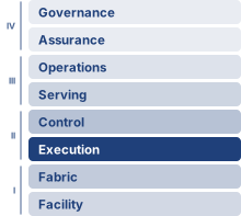
Fleet stack focus for this chapter.
Why can adding accelerators make training slower?
Splitting a training job across machines creates more compute capacity, but it also requires those machines to exchange state and agree on updates. Each accelerator may finish its local work sooner while spending more of the step waiting for other workers. Once communication and waiting consume the time saved by parallel execution, adding accelerators raises the bill without shortening the run. Single-node optimization remains necessary, yet faster local arithmetic cannot remove a dependency on data that another machine has not delivered. Memory pressure complicates the decision, because a model may require distribution simply to fit, even when the resulting exchanges are expensive. Dividing its state across more devices can relieve that limit while exposing another in network bandwidth or scheduling. Conversely, replicating a model can process more examples at once without reducing the memory needed for each copy. Neither improvement alone establishes that training will finish sooner. Changing how examples are grouped or when updates become available can change the work required to reach the target quality. Engineers must therefore compare complete training configurations, accounting for memory, communication, update behavior, and elapsed time together. The practical question is where additional hardware buys useful progress and where it merely creates more coordination. That judgment determines which models and experiments fit the available schedule and budget. In C³ terms, each partitioning strategy trades parallelized compute against network-bound communication and coordination across workers.
Learning Objectives
- Apply the Fleet Law to diagnose compute-, memory-, communication-, or coordination-bound distributed training regimes
- Calculate scaling efficiency, estimate useful batch size, and budget synchronization overhead for data-parallel training
- Design memory-sharding plans that trade accelerator capacity for additional communication
- Map tensor, pipeline, sequence, expert, and data parallelism onto hardware bandwidth tiers and model structure
- Analyze microbatch pipeline schedules for bubble overhead, activation residency, and synchronous update ordering
- Evaluate synchronization and low-precision policies under staleness, straggler, and numerical-stability constraints
- Synthesize hybrid parallelism configurations for frontier, recommendation, and alignment training constraints
6.1 Why Distribution Is Necessary
A 175B-parameter reference model cannot even load onto a single accelerator because its FP16 weights alone exceed the memory of the device that must hold them (Data Storage), and the empirical scaling law (principle 9) keeps pushing frontier models further past what one machine can store or finish in calendar time. The accelerator hierarchy, network fabric, and storage pipeline form the physical foundation of the fleet, and Collective Communication priced the collective operations that move state across it. The remaining challenge is deciding how to partition the training job: which intermediate results and gradients must cross that fabric, and when workers must synchronize, while preserving the optimization process a single device would have followed.
↩︎ The power-law relationship between quality and compute, data, and parameters, and the compute-optimal allocation it implies, are established in AI Scaling Laws.
A hypothetical accelerator with 100 terabytes of memory and an exaflop of compute would make distributed training unnecessary for that model. Real accelerators instead have finite high-bandwidth memory (HBM) capacity, compute throughput, and input bandwidth, and more capable designs move the distribution threshold without removing it. The reference workload must be evaluated against those limits before selecting a partition. In the fleet stack (The Fleet Stack), distributed training occupies the Distributed Execution row of the Distribution band, the logic that partitions the mathematical workload across the physical fleet. Data, tensor, pipeline, and hybrid parallelism create different traffic patterns for the interconnect to carry.
Three distinct limits push a training workload past a single accelerator. Memory exhaustion hits first when model parameters, optimizer states, and activation storage exceed single-device capacity. For full mixed-precision training with Adaptive Moment Estimation (Adam), the convention of 16 bytes per parameter can exceed an 80 GB accelerator at roughly 5 billion parameters before activations. Larger 10–20B models therefore need sharding, offload, or another memory-saving approach (Rajbhandari et al. 2020); the failed allocation establishes a capacity problem without by itself choosing the remedy.
↪ Accelerator HBM capacity, the ceiling these per-parameter budgets are measured against, is developed in Accelerator Memory Hierarchy.
Even when a model fits in memory, unacceptable training duration can still force distribution because a single device may require weeks or months to converge, turning wall-clock time itself into a systems constraint. GPT-3’s 175B-parameter training run used a cluster of V100 GPUs (Brown et al. 2020), illustrating why the calendar, alongside HBM capacity, drives scale-out.
Input demand at dataset scale adds a third pressure: dataset bytes govern storage capacity, whereas the training schedule governs the required delivery rate. As The Data Pipeline Equation showed, either can motivate distributed data services, although a large dataset alone does not require distributing model computation. Together, capacity, calendar, and input delivery define the constraints a training configuration must satisfy.
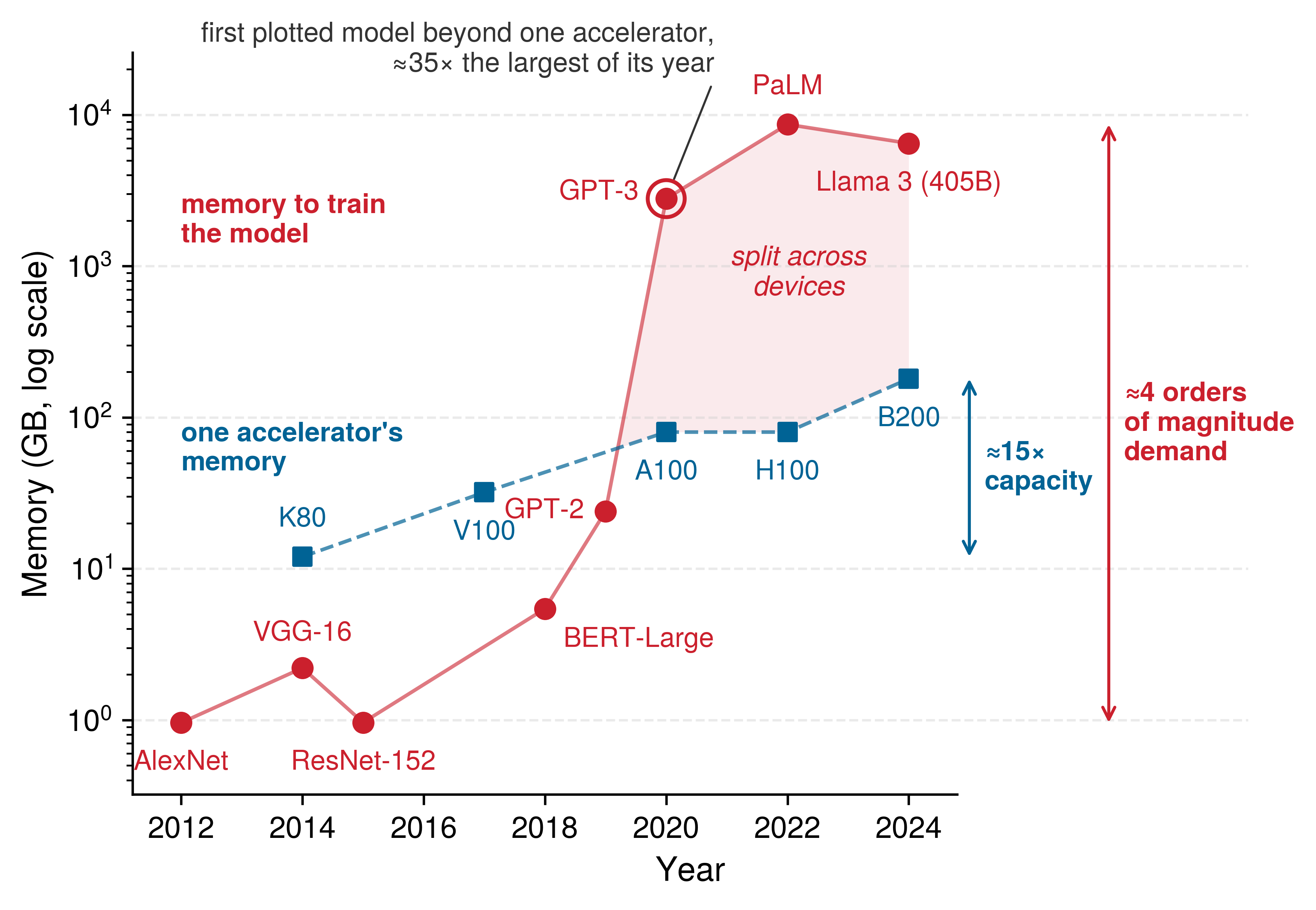
The first signal, memory exhaustion, has a long history, traced in figure 1. Over the plotted span, single-accelerator memory grew about 15× from the K80 to the B200, while the memory needed to train a state-of-the-art model grew by roughly 4 orders of magnitude. Among the plotted models, the curves cross in 2020 at GPT-3, whose training state exceeded the largest accelerator then available by about 35×. GPT-3 marks where the gap passed an order of magnitude, and every later plotted frontier model also sits far above the capacity curve. For those models, spreading state beyond one device’s memory is a precondition for training at all rather than a way to train faster.
Epoch AI. 2026. Notable AI Models.
Whichever signal motivates distribution, the system must state which optimization update it implements. In the synchronous baseline developed first, the 1,024 GPUs of the volume’s Archetype A (GPT-4/Llama-3) reference cluster, whose running instance in this chapter is a GPT-3-class 175B-parameter dense transformer, combine their contributions before advancing to the next parameter version. Matching the global batch, loss normalization, and optimizer state preserves the corresponding single-device update mathematically. Later synchronization models deliberately relax that update ordering and must be evaluated under their own convergence assumptions.
↩︎ The three systems archetypes and their binding constraints are established in Three systems archetypes.
Definition 6.1: Distributed training
Distributed training partitions the optimization loop across multiple compute nodes, distributing data or model computation and coordinating contributions according to a specified update protocol.
- Significance: Partitioning training state across devices can meet a memory budget that exceeds one accelerator. GPT-3 (175B parameters) requires approximately 350 GB in BF16 (FP16 also stores 2 bytes per value, so the chapter’s byte counts hold for either format), more than 4× the 80 GB capacity of a single H100. If weights remain entirely in HBM, their aggregate capacity lower bound is 5 H100s. Adding BF16 gradients plus FP32 Adam master weights and moments gives about 2.8 TB, or at least 35 H100s before activations. These lower bounds do not establish a runnable placement; offload changes the capacity calculation, and the time budget can require more accelerators than memory alone.
- Distinction: CPU threads can share a coherent address space, while accelerators generally hold separate training-state allocations even within one node. Distributed training extends coordination across those devices and node boundaries through collectives or point-to-point transfers governed by the chosen update protocol.
- Common pitfall: A frequent misconception is that distributed training scales linearly with node count. In practice, communication overhead grows with cluster size and the serial fraction of each step (Amdahl’s Law): a fixed serial fraction of the single-device baseline bounds strong-scaling speedup.
Distribution expands three costs that determine whether a partition is viable. Communication overhead includes gradient aggregation through AllReduce, which returns the same reduced tensor to each participant, or rank. For \(\Parameters\) parameters across \(\DeviceCount\) devices, a ring AllReduce, in which each worker passes gradient chunks only to its neighbor in a logical ring, sends approximately \(2(\DeviceCount-1)/\DeviceCount\times \GradientPayload\) bytes per worker per step, where the gradient payload \(\GradientPayload\) is the \(\Parameters\) gradient values times their storage width; this is not total fleet traffic.
↩︎ The ring schedule and the derivation of its \(2(\DeviceCount-1)/\DeviceCount\) volume are established in Collective Communication.
Fault tolerance becomes more demanding as the number of failure sources grows. Under independent constant-rate failures, 1,024 GPUs that each have a mean time to failure (MTTF) of 50,000 hours produce a GPU failure about every 49 hours, the cluster’s mean time between failures (MTBF). Whether each event interrupts training depends on recovery and redundancy; The MTBF cascade develops the assumptions.
Algorithmic stability adds a separate constraint when the partition changes global batch size or update ordering. Learning-rate scaling and warmup are candidate responses to large-batch behavior (Goyal et al. 2017), not requirements unique to multiple machines. A viable design must satisfy all three budgets.
Communication and coordination costs enter every step through the Fleet Law (principle 10), which decomposes the per-step time:
\[ \DistributedStepTime(\DeviceCount) = \frac{\IronLawComputeTime}{\DeviceCount} + \CommunicationTime(\DeviceCount) + \SynchronizationTime(\DeviceCount) - \OverlappedTime \]
↩︎ The Fleet Law and its compute, communication, and coordination terms are established in The Fleet Law.
The communication-computation ratio, \(\CommunicationComputeRatio= \CommunicationTime(\DeviceCount)/(\IronLawComputeTime/\DeviceCount)\), compares communication time with ideally partitioned compute time for fixed global work. It is the time consequence of communication intensity \(\CommunicationIntensity\) (equation 1.1), the bytes moved per operation of the workload. When transfers run at link bandwidth \(\LinkBandwidth\) and each device computes at sustained rate \(\PeakRate\EfficiencyHw\), \(\CommunicationComputeRatio\approx \CommunicationIntensity \times \PeakRate\EfficiencyHw/\LinkBandwidth\), so the same workload becomes more communication-bound on faster accelerators or slower links. This ratio identifies the pressure to overlap communication; the complete step time also depends on how much exchange is hidden and how much coordination remains exposed.
↩︎ The \(\MessageStartupLatency\)-\(\LinkBandwidth\) message model, with startup latency \(\MessageStartupLatency\) and sustained bandwidth \(\LinkBandwidth\), is established in The \MessageStartupLatency-\LinkBandwidth performance model.
↪ The communication-computation ratio, evaluated for representative data-parallel and point-to-point transfers and related to communication intensity, is developed in The communication-computation ratio.
Two regimes follow from this ratio. When \(\IronLawComputeTime/\DeviceCount\gg \CommunicationTime(\DeviceCount)\), the cluster is compute-bound, and communication is small relative to useful computation, provided coordination and input delivery do not introduce another limit. Large-batch training of a dense convolutional model such as ResNet commonly sits here. When \(\CommunicationComputeRatio\gtrsim 1\), \(\CommunicationTime(\DeviceCount)\) matches or exceeds \(\IronLawComputeTime/\DeviceCount\), the cluster is communication-bound, and insufficient overlap leaves substantial time waiting for gradients or activations. Large language models (LLMs) with billions of parameters to synchronize, and Deep Learning Recommendation Model (DLRM)-style workloads whose embedding exchanges saturate the network, frequently land in this regime. These are typical operating points rather than fixed labels. Batch size, partitioning, and placement can move the same workload across the boundary, so the ratio must be measured for the configuration at hand. Where a workload lands also depends on how its training loop is cut across devices, the choice each parallelism strategy makes.
↪ The optimizations that help, and the ones that are wasted, for a compute-bound, communication-bound, or coordination-bound fleet are collected for reference in The bottleneck diagnostic table.
Self-Check: Question
A research team is training a 3B-parameter transformer that fits comfortably in one H100 GPU’s 80 GB of memory, but projected single-GPU training would take 18 months to reach target loss. The dataset is 3 TB and fits on local NVMe storage. Which signal makes distributed training necessary in this scenario?
- Dataset exceeding GPU HBM capacity, which automatically mandates tensor parallelism regardless of execution time
- The presence of NVLink inside the node, which makes multi-machine scaling mandatory by default
- Unacceptable wall-clock training duration, even though single-device memory capacity and local storage are sufficient
- Fault tolerance limitations, because single-GPU training cannot survive hardware restarts
A team doubles a data-parallel cluster from 64 to 128 GPUs and observes that total step time drops by only 12 percent even though per-worker compute time halves. Using the distributed step-time equation \(T_{\text{step}}(N) = T_{\text{compute}}/N + T_{\text{comm}}(N) + T_{\text{sync}}(N) - T_{\text{overlap}}\), explain what the observation establishes and what measurement would distinguish possible causes.
True or False: A cluster of 1,024 GPUs, each with a 50,000-hour mean time to failure, should expect a GPU failure roughly every two days if failures are independent, even though any single GPU fails only about once every five to six years.
The dimensionless ratio \(\rho = T_{\text{comm}}(N) / (T_{\text{compute}}/N)\), which screens communication demand relative to per-worker compute time, is defined as the ____.
6.2 The Parallelism Design Space
Once a model or its training time outgrows a single GPU, the training loop offers three nested axes to split across devices: the examples in a batch, the layers of the model, and the matrix operations inside each layer. Data parallelism assigns different examples to model replicas; pipeline parallelism assigns successive layer groups to different devices; tensor parallelism splits the operations inside a layer. Because every split adds inter-device communication and synchronization overhead on top of single-machine compute and memory limits (The D·A·M Taxonomy), profiling and design must treat these three strategies as loop transformations applied by a cluster-level compiler.
In compiler terms, data parallelism acts like a parallel for-loop that assigns different batch indices to devices running the same model, whereas tensor parallelism resembles vectorization, or single instruction, multiple data (SIMD), by partitioning the work inside matrix operations—an analogy for the work split rather than a shared instruction stream or register file, since the devices still exchange tensor shards over an interconnect. Pipeline parallelism instead resembles instruction pipelining, assigning successive layer groups to stages so that overlapping microbatches keep those stages active, subject to dependency delays and load balance.
Whichever loop a strategy unrolls, distributed training1 spreads the workload across machines that must coordinate to train a single model. Coordination here means keeping every model shard or replica on a compatible training step. Basic barriers can keep a small research run ordered, but long-running training jobs also need timeout, checkpoint, and recovery mechanisms so one failed worker does not waste days of compute.
1 Distributed training: Google’s DistBelief (2012) was an early framework for training neural networks across thousands of machines, but its parameter server architecture created bandwidth bottlenecks at central nodes. This limitation drove the shift to decentralized AllReduce patterns in successors such as Horovod and PyTorch DistributedDataParallel (DDP), where each data-parallel worker sends and receives about \(2(\DeviceCount-1)/\DeviceCount\) times the gradient size per step rather than concentrating traffic at a single server (Dean et al. 2012; Sergeev and Balso 2018; Li et al. 2020; Patarasuk and Yuan 2009).
Dean, Jeffrey, Greg Corrado, Rajat Monga, Kai Chen, Matthieu Devin, Quoc V. Le, Mark Z. Mao, et al. 2012. “Large Scale Distributed Deep Networks.” In Advances in Neural Information Processing Systems (NeurIPS), edited by Peter L. Bartlett, Fernando C. N. Pereira, Christopher J. C. Burges, Léon Bottou, and Kilian Q. Weinberger, vol. 25. Curran Associates.
Sergeev, Alexander, and Mike Del Balso. 2018. “Horovod: Fast and Easy Distributed Deep Learning in TensorFlow.” CoRR abs/1802.05799.
Li, Shen, Yanli Zhao, Rohan Varma, Omkar Salpekar, Pieter Noordhuis, Teng Li, Adam Paszke, et al. 2020. “PyTorch Distributed: Experiences on Accelerating Data Parallel Training.” Proceedings of the VLDB Endowment 13 (12): 3005–18. https://doi.org/10.14778/3415478.3415530.
Patarasuk, Pitch, and Xin Yuan. 2009. “Bandwidth Optimal All-Reduce Algorithms for Clusters of Workstations.” Journal of Parallel and Distributed Computing 69 (2): 117–24. https://doi.org/10.1016/j.jpdc.2008.09.002.
↪ Checkpointing and recovery for long-running training jobs are developed in Fault Tolerance.
2 NVLink: NVIDIA’s point-to-point GPU interconnect delivers 300 GB/s–450 GB/s per-direction bandwidth, roughly 12×–18× InfiniBand HDR per port. This bandwidth gap is why tensor parallelism, which requires AllReduce on every layer, favors the fast NVLink domain, while pipeline and data parallelism can tolerate slower links when their traffic budgets fit. NVLink Switch systems can extend that fast domain beyond one server.
Each rung of the scaling path inherits earlier challenges. A single GPU already needs input delivery, memory management, scheduling, and recovery from interrupted work. Multiple GPUs add coordination across separate device memories, even within one node. Interconnects such as NVLink or PCIe carry these exchanges,2 with collective libraries such as NCCL selecting communication schedules.
The leap to multi-node training adds network communication overhead, fault tolerance requirements, and cluster orchestration. Because each stage compounds the previous one’s bottlenecks, single-GPU performance must be optimized before scaling out, so inefficiency does not multiply across the fleet. The resulting design space decomposes onto a three-dimensional grid, \(\DeviceCount= \DataParallelDegree \times \PipelineParallelDegree \times \TensorParallelDegree\), that partitions cluster execution across tensor parallelism (\(\TensorParallelDegree\), intra-layer sharding), pipeline parallelism (\(\PipelineParallelDegree\), sequential stage partitioning), and data parallelism (\(\DataParallelDegree\), batch replication), and each cell of the grid is one accelerator coordinate (figure 2).
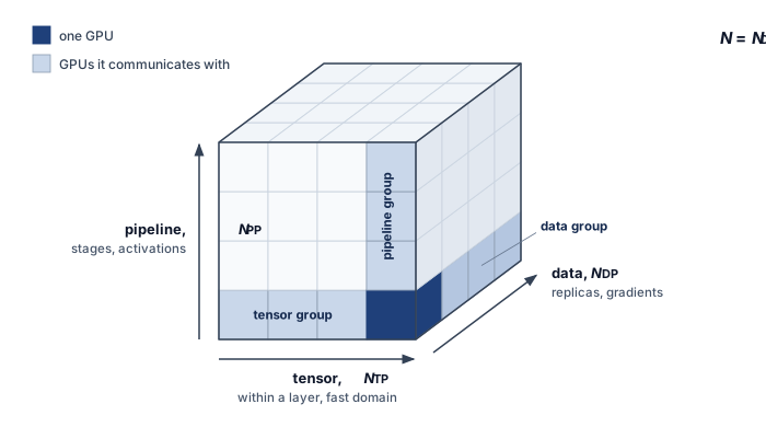
Under the three-dimensional partitioning of figure 2, called 3D parallelism, the total accelerator allocation scales as the product \(\DeviceCount= \DataParallelDegree \times \PipelineParallelDegree \times \TensorParallelDegree\). The axes represent distinct mathematical partitions, but they are not independent configuration knobs. Tensor and pipeline degrees must divide the model structure, the data-parallel degree and microbatch schedule must produce a viable global batch, every partition must fit memory, and each communication group must map onto an adequate topology and acceptable failure domain. Training systems therefore select a jointly feasible coordinate rather than tuning \(\DataParallelDegree\), \(\PipelineParallelDegree\), and \(\TensorParallelDegree\) in isolation.
6.2.1 Parallelism strategy selection and engineering trade-offs
A parallelism strategy that places frequent, high-volume exchanges on a slow link fails before it leaves the whiteboard, because communication stalls the accelerators it was meant to feed. Choosing a strategy is therefore a constraint satisfaction problem governed by parameter count \((\Parameters)\), batch size \((\BatchSize)\), and interconnect bandwidth. A first feasibility screen compares the traffic each strategy creates against the hardware topology (table 1). In that screen, \(\LayerCount\) denotes layer count, \(\SequenceLength\) sequence length, and \(\HiddenDimension\) hidden width. The table identifies traffic sources rather than complete byte budgets; datatype width, partition degree, and communication frequency enter the worked mechanisms below.
| Strategy | Communication pattern | Comm. volume | Hardware constraint |
|---|---|---|---|
| Data Parallel (DP) | AllReduce Gradients | \(\propto \GradientPayload\) (gradient bytes) | Requires high bisection BW |
| Tensor Parallel (TP) | AllReduce Activations | \(\propto \BatchSize\times \SequenceLength\times \HiddenDimension\times \LayerCount\) (per-layer activations) | Fast domain matched to layer traffic |
| Pipeline Parallel (PP) | Point-to-Point (P2P) | \(\propto \BatchSize\times \SequenceLength\times \HiddenDimension\) (Activations) | Link must sustain stage activations |
Those bandwidth requirements impose a hard constraint on hardware placement: each parallelism axis must map onto an interconnect tier that can sustain its traffic within the compute budget. A quick back-of-envelope bandwidth feasibility check catches a mismatch before any code is written.
↩︎ The communication domains and bandwidth hierarchy used to evaluate placement are established in Bandwidth hierarchy.
Systems Perspective 6.1: Bandwidth feasibility check
Frequent tensor-parallel collectives must fit the layer-time budget. The test compares the time one layer’s local share of computation takes with the time its collectives take on each candidate link. For the forward pass of one GPT-3 layer split 8 ways, processing one 2,048-token sequence at half of an H100’s dense FP16 peak:
- Local compute per layer: about 1.9 ms
- Tensor-parallel transfer per layer over NVLink: about 0.4 ms
- The same transfer over one NDR InfiniBand port: about 3.5 ms
On NVLink the exchange is a fraction of the layer’s compute; across InfiniBand it would take longer than the compute it serves. The amount hidden depends on independent work available in the execution schedule. NVLink is one suitable fast domain, but the test uses message bytes, exposed latency, and sustained link rate rather than an interconnect brand or chassis boundary. Cross-rack placement may favor pipeline or data parallelism when the available fabric cannot meet the tensor-parallel budget; their activation and gradient traffic must also be checked.
The communication costs in table 1 already narrow the choice before any mechanism has been developed, because a strategy is viable only when its traffic fits the tier that must carry it. What each formula implies in practice depends on the mechanics of data, tensor, and pipeline parallelism developed over the rest of the chapter, and section 6.8 turns the same constraints into a decision procedure once those mechanics are in place.
Self-Check: Question
Framing distributed parallelism strategies as compiler loop transformations across the training loop’s iterators (batches, layers, and operations), which distributed strategy corresponds to vectorization (SIMD) of inner matrix multiplications?
- Tensor parallelism, which partitions inner matrix-multiplication operations across devices and exchanges partial results over the interconnect
- Data parallelism, which unrolls the outer batch loop across devices so each rank processes independent data indices
- Pipeline parallelism, which stages sequential layer operations across devices analogous to CPU instruction pipelining
- Model replication, which duplicates the entire forward and backward execution redundantly across machines
In the 3D parallelism cube, where the device count equals the product of the data-, pipeline-, and tensor-parallel degrees, how do the three scaling axes interact to allocate cluster accelerators for large models?
- The three axes are mutually exclusive; choosing data parallelism precludes using tensor or pipeline parallelism in the same cluster
- Tensor and pipeline parallelism can combine within a node, but data parallelism can only be used if model parallelism is disabled
- The total accelerator count is the sum of the three degrees, with each parallelism type requiring a disjoint node pool
- The axes compose multiplicatively, so one layout can split layers (TP), stage the layer stack (PP), and replicate the pipeline across data shards (DP), and its device count is the product of the three degrees
True or False: If a neural network’s parameters exceed a single GPU’s memory capacity, tensor parallelism can be scaled across standard commodity Ethernet switches between server racks, provided the global batch size is made large enough.
For one GPT-3 layer split eight ways, the chapter’s bandwidth feasibility check finds about 1.9 ms of local compute, about 0.4 ms of tensor-parallel transfer over NVLink, and about 3.5 ms for the same transfer over one NDR InfiniBand port. Explain what these numbers imply for where the tensor-parallel group should be placed and what a planner must still check before accepting that placement.
6.3 Data Parallelism
When a model fits on one accelerator but training takes weeks, replicating its computation lets several workers process examples concurrently. The initial data-parallel baseline gives each worker the same model state and a local portion of one global minibatch. Combining those local contributions before the optimizer update preserves the intended global-batch estimator; the sampling and weighting conditions below explain when that equivalence holds.
Definition 6.2: Data parallelism
Data parallelism distributes training examples across workers that execute the model and combine their contributions to its optimization updates.
- Significance: With \(\DeviceCount\) workers each processing a local batch of \(\LocalBatchSize\) examples once per update, the global batch size is \(\DeviceCount\times \LocalBatchSize\). At fixed local work, 1,024 workers offer an ideal 1,024\(\times\) throughput increase before exposed overhead. A 1B-parameter model with BF16 gradients contributes a 2 GB gradient payload; ring AllReduce moves \(2(\DeviceCount-1)/\DeviceCount\) times that payload per worker. Realized speedup depends on local compute, collective service, overlap, and load balance.
- Distinction: The replicated synchronous baseline keeps a full model copy on each worker and aggregates gradients before each optimizer update. Model parallelism instead partitions the model’s computation. Sharded data parallelism, developed below, retains data-parallel computation while distributing training-state storage.
- Common pitfall: Data parallelism does not scale indefinitely with worker count. Holding the local batch \(\LocalBatchSize\) fixed while adding workers grows the global batch. Beyond the workload-dependent critical batch size, additional examples yield diminishing reductions in the steps needed to reach target quality (Shallue et al. 2019). The crossover developed in section 6.4.6 therefore limits the statistical benefit even when gradient variance continues to decrease.
He, Kaiming, Xiangyu Zhang, Shaoqing Ren, and Jian Sun. 2016. “Deep Residual Learning for Image Recognition.” 2016 IEEE Conference on Computer Vision and Pattern Recognition (CVPR), 770–78. https://doi.org/10.1109/cvpr.2016.90.
Data parallelism applies when examples can be processed independently, as in training a ResNet model (He et al. 2016) on ImageNet. Each replica computes its local loss gradient, and the workers combine those contributions to reproduce the intended global-batch gradient. The averaging rule makes the sampling and weighting assumptions explicit.
Consider a model with parameters \(\ModelParameters\) training on a dataset \(\TrainingDataset\). The loss function for a single data point \(\ModelInput_i\) is \(\LossFunction(\ModelParameters, \ModelInput_i)\). In standard stochastic gradient descent (SGD) with batch size \(\BatchSize\), the gradient update for a minibatch is: \[ \MinibatchGradient= \frac{1}{\BatchSize} \sum_{i=1}^\BatchSize\nabla_{\ModelParameters} \LossFunction(\ModelParameters, \ModelInput_i) \]
In data parallelism with \(\DeviceCount\) devices, each device \(\WorkerIndex\) computes gradients on its own minibatch \(\MiniBatchSet_k\): \[ \MinibatchGradient_k = \frac{1}{|\MiniBatchSet_k|} \sum_{\ModelInput_i \in \MiniBatchSet_k} \nabla_{\ModelParameters} \LossFunction(\ModelParameters, \ModelInput_i) \]
When all workers use the same local batch size, the global update averages these local gradients: \[ \GlobalBatchGradient= \frac{1}{\DeviceCount} \sum_{k=1}^\DeviceCount\MinibatchGradient_k \]
Under that equal-batch assumption, the averaging is mathematically equivalent to computing the gradient on the combined batch \(\CombinedBatch= \bigcup_{k=1}^\DeviceCount \MiniBatchSet_k\): \[ \GlobalBatchGradient= \frac{1}{|\CombinedBatch|} \sum_{\ModelInput_i \in \CombinedBatch} \nabla_{\ModelParameters} \LossFunction(\ModelParameters, \ModelInput_i) \]
For unequal local batch sizes, the combined-batch gradient is the weighted average \(\GlobalBatchGradient= (1/|\CombinedBatch|)\sum_k |\MiniBatchSet_k|\MinibatchGradient_k\). Data parallelism therefore maintains the statistical properties of SGD training, because sampling the intended global batch across devices, computing local gradient sums independently, and normalizing by the aggregate denominator reproduces its estimator. The reduction step uses an AllReduce over local gradient sums and valid-item counts.
Three batch quantities recur from here on, and the chapter keeps them apart. A worker’s local batch \(\LocalBatchSize\) is the set of examples it processes for one update, playing the role of \(\MiniBatchSet_k\) above. The global batch \(\GlobalBatchSize= \DeviceCount\times \LocalBatchSize\) is the set the update averages over. Pipeline parallelism later splits a batch into \(\MicrobatchCount\) microbatches of size \(\MicrobatchSize\) that flow through stages one after another; the word microbatch is reserved for those pipeline slices.
↪ The ring and tree AllReduce cost models that set the price of this synchronization are developed in AllReduce.
Checkpoint 6.1: Data parallelism mechanics
Verify your understanding of how data parallelism distributes work:
The method parallels gradient accumulation, where a device accumulates contributions from multiple forward and backward passes before one optimizer update. Both techniques use gradient addition and the intended loss denominator to process a larger effective batch. Distribution adds communication, partial failures, and coordination to that arithmetic. The implementation must preserve the update while accounting for those costs.
6.3.1 Data parallelism implementation
The implementation details matter because the SGD equivalence only holds when each phase preserves the intended aggregate sampling and weighting, complete local gradient contributions, and a single synchronized update. The concrete workflow follows the dataflow from assigning local batches to synchronizing the computed gradients. The five-stage execution pipeline in figure 3 follows four GPU swimlanes, tracking how identical model replicas ingest disjoint batch shards, compute local gradients (\(\MinibatchGradient_0\)–\(\MinibatchGradient_3\)), and synchronize through a ring AllReduce collective before applying uniform parameter updates.
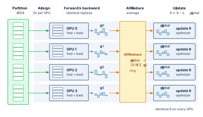
The gradient synchronization stage of figure 3 (stage 4) creates a dependency, because each rank must receive the completed reduction before applying its optimizer update. The exposed wait can reflect bandwidth, collective startup, or a late contribution. Measuring that wait determines whether synchronization limits scaling; the dependency alone does not identify the binding resource.
Dataset splitting
Data splitting is the first place where the SGD equivalence can fail, but uniqueness and equal-sized shards are sufficient conditions rather than the invariant itself. The aggregate examples or tokens, their sampling probabilities, and their gradient weights must reproduce the intended global-batch estimator. Uniform sampling without replacement can assign disjoint shards; sampling with replacement can legitimately repeat examples; and variable-length batches can assign unequal token counts if the reduction weights each worker by its valid-example or valid-token denominator. An unweighted mean of unequal local means instead overweights workers with smaller denominators.
The sampler is therefore an integral component of the distributed training system rather than merely an input-loader convenience. A distributed sampler coordinates workers by rank and can deterministically partition or draw indices from a seeded sampling stream. The 1.28 million training images of ImageNet-1k do not divide evenly across 32 GPUs, so a sampler that pads by repeating examples gives each GPU 40,037 examples per epoch and adds 17 repeats across the job. The loss normalization or sample weights must account for those repeats when exact epoch-level weighting matters. A recorded seed and deterministic index stream make sample assignment repeatable; bitwise run reproducibility additionally depends on kernel determinism, collective reduction order, numerical precision, and checkpointed random-number-generator state.
Compute-phase forward and backward passes
For a replicated model whose local forward and backward operations require no cross-worker state, the computation phase is embarrassingly parallel. Each GPU executes the model on its local batch; synchronized normalization or additional model partitioning can introduce communication within that phase. To isolate the activation term, consider an unpartitioned 175B reference model at a local batch of 4 sequences and sequence length 2048. This is a hypothetical memory budget, not a feasible one-GPU training configuration, because weights and optimizer state must fit as well. Without optimization, storing these activations for backpropagation would consume roughly 1.1 TB of HBM, an order of magnitude beyond the capacity of even an H100 GPU. Activation checkpointing recomputes selected activations during the backward pass rather than retaining them, reducing this example’s footprint to ~19.3 GB at the cost of extra computation.
The capacity test must include activations rather than stopping at bytes per parameter. Numeric Precision and Training Memory tabulates the 16-byte-per-parameter training state from which this test starts. At the point of peak residency, \[ \TotalMemoryFootprint = \WeightMemory + \GradientMemory + \OptimizerStateMemory + \ActivationMemory, \] with communication buffers and temporary workspaces consuming additional headroom. Sharding reduces the first three terms according to its stage, whereas sequence length, local batch size, and pipeline scheduling govern \(\ActivationMemory\). Activation checkpointing reduces that last term by retaining only selected boundaries and recomputing the omitted forward operators during backpropagation (Narayanan et al. 2021). Full recomputation re-executes about one extra forward pass per step. Because a backward pass costs roughly two forward passes, a step that needed three forward-pass equivalents of arithmetic now needs four, about a third more (Chen et al. 2016). Selective recomputation re-executes only operators whose activations are large but cheap to produce, such as the attention softmax and dropout, and keeps most of the memory saving for a few percent of extra arithmetic (Korthikanti et al. 2023). Recomputed operations raise hardware FLOPs utilization (HFU) but not model FLOPs utilization (MFU), which credits only the model’s own forward and backward work, so a plan that buys feasibility with full recomputation pays for it in useful throughput. The memory saved is therefore purchased with additional FLOPs and a longer critical path; a feasible parallelism plan must budget both effects.
Narayanan, Deepak, Mohammad Shoeybi, Jared Casper, Patrick LeGresley, Mostofa Patwary, Vijay Korthikanti, Dmitri Vainbrand, et al. 2021. “Efficient Large-Scale Language Model Training on GPU Clusters Using Megatron-LM.” Proceedings of the International Conference for High Performance Computing, Networking, Storage and Analysis, 1–15. https://doi.org/10.1145/3458817.3476209.
Chen, Tianqi, Bing Xu, Chiyuan Zhang, and Carlos Guestrin. 2016. “Training Deep Nets with Sublinear Memory Cost.” arXiv Preprint arXiv:1604.06174.
As the backward pass traverses the computation graph in reverse, it produces gradients for the parameters held by each replica or shard. Under pure data parallelism, a full 175B FP16 replica would imply a 350 GB gradient tensor per worker, which exceeds single-accelerator memory budgets; large runs therefore combine data parallelism with sharding, tensor parallelism, or pipeline parallelism. Each local gradient contributes to the intended global-batch estimator. Aggregation can begin as gradient tensors become ready, overlapping later backward computation, but the optimizer must wait for the completed contributions it consumes. This readiness schedule connects local computation to collective communication.
Gradient synchronization
Gradient synchronization combines local contributions into the synchronous update. Each replica must receive the aggregate before applying that update. In a centralized parameter-server design with fixed per-worker payload and update frequency, the server receives \(\mathcal{O}(\DeviceCount)\) incoming traffic. That concentration becomes a bottleneck when demand exceeds the server tier’s service capacity; sharding the server state or changing the communication pattern can relieve it.
The replicated synchronous baseline distributes aggregation through collective communication. AllReduce lets each worker contribute its local gradient tensor and receive the same reduced result, which the training loop normalizes to obtain the global average. In sharded variants such as ZeRO and FSDP, ReduceScatter and AllGather change which result each worker retains, leaving each worker only its own shard of the reduced gradient and reconstructing full parameters on demand. Small messages emphasize startup latency; large messages emphasize sustained bandwidth. Centralized aggregation remains another design choice, particularly for the sparse workloads developed later.
↩︎ The result contracts of AllReduce, ReduceScatter, and AllGather, and the decomposition of AllReduce into a ReduceScatter followed by an AllGather, are established in The six core primitives.
At the Distributed Execution row of the fleet stack, the loop specifies an AllReduce contract while its implementation determines the cost. For a large worker group, ring AllReduce transfers approximately \(2\GradientPayload\) bytes per worker for an \(\GradientPayload\)-byte gradient payload. Collective Communication derived this approximate \(2\GradientPayload\) volume, compared algorithms whose startup costs, topology, and contention differ, and examined how libraries such as NCCL schedule exchanges within and across communication domains.
When a measured collective deviates from these estimates, the diagnosis compares the trace against what each candidate algorithm predicts on the same hardware, for example a flat ring against a hierarchical AllReduce that reduces within each NVLink node before crossing the inter-node fabric. A hypothetical trace on an A100 cluster with HDR InfiniBand shows the comparison at work. An AllReduce of a 3 GB gradient tensor across 128 nodes (1,024 GPUs) takes 100 ms, against a flat-ring estimate of 239.8 ms and an idealized hierarchical estimate of 48.5 ms. The observation rules out the flat schedule, and the residual above the hierarchical ideal must come from lower achieved rates, startup, or a late participant. Switch counters showing inter-node links at 60 percent utilization do not settle the question, because an aggregate can hide one saturated port during the exposed interval; per-port and per-channel traces must locate the bottleneck before any topology change.
↩︎ Hierarchical AllReduce and its cost relative to a flat ring are established in Hierarchical AllReduce.
Gibiansky, A. 2017. Bringing HPC Techniques to Deep Learning. Baidu Research Technical Blog.
Across the wider design space, figure 4 compares three synchronization topologies: the bandwidth-optimal ring AllReduce that circulates chunks along neighbor links (\(2(\DeviceCount-1)/\DeviceCount\) volume), the centralized parameter server constrained by network interface card (NIC) saturation at the server node, and the dense mesh of logical AllToAll peer traffic (\(\DeviceCount(\DeviceCount-1)\) messages). In dense synchronous data-parallel settings, ring AllReduce avoids a single reducer bottleneck by distributing traffic evenly across participating links, as Baidu’s implementation illustrates (Gibiansky 2017).
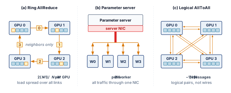
The panels separate an aggregation algorithm, a centralized architecture, and a collective traffic pattern. They do not provide interchangeable implementations of the same operation. Only the first two aggregate gradients; the AllToAll panel previews the exchange that sparse embedding tables and mixture-of-experts layers need, in which every worker sends different data to every other worker (section 6.5.5). Libraries choose algorithms and routes for the requested collective on the available fabric; a logical complete graph does not guarantee one-round physical delivery.
Parameter updating
Parameter updating closes the replicated synchronous contract. After the gradient AllReduce (Patarasuk and Yuan 2009), every worker holds the same global gradient and applies it to its own replica with SGD, momentum, or Adam, so the update stays decentralized without losing equivalence to single-device training. Identical gradients alone are insufficient, because optimizer moments, learning rates, and step counts must also match across replicas. Frameworks automate the cycle of splitting data, computing gradients, synchronizing, and updating, but they cannot remove the ordering constraint that keeps the replicas coherent, which requires every worker to update only after the synchronized gradient is complete.
Synchronization models
Distributed training systems use synchronization models to specify when workers observe and apply updates. The baseline is bulk synchronous parallel (BSP), the superstep-and-barrier model. In the replicated training loop, workers compute from one parameter version, combine their gradient contributions, and complete the update before computing from the next version. This is a dependency order, not a requirement that every device update at the same wall-clock instant. Relaxing it changes the optimization process as well as the waiting time.
↩︎ Bulk synchronous parallel execution and its barrier cost are established in How ML Networking Inverts Data-Center Assumptions.
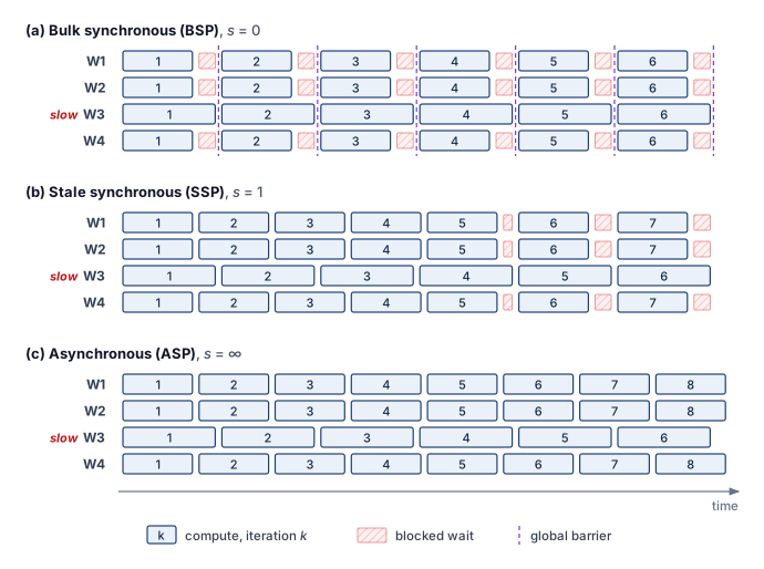
BSP provides synchronous update semantics, in which every worker computes from the same parameter version and reaches the next update boundary together. With the same global batch and reduction, this matches the corresponding synchronous single-device update mathematically. It does not by itself guarantee bitwise reproducibility. Floating-point reduction order, nondeterministic kernels, data-order state, and failure recovery can still change the result. The synchronization cost is that the slowest worker determines iteration time. A worker that keeps producing correct results but runs markedly slower than its peers is a straggler, and under BSP every straggler delays the entire step.
Stale synchronous parallel (SSP) relaxes this constraint by allowing workers to proceed up to \(\StalenessBound\) iterations ahead of the slowest worker before blocking. This bounds staleness while reducing synchronization delays. SSP requires careful learning rate tuning since workers compute gradients on slightly different parameter versions. The bounded staleness guarantee provides a middle ground between BSP’s strong consistency and fully asynchronous approaches (Ho et al. 2013).
Asynchronous parallel (ASP) execution removes the global update barrier, allowing a worker’s contribution to be applied while others continue computing; asynchronous SGD is the optimizer run under that protocol. Less barrier waiting can improve update throughput, but communication and shared-state contention remain. Gradients computed from older parameter versions introduce staleness that can affect convergence. Section 6.4.4 develops the objective and delay assumptions needed to evaluate that trade-off. The three models lie on one spectrum, from the strong consistency of BSP to the barrier-free updates of ASP (table 2).
| Model | Consistency | Throughput | Convergence | Use case |
|---|---|---|---|---|
| BSP | Strong | Bounded by slowest worker | Same synchronous update semantics | Controlled final training runs |
| SSP | Bounded staleness | Less global-barrier waiting | Depends on delay and tuning | Hyperparameter search |
| ASP | Weak | No global update barrier | Depends on staleness and objective | Large heterogeneous clusters |
Execution traces for four workers with one straggler make the differences visible (figure 5). Under BSP, global barriers force the faster workers into idle wait blocks while straggler W3 completes. Under SSP, bounded slack (\(\StalenessBound=1\)) lets them run ahead and throttles the drift with brief pauses. Under ASP, asynchronous updates remove the global barrier without imposing a finite staleness bound, although communication and resource contention can still leave workers waiting.
Barrier semantics and failure modes
An optimizer update that consumes an AllReduce result must wait for every required contribution. Workers can execute independent computation while a collective is in flight, but they must issue compatible collectives in the same group order and wait for completion before consuming the result. This coupling creates failure modes absent from single-device training.
A worker failure can leave peers waiting for a contribution that will never arrive. The runtime may report a communication error, or the operation may remain blocked until a timeout detects the failure. Watchdogs bound that wait so the job can enter recovery rather than retain an unusable allocation indefinitely.
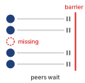
One missing worker stalls the entire AllReduce barrier.
Collective mismatches occur when workers issue incompatible operations, tensor shapes, or ordering within a communication group. Conditional computation can create such a mismatch if some workers omit an expected reduction. Variable sequence lengths or different expert routes do not inherently violate the protocol; the runtime must construct a compatible communication schedule for those varying local computations.
Stragglers extend an iteration when their late work lies on its critical path. Thermal throttling, network congestion, or OS jitter can delay a required contribution even when other workers are ready. At 1,000 GPUs with a 1 percent straggler probability per GPU per step, the expected count is 10 stragglers per step, but the number that matters under BSP is the chance of a step with none at all. That chance is the per-GPU on-time probability raised to the GPU count, about 0.004 percent. Almost every step therefore waits for at least one slow worker, which is why the slowest worker, not the typical one, sets step time. The resulting exposed wait depends on how late that contribution arrives and what independent work remains. Deployed systems bound these waits with timeouts and heartbeat monitoring, and elastic training lets a job continue with a resized worker group after a failure.
↪ Heartbeat and collective-timeout failure detection, and the trade-off between restarting healthy workers and leaving peers blocked, are developed in Failure detection mechanisms.
6.3.2 Data parallelism trade-offs
Data parallelism is the simplest way to add accelerators because it leaves each replica’s model computation intact, but adding workers eventually hits either a communication wall or a statistical wall (Ben-Nun and Hoefler 2019). Near-linear throughput scaling requires local compute efficiency, balanced input delivery, and small exposed synchronization costs. Which wall arrives first depends on whether the global batch stays fixed or grows as workers are added. Holding the global batch fixed while adding workers is strong scaling: each worker’s local batch shrinks, so communication must hide behind less computation. Holding the local batch fixed so that the global batch grows with \(\DeviceCount\) is weak scaling: per-worker computation stays constant, but each update averages more examples, which eventually stops reducing the number of updates needed. The rest of the chapter refers to the two regimes by these names.
Ben-Nun, Tal, and Torsten Hoefler. 2019. “Demystifying Parallel and Distributed Deep Learning: An in-Depth Concurrency Analysis.” ACM Computing Surveys 52 (4): 1–43. https://doi.org/10.1145/3320060.
Weak scaling pays off when the larger global batch still reaches the target accuracy. Goyal et al. (2017) trained ResNet-50 on ImageNet in about one hour on 256 GPUs at a global batch of 8,192 images; the learning-rate rules that let that batch reach the target accuracy are developed in section 6.4.5. Replicated data parallelism retains the model’s local operators, and frameworks can trigger gradient reductions as backward computation produces them. Each replica executes a complete forward and backward pass, avoiding the layer-stage fill and drain bubbles of pipeline parallelism. Input stalls, imbalance, and exposed reductions can still leave devices idle.
These advantages hold only until replication runs into memory capacity, communication bandwidth, or statistical diminishing returns. The memory wall binds first on large models because a replicated worker holds every parameter, gradient, and optimizer state, demanding more than 1 TB per replica for the 175B-parameter example before activations. Even when the state fits, communication limits useful scaling once its exposed cost grows relative to local work: as \(\DeviceCount\) increases, the ideal ring bandwidth term \(\frac{2(\DeviceCount-1)}{\DeviceCount} \frac{\GradientPayload}{\LinkBandwidth}\) approaches a constant for a fixed gradient payload \(\GradientPayload\) and link bandwidth \(\LinkBandwidth\), while startup latency, topology, and shrinking local computation worsen the balance. Statistical efficiency then sets the ceiling under weak scaling, because growing \(\GlobalBatchSize= \DeviceCount\times \LocalBatchSize\) with \(\DeviceCount\) eventually yields diminishing reductions in update count, whereas strong scaling avoids that batch-size ceiling only by shrinking each worker’s local batch and exposing the communication trade-off sooner.
Napkin Math 6.1: GPT-2 data parallel scaling: Single node
A GPT-2 scaling scenario makes the efficiency loss concrete by holding the model fixed and changing only the communication domain. GPT-2 stands in for the 175B reference here because it fits on one GPU, so pure replicated data parallelism applies and communication is the only variable. The first case keeps all eight GPUs inside a single NVLink node.
Single-GPU baseline
- Batch size: 16 (with gradient checkpointing, fits in 32 GB)
- Time per step: 1.8 s
- Baseline time for 50K single-GPU steps: 25 hours
The following durations hold the total sample budget fixed, so larger global batches require fewer optimizer updates. They assume those samples attain the same quality; the calculation establishes throughput scaling, not convergence equivalence.
8 GPUs: single node with NVLink
- Per-GPU batch: 16, global batch: 128
- Gradient synchronization: 5.2 GB @ 450 GB/s (NVLink, per direction) \(\approx\) 11.7 ms
Performance results:
- Compute: 1800 ms per step
- Communication: 11.7 ms per step
- Total: 1811.7 ms per step
- Speedup (throughput): 8×
- Parallel efficiency: 99.4 percent
Training time: 25 hours ÷ 8 = 3.1 hours
Inside the node, NVLink keeps gradient exchange small relative to compute, so efficiency stays near 99.4 percent. The picture inverts once the same model must synchronize across nodes over a commodity network.
Napkin Math 6.2: GPT-2 data parallel scaling: Commodity scale-out
The second case scales the same GPT-2 run across multiple nodes, replacing the intra-node NVLink hop with inter-node Ethernet for the bulk of the AllReduce. The 10 Gb Ethernet link models a commodity cloud tier without a dedicated training fabric, far slower than the InfiniBand of the reference cluster, which makes the cost of leaving the node easy to see.
Commodity network configuration: 32 GPUs across 4 nodes
- Per-GPU batch: 16, global batch: 512
- Intra-node communication: 11.7 ms (NVLink)
- Inter-node communication: 5.8 GB @ 1.25 GB/s (10GbE) \(\approx\) 4650 ms
Performance results:
- Compute: 1800 ms (27.9 percent of time)
- Communication: 4661.7 ms (72.1 percent of time), so communication dominates and becomes the bottleneck.
- Total: 6461.7 ms per step
- Speedup (throughput): 8.9× faster → 2.8 hours
- Parallel efficiency: 27.9 percent
The scale-out run bought its larger global batch with four nodes on a slow network. A single node can reach the same global batch another way, by running several local microsteps and accumulating their gradients before one AllReduce. The comparison below is therefore between two placements, one node with accumulation against four nodes without it; accumulation’s job is to keep the global batch equal, while the saving comes from never leaving the NVLink domain.
Napkin Math 6.3: Gradient accumulation speedup
Problem: A GPT-2 run on a commodity 10G network is communication-bound at 32 GPUs across 4 nodes, costing $359 for a fixed number of samples. Can a single 8-GPU node that uses gradient accumulation to match that global batch process the same samples for less?
Math:
- Effective batch size: 8 GPUs \(\times\) batch 16 \(\times\) 4 accumulation steps = 512.
- Communication overhead: With 4-step accumulation, the job AllReduces once every 4 steps (overhead = 11.7 ms / (4 \(\times\) 1800 ms) \(\approx\) \(0.162\%\)).
- Training duration: Total time is 3.1 hours.
- Scale-out baseline cost: 4 nodes \(\times\) 2.8 hours \(\times\) $32/hr = $359.
- Accumulation cost: 3.1 hours \(\times\) $32/hr = $100.
Systems insight: The one-node plan saves $259 (72.1 percent). Almost all of that saving comes from placement, because the four-node run spent most of each step on the slow inter-node link and the single node never uses it. Gradient accumulation is what makes the single node a fair substitute, because it reproduces the four-node global batch, and its own contribution to speed is small, since the same node already ran at 99.4 percent parallel efficiency without accumulation. Accumulation on a multi-node job still requires inter-node synchronization once per window.
In this GPT-2 scenario, changing the communication domain drops efficiency from 99.4 percent to 27.9 percent. Accumulation can preserve the effective batch while avoiding the slow scale-out link, at the cost of additional local computation between updates. It leaves each worker’s replicated model state unchanged, however; reducing that memory burden requires sharding.
6.3.3 Memory-efficient data parallelism with ZeRO and FSDP
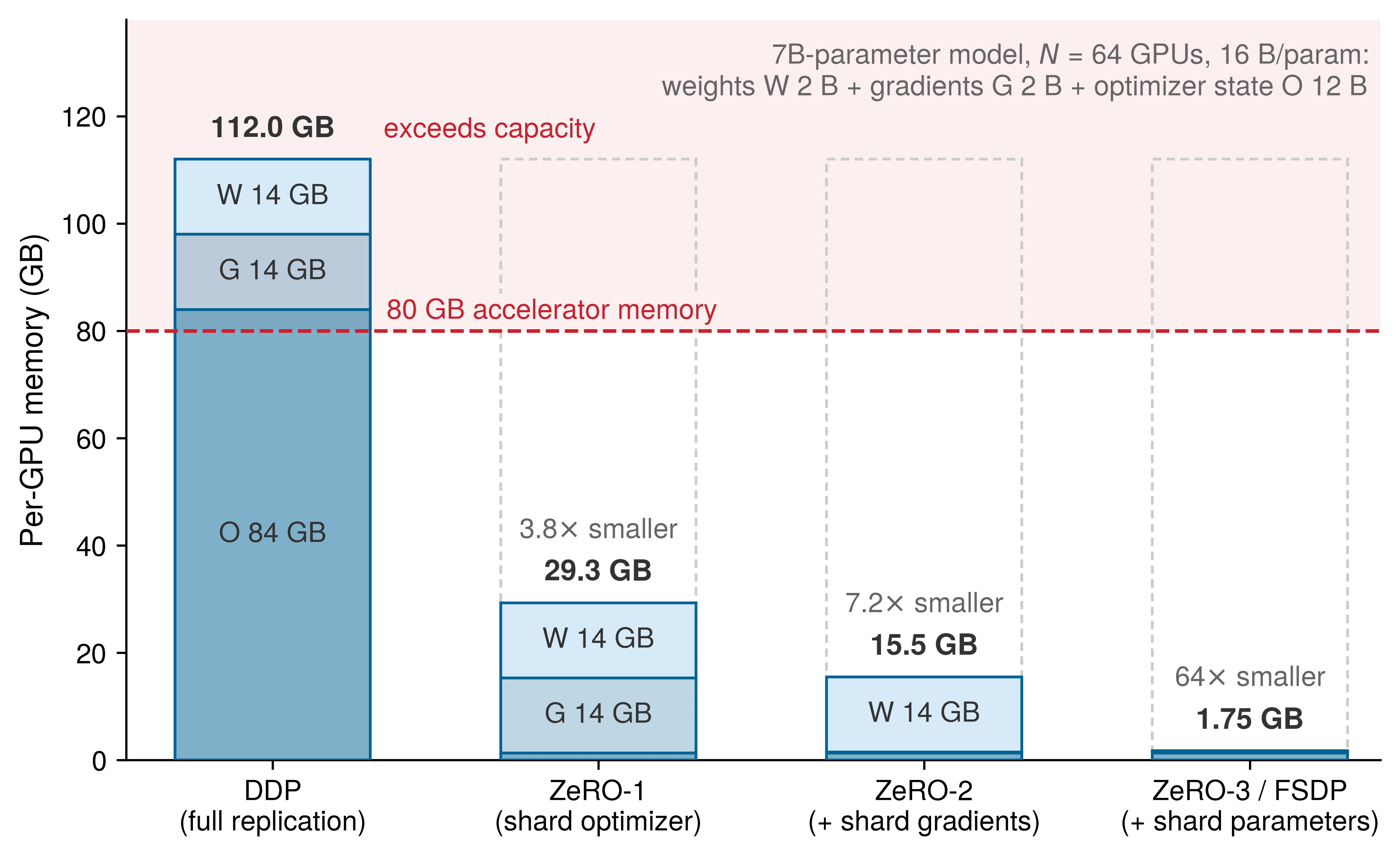
Replicated data parallelism stores an identical copy of weights, gradients, and optimizer state on every GPU, so a 7B-parameter model demands 112 GB on each device and overflows an 80 GB accelerator before a single activation is allocated. The Zero Redundancy Optimizer (ZeRO) (Rajbhandari et al. 2020) and PyTorch’s Fully Sharded Data Parallel (FSDP) (Zhao et al. 2023) remove that duplication by sharding training state across workers while keeping each worker’s full forward and backward computation.3 Sharding can make a model fit in memory without splitting its layer computations across devices.
Rajbhandari, Samyam, Jeff Rasley, Olatunji Ruwase, and Yuxiong He. 2020. “ZeRO: Memory Optimizations Toward Training Trillion Parameter Models.” SC20: International Conference for High Performance Computing, Networking, Storage and Analysis, 1–16. https://doi.org/10.1109/sc41405.2020.00024.
Zhao, Yanli, Andrew Gu, Rohan Varma, Liang Luo, Chien-Chin Huang, Min Xu, Less Wright, et al. 2023. “PyTorch FSDP: Experiences on Scaling Fully Sharded Data Parallel.” Proceedings of the VLDB Endowment 16 (12): 3848–60. https://doi.org/10.14778/3611540.3611569.
3 ZeRO (Zero Redundancy Optimizer): Introduced by Microsoft researchers in 2019 and released in the DeepSpeed library (Rasley et al. 2020), ZeRO’s stages progressively partition optimizer states, gradients, and parameters. FSDP draws on the fully sharded approach associated with ZeRO’s deepest stage; the shared partitioning principle does not imply identical implementations or communication schedules.
Rasley, Jeff, Samyam Rajbhandari, Olatunji Ruwase, and Yuxiong He. 2020. “DeepSpeed: System Optimizations Enable Training Deep Learning Models with over 100 Billion Parameters.” Proceedings of the 26th ACM SIGKDD International Conference on Knowledge Discovery & Data Mining, 3505–6. https://doi.org/10.1145/3394486.3406703.
Definition 6.3: Sharded data parallelism
Sharded data parallelism partitions optimizer state, gradients, and at the deepest stage the parameters themselves across data-parallel workers. Each worker processes its own minibatch shard and uses collectives to obtain the parameters and reduced gradients it needs. Full sharding reduces each worker’s persistent state toward \(1/\DeviceCount\) of the replicated training state; activations and temporary buffers still contribute to peak memory.
- Significance: Under the mixed-precision Adam convention used here, 16 bytes of state per parameter gives a 7B-parameter model 112 GB of training state, exceeding a 80 GB accelerator before activations. ZeRO Stage 3 across 64 workers reduces persistent state per device to 1.75 GB (0.25 bytes per parameter). The resulting AllGather and ReduceScatter traffic trades memory capacity for communication whose exposed cost depends on the interconnect and available overlap.
- Distinction: Unlike vanilla data parallelism, which replicates training state, sharded data parallelism partitions its storage. Unlike model parallelism, it retains each worker’s full forward and backward computation. Fully sharded execution gathers parameters for the current computation; the resharding schedule determines when it releases them.
- Common pitfall: A frequent misconception is that sharding is free memory. The on-demand AllGathers place parameter traffic on the critical path of every layer in every step; on slower interconnects or at small per-worker batch sizes, the exposed communication erodes throughput faster than the memory savings help. Capacity is purchased with bandwidth.
The scale of the savings is clearest on a model whose replicated training state only modestly overflows one accelerator, so that the effect of each sharding stage stays visible. The 175B reference returns after this trace when the question becomes whether sharding alone is enough.
Napkin Math 6.4: ZeRO memory savings
Problem: Training a 7B parameter Llama-2 model in mixed precision requires 16 bytes per parameter for weights, gradients, and optimizer state. Does the full training state fit on a single A100-80 GB, and how does ZeRO Stage 3 with 64 GPUs change the per-device memory requirement?
Baseline: Standard DDP (replicated state) Per-Parameter Memory Cost:
- Weights (FP16): 2 bytes
- Gradients (FP16): 2 bytes
- Optimizer state (FP32): 12 bytes (4 master weight + 4 momentum + 4 variance)
- Total: 16 bytes/parameter
Total Memory for 7B Model:
\[C_{\text{state,total}} = 7 \times 10^9 \times 16 \text{ bytes} \approx 112 \text{ GB}\]
Baseline outcome: Out-of-memory (OOM) on A100-80 GB.
Optimization: ZeRO-3 (fully sharded) With \(\DeviceCount=\) 64 GPUs, state is partitioned:
- Weights: 2\(/\DeviceCount\) bytes
- Gradients: 2\(/\DeviceCount\) bytes
- Optimizer: 12\(/\DeviceCount\) bytes
- Total: 16\(/\DeviceCount=\) 0.25 bytes/parameter effective storage
Per-GPU Memory:
\[C_{\text{state,ZeRO3}} = \frac{112 \text{ GB}}{64} \approx 1.75 \text{ GB}\]
Result: The persistent state fits, leaving ~78 GB for activations, gathered parameters, temporary buffers, and runtime allocations. Their simultaneous peak determines whether the chosen batch size fits.
ZeRO reaches that result in stages, and the intermediate stages matter because each one buys memory with a different communication pattern. Optimizer sharding alone (ZeRO-1) already brings the replicated footprint of the same model under the accelerator ceiling, because optimizer state is three-quarters of it; gradient sharding (ZeRO-2) and parameter sharding (ZeRO-3/FSDP) continue toward the fully sharded figure (figure 6). Each stage also changes which collectives the update uses (table 3).
| Stage | What is sharded | Memory reduction | Communication overhead |
|---|---|---|---|
| ZeRO-1 | Optimizer states only | ~4\(\times\) | Reduce to owner + AllGather (\(1\times\) DDP volume) |
| ZeRO-2 | + Gradients | ~8\(\times\) | ReduceScatter + AllGather (\(1\times\) DDP volume) |
| ZeRO-3/FSDP | + Parameters | ~\(\DeviceCount\) (linear in workers) | AllGather before each layer (\(1.5\times\) DDP volume) |
The first step, ZeRO-1, shards optimizer states across GPUs so each GPU stores only \(1/\DeviceCount\) of the Adam optimizer-related state. Gradients need only be reduced to the worker responsible for each parameter shard; after updating that shard, workers AllGather the updated parameters to restore the full replicas. This schedule supports the table’s baseline communication volume, whereas a full gradient AllReduce followed by a parameter AllGather would add traffic. Under the 12-byte convention that counts FP32 master weights, momentum, and variance, memory savings reduce optimizer state from \(12\DeviceCount\) bytes/param to \(12\) bytes/param total across the cluster.
Building on that owner-update contract, ZeRO-2 also shards gradients by replacing the full reduction with a ReduceScatter that leaves each GPU with only its \(1/\DeviceCount\) shard of reduced gradients. Each worker updates its \(1/\DeviceCount\) parameter partition using the corresponding optimizer state, and an AllGather then restores the updated parameter replicas. In the ideal ring accounting, each phase transfers \(\Parameters(\DeviceCount-1)/\DeviceCount\) elements per worker, for \(2\Parameters(\DeviceCount-1)/\DeviceCount\) across both phases, matching DDP’s byte volume (\(1\times\)) when gradient and parameter communication widths match. Replicated parameters avoid forward parameter gathers, although model operations may still communicate. Under the FP16-gradient convention, gradient storage falls from \(2\DeviceCount\) bytes per parameter across \(\DeviceCount\) workers to \(2\) bytes per parameter in total, or \(2/\DeviceCount\) per GPU, apart from transient buffers.
At the deepest stage, ZeRO-3 and FSDP partition the parameters as well, leaving each GPU with a \(1/\DeviceCount\) persistent slice of all three training states. The full-shard schedule considered here gathers each unit before forward computation, releases its unsharded parameters, and gathers them again for backward, before a ReduceScatter distributes the completed gradients for local shard updates. Across four ranks (figure 7) and under matching communication widths, ZeRO-1 (\(\OptimizerStateMemory/4\)) and ZeRO-2 (\(\OptimizerStateMemory/4, \GradientMemory/4\)) retain baseline \(1\times\) communication volume, whereas ZeRO-3 (\(\WeightMemory/4, \GradientMemory/4, \OptimizerStateMemory/4\)) adds the second parameter gather, yielding \(1.5\times\) the baseline volume in this accounting.
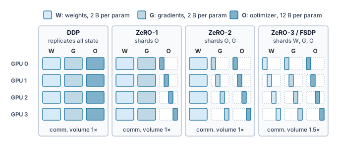
Full sharding adds parameter-readiness dependencies that replicated DDP avoids. With one sharding unit per layer, the forward pass needs an AllGather to reconstruct parameters (\(\LayerParameterPayload\) bytes); resharding after forward requires another gather before backward (\(\LayerParameterPayload\) bytes), followed by a ReduceScatter for gradients (\(\LayerParameterPayload\) bytes under equal communication precision). For a model with \(\LayerCount\) layers, this schedule performs about \(3\LayerCount\) collective operations per step; DDP instead AllReduces gradient buckets as they become ready. At large worker counts, the ideal per-worker transfer volumes approach \(3\ParameterPayload\) bytes versus \(2\ParameterPayload\) for DDP, where \(\ParameterPayload\) is the model’s parameter bytes at the communication precision, not full training state, and equals \(\GradientPayload\) when parameters and gradients travel at the same width. These volumes do not determine elapsed time alone. While layer \(\LayerIndex\) computes, layer \(\LayerIndex+1\) can prefetch parameters, subject to memory headroom and fabric contention.
The choice between FSDP and DDP begins with peak memory. If replicated state, activations, and working buffers fit, DDP avoids repeated parameter gathers. When optimizer and gradient storage are the obstacle, ZeRO-2 offers savings while leaving parameters replicated. If parameters themselves do not fit, ZeRO-3/FSDP, offload, or partitioned computation must address that remaining constraint. For a 70B+ model on 80 GB devices, the need for tensor parallelism depends on the gathered layer size, activation budget, and throughput target; parameter count alone does not decide it.
Memory-efficient data parallelism requires careful tuning of sharding strategy (by layer, by transformer block, or flat) and mixed precision settings. Finer sharding reduces per-GPU memory but increases communication frequency, because more AllGather and ReduceScatter operations must execute per training step. Replicated or sharded, a data-parallel design earns its added workers only when they turn into faster progress toward target quality, and scaling efficiency measures that conversion.
Self-Check: Question
A 7B-parameter transformer in mixed precision requires 112 GB of static memory for standard replicated DDP (14 GB for FP16 weights, 14 GB for FP16 gradients, and 84 GB for FP32 Adam master weights, momentum, and variance). Under ZeRO Stage 3 (or FSDP Full Shard) across 64 GPUs, what is the resulting static training memory per GPU?
- \(112\text{ GB}\), because ZeRO-3 only reduces dynamic activation memory rather than model state
- \(28\text{ GB}\), because only optimizer states are sharded while parameters and gradients remain fully replicated
- \(1.75\text{ GB}\), because weights, gradients, and optimizer states are each partitioned equally across all 64 workers
- \(0.25\text{ GB}\), because INT4 quantization eliminates floating-point representation entirely
An 8-GPU node can use four-step gradient accumulation to match the effective batch of 32 GPUs connected by 10 Gb/s Ethernet. Explain why the smaller allocation can cost less even when the larger allocation completes the fixed-sample workload sooner.
Order the memory sharding stages of data parallelism from least sharded (highest memory footprint) to deepest sharded (lowest memory footprint):
- ZeRO-2 (shards optimizer states and gradients using ReduceScatter)
- Standard DDP (full replication of parameters, gradients, and optimizer states)
- ZeRO-3 / FSDP (shards optimizer states, gradients, and model parameters with layer-wise AllGather/ReduceScatter)
- ZeRO-1 (shards optimizer states only, keeping parameters and gradients replicated)
If a model’s parameters, gradients, optimizer state, activations, and working buffers already fit comfortably within single-GPU memory with high compute utilization under standard DDP, what is the expected throughput impact of enabling ZeRO-3 / FSDP Full Sharding?
- Throughput will increase linearly by \(N\times\) because sharding reduces per-GPU gradient memory
- Throughput can decrease because FSDP introduces additional AllGather collectives before forward and backward passes and ReduceScatter on the critical path
- Throughput will remain exactly identical because NCCL automatically hides all collective communication overhead
- Throughput will double because parameter sharding eliminates the backward pass entirely
Why did modern distributed training frameworks replace centralized parameter servers with decentralized AllReduce collective topologies for dense synchronous training?
- Parameter servers cannot execute stochastic gradient descent updates with mathematical validity
- Parameter servers are restricted to CPU hosts and cannot interface with GPU accelerators
- AllReduce eliminates all network traffic by updating weights locally without exchanging data
- Centralized parameter servers create an \(\mathcal{O}(N)\) network bottleneck at the server’s network interface, whereas AllReduce distributes communication symmetrically across all workers
In standard PyTorch DistributedDataParallel, each worker uses a ____ to partition dataset indices deterministically and assign rank-specific shards based on process rank and epoch seed.
6.4 Scaling Efficiency and Convergence
When doubling the number of GPUs yields only 1.5\(\times\) speedup for the same work, scaling efficiency is 75 percent. The ratio quantifies the shortfall but does not identify its cause; communication, synchronization, input delivery, and changed local kernel efficiency require separate examination. Understanding why scaling efficiency degrades and how convergence changes with parallelism also requires distinguishing hardware throughput from time to a target loss. The scaling metrics apply to every strategy; the convergence analysis that follows concerns data-parallel batch growth and stale updates. It supplies a batch-size constraint that tensor and pipeline configurations must also respect when they are combined with data parallelism.
6.4.1 The mathematics of scaling efficiency
Whether scaling from one device to many is worthwhile is measured by scaling efficiency, the fleet-level ratio introduced with the Fleet Law in The Fleet Law. If a model trains in time \(\SingleDeviceRunTime\) on one device, ideal (linear) scaling would train it in time \(\SingleDeviceRunTime/\DeviceCount\) on \(\DeviceCount\) devices; communication overhead, pipeline bubbles, and load imbalance reduce the speedup. Equation 1 restates the ratio:
\[\ScalingEfficiency = \frac{\SingleDeviceRunTime}{\DeviceCount\times \MultiDeviceRunTime} \tag{1}\]
where \(\MultiDeviceRunTime\) is the training time on \(\DeviceCount\) devices. Measured per step of the same work, \(\SingleDeviceRunTime\) is the quantity the Fleet Law writes as \(\IronLawComputeTime\), the single-device compute time that its compute term divides by \(\DeviceCount\). An efficiency of 1.0 means perfect linear scaling; an efficiency of 0.5 means the run achieves only half the ideal speedup.
Definition 6.4: Scaling efficiency
Scaling efficiency \((\ScalingEfficiency)\) is the ratio of actual training throughput to ideal linear throughput when increasing the number of ML compute devices (\(\DeviceCount\)).
- Significance: The ratio in equation 1 measures added devices against the specified baseline. At 0.50 efficiency, a 10,000-GPU run delivers the throughput that 5,000 perfectly scaled devices would, so half of the accelerator-hours buy no progress relative to ideal scaling. The equivalence is to an idealized baseline; a real 5,000-GPU run would have its own, typically higher, efficiency, and the loss is spread across every device as waiting rather than concentrated in idle ones.
- Distinction: Unlike single-node efficiency, which captures local bottlenecks like \(\Bandwidth\), scaling efficiency measures how performance changes with device count. Communication time \((\CommunicationTime(\DeviceCount))\) and synchronization contribute, but changing local kernel shapes or input delivery can also affect the ratio.
- Common pitfall: A frequent misconception is that scaling efficiency is constant. In reality, it depends on both device count and problem size. For a fixed model, the communication-to-compute ratio typically worsens as \(\DeviceCount\) increases (Amdahl’s Law). At a fixed \(\DeviceCount\), a smaller model or local batch leaves less computation per device to hide startup latency and coordination, so its efficiency falls sooner.
The Fleet Law leads to the scaling efficiency metric for fixed global work. Substituting its step time (principle 10) for \(\MultiDeviceRunTime\) in equation 1, with \(\IronLawComputeTime\) standing for \(\SingleDeviceRunTime\) per step as noted there, gives equation 2:
\[ \ScalingEfficiency = \frac{\IronLawComputeTime}{\DeviceCount\times \DistributedStepTime(\DeviceCount)} = \frac{1}{1 + \frac{\DeviceCount(\CommunicationTime(\DeviceCount) + \SynchronizationTime(\DeviceCount) - \OverlappedTime)}{\IronLawComputeTime}} \tag{2}\]
This form states the scaling efficiency bound (principle 12), under which perfect linear scaling \((\ScalingEfficiency = 1.0)\) is a theoretical limit, not a practical target. Real systems fall short of it by an amount that depends on the configuration and grows with \(\DeviceCount\). The 175B data-parallel example below reaches only 15 percent, and the hybrid layouts later in the chapter recover much of that loss without reaching 1.0. The gap between \(\ScalingEfficiency = 1.0\) and the achieved efficiency is the price of distributed execution, paid in communication and coordination.
The equation also exposes the scaling wall. As \(\DeviceCount\) increases, the compute term \((\IronLawComputeTime/\DeviceCount)\) shrinks, but the communication and synchronization terms can remain constant or grow; a ring AllReduce’s bandwidth term, for example, stays near its bound however many workers join (principle 11). Eventually, the denominator is dominated by overhead, driving efficiency toward zero.
For data-parallel training of the 175B reference model, the per-step communication cost is dominated by the AllReduce of 350 GB of gradients, and how much of that exchange hides behind computation decides the efficiency. The scaling efficiency depends critically on computation per communicated byte. At fixed tokens per update, increasing parameter count raises both transformer computation and gradient bytes roughly proportionally, so model size alone does not guarantee better scaling. Larger batches raise computation per optimizer step without changing gradient size; the catch is that large batches can harm convergence and so require learning-rate tuning and warmup schedules. Network bandwidth enters directly because doubling InfiniBand bandwidth halves the bandwidth term, but efficiency changes according to the full step-time denominator rather than in direct proportion. The network fabric is therefore a first-order determinant of cluster productivity, not a secondary concern. Every point of scaling efficiency it recovers is returned across the much larger accelerator investment, which is why fabric spending is judged by the efficiency it buys rather than by its own price.
These factors interact, so efficiency cannot be inferred from model size or GPU count alone. The following worked model fixes the parameter count, tokens per update, accelerator count, effective bandwidth, local compute efficiency before communication, and overlap before calculating one efficiency point. Changing any of those inputs requires recomputing the full step-time model.
Napkin Math 6.5: Scaling efficiency for a 175B model
Setup: A communication-only model for training a 175B model on a DGX H100 cluster with 400 Gb/s InfiniBand per GPU. Pure replicated data parallelism is a counterfactual baseline here: the calculation isolates gradient exchange but does not establish that the full training state fits on each device.
Compute per step (assuming batch size 2M tokens, 6 FLOPs per parameter per token): \(\TrainingStepOperations = 6 \times 175 \times 10^9 \times 2 \times 10^6 \approx 2.1 \times 10^{18}\) FLOPs
Per-GPU compute time on 1,024 GPUs, each at 1,979 TFLOP/s peak in the 8-bit floating-point (FP8) format developed in section 6.4.8 (50 percent local compute efficiency before communication). The general matrix multiplications (GEMMs) run in FP8 while the gradients below still cross the wire in FP16, because the collective’s data type is chosen independently of the arithmetic’s: \(\IronLawComputeTime/\DeviceCount \approx 2.1\) seconds
AllReduce time (for 350 GB of gradients using ring-AllReduce with overlap): \(\ExposedCommunicationTime(\DeviceCount) \approx 11.9\) seconds (raw ring transfer takes \(2 \times (N-1)/N \times 350 / 50\), about 14 seconds; the schedule could hide 75 percent of that transfer, but the available compute window caps hidden communication at 15 percent of raw transfer time)
Scaling efficiency: \(\ScalingEfficiency = \PerDeviceComputeTime/(\PerDeviceComputeTime+ \ExposedCommunicationTime)\), which is equation 2 with the per-device compute window \(\PerDeviceComputeTime= \IronLawComputeTime/\DeviceCount\) and the exposed term standing for \(\CommunicationTime(\DeviceCount) + \SynchronizationTime(\DeviceCount) - \OverlappedTime\). Here the numerator is 2.1 s and the complete denominator is 14 s, giving 15 percent. The exposed communication term already subtracts the hidden portion from the raw transfer time and includes collective synchronization; subtracting overlap again would double-count the same saving.
Systems insight: The low efficiency (15 percent) shows why naive data parallelism at this scale is insufficient. It is one operating point, fixed by 2M per update, 1,024 GPUs, and 15 percent overlap, not a universal threshold; another cluster size requires recomputing per-device compute time, collective cost, overlap, and topology. Hierarchy-aware systems recover much of the lost efficiency by combining data parallelism with tensor parallelism, which communicates over NVLink, and pipeline parallelism, which overlaps computation with communication.
↩︎ The compute window that bounds how much of a collective can hide is established in Overlap limits and exposed communication.
Parallelism-infrastructure interaction
The scaling efficiency of a run is set by the interaction between the model’s communication requirements and the infrastructure’s bandwidth hierarchy, not by the model architecture alone. Recovering the efficiency that pure data parallelism lost above means mapping each parallelism dimension onto the bandwidth tier that can carry its traffic, which section 6.6 works through three concrete configurations once tensor and pipeline parallelism have been developed.
The collective algorithm adds its own dependence on message size. Tree-based AllReduce reaches every rank in \(\mathcal{O}(\log \DeviceCount)\) steps and suits small, latency-bound messages, whereas large gradient buffers favor the bandwidth-optimal ring; message size, topology, and contention decide between them.
↩︎ The message size at which ring AllReduce overtakes tree AllReduce, derived from the latency and bandwidth terms of each algorithm, is established in The algorithm crossover point.
Interconnect selection determines whether large-scale deployments remain compute-bound or collapse into communication-bound regimes, and the bandwidth requirements for efficient distributed training are substantial, particularly for transformer models. BERT-Base (110M parameters) requires approximately 440 MB of gradient synchronization per iteration in FP32, while BERT-Large (340M parameters) requires approximately 1.4 GB. A ring AllReduce across 64 GPUs moves nearly twice the gradient bytes through each GPU’s link, so finishing BERT-Large synchronization within 50 ms requires roughly 54 GB/s of sustained per-GPU bandwidth, and BERT-Base about a third of that. For 175B-parameter language models, exact bandwidth requirements depend on the 3D-parallel configuration, gradient accumulation, overlap, and interconnect topology rather than a single universal number.
6.4.2 Scaling physics and Amdahl’s Law with communication
Even a small unscalable cost in a single-device step eventually dominates distributed execution, because adding \(\DeviceCount\) devices shrinks the parallelizable compute share (\(\SingleDeviceRunTime / \DeviceCount\)) while leaving the fixed residual untouched. An Amdahl-style model separates that scalable work from the fixed residual fraction \(\SerialFraction\) of the single-device baseline (Amdahl's Law at fleet scale).
That baseline fraction is not the synchronization share a profiler reports for a distributed step (the distributed Amdahl pitfall of The Fleet Law), because the compute share has been divided by \(\DeviceCount\) while the residual has not. A residual of 1 percent of the single-device step occupies about 84 percent of each step on 512 GPUs. Reading the observed share as \(\SerialFraction\) would therefore overstate the residual many times over and predict a far lower speedup ceiling than the model implies.
Plotted on log-log axes up to 512 GPUs, the same fixed-residual model shows how much speedup each residual fraction gives up (figure 8), complementing the scaling efficiency bound (principle 12). In this illustrative model, a small baseline fraction (\(\SerialFraction= 0.1\%\)) stays closer to ideal scaling than a larger fraction (\(\SerialFraction= 1\%\)). A residual equal to a tenth of baseline time (\(\SerialFraction= 0.10\)) limits asymptotic speedup to \(1/\SerialFraction= 10\times\). Actual collective and coordination costs can change with worker count, so predicting a training run requires the full step-time accounting of equation 2.
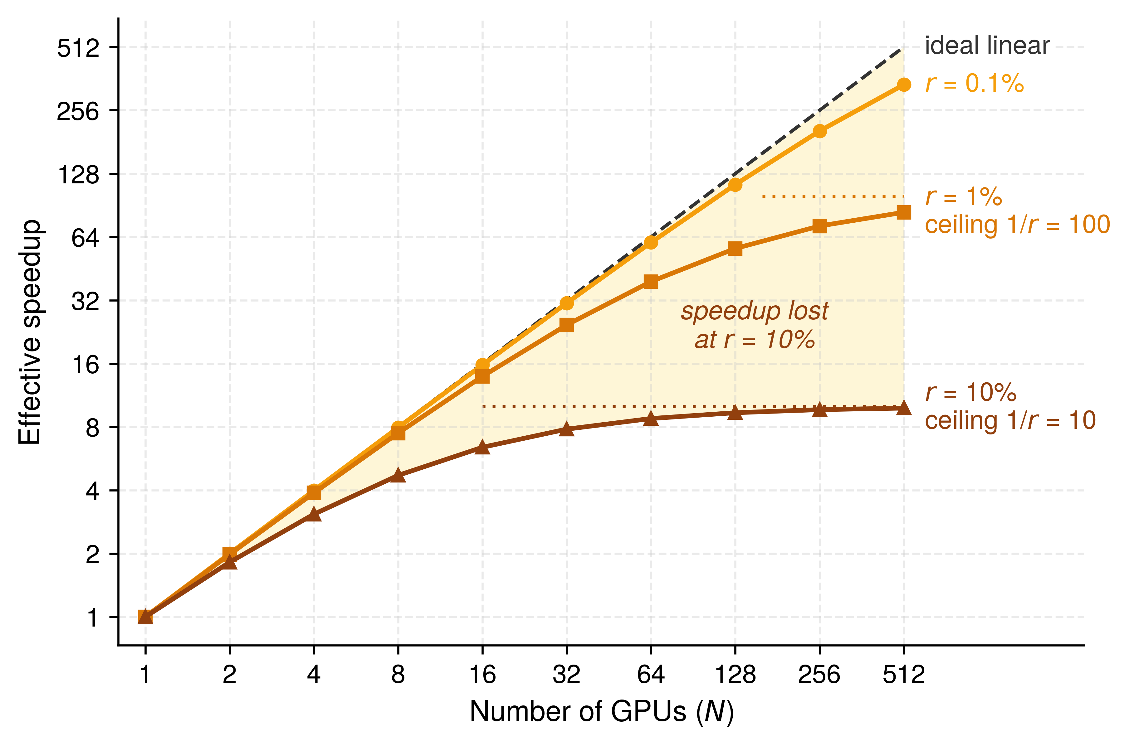
Published benchmark runs show the same shortfall in practice. MLPerf Training times complete runs to a fixed quality target, and several submitters report the same system at several sizes within one round (Mattson et al. 2020; MLCommons 2025). Each of 5 such series for the GPT-3 and Llama 3.1 405B benchmarks falls below the ideal line drawn through its smallest configuration (figure 9). On NVIDIA’s Eos cluster, GPT-3 trained in about 58 minutes on 512 H100 GPUs and 3.9 minutes on 10,752, so a 21× increase in accelerators cut the time 14.9×, a scaling efficiency (equation 1, measured relative to the smallest configuration rather than one device) of 71 percent. Across the series, the largest configuration keeps 71–84 percent of ideal. Two effects compound in these numbers. Communication and coordination grow with worker count, and the larger configurations also train with larger global batches, which can require more samples to reach the target (section 6.4.6). Separating the two requires the step-level accounting of equation 2.
Mattson, Peter, Christine Cheng, Cody Coleman, Greg Diamos, Paulius Micikevicius, David Patterson, Hanlin Tang, et al. 2020. “MLPerf Training Benchmark.” Proceedings of Machine Learning and Systems (MLSys) 2: 336–49.
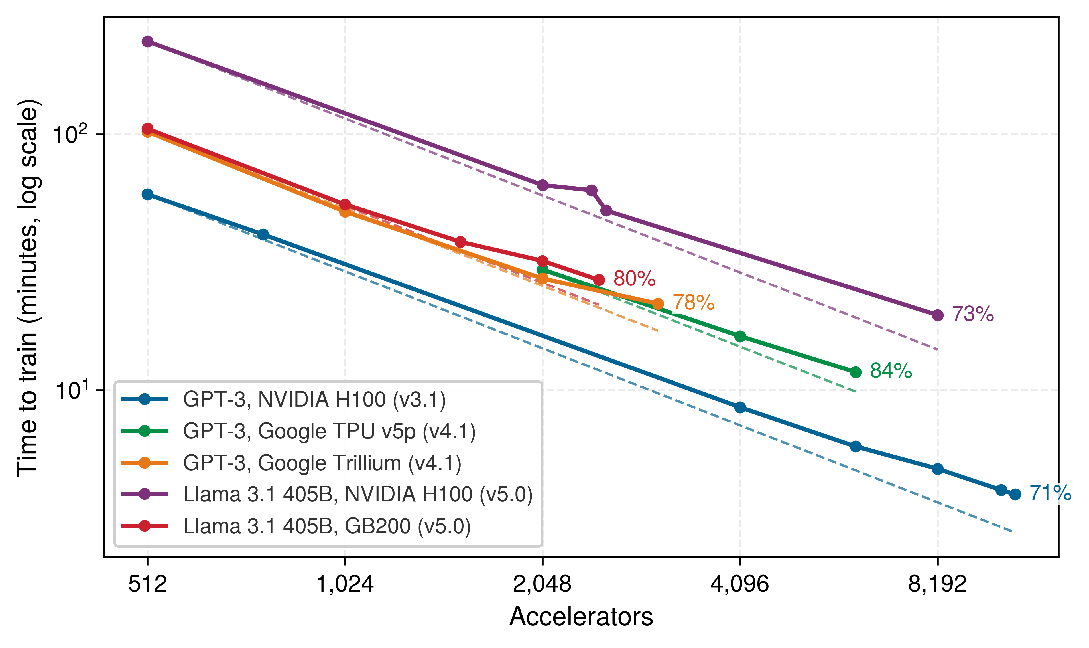
MLCommons. 2025. MLPerf Training Benchmark Results, Rounds V3.1 to V5.1.
Predicting a run means pricing each term of equation 2 for the configuration at hand. For a large-message ring AllReduce, the communication term’s bandwidth contribution, the fleet counterpart of the single-machine iron law’s data-movement ratio \(\DataVolume/\Bandwidth\), is \(\frac{2(\DeviceCount-1)}{\DeviceCount} \frac{\DataVolume}{\LinkBandwidth}\), where \(\DataVolume\) is the payload being reduced (the gradient bytes \(\GradientPayload\) under data parallelism, or a shard of model state under sharding) and \(\LinkBandwidth\) is sustained per-link bandwidth; this expression omits per-message startup latency. Each wait must enter the accounting once.
↪ The single-machine iron law and its data-movement term are developed in Iron Law Mapping.
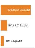
Communication energy climbs from HBM out to the network.
This communication overhead costs energy as well as wall-clock time, and the energy cost of communication grows with the physical distance between devices. At the scale of 10,000 GPUs, moving data is itself a power load. A full H100 NVLink envelope of roughly 9 PB/s at 7.5 pJ/bit represents about 540 kW before cooling and switch overhead, and the smaller NDR InfiniBand envelope (500 TB/s at 35 pJ/bit) still represents about 140 kW. The per-boundary accounting behind these per-bit costs is developed in The Physics of Data Movement. Overlap hides communication time but not its energy, so avoiding unnecessary movement is the direct way to reduce the power term.
As the device count grows for a fixed workload, the balance can move from a linear scaling regime toward a communication-bound regime. The transition has no universal GPU count, because it depends on compute per device, message sizes, topology, and overlap. Coordination overhead becomes consequential when its exposed time is no longer small relative to useful computation. Measurements at the intended workload and placement must establish the efficiency curve.
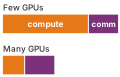
More GPUs shrink each step’s compute, not its communication.
The efficiency metrics directly influence the choice of parallelism strategy. Data parallelism works well in the linear scaling regime but becomes communication bound at scale, whereas the model-parallel strategies developed after this section replace part of that gradient traffic with other costs that the same efficiency equation prices once each mechanism is in place. Hardware efficiency metrics govern throughput, yet convergence theory determines whether distributed training reaches the same solution quality as single-device training. Parallelism affects optimization convergence in three ways: convergence rate changes with batch size, adding workers yields diminishing returns beyond the critical batch size, and learning-rate schedules must be revalidated when the global batch changes.
6.4.3 Convergence rate for synchronous data parallel SGD
Averaging gradients across \(\DeviceCount\) workers processes \(\DeviceCount\) times as many examples per step, but only reduces the number of steps to convergence when gradient noise—rather than loss curvature—is what holds back a larger step size. Formally, let \(\LossFunction\) be lower bounded by \(\LossLowerBound\) and have \(\SmoothnessConstant\)-Lipschitz gradients, so the smoothness constant limits how sharply the gradient can change as parameters move. Each worker computes gradients from \(\LocalBatchSize\) independent samples. At update \(\OptimizerStepIndex\), the aggregated estimator \(\MinibatchGradient_t\), the average of the \(\DeviceCount\) workers’ local gradients, is unbiased, and its conditional variance satisfies \(\mathbb{E}[\|\MinibatchGradient_t-\nabla\LossFunction(\ModelParameters_t)\|^2\mid\ModelParameters_t]\leq\SampleGradientStandardDeviation^2/(\DeviceCount \LocalBatchSize)\). When averaging reduces that noise, synchronous SGD makes steady progress toward parameters where the gradient is small; these assumptions bound progress toward a small gradient norm, not convergence to a global minimizer or a particular validation accuracy.
Theorem 6.1: Convergence rate for distributed SGD
For the update \(\ModelParameters_{t+1}=\ModelParameters_t-\LearningRate\MinibatchGradient_t\) with constant step size \(0<\LearningRate\leq 1/\SmoothnessConstant\), after \(\OptimizerUpdateCount\) synchronized updates,
\[ \frac{1}{\OptimizerUpdateCount}\sum_{t=0}^{\OptimizerUpdateCount-1}\mathbb{E}\!\left[\|\nabla\LossFunction(\ModelParameters_t)\|^2\right] \leq \underbrace{\frac{2\bigl(\LossFunction(\ModelParameters_0)-\LossLowerBound\bigr)}{\LearningRate \OptimizerUpdateCount}}_{\text{optimization term}} + \underbrace{\frac{\LearningRate \SmoothnessConstant\SampleGradientStandardDeviation^2}{\DeviceCount \LocalBatchSize}}_{\text{stochastic-variance term}}. \]
Choosing \(\LearningRate=\min\!\left\{1/\SmoothnessConstant,\sqrt{2(\LossFunction(\ModelParameters_0)-\LossLowerBound)\DeviceCount \LocalBatchSize/(\SmoothnessConstant\SampleGradientStandardDeviation^2\OptimizerUpdateCount)}\right\}\) balances the two terms. Before the smoothness cap becomes active, the stochastic contribution scales as \(\mathcal{O}(1/\sqrt{\DeviceCount \LocalBatchSize \OptimizerUpdateCount})\).
The theorem isolates the benefit that follows from the assumptions. With equal local batch size \(\LocalBatchSize\), synchronous data-parallel SGD computes the same minibatch estimator as one worker using batch size \(\DeviceCount\times \LocalBatchSize\) for that update, and the estimator variance decreases as \(1/(\DeviceCount\times \LocalBatchSize)\). It does not say that every increase in batch size proportionally reduces time to a target loss; learning-rate limits and critical-batch-size effects still apply. This distinction is the statistical efficiency of distributed training, separate from hardware efficiency. Because the theorem assumes perfect synchronization (BSP), convergence guarantees degrade as staleness increases whenever workers proceed at different rates or apply stale gradients.
6.4.4 Staleness impact across synchronization models
When a slow worker applies a gradient computed on an older parameter version, the update pushes the model along a direction that the current parameters may have already outgrown. The staleness parameter \(\GradientStaleness\) counts how many updates occur between computing and applying a gradient, tying the barrier savings of BSP, SSP, and ASP (section 6.3.1.5) to solution quality (Ho et al. 2013; Dutta et al. 2018). Because the damage from stale gradients depends on the objective, step-size schedule, worker count, and delay distribution, no single additive penalty applies across all runs.
Definition 6.5: Gradient staleness
Gradient staleness (\(\GradientStaleness\)) is the number of parameter updates that occur between the time a gradient is computed and the time it is applied to the global model state.
- Significance: It represents the synchronization error in distributed optimization. Increasing \(\GradientStaleness\) can improve throughput by reducing barrier waits \((\SynchronizationTime(\DeviceCount))\), but it typically degrades the rate of convergence, requiring more optimizer steps, and therefore more FLOPs, to reach the same accuracy.
- Distinction: Unlike network latency, which is a physical delay, staleness is an algorithmic offset that arises from the choice of synchronization protocol (e.g., ASP, SSP).
- Common pitfall: A frequent misconception is that staleness is “always bad.” In reality, it is a throughput-convergence trade-off: for some large-scale workloads, allowing bounded staleness is one practical way to keep thousands of GPUs in use.
The convergence behavior differs across these models in ways that directly affect training cost and solution quality. In BSP (\(\GradientStaleness=0\)), all workers compute on the same parameter version and aggregate before updating. Under the assumptions of theorem 6.1, the synchronized estimator inherits the \(\DeviceCount\times \LocalBatchSize\) minibatch guarantee.
SSP (\(\GradientStaleness\leq \StalenessBound\)) allows workers to proceed up to \(\StalenessBound\) iterations ahead of the slowest worker. Ho et al. (2013) bound the average regret of their SSP update sequence, the per-update gap between the loss its iterates incur and the loss of the best fixed parameters chosen in hindsight, at \(\mathcal{O}(\sqrt{(\StalenessBound+1)\DeviceCount/\OptimizerUpdateCount})\) for \(\DeviceCount\) workers and \(\OptimizerUpdateCount\) updates. The bound assumes convex Lipschitz component functions, a bounded domain, and a decreasing step size. It makes the staleness dependence explicit, since the bound grows with \(\StalenessBound\), but it measures a different quantity from the gradient-norm bound of theorem 6.1, which covers nonconvex objectives, so the two rates cannot be compared directly.
Dutta, Sanghamitra, Gauri Joshi, Soumyadip Ghosh, Parijat Dube, and Priya Nagpurkar. 2018. “Slow and Stale Gradients Can Win the Race: Error-Runtime Trade-Offs in Distributed SGD.” Proceedings of the Twenty-First International Conference on Artificial Intelligence and Statistics 84: 803–12.
Asynchronous SGD imposes no protocol-wide finite delay bound. Removing the barrier can improve update throughput, but a convergence rate requires additional assumptions about realized delays, the objective, and the step-size schedule. Dutta et al. (2018) analyze this as an error-runtime trade-off in which worker speed and gradient staleness jointly determine whether accepting a delayed update helps. Therefore neither a fixed square-of-average-delay penalty nor the complete loss of \(\DeviceCount\)-worker variance reduction follows from asynchronous execution alone. The protocol fixes each model’s delay control, but the strength of its convergence guarantee depends on further assumptions (table 4).
| Model | Delay control | Scoped guarantee | Systems effect |
|---|---|---|---|
| BSP | \(\GradientStaleness=0\) | Synchronous \(\DeviceCount\times \LocalBatchSize\)-minibatch theorem 6.1 | Waits for the slowest worker |
| SSP | \(\GradientStaleness\leq \StalenessBound\) | \(\mathcal{O}(\sqrt{(\StalenessBound+1)\DeviceCount/\OptimizerUpdateCount})\) average regret under convex assumptions (Ho et al. 2013) | Bounds delay while reducing some waits |
| ASP | No protocol-wide finite bound | No universal rate without additional delay and objective assumptions | Removes the global barrier but applies stale updates |
Ho, Qirong, James Cipar, Henggang Cui, Seunghak Lee, Jin Kyu Kim, Phillip B. Gibbons, Garth A. Gibson, Greg Ganger, and Eric P. Xing. 2013. “More Effective Distributed ML via a Stale Synchronous Parallel Parameter Server.” Advances in Neural Information Processing Systems (NeurIPS) 26.
6.4.5 Learning rate scaling rules
Multiplying the global batch by \(\BatchScalingFactor\) across data-parallel workers cuts the number of optimizer updates per epoch by the same factor, so keeping the single-GPU learning rate leaves the model under-trained while jumping straight to a \(\BatchScalingFactor\)-fold larger step size can destabilize early epochs. Whenever data parallelism changes the effective batch size, the learning-rate schedule must be revalidated against the target quality. Two scaling rules provide starting points for that adjustment.
The linear scaling rule (Goyal et al. 2017) proposes that when batch size is multiplied by \(\BatchScalingFactor\), learning rate also increases by \(\BatchScalingFactor\):
\[ \ScaledLearningRate = \BatchScalingFactor\cdot \BaseLearningRate\]
The approximation compares one large-batch step at learning rate \(\BatchScalingFactor\LearningRate\) with \(\BatchScalingFactor\) consecutive small-batch steps at learning rate \(\LearningRate\). At batch size \(\BatchScalingFactor\times \BatchSize\), independent gradient contributions reduce estimator variance by factor \(\BatchScalingFactor\), but lower variance alone does not establish stability. The approximation also requires gradients to change little over the corresponding \(\BatchScalingFactor\) small-batch steps. Goyal et al. (2017) validated the recipe for ResNet-50/ImageNet at global batch size 8,192 with gradual warmup. Layer-wise adaptive rate scaling (LARS) and layer-wise adaptive moments based optimizer (LAMB) provide related large-batch approaches for ImageNet and BERT-style pretraining (You et al. 2017; You et al. 2020). A warmup period increases the learning rate from \(\BaseLearningRate\) to \(\BatchScalingFactor\cdot \BaseLearningRate\) over the first \(\WarmupStepCount\) iterations to reduce early instability; the schedule still requires validation:
\[ \LearningRate_t = \BaseLearningRate+ \frac{\OptimizerStepIndex}{\WarmupStepCount}(\BatchScalingFactor\cdot \BaseLearningRate- \BaseLearningRate) \quad \text{for } \OptimizerStepIndex< \WarmupStepCount\]
The rule and the warmup were introduced together, and the run that introduced them shows why the scaled learning rate needs the warmup. A learning-rate schedule tuned for an eight-GPU run need not reach the same accuracy at 256 GPUs once the global batch grows with the worker count.
War Story 6.1: The one-hour ImageNet run (2017)
Context: Facebook AI Research set out to train ResNet-50 on ImageNet in one hour using 256 GPUs, pushing data parallelism far beyond the batch sizes that earlier practice treated as safe (Goyal et al. 2017).
Mechanism: Scaling the global batch to 8,192 cut the number of optimizer updates per epoch by the same factor. Keeping the small-batch learning rate left too few effective updates to reach the target accuracy, while scaling the learning rate up by the same factor destabilized optimization in the first epochs, when the loss surface changes fastest.
Impact: Without the gradual warmup recipe, the large-batch runs reported higher training and validation error than the small-batch baseline. Higher hardware throughput alone did not preserve the quality target.
Fix: The team introduced the linear learning-rate scaling rule paired with a 5-epoch gradual warmup schedule, stabilizing optimization at batch size 8,192.
Systems lesson: Distributed training demands more than parallel hardware alone. Scaling changes the optimization regime, so the cluster, communication schedule, batch size, and learning-rate schedule must be tuned as one system.
The square root scaling rule is an alternative learning-rate heuristic to test when increasing batch size:
\[ \ScaledLearningRate = \sqrt{\BatchScalingFactor} \cdot \BaseLearningRate\]
This rule increases the learning rate more slowly than linear scaling. Its suitability depends on the optimizer, schedule, and training regime; exceeding a critical-batch estimate does not make it mandatory or guarantee convergence. The learning rate must be validated against the same target quality.
LARS (You et al. 2017) scales each layer’s update relative to its weight norm. The simplified LARS expression below illustrates the ratio of weight norm to gradient norm with weight decay. LAMB (You et al. 2020) applies a related layer-wise adaptation to an Adam-based update rather than using this raw-gradient denominator:
\[ \LearningRate_\ell = \LarsGlobalLearningRate\cdot \frac{\|\LayerWeights_\ell\|}{\|\MinibatchGradient_\ell\| + \WeightPenaltyStrength\|\LayerWeights_\ell\|} \]
Here \(\WeightPenaltyStrength\) is the weight-decay coefficient in the illustrated LARS expression, distinct from the failure-rate parameter used in reliability analysis. Layer-wise scaling controls update magnitude relative to parameter magnitude, but does not guarantee convergence for arbitrary batches. Its systems role is to extend the range of validated batch sizes over which added data-parallel workers can reduce time to quality.
6.4.6 Critical batch size and diminishing returns
Increasing the global batch eventually yields diminishing reductions in the optimization steps needed to reach a fixed target quality. The critical batch size \(\CriticalBatchSize\) marks the transition point beyond which increasing batch size yields diminishing returns in convergence per sample seen.
Definition 6.6: Critical batch size
Critical batch size \((\CriticalBatchSize)\) is a workload-dependent crossover batch size beyond which further batch growth yields diminishing reductions in optimization steps per added sample (McCandlish et al. 2018; Shallue et al. 2019).
- Significance: It characterizes statistical scaling, separately from hardware throughput. In the gradient-noise model, batches well below \(\CriticalBatchSize\) can reduce step count approximately in proportion to batch growth; above it, additional samples buy progressively smaller step-count reductions.
- Distinction: Unlike the memory-limited batch size (determined by memory capacity and activation footprint), the critical batch size depends on the model, data, optimizer, training phase, and target quality.
- Common pitfall: A frequent misconception is that training can be sped up indefinitely by adding GPUs. In reality, \(\CriticalBatchSize\) is a guide to diminishing statistical returns, not a hard physical ceiling or a universal optimum in wall-clock time.
Shallue, Christopher J, Jaehoon Lee, Joseph Antognini, Jascha Sohl-Dickstein, Roy Frostig, and George E Dahl. 2019. “Measuring the Effects of Data Parallelism on Neural Network Training.” Journal of Machine Learning Research 20: 1–49.
The gradient-noise-scale proxy for the critical batch size can be estimated as:
\[ \CriticalBatchSize\approx \frac{\text{tr}(\GradientCovarianceMatrix)}{\|\nabla \LossFunction(\ModelParameters)\|^2} \]
where \(\text{tr}(\GradientCovarianceMatrix)\) is the trace of the gradient covariance matrix (total gradient variance) and \(\|\nabla \LossFunction(\ModelParameters)\|^2\) is the squared gradient norm (signal strength). Intuitively, \(\CriticalBatchSize\) is the batch size at which averaging reduces gradient variance to the level of the true gradient magnitude.
Published large-batch regimes illustrate the scale rather than providing fixed thresholds. On ImageNet, Goyal et al. (2017) stabilized ResNet-50 at global batch 8,192 with warmup, and LARS extends ImageNet large-batch training further in some settings (You et al. 2017). For BERT-Large pretraining, LAMB reports training at 32K–64K batch sizes with layer-wise adaptive updates (You et al. 2020). Across other domains, McCandlish et al. (2018) show useful batch-size limits ranging from tens of thousands in ImageNet-like settings to millions in reinforcement-learning workloads, so new frontier-language-model thresholds should be measured rather than copied.
Goyal, Priya, Piotr Dollár, Ross Girshick, Pieter Noordhuis, Lukasz Wesolowski, Aapo Kyrola, Andrew Tulloch, Yangqing Jia, and Kaiming He. 2017. “Accurate, Large Minibatch SGD: Training ImageNet in 1 Hour.” arXiv Preprint arXiv:1706.02677 abs/1706.02677.
You, Yang, Igor Gitman, and Boris Ginsburg. 2017. “Large Batch Training of Convolutional Networks.” arXiv Preprint arXiv:1708.03888.
You, Y., J. Li, S. Reddi, J. Hseu, S. Kumar, S. Bhojanapalli, X. Song, J. Demmel, K. Keutzer, and C.-J. Hsieh. 2020. “Large Batch Optimization for Deep Learning: Training BERT in 76 Minutes.” International Conference on Learning Representations (ICLR).
The gradient-noise model separates statistical efficiency from hardware efficiency. Well below \(\CriticalBatchSize\), increasing batch size can reduce optimization steps almost proportionally while preserving similar total sample use. Near \(\CriticalBatchSize\), the trade-off between fewer updates and more samples becomes material. Above it, step count approaches a lower limit while sample use continues to increase. Neither maximum samples per second nor minimum training time necessarily occurs at \(\CriticalBatchSize\): those objectives also depend on device utilization, communication, and the validated learning-rate schedule.
On log-log axes, the gradient-noise trade-off appears as a divergence between optimization step count and total sample consumption (figure 10). Below the critical threshold (\(\BatchSize/\CriticalBatchSize< 1\)), increasing batch size yields near-linear reductions in optimization steps with negligible sample waste; past the crossover point at \(\BatchSize/\CriticalBatchSize= 1\) (where both normalized costs equal 2), the step count curve asymptotically flattens toward 1 while total examples processed climb steeply along the \(1 + \BatchSize/\CriticalBatchSize\) trajectory.
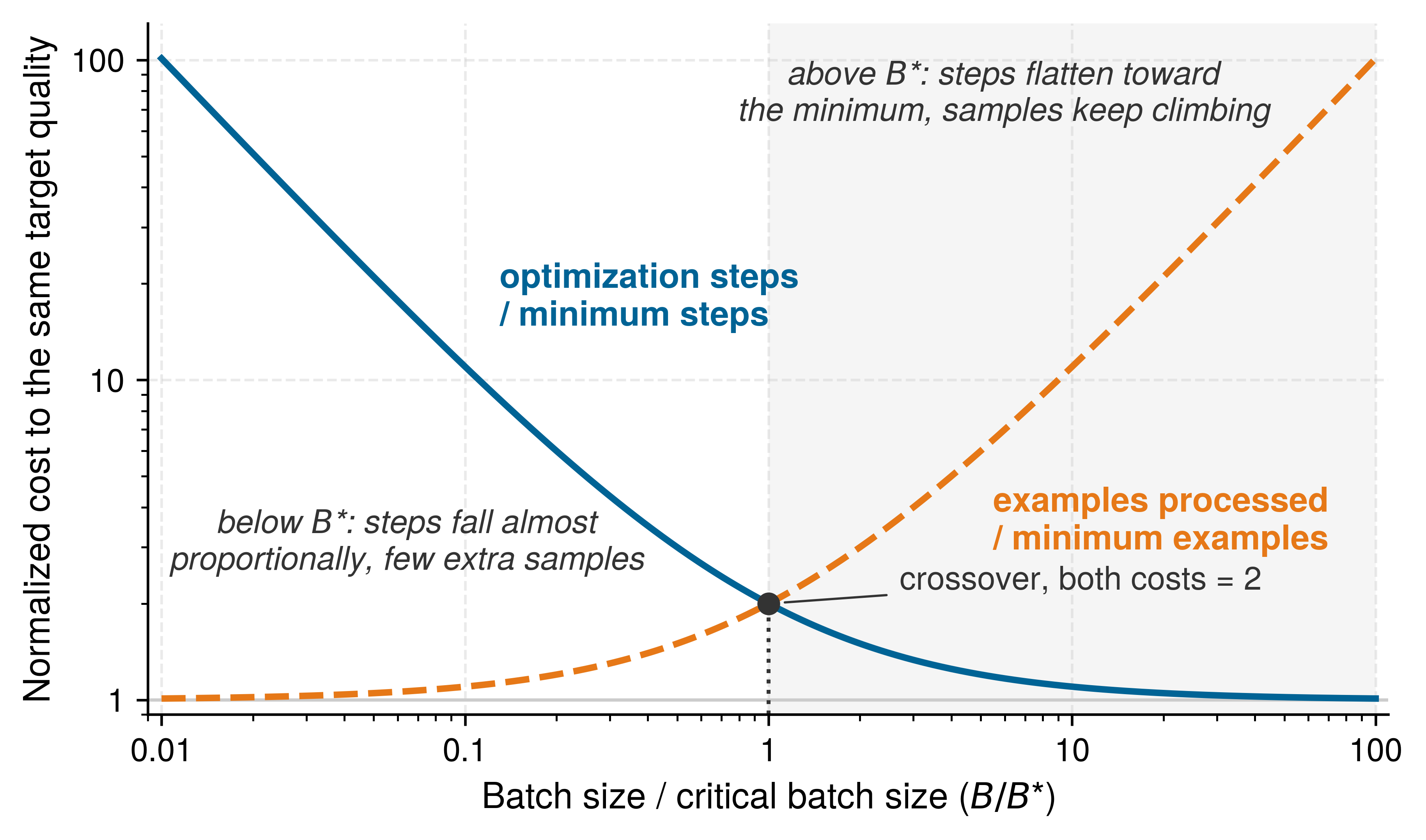
McCandlish, Sam, Jared Kaplan, Dario Amodei, and OpenAI Dota Team. 2018. “An Empirical Model of Large-Batch Training.” arXiv Preprint arXiv:1812.06162, ahead of print. https://doi.org/10.48550/arXiv.1812.06162.
Dividing the critical batch by the per-worker batch \(\LocalBatchSize\) estimates where worker growth leaves the near-proportional statistical scaling regime. With one local batch per update and its size held fixed, the crossover occurs around \(\DeviceCount\approx \CriticalBatchSize/\LocalBatchSize\) workers. Past that point, additional workers mainly raise sample throughput that the optimizer cannot convert into proportionally fewer steps. Gradient accumulation increases each worker’s contribution per update and lowers the corresponding worker count. Shrinking \(\LocalBatchSize\) moves the crossover outward but leaves less computation per worker to hide communication, coupling statistical and hardware efficiency.
That crossover informs a cost-time trade-off rather than setting a mandatory worker count. Larger batches may still reduce time to target even as they consume more examples. That benefit must be established with measured step time and a validated learning-rate schedule at the same target quality. Changing synchronization or compression also changes the optimization process, so its communication savings must be weighed against any additional steps required.
Checkpoint 6.2: Scaling decisions
Given a 7B-parameter model distributed across a cluster of 64 A100 GPUs (80 GB HBM2e each), estimate the critical-batch crossover. Use a pilot trace with \(\text{tr}(\GradientCovarianceMatrix)=1.6 \times 10^6\), \(\|\nabla \LossFunction(\ModelParameters)\|^2=100\), per-GPU batch \(\LocalBatchSize=4\), and a proposed gradient-accumulation depth of 32 steps, giving \(\GlobalBatchSize= 64 \times 4 \times 32 = 8{,}192\) samples.
6.4.7 Communication cost versus convergence speed
Communication savings matter only through the resulting time and cost to reach target model quality. Scaling a transformer language model from 8 to 64 workers, with a per-worker batch of \(\LocalBatchSize= 32\), shows how shorter steps and extra iterations to the same target combine into that cost.
Napkin Math 6.6: Scaling from 8 to 64 workers
Setup: This illustrative comparison assumes the iteration counts needed to reach one fixed target quality. They are scenario inputs, not measured convergence results or predictions from GPU count. The baseline is 100K iterations on single GPU with \(\LocalBatchSize=\) 32.
Table 5: Illustrative Scaling Comparison: Assumed iteration counts to one target quality, communication increments relative to local compute time, and the resulting speedup and sample efficiency. These are scenario calculations, not empirical optimizer benchmarks.
8 workers (BSP)
- Effective batch size: \(\BatchSize=\) 8 \(\times\) 32 = 256
- Learning rate: \(\LearningRate=\) 8 \(\times \BaseLearningRate\) (illustrative candidate with warmup; validate for the workload)
- Expected iterations: 100K \(/\) 8 = 12.5K iterations
- Assumed iterations to the same target: 12.8K iterations (98 percent efficiency)
- Communication overhead: 15 percent (NVLink intra-node)
- Wall-clock speedup: 100K \(\times\) 1 \(/\) (12.8K \(\times\) 1.15×) = 6.8×
64 workers (BSP)
- Effective batch size: \(\BatchSize=\) 64 \(\times\) 32 = 2,048
- Learning rate (\(\DeviceCount=\) 64 workers): \(\LearningRate= \DeviceCount\times \BaseLearningRate\) is the scenario’s assumed candidate schedule, not a prescription determined by \(\CriticalBatchSize\) alone
- Assuming \(\CriticalBatchSize\approx\) 4,000 (below critical): the useful-worker bound is \(\CriticalBatchSize/\LocalBatchSize\approx\) 4,000 \(/\) 32 \(\approx\) 125 workers, so 64 workers stay inside the near-proportional regime; this estimate does not validate a learning-rate schedule
- Expected iterations: 100K \(/\) 64 = 1.56K iterations
- Assumed iterations to the same target: 1.72K iterations (91 percent efficiency)
- Communication overhead: 45 percent (InfiniBand inter-node, 8 nodes)
- Wall-clock speedup: 100K \(\times\) 1 \(/\) (1.72K \(\times\) 1.45×) = 40.1×
SSP workers: 64 workers (\(\StalenessBound=\) 4)
- Same effective batch size: \(\BatchSize=\) 2,048
- Illustrative learning-rate reduction, not a staleness theorem: \(\StalenessAdjustedLearningRate= \BspLearningRate/ \sqrt{1 + \StalenessBound}\) with \(\StalenessBound=\) 4, giving \(\StalenessAdjustedLearningRate\approx\) 0.45 \(\times \BspLearningRate\)
- Expected iterations: Higher due to staleness penalty
- Assumed iterations to the same target: 2.1K iterations (74 percent efficiency)
- Communication overhead: 25 percent (reduced synchronization)
- Wall-clock speedup: 100K \(\times\) 1 \(/\) (2.1K \(\times\) 1.25×) = 38.1×
Analysis (table 5)
| Configuration | Iterations | Comm. overhead | Wall-clock speedup | Sample efficiency |
|---|---|---|---|---|
| 1 GPU (baseline) | 100,000 | 0% | 1\(\times\) | 100% |
| 8 GPU BSP | 12,800 | 15% | 6.8× | 98% |
| 64 GPU BSP | 1,720 | 45% | 40.1× | 91% |
| 64 GPU SSP | 2,100 | 25% | 38.1× | 74% |
The 64-GPU BSP configuration achieves 40× speedup despite only 91 percent sample efficiency because the communication overhead (45 percent) is offset by the larger worker count. SSP at 64 workers comes close in wall-clock time with lower per-iteration communication (25 percent), but the extra iterations its stale updates require hold it to 38.1× against BSP’s 40.1×. In this scenario it therefore finishes slightly later and costs slightly more than 64-worker BSP.
Cost Analysis (assuming $2/GPU-hour):
- 8: 12.8K iters \(\times\) 0.46 s/iter \(\times\) 8/3600 \(\times\) $2/GPU-hour = $26
- 64 BSP: 1.72K iters \(\times\) 0.58 s/iter \(\times\) 64/3600 \(\times\) $2/GPU-hour = $35
- 64 SSP: 2.1K iters \(\times\) 0.50 s/iter \(\times\) 64/3600 \(\times\) $2/GPU-hour = $37
Despite higher parallelism, 64-GPU training costs more per run due to communication overhead and reduced sample efficiency. The 8-GPU configuration is more cost-efficient, but its 6.8× speedup against the 64-GPU run’s 40.1× leaves it several times slower in wall-clock time. The choice depends on whether minimizing cost or minimizing time-to-result is the priority.
On the cost-time plane of figure 11, 64-worker BSP dominates 64-worker SSP on both axes. SSP saves communication per iteration, but its stale updates need enough extra iterations to cost more and finish later, while 8-worker BSP remains the cheaper and slower option.
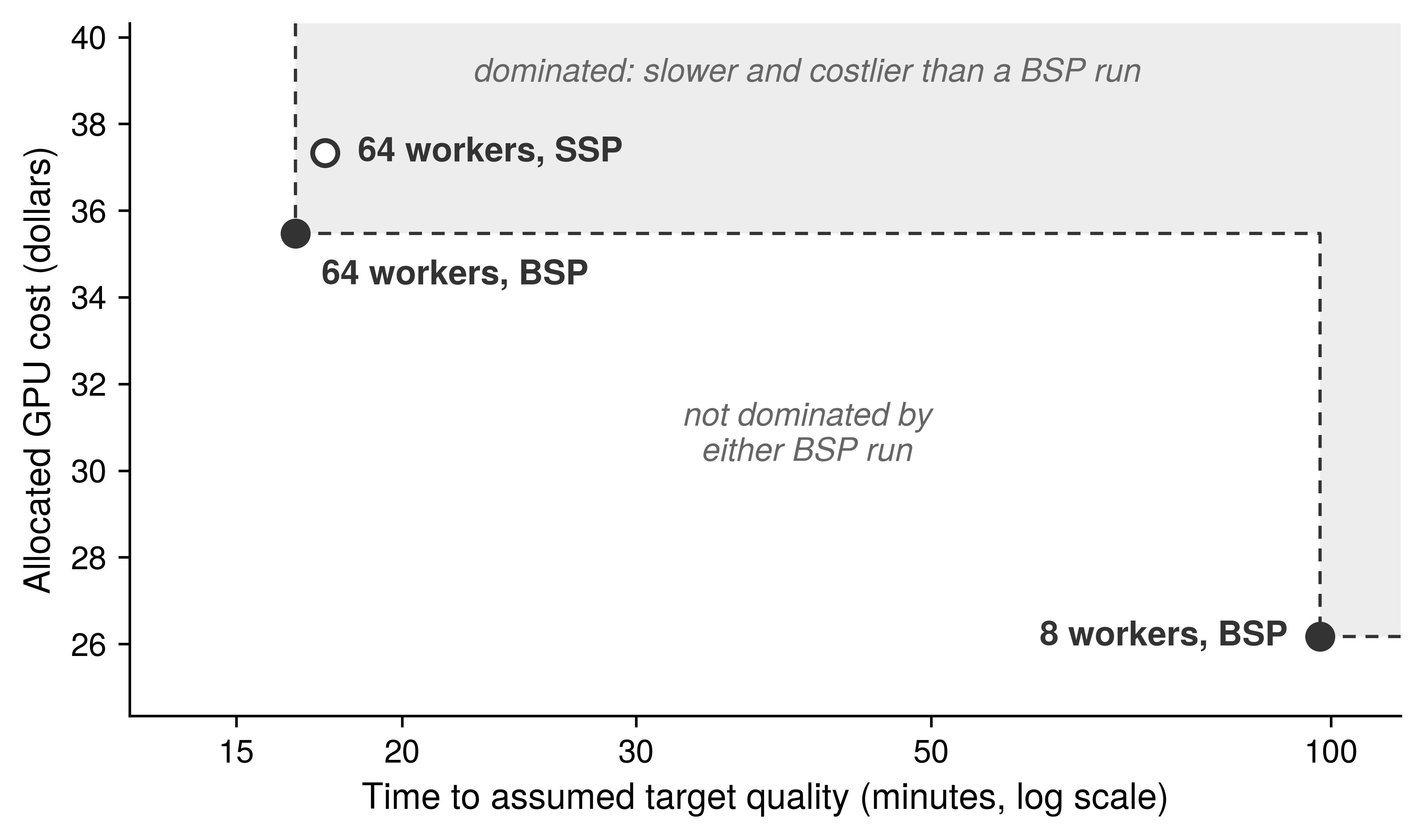
Moving a job along this cost-time frontier requires shrinking each message, synchronizing less often, or relaxing the global reduction topology. Gradient compression shrinks the payload directly by transmitting quantized, sparsified, or low-rank approximations, as in sign-based updates (Bernstein et al. 2018), Deep Gradient Compression (Lin et al. 2018), PowerSGD (Vogels et al. 2019), quantized SGD with convergence analysis (Alistarh et al. 2017), and empirical sparse gradient dropping for neural machine translation (Aji and Heafield 2017).
Bernstein, Jeremy, Yu-Xiang Wang, Kamyar Azizzadenesheli, and Animashree Anandkumar. 2018. “signSGD: Compressed Optimisation for Non-Convex Problems.” International Conference on Machine Learning (ICML) 80: 560–69.
Lin, Yujun, Song Han, Huizi Mao, Yu Wang, and William J Dally. 2018. “Deep Gradient Compression: Reducing the Communication Bandwidth for Distributed Training.” International Conference on Learning Representations (ICLR).
Vogels, Thijs, Sai Praneeth Karimireddy, and Martin Jaggi. 2019. “PowerSGD: Practical Low-Rank Gradient Compression for Distributed Optimization.” Advances in Neural Information Processing Systems (NeurIPS) 32.
Alistarh, Dan, Demjan Grubic, Jerry Z. Li, Ryota Tomioka, and Milan Vojnovic. 2017. “QSGD: Communication-Efficient SGD via Gradient Quantization and Encoding.” Advances in Neural Information Processing Systems (NeurIPS) 30: 1709–20.
Aji, Alham Fikri, and Kenneth Heafield. 2017. “Sparse Communication for Distributed Gradient Descent.” Proceedings of the 2017 Conference on Empirical Methods in Natural Language Processing, 440–45. https://doi.org/10.18653/v1/d17-1045.
↩︎ Quantized, sparsified, and low-rank gradient compression, the error feedback that keeps them convergent, and the criteria for when they pay, are established in Gradient Compression Under Bandwidth Scarcity.
Stich, Sebastian U. 2019. “Local SGD Converges Fast and Communicates Little.” International Conference on Learning Representations (ICLR).
Instead of shrinking each payload, Local SGD lowers synchronization frequency by letting workers perform \(\LocalUpdateCount\) local updates before averaging, which cuts collective calls per local update by a factor of \(\LocalUpdateCount\). Results for smooth, strongly convex objectives can recover synchronous SGD’s asymptotic rate under specified learning-rate and local-update-interval conditions (Stich 2019), so the synchronization interval remains part of the convergence contract rather than an unrestricted communication saving.
Where Local SGD keeps a global AllReduce at wider intervals, Decentralized SGD replaces the global collective with sparse neighbor exchanges along a communication graph. Immediate bandwidth demand drops, at the cost of taking additional rounds to spread information across the group; graph connectivity, link service time, and the optimization effect of delayed mixing determine whether that trade-off helps a geographically distributed workload.
Choosing among these three levers depends on which bottleneck binds and how many extra iterations the altered update costs. Each candidate must be judged by measured time to the same target quality. A narrower numeric format offers one more way to shrink the payload without changing the collective schedule, under conditions that FP8 makes precise.
6.4.8 FP8 for distributed training
Running matrix multiplications in 8-bit floating point (FP8) accelerates local compute, which can make a distributed job more communication-bound if gradients still cross the network in 16-bit precision. Compute precision and communication precision are separate choices: casting GEMM operands to half as many bytes reduces operand storage and local memory traffic, but it halves a collective payload only when the communication path explicitly transmits that narrower representation.
↩︎ The throughput that narrower precisions buy on current accelerators is established in Precision and throughput trade-offs.
FP8 matters to distributed training only after four dtypes are distinguished: the stored parameter dtype, the GEMM operand dtype, the accumulator or master-state dtype, and the collective wire dtype. Traditional mixed-precision training commonly retains FP32 optimizer or master state while using FP16/BF16 operands. FP8-capable accelerators add E4M3 (four exponent bits and three mantissa bits) and E5M2 (five exponent bits and two mantissa bits) operand formats optimized for different tensor distributions (Micikevicius et al. 2022).
The two FP8 formats trade precision against range. E4M3 keeps an extra mantissa bit for scaled weights and activations, which cluster within a predictable range, while E5M2 keeps an extra exponent bit for scaled gradients, which can span many orders of magnitude during backpropagation. Because tensor magnitudes drift during training, each tensor is multiplied before conversion by a scale, commonly derived from its recent maximum absolute value, a policy called dynamic scaling. Neither the format nor the scaling policy guarantees that every value survives conversion, so training quality must be validated for each workload.
↪ Per-parameter training memory under each of these formats is collected for reference in Numeric Precision and Training Memory.
Micikevicius, Paulius, Dusan Stosic, Neil Burgess, Marius Cornea, Pradeep Dubey, Richard Grisenthwaite, Sangwon Ha, et al. 2022. “FP8 Formats for Deep Learning.” arXiv Preprint arXiv:2209.05433.
An FP8 training contract pairs FP32 master or optimizer state and FP8 GEMM operands with higher-precision accumulation, and it can approach FP16 training quality on suitable workloads (Micikevicius et al. 2022). FP8 halves bytes only for tensors actually stored or transmitted in FP8, so a collective that reduces FP16 gradients still moves FP16 bytes even when every preceding GEMM ran in FP8. FP8 therefore earns its place in distributed training when lower-precision compute shortens the local critical path, or when an explicit communication cast shrinks payloads while the accumulation and scaling policy protects convergence. It changes representation, not the parallelization axis. Compression, local updates, and narrower formats all make each data-parallel step cheaper, yet none of them partitions an individual layer or its activations; that remaining capacity constraint motivates model parallelism.
Self-Check: Question
A team scales a data-parallel training run from 8 to 64 workers, increasing the effective global batch size from 512 to 4,096 samples. If the model operates comfortably below its critical batch size, which learning-rate adjustment follows the linear scaling heuristic?
- Keep the learning rate unchanged, because large-batch variance reduction automatically stabilizes optimization
- Multiply the learning rate by 64 to match the total worker count rather than the batch expansion ratio
- Multiply the learning rate by \(\sqrt{8}\) from step zero without a warmup schedule
- Multiply the learning rate by \(8\times\) (matching the batch expansion ratio) and include a gradual linear warmup schedule
Explain the distinction between hardware efficiency and statistical efficiency in distributed training, and describe a concrete scenario where a cluster configuration achieves high hardware efficiency but poor statistical efficiency.
Why must the learning-rate schedule be revalidated when moving from Bulk-Synchronous Parallel (BSP) to Stale-Synchronous Parallel (SSP) at the same global batch size?
- Gradients computed against stale parameters can alter update stability, with effects that depend on delay, objective, and optimizer schedule
- SSP workers compute exact full-batch gradients instead of stochastic minibatches
- SSP eliminates all inter-GPU network communication, which alters the loss landscape
- SSP is mathematically restricted to second-order quasi-Newton optimizers that require small step sizes
The threshold batch size \(B^* \approx \frac{\text{tr}(\Sigma)}{\|\nabla \mathcal{L}(\theta)\|^2}\), representing the point where gradient variance equals true gradient magnitude and past which larger batches yield diminishing returns in sample efficiency, is known as the ____.
Why does the FP8 recipe described in this chapter pair the E4M3 format for forward-pass activations and weights with the E5M2 format for backward-pass gradients?
- E4M3 has a wider numerical range than E5M2, which prevents gradient underflow during backpropagation
- E4M3 spends more bits on the mantissa, giving finer precision for bounded weights and activations, while E5M2 spends more bits on the exponent, giving the wider dynamic range that small and widely varying gradients need
- E4M3 is an integer format while E5M2 is a floating-point format supported exclusively on CPU hosts
- E5M2 requires half the memory bandwidth of E4M3, accelerating the backward pass AllReduce
Explain why per-tensor dynamic scaling is necessary in FP8 distributed training and describe how the scaling factor is computed during execution.
6.5 Model Parallelism
Sharded data parallelism distributes stored state but still asks each worker to execute every layer on its local examples. If one layer’s gathered parameters and working memory exceed device capacity, or its execution is too slow for the target schedule, splitting that computation becomes a candidate. Model parallelism addresses this form of the memory capacity gap (principle 2) by assigning different computations to different devices. Its value must be compared with offload, recomputation, and smaller local batches under the same throughput and quality requirements.
Definition 6.7: Model parallelism
Model parallelism is a distributed training strategy that partitions a single neural network’s parameters or operations across multiple devices so each device computes a distinct portion of the model.
- Significance: If a model with parameter state \(\WeightMemory\) is split across \(\TensorParallelDegree \PipelineParallelDegree\) model-parallel devices, the ideal per-device parameter footprint falls toward \(\WeightMemory/(\TensorParallelDegree \PipelineParallelDegree)\), enabling training of models that exceed single-device memory. The cost is extra communication for activations and gradients plus idle time from sequential dependencies, so the memory gain must exceed the transfer and pipeline-bubble overhead introduced by the partition.
- Distinction: Unlike data parallelism, which replicates the full model on every worker and shards the minibatch, model parallelism shards the model itself. Pipeline parallelism and tensor parallelism are implementation forms of model parallelism: one partitions layers into stages, while the other partitions individual tensor operations.
- Common pitfall: A frequent misconception is that model parallelism automatically speeds up training. Its primary benefit is capacity, not throughput; without careful scheduling and overlap, downstream devices wait for upstream activations and utilization can fall below a single-device baseline.
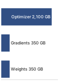
Weights are only a small slice of the full Adam training state.
Memory fit alone does not settle whether a model needs this kind of partition. For a 175B-parameter model, weights alone occupy 350 GB, or about 5.5 GB per GPU across a 64-GPU group, one-sixteenth of the 1,024-GPU reference cluster. Full mixed-precision Adam training state is much larger, 2,800 GB globally, yet ZeRO-3 across the same 64 GPUs reduces it to roughly 43.8 GB per GPU before activations, which fits an 80 GB accelerator. ZeRO-3 can therefore make the static state fit, as the notebook below confirms. It pays for that fit in traffic, because every step regathers every layer’s parameters across the data-parallel fabric, roughly three times the model’s parameter bytes per worker (section 6.3.3). It also cannot split an individual layer’s computation or activations across devices. Tensor parallelism addresses both limits by partitioning individual weight matrices across devices, using the column-then-row pairing of figure 15, detailed in section 6.5.3, which confines collective communication to block boundaries. Pipeline parallelism instead stages sequential layers across devices (section 6.5.2).
Activations add a separate memory requirement. Under the earlier unchecked-storage assumptions, a 2048-token sequence through 175B parameters produces roughly 1.1 TB at a local batch of 4 sequences; optimizer sharding does not reduce that storage. Recomputation trades memory for extra FLOPs, partitioning distributes activations, and offload moves them to another memory tier. Kernel and batch-size choices also change the budget. Full activation checkpointing brings the same modeled case down to ~19.3 GB. The following notebook, which uses a single-sequence local batch, checks whether ZeRO-3 plus checkpointing fits the model without partitioning its computation.
Napkin Math 6.7: The memory wall of scale
Problem: Training a 175B-parameter model (like GPT-3) on a 64-GPU group of NVIDIA A100s (80 GB), smaller than the 1,024-GPU reference cluster. The A100 carries the same 80 GB of HBM as the reference H100, so the capacity verdict carries over, and a small group is the harder test of whether sharding alone suffices. Can data parallelism with ZeRO-3 handle this?
Math:
- Parameter storage: 175B params \(\times\) 2 bytes (FP16) = 350 GB.
- Gradients and optimizer state: Gradients add 175B params \(\times\) 2 bytes = 350 GB, while Adam FP32 master weights, momentum, and variance add 175B params \(\times\) 12 bytes = 2,100 GB.
- Total static memory: 2,800 GB.
- ZeRO-3 sharding: With 64 GPUs, per-GPU static memory = 2,800 GB/64 GPUs \(\approx\) 43.8 GB.
- Activation memory: For sequence length 2048 and batch size 1, the canonical full-checkpointing strategy stores \(\approx\) 4.8 GB of activations per GPU.
Systems insight: 43.8 GB (static) + 4.8 GB (dynamic) = 48.6 GB. Under this simplified accounting, ZeRO-3 plus full activation checkpointing fits within the 80 GB A100 capacity, leaving material headroom for framework buffers and transient layer gathers. If those additional allocations exceed the remaining HBM, the design can reduce the local batch, offload state, increase the sharding degree, or add tensor or pipeline parallelism; tensor parallelism is not the only recourse.
In this example, sharding and checkpointing make the modeled state fit, leaving two distinct reasons to partition the model itself. One is regather traffic: on the 1,024-GPU reference cluster, ZeRO-3 moves about 1.1 TB per worker per step for this model, which on one NDR InfiniBand port takes about 10× as long as the step’s computation. The other is layer execution, since full sharding gathers parameters on demand without ever splitting a single layer’s computation or activations across devices. Model parallelism instead cuts the computation graph directly, either between sequential layer groups (such as layers 1–4 and layers 5–8) or inside a layer across channels and attention heads. Layer cuts introduce pipeline dependencies that leave downstream devices idle while an upstream stage computes, creating the pipeline bubble that governs utilization for this partition, whereas channel and head cuts expose concurrent work within a layer at the price of intra-layer exchanges. Other workloads still need these cuts simply to fit peak memory capacity.
These cuts enable the large-scale cases that exceed a single device for different reasons. GPT-3, with 175B parameters, was trained with model parallelism within each matrix multiplication and across layers (Brown et al. 2020), avoiding a full-parameter regather on every step; vision transformers processing high-resolution \(16\Glyph{k}{\times}16\Glyph{k}\) pixel images use model parallelism to bound activation memory; and mixture-of-experts (MoE) architectures, whose sparsely activated feed-forward blocks are developed in section 6.5.5, distribute their conditional computation paths across hardware (Shazeer et al. 2017; Lepikhin et al. 2021; Fedus et al. 2022).
Brown, Tom B., Benjamin Mann, Nick Ryder, Melanie Subbiah, Jared Kaplan, Prafulla Dhariwal, Arvind Neelakantan, et al. 2020. “Language Models Are Few-Shot Learners.” Advances in Neural Information Processing Systems 33: 1877–901. https://doi.org/10.48550/arxiv.2005.14165.
Each partitioning strategy trades single-device memory overflow for a different systems cost: layer-wise partitioning pays in idle time, pipeline parallelism pays in scheduling complexity to hide that idle time, and tensor parallelism pays in NVLink bandwidth to split individual layers. Sequence and context parallelism, expert parallelism, and sparse embedding sharding then extend the same trade-off to long-context activations, sparsely activated experts, and sparsely touched embedding tables.
Checkpoint 6.3: Model parallelism foundations
Verify your understanding of model sharding:
6.5.1 Layer-wise partitioning
Assigning consecutive blocks of layers to separate GPUs cuts each device’s weight footprint in proportion to the number of stages, but a single batch passing through those stages in sequence leaves every other GPU waiting for its turn. Where ZeRO-3 met the capacity limit by sharding storage while every worker still executed every layer, layer-wise model parallelism gives each device a unique fraction of the model to compute. With 8-way partitioning, the 175B-parameter model’s 350 GB of FP16 weights fall to approximately 44 GB per GPU. That is only the weights budget; activations, gradients, and optimizer state still need sharding, offload, or pipeline scheduling, the composition developed in section 6.6.
Layer-wise partitioning is the least invasive model cut. It saves memory by assigning consecutive layers to separate devices, but it preserves the model’s sequential dependence. In transformer architectures, this translates to specific devices managing defined sets of attention and feed-forward blocks. For a 16-layer transformer on four GPUs (figure 12), panel (a) maps the weight footprint reduction to one-quarter per device alongside forward activation and backward gradient transfers across stage boundaries, while panel (b) charts the resulting execution timeline, revealing that each GPU remains idle for six of eight time slots without microbatch pipelining.
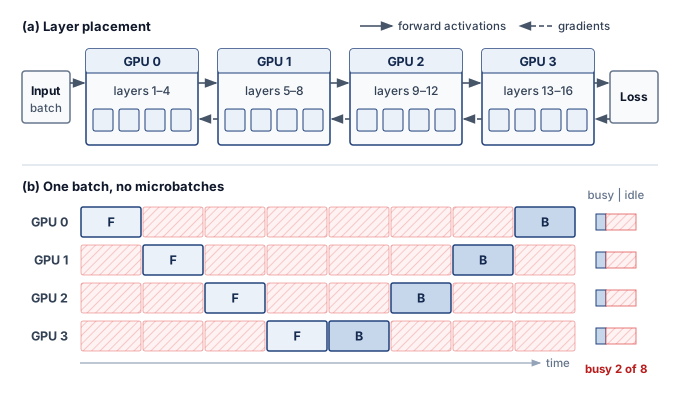
Partitioning layers changes where an optimizer update runs without necessarily changing the update rule. Each GPU can apply Adam (Kingma and Ba 2015), AdaFactor, or another optimizer to its parameter slice once the required gradients are complete. A device holding transformer layers 1–12 updates those layers; tied parameters, global gradient clipping, or a combined data-parallel group can still require coordination. Preserving synchronous optimization also requires the schedule to use consistent parameter versions. Sequential dependencies introduce pipeline bubbles, and unequal stage service times add waiting. The engineering problem is to overlap microbatches and balance stage work while preserving that update contract (Rasley et al. 2020).
Kingma, Diederik P., and Jimmy Ba. 2015. “Adam: A Method for Stochastic Optimization.” 3rd International Conference on Learning Representations (ICLR).
6.5.2 Pipeline parallelism
Without pipelining, a four-stage layer partition leaves three of the four GPUs idle at any moment because downstream stages cannot start until upstream stages finish the entire batch (figure 12). Pipeline parallelism breaks that stall by splitting the batch into smaller microbatches and streaming them through the stages like a relay race. As soon as GPU 1 finishes the initial transformer blocks on microbatch 1, it hands the resulting activation tensor to GPU 2 and immediately starts microbatch 2. For the 175B model with hidden dimension 12,288 and a microbatch of 4 sequences at 2,048 tokens each, that forward handoff carries approximately 201 MB per stage boundary per microbatch. GPU 2 needs that payload before processing the same microbatch, creating a dependency chain through the stages, while other microbatches occupy the remaining stages concurrently. Backward propagates activation gradients in reverse as each stage computes gradients for its own parameters.
Definition 6.8: Pipeline parallelism
Pipeline parallelism is a model parallelism technique that partitions a neural network’s layers into sequential stages assigned to different devices, passing activations forward and gradients backward between stages while overlapping computation across stages using microbatches to maintain throughput.
- Significance: Each boundary transfers forward activations and backward activation gradients. A forward tensor contains \(\MicrobatchSize \times \SequenceLength\times \HiddenDimension\times 2\) bytes at BF16, where \(\MicrobatchSize\) is the microbatch size. For a hidden dimension of 8,192 with microbatch size 1 and a 2,048-token sequence, the forward payload is approximately 8,192 \(\times\) 2,048 \(\times\) 2 \(\approx\) 34 MB per microbatch per boundary. Backward traffic and all microbatches must be counted before comparing this with a per-update gradient AllReduce or sizing a 50 GB/s InfiniBand link. In a balanced noninterleaved schedule with ideal transfers, the idle fraction is approximately \((\PipelineParallelDegree-1)/(\MicrobatchCount+\PipelineParallelDegree-1)\), where \(\PipelineParallelDegree\) is the stage count and \(\MicrobatchCount\) the microbatch count.
- Distinction: Tensor parallelism partitions operations within a layer and introduces communication among their participants. Pipeline parallelism instead transfers activations and their gradients between sequential stages. This coarser exchange can suit slower links when the transfer fits within the stage schedule; the interconnect name alone does not establish feasibility.
- Common pitfall: A frequent misconception is that adding pipeline stages always improves throughput. Each additional stage increases the pipeline bubble fraction \((\PipelineParallelDegree-1)/(\MicrobatchCount+\PipelineParallelDegree-1)\) unless the number of microbatches \(\MicrobatchCount\) scales proportionally, causing hardware to idle and erasing the benefit of deeper partitioning.
In the GPipe schedule of figure 13, a four-stage pipeline processes four microbatches (\(\PipelineParallelDegree=4, \MicrobatchCount=4\)), and dividing the global batch into discrete microbatches allows forward passes to overlap diagonally across stages before backward passes unfold in reverse order. While microbatching raises hardware utilization above naive sequential placement, pipeline fill (\(\PipelineTimeSlot_1\)–\(\PipelineTimeSlot_3\)) and drain (\(\PipelineTimeSlot_{12}\)–\(\PipelineTimeSlot_{14}\)) bubbles still leave each device idle for 6 of 14 time slots.
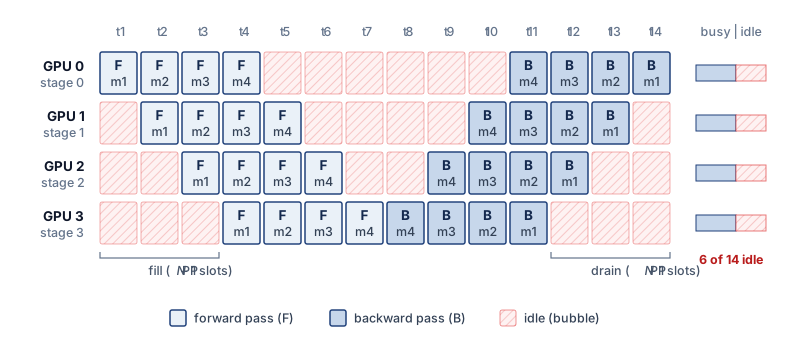
Tracing the schedule grid in figure 13 column by column reveals how the fill and drain bubbles arise. In the first slot only stage 0 has work, the forward pass of microbatch 1. In the second, stage 0 starts microbatch 2 while stage 1 receives microbatch 1’s activations, and by the fourth slot every stage holds a different microbatch. The last stage then turns microbatch 4 around into its backward pass, and gradients travel upstream in reverse microbatch order, so stage 0 waits until the eleventh slot for its first gradient. Each stage therefore idles 3 slots in the forward phase and 3 more in the backward phase, 6 of the 14 slots in the step, whether those slots fall at the start of its row, the middle, or the end. That share, about 43 percent, is the bubble fraction \((\PipelineParallelDegree-1)/(\MicrobatchCount+\PipelineParallelDegree-1)\) at \(\PipelineParallelDegree=\MicrobatchCount=\) 4. Adding microbatches lengthens the busy diagonal without lengthening fill and drain in this balanced schedule. Increasing \(\MicrobatchCount\) is therefore one way to reduce the idle fraction; later schedules also change which work can occupy the gaps.
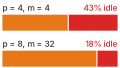
Enough microbatches shrink the bubble even as stages double.
The same bubble term becomes concrete in the following worked example, where an 8-stage pipeline and 32 microbatches still leave a measurable amount of idle time.
↪ The bubble fraction across stage and microbatch counts, and its interleaved-schedule variant, are developed in Pipeline Arithmetic.
Napkin Math 6.8: The cost of the pipeline bubble
Problem: A large-model training run uses pipeline parallelism across 8 stages. To hide the sequential delay, the batch is split into 32 microbatches. What fraction of GPU cycles does the pipeline bubble leave idle?
Math: For balanced, noninterleaved synchronous stages under the one-forward-one-backward (1F1B) schedule developed below, with ideal transfers, the bubble fraction follows from the stage and microbatch counts. The time units below each combine one forward and one backward service interval; they are not individual optimizer steps.
- Wait time: At the start and end of each batch, GPUs sit idle for \(\PipelineParallelDegree-1\) steps.
- Productive time: GPUs compute for \(\MicrobatchCount\) steps.
- Bubble fraction: \((\PipelineParallelDegree-1) / (\PipelineParallelDegree-1+\MicrobatchCount) =\) 7 \(/\) (7 \(+\) 32) \(\approx\) 17.9 percent.
Systems insight: Pipeline parallelism is a utilization-memory trade-off. With this stage count and schedule fixed, reducing the bubble from 18 percent to 5 percent requires more microbatches \((\MicrobatchCount)\). In general, holding the bubble under 10 percent requires \(\MicrobatchCount> 9(\PipelineParallelDegree-1)\), because \((\PipelineParallelDegree-1)/(\MicrobatchCount+\PipelineParallelDegree-1) < 0.1\) rearranges to that bound. The activation memory those microbatches need depends on the schedule. GPipe retains activations across the microbatches, whereas the 1F1B schedule developed next releases them during the steady state. The modeled 17.9 percent idle fraction also motivates interleaved pipelining, which divides each device’s work into smaller stages. Interleaving can reduce the original 18 percent bubble, but additional transfers and memory requirements determine the net gain.
GPipe4 (Huang et al. 2019) introduced synchronous pipeline parallelism with microbatch accumulation, while PipeDream (Narayanan et al. 2019) developed asynchronous approaches with weight stashing. Modern systems employ 1F1B (one-forward-one-backward)5 scheduling to reclaim activation memory earlier; that lower memory pressure makes larger microbatch counts practical, and the larger \(\MicrobatchCount\) is what shrinks the bubble term.
4 GPipe: Published by Google in 2019, GPipe introduced synchronous microbatch pipelining that trained a 557M-parameter AmoebaNet across 8 Tensor Processing Units (TPUs) with near-linear scaling. Its schedule keeps every microbatch’s activations live until the backward pass, the cost that later schedules reduce.
Huang, Y., Y. Cheng, A. Bapna, O. Firat, D. Chen, M. X. Chen, H. Lee, et al. 2019. “GPipe: Efficient Training of Giant Neural Networks Using Pipeline Parallelism.” Advances in Neural Information Processing Systems (NeurIPS) 32: 103–12.
Narayanan, Deepak, Aaron Harlap, Amar Phanishayee, Vivek Seshadri, Nikhil R. Devanur, Gregory R. Ganger, Phillip B. Gibbons, and Matei Zaharia. 2019. “PipeDream: Generalized Pipeline Parallelism for DNN Training.” Proceedings of the 27th ACM Symposium on Operating Systems Principles, 1–15. https://doi.org/10.1145/3341301.3359646.
5 1F1B (one-forward-one-backward) scheduling: Unlike GPipe (which processes all forward passes before any backward passes), 1F1B interleaves them. For equal-sized microbatch activations and a non-interleaved schedule, peak retained activations per stage fall from \(\mathcal{O}(\MicrobatchCount)\) under GPipe to at most \(\mathcal{O}(\PipelineParallelDegree)\) under 1F1B, where \(\MicrobatchCount\) is the microbatch count and \(\PipelineParallelDegree\) the pipeline-stage count. Summed across stages, the corresponding bounds are \(\mathcal{O}(\MicrobatchCount\PipelineParallelDegree)\) and \(\mathcal{O}(\PipelineParallelDegree^2)\). This memory reclamation is what enables the large microbatch counts \((\MicrobatchCount\gg \PipelineParallelDegree)\) required to keep the pipeline bubble small.
At the schedule level, 1F1B is a warmup, steady-state, and drain loop. In algorithm 1, each stage alternates forward work for newer microbatches with backward work for older microbatches once gradients arrive, so activations can be released before the whole batch has completed.
Run on four stages with eight microbatches, the schedule gives each stage a short warm-up of forward passes, a steady state that alternates one backward with one forward, and a drain of the remaining backward passes (figure 14). The warm-up and drain phases still leave a bubble of roughly \((\PipelineParallelDegree-1)/(\MicrobatchCount+\PipelineParallelDegree-1)\), 6 of 22 slots here. Interleaving backward work in the steady state, however, frees each activation as soon as its backward consumes it. Stage 0 never holds more than four microbatches’ activations where an all-forwards-first schedule would hold all eight, so peak activation memory grows with the stage count rather than the microbatch count. That is the gain over GPipe-style all-forward-then-all-backward scheduling, and it lets the system raise \(\MicrobatchCount\) until activation memory, recomputation, or the global-batch constraint becomes the next limit.
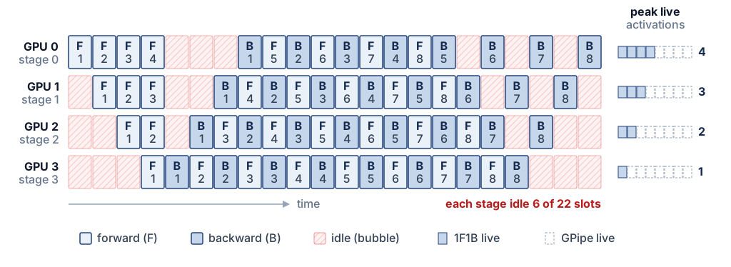
The activation handoff has shape \(\MicrobatchSize \times \SequenceLength\times \HiddenDimension\); its completion still constrains the next stage. The 1F1B schedule in algorithm 1 reduces activation residency, but fill, drain, communication, and load imbalance leave idle time. Filling those remaining slots requires separating work that releases an upstream dependency from work that can wait.
Zero-bubble pipeline schedules further reduce idle time by overlapping weight gradient computation with activation gradient communication. In a standard backward pass, the GPU computes \(\partial \LossFunction/ \partial \WeightMatrix\) (weight gradient) and \(\partial \LossFunction/ \partial \LayerInputMatrix\) (activation gradient, sent to the previous stage) together. Zero-bubble scheduling splits these into separate kernels: a B kernel that computes only the activation gradient \(\partial \LossFunction/ \partial \LayerInputMatrix\) and sends it to the previous stage, and a W kernel that computes the weight gradient \(\partial \LossFunction/ \partial \WeightMatrix\) locally. The B kernel must execute promptly (it is on the critical path), but the W kernel can be scheduled opportunistically to fill bubbles.
The B/W split creates scheduling freedom, but weight-gradient work must still finish before the corresponding optimizer update. In the balanced four-stage, eight-microbatch schedule of figure 14, noninterleaved 1F1B still leaves \(3/11 \approx 27\%\) of each stage’s time idle, by the bubble fraction derived above. Reordering forward, activation-gradient, and weight-gradient work can reduce that gap. Approaching zero also depends on kernel durations, memory headroom, and optimizer synchronization; splitting backward alone does not guarantee it.
The trade-off is memory. Zero-bubble scheduling requires storing intermediate activations for longer (because the W computation is deferred), increasing peak memory usage. Some implementations address this by combining zero-bubble scheduling with activation checkpointing, selectively recomputing certain activations rather than storing them. The interaction between these techniques creates a three-way trade-off among pipeline bubble size, memory consumption, and recomputation overhead, an example of the displacement of overhead (principle 14).
6.5.3 Tensor parallelism
Every pipeline schedule so far keeps whole layers on each device, which is why its traffic is confined to stage boundaries and tolerates moderate interconnect bandwidth. The same property sets its limit. A pipeline cannot help when a single layer’s weights or activations exceed one device, and it cannot shorten the time one layer takes, because that layer still runs on one accelerator.
Tensor parallelism splits the weight matrices within each layer instead of assigning complete layers to devices. This operator-level parallelism (also called intra-layer parallelism) enables finer-grained distribution but requires high-bandwidth interconnects for the frequent intra-layer communication it introduces.
Definition 6.9: Tensor parallelism
Tensor parallelism partitions individual tensor operations across devices, commonly through column-parallel or row-parallel weight splits. Communication combines or redistributes the resulting tensor shards as required by the next operation. The Megatron-style forward-pass example below illustrates one such arrangement.
- Significance: The Megatron-LM arrangement developed below uses two AllReduce operations per transformer block in the forward pass, one after attention and one after the MLP, each reducing a 2-byte activation tensor of \(\BatchSize\times \SequenceLength\times \HiddenDimension\) elements, where \(\BatchSize\) counts the sequences in flight through the layer. A ring AllReduce moves roughly \(2(\TensorParallelDegree-1)/\TensorParallelDegree\) times that payload per GPU, and the exchange recurs in every one of the 96 blocks of the GPT-3 shape, with backward adding corresponding exchanges. Whether that traffic hides behind computation depends on the link that carries it, which the arithmetic after the mechanism quantifies. Computing model FLOPs utilization (MFU) requires the complete compute and exposed-communication time, not the bandwidth ratio alone.
- Distinction: Unlike pipeline parallelism, which communicates only at layer boundaries and transfers small activation slices, tensor parallelism synchronizes within every layer via AllReduce, making it sensitive to the per-operation latency of the interconnect and favoring a fast communication domain such as NVLink, which can extend beyond one node.
- Common pitfall: Extending tensor parallelism across nodes without checking the transfer budget can erase the compute saving. The reference NVLink specification is approximately 900 GB/s bidirectional, or 450 GB/s per direction; InfiniBand NDR provides 50 GB/s per port, a 9× per-direction gap. These specifications identify a placement risk. Whether the split helps depends on sustained bandwidth, operation size, compute saved, and overlap.
Frequent intra-layer exchanges favor placing tensor-parallel groups within the fastest available communication domain. Pipeline stages communicate at coarser boundaries and can often span slower domains when their transfers fit the schedule. This difference motivates a hybrid that maps each exchange to a suitable fabric tier; it does not impose a universal node boundary for either strategy.
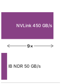
Tensor-parallel exchanges belong on the fast tier, about 9\(\times\) an NDR port.
6 Megatron-LM: NVIDIA’s 2019 framework that trained an 8.3B-parameter transformer (24× BERT-Large and 5.5× GPT-2 at the time) with only two AllReduce operations per transformer block in the forward pass (one after attention, one after the multilayer perceptron (MLP)). The run reached 76 percent scaling efficiency across 512 GPUs, and its partitioning remains influential in large-scale transformer training.
Shoeybi, Mohammad, Mostofa Patwary, Raul Puri, Patrick LeGresley, Jared Casper, and Bryan Catanzaro. 2019. “Megatron-LM: Training Multi-Billion Parameter Language Models Using Model Parallelism.” arXiv Preprint arXiv:1909.08053.
Megatron-style tensor parallelism6 (Shoeybi et al. 2019) partitions matrix multiplications by alternating column and row splits. In the two-GPU dataflow of figure 15, column-parallel splitting partitions the first weight matrix \(\ColumnParallelWeightMatrix= [\ColumnParallelWeightMatrix_1 \mid \ColumnParallelWeightMatrix_2]\) to produce local activation slices \(\LayerOutputMatrix_1, \LayerOutputMatrix_2\) from replicated input \(\LayerInputMatrix\); row-parallel splitting then partitions the second weight matrix \(\RowParallelWeightMatrix= [\RowParallelWeightMatrix_1 ; \RowParallelWeightMatrix_2]\) so that each GPU computes partial products \(\RowParallelOutputMatrix_1, \RowParallelOutputMatrix_2\) locally, deferring cross-device communication to a single amber AllReduce that reconstructs output \(\RowParallelOutputMatrix\).
Column-parallel linear layers split weights along columns. For input \(\LayerInputMatrix\) and weight matrix \(\WeightMatrix= [\WeightMatrix_1 \mid \WeightMatrix_2]\) split across 2 GPUs: \[\LayerOutputMatrix= \LayerInputMatrix\WeightMatrix= \LayerInputMatrix[\WeightMatrix_1 \mid \WeightMatrix_2] = [\LayerInputMatrix\WeightMatrix_1 \mid \LayerInputMatrix\WeightMatrix_2]\] Each GPU computes its partition independently. The concatenation in the equation is logical, because when the next operation is row-parallel, each output shard remains on its producing device and feeds the matching weight shard without an AllGather. The row-parallel half of the pattern splits weights along rows, \(\WeightMatrix= \begin{bmatrix} \WeightMatrix_1 \\ \WeightMatrix_2 \end{bmatrix}\): \[\LayerOutputMatrix= \LayerInputMatrix\WeightMatrix= \LayerInputMatrix_1 \WeightMatrix_1 + \LayerInputMatrix_2 \WeightMatrix_2\] Each GPU computes a partial sum, and the system pays one AllReduce to combine the partial outputs.
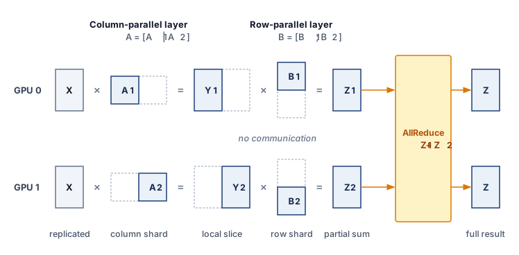
The column-then-row sequence of figure 15 embodies the governing architectural invariant. Pairing a column-parallel layer directly with a row-parallel layer allows intermediate activations (\(\LayerOutputMatrix_1, \LayerOutputMatrix_2\)) to remain strictly local on each GPU, confining inter-device synchronization to a single collective at the end of the block. Megatron applies that pattern twice in each transformer block. The QKV projection is column-parallel and its attention output projection is row-parallel, then the first feed-forward layer is column-parallel and the second feed-forward layer is row-parallel. The design places one AllReduce after attention and one after the feed-forward network, for two AllReduce operations per transformer layer. Communication volume per transformer layer depends on sequence length \(\SequenceLength\), hidden dimension \(\HiddenDimension\), tensor-parallel degree \(\TensorParallelDegree\), and batch size \(\BatchSize\), the number of sequences in flight through the layer (the local batch, or the microbatch \(\MicrobatchSize\) when the layer also sits in a pipeline). The activation payload is: \[\ActivationPayloadSize= \BatchSize\times \SequenceLength\times \HiddenDimension\times \ElementStorageSize\]
A ring AllReduce transfers approximately \(2(\TensorParallelDegree-1)/\TensorParallelDegree \times \ActivationPayloadSize\) bytes per GPU, which is close to \(2\ActivationPayloadSize\) for large \(\TensorParallelDegree\). For the GPT-3 shape (\(\SequenceLength=\) 2048, \(\HiddenDimension=\) 12,288, 96 layers) with \(\BatchSize=\) 4 and FP16, the activation payload is 4 \(\times\) 2048 \(\times\) 12,288 \(\times\) 2 \(\approx\) 201 MB.
At \(\TensorParallelDegree=\) 8 the ring factor is 1.75, giving roughly 352 MB per AllReduce. With two AllReduces in each of the 96 layers, this totals approximately 67.6 GB per forward microbatch. The symmetric backward exchanges bring the total to roughly 135 GB per forward/backward microbatch, before any recomputation. Set against the computation it serves, that volume is modest on the right link and prohibitive on the wrong one. At the per-layer compute rate of the earlier feasibility check, one such microbatch takes about 2.2 s of forward and backward computation per GPU; its tensor-parallel traffic takes about 0.3 s on NVLink but about 2.7 s on one InfiniBand port, longer than the computation. The number of microbatches per update and the available overlap then determine the required fabric service rate.
Tensor parallelism eventually reaches a workload-dependent limit because smaller operation shards leave less computation to cover communication. Per-GPU ring AllReduce bytes approach 2\(\times\) the activation tensor size, while local matrix shapes and collective startup costs change with group size. The useful degree therefore depends on layer shape, microbatch size, and the fast communication domain. Llama 3 405B’s TP=8 arrangement within NVLink-connected H100 nodes (Dubey et al. 2024) and node-local groups in other large training systems (Z. Jiang et al. 2024) illustrate a placement choice, not a universal eight-device limit. Tensor parallelism also costs more to adopt than data parallelism. It replaces standard linear layers with column-parallel and row-parallel variants inside the model definition, whereas data parallelism wraps the model externally without modifying its internals.
Dubey, Abhimanyu, Abhinav Jauhri, Abhinav Pandey, Abhishek Kadian, et al. 2024. The Llama 3 Herd of Models. arXiv preprint arXiv:2407.21783.
Jiang, Ziheng, Haibin Lin, Yinmin Zhong, Qi Huang, Yangrui Chen, Zhi Zhang, Yanghua Peng, et al. 2024. “MegaScale: Scaling Large Language Model Training to More Than 10,000 GPUs.” 21st USENIX Symposium on Networked Systems Design and Implementation (NSDI 24), 745–60.
6.5.4 Sequence and context parallelism
While tensor parallelism partitions weight matrices within linear layers, the memory footprint of large-scale transformer training is increasingly dominated by activations. As models scale their context length from thousands to hundreds of thousands or millions of tokens (\(\SequenceLength\ge 32\text{k}\dots 1\text{M}+\)), the activation footprint scales proportionally: \[\ActivationMemory = \mathcal{O}(\BatchSize\times \SequenceLength\times \HiddenDimension\times \LayerCount)\] for linear, normalization, and residual layers, and \(\mathcal{O}(\BatchSize\times \AttentionHeadCount \times \SequenceLength^2 \times \LayerCount)\) for un-tiled attention (or \(\mathcal{O}(\BatchSize\times \SequenceLength\times \HiddenDimension\times \LayerCount)\) with tiled FlashAttention). At long contexts, activation memory dwarfs parameter storage, exposing the memory capacity gap (principle 2). Two complementary paradigms address this constraint by sharding along the sequence axis: sequence parallelism (SP) within the tensor-parallel domain, and context parallelism (CP) across dedicated long-sequence process groups.
Definition 6.10: Sequence and context parallelism
Sequence and context parallelism partition the token sequence dimension to reduce per-device activation storage. Sequence parallelism (SP) retains sequence shards during operations such as LayerNorm and Dropout within a tensor-parallel group. Context parallelism (CP) partitions the sequence across a dedicated group and exchanges the information needed for attention, through mechanisms developed below that either pass key/value blocks around a ring or transpose between sequence and head partitions.
- Significance: Long contexts can exhaust activation memory even when sharded model state fits. The relevant limit depends on batch size, layer shapes, attention kernels, and checkpointing. Sequence parallelism divides the targeted activation storage by \(\TensorParallelDegree\) while preserving the ideal collective payload volume in the decomposition below. Context parallelism distributes sequence-dependent storage; linear context growth (\(\ContextParallelDegree\times \SingleDeviceContextLength\), with \(\ContextParallelDegree\) denoting the context-parallel degree) is an ideal capacity estimate that still requires communication buffers and computation to fit the budget.
- Distinction: Tensor parallelism partitions weight matrices along hidden dimensions \(\HiddenDimension\), whereas context parallelism partitions the sequence axis \(\SequenceLength\). Ring Attention exchanges key/value chunks between devices, while Ulysses uses an AllToAll to transpose between sequence and head dimensions. Both require placement that can service their exchanges within the attention schedule.
- Common pitfall: Assuming context parallelism eliminates the quadratic attention compute complexity. CP distributes the attention computation across devices, reducing per-device memory and FLOPs by \(1/\ContextParallelDegree\), but the aggregate cluster FLOPs for dense self-attention still scale quadratically as \(\mathcal{O}(\SequenceLength^2)\).
Megatron sequence parallelism
In the Megatron-style arrangement just derived, the column-then-row pairing in figure 15 splits the QKV projection and first MLP layer column-wise, and the attention output projection and second MLP layer row-wise. The surrounding LayerNorm, Dropout, and residual operations retain replicated activations across all \(\TensorParallelDegree\) devices. LayerNorm operates across a token’s hidden features, while Dropout and residual addition operate element-wise; none requires another token’s features. This token independence permits partitioning the otherwise replicated \(\BatchSize\times \SequenceLength\times \HiddenDimension\) activation tensor along its sequence dimension.
Megatron Sequence Parallelism (Korthikanti et al. 2023) eliminates this redundancy by sharding the sequence dimension across the \(\TensorParallelDegree\) ranks for all non-tensor-parallel operations. Instead of replicating activations, each GPU holds only a \(\BatchSize\times (\SequenceLength/\TensorParallelDegree) \times \HiddenDimension\) slice during LayerNorm and Dropout.
Korthikanti, Vijay Anand, Jared Casper, Sangkug Lym, Lawrence McAfee, Michael Andersch, Mohammad Shoeybi, and Bryan Catanzaro. 2023. “Reducing Activation Recomputation in Large Transformer Models.” Proceedings of Machine Learning and Systems (MLSys) 5: 341–53.
This sharding incurs zero additional communication volume. In standard tensor parallelism, the row-parallel matrix multiplication is followed by an AllReduce to sum partial products across ranks. An AllReduce decomposes into a ReduceScatter followed by an AllGather, the identity established among the collective primitives in The six core primitives: \[\text{AllReduce}(\RankContribution) \equiv \text{AllGather}(\text{ReduceScatter}(\RankContribution))\] Megatron-SP decouples this collective pair across the transformer block. Following the row-parallel linear layer, a ReduceScatter reduces partial sums while scattering the resulting activations along the sequence dimension, leaving each GPU with an \(\SequenceLength/\TensorParallelDegree\) token slice. LayerNorm, residual additions, and Dropout then execute on these local slices with zero cross-device communication. Immediately before the next column-parallel linear layer, an AllGather across the sequence dimension reassembles the complete \(\SequenceLength\) tokens required for the weight-partitioned matrix multiplication.
In this ideal payload accounting, standard TP executes two AllReduces per transformer block (\(2 \times 2(\TensorParallelDegree-1)/\TensorParallelDegree \times \ActivationPayloadSize\) bytes), while Megatron-SP executes two ReduceScatter and AllGather pairs (\(2 \times [(\TensorParallelDegree-1)/\TensorParallelDegree + (\TensorParallelDegree-1)/\TensorParallelDegree] \times \ActivationPayloadSize= 2 \times 2(\TensorParallelDegree-1)/\TensorParallelDegree \times \ActivationPayloadSize\) bytes). The volumes match while the targeted activation storage falls by a factor of \(\TensorParallelDegree\). Equal bytes do not imply equal elapsed time, because separating the collectives changes readiness, startup costs, and overlap opportunities.
Context parallelism with ring attention versus Ulysses
Increasing sequence length \(\SequenceLength\) can exhaust the remaining activation budget after sequence parallelism and checkpointing. Context parallelism of degree \(\ContextParallelDegree\) distributes the sequence across \(\ContextParallelDegree\) accelerators. Attention then needs exchanges across sequence partitions. Ring-based point-to-point transfers and AllToAll transpositions provide two ways to supply that information, and can also be combined hierarchically. The ring method relies on an online softmax, which keeps a running maximum and a running sum of the attention scores seen so far. Each arriving key/value tile can then be folded into the partial result, with the earlier contribution rescaled whenever the maximum changes, so no device ever stores the full attention matrix.
Ring Attention (Liu et al. 2023) organizes devices in a logical ring where each GPU holds a query chunk \(\AttentionQueryMatrix_i\) of length \(\SequenceLength/\ContextParallelDegree\) and an initial key/value chunk \((\AttentionKeyMatrix_i, \AttentionValuesMatrix_i)\). Computation proceeds in \(\ContextParallelDegree\) rounds along the ring. In each round, GPU \(\ContextParallelRankIndex\) computes block attention between its stationary \(\AttentionQueryMatrix_i\) and resident \((\AttentionKeyMatrix_j, \AttentionValuesMatrix_j)\) tiles using an online softmax accumulator, while asynchronously transmitting \((\AttentionKeyMatrix_j, \AttentionValuesMatrix_j)\) to ring neighbor \((\ContextParallelRankIndex+1) \bmod \ContextParallelDegree\) and receiving \((\AttentionKeyMatrix_{j-1}, \AttentionValuesMatrix_{j-1})\) from \((\ContextParallelRankIndex-1) \bmod \ContextParallelDegree\). After \(\ContextParallelDegree\) rounds every query chunk has attended to every key/value tile, yet no device ever stores the full key/value sequence (figure 16).
Liu, Hao, Matei Zaharia, and Pieter Abbeel. 2023. “Ring Attention with Blockwise Transformers for Near-Infinite Context.” arXiv Preprint arXiv:2310.01889, ahead of print. https://doi.org/10.48550/arXiv.2310.01889.
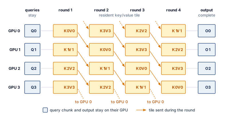
For one sequence with standard multi-head attention, let \(\ContextChunkTokenCount=\SequenceLength/\ContextParallelDegree\) be the tokens per chunk, \(\HiddenDimension\) the total head width, \(\ElementStorageSize\) the bytes per stored element, \(\PeakRate\EfficiencyHw\) the sustained attention FLOP/s, and \(\SingleLinkBandwidth\) the one-way transfer rate. Computing both \(\AttentionQueryMatrix\AttentionKeyMatrix^T\) and the weighted-value product costs approximately \(4\ContextChunkTokenCount^2 \HiddenDimension\) FLOPs, while sending \(\AttentionKeyMatrix\) and \(\AttentionValuesMatrix\) costs \(2 \ContextChunkTokenCount \HiddenDimension\, \ElementStorageSize\) bytes. Ignoring startup, softmax, and overlap interference gives the necessary tile-size estimate: \[\frac{4\ContextChunkTokenCount^2 \HiddenDimension}{\PeakRate\EfficiencyHw} \ge \frac{2 \ContextChunkTokenCount \HiddenDimension\, \ElementStorageSize}{\SingleLinkBandwidth} \iff \ContextChunkTokenCount\ge \frac{\ElementStorageSize \PeakRate\EfficiencyHw}{2\SingleLinkBandwidth}\] This compares computation time with transfer time; HBM bandwidth cannot substitute for \(\PeakRate\EfficiencyHw\). It is an idealized overlap condition, not a guarantee.
For an H100 sustaining half its dense FP16 peak with 2-byte elements, the condition requires chunks of at least about 1,100 tokens per device when KV tiles travel over NVLink, and about 9,900 tokens when they cross one NDR InfiniBand port. A million-token context split across a few dozen devices clears both bounds, whereas splitting a 32K context across many nodes can leave each chunk too short to hide its transfers.
Grouped-query attention changes the transferred KV width, and causal masking changes the tile work; both require recomputing the two costs. In causal autoregressive attention, upper-triangular tiles are masked out (\(\KvTileIndex> \ContextParallelRankIndex\)). A naive ring execution leaves half the GPUs idle during later rounds; production implementations employ zigzag or striped token partitioning, which gives each device a mix of early and late tokens (for example, one chunk from the start of the sequence and one from the end), so every device holds a similar share of the unmasked causal tiles.
DeepSpeed Ulysses (Jacobs et al. 2023) exploits the independence of attention heads rather than circulating tiles along a ring. Each head attends over the whole sequence without reading any other head’s scores, so the attention work can be split by heads instead of by tokens. Outside the attention core, activations are sharded along the sequence dimension (\(\SequenceLength/\ContextParallelDegree\) tokens, all \(\AttentionHeadCount\) attention heads). Before computing self-attention, an AllToAll collective transposes the tensor from sequence-partitioned [S/c, h, d_head] to head-partitioned [S, h/c, d_head]. Each GPU now holds the full sequence length \(\SequenceLength\), but only a subset \(\AttentionHeadCount/\ContextParallelDegree\) of attention heads. Each device computes standard local FlashAttention across the full sequence for its heads; each rank owns complete heads, while the kernel handles causal masking locally. A second AllToAll collective transposes the attention output back to [S/c, h, d_head]. Ulysses is conceptually clean and reuses single-GPU attention kernels, but requires that the head count be divisible by the context degree (\(\AttentionHeadCount \ge \ContextParallelDegree\)). Under Grouped Query Attention (GQA), where the key-value head count \(\KvHeadCount\) is smaller, a direct head-sharding implementation requires compatible divisibility and \(\ContextParallelDegree\le \KvHeadCount\). Replicating KV heads changes that limit and its communication budget.
Jacobs, Sam Ade, Masahiro Tanaka, Chengming Zhang, Minjia Guo, Shuaiwen Zhu, Shuai Song, Samyam Rajbhandari, Ammar Ahmad Awan, Connor Zheng, and Yuxiong He. 2023. “DeepSpeed Ulysses: System Optimizations for Enabling Training of Extreme Long Sequence Transformer Models.” arXiv Preprint arXiv:2309.14509.
A hierarchical configuration can combine head-sequence transposes within a fast domain and ring exchanges between domains. For an eight-device intra-node domain, a Ulysses group satisfies (\(\IntraNodeContextParallelDegree\le 8\)), while a second degree (\(\InterNodeContextParallelDegree\)) determines the ring’s inter-node partition. In this example, Ulysses partitions heads locally and Ring Attention circulates KV blocks across nodes. The arrangement is feasible only if head divisibility, peak memory, link service time, and the overlap condition all hold; hierarchy alone does not prevent fabric saturation.
6.5.5 Expert parallelism (mixture of experts)
Scaling a dense model’s parameter count increases its per-token compute cost in lockstep, because every token must multiply through every weight matrix in the network. MoE architectures (Shazeer et al. 2017) break that lockstep through conditional computation, and expert parallelism distributes the resulting capacity across devices. In an MoE layer, the feed-forward block contains \(\ExpertCount\) independent feed-forward networks (“experts”), and a gating network selects only a small subset—often top-1 or top-2—for each token. Adding more experts while holding each expert’s shape and the selected count fixed expands stored parameters without increasing expert FLOPs per token, trading dense matrix work for routing and all-to-all communication.
Shazeer, Noam, Azalia Mirhoseini, Krzysztof Maziarz, Andy Davis, Quoc Le, Geoffrey Hinton, and Jeff Dean. 2017. “Outrageously Large Neural Networks: The Sparsely-Gated Mixture-of-Experts Layer.” International Conference on Learning Representations (ICLR).
In a distributed setting, experts are partitioned across workers, with each rank hosting a disjoint subset of expert networks. One routing cycle across four ranks shows the sequence (figure 17). After top-\(\RoutedExpertCount\) gating selects destination experts, an AllToAll dispatch shuffles tokens across the fabric to the hosting ranks, expert FFNs compute locally, and a second AllToAll return routes the processed activations back to the originating ranks to form the gate-weighted sum. The backward pass repeats both exchanges in reverse order, sending output gradients to the ranks hosting the experts and returning input gradients to the ranks that own the tokens. The primary advantage is decoupling model size from per-token compute, which lets parameter count grow within feasible hardware budgets, while the primary constraint is the AllToAll communication, which is bandwidth-intensive and sensitive to load imbalance.
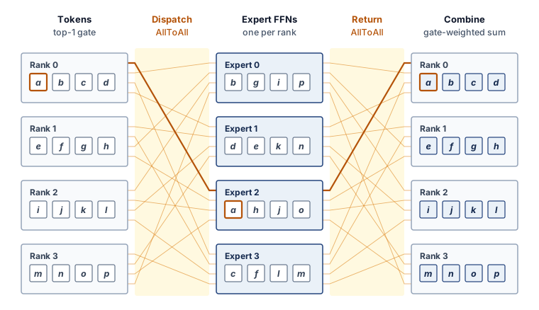
Definition 6.11: Expert parallelism
Expert parallelism is the distribution strategy for mixture-of-experts models that places different experts on different devices and routes each token’s activations to the devices hosting its selected experts through AllToAll collectives, scaling total parameter count across the cluster without scaling the compute each token consumes.
- Significance: It decouples model capacity from compute budget. For illustration, a trillion-parameter MoE model may activate on the order of 10B parameters per token, so per-token FLOPs remain near those of a 10B dense model while capacity grows roughly 100\(\times\). The price is communication structure: every MoE layer requires two AllToAll shuffles per pass (dispatch and combine) whose volume scales with tokens moved times hidden dimension, stressing the cluster’s bisection bandwidth rather than any single link.
- Distinction: Unlike tensor parallelism, which splits dense operations so that every device computes a fraction of every token, expert parallelism is conditional computation: each device computes only the tokens routed to its experts, making both the communication pattern and the load distribution data-dependent rather than fixed by the architecture.
- Common pitfall: A frequent misconception is that experts share work evenly. A hot expert receiving, for example, 3–5\(\times\) its uniform share can overflow its device’s activation buffer while sibling devices idle. Capacity limits and routing penalties are possible responses; a design that retains every assignment must instead accommodate the resulting memory and scheduling demand.
↩︎ The terms that set an AllToAll’s completion time, from traffic across the fabric bisection to hotspots created by skewed expert loads, are established in AllToAll Exchanges at Scale.
Fedus, William, Barret Zoph, and Noam Shazeer. 2022. “Switch Transformers: Scaling to Trillion Parameter Models with Simple and Efficient Sparsity.” Journal of Machine Learning Research 23 (120): 1–39.
Lepikhin, Dmitry, HyoukJoong Lee, Yuanzhong Xu, Dehao Chen, Orhan Firat, Yanping Huang, Maxim Krikun, Noam Shazeer, and Zhifeng Chen. 2021. “GShard: Scaling Giant Models with Conditional Computation and Automatic Sharding.” International Conference on Learning Representations (ICLR).
AllToAll dispatch routes token activations to their assigned experts. Consider \(\ExpertCount=\) 64 experts across 64 GPUs, processing a routing-group batch of \(\BatchSize=\) 4 sequences of length \(\SequenceLength=\) 2048 and hidden dimension \(\HiddenDimension=\) 4096. Under top-1 routing, \(\BatchSize\times \SequenceLength\) tokens each contribute one activation vector. At FP16, the logical dispatch payload is \(\BatchSize\cdot \SequenceLength\cdot \HiddenDimension\cdot 2\) bytes, approximately 67 MB; returning expert outputs doubles the forward payload to about 134 MB per block. Local destinations reduce bytes crossing the network, multiple selected experts increase routes, and backward adds gradient transfers. The resulting service time depends on placement and load balance, including in Switch Transformer (Fedus et al. 2022) (up to 2,048 experts) and GShard (Lepikhin et al. 2021).
Uniform routing is a useful capacity baseline, not a guarantee. An expert receiving several times its uniform share, the hot expert of the definition above, needs correspondingly more token processing and activation storage. The actual skew depends on the learned router and batch. A hot expert can exhaust its buffer or delay the step while other experts remain underused, coupling memory feasibility to load balance.
One response bounds expert workload with a capacity factor \(\ExpertCapacityFactor\). For top-1 routing, a capacity of roughly \(\ExpertCapacityFactor\cdot (\BatchSize\times \SequenceLength)/\ExpertCount\) token assignments per expert provides headroom above uniform load. A dropping implementation sends excess tokens past that expert through the residual connection; implementations that retain every assignment instead need memory and scheduling to accommodate the imbalance. An auxiliary load balancing loss can encourage less concentrated routing. Models using more than one expert per token, such as Mixtral 8x7B with top-2 routing (A. Q. Jiang et al. 2024), require a capacity budget that counts all selected assignments rather than reusing the top-1 denominator unchanged.
Jiang, A. Q., A. Sablayrolles, A. Roux, A. Mensch, B. Savary, C. Bamford, D. S. Chaplot, et al. 2024. “Mixtral of Experts.” arXiv Preprint arXiv:2401.04088.
Sparse routing gives MoE layers the same coordination problem that the embedding tables of Archetype B (DLRM at Scale) pose. In both, which device a token’s data must reach depends on the data itself, so load balance cannot be fixed in advance. MoE language models nonetheless remain Archetype A (GPT-4/Llama-3) workloads, because their dense layers still carry the tensor, pipeline, and data-parallel traffic developed above.
6.5.6 Sparse embedding sharding
Expert parallelism places parameters that only some tokens touch. Recommendation models push that sparsity much further. Their parameters are dominated by embedding tables (often 10 TB+) that no single GPU can hold, and their updates are sparse, because a batch of users interacts with only a tiny fraction of the items. Sharding those tables is model parallelism over stored state rather than over computation. The parameter server (PS) architecture, formalized by Li et al. (2014), remains a common way to do it. A parameter server architecture separates workers, which compute gradients, from servers, which store parameters and apply updates.
For dense models such as ResNet or BERT, that separation concentrates traffic, as section 6.3.1.3 noted. With \(\DeviceCount\) workers, a server’s inbound links must absorb \(\DeviceCount\) gradient streams at once. This incast problem is why dense training moved to ring AllReduce, in which every worker sends and receives at its own link rate and the aggregate load spreads across all nodes.
Sparse embedding tables reverse that balance. In a sparse parameter-server design, the tables are sharded across servers, and workers request only rows indexed by their local minibatches. A sparse pull returns those embedding vectors; a sparse push sends updates for the touched rows. This pattern avoids exchanging the complete table, but hot rows, lookup rates, and network contention can still limit throughput. Embedding-sharding frameworks such as TorchRec also support accelerator-based layouts, so sparse partitioning should not be equated with a CPU-only server architecture. Recommendation training at this scale is the volume’s Archetype B (DLRM at Scale) regime, and it differs from the dense running example in which resource binds first.
Whether the shards live on servers or in accelerator memory, each table must be split along some axis. Row-wise sharding partitions embedding tables by row, placing the whole embedding vector of the entity with identifier id on the shard that equation 3 selects:
\[\ShardIndex = \text{hash}(\text{id}) \bmod \EmbeddingShardCount \tag{3}\]
Each shard \(\ShardIndex\) contains approximately \(\EntityCount/\EmbeddingShardCount\) embeddings, where \(\EntityCount\) is the total number of entities and \(\EmbeddingShardCount\) is the shard count. Column-wise sharding instead partitions each embedding vector \(\EntityEmbedding\) across devices, as equation 4 writes it:
\[\EntityEmbedding = [\EntityEmbedding^{(0)}, \EntityEmbedding^{(1)}, \ldots, \EntityEmbedding^{(\EmbeddingShardCount-1)}] \tag{4}\]
Each device stores a slice of every embedding. Hybrid sharding combines both approaches, and the choice among the three depends on lookup patterns and communication overhead (table 6).
| Sharding strategy | Lookup pattern | Communication | Best for |
|---|---|---|---|
| Row-wise | Single device per lookup | AllToAll gather | Uniform access patterns |
| Column-wise | All devices per lookup | AllGather | Hot embeddings |
| Hybrid | Varies by embedding | Mixed | Production RecSys |
The trade-off is locality against load balance. Row-wise sharding keeps each embedding vector whole on one device, while column-wise sharding spreads its dimensions across devices. Both require returning the pieces each consuming computation needs, but placement alone does not prescribe a collective; the runtime can use shard RPCs or collectives according to where inputs and outputs reside. A row-wise layout commonly realizes its lookups as an AllToAll of whole vectors, and a column-wise layout as an AllGather of slices of each vector (figure 18). Hybrid placement can replicate or column-partition hot embeddings while row-sharding the cold tail, trading additional storage and communication against concentrated lookup load.
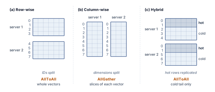
On accelerators, a row-wise layout turns each training step’s lookups into an AllToAll exchange. Every worker sends the indices its minibatch touches to the shards that own them and receives the embedding vectors back, and the backward pass returns gradients for the touched rows along the same routes. The exchange obeys the AllToAll bound of AllToAll Exchanges at Scale, and like MoE dispatch its volume and balance depend on which rows the data touches, so hot rows overload their owners unless the layout replicates or splits them.
Lighthouse 6.1: Archetype B (DLRM at Scale): DLRM vs. LLM scaling
Each workload scales through a distinct mechanism and is bound by a different resource. Dense LLMs scale through data, tensor, and pipeline parallelism, constrained by compute throughput and by the bandwidth that dense gradient and activation collectives need over fabrics such as NVLink and InfiniBand. Sparse recommendation models such as DLRM scale by sharding embedding tables of 10 TB or more across parameter servers or accelerator memory, where aggregate memory capacity, lookup rate, and the latency of many small random accesses dominate. The distinction shapes cluster design, favoring accelerator pods built around high-bandwidth dense fabrics for LLMs and memory-capacity-rich layouts for recommendation systems, whether the embedding shards live in CPU-hosted servers, in accelerator HBM, or in a tiered hybrid that keeps hot rows on accelerators and cold rows in host memory.
Self-Check: Question
In Megatron-LM style tensor parallelism for a transformer layer, how are the linear projections in the multi-head attention block arranged to minimize cross-device collective communication?
- Both QKV and Output projections are column-parallel, requiring an AllGather after each projection
- Both QKV and Output projections are row-parallel, requiring an AllReduce before each projection
- The QKV projection is column-parallel and the Output projection is row-parallel, requiring only a single AllReduce at the end of the attention block
- The QKV projection is partitioned across pipeline stages while the Output projection is replicated across data-parallel ranks
In a synchronous 1F1B pipeline-parallel training schedule with \(p=8\) stages and \(m=32\) microbatches, calculate the theoretical pipeline bubble fraction and explain how increasing the microbatch count \(m\) affects bubble overhead and activation memory.
Order the four sequential phases of token routing and execution in Expert Parallelism (Mixture of Experts) across distributed workers:
- AllToAll Combine: Processed token embeddings are routed back to their original source devices for residual connections
- Computation: Sharded expert feed-forward networks process their assigned token batches
- Gating: A router network evaluates tokens and selects top-k destination experts
- AllToAll Dispatch: Tokens are shuffled across the network fabric to the devices hosting their selected experts
In a capacity-limited Mixture of Experts (MoE) system using top-1 routing and token dropping, what occurs when a hot expert receives more tokens than its allocated buffer capacity determined by the Capacity Factor \(C\)?
- Excess tokens are dropped and pass through the MoE layer unprocessed via the residual connection
- The expert GPU dynamically allocates host CPU memory over PCIe, halting computation on other ranks
- The AllToAll collective automatically pauses until all sibling experts process matching token counts
- The extra tokens are rerouted to a random cold expert regardless of gating network weights
Contrast the communication patterns and hardware interconnect requirements of dense LLM training (Megatron-style Tensor Parallelism) with large-scale Recommendation Systems (DLRM embedding sharding).
True or False: Ring Attention scales context length beyond single-GPU memory capacity by circulating key/value blocks in an accelerator ring across \(N-1\) communication rounds while overlapping transfer with block-level attention computation.
6.6 Hybrid Parallelism
The 175B running example has now exhausted each family on its own. Data parallelism with ZeRO-3 makes the state fit, but the per-step parameter regather priced in section 6.5 would take about 10× as long as the computation it serves. Tensor parallelism confined to one 8-GPU node, meanwhile, still leaves several hundred gigabytes of training state per device. The preceding strategies address different constraints and need not be used in isolation. Section 6.3 established how replication and state sharding distribute examples and storage; section 6.5 showed how partitioned operations and pipeline stages distribute computation. Hybrid design chooses the dimensions needed to satisfy memory, communication, and global-batch constraints together.
Hybrid parallelism applies both families orthogonally: model parallelism splits the architecture to fit available memory, while data parallelism scales throughput across multiple model replicas. Training a 175B parameter language model on a dataset of 300 billion tokens demonstrates this approach in practice. The neural network layers distribute across multiple GPUs through model parallelism, while data parallelism enables different GPU groups to process separate batches. This dual strategy addresses both memory constraints from model size and computational demands from dataset scale simultaneously, and this combination defines Archetype A training at large-model scale.
Lighthouse 6.2: Archetype A (GPT-4/Llama-3): Physics of 3D parallelism
Archetype A (GPT-4/Llama-3) illustrates the motivation for hybrid parallelism. Parameter count \((\Parameters)\) must first be converted to a complete memory budget before comparison with device capacity \((\DeviceMemoryCapacity)\), while dataset size \((\DatasetSize)\) and the deadline determine the throughput target. Tensor parallelism partitions layer computations within a suitable communication domain; pipeline parallelism assigns consecutive layers to stages; and data parallelism distributes examples from \(\DatasetSize\) across replicas. A design combines the dimensions that address its constraints; efficient execution does not require all three in every case.
To see why the combination matters, consider three parallelism configurations for training the 175B model on a 1,024-GPU cluster organized as 128 nodes of 8 GPUs each. The progression from pure data parallelism through tensor and pipeline parallelism makes the efficiency gain concrete.
In Configuration A, pure data parallelism (DP-1024) serves as a communication counterfactual rather than a feasible placement for this model. The FP16 weights alone occupy 350 GB, so an A100 or H100 cannot replicate them; sharding only optimizer states does not change that fact. If replication were possible, all 1,024 ranks would form one data-parallel group, and each rank would participate in an AllReduce of the 350 GB gradient tensor across the InfiniBand fabric. The 15 percent calculation in section 6.4 isolates that communication cost.
Configuration B introduces intra-node tensor parallelism alongside data parallelism (TP-8, DP-128). Within each of 128 model replicas, 8 GPUs use tensor parallelism over NVLink. The corresponding tensor shard from every replica forms one 128-rank data-parallel group, so the layout contains 8 such groups. Each rank AllReduces its 1/8 gradient shard, 43.75 GB rather than 350 GB, and TP communication remains within the fast NVLink domain. This is a communication comparison only. At 16 bytes per parameter each GPU would still hold about 350 GB of training state, so the layout also needs optimizer and gradient sharding across its data-parallel group before it fits. The inter-node AllReduce time drops from 14 seconds to approximately 1.75 seconds. If the compute time is still 2.1 seconds, the unoverlapped efficiency improves to about 54.5 percent. The smaller transfer also fits inside the compute window, so the same optimistic schedule assumed for the data-parallel baseline can now hide its full 75 percent of the transfer behind backward computation, which lifts efficiency to about 83 percent.
Configuration C adds pipeline stages across nodes (TP-8, PP-4, DP-32) so that each of 32 model replicas uses 8-way tensor parallelism within a stage and 4 pipeline stages across nodes. For each of the 8 \(\times\) 4 tensor-and-pipeline shard positions, the corresponding ranks from all replicas form one 32-rank data-parallel group. Each rank therefore AllReduces a \(350/(8\times4)\approx10.94\) GB gradient shard. Pipeline communication forwards activations between stages and has lower volume than a full-model AllReduce. The trade-off is the pipeline bubble. At the beginning and end of each training step, some pipeline stages are idle while waiting for activations from earlier stages or gradients from later stages. The bubble fraction is approximately \((\PipelineParallelDegree-1)/(\MicrobatchCount+\PipelineParallelDegree-1)\), so with 4 pipeline stages and 32 microbatches per training step, the bubble wastes roughly 9 percent of compute (\(3/35 \approx 8.6\%\)). The smaller shard takes about 0.44 seconds to AllReduce, and under the same overlap model as configuration B most of it hides behind backward computation. Charging the bubble against the compute window and adding the remaining exposed transfer gives a predicted efficiency of about 87 percent, a few points above configuration B’s 83 percent. The pipeline cuts the data-parallel traffic by another factor of 4, and that saving slightly outweighs the bubble it introduces. Configuration C does not fit memory by itself either. Its training state is about 87.5 GB per GPU, above the 80 GB of an H100. Adding ZeRO-1 across its 32-rank data-parallel group closes that gap. Each GPU then keeps its tensor-and-pipeline slice of weights and gradients but only a 1/32 share of that slice’s optimizer state, about 24 GB in all, which leaves most of the HBM for activations and buffers. ZeRO-1 matches plain DDP’s ideal data-parallel byte volume at matching communication widths (table 3), but equal bytes do not preserve the overlap schedule. Gradient reduction to owners must precede their optimizer updates, and the updated-parameter AllGather follows those updates. The predicted efficiency remains conditional on that schedule achieving the modeled exposed communication time. TP-8, PP-4, DP-32 with ZeRO-1 passes this simplified persistent-state memory budget; its reduction, update, and parameter-gather readiness must still be priced before accepting the throughput prediction.
Within this comparison’s communication model, the configuration that places frequent tensor-parallel exchanges in the fast NVLink domain, pipelines across nodes, and leaves only small data-parallel gradient shards for InfiniBand has the best predicted efficiency. Peak memory, kernel shape, and scheduling still need verification before that prediction becomes a runnable design. The infrastructure hierarchy therefore dictates the parallelism hierarchy. Here, hierarchy-aware parallelism means matching exchange requirements to measured communication domains rather than choosing each degree independently.
Definition 6.12: Hierarchy-aware parallelism
Hierarchy-aware parallelism is the strategy of mapping different parallel execution modes to the physical bandwidth tiers of the cluster.
- Significance: It places high-frequency synchronization (for example, tensor parallelism) on fast links such as NVLink, while assigning lower-frequency exchanges (for example, data parallelism) to slower tiers when their transfers fit the schedule. This alignment can improve scaling efficiency \((\ScalingEfficiency)\) by reducing exposed communication time \((\CommunicationTime)\) and latency \((\Latency)\); the gain depends on readiness, contention, and available overlap.
- Distinction: Unlike uniform parallelism, which treats all node-to-node links as equal, hierarchy-aware strategies respect the bandwidth cliffs between die, node, and rack boundaries.
- Common pitfall: A frequent misconception is that any model can be sharded across any number of nodes. In reality, if the hierarchy mapping is wrong (for example, sharding a large tensor across a slow inter-rack link), the communication time will dwarf the compute time, making the scale-out useless.
The dependence runs both ways, because a parallelism configuration also determines which traffic the fabric must carry. In the TP-8, PP-4, DP-32 layout, tensor reductions stay within each fast local domain, pipeline traffic crosses neighboring stages, and data-parallel groups synchronize corresponding shards across replicas. Rail-optimized and hierarchical fabrics can exploit that structure, but a workload mix that adds expert AllToAll traffic changes the global bandwidth requirement. Infrastructure planning must therefore evaluate the anticipated communication groups together rather than optimizing the fabric for a single layout.
↩︎ Rail-optimized fabrics, which cable each GPU slot position to its own rail switch, are established in Rail-optimized topology.
6.6.1 The 3D training loop
Training a 175B-parameter model using 3D parallelism—the coordinated composition of data, pipeline, and tensor parallelism introduced with figure 2—can be traced on a fleet configured with tensor parallelism (TP) of 8 GPUs, pipeline parallelism (PP) of 16, and data parallelism (DP) of 128. This configuration uses 16,384 GPUs (8 GPUs \(\times\) 16 \(\times\) 128) organized into a hierarchy of bandwidth domains, sixteen times the 1,024-GPU reference cluster so that every level of the hierarchy is exercised even though parameter count alone would not require all three dimensions.
The training step begins at the data-parallel level. Each of the 128 model replicas receives a distinct slice of the global batch. Within each replica, the model is split across 16 pipeline stages (nodes), with microbatches flowing sequentially from the embedding layer on Node 0 to the loss calculation on Node 15. At the finest granularity, within each node, the 8 GPUs fuse into a single “super-accelerator” via TP. The transformer matrix multiplications are split across these devices; column- and row-parallel pairs retain local intermediate shards and exchange partial results at the reduction points already derived. For a 175B-scale hidden dimension, the activation payload is roughly 201.3 MB; the resulting tensor-parallel traffic is about 4.2 GB per pipeline stage per microbatch in the forward pass, or 8.5 GB including the backward pass. Across the full 96-layer replica, the forward tensor-parallel traffic is about 67.6 GB. This traffic is the highest-intensity in the system, but its exposed latency can remain small relative to compute because the chips communicate over 300 GB/s–450 GB/s of local bandwidth per direction.
The backward pass exposes dependencies between parallelism dimensions. Nodes exchange activation gradients point-to-point, roughly 201.3 MB per microbatch per stage boundary in this example. A smaller payload still stalls a stage if it arrives after the stage needs it. Data-parallel synchronization creates another dependency. Although full-model gradients occupy about 350 GB, each data-parallel group exchanges only the corresponding tensor- and pipeline-parallel parameter shard. Gradient bucketing groups ready gradients as backward computation proceeds. Which exchange limits the step depends on its readiness, service time, and overlap; data parallelism is not necessarily the final bottleneck.
↩︎ Bucket fusion, which groups gradients that become ready together into larger reductions so communication can begin during backpropagation, is established in Bucket fusion.
The architectural imperative is bandwidth matching, in which each exchange’s startup and transfer time must fit its available compute or overlap interval. In this mapping, frequent TP exchanges use the NVLink domain (300 GB/s per direction or higher), while PP transfers cross nodes and DP reductions overlap backward computation. Accumulation can enlarge the compute interval between DP synchronizations, subject to the global-batch constraint. An infeasible mapping leaves part or all of the 16,384 GPUs fleet waiting. Comparing service time with the schedule completes the feasibility check introduced in section 6.2.1.
6.6.2 Hybrid-parallelism worked example
Applied to physical infrastructure, bandwidth matching turns cluster design into a placement problem, and memory capacity per device (80 GB–80 GB) bounds every placement. For the 3D training loop’s layout on 16,384 GPUs, built from 8-GPU NVLink nodes, this reasoning leads to a concrete placement. Fix tensor parallelism at \(\TensorParallelDegree=8\) so the bandwidth-heavy matrix-multiplication collectives stay within one 8-GPU node. Map pipeline parallelism across nodes in the same high-bandwidth rack or island, here \(\PipelineParallelDegree=16\), with \(\PipelineParallelDegree=8\) as the alternative when the per-device memory budget allows. Use data parallelism for the remaining scale-out dimension across pods. The result is not a generic rule but a consequence of matching each traffic pattern to the cheapest fabric tier that can carry it, and with the placement fixed, the next question is whether the static model state fits inside each accelerator’s HBM budget.
The memory budget for a 175B model must include every persistent training component. Under the mixed-precision Adam convention used here, each parameter has FP16 weights and gradients, an FP32 master weight, and two FP32 optimizer moments, totaling 16 bytes before activations and workspaces. With tensor parallelism degree 8 alone, these components occupy 350 GB per device, exceeding H100-class capacity. Adding 16 pipeline stages spreads that state across the product of the two degrees, yielding 21.9 GB per device under even partitioning. A budget that counts only weights and optimizer moments, about 13.7 GB per device here, understates this total. Activation peaks, layer imbalance, and communication workspaces must fit in the remaining memory before this configuration is feasible.
Once the configuration fits in memory, its traffic still follows the same tiers, and each data-parallel group reduces only its tensor-and-pipeline shard of the 350 GB gradient buffer once per update. Gradient bucketing overlaps that reduction with backward computation, so its exposed cost depends on the computation remaining before the optimizer needs the reduced shard.
The last cost is scheduling rather than bandwidth, because a pipelined model is only efficient when enough microbatches are in flight to keep all stages busy. This remaining cost is the pipeline bubble developed in section 6.5.2. Applying its bubble fraction \(\frac{\PipelineParallelDegree-1}{\MicrobatchCount+ \PipelineParallelDegree - 1}\) to this hybrid layout, \(\PipelineParallelDegree=\) 16 stages with \(\MicrobatchCount=\) 32 microbatches waste \(\frac{15}{47} \approx 31.9\%\) of theoretical compute capacity, nearly one-third, against roughly 9 percent for configuration C’s 4 stages at the same microbatch count. The deeper pipeline is chosen at this scale for two reasons. Its 16 stages spread the full training state to about 21.9 GB per device without optimizer sharding. Filling 16,384 GPUs with configuration C’s 32-GPU replicas would instead need 4× as many data-parallel replicas, which multiplies the global batch \(\DataParallelDegree \times \MicrobatchCount\times \MicrobatchSize\) by the same factor at the same per-replica schedule. The shallow pipeline spends global batch; the deep one spends bubble. The 1F1B scheduling that reclaims activation memory, and the larger microbatch counts it makes practical, drive the bubble fraction down asymptotically, but every added microbatch also enlarges the global batch, so the bubble target must be reconciled with the critical-batch constraint from section 6.4.6.
The Blackwell reference shows how a wider fast communication domain changes 3D parallelism choices. NVLink 5 provides 1.8 TB/s of bidirectional bandwidth per GPU, twice the Hopper reference’s capacity, which shortens the transfer term for a fixed payload but does not reduce message startup latency. Larger tensor-parallel (\(\TensorParallelDegree\)) groups, such as \(\TensorParallelDegree=\) 16 or \(\TensorParallelDegree=\) 32 across nodes, remain subject to topology and local-kernel efficiency. For a 1 trillion-parameter model, one candidate uses \(\TensorParallelDegree=\) 16 across two 8-GPU nodes joined by NVLink Switch and \(\PipelineParallelDegree=\) 8. Relative to the Hopper layout’s \(\TensorParallelDegree=\) 8 and \(\PipelineParallelDegree=\) 16, this preserves the model-partition product while halving stage count, and the bubble must be recomputed from the new stage and microbatch counts rather than assumed to halve. The 10 TB/s internal link joins Blackwell’s two dies behind one logical GPU, so those dies are not separate tensor-parallel ranks. Improving local bandwidth shifts pressure outward. Once intra-node exchanges bind less, the inter-node fabric that carries pipeline and data-parallel traffic, together with any expert AllToAll service, becomes the term to check against the next tier. The same placement constraints can be made operational through design-space search.
Example 6.1: Automated design space search
Scenario: An engineering team schedules a 175B-parameter model across 8,192 H100 GPUs (80 GB HBM each), eight times the 1,024-GPU reference cluster so that the pipeline and data-parallel degrees both have room to vary, navigating the multi-dimensional 3D-parallelism search space (TP \(\times\) PP \(\times\) DP).
Diagnosis: Candidate configurations must fit within 80 GB HBM and satisfy the modeled communication budget. The search evaluates TP \(\times\) PP \(\times\) DP factorizations and selects TP=8 GPUs, PP=8, and DP=128 as the best predicted MFU among configurations feasible under its assumptions. That result is a candidate for measurement, not proof of the best attainable runtime.
Systems lesson: This search favors TP=8 GPUs within the reference topology’s fast domain and PP=8, with 36.4 percent projected MFU. The result balances memory, local computation, transfers, and pipeline idle time within the model. A different topology, microbatch schedule, or kernel efficiency can change the preferred factorization.
Adjusting any one dimension shifts the pressure onto the other two, making the factorization TP \(\times\) PP \(\times\) DP a tightly coupled system rather than three independent knobs. A projected MFU such as this search’s still needs comparison with measured execution, and published runs report MFU well below peak that can fall as the same model moves to more GPUs (figure in Program goodput and its measure).
Checkpoint 6.4: Hybrid 3D parallelism
Verify your understanding of how parallelism strategies combine:
The three configurations and the worked layout tell one story. Pure data parallelism moves the full 350 GB gradient over the slowest tier and reaches only 15 percent scaling efficiency. Keeping tensor parallelism inside the NVLink domain cuts each rank’s share of that traffic by the tensor-parallel degree, and pipeline stages cut it again at the price of a bubble. Communication alone does not make a layout feasible, however. Each layout must also hold the full training state, which is why configurations B and C still need optimizer sharding and why the worked layout adds pipeline depth until the persistent state falls to about 21.9 GB per device. Hybrid parallelism is therefore the joint solution of a memory constraint, a bandwidth hierarchy, and a batch-size limit, and every axis added to satisfy one of them tightens another. Alignment training tests that joint solution hardest, because it asks one fleet to host several models with different memory and compute profiles at the same time.
Self-Check: Question
In a 3D parallelism layout whose device count is the product of the data-, pipeline-, and tensor-parallel degrees, what hardware-matching principle dictates mapping tensor parallelism intra-node while pipeline parallelism spans inter-node links?
- Pipeline parallelism requires more memory bandwidth than NVLink can provide, forcing it onto InfiniBand
- Tensor parallelism requires only point-to-point transfers, making it insensitive to link latency
- Hierarchy-aware parallelism maps frequent TP exchanges to the fastest local fabric and PP boundary transfers to slower inter-node links.
- Data parallelism cannot execute across nodes that use tensor parallelism internally
A 175B-parameter model uses mixed-precision Adam with 2-byte weights, 2-byte gradients, a 4-byte master copy, and two 4-byte moments per parameter. With tensor degree \(t=8\) and pipeline degree \(p=16\), calculate the ideally balanced static memory per GPU before data-parallel state sharding, and explain why tensor parallelism alone cannot fit this state on 80 GB GPUs.
For one rank in a balanced 3D layout with eight transformer layers per pipeline stage, 32 microbatches per update, two tensor-parallel reductions per layer in each pass, and one unbucketed data-parallel reduction after accumulation, order these communication patterns by invocation count per update, highest to lowest:
- Data-parallel gradient reduction
- Tensor-parallel reductions
- Pipeline stage-boundary transfers
In a 16,384-GPU cluster configured with \(\text{TP}=8\), \(\text{PP}=16\), and \(\text{DP}=128\), how many GPUs participate in each individual data-parallel AllReduce communicator group?
- \(16{,}384\text{ GPUs}\), because all accelerators in the cluster must synchronize in a single global collective
- \(128\text{ GPUs}\), because each rank communicates only with its corresponding tensor-and-pipeline shard position across the 128 model replicas
- \(8\text{ GPUs}\), matching the tensor-parallel degree within each local node
- \(16\text{ GPUs}\), matching the pipeline stage depth across the cluster spine
True or False: A uniform fat-tree network topology providing equal bisection bandwidth between all node pairs is always more cost-effective than a rail-optimized topology when training large language models with hierarchy-aware 3D parallelism.
6.7 Multi-Model Training for Alignment and RLHF
A cluster partitioned to train a single model cannot simply run post-training alignment in place, because reinforcement learning from human feedback (RLHF) coordinates up to four distinct models inside a single training step. In proximal policy optimization (PPO), an active policy generates responses token by token, a preference-trained reward model scores them, a frozen reference copy constrains policy drift, and a learned value model estimates expected returns to guide the gradient update. Those roles carry wildly different memory footprints and alternate between memory-bandwidth-bound autoregressive generation and compute-bound backward passes. Direct preference optimization (DPO) sidesteps online generation and drops the separate reward and value models, trading live exploration for a simpler two-model loop. Designing an alignment cluster therefore starts by tallying which models, states, and execution phases must coexist on the fleet.
6.7.1 The multi-model coordination problem
Holding four models in accelerator memory at once multiplies the static state budget before a single prompt is even decoded, and only two of those models ever run a backward pass. In PPO (Schulman et al. 2017), as used in InstructGPT-style systems (Ouyang et al. 2022), the four roles differ sharply in execution mode and memory burden (table 7). In figure 19, the policy \(\Policy\) generates responses for scoring by the frozen reference and reward models and evaluation by the value model \(\CriticModel\). The penalized reward (\(\ResponseReward- \KlPenaltyCoefficient\,\text{KL}\)) subtracts a Kullback–Leibler divergence penalty, weighted by a coefficient \(\KlPenaltyCoefficient\) unrelated to link bandwidth \(\LinkBandwidth\), to discourage drift from the reference. Generalized advantage estimation (GAE) combines rewards and value estimates to judge how much better a response was than expected. Those estimates guide policy updates; the value model learns to predict returns, the cumulative discounted reward that follows each generated token. Reference and reward models remain forward-only in this loop, and shared-backbone implementations can combine roles without changing their distinct responsibilities.
Schulman, John, Filip Wolski, Prafulla Dhariwal, Alec Radford, and Oleg Klimov. 2017. “Proximal Policy Optimization Algorithms.” arXiv Preprint arXiv:1707.06347, ahead of print. https://doi.org/10.48550/arXiv.1707.06347.
Ouyang, L., J. Wu, X. Jiang, D. Almeida, C. L. Wainwright, P. Mishkin, C. Zhang, et al. 2022. “Training Language Models to Follow Instructions with Human Feedback.” Advances in Neural Information Processing Systems (NeurIPS) 35: 27730–44. https://doi.org/10.52202/068431-2011.
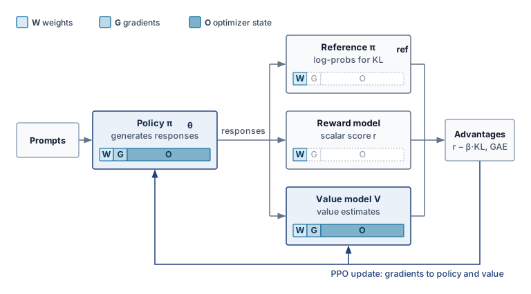
| Model | Role in PPO-style RLHF | Execution mode | Memory burden |
|---|---|---|---|
| Policy Model | The model being aligned and optimized. | Training mode with gradients, optimizer moments, and activations. | For a 70B-parameter model in mixed precision with Adam, memory is approximately 70B \(\times\) (2 \(+\) 2 \(+\) 12) = 1,120 GB, the same budget as standard pretraining. |
| Reference Model | A frozen copy of the pretrained policy that supplies the KL-divergence penalty. | Inference mode only. | FP16/BF16 parameters without gradients or optimizer state; a 70B model needs about 70B \(\times\) 2 = 140 GB, roughly 8× less than the training configuration. |
| Reward Model | A preference-trained scorer that produces scalar rewards for generated sequences. | Inference mode only. | Often smaller than the policy; a 13B reward model requires approximately 26 GB in FP16, but it must process every generated sequence. |
| Value Model | The PPO critic that estimates expected future reward. | Training mode, either separate or sharing a policy backbone. | A full-size separate critic can add another 1,120 GB; smaller models or shared-backbone designs reduce this to 200–400 GB. |
The aggregate memory demand of the four-model PPO system dwarfs standard pretraining. A naive co-location of a 70B policy, 70B reference, 13B reward, and 13B value model requires approximately 1,494 GB of accelerator memory, before accounting for the KV caches and intermediate activations generated during sequence generation. A key-value (KV) cache stores attention keys and values for previously processed tokens so the policy can generate the next token without recomputing that state. It grows with the number and length of active sequences, creating a temporary memory budget distinct from weights and optimizer state. On H100 GPUs with 80 GB of HBM each, this system requires a minimum of 19 GPUs as an aggregate static-state capacity lower bound, including optimizer state and gradients. This division does not establish a feasible placement, because each phase must also fit its KV or activation peak, workspaces, and uneven shards. Replicated policy groups increase the total state further.
6.7.2 Infrastructure asymmetry between training and inference models
The defining infrastructure challenge of RLHF is not the total memory footprint but the asymmetry between the models’ compute profiles. The policy and value models require full backward passes with gradient computation, activation checkpointing, and optimizer updates, compute-intensive operations that benefit from tensor parallelism and high arithmetic intensity. The reference and reward models, by contrast, perform only forward passes over generated sequences. Their scoring passes do not require optimizer state, and they need not decode token by token. The policy’s rollout phase creates the autoregressive generation workload and its KV-cache budget. Separating scoring from generation matters because forward-only execution does not imply a single memory or compute profile.
The asymmetry creates a placement dilemma. Co-location permits devices to serve different phases, but inactive model state can occupy memory needed for the active phase. Dedicated pools allow each role to use a suitable execution configuration, but pools may idle while waiting for another role’s output. Separation also adds transfers of generated sequences, scores, and updated policy weights. The design must compare phase utilization and data movement rather than assume that either placement eliminates waste.
The PPO rollout phase introduces autoregressive dependencies absent from the teacher-forced pretraining baseline. The policy generates responses before sequence-level rewards guide its updates. At small active batches, decoding is often memory bandwidth bound because each new token requires another model pass. For a Llama-2-70B-style grouped-query attention policy generating 1,024 tokens for each of 256 active sequences, the per-token cache bytes of equation 10.5 put the generated-token portion at 85.9 GB. That portion alone already exceeds the 80 GB of HBM on one H100, and prompt tokens add KV state as well. This temporary cache must fit alongside the state live during rollout; its lifetime differs from training activations and optimizer state.
↪ The capacity wall this cache imposes on serving systems is developed in The KV cache wall and memory capacity.
RLHF systems address this asymmetry through temporal multiplexing. During the generation phase, the cluster behaves like an inference system. The policy model generates sequences while the reference model computes log-probabilities, and the dominant resource is HBM reserved for token-by-token attention state. During the training phase, the same fleet switches back to training mode and computes gradients through the policy and value models using the 3D parallelism configuration developed in section 6.6. During generation, batching active sequences and placing their KV state determine how much useful work shares each weight read. During the update phase, activation residency and gradient synchronization again govern the schedule. RLHF is not one steady training loop, but an alternation between inference-shaped work and training-shaped work, and standard training frameworks rarely manage that transition by themselves.
6.7.3 Resource requirements for PPO versus DPO
Standard offline DPO (Rafailov et al. 2023) removes the separate reward and value models from the update loop by reformulating alignment as a loss over preference pairs. The policy learns from preferred and dispreferred responses using their log-probabilities relative to a frozen reference. Because those responses are already in the training data, the update requires neither online generation nor advantage estimation.
A DPO implementation that retains a resident reference has two model roles, the trainable policy and the frozen reference. For fixed preference pairs and a fixed reference, reference log-probabilities can instead be precomputed, removing that model from the repeated update loop. Offline DPO needs no autoregressive rollout during those updates. Variable lengths still require padding, packing, or length-aware batching, and policy training can use the same partitioning, accumulation, and overlap mechanisms as pretraining.
The infrastructure difference follows from how each method obtains feedback. Offline DPO learns from a fixed preference dataset, so the policy never receives feedback on new responses. PPO-style training scores responses from the evolving policy and can expose behavior the dataset lacks, provided the reward signal is reliable. The generation phase, the reward and value models, and the memory they occupy are the price of that online loop, so the choice is settled by achieved quality per unit of total resource cost.
To make the infrastructure trade-off concrete, consider aligning a 70B policy model using a policy/reference pool of 256 H100 GPUs (80 GB HBM each). PPO’s separate reward and value pools sit outside that allocation. The policy is a 70B-class model rather than the 175B reference, a size at which each role’s memory budget stays readable while the four PPO roles together still need at least 19 GPUs, more than one node.
Napkin Math 6.9: RLHF infrastructure budget: PPO vs. DPO
Problem: This alignment setup co-locates a 70B policy model with a 70B reference model and, for PPO, uses pools outside the 256-GPU policy/reference allocation for a 13B reward model and a 13B value model. Under 3D parallelism (TP=8 GPUs, PP=4, DP=8), how much memory resides on each policy GPU, and which separate model pools and generation-phase memory requirements does DPO remove?
Table 8: PPO vs. DPO State and Execution Phases: Static-state totals sum one copy of each model across its device pool, including trainable optimizer state and gradients. Data-parallel replication and phase-specific runtime allocations add to these totals; the table does not determine a minimum device count or measured MFU.
PPO memory budget (per-GPU, with TP=8 GPUs, PP=4, DP=8 for policy)
The policy model under 3D parallelism with TP=8 GPUs and PP=4 distributes one replica’s 1,120 GB training state across 32 GPUs, yielding 35 GB per GPU. The reference model, requiring only 140 GB for inference, can instead be sharded across an additional 8 GPUs pool outside the policy allocation at 17.5 GB each, or co-located with the policy GPUs at an additional 4.4 GB per GPU (140 GB / 32 GPUs). The 13B reward model adds 26 GB shared across its pool. The 13B value model in training mode adds approximately 208 GB (13B \(\times\) 16 bytes/param) across its pool.
Total static memory (one co-located policy + reference replica on 32 GPUs): 35 GB + 4.4 GB \(\approx\) 39.4 GB per GPU, leaving \(\sim\) 46.5 GB for activations and KV cache. With generation-phase KV caches for a rollout batch containing 256 sequences and 1,024 tokens inside one \(\Glyph{T} \Glyph{P}{\times}\Glyph{P} \Glyph{P}\) policy replica, each policy GPU must reserve an additional 85.9 GB/32 GPUs \(\approx\) 2.7 GB for its KV cache shard. The remaining \(\sim\) 43.8 GB is generation-phase headroom. Once rollout KV state is released, the update phase recovers the 46.5 GB headroom before allocating training activations and other runtime buffers. The phase peaks must be evaluated separately.
DPO memory budget (same parallelism configuration)
The policy model uses the same 35 GB per GPU. The reference model adds 4.4 GB per GPU (co-located). No reward model, no value model, no KV cache for generation.
On the policy GPUs, total static memory is 35 GB + 4.4 GB = 39.4 GB per GPU, identical to PPO’s co-located policy/reference footprint. Both have 46.5 GB available before update-phase activations and runtime buffers when PPO releases its rollout KV cache. DPO removes the separate generation peak and the reward/value model pools; the absence of rollout KV state alone does not establish larger update microbatches.
Throughput comparison
PPO alternates generation and parameter updates. If generation consumes 60 percent of an iteration in this illustrative schedule, updates occupy the remaining 40 percent; this time fraction is not MFU. Update-phase MFU must be multiplied by that fraction to report update computation over the whole iteration, using the same allocated hardware denominator. DPO eliminates online generation, but its measured throughput still depends on sequence lengths, reference scoring, parallelism, and memory use. The static-state comparison in table 8 is therefore kept separate from these schedule-dependent effects.
| Metric | PPO (70B policy) | DPO (70B policy) |
|---|---|---|
| Models required | 4 (policy, ref, reward, value) | 2 (policy, reference) |
| Static state, one copy of each model | \(\sim\) 1,494 GB | \(\sim\) 1,260 GB |
| Device count | Depends on placement and phase peak | Depends on placement and activation peak |
| Generation phase | Yes (autoregressive) | None |
| Update throughput | Shares the schedule with generation | No online-generation phase |
| Data pipeline | Online generation | Static preference pairs |
Systems insight: In this 13B reward/value-model scenario, DPO reduces the one-copy static-state budget by 15.7 percent by eliminating the reward and value models. It also removes online generation, but the throughput benefit requires a measured schedule. Infrastructure constraints therefore weigh on the choice between PPO and DPO as much as modeling preferences do, and an organization with a limited GPU budget may prefer DPO because it restores the workload to a fixed-data training loop. If the PPO value model is policy-sized rather than 13B, the reduction is larger still, from 2,406 GB to 1,260 GB.
6.7.4 Sequence length variance and batching challenges
PPO and DPO make variable sequence length a prominent scheduling concern. Pretraining often packs documents into fixed-length blocks, such as 2,048 or 4,096 tokens, although variable-length workloads also occur. Alignment batches combine prompts and responses whose lengths can differ substantially; an illustrative batch can span a 10–50\(\times\) length range. Those lengths determine activation residency, padding, and work assigned to each worker.
Length variance creates two interacting problems. Padding every sequence to the longest in a batch can leave most token positions unused. A batch of one 2,048-token sequence and fifteen 128-token sequences, padded to 2,048 tokens, fills only 3,968 of its 32,768 positions, so kernels that execute padded positions spend about 88 percent of their work on padding; kernels that skip them recover most of that waste. Dynamic batching groups similar lengths to reduce padding, but assignments across workers still need balancing. A worker processing longer sequences can have a larger activation peak and finish later, leaving other workers waiting for the required gradient contributions.
Sequence packing combines short sequences within a fixed-length input, with attention masking that keeps their contexts separate, and adaptive microbatching sizes each microbatch by token count or predicted memory. Alignment adds a constraint that pretraining lacks. The reduction must keep the objective’s own denominator, valid-token counts for a token-mean PPO loss and pair counts for standard DPO (Rafailov et al. 2023), so packing changes layout but not weighting. Balancing token work across workers then remains a performance goal rather than a correctness requirement.
Rafailov, Rafael, Archit Sharma, Eric Mitchell, Stefano Ermon, Christopher D. Manning, and Chelsea Finn. 2023. “Direct Preference Optimization: Your Language Model Is Secretly a Reward Model.” Advances in Neural Information Processing Systems (NeurIPS) 36: 53728–41. https://doi.org/10.52202/075280-2338.
RLHF shows why no single parallelism strategy is sufficient by itself. The policy model may need tensor and pipeline parallelism, the reference and reward models behave like inference services, the value model may require training state, and the rollout data pipeline changes shape from step to step. The procedure that handles this case is the general one, which identifies the binding constraint first and then chooses the parallelism pattern that moves the least data while fitting the required state.
Self-Check: Question
Why does Proximal Policy Optimization (PPO) in multi-model RLHF create an infrastructure asymmetry challenge that does not exist in standard pretraining?
- It combines policy and value-model training with policy-generated autoregressive rollouts and forward-only scoring by frozen reference and reward models.
- All four models in PPO must be trained with identical optimizer hyperparameters on the same GPU
- PPO requires all models to be converted to INT4 precision to enable cross-node gradient synchronization
- PPO eliminates backward passes entirely, turning distributed training into a stateless inference service
Explain how Direct Preference Optimization (DPO) simplifies cluster infrastructure compared to PPO, detailing which models and computational phases are eliminated.
During the autoregressive generation phase of PPO alignment for a 70B-parameter model, which growing runtime state can limit generation concurrency in accelerator memory?
- FP32 Adam momentum and variance buffers stored on CPU hosts
- Key-Value (KV) cache memory in GPU HBM, bounded by memory bandwidth during token-by-token generation
- AllReduce gradient communication buffers across InfiniBand switches
- Host filesystem NVMe write bandwidth for checkpoint dumping
The scheduling approach in RLHF distributed systems where the accelerator fleet alternates between an autoregressive rollout phase dominated by KV cache memory and a backward training phase dominated by matrix GEMM compute is known as ____.
True or False: Because Direct Preference Optimization (DPO) eliminates reward and value models and avoids online sequence generation, it is strictly superior to PPO for all model alignment and exploration tasks.
6.8 Parallelism Strategy Comparison
A parallelism strategy is useful only if it moves the binding constraint without creating a larger one. Assembling data, tensor, pipeline, and hybrid partitioning into a coherent decision procedure requires evaluating where each strategy relocates overhead across the cluster’s memory and interconnect hierarchy. For a new model, the decisive questions are which memory state fits, how often communication occurs, where the pipeline bubble appears, and which abstraction cost the engineering team can tolerate. Sequence, context, and expert parallelism sit beside the 3D core in table 9, and they remain subject to the same batch, memory, and topology constraints.
| Strategy | Binding constraint | Primary movement | Placement decision | Validation signal |
|---|---|---|---|---|
| DDP | Model state fits on one accelerator | AllReduce gradients every step | Replicate full model across data-parallel workers | Step time dominated by compute, not synchronization |
| FSDP/ZeRO | Model state exceeds one accelerator | Gather parameters; ReduceScatter gradients | Size prefetch and reshard windows within peak memory | State plus activations and workspaces fit |
| Tensor parallelism | One layer or tensor operation exceeds local capacity | Reduce or gather partial layer results | Keep tightly coupled partitions on fast local links | Exposed collective time fits the layer-time budget |
| Pipeline parallelism | Layer stack fits only when split by stage | Activations and gradients between stages | Balance stages and live microbatch activations | Bubble and peak activation memory meet budget |
| Sequence/context parallelism | Activations or attention context exceed local capacity | Exchange sequence shards or attention state | Partition long sequences across a low-latency group | Longer context fits without communication dominating |
| Expert parallelism | Sparse expert capacity exceeds local memory | Route token activations with AllToAll | Balance expert load across a high-bisection group | Expert imbalance and dropped-token rate stay bounded |
| Hybrid parallelism | More than one constraint binds at once | Multiple collectives on coupled axes | Satisfy divisibility, batch, topology, and failure domains | MFU improves within memory and network budgets |
A decision path condenses the table, starting from memory fit and then asking which structure breaks the budget (figure 20). Before accepting any branch, check peak memory, global batch, communication service time, and load balance together; bandwidth is a feasibility constraint throughout the decision, not an afterthought.
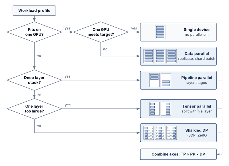
Identifying the binding constraint comes before choosing an implementation stack, which is why both the strategy comparison and the decision path stay deliberately coarse. Dense large-model training and recommendation-style workloads motivated each of these partitioning strategies, but the same constraint logic also reaches the federated edge case (table 10), where the bottleneck shifts from accelerator memory and fabric bandwidth to unreliable devices, privacy, and intermittent connectivity. A configuration chosen across these regimes still has to be expressed in software, and the way a framework expresses it decides which of the chapter’s budgets the engineer controls directly.
Lighthouse 6.3: Distributed archetype spectrum
Partitioning and coordination choices differ with the system’s primary bottleneck:
| Archetype | Primary partitioning strategy | The logic |
|---|---|---|
| Archetype A (GPT-4/Llama-3) | Hybrid 3D parallelism | Combine tensor (width), pipeline (depth), and data (throughput) parallelism to fit roughly 3.5 TB of weights under third-party estimates (OpenAI has not disclosed the parameter count). |
| Archetype B (DLRM at Scale) | Embedding sharding | Partition massive 10 TB+ tables across parameter servers or accelerator shards; use sparse AllToAll updates. |
| Archetype C (Federated MobileNet) | Federated learning | The same logic extends to coordinating on-device MobileNet updates across unreliable, privacy-constrained edge devices; Federated Learning Systems at Scale develops this regime. |
Self-Check: Question
According to the chapter’s parallelism decision framework, which condition indicates that standard DistributedDataParallel (DDP) is a sensible baseline to evaluate over FSDP, TP, or PP?
- The model’s single layer weight matrices exceed the HBM capacity of an individual GPU
- The cluster is connected by slow 10 Gb/s commodity Ethernet across 1,024 nodes
- The entire model state (parameters, gradients, and optimizer state) fits comfortably within single-device memory with sufficient headroom for activations
- The model architecture contains sparse Mixture-of-Experts routing layers
An engineering team observes that an 8-GPU training job using pure pipeline parallelism achieves only 35 percent Model Flops Utilization (MFU), while interconnect links are largely idle. Using the bubble formula \(F_{\text{bubble}} = \frac{p-1}{m+p-1}\), explain how to assess the pipeline-bubble hypothesis and propose two adjustments if the trace confirms it.
Order the following parallelism strategies by their structural granularity from coarsest (whole model / batch level) to finest (intra-operator level):
- Tensor Parallelism (Megatron column/row splits)
- Standard Data Parallelism (batch dimension splitting)
- Pipeline Parallelism (inter-layer stage splitting)
6.9 Frameworks and Runtime Contracts
A TP-8, PP-16, DP-128 layout that passes every feasibility check on paper can still hang at its first collective if two ranks disagree on group membership, or run slowly if gradient buckets become ready in an order the collective runtime cannot overlap. Choosing DDP, FSDP/ZeRO-style sharding, tensor parallelism, or pipeline parallelism is therefore also a decision about which constraints the runtime owns and which constraints the engineer must manage directly. Sparse workloads add a fourth contract, the parameter-server push/pull interface (Li et al. 2014) developed for Archetype B in section 6.5.6.
Li, M., D. G. Andersen, J. W. Park, A. J. Smola, A. Ahmed, V. Josifovski, J. Long, E. J. Shekita, and B.-Y. Su. 2014. “Scaling Distributed Machine Learning with the Parameter Server.” Proceedings of the 2014 International Conference on Big Data Science and Computing, 583–98. https://doi.org/10.1145/2640087.2644155.
The training framework defines process groups, gradient buckets, and the point in backpropagation when each reduction becomes ready; the collective runtime maps those reductions onto ring, tree, or hierarchical algorithms. The engineer must choose compatible group membership and bucket order and verify which communication remains exposed on the step’s critical path.
Production frameworks expose these same strategies under different names, which makes a translation aid useful when reading their documentation or configuration files. Four widely used stacks name the chapter’s strategies differently (table 11); the names change between releases, but the partition each one implements does not.
| Strategy | PyTorch | DeepSpeed | Megatron-LM | JAX |
|---|---|---|---|---|
| Data parallel | DistributedDataParallel (DDP) | DeepSpeed engine, ZeRO stage 0 | Data-parallel process groups | Batch axis sharded over a device mesh |
| Sharded data parallel | Fully Sharded Data Parallel (FSDP) | ZeRO stages 1–3 | Distributed optimizer | Parameter and optimizer state sharded over a mesh axis |
| Tensor parallel | DTensor tensor-parallel APIs | AutoTP or Megatron integration | Column- and row-parallel linear layers | Sharding annotations on model axes, partitioned by the compiler |
| Pipeline parallel | torch.distributed.pipelining |
Pipeline engine | Pipeline schedules (1F1B, interleaved) | User-written stage schedules |
The training design therefore determines message size, readiness order, and frequency, while collective algorithms determine how those messages move. No framework abstraction changes those physical costs, so distributed-training efficiency ultimately depends on interconnect bandwidth, memory capacity, synchronization latency, and the useful overlap admitted by the computation graph.
↩︎ Overlap of gradient exchange with backpropagation, the lever that takes communication off a step’s critical path, is established in Communication-Computation Overlap.
Self-Check: Question
In distributed training framework runtimes (such as PyTorch DDP), what mechanism combines multiple small layer gradient tensors into contiguous memory buffers before launching collective communication?
- Activation checkpointing
- ZeRO Stage 3 parameter gathering
- Temporal multiplexing
- Gradient bucketing
Contrast the collective communication primitive invocation frequency of standard DDP against full-shard FSDP with resharding for a model with \(N_L\) layers during a single training step.
Explain why framework optimizations such as CUDA graphs and asynchronous communication streams cannot eliminate the physical scaling penalty of distributed training as the cluster size \(N\) becomes very large.
6.10 Fallacies and Pitfalls
The GPT-2 notebooks showed the trap in miniature. Moving the same model from one NVLink node to four Ethernet-connected nodes quadrupled the GPU count but cut parallel efficiency from 99.4 percent to 27.9 percent. The following misconceptions generalize that error, each treating one term of the step-time accounting as if it were the whole budget.
Fallacy: Linear speedup is achievable with sufficient engineering effort.
Amdahl’s Law limits speedup when a fixed serial component remains exposed. Synchronous gradient aggregation creates an update dependency, but some of its work can overlap backward computation. As section 6.4 shows, \(\ScalingEfficiency = 1/(1 + \DeviceCount(\CommunicationTime(\DeviceCount) + \SynchronizationTime(\DeviceCount) - \OverlappedTime)/\IronLawComputeTime)\) depends on the exposed overhead relative to useful compute as \(\DeviceCount\) changes. A 1,000-GPU allocation therefore does not by itself justify a 1,000\(\times\) speedup forecast. Local kernel efficiency, memory feasibility, communication, and convergence must be evaluated against the specified baseline. Linear scaling is a result to demonstrate for an operating range, not a return guaranteed by device count.
Pitfall: Optimizing MFU without considering scaling efficiency.
A single-node MFU measurement does not predict fleet throughput by itself. For a fixed workload and hardware peak convention, scaling efficiency compares measured distributed throughput with ideal replication of that single-node baseline. Multiplying the baseline MFU by this scaling efficiency gives distributed MFU; multiplying an already measured distributed MFU by the same scaling efficiency counts communication and synchronization losses twice. The chapter’s own numbers make the difference concrete. A single node running at 50 percent MFU, scaled with the 83 percent scaling efficiency of the overlapped TP-8 layout in section 6.6, delivers about 41 percent MFU across the fleet. A planner who measures that 41 percent on the full cluster and then applies the 83 percent again would budget for about 34 percent and buy capacity the job does not need. Capacity planning must state the device count and measurement window for each metric. Checkpointing, recovery, and replay require additional accounting only when those losses fall outside that window, and useful goodput must count retained model progress rather than repeated work, under the accounting boundaries of Accounting boundaries.
Fallacy: Hyperparameters tuned on small clusters transfer directly to large-scale training.
Engineers tune hyperparameters on 8-GPU workstations then deploy to 256-GPU clusters expecting identical behavior. At scale, convergence behavior changes. The most critical hyperparameter is learning rate. As section 6.3 explains, global batch increases with GPU count when local batch and accumulation depth remain fixed, so the learning-rate schedule must be revalidated. The linear scaling rule of section 6.4.5, which the one-hour ImageNet run established, suggests \(\ScaledLearningRate = \BaseLearningRate\times (\ScaledBatchSize/\BaseBatchSize)\), but this relationship holds only within bounds. As models scale, they eventually encounter the critical batch size of section 6.4.6, where adding more data per step yields diminishing returns in convergence.
Beyond the critical batch size, this relationship breaks down in a model-, data-, and optimizer-dependent way. A team that takes a small-cluster learning rate, multiplies it mechanically with GPU count, and jumps directly to a much larger global batch may see lower final quality or slower sample efficiency even though hardware throughput improved. Warmup schedules, weight decay adjustment, layer-wise optimizers such as LARS/LAMB, and careful momentum tuning can recover accuracy in some regimes, but require systematic experimentation at target scale. Organizations that skip these scaling studies waste thousands of GPU-hours on suboptimal runs.
Pitfall: Adding GPUs to data-parallel jobs without modeling communication.
More GPUs improve time to target only if the gain in processing rate outweighs communication overhead and any additional sample use. With fixed local batch size, adding data-parallel workers increases the global batch; fixing the global batch instead reduces local work and can expose more communication. The critical-batch analysis in section 6.4.6 supplies a workload-dependent statistical guide, not universal GPU-count or model-size thresholds. Compare complete learning curves and cost at the same target quality before committing to a larger allocation.
Fallacy: Memory capacity alone determines the parallelism strategy.
A model that exceeds device capacity needs a feasible partition, but memory fit does not select the fastest one. Tensor parallelism exchanges partial results within layers, while pipeline parallelism transfers stage-boundary activations and introduces scheduling bubbles. Their relative cost depends on layer shapes, microbatch count, placement, and overlap. Compare complete training-state and activation budgets together with measured time to target; an unsupported throughput percentage or a weights-only fit cannot settle the choice.
Pitfall: Applying FSDP or ZeRO without measuring efficiency trade-offs.
Engineers adopt FSDP universally after reading that it “reduces memory and enables larger models.” Sharding trades memory capacity for communication overhead: full-shard FSDP gathers parameters before layer execution and reduces gradient shards during backward, with another parameter gather when the forward pass resharded them. The relevant comparison begins with the complete training-state budget. Under the mixed-precision Adam convention established here, the 7B worked example exceeds single-device capacity before activations, so standard DDP cannot fit that state on an A100-80 GB. A weights-only fit does not establish a feasible training baseline. When the complete state, activations, and workspaces fit without sharding, DDP can avoid the repeated gathers; when they exceed the 80 GB capacity, the comparison must include a feasible alternative such as sharding or offload. FSDP provides value when it enables training at all or when the larger local batch it permits offsets its communication cost. ZeRO-Offload extends capacity through CPU memory but adds transfers of its own. The decision therefore requires measuring peak memory and exposed communication for the same workload and optimizer contract.
Fallacy: Parallelism overhead is roughly constant regardless of model size.
Engineers benchmark parallelism strategies on convenient small models then apply those conclusions to large-scale training. For dense transformers at fixed tokens per update, computation and gradient bytes both grow roughly proportionally with parameter count, as the earlier scaling analysis established. Larger parameter count alone therefore does not imply a better computation-to-communication ratio. Architecture, sequence length, local batch size, partition degree, and kernel efficiency determine how much useful work each rank performs; gradient representation and process-group membership determine how much it communicates. A larger model can also require a different partition that introduces new layer collectives or pipeline bubbles. Reliable strategy selection holds the workload and target quality explicit, then recomputes memory fit, local compute time, communication volume, and the available overlap window at the target scale. A small-model benchmark becomes transferable evidence only when those governing terms remain comparable.
Pitfall: Treating scaling efficiency as a property of the hardware alone.
A vendor benchmark might report 85 percent scaling efficiency at 1,024 GPUs, and procurement teams then plan capacity as if that number were a cluster constant. Scaling efficiency is a joint property of four things: the workload’s communication-to-computation ratio, the parallelism strategy (data, pipeline, tensor, hybrid), the network topology (fat-tree vs. torus vs. dragonfly), and the software stack (NCCL version, kernel fusion, overlap quality). Reference numbers from dense large-language-model benchmarks transfer poorly to other workloads and fabrics. They may overstate scaling for graph neural networks with irregular communication and for embedding-heavy recommendation models, whose AllToAll embedding exchanges and many small random lookups load the fabric differently from dense gradient AllReduce (section 6.5.6), and they say nothing about a commodity-Ethernet placement like the GPT-2 scale-out, which lost most of its parallel efficiency on leaving the node. Capacity planning should use measured scaling on the target workload, not a vendor hero benchmark.
Fallacy: Gradient accumulation is free.
Gradient accumulation can reduce synchronization from every microstep to once per window of \(\AccumulationStepCount\) microsteps, eliminating \((\AccumulationStepCount-1)/\AccumulationStepCount\) of those synchronization events when the implementation defers reduction. The saving has costs. A resident gradient buffer remains live throughout the accumulation window; for the 7B model, the FP16 buffer occupies 14 GB. Retaining graphs across microsteps or increasing the local batch size can add activation pressure. Accumulating eight microsteps makes updates 8\(\times\) less frequent per processed microstep, but wall-clock spacing also depends on the communication saved. Larger effective batches can change convergence, and narrow accumulation formats can lose small contributions or overflow. The dtype, loss normalization, and reduction schedule must therefore be validated at the intended batch size. Accumulation trades communication frequency against update spacing, memory residency, and numerical stability.
Self-Check: Question
A team achieves 50 percent Model Flops Utilization (MFU) on a single node, scales to 1,024 GPUs, and measures a scaling efficiency \((\eta_{\text{scaling}})\) of 50 percent on their communication-heavy workload. What is the cluster’s realized model-FLOP rate during distributed execution as a fraction of peak hardware compute?
- 25 percent of peak compute (delivering 256 GPU-equivalents of model computation)
- 50 percent of peak compute (delivering 512 GPU-equivalents of useful work)
- 100 percent of peak compute (delivering 1,024 GPU-equivalents of useful work)
- 12.5 percent of peak compute (delivering 128 GPU-equivalents of useful work)
A procurement team plans capacity for a graph neural network workload using a vendor benchmark that reports 85 percent scaling efficiency at 1,024 GPUs for large-language-model training. Explain why this figure cannot be treated as a property of the cluster and what the team should measure instead.
Why is gradient accumulation NOT a cost-free substitute for true physical scale-out even though it reduces gradient AllReduce communication frequency by a factor of \(k\)?
- It is mathematically incompatible with the Adam optimizer
- It keeps a live gradient buffer resident, spaces optimizer updates by \(k\) microsteps, and requires appropriate accumulation precision and normalization
- It requires dedicated InfiniBand links between CPU and GPU for each microstep
- It forces batch normalization layers to synchronize across all nodes on every forward pass
The largest global batch size beyond which adding more samples per step yields diminishing reductions in the number of steps needed to reach target quality is called the ____.
True or False: If a 7B-parameter model fits comfortably in single-GPU memory with high compute utilization under standard DDP, universally enabling ZeRO-3 / FSDP full sharding will always increase training throughput by reducing per-GPU memory consumption.
6.11 Summary
Scaling laws keep pushing frontier training budgets past what one machine can hold or finish in time, and distributed training is how the fleet absorbs that growth. It confronts the scaling wall, the workload-dependent operating point beyond which communication and coordination can consume the compute time saved by adding accelerators. A feasible design must preserve the intended optimization update while satisfying model-state, activation, batch-size, and interconnect constraints. Hardware throughput alone is insufficient; the comparison must also account for time to the target model quality.
Each partition relocates cost along the C³ axes. Data parallelism divides compute across replicas and pays in communication, the gradient aggregation whose exposed share set the scaling efficiency of the 175B communication example. Tensor parallelism divides work inside a layer and pays in communication on the critical path, which confines it to a fast domain. Pipeline parallelism divides layer depth and pays mostly in coordination, the fill and drain bubble that only more microbatches, better balance, or a smarter schedule can shrink. The 3D parallelism cube in figure 2 unites these trade-offs in one coordinate space (\(\DataParallelDegree \times \PipelineParallelDegree \times \TensorParallelDegree\)). A feasible point must satisfy peak memory and global-batch constraints as well as communication and coordination budgets.
Sharding and model partitioning make different parts of the training state fit, while synchronization and precision policies determine whether the resulting updates remain useful. Hybrid layouts compose these choices within the bandwidth hierarchy. The alignment workload extends the same reasoning to multiple models and alternating generation and update phases, where peak memory depends on which state is live together.
The chapter’s strategies are complementary dimensions of one design space rather than alternatives. Systems such as Megatron-LM map tensor, pipeline, data, and expert exchanges to the communication domains that can carry them, and that matching is what delays the communication-bound regime as the fleet grows. The workload archetypes weight those dimensions differently. Archetype A (GPT-4/Llama-3) combines dense-model partitioning with state sharding and, at long contexts, sequence or context partitioning; Archetype B (DLRM at Scale) shards sparse embedding state and pays in lookup traffic rather than layer collectives; Archetype C (Federated MobileNet) moves the coordination problem onto unreliable edge devices. In each case the binding constraint, not the archetype label, selects the configuration.
Key Takeaways: Parallelism relocates overhead
- Splitting work moves the bottleneck: Distributed training does not make the underlying computation smaller; it converts memory pressure into communication volume, synchronization delay, or idle pipeline time (principle 12). The winning strategy is the split that sends overhead to the least binding part of the fleet.
- The slowest worker sets synchronous step time: Under bulk-synchronous updates every step waits for its last required contribution, so a rare per-worker delay becomes a near-certain per-step delay at thousands of workers. Stale and asynchronous protocols trade that waiting for staleness, which can cost extra steps to the same target quality.
- Throughput must serve convergence: Larger global batches can improve hardware efficiency while yielding diminishing progress per sample. Compare time to the same target quality, and treat the critical-batch estimate as a workload-dependent guide for selecting batch size and update schedules.
- Sharding buys memory with messages: ZeRO and FSDP partition optimizer state, gradients, and parameters (principle 2), reducing replicated storage. Peak memory must still include activations, temporary gathers, and workspaces; exposed ReduceScatter and AllGather costs determine whether the capacity gain also improves throughput.
- Tensor parallelism needs a fast domain: Splitting operations inside layers creates frequent communication on the dependency path. Place those groups on links with sufficient bandwidth and low latency; the relevant boundary is the communication domain, which may span nodes, rather than the server enclosure.
- Pipeline parallelism trades bytes for bubbles: Layer staging reduces communication frequency, but fill and drain slots leave accelerators idle (principle 10). Microbatching with \(\MicrobatchCount\gg \PipelineParallelDegree\) is the mechanism that turns model depth into throughput rather than pipeline slack.
- Hybrid layouts are joint decisions: Combine only the partitioning and sharding strategies needed to satisfy the workload’s constraints (principle 14). Model divisibility, batch size, peak memory, communication groups, and failure domains must form one feasible configuration; improving one axis can expose a limit on another.
The displacement of overhead (principle 14) makes a feasible partition the beginning of the design problem. A memory-saving split is useful only if its communication and schedule still meet the run’s time-to-quality budget. Every mechanism in this chapter shrinks the per-device compute term \(\IronLawComputeTime/\DeviceCount\) or the per-device training state, and pays for it in \(\CommunicationTime(\DeviceCount)\), in \(\SynchronizationTime(\DeviceCount)\) through barriers, stragglers, and pipeline bubbles, or in lost overlap. In C³ terms, no partition removes the overhead of scale; it only relocates that overhead among compute, communication, and coordination. The engineering judgment is therefore to compare complete configurations, including their exposed dependencies, rather than optimize each parallelism axis independently.
What’s Next: From logic to resilience
The fleet now has its traffic patterns (communication) and its logic (parallelism). Every configuration in this chapter, however, assumed that all ranks in each communication group arrive, on time and with correct data. A collective is not a barrier, but each dependent consumer still waits for every contribution, so one crashed node, failed link, or GPU that slows down without failing stalls the whole synchronous group, and a contribution corrupted in transit is reduced into every replica’s update. Across thousands of accelerators such events stop being rare. Fault Tolerance begins by computing how often they arrive, then builds the checkpointing, recovery, and elastic training that keep the computation making progress on imperfect hardware.
6.12 Self-Check Answers
Self-Check: Answer
A research team is training a 3B-parameter transformer that fits comfortably in one H100 GPU’s 80 GB of memory, but projected single-GPU training would take 18 months to reach target loss. The dataset is 3 TB and fits on local NVMe storage. Which signal makes distributed training necessary in this scenario?
- Dataset exceeding GPU HBM capacity, which automatically mandates tensor parallelism regardless of execution time
- The presence of NVLink inside the node, which makes multi-machine scaling mandatory by default
- Unacceptable wall-clock training duration, even though single-device memory capacity and local storage are sufficient
- Fault tolerance limitations, because single-GPU training cannot survive hardware restarts
Answer: The correct answer is C. The deadline is the binding constraint even though the complete model fits and local storage is sufficient. Memory exhaustion can motivate sharding, offload, or other capacity remedies; dataset capacity and delivery rate can motivate distributed data services without forcing model computation across devices. NVLink enables exchanges when needed but does not mandate distribution. Single-device jobs can checkpoint and recover from interruption.
Learning Objective: Analyze which physical trigger necessitates distributed training when model memory and dataset storage are not binding constraints
A team doubles a data-parallel cluster from 64 to 128 GPUs and observes that total step time drops by only 12 percent even though per-worker compute time halves. Using the distributed step-time equation \(T_{\text{step}}(N) = T_{\text{compute}}/N + T_{\text{comm}}(N) + T_{\text{sync}}(N) - T_{\text{overlap}}\), explain what the observation establishes and what measurement would distinguish possible causes.
Answer: The observation establishes that halving per-worker compute did not halve the complete step. Exposed communication, synchronization, reduced overlap, or another critical-path delay can explain the residual; the step-time ratio alone does not identify which one binds. Compare aligned rank timelines for gradient readiness, collective transfer, barrier waiting, input delivery, and kernel execution. Collective waiting may reflect a late participant rather than limited fabric capacity, so link utilization during the critical interval is needed to support a network diagnosis.
Learning Objective: Analyze how the communication-computation ratio limits scaling when per-worker compute shrinks faster than communication cost
True or False: A cluster of 1,024 GPUs, each with a 50,000-hour mean time to failure, should expect a GPU failure roughly every two days if failures are independent, even though any single GPU fails only about once every five to six years.
Answer: True. Independent constant-rate failures add, so the cluster failure rate is about 1,024/50,000 per hour and the cluster mean time between failures is about 49 hours. Whether each failure interrupts training depends on recovery and redundancy, which is why distribution makes fault tolerance a first-order budget rather than an afterthought.
Learning Objective: Estimate how cluster size converts a rare per-device failure into a frequent cluster-level event
The dimensionless ratio \(\rho = T_{\text{comm}}(N) / (T_{\text{compute}}/N)\), which screens communication demand relative to per-worker compute time, is defined as the ____.
Answer: Communication-Computation Ratio. The ratio compares communication time with per-worker compute time. A large ratio warns that communication may limit scaling, but actual step time depends on overlap, readiness, and other exposed work. A small ratio alone does not guarantee near-linear scaling.
Learning Objective: Define the metric governing the transition between compute-bound and communication-bound cluster operation
Self-Check: Answer
Framing distributed parallelism strategies as compiler loop transformations across the training loop’s iterators (batches, layers, and operations), which distributed strategy corresponds to vectorization (SIMD) of inner matrix multiplications?
- Tensor parallelism, which partitions inner matrix-multiplication operations across devices and exchanges partial results over the interconnect
- Data parallelism, which unrolls the outer batch loop across devices so each rank processes independent data indices
- Pipeline parallelism, which stages sequential layer operations across devices analogous to CPU instruction pipelining
- Model replication, which duplicates the entire forward and backward execution redundantly across machines
Answer: The correct answer is A. Tensor parallelism partitions inner matrix operations, analogous to vectorizing the inner loop. The analogy describes the computational cut; NVLink still exchanges messages between devices with separate memory and does not provide a shared vector register file. Unrolling the outer batch loop describes data parallelism, while staging layer groups describes pipeline parallelism. Replication does not partition an operation.
Learning Objective: Classify distributed parallelism strategies according to compiler loop transformations
In the 3D parallelism cube, where the device count equals the product of the data-, pipeline-, and tensor-parallel degrees, how do the three scaling axes interact to allocate cluster accelerators for large models?
- The three axes are mutually exclusive; choosing data parallelism precludes using tensor or pipeline parallelism in the same cluster
- Tensor and pipeline parallelism can combine within a node, but data parallelism can only be used if model parallelism is disabled
- The total accelerator count is the sum of the three degrees, with each parallelism type requiring a disjoint node pool
- The axes compose multiplicatively, so one layout can split layers (TP), stage the layer stack (PP), and replicate the pipeline across data shards (DP), and its device count is the product of the three degrees
Answer: The correct answer is D. Data, pipeline, and tensor parallelism partition different workload dimensions, and the product of their degrees gives the accelerator count. The degrees are not independent knobs: tensor and pipeline degrees must divide the model, the data-parallel degree and microbatch schedule must give a viable global batch, every partition must fit memory, and each axis’s traffic must map onto a tier that can carry it. Large-model configurations routinely compose all three, for example TP=8 inside an NVLink node, PP=16 across nodes, and DP=128 across the cluster. Mutual exclusivity, a ban on combining data and model parallelism, and an additive count all contradict that multiplicative composition.
Learning Objective: Calculate total cluster resource allocation using the multiplicative axes of the 3D parallelism cube
True or False: If a neural network’s parameters exceed a single GPU’s memory capacity, tensor parallelism can be scaled across standard commodity Ethernet switches between server racks, provided the global batch size is made large enough.
Answer: False. Increasing global batch size does not guarantee that frequent tensor-parallel exchanges fit within the compute window. Slow inter-rack links can dominate every layer. Tensor parallelism should use the fastest available domain; pipeline or data parallelism usually better matches slower links, subject to measured workload and topology constraints.
Learning Objective: Evaluate the physical feasibility of tensor parallelism across commodity network fabrics
For one GPT-3 layer split eight ways, the chapter’s bandwidth feasibility check finds about 1.9 ms of local compute, about 0.4 ms of tensor-parallel transfer over NVLink, and about 3.5 ms for the same transfer over one NDR InfiniBand port. Explain what these numbers imply for where the tensor-parallel group should be placed and what a planner must still check before accepting that placement.
Answer: Over NVLink the per-layer exchange is a fraction of the layer’s compute, so it can fit inside the layer-time budget; over one InfiniBand port it takes longer than the compute it serves, so every layer would wait on the network. The tensor-parallel group therefore belongs in the fast communication domain. The planner must still check how much of the transfer the schedule can actually hide, the message startup latency, and whether the pipeline and data-parallel traffic placed on the slower tiers fits their own budgets.
Learning Objective: Apply a per-layer bandwidth feasibility test to place tensor parallelism on a fabric tier
Self-Check: Answer
A 7B-parameter transformer in mixed precision requires 112 GB of static memory for standard replicated DDP (14 GB for FP16 weights, 14 GB for FP16 gradients, and 84 GB for FP32 Adam master weights, momentum, and variance). Under ZeRO Stage 3 (or FSDP Full Shard) across 64 GPUs, what is the resulting static training memory per GPU?
- \(112\text{ GB}\), because ZeRO-3 only reduces dynamic activation memory rather than model state
- \(28\text{ GB}\), because only optimizer states are sharded while parameters and gradients remain fully replicated
- \(1.75\text{ GB}\), because weights, gradients, and optimizer states are each partitioned equally across all 64 workers
- \(0.25\text{ GB}\), because INT4 quantization eliminates floating-point representation entirely
Answer: The correct answer is C. ZeRO-3 / FSDP partitions all three components of static training state, namely FP16 model weights (2 bytes/param), FP16 gradients (2 bytes/param), and FP32 Adam states (12 bytes/param), across the \(N=64\) ranks (\(16\text{ bytes/param} / 64 = 0.25\text{ bytes/param}\) per device). For a 7B model (\(7 \times 10^9 \times 0.25\text{ bytes} = 1.75\text{ GB}\) per GPU), this leaves substantial HBM headroom for dynamic activations. Asserting that state remains 112 GB ignores parameter and optimizer sharding. ZeRO-1 retains 28 GB of weights and gradients plus its optimizer shard, so its total is greater than 28 GB. Claiming INT4 compression confuses precision quantization with state sharding.
Learning Objective: Calculate per-GPU static memory reduction under ZeRO-3 parameter, gradient, and optimizer state sharding
An 8-GPU node can use four-step gradient accumulation to match the effective batch of 32 GPUs connected by 10 Gb/s Ethernet. Explain why the smaller allocation can cost less even when the larger allocation completes the fixed-sample workload sooner.
Answer: Four accumulation microsteps synchronize once per optimizer update, keeping collective traffic inside the fast local interconnect while matching the effective global batch. The 32-GPU allocation adds arithmetic capacity but pays inter-node communication overhead and rents four nodes. Compare node-hours at the same sample budget and target quality: lower hourly capacity cost can outweigh longer elapsed time, so better cost efficiency does not imply higher throughput.
Learning Objective: Compare gradient accumulation on high-speed intra-node fabrics against naive scale-out across bandwidth-constrained networks
**Order the memory sharding stages of data parallelism from least sharded (highest memory footprint) to deepest sharded (lowest memory footprint):
- ZeRO-2 (shards optimizer states and gradients using ReduceScatter)
- Standard DDP (full replication of parameters, gradients, and optimizer states)
- ZeRO-3 / FSDP (shards optimizer states, gradients, and model parameters with layer-wise AllGather/ReduceScatter)
- ZeRO-1 (shards optimizer states only, keeping parameters and gradients replicated)**
Answer: (2) -> (4) -> (1) -> (3). First, (2) Standard DDP replicates all 16 bytes/param on every GPU. Next, (4) ZeRO-1 shards optimizer states (~4\(\times\) static reduction). Then, (1) ZeRO-2 additionally shards gradients (~8\(\times\) static reduction). Finally, (3) ZeRO-3 / FSDP shards the parameters themselves, achieving linear \(1/N\) memory reduction.
Learning Objective: Classify the memory sharding stages of ZeRO and FSDP by depth of partitioned state
If a model’s parameters, gradients, optimizer state, activations, and working buffers already fit comfortably within single-GPU memory with high compute utilization under standard DDP, what is the expected throughput impact of enabling ZeRO-3 / FSDP Full Sharding?
- Throughput will increase linearly by \(N\times\) because sharding reduces per-GPU gradient memory
- Throughput can decrease because FSDP introduces additional AllGather collectives before forward and backward passes and ReduceScatter on the critical path
- Throughput will remain exactly identical because NCCL automatically hides all collective communication overhead
- Throughput will double because parameter sharding eliminates the backward pass entirely
Answer: The correct answer is B. With full resharding, FSDP adds parameter AllGathers before forward and backward computation and uses ReduceScatter for gradients. When memory savings do not enable a better execution configuration, exposed extra communication can reduce throughput. The penalty depends on overlap and topology; neither linear speedup nor perfect hiding follows from sharding alone.
Learning Objective: Evaluate the communication throughput overhead of FSDP when device memory is not the binding constraint
Why did modern distributed training frameworks replace centralized parameter servers with decentralized AllReduce collective topologies for dense synchronous training?
- Parameter servers cannot execute stochastic gradient descent updates with mathematical validity
- Parameter servers are restricted to CPU hosts and cannot interface with GPU accelerators
- AllReduce eliminates all network traffic by updating weights locally without exchanging data
- Centralized parameter servers create an \(\mathcal{O}(N)\) network bottleneck at the server’s network interface, whereas AllReduce distributes communication symmetrically across all workers
Answer: The correct answer is D. A centralized server must service the dense gradient and parameter streams of all workers, concentrating traffic at its interfaces. AllReduce distributes that exchange among participants. For an ideal ring, each worker transfers \(2(N-1)/N \times M_{\text{grad}}\) bytes; tree schedules have their own transfer and startup accounting. Whether either design meets the step budget depends on sustained bandwidth, topology, readiness, and overlap. Parameter servers can implement valid SGD on CPU or GPU hosts, and AllReduce still requires communication.
Learning Objective: Compare centralized and decentralized synchronization topologies in terms of bandwidth bottlenecks for dense gradient traffic
In standard PyTorch DistributedDataParallel, each worker uses a ____ to partition dataset indices deterministically and assign rank-specific shards based on process rank and epoch seed.
Answer: DistributedSampler. It assigns rank-specific dataset indices using the rank and epoch seed. When the dataset size is not divisible by the worker count, padding can repeat samples unless the remainder is dropped; the sampler and loss accounting must handle that boundary explicitly.
Learning Objective: Identify deterministic rank-specific dataset partitioning and account for repeated or dropped remainder samples
Self-Check: Answer
A team scales a data-parallel training run from 8 to 64 workers, increasing the effective global batch size from 512 to 4,096 samples. If the model operates comfortably below its critical batch size, which learning-rate adjustment follows the linear scaling heuristic?
- Keep the learning rate unchanged, because large-batch variance reduction automatically stabilizes optimization
- Multiply the learning rate by 64 to match the total worker count rather than the batch expansion ratio
- Multiply the learning rate by \(\sqrt{8}\) from step zero without a warmup schedule
- Multiply the learning rate by \(8\times\) (matching the batch expansion ratio) and include a gradual linear warmup schedule
Answer: The correct answer is D. The batch expansion is \(4096/512=8\), so the linear scaling heuristic multiplies the learning rate by eight, with warmup to limit early instability. It is a starting configuration to validate, not a universal optimizer rule. Scaling by the total worker count uses the wrong ratio; square-root scaling is a different heuristic.
Learning Objective: Apply linear learning rate scaling with warmup for large-batch data-parallel training
Explain the distinction between hardware efficiency and statistical efficiency in distributed training, and describe a concrete scenario where a cluster configuration achieves high hardware efficiency but poor statistical efficiency.
Answer: Hardware efficiency measures how effectively compute capacity produces step throughput after exposed execution overhead. Statistical efficiency measures how effectively processed samples advance learning toward the target quality. A global batch far beyond the critical-batch crossover can keep MFU high while added examples yield diminishing reductions in update count. This can increase the examples and allocated GPU-hours needed to reach the target. Whether wall-clock time also increases depends on achieved throughput and the measured steps to the same target; high throughput alone does not establish either a faster or slower complete run.
Learning Objective: Compare hardware throughput efficiency with statistical sample efficiency in distributed optimization
Why must the learning-rate schedule be revalidated when moving from Bulk-Synchronous Parallel (BSP) to Stale-Synchronous Parallel (SSP) at the same global batch size?
- Gradients computed against stale parameters can alter update stability, with effects that depend on delay, objective, and optimizer schedule
- SSP workers compute exact full-batch gradients instead of stochastic minibatches
- SSP eliminates all inter-GPU network communication, which alters the loss landscape
- SSP is mathematically restricted to second-order quasi-Newton optimizers that require small step sizes
Answer: The correct answer is A. SSP permits gradients from parameter snapshots that lag behind the current state. Their effect on stability depends on the delay bound, objective, and optimizer schedule; there is no universal staleness penalty or mandatory learning-rate reduction. A smaller learning rate is one candidate to validate by comparing complete runs to the same target quality. SSP still communicates, uses stochastic minibatches, and is not restricted to second-order optimizers.
Learning Objective: Explain the impact of bounded gradient staleness on optimizer stability and learning rate selection
The threshold batch size \(B^* \approx \frac{\text{tr}(\Sigma)}{\|\nabla \mathcal{L}(\theta)\|^2}\), representing the point where gradient variance equals true gradient magnitude and past which larger batches yield diminishing returns in sample efficiency, is known as the ____.
Answer: critical batch size. The gradient-noise-scale proxy estimates the crossover where larger batches give diminishing reductions in optimization steps per added sample. Below that crossover, steps can fall approximately inversely with batch size; the relationship depends on optimizer, training phase, and target quality.
Learning Objective: Define critical batch size in terms of gradient covariance trace and gradient norm
Why does the FP8 recipe described in this chapter pair the E4M3 format for forward-pass activations and weights with the E5M2 format for backward-pass gradients?
- E4M3 has a wider numerical range than E5M2, which prevents gradient underflow during backpropagation
- E4M3 spends more bits on the mantissa, giving finer precision for bounded weights and activations, while E5M2 spends more bits on the exponent, giving the wider dynamic range that small and widely varying gradients need
- E4M3 is an integer format while E5M2 is a floating-point format supported exclusively on CPU hosts
- E5M2 requires half the memory bandwidth of E4M3, accelerating the backward pass AllReduce
Answer: The correct answer is B. E4M3 provides finer precision, while E5M2 provides a wider representable range. The cited recipe uses these properties for scaled weights/activations and gradients respectively. Tensor distributions and scaling determine suitability; neither format guarantees that all values avoid underflow or overflow. Both are one-byte floating-point formats, so choosing E5M2 rather than E4M3 does not halve wire traffic.
Learning Objective: Compare E4M3 and E5M2 FP8 formats based on numerical range, precision, and training tensor roles
Explain why per-tensor dynamic scaling is necessary in FP8 distributed training and describe how the scaling factor is computed during execution.
Answer: FP8 scaling maps each tensor into the limited representable range. A simple current-maximum rule uses \(S=\mathrm{FP8}_{\max}/\max(|X|)\) before casting, with an appropriate zero-tensor guard. For a product of independently scaled operands, the output must be divided by the product of their scales. Practical policies may use history or smaller scaling blocks; the objective is to balance rounding, underflow, and overflow.
Learning Objective: Explain how scaling balances rounding, underflow, and overflow in FP8 tensors
Self-Check: Answer
In Megatron-LM style tensor parallelism for a transformer layer, how are the linear projections in the multi-head attention block arranged to minimize cross-device collective communication?
- Both QKV and Output projections are column-parallel, requiring an AllGather after each projection
- Both QKV and Output projections are row-parallel, requiring an AllReduce before each projection
- The QKV projection is column-parallel and the Output projection is row-parallel, requiring only a single AllReduce at the end of the attention block
- The QKV projection is partitioned across pipeline stages while the Output projection is replicated across data-parallel ranks
Answer: The correct answer is C. In Megatron-LM, the first linear layer (QKV projection) is column-parallel (\(W = [W_1 | W_2]\)), producing partitioned intermediate activations without communication. The second linear layer (Output projection) is row-parallel (\(W = [W_1 ; W_2]\)), taking those partitioned activations directly as inputs and generating partial sums. Only a single AllReduce at the end of the row-parallel projection is required to sum the partial outputs. Using column-parallel for both layers would require an intermediate AllGather. Using row-parallel for both layers would require an AllReduce before the second layer. Splitting QKV and Output across pipeline stages confuses intra-layer tensor parallelism with inter-layer pipelining.
Learning Objective: Analyze the column-then-row linear layer pairing in Megatron-LM tensor parallelism
In a synchronous 1F1B pipeline-parallel training schedule with \(p=8\) stages and \(m=32\) microbatches, calculate the theoretical pipeline bubble fraction and explain how increasing the microbatch count \(m\) affects bubble overhead and activation memory.
Answer: The bubble fraction is \(F_{\text{bubble}} = \frac{p-1}{m+p-1} = \frac{8-1}{32+8-1} = \frac{7}{39} \approx 17.9\%\). Increasing the microbatch count \(m\) relative to stage count \(p\) drives the bubble fraction down toward zero (\(F_{\text{bubble}} \to 0\)). Under 1F1B scheduling, with equal activation sizes per microbatch, peak activation memory per stage is bounded at \(\mathcal{O}(p)\) rather than GPipe’s \(\mathcal{O}(m)\), making larger microbatch counts practical.
Learning Objective: Calculate pipeline bubble overhead and explain the role of microbatch count in pipeline utilization
**Order the four sequential phases of token routing and execution in Expert Parallelism (Mixture of Experts) across distributed workers:
- AllToAll Combine: Processed token embeddings are routed back to their original source devices for residual connections
- Computation: Sharded expert feed-forward networks process their assigned token batches
- Gating: A router network evaluates tokens and selects top-k destination experts
- AllToAll Dispatch: Tokens are shuffled across the network fabric to the devices hosting their selected experts**
Answer: (3) -> (4) -> (2) -> (1). First, (3) Gating evaluates token representations to select destination experts. Next, (4) AllToAll Dispatch routes tokens across the interconnect to the GPUs hosting the chosen experts. Then, (2) Computation executes the local expert feed-forward layers on the received tokens. Finally, (1) AllToAll Combine routes the processed representations back to their originating devices.
Learning Objective: Order the four phases of token routing and execution in expert parallelism
In a capacity-limited Mixture of Experts (MoE) system using top-1 routing and token dropping, what occurs when a hot expert receives more tokens than its allocated buffer capacity determined by the Capacity Factor \(C\)?
- Excess tokens are dropped and pass through the MoE layer unprocessed via the residual connection
- The expert GPU dynamically allocates host CPU memory over PCIe, halting computation on other ranks
- The AllToAll collective automatically pauses until all sibling experts process matching token counts
- The extra tokens are rerouted to a random cold expert regardless of gating network weights
Answer: The correct answer is A. To prevent memory overflow and load-imbalance stalls on devices hosting popular experts, the stated top-1 dropping implementation enforces a capacity limit \(C \cdot (B \times S)/E\). When an expert’s assigned token count exceeds this buffer, the excess tokens are dropped and bypass the feed-forward computation, flowing directly through the residual connection. Dynamically allocating host CPU memory would stall GPU execution. Collective communication does not pause dynamically for uneven token counts. Rerouting to random unselected experts would violate gating semantics.
Learning Objective: Explain the function of the capacity factor and token dropping in distributed MoE routing
Contrast the communication patterns and hardware interconnect requirements of dense LLM training (Megatron-style Tensor Parallelism) with large-scale Recommendation Systems (DLRM embedding sharding).
Answer: Dense LLM tensor parallelism places frequent activation reductions on the layer critical path, favoring high-bandwidth, low-latency local fabrics. DLRM instead shards large embedding tables and exchanges the rows selected by each batch. Its memory-capacity and random-access constraints differ from dense arithmetic, but sparse lookup and redistribution traffic can still saturate network links under fan-out or skew.
Learning Objective: Compare dense model tensor parallelism against sparse embedding sharding communication patterns
True or False: Ring Attention scales context length beyond single-GPU memory capacity by circulating key/value blocks in an accelerator ring across \(N-1\) communication rounds while overlapping transfer with block-level attention computation.
Answer: True. Ring Attention partitions the query, key, and value sequences across \(N\) GPUs so each device holds only \(S/N\) tokens of key/value state. Each GPU evaluates its query block against all \(N\) key/value blocks, including its local block, using \(N-1\) transfers. Transfer can overlap block computation when the interconnect and compute budget permit; the distributed state capacity grows with worker count.
Learning Objective: Evaluate the memory and communication mechanism of Ring Attention for long-context sequence parallelism
Self-Check: Answer
In a 3D parallelism layout whose device count is the product of the data-, pipeline-, and tensor-parallel degrees, what hardware-matching principle dictates mapping tensor parallelism intra-node while pipeline parallelism spans inter-node links?
- Pipeline parallelism requires more memory bandwidth than NVLink can provide, forcing it onto InfiniBand
- Tensor parallelism requires only point-to-point transfers, making it insensitive to link latency
- Hierarchy-aware parallelism maps frequent TP exchanges to the fastest local fabric and PP boundary transfers to slower inter-node links.
- Data parallelism cannot execute across nodes that use tensor parallelism internally
Answer: The correct answer is C. Tensor parallelism communicates inside each layer, so its exposed latency strongly favors the fastest local fabric. Pipeline parallelism exchanges boundary activations and gradients between stages and can tolerate slower links when enough compute separates transfers. Data parallelism can wrap both dimensions. This is bandwidth matching, not a universal minimum bandwidth or prohibition on inter-node tensor parallelism.
Learning Objective: Apply the hierarchy-aware bandwidth matching principle to place 3D parallelism dimensions onto hardware tiers
A 175B-parameter model uses mixed-precision Adam with 2-byte weights, 2-byte gradients, a 4-byte master copy, and two 4-byte moments per parameter. With tensor degree \(t=8\) and pipeline degree \(p=16\), calculate the ideally balanced static memory per GPU before data-parallel state sharding, and explain why tensor parallelism alone cannot fit this state on 80 GB GPUs.
Answer: The 16-byte-per-parameter state totals \(175\times10^9\times16=2{,}800\) GB. Tensor parallelism alone leaves \(2{,}800/8=350\) GB per GPU, exceeding 80 GB. Adding 16 balanced pipeline stages reduces the static state to \(2{,}800/(8\times16)=21.875\) GB per GPU. Activations, temporary parameter gathers, communication buffers, and uneven layer placement require additional headroom.
Learning Objective: Calculate per-GPU static memory requirements in a 3D hybrid parallelism configuration
**For one rank in a balanced 3D layout with eight transformer layers per pipeline stage, 32 microbatches per update, two tensor-parallel reductions per layer in each pass, and one unbucketed data-parallel reduction after accumulation, order these communication patterns by invocation count per update, highest to lowest:
- Data-parallel gradient reduction
- Tensor-parallel reductions
- Pipeline stage-boundary transfers**
Answer: (2) -> (3) -> (1). Tensor reductions recur within each layer of each microbatch. Pipeline transfers recur at stage boundaries for each microbatch. The specified unbucketed data-parallel reduction occurs once after accumulation. This ordering depends on the supplied layer count, schedule, and bucketing; it is not a universal ranking of bandwidth demand or exposed time.
Learning Objective: Compare communication invocation counts under an explicitly specified hybrid schedule
In a 16,384-GPU cluster configured with \(\text{TP}=8\), \(\text{PP}=16\), and \(\text{DP}=128\), how many GPUs participate in each individual data-parallel AllReduce communicator group?
- \(16{,}384\text{ GPUs}\), because all accelerators in the cluster must synchronize in a single global collective
- \(128\text{ GPUs}\), because each rank communicates only with its corresponding tensor-and-pipeline shard position across the 128 model replicas
- \(8\text{ GPUs}\), matching the tensor-parallel degree within each local node
- \(16\text{ GPUs}\), matching the pipeline stage depth across the cluster spine
Answer: The correct answer is B. In 3D parallelism, the cluster contains \(\text{DP}=128\) complete model replicas, each partitioned across \(\text{TP} \times \text{PP} = 8 \times 16 = 128\) distinct shard positions. For each shard position, the corresponding rank in every replica forms an independent data-parallel group of 128 GPUs that AllReduces its specific parameter shard. Participating in a single global collective of 16,384 GPUs would discard 3D partitioning. Confining DP groups to 8 or 16 GPUs confuses data-parallel replica count with tensor or pipeline dimensions.
Learning Objective: Analyze communicator group sizes and partitioning in a large-scale 3D parallelism cluster
True or False: A uniform fat-tree network topology providing equal bisection bandwidth between all node pairs is always more cost-effective than a rail-optimized topology when training large language models with hierarchy-aware 3D parallelism.
Answer: False. A rail-optimized fabric can reduce hardware and cabling costs when its connectivity matches the intended pipeline and data-parallel groups. The saving requires a workload and placement comparison; expert AllToAll traffic, mixed jobs, routing constraints, and contention can change the required fabric. Neither topology is always more cost-effective.
Learning Objective: Evaluate how network topology design interacts with hierarchy-aware parallelism communication locality
Self-Check: Answer
Why does Proximal Policy Optimization (PPO) in multi-model RLHF create an infrastructure asymmetry challenge that does not exist in standard pretraining?
- It combines policy and value-model training with policy-generated autoregressive rollouts and forward-only scoring by frozen reference and reward models.
- All four models in PPO must be trained with identical optimizer hyperparameters on the same GPU
- PPO requires all models to be converted to INT4 precision to enable cross-node gradient synchronization
- PPO eliminates backward passes entirely, turning distributed training into a stateless inference service
Answer: The correct answer is A. The policy generates autoregressive rollouts, requiring a generation-time KV cache; policy and value updates require backward passes and optimizer state. Frozen reference and reward models score generated sequences without generating those sequences themselves. These phases have different memory and compute demands. Freezing scoring models does not eliminate the policy and value-model training work.
Learning Objective: Analyze the infrastructure asymmetry between training and inference models in multi-model RLHF
Explain how Direct Preference Optimization (DPO) simplifies cluster infrastructure compared to PPO, detailing which models and computational phases are eliminated.
Answer: Standard offline DPO removes separate reward and value models and online autoregressive rollouts from the update loop. It trains on fixed preference pairs using a policy and a frozen reference, whose scores may be precomputed. Static-state savings depend on the PPO model sizes and placement. Removing rollout KV state eliminates a generation peak; it does not by itself enlarge update microbatches because both methods still need policy activations and other live buffers.
Learning Objective: Compare the memory and execution pipeline requirements of PPO and DPO alignment architectures
During the autoregressive generation phase of PPO alignment for a 70B-parameter model, which growing runtime state can limit generation concurrency in accelerator memory?
- FP32 Adam momentum and variance buffers stored on CPU hosts
- Key-Value (KV) cache memory in GPU HBM, bounded by memory bandwidth during token-by-token generation
- AllReduce gradient communication buffers across InfiniBand switches
- Host filesystem NVMe write bandwidth for checkpoint dumping
Answer: The correct answer is B. The KV cache grows with concurrent sequence count, context length, layer count, and KV-head width. It can limit how many rollouts fit beside model weights and other resident state. Small-batch decoding is often memory-bandwidth bound, but cache capacity and compute limits must be evaluated separately. Optimizer buffers and checkpoint I/O do not explain this per-sequence growth.
Learning Objective: Identify the binding resource bottleneck during the generation phase of online RLHF
The scheduling approach in RLHF distributed systems where the accelerator fleet alternates between an autoregressive rollout phase dominated by KV cache memory and a backward training phase dominated by matrix GEMM compute is known as ____.
Answer: temporal multiplexing. Temporal multiplexing reconfigures hardware resources dynamically between inference-shaped sequence generation and training-shaped gradient backpropagation.
Learning Objective: Define temporal multiplexing as the scheduling strategy for alternating execution phases in RLHF
True or False: Because Direct Preference Optimization (DPO) eliminates reward and value models and avoids online sequence generation, it is strictly superior to PPO for all model alignment and exploration tasks.
Answer: False. DPO is restricted to optimizing against a static offline dataset of preference pairs, preventing the policy from generating novel outputs and exploring beyond the provided data. For tasks requiring iterative self-improvement and exploration (such as multi-step mathematical reasoning), PPO’s online rollout and reward feedback loop can discover superior trajectories, justifying its higher infrastructure overhead.
Learning Objective: Evaluate the functional trade-offs between static DPO optimization and dynamic PPO exploration
Self-Check: Answer
According to the chapter’s parallelism decision framework, which condition indicates that standard DistributedDataParallel (DDP) is a sensible baseline to evaluate over FSDP, TP, or PP?
- The model’s single layer weight matrices exceed the HBM capacity of an individual GPU
- The cluster is connected by slow 10 Gb/s commodity Ethernet across 1,024 nodes
- The entire model state (parameters, gradients, and optimizer state) fits comfortably within single-device memory with sufficient headroom for activations
- The model architecture contains sparse Mixture-of-Experts routing layers
Answer: The correct answer is C. Comfortable full-state and activation fit makes DDP a sensible baseline because it avoids sharded parameter reconstruction and pipeline bubbles. Memory fit alone does not prove maximum throughput; exposed communication and useful batch size still need evaluation. An oversized layer makes tensor parallelism a candidate, while offload or recomputation may enable other layouts. Slow Ethernet requires a workload-specific communication budget; accumulation or a faster fabric may help. Sparse MoE routing motivates evaluating expert placement and its AllToAll demand.
Learning Objective: Identify the binding constraint criteria that validate using standard Data Parallelism
An engineering team observes that an 8-GPU training job using pure pipeline parallelism achieves only 35 percent Model Flops Utilization (MFU), while interconnect links are largely idle. Using the bubble formula \(F_{\text{bubble}} = \frac{p-1}{m+p-1}\), explain how to assess the pipeline-bubble hypothesis and propose two adjustments if the trace confirms it.
Answer: Low MFU and idle interconnect links make pipeline bubbles a candidate, but they do not prove the cause. Measure stage timelines and the microbatch count, and compare observed fill/drain idle slots with the bubble formula. Stage imbalance, input stalls, or inefficient local kernels can also lower MFU. If bubbles bind, increasing microbatch count can reduce their fraction, subject to activation memory and useful global batch size. Reducing stage count can also help when the revised memory budget fits; replacing some intra-node stages with tensor parallelism additionally requires a suitable communication budget.
Learning Objective: Analyze pipeline bubble underutilization and propose architectural remedies
**Order the following parallelism strategies by their structural granularity from coarsest (whole model / batch level) to finest (intra-operator level):
- Tensor Parallelism (Megatron column/row splits)
- Standard Data Parallelism (batch dimension splitting)
- Pipeline Parallelism (inter-layer stage splitting)**
Answer: (2) -> (3) -> (1). First, (2) Standard Data Parallelism operates at the coarsest granularity, replicating the entire model and partitioning only the outer batch loop. Next, (3) Pipeline Parallelism partitions at the inter-layer boundary (assigning sequential layer groups to stages). Finally, (1) Tensor Parallelism operates at the finest intra-operator granularity, partitioning individual weight matrices within each layer.
Learning Objective: Rank distributed parallelism strategies by their structural decomposition granularity
Self-Check: Answer
In distributed training framework runtimes (such as PyTorch DDP), what mechanism combines multiple small layer gradient tensors into contiguous memory buffers before launching collective communication?
- Activation checkpointing
- ZeRO Stage 3 parameter gathering
- Temporal multiplexing
- Gradient bucketing
Answer: The correct answer is D. Gradient bucketing groups individual layer gradient tensors into larger contiguous memory buffers (typically 25–50 MB buckets) during the backward pass. Launching an AllReduce on a single aggregated bucket amortizes collective invocation latency and saturates network link bandwidth far more effectively than issuing hundreds of tiny per-tensor transfers. Activation checkpointing recomputes activations to save memory. ZeRO-3 parameter gathering reconstructs sharded weights on demand. Temporal multiplexing alternates execution modes in multi-model RLHF.
Learning Objective: Explain the role of gradient bucketing in amortizing collective communication latency
Contrast the collective communication primitive invocation frequency of standard DDP against full-shard FSDP with resharding for a model with \(N_L\) layers during a single training step.
Answer: DDP launches one AllReduce per ready gradient bucket, often overlapping those calls with backward computation. Full-shard FSDP with layer-level wrapping and resharding after forward typically adds an AllGather before forward, another before backward, and a ReduceScatter after backward: approximately \(3N_L\) calls. Actual counts depend on wrapping, bucketing, prefetch, and resharding policy.
Learning Objective: Compare collective communication primitive invocations between standard DDP and full-shard FSDP
Explain why framework optimizations such as CUDA graphs and asynchronous communication streams cannot eliminate the physical scaling penalty of distributed training as the cluster size \(N\) becomes very large.
Answer: Framework optimizations can reduce launch overhead and change readiness, overlap, and effective communication service time. They cannot make a required payload cross a finite-bandwidth link instantaneously. At fixed global work, adding ranks reduces local compute while required transfers and coordination can remain exposed. A scaling prediction therefore needs the actual workload, collective schedule, and critical path; a fixed-residual Amdahl ceiling applies only under that model’s assumptions.
Learning Objective: Evaluate the physical limits of framework-level communication optimizations
Self-Check: Answer
A team achieves 50 percent Model Flops Utilization (MFU) on a single node, scales to 1,024 GPUs, and measures a scaling efficiency \((\eta_{\text{scaling}})\) of 50 percent on their communication-heavy workload. What is the cluster’s realized model-FLOP rate during distributed execution as a fraction of peak hardware compute?
- 25 percent of peak compute (delivering 256 GPU-equivalents of model computation)
- 50 percent of peak compute (delivering 512 GPU-equivalents of useful work)
- 100 percent of peak compute (delivering 1,024 GPU-equivalents of useful work)
- 12.5 percent of peak compute (delivering 128 GPU-equivalents of useful work)
Answer: The correct answer is A. Starting from the single-node MFU baseline, the distributed model-FLOP rate is \(0.50\times0.50=0.25\) of fleet peak, or 256 peak-GPU equivalents. The scaling factor accounts for losses relative to that baseline. A measured distributed MFU would already include those losses and must not be multiplied by scaling efficiency again. Retained-progress goodput additionally requires accounting for replay and recovery outside this measurement.
Learning Objective: Calculate distributed model-FLOP rate from a local MFU baseline and scaling efficiency without double-counting losses
A procurement team plans capacity for a graph neural network workload using a vendor benchmark that reports 85 percent scaling efficiency at 1,024 GPUs for large-language-model training. Explain why this figure cannot be treated as a property of the cluster and what the team should measure instead.
Answer: Scaling efficiency is a joint property of the workload’s communication-to-computation ratio, the parallelism strategy, the network topology, and the software stack (collective library version, kernel fusion, overlap quality). The benchmark fixes all four for a language model; a graph neural network with irregular communication changes the first and likely the second, so the same hardware can deliver much lower efficiency. The team should measure scaling on the target workload, at the intended device count and parallelism layout, and plan capacity from that measured curve rather than from a hero benchmark.
Learning Objective: Explain why scaling efficiency must be measured on the target workload rather than inherited from vendor benchmarks.
Why is gradient accumulation NOT a cost-free substitute for true physical scale-out even though it reduces gradient AllReduce communication frequency by a factor of \(k\)?
- It is mathematically incompatible with the Adam optimizer
- It keeps a live gradient buffer resident, spaces optimizer updates by \(k\) microsteps, and requires appropriate accumulation precision and normalization
- It requires dedicated InfiniBand links between CPU and GPU for each microstep
- It forces batch normalization layers to synchronize across all nodes on every forward pass
Answer: The correct answer is B. One optimizer update follows \(k\) forward/backward microsteps, but this does not imply \(k\) times the wall-clock update latency: saved synchronization and the comparison schedule affect elapsed time. A live gradient buffer remains resident during the window. Unscaled FP16 accumulation can overflow; accumulation precision and loss normalization must preserve the intended update. Changes in effective batch size must be evaluated at matched target quality. Accumulation is compatible with Adam and requires neither special CPU-GPU links nor mandatory cross-node batch normalization.
Learning Objective: Analyze the memory, latency, and numerical stability trade-offs of gradient accumulation
The largest global batch size beyond which adding more samples per step yields diminishing reductions in the number of steps needed to reach target quality is called the ____.
Answer: critical batch size. Beyond this workload-dependent point, larger global batches can raise hardware throughput without proportionally reducing the steps to target quality, so hardware scaling and statistical scaling must be evaluated separately.
Learning Objective: Identify the critical batch size as the statistical limit on useful data-parallel scale-out.
True or False: If a 7B-parameter model fits comfortably in single-GPU memory with high compute utilization under standard DDP, universally enabling ZeRO-3 / FSDP full sharding will always increase training throughput by reducing per-GPU memory consumption.
Answer: False. FSDP trades memory capacity for parameter-gather and gradient-reduction traffic. If its memory savings do not enable a more efficient batch or layout, the exposed communication can lower throughput. The outcome depends on wrapping, resharding, overlap, and network capacity, so neither a universal gain nor a fixed percentage penalty follows from sharding.
Learning Objective: Evaluate the performance pitfall of applying FSDP when memory capacity is not binding