8 Fleet Orchestration

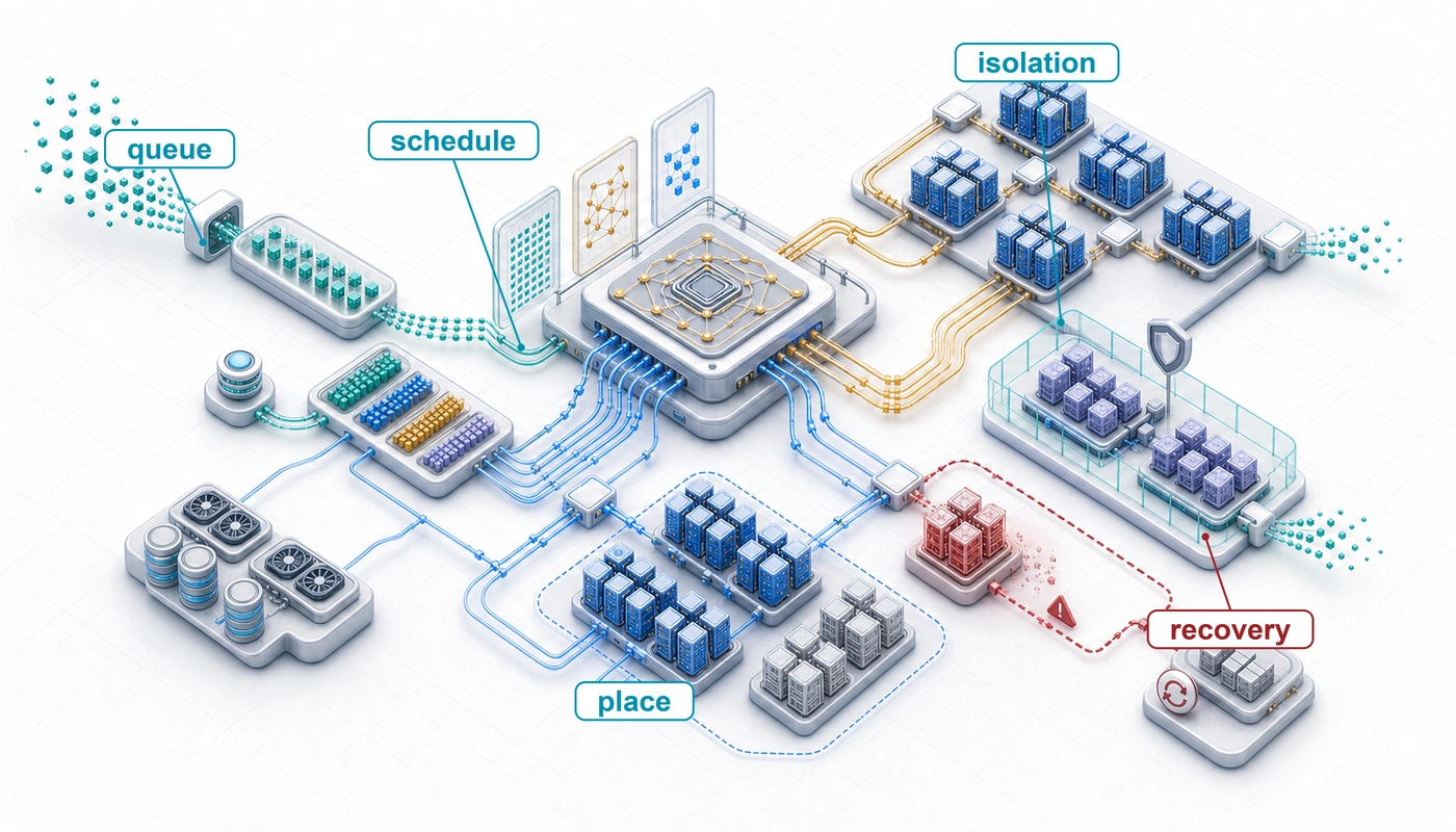
Purpose

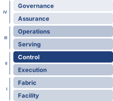
Fleet stack focus for this chapter.

Why can jobs wait while expensive accelerators sit idle?

A thousand idle accelerators still incur ownership or reservation costs while queued experiments make no progress. More hardware does not resolve that waste when available resources cannot form the groups that pending jobs need. Free devices may be scattered across machines with unsuitable connections, or several jobs may each hold resources while waiting for the rest. On one machine, improving execution usually begins with the work already running. Across a shared fleet, useful progress also depends on which work can start, how long it waits, and what other work its allocation displaces. A short experiment needs a timely result, a long training run needs continuity, and a serving workload needs capacity before requests miss their deadlines. Favoring any one claim without considering the others can leave the fleet busy while delaying the results it exists to produce. Interrupting a job can free capacity, but preserving its state and restoring progress consume time and bandwidth. Waiting for a better placement can accelerate execution while extending completion time. Fair access therefore cannot be judged from device counts alone, and high utilization cannot establish that capacity is being used well. The engineering challenge is to honor these competing claims under changing demand and uncertain resource availability, while keeping the allocation process itself reliable. In C³ terms, orchestration pays coordination overhead to turn compute and communication capacity into useful progress while preserving fairness and latency headroom.

Learning Objectives

Explain how batch and declarative control planes admit, place, and reconcile allocations under stale state and partial failure
Apply gang, multi-dimensional fit, and topology constraints before dominant-resource fairness to find allocations a job can run
Analyze conflicts among throughput, latency, fairness, and cost using slowdown, queueing delay, and ML-specific scheduling signals
Design topology-aware placements that map tensor-, pipeline-, and data-parallel groups onto NVLink domains and switch tiers
Design elastic, preemption, and spot policies whose throughput or price gains repay their transition and interruption costs
Diagnose utilization losses by separating allocated, active, and productive capacity and tracing each gap to its cause
Evaluate serving-capacity and quota policies that balance serving headroom, team guarantees, and reclaimable borrowed capacity

8.1 The Scheduling Problem

Consider two research teams sharing a 1,000-GPU cluster: Team A submits a 512-GPU job that will run for a month, while Team B submits hundreds of 8-GPU experiments that each run for an hour. If the scheduler continually admits whichever jobs fit, Team B’s small experiments can indefinitely block Team A’s large training run. The scheduling problem is to resolve this conflict among throughput, fairness, and cluster utilization.

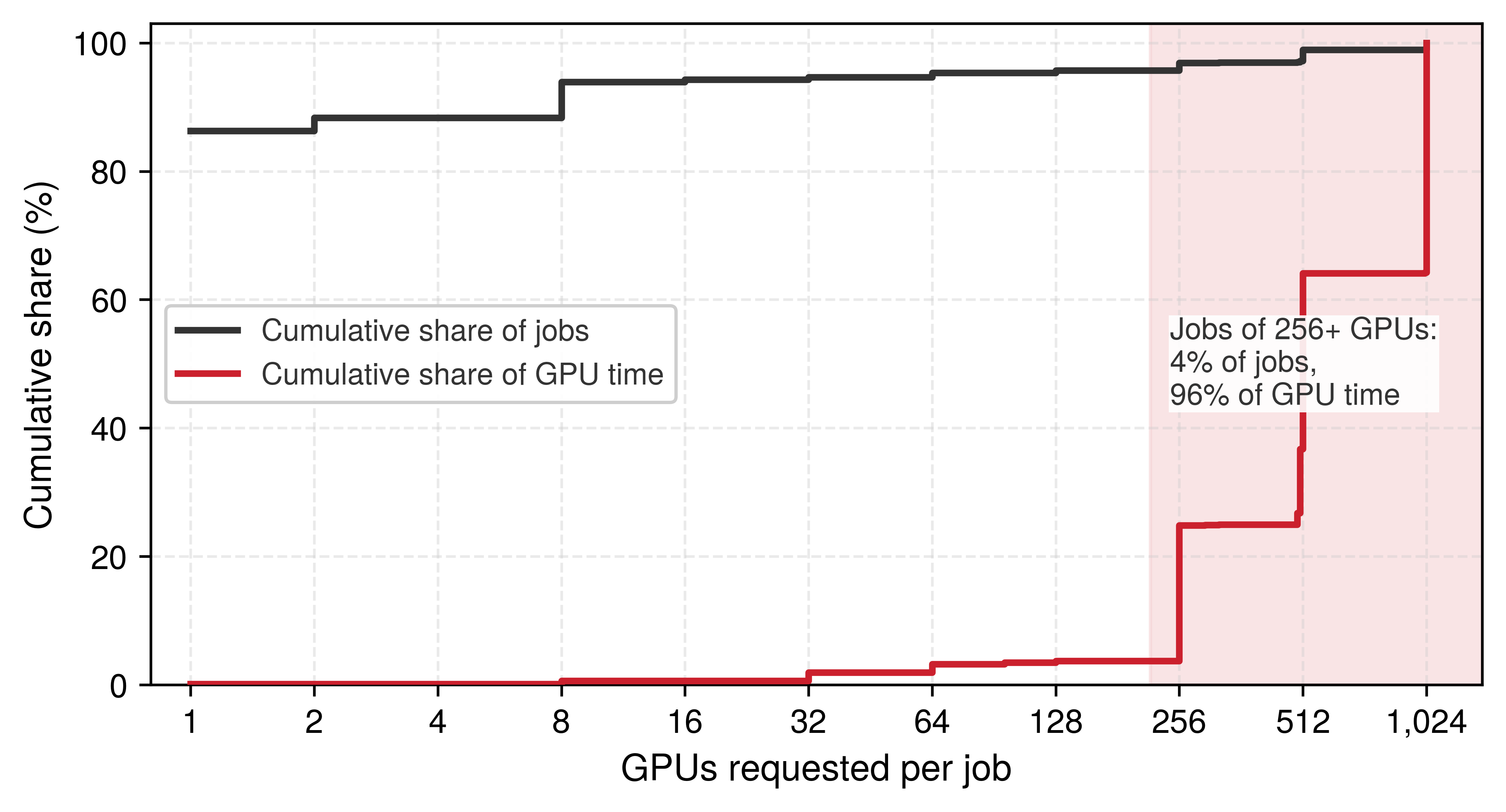
Production traces show that this mix is the normal case rather than a contrived one. In the Kalos cluster that Shanghai AI Laboratory used for language-model development in 2023, 86 percent of 19,907 GPU jobs requested a single GPU, yet together they consumed 0.1 percent of the cluster’s GPU time. Jobs of 256 GPUs or more made up 4 percent of submissions and consumed 96 percent of GPU time (Hu et al. 2024), two distributions that figure 1 plots side by side. Counted by jobs, the cluster is a stream of small experiments; counted by GPU-hours, it is a few percent of jobs that hold nearly all the accelerators. A scheduler must serve both views at once, which is why fairness, packing, and preemption policies cannot be judged by either count alone.

Figure 1: **Jobs versus GPU Time by Job Size**: Cumulative share of GPU jobs (gray) and of GPU time (red) against the number of GPUs each job requested, for the Kalos LLM-development cluster from March to August 2023. Almost every job is small, while almost all GPU time goes to jobs of 256 GPUs or more. Data from the AcmeTrace release of Hu et al. (2024).

Synchronizing workers efficiently (Collective Communication), partitioning computation across them (Distributed Training), and recovering from hardware failures (Fault Tolerance) solve the single-job scaling problem, but each of those mechanisms assumed that the job already held its accelerators. Fault tolerance assumed more than that. Its recovery paths drew on a spare pool deep enough to replace a drained node and on spot capacity whose loss the job could absorb, and neither exists unless something outside the job grants it, holds it in reserve, or takes it back. That something is orchestration, the policy that decides which jobs run, where they run, when one is preempted for another, and how competing demands share the fleet. A useful allocation must first be feasible, then worth granting under the fleet’s fairness, latency, and cost objectives. That ordering motivates the progression from admission and packing constraints to control-plane designs, topology-aware placement, elastic and cost-aware policies, schedulers built around ML workload signals, and finally the serving and multi-tenant contracts under which many owners share one fleet. Training and serving draw on the same fleet, so the capacity envelope this chapter allocates is the one both depend on; how a serving system spends its share, request by request, is the subject of Serving at Scale.

In the fleet stack (shown in the margin), orchestration occupies the Reliability & Control row of the distribution band, but the infrastructure band beneath it constrains its decisions. The scheduler must account for GPU heterogeneity, NVLink topology, rack power limits, and network bisection bandwidth. When scheduling goes wrong, debugging can require examining all four bands to identify whether the root cause lies in infrastructure (hardware constraints), distribution (algorithm limitations), serving (workload mismatch), or governance (policy misconfiguration). Orchestration connects physical infrastructure to distributed algorithms, translating resource requests into placements that respect both hardware topology and organizational policy.

The same conflict grows with the fleet. Consider a research organization operating a 10,000-GPU cluster. A single pretraining run of a GPT-3-class 175B-parameter model (Brown et al. 2020), the running instance of Archetype A (GPT-4/Llama-3) throughout this book, can hold a 1,024-GPU allocation for weeks. Because the scaling laws of AI Scaling Laws reward larger models trained on more tokens, each new generation of such runs asks for a larger gang held for longer, so the scheduler’s hardest requests keep growing. Suppose enough jobs of that class are queued that together they ask for more GPUs than the cluster holds, alongside thousands of smaller experiments and inference workloads all competing for the same resources. The system must decide which jobs run, when they run, and where they run. A first-come-first-served policy without backfilling or preemption can let large jobs occupy the cluster for weeks, delaying smaller experiments that researchers need to iterate quickly. A fair-share policy that divides capacity without respecting each job’s minimum resource bundle can leave many partial allocations and no runnable large job.

Brown, Tom B., Benjamin Mann, Nick Ryder, Melanie Subbiah, Jared Kaplan, Prafulla Dhariwal, Arvind Neelakantan, et al. 2020. “Language Models Are Few-Shot Learners.” Advances in Neural Information Processing Systems 33: 1877–901. https://doi.org/10.48550/arxiv.2005.14165.

↩︎ Archetype A and its 175B-parameter running instance are established in Archetype A (GPT-4/Llama-3).

The economic stakes make these decisions consequential at every scale. A continuously provisioned 10,000-GPU cluster, valued at the chapter’s cloud-equivalent rate of $2/GPU-hour, represents $480,000 per day in capacity, whether the GPUs are computing useful work or sitting idle while jobs wait in a queue. If scheduling inefficiencies leave 30 percent of GPUs idle, that translates to $144,000 per day in unused capacity value, or about $52.6M annually. Holding useful work per active GPU-hour constant, improving utilization from 50 percent to 80 percent adds 3,000 fully active GPU-equivalents of productive capacity without purchasing additional hardware. That count measures the gain in useful work. Procurement planning asks a different question, namely how much hardware the gain replaces, and for that comparison the answer is 6,000 raw GPUs, because new GPUs run under the same scheduling policy would also reach only 50 percent utilization. Recovered capacity becomes cash savings only when it avoids purchases or billed resource time. Scheduling can therefore increase the useful work delivered by an existing investment, even when the fleet’s immediate expenditure remains unchanged.

Workload semantics, rather than an ML-versus-high-performance computing (HPC) boundary, determine scheduling flexibility. Rigid synchronous jobs in both domains require a fixed set of co-scheduled ranks, whereas malleable jobs can make progress across a declared range of resource counts. Gang scheduling¹ represents the critical allocation constraint for a rigid training group: a job configured to require 1,024 GPUs cannot complete its distributed iterations with only half of them. Malleable data-parallel training can instead vary its replica count at explicit reconfiguration boundaries, but tensor- and pipeline-parallel groups usually retain a rigid base allocation. The scheduler must therefore model each job’s minimum viable gang and permitted resize points rather than infer rigidity from the workload’s field.

¹ Gang scheduling: Formalized by Ousterhout (1982) for parallel systems, where the “Ousterhout matrix” co-schedules related threads across processors in synchronized time slices. In a rigid ML training group, incomplete allocation prevents collective completion, so held resources can remain idle until the missing ranks launch.

Ousterhout, John K. 1982. “Scheduling Techniques for Concurrent Systems.” Proceedings of the 3rd International Conference on Distributed Computing Systems (ICDCS), 22–30.

² Placement group: A cloud-native abstraction that requests instances be placed within a high-bandwidth, low-latency network domain. For the ML Fleet, placement groups reduce placement scatter and may expose higher network limits than unconstrained placement. They do not guarantee workload-level bisection bandwidth: topology oversubscription, concurrent traffic, routing, and the collective pattern still determine delivered AllReduce bandwidth.

If gang scheduling determines which resources must be available together, topology awareness via placement groups² determines how efficiently they can communicate. Tensor-parallel groups benefit from placement within a high-bandwidth NVLink domain; a placement across slower links must still meet the job’s communication budget. Two allocations of the same size can therefore deliver very different useful throughput.

GPU heterogeneity is the third dimension. Many clusters contain mixtures of A100 and H100 accelerators with different compute throughput and interconnect bandwidth. Their training-throughput ratio depends on the workload, numerical precision, and communication path, so the scheduler needs measured performance and the applicable allocation cost. Memory capacity adds a hard admission test once pools differ in it. The common A100 and H100 variants both carry 80 GB of high-bandwidth memory (HBM), but smaller-memory variants of the same accelerator and older generations often share the fleet, and a job whose working set fits only the larger devices cannot run on the rest at any priority. The debugging example in section 8.12 returns to exactly such a mixed fleet. The scheduler must match workloads to appropriate hardware based on actual requirements, not user preferences, while maintaining high utilization across heterogeneous pools. When users request specific GPU types out of habit rather than necessity, the mismatch between requested and required resources can leave entire hardware pools idle while queues overflow on preferred hardware.

Job duration unpredictability compounds these challenges further: a training run may converge early and complete in days rather than weeks, hardware failures may abort jobs and return resources at unpredictable times, and hyperparameter searches may terminate unpromising configurations early. In both ML and scientific computing, fixed-step jobs with stable iteration times permit better release-time estimates than jobs whose stopping conditions or execution rates vary, so the scheduler must distinguish an estimated completion time from an enforced runtime limit when deciding whether another job can safely use a temporary gap in capacity.

The interaction between these challenges creates combinatorial complexity. A scheduler must simultaneously handle gang scheduling constraints (atomic allocation), heterogeneous resources (capability matching), topology requirements (NVLink locality for tensor parallelism), priority and fairness policies (organizational equity), preemption decisions (which running jobs to interrupt), and cost optimization (spot vs. on-demand placement). Each dimension constrains the others: a topology-optimal placement may violate fairness policies, a cost-optimal spot placement may violate reliability requirements, and a fairness-driven allocation may fragment resources in ways that prevent gang scheduling. The scheduler therefore does more than pack jobs onto GPUs; it must maintain a consistent, economically useful view of a failing, heterogeneous fleet, and at that scale placement stops being only an optimization problem and becomes a distributed systems problem of keeping state coherent across thousands of machines.

Self-Check: Question

In the Kalos language-model cluster trace, most jobs requested a single GPU yet consumed a tiny share of GPU time, while jobs of 256 or more GPUs were a few percent of submissions and consumed nearly all GPU time. What does this distribution imply for judging a scheduling policy?
1. Judge the policy by job count alone, because most users submit small jobs.
2. Judge the policy by GPU-hours alone, because large jobs hold nearly all of the capacity.
3. Judge the policy under both views, because small jobs set most users’ waits while a few large gangs hold most of the capacity.
4. Treat the distribution as an artifact of one cluster, because production fleets have uniform job sizes.
A 10,000-GPU cluster raises utilization from 50 percent to 80 percent with no new hardware, holding useful work per active GPU-hour constant. Why does the gain count as 3,000 productive GPU-equivalents but replace 6,000 raw GPUs, and when does it become a cash saving?
True or False: Whether a job must be scheduled as a rigid gang follows from whether it is labeled an ML training job or an HPC job.

See Answers →

8.2 Distributed Scheduling Complexity

A single-machine scheduler works inside one operating-system boundary, where three properties hold closely enough to design around: it observes resource state directly and consistently, its allocation decisions take effect atomically, and failures are nearly binary (the machine is up or it is down). Device faults and delayed cleanup still occur, but they do not hide behind a network. A cluster scheduler surrenders all three properties. It coordinates independent nodes through delayed messages and uncertain observations, so an authoritative allocation decision does not establish that every node has received or completed it, and several distributed systems problems emerge from that gap.

Partial failures pose the first challenge. A node can fail between allocation and job start, creating a gap between the scheduler’s decision and its effect. The scheduler may successfully allocate 32 GPUs across 4 nodes, only to have one node fail before the job launches. The remaining 24 GPUs sit idle while the scheduler detects the failure, updates its state, and re-plans the allocation. Meanwhile, other jobs that could have used those 24 GPUs have already been placed elsewhere, potentially on suboptimal hardware. Before the first training step, recovery must repair allocation and launch state even though no new model progress exists to restore. Once execution begins, resource recovery must also coordinate with the framework’s checkpoint and membership mechanisms.

Network partitions create a second problem. The scheduler may lose connectivity to a subset of nodes while those nodes continue operating normally. From the scheduler’s perspective, their status is uncertain; from the nodes’ perspective, jobs may still be running and producing useful work. Reallocating their GPUs risks double allocation if the partition heals while the old work still runs; waiting for reconnection leaves possibly healthy capacity idle. The partition’s duration cannot be known in advance, so any fixed timeout is a guess about network behavior that may prove wrong. A timeout can trigger recovery, but it does not prove that the old execution has stopped. Reusing a GPU therefore requires confirmed cleanup or an enforced revocation of the old allocation. Restarting a job on reachable replacement nodes also requires fencing stale attempts from shared outputs. The recovery policy can choose how long to wait for reconnection, but each choice must preserve exclusive ownership where the workload requires it.

State inconsistency emerges as a third challenge that compounds the first two. Resource state may differ between the scheduler’s view and reality on individual nodes. A GPU the scheduler believes is free may still be cleaning up from a previous job: flushing caches, deallocating device memory, running a zombie process from a failed container, or completing a CUDA driver reset after an error. Conversely, a GPU marked as “in use” may have been freed by a job that terminated between heartbeat intervals. This inconsistency means the scheduler operates on a model of cluster state that is always slightly stale, and the degree of staleness varies across nodes depending on heartbeat frequency, network latency, and the complexity of cleanup operations.

Ordering without global time presents the fourth fundamental issue. Allocation messages issued before and after a partition can arrive out of order. Logical timestamps can describe an order, but do not by themselves prevent conflicting ownership. The control plane must serialize conflicting allocation decisions, and the resource manager must reject stale allocation generations before acting on them. Otherwise, an old launch request can revive work after a newer allocation has taken ownership.

These four challenges echo the CAP theorem of The CAP theorem reality, under which a partitioned system cannot guarantee both consistency and availability. CAP is a theorem about distributed data systems, not a literal proof about every scheduler, but the analogy draws attention to which allocation decisions remain safe when nodes cannot communicate. Slurm, an HPC workload manager, and Kubernetes, a container orchestration platform, both need authoritative allocation records and mechanisms that reconcile those records with execution. Optimistic concurrency permits schedulers to plan against potentially stale snapshots, then validate proposed changes before committing them. Rejecting a conflicting proposal costs scheduling work; accepting conflicting ownership would violate a different, essential invariant.

The control-plane tension becomes concrete when the scheduler interacts with the ML framework’s own distributed coordination plane during a partition. A scheduler may decide that a subset of nodes is unavailable while workers on those nodes are still blocked inside a collective operation. That creates a brief window of conflicting intent: the scheduler wants to recover the allocation, but the training job has not yet converged on a new membership view. Elastic launch and rendezvous mechanisms such as TorchElastic reduce this ambiguity by using heartbeats and re-rendezvous so the framework can either reform a viable worker group or terminate cleanly, giving the scheduler a clearer recovery signal than an opaque collective timeout (PyTorch Contributors 2026b, 2026a). This layered coordination, with scheduler-level policy for coarse allocation and framework-level membership for workers, is the characteristic architecture of production distributed training clusters.

PyTorch Contributors. 2026b. Torchrun (Elastic Launch). PyTorch documentation.

PyTorch Contributors. 2026a. Torch Distributed Elastic Rendezvous. PyTorch documentation.

8.2.1 Admission, placement, and reconciliation

When a single undifferentiated queue mixes quota checks, hardware binding, and crash recovery, operators cannot tell whether a pending job is blocked by team quota, fragmented topology, or a dead node whose lease has not yet expired, and a stale retry can assign the same accelerators to two jobs at once. A scheduler control plane avoids this ambiguity by separating three decisions. Admission control decides whether a job may enter the runnable set under quota, priority, gang, and safety constraints. Placement binds an admitted job to a feasible set of nodes while accounting for accelerator capability, topology, power, storage, and network capacity. Reconciliation compares desired allocations with observed node and job state, then starts, retries, evicts, or fences work until the two agree. Keeping these stages explicit makes it possible to distinguish admission denial from placement failure, while versioned decisions and resource-level enforcement prevent stale observations from authorizing competing owners.

Control-plane architectures distribute these decisions differently (Hindman et al. 2011; Burns et al. 2016). A centralized scheduler serializes admission and placement against one authoritative state, which simplifies conflict handling but concentrates scheduling latency and failure impact. A two-level design offers resources to framework schedulers, gaining policy specialization at the cost of delayed or rejected offers. A shared-state design lets several schedulers plan concurrently against a common state and resolves conflicts through version checks or optimistic concurrency. In every design, reconciliation closes the loop. Node agents must enforce allocation generations and lease validity so that an old decision cannot revive after a newer placement has taken ownership.

Hindman, Benjamin, Andy Konwinski, Matei Zaharia, Ali Ghodsi, Anthony D. Joseph, Randy Katz, Scott Shenker, and Ion Stoica. 2011. “Mesos: A Platform for Fine-Grained Resource Sharing in the Data Center.” 8th USENIX Symposium on Networked Systems Design and Implementation (NSDI 11), 295–308.

Feasibility also extends beyond free accelerator count. Power-aware admission rejects or delays a placement whose worst-case draw would exceed a rack or facility envelope; relying on average draw risks correlated throttling when colocated jobs enter compute-heavy phases together. I/O-aware placement treats dataset-read and checkpoint-write bandwidth as reservable capacity, so a gang that fits in GPU memory does not start where concurrent input pipelines or checkpoint bursts will saturate the same storage path. These constraints can deliberately leave accelerators idle. The idle capacity is the cost of preserving the power and data-movement budgets required for the admitted jobs to make progress.

8.2.2 Failure as a scheduling input

A scheduler that allocates 10,000 GPUs as if every granted node will stay healthy until the job finishes will see a multi-thousand-GPU training gang stall every few hours waiting for replacement capacity that was already handed out to other workloads. As The Mathematics of Inevitable Failure established, the fleet failure rate is the per-device rate multiplied by the population (equation 7.4), so a cluster of ten thousand GPUs loses a device every few hours (Cluster MTBF Scaling). Where fault tolerance turns that failure rate into checkpoints, detection, and elastic recovery for a running job, the scheduler must plan for failure in every allocation decision. It uses two failure rates: it sizes spare capacity and replacement paths from the GPU-only count of devices it must replace, while job interruptions follow the shorter full-system interval of Cluster MTBF calculation, which adds PCIe and network failure domains.

The scheduler cannot treat the cluster as a static resource pool where resources, once allocated, remain available until voluntarily released. It must anticipate loss of allocated resources during execution and provide replacement capacity or rescheduling paths. The response depends on the fault and the validity of the surviving state. A transient disruption may permit recovery in place if the execution state remains usable; a persistent hardware failure requires replacement resources. Even a short disruption can force checkpoint recovery if the framework cannot safely continue (Tiwari et al. 2015).

Tiwari, Devesh, Saurabh Gupta, James Rogers, Don Maxwell, Paolo Rech, Sudharshan Vazhkudai, Daniel Oliveira, et al. 2015. “Understanding GPU Errors on Large-Scale HPC Systems and the Implications for System Design and Operation.” 2015 IEEE 21st International Symposium on High Performance Computer Architecture (HPCA), 331–42. https://doi.org/10.1109/hpca.2015.7056044.

When a node heartbeat is missed, the scheduler faces three recovery policies with different delay and capacity costs. It can wait to see whether the heartbeat resumes, though this delays recovery if the machine has permanently crashed. It can instead begin recovery promptly on replacement resources, provided stale execution is fenced before conflicting work resumes. An intermediate approach marks the node as suspect and prepositions replacement capacity while checking its status; this reduces launch delay if replacement becomes necessary, but holds capacity that could otherwise serve pending work. Whichever policy it picks, reuse of the node’s GPUs still waits on the fencing that network partitions require. Historical failure and recovery measurements set how long to wait and how much replacement capacity to hold. The recovery-time decomposition of fault tolerance (equation 7.10) shows where scheduler policy intervenes most effectively. Of its detection, restart, load, and warmup terms, the scheduler owns most of $\JobRestartTime$, the time to allocate replacement resources and launch processes, and that is the term its spare-capacity policy shortens. Waiting longer on a missed heartbeat lengthens $\FailureDetectionTime$ in exchange for avoiding a needless restart, so the wait is worth extending only while a transient fault remains more likely than a permanent one.

↪ The same decomposition in scheduler-facing phases (detect, reschedule, reload, and replay of work since the last checkpoint) is developed in The anatomy of recovery time.

These requirements connect the scheduler directly to checkpoint and recovery infrastructure. Scheduling decisions about spare capacity, preemption policies, and elastic training support determine how quickly the system recovers from statistically expected failures. A scheduler that reserves spare capacity or supports elastic recovery can restore throughput much faster than one that requires every failed job to wait for a full fresh allocation and reload. The reserve fraction follows from the measured failure rate and recovery time of the fleet’s own workloads.

↩︎ Failure detection, recovery procedures, and spare pools are established in Failure Detection and Recovery.

Self-Check: Question

A scheduler control plane separates admission control, placement, and reconciliation. State what each decides, and explain why keeping them separate helps an operator diagnose a job that has not started.
A network partition cuts the scheduler off from four nodes running a training job, and their heartbeats time out. What must hold before the scheduler reassigns those nodes’ GPUs to another job?
1. Nothing beyond the timeout, because a missed heartbeat proves the old processes have stopped.
2. The old allocation must be revoked with confirmed cleanup or fenced, for example by rejecting stale allocation generations, so the old work cannot keep using or writing through those GPUs.
3. The partition must heal first, because no recovery may begin while nodes are unreachable.
4. The new job must run at higher priority, because priority resolves conflicting ownership.
True or False: A hypothetical per-device annual hardware-fault probability of 0.001 is sufficient to conclude that all-cause interruptions will remain rare during multi-week jobs on a 10,000-GPU fleet.

See Answers →

8.3 Scheduling Objectives and Their Conflicts

Giving a large training gang an unbroken allocation for weeks amortizes launch and data-movement overhead, but leaves short interactive debugging jobs waiting hours in the queue; preempting the large gang so short jobs start immediately burns cluster capacity on checkpoint saves and restarts. Every scheduling policy trades four competing objectives against one another: throughput, fairness, latency, and cost efficiency. Throughput benefits from allocations that sustain useful work and amortize launch, interruption, and data-movement overhead; a large allocation helps only while the job scales effectively. Maintaining fairness demands an equitable distribution of resources across competing tenants to prevent a single dominant project from monopolizing the fleet; dominant resource fairness (Ghodsi et al. 2011) formalizes this balance by equalizing each tenant’s largest normalized share across GPUs, CPU, and memory. Reducing queue latency helps short, interactive jobs complete promptly, but aggressive preemption can repeatedly interrupt long-running training. Pursuing cost efficiency introduces different costs for different policies: spot capacity risks interruption, off-peak scheduling delays admission, and dense packing can increase interference. Each policy must be evaluated against useful work completed and the delays it imposes.

Fairness requires an outcome metric rather than an input quota rule alone. For job $\JobIndex$, slowdown $\JobSlowdown_j=(\JobQueueWaitTime_j+\IsolatedJobRunTime_j)/\IsolatedJobRunTime_j$ compares its queueing-plus-running time with its isolated runtime $\IsolatedJobRunTime_j$, assuming the running time is unchanged by sharing; a one-hour job that waits nine hours has $\JobSlowdown_j=10$, even if its team eventually receives its nominal GPU share. When contention or resizing changes execution time, the numerator must instead use the observed queueing-plus-running duration while the denominator retains the isolated baseline. A scheduler should report the distribution of slowdown by user and job class, together with the age of the oldest pending feasible job. Dominant-share parity detects unequal resource allocation, slowdown exposes unequal delay, and the maximum feasible wait exposes starvation risk. These metrics separate a policy that is fair in allocated GPU-hours from one that is fair in the time users wait to obtain useful results.

Each of the four objectives, pursued alone, schedules the same pool differently and gives up something the others protect (figure 2). Favoring a large unbroken allocation can delay short experiments, while repeatedly admitting short jobs can prevent a large gang from assembling. These conflicts depend on the workload and available capacity; improving one objective does not necessarily worsen every other objective. Resource-share fairness and completion-delay fairness therefore need separate measurements.

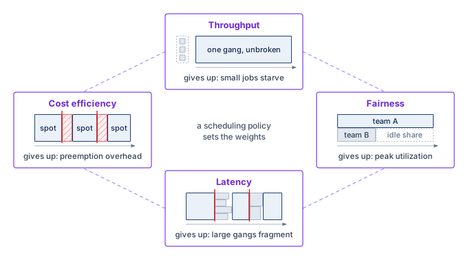
Figure 2: **Scheduling Trade-Offs across Competing Fleet Objectives**: A four-way trade-off diamond (Throughput, Latency, Fairness, Cost Efficiency) illustrates the tensions governing cluster scheduling. Throughput favors long, unbroken runs; Latency favors aggressive preemption for interactive jobs; Resource-share fairness can constrain placement to equalize shares; and Cost Efficiency uses discounted, interruptible capacity. Each vertex sketches a four-GPU pool over time as that objective would schedule it and names a possible cost of favoring it; the conflicts depend on workload and available capacity.

Consider a 64-GPU fine-tuning run of the same 175B-parameter model, a far smaller allocation than its 1,024-GPU pretraining run. If it sustains high utilization for days, an uninterrupted allocation amortizes launch overhead across a long execution. Admitting it may nevertheless require draining 64 suitably placed GPUs, delaying smaller experiments. Conversely, repeatedly filling available gaps with short jobs can prevent the large job from assembling its required group. Preemption or resizing can recover flexibility only if the job supports the transition and its cost is acceptable. The policy must therefore compare useful throughput with completion delay for both job classes. In scheduler terminology, those choices often appear as quality-of-service classes: job-priority tiers that decide which objective wins when throughput, latency, fairness, and cost collide.

Queueing adds a further conflict between utilization and latency, because a fleet run close to full load leaves arriving jobs little spare capacity. In a single-server queue with random arrivals, mean waiting time, expressed as a multiple of the mean job duration, is the product of a load factor $\ServingUtilization/(1-\ServingUtilization)$ and a variability factor $(1+\ServiceTimeVariationCoefficient^2)/2$, where $\ServingUtilization$ is offered load relative to service capacity and $\ServiceTimeVariationCoefficient$ is the coefficient of variation of job duration. The load factor stays small through moderate load and grows without bound as load approaches capacity, so waiting time bends sharply upward near saturation instead of rising in proportion to utilization. The variability factor scales the whole curve. A queue that mixes minute-long debugging jobs with week-long training runs waits several times longer at the same load than a queue of similar-length jobs, so each added point of utilization costs more waiting time in an ML fleet than in a uniform one. Notebook 8.1 derives the relation and prices both factors.

Napkin Math 8.1: The queuing theory of GPU clusters

To isolate the effect of runtime variability, consider an M/G/1 queue with first-come-first-served service. Kendall notation names the queue by its arrival process, service-time distribution, and server count: M for memoryless (Poisson) arrivals, G for a general service-time distribution, and 1 for a single server. Treating a fleet as one server means modeling its aggregate capacity as a single resource that works through one job at a time, with each job’s service time equal to its GPU-hours divided by the fleet’s GPU count. That mapping ignores gang packing and parallel admission, so it isolates the variability effect rather than predicting a real fleet’s wait. Jobs arrive according to a Poisson process $(\ArrivalRate)$, and independent service times follow a general distribution $(\Glyph{G})$ with mean $1/\ServiceRate$ and finite standard deviation $\ServiceTimeStandardDeviation$. When offered load is below service capacity, the Pollaczek-Khinchine formula gives the steady-state expected waiting time in the queue $(\QueueWaitTime)$:

\[ \frac{\QueueWaitTime}{1/\ServiceRate} = \frac{\ServingUtilization}{1-\ServingUtilization} \cdot \frac{1+\ServiceTimeVariationCoefficient^2}{2} \]

Here, $\ServingUtilization = \ArrivalRate/\ServiceRate$ represents offered load relative to the model’s service capacity, $1/\ServiceRate$ is the average job duration, and $\ServiceTimeVariationCoefficient= \ServiceTimeStandardDeviation\ServiceRate$ is the coefficient of variation of job duration. The right-hand side is therefore the waiting time expressed as a multiple of the average job duration; a fleet’s measured GPU-busy percentage is not automatically this model’s load.

An exponential service-time distribution provides a reference case, yielding $\ServiceTimeVariationCoefficient\approx 1$. A mixed ML queue can have much greater variability when short debugging jobs measured in minutes share capacity with training runs measured in weeks. The representative $\ServiceTimeVariationCoefficient=3$ calculation in this callout captures that variability without claiming a universal fleet constant. The impact on wait times is multiplicative. For the scheduling argument here, the single-server multiplier is sufficient; Queuing theory for batched inference develops an explicit single-server surrogate for batched serving and explains why multi-server, finite-buffer M/G/c/K systems require additional modeling.

At 80 percent utilization $(\ServingUtilization = 0.8)$: with an exponential workload $(\ServiceTimeVariationCoefficient= 1)$, $\QueueWaitTime=$ 4 $\times$ the average job duration. With an illustrative high-variability workload $(\ServiceTimeVariationCoefficient= 3)$, $\QueueWaitTime=$ 20 $\times$ the average job duration. In this M/G/1 model, service-time variability multiplies waiting time at the same offered load. The example does not prescribe a universal GPU-utilization threshold or model gang placement directly. It explains why capacity planning needs the service-time distribution and queue-delay objective as well as average load.

Self-Check: Question

A one-hour job waits nine hours in the queue and then runs for its isolated runtime of one hour. Its ____, the ratio of its queueing-plus-running time to its isolated runtime, is 10, even if its team eventually receives its nominal GPU share.
Two teams receive equal dominant shares of the fleet over a month, yet one team’s jobs routinely wait days. Which measurements expose this unfairness, and why does share parity miss it?
Based on the Pollaczek-Khinchine queue model $\frac{W_q}{1/\mu} = \frac{\rho}{1-\rho} \cdot \frac{1+C_s^2}{2}$, under this illustrative single-server approximation, how does a queue with heavy-tailed job durations ($C_s = 3$) operating at $\rho = 0.8$ utilization compare in expected waiting time ($W_q$) to a queue with the same mean service time and exponential durations ($C_s = 1$) at the same utilization?
1. The ML cluster experiences a $2\times$ increase in expected wait time ($8\times$ vs. $4\times$ the average job duration).
2. The ML cluster experiences a $5\times$ increase in expected wait time ($20\times$ vs. $4\times$ the average job duration).
3. The ML cluster experiences a $9\times$ increase in expected wait time ($36\times$ vs. $4\times$ the average job duration).
4. The ML cluster experiences no change in expected wait time because utilization $\rho$ dominates the Pollaczek-Khinchine denominator.

See Answers →

8.4 Core Allocation Constraints

A scheduling objective can only choose among allocations that a job can actually run. Fairness must be computed across every resource a tenant consumes, a request must fit every dimension of the node that receives it, a rigid group must arrive whole, and the resources each job holds must not block one another. Each of these constraints narrows the feasible set before any objective selects within it.

8.4.1 Dominant-resource fairness allocation

Equalizing GPU counts alone fails when one tenant’s jobs saturate host CPU and memory while another’s saturate the network fabric, leaving free GPUs unusable behind exhausted auxiliary resources. Dominant-resource fairness (DRF) makes a multi-resource entitlement comparable by normalizing each tenant’s allocation against fleet capacity and taking its largest share (Ghodsi et al. 2011). Consider the deliberately small cluster in table 1: 8 GPUs, 32 CPU cores, 256 GB of memory, and 80 Gb/s of network capacity. Tenant A’s replica requires 1 GPU, 4 cores, 32 GB, and 10 Gb/s; Tenant B’s distributed worker requires 2 GPUs, 2 cores, 16 GB, and 20 Gb/s.

Ghodsi, Ali, Matei Zaharia, Benjamin Hindman, Andy Konwinski, Scott Shenker, and Ion Stoica. 2011. “Dominant Resource Fairness: Fair Allocation of Multiple Resource Types.” 8th USENIX Symposium on Networked Systems Design and Implementation (NSDI 11), 323–36.

Table 1: Worked DRF Allocation: Progressive filling gives Tenant A four one-GPU replicas and Tenant B a pair of two-GPU workers. Both tenants reach a dominant share of 0.50 even though their CPU and memory allocations differ. GPUs and network are jointly saturated; CPU and memory remain available but cannot increase either allocation without exceeding a saturated resource.

Tenant	Allocation	GPU share	CPU share	Memory share	Network share	Dominant share
A	4 replicas	$4/8=0.50$	$16/32=0.50$	$128/256=0.50$	$40/80=0.50$	$0.50$
B	2 workers	$4/8=0.50$	$4/32=0.125$	$32/256=0.125$	$40/80=0.50$	$0.50$

For tenant $\TenantIndex$, define its dominant share as $\DominantShare_i=\max_\ResourceTypeIndex(\TenantResourceAllocation/\FleetResourceCapacity)$, where $\TenantResourceAllocation$ is its allocation of resource $\ResourceTypeIndex$ and $\FleetResourceCapacity$ is fleet capacity for that resource. The calculation equalizes $\DominantShare_i$, not every resource share. One A replica raises A’s dominant share by $1/8$; one B worker raises B’s by $2/8$. Progressive filling therefore grants roughly two A replicas for each B worker until both dominant shares reach $0.50$. This is a fair policy target, but it is not yet a feasible placement. If B’s two workers form one four-GPU gang, the four GPUs must become available atomically; if tensor parallelism requires one NVLink domain, four free GPUs scattered across nodes do not satisfy the allocation; and if the job requires 80 GB HBM accelerators, four incompatible GPUs do not count at all. A production scheduler therefore applies capability, gang, and topology constraints to the feasible set, then uses DRF to choose fairly among allocations that can actually run. The order is not a convenience. Feasibility comes before fairness (principle 15) because a fair share of accelerators on which the job cannot run delivers no progress to the tenant who holds it. When no equal-share placement exists, the scheduler should report the constraint causing the deviation rather than silently presenting an infeasible entitlement as service delivered.

Lighthouse 8.1: Lighthouse archetypes: Placement changes fairness

The same resource share has different meaning across the three lighthouse workloads introduced in Three systems archetypes:

Archetype A (GPT-4/Llama-3) needs a rigid, topology-compatible gang. Fractional allocations below its minimum parallel configuration deliver no progress, so fairness must include maximum feasible wait for a contiguous placement rather than GPU-hours alone.
Archetype B (DLRM at Scale) couples accelerator memory to sparse-routing bandwidth. A nominal GPU allocation is infeasible when embedding shards or network capacity cannot follow it, so network and memory must enter the dominant share and placement must protect the serving-latency envelope.
Archetype C (Federated MobileNet) schedules participation rather than data-center GPUs. Eligibility filters for power, connectivity, and device capability can systematically exclude parts of the population, so fairness must be audited through participation and outcome rates across device and user groups, not equal device counts in a round.

The common rule is to define the feasible bundle first and assess fairness over useful progress second. Treating every accelerator or client as interchangeable would conceal the constraint that makes each archetype difficult.

8.4.2 Bin packing

Even when a cluster has dozens of free GPUs in total, a pending 8-GPU job will sit blocked if previous placements scattered those free GPUs in 1- and 2-GPU remnants across partially occupied nodes. Fitting jobs of varying sizes into fixed-capacity nodes without stranding capacity is an instance of bin packing.³ Because general bin packing is NP-hard, no known algorithm finds optimal solutions in polynomial time. Practical heuristics such as first-fit decreasing and best-fit decreasing offer tractable choices, but their performance depends on job sizes and placement constraints. How much usable capacity a heuristic recovers in a heterogeneous ML fleet has to be measured against that fleet’s job mix, because the classical guarantees cover only one-dimensional packing.

³ Bin packing: First-fit decreasing has a classical asymptotic $11/9$ approximation ratio for one-dimensional bin packing, with an additive constant in the finite-instance bound. That result does not guarantee the same ratio for ML placement with several resource dimensions, topology constraints, and indivisible gangs. A scheduler must evaluate its heuristic against feasible placements and the stranded capacity it leaves.

Consider a 64-node cluster with 8 GPUs per node, totaling 512 GPUs. If every job requires 6 GPUs within one node, only one such job fits per node, leaving 2 GPUs unused and reducing effective capacity for this workload to 75 percent. The remaining 2 GPUs per node cannot be combined across nodes into another feasible six-GPU allocation, although smaller compatible jobs could use them. With a mix of 1-GPU, 3-GPU, and 7-GPU jobs, fragmentation depends on the placement and the pending requests; total free capacity can exceed a waiting job’s demand while no individual node has enough space. Figure 3 maps this stranded capacity across an $8{\times}8$ allocation grid: although 19 slots (30 percent of cluster capacity, dashed white cells) sit idle across nodes 0 through 7, active allocations (J1 through J15) leave every node partially occupied, blocking a pending 8-GPU job that requires an entire unfragmented node.

ML placement is a multi-dimensional packing problem. Jobs require GPUs together with CPU cores for data preprocessing, host memory for data loading and augmentation pipelines, local SSD storage for dataset caching, and network bandwidth for gradient synchronization. A job requesting 4 GPUs, 32 CPU cores, and 256 GB of RAM may not fit on a node that has 4 free GPUs but only 16 free CPU cores because other jobs have consumed the host CPU for preprocessing. The scheduler must simultaneously satisfy all resource dimensions, and the job fits only if every dimension has sufficient capacity on the selected node. A bottleneck in any one dimension can therefore strand capacity in the others.

Locality constraints further restrict placement beyond simple resource availability. A training job may require tensor-parallel groups to remain within NVLink-connected nodes when its communication budget cannot tolerate the lower per-endpoint bandwidth of the external fabric (450 GB/s per direction intra-node vs. 50 GB/s per port inter-node). On this topology, where NVLink does not connect the nodes, a job requesting “4 GPUs with NVLink connectivity” cannot use 2 GPUs from node A and 2 from node B, even if all 4 GPUs are individually available and the total capacity is sufficient. These topology constraints turn resource counts into a placement problem where which specific resources are available matters as much as how many. A capacity-feasible packing must also pass the job’s locality constraints.

Schedulers address fragmentation through several complementary strategies, each targeting a different aspect of the problem. The first, backfill, lets smaller jobs run in the gaps while a large job waits for contiguous resources; section 8.4.3 develops it together with the reservation it must protect and the runtime estimates it depends on. A second strategy, periodic defragmentation, migrates or preempts low-priority jobs to consolidate free resources into contiguous blocks, analogous to memory compaction in operating systems. The scheduler identifies nodes where partial allocations leave stranded resources, preempts the jobs occupying those resources, and re-schedules them on nodes where they can be packed more efficiently. The cost includes state transfer and restart, plus replay of work not captured by a valid checkpoint. A graceful checkpoint can preserve recent progress, but still takes time and storage bandwidth. The scheduler must weigh these costs against the benefit of starting large jobs sooner, and low-demand periods reduce the number of competing jobs affected by the move.

A third strategy, over-subscription, admits more demand than a capacity dimension can sustain simultaneously, but only where the resource is divisible and the scheduler can bound interference. Average activity of a GPU’s streaming multiprocessors (SMs), its compute units, does not create fractional whole GPUs. A job that reserves device memory, requires an exclusive CUDA context, or belongs to a rigid gang still occupies its assigned device while kernels are idle. Statistical multiplexing can be safe for explicitly shareable CPU, network, storage, or partitioned GPU capacity when tenants have measured, weakly correlated peaks and enforceable limits. It is unsafe to convert 70 percent average GPU utilization into a 1.4$\times$ device overcommit ratio. Whole-device capacity should instead be recovered through preemption, elastic resizing, or an isolation mechanism such as Multi-Instance GPU (MIG) hardware partitioning or NVIDIA’s Multi-Process Service (MPS), which lets several processes’ kernels share one device, provided the scheduler models each mechanism’s memory, compute, and fault-sharing contract explicitly. Both reappear with the serving workloads they suit best in section 8.10.1.

Figure 3: **The Fragmentation Problem**: A snapshot of an 8-node cluster (rows) with 8 GPUs each (columns). Blue blocks mark the slots each active job holds (J1 to J15); dashed white cells are free, and the count at the right of each row gives that node’s free slots. Although 19 GPUs, roughly 30 percent of capacity, are free, every node still holds at least one busy slot, so the pending job above the grid, which needs a full node, cannot be placed. Fragmentation, not total capacity, sets what the scheduler can admit.

8.4.3 Gang scheduling

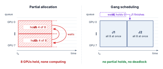
Partial allocation of rigid multi-GPU jobs creates a distributed scheduling failure mode in which two jobs each hold half the resources they need and block each other indefinitely while every allocated GPU sits idle. In the left panel of figure 4, jobs J1 and J2 each hold 4 of the 8 GPUs they require, and the whole pool stalls. Atomic gang scheduling (right panel) instead grants J1 all 8 GPUs as one allocation while J2 waits without holding any, which prevents this allocation deadlock.

Figure 4: **The Distributed Deadlock (Hold and Wait)**: In a non-gang scheduler (left), job J1 acquires half the cluster and waits for the rest, while job J2 acquires the other half and waits for J1 to release its GPUs. Neither can proceed, and 100 percent of the cluster sits idle. Gang scheduling (right) solves this by mandating atomic allocation: a job is either granted its entire $\DeviceCount$-GPU requirement simultaneously or it waits in the queue without holding any resources.

Definition 8.1: Gang scheduling

Gang scheduling is the ML cluster scheduling policy that atomically allocates the resources required by a job’s minimum viable execution group, so a rigid group either receives its complete allocation or waits without retaining a partial one.

Significance: A rigid synchronous job configured for 1,024 GPUs but holding only 512 GPUs completes zero training steps, not half as many: each collective stalls until every rank in its communication group arrives, so the held GPUs consume power and capital at zero useful output. Without atomic allocation, two such jobs can each acquire half the cluster and deadlock, both at zero progress while consuming the full cluster’s operating cost.
Distinction: Unlike a malleable service or parallel job that can make progress across a resource range, rigid synchronous training has step-function utility: the minimum viable gang or nothing. The distinction is a property of the execution graph, not of whether the workload is labeled ML, cloud, or HPC.
Common pitfall: A frequent misconception is that priorities or quotas alone solve this. Atomicity must extend to every co-scheduled resource the job needs to make progress (accelerators, high-bandwidth interconnect domains, network capacity for collectives); enforcing it at GPU granularity alone recreates the deadlock one resource layer down.

↩︎ Ring and tree AllReduce schedules, each of which completes only after every rank’s contribution has been reduced, are established in AllReduce Algorithms and Topologies.

⁴ Hold-and-wait: One of the four Coffman conditions (mutual exclusion, hold-and-wait, no preemption, and circular wait), all of which must hold for deadlock to occur (Coffman et al. 1971). Gang scheduling removes hold-and-wait through atomic allocation, which is why it prevents this deadlock by construction; the price is reduced packing flexibility.

Coffman, Edward G., Michael Elphick, and Arie Shoshani. 1971. “System Deadlocks.” ACM Computing Surveys 3 (2): 67–78. https://doi.org/10.1145/356586.356588.

The partial-allocation pattern is a hold-and-wait deadlock⁴ in which two jobs each hold half the cluster and neither can proceed. Its price is the whole allocation for as long as the cycle persists. At the scale of the chapter’s reference workload, two 1,024-GPU gangs that have each acquired 900 GPUs from a pool too small to complete either one burn about $1,800 per hour apiece. The limiting case is two jobs that each request the entire cluster, the example OpenAI used to motivate group admission (war story 8.1). On the 10,000-GPU cluster, a deadlock that strands every device wastes $20,000 per hour at the chapter’s rate while producing no progress for either job. Measured against the stake computed at the start of the chapter, raising utilization from 50 percent to 80 percent recovers about $144,000 per day in equivalent capacity value, so about 7 hours of such a deadlock erase a full day of that gain. Gang scheduling does not create the gain, but it protects it. For a rigid job $\RigidGangJob$ requiring $\DeviceCount$ GPUs, the scheduler must grant all $\DeviceCount$ GPUs atomically or leave the job queued without a partial allocation. This removes hold-and-wait for the resources covered by that allocation; it does not prevent later deadlocks in application code or auxiliary resources.

Naive gang scheduling is wasteful in predictable ways. Atomic allocation means the waiting job holds nothing, yet a large gang will never assemble if every freed GPU goes to a smaller job. The scheduler therefore places a reservation for the job at the head of the queue, draining capacity toward it by declining to start new work on GPUs that the gang will need. If the cluster has 900 free GPUs and that job requests 1,024, the reservation keeps the 900 GPUs idle until 124 more become available, potentially wasting thousands of GPU-hours. Backfill scheduling addresses this by identifying jobs in the queue that can fit within the 900 available GPUs without delaying the large job’s expected start time (figure 5), an idea popularized in the ANL/IBM SP scheduling system (Lifka 1995). A 128-GPU job with an estimated runtime of 2 hours is a backfill candidate if the 124 additional GPUs needed by the large job will remain unavailable for at least 2 hours. Protecting the reservation requires an enforced runtime bound or a preemption contract that releases the backfill allocation in time, including any checkpoint and cleanup delay. The estimate identifies an opportunity; the release contract makes the reservation enforceable.

Lifka, David A. 1995. “The ANL/IBM SP Scheduling System.” In Job Scheduling Strategies for Parallel Processing, edited by Dror G. Feitelson and Larry Rudolph, vol. 949. Lecture Notes in Computer Science. Springer. https://doi.org/10.1007/3-540-60153-8_35.

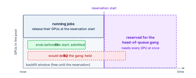
Figure 5: **Backfill under a Reservation**: The head-of-queue gang holds a reservation that begins when the running jobs release their GPUs. Until then, the free GPUs form a backfill window. A short job that ends before the reservation start runs in that window, while a job whose runtime bound would carry it past the start is held, because admitting it would delay the gang. The schematic carries no measured values.

The accuracy of runtime estimates determines backfill effectiveness, and this creates a game-theoretic challenge. If users overestimate runtimes, fewer jobs appear to fit a backfill window. If they underestimate, the scheduler may need to preempt a backfilled job to honor the reservation, paying recovery costs and losing unsaved progress. A policy that kills jobs at their declared limit encourages conservative estimates. Tiresias (Gu et al. 2019), discussed in section 8.9.1, avoids duration estimates when setting priority by using observed resource consumption. That choice addresses ordering under uncertainty, while reservation protection still needs an enforced runtime bound or release contract that says when a backfilled job will give its capacity back.

8.4.4 Deadlock prevention and detection

Gang scheduling eliminates the hold-and-wait condition for the atomically allocated bundle, but it does not immunize the cluster against all forms of resource contention. Later requests for auxiliary resources can still create a cycle of dependencies. Priority rules can also prevent a resource holder from making progress without creating a cycle. Distinguishing these cases matters because breaking a deadlock and providing a starved job with enough resources to exit require different interventions.

Priority inversion occurs when a high-priority job waits on a low-priority resource holder whose progress other work delays. Consider the 64-GPU fine-tuning run of the 175B-parameter model, submitted at high priority. The scheduler has reserved 60 available GPUs, but the remaining 4 are held by a low-priority data processing job. Normally, the scheduler would preempt the low-priority job to satisfy the high-priority request. However, if a stream of medium-priority development jobs saturates the cluster’s CPU or network bandwidth, starving the low-priority job of the resources it needs to checkpoint and exit, the low-priority job stalls. Its graceful release path cannot complete. The high-priority job waits for the low-priority job, which is effectively blocked by the medium-priority jobs. The 60-GPU idle block persists until the exit path receives resources or an enforced termination policy reclaims the remaining GPUs, potentially losing uncheckpointed work.

Priority inversion: the high-priority job waits on a low-priority holder that medium-priority work starves.

Definition 8.2: Priority inversion

Priority inversion is an ML cluster scheduling pathology in which a high-priority task is forced to wait for a lower-priority task to release a shared resource.

Significance: It ties the progress of a high-priority job, and the accelerators reserved for it, to the progress of the lowest-priority job in the wait-for chain. In ML clusters, this typically occurs when a low-priority job holding GPUs is starved of auxiliary resources (for example, bandwidth for checkpointing), preventing it from finishing and releasing the accelerators needed by high-priority workloads.
Distinction: Unlike standard queuing (where tasks wait their turn), priority inversion involves an active blockage: the high-priority task is ready to run but is transitively dependent on a task that the scheduler does not prioritize.
Common pitfall: A frequent misconception is that strict priority levels solve this. Raising the waiting job’s priority does not supply the CPU or bandwidth that its lower-priority resource holder needs to exit; the preemption policy must protect that release path.

Prevention and detection address different parts of this problem. Atomic allocation prevents hold-and-wait for the resources included in the gang, while reserving checkpoint bandwidth allows a preempted job to complete its exit path. Timeouts instead bound how long the system waits before investigating or reclaiming an allocation; they do not prevent deadlock states from arising. Monitoring can trigger recovery when progress stops, but safe reclamation still requires enforcing the new ownership decision.

Detection, unlike exact placement search, is computationally cheap. Before feasibility filtering, a cluster with 10,000 GPUs and 500 pending jobs can have more than $10^{15}$ candidate allocations, which puts exhaustive allocation search out of reach. Detection instead works on a wait-for graph, a directed graph with one vertex per job and an edge from job A to job B whenever A waits for a resource that B holds. A cycle identifies a potential deadlock. It establishes deadlock when every edge is an unavoidable blocking dependency and no alternative resource allocation can let a member proceed. Finding a cycle in an already constructed graph takes time linear in its vertices and edges. The difficulty lies in construction. Resource state changes continuously across a distributed control plane, so the scheduler rarely holds a complete, current graph, and a cycle detected on stale state may already have resolved while a real one goes unseen.

Large-scale schedulers therefore supplement wait-for detection with mechanisms that preserve liveness under incomplete state. A lease-based resource gives every allocation a time-to-live; expiry authorizes reclamation only when the resource manager enforces revocation and cleanup before reuse. Progress monitoring checks advancement through signals such as completed-step counters, using GPU utilization and heartbeats as supporting observations rather than proof of useful work. When the scheduler must preempt a lower-priority job, holistic preemption reserves the CPU, network, and storage bandwidth needed for that job to checkpoint and exit cleanly; otherwise, the victim can be too starved to release the accelerators. False failure suspicions can cost useful work, but must not bypass the ownership checks required for safe recovery.

8.4.5 Heterogeneous gang scheduling

In preference-training pipelines such as reinforcement learning from human feedback (RLHF), allocating the policy-training GPUs while the rollout-generation or reward-scoring workers sit queued stalls the workflow just as completely as a missing AllReduce rank. Whereas homogeneous gang scheduling allocates $\DeviceCount$ identical workers executing the same compute graph, heterogeneous workflows combine trainers, evaluators, and inference-style workers that need different GPU counts, memory footprints, and lifetimes, yet still must run together as a single job.

↩︎ The models that alignment training co-locates, and their unequal resource demands, are established in Multi-Model Training for Alignment and RLHF.

Systems Perspective 8.1: Routing over synchrony

Heterogeneous gang scheduling extends atomic allocation to the roles that must coexist for a workflow to progress. A viable group might pair high-HBM nodes for memory-bound generation with compute-oriented nodes for policy updates. The orchestration problem then shifts from packing a homogeneous ring toward routing data: rather than reducing gradients among identical workers, the job streams rollouts from generation workers to the workers that compute policy updates, so placement must also support the data exchanged between those roles. Rollout and training stages may exchange work in batches or through a buffered pipeline; their measured production and consumption rates determine where queues grow or accelerators wait. The scheduler needs a minimum viable resource bundle and a supported scaling policy for each role, rather than an assumption that all workers are interchangeable or perfectly balanced.

Homogeneous and heterogeneous jobs share an allocation requirement: the scheduler must assemble a viable group before expecting progress. Backfill can use capacity while that group waits, provided runtime estimates or preemption contracts protect the reservation. Enforcing these policies requires a control plane that represents ownership and reconciles allocations after failures.

Self-Check: Question

True or False: Under Dominant Resource Fairness (DRF), if Team A’s workload requires $4\text{ GPUs}$ and $8\text{ CPU cores}$ per worker while Team B’s workload requires $1\text{ GPU}$ and $64\text{ CPU cores}$ per worker on a cluster with $100\text{ GPUs}$ and $1000\text{ CPU cores}$, DRF equalizes each team’s share of their dominant resource (GPUs for Team A, CPUs for Team B).
When multi-GPU jobs leave unallocated accelerators spread across nodes that cannot be combined to satisfy pending multi-GPU requests due to intra-node interconnect requirements, the cluster suffers from ____.
In a 1,024-GPU cluster receiving two 1,024-GPU synchronous training jobs, what condition causes a hold-and-wait deadlock under a non-gang scheduler, and how does gang scheduling eliminate it?
1. Non-gang schedulers allocate partial subsets (e.g., 512 GPUs to each job) where neither job can progress through synchronous AllReduce collectives, whereas gang scheduling enforces atomic all-or-nothing allocation so unallocated jobs hold zero resources.
2. Non-gang schedulers force jobs to time-slice GPU compute cycles, causing NCCL timeouts during AllReduce, whereas gang scheduling disables CUDA preemption entirely.
3. Non-gang schedulers assign GPUs across multiple racks, creating switch contention, whereas gang scheduling restricts all 1,024 GPUs to a single physical server chassis.
4. Non-gang schedulers allow lower-priority jobs to preempt higher-priority jobs, whereas gang scheduling locks node allocations until all jobs in the queue complete.
Describe how priority inversion occurs when a high-priority distributed training job requires accelerators held by a low-priority job, and explain why simply setting higher priority levels does not resolve the blockage.
How does heterogeneous gang scheduling differ from traditional homogeneous gang scheduling in the context of reinforcement learning from human feedback (RLHF) workflows?

See Answers →

8.5 Orchestration Paradigms

A pending gang and a queue of small backfill jobs need both a policy for sharing capacity and a control plane that can enforce it. The policies just developed apply across platforms; the orchestration paradigm determines how the platform represents allocations and recovers when observed state diverges from them. Slurm, shaped by HPC batch systems, favors explicit resource requests and predictable allocation. Kubernetes, shaped by cloud-native service management, favors declared desired state and continuous reconciliation. The choice is therefore not Slurm vs. Kubernetes as products; it is which control model best matches the workload mix, failure behavior, and operational culture of the fleet.

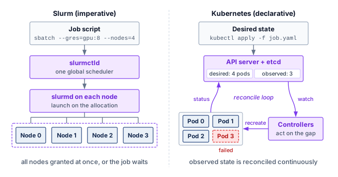
The two platforms embody two control models (figure 6). Slurm follows an imperative batch model, in which the user states the resources a job needs and the central slurmctld dispatches that allocation through per-node slurmd daemons. Kubernetes follows a declarative model, in which the user states what should be running and controllers reconcile observed state toward that declaration through the API server and node agents. Both platforms accept explicit resource requirements and track execution state, so the useful distinction is which lifecycle the platform manages directly: an allocated batch job or a collection of workloads maintained by controllers. That distinction shapes how ML workloads are admitted, monitored, and recovered from failure, and distributed training still needs framework-level coordination under either model.

Figure 6: **Architectural Paradigms: Slurm vs. Kubernetes**: Slurm (left) uses an imperative batch model where users submit explicit resource requests to a centralized controller (`slurmctld`) providing deterministic atomic allocation. Kubernetes (right) uses a declarative service model where controllers continuously reconcile observed cluster state in `etcd` against desired state specifications.

8.5.1 Slurm and HPC scheduling heritage

When a multi-node job needs an exclusive, non-overlapping block of accelerators for days at a time without partial-allocation deadlocks or conflicting node ownership, a centralized batch allocator is the most direct control plane. The Slurm Workload Manager⁵ originated at Lawrence Livermore National Laboratory to solve that problem for Linux supercomputers (Yoo et al. 2003): long-running jobs, expensive shared hardware, and users who can specify resource needs in advance. In ML infrastructure, the same batch model maps to GPU training through partitions for heterogeneous accelerator pools and predictable atomic allocations for long-running distributed jobs.

⁵ Slurm Workload Manager: Originally “SLURM,” an acronym for Simple Linux Utility for Resource Management, the project dropped the acronym capitalization in 2012. Developed at Lawrence Livermore National Laboratory beginning in 2002, Slurm’s centralized controller (slurmctld) maintains a single authoritative view of resource allocations. At very large scale, operators may partition fleets or federate schedulers to keep scheduling latency, policy isolation, and failure domains manageable.

Yoo, A. B., M. A. Jette, and M. Grondona. 2003. “SLURM: Simple Linux Utility for Resource Management.” In Job Scheduling Strategies for Parallel Processing. Springer Berlin Heidelberg. https://doi.org/10.1007/10968987_3.

Slurm’s batch submission model makes resource requirements explicit. Users submit job scripts, and the scheduler allocates resources within eligible partitions according to policy and availability. A submission of sbatch --gres=gpu:8 --nodes=4 requests 8 GPUs on each of 4 nodes, a 32-GPU allocation. The request supplies a capacity contract, but useful execution still depends on the selected hardware and the application’s launch configuration. Overstating requirements strands resources; understating them can cause memory failures or poor performance.

Slurm’s architecture consists of a central controller daemon (slurmctld) that maintains the global view of cluster state and makes scheduling decisions, and per-node daemons (slurmd) that manage local resources and execute jobs. This centralized architecture provides the authoritative allocation model discussed in section 8.2: the controller is the source of truth for resource assignments, reducing the risk of conflicting allocations. The cost is a potential single point of failure (addressed through active-passive failover) and a scheduling-throughput limit. As fleets grow, organizations may partition the cluster or federate schedulers to bound scheduling latency and failure impact; within a cluster, a typical ML configuration defines Slurm partitions by accelerator type and interconnect (table 2).

Table 2: Slurm Partition Configuration: Partitions organize heterogeneous accelerators into logical pools matched to workload characteristics. NVLink-connected partitions support tensor parallelism, while PCIe partitions serve workloads that rely primarily on data parallelism. Separating inference and debug partitions prevents experimental workloads from impacting production serving.

Partition	GPUs/node	Interconnect	Typical use
dgx-a100	8$\times$ A100	NVLink + IB NDR	Large LLM training
a100-pcie	4$\times$ A100	PCIe + IB HDR	Medium training
inference	2$\times$ A10G	Ethernet	Model serving
debug	1$\times$ V100	Ethernet	Development

Within a partition, a request specifies both the number of GPUs a job needs and the allocation shape: how those GPUs are distributed across nodes. In Slurm, --gres=gpu:N or --gpus-per-node=N requests a per-node count, while --gpus=N requests a job-wide total. Whether the scheduler may split a node between jobs is a separate consumable-resource policy (Slurm’s select/cons_tres plugin), and a node-exclusive policy strands the unused devices in the six-on-eight example of section 8.4.2. Shape decides communication. In an eight-GPU-per-node pool, a 16-GPU request that also fixes eight GPUs per node (--gpus-per-node=8) yields two fully populated nodes, whose NVLink domains follow from the node hardware rather than the count. A request for 16 GPUs with no per-node constraint gives the scheduler more freedom, so it can start sooner on partially occupied nodes, but it may spread the group across several of them. Whether that flexibility is useful depends on the parallelism configuration and its communication budget. Tensor-parallel groups with frequent exchanges may justify compact placement, while data-parallel groups with well-overlapped communication may tolerate a wider allocation.

The fair-share scheduling mechanism uses past consumption to influence future priority under contention. An illustrative heuristic combines base priority, the user’s target fair share ($\TargetFairShare$), recent actual consumption ($\RecentUsageShare$), and a small stabilizing constant ($\FairShareStabilizingConstant$); it illustrates the feedback without reproducing Slurm’s multifactor priority calculation:

\[\text{Priority}_{\text{effective}} = \text{Priority}_{\text{base}} \times \frac{\TargetFairShare}{\RecentUsageShare+ \FairShareStabilizingConstant} \tag{1}\]

With base priority and target share fixed, equation 1 lowers priority as recent consumption increases. Doubling consumption approximately halves this illustrative priority when the stabilizing constant is negligible. Actual admission also depends on other priority factors and feasible resources; low recent usage does not guarantee an immediate start.

The time decay of usage history determines how quickly the system “forgives” past heavy usage. A half-life of one week means that a researcher’s heavy usage from two weeks ago contributes only 25 percent to their current usage calculation. Short half-lives make the policy more responsive to recent changes but can encourage alternating bursts of usage. Long half-lives retain the effect of a completed large project when its researchers return with smaller jobs. The useful decay window depends on the fleet’s job durations and the period over which the organization intends to balance access. Usage itself need not count every device alike. Trackable resources (TRES) let accounting charge different accelerator classes different billing weights in fair-share usage, an administrative valuation that tracks economic cost only as far as the chosen weights do.

Preemption policies enable high-priority jobs to reclaim resources from running workloads, and for ML training the reclaim must leave time to save state. Slurm expresses that time as a grace period. It signals the selected job (SIGTERM), waits the configured GraceTime, and only then kills it (SIGKILL); under PreemptMode=REQUEUE it can also requeue an eligible job to run again later. Neither the signal nor the requeue saves model state. The application must handle the signal, publish a valid checkpoint within the grace period, and restore it on restart. If termination precedes completion of that save, recovery uses the last valid checkpoint and replays subsequent work. Preemption therefore buys access for high-priority work with the victim’s replay and restart time, a price that section 8.8.1 develops.

↩︎ Checkpointing for progress preservation, including the checkpoint interval and coordination patterns, is established in Checkpointing and Progress Preservation.

Several Slurm features expose ML structure to the batch system. A hyperparameter sweep is the opposite of a gang. Job arrays submit many trials as one record (for example, --array=0-99), and each trial reads its index from the SLURM_ARRAY_TASK_ID environment variable to select its configuration. Slurm schedules the elements independently, so individual trials become ideal backfill candidates that fill small gaps in capacity, while the array keeps submission and management overhead low without making the trials one indivisible gang.

Heterogeneous jobs carry the heterogeneous gang of section 8.4.5 into a batch allocation. One job can contain components with distinct resource requests, admitted together. The 64-GPU fine-tuning run of the 175B model, for example, could request 8 GPU nodes for training and 2 CPU-only nodes for on-the-fly tokenization as a single allocation, then launch training on the GPU component and data workers on the CPU component (srun --het-group=0 and --het-group=1). This separation helps only if the data workers and transfer path sustain the training stage’s consumption rate; a heterogeneous allocation exposes that choice but does not itself balance the pipeline. At the boundaries of each allocation, prolog and epilog scripts turn job transitions into health checks, with a prolog that tests reported topology, ECC counters, and link status on each allocated node and drains a failing node before launch, and an epilog that removes the job’s orphan processes and shared-memory segments. They apply the quarantine idea of section 8.6.4 at job boundaries, reducing exposure to known faults without establishing delivered bandwidth.

Slurm’s strengths for ML training include explicit batch allocations, configurable fair-share policies, and integration with MPI-based distributed training frameworks. A mixed training-serving fleet also needs a service lifecycle that maintains ready replicas as demand and failures change. Inside a batch scheduler, adding or removing an inference replica means submitting or canceling a job, a far heavier operation than a controller adjusting a replica count, and a failed replica stays down until something resubmits it. Operators must integrate replica health, replacement, and demand-driven scaling with the batch scheduler, or assign those responsibilities to a service orchestration platform. Kubernetes starts from that service contract, in which users declare the desired state of services and jobs and controllers continuously reconcile the cluster toward it.

8.5.2 Kubernetes declarative container orchestration

When a cluster runs always-on inference services alongside training jobs, managing serving replicas as batch scripts forces operators to rebuild health checks, rolling updates, and replica replacement by hand. Kubernetes addresses this mixed workload by managing both services and batch jobs through a declarative model that expresses a workload’s desired state and uses control loops to reconcile observations with that state (Burns et al. 2016; Cloud Native Computing Foundation 2024). The unit it places is the pod, one or more containers that share a node and a network identity, and its default scheduler places pods one at a time. The name collides with the hardware pod of The Pod, the many racks joined under one fabric. A Kubernetes pod is a software unit that never spans more than one node, so a 64-pod training job is 64 container groups placed onto nodes, all of which can sit inside one hardware pod. Controllers above the scheduler give groups of pods a purpose: a Deployment keeps a set number of identical replica pods running, while a Job runs pods until they complete, retrying failures under a stated policy. The workload controller therefore determines what completion, replacement, or continued availability means.

Burns, Brendan, Brian Grant, David Oppenheimer, Eric Brewer, and John Wilkes. 2016. “Borg, Omega, and Kubernetes.” Communications of the ACM 59 (5): 50–57. https://doi.org/10.1145/2890784.

Cloud Native Computing Foundation. 2024. Kubernetes: Production-Grade Container Orchestration.

Failure handling reveals the importance of the workload contract. Slurm can detect node failures and requeue eligible jobs when configured to do so. Kubernetes controllers maintain workload-specific goals, such as a Deployment’s replica count or a Job’s completion and retry policy. A replacement pod still has to be placed, become ready, and rejoin the distributed training run before progress resumes. Training operators can coordinate worker creation, while the framework remains responsible for valid state and group recovery. Both platforms therefore require an explicit agreement between allocation, process lifecycle, and application recovery.

Kubernetes’ control loop architecture uses the controller pattern:⁶ controllers observe and update API objects through the API server, which persists cluster state in etcd, a replicated key-value store. Those objects contain desired state and reported observations, not instantaneous physical truth. The pattern repeats at every level: the Deployment controller reconciles the number of pod replicas, the scheduler binds pending pods to nodes, the kubelet (the agent on each node) keeps its assigned containers running, and the node controller marks nodes that stop reporting. Each component acts independently and communicates only through API objects, which makes the system resilient to the failure of any single controller. The price of that independence is that their interactions require clear ownership and retry behavior, particularly when a failed node’s last reported state no longer describes its execution.

⁶ Controller pattern (reconciliation loop): A “level-triggered” design reconciles the current desired and observed states rather than depending on every intermediate event. A restarted controller can resume from durable state if its actions tolerate retries and its observations expose unfinished work. Multiple controllers still need distinct responsibilities so that one controller’s correction does not repeatedly undo another’s.

Kubernetes needs an explicit resource representation before it can place GPU workloads. In the device-plugin model, device plugins expose accelerators as schedulable extended resources. The NVIDIA device plugin registers GPUs with the kubelet, enabling pod specifications that request GPU resources declaratively through the standard Kubernetes resource model. A pod then asks for whole GPUs by naming the nvidia.com/gpu resource in its limits (listing 1).

Listing 1: Kubernetes GPU Allocation: Pod resource specification requesting GPUs through the NVIDIA device plugin. The nvidia.com/gpu resource name follows Kubernetes extended resource conventions, where the domain prefix identifies the device plugin vendor. This declarative syntax enables portable GPU workload definitions across any Kubernetes cluster with the NVIDIA device plugin installed.

# Kubernetes pod resource specification for GPU allocation
resources:
  limits:
    nvidia.com/gpu: 4  # Request exactly 4 GPUs for this pod
  requests:
    cpu: "32"
    memory: "256Gi"

When the device plugin exposes exclusive whole GPUs, a small model serving occasional requests can reserve a device while using only a fraction of its compute and memory capacity. Whole-device allocation suits workloads that need the capacity or isolation, but can strand resources for smaller workloads. The resource unit exposed by the plugin therefore matters, because sharing or partitioning changes what the scheduler can allocate and what isolation each allocation receives. Device plugins can also expose hardware partitions, such as MIG instances, as schedulable units, a choice that section 8.10.1 develops with the serving workloads it suits.

Kubernetes’ default scheduler places pods independently, so it does not supply the group admission that section 8.4.3 requires. Under that default, a 64-pod training job receives 64 separate placement decisions, with no guarantee that all will succeed. If the cluster has resources for 60 pods but not 64, those 60 can occupy capacity while the remaining 4 wait. The platform must therefore configure a group-level admission and placement contract for a rigid job. PodGroup-style abstractions give that contract a unit matching the job’s minimum viable execution group rather than an individual pod.

The mechanism that closes this gap is group admission. A PodGroup declares a group’s minimum runnable membership. The scheduler tentatively reserves a placement for each member as it finds one but binds none of them to nodes until the minimum membership is placed, and it releases every reservation if the attempt fails or times out. Admission and placement thereby become two decisions, with the group admitted only when placement has succeeded for enough of it. The Volcano⁷ batch scheduler and the Coscheduling scheduler plugin both implement this pattern. Group admission does not make physical launches simultaneous; nodes can still fail or start at different times, so the framework must establish the communication group before training proceeds.

⁷ Volcano: Volcano provides a scheduler with batch and gang-scheduling mechanisms. Pods select it through their scheduler name, so it can coexist with Kubernetes’ default scheduler. The operational contract must account for interactions between schedulers sharing the same nodes; installing Volcano does not automatically transfer every workload’s scheduling to it.

War Story 8.1: OpenAI's gang-scheduling example (2021)

Context: OpenAI scaled Kubernetes clusters to 7,500 nodes for workloads including GPT-3, CLIP, and DALL-E. Its account explains that MPI-coordinated optimizer groups needed all members scheduled before training could progress (Sigler 2021).

Mechanism: The account illustrates the risk with two experiments each requesting the entire cluster. Incremental pod placement could allocate half the capacity to each, leaving neither with a complete group.

Impact: In that example, both jobs hold capacity without making progress. It demonstrates the deadlock mechanism rather than documenting a particular pair of stalled production runs.

Fix: OpenAI reports adopting the coscheduling plugin to add group-aware admission to the Kubernetes scheduler.

Systems lesson: Distributed ML scheduling must encode the job’s execution semantics. For MPI-style training, “some pods scheduled” is not partial progress; it is wasted allocation. Production schedulers need gang scheduling, quota controls, and workload-aware policies rather than generic pod placement alone.

Priority classes control scheduling precedence and preemption eligibility. A fleet might give inference higher priority than training to help protect serving service-level objectives (SLOs), but priority cannot replace ready capacity during a demand spike. With preemptionPolicy: PreemptLowerPriority, a pending pod can displace lower-priority pods when their removal makes placement feasible. With preemptionPolicy: Never, it retains queue precedence without initiating preemption and remains subject to higher-priority preemption. Termination, cleanup, and replacement startup take time. Training applications also need a checkpoint-aware shutdown path that fits the allowed grace period; assigning priorities does not create that path. The policy must balance serving readiness against repeated interruption of training.

Kueue⁸ makes admission a separate control decision. It manages when workloads may consume quota, while a compatible scheduler binds their pods to nodes. The admission policy and placement policy must agree on resource types, group requirements, and topology. Separating these responsibilities lets each layer run its own policy, at the price of keeping the two consistent. Kueue represents each team or project as a queue with a configured quota (a ClusterQueue) and groups queues into cohorts whose members may lend one another unused quota, under the borrowing and reclaim contract of section 8.11.2.

⁸ Kueue: Kueue separates workload admission from pod placement. Its all-or-nothing mechanisms include waiting for admitted pods to become ready and requeuing workloads that exceed the configured timeout. Aggregate quota admission alone does not prove that a gang fits the physical topology; the guarantee depends on the configured readiness, topology, and placement mechanisms.

8.5.3 Kubernetes ecosystem for ML training

Group admission handles one constraint that microservice orchestration leaves implicit and distributed training cannot. Four more remain. Workers must launch knowing their peers, collective traffic must avoid network layers built for request traffic, checkpoint writes need bandwidth rather than only storage capacity, and progress must be observable below the container. Operators and plugins add each constraint to the platform; the mechanism matters more than the product that happens to implement it.

Peer discovery is the job of the training operator ecosystem, which extends Kubernetes with job-specific resource types (custom resource definitions). In the Kubeflow Training Operator, a PyTorchJob declares the number of workers, the container image, and resource requirements; the operator creates the pods and injects the rendezvous address (MASTER_ADDR and MASTER_PORT), the group size, and each worker’s rank (WORLD_SIZE and RANK), which the framework uses to form its communication group. If a worker pod fails, the operator can detect the deviation and create a replacement pod to restore the desired replica count, but training-state recovery still depends on the framework’s checkpoint and rendezvous logic.

Collective traffic is the second constraint. The pod overlay network that the Container Network Interface (CNI) configures, designed for microservice requests, routes packets through software switching on the host CPU, which adds latency and caps bandwidth when it sits on the critical gradient-synchronization path. For bandwidth-sensitive training, host networking (hostNetwork: true) places pods in the host’s network namespace, bypassing the ordinary pod overlay path. It does not itself allocate remote direct memory access (RDMA) devices or grant permission to use them; device exposure, resource requests, drivers, and access controls require separate configuration. Operators such as NVIDIA’s Network Operator automate that exposure through RDMA device plugins and GPUDirect RDMA configuration, letting containerized workloads approach bare-metal interconnect performance once the rest of the stack is configured.

Checkpoint bandwidth is the third constraint, because storage integration must account for the checkpoint storm of definition 4.5, in which many workers write large amounts of state together. Kubernetes PersistentVolumeClaims (PVCs) request capacity on a configured storage system but do not reserve checkpoint throughput. A 1,024-GPU training job writing the 2.45 TB resumable checkpoint of the 175B model needs a measured write budget shared with other workloads. Backend bandwidth controls, client throttling, or staggered writes can limit interference; the platform must verify which controls the storage implementation enforces.

Visibility into progress is the fourth. The observability stack for training clusters combines general-purpose cluster monitoring (commonly Prometheus and Grafana) with accelerator telemetry such as the Data Center GPU Manager (DCGM) exporter, which reports utilization, memory bandwidth, temperature, and ECC errors. These observations locate symptoms. Correlating them with step progress, input waits, and communication traces is what distinguishes useful computation from stalls and identifies which dependency limits a training job.

↪ Fleet telemetry across device, network, and facility levels, and the correlation that narrows a failure domain, is developed in Fleet telemetry and hardware observability.

The 1,024-GPU pretraining run for our 175B model illustrates how these responsibilities fit together. One possible deployment defines a PyTorchJob with 128 worker pods, each requesting 8 GPUs. Host networking removes the pod overlay from the gradient path, and the Network Operator exposes each node’s InfiniBand adapters to the workers through RDMA device plugins. A PVC backed by Lustre provides access to the 6 TB tokenized training corpus and a checkpoint path whose sustained bandwidth must be validated. DCGM metrics stream to Prometheus, supporting alerts on uncorrectable ECC errors and deviations from workload-specific communication baselines.

8.5.4 Paradigm trade-offs and selection criteria

Selecting a control plane requires matching its allocation and recovery contract to the workload mix. Rigid training groups need reliable atomic placement and checkpoint-aware interruption; serving replicas need readiness checks and continuous recovery. Existing operational expertise and the cost of running a second control plane also shape the choice. A fleet dedicated to long, homogeneous training runs that use bare-metal collectives, operated by a team fluent in batch scheduling, gains most from Slurm’s authoritative allocation and mature fair-share. A fleet that mixes training with always-on serving, and already runs cloud-native deployment and observability tooling, gains more from Kubernetes with a gang-admission layer added for its rigid jobs. The Slurm vs. Kubernetes trade-off organizes around the dimensions most relevant to ML workloads (table 3).

Table 3: Slurm vs. Kubernetes for ML Workloads: The two paradigms reflect different design philosophies optimized for different workload characteristics. Most production ML platforms use elements of both, with Slurm managing dedicated training clusters and Kubernetes managing inference serving and pipeline orchestration.

Dimension	Slurm	Kubernetes
Scheduling model	Imperative: user specifies exact resources and scheduler allocates them	Declarative: user specifies desired state, system reconciles continuously
Failure handling	Configuration-dependent requeue and checkpoint workflows	Self-healing through control loops
Gang/atomic multi-node start	Atomic job allocation plus backfill; Slurm “gang scheduling” specifically refers to time-slicing/preemption	Production clusters commonly use PodGroup-based support such as Volcano, Coscheduling, Kueue, or upstream alpha gang scheduling
Fair-share	Mature multi-factor priority with configurable decay	Kueue provides basic fair-share with ClusterQueue borrowing
Container overhead	None from a container runtime when jobs run directly on nodes	Configuration-dependent networking overhead and container startup time
Service management	No native support for long-running services	Native Deployment, rolling updates, health checks
Ecosystem	MPI, OpenMP, scientific computing libraries	Cloud-native, microservices mesh, observability stack

The gang-scheduling row of the table compresses a naming collision that is easy to miss. This chapter uses gang scheduling for atomic allocation of a whole execution group, which is the requirement distributed training imposes. Slurm reserves the name for the older, Ousterhout-style meaning of the term, in which co-scheduled jobs share nodes by time-slicing in synchronized rounds. Slurm provides atomic multi-node allocation under its ordinary job model, so the requirement is met even though Slurm’s “gang scheduling” option means something else.

The choice of scheduling paradigm also reflects organizational trajectory. Teams starting with HPC-focused training infrastructure may begin with Slurm and add Kubernetes for serving. Teams starting from cloud-native application infrastructure may begin with Kubernetes and add HPC-oriented extensions (Volcano, Kueue) for training. Slurm has meanwhile added a REST interface and container support, so the two platforms now overlap in capability. Either path can reach a functional hybrid architecture, but the starting point determines which capabilities are strongest and which require the most investment to develop.

8.5.5 Hybrid architectures in practice

While the choice between Slurm and Kubernetes often appears binary, engineering organizations can deploy hybrid architectures that use the strengths of both systems. The relevant boundary again follows workload semantics rather than labels. Rigid, topology-sensitive jobs fit a batch scheduler’s atomic allocation contract, while malleable services fit a reconciliation loop that adjusts replica count continuously. Some training jobs are elastic, and some serving replicas are rigid multi-accelerator gangs, so neither “training” nor “serving” selects a control plane by itself.

The Kubernetes-over-Slurm pattern wraps the HPC scheduler within a cloud-native control plane. Kubernetes manages the lifecycle of training jobs through custom operators while delegating batch admission and placement to Slurm. The central engineering problem is ownership: exactly one control plane must authorize each placement, while the outer controller reconciles lifecycle state without issuing a conflicting allocation. The arrangement combines a declarative management surface with Slurm’s batch and topology policies, but it also creates a cross-control-plane failure boundary that operators must fence explicitly.

The Slurm-alongside-Kubernetes pattern takes a coarser-grained approach, maintaining separate clusters for training and serving that draw from a shared pool of physical nodes. A meta-scheduler or capacity broker acts as an arbitrator, dynamically reassigning nodes between the Slurm partition and the Kubernetes cluster based on demand signals. During intensive training campaigns, nodes are drained from Kubernetes and joined to Slurm; during product launches or traffic spikes, the flow reverses. The primary challenge is the mode-switching cost: draining a node, changing its ownership and configuration, and admitting it to the other control plane takes much longer than an ordinary placement decision. This latency limits sharing to planned capacity shifts rather than second-by-second inference bursts.

A shared application runtime such as Ray provides task and actor abstractions for both training and serving. Ray’s placement groups, unlike the cloud network-locality abstraction of the same name, reserve bundles of logical resources for work that must run together, and serving replicas can also require multi-device groups. Inside a shared runtime the workloads keep their different state, latency, and recovery requirements, so the platform must still coordinate Ray’s logical allocations with the underlying resource manager and validate the isolation and recovery behavior needed by each workload.

Threading these patterns together, consider the lifecycle of our 175B parameter model. A hybrid platform can allocate the training gang through Slurm and later place serving replicas through Kubernetes. The orchestration boundary concerns resource ownership: the training job releases its allocation, and the serving control plane admits replicas against its own capacity and readiness requirements. Deciding whether the trained artifact is ready for production requires validation and release policy beyond the scheduler; CI/CD for ML at Scale develops those validation gates and rollout policies.

A hybrid platform is useful when its separate allocation contracts justify the additional ownership and recovery boundary. The cost to measure is the coordination between control planes, including node draining and reassignment, rather than a presumed performance advantage from either product name. Because Slurm and Kubernetes now overlap in capability, the paradigm choice is a workload-specific design decision, and teams must establish the allocation and recovery guarantees they need before layering physical placement constraints on top of them.

Checkpoint 8.1: Scheduling paradigm trade-offs

Before the chapter turns to topology-aware placement, review the core trade-offs:

Gang scheduling: explain why a rigid synchronous execution group needs atomic allocation, and why the scheduler must still reserve capacity for a waiting gang that holds no GPUs itself.
Slurm vs. Kubernetes: compare authoritative allocation with desired-state reconciliation, and explain why either design must prevent duplicate ownership during a network partition.
Group admission: explain why a default scheduler that places pods one at a time can strand capacity for a 64-pod training job, and how a PodGroup’s minimum membership prevents it.
Resource units: explain how the resource unit a device plugin exposes changes what the scheduler can pack, and why a small model on an exclusively assigned GPU strands capacity.
Backfill incentives: explain why backfill scheduling depends on accurate job runtime estimates and why users have game-theoretic incentives to provide inaccurate estimates.

A control plane can now represent, admit, and reconcile an allocation, yet it still counts accelerators as if any group of the requested size were interchangeable. Two allocations of the same size can meet very different communication budgets depending on where the devices sit in the cluster fabric. The next layer of the scheduler must therefore weigh physical location alongside resource count.

Self-Check: Question

What is the fundamental difference in control philosophy between Slurm and Kubernetes when managing distributed ML training workloads?
1. Slurm relies on continuous reconciliation loops against desired state stored in etcd, whereas Kubernetes executes imperative one-time allocation scripts via a centralized daemon.
2. Slurm uses peer-to-peer gossip protocols to schedule tasks across nodes, whereas Kubernetes enforces hierarchical master-slave token ring passing.
3. Slurm employs an imperative allocation model where users request explicit physical resources guaranteed at launch, whereas Kubernetes uses a declarative model where controllers continuously reconcile observed cluster state toward declared desired state.
4. Slurm schedules containerized microservices with dynamic horizontal auto-scaling, whereas Kubernetes only supports uncontainerized bare-metal MPI processes.
Kubernetes’ default scheduler places a 64-pod training job one pod at a time, and the cluster has room for only 60 of the pods. How does a PodGroup with a minimum membership of 64 change the outcome?
1. The scheduler binds the first 60 pods immediately and starts training with a smaller communication group, adding the last 4 pods as capacity frees.
2. The scheduler tentatively reserves placements but binds no pod until all 64 members are placed, releasing every reservation if the attempt fails or times out.
3. The scheduler preempts every lower-priority pod in the cluster until 64 GPUs are free, regardless of priority-class settings.
4. The PodGroup guarantees that all 64 containers start at the same instant, so the framework no longer needs to establish its communication group.
In the illustrative fair-share priority model ($\text{Priority}_{\text{effective}} = \text{Priority}_{\text{base}} \times \frac{F_{\text{target}}}{F_{\text{actual}} + \epsilon}$), what role does the usage decay half-life play, and what is the trade-off between setting a short versus a long half-life?
Why do high-performance distributed training jobs in Kubernetes typically enable hostNetwork: true and leverage the NVIDIA Network Operator instead of relying on default Container Network Interface (CNI) overlay networks?
True or False: Kueue replaces the native Kubernetes kube-scheduler binary entirely to implement custom gang scheduling algorithms, whereas Volcano acts purely as an admission controller layered on top of the default scheduler.
Order the dependencies in this illustrative launch path for a Kubernetes training job configured with a compatible training operator and Volcano group admission:

Volcano verifies a feasible placement for the PodGroup’s minimum viable membership.
The developer submits the training-job manifest defining workers and resource requirements.
Volcano authorizes group placement, and node agents launch the admitted workers using the separately configured device and network resources.
Launched workers establish their communication group through rendezvous before synchronized training begins.
The operator and configured scheduling integration create worker pods and their PodGroup.

See Answers →

8.6 Topology-Aware Scheduling

A scattered allocation can place frequent collective traffic on shared cross-rack paths, exposing latency or bandwidth limits that a more compact allocation avoids. The penalty is set by how much of the job’s traffic crosses those paths and how much capacity the fabric provisions there, not by the rack count itself. The earlier feasibility rules already required compatible topology; topology-aware scheduling makes that requirement explicit in the placement objective, accounting for communication paths as well as raw compute.

8.6.1 The topology hierarchy

Splitting a tensor-parallel group across node boundaries moves its per-layer activation exchanges off intra-node NVLink onto the external network fabric, where an H100’s per-direction NVLink rate is 9× the rate of one NDR port (Bandwidth hierarchy). Each level of a cluster’s communication hierarchy comes from the hardware that builds it and sets a distinct bandwidth and latency budget. GPUs inside a node exchange data over NVLink, the tier fast enough for the per-layer exchanges of tensor parallelism; nodes under one leaf switch communicate over an external fabric such as InfiniBand or RoCE; and racks joined through spine switches add switch hops whose delivered bandwidth depends on concurrent flows and oversubscription even in a fat-tree. Cross-rack communication also adds tail latency variability: while median latency may be only slightly higher, p99 latency can spike during congestion events, creating straggler effects in synchronous training where the slowest communicator determines the pace for all workers.

↩︎ Bisection bandwidth and fat-tree network topologies are established in Fat-tree (Clos) networks.

A 64-GPU job within one rack can avoid cross-rack paths that a spread allocation must use. It outperforms the spread allocation only when those paths add exposed latency or bandwidth contention; a non-blocking, uncongested spine need not reduce sustained throughput. The performance difference stems directly from the hierarchical communication analysis in Hierarchical AllReduce: a flat ring AllReduce runs at the speed of the slowest link in the ring, and cross-rack hops introduce both higher latency and increased contention risk. For synchronous training, every iteration waits for the slowest worker to complete its AllReduce, so even occasional cross-rack congestion inflates the Fleet Law’s communication term $\CommunicationTime(\DeviceCount)$ (equation 1.3) on every step it touches.

The scheduler must therefore model the cluster as a hierarchical graph with discrete bandwidth boundaries (figure 7). In the illustrated H100 fleet, per-direction bandwidth steps down from 450 GB/s across the NVSwitch inside a node to 50 GB/s per port under a leaf switch, and to roughly 12.5–25 GB/s per endpoint when balanced traffic saturates an oversubscribed spine. A node boundary can introduce a large bandwidth reduction, but a non-blocking rack or pod boundary need not reduce per-endpoint bandwidth. Oversubscription adds a separate constraint when traffic saturates shared uplinks. Topology-aware placement minimizes the communication cost of the job’s actual traffic pattern rather than applying a fixed penalty to every boundary.

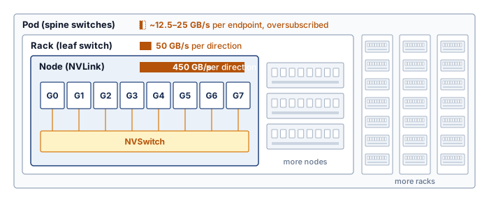
Figure 7: **Physical Topology Hierarchy and Bandwidth Cliffs**: Hardware boundaries dictate communication performance across three distinct domains. The example compares a 450 GB/s per-direction NVLink endpoint budget with a 50 GB/s per-direction external port. Under balanced load saturating a 2:1 to 4:1 oversubscribed spine, the external per-endpoint share falls to approximately 12.5–25 GB/s. A non-blocking spine need not impose this reduction. The bar in each domain’s header draws its bandwidth on one shared linear scale.

For a 4-GPU collective group, the routing paths make that cost concrete (figure 8). In the illustrated contended fabric, scattering ranks across Rack A and Rack B forces a 3-hop leaf-spine-leaf path with about 12.5 GB/s of effective bandwidth per endpoint, a share of contended uplinks rather than a physical link rate. Consolidating all four ranks (G0–G3) under Rack A’s leaf switch avoids those shared uplinks and provides about 50 GB/s per GPU under the example’s load assumptions.

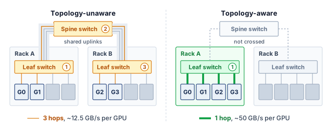
Figure 8: **Topology-Unaware vs. Topology-Aware Placement**: An illustrative 4-GPU job that permits inter-node placement and uses an oversubscribed cross-rack fabric, placed across two racks (left, topology-unaware) must traverse leaf-spine-leaf hops: 3 switch hops per AllReduce message at about 12.5 GB/s effective bandwidth. The same 4-GPU job packed within one rack (right, topology-aware) uses a single leaf switch: 1 hop at about 50 GB/s, roughly 4× faster. Blue squares are the job’s GPUs; gray squares are GPUs held by other jobs.

8.6.2 Placement algorithms

The illustrated 4× bandwidth difference between the 1-hop leaf path and the 3-hop spine route (figure 8) stretches the transfer component by the same factor when transfer time is bandwidth-dominated. Crossing a spine does not impose that ratio independently of load and topology. Whether communication exceeds computation also depends on the model and overlap schedule, and repeated exchanges can amplify the exposed cost. Topology-aware placement algorithms assign jobs to nodes that reduce this cost, turning resource packing into graph optimization over the physical topology. A simple locality cost, defined in equation 2, penalizes allocations spanning multiple topology domains:

\[ \text{Cost}_{\text{locality}} = \sum_{i < j} \LocalityPenaltyFunction(\GpuTopologicalDistance(\AssignedJobGpu_i, \AssignedJobGpu_j)) \tag{2}\]

where $\AssignedJobGpu_i$ and $\AssignedJobGpu_j$ are GPUs assigned to the job, $\GpuTopologicalDistance(\AssignedJobGpu_i, \AssignedJobGpu_j)$ is their topological distance (0 for same node, 1 for same rack, 2 for different racks), and $\LocalityPenaltyFunction(\cdot)$ is a weighting function that increases with distance. The scheduler minimizes this score when selecting an allocation from the set of feasible placements. An illustrative heuristic assigns locality penalties of $\LocalityPenaltyFunction(0) = 0$ (same node, NVLink, no penalty), $\LocalityPenaltyFunction(1) = 1$ (same rack, one switch hop), and $\LocalityPenaltyFunction(2) = 10$ (different racks, multiple switch hops); because these dimensionless weights are policy assumptions rather than measured latency or bandwidth ratios, a deployment must calibrate them to its traffic and topology, and an unweighted pairwise score still cannot distinguish heavily communicating rank pairs from pairs that rarely exchange data.

More sophisticated algorithms distinguish the communication requirements of different parallelism strategies. Frequent tensor-parallel activation exchanges favor a high-bandwidth, low-latency domain that meets the measured communication budget; that domain need not coincide with one server. Pipeline parallelism exchanges activations across stage boundaries rather than between every layer, but its tolerance for link delay depends on microbatch size and the pipeline schedule. Data-parallel gradient synchronization can overlap computation, making wider placement feasible when the exposed communication remains within budget. These patterns guide placement without establishing a universal ranking for every model or fabric.

Algorithm 1 combines the all-or-nothing gang constraint of section 8.4.3, the locality cost of equation 2, and an illustrative parallelism-to-topology mapping. Its enumeration expresses the decision conceptually: construct feasible rank mappings, score their allocations, and choose the lowest illustrative locality score, leaving the job queued when none fits. This surrogate does not guarantee minimum communication time or completion time. A fleet-scale implementation must restrict that search using heuristics rather than enumerate every allocation.

\begin{algorithm}
\caption{Topology-aware placement}
\begin{algorithmic}
\Require job requesting $N$ accelerators with tensor-, pipeline-, and data-parallel groups; cluster topology with illustrative per-level locality weights $w(\cdot)$
\Ensure an all-or-nothing feasible placement with the lowest illustrative locality score, or the job stays queued
\State enumerate candidate slots: sets of $N$ free accelerators that satisfy every resource dimension \Comment{gang: all or nothing}
\State retain only slots that admit a rank mapping satisfying the job's tensor-, pipeline-, and data-parallel communication constraints
\If{no feasible slot exists}
    \State leave the job queued without holding any accelerators \Comment{prevents hold-and-wait deadlock}
    \State \Return no placement
\EndIf
\For{each feasible slot}
    \State use a feasible rank mapping: tensor-parallel ranks within an NVLink domain, pipeline stages within a rack, data-parallel replicas across racks where permitted
    \State score the slot by $\text{Cost}_{\text{locality}} = \sum_{i < j} w(d(g_i, g_j))$
\EndFor
\State \Return the feasible slot of least $\text{Cost}_{\text{locality}}$ \Comment{minimum score among enumerated feasible placements; atomic allocation}
\end{algorithmic}
\end{algorithm}

Applied to a whole job, the same reasoning ranks placement strategies. The latencies in this comparison are illustrative, not derived. They are constructed to stay above the ring-AllReduce bandwidth bound for the payload, and they show the order in which placement removes delay rather than values a reader could recompute from topology names. For a 0.5 GB gradient synchronization on 64 GPUs, random placement spans multiple racks and spine switches and takes an assumed 120 ms. Each successive strategy removes a source of delay that the previous one leaves. Confining the group to a single rack removes spine hops and reduces latency to 85 ms. Rail-optimized alignment maps ranks so that every member of each collective group sits at the same local GPU index and therefore on the same network rail (developed in section 8.6.3). Traffic that previously hopped between rails through the spine now stays within one rail’s switches, which cuts latency to 40 ms. Topology-optimal placement additionally avoids leaf ports that other jobs are using and reaches 25 ms, a 4.8× reduction (figure 9, where each bar also carries its algorithm throughput). This ratio compares whole collectives under four assumed placements, so it need not match the link-bandwidth ratio of the two-rack paths above.

Figure 9: **Topology Placement Impact**: Assumed AllReduce latency across four placement strategies (Random, Rack-Aware, Rail-Optimized, and Topology-Optimal) for a 0.5 GB gradient sync on 64 GPUs. The assumed latency falls from 120 ms to 25 ms, a 4.8$\times$ ratio. Labels report payload divided by completion time (algorithm throughput), not physical link bandwidth. The dashed ghost above each bar names the source of delay that strategy removes.

A hierarchical placement algorithm applies these constraints from the most restrictive communication domain outward, matching each 3D parallelism dimension to the interconnect tier its traffic can tolerate (figure 10). In the illustrated fleet, it places each tensor-parallel group within an NVLink-connected node, where the per-layer activation exchanges run at 450 GB/s. It places consecutive pipeline stages under the same leaf switch, where stage boundaries cross at 50 GB/s, and it distributes data-parallel replicas across racks only when the once-per-step gradient synchronization fits the roughly 12.5–25 GB/s per endpoint that an oversubscribed spine leaves. This alignment reduces costly boundary crossings, but placement alone cannot reserve the fabric’s full bisection bandwidth against other jobs.

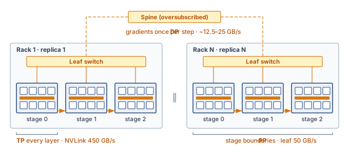
Figure 10: **Hierarchical Placement for 3D Parallelism**: This placement example maps distributed training dimensions to physical interconnect layers. Tensor parallelism (TP), which exchanges activations at every layer, stays inside a node on NVLink (450 GB/s); pipeline parallelism (PP) maps across adjacent nodes under one leaf switch (50 GB/s); and data parallelism (DP), which exchanges gradients only once per step, spans racks through the oversubscribed spine. Bandwidths are per direction, as in figure 7.

Evaluating all possible placements for a 256-GPU job across a 10,000-GPU cluster is combinatorially intractable, so production schedulers rely on heuristic approaches. Common choices include greedy algorithms that build placements bottom-up (first fill NVLink domains, then fill racks, then spread across racks), tree-search algorithms with pruning that explore the most promising placements first, and scoring-based approaches that evaluate a sample of feasible placements and select the best. Long jobs can amortize a more expensive search, but frequent submissions, short jobs, and recovery bursts also consume scheduler capacity, making end-to-end completion time, including placement delay, the useful comparison rather than execution throughput alone.

Napkin Math 8.2: Placement impact on 3D-parallel training

Scenario: Consider a 256-GPU training job using 3D parallelism: 8-way tensor parallel, 4-way pipeline parallel, 8-way data parallel.

Good placement (topology-aware):

Tensor parallel groups: 32 groups of 8 GPUs, each confined to one 8-GPU node (NVLink: 450 GB/s per direction)
Pipeline stages: 4 consecutive nodes within the same rack (1 switch hop, InfiniBand: 50 GB/s per direction)
Data parallel replicas: 8 racks (3 switch hops through leaf-spine-leaf paths)

Bad placement (topology-unaware):

Tensor parallel groups split across 2 nodes (InfiniBand instead of NVLink)
Pipeline stages scattered across racks (3 switch hops instead of 1)
Data parallel replicas randomly distributed

Math: The tensor parallel communication alone illustrates the impact. With NVLink delivering 450 GB/s per direction, a 1 GB activation transfer takes approximately 2.2 ms. Over InfiniBand at 50 GB/s, the same transfer takes approximately 20 ms, a 9× slowdown.

Systems insight: This calculation prices only the tensor-parallel component of the bad placement. Splitting a tensor-parallel group across nodes makes each activation exchange 9× slower, and the group performs such exchanges at every transformer layer of every step, so the penalty multiplies with model depth rather than appearing once. How much of it reaches step time depends on how much of the exchange was hidden behind computation, and it is why hierarchical placement gives tensor-parallel groups the fastest tier first. The scattered pipeline stages and data-parallel replicas add their own penalties on top, and the scheduler must profile the complete job before assigning a throughput benefit to the placement.

8.6.3 Rail-optimized scheduling

Even when two nodes sit in the same pod, placing corresponding data-parallel shards on mismatched local GPU indices forces their gradient collective to cross between network rails through the spine instead of staying on a single rail switch. In rail-optimized topologies, corresponding GPU positions across nodes connect through parallel network “rails” that a suitable rank mapping can use concurrently. Balanced bandwidth depends on distributing traffic across those paths rather than concentrating it on a subset. Keeping a collective group on one rail avoids cross-rail transfers for that group, while the placement of other groups determines how much rail capacity it must share.

↩︎ Rail-optimized fabric architectures and rail-to-rail traffic isolation are established in Rail-optimized topology.

Rail-aware scheduling assigns corresponding model shards across data-parallel replicas to GPUs attached to the same rail. In the eight-GPU-per-node example, local GPU index $\LocalRankIndex$ connects to rail $\LocalRankIndex$. Every replica’s copy of shard $\LocalRankIndex$ therefore stays at that local index on its selected node; the data-parallel replica rank varies across nodes, not across local GPU indices. The resulting collective can remain within the rail fabric. This removes cross-rail transfers for that group, but other groups or tenants can still contend for the same rail’s links, so full dedicated bandwidth requires an explicit capacity and sharing contract.

Rail alignment therefore acts at two levels, and they belong to different components. Within a node it is a rank-mapping decision. The launcher or framework must give every member of a data-parallel group the same local GPU index on its node, which is what removes the cross-rail hops in the placement comparison above; a mapping that puts shard $\LocalRankIndex$ at index $\LocalRankIndex$ on one node and at another index elsewhere sends that group’s traffic between rails. Across nodes it constrains the scheduler only when allocations are smaller than a node. When each replica’s pipeline stage occupies a complete node and every node wires local GPU $\LocalRankIndex$ to rail $\LocalRankIndex$, any free node already offers every rail, so rail alignment does not narrow which racks the scheduler can choose. With partial-node allocations, a job can receive different local indices on different nodes, and the scheduler must then choose GPU positions as well as nodes so that each group’s members share a rail. Those positions can conflict with the tensor-parallel budget and the paths between pipeline stages when only particular GPU positions remain free, so the packing cost follows the allocation granularity and the available topology rather than an inherent conflict among the three parallelism dimensions. Even a single-node allocation can have meaningful topology constraints when GPUs occupy different interconnect, PCIe, or non-uniform memory access (NUMA) domains, so packing efficiency should be optimized only among placements that satisfy the job’s local and external communication contract.

8.6.4 Topology discovery and dynamic adaptation

When a spine switch fails or an optical link degrades and begins retransmitting, a static configuration file such as Slurm’s topology.conf or Kubernetes node labels still reports the rack as healthy and full-bandwidth, leading the scheduler to place communication-heavy gangs onto a crippled path. Runtime topology discovery supplements static maps with information exposed by the operating system and device libraries. NCCL uses system topology information, including the PCIe hierarchy and network devices exposed through paths such as /sys/class/infiniband, to identify communication paths and network interface card (NIC) proximity. The discovered graph describes reported connectivity; health checks and traffic measurements must establish whether those paths deliver the expected performance.

Cluster topology is an operating state, not a fixed schematic. Hardware failures, maintenance windows, and thermal throttling change the paths and effective capacity available to the scheduler. A spine switch failure in a redundant Clos network can leave connectivity intact while removing capacity. The effect on our 175B parameter model’s data-parallel AllReduce depends on rerouting, concurrent traffic, and how much bandwidth the job was using. If the failure increases exposed communication time, the scheduler must compare continuing at reduced throughput with the cost of moving to a healthier allocation. A degraded link can also pass binary up/down probes while cutting delivered bandwidth, so the scheduler needs performance evidence such as retransmission counts and collective bandwidth, the link-level telemetry of Link-level telemetry, as well as reachability.

A checkpoint-and-restart migration spends time saving state, releasing the old allocation, obtaining a new one, and restoring execution. Its value depends on measured transition cost and remaining work. If migration takes 10 minutes and restores throughput after a sustained 20 percent penalty, it pays back in less than an hour of subsequent training. That comparison assumes a healthy destination is available and the gain persists. A practical policy also accounts for queue delay and requires evidence that placement causes the slowdown, such as rising collective time on the affected path, before it moves the job.

War Story 8.2: Performance-aware health checks (2021)

Context: OpenAI’s account of scaling Kubernetes describes automated health checks that remove misbehaving nodes from the schedulable pool (Sigler 2021).

Mechanism: Passive checks monitor reachability, disks, and GPU errors, but error codes do not expose every hardware or driver problem. Active GPU tests exercise the device before admitting ordinary workloads and periodically during its lifetime.

Fix: Nodes enter with a preflight taint, a node marking that repels ordinary pods, which blocks normal scheduling until the tests pass. Failed passive checks cordon a node; more serious failures can trigger eviction requests.

Systems lesson: Reachability alone is not a sufficient admission test. A scheduler needs health evidence that reflects the resources its jobs depend on, together with a policy for removing suspect nodes from placement.

Sigler, Eric. 2021. Scaling Kubernetes to 7,500 Nodes. OpenAI Blog.

⁹ Taints and tolerations: Node taints can block scheduling of pods without matching tolerations. A toleration permits consideration of a node but neither requires placement there nor reserves it exclusively for training. Dedicated GPU pools also need controlled toleration assignment and placement constraints; removing existing workloads requires an eviction or drain policy appropriate to the taint’s effect.

The general scheduling idea is quarantine: when runtime evidence says a node, rack, or link is degraded, the scheduler should stop placing sensitive work there even if the nominal resource count still looks available. Kubernetes implements this pattern through taints and tolerations,⁹ while Slurm clusters commonly use drain states, node features, or partition rules. The complementary problem is how jobs adapt when available resources change dynamically. Rather than treating resource allocation as fixed for a job’s lifetime, elastic training allows logical jobs to grow, shrink, and recover. Whether worker processes restart depends on the framework; TorchElastic restarts its worker group when membership changes.

↩︎ Slow components that pass liveness checks while setting the pace of every synchronous step, and how to tell them from fail-stop failures, are established in Stragglers versus fail-stop failures.

Self-Check: Question

When scheduling a 3D-parallel large language model across a multi-rack GPU cluster, how should Tensor Parallelism (TP), Pipeline Parallelism (PP), and Data Parallelism (DP) be mapped across the topology hierarchy to maximize throughput?
1. Map DP strictly within intra-node NVLink domains, TP across inter-rack spine switches, and PP across rail-aligned network switches.
2. Map PP strictly within intra-node NVLink domains, DP across Top-of-Rack switches, and TP across multi-hop spine switches.
3. Map TP to the highest-bandwidth domain, place PP stages along suitable low-contention paths, and align corresponding DP shards with network rails while checking available capacity.
4. Map TP, PP, and DP uniformly at random across all available nodes to balance switch thermal loads across the datacenter fabric.
A persistent degraded switch path lowers measured end-to-end training throughput by 30 percent. A checkpoint-and-migration pause would take 10 minutes, healthy replacement capacity is available, and days of training remain. What is the appropriate orchestration response?
1. Continue running the job indefinitely because a 10-minute checkpoint-and-reschedule migration would cost more compute than a 30% slowdown over a multi-week run.
2. Rely on the GPU driver to disable NVLink and route all tensor-parallel traffic through host memory over PCIe.
3. Trigger a performance-aware topology quarantine via taints or drain states, checkpoint the running job, and migrate it to healthy nodes where the break-even time is under an hour.
4. Terminate the job and permanently de-allocate all 10,000 GPUs in the datacenter until all network transceivers are manually replaced.
In an 8-GPU-per-node cluster with eight network rails, how should rail-aware placement map corresponding model shards across replicas, and what contention limits remain?
Why are static topology configuration files (such as Slurm’s topology.conf or static Kubernetes node labels) insufficient on their own for optimal collective placement in large-scale ML clusters?
For the illustrated eight-GPU-per-node fleet, explain how a scheduler combines tensor-parallel locality, pipeline paths, and data-parallel rail alignment when selecting a placement. Why does minimizing the chapter’s illustrative locality score not establish minimum communication time?
In cloud orchestration environments such as AWS and GCP, a user specifies a ____ to request close placement of virtual machine instances for high-bandwidth, low-latency communication.

See Answers →

8.7 Elastic Scheduling

When cluster demand fluctuates, rigid allocation creates two categories of waste. During off-peak hours, a job running on 256 GPUs cannot absorb idle resources to speed up training. During peak demand, the same job cannot release excess resources to accommodate higher-priority work without being fully preempted. The scheduler’s only options are “let it keep all its resources” or “kill it entirely,” with nothing in between.

Elastic scheduling expands this binary choice. The recovery mechanics of elastic training show how a distributed job can adjust its worker count, adapt its batch policy, and reconstruct its communication group after a failure. From the scheduler’s perspective, the same capability solves a resource-allocation problem under fluctuating demand. A training job might start with 128 GPUs, scale up to 256 when resources become available, and scale back to 192 when higher-priority work arrives, provided each allocation supports a viable worker group. Resizing may pause training and restart workers from saved state. The scheduler therefore chooses among supported allocation sizes, each with a transition cost, rather than assuming uninterrupted progress at any resource level.

↩︎ Batch-size and learning-rate adjustment and communication-group contraction during elastic recovery are established in Recovery adaptation mechanisms.

8.7.1 The scheduler-framework contract

If a scheduler reclaims four nodes from a running job by abruptly killing their containers—or adds four idle nodes without triggering a new rendezvous—the surviving ranks treat the change as a fatal collective timeout rather than an elastic resize. Resizing a live job without crashing it requires an explicit contract between the scheduler and the training framework. For planned resizing, the scheduler and framework coordinate resource release through defined signals and an agreed adaptation window. Unexpected failures can bypass that window, so the framework must also recover from valid saved state. Its recovery path reconstructs communication groups and either preserves the global batch or applies a validated batch-size and learning-rate policy. The worker-membership lifecycle therefore behaves as a state machine centered on active training (figure 11). Idle GPUs trigger scale-up, preemptions trigger scale-down, and host timeouts or ECC errors divert ranks to worker replacement; each path returns to active training once the communication group is rebuilt or a spare node joins.

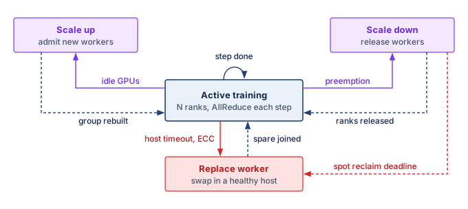
Figure 11: **Elastic Training Worker Lifecycle and State Machine**: The state machine governing dynamic worker membership. Active training loops on step completion and leaves that state along three paths: idle GPUs trigger scale up, a preemption for higher-priority work triggers scale down, and a host timeout or ECC error triggers worker replacement. Each path rebuilds the communication group and returns to active training (dashed arrows), and a spot reclamation deadline can force a shrinking job straight into replacement. Worker processes may restart during resizing, so recovery requires the application to restore valid training state.

From the scheduler’s perspective, this contract is defined by three governing parameters: the elastic range, the transition cost, and the scaling efficiency curve. The elastic range, $[\ElasticMinimumWorkerCount, \ElasticMaximumWorkerCount]$, specifies lower and upper worker bounds; the job’s parallelism layout determines the valid allocation increments within them. The transition cost includes any checkpoint, restart, state redistribution, and rendezvous required by the runtime. Measuring the full interruption determines how frequently the scheduler can trigger reallocations before transition overhead wipes out any throughput advantage. Finally, the scaling efficiency curve quantifies the marginal throughput gained from each added worker, indicating whether assigning idle GPUs to this job yields more aggregate progress than holding them for an assembling gang-scheduled workload. Together, these parameters provide the scheduler with the quantitative bounds needed to resize jobs dynamically without treating elasticity as free capacity.

The scheduler must also account for the effect of worker count on global batch size ($\GlobalBatchSize = \PerWorkerBatchSize\times \DeviceCount$), where the per-worker batch counts examples contributing to one optimizer update, including gradient accumulation. Holding the global batch constant requires each remaining worker to process more examples after a shrink. Larger microbatches consume more memory; additional accumulation steps extend the update time. Preserving the batch removes one source of optimization change but does not guarantee identical convergence. Allowing the global batch to change instead requires validating the learning-rate policy and resulting model quality, so throughput alone cannot determine the best allocation.

Listing 2: TorchElastic Launch Configuration: The --nnodes=4:16 range configures the elastic worker group to admit 4 to 16 nodes, or 32 to 128 workers. A separate cluster scheduler or operator must acquire, launch, and release nodes within that range.

# Launch elastic training with min 32 to max 128 workers
torchrun \
  --nnodes=4:16 \
  --nproc_per_node=8 \
  --rdzv_backend=c10d \
  --rdzv_endpoint=head-node:29500 \
  --max_restarts=3 \
  train.py

TorchElastic sets the elastic range in its launch configuration as a minimum and maximum node count (listing 2). There, the --nnodes=4:16 specification configures TorchElastic’s rendezvous and worker-membership range as 4 to 16 nodes (32 to 128 workers with 8 processes per node). It does not acquire or resize cluster resources; a separate cluster scheduler or operator must place the nodes and start or stop elastic agents as capacity changes.

Systems Perspective 8.2: Elastic vs. rigid scheduling

Consider a congested cluster where a 128-GPU job waits 8 hours for a full gang allocation. This first comparison assumes throughput scales linearly with worker count, equivalent learning progress per processed example, and negligible resize overhead; the later scaling decision relaxes the throughput and transition assumptions.

Rigid scheduling: Wait 8 hours, then train for 24 hours at full throughput. Total wall-clock: 32 hours.

Elastic scheduling (min 32, max 128):

Start immediately with 32 GPUs (throughput = 25 percent of full)
At hour 2, when 64 GPUs free, scale to 64 (throughput = 50 percent)
At hour 8, when the full gang frees and the rigid job would also start, scale to 128 (throughput = 100 percent)

Work completed during the 8-hour queue wait, in hours of full-scale training:

Hours 0 to 2: 25 percent throughput $\times$ 2 hours = 0.5
Hours 2 to 8: 50 percent throughput $\times$ 6 hours = 3
Total: 3.5 hours of equivalent full-scale work

The elastic job completes in approximately 28.5 hours (8 hours of partial-scale training plus 20.5 hours at full scale), saving 3.5 hours compared to rigid scheduling. This improvement of about 11 percent comes entirely from using resources productively during what would otherwise be idle queue time.

The scheduler cannot treat every worker count as a valid elastic configuration. Model parallelism constrains the allocation increment when the resize policy keeps tensor and pipeline layouts fixed and adds or removes whole data-parallel replicas. For a 175B-parameter job that relies on 8-way tensor parallelism within each node and 8 pipeline stages across nodes, this policy operates at the granularity of a whole model replica of 64 GPUs. The pipeline depth of 8 is the smallest power of two at which each GPU’s share of the mixed-precision Adaptive Moment Estimation (Adam) training state fits in its HBM when that state is not sharded across replicas. The feasible layout of Distributed Training instead uses a shallower pipeline and shards optimizer state across the data-parallel group with ZeRO (Memory-efficient data parallelism with ZeRO and FSDP). Keeping each replica’s state self-contained costs memory, but it lets the scheduler add or remove a replica without redistributing every other replica’s optimizer shards. The job can scale between 128 nodes (1,024 GPUs) and 32 nodes (256 GPUs) one replica at a time, changing the data-parallel degree. Removing a single GPU from a tensor-parallel group would instead require a new sharding layout and redistribution of training state. Changing the pipeline degree would also require repartitioning stages and rebuilding the pipeline schedule. A runtime that supports these transitions can expose them to the scheduler, but their feasibility and measured costs belong in the resize contract rather than following automatically from data-parallel elasticity.

The transition cost also constrains the scheduler’s resize frequency. Each scaling event can interrupt useful work while the framework reconstructs its communication group and restores or redistributes state. The duration must be measured for the chosen runtime and checkpoint path. The scheduler must amortize this cost over the subsequent run duration, so small resize increments are only worthwhile if the job will run at the new scale for significantly longer than the transition window; section 8.7.3 shows the thrashing that results when a policy ignores this amortization.

8.7.2 Scheduler integration

Without scheduler integration, a job that declares an elastic range $[\ElasticMinimumWorkerCount, \ElasticMaximumWorkerCount]$ in its launch script still waits in the queue for its full node count and still gets killed outright when a higher-priority job arrives. Integrating the $[\ElasticMinimumWorkerCount, \ElasticMaximumWorkerCount]$ bounds into the scheduler lets it start a job early at the minimum, expand the job into newly idle capacity, or shrink it to release borrowed capacity without terminating the logical job. Which action wins depends on the job’s scaling curve and transition cost, and the policies below compare the choices by the work completed over the same time window.

Each action must respect the framework contract. The most consequential of the three is graceful preemption: when higher-priority work arrives, the scheduler first shrinks an elastic job toward $\ElasticMinimumWorkerCount$, reclaiming whole replicas at the next resize boundary, and resorts to checkpoint-and-preempt only when the final viable group itself must yield. Quota borrowing across teams, developed in section 8.11, depends on this primitive whenever an owner reclaims capacity it lent. Scaling curves and transition costs determine whether the extra progress repays the disruption. Because batch changes can affect convergence, the test of a resize is time to target model quality, not throughput.

8.7.3 Elastic scaling policies

Adding resources to a running job does not always accelerate time-to-convergence. Communication and synchronization overhead limit throughput gains, requiring the scheduler to enforce elastic scaling policies based on empirical efficiency curves rather than resource availability alone. With fixed global work per step, a job’s scaling efficiency $\ScalingEfficiency(\ScalingCurveWorkerCount)$ at $\ScalingCurveWorkerCount$ workers (definition 6.4) typically passes through three regimes: a near-linear regime where per-worker computation dwarfs every fixed per-step cost, a sublinear regime where pipeline fill and drain and the unhidden part of gradient synchronization become a visible share of each step, and a saturation regime where those fixed costs rival the shrinking computation itself. Assigning available GPUs to a saturated job can yield less useful progress than serving queued work. The lower allocation bound answers a different question. Below its minimum viable scale, a job may lack the memory or complete parallel groups needed to execute at all. A policy can impose a higher minimum to meet a deadline, even when a smaller allocation remains computationally efficient.

Throughput falls away from ideal linear scaling and saturates.

The 175B reference job shows these regimes with the chapter’s own numbers. Modeled at a fixed global batch with the step-time decomposition of the Fleet Law (equation 1.3), its scaling efficiency falls from 87 percent at 256 GPUs to 83 percent at 1,024 GPUs and 69 percent at 4,096 GPUs (figure 12, panel a). Efficiency falls, yet quadrupling from 1,024 to 4,096 GPUs still raises throughput 3.3×, so a lower efficiency is a declining marginal return rather than a slowdown. Panel (b) locates the loss. Tensor-parallel communication shrinks along with each worker’s computation, so its share of the step never rises above 11 percent. The decline comes instead from pipeline fill and drain and unhidden gradient synchronization, which take roughly fixed time per step while each worker’s share of the batch shrinks. The pipeline bubble grows fastest of the three, for a reason the bubble fraction $(\PipelineParallelDegree-1)/(\MicrobatchCount+\PipelineParallelDegree-1)$ of Pipeline parallelism makes explicit. With the global batch fixed, each added replica takes a share of the sequences, so the microbatch count $\MicrobatchCount$ per replica falls while the stage count stays at 8, and the idle fraction rises. The shaded window from 256 to 1,024 GPUs is therefore a policy choice, not an interval derived from these efficiencies alone. A minimum allocation could follow from a completion deadline or the job’s declared resource contract. It does not follow from insufficient per-worker computation at smaller scale, since with fixed global work fewer workers generally perform more work each. The upper limit likewise requires comparing additional useful progress with resize cost and the value of serving queued jobs. A real scheduler must obtain those inputs from profiling and the workload’s quality target.

Figure 12: **Modeled Scaling Efficiency and Elastic Operating Range**: (a) Scaling efficiency ($\ScalingEfficiency$) of the 175B reference job from 64 to 4,096 GPUs, computed with 8-way tensor parallelism within each DGX H100 node, 8 pipeline stages, HDR InfiniBand, and a fixed global batch of 1,536 sequences. The shaded window is an assumed admission policy; efficiency alone establishes neither its minimum nor its maximum. (b) Share of each step lost to tensor-parallel communication, pipeline bubble, and exposed gradient synchronization. Lower efficiency does not imply that adding workers reduces throughput.

This logic extends to the temporal dimension, where the scheduler must weigh the immediate progress of a smaller allocation against waiting for a larger one. If a 512-GPU job can start immediately with 128 GPUs or wait for the full request, the better choice depends on the integration of throughput over time. The resize overhead (the cost of stopping, checkpointing, and restarting when the runtime requires them) must be amortized over the subsequent run duration. A policy of “opportunistic scaling” that resizes a job every time a single node becomes free can lose its throughput advantage to repeated interruptions, completing less useful work than a stable allocation.

Napkin Math 8.3: The elastic scaling decision

The comparison of elastic and rigid scheduling above assumed linear scaling and free resizing; this decision drops both assumptions. Consider a training job with a target batch size that requires 512 GPUs for the highest throughput among the configurations considered. Three scheduling strategies are evaluated over a window of 24 hours.

Given: Throughput at 128 GPUs is 1 epoch/hour (baseline). Throughput at 256 GPUs is 1.8 epochs/hour (90 percent scaling efficiency relative to that baseline). Throughput at 512 GPUs is 3.2 epochs/hour (80 percent scaling efficiency). Re-scaling cost is 10 minutes (0.17 hours) to checkpoint, re-shard, and restart.

Strategy 1 (immediate start, no scaling): The job starts immediately with 128 GPUs and runs for the full 24 hours. Total work: $24 \times 1.0 = 24$ epochs.

Strategy 2 (wait for the full allocation): The job waits in the queue for 4 hours until 512 GPUs become available, then runs for 20 hours. Total work: $20 \times 3.2 = 64$ epochs.

Strategy 3 (elastic step-up): The job starts immediately with 128 GPUs. After 4 hours, the capacity that lets Strategy 2 start frees up, but the elastic policy caps growth at 256 GPUs so that the remaining GPUs stay available to queued jobs. The job pauses, scales up, and resumes. Phase 1: $4 \times 1.0 = 4$ epochs. Phase 2: $(24 - 4 - 0.17) \times 1.8 \approx 35.7$ epochs. Total work: 4 + 35.7 = 39.7 epochs.

The elastic strategy completes nearly 1.7× the epoch-equivalent work of the immediate small-scale run, but still trails the full allocation by about 38 percent. That comparison counts this job’s epochs, not the GPU-hours spent on them. Strategy 2 holds twice as many GPUs as Strategy 3 for most of the window and runs them at 80 percent scaling efficiency against Strategy 3’s 90 percent, so the elastic job does more work per GPU-hour, and the GPUs it leaves free serve queued jobs. Which strategy wins therefore depends on whether the fleet values this job’s completion time or the total work completed across all jobs. That gap shrinks when queue waits grow or peak capacity stays scarce; re-scaling overhead is only 10 minutes, so the step-up strategy keeps its lead over the immediate small-scale run unless slow checkpoint transfer or compilation stretches that overhead beyond about 9 hours.

Placement and elasticity determine which allocations are feasible and how much useful progress they produce across competing jobs. Fleet economics adds the price of those choices. Every placement, preemption, and reservation consumes capacity that could serve another workload, so the scheduler must compare both useful progress and opportunity cost.

Self-Check: Question

When an elastic scheduler resizes a distributed training job from 64 GPUs to 128 GPUs, what trade-off exists between maintaining a constant global batch size versus scaling batch size proportionally with worker count?
1. Constant global batch size halves the effective examples per worker per optimizer update, removing one source of optimization change without guaranteeing identical convergence; proportional batch scaling preserves that per-worker count but changes optimization and requires a validated learning-rate policy.
2. Constant global batch size requires restarting the model weights from epoch zero, whereas proportional batch size allows continuous gradient descent without learning rate adjustment.
3. Constant global batch size disables NVLink communication across workers, whereas proportional batch size enables ring AllReduce.
4. Constant global batch size doubles the learning rate automatically via PyTorch hooks, whereas proportional batch size keeps the learning rate fixed to prevent divergence.
An elastic job running on 64 GPUs at 100 steps/minute can scale to 128 GPUs, reaching 180 steps/minute. If resizing triggers a dynamic rendezvous and checkpoint-sync transition pause of 60 seconds (0 steps during pause), what is the break-even duration the job must run after the pause at 128 GPUs to recover the lost progress in total steps completed?
1. At least 15 seconds.
2. At least 30 seconds.
3. At least 45 seconds.
4. At least 75 seconds.
What three parameters define the operational contract between an elastic scheduler and an elastic training framework (such as TorchElastic), and why is each necessary?
True or False: Under a supported resize and checkpoint contract, an elastic scheduler can reclaim capacity by shrinking a training job to a smaller viable configuration without terminating the logical job, although worker processes may restart.
A worker encounters an unhandled CUDA fault during a TorchElastic training run. Explain the dependencies that must hold before useful training resumes, and why recovery cannot require every surviving worker to finish a clean step boundary.

See Answers →

8.8 Cost Optimization

An idle accelerator in an enterprise fleet incurs operational costs every hour whether computing or blocked in a queue, turning placement and preemption decisions into direct financial trade-offs. The orchestrator translates this utilization-to-dollars relationship from section 8.1 into an online scheduling signal, balancing resource prices, reservation commitments, interruption risk, checkpoint cost, and job deadlines to decide whether to admit, delay, preempt, or resize work. Capital planning, portfolio return, cost attribution, and lifecycle total cost of ownership are larger, slower decisions developed in Fleet Economics and Utilization; the scheduler consumes their outcomes as prices and constraints.

At a fixed utilization, idle capacity grows linearly with fleet size, so the dollar cost of a scheduling inefficiency grows with every procurement (figure 13). At 10,000 GPUs operating at 50 percent utilization, annual waste reaches $87.6M under the chapter’s $2/GPU-hour accounting scenario. Published measurements show that such underutilization occurs in production. Microsoft’s Philly cluster study (Jeon et al. 2019) measured mean GPU utilization of approximately 52 percent. The 30 to 70 percent shaded band in the figure is an illustrative operating range for the cost model, not a universal empirical claim about all production clusters. Moving from 50 percent to 80 percent utilization, the improvement priced in the chapter opening, recovers over $52M annually in equivalent capacity value; that is the same 3,000 GPU-equivalents the opening counted as waste at 30 percent idle, and it becomes cash savings only when it avoids billed usage or a planned purchase.

Figure 13: **The Cost of Idle GPUs**: Annual wasted cost as a function of cluster size for different GPU utilization levels, assuming $2/GPU-hour (cloud equivalent). The shaded region between 30 percent and 70 percent is an illustrative operating range for the scenario analysis. At 10,000 GPUs with 50 percent utilization, the model yields $87.6M in annual wasted capacity. The thin violet line traces the published Microsoft Philly mean GPU utilization of 52 percent across all cluster sizes; it is a utilization reference, not a measured cluster size or cost. Data source: Jeon et al. (2019).

The idle-capacity figure establishes the economic target, and the remaining cost controls explain how the scheduler moves toward it. Most of those controls recover capacity by interrupting running work, so the price of a single interruption comes first. Interruptible capacity then lowers the price of tolerant work, reservation and quota policy decide which jobs deserve scarce guaranteed capacity, and accountability mechanisms make idle GPUs visible to the teams that create demand.

8.8.1 Preemption cost and cascades

Each eviction can evict again, so one admission reaches $\PreemptionFanoutCount + \PreemptionFanoutCount^2$ jobs.

When a high-priority job enters a saturated cluster, the scheduler must decide which running workloads to terminate to free up resources. This decision is rarely isolated. In tightly packed clusters, evicting a medium-priority job to accommodate a high-priority request often triggers a preemption cascade, where the evicted job immediately attempts to reschedule itself by displacing lower-priority workloads. The disruption multiplies with each level. If the urgent job displaces $\PreemptionFanoutCount$ medium-priority jobs and each of those, on rescheduling, displaces $\PreemptionFanoutCount$ lower-priority jobs, one admission interrupts $\PreemptionFanoutCount+ \PreemptionFanoutCount^2$ jobs after two levels, every one of which pays the preemption overhead quantified below and adds a checkpoint reload to the storage system at the same moment. Two dampening controls cap that growth. A rule that evicted jobs requeue without preempting anyone themselves stops the chain at the first level, so one admission costs at most $\PreemptionFanoutCount$ interruptions. A preemption budget limits how often any single job, or what fraction of capacity, may be displaced in a time window, which protects the jobs at the bottom of the priority order that every chain would otherwise reach.

The engineering cost of preemption extends beyond scheduling latency. The preemption overhead depends on the exit path. A successful graceful checkpoint adds the time to save and restart while preserving completed progress; a forced stop can instead discard work since the last durable checkpoint. Consider such a victim, a forced interruption of the 64-GPU fine-tuning run for our 175B parameter model. The scenario assumes lost work equivalent to 15 minutes of execution. The restart then repeats the cold-restart steps of the recovery budget in Recovery procedures, without its detection step because the scheduler itself stopped the job: 3 minutes to relaunch, 24.5 seconds to reload the 2.45 TB checkpoint with its optimizer state, and 2 minutes of warmup as data pipelines refill and just-in-time (JIT) compilation and runtime initialization complete. The calculation prices replay and restart across the same allocation; it does not also charge for a successful final save.

Reconstructing the distributed data pipeline also belongs in the preemption contract. The checkpoint must preserve the sampling and loader state needed to resume the intended data order, alongside model and optimizer state. If the restart path omits that state, it can repeat or skip samples and lose exact replay of the training trajectory. A different shuffle order does not by itself prove statistical corruption, but the recovery policy must specify which changes are acceptable. The scheduler should therefore measure restoration and pipeline warmup as part of recovery cost, rather than assume that reloading model weights alone makes the job productive.

The resulting 20.4-minute overhead combines discarded execution, its larger part, with relaunch, reload, and warmup time; it is not a measurement of continuous kernel activity after eviction. Spread over the run, it belongs to the Fleet Law’s coordination term $\SynchronizationTime(\DeviceCount)$ (equation 1.3), which counts scheduling decisions and failure recovery alongside barrier waits, so frequent preemption lengthens the average step exactly as frequent failure does. At $2/GPU-hour, the scenario values each event at $44 in allocation time. A low-priority run sits at the bottom of every cascade, so without a budget it can be struck many times a day. At the scenario’s 12 forced preemptions per day, it loses 4.1 hours of equivalent allocation time, or 261 GPU-hours for this 64-GPU run. A per-job budget bounds that loss directly. When a budget binds, the scheduler must consider waiting, another placement, or a defined emergency exception. The trade-off is reduced recovery churn against delayed admission, measured under the workload’s deadlines.

8.8.2 Spot instances and preemptible VMs

Renting on-demand cloud GPUs for a multi-week training run protects the job from provider reclamation, but pays full price even when spare GPUs sit idle in the provider’s data center; renting interruptible capacity cuts the hourly rate by 60 to 90 percent, but lets the provider reclaim those GPUs on best-effort notice. Cloud providers sell this spare capacity through spot instances¹⁰ (AWS) or preemptible VMs (GCP), where actual discounts depend on the resource and market. The reference interruption windows range from up to 30 seconds for GCP preemptible shutdown to 2 minutes for AWS stop or termination notices, with best-effort delivery rather than a guaranteed recovery interval. At the scenario rates of $0.70/GPU-hour instead of $2/GPU-hour, the worked comparison below shows how savings can exceed half the on-demand cost after accounting for its assumed interruption overhead.

¹⁰ Spot instances: The scenario’s 60 to 90 percent discount purchases reclaimable capacity, not a guaranteed interval for saving state. AWS’s best-effort stop or termination notice targets 2 minutes, while GCP preemptible shutdown allows up to 30 seconds; AWS hibernation begins immediately. If a job’s measured checkpoint time exceeds the reference 30-second window, a notice-triggered save cannot be its only recovery path.

The viability of spot instances for ML training depends on two factors that determine whether the discount translates into actual savings: the cost of each interruption (checkpoint overhead plus restart time plus lost work since the last checkpoint) and the frequency of interruption (which varies by instance type, region, time of day, and overall cloud demand). Equation 3 gives the effective cost of spot training:

\[ \EffectiveSpotTrainingCost= \SpotHourlyPrice\times \frac{\BilledAllocationTime}{\RetainedProductiveTime} \tag{3}\]

where $\BilledAllocationTime$ is billed allocation time, including checkpointing, recovery, and work later discarded after an interruption, and $\RetainedProductiveTime$ is the equivalent training time represented by retained progress. The ratio assumes a fixed allocation size and price, with unchanged useful throughput while training; variable allocations require summing the cost of each allocation interval. Waiting for replacement capacity extends completion time but contributes to billed time only while resources remain allocated. When checkpointing and interruption losses consume a small fraction of billed time, effective cost stays near the spot price. Frequent interruptions, expensive recovery, or substantial replay can instead erase the discount.

Spot savings and fault tolerance infrastructure are coupled. Fault tolerance mechanisms (frequent asynchronous checkpointing, fast checkpoint loading, elastic recovery) make spot capacity usable by lowering the cost of each interruption. Elastic training can resume a logical job with fewer workers after reclamation, provided the remaining allocation is viable, although the framework may still restart worker processes and restore checkpointed state, so elasticity reduces recovery cost rather than eliminating it. The same infrastructure therefore earns a double return. It protects against hardware losses, and it enables the deliberate use of interruptible capacity. Both benefits require measurement. The scheduler combines observed interruption rates, recovery costs, and retained training progress with resource prices to estimate whether spot savings repay the additional recovery infrastructure. The same evidence supports valuing protection against hardware failures; neither benefit follows from the discount or checkpoint mechanism alone.

8.8.3 Spot instance strategies for ML training

Spot capacity pays off only when an interruption rarely removes the whole job at once, so schedulers that use it diversify where capacity comes from instead of simply retrying on failure. Availability zone diversification reduces the probability of simultaneous fleet-wide reclamation. Cloud providers typically manage spot pools independently per availability zone (AZ). If a training job requires 1,024 GPUs, allocating them as a single block in one zone exposes the job to a complete stop if that specific zone’s spot pool is reclaimed. Diversifying independent jobs or restart destinations across zones reduces exposure to one exhausted pool. Splitting a single synchronous gang across zones also changes its communication paths, so the scheduler must include cross-zone bandwidth, latency, and transfer costs before accepting that placement. The scheduler still must model correlation carefully: independent per-instance interruptions make large simultaneous losses unlikely, but pool-level or AZ-level reclamations can remove hundreds of GPUs at once and must be treated as elastic-shrink or failover events rather than ordinary isolated failures.

Instance type diversification expands the set of capacity pools a job can use, though availability across those pools can remain correlated. A job that requests only one instance type cannot use spare capacity in another pool. Accepting alternatives therefore requires a compatibility list that includes memory capacity, runtime support, communication paths, and measured throughput. An instance with more memory can still be an unsuitable substitute if its runtime support, communication paths, or throughput differ. The scheduler compares each feasible alternative’s price and recovery cost per unit of retained progress; mixing devices within a synchronous gang also requires accounting for unequal worker speeds.

Spot capacity signals can guide placement but do not necessarily predict interruption frequency. For example, the AWS Spot Placement Score estimates the current likelihood that a capacity request will succeed in a region or availability zone; it explicitly does not predict interruption risk. A scheduler can use this signal to choose where to request capacity, but estimating interruptions per day requires separate historical measurements for the instance type and region. If the resulting workload-specific recovery model shows that interruption overhead erases the discount, the scheduler should migrate the job to on-demand capacity or a different region.

Checkpoint frequency optimization for spot instances extends the reliability logic. The Young-Daly formula developed in The Young-Daly checkpoint interval models losses from unpredicted interruptions, whether caused by hardware failure or reclamation without a usable warning. Provider notices offer an additional opportunity to save state, using the reference windows of 2 minutes on AWS and up to 30 seconds on GCP preemptible VMs. A two-tier checkpointing approach combines periodic checkpoints, with an interval chosen for the workload’s interruption model, and a best-effort checkpoint triggered by a notice. The notice-triggered checkpoint reduces lost work only if it becomes durable before reclamation; otherwise, the job restores its last durable state, whether produced by a periodic, asynchronous, or incremental checkpoint, and replays subsequent work. That contingency planning becomes even more critical when spot interruptions are correlated across a pool rather than isolated to single machines.

Systems Perspective 8.3: Correlated spot risk

Context: Spot capacity is cheap because it is reclaimable. That risk is not independent across instances: cloud regions, instance types, product launches, and deadline cycles can create correlated demand.

Failure mode: A fleet that concentrates all interruptible training in one region and one instance type can lose a large fraction of workers at once, even if each individual worker appears restartable.

Consequence: Checkpointing handles isolated interruptions; it does not solve fleet-wide preemption when every retry targets the same exhausted pool.

Systems insight: A robust scheduler diversifies compatible restart destinations, monitors interruption risk, and plans an on-demand fallback when spot capacity cannot meet the job’s deadline or cost target. That fallback still depends on available capacity and the time needed to restore state.

8.8.4 Capacity reservation strategies

Committing to long-term reserved capacity for 100 percent of peak demand leaves expensive GPUs idle whenever traffic dips, while relying solely on spot or on-demand pools risks capacity shortages during product launches and sudden reclamations during deadline crunches. To avoid paying for idle reservations or starving urgent workloads, organizations that rely on cloud infrastructure (or that price on-premises capacity in economic terms) combine three tiers of compute capacity, each trading cost and commitment against availability and interruption risk (table 4).

Table 4: Cloud Capacity Reservation Tiers: Capacity tiers trade cost and commitment against availability guarantees and interruption risk, giving the scheduler a price ladder for routing workloads by urgency and restart tolerance.

Capacity tier	Cost and commitment	Availability and interruption risk	Best-fit workloads
Reserved capacity	Capacity reservation; price discounts require a separate purchasing contract.	Capacity assurance within the reservation terms; startup still takes time.	Predictable continuous workloads: 24/7 inference, scheduled training, CI and regression testing, jobs under service-level agreements (SLAs).
On-demand capacity	Full price with no long-term commitment.	Admission depends on available capacity; provisioning and startup add delay.	Urgent retraining, interactive debugging, and short-lived jobs that do not justify spot management.
Spot capacity	Discounted interruptible capacity.	Availability varies with cloud demand, and workers can be reclaimed.	Restart-tolerant jobs: hyperparameter sweeps, ablations, checkpointed pretraining, and exploratory research.

The constructed portfolio in figure 14 divides capacity into a reserved tier covering the steady 60 percent baseline, an on-demand band between 60 and 80 percent, and an interruptible spot tier serving peaks up to 92 percent. An organization with 60 percent steady-state utilization and 40 percent burst demand might reserve capacity for 60 percent of peak need, use on-demand for bursts whose deadlines tolerate admission and startup delay, and use spot for restart-tolerant work. These shares illustrate a policy rather than establish an optimal portfolio. The scheduler must match each workload’s deadline and recovery contract to the capacity tier: reserved capacity can support the steady serving load or a training job’s base allocation, while spot can support elastic replicas or independent experiments that tolerate reclamation. A peak in urgent demand cannot automatically be assigned to spot merely because it lies above the reserved band.

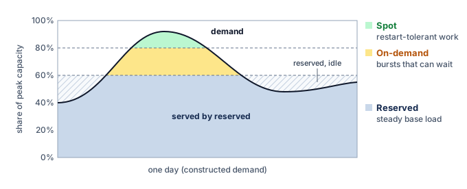
Figure 14: **Capacity Reservation Tiers and Portfolio Optimization**: This constructed portfolio combines reserved physical capacity, on-demand acquisitions, and interruptible workers. Reserved capacity covers the steady 60 percent base, on-demand the next 20 percent, and spot the peak; these shares and the demand curve are scenario assumptions. A discount commitment alone does not reserve capacity, and on-demand admission is not instantaneous. Schedulers map steady-state baseline demand to reserved capacity, diurnal spikes to on-demand instances, and restart-tolerant training to discounted spot pools. Hatching marks reserved capacity that is held while demand sits below it.

Systems Perspective 8.4: Spot vs. on-demand training

Consider training a 70B parameter model, a smaller workload than the chapter’s 175B reference, on 512 GPUs for 14 days. The scenario fixes the event budget at 196 interruptions over the run and treats each as graceful, so no progress is replayed.

On-Demand: 512 GPUs $\times$ 336 hours $\times$ $2/GPU-hour = $344,064

Spot (65 percent discount, 5 percent checkpoint overhead, 14 interruptions per day of useful training with 30 minutes restart):

Base cost: 512 GPUs $\times$ 336 hours $\times$ $0.70/GPU-hour = $120,422
Checkpoint overhead: $5\%$ $\times$ 336 hours = 16.8 hours
Restart overhead: 196 interruptions $\times$ 0.5 hours = 98 hours
Total time: 336 hours + 16.8 hours + 98 hours = 450.8 hours
Total cost: 512 GPUs $\times$ 450.8 hours $\times$ $0.70/GPU-hour = $161,567

Savings: $182,497 (53.0 percent), at the cost of approximately 34.2 percent longer wall-clock time.

These savings assume fault tolerance infrastructure is already in place. Without checkpointing, a single interruption forces restart from scratch, potentially wasting days of compute and negating all savings.

8.8.5 Cost-aware scheduling policies

Cost-aware scheduling adds financial efficiency to the completion-time, utilization, and fairness objectives already introduced. The orchestrator evaluates three recurring classes of trade-offs: waiting versus running immediately, preempting existing tasks versus paying more for on-demand capacity, and falling back versus shrinking elastically. For example, it might compare an immediate launch on reserved A100 GPUs with waiting two hours for spot H100 instances. If workload profiling and the price model predict twice the throughput at half the execution cost, the remaining question is whether those gains repay the delay and interruption risk. When capacity becomes constrained, the scheduler must balance preempting a low-priority hyperparameter sweep on reserved capacity against routing a high-priority training run to more expensive on-demand instances. When a provider reclaims spot instances, the policy compares replacing them with on-demand nodes against shrinking elastically. These choices require the costs of waiting, recovery, and displaced work as well as the price of the new allocation.

These decisions require the scheduler to model both the time-value of computation (the organizational cost of a 2-hour delay in researcher productivity, product launch schedules, or competitive position) and the financial cost of different resource allocations. Delaying a production model retrain by 2 hours might violate a service level agreement (SLA), while the same delay to an exploratory experiment can postpone a research decision or block dependent work. A workload class’s delay tolerance is therefore a policy input grounded in its dependencies and deadlines, not an assumption that exploratory work has no time cost.

Production systems can define cost policies per workload class that encode these trade-offs as configuration rather than requiring per-decision human judgment. One policy places steady inference demand on reserved capacity and maintains ready replicas to meet its latency target; the reservation alone does not guarantee application availability or latency. Large training runs can combine a reserved minimum viable allocation with interruptible elastic expansion, requesting on-demand replacements when a deadline justifies the cost and capacity is available. Exploratory workloads with flexible deadlines can use spot capacity while accepting interruptions and variable completion times. These assignments express the organization’s priorities rather than a universal mapping from workload type to purchasing tier.

The scheduler does not implement the organization’s financial accounting system. It consumes the resulting price and policy signals: the marginal price of each capacity tier, the reservation a project may claim, the interruption risk it may accept, and the deadline it must meet. Showback, chargeback, and attribution belong to that accounting system; the scheduler uses their outputs only to rank feasible scheduling actions. Lifecycle total cost of ownership (TCO) reaches the scheduler the same way, as per-resource opportunity costs and constraints that record whether capacity is owned, reserved, on demand, or interruptible, rather than as a scheduling mechanism.

↪ Tag-based cost attribution, shared-cost allocation, and chargeback are developed in Cost visibility and attribution.

↪ The lifecycle TCO framework, which combines training, inference, data, and iteration costs, is developed in ML systems TCO framework.

Checkpoint 8.2: Cost-aware scheduling trade-offs

Before moving to ML-specific schedulers, review how the cost-optimization mechanisms interact:

Spot break-even: identify the additional inputs needed to compute a break-even checkpoint interval for the 512-GPU, 14-day training job of the spot comparison above (65 percent spot discount, 14 interruptions per day, 30-minute restart overhead), including checkpoint duration, the interruption-rate clock, and lost-progress assumptions.
Double return: explain why fault tolerance infrastructure has a “double return” for reliability and cost savings, and identify the minimum fault tolerance investment needed to make spot instances viable.
Reservation sizing: starting from the constructed portfolio that reserves 60 percent of peak, identify the demand history, reservation terms, unit prices, and unused-capacity costs needed to decide whether raising the reserved share to 70 percent reduces total spending.

Spot pricing and reservation strategy reduce the cost of capacity, but they do not determine which competing job should receive it. Runtime uncertainty, unequal completion delays, and the cost of interrupting an iteration remain even when prices are known. Resolving them requires signals from the workload itself, such as how much service a job has consumed, where its iteration boundaries fall, or how fast it is learning. A scheduler that tracks learning progress can optimize time-to-accuracy, the wall-clock time until a run reaches a target validation metric, rather than execution speed alone.

Self-Check: Question

What is a preemption cascade in a shared GPU cluster, and which control stops it at the first level?
1. A cascade is a burst of hardware failures in one rack; spare-capacity reservation stops it.
2. A cascade is a high-priority admission that evicts medium-priority jobs, each of which then evicts lower-priority jobs to reschedule itself; requiring evicted jobs to requeue without preempting anyone stops it after the first level.
3. A cascade is a queue of jobs waiting behind a large gang; backfill scheduling stops it.
4. A cascade is repeated checkpointing by one job; lengthening its checkpoint interval stops it.
A training job moves from on-demand to spot capacity at the chapter’s scenario discount. According to the effective-cost relation, in which effective cost equals the spot price times billed allocation time divided by retained productive time, what determines whether the discount survives?
1. Only the advertised discount, because interruptions are free once a provider sends a notice.
2. The ratio of billed allocation time to retained productive time, which grows with checkpoint overhead, restart time, and work replayed after each interruption.
3. The number of GPUs in the job, because larger jobs always receive deeper spot discounts.
4. The provider’s capacity-placement score, which predicts how many interruptions the job will see per day.
An organization runs steady 24/7 inference, urgent retraining with tight deadlines, and a large hyperparameter sweep. Which assignment of these workloads to reserved, on-demand, and spot capacity matches each workload’s deadline and recovery contract?
1. Inference on spot, retraining on reserved, sweep on on-demand.
2. Inference on reserved, retraining on on-demand, sweep on spot.
3. All three on spot, because the discount outweighs any interruption risk.
4. Inference on on-demand, retraining on spot, sweep on reserved.
This chapter treats lifecycle total cost of ownership (TCO) as an input to the scheduler rather than as a scheduling mechanism. What does the scheduler consume from TCO analysis and cost accounting, and how does it use those inputs?
A low-priority 64-GPU fine-tuning run is forcibly preempted. What makes up the preemption overhead for that event, and why does a per-job preemption budget matter more for this run than for a high-priority job?
True or False: Because each VM instance in a cloud provider has an independent lifecycle, placing worker nodes of a 64-node distributed training job across different instance types within the same Availability Zone guarantees that preemption events will remain uncorrelated and statistically independent.

See Answers →

8.9 Custom ML Schedulers

A short experiment waiting behind a long training run can suffer even when every running job has an efficient placement. Improving that outcome requires a policy for deciding which job receives the next available resources. Custom ML schedulers use different signals to make that decision: consumed service can prioritize jobs without runtime estimates, iteration boundaries can make preemption cheaper, normalized finish time can expose unfair delay, and measured goodput can guide joint resource and batch-size changes. Only the last of these requires a model of learning progress; the others improve completion time, utilization, or fairness without predicting convergence.

8.9.1 Duration-agnostic scheduling (Tiresias)

Tiresias (Gu et al. 2019) addresses the fundamental problem identified in section 8.4.3: ML job durations are unpredictable, and scheduling policies that rely on exact duration estimates can make poor decisions when those estimates are unavailable or unreliable. Rather than fighting this information asymmetry, Tiresias eliminates the requirement for duration estimates entirely. It uses a two-dimensional attained service¹¹ scheduler that makes priority decisions based on what a job has already consumed, not what it claims it will consume. Jobs accumulate “service” based on GPU-time consumed, with priority decreasing as service increases. The two dimensions are time (how long the job has been running) and resources (how many GPUs the job uses), capturing both elapsed duration and resource intensity.

¹¹ Attained service scheduling: A discipline that uses consumed service to set priority when remaining work is unknown. Unlike shortest remaining processing time (SRPT), it cannot distinguish a newly arrived long job from a short one before either receives service. Its benefit depends on the workload distribution; protection against starvation remains necessary when new jobs repeatedly displace older ones.

A discretized version groups jobs into service bins (illustratively, less than 1 GPU-hour, 1 to 10 GPU-hours, 10 to 100 GPU-hours, greater than 100 GPU-hours), giving lower-service bins higher priority. When job durations are heavy-tailed, a job that has consumed little service is likely to be short, so favoring low-service jobs approximates shortest-remaining-processing-time ordering without any runtime estimate. New jobs can receive service before long-running jobs, but their eventual duration remains unknown, and a high-priority gang still needs a feasible allocation. Tiresias also promotes jobs that have waited too long, trading some average-completion-time benefit for protection against starvation. The priority rule therefore replaces runtime prediction with an observable signal and an explicit waiting-time policy; it does not guarantee that every short job starts promptly.

The Tiresias evaluation reports lower average job completion time (JCT) on its testbed and trace-driven workloads (Gu et al. 2019). The result depends on job arrivals, sizes, and the comparison policy. Prioritizing low-service jobs can delay long-running jobs, so average completion time must be evaluated alongside starvation prevention and the delay experienced by each job class.

Gu, J., M. Chowdhury, K. G. Shin, Y. Zhu, M. Jeon, J. Qian, H. H. Liu, and C. Guo. 2019. “Tiresias: A GPU Cluster Manager for Distributed Deep Learning.” Proceedings of the 16th USENIX Symposium on Networked Systems Design and Implementation (NSDI ’19), 485–500.

8.9.2 Iteration-aware scheduling (Gandiva)

Preempting a job in the middle of a training step either discards the partial step or requires saving gigabytes of temporary forward-pass activations alongside the model weights. Gandiva (Xiao et al. 2018) avoids that mid-step state transfer by exploiting repetitive training iterations to profile jobs and time-slice GPUs at iteration boundaries. To give a GPU to another job, Gandiva suspends the running job at the end of a minibatch, copies its live GPU memory to host memory, and resumes another job on the device; switching back reverses the copy. Several jobs can therefore take turns on one GPU, and the same suspend-and-resume path lets Gandiva migrate a job to better-placed devices or pack compatible jobs onto one GPU when their combined memory fits. The boundary is the cheap place to switch because temporary activations have been released, so far less state must move than in the middle of a step. Weights, optimizer state, and runtime allocations remain, so each switch still costs a transfer proportional to that persistent state, and a job whose persistent state nearly fills the device cannot share it. The scheduler must measure memory demand, interference, and transition cost before admitting additional jobs.

Xiao, Wencong, Romil Bhardwaj, Ramachandran Ramjee, Muthian Sivathanu, Nipun Kwatra, Zhenhua Han, Prabal Patel, et al. 2018. “Gandiva: Introspective Cluster Scheduling for Deep Learning.” 13th USENIX Symposium on Operating Systems Design and Implementation (OSDI 18), 595–610.

Gandiva also implements grow-shrink elasticity, applying the allocation mechanism of section 8.7 to jobs that explicitly permit resizing. It expands eligible jobs into idle capacity and shrinks them when demand returns, using profiles to estimate which jobs benefit. The published implementation limits growth to one server and waits through an idle period before expanding. Its contribution is the connection between measured job behavior and resource control, rather than a claim that arbitrary training jobs can resize cheaply.

8.9.3 Finish-time fairness (Themis)

Equal GPU-time shares can produce unequal completion delays when workloads respond differently to placement. Themis (Mahajan et al. 2020) measures fairness in normalized finish time. Each application, which can contain related training jobs, compares its completion time in the shared cluster with its completion time on an isolated $1/\ContendingApplicationCount$ share of the cluster, where $\ContendingApplicationCount$ is the number of applications contending for it. The ratio has the same form as the slowdown $\JobSlowdown_j$ defined with the scheduling objectives, except in its denominator. Themis divides by the completion time on a fair share of the cluster rather than by the isolated runtime on the job’s own allocation, so a ratio of one means the application finished no later than its fair share would have allowed.

Mahajan, Kshiteej, Arjun Balasubramanian, Arjun Singhvi, Shivaram Venkataraman, Aditya Akella, Amar Phanishayee, and Shuchi Chawla. 2020. “Themis: Fair and Efficient GPU Cluster Scheduling.” 17th USENIX Symposium on Networked Systems Design and Implementation (NSDI 20), 289–304.

Themis targets the worst finish-time fairness ratio across applications. Its auction rounds offer available resources to applications farthest from fair completion, while allowing placement efficiency to influence the allocation within a round. With two applications whose current estimates are 1.2 and 2.0, the second is projected to finish twice as late as its fair share would allow, so it is offered the next round’s GPUs first. The first application’s ratio rises while it waits, and once it overtakes the second it moves to the front of later rounds. The signal is relative completion delay, not proximity to completion or GPU-hours already consumed.

Applications bid by reporting estimated finish-time fairness for candidate GPU subsets. These bids expose placement preferences rather than monetary willingness to pay. The auction trades short-term allocation efficiency against the long-term fairness objective, making the quality of completion-time and placement estimates part of the scheduler’s operating assumptions.

8.9.4 Adaptive resource allocation (Pollux)

Adding GPUs to a running job by increasing its global batch size raises throughput in examples per second, but past the critical batch size each example contributes less optimization progress, so the extra GPUs can slow convergence rather than speed it up. Pollux (Qiao et al. 2021) addresses this coupling by extending resource adaptation to training hyperparameters. Where Gandiva changes only device allocations, Pollux jointly considers allocation, batch size, and learning-rate scaling because a larger batch can use more devices efficiently while changing the amount of work needed to converge. The preferred configuration can therefore change with both cluster demand and the stage of training.

Pollux uses statistical goodput to connect system throughput, measured in training examples per second, with statistical efficiency, which measures progress per example relative to a reference batch size. It is a third use of the word, and One word, several measures sets it beside the others. The run-level goodput of The Fleet Law discounts work lost to failures and restarts, and Google’s ML productivity goodput multiplies program, runtime, and scheduling factors; statistical goodput instead discounts each example by the optimization progress it contributes at the current batch size. Statistical efficiency falls as the batch grows past the critical batch size of Critical batch size and diminishing returns, which is why more GPUs at a larger batch can raise throughput while lowering goodput. It estimates how allocation and batch changes affect both quantities, then uses those estimates to guide resource sharing across jobs. Additional GPUs are valuable only when their throughput gain survives the corresponding change in statistical efficiency and the cost of changing the allocation.

The Pollux evaluation reports average job completion times 37 to 50 percent lower than the state-of-the-art deep learning schedulers it was compared against, which do not make the same combined adjustment of resources and batch size (Qiao et al. 2021). The number belongs to that testbed and trace. Its durable lesson is the coupling: an allocation can increase samples per second while reducing progress per sample. The scheduler must estimate both effects and validate completion time at the same target quality, rather than transferring a reported improvement to a different workload.

Qiao, Aurick, Sang Keun Choe, Suhas Jayaram Subramanya, Willie Neiswanger, Qirong Ho, Hao Zhang, Gregory R. Ganger, and Eric P. Xing. 2021. “Pollux: Co-Adaptive Cluster Scheduling for Goodput-Optimized Deep Learning.” 15th USENIX Symposium on Operating Systems Design and Implementation (OSDI 21), 1–18.

8.9.5 Scheduler comparison framework

Each research scheduler pursues a different objective, and each objective requires its own observations and controls (table 5). Consumed service can be obtained from resource accounting, while iteration timing and learning-progress estimates require closer runtime integration. The choice therefore turns on what the platform can observe and control, not on a ranking of scheduler sophistication.

Table 5: Custom ML Scheduler Comparison: A taxonomy of research schedulers based on the specific workload characteristic they exploit. Tiresias uses attained-service accounting, Gandiva profiles iterations, Themis estimates relative finish times and placement effects, and Pollux models goodput under allocation and batch-size changes.

Scheduler	Key insight	Scheduling signal	Optimization target	Integration requirement
Tiresias	Attained service informs priority	GPU-hours consumed	Minimize average JCT	Resource accounting and queue reprioritization
Gandiva	Iteration boundaries enable sharing	Iteration timing	Improve utilization	Runtime profiling and coordinated time slicing
Themis	Completion delay defines fairness	Normalized finish time	Improve worst fairness	Finish-time estimates and allocation auctions
Pollux	Batch size and allocation are coupled	Goodput	Maximize cluster goodput	Runtime resizing and batch-size adaptation

The common lesson is to match the policy signal to the scheduling objective. Attained service addresses runtime uncertainty and can work from accounting records. Iteration boundaries lower the cost of interrupting work but need reliable timing profiles. Normalized finish time measures unequal delay, and goodput couples resource allocation to learning progress, which requires the training loop to accept allocation and batch-size changes. Each added control creates a failure mode of its own: inaccurate profiles can increase interference, and an inaccurate learning-progress model can choose allocations that fail to improve convergence. A platform should therefore test the chosen policy against queue delay, starvation risk, and measured recovery cost before adopting it.

8.9.6 From research to production

A research scheduler’s evaluation establishes results for a particular workload, hardware configuration, and set of runtime controls. A production fleet must test whether its own conditions preserve those results. A cluster containing V100s alongside A100s and H100s, with both InfiniBand and Ethernet paths, can give the same allocation count different performance across placements. Jobs can also crash, hang, or exceed declared memory needs. Deploying a policy therefore requires integrating its decisions with admission, failure recovery, and the existing orchestrator, then measuring its benefit under the fleet’s actual workload.

Consider applying adaptive allocation to our 175B-parameter model training run. The runtime must first expose viable resize configurations and their costs. A checkpoint-and-restart path can require persisting and restoring large optimizer state, while other state-transfer mechanisms impose different costs. Repeated resizing can consume the expected throughput gain before the job benefits from its new allocation. The policy should therefore compare predicted additional progress over the expected allocation duration with the measured transition cost, retaining a stable placement when resizing does not repay that cost. The decision follows the workload and cluster demand, not a universal training phase.

The production decision is whether a specialized policy improves marginal allocation enough to justify its operational burden, judged by the measures this chapter has already built: queue delay and slowdown, useful GPU-hours, preemption overhead, and placement efficiency. Group admission settles whether a gang can start at all; the research schedulers answer the next question, which feasible group to admit, and each imposes different requirements on the runtime. Selecting a policy therefore means matching its objective and assumptions to the fleet rather than choosing a single scheduler as universally best.

Checkpoint 8.3: Custom scheduler design space

Consider the trade-offs between the four research schedulers:

Estimate-free scheduling: identify the information Tiresias sacrifices by eliminating runtime estimates, and describe when that sacrifice hurts scheduling quality.
Time-slicing limits: identify workloads for which Gandiva’s iteration-boundary time-slicing fails, and explain why.
Job starvation: explain how waiting changes an application’s finish-time fairness ratio in Themis, and why this differs from favoring jobs that are nearly complete.
Goodput-model risk: describe the failure mode when Pollux’s goodput model is wrong.

The training policies just compared balance completion time, fairness, utilization, and learning progress. Serving adds a different deadline: capacity must be ready before an arriving request exhausts its latency budget. That requirement makes provisioning delay and burst headroom central to how the fleet allocates capacity to serving.

Self-Check: Question

How does the Tiresias scheduler solve the problem of inaccurate and inflated user runtime estimates in GPU cluster scheduling?
1. It uses two-dimensional least attained service based on observed spatial (GPU count) and temporal (elapsed execution time) resource attainment, prioritizing jobs that have consumed less cumulative compute without asking users for duration estimates.
2. It requires users to pay monetary deposits that are forfeited if their job runtime deviates by more than $10\%$ from their initial estimate.
3. It parses Python ASTs at submission time to statically calculate the exact loop iteration count and FLOP requirements of every training script.
4. It forces all jobs to run for exactly 60 minutes before automatically killing and requeueing them.
In the Pollux scheduling architecture, how is the Goodput metric ($G_j$) defined to co-optimize cluster resource allocation and job-level training dynamics?
1. Goodput is the total number of raw GPU clock cycles executed divided by the cluster’s electricity consumption in kilowatt-hours.
2. Goodput is the ratio of network packets transmitted over InfiniBand to the number of retransmissions caused by packet drops.
3. Goodput is training throughput in examples per second multiplied by statistical efficiency, the progress per example relative to a reference batch size.
4. Goodput is the percentage of time GPUs spend running CUDA kernels compared to CPU data loading time.
What mechanisms does Gandiva use to achieve fine-grained, low-overhead time-slicing and job migration across GPUs?
The custom ML scheduler Themis optimizes for ____ fairness, ensuring that each job completes in a time comparable to what it would achieve in a dedicated cluster share, thereby preventing gaming and multi-resource allocation monopolies.
Under a two-dimensional attained-service policy with service bins of less than 1, 1 to 10, 10 to 100, and more than 100 GPU-hours, order these running jobs from highest to lowest scheduling priority: (1) 64 GPUs for 2 hours, (2) 1 GPU for 30 minutes, (3) 8 GPUs for 1 hour, (4) 16 GPUs for 4 hours.

See Answers →

8.10 Serving Capacity in the Shared Fleet

When an e-commerce platform launches a major sale, requests can arrive faster than its serving replicas can process them. A training job may tolerate waiting in the admission queue; a serving request misses its deadline while additional capacity is still starting. To the fleet orchestrator, serving is therefore a claim on accelerators that must be honored quickly and that competes with training gangs for the same devices.

The orchestrator’s unit is the serving replica, a ready execution group with a loaded model that may occupy one accelerator, a device partition, or a multi-accelerator gang. A 175B-parameter model may make an eight-GPU tensor-parallel group the schedulable replica, and Archetype B (DLRM at Scale) imposes the same constraint through its embedding tables: a replica whose tables are sharded across several accelerators can serve only when every shard is placed. Each replica has a measured request-processing capacity at a specified workload mix and latency target, and that measured capacity is the quantity the orchestrator uses to size and place replicas. It decides how many such groups exist, where they reside, how they are protected from interference, and which lower-priority allocations yield when serving demand grows. Language models add a memory dimension to the claim. Each in-progress response retains per-token attention state, the key-value (KV) cache, whose footprint grows with context length and concurrency even though the weights stay fixed, so a replica can exhaust its memory before it exhausts its compute.

How many replicas to run at each moment is a control problem with its own signals and delays. Accelerator utilization alone does not identify the capacity needed to meet a request-latency target, and loading large models can delay a new replica’s readiness. The controller must combine demand signals with measured startup time and ready reserve capacity; Autoscaling and Capacity Control develops that control loop. For the orchestrator, the immediate consequence is that reclaiming a device from training does not instantly make it available for serving. Three fleet-level questions follow, namely how serving workloads share devices without unacceptable interference, when sharing pays for itself, and where the boundary between training and serving pools should sit.

8.10.1 Resource isolation

When multiple inference workloads share physical hardware, noisy-neighbor contention¹² arises whenever one workload’s resource consumption degrades another’s execution speed. On GPUs, shared execution units can limit concurrent kernels, while saturated HBM interfaces constrain memory-bound work. Contending working sets can evict lines from the shared L2 cache, and simultaneous host-to-device transfers can compete for PCIe bandwidth. Aggregate power and temperature limits can also reduce operating clocks. These mechanisms connect the placement decision to the request’s critical path. A placement that fits every model in memory can still miss its service-level objective if sharing extends execution or queueing enough to exhaust the latency budget.

¹² Noisy neighbor: In GPU clusters, interference arises when one job’s bursty network traffic or memory bus utilization slows down a co-located job on the same node. In synchronous training, a delayed flow can extend collective completion when it lies on the communication critical path, propagating one tenant’s interference across a worker group.

¹³ Multi-Instance GPU (MIG): Introduced with the A100 (2020), MIG partitions a single GPU into up to 7 hardware-isolated instances with dedicated memory controllers, L2 cache slices, and compute units (NVIDIA Corporation 2020). The isolation is enforced at the hardware level, not by time-slicing, reducing noisy-neighbor interference relative to software-only sharing. Changing the partition layout requires stopping affected GPU workloads; the scheduler must include that disruption when adapting profiles to a changing workload mix.

NVIDIA Corporation. 2020. NVIDIA A100 Tensor Core GPU Architecture. NVIDIA Whitepaper, V1.0.

Multi-Instance GPU (MIG)¹³ closes several of these channels in hardware by partitioning A100 (80 GB) and H100 (80 GB) GPUs into hardware-isolated instances. Unlike software-based GPU sharing, such as time-slicing that context-switches several processes over one whole device, MIG dedicates memory, cache, and compute resources to each instance, reducing interference through those partitioned resources. The A100 MIG profiles in table 6 show the scheduling consequence. A single physical A100 becomes several fixed-size resources that the device plugin of section 8.5.2 can expose as independently schedulable accelerators.

Table 6: A100 MIG Profiles: Multi-Instance GPU configurations trade GPU memory and compute resources for increased sharing density. Each profile provides hardware-isolated resources, making MIG suitable for multi-tenant inference clusters where workloads from different teams or customers must not interfere. The streaming multiprocessor (SM) count determines compute throughput within each instance.

MIG profile	GPU memory	SM count	Typical workload
1g.10gb	10 GB	14 SMs	Small inference
2g.20gb	20 GB	28 SMs	Medium inference
3g.40gb	40 GB	42 SMs	Large inference
7g.80gb	80 GB	98 SMs	Training

MIG therefore sits at the strong resource-isolation end of this design space. The operational implication is that hardware partitioning reduces cross-workload interference but turns partition choice into a placement constraint. MIG is available on supported MIG-capable NVIDIA data-center GPUs, profiles may require draining affected workloads before reconfiguration, and fixed partition sizes may not match workload requirements. The memory-fit and sharing examples use the displayed device and profile capacities as conservative decimal-GB admission budgets, rather than as conversions of their modeled byte capacities. A workload that needs 15 GB of GPU memory leaves 5 GB of a 20 GB MIG instance budget unused or exceeds a 10 GB instance budget.

Software sharing offers different controls over execution, memory, and fault isolation; these do not form a single performance-versus-security scale. At the simplest level, CUDA time-slicing allows multiple processes to share a GPU by context-switching the compute resources. While flexible, it offers weak performance isolation because contexts compete for the entire device over time. NVIDIA’s Multi-Process Service (MPS)¹⁴ allows kernels and memory copies from different processes to overlap, reducing context-switch overhead and improving utilization when one process cannot fill the device (NVIDIA 2026). In the shared-resource MPS configuration considered here, Volta and newer clients have distinct GPU virtual address spaces but compete for execution and memory-system resources. Additional partitioning controls depend on the hardware, software version, and selected mode, and those configured limits, not address-space separation, determine how much performance and fault isolation MPS provides.

¹⁴ CUDA MPS (Multi-Process Service): NVIDIA’s runtime supports concurrent CUDA clients, with distinct virtual address spaces on Volta and newer GPUs. Its isolation contract depends on configured resource limits and partitioning support; the shared-resource mode used in this example does not reserve an independent hardware slice for each client. A deployment must also account for its fault domain, since address-space separation alone does not contain every GPU fault (NVIDIA 2026).

NVIDIA. 2026. NVIDIA CUDA Multi-Process Service.

GPU memory accounting must still prevent one model from consuming capacity reserved for another. A distinct virtual address space blocks direct addressing of another client’s allocations, but it does not create a fixed memory-capacity partition. Without enforceable per-client limits, a memory leak or unexpectedly large batch can exhaust shared device memory and disrupt colocated workloads. MPS therefore fits mutually trusting workloads whose aggregate memory footprint and interference have been measured; MIG or full-device assignment fits stronger trust and predictability requirements. At the host level, CPU core pinning and NUMA-aware placement complement these device controls by keeping inference processes off contended cores and away from remote memory, which shortens tail latency whenever those host paths lie on the request’s critical path.

The GPU mechanisms form a spectrum from flexible software sharing (time-slicing and MPS) through hardware partitioning (MIG) to exclusive assignment, and each point gives up packing efficiency for isolation (table 7). For serving, the choice turns on interference and memory accounting; when colocated workloads belong to different teams, it also becomes a trust-boundary decision, which section 8.11.3 takes up with the rest of multi-tenant security.

Table 7: GPU Virtualization Isolation Spectrum: GPU sharing mechanisms trade device-resource isolation against packing efficiency. External tenant isolation additionally depends on the host, driver, identity, network, and storage security boundaries.

Option	Isolation strength	Efficiency and flexibility	Suitable workload or trust boundary
Time-slicing	Separate contexts; shared performance and device fault domains.	Flexible; no spatial reservation.	Trusted, bursty jobs.
MPS	Separate address spaces; shared performance and GPU fault domains.	Concurrent kernels; configurable limits.	Mutually trusting jobs with measured demand.
MIG	Hardware-partitioned memory, cache, and compute.	Predictable; fixed profiles.	SLO-sensitive work; external tenants also need platform security controls.
Full device passthrough	Exclusive access to the GPU.	Strongest device isolation; lowest packing efficiency.	Jobs that saturate the device or forbid sharing.

8.10.2 GPU sharing economics

The decision to co-locate multiple models on a single GPU trades potential capacity savings against interference. Choosing exclusive access avoids competition from another device tenant but can leave capacity unused when one workload cannot fill the device. Production evidence suggests such stranded capacity is common. On NERSC’s Perlmutter supercomputer, Li et al. (2023) found that 50 percent of jobs used less than 25 percent of their allocated GPU memory. Moving to aggressive sharing (via MPS or time-slicing) can admit more work, provided contention does not erase the gain or violate latency objectives. Exclusive device assignment still depends on the surrounding host, driver, identity, network, and storage controls for tenant security. The scheduler must therefore evaluate memory fit and measured service capacity together.

Li, Jie, George Michelogiannakis, Brandon Cook, Dulanya Cooray, and Yong Chen. 2023. “Analyzing Resource Utilization in an HPC System: A Case Study of NERSC’s Perlmutter.” Lect. Notes Comput. Sci., Lecture notes in computer science, vol. 13948: 297–316. https://doi.org/10.1007/978-3-031-32041-5_16.

Sharing packs two tenants, cutting the unused memory budget from 67.5 percent to 35 percent.

Using the same conservative admission budget, consider an A100 GPU with a 80 GB memory budget serving a 7B parameter model. The model weights in FP16 consume approximately 14 GB. With the scenario’s assumed KV cache and activation overhead, the total runtime footprint is roughly 26 GB. Exclusive access leaves 54 GB (67.5 percent) of the memory budget unused at this load. That budget is reclaimable only to the extent that it exceeds required runtime and burst headroom. A MIG partition (for example, a 3g.40gb profile) leaves roughly 35 percent of the assigned partition budget unused; the remaining device capacity is subject to valid partition combinations. Packing two such models onto the same 80 GB device through MPS consumes 52 GB, leaving 35 percent of the device memory budget unused under the same footprint assumption. Reducing the device count also requires enough compute and bandwidth headroom to preserve throughput and latency under concurrent demand; fitting the models in memory is only the first admission condition.

This density introduces interference. When two workloads share execution and memory resources through MPS, their demands can overlap on SMs and memory bandwidth. A compute-bound model paired with a memory-bound model is a candidate for complementary placement because, in isolation, each saturates a different resource, but the bottleneck labels describe isolated behavior, not a guarantee of compatibility. Both workloads still use multiple resources, and concurrent demand can change the limiting resource. The scheduler must measure the pair’s throughput and tail latency across its expected load range before treating memory density as usable capacity.

For a heterogeneous fleet, this logic dictates a bifurcated strategy. Our 175B parameter model requires about 350 GB just for FP16 weights; with the 80 GB per-device admission budget that means at least 5 GPUs before KV cache, activation buffers, runtime workspace, and tensor-parallel granularity are included. In practice, an 8-GPU tensor-parallel replica is the cleaner scheduling unit and is a candidate for exclusive access. Conversely, the dozens of 1B to 7B parameter support models, such as toxicity classifiers, query embedding encoders, and auxiliary generation models, are candidates for sharing. Packing these smaller models onto shared utility nodes frees the high-performance nodes for foundation-model replicas.

8.10.3 The training-serving resource boundary

Separate training and serving pools simplify capacity ownership but can leave useful work queued beside idle devices. Consider a serving pool reserved for peak traffic while a training pool remains backlogged. This static partitioning protects serving capacity from training demand, but unused serving resources cannot help the training queue. Dynamic sharing allows that borrowing only when the orchestrator can return ready serving capacity before it is needed. The mode-switching cost determines how much capacity can safely move between the pools.

Repurposing a GPU from training to serving can require saving training state, releasing the old allocation, launching the inference runtime, loading weights, and warming the replica. The orchestrator must measure the complete path to readiness, including any overlap between these operations. If that path takes minutes, reclaiming training capacity cannot cover a burst that exhausts the serving reserve in seconds. Forecasts can schedule transfers ahead of predictable demand, while already-ready headroom covers shorter bursts; the required reserve depends on forecast error and measured reclaim time.

Consider a daily traffic pattern with low demand at 3 AM, growth at 8 AM, a peak at 2 PM, and a decline at 10 PM. A forecast with a 30-minute lead allows the orchestrator to begin reclaiming training allocations at 7:30 AM, provided measured replica startup fits within that lead time. As traffic falls, it drains surplus replicas before returning their devices to training. Pricing that policy against a static split needs three quantities: what serving reserves, what it uses on average, and how much of the difference training can absorb without eroding the surge buffer. The example below assumes its surge buffer suffices; a production policy must size the buffer against its own burst distribution and forecast errors.

Napkin Math 8.5: The diurnal GPU shift

Consider a fleet of 1,024 GPUs managed under two regimes:

Scenario A (static partitioning): The serving pool reserves 400 GPUs. That reservation is the forecast peak of 283 GPUs plus a 117-GPU surge buffer that absorbs forecast error and bursts shorter than a replica’s startup time, but average usage is only 150 GPUs (37.5 percent utilization). The training pool takes the rest of the fleet after the serving reservation and 6 GPUs held back as maintenance headroom, which leaves 618 GPUs, and its backlog keeps them at 100 percent utilization. Result: 150 GPUs + 618 GPUs = 768 active GPUs. Fleet utilization: 75 percent. The maintenance headroom stays unallocated in both scenarios.

Scenario B (dynamic sharing): Serving holds forecast demand (average 150 GPUs) plus the same 117-GPU surge buffer. Training reclaims the rest of the serving reservation, which is the unused 250 GPUs on average minus the buffer and averages 133 GPUs over the course of the day (the medium-blue band in figure 15). Because each role switch costs minutes, the orchestrator moves this capacity on the forecast rather than chasing individual traffic spikes. Result: serving (150 GPUs) + training (618 GPUs + 133 GPUs) = 901 active GPUs (the second training term is reclaimed serving capacity). Fleet utilization: 88 percent.

Dynamic sharing recovers 133 GPUs of effective capacity. At $2/GPU-hour, this creates approximately $2.3M per year in value without purchasing a single additional accelerator.

Figure 15: **Training vs. Serving Diurnal GPU Capacity Shift**: One day on the 1,024 GPUs fleet of the diurnal GPU shift notebook, drawn from the same numbers. Serving demand (green) averages 150 GPUs and peaks at 283 GPUs; the orchestrator keeps a 117-GPU surge buffer above the forecast, so the serving side never exceeds the 400 GPUs a static partition would reserve (dashed line). Everything between the buffer and that line returns to training, averaging 133 GPUs over the day, on top of the 618 GPUs training base. The remaining 6 GPUs of maintenance headroom at the top of the fleet are too thin to draw and are named in the upper panel. The shape of the daily curve is illustrative; its average and peak are the notebook’s.

Safe sharing requires both a measured interference budget and an enforceable right to reclaim capacity. Isolation mechanisms address the first requirement; they do not decide which team owns a device or when a borrower must release it. That second requirement is an allocation contract across teams, and it applies to every pool the orchestrator manages, serving and training alike.

Self-Check: Question

Why does the fleet orchestrator schedule a 175B-parameter serving replica as an eight-GPU group rather than as eight independent GPUs?
1. Kubernetes cannot address more than one GPU per pod unless the pod is marked as a gang.
2. The replica’s weights are sharded across a tensor-parallel group, so it can serve only when every member is placed; a partial placement delivers no serving capacity at all.
3. Eight independent GPUs would each need a full copy of the weights, which improves fault tolerance but wastes memory.
4. Grouping GPUs lets the orchestrator skip readiness checks for the replica.
In a multi-tenant inference environment hosting multiple smaller models on shared GPUs, what is the primary architectural trade-off between NVIDIA Multi-Process Service (MPS) and Multi-Instance GPU (MIG)?
1. MIG is only supported on consumer GeForce cards, whereas MPS requires enterprise Grace Hopper superchips.
2. MPS provides sub-nanosecond hardware memory encryption, whereas MIG only supports unencrypted cleartext transfers.
3. MPS requires dedicated physical PCIe switches per tenant, whereas MIG operates over standard Ethernet cables.
4. MPS permits concurrent clients sharing execution and memory-bandwidth resources, while MIG partitions device compute and memory resources more strongly at the cost of fixed profiles and placement constraints.
How can an organization exploit predictable diurnal serving demand, and what readiness and reclamation contract is necessary to protect serving SLOs?
Why can a shared fleet not move GPUs between training and serving in response to second-by-second traffic bursts, and how does the orchestrator use the diurnal traffic curve instead?
True or False: If two serving models fit together within an 80 GB GPU’s memory under MPS, co-locating them is guaranteed to halve the number of GPUs the fleet needs without affecting latency.
Instead of statically partitioning a serving cluster sized for peak traffic and a separate training cluster, an orchestrator that lends idle overnight serving GPUs to training and reclaims them before the morning ramp practices dynamic ____.

See Answers →

8.11 Multi-Tenancy and Quotas

When the computer vision team hoards 500 GPUs for a week while the natural language processing team sits blocked trying to push a critical bug fix to production, shared clusters devolve into a tragedy of the commons. Teams with the most aggressive job submission rates, the largest jobs, or the most persistent resubmission scripts consume disproportionate resources, while teams with more modest or intermittent needs find the cluster perpetually occupied. The result is organizational friction and underinvestment in slower-moving but potentially higher-value projects whose teams cannot compete for capacity on submission volume alone. A static serving reservation faces the same pressure from the other direction, since a training team that sees idle serving devices will want them.

Multi-tenancy and quotas turn organizational priorities into rules for resource allocation, borrowing, and reclamation that the scheduler can enforce. A quota defines an entitlement or a limit. Whether that entitlement becomes prompt, productive access depends on borrowing that lends idle guarantees to other teams and on reclamation that returns them within a bounded time, both developed below. Accounting that separates the capacity a team holds from the capacity it uses well belongs with utilization debugging in section 8.12.1.

8.11.2 Burst capacity and quota borrowing

Lending turns unused guarantees into burst capacity. Suppose a small team holds a guarantee of 64 GPUs but needs 256 for a weekend-long training run while a sibling team’s guaranteed share sits idle. The small team may borrow idle whole devices up to its maximum quota. Those devices remain part of physical cluster capacity rather than becoming virtual capacity, and they carry lower preemption priority than owned resources. When the sibling team submits work that needs its guarantee, the scheduler reclaims the borrowed devices by preempting or shrinking the borrower’s opportunistic jobs.

Borrowing is what allows a multi-tenant cluster to reach high utilization. Without it, organizations face a painful choice between reserving enough quota to handle each team’s peak demand, which leaves capacity idle when peaks do not coincide, and allocating less, which blocks teams during peak periods even when reclaimable capacity exists elsewhere. Borrowing provides a reclaimable entitlement subject to the platform’s response-time objective, safety headroom, and current physical capacity. A team entitled to 500 GPUs can reclaim borrowed devices according to that contract, but the scheduler must not promise an immediate 500-GPU allocation when failures, nonpreemptible reservations, or recovery headroom reduce reclaimable capacity.

Burst capacity therefore expands aspirational maxima and fair-share weights, not simultaneous guarantees. The sum of guarantees that the platform promises to honor concurrently must fit reclaimable physical capacity after nonpreemptible reservations and safety headroom. Teams may advertise higher maximums or weights because borrowed jobs yield when guaranteed demand returns, but those values are not guarantees. Fractional sharing is a separate mechanism that requires an explicit MIG, MPS, or time-slicing contract.

Reclamation couples quota policy to the checkpoint infrastructure. The admission controller separates guaranteed jobs, which run on the team’s owned quota and face preemption only from higher-priority work, from opportunistic jobs, which run on borrowed capacity, yield first, and must checkpoint often enough that reclamation wastes little work, since every forced reclaim pays the preemption overhead of section 8.8.1. Elastic jobs soften reclamation further through the graceful preemption of section 8.7.2, shrinking one replica at a time toward their minimum viable allocation rather than terminating.

One policy for quota borrowing uses four tiers. Production serving (Priority 0) holds capacity protected from routine preemption. Production training (Priority 1) yields only under a defined serving-failover policy. Interactive and debug sessions (Priority 2) receive short execution limits to preserve iteration speed without indefinite resource occupation. Batch and research tasks (Priority 3) use surplus capacity and yield under their reclamation contract. These numbers label this example’s tiers; they are not Kubernetes priority values, where larger integers indicate higher priority. The hierarchy establishes precedence, but deadline protection still requires feasible capacity and bounded reclamation time, while lower-priority work needs an explicit starvation policy.

As the over-subscription discussion in section 8.4.2 showed, a partly idle device is still a whole allocated device, so the safe burst limit follows from reclaimability rather than average SM utilization. The scheduler must measure how quickly borrowed jobs can checkpoint, shrink, or terminate, and it must reserve the I/O and network bandwidth required for that transition. Only then can it bound the amount of opportunistic capacity that is safe to lend while still honoring the guarantee’s response-time objective.

8.11.3 Security and namespace isolation

Teams that share a fleet must also be kept from observing or altering one another’s model weights, training data, and inference traffic. A namespace provides only an administrative boundary that host, device, network, and storage controls must enforce. Network policy must cover the collective paths an admitted gang actually uses, and host networking moves the enforcement point off the pod network, so each path needs its own verification.

↩︎ Fabric-level isolation, through virtual lanes and traffic classes that keep one job’s bursts from stretching another job’s collectives, is established in Traffic isolation and quality of service.

Across teams, the isolation spectrum of table 7 becomes a trust-boundary choice, because colocated workloads now belong to owners with different exposure to one another. Side-channel attacks on shared GPUs are a documented vulnerability; by monitoring contention on shared caches or memory controllers, a malicious tenant can infer the architecture or even data properties of a co-resident model. In sensitive environments, MIG or dedicated devices can strengthen device-resource isolation, but neither creates a complete external-tenant security boundary by itself. A multi-tenant platform combines device partitioning with VM or container isolation, IOMMU configuration, driver and runtime hardening, authentication and authorization, and network and storage controls. Single-organization workloads with a narrower trust boundary can use MPS or time-slicing when weaker fault and performance isolation is acceptable.

↪ The attack surface of shared accelerators, and which sharing mechanisms leave co-resident tenants observable to one another, is developed in Shared accelerators and caches.

8.11.4 Quota governance and organizational dynamics

Even when a scheduler enforces quotas accurately, a guarantee set six months ago can leave 60 percent of a team’s reserved GPUs underused after its flagship model ships while another team’s urgent launch queue backs up. While the scheduler manages immediate resource assignments, quota governance revises the entitlements and limits those assignments must honor. Periodic quota review cycles compare observed use, forecast demand, and the cost of meeting each team’s capacity promise. A team using only 40 percent of a 128-GPU guarantee does not necessarily block other teams if unused devices can be borrowed. The governance question is whether the guarantee remains justified and whether its reclamation contract lets the fleet use spare capacity productively between demand peaks.

The central tension in quota management is the hoarding problem, in which teams retain idle reservations to avoid queuing again when work becomes ready. A workflow that pauses policy training while awaiting human annotations or a training run delayed by unfinished tokenization can leave its reserved accelerators unused, reflecting dependencies in particular workflows rather than an unavoidable idle phase of all training. Utilization-based reclamation can release idle physical allocations to borrowers, provided the platform preserves any promised return time; revising the team’s longer-term guarantee instead requires comparing expected demand with observed use. Clear return contracts reduce the incentive to hold idle devices without making low activity alone grounds for breaking a capacity promise.

Quota accounting should remain close to the scheduling decision. Every admitted job needs an owner, project, workload class, and preemption contract so the scheduler can apply quota and recovery policy consistently, and Kubernetes labels and Slurm accounts carry this scheduling identity. GPU-hours charged against a reservation, borrowed share, or preemption class then make the opportunity cost of hoarding visible and let the control plane reclaim idle guarantees.

Example 8.1: Quota hoarding

Scenario: A research team reserves a static block of 500 GPUs for an upcoming model refresh.

Diagnosis: Upstream data delays postpone training, but the team retains the reservation to ensure future availability. The GPUs sit idle for 3 weeks, accumulating $504,000 in capital waste while other teams’ queues back up.

Systems lesson: An idle reservation should trigger a review of lending eligibility and future demand. The orchestrator can admit opportunistic borrowers under a bounded reclamation contract without changing the owner’s guarantee. Reducing that guarantee is a separate governance decision; lending owned capacity does not turn it into cloud spot capacity.

A “use it or lose it” reclamation policy addresses the most visible symptom of quota hoarding. Lending idle capacity to another team, however, requires the system to distinguish borrowed capacity that is preemptible on short notice from guaranteed reservations protected by SLOs. Defining borrowing, preemption, and guaranteed tiers as first-class policy primitives is the core multi-tenancy design decision.

Checkpoint 8.4: Multi-tenancy design decisions

Consider a 2,000-GPU cluster shared between a research team (60 percent allocation) and a production team (40 percent allocation):

Idle reclamation: decide whether the production team can borrow the research team’s allocation while half of it sits idle, and describe the preemption behavior when the research team submits a large job.
Priority classes: configure priority classes for a production inference workload that needs 100 GPUs with guaranteed latency SLOs and a research training job that can tolerate preemption.
Sharing contract: explain why 65 percent average SM utilization does not justify whole-device overcommitment, then identify which measured resource and isolation constraints would make statistical multiplexing safe.

Even with isolation, quotas, and dynamic sharing in place, a cluster can report low utilization beside a full queue. Top-level dashboards rarely explain why pending jobs cannot claim the free devices. Locating that loss requires systematic utilization debugging across hardware pools, scheduler constraints, and user request habits.

Self-Check: Question

In a multi-tenant cluster, how does decoupling ‘guaranteed quota’ from ‘limit (burst) quota’ prevent stranded idle capacity while protecting team allocations?
What is ‘quota hoarding’ in shared GPU clusters, and what automated scheduler policies prevent researchers from engaging in it?
Team A in Department X submits a new 16-GPU job. Which entitlement, feasibility, fairness, and ownership checks must its scheduler enforce before granting the allocation, and why is checking free GPU count alone insufficient?

See Answers →

8.12 Debugging Cluster Utilization

A cluster dashboard shows average GPU utilization stuck at 60 percent, yet developers complain about three-day queue times for small debugging jobs. Hundreds of GPUs sit idle, but no jobs are starting. Explaining the gap requires tracing the interactions among hardware topology, scheduler policies, and user behavior. Part of the paradox is the queueing arithmetic of notebook 8.1. The $\ServingUtilization/(1-\ServingUtilization)$ factor grows without bound as offered load approaches service capacity, so mean wait rises gently through moderate load and then steeply above 80 percent for small, mixed, and large workloads alike (figure 16, plotted on a logarithmic scale). The curves use the notebook’s exponential reference case ($\ServiceTimeVariationCoefficient= 1$), so they are the gentlest version of the effect. A mixed ML queue with the notebook’s representative $\ServiceTimeVariationCoefficient= 3$ multiplies every curve by the larger variability factor, shifting each one upward without changing where it bends. The curves also describe offered service load rather than allocated or kernel-active GPU percentages, and their 75 percent headroom marker is an illustrative choice rather than a universal cluster threshold. Queueing explains why a busy fleet waits. A fleet whose queue is full while devices sit idle is waiting for a different reason, and finding it requires looking past the dashboard.

Figure 16: **The Utilization Paradox**: As cluster utilization approaches saturation (100 percent), job wait times increase hyperbolically and diverge near saturation, not linearly. The shaded region above 80 percent and the dashed 75 percent target illustrate headroom choices in this toy queue model, not measured GPU-utilization thresholds. Real queue delay also depends on job sizes, gang constraints, and arrival variability.

8.12.1 Allocated, active, and productive utilization

The 64 GPUs that sat idle for a weekend because a researcher forgot to cancel a reservation represent invisible waste in a multi-tenant cloud fleet. In a dedicated cluster, such waste is at least visible to the team that owns the hardware. In a shared environment, the cost is hidden and compounds across thousands of jobs. Effective governance requires moving beyond simple “allocation” metrics to a tiered accounting model that distinguishes between what was requested, what was used, and what was useful.

Three tiers of measurement expose this gap between requested hardware and actual progress. Allocated capacity counts resources held by complete allocations, so devices assigned to a gang that still waits for its remaining members do not count. Active utilization measures hardware activity under a stated counter definition, which can include communication kernels or work later replayed. Productive utilization requires a workload-level measure of retained training progress or serving work that meets its objective, normalized to the job’s own fault-free step rate. For example, a team allocated 500 GPUs might average 350 active-device equivalents (70 percent activity) while delivering 280 device-equivalents of useful work at its fault-free rate (56 percent of its allocation). These are time-averaged equivalents, not necessarily distinct sets of active and productive devices. The gap motivates profiling; it does not identify its cause or imply that necessary communication and recovery can all be eliminated. Accounting boundaries uses the allocated and productive tiers as the boundaries of scheduling and runtime goodput.

Allocated, active, and productive capacity in GPU equivalents, each tier counting less than the one above.

This data feeds the utilization dashboard, the cluster operator’s primary instrument for fleet health. This view must synthesize per-team utilization against quotas, queue depth by priority class, and the fragmentation index, a measure of free GPUs that cannot be allocated due to topology constraints. It must also track preemption rates, spot interruptions, checkpoint traffic, and the recovery overhead they induce. These measurements let the scheduler distinguish idle capacity it can reclaim from allocated capacity whose apparent idleness reflects communication, I/O, or a rigid gang dependency.

Automated anomaly detection turns these metrics into investigation triggers. A sudden spike in a team’s consumption to 3$\times$ its historical norm might reflect a runaway submission script or an intentional experiment. A growing queue can indicate insufficient capacity, but it can also reflect quota limits, fragmented placements, or a stalled dependency. A sudden power drop can accompany a shared storage stall, though job completions and changes in workload mix can produce a similar signal. Operators must correlate these alerts with admission decisions and job progress before changing capacity or policy.

Systems Perspective 8.5: The three utilization metrics

Each tier narrows the investigation. Low allocated utilization calls for checking demand, quotas, device health, and placement feasibility. Low active utilization on allocated devices calls for tracing input supply, communication waits, and runtime execution. Low productive utilization despite busy kernels calls for comparing retained progress with replay, synchronization, and other overhead. The metric selects the next evidence to collect; it does not by itself select the remedy.

8.12.2 Policy-infrastructure mismatch

When a cluster adds a new generation of high-memory GPUs alongside older pools, job templates written for the newest hardware can leave the older pools sitting idle while dozens of jobs queue behind the newest partition. Diagnosing this policy-infrastructure mismatch requires comparing scheduler state with physical capability and inspecting job requests against each hardware pool. A full queue and idle accelerators can coexist when the scheduler is honoring constraints that the top-level dashboard has aggregated away. The cluster at the center of example 8.2 runs the heterogeneous hardware in table 8, accumulated across three procurement cycles.

Table 8: Cluster Hardware Inventory: Three procurement generations create distinct resource pools with different capabilities. In this inventory, A100 nodes have NVLink and the V100 pool uses PCIe. That difference changes tensor-parallel communication cost; it does not make tensor parallelism impossible on V100 devices.

GPU type	Count	Memory	Interconnect	Nodes
A100-80 GB	400 GPUs	80 GB HBM2e	NVLink (600 GB/s)	50 nodes $\times$ 8 GPUs
A100-40 GB	424 GPUs	40 GB HBM2e	NVLink (600 GB/s)	53 nodes $\times$ 8 GPUs
V100-32 GB	200 GPUs	32 GB HBM2	PCIe Gen3 (15.8 GB/s)	50 nodes $\times$ 4 GPUs

Example 8.2: Debugging low GPU utilization

Scenario: A 1,024-GPU cluster reports 60 percent average utilization despite over 50 pending jobs in queue.

Diagnosis: Over-specification (users copying A100-80 GB templates for 35 GB memory jobs), pool fragmentation, and legacy V100 avoidance leave A100-40 GB and V100 nodes idle while large jobs wait for A100-80 GB allocations. The scheduler correctly enforced policies written for a homogeneous fleet that no longer matched the heterogeneous infrastructure.

Systems lesson: Surface-level diagnosis often mistakes policy-infrastructure mismatches for scheduling algorithm bugs. Updating scheduler policies to support automatic capability matching, dynamic memory profiling, and backfilling raises cluster utilization to 84 percent, recovering $7M in annual compute capacity; table 9 breaks that gain out pool by pool, using the allocated and active tiers of section 8.12.1.

Table 9: Utilization Recovery Results: Before the fix, A100-80 GB GPUs were almost fully allocated but less than fully active, while strict job templates stranded the other pools. Pool rows report allocated utilization, and for the A100-80 GB pool also the active share of its allocated GPUs; the A100-80 GB change is in that active share, the others in allocation. The cluster-wide row is the fleet’s separately observed average utilization, so the pool rows are diagnostic signals that locate the loss rather than terms that add up to the total.

Pool	Before	After	Change
A100-80 GB	95% allocated, 72% active	89% allocated, 94% active	+22 pp
A100-40 GB	64% allocated	88% allocated	+24 pp
V100	0% allocated	71% allocated	+71 pp
Cluster-wide	60%	84%	+24 pp

For this capacity valuation, assume that each active GPU-hour delivers the same retained useful work before and after the policy change, including across hardware pools. Under that simplifying assumption, the observed utilization gain is equivalent to approximately 246 fully active GPUs of productive work (table 9). A heterogeneous production fleet must validate that conversion against workload progress and measured throughput in each pool. As at the start of the chapter, procurement planning compares the gain with the hardware it replaces, here 410 additional raw GPUs, because new devices under the old policies would also run at only 60 percent utilization. At $2/GPU-hour, that avoided purchase represents approximately $7M in annual recovered value, achieved through policy changes requiring zero additional hardware investment.

8.12.3 Common utilization anti-patterns

High-level metrics can hide the gap between reserved capacity and useful progress. A dashboard reporting 85 percent allocation says how much capacity is assigned, not how effectively jobs use it. Debugging requires comparing that allocation with hardware activity and workload progress, then correlating telemetry with execution timelines to test the suspected bottleneck.

A zombie job retains an allocation after its useful execution has stopped. In a distributed run training a 175B parameter model, a rank failure can leave a 128-GPU group idle if worker cleanup or failure propagation does not complete. The surviving ranks may block inside a collective that will never finish, or a process left behind by a driver-level fault may resist reaping by the container runtime, so the devices stay allocated until a timeout or node-level remediation clears them. Persistent memory allocation combined with low SM activity is an investigation signal, not proof of a driver fault; valid input or communication waits can look similar. The operator must compare runtime health, step progress, and the workload’s timeout contract, then verify that old workers have stopped before releasing or reassigning their devices.

The data starvation pattern manifests as a high-frequency sawtooth wave in GPU utilization, where the device oscillates between 100 percent load (forward/backward pass) and 0 percent load (waiting for the next batch). While the average utilization might appear acceptable at 60 to 70 percent, the GPU is effectively idling for a third of its life. This occurs when the CPU-bound data pipeline cannot sustain the throughput required by the GPU, a common scenario in computer vision where JPEG decoding and augmentation saturate host CPUs. The data stall ratio of equation 4.4 quantifies the loss as the fraction of each step spent waiting for input, and a timeline that aligns the idle intervals with input waits supports the diagnosis; utilization variance alone does not identify the cause. The remedy depends on whether decoding, storage, or transfer limits the input path.

A communication bottleneck can leave ranks waiting for collectives, though communication kernels can also keep SM activity high. Per-rank gradient traffic depends on gradient precision, sharding, and the parallelism layout, so the ratio of step time to compute-only time (forward plus backward passes in isolation) is a quicker first bound on exposed overhead. If total iteration time exceeds 1.5$\times$ compute-only time, non-compute overhead exceeds 0.5$\times$ compute time, which is material but not dominant. Setting $\SynchronizationTime(\DeviceCount)$ and $\OverlappedTime$ to zero in the Fleet Law (equation 1.3) leaves $\DistributedStepTime(\DeviceCount) = \IronLawComputeTime/\DeviceCount+ \CommunicationTime(\DeviceCount)$, under which communication exceeds per-device computation only when the ratio is greater than 2$\times$. Real steps also contain synchronization waits and input stalls, so profiling must separate communication from those before the ratio is read as a communication diagnosis. Placement can reduce exposed communication when it improves the relevant paths. Gradient accumulation can reduce synchronization frequency only when the runtime defers gradient exchange across accumulation steps.

Memory fragmentation can prevent a serving replica from admitting new requests even when its HBM occupancy suggests free capacity. The KV-cache allocator, rather than the aggregate occupancy percentage, decides whether a new sequence fits in contiguous or paged memory blocks. For the fleet scheduler, the allocator matters through its result, the number of concurrent requests a replica can hold, because that measured capacity sets how many replicas the serving envelope needs.

↪ Paged KV-cache allocation and its effect on replica concurrency are developed in PagedAttention.

The debugging example connects scheduling mechanics to fleet governance. Technical policies (GPU type matching, gang scheduling timeouts, preemption grace periods) interact with organizational policies (team quotas, priority hierarchies, cost allocation) and human behavior (job template reuse, resource request habits, queue submission patterns). Effective fleet orchestration requires attending to all three layers simultaneously, because the most expensive scheduling bug is often not a software defect but a policy that was correct for the old infrastructure and was never updated for the new one.

Self-Check: Question

A cluster dashboard reports $85\%$ GPU utilization, yet researchers see slow progress. Which distinction between utilization tiers explains the contradiction?
1. Allocated capacity can be high while active utilization is low because jobs wait on input or communication, and productive utilization can be lower still because of restarts and replayed work.
2. The dashboard counts only CPU time, so GPU activity is invisible to it.
3. High utilization always means the cluster is healthy, so the researchers’ perception must be wrong.
4. Productive utilization always exceeds allocated utilization, so the dashboard understates the cluster’s progress.
An administrator observes that average GPU compute utilization across a 1,000-GPU cluster is only $55\%$, yet users experience multi-day queue wait times for 64-GPU jobs. Which diagnostic finding points to the primary root cause?
1. Demand exceeds the cluster’s capacity, so the queue can shrink only after more GPUs are purchased.
2. Severe resource fragmentation and strict gang scheduling constraints prevent 64-GPU contiguous blocks from forming, while short jobs hold scattered GPUs across nodes without filling them.
3. At 55 percent load, the queueing factor $\ServingUtilization/(1-\ServingUtilization)$ alone already makes multi-day waits unavoidable.
4. Input-pipeline stalls lower SM activity on running jobs, and low SM activity is what keeps the scheduler from admitting the 64-GPU jobs.
During a multi-GPU training job, GPU SM utilization oscillates between 10 percent and 95 percent, host CPUs are busy, and disk wait is high. What hypothesis should the operator test next before choosing a remedy?
1. A zombie allocation; the low phases show that the job has stopped making progress, so it should be terminated.
2. A communication bottleneck; the ranks are waiting on collectives, so the job should be moved under a single leaf switch.
3. The input pipeline may be limiting progress; align GPU idle intervals with batch-readiness waits, then measure whether decoding, storage, or transfer is the limiting stage.
4. KV-cache memory fragmentation; the allocator cannot fit the next batch even though HBM occupancy shows free capacity.
What is a ‘zombie allocation’ (or ghost job) in a GPU cluster, and how can automated health monitors detect and remediate it?
True or False: In a ring AllReduce across 32 nodes, if 31 nodes show $95\%$ GPU utilization and 1 node shows $10\%$ utilization, the node with $10\%$ utilization is the only healthy node while the 31 nodes are encountering network hardware faults.
A dashboard shows 120 free GPUs, yet a 64-GPU gang waits for days because the free devices sit one or two per node across racks that its topology constraint cannot combine. A ____ index, which counts free GPUs that cannot be allocated because of topology constraints, makes this stranded capacity visible where aggregate utilization hides it.

See Answers →

8.13 Fallacies and Pitfalls

Those policy-infrastructure mismatches recur as a small set of misconceptions that can make an apparently healthy scheduler waste expensive fleet capacity. A cluster running at 98 percent utilization can look healthy while researchers have stopped submitting jobs because wait times have stretched into weeks. Each misconception below follows the same pattern, in which optimizing one visible metric degrades the outcome the fleet exists to deliver.

Fallacy: More sophisticated scheduling algorithms always improve utilization.

Engineers facing low utilization often reach for more advanced schedulers, assuming the algorithm is the bottleneck. As the debugging example in section 8.12 demonstrates, the root cause is frequently policy misconfiguration, not algorithmic limitation. A simple FIFO scheduler with correct policies (capability-based matching, backfill with timeouts, appropriate gang scheduling constraints) often outperforms a sophisticated scheduler with incorrect policies. Before upgrading the scheduler, audit the policies: confirm that users are not requesting resources they do not need, that heterogeneous resources are properly exposed, and that gang-scheduling timeouts are configured. The audit recurs as workloads evolve, because a preemption grace period that suffices for one model can be too short for another to save state, and placement weights suited to an earlier topology can strand capacity after an expansion.

Pitfall: Treating all GPU-hours as equal when measuring utilization.

An unlabeled “GPU utilization” percentage can conflate allocation with activity or useful work. For example, 80 percent of fleet capacity might be assigned to jobs while 15 percent of the fleet sits in groups still waiting for their remaining members and another 5 percent waits for input. Only 65 percent is then allocated to complete groups, and at most 60 percent executes useful training in that snapshot. Such a breakdown comes from scheduler and runtime evidence, which an activity counter cannot supply. The allocated, active, and productive tiers of section 8.12.1 keep these measurements distinct, with productive capacity tied to a stated workload objective and the job’s fault-free rate.

Fallacy: Gang scheduling is always necessary for distributed training.

Gang scheduling prevents partial-allocation deadlock for a rigid synchronous group, but the required group need not equal the job’s maximum requested size. Asynchronous workers may progress independently, while elastic training can begin with its minimum viable gang and resize at supported boundaries. Independent hyperparameter trials can also run separately. The scheduler gains flexibility by admitting the actual unit of progress, while preserving atomic allocation wherever synchronous dependencies require it. Changes to worker count or synchronization policy still require convergence validation.

Pitfall: Setting static quotas based on peak demand.

Organizations commonly set team quotas to handle worst-case demand, reasoning that teams need guaranteed access during crunch periods. If Team A’s peak demand is 500 GPUs and Team B’s is 300 GPUs, the cluster needs 800 GPUs with static quotas. In practice, peaks rarely coincide. A 600-GPU cluster can accommodate either peak when the other team’s simultaneous demand leaves enough capacity, but it cannot guarantee both peaks concurrently. Hierarchical fair-share with borrowing uses that statistical opportunity only when the declared guarantees fit physical capacity and borrowed work can yield within the reclamation contract. In this example, sizing static quotas to the sum of the peaks provisions 200 GPUs, a quarter of the 800-GPU cluster, as guarantees that sit unused whenever the peaks do not coincide.

Fallacy: Spot instances are always cheaper for training.

Actual savings depend on the billed overhead each interruption adds, not on the scenario’s 60 to 90 percent discount band. Consider 15-minute checkpoint overhead to slow storage and 30-minute restart overhead to reacquire capacity and reload, far longer than a restart on a cluster’s own file system, totaling 45 minutes of billed nonproductive time per event. If each event follows 2 hours of retained training progress, the nominal 65 percent discount becomes about 52 percent savings under the fixed-allocation model. This illustration assumes a successful save and no replay; a real interruption budget must also include discarded progress when the save cannot finish. The scheduler must separately account for unbilled capacity waits when evaluating deadlines. Sufficient billed overhead can erase the discount, regardless of the advertised rate.

Pitfall: Ignoring topology when scheduling distributed training.

Schedulers that ignore connectivity can place communication-intensive groups across paths with less available bandwidth or more contention. On a fleet with NVLink confined to each node, spreading a tensor-parallel group across nodes moves its traffic onto the inter-node fabric; other hardware can expose larger NVLink domains. Crossing a spine switch does not itself prove congestion, so the placement decision must compare effective path capacity and competing traffic. A measured throughput penalty accumulates over a long run and may exceed the delay of waiting for a more suitable allocation. The scheduler must weigh that gain against queue delay and fragmentation.

Pitfall: Using elastic training to avoid gang-scheduling decisions.

Elastic training complements gang scheduling by moving between viable execution groups. With a fixed 8-way tensor-parallel layout, each group still requires eight workers; changing the number of data-parallel replicas does not relax that requirement. A runtime that changes the tensor or pipeline layout must also redistribute state and establish a new viable group. The scheduler must honor the supported resize granularity, atomic admission requirements, and placement budget for each configuration. Elasticity adds feasible choices; it does not make an incomplete group productive or an arbitrary placement efficient.

Pitfall: Treating high utilization as proof of cluster health.

A high allocated-GPU percentage does not establish that the cluster has enough headroom to admit new work promptly, because waiting time climbs steeply as offered load nears capacity (figure 16). That queueing model does not turn a GPU-busy percentage into a prediction for a gang-scheduled fleet. Real headroom targets depend on arrival bursts, job sizes, placement constraints, and the queue-delay or serving-latency objective. Measuring those outcomes instead of applying a universal utilization threshold keeps platform teams from optimizations that improve a dashboard metric while delaying the work the fleet exists to complete.

Self-Check: Question

Why is targeting near $100\%$ GPU cluster utilization an operational anti-pattern for an interactive AI research and development organization?
1. GPU hardware components melt if utilization exceeds $90\%$ for more than 5 consecutive minutes.
2. Modern deep learning frameworks automatically downgrade model accuracy when cluster utilization exceeds $85\%$.
3. Operating above $95\%$ utilization causes cloud providers to double their hourly billing rates without warning.
4. Near saturation, queueing delays can rise sharply and delay experimental feedback; allocation utilization alone does not establish a safe headroom target for the fleet.
Explain the fallacy that ‘more sophisticated scheduling algorithms always improve utilization,’ and describe what operators should audit before replacing their cluster scheduler.
True or False: Gang scheduling is strictly mandatory for every distributed ML workload, including asynchronous parameter-server training, hyperparameter sweeps, and elastic fine-tuning jobs.

See Answers →

8.14 Summary

Fleet orchestration turns data center capacity into useful ML work by deciding which jobs hold which accelerators, where, and for how long. Orchestration spends Coordination, the third axis of C³, so that Compute and Communication capacity turn into useful progress. In Fleet Law terms (equation 1.3), placement sets the communication term $\CommunicationTime(\DeviceCount)$ of every step, and preemption and recovery, amortized over the run, enter the coordination term $\SynchronizationTime(\DeviceCount)$. Queue wait and gang admission are coordination costs too, but they delay the first step rather than lengthening any step, so they appear in end-to-end completion time rather than in the per-step Fleet Law. Multi-tenancy and quota policy decide how much of that time allocated compute spends doing useful work. Hardware capability sets the feasible choices; the scheduler turns those choices into useful allocations by preserving ownership, coordinating recovery, and matching placement to workload demand.

Feasibility is the first filter. Gang size, topology locality, multi-dimensional fit, and accelerator compatibility decide which allocations a job can actually run, and only then can a fairness policy choose among them (principle 15). Quota borrowing extends the same reasoning across teams, since a guarantee is worth what the platform can reclaim within its response-time objective rather than the number printed on the quota.

Placement changes the physical paths available to a workload. Aligning model parallelism with the network hierarchy reduces exposed communication when placement is the binding constraint, but it cannot create fabric capacity that is not there. Elastic resizing and spot capacity widen the set of feasible choices by trading worker continuity for flexibility and price, and ML-aware schedulers sharpen the choice among them with workload signals such as attained service, iteration boundaries, finish-time ratios, and goodput. Every one of these levers pays a transition or integration cost that must be measured against the progress it buys.

At serving time, the fleet scheduler preserves a capacity envelope of indivisible replicas with SLO headroom and moves the training-serving boundary on measured demand, leaving request-level routing and batching to the serving system. When that envelope, the quotas around it, or the placements inside it go wrong, the visible symptom is usually a full queue beside idle accelerators. In practice, the root cause is more often a policy written for an earlier fleet than a defect in the scheduling algorithm.

Key Takeaways: Scheduling is systems engineering

Distributed scheduling is fundamentally hard: Cluster scheduling must coordinate allocation ownership across machines despite partial failures, network partitions, and stale observations. Control planes balance prompt recovery against the risk of authorizing a replacement while an old worker still runs.
Gang scheduling prevents deadlock but reduces flexibility: Gang scheduling gives rigid execution groups atomic resource allocation to prevent hold-and-wait deadlocks, while backfilling and elastic resizing recover flexibility within the job’s minimum viable gang and transition constraints.
Fairness is measured over feasible bundles: DRF equalizes each tenant’s dominant normalized share across GPUs, CPU, memory, and network, but only among bundles that already pass gang, topology, and compatibility constraints (principle 15). Slowdown and maximum feasible wait test whether the resulting policy avoids delay and starvation, and a quota guarantee holds only as far as lent capacity can be reclaimed in time.
Topology determines performance: Where GPUs are placed within the cluster hierarchy changes the communication paths available to a job. Locality can reduce exposed communication, but waiting for a compact placement also costs time; compare end-to-end completion rather than iteration throughput alone.
Scheduling signals must match the objective: Workload characteristics support different improvements: attained service addresses runtime uncertainty, iteration boundaries reduce interruption cost, finish-time ratios expose unfair delay, and goodput guides adaptive allocation. Each policy requires validation against the fleet’s workload mix and recovery costs.
Useful utilization creates economic capacity: Reducing avoidable idle time can deliver more useful work from an existing fleet. Distinguish allocated, active, and productive capacity before valuing an improvement, and preserve the headroom required for recovery and latency targets.
Policies must evolve with infrastructure: Scheduling algorithms are only as effective as the policies they implement. When infrastructure changes (heterogeneous hardware additions, topology upgrades, workload mix shifts), policies must be re-evaluated and updated.

The same placement decision makes the displacement of overhead (principle 14) concrete. Co-locating a tensor-parallel gang keeps its collectives on NVLink and shrinks the exposed communication of every step, but the scheduler pays for that locality in coordination time while it waits for a feasible contiguous allocation. The bottleneck moves from collective bandwidth to queue delay or fragmentation rather than disappearing, so the right placement is the one that minimizes end-to-end completion time, not iteration time alone.

What’s Next: From allocation to useful work

An allocation is the start of fleet efficiency, not evidence of it. A training job can hold a complete allocation while it restarts, waits for input, or exposes communication in every step, and a serving replica can hold a full node while its decode steps stream weights and leave most of its arithmetic idle. The productive tier says how much of an allocation became useful work but not which part of a job’s life lost the rest, so the owners of scheduling, recovery, and execution each see their own loss and none can see which is largest. Following every hour of capacity from the moment the fleet offers it until it becomes useful work, and charging each loss to the boundary where it occurs, turns those separate reports into one product whose levers can be compared.

↪ How much of an allocation becomes useful work, and whether scheduling, runtime, or the program loses the rest, is developed in Fleet Efficiency.

8.15 Self-Check Answers

Self-Check: Answer

In the Kalos language-model cluster trace, most jobs requested a single GPU yet consumed a tiny share of GPU time, while jobs of 256 or more GPUs were a few percent of submissions and consumed nearly all GPU time. What does this distribution imply for judging a scheduling policy?
1. Judge the policy by job count alone, because most users submit small jobs.
2. Judge the policy by GPU-hours alone, because large jobs hold nearly all of the capacity.
3. Judge the policy under both views, because small jobs set most users’ waits while a few large gangs hold most of the capacity.
4. Treat the distribution as an artifact of one cluster, because production fleets have uniform job sizes.
Answer: The correct answer is C. Counted by jobs, the cluster is a stream of small experiments whose users feel queue delay; counted by GPU-hours, it is a few large gangs that decide packing, reservation, and preemption. A policy tuned to either view alone harms the other. Job count alone ignores where the capacity goes, GPU-hours alone ignores most users’ experience, and the trace shows this mix is the normal production case rather than an artifact.

Learning Objective: Interpret a production job-size distribution under both job-count and GPU-time views.
A 10,000-GPU cluster raises utilization from 50 percent to 80 percent with no new hardware, holding useful work per active GPU-hour constant. Why does the gain count as 3,000 productive GPU-equivalents but replace 6,000 raw GPUs, and when does it become a cash saving?

Answer: The productive gain is 10,000 times 0.30, or 3,000 fully utilized GPU-equivalents of useful work. Procurement asks how much hardware that gain replaces: new GPUs run under the old policy would also reach only 50 percent utilization, so delivering 3,000 productive equivalents would take 6,000 raw GPUs. The recovered capacity becomes cash only when it avoids a planned purchase or reduces billed resource time; otherwise it is more useful work from the same investment.

Learning Objective: Distinguish productive GPU-equivalents from raw hardware replaced when valuing a utilization improvement.
True or False: Whether a job must be scheduled as a rigid gang follows from whether it is labeled an ML training job or an HPC job.

Answer: False. Rigidity is a property of the execution graph, not of the workload’s field. Rigid synchronous jobs in either domain need a fixed set of co-scheduled ranks, while malleable jobs can progress across a declared range of resource counts. The scheduler must model each job’s minimum viable gang and permitted resize points.

Learning Objective: Classify jobs as rigid or malleable by workload semantics rather than by domain label.

← Back to Questions

Self-Check: Answer

A scheduler control plane separates admission control, placement, and reconciliation. State what each decides, and explain why keeping them separate helps an operator diagnose a job that has not started.

Answer: Admission decides whether a job may enter the runnable set under quota, priority, gang, and safety constraints. Placement binds an admitted job to a feasible set of nodes given accelerator capability, topology, power, storage, and network capacity. Reconciliation compares desired allocations with observed node and job state and starts, retries, evicts, or fences work until they agree. Separating them distinguishes an admission denial (for example, quota) from a placement failure (no feasible nodes) and from a reconciliation problem (allocation granted but not realized on the nodes).

Learning Objective: Explain the roles of admission, placement, and reconciliation in a cluster scheduler.
A network partition cuts the scheduler off from four nodes running a training job, and their heartbeats time out. What must hold before the scheduler reassigns those nodes’ GPUs to another job?
1. Nothing beyond the timeout, because a missed heartbeat proves the old processes have stopped.
2. The old allocation must be revoked with confirmed cleanup or fenced, for example by rejecting stale allocation generations, so the old work cannot keep using or writing through those GPUs.
3. The partition must heal first, because no recovery may begin while nodes are unreachable.
4. The new job must run at higher priority, because priority resolves conflicting ownership.
Answer: The correct answer is B. A timeout can trigger recovery, but it does not prove the old execution has stopped; reassigning without revocation or fencing risks two owners of the same devices when the partition heals. Waiting for the partition to heal is one policy choice, not a requirement, and priority orders requests without preventing duplicate ownership.

Learning Objective: Identify the ownership guarantees required before reusing resources after a network partition.
True or False: A hypothetical per-device annual hardware-fault probability of 0.001 is sufficient to conclude that all-cause interruptions will remain rare during multi-week jobs on a 10,000-GPU fleet.

Answer: False. That hypothetical probability covers only the stated device-fault event. Job interruptions also depend on worker count, runtime faults, links, hosts, and shared power or storage domains. A fleet interruption model must include those causes and their dependencies; a device-level annual figure does not establish a measured all-cause job failure rate.

Learning Objective: Evaluate the mathematical relationship between individual component reliability and aggregate fleet failure frequency in large GPU clusters.

← Back to Questions

Self-Check: Answer

A one-hour job waits nine hours in the queue and then runs for its isolated runtime of one hour. Its ____, the ratio of its queueing-plus-running time to its isolated runtime, is 10, even if its team eventually receives its nominal GPU share.

Answer: slowdown. Slowdown divides the time from submission to completion by the isolated runtime, here (9 + 1) / 1 = 10. It measures the delay a job experiences, which resource-share parity cannot reveal.

Learning Objective: Define job slowdown as an outcome measure of the delay a job experiences.
Two teams receive equal dominant shares of the fleet over a month, yet one team’s jobs routinely wait days. Which measurements expose this unfairness, and why does share parity miss it?

Answer: Share parity measures allocated resources, not the delay users experience before obtaining results. The scheduler should report the distribution of slowdown by user and job class and the age of the oldest pending feasible job: slowdown exposes unequal delay, and maximum feasible wait exposes starvation risk. A policy can be fair in GPU-hours while unfair in the time users wait.

Learning Objective: Distinguish resource-share fairness from completion-delay fairness and name the metrics for each.
Based on the Pollaczek-Khinchine queue model $\frac{W_q}{1/\mu} = \frac{\rho}{1-\rho} \cdot \frac{1+C_s^2}{2}$, under this illustrative single-server approximation, how does a queue with heavy-tailed job durations ($C_s = 3$) operating at $\rho = 0.8$ utilization compare in expected waiting time ($W_q$) to a queue with the same mean service time and exponential durations ($C_s = 1$) at the same utilization?
1. The ML cluster experiences a $2\times$ increase in expected wait time ($8\times$ vs. $4\times$ the average job duration).
2. The ML cluster experiences a $5\times$ increase in expected wait time ($20\times$ vs. $4\times$ the average job duration).
3. The ML cluster experiences a $9\times$ increase in expected wait time ($36\times$ vs. $4\times$ the average job duration).
4. The ML cluster experiences no change in expected wait time because utilization $\rho$ dominates the Pollaczek-Khinchine denominator.
Answer: The correct answer is B. For $\rho = 0.8$, the utilization multiplier $\frac{\rho}{1-\rho} = \frac{0.8}{0.2} = 4$. For an exponential distribution ($C_s = 1$), the variance term is $\frac{1+1^2}{2} = 1$, yielding $W_q = 4 \times (1/\mu)$. For an ML cluster with heavy-tailed durations ($C_s = 3$), the variance term is $\frac{1+3^2}{2} = 5$, yielding $W_q = 4 \times 5 = 20 \times (1/\mu)$, which represents a $5\times$ increase in expected wait time. The assertion of a $2\times$ increase mistakenly scales linearly with $C_s$ rather than quadratic variance. The $9\times$ multiplier erroneously squares $C_s$ without averaging with the baseline offset. The claim of no change ignores service-time variability. This single-server model illustrates queue pressure; a gang-scheduled fleet requires its own measured arrival, placement, and service behavior.

Learning Objective: Calculate the expected queue waiting time multiplier for heavy-tailed ML workloads compared to uniform workloads using the Pollaczek-Khinchine formula.

← Back to Questions

Self-Check: Answer

True or False: Under Dominant Resource Fairness (DRF), if Team A’s workload requires $4\text{ GPUs}$ and $8\text{ CPU cores}$ per worker while Team B’s workload requires $1\text{ GPU}$ and $64\text{ CPU cores}$ per worker on a cluster with $100\text{ GPUs}$ and $1000\text{ CPU cores}$, DRF equalizes each team’s share of their dominant resource (GPUs for Team A, CPUs for Team B).

Answer: True. Dominant Resource Fairness (DRF) multi-resource allocation identifies each tenant’s dominant resource (the resource type for which the tenant requests the largest fraction of total cluster capacity) and equalizes the dominant shares across all active tenants, ensuring multi-resource equity without allowing single-resource monopolies.

Learning Objective: Apply Dominant Resource Fairness (DRF) principles to multi-resource ML allocations.
When multi-GPU jobs leave unallocated accelerators spread across nodes that cannot be combined to satisfy pending multi-GPU requests due to intra-node interconnect requirements, the cluster suffers from ____.

Answer: fragmentation (or resource fragmentation). In ML scheduling, fragmentation refers to stranded, non-contiguous capacity across nodes that individually satisfy no pending job, despite the aggregate free GPU count being theoretically sufficient.

Learning Objective: Identify the primary operational inefficiency caused by multi-dimensional bin-packing constraints in GPU clusters.
In a 1,024-GPU cluster receiving two 1,024-GPU synchronous training jobs, what condition causes a hold-and-wait deadlock under a non-gang scheduler, and how does gang scheduling eliminate it?
1. Non-gang schedulers allocate partial subsets (e.g., 512 GPUs to each job) where neither job can progress through synchronous AllReduce collectives, whereas gang scheduling enforces atomic all-or-nothing allocation so unallocated jobs hold zero resources.
2. Non-gang schedulers force jobs to time-slice GPU compute cycles, causing NCCL timeouts during AllReduce, whereas gang scheduling disables CUDA preemption entirely.
3. Non-gang schedulers assign GPUs across multiple racks, creating switch contention, whereas gang scheduling restricts all 1,024 GPUs to a single physical server chassis.
4. Non-gang schedulers allow lower-priority jobs to preempt higher-priority jobs, whereas gang scheduling locks node allocations until all jobs in the queue complete.
Answer: The correct answer is A. In synchronous distributed training, the marginal utility of a partial allocation is zero because every worker must participate in every AllReduce collective. If a non-gang scheduler grants 512 GPUs to Job 1 and 512 GPUs to Job 2, both jobs stall waiting for the remaining GPUs, burning idle power at 0% useful progress. Gang scheduling eliminates the Coffman hold-and-wait condition by mandating atomic all-or-nothing allocation: a job is either granted its full requirement or holds nothing in the queue. The time-slicing distractor confuses multi-tasking with resource allocation. The single-chassis distractor states a physical impossibility for 1,024 GPUs. The lock-queue distractor misrepresents priority preemption.

Learning Objective: Analyze how gang scheduling prevents distributed deadlocks in synchronous multi-node training.
Describe how priority inversion occurs when a high-priority distributed training job requires accelerators held by a low-priority job, and explain why simply setting higher priority levels does not resolve the blockage.

Answer: Priority inversion occurs when a high-priority job is blocked waiting for accelerators held by a low-priority job that cannot complete its exit path because intermediate-priority jobs are saturating auxiliary resources (such as host CPU, storage I/O, or network bandwidth needed to write a checkpoint). Simply increasing priority levels fails because the blockage is transitive: the high-priority job depends on the low-priority job exiting, which in turn depends on the low-priority job receiving sufficient auxiliary bandwidth (holistic preemption) to finish checkpointing and release the accelerators.

Learning Objective: Explain how priority inversion manifests in multi-tenant ML clusters and why strict priority levels alone fail to prevent it.
How does heterogeneous gang scheduling differ from traditional homogeneous gang scheduling in the context of reinforcement learning from human feedback (RLHF) workflows?

Answer: Traditional gang scheduling allocates identical worker nodes executing symmetric bulk-synchronous parallel graphs. In contrast, heterogeneous gang scheduling atomically co-allocates asymmetric roles within a single logical job, such as memory-optimized nodes with high HBM for inference rollout generation alongside compute-dense nodes for policy gradient updates. The co-allocation requires viable resource bundles and sufficient data-transfer capacity across roles. Measured production and consumption rates reveal imbalance; continuous or perfectly balanced routing is not guaranteed.

Learning Objective: Compare traditional homogeneous gang scheduling with heterogeneous gang scheduling in multi-role pipelines such as RLHF.

← Back to Questions

Self-Check: Answer

What is the fundamental difference in control philosophy between Slurm and Kubernetes when managing distributed ML training workloads?
1. Slurm relies on continuous reconciliation loops against desired state stored in etcd, whereas Kubernetes executes imperative one-time allocation scripts via a centralized daemon.
2. Slurm uses peer-to-peer gossip protocols to schedule tasks across nodes, whereas Kubernetes enforces hierarchical master-slave token ring passing.
3. Slurm employs an imperative allocation model where users request explicit physical resources guaranteed at launch, whereas Kubernetes uses a declarative model where controllers continuously reconcile observed cluster state toward declared desired state.
4. Slurm schedules containerized microservices with dynamic horizontal auto-scaling, whereas Kubernetes only supports uncontainerized bare-metal MPI processes.
Answer: The correct answer is C. Slurm originates from HPC batch systems and uses an imperative model (sbatch requests explicit resources like --gres=gpu:8 --nodes=4), providing authoritative upfront allocation. Kubernetes uses a declarative model where controllers continuously observe actual state and execute reconciliation loops to converge toward desired state (e.g., Pods, Deployments). The option swapping Slurm and Kubernetes mechanisms reverses their core architectures. The gossip protocol alternative invents a non-existent scheduling model for Slurm. The containerization claim reverses the platforms’ primary native workload types.

Learning Objective: Compare the core architectural control mechanisms of Slurm and Kubernetes for ML training workflows.
Kubernetes’ default scheduler places a 64-pod training job one pod at a time, and the cluster has room for only 60 of the pods. How does a PodGroup with a minimum membership of 64 change the outcome?
1. The scheduler binds the first 60 pods immediately and starts training with a smaller communication group, adding the last 4 pods as capacity frees.
2. The scheduler tentatively reserves placements but binds no pod until all 64 members are placed, releasing every reservation if the attempt fails or times out.
3. The scheduler preempts every lower-priority pod in the cluster until 64 GPUs are free, regardless of priority-class settings.
4. The PodGroup guarantees that all 64 containers start at the same instant, so the framework no longer needs to establish its communication group.
Answer: The correct answer is B. A PodGroup turns admission into a group decision. The scheduler reserves placements as it finds them but binds none until the minimum membership is placed, and it releases the reservations on failure or timeout, so 60 pods never hold GPUs while waiting for 4 more. Binding 60 pods recreates the partial allocation that strands capacity, and preemption follows priority-class policy rather than group admission. Group admission also does not make launches simultaneous; the framework must still form its communication group.

Learning Objective: Explain how PodGroup minimum membership supplies the group admission that a rigid training job needs on Kubernetes.
In the illustrative fair-share priority model ($\text{Priority}_{\text{effective}} = \text{Priority}_{\text{base}} \times \frac{F_{\text{target}}}{F_{\text{actual}} + \epsilon}$), what role does the usage decay half-life play, and what is the trade-off between setting a short versus a long half-life?

Answer: The half-life determines how quickly the scheduler discounts past GPU consumption in $F_{\text{actual}}$, allowing heavy users to gradually restore their priority. A short half-life (e.g., 1-2 days) rapidly restores priority but can cause oscillatory usage where teams cycle between hogging and starvation; a long half-life (e.g., 2-4 weeks) stabilizes priority order but penalizes researchers long after a major burst project has completed.

Learning Objective: Explain how usage decay affects priority in the illustrative fair-share model.
Why do high-performance distributed training jobs in Kubernetes typically enable hostNetwork: true and leverage the NVIDIA Network Operator instead of relying on default Container Network Interface (CNI) overlay networks?

Answer: Host networking changes which network namespace a pod uses and can avoid an overlay path. It does not allocate an RDMA device or grant access to its device files. Device plugins and operators must arrange the required devices, drivers, permissions, and GPU-to-NIC mapping; the fabric must also support the intended transport. Validate bandwidth and latency for that configured path rather than inferring RDMA from hostNetwork alone.

Learning Objective: Explain the separate network-namespace, device-access, and transport requirements of high-performance training in Kubernetes.
True or False: Kueue replaces the native Kubernetes kube-scheduler binary entirely to implement custom gang scheduling algorithms, whereas Volcano acts purely as an admission controller layered on top of the default scheduler.

Answer: False. Kueue governs admission and quota reservation while delegating pod placement to a scheduler. Its all-or-nothing mechanisms can track workload readiness and return quota when an admitted workload cannot become ready within its configured contract. Volcano provides batch and gang scheduling and may coexist with the default scheduler. Admission, placement, and readiness are separate controls.

Learning Objective: Differentiate between scheduler replacement (Volcano) and queue admission control (Kueue) in the Kubernetes batch ecosystem.
**Order the dependencies in this illustrative launch path for a Kubernetes training job configured with a compatible training operator and Volcano group admission:

Volcano verifies a feasible placement for the PodGroup’s minimum viable membership.
The developer submits the training-job manifest defining workers and resource requirements.
Volcano authorizes group placement, and node agents launch the admitted workers using the separately configured device and network resources.
Launched workers establish their communication group through rendezvous before synchronized training begins.
The operator and configured scheduling integration create worker pods and their PodGroup.**

Answer: The correct order is (2) -> (5) -> (1) -> (3) -> (4). Submission supplies the desired job, the configured integration represents its workers and group, and the scheduler checks minimum-group feasibility before authorizing placement. Node launches can complete at different times; group admission does not make them simultaneous. RDMA access requires separate device, driver, permission, and fabric configuration. The framework then forms the communication group before training proceeds.

Learning Objective: Order the operational stages of launching a distributed PyTorch training job via the Kubeflow Training Operator and Volcano.

← Back to Questions

Self-Check: Answer

When scheduling a 3D-parallel large language model across a multi-rack GPU cluster, how should Tensor Parallelism (TP), Pipeline Parallelism (PP), and Data Parallelism (DP) be mapped across the topology hierarchy to maximize throughput?
1. Map DP strictly within intra-node NVLink domains, TP across inter-rack spine switches, and PP across rail-aligned network switches.
2. Map PP strictly within intra-node NVLink domains, DP across Top-of-Rack switches, and TP across multi-hop spine switches.
3. Map TP to the highest-bandwidth domain, place PP stages along suitable low-contention paths, and align corresponding DP shards with network rails while checking available capacity.
4. Map TP, PP, and DP uniformly at random across all available nodes to balance switch thermal loads across the datacenter fabric.
Answer: The correct answer is C. Frequent tensor-parallel exchanges favor the highest-bandwidth domain, which is not universally limited to one node. Pipeline boundaries and data-parallel groups must then be mapped to the actual topology and traffic pattern. Same-rack placement and rail alignment can help, but neither guarantees uncongested bandwidth. Reversing bandwidth priorities or choosing random placement ignores the communication requirements.

Learning Objective: Justify a feasible topology mapping of tensor-, pipeline-, and data-parallel groups under their communication budgets.
A persistent degraded switch path lowers measured end-to-end training throughput by 30 percent. A checkpoint-and-migration pause would take 10 minutes, healthy replacement capacity is available, and days of training remain. What is the appropriate orchestration response?
1. Continue running the job indefinitely because a 10-minute checkpoint-and-reschedule migration would cost more compute than a 30% slowdown over a multi-week run.
2. Rely on the GPU driver to disable NVLink and route all tensor-parallel traffic through host memory over PCIe.
3. Trigger a performance-aware topology quarantine via taints or drain states, checkpoint the running job, and migrate it to healthy nodes where the break-even time is under an hour.
4. Terminate the job and permanently de-allocate all 10,000 GPUs in the datacenter until all network transceivers are manually replaced.
Answer: The correct answer is C. Quarantine the degraded path and migrate onto verified healthy capacity. At a measured 30-percent end-to-end throughput loss, recovering the work forgone during a 10-minute pause takes about 33 minutes of subsequent healthy execution relative to staying on the degraded placement. This payback uses job throughput, not merely a collective microbenchmark, and assumes the slowdown would persist.

Learning Objective: Evaluate scheduler diagnostic mechanisms and migration economics for degraded network hardware.
In an 8-GPU-per-node cluster with eight network rails, how should rail-aware placement map corresponding model shards across replicas, and what contention limits remain?

Answer: Keep corresponding model shard $j$ at local GPU index $j$ across replicas so its data-parallel group follows the matching GPU-to-NIC rail. A global rank modulo eight is insufficient unless the rank layout already encodes that shard mapping. Rail alignment reduces avoidable cross-rail traffic, but concurrent jobs, oversubscribed links, and skew can still contend for bandwidth.

Learning Objective: Explain how rail alignment reduces cross-rail traffic and why contention can remain.
Why are static topology configuration files (such as Slurm’s topology.conf or static Kubernetes node labels) insufficient on their own for optimal collective placement in large-scale ML clusters?

Answer: Static files represent nominal design schematics rather than operational reality; they cannot reflect dynamic runtime anomalies such as degraded transceiver link widths, PCIe bus renegotiations, blown spine switch links, or thermal throttling. Runtime introspection supplements reported connectivity, while health tests and measured traffic performance establish whether the paths deliver the required communication budget.

Learning Objective: Compare static topology configuration files with dynamic runtime topology introspection in distributed ML orchestration.
For the illustrated eight-GPU-per-node fleet, explain how a scheduler combines tensor-parallel locality, pipeline paths, and data-parallel rail alignment when selecting a placement. Why does minimizing the chapter’s illustrative locality score not establish minimum communication time?

Answer: Filter candidates by resource capability and health, then retain only complete allocations admitting the required tensor-, pipeline-, and data-parallel rank mappings. Within the illustrated topology, tensor groups use NVLink domains, pipeline stages use suitable rack-local paths, and corresponding data-parallel shards align with available rails where feasible. These constraints must hold together rather than in one universal serial ordering. The dimensionless pairwise score ranks locality under assumed weights; it omits traffic volumes, overlap, and concurrent contention, so measured communication and end-to-end completion still require validation.

Learning Objective: Explain how feasibility constraints and an illustrative locality score guide topology-aware placement without guaranteeing minimum communication time.
In cloud orchestration environments such as AWS and GCP, a user specifies a ____ to request close placement of virtual machine instances for high-bandwidth, low-latency communication.

Answer: placement group. A cluster placement policy requests nearby, high-bandwidth placement under the provider’s documented contract. It is not a universal guarantee of identical bisection bandwidth or a substitute for measuring collective performance.

Learning Objective: Identify the cloud-native abstraction used to enforce low-latency, high-bandwidth network proximity.

← Back to Questions

Self-Check: Answer

When an elastic scheduler resizes a distributed training job from 64 GPUs to 128 GPUs, what trade-off exists between maintaining a constant global batch size versus scaling batch size proportionally with worker count?
1. Constant global batch size halves the effective examples per worker per optimizer update, removing one source of optimization change without guaranteeing identical convergence; proportional batch scaling preserves that per-worker count but changes optimization and requires a validated learning-rate policy.
2. Constant global batch size requires restarting the model weights from epoch zero, whereas proportional batch size allows continuous gradient descent without learning rate adjustment.
3. Constant global batch size disables NVLink communication across workers, whereas proportional batch size enables ring AllReduce.
4. Constant global batch size doubles the learning rate automatically via PyTorch hooks, whereas proportional batch size keeps the learning rate fixed to prevent divergence.
Answer: The correct answer is A. With constant global batch, doubling worker count halves the effective per-worker batch, which includes gradient accumulation rather than necessarily requiring smaller microbatches. Shrinking instead raises the examples each worker must contribute, potentially increasing memory demand or accumulation time. Preserving global batch controls one source of optimization change but does not prove identical convergence or hardware efficiency. Keeping the per-worker batch fixed changes global batch, so the learning-rate policy and target quality must be validated. The other options incorrectly tie batch policy to restarting weights, disabling NVLink, or automatic learning-rate changes.

Learning Objective: Analyze the trade-offs between constant global batch size and adaptive learning rate during elastic worker scaling.
An elastic job running on 64 GPUs at 100 steps/minute can scale to 128 GPUs, reaching 180 steps/minute. If resizing triggers a dynamic rendezvous and checkpoint-sync transition pause of 60 seconds (0 steps during pause), what is the break-even duration the job must run after the pause at 128 GPUs to recover the lost progress in total steps completed?
1. At least 15 seconds.
2. At least 30 seconds.
3. At least 45 seconds.
4. At least 75 seconds.
Answer: The correct answer is D. In the 60-second (1.0 minute) pause, the 64-GPU baseline would have completed $100 \text{ steps/min} \times 1.0 \text{ min} = 100 \text{ steps}$. At 128 GPUs, the job produces $180 \text{ steps/min}$, which is an incremental gain of $\Delta = 180 - 100 = 80 \text{ steps/min}$. To recover the 100 lost steps, the job must run at 128 GPUs for $t = 100 / 80 = 1.25 \text{ minutes} = 75 \text{ seconds}$. At 75 seconds the runs tie; a net gain requires running longer. The shorter choices do not recover the 100 lost steps.

Learning Objective: Calculate the break-even duration required for an elastic scaling resize to deliver positive net training throughput.
What three parameters define the operational contract between an elastic scheduler and an elastic training framework (such as TorchElastic), and why is each necessary?

Answer: The contract specifies the elastic range and valid allocation increments, the measured transition cost including any checkpoint, restart, redistribution, and rendezvous, and the scaling-efficiency curve for supported configurations. The range identifies viable execution groups; the transition cost determines how long a new allocation must persist to repay disruption; the curve supports comparing marginal progress with the value of allocating those devices elsewhere. Batch and quality policies must also remain valid under the chosen resize.

Learning Objective: Explain the three core parameters of the contract between an elastic scheduler and a training framework.
True or False: Under a supported resize and checkpoint contract, an elastic scheduler can reclaim capacity by shrinking a training job to a smaller viable configuration without terminating the logical job, although worker processes may restart.

Answer: True. Elasticity adds supported allocation increments between the declared bounds rather than permitting arbitrary or continuous worker counts. A planned shrink can save state, restart or redistribute workers, and rebuild the group at reduced throughput. It still pays transition overhead; preserving recent progress depends on a valid save, while a forced interruption can require replay from the last durable checkpoint.

Learning Objective: Compare binary preemption with elastic worker downsizing under sudden cluster contention.
A worker encounters an unhandled CUDA fault during a TorchElastic training run. Explain the dependencies that must hold before useful training resumes, and why recovery cannot require every surviving worker to finish a clean step boundary.

Answer: Failure detection triggers worker-group recovery; the scheduler must preserve exclusive resource ownership and provide or authorize a viable allocation, while elastic agents stop and restart the worker group as required by the runtime. Restarted workers re-rendezvous, rebuild ranks and process groups, and restore valid durable training state before resuming. Detection, allocation, and cleanup can overlap rather than follow one universal serial order. A fault can strand peers inside a collective, so a clean step boundary is not guaranteed; recovery may replay work after the last valid checkpoint.

Learning Objective: Explain the allocation, membership, and durable-state dependencies of elastic recovery after an unexpected worker failure.

← Back to Questions

Self-Check: Answer

What is a preemption cascade in a shared GPU cluster, and which control stops it at the first level?
1. A cascade is a burst of hardware failures in one rack; spare-capacity reservation stops it.
2. A cascade is a high-priority admission that evicts medium-priority jobs, each of which then evicts lower-priority jobs to reschedule itself; requiring evicted jobs to requeue without preempting anyone stops it after the first level.
3. A cascade is a queue of jobs waiting behind a large gang; backfill scheduling stops it.
4. A cascade is repeated checkpointing by one job; lengthening its checkpoint interval stops it.
Answer: The correct answer is B. If an urgent job displaces a handful of jobs and each of those displaces as many again on rescheduling, the interruptions multiply with each level, each paying the preemption overhead and adding checkpoint reload traffic at the same moment. A rule that evicted jobs requeue without preempting caps the damage at the first level, and a preemption budget limits how often any one job can be displaced. Failure bursts, queueing behind a gang, and checkpoint frequency are different problems.

Learning Objective: Explain how preemption cascades multiply interruption cost and which controls bound them.
A training job moves from on-demand to spot capacity at the chapter’s scenario discount. According to the effective-cost relation, in which effective cost equals the spot price times billed allocation time divided by retained productive time, what determines whether the discount survives?
1. Only the advertised discount, because interruptions are free once a provider sends a notice.
2. The ratio of billed allocation time to retained productive time, which grows with checkpoint overhead, restart time, and work replayed after each interruption.
3. The number of GPUs in the job, because larger jobs always receive deeper spot discounts.
4. The provider’s capacity-placement score, which predicts how many interruptions the job will see per day.
Answer: The correct answer is B. Effective cost is the spot price scaled by billed time over retained progress. Checkpointing, recovery, and discarded work all add billed time without adding retained progress, so frequent or expensive interruptions can erase the discount. A notice gives an opportunity to save state but does not make the interruption free, and a placement score estimates whether a request will succeed, not how often the job will be interrupted.

Learning Objective: Apply the spot effective-cost relation to decide whether a discount survives interruption overhead.
An organization runs steady 24/7 inference, urgent retraining with tight deadlines, and a large hyperparameter sweep. Which assignment of these workloads to reserved, on-demand, and spot capacity matches each workload’s deadline and recovery contract?
1. Inference on spot, retraining on reserved, sweep on on-demand.
2. Inference on reserved, retraining on on-demand, sweep on spot.
3. All three on spot, because the discount outweighs any interruption risk.
4. Inference on on-demand, retraining on spot, sweep on reserved.
Answer: The correct answer is B. Reserved capacity suits predictable continuous load such as steady inference. On-demand capacity avoids long-term commitment for urgent work that cannot tolerate reclamation, at full price and with admission and startup delay. Spot capacity suits restart-tolerant work such as independent sweep trials. Placing inference or deadline-bound retraining on reclaimable capacity, or reserving capacity for a bursty sweep, mismatches the tier to the workload’s contract.

Learning Objective: Map workloads to reserved, on-demand, and spot capacity tiers by deadline and restart tolerance.
This chapter treats lifecycle total cost of ownership (TCO) as an input to the scheduler rather than as a scheduling mechanism. What does the scheduler consume from TCO analysis and cost accounting, and how does it use those inputs?

Answer: It consumes per-resource opportunity costs and policy constraints: the marginal price of each capacity tier (owned, reserved, on-demand, or interruptible), the reservation a project may claim, the interruption risk it may accept, and the deadline it must meet. It uses them only to rank feasible scheduling actions such as waiting, preempting lower-priority work, falling back to on-demand capacity, or shrinking elastically. Building the TCO model, attributing costs, and chargeback belong to the fleet’s accounting and economics processes, not to the orchestrator.

Learning Objective: Explain how lifecycle cost analysis reaches the scheduler as price signals and constraints rather than as a scheduling mechanism.
A low-priority 64-GPU fine-tuning run is forcibly preempted. What makes up the preemption overhead for that event, and why does a per-job preemption budget matter more for this run than for a high-priority job?

Answer: The overhead is the work discarded since the last durable checkpoint plus the relaunch, checkpoint reload, and warmup needed before the job is productive again, charged across every GPU of the allocation. A low-priority run sits at the bottom of every preemption cascade, so without a budget it can be struck many times a day and lose hours of allocation time; a budget caps how often it can be displaced, at the cost of delaying some higher-priority admissions.

Learning Objective: Decompose the preemption overhead and explain why preemption budgets protect low-priority work.
True or False: Because each VM instance in a cloud provider has an independent lifecycle, placing worker nodes of a 64-node distributed training job across different instance types within the same Availability Zone guarantees that preemption events will remain uncorrelated and statistically independent.

Answer: False. Cloud capacity pressures and spot revocations are driven by macroeconomic cluster demand spikes and provider-level resource reclamation within a datacenter or Availability Zone. Preemption events for high-demand GPU types (e.g., A100/H100) are heavily correlated within an AZ; when capacity becomes scarce, providers reclaim multiple instances simultaneously, invalidating assumptions of independent failure.

Learning Objective: Evaluate the assumption of statistical independence in cloud spot instance preemption events.

← Back to Questions

Self-Check: Answer

How does the Tiresias scheduler solve the problem of inaccurate and inflated user runtime estimates in GPU cluster scheduling?
1. It uses two-dimensional least attained service based on observed spatial (GPU count) and temporal (elapsed execution time) resource attainment, prioritizing jobs that have consumed less cumulative compute without asking users for duration estimates.
2. It requires users to pay monetary deposits that are forfeited if their job runtime deviates by more than $10\%$ from their initial estimate.
3. It parses Python ASTs at submission time to statically calculate the exact loop iteration count and FLOP requirements of every training script.
4. It forces all jobs to run for exactly 60 minutes before automatically killing and requeueing them.
Answer: The correct answer is A. Tiresias eliminates the game-theoretic distortion of user runtime estimates by adopting duration-agnostic scheduling. It implements a two-dimensional least-attained-service policy that tracks both spatial (GPU count) and temporal (time elapsed) resources consumed. Jobs with low attained service are given higher priority, naturally prioritizing short exploratory jobs over long pretraining runs without requiring users to predict runtimes. Financial penalties, AST-based static runtime calculation, and fixed 60-minute time limits are incorrect.

Learning Objective: Explain how Tiresias eliminates reliance on user runtime estimates using Least Attained Service (LAS) scheduling.
In the Pollux scheduling architecture, how is the Goodput** metric ($G_j$) defined to co-optimize cluster resource allocation and job-level training dynamics?**
1. Goodput is the total number of raw GPU clock cycles executed divided by the cluster’s electricity consumption in kilowatt-hours.
2. Goodput is the ratio of network packets transmitted over InfiniBand to the number of retransmissions caused by packet drops.
3. Goodput is training throughput in examples per second multiplied by statistical efficiency, the progress per example relative to a reference batch size.
4. Goodput is the percentage of time GPUs spend running CUDA kernels compared to CPU data loading time.
Answer: The correct answer is C. Pollux combines examples processed per second under an allocation and batch size with the relative optimization progress each example contributes at that batch size. Increasing batch size can raise system throughput while lowering statistical efficiency, so more examples per second do not necessarily mean faster convergence. Allocation changes also pay a transition cost, and the selected policy must be validated at the same target quality. The other choices describe energy efficiency, network reliability, and hardware activity.

Learning Objective: Apply the Pollux Goodput optimization metric to balance cluster-wide resource allocation and job-level batch size.
What mechanisms does Gandiva use to achieve fine-grained, low-overhead time-slicing and job migration across GPUs?

Answer: Gandiva uses iteration boundaries as preemption points after temporary activations have been released. Weights and optimizer state remain and may still be expensive to serialize or transfer. Profiling iteration and transition costs lets the scheduler choose when time-slicing or migration is worthwhile; the boundary reduces transient state without making switching free or eliminating all lost progress.

Learning Objective: Describe the core mechanisms used by Gandiva to achieve low-latency scheduling without wasting training progress.
The custom ML scheduler Themis optimizes for ____ fairness, ensuring that each job completes in a time comparable to what it would achieve in a dedicated cluster share, thereby preventing gaming and multi-resource allocation monopolies.

Answer: finish-time (or finish-time fairness, finish time). Themis designs an auction-based, finish-time fairness metric that balances resource allocation based on how much a scheduler’s decision affects the actual completion time of competing jobs.

Learning Objective: Identify the fairness concept implemented by Themis to prevent users from gaming cluster resource allocators.
Under a two-dimensional attained-service policy with service bins of less than 1, 1 to 10, 10 to 100, and more than 100 GPU-hours, order these running jobs from highest to lowest scheduling priority: (1) 64 GPUs for 2 hours, (2) 1 GPU for 30 minutes, (3) 8 GPUs for 1 hour, (4) 16 GPUs for 4 hours.

Answer: The correct order is: (2) 1 GPU for 30 minutes, (3) 8 GPUs for 1 hour, (4) 16 GPUs for 4 hours, (1) 64 GPUs for 2 hours. Attained service multiplies GPU count by elapsed time, giving 0.5, 8, 64, and 128 GPU-hours, which fall in four successive bins, and lower-service bins run first. Ranking by elapsed time alone would place the 64-GPU job ahead of the 16-GPU job and miss that it has already consumed twice the GPU-time. Under heavy-tailed durations, low attained service predicts a short job, and a starvation guard can still promote a job that has waited too long.

Learning Objective: Apply two-dimensional attained service to rank jobs by scheduling priority and explain why GPU count must enter the ranking.

← Back to Questions

Self-Check: Answer

Why does the fleet orchestrator schedule a 175B-parameter serving replica as an eight-GPU group rather than as eight independent GPUs?
1. Kubernetes cannot address more than one GPU per pod unless the pod is marked as a gang.
2. The replica’s weights are sharded across a tensor-parallel group, so it can serve only when every member is placed; a partial placement delivers no serving capacity at all.
3. Eight independent GPUs would each need a full copy of the weights, which improves fault tolerance but wastes memory.
4. Grouping GPUs lets the orchestrator skip readiness checks for the replica.
Answer: The correct answer is B. A model of this size does not fit on one accelerator, so its replica is a tensor-parallel execution group that can accept requests only when every shard is resident. The orchestrator must therefore place the group atomically, just as it places a training gang. Pod-level GPU limits, full weight copies, and readiness checks are not the reason for the grouping.

Learning Objective: Explain why serving replicas for large models are indivisible scheduling units in the shared fleet.
In a multi-tenant inference environment hosting multiple smaller models on shared GPUs, what is the primary architectural trade-off between NVIDIA Multi-Process Service (MPS) and Multi-Instance GPU (MIG)?
1. MIG is only supported on consumer GeForce cards, whereas MPS requires enterprise Grace Hopper superchips.
2. MPS provides sub-nanosecond hardware memory encryption, whereas MIG only supports unencrypted cleartext transfers.
3. MPS requires dedicated physical PCIe switches per tenant, whereas MIG operates over standard Ethernet cables.
4. MPS permits concurrent clients sharing execution and memory-bandwidth resources, while MIG partitions device compute and memory resources more strongly at the cost of fixed profiles and placement constraints.
Answer: The correct answer is D. Modern MPS clients have separate virtual address spaces but share execution, memory bandwidth, capacity, and parts of the device fault domain. MIG provides hardware resource partitions and stronger performance and fault containment, with fixed profiles. Neither guarantees immunity to all device, host, or platform failures, and a client OOM is not itself proof that the entire MPS server crashes.

Learning Objective: Compare GPU resource sharing mechanisms (MIG, MPS, Time-slicing) along isolation, memory protection, and efficiency dimensions.
How can an organization exploit predictable diurnal serving demand, and what readiness and reclamation contract is necessary to protect serving SLOs?

Answer: Lend surplus serving capacity to opportunistic training during forecast low demand, while preserving already-ready headroom for bursts faster than reclamation. Begin transfers before predicted demand rises, allowing for the measured complete path through training checkpoint or shrink, cleanup, serving launch, weight loading, and warmup. Priority establishes which workload yields; it does not make released GPUs immediately ready or establish a universal overnight demand reduction. Size the reserve against burst demand, forecast error, and measured readiness delay.

Learning Objective: Design an operational policy for harvesting diurnal idle inference GPU capacity for batch training.
Why can a shared fleet not move GPUs between training and serving in response to second-by-second traffic bursts, and how does the orchestrator use the diurnal traffic curve instead?

Answer: The full path can include training checkpoint or shrink, allocation release and cleanup, inference launch, weight loading, and warmup, with any overlap measured for the runtime. When it takes minutes, it cannot cover bursts that exhaust ready headroom in seconds. The orchestrator therefore starts transfers ahead of forecast demand and retains already-ready reserve for faster changes; the required lead and reserve depend on the workload, startup measurements, and forecast error.

Learning Objective: Analyze how mode-switching cost determines the timescale on which the training-serving boundary can move.
True or False: If two serving models fit together within an 80 GB GPU’s memory under MPS, co-locating them is guaranteed to halve the number of GPUs the fleet needs without affecting latency.

Answer: False. Memory fit is only the first admission condition. Co-located models under MPS share execution units and memory bandwidth, so two compute-bound models contend for the same SMs and each loses throughput, while differing isolated bottlenecks make a pair a candidate for complementary placement rather than prove compatibility. The size of either penalty must be measured for the actual pair. Consolidation is justified only after load testing shows that each co-resident pair still meets its throughput and tail-latency objectives with the required headroom.

Learning Objective: Evaluate the interference conditions that must hold before GPU sharing reduces fleet size.
Instead of statically partitioning a serving cluster sized for peak traffic and a separate training cluster, an orchestrator that lends idle overnight serving GPUs to training and reclaims them before the morning ramp practices dynamic ____.

Answer: The correct answer is sharing (dynamic sharing). It unifies the serving and training pools, recovering idle serving capacity at the cost of mode-switching time that must be planned around the diurnal forecast.

Learning Objective: Identify the policy that replaces static training-serving partitioning in a shared fleet.

← Back to Questions

Self-Check: Answer

In a multi-tenant cluster, how does decoupling ‘guaranteed quota’ from ‘limit (burst) quota’ prevent stranded idle capacity while protecting team allocations?

Answer: A guaranteed quota defines baseline access under an explicit reclaim-time contract; a burst limit permits borrowing otherwise idle devices above that baseline. When the owning team needs its guarantee, borrowed work must shrink or be preempted within that contract. Concurrent guarantees must fit reclaimable physical capacity, and checkpoint or shutdown delays mean access is not necessarily instantaneous.

Learning Objective: Explain the architectural difference between guaranteed quota and limit quota in shared GPU clusters.
What is ‘quota hoarding’ in shared GPU clusters, and what automated scheduler policies prevent researchers from engaging in it?

Answer: Quota hoarding retains idle physical allocations to avoid waiting again when work becomes ready. Low activity should trigger investigation against step progress, runtime health, dependencies, and the workload’s timeout and return contract; legitimate input or communication waits can look idle. Eligible capacity can be lent under bounded reclamation, and leases permit reuse only after enforced revocation and cleanup. Charging holding time exposes opportunity cost, while revising a longer-term guarantee requires a separate demand review.

Learning Objective: Analyze the organizational anti-pattern of quota hoarding and describe governance mechanisms to eliminate it.
Team A in Department X submits a new 16-GPU job. Which entitlement, feasibility, fairness, and ownership checks must its scheduler enforce before granting the allocation, and why is checking free GPU count alone insufficient?

Answer: Check department and team caps, distinguish guaranteed from borrowed capacity, and establish any required reclamation contract. Candidate bundles must satisfy accelerator capability, every requested resource dimension, gang membership, and topology before fairness chooses among runnable alternatives. Commit the allocation against current authoritative state, enforce its ownership at the resources, and update accounting. Free GPU count alone does not prove a viable group, timely return of borrowed capacity, or absence of conflicting ownership; implementations can interleave checks while preserving these dependencies.

Learning Objective: Explain how hierarchical entitlements and feasible resource bundles constrain fair admission in a multi-tenant fleet.

← Back to Questions

Self-Check: Answer

A cluster dashboard reports $85\%$ GPU utilization, yet researchers see slow progress. Which distinction between utilization tiers explains the contradiction?
1. Allocated capacity can be high while active utilization is low because jobs wait on input or communication, and productive utilization can be lower still because of restarts and replayed work.
2. The dashboard counts only CPU time, so GPU activity is invisible to it.
3. High utilization always means the cluster is healthy, so the researchers’ perception must be wrong.
4. Productive utilization always exceeds allocated utilization, so the dashboard understates the cluster’s progress.
Answer: The correct answer is A. Allocated capacity counts devices held by complete allocations, active utilization counts hardware activity under a stated counter, and productive utilization counts retained progress at the job’s fault-free rate. Each tier counts no more than the one above it, so an 85 percent allocation figure can hide idle kernels and discarded work. High utilization does not establish health, and productive capacity cannot exceed what is allocated.

Learning Objective: Distinguish allocated, active, and productive utilization when diagnosing a cluster.
An administrator observes that average GPU compute utilization across a 1,000-GPU cluster is only $55\%$, yet users experience multi-day queue wait times for 64-GPU jobs. Which diagnostic finding points to the primary root cause?
1. Demand exceeds the cluster’s capacity, so the queue can shrink only after more GPUs are purchased.
2. Severe resource fragmentation and strict gang scheduling constraints prevent 64-GPU contiguous blocks from forming, while short jobs hold scattered GPUs across nodes without filling them.
3. At 55 percent load, the queueing factor $\ServingUtilization/(1-\ServingUtilization)$ alone already makes multi-day waits unavoidable.
4. Input-pipeline stalls lower SM activity on running jobs, and low SM activity is what keeps the scheduler from admitting the 64-GPU jobs.
Answer: The correct answer is B. Moderate average utilization can coexist with long waits when small jobs hold one or two GPUs on many nodes. Hundreds of GPUs sit idle in aggregate, but no 64-GPU gang can assemble within the placement constraints. A capacity shortfall would not leave hundreds of GPUs idle while jobs wait, so adding hardware treats a placement-feasibility problem as a demand problem. At a load of 0.55 the factor $\ServingUtilization/(1-\ServingUtilization)$ is only about 1.2, far from the steep part of the curve. Admission depends on whether a complete allocation is feasible, not on the SM activity of jobs already running.

Learning Objective: Analyze the root causes of high queue wait times coexisting with moderate average cluster utilization.
During a multi-GPU training job, GPU SM utilization oscillates between 10 percent and 95 percent, host CPUs are busy, and disk wait is high. What hypothesis should the operator test next before choosing a remedy?
1. A zombie allocation; the low phases show that the job has stopped making progress, so it should be terminated.
2. A communication bottleneck; the ranks are waiting on collectives, so the job should be moved under a single leaf switch.
3. The input pipeline may be limiting progress; align GPU idle intervals with batch-readiness waits, then measure whether decoding, storage, or transfer is the limiting stage.
4. KV-cache memory fragmentation; the allocator cannot fit the next batch even though HBM occupancy shows free capacity.
Answer: The correct answer is C. Busy host CPUs and high disk wait point toward an input-pipeline investigation, but they do not establish its cause. Confirm that GPU idle intervals coincide with waits for the next batch, then separate storage, decoding or augmentation, and host-to-device transfer costs before choosing a remedy. A zombie allocation makes no further progress, whereas this job keeps returning to 95 percent activity. Collective waits do not explain busy host CPUs and disk wait, and communication kernels can keep SM activity high. KV-cache fragmentation limits how many requests a serving replica admits; it does not describe a training job’s input supply.

Learning Objective: Use aligned runtime and host telemetry to test an input-pipeline bottleneck hypothesis before selecting a remedy.
What is a ‘zombie allocation’ (or ghost job) in a GPU cluster, and how can automated health monitors detect and remediate it?

Answer: A zombie allocation remains assigned after useful execution has stopped, for example when failure propagation leaves ranks blocked or orphaned processes retain device state. Low SM activity or retained memory alone cannot establish that diagnosis because legitimate input and communication waits can look similar. Correlate scheduler state with step progress, runtime health, process evidence, and the timeout contract; then enforce termination or node remediation and confirm old execution has stopped before releasing or reassigning the devices.

Learning Objective: Formulate a diagnostic procedure to identify and clean up zombie GPU allocations.
True or False: In a ring AllReduce across 32 nodes, if 31 nodes show $95\%$ GPU utilization and 1 node shows $10\%$ utilization, the node with $10\%$ utilization is the only healthy node while the 31 nodes are encountering network hardware faults.

Answer: False. Utilization alone cannot identify which node is healthy: high activity may be useful compute or waiting inside communication kernels, and low activity may reflect input starvation or another dependency. Correlate per-rank compute and collective timelines, link health, and input waits to identify the rank or path delaying the group before assigning a hardware diagnosis.

Learning Objective: Evaluate telemetry signals to pinpoint straggler nodes in multi-node AllReduce rings.
A dashboard shows 120 free GPUs, yet a 64-GPU gang waits for days because the free devices sit one or two per node across racks that its topology constraint cannot combine. A ____ index, which counts free GPUs that cannot be allocated because of topology constraints, makes this stranded capacity visible where aggregate utilization hides it.

Answer: fragmentation. The fragmentation index separates idle capacity the scheduler could use from idle capacity that no pending request can fit, so an operator can tell a placement-feasibility problem from a demand shortfall before adding hardware or changing priorities.

Learning Objective: Identify the dashboard metric that exposes stranded, unallocatable capacity and distinguish it from aggregate utilization.

← Back to Questions

Self-Check: Answer

Why is targeting near $100\%$ GPU cluster utilization an operational anti-pattern for an interactive AI research and development organization?
1. GPU hardware components melt if utilization exceeds $90\%$ for more than 5 consecutive minutes.
2. Modern deep learning frameworks automatically downgrade model accuracy when cluster utilization exceeds $85\%$.
3. Operating above $95\%$ utilization causes cloud providers to double their hourly billing rates without warning.
4. Near saturation, queueing delays can rise sharply and delay experimental feedback; allocation utilization alone does not establish a safe headroom target for the fleet.
Answer: The correct answer is D. Simple queue models contain a $1/(1-\rho)$ delay term as offered load approaches service capacity. This explains why headroom matters, but allocated-GPU utilization is not that model’s load parameter. Actual targets depend on arrivals, job sizes, gang placement, and delay objectives; no universal 80–85 percent threshold predicts multi-day waits.

Learning Objective: Evaluate why operating a research GPU cluster at near 100% utilization is counterproductive to organizational velocity.
Explain the fallacy that ‘more sophisticated scheduling algorithms always improve utilization,’ and describe what operators should audit before replacing their cluster scheduler.

Answer: Low cluster utilization and long wait times are more frequently caused by policy misconfigurations than algorithmic limitations. Before replacing or upgrading a scheduler, operators should audit: (1) Resource request inflation (users requesting 8 GPUs when 1 is needed); (2) Unconfigured gang scheduling timeouts; (3) Mismatched hardware partitions (e.g., jobs requiring A100s when A10s suffice); and (4) Stale fair-share decay parameters that fail to balance contention.

Learning Objective: Explain why policy misconfigurations rather than scheduling algorithm limitations are often the root cause of poor cluster efficiency.
True or False: Gang scheduling is strictly mandatory for every distributed ML workload, including asynchronous parameter-server training, hyperparameter sweeps, and elastic fine-tuning jobs.

Answer: False. The required atomic group follows the execution dependencies, not the workload label or maximum request. Independent trials or asynchronous workers may progress separately, while elastic synchronous jobs still require their minimum viable tensor-, pipeline-, or collective groups and supported resize boundaries. Elasticity permits changing between complete feasible configurations; it does not make an incomplete synchronous group productive. Changes to synchronization or worker count still require quality validation.

Learning Objective: Evaluate when gang scheduling constraints can be relaxed in distributed machine learning workloads.

← Back to Questions

Tenant	Allocation	GPU share	CPU share	Memory share	Network share	Dominant share
A	4 replicas	\(4/8=0.50\)	\(16/32=0.50\)	\(128/256=0.50\)	\(40/80=0.50\)	\(0.50\)
B	2 workers	\(4/8=0.50\)	\(4/32=0.125\)	\(32/256=0.125\)	\(40/80=0.50\)	\(0.50\)

8 Fleet Orchestration

Purpose

8.1 The Scheduling Problem

8.2 Distributed Scheduling Complexity

8.2.1 Admission, placement, and reconciliation

8.2.2 Failure as a scheduling input

8.3 Scheduling Objectives and Their Conflicts

8.4 Core Allocation Constraints

8.4.1 Dominant-resource fairness allocation

8.4.2 Bin packing

8.4.3 Gang scheduling

8.4.4 Deadlock prevention and detection

8.4.5 Heterogeneous gang scheduling

8.5 Orchestration Paradigms

8.5.1 Slurm and HPC scheduling heritage

8.5.2 Kubernetes declarative container orchestration

8.5.3 Kubernetes ecosystem for ML training

8.5.4 Paradigm trade-offs and selection criteria

8.5.5 Hybrid architectures in practice

8.6 Topology-Aware Scheduling

8.6.1 The topology hierarchy

8.6.2 Placement algorithms

8.6.3 Rail-optimized scheduling

8.6.4 Topology discovery and dynamic adaptation

8.7 Elastic Scheduling

8.7.1 The scheduler-framework contract

8.7.2 Scheduler integration

8.7.3 Elastic scaling policies

8.8 Cost Optimization

8.8.1 Preemption cost and cascades

8.8.2 Spot instances and preemptible VMs

8.8.3 Spot instance strategies for ML training

8.8.4 Capacity reservation strategies

8.8.5 Cost-aware scheduling policies

8.9 Custom ML Schedulers

8.9.1 Duration-agnostic scheduling (Tiresias)

8.9.2 Iteration-aware scheduling (Gandiva)

8.9.3 Finish-time fairness (Themis)

8.9.4 Adaptive resource allocation (Pollux)

8.9.5 Scheduler comparison framework

8.9.6 From research to production

8.10 Serving Capacity in the Shared Fleet

8.10.1 Resource isolation

8.10.2 GPU sharing economics

8.10.3 The training-serving resource boundary

8.11 Multi-Tenancy and Quotas

8.11.1 Hierarchical fair-share

8.11.2 Burst capacity and quota borrowing

8.11.3 Security and namespace isolation

8.11.4 Quota governance and organizational dynamics

8.12 Debugging Cluster Utilization

8.12.1 Allocated, active, and productive utilization

8.12.2 Policy-infrastructure mismatch

8.12.3 Common utilization anti-patterns

8.13 Fallacies and Pitfalls

8.14 Summary

8.15 Self-Check Answers