11 Edge Intelligence
Purpose
Fleet stack focus for this chapter.
When does learning need to move from the data center to the devices it serves?
A model trained in a data center encounters new conditions when deployed to a user’s device. Vocabulary, lighting, acoustics, and usage patterns may differ from the distributions that shaped its parameters, and the gap can widen as behavior evolves. Centralized training cannot anticipate every context, while privacy constraints or limited connectivity may prevent local observations from reaching it. Learning where the data is produced can improve local behavior, but running predictions offline does not by itself justify training there. Adaptation must provide enough benefit to justify its memory, battery, and thermal costs without disrupting the device’s primary work. A training job that fits on an idle phone may become unacceptable when the user starts another application. Even successful local learning leaves a fleet problem: improvements must be evaluated across devices whose capabilities, data, and availability differ. A policy that accepts updates only from well-connected devices may improve measured results while neglecting users whose devices rarely qualify. Making one device learn efficiently therefore does not establish that a population can learn reliably or that exchanging model updates protects private information. The engineering decision joins the value of local adaptation with the cost of participation and the evidence needed to trust shared improvements. In C³ terms, compute must fit each device, communication must carry useful updates within limited connectivity windows, and coordination must preserve a representative learning population despite dropout and unequal resources.
Learning Objectives
- Contrast centralized cloud training, on-device learning, and federated learning by analyzing their data flow, privacy properties, and operational trade-offs
- Quantify edge-device training overhead relative to inference-only deployment across memory, compute, and energy
- Derive an admission condition for background adaptation from energy, thermal, and foreground-latency slack
- Select model-adaptation and data-efficiency methods by the memory term each shrinks, its forgetting risk, and its storage cost
- Analyze how client sampling, dropout, and non-IID data determine which population a federated model learns from and its time to target
- Design federated learning systems that aggregate privacy-preserving updates within uplink, secure-aggregation, and version-compatibility limits
- Explain the operational controls needed for on-device learning: device-aware deployment, distributed validation, privacy-preserving monitoring, and rollback across heterogeneous populations
11.1 The Edge Learning Paradigm
Imagine a voice assistant trained on millions of generic audio samples in a cloud data center. When deployed, it may struggle with a regional accent or household vocabulary. Without local adaptation, its performance can decline as usage diverges from the training distribution. Edge intelligence places inference, adaptation, and coordination on or near the devices that observe the data, allowing models to respond to local context under power, memory, privacy, and connectivity constraints.
The serving fleet already has to meet latency targets despite failures and uneven demand. At the edge, the operator also loses control over when a device has power, connectivity, or spare memory. The unit of design remains the fleet, but its participants can disappear between selection and completion. Local adaptation matters here because its cost determines which users can contribute to population learning.
↩︎ Serving fleets that hold latency service-level objectives (SLOs) through replica failures and uneven demand are established in Serving at Scale.
Definition 11.1: On-device learning
On-device learning is the local training or adaptation of machine learning models directly on deployed hardware, using data that remains on the device; a local update needs no server connection, although sharing its result does.
- Significance: It enables personalization and continued adaptation where connectivity is intermittent or raw data may not leave the device. In single-machine iron-law terms, each update adds backward and optimizer work to the compute term \(\Operations/(\PeakRate \cdot \EfficiencyHw)\) that foreground inference also needs, and it draws on a separate battery and thermal budget that equation 2 makes explicit.
- Distinction: Unlike edge inference, which only executes a fixed model, on-device learning runs a local optimization loop (forward and backward passes plus parameter updates) that requires more memory and compute than the forward pass alone.
- Common pitfall: A frequent misconception is that on-device learning requires training from scratch. In reality, it is almost always on-device adaptation, which fine-tunes a small subset of a pretrained base model’s parameters to fit the data distribution of a local environment.
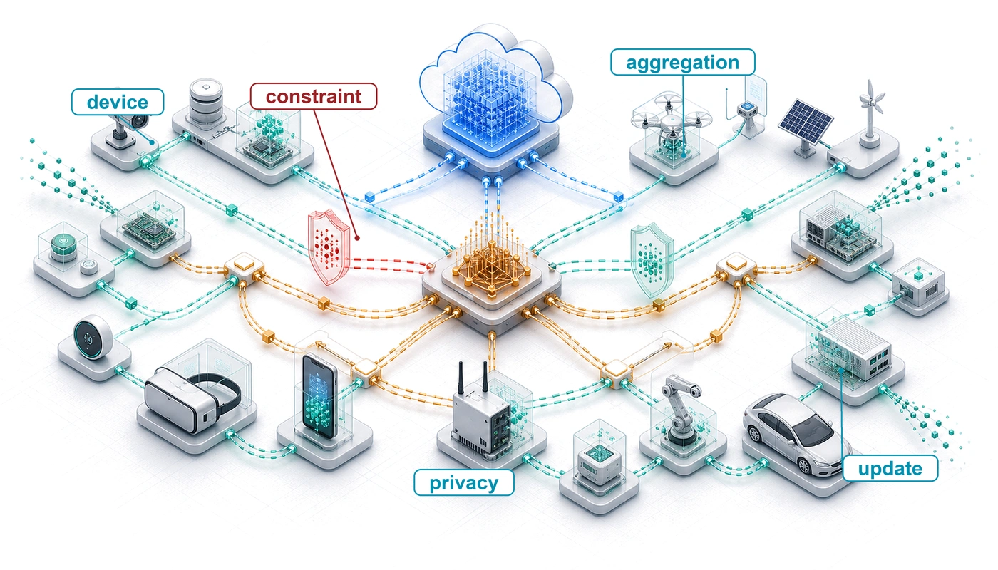
Consider one federated round for the voice assistant. A coordinator selects eligible devices and distributes a shared model version and a bounded training policy. Each selected device trains on local examples when its policy admits background work, then returns a model update tagged with the starting version. Some devices lose connectivity or exhaust their resource allowance. The coordinator closes the round according to its deadline and participation requirements, combines compatible updates, evaluates the candidate shared model, and publishes an accepted version for later download. Local personalization can remain on the device instead of entering that aggregate.
This round has the shape of Archetype C (Federated MobileNet), with phone-class clients, private local data, and intermittent availability, and it exposes the C³ trade-off before any adaptation method is chosen. The Fleet Law (equation 1.3) gives it a time budget, with one change of reading. In a data center the compute term divides one job’s work across \(\DeviceCount\) devices; here every selected device trains its own copy on its own data, so the term is set by local training on the slowest device the round still waits for rather than divided by \(\DeviceCount\). The communication term is the update transfer over a wide-area uplink, the synchronization term is the wait for enough participants to report, and the overlap term credits whatever downloading and training proceed concurrently. More local compute can reduce the frequency of communication, but devices then need longer uninterrupted training windows and their models can drift toward different local distributions. Short deadlines improve coordination speed while excluding slow participants. The fleet must therefore account for whose updates complete, rather than merely how many devices were selected. Device budgets, adaptation methods, and data reuse determine the work inside the round; aggregation and scheduling determine whether that work improves the shared model. A round of this kind, repeated across a population, is federated learning.
↩︎ Archetype C (Federated MobileNet), the phone-class federated workload with private local data and intermittent availability, is established in Archetype C (Federated MobileNet).
Definition 11.2: Federated learning
Federated learning is a decentralized training paradigm where distributed devices collaboratively train a shared model using local data while exchanging only model updates (gradients or weights).
- Significance: It transforms the constraint of data locality into a privacy feature. Within the Fleet Law (equation 1.3), federated learning is constrained by wide-area bandwidth (\(\Bandwidth\)) in its communication term and by the extreme heterogeneity of the fleet, where device-specific efficiency \((\EfficiencyHw)\) and availability can vary by orders of magnitude.
- Distinction: Unlike centralized training, where data is moved to the compute, federated learning moves compute to the data. Raw training examples can remain local, but model updates, participation metadata, and protocol messages still cross the device boundary and may carry personal information.
- Common pitfall: A frequent misconception is that federated learning is “inherently private.” In reality, model updates themselves can leak information through gradient inversion attacks, which search for inputs whose gradient matches a submitted update and so reconstruct training examples, requiring additional protections like differential privacy or secure aggregation.
Keeping raw examples local reduces one source of exposure, but an update can still reveal information about the examples that produced it. Secure aggregation lets the coordinator obtain a combined update without inspecting each client’s contribution under the protocol’s trust assumptions. Differential privacy1 bounds how much a specified user’s or record’s participation can change the released result, usually by limiting contributions and adding calibrated noise. Neither protection follows automatically from federation. Their costs and assumptions belong in the round design alongside dropout handling and communication.
1 Differential privacy: A mathematical framework that bounds information leakage by adding calibrated noise to computations. In edge learning, that noise becomes a systems cost because noisier updates usually require more rounds or more data to reach the same utility.
↪ Differential privacy definitions, noise mechanisms, and privacy accounting are developed in Differential Privacy.
A smartphone predicting user text input, a smart home device responding to household routines, and an autonomous vehicle interpreting local driving conditions can all encounter variation underrepresented in centralized training data: the smartphone meets user-specific phrasing, the home device observes seasonal shifts in household routines, and the vehicle faces local road conditions, weather patterns, and traffic habits that differ from its training environment. Such gaps make a case for on-device learning (definition 11.1). A gap is a case, not a verdict; whether local training is necessary, and whether a given update improves behavior, are questions the engineering analysis must answer with measurements. Machine learning then moves from centralized training to distributed learning across heterogeneous devices, each operating under local constraints. Within the fleet stack, this pushes computation toward the limits of device power, memory, and thermal capacity.
Self-Check: Question
A mobile robotics vision system must process each frame within \(33\text{ ms}\), while cloud network round-trip time is \(80\text{–}150\text{ ms}\). Why must the foreground perception path execute locally even if model training remains in the cloud?
- Network round-trip latency alone exceeds the foreground deadline, so a frame cannot wait for a cloud response.
- Cloud data centers are physically incapable of computing backpropagation gradients on batch sizes of one within milliseconds.
- The on-device camera sensor cannot serialize video frames into digital packets without first running an on-device forward-backward training pass.
- On-device adaptation reduces model parameter count to zero before sending updates across the cellular uplink.
Before investing in an on-device gradient-based learning pipeline for a mobile news app, an ML systems architect considers feature-based personalization (local feature caching with a frozen global model) versus on-device gradient fine-tuning. Under what systems criteria is feature-based personalization preferred, and what eliminates the need for local backpropagation?
In comparing learning paradigms across edge fleets, what fundamental systems distinction separates isolated on-device learning from federated learning?
- Isolated on-device learning transmits raw private data to centralized servers, whereas federated learning processes data locally without communication.
- Isolated on-device learning restricts parameter updates entirely to a single node, preventing collective fleet knowledge sharing, whereas federated learning coordinates model updates across devices while preserving data locality.
- Federated learning trains models from scratch on client devices without a pretrained base model, whereas isolated on-device learning requires continuous cloud synchronization.
- Isolated on-device learning uses only INT4 integer arithmetic, whereas federated learning requires double-precision FP64 hardware accelerators on all mobile clients.
True or False: Because on-device learning keeps raw user observations (such as typed keystrokes or biometric sensor traces) on the client device, it inherently guarantees full compliance with privacy regulations like GDPR and HIPAA without requiring any additional cryptographic or governance safeguards.
Compare the coordination responsibilities of isolated on-device learning, centralized cloud training, and cross-device federated learning. Why does the paradigm alone not establish a universal ranking of implementation complexity?
11.2 Why Learn on the Device
When a cloud-trained model relies on a server round trip or a raw-data upload for every adjustment, it fails whenever a user has an unfamiliar accent, a remote sensor loses connectivity, a regulation forbids exporting personal traces, or millions of devices would overwhelm backend ingestion. Those four pressures—personalization, latency and availability, privacy, and infrastructure efficiency—motivate shifting learning to the edge (Li et al. 2020). Personalization matters when deployed models encounter usage patterns and data distributions that their training environments represent poorly. Local adaptation can refine behavior using user-specific data, including linguistic preferences, physiological baselines, sensor characteristics, or environmental conditions. High inter-user variability motivates testing this approach against a fixed model with local context; the measured quality difference determines whether changing weights is worthwhile.
Latency and availability constraints determine where an update can run and how soon it can become useful. In edge computing scenarios, connectivity to centralized infrastructure may be unreliable, delayed, or intentionally limited to preserve bandwidth or reduce energy consumption. When adaptation is justified, local learning permits updates during disconnected periods. The update must still fit the device’s resource budget, and its completion deadline is separate from the response deadline for foreground inference.
Privacy is the third driver. Many applications involve sensitive or regulated data including biometric measurements, typed input, location traces, or health information. Local learning can reduce privacy exposure by keeping raw data on the device and limiting transmission to centralized systems. This can simplify compliance engineering, but it does not by itself establish adherence to regulations such as the General Data Protection Regulation (GDPR), the Health Insurance Portability and Accountability Act (HIPAA) (U.S. Department of Health and Human Services 2026), or region-specific data sovereignty laws.
U.S. Department of Health and Human Services. 2026. The HIPAA Security Rule. HHS.gov guidance.
Infrastructure efficiency is the economic driver. Centralized training pipelines require backend infrastructure to collect, store, and process user data from potentially millions of devices. Shifting learning to the edge distributes computation and can reduce raw-data ingestion. The resulting savings must be compared with device energy, repeated model transfers, and coordination overhead; whether moving work off the server lowers end-to-end cost depends on that whole sum, not on the server bill alone.
11.2.1 Simpler alternatives first
Before paying that device and coordination cost, an engineering team should test whether a static model paired with local state already meets the requirement. Shipping an on-device gradient-training loop when a local feature store or lookup table suffices spends memory, battery, and rollback margin for no measurable gain, whereas simpler alternatives often achieve comparable quality with far lower operational overhead. Three such alternatives often satisfy personalization and adaptation requirements without the complexity of local training (table 1).
| Alternative | Mechanism | When it fits |
|---|---|---|
| Feature-based personalization | Store user preferences, interaction history, and behavioral features locally, then feed those features into a static model rather than adapting model weights. | News recommendation systems can store topic preferences and reading patterns locally, then combine those features with a centralized content model. |
| Cloud-based fine-tuning with privacy controls | Fine-tune centrally on data authorized for transfer, with access controls and, where required, a specified differential-privacy mechanism. Federated analytics and secure aggregation (Bonawitz et al. 2017) can support aggregate statistics but do not themselves provide centralized training examples. | Centralized updates fit when authorized data transfer, update latency, and the specified privacy guarantees meet the application requirements. |
| User-specific lookup tables | Combine global models with personalized retrieval mechanisms by maintaining a lightweight table for frequently accessed local patterns. | Personalization benefits are needed with minimal computational and storage overhead. |
The decision to implement on-device learning should follow evidence that simpler alternatives cannot meet the deployment requirements, such as restrictions on transferring training data or unreliable connectivity when adaptation is needed. Latency is the requirement most often mistaken for such evidence. For applications whose foreground deadlines are shorter than the network round-trip time, cloud inference is architecturally infeasible. Camera processing under 33 ms, voice response under 500 ms, AR/VR motion-to-photon latency under 20 ms, or safety-critical control under 10 ms all face network round-trip times typically ranging from 50 to 200 ms. When the network cannot meet the foreground deadline, inference must remain local. A fixed model also executes offline, however, so the deadline settles where the model runs and leaves open where it learns. Local training earns its engineering investment only when a measured adaptation gain justifies its added resource and operational costs.
11.2.2 Where adaptation pays
Every application domain must justify adaptation against its simpler alternatives, and the domains differ in which resource binds first. A smartphone keyboard encounters personal vocabulary and changing typing patterns that may be poorly represented in its released model. Local training can use those observations for personalization or contribute updates to a shared model; these are separate objectives. Google’s Gboard,2 for instance, employs federated learning to improve shared models across a large population of users while keeping raw data local to each device (Hard et al. 2018).
2 Gboard (2017): One of the first widely reported commercial federated learning deployments at mobile scale. Published reports showed that keyboard models could improve from aggregated on-device updates while raw typed text remained local. The systems consequence is durable. Compressed updates and privacy mechanisms make cross-fleet learning possible over constrained mobile networks without centralizing raw keystrokes.
Hard, Andrew, Kanishka Rao, Rajiv Mathews, Swaroop Ramaswamy, Françoise Beaufays, Sean Augenstein, Hubert Eichner, Chloé Kiddon, and Daniel Ramage. 2018. “Federated Learning for Mobile Keyboard Prediction.” arXiv Preprint arXiv:1811.03604.
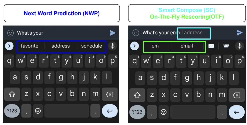
The same keyboard also runs two interactive prediction strategies at inference time (figure 1). Next-word prediction ranks discrete candidate tokens (“favorite,” “address,” “schedule”) in the suggestion bar, whereas Smart Compose generates multi-word inline ghost text (“ail address”) through on-the-fly rescoring directly inside the input buffer. Both mechanisms personalize the immediate interaction through local context; longer-lived model improvement occurs separately when federated training aggregates eligible on-device updates.
Xu, Zheng, Yanxiang Zhang, Galen Andrew, Christopher A. Choquette-Choo, Peter Kairouz, H. Brendan McMahan, Jesse Rosenstock, and Yuanbo Zhang. 2023. “Federated Learning of Gboard Language Models with Differential Privacy.” arXiv Preprint arXiv:2305.18465.
Wearable health monitors, which track activity and physiology from accelerometers, heart rate sensors, and electrodermal activity monitors, face a different personalization problem. Individual physiological baselines and sensor placement can affect predictions, motivating calibration or local adaptation. Evaluation must distinguish useful personalization from learning away a change the application is meant to detect. A monitor that adapts to a user’s steadily rising resting heart rate has normalized the very signal it exists to flag. Keeping observations local reduces raw-data transfer; whether the adapted model is more accurate is a separate measurement against held-out outcomes.
Voice interfaces in smart speakers and earbuds must recognize commands quickly and accurately in noisy, changing acoustic environments, starting with wake-word detection.3 These systems face foreground latency requirements, such as an end-to-end response target under 500 ms and a wake-word detection target below 100 ms. Those targets constrain inference and the interference permitted from background learning. Local adaptation addresses a separate quality objective: reducing false activations and missed detections for a user’s voice and acoustic environment. Far-field microphone configurations and room acoustics motivate that adaptation, but its value must be measured while preserving foreground response times.
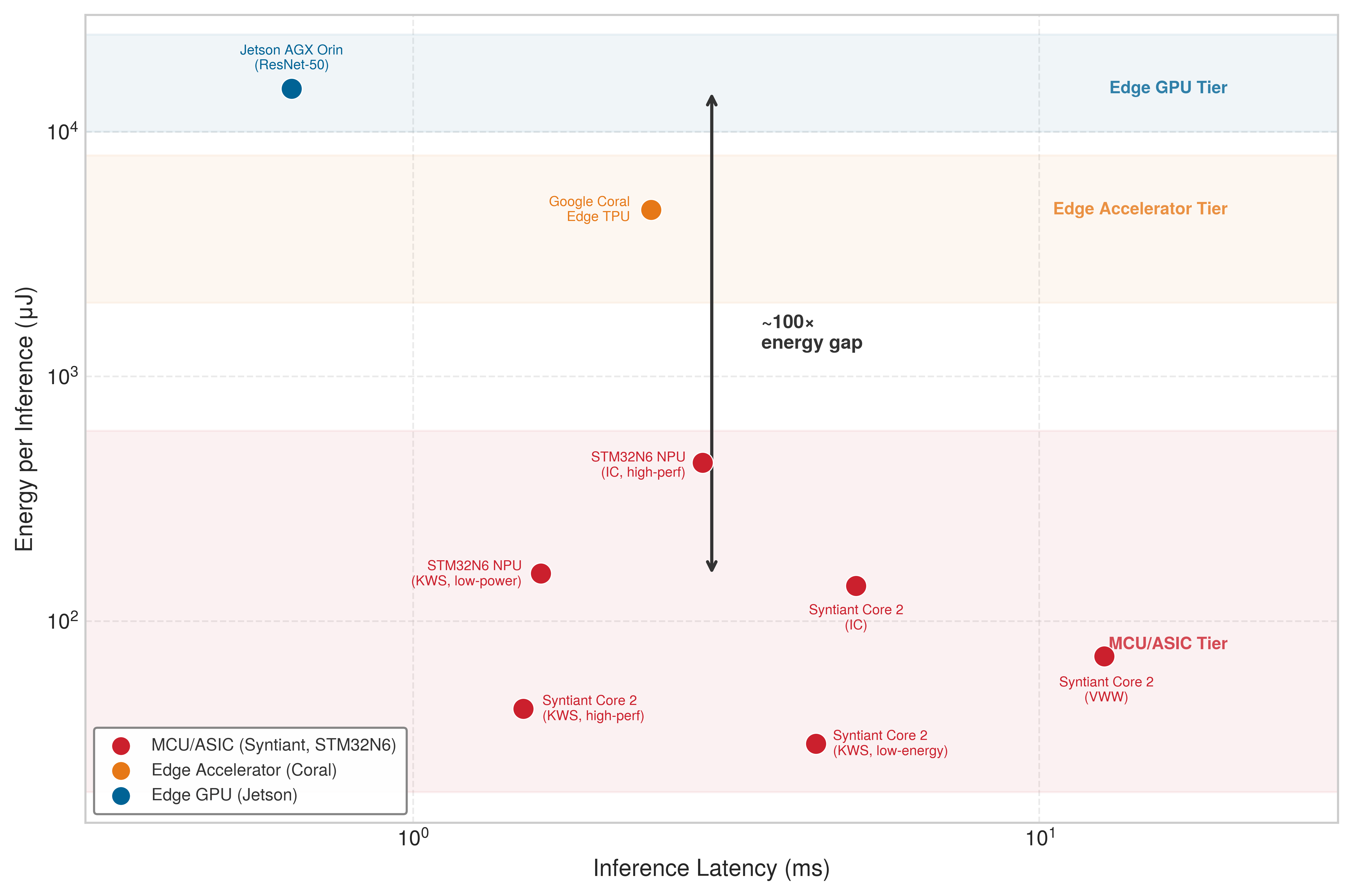
3 Wake-word detection: An always-on detector incurs inference cost throughout the listening period, even when no keyword occurs. Published keyword-spotting results on dedicated neural processors, plotted in figure 6, spend on the order of 30 to 160 \(\Glyph{\mu}\)J per evaluation, so the energy budget is set by how often the detector evaluates over the listening period as much as by the cost of any one evaluation. Local personalization adds a separate update cost and earns its place only if evaluation shows an acceptable trade-off between missed keywords, false activations, and energy use.
Industrial IoT and remote monitoring systems expose the availability side of the decision. In agricultural sensing, pipeline monitoring, or environmental surveillance, connectivity to centralized infrastructure may be limited, expensive, or unavailable. Local inference permits continued detection while disconnected. Local learning adds the ability to adjust thresholds or track seasonal trends, provided the update preserves the distinction between expected variation and anomalies. The consequences of missed detections make validation and a recoverable baseline part of the adaptation design.
Embedded computer vision systems, including robotics, AR/VR, and smart cameras, combine substantial visual processing with the tight foreground deadlines of section 11.2.1, from a 33 ms frame interval down to a sub-10 ms control loop. On-device adaptation can recalibrate a model to new lighting conditions, object appearances, or motion patterns, but it spends resources needed by that foreground pipeline. A useful update must improve validated behavior without exhausting the latency margin that made local inference viable.
Each domain turns a possible adaptation benefit into a resource decision. Mobile keyboards must fit update state alongside typing, wearables must budget energy across repeated updates, voice and vision systems must preserve foreground deadlines, and disconnected sensors must decide whether a fixed model remains adequate.
11.2.3 What crosses the device boundary
Once a domain justifies local learning, the next question is whether each device learns in isolation or shares what it discovers with the fleet. Keeping all learning strictly inside each device prevents a fleet from sharing new words, road hazards, or acoustic patterns discovered across millions of users, yet uploading raw observations to a central cluster exposes private data and consumes wide-area bandwidth. Centralized training collects data on managed infrastructure and releases validated model versions to devices; local adaptation instead changes a device’s model using observations that may be unavailable centrally. Hardware, software, power, and connectivity then vary across the learning population, so an operator must coordinate model versions and evaluate updates from intermittently participating clients (Bonawitz et al. 2019).
A returning device may hold an old model or fail to apply a release. Signed updates, functional checks, deployment telemetry, and rollback therefore form part of the learning protocol (Bonawitz et al. 2019). The central decision is how much state to share across devices. Centralized training, local-only adaptation, and federated coordination are architectural choices that can coexist in one deployment.
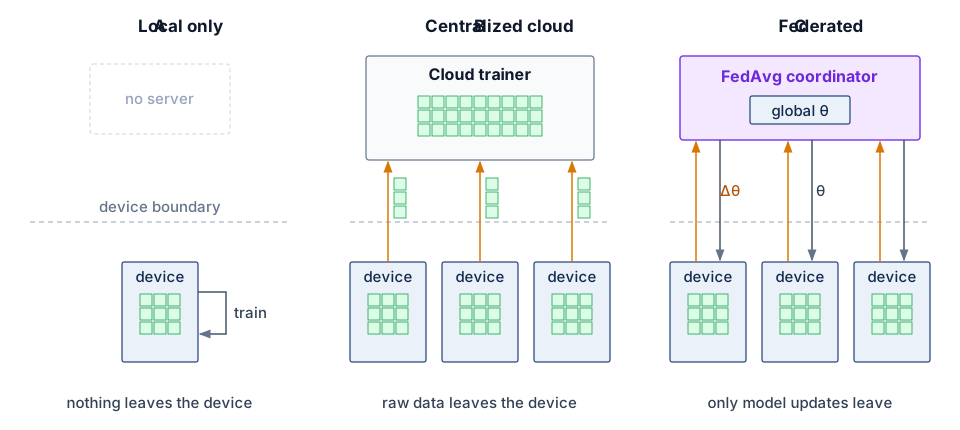
Local-only adaptation specializes a model to its user’s observations, which are often non-IID4 and noisy, so sharing that specialization requires an explicit boundary between personal state and the parameters intended to improve the population model. Federated coordination adds population learning by periodically aggregating updates to shared parameters. A deployment must specify which parameters enter the aggregate and which remain personal; averaging every local adaptation would erase that distinction. Data locality limits raw-data transfer, while separate privacy controls govern the updates that leave each device. The three architectures therefore differ in what crosses the device boundary, not in how advanced they are (figure 2): local-only learning sends nothing, centralized training sends raw examples, and federated learning sends only model updates \(\FiniteChange\ModelParameters\) while receiving the shared weights \(\ModelParameters\).
4 Non-IID (not independent and identically distributed): Samples may be dependent or drawn from different distributions; in a device fleet, user-specific label and feature distributions can make local updates conflict. Such distributions can degrade federated averaging relative to independent and identically distributed (i.i.d.) baselines (Zhao et al. 2018). The observed failure determines whether to change local work, aggregation, or personalization rather than prescribing one remedy for every non-IID population.
Zhao, Yue, Meng Li, Liangzhen Lai, Naveen Suda, Damon Civin, and Vikas Chandra. 2018. “Federated Learning with Non-IID Data.” CoRR abs/1806.00582.
The choice of shared and personal state must fit the devices that execute it. Managed data centers can provision capacity and schedule training across dedicated resources; edge devices share limited power, memory, and cooling with foreground applications. Those local budgets determine which adaptation and coordination choices remain feasible.
11.3 Design Constraints
Fine-tuning a neural network on a smartphone is constrained by power and heat: a GPU training cluster may consume megawatts in a controlled facility, whereas a smartphone sustains only a few watts before throttling. Across the edge spectrum, memory ranges from a few gigabytes on phones down to hundreds of kilobytes on microcontrollers, sustained power ranges from a few watts down to milliwatts, and network connectivity may be intermittent or entirely absent. On-device learning must therefore use compute, memory, and data sparingly, and when a local model operates in a safety-critical loop, these resource limits become life-safety engineering problems.
Lighthouse 11.1: Archetype C (Federated MobileNet): The edge power wall
These constraints run through Archetype C (Federated MobileNet), where learning happens on phone-class devices whose power budget spans roughly 2–10 W, a few watts sustained with brief bursts toward 10 W, and which must share that budget with the user’s foreground work. Privacy and policy constraints often forbid moving raw examples off the device, and even where transfer is permitted, a mobile uplink and battery rarely afford shipping raw data to the cloud. Data locality is therefore both a policy requirement and a bandwidth and energy constraint. Quantized training, sparse updates, and federated coordination are the strategies that let Archetype C learn within that envelope. Held at that burst ceiling, an idealized 15 Wh battery would be exhausted in about 1.5 hours, and thermal throttling would end the workload sooner. Microcontroller-class sensors with hundreds of kilobytes of memory and milliwatt budgets sit at an extreme below Archetype C, and this chapter treats them as such.
The constraints on parameters, operations, and data interact. A larger batch can improve hardware utilization while exceeding memory capacity; a smaller trainable state can fit memory while extracting too little signal from local data. Compression provides one way to reach a feasible starting point. Quantization shrinks bytes per weight, pruning removes selected parameters, and knowledge distillation transfers behavior into a smaller architecture. Once the base model fits, local learning must also accommodate the state and work needed to adapt it.
On-device learning adds training state and work to the inference workload. A full-model update requires forward propagation, gradient computation through backpropagation, and weight updates. Memory grows because the update must hold gradients, optimizer state, and the activations saved for the backward pass, and arithmetic grows because the backward pass computes gradients with respect to both activations and weights, up to roughly twice the work of the forward pass. The size of each increase depends on the model, batch, precision, and execution schedule. Compression and selective adaptation address different parts of that pressure, so feasibility requires accounting for the resulting working set rather than applying a universal multiplier.
The relevant budget is the capacity available to the learning task. Centralized training can reserve resources and assemble datasets under a common management policy. A device must fit an update around the operating system, foreground applications, and locally available examples. Total installed memory or peak accelerator throughput therefore overstates what background learning can use.
These constraints define eligibility for a federated round. Model footprint and trainable state determine which device tiers can participate. Sparse, nonuniform data determines how much signal each local update can extract. Limited compute determines when training can run at all. A policy that exceeds the budget on weaker devices changes the population represented in the aggregate, even if it improves throughput on stronger devices.
11.3.1 Quantifying training overhead on edge devices
A compact 10M-parameter model whose 40 MB of FP32 weights fit comfortably inside a smartphone’s background-memory allowance can balloon to 360 MB as soon as backpropagation adds gradients, optimizer state, and saved activations—exceeding the background memory ceiling and crashing the process on its first backward pass. Training changes memory footprint, memory bandwidth, and hardware utilization through additional live state and backward operations. The illustrative increases in table 2 count different things from row to row, so each multiplier carries its own denominator. The 4–12× memory range compares a training working set with the inference weights alone, leaving inference activations and workspace out of the denominator. The 2–3\(\times\) compute range compares one update (forward plus a backward pass of one to two times the forward work) with one inference. The 10–50\(\times\) energy range compares a converged adaptation, which takes many gradient steps, with a single inference, so it is not a per-sample multiplier.
| Constraint dimension | Inference | Training amplification | Impact on design |
|---|---|---|---|
| Memory Footprint | Model weights + single activation map | Weights + full activation cache + gradients + optimizer state | 4–12\(\times\) the inference weights alone; forces aggressive compression |
| Compute Operations | Forward pass only | Forward + backward + weight update | 2–3\(\times\) one inference, per update step; limits model complexity |
| Memory Bandwidth | Sequential weight reads | Bidirectional data flow for gradients | Additional traffic depends on update scope and activation schedule |
| Energy per Adaptation | Single inference operation | Multiple gradient steps with convergence | 10–50\(\times\) one inference, per converged adaptation; requires opportunistic scheduling |
| Data Requirements | Current inputs; no training labels required | Local update examples, often sparse or noisy | Necessitates sample-efficient methods |
| Hardware Utilization | Optimized for forward passes | Different access patterns for backprop | Inference accelerators may not help training |
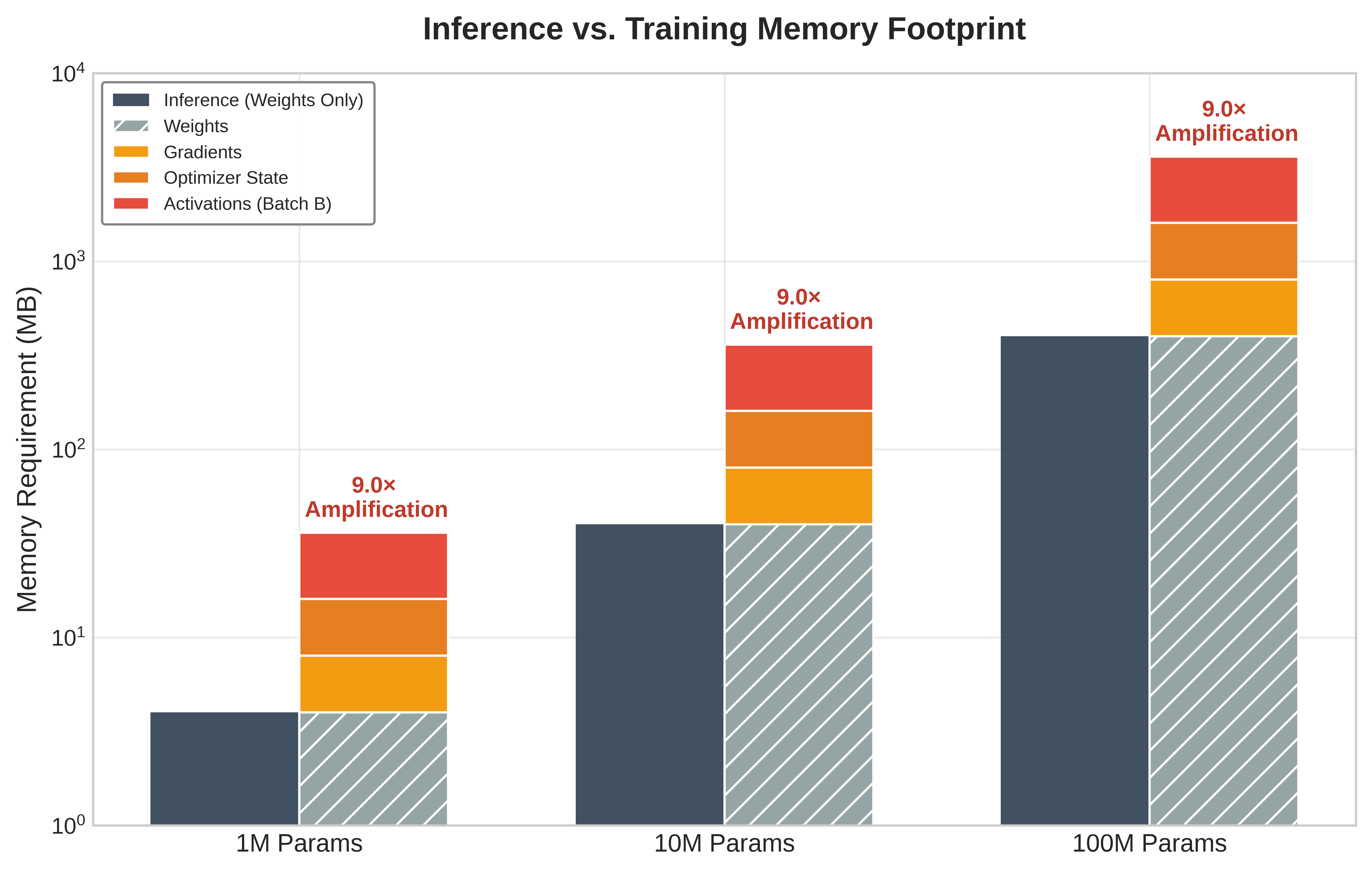
The memory row decomposes into four arrays (figure 3). Panel (a) starts with 40 MB of FP32 weights for a 10M-parameter model and adds 40 MB of gradients, 80 MB of Adaptive Moment Estimation (Adam) state for its two moment arrays, and 200 MB of assumed activation state to reach 360 MB, a 9× amplification over the weights. The same accounting spans the table’s range. Weights, gradients, and Adam’s two moments alone are four weight-sized arrays, the 4× floor reached when saved activations are negligible, and activations between five and eight times the weight bytes carry the total from 9× to 12×. Panel (b) holds the 9× proportions fixed across model scales from 1M to 100M parameters, so its constant ratio is an assumption rather than a finding. What it shows is the absolute cost of that ratio. The gap between weights and training stack grows from tens of megabytes at 1M parameters to gigabytes at 100M, so a model whose weights fit comfortably can still have a training stack that does not. Actual peak memory depends on optimizer choice, batch size, activation checkpointing, and how many layers are updated, and the 4–12× range describes these configurations rather than predicting any particular device.
↪ The bytes per parameter that weights, gradients, and optimizer state occupy in mixed-precision Adam training are developed in Numeric Precision and Training Memory.
Peak memory usage
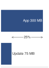
One gradient update claims a quarter of the background-memory allowance.
Consider a smartphone keyboard that uses local gradient updates to adapt to a user’s vocabulary and typing patterns. In the illustrative device profile, an update requires 50 MB–100 MB for activations and optimizer state, against a background-memory allowance of 200 MB–300 MB. The actual allowance depends on the operating system, device, and foreground workload. At the selected operating point, the update consumes 25 percent of that allowance before other application state is counted. The design decision is how much learning can fit in the remaining budget while preserving responsive typing; the device’s total installed RAM does not answer it.
Memory consumption changes over an update as tensors are allocated and released. The peak depends on when weights, saved activations, gradients, optimizer state, and temporary workspace coexist; it need not occur at the same operation in every implementation. For the 10M-parameter model of figure 3, 40 MB of FP32 weights belong to a 360 MB training working set, of which 200 MB is saved activations. Set against a smartphone’s 8 GB of installed RAM, that working set looks small, but installed RAM is not the budget. A background task receives only the allowance the operating system grants after itself and the foreground applications, 200 MB–300 MB in the keyboard profile above, and 360 MB exceeds even the top of that range. Activation checkpointing (also called gradient checkpointing) discards selected intermediate activations and recomputes them during the backward pass (Chen et al. 2016), the same trade that cuts activation memory in data-center training. It trades extra computation for lower activation storage, so its value depends on both the peak it removes and the additional time and energy the device can afford.
Chen, Tianqi, Bing Xu, Chiyuan Zhang, and Carlos Guestrin. 2016. “Training Deep Nets with Sublinear Memory Cost.” arXiv Preprint arXiv:1604.06174.
↩︎ Activation checkpointing, which recomputes selected activations in the backward pass to cut activation memory at the cost of extra FLOPs, is established in Compute-phase forward and backward passes.
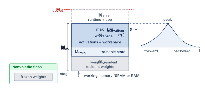
That allowance, not installed RAM, is the ceiling for a working-memory budget that every adaptation strategy in this chapter must meet (figure 4). The runtime stages frozen weights from nonvolatile flash into volatile working memory and reserves headroom below the physical device ceiling \(\DeviceMemoryCapacity\) for runtime and application state. Within the working-memory envelope \(\AdaptationPeakMemory\), four quantities contribute: let \(\ResidentWeightMemory\) be the backbone weights that must reside in working memory, \(\TrainableStateMemory\) the trainable parameters plus their gradients and optimizer state, \(\ActivationMemory(\TimeInstant)\) the saved activation state, and \(\OperatorWorkspaceMemory(\TimeInstant)\) operator workspace. With all terms counted in bytes and disjoint, the required working memory is
\[ \AdaptationPeakMemory= \ResidentWeightMemory+ \TrainableStateMemory+ \max_t\left[\ActivationMemory(\TimeInstant) + \OperatorWorkspaceMemory(\TimeInstant)\right]. \tag{1}\]
Admission then requires \(\AdaptationPeakMemory+ \ReservedDeviceMemory\le \DeviceMemoryCapacity\), where \(\ReservedDeviceMemory\) holds the runtime, the operating system, and the foreground application; for a background task, \(\DeviceMemoryCapacity- \ReservedDeviceMemory\) is the allowance just described. Weights stored in nonvolatile memory still consume deployment storage, and any staging buffers belong in \(\OperatorWorkspaceMemory(\TimeInstant)\). The maximum must follow the actual execution schedule because activation and workspace peaks need not coincide. Each term is a separate lever, and the adaptation strategies of section 11.4 differ in which term they shrink. Freezing weights removes their gradients and optimizer state from \(\TrainableStateMemory\), but it does not make the frozen base or every backward dependency disappear.
An inference optimization therefore needs a second feasibility check before it is used for adaptation. Reducing stored weights may leave activations or optimizer state as the dominant cost. Selecting which parameters to train changes that accounting, linking the memory analysis to the adaptation choices that follow.
Checkpoint 11.1: On-device training constraints
Verify understanding of how training amplifies edge constraints:
11.3.2 Model constraints
A model that fits comfortably on a smartphone can fail before a single backward pass on a smaller edge tier: MobileNetV2 requires approximately 14 MB of storage in its standard configuration, which fits easily in smartphone RAM yet far exceeds the 256 KB of SRAM and 1 MB of flash storage on microcontrollers such as the Arduino Nano 33 BLE Sense.5 On such severely constrained platforms, even a single convolutional layer may exceed available RAM during training due to intermediate feature maps and gradient storage. While cloud-deployed models can span billions of parameters across multi-gigabyte memory budgets, models intended for on-device learning must conform to tight limits on memory, storage, and compute, each tightened further by the factors of table 2.
5 Arduino Nano 33 BLE Sense: With 256 KB SRAM, roughly 65,536× smaller than a flagship smartphone’s 16 GB, a single \(224{\times}224{\times}3\) RGB image occupies ~151 KB and consumes roughly 60 percent of available memory; activation and gradient storage add several more live tensors, and optimizer state can push the training footprint far beyond the inference footprint. A convolutional neural network (CNN) layer can therefore exceed SRAM during backpropagation even when its weights fit. Quantization can reduce this footprint, but feasibility also depends on input size, saved activations, and which parameters are updated.
Training adds state whose size cannot be inferred from layer count alone. Backpropagation retains or recomputes intermediate activations, with storage determined by tensor shapes, precision, batch size, and the update schedule. The arithmetic grows quickly. A 10-layer convolutional model processing \(64{\times}64\) images saves feature maps of \(64{\times}64\) values per channel when its layers keep the input resolution, so at FP32 every channel of every retained map costs 16,384 bytes, about 16 KB. Ten layers of even a few channels each therefore outgrow the 256 KB of microcontroller SRAM before a single gradient or optimizer value is stored. The relevant comparison is that peak against the memory available to learning after runtime and application reserves, which is why the techniques later in this chapter attack saved activations as well as trainable parameters.
Model complexity also affects runtime energy consumption and thermal limits. In smartwatches or battery-powered wearables, sustained training can deplete the energy allowance or trigger thermal throttling even when its tensors fit in memory. Arithmetic precision alone does not determine feasibility; the update duration and measured power determine its energy cost. Benchmarks such as MLPerf Tiny provide small quantized inference targets for constrained devices (Banbury et al. 2021). On-device adaptation techniques address the additional training cost by freezing most parameters, reducing activation storage, or selecting sparse update sets (Cai et al. 2020; Kwon et al. 2024).
Banbury, Colby, Vijay Janapa Reddi, Peter Torelli, Jeremy Holleman, Nat Jeffries, Csaba Kiraly, Pietro Montino, et al. 2021. “MLPerf Tiny Benchmark.” arXiv Preprint.
Battery and thermal constraints also determine when learning can run. The illustrative smartphone profile uses a sustained processing envelope of 2–3 W and brief bursts of 5–10 W. An update that fits during an idle interval may exceed the available headroom when foreground work starts. Charging supplies energy, but the runtime must still monitor heat and contention, reducing the update duty cycle or suspending learning when limits are approached. An overnight idle-and-charging policy provides one candidate window; measured device conditions determine whether that window remains usable.
These constraints make adaptation feasibility part of architecture selection. When the base model exceeds device capacity, partitioning, quantization, offloading, or a smaller architecture can change the deployment footprint, each with its own execution cost. INT8 or INT4 weights often decide whether the base model fits at all, and 1-bit weights cut weight bytes 16\(\times\) relative to FP16 (32\(\times\) relative to FP32) before scale metadata and activations are counted. Fitting the forward path is the starting point; quantization support and selective-update costs must then be established for the training path.
11.3.3 Data constraints
Fitting the model and its update state into memory solves only the capacity side of the problem, because the available local data still sets how much a fitted update can actually learn. A fitness tracker that records thousands of accelerometer readings across a workout may receive only a single user-supplied activity label, or it may record from a sensor whose calibration has drifted. Unlike the curated datasets used in cloud training, edge data is locally collected, temporally sparse, and often unlabeled. Because sampling frequency, windowing, and temporal correlation can collapse an entire session of correlated sensor readings into a single independent observation, the learning policy must budget for usable supervision rather than raw stored bytes.
On-device data is also frequently non-i.i.d. (Zhao et al. 2018). A voice assistant deployed across households encounters variation in accents, languages, speaking styles, and command patterns. Smartphone keyboards observe individual typing patterns, autocorrect preferences, and multilingual usage. Centralized systems also encounter such variation, but a federated coordinator cannot freely shuffle raw examples across clients. Local updates therefore reflect different data distributions, complicating the balance between shared generalization and personalization.
Label scarcity compounds the distribution problem. Most edge-collected data is unlabeled by default, requiring systems to learn from weak or implicit supervision signals. A smartphone camera may capture thousands of images throughout the day, but only a few are associated with meaningful user actions (tagging, favoriting, or sharing) that could serve as implicit labels. In many applications, including anomaly detection in sensor data and gesture recognition adaptation, explicit labels may be entirely unavailable, making traditional supervised learning infeasible without alternative methods for weak supervision or unsupervised adaptation.
Data quality introduces further challenges. Environmental sensors or automotive ECUs can experience calibration changes, interference, or mechanical wear that corrupt or shift input signals. An adaptation loop may learn from those changes as if they represented useful new behavior. Local input checks and validated outcome signals must distinguish sensor faults from changes the model should learn, especially when raw observations are unavailable for central inspection.
Privacy and security requirements can further restrict which examples may be retained or shared. Keeping health data, personal communications, or behavioral traces on the device narrows raw-data exposure, but local storage and transmitted updates remain sensitive. The learning design must specify access, retention, and permitted disclosures alongside the data needed for adaptation and validation.
11.3.4 Compute constraints
A mobile neural processing unit (NPU) advertised at tens of TOPS for INT8 inference can lack backward-pass or optimizer kernels entirely, forcing an on-device update to fall back to the CPU and run an order of magnitude slower and hotter than the chip’s inference rating suggests. Across the edge hardware spectrum—from microcontrollers like the STM32F4 and ESP32, through mobile processors with dedicated AI accelerators (Apple Neural Engine, Qualcomm Hexagon, Google Tensor), to high-capability edge modules—inference ratings measure forward-pass throughput on fixed weights, whereas training workloads add backward and optimizer operations with very different execution paths.
Because an inference rating does not measure this backward path, feasibility depends on tracing where each update operator actually executes. Backpropagation reads saved or recomputed activations, produces gradients, and updates parameters and optimizer state. These operations add memory traffic, with the amount determined by the trainable subset and execution schedule, and a specialized accelerator can expand the inference budget without executing any backward operator. The feasibility test is therefore the actual update path. It identifies which processor runs each backward and optimizer operator, including any fallback to the CPU or GPU, and measures time, memory, and energy for that path under foreground load. Each device class that follows gets this update-path test, applied to its own memory, operators, and power, rather than a verdict read from its inference rating.
At the most constrained end, devices such as the STM32F46 or ESP32-S3 microcontrollers offer only a few hundred kilobytes of SRAM and limited compute and power budgets (Warden and Situnayake 2020). Although these families include single-precision floating-point support, practical ML deployments commonly rely on quantized or fixed-point kernels for efficiency. Libraries like CMSIS-NN (Lai et al. 2018) provide optimized neural network kernels for Arm Cortex-M processors, achieving 4.6\(\times\) runtime improvement through fixed-point arithmetic and single instruction, multiple data optimizations. These severe limitations preclude conventional deep learning libraries and require models designed for quantized arithmetic and minimal runtime memory allocation. Quantization-aware training7 can prepare models for efficient quantized inference. Executing local updates requires a separately supported training path, potentially with selective updates, quantized gradients, or a compact floating-point working set.
6 STM32F4 microcontroller: With 192 KB SRAM, a 168 MHz clock speed, and a single-precision floating-point unit, the main constraint is not the absence of floating point but the tiny memory and energy envelope. A dense layer with 1,000 input features and 10 hidden units requires approximately 40 KB for weights and biases in FP32, consuming about 20 percent of total SRAM before accounting for activations or gradients. Local updates must therefore fit around the device’s primary workload and power budget, and INT8 or fixed-point kernels remain preferable when accuracy allows.
Warden, Pete, and Daniel Situnayake. 2020. TinyML: Machine Learning with TensorFlow Lite on Arduino and Ultra-Low-Power Microcontrollers. O’Reilly Media.
Lai, Liangzhen, Naveen Suda, and Vikas Chandra. 2018. “CMSIS-NN: Efficient Neural Network Kernels for Arm Cortex-M CPUs.” ArXiv Preprint abs/1801.06601.
7 Quantization-aware training (QAT): Simulates quantization during training to adapt the model to low-precision inference (Jacob et al. 2018; Krishnamoorthi 2018). Fake-quantization operations commonly retain floating-point training tensors, so QAT does not itself imply integer backward kernels or a smaller training-state budget. On-device adaptation must separately establish supported update arithmetic, state storage, and measured energy costs.
Jacob, Benoit, Skirmantas Kligys, Bo Chen, Menglong Zhu, Matthew Tang, Andrew Howard, Hartwig Adam, and Dmitry Kalenichenko. 2018. “Quantization and Training of Neural Networks for Efficient Integer-Arithmetic-Only Inference.” 2018 IEEE/CVF Conference on Computer Vision and Pattern Recognition, 2704–13. https://doi.org/10.1109/cvpr.2018.00286.
Krishnamoorthi, Raghuraman. 2018. “Quantizing Deep Convolutional Networks for Efficient Inference: A Whitepaper.” arXiv Preprint arXiv:1806.08342 abs/1806.08342.
8 SGD (stochastic gradient descent): Plain SGD keeps parameters and gradients, two parameter-sized arrays where Adam keeps four, so its lower state cost must still be weighed against the updates needed to reach the quality target.
Microcontroller memory rules out training configurations whose live tensors exceed SRAM, rather than every convolutional model. Feasibility depends on tensor shapes, update scope, numerical representation, and the compiled execution schedule. Plain stochastic gradient descent (SGD) reduces optimizer state compared with methods that retain additional moment arrays.8 Non-neural adaptation, such as \(\ClusterCount\)-means clustering, offers a different way to update local centroids for sensor analysis. The method and its arithmetic must still fit the available memory and produce a validated improvement; neither a simple optimizer nor integer execution establishes that result alone.
Moving up the computational hierarchy, mobile-class hardware represents improvement but still operates under severe constraints. Platforms including the Qualcomm Snapdragon, Apple Neural Engine,9 and the Google Tensor system-on-chip (SoC) provide significantly more compute power than microcontrollers, often featuring dedicated AI accelerators and optimized support for 8-bit or mixed-precision matrix operations. These accelerators offer dedicated matrix multiplication units, on-chip memory hierarchies, and power management features specifically designed for neural network inference, with varying support for local training workloads. While these platforms can support more sophisticated training routines, including full backpropagation over compact models, they still fall far short of the computational throughput and memory bandwidth available in centralized data centers. Training a lightweight transformer on a smartphone, for instance, is technically feasible but must be tightly bounded in both time and energy to avoid degrading the user experience.
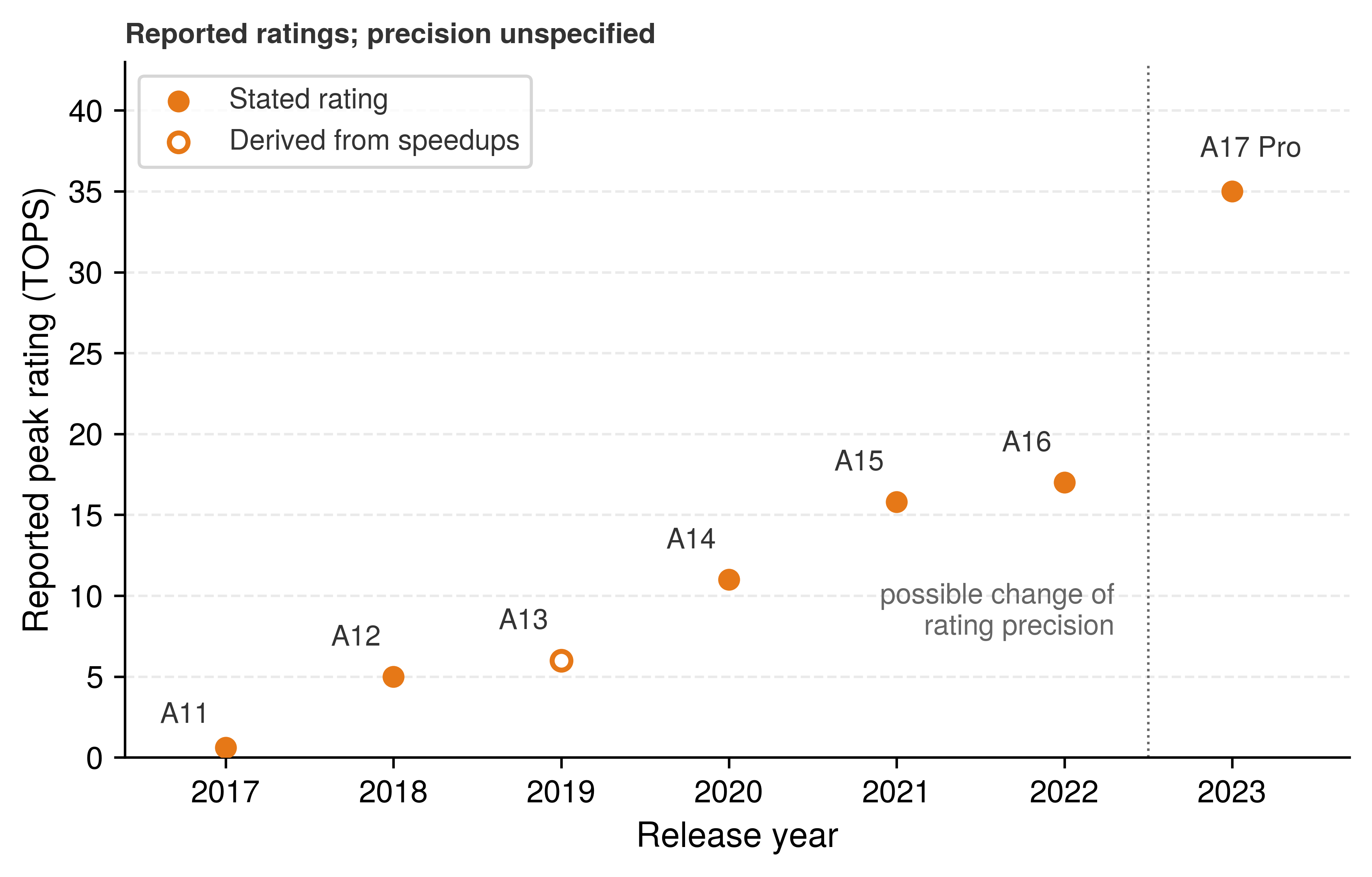
9 Apple Neural Engine: Apple’s dedicated neural accelerator, first shipped in the A11 Bionic in 2017; its rating growth through the A17 Pro is tracked in figure 5. Which of an update’s operators actually reach it, rather than falling back to the CPU or GPU, is the runtime question worked through in section 11.3.4.3.
Hardware capability contributes to on-device adaptation feasibility alongside the algorithm and runtime. The mobile accelerator scaling tracked in figure 5 shows Apple’s stated rating climbing from under 1 TOPS on the A11 Bionic to nearly 35 TOPS on the A17 Pro, a step in 2023 that may partly reflect a change in rating precision rather than in the hardware alone. That growth expanded the forward inference budget, which is not yet a training budget.
Apple. 2017. The Future Is Here: iPhone x.
Apple. 2018. iPhone XS and iPhone XS Max Bring the Best and Biggest Displays to iPhone.
Apple. 2020. Apple Unveils All-New iPad Air with A14 Bionic, Apple’s Most Advanced Chip.
Apple. 2021. Apple Unveils iPhone 13 Pro and iPhone 13 Pro Max.
Apple. 2022. Apple Debuts iPhone 14 Pro and iPhone 14 Pro Max.
Apple. 2023. iPhone 15 Pro and iPhone 15 Pro Max (Product Page, Archived 20 October 2023).
Systems Perspective 11.1: The silicon dividend of a dedicated NPU
The gap between running a model on a generic mobile CPU and on a dedicated NPU is best understood as a “silicon dividend” rather than a marginal speedup. Published NPU profiles vary by silicon generation and workload, so this callout uses explicit scenario assumptions rather than a benchmark: a 20× latency improvement and a 60× energy-efficiency improvement relative to the modeled MobileNetV2 baseline (1.883 ms per inference on the CPU).
The dividend belongs to the operators the NPU actually executes. An update adds backward and optimizer work that costs roughly one to two more forward passes, because the backward pass computes gradients with respect to both activations and weights. If the runtime cannot place those operators on the NPU, they fall back to the CPU. The forward pass may still collect its 20× dividend, but CPU backward work and transfers between processors can dominate the complete update. The resulting speed and energy depend on that mixed execution path. An inference-dominated product and an adaptation-dominated one can therefore see very different returns from the same silicon, and only the traced update path says which case a deployment is in.
Published benchmark results from MLPerf Tiny and vendor data illustrate the range of edge inference costs in figure 6. The plotted tiers span roughly 100\(\times\) in energy per inference. Dedicated neural processors such as the Syntiant Core 2 and STM32N6 NPU occupy the sub-millijoule MCU and application-specific integrated circuit (ASIC) band (30 to 444 \(\Glyph{\mu}\)J per inference across keyword spotting, visual wake words, and small-image classification, with keyword spotting finishing in under 5 ms), Google Coral appears near 4.8 mJ, and the Jetson AGX Orin appears near 15 mJ for ResNet-50. The roughly 100\(\times\) gap mixes different workloads with different hardware, so it is not a matched-task efficiency comparison. Energy per inference does not determine battery lifetime on its own, because inference frequency, sleep power, sensing, radio use, and usable battery capacity also enter that budget. For a learning device the figure sets the scale against which an update must be judged. One evaluation costs microjoules to millijoules, while each second of training inside the 2–3 W sustained envelope spends joules, more than a thousand keyword-spotting evaluations at the plotted 30 to 160 \(\Glyph{\mu}\)J. An update can therefore be a substantial energy cost, but its share of the device budget depends on how often training and inference run. Both paths need measurement over the same operating period.
These computational limitations become especially acute in real-time or battery-operated systems, where the foreground latency budgets of section 11.2.1 bound the interference local training may introduce without requiring training to finish within an inference deadline. Training also has different memory access patterns from inference. Gradient computation, activation storage, and optimizer updates add memory traffic whose magnitude depends on which parameters train and which intermediate states are retained. These transfers can create bottlenecks that pure computational metrics do not capture. Hardware designs can address these challenges with specialized support, but a particular device must expose that support through its training runtime. Mixed-precision datapaths may execute different formats in forward and backward kernels when those kernels exist. Sparse-update savings require an execution path that can actually skip the selected work; zero gradients alone do not establish reduced hardware cost (section 11.4.4). Near-memory compute architectures10 reduce data movement costs by performing gradient updates directly adjacent to weight storage, addressing the memory bandwidth bottleneck. Most edge accelerators, however, remain optimized for inference, which leaves the backward and optimizer operators of local adaptation as an open hardware-software co-design problem.
10 Near-memory computing: Places processing elements adjacent to or within memory arrays to cut the data movement that often dominates arithmetic energy (Horowitz 2014; Kwon and Rhu 2018), which could make write-heavy on-device backpropagation more practical.
Horowitz, Mark. 2014. “1.1 Computing’s Energy Problem (and What We Can Do about It).” 2014 IEEE International Solid-State Circuits Conference Digest of Technical Papers (ISSCC), 10–14. https://doi.org/10.1109/isscc.2014.6757323.
Kwon, Youngeun, and Minsoo Rhu. 2018. “TensorDIMM: A Practical Near-Memory Processing Architecture for Embeddings and Tensor Operations in Deep Learning.” Proceedings of the 52nd Annual IEEE/ACM International Symposium on Microarchitecture, 740–53. https://doi.org/10.1145/3352460.3358284.
The mobile memory wall
Rising NPU ratings tempt designers to read device capability from TOPS, but every byte a local update moves crosses the same memory interface as inference traffic, and an update moves far more bytes than an inference. Counting them for the 10M-parameter model of figure 3, under the simplest assumption that each tensor crosses DRAM once per use with no cache reuse, shows how far. The forward pass reads the weights and writes the saved activations, and the backward pass rereads the activations and weights and writes the gradients. An Adam step then reads the weights, gradients, and both moments and writes the weights and moments back. One update step moves about 800 MB, 20× the weight bytes a single inference reads, and at the 51 GB/s peak bandwidth of an A17 Pro that traffic alone needs about 16 ms per step before any arithmetic is counted. Mobile language-model decode, the case already met as the autoregressive bottleneck (principle 18), shows the same ceiling at its starkest, since decode pressure falls on memory and interconnect rather than peak arithmetic throughput (Ma and Patterson 2026). The interface itself is narrow by data-center standards. Data-center HBM3 on an H100 provides 3,350 GB/s of peak unidirectional DRAM memory bandwidth, while flagship mobile systems sit near 51 GB/s (A17 Pro, LPDDR5) to 77 GB/s (Snapdragon 8 Gen 3, LPDDR5X), a gap of roughly 44–65×.
Ma, Xiaoyu, and David Patterson. 2026. Challenges and Research Directions for Large Language Model Inference Hardware. No. 5. Vol. 59. https://doi.org/10.1109/mc.2026.3652916.
↩︎ The memory wall, the widening gap between arithmetic throughput and the memory bandwidth that feeds it, is established in The Memory Wall.

Data-center high-bandwidth memory (HBM) outruns flagship mobile memory bandwidth by about 44 times.
A bandwidth gap of this size gives a corresponding gap in a bandwidth-only time ceiling only when both devices stream the same bytes and sustain the same fraction of their peak bandwidth; precision, batching, cache reuse, and runtime overhead all move the measured ratio. Low-precision weights attack that ceiling when weight traffic is what binds. Storing FP32 weights at 4 bits, for example, reduces weight bytes by 8\(\times\) and reduces that component of traffic by the same factor if the runtime consumes the compressed representation efficiently. It does not increase physical bandwidth or remove cache-state traffic and decoding overhead, and the precision choice must satisfy both quality and measured latency requirements. For an on-device update the relief is smaller still. In the count above, the three weight reads are only about 15 percent of the step’s traffic, and a quantized base leaves the saved activations, gradients, and optimizer state that make up the rest untouched.
Systems Perspective 11.2: Why bandwidth, not TOPS, is the binding constraint
Small-batch decode is the familiar memory-bound case. Each token rereads weights too large to stay in cache, so the data term \((\DataVolume / \Bandwidth)\) of the single-machine iron law sets its time, and sustained bandwidth and bytes per token predict it better than peak TOPS. The roofline recap in The roofline bound works that decode example. Local adaptation needs the same comparison applied to its own forward, backward, and optimizer traffic, counted per update step rather than per token, where the count above puts it at about 800 MB.
Memory hierarchy optimization
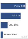
Device memory spans more than four orders of magnitude, phone to microcontroller.
Han, Song, Jeff Pool, John Tran, and William J. Dally. 2015. “Learning Both Weights and Connections for Efficient Neural Networks.” Advances in Neural Information Processing Systems 28 (NeurIPS 2015), 1135–43.
Hinton, Geoffrey, Oriol Vinyals, and Jeff Dean. 2015. “Distilling the Knowledge in a Neural Network.” arXiv Preprint.
Capacity is the question equation 1 already answers. Quantization, pruning, and distillation can each shrink the resident and trainable terms of that working set (Jacob et al. 2018; Han et al. 2015; Hinton et al. 2015), but their gains are workload-specific and do not combine automatically, so they must be validated together against the same budget. Once the working set fits, capacity says nothing about the second question, which is how much traffic the update drives through the hierarchy and how much of that traffic the caches can absorb. Operator tiling and memory layout aim to reuse active tensor blocks before eviction, while batch size controls activation storage and available parallelism. Gradient accumulation can limit the microbatch working set, but it also retains accumulation state and adds accesses, so its effect on traffic must be measured.
Training adds gradient and optimizer traffic to the tensor reads and writes already required by inference. When these transfers saturate memory bandwidth, additional arithmetic capacity cannot shorten the update. The activation checkpointing introduced with peak memory usage shows why capacity and traffic must be counted separately. Recomputing activations lowers the peak footprint while adding forward work and its memory reads, so capacity can improve as traffic and energy rise. Mixed-precision training changes bytes per stored tensor, but numerical stability and supported backward kernels determine whether the smaller representation is useful. Capacity, traffic, and update time therefore need separate measurements.
Mobile AI accelerator optimization
Accelerator choice depends on the training primitives that the device’s software stack exposes. Apple Neural Engine, Qualcomm Hexagon DSP, and Google Tensor devices have different compiler and runtime contracts, so the same update can follow different paths on each. A useful execution plan identifies where feature extraction, head or adapter training, and optimizer updates run. A dedicated engine may accelerate the frozen forward path while another processor handles learning, but transfers and duplicate representations then enter the cost. The supported operators and data movement must be established for the actual device and runtime version.
A local update may therefore execute on a CPU or GPU even when inference uses the dedicated neural accelerator. On a real device, the update-path test that opened the discussion of compute constraints becomes a short procedure.
- List the update’s operators in execution order: the forward pass, each backward operator that the trainable subset requires, and the optimizer step.
- For each operator, record the processor the runtime actually places it on, noting every fallback from the neural engine to the CPU or GPU.
- At each change of processor, add the transfer and any duplicate tensor representation to the update’s memory and traffic accounting.
- Measure time, peak memory, and energy for the complete traced path while a representative foreground workload runs.
- Feed those measurements into the peak-memory budget of equation 1 and the admission test of equation 2 that follows, which together decide whether the update may run.
Mixed-precision datapaths, sparse-update support, and near-memory compute can reduce those costs, but none of them is a prerequisite for training. What matters is whether the available runtime can execute the required operators within the device envelope. Architecture selection therefore shapes update precision, parameter selection, communication, and thermal policy together.
11.3.5 Energy, heat, and background admission
Energy and heat reach the user directly, through battery life and a device that grows warm or slows, which makes them among the most demanding limits that on-device learning must respect. A mobile power budget limits both the model complexity a device can train and the schedule on which it can train.
Napkin Math 11.1: Battery drain: The cost of edge learning
Problem: A team is designing a background fine-tuning job for a personalized voice assistant on a smartphone. Run unconstrained, the training job draws 4.5 W, above the 2–3 W sustained envelope given earlier, and takes 30 minutes to complete. If the phone has a 15 Wh battery, how much of the user’s battery will this “invisible” update consume?
Math:
- Total energy: 4.5 W \(\times\) 0.5 h = 2.25 Wh.
- Battery impact: 2.25 Wh/15 Wh = 15 percent.
Systems insight: Consuming 15 percent of a user’s battery for one background task makes update frequency a deployment decision. That energy cannot be translated into a fixed amount of screen-on time without specifying the foreground workload. A policy of opportunistic scheduling admits learning when device conditions permit it; a federated policy might require charging, Wi-Fi, and thermal headroom. Charging supplies energy but does not remove heat or foreground contention, so those constraints still need separate checks.
This battery calculation is the local edge-learning version of a broader energy constraint. Training must satisfy the user’s energy budget in addition to the model’s accuracy target. A production design therefore has to account for energy at scheduling time, compare local computation against communication cost, and defer learning when the user’s device cannot absorb the update.
That decision can be expressed as a background-work admission condition. Let \(\AdaptationWindowEnergy\) be the predicted energy for one adaptation window, \(\AdaptationEnergyAllowance\) the energy the policy permits before the next charging opportunity, \(\DevicePower\) the current sustained power, \(\AdaptationPowerIncrement\) the adaptation increment, and \(\ThermalPowerLimit\) the thermally sustainable limit. Let \(\ForegroundLatency\) be measured foreground latency, \(\AdaptationLatencyIncrease\) the worst-case latency increase under concurrent adaptation, and \(\CompletionDeadline\) the foreground deadline. The runtime admits an update only if
\[ \AdaptationWindowEnergy\le \AdaptationEnergyAllowance\quad \land \quad \DevicePower+ \AdaptationPowerIncrement\le \ThermalPowerLimit\quad \land \quad \ForegroundLatency+ \AdaptationLatencyIncrease\le \CompletionDeadline. \tag{2}\]
Charging can enlarge the energy allowance, but it does not waive the thermal or foreground-latency tests. The quantities must come from device- and workload-specific profiling, and the runtime must revoke admission when the measured envelope changes. Shorter update windows, a lower duty cycle, or a smaller trainable parameter set can make a rejected update feasible; allowing background learning to consume the foreground deadline cannot.
The same test also decides who teaches a shared model. Passing it correlates with hardware class, charging habits, and connectivity, so devices that are old, rarely charged, or thermally tight contribute few updates, and the population a federated model learns from is the admitted population rather than the deployed one (principle 20). The admission policy that protects each device is therefore also a sampling policy, and section 11.7.1 measures the skew it creates.
Example 11.1: On-device keyboard learning
Scenario: Consider a mobile keyboard that trains its next-word predictor locally and contributes updates to a shared model through federated averaging (McMahan et al. 2017).
Diagnosis: In the keyboard profile of section 11.3.1.1, one local update needs 50 MB–100 MB of working memory against a background allowance of 200 MB–300 MB, so at the selected operating point the update alone claims 25 percent of the allowance before the keyboard’s own state is counted, and the resident weights in \(\AdaptationPeakMemory\) claim more. Exceeding the allowance risks process eviction mid-update. Energy is the second constraint. An unconstrained job like the one in notebook 11.1 would take 15 percent of the battery, more than a policy that protects the user’s charge is likely to grant as \(\AdaptationEnergyAllowance\) in equation 2 while the phone runs on battery. The pipeline therefore admits training only when the device is idle, charging, and on Wi-Fi, and it quantizes update vectors to shrink the transmitted payload \(\DataVolume\).
Systems lesson: A federated keyboard must satisfy all three terms of equation 2 (energy \(\AdaptationWindowEnergy\le \AdaptationEnergyAllowance\), sustained power under \(\ThermalPowerLimit\), and typing latency under its deadline), fit \(\AdaptationPeakMemory\) within its memory allowance, respect uplink bandwidth \(\Bandwidth\), and meet its declared privacy guarantees together. Differential privacy adds a specific release guarantee and its associated costs; it is not implied by keeping raw text local.
11.3.6 Matching edge constraints to adaptation pillars
The memory, data, and compute constraints of the preceding sections act on the same update window at once: shrinking trainable parameters so an update fits in RAM still fails if local supervision is too sparse to guide the step or if intermittent connectivity drops the device from every federated round. The constraint analysis therefore yields three linked design decisions. The training amplification of table 2 motivates measuring the update footprint against equation 2 and choosing which parameters to adapt. Information scarcity, including limited local datasets, non-IID distributions, restrictions on data sharing, and minimal supervision, motivates data efficiency methods that reuse available evidence. When shared learning is useful, device heterogeneity and intermittent availability motivate federated coordination with explicit validation and privacy controls. Each pillar answers a different constraint within the same deployment budget and brings its own techniques to that answer (table 3).
| Constraint category | Key challenges | Solution approach |
|---|---|---|
| Resource Amplification | • Training workloads (4–12\(\times\) memory) • Memory limitations • Power constraints |
Model Adaptation • Parameter-efficient updates • Selective layer fine-tuning • Low-rank adaptations |
| Information Scarcity | • Limited local datasets • Non-IID distributions • Privacy restrictions |
Data Efficiency • Few-shot and streaming adaptation • Experience replay • Compressed representations |
| Coordination Challenges | • Device heterogeneity • Intermittent connectivity • Distributed validation complexity • Scalability requirements |
Federated Coordination • Federated averaging and asynchronous aggregation • Secure aggregation and differential privacy • Client selection and straggler handling |
Self-Check: Question
A mobile engineering team observes that fine-tuning a 10M parameter vision model on a smartphone with 8 GB of RAM causes the background training process to be killed by the operating system’s out-of-memory (OOM) killer during backpropagation. Why does training memory demand spike so severely compared to inference for the exact same model?
- The base model weights dynamically expand by \(100\times\) during the forward pass due to weight unpacking.
- Floating-point units on mobile SoCs automatically convert all INT8 weights to FP64 double precision during training.
- Training adds gradients, optimizer state, and saved backward activations to the weights; the simultaneous peak can exceed the app’s budget even when inference fits.
- The mobile operating system creates a separate virtual machine sandbox for every individual neuron in the neural network.
A quantized 7B-parameter language model achieves 12 tokens/sec on a mobile SoC advertised at 45 peak TOPS. Profiling shows that low-batch decode saturates available DRAM bandwidth while arithmetic units wait. Which hardware resource is the binding constraint?
- Insufficient CPU integer arithmetic capacity for calculating cross-entropy loss.
- Thermal throttling of the wireless 5G modem during token generation.
- Flash storage read latency when loading the token tokenizer vocabulary.
- Mobile LPDDR5X memory bandwidth (\(64\text{–}100\text{ GB/s}\)), which is roughly \(34\times\) lower than data-center HBM3, causing the memory streaming term \((D_{\text{vol}} / \text{BW})\) to dominate execution time per token.
A proposed background personalization task on a smartphone draws \(4.5\text{ W}\) of sustained SoC power and requires 30 minutes to complete. Calculate the total energy consumed (in \(\text{Wh}\)) and the percentage drain on an idealized \(15\text{ Wh}\) smartphone battery. Explain why this result mandates opportunistic scheduling.
True or False: Gradient checkpointing reduces the total electrical energy consumed by an on-device training workload because it reduces peak SRAM/DRAM memory allocation.
Consider the end-to-end memory lifecycle of a single gradient update during on-device backpropagation for a convolutional layer. Order the following operational stages from first to last in execution sequence:
- Discard intermediate activations and compute parameter updates in optimizer state
- Forward pass computes and caches layer activations
- Fetch batch inputs into SRAM buffer
- Loss evaluation and backward pass calculates layer gradients using cached activations
11.4 Model Adaptation
The 10M-parameter model of figure 3 is an inference candidate for a smartwatch with 500 MB of total system memory, because its FP32 weights occupy 40 MB. Training every parameter would need the full 360 MB stack, most of the watch’s memory before its operating system and foreground application take their share. The weight footprint alone does not establish inference fit; activation buffers, runtime workspace, and foreground reserve must also fit. Full-model training leaves much less room for that remaining state. Freezing parameters removes their gradients and optimizer state but not the storage or execution cost of the frozen network, so the system trains only a compact, strategically placed parameter set and, where it can, also shrinks the activations that the backward pass must keep. Resource-efficient model adaptation then determines both the local work a device can complete and the shared update format the fleet can aggregate.
The engineering choice balances adaptation expressivity against resource consumption. Full fine-tuning exposes all parameters to learning and can fit sufficiently small models; retaining a fixed model can be adequate when local context already supplies the needed personalization. Between these choices, selective updates offer smaller training state. The device resource envelope determines which candidates fit: a wearable-class device with 1 MB RAM has a different budget from a smartphone with 8 GB. The local variation then determines how much trainable capacity is useful. Bias updates may capture calibration changes, while shifts requiring new features need a richer update space. Runtime support, inference cost, shared-update compatibility, and rollback determine whether the candidate can enter the deployed system.
The selection of adaptation techniques follows this matching logic, from weight freezing (section 11.4.2) to structured and sparse updates (section 11.4.4). Their order of presentation is not a universal ranking of cost or expressivity; placement, update size, and runtime support determine those properties. Building on the resource accounting in section 11.3, the target is the smallest update space that captures the local variation: preserve what works globally, adapt what matters locally. Weight freezing restricts training to selected existing parameters, such as bias terms or final layers, whereas structured updates add low-rank or residual components to a frozen base and sparse updates select existing parameters according to their adaptation value and measured cost. Each choice must preserve enough useful capacity while fitting the device’s update budget.
11.4.1 Transfer as the premise
All three adaptation families work only because the device does not learn its representation from scratch: training a feature extractor from random initialization on a few dozen noisy phone interactions would overfit immediately and exhaust the energy allowance before learning anything generalizable. Instead, every local update that fits an edge budget relies on knowledge transfer, in which a cloud-pretrained model supplies representations useful for a new task or domain. Reusing those representations reduces what the device must learn from local examples, and the benefit depends on what the tasks share. A model pretrained in the cloud can adapt with limited local updates when its representations retain the distinctions the new task requires. If a new input modality or objective requires features the base model does not provide, a small local update may be insufficient.
Transfer is therefore the premise of the adaptation methods that follow. When pretrained representations carry the distinctions a personal typing vocabulary, an individual gait, or a drifting sensor needs, bias-only updates, adapters, and head-only training can learn a small correction while freezing most of the network. When that premise fails, head-only adaptation cannot recover distinctions absent from its fixed features. Earlier-layer adapters or broader updates may learn them, but their added state, computation, and data requirements must fit the device budget.
11.4.2 Weight freezing
When pretrained features already capture the structure of the task, the most direct way to shrink \(\TrainableStateMemory\) in equation 1 is to freeze the majority of a model’s parameters and adapt only a minimal subset. Bias-only adaptation holds all weights fixed and updates only the bias terms (scalar offsets applied after linear or convolutional layers). The constraint reduces trainable parameters by 100–1000\(\times\), removes the weight gradients and their optimizer state from \(\TrainableStateMemory\), and helps mitigate overfitting when training data is sparse or noisy.
Consider a standard neural network layer: \[ \LayerOutputVector= \WeightMatrix\LayerInputVector+ \BiasVector\] where \(\WeightMatrix\in \mathbb{R}^{\WeightMatrixRowCount\times \WeightMatrixColumnCount}\) is the weight matrix, \(\BiasVector\in \mathbb{R}^\WeightMatrixRowCount\) is the bias vector, and \(\LayerInputVector\in \mathbb{R}^\WeightMatrixColumnCount\) is the input. In full training, gradients are computed and applied to both \(\WeightMatrix\) and \(\BiasVector\). In bias-only adaptation, the system freezes the weight tensor (\(\FiniteChange\WeightMatrix= \ZeroMatrix\)) and computes gradients exclusively for the bias: \[ \WeightMatrix\leftarrow \WeightMatrix, \quad \BiasVector\leftarrow \BiasVector- \LearningRate\frac{\partial \LossFunction}{\partial \BiasVector} \]
This reduces the number of stored gradients and optimizer states, enabling training to proceed under memory-constrained conditions. The smaller trainable state helps only if the device also supports the arithmetic and activation schedule required by the update. In the bias-only setup of listing 1, all convolutional and fully connected weights remain frozen, and only the bias terms adapt to local data.
# Freeze all parameters
for name, param in model.named_parameters():
    param.requires_grad = False

# Enable gradients for bias parameters only
for name, param in model.named_parameters():
    if "bias" in name:
        param.requires_grad = True
This pattern restricts optimizer updates to bias terms. What it saves, and what it does not, follows from the two derivatives of the layer above. The weight gradient \(\partial \LossFunction/\partial \WeightMatrix= (\partial \LossFunction/\partial \LayerOutputVector)\,\LayerInputVector^T\) needs the layer’s saved input \(\LayerInputVector\), whereas the bias gradient \(\partial \LossFunction/\partial \BiasVector= \partial \LossFunction/\partial \LayerOutputVector\) needs only the gradient arriving from above. A frozen linear layer therefore no longer has to keep its input for its own sake. Reaching a bias in an earlier layer, however, still sends the gradient back through every later layer, and each nonlinearity or normalization on that path needs its own saved state (a ReLU needs at least the mask of which inputs were positive). Freezing parameters thus shrinks \(\TrainableStateMemory\) without eliminating backward computation or all saved activation state. This is valuable when adapting pretrained models to user-specific or device-local data where the core representations remain relevant but require calibration.
Tiny Transfer Learning (TinyTL) (Cai et al. 2020) targets the activation term of equation 1 as well as trainable state. It builds on the derivative argument above. Frozen linear layers drop their saved inputs, so what remains is the backward state of nonlinearities and normalization. TinyTL combines bias adaptation with activation and normalization choices that reduce that state; optional lite residual modules restore some adaptation capacity at an additional memory cost.
Full fine-tuning (Panel A of figure 7) computes gradients for every intermediate layer weight, whereas TinyTL (Panel B) freezes the convolutional backbone (gray blocks) and confines parameter updates to lightweight residual side-paths and bias vectors \(\BiasVector\) (blue blocks). The dashed backward-pass arrow spans the full network depth in both architectures. TinyTL’s memory reduction therefore stems not from truncating the backward pass but from avoiding the storage of intermediate feature maps needed to compute weight gradients.
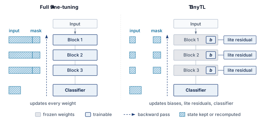
The memory reduction is useful only when the frozen backbone remains expressive enough for the downstream task. The bias terms allow for minor but meaningful shifts in model behavior, particularly for personalization tasks. When domain shift is more significant, TinyTL can optionally incorporate small residual adapters to improve expressivity, all while preserving the system’s tight memory and energy profile.
TinyTL demonstrates that reducing saved activation state can matter more than reducing the number of trainable parameters alone (Cai et al. 2020). On its image-classification transfer benchmarks, TinyTL reports training-memory savings of up to 6.5× relative to fine-tuning the full network with little accuracy loss, so the adaptation working set can shrink to roughly 15 percent of the full fine-tuning footprint. The lite residual modules that recover adaptation capacity add only about 3.8 percent memory overhead in that study. Those savings depend on the selected feature extractor, input resolution, batch size, normalization, and residual-module configuration, and a saving measured on those benchmarks says nothing about whether an arbitrary frozen backbone fits into microcontroller SRAM.
Cai, Han, Chuang Gan, Ligeng Zhu, and Song Han. 2020. “TinyTL: Reduce Activations, Not Trainable Parameters for Efficient on-Device Learning.” Advances in Neural Information Processing Systems 33: 11285–97.
11.4.3 Structured parameter updates
When bias-only updates cannot capture the local change, the system can add trainable capacity while retaining a frozen backbone. Residual adaptation modules (Houlsby et al. 2019) and low-rank parameterizations (Hu et al. 2021) implement this choice in different ways. They restrict learning to added components, but their training cost includes the backward path through the surrounding network. The comparison with bias-only or full fine-tuning therefore requires both a quality target and a peak-memory measurement.
Houlsby, Neil, Andrei Giurgiu, Stanislaw Jastrzebski, Bruna Morrone, Quentin de Laroussilhe, Andrea Gesmundo, Mohammad Attariyan, and Sylvain Gelly. 2019. “Parameter-Efficient Transfer Learning for NLP.” Proceedings of the 36th International Conference on Machine Learning (ICML), Proceedings of machine learning research, vol. 97: 2790–99.
Adapter-based adaptation
A common implementation involves inserting residual adapters, which are small residual bottleneck layers, between existing layers in a pretrained model. Consider a hidden representation \(\HiddenActivation\) passed between layers. A residual adapter introduces a transformation: \[ \AdaptedHiddenActivation= \HiddenActivation+ \ResidualAdapterFunction(\HiddenActivation) \] where \(\ResidualAdapterFunction(\cdot)\) is a trainable function, typically composed of two linear layers with a nonlinearity: \[ \ResidualAdapterFunction(\HiddenActivation) = \WeightMatrix_2 \, \AdapterActivationFunction(\WeightMatrix_1 \HiddenActivation) \] with \(\WeightMatrix_1 \in \mathbb{R}^{\AdapterRank\times \HiddenDimension}\) and \(\WeightMatrix_2 \in \mathbb{R}^{\HiddenDimension\times \AdapterRank}\), where \(\AdapterRank\ll \HiddenDimension\). This bottleneck design ensures that only a small number of parameters are introduced per layer.
The adapters act as learnable perturbations on top of a frozen backbone. Because they are small and sparsely applied, their weights add little storage, although their saved activations and optimizer state still count against the training budget, and they let the model shift its predictions in response to new inputs.
The residual bottleneck in listing 2 maps onto the adapter equation term by term. Its down-projection plays the role of \(\WeightMatrix_1\), mapping width \(\HiddenDimension\) to the bottleneck width \(\AdapterRank\), a ReLU supplies \(\AdapterActivationFunction\), and its up-projection plays the role of \(\WeightMatrix_2\), restoring width \(\HiddenDimension\) before the input is added back. Such modules can be implemented efficiently on edge devices, particularly when the two projection matrices are small and fixed-point representations are supported.
import torch.nn as nn


class Adapter(nn.Module):
    def __init__(self, dim, bottleneck_dim):
        super().__init__()
        # Project from full dimension to bottleneck (e.g., 768 -> 16)
        self.down = nn.Linear(
            dim, bottleneck_dim
        )  # W1: learns compression
        # Project back to original dimension (e.g., 16 -> 768)
        self.up = nn.Linear(
            bottleneck_dim, dim
        )  # W2: learns expansion
        self.activation = nn.ReLU()

    def forward(self, x):
        # Residual connection: original + nonlinear bottleneck
        # Only adapter params trained; base model frozen
        return x + self.up(self.activation(self.down(x)))
Low-rank techniques
Another efficient strategy is to constrain the weight update itself to low rank. Low-rank adaptation (LoRA)11 leaves a base matrix \(\WeightMatrix_0 \in \mathbb{R}^{\WeightMatrixRowCount\times \WeightMatrixColumnCount}\) frozen and learns its change as the product of a down-projection \(\AdapterDownProjectionMatrix\in \mathbb{R}^{\AdapterRank\times \WeightMatrixColumnCount}\) and an up-projection \(\AdapterUpProjectionMatrix\in \mathbb{R}^{\WeightMatrixRowCount\times \AdapterRank}\), with \(\AdapterRank\ll \min(\WeightMatrixRowCount,\WeightMatrixColumnCount)\). The adapted layer adds \(\AdapterUpProjectionMatrix\AdapterDownProjectionMatrix\LayerInputVector\) to the frozen output \(\WeightMatrix_0 \LayerInputVector\), the same forward pass a serving fleet runs when many adapters share one base model. Training cost follows from that structure. The update \(\FiniteChange\WeightMatrix= \AdapterUpProjectionMatrix\AdapterDownProjectionMatrix\) has \(\AdapterRank(\WeightMatrixRowCount+ \WeightMatrixColumnCount)\) trainable parameters instead of \(\WeightMatrixRowCount \WeightMatrixColumnCount\), and only those parameters carry gradients and optimizer state.
11 LoRA (low-rank adaptation): Hu et al. (2021) learn rank-\(\AdapterRank\) decomposition matrices \(\AdapterDownProjectionMatrix\) and \(\AdapterUpProjectionMatrix\) instead of updating full weight matrices, reporting a 10,000\(\times\) reduction in trainable parameters for their GPT-3 comparison. That reduction does not apply to the full model footprint: a model with 7B parameters has about a 14 GB FP16 weight footprint before gradients, optimizer state, and activations. Even at rank 16, adapter storage depends on the dimensions and number of adapted matrices, and deployment must still accommodate the frozen base model.
Hu, Edward J., Yelong Shen, Phillip Wallis, Zeyuan Allen-Zhu, Yuanzhi Li, Shean Wang, Lu Wang, and Weizhu Chen. 2021. “LoRA: Low-Rank Adaptation of Large Language Models.” arXiv Preprint arXiv:2106.09685.
↩︎ The low-rank adapter forward pass, in which a frozen base projection is summed with a trainable down- and up-projection, is established in Multi-LoRA serving and batched adapter execution.
The decomposition rests on a linear-algebra fact. Any matrix can be expressed as a sum of rank-one matrices through singular value decomposition. Constraining updates to low rank (typically \(\AdapterRank= 4\) to \(16\)) captures a restricted set of variation modes while reducing parameters. For a typical transformer layer with dimensions \(768{\times}768\), full fine-tuning requires updating 589,824 parameters. With rank-4 decomposition, only \(768{\times}4{\times}2 =\) 6,144 parameters are updated, a 99 percent reduction. Whether this retains most of the adaptation quality depends on the task, rank, and base model; the LoRA authors report that low-rank adapters can match or approach full fine-tuning on several transformer adaptation benchmarks (Hu et al. 2021).
LoRA was developed for transformer models but applies to any layer built on a weight matrix. From a systems engineering perspective, LoRA makes the trainable adapter the artifact that can be stored, transmitted, scheduled, and rolled back separately from the frozen base model.
Drawn to proportion for a square layer of width \(\HiddenDimension\), the adapted layer shows where the saving comes from (figure 8). Input \(\LayerInputVector\in \mathbb{R}^\HiddenDimension\) passes through the frozen \(\HiddenDimension{\times}\HiddenDimension\) base matrix \(\WeightMatrix_0\) and, in parallel, through a thin \(\AdapterRank{\times}\HiddenDimension\) down-projection \(\AdapterDownProjectionMatrix\) and a \(\HiddenDimension{\times}\AdapterRank\) up-projection \(\AdapterUpProjectionMatrix\), and the two paths sum to \(\HiddenActivation= \WeightMatrix_0 \LayerInputVector+ \AdapterUpProjectionMatrix\AdapterDownProjectionMatrix\LayerInputVector\). The base weights need no parameter gradients or optimizer state, although backward computation may still traverse the base path. Folding the product into the base weights (\(\WeightMatrix_0 + \AdapterUpProjectionMatrix\AdapterDownProjectionMatrix\)) removes separate adapter arithmetic for that merged model. Numerical compatibility, any requantization, and the cost of retaining merged copies determine whether this is the appropriate serving representation.
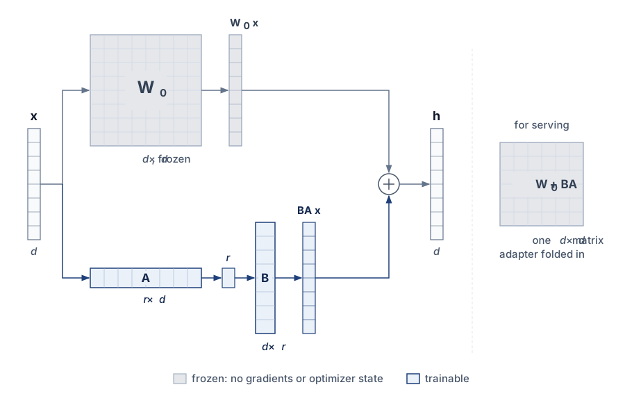
Consider a mobile deployment where a language model with 7B parameters has a 14 GB FP16 weight footprint, before accounting for the additional gradients, optimizer states, and activations required by full fine-tuning. That footprint exceeds smartphones with about 8 GB total memory unless the base model is quantized, partitioned, or offloaded. Choosing LoRA rank 16 restricts the update space, and this chapter’s fleet examples budget a reference adapter update of 50 MB. That figure is a communication payload, not a training-memory estimate. The device must also fit the base model, gradients, optimizer state, and live activations under its execution plan.
The smaller payload also matters under intermittent connectivity. Transferring the full FP16 model in this example requires 14 GB, while the reference adapter update is 50 MB. Transfer time depends on encoded bytes, effective link throughput, and interruptions. An adapter-only transfer provides the saving only when the receiving device already holds a compatible base model; base-version changes must be included in the communication budget. In both the residual bottleneck and LoRA, the width or rank \(\AdapterRank\) sets the trainable cost, so a deployment can size it to the memory each device class leaves for learning; which mechanism each class receives is decided by the device-tier framework of section 11.4.3.4.
Edge personalization
Adapters support multiple personalized contexts with one frozen backbone. For an input width \(\HiddenDimension\), a residual bottleneck of width \(\AdapterRank\) uses \(2d\AdapterRank\) matrix parameters, plus \(\AdapterRank+\HiddenDimension\) biases when both projections include them. A deployment with several adapters must sum this count over their insertion sites; rank or bottleneck width alone does not determine the total. Stored bytes then equal parameter count times bytes per stored value. With \(\HiddenDimension= 768\) and \(\AdapterRank= 16\), one adapter holds 25,360 parameters, about 50.7 KB in FP16; one adapter after each of 12 blocks totals 304,320 parameters, roughly 0.6 MB. During training, gradients, optimizer state, and saved activations add to that storage footprint. A device can swap context-specific modules while sharing the much larger base model, provided it can hold the base and active adaptation state together.
This adapter switching pattern lets a smartphone select context-specific behavior without replacing the entire backbone. When the user enters a low-light environment, the system can load a compatible adapter into the vision pipeline; selecting an existing adapter does not itself require learning. The modularity extends naturally to federated learning: transmitting only the adapted parameters can reduce upload traffic relative to a full-model update, with savings determined by the total adapter count and encoding. Residual-adapter studies show that small trainable modules can adapt a shared visual backbone across multiple visual domains (Rebuffi et al. 2017), making them a useful design point between personalization quality and system resources. Freezing the backbone preserves its parameters, while adapters provide a bounded place for user- or context-specific updates. The resulting model can still suffer catastrophic forgetting, the loss of previously learned behavior after new updates (defined in section 11.5.2).
Rebuffi, Sylvestre-Alvise, Hakan Bilen, and Andrea Vedaldi. 2017. “Learning Multiple Visual Domains with Residual Adapters.” Advances in Neural Information Processing Systems (NeurIPS) 30.
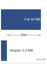
Each new context costs an adapter, not a full model copy.
In smartphone camera pipelines, environmental lighting, user preferences, and lens distortion vary between users. Residual modules can adapt a frozen shared model to these differences while leaving its base weights unchanged; the combined model’s behavior still requires validation. In voice-based systems, adapters similarly provide a way to test personalized speech recognition without retraining the full acoustic model. Keeping the base and adapter versions compatible also supports rollback or switching between user-specific versions when adaptation degrades performance.
Performance vs. resource trade-offs
Selecting an adaptation strategy requires accounting for both resource cost and expressivity. Bias-only updates retain a small trainable state but may lack the capacity to handle structural domain shifts. Full fine-tuning exposes every parameter to adaptation and adds corresponding gradient and optimizer state. LoRA and residual adapters offer intermediate choices whose cost depends on rank or width, insertion sites, and numerical representation. The same budget, equation 1, governs each of these strategies. Because peak working memory \(\AdaptationPeakMemory\) must jointly contain resident weights, trainable state \(\TrainableStateMemory\), and the peak of live activations under the device ceiling \(\DeviceMemoryCapacity\), each strategy shrinks a different term: bias-only and adapter methods shrink \(\TrainableStateMemory\), TinyTL-style choices also shrink the activation term, and training only the final classifier, whose backward pass stops at the head, removes most of that term. Parameter storage alone therefore cannot determine whether background adaptation fits.
LoRA and residual adapters impose different deployment costs. For a fixed adapter and compatible numerical representation, LoRA’s linear update can be merged into the backbone before inference \((\WeightMatrix_0 + \AdapterUpProjectionMatrix\AdapterDownProjectionMatrix)\), avoiding separate adapter arithmetic in the forward path. A quantized base may require requantization and renewed quality validation after merging. Keeping a separate merged backbone for every context also sacrifices the storage benefit of sharing one base. Residual adapters remain distinct modules (\(\LayerOutputVector= \FrozenBackboneFunction(\LayerInputVector) + \text{Adapter}(\LayerInputVector)\)); their latency cost depends on shape, placement, and runtime, while switching contexts requires only the corresponding adapter state.
The runtime must support the selected adapter’s forward operators and its training path. These can use a dynamic graph or a statically compiled update schedule; dynamic graph construction is not itself a requirement. For an inference engine such as Open Neural Network Exchange (ONNX) Runtime Mobile, a runtime that executes an adapter’s forward path may still lack its backward operators, optimizer, or state management. The deployment must verify both paths, including any transfers between the processor that runs inference and the processor that performs updates.
For this multi-context personalization workload, where one device switches among several adapters, system architects can use a device-tier framework to organize candidate mechanisms. On flagship phones (Tier 1) with dedicated Neural Engines and 8 GB of RAM or more, residual adapters provide a strong balance of modularity and speed, because switching contexts swaps only adapter state. On mid-range devices (Tier 2) with 1 GB up to that ceiling, LoRA may fit when a fixed adapter can be merged into a compatible base representation before inference, trading switching flexibility for zero added inference arithmetic. For ultra-constrained IoT endpoints (Tier 3) with less than 1 GB RAM, bias-only updates may be the only practical option. Budget phones show that the tier follows the memory available to learning rather than installed RAM. Their 4 GB places them in Tier 2, yet only 1 GB–2 GB remains for ML work after the operating system, and a background adaptation task may be granted less, so a deployment can reasonably hold them to the Tier 3 mechanism. The assignments follow from the workload as much as from the hardware. A workload that keeps one adaptation per user, rather than many switchable contexts, loses the reason to keep adapters separate and can favor merged LoRA even on flagship devices. The runtime must still verify the base-model footprint and admit training within the measured device envelope.
Checkpoint 11.2: Edge personalization
Verify understanding of efficient on-device adaptation:
11.4.4 Sparse updates
Bias-only updates and fixed adapters choose where the model may change before seeing local data, yet a local shift can alter specific convolutional filters or attention channels rather than every block uniformly. Sparse updates instead adapt selected existing parameters rather than adding modules. Their expressivity relative to adapters depends on the selected locations and parameter budget. A task-adaptive policy selects those locations using evidence about the current task or user. The resulting update space can target changes that a fixed subset misses, but selection itself consumes resources and does not guarantee that the complete training path fits the device.
The useful savings depend on what the runtime can omit. Unselected parameters need no gradient or optimizer state, but their operations may still lie on the backward path to selected parameters. A policy must therefore compare the measured update cost with its adaptation benefit; the fraction of trainable parameters alone does not predict the reduction in compute. Because layers do not contribute equally to local performance gains, identifying the minimal subset with the highest adaptation value lets the system spend scarce training capacity where it changes the model’s behavior most.
Sparse update design
Let a neural network be defined by parameters \(\ModelParameters= \{\ModelParameters_1, \ModelParameters_2, \ldots, \ModelParameters_{\LayerCount}\}\) across \(\LayerCount\) layers. In standard fine-tuning, gradients are computed and updates are performed on all parameters: \[ \ModelParameters_i \leftarrow \ModelParameters_i - \LearningRate\frac{\partial \LossFunction}{\partial \ModelParameters_i}, \quad \text{for } \LayerSelectionIndex= 1, \ldots, \LayerCount \]
In task-adaptive sparse updates, the system selects a small subset \(\SelectedLayerSet\subset \{1, \ldots, \LayerCount\}\) such that only parameters in \(\SelectedLayerSet\) are updated: \[ \ModelParameters_i \leftarrow \begin{cases} \ModelParameters_i - \LearningRate\frac{\partial \LossFunction}{\partial \ModelParameters_i}, & \text{if } \LayerSelectionIndex\in \SelectedLayerSet\\ \ModelParameters_i, & \text{otherwise} \end{cases} \]
The challenge lies in selecting the optimal subset \(\SelectedLayerSet\) given memory and compute constraints. A principled strategy is contribution analysis, an empirical method that estimates how much each layer contributes to downstream performance improvement. For example, one can measure the marginal gain from updating each layer independently:
- Freeze the entire model.
- Unfreeze one candidate layer.
- Finetune briefly and evaluate improvement in validation accuracy.
- Rank layers by performance gain per unit cost (e.g., per KB of trainable memory).
This layer-wise profiling yields a candidate ranking from which \(\SelectedLayerSet\) can be constructed subject to a memory budget. Gains measured one layer at a time need not add when layers train together, and shared backward dependencies change the combined cost. The selected set therefore needs a joint quality and resource check, with the profiling cost included in the adaptation budget.
In a complete selective fine-tuning pipeline, that ranking is the middle of three stages (figure 9). Stage 1 meta-trains the network in the cloud, which means training its initial weights so that a few later updates on new data adapt it well (the idea behind model-agnostic meta-learning, taken up in section 11.7.3). Stage 2 ranks layers or channel groups by adaptation benefit per unit of device cost and lets the device budget set the cut, and Stage 3 updates only the units above the cut on local data. Freezing the units below the cut removes their gradient and optimizer state, but the backward pass still runs through any frozen layer that lies between the loss and a selected one, so the selected set must be costed under the complete execution schedule.
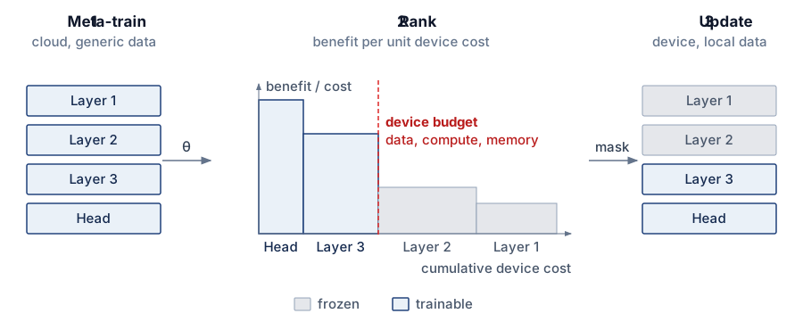
A concrete example is TinyTrain, a method designed to allow rapid adaptation on-device (Kwon et al. 2024). TinyTrain combines offline preparation with a task-adaptive sparse-update method that dynamically selects layers or channels to update using user data, memory limits, and compute limits. At runtime, the system updates only the selected subset rather than treating the whole network as trainable.
In implementation, selective layer updating turns the ranking into requires_grad decisions or equivalent graph masks. In the profiling-driven version, contribution scores and the memory limit decide which layers are unfrozen (listing 3).
# Selective layer update based on contribution analysis
# Layers selected via profiling: conv2 and fc have highest
# accuracy-per-KB impact for this task

for name, param in model.named_parameters():
    if "conv2" in name or "fc" in name:
        param.requires_grad = True  # Train high-impact layers
    else:
        param.requires_grad = False  # Freeze low-impact layers

# Parameter fraction follows layer shapes; adaptation quality requires evaluation
# Memory savings: gradient storage only for selected layers
Consider a user wearing an augmented reality headset that performs real-time object recognition. As lighting and environments shift, the system must adapt to maintain accuracy, but training must occur during brief idle periods or while charging. TinyTrain addresses this constraint with task-adaptive sparse updates, in which the deployment process selects a small update set that fits the device’s memory and compute budget. The approach keeps adaptation fast, energy-efficient, and memory-aware when the target task and device profile match the method’s assumptions.
Task-adaptive sparse updates still introduce system-level trade-offs. Contribution analysis has a nontrivial computational cost even when it occurs during pretraining or initial profiling, so the deployment pipeline must budget for it. Stability also requires attention: if too few parameters are selected for updating, the model may underfit the target distribution, so teams need validation thresholds for the selected subset before deployment. The selection policy must also account for hardware-specific execution costs because some parameters show high contribution scores but prove expensive to update on certain architectures. Despite these trade-offs, task-adaptive sparse updates provide a practical mechanism to scale adaptation across deployment contexts from microcontrollers to mobile devices (Kwon et al. 2024).
Kwon, Y. D., R. Li, S. I. Venieris, J. Chauhan, and N. D. Lane. 2024. “TinyTrain: Resource-Aware Task-Adaptive Sparse Training of DNNs at the Data-Scarce Edge.” Proceedings of the 41st International Conference on Machine Learning (ICML).
Adaptation strategy comparison
The design target is the smallest update space that captures the local change. Full fine-tuning pays every term of equation 1; bias-only updates and head-only training fit minor calibration or new output categories; LoRA and residual adapters add bounded capacity beside a frozen backbone; task-adaptive sparse updates spend profiling effort to select valuable existing parameters. A larger update space is justified only if the measured quality gain fits the device’s training budget. Each strategy shrinks a different budget term, and the choice must still be checked against expressivity, runtime support, and selection cost; table 4 sets these adaptation strategy trade-offs side by side.
| Technique | Trainable parameters | Memory overhead | Expressivity | Use case suitability | System requirements |
|---|---|---|---|---|---|
| Full Fine-Tuning | All parameters | Highest; every term of the peak budget | Highest | Large domain shift on capable devices | Full backward support and memory headroom |
| Bias-Only Updates | Bias terms only | Minimal \(\TrainableStateMemory\); activations remain | Low | Simple personalization; low variance | Extreme memory/compute limits |
| Head-Only Training | Final classifier | Minimal; backward pass stops at the head | Low | New output classes; custom wake words | Frozen encoder; reusable cached features |
| LoRA | Low-rank factors per adapted matrix | Low \(\TrainableStateMemory\); activations remain | Moderate to High | One mergeable adaptation per user | Merge step and requantization check for serving |
| Residual Adapters | Adapter modules | Low \(\TrainableStateMemory\); activations remain | Moderate to High | Switching among several contexts on mobile | Mobile-class SoCs with runtime support |
| Sparse Layer Updates | Selective parameter subsets | Variable; depends on the selected layers | High (task-adaptive) | Real-time adaptation; domain shift | Requires profiling or meta-training |
Once an adaptation mechanism fits the device’s memory and execution budget, it must still learn from the available examples. Reducing trainable state does not create labels or ensure that a user’s recent observations represent future use. The next constraint is therefore statistical: extracting reliable learning signal from sparse local data while retaining useful prior behavior.
Self-Check: Question
Why does Tiny Transfer Learning (TinyTL) freeze convolutional backbone weights and adapt biases with optional lite residual modules?
- Freezing removes backbone weight-gradient and optimizer state; suitable activation and normalization choices also reduce saved backward state.
- Microcontroller hardware units physically short-circuit if matrix multiplications are performed in reverse during backpropagation.
- Bias parameters have mathematical properties that prevent all forms of numerical underflow in 8-bit fixed-point arithmetic.
- Training bias parameters modifies the underlying kernel weights directly through implicit singular value decomposition.
A mobile vision engineer chooses between Low-Rank Adaptation (LoRA) and Residual Bottleneck Adapters for on-device camera personalization. The system requires zero additional inference latency during real-time 60 FPS video capture, while another use case requires hot-swapping between 10 user contexts without reloading the base model. How do LoRA and Residual Adapters compare across these requirements?
- Residual Adapters introduce zero inference latency because they replace the backbone, while LoRA requires recomputing matrix inverses on every video frame.
- LoRA updates can be merged into compatible base weights to remove the adapter execution path, while residual adapters retain separate computation and support modular context switching.
- LoRA updates require storing 10 full copies of the 7B base model in SRAM, whereas Residual Adapters operate without trainable parameters.
- Both methods require identical memory footprints and add exactly 50 ms of inference latency per layer.
A smart camera supports 10 personalization contexts. Its base model has 10M parameters (\(40\text{ MB}\) in FP32), and assume each complete adapter checkpoint occupies \(200\text{ KB}\). Compare storage for 10 full fine-tuned models with one shared base plus 10 adapters. Explain the architectural advantage.
In structured parameter adaptation, a technique that approximates a full weight matrix update \(\FiniteChange\WeightMatrix \in \mathbb{R}^{\WeightMatrixRowCount \times \WeightMatrixColumnCount}\) as the product of a low-rank up-projection \(\AdapterUpProjectionMatrix \in \mathbb{R}^{\WeightMatrixRowCount \times \AdapterRank}\) and down-projection \(\AdapterDownProjectionMatrix \in \mathbb{R}^{\AdapterRank \times \WeightMatrixColumnCount}\) (where \(\AdapterRank \ll \min(\WeightMatrixRowCount, \WeightMatrixColumnCount)\)) is known as ____ (low-rank adaptation).
Task-adaptive sparse updates use individual-layer profiling to propose a trainable subset. Order the steps from profiling to deployment:
- Fine-tune each candidate layer separately and measure its validation gain and resource cost
- Freeze the pretrained model to establish a baseline
- Deploy the jointly validated subset with other parameters frozen
- Rank layers by gain per unit cost and propose a subset
- Measure the selected combination against memory, energy, foreground-latency, and quality budgets, including profiling cost
11.5 Data Efficiency
A user corrects smartphone keyboard autocorrect perhaps three times a day. The system cannot require 10,000 labeled sentences to train a local language model. Data efficiency at the edge means learning aggressively from a sparse, noisy, and uncurated trickle of implicit user feedback, maximizing the signal extracted from each interaction.
The systems trade-off is data collection cost against adaptation quality. Every retained example costs user friction, energy, storage, and privacy exposure. A voice assistant adapting to speech samples weighs model improvement against battery drain and user comfort with always-on recording, and a keyboard chooses between logging shallow keystroke statistics and keeping full typing sessions. Unlike a central pipeline, the device cannot reach into a larger dataset when its own evidence runs short, and an application that needs a decision before enough evidence accumulates may be better served by a validated fixed model than by immediate learning. Whatever the device does learn must also stay compatible with the adaptation mechanism of section 11.4 and with any federated protocol that later consumes it.
The strategy choice depends on which scarcity binds first, and practical systems usually combine several: few-shot learning handles cases where only a handful of labeled or weakly labeled examples must drive personalization, whereas streaming updates handle observations that arrive incrementally and cannot be batched in advance. Because continual streaming updates can overwrite earlier behavior, experience replay spends memory to retain and reuse scarce examples, while data compression shrinks those stored histories so that replay and lightweight training remain feasible within edge memory budgets. Data scarcity thus becomes an allocation problem, in which the device spends labels, memory, compute, and privacy budget where they produce the most reliable local signal.
11.5.1 Few-shot learning and data streaming
Unlike cloud training workflows that rely on large, curated labeled datasets, on-device learning must often proceed from only a handful of examples collected passively through user interaction or ambient sensing—a user will record five wake-word samples during setup, not five thousand. These constraints motivate two complementary adaptation strategies: few-shot learning, in which models generalize from a small, static set of examples, and streaming adaptation, where incremental observations support updates scheduled within device budgets.
Few-shot adaptation uses limited labeled or weakly labeled evidence for a new task or user condition (Wang et al. 2020). Bias-only updates, adapter modules, and prototype-based classification restrict what must be learned, but each still needs validation against overfitting. Let \(\FewShotSupportSet= \{(\ModelInput_i, \ExampleLabel_i)\}_{i=1}^{\SupportSetSize}\) denote the local support set; here \(\SupportSetSize\) counts all examples in the set, rather than examples per class. A candidate policy might permit few gradient steps (\(\FewShotStepCount\ll 100\)) and a small trainable subset (\(|\UpdatedParameterSubset| \ll |\ModelParameters|\)). These are illustrative restrictions, not universal feasibility conditions. The actual step and parameter budgets follow from measured device cost and the quality target, including retained performance on earlier tasks.
Wang, Y., Q. Yao, J. T. Kwok, and L. M. Ni. 2020. “Generalizing from a Few Examples: A Survey on Few-Shot Learning.” ACM Computing Surveys 53 (3): 1–34. https://doi.org/10.1145/3386252.
Warden, Pete. 2018. “Speech Commands: A Dataset for Limited-Vocabulary Speech Recognition.” arXiv Preprint arXiv:1804.03209, ahead of print. https://doi.org/10.48550/arXiv.1804.03209.
Keyword spotting (KWS) systems are a common target for data-efficient on-device adaptation; Speech Commands provides a dataset for training and evaluating limited-vocabulary KWS models (Warden 2018). A detector must distinguish its target phrase from background speech while meeting latency and false-activation requirements. One design uses a pretrained acoustic encoder, such as a small convolutional or recurrent network, to map audio into embeddings for a lightweight classifier. A shared encoder supplies reusable features, while local examples can support a custom wake word or an underrepresented accent. Whether those examples justify local training depends on their coverage, transfer restrictions, and the improvement over the shared detector.
Few-shot adaptation can train an output classifier or another small parameter subset from utterances collected directly on the device. A user might provide 5–10 recordings of a custom wake word while the acoustic encoder remains frozen. Those positive examples define what to recognize, but the false-activation rate on other speech and background noise is a separate measurement, and the personalized detector should not be accepted until it has been made.
Head-only adaptation is cheap in a way the peak-memory budget of equation 1 makes precise. Because the backward pass stops at the classifier, the encoder’s saved activations leave the activation term, and the encoder outputs for the support set can be computed once and reused across update steps. What remains is running the encoder forward, holding the support examples or their features, and evaluating the adapted classifier. Those costs, not the size of the head, decide whether the update fits a particular phone or microcontroller.
Many on-device scenarios instead call for streaming adaptation, in which the model learns incrementally as data arrives over time rather than from a fixed support set (Hayes et al. 2020). Let \(\{\ModelInput_t\}_{t=1}^{\infty}\) represent the observations selected from the stream for admitted updates. In streaming settings, observations arrive continuously, but the runtime admits training only when memory, energy, and foreground-latency budgets permit. The following rule describes one admitted update; it does not require a gradient step on every arrival. The index \(\OptimizerStepIndex\) counts these update steps. The computable loss may come from implicit feedback, pseudo-labels, self-supervised objectives, reconstruction error, or a task-specific proxy rather than explicit human labels. The model update can be written generically as: \[ \ModelParameters_{t+1} = \ModelParameters_t - \LearningRate_t \nabla \LossFunction(\ModelInput_t; \ModelParameters_t) \] where \(\LearningRate_t\) is the learning rate at time \(\OptimizerStepIndex\). This form of adaptation is sensitive to noise and drift in the input distribution, and thus often incorporates mechanisms such as learning rate decay, meta-learned initialization, or update gating to improve stability.
The same strategies apply beyond keyword spotting. In wearable health devices, a model that classifies physical activities may begin with a generic classifier and adapt to user-specific motion patterns using only a few labeled activity segments. In smart assistants, user voice profiles are fine-tuned over time using ongoing speech input, even when explicit supervision is unavailable. Local corrections, repetitions, or downstream task completion can provide implicit signals, but only after the system defines which event counts as feedback and tests its validity. A user may accept a suggestion because it is convenient rather than correct, abandon a task for reasons unrelated to the model, or correct an error that the model itself induced. Production adaptation should therefore separate observed events from inferred labels, retain a nonadapting control cohort, measure delayed outcomes when available, and gate learning when the proxy-to-outcome relationship drifts. A stream of such updates also raises a stability problem that few-shot and streaming rules do not address on their own.
11.5.2 Experience replay
When a streaming update rule trains only on a user’s newest interactions, gradient steps on recent examples overwrite the weights that recognized earlier classes, causing accuracy on prior tasks to collapse within a few updates. Retaining a small sample of earlier observations on the device directly counters this failure mode.
Definition 11.3: Catastrophic forgetting
Catastrophic forgetting is the phenomenon in which a neural network trained sequentially on new tasks or data distributions rapidly loses performance on previously learned tasks, because gradient updates that optimize the new objective overwrite weight configurations that supported the old ones.
- Significance: Without explicit mitigation, fine-tuning a deployed classifier on a new domain can sharply reduce prior-task accuracy, even when the new domain is closely related to the old one (Kirkpatrick et al. 2017). This is the central failure mode of on-device and federated learning: every device that adapts locally to its user’s recent data risks erasing the general capabilities the centralized training run paid for, and the loss is invisible until inference encounters out-of-recent-context inputs.
- Distinction: Unlike overfitting (a generalization failure on a single fixed task) and distribution shift (a deployment-time mismatch between training and inference data), forgetting is a training-time phenomenon caused by the sequential structure of the update stream itself; updates for new data can interfere with earlier solutions even when a representation capable of supporting both tasks exists.
- Common pitfall: A frequent misconception is that a small experience-replay buffer is sufficient protection. A small buffer can hold aggregate accuracy on a held-out set while rare classes, which it samples too seldom, continue to degrade. Forgetting must therefore be measured per class or per cohort, and the remedies range from capacity-proportional or prioritized buffers to weight-regularization methods such as elastic weight consolidation, which store no examples (section 11.8.2).

Learning a new task can erode accuracy on an earlier one.
Mnih, Volodymyr, Koray Kavukcuoglu, David Silver, Andrei A. Rusu, Joel Veness, Marc G. Bellemare, Alex Graves, et al. 2015. “Human-Level Control Through Deep Reinforcement Learning.” Nature 518 (7540): 529–33. https://doi.org/10.1038/nature14236.
Experience replay addresses forgetting by retaining examples from earlier learning episodes and reusing them during later updates. Replay also appears in reinforcement learning (Mnih et al. 2015); here its role is to keep earlier local observations represented as new data arrives. It is one stability mechanism with an explicit storage cost. Section 11.8.2 returns to the problem with parameter-importance penalties, bounded update footprints, and rollback.
Unlike server-side replay strategies that rely on large datasets and extensive compute, on-device replay must operate with extremely limited capacity, often with tens or hundreds of samples, and must avoid interfering with user experience (Rolnick et al. 2019). Buffers may store only compressed features or distilled summaries, and updates must occur opportunistically (e.g., during idle cycles or charging). These system-level constraints reshape how replay is implemented and evaluated in the context of embedded ML.
Rolnick, David, Arun Ahuja, Jonathan Schwarz, Timothy Lillicrap, and Greg Wayne. 2019. “Experience Replay for Continual Learning.” Advances in Neural Information Processing Systems (NeurIPS).
Let \(\ReplayBuffer\) represent a memory buffer that retains a fixed-size subset of training examples. At time step \(\OptimizerStepIndex\), the model receives a new data point \((\ModelInput_t, \ExampleLabel_t)\) and appends it to \(\ReplayBuffer\). A replay-based update then samples a batch \(\{(\ModelInput_i, \ExampleLabel_i)\}_{i=1}^{\BatchSize}\) of size \(\BatchSize\) from \(\ReplayBuffer\) and applies a gradient step: \[ \ModelParameters_{t+1} = \ModelParameters_t - \LearningRate\nabla_\ModelParameters\left[ \frac{1}{\BatchSize} \sum_{i=1}^{\BatchSize} \LossFunction(\ModelInput_i, \ExampleLabel_i; \ModelParameters_t) \right] \] This is the streaming update of section 11.5.1 with one change of data source, from the newest observation to a batch drawn from \(\ReplayBuffer\). The systems cost lies in what that change requires, namely buffer storage that competes with model state and forward and backward work on old examples in every admitted window. Over time, this replay mechanism allows the model to reinforce prior knowledge while incorporating new information.
A practical on-device implementation might use a ring buffer to store a small set of compressed feature vectors rather than full input examples. The buffer has a fixed capacity and overwrites its oldest entry once full, so one parameter bounds its memory and sets the balance between retained history and new data (listing 4).
import random


# Ring buffer for experience replay on memory-constrained devices
# Stores compressed features (not raw inputs) to minimize footprint
class ReplayBuffer:
    def __init__(self, capacity):
        self.capacity = capacity  # Fixed size, e.g., 1000 examples
        self.buffer = []
        self.index = 0  # Circular write pointer

    def store(self, feature_vec, label):
        if len(self.buffer) < self.capacity:
            self.buffer.append((feature_vec, label))  # Fill phase
        else:
            self.buffer[self.index] = (
                feature_vec,
                label,
            )  # Overwrite oldest
        self.index = (self.index + 1) % self.capacity  # Wrap around

    def sample(self, k):
        # Uniform sampling within the retained buffer; older examples are absent
        return random.sample(self.buffer, min(k, len(self.buffer)))
This implementation maintains a fixed-capacity cyclic buffer, storing compressed representations (e.g., last-layer embeddings) and associated labels. Uniform sampling here covers only the retained recent window; it does not remove the history bias introduced by overwriting old examples. Reservoir sampling is an alternative when the goal is to represent the full stream, though any finite buffer still requires coverage checks.
In TinyML applications, experience replay has been applied to problems such as gesture recognition, where devices must continuously improve predictions while observing a small number of events per day. Instead of training directly on the streaming data, the device stores representative feature vectors from recent gestures and uses them to finetune classification boundaries periodically. Similarly, in on-device keyword spotting, replaying past utterances can improve wake-word detection accuracy without the need to transmit audio data off-device.
Experience replay spends storage and additional update work to preserve earlier behavior. Raw inputs can exceed storage or retention budgets, especially in vision and audio applications. Cached feature vectors reduce that footprint, but an update starting from those vectors trains the downstream model without reconstructing the original encoder computation. If the encoder changes, old features may no longer match its current representation; the system must retain a compatible encoder, refresh the features from retained inputs, or expire incompatible entries. Persistent replay also consumes flash write cycles. Buffer contents, representation versions, and replay frequency therefore belong in the same resource and retention policy.
11.5.3 Data compression
Experience replay is limited by how many examples fit in the buffer: storing raw \(224{\times}224\) camera frames or uncompressed audio waveforms inside an on-device replay buffer fills a wearable’s or microcontroller’s memory after only a few dozen observations. When raw training inputs are too large, noisy, or redundant to store and process directly, transforming them into lower-dimensional embeddings or compact encodings preserves task-relevant structure while shrinking memory and compute costs. Compressed representations serve two complementary goals: they reduce the footprint of stored data, allowing devices to maintain longer histories or replay buffers under tight memory budgets (Hayes et al. 2020), and they simplify the learning task by projecting raw inputs into more structured feature spaces, often learned via pretraining or meta-learning, in which efficient adaptation is possible with minimal supervision.
Hayes, T. L., K. Kafle, R. Shrestha, M. Acharya, and C. Kanan. 2020. “REMIND Your Neural Network to Prevent Catastrophic Forgetting.” In Computer Vision – ECCV 2020. Springer. https://doi.org/10.1007/978-3-030-58598-3_28.
One common approach is to encode data points using a pretrained feature extractor and discard the original high-dimensional input. For example, an image \(\ModelInput_i\) might be passed through a CNN to produce an embedding vector \(\StoredEmbedding_i = \FrozenFeatureEncoder(\ModelInput_i)\), where \(\FrozenFeatureEncoder(\cdot)\) is a fixed feature encoder. This embedding captures visual structure (e.g., shape, texture, or spatial layout) in a compact representation, usually ranging from 64 to 512 dimensions, suitable for lightweight downstream adaptation.
Mathematically, training can proceed over compressed samples \((\StoredEmbedding_i, \ExampleLabel_i)\) using a lightweight decoder or projection head. Let \(\ModelParameters\) represent the trainable parameters of this decoder model, which is typically a small neural network that maps from compressed representations to output predictions. As each example is presented, the model parameters are updated using gradient descent: \[ \ModelParameters_{t+1} = \ModelParameters_t - \LearningRate\nabla_\ModelParameters\LossFunction\big(\PredictionHeadFunction(\StoredEmbedding_i; \ModelParameters), \ExampleLabel_i\big) \] The rule is the same gradient step once more, now applied to stored embeddings \(\StoredEmbedding_i\) and a small head whose prediction is \(\PredictionHeadFunction(\StoredEmbedding_i; \ModelParameters)\), rather than to raw inputs. Only the head’s parameters \(\ModelParameters\) change, so this is the head-only case of equation 1, and the encoder runs once per example when the embedding is stored rather than on every update. This bounds the trainable portion of the model, but feasibility still depends on the head’s activations and optimizer state alongside the replay buffer and runtime reserves.
When replay storage rather than model compute binds, a device can go further and learn a dictionary of recurring sensor-trace patterns, storing each example as a few nonzero coefficients over that dictionary instead of as raw samples. A dataset of traces \(\SensorTraceMatrix\) then factorizes as \(\SensorTraceMatrix\approx \SensorPatternDictionary\DictionaryCoefficientMatrix\), where the columns of \(\SensorPatternDictionary\) are the basis patterns and the block-sparse coefficient matrix \(\DictionaryCoefficientMatrix\) records which patterns are active in each example. The saving is real only if the dictionary plus all stored coefficients is smaller than the raw replay examples, and updating the dictionary changes the representation of every stored example, so reconstruction quality and compatibility become part of the replay policy.
Compressed representations can reduce how long raw inputs remain stored, but an embedding is not anonymized merely because it is lower dimensional. It may preserve identity, attributes, or enough structure for inversion, and it must receive the same access-control, retention, and deletion analysis as the source data unless a separate privacy mechanism establishes a stronger guarantee. Compression can also act as an implicit regularizer, smoothing learning and mitigating overfitting when only a few training examples are available.
In keyword spotting, raw audio can first be transformed into mel-frequency cepstral coefficients (MFCCs),12 a compact, lossy representation derived from the speech power spectrum. Storing these vectors instead of waveforms reduces the replay payload. The complete adaptation budget must still include feature extraction, model state, and the working memory needed for updates.
12 MFCCs (mel-frequency cepstral coefficients): For a 320-sample audio window (20 ms at 16 kHz), 16-bit samples occupy 640 bytes, while 12–13 coefficients stored at 32 bits each occupy approximately 50 bytes. The roughly 13\(\times\) reduction compares one waveform window with one feature vector; overlapping windows, additional features, and metadata change the storage ratio for a complete recording. Replay capacity depends on that complete representation, and keyword detection quality must be evaluated separately from byte savings.
11.5.4 Data efficiency strategy comparison
Each of these three mechanisms spends a different scarce resource: replaying raw observations when memory is the bottleneck overflows device storage, whereas compressing inputs into fixed embeddings when the feature extractor itself needs to adapt freezes the wrong representation. Few-shot adaptation uses a small informative support set, replay spends memory and compute to preserve prior behavior, and compressed representations extend the history that fits on-device. Their limits remain different: weak pretrained features can defeat few-shot adaptation, a replay buffer can omit rare cases, and compression can discard task-relevant information. Combining mechanisms does not escape these on-device learning trade-offs (table 5), because every combination must fit the same memory, energy, and privacy budget.
| Technique | Data requirements | Memory/compute overhead | Use case fit |
|---|---|---|---|
| Few-Shot Adaptation | Small labeled set (\(\SupportSetSize\) examples) | Low | Personalization, quick on-device finetuning |
| Experience Replay | Streaming data | Moderate (buffer & update) | Non-stationary data, stability under drift |
| Compressed Representations | Unlabeled or encoded data | Low to Moderate | Memory-limited devices; privacy-sensitive contexts |
In practice, these methods are not mutually exclusive. Many real-world systems combine them to achieve robust, efficient adaptation. For example, a keyword spotting system may use compressed audio features (e.g., MFCCs), finetune a few parameters from a small support set, and maintain a replay buffer of past embeddings for continual refinement.
Efficient adaptation and data strategies establish how a single device can learn from its user. Sharing those gains requires another decision: whether local updates contain information useful to a common model and can be combined within communication and privacy constraints. Federated learning supplies that coordination protocol. Personal state can remain local when sharing would not improve the population objective, and privacy controls must separately limit what transmitted updates disclose.
Self-Check: Question
A developer of a keyword spotting (KWS) system for smart home appliances wants users to configure custom wake words using 5 to 10 spoken samples. Why is few-shot adaptation of a classification head on top of a frozen acoustic encoder preferred over end-to-end retraining?
- End-to-end retraining of acoustic encoders produces audio waveforms that violate device speaker impedance limits.
- Spoken custom wake words cannot be processed by neural networks unless the entire encoder architecture is expanded by \(10\times\).
- Updating only the head restricts trainable state and preserves frozen encoder representations, reducing adaptation cost and overfitting risk relative to full retraining.
- The Fourier transform algorithm only converges when supervised labels exceed 100,000 samples.
An edge health tracker adapts a continuous activity classifier to a user’s walking gait over several weeks. When the user starts cycling, the device adapts its model, but suddenly misclassifies normal walking as cycling. What core failure mode has occurred, and why did it happen?
- Overfitting on a single static batch caused by excessive L2 regularization.
- Numerical floating-point overflow in the hardware accelerometer sensor buffer.
- Model inversion attack where cycling data erased the operating system kernel.
- Catastrophic forgetting, where sequential gradient updates on new data distributions overwrite the weight configurations responsible for preserving performance on previously learned tasks.
In on-device continuous learning, why do production experience-replay implementations store compressed feature embeddings (e.g., penultimate-layer activations or MFCCs) in a circular ring buffer rather than saving raw sensor observations (such as raw images or audio waveforms)?
True or False: In on-device experience replay, maintaining a small buffer of 100 uniformly sampled past examples guarantees that the adapted model will not suffer from catastrophic forgetting across rare or long-tail edge cases.
In continuous edge adaptation, the fundamental trade-off between retaining previously acquired knowledge and acquiring new patterns from dynamic local data is known as the stability-____ trade-off.
11.6 Federated Learning Algorithms
The voice assistant of the chapter’s opening, now deployed to millions of homes whose intermittently available devices contribute updates when local conditions permit, shows what local adaptation alone cannot do. One household pronounces “data” as “DAY-tuh” and another as “DA-tuh”; a third, a technical household, says “machine learning” every day, while a fourth never has. Local adaptation can specialize each model to its own household, but nothing it learns travels. If the fourth household starts using the phrase, its model must learn it from scratch, even though millions of other devices already handle it. Federation offers that transfer when the observations support a common objective. The system must decide which changes improve shared representations and which should remain personal, then evaluate whether aggregation helps the intended users.
Federated learning (definition 11.2) supplies that transfer while each device keeps its raw examples local. The approach turns data locality into one privacy control, not a complete privacy guarantee. A system must still treat gradients, model deltas, participation timing, device identifiers, and aggregate statistics as sensitive outputs because these signals can reveal information about local users (Kairouz and McMahan 2021; Zhu et al. 2019). Of the three architectures in figure 2, only federated learning pools experience across users without moving raw examples, and it buys that position with a protocol.
11.6.1 Cross-device and cross-silo federations
Before choosing a federated optimization or privacy protocol, an architect must specify who the participants are, because a mobile cohort-sampling protocol applied to ten collaborating hospitals—or a hospital consortium’s stable round membership expected from millions of intermittently connected phones—breaks scheduling, weighting, and fault recovery. The voice assistant is cross-device, with millions of unreliable phones, whereas a group of hospitals that want to train a complication-prediction model without centralizing patient records is cross-silo, with a few reliable institutions that each hold a large dataset. That distinction changes the failure model, scheduling policy, and privacy unit before any optimizer is selected (table 6) (Kairouz and McMahan 2021).
| Design dimension | Cross-device federation | Cross-silo federation |
|---|---|---|
| Participants | Large population of intermittently available personal devices | Small set of known organizations or sites |
| Round semantics | Sample an eligible cohort; expect stragglers and dropouts | Coordinate a stable membership; investigate missing sites |
| Trust boundary | Treat client software and local data as potentially compromised | Authenticate institutions, but still isolate each data custodian |
| Weighting default | Decide whether the objective represents examples or users | Weighting follows the agreed institutional objective, not site size by default |
| Privacy unit | Usually a user or device across its participation history | Usually a person or record within a site’s data, sometimes the site itself |
11.6.2 Learning protocols
Once the participant population is defined, a federated round must coordinate devices that hold different data distributions, connect over constrained links, and drop out unpredictably; if devices trained on unaligned starting versions and uploaded raw weight tensors whenever they came online, the coordinator would sum incompatible parameter spaces and stall on offline stragglers. Practical distributed coordination protocols must therefore solve three engineering challenges simultaneously: ensuring that local training produces compatible updates despite non-IID data distributions, aggregating those updates efficiently despite bandwidth constraints, and coordinating timing across devices with heterogeneous availability patterns.
Local training
Local training turns the device’s adaptation policy into a contribution to a shared model. Every contribution needs a known starting version, a compatible parameter schema, and a declared local update rule. Otherwise, arrays with the same shape may describe changes to different models. A synchronous protocol therefore starts every participating client from the same shared version, trains on local examples under that rule, and returns the difference from the starting parameters, while personal parameters stay outside the aggregate.
The process repeats with a new shared version for each accepted round. Update frequency depends on device availability, local work, and communication cost. A secure transmission channel protects the transfer, but the receiving server can still inspect the update unless the aggregation protocol separately hides individual contributions. Model compatibility and update confidentiality are therefore distinct protocol obligations.
Federated aggregation protocols
The most widely used rule for combining client updates is federated averaging (FedAvg), which has become a canonical algorithm for federated learning (McMahan et al. 2017). In FedAvg, each device trains its local copy of the model using SGD on its private data. The algorithm is local SGD, which synchronizes only after several local steps to save communication, run with two changes that the data center version never faces. Only a sampled subset of clients participates in each round, and each client’s data is a non-IID shard of the population, so the local steps that save communication also pull each client toward its own optimum.
↩︎ Local SGD and the trade-off between synchronization frequency and convergence that it exposes are established in Scaling Efficiency and Convergence.
Formally, let \(\ClientLocalDataset_k\) denote the local dataset on client \(\ClientIndex\), and let \(\ModelParameters_k^\FederatedRoundIndex\) be the parameters of the model on client \(\ClientIndex\) at round \(\FederatedRoundIndex\). Each client performs \(\LocalEpochCount\) epochs of SGD on its local data, yielding an update \(\ModelParameters_k^{\FederatedRoundIndex+1}\). The central server then aggregates these updates as: \[ \ModelParameters^{\FederatedRoundIndex+1} = \sum_{k=1}^{\ParticipatingClientCount} \frac{\ClientSampleCount_k}{\RoundSampleCount} \ModelParameters_k^{\FederatedRoundIndex+1} \tag{3}\] where \(\ClientSampleCount_k = |\ClientLocalDataset_k|\) is the number of samples on device \(\ClientIndex\), \(\RoundSampleCount= \sum_k \ClientSampleCount_k\) is the total number of samples across participating clients, and \(\ParticipatingClientCount\) is the number of active devices in the current round. Here \(\ParticipatingClientCount\) is a client count, unrelated to the C³ axes, and bare \(\LocalEpochCount\) counts local epochs; the energy quantities of equation 2 always carry a subscript.
This formula optimizes an example-weighted objective, in which a client with ten times as many local examples receives ten times the influence. That choice is appropriate when every example should contribute equally, but it can let prolific users or large institutions dominate the model. A user-weighted objective instead assigns each participating client weight \(1/\ParticipatingClientCount\), optionally capping or normalizing each client’s local contribution before aggregation. Neither choice is universally fair. The system must declare whether its unit of interest is an example, a user, an organization, or a deployment cohort, then evaluate that population rather than inherit \(\ClientSampleCount_k/\RoundSampleCount\) as an implementation default.
A deployed round wraps the averaging rule in policy that the equation leaves unstated (figure 10). Equation 3 fixes how completed models combine, but not which clients are invited, how long the coordinator waits, or how few completions force a round to be abandoned. Those protocol choices decide which contributions enter the sum. A client that misses the deadline contributes nothing, and its examples are absent from \(\RoundSampleCount\) for that round. Over-selection and its population-coverage trade-off are developed in section 11.7.1.
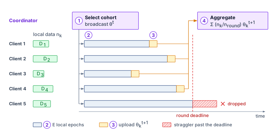
This basic structure introduces a number of design choices and trade-offs. The number of local epochs \(\LocalEpochCount\) sets the balance between computation and communication. A larger \(\LocalEpochCount\) reduces communication frequency but risks divergence if local data distributions vary too much. The selection of participating clients affects convergence stability and fairness. In real-world deployments, not all devices are available at all times, and hardware capabilities may differ substantially, requiring robust participation scheduling and failure tolerance.
⇄ Contrast: Federated rounds over intermittent wide-area clients contrast with the synchronous AllReduce collectives on low-latency cluster fabrics established in AllReduce Algorithms and Topologies.
Time to target under client drift
A federated deployment must reach a quality target within its time, energy, and participation budgets. More local training can reduce how often clients communicate, but it also changes their updates and the time each selected cohort takes to finish. The engineering comparison is therefore time to an agreed quality target, not communication rounds alone.
What the FedAvg controls count
FedAvg exposes the number of participating clients \(\ParticipatingClientCount\), local epochs \(\LocalEpochCount\), and communication rounds \(\FederatedRoundCount\) as controls (McMahan et al. 2017). Their product \(\ParticipatingClientCount \LocalEpochCount \FederatedRoundCount\) counts client-epochs when participation is fixed, which makes it a tally of the work a run performs rather than a measure of its progress. Clients can have different dataset sizes, and equal client-epoch counts can process different examples or produce conflicting updates, so two runs with the same \(\ParticipatingClientCount \LocalEpochCount \FederatedRoundCount\) can end at very different quality. A convergence result is useful only when its assumptions match the optimizer, client sampling, and data distributions.
McMahan, Brendan, Eider Moore, Daniel Ramage, Seth Hampson, and Blaise Agüera y Arcas. 2017. “Communication-Efficient Learning of Deep Networks from Decentralized Data.” International Conference on Artificial Intelligence and Statistics (AISTATS), Proceedings of machine learning research, vol. 54: 1273–82.
Non-IID data impact
Non-IID data is where federated averaging departs from the data center version of local SGD. Each local step moves a client toward the optimum of its own shard, so after many local steps the client models sit near different optima, and their weighted average lands at a point that need not minimize the population objective. This client drift grows with the number of local steps and with how far the client distributions differ, and it degrades federated averaging relative to i.i.d. baselines (Li et al. 2020; Zhao et al. 2018). It therefore eats into the benefit of fewer communications exactly where communication is most expensive. How strongly depends on the partition, update rule, participation policy, and local step size, and no universal heterogeneity score predicts a round count across applications, which is why section 11.6.2.3.3 measures the trade-off rather than computing it.
When statistical heterogeneity causes FedAvg to diverge or stall, two foundational algorithmic extensions address the root cause of client drift:
- FedProx (Li et al. 2020) adds a proximal regularization term \(\frac{\mu}{2}\|\ModelParameters - \GlobalModelParameters^{\FederatedRoundIndex}\|^2\) to each client’s local loss function. This penalty constrains local updates to remain in the neighborhood of the current global model \(\GlobalModelParameters^{\FederatedRoundIndex}\), stabilizing convergence under statistical heterogeneity and permitting devices to execute variable numbers of local epochs without destabilizing the server aggregate.
- SCAFFOLD (Kairouz and McMahan 2021) corrects the local update direction directly using control variates. By maintaining a server control variate and per-client control variates that estimate the difference between client-local and global gradient directions, SCAFFOLD applies an additive correction to each local SGD step. This correction counters client drift under heterogeneous local data, although it roughly doubles the communication volume per round by transmitting control variates alongside model parameters.
Measuring the local-work trade-off
Compare candidate local-epoch settings under the same initialization, data partition, participation policy, and held-out quality target. For each setting \(\LocalEpochCount\), record the first validated round \(\FederatedRoundCount(\LocalEpochCount)\) that reaches the target and the elapsed duration \(\RoundDuration(\LocalEpochCount)\) of each completed round, including client selection, local work, transfer, aggregation, and any waiting. The observed time to target is
\[ \TimeToTarget(\LocalEpochCount) = \sum_{\CompletedRoundIndex=1}^{\FederatedRoundCount(\LocalEpochCount)} \RoundDuration(\LocalEpochCount). \]
Each \(\RoundDuration(\LocalEpochCount)\) is one instance of the round budget sketched at the opening of the chapter. Read through the Fleet Law, it is the local training on the slowest client the round still awaits, plus the upload, plus the wait for enough reports, less whatever overlaps. The communication piece is easy to estimate. Over a constrained mobile uplink of 1–10 Mb/s, the chapter’s reference adapter update of 50 MB takes about 7 minutes to upload at the low end and about 42 seconds at the high end, and that cost recurs in every one of the \(\FederatedRoundCount(\LocalEpochCount)\) rounds. A setting of \(\LocalEpochCount\) that halves \(\FederatedRoundCount(\LocalEpochCount)\) therefore removes half of the cumulative upload time, and it pays off only if the extra local training it adds to each round, on the slowest awaited client, costs less than the uploads it removes. Client drift keeps that comparison from being settled on paper, because more local steps can also raise \(\FederatedRoundCount(\LocalEpochCount)\), and only measured runs can rank the settings.
A useful experiment log records local epochs, completed clients, rounds to target, elapsed time, transmitted bytes, and device energy. If a run never reaches the quality target within the budget, report that outcome rather than extrapolating an invented convergence curve. Repeated runs and cohort-level validation distinguish a stable improvement from a fortunate sample of participating devices.
Communication-computation trade-off
Local work \(\LocalEpochCount\) acts on the wall clock through two opposing paths, drawn as a timeline of rounds in figure 11. Increasing local epochs lengthens per-round execution duration \(\RoundDuration(\LocalEpochCount)\) (the width of each round) while reducing synchronization frequency (the number of rounds in a row), which can lower the required rounds \(\FederatedRoundCount(\LocalEpochCount)\) until client drift penalizes convergence. Both paths combine into the cumulative time to target \(\TimeToTarget(\LocalEpochCount)\), where each row ends, which remains admissible only if total consumption fits within client energy and fleet-coverage budgets. A setting that requires fewer rounds can still prolong total wall-clock duration. Selecting \(\LocalEpochCount\) therefore requires comparing measured times to target against physical admission constraints, rather than relying on ungrounded heuristics.
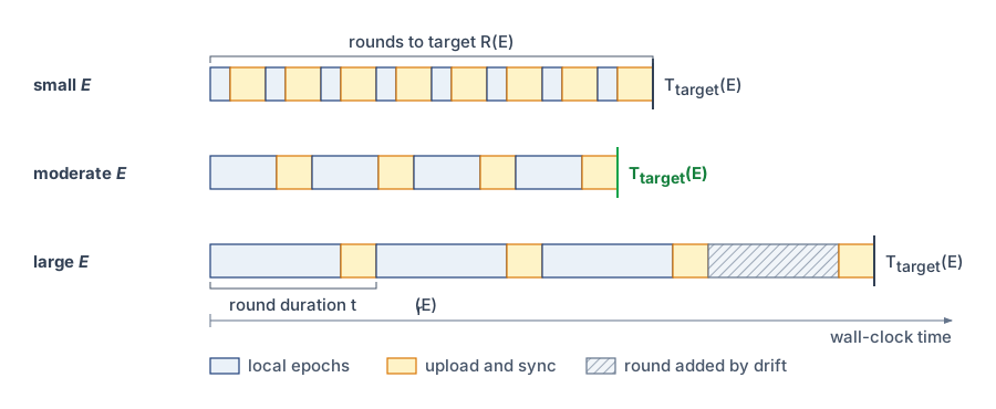
The operating point depends on the deployment. Larger local updates can amortize transfer overhead, but they also change drift, completion time, and which clients finish. The network alone can move the optimum, as a cost model in relative units shows (figure 12). Its minimum \(\LocalEpochCount^*\) shifts from \(\LocalEpochCount=10\) on the fast-network curve to \(\LocalEpochCount=40\) on the slow-network curve because amortizing expensive transfers justifies more local work. These curves are not measured convergence results. A deployment must establish whether additional local work actually reduces time to target after drift and client completion are counted, and adaptive epoch policies need the same outcome and coverage checks as fixed settings.
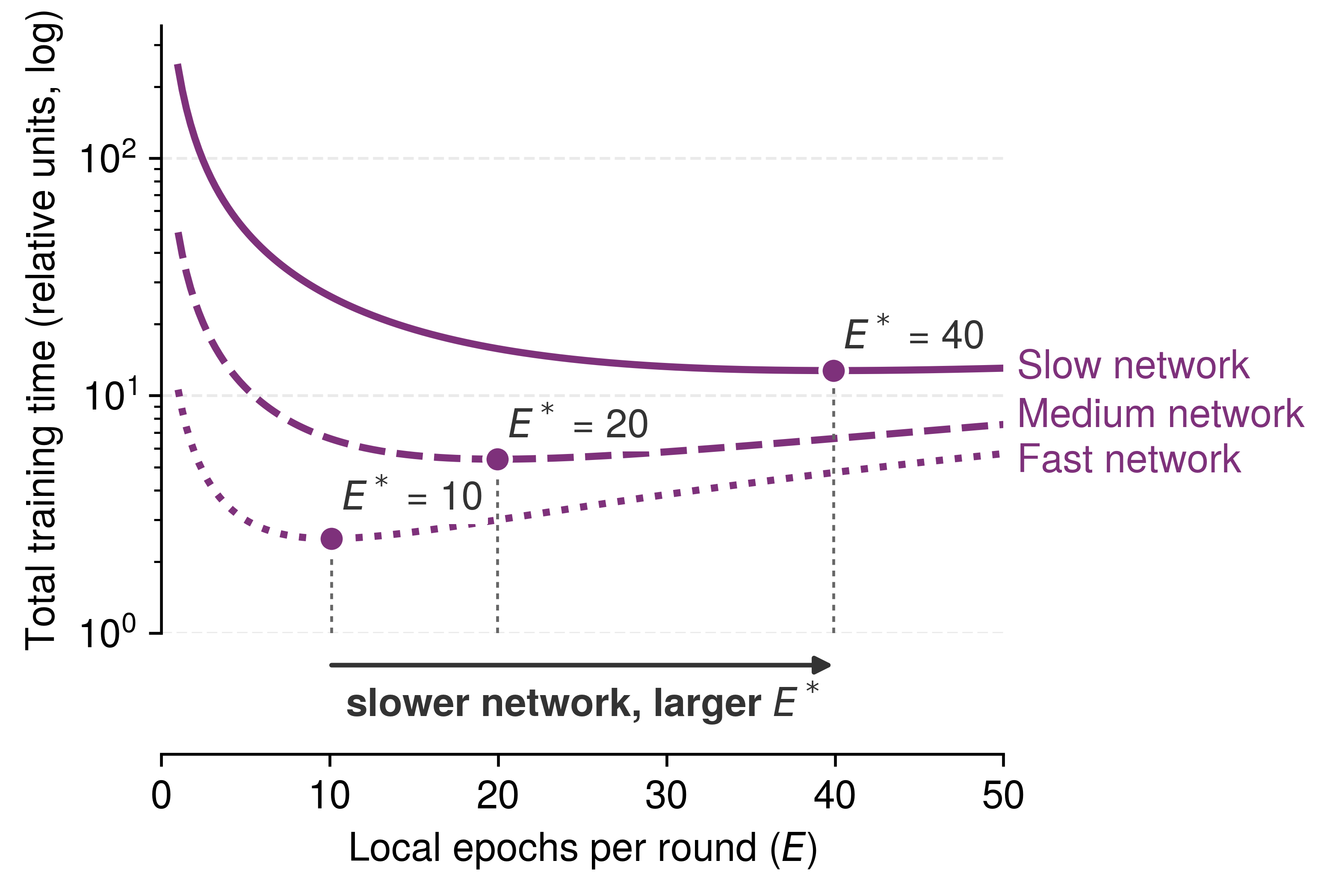
Diagnosing a missed target
Federated convergence results depend on the update rule, objective, sampling policy, and assumptions about client data (Kairouz and McMahan 2021). Heterogeneity, participation, and local sample counts are therefore inputs to a feasibility assessment, not universal pass/fail thresholds. A deployment must demonstrate that its chosen configuration reaches the declared quality target within time and device budgets, with evaluation that represents the intended population.
When a configuration misses that target, the measured failure guides the next experiment. Conflicting local updates motivate testing less local work, adding proximal regularization (FedProx), incorporating control variates (SCAFFOLD), or switching to personalization. Long waits motivate scheduling or asynchronous alternatives, subject to privacy-protocol compatibility. Sparse local evidence motivates bounded adaptation and stronger validation. None of these changes replaces observations from absent cohorts; each must be reevaluated for quality, resource cost, and population coverage.
The aggregation rule specifies how compatible local models produce a shared model; the measured time to target establishes whether a configuration reaches its objective within budget. A controlled lab can hold participant availability and network conditions steady. A phone fleet cannot, so the implementation must define how selection, deadlines, and failures change the set of updates that actually enters each aggregate. These protocol decisions connect learning behavior to fleet orchestration.
Self-Check: Question
In the Federated Averaging (FedAvg) algorithm, what is the primary algorithmic trade-off when tuning the number of local training epochs (\(\LocalEpochCount\)) on client devices?
- Increasing local work can amortize communication, but may increase client drift on non-IID data; rounds and elapsed time to the same quality target must be measured.
- Increasing \(\LocalEpochCount\) forces the central server to store full training datasets from all participating clients in server DRAM.
- Increasing \(\LocalEpochCount\) eliminates the need for clients to compute backward passes during local training.
- Increasing \(\LocalEpochCount\) increases the size (in megabytes) of the transmitted model parameter vector by a factor of \(\LocalEpochCount^2\).
A mobile federated learning deployment encounters severe client drift due to extreme non-IID typing patterns across users, causing standard FedAvg to oscillate and fail to converge. Which algorithmic modification directly addresses client drift by constraining local updates to stay close to the global model?
- Switching from 32-bit floating-point to 1-bit stochastic sign quantization without error compensation.
- Adding a proximal regularization term \(\frac{\mu}{2} \|w - w_t\|^2\) to the local client objective (as in FedProx) to penalize excessive deviation from the global server model \(w_t\).
- Increasing the local learning rate by \(10\times\) to accelerate convergence on outlier devices.
- Dropping the central aggregation server and allowing devices to train purely in isolation without synchronization.
Contrast cross-silo federated learning and cross-device federated learning across three dimensions: participant scale/reliability, network connectivity, and client incentive/governance.
In federated optimization, the phenomenon where multiple local gradient steps on non-identically distributed client data cause local models to diverge toward disparate local optima is called client ____.
11.7 Federated Learning Systems at Scale
A round selects a cohort from the deployment population, but some selected devices overheat, lose Wi-Fi, enter power-saving mode, or power off before returning an update. A fleet of millions of smartphones need not participate in one round for these failures to matter. The orchestrator must decide which clients are eligible, how long to wait, and what evidence permits aggregation when only part of the selected cohort completes.
11.7.1 Client scheduling
The first decision in any round is which devices to invite: sampling devices uniformly at random without checking their power and network state would interrupt users mid-task, whereas accepting updates only from plugged-in flagship phones on fast Wi-Fi trains a global model skewed toward affluent, overnight-charging cohorts. Because real-world client availability is intermittent and variable—devices may be turned off, disconnected from power, or out of network coverage at any moment—client scheduling governs both the efficiency and the population coverage of distributed learning.
At a baseline level, federated ML systems define eligibility criteria for participation. A mobile deployment may require devices to be plugged in, connected to Wi-Fi, and idle to limit interference with foreground work and battery use. The chosen criteria determine which subset of the total population is considered “available” for a training round; they are deployment policy rather than requirements of federated learning itself.
Beyond these operational filters, devices also differ in their hardware capabilities, data availability, and network conditions. Some smartphones contain many recent examples relevant to the current task, while others have outdated or irrelevant data. Network bandwidth and upload speed may vary widely depending on geography and carrier infrastructure. As a result, uniform random selection from the eligible pool does not guarantee coverage of the full deployment population; eligibility has already excluded some devices and their data.
Availability-driven selection introduces participation bias, the fleet-level consequence of the admission test in equation 2 (principle 20). Clients with favorable conditions, such as frequent charging, high-end hardware, and consistent connectivity, pass admission and participate repeatedly, while others are systematically underrepresented. This can skew the resulting model toward behaviors and preferences of a privileged subset of the population, raising both fairness and generalization concerns.
Participation bias becomes severe when a small eligible cohort supplies most completed updates while other cohorts rarely participate. The skew is measured per cohort as a coverage ratio, the cohort’s share of completed updates divided by its share of the deployed population. A ratio near one means the cohort is represented in proportion to its size, and a ratio well below one means the shared model learns that cohort’s behavior at less than its population weight. Completion logs supply the numerator and the deployment inventory the denominator, so the ratio can be computed without inspecting any update. The admission test and the round deadline both remove constrained devices faster than capable ones, and uniform selection among admitted devices passes the resulting skew through unchanged, so a budget cohort can fall from a fifth of the fleet to a sliver of the completed updates (figure 13). Low coverage also feeds itself, because models become more strongly optimized for users with high-end devices and stable connectivity, potentially degrading performance for resource-constrained users who need adaptation the most. A keyboard prediction model might become biased toward the typing patterns of users with flagship phones who charge overnight, missing important linguistic variations from users with budget devices or irregular charging patterns.
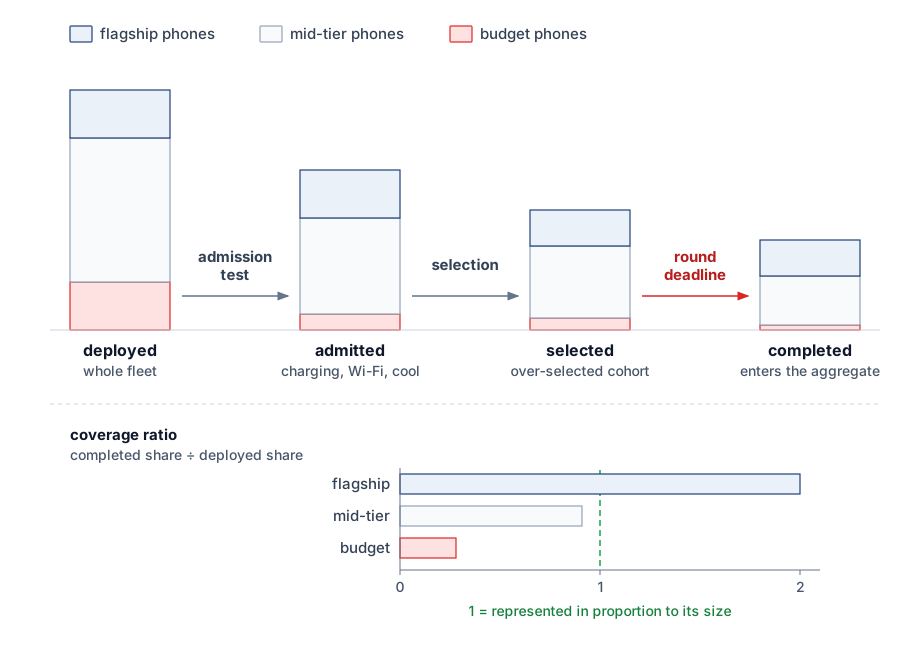
The order of these decisions limits what any remedy can do. Fleet orchestration admits only feasible allocations before a fairness policy divides them (principle 15), and a federated scheduler inherits the same order with a sharper consequence. Its eligibility filter fixes the candidate pool, so a fairness policy can redistribute rounds only among devices the admission test already accepted; a device that never qualifies is invisible to it.
Scheduling must therefore balance completion speed with population coverage. Stratified or quota-based sampling can prioritize underrepresented groups among eligible devices, while cumulative participation records can guide later invitations. Weighting methods require estimates of the population and selection process; they cannot recover observations from a cohort that never participates. Buffered asynchronous aggregation (Nguyen et al. 2021), whose mechanism section 11.7.5.1 describes, staleness-aware methods (Rodio and Neglia 2024), and fairness-oriented weighting (Ma et al. 2024) offer additional controls. Their effectiveness must be checked through completed participation and cohort quality, rather than inferred from the scheduling rule alone. Example weighting in the aggregate (equation 3) also gives large local datasets more influence whether or not they represent the target population any better.
Rodio, Angelo, and Giovanni Neglia. 2024. “FedStale: Leveraging Stale Client Updates in Federated Learning.” Frontiers in Artificial Intelligence and Applications (ECAI 2024) 78. https://doi.org/10.3233/faia240849.
Ma, Jeffrey, Alan Tu, Yiling Chen, and Vijay Janapa Reddi. 2024. “FedStaleWeight: Buffered Asynchronous Federated Learning with Fair Aggregation via Staleness Reweighting.” arXiv Preprint arXiv:2406.02877.
Scheduling must also bound how long a round waits on its slowest participants. Network latency, battery depletion, or background process contention can make some devices (stragglers) take 10\(\times\) longer than the median, and the round cannot aggregate until enough updates arrive.

Enough valid reports let the round close before its slowest clients finish.
To reduce waiting for stragglers, production federated learning (FL) systems employ over-selection. The server selects a candidate pool size \(\CandidateClientCount\) larger than the target number of updates \(\TargetUpdateCount\) (the production system of Bonawitz et al. (2019) selects about 130 percent of the target, \(\CandidateClientCount \approx 1.3 \times \TargetUpdateCount\)). When enough valid reports arrive, the server can form an aggregate from \(\TargetUpdateCount\) completed updates rather than wait for every selected device. Completion then depends on the target-th valid report, but over-selection alone does not guarantee that the target is reached. A round deadline and an explicit acceptance or abandonment rule handle insufficient completion. Secure aggregation adds a participation floor and dropout recovery (section 11.7.4); selecting the fastest reports must remain compatible with that protocol. Accepting the fastest responders can amplify the participation bias just described, so shorter rounds must be evaluated against cohort coverage and wall-clock time to the declared quality target. Because these scheduling decisions set convergence rate, model generalization, energy consumption, and user experience together, poor scheduling produces excessive stragglers, overfitting to narrow client segments, or wasted computation.
11.7.2 Bandwidth-aware update compression
Transmitting full-precision weights or gradients over an asymmetric mobile uplink can exhaust a client’s connectivity window or battery allowance before its update ever reaches the coordinator.13 Update compression therefore begins with a bottleneck diagnosis: when transfer is limiting, the design decision is which information to quantize, sparsify, or keep local. The smaller payload must then be evaluated against encoding cost, update error, and the rounds required to reach the quality target.
13 Wireless upload asymmetry: Federated updates use the uplink, whose available throughput can differ substantially from the downlink and vary with coverage and contention. Transfer time depends on encoded update size and effective uplink goodput; energy also depends on radio state and transfer duration. Low-power links may add duty-cycle constraints. Compression is useful when these costs bind the update budget, but its necessity depends on the payload, link, and permitted synchronization interval.
14 Gradient sparsification: Selecting the largest 1–10 percent of gradient elements by magnitude reduces transmitted value count by 10–100\(\times\) before coordinate indices and other metadata are included. Sparsified SGD and deep gradient compression retain untransmitted residuals for later updates rather than assuming that small components can be discarded permanently (Stich et al. 2018; Lin et al. 2018). Wire-byte savings depend on the encoding, while convergence depends on the residual handling, optimizer, and compression schedule; a value-count reduction alone establishes neither.
Stich, S. U., J.-B. Cordonnier, and M. Jaggi. 2018. “Sparsified SGD with Memory.” Advances in Neural Information Processing Systems 31.
Lin, Yujun, Song Han, Huizi Mao, Yu Wang, and William J Dally. 2018. “Deep Gradient Compression: Reducing the Communication Bandwidth for Distributed Training.” International Conference on Learning Representations (ICLR).
The compression decision separates into three levers, each changing a different part of the communication bottleneck: model compression reduces bits per update, selective sharing reduces which parameters travel, and architectural partitioning keeps some state local. Model compression methods reduce the wire footprint of transmitted updates through quantization, sparsification, or subsampling. Instead of sending full-precision gradients, a client transmits 8-bit quantized updates or communicates only the top-\(\RetainedGradientElementCount\) gradient elements14 with highest magnitude, the same encodings that cluster training applies to its collective payloads. At the edge they bind in a different place. They act on a slow, asymmetric uplink rather than a fabric, under secure aggregation that must still combine the encoded updates, and inside a per-round communication total (equation 4) that also counts downloads and retries. These transformations are communication mechanisms, not privacy mechanisms; a smaller embedding, sparse update, or low-precision gradient may still expose membership, attributes, or reconstructable features.
↩︎ Gradient quantization, top-\(\Glyph{k}\) sparsification, and error feedback that carries unsent updates forward are established in Gradient Compression Under Bandwidth Scarcity. Convergence depends on the optimizer and compression assumptions.
Selective update sharing further reduces communication by transmitting only subsets of model parameters or updates. In layer-wise selective sharing, clients update only certain layers, typically the final classifier or adapter modules, while keeping the majority of the backbone frozen. This reduces the update payload and limits which shared representations can change, but the trainable subset can still overfit nonrepresentative client data.
Architectural partitioning requires specifying what crosses the boundary. A personal/shared parameter partition keeps local modules private while aggregating selected shared parameters. Split learning instead divides execution between client and server, exchanging intermediate activations and backward gradients at the cut. These designs have different traffic and exposure patterns; neither guarantees a communication reduction or privacy merely by dividing the model.
These approaches can use the FedAvg aggregation protocol (section 11.6.2.2) only when their encoding and shared parameter schema support weighted aggregation. Quantization requires compatible scales, sparse updates require coordinate identities, and local-only parameters must stay outside the shared aggregate. With secure aggregation, the encoding must support combination without exposing individual decoded updates. The total communication volume for round \(\CompletedRoundIndex\) is
\[ \RoundCommunicationVolume= \RoundDownloadVolume+ \RoundUploadVolume+ \RoundProtocolVolume+ \RoundRetryVolume, \tag{4}\]
Equation 4 makes download, upload, protocol, and retry traffic explicit. The download distributes model state, the upload carries client updates, protocol traffic covers authentication and cryptographic setup, and retries account for failed or repeated transfers. Optimizing only \(\RoundUploadVolume\) can therefore move rather than remove the bottleneck. Additional local computation amortizes network transfers, and each communication-efficient alternative to it carries its own cost. Compression may degrade gradient fidelity, selective updates can limit model capacity, and split architectures complicate coordination. Summed over a training run, the upload term alone can exceed the raw data that federation was meant to keep local, even when each update is far smaller than that data.
↪ The break-even condition under which encoding and decoding time costs less than the transfer time compression saves is developed, with a worked example, in Compression Economics.
One compressed update is 80× smaller than a week’s raw-image upload.
Napkin Math 11.3: Model updates vs. raw data
Problem: A team is designing a federated camera-personalization system that learns from 200 MB of compressed user images per week. Compare one upload of those images with one compressed model-update uplink round.
Math: Bandwidth efficiency is the ratio of raw data volume to model update size.
- Raw data upload: 200 MB/week.
- One federated uplink round: A compressed model update (5M params) is 2.5 MB.
- One-round uplink reduction: 200 MB/2.5 MB = 80×.
Systems insight: For this scenario, one 2.5 MB uplink is 80× smaller than one 200 MB raw-data upload. That ratio is not the end-to-end communication saving of a training run: after roughly 80× uplink rounds, cumulative update uploads alone equal the raw-data volume, before counting global-model downloads, retries, or protocol overhead. The verdict therefore turns on the round schedule. A deployment that runs one round per day uploads seven updates per week of data, far below the break-even count, and saves most of the uplink traffic; one that runs a round every hour uploads 168 updates per week, more than the break-even count, and moves more bytes than shipping the images would. Per-round traffic must be multiplied by the expected round count before federation can claim a bandwidth saving.
The local-work schedule and update encoding jointly determine communication cost. Figure 14 compares uncompressed 32-bit values (Panel A) with uniform 8-bit quantization (Panel B), which gives a \(4\times\) reduction in value bytes before scales and other metadata are counted. Top-\(k\) sparsification with retained error feedback (Panel C) must encode coordinate identities as well as selected values. Error feedback retains one residual value per update coordinate between transmissions. Its storage depends on the update size and residual precision and must fit the device allowance alongside training and replay state. The receiving path must reconstruct or aggregate these encodings consistently, with separate compatibility requirements when secure aggregation hides individual updates.
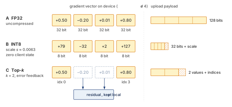
The quantization panel’s “zero client state” means no persistent error-feedback residual; encoding buffers, scales, and temporary workspace still enter the device budget. Compression is useful when its reduction in total communication outweighs encoding work and any extra rounds needed to reach the quality target. A smaller upload helps a round only if transfer was what made clients miss the deadline or excluded a cohort, and the round’s completion logs show which. Smaller payloads can let clients on slow or congested uplinks finish before their resource window closes, so compression is judged by completed participation and cohort outcomes, not by bytes saved alone. Even when transfer becomes feasible, the shared model may still fail to capture local variation.
11.7.3 Federated personalization
Devices can complete compatible updates yet disagree about which behavior improves their local task. A shared model may serve that population adequately, or its aggregate gain may conceal persistent losses for particular users. Personalized federated learning retains shared learning while allowing selected parameters or models to specialize. Its value must be evaluated against the added local state, training cost, and risk of overfitting sparse user data.
Let \(\ModelParameters_k\) denote the model parameters on client \(\ClientIndex\), and \(\GlobalModelParameters\) the aggregated global model. For \(\ParticipatingClientCount\) clients, counted as in equation 3, traditional FL seeks to minimize a global objective: \[ \min_\ModelParameters\sum_{k=1}^{\ParticipatingClientCount} \ClientObjectiveWeight_k \LossFunction_k(\ModelParameters) \] where \(\LossFunction_k(\ModelParameters)\) is the local loss on client \(\ClientIndex\), and \(\ClientObjectiveWeight_k\) is a weighting factor (e.g., proportional to local dataset size). This formulation optimizes the weighted average loss of a shared model \(\ModelParameters\); it does not guarantee acceptable performance for every client. Local loss landscapes \(\LossFunction_k\) can differ across clients, reflecting non-IID data distributions and varying task requirements.
Personalization modifies this objective to allow each client to maintain its own adapted parameters \(\ModelParameters_k\), optimized with respect to both the global model and local data: \[ \min_{\ModelParameters_1, \ldots, \ModelParameters_{\ParticipatingClientCount}} \sum_{k=1}^{\ParticipatingClientCount} \left( \LossFunction_k(\ModelParameters_k) + \PersonalizationPenaltyWeight\cdot \GlobalDeviationPenalty(\ModelParameters_k, \GlobalModelParameters) \right) \]
Here, \(\GlobalDeviationPenalty\) penalizes deviation from the global model, and \(\PersonalizationPenaltyWeight\) controls the strength of that penalty. The displayed objective describes local specialization around a given global reference; a complete protocol must additionally specify how that reference is trained and refreshed. The penalty trades local fit against proximity to the shared model, without guaranteeing improvement for every client.
Real-world use cases illustrate the importance of this approach. Consider a wearable health monitor that tracks physiological signals to classify physical activities. While a global model may perform reasonably well across the population, individual users show different motion patterns, gait signatures, or sensor placements. Finetuning the final classification layer or low-rank adapters provides a way to address these differences. Evaluation must establish whether the local examples support an improvement, especially for rare classes with little supervision.
Several personalization strategies address the trade-offs between compute overhead, information exposure, and adaptation speed. One widely used approach is local finetuning, in which each client downloads the latest global model and performs a small number of gradient steps using its local data. This method avoids transmitting those examples during adaptation, but the resulting local state and any later update remain privacy-sensitive. It may also yield suboptimal results when the global model is poorly aligned with the client’s data distribution or when the local dataset is extremely limited.
Another effective technique involves personalization layers, where the model is partitioned into a shared backbone and a lightweight, client-specific head, typically the final classification layer (Arivazhagan et al. 2019). In FedPer, clients train both the shared base and their personal head, but only the shared base participates in server aggregation; the head remains local. A separate head-only adaptation policy can freeze a downloaded backbone to reduce local training cost when the relevant variation lies mainly in output categories or decision boundaries.
Arivazhagan, Manoj Ghuhan, Vinay Aggarwal, Aaditya Kumar Singh, and Sunav Choudhary. 2019. “Federated Learning with Personalization Layers.” CoRR abs/1912.00818.
15 MAML (model-agnostic meta-learning): Finn et al. (2017) optimize for a model initialization from which one or a few gradient steps can yield good performance on a new task, with experiments including one-shot and few-shot settings. Meta-training is more expensive than ordinary finetuning because it differentiates through the adaptation process, but deployment adaptation can be limited to a small number of local updates. This makes MAML relevant for edge scenarios where inference compute is cheap but training data is scarce.
Finn, Chelsea, Pieter Abbeel, and Sergey Levine. 2017. “Model-Agnostic Meta-Learning for Fast Adaptation of Deep Networks.” Proceedings of the 34th International Conference on Machine Learning (ICML).
Clustered federated learning offers an alternative by grouping clients according to similarities in their data or performance characteristics, and training separate models for each cluster. This strategy can enhance accuracy within homogeneous subpopulations, though it introduces additional system complexity and may require exchanging metadata to determine group membership. Finally, meta-learning approaches, such as model-agnostic meta-learning (MAML),15 aim to produce a global model initialization that can be quickly adapted to new tasks with just a few local updates (Finn et al. 2017), which is especially useful when clients have limited data or operate in environments with frequent distributional shifts.
Each strategy occupies a different point in the personalization trade-off space. Local finetuning, personalization layers, clustered federated learning, and meta-learning differ in compute overhead, information exposure, and adaptation latency (table 7). The mechanism determines what state is shared; a privacy guarantee requires separately specified controls and assumptions.
| Strategy | Personalization mechanism | Compute overhead | Privacy preservation | Adaptation speed |
|---|---|---|---|---|
| Local Finetuning | Gradient descent on local loss postaggregation | Low to Moderate | Raw examples stay local; adapted state remains sensitive | Fast (few steps) |
| Personalization Layers | Split model: shared base + user-specific head | Moderate | Narrows shared state; does not guarantee privacy | Fast (train small head) |
| Clustered FL | Group clients by data similarity, train per group | Moderate to High | Group membership and updates can leak attributes | Medium |
| Meta-Learning | Train for fast adaptation across tasks/devices | High (meta-objective) | Depends on meta-training and adaptation protocol | Very Fast (few-shot) |
Selecting an on-device personalization strategy requires balancing adaptation capacity against memory residency. Three fine-tuning paradigms differ in structural footprint (figure 15). Full fine-tuning updates every backbone layer (Column A), head-only adaptation freezes the feature extractor (Column B), and parameter-efficient adapters sit beside frozen backbone blocks (Column C).
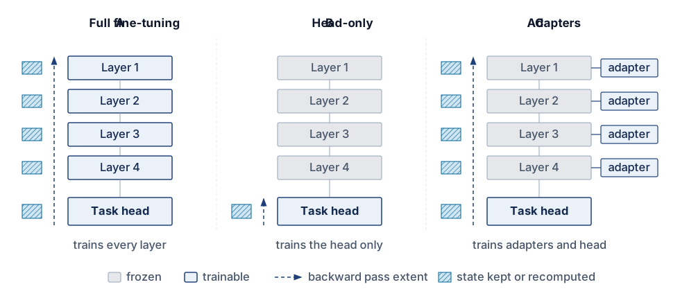
The dashed backward-pass arrows in figure 15 are the activation term of equation 1 drawn as distance. Adapters at early layers in Column C pull the backward path through the later backbone, whose saved state must be retained or recomputed, while head-only adaptation in Column B ends it at the head, as in the wake-word case of section 11.5.1. Placement sets the dependency path, and the execution schedule sets how much of that state stays resident.
11.7.4 Federated privacy
Federated learning keeps raw data on the device, but the model updates it transmits (gradients or weight changes) can still leak information about the private data that produced them. Techniques such as model inversion attacks16 and membership inference attacks demonstrate that adversaries may partially reconstruct or infer properties of local datasets by analyzing these updates.
16 Model inversion attack: Reconstructs training data from model outputs or gradients by optimizing inputs that maximize confidence scores (Fredrikson et al. 2015; Zhu et al. 2019). In federated learning, gradient updates can leak more information than model outputs alone because they expose training-step information directly. Defenses such as gradient perturbation, secure aggregation, and differential privacy add protocol, utility, communication, or compute trade-offs whose magnitude depends on the threat model and deployment; Gradient leakage and privacy-preserving computation develops the threat model for these attacks.
Fredrikson, Matt, Somesh Jha, and Thomas Ristenpart. 2015. “Model Inversion Attacks That Exploit Confidence Information and Basic Countermeasures.” Proceedings of the 22nd ACM SIGSAC Conference on Computer and Communications Security, 1322–33. https://doi.org/10.1145/2810103.2813677.
Zhu, Ligeng, Zhijian Liu, and Song Han. 2019. “Deep Leakage from Gradients.” Advances in Neural Information Processing Systems (NeurIPS) 32: 14774–84.
17 Secure aggregation: Cryptographic protocol where client pairs exchange random masks that cancel in the server-side sum, revealing only the aggregate gradient without exposing individual contributions (Bonawitz et al. 2017). Production-scale federated systems such as Gboard combine secure aggregation with eligibility checks, drop-out handling, and round scheduling (Bonawitz et al. 2019). The communication expansion and minimum-participation requirements depend on protocol parameters and the security model, so aggregation systems must wait for enough eligible devices before releasing a round.
Bonawitz, Keith, Vladimir Ivanov, Ben Kreuter, Antonio Marcedone, H. Brendan McMahan, Sarvar Patel, Daniel Ramage, Aaron Segal, and Karn Seth. 2017. “Practical Secure Aggregation for Privacy-Preserving Machine Learning.” Proceedings of the 2017 ACM SIGSAC Conference on Computer and Communications Security, 1175–91. https://doi.org/10.1145/3133956.3133982.
Two protective measures address that leakage. Secure aggregation17 protocols reveal a combined result while hiding individual updates beyond what that result itself reveals, subject to the protocol’s assumptions about collusion and participating clients. Differential privacy, a formal bound on how much any one protected user’s or record’s inclusion can change a released result, is obtained by clipping each contribution and adding noise calibrated to that bound. The deployment must specify which unit receives that protection.
These controls solve different problems. Secure aggregation limits what the coordinator learns about each submitted update, whereas differential privacy bounds how much a declared privacy unit can affect a released result. A deployment therefore needs a privacy accounting log that records the unit of protection, clipping rule, noise mechanism, sampling assumptions, \((\PrivacyBudget,\PrivacyAdditiveSlack)\) expenditure for every release, and cumulative composition across training and federated analytics (Abadi et al. 2016; Kairouz and McMahan 2021). Clipping bounds each contribution before noise is calibrated. The parameters \(\PrivacyBudget\) and \(\PrivacyAdditiveSlack\) describe the permitted change in output probabilities when the protected user or record is included or removed; composition accounts for repeated releases involving that unit. Resetting a round counter does not reset privacy loss for a user who participates again.
Abadi, M., A. Chu, I. Goodfellow, H. B. McMahan, I. Mironov, K. Talwar, and L. Zhang. 2016. “Deep Learning with Differential Privacy.” Proceedings of the 2016 ACM SIGSAC Conference on Computer and Communications Security, CCS ’16, 308–18. https://doi.org/10.1145/2976749.2978318.
↪ The composition rules that turn a privacy accounting log’s per-release entries into one cumulative privacy budget are developed in Privacy budget composition.
Blanchard, Peva, El Mahdi El Mhamdi, Rachid Guerraoui, and Julien Stainer. 2017. “Machine Learning with Adversaries: Byzantine Tolerant Gradient Descent.” Advances in Neural Information Processing Systems (NeurIPS), 119–29.
Secure aggregation also creates a robustness conflict. Byzantine-resilient rules such as Krum, coordinate-wise filtering, or per-client anomaly inspection need access to individual updates, while secure aggregation deliberately hides those updates (Blanchard et al. 2017; Bonawitz et al. 2017). A system cannot claim both arbitrary per-client inspection and conventional secure aggregation over the same messages. It must instead validate clients before masking, use attested execution and bounded local updates, compute only aggregation-compatible checks, or adopt a protocol designed to evaluate approved robust statistics without revealing raw client contributions. Figure 16 models this cryptographic boundary through pairwise zero-sum masking: Clients A and B negotiate a shared random mask \(\PairwiseMaskSecret\) via Diffie-Hellman key agreement, perturbing their local updates into pseudo-random vectors (\(\FirstClientMaskedUpdate = \FiniteChange\FirstClientModelParameters+ \PairwiseMaskSecret\) and \(\SecondClientMaskedUpdate = \FiniteChange\SecondClientModelParameters- \PairwiseMaskSecret\)) before crossing into the server domain. When the aggregation server sums the received vectors, the symmetric masks cancel (\(\PairwiseMaskSecret - \PairwiseMaskSecret = 0\)), yielding the exact unmasked aggregate \(\FiniteChange\FirstClientModelParameters+ \FiniteChange\SecondClientModelParameters\). This two-client illustration assumes both clients complete the exchange and neither reveals its mask to the server. It demonstrates cancellation, not a complete protocol for collusion resistance or dropout recovery.
A real round has many clients, and some drop out after agreeing on masks but before uploading. Each dropped client leaves its pairwise masks uncancelled in the sum, so the full protocol has every client split the secret seeds of its masks into shares held by the other clients, any threshold number of which can rebuild a seed (Bonawitz et al. 2017). After the upload deadline, surviving clients send the shares of the dropped clients’ seeds, and the server regenerates and subtracts the dangling masks. Recovery therefore costs an extra message round and computation that grows with the number of dropouts, and it succeeds only if at least the threshold number of clients survive; otherwise the round is abandoned. That threshold is one reason for a participation floor. The other is the sum itself, because an aggregate over a few clients reveals too much about each of them. The coordinator must therefore invite enough clients that the expected survivors clear the floor, and a cohort that falls short is held for a later round rather than aggregated.
↩︎ Byzantine failures, in which a worker stays alive but returns wrong results, and aggregation rules such as Krum and trimmed mean that bound their influence are established in Byzantine failures.
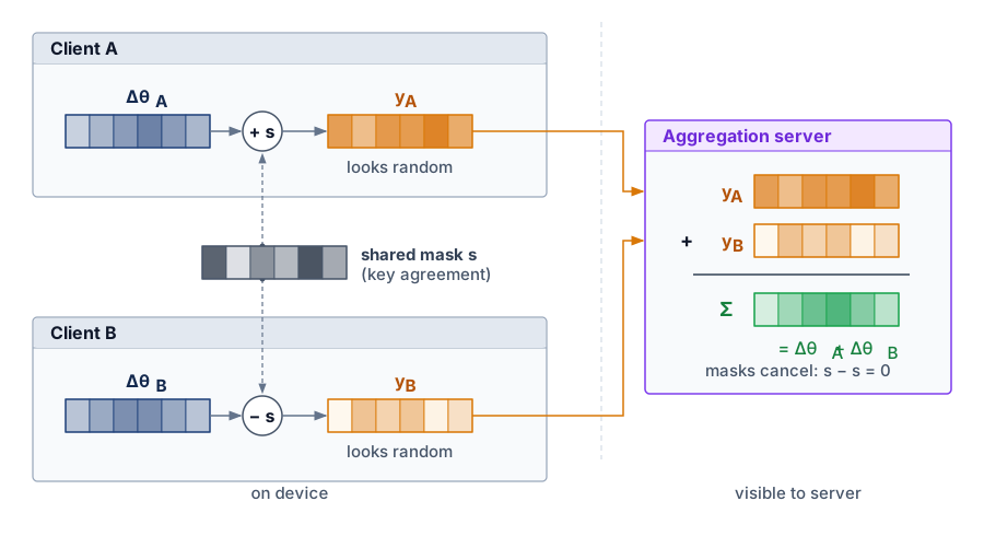
Secure aggregation and differential privacy can protect different boundaries, but their composition must follow the threat model. If a trusted server adds noise after receiving an exact aggregate, the privacy guarantee applies to the released noisy result; it does not hide that exact aggregate from the server. A protocol designed for distributed noise can instead let the server receive only a noisy aggregate. Clipping, noise calibration, dropout assumptions, and repeated-release accounting must match the chosen protocol. Neither mechanism establishes that local data or updates are trustworthy.
Checkpoint 11.3: Federated system design
Consider architecting a federated learning system for a fleet of 10 million mobile devices. The data is highly non-IID (users have distinct, clustered typing patterns), and the network environment is constrained (1–10 Mb/s). Before choosing optimizations for this scenario, classify the local bottlenecks and state which system constraint dominates each decision.
Consider three design decisions:
- Aggregation: Select plain FedAvg, reduced local epochs, or personalization/clustering for the non-IID population, and justify how the choice controls client drift.
- Privacy: Decide whether the deployment needs formal differential-privacy noise or whether secure aggregation and data minimization are sufficient for the stated threat model; using the clipping and noise described in this section, explain how noise can affect utility and rounds to the same quality target, and what measurements would establish that cost.
- Communication: Choose between gradient quantization (e.g., 8-bit) and structured sparsity under constrained bandwidth, and justify the bandwidth/accuracy trade-off.
11.7.5 Large-scale device orchestration
A round that selects a million phones overnight will see some fraction overheat, lose connectivity, or be unplugged before they report, and a few may submit corrupted or deliberately malicious updates. Coordinating that population requires protocols that handle Byzantine clients, network partitions that temporarily cut participants off, and constrained communication. These challenges differ from controlled data center training, where high-bandwidth networks and managed infrastructure narrow the trust and availability envelope.
Asynchronous device synchronization
Federated learning inherits failures from distributed systems and machine learning, but its coordination objective is not consensus, the problem of making replicated servers agree on one ordered log of operations. Federated clients agree on no such log. A coordinator instead decides which stochastic client updates are eligible, how stale updates are weighted, and which aggregation rule can tolerate faulty participants without letting them steer the model. Devices crash, lose power, or disconnect during rounds, while compromised clients can submit poisoned updates crafted to push the shared model toward an attacker’s goal. Robust aggregation can reduce the influence of some faulty participants, but its assumptions, compute cost, and compatibility with secure aggregation must be explicit.
The trust chain begins before aggregation. A production coordinator authenticates the device and application instance, verifies the signed model and training-policy version, checks eligibility and freshness, binds the returned update to that version and round nonce, and records whether the update passed protocol-level bounds. Hardware-backed attestation can strengthen claims about code identity on supported devices, but it cannot prove that local examples are benign or representative. The resulting update-integrity record supports rejection, rollback, and incident analysis without treating device identity as evidence that the gradient is correct.
Network partitions are the harder case. Unlike a data center network, a federated fleet must absorb clients that stay offline for hours or days while traveling, out of coverage, or powered down. Asynchronous coordination protocols keep training moving despite missing participants, but they must balance staleness (accepting outdated contributions) against freshness (prioritizing recent but possibly sparse updates). Buffered asynchronous aggregation (Nguyen et al. 2021) shows the mechanism. It removes the round barrier, letting each client train whenever its admission test passes and upload when done, while the server accumulates arriving updates in a buffer and applies their aggregate once a fixed number have arrived. Each update is down-weighted by its staleness, the number of server versions published since the client downloaded its starting model, so a slow client still contributes without dragging the shared model back toward an old state.
Nguyen, John, Kshitiz Malik, Hongyuan Zhan, Ashkan Yousefpour, Michael Rabbat, Mani Malek, and Dzmitry Huba. 2021. “Federated Learning with Buffered Asynchronous Aggregation.” Proceedings of Machine Learning Research (AISTATS) 164.
↩︎ Gradient staleness, the delay between the model version a worker computed against and the version its update modifies, and its effect on convergence under bounded and fully asynchronous synchronization are established in Staleness impact across synchronization models.
18 Straggler problem: In data center training, stragglers slow synchronous progress; in federated learning, the problem is amplified by heterogeneous hardware, intermittent connectivity, and eligibility windows (Bonawitz et al. 2019; Kairouz and McMahan 2021). Solutions like asynchronous aggregation and bounded staleness (ignoring updates computed against a model more than a fixed number of rounds old) improve throughput but introduce a fairness trade-off: aggressive straggler mitigation biases models toward users with high-end devices, potentially degrading performance for the most constrained users who need personalization most.
Bonawitz, K., H. Eichner, W. Grieskamp, D. Huba, A. Ingerman, V. Ivanov, C. Kiddon, et al. 2019. “Towards Federated Learning at Scale: System Design.” Proceedings of Machine Learning and Systems 3.
Kairouz, P., and H. B. McMahan. 2021. “Advances and Open Problems in Federated Learning.” Foundations and Trends in Machine Learning 14 (1-2): 1–210. https://doi.org/10.1561/2200000083.
Recovery must distinguish coordinator state from device-local state. The coordinator checkpoints the global model and the optimizer and protocol state needed to resume accepted progress; this does not require a simultaneous checkpoint on every device. An incomplete round needs an explicit acceptance or abandonment rule, followed by evaluation of the population represented by its completed updates. State reconciliation identifies a returning device’s base version and determines which shared state it must download and which personal state remains compatible. Server-side load balancing can redistribute coordination work, but replacing an unavailable client with a faster one also changes the local data contributing to training. Whereas convergence guarantees for synchronous training assume that every participant completes each round, a federated coordinator must treat stragglers18 and dropouts as the normal case and state what its convergence argument assumes about them.
Heterogeneity management at fleet scale
Million-device orchestration is a tiering decision, in which the system decides which clients can train, which can only report lightweight updates, and how much bias that selection introduces. The difficulty is that hardware capabilities, network conditions, data distributions, and availability patterns vary simultaneously, challenging traditional distributed machine learning assumptions about homogeneous participants operating under similar conditions.
Real-world federated learning deployments face simultaneous variation in compute, memory, energy, and connectivity. The illustrative peak compute ratings differ by about 1,200× between flagship smartphones rated at 35 TOPS and, below Archetype C’s phone-class clients, IoT microcontrollers rated at 0.03 TOPS. These ratings do not translate into a training-speed ratio, because supported precision, backward operators, memory traffic, and sustained execution determine update time. Memory spans the same 65,536× range from microcontroller SRAM to flagship phone RAM met in section 11.3.2, and at fleet scale that range decides which update state each tier can retain at all. Energy budgets further restrict when that work can run. Background adaptation in this example targets roughly 500–1000 mW, while phones may sustain 2–3 W for foreground ML workloads and burst higher briefly. Network throughput, latency, and interruption patterns must likewise be measured for the participating clients before selecting update frequency and compression.
Measured scores show a spread of the same order among phones alone, without counting microcontrollers. The AI Benchmark from ETH Zurich runs a fixed suite of quantized and floating-point inference workloads on each phone processor through its Android acceleration path (Ignatov et al. 2019; ETH Zurich Computer Vision Lab 2026). Among processors released from 2020 on, which a client fleet can still contain, the scores span about 400×, from the Snapdragon 460 (2020) to the Dimensity 9600 Pro (2026), and figure 17 plots every processor in the ranking. Even flagships of the same generation differ by 14×, with the Google Tensor G4 scoring that far below the Dimensity 9600 M, largely because each score reflects the processor’s software path as well as its silicon; the Tensor G4 result runs through Android’s generic neural-network interface, while the leaders use their vendors’ own runtimes. These are inference scores, not training speeds, but they bound the problem from the side that matters for scheduling. No single local-work quota fits devices that differ by two orders of magnitude in measured throughput.
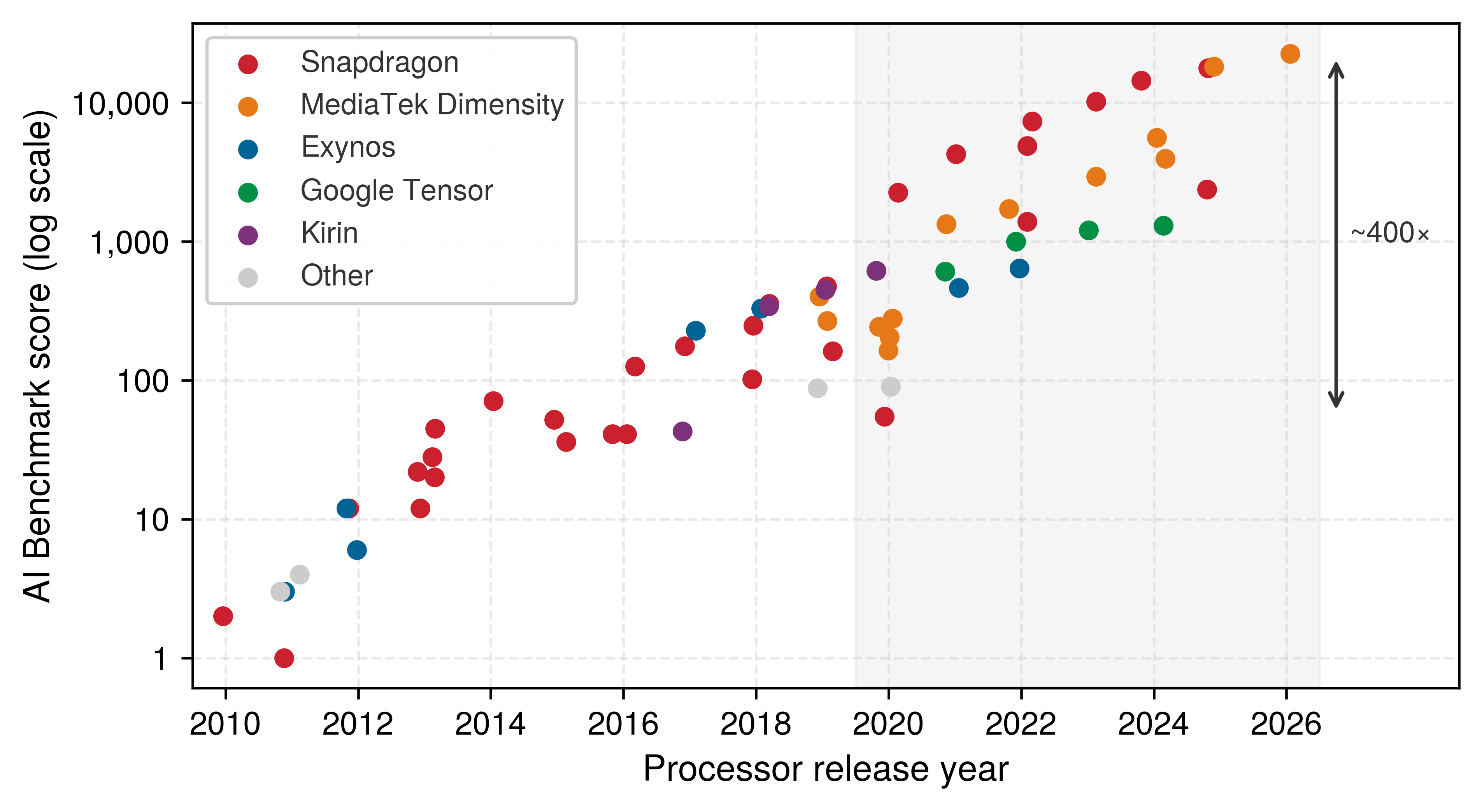
ETH Zurich Computer Vision Lab. 2026. AI Benchmark: Mobile SoC Ranking.
Ignatov, Andrey, Radu Timofte, Andrei Kulik, Seungsoo Yang, Ke Wang, Felix Baum, Max Wu, Lirong Xu, and Luc Van Gool. 2019. “AI Benchmark: All about Deep Learning on Smartphones in 2019.” arXiv Preprint arXiv:1910.06663.
Tiered participation can assign different amounts of local work while preserving a compatible shared-update contract. A capable phone may complete more steps, while a constrained client contributes a smaller update or a separately defined aggregate statistic. These outputs are not interchangeable simply because they come from the same fleet. More work on strong devices also cannot replace the observations held by weak devices, so the policy must evaluate both computational contribution and population coverage.
The scale challenges extend beyond device heterogeneity to coordination overhead. Federated learning does not run a consensus protocol among millions of clients, nor does hierarchical aggregation perform local consensus. Regional aggregators reduce fan-in by validating an eligible cohort and combining updates before forwarding a partial aggregate; agreement on an ordered replicated log, if needed for the coordinator’s own metadata, remains a separate control-plane service. Edge infrastructure can provide aggregation points, but each added tier creates another trust boundary and another place where weighting, clipping, privacy accounting, and failure recovery must remain consistent.
Tiering interacts with the participation bias analyzed under client scheduling (section 11.7.1). Capability-based selection shortens rounds but concentrates completed updates on strong devices, so stratified sampling across tiers must be paired with per-cohort evaluation of completed participation and model quality. Availability also has a daily rhythm; devices that charge overnight in one time zone form a different cohort from those available during another zone’s working hours.
Orchestration brings device updates, data selection, and federated participation into one deployment policy. If that policy permits repeated adaptation, the components interact over time. Earlier updates change the model, replay determines which observations persist, and participation determines which clients influence the next shared version. Continual learning must manage these accumulated effects rather than treating each update as an isolated event.
Self-Check: Question
In production cross-device federated learning (such as Google Gboard), why do systems implement Over-Selection of clients (selecting \(\CandidateClientCount \approx 1.3 \times \TargetUpdateCount\) devices per round) rather than selecting exactly \(\TargetUpdateCount\) devices?
- Over-selection ensures that every mobile client receives \(1.3\times\) the monetary payment for participating.
- Over-selection forces client devices to increase their CPU clock frequencies by \(30\%\) during training.
- Selecting surplus candidates can reach the target number of valid reports earlier than waiting for every selected device, provided enough clients complete; a deadline and incomplete-round policy are still required.
- The aggregation server requires exactly \(30\%\) redundant updates to perform parity-bit error correction on the GPU memory bus.
How does the Secure Aggregation (SecAgg) cryptographic protocol protect individual client privacy during federated aggregation on a central server?
- Clients transmit raw unencrypted updates, and the server permanently deletes its hard drive after every round.
- Clients train on synthetic dummy data generated by the server, ensuring real gradients are never computed.
- The server encrypts all client devices using a remote ransomware key until the global round terminates.
- Participating client pairs agree on shared pseudo-random masks that are added by one client and subtracted by the other; when the server sums all received masked updates, the masks algebraically cancel out, revealing the exact global aggregate without exposing any individual update.
In Differential Privacy for Federated Learning (DP-FedAvg), explain why gradient clipping to a fixed threshold \(S\) (\(\|\Delta \theta_k\|_2 \le S\)) is a mandatory prerequisite before adding calibrated Gaussian noise to the aggregate.
True or False: In top-\(k\) gradient sparsification for federated learning, discarding all gradient components outside the top \(1\text{–}10\%\) by magnitude without maintaining a local error accumulation buffer preserves the exact convergence rate of uncompressed SGD.
In a federated camera-personalization deployment, a user captures \(200\text{ MB}\) of compressed images per week. A 4-bit quantized model update for the 5M-parameter on-device model requires \(2.5\text{ MB}\) per uplink round. Calculate the single-round communication savings of transmitting model updates versus uploading raw weekly data, and explain why cumulative round counts must be accounted for in production network budgets.
For a round using secure aggregation and a trusted server that adds differential-privacy noise, order these stages. Assume protocol participation thresholds and dropout recovery are satisfied:
- Select eligible clients and distribute a compatible global model and training policy
- Form the authorized aggregate and add noise calibrated to bounded client contributions and the declared privacy unit
- Clients train, clip their contributions under the policy, and apply protocol masks
- Update the global model and evaluate progress and completed-cohort coverage
- Receive enough valid masked reports before the round deadline, or apply the incomplete-round policy
11.8 Continual Adaptation Under Edge Budgets
A keyboard model that adapts each night for a year passes through hundreds of admitted update windows, and each window moves it a little further from the version that was validated at release. Every update the chapter has built so far was judged one at a time, by whether it fit the memory budget, passed the admission test, and improved a local metric. Repeated across a deployment’s lifetime, those individually acceptable updates compound. Earlier changes alter what later updates start from, the replay buffer decides which old observations still count, and participation decides which devices shape the next shared version.
The mechanisms that keep this trajectory stable are the ones already introduced, now applied over time. Selective updates bound how far any one window can move the model, and they save work only when the execution path can skip it. Replay protects earlier behavior at the cost of retained examples and additional training. Opportunistic admission delays learning until device conditions permit it. Each needs a resource budget and an outcome check on retained behavior alongside the newest data. The long-lived stream that drives this learning is mostly unlabeled, which sets the first design question.
11.8.1 Learning from unlabeled sensor streams
A camera stream running continuously at 30 frames per second produces roughly 2.6 million frames daily before retention filtering, and an accelerometer sampling at 100 Hz generates 8.6 million readings—almost none of them accompanied by a user label. Cameras, accelerometers, location sensors, and touch interactions all supply data that can support self-supervised learning, turning continual learning into a storage and scheduling decision. The engineering question is which traces encode stable structure worth learning from and which should expire before they crowd out model state, replay buffers, or user-facing storage.
Learning from such traces without labels requires the supervision to come from the data’s own structure. Contrastive learning is the common way to manufacture it on a sensor stream, training a representation to bring designated positive pairs closer and distinguish them from designated negative pairs. Nearby camera frames or augmented views of one frame can supply positives when they preserve the task-relevant content; scene changes can invalidate that assumption. Different frames or replay entries can supply negatives, but may depict the same underlying event. The pair-selection policy therefore defines a learning signal that needs validation. Other devices’ samples are not automatically available under a federated data-locality policy, and stored pairs or representations compete with replay and model state for memory.
11.8.2 Continual adaptation and catastrophic forgetting
A model that adapts continually to recent summer lighting, a new work commute, or a shift in user vocabulary can overwrite the weights it needed for winter weather or older commands if each update moves parameters purely to minimize recent loss. When a deployment uses continual adaptation to address changing environments, user behavior, or task requirements, each update must balance new evidence against previously learned behavior. This is the stability-plasticity trade-off: models must remain stable enough to preserve useful knowledge while plastic enough to learn new patterns.
Continual learning on edge devices faces several interconnected challenges. Catastrophic forgetting (section 11.5.2) is magnified when devices cannot store or revisit historical training data. Task interference compounds it when several learning objectives compete for limited parameter capacity, and distribution shift between pretraining and local deployment demands continued adaptation without eroding the model’s core representations. Restricted device memory rules out the comprehensive replay buffers that centralized infrastructure can afford.
Three families of mechanisms manage the stability-plasticity trade-off during continual learning. Elastic weight consolidation19 (Kirkpatrick et al. 2017) mitigates catastrophic forgetting by penalizing changes to weights important for previous tasks, experience replay (section 11.5.2) maintains stability during adaptation by interleaving new training with replayed examples from previous tasks, and progressive neural architectures allocate new capacity for new tasks rather than forcing all knowledge into fixed-capacity networks (Rusu et al. 2016). That last option is attractive when interference is severe, but it consumes additional memory and therefore fits only devices with enough spare capacity.
19 EWC (elastic weight consolidation): Uses a diagonal approximation to the Fisher information to weight a penalty on changes from previously learned parameters (Kirkpatrick et al. 2017). In addition to current parameters, a basic implementation stores importance scores and reference parameter values. Retaining separate penalties for earlier tasks can increase that state further. Compared with replay, EWC trades stored examples for parameter-sized statistics; which uses less memory depends on model size, retained history, precision, and the penalty implementation.
Kirkpatrick, J., R. Pascanu, N. Rabinowitz, J. Veness, G. Desjardins, A. A. Rusu, K. Milan, et al. 2017. “Overcoming Catastrophic Forgetting in Neural Networks.” Proceedings of the National Academy of Sciences 114 (13): 3521–26. https://doi.org/10.1073/pnas.1611835114.
Rusu, A. A., N. C. Rabinowitz, G. Desjardins, H. Soyer, J. Kirkpatrick, K. Kavukcuoglu, R. Pascanu, and R. Hadsell. 2016. “Progressive Neural Networks.” arXiv Preprint arXiv:1606.04671.
Bommasani, Rishi, Drew A. Hudson, Ehsan Adeli, Russ Altman, Simran Arora, Sydney von Arx, Michael S. Bernstein, et al. 2021. “On the Opportunities and Risks of Foundation Models.” arXiv Preprint arXiv:2108.07258.
The earlier mechanisms bound each step without guaranteeing the trajectory. Meta-learned initializations (section 11.7.3) and few-shot adaptation (section 11.5.1) reach useful local behavior in few updates, and restricting updates to bias terms, adapters, or heads (section 11.4) keeps the base parameters intact while useful pretrained representations reduce what the device must learn (Bommasani et al. 2021). Even a single update to a head or adapter can alter predictions on earlier tasks, and a year of individually small updates can accumulate into significant behavioral drift. The acceptance test for each window must therefore measure retained capability alongside improvement on the new data, against a recoverable baseline, because neither a small update count nor a frozen backbone is a stability guarantee.
Once the update footprint is bounded, the runtime must decide when the update can execute and whether it should be shared. The admission condition in equation 2 already governs when a continual update may run; what changes over a long deployment is that each admitted window also moves the device further from its last validated state. When the device also shares updates, the compression and selective transmission of section 11.7.2 keep that repeated traffic inside the bandwidth and energy budgets (Konečný et al. 2016).
Gama, João, Indrė Žliobaitė, Albert Bifet, Mykola Pechenizkiy, and Abdelhamid Bouchachia. 2014. “A Survey on Concept Drift Adaptation.” ACM Computing Surveys 46 (4): 1–37. https://doi.org/10.1145/2523813.
Stability then becomes a state-management problem. Replay buffers, support sets, adaptation logs, and model update metadata must be protected against unauthorized access or tampering because they encode the local evidence that shaped the model. Lightweight encryption or hardware-backed secure storage can reduce that exposure, but security controls do not prove that adaptation remains beneficial. Lightweight validation techniques, including confidence scoring, drift detection heuristics (Gama et al. 2014), and shadow model evaluation, monitor adaptation dynamics and can hold an update for validated review before severe degradation occurs. Robust rollback procedures require a trusted baseline checkpoint that can be restored quickly, especially in safety-important and regulated domains where failure recovery must be provable.
Privacy and compliance requirements close the loop. User consent, data minimization, retention limits, and the right to erasure must be designed into the adaptation pipeline rather than added after deployment. Meeting regulatory obligations at scale demands on-device learning workflows in which the model can adapt in place while the operator can still explain, bound, and reverse each change. Because a fleet applies these rules on flagship phones, budget phones, and microcontroller sensors at once, the pillars and their stability controls must be assembled into one policy whose terms change with the device that runs it.
Self-Check: Question
A keyboard adapts nightly for a year. Each update fits its device budget and improves a metric on recent typing. Why must acceptance also check previously learned behavior against a recoverable baseline?
- Passing the memory and energy tests guarantees that earlier-task predictions remain unchanged.
- Freezing the backbone prevents head or adapter updates from changing any earlier-task prediction.
- Individually useful updates can accumulate into forgetting; retained-task evidence and a compatible recovery point remain necessary.
- Improving the recent-data metric establishes quality for all past tasks, so a recovery point is unnecessary.
In lifelong on-device learning without catastrophic forgetting, Elastic Weight Consolidation (EWC) and Experience Replay offer distinct memory-compute trade-offs. Under which deployment condition is EWC architecturally preferred over Experience Replay?
- When model weights exceed 100 billion parameters and local RAM is strictly 64 KB.
- When the device has unlimited flash storage but cannot perform floating-point addition.
- When the device must continuously store raw 4K video feeds for retrospective auditing.
- When the model is relatively compact and storing past private data samples in a replay buffer violates strict privacy regulations or storage constraints.
An on-device sensor application receives a continuous unlabeled stream. Explain how contrastive learning can construct a useful local training signal while respecting memory, energy, and retention limits. What must be checked before treating nearby observations as positive pairs?
True or False: In lifelong edge learning, Elastic Weight Consolidation (EWC) requires zero additional memory overhead beyond the standard model weights because Fisher Information scores are computed and discarded instantaneously during the forward pass.
11.9 Integrating the Edge Intelligence Pillars
Consider the voice assistant from the opening of this chapter, now deployed across 50 million devices that range from flagship phones to budget handsets. The chapter built model adaptation, data efficiency, and federated coordination as separate pillars, and treated separately, each solves its own constraint while leaving the others free to misbehave. An adapter rank chosen without regard to replay memory can crowd out the buffer that protects earlier behavior, and an update format chosen without regard to aggregation can produce arrays no coordinator can combine. The integration that works makes one per-tier policy decide how much a device may adapt, how much it may remember, and how it may participate in the fleet, because all three draw on the same memory, energy, and connectivity budget.
The model adaptation layer starts with candidate policies for the scenario’s device tiers. Flagship phones (Tier 1) representing 20 percent of the deployment receive LoRA adapters of rank 32. Mid-tier devices (Tier 2), comprising 60 percent, receive rank 16 adapters. Budget devices, the remaining 20 percent, use bias-only updates under a 1 GB memory limit. These assignments apply the device-tier framework of section 11.4.3.4. Budget phones receive the Tier 3 mechanism because the memory granted to background adaptation, not installed RAM, sets their tier. The voice assistant keeps one adaptation per user on a latency-sensitive speech path, so it uses mergeable LoRA on both capable tiers rather than the switchable residual adapters that suited the multi-context workload. These assignments specify an initial policy, not a demonstrated fit. Profiling must include the base model, activations, optimizer state, runtime, and foreground reserve, while local validation determines whether each update space captures useful voice variation.
The data efficiency layer allocates part of the same device budget to experience replay, with candidate buffers of 10 MB on budget devices and 100 MB on flagship models. Buffer coverage and retention tests determine whether these allocations preserve earlier behavior. The policy targets initial adaptation within 5–10 interactions, addressing the cold-start problem of limited evidence for a new user. That target requires enough valid feedback, since a handful of ambiguous interactions supervises nothing. Later streaming updates are admitted only when both learning evidence and device resources permit them.
The federated coordination layer combines explicitly compatible shared state. Different adapter ranks and bias-only policies do not produce interchangeable arrays, so the coordinator needs separate compatible groups or a defined mapping to common parameters. Even equal-rank LoRA factors require a stated aggregation rule: averaging factors and then multiplying them generally differs from averaging the weight updates they represent. Tier-specific personal state can remain local. The scenario’s 50 MB adapter payload is smaller than the 14 GB full-model payload, but downloads, repeated rounds, and protocol overhead still enter the communication budget. Each participating device must pass the energy, thermal, and foreground-latency admission tests. Raw audio can remain local while derived updates and participation metadata remain sensitive; secure aggregation, privacy accounting, access controls, and retention policies must cover that shared state.
These layers only work as a system when the integration policy protects against capability mismatch, component failure, resource conflicts, and untested emergent behavior. Four edge-learning integration controls answer those risks one for one in table 8: hierarchical capability matching, graceful degradation, explicit priority policy, and performance validation.
| Integration risk | Control | Why it matters |
|---|---|---|
| Capability mismatch | Hierarchical capability matching | Deploys more sophisticated techniques on capable devices while preserving basic functionality across the full device spectrum. |
| Component failure | Graceful degradation | Keeps local adaptation useful when connectivity is poor or battery constraints force the system into a minimal adaptation mode. |
| Resource conflict | Explicit priority policy | Prevents model adaptation and replay buffers from competing for the same memory, energy, or latency budget without a predefined owner. |
| Emergent behavior | Performance validation | Tests combinations of device tier, network state, and adaptation policy because integrated systems fail in ways individual techniques do not expose. |
The same reasoning reduces to three questions (figure 18). The first asks how much adaptation the local change needs, the second whether a larger update is needed for the quality target and fits the measured device budget, and the third whether the updates are valuable across devices. The flowchart’s branch labels describe adaptation demand, not the Tier 1–3 device classes. Tier 3 devices sit in the lightweight branch, Tier 1 and Tier 2 phones in the moderate branch, and wall-powered edge servers are candidates for the larger-update branch, so the voice-assistant policy spans the lightweight and moderate branches, with budget phones held to the lightweight branch by a memory limit that the flowchart does not draw.
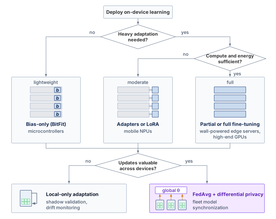
Checkpoint 11.4: Integrating the three pillars across device tiers
The chapter built three pillars for on-device learning: model adaptation (bias-only updates, adapters, full fine-tuning), data efficiency (few-shot, experience replay, compressed representations), and federated coordination (aggregation, client scheduling, secure aggregation). The decision framework in figure 18 maps each technique to device-class capability and coordination pathway. Test integration of the three pillars across the same deployment.
The hardest edge-learning failures appear when the pillars interact rather than when any one fails alone. An adapter can fit memory yet overfit sparse local data, a replay buffer can stabilize learning yet leak sensitive history, and a federated round can improve the global model while amplifying participation bias. These interactions decide when on-device learning is appropriate and when a simpler strategy is safer.
A tiered policy is still a design. Centralized training can standardize hardware, curate data, and validate a model before release; this policy instead ships to millions of devices whose runtimes, update histories, and connectivity differ, and it keeps changing the model after release. Shipping it turns each tier assignment into a release artifact that must be versioned, validated without central labels, and rolled back when an adapted model degrades.
Self-Check: Question
A production voice assistant is deployed across a heterogeneous fleet of 10 million devices comprising 20% flagship smartphones, 50% mid-tier phones, and 30% budget devices. How does the three-pillar integration framework structure model adaptation across this fleet?
- It mandates that all 10 million devices execute full 32-bit fine-tuning of the 7B-parameter backbone during active voice calls.
- It restricts learning exclusively to cloud data centers, disabling all on-device learning across all device tiers.
- It proposes tier-specific LoRA ranks and replay allowances, with bias-only updates for budget devices, then validates joint resource fit and useful adaptation for each permitted path.
- It assigns the highest-rank adapters to budget microcontrollers because microcontrollers have no operating system overhead.
In a multi-pillar edge architecture, an explicit priority policy is established to arbitrate runtime resource contention between active user inference and background adaptation. What is the fundamental operational rule enforced by this control?
- Background gradient updates take absolute priority over interactive user requests to maximize training convergence speed.
- When battery drops below 5%, the device shuts down display output to continue running backpropagation.
- Memory buffers for experience replay are allowed to grow dynamically until they consume 100% of physical system RAM.
- Interactive user inference strictly preempts background training tasks, and training is immediately suspended if memory pressure, thermal limits, or QoS latency thresholds are approached.
In the integrated voice assistant case study, participating devices exchange LoRA adapter updates (\(2.2\text{–}4.5\text{ MB}\)) rather than full model updates (\(14\text{ GB}\) in FP16). Explain how this parameter-efficient adaptation strategy simultaneously satisfies constraints across all three pillars: Model Adaptation, Data Efficiency, and Federated Coordination.
When a mobile device experiences poor cellular connectivity, high thermal load, or battery depletion during deployment, an edge-learning control mechanism known as graceful ____ ensures the device seamlessly transitions into a minimal or inference-only adaptation mode without disrupting active user functionality.
11.10 Production Integration
A prototype can fine-tune an adapter on one Raspberry Pi under controlled conditions. Deploying adaptation across 50 million devices requires release tests for different runtimes, resource budgets, and update histories. The production artifact must specify what each device may learn, how the result is validated, and how to restore a trusted state when adaptation fails.
11.10.1 MLOps integration challenges
In a traditional cloud MLOps pipeline, the release artifact is a single immutable model binary; once millions of devices begin updating adapters offline on different schedules, the released weights no longer describe the behavior running in the field. Integrating on-device learning into machine learning operations (MLOps)—the practices that version, deploy, monitor, and roll back production models—expands what a release must validate because backbones, adapters, update policies, and local histories evolve independently across heterogeneous hardware. Existing integration tests, version registries, and monitoring remain useful, but operations must now validate the permitted adaptation process and its recovery path alongside the initial model.
An edge learning lifecycle splits five stages between the cloud and the device (figure 19). Centralized base-model pretraining (Stage 1), per-tier hardware compression (Stage 2), and staged over-the-air rollouts (Stage 3) originate in the cloud, while local adaptation executes on-device under the released update policy (Stage 4). Aggregate telemetry (Stage 5) supplies evidence for deciding whether cloud retraining is warranted. The telemetry needs its own privacy controls; aggregation alone does not establish a privacy guarantee, and a detected change must be distinguished from a quality regression before triggering a new training cycle.
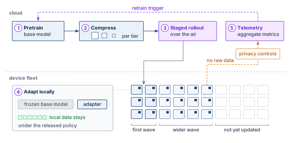
Deployment pipeline transformations
A release that enables local learning includes an adaptation policy alongside model artifacts. For example, the voice-assistant policy of section 11.9 assigns bias-only updates to budget devices and different LoRA ranks to mid-tier and flagship phones. These are conditional assignments: model footprint, runtime support, and live admission tests determine whether a device may execute them. CI/CD must therefore validate the selection logic and permitted update behavior across device configurations in addition to the initial weights.
Versioning must preserve relationships among those artifacts. A local adapter belongs to a particular base model, training policy, and representation schema; a replay buffer may also depend on the encoder that produced its features. Federated round identifiers record which shared version produced a returned contribution. Updating the base therefore requires a decision to retain, migrate, retrain, or discard dependent local state. A newer version number alone does not establish compatibility, and rollback must restore a compatible set of artifacts rather than independently selecting older files.
Continuous training orchestration
Continuous training on devices combines fleet-level round or release schedules with local admission decisions. A coordinator can request work, but a device trains only when its resource and availability tests pass. The orchestrator must therefore track eligible work and compatible state without assuming simultaneous execution across clients. Because devices run different base versions at once and may reconnect after days or weeks offline, a returned update must identify its base version for the coordinator to reject it, apply a stated staleness policy, or request new training from the current base (section 11.7.5.1), while per-device adapters and replay buffers carry their own version tags and need not be merged into the shared model.
Resource-aware scheduling applies equation 2 at fleet scale, where federated rounds usually add idle, charging, and unmetered-network requirements on top of the local admission test, and a daily energy cap bounds cumulative learning cost across many admitted windows. Admission also has a runtime half. Bias updates in early layers require backward computation through later operations; head-only adaptation confines that computation to the head. Either path competes with inference for compute, memory bandwidth, and thermal headroom on a shared SoC. Users judge the device by its quality of service (QoS), so the runtime gives inference priority and throttles or revokes a training window as foreground latency approaches its deadline. At the microcontroller extreme, measured update energy and available reserves determine how much learning a duty-cycled or harvested-power budget can support.20
20 Microcontroller power budget: In an illustrative operating point, 10 mW of active training for 10 seconds consumes 0.1 J. The number of updates that fit that session requires a measured time or energy per update. Battery lifetime additionally depends on usable capacity under the actual load, sleep power, radio activity, conversion losses, and duty cycle; nameplate capacity alone does not establish continuous-training lifetime.
When a representative central validation set is unavailable, federated evaluation can aggregate metrics computed on local held-out data. Update magnitudes provide an optimization diagnostic, but small changes can reflect stalled learning rather than acceptable quality. Participation audits must accompany outcome measurements so that apparent progress is not confined to an overrepresented cohort.
Monitoring system evolution
Traditional monitoring aggregates metrics from centralized inference servers that see every request, whereas an adaptive fleet’s monitor sees only what devices report about models that may differ on every device. Fleet telemetry for edge devices, including federated analytics that report aggregate or differentially private summaries, is one of the fleet release controls in section 11.10.1.5. Adaptation adds local model states that the operator may not observe centrally. Monitoring must distinguish a change in behavior from a change in quality. Unlabeled signals can identify divergence, while deciding whether the adapted model is better requires validated outcome evidence.
Drift detection presents additional challenges without access to ground truth labels. While traditional monitoring compares model predictions against labeled validation sets maintained on centralized infrastructure, on-device systems must detect drift using only the indirect local signals available during deployment. Confidence calibration compares output probabilities with eventual outcomes whenever labels exist; without verified outcomes, confidence shifts merely flag an altered score distribution. In parallel, input distribution monitoring applies statistical tests to detect when runtime feature distributions diverge from pretraining data without requiring labels. Task performance proxies use implicit feedback such as user corrections or session abandonment, though only after validating the causal link to task quality and accounting for how model suggestions alter subsequent user behavior. Finally, shadow baseline comparisons run a frozen base model alongside the adapted one; section 11.10.1.4 develops why that comparison measures divergence rather than quality.
↪ Covariate shift, label shift, and concept drift, and why input monitors can stay silent under pure concept drift, are developed in Distribution shift and concept drift.
Cohort evaluation must separate contribution from benefit. A device that never trains can still download an improved shared model, but its users’ data may be poorly represented among the completed updates. Participation metrics reveal that coverage gap; per-cohort quality measurements establish whether it harms those users. A favorable global average cannot substitute for either measurement.
Validation strategy adaptation
Traditional validation measures model quality directly against a held-out test set with known ground truth, whereas on-device learning has to validate adapted models where their inputs live, within privacy and resource limits, and usually without labels. Shadow model evaluation maintains multiple model variants on each device and compares their behavior. Devices can run a frozen, last-known-good model beside a locally adapted version and measure prediction divergence, confidence shifts, latency, and resource use on the same input stream. Without labels or a validated outcome proxy, these comparisons detect change, not performance degradation: agreement can hide a shared error, and disagreement does not reveal which model is correct. A shadow comparison can therefore suspend an update for further evaluation, but automatic rollback requires labeled outcomes, a validated behavioral invariant, or a proxy whose relationship to task quality has been established for the deployment.
The comparator can therefore act only as a gate, never as a judge (figure 20). The live input stream is mirrored to the frozen baseline and the adapted candidate, and the comparator tracks their disagreement, confidence shift, and resource deltas. When disagreement exceeds a tolerance \(\ResponseThreshold\), the gate holds the candidate out of service; validated outcome evidence then either clears it or confirms the regression that justifies rollback.
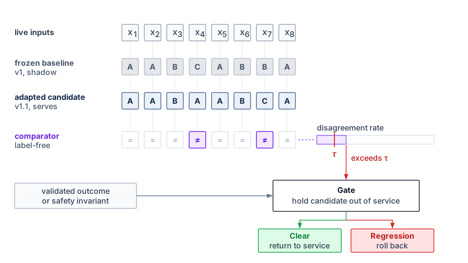
Confidence-based gates provide another change signal when labels are unavailable. Even a calibrated model’s confidence is interpretable only relative to the population and task on which calibration was measured. A drop can reflect distribution shift, ambiguity, or a changed score scale; stable confidence can coexist with overconfident errors. Systems may use confidence to trigger investigation or halt adaptation conservatively, but they should not call the adapted model worse without delayed labels, randomized evaluation, trusted user corrections, or another validated outcome signal.
Federated A/B testing randomly assigns devices to treatment and control adaptation policies, balanced across device tiers, and compares privacy-preserving aggregates of adaptation success rate, time to improvement, and final quality. A strategy that wins is then released through the staged rollout process that fleet operations owns. Because aggregated validation signals are themselves releases, they need data minimization, secure aggregation where appropriate, a declared privacy unit, and privacy accounting across repeated rounds, and even then a population summary can miss a failure confined to a few users. Local gates and population summaries therefore provide different evidence, and evaluating an adaptive fleet requires measuring adaptation benefit, resource cost, and cohort coverage together.
↪ Staged rollout, which widens a release’s exposure only after each stage performs acceptably, is developed in Staged rollout strategies.
Fleet release controls
The preceding controls act on one adapted device or one federated round. Operating the whole population as one fleet adds three interacting constraints beyond those of any single device, so they form one operational design problem. Each constraint calls for its own platform control (table 9), including hardware-in-the-loop validation and federated analytics.
| Edge fleet constraint | Why it appears | Platform control |
|---|---|---|
| Extreme version skew | Rollouts can take weeks or months because devices are offline, on low battery, or on restricted networks. At any time, 50 model versions may remain active. | Maintain backward-compatible data pipelines and serving contracts for models deployed months earlier. |
| Device-aware validation | Accuracy gates do not reveal whether a model exceeds a phone’s memory budget or triggers thermal throttling on its system-on-chip (SoC); microcontroller-class targets below Archetype C tighten the budget to about 1 MB. | Add hardware-in-the-loop validation on physical or emulated target devices before promotion. |
| Privacy-limited telemetry | Raw predictions cannot stream back continuously because privacy rules and bandwidth costs constrain observability. | Use federated analytics: devices compute local statistics such as error rates or drift, then transmit permitted aggregate health signals under explicit privacy and retention controls. |
Federated health signals inherit the participation bias that section 11.7.1 identified for federated training. A device reports its local error rate or drift statistic only when its admission policy allows the work and its connectivity allows the upload, so the devices that report most are the well-charged, well-connected, newer ones. The fleet’s health dashboard then describes the admitted population rather than the deployed one, the same skew the participation selection principle (20) names for training. A staged edge rollout can look healthy because the devices most likely to fail, older hardware and thermally constrained phones, are also the least likely to report. The platform therefore tracks reporting coverage per device class and cohort alongside the health signals themselves, and holds promotion when a cohort’s coverage falls too low for its signal to count as evidence.
Performance evaluation in dynamic environments
Static inference benchmarks characterize latency, throughput, energy efficiency, and accuracy for a fixed model, whereas on-device learning requires additional measurements of adaptation quality and training efficiency across successive updates to explain whether local learning is worth its resource cost. Sample efficiency measures the examples needed to reach a declared quality improvement under a fixed evaluation protocol. Gaining two percentage points from 100 local samples rather than 500 is an advantage when collecting useful samples is the binding constraint. Fewer samples need not mean faster or cheaper adaptation, because the more sample-efficient method may perform more work per example or retain more state; elapsed time, peak memory, and energy complete the comparison.
Because a sample-efficient update can still exceed hardware limits, device-envelope fit tests whether the improvement stays inside resource budgets. Memory-constrained convergence evaluates validation loss under a fixed RAM budget, such as “convergence within 256 KB training footprint,” while energy-per-update measures millijoules consumed per gradient step; an illustrative background envelope of 500–1000 mW corresponds to 1.8–3.6 kJ/hour while active. Battery impact depends on duty cycle, usable battery capacity, foreground demand, and charging state. Time-to-adaptation extends the same idea to scheduling by measuring wall-clock time from new data to measurable improvement, including waiting for idleness, charging status, and thermal headroom rather than only raw accelerator throughput.
Even an update that fits the device envelope must still prove its value to the user, so personalization quality evaluates whether adaptation improves the intended behavior while retaining earlier capabilities. Per-user performance delta compares the adapted model with the global baseline on user-specific holdout data; acceptance requires a declared improvement threshold and reported uncertainty. Privacy must be assessed under the specified disclosure policy and guarantee, rather than treated as an unspecified unit of exposure. Catastrophic forgetting measures degradation on the original task after adaptation. Its acceptable magnitude is application-specific, and accuracy changes must distinguish percentage points from relative percent.
When devices coordinate through the federated protocols examined in section 11.6, evaluation expands from the device to the population. Communication efficiency relates quality improvement to total transmitted bytes; compression gains depend on the model, optimizer, data heterogeneity, and encoding (Konečný et al. 2016; Kairouz and McMahan 2021). Comparisons should also report bytes and elapsed time to the same quality target. Straggler policies change both waiting time and the cohort that contributes. Participation count, cohort coverage, and outcome uncertainty must therefore be evaluated together, without assuming that one participation threshold determines stability across all policies.
Konečný, J., H. B. McMahan, D. Ramage, and P. Richtárik. 2016. “Federated Optimization: Distributed Machine Learning for on-Device Intelligence.” CoRR abs/1610.02527.
A system that infers quickly but adapts slowly, or adapts efficiently but ends at poor accuracy, still fails its deployment, so these training metrics and operational controls extend inference benchmarks and established MLOps practice to distributed, heterogeneous learning. Together they detect, hold, and reverse an adaptation that misbehaves, though they do not remove the underlying conditions that make adaptive fleets misbehave, from heterogeneous hardware and non-IID data to slow drift and adversarial clients.
Self-Check: Question
In traditional cloud MLOps, a deployment pipeline releases a single monolithic model binary to uniform server clusters. How does this deployment artifact transform when shipping an on-device learning system across a heterogeneous mobile fleet?
- The deployable artifact becomes a policy bundle containing a shared base model along with device-tier adaptation strategies (e.g., bias-only for microcontrollers, LoRA for mid-tier, selective layers for flagship), resource execution rules, and rollback thresholds.
- The artifact is replaced by an uncompiled Python script executed directly on bare-metal microcontroller sensors.
- The deployment pipeline requires manual per-device flashing over USB cables for every smartphone in the world.
- The deployment artifact eliminates model weights entirely, transmitting only random seeds to client operating systems.
What can a frozen shadow model establish when compared with a locally adapted model without labeled outcomes or a validated task-quality proxy?
- The Shadow Model connects to cloud labeling services via satellite to annotate live user keystrokes in real time.
- Prediction and confidence differences reveal behavioral change and can suspend an update for evaluation, but do not by themselves establish which model is more accurate.
- The Shadow Model inverts user biometric features into cryptographic tokens to bypass operating system security firewalls.
- The Shadow Model permanently deletes the active model whenever the device battery drops below 90%.
A production edge ML team cannot collect raw user inputs or ground-truth prediction labels due to privacy policies. Explain how Federated Analytics and privacy-preserving telemetry allow the platform team to monitor fleet-wide model health and detect cohort regressions.
True or False: In production edge learning systems, tracking global fleet-wide average accuracy is sufficient to ensure high quality, because individual device variances cancel out across millions of deployed nodes.
A production MLOps system executes a federated A/B deployment to validate a new on-device adaptation algorithm before fleet-wide rollout. Order the stages of this validation workflow from first to last:
- Gradually expand rollout across the general population once treatment confirms statistically significant quality gains without regressions
- Deploy candidate adaptation strategy to treatment cohort while control cohort retains baseline strategy
- Stratify device fleet into statistically balanced treatment and control cohorts across hardware capability tiers
- Aggregate differentially private validation metrics and compare convergence speed and user task-proxy satisfaction
11.11 Engineering Challenges and Mitigations
A billion-user predictive text model that learns from live keyboard inputs can be poisoned if a coordinated group of malicious users repeatedly types a specific slur and those local updates enter the global federated aggregate. The tiered integration policy bounds where each pillar may act, but it does not erase the failure surfaces that exposing an adapting model to the real world creates: device and data heterogeneity, non-IID distributions, silent failures, and the security and compliance risks of post-release adaptation. These surfaces are coupled. Hardware variation changes who can participate, participation changes the observed data distribution, limited feedback weakens validation, and post-release adaptation complicates audit and rollback. Observability and runtime resource contention already have their controls in section 11.10. Of the challenges that remain, device and data variation comes first, because it is present from the first rollout. The poisoned keyboard returns in section 11.11.5 once the quieter failure surfaces that let it go unnoticed are in view.
11.11.1 Device and data heterogeneity management
An adaptation policy that passes lab tests on one reference smartphone can produce divergent weights, crash on unsupported kernels, or stall indefinitely across a production fleet whose OS versions, driver stacks, floating-point implementations, and charging habits differ. Heterogeneity determines which devices can train, which can validate, and which can only contribute lightweight signals. Tier assignment already gives each hardware class its own model format and update policy, so the management problem here is reproducibility across devices whose software stacks, connectivity, and power availability diverge.
Software heterogeneity is what makes even a correct assignment hard to reproduce. Devices may run different versions of operating systems, kernel-level drivers, and runtime libraries. Some environments support optimized ML runtimes like TensorFlow Lite Micro or ONNX Runtime Mobile, while others rely on custom inference stacks or restricted APIs. These discrepancies can lead to subtle inconsistencies in behavior, especially when models are compiled differently or when floating-point precision varies across platforms.
Connectivity and uptime add the scheduling dimension. Some devices are intermittently connected, plugged in only occasionally, or operating under strict bandwidth constraints. Others have continuous power and reliable networking, but still prioritize user-facing responsiveness over background learning. These differences complicate coordinated learning because update eligibility changes with the device’s current state rather than with its hardware tier alone.
System fragmentation closes the loop by making reproducibility and testing a fleet property rather than a lab property. With such a wide range of execution environments, consistent model behavior is difficult to guarantee and failures are difficult to reproduce. Monitoring, validation, and rollback therefore become more important, while also becoming harder to implement uniformly across the fleet.
The consequence is visible in a mobile-keyboard deployment. One device might provide 8 GB of RAM and a supported accelerator path, while another has 2 GB, a slower update path, and intermittent connectivity. These differences affect update duration and completion frequency. Adjusting schedules, model formats, and compression can broaden participation, but whether the improvement is equitable shows up only in outcome measurements across those device cohorts, because respecting each device’s budget is not the same as delivering equal benefit.
11.11.2 Non-IID data distribution challenges
A federated round whose global validation loss improves steadily can still degrade next-word accuracy for an entire regional dialect or budget-handset cohort because no central shuffle can equalize non-IID client distributions. In production, non-IID data becomes an evaluation and control problem: evaluation must cover the intended deployment population through a representative central test set or distributed held-out data, and aggregate quality needs cohort-level checks because a population average can conceal a persistent local failure. The mitigation should follow the observed failure rather than the generic label “non-IID,” and each of four common observations points to a bounded control and a release criterion (table 10).
| Observed evidence | Likely failure | Control to test | Release criterion |
|---|---|---|---|
| Cohort metrics diverge while aggregate quality improves | Population underrepresentation | Stratified sampling or capped importance weights | Worst-cohort metric improves without unacceptable aggregate loss |
| More local steps increase update disagreement and rounds to target | Client drift | Reduce local steps, add proximal regularization (FedProx), incorporate control variates (SCAFFOLD), or adapt the server optimizer | Wall-clock time and bytes to target decrease on representative cohorts |
| One global model leaves stable, distinct clusters underserved | Multimodal client objectives | Clustered models or shared backbone with local heads | Each cluster has enough support and outperforms the global baseline |
| Heavy users dominate the aggregate | Objective-weight mismatch | Replace example weighting with user weighting or cap per-user contribution | Evaluation matches the declared user- or example-level objective |
11.11.3 Failure modes and prevention mechanisms
Heterogeneous devices and fragmented data also make failures hard to see, because failures in on-device learning emerge slowly, locally, and often without centralized evidence (Kairouz and McMahan 2021). The most basic risk is unbounded adaptation drift, where continuous learning without constraints causes models to gradually diverge from their intended behavior. Consider a hypothetical keyboard prediction system that learns from all user inputs, including corrections. It might begin incorporating typos as valid suggestions, leading to progressively degraded predictions. This risk becomes acute in health monitoring applications where gradual changes in user baselines could be learned as “normal,” potentially causing the system to miss anomalies that a static model would have detected. Because this drift is slow and local, it escapes detection without monitoring designed to look for it.
Wang, Jianyu, Zachary Charles, Zheng Xu, Gauri Joshi, H. Brendan McMahan, Blaise Aguera y Arcas, Maruan Al-Shedivat, et al. 2021. “A Field Guide to Federated Optimization.” arXiv Preprint arXiv:2107.06917.
Beyond individual device drift, the participation bias described under client scheduling (section 11.7.1) can amplify itself over time. Users whose models improve less engage less, which further reduces their representation in later rounds (Wang et al. 2021). The failure is slow and invisible in aggregate metrics, which is why cohort-level evaluation must accompany every accepted round.
These systematic biases interact with data quality issues to create autocorrection feedback loops, particularly in text-based applications. When systems cannot distinguish between intended inputs and corrections, they may develop unexpected behaviors. Frequently corrected domain-specific terminology might be incorrectly learned as errors, leading to inappropriate suggestions in professional contexts. This problem compounds the drift issue, because models adapt to individual quirks and can simultaneously reinforce their own mistakes when users accept autocorrections without realizing the system learns from those interactions.
These failure modes connect individual drift, population bias, and data-quality degradation. Federated-learning surveys identify heterogeneity, participation bias, privacy, and optimization instability as deployment risks (Li et al. 2020; Kairouz and McMahan 2021). In response, successful systems can bound adaptation, stratify sampling, distinguish corrections from reliable labels, and use shadow comparisons to identify changes that warrant validated evaluation.
Li, Tian, Anit Kumar Sahu, Ameet Talwalkar, and Virginia Smith. 2020. “Federated Learning: Challenges, Methods, and Future Directions.” IEEE Signal Processing Magazine 37 (3): 50–60. https://doi.org/10.1109/msp.2020.2975749.
11.11.4 Compliance, security, and recovery risks in production
When a medical wearable, financial fraud detector, or vehicle controller adapts its weights after release, the deployed model diverges from the artifact that passed regulatory review, and an unverified local update can invalidate the audit trail, absorb poisoned inputs, or violate data-erasure rules. In domains where compliance, auditability, and regulatory approval are required, on-device learning creates a direct tension between local autonomy and operational control.
A centrally managed training pipeline can record a common release’s data, checkpoints, and evaluation results. On-device learning distributes the update history across local models and observations that may remain private. Traceability therefore depends on what the adaptation protocol records: the base version, permitted update policy, validation result, and available recovery point. The operator can retain control over those boundaries without collecting every local training example.
This autonomy creates a validation gap. Evidence collected for the released model does not automatically establish the behavior of each adapted version. When inputs and update histories remain local, the deployment needs a defined set of local acceptance checks and a way to report failures within its privacy constraints. An adapted model can leave its validated operating range before aggregate monitoring detects the change, so the update policy must specify when to reject a candidate or restore the trusted baseline.
Delayed detection complicates recovery, especially while a device is offline. A trusted baseline must remain available independently of the adapted candidate, and the restore policy must account for compatible preprocessing, adapters, and runtime state. Restoring weights alone may leave the faulty update trigger or contaminated replay data in place. Recovery therefore includes deciding which adaptation state to retain, quarantine, or reset before learning resumes.
In addition to compliance challenges, on-device learning introduces new security vulnerabilities. Because model adaptation occurs locally and relies on device-specific, potentially untrusted data streams, adversaries may attempt to manipulate the learning process by tampering with stored data, such as replay buffers, or by injecting poisoned examples during adaptation, to degrade model performance or introduce vulnerabilities. Any locally stored adaptation data, such as feature embeddings or few-shot examples, must be secured against unauthorized access to prevent unintended information leakage.
Maintaining model integrity over time is particularly difficult in decentralized settings, where central monitoring and validation are limited. Autonomous updates could, without external visibility, cause models to drift into unsafe or biased states. Compliance obligations such as the GDPR’s right to erasure compound these risks, because a user’s data can influence an adapted model in ways that are difficult to trace and reverse.
Every recovery path in this section assumes that something safe keeps operating while an adapted model is suspect or being restored. When perception and control loops rely on local models, that something is often a human supervisor, and a human fallback is not a safety mechanism unless the fallback itself is engineered as part of the system. A fatal 2016 crash under driver-assistance automation shows what happens when it is assumed instead.
War Story 11.1: The edge model with a human fallback (2016)
Context: A 2015 Tesla Model S was using Traffic-Aware Cruise Control and Autosteer when it collided with a crossing semitrailer near Williston, Florida, on May 7, 2016 (National Transportation Safety Board 2017). The driver remained responsible for supervision.
Mechanism: The NTSB attributed the crash to the truck driver’s failure to yield and the car driver’s inattention associated with overreliance on automation. The automation’s operational design contributed by permitting prolonged disengagement and use inconsistent with the manufacturer’s guidance.
Impact: The car passed beneath the semitrailer, and its driver died.
Fix: The NTSB issued safety recommendations addressing automation safeguards and oversight. For an edge-system designer, the corresponding requirement is to make operational limits and the supervision contract enforceable rather than assume a human will recover from every local failure.
Systems lesson: Fast local execution is insufficient if the combined sensing, automation, and human-supervision system lacks a reliable fallback. The vehicle did not learn on the device, yet its lesson applies directly to edge learning. A fallback contract is validated against fixed model behavior, and local adaptation changes that behavior after release, so every accepted update must leave the operational limits and the validated recovery path intact.
National Transportation Safety Board. 2017. Collision Between a Car Operating with Automated Vehicle Control Systems and a Tractor-Semitrailer Truck Near Williston, Florida, May 7, 2016. HAR-17/02. National Transportation Safety Board.
The immediate design obligation is to treat model state, replay buffers, and adaptation triggers as security-sensitive assets: edge learning cannot rely on central inspection after the fact, so it needs local integrity checks, protected storage, and conservative update policies before adaptation begins. Privacy regulations also interact with on-device learning in nontrivial ways. While local adaptation can reduce the need to transmit sensitive data, it may still require storage and processing of personal information, including sensor traces or behavioral logs, on the device itself. Depending on jurisdiction, this may invoke additional requirements for data retention, user consent, and auditability. Systems must be designed to satisfy these requirements without compromising adaptation effectiveness, which often involves encrypting stored data, enforcing retention limits, or implementing user-controlled reset mechanisms.
Distributed adaptation also complicates debugging and failure analysis (Kairouz and McMahan 2021). A deployment must assign responsibility for detecting regressions, suspending learning, restoring a baseline, and investigating failures before release. Local data drift, poor initialization, and faulty safeguards can produce similar symptoms, so the version and validation records must support diagnosis within the permitted disclosure limits. Autonomous execution does not remove the need for an accountable recovery process; addressing these deployment and compliance risks requires tooling, protocols, and design practices that extend the ability to explain, bound, and reverse local adaptation (section 11.8.2) to external requirements for traceability, reproducibility, and user protection.
11.11.5 Poisoned updates and the combined control path
Poisoning, inversion, drift, and validation failures also occur in centralized ML systems, but local adaptation makes them harder to observe, attribute, and roll back across a heterogeneous fleet. The billion-user keyboard model poisoned by a coordinated group of users shows why. The malicious updates arrive as ordinary contributions from authenticated devices, secure aggregation hides each one from inspection, and the shift they cause can stay below what a population average reveals. Defending against such poisoned updates21 is one of three obligations that local adaptation adds, alongside limiting what updates disclose and detecting local shift that population averages hide.
21 Byzantine fault tolerance in federated learning (FL): Named after the Byzantine Generals Problem (Lamport et al. 1982), this property enables useful aggregation despite malicious or faulty participants; how many faulty participants a rule such as Krum or trimmed mean tolerates depends on that rule’s own conditions, which Byzantine failures states. These defenses can increase communication and compute overhead because they require extra validation, robust statistics, or redundant participation.
Lamport, Leslie, Robert Shostak, and Marshall Pease. 1982. “The Byzantine Generals Problem.” ACM Transactions on Programming Languages and Systems 4 (3): 382–401. https://doi.org/10.1145/357172.357176.
↪ Data poisoning as a threat model, including poisoned contributions to federated training, is developed in Data poisoning.
The edge architecture must therefore bind adaptation range, update integrity, privacy accounting, robust aggregation, validation evidence, and rollback into one control path. These mechanisms do not substitute for one another. Secure aggregation hides individual contributions, robust statistics limit some malicious influence, and validated outcomes establish whether behavior improved.
Self-Check: Question
A mobile keyboard application allows continuous, unconstrained on-device model adaptation on all typed keystrokes. After several months of deployment, users report that the keyboard frequently suggests misspelled words and typos as high-confidence autocomplete options. What failure mode has occurred, and what is the standard architectural mitigation?
- Unbounded adaptation drift and autocorrection feedback loop; mitigated by bounding parameter update ranges, filtering user corrections, and validating against a frozen shadow model.
- Cryptographic hash collision in the secure aggregation protocol; mitigated by increasing RSA key size to 4096 bits.
- Memory leak in the LPDDR5X DRAM controller; mitigated by rewriting the keyboard in assembly language.
- Quantization underflow in the NPU matrix multipliers; mitigated by disabling all integer arithmetic.
In a federated learning fleet of 100,000 devices, malicious or compromised clients attempt to corrupt the global model by uploading maliciously crafted gradient vectors with extreme magnitudes. Which aggregation defense mitigates this Byzantine attack?
- Standard arithmetic mean aggregation with no client filtering.
- Byzantine-resilient aggregation rules (such as coordinate-wise median, trimmed mean, or Krum) combined with gradient norm clipping.
- Increasing the local training epochs on all clients to \(E = 100\).
- Disabling secure aggregation and publishing all client IP addresses to an open web dashboard.
Explain the mechanism of ‘participation bias amplification’ in large-scale mobile federated learning, and describe how it creates a digital inequality feedback loop across user cohorts.
What does the 2016 Williston Tesla crash illustrate about relying on human supervision as the fallback for an automated driving feature?
True or False: Because on-device learning decentralizes computation to user hardware, platform engineering teams no longer need to budget for server-side orchestration, verification, or monitoring infrastructure.
11.12 Fallacies and Pitfalls
A team ports a cloud-trained recommendation model to a mobile app and assumes that successful inference also permits local fine-tuning. The first update can exceed the app’s memory allowance as gradients and saved activations accumulate; a configuration that fits can still consume more energy than the background policy permits. These distinct failures motivate the following fallacies and pitfalls:
Fallacy: On-device learning provides the same adaptation capabilities as cloud-based training.
Teams expect local learning to match centralized training’s model improvements, ignoring the device’s resource constraints. Full-model training adds activations, gradients, and optimizer state to the weights; the configurations in section 11.3.1 require 4–12× the inference weights alone, depending on the model and execution schedule. Local datasets are typically small, biased, and nonrepresentative, while compute budgets remain orders of magnitude below cloud GPUs. A smartphone with 8 GB RAM and a sustained power budget of 2–3 W cannot replicate the adaptation achieved by data center systems with terabytes of memory and kilowatts of power. Effective on-device learning requires designing adaptation strategies that provide meaningful improvements within these constraints rather than attempting to replicate cloud-scale learning capabilities.
Pitfall: Assuming federated learning automatically preserves privacy without additional safeguards.
Practitioners believe that keeping data on local devices inherently provides privacy protection, ignoring what can be inferred from model updates. Gradient and parameter updates leak significant information about local training data through various inference attacks, while device participation patterns reveal sensitive information about users and activities. Stronger privacy preservation requires additional mechanisms: differential privacy provides a tunable probabilistic bound on how much the output distribution can change because of one individual’s data, while secure aggregation protocols prevent parameter inspection during server-side coordination through zero-sum cryptographic masking (figure 16) (Bonawitz et al. 2017). Data locality alone is insufficient for privacy protection.
Fallacy: Resource-constrained adaptation always produces better personalized models than generic models.
This belief assumes that any local adaptation is beneficial regardless of the quality or quantity of local data available. On-device learning with insufficient, noisy, or biased local data can actually degrade model performance compared to well-trained generic models (section 11.5). Small datasets may not provide enough signal for meaningful learning, while adaptation to local noise can harm generalization. Effective on-device learning systems must include mechanisms to detect when local adaptation is beneficial and fall back to generic models when local data is inadequate for reliable learning.
Pitfall: Ignoring heterogeneity across different device types and capabilities.
Teams design on-device learning systems assuming uniform hardware capabilities across deployment devices. Real-world deployments span diverse hardware with varying computational power, memory capacity, energy constraints, and networking capabilities. Available memory alone spans roughly 65,536× between 256 KB microcontroller SRAM and 16 GB flagship phones (section 11.7.5.2), and supported operators and power envelopes differ as sharply. Clock frequency or peak ratings from unrelated architectures do not convert into a common training-throughput ratio, so the comparison needs measured update cost under matched tasks and declared operating states. A learning algorithm that works well on high-end smartphones may fail catastrophically on resource-constrained IoT devices. Federated learning algorithms must account for heterogeneous clients and availability (Kairouz and McMahan 2021; Bonawitz et al. 2019), using selective participation, compression, and tiered aggregation strategies when devices have substantially different measured update costs.
Pitfall: Underestimating the complexity of coordinating learning across distributed edge systems.
Many teams focus on individual device optimization and treat coordination as a stateless averaging server, as if local updates arrived regularly from comparable devices. At fleet scale the aggregator is one component of a control loop that must know which devices are eligible, which model version each holds, and whether a returned update is safe to promote; a production system selects about 130 percent of its target cohort (Bonawitz et al. 2019) because a substantial fraction of selected devices never report. Edge orchestration (section 11.7.5) must also handle intermittent connectivity, varying power states, time zones, and version skew across devices that return after days offline. A design that budgets only for the averaging step leaves round deadlines, partial participation, and state reconciliation unowned, although those parts of the loop decide whether each round completes with a representative cohort.
Self-Check: Question
A product manager asserts: ‘Because our smart home devices keep all audio recordings strictly on the local device and only upload federated gradient updates to the cloud, our architecture is mathematically immune to user privacy leakage.’ What technical fallacy does this statement commit?
- It ignores that raw model updates and gradients directly expose training-step information, enabling adversaries to reconstruct private training samples via gradient inversion attacks or verify user participation via membership inference unless protected by secure aggregation and differential privacy.
- It ignores that audio recordings stored in flash memory are automatically broadcast over FM radio frequencies by microcontrollers.
- It incorrectly assumes that federated learning requires quantum computers to achieve privacy.
- It assumes that gradient vectors always have a mathematical magnitude of zero on edge devices.
A development team attempts to deploy an on-device personalization algorithm across an IoT ecosystem spanning both 64 MHz ARM Cortex-M microcontrollers (with 256 KB SRAM) and flagship mobile phones (with 12 GB RAM). The team uses identical full-model fine-tuning hyperparameters across all endpoints. What pitfall does this design encounter?
- Mobile phones will refuse to execute floating-point operations because microcontrollers only understand binary code.
- It ignores differences in available working memory, supported update operators, and energy budgets; an identical policy needs a separate feasibility and quality check on each device class.
- Microcontroller clock speeds will accelerate to 3 GHz due to thermal resonance with mobile phones.
- Full-model fine-tuning requires all microcontrollers to be physically connected via optical fiber cables.
Explain why performing on-device personalization on scarce, noisy, or uncurated local data can actually degrade model performance compared to a static, well-trained centralized base model.
A common fallacy in federated learning treats the central coordinator as a simple stateless aggregation server, ignoring that production fleet coordination is an active control loop that must manage client ____ criteria (such as verifying that devices are charging, on unmetered Wi-Fi, and thermally stable).
11.13 Summary
Edge intelligence extends the fleet to devices whose memory, power, and availability the operator cannot standardize. Sensors, microcontrollers, and smartphones contribute under different resource budgets, so a locally feasible learning policy also determines which parts of the population can participate. Archetype C (Federated MobileNet) makes this concrete. Local adaptation spends the compute axis of C³ inside each phone’s power and memory envelope, adapters and update compression shrink the wide-area transfer in the Fleet Law’s communication term, and over-selection with round deadlines caps its synchronization term at the price of which devices are represented.
Three levers make learning possible under those constraints, and each acts on a different part of the same budget. Model adaptation shrinks trainable state and, when placed well, the saved activations that dominate peak memory. Data efficiency raises the signal extracted from each scarce example and protects earlier behavior with bounded replay. Federated coordination lets compatible updates from many devices improve one shared model without centralizing raw data. None of the three moves the device’s thermal, energy, or bandwidth limits; each decides how much useful learning fits inside them.
At runtime, those realities become an admission decision rather than a general preference to run “when idle.” Background adaptation may execute only when its predicted energy and sustained power fit the current device slack and profiled worst-case interference preserves the foreground deadline. Because charging status does not eliminate heat or contention, every admitted window remains revocable as the device state changes.
Local execution can meet latency, data-locality, and offline requirements, but those requirements alone do not justify local training. Adaptation must improve a validated outcome within its resource budget; federation must then preserve update compatibility, control disclosure, and evaluate the population actually represented by completed updates.
Key Takeaways: Physics sets the budget
- The edge reverses the fleet: Data centers fight to keep many accelerators busy; edge devices fight to learn under batteries, kilobytes, thermal throttling (the device-scale counterpart of principle 3), and intermittent links. The same Compute, Communication, Coordination constraints must account for device eligibility as well as aggregate throughput.
- Bandwidth beats advertised TOPS: One update step of the chapter’s 10M-parameter example moves about 800 MB, 20× the weight bytes read by an inference, across a phone memory interface roughly 44–65× narrower than data-center HBM, the same ceiling that bounds memory-bound decode (principle 18). Quantization and locality help, but measured update speed depends on bytes moved and sustained bandwidth.
- Learning multiplies the footprint: Full-model backpropagation can require 4–12× the memory occupied by inference weights alone in the chapter’s configurations, depending on optimizer state, activations, and precision. Reducing trainable state helps only when the frozen model and remaining execution state also fit.
- Background learning is conditional work: Admit an adaptation window only when equation 2 preserves energy, thermal, and foreground-latency budgets under worst-case measured interference. Charging alone is not sufficient.
- Admission selects the population: Passing the admission test correlates with hardware, charging habits, and connectivity, so the shared model learns from the admitted devices rather than the deployed fleet (principle 20). Per-cohort participation and quality must be measured and corrected; loosening admission spends the budgets it exists to protect.
- Adaptation needs three levers: Bias-only updates, LoRA, sparse layers, few-shot data reuse, and experience replay each spend different memory, energy, and privacy budgets. Federated coordination adds population learning only when cumulative uploads stay below the data they replace, enough clients survive to clear secure aggregation’s participation floor so individual updates stay hidden, and shared state stays version-compatible.
- Heterogeneity is normal operation: Edge fleets span microcontrollers, phones, gateways, and NPUs with uneven availability, performance, and non-IID data. Stragglers, client drift, participation bias, and privacy-preserving observability are protocol design constraints, not deployment cleanup, and once models learn after release the release artifact is the adaptation policy, versioned against a base model that rollback can restore.
An edge learning policy determines both the work a device may perform and the population the fleet learns from. Tightening a resource budget can protect a user’s foreground experience while excluding that user’s data from shared improvement. The useful design target is therefore validated adaptation across the intended population, with local feasibility and fleet representation evaluated together.
What’s Next: From devices to operations
Once a model continues learning after release, the operator ships an adaptation policy rather than a static set of weights: an adaptation rule versioned against a base model, admitted device by device, validated through distributed outcome evidence when central labels are unavailable, and judged by which cohorts its completed updates represent. Production organizations run hundreds of models at once, many sharing features, data pipelines, and release machinery, so a change made for one can silently break another. Keeping that portfolio versioned, observable, and recoverable is a coordination problem in its own right.
↪ The control plane that versions, releases, monitors, and rolls back a portfolio of models is developed in ML Operations at Scale.
11.14 Self-Check Answers
Self-Check: Answer
A mobile robotics vision system must process each frame within \(33\text{ ms}\), while cloud network round-trip time is \(80\text{–}150\text{ ms}\). Why must the foreground perception path execute locally even if model training remains in the cloud?
- Network round-trip latency alone exceeds the foreground deadline, so a frame cannot wait for a cloud response.
- Cloud data centers are physically incapable of computing backpropagation gradients on batch sizes of one within milliseconds.
- The on-device camera sensor cannot serialize video frames into digital packets without first running an on-device forward-backward training pass.
- On-device adaptation reduces model parameter count to zero before sending updates across the cellular uplink.
Answer: The correct answer is A. An \(80\text{–}150\text{ ms}\) round trip cannot fit inside a \(33\text{ ms}\) foreground deadline, regardless of server compute speed. This establishes the need for local inference; it does not establish the need for local training, which requires a separate adaptation benefit and resource budget.
Learning Objective: Distinguish latency-driven local inference requirements from the separate justification for on-device training.
Before investing in an on-device gradient-based learning pipeline for a mobile news app, an ML systems architect considers feature-based personalization (local feature caching with a frozen global model) versus on-device gradient fine-tuning. Under what systems criteria is feature-based personalization preferred, and what eliminates the need for local backpropagation?
Answer: Feature-based personalization is preferred when local preference vectors, interaction histories, or lookup embeddings give a frozen model the useful context it needs. Its parameters do not change, so this path avoids weight-gradient, backward-pass, and optimizer-state costs. Local feature state and inference buffers still consume resources. Compare validated personalization quality and the complete footprint against a gradient-based candidate; the chapter’s 4–12x range describes particular full-model training configurations relative to weight storage, not a universal amplification.
Learning Objective: Compare feature-based personalization against on-device gradient adaptation in terms of systems overhead and implementation complexity.
In comparing learning paradigms across edge fleets, what fundamental systems distinction separates isolated on-device learning from federated learning?
- Isolated on-device learning transmits raw private data to centralized servers, whereas federated learning processes data locally without communication.
- Isolated on-device learning restricts parameter updates entirely to a single node, preventing collective fleet knowledge sharing, whereas federated learning coordinates model updates across devices while preserving data locality.
- Federated learning trains models from scratch on client devices without a pretrained base model, whereas isolated on-device learning requires continuous cloud synchronization.
- Isolated on-device learning uses only INT4 integer arithmetic, whereas federated learning requires double-precision FP64 hardware accelerators on all mobile clients.
Answer: The correct answer is B. Isolated adaptation updates one device without aggregating knowledge from its peers. Federated learning coordinates local updates while keeping raw training data local. A shared initialization may be pretrained or initialized for federated training; pretraining is not a defining requirement. Neither approach requires FP64 arithmetic.
Learning Objective: Contrast isolated on-device adaptation and federated learning in terms of knowledge aggregation and communication boundaries.
True or False: Because on-device learning keeps raw user observations (such as typed keystrokes or biometric sensor traces) on the client device, it inherently guarantees full compliance with privacy regulations like GDPR and HIPAA without requiring any additional cryptographic or governance safeguards.
Answer: False. Keeping raw data on-device significantly reduces privacy exposure and data transmission risks, but it does not automatically guarantee full regulatory compliance. First, intermediate artifacts such as gradient updates or adapter checkpoints can still leak sensitive private information via gradient inversion or membership inference attacks if transmitted or observed. Second, regulatory frameworks like GDPR and HIPAA impose strict obligations regarding lawful basis, user consent, purpose limitation, auditability, data retention limits, and secure local storage of protected health information (PHI) or personal data on the physical device.
Learning Objective: Evaluate the privacy and regulatory compliance boundaries of on-device learning beyond simple raw data localization.
Compare the coordination responsibilities of isolated on-device learning, centralized cloud training, and cross-device federated learning. Why does the paradigm alone not establish a universal ranking of implementation complexity?
Answer: Isolated learning keeps the update loop on one device. Centralized training coordinates data ingestion, training infrastructure, and artifact release. Cross-device federation adds client eligibility, compatible versions, partial participation, aggregation, and population coverage across intermittent devices. These responsibilities differ, but deployment scale, trust boundaries, and reliability requirements determine implementation complexity; a large cloud training service need not be simpler than a small federated deployment.
Learning Objective: Distinguish coordination responsibilities across learning paradigms without inferring a universal complexity ordering.
Self-Check: Answer
A mobile engineering team observes that fine-tuning a 10M parameter vision model on a smartphone with 8 GB of RAM causes the background training process to be killed by the operating system’s out-of-memory (OOM) killer during backpropagation. Why does training memory demand spike so severely compared to inference for the exact same model?
- The base model weights dynamically expand by \(100\times\) during the forward pass due to weight unpacking.
- Floating-point units on mobile SoCs automatically convert all INT8 weights to FP64 double precision during training.
- Training adds gradients, optimizer state, and saved backward activations to the weights; the simultaneous peak can exceed the app’s budget even when inference fits.
- The mobile operating system creates a separate virtual machine sandbox for every individual neuron in the neural network.
Answer: The correct answer is C. Training can retain activations needed for backward computation, gradients, and optimizer state in addition to weights. Their simultaneous peak can exceed a background process budget even when total device RAM is much larger. The amplification is configuration-dependent; inference also requires activation buffers and workspace, not necessarily only one layer of activations.
Learning Objective: Analyze the sources of memory amplification in edge training compared to inference-only execution.
A quantized 7B-parameter language model achieves 12 tokens/sec on a mobile SoC advertised at 45 peak TOPS. Profiling shows that low-batch decode saturates available DRAM bandwidth while arithmetic units wait. Which hardware resource is the binding constraint?
- Insufficient CPU integer arithmetic capacity for calculating cross-entropy loss.
- Thermal throttling of the wireless 5G modem during token generation.
- Flash storage read latency when loading the token tokenizer vocabulary.
- Mobile LPDDR5X memory bandwidth (\(64\text{–}100\text{ GB/s}\)), which is roughly \(34\times\) lower than data-center HBM3, causing the memory streaming term \((D_{\text{vol}} / \text{BW})\) to dominate execution time per token.
Answer: The correct answer is D. Low-batch autoregressive decode often streams a large weight volume per token, so limited mobile DRAM bandwidth can dominate despite high peak TOPS. The stated peak rates alone do not prove the measured bottleneck: profiling must check achieved bandwidth, operator support, and thermal limits. Tokenizer initialization and loss computation do not explain steady-state decode throughput.
Learning Objective: Analyze why memory bandwidth, rather than peak TOPS, is the binding constraint for on-device autoregressive transformer decoding.
A proposed background personalization task on a smartphone draws \(4.5\text{ W}\) of sustained SoC power and requires 30 minutes to complete. Calculate the total energy consumed (in \(\text{Wh}\)) and the percentage drain on an idealized \(15\text{ Wh}\) smartphone battery. Explain why this result mandates opportunistic scheduling.
Answer: The task consumes \(4.5\text{ W}\times0.5\text{ h}=2.25\text{ Wh}\), or \(15\%\) of the idealized battery. That is a substantial background cost, motivating charging, idle, and thermal eligibility gates. Network restrictions are needed when the workflow communicates; the exact scheduling policy depends on the deployment rather than following from the energy calculation alone.
Learning Objective: Calculate battery energy consumption of background on-device training and justify opportunistic scheduling constraints.
True or False: Gradient checkpointing reduces the total electrical energy consumed by an on-device training workload because it reduces peak SRAM/DRAM memory allocation.
Answer: False. Checkpointing trades saved activations for recomputation. The extra arithmetic can increase energy, while reduced memory traffic or avoiding spill may offset that cost. Lower peak allocation alone therefore does not determine energy per update; measure the complete workload on the target device.
Learning Objective: Evaluate the compute, memory, and energy trade-offs of gradient checkpointing in edge training.
**Consider the end-to-end memory lifecycle of a single gradient update during on-device backpropagation for a convolutional layer. Order the following operational stages from first to last in execution sequence:
- Discard intermediate activations and compute parameter updates in optimizer state
- Forward pass computes and caches layer activations
- Fetch batch inputs into SRAM buffer
- Loss evaluation and backward pass calculates layer gradients using cached activations**
Answer: The correct order is (3) -> (2) -> (4) -> (1). First, (3) Fetch batch inputs into SRAM buffer prepares the raw or preprocessed batch tensors in accessible working memory. Second, (2) Forward pass computes and caches layer activations sequentially through the network layers, saving feature maps needed for gradient calculation. Third, (4) Loss evaluation and backward pass calculates layer gradients using cached activations, traversing backward from the loss through the computation graph. Finally, (1) Discard intermediate activations and compute parameter updates in optimizer state applies the optimizer step (e.g., SGD or Adam) to update weights, freeing cached activations and gradients.
Learning Objective: Analyze the chronological memory allocation and deallocation stages of an on-device backpropagation training step.
Self-Check: Answer
Why does Tiny Transfer Learning (TinyTL) freeze convolutional backbone weights and adapt biases with optional lite residual modules?
- Freezing removes backbone weight-gradient and optimizer state; suitable activation and normalization choices also reduce saved backward state.
- Microcontroller hardware units physically short-circuit if matrix multiplications are performed in reverse during backpropagation.
- Bias parameters have mathematical properties that prevent all forms of numerical underflow in 8-bit fixed-point arithmetic.
- Training bias parameters modifies the underlying kernel weights directly through implicit singular value decomposition.
Answer: The correct answer is A. Frozen weights need no weight gradients or optimizer state, but they remain part of the deployed model. Gradients may still traverse frozen operators, and nonlinearities can require saved state. TinyTL reduces these costs through its adaptation path and operator choices; it does not guarantee an arbitrary backbone fits microcontroller SRAM. Bias updates do not modify frozen kernels.
Learning Objective: Explain how TinyTL reduces trainable and saved activation state without eliminating the full deployment memory budget.
A mobile vision engineer chooses between Low-Rank Adaptation (LoRA) and Residual Bottleneck Adapters for on-device camera personalization. The system requires zero additional inference latency during real-time 60 FPS video capture, while another use case requires hot-swapping between 10 user contexts without reloading the base model. How do LoRA and Residual Adapters compare across these requirements?
- Residual Adapters introduce zero inference latency because they replace the backbone, while LoRA requires recomputing matrix inverses on every video frame.
- LoRA updates can be merged into compatible base weights to remove the adapter execution path, while residual adapters retain separate computation and support modular context switching.
- LoRA updates require storing 10 full copies of the 7B base model in SRAM, whereas Residual Adapters operate without trainable parameters.
- Both methods require identical memory footprints and add exactly 50 ms of inference latency per layer.
Answer: The correct answer is B. A compatible linear LoRA update can be merged as \(W_{\text{final}}=W_{\text{base}}+BA\), removing separate adapter operations. Residual adapters retain their own computation, whose latency must be measured. Unmerged LoRA also supports context switching; the distinction is mergeability, not exclusive access to hot-swapping. Neither method requires copies of the entire base model per context.
Learning Objective: Compare LoRA and Residual Bottleneck Adapters regarding inference latency, weight merging, and multi-tenant context swapping.
A smart camera supports 10 personalization contexts. Its base model has 10M parameters (\(40\text{ MB}\) in FP32), and assume each complete adapter checkpoint occupies \(200\text{ KB}\). Compare storage for 10 full fine-tuned models with one shared base plus 10 adapters. Explain the architectural advantage.
Answer: Ten full models require \(400\text{ MB}\). One \(40\text{ MB}\) base plus ten \(0.2\text{ MB}\) adapter checkpoints requires \(42\text{ MB}\). The incremental per-context checkpoint is \(200\times\) smaller, while total storage is about \(9.5\times\) smaller. Sharing the base enables compact context switching; the stated checkpoint size is an assumption, not a consequence of adapter rank alone, and excludes training state.
Learning Objective: Calculate storage savings of multi-tenant adapter personalization over full model fine-tuning.
In structured parameter adaptation, a technique that approximates a full weight matrix update \(\FiniteChange\WeightMatrix \in \mathbb{R}^{\WeightMatrixRowCount \times \WeightMatrixColumnCount}\) as the product of a low-rank up-projection \(\AdapterUpProjectionMatrix \in \mathbb{R}^{\WeightMatrixRowCount \times \AdapterRank}\) and down-projection \(\AdapterDownProjectionMatrix \in \mathbb{R}^{\AdapterRank \times \WeightMatrixColumnCount}\) (where \(\AdapterRank \ll \min(\WeightMatrixRowCount, \WeightMatrixColumnCount)\)) is known as ____ (low-rank adaptation).
Answer: LoRA. Low-rank factors restrict the trainable update to a compact subspace, reducing parameter and optimizer-state storage relative to full-matrix adaptation.
Learning Objective: Apply low-rank matrix decomposition principles to parameter-efficient edge fine-tuning.
**Task-adaptive sparse updates use individual-layer profiling to propose a trainable subset. Order the steps from profiling to deployment:
- Fine-tune each candidate layer separately and measure its validation gain and resource cost
- Freeze the pretrained model to establish a baseline
- Deploy the jointly validated subset with other parameters frozen
- Rank layers by gain per unit cost and propose a subset
- Measure the selected combination against memory, energy, foreground-latency, and quality budgets, including profiling cost**
Answer: The correct order is (2) establish the frozen baseline, (1) profile individual layers, (4) rank and propose a subset, (5) measure the combined update, then (3) deploy the validated subset. Individual gains need not add, and shared backward dependencies change combined resource cost. Deploying directly from the ranking skips the joint feasibility and quality test; a subset that fails it must be revised or rejected.
Learning Objective: Design a task-adaptive sparse parameter selection workflow using layer contribution profiling.
Self-Check: Answer
A developer of a keyword spotting (KWS) system for smart home appliances wants users to configure custom wake words using 5 to 10 spoken samples. Why is few-shot adaptation of a classification head on top of a frozen acoustic encoder preferred over end-to-end retraining?
- End-to-end retraining of acoustic encoders produces audio waveforms that violate device speaker impedance limits.
- Spoken custom wake words cannot be processed by neural networks unless the entire encoder architecture is expanded by \(10\times\).
- Updating only the head restricts trainable state and preserves frozen encoder representations, reducing adaptation cost and overfitting risk relative to full retraining.
- The Fourier transform algorithm only converges when supervised labels exceed 100,000 samples.
Answer: The correct answer is C. A pretrained encoder can supply reusable acoustic features while a small head adapts to a few user examples. Freezing the encoder reduces trainable state and preserves its parameters, but does not guarantee accuracy or a particular power and memory footprint. Measure the adaptation path separately from always-on inference; speaker impedance and Fourier-transform convergence do not govern this choice.
Learning Objective: Apply few-shot transfer learning principles to always-on keyword spotting adaptation under severe data and energy scarcity.
An edge health tracker adapts a continuous activity classifier to a user’s walking gait over several weeks. When the user starts cycling, the device adapts its model, but suddenly misclassifies normal walking as cycling. What core failure mode has occurred, and why did it happen?
- Overfitting on a single static batch caused by excessive L2 regularization.
- Numerical floating-point overflow in the hardware accelerometer sensor buffer.
- Model inversion attack where cycling data erased the operating system kernel.
- Catastrophic forgetting, where sequential gradient updates on new data distributions overwrite the weight configurations responsible for preserving performance on previously learned tasks.
Answer: The correct answer is D. Catastrophic forgetting is the fundamental stability failure of sequential learning in neural networks: when a model updates parameters on a new data stream (cycling) without mechanisms to preserve prior distributions (walking), gradient steps overwrite the representations that encoded the old task. Overfitting on a single batch does not describe sequential task erosion. Sensor overflow is a hardware I/O fault, and model inversion is an adversarial privacy attack, not a continuous learning stability failure.
Learning Objective: Analyze catastrophic forgetting in streaming on-device adaptation.
In on-device continuous learning, why do production experience-replay implementations store compressed feature embeddings (e.g., penultimate-layer activations or MFCCs) in a circular ring buffer rather than saving raw sensor observations (such as raw images or audio waveforms)?
Answer: Compact embeddings can retain useful replay information with less storage than raw sensor streams, allowing a bounded ring buffer. Discarding raw samples reduces one exposure path, but embeddings may still reveal sensitive information and need access and retention controls. Replay quality also depends on representation stability: changing the encoder can make stored embeddings stale, so this design is easiest with a stable feature extractor.
Learning Objective: Justify the use of compressed feature embeddings over raw inputs in edge experience replay buffers.
True or False: In on-device experience replay, maintaining a small buffer of 100 uniformly sampled past examples guarantees that the adapted model will not suffer from catastrophic forgetting across rare or long-tail edge cases.
Answer: False. A bounded uniform sample does not guarantee coverage of rare classes or preservation of earlier behavior. A ring buffer favors recent observations; reservoir sampling gives historical examples an equal inclusion probability but a small reservoir can still contain few or no rare examples. Compare retention policies, capacity, and regularization under retained-task and rare-event evaluation; none is a universal forgetting guarantee.
Learning Objective: Evaluate the limitations of naive uniform experience replay for long-tail robustness in edge learning.
In continuous edge adaptation, the fundamental trade-off between retaining previously acquired knowledge and acquiring new patterns from dynamic local data is known as the stability-____ trade-off.
Answer: plasticity. Stability preserves previously learned behavior; plasticity allows adaptation to new observations. Continual learning must balance both rather than maximize either alone.
Learning Objective: Explain the stability-plasticity dilemma in continual on-device learning.
Self-Check: Answer
In the Federated Averaging (FedAvg) algorithm, what is the primary algorithmic trade-off when tuning the number of local training epochs (\(\LocalEpochCount\)) on client devices?
- Increasing local work can amortize communication, but may increase client drift on non-IID data; rounds and elapsed time to the same quality target must be measured.
- Increasing \(\LocalEpochCount\) forces the central server to store full training datasets from all participating clients in server DRAM.
- Increasing \(\LocalEpochCount\) eliminates the need for clients to compute backward passes during local training.
- Increasing \(\LocalEpochCount\) increases the size (in megabytes) of the transmitted model parameter vector by a factor of \(\LocalEpochCount^2\).
Answer: The correct answer is A. More local epochs can reduce communication frequency, but do not guarantee fewer rounds or less time to a fixed quality target. Non-IID local updates can increase client drift. Compare candidate \(\LocalEpochCount\) values under matched data and participation conditions, recording validated target quality, elapsed round times, bytes, and energy. More epochs neither transfer raw data nor change the parameter vector dimension.
Learning Objective: Analyze the trade-off between local computation epochs (\(\LocalEpochCount\)) and communication rounds in FedAvg under non-IID data.
A mobile federated learning deployment encounters severe client drift due to extreme non-IID typing patterns across users, causing standard FedAvg to oscillate and fail to converge. Which algorithmic modification directly addresses client drift by constraining local updates to stay close to the global model?
- Switching from 32-bit floating-point to 1-bit stochastic sign quantization without error compensation.
- Adding a proximal regularization term \(\frac{\mu}{2} \|w - w_t\|^2\) to the local client objective (as in FedProx) to penalize excessive deviation from the global server model \(w_t\).
- Increasing the local learning rate by \(10\times\) to accelerate convergence on outlier devices.
- Dropping the central aggregation server and allowing devices to train purely in isolation without synchronization.
Answer: The correct answer is B. FedProx adds \(\frac{\mu}{2}\|w-w_t\|^2\) to penalize departure from the current global reference. This can mitigate client drift, but does not guarantee convergence for every workload or hyperparameter choice; evaluate matched quality and resource budgets. Raising the learning rate can worsen drift, while isolated training abandons the federated objective.
Learning Objective: Apply algorithmic regularizers (FedProx proximal term) to mitigate client drift in non-IID federated optimization.
Contrast cross-silo federated learning and cross-device federated learning across three dimensions: participant scale/reliability, network connectivity, and client incentive/governance.
Answer: 1. Participant scale and reliability: Cross-silo FL involves a small, fixed number of known, highly reliable institutional organizations (e.g., 2–100 hospitals or banks) that participate in almost every round. Cross-device FL involves massive fleets of millions of anonymous, unreliable mobile or IoT devices with high dropout and churn rates.
Network connectivity: Cross-silo participants connect via high-speed, reliable data-center or enterprise WAN connections. Cross-device clients connect over unmetered/metered mobile Wi-Fi or cellular networks with asymmetric bandwidth and frequent disconnects.
Incentive and governance: Cross-silo systems operate under formal legal data-sharing agreements and regulatory audits (e.g., BAA/HIPAA consortia). Cross-device systems operate under consumer platform operating policies (e.g., opt-in telemetry, strict opportunistic gating when idle/charging).
Learning Objective: Compare cross-silo and cross-device federated learning across infrastructure, reliability, and governance characteristics.
In federated optimization, the phenomenon where multiple local gradient steps on non-identically distributed client data cause local models to diverge toward disparate local optima is called client ____.
Answer: drift. Repeated local steps on different client distributions move models toward different objectives, making their aggregated update less aligned with the global objective.
Learning Objective: Explain the mechanism and consequences of client drift in federated optimization.
Self-Check: Answer
In production cross-device federated learning (such as Google Gboard), why do systems implement Over-Selection of clients (selecting \(\CandidateClientCount \approx 1.3 \times \TargetUpdateCount\) devices per round) rather than selecting exactly \(\TargetUpdateCount\) devices?
- Over-selection ensures that every mobile client receives \(1.3\times\) the monetary payment for participating.
- Over-selection forces client devices to increase their CPU clock frequencies by \(30\%\) during training.
- Selecting surplus candidates can reach the target number of valid reports earlier than waiting for every selected device, provided enough clients complete; a deadline and incomplete-round policy are still required.
- The aggregation server requires exactly \(30\%\) redundant updates to perform parity-bit error correction on the GPU memory bus.
Answer: The correct answer is C. Over-selection accommodates dropout and slow completion. If enough valid reports arrive, the round can proceed at the target-th completion rather than waiting for the slowest selected device. A surplus pool does not guarantee that the target is reached or prevent a stalled round by itself. The coordinator also needs a deadline, acceptance or abandonment rules, and evaluation of the completed cohort. The approximate 1.3 factor is a deployment example, not a universal setting.
Learning Objective: Design client selection and straggler mitigation mechanisms using over-selection in large-scale federated systems.
How does the Secure Aggregation (SecAgg) cryptographic protocol protect individual client privacy during federated aggregation on a central server?
- Clients transmit raw unencrypted updates, and the server permanently deletes its hard drive after every round.
- Clients train on synthetic dummy data generated by the server, ensuring real gradients are never computed.
- The server encrypts all client devices using a remote ransomware key until the global round terminates.
- Participating client pairs agree on shared pseudo-random masks that are added by one client and subtracted by the other; when the server sums all received masked updates, the masks algebraically cancel out, revealing the exact global aggregate without exposing any individual update.
Answer: The correct answer is D. Clients establish pairwise secrets and generate opposite masks, so masks cancel when the protocol forms an authorized aggregate. Dropout recovery requires additional protocol steps. Individual-update confidentiality depends on the participant threshold and threat model; it does not make the released aggregate differentially private. Deleting a server disk after receiving raw updates offers no comparable protection.
Learning Objective: Explain the algebraic masking and cancellation mechanism of Secure Aggregation (SecAgg).
In Differential Privacy for Federated Learning (DP-FedAvg), explain why gradient clipping to a fixed threshold \(S\) (\(\|\Delta \theta_k\|_2 \le S\)) is a mandatory prerequisite before adding calibrated Gaussian noise to the aggregate.
Answer: Clipping bounds each client update norm by \(S\), making sensitivity finite. The bound depends on the aggregation rule and neighboring-dataset definition: replacing one contribution in a fixed-size mean can change it by at most \(2S/K\). Noise must be calibrated to the chosen bound, sampling procedure, and privacy budget, with composition across rounds; clipping alone does not establish an \((\PrivacyBudget,\PrivacyAdditiveSlack)\) guarantee.
Learning Objective: Analyze why \(L_2\) norm clipping is essential for establishing sensitivity bounds in DP-FedAvg.
True or False: In top-\(k\) gradient sparsification for federated learning, discarding all gradient components outside the top \(1\text{–}10\%\) by magnitude without maintaining a local error accumulation buffer preserves the exact convergence rate of uncompressed SGD.
Answer: False. Dropping unsent components need not preserve the convergence rate of uncompressed SGD and can introduce optimization bias. Error feedback carries those components into subsequent compression steps, but its update-sized residual consumes persistent device memory. Neither immediate transmission of every component nor convergence for every optimizer and workload is guaranteed; compare quality, rounds, and total communication under the chosen assumptions.
Learning Objective: Evaluate the role of error accumulation buffers in gradient sparsification for federated learning.
In a federated camera-personalization deployment, a user captures \(200\text{ MB}\) of compressed images per week. A 4-bit quantized model update for the 5M-parameter on-device model requires \(2.5\text{ MB}\) per uplink round. Calculate the single-round communication savings of transmitting model updates versus uploading raw weekly data, and explain why cumulative round counts must be accounted for in production network budgets.
Answer: The single-round upload reduction is \(200\text{ MB} / 2.5\text{ MB} = 80\times\) less data transferred on the uplink. However, this \(80\times\) factor represents only a single training round. Over the course of training, if a device participates in 80 federated uplink rounds (\(80 \times 2.5\text{ MB} = 200\text{ MB}\)), cumulative update uploads alone equal the total raw data volume, before accounting for downlink global-model broadcasts, dropped-round retransmissions, or protocol handshake metadata. Therefore, production network planning must evaluate total communication cost over the entire convergence trajectory rather than single-round ratios.
Learning Objective: Calculate single-round versus cumulative communication volume in federated learning deployments.
**For a round using secure aggregation and a trusted server that adds differential-privacy noise, order these stages. Assume protocol participation thresholds and dropout recovery are satisfied:
- Select eligible clients and distribute a compatible global model and training policy
- Form the authorized aggregate and add noise calibrated to bounded client contributions and the declared privacy unit
- Clients train, clip their contributions under the policy, and apply protocol masks
- Update the global model and evaluate progress and completed-cohort coverage
- Receive enough valid masked reports before the round deadline, or apply the incomplete-round policy**
Answer: The correct order is (1) -> (3) -> (5) -> (2) -> (4). Eligibility and compatible state precede local work; clipping precedes calibrated noise. Secure aggregation forms an authorized aggregate under its threshold and dropout rules, rather than relying on arbitrary masks to cancel after clients are dropped. In this trusted-server design, differential privacy protects the released noisy result, not the exact aggregate from that server. Repeated releases require privacy accounting. Failure to meet the deadline or threshold follows the incomplete-round policy rather than proceeding with an unauthorized aggregate.
Learning Objective: Synthesize the complete end-to-end execution lifecycle of a production federated learning round.
Self-Check: Answer
A keyboard adapts nightly for a year. Each update fits its device budget and improves a metric on recent typing. Why must acceptance also check previously learned behavior against a recoverable baseline?
- Passing the memory and energy tests guarantees that earlier-task predictions remain unchanged.
- Freezing the backbone prevents head or adapter updates from changing any earlier-task prediction.
- Individually useful updates can accumulate into forgetting; retained-task evidence and a compatible recovery point remain necessary.
- Improving the recent-data metric establishes quality for all past tasks, so a recovery point is unnecessary.
Answer: The correct answer is C. Repeated updates can erode earlier behavior even when each improves recent data. A frozen backbone does not freeze predictions when its head or adapters change. Acceptance therefore needs retained-task evaluation and a compatible baseline to restore if the accumulated trajectory becomes unacceptable.
Learning Objective: Evaluate why repeated local improvements require retained-behavior checks and a recoverable baseline.
In lifelong on-device learning without catastrophic forgetting, Elastic Weight Consolidation (EWC) and Experience Replay offer distinct memory-compute trade-offs. Under which deployment condition is EWC architecturally preferred over Experience Replay?
- When model weights exceed 100 billion parameters and local RAM is strictly 64 KB.
- When the device has unlimited flash storage but cannot perform floating-point addition.
- When the device must continuously store raw 4K video feeds for retrospective auditing.
- When the model is relatively compact and storing past private data samples in a replay buffer violates strict privacy regulations or storage constraints.
Answer: The correct answer is D. EWC replaces a replay buffer with parameter-sized importance scores and reference values. A compact model may make that state affordable when retaining examples is prohibited. Memory depends on precision and retained task history; a basic same-precision implementation adds two parameter-sized arrays beyond current weights, and separate task penalties can add more. Very large models can therefore make EWC impractical.
Learning Objective: Compare Elastic Weight Consolidation (EWC) and Experience Replay in terms of memory scaling and privacy trade-offs.
An on-device sensor application receives a continuous unlabeled stream. Explain how contrastive learning can construct a useful local training signal while respecting memory, energy, and retention limits. What must be checked before treating nearby observations as positive pairs?
Answer: Positive pairs must preserve task-relevant content; nearby frames across a scene change may not, and apparent negatives may depict the same event. A bounded pair or feature buffer limits retention, but the complete update still needs profiled model, activation, optimizer, energy, and foreground budgets. Training from fixed cached features changes only the downstream trainable path; changing the encoder requires compatible replay state or refreshed features. Pair validity and retained-task quality need separate evaluation.
Learning Objective: Design a self-supervised contrastive learning workflow for continuous on-device sensor adaptation.
True or False: In lifelong edge learning, Elastic Weight Consolidation (EWC) requires zero additional memory overhead beyond the standard model weights because Fisher Information scores are computed and discarded instantaneously during the forward pass.
Answer: False. In addition to current parameters, a basic EWC implementation stores importance scores and reference parameter values. At equal precision, these two extra arrays add twice the current parameter storage, making three times that storage in total before other training state. Separate task histories can require more.
Learning Objective: Calculate the memory overhead incurred by Elastic Weight Consolidation on edge devices.
Self-Check: Answer
A production voice assistant is deployed across a heterogeneous fleet of 10 million devices comprising 20% flagship smartphones, 50% mid-tier phones, and 30% budget devices. How does the three-pillar integration framework structure model adaptation across this fleet?
- It mandates that all 10 million devices execute full 32-bit fine-tuning of the 7B-parameter backbone during active voice calls.
- It restricts learning exclusively to cloud data centers, disabling all on-device learning across all device tiers.
- It proposes tier-specific LoRA ranks and replay allowances, with bias-only updates for budget devices, then validates joint resource fit and useful adaptation for each permitted path.
- It assigns the highest-rank adapters to budget microcontrollers because microcontrollers have no operating system overhead.
Answer: The correct answer is C. Tier assignments are candidates, not proof of fit. Profiling must count the resident base, trainable and backward state, replay, runtime support, and foreground reserve; live admission then checks energy, heat, and latency. Validation must establish useful adaptation. An available NPU does not establish backward support, and inference-only operation remains valid when learning fails these tests.
Learning Objective: Design a tiered edge-learning architecture that integrates model adaptation, data efficiency, and federated coordination across device capability tiers.
In a multi-pillar edge architecture, an explicit priority policy is established to arbitrate runtime resource contention between active user inference and background adaptation. What is the fundamental operational rule enforced by this control?
- Background gradient updates take absolute priority over interactive user requests to maximize training convergence speed.
- When battery drops below 5%, the device shuts down display output to continue running backpropagation.
- Memory buffers for experience replay are allowed to grow dynamically until they consume 100% of physical system RAM.
- Interactive user inference strictly preempts background training tasks, and training is immediately suspended if memory pressure, thermal limits, or QoS latency thresholds are approached.
Answer: The correct answer is D. In edge systems, user experience and interactive Quality of Service (QoS) are paramount. The explicit priority control mandates that foreground inference tasks (e.g., wake-word detection, keyboard typing, camera rendering) strictly preempt background training tasks. If memory headroom shrinks, device temperature crosses thermal limits, or frame latency degrades, background gradient updates and replay processing are throttled or suspended immediately. Prioritizing training over user interaction or exhausting battery/memory violates fundamental edge engineering principles.
Learning Objective: Apply explicit priority policies and graceful degradation controls to prevent resource conflicts in edge learning systems.
In the integrated voice assistant case study, participating devices exchange LoRA adapter updates (\(2.2\text{–}4.5\text{ MB}\)) rather than full model updates (\(14\text{ GB}\) in FP16). Explain how this parameter-efficient adaptation strategy simultaneously satisfies constraints across all three pillars: Model Adaptation, Data Efficiency, and Federated Coordination.
Answer: Compact adapter updates reduce trainable parameter and optimizer-state storage, although frozen weights and backward activation state still require memory. Restricting the update space can help with scarce data, but does not guarantee freedom from overfitting or forgetting. For the stated checkpoints, \(14\text{ GB}\) divided by \(2.2\text{–}4.5\text{ MB}\) exceeds \(3{,}000\times\) per transfer. Total communication still includes participation frequency, downloads, and protocol overhead.
Learning Objective: Synthesize how parameter-efficient adaptation (LoRA) simultaneously resolves bottlenecks across model adaptation, data efficiency, and federated coordination.
When a mobile device experiences poor cellular connectivity, high thermal load, or battery depletion during deployment, an edge-learning control mechanism known as graceful ____ ensures the device seamlessly transitions into a minimal or inference-only adaptation mode without disrupting active user functionality.
Answer: degradation. The controller reduces or suspends background adaptation when resources become scarce, preserving foreground inference and user-facing service requirements.
Learning Objective: Explain graceful degradation mechanisms under adverse edge operating conditions.
Self-Check: Answer
In traditional cloud MLOps, a deployment pipeline releases a single monolithic model binary to uniform server clusters. How does this deployment artifact transform when shipping an on-device learning system across a heterogeneous mobile fleet?
- The deployable artifact becomes a policy bundle containing a shared base model along with device-tier adaptation strategies (e.g., bias-only for microcontrollers, LoRA for mid-tier, selective layers for flagship), resource execution rules, and rollback thresholds.
- The artifact is replaced by an uncompiled Python script executed directly on bare-metal microcontroller sensors.
- The deployment pipeline requires manual per-device flashing over USB cables for every smartphone in the world.
- The deployment artifact eliminates model weights entirely, transmitting only random seeds to client operating systems.
Answer: The correct answer is A. On-device learning systems operate across heterogeneous hardware tiers with vast differences in memory, compute, and power. Consequently, MLOps cannot release a single monolithic binary; it ships a validated policy bundle that specifies the base model backbone, tier-specific adaptation mechanisms (e.g., bias-only updates for extreme constraints, LoRA rank configurations for mid-tier devices), opportunistic execution policies (battery, thermal, and network triggers), and automated validation/rollback gates. The other choices mischaracterize production software deployment.
Learning Objective: Analyze how MLOps deployment pipelines transform from static model artifacts into tiered policy bundles for edge fleets.
What can a frozen shadow model establish when compared with a locally adapted model without labeled outcomes or a validated task-quality proxy?
- The Shadow Model connects to cloud labeling services via satellite to annotate live user keystrokes in real time.
- Prediction and confidence differences reveal behavioral change and can suspend an update for evaluation, but do not by themselves establish which model is more accurate.
- The Shadow Model inverts user biometric features into cryptographic tokens to bypass operating system security firewalls.
- The Shadow Model permanently deletes the active model whenever the device battery drops below 90%.
Answer: The correct answer is B. A shadow comparison detects disagreement, confidence shifts, latency changes, and resource regressions. Without labels or a validated quality proxy, lower confidence is not proof of lower accuracy, and agreement can hide shared errors. Automatic rollback needs an established outcome criterion or safety invariant, rather than confidence comparison alone.
Learning Objective: Distinguish unlabeled shadow-model change detection from validated quality and rollback decisions.
A production edge ML team cannot collect raw user inputs or ground-truth prediction labels due to privacy policies. Explain how Federated Analytics and privacy-preserving telemetry allow the platform team to monitor fleet-wide model health and detect cohort regressions.
Answer: Devices can compute confidence histograms, task proxies, and locally available outcome metrics without exporting raw observations. Secure aggregation hides individual contributions under its protocol assumptions, while differential privacy bounds release leakage through clipping, calibrated noise, and accounting. Cohort summaries help detect regressions, but small cohorts need disclosure controls and unlabeled confidence statistics remain change signals rather than direct accuracy measurements.
Learning Objective: Design a privacy-preserving telemetry and observability pipeline using federated analytics.
True or False: In production edge learning systems, tracking global fleet-wide average accuracy is sufficient to ensure high quality, because individual device variances cancel out across millions of deployed nodes.
Answer: False. Tracking only global fleet-wide averages masks critical cohort-specific failures. Because edge fleets exhibit extreme heterogeneity, high-performing flagship devices with fast networks can skew the global average upward, completely hiding severe regressions or adaptation failures occurring on budget devices, specific geographic regions, or underrepresented device demographics. Production monitoring requires segmented cohort tracking across hardware tiers, connectivity types, and participation frequencies.
Learning Objective: Evaluate why global fleet metrics fail to capture cohort-specific regressions in heterogeneous edge deployments.
**A production MLOps system executes a federated A/B deployment to validate a new on-device adaptation algorithm before fleet-wide rollout. Order the stages of this validation workflow from first to last:
- Gradually expand rollout across the general population once treatment confirms statistically significant quality gains without regressions
- Deploy candidate adaptation strategy to treatment cohort while control cohort retains baseline strategy
- Stratify device fleet into statistically balanced treatment and control cohorts across hardware capability tiers
- Aggregate differentially private validation metrics and compare convergence speed and user task-proxy satisfaction**
Answer: The correct order is (3) -> (2) -> (4) -> (1). First, (3) Stratify device fleet into statistically balanced treatment and control cohorts across hardware capability tiers to ensure fair comparative groups. Second, (2) Deploy candidate adaptation strategy to treatment cohort while control cohort retains baseline strategy under identical operating policies. Third, (4) Aggregate differentially private validation metrics and compare convergence speed and user task-proxy satisfaction between cohorts. Finally, (1) Gradually expand rollout across the general population once treatment confirms statistically significant quality gains without regressions.
Learning Objective: Design a federated A/B testing workflow for safe production rollout on edge fleets.
Self-Check: Answer
A mobile keyboard application allows continuous, unconstrained on-device model adaptation on all typed keystrokes. After several months of deployment, users report that the keyboard frequently suggests misspelled words and typos as high-confidence autocomplete options. What failure mode has occurred, and what is the standard architectural mitigation?
- Unbounded adaptation drift and autocorrection feedback loop; mitigated by bounding parameter update ranges, filtering user corrections, and validating against a frozen shadow model.
- Cryptographic hash collision in the secure aggregation protocol; mitigated by increasing RSA key size to 4096 bits.
- Memory leak in the LPDDR5X DRAM controller; mitigated by rewriting the keyboard in assembly language.
- Quantization underflow in the NPU matrix multipliers; mitigated by disabling all integer arithmetic.
Answer: The correct answer is A. When an adaptive system trains naively on streaming user inputs without validation, it cannot distinguish between intentional typing and accidental typos. If users accept or correct typos, the model adapts to its own mistakes, causing unbounded adaptation drift and creating an autocorrection feedback loop. The mitigation requires bounded adaptation ranges, input filtering (e.g., ignoring unverified corrections), task-proxy gating, and shadow evaluation against a frozen baseline model. RSA key size, DRAM memory leaks, and NPU quantization do not address adaptation drift.
Learning Objective: Analyze unbounded adaptation drift and feedback loops in on-device text prediction systems and identify mitigation controls.
In a federated learning fleet of 100,000 devices, malicious or compromised clients attempt to corrupt the global model by uploading maliciously crafted gradient vectors with extreme magnitudes. Which aggregation defense mitigates this Byzantine attack?
- Standard arithmetic mean aggregation with no client filtering.
- Byzantine-resilient aggregation rules (such as coordinate-wise median, trimmed mean, or Krum) combined with gradient norm clipping.
- Increasing the local training epochs on all clients to \(E = 100\).
- Disabling secure aggregation and publishing all client IP addresses to an open web dashboard.
Answer: The correct answer is B. Clipping limits update magnitude, while robust aggregation can reduce the influence of outliers under assumptions about malicious participation and honest-data variation. These methods do not guarantee stability against arbitrary attacks. Many require access to individual updates, creating a design tension with secure aggregation. Unfiltered averaging remains vulnerable; extra local epochs do not remove poisoned updates.
Learning Objective: Apply Byzantine-resilient aggregation techniques (trimmed mean, median, Krum) to protect federated systems against poisoned updates.
Explain the mechanism of ‘participation bias amplification’ in large-scale mobile federated learning, and describe how it creates a digital inequality feedback loop across user cohorts.
Answer: Participation bias amplification occurs when client eligibility requirements (e.g., connected to Wi-Fi, fully charged, idle overnight) are systematically met more frequently by users with high-end flagship devices, high-speed home broadband, and regular charging habits. As a result, the global model receives a disproportionate volume of updates from this privileged cohort, becoming heavily optimized for their language patterns, accents, and usage contexts. Conversely, budget devices with irregular charging or limited connectivity participate rarely, causing global model quality to degrade for those underserved populations. This degradation reduces app engagement among budget users, causing them to participate even less and amplifying digital inequality across the fleet.
Learning Objective: Analyze the sociological and algorithmic causes of participation bias amplification in federated learning fleets.
What does the 2016 Williston Tesla crash illustrate about relying on human supervision as the fallback for an automated driving feature?
Answer: The NTSB identified the truck driver’s failure to yield and the car driver’s inattention associated with overreliance on automation; the automation design permitted prolonged disengagement and use outside guidance. The engineering lesson is to enforce operational limits and the supervision contract. A fast local inference loop alone cannot ensure that a disengaged driver will intervene when needed.
Learning Objective: Evaluate why operational limits and enforceable supervision are part of a safety-critical edge deployment.
True or False: Because on-device learning decentralizes computation to user hardware, platform engineering teams no longer need to budget for server-side orchestration, verification, or monitoring infrastructure.
Answer: False. Decentralizing learning to edge devices actually increases server-side and platform engineering complexity. The central infrastructure must manage complex client selection protocols, secure aggregation handshakes, straggler mitigation, differential privacy accounting, multi-stage cryptographic verification of updates, distributed telemetry aggregation (Federated Analytics), shadow model tracking, and tiered rollback mechanisms across millions of heterogeneous clients.
Learning Objective: Analyze the server-side orchestration and platform infrastructure required to support decentralized edge learning fleets.
Self-Check: Answer
A product manager asserts: ‘Because our smart home devices keep all audio recordings strictly on the local device and only upload federated gradient updates to the cloud, our architecture is mathematically immune to user privacy leakage.’ What technical fallacy does this statement commit?
- It ignores that raw model updates and gradients directly expose training-step information, enabling adversaries to reconstruct private training samples via gradient inversion attacks or verify user participation via membership inference unless protected by secure aggregation and differential privacy.
- It ignores that audio recordings stored in flash memory are automatically broadcast over FM radio frequencies by microcontrollers.
- It incorrectly assumes that federated learning requires quantum computers to achieve privacy.
- It assumes that gradient vectors always have a mathematical magnitude of zero on edge devices.
Answer: The correct answer is A. Keeping raw observations local does not make transmitted updates immune to inference attacks. Reconstruction and membership inference depend on attacker access, auxiliary information, and the training configuration. Secure aggregation can hide individual updates under its threat-model assumptions, while differential privacy bounds a declared privacy unit’s influence on released results through clipping, calibrated noise, and composition. Required controls follow the deployment’s disclosure policy and threat model; locality alone supplies neither guarantee.
Learning Objective: Analyze the fallacy that data locality in federated learning guarantees privacy without cryptographic masking or differential privacy.
A development team attempts to deploy an on-device personalization algorithm across an IoT ecosystem spanning both 64 MHz ARM Cortex-M microcontrollers (with 256 KB SRAM) and flagship mobile phones (with 12 GB RAM). The team uses identical full-model fine-tuning hyperparameters across all endpoints. What pitfall does this design encounter?
- Mobile phones will refuse to execute floating-point operations because microcontrollers only understand binary code.
- It ignores differences in available working memory, supported update operators, and energy budgets; an identical policy needs a separate feasibility and quality check on each device class.
- Microcontroller clock speeds will accelerate to 3 GHz due to thermal resonance with mobile phones.
- Full-model fine-tuning requires all microcontrollers to be physically connected via optical fiber cables.
Answer: The correct answer is B. The stated memory capacities differ by several orders of magnitude, but they do not establish a CPU-throughput ratio or NPU underutilization. The same model can have different residency, backward support, and sustained costs on each device. Compare measured update paths under matched tasks and operating states, then choose and validate feasible tier-specific policies; full fine-tuning is not automatically admissible on either class.
Learning Objective: Analyze system failures resulting from ignoring hardware heterogeneity across microcontroller and mobile edge tiers.
Explain why performing on-device personalization on scarce, noisy, or uncurated local data can actually degrade model performance compared to a static, well-trained centralized base model.
Answer: A well-trained base can generalize better than a locally adapted candidate when local examples are scarce, noisy, or unrepresentative. Unconstrained updates may overfit accidental inputs or distort useful decision boundaries. This is a risk to test, not an inevitable result: evaluate local improvement and retained behavior against a trusted baseline, using validated outcomes and a compatible recovery path. Centralized training also does not inherently guarantee balanced data or broad generalization.
Learning Objective: Explain the conditions under which local on-device adaptation degrades model accuracy relative to static base models.
A common fallacy in federated learning treats the central coordinator as a simple stateless aggregation server, ignoring that production fleet coordination is an active control loop that must manage client ____ criteria (such as verifying that devices are charging, on unmetered Wi-Fi, and thermally stable).
Answer: eligibility. Admission checks enforce device resource and availability requirements before local training, protecting foreground service and reducing round failures.
Learning Objective: Analyze client eligibility filtering and admission control requirements in production federated orchestration.