2 Compute Infrastructure

Purpose

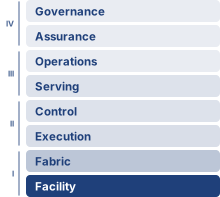
Fleet stack focus for this chapter.

Why does infrastructure, not algorithms alone, determine who can participate in advancing machine learning at scale?

Machine learning systems have a physical reality beyond their code. Public algorithms do not make large-scale training equally accessible: executing them requires power, cooling, memory, and communication capacity that organizations must build and sustain. A model that outgrows one machine turns a local resource problem into a shared infrastructure commitment. Buying more accelerators adds arithmetic capacity, but it also adds data transfers, heat, and components whose failures can interrupt collective work. The useful capacity of the fleet depends on whether those demands can be met together. Hardware that appears attractive in isolation may spend much of its deployment waiting for data or operating below its advertised speed. A facility that can house equipment may lack the electrical or cooling capacity to run it at the intended density. These mismatches consume both capital and operating budgets while reducing the experiments that can finish on schedule. Infrastructure decisions also outlast individual models, so an organization must weigh the efficiency of specialization against the flexibility needed for future workloads. Single-machine performance remains part of that judgment, but multiplying it by the number of machines cannot establish what the complete installation will deliver. Participation at scale therefore depends on turning purchased hardware into sustained, usable capacity within physical and financial limits. In C³ terms, the physical substrate sets the compute and communication bounds within which the fleet must coordinate useful work.

Learning Objectives

Explain how the memory, communication, power, and reliability walls bind at successive physical scales and cascade upward
Compare GPU, TPU, and ASIC specialization as a bet on workload stability against refresh cycles and facility lifetime
Distinguish memory capacity from memory bandwidth as separate procurement tests, using roofline placement to find bandwidth-bound phases
Calculate token-latency floors, memory budgets, and pod training time from accelerator specifications and sustained utilization
Match tensor, pipeline, and data parallelism to the available interconnect bandwidth hierarchy
Evaluate rack and pod designs using power density, cooling limits, topology, and facility reliability constraints
Select accelerator infrastructure using sustained throughput, power constraints, workload fit, and deployment cost

2.1 The Infrastructure Walls

The scaling laws of AI Scaling Laws are why demand outruns any single device. Loss falls predictably as parameters, training tokens, and compute grow together, so each step up in capability multiplies both the memory a model occupies and the arithmetic its training consumes; a GPT-3-class model already needs several accelerators merely to store its FP16 weights. A model that exceeds one accelerator’s memory capacity forces a hardware decision before training begins. Adding accelerators supplies capacity, but also creates transfers between devices, increases power demand, and couples progress to more components that can fail. The familiar single-node compute and memory limits therefore become inputs to fleet design. Four recurring physical constraints appear at escalating physical scales, from an eight-GPU node to a 25K-accelerator fleet (figure 1). Memory bandwidth, rack power, pod communication, and fleet failure exposure provide the examples; the workload and configuration determine which constraint binds at each scale. These are the memory, energy, and network walls of the scale moment and the fleet’s reliability gap, seen from the hardware that imposes them. Because this chapter studies the hardware, it names each constraint by the physical resource that runs out, and it uses these four names from here on: the memory wall, the power wall (the energy wall as power delivery and heat removal), the communication wall (the network wall as link bandwidth), and the reliability wall (the reliability gap as a failure interval).

The reliability wall starts from a per-GPU failure figure that The Scale Moment calls an MTBF. A failed GPU is replaced rather than repaired, so this chapter calls the per-device figure a mean time to failure (MTTF) and reserves mean time between failures (MTBF) for nodes and fleets, which keep running through repeated failures and replacements. The number is the same; only the label records what is being counted.

↩︎ The memory, network, and energy walls of the scale moment are established in The Scale Moment.

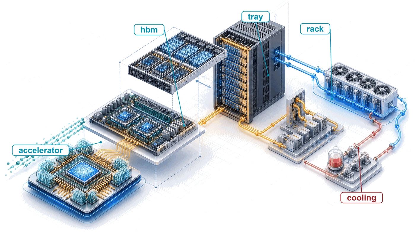
The 175B model anchors this progression. It is the chapter’s running instance of Archetype A (GPT-4/Llama-3), a GPT-3-class dense transformer trained with mixed precision and the Adaptive Moment Estimation (Adam) optimizer, whose reference training cluster is 1,024 H100 GPUs in 128 eight-GPU nodes. Accelerator selection establishes the compute rate, memory capacity, and power envelope that a fleet can buy. The node must connect enough of those accelerators to hold and execute the workload; the rack must power and cool them; the pod must sustain communication and survive component failures. This is the hardware contribution to C³: useful fleet compute depends on the communication and coordination costs created at each physical boundary.

↩︎ The three fleet workload archetypes are established in Three systems archetypes.

↪ The running model’s parameters and reference cluster are developed in Reference Workload.

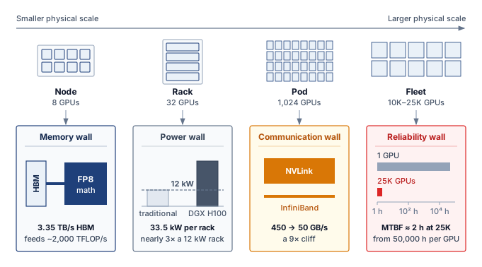
Figure 1: **The Four Infrastructure Walls**: Read left to right, the examples illustrate four constraints at increasing physical scales; the workload and configuration determine which one binds. The node compares 3.35 TB/s of HBM3 with about 2,000 TFLOP/s of FP8 arithmetic; the four-node DGX H100 rack draws 33.5 kW; the pod compares per-direction NVLink bandwidth with one InfiniBand port, a ninefold budget gap; and the fleet assumes independent GPU failures, reducing a 50,000-hour per-GPU mean time to failure (MTTF) to about 2 hours between failures at 25K GPUs.

The chapter climbs the same scale ladder, so the four walls arrive in the order the figure reads, though not one wall per section. The memory wall begins at the accelerator and is developed in section 2.3. The communication wall first appears inside the node, where section 2.5.1 measures the cliff between local and inter-node links, and returns at pod scale in section 2.7. The power wall binds at the rack (section 2.6.1), and the reliability wall accumulates from node health (section 2.5.5) through facility controls to the fleet-scale failure interval of section 2.7.1.

Self-Check: Question

Which statement correctly describes representative constraints and mitigation mechanisms across the accelerator, node, rack, and pod hierarchy, without assigning one universally dominant wall to each tier?
1. Accelerator: arithmetic throughput vs. generality tax $\rightarrow$ mitigated by specialized silicon; Node: single-chip memory capacity limit $\rightarrow$ mitigated by high-speed intra-node fabrics aggregating HBM; Rack: thermal and power density $\rightarrow$ mitigated by facility cooling and power distribution; Pod: network bisection and fleet MTBF $\rightarrow$ mitigated by pod-scale fabrics and fault-tolerant orchestration.
2. Accelerator: network latency $\rightarrow$ mitigated by InfiniBand; Node: transistor count $\rightarrow$ mitigated by photolithography; Rack: memory bandwidth $\rightarrow$ mitigated by PCIe Gen5; Pod: power delivery $\rightarrow$ mitigated by running jobs asynchronously without barriers.
3. Accelerator: single-chip memory capacity wall $\rightarrow$ mitigated by on-die branch predictors; Node: power wall $\rightarrow$ mitigated by host underclocking; Rack: communication wall $\rightarrow$ mitigated by standard commodity Ethernet; Pod: memory bandwidth wall $\rightarrow$ mitigated by building-wide CXL pooling.
4. Accelerator: storage I/O capacity $\rightarrow$ mitigated by local NVMe drives; Node: compilation time $\rightarrow$ mitigated by JIT compilers; Rack: clock jitter $\rightarrow$ mitigated by atomic clocks; Pod: software bug rate $\rightarrow$ mitigated by unit testing frameworks.
Explain how relieving a constraint at one physical level of the compute infrastructure stack can expose another constraint. Use the accelerator, node, rack, and pod hierarchy, and explain why it is not a fixed one-wall-per-tier sequence.
True or False: In a warehouse-scale training cluster, the reliability wall implies that as the cluster scales to tens of thousands of GPUs, the aggregate fleet Mean Time Between Failures (MTBF) remains bounded primarily by the lifetime of the most resilient server chassis.

See Answers →

2.2 The Accelerator

The progression begins with the accelerator, because every wall above it is measured against the rates one device can compute, store, and draw. An accelerator purchase commits the fleet to a workload and software stack for longer than one experiment. A research group changing model operations frequently needs programmability; a service executing a stable computation at sustained volume can justify more specialization. The familiar trade-off between control flexibility and arithmetic efficiency matters here because an architectural mismatch is replicated across the fleet. Comparing programmable and specialized accelerators therefore starts with how much of the workload and compiler stack can remain stable over the deployment’s lifetime.

Systems Perspective 2.1: The generality tax

General-purpose CPUs allocate silicon to caches and control logic as well as arithmetic. Branch predictors, reorder buffers, and instruction decoders support code with irregular control flow and data access. Matrix multiplication has a more regular schedule, so some of that flexibility contributes little to its dominant computation. The generality tax (principle 1) is the area and energy devoted to capabilities outside the dominant workload.

Specialized accelerators reduce this tax by replacing general-purpose control with a dataflow matched to the workload. In the approximate shares of figure 2, the arithmetic fraction of the die rises from roughly 5–10 percent on a CPU to 50–60 percent on a GPU, 70–80 percent on a Tensor Processing Unit (TPU), and over 90 percent on a custom application-specific integrated circuit (ASIC). The shares mark a direction rather than measured proportions for any product. The selection question is how much of the complete workload can use the specialized hardware.

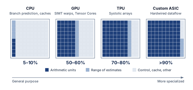
Figure 2: **The Accelerator Spectrum**: Each die is drawn as a grid of 100 cells divided between arithmetic units (dark) and control, cache, and other logic (light), with the medium cells marking the spread of each approximate, illustrative share. Read left to right, the arithmetic share grows from 5 to 10 percent on a CPU to over 90 percent on a custom ASIC, because hardwired dataflow replaces instruction fetch, decode, and scheduling; each step buys throughput per watt by narrowing the range of model architectures the silicon runs well.

Along the spectrum of figure 2, GPUs retain substantial programmability and provide 10–100$\times$ the matrix throughput of CPUs, while custom ASICs at the far end hardwire a specific dataflow for maximum efficiency at the cost of flexibility. The spectrum is not a ranking from “bad” (general-purpose CPU) to “good” (custom ASIC). It is a continuum of trade-offs in which each position is the best match for a different combination of workload characteristics and deployment constraints.

GPUs represent the first major step away from general-purpose computing toward massive parallelism while retaining programmability. An NVIDIA H100, for example, contains 16,896 CUDA cores organized into 132 streaming multiprocessors (SMs) that keep thousands of threads in flight under the single instruction, multiple threads (SIMT) model, so a programmer-written kernel can express any mathematical operation, from convolutions to attention to custom loss functions. Neural network operations have uniform enough control flow that this programmability costs the GPU little on ML workloads.

TPUs specialize the matrix dataflow while retaining other units for operations that do not map onto it. Google’s Tensor Processing Units use a systolic array¹ architecture, a fixed grid of multiply-accumulate (MAC) units that pass operands and partial results between neighboring cells on a regular schedule, so local reuse replaces per-operation instruction fetch and memory traffic. The complete accelerator still needs control, data movement, and execution of nonmatrix operations.

¹ Systolic array: From Greek systole (contraction), the name describes data pulsing through a grid of processing elements in a heart-like rhythm. Kung and Leiserson (1979) proposed the design for VLSI chips whose limiting resource was memory access rather than logic (Kung 1982): each operand fetched once is reused by every cell it passes. That ratio of computation to memory traffic is exactly what matrix multiplication at ML scale rewards.

Kung, Hsiang Tsung, and Charles E Leiserson. 1979. “Systolic Arrays (for VLSI).” Sparse Matrix Proceedings 1978 1: 256–82.

Kung, H. T. 1982. “Why Systolic Architectures?” Computer 15 (1): 37–46. https://doi.org/10.1109/mc.1982.1653825.

The cost of this efficiency is reduced programmability. Models must be compiled through Accelerated Linear Algebra (XLA), which maps high-level operations onto the fixed dataflow. Workloads with irregular control flow or dynamic shapes may not map well to this architecture, and the compilation process itself can be time-consuming (minutes to hours for complex models), which slows the iteration cycle during model development.

The programming model distinction between GPUs and TPUs has practical implications for organizational decisions. A research team that frequently adds custom operations, such as new attention patterns or activation functions, needs a path to implement them as kernels without waiting for compiler support, and must check how each platform expresses and optimizes those operations. A team running a stable computation at scale can place more weight on sustained utilization and compilation cost amortized over many runs. CUDA kernel support and XLA graph compilation offer different development paths, but neither establishes a utilization advantage without evaluating the workload and implementation. Software fit belongs in the hardware comparison because unsupported or poorly mapped work can leave specialized arithmetic idle.

Example 2.1: The TPU origin story

Scenario: In 2013, Google projected that if users spoke to Android phones for 3 minutes per day using voice search, handling the inference load on general-purpose CPUs would require doubling data center compute capacity at prohibitive cost (Jouppi et al. 2017).

Diagnosis: Standard CPU architectures paid a heavy generality tax, spending significant silicon area and power on out-of-order execution, branch prediction, and complex caches rather than matrix multiplication throughput.

Systems lesson: Hardware specialization is economically justified when a workload is large, stable, and dominated by a single mathematical kernel (MatMul). The TPU v1 hardwired a $256 \times 256$ systolic array to deliver 92 TOPS (INT8) within a 75 W footprint, establishing custom ASIC accelerators in production serving infrastructure.

Custom ASICs occupy the specialized end of the spectrum, where the economics of silicon can justify giving up much of the general-purpose programmability. When an organization runs a stable workload at enormous scale, designing a chip specifically for that workload may become economically rational. A custom ASIC can improve energy per operation and sustained utilization on its target workload by removing features that computation does not require.

Tesla’s Dojo D1 chip, for example, is optimized for the spatial and temporal structure of video-based vision models. Its hundreds of tightly coupled processing nodes are designed around the dataflow needs of Tesla’s vision pipeline, with on-chip SRAM sized to keep spatial tiles close to the compute units. This reduces the repeated round-trips to off-chip memory that a general-purpose GPU would require for the same computation. AWS Trainium takes a different approach, targeting the broad category of Transformer training rather than a single model. Trainium systems combine compiler-managed memory scheduling with hardware-assisted collective communication, so common training patterns such as tensor-parallel synchronization and data-parallel reductions can be optimized in the accelerator fabric rather than handled entirely by host software.

The risk of custom silicon follows from the same specialization. A change in the dominant model architecture can reduce the value of a fixed dataflow if the new operators, tensor shapes, or memory demands map poorly onto it. Sharing matrix operations across model families can preserve some of that investment, so a change from convolutional neural networks (CNNs) to Transformers does not by itself make an accelerator unusable. The forecasting window is long. Even Google’s first TPU, a high-priority project, took 15 months to design, verify, build, and deploy (Jouppi et al. 2017), and a chip then serves for several years more, so the design decision must anticipate which operations will remain useful years after the workload was profiled, and how much flexibility is needed for the rest. In 2015, few would have predicted that attention-based Transformers would replace CNNs as the dominant architecture within five years, a span of only a few ASIC design cycles.

Custom silicon is therefore a bet on workload stability, and the organizations that make this bet are typically those with enough scale to justify a large up-front design investment and enough workload volume to amortize that NRE (nonrecurring engineering) cost across many chips. Google can justify the TPU’s development cost because high-volume services such as Search, YouTube recommendations, and Gmail spam filtering can amortize a shared accelerator platform. A research lab running a few hundred GPUs cannot justify the same investment.

The bet can pay off when workloads are stable. The first-generation TPU reported 30–80$\times$ the performance per watt of contemporary GPUs and CPUs on its inference workloads (Jouppi et al. 2017), and TPU v4 reported 1.3–1.9$\times$ lower power than the A100 for similar-sized training systems (Jouppi et al. 2023). A workload shift can strand that advantage because the chip’s fixed dataflow may not accommodate a substantially different computational pattern. Pushing the locality argument further raises a question of physical scale: whether the compute fabric can expand to the size of an entire wafer.

Jouppi, Norman P., Cliff Young, Nishant Patil, David Patterson, Gaurav Agrawal, Raminder Bajwa, Sarah Bates, et al. 2017. “In-Datacenter Performance Analysis of a Tensor Processing Unit.” Proceedings of the 44th Annual International Symposium on Computer Architecture, ISCA ’17, 1–12. https://doi.org/10.1145/3079856.3080246.

Jouppi, Norm, George Kurian, Sheng Li, Peter Ma, Rahul Nagarajan, Lifeng Nai, Nishant Patil, et al. 2023. “TPU v4: An Optically Reconfigurable Supercomputer for Machine Learning with Hardware Support for Embeddings.” Proceedings of the 50th Annual International Symposium on Computer Architecture, 1–14. https://doi.org/10.1145/3579371.3589350.

2.2.1 Wafer-scale engines

Slicing a silicon wafer into discrete chips forces every exchange between accelerators to leave the die and cross slower, higher-energy package, board, or rack links. Wafer-scale engines (WSE) avoid those crossings by keeping most of a silicon wafer intact as one continuous compute fabric the size of a dinner plate, as in the Cerebras WSE-3, rather than dicing the wafer and reconnecting the pieces across packages and boards.

For its 2024 WSE-3 configuration, Cerebras reported 900,000 AI-optimized cores, 44 GB of distributed on-chip SRAM, and 21 PB/s of aggregate memory bandwidth in its registration filing (Cerebras Systems 2024). These specifications are not directly comparable to GPU-cluster peak FLOP/s or high-bandwidth memory (HBM) bandwidth because the architectures expose different dataflows, memory organizations, precisions, and workload mappings. The durable comparison is topological: on-wafer links avoid package-, board-, and rack-level transfers for work that maps onto the fabric.

Cerebras Systems. 2024. Cerebras Systems, Inc. Registration Statement on Form S-1.

Systems, Cerebras. 2021. “Wafer-Scale Deep Learning Acceleration with the Cerebras CS-2.” Cerebras Technical Paper 2021.

A multi-GPU chassis and a wafer-scale engine draw their package and board boundaries in different places (figure 3). The eight GPUs of a chassis exchange state through NVSwitch, and transfers to other nodes cross the external network. A wafer-scale engine instead routes between 900,000 on-wafer cores on the 300 mm wafer. Defect-aware routing lets the fabric use working regions despite local manufacturing flaws. In the documented CS-2 configuration, twelve power supplies in a 9+3 redundant arrangement could deliver up to 23 kW to the WSE-2 (Systems 2021). That configuration-specific design illustrates why wafer-scale power delivery and cooling require system-level liquid-cooling hardware rather than a conventional accelerator heatsink.

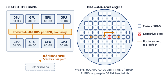
Figure 3: **Wafer-Scale Engine (WSE) Architecture**: A DGX H100 node (left) joins eight separately packaged GPUs through an NVSwitch fabric and must leave the chassis over InfiniBand to reach other nodes, so every exchange crosses a package, board, or network boundary. A WSE (right) instead uses most of a 300 mm wafer as one routed mesh of cores, each with local SRAM; defect-aware routing steers traffic around unusable cores, and the on-wafer mesh replaces off-package transfers for mapped operations. The WSE-3 figures are the vendor’s reported totals and are not directly comparable to GPU HBM bandwidth.

Wafer-scale engines specialize the physical architecture while retaining flexibility in the computational model through programmable cores. That trade-off exchanges manufacturing complexity and defect-aware routing for an on-wafer fabric that replaces package- and board-level communication between its cores, though SRAM capacity and data injection still constrain which parts of a workload can benefit from that locality. Where the wafer-scale engine removes the package boundary by never dicing the wafer, chiplet designs keep the package and change what goes inside it.

2.2.2 Chiplet-based accelerators

Once a monolithic processor die grows to the optical exposure limit of a lithography scanner, adding more arithmetic units or HBM controllers on a single piece of silicon becomes impossible without stitching exposures at lower yield and sharply higher cost. Chiplet architectures, exemplified by NVIDIA’s Blackwell and AMD’s Instinct MI300 series, break through that ceiling by partitioning the processor into smaller dies connected by a high-bandwidth die-to-die interconnect on a common package substrate. This approach addresses two physical limits that constrain monolithic designs.

First, the maximum die size is capped by the photolithographic reticle limit, the largest area that a lithography scanner can pattern in a single exposure. The limit comes from the optics of photolithography, because the lens system of an extreme-ultraviolet (EUV) scanner projects a pattern onto a field of only about $26{\times}33$ mm (858 mm²). A larger die would need multiple exposures stitched together, which is technically possible but sharply raises cost and lowers yield. The limit caps the number of Tensor Cores, SMs, and HBM stacks a monolithic GPU can integrate. Chiplet designs bypass this limit by placing multiple dies on a single package, with the B200’s two reticle-limited dies effectively creating a processor of about 1,700 mm².

Second, manufacturing yield depends on die area and defect density. Under the standard Poisson defect model, the fraction of defect-free dies falls exponentially with die area at a fixed defect density, because a single killer defect anywhere on the die can render it unusable. Smaller dies expose less area to each defect, and testing can select known-good chiplets before package assembly, so one defect discards a small die rather than a reticle-sized one. The resulting yield advantage must be weighed against the cost and yield of the package, its interconnects, and the additional testing. Chiplets change the manufacturing trade-off; they do not guarantee a lower cost per unit of compute.

The trade-off is the die-to-die interconnect. Communication between chiplets within a package is faster than communication between packages (NVLink) but slower than communication within a single monolithic die (the on-die mesh network). Workloads that generate frequent, fine-grained communication between processing elements (such as operations that share data between nonadjacent SMs) may experience a latency penalty when those SMs reside on different chiplets. GPU vendors mitigate this by making the die-to-die link transparent to the programmer, so the software sees a single logical GPU regardless of the underlying chiplet topology.

2.2.3 Evolution of GPU architectures

NVIDIA’s data center GPUs show the specialization bet placed one generation at a time. Each generation added hardware aimed at a bottleneck that production ML workloads had exposed, rather than more transistors of the same kind. The Volta architecture (2017) introduced the first-generation Tensor Core, dedicated matrix-multiply-accumulate hardware placed beside the existing CUDA cores, because neural network training spends most of its time in matrix multiplications. Volta accelerated that dominant pattern without giving up the general-purpose programmability that made GPUs attractive for research.

The Ampere architecture (2020) expanded Tensor Core support to TF32 and BF16 and introduced Multi-Instance GPU (MIG), which partitions one GPU into up to seven isolated instances so that several inference workloads can share it. The change that mattered most for infrastructure was Ampere’s third-generation NVLink, which doubled per-GPU bandwidth to 600 GB/s from Volta’s 300 GB/s, the bandwidth that tensor parallelism needs because it splits each layer’s matrices across GPUs.

The Hopper architecture (2022) added the Transformer Engine, whose FP8 recipes and autocast integration run supported Transformer operations in FP8 with managed scaling while retaining higher precision where the configured recipe or implementation requires it. Hopper also introduced NVLink 4.0 at 900 GB/s per GPU and the NVLink Switch, enabling NVLink connectivity beyond the 8-GPU boundary.

The Blackwell architecture (2024) takes the chiplet route of section 2.2.2 past the 858 mm² reticle limit. The B200 pairs two GPU dies in one package over a 10 TB/s die-to-die link, fast enough that the two dies appear to software as a single logical GPU for many operations, and its fifth-generation NVLink doubles intra-node bandwidth again to 1800 GB/s per GPU. Its FP8 rating in table 1 is not an FP16/BF16 figure; those comparisons should use the lower precision-specific vendor rate.

Each generation thus targeted the bottleneck its predecessor exposed. Volta added dedicated matrix hardware, Ampere widened mixed-precision support, Hopper added FP8 for Transformer workloads, and Blackwell worked around the die-size limit with two dies in one package. Because architects choose those targets by profiling the workloads of their era, accelerator design follows model architecture, which is why Transformer workloads have shaped accelerator design since 2017.

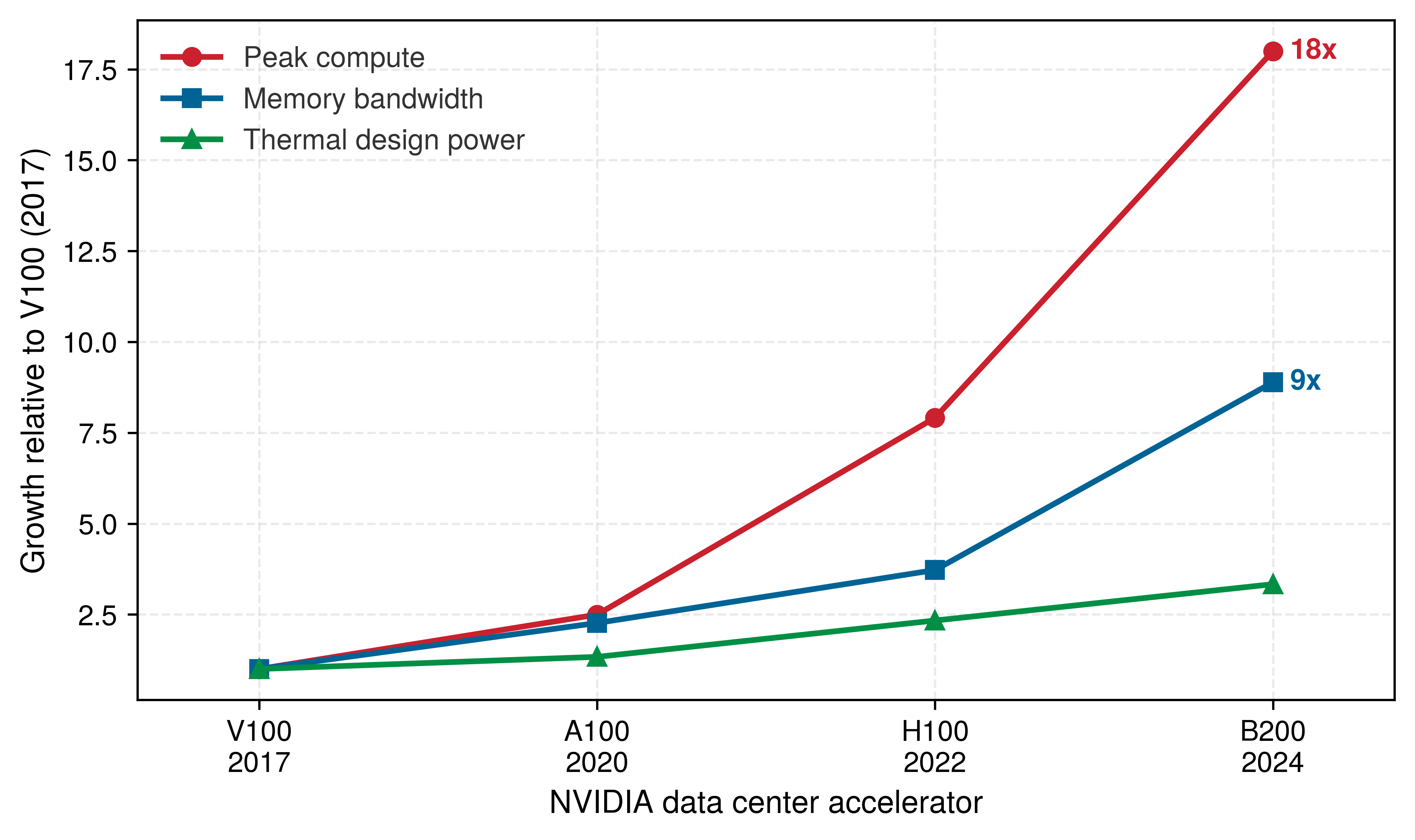
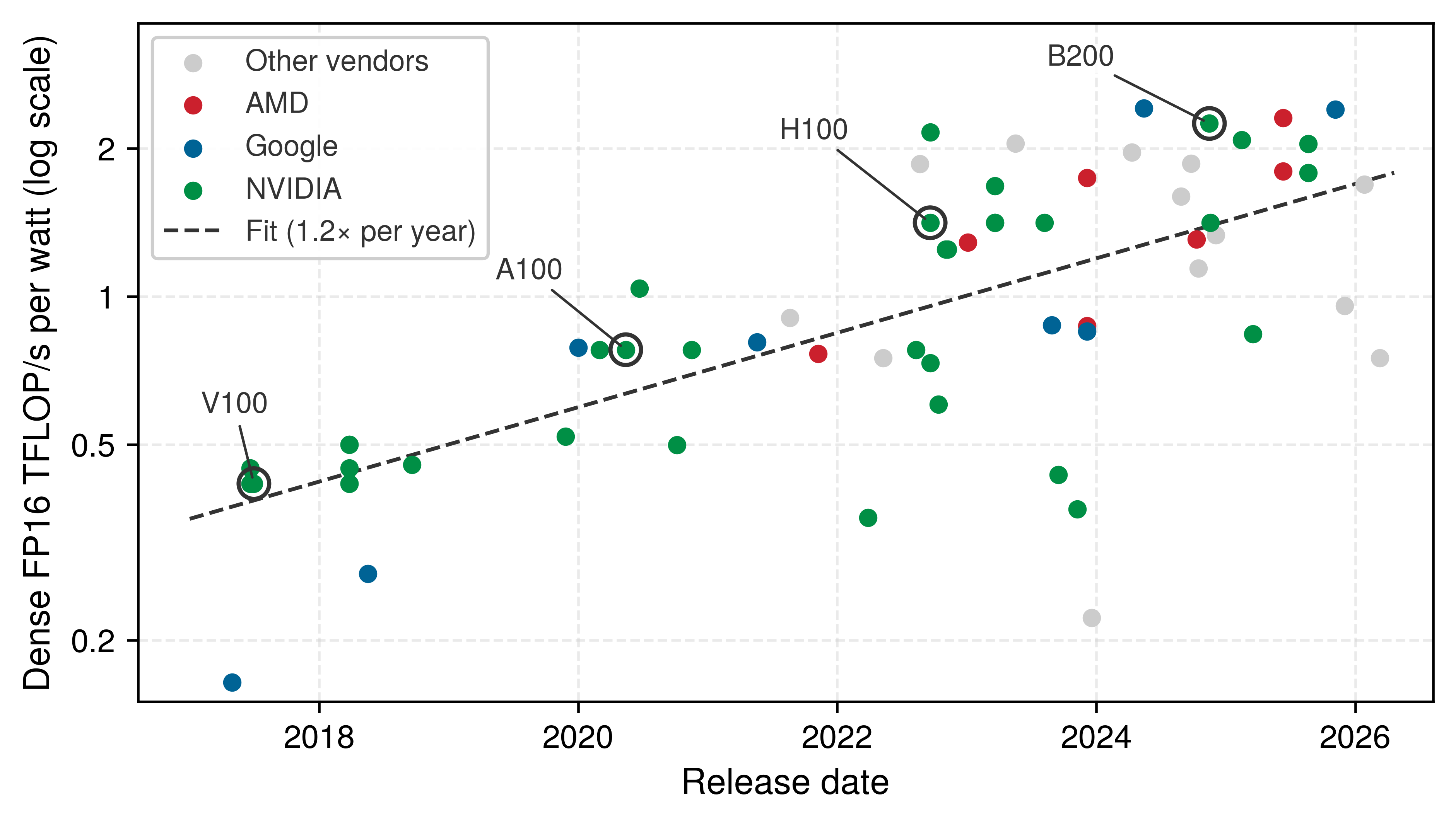
Because accelerator generations turn over faster than the facility that houses them, a data center must anticipate refresh cycles before the first rack arrives. Those generations also changed interconnect capacity and power (table 1). From V100 to B200, dense FP16 throughput rose 18$\times$, memory bandwidth 8.9$\times$, and thermal design power (TDP) 3.3$\times$ (figure 4). These are growth multiples over the whole span, not annual rates, and their ratios carry the planning lesson. Each byte delivered from memory must now feed about twice as many operations, and each watt of the power allowance supplies more than five times as many peak operations. The first ratio changes which workloads can approach peak throughput; the second, multiplied by device count, sets the proposed rack load. A facility refreshed only for compute density therefore outruns both its memory delivery and its cooling envelope.

Figure 4: **Compute, Bandwidth, and Power Scale at Three Different Rates**: Dense FP16 Tensor throughput, memory bandwidth, and thermal design power for NVIDIA data center accelerators, normalized to the V100 on a log scale, where the shaded gap between the compute and bandwidth lines is the growth in arithmetic intensity a kernel needs to stay compute-bound. Compute rises 18$\times$, bandwidth 8.9$\times$, and TDP 3.3$\times$, so the endpoint gains in arithmetic exceed the gains in memory bandwidth and power allowance. These are peak specifications, not measured application throughput. Specifications come from the MLSysIM hardware registry.

Table 1: NVIDIA GPU Architecture Evolution: Each generation introduces architectural features targeted at the dominant ML workload pattern of its era. Efficiency rises substantially but unevenly across generations, while NVLink bandwidth increases from 300 GB/s on V100 to 1,800 GB/s on B200, with a smaller 1.5$\times$ A100-to-H100 step between the larger doubling jumps.

Architecture	Year	Key innovation	Peak tensor	TDP	NVLink BW
Volta (V100)	2017	First Tensor Core	125 TFLOP/s FP16	300 W	300 GB/s
Ampere (A100)	2020	Multi-precision, MIG	312 TFLOP/s FP16	400 W	600 GB/s
Hopper (H100)	2022	Transformer Engine, FP8	1,979 TFLOP/s FP8	700 W	900 GB/s
Blackwell (B200)	2024	Dual-die, NVLink 5	4,500 TFLOP/s FP8	1000 W	1,800 GB/s

Because table 1 mixes FP16 and FP8 peaks, its per-watt efficiency must be read at fixed precision. At dense FP16, dividing each generation’s peak throughput by its TDP (table 2) gives a V100-to-B200 gain of 5.4× in peak throughput per watt, the more-than-fivefold figure above, against 18× in raw throughput; the rest of the raw gain came from a power allowance that itself rose 3.3×. The same caution applies between adjacent generations. The H100’s FP8 peak per watt of TDP is 6.8× the V100’s FP16 figure, but a factor of two of that comes from the change of precision, and at equal FP16 precision the gain is 3.4×. Facilities must therefore accommodate higher device power as well as greater arithmetic capacity, which connects this trend to the power wall in section 2.6.1.

Table 2: Power Efficiency across GPU Generations: Dense FP16 tensor arithmetic peak divided by accelerator TDP, with no sparsity multiplier. These ratios compare arithmetic ceilings, not measured training throughput or facility energy. Matched workload measurements must also include achieved utilization, memory and communication stalls, and non-accelerator power.

Generation	Dense FP16 peak TFLOP/s	TDP (W)	TFLOP/s per watt	Relative efficiency
V100 (2017)	125 TFLOP/s (FP16)	300 W	0.42 TFLOP/s/W	1×
A100 (2020)	312 TFLOP/s (FP16)	400 W	0.78 TFLOP/s/W	1.9×
H100 (2022)	989 TFLOP/s (FP16)	700 W	1.41 TFLOP/s/W	3.4×
B200 (2024)	2250 TFLOP/s (FP16)	1000 W	2.25 TFLOP/s/W	5.4×

The four generations in table 2 sit on a broader and slower trend. Across the 64 accelerator models released since 2017 for which Epoch AI records both a dense FP16 tensor rate and a TDP, from every major vendor, peak arithmetic per watt improved about 1.2× per year, doubling roughly every 4 years (figure 5) (Epoch AI 2026b). The leading NVIDIA parts improved faster, 5.4× from the V100 to the B200 in seven years (the fixed-precision gain noted earlier), because frontier devices adopt new process nodes and tensor formats first. A fleet on a 4-year refresh cycle therefore gains about 2× in peak arithmetic per watt each cycle on the broad trend. Peak ratios bound what a refresh can deliver, and only measurements at the workload level decide how much of it a given fleet realizes.

↪ How these peak ratios screen a fleet refresh decision is developed in Refresh screening.

Figure 5: **Peak Arithmetic per Watt over Time**: Dense FP16 tensor throughput divided by TDP for ML accelerators released since 2017, on a logarithmic axis, colored by vendor. The dashed line is a least-squares fit across all devices; the four GPUs of table 2 are circled and labeled. The ratio compares arithmetic ceilings, not measured energy per workload. Data from Epoch AI (2026b).

2.2.4 Evolution of TPU architectures

Faster per-chip arithmetic leaves a cluster stalled if inter-chip collectives still have to traverse host CPUs and general-purpose PCIe switches. Google’s TPU trajectory attacked that bottleneck directly by treating the multi-rack pod, rather than the individual chip, as its unit of design from its second generation onward. While GPUs emphasize peak per-chip throughput and software flexibility (CUDA), every TPU chip since TPU v2 integrates dedicated inter-chip interconnect (ICI) links that route traffic directly between accelerators without touching the host CPU.

The generation sequence shows how that pod-first design moved from inference to training. After the inference-only TPU v1 of the origin story, TPU v2 (2017) and TPU v3 (2018) shifted the architecture toward training by adding bfloat16 (BF16), avoiding the dynamic range problems of standard FP16, and scaling the pod concept until a TPU v3 pod joined 1,024 chips with about 126 PFLOP/s of aggregate BF16 peak. TPU v4 (2021) extended the same logic into the network itself: it added an optical circuit switch so the physical topology could be reconfigured for different workloads, introduced SparseCore units that accelerate embedding lookups, and raised per-chip BF16 throughput to 275 TFLOP/s.

The TPU v5p (2023) continued this pod-scale design for high-end training. It features 459 TFLOP/s of BF16 compute, 95 GB of HBM2e with 2,760 GB/s memory bandwidth, and 1,200 GB/s bidirectional ICI bandwidth per chip. The ICI figure matters for hardware selection because collectives such as AllReduce, which combine values such as gradient sums across a group of accelerators and return the result to every participant, run over those links; AllReduce develops the complexity model and algorithm choices that determine when those exchanges limit training throughput. The pod-first design took shape over successive TPU generations (table 3).

Table 3: Google TPU Architecture Evolution: The TPU’s development highlights a “pod-first” design philosophy where inter-chip interconnect bandwidth and compiler-level optimization (XLA) are as important as peak per-chip arithmetic. Note: TPU v1 was INT8 only.

Generation	Year	Key innovation	Peak BF16	HBM	ICI BW (aggregate, one direction)
TPU v1	2015	Systolic array (inference)	92 TOPS*	—	—
TPU v2	2017	High-bandwidth memory	46 TFLOP/s	16 GB	248 GB/s
TPU v3	2018	Liquid cooling, pod scale	123 TFLOP/s	32 GB	280 GB/s
TPU v4	2021	Optical switch, SparseCore	275 TFLOP/s	32 GB	300 GB/s
TPU v5p	2023	Larger pods, HBM2e	459 TFLOP/s	95 GB	600 GB/s

The GPU and TPU lines follow two design philosophies (table 1, table 3). GPU evolution packs more arithmetic, in ever lower-precision Tensor Core formats, onto one package, and turns to chiplets once a single die reaches its size limit. TPU evolution treats the pod as the product. Per-chip arithmetic matters, but inter-chip bandwidth and reconfigurability decide how much of it a large training job can use. Both lines combine local computation with memory and interconnect improvements; they place those resources differently. The warehouse-scale perspective of The shift to the warehouse-scale computer treats chip throughput, collective bandwidth, and reconfigurability as parts of one system (Barroso et al. 2019), so the useful comparison is how each candidate sustains the intended workload across that complete system.

2.2.5 Matrix units

Both lines concentrate their peak arithmetic in specialized matrix units, called Tensor Cores on NVIDIA GPUs and Matrix Multiply Units (MXUs) on Google TPUs. A Tensor Core executes matrix-multiply-accumulate instructions of the form $\MatrixMultiplyDestination = \GemmLeftOperand\times \GemmRightOperand+ \GemmOutputMatrix$ on small tile matrices, concentrating the dominant neural-network operation in dedicated hardware that supplies most of the chip’s peak arithmetic.

With 528 Tensor Cores across the chip (4 per SM, 132 SMs), the H100 reaches its 989 TFLOP/s dense FP16/BF16 peak. The important systems point is the architectural specialization rather than the exact per-cycle instruction accounting. The die dedicates a large fraction of its arithmetic area to dense tiled matrix operations rather than general-purpose scalar execution.

Google’s MXUs organize multiply-accumulate units into the systolic array introduced with the TPU above. In the MXU’s weight-stationary dataflow, a weight tile stays resident in the array while activations stream through it, so every operand fetched from memory is reused by an entire row or column of cells, the reuse that a Tensor Core kernel obtains by staging tiles in shared memory and registers. Each TPU v5p chip contains two TPU cores (which Google calls TensorCores, a name unrelated to NVIDIA’s Tensor Cores) with four $128{\times}128$ MXUs each, together providing 459 TFLOP/s of BF16 throughput. Approaching that peak requires compatible tile shapes and a sustained operand supply; pipeline fill, partial tiles, and dependencies can leave cells idle. Vector and scalar units handle other operations, so complete-workload efficiency depends on how computation maps across the accelerator.

For our 175B model, compiler and kernel support determine how much work reaches the specialized arithmetic units. CUDA kernels can combine matrix operations with thread-level work, while XLA maps the computation graph onto the TPU dataflow. In either stack, fusion keeps intermediate results in registers or shared memory instead of repeatedly writing them to HBM. Sustained throughput therefore depends on operation coverage and data reuse as well as the matrix units themselves.

Definition 2.1: Tensor core

Tensor Core is a specialized ML accelerator hardware unit that performs a fused matrix-multiply-accumulate operation $\MatrixMultiplyDestination = \GemmLeftOperand\times \GemmRightOperand+ \GemmOutputMatrix$ on small tiles (for example, $16{\times}8{\times}16$ in BF16) as a single hardware instruction, delivering dramatically higher throughput than general-purpose CUDA cores by trading programmability for fixed-function matrix arithmetic.

Significance: Tensor Cores provide the bulk of the H100’s 989 TFLOP/s FP16/BF16 peak (and ~1,979 TFLOP/s at FP8), roughly 14.8× the ~67 TFLOP/s delivered by CUDA (vector) cores alone. This comparison changes both the execution unit and precision. Reductions and element-wise operations in layer normalization or softmax require a different performance model; their throughput is not a fixed fraction of the matrix peak.
Distinction: A Tensor Core is a fixed-function matrix-multiply-accumulate unit, not a faster general-purpose core. CUDA cores execute arbitrary scalar and vector work; Tensor Cores execute only the tiled $\MatrixMultiplyDestination = \GemmLeftOperand\times \GemmRightOperand+ \GemmOutputMatrix$ primitive, which is why peak throughput and delivered throughput diverge so sharply by workload.
Common pitfall: A frequent misconception is that all GPU operations benefit from Tensor Cores. Operations must map to the $\MatrixMultiplyDestination = \GemmLeftOperand\times \GemmRightOperand+ \GemmOutputMatrix$ tile computation to use those units. Element-wise activations, normalization, and embedding lookups have different execution and data-access demands. A fixed 10–30$\times$ penalty per FLOP is not a workload-independent model for their runtime.

Table 4: The Accelerator Spectrum: The architectures place arithmetic, control, and memory differently. Specialization can improve throughput per watt when the workload and software stack use its dataflow; the table does not rank measured efficiency. Wafer-scale engines replace package and board boundaries with an on-wafer fabric of programmable cores.

Feature	CPU	GPU (H100)	TPU (v5p)	Wafer-scale	Custom ASIC
Arithmetic core	Scalar/vector	Tensor Core	Systolic array	RISC-style core	Fixed dataflow
Execution	Instruction	SIMT	Data-driven	Dataflow	Hardwired
Memory control	Cache	L1/L2 + HBM	Scratchpad	On-chip SRAM	Compiler-managed
Flexibility	Extreme	High	Moderate	High	Low

Across the whole spectrum, from CPU to custom ASIC, the architectures differ in arithmetic core, execution model, and memory control (table 4). For the 175B running model, the choice among these columns is not purely about peak FLOP/s. A research lab experimenting with novel architectures weekly can justify the GPU’s generality tax by its flexibility. An organization deploying a fixed Transformer at scale for years may find that the TPU’s dataflow efficiency or a custom ASIC’s power advantage dominates total cost. The accelerator spectrum is ultimately an economic question of how much flexibility can be surrendered, given the stability of the workload. Even when the H100’s arithmetic engine reaches 1,979 TFLOP/s in its advertised low-precision mode, eligible operations approach that throughput only when data reaches the compute units fast enough. Accelerator selection therefore requires a second comparison, between the workload’s data demand and the memory system that feeds the arithmetic.

Self-Check: Question

A hardware vendor transitions their next-generation accelerator from a monolithic $800\text{ mm}^2$ die to a dual-die chiplet architecture (such as the NVIDIA B200 with an equivalent area of about $1{,}700\text{ mm}^2$) connected on a single package. What physical constraint is this transition primarily designed to bypass, and what trade-off does it introduce?
1. It bypasses the memory wall by moving all memory on-chip, but introduces warp divergence because threads must synchronize across the die boundary.
2. It bypasses the photolithographic reticle limit ($\approx 858\text{ mm}^2$) and improves manufacturing yield, but introduces a die-to-die interconnect that is slower than a continuous on-die mesh.
3. It bypasses the maximum TDP limit of a single package by separating thermal loads into different server chassis, but requires developers to write separate CUDA kernels for each chiplet.
4. It bypasses the communication wall by replacing electrical copper signaling with optical waveguides, but increases the generality tax of control logic.
A research lab frequently experiments with novel, custom attention patterns and dynamic sparsity, while a production platform team trains a fixed standard Transformer at massive scale for months. Compare the systems trade-offs of choosing GPUs (CUDA) versus TPUs (XLA) for these two organizational teams.
Comparing the V100 and B200 at dense FP16 separates peak throughput growth from growth in throughput per TDP watt. Which statement correctly captures that difference and its infrastructure consequence?
1. Peak throughput per TDP watt grew faster than peak throughput, allowing higher-density clusters to ignore power delivery.
2. Both peak throughput and power efficiency scaled linearly at exactly the same rate, confirming that Dennard scaling remains fully active in modern 4nm nodes.
3. Peak dense FP16 throughput grew about 18 times while peak throughput per TDP watt grew about 5.4 times, so facilities must accommodate higher device power as well as greater arithmetic capacity.
4. Peak throughput plateaued after Volta (V100), meaning all recent performance gains stem exclusively from host CPU software optimizations.
The area and energy devoted by a processor to capabilities outside the dominant neural network matrix-multiplication workload, such as out-of-order scheduling, branch prediction, and complex hardware caches, is called the ____.
Arrange the following processor architectures in ascending order of the approximate percentage of their die area devoted strictly to arithmetic units (from lowest arithmetic die allocation to highest): (1) Google TPU (systolic array), (2) Purpose-built custom ASIC, (3) General-purpose server CPU, (4) NVIDIA GPU (with Tensor Cores).

See Answers →

2.3 The Memory Wall

As arithmetic throughput grows faster than data-access speed, compute units can spend more time waiting for operands. This divergence is known as the memory wall (Wulf and McKee 1995). While transistor scaling has increased logic performance by orders of magnitude, the interconnects that feed data to those cores have not kept pace. Neural networks can require large weight and activation streams, making bandwidth rather than compute the governing constraint for some inference and training regimes.

Wulf, Wm. A., and Sally A. McKee. 1995. “Hitting the Memory Wall: Implications of the Obvious.” ACM SIGARCH Computer Architecture News 23 (1): 20–24. https://doi.org/10.1145/216585.216588.

↪ The diagnostic table that maps memory-bound, compute-bound, and latency-bound symptoms to the optimizations that help is developed in Bottleneck diagnostic.

The implications are concrete in our running example. Our 175B model’s weights occupy 350 GB in FP16. In dense autoregressive decode at batch size 1, each generated token uses all of those weights, whose footprint far exceeds on-chip storage, so every token must stream them in from memory. Suppose, hypothetically, that one H100 could hold them. Streaming the whole 350 GB through that device’s HBM at about 3.35 TB/s takes over 100 ms per token, long enough to be a perceptible pause between generated words. No real H100 holds the model, so the figure is a floor on bandwidth demand rather than a prediction of deployed latency, but it shows that the memory wall is a delay a user can notice, not an abstract architectural ratio.

Three levers lower that floor. Sharding spreads the weights across more memory paths, so each path streams fewer bytes. Quantization shrinks the bytes themselves. Reuse lets each fetched byte feed more arithmetic, which HBM’s bandwidth and on-chip tiling make possible. The Roofline Model, recapped for one machine in The roofline bound, tests whether the resulting data supply can feed the arithmetic units. Its ridge point, peak arithmetic divided by memory bandwidth, is the number of operations a kernel must perform per byte fetched before arithmetic rather than memory becomes the limit. The ridge point recurs throughout the analysis below, and section 2.3.2 evaluates it for the H100. Where each architecture places its bytes sets how much bandwidth those levers can draw on (figure 6), because moving the active working set closer to arithmetic increases available bandwidth while reducing the capacity that can reside there.

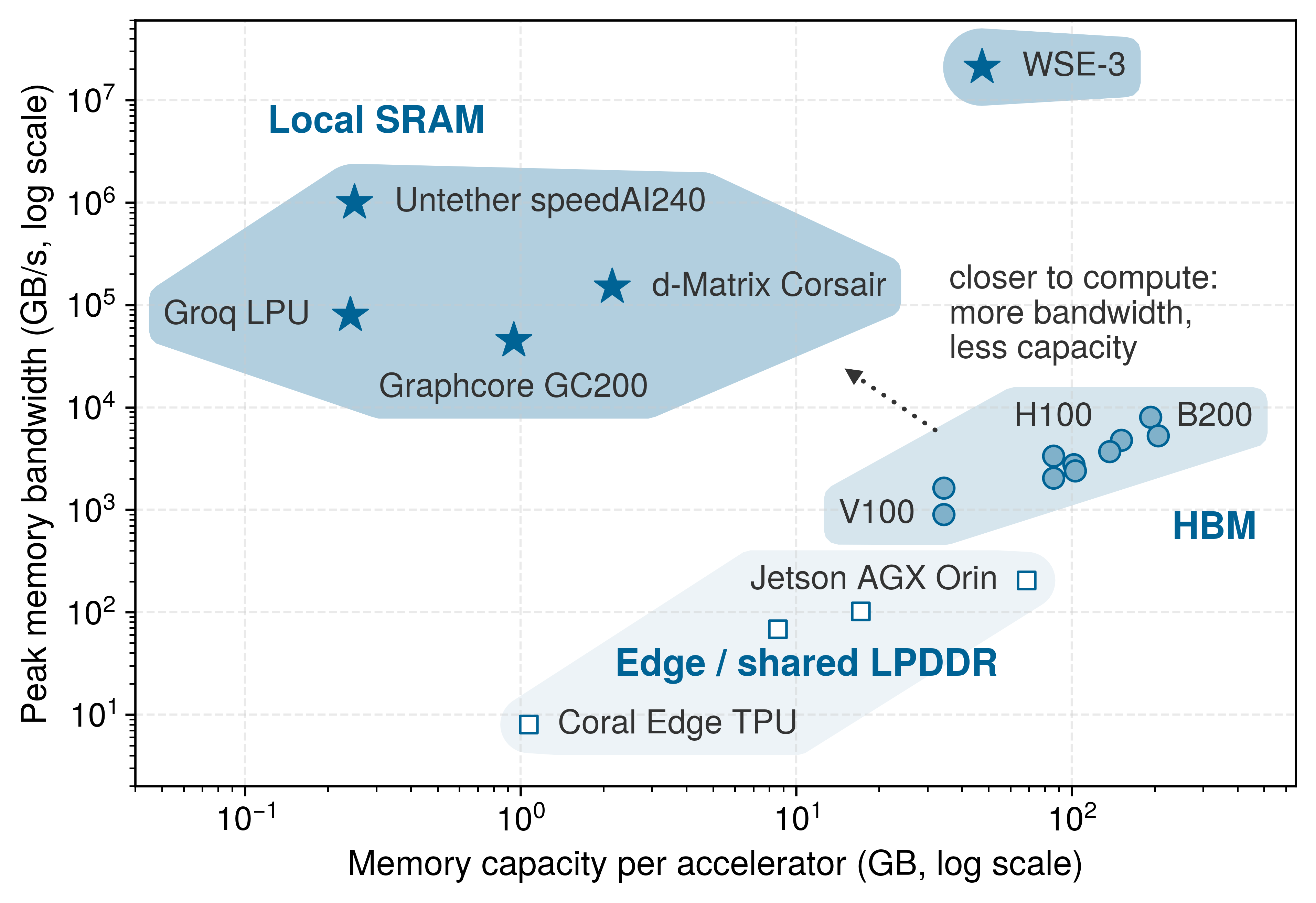
Figure 6: **Accelerator Memory Tiers**: Peak memory bandwidth and capacity separate local-SRAM designs (solid stars), HBM accelerators (half-tone filled circles), and edge and shared-LPDDR devices (hollow squares); all three are memory, so they share one hue and differ by marker. The dotted arrow marks the design trade-off: moving data closer to compute raises bandwidth but reduces capacity.

Accelerators do not line up along a single performance axis; they fall into structural clusters according to where each architecture places its bytes (figure 6). Edge devices in the lower band keep memory cheap and compact, but their bandwidth remains constrained, and the devices of Archetype C (Federated MobileNet) sit in that corner. On each device, the binding limit is the power envelope that bounds compute. A phone-class device sustains only 2 W to 3 W, while one H100’s thermal envelope is about 233× larger. A federated fleet therefore grows by adding devices rather than by moving up the memory tiers, and at fleet scale, as Three systems archetypes noted, communication and which devices participate in each round limit progress as well.

Within the data center tiers, HBM moves memory onto the accelerator package, buying enough capacity and enough bandwidth for active model state. Local-SRAM designs push the working set still closer to arithmetic, buying extraordinary bandwidth at the cost of much smaller resident capacity. That tier map explains why HBM is the next engineering response. HBM is not the fastest memory in the system, but it is the highest-bandwidth tier that can hold tens to hundreds of gigabytes next to the compute die.

↪ The power, thermal, and memory limits of phone-class edge devices are developed in Design Constraints.

2.3.1 HBM and the memory wall

An H100 can execute 1,979 TFLOP/s of low-precision matrix arithmetic, but the batch-1 weight-streaming example for our 175B model supplies too little reuse to approach that peak. In a bandwidth-floor model its arithmetic units would use well under 1 percent of the matrix peak while the weights stream in. The limiting resource is the speed of delivery relative to multiplication. Once weights fit through sharding or compression, the serving path must still deliver the active shards at the required rate. Additional arithmetic capacity alone does not raise a binding bandwidth ceiling. HBM increases that data supply within the package.²

² HBM origin: Standardized by JEDEC in 2013 as a joint development between AMD and SK Hynix, originally for graphics cards. ML accelerators adopted HBM because neural networks share the same bandwidth-hungry, capacity-moderate access pattern as high-end rendering. Each HBM generation has roughly doubled bandwidth (128 GB/s in HBM1 to 1.2 TB/s per stack in HBM3e), yet the gap between memory bandwidth and arithmetic throughput continues to widen, which makes HBM a necessary but never sufficient response to the memory wall.

³ SRAM energy (pJ/bit): Reading a bit from an 8–32 KB on-chip SRAM array costs roughly 0.15–0.3 pJ at the 45 nm node (Horowitz 2014), while fetching a bit from HBM2 costs about 4 pJ (O’Connor et al. 2017). This order-of-magnitude energy difference is the physical driver behind kernel fusion: every intermediate result kept in SRAM instead of written to HBM saves both time and significant power and thermal headroom.

Horowitz, Mark. 2014. “1.1 Computing’s Energy Problem (and What We Can Do about It).” 2014 IEEE International Solid-State Circuits Conference Digest of Technical Papers (ISSCC), 10–14. https://doi.org/10.1109/isscc.2014.6757323.

O’Connor, Mike, Niladrish Chatterjee, Donghyuk Lee, John Wilson, Aditya Agrawal, Stephen W. Keckler, and William J. Dally. 2017. “Fine-Grained DRAM: Energy-Efficient DRAM for Extreme Bandwidth Systems.” Proceedings of the 50th Annual IEEE/ACM International Symposium on Microarchitecture, 41–54. https://doi.org/10.1145/3123939.3124545.

HBM is the bottom on-package tier of the accelerator memory hierarchy, beneath the register file, the L1 and shared memory (SRAM),³ and the L2 cache. Aggregate bandwidth falls from hundreds of TB/s at the registers to the 3.35 TB/s of the H100’s 80 GB of HBM3, while capacity grows in the opposite direction.

↪ The single-accelerator memory hierarchy, from registers and shared memory through HBM to host memory, is collected for reference in Accelerator Memory Hierarchy.

The bandwidth gap between registers and HBM is approximately 100$\times$, but that ratio alone does not specify stalled time. Utilization depends on arithmetic intensity, the floating-point operations performed per byte moved from memory (FLOP/byte), which tiling raises by staging matrix blocks on chip so that each fetched operand feeds many multiply-accumulate operations. Kernel-Level Levers collects tiling with the other kernel-level levers for reference.

↪ Arithmetic intensity and the boundary it draws between memory-bound and compute-bound work are collected for reference in Arithmetic Intensity Boundary.

Definition 2.2: HBM

HBM is a 3D-stacked DRAM architecture used by ML accelerators, with through-silicon vias (TSVs) connecting memory dies vertically within each stack and a wide interface across the package interposer connecting the stack to the processor.

Significance: HBM3 in the H100 delivers approximately 3.35 TB/s of memory bandwidth (roughly 17× DDR5’s ~200 GB/s) at roughly 4 pJ/bit for an HBM2-class stack (O’Connor et al. 2017) vs. roughly 20 pJ/bit for off-package DRAM (Horowitz 2014). This bandwidth sets the $\Bandwidth$ term of the single-machine iron law given in Iron Law Mapping, and the H100’s FP16 ridge point is approximately $989\,\text{TFLOP/s} / 3.35\,\text{TB/s} \approx 295$ FLOP/byte, so any operator with arithmetic intensity below 295 FLOP/byte (for example, single-request decode, which performs two FLOPs for every two-byte FP16 weight it reads) remains memory-bound even with HBM.
Distinction: Unlike socketed DDR memory, which communicates across centimeters of printed circuit board (PCB) trace, an HBM stack sits beside the processor on the package. Its micrometer-scale vertical connections can be 1,000$\times$ shorter than board traces, but the complete processor-to-memory path also crosses the interposer. The wide, short on-package interface raises bandwidth without relying on a proportionate increase in per-pin signaling rate.
Common pitfall: A frequent misconception is that HBM solves the memory wall. HBM moves the wall rather than eliminating it. From the V100 (900 GB/s with 125 TFLOP/s FP16) to the H100 (3.35 TB/s with 989 TFLOP/s FP16), peak arithmetic $(\PeakRate)$ grew faster than HBM bandwidth.

Traditional DDR memory connects to the processor through pins on the edge of a printed circuit board. Each DIMM communicates over a 64-bit bus, and even with multiple channels (8 channels is typical for a high-end server CPU), a modern server tops out at roughly 200 GB/s of aggregate memory bandwidth.

The physical distance from the DIMM slot to the processor die is measured in centimeters, and every centimeter of copper trace introduces capacitance, signal attenuation, and energy loss. At DDR5 data rates (4,800–6,400 MT/s per pin), the signal conditioning circuits must compensate for significant channel impairment, consuming substantial power per bit transferred. Increasing the data rate on these long traces requires progressively more power for signal conditioning, creating a diminishing-returns curve that DDR5 is already approaching.

HBM sidesteps that board-level degradation through 2.5D integration (figure 7). Instead of driving signals horizontally across centimeters of motherboard trace over a narrow 64-bit bus, it stacks DRAM dies vertically and places the stack beside the processor on a silicon interposer.

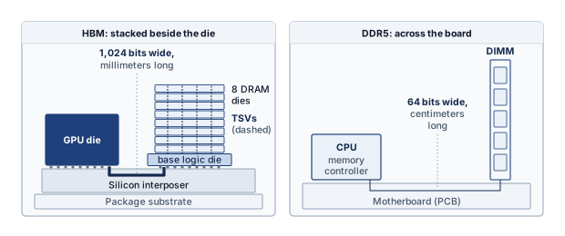
Figure 7: **HBM 3D-Stacked Architecture**: Left: high-bandwidth memory stacks DRAM dies on a base logic die, links them vertically with through-silicon vias (TSVs), and places the stack on a silicon interposer beside the GPU die, so each stack reaches the GPU over a 1,024-bit interface only millimeters long. Right: DDR5 instead sits on a DIMM across the motherboard, reached over a 64-bit channel through centimeters of board trace. The wider, shorter path raises bandwidth and lowers energy per bit, but HBM bandwidth and capacity remain finite, so the memory wall moves rather than disappears.

The vertical stacking changes how bandwidth scales. Rather than pushing signals faster through long copper traces (the DDR approach, which has diminishing returns), HBM multiplies the number of parallel signal paths. A single HBM stack bonds 8–12 DRAM dies, threading thousands of through-silicon vias (TSVs),⁴ copper pillars etched through each die, to form a 1024-bit-wide interface per stack, compared to 64 bits for a DDR5 channel. This 16$\times$ wider interface is the main source of HBM’s bandwidth advantage; HBM need not exceed DDR’s per-pin signaling rate. The processor and HBM stacks share a package and communicate across the silicon interposer, shortening the electrical path relative to socketed DIMMs. This packaging primarily improves bandwidth and energy per transferred bit; it does not by itself imply that complete HBM load latency is only a few nanoseconds.

⁴ TSV (through-silicon via): A vertical copper pillar, 5–10 micrometers in diameter, etched through a silicon die to connect stacked layers. Originally developed for CMOS image sensors in smartphone cameras, TSVs enabled HBM by replacing centimeters of PCB trace with tens of micrometers of vertical silicon, roughly a 1,000$\times$ shorter signal path, which is what lets a stack expose a 1024-bit interface within an accelerator’s power budget.

The shorter path also lowers transfer energy per bit by roughly 5$\times$, from approximately 20 pJ/bit for off-package DRAM (Horowitz 2014) to about 4 pJ/bit for HBM2 (O’Connor et al. 2017), because the short interconnects present less capacitance and need less driving current. The same reduced loading lets the 1024-bit interface run at moderate per-pin rates instead of the high-power signaling that long board traces require. Propagation delay shrinks by only a fraction of a nanosecond, small next to the DRAM array and controller delays that dominate access latency, so HBM’s advantage lies in bandwidth and energy per bit rather than in latency. Modern accelerators therefore widen the memory interface across an interposer rather than driving off-package pins faster; set side by side in table 5, the bandwidth, interface-width, and energy differences all trace to placement and width rather than to faster signaling.

Checkpoint 2.1: HBM and the memory wall

These questions check whether the physical benefits of 3D-stacked memory are clear:

HBM vs. DDR5: explain why HBM achieves higher bandwidth than DDR5 despite having a lower clock frequency.
Off-package signaling cost: explain why off-package DDR memory has higher energy per bit and how vertical stacking (TSVs) reduces that cost.
Capacity overflow: locate where the remaining 60 GB must reside when an H100 has 80 GB of HBM and a 70B parameter model requires 140 GB for FP16 weights.
Bandwidth not capacity: classify the claim as true or false: HBM’s primary benefit is increasing the total memory capacity available to the GPU.

Table 5: HBM vs. Standard DRAM Comparison: HBM achieves its bandwidth advantage through three simultaneous innovations: 3D die stacking (more bits per package), TSV interconnects (shorter signal paths), and on-package placement (proximity to the processor). The bandwidth figures describe each memory’s local requester path: CPU to host DDR5 and H100 GPU to its own HBM3. A GPU request to host DRAM must also traverse the node interconnect and is not represented by the DDR5 channel figure. The energy row uses published per-bit access estimates for off-package DRAM at the 45 nm node (Horowitz 2014) and for HBM2 (O’Connor et al. 2017) rather than measurements of the DDR5 and HBM3 parts named in the column heads.

Metric	CPU-local host DRAM (DDR5)	GPU-local accelerator HBM (H100 HBM3)	Scaling factor
Mechanism	2D PCB traces	3D die stacking	-
Placement	Socketed DIMMs	On-package (substrate)	Physical proximity
Bandwidth	~200 GB/s	~3.35 TB/s	~17× faster
Interface width	64-bit	1024-bit per stack	16$\times$ wider
Energy	~20 pJ/bit	~4 pJ/bit	~5$\times$ efficiency

This bandwidth advantage comes at a price. HBM costs approximately $10–$15 per GB, compared to roughly $3 per GB for DDR5 server memory. For an H100 with 80 GB of HBM3, the memory alone represents approximately $800–$1,200 of the accelerator’s manufacturing cost. For a B200 with 180 GB of HBM3e, the memory cost rises to $1,800–$2,700 per accelerator, making HBM one of the most expensive components in the system.

Packaging adds manufacturing stages beyond fabricating the memory dies. The stacking process includes thinning, alignment, bonding, and vertical interconnection, so usable stack yield depends on both the dies and their assembly. Those yields compound, because a 12-high HBM3e stack is usable only if every die and every bonding step succeeds, so even small per-step losses multiply into a complete-stack yield below that of a single DRAM die. The silicon interposer must also accommodate the processor and multiple HBM stacks. With each stack occupying roughly 100 mm², an illustrative large package that pairs a reticle-sized processor with several stacks needs an interposer exceeding 1,000 mm². Testing, repair provisions, and assembly yield all affect cost; die count alone does not determine how many complete stacks remain usable. Supply is a constraint as well as cost: HBM production is concentrated among a few manufacturers whose stacking steps need specialized equipment, so memory availability can pace accelerator delivery, a lead-time risk that Capacity lead time as operational risk plans for.

For our 175B model, this cost-capacity trade-off explains why accelerators typically offer 80 GB to 192 GB of HBM while the host server provides 512 GB to 2 TB of DDR. The fast memory holds state touched every step (weight shards, activations, gradients, and usually the sharded optimizer state), while the cheap memory holds staging buffers, data loading queues, and colder state that capacity pressure forces out, such as offloaded optimizer shards.

The boundary between what resides in HBM and what resides in DDR is a critical design parameter for training frameworks, and managing this boundary efficiently is one of the key challenges addressed by ZeRO (Zero Redundancy Optimizer) sharding and offloading strategies. Sharding divides optimizer, gradient, and parameter state across workers; offloading places colder state in host DRAM or Non-Volatile Memory Express (NVMe) when HBM capacity is the binding limit. Getting this boundary wrong in either direction is costly. Placing too much data in HBM wastes expensive capacity, while placing too much in DDR creates bandwidth stalls that idle the arithmetic units.

↪ Memory-efficient sharding of optimizer, gradient, and parameter state is developed in Memory-efficient data parallelism with ZeRO and FSDP.

Lighthouse 2.1: Archetype B (DLRM at Scale): The capacity wall

Archetype A (GPT-4/Llama-3) has so far exposed the bandwidth side of the memory wall. Archetype B (DLRM at Scale) exposes the capacity side, the boundary between fast and cheap memory just examined. An embedding table of 10 TB or more cannot fit into the 80 GB HBM of a single H100, nor can it fit into the aggregate HBM of a single 8-GPU node (640 GB nameplate, about 687 GB in decimal bytes). Capacity alone requires at least 15 such nodes before accounting for replication, hot-table headroom, and bandwidth balance. Sharding makes lookup routing and result exchange part of the request path. An AllToAll exchange sends distinct portions to different participants; its traffic depends on the batch and placement. Clearing the capacity limit therefore creates a second question about bandwidth and latency.

Energy cost of data movement

Data movement also dominates energy. At 3.97 pJ per bit, the HBM2 access energy that O’Connor et al. estimate (2017), reading one 16-bit operand costs about 64 pJ, while one FP16 multiply-accumulate costs roughly 1.5 pJ at the 45 nm node (Horowitz 2014), so the raw fetch costs about 42× the arithmetic it feeds until tiling and reuse spread it across many operations; from off-package DRAM at about 20 pJ per bit the same fetch costs roughly 5× more again. That ratio is why accelerators devote so much silicon to reuse, and why the levers that cut bytes, such as quantization and fusion, improve power efficiency as well as speed. The Physics of Data Movement extends the per-boundary accounting to collective communication, and Arithmetic intensity and energy roofline turns these per-byte costs into an energy roofline.

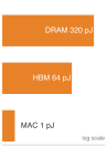
Data movement dwarfs arithmetic in energy cost.

HBM generations and the scaling boundary

HBM has grown alongside model sizes, but far more slowly than parameter counts, which is why capacity pressure keeps pushing models across devices. Each generation increases the number of stacked dies, the signaling rate per pin, and the total capacity per stack. The projected HBM4 generation in table 6 marks the scaling boundary, doubling the interface width from 1024 to 2048 bits for the first time since HBM’s introduction, because pin-rate increases alone no longer sustain the required bandwidth growth. The wider bus also needs more interposer area for routing, one reason accelerator packages have grown as bandwidth targets rise.

Table 6: Evolution of High-Bandwidth Memory: Each generation increases aggregate accelerator memory bandwidth, tracking the growth of large model sizes. The jump to HBM4 doubles the interface width for the first time since HBM’s introduction, signaling that pin-rate increases alone can no longer sustain the required bandwidth growth.

Metric	HBM2e (A100)	HBM3 (H100)	HBM3e (B200)	HBM4 (future)
Peak bandwidth	~2.04 TB/s	~3.35 TB/s	~8 TB/s	12–16 TB/s (projected)
Typical capacity	40–80 GB	80–96 GB	180 GB	288 GB+
Interface width	1024-bit	1024-bit	1024-bit	2048-bit
Stack height	8 dies	8–12 dies	12 dies	16 dies

The generations in table 6 move both capacity and bandwidth for our running example, and the step to HBM3e matters most. Using decimal bytes consistently, an A100 with 85.9 GB of HBM2e holds 24.5 percent of our 175B model’s FP16 weights; an H100 with 85.9 GB of HBM3 holds the same fraction while delivering the data 64 percent faster; and a B200 with 193.3 GB of HBM3e raises the resident share to 55.2 percent at about 8 TB/s. Because even HBM3e leaves nearly half the model outside a single package, multiple accelerators are still needed in a node (section 2.5).

Quantization changes the capacity story for inference. Storing weights in INT8 or INT4 halves or quarters the footprint, and section 2.8.1 works through how many accelerators the running model then needs. The capacity constraints that drive multi-accelerator nodes for training, where FP16 or BF16 precision is typically required, are substantially relaxed for inference, where INT8 or INT4 quantization is often acceptable, which is one reason training and inference infrastructure have different optimal configurations.

An important architectural consideration is the number of HBM stacks per accelerator and how they connect to the processor. The H100 has 5 HBM3 stacks, each providing approximately 670 GB/s, for a total of 3.35 TB/s aggregate bandwidth. A B200-class Blackwell GPU package uses 8 HBM3e stacks for an aggregate of about 8 TB/s. The number of stacks is constrained by the interposer area available for HBM placement. Each HBM stack occupies approximately 100 mm² of interposer area, and the total interposer must accommodate both the processor die(s) and all HBM stacks. Larger interposers allow more HBM stacks (and therefore higher bandwidth and capacity) but are more expensive and harder to manufacture.

The interposer area constraint creates a concrete design tension. Making the processor die larger (more Tensor Cores, more SMs) leaves less interposer area for HBM stacks, potentially reducing bandwidth. Making the processor die smaller (fewer Tensor Cores) frees interposer area for more HBM but reduces peak compute throughput. The optimal balance depends on the target workload’s position relative to the ridge point. Compute-bound workloads, whose arithmetic intensity sits above it, benefit from a larger processor die (more Tensor Cores), while bandwidth-bound workloads below it benefit from more HBM stacks, so a workload’s arithmetic intensity predicts which side of the balance it falls on before any silicon is committed.

Memory bandwidth and token latency

The distinction between memory capacity (how many gigabytes the HBM can store) and memory bandwidth (how many terabytes per second it can deliver) separates two infrastructure questions. Capacity determines whether a model’s weights fit, with headroom for the remaining live state. Bandwidth limits how fast the model can run when data movement sets the critical path. Dense autoregressive decode at batch size 1 supplies a useful example because each weight serves only one token before the next weight load. The next three calculations step down from the running model to Llama-3 70B. Its FP16 weights span two H100s rather than the running model’s five, and the H200 comparison that follows needs a model whose serving behavior a real memory upgrade can change; the arithmetic carries over to the 175B model by scaling the bytes.

Napkin Math 2.1: The physics of token latency

Problem: A weight-only model of batch-1 decode for Llama-3 70B uses 141.2 GB of FP16 weights. To isolate the two resource demands, assume hypothetical capacity sufficient to hold them while retaining one H100-equivalent compute rate and HBM path. Which term gives the larger time estimate: arithmetic or weight transfer?

Compute time: Each token requires $2 \times 70 \times 10^9 = 1.4 \times 10^{11}$ floating-point operations. At 989 TFLOP/s of FP16/BF16 Tensor Core peak throughput, the arithmetic takes $\IronLawComputeTime \approx \text{\textbf{0.14}}\text{ ms}$.
Memory time: Loading 141.2 GB of weights from HBM at 3.35 TB/s takes $\IronLawMemoryTime \approx \text{\textbf{42.1}}\text{ ms}$.

Systems insight: The memory term accounts for 99.7 percent of the sum of these two idealized times. That ratio identifies a bandwidth-dominated estimate; it is not a measurement of cycles spent idle. Raising compute throughput alone barely changes this estimate. A faster memory path reduces the weight-transfer floor, while actual token latency also includes the other memory traffic, communication, and execution costs omitted here.

Holding that weight load fixed and changing only the memory system shows how directly each HBM generation moves the floor. For the same 70.6B FP16 model, with 141 GB of weights, the single-path streaming floor is roughly 141 GB/2.04 TB/s = 69.2 ms at A100-class bandwidth, 141 GB/3.35 TB/s = 42.1 ms at H100-class bandwidth (the notebook’s memory term), and 141 GB/8 TB/s = 17.7 ms at B200-class bandwidth, falling nearly in proportion to each bandwidth gain. As in the notebook, each case isolates one accelerator-equivalent HBM path even though the full FP16 model does not fit on one A100 or H100. These bounds screen memory bandwidth against a latency target; whether token latency improves by the same ratio depends on the other work on the request’s critical path.

The same floor at trillion-parameter scale shows the limit of bandwidth gains alone, even at the projected 12–16 TB/s of an HBM4-class package. A dense 1T-parameter model requires roughly 2 TB of FP16 weight storage. Streaming those weights through one B200-class path at about 8 TB/s gives 2000 GB/8 TB/s = 250 ms for one batch-1 weight load. At the assumed 16 TB/s, that floor becomes roughly 125 ms. Neither path has been shown to hold the full model, and even the faster floor limits a single path to about eight tokens per second for one request. A responsive trillion-parameter service must therefore split its weights across many memory paths, shrink them with reduced precision, or both; which combination depends on the latency target and the quality the reduced precision preserves. The cleanest test of how far a memory upgrade moves real latency compares two accelerators that differ only in their memory system.

Napkin Math 2.2: The memory wall: H100 vs. H200

Comparing the NVIDIA H100 against the H200 isolates a memory-system upgrade for large language models (LLMs). While both chips share the same compute cores (same peak TFLOP/s), the H200 provides 1.4× higher memory bandwidth and 1.6× more HBM capacity.

This comparison uses a Llama 3 model with 70.6B parameters, sequence length 2,048, and batch size 1. Both cases retain FP16 weights and the hypothetical capacity convention of notebook 2.1: each streams the complete payload through one accelerator-equivalent HBM path, even though it cannot fit on one H100. The comparison isolates path latency rather than establishing two feasible single-device deployments.

The reported speedup comes from a serving-latency model whose inter-token latency adds two terms to the weight-streaming time, the key-value cache reads for the request’s context and a fixed per-layer kernel-launch overhead, so it is not a raw bandwidth ratio alone. The weight-only estimate provides a comparison. Its memory term accounts for 99.7 percent of the summed compute and transfer times, so reducing that term suggests a gain near the HBM bandwidth ratio, 4.8 TB/s $\div$ 3.35 TB/s $\approx$ 1.4×.

Systems insight: For the modeled configuration, the latency model predicts an H200 speedup of 1.4× over the H100 despite equal peak arithmetic throughput. Its agreement with the bandwidth ratio supports the memory-bound diagnosis for this case. Changing batch size, context length, or partitioning requires evaluating the new configuration; the estimate does not establish one bottleneck for all autoregressive models.

The modeled memory-time share, 99.7 percent in this example, indicates the memory-boundedness of this workload under the stated assumptions. A workload this memory-bound gains almost nothing from more TFLOP/s and nearly proportionally from more TB/s, which is what the H200 comparison shows, so bandwidth per dollar rather than peak arithmetic is the useful procurement metric for this regime. A measured execution timeline is still needed to determine how much transfer overlaps computation and which delays remain exposed, which keeps a hardware-screening calculation separate from a performance forecast. For training workloads, reusing weights across more tokens can instead shift the constraint toward arithmetic throughput; the Roofline Model tests the compute and bandwidth ceilings for the actual operation and batch shape before either specification becomes a procurement metric.

2.3.2 Roofline model

The token latency calculation in notebook 2.1 makes memory bandwidth the relevant procurement metric for the batch-1 workload. The Roofline Model of Williams, Waterman, and Patterson (Williams et al. 2009) tests whether that diagnosis survives a change in batch shape, precision, or accelerator by relating the workload’s arithmetic intensity to the candidate accelerator’s compute and bandwidth ceilings.

Williams, Samuel, Andrew Waterman, and David Patterson. 2009. “Roofline: An Insightful Visual Performance Model for Multicore Architectures.” Communications of the ACM 52 (4): 65–76. https://doi.org/10.1145/1498765.1498785.

For an H100 (989 TFLOP/s FP16, 3.35 TB/s HBM), the ridge point is about 295 FLOP/byte; most LLM inference operators fall well below this threshold, which is why the roofline remains the first diagnostic tool for identifying whether more compute or more bandwidth will improve performance. The quantity that places a workload on the plot is the arithmetic intensity introduced with tiling above, written $\ArithmeticIntensity$ in FLOP/byte.

↪ Placing measured kernels on the roofline by arithmetic intensity is developed in Drilling into the step.

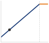
Decode sits deep in the memory-bound regime, far below the ridge.

As the single-machine recap in The roofline bound derives, the Roofline Model expresses the maximum achievable performance of a workload as the lesser of two ceilings:

\[ \text{Achievable FLOP/s} = \min\left(\PeakRate,\ \Bandwidth \times \ArithmeticIntensity\right) \tag{1}\]

In equation 1, below the ridge point the sloped bandwidth ceiling, which grows with $\ArithmeticIntensity$, is the lower one; above it the flat compute roof binds, and a measured kernel can sit below either.

Definition 2.3: Ridge point

Ridge point is the ML accelerator arithmetic intensity where the memory bandwidth ceiling meets the compute ceiling $(\RooflineRidgePoint = \frac{\PeakRate}{\Bandwidth})$.

Significance: It is the accelerator’s efficiency threshold. Below the ridge point, bandwidth supplies the lower modeled ceiling $(\Bandwidth)$; above it, arithmetic supplies the lower ceiling $(\PeakRate)$.
Distinction: Unlike peak FLOP/s, which describes only the horizontal ceiling, the ridge point describes the balance between arithmetic and memory delivery in the architecture. A rising ridge point over hardware generations indicates that compute is growing faster than bandwidth, making utilization harder.
Common pitfall: A frequent misconception is that an accelerator has a single ridge point. In reality, it varies by precision: because $\PeakRate$ is higher for INT8 than FP32 while $\Bandwidth$ is constant, the ridge point for INT8 is much higher, requiring more data reuse to saturate the hardware.

Machine learning workloads land in different regions of the roofline plot depending on the operation and the batch configuration, not on the model family. Single-request autoregressive decode streams the full weight tensor (two bytes per parameter in FP16) from HBM to perform two floating-point operations per parameter, an arithmetic intensity of about 1 FLOP/byte, far below the H100’s ridge point of 295 FLOP/byte. The token-latency calculation in notebook 2.1 showed that the arithmetic finishes in microseconds while the weight movement takes milliseconds. Every other regime in table 7 comes from reusing each byte fetched from HBM across more operations. Decode also reads the key-value (KV) cache, the stored attention keys and values of earlier tokens, and because each request has its own cache, batching does not amortize that traffic.

Table 7: Roofline Placement by Workload Phase: Language-model intensities count only weight traffic at the HBM level, the same idealization used for figure 8, against an H100 FP16 ridge point of 295 FLOP/byte; the convolution value is a representative scenario figure rather than a derived count. Attention is not plotted in the figure because its placement depends on shape. Measured placement must also count activation, key-value cache, and optimizer traffic.

Workload phase	Source of reuse	Idealized intensity	What moves it
Decode, batch 1	None; each weight serves one token	1 FLOP/byte	Batching requests, lower-precision weights
Decode, batch 32	Each weight read serves every request in the batch	32 FLOP/byte	Batch size, until key-value cache traffic dominates
Prefill, 512-token prompt	Each weight read serves every prompt token	512 FLOP/byte	Prompt length and batch size
Convolution training (ResNet-50)	Filters reused across spatial positions and the batch	200 FLOP/byte	Channel depth, tensor layout, operator fusion
LLM training, 2048 local tokens	Each weight read serves every token on the device	2,048 FLOP/byte	Local microbatch size and sequence length
Attention	Keys and values reused across queries	Shape-dependent, on either side of the ridge	Sequence length, head dimension, SRAM tiling

The table’s intensities are idealized reuse counts that classify an execution phase and batch shape, not a model family, and tensor layout, fusion, precision, and cache residency move the measured point. Which kernel-level change then helps, more reuse and fewer bytes below the ridge or a cheaper operation above it, is a diagnosis that Drilling into the step develops.

A measured workload point below its roofline ceiling needs further diagnosis. Dependencies, insufficient parallel work, irregular accesses, synchronization, and power limits can all prevent a kernel from approaching that ceiling. The gap identifies a question for profiling; it does not establish that software optimization can recover the entire difference.

Whole phases spread even wider than individual operators. The idealized intensities of decode and training differ by 2,048×, which is why the same hardware shows very different utilization across them. Batch-1 decode sits near 1 FLOP/byte, far left of the ridge and deeply bound by memory bandwidth, while large-batch training near 2,048 FLOP/byte crosses the ridge and reaches the compute roof (figure 8). The training point assumes that 2048 tokens on one accelerator share each weight read, the local reuse that a large global batch alone does not guarantee, so it counts tokens rather than sequences and local rather than global batch. It is a contrast case, not a universal intensity for training. Actual placement requires counting bytes at the memory level being modeled and accounting for tensor shapes, fusion, and reuse.

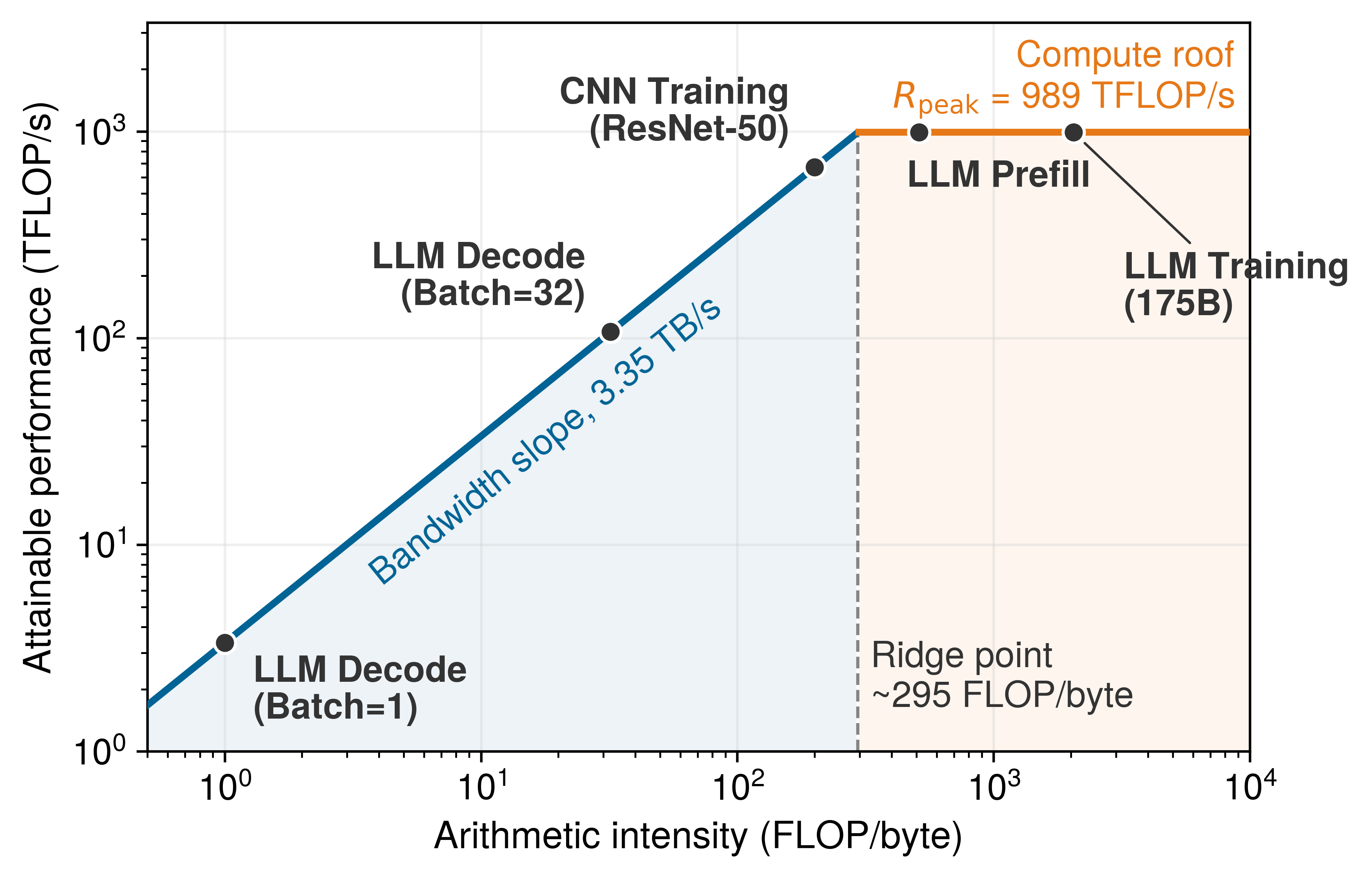
Figure 8: **The H100 Roofline Landscape**: Attainable FP16 throughput is the lower of two ceilings, the memory-bandwidth slope (blue) and the compute roof (orange), which meet at the dashed ridge point. Each dot places a representative workload by its arithmetic intensity; workloads left of the ridge stay capped by bandwidth however much compute the chip offers, and only those to its right can approach peak throughput.

The table’s batching rows can be turned into a utilization bound. For inference serving, batching multiple requests together moves the workload point rightward on the plot, because each weight read is multiplied against more activations. Under the weight-traffic-only bound, batch-1 decode on an H100 can use at most 0.34 percent of the FP16 peak. At batch size 64, each weight read from HBM serves every request in the batch, the intensity rises to 64 FLOP/byte, and the bound climbs to about 22 percent of peak, a 64× gain that still leaves the workload below the ridge. The linear growth holds only in this approximation; key-value cache traffic, which batching does not amortize, activation traffic, and capacity limits lower both figures in practice. The gain has a cost. Waiting to assemble a batch can introduce queuing latency, although a serving policy can instead dispatch a smaller batch when a latency deadline approaches. Serving systems must carefully balance this trade-off between throughput (larger batches, higher utilization) and latency (smaller batches, faster response per request).

For fleet procurement, the roofline is a screening test rather than a throughput forecast. It rules out upgrades that raise a nonbinding ceiling, while the gap below the relevant ceiling identifies work still needed in software or communication. Collected into a single procurement comparison for the running model, the two ends of the landscape give opposite hardware answers, and that diagnostic becomes most valuable when a proposed upgrade changes the wrong ceiling. Memory capacity and bandwidth therefore screen out infeasible accelerator choices, while for the candidates that remain, fleet sizing also needs a sustained compute rate at a precision the workload can use, within the node’s memory budget, the interconnect, and the facility power envelope.

Example 2.2: Roofline analysis: Training vs. inference

Scenario: An engineering team evaluates hardware choices for serving (decode batch size 1) vs. training (batch size 2048) a 175B parameter model on an H100 GPU (ridge point 295.2 FLOP/byte).

Diagnosis: The weight-traffic model gives single-token decode arithmetic intensity $\ArithmeticIntensity=$ 1 FLOP/byte $\ll$ 295.2 FLOP/byte, bounding throughput to 0.34 percent of the selected peak FLOP/s. The assumed training reuse raises intensity to $\ArithmeticIntensity=$ 2,048 FLOP/byte $\gg$ 295.2 FLOP/byte, making arithmetic the lower roofline ceiling. This placement identifies the relevant bound without establishing achieved throughput.

Systems lesson: Hardware selection starts with the phase’s arithmetic intensity and memory footprint. The modeled training phase benefits from arithmetic capacity, while batch-1 decode benefits from bandwidth. Sustained throughput at the required quality and latency determines whether either advantage justifies its cost.

Checkpoint 2.2: Roofline diagnosis

A team is serving a 13B-parameter model at batch size 1 on an H100 and observing 25 ms per token. The profile shows low tensor-core utilization during decode.

Arithmetic intensity: estimate the arithmetic intensity of the workload.
Peak-throughput upgrade: explain what the roofline estimate can establish about a higher peak-TFLOP/s accelerator and what requires measured execution.
Binding constraint: identify the profile measurements needed to distinguish exposed HBM transfers from communication, launch overhead, or insufficient parallel work before selecting an improvement.

Self-Check: Question

HBM3 provides a much wider interface and lower signaling energy per bit than socketed DDR5. Which packaging mechanism explains these advantages?
1. HBM3 runs individual pins at $16\times$ higher clock frequency than DDR5, overcoming PCB trace attenuation through high-frequency signaling.
2. HBM3 uses a novel DRAM cell structure that eliminates capacitor refresh cycles, reducing dynamic power consumption.
3. HBM3 stacks DRAM dies vertically with through-silicon vias (TSVs) and connects the stack to the processor through a wide, short silicon-interposer path on the package.
4. HBM3 compresses weight matrices on-die, transferring fewer physical bits across the memory bus.
An engineering team compares an H100 with a hypothetical successor offering twice the dense FP16 peak but the same HBM bandwidth. Hold the FP16 weight payload, partition, and batch-1 shape fixed, assume sufficient capacity, and consider a weight-streaming model whose bandwidth ceiling is lower than its compute ceiling on both devices. What changes in the modeled token-latency floor, and which levers could lower it?
A custom attention kernel has arithmetic intensity of 1.2 FLOP/byte on an H100 under the FP16 roofline convention. Which change most directly raises its memory-bandwidth performance ceiling, subject to measuring the resulting execution?
1. Use SRAM-sized attention tiles and fusion to avoid materializing the full score matrix in HBM and reduce intermediate HBM round-trips.
2. Overclocking Tensor Cores to increase peak FP16 TFLOP/s, raising the horizontal ceiling of the roofline.
3. Adding dummy memory reads to artificially raise the measured memory traffic of the kernel.
4. Offloading the layer normalization and attention operations to host CPU DRAM over PCIe Gen5.
Order the following tiers of an H100-class accelerator’s memory hierarchy from the highest aggregate bandwidth to the highest capacity: (1) HBM3 on the package, (2) the streaming multiprocessors’ register files, (3) the L2 cache, (4) L1 and shared memory (on-chip SRAM).
In the Roofline Model, the specific arithmetic intensity where the diagonal memory bandwidth slope meets the horizontal peak compute ceiling ($I = R_{\text{peak}} / \text{BW}$) is called the ____.

See Answers →

2.4 Sustained Compute and Precision

A fleet sized from advertised matrix throughput can miss its training deadline when operations cannot use the advertised precision or keep the matrix units of section 2.2.5 busy. The relevant hardware contract includes both the eligible matrix operations and their sustained contribution to the complete workload.

Tensor Core precision support widened with each generation traced in section 2.2.3, from FP16 on Volta to FP8 on Hopper, because neural network training and inference tolerate lower numerical precision than was once assumed. Transformer Engine recipes and FP8 autocast decide which supported operations run in FP8, recording tensor ranges and applying scale factors so values fit the format, but they do not establish that a layer is numerically safe at that precision; precision policy therefore remains a software configuration and validation decision, which FP8 for distributed training develops for training.

The relationship between numerical precision and hardware throughput matters for infrastructure planning because it directly affects how much useful work each accelerator can perform per second. Lower precision representations use fewer bits per number, which has two compounding benefits: more numbers fit in the same HBM capacity (reducing memory pressure), and the arithmetic units can process more operations per cycle (increasing throughput). Each format an H100-class accelerator supports unlocks a different dense peak rate and plays a usual role in training or inference (table 8).

Table 8: Precision Formats and Hardware Throughput on H100: The table uses dense peak throughput where Tensor Core support exists; structured sparsity can roughly double several of these advertised peaks. The choice of precision affects both the training dynamics (convergence, numerical stability) and the infrastructure requirements (memory capacity, bandwidth utilization). TF32 preserves the FP32 exponent width but reduces mantissa precision so Tensor Cores can accelerate common FP32 training workloads.

Format	Bits	Exponent	Mantissa	H100 dense peak	Typical use
FP32	32	8	23	~67 TFLOP/s	Master weights, loss computation
TF32	19	8	10	494 TFLOP/s	Training (NVIDIA default)
BF16	16	8	7	989 TFLOP/s	Training, fine-tuning
FP16	16	5	10	989 TFLOP/s	Training with loss scaling
FP8 (E4M3)	8	4	3	1,979 TFLOP/s	Forward pass, weights
FP8 (E5M2)	8	5	2	1,979 TFLOP/s	Backward pass, gradients
INT8	8	N/A	N/A	1,979 TOPS	Post-training quantization

For training, many workloads use the standard mixed-precision recipe, which decouples storage from arithmetic precision by keeping FP32 master weights while the forward and backward passes run in BF16 or FP16 at full Tensor Core throughput. The node memory examples in section 2.5.3 assume retained FP16 gradients; implementations that retain a full FP32 accumulation buffer must add that buffer to their peak budget. The FP8 recipes described earlier extend the same decoupling one step further, running eligible matrix operations in eight bits while the master weights stay in FP32.

↪ The byte widths of each format and the per-parameter memory of mixed-precision training are collected for reference in Numeric Precision and Training Memory.

The practical implication for fleet design is that peak TFLOP/s specifications are precision-dependent. The H100 delivers 989 TFLOP/s in FP16 but twice that (1,979 TFLOP/s) in FP8. FP8 therefore doubles the advertised arithmetic ceiling for supported operations on the same hardware. The complete training run gains less when communication, memory traffic, or higher-precision operations remain on the critical path. Precision engineering is therefore a primary optimization lever for infrastructure planners, alongside its effect on model accuracy.

Approaching peak throughput requires pipeline balance. Operand staging and reuse must supply the arithmetic units at the rate the operation requires. Kernel fusion and tiled attention such as FlashAttention improve that balance by keeping intermediate values on chip instead of making separate HBM round-trips, mechanisms that Kernel-Level Levers collects for reference. For our 175B model, the fleet-level gain depends on how much step time the affected kernels consume. A faster attention kernel shortens the step only in proportion to attention’s share of it, the same Amdahl accounting that bounds every partial speedup.

2.4.1 Peak vs. sustained throughput

A training run budgeted for 1,000 GPU-hours from datasheet TFLOP/s will consume 2,500 GPU-hours in practice when the workload sustains only 40 percent of peak throughput. Infrastructure planning therefore separates peak throughput (the maximum rate for the vendor-specified operation and precision) from sustained throughput (what the complete workload delivers). Peak TFLOP/s assumes that eligible arithmetic units remain fed under the stated sparsity, precision, and clock conditions; it does not include memory stalls, ineligible operations, communication, or software overhead. Sustained fractions therefore vary with model shape, batch size, precision, implementation, and scale. The gap arises from several sources, each representing a different physical or software limitation.

Memory stalls occur when the Tensor Cores complete their current tile multiplication before the next tile has been loaded from HBM. Even with the H100’s 3.35 TB/s HBM bandwidth, the Tensor Cores can consume data faster than HBM can deliver it for certain matrix dimensions, creating idle cycles while the arithmetic units wait for data.

Dependency stalls arise when one operation must complete before the next can begin, leaving some processing elements idle. In a Transformer layer, the attention computation must complete before the feed-forward network can begin, and the feed-forward computation must complete before the next layer’s attention can start. These sequential dependencies create brief periods where some hardware resources are unused, even within one accelerator. When the model is split into sequential stages on different accelerators (pipeline parallelism), the same dependencies become pipeline bubbles, idle slots in which a whole stage waits for its predecessor; splitting each batch into microbatches reduces the waste by feeding later microbatches into stages that would otherwise wait. The term pipeline bubble refers only to this cross-device case, whose scheduling Distributed Training develops. At the infrastructure level, the lesson is that peak throughput assumes every unit stays busy, while real training includes dependency gaps that lower sustained utilization.

AllReduce operations used in tensor parallelism and gradient synchronization used in data parallelism can likewise delay computations that depend on their results; even when communication overlaps computation on separate streams, operations that depend on the collective output cannot proceed until the transfer completes. Kernel submission, memory allocation, and framework control also consume time, and when each kernel completes in microseconds, launch overhead of a similar size becomes a comparable share of the step that only a host-and-device execution trace can separate from slow arithmetic or memory access. Achieving high sustained utilization is therefore largely a matter of minimizing the time Tensor Cores spend idle between operations, which is why kernel fusion and specialized kernel libraries such as FlashAttention and the Transformer Engine exist.

The last source of the gap is the device itself, and no kernel change removes it. Device variation, sometimes called the silicon lottery, means that nominally identical accelerators sustain different clocks. Clock behavior also depends on the configured power limit, temperature, and workload, so a slow participant should not be diagnosed from its product label or frequency alone. In synchronous training, a participant that finishes dependent work late delays its whole process group. One device sustaining a clock about 2.5 percent below its peers can slow every synchronous step it joins by up to that fraction, because the other participants wait for it at each collective. Fleet management systems therefore track per-device sustained throughput and can move persistent underperformers to pools, such as inference serving, where they do not gate a synchronized group. Profiling must determine whether local arithmetic, memory, communication, or a power limit caused that delay before changing placement or replacing hardware.

Capacity planning must use a measured or conservatively modeled sustained rate, not the peak specification. A run estimated at 1,000 GPU-hours from peak FLOP/s requires $1/\EfficiencyHw$ times that estimate when its measured utilization fraction is $\EfficiencyHw$. Infrastructure teams track model FLOPs utilization (MFU), the useful model computation per second divided by the selected hardware peak, as the standard measure of $\EfficiencyHw$, but comparisons remain meaningful only when model-FLOP conventions, precision, hardware peak, and system scale match.

↪ MFU as the measure of program goodput, one factor of fleet-level ML goodput, is developed in Program goodput and its measure.

The accelerator’s physics establish a concrete problem. Our 175B model requires 350 GB of memory for its weights alone in FP16, and Adam-style training state raises the requirement to multiple terabytes once optimizer moments, gradients, and activations are included. A single H100 provides 80 GB of HBM. No single accelerator can hold this model, an instance of the memory capacity gap (principle 2), in which frontier memory requirements outgrow single-accelerator HBM. The system must expand to the next physical level: the node.

Self-Check: Question

An H100 advertises twice the dense arithmetic rate in FP8 that it advertises in FP16. A team sizes a training run’s GPU-hours by assuming the full FP8 rate. Which statement best describes the planning error?
1. FP8 halves the bytes per weight, so memory-bound phases also run exactly twice as fast and the plan is correct.
2. The FP8 rating is a ceiling for eligible matrix operations; ineligible operations, memory stalls, communication, and the need to validate the precision policy keep the sustained rate below it, so the plan must use a measured sustained rate.
3. FP8 Tensor Core rates apply only to inference, so a training plan must use the FP32 rate instead.
4. FP8 runs slower than FP16 on Tensor Cores because of scaling overhead, so the plan overestimates the time.
A training run is estimated at 1,000 GPU-hours from peak FLOP/s. Profiling a representative window shows a model FLOPs utilization (MFU) of 0.4. How many GPU-hours should the plan budget, and what must match before this MFU can be compared with another team’s figure?
True or False: In synchronous training, an accelerator that sustains a clock about 2.5 percent below its peers costs the job at most 2.5 percent of that one device’s throughput.
The standard mixed-precision recipe runs the forward and backward passes in BF16 or FP16 but keeps a full-precision FP32 copy of the parameters, called the ____ weights, so that updates much smaller than a weight are not lost to FP16 rounding.

See Answers →

2.5 The Node

The running model needs more memory than one accelerator provides. A node supplies several accelerators in one chassis, but each retains its own memory; dividing the work creates communication that the local fabric must sustain. Tensor parallelism divides an operation across accelerators, pipeline parallelism assigns successive model stages to different groups, and data parallelism assigns different training examples to model replicas whose updates must be combined. These strategies impose different traffic patterns, and the node’s internal fabric decides which of them it can carry at the speed the partition needs.

Aggregating accelerators solves the capacity problem only if the interconnect between them is fast enough that the group behaves as one machine rather than as several machines passing messages. The 175B model’s weights span at least five accelerators, and the full training state spans an entire 8-H100 node and more, so some model state must live on different chips. Depending on the partition, execution exchanges partial results, activations, gradients, or parameter shards. Whether those exchanges are cheap or ruinous depends on the local fabric, which is why the node is the first scale level where the accelerator’s specifications matter less than the wires between accelerators. The training system can combine tensor parallelism, optimizer sharding, and memory offload as needed to meet its capacity budget, and each strategy places a different demand on the interconnect.

Definition 2.4: Node

Node is the ML training cluster’s physical server chassis that aggregates multiple accelerators (typically 8) through a high-speed intra-node interconnect (NVLink or ICI), providing a physical packaging and failure boundary. The fast communication domain can coincide with one chassis or extend across several, depending on the fabric.

Significance: The NVLink bandwidth within a DGX H100 node reaches 900 GB/s bidirectional, or 450 GB/s per direction, while inter-node InfiniBand NDR provides 50 GB/s, a 9× per-direction gap that constrains where each parallelism strategy can run. For this DGX H100 topology, frequent tensor-parallel collectives favor the intra-node NVLink domain; pipeline parallelism can span nodes when the network sustains stage-boundary activation traffic. The node is also the primary failure domain: a single node failure in a bulk synchronous parallel training job, where workers advance in lockstep at step barriers, idles the entire cluster until recovery.
Distinction: Unlike a single accelerator (which provides fast HBM bandwidth but limited capacity), a node aggregates 8$\times$ the HBM capacity and 8$\times$ the compute of a single chip, enough to place large FP16 weight shards (8 $\times$ 80 GB = 640 GB on DGX H100), but not enough to keep the full Adam training state in HBM.
Common pitfall: A frequent misconception is that nodes in a distributed training job operate independently. In bulk synchronous parallel training, all nodes are synchronously coupled at every step barrier: a performance degradation on one node (from thermal throttling, a faulty NIC, or a slow storage read) stalls the entire cluster and drops overall MFU for the duration of that step.

The node exists because of a gap in the memory hierarchy: HBM provides enough bandwidth to feed the accelerator’s arithmetic units, but not enough capacity to hold the full 175B-parameter running example, whereas host DRAM provides capacity (512 GB to 2 TB per server) but not enough bandwidth. The node bridges this gap by aggregating the HBM of multiple accelerators into distributed capacity connected by a fast interconnect. Each accelerator’s HBM remains private to that device: software must shard or replicate tensors explicitly and use collectives or peer transfers when an operation crosses device boundaries. Placing 8 accelerators in one chassis therefore provides 8$\times$ aggregate capacity and 8$\times$ aggregate compute, but it does not create a single shared-memory accelerator; performance depends on how well the partitioning limits traffic over the fabric.

The capacity arithmetic also explains the appeal of multiple packages. Holding a 175B model’s 350 GB of FP16 weights on one accelerator, at the example 17–24 GB per HBM stack, would require 350 GB spread across roughly 15–21 stacks. That exceeds the 5-stack H100 and 8-stack B200-class configurations used here. Such a package would need its own area, yield, power, and cooling analysis. Distributing capacity across 8 accelerators instead uses available packages and pays for communication between their private memories.

2.5.1 Bandwidth hierarchy

Placing a layer-by-layer tensor-parallel collective across a 50 GB/s inter-node link instead of a 450 GB/s intra-node link multiplies its transfer floor ninefold and stalls every accelerator in the group. Multi-accelerator systems are governed less by the number of chips than by the speed at which they can exchange data across physical boundaries. Data movement speed drops by orders of magnitude as it crosses package, board, and rack boundaries, each with a different physical medium, connector technology, and signaling constraint. This physical ordering of data transfer rates, from on-chip SRAM at the fast end to the wide-area network at the slow end, is the bandwidth hierarchy; this ordering dictates where in the hierarchy each type of parallelism can operate efficiently.

The hierarchy reflects the physical cost of distance. Shorter signal paths over denser wiring achieve higher throughput at lower energy per bit, so at each boundary the effective bandwidth $(\Bandwidth)$ drops by roughly an order of magnitude while latency $(\Latency)$ rises. The exact size of each gap depends on link count, signaling, and the measurement boundary, but the gradient itself sets a scaling ceiling for distributed training. The common mistake is to treat all cluster communication as equal. Parallelism placement must be hierarchy-aware, because putting high-frequency synchronization such as tensor parallelism on a slow tier leaves the arithmetic units $(\PeakRate)$ waiting and collapses scaling efficiency $(\ScalingEfficiency)$.

The bandwidth hierarchy can be read as concentric zones around each accelerator (figure 9), losing 7.4$\times$ to 9$\times$ of bandwidth at each physical boundary on the way out through NVLink, InfiniBand, and remote storage. The innermost zone is the HBM on the same package, with terabytes per second of bandwidth and sub-microsecond access latency. The next zone holds the other accelerators in the node’s NVLink domain, reachable at hundreds of gigabytes per second per GPU with microsecond-scale transfer latency. The outermost zone spans the other nodes in the cluster, reached through InfiniBand ports that each supply tens of gigabytes per second per direction, with point-to-point latency measured in single-digit microseconds. Latency figures are comparable only when they measure the same thing (a memory access, a link transfer, or a complete collective), and bandwidth ratios only when they compare matching endpoints and directions, as the representative paths of table 9 do.

Table 9: The Bandwidth Hierarchy: These representative paths have different bandwidth budgets. Link bandwidths are per direction; link count, signaling, and system configuration determine the gap between tiers. These example bandwidth gaps favor placing frequent tensor-parallel collectives within the fast communication domain, which need not coincide with a server boundary.

Domain	Interconnect	Bandwidth	Latency	Scaling limit
Intra-package	Silicon interposer	~3.35 TB/s	$<100\text{ ns}$	Single chip
Intra-node	NVLink/ICI	~450 GB/s	~0.5 μs	Node (8–16 chips)
Intra-node (I/O)	PCIe Gen5 x16	~64 GB/s	~1 μs	CPU-GPU, NIC-GPU
Inter-node	InfiniBand NDR	~50 GB/s	~5 μs	Pod (thousands)

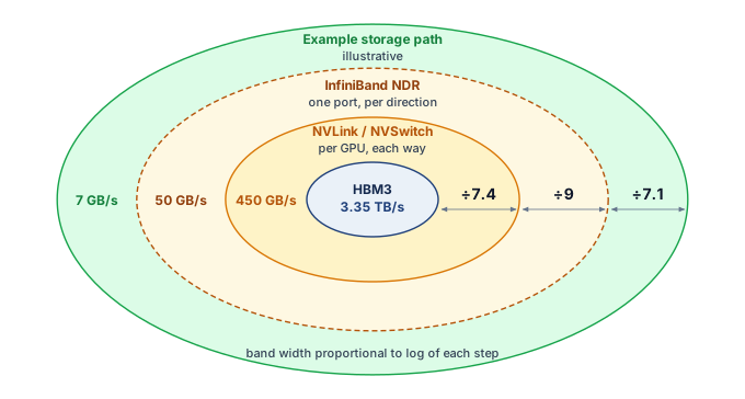
Figure 9: **The Infrastructure Bandwidth Hierarchy**: Concentric zones place each tier an ML workload crosses farther from the accelerator’s own memory. HBM (3.35 TB/s) sits at the center; the outward tiers are NVLink/NVSwitch (450 GB/s per direction per GPU), one InfiniBand NDR port (50 GB/s per direction), and an illustrative 7 GB/s storage path. Each step outward cuts bandwidth by roughly 7.4, 9, and 7.1 times, not by a universal tenfold law. Exploiting this hierarchy through tiered algorithms is the primary task of distributed systems engineering.

Napkin Math 2.3: The physics of the staircase

Problem: A 10 GB buffer must move one hop at each tier of the hierarchy, with a local HBM read as the reference point. How much does the tier it crosses change the transfer time?

Math: Transfer time is $\TransferTimeForPayload= \DataVolume / \Bandwidth$.

HBM (local read, the reference point): 10 GB / 3,350 GB/s $\approx$ 3.0 ms.
NVLink (intra-node): 10 GB / 450 GB/s $\approx$ 22.2 ms.
InfiniBand (inter-node): 10 GB / 50 GB/s $\approx$ 200 ms.

Systems insight: For the same payload, the example inter-node path has a transfer-time lower bound 9× larger than the example intra-node path. Size alone does not decide which traffic may cross that cliff; frequency and overlap do. Tensor parallelism exchanges activations inside every layer, on the critical path, so it favors the fast local NVLink domain in this configuration. Data parallelism moves the largest buffer, the full gradient, but only once per step and overlapped with the backward pass, so it can cross the scarce InfiniBand tier. A partition that fits in memory can still spend much of a step waiting if its exposed exchanges exceed the communication budget.

Each cliff in the bandwidth staircase has a physical cause at its distance scale. Millimeter-long traces on a silicon interposer can carry a very wide, slow-clocked parallel interface without serializer/deserializer (SerDes) transceivers. NVLink crosses tens of centimeters of board copper, which requires SerDes transceivers with equalization to recover the signal at high per-lane rates. PCIe pays for universal compatibility with protocol overhead (packet headers, flow-control credits, and error checking). InfiniBand crosses meters of cable between racks, adding optical conversion on longer runs, forward error correction, and switch hops. SerDes, link budget, and power develops the signaling physics behind these cliffs. For node design, link count and sustained bandwidth must be evaluated together with the power and cooling load of the components that provide them.

The practical consequence for model partitioning is that tensor parallelism (TP), which splits individual matrix multiplications across accelerators and requires collective exchanges within layers, generates communication volume proportional to the model’s hidden dimension hundreds of times per second. Over NVLink, each of these exchanges takes under a millisecond for the running model (section 2.5.2 computes the idealized lower bound). At the reference InfiniBand port rate, the bandwidth-only lower bound for the same exchange is 9× as large; the step-time effect also depends on startup, routing, and overlap. For this topology TP therefore stays within a node, although a system whose fast scale-up fabric spans several chassis can place a tensor-parallel group across them; communication cost, rather than the server enclosure, determines the useful partition.

The hierarchy also explains why pipeline parallelism occupies an intermediate position in the bandwidth requirements. In pipeline parallelism, the model is divided into sequential stages, with each stage assigned to a different group of accelerators. The communication between stages consists of activations flowing forward during the forward pass and gradients flowing backward during the backward pass, with a volume proportional to the batch size times the hidden dimension.

For our 175B model with hidden dimension 12,288 and a microbatch of 4 sequences at 2,048, the activation tensor at each stage boundary is approximately $4 \times 2,048 \times 12,288 \times 2 B$ bytes (FP16) $\approx$ 201 MB. This is far smaller than the 350 GB gradient AllReduce required by data parallelism, which is why pipeline parallelism places less demanding requirements on the inter-node network.

Activation transfers occur once per microbatch per stage boundary. That is far less often than tensor parallelism’s AllReduce inside every layer, yet more often than data parallelism’s gradient exchange, which happens once per step. Small messages at an intermediate frequency let pipeline parallelism tolerate the lower bandwidth of inter-node links, which makes it the natural way to split a model whose layers do not fit in one node.

Both pipeline and data parallelism therefore cross node boundaries, for different reasons (table 10). Pipeline traffic is small per message and sits between the other two in frequency; the data-parallel gradient exchange is the largest transfer, but it occurs once per step and can overlap the backward pass, which makes it the most latency-tolerant of the three, although any unfinished exchange still delays the update. For the example topology, the resulting mapping places tensor parallelism within the node, pipeline stages across nodes, and data-parallel groups across the cluster. This de facto pattern is a starting point for the capacity and timing calculation; a different scale-up domain, message size, or overlap opportunity can justify a different placement.

Table 10: Traffic Shape by Parallelism Strategy: The placement rule follows from size and frequency together. Frequent exchanges on the critical path need the fastest tier, while the largest exchange can cross the slowest tier because it happens once per step and overlaps the backward pass.

Strategy	Size per exchange	Frequency	Overlap with computation	Placement on this topology
Tensor parallelism	Activation-sized partial results	Inside every layer, forward and backward	Little; later operations depend on the result	Within the NVLink domain
Pipeline parallelism	One microbatch’s activations at a stage boundary	Once per microbatch per boundary	Partial, through microbatch scheduling	Across nodes, adjacent stages close together
Data parallelism	The full gradient	Once per step	Substantial, during the backward pass	Across the cluster

The mapping constrains how the scheduler assigns devices and nodes. Members of a tensor-parallel group belong inside one fast domain (on this topology, one chassis joined by NVLink), because their dependent exchanges recur inside every layer. Adjacent pipeline stages belong in the same rack or neighboring racks, where their activation and gradient traffic crosses the fewest InfiniBand switch hops. Data-parallel groups can span the whole cluster. Physical adjacency helps only when it corresponds to better connectivity. The node’s PCIe hierarchy adds another placement constraint by connecting accelerators to host CPUs, network interface cards (NICs), and storage, including the path used to reach host DRAM.

The PCIe hierarchy within a node

While NVLink carries GPU-to-GPU traffic, PCIe Gen5 connects accelerators, host CPUs, network adapters, and storage through the node’s peripheral hierarchy. Host DRAM attaches to the CPU’s memory controllers; a GPU transfer to that memory also traverses its host-facing PCIe path. PCIe bandwidth, approximately 64 GB/s per direction (128 GB/s bidirectional) per x16 link, can therefore constrain data loading, checkpointing, or GPU-to-network transfers. Which traffic competes depends on the actual links and switches those paths share.

A standard DGX H100 node features two host CPUs, each managing a PCIe root complex, with PCIe switches fanning those lanes out so that each of the 8 GPUs and each of the 8 InfiniBand host channel adapters (HCAs, the network interface cards of an InfiniBand fabric) has its own x16 link (figure 10). This configuration provides an aggregate theoretical bandwidth of about 2 TB/s within the chassis. However, this bandwidth is shared among competing traffic streams. During a single training step, the PCIe bus simultaneously carries host-to-GPU data batches, GPU-to-HCA gradient shards for inter-node AllReduce (via GPUDirect remote direct memory access (RDMA)), and periodic CPU-to-NVMe checkpoint writes. Contention between these streams can cause unexpected pipeline stalls, particularly when gradient synchronization saturates the links typically used for data loading.

The dual-CPU architecture introduces significant non-uniform memory access (NUMA) effects. The 8 GPUs are physically partitioned, with 4 connected to CPU 0’s root complex and 4 to CPU 1’s. A GPU connected to CPU 0 can reach CPU 0’s DRAM through its local PCIe root complex, whereas access to CPU 1’s DRAM also traverses the inter-socket link. The latency and bandwidth penalty depends on the processor, socket interconnect, PCIe topology, transfer size, and concurrent traffic, so no fixed percentage applies across nodes. Data-loading pipelines should measure this topology and place worker processes, pinned buffers, NICs, and target GPUs within the same NUMA domain when the local path improves sustained ingestion; placement is therefore part of the parallelism strategy, because a scheduler that ignores PCIe roots, NIC locality, and NUMA domains can turn an otherwise valid tensor- or pipeline-parallel plan into a host-bound bottleneck.

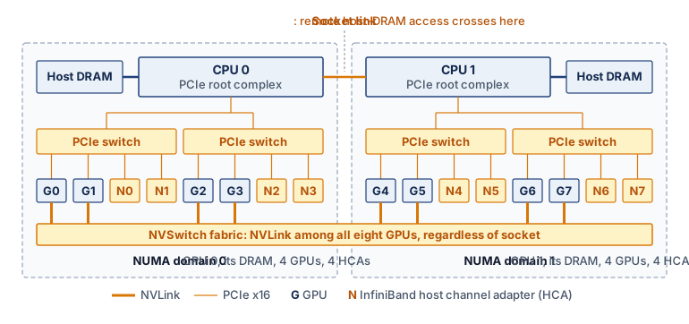
Figure 10: **Two Fabrics inside One Eight-GPU Node**: NVSwitch joins all eight GPUs for GPU-to-GPU traffic, but every path to host memory, storage, or the network runs through a PCIe tree rooted at one of two CPU sockets. A GPU, its InfiniBand host channel adapter (HCA), and the host DRAM it reaches most cheaply therefore sit in one non-uniform memory access (NUMA) domain, and a transfer to the other socket’s DRAM also crosses the socket link. The two PCIe switches per socket are schematic; switch count and lane routing vary by server design.

↪ Mapping data, tensor, and pipeline parallelism onto intra-node and inter-node bandwidth tiers is developed in Hybrid Parallelism.

2.5.2 Dense node designs

Given the bandwidth hierarchy, the node must connect 8 accelerators with enough bandwidth for tensor-parallel operations across their private memories. A switched fabric can provide full bisection bandwidth, enough capacity across any equal division of the endpoints to carry their full injection rate. Comparing a ring, a mesh, and a switched design shows what connectivity costs and which communication patterns it supports.

Eight GPUs in one chassis can be wired as a ring, a full mesh, or a switched fabric (figure 11). A ring is inexpensive, needing only $\AcceleratorsPerNode$ links for $\AcceleratorsPerNode$ GPUs, and suits ring-AllReduce, in which each GPU sends to one neighbor while receiving from the other so that every link stays busy. Tensor parallelism, however, issues frequent collectives after sharded matrix operations, including ReduceScatter, which leaves each participant with one shard of a combined result, and AllGather, which assembles shards at every participant, and a ring’s fixed multi-hop paths (up to four hops between distant GPUs) constrain those patterns. A full mesh reaches every peer in one hop but needs $\AcceleratorsPerNode(\AcceleratorsPerNode-1) / 2 = 28$ links for 8 GPUs, a count that grows quadratically and soon becomes impractical to route. The NVSwitch crossbar puts every pair one switch hop apart and provides full-bisection switched connectivity with a manageable number of switch chips.

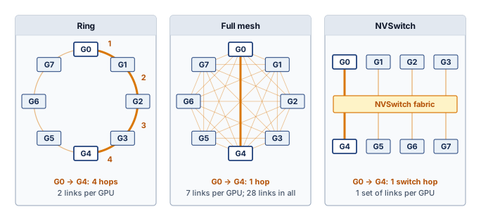
Figure 11: **Intra-node GPU Topology Comparison**: Three ways to wire eight GPUs inside one node. Left: a ring gives each GPU only two links, so traffic between distant GPUs passes through up to four hops. Center: a full mesh reaches every peer in one hop but needs $\AcceleratorsPerNode-1$ links per GPU and $\AcceleratorsPerNode(\AcceleratorsPerNode-1)/2$ links in total, which becomes impractical to route beyond about eight GPUs. Right: an NVSwitch fabric gives each GPU one set of links to the switch and puts every pair one switch hop apart, with up to 450 GB/s per direction per H100 SXM GPU (900 GB/s bidirectional); that per-GPU injection bandwidth is not the aggregate bisection bandwidth of the switch fabric.

Consider the NVIDIA DGX H100 architecture. Eight H100 GPUs sit on a single baseboard, each connected to four NVSwitch chips via 18 NVLink 4.0 lanes. The NVSwitch chips form a non-blocking crossbar⁵ through which any GPU can reach any other GPU. Each GPU’s port budget is 900 GB/s bidirectional, or 450 GB/s in one direction, shared across that GPU’s simultaneous transfers; it is not a separate full-bandwidth link for every GPU pair.

⁵ Crossbar switch: A topology providing a dedicated path between every input-output pair simultaneously. An $\SwitchRadix{\times}\SwitchRadix$ crossbar needs $\SwitchRadix^2$ crosspoints, so its cost grows quadratically with port count; that growth is why a full crossbar stays inside a node and larger systems switch to multi-stage fabrics. Within that bound, the crossbar buys the all-to-all bandwidth that tensor parallelism demands.

The result is a node with 640 GB of aggregate HBM capacity and a combined peak compute throughput of 8 $\times$ 1,979 TFLOP/s, while each GPU retains private HBM. Training frameworks partition tensors explicitly across those devices, and NVSwitch reduces the communication cost between shards without making placement or collective synchronization transparent. The NVSwitch chips themselves consume approximately 200 W each (800 W total for the NVSwitch fabric), a nontrivial power overhead justified by the bisection bandwidth it provides. In physical terms, the NVSwitch fabric alone consumes more power than an entire previous-generation GPU (the V100 drew 300 W).

This node-budget example assumes one activation-sized AllReduce per layer in each forward and backward pass. The partition and collective schedule are scenario inputs, not a universal Transformer schedule. During the modeled tensor-parallel forward pass, each GPU holds one shard of each weight matrix and computes its portion of the matrix multiplication. For a Transformer layer with hidden dimension 12,288 (typical for a 175B model), each of the 8 GPUs holds a $12{,}288{\times}1{,}536$ slice of the weight matrix. After each GPU computes its partial result, an AllReduce operation sums the partial results across all 8 GPUs over NVLink.

The logical output tensor for one AllReduce contains $4 \times 2{,}048 \times 12{,}288 \times 2$ bytes (FP16). For a microbatch of 4 sequences at 2,048 tokens, that payload is roughly 201 MB. An ideal ring AllReduce with 8 participants moves $2(\DeviceCount-1)/\DeviceCount=$ 1.75 times the payload per GPU (Collective Communication derives this factor), or about 352 MB. At 450 GB/s of one-direction bandwidth, the transfer-time lower bound is approximately 0.783 ms.

Across 96 forward layers and 96 backward layers, the 192 transfers sum to about 150.3 ms per step before overlap. NVSwitch provides the paths needed for the collective, but this value remains an ideal bandwidth-only lower bound that excludes startup latency, software overhead, and competing traffic.

↪ The $\MessageStartupLatency$-$\LinkBandwidth$ model, which adds the fixed per-message startup latency this bound omits to the bytes-over-bandwidth transfer time, is developed in The \MessageStartupLatency-\LinkBandwidth Communication Model.

Judging that bound needs a compute time to compare it with. This scenario assumes 200 ms of computation per step for the tensor-parallel group, a stated input rather than a derived value; the fractions below scale with it, so a longer compute time makes the same communication matter less. Against that assumption, the unoverlapped NVLink lower bound leaves computation at 57.1 percent of combined compute-plus-communication time. Actual tensor-parallel efficiency can be higher when collectives overlap useful computation or lower when latency, contention, load imbalance, and nonparallel work add delay, so it must be measured rather than inferred from peak link bandwidth alone.

Example 2.3: The NVLink bandwidth surprise

Scenario: A team evaluates tensor parallelism over a hypothetical PCIe Gen5 path with 64 GB/s bandwidth, using the payload and the assumed 200 ms per-step compute time stated with the NVLink estimate above.

Diagnosis: The modeled tensor-parallel schedule executes 192 AllReduce events per step across 96 layers. Its PCIe bandwidth-only transfer times sum to 1057 ms per step. Without overlap, communication accounts for 84.1 percent of the combined compute and transfer estimate; this is not a measured stall fraction.

Systems lesson: Under the same assumptions, NVLink lowers the transfer bound to 0.783 ms per AllReduce and raises computation to 57.1 percent of the combined time. The comparison explains why this partition favors a fast local fabric. Real collective performance must also include startup, topology, contention, and overlap.

The DGX H100 pairs each GPU with its own InfiniBand ConnectX-7 HCA, which reads and writes GPU memory directly over PCIe through GPUDirect RDMA, so inter-node gradient exchange avoids staging copies in host DRAM while still consuming PCIe and network bandwidth. The host CPU prepares and loads batches, submits kernels, and coordinates the training framework. Sufficient CPU capacity and I/O bandwidth let that work overlap the accelerator fabric’s computation and communication; otherwise, slow preprocessing or submission can starve the GPUs even when their local memory and interconnect are fast enough.

↪ The RDMA and GPUDirect data path that bypasses host memory is developed in RDMA and GPUDirect.

Kanev, Svilen, Juan Pablo Darago, Kim Hazelwood, Parthasarathy Ranganathan, Tipp Moseley, Gu-Yeon Wei, and David Brooks. 2015. “Profiling a Warehouse-Scale Computer.” Proceedings of the 42nd Annual International Symposium on Computer Architecture, 158–69. https://doi.org/10.1145/2749469.2750392.

Host CPUs also pay a “data center tax” of shared infrastructure work. A profile of Google’s fleet found that such common building blocks consumed nearly 30 percent of cycles across jobs (Kanev et al. 2015), and network protocol processing, storage virtualization, and security functions add to that load on cloud hosts. ML nodes can therefore incorporate data processing units (DPUs) or SmartNICs. Devices like the NVIDIA BlueField DPU offload these infrastructure tasks to dedicated ARM cores and hardware accelerators integrated into the network adapter itself. Moving the control plane for RDMA, firewall rules, and storage protocols to the DPU recovers cycles for the ML pipeline: data loading, tokenization, and kernel orchestration on the host CPU. The DPU also acts as an isolated security domain, allowing cloud providers to maintain control over the network and storage layer via the DPU while granting customers full access to the host CPU and GPUs. For our 175B model training, DPU offload can keep RDMA protocol processing outside the host CPU critical path for gradient synchronization, which flows from GPU HBM toward the network fabric without host CPU involvement.

Alternative node architectures

Spending board area, power, and cost on four NVSwitch chips makes sense when tensor-parallel collectives sit inside every layer, but workloads dominated by embedding capacity, data parallelism, or cost-sensitive serving hit different limits first. Alternative node designs reallocate that budget: an AMD MI300X server emphasizes very large HBM capacity on each package, Google TPU pods wire chips directly into a mesh without a central baseboard switch, and Intel/Habana Gaudi nodes integrate Ethernet RDMA ports directly onto the accelerator die. Comparing them against a DGX H100 node reveals where each architecture spends its scarce budget.

The DGX H100 answers a general node-design problem by making local accelerator exchange cheap. A switch-rich design spends power, board area, and cost on universal any-to-any exchange. That choice is easy to justify when tensor parallelism is the critical path, because each Transformer layer turns local accelerator communication into part of the model’s inner loop. The 900 GB/s H100 NVLink fabric therefore buys a software abstraction, in which the training framework can treat eight accelerators as one tightly coupled tensor-parallel group for the layers that must be split across chips.

Other systems move that boundary. TPU pods use the inter-chip interconnect and a mesh-oriented topology instead of making a central switch the defining component of the node; a TPU v5p chip’s vendor-specified ICI bandwidth is 1,200 GB/s. The mesh can reduce switch cost and expose a regular structure to the compiler, but it also makes placement more visible, because the runtime must respect neighbor relationships rather than assuming that every chip pair has the same communication path. That is a reasonable trade when the workload is regular enough for the compiler and collective libraries to map communication onto the topology.

The MI300X shifts the pressure point from local switching toward memory capacity. Its package exposes 192 GB of HBM at 5.3 TB/s, compared with 80 GB on an H100-class accelerator. An eight-accelerator MI300X node would therefore provide 1,536 GB of aggregate HBM, enough to hold the 350 GB FP16 weight tensor for our 175B running model. That does not eliminate the optimizer, gradient, activation, and fragmentation problem that section 2.5.3 quantifies, but it changes how often the system must spill state into slower memory tiers and how much microbatch headroom remains before offload becomes mandatory.

Gaudi takes a different route by integrating RDMA-capable Ethernet into the accelerator and using a more network-centric design for communication. A Gaudi 2 accelerator’s 24 integrated 100 GbE ports supply 300 GB/s of aggregate RDMA over Converged Ethernet (RoCE) bandwidth, against the 900 GB/s of local exchange per GPU in an H100-class NVLink node. The newer Gaudi 3 keeps that Ethernet-centric design while carrying 128 GB of HBM per accelerator, so capacity is not the trade being made. The question is whether simplifying the fabric and using Ethernet consistently across node and pod is worth giving up the very high local exchange bandwidth of a switch-rich NVLink design. That trade can be attractive when data parallelism, inference serving, or cluster cost dominates, and less attractive when tensor-parallel collectives sit inside every layer.

These alternatives are not a ranking of vendors. They are different placements of scarce resources: switching bandwidth in the node, regular topology in the pod, HBM capacity in the package, or network attachment on the accelerator. For the 175B model used throughout this chapter, the tensor-parallel portion of training makes local accelerator communication unusually important, so the DGX-style answer is natural. In other regimes, especially memory-heavy recommenders, topology-regular training, or cost-sensitive serving fleets, a different boundary can become the one that matters most. Software ecosystem maturity, supply availability, and total cost of ownership then decide whether the theoretical architectural fit becomes a deployable system.

2.5.3 Node memory partitioning

The node’s aggregate HBM must hold far more than the weights, and how that state divides across the node’s memory tiers decides which parallelism strategies are possible. Consider the memory budget for training our 175B model. The model weights in FP16 require 350 GB. The Adam optimizer maintains two additional values for every parameter (first and second moments) in FP32 precision, adding 175 $\times 10^9 \times 2 \times 4$ bytes = 1,400 GB. Gradients require another 350 GB. This subtotal is approximately 2.1 TB, far exceeding both a single accelerator’s 80 GB HBM and an 8-H100 node’s 640 GB aggregate HBM, and it still omits two terms. Activations are the intermediate results the backward pass needs. The FP32 master weights are a full-precision copy of the parameters that the optimizer updates, kept because an update far smaller than a weight would be lost to FP16 rounding; this is the mixed-precision copy introduced with the precision formats in section 2.4.

A common misconception is that a model’s memory footprint equals its weight storage. With those two terms included, the FP32 master weights, optimizer moments, gradients, and activations collectively consume about 7–8$\times$ more memory than the FP16 parameters alone, and these components reside in different tiers of the node’s memory hierarchy; for our 175B model, training memory partitions across six distinct components (table 11).

Table 11: Training Memory Breakdown for a 175B-Parameter Frontier Model: The optimizer state alone (first and second moments in FP32) consumes 4$\times$ the memory of the model weights, making optimizer memory the dominant component of training memory. This is why memory optimization techniques focus heavily on optimizer state sharding and offloading.

Component	Precision	Memory per parameter	Total for 175B model
Model weights	FP16	2 bytes	350 GB
Gradients	FP16	2 bytes	350 GB
Master weights	FP32	4 bytes	700 GB
Optimizer (Adam $\AdamFirstMoment$)	FP32	4 bytes	700 GB
Optimizer (Adam $\AdamSecondMoment$)	FP32	4 bytes	700 GB
Activations	Mixed	Variable	100–400 GB
Total			2.9–3.2 TB

The 2.9–3.2 TB budget of table 11 extends the earlier subtotal with the master weights and activations. Its five persistent rows sum to 16 bytes per parameter, or 2.8 TB, the training state given for Archetype A in Archetype A (GPT-4/Llama-3), and activations add the rest. The Adam optimizer state in FP32, not the FP16 weights, is the dominant term, and the activation peak, which scales with batch size and sequence length, is the most variable. The lesson for parallelism selection is that the FP16 weights are among the smaller pieces of what the node must hold, so a strategy that only shards weights leaves the largest consumers, the FP32 optimizer moments and master weights, untouched.

A DGX H100 node provides 640 GB of aggregate HBM across its 8 GPUs, plus 2 TB of host DDR5 DRAM. The HBM capacity alone is insufficient for the full training state. The memory arithmetic for different parallelism strategies shows why. With pure data parallelism, each GPU must hold replicated state, and even the 2,100 GB subtotal of weights, gradients, and optimizer moments, before master weights and activations, is physically impossible on an 80 GB device. Even ZeRO stage 3, which shards all three components across only 8 GPUs, yields 2,100 GB / 8 ≈ 262.5 GB per GPU, still more than triple the available HBM. The solution is to combine tensor parallelism (which splits tensors and operations within layers across GPUs, reducing per-GPU weights to 350 GB / 8 = 43.75 GB) with data-parallel sharding across many replicas. In a configuration with TP-8 within each node and 128-way data parallelism across the cluster, each GPU holds 43.75 GB of weight shards. The optimizer state is likewise partitioned, first by the 8-way tensor split and then across the 128 data-parallel replicas, so each GPU holds approximately 1,400 GB / (1024) ≈ 1.4 GB of optimizer state, or 10.9 GB per 8-GPU tensor-parallel group, before gradients, activations, buffers, and fragmentation. The weight-plus-optimizer subtotal of roughly 45.1 GB is only the starting point; the memory-budget exercise in section 2.5.3.1 examines a node without this cross-node sharding and shows why optimizer offload alone is insufficient there. This arithmetic is why tensor parallelism, optimizer sharding, activation checkpointing, and memory tiering are used together for large-model training. The node is therefore a high-bandwidth compute and communication unit, not a standalone container for the entire training state.

Because even full ZeRO-3 sharding within one node leaves each GPU above its HBM capacity, sharding must be combined with other techniques. Activation checkpointing stores only a subset of intermediate activations for the backward pass and recomputes the rest from the nearest checkpoint, trading extra forward computation for activation memory, a trade that Compute-phase forward and backward passes develops.

CPU offloading stores state in host DDR5 DRAM and may also move optimizer computation to the CPU. The implementation determines which gradients, weights, or optimizer buffers traverse the PCIe Gen5 path at 64 GB/s. Its cost depends on those bytes, host computation, and the time available to overlap transfers; a short GPU update does not establish cheap offload. NVMe offloading extends storage to SSDs, with the illustrative 5–7 GB/s sequential read rate introducing a further bandwidth constraint that prefetching can hide only when consumption leaves enough time.

An offloaded configuration uses the node’s memory hierarchy as a tiered system sorted by how often each piece of state is touched: HBM holds the weight shards, activations, and accumulating gradients needed on every layer of the forward and backward passes, whereas host DDR5 absorbs the optimizer moments and master weights read and written only once per step during the parameter update, and NVMe extends capacity for the largest models by holding seldom-accessed shards that can be prefetched within the step budget. A configuration with sufficient distributed HBM can instead retain optimizer shards on accelerators. The placement follows the capacity and transfer-time calculation, rather than a fixed assignment of every state type to one tier.

The training framework’s memory manager moves state between these tiers much as a cache controller does, prefetching the next layer’s offloaded weights into HBM during the current layer’s computation and evicting state that will not be needed soon. Prefetch depth sets the balance, because too shallow a prefetch stalls computation on PCIe transfers and too deep a prefetch crowds out the current step’s activations and gradients; table 12 quantifies the gaps the manager must bridge, more than two orders of magnitude in bandwidth between HBM and an NVMe drive. For our 175B model, a capacity plan must therefore choose among additional sharding, offload, and reductions in live state, and the next budget tests whether a proposed combination actually fits within one node.

Table 12: Node Memory Hierarchy: Each tier trades capacity for bandwidth. Latencies are seen from the GPU, so host DRAM includes the PCIe crossing, and a GPU’s own share of host bandwidth is limited by its PCIe link rather than by the aggregate DDR5 figure. The training framework’s memory manager must orchestrate data flow across these tiers to fit models whose total state exceeds the aggregate HBM capacity.

Memory tier	Capacity	Bandwidth	Latency	Role
GPU HBM3	80 GB $\times$ 8 = 640 GB	3.35 TB/s per GPU	$<1\text{ }\MicroUnitPrefix\text{s}$	Active computation
Host DDR5	2 TB	hundreds of GB/s aggregate	~1 μs over PCIe	Optimizer state
NVMe SSD	8–30 TB	up to 7 GB/s per drive	~100 μs	Overflow, checkpoints

Node-level memory budget

A concrete sizing exercise applies these memory planning concepts to our 175B model on a DGX H100 node. Memory planning for large models is a careful engineering exercise rather than a simple capacity calculation, and even after the memory budget closes, the accelerators still need a continuous stream of training data from outside the chassis.

Example 2.4: Memory budget for 175B training on DGX H100

Scenario: An engineering team calculates the memory budget for training a 175B parameter model using 8-way tensor parallelism on an 8-GPU DGX H100 node (80 GB HBM per GPU).

Diagnosis: Without ZeRO sharding, each GPU’s TP-8 slice of the optimizer state alone requires 175 GB per GPU, which is more than the weights and gradients combined (88 GB). A separate FP32 master-weight shard adds 87.5 GB. Together with retained FP16 gradients, the assumed activations, and workspace, these components bring the per-GPU budget to 375 GB, well past the 80 GB HBM limit. That budget already assumes activation checkpointing; its activation peak is a scenario input that must be replaced by measurements for the chosen microbatch and sequence length.

Systems lesson: Sizing training memory requires managing weights, gradients, optimizer states, activations, and buffers holistically, because relieving one component does not necessarily clear the envelope. Offloading the optimizer moments and master weights to host DDR5 removes those FP32 components and still leaves 113 GB per GPU, because 8-way tensor parallelism keeps a full weight and gradient shard resident on every GPU. Further reductions require offloading or shrinking another live component. Alternatively, adding devices creates an additional data-parallel group across which ZeRO can shard state. The same eight GPUs already assigned to TP-8 do not provide an independent eight-way data-parallel sharding axis; parallel degrees multiply to the allocated device count.

2.5.4 Data loading and I/O pipeline

If the data loading pipeline cannot keep pace with the accelerators’ consumption rate, the most expensive component in the node sits idle; this is the I/O bottleneck. For pre-tokenized language-model training, the raw demand is small: at 500,000 tokens/s stored as 4-byte token IDs, ingestion is only 2 MB/s. The pressure falls instead on the host CPU cores that read, decode, shuffle, and batch examples, on the PCIe paths that data shares with gradient and checkpoint traffic (section 2.5.1.1), and on shared storage that every node reads at once. GPUDirect Storage can remove the host-memory bounce copy for data that needs no host-side preprocessing, and staging data on local NVMe can absorb synchronized bursts that would otherwise hit a shared filesystem. For node design, the hardware contract is end-to-end sustained bandwidth at the intended concurrency: storage servers, network paths, host preprocessing, host memory, and accelerator transfer must all keep pace, because a local benchmark that satisfies one node says little about a shared path serving the fleet.

↪ Sizing the input pipeline end to end, with every stage from storage read to host-to-device transfer held at or above the required bandwidth, is developed in The Data Pipeline Equation.

2.5.5 Node health and reliability

When a single GPU suffers an uncorrectable HBM error or a rack power shelf trips, it does not fail in isolation; it takes its entire eight-GPU tensor-parallel group or multi-node rack out of the synchronous training step. A failure domain is the set of resources that a single fault takes out of service together, and the physical hierarchy nests these domains inside one another. A failed GPU breaks its tensor-parallel group, which usually spans its node. The node sits in a rack whose shared power shelf, top-of-rack switch, and cooling loop can take every node in it down at once. Racks share row-level power and coolant distribution, and halls share a building’s utility feed, cooling plant, and fire compartment. For a synchronous training job the node is the smallest domain that matters. An eight-way tensor-parallel group within a node becomes unusable when any one GPU fails, because its collectives require all eight participants. The node’s effective MTBF depends on the combined failure exposure of every component whose loss stops the job, as well as shared power and cooling failures. The node’s figure is therefore an MTBF, the expected interval between successive failures of a unit that keeps running through replacements, while each GPU contributes an MTTF, the distinction drawn with the reliability wall in section 2.1.

Failure exposure spans memory, interconnects, and the electrical and mechanical systems that support them. An uncorrectable error-correcting code (ECC) fault in an HBM stack forces the accelerator out of service and aborts the active training step. High-speed links degrade as repeated thermal cycles stress connectors and cables, which shows up as link retraining or a fatal communication drop. Power-supply components and the pumps and fans of the cooling path wear out under sustained load, and a loss of power or cooling can take several accelerators down together. The accelerator itself usually dominates the count. In Meta’s report on the Llama 3 405B pretraining run, faulty GPUs and HBM3 memory errors together caused nearly half of the unexpected interruptions, ahead of software bugs and network switches and cables (Dubey et al. 2024). The ordering in a given fleet still depends on its equipment and operating conditions, so local incident data should confirm it before it guides spare capacity or preventive maintenance.

Dubey, Abhimanyu, Abhinav Jauhri, Abhinav Pandey, Abhishek Kadian, et al. 2024. The Llama 3 Herd of Models. arXiv preprint arXiv:2407.21783.

Health monitoring can flag a node for investigation before another long job lands on it. A rising rate of corrected ECC errors, rising junction temperature at constant load, and intermittent link retraining are the most useful early signals, although no single signal establishes a cause or a time to failure, and the fleet telemetry that collects them is developed in Fleet telemetry and hardware observability. For our 175B model training across 128 nodes, a composite node-level MTBF assumption of 1,000 hours, which includes GPUs, host components, power, cooling, and network links, predicts about 43 node failures over a run of 336 hours, roughly 3.1 failures/day, where a GPU-only bound from the per-GPU MTTF of 50,000 hours would predict only 6.9. The node, not the GPU, is therefore the unit that spare capacity and recovery tooling must be sized for. The same accounting, applied to every component of a facility and then to every GPU of a fleet, reappears at larger scope in the facility reliability controls of the rack and the hours-scale fleet failure interval of section 2.7.1.

↪ Layered fault detection, from ECC and error-rate monitoring to known-answer stress tests on nodes pulled from production, is developed in Fleet-scale detection and mitigation.

For our 175B model, a single DGX H100 node provides 640 GB of aggregate HBM, enough to hold the FP16 model weights but not the full Adam training state without sharding and offload. Training also requires processing hundreds of billions of tokens, and a single node would need more than a year of compute to do so (section 2.7 works through the numbers), so completing training in weeks requires tens to hundreds of nodes. Stacking those nodes into a physical enclosure defines the next level of infrastructure, where the constraints shift from bandwidth and capacity to raw power and heat.

Self-Check: Question

A team considers running 8-way tensor parallelism across 8 separate single-GPU server nodes connected by InfiniBand NDR ($50\text{ GB/s}$ per GPU), rather than within an 8-GPU DGX H100 node over NVSwitch ($450\text{ GB/s}$ per direction per GPU). What is the primary system consequence on training step time?
1. Tensor parallelism transfers only stage-boundary activations, so the network difference produces less than a 1% change in step time.
2. InfiniBand protocols cannot transmit floating-point data, forcing CPU format conversions on every step.
3. Inter-node tensor parallelism requires optical circuit switching, causing laser thermal shutdown.
4. Tensor parallelism requires frequent layer-level exchanges; placing them on the $\approx 9\times$ slower per-direction fabric increases exposed communication and can substantially reduce MFU.
Rank the quoted peak data-movement bandwidth per GPU across the four primary hardware tiers in a modern DGX H100 cluster, from highest quoted bandwidth to lowest: (1) Inter-node InfiniBand NDR, (2) Intra-package HBM3, (3) Intra-node NVLink 4 (one direction), (4) Host-to-device PCIe Gen5 x16.
A training framework offloads Adam first- and second-moment optimizer states (FP32, 8 bytes per parameter total) to host DDR5 DRAM over PCIe Gen5, while keeping weights and activations in GPU HBM. Justify this asymmetric placement using access frequency and bandwidth requirements, and quantify the HBM capacity freed for a 175B-parameter model.
A Mixture-of-Experts (MoE) workload routes tokens dynamically across experts, producing heavy AllToAll collective traffic where every GPU in a node sends distinct token buffers to every other GPU. Why does an NVSwitch crossbar topology significantly outperform a physical GPU ring topology for this workload?
1. NVSwitch provides non-blocking full bisection bandwidth enabling any-GPU-to-any-GPU communication in a single hop, whereas a ring forces non-neighbor transfers through intermediate hops, causing link contention and $\mathcal{O}(N)$ latency.
2. NVSwitch converts AllToAll network collectives into local register-file reads, eliminating inter-GPU data transfer entirely.
3. Ring topologies cannot support mixed precision, forcing all token embeddings to be cast to FP64.
4. NVSwitch increases individual GPU HBM3 bandwidth from $3.35\text{ TB/s}$ to $19\text{ TB/s}$.
The supported direct storage-to-GPU data path that can remove the host-memory bounce copy for data requiring no host-side preprocessing is called ____.
In a dual-socket server node hosting 8 GPUs across two CPU root complexes, explain how Non-Uniform Memory Access (NUMA) effects impact data loading throughput and what architectural scheduling rule prevents CPU-to-GPU bottlenecks.

See Answers →

2.6 The Rack

A standard 42U server rack in a traditional data center draws about 12 kW and can be cooled by room-temperature air pushed through perforated floor tiles. The chapter’s four-node DGX H100 rack scenario draws 33.5 kW, a figure that includes the rack’s allocated cooling overhead. At this density, the engineering constraints shift from silicon and signal integrity to power delivery and thermodynamics. The rack is where the power wall and heat transfer become dominant design forces.

For our 175B model, training across 1,024 GPUs requires 32 racks (4 nodes of 8 GPUs each per rack). Across the cluster, the modeled rack power, which includes each rack’s allocated cooling overhead, sums to approximately 1.1 MW. Delivering this power reliably and removing the resulting heat without allowing any component to exceed its thermal limit is a multidisciplinary engineering challenge spanning electrical, mechanical, and civil engineering. A failure at any point in the power delivery chain, from the utility substation to the individual GPU voltage regulator, can halt the entire training run, wasting hours of computation and potentially corrupting the training state.

Definition 2.5: Rack

Rack is the physical infrastructure unit, a standardized 42U enclosure, that houses multiple compute nodes, a top-of-rack (ToR) switch (the first network aggregation point connecting all nodes in the rack to the broader cluster fabric), power distribution units, and cooling distribution manifolds, defining the granularity at which power and cooling capacity must be provisioned.

Significance: AI rack power density has grown dramatically. The chapter’s four-node DGX H100 scenario contains 32 GPUs at 700 W each and draws 33.5 kW once host, network, conversion, and allocated cooling overhead are included. This exceeds the roughly 12 kW typical of general-purpose data center racks and requires purpose-designed electrical distribution and cooling capacity. Whether that cooling is engineered air or liquid depends on the system configuration and facility design.
Distinction: A node packages compute; a rack integrates shared power, cooling, and network distribution. Components and nodes remain individually serviceable, but their maintenance and replacement must respect the capacity and failure boundaries of those shared systems.
Common pitfall: A frequent misconception is that rack placement is a logistical afterthought. Nodes within the same rack share a ToR switch and have single-hop connectivity; nodes in different racks cross at least two switch hops. Placing pipeline stages within a rack can reduce inter-rack traffic when the actual paths and available capacity support the stage-boundary exchanges.

2.6.1 Power and thermal envelopes

Sustaining the compute rate that HBM and Tensor Cores make possible requires a power-delivery and cooling system sized for the workload. Delivery itself adds heat before any computation does, because each of the five voltage-conversion stages between the medium-voltage utility grid and the sub-volt GPU die loses part of the power it passes on (figure 12).

Figure 12: **The Power Delivery Path**: Energy passes through five conversion stages between the medium-voltage grid and the sub-volt supply at the GPU die, and each stage loses a few percent as heat; the band’s height is drawn proportional to the power it carries. The per-stage losses shown are illustrative round values, not measurements of a particular facility; compounded, they lose about a fifth of the power, so delivering 1 MW to the dies draws about 1.3 MW before cooling. PUE uses an IT-equipment boundary and includes facility conversion losses as well as cooling; these losses must not be counted twice. The critical engineering challenge is the rack power distribution unit (PDU) to voltage regulator module (VRM) transition, where 10–40 kW of power must be delivered within a single cabinet.

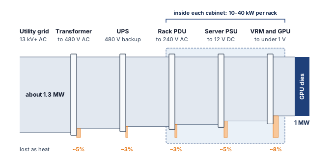
The illustrative conversion losses in figure 12 require roughly 1.3 MW upstream to deliver 1 MW to the dies, before heat removal is counted. Facilities summarize that overhead with power usage effectiveness (PUE), total facility power divided by IT-equipment power, and because the IT boundary already contains some of these conversion losses they must not be counted twice. Facility-level power metrics defines the ratio and draws its boundary.

Every floating-point operation dissipates energy as heat. Dense Tensor Core activity during large matrix multiplications drives heat proportional to the switching activity of billions of transistors. Fleet design must pair each accelerator’s sustained power envelope with any documented transient excursion requirement. At dense fleet scale, this produces the power wall, the point at which facility power delivery and heat removal, rather than available arithmetic units, determine how much compute can be installed and sustained.

The thermodynamic limit (principle 4), which holds that every joule a computation draws ends as heat and that a facility can run only as fast as it removes that heat, makes heat removal part of usable compute capacity. A facility can reach its power or cooling envelope while arithmetic capacity is still available to purchase, so the scarce quantity becomes watts per unit of floor area rather than FLOP/s. The power density wall (principle 3) adds that spatial constraint, bounding cluster scaling by the watts each rack can dissipate rather than only by silicon area or floor space. If a proposed rack exceeds the engineered airflow’s heat-removal capability, the design must lower its density or move to liquid, which at the 100 kW class of high-density training racks is part of the rack design rather than an option.

Definition 2.6: Thermal design power (TDP)

Thermal design power (TDP) is a vendor-defined sustained thermal design target in watts for a specified product configuration and operating condition.

Significance: The H100 SXM5 configuration used in this chapter carries a 700 W design target. Sustaining the intended operating point requires a thermal path and facility loop qualified for that target under the vendor’s inlet and coolant conditions.
Distinction: TDP does not denote one universal instantaneous-power maximum. TGP, board power, configurable limits, and transient specifications describe related electrical constraints under conventions that differ by vendor and product.
Common pitfall: A frequent misconception is that the advertised wattage alone specifies rack power and cooling. Fleet design must combine the sustained thermal target, configured power limit, workload behavior, component overhead, and transient-power requirement.

The trajectory of TDP records a scaling regime reaching its limits. For three decades, Dennard scaling⁶ allowed chip designers to shrink transistors while maintaining approximately constant power density: smaller transistors required lower voltage, so packing more transistors into the same area did not increase heat output per unit area. As voltage scaling and leakage limits ended that regime, architects had to treat energy, cooling, and parallelism as first-order constraints rather than free byproducts of process shrinks (Dennard et al. 1974; Hennessy and Patterson 2019). Since then, each generation of accelerator has had to trade performance against power and heat. The era of “free” performance improvements through process shrinks is over; every gain in throughput now has to be paid for in watts, cooling capacity, or specialization.

⁶ Dennard scaling: Named after Dennard et al. (1974) at IBM, who showed how MOSFET dimensions, voltage, and current could scale so that power density stayed roughly constant. Later voltage-scaling limits and leakage effects ended that constant-power-density regime; Hennessy and Patterson (2019) describe the resulting post-Dennard power wall as one reason modern architecture turned toward parallelism and specialization. For ML infrastructure, the V100-to-B200 TDP trajectory (300 W to 1,000 W) is an illustration of the post-Dennard planning problem: cooling and power delivery are now co-equal design constraints with the silicon itself.

Dennard, Robert H., Frank H. Gaensslen, Hwa-Nien Yu, Victor L. Rideout, Elias Bassous, and Antoine R. LeBlanc. 1974. “Design of Ion-Implanted MOSFET’s with Very Small Physical Dimensions.” IEEE J. Solid-State Circuits 9 (5): 256–68. https://doi.org/10.1109/jssc.1974.1050511.

Hennessy, John L., and David A. Patterson. 2019. “A New Golden Age for Computer Architecture.” Communications of the ACM 62 (2): 48–60. https://doi.org/10.1145/3282307.

The V100 (2017) operated at 300 W TDP, the A100 (2020) increased to 400 W, the H100 (2022) reached 700 W, and the B200 (2024) draws 1000 W. In seven years, TDP has more than tripled, growing at approximately 19 percent per year.

If this growth rate continued as a planning scenario on a two-year product cadence, a generation after Blackwell would approach 1,400 W per accelerator, and the generation after that would reach about 2,000 W. At that level, a single 8-GPU node would consume 16 kW of GPU power alone, requiring liquid cooling infrastructure (section 2.6.2) that can remove heat at rates approaching those of industrial process cooling equipment. The applicable sustained power envelope is not merely a specification on a data sheet; it propagates through every level of the infrastructure stack. The power-delivery chain, cooling system, rack design, and facility electrical infrastructure must accommodate deployed accelerators, their documented transients, and the plausible envelope of future refresh cycles.

The propagation is visible at both ends of the stack in published data. Vendors publish a power rating for each accelerator package, and figure 13 (a) collects those ratings across 14 NVIDIA, Google, AMD, and Intel parts. The ratings follow each vendor’s own convention (TDP, maximum board power, or maximum TGP), so they bound design envelopes rather than measure consumption, but they climb steadily from one generation to the next. Panel (b) plots the facility power of supercomputers that Epoch AI tracks for AI work, together with the largest one operating at each date (Epoch AI 2026a; Pilz et al. 2025). From 2013 through 2021 that record stayed between 20 MW and 30 MW, a level set by national high-performance computing systems. The Frontier supercomputer raised it to 40 MW in 2022, and AI training clusters then lifted it to about 350 MW by 2025, a 9× increase in three years. Over the same three years the rating of one package rose from the H100’s 700 W TDP to the B300’s 1,400 W maximum TGP, roughly a 2× increase across the two rating conventions. Hotter packages explain only a small part of the jump. The rest comes from the number of accelerators a single system joins together and the facility built to feed them, which is why the power wall at fleet scale is a provisioning problem for the building as much as a thermal problem for the chip.

Pilz, Konstantin F., James Sanders, Robi Rahman, and Lennart Heim. 2025. “Trends in AI Supercomputers.” arXiv Preprint arXiv:2504.16026.

Figure 13: **Package Power versus System Power**: (a) Published power rating of one accelerator package by release year. Ratings follow each vendor’s convention (TDP, maximum board power, or maximum TGP) and describe design envelopes, not measured workload power. (b) Facility power of AI supercomputers by first operational date on a logarithmic axis; the red line tracks the largest system operating at each date. The record held near 20 to 30 MW for most of a decade before AI training clusters raised it roughly ninefold between 2022 and 2025. Sources: (a) NVIDIA (2013), Foley and Danskin (2017), Choquette et al. (2018), Choquette et al. (2021), Choquette (2023), NVIDIA (2024), NVIDIA (2025), Jouppi et al. (2021), Advanced Micro Devices (2021), AMD (2023), Intel Habana Labs (2023), Intel (2024); (b) Epoch AI (2026a).

Accelerators implement sophisticated power management to operate within their TDP envelope. When the workload does not fully use all SMs (for example, during the communication phase of a training step when the GPUs are waiting for AllReduce to complete), the GPU firmware can disable the clock signal to idle circuitry through clock gating, eliminating dynamic switching power and freeing thermal headroom for the active SMs. A separate mechanism, dynamic voltage and frequency scaling (DVFS), adjusts the chip’s clock frequency and supply voltage to stay within power and thermal limits; during a large matrix multiplication that activates all SMs simultaneously, DVFS reduces the clock frequency to keep total power within TDP. When some SMs are idle, the active SMs can boost frequency because total chip power is below TDP, so the actual clock, and therefore the actual throughput, varies throughout a training step.

Dynamic power management means that the actual power draw of a GPU varies continuously during training. A typical training step might see power swing from 400 W (during communication phases when most SMs are idle) to 700 W (during the forward and backward pass when all Tensor Cores are active) and back, with each transition occurring in microseconds. The voltage regulator modules (VRMs) on the baseboard, which convert the board supply to the sub-volt core voltage, must respond to these transitions fast enough to maintain a stable supply voltage despite the rapidly changing current draw.

DVFS also couples software optimization to the power envelope. A kernel that achieves high SM occupancy (many active warps per SM) draws more power, potentially triggering a frequency reduction that partially offsets the occupancy benefit. Conversely, a kernel with moderate occupancy may run at a higher clock frequency, achieving comparable throughput at lower power. Power-normalized throughput (TFLOP/s per watt) is therefore a more robust comparison metric than raw TFLOP/s, and it explains why the same GPU can show different sustained clock frequencies depending on the workload and the cooling solution.

At fleet scale, DVFS also affects power planning. Average workload draw can fall below the configured limit because communication phases and incomplete occupancy leave circuitry idle, but averages do not replace sustained and transient design cases. Some operators deliberately lower accelerator power caps to fit more devices within a fixed facility budget, accepting workload-dependent throughput loss in exchange for lower per-device draw. Power capping is a form of the compute-efficiency trade-off at the operational level.

To appreciate the physical challenge, consider what 700 W means in terms of heat flux. An H100 die measures approximately 814 mm² (roughly $29{\times}28$ mm). Dissipating 700 W from this area produces a heat flux of approximately 86 W/cm². For comparison, the surface of an electric stovetop burner at high heat produces approximately 10 W/cm². An H100 die generates 8.6× the heat flux of a stove burner, concentrated on an area the size of a large postage stamp.

The B200’s 1,000 W envelope spans a dual-die package. In this comparison, the average heat flux remains comparable while the package heat-removal rate increases by 43 percent. Cooling must keep junction temperature and memory temperature within the applicable product limits under the specified inlet and load conditions. A single temperature threshold cannot stand in for those separate requirements.

The thermal interface material (TIM) between the package and its cooling assembly is one part of that heat-transfer path, and it is the part that ages. Training alternates compute-dense phases with communication phases, so the die heats and cools many times per minute; under that cycling, a phase-change or paste TIM can pump out (migrate away from the contact surface) or crack. Increased thermal resistance can raise temperature at the same load, but the performance effect depends on the remaining thermal margin and the device’s control policy. A temperature trend alone does not identify the cause; inlet conditions, flow, contact, and workload also require inspection. When thermal limits reduce clocks without stopping execution, the result is a gray failure, a performance degradation that monitoring must distinguish from an application or network bottleneck.

Arithmetic per watt offsets only part of rising TDP, and a larger capability target can increase total work despite improved efficiency, so facility planning must compare the proposed device count, power envelope, and completion time together. Packing accelerators close together shortens communication paths but concentrates heat: a four-node DGX H100 rack already draws 33.5 kW including its allocated cooling overhead, several times the load of a conventional server rack, and the accelerators of a 10,000-GPU cluster, the round fleet size this chapter uses for warehouse-scale examples, alone draw 7 MW before hosts, network, and cooling are counted. Rack and pod designs must reconcile that proximity with enough space and infrastructure to deliver power and remove heat across all participating nodes.

Power-envelope implications recur throughout the infrastructure hierarchy. At the node level, configured limits constrain how many accelerators can share a chassis (section 2.5). At the rack level, aggregate sustained load and heat flux help determine whether engineered air or liquid cooling can meet the design point (section 2.6.2). At the pod level, coincident demand and transient behavior shape megawatt-scale power delivery (section 2.7). Every level above the die must therefore manage both sustained heat and electrical variation. Accelerator selection must compare useful workload throughput within that facility envelope, rather than treating power as a cost added after the compute decision.

Power delivery networks and transient dynamics

Fitting redundant AC power supply units inside every eight-GPU chassis consumes enclosure volume needed for cooling manifolds and high-speed interconnects, especially as rack loads climb toward 100 kW in liquid-cooled clusters. Many dense-rack designs therefore replace per-chassis AC supplies with rack-level DC power distribution. In this architecture, a centralized power shelf converts mains AC to a 48V DC busbar that runs the height of the rack. Power reaches the server backplane through the 48V bus, and local DC-to-DC converters supply the lower voltages required by the components. Consolidation can recover chassis volume for cooling loops and high-bandwidth interconnects, but it does not by itself establish fewer conversion stages or a fixed efficiency gain. The comparison must account for each design’s actual stages and conversion efficiency across the intended load range. Shared power shelves and busbars also create a rack-level failure boundary whose redundancy and serviceability must be qualified.

A training step makes each accelerator’s current draw jump. When a collective barrier releases a node’s GPUs from a communication phase into dense arithmetic, each one steps from a few hundred watts toward its full power envelope within microseconds, and the barrier correlates those steps across the node. The power delivery network (PDN) must hold the supply voltage steady through that step, and the difficulty grows as the voltage falls from the 48V busbar to the sub-1V rail at the die.

At a fixed power, current scales inversely with voltage, so the core rail carries far more current than the busbar; the voltage regulators transform voltage and current between those boundaries. What disturbs the supply is the rate of change of that current, its slew rate $d\AcceleratorSupplyCurrent/d\TimeInstant$. Every conductor loop has inductance, a property that resists changes in current, so a fast current step produces a momentary voltage dip, or droop, even when average power remains within the facility budget.

Definition 2.7: Power delivery network (PDN) and transient dynamics

Power delivery network (PDN) is the electrical distribution hierarchy that supplies the processor through regulators, interconnects, and decoupling capacitors. Parasitic loop inductance contributes to voltage fluctuations during changes in current.

Significance: Synchronized workload transitions can correlate accelerator demand. Supply excursions outside the device’s specified limits can cause timing errors, protective throttling, or resets.
Distinction: Local electrical transients require a faster response than facility power-control loops can provide. Regulators and nearby charge storage address different timescales within the same hierarchy.
Common pitfall: A frequent misconception is that the full core-current slew acts on a single inductance summed from rack to die. Regulation and decoupling change the current waveform at each stage; the relevant inductance and current must belong to the same path.

For a particular inductive path, the voltage excursion contributed by its inductance follows equation 2:

\[\FiniteChange \SupplyVoltage= \ParasiticLoopInductance\frac{d\AcceleratorSupplyCurrent}{d\TimeInstant} \tag{2}\]

Here $\ParasiticLoopInductance$ is the loop inductance of that path, and $d\AcceleratorSupplyCurrent/d\TimeInstant$ is the current slew through it. Local capacitors initially supply part of a load-current increase, so the current slew seen upstream need not equal the slew at the core. A complete rail model also accounts for resistance, capacitance, and regulator response.

A worked estimate for one accelerator shows why the hierarchy matters. When an H100 moves from its communication-phase draw of about 400 W to its 700 W envelope on a 0.8 V core rail, its core current rises by about 375 A. Suppose the board loop between the voltage regulator and the package has 50 pH of inductance. If package capacitors supply the fast edge so that this loop sees the step over 1 μs, equation 2 gives a droop of about 19 mV, or 2.3 percent of the rail. If the same step reached that loop in 100 ns, the droop would be about 190 mV, roughly 23 percent of the rail and far outside a 5 percent operating band. The inputs are scenario assumptions, but the tenfold sensitivity to rise time is physical. The same current step stays inside tolerance or corrupts timing depending on which charge store answers it first.

The collective barrier that aligns transitions from communication to arithmetic raises the correlation of demand across a rack, but it does not imply that every accelerator switches on the same nanosecond or that their core currents flow through one shared low-voltage loop; engineers must evaluate both each device’s local voltage excursion and the aggregate demand seen by upstream supplies. A rising load can produce voltage droop, where droop below the specified operating minimum can invalidate timing margins, while an abrupt load reduction can produce overshoot that must remain within the device’s specified limits as well. Neither the magnitude nor the resulting failure mode follows from workload synchronization alone. The mitigation is a hierarchy of charge storage and control, in which each tier answers the transients too fast for the tier above it (table 13), with placement and parasitic impedance determining which frequencies each tier can address.

Table 13: Decoupling Tiers in the Power Delivery Network: Each tier supplies charge on a timescale the slower tier above it cannot reach, so a fast edge that bypasses a tier lands on a larger inductance.

Tier	Charge store or control	Response timescale	Transients it absorbs
On-die	On-die capacitance	Sub-nanosecond	Switching activity within a kernel
Package	Package and interposer capacitors	Nanoseconds	Kernel launches and streaming-multiprocessor activation edges
Board	Bulk capacitors, regulator control loop	Microseconds	Communication-to-compute phase changes of one accelerator
Facility	Uninterruptible power supply (UPS), utility	Milliseconds to seconds	Synchronized power swings across racks and the cluster

The facility row of table 13 is where the barrier’s correlation appears in aggregate. For an illustrative calculation, assume 1,024 GPUs change together from 400 W to 700 W each over 100 μs. The assumed aggregate step is 307 kW, giving a ramp rate of 3.07 GW/s. This is a load-side scenario, not a measured utility input. No single regulator carries this step, because each accelerator draws its share through its own board, yet the shared upstream supplies see the sum.

↪ How energy buffering presents this ramp to the grid as a smoother, more easily connected load is developed in Power delivery.

Workload-level controls complement these hardware tiers. Power ramping can reduce abrupt demand changes where the hardware and firmware support it, but a design must verify those controls rather than assume that every kernel launch receives automatic smoothing. The fleet-level lesson is that average power capacity and transient voltage integrity require separate checks.

2.6.2 Cooling class and heat removal

The power path ends in heat. Under the thermodynamic limit (principle 4), nearly every joule an accelerator draws leaves as heat through switching, leakage, and resistive losses. During a transient some of that energy warms the chip and its surroundings, but in steady operation the stored thermal energy stops rising, so cooling must remove heat at about the rate the rack consumes electricity. When removal falls behind generation, temperature climbs through the available thermal margin until throttling lowers clocks and throughput, and sustained overheating can damage the hardware. The rack’s cooling class, air or liquid, is the choice of fluid that carries this heat away, and it bounds how dense the rack can be.

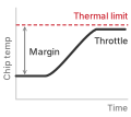
When cooling falls behind, temperature climbs through the thermal margin until throttling caps it.

Heat transfer explains why density reshapes the rack. Air carries far less heat per unit volume than liquid, so an air-cooled rack needs enough airflow, pressure, and temperature rise to carry away its heat, and how much a hall can supply depends on the server and facility design rather than on one rack-power threshold.

Air cooling, the dominant technology for decades, works by blowing room-temperature air across heat sinks attached to the chips. The air absorbs heat at a rate determined by its specific heat capacity, roughly 1.0 kJ/kg/K. The heated air is exhausted from the rear of the rack, typically 15–20 degrees Celsius warmer than the inlet, and directed to a computer room air conditioning (CRAC) unit that cools it before recirculating.

Air is a poor thermal conductor. Its thermal conductivity is only 0.026 W/m/K, compared to 0.6 W/m/K for water and 400 W/m/K for copper. Removing a large heat load with air requires substantial volumetric flow. Fan power depends on that flow, pressure drop, and fan efficiency; rack power alone does not specify a fixed cooling fraction.

The heat that a coolant stream removes depends on how much fluid flows, how much heat each kilogram absorbs per degree of warming, and how far the fluid warms (equation 3):

\[\CoolantHeatLoad = \CoolantMassFlowRate\times \SpecificHeatCapacity\times \FiniteChange\CoolantTemperature \tag{3}\]

where $\CoolantHeatLoad$ is the heat removed (watts), $\CoolantMassFlowRate$ is the mass flow rate (kg/s), $\SpecificHeatCapacity$ is the specific heat capacity (J/kg/K), and $\FiniteChange\CoolantTemperature$ is the temperature difference between outlet and inlet. For air with $\SpecificHeatCapacity$ of 1,005 J/kg/K and a typical $\FiniteChange\CoolantTemperature$ of 15 K (inlet at 20 degrees C, outlet at 35 degrees C), removing 100 kW requires a mass flow rate of 100,000 $\div$ (1,005 $\times$ 15) $\approx$ 6.6 kg/s. At sea-level air density of 1.2 kg/m³, this corresponds to a volumetric flow rate of 5.5 m³/s, or approximately 11,713 CFM (cubic feet per minute). Moving this much air through the confined space of a server rack requires powerful fans that themselves consume substantial power.

At higher power densities, the airflow and pressure required to cool a rack raise fan energy and can make air cooling impractical before the IT load itself reaches a power limit. The exact crossover depends on rack geometry, inlet temperature, pressure drop, and fan-control policy rather than on one universal rack-power threshold.

Water has a specific heat capacity of 4.18 kJ/kg/K, over four times that of air, and a thermal conductivity roughly 23× higher. Its much greater density also lets a small fluid volume carry substantial heat. To appreciate the magnitude of the difference, consider how much fluid must flow to remove 700 W from a single GPU. Air at a 15-degree temperature rise requires tens of liters per second of airflow (a small wind tunnel). Water at the same temperature rise requires only about 0.01 liters per second (a thin stream). This thousands-fold difference in volumetric flow permits compact liquid paths, but it does not determine pumping energy. Pressure drop through cold plates, pipes, and fittings, together with pump efficiency, determines the power needed to sustain that flow.

At rack scale the same equation sizes the liquid loop. Removing the modeled 120 kW load of a GB200 NVL72 rack through water that warms by 10 °C takes about 170 liters per minute, and a smaller temperature rise needs proportionally more flow. A real design must use the heat fraction the liquid loop actually captures and account for residual air cooling; flow capacity, pressure, leak containment, and loss-of-flow response are separate requirements, which the facility controls of section 2.6.4 treat as failure domains.

Direct-to-chip liquid cooling routes coolant through cold plates mounted on GPU packages. The cold plate contacts the heat spreader through thermal interface material; the resulting thermal resistance depends on the package, interface, plate design, and flow. The coolant carries heat through manifolds and pipes to a coolant distribution unit (CDU) at the rack or row level. The permissible supply temperature depends on the equipment, so liquid cooling need not require chilled water.

In a two-loop design, the CDU transfers heat from the chip-level coolant to the facility water loop, which carries it toward cooling towers or dry coolers. Isolation lets each loop maintain its required fluid chemistry and pressure. The chip-level coolant must satisfy the equipment’s compatibility and cleanliness requirements to control deposits, corrosion, and blockage; purity alone does not establish suitability. Liquid cooling can reduce server airflow requirements, although memory modules (DIMMs), voltage regulator modules (VRMs), and other components without cold plates may still need fans, and lower fan demand can also reduce noise.

A more aggressive approach, immersion cooling, submerges entire server boards in a tank of nonconductive dielectric fluid. The fluid absorbs heat from wetted surfaces, replacing server airflow; high-heat-flux components may still need heat sinks or directed flow, and flow, local heat flux, material compatibility, and heat-exchanger capacity still determine component temperatures. Single-phase immersion cooling uses a fluid that remains liquid throughout the process, with heat carried away by convection currents in the tank: the heated fluid rises to the surface, is pumped through a heat exchanger to reject the heat to the building’s chilled water loop, and returns to the bottom of the tank. Two-phase immersion cooling takes this further: fluid boils at heated surfaces, carries latent heat to a condenser, and returns as liquid, with heat removal depending on the fluid, pressure, condenser capacity, and operating conditions. The complete facility still spends energy on heat rejection and electrical distribution, so the cooling mechanism alone does not settle facility energy.

The trade-off is serviceability. Accessing a failed component requires handling fluid-wetted hardware, and the dielectric fluids themselves are expensive ($20–$50 per liter). A single immersion tank holding four server boards may contain 500–1,000 liters of fluid, representing $10,000–$50,000 in coolant cost alone. The operational procedures for immersion-cooled facilities differ sharply from air-cooled ones, requiring specialized training for technicians and different approaches to cable management, since all wetted materials must be compatible with prolonged fluid exposure. Depending on the fluid and its additives, metals can corrode, while polymer insulation and seals can swell or degrade. Qualifying compatible materials adds engineering work and can constrain component choices. These serviceability costs enter the design decision alongside the heat paths, binding limits, and parasitic loads of the air and liquid regimes (table 14).

Table 14: Cooling Architecture Trade-Offs: Feasible rack density follows from the particular equipment and facility design. The example design points differ by 10× in rack power, yet there is no universal rack-power threshold or PUE that separates air and liquid cooling. Compare qualified operating envelopes and total facility energy.

Design question	Air cooling	Direct-to-chip liquid cooling
Heat path	Chip to heat sink to moving air	Chip to cold plate to coolant loop
Binding limits	Airflow, pressure drop, inlet temperature, and allowable component temperature	Cold-plate resistance, flow, coolant temperature, and heat-rejection capacity
Parasitic loads	Server and facility fans; conditioning where required	Pumps, CDU, heat rejection, and any residual air cooling
Service constraints	Air containment, filters, and access paths	Fluid compatibility, leak management, and maintainable connections
Facility metric	Measure complete IT and non-IT energy	Measure the same boundary; liquid cooling does not determine PUE by itself
Example design point	Enterprise rack near 12 kW; best air-cooled facility profile PUE 1.12	GB200 NVL72 rack at 120 kW; liquid-cooled facility profile PUE 1.06

Direct-to-chip liquid cooling supports higher heat flux than forced air because cold plates route chip heat directly into circulating fluid with high volumetric heat capacity before reaching facility heat rejection, whereas air systems rely on convective dissipation across finned heat sinks (figure 14). Ambient wet-bulb temperature (the lowest temperature that evaporation can bring outdoor air to, which bounds evaporative heat rejection) and rack power density determine whether an air, liquid, or hybrid loop satisfies the chip junction temperature envelope.

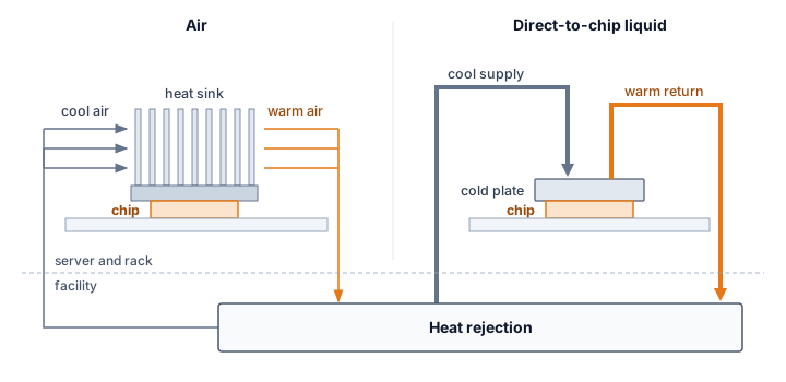
Figure 14: **Air and Liquid Heat Paths**: Air transfers chip heat through a heat sink and moving air; direct-to-chip liquid cooling transfers it through a cold plate and coolant. Both require heat rejection. Capacity, parasitic energy, and water use depend on the engineered system rather than the cooling medium alone.

Two anchors bound the choice for this chapter’s racks. The four-node DGX H100 scenario at 33.5 kW can use engineered air cooling in a suitable facility, while racks in the 100 kW class of high-density training racks need liquid, which raises heat-removal capacity and can reduce fan energy; between the two anchors, the facility’s airflow capacity decides. Cooling class is therefore a configuration constraint. Rack layout and heat-removal capacity, not accelerator count alone, determine whether the intended configuration can sustain its workload or must reduce density or power.

Engineered air can still cool the DGX rack; the 100 kW class needs liquid.

↪ What heat removal adds to facility energy (PUE), and the water that heat rejection consumes, are developed in Cooling energy, heat rejection, and water.

2.6.3 Rack design considerations

Packing 33.5 kW of compute and thermal hardware into a standard 42U frame leaves almost no room for conventional server layouts. In an enterprise 42U rack, servers are installed as independent 1U or 2U pizza-box units, each with its own fans, power supplies, and cable connections. A single DGX H100 instead occupies 8U and contains 8 GPUs, the NVSwitch fabric, multiple power supplies, and (in liquid-cooled configurations) coolant manifolds with quick-connect fittings. Four DGX units fill 32U of a 42U rack, leaving only 10U for networking switches, cable management, and PDUs.

The transition from traditional server form factors to ML-optimized designs is driven by the same power density challenge that motivates engineered airflow or liquid cooling. A traditional 1U server dissipates 300–500 W and requires only modest airflow for cooling. A DGX H100 node dissipates approximately 8.4 kW across its 8 GPUs, NVSwitches, and supporting components, requiring either high-volume forced airflow (in air-cooled configurations) or liquid cooling plumbing (in liquid-cooled configurations). The form factor must accommodate both the compute hardware and the thermal management infrastructure, which is why ML nodes are substantially taller (8U vs. 1U) than traditional servers.

Cable management is a nontrivial engineering challenge. Each DGX H100 node has eight InfiniBand cables (one per GPU), two Ethernet management cables, power cables, and, for liquid-cooled units, coolant hoses. A fully populated rack contains over 40 high-speed cables whose layout is governed by three strict physical constraints: airflow clearance, minimum bend radius, and electromagnetic interference. In air-cooled designs, cables must not obstruct intake or exhaust airflow, because even a localized blockage creates hot spots that trigger thermal throttling. High-speed cables simultaneously enforce a minimum bend radius (for installed fiber optic cable, typically 10–15$\times$ the outer diameter, per the manufacturer’s specification (The Fiber Optic Association 2020)), below which optical fibers suffer attenuation and induce bit errors or complete link drops. Densely bundling high-speed copper cables can also induce electromagnetic crosstalk that degrades signal quality. In large installations, the cable plant alone can take weeks to install and test, and cable routing errors are one of the most common causes of post-installation debugging delays.

The Fiber Optic Association. 2020. Fiber Optic Cable Bend Radius or Diameter.

The rack’s network attachment needs the same density-driven rethinking, starting with the top-of-rack (ToR) switch. In traditional data centers, a ToR switch provides 1–10 Gb/s Ethernet connectivity to each server, aggregated into uplinks to higher-level switches. In an ML rack, the ToR switch is an InfiniBand or high-speed Ethernet switch providing 400 Gb/s per port, and it must handle the bursty, synchronized traffic patterns of distributed training. In a conventional design all eight GPUs of a node share one ToR switch, so a data-parallel AllReduce converges on that switch and its uplinks. A rail-optimized design instead gives each GPU index its own leaf switch (GPU 0 of every node on leaf 0, GPU 1 on leaf 1, and so on), so same-index collectives stay on one switch, at the price of extra switches and cabling whose benefit depends on how the job’s process groups map onto the rails.

↪ How rail-optimized topologies align cabling with collective traffic is developed in Rail-optimized topology.

2.6.4 Facility reliability and environmental controls

A coolant leak or electrical fault in a single DGX H100 rack threatens $1.4 million in hardware and can halt a multi-rack training job across the upper levels of the failure-domain hierarchy introduced in section 2.5.5. Data centers housing ML infrastructure therefore pair physical security with continuous environmental monitoring that becomes part of the compute design rather than a facilities afterthought. Beneath raised floor tiles and along liquid cooling piping, water sensors identify leaks within seconds and close automatic coolant isolation valves, while humidity controls keep the air within a moderate band, dry enough to prevent condensation and humid enough to limit static discharge. Inside the cabinets, aspirating smoke detectors sample rack air continuously to catch combustion byproducts at concentrations far below what sprinkler-activating detectors can sense, and vibration sensors on the building structure and rack frames flag seismic events or construction shocks before they can damage disk drives or loosen cable connections.

Cooling failures threaten both hardware and useful fleet work. When coolant flow stops, a dense rack loses heat-removal capacity and must throttle or shut down before thermal runaway. N+1 redundancy in CDUs, temperature monitoring, and automatic load shedding limit the affected capacity. An emergency air path can support reduced-power operation where the facility design provides one.

Serviceability also changes the failure budget. Leaks can damage equipment and drain cooling capacity, which is why the leak sensors above drive isolation valves, while quick-disconnect fittings allow node replacement without draining the entire loop. Their seals and coolant compatibility therefore belong in the maintenance plan. The fleet-level consequence depends on how much synchronized work shares the failed cooling domain.

The economics of cooling reliability shift when moving from independent inference servers to tightly coupled training clusters. In a distributed training run using synchronous parallelism, a cooling-loop failure that idles one slice of the cluster can halt the entire job. Consider a cooling failure that triggers a thermal shutdown of the 256 GPUs served by one coolant distribution unit within a 10,000-GPU cluster, about ten times the 1,024-GPU reference cluster. The example counts lost compute capacity, excluding repair and replacement costs. If the repair time for a CDU pump is 4 hours, the immediate loss of 256 GPUs at the fleet’s reference in-service rate of $2 per GPU-hour is $2,048. Assuming the job cannot continue elastically and the remaining 9,744 GPUs remain unavailable for other work, the synchronous blast radius inflates the cost to $80,000 in lost compute time. Adding checkpoint retrieval and rollback of 30 to 60 minutes of lost computation brings the illustrative lost-compute total to $90,000–$100,000 before any additional recovery delay. Whether N+1 cooling redundancy is worth its price follows from comparing these expected outage losses and recovery behavior with that price, rather than from treating redundancy as an unconditional requirement. The energy the rollback repeats belongs to the facility energy account of Cooling energy, heat rejection, and water.

One cooling failure can idle the whole training job.

Coolant condition is another reliability input. Deionized water and compatible inhibitors control galvanic corrosion, the damage caused by electrochemical differences between metals in the loop. Biofilm on heat-transfer surfaces impedes cooling and increases pumping demand. Maintenance must preserve coolant chemistry and heat-transfer performance, because a fouled or corroding loop loses capacity before it fails outright.

These controls bear directly on reliability and uptime. A fire in a single rack can shut down an entire data center hall for days while the fire suppression system is recharged and the affected area is decontaminated. The 2021 OVHcloud fire in Strasbourg shows how a single-building incident, absent the right compartmentalization, escalates into a site-wide failure domain.

War Story 2.1: The data center that became the failure domain (2021)

Context: OVHcloud operated four data centers at its Strasbourg site, serving customers whose systems depended on the site’s physical power, fire, and recovery design (OVHcloud 2021).

Mechanism: On March 10, 2021, a fire broke out in building SBG2. Uncontained fire spread and shared power pathways destroyed building SBG2, damaged adjacent SBG1, and forced emergency shutdown of SBG3 and SBG4.

Impact: Thousands of servers were physically destroyed, taking over 3.6 million websites offline worldwide and destroying unbacked-up customer data.

Fix: OVHcloud rebuilt the site with independent physical fire barriers, isolated power distribution per building, and mandatory free off-site backup storage.

Systems lesson: Compute infrastructure extends beyond GPUs and network topology. Fire compartments, power isolation, backup geography, and disaster-recovery assumptions determine whether a rack-scale incident becomes a site-scale outage. Multi-node ML training clusters inherit this physical dependency: a single data-center power or cooling domain failure halts active training runs and destroys un-replicated checkpoint states unless recovery paths cross physical facility boundaries.

OVHcloud. 2021. Strasbourg Datacentre: Latest Information. OVHcloud incident update.

Uptime Institute. 2026. Tier Classification System. Uptime Institute web page.

Once rack-level controls are in place, the reliability question moves up to facility redundancy, where the same failure-domain logic that isolates a leaking rack also decides how much duplicate power, cooling, and recovery capacity the site should buy. Data center reliability is commonly classified using the Uptime Institute Tier system, with Tier III and Tier IV representing common options for mission-critical compute (Uptime Institute 2026). A Tier III facility is concurrently maintainable: redundant capacity components and distribution paths let operators maintain or replace equipment without shutting down IT operations. Tier IV adds fault tolerance through independent, physically isolated systems, so a single equipment failure or distribution-path interruption should not affect IT operations. The practical difference is not a magic availability number; it is how much failure prevention the building buys in electrical and mechanical infrastructure before software-level resilience takes over.

For ML training, the calculus differs from traditional enterprise computing. A training run is a long-running batch process, not a real-time transaction system, so a facility outage during a two-week run usually costs a restart from the last checkpoint rather than permanent data loss, provided a valid checkpoint survives in an accessible failure domain and usable compute becomes available. The restart still incurs lost work, recovery time, and potentially a missed deadline. Many training deployments therefore pair concurrently maintainable (Tier III) facilities with aggressive application-level fault tolerance. Rather than buying every layer of building-level redundancy, they invest in checkpointing, job restart, and storage that can absorb rare facility interruptions, and redirect the avoided resiliency spend toward accelerators, networking, or storage. Facility redundancy and application-level recovery address different parts of the same risk. A design can trade some preventive infrastructure for checkpointing and recovery capacity only after checking which failures the recovery path survives and whether the resulting completion-time risk is acceptable.

Checkpoint 2.3: Infrastructure physics

A team is planning to deploy 256 H100 GPUs (32 nodes, each drawing about 8.4 kW as computed in section 2.6.3) in an existing air-cooled data center with 250 kW of available facility power, a PUE of 1.5, and a cooling plant that can reject 200 kW of IT heat.

Facility power: calculate the total power draw, including cooling overhead.
Binding capacity: identify whether power capacity or cooling capacity is the binding constraint.
Required modifications: specify what modifications would be needed to support the full deployment.

The rack concentrates power and heat into a physical volume where thermodynamics, not software, sets the limits. A single rack of 32 GPUs, however, is far from sufficient for our 175B model, which needs tens to hundreds of nodes, many racks’ worth, to train on a practical schedule. The next level of infrastructure aggregates tens to hundreds of racks into a unified computing system: the pod, whose physical interconnect fabric must be engineered around the communication patterns and failure domains the workload creates.

Self-Check: Question

A four-node DGX H100 rack draws approximately $33\text{ kW}$ of IT power. Which heat-transfer property can make direct-to-chip liquid cooling attractive as rack density rises, even though engineered air cooling remains possible in a suitable facility?
1. Liquid cooling increases GPU arithmetic intensity by lowering electrical resistance inside Tensor Cores.
2. Water has much higher volumetric heat capacity than air, so it can carry away the same heat with a much smaller volumetric flow for a comparable temperature rise.
3. Air cooling causes optical transceivers to melt when exposed to fan airflow velocities above 5 meters per second.
4. High-density racks require full dielectric immersion because cold plates cannot conduct heat from silicon heat spreaders.
A facilities team provisions its cooling and electrical infrastructure for the average GPU power observed during training ($\approx 500\text{ W}$ per GPU) rather than the $700\text{ W}$ sustained design target. Explain why this choice can silently degrade cluster training throughput even when no hardware errors or crashes occur.
Synchronous ML training can correlate accelerator power ramps across a cluster. How does this electrical behavior distinguish its power-delivery requirements from those of largely uncorrelated web-serving workloads?
1. ML clusters operate on direct current exclusively, eliminating the need for uninterruptible power supplies.
2. Web-serving data centers experience higher $di/dt$ transients because individual HTTP requests draw more peak current than matrix multiplications.
3. ML training consumes purely reactive power that causes step-down transformers to freeze mechanically.
4. Correlated demand changes require checking both local regulator and decoupling response and the aggregate demand seen by upstream supplies, rather than sizing solely for average power.
True or False: Replacing individual server AC supplies with a centralized 48V DC power shelf and busbar guarantees one fewer conversion stage and a 2–3% electrical efficiency gain.
A facility aisle is qualified to remove a sustained 25 kW of IT heat per rack with its existing air-cooling design under the specified inlet temperature and airflow. The proposed AI workload measures 60 kW per rack over its sustained operating interval. Which observation establishes the need to change the cooling design or reduce the rack load?
1. Web workloads have higher peak memory bandwidth requirements, causing localized thermal spikes.
2. AI training generates bursty, millisecond-scale CPU spikes followed by long idle periods, creating thermal cycling fatigue.
3. The measured 60 kW rack load exceeds this aisle’s qualified 25 kW air-cooling envelope; a qualified liquid, hybrid, or redesigned air system, or a lower rack load, must restore thermal feasibility.
4. AI models require lower ambient operating temperatures to maintain FP16 arithmetic precision.
Order the thermal stages of heat removal in a direct-to-chip liquid-cooled data center, from the silicon die to the external environment: (1) heat transfers through a thin thermal interface material (TIM) into a copper cold plate, (2) the Coolant Distribution Unit (CDU) heat exchanger transfers thermal energy from the closed rack loop to the facility secondary loop, (3) external cooling towers or dry coolers reject heat into the ambient outdoor atmosphere, (4) liquid coolant absorbs heat as it flows through microchannels directly above the accelerator package, (5) active switching in transistor junctions generates heat on the silicon die.

See Answers →

2.7 The Pod

Training our 175B model on a single DGX H100 node (8 GPUs, 15,832 TFLOP/s of aggregate FP8 peak) would take about 1.4 years at the efficiency assumed below, even if the model state could fit. Roughly 37 nodes bring the compute-only time down to two weeks, and about 512 nodes bring it to a single day, before any communication or recovery overhead. A pod is the cluster-scale unit that makes this possible: many racks under one high-speed fabric, power envelope, and cooling design, where the engineering challenge is wiring those nodes together into a network fast enough to keep gradient synchronization from becoming the bottleneck so that the fabric serves the role a system bus serves within a single machine. Pod design is the first point where topology, power, and failure domains become shared infrastructure rather than per-rack concerns. Two fabric families dominate: a switched fat tree supplies full bisection bandwidth across node uplinks, while a direct-connect torus wires each node to its neighbors, using fewer switches but giving bisection bandwidth that grows more slowly than node count; Fat-tree (Clos) networks and Dragonfly and torus alternatives develop both.

The pod-scale examples that follow deliberately step up to eight times the 1,024-GPU reference cluster. A 1,024-node DGX H100 cluster contains 8,192 GPUs, 4,096 NVSwitch chips, 8,192 InfiniBand HCAs, several hundred InfiniBand switches, tens of thousands of cables, and draws approximately 8.6 MW of rack power, including each rack’s allocated cooling overhead. It occupies 256 four-node racks across one or more data center halls.

The physical weight of such a cluster is also substantial. Each DGX H100 node weighs approximately 130 kg (288 lb), so 1,024 nodes weigh over 133 metric tons. Racks, switches, cables, and cooling infrastructure add substantially to that total. The data center floor must be structurally engineered to support this concentrated load, which is far denser than the loading that traditional server rooms were designed for. This structural requirement is often overlooked during facility planning and can be a blocking constraint for retrofitting existing buildings.

The physical layout of the data center hall reflects these density constraints. The high power density of ML training racks requires strict hot aisle/cold aisle containment in air-cooled sections, where cold air is forced into the enclosed front of the rack and waste heat is captured immediately at the rear exhaust. The “spine” of the hall, the central cable corridor connecting all racks to the aggregation switches, must accommodate thousands of fiber optic cables and power feeds. Overhead cable trays are preferred over under-floor routing to improve airflow and accessibility, carrying the heavy copper power feeds and fragile fiber interconnects that form the nervous system of the cluster. The layout must also accommodate the liquid cooling infrastructure: coolant distribution unit placement, coolant piping runs, and isolation valves that allow individual racks to be serviced without draining the entire cooling loop. These physical layout decisions, made during facility design, constrain the network topology options available to the training team years later.

Training a 175B model on this cluster costs about $6 \times \Parameters\times \DatasetSize$ floating-point operations for $\Parameters$ parameters and $\DatasetSize$ training tokens, the training-compute estimate of Compute-optimal resource allocation. The token count is where the scaling laws of AI Scaling Laws enter the hardware plan, because a compute-optimal allocation would give a model of this size many times more tokens than GPT-3 saw, multiplying this budget, and the pod-hours it consumes, by the same factor. Notebook 2.4 turns the budget into a compute-only baseline under an assumed local compute efficiency, which is not measured distributed MFU because MFU over a distributed step already includes its communication and pipeline losses; on the 1,024-GPU reference cluster itself the same baseline would take about 4 days. In the terms of the Fleet Law (equation 1.3), that baseline is the $\IronLawComputeTime/\DeviceCount$ term alone.

In practice, communication overhead, pipeline bubbles, checkpoint I/O, hardware failures, and maintenance windows compound to extend the actual wall-clock time beyond that baseline. The first two are the Fleet Law’s exposed $\CommunicationTime(\DeviceCount)$ and $\SynchronizationTime(\DeviceCount)$ terms, and the rest are operational losses around the step. The notebook chains these factors into a scenario estimate of wall-clock time; production schedules can stretch further once queueing, data readiness, debugging, reruns, and site-specific operational margins enter the plan. At pod scale, the schedule therefore depends on fleet overhead as well as on local execution, and recovering the lost time draws on better networks, overlapped communication, and proactive maintenance.

Napkin Math 2.4: Training time for 175B

The training time for our 175B model derives from first principles.

Total FLOPs: Using the same $6 \times \Parameters\times \DatasetSize$ approximation, where $\Parameters = 175 \times 10^9$ and $\DatasetSize = 300 \times 10^9$ tokens: $3.15 \times 10^{23}$ FLOPs
Cluster throughput: 8,192 H100 GPUs at 1,979 TFLOP/s peak, assuming 45 percent local compute efficiency before distributed overhead: $8,192 \times 1979 \times 10^{12} \times 0.45$ FLOP/s before distributed overhead $\approx$ 7.30 EFLOP/s
Compute-only training baseline: ($3.15 \times 10^{23}$ FLOPs)/($8,192 \times 1979 \times 10^{12} \times 0.45$ FLOP/s) $\div 3600 \approx$ 12.0 hours
Illustrative overhead chain: The scaling factor already includes pipeline fill and drain, so no separate bubble step follows. Each subsequent percentage adds time relative to the preceding subtotal, not to final wall time; the factors are scenario assumptions, not independent measured losses:
- Distributed-step losses (scaling efficiency 0.56, the modeled tier for 8,192 GPUs, covering communication and pipeline bubbles): $\div$ 0.56 $\rightarrow$ 21.4 hours
- Checkpoint overhead ($\approx 3\%$): $\times 1.03 \rightarrow$ 22.1 hours
- Hardware failures and restarts ($\approx 10\%$ of the checkpoint-adjusted subtotal): $\times 1.10 \rightarrow$ 24.3 hours
- Maintenance windows ($\approx 5\%$): $\times 1.05 \rightarrow$ 25.5 hours

The total training time is 25.5 hours in this simplified scenario chain, or about 1.1 days. Real production calendars may still stretch to weeks after queueing, debugging, reruns, and site-specific operational margins are included. Recovering this lost time is the domain of distributed systems engineering.

2.7.1 The pod as a warehouse-scale computer

When a single training job spans 10,000 H100 GPUs across an entire data center hall, about ten times the reference cluster, a slow network tier or a single device failure stalls the whole building’s computation. At this scale, the pod operates as a warehouse-scale computer (WSC) (Barroso et al. 2019) and requires a matched budget for arithmetic, communication, and recovery. Rounding the pod up to 10,000 GPUs keeps the warehouse-scale arithmetic easy to follow, and the chapter’s other fleet-scale power, cost, and failure examples use the same round figure. Such a WSC supplies approximately 9.89 EFLOP/s of FP16 peak and 19.8 EFLOP/s at FP8. Non-blocking InfiniBand at 50 GB/s per GPU, the injection bandwidth each endpoint can push into the fabric, provides 500 TB/s of aggregate injection bandwidth and 250 TB/s across the bisection, the cut that splits the cluster into two equal halves. With 4:1 oversubscription at that boundary, meaning the switch tier above it has one quarter as much uplink as downlink capacity, the modeled crossing capacity falls to 62.5 TB/s. The effect on a collective depends on how much traffic crosses the constrained paths, its schedule, and competing transfers. The bandwidth ratio alone is not a collective-time multiplier.

↩︎ The warehouse-scale computer as the unit of fleet design is established in The shift to the warehouse-scale computer.

Treating the building as one computer means that a server assigned to a distributed training job contributes to a shared completion time, and the network fabric, distributed storage, and fleet orchestrator make the building’s resources available as one training system. Rack placement, the power delivery chain, and the network topology must therefore be co-designed, because a mistake at any layer propagates through the others. The first physical consequence concerns communication: the network can set the scaling ceiling. Within a single node NVLink supplies enough bandwidth for tensor parallelism, but across nodes the fabric must carry gradient tensors, activation checkpoints, and pipeline stage outputs, so a building-scale machine is only as fast as the wires that bind its cores. The WSC reframing makes the interconnect a first-class architectural component rather than a peripheral.

The second consequence is that failure is a physical certainty, not an exceptional event. Under the scenario assumption of independent failures and a per-GPU MTTF of approximately 50,000 hours, a cluster of 10,000 GPUs has a mean interval of roughly five hours between GPU failures, and the 25K-GPU fleet of figure 1 about two. That is an expectation, not a periodic schedule, and shared power or cooling faults add correlated exposure. The node failure estimate of section 2.5.5 and the facility controls of section 2.6.4 are the same exposure at smaller scope. Redundant infrastructure, such as dual-path power feeds and redundant switch fabrics, can prevent some interruptions; checkpoint storage and recovery capacity limit lost progress when a running job must stop. Both belong in the physical design. Redundancy keeps many component failures from halting the job, and checkpoints bound the work lost when one does.

The third consequence is that the building blocks combine differently depending on the workload they must carry. A pod is not assembled from a single canonical part list; the interconnect, the switching, and the memory placement are each chosen against the communication and capacity pattern the dominant workload imposes. Three pod designs show the range (table 15). An NVIDIA SuperPOD wires GPUs through an InfiniBand fat-tree for any-to-any flexibility, a Google TPU pod hard-wires chips into a torus for dataflow throughput, and a recommendation pod built for Archetype B arranges the same class of accelerators around embedding memory rather than raw compute.

Table 15: Pod Architecture by Workload: Each pod’s interconnect, switching, and memory emphasis reflects the communication and capacity pattern of its dominant workload, not a single best design.

System	NVIDIA SuperPOD	Google TPU Pod	Recommendation pod
Interconnect	InfiniBand Fat-Tree	3D Torus ICI	RoCE (RDMA over Ethernet)
Switching	External Switches	Direct Chip-to-Chip	Leaf/Spine Ethernet
Topology	Any-to-any	Nearest-Neighbor Mesh	Rail-optimized
Optimization	Flexibility	Dataflow Throughput	Embedding Memory
Dominant workload	Diverse Research	LLM Training	Recommendation

The recommendation pod is the clearest case of memory placement, not compute, driving the layout, and it is the physical form of Archetype B (DLRM at Scale). Its embedding tables reach 10 TB or more, which lighthouse 2.1 showed would need at least 15 DGX H100 nodes of HBM merely to hold, while the dense neural-network layers that operate on those embeddings are comparatively small. A recommendation-first design splits the two across the memory hierarchy. The terabyte-scale embedding tables reside in host CPU DRAM (roughly $3–$5/GB), and the dense layers execute on GPUs, where the compute density justifies the $10–$15/GB cost of HBM. Embedding tables create a capacity requirement, but small random lookups can also saturate aggregate memory bandwidth or expose access latency at high concurrency. Host placement trades capacity cost against lookup throughput and host-to-accelerator transfer, so the workload must validate both budgets. The systems lesson is that optimal infrastructure is workload-specific, not specification-maximizing. Deploying compute-optimized nodes for a memory-capacity-bound workload would strand most of the accelerator’s throughput on a problem its silicon was never the bottleneck for.

The physical design supplies constraints, not an operating policy; later chapters turn its power, capacity, topology, reliability, and sustained-throughput measurements into placement, recovery, monitoring, and ownership decisions. One hardware decision remains for this chapter. With every level from the accelerator to the warehouse-scale computer in view, the choice of accelerator can now be judged against the whole hierarchy rather than against its data sheet.

↪ The ownership decision, in which sustained fleet utilization sets the build-versus-buy threshold, is developed in Utilization as the economic invariant.

Self-Check: Question

Barroso and Hölzle’s Warehouse-Scale Computer (WSC) thesis reframes an ML pod from ‘a room full of computers’ to ‘a single computer that fills a room.’ Which practical consequence most directly shapes infrastructure engineering at pod scale?
1. The entire facility is engineered as a unified machine where the network fabric acts as the system bus, distributed storage acts as the disk subsystem, and the cluster orchestrator acts as the operating system.
2. All servers share a single hardware cache-coherence bus across the entire building, eliminating the need for message-passing software.
3. Workloads are structured as embarrassingly parallel, uncoordinated batch jobs that completely isolate nodes from one another.
4. Component failure rates decrease at warehouse scale, allowing fault tolerance to be managed as an offline manual process.
A team doubles a distributed training cluster from 1,024 to 2,048 GPUs and observes wall-clock training time drop from 14 days to 10 days rather than the ideal 7 days. Calculate the realized scaling efficiency, determine whether the cost per useful FLOP increased, and identify the next diagnostic step.
A synchronous training job spans 10,000 GPUs. Assume a hard crash is detected and recovered from a valid checkpoint, while a persistent gray failure remains undetected and delays dependent steps. Why can the gray failure cost more useful work over a long run?
1. Gray failures permanently corrupt the model weights, forcing the entire training run to restart from step zero.
2. Gray failures trip circuit breakers in the rack, causing cascading facility blackouts.
3. The hard crash incurs detection, restart, and lost-work costs, while the undetected straggler can repeatedly delay the participating job until it is diagnosed.
4. Gray failures disable FP8 Tensor Cores, silently falling back to double-precision FP64 and exhausting memory.
A pod fabric that uses tiers of switches to supply full bisection bandwidth across node uplinks, in contrast to a direct-connect torus, is called a ____ topology.
Arrange the stages in the worked scenario’s accounting sequence: begin with the compute-only baseline, add the distributed-step losses, then checkpointing, restart, and maintenance allowances. (1) Checkpoint I/O overhead ($\approx 3\%$), (2) Compute-only training time ($6PD$ FLOPs divided by aggregate peak throughput times assumed local compute efficiency), (3) Hardware failure and restart overhead ($\approx 10\%$), (4) Scaling efficiency covering communication and pipeline bubbles ($\approx 0.56$), (5) Maintenance overhead ($\approx 5\%$). Each additive percentage is relative to the preceding subtotal.

See Answers →

2.8 Accelerator Selection for Fleet Workloads

The same H100 that sustains 30–50 percent of peak throughput during well-tuned large-batch training may achieve less than 5 percent utilization during single-request inference, because the binding constraint shifts from arithmetic to memory bandwidth. An accelerator’s compute throughput, memory bandwidth, memory capacity, and power consumption are meaningful only in relation to the workload running on it. Selecting the right accelerator therefore requires mapping each workload archetype to its position on the roofline plot and identifying which physical resource dominates its performance.

For the 175B running example, large local matrix operations can place substantial training work above the roofline ridge point. Arithmetic throughput then matters alongside the capacity needed for sharded state and the interconnect needed by the partition. H100, B200, and TPU v5p configurations are candidates to evaluate under the same workload and quality target. The selected software stack must express the required operations efficiently enough for the hardware advantage to appear in sustained execution.

Serving the same language model changes the answer, for the reason the token-latency notebook 2.1 established. At batch size 1, the H100’s 3.35 TB/s bandwidth determines decode throughput while much of the arithmetic silicon waits, so the key metric becomes memory bandwidth per dollar rather than peak TFLOP/s. Batching helps for the reason section 2.3.2 quantified, reusing each weight read across more requests, which is why serving systems work so hard to batch without violating tail-latency service-level objectives (SLOs). The workload did not change names, but the binding term of the single-machine iron law moved from arithmetic to data movement, and the accelerator choice changes with it.

Where recommendation models split the decision across sparse lookup and dense computation—the memory-placement case that the recommendation pod of section 2.7.1 already resolved—vision and diffusion workloads move back toward arithmetic throughput because convolutions, attention blocks, and denoising networks reuse data heavily. Diffusion inference makes this especially clear. A standard Stable Diffusion v1.5 configuration runs 50 denoising steps, so the service pays for a sequence of full model evaluations rather than one decode step per token. For these workloads, TFLOP/s per dollar often dominates bandwidth per dollar once model state fits in memory.

Mixture of experts (MoE) activates only part of a much larger parameter set for each token (Shazeer et al. 2017); Mixtral-8x7B (Jiang et al. 2024) has 46.7B total parameters but only 12.9B active per token because its router chooses 2 experts of 8 experts experts. That saving routes tokens among devices through the AllToAll collective, so the selection consequence is a fabric with enough bisection bandwidth, together with load balancing, for the theoretical saving to appear in the training trace (Fedus et al. 2022; Lepikhin et al. 2021). Multi-modal models similarly combine phases with different arithmetic intensity and batching behavior, such as vision encoding and text decode. Their relative cost and placement determine whether flexible scheduling, additional memory, or communication capacity changes the critical path; modality count alone does not select an accelerator architecture, so the planner must follow the data exchanged between the actual phases.

Shazeer, Noam, Azalia Mirhoseini, Krzysztof Maziarz, Andy Davis, Quoc Le, Geoffrey Hinton, and Jeff Dean. 2017. “Outrageously Large Neural Networks: The Sparsely-Gated Mixture-of-Experts Layer.” International Conference on Learning Representations (ICLR).

Jiang, A. Q., A. Sablayrolles, A. Roux, A. Mensch, B. Savary, C. Bamford, D. S. Chaplot, et al. 2024. “Mixtral of Experts.” arXiv Preprint arXiv:2401.04088.

Fedus, William, Barret Zoph, and Noam Shazeer. 2022. “Switch Transformers: Scaling to Trillion Parameter Models with Simple and Efficient Sparsity.” Journal of Machine Learning Research 23 (120): 1–39.

Lepikhin, Dmitry, HyoukJoong Lee, Yuanzhong Xu, Dehao Chen, Orhan Firat, Yanping Huang, Maxim Krikun, Noam Shazeer, and Zhifeng Chen. 2021. “GShard: Scaling Giant Models with Conditional Computation and Automatic Sharding.” International Conference on Learning Representations (ICLR).

↪ MoE AllToAll routing and expert load imbalance are developed in Dynamic routing and expert imbalance in MoE AllToAll.

Systems Perspective 2.2: Matching hardware to workload

Workload diversity can justify a heterogeneous fleet, with each pool provisioned for its binding resource. The gain comes from matching hardware to the work assigned to it, while keeping each tightly synchronized training group balanced. The fleet-wide decision must account for that matching benefit together with the cost of supporting multiple platforms.

2.8.1 Precision and throughput trade-offs

Booking a twofold training speedup from FP8 on a capacity spreadsheet, or sizing a serving pool for FP16 weights when INT4 would pass quality validation, can misstate fleet device counts by a factor of two or more. The number formats and peak rates of section 2.4 become fleet decisions as soon as they set how many accelerators a job requires. FP8 doubles the H100’s advertised arithmetic ceiling for supported operations, from 989 TFLOP/s to 1,979 TFLOP/s per GPU, but that doubling is a peak-capacity comparison, not a training speedup that can be booked before workload validation. Infrastructure sizing must use the sustained rate of a validated precision policy.

For inference, quantization changes both weight storage and the possible hardware topology. Our 175B model at FP16 requires 350 GB, so the parameters alone span at least five 80 GB H100 GPUs; quantizing to INT8 halves the weight payload to 175 GB, which fits on three GPUs, and INT4 shrinks it further to 87.5 GB, which fits on two GPUs. These are weight-only capacity bounds; quantization metadata, attention state, and workspace also need memory. Reading 4-bit rather than 16-bit weights quarters the raw payload, but it does not change physical bandwidth or guarantee a fourfold token-latency reduction. Kernel support, conversion work, other traffic, and any change in device count determine the realized gain, subject to validation of model quality.

2.8.2 Benchmarking accelerator performance

A procurement team comparing accelerators needs a published number that predicts the performance the organization will actually achieve. Peak TFLOP/s, memory bandwidth, and TDP describe potential, not achieved performance, so the decision turns on whose measured results to trust and under what rules they were produced. The industry-standard reference is MLPerf, maintained by MLCommons: MLPerf Training reports the time to train reference models to a target accuracy, and MLPerf Inference reports serving throughput and latency under realistic batching and streaming conditions. Both capture complete system performance, including software stack efficiency, communication overhead, and memory management, rather than raw silicon speed alone.

Closed-division results fix the workload and quality target so implementations can be compared, and open-division results allow broader changes, rules that The measurement contract reads as one instance of a measurement contract. Neither division predicts a deployment automatically. Compare the submission’s workload, software, precision, hardware count, and quality target with the intended system before using its result for procurement.

For our 175B model, training, fine-tuning, and serving need separate measurements. Batch shape, trainable state, sequence length, and partitioning can change both capacity demand and the critical path. Fine-tuning does not occupy a fixed point between training and decode merely because it updates an existing model. Evaluate the intended phases on candidate hardware with the actual model and data pipeline, using published MLPerf results as comparative evidence rather than deployment forecasts. MFU reports the share of the chosen peak that useful model computation averages over a measurement window. Time to train a reference model to a target metric also captures the I/O stalls, checkpointing, and restart delays that a steady-state MFU window can omit, although neither establishes the model quality reached.

2.8.3 Inference-specific infrastructure considerations

Training and serving place opposite demands on the same cluster because they optimize over different timescales. A large training run is one long job that occupies its allocation for days or weeks and is judged by sustained throughput and time to a target quality. Its steps repeat the same exchanges, so communication demand is easier to characterize than an arrival stream, and an individual operation can take milliseconds to seconds without harm, although failures, I/O, and changes in execution shape still affect the schedule. Serving trained models must instead turn the same hardware into responses for many independent, short-lived requests arriving at irregular intervals, each under a latency target that for interactive use is measured in tens of milliseconds.

Serving infrastructure must meet latency targets at an acceptable cost per query under a variable request load. Independent requests can be assigned to separate replicas, but a replica that shards a model across devices still communicates within each request. Prompt processing, successive decode steps, and complete responses also have different latency budgets. Capacity planning must therefore specify the request mix, model placement, and service targets before concluding that serving needs less network capacity than training; training and serving part ways on utilization, model placement, network traffic, and the cost metric that judges them (table 16).

Table 16: Training vs. Serving Infrastructure: Training and serving optimize different hardware behaviors, so capacity planning must compare utilization, model placement, network traffic, and cost in the mode the fleet will actually run.

Dimension	Training infrastructure	Serving infrastructure
GPU utilization	Large local batches push dense layers into the compute-bound regime; well-tuned runs commonly sustain 30–50% MFU.	Batch-1 decode is deeply memory bound and can fall below 5% MFU; batching raises utilization at the cost of latency, within memory capacity.
Model placement	Tensor and pipeline parallelism distribute a single model across many GPUs.	Replicas of the model, or large shards of it, handle independent requests, so memory demand scales with concurrent serving capacity.
Network traffic	The partition determines gradient, activation, and parameter exchanges between workers.	Independent replicas can serve separate requests, but sharded replicas still require inter-device exchanges within each request.
Cost metric	Cost per completed run at a target quality includes the measured schedule and recovery overhead.	Cost per request or per 1,000 tokens depends on request shape, latency targets, utilization, and provisioned capacity.

Serving therefore cannot be planned as training with smaller batches, because the optimization target changes from synchronized throughput to latency-bounded, continuously billed requests. The implication is that effective serving infrastructure often uses different hardware, different software, and different facility designs than the training infrastructure. Some organizations use previous-generation GPUs (A100s) for serving because the memory bandwidth per dollar can be competitive with newer GPUs, and the lower TDP (400 W vs. 700 W) allows higher rack density and lower cooling costs.

The inference workload itself splits into two distinct phases with opposing bottlenecks. The prefill phase processes prompt tokens in parallel, increasing weight reuse and potentially approaching the compute ceiling when the prompt and batch shapes supply enough work. The decode phase generates tokens sequentially for each request and is deeply memory-bandwidth-bound at small batch sizes. Serving systems raise utilization by admitting and retiring requests at iteration boundaries, called continuous batching, and by limiting how much prompt work delays the next decode iteration, mechanisms that Serving at Scale develops.

A napkin estimate shows how quickly serving capacity reaches training scale. One tensor-parallel replica of the running model on an eight-GPU node streams its FP16 weights once per decode step, which takes at least 13.1 ms at H100 HBM bandwidth. Batching 32 concurrent requests yields about 2,450 tokens/s per replica. A service handling 1,000 requests/s at 250 output tokens each must generate 250,000 tokens/s, which requires at least 103 replicas, or 824 GPUs, most of the 1,024-GPU training reference cluster. The estimate is a lower bound because it ignores key-value cache traffic, prefill work, and headroom for bursts and failures; Batching Strategies at Scale replaces it with batching models that account for key-value cache capacity, variable request lengths, and latency targets. Reliability objectives differ as well: a training job can absorb an occasional failure because checkpointing recovers the lost progress, whereas a stalled serving replica delays every request routed to it until traffic fails over.

2.8.4 The accelerator decision matrix

A practical decision framework starts with the workload’s likely limiting resources and tests them against its execution shape. The candidate configurations in table 17 rest on representative assumptions; they are not fixed assignments of model families to bottlenecks or vendors. The selection rule is to diagnose the binding constraint, then compare sustained useful work within the capacity, quality, latency, and facility budgets. The table’s constraint column is the per-device one, what a single accelerator must supply. The archetype roster of Three systems archetypes answers a different question, which constraint binds the fleet as a whole, so a workload can be compute-bound on each device and still communication-bound across the cluster, as Archetype A is.

Table 17: The Accelerator Decision Matrix: The optimal accelerator depends not on peak specifications but on which physical resource (compute, bandwidth, or capacity) is the binding constraint for the target workload. The Roofline Model screens the compute and bandwidth ceilings at the intended precision and shape. Among candidates that clear capacity and facility constraints, measured sustained useful work at the required quality and latency determines value.

Workload	Binding constraint	Key metric	Recommended class
LLM training ($>100\text{B}$)	Compute (high batch size)	Sustained useful throughput at validated precision, interconnect BW	H100/B200, TPU v5p
LLM inference (batch=1)	Memory bandwidth	GB/s per dollar	A100, H100 (bandwidth/$)
LLM inference (batched)	Compute + bandwidth	Sustained token throughput within latency and capacity limits	H100, B200
Vision model training	Compute (large spatial dims)	Sustained useful throughput at validated precision	H100/B200 configurations to evaluate
Recommendation (embeddings)	Memory capacity	GB per dollar	CPU DRAM + GPU hybrid
Fine-tuning ($<13\text{B}$)	Memory capacity (state near HBM limit)	HBM capacity	A100-class capacity candidate
Research/prototyping	Flexibility	Software ecosystem	GPU or accelerator with required operator support

For our 175B running example, table 17 separates the training purchase from the serving purchase. The workload constraint comes first; software support, deployment lifetime, and measured sustained throughput are compared only among candidates that clear it. A cheaper accelerator-hour is useful only if it supplies the required throughput within the capacity, latency, and facility budgets.

Checkpoint 2.4: Accelerator selection

An engineering team needs to deploy a 70B-parameter model for both training and inference. Training will use batch size 2048 across 256 GPUs for 3 months. Inference will serve 10,000 requests per second at batch size 1 for 2 years.

Training intensity: identify the local microbatch, sequence length, and partitioning information needed to estimate training intensity; compare it with batch-1 decode under the chapter’s weight-traffic approximation.
Hardware split: identify which measurements are needed to determine whether training and inference should use the same hardware or different hardware.
Two-year cost: formulate the 2-year inference-cost comparison between H100s rented at a cloud rate of $4/GPU-hour and A100s already in the fleet, charged at its reference in-service rate of $2/GPU-hour, and identify the prompt and output lengths, replica placement, sustained throughput, and capacity assumptions required to evaluate it.

Each of these selections assumes the walls stay where they are. New technologies do not remove the walls; they move them. The technologies in section 2.9 matter because they change where the memory, communication, or power constraint binds.

Self-Check: Question

A team will serve a dense language model at batch size 1 with a strict per-token latency target. Which metric should dominate its comparison of candidate accelerators?
1. Peak FP8 TFLOP/s per dollar, because decode performs two floating-point operations per parameter.
2. Memory bandwidth per dollar, confirmed by measured throughput at the required latency, because batch-1 decode streams the weights with little reuse.
3. Host DRAM capacity per dollar, because the weights should be served from host memory.
4. Bisection bandwidth of the cluster fabric, because every request crosses the network.
The 175B running model needs about 350 GB for FP16 weights. Using 80 GB accelerators, how many devices are needed for the weights alone at FP16, INT8, and INT4, and why does a fourfold smaller payload not guarantee a fourfold lower token latency?
True or False: A workload whose binding constraint on each device is arithmetic throughput cannot be communication-bound across the cluster.
MLPerf results that fix the workload and the quality target so that different implementations can be compared belong to the ____ division.

See Answers →

2.9 Infrastructure Technologies That Move the Walls

A new data center will host several generations of accelerators over its facility life, which operators typically depreciate across 15–20 years (Barroso et al. 2019), so future-facing technologies matter only when they change a durable planning constraint. The useful test is not whether a technology is novel, but which wall it moves, what new wall appears after the move, and which fleet-design decision changes as a result. Compute Express Link (CXL) moves the memory-capacity boundary, wafer-scale integration the chip-to-chip communication boundary, and optical circuit switching the fabric topology and power boundary, while advanced packaging moves the die boundary inside the accelerator package. None of them repeals the physics of data movement; each relocates the place where infrastructure teams must spend power, cooling, cost, and software complexity.

Barroso, Luiz André, Urs Hölzle, and Parthasarathy Ranganathan. 2019. The Datacenter as a Computer: Designing Warehouse-Scale Machines. Synthesis Lectures on Computer Architecture. Springer International Publishing. https://doi.org/10.1007/978-3-031-01761-2.

2.9.1 Compute express link (CXL)

Holding 1,400 GB of Adam optimizer state or terabyte-scale embedding tables inside accelerator HBM consumes the most expensive memory tier in the cluster for data touched only once per parameter update or sparse lookup. CXL addresses this capacity bottleneck by building protocols for I/O, caching, and coherent memory access on top of the PCIe physical layer. Supported device types and platform configurations determine which of those capabilities are available. Memory expanders and pooled memory can make host capacity less rigid, but accelerator access also requires a supported data path and software placement. Fleet planning must establish those capabilities before treating a pool as available training memory.

For ML training, the natural target is cold or phase-local state rather than the active matrix-multiply working set. Because the 1,400 GB Adam optimizer state of our 175B model is touched during parameter updates rather than streamed through every Tensor Core operation, a shared CXL pool could reduce per-node memory pressure by holding optimizer shards, embedding-table spillover, or local data-cache buffers outside the accelerator HBM tier. The training framework still has to schedule this state carefully, but the placement problem becomes less binary than “fits in this node” or “spills to storage.”

The new wall is bandwidth. A representative CXL memory path over PCIe Gen5 x16 provides 64 GB/s, while H100 HBM provides 3.35 TB/s. That 52× gap means weights and activations for the forward and backward passes still belong in HBM. CXL is a capacity tier, not an HBM replacement. For fleet design, planners should ask whether server platforms, rack layouts, and orchestration software can absorb CXL memory pooling, not whether CXL removes the need for high-bandwidth accelerator memory.

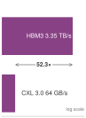
HBM remains 52× faster, so CXL is capacity only.

2.9.2 Wafer-scale planning constraint

At the opposite extreme from CXL sits the wafer-scale engine introduced in section 2.2.1. Its on-wafer fabric removes package- and board-level transfers for mapped operations, but it does not make communication free. Infrastructure planning instead shifts toward capacity, placement, and injection bandwidth.

Our 175B running model needs 350 GB for FP16 weights alone, far beyond the 44 GB of on-wafer SRAM. Cerebras addresses this through weight streaming: external MemoryX units feed weights to the wafer over a 1.2 TB/s path while the wafer executes each layer, decoupling model capacity from the on-wafer memory. Weight streaming was designed for training. Activations stay on the wafer while weights stream in layer by layer and gradients stream back to MemoryX, which performs the optimizer update. The approach works when each layer’s computation is large enough to hide the streaming time. The wafer trades the communication wall for a streaming-bandwidth wall.

The lesson for infrastructure planners is not that wafer-scale systems replace GPU fleets. It is that memory proximity and memory capacity trade against each other. WSE-style designs buy extraordinary local bandwidth by putting the working set near the arithmetic, while CXL buys flexible capacity by moving memory farther away. HBM sits between those extremes: off-chip but on-package, smaller than host memory but fast enough for the active computation. The right architecture is the one whose memory tier matches the workload’s reuse pattern.

2.9.3 Reconfigurable topologies and optical circuit switching

Beyond the package, optical circuit switching (OCS) moves the fabric topology and power boundary. Micro-electro-mechanical systems (MEMS) mirror arrays steer light between fiber ports without converting it to electrical form, so a pod’s physical topology can be rewired for each job and around failed hardware, as in Google’s TPU v4 pods, while millisecond-scale reconfiguration limits OCS to job-level allocation rather than per-message routing. Optical circuit switching and reconfigurable topology develops the mechanism, the TPU v4 deployment, and its fault-isolation limits.

The common theme is relocation rather than elimination. CXL pushes capacity outward into a fabric where PCIe bandwidth becomes the limiting discipline, whereas wafer-scale integration pulls communication inward onto silicon where on-wafer capacity and yield take over. In the same way, advanced packaging, with 2.5D interposers such as TSMC’s CoWoS and 3D stacking such as SoIC, compresses die-to-die distance past the reticle limit and leaves the rack to absorb the resulting power density, which must be checked against the package and cooling budgets, while optical circuit switching removes the optical-electrical-optical conversion inside the switch only to make reconfiguration latency the new boundary. Infrastructure planning therefore still begins by identifying where the next byte moves, how quickly it must arrive, and what physical system must be built so that movement does not dominate the workload.

Self-Check: Question

A representative CXL memory path over PCIe Gen5 x16 delivers roughly $64\text{ GB/s}$ of bandwidth, approximately $50\times$ lower than an H100’s $3.35\text{ TB/s}$ HBM3 bandwidth. Which infrastructure bottleneck is CXL memory pooling designed to relieve, and which bottleneck does it explicitly not solve?
1. It relieves peak Tensor Core throughput shortages, but does not solve the memory capacity limit.
2. It relieves rack cooling limits by eliminating electrical resistance, but does not solve chip-to-chip latency.
3. It relieves the memory capacity ceiling by holding phase-local optimizer state in shared pooled memory, but explicitly does not replace HBM for bandwidth-critical forward and backward pass weight streaming.
4. It relieves wafer-scale weight injection bottlenecks, but does not solve semiconductor yield.
A systems team proposes moving a 1.8-trillion parameter LLM training workload to a Wafer-Scale Engine (such as Cerebras WSE-3) to eliminate chip-to-chip network communication delays. Explain why this move changes rather than eliminates communication constraints and identify the resulting capacity and bandwidth budgets.
Advanced packaging technologies (such as 2.5D silicon interposers and 3D chiplet stacking) enable dense die-to-die interconnects on a single package. According to systems engineering principles, how does advanced packaging alter the landscape of infrastructure bottlenecks?
1. It allows accelerators to run uncooled at ambient room temperature by eliminating electrical resistance across die boundaries.
2. It permanently eliminates both the memory wall and the power wall by integrating optical waveguides directly onto the silicon substrate.
3. It eliminates the need for distributed training frameworks because all model parameters can fit permanently in on-die SRAM caches.
4. It shortens die-to-die paths while requiring package power density, current transients, and heat removal to be checked against the intended configuration.
True or False: Emerging infrastructure technologies such as CXL memory pooling, wafer-scale integration, and 2.5D packaging eliminate physical infrastructure constraints, allowing data center operators to deploy dense ML clusters without modifying cooling or power delivery.

See Answers →

2.10 Fallacies and Pitfalls

Because the bottlenecks move rather than disappear, compute infrastructure teams often optimize the visible specification while missing the binding physical constraint. Each fallacy and pitfall below turns a node, rack, pod, or facility lesson into an operational warning.

Fallacy: More GPUs always means faster training.

Fallacies and Pitfalls warned against reading a compute budget as a wall-clock prediction. The hardware form of the same error assumes that training time scales linearly with GPU count, so that doubling the GPUs halves the training time. In practice, communication overhead grows with cluster size, and this chapter’s modeled scaling efficiencies show how fast.

Amdahl’s law bounds speedup when a fixed workload has a fixed serial fraction. Distributed training also incurs communication, pipeline, and I/O costs that can change with partitioning and scale; these are not all an invariant serial fraction. For a 175B-parameter model with 350 GB of gradients, the AllReduce at each training step must combine contributions across the participating group. It can do so through ring or tree exchanges; direct transfers between every pair are not required.

Even for a carefully engineered fabric, the modeled scaling efficiency of the running model falls from 0.87 at 256 GPUs to 0.83 at 1,024 GPUs and 0.56 at 8,192. Growing from the reference cluster to the 8,192-GPU scenario of section 2.7 therefore multiplies the hardware 8× but the speed only 5.4×, and 44 percent of the larger cluster’s locally achievable throughput is lost to communication and pipeline bubbles. That run still finishes in days, so the scale is worth buying for a deadline, but each added GPU returns less than the one before it; without an engineered fabric and overlapped communication, the curve flattens far sooner.

The correct approach is to profile useful compute time, exposed communication time, and idle time at the current scale before buying the next pod. If the added GPUs mostly increase exposed communication, procurement is buying idle time rather than training progress. The mathematics of scaling efficiency turns this local ratio into a scaling-efficiency estimate before committing to procurement.

Pitfall: Planning training throughput from peak FLOP/s alone.

Peak FLOP/s describes only one roofline ceiling. At the H100 FP16 ridge point of approximately 295.2 FLOP/byte, the bandwidth and arithmetic ceilings meet; lower-intensity operations cannot reach the arithmetic peak through more compute alone. In the chapter’s batch-1 weight-streaming estimate, decode near 1 FLOP/byte uses well under 1 percent of the arithmetic peak. Prefill and training supply more reuse, yet even well-tuned large training runs commonly sustain only 30–50 percent of peak once memory-bound attention and normalization kernels, activation recomputation, dependencies, and communication are counted. Procurement needs those measurements for the intended execution phase.

Fallacy: Power and cooling constraints can be handled after accelerator purchase.

Teams that plan GPU purchases from compute requirements without verifying that the target facility can deliver the required power and cooling run into hard physical limits with long lead times. A single rack of four DGX H100 systems requires 33.5 kW of power. Upgrading a data center’s electrical infrastructure (new transformers, switchgear, and UPS capacity) and its cooling plant (chillers, piping, pumps) are construction projects planned in months, not days. Even seemingly simple changes, such as upgrading the PDU in a single rack from 20 kW to 60 kW, can require new cabling and circuit breaker panels. Organizations that order hardware without confirming facility readiness risk having millions of dollars of GPUs sitting in shipping containers in the parking lot while the building is retrofitted. Accelerators can arrive faster than a facility can be upgraded to power and cool them, which makes this mismatch a practical planning risk.

Pitfall: Buying a newer accelerator without checking the workload’s arithmetic intensity.

Suppose a team deploys B200 GPUs (4,500 TFLOP/s FP8 peak) for an inference workload serving a 7B-parameter model at batch size 1, where an arithmetic intensity of approximately 1 FLOP/byte places the workload deep in the memory-bound region. The B200’s memory bandwidth (8 TB/s) is 2.4× higher than the H100’s (3.35 TB/s). Comparing B200 FP8 against H100 FP16/BF16-class throughput gives a peak arithmetic ratio of about 4.6×, but also changes the precision convention. At a fixed weight footprint, the bandwidth-only model instead predicts a gain of about 2.4×. The low intensity limits the fraction of arithmetic peak that this model can use, though it does not measure idle time; the comparison that matters is bandwidth per dollar at the measured serving rate, and the larger arithmetic peak alone does not establish better value.

Fallacy: Air cooling is sufficient for AI workloads.

Operators of legacy facilities may assume that adding fans and chiller capacity is sufficient for any denser AI rack. In practice, the cooling choice depends on the system’s heat-rejection design and the facility’s available airflow, pressure, inlet temperature, and containment. Engineered air remains viable for some dense configurations, while higher rack densities can require direct liquid cooling to avoid thermal throttling or exceeding facility limits.

Fallacy: All GPU-hours are equivalent.

A common error in cost comparisons is to treat one GPU-hour on an H100 as interchangeable with one GPU-hour on an A100 or V100. Under the same dense FP16 peak convention, H100 offers 3.2× the arithmetic rate of A100 and 7.9× that of V100. If a workload sustained the same fraction of those peaks with the same operation count and target quality, 10,000 V100 GPU-hours would correspond to approximately 1,264 H100 GPU-hours. That is a conditional compute-only comparison, not a predicted training time, because memory, communication, numerical recipes, and software can change sustained efficiency. Procurement must compare measured cost per useful computation or per completed run, rather than rental price or peak FLOP/s alone.

Pitfall: Upgrading the network before identifying the training bottleneck.

A network upgrade from 200 Gb/s to 400 Gb/s InfiniBand changes training time only through the communication it accelerates on the critical path, the mirror image of the faster-accelerator fallacy in Fallacies and Pitfalls. In a no-overlap example with 20 seconds of computation and 2 seconds of communication, doubling transfer bandwidth reduces the estimated step from 22 to 21 seconds, an improvement of 4.5 percent. That result assumes the communication term scales with bandwidth and other terms remain fixed. Adding GPUs or optimizing kernels requires a separate estimate because either can change communication and overlap. The Fleet Law keeps those costs visible when comparing investments.

Fallacy: Average power draw is sufficient for cooling design.

Accelerator power draw varies across communication, memory, and compute phases. A workload average below the configured sustained envelope does not establish the cooling requirement because synchronized compute phases can raise many devices toward that envelope together. Thermal design must use the vendor’s sustained design target under the intended inlet and cooling conditions, while the electrical path must separately tolerate documented transients. Otherwise thermal throttling can reduce sustained throughput without producing a crash or explicit application error.

Pitfall: Selecting accelerators by HBM capacity without checking bandwidth.

Capacity and bandwidth answer separate feasibility questions, and a model that fits in HBM but cannot be served within its latency target is as unusable as one that does not fit. Consider two hypothetical options for a 70-billion-parameter model: (a) 192 GB of HBM2e at 2.04 TB/s, and (b) 80 GB of HBM3 at 3.35 TB/s. Option (a) holds the 141 GB FP16 weight payload, whose streaming floor is 141 GB/2.04 TB/s = 69.2 ms. Option (b) cannot hold 141 GB in its 80 GB capacity, but the 71 GB INT8 payload fits before other live state is counted. Its weight-transfer floor is 71 GB/3.35 TB/s = 21 ms, a 3.3× ratio between the two estimates. That ratio combines faster memory with fewer bytes; option (a) could also use a validated INT8 recipe. Selection must compare like-for-like quality, complete live-state capacity, and measured latency at the intended concurrency.

Fallacy: Data loading can be fixed after deployment.

Teams that optimize only GPU kernels and communication can still find their accelerators waiting for input. The data loading pipeline must sustain the cluster’s consumption rate across storage, preprocessing, and host-to-GPU transfer. The chapter’s pre-tokenized language-model example needs modest raw bandwidth, but tokenization, sequence packing, and shuffling can change the host-side demand. Size CPU workers, buffering, and storage concurrency from the actual pipeline. Local NVMe staging and prefetching are useful when they relieve the measured bottleneck; neither substitutes for testing the complete path at fleet concurrency.

Pitfall: Buying homogeneous clusters without modeling workload diversity.

Uniform hardware simplifies support and placement, but that benefit must be weighed against the useful work existing devices can still perform. For our 175B model, training and low-batch decode stress different resources. Separate pools can exploit that difference without placing mismatched devices in the same tightly synchronized group.

The A100’s 2.04 TB/s and the H100’s 3.35 TB/s supply different bandwidth ceilings. Retaining older devices for an inference pool can reduce cost when their measured throughput, power, and support costs compare favorably at the required latency. The distinction is between job-level balance within a synchronized group and cluster-level hardware uniformity. A heterogeneous fleet can preserve balanced groups, but its matching benefit must cover the added scheduling and operational complexity.

Pitfall: Treating commissioning and burn-in as schedule slack.

Commissioning is part of the system build, not a buffer that can be consumed when hardware delivery slips. Burn-in tests, cable validation, firmware qualification, thermal soak, and NCCL stress runs are the first time the node, rack, network, and facility layers operate as one machine. Compressing that phase turns installation defects into production failures, where each debugging cycle idles the full fleet rather than a small acceptance-test window.

Self-Check: Question

A 175B-parameter model training run on 1,024 GPUs has a step time of $1{,}000\text{ ms}$, broken down into $700\text{ ms}$ of compute ($T_{\text{compute}}$) and $300\text{ ms}$ of gradient AllReduce communication ($T_{\text{comm}}$). If the team scales out to 2,048 GPUs (assuming compute scales linearly to $350\text{ ms}$, while AllReduce communication time remains constant at $300\text{ ms}$), what is the resulting scaling efficiency?
1. 100% (ideal linear speedup, halving step time to $500\text{ ms}$).
2. $\approx 77\%$ (speedup of $\approx 1.54\times$ from $1{,}000\text{ ms}$ to $650\text{ ms}$, demonstrating diminishing returns on the $2\times$ hardware investment).
3. 50% (step time remains completely unchanged at $1{,}000\text{ ms}$).
4. $\approx 125\%$ (superlinear speedup due to increased aggregate L2 cache capacity).
Explain how neglecting facility readiness and commissioning can delay an ML training program by months even after GPUs have been delivered to the loading dock. Identify two concrete critical-path failure modes.
A team serving a 70B-parameter LLM at batch size 1 on H100s observes poor token generation latency and proposes upgrading to a B200 ($4{,}500\text{ FP8 TFLOP/s}$ peak, $\approx 8\text{ TB/s}$ HBM3e) primarily to capture the $\approx 2.3\times$ boost in peak arithmetic throughput. Which hidden assumption in their reasoning is fundamentally flawed?
1. Assuming liquid-cooled racks are capable of hosting high-density B200 servers.
2. Assuming checkpoint storage bandwidth is necessary during inference serving.
3. Assuming InfiniBand switches are required for single-node inference deployments.
4. Assuming that peak arithmetic throughput governs performance when the modeled batch-1 decode workload is limited by weight bandwidth; the HBM bandwidth ratio is the relevant first estimate.
A cost analyst evaluates cloud GPU pricing by comparing hourly rates: H100 at $4.00/GPU-hour vs. V100 at $0.80/GPU-hour, concluding that V100 is $5\times$ cheaper. Using throughput equivalence (an H100 delivers $\approx 7.9\times$ the FP16 Tensor throughput of a V100), explain why this hourly rate comparison is a procurement fallacy.

See Answers →

2.11 Summary

Training our 175B-parameter model exposes a constraint cascade: accelerator capacity and throughput shape the node, node power shapes rack cooling, rack density shapes pod layout, and pod topology and reliability determine how much useful work the fleet sustains. At the device level, the generality tax (principle 1) explains the trade between flexibility and workload-specific efficiency. A GPU delivers 10–100$\times$ the matrix throughput of a CPU on suitable workloads, but that specialization pays only when the workload and software stack can use the dedicated arithmetic over the deployment’s lifetime. The roofline in section 2.3.2 identifies the binding compute or memory ceiling, while the bandwidth hierarchy in section 2.5.1 guides where communicating work belongs. Together, these models connect software choices to the physical limits of the fleet.

Our 175B-parameter model connects the decisions at each level. Its low-batch decode estimate requires about 350 billion floating-point operations per token, but moving the 350 GB FP16 weight payload through one hypothetical 3.35 TB/s HBM path takes over 100 ms. A feasible partition changes that path budget as well as solving capacity. At the node level, training state exceeds 2 TB, requiring additional sharding or reductions in resident state. At the rack level, 32 accelerators at 700 W each, plus modeled host and network overhead, require 33.5 kW of qualified power and cooling capacity. The reference cluster coordinates 1,024 GPUs, while the worked pod scenario uses eight times that number. Communication, failure recovery, and sustained utilization determine how much of the purchased capacity becomes completed work. The model’s size exposes these interactions, but the same accounting applies whenever a workload crosses physical resource boundaries.

The method transfers beyond this model. At each level, identify the binding constraint, quantify its effect, and propagate the consequence upward. A faster accelerator is counterproductive if cooling cannot remove its heat; a denser rack is futile if the grid cannot supply it; and a wider network is wasteful if the workload cannot use its bandwidth. Infrastructure engineering is thus a quantitative discipline for tracing chip-level choices into rack power, facility cooling, network topology, reliability, and ownership cost.

Key Takeaways: The data center is the computer

Capacity and bandwidth are separate tests: Capacity decides whether model state fits; bandwidth decides how fast low-reuse phases run. For single-request LLM decode, weight traffic commonly sets the latency floor. The ridge point ($\RooflineRidgePoint$ = peak FLOP/s divided by memory BW) separates bandwidth- from compute-bound operation, but batch shape, fusion, precision, reuse, and the modeled memory level determine where each training or inference phase lies.
Bandwidth hierarchy guides parallelism placement: The 9× per-direction bandwidth gap in the NVLink–InfiniBand example favors keeping frequent tensor-parallel exchanges inside the fast interconnect domain. Pipeline and data parallelism can span slower links, but their traffic and synchronization still have to fit the workload’s time budget.
A node aggregates private memories: Eight accelerators multiply HBM capacity, but each device’s memory stays private, so the running model’s 2.8 TB of persistent training state forces tensor parallelism, optimizer sharding, activation checkpointing, and memory tiering to be combined.
Peak vs. sustained: Capacity planning must use sustained throughput measured with a consistent model-FLOP convention, precision, system scale, and workload shape, not peak specifications.
Rack power and cooling bound installable compute: Watts per rack, delivery losses, and cooling class, not FLOP/s, set how much compute a facility can install and sustain; at pod scale, network topology, cooling, and power delivery must be co-designed for the dominant workload.
Failure exposure grows with fleet size: With independent failures and a per-GPU MTTF of 50,000 hours, the 10,000-GPU example has a mean interval of about five hours between GPU failures. Recovery and checkpoint storage therefore belong in infrastructure planning from the start.
Price useful work, not hardware: GPU-hours from different generations, an FP8 peak that doubles advertised capacity, and bandwidth per dollar for decode compare only through sustained throughput on the target workload. Power, cooling, facilities, and utilization then set the lifetime cost of that useful work, so hardware price alone cannot settle a purchase.

Applied through C³, choosing liquid cooling for a dense accelerator rack changes more than heat removal. It raises the compute a rack can hold, which concentrates communication onto fewer top-of-rack links and adds coordination work for power capping, failure isolation, and maintenance. In the Fleet Law’s accounting, the hardware in this chapter fixes the per-device rate behind $\IronLawComputeTime/\DeviceCount$ and the link bandwidths behind $\CommunicationTime(\DeviceCount)$, while rack and pod reliability decide how often synchronization and recovery interrupt the step. Removing one physical ceiling therefore requires checking the rest of the fleet again; otherwise the investment creates capacity that the workload cannot use.

What’s Next: From silicon to wires

Physical infrastructure spans from Tensor Core transistors to megawatt data-center substations. A fleet of disconnected nodes, however, is not yet a computer; it is a warehouse of expensive accelerators. The network fabric turns those nodes into a unified training system by carrying gradients, activations, and checkpoints between them. At every scale above the node, this chapter met the same limit in a new form. The bandwidth hierarchy showed a 9× cliff between NVLink and InfiniBand, and the pod showed why usable bandwidth depends on the communication pattern and where it is placed. Every training step of our 175B model ends by combining gradients across all 1,024 GPUs of the reference cluster, so the slowest required transfer sets when the next step can begin. Network Fabrics starts from that synchronization and climbs from signaling on a single link through transport protocols, switch topology, and congestion behavior to the integrated cluster, asking at each level whether the fabric lets those GPUs train as one coherent machine or leaves them waiting as isolated devices.

2.12 Self-Check Answers

Self-Check: Answer

Which statement correctly describes representative constraints and mitigation mechanisms across the accelerator, node, rack, and pod hierarchy, without assigning one universally dominant wall to each tier?
1. Accelerator: arithmetic throughput vs. generality tax $\rightarrow$ mitigated by specialized silicon; Node: single-chip memory capacity limit $\rightarrow$ mitigated by high-speed intra-node fabrics aggregating HBM; Rack: thermal and power density $\rightarrow$ mitigated by facility cooling and power distribution; Pod: network bisection and fleet MTBF $\rightarrow$ mitigated by pod-scale fabrics and fault-tolerant orchestration.
2. Accelerator: network latency $\rightarrow$ mitigated by InfiniBand; Node: transistor count $\rightarrow$ mitigated by photolithography; Rack: memory bandwidth $\rightarrow$ mitigated by PCIe Gen5; Pod: power delivery $\rightarrow$ mitigated by running jobs asynchronously without barriers.
3. Accelerator: single-chip memory capacity wall $\rightarrow$ mitigated by on-die branch predictors; Node: power wall $\rightarrow$ mitigated by host underclocking; Rack: communication wall $\rightarrow$ mitigated by standard commodity Ethernet; Pod: memory bandwidth wall $\rightarrow$ mitigated by building-wide CXL pooling.
4. Accelerator: storage I/O capacity $\rightarrow$ mitigated by local NVMe drives; Node: compilation time $\rightarrow$ mitigated by JIT compilers; Rack: clock jitter $\rightarrow$ mitigated by atomic clocks; Pod: software bug rate $\rightarrow$ mitigated by unit testing frameworks.
Answer: The correct answer is A. Specialized arithmetic, distributed HBM capacity, qualified power and cooling, and pod fabrics with recovery capacity address different physical demands. These demands overlap across tiers: memory bandwidth can bind an accelerator, communication also matters inside a node, and shared power or cooling can interrupt a pod. Workload and configuration determine which constraint binds. The other choices pair constraints with mechanisms that do not address them, such as branch predictors for memory capacity or asynchronous execution for physical power delivery.

Learning Objective: Relate representative physical constraints to mitigation mechanisms across the ML infrastructure hierarchy.
Explain how relieving a constraint at one physical level of the compute infrastructure stack can expose another constraint. Use the accelerator, node, rack, and pod hierarchy, and explain why it is not a fixed one-wall-per-tier sequence.

Answer: Adding accelerators can clear a memory-capacity limit while creating transfers between private memories and increasing power demand. Concentrating nodes into racks requires qualified power delivery and heat removal, while connecting racks adds fabric and shared-failure budgets. These constraints coexist; their binding order depends on workload, placement, and facility design. Each proposed expansion must therefore be checked against the remaining budgets rather than assumed to advance to one predetermined wall.

Learning Objective: Analyze how relieving one infrastructure constraint can expose another without implying a fixed sequence of dominant bottlenecks.
True or False: In a warehouse-scale training cluster, the reliability wall implies that as the cluster scales to tens of thousands of GPUs, the aggregate fleet Mean Time Between Failures (MTBF) remains bounded primarily by the lifetime of the most resilient server chassis.

Answer: False. Under the independent, equal-rate failure model, fleet-level MTBF degrades inversely with the total component count ($MTBF_{\text{fleet}} \approx MTBF_{\text{component}} / N$). Even if individual GPUs possess an exceptional MTBF of $\approx 50{,}000\text{ hours}$, a cluster of $10{,}000$ GPUs operating synchronously will experience a hardware failure approximately every 5 hours ($50{,}000 / 10{,}000 = 5$), making failures a continuous operational certainty rather than an exceptional event governed by the best server.

Learning Objective: Explain how fleet-level MTBF scales inversely with total component count in large distributed training systems.

← Back to Questions

Self-Check: Answer

A hardware vendor transitions their next-generation accelerator from a monolithic $800\text{ mm}^2$ die to a dual-die chiplet architecture (such as the NVIDIA B200 with an equivalent area of about $1{,}700\text{ mm}^2$) connected on a single package. What physical constraint is this transition primarily designed to bypass, and what trade-off does it introduce?
1. It bypasses the memory wall by moving all memory on-chip, but introduces warp divergence because threads must synchronize across the die boundary.
2. It bypasses the photolithographic reticle limit ($\approx 858\text{ mm}^2$) and improves manufacturing yield, but introduces a die-to-die interconnect that is slower than a continuous on-die mesh.
3. It bypasses the maximum TDP limit of a single package by separating thermal loads into different server chassis, but requires developers to write separate CUDA kernels for each chiplet.
4. It bypasses the communication wall by replacing electrical copper signaling with optical waveguides, but increases the generality tax of control logic.
Answer: The correct answer is B. The photolithographic reticle limit restricts monolithic single-exposure dies to approximately $26 \times 33\text{ mm} = 858\text{ mm}^2$, and manufacturing yield decreases exponentially with die area. Chiplet-based packaging bypasses this ceiling by integrating multiple smaller, higher-yielding dies on a common substrate (e.g., connected at 10 TB/s on the B200), though this package-level link is inherently slower than a continuous on-die mesh. The claim that chiplets eliminate off-package DRAM or cause warp divergence is false. The assertion that dies are placed in separate server chassis is incorrect because chiplets reside on a single package substrate presented as a single logical GPU. The choice mentioning optical waveguides misattributes optical signaling to standard silicon chiplet packaging.

Learning Objective: Analyze why physical manufacturing constraints force the adoption of chiplet-based accelerator architectures and identify the resulting communication trade-off.
A research lab frequently experiments with novel, custom attention patterns and dynamic sparsity, while a production platform team trains a fixed standard Transformer at massive scale for months. Compare the systems trade-offs of choosing GPUs (CUDA) versus TPUs (XLA) for these two organizational teams.

Answer: GPU kernel programming can support rapid experimentation with custom operations, while TPU execution requires an XLA mapping onto its specialized dataflow. The research team must check operator support and iteration cost on each platform; the production team can amortize compilation over stable runs and compare sustained useful throughput at matched precision and quality. Neither SIMT nor systolic execution alone establishes higher utilization or a universal platform winner.

Learning Objective: Compare the SIMT and systolic array execution models to justify when organizational flexibility outweighs dataflow efficiency.
Comparing the V100 and B200 at dense FP16 separates peak throughput growth from growth in throughput per TDP watt. Which statement correctly captures that difference and its infrastructure consequence?
1. Peak throughput per TDP watt grew faster than peak throughput, allowing higher-density clusters to ignore power delivery.
2. Both peak throughput and power efficiency scaled linearly at exactly the same rate, confirming that Dennard scaling remains fully active in modern 4nm nodes.
3. Peak dense FP16 throughput grew about 18 times while peak throughput per TDP watt grew about 5.4 times, so facilities must accommodate higher device power as well as greater arithmetic capacity.
4. Peak throughput plateaued after Volta (V100), meaning all recent performance gains stem exclusively from host CPU software optimizations.
Answer: The correct answer is C. Holding precision fixed, the registered V100-to-B200 comparison gives about 18 times the dense FP16 throughput but only 5.4 times the throughput per TDP watt. The gap reflects a higher device power allowance. Reversing the metrics misses this infrastructure cost; these specification ratios do not establish measured application energy efficiency or require one universal cooling design.

Learning Objective: Evaluate the historical scaling relationship between peak accelerator throughput and power efficiency to identify the physical root of the power wall.
The area and energy devoted by a processor to capabilities outside the dominant neural network matrix-multiplication workload, such as out-of-order scheduling, branch prediction, and complex hardware caches, is called the ____.

Answer: The correct answer is Generality Tax (or generality tax). A general-purpose CPU devotes roughly 30–40% of its die to caches, 20–30% to control logic, and only 5–10% to arithmetic units. ML accelerators reduce this generality tax by allocating 50–90%+ of silicon area to dense arithmetic units (Tensor Cores or systolic arrays), trading general-purpose programmability for matrix compute density.

Learning Objective: Define the generality tax and explain how moving from CPUs to specialized ML accelerators reduces it.
Arrange the following processor architectures in ascending order of the approximate percentage of their die area devoted strictly to arithmetic units (from lowest arithmetic die allocation to highest): (1) Google TPU (systolic array), (2) Purpose-built custom ASIC, (3) General-purpose server CPU, (4) NVIDIA GPU (with Tensor Cores).

Answer: The correct sequence is: (3) General-purpose server CPU ($\approx 5--10\%$) $\rightarrow$ (4) NVIDIA GPU (with Tensor Cores, $\approx 50--60\%$) $\rightarrow$ (1) Google TPU (systolic array, $\approx 70--80\%$) $\rightarrow$ (2) Purpose-built custom ASIC ($>90\%$). Moving along this accelerator spectrum progressively reclaims silicon area from general-purpose control logic (branch prediction, instruction decoders, reorder buffers) and caches to dedicate more transistors directly to matrix arithmetic units.

Learning Objective: Order processor classes along the accelerator spectrum by their arithmetic die-area allocation.

← Back to Questions

Self-Check: Answer

HBM3 provides a much wider interface and lower signaling energy per bit than socketed DDR5. Which packaging mechanism explains these advantages?
1. HBM3 runs individual pins at $16\times$ higher clock frequency than DDR5, overcoming PCB trace attenuation through high-frequency signaling.
2. HBM3 uses a novel DRAM cell structure that eliminates capacitor refresh cycles, reducing dynamic power consumption.
3. HBM3 stacks DRAM dies vertically with through-silicon vias (TSVs) and connects the stack to the processor through a wide, short silicon-interposer path on the package.
4. HBM3 compresses weight matrices on-die, transferring fewer physical bits across the memory bus.
Answer: The correct answer is C. TSVs connect the stacked dies vertically, while the processor-to-stack path also crosses the lateral interposer. On-package placement shortens the complete electrical path relative to socketed DDR5, lowering signaling energy, and the 1,024-bit interface per stack supplies parallel bandwidth without requiring proportionately faster pins. TSV length alone does not establish a 1,000-fold reduction in complete-path capacitance. Faster clocks, refresh-free cells, and on-die compression do not explain this packaging mechanism.

Learning Objective: Analyze how HBM’s 3D-stacked TSV packaging simultaneously raises memory bandwidth and lowers energy per bit relative to DDR5.
An engineering team compares an H100 with a hypothetical successor offering twice the dense FP16 peak but the same HBM bandwidth. Hold the FP16 weight payload, partition, and batch-1 shape fixed, assume sufficient capacity, and consider a weight-streaming model whose bandwidth ceiling is lower than its compute ceiling on both devices. What changes in the modeled token-latency floor, and which levers could lower it?

Answer: The weight-only FP16 model performs two FLOPs per two-byte weight, so its intensity is about 1 FLOP/byte, below the H100 FP16 ridge. Doubling the matched-precision arithmetic peak raises only the nonbinding ceiling; fixed bytes divided by unchanged bandwidth gives the same streaming floor. More bandwidth, fewer bytes through validated quantization, or more reuse can change that bound. Actual latency must also account for other traffic, communication, execution overhead, and any changed partition.

Learning Objective: Apply the Roofline Model to explain why compute-only upgrades cannot improve deeply memory-bound inference and identify the architectural levers that can.
A custom attention kernel has arithmetic intensity of 1.2 FLOP/byte on an H100 under the FP16 roofline convention. Which change most directly raises its memory-bandwidth performance ceiling, subject to measuring the resulting execution?
1. Use SRAM-sized attention tiles and fusion to avoid materializing the full score matrix in HBM and reduce intermediate HBM round-trips.
2. Overclocking Tensor Cores to increase peak FP16 TFLOP/s, raising the horizontal ceiling of the roofline.
3. Adding dummy memory reads to artificially raise the measured memory traffic of the kernel.
4. Offloading the layer normalization and attention operations to host CPU DRAM over PCIe Gen5.
Answer: The correct answer is A. At the supplied intensity, bandwidth supplies the lower roofline ceiling. SRAM-sized tiles and fusion can reduce HBM bytes per useful operation without requiring the complete attention matrix to fit on chip. Raising only the arithmetic peak leaves that ceiling unchanged; dummy reads lower intensity, and host offload adds a slower path. Intensity alone does not establish the measured bottleneck or guarantee the achieved speedup, so profiling must check the result.

Learning Objective: Apply roofline geometry to select a change that raises the limiting ceiling and distinguish that bound from achieved throughput.
Order the following tiers of an H100-class accelerator’s memory hierarchy from the highest aggregate bandwidth to the highest capacity: (1) HBM3 on the package, (2) the streaming multiprocessors’ register files, (3) the L2 cache, (4) L1 and shared memory (on-chip SRAM).

Answer: The correct order is: (2) register files, (4) L1 and shared memory, (3) the L2 cache, (1) HBM3. Each step away from the arithmetic units trades aggregate bandwidth for capacity, falling from hundreds of TB/s at the registers to a few TB/s at HBM while capacity grows from tens of megabytes to tens of gigabytes. Tiling exploits the order by staging operand blocks in the fast tiers so that each byte fetched from HBM feeds many multiply-accumulate operations.

Learning Objective: Order the accelerator memory tiers by bandwidth and capacity and connect that order to operand reuse.
In the Roofline Model, the specific arithmetic intensity where the diagonal memory bandwidth slope meets the horizontal peak compute ceiling ($I = R_{\text{peak}} / \text{BW}$) is called the ____.

Answer: The correct answer is ridge point. It is the hardware balance threshold where the bandwidth and arithmetic ceilings meet. Below it, bandwidth supplies the lower modeled ceiling; above it, arithmetic does. A measured kernel can remain below either ceiling, so this classification does not establish its actual bottleneck.

Learning Objective: Define the ridge point and distinguish the lower roofline ceiling from a measured execution bottleneck.

← Back to Questions

Self-Check: Answer

An H100 advertises twice the dense arithmetic rate in FP8 that it advertises in FP16. A team sizes a training run’s GPU-hours by assuming the full FP8 rate. Which statement best describes the planning error?
1. FP8 halves the bytes per weight, so memory-bound phases also run exactly twice as fast and the plan is correct.
2. The FP8 rating is a ceiling for eligible matrix operations; ineligible operations, memory stalls, communication, and the need to validate the precision policy keep the sustained rate below it, so the plan must use a measured sustained rate.
3. FP8 Tensor Core rates apply only to inference, so a training plan must use the FP32 rate instead.
4. FP8 runs slower than FP16 on Tensor Cores because of scaling overhead, so the plan overestimates the time.
Answer: The correct answer is B. Peak FLOP/s assumes every eligible arithmetic unit stays fed at the stated precision. Operations that cannot run in FP8, memory and dependency stalls, exposed communication, and launch overhead all sit outside that ceiling, and a layer is not numerically safe in FP8 merely because the hardware supports it. Halving the bytes does not double a whole run, FP8 recipes are used in training, and FP8 is not slower than FP16 on supported operations.

Learning Objective: Distinguish a precision-specific peak rate from the sustained throughput that capacity planning must use.
A training run is estimated at 1,000 GPU-hours from peak FLOP/s. Profiling a representative window shows a model FLOPs utilization (MFU) of 0.4. How many GPU-hours should the plan budget, and what must match before this MFU can be compared with another team’s figure?

Answer: The plan should budget 1,000 / 0.4 = 2,500 GPU-hours, because a run planned from peak needs 1/MFU times the peak-based estimate at the measured utilization. The comparison is meaningful only when both figures use the same model-FLOP convention, the same precision and hardware peak, and a similar system scale and workload shape; otherwise a higher MFU can reflect a different denominator rather than better execution.

Learning Objective: Apply measured utilization to a peak-based estimate and state the conditions under which MFU figures are comparable.
True or False: In synchronous training, an accelerator that sustains a clock about 2.5 percent below its peers costs the job at most 2.5 percent of that one device’s throughput.

Answer: False. Every participant waits for the slowest one at each collective, so a device that finishes its dependent work late can slow every synchronous step of its whole group by up to that fraction. Fleets therefore track per-device sustained throughput and move persistent underperformers to pools, such as inference serving, where they do not gate a synchronized group, after profiling confirms the cause.

Learning Objective: Explain how device variation propagates through synchronous training.
The standard mixed-precision recipe runs the forward and backward passes in BF16 or FP16 but keeps a full-precision FP32 copy of the parameters, called the ____ weights, so that updates much smaller than a weight are not lost to FP16 rounding.

Answer: The correct answer is master. The FP32 master weights are the copy the optimizer updates; they add four bytes per parameter to the training state, which the node memory budget must hold or offload.

Learning Objective: Identify the FP32 master weights in the mixed-precision recipe and their memory cost.

← Back to Questions

Self-Check: Answer

A team considers running 8-way tensor parallelism across 8 separate single-GPU server nodes connected by InfiniBand NDR ($50\text{ GB/s}$ per GPU), rather than within an 8-GPU DGX H100 node over NVSwitch ($450\text{ GB/s}$ per direction per GPU). What is the primary system consequence on training step time?
1. Tensor parallelism transfers only stage-boundary activations, so the network difference produces less than a 1% change in step time.
2. InfiniBand protocols cannot transmit floating-point data, forcing CPU format conversions on every step.
3. Inter-node tensor parallelism requires optical circuit switching, causing laser thermal shutdown.
4. Tensor parallelism requires frequent layer-level exchanges; placing them on the $\approx 9\times$ slower per-direction fabric increases exposed communication and can substantially reduce MFU.
Answer: The correct answer is D. Tensor parallelism exchanges partial results within layers, so placement on the slower fabric can expose substantially more communication. The quoted per-direction rates are $450\text{ GB/s}$ and $50\text{ GB/s}$. The actual step-time penalty depends on message sizes, overlap, and workload shape; it is not fixed by the bandwidth ratio alone. Exchanging only stage-boundary activations describes pipeline parallelism.

Learning Objective: Analyze why frequent tensor-parallel exchanges favor the fast interconnect domain and what must be measured before spanning slower links.
Rank the quoted peak data-movement bandwidth per GPU across the four primary hardware tiers in a modern DGX H100 cluster, from highest quoted bandwidth to lowest: (1) Inter-node InfiniBand NDR, (2) Intra-package HBM3, (3) Intra-node NVLink 4 (one direction), (4) Host-to-device PCIe Gen5 x16.

Answer: The correct sequence is: (2) Intra-package HBM3 ($\approx 3.35\text{ TB/s}$) $\rightarrow$ (3) Intra-node NVLink 4 (one direction, $\approx 450\text{ GB/s}$) $\rightarrow$ (4) Host-to-device PCIe Gen5 x16 ($\approx 64\text{ GB/s}$) $\rightarrow$ (1) Inter-node InfiniBand NDR ($\approx 50\text{ GB/s}$ per port). NVLink and the network port are compared in one direction; the $450/50 = 9$ ratio compares per-GPU NVLink injection with one network port, not fabric bisection bandwidth. Adjacent entries in this four-tier ranking do not imply an order-of-magnitude drop at every boundary. The hierarchy favors placing frequent exchanges within the fast interconnect domain, subject to measured workload costs.

Learning Objective: Rank the data-movement tiers across the node-and-cluster hierarchy to explain the bandwidth cliffs governing distributed parallelism placement.
A training framework offloads Adam first- and second-moment optimizer states (FP32, 8 bytes per parameter total) to host DDR5 DRAM over PCIe Gen5, while keeping weights and activations in GPU HBM. Justify this asymmetric placement using access frequency and bandwidth requirements, and quantify the HBM capacity freed for a 175B-parameter model.

Answer: Model weights and activations are accessed multiple times per layer during both forward and backward passes, demanding HBM’s $3.35\text{ TB/s}$ bandwidth to avoid stalling Tensor Cores. In contrast, Adam optimizer moments are accessed only once per training step during the parameter update, making them candidates for offload. PCIe Gen5 ($\approx 64\text{ GB/s}$) still imposes a transfer budget; the framework must verify that moving the state fits the update interval or can be overlapped. For a 175B-parameter model, the two FP32 moments require $175 \times 10^9 \times 8\text{ bytes} = 1{,}400\text{ GB}$ ($1.4\text{ TB}$). Offloading them frees $1.4\text{ TB}$ of premium HBM across the node/cluster, which can be repurposed for larger batch sizes, longer sequences, or larger model shards.

Learning Objective: Justify memory-tier placement for training state by matching access frequency to interconnect bandwidth and calculating the freed HBM capacity.
A Mixture-of-Experts (MoE) workload routes tokens dynamically across experts, producing heavy AllToAll collective traffic where every GPU in a node sends distinct token buffers to every other GPU. Why does an NVSwitch crossbar topology significantly outperform a physical GPU ring topology for this workload?
1. NVSwitch provides non-blocking full bisection bandwidth enabling any-GPU-to-any-GPU communication in a single hop, whereas a ring forces non-neighbor transfers through intermediate hops, causing link contention and $\mathcal{O}(N)$ latency.
2. NVSwitch converts AllToAll network collectives into local register-file reads, eliminating inter-GPU data transfer entirely.
3. Ring topologies cannot support mixed precision, forcing all token embeddings to be cast to FP64.
4. NVSwitch increases individual GPU HBM3 bandwidth from $3.35\text{ TB/s}$ to $19\text{ TB/s}$.
Answer: The correct answer is A. In an AllToAll collective, all $N$ GPUs simultaneously exchange unique data with all other $N-1$ GPUs ($N \times (N-1)$ distinct streams). An NVSwitch crossbar fabric provides non-blocking, full-bisection single-hop connectivity between all 8 GPUs. In contrast, a ring topology forces traffic between non-adjacent GPUs to traverse intermediate nodes, creating severe link contention and $\mathcal{O}(N)$ multi-hop latency. The claim that NVSwitch eliminates inter-GPU communication is false because NVSwitch is a network switch. The claim that rings force FP64 is fabricated. The claim that NVSwitch raises on-package HBM bandwidth confuses the intra-node interconnect with on-package memory.

Learning Objective: Compare intra-node topologies by mapping their connectivity structure to the communication patterns of AllToAll-heavy workloads.
The supported direct storage-to-GPU data path that can remove the host-memory bounce copy for data requiring no host-side preprocessing is called ____.

Answer: The correct answer is GPUDirect Storage (or GDS). On a supported platform and data path, direct DMA avoids staging the payload through host DRAM. It still uses the storage and node interconnects; aggregate throughput depends on shared links, concurrent traffic, and whether preprocessing requires host access. Per-drive bandwidths therefore cannot simply be added to guarantee node throughput.

Learning Objective: Identify GPUDirect Storage (GDS) as the architectural mechanism for bypassing host CPU memory during high-throughput data loading.
In a dual-socket server node hosting 8 GPUs across two CPU root complexes, explain how Non-Uniform Memory Access (NUMA) effects impact data loading throughput and what architectural scheduling rule prevents CPU-to-GPU bottlenecks.

Answer: In the stated dual-socket topology, remote memory traffic also crosses the inter-socket link, which can add latency and contention. The penalty depends on the processor, transfer size, and concurrent traffic; there is no universal percentage. Measure ingestion and place data-loader workers, pinned buffers, NICs, and target GPUs in the same NUMA domain when the local path improves sustained throughput.

Learning Objective: Explain NUMA effects on intra-node data loading and identify the scheduling policy required to maximize CPU-to-GPU bandwidth.

← Back to Questions

Self-Check: Answer

A four-node DGX H100 rack draws approximately $33\text{ kW}$ of IT power. Which heat-transfer property can make direct-to-chip liquid cooling attractive as rack density rises, even though engineered air cooling remains possible in a suitable facility?
1. Liquid cooling increases GPU arithmetic intensity by lowering electrical resistance inside Tensor Cores.
2. Water has much higher volumetric heat capacity than air, so it can carry away the same heat with a much smaller volumetric flow for a comparable temperature rise.
3. Air cooling causes optical transceivers to melt when exposed to fan airflow velocities above 5 meters per second.
4. High-density racks require full dielectric immersion because cold plates cannot conduct heat from silicon heat spreaders.
Answer: The correct answer is B. Heat removal depends on mass flow, specific heat, and temperature rise. Liquid can transport the same heat with far less volumetric flow than air. Cooling choice still depends on the server and facility; rack power alone does not impose a universal cutoff. Cooling does not change algorithmic arithmetic intensity, and cold plates do conduct heat from the package.

Learning Objective: Explain why liquid cooling can support higher rack density while cooling selection remains dependent on server and facility design.
A facilities team provisions its cooling and electrical infrastructure for the average GPU power observed during training ($\approx 500\text{ W}$ per GPU) rather than the $700\text{ W}$ sustained design target. Explain why this choice can silently degrade cluster training throughput even when no hardware errors or crashes occur.

Answer: Synchronized compute phases can raise many devices toward the configured sustained envelope together. A cooling design based only on the $500\text{ W}$ average may not sustain the intended $700\text{ W}$ operating condition. If junction temperatures reach thermal limits, clock throttling can lower throughput while the application continues running. The design must check sustained thermal conditions separately from fast electrical transients; no fixed MFU penalty follows from average power alone.

Learning Objective: Analyze why synchronous training forces cooling provisioning to meet the sustained design envelope rather than only the average load and recognize the silent-throttling signature.
Synchronous ML training can correlate accelerator power ramps across a cluster. How does this electrical behavior distinguish its power-delivery requirements from those of largely uncorrelated web-serving workloads?
1. ML clusters operate on direct current exclusively, eliminating the need for uninterruptible power supplies.
2. Web-serving data centers experience higher $di/dt$ transients because individual HTTP requests draw more peak current than matrix multiplications.
3. ML training consumes purely reactive power that causes step-down transformers to freeze mechanically.
4. Correlated demand changes require checking both local regulator and decoupling response and the aggregate demand seen by upstream supplies, rather than sizing solely for average power.
Answer: The correct answer is D. Synchronized workload transitions can correlate demand, but regulation and decoupling change the current waveform at each supply boundary. Local current slew is measured in amperes per second, not watts per second, and must be paired with the impedance of that same path. Average facility capacity cannot establish local voltage integrity. Synchronization neither eliminates UPS requirements nor implies purely reactive power.

Learning Objective: Explain why synchronized training workloads create severe electrical power-delivery challenges ($di/dt$) that average-power analyses miss.
True or False: Replacing individual server AC supplies with a centralized 48V DC power shelf and busbar guarantees one fewer conversion stage and a 2–3% electrical efficiency gain.

Answer: False. Rack-level distribution consolidates AC conversion and can recover chassis volume, but local DC-to-DC conversion remains. Compare the actual conversion stages and their efficiency at the intended loads rather than assume a fixed saving. Shared shelves and busbars also require redundancy and serviceability appropriate to their rack-level failure boundary.

Learning Objective: Evaluate centralized 48V rack distribution using conversion efficiency, packaging volume, and shared failure boundaries.
A facility aisle is qualified to remove a sustained 25 kW of IT heat per rack with its existing air-cooling design under the specified inlet temperature and airflow. The proposed AI workload measures 60 kW per rack over its sustained operating interval. Which observation establishes the need to change the cooling design or reduce the rack load?
1. Web workloads have higher peak memory bandwidth requirements, causing localized thermal spikes.
2. AI training generates bursty, millisecond-scale CPU spikes followed by long idle periods, creating thermal cycling fatigue.
3. The measured 60 kW rack load exceeds this aisle’s qualified 25 kW air-cooling envelope; a qualified liquid, hybrid, or redesigned air system, or a lower rack load, must restore thermal feasibility.
4. AI models require lower ambient operating temperatures to maintain FP16 arithmetic precision.
Answer: The correct answer is C. The proposed sustained heat load exceeds the particular facility’s qualified envelope. This establishes a local feasibility problem, not a universal rack-power threshold at which air cooling fails. Liquid cooling is a candidate whose complete heat path, parasitic energy, and serviceability must be qualified. Neither memory-bandwidth comparisons nor numerical precision establishes the required heat-removal capacity.

Learning Objective: Compare a measured rack heat load with a qualified facility envelope before selecting a cooling intervention
Order the thermal stages of heat removal in a direct-to-chip liquid-cooled data center, from the silicon die to the external environment: (1) heat transfers through a thin thermal interface material (TIM) into a copper cold plate, (2) the Coolant Distribution Unit (CDU) heat exchanger transfers thermal energy from the closed rack loop to the facility secondary loop, (3) external cooling towers or dry coolers reject heat into the ambient outdoor atmosphere, (4) liquid coolant absorbs heat as it flows through microchannels directly above the accelerator package, (5) active switching in transistor junctions generates heat on the silicon die.

Answer: The correct order is: (5) active switching in transistor junctions generates heat on the silicon die, (1) heat transfers through a thin thermal interface material (TIM) into a copper cold plate, (4) liquid coolant absorbs heat as it flows through microchannels directly above the accelerator package, (2) the Coolant Distribution Unit (CDU) heat exchanger transfers thermal energy from the closed rack loop to the facility secondary loop, (3) external cooling towers or dry coolers reject heat into the ambient outdoor atmosphere. Thermal conduction originates in the silicon junction, transfers across the TIM into the cold plate, is absorbed convectively by the rack liquid coolant, transfers across the CDU heat exchanger to the facility water loop, and is ultimately rejected to the ambient environment. Reversing any intermediate steps violates the physical conduction and convection path.

Learning Objective: Analyze the thermodynamic heat rejection path in direct-to-chip liquid-cooled AI infrastructure

← Back to Questions

Self-Check: Answer

Barroso and Hölzle’s Warehouse-Scale Computer (WSC) thesis reframes an ML pod from ‘a room full of computers’ to ‘a single computer that fills a room.’ Which practical consequence most directly shapes infrastructure engineering at pod scale?
1. The entire facility is engineered as a unified machine where the network fabric acts as the system bus, distributed storage acts as the disk subsystem, and the cluster orchestrator acts as the operating system.
2. All servers share a single hardware cache-coherence bus across the entire building, eliminating the need for message-passing software.
3. Workloads are structured as embarrassingly parallel, uncoordinated batch jobs that completely isolate nodes from one another.
4. Component failure rates decrease at warehouse scale, allowing fault tolerance to be managed as an offline manual process.
Answer: The correct answer is A. In the WSC paradigm, the building is the computer. The high-speed network fabric (InfiniBand/RoCE) functions as an internal system bus, distributed storage functions as a disk hierarchy, and the cluster orchestrator schedules resources like an OS kernel. Subsystems must be co-designed for tight, synchronous execution. The claim that building-scale systems share a single hardware cache-coherence bus is false. The description of embarrassingly parallel batch jobs characterizes traditional web scraping rather than synchronously coupled ML training. The claim that failure rates decrease with scale is backwards: component failures compound linearly, occurring every few hours at warehouse scale.

Learning Objective: Explain the warehouse-scale-computer perspective and its implications for how pod-scale infrastructure is engineered.
A team doubles a distributed training cluster from 1,024 to 2,048 GPUs and observes wall-clock training time drop from 14 days to 10 days rather than the ideal 7 days. Calculate the realized scaling efficiency, determine whether the cost per useful FLOP increased, and identify the next diagnostic step.

Answer: Scaling efficiency is $\eta = \text{Speedup} / (\text{Hardware Factor}) = (14 / 10) / (2048 / 1024) = 1.4 / 2.0 = 0.70$ (70%). The team pays for 2,048 GPUs but extracts the useful throughput of only $\approx 1{,}434$ GPUs, so cost per useful FLOP increases by $\approx 43\%$ ($1 / 0.70 - 1$). The scale-out is economically justified only if saving 4 calendar days has high strategic value. To diagnose the $30\%$ efficiency loss, the team should profile the step-time breakdown to measure whether exposed gradient AllReduce communication, pipeline bubbles, or I/O stragglers expanded at the larger scale.

Learning Objective: Calculate distributed scaling efficiency to evaluate the economic returns of cluster scale-out and identify diagnostic profiling steps.
A synchronous training job spans 10,000 GPUs. Assume a hard crash is detected and recovered from a valid checkpoint, while a persistent gray failure remains undetected and delays dependent steps. Why can the gray failure cost more useful work over a long run?
1. Gray failures permanently corrupt the model weights, forcing the entire training run to restart from step zero.
2. Gray failures trip circuit breakers in the rack, causing cascading facility blackouts.
3. The hard crash incurs detection, restart, and lost-work costs, while the undetected straggler can repeatedly delay the participating job until it is diagnosed.
4. Gray failures disable FP8 Tensor Cores, silently falling back to double-precision FP64 and exhausting memory.
Answer: The correct answer is C. A late required participant can delay dependent work in its synchronous job or process group. A hard failure has a bounded interruption only under the stated detection and recovery assumptions; an undetected slowdown accumulates loss for as long as it persists. Which costs more depends on the exposed delay, its duration, and recovery cost. This does not imply that unrelated jobs wait, that detection is immediate, or that every gray failure preserves numerical correctness.

Learning Objective: Contrast the impact of gray failures versus hard crashes on cluster-wide throughput in synchronous distributed training.
A pod fabric that uses tiers of switches to supply full bisection bandwidth across node uplinks, in contrast to a direct-connect torus, is called a ____ topology.

Answer: The correct answer is Fat-Tree (or fat-tree). In a fully provisioned design, uplink capacity supports the endpoint rate across an equal cut. This removes the modeled oversubscription limit at that boundary; it does not guarantee congestion-free execution or an optimal AllReduce. Collective schedule, routing, traffic placement, and competing load still determine performance.

Learning Objective: Identify the Fat-Tree network topology and its role in delivering non-blocking full bisection bandwidth for distributed training.
Arrange the stages in the worked scenario’s accounting sequence: begin with the compute-only baseline, add the distributed-step losses, then checkpointing, restart, and maintenance allowances. (1) Checkpoint I/O overhead ($\approx 3\%$), (2) Compute-only training time ($6PD$ FLOPs divided by aggregate peak throughput times assumed local compute efficiency), (3) Hardware failure and restart overhead ($\approx 10\%$), (4) Scaling efficiency covering communication and pipeline bubbles ($\approx 0.56$), (5) Maintenance overhead ($\approx 5\%$). Each additive percentage is relative to the preceding subtotal.

Answer: The correct order is: (2) Compute-only baseline, (4) Scaling efficiency, (1) Checkpoint I/O overhead, (3) Failure and restart overhead, (5) Maintenance overhead. Starting near 12 hours gives successive subtotals near 21.4, 22.1, 24.3, and 25.5 hours. The scaling factor already includes pipeline fill and drain, so adding a separate bubble step would count that loss twice. This is an illustrative accounting convention, not a physical chronology or universal minimum. Local compute efficiency excludes the distributed losses added here; using measured distributed MFU would double-count them.

Learning Objective: Sequence the worked training-time accounting model and distinguish its local efficiency and incremental overhead denominators.

← Back to Questions

Self-Check: Answer

A team will serve a dense language model at batch size 1 with a strict per-token latency target. Which metric should dominate its comparison of candidate accelerators?
1. Peak FP8 TFLOP/s per dollar, because decode performs two floating-point operations per parameter.
2. Memory bandwidth per dollar, confirmed by measured throughput at the required latency, because batch-1 decode streams the weights with little reuse.
3. Host DRAM capacity per dollar, because the weights should be served from host memory.
4. Bisection bandwidth of the cluster fabric, because every request crosses the network.
Answer: The correct answer is B. Batch-1 decode sits near 1 FLOP/byte, far below the ridge point, so the weight-streaming time set by memory bandwidth dominates and more arithmetic barely changes it. Peak FLOP/s raises a nonbinding ceiling, host memory is far slower than HBM, and independent replicas need not send every request across the cluster fabric. Measured throughput at the latency target confirms the screen.

Learning Objective: Select the procurement metric that matches the binding constraint of a serving workload.
The 175B running model needs about 350 GB for FP16 weights. Using 80 GB accelerators, how many devices are needed for the weights alone at FP16, INT8, and INT4, and why does a fourfold smaller payload not guarantee a fourfold lower token latency?

Answer: The weights need at least five devices at FP16 (350 GB), three at INT8 (175 GB), and two at INT4 (87.5 GB). These are weight-only capacity bounds; quantization metadata, key-value cache, and workspace also need memory. Reading 4-bit instead of 16-bit weights quarters the raw payload, but kernel support, dequantization work, other memory traffic, any change in device count and communication, and validation of model quality determine the realized latency gain.

Learning Objective: Calculate how quantization changes serving device counts and explain why payload reduction does not translate directly into latency.
True or False: A workload whose binding constraint on each device is arithmetic throughput cannot be communication-bound across the cluster.

Answer: False. The decision matrix names the per-device constraint, what one accelerator must supply. Whether the fleet as a whole is limited by compute, communication, or coordination is a separate question. Large-batch LLM training can be compute-bound on each device and still be communication-bound across the cluster, as Archetype A (GPT-4/Llama-3) is.

Learning Objective: Distinguish the per-device binding constraint from the constraint that binds the fleet as a whole.
MLPerf results that fix the workload and the quality target so that different implementations can be compared belong to the ____ division.

Answer: The correct answer is closed. The open division permits broader changes. Neither predicts a deployment automatically, so a procurement team must compare the submission’s workload, software, precision, hardware count, and quality target with the intended system.

Learning Objective: Interpret benchmark results under the measurement rules that produced them.

← Back to Questions

Self-Check: Answer

A representative CXL memory path over PCIe Gen5 x16 delivers roughly $64\text{ GB/s}$ of bandwidth, approximately $50\times$ lower than an H100’s $3.35\text{ TB/s}$ HBM3 bandwidth. Which infrastructure bottleneck is CXL memory pooling designed to relieve, and which bottleneck does it explicitly not solve?
1. It relieves peak Tensor Core throughput shortages, but does not solve the memory capacity limit.
2. It relieves rack cooling limits by eliminating electrical resistance, but does not solve chip-to-chip latency.
3. It relieves the memory capacity ceiling by holding phase-local optimizer state in shared pooled memory, but explicitly does not replace HBM for bandwidth-critical forward and backward pass weight streaming.
4. It relieves wafer-scale weight injection bottlenecks, but does not solve semiconductor yield.
Answer: The correct answer is C. CXL memory expansion and pooling can relieve host capacity pressure; accelerator access requires a supported platform, device type, data path, and software placement. Phase-local optimizer shards are candidates only when their transfer schedule fits the update budget. The representative PCIe-based path remains far slower than local HBM and does not replace its bandwidth-critical working set. The other choices confuse memory capacity with arithmetic, cooling, or wafer-scale injection.

Learning Objective: Analyze how CXL relieves memory-capacity pressure without displacing HBM for bandwidth-critical computation.
A systems team proposes moving a 1.8-trillion parameter LLM training workload to a Wafer-Scale Engine (such as Cerebras WSE-3) to eliminate chip-to-chip network communication delays. Explain why this move changes rather than eliminates communication constraints and identify the resulting capacity and bandwidth budgets.

Answer: Wafer-scale integration removes package- and board-level transfers for operations mapped onto one wafer, but communication remains. A 1.8-trillion-parameter model requires several terabytes for weights alone, exceeding $44\text{ GB}$ of on-wafer SRAM. External weight streaming introduces an injection-bandwidth constraint, while training must also schedule activations, gradients, and updates. The planner must budget external data movement and power density rather than assume that a larger chip eliminates the network or memory problem.

Learning Objective: Analyze the capacity and injection-bandwidth constraints introduced by wafer-scale integration when model size exceeds on-wafer memory.
Advanced packaging technologies (such as 2.5D silicon interposers and 3D chiplet stacking) enable dense die-to-die interconnects on a single package. According to systems engineering principles, how does advanced packaging alter the landscape of infrastructure bottlenecks?
1. It allows accelerators to run uncooled at ambient room temperature by eliminating electrical resistance across die boundaries.
2. It permanently eliminates both the memory wall and the power wall by integrating optical waveguides directly onto the silicon substrate.
3. It eliminates the need for distributed training frameworks because all model parameters can fit permanently in on-die SRAM caches.
4. It shortens die-to-die paths while requiring package power density, current transients, and heat removal to be checked against the intended configuration.
Answer: The correct answer is D. Dense package-level interconnects can reduce communication distance while concentrating compute and memory power. The resulting design must qualify power delivery, current transients, and cooling; which constraint binds still depends on workload and configuration. Packaging does not eliminate switching energy, permit uncooled operation, or make arbitrary model state fit in SRAM.

Learning Objective: Explain how advanced packaging changes communication paths and power-density budgets without determining one universal binding constraint.
True or False: Emerging infrastructure technologies such as CXL memory pooling, wafer-scale integration, and 2.5D packaging eliminate physical infrastructure constraints, allowing data center operators to deploy dense ML clusters without modifying cooling or power delivery.

Answer: False. Emerging infrastructure technologies do not eliminate physical constraints; they relocate them. CXL moves memory capacity into a shared fabric but leaves interconnect bandwidth as the limiting factor. Wafer-scale integration removes some inter-package transfers for mapped operations but leaves on-wafer communication, external streaming bandwidth, and power concentration as constraints. Advanced packaging compresses die-to-die distances but concentrates thermal flux, requiring cooling and power delivery qualified for the package and rack.

Learning Objective: Evaluate the principle that emerging technologies relocate rather than eliminate physical infrastructure bottlenecks.

← Back to Questions

Self-Check: Answer

A 175B-parameter model training run on 1,024 GPUs has a step time of $1{,}000\text{ ms}$, broken down into $700\text{ ms}$ of compute ($T_{\text{compute}}$) and $300\text{ ms}$ of gradient AllReduce communication ($T_{\text{comm}}$). If the team scales out to 2,048 GPUs (assuming compute scales linearly to $350\text{ ms}$, while AllReduce communication time remains constant at $300\text{ ms}$), what is the resulting scaling efficiency?
1. 100% (ideal linear speedup, halving step time to $500\text{ ms}$).
2. $\approx 77\%$ (speedup of $\approx 1.54\times$ from $1{,}000\text{ ms}$ to $650\text{ ms}$, demonstrating diminishing returns on the $2\times$ hardware investment).
3. 50% (step time remains completely unchanged at $1{,}000\text{ ms}$).
4. $\approx 125\%$ (superlinear speedup due to increased aggregate L2 cache capacity).
Answer: The correct answer is B. At 1,024 GPUs, step time is $T_1 = 700 + 300 = 1{,}000\text{ ms}$. At 2,048 GPUs, the compute term halves to $700 / 2 = 350\text{ ms}$, while the communication term remains $300\text{ ms}$, yielding a new step time of $T_2 = 350 + 300 = 650\text{ ms}$. The realized speedup is $S = 1{,}000 / 650 \approx 1.538\times$. Scaling efficiency is $\eta = S / 2.0 = 1.538 / 2.0 \approx 76.9\%$. The team pays for $2\times$ the hardware to achieve only a $1.54\times$ speedup, illustrating the fallacy that doubling GPUs halves training duration when communication is non-trivial. The choice predicting 100% efficiency ignores the unscaled communication bottleneck (violating Amdahl’s law). The choice predicting 50% efficiency assumes zero compute speedup. The choice predicting superlinear speedup invents unphysical scaling for communication-limited training.

Learning Objective: Calculate the scaling efficiency of a distributed training cluster to quantify diminishing returns caused by communication bottlenecks.
Explain how neglecting facility readiness and commissioning can delay an ML training program by months even after GPUs have been delivered to the loading dock. Identify two concrete critical-path failure modes.

Answer: Power, cooling, cabling, firmware qualification, and integrated burn-in belong on the deployment critical path. First, unresolved utility or transformer readiness can leave delivered accelerators unpowered. Second, compressing cable validation, thermal soak, and collective stress checks can move installation defects into production, where diagnosis idles an active job or shared infrastructure. Commissioning duration must be planned from the actual acceptance work; the chapter does not establish a universal percentage of project time.

Learning Objective: Analyze how facility-readiness and commissioning failures create hidden delays in ML infrastructure deployment and identify concrete critical-path failure modes.
A team serving a 70B-parameter LLM at batch size 1 on H100s observes poor token generation latency and proposes upgrading to a B200 ($4{,}500\text{ FP8 TFLOP/s}$ peak, $\approx 8\text{ TB/s}$ HBM3e) primarily to capture the $\approx 2.3\times$ boost in peak arithmetic throughput. Which hidden assumption in their reasoning is fundamentally flawed?
1. Assuming liquid-cooled racks are capable of hosting high-density B200 servers.
2. Assuming checkpoint storage bandwidth is necessary during inference serving.
3. Assuming InfiniBand switches are required for single-node inference deployments.
4. Assuming that peak arithmetic throughput governs performance when the modeled batch-1 decode workload is limited by weight bandwidth; the HBM bandwidth ratio is the relevant first estimate.
Answer: The correct answer is D. Under the stated weight-streaming model, token throughput is bounded by HBM bandwidth divided by bytes per token. Holding precision, payload, and partition fixed, the bandwidth ratio changes that bound; it does not guarantee the measured token-rate gain. Low arithmetic intensity limits the usable fraction of peak without measuring how much time arithmetic units are idle. Procurement must compare sustained serving throughput at the required quality and latency, rather than pay for a larger arithmetic peak alone.

Learning Objective: Analyze when peak-performance specifications mislead infrastructure procurement for memory-bandwidth-bound inference.
A cost analyst evaluates cloud GPU pricing by comparing hourly rates: H100 at $4.00/GPU-hour vs. V100 at $0.80/GPU-hour, concluding that V100 is $5\times$ cheaper. Using throughput equivalence (an H100 delivers $\approx 7.9\times$ the FP16 Tensor throughput of a V100), explain why this hourly rate comparison is a procurement fallacy.

Answer: At dense FP16, the peak ratio is about $989/125 \approx 7.9$. If both devices sustain the same fraction of those peaks on this workload, $10{,}000$ V100 GPU-hours become about $1{,}264$ H100 GPU-hours: roughly $5,056 rather than $8,000 at the stated rates. The H100 is then about 1.6 times cheaper per completed workload despite its higher hourly rate. Actual procurement must compare measured useful throughput at consistent precision and quality; mixed FP8/FP16 peaks are not interchangeable.

Learning Objective: Compare accelerator total cost of ownership using throughput-normalized cost per useful TFLOP-hour rather than nominal hourly GPU rental rates.

← Back to Questions