14 Robust AI
Purpose
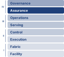
Fleet stack focus for this chapter.
Why can machine learning systems fail silently even when conventional health signals remain normal?
A model service can maintain stable latency and uptime while its predictions become unreliable. Changes in operating conditions, manipulated inputs, or corrupted computation may leave ordinary health signals untouched, allowing errors to affect decisions long before business metrics expose them. Conventional software can also fail silently; machine learning adds statistical failures that a successful request cannot reveal. At fleet scale, replicating a model across healthy machines does not remove a weakness shared by every copy. Traffic also spans different regions, devices, and user populations, so acceptable average performance can conceal a serious failure in one group. The decision to continue answering therefore requires evidence about the conditions under which the predictions remain useful, not merely confirmation that the service is available. Producing that evidence consumes resources, and responding to it creates further obligations. Additional checks can delay answers; rejecting uncertain requests can overwhelm reviewers or a backup service. A replacement model must demonstrate acceptable behavior before the fleet adopts it, while waiting too long can prolong exposure to errors. The engineering challenge is to connect evidence to a bounded response without exhausting the resources needed to serve useful predictions. Protection must cover the model and the surrounding data path, because either can invalidate the result. In C³ terms, verification spends compute and communication, while coordination determines when the evidence should trigger investigation, fallback, or a halt.
Learning Objectives
- Classify a silent failure by robustness pillar and diagnose its source using input replay, deployment history, and system telemetry
- Distinguish covariate shift, label shift, and concept drift, and judge when drift evidence justifies a model update
- Distinguish calibration, selective prediction, and conformal coverage, including the assumptions and operational costs of each
- Evaluate adversarial attacks by attacker access, and select defenses such as adversarial training, certification, and input detection
- Select layered poisoning defenses that combine source controls, anomaly detection, robust training, and post-training checks
- Evaluate generative-model reliability against a named evidence source, treating entropy, self-consistency, and output guardrails as priced routing signals
- Evaluate robustness designs against clean accuracy, compute, latency, and fallback-capacity budgets
14.1 The Silent Failure Problem
A vehicle’s vision model validated on sunny roads may become unreliable when snow changes the visual distribution. A confident misclassification, such as reading a snow-covered stop sign as a speed-limit sign, need not throw an exception or produce a stack trace. Whether that error leads to an unsafe action depends on the surrounding perception, planning, and fallback systems. Robustness engineering evaluates and constrains behavior under specified operational stresses, including distribution shift, sensor noise, adversarially crafted inputs, and hardware or software faults that can leave the service apparently healthy while its answers become unreliable.
Robust AI occupies the Assurance row of the fleet stack’s governance band, alongside security and privacy. Security and privacy establish who can manipulate, extract from, or infer through the model and which controls constrain that access or disclosure. Robustness adds a behavioral requirement when inputs, data distributions, hardware, or software depart from the conditions assumed during validation. Within a specified operating envelope, the fleet needs evidence that predictions or fallback actions remain acceptable. Adversarial examples become perturbations to measure and defend against, with certification available under particular assumptions; nonadversarial drift and faults require their own evaluations. Diagnosing the failure source comes first. Population-shift tests then supply evidence of environmental change, while attack-specific evaluation tests whether deliberate manipulation defeats the model or its defenses.
The failure may be visible in predictions before it appears in infrastructure telemetry. A self-driving car’s perception system does not crash when it misclassifies a truck as the sky; a demand forecasting model does not error out when it produces wildly inaccurate predictions; a medical diagnosis system does not shut down when it quietly provides incorrect classifications that could endanger patient lives. This silent failure mode requires ML-specific behavioral checks alongside conventional software checks, because only a behavioral test reveals how a model responds when deployment conditions depart from its training data.
Checkpointing and recovery restore execution state, while access control enforces permissions at the system boundary. These mechanisms do not establish that predictions remain useful. An adversarial input may satisfy the interface contract, the data distribution may drift beyond the model’s validated conditions, or a preprocessing fault may alter inputs without stopping inference. Recovery can restore a clean checkpoint after some failures, but behavioral checks must determine whether that restored system meets its acceptance criteria. Fault detection, diagnosis, and recovery therefore need evidence about both execution and prediction quality, motivating a precise definition of Robust AI:
Definition 14.1: Robust AI
Robust AI is the measurable systems property that a model’s predictions remain valid (within specified error bounds) under distribution shift, adversarial perturbation, and hardware or software faults, as opposed to the average-case accuracy achieved under ideal independent and identically distributed (i.i.d.) conditions.
- Significance: Robustness is quantified against an explicit operating or threat set. A certified classifier can prove that its prediction cannot change for any input within a specified perturbation set, such as an \(\ell_\infty\) ball of fixed radius around one test point (every input coordinate changed by at most that radius). Empirical stress tests instead measure performance on named corruptions, shifts, or attacks without proving behavior outside the evaluated cases.
- Distinction: Standard generalization measures average-case accuracy on held-out i.i.d. data drawn from the training distribution. Robustness measures behavior under specified departures from that distribution, including natural shifts, semantic transformations, physical changes, malicious queries, and norm-bounded perturbations. Some evaluations are worst-case within a formal set; others provide empirical evidence over a sampled deployment envelope.
- Common pitfall: A frequent misconception is that robustness can be added as a post-hoc monitoring layer to any existing model. Monitoring supplies evidence about observed behavior; it does not establish certified robustness. Training-time hardening and serving-time defenses each require evaluation of the complete defended system against a specified threat model. A certificate applies only within its stated perturbation set and assumptions.
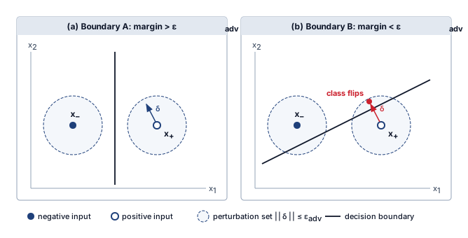
Two models can agree on every clean input and still differ in how far an input can move before its label flips. In figure 1, each labeled point is surrounded by the same perturbation radius, the largest input change the evaluation allows. Vertical boundary A keeps every allowed change on the correct side, while oblique boundary B cuts through the neighborhood around \(\PositiveClassInput\), so a small displacement \(\AdversarialPerturbation\) flips the predicted class. The adversarial defenses of section 14.6 turn that distance into a measured quantity and, under stated assumptions, a certified one.
Three categories organize these silent failures and the responses they require, and the rest of the chapter calls them the three pillars of robust AI. The first, environmental change, includes distribution shifts, concept drift, and evolving operating conditions. A model trained on last year’s transaction patterns may become unreliable as customer behavior evolves. Monitoring must establish whether the change affects predictive quality before an adaptation strategy can address it.
The second category, input-level attacks, is malicious manipulation that targets model behavior directly through the data a model receives or learns from. Adversarial attacks, data poisoning attempts, and prompt injection seek incorrect predictions or unauthorized behavior. Authentication and access controls constrain who can submit data and which actions the system permits, but an authorized input can still induce an incorrect result. Behavioral evaluation must therefore examine the manipulation possible within the access that remains.
The third category is system-level faults: hardware faults, software bugs, dependency failures, and runtime errors that corrupt the machinery around the model. Software and pipeline defects belong to this pillar by origin, yet their symptoms can amplify, mask, or mimic the other two, which is why they also cut across the whole taxonomy. Bugs, design flaws, and implementation errors within algorithms, libraries, and frameworks propagate through the system, creating systemic vulnerabilities1 that transcend individual component failures. A preprocessing bug might create artificial distribution shifts; a numerical error might corrupt model behavior in ways indistinguishable from adversarial attack; a race condition might corrupt learned representations. Because these faults originate in the systems layer, their detailed taxonomy and mitigation strategies are covered in Fault Tolerance; this chapter focuses on how system-level faults interact with environmental shifts and input-level attacks.
1 Systemic vulnerability: A shared dependency can expose many components to the same defect or attack. Pinning one CUDA or PyTorch version across a fleet makes that version a common dependency, but exploitation still depends on the affected code paths, configuration, and attacker access. Dependency inventories and staged updates help identify and contain the exposed population; replication alone does not remove a shared weakness.
The appropriate defense depends on where the system runs and which failures it must contain. A cloud service may have capacity for redundant execution that exceeds an edge device’s power and memory budget, but additional replicas do not remove a model weakness shared by every copy. Edge devices can concentrate checks on critical inference paths and use a validated local fallback. Both settings require measured protection within their resource and response-time limits.
Each protection consumes resources in the path where it operates. Error correction adds storage and checking work, redundant processing repeats computation, and monitoring uses compute and telemetry capacity. Their effects on bandwidth, energy, and response time depend on the implementation and workload. The robustness decision compares those measured costs with the failures detected or contained and the consequences of errors that remain. Because every layer of the pipeline, from input validation and training through drift detection and fault isolation, carries part of this cost, robustness constrains the architecture rather than wrapping a finished system. The incidents that follow show what ignoring that constraint has cost in cloud, edge, and embedded deployments.
Self-Check: Question
A medical imaging classifier reports 95 percent accuracy on its i.i.d. held-out test set. Applying the chapter’s quantitative definition of Robust AI, which finding would indicate the model lacks robustness rather than generalization ability?
- Accuracy drops to 94.8 percent when tested on a second random split from the same historical training distribution.
- Accuracy drops to 35 percent under an imperceptible \(\ell_\infty\) perturbation of radius \(\epsilon_{\text{adv}} = 8/255\) on the same test images.
- Inference latency increases from 50 ms to 120 ms when batch size is doubled on the deployment GPU.
- Training loss fails to reach zero because the learning rate schedule decayed too early in optimization.
True or False: A classifier trained only with standard cross-entropy loss can achieve certified robustness after deployment by wrapping it in a runtime filter that rejects inputs whose predicted confidence falls below a threshold.
An engineering team must deploy a perception model across two platforms: a data-center inference cluster with elastic capacity and an industrial inspection drone with a fixed 10 W thermal budget. Per the section, which deployment strategy correctly balances their respective constraints?
- Apply identical full-stack redundancy and continuous background verification on both platforms to maintain uniform safety guarantees.
- Disable monitoring in the data center to minimize serving latency and move all verification onto the drone.
- Offload all drone perception requests over a wireless network to the data-center backup cluster and disable on-device inference.
- Equip the data center with broad redundancy and ensemble fallbacks while the drone selectively hardens critical paths and relies on graceful degradation.
A preprocessing library silently converts pixel values from 0-1 floats to 0-255 integers for 1 in 10,000 requests. Downstream monitoring flags occasional confidence drops that resemble adversarial attacks. Identify the fault’s pillar by origin and explain why its symptoms cut across the other pillars.
When a battery-powered device’s full redundancy and verification budget exceeds its thermal envelope, the chapter prescribes a controlled, predictable reduction to a simpler model or reduced-feature mode so core functionality continues safely rather than silently returning invalid predictions. This behavior is known as ____.
The section states that robustness protection is not free: error correction adds storage and checking work, redundant processing repeats computation, and monitoring consumes compute and telemetry capacity. Explain why these overheads require robustness to be treated as an architectural constraint budgeted from inception rather than an add-on feature.
14.2 Real-World Robustness Failures
A shared storage outage can stop a service, while a perception error can leave it running with an unsafe result. The incidents below separate those two outcomes, so that a successful request or an operational processor is never mistaken for evidence of a valid prediction. Each deployment tier also exposes a different failure most sharply. Cloud fleets show a population slice whose failure hides inside aggregate accuracy, and silent hardware corruption entering training, a system-level fault. Edge vehicles show perception failing under operating conditions the model was never validated for, the environmental pillar with no time for a remote fallback. Embedded controllers show what happens when a false input drives an irreversible action with no human in the loop; those cases predate learned components, so they illustrate the hazard a learned component inherits rather than a model failure. Deliberate attacks are absent from the list because their best-documented evidence comes from controlled field studies, which section 14.5 examines.
War Story 14.1: The label that exposed the test gap (2015)
Context: In June 2015, Google Photos used automatic image tagging to organize user photos (Kasperkevic 2015).
Mechanism: A deep convolutional image classifier placed Jacky Alciné’s photos of himself and a Black friend under the album tag “Gorillas,” a severe slice-level failure mode. The failure demonstrates why aggregate top-1/top-5 accuracy over a full test set cannot establish acceptable behavior for high-risk population slices.
Impact: The high-visibility misclassification caused public outrage and exposed a major gap in multi-class vision model safety validation.
Fix: Google disabled the “gorilla” label, blocking the symptom without demonstrating that the classifier itself had been corrected.
Systems lesson: Production ML robustness cannot be defined by aggregate test set accuracy. High-risk classification tasks require slice-level evaluation and a serving response to harmful errors. Automated toxicity guards and validated fallbacks are candidate controls whose coverage must be tested against the specific failure.
Kasperkevic, Jana. 2015. “Google Says Sorry for Racist Auto-Tag in Photo App.” The Guardian, July.
That test-gap failure is the model-facing version of a broader reliability problem. In cloud infrastructure, the hidden assumption is often that a shared dependency remains available and correct.
14.2.1 Cloud infrastructure failures
The 2017 AWS S3 outage2 shows the familiar half of that assumption, in which a shared storage dependency failed and otherwise healthy services stopped (Amazon Web Services 2017). An outage at least announces itself. The robustness problem is the other half, when the dependency stays up but returns plausible, corrupted data, so the service keeps answering while incorrect results propagate.
2 AWS S3 outage (2017): A mistyped command during routine maintenance removed too much capacity from S3’s index and placement subsystems in US-East-1. While those subsystems restarted, S3 could not service requests and dependent AWS services experienced elevated errors or impaired functionality. The incident exposed a single-region dependency pattern: systems that assume regional storage availability as an invariant can fail even when their own application code and model-serving logic remain unchanged.
Amazon Web Services. 2017. Summary of the Amazon S3 Service Disruption in the Northern Virginia (US-EAST-1) Region. AWS service event summary.
Dixit, H. D., S. Pendharkar, M. Beadon, C. Mason, T. Chakravarthy, B. Muthiah, and S. Sankar. 2021. Silent Data Corruptions at Scale. arXiv preprint arXiv:2102.11245.
Ma, Jeffrey, Hengzhi Pei, Leonard Lausen, and George Karypis. 2025. Understanding Silent Data Corruption in LLM Training. https://doi.org/10.48550/arXiv.2502.12340.
Silent data corruption (SDC) is that case. The decompression incident analyzed in The physics of silent corruption demonstrates the failure signature. A defective CPU returned zero during a size computation for a valid file, causing the decompression pipeline to omit files from its output even though system and kernel logs showed no fault (Dixit et al. 2021). The separate training illustration in Silent Data Corruption Propagation traces how unhandled corruption can enter gradients, weights, and later checkpoints. In distributed ML training, a corrupted gradient or activation can perturb optimizer state, spread to every replica through gradient synchronization, and persist into later checkpoints, so its blast radius grows with the synchronization and checkpointing design and recovery may require rollback to the last clean checkpoint (Dixit et al. 2021; Ma et al. 2025). In both settings, checking that execution continues is insufficient; evaluation must test the validity of the resulting data or model behavior.
↩︎ Silent data corruption during training and its fleet-scale evidence are established in Verification at fleet scale.
14.2.2 Edge and embedded failures
In May 2016, a Tesla Model S operating on Autopilot failed to identify a tractor-trailer crossing its path and struck it at highway speed with neither warning nor braking (National Transportation Safety Board 2017). The system had not been validated for that scene, and nothing in its own behavior signaled that it had left its validated envelope. Edge deployments must respond within local compute, power, and connectivity limits, and in a vehicle, a perception or planning failure can require intervention before a remote service or human operator can respond. Vehicle safety therefore depends on the conditions the system can handle locally and the fallback available when those conditions no longer hold.
National Transportation Safety Board. 2017. Collision Between a Car Operating with Automated Vehicle Control Systems and a Tractor-Semitrailer Truck Near Williston, Florida, May 7, 2016. HAR-17/02. National Transportation Safety Board.
↩︎ The 2016 crash, read as an edge model whose fallback was a supervising driver, is established in Compliance, security, and recovery risks in production.
National Transportation Safety Board. 2019. Collision Between Vehicle Controlled by Developmental Automated Driving System and Pedestrian, Tempe, Arizona, March 18, 2018. HAR-19/03. National Transportation Safety Board.
In March 2018 in Tempe, Arizona, an Uber self-driving test vehicle struck and killed a pedestrian (National Transportation Safety Board 2019). The system detected her 5.6 seconds before impact, but its classification of her was unstable. Repeated reclassification among “vehicle,” “other,” and “bicycle” caused path prediction to discard tracking history. The final investigation placed recognition of the imminent collision at 1.2 seconds before impact. The system then suppressed action for one second without alerting the operator; only afterward did it issue an alert and plan gradual slowdown. The operator did not intervene in time. The case connects perception, tracking, response timing, and human fallback, and it shows that detecting an object did not establish that the system would act safely on that detection.
An inspection drone surveying power lines may likewise lose reliable localization when lighting changes or repetitive textures confuse visual odometry. An alternate inference or control path provides fallback redundancy when the primary path cannot support the required decision, but its value depends on independent failure coverage and response time. A local sensor-based controller or validated landing mode may be more useful than a remote model that cannot answer before the control deadline. Edge AI must provision that response within the device’s resource limits; a data center’s additional replicas would not by themselves correct the same perception error.
Embedded systems can operate through critical intervals in which external intervention is too slow. Remote maintenance may remain possible between those intervals, but an autonomous landing or control maneuver needs a local response before its deadline. Validation must therefore cover both the component’s failure modes and the system behavior that follows, including any ML model in the decision loop. NASA’s Mars Polar Lander was lost in 1999 when, according to its review board, a spurious touchdown indication likely shut down the engines before landing (NASA Mars Program Independent Assessment Team 2000). For a learned component in such a control loop, validation must connect plausible input and sensor failures to the actions they can trigger, because exhaustive testing of every possible input is not a feasible safety argument.
NASA Mars Program Independent Assessment Team. 2000. Report on the Loss of the Mars Polar Lander and Deep Space 2 Missions. National Aeronautics; Space Administration.
3 Failsafe mechanism: A mechanism that moves the system to a validated safe state when a fault is detected. Circuit breakers, model fallback, rejection, and rollback are possible components, but none is inherently safe for every application. The service must establish that its chosen response meets the hazard and timing constraints; rejection thresholds also trade accepted workload against residual error and review capacity.
Federal Aviation Administration. 2015. Airworthiness Directive: Boeing 787 Generator Control Units Failsafe Reset. FAA Airworthiness Directive 2015-10066.
4 ASIL (automotive safety integrity levels): ISO 26262 uses automotive safety integrity levels to scale functional-safety obligations according to the hazard analysis. ASIL D is the most stringent level, but it is not a universal component-reliability percentage. An ML perception component complicates the resulting safety case because its behavior depends on the operational distribution and cannot be justified by aggregate test accuracy alone.
Commercial aviation shows the same inherited hazard: a 2015 FAA airworthiness directive followed Boeing’s discovery that a 787 powered continuously for 248 days could lose all AC power if all four generator control units entered failsafe mode at once,3 so that uptime itself became the risk factor (Federal Aviation Administration 2015). An endurance test shorter than that interval would not have exposed the defect. A learned component inherits the same hazard whenever deployment reaches a condition its evaluation never covered, such as accumulated state, a rare season, or an unusual sensor reading, and safety-critical systems4 impose stringent reliability requirements precisely because such latent hazards surface only in the field. Across these settings, robustness depends on connecting the failure signal to a bounded response, and the fleet framework must distinguish the source of that signal before choosing a defense.
Self-Check: Question
During the February 2017 AWS S3 outage, dependent services such as EC2 launches, EBS snapshot-dependent volumes, and Lambda experienced elevated error rates. Which design assumption does this incident most directly invalidate for robust ML systems?
- That deep neural networks are too computationally intensive for cloud object stores and must be compressed.
- That adversarial inputs are the dominant cause of availability loss in production inference services.
- That regional cloud storage availability can be treated as an absolute invariant rather than a probabilistic dependency in the serving pipeline.
- That distributed training clusters must enforce Byzantine-tolerant gradient aggregation to prevent worker dropouts.
The chapter describes a defective CPU that returned zero in a file-size calculation, causing a decompression pipeline to omit files without raising a fault. Explain how an analogous undetected error can persist and propagate through distributed ML training, and why its blast radius depends on synchronization and checkpointing.
In the March 2018 Uber ATG pedestrian fatality in Tempe, the vehicle perception stack detected the pedestrian 5.6 seconds prior to impact but did not recognize the imminent collision until 1.2 seconds before impact. Which perception and tracking mechanism described in the chapter contributed to that delay?
- Object classification instability, where the model toggled between ‘vehicle’, ‘other’, and ‘bicycle’, resetting the trajectory prediction history on each reclassification.
- Complete radar transceiver hardware failure that left the vehicle with zero sensor measurements.
- A sudden geographic covariate shift that rendered the obstacle detection model unable to process Arizona road layouts.
- A cloud network disconnection that prevented the on-vehicle computer from receiving remote classification confirmations.
True or False: During a safety-critical embedded maneuver such as autonomous landing, a sensor or software fault can cause irreversible harm before remote intervention, so validation must cover both the fault and the local response within the maneuver’s deadline.
Order the stages of a silent data corruption cascade in a distributed ML system from initial hardware fault to final production failure: (1) Contaminated parameters persist through optimizer updates and are saved into a checkpoint artifact, (2) An undetected bit flip occurs in the ALU or memory during forward-backward computation on a single worker node, (3) The deployed model serves degraded or erratic predictions while standard latency and uptime health checks stay green, (4) Corrupted gradients are broadcast and aggregated across all workers during AllReduce synchronization.
14.3 A Unified Framework for Robust AI
One flipped exponent bit in accelerator memory can turn a trained weight of 0.042 into a finite value near \(1.4 \times 10^{37}\) that passes every NaN check (section 14.9.1). A gradual change in user demographics can erode recommendation quality while latency and uptime stay flat. Production ML systems cannot treat these as isolated bugs. A unified framework must map how low-level hardware faults, software bugs, data drift, and adversarial inputs propagate upward into the model’s output.
14.3.1 Shared state and fault surfaces across the fleet

One corrupted gradient in AllReduce reaches every replica’s weights.
In distributed training, a single node transmitting corrupted gradients during an AllReduce operation can poison the global model weights across every worker, because the mechanisms that make a fleet efficient also share state or work across many machines. Fault detection and recovery mechanisms keep training jobs running and support inference-time availability, yet a restored checkpoint or a responsive replica does not establish that the model behaves acceptably on current inputs. Robustness extends the recovery argument to graceful degradation, in which a reduced service must still meet a validated behavioral contract when inputs are adversarial or components degrade. Containing shared training state requires evidence that corrupted updates are detected or isolated: Byzantine fault tolerance protocols address the case in which a contributor sends arbitrary or malicious values rather than simply stopping, while ordinary hardware corruption also demands the fault diagnosis and recovery mechanisms already established for the fleet.
↩︎ Gradient synchronization through AllReduce, in which every replica receives the same reduced gradient, is established in Gradient synchronization.
↩︎ Byzantine failures, in which a component returns arbitrary values rather than stopping, are established in Byzantine failures.
Serving repeats the same sharing at inference time. Batching, request routing, and pipeline-parallel stages place many users’ requests on one model replica or one stage, so a corrupted replica or stage returns wrong answers to every request routed through it while its health checks still pass. When the cause is deliberate rather than accidental, the threat-vector classification in Threat vector classification, by attacker access, knowledge, and timing, defines the attacker that a defense must assume.
↩︎ Batching, request routing, and pipeline-parallel serving are established in Serving at Scale.
Large dense models amplify these risks. The Archetype A (GPT-4/Llama-3) reference model, a GPT-3-class dense transformer with 175B parameters, needs 350 GB for its weights alone at FP16/BF16 serving precision (\(\ElementStorageSize = 2\text{ bytes/param}\), with no optimizer state). Because that footprint exceeds the 80 GB per-device memory capacity \(\DeviceMemoryCapacity\) of a single A100- or H100-class accelerator, keeping these weights accelerator-resident requires distributing them across multiple devices. Each additional pipeline or tensor-parallel stage increases the fault surface compared with a monolithic deployment. A single bit flip or network partition in one stage can fail the entire inference request, and silent corruption can propagate through downstream computations that consume the affected values. Whether it changes the final prediction depends on the corrupted value, the computation, and the available detection or containment.
The pressure that shards a model across devices also compresses it. Efficiency techniques that let a model fit on fewer devices or serve more requests change the deployed computation itself, so each one must be checked against the robustness evidence gathered for the uncompressed model. Checking that evidence draws on reliability engineering:5 fault models that describe how failures occur, error detection mechanisms that identify problems before they impact results, and recovery strategies that restore system operation. Compression meets these concepts through the model’s robustness margin, the amount of input perturbation, numerical error, or representation change the model can absorb before its prediction changes. INT8 quantization, pruning, and knowledge distillation change the deployed computation, and each can shrink that headroom, so a compressed model that matches the original’s clean-data accuracy has not thereby shown that its margin survived. An optimized system therefore needs evidence that its detection and recovery mechanisms cover the faults in its operating model and that the resulting predictions still meet the service contract.
5 Reliability engineering: Uses fault models and failure-mode analysis to connect component behavior to system outcomes. A series model gives system reliability as \(\SystemReliability(\TimeInstant)=e^{-\SeriesComponentCount\ComponentFailureRate \TimeInstant}\) when all \(\SeriesComponentCount\) components must survive, failures are independent, and each has the same constant exponential failure rate. ML deployments also need behavioral evidence for drift, crafted inputs, and uncertainty; the component-survival model alone does not cover these failure modes.
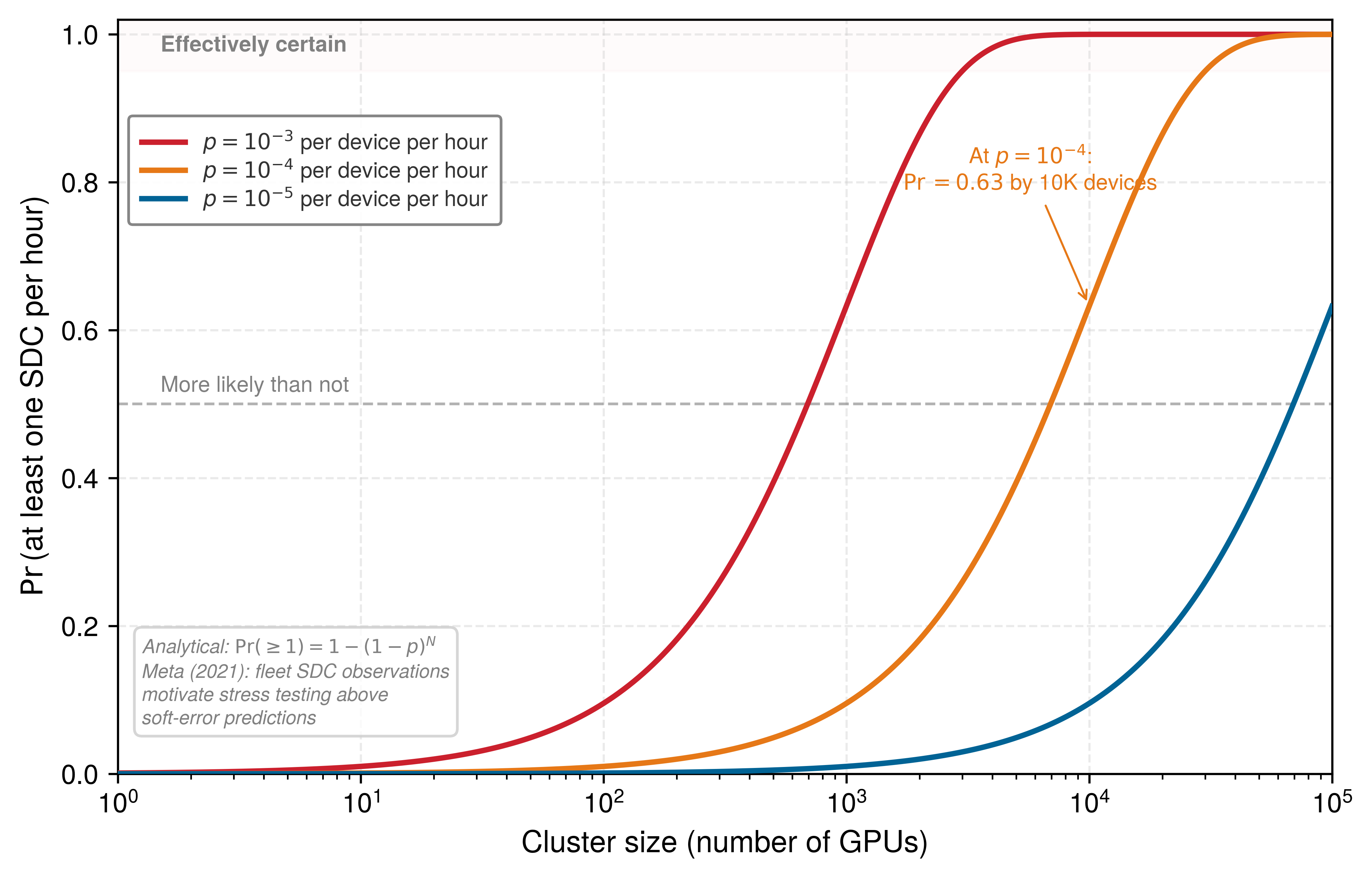
Scale also compounds the chance that silent corruption occurs somewhere in the fleet. Under the fleet model of Verification at fleet scale, \(\DeviceCount\) devices, each with independent residual-error probability \(\DeviceSilentCorruptionProbability\) over the same interval, see at least one silent error with probability \(\Pr(\geq 1) = 1 - (1 - \DeviceSilentCorruptionProbability)^\DeviceCount\), so a per-device rate that is negligible on one machine becomes a routine event on a fleet of tens of thousands of accelerators. At cluster scale a per-device reliability number therefore becomes a coordination cost, the third axis of C\(^3\). Once a silent error is likely somewhere in the fleet, operators must agree on which replicas, checkpoints, and outputs remain trustworthy before they can contain it, and that agreement requires evidence that ordinary health checks do not collect. Hardware faults, adversarial inputs, and software defects all create this evidence problem, which is why the chapter treats them within one framework.
14.3.2 The three pillars of robust AI
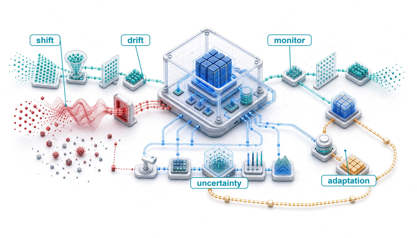
When a model’s error rate climbs without a service outage, an engineer must determine whether customer behavior shifted, an attacker perturbed the inputs, or an accelerator corrupted a weight before choosing a defense. Each of the three pillars named at the start of the chapter decomposes into concrete failure subtypes, and each subtype pairs with the defense that targets it (figure 2).
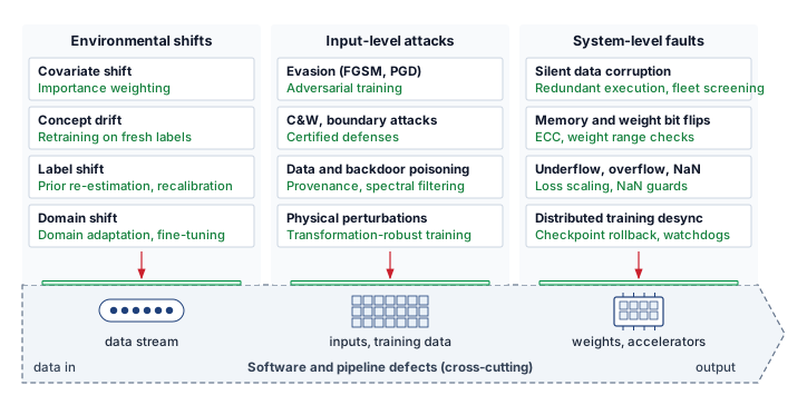
The subtype names matter less than the evidence each pillar produces, because the evidence is what an operator actually observes and what selects the defense family. Environmental shifts can produce statistical differences between production data and a reference population. Those differences motivate investigation, but an input-distribution monitor cannot detect every change in the relationship between inputs and outcomes. Monitoring, recalibration, and retraining address different parts of that problem; outcome evidence helps determine which response is warranted.
Input-level attacks deliberately target model behavior through crafted inputs or poisoned training samples. Anomalous inputs can raise suspicion, but an effective attack need not expose a recognizable perturbation or statistical outlier. Adversarial training, certification, and input sanitization address different threat models. Authentication and access control constrain who can submit data and what actions a model-driven system may take; they do not establish that every permitted input will receive a correct prediction.
System-level faults originate in the hardware, code, frameworks, and deployment infrastructure that support ML systems: numerical instability, preprocessing bugs, race conditions and replica desynchronization, dependency mismatches, and hardware faults such as bit flips. Many produce explicit errors or outages, but a fault that leaves the service answering appears instead as changed model behavior that can pass for either of the other pillars, and section 14.9 develops the signals that separate them after both pillars have been treated.
↩︎ The mechanics of hardware and software faults, and their detection and recovery, are established in Fault Tolerance.
14.3.3 Common robustness principles
An uncalibrated monitor that fires on harmless traffic fluctuations can trigger unnecessary retraining or flood a fallback service just as easily as an undetected failure can corrupt predictions. Across all three categories, the shared engineering problem is deciding which signal triggers which response. Robust systems need a detection threshold, a degradation path, and an adaptation mechanism, each with an explicit cost budget.
Detection and monitoring form the foundation of that strategy, and each pillar asks for a different signal because each failure originates in a different layer. System-level monitoring samples hardware and runtime metrics for evidence of temperature anomalies, voltage fluctuations, memory errors, or silent data corruption; detection can limit further propagation, although the first observable symptom may follow a corrupted state update. Where system monitors watch the machinery, input-level attack monitoring uses statistical or activation-space tests to flag suspected adversarial inputs and poisoning attempts for rejection or investigation, while environmental-shift monitoring compares production traffic with reference distributions using tools such as maximum mean discrepancy (MMD),6 population stability index (PSI), or Kolmogorov-Smirnov (KS) tests, the statistics developed in section 14.4.2. The same quantitative discipline applies to defense cost: robustness mechanisms must be budgeted, not merely enabled, because every detector trades sensitivity against false positives, latency, and compute overhead.
6 Maximum mean discrepancy (MMD): A discrepancy between kernel mean representations of distributions, used to construct two-sample tests. A kernel on input vectors lets MMD respond to joint-distribution changes that per-feature comparisons can miss; sensitivity depends on the kernel and test calibration. Direct pairwise estimation costs \(\mathcal{O}(\DriftTestSampleSize^2)\) in sample size, while linear-time estimators and approximations trade computation against statistical efficiency.
Graceful degradation turns detection into a bounded operating mode instead of a crash, stepping down a predeclared ladder of cheaper models and simpler features rather than failing outright. Robustness adds a behavioral condition to that ladder, because the degraded model and its fallback must still satisfy the service’s acceptance criteria under the failure that triggered them. A quantized replica that keeps serving when capacity drops therefore needs its own validation under the degraded operating conditions, since quantization can shrink the robustness margin even when clean accuracy holds. Ensemble fallback systems likewise preserve service only if the alternate models cover the relevant failure and complete within the serving deadline; their quality under that failure, switching delay, and capacity under diverted traffic require evaluation, and ensemble membership alone establishes none of these properties.
↩︎ Graceful degradation as a ladder of model and feature fallbacks, each validated before it is needed, is established in Graceful Degradation.
Adaptive response completes the loop by changing system behavior when the signal persists, for example by activating error correction, adding input preprocessing, or updating model parameters, so robustness is an ongoing adjustment rather than a one-time configuration. Across the three pillars of figure 2, hardware ECC and redundant execution detect faults, weight range checks and checkpoint rollbacks contain the damage, and retraining or adversarial training adapts the model, which is why each pillar needs its own version of all three mechanisms and no single defense covers the taxonomy.
The evaluation plan must preserve those distinctions, and one row of it is not a pillar at all. Population monitors ask whether traffic as a whole has changed, while a serving system must also decide, request by request, whether this particular input lies inside the model’s demonstrated competence. The tools for that per-request decision, namely calibration, out-of-distribution (OOD) scores, and selective prediction with its risk-coverage curve, are developed in section 14.4.4, after the drift statistics they complement. Each failure class needs its own minimum evidence (table 1), so a passed test in one row cannot become a robustness claim about another. Several of the matrix’s terms are developed later in the chapter. Near-OOD inputs resemble the training data but fall outside its classes or conditions, while far-OOD inputs come from unrelated sources; robust and certified accuracy are developed with the adversarial defenses (section 14.6.1.1), and sybil and Byzantine contributors with the poisoning defenses (section 14.7).
| Failure class | Evaluation set or intervention | Primary evidence | Required slice | Decision boundary |
|---|---|---|---|---|
| Natural shift | Time-, geography-, device-, and environment-held-out data | Accuracy or loss, calibration error, and drift statistics | Critical cohorts and tail conditions | Continue, investigate, recalibrate, retrain, or fall back |
| Per-request competence | In-distribution errors plus near- and far-OOD inputs | Risk-coverage curve, OOD score, and fallback load | High-consequence request classes | Answer, route, abstain, or reject |
| Adversarial manipulation | White-box, black-box, transfer, and physical attacks matched to the threat model | Robust accuracy by attack budget; certified accuracy where available | Targeted classes and attacker capabilities | Accept, harden, restrict, or block release |
| Poisoning | Source-compromise, label-flip, backdoor, fake-identity (sybil), and Byzantine-contributor scenarios | Clean and attack-success metrics, slice loss, and detector recall | Sources, contributors, and subpopulations | Quarantine, exclude, reweight, or roll back |
| System fault | Fault injection across data, runtime, accelerator, and network paths | Silent-error rate, detection latency, and recovery success | Correlated and multi-component faults | Retry, isolate, degrade, or fail safe |
14.3.4 Integration across the ML pipeline
A serving-time filter cannot repair a fraud model that was trained on poisoned records, and an ingestion filter cannot stop an attacker who perturbs inputs at inference time. Robustness therefore requires evidence across the entire ML lifecycle, with complementary controls at each stage—the defense-in-depth principle applied to model behavior. Ingestion checks flag malformed or statistically anomalous records before training, training-time defenses target specified perturbations, validation stress-tests behavior on out-of-distribution data within a named deployment envelope, and serving-time filters and monitors watch live traffic. No stage establishes what another stage must show.
↩︎ Defense in depth, which requires independent layers so that defeating one does not defeat the system, is established in Defense strategy framework.
A production fraud detection pipeline therefore evaluates its ingestion checks against poisoned training records and its serving-time filters against evasion attempts separately, and neither guarantees interception. The monitoring layer acts as the safety net, detecting distribution drift, such as a sudden shift in transaction amounts or user geolocations, and opening an investigation. Retraining follows only when validated outcome evidence, root-cause analysis, and the release gate show that a model update is the appropriate response.
Hardware faults (transient, permanent, and intermittent) and the fleet’s mechanisms for detecting and recovering from them are classified in Hardware Faults at Fleet Scale. Robustness evaluation adds a behavioral test to those mechanisms: after a fault is detected or a request retried, the output must still satisfy the model’s acceptance criteria. A retry alone does not establish that the result is correct. The same distinction between service health and prediction quality applies when the machinery works correctly but the world evolves beyond its training data.
Checkpoint 14.1: Diagnosing the failure signal
The unified framework requires identifying which of the three pillars produced a silent failure before choosing a defense, and recognizing that software faults can masquerade as any of them.
Classifying the threat
Choosing the response
Self-Check: Question
An engineering organization is structuring its reliability teams according to the chapter’s Three Pillars Framework. Which team structure correctly maps to the taxonomy?
- Three separate teams dedicated respectively to training failures, validation failures, and serving failures.
- Complementary teams address environmental shifts, input-level attacks, and system-level faults, with software diagnosis coordinated across all three categories.
- Three teams organized around model throughput, GPU memory footprint, and floating-point quantization.
- Two independent teams focused exclusively on user data privacy and carbon accounting.
Assuming independent devices over the same one-hour interval and an assumed residual silent data corruption probability of \(p = 10^{-4}\) per device per hour, what is the probability \(\Pr(\ge 1)\) of at least one SDC event occurring in a single hour across a 10,000-GPU training cluster, and what does this imply for systems design?
- \(\Pr \approx 10^{-8}\) per hour, proving SDC is too rare to justify architectural defenses in distributed clusters.
- \(\Pr = 10^{-4}\) per hour, because device-level failure rates do not compound across independent nodes.
- \(\Pr \approx 0.63\) (63 percent) per hour, meaning silent corruption is an expected operational event that requires automated verification and checksumming.
- \(\Pr = 1.0\) (100 percent) per hour with deterministic certainty, guaranteeing every training step fails.
True or False: Preserving clean-set accuracy after FP32-to-INT8 quantization is sufficient evidence that the compressed model also preserves its robustness margin against input perturbations and numerical faults.
A drift alert fires while measured prediction quality remains within tolerance. Explain the distinct roles of detection, graceful degradation, and adaptive response, and why the alert need not trigger all three in a fixed sequence.
Explain the defense-in-depth principle across the ML lifecycle by describing the distinct robustness functions performed at data ingestion, model training, deployment validation, and live serving.
14.4 Environmental Shifts
A credit-scoring or recommendation model trained on last quarter’s user behavior can lose accuracy as seasonal demand, demographics, or economic conditions move, because training data freezes a past world while production traffic keeps changing. Environmental shifts arise as data distributions, user behavior, and operational contexts move after training, and a shift becomes a robustness failure when model behavior no longer meets the service contract. Changed conditions can also expose software defects or alter the effectiveness of an adversarial defense, so the response depends on both the distribution change and its measured consequences.
14.4.1 Distribution shift and concept drift
Consider a medical diagnosis model trained on X-ray images from one hospital and deployed in a clinic with different imaging equipment. Even for the same medical conditions, acquisition settings can change the image characteristics. This difference between training and deployment populations is distribution shift; whether it reduces diagnostic accuracy requires evaluation on the clinic’s data. A move to a different source altogether, such as a new hospital, sensor, or region, is often called domain shift, and it can combine several of the shift types distinguished below.
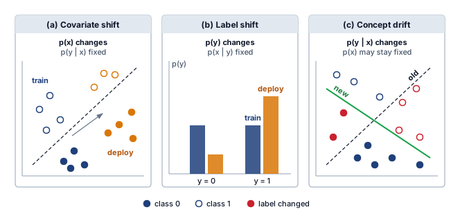
Distribution shift takes three geometric and statistical forms (figure 3). Inputs can migrate to an unfamiliar region of feature space (panel a), label priors can skew (panel b), or the underlying mapping itself can invert (panel c). Here, \(\ModelInput\) denotes an input and \(\ExampleLabel\) its outcome label. Input-only monitors can detect changes in \(\ProbabilityFunction(\ModelInput)\); distinguishing changes in label frequencies or in \(\ProbabilityFunction(\ExampleLabel\mid \ModelInput)\) generally requires outcome evidence or additional assumptions.
These shifts occur naturally as environments evolve. User preferences change seasonally, language evolves with new slang, and economic patterns shift with market conditions. Unlike adversarial attacks that require malicious intent, these shifts emerge organically from the dynamic nature of real-world systems. When a deployed model actively influences user behavior, as in fraud detection, recommendation engines, or credit underwriting, the shift is not merely exogenous. The sociotechnical feedback invariant (principle 27) governs these performative environments, in which the probability distribution of future inputs \(\ProbabilityFunction_{t+1}(\ModelInput)\) depends directly on the model’s past decisions \(\ModelPredictor_t(\ModelInput)\) through the environment’s response function \(\EnvironmentResponseFunction(\ProbabilityFunction_t(\ModelInput), \ModelPredictor_t(\ModelInput))\). Deployed predictions induce user and adversary adaptations that accelerate distribution shift, compressing the model’s viable operating window and demanding closed-loop monitoring rather than static validation.
Technical categories
Covariate shift changes the input distribution while the relationship between inputs and outputs stays fixed (Quiñonero-Candela et al. 2009). A vehicle perception model trained mostly on daytime images may encounter unfamiliar inputs at night, or in rain, snow, and fog. Treating this as covariate shift requires assuming that the conditional labeling relationship stays fixed; an unchanged task name alone does not establish that assumption. Any accuracy loss depends on the luminance shift, the sensor, and how much adverse-condition data the training set contained, so each deployment must measure it on held-out night and weather slices rather than assume a published figure. Under the covariate-shift assumption, the changed population can place more probability in regions the model learned poorly, as illustrated in panel (a) of figure 3. Aggregate accuracy can then decline even though the labeling rule remains fixed. This is a change in the distribution of errors, not a claim that every affected request becomes incorrect.
Quiñonero-Candela, Joaquin, Masashi Sugiyama, Anton Schwaighofer, and Neil D. Lawrence, eds. 2009. Dataset Shift in Machine Learning. Neural Information Processing Series. The MIT Press.
↩︎ A fleet drift monitor that must tell input-distribution change from input-output change is established in Drift detection; the covariate, label, and concept shifts it separates are defined here.
Even a shift that was designed to be no shift at all costs accuracy. Recht et al. (2019) rebuilt the ImageNet validation set a decade after the original by following the original collection and labeling protocol, then evaluated existing models on the new images. In the larger testbed of Taori et al. (2020), every one of the 212 models that reach at least 55 percent on the original set scores lower on the new one, by 7 to 14 points with a median of 12 (figure 4). The loss follows a nearly straight line, so a model that is better on the original set is better on the new one, yet no architecture, training recipe, or amount of extra data closes the gap. Whatever separates the two sets is not an obvious visual change, yet it is costly to every model. For a fleet, accuracy measured on held-out data from the training distribution is therefore an optimistic estimate of accuracy on the next population of inputs, not a prediction of it.
Recht, Benjamin, Rebecca Roelofs, Ludwig Schmidt, and Vaishaal Shankar. 2019. “Do ImageNet Classifiers Generalize to ImageNet?” Proceedings of the 36th International Conference on Machine Learning (ICML), 5389–400.
Taori, Rohan, Achal Dave, Vaishaal Shankar, Nicholas Carlini, Benjamin Recht, and Ludwig Schmidt. 2020. “Measuring Robustness to Natural Distribution Shifts in Image Classification.” arXiv Preprint arXiv:2007.00644.
Covariate shift moves the inputs while the true mapping \(\ProbabilityFunction(\ExampleLabel\mid \ModelInput)\) stays fixed. A more insidious variant occurs when the mapping itself changes, so that the correct label for a given input today differs from its label during training.
Definition 14.2: Concept drift
Concept drift is the deployed-model subtype of distribution shift in which the statistical relationship \(\ProbabilityFunction(\ExampleLabel\mid \ModelInput)\) changes over time, potentially changing the correct class decision or its probability even when the input distribution stays fixed. Data drift names a change in \(\ProbabilityFunction(\ModelInput)\); the more restrictive covariate-shift case additionally assumes that \(\ProbabilityFunction(\ExampleLabel\mid \ModelInput)\) remains stable.
- Significance: It causes silent model degradation because the historical mapping learned by the model is no longer representative of current reality. In amortized cost terms, it compresses the effective deployment window before retraining is required: fraud-detection models, recommender systems, and other behavior-dependent models may need periodic retraining or recalibration as adversaries, users, and policies change. The remediation cost can range from recalibration or incremental fine-tuning to a full training run, so drift velocity affects amortized per-prediction cost without fixing every response at the cost of the original run.
- Distinction: Under covariate shift, \(\ProbabilityFunction(\ModelInput)\) changes while \(\ProbabilityFunction(\ExampleLabel\mid \ModelInput)\) remains stable, so resampling or reweighting may help where the reference data cover the new inputs. Detecting data drift alone does not establish that the conditional relationship stayed fixed. Concept drift instead requires adapting to a new \(\ProbabilityFunction(\ExampleLabel\mid \ModelInput)\), usually using recent ground-truth outcomes. This can make concept drift structurally more expensive to remediate than resampling an existing labeled distribution.
- Common pitfall: A frequent misconception is that concept drift is detectable by monitoring input feature statistics. Because \(\ProbabilityFunction(\ModelInput)\) may be entirely unchanged, input-level monitoring (PSI, KL divergence on features) will show no signal. An outcome-based detector compares predictions with ground-truth outcomes and must wait for those labels to confirm a change. Proxy signals can still justify investigation or containment before that confirmation.
Because input monitors can miss concept drift entirely, classic drift-adaptive learners watch error on recently labeled examples and shrink or grow their training window when that error changes, rather than tracking feature statistics (Widmer and Kubat 1996). A production detector that relies on labeled errors must wait for those outcomes. Input statistics and other proxy signals may justify earlier investigation or containment, but they do not by themselves establish that the input-output relationship has changed.
Widmer, Gerhard, and Miroslav Kubat. 1996. “Learning in the Presence of Concept Drift and Hidden Contexts.” Machine Learning 23 (1): 69–101. https://doi.org/10.1023/a:1018046501280.
Lipton, Zachary, Yu-Xiang Wang, and Alexander Smola. 2018. “Detecting and Correcting for Label Shift with Black Box Predictors.” International Conference on Machine Learning (ICML), 3122–30.
Label shift occurs when the label marginal \(\ProbabilityFunction(\ExampleLabel)\) changes while the class-conditional input distribution \(\ProbabilityFunction(\ModelInput\mid \ExampleLabel)\) remains fixed (Lipton et al. 2018). For example, a disease can become more prevalent, as respiratory illness did in hospital case mix during the COVID-19 pandemic, while the distribution of observed features within each diagnosis remains stable. That assumption permits prevalence correction without learning a new within-class feature distribution. The probability of a diagnosis given an observed image can nevertheless change as prevalence changes. A real clinical population may violate the stable within-class assumption, so prevalence change alone does not establish pure label shift.
The taxonomy names what changed; it does not explain why a change that leaves the labeling rule intact can still hurt. Often the reason is a shortcut the model learned from its training data, which a covariate shift then exposes. A classic example is a model that learns to identify “cow” by detecting “grass” background. When presented with a cow on a sandy beach, the model fails. The underlying cause is a spurious correlation: a feature that is predictive in the training set but not causally related to the label.
Standard training by empirical risk minimization can favor a shortcut that predicts labels well in the training distribution, even when that association fails in deployment. Shape or texture may provide useful evidence, but either can also become a shortcut when its training association does not hold across contexts. Techniques like group distributionally robust optimization explicitly mitigate this by minimizing the worst-case group loss (for example, cows on sand) rather than the average loss. The method requires groups to be known or inferred in advance, and optimizes the worst represented-group loss rather than guaranteeing performance in every context. Its effect must be evaluated on the named groups and on held-out contexts; unseen groups remain outside that objective’s direct coverage.
14.4.2 Measuring distribution drift
An operations team that retrains on every visible feature shift wastes compute on harmless fluctuations, while a team that waits for customer complaints misses silent degradation in a critical cohort. Deciding whether a suspected shift matters requires a measured signal rather than an impression. Drift metrics must answer an operational question: whether the model should keep serving, be monitored more closely, or enter a root-cause investigation that may justify recalibration, data repair, or retraining. PSI supplies a cheap fleet-wide alert that starts that decision; the statistics recalled below show how a service can calibrate thresholds without mistaking them for universal policy.
Population stability index (PSI)
equation 12.10 defined PSI over \(\PopulationStabilityBinCount\) bins as a symmetric log-ratio difference between the current bucket proportions \(\CurrentBinProportion_{\ReferenceBinIndex}\) and the baseline proportions \(\ReferenceBinProportion_{\ReferenceBinIndex}\), for use as a cheap fleet-wide alert. An investigation needs the same quantity in a form that exposes each bin’s contribution. Bin \(\ReferenceBinIndex\) contributes \((\CurrentBinProportion_{\ReferenceBinIndex} - \ReferenceBinProportion_{\ReferenceBinIndex})\ln(\CurrentBinProportion_{\ReferenceBinIndex}/\ReferenceBinProportion_{\ReferenceBinIndex})\), and each such term is nonnegative, because \(\CurrentBinProportion_{\ReferenceBinIndex} - \ReferenceBinProportion_{\ReferenceBinIndex}\) and \(\ln(\CurrentBinProportion_{\ReferenceBinIndex}/\ReferenceBinProportion_{\ReferenceBinIndex})\) always share a sign. The logarithmic factor penalizes large relative changes, while the difference weights them by absolute magnitude, so a per-bin decomposition shows which feature ranges or categories contribute to an alert. Identifying an affected population cohort requires connecting those bins to the corresponding requests.
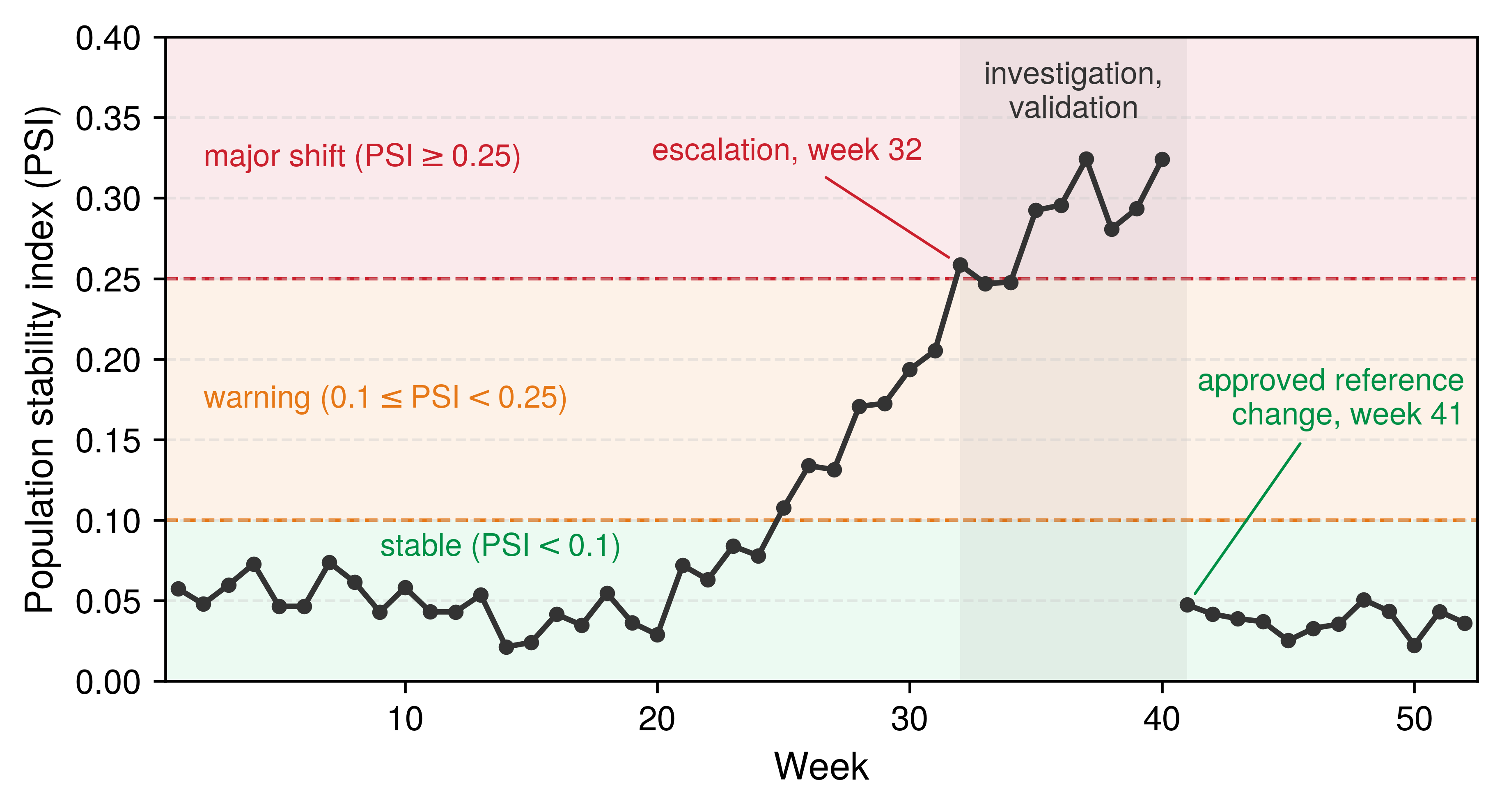
The fleet convention bands of Drift detection map PSI values to negligible, moderate, and major shift. They are monitoring conventions, especially common in credit-scoring practice, rather than universal statistical guarantees, so a service validates them against its own binning, baseline, sample size, predictive features, and response cost, and reads PSI together with feature importance and downstream model-performance metrics (Yurdakul and Naranjo 2020).
Yurdakul, Bilal, and Joshua Naranjo. 2020. “Statistical Properties of the Population Stability Index.” The Journal of Risk Model Validation 52. https://doi.org/10.21314/jrmv.2020.227.
Binning and the treatment of empty bins change what PSI can see, so the bin boundaries chosen on the reference sample must be reused for the comparison population. An empty bin is handled with a smoothing constant \(\PopulationStabilitySmoothingConstant\) and renormalization; because that choice can materially change PSI on sparse bins, the monitoring configuration records it alongside the reference. Monitoring population stability index over time as plotted in figure 5 reveals when the input population moves from the stable band into the warning band and then the major-shift band, triggering an escalation path that may lead to retraining after performance correlation. At week 41, the service approves and versions a new input reference after validating the changed operating population. The lower PSI thereafter compares traffic with that new reference, not the original one. Changing model weights alone would not reduce input PSI against a fixed reference, and the discontinuity does not establish improved predictions.
This threshold-based path automates alerting, not remediation. Operators still need labels or other outcome evidence, root-cause analysis, and an evaluated response before changing the model. Forcing continuous variables into discrete bins also discards information about distribution shape, motivating continuous drift metrics.
Kullback-Leibler divergence
For continuous features, the Kullback-Leibler (KL) divergence compares fitted densities rather than fixed bins, at the price of the density estimate’s own assumptions and error. From baseline distribution \(\TrainingDistribution\) to current distribution \(\CurrentDistribution\) it is:
\[ \KlDivergence(\TrainingDistribution \lVert \CurrentDistribution) = \int_{-\infty}^{\infty} \TrainingDistribution(\MonitoredFeatureLevel) \ln\left(\frac{\TrainingDistribution(\MonitoredFeatureLevel)}{\CurrentDistribution(\MonitoredFeatureLevel)}\right) d\MonitoredFeatureLevel \]
where \(\TrainingDistribution(\MonitoredFeatureLevel)\) and \(\CurrentDistribution(\MonitoredFeatureLevel)\) are the probability density functions of the baseline and current distributions, respectively. Unlike PSI, KL divergence is asymmetric: \(\KlDivergence(\TrainingDistribution \lVert \CurrentDistribution) \neq \KlDivergence(\CurrentDistribution \lVert \TrainingDistribution)\). The fraud-monitoring example in section 14.4.2.4 uses \(\KlDivergence(\text{baseline} \lVert \text{current})\), measuring how much information is lost when using the current distribution to approximate the baseline.
To address asymmetry, practitioners often use the Jensen-Shannon divergence:
\[ \JensenShannonDivergence(\TrainingDistribution \lVert \CurrentDistribution) = \frac{1}{2} \KlDivergence(\TrainingDistribution \lVert \JensenShannonMixtureDistribution) + \frac{1}{2} \KlDivergence(\CurrentDistribution \lVert \JensenShannonMixtureDistribution) \]
where \(\JensenShannonMixtureDistribution = \frac{1}{2}(\TrainingDistribution + \CurrentDistribution)\) is the mixture distribution. Jensen-Shannon divergence is bounded between 0 and \(\ln(2)\) (approximately 0.693), making threshold selection more intuitive than unbounded KL divergence.
KL divergence has no conventional bands comparable to PSI’s, so each service sets its own. The fraud service analyzed in section 14.4.2.4 starts from the bands in table 2 and validates them against its historical traffic.
| \(\KlDivergence\) value | Interpretation |
|---|---|
| \(\KlDivergence< 0.05\) | Minimal divergence |
| \(0.05 \le \KlDivergence< 0.1\) | Moderate divergence |
| \(\KlDivergence\ge 0.1\) | Significant divergence |
For practical computation, kernel density estimation with Gaussian kernels provides smooth density approximations suitable for integration. Direct evaluation at every sample against every kernel costs \(\mathcal{O}(\DriftTestSampleSize^2)\) for \(\DriftTestSampleSize\) samples. Sampling, a fixed evaluation grid, or faster approximation methods change this cost; bandwidth selection also changes the estimated divergence and must be part of threshold calibration.
Statistical significance testing
PSI and KL divergence quantify how large a distributional change appears to be; statistical hypothesis tests ask the complementary question of whether the observed difference is larger than sampling noise. The simplest case is a shift in the mean of one feature whose spread is known, which a normal approximation can test directly.
Napkin Math 14.1: Detecting a real distribution shift
Problem: A model monitors a critical input feature with a known standard deviation of 0.3. The baseline mean was 0.5. Over the last 1,000 requests, the mean has shifted to 0.55. The engineering question is whether this is a random fluctuation or a real distribution shift.
Math: The calculation treats the baseline mean as known and the requests as independent observations with the stated standard deviation. A normal approximation then measures how unusual the observed mean would be under that baseline. If the baseline mean is itself estimated from a finite sample, its uncertainty also contributes to the comparison.
- Difference in means: 0.05.
- Standard error: \(0.3/\sqrt{1,000} \approx 0.009\).
- Statistical significance: The shift is approximately 5.3 standard errors away from the mean.
- P-value: < 0.001.
Systems insight: Statistical significance assesses the observed change against sampling variability under the baseline model. A shift of 0.05 might seem “small,” but under the baseline model, the probability of observing a sample mean at least this far from the baseline is less than 0.1 percent. In the machine learning fleet, this supports a drift alert under the test assumptions, not yet a confirmed model regression. The system should trigger investigation, increased monitoring, and correlation with precision, recall, latency, and business metrics. Feature importance and shift magnitude help prioritize that investigation; fallback or retraining requires evidence that the response addresses the cause or contains the resulting risk.
A mean test sees only a change in location and needs the spread in advance. The two-sample Kolmogorov-Smirnov (KS) test (Berger and Zhou 2014) compares the empirical cumulative distribution functions (CDFs) of two samples without assuming any specific parametric form. The test statistic is:
Berger, Vance W., and YanYan Zhou. 2014. “Kolmogorov–Smirnov Test: Overview.” In Wiley StatsRef: Statistics Reference Online. Wiley. https://doi.org/10.1002/9781118445112.stat06558.
\[ \KolmogorovSmirnovStatistic = \sup_{\MonitoredFeatureLevel} |\ReferenceSampleEmpiricalCdf_n(\MonitoredFeatureLevel) - \ComparisonSampleEmpiricalCdf(\MonitoredFeatureLevel)| \]
where \(\ReferenceSampleEmpiricalCdf_n\) and \(\ComparisonSampleEmpiricalCdf\) are the empirical CDFs of samples of size \(\DriftTestSampleSize\) and \(\ComparisonSampleSize\) respectively. For independent samples from continuous distributions, the following asymptotic rule rejects the null hypothesis of no distributional difference. Small samples, ties, or dependent traffic require an appropriately calibrated test.
\[ \KolmogorovSmirnovStatistic > \KsCriticalCoefficient(\HypothesisTestSignificanceLevel) \sqrt{\frac{\DriftTestSampleSize+ \ComparisonSampleSize}{\DriftTestSampleSize \ComparisonSampleSize}} \]
where \(\KsCriticalCoefficient(\HypothesisTestSignificanceLevel)\) depends on the significance level (for example, \(\KsCriticalCoefficient(0.05) \approx 1.36\)). The KS statistic is most sensitive to differences near the center of the distribution, such as a location shift, and less sensitive to differences confined to the tails.
For categorical features, the chi-square goodness-of-fit test compares observed frequencies to expected frequencies under the baseline distribution:
\[ \PearsonFitStatistic= \sum_{i=1}^{\FeatureCategoryCount} \frac{(\ObservedCategoryCount- \ExpectedCategoryFrequency)^2}{\ExpectedCategoryFrequency} \]
where \(\ObservedCategoryCount\) is the observed count in category \(\FeatureCategoryIndex\) and \(\ExpectedCategoryFrequency\) is the expected count based on the baseline distribution. With independent observations and well-populated expected counts, \(\PearsonFitStatistic\) is compared with the chi-square critical value for \(\FeatureCategoryCount-1\) degrees of freedom at significance level \(\HypothesisTestSignificanceLevel\).
When monitoring many features simultaneously, the significance test must also account for repeated comparisons. Applying Bonferroni correction (dividing \(\HypothesisTestSignificanceLevel\) by the number of tests) controls the probability of at least one false rejection within the specified test family. False discovery rate procedures instead target the expected fraction of false discoveries among rejections under their own assumptions. For \(\AlertCheckCount\) monitored features, one test each, at significance level \(\HypothesisTestSignificanceLevel = 0.05\), Bonferroni requires each test to achieve \(\ObservedSignificanceLevel < 0.05/\AlertCheckCount\) for significance. This correction across features does not by itself control false alarms over an indefinitely repeated sequence of monitoring windows.
Production fraud detection drift analysis
Consider a fraud detection model serving an e-commerce platform with two key input features: user country (categorical) and transaction amount (continuous). After six months in production, the operations team suspects distribution drift and must decide whether to retrain. From its historical baseline the team has already configured three investigation triggers: a population stability index above 0.1 on any high-importance feature, a KL divergence above 0.05 on a continuous feature, and a KS test \(\Glyph{p}\)-value below 0.01, the per-test level left after a Bonferroni correction across its monitored features.
Step 1 categorical feature analysis
The user-country feature has four named countries and an Other bucket, and decomposing its PSI bucket by bucket shows which part of the traffic moved (table 3). Each row compares the baseline share against the current share so that localized shifts do not hide inside the aggregate score.
| Country | Baseline (\(\ReferenceBinProportion_i\)) | Current (\(\CurrentBinProportion_i\)) | \(\ReferenceBinProportion_i - \CurrentBinProportion_i\) | \(\ln(\ReferenceBinProportion_i/\CurrentBinProportion_i)\) | Contribution |
|---|---|---|---|---|---|
| USA | 0.45 | 0.38 | 0.07 | 0.169 | 0.0118 |
| UK | 0.20 | 0.18 | 0.02 | 0.105 | 0.0021 |
| Germany | 0.15 | 0.14 | 0.01 | 0.069 | 0.0007 |
| France | 0.10 | 0.12 | -0.02 | -0.182 | 0.0036 |
| Other | 0.10 | 0.18 | -0.08 | -0.588 | 0.0470 |
Summing the per-country contributions gives \(\text{PSI}_{\text{country}} = 0.0118 + 0.0021 + 0.0007 + 0.0036 + 0.0470 = 0.065\). The PSI of 0.065 remains inside this fraud service’s calibrated baseline for user country, so the aggregate feature does not independently escalate the investigation, yet the decomposition still matters. The Other bucket nearly doubled its share of traffic, so the team checks performance within that slice rather than relying on the aggregate PSI. The changed share warrants investigation without establishing that those transactions are less accurately classified.
Step 2 continuous feature analysis
For the transaction amount feature (log-transformed for approximate normality), fitting Gaussian distributions to the samples yields a baseline distribution of \(\BaselineFeatureMean\) = 4.2 and \(\BaselineFeatureStandardDeviation\) = 1.1 log-dollars, compared with a current distribution of \(\CurrentFeatureMean\) = 4.5 and \(\CurrentFeatureStandardDeviation\) = 1.3 log-dollars.
For the fitted Gaussian distributions, KL divergence has the following closed-form solution. It is exact for those density models; its fidelity to the transaction populations depends on the fit.
\[ \KlDivergence= \ln\frac{\CurrentFeatureStandardDeviation}{\BaselineFeatureStandardDeviation} + \frac{\BaselineFeatureStandardDeviation^2 + (\BaselineFeatureMean- \CurrentFeatureMean)^2}{2\CurrentFeatureStandardDeviation^2} - \frac{1}{2} \]
The closed-form solution evaluates to \(\KlDivergence = \ln\frac{1.3}{1.1} + \frac{1.30}{3.38} - 0.5 = 0.167 + 0.385 - 0.5 = 0.052\). The KL divergence of 0.052 indicates moderate drift, warranting further investigation but not immediate retraining.
Step 3 statistical significance via KS test
The KS test on 10,000 baseline samples and 10,000 current samples of transaction amount returns \(\KolmogorovSmirnovStatistic\) = 0.089. The service tests at the Bonferroni-corrected level \(\HypothesisTestSignificanceLevel\) = 0.01 that the team configured. At this per-test level, the asymptotic coefficient is \(\KsCriticalCoefficient(\HypothesisTestSignificanceLevel) = \sqrt{-\ln(\HypothesisTestSignificanceLevel/2)/2}\), so the critical value is \(\KsCriticalCoefficient(0.01) \sqrt{\frac{\DriftTestSampleSize+\ComparisonSampleSize}{\DriftTestSampleSize\ComparisonSampleSize}} \approx 1.63 \times 0.0141 \approx 0.023\).
The observed statistic is several times that critical value. Tightening the level tenfold, to \(\HypothesisTestSignificanceLevel = 0.001\), raises the coefficient \(\KsCriticalCoefficient(\HypothesisTestSignificanceLevel)\) only modestly, because it grows with the square root of \(\ln(2/\HypothesisTestSignificanceLevel)\), so the same statistic also rejects at that stricter level. The difference is therefore statistically significant \((\ObservedSignificanceLevel < 0.001)\). However, statistical significance alone does not mandate retraining; the practical significance (PSI, KL values) supports investigation while monitoring continues, rather than immediate retraining.
Step 4 decision framework application
Set against the team’s configured triggers, the three results split into one signal to monitor and two to investigate (table 4). Comparing all three metrics side by side prevents a single statistical rejection from bypassing the practical-significance check.
| Metric | Value | Threshold | Action level |
|---|---|---|---|
| PSI (country) | 0.065 | \(< 0.1\) | Monitor |
| \(\KlDivergence\) (amount) | 0.052 | \(> 0.05\) | Investigate |
| KS test | \(\ObservedSignificanceLevel < 0.001\) | \(\HypothesisTestSignificanceLevel\) = 0.01 (Bonferroni) | Investigate |
Decision: Continue serving this fraud model with increased monitoring frequency (weekly instead of monthly), while investigating the transaction-amount shift. The moderate KL divergence and significant KS result justify that review under the team’s configured triggers; the country PSI does not add an independent alert. A model update becomes a candidate only if delayed labels show degradation beyond the team’s validated tolerance and the investigation identifies a shift that retraining can address. The numerical cutoffs belong to this worked service; another model must calibrate its own thresholds from baseline variation, failure consequences, and response capacity.
Retraining decision framework
A systematic decision framework integrates drift metrics with performance monitoring to decide whether a model update is warranted. The three levels below deliberately separate detection, correlation, and action so metric alerts do not become automatic retraining commands.
Level 1 automated monitoring
The first level automates detection only. The fraud team’s three triggers show its general form. Each threshold is derived from the service’s own historical baseline rather than copied from a convention, and any significance level is a per-test level after correction for the configured family of tests, so it must be recomputed when features are added to the family or its error budget changes. Crossing any threshold initiates an operational investigation rather than triggering an automated retraining pipeline.
Level 2 performance correlation
Comparing scenario-calibrated alerts with observed performance yields three cases that guide investigation. If observed performance degradation exceeds the service’s validated tolerance and coincides with detected drift, operators isolate the affected data slices to test whether recalibration, data repair, or retraining directly addresses the root cause. Conversely, when drift is detected while serving performance remains stable, the service continues operating under elevated monitoring while the team investigates the drift source. Finally, if performance degrades without detectable feature drift, operators investigate changes the monitored marginals could miss, including concept drift, joint-feature changes, and pipeline or model faults. An unchanged feature dashboard does not identify which of these caused the error.
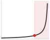
Degradation without drift is the case the feature dashboard cannot explain.
Level 3 retraining vs. investigation
Not all drift requires retraining. The evidence decides among three responses (a model update, investigation first, or continued monitoring), and each demands a different combination of statistical signal, observed performance, and external context (table 5).
| Action | Trigger conditions | Response logic |
|---|---|---|
| Update model | Performance exceeds a validated error tolerance, labels confirm a shift, root-cause analysis shows a model update addresses it, and offline plus shadow evaluation clears the release gate | The evidence identifies recalibration or retraining as the appropriate response rather than merely detecting a population change |
| Investigate first | A scenario-calibrated drift alert fires while performance remains stable, the shift is localized to nonpredictive features, or a seasonal or one-time event is plausible | The signal justifies diagnosis, but not a predetermined remediation |
| Continue monitoring | Drift statistics remain inside the service’s calibrated baseline, performance stays within tolerance, and no external evidence suggests environmental change | The evidence does not yet justify changing the model, but the baseline remains under observation |
The three-level framework turns drift detection from reactive troubleshooting into planned model maintenance as production environments evolve (Gama et al. 2014). No PSI band is a universal retraining rule: a large shift in a nonpredictive feature may be harmless, while a small shift in a safety-critical subgroup may demand immediate containment.
14.4.3 Monitoring and adaptation strategies
The fraud example compared two features of one service against one baseline. A fleet runs the same comparison for thousands of features across many replicas, regions, and model versions, so the design of the monitor itself determines what the fleet can detect and what detection costs. The decision rules above still apply; the new questions are which statistic to compute where, and what to change once the evidence warrants a model update.
Each statistic carries a computational and sampling price, and the price decides where and how often it runs. In this illustrative H100-class monitoring scenario, one MMD comparison with radial basis function kernels (\(\RadialBasisKernelCoefficient= 1.0\)) over a window of 10,000 samples takes an assumed 150 ms per window. Run hourly on sampled traffic, that is a small fraction of one accelerator’s time, but the direct estimator’s cost grows with the square of the window size, so doubling the window to gain detection power roughly quadruples the cost. The per-feature two-sample KS tests use 1,000 samples per window in this scenario. Each costs \(\mathcal{O}(\DriftTestSampleSize\log \DriftTestSampleSize)\), dominated by sorting its window, which is cheap enough to run on every window for every feature, but these tests miss joint changes that preserve each feature’s marginal distribution. The design therefore runs the cheap marginal tests continuously and reserves the joint kernel test for periodic, sampled checks. Neither sample count is a universal detection minimum; power depends on the shift and significance level. The service in this example uses PSI values from 0.1 to 0.25 as investigation triggers, not as universal statistical thresholds.
High-dimensional and temporal traffic requires more than one fleet-wide scalar. Marginal feature monitors can remain flat while correlations, sequence structure, or a small cohort changes. A production design therefore combines cheap per-feature alarms with embedding- or kernel-space tests, cohort slices, rolling windows at several durations, and change-point checks. Where these statistics run, on each replica or centrally from exported samples or sketches, sets both the telemetry load on the C\(^3\) communication axis and the evidence the detector sees. The windows must preserve seasonality and event context: comparing Monday traffic with Sunday traffic can manufacture an alert, while averaging a week can hide an abrupt one-hour failure. Monitor design is part of the hypothesis, not a neutral wrapper around the model.
↩︎ The fleet monitoring hierarchy that decides where drift statistics run and which signals reach an owner is established in Hierarchical monitoring architecture.
Shalev-Shwartz, S. 2012. “Online Learning and Online Convex Optimization.” Foundations and Trends in Machine Learning 4 (2): 107–94. https://doi.org/10.1561/2200000018.
Kirkpatrick, J., R. Pascanu, N. Rabinowitz, J. Veness, G. Desjardins, A. A. Rusu, K. Milan, et al. 2017. “Overcoming Catastrophic Forgetting in Neural Networks.” Proceedings of the National Academy of Sciences 114 (13): 3521–26. https://doi.org/10.1073/pnas.1611835114.
When the Level 3 rules do call for a model update, the update itself is a budgeted response rather than an automatic retraining command. Online learning updates a model from sequential observations (Shalev-Shwartz 2012); preserving earlier behavior remains a separate design objective. The adaptation budget depends on model size, drift rate, and feedback latency: updating too aggressively can chase noise, while updating too slowly lets performance drift. In production, online-learning systems usually bound update frequency, state size, and serving latency explicitly rather than assuming adaptation is free. An update that fits the new distribution can also erase behavior the old one required, the catastrophic forgetting that also constrains on-device adaptation. Techniques like Elastic Weight Consolidation reduce it by penalizing changes to parameters important for previous tasks (Kirkpatrick et al. 2017).
↩︎ Catastrophic forgetting and the continual-adaptation techniques that limit it are established in Continual adaptation and catastrophic forgetting.
Gama, João, Indrė Žliobaitė, Albert Bifet, Mykola Pechenizkiy, and Abdelhamid Bouchachia. 2014. “A Survey on Concept Drift Adaptation.” ACM Computing Surveys 46 (4): 1–37. https://doi.org/10.1145/2523813.
Adaptive ensemble methods maintain multiple models or hypotheses and weight or select among them using recent performance, making them useful under gradual concept drift (Gama et al. 2014). This approach trades extra serving and monitoring complexity for the ability to respond when a single static model no longer matches the deployment distribution. When the drifted data cannot leave the devices or regions that produce it, the same update can run as federated learning (Federated Learning Algorithms), which moves the adaptation to the data. The drift response then pays in communication rounds and transmitted bytes as well as training work, so the time from a confirmed shift to a validated update must be measured on the federated path rather than assumed from centralized retraining.
14.4.4 Per-request competence and selective prediction
The drift monitors and adaptation paths above ask whether traffic has changed in aggregate, yet a stable daily PSI can coexist with a rare, dangerous out-of-distribution request, while a large population shift can leave individual predictions well supported. Because a serving system must decide on every request whether that particular input lies within the model’s demonstrated competence, fleet robustness needs a per-request decision contract alongside its population monitors.
That contract combines three distinct signals because no single score answers the whole question. Calibration tests whether a score of 0.8 corresponds to approximately 80 percent correctness on a defined validation population (Guo et al. 2017), whereas out-of-distribution detection scores how unlike the request is from the model’s validated input distribution (Hendrycks and Gimpel 2017), because a calibrated classifier can remain confidently wrong on unfamiliar inputs. Selective prediction then turns both signals into an action policy, answering above the acceptance threshold, routing uncertain cases to a stronger model or reviewer, and abstaining when neither path can satisfy the risk bound (figure 6), since an OOD detector can flag novelty without estimating task error.
Guo, Chuan, Geoff Pleiss, Yu Sun, and Kilian Q. Weinberger. 2017. “On Calibration of Modern Neural Networks.” International Conference on Machine Learning (ICML) 70: 1321–30.
Hendrycks, Dan, and Kevin Gimpel. 2017. “A Baseline for Detecting Misclassified and Out-of-Distribution Examples in Neural Networks.” International Conference on Learning Representations (ICLR).
Let \(\SelectiveAcceptanceScore(\ModelInput)\) be an acceptance score whose larger values indicate stronger evidence for answering, \(\ResponseThreshold\) its threshold, \(\ModelPredictor(\ModelInput)\) the prediction, and \(\LossFunction(\ModelPredictor(\ModelInput),\ExampleLabel)\) its loss against the observed outcome. For accepted set \(\AcceptedInputSet = \{\ModelInput: \SelectiveAcceptanceScore(\ModelInput) \ge \ResponseThreshold\}\) at threshold \(\ResponseThreshold\), coverage is \(\Pr(\ModelInput\in \AcceptedInputSet)\) and selective risk is the mean loss conditioned on acceptance:
\[ \operatorname{coverage}(\ResponseThreshold)=\Pr(\ModelInput\in \AcceptedInputSet), \qquad \operatorname{risk}(\ResponseThreshold)=\mathbb{E}[\LossFunction(\ModelPredictor(\ModelInput),\ExampleLabel)\mid \ModelInput\in \AcceptedInputSet]. \]
Sweeping \(\ResponseThreshold\) produces a risk-coverage curve rather than one accuracy number. Raising the threshold reduces coverage, but lowers accepted-request risk only when the score orders requests by error risk well enough. That relationship must be measured on the deployment population, and the rejected traffic does not disappear. The fallback path needs enough queue, reviewer, or secondary-model capacity to absorb the abstention rate within the original latency and safety budget. If labels arrive days later, the system can monitor scores and fallback load immediately but cannot confirm selective risk until outcomes return. During that delay, rate limits and conservative thresholds can limit exposure, while the default response still requires validation against the application’s hazards.
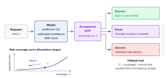
Finite-sample coverage with conformal prediction
Calibration describes whether predicted probabilities match empirical frequencies; selective prediction chooses which requests the system will answer. Conformal prediction provides a different contract: it wraps a fitted predictor with a nonconformity score \(\NonconformityScore(\ModelInput,\ExampleLabel)\) and a held-out calibration set. Here the score measures how poorly a candidate outcome \(\ExampleLabel\) agrees with input \(\ModelInput\), so larger values mean less conformity; it is distinct from the acceptance score above. For a skin-lesion classifier, the prediction set might contain both benign and malignant rather than force a single diagnosis. Each candidate label remains in the set when its nonconformity score does not exceed a cutoff calibrated on held-out examples. The target miscoverage rate is \(\ConformalMiscoverageRate\). For the finite threshold below, assume \(1/(\CalibrationExampleCount+1) \leq \ConformalMiscoverageRate < 1\). For \(\CalibrationExampleCount\) calibration scores sorted in ascending order, set \(\ConformalQuantileRank=\min\{\lceil(\CalibrationExampleCount+1)(1-\ConformalMiscoverageRate)\rceil,\CalibrationExampleCount\}\) and \(\ConformalScoreQuantile=\NonconformityScore_{(\ConformalQuantileRank)}\). The prediction set is
\[ \ConformalPredictionSet(\ModelInput)=\{\ExampleLabel:\NonconformityScore(\ModelInput,\ExampleLabel)\leq \ConformalScoreQuantile\}, \qquad \Pr\!\left(\ExampleLabel_{n+1}\in \ConformalPredictionSet(\ModelInput_{n+1})\right)\geq 1-\ConformalMiscoverageRate. \]
Here the test pair \((\ModelInput_{n+1},\ExampleLabel_{n+1})\) follows the \(\Glyph{n}=\CalibrationExampleCount\) calibration examples. Exchangeability means that permuting their order does not change their joint distribution; i.i.d. sampling is sufficient. Under this assumption and the stated range of \(\ConformalMiscoverageRate\), the \((\CalibrationExampleCount+1)\) rank correction makes this a finite-sample marginal coverage guarantee: exchangeability makes the test point’s score equally likely to take any of the \(\CalibrationExampleCount+1\) ranks among the combined scores, so when averaging over the calibration sample and the new test example, the set contains the true outcome at least at the target rate (Lei et al. 2018). Using the ordinary empirical \((1-\ConformalMiscoverageRate)\) quantile instead can undercover at finite sample sizes. The guarantee is not conditional on a particular realized calibration set, input, or subgroup. A rare subgroup can have poor coverage even when aggregate coverage is correct, particularly when it contributes few calibration examples.
Lei, Jing, Max G’Sell, Alessandro Rinaldo, Ryan J. Tibshirani, and Larry Wasserman. 2018. “Distribution-Free Predictive Inference for Regression.” Journal of the American Statistical Association 113 (523): 1094–111. https://doi.org/10.1080/01621459.2017.1307116.
The systems obligation is to preserve the conditions behind the guarantee. A distribution change between calibration and serving can invalidate the exchangeability argument; calibration age alone does not establish such a change. Even if observed coverage remains adequate, the original guarantee needs its assumptions rechecked. Repeatedly tuning the model, score, or threshold against the same calibration outcomes makes the held-out evidence adaptive rather than independent. Production systems therefore version the predictor, score, calibration snapshot, and target \(\ConformalMiscoverageRate\) together; monitor realized coverage by consequential slice once labels arrive; and refresh or quarantine the contract when traffic changes. Conformalization does not protect against arbitrary shift.
Set size or interval width supplies an operational load signal. Larger outputs convey less specific predictions and can trigger abstention, a stronger model, or human review, so their tail distribution determines fallback capacity just as the risk-coverage curve determines rejected traffic. The target coverage is therefore not free: increasing it usually widens sets, raises review demand, or reduces the fraction of requests on which the system can act automatically.
The failure modes above arise without an adversary, but the boundary with deliberate manipulation is porous. Distribution monitors can themselves be evaded by inputs crafted to stay under their thresholds, turning a defensive tool into a blind spot. Once an adversary stops relying on natural variation and begins optimizing against the model’s decision boundaries to force specific errors, the threat model moves from environmental robustness to input-level attacks.
Checkpoint 14.2: Drift detection and the retraining decision
Environmental shifts split into distinct types, and the chapter’s drift framework deliberately separates a fired metric from a retraining command.
Distinguishing the shift type
Reasoning about thresholds and cost
Self-Check: Question
A credit scoring model encounters a scenario where loan applicants’ demographic and financial feature distributions \(p(x)\) remain unchanged, yet default rates increase due to a sudden macroeconomic policy change that alters the relationship between income and repayment probability \(p(y \mid x)\). Which type of environmental shift does this represent?
- Concept drift, because the conditional relationship \(p(y \mid x)\) changed while the input marginal \(p(x)\) stayed constant.
- Covariate shift, because input feature values moved relative to the training distribution.
- Label smoothing, because target probabilities were regularized during training.
- Hardware bit corruption, because inference activations deviated from ground truth.
A monitoring service evaluates an input feature over 1,000,000 requests, reporting a Kolmogorov-Smirnov test \(p\)-value of \(10^{-5}\) (\(p < 0.001\)), but the calculated Population Stability Index (PSI) is 0.04 and model precision is unaffected. Explain why the team should continue monitoring rather than triggering an immediate retraining job.
A fraud detection team uses service-calibrated drift alerts. Which scenario most strongly warrants urgent investigation and containment, with retraining considered after the cause and candidate update are validated?
- A non-predictive logging metadata feature exhibits \(\text{PSI} = 0.28\) while all predictive features show \(\text{PSI} < 0.05\).
- A primary feature shows \(\text{PSI} = 0.06\) and \(\mathcal{D}_{\text{KL}} = 0.03\), with downstream precision and recall holding steady.
- A two-sample KS test on a continuous feature yields \(p = 0.01\) over \(10^6\) samples, but \(\text{PSI} = 0.08\) and accuracy is unchanged.
- A critical predictive feature crosses \(\text{PSI} = 0.29\) accompanied by a confirmed 7 percent drop in production precision.
Order these stages of a drift investigation that considers a validated model update, while treating urgent containment as a separate response when needed: (1) Compute drift metrics against versioned reference distributions, (2) Compare the signal with available predictive and business outcomes, (3) Ingest and log production features and outcomes, (4) Validate a candidate response and apply it only if the evidence and release gate support it, (5) Investigate pipeline faults, environmental changes, and temporary events.
True or False: If PSI, KL divergence, and two-sample KS tests on every input feature remain within green thresholds for six months, the engineering team can guarantee that no concept drift has occurred without checking ground-truth labels.
A triage classifier answers every request whose calibrated confidence exceeds a threshold and routes the rest to clinician review. The team proposes raising the threshold to cut errors on answered requests. Explain what this change trades, what must be true of the score for it to help, and which capacity it consumes.
14.5 Adversarial Attacks
Consider an attacker who modifies an image of a benign skin lesion to induce a malignant prediction while preserving its apparent clinical content. Whether that attack succeeds depends on the classifier, the allowed modifications, and the evaluation conditions. The high-dimensional decision boundaries learned by deep neural networks possess counterintuitive blind spots that malicious actors can deliberately exploit. The practical question is what the attacker can see or control: gradients, queries, physical sensors, or training data. Adversarial attacks expose these blind spots.
Definition 14.3: Adversarial attack
Adversarial attack is a deliberate manipulation of a model’s input, interaction, or environment designed to violate a specified behavioral objective. The manipulation may be norm-bounded and visually subtle, but it can also be semantic, physical, query-based, or conspicuous.
- Significance: Adversarial evaluation asks whether an attacker can choose inputs or transformations that drive the model outside its intended behavioral envelope. High-dimensional, norm-bounded image perturbations are one important case, but patches, rotations, printed objects, malicious text, and repeated black-box queries expose different system boundaries.
- Distinction: Unlike random corruption sampled independently of the target, an adversarial manipulation is selected to cause failure. It need not use gradients: attackers may use surrogate models, decision-only queries, search, semantic edits, or control over the physical sensing environment.
- Common pitfall: A frequent misconception is that adversarial vulnerability is a “bug” to be patched. In reality, it is a structural vulnerability of many standard neural networks trained by empirical risk minimization; robust defense typically requires fundamental changes to the objective function (for example, adversarial training).
Adversarial attack categories encode access and cost. A white-box attacker can use gradients directly, a black-box attacker uses surrogate transfer or queries to the target, and a physical attacker must survive cameras, lighting, and distance. With gradient access, a change no person can see is enough to fool an image classifier. A perturbation that follows the sign of the loss gradient (\(\AdversarialPerturbationBudget = 0.007\)), the fast gradient sign method defined below, flips GoogLeNet’s prediction (figure 7) from panda (57.7 percent confidence) to gibbon (99.3 percent confidence), leaving the classifier paradoxically more confident in the erroneous label than the ground truth.
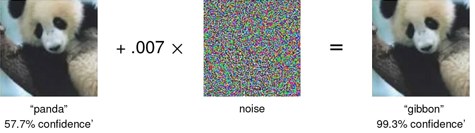
A visually small change need not produce a small change in a classifier’s score.7 Adversarial perturbations exploit how input changes accumulate in the model’s decision function. Even a linear function can be sensitive to many small, aligned changes across input dimensions; nonlinearity alone does not explain the vulnerability. The relevant constraint is whether the allowed perturbation can move the input across the learned decision boundary.
7 Human vs. machine perception: First highlighted by Szegedy et al. (2013), neural networks learn statistical correlations in pixel space rather than the semantic invariances human vision enforces. Agreement on clean examples does not establish agreement under every small image change. Evaluation must therefore specify which transformations should preserve the label and test whether the model preserves that behavior; gradient-based training alone neither explains every attack nor guarantees the required invariance.
Szegedy, Christian, Wojciech Zaremba, Ilya Sutskever, Joan Bruna, Dumitru Erhan, Ian Goodfellow, and Rob Fergus. 2013. “Intriguing Properties of Neural Networks.” arXiv Preprint arXiv:1312.6199.
14.5.1 Attacks by attacker access
An attacker who can read a model’s weights and gradients can flip a prediction in a single backward pass, whereas an attacker facing a rate-limited API must spend thousands of queries or train a local surrogate model to find a boundary-crossing input. The useful axis is therefore not the attack name by itself, but the attacker’s access. Each mechanism reveals a different cost that the defense must raise: gradient access, optimization time, surrogate-model construction, or physical control over the sensor environment.
The most direct case is white-box gradient access. Neural networks compute gradients to learn how parameter changes reduce loss; an attacker with access to gradients can run that logic against the input instead. For an image classifier that correctly identifies a panda, the gradient with respect to the input image gives a local, first-order estimate of how pixel changes affect the loss. The fast gradient sign method (FGSM)8 turns that idea into a single-step attack by choosing each feature’s perturbation sign to maximize that first-order increase within a coordinate-wise budget.
8 Fast gradient sign method (FGSM): Proposed by Goodfellow et al. (2015) at ICLR, FGSM generates adversarial examples in a single gradient step, making it practical to use during training. This dual role is its lasting systems significance: the same attack that exposed neural network fragility became a simple adversarial-training primitive, where FGSM-generated perturbations augment clean batches with examples chosen to increase loss.
Goodfellow, I. J., J. Shlens, and C. Szegedy. 2015. “Explaining and Harnessing Adversarial Examples.” International Conference on Learning Representations (ICLR).
FGSM computes the adversarial example in one step:
\[ \AdversarialExample= \ModelInput+ \AdversarialPerturbationBudget \cdot \text{sign}\big(\nabla_\ModelInput\LossFunction(\ModelParameters, \ModelInput, \ExampleLabel)\big) \]
In this formulation, \(\ModelInput\) denotes the original input, \(\AdversarialExample\) is the generated adversarial example, and \(\LossFunction(\ModelParameters, \ModelInput, \ExampleLabel)\) represents the prediction loss evaluated at model parameters \(\ModelParameters\) and true label \(\ExampleLabel\). The gradient term \(\nabla_\ModelInput\LossFunction\) describes local loss sensitivity, \(\text{sign}(\cdot)\) extracts each component’s sign to maximize the linearized loss within the coordinate-wise budget, and the scalar \(\AdversarialPerturbationBudget\) bounds the maximum allowable perturbation magnitude under the \(\ell_\infty\) norm. This single step need not maximize the nonlinear loss or cause misclassification. Image implementations also clip the perturbed input to its valid pixel range. The subscript distinguishes this adversarial radius from other uses of \(\Glyph{\epsilon}\) in the book, such as the differential-privacy budget.
Geometrically, moving along the sign vector of \(\nabla_\ModelInput\LossFunction(\ModelParameters, \ModelInput, \ExampleLabel)\) carries input \(\ModelInput\) to a corner of the bounding cube defined by the \(\ell_\infty\) budget \(\AdversarialPerturbationBudget\), producing \(\AdversarialExample\); in the illustration of figure 8, that corner lies across the decision boundary in the adjacent class region. A different boundary or gradient need not produce a successful attack within the same budget.
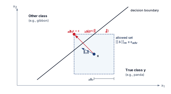
FGSM is cheap because it takes one step. The projected gradient descent (PGD) attack (Madry et al. 2018) spends more compute for a stronger attack: it repeatedly applies gradient updates and projects each step back into the allowed norm ball around the original input. That iterative refinement makes PGD a standard white-box robustness benchmark. The Jacobian-based saliency map attack (JSMA) (N. Papernot et al. 2016) uses the Jacobian to identify the most influential input features and perturb a smaller set of dimensions toward a target class. These methods are most effective in white-box settings,9 where the attacker knows the model architecture and gradients.
Papernot, N., P. McDaniel, S. Jha, M. Fredrikson, Z. Berkay Celik, and A. Swami. 2016. “The Limitations of Deep Learning in Adversarial Settings.” 2016 IEEE European Symposium on Security and Privacy (EuroS&P), 372–87. https://doi.org/10.1109/eurosp.2016.36.
9 White-box attack: Adversarial attack with complete model knowledge (architecture, weights, gradients); methods like PGD and Carlini-Wagner (C&W) are strong because they optimize directly against the model rather than probing it from the outside. Though less realistic than black-box scenarios for many deployed systems, white-box analysis establishes a demanding benchmark within a specified norm, perturbation budget, and attack procedure. Passing PGD is evidence for that threat model, not a universal guarantee against every weaker-looking attack.
10 Carlini and Wagner (C&W) attack: Proposed in 2016 (IEEE S&P 2017), C&W formulates adversarial example generation as a constrained optimization problem that searches for a small perturbation causing misclassification without guaranteeing a global minimum. Its significance is methodological: C&W broke defensive distillation (an early defense that masked gradients to blunt weaker attacks) and other evaluated defenses, establishing the principle that robustness claims must be evaluated against optimization-based attacks, not merely gradient-sign heuristics.
When the attacker cares less about speed and more about stealth, the attack becomes an optimization problem. The Carlini and Wagner (C&W) attack10 (Carlini and Wagner 2017) searches for a small perturbation that causes misclassification under a chosen distance measure. Minimizing that distance encourages similarity, but does not certify human perceptual equivalence or a globally minimal perturbation. Instead of merely following the sign of a gradient, C&W optimizes a custom objective that trades perturbation size against confidence in the wrong answer.
C&W perturbations can be visually subtle, but human imperceptibility alone does not establish whether a detector will identify them. The attack can search under different norm constraints, such as \(\ell_2\) or \(\ell_\infty\). The elastic net attack to DNNs (EAD) adds elastic net regularization, combining \(\ell_1\) and \(\ell_2\) penalties to generate sparse, localized perturbations. DeepFool (Moosavi-Dezfooli et al. 2015) takes a geometric route to the same goal: it linearizes the classifier around the input, steps to the nearest boundary of that linear approximation, and repeats until the label flips, giving a fast estimate of the smallest perturbation that suffices. These optimization-based methods are more computationally intensive than gradient-sign attacks, but they give the attacker finer control over the adversarial example’s geometry.
Moosavi-Dezfooli, Seyed-Mohsen, Alhussein Fawzi, and Pascal Frossard. 2015. “DeepFool: A Simple and Accurate Method to Fool Deep Neural Networks.” 2016 IEEE Conference on Computer Vision and Pattern Recognition (CVPR) 2016: 2574–82. https://doi.org/10.1109/cvpr.2016.282.
Black-box attackers lose direct gradient access but keep two routes. Transfer attacks rely on transferability, the tendency of an adversarial example to fool models other than the one it was crafted on. The attacker crafts examples offline on a surrogate model and submits them to the target, typically through its public API, without seeing its weights or gradients. Query-based attacks probe the target itself. A decision-based, or boundary, attack needs only the returned label. It starts from an input the model already misclassifies and walks along the decision boundary toward the original input, querying at each step to stay on the wrong side. Its cost is the number of queries, which is why query budgets and rate limits belong to the defense.
↩︎ The adversary knowledge spectrum, from white-box gradient access to black-box attackers who work through a surrogate or a public interface, is established in Threat vector classification.
Tramèr, Florian, Alexey Kurakin, Nicolas Papernot, Ian Goodfellow, Dan Boneh, and Patrick McDaniel. 2017. “Ensemble Adversarial Training: Attacks and Defenses.” International Conference on Learning Representations abs/1705.07204.
Transfer success depends on model similarity, training-data overlap, and regularization, and attackers can improve it with input diversity, such as random resizing or cropping, and with momentum during optimization. Closing that route costs the defender training work. Ensemble adversarial training trains against perturbations generated on several models to improve transfer robustness, but the extra attack generation and model diversity make it a deliberate training-budget decision rather than a free mitigation (Tramèr et al. 2017).

An example crafted on a surrogate fools similar models more often than dissimilar ones.
14.5.2 Physical-world attacks
Physical-world attackers face an additional constraint: the perturbation must survive sensors, distance, lighting, viewing angle, and ordinary deployment variation. Adversarial patches are printed patterns placed on objects so that cameras and detectors misread the scene. Modified road signs, clothing patches, and 3D-printed objects move the attack from the digital input tensor into the physical environment, and the modification need not be subtle: graffiti-style markings and sticker patches that pass for ordinary vandalism can also induce misclassification through the camera pipeline (Eykholt et al. 2017). The robustness question therefore becomes operational rather than purely mathematical, because a defense that works on a saved image may fail once the attack passes through a camera lens, compression, motion blur, and changing illumination. These threats matter most for AI systems deployed in physical spaces, such as autonomous vehicles, drones, and surveillance systems, where a model error becomes a safety, security, and accountability problem in the world.
Eykholt, Kevin, Ivan Evtimov, Earlence Fernandes, Bo Li, Amir Rahmati, Chaowei Xiao, Atul Prakash, Tadayoshi Kohno, and Dawn Song. 2017. “Robust Physical-World Attacks on Deep Learning Models.” ArXiv Preprint abs/1707.08945 (July).
Example 14.1: The stop sign attack
Scenario: The road-sign sticker attack, already familiar as a security threat, places black and white stickers on a stop sign so that a vision model reads it as a speed limit sign (figure 9) (Eykholt et al. 2018). The robustness question is what its two reported success rates say about how an evaluation must be run.
Diagnosis: The attack succeeded on every tested laboratory image but on 84.8 percent of frames in the moving-vehicle field test. Each number is evidence only for its own capture conditions, and the gap between them does not isolate any one factor, such as distance, viewing angle, lighting, or motion.
Systems lesson: A physical attack must be evaluated through the full sensor loop, not on saved benchmark images. The evaluation should optimize the attack over the expected range of transformations (expectation over transformation) and then test it with real captures, and any claimed mitigation, such as spatio-temporal validation or sensor fusion, must be tested against attacks on the complete perception stack.
↩︎ The road-sign sticker attack is established as a security threat in Model-Specific Attack Vectors.
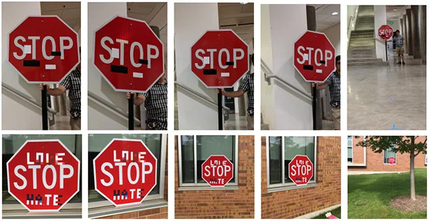
Eykholt, K., I. Evtimov, E. Fernandes, B. Li, A. Rahmati, C. Xiao, A. Prakash, T. Kohno, and D. Song. 2018. “Robust Physical-World Attacks on Deep Learning Visual Classification.” 2018 IEEE/CVF Conference on Computer Vision and Pattern Recognition 1707.08945: 1625–34. https://doi.org/10.1109/cvpr.2018.00175.
The attacker’s access determines the evaluation a defense must survive. Gradient access, optimization, surrogate transfer, and physical sensor manipulation each call for their own evaluation (table 6), so a result under one attack mechanism does not become a claim about all of them.
| Category | Method | Mechanism |
|---|---|---|
| Gradient | FGSM | Perturbs inputs along the loss gradient |
| PGD | Iterative multi-step FGSM refinement | |
| JSMA | Targets the most influential features | |
| Optimization | C&W | Minimizes perturbation size subject to misclassification |
| DeepFool | Estimates a small boundary-crossing perturbation by local linearization | |
| EAD | Elastic net regularization for sparse perturbations | |
| Transfer | Transferability | Adversarial examples transfer across models (black-box) |
| Physical | Patches | Printed patches fool detectors in the real world |
| 3D Objects | Sculpted objects deceive sensors in deployment |
Medical-imaging attacks can cause misdiagnosis (Tsai et al. 2023), while fraud and trading models face analogous manipulation risks. The common vulnerability is reliance on features that remain predictive on clean data but fail under crafted perturbations (Goodfellow et al. 2015; Madry et al. 2018). Defense shifts the resource cost: adversarial training adds training work (Bai et al. 2021), while runtime detection such as feature squeezing adds inference evaluations (Xu et al. 2018). The choice among these spending points motivates the defenses in section 14.6.
Tsai, Min-Jen, Ping-Yi Lin, and Ming-En Lee. 2023. “Adversarial Attacks on Medical Image Classification.” Cancers 15 (17): 4228. https://doi.org/10.3390/cancers15174228.
Self-Check: Question
Why can a small gradient-directed perturbation change a high-dimensional classifier’s score more than independently sampled, zero-mean noise of comparable coordinate scale?
- Random noise changes model parameters directly, whereas gradient perturbations only affect input metadata.
- Gradient-directed perturbations require visible, large-scale pixel alterations that physically overwhelm convolutional filters.
- The perturbation aligns coordinate changes with local loss sensitivity, while independent zero-mean changes can cancel in the first-order sum.
- Random noise affects only training data, whereas adversarial noise can only exist during inference.
An attacker lacking access to a commercial vision API’s internal weights or gradients trains a local ResNet surrogate, crafts PGD adversarial images against that surrogate, and successfully fools the target API on 50 percent of queries. Which property of adversarial examples enables this black-box attack?
- Differential privacy, which guarantees perturbation bounds across diverse neural architectures.
- Transferability, where adversarial examples crafted to exploit decision boundaries of one model frequently deceive different models trained on similar tasks.
- Quantization noise, which forces all deployed models into identical weight matrices.
- Batch normalization collapse, which disables activation functions across distributed API servers.
Which scenario represents a physical-world adversarial attack rather than a digital evasion attack or an environmental covariate shift?
- An attacker submits a JSON payload containing an \(\ell_\infty\)-perturbed pixel array directly to a cloud inference API endpoint.
- A sudden heavy snowfall changes ambient lighting and road surface reflections, reducing camera detection accuracy by 15 percent.
- An engineer accidentally inverts the normalization constants in a client-side image preprocessing script.
- An attacker places small, calibrated black-and-white stickers on a roadside stop sign that cause a vehicle camera to classify it as a speed limit sign across varying distances, angles, and lighting.
The foundational single-step adversarial attack method that computes the gradient of the loss with respect to the input and perturbs features by \(\epsilon \cdot \text{sign}(\nabla_x \mathcal{L})\) is called the ____.
14.6 Adversarial Defenses
The classifier that called a panda a gibbon in figure 7 was not broken by random noise; a perturbation budget of 0.007 per pixel, spent along the gradient sign, was enough. Defending a deployed perception model against that attacker requires a threat model that names the attacker’s access and a budget for testing and mitigation. The resulting robustness claim must state what the system pays in clean accuracy, training compute, inference latency, or operational coverage.
14.6.1 Adversarial defense workflow
A team that applies adversarial training without first naming the perturbation norm and budget can multiply training compute several-fold and lose clean accuracy while leaving the actual deployment threat uncovered. Preventing that misallocation requires an adversarial-defense workflow with four ordered layers:
- Define the threat model: Specify the perturbation budget, attacker knowledge, and whether the attack occurs at inference time or during training.
- Choose the robustness budget: Decide whether to spend the budget in training, certification, input detection, or serving-time guardrails.
- Measure the trade-off: Evaluate both sides of the defense, because improving worst-case behavior can reduce clean accuracy, raise inference latency, or multiply training cost.
- Keep evaluation adversarial: Test the defense against attacks stronger than the ones used to design it.
The order matters because an uncalibrated threat model makes the budget and evaluation loop meaningless. For model-facing perturbation threats, the most direct training-time defense is adversarial training, which incorporates adversarial examples into the training process itself. The mechanism reuses the attacks of the previous section as a data generator. Each training step augments the batch with perturbed copies of its own inputs, so the model is trained on the high-loss points an attacker would choose. In the simplest form, FGSM generates the perturbations and each batch mixes clean and adversarial examples (listing 1).
function adversarial_training_step(model, clean_batch, labels, epsilon):
    logits = model(clean_batch)
    clean_loss = loss(logits, labels)

    input_gradient = gradient(clean_loss, clean_batch)
    perturbation = epsilon * sign(input_gradient)
    adversarial_batch = stop_gradient(
        clip(clean_batch + perturbation, valid_input_range))

    mixed_batch = concatenate(clean_batch, adversarial_batch)
    mixed_labels = concatenate(labels, labels)

    return loss(model(mixed_batch), mixed_labels)
In listing 1, the sign step bounds each coordinate’s change by the perturbation budget, while clipping keeps the perturbed input inside the valid input range (for example, \([0,1]\) for normalized pixels). Concatenation doubles the effective batch size. The stop-gradient operation treats generated adversarial inputs as fixed during the outer weight update, rather than differentiating through attack construction. The caller differentiates the returned loss with respect to the model parameters and performs the optimizer update. The perturbation budget \(\AdversarialPerturbationBudget\) (the epsilon argument) bounds the allowed input change, while the attack algorithm determines how effectively it searches that set; computation reuse can reduce its training overhead (Shafahi et al. 2019).
Adversarial example generation increases training time because each training step requires additional forward and backward passes through the model (Madry et al. 2018; Bai et al. 2021). Memory overhead depends on whether the implementation stores clean and adversarial examples together, recomputes perturbations, or reuses gradient information. Iterative attacks like PGD add multiple optimization steps, so the implementation must budget that gradient work; optimized variants reduce overhead by reusing computations rather than treating every attack step as a separate full training pass (Shafahi et al. 2019). A robustness recipe that increases model capacity also adds memory and training cost. The perturbation budget and training recipe require matched clean and adversarial validation, and the perspective below shows why that matching decides what the robustness penalty actually is.
Systems Perspective 14.1: Pricing the robustness penalty correctly
Suppose a standard ResNet-50 records 76 percent Top-1 accuracy on clean ImageNet, while an adversarially trained model records about 50 percent under a specified \(\ell_\infty\) attack at \(\AdversarialPerturbationBudget=4/255\), the budget conventionally used for ImageNet. Subtracting these values yields 26 percentage points, but that gap compares different models under different evaluation conditions. It is not the clean-accuracy cost of robustness.
The clean-accuracy penalty must compare standard and robust models on the same clean test set. The robustness benefit must compare those models under the same attack, perturbation budget, and attack strength. The four cells are the standard model on clean data, the standard model under attack, the robust model on clean data, and the robust model under attack. The penalty is the first minus the third, the benefit is the fourth minus the second, and the quoted pair supplies only the first and the fourth. Reporting all four cells prevents an apparent trade-off from mixing a model effect with an evaluation-condition effect.
Systems insight: Robustness can reduce clean accuracy and increase compute, but each cost needs a like-for-like baseline. A deployment gate should report clean accuracy, empirical robust accuracy, attack specification, and evaluation cost separately.
The robustness compute penalty (principle 24) quantifies this cost: PGD-style adversarial robustness can demand several times more compute per epoch than standard optimization because each batch runs inner attack steps. In Fleet Law terms (equation 1.3) the multiplier lands on \(\IronLawComputeTime\). At a fixed worker count it adds local work, but the elapsed-time penalty depends on reuse and on which term limits the step. Adding workers changes communication and synchronization costs with \(\DeviceCount\) and may not recover the original duration. Notebook 14.2 makes the multiplier concrete.
Napkin Math 14.2: The cost of defense
Problem: A team is training a robust classifier for an autonomous vehicle. Instead of the single FGSM step in listing 1, it uses adversarial training with a seven-step PGD attack (PGD-7) that searches for a high-loss perturbation inside a specified norm ball for every training batch, and, following the standard PGD adversarial-training recipe (Madry et al. 2018), it trains on the adversarial batch alone rather than on the listing’s doubled clean-plus-adversarial batch. How much does this extra attack-generation work slow down the training run?
Math: In this example, generating the adversarial input uses \(\AttackStepsPgd\) additional gradient steps per training sample, each a forward and backward pass with respect to the input, before the one weight-update pass on the adversarial batch. The estimate treats each attack step as equal in cost to the standard training pass, with no reuse; it is a work model rather than a measured wall-clock slowdown. By the same accounting, the FGSM listing spends one attack pass plus an update pass over a batch twice the original size, about three standard passes in all, so PGD-7 trades a further factor of more than two in training work for a stronger inner attack.
- Forward/backward passes: 1 (Standard) + 7 (Attack Generation) = 8 total passes.
- Training slowdown: 8× under the equal-cost-pass assumption.
- Utility evidence: The added work must be justified by measured robust accuracy under the specified attack. Generalization to other attacks requires separate evaluation. Pricing any clean-accuracy cost requires the like-for-like comparison in perspective 14.1, not a subtraction of robust accuracy from another model’s clean accuracy.
Systems insight: In this PGD-7 work model, the team budgets 8× the baseline compute before measuring the robustness benefit or actual elapsed-time penalty. In a machine learning fleet, robustness is not a setting that can be switched on; it is a budget the team spends, and the budget must be justified by the failure consequence of the component being hardened.
For lower-risk components, external guardrails such as input filtering and output verification can cost less than training intrinsic robustness into the weights, provided adaptive evaluation (section 14.6.1.3) supports acceptable residual risk against an attacker who knows the guardrail. Passing a finite set of attacks does not prove that no bypass exists. Safety-critical paths more often justify the training and certification budget.
Certified defenses
Adversarial training provides empirical resistance that must be tested against the deployment threat model. It can generalize beyond the examples generated during training, but attack evaluation alone does not prove invariance throughout an allowed perturbation set. Certified robustness offers a mathematical guarantee: for a given input \(\ModelInput\) and radius \(\AdversarialPerturbationBudget\), no perturbation \(\|\AdversarialPerturbation\|_\PerturbationNormOrder< \AdversarialPerturbationBudget\) exists that changes the model’s prediction. This certifies local prediction stability, not that the unchanged prediction is correct. The certified radius is a provable lower bound on the input-perturbation part of the robustness margin that compression and other efficiency changes must preserve. The guarantee formalizes the intuition that a robust model limits how quickly its outputs can change as its inputs change. The model’s Lipschitz constant11 bounds that rate, so a prediction cannot change within any radius over which the largest possible score change stays below its top-class margin. A widely used technique for scaling this idea to high-dimensional inputs like ImageNet is randomized smoothing. Instead of classifying \(\ModelInput\) directly, it classifies the smoothed function \(\SmoothedClassifier(\ModelInput)\), defined as the most probable class predicted by the base classifier \(\ModelPredictor\) under Gaussian noise: \(\SmoothedClassifier(\ModelInput) = \operatorname{arg\,max}_\ClassIndex \Pr(\ModelPredictor(\ModelInput+\RandomizedSmoothingNoise) = \ClassIndex)\) where \(\RandomizedSmoothingNoise \sim \GaussianDistribution(\ZeroVector, \SmoothingNoiseStandardDeviation^2 \IdentityMatrix)\).
11 Lipschitz continuity: A mathematical property that bounds how much a function’s output changes relative to its input change (\(\lVert \ModelPredictor(\ModelInput) - \ModelPredictor(\AlternateModelInput) \rVert \le \LipschitzConstant\lVert \ModelInput- \AlternateModelInput\rVert\)). A small Lipschitz constant \((\LipschitzConstant)\) limits score movement but does not by itself prevent a label flip. Reducing \(\LipschitzConstant\) can enlarge the certified radius, though enforcing a low constant can trade away clean-data accuracy and add training cost.
Cohen, Jeremy, Elan Rosenfeld, and Zico Kolter. 2019. “Certified Adversarial Robustness via Randomized Smoothing.” International Conference on Machine Learning (ICML), Proceedings of machine learning research, vol. 97: 1310–20.
Cohen et al. (2019) proved a tight multiclass bound for the certified radius \(\CertifiedRadius\) using a lower bound on the top-class probability \(\SmoothedTopClassProbability\) and an upper bound on the runner-up probability \(\SmoothedRunnerUpProbability\): \(\CertifiedRadius= \frac{\SmoothingNoiseStandardDeviation}{2}\left(\StandardNormalCumulativeDistribution^{-1}(\SmoothedTopClassProbability) - \StandardNormalCumulativeDistribution^{-1}(\SmoothedRunnerUpProbability)\right)\), where \(\StandardNormalCumulativeDistribution^{-1}\) is the inverse standard normal CDF. In the binary special case, where \(\SmoothedRunnerUpProbability= 1 - \SmoothedTopClassProbability\), this reduces to \(\CertifiedRadius= \SmoothingNoiseStandardDeviation\StandardNormalCumulativeDistribution^{-1}(\SmoothedTopClassProbability)\). This Gaussian-smoothing bound certifies a Euclidean (\(\ell_2\)) perturbation radius, measured in the same units as the input to which the noise is added; it does not automatically certify the other norms used in attack benchmarks. If a binary decision has top-class probability \(\SmoothedTopClassProbability\) = 0.999 under noise \(\SmoothingNoiseStandardDeviation\) = 0.5, the simplified radius is approximately 1.5 in those input units. For an image scaled to \([0,1]\), that radius bounds the Euclidean length of the whole perturbation vector. It is not directly comparable to the per-coordinate \(\ell_\infty\) budget of the robustness-penalty comparison, because an \(\ell_\infty\) perturbation of size \(\AdversarialPerturbationBudget\) spread over \(\InputCoordinateCount\) pixels can have Euclidean length up to \(\AdversarialPerturbationBudget\sqrt{\InputCoordinateCount}\), so a per-pixel budget that looks tiny can correspond to a long Euclidean vector on a high-dimensional image.
The multiclass case rarely estimates the runner-up probability separately. Because the class probabilities sum to one, no competing class can exceed \(1 - \SmoothedTopClassProbability\), so a lower bound on \(\SmoothedTopClassProbability\) alone also bounds every competitor. Estimating that lower bound from samples turns certification into a statistical estimation problem and adds a confidence level to the certificate; an observed class frequency alone is not a certified probability bound. Certification also carries accuracy and compute trade-offs. On ImageNet, the same work reports nontrivial certified accuracy for randomized smoothing, including certification at radius 0.5, but certification requires sampling many noise vectors per inference to estimate class probabilities with sufficient confidence. The increase in inference latency makes the sample budget a deployment constraint. Two designs keep certification outside the tight serving budget. Asynchronous auditing certifies a sampled fraction of served requests offline, so the fleet learns how often its answers were certifiable without delaying any of them. A selective safety interlock certifies only the requests routed to a safety-critical action, such as a braking decision, and lets the remaining traffic take the uncertified path.
Certified defenses cover one part of the adversarial workflow. Production systems still need detection paths for suspicious inputs, mitigation strategies that change training or serving behavior, and evaluation procedures that verify which threat models remain covered.
Detection techniques
Detecting adversarial examples before they reach the model forms the first line of defense only when the signal reaches a serving decision: reject, transform, route, or audit. A population-level signal asks whether a window of current inputs still resembles the reference population. The two-sample tests of section 14.4.2.3 serve here unchanged. A KS test, or the Anderson-Darling test, a variant that weights differences in the distribution tails more heavily, can flag a traffic window whose inputs no longer resemble the reference. Such an alert does not identify an individual request as adversarial; per-request rejection requires an additional decision rule. These tests also inherit the drift monitors’ blind spot, since an adversarial perturbation can preserve each feature’s marginal distribution while corrupting the joint structure that joint-distribution or embedding-space comparisons would expose.
An attack that preserves marginal distributions can evade that signal, motivating a complementary comparison under input transformations. Feature squeezing12 (Xu et al. 2018) reduces input-space complexity through color bit-depth reduction or spatial smoothing, then compares the model’s prediction before and after the transformation. A large prediction change flags sensitivity to the transformation. It does not by itself establish malicious intent or identify which image detail caused the change; legitimate inputs can also trigger the detector.
12 Feature squeezing: In the original evaluation (Xu et al. 2018), squeezing 256 color levels to 16 or applying median filtering eliminated many adversarial examples while maintaining high clean accuracy. The same transformations can remove useful clean-input features and do not cover every attack mechanism, so adaptive attacks that anticipate the squeezer require separate validation before the defense is treated as production-ready.
Xu, Weilin, David Evans, and Yanjun Qi. 2018. “Feature Squeezing: Detecting Adversarial Examples in Deep Neural Networks.” Proceedings 2018 Network and Distributed System Security Symposium 26. https://doi.org/10.14722/ndss.2018.23198.
13 Model uncertainty (epistemic uncertainty): Uncertainty associated with limited knowledge of the predictive model, distinguished from aleatoric uncertainty in the observations. An estimate can support deferral, but it must be evaluated against actual errors and unfamiliar inputs; a low estimate does not certify competence. Repeated-pass or ensemble estimators add inference work, and any human fallback must meet the application’s response deadline.
Lakshminarayanan, Balaji, Alexander Pritzel, and Charles Blundell. 2017. “Simple and Scalable Predictive Uncertainty Estimation Using Deep Ensembles.” Advances in Neural Information Processing Systems (NeurIPS) 30.
Another signal asks whether the model is uncertain about its own answer. An estimate of model uncertainty13 can route an input for rejection, human review, or a more robust model. Bayesian neural networks estimate uncertainty by placing a probability distribution over each weight and averaging predictions over sampled weights, so disagreement among those samples signals uncertainty, while ensemble methods compare predictions from independently trained models and use disagreement as the warning signal (Lakshminarayanan et al. 2017). Their detection value depends on whether uncertainty distinguishes harmful inputs from legitimate ones under the chosen attack. Repeated predictions add inference work, so deployments must evaluate both missed attacks and serving cost rather than assume that a more expensive estimator detects more.
Dropout, the training-time regularizer that randomly deactivates neurons (Hinton et al. 2012), offers a cheaper approximation to that weight sampling. It can be repurposed for uncertainty estimation through Monte Carlo dropout14 at inference time, where multiple forward passes with different dropout masks approximate the uncertainty distribution. Monte Carlo dropout is itself an approximate Bayesian method. Its uncertainty estimates must be validated on the deployment population rather than ranked by the original purpose of dropout. Hybrid approaches that combine dropout with lightweight ensemble methods or Bayesian approximations balance computational efficiency with estimation quality, making uncertainty-based detection more practical for production deployment.
Hinton, G. E., N. Srivastava, A. Krizhevsky, I. Sutskever, and R. R. Salakhutdinov. 2012. “Improving Neural Networks by Preventing Co-Adaptation of Feature Detectors.” arXiv Preprint arXiv:1207.0580.
14 Monte Carlo dropout: Proposed by Gal and Ghahramani (2016), MC dropout reinterprets dropout as approximate Bayesian inference by keeping dropout active across repeated stochastic forward passes. The variance across predictions provides an uncertainty estimate with no architectural changes. Each additional sample adds inference work, so deployments must select the sample count against their latency and uncertainty budgets.
Gal, Yarin, and Zoubin Ghahramani. 2016. “Dropout as a Bayesian Approximation: Representing Model Uncertainty in Deep Learning.” Proceedings of the 33rd International Conference on Machine Learning (ICML) 48: 1050–59.
Evaluation and testing
Adversarial training, certification, and detection do not exhaust the options. The remaining strategies move the spending point rather than eliminating the cost. Defensive distillation (Nicolas Papernot et al. 2016) teaches a student model from the teacher’s soft labels, but its apparent adversarial protection proved vulnerable to attacks that bypassed the resulting gradient masking (Carlini and Wagner 2017). It illustrates why making an attack optimizer fail is not evidence that nearby adversarial inputs are absent. Input preprocessing spends the defense budget at serving time: image denoising, JPEG compression, random resizing, padding, and random transformations try to erase perturbations before the model sees them. Ensembles spend it through redundancy, combining models with different architectures, training data, or preprocessing paths so that a perturbation that fools one member is less likely to fool all of them.
Papernot, Nicolas, Patrick McDaniel, Xi Wu, Somesh Jha, and Ananthram Swami. 2016. “Distillation as a Defense to Adversarial Perturbations Against Deep Neural Networks.” 2016 IEEE Symposium on Security and Privacy (SP), 582–97. https://doi.org/10.1109/sp.2016.41.
Carlini, Nicholas, and David Wagner. 2017. “Towards Evaluating the Robustness of Neural Networks.” 2017 IEEE Symposium on Security and Privacy (SP), 39–57. https://doi.org/10.1109/sp.2017.49.
Mu, Norman, and Justin Gilmer. 2019. MNIST-C: A Robustness Benchmark for Computer Vision.
Hendrycks, Dan, and Thomas Dietterich. 2019. “Benchmarking Neural Network Robustness to Common Corruptions and Perturbations.” arXiv Preprint arXiv:1903.12261.
Evaluation closes the budget loop: the system must measure which attacks the defense actually covers and what performance it sacrifices under controlled attack conditions. Robustness metrics quantify resilience through accuracy on adversarial examples, the distortion required to fool the model, and performance over attack budgets. Standardized benchmarks such as MNIST-C (Mu and Gilmer 2019), CIFAR-10-C, and ImageNet-C (Hendrycks and Dietterich 2019) measure common corruptions rather than malicious worst-case behavior, so their results occupy a different cell of table 1.
Empirical attack evaluation must be adaptive to the defense. The evaluator should know the preprocessing, detector, randomness, ensemble, and rejection rule; optimize through differentiable components; use expectation over transformation for randomness; test transfer and query-based attacks when gradients are unavailable; and include the complete pipeline rather than a saved model alone. Multiple random restarts and attack budgets can strengthen evidence within that threat model, but a passed PGD test proves neither that PGD found the inner maximum nor that semantic, physical, or differently normed attacks are covered. Only a certificate establishes a guarantee, and only for its stated input, norm, radius, and assumptions.
RobustBench approximates that discipline at scale with one standardized, parameter-free attack ensemble, AutoAttack, applied to every published defense under one fixed threat model, which for CIFAR-10 is a perturbation of at most 8/255 per pixel in the \(\ell_\infty\) norm (Croce et al. 2020; Croce and Hein 2020). Across the 91 dated entries (figure 10), the best accuracy under attack rose from 44 percent in 2018 to 75 percent in 2024, while the same model kept 94 percent accuracy on clean images, so even the strongest defense still fails on about 25 percent of attacked inputs. The four entries at the bottom of the plot are published defenses that keep high clean accuracy yet fall below 5 percent accuracy under the standardized attack, the result an evaluation that is not adaptive to the defense can miss.
Croce, Francesco, and Matthias Hein. 2020. “Reliable Evaluation of Adversarial Robustness with an Ensemble of Diverse Parameter-Free Attacks.” arXiv Preprint arXiv:2003.01690.
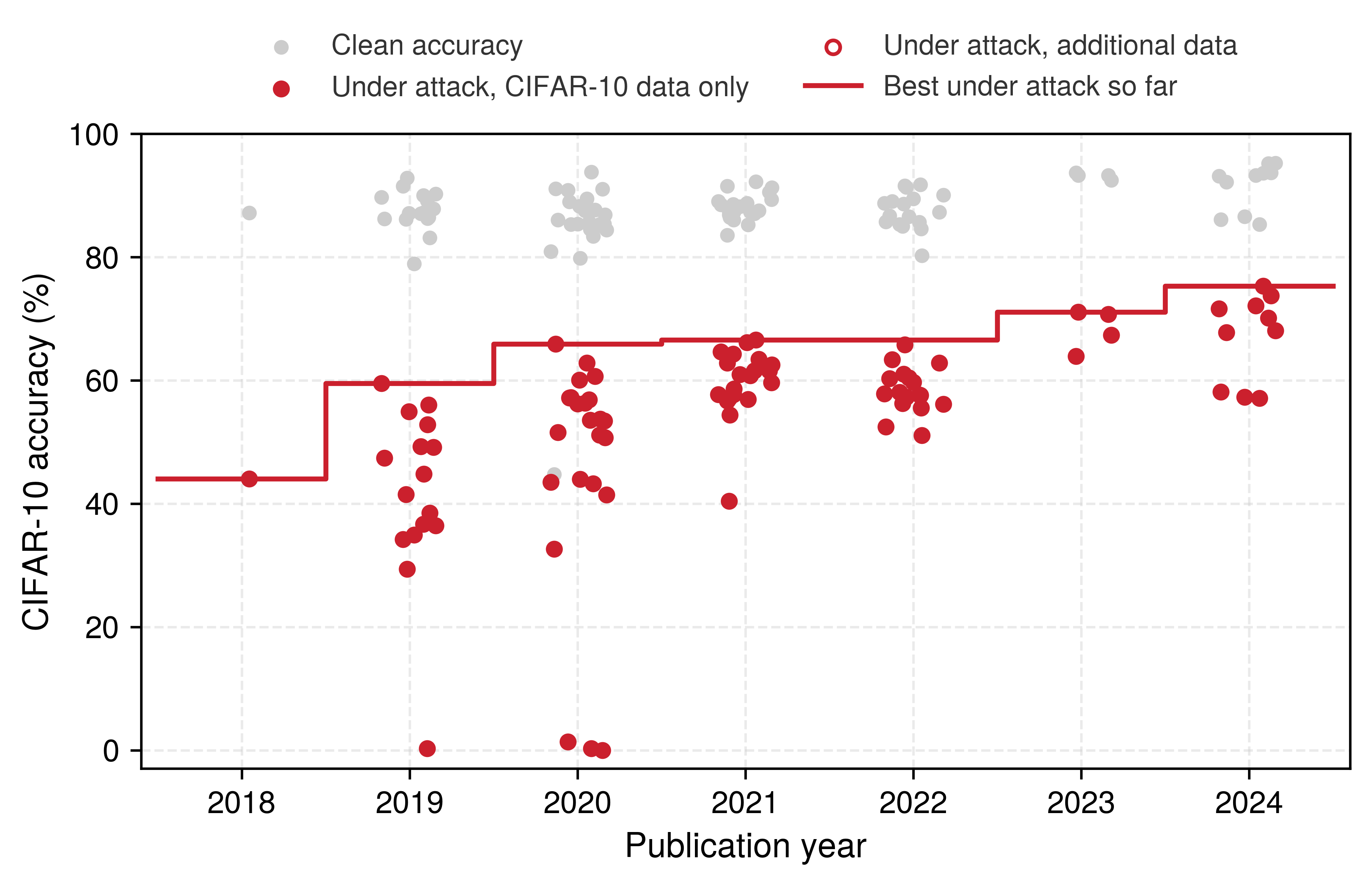
Croce, Francesco, Maksym Andriushchenko, Vikash Sehwag, Edoardo Debenedetti, Nicolas Flammarion, Mung Chiang, Prateek Mittal, and Matthias Hein. 2020. “RobustBench: A Standardized Adversarial Robustness Benchmark.” arXiv Preprint arXiv:2010.09670.
Adversarial training, certified defenses, and input detection address attacks on model inputs at inference time within bounded threat models. They do not establish that the model was trained on trustworthy data. If an adversary compromises the data pipeline long before the model is compiled, inference-time behavioral tests may reveal a backdoor, but cannot by themselves establish the integrity of the training pipeline. Poisoning attacks therefore demand their own class of defenses.
Checkpoint 14.3: Choosing and budgeting an adversarial defense
An adversarial defense is a budgeted response to a specific threat model. Stronger guarantees commonly change clean accuracy, compute, latency, or coverage, but the direction and magnitude depend on the workload, model, defense, and evaluation boundary.
Matching defense to threat
Reasoning about the budget
Self-Check: Question
How does multi-step adversarial training (such as PGD-7) improve a neural network’s robustness against evasion attacks during inference?
- It approximately searches for high-loss perturbations within the threat set and trains the model to reduce loss on those perturbed inputs.
- It encrypts the model’s weight matrices so attackers cannot estimate loss gradients via backward passes.
- It removes all non-linear activation functions from the architecture, ensuring the decision boundary is strictly linear.
- It replaces model weights with random distributions at inference time without requiring any changes during training.
In the chapter’s equal-cost-pass PGD-7 work model, one update pass and seven attack-generation passes cost eight standard passes per batch. Standard-model clean accuracy is 76 percent, and robust-model accuracy under the specified attack is 50 percent. Explain what these quantities establish and what further measurements are needed to isolate a clean-accuracy penalty and elapsed-time cost.
Which statement correctly distinguishes certified robustness (such as randomized smoothing) from empirical robustness (such as PGD adversarial training)?
- Empirical robustness provides mathematical guarantees across all possible norm balls, whereas certified robustness is validated only against specific attacks.
- Certified defenses require zero additional compute at inference time, making them ideal for high-throughput microservices.
- A valid certificate bounds prediction stability within its stated set and assumptions; empirical attack tests supply evidence for tested cases, while randomized smoothing adds sampling cost on the inputs certified.
- Certified robustness is applicable only to training data poisoning and cannot defend against test-time evasion.
Order the four stages of the chapter’s adversarial defense workflow: (1) Choose the robustness budget across training-time, inference-time, and guardrail layers, (2) Define the threat model by specifying perturbation bounds (\(\epsilon\)), norm constraints, and attacker access, (3) Keep evaluation adversarial by testing defenses against adaptive and stronger optimization attacks, (4) Measure the trade-off between clean accuracy, training compute, and serving latency.
A real-time image moderation service with a strict 50 ms p99 latency SLA cannot afford randomized smoothing, which requires thousands of forward passes. Design an adversarial defense portfolio that fits this latency budget and explain the trade-offs involved.
14.7 Data Poisoning Defenses
A recommendation model may retain its overall accuracy while promoting an attacker’s chosen item to a small group of users. Defending against that failure requires testing the targeted behavior as well as securing the integrity of the training supply chain. Source permissions set the security boundary, and robustness evaluation measures what happens when poisoned records or updates cross it anyway.
Poisoning changes the data from which a model learns rather than perturbing a fixed model at inference time, and its threat runs from early attacks on support-vector machines (Biggio et al. 2012) to web-scale and generative-model data pipelines (Shan et al. 2023). Microsoft’s Tay chatbot, which its operator reported was subverted by a coordinated attack within a day of launch (Lee 2016), shows why any system that learns from live interaction makes every user a potential contributor of training evidence, so the engineering question becomes which contributions may enter training and how their influence can be audited.
Biggio, Battista, Blaine Nelson, and Pavel Laskov. 2012. “Poisoning Attacks Against Support Vector Machines.” Proceedings of the 29th International Conference on Machine Learning, ICML 2012, Edinburgh, Scotland, UK, June 26 - July 1, 2012.
Shan, S., W. Ding, J. Passananti, S. Wu, H. Zheng, and B. Y. Zhao. 2023. “Nightshade: Prompt-Specific Poisoning Attacks on Text-to-Image Generative Models.” 2024 IEEE Symposium on Security and Privacy (SP) abs/2310.13828: 807–25. https://doi.org/10.1109/sp54263.2024.00207.
Lee, Peter. 2016. Learning from Tay’s Introduction. The Official Microsoft Blog.
↩︎ Data poisoning, the corruption of training data or updates so that the learned model misbehaves later, and its sequence of admission, training, and exploitation are established in Data poisoning.
A dirty-label attack corrupts the label, so a label audit can catch it. Its counterpart, clean-label poisoning, keeps every label correct and corrupts the features instead, which is why several of the defenses below must look past labels to features and representations. Generative-model training corpora are exposed to the same threat in a concept-poisoning form, in which a few hundred perturbed images can redirect what a text-to-image model draws for a prompt; Data poisoning examines these mechanisms, that case, and the paths by which poisoned records enter the pipeline.
Poisoned records can resemble legitimate data, so clean aggregate validation accuracy alone cannot establish that a training corpus is trustworthy, and a targeted attack is designed to hide inside otherwise normal performance. Attacks may originate from internal actors with privileged pipeline access or from external adversaries who exploit crowdsourced collection or open data pipelines that lack integrity checks and lineage tracking. The defense therefore runs as four ordered layers along the data path:
- Ingress controls establish provenance and access limits, dictating which sources may contribute or modify data.
- Anomaly detection and sanitization inspect candidate records before training and filter suspicious submissions.
- Robust training objectives reduce the weight that extreme residuals receive for poisoned samples that evade ingestion filtering, although they do not by themselves bound parameter updates.
- Post-training checks test the trained model’s behavior on the poisoning objectives that aggregate accuracy hides before the model is released.
Each layer covers a distinct point along the data path and has its own blind spot, so no single detector can substitute for end-to-end controls. Representation learning sits beneath all four as a foundation rather than a fifth gate: it reduces the model’s reliance on brittle features that poisoned instances can exploit, but it cannot prove that the training corpus is uncompromised.
For the recommendation system, the interception layer in figure 11 examines contributed ratings before they reach training. Its decisions must preserve provenance so later model failures can be traced back to the accepted records.
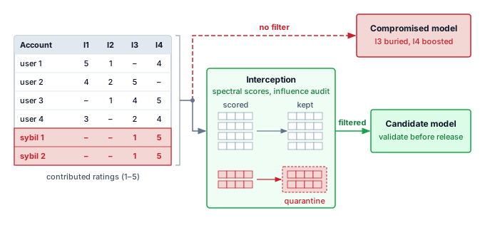
14.7.1 Ingress and anomaly controls
If an unverified data source or a compromised contributor account can write directly into a training table, statistical outlier filters will only ever see the attacks that fail to blend in. Poisoning defense therefore begins at the data boundary, before any statistical detector runs. The pipeline must know which sources are allowed to contribute training data, how their authenticity is verified, and which roles can modify accepted records. Strong governance enforces the principle of least privilege,15 logs data access and modification events, and gives each accepted batch a source identity. These controls do not prove that every record is clean, but they bound the attack surface and give anomaly findings a traceable origin.
15 Principle of least privilege: Articulated by Saltzer and Schroeder (1975), this principle restricts access rights to the minimum necessary for each component. In an ML pipeline, a training job allowed to read unverified sources has an additional path through which adversarial data can enter, so write and read rights become part of the poisoning attack surface. The same principle governs the model registry, the artifact store that maps version identifiers to weight files and controls which alias (for example, staging, production) resolves to which checkpoint. Promotion to the production alias should be restricted to a narrow, audited set of automated evaluation services and named release engineers; if a researcher’s credentials are compromised, excluding those credentials from promotion authority blocks that direct path to replacing the live model, while other authorized paths still require scrutiny.
Saltzer, J. H., and M. D. Schroeder. 1975. “The Protection of Information in Computer Systems.” Proceedings of the IEEE 63 (9): 1278–308. https://doi.org/10.1109/proc.1975.9939.
Lighthouse 14.1: Archetype B (DLRM at Scale): Fake profile injection
Archetype B (DLRM at Scale) is especially exposed to fake profile injection. Because recommendation systems often use online learning to adapt to user trends in real time, an adversary can create a network of “sybil” accounts, fake identities controlled by the same attacker, that interact with specific items to artificially boost their popularity or associate them with high-value demographics. This poisoning bypasses traditional firewalls because the malicious interactions look like legitimate user behavior, motivating checks on contributor identity, interaction patterns, and learned representations. Spectral-signature defenses (developed in section 14.7.1.1) search activation patterns for suspicious separation, but their effectiveness depends on whether the poisoned and clean contributions separate in that representation.
After the source boundary, anomaly detection asks whether a candidate training example belongs to the distribution that the pipeline intended to learn from. The cheapest tests compare each record against the bulk distribution: Z-score filtering, Tukey’s method, and Mahalanobis distance flag examples whose feature values sit far from normal ranges. These tests are useful because they are fast enough to run at ingestion, but they catch only poisons that look like statistical outliers in raw feature space. For high-dimensional or multimodal data, raw-feature distances are a weak signal: a manipulated image or caption that passes raw-feature checks may separate from clean examples in a pretrained vision or language model’s embedding space. That separation depends on the encoder and attack, so it must be measured rather than inferred from the use of a learned representation. Applying Mahalanobis distance or clustering to those representations tests a different hypothesis from raw-feature screening. The pipeline must check whether the resulting outliers correspond to malicious contributions or to legitimate variation it needs to retain.
More coordinated attacks require structure-aware checks. Clustering methods such as K-means, DBSCAN, and hierarchical clustering look for anomalous groups or isolated points rather than single extreme values, whereas the autoencoder ingestion gate in figure 12 adds a learned representation to the screening pipeline: the model compresses inputs through a bottleneck layer \(\EncoderLatentRepresentation\), accepting records whose reconstruction error \(\AutoencoderReconstructionError\) falls below threshold \(\ResponseThreshold\) and quarantining anomalous outliers. Each method has a blind spot, because clean-label poisons need not be statistical outliers, clustering depends on the representation, and autoencoders can reconstruct unfamiliar inputs well or learn an attack pattern from a contaminated reference corpus, so each gate requires evaluation on both poisons and legitimate rare examples.
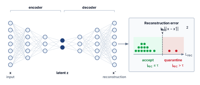
Sanitization and preprocessing
Sanitization turns anomaly signals into training-set changes before the poison reaches optimization. A suspicious record can be rejected, quarantined for review, down-weighted during training, or kept with an explicit provenance flag. Routine cleaning still matters: deduplication, missing-value handling, type checks, range constraints, and cross-field validation remove many low-effort poisoning attempts while improving ordinary data quality.
Data provenance and lineage tracking make those decisions reversible. Each datum needs a record of its source, transformations, validation outcomes, and movement through the pipeline. When a model later shows a poisoning symptom, lineage lets the operator trace model dependencies back to candidate source batches, investigate which contributions caused the behavior, estimate which trained models consumed confirmed compromised examples, and decide whether to remove, relabel, or reweight the affected records.
When suspicious data has already entered the corpus, sanitization moves from source checks to representation checks. Spectral signatures exploit separation between clean and poisoned samples in a learned representation (Tran et al. 2018). In the backdoor attacks studied by Tran and colleagues, the trigger created a strong signal in the target class’s activations. Projecting centered representations onto the top singular vector and removing high-scoring samples exposed many poisoned records without requiring prior knowledge of the trigger. The method depends on sufficient separation relative to within-group variation; an effective backdoor does not by itself guarantee a usable spectral signature. Filtering therefore requires attack-specific evaluation and checks for discarded clean samples.
Koh, Pang Wei, and Percy Liang. 2017. “Understanding Black-Box Predictions via Influence Functions.” International Conference on Machine Learning (ICML), Proceedings of machine learning research, vol. 70: 1885–94.
Influence functions (Koh and Liang 2017) serve a narrower debugging role. They approximate how infinitesimally increasing a training point \(\TrainingExample\)’s weight changes the model’s loss for a test point \(\TestExample\), without retraining. The fitted parameters are the trained model’s weights, and the Hessian is the curvature matrix of the average training loss at those parameters. Its inverse translates a small change in a training point’s weight into an approximate change in the fitted parameters. Calculated through inverse-Hessian-vector products, influence \(\InfluenceFunction(\TrainingExample, \TestExample) \approx -\nabla_\ModelParameters\LossFunction(\TestExample, \OptimalModelParameters)^T \LossHessian^{-1} \nabla_\ModelParameters\LossFunction(\TrainingExample, \OptimalModelParameters)\), this metric measures local sensitivity to upweighting \(\TrainingExample\). For an average training loss over \(\DatasetSize\) examples, removing one point corresponds approximately to a weight change of \(-1/\DatasetSize\), reversing the sign and scaling this influence by \(1/\DatasetSize\). If a model begins assigning an attacker’s target label to one narrow class of inputs, influence functions can rank the training examples that contributed most to that decision. The method avoids forming an explicit inverse Hessian by using iterative approximations, but its results remain approximate in deep nonconvex networks. At modern model scale, influence analysis therefore requires validation against the specific architecture, approximation, and debugging task rather than serving as exact attribution.
14.7.2 Robust training objectives
Huber limits a surviving outlier by growing linearly where MSE keeps squaring.
16 Huber loss: This piecewise loss transitions from quadratic to linear beyond a chosen residual threshold, bounding its derivative with respect to the residual. The parameter gradient also multiplies that derivative by the model’s prediction Jacobian, so Huber loss alone does not bound parameter updates or prevent poisoning. Under MSE, an outlier with 100× normal error contributes 10,000× squared-error loss and 100× residual-gradient magnitude. Under Huber loss, once that residual passes the threshold the loss grows only linearly and the residual derivative stays at the threshold value, so the same outlier pulls no harder than any other point beyond the threshold.
Beaton, A. E., and J. W. Tukey. 1974. “The Fitting of Power Series, Meaning Polynomials, Illustrated on Band-Spectroscopic Data.” Technometrics 16 (2): 147–85. https://doi.org/10.1080/00401706.1974.10489171.
17 Minimax: Game-theoretic strategy from Neumann (1928) that minimizes the maximum possible loss. In adversarial robustness, Madry et al. (2018) formulate training as \(\min_\ModelParameters\max_{\|\AdversarialPerturbation\| \leq \AdversarialPerturbationBudget} \LossFunction(\ParameterizedPredictor(\ModelInput+ \AdversarialPerturbation), \ExampleLabel)\): the model learns to minimize loss under a worst-case perturbation within the chosen norm ball. The inner maximization is computationally expensive because it is usually approximated with iterative attacks such as PGD, so PGD-adversarial training is a budgeted robustness choice rather than a free objective change (Bai et al. 2021; Shafahi et al. 2019).
Neumann, John von. 1928. “Zur Theorie Der Gesellschaftsspiele.” Mathematische Annalen 100 (1): 295–320. https://doi.org/10.1007/bf01448847.
Madry, Aleksander, Aleksandar Makelov, Ludwig Schmidt, Dimitris Tsipras, and Adrian Vladu. 2018. “Towards Deep Learning Models Resistant to Adversarial Attacks.” International Conference on Learning Representations (ICLR).
Bai, Tao, Jinqi Luo, Jun Zhao, Bihan Wen, and Qian Wang. 2021. “Recent Advances in Adversarial Training for Adversarial Robustness.” Proceedings of the Thirtieth International Joint Conference on Artificial Intelligence, 4312–21. https://doi.org/10.24963/ijcai.2021/591.
Shafahi, Ali, Mahyar Najibi, Amin Ghiasi, Zheng Xu, John Dickerson, Christoph Studer, Larry S. Davis, Gavin Taylor, and Tom Goldstein. 2019. “Adversarial Training for Free!” arXiv Preprint arXiv:1904.12843, ahead of print. https://doi.org/10.48550/arXiv.1904.12843.
Under a standard squared-error objective, a single poisoned sample that survives ingestion filtering with a large residual error contributes quadratically to the loss and pulls the gradient far harder than a typical point. To limit the influence of surviving outliers before release evaluation, robust optimization modifies the training objective itself. Robust loss functions such as the Huber loss,16 the Tukey loss (Beaton and Tukey 1974), and the trimmed mean loss down-weight or ignore the contribution of abnormal instances during training. Regularization techniques (\(\ell_1\) or \(\ell_2\) regularization) constrain model complexity and can reduce sensitivity to some poisoned data. At a higher level, minimax17 and distributionally robust objectives optimize performance over a specified uncertainty set. The objective supplies a formal target; an approximate optimizer does not by itself prove that the trained model attains the target or resists attacks outside that set.
Data augmentation expands training diversity by applying horizontal flips, padded crops, rotations, and color jitter (figure 13), creating variants that preserve the label when the transform respects the class (a horizontally flipped digit need not) and can disrupt some localized poison patterns. Other transformations preserve an attack’s trigger, so augmentation does not guarantee dilution. Random subsampling or bootstrap aggregating changes which poisoned records each model encounters; whether combining those models reduces the attack’s effect requires evaluation against coordinated poisoning.
Distributed and federated training adds a contributor axis to the same threat, and robust aggregation is the training-objective layer’s counterpart at the level of contributors. A malicious client need not insert a visible record into a central corpus; it can submit a model update chosen to move the aggregate, implant a backdoor, or exploit sybil identities to gain disproportionate weight. Archetype C (Federated MobileNet) makes this concrete: the server aggregates updates from a large population of smartphone-class clients whose raw data it never sees, so contributor-level checks screen updates before aggregation. Krum, coordinate-wise median, and trimmed mean (Byzantine failures) tolerate bounded Byzantine behavior only under their stated assumptions (Blanchard et al. 2017; Yin et al. 2018); high dimensionality and non-i.i.d. client updates can make honest contributors look anomalous. These rules also change the collective, because a median, trimmed mean, or Krum selection needs the individual updates rather than their sum, which raises per-worker traffic over a ring AllReduce.
Blanchard, Peva, El Mahdi El Mhamdi, Rachid Guerraoui, and Julien Stainer. 2017. “Machine Learning with Adversaries: Byzantine Tolerant Gradient Descent.” Advances in Neural Information Processing Systems (NeurIPS), 119–29.
Yin, Dong, Yudong Chen, Kannan Ramchandran, and Peter Bartlett. 2018. “Byzantine-Robust Distributed Learning: Towards Optimal Statistical Rates.” International Conference on Machine Learning (ICML), 5650–59.
↩︎ The traffic cost of gather-based robust aggregation relative to ring AllReduce is established in Gradient synchronization integrity.
14.7.3 Post-training behavioral checks
Admitting a poisoned record does not by itself guarantee that training will learn the attacker’s behavior, so the last layer tests the trained model rather than its inputs. The evidence that exposes poisoning differs across the four objective classes that Data poisoning distinguishes: availability, targeted, backdoor, and subpopulation poisoning. The robustness question is which evidence exposes each class and what that evidence costs (Oprea et al. 2022). Successful availability attacks can lower aggregate validation accuracy, giving broad evaluation a signal to investigate. Targeted and subpopulation attacks can leave that aggregate nearly intact, making evaluation on the named targets and cohorts particularly important. Backdoors can also preserve clean-data accuracy while responding to a trigger the evaluator has never seen, as the BadNets pixel-pattern trigger does (Gu et al. 2017); possible detection strategies include trigger search, canary inputs, and activation-space inspection when poisoned and clean representations separate (Tran et al. 2018).
Oprea, Alina, Anoop Singhal, and Apostol Vassilev. 2022. “Poisoning Attacks Against Machine Learning: Can Machine Learning Be Trustworthy?” Computer 55 (11): 94–99. https://doi.org/10.1109/mc.2022.3190787.
Gu, Tianyu, Brendan Dolan-Gavitt, and Siddharth Garg. 2017. “BadNets: Identifying Vulnerabilities in the Machine Learning Model Supply Chain.” arXiv Preprint arXiv:1708.06733.
Tran, Brandon, Jerry Li, and Aleksander Madry. 2018. “Spectral Signatures in Backdoor Attacks.” Advances in Neural Information Processing Systems (NeurIPS).
For federated and distributed contributors the release gate takes the same form. Held-out behavioral tests on the resulting global model must vary the number and coordination of malicious contributors, their data heterogeneity, participation schedule, and knowledge of the aggregation rule. Global clean accuracy is again insufficient: the gate needs attack success on the trigger or target subpopulation, contributor-level anomaly recall, and the clean-utility cost of robust aggregation. Provenance, participation limits, robust aggregation, and held-out canaries must therefore work together rather than treating one distance rule as a poisoning proof.
The operating rule is layered: authenticate and govern sources before ingestion, sanitize suspicious data before training, limit surviving outliers during optimization, test the trained model on the poisoning objectives before release, and preserve lineage so an incident can be traced back to the compromised source. Data poisoning remains an active research area, but production systems should treat the training corpus as a supply chain rather than a passive dataset.
The four layers act on records, objectives, and the trained model. A representation that does not lean on brittle shortcuts gives a poisoned shortcut less to exploit, and the same property helps the model survive ordinary deployment variation, so representation learning serves the poisoning defense and the environmental pillar at once. Beyond detecting and correcting shifts after they occur (section 14.4), a complementary approach builds shift-resilient representations from the start, drawing on transfer-learning and domain-adaptation foundations (Pan and Yang 2010).
Pan, Sinno Jialin, and Qiang Yang. 2010. “A Survey on Transfer Learning.” IEEE Transactions on Knowledge and Data Engineering 22 (10): 1345–59. https://doi.org/10.1109/tkde.2009.191.
14.7.4 Self-supervised representations for robustness
Supervised models often overfit to whichever labeled shortcut is easiest to exploit, such as a background texture, an annotation artifact, or a narrow phrasing pattern, and fail when deployment shifts or a poisoning attack targets that cue. Self-supervised learning (SSL) changes the source of supervision so the model learns by solving pretext tasks that require structure in the data itself. A pretraining task that rewards stable structure across views, missing tokens, or masked image patches gives the representation a chance to learn signals that survive more deployment variation.
Contrastive learning methods such as SimCLR (Chen et al. 2020) make this idea concrete by pushing different views of the same example toward a shared representation. The model is rewarded for treating a crop, color shift, or augmentation as the same underlying object rather than as a new class-specific cue. Masked language modeling in BERT (Devlin et al. 2019) and masked autoencoding in vision (He et al. 2021) use a different route: they hide part of the input and force the model to reconstruct or predict it from context. Both families provide supervision beyond the downstream task labels. Whether the resulting representations transfer better depends on the pretraining data, objective, and deployment shift; removing task labels does not remove shortcut learning.
Chen, Ting, Simon Kornblith, Mohammad Norouzi, and Geoffrey Hinton. 2020. “A Simple Framework for Contrastive Learning of Visual Representations.” Proceedings of the 37th International Conference on Machine Learning, ICML’20, vol. 119: 1597–607.
Devlin, Jacob, Ming-Wei Chang, Kenton Lee, and Kristina Toutanova. 2019. “BERT: Pre-Training of Deep Bidirectional Transformers for Language Understanding.” Proceedings of the 2019 Conference of the North American Chapter of the Association for Computational Linguistics: Human Language Technologies, 4171–86. https://doi.org/10.18653/v1/n19-1423.
He, K., X. Chen, S. Xie, Y. Li, P. Dollár, and R. Girshick. 2021. “Masked Autoencoders Are Scalable Vision Learners.” 2022 IEEE/CVF Conference on Computer Vision and Pattern Recognition (CVPR) 18: 15979–88. https://doi.org/10.1109/cvpr52688.2022.01553.
That transfer benefit is the main systems reason to use SSL in a robustness pipeline. Larger unlabeled corpora expose the model to domains, transformations, and rare cases that would be too expensive to label exhaustively. The same uncurated scale widens the poisoning surface, so SSL pretraining data still needs the ingress and sanitization controls described earlier. In production, SSL usually acts as a foundation rather than a complete defense: pretrain on broad unlabeled data, fine-tune on the supervised task, then apply the adversarial, drift, and poisoning defenses established earlier in this chapter to the task-specific model. Multi-task training can preserve some of this benefit by keeping a self-supervised objective active while the supervised task pulls the representation toward the deployment metric.
The limitation is that SSL is not a robustness guarantee. A contrastive or masked-pretraining objective can still learn brittle shortcuts, and an attacker who understands the pretext task can target those shortcuts directly. The theory explaining when SSL improves robustness remains incomplete, and the compute cost can be substantial because pretraining moves work earlier in the lifecycle. Whether broader representation learning lowers the expected cost of drift, relabeling, and robust fine-tuning enough to justify the added pretraining budget is a per-service calculation. When the model generates open-ended text rather than discrete class labels, the robustness contract itself must expand beyond label stability.
Self-Check: Question
Compare availability poisoning with backdoor poisoning, and explain why an evaluation that checks only aggregate clean accuracy can miss a successful backdoor.
A machine learning team relies on standard Z-score outlier filtering and label-consistency checks on its crowdsourced training data, yet finds its deployed model contains a severe backdoor vulnerability. Why do naive data-cleaning filters fail against sophisticated poisoning attacks?
- Poisoning attacks only modify model weights during inference and leave training data untouched.
- Poisoned samples can have valid feature ranges and correct labels while passing the pipeline’s univariate checks.
- Z-score filtering only works on text data and cannot be applied to numerical or image features.
- Standard regularization during training completely disables all data validation checks.
Explain how spectral signatures detect backdoor-poisoned samples in activation space without requiring the defender to know what the trigger pattern looks like.
Following an incident where an unauthorized training batch degraded a recommendation model, an audit team must identify the origin of the poisoned records, the pipeline transformation steps applied, and all downstream model artifacts trained on that batch. Which system capability provides this audit trail?
- Randomized smoothing certificates
- Monte Carlo dropout sampling
- Huber loss gradient clipping
- Data provenance and lineage tracking
True or False: In training pipelines susceptible to data poisoning, replacing standard mean squared error loss with Huber loss prevents extreme outliers from exerting unbounded derivative with respect to the residual, because Huber loss transitions from quadratic to linear error growth beyond a threshold \(\delta\).
The chapter argues that secure data sourcing, least-privilege pipeline access, and signed model registries are first-class robustness defenses rather than generic security hygiene. Justify this claim by identifying the failure modes that algorithmic data-cleaning methods cannot prevent.
14.8 Robustness of Generative Models
An aligned language model of the Archetype A (GPT-4/Llama-3) class can pass its safety evaluations and still comply with a harmful request once an automatically optimized suffix is appended to the prompt, and suffixes optimized against open models transfer to other models (Zou et al. 2023). That suffix is an adversarial example in token space, found by gradient-guided search over discrete tokens rather than continuous pixels. Generative models also fail without any attacker. Their output is open-ended text rather than a label, so the robustness question changes from whether a label flips under perturbation to whether the generated content preserves factuality, policy constraints, and task intent across prompt variations. A fluent answer can be factually baseless while latency and uptime stay healthy, which makes hallucination the generative form of silent failure.
Zou, Andy, Zifan Wang, Nicholas Carlini, Milad Nasr, J. Zico Kolter, and Matt Fredrikson. 2023. Universal and Transferable Adversarial Attacks on Aligned Language Models.
The evaluation discipline of table 1 carries over with three adjustments. First, correctness needs a named reference. A hallucination rate is meaningful only against a stated evidence source, such as the retrieved context, a verified knowledge base, or an expert-labeled answer set, and it counts the generated claims that this reference does not support. The measured rate also depends on the model, the retrieval context, the prompt design, and the sampling temperature, so a reported rate holds only for its prompt set and decoding settings and cannot be carried to another domain without re-measurement. Second, the perturbation budget becomes a family of prompt variations. Paraphrases, reordered context, and inserted distractors play the role that the \(\ell_\infty\) ball plays for an image classifier, and robustness is reported for each family. Third, the slices are domains and user populations, because an aggregate rate can hide a domain in which the model invents answers, just as the Google Photos failure hid inside aggregate image accuracy.
Detecting a hallucination on an individual request is the per-request competence problem of section 14.4.4 with an open-ended output. Token entropy and log-probability can expose instability in a generation, but neither is a factuality score. A model can assign high probability to a false statement learned from its data, or low probability to a correct but rare statement. Production routing must therefore calibrate these signals against task-specific errors and combine them with evidence checks, retrieval support, or external verification.
The self-consistency technique samples multiple reasoning paths or answers for the same query. Disagreement supplies an instability signal that can route the request for review; agreement supplies weaker evidence because correlated samples can repeat the same misconception or unsupported claim. Sequence-level entropy has the same limitation: it can serve as a calibrated routing feature for a named task, but it does not transform uncertainty into truthfulness. The signal also has a price. Each additional sample repeats the decode phase for that request, so drawing \(\SelfConsistencySampleCount\) samples multiplies its decode work roughly \(\SelfConsistencySampleCount\)-fold; only the prompt’s prefill can be shared, when the serving system reuses the prompt’s cached key-value state. Like the noise samples of randomized smoothing, this cost lands on the compute term of every request it covers, and the same remedy applies. The expensive signal should be spent on the requests whose cheap signals already indicate uncertainty rather than on all traffic. The operational contract must measure error conditional on the routing score and provision the refusal, retrieval, tool, or human path that receives flagged generations.
↩︎ Reuse of a shared prompt’s cached key-value state across requests is established in Prefix caching.
In retrieval-augmented generation (RAG) architectures, robustness depends heavily on the quality of the retrieved context. Retrieval noise, the injection of irrelevant or conflicting documents into the prompt, can distract the model, causing it to ignore its internal parametric knowledge and propagate errors from the context. Robust RAG deployments can use re-ranking models and context verifiers to filter out noise before it reaches the generation step. Their evaluation must separate retrieval failure from generation failure. Measuring answer support separately for requests whose retrieved context contains the answer and for requests whose context does not shows whether errors come from the retriever or from a model that ignores or overrides good evidence. The retrieval corpus is also an input an attacker may be able to write to, so a planted document can corrupt retrieval evidence or carry prompt injection, and the ingress controls of section 14.7 apply to it. It becomes a training-poisoning path if the pipeline later admits it into learning.
Language interfaces also carry the input-level attacker into text. Prompt injection, a failure of the boundary between control and data, embeds instructions in user content or retrieved documents so that the model overrides its system prompt. The payload can arrive through a legitimate input channel, so permission to submit content does not make that content trustworthy. External access controls still constrain which data or tools the surrounding system exposes. From the robustness side, evaluation asks whether the content induces behavior outside the intended output contract, and it is measured the way adversarial robustness is measured: as an attack success rate over an injection suite matched to the threat model, run by an evaluator who knows the system prompt and filters. Keeping those details secret is not a defense, because optimized suffixes transfer across models.
↩︎ Prompt injection as a failure of the boundary between control and data is established in LLM-specific attack vectors.
A common deployment pattern adds output guardrails, lightweight classifiers that scan generated text for policy violations or toxicity before the response returns to the user. A guardrail threshold trades the same two quantities as a selective-prediction threshold. Each false positive refuses or escalates a legitimate response, so the false-positive rate multiplied by the legitimate-request rate estimates false refusals or escalations; each false negative is residual risk that reaches the user. Total diverted load also includes correctly flagged harmful responses. The arrival rate at each refusal, retrieval, or human path is the incoming request rate multiplied by the fraction routed to that path under the policy, counting both true and false flags. Choosing the threshold from a curve measured on representative traffic, rather than from the classifier’s default, allows the team to compare that load with the path’s capacity. The guardrail also adds a model inference to every response, so its latency counts against the serving deadline. Because a guardrail is itself a model with its own decision boundary, it carries the same obligation as any other defense and must pass the adaptive evaluation of section 14.6.1.3 against an attacker who knows it is there. Every routing signal for generative models, from token entropy to a guardrail score, is also computed by the same serving system that the remaining pillar can corrupt.
Self-Check: Question
A team reports that its retrieval-augmented assistant has a 3 percent hallucination rate and proposes quoting that figure for a new legal-research deployment. Which condition must hold before the figure says anything about the new deployment?
- The rate must be re-measured against a stated evidence source on the new domain’s prompt set with the same retrieval context and decoding settings.
- The model’s mean token entropy on the new domain must be no higher than on the original domain.
- The new deployment must use self-consistency sampling, because agreement among samples certifies factuality.
- No condition is needed, because a hallucination rate is a property of the model weights alone.
In large language models, robustness failures manifest as confident, fluent hallucinations rather than discrete label misclassifications. Describe two uncertainty quantification mechanisms used to detect semantic instability in generative AI and explain their systems trade-offs.
14.9 System-Level Faults
A preprocessing bug that silently rescales an input feature or an accelerator bit flip that corrupts a stored weight can make a healthy replica emit wrong predictions while triggering the exact same alarms as distribution drift or an adversarial attack. Every defense in the two preceding pillars reads evidence produced by the system it protects: drift monitors read preprocessed features, adversarial detectors read model scores, and poisoning filters read learned representations. The third pillar asks what happens when that machinery is itself wrong. Execution-level detection and recovery belong to fault tolerance. Robustness adds two obligations on top of them: behavioral checks that run on the model’s own values and outputs, and a diagnosis that decides whether a behavioral alarm came from a fault at all.
14.9.1 Behavioral checks for silent faults
A single physical bit flip can cascade through neural inference (figure 14). In panel (b), flipping bit 30 of an FP32 weight scales its magnitude by \(2^{128}\), transforming a modest weight \(\ModelWeight\) of 0.042 into an extreme outlier \(\CorruptedModelWeight\) of about \(1.4 \times 10^{37}\). Panel (a) traces the affected path through hidden unit \(\HiddenUnitOutput_2\) to output logits (\(\NetworkOutput_1, \NetworkOutput_2\)). The corrupted weight is finite and can evade NaN or infinity checks; whether it dominates those outputs depends on the input, activation function, and downstream weights. Targeted bit-flip attacks deliberately select vulnerable weight bits, so their results should not be interpreted as the effect of one random hardware upset. Memory subsystem failures during training can likewise corrupt gradient updates and prevent model convergence. Scale turns one corrupted value into a persistent exposure. Every forward pass of a dense GPT-3-class model reads all 175B of its parameters, so a corrupted weight resident in memory participates in every request that replica serves until something detects it.
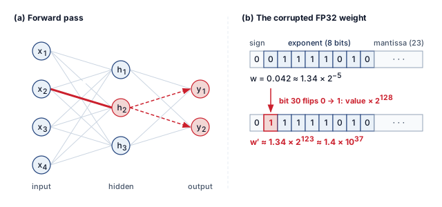
The cheapest behavioral checks test invariants that a correctly executing model satisfies. A range check \(|\ModelWeight| \le \WeightRangeBound\) against the trained weight distribution catches the exponent flip above at the cost of one comparison per stored value, and the same idea bounds each layer’s activations at serving time against the range observed on validation traffic. Where range checks catch extreme values, golden-input canaries replay a fixed set of requests through each replica on a schedule and compare the outputs with stored references, catching a corrupted replica whose liveness and readiness probes still pass. For corruption that stays inside normal ranges and appears only on live inputs, cross-replica comparison runs the same request on two replicas; because that doubles the work for every request it covers, fleets apply it to sampled traffic, following the check-and-verify pattern used against silent data corruption elsewhere in the fleet. Each check spends along a different C\(^3\) axis: invariant checks add compute on the serving path, canaries and cross-replica comparison add compute and communication, and deciding which replicas and checkpoints remain trustworthy after a check fails is coordination.
↩︎ Check-and-verify defenses against silent data corruption, and their cost relative to full redundancy, are established in Check-and-Verify Defenses Against Silent Data Corruption.
14.9.2 Distinguishing faults from shift and attack
These checks cover faults that leave a numerical signature. The harder case is a fault whose symptom looks like one of the other pillars. Consider an operator who sees the same surface symptom from all three pillars, falling model accuracy while latency and uptime hold steady. A preprocessing bug that silently rescales a feature looks exactly like covariate shift to a drift monitor, because the feature statistics have genuinely moved. A numerical overflow that corrupts a layer’s activations produces confident misclassifications that look exactly like an adversarial example, because the decision flipped without a visible input cause. The difficulty lies in the disguise, because the cheap pillar-specific detectors fire on the symptom rather than the cause. Three complementary signals guide this investigation: the timing boundary of the change, reproducibility under fixed inputs, and cross-layer correlation with infrastructure telemetry.
The boundary and timing of a change often provide the first diagnostic clue. While environmental shift can evolve gradually or appear abruptly with real-world events, a shift synchronized with a deployment, dependency bump, or schema migration raises the pipeline-fault hypothesis. This suspicion strengthens when multiple features shift simultaneously in directions that the underlying physical process cannot explain. Timing alone narrows the search space without proving causation.
Reproducibility under fixed inputs helps locate the failure boundary. Replaying golden inputs through version-pinned preprocessing pipelines and model artifacts can expose the stage where outputs begin to differ. A deterministic software defect fails at the same stage on every replay, a transient hardware upset usually vanishes on replay, and race conditions or marginal hardware fail intermittently, so isolating them takes repeated runs or a second device. Stochastic execution also requires controlling random state or comparing repeated runs. Because shifted or adversarial inputs can reproduce the same error under fixed execution conditions, replay alone cannot settle the diagnosis; operators must compare raw and preprocessed tensors, artifact versions, and population-level statistics alongside the replay output.
Finally, cross-layer correlation links model behavior to surrounding infrastructure telemetry. Query-rate spikes or unusual input patterns can support an attack hypothesis, while deployment releases, error-correcting code (ECC) memory counters, SDC checkers, or memory-pressure alarms can support a system-fault hypothesis. Neither pattern is necessary or sufficient. An attack can remain within normal traffic patterns, and silent corruption can escape the available counters. Correlation guides the next diagnostic test rather than establishing the cause.
Example 14.2: A drift alert that was a pipeline fault
Scenario: A credit-risk service raises drift alerts on three income-related features on the morning after a routine dependency update, and the approval rate for applicants in the affected income bands shifts sharply. Latency, error rates, and uptime are unchanged, and every request that the on-call engineer retries returns a score without error.
Diagnosis: The three signals point the same way. The alerts begin at the release boundary, and the three features moved together in a direction that no change in applicant behavior explains. Replaying a stored set of golden requests through the previous and current pipeline versions produces identical raw inputs but preprocessed tensors that differ by a constant factor on exactly those features, because the updated library changed a default normalization. Deployment telemetry correlates with the change; query-rate and hardware counters do not. The failure is a software fault disguised as covariate shift. Retraining on the corrupted features would have taught the model the bug, and the successful retries proved only that the service answered, not that its answers passed acceptance.
Systems lesson: A replay harness that pins artifact versions and compares tensors at each pipeline stage turns an ambiguous drift alert into an attributable fault. Recovery is complete only when the replayed outputs satisfy the model’s acceptance tests again, which is a behavioral check that a successful retry or a green health dashboard cannot supply.
The diagnostic discipline is therefore to read the system-level evidence before accepting the drift or attack hypothesis the surface symptom suggests, because each pillar suggests a different intervention and more than one cause can be active at once. Skipping that diagnosis, or mistaking a passed clean-data or single-norm test for comprehensive protection, produces the recurring engineering pitfalls examined next.
Self-Check: Question
A serving replica’s liveness and readiness probes pass and its latency is normal, but one of its weights has suffered an exponent bit flip that left the value finite and very large. Which check is designed to catch this replica?
- A range check of stored weights or layer activations against the distribution observed on trusted data, or a scheduled golden-input canary compared with stored reference outputs.
- A NaN and infinity check on the replica’s outputs, because a corrupted weight always produces a non-finite value.
- A population stability index alarm on the replica’s input features.
- A retry of failed requests, because a successful retry shows that the replica’s answers are valid.
A preprocessing library update introduces a feature scaling bug that shifts input distributions, causing a drift detector to alarm and trigger an automated model retraining pipeline. Explain why this response fails, and describe how cross-layer correlation separates software faults from true environmental shifts.
True or False: If replaying a fixed set of golden inputs through the current pipeline reproduces the same wrong outputs every time, the failure must be a software or hardware fault rather than distribution shift or an adversarial input.
14.10 Fallacies and Pitfalls
Robustness spans environmental shifts, input-level attacks, and system-level faults. Each threat domain introduces misconceptions that lead to inadequate defenses or misallocated engineering resources.
Fallacy: Adversarial examples are an academic curiosity with no real-world impact.
Published physical-world attacks, such as adversarial patches on clothing or stickers on stop signs, have fooled evaluated vision models under controlled patch and road-sign settings without digital access. Defense requires evaluation under the relevant physical conditions. Physical-world data augmentation, patch-aware training, and serving-time detection are candidate interventions, each with its own coverage and cost. Related PGD-style digital adversarial training adds work according to its attack steps, but its results do not establish resistance to physical attacks. Ordinary digital test sets can miss these deployment failure modes.
Pitfall: Treating test-set success as robustness proof.
A test set drawn from the same i.i.d. distribution as training data measures performance in that population; it does not establish resilience to a different deployment distribution or to a critical slice inside the same one. The Google Photos labeling failure shows how a harmful error on one population slice can hide inside aggregate accuracy, and the night-driving and clinic-imaging examples of distribution shift fail on populations the test set underrepresents. Robustness evidence needs held-out shifts, named slices, and the other cells of table 1.
Fallacy: Distribution shift monitoring is optional after deployment.
Models often degrade silently, maintaining high confidence scores even as predictive performance falls due to drift. Monitoring metrics like PSI can surface population shifts before accuracy falls below service level agreement (SLA) thresholds, enabling proactive intervention when the monitored features are predictive of downstream performance.
Pitfall: Ignoring poisoning defenses unless the attacker controls the training pipeline.
Clean-label poisoning compromises models by injecting correctly labeled but manipulated samples into public datasets or scraped data sources, requiring no access to internal code. Low-dose attacks can still target a particular prediction or implant a backdoor; the size of the poisoned slice and the apparent correctness of its labels do not establish integrity.
Fallacy: Average accuracy is sufficient for robustness measurement.
High average accuracy often masks fragility. A model that is accurate on nearly all clean test inputs can still fail on every input in a critical slice once an attacker applies a small, targeted perturbation (Madry et al. 2018). Reliable evaluation requires evidence for the claimed failure class: slice-level performance under shifts, empirical attack accuracy under a stated budget, or a certified radius where a formal guarantee is available. A finite attack search supplies empirical evidence rather than exact worst-case accuracy.
Pitfall: Treating adversarial training as a complete robustness solution.
Adversarial training does not establish universal robustness. A model trained against \(\ell_\infty\) attacks needs separate evaluation for \(\ell_2\) or geometric attacks. Perturbation sets can overlap, so resistance need not vanish across norms, but the training threat model alone does not establish the extent of that transfer.
Fallacy: Software faults do not matter when the model is correct.
Focusing solely on algorithmic robustness ignores the reality that software bugs in data pipelines and serving infrastructure are a major cause of ML failures. Incident analyses often find pipeline and data issues, not model architecture or adversarial attacks alone, at the center of failures. Checksums can detect changed bytes, while behavioral validation must also catch incorrect transformations of intact data. A model hardened against adversarial perturbations can still fail when a preprocessing bug supplies validly stored but wrongly computed inputs.
Pitfall: Hardening the model while leaving pipeline checks untested.
Robustness work can concentrate on adversarial training, certified radii, or poisoning defenses while leaving schema validation, preprocessing parity, feature freshness, and rollback drills under-tested. That imbalance creates a system that resists one class of attack but fails on ordinary operational faults. In the credit-risk example of section 14.9.2, a changed library default would have been caught at release time by a golden-request replay comparing preprocessed tensors across pipeline versions; without that check, the fault surfaced as a drift alert, and retraining on the corrupted features would have taught the model the bug. A robust deployment validates the model and the pipeline together and exercises the replay harness and rollback path before an incident needs them.
Self-Check: Question
True or False: Achieving 98 percent accuracy on a held-out i.i.d. test set is sufficient proof that a computer vision model will operate reliably in production without experiencing silent degradation.
An engineering team wants to reform its model evaluation metrics to avoid the pitfall of using aggregate average accuracy as the sole measure of model quality. Which evaluation practice directly resolves this pitfall?
- Measure consequential population slices, empirical accuracy under specified attacks, and certified accuracy where a valid certificate is available.
- Expand the held-out i.i.d. test split by 10\(\times\) to reduce the variance of the average accuracy estimate.
- Replace all predictive accuracy metrics with p99 serving latency benchmarks.
- Evaluate the model exclusively on synthetic training data generated by the same architecture.
A perception model is hardened using multi-step PGD adversarial training bounded by an \(\ell_\infty\) norm of \(\epsilon_{\text{adv}} = 8/255\). When deployed, an adversary attacks the model using an \(\ell_2\) optimization attack (such as C&W) and spatial rotation perturbations. What does the chapter’s discussion of adversarial training pitfalls predict?
- The model will be mathematically immune to all attacks because adversarial training provides universal robustness across all norms.
- The model will automatically detect and reject the \(\ell_2\) attack because \(\ell_\infty\) robustness is strictly stronger than all other defenses.
- The model may remain highly vulnerable to the \(\ell_2\) and spatial attacks, because adversarial training hardens boundaries specifically against the threat model and norm ball used during training.
- The model will fail to execute forward passes because the runtime input tensor dimensions will be rejected by the GPU driver.
A perception model achieves a certified robustness radius against digital \(\ell_\infty\) input perturbations. An engineer concludes that upstream data-pipeline validation and schema checks can now be deprioritized. Explain why this conclusion is dangerous, using the chapter’s systems-layer failure analysis.
14.11 Summary
Robust AI makes prediction quality an explicit engineering obligation alongside uptime and latency. Environmental shifts, adversarial manipulation, poisoning, and system faults can leave a service apparently healthy while its outputs become unreliable. The chapter’s diagnostic framework reads release timing, fixed-input replay, and infrastructure telemetry before accepting a drift or attack hypothesis, then connects each failure class to its own evidence and response; fleet recovery mechanisms must therefore be paired with behavioral acceptance tests.
Inside the training step, robustness is paid for in the terms of the Fleet Law (equation 1.3). Multi-step PGD adds gradient work in \(\IronLawComputeTime\); at a fixed worker count \(\DeviceCount\), the wall-clock increase depends on implementation, reuse, and the other terms in the step. Whether it also reduces clean accuracy, and by how much, depends on the model, data, perturbation set, and training recipe. Robust aggregation for distributed or federated contributors replaces a reducible mean with a median, trimmed mean, or Krum selection, which moves cost into \(\CommunicationTime(\DeviceCount)\) because the individual updates must be gathered rather than summed.
Outside the training step the same C\(^3\) axes set the price. Randomized smoothing and self-consistency sampling spend compute on every request they cover, invariant checks and golden-input canaries spend compute and communication to catch faults that health probes miss, and poisoning sanitization spends compute and storage bandwidth on extra passes over the training corpus. Drift monitoring spends communication, shipping reference statistics and serving telemetry between machines. Release gates, abstention thresholds, and escalation ownership spend coordination, because validated model versions must be adopted consistently across the fleet. Conformal routing touches all three axes: computing prediction sets adds bounded compute, returning larger sets adds communication, and routing abstentions to reviewers adds coordination. If prediction sets grow and trigger more deferrals, human-review or fallback capacity can become the bottleneck. Distribution shift can also invalidate coverage without enlarging the sets, so set size is a load signal rather than a complete drift detector. A coverage claim is operationally useful only when the deployment also provisions the path that consumes uncertain cases. Robustness engineering measures these workload-specific costs against the reduction in silent risk where failure consequences are highest.
Key Takeaways: Silent failure is the real threat
- Silence is the failure mode: Robustness exists because drift, adversarial perturbations, poisoning, and numerical faults often preserve uptime and latency while corrupting predictions. Production systems need monitors that surface competence loss before user complaints or downstream business metrics reveal it.
- Diagnose before defending: A software fault can look like concept drift, a poisoned sample like a rare outlier, and an adversarial input like natural variation. Read the release timing, fixed-input replay, and infrastructure telemetry before spending a defense budget on the hypothesis the surface symptom suggests, then combine ingress validation, training defenses, uncertainty signals, and output verification.
- Robustness is bought explicitly: Strong adversarial training (principle 24) can reduce clean accuracy and multiply training compute, while certified defenses and uncertainty sampling add serving cost. Price each effect against a like-for-like baseline before deciding how much resilience the failure consequence justifies.
- Poisoning defense follows the data path: Poisoned records can leave clean aggregate accuracy intact, so no single detector suffices. Layer source controls, sanitization, robust objectives, and post-training behavioral checks, and keep lineage so every admission decision can be traced and reversed.
- Drift alerts begin an investigation: Calibrated distance measures identify changes that need review. Outcome evidence and root-cause analysis determine whether the response should be continued monitoring, data repair, recalibration, retraining, or fallback.
- Coverage guarantees have operating conditions: Conformal prediction provides finite-sample marginal coverage under exchangeability, not per-input or per-subgroup certainty. Version and refresh the calibration evidence, and provision fallback capacity for large prediction sets.
- Generative reliability is semantic: Large language model hallucinations are confidently fluent failures rather than simple label mistakes. Entropy and self-consistency are routing signals, not factuality guarantees; grounding checks, external verification, and escalation policies must bound what the system is allowed to assert.
No finite evaluation establishes robustness to every shock. A deployable claim must bind behavioral evidence to the evaluated artifact and operating conditions, then provision the detection and fallback paths without violating service-level objectives (SLOs). The release record in The end-to-end evaluation contract preserves that link so a changed model or workload cannot silently inherit obsolete evidence. Governance uses the resulting record to assign acceptable residual risk and decision authority; a robustness score alone cannot make those decisions.
What’s Next: From resilience to sustainability
Even when a fleet is secure and robust, it can still be bounded by the electrical power its accelerators demand. Every defense in this chapter is paid for in compute. Adversarial training multiplies gradient work, randomized smoothing and self-consistency sampling repeat inference, and replay harnesses and redundant checks run beside the serving path. That compute draws electricity and rejects heat, and a facility’s power and cooling capacity bounds how much of it the fleet can run. The next chapter treats those limits as design constraints, beginning with the energy ceiling on fleet capacity and extending to operational and embodied carbon and carbon-aware operation.
↪ Facility power and cooling limits, lifecycle carbon accounting, and carbon-aware scheduling are developed in Sustainable AI.
14.12 Self-Check Answers
Self-Check: Answer
A medical imaging classifier reports 95 percent accuracy on its i.i.d. held-out test set. Applying the chapter’s quantitative definition of Robust AI, which finding would indicate the model lacks robustness rather than generalization ability?
- Accuracy drops to 94.8 percent when tested on a second random split from the same historical training distribution.
- Accuracy drops to 35 percent under an imperceptible \(\ell_\infty\) perturbation of radius \(\epsilon_{\text{adv}} = 8/255\) on the same test images.
- Inference latency increases from 50 ms to 120 ms when batch size is doubled on the deployment GPU.
- Training loss fails to reach zero because the learning rate schedule decayed too early in optimization.
Answer: The correct answer is B. The reported accuracy collapse under the specified perturbation supplies evidence of vulnerability within that evaluated threat model. A second random split from the same historical population measures i.i.d. generalization, while changed batch latency and a learning-rate schedule concern execution and optimization. This empirical attack result does not establish behavior under every allowed perturbation or under other shifts and attacks.
Learning Objective: Distinguish worst-case robustness from i.i.d. generalization using the chapter’s quantitative definition
True or False: A classifier trained only with standard cross-entropy loss can achieve certified robustness after deployment by wrapping it in a runtime filter that rejects inputs whose predicted confidence falls below a threshold.
Answer: False. A confidence threshold supplies a rejection policy, not a proof that accepted predictions remain unchanged throughout a specified perturbation set. Certification requires a valid verification or certified-defense procedure with explicit assumptions. It need not require adversarial training, and monitoring alone does not provide it.
Learning Objective: Explain why a confidence filter alone does not establish certified robustness
An engineering team must deploy a perception model across two platforms: a data-center inference cluster with elastic capacity and an industrial inspection drone with a fixed 10 W thermal budget. Per the section, which deployment strategy correctly balances their respective constraints?
- Apply identical full-stack redundancy and continuous background verification on both platforms to maintain uniform safety guarantees.
- Disable monitoring in the data center to minimize serving latency and move all verification onto the drone.
- Offload all drone perception requests over a wireless network to the data-center backup cluster and disable on-device inference.
- Equip the data center with broad redundancy and ensemble fallbacks while the drone selectively hardens critical paths and relies on graceful degradation.
Answer: The correct answer is D. Cloud capacity can support broader redundancy and ensemble fallbacks, while the drone must budget selective checks and a validated degraded mode within its power, memory, and response-time limits. Neither platform gains a safety guarantee from redundancy alone. The stem does not quantify the cost of full redundancy or wireless latency, so those alternatives require measurement; relying entirely on remote inference also requires a fallback for lost connectivity. Disabling monitoring leaves the cloud service without behavioral evidence.
Learning Objective: Design deployment-specific robustness strategies matching cloud versus edge resource envelopes
A preprocessing library silently converts pixel values from 0-1 floats to 0-255 integers for 1 in 10,000 requests. Downstream monitoring flags occasional confidence drops that resemble adversarial attacks. Identify the fault’s pillar by origin and explain why its symptoms cut across the other pillars.
Answer: The preprocessing bug alters input tensors outside the model’s expected distribution (inducing an artificial input-distribution shift) while creating abnormal internal activation patterns that mimic adversarial manipulation, meaning a single software bug simultaneously produces symptoms of environmental shift and input attack. A defense monitoring only input distributions or gradient-based evasion would observe symptoms without diagnosing the root cause in the preprocessing library. The fault belongs to the system-level pillar by origin. Diagnosis must compare pipeline versions and tensors alongside behavioral signals, because a detector’s symptom does not identify the cause; algorithmic checks can help expose the problem without locating it.
Learning Objective: Analyze how software faults masquerade as distribution shift and adversarial attack
When a battery-powered device’s full redundancy and verification budget exceeds its thermal envelope, the chapter prescribes a controlled, predictable reduction to a simpler model or reduced-feature mode so core functionality continues safely rather than silently returning invalid predictions. This behavior is known as ____.
Answer: graceful degradation. This is a bounded reduction in capability through a validated simpler model or reduced-feature mode. Continuing operation is acceptable only when the degraded path meets the application’s behavioral and timing contract; reducing capability alone does not establish safety.
Learning Objective: Explain the graceful degradation principle under operational resource stress
The section states that robustness protection is not free: error correction adds storage and checking work, redundant processing repeats computation, and monitoring consumes compute and telemetry capacity. Explain why these overheads require robustness to be treated as an architectural constraint budgeted from inception rather than an add-on feature.
Answer: Robustness overheads directly compete with throughput, latency, and thermal budgets across every hardware layer; for example, redundant processing repeats computation and adds energy and heat, which can breach edge power envelopes or data-center cooling limits. If treated as an afterthought, engineers discovering these costs late in deployment are forced to disable safeguards to meet latency SLOs or physical thermal limits. Budgeting robustness from inception ensures compute, memory bandwidth, and thermal margins are co-designed with model architecture, serving topology, and fallback paths.
Learning Objective: Justify treating robustness as an architectural constraint budgeted across the system lifecycle
Self-Check: Answer
During the February 2017 AWS S3 outage, dependent services such as EC2 launches, EBS snapshot-dependent volumes, and Lambda experienced elevated error rates. Which design assumption does this incident most directly invalidate for robust ML systems?
- That deep neural networks are too computationally intensive for cloud object stores and must be compressed.
- That adversarial inputs are the dominant cause of availability loss in production inference services.
- That regional cloud storage availability can be treated as an absolute invariant rather than a probabilistic dependency in the serving pipeline.
- That distributed training clusters must enforce Byzantine-tolerant gradient aggregation to prevent worker dropouts.
Answer: The correct answer is C. That regional cloud storage availability can be treated as an absolute invariant rather than a probabilistic dependency in the serving pipeline. The outage cascaded through EC2, EBS, and Lambda because these subsystems assumed regional S3 availability was guaranteed; when maintenance removed capacity, dependent services failed despite their own application code remaining unchanged. The computational footprint of deep neural networks does not explain an external storage outage. Adversarial inputs and Byzantine gradient aggregation describe unrelated threat models that played no role in the storage infrastructure failure.
Learning Objective: Analyze the architectural dependency lessons exposed by cloud infrastructure outages
The chapter describes a defective CPU that returned zero in a file-size calculation, causing a decompression pipeline to omit files without raising a fault. Explain how an analogous undetected error can persist and propagate through distributed ML training, and why its blast radius depends on synchronization and checkpointing.
Answer: A corrupted gradient or activation can alter an optimizer update, and gradient synchronization can distribute that error to replicas. The resulting parameter and optimizer state can persist through later steps and checkpoints, so recovery may require a clean checkpoint and replay of affected work. Conventional data-processing systems can also propagate corruption into persistent state and downstream decisions. The ML-specific mechanism is the embedding of an error in learned parameters; neither a bit flip nor successful execution alone establishes the final quality impact.
Learning Objective: Explain how synchronization and optimizer updates propagate silent corruption into persistent ML state
In the March 2018 Uber ATG pedestrian fatality in Tempe, the vehicle perception stack detected the pedestrian 5.6 seconds prior to impact but did not recognize the imminent collision until 1.2 seconds before impact. Which perception and tracking mechanism described in the chapter contributed to that delay?
- Object classification instability, where the model toggled between ‘vehicle’, ‘other’, and ‘bicycle’, resetting the trajectory prediction history on each reclassification.
- Complete radar transceiver hardware failure that left the vehicle with zero sensor measurements.
- A sudden geographic covariate shift that rendered the obstacle detection model unable to process Arizona road layouts.
- A cloud network disconnection that prevented the on-vehicle computer from receiving remote classification confirmations.
Answer: The correct answer is A. Repeated reclassification discarded trajectory history, contributing to the delayed recognition of the collision course. The chapter also describes action suppression and an operator who did not intervene in time, so the classification mechanism is not a complete explanation of the crash. The other choices introduce a total sensor failure, geographic cause, or cloud dependency that the case does not establish.
Learning Objective: Analyze perception failure modes in safety-critical autonomous systems
True or False: During a safety-critical embedded maneuver such as autonomous landing, a sensor or software fault can cause irreversible harm before remote intervention, so validation must cover both the fault and the local response within the maneuver’s deadline.
Answer: True. A critical control interval can leave too little time for remote repair or human intervention. Maintenance may remain possible between those intervals, and the system may have a local fallback. Cloud retries and rollback likewise restore execution without establishing prediction correctness. Validation must match the application’s hazards and response deadline rather than assume that every embedded system is unrecoverable or every cloud error is harmless.
Learning Objective: Explain how hazard and response-time constraints determine embedded validation and fallback obligations
Order the stages of a silent data corruption cascade in a distributed ML system from initial hardware fault to final production failure: (1) Contaminated parameters persist through optimizer updates and are saved into a checkpoint artifact, (2) An undetected bit flip occurs in the ALU or memory during forward-backward computation on a single worker node, (3) The deployed model serves degraded or erratic predictions while standard latency and uptime health checks stay green, (4) Corrupted gradients are broadcast and aggregated across all workers during AllReduce synchronization.
Answer: The correct order is: (2) An undetected bit flip occurs in the ALU or memory during forward-backward computation on a single worker node, (4) Corrupted gradients are broadcast and aggregated across all workers during AllReduce synchronization, (1) Contaminated parameters persist through optimizer updates and are saved into a checkpoint artifact, (3) The deployed model serves degraded or erratic predictions while standard latency and uptime health checks stay green. In this stipulated cascade, an undetected fault corrupts a gradient (2), synchronization spreads the corrupted contribution (4), the resulting update persists in parameters and a saved checkpoint (1), and the deployed artifact produces degraded predictions (3). A bit flip need not cause every stage; detection, update dynamics, clean-checkpoint recovery, and behavioral validation can interrupt the cascade.
Learning Objective: Order the propagation stages of silent data corruption in distributed ML pipelines
Self-Check: Answer
An engineering organization is structuring its reliability teams according to the chapter’s Three Pillars Framework. Which team structure correctly maps to the taxonomy?
- Three separate teams dedicated respectively to training failures, validation failures, and serving failures.
- Complementary teams address environmental shifts, input-level attacks, and system-level faults, with software diagnosis coordinated across all three categories.
- Three teams organized around model throughput, GPU memory footprint, and floating-point quantization.
- Two independent teams focused exclusively on user data privacy and carbon accounting.
Answer: The correct answer is B. The framework distinguishes environmental shifts, input-level attacks, and system-level faults by their evidence and response families. Software defects can appear within or amplify any category, so teams must correlate model symptoms with pipeline and infrastructure evidence. Lifecycle-only teams can fragment diagnosis, while throughput, privacy, and carbon categories do not describe these three robustness failure classes.
Learning Objective: Classify robustness organizational concerns using the Three Pillars Framework
Assuming independent devices over the same one-hour interval and an assumed residual silent data corruption probability of \(p = 10^{-4}\) per device per hour, what is the probability \(\Pr(\ge 1)\) of at least one SDC event occurring in a single hour across a 10,000-GPU training cluster, and what does this imply for systems design?
- \(\Pr \approx 10^{-8}\) per hour, proving SDC is too rare to justify architectural defenses in distributed clusters.
- \(\Pr = 10^{-4}\) per hour, because device-level failure rates do not compound across independent nodes.
- \(\Pr \approx 0.63\) (63 percent) per hour, meaning silent corruption is an expected operational event that requires automated verification and checksumming.
- \(\Pr = 1.0\) (100 percent) per hour with deterministic certainty, guaranteeing every training step fails.
Answer: The correct answer is C. \(\Pr \approx 0.63\) (63 percent) per hour, meaning silent corruption is an expected operational event that requires automated verification and checksumming. Compounding per-device probability across \(N\) independent devices follows \(\Pr(\ge 1) = 1 - (1 - p)^N = 1 - (1 - 10^{-4})^{10000} \approx 1 - e^{-1} \approx 0.632\). This is a residual-error model, excluding raw bit flips already corrected by hardware. The scenario motivates checksumming and validation but does not prove either mechanism catches every corruption before it affects results. Assuming the cluster rate is \(10^{-8}\) or \(10^{-4}\) ignores binomial compounding across thousands of workers, while asserting exact deterministic certainty contradicts probabilistic compounding.
Learning Objective: Calculate cluster-scale silent data corruption probabilities and evaluate their systems design implications
True or False: Preserving clean-set accuracy after FP32-to-INT8 quantization is sufficient evidence that the compressed model also preserves its robustness margin against input perturbations and numerical faults.
Answer: False. Quantization changes the deployed computation, and clean-data accuracy does not establish behavior under perturbations or faults. The compressed model and any fallback must be evaluated under their stated operating conditions; the direction and magnitude of robustness changes depend on the model and quantization method.
Learning Objective: Analyze the trade-off between model quantization efficiency and geometric robustness margin
A drift alert fires while measured prediction quality remains within tolerance. Explain the distinct roles of detection, graceful degradation, and adaptive response, and why the alert need not trigger all three in a fixed sequence.
Answer: Detection surfaces a signal for investigation. Graceful degradation supplies a validated bounded service when the risk or resource conditions require it; adaptation changes the model or system when evidence supports that response. With stable quality, increased monitoring and investigation may be appropriate without immediate degradation or retraining. The mechanisms complement one another, but a fired alert does not establish a universal response sequence.
Learning Objective: Choose evidence-dependent detection, degradation, and adaptation responses
Explain the defense-in-depth principle across the ML lifecycle by describing the distinct robustness functions performed at data ingestion, model training, deployment validation, and live serving.
Answer: At ingestion, provenance and anomaly checks limit some malformed or poisoned contributions but do not prove that accepted data are clean. Training objectives target specified perturbations or reduce some outlier influence. Validation measures behavior on named shifts, threats, and consequential slices. Serving checks and monitors provide evidence for rejection, investigation, or validated fallback. Each layer needs coverage and cost evaluation; passing one layer does not establish end-to-end robustness.
Learning Objective: Design a defense-in-depth strategy integrating robustness safeguards across the ML lifecycle
Self-Check: Answer
A credit scoring model encounters a scenario where loan applicants’ demographic and financial feature distributions \(p(x)\) remain unchanged, yet default rates increase due to a sudden macroeconomic policy change that alters the relationship between income and repayment probability \(p(y \mid x)\). Which type of environmental shift does this represent?
- Concept drift, because the conditional relationship \(p(y \mid x)\) changed while the input marginal \(p(x)\) stayed constant.
- Covariate shift, because input feature values moved relative to the training distribution.
- Label smoothing, because target probabilities were regularized during training.
- Hardware bit corruption, because inference activations deviated from ground truth.
Answer: The correct answer is A. Concept drift, because the conditional relationship \(p(y \mid x)\) changed while the input marginal \(p(x)\) stayed constant. Concept drift is specifically defined by a change in the statistical mapping \(p(y \mid x)\), meaning the true relationship between features and outcomes has changed even if the input distribution \(p(x)\) appears identical. Strict covariate shift changes \(p(x)\) while preserving \(p(y \mid x)\); an observed input-distribution change alone does not establish that condition. Label smoothing is a training-time loss regularization technique. Hardware bit corruption is an internal systems fault rather than an environmental distribution shift.
Learning Objective: Classify distribution shifts using formal probability distributions \(p(x)\), \(p(y)\), and \(p(y \mid x)\)
A monitoring service evaluates an input feature over 1,000,000 requests, reporting a Kolmogorov-Smirnov test \(p\)-value of \(10^{-5}\) (\(p < 0.001\)), but the calculated Population Stability Index (PSI) is 0.04 and model precision is unaffected. Explain why the team should continue monitoring rather than triggering an immediate retraining job.
Answer: With a million requests, the KS test can detect small differences that have little measured operational impact. PSI 0.04 and stable precision do not, by themselves, justify retraining. Continue monitoring under service-calibrated rules, inspect relevant subgroup and joint-distribution evidence, and investigate when changes exceed the validated tolerance. PSI bands are conventions, not universal guarantees; retraining requires a diagnosed change that an update can address.
Learning Objective: Evaluate drift alerts by separating sample-size-driven statistical significance from operational decision thresholds
A fraud detection team uses service-calibrated drift alerts. Which scenario most strongly warrants urgent investigation and containment, with retraining considered after the cause and candidate update are validated?
- A non-predictive logging metadata feature exhibits \(\text{PSI} = 0.28\) while all predictive features show \(\text{PSI} < 0.05\).
- A primary feature shows \(\text{PSI} = 0.06\) and \(\mathcal{D}_{\text{KL}} = 0.03\), with downstream precision and recall holding steady.
- A two-sample KS test on a continuous feature yields \(p = 0.01\) over \(10^6\) samples, but \(\text{PSI} = 0.08\) and accuracy is unchanged.
- A critical predictive feature crosses \(\text{PSI} = 0.29\) accompanied by a confirmed 7 percent drop in production precision.
Answer: The correct answer is D. A changed critical feature together with a confirmed precision decline supplies stronger evidence of operational harm than a nonpredictive shift or a small statistical difference with stable outcomes. Investigate pipeline faults and environmental causes, contain unacceptable harm, and validate the response. Neither PSI 0.25 nor a 5% decline is a universal retraining rule; the thresholds and remediation must fit the service.
Learning Objective: Apply the multi-metric retraining decision matrix to select appropriate operational responses
Order these stages of a drift investigation that considers a validated model update, while treating urgent containment as a separate response when needed: (1) Compute drift metrics against versioned reference distributions, (2) Compare the signal with available predictive and business outcomes, (3) Ingest and log production features and outcomes, (4) Validate a candidate response and apply it only if the evidence and release gate support it, (5) Investigate pipeline faults, environmental changes, and temporary events.
Answer: The correct order is: (3) Ingest and log production features and outcomes, (1) Compute drift metrics against versioned references, (2) Compare with available predictive and business outcomes, (5) Investigate pipeline faults, environmental changes, and temporary events, (4) Validate and apply an evidence-supported candidate response. Logged traffic supports the statistical comparison; predictive and business outcomes help determine its consequences; root-cause investigation identifies which response might address them; and a candidate must pass validation before deployment. Outcome comparison and investigation can proceed iteratively while labels arrive. Urgent containment need not wait for that entire sequence, and an alert alone does not command retraining.
Learning Objective: Order the evidence dependencies of a drift investigation and validated update
True or False: If PSI, KL divergence, and two-sample KS tests on every input feature remain within green thresholds for six months, the engineering team can guarantee that no concept drift has occurred without checking ground-truth labels.
Answer: False. Input-level statistical tests (PSI, KL, KS) monitor only the input feature distribution \(p(x)\). Concept drift is defined by changes in the conditional distribution \(p(y \mid x)\), which can occur even when \(p(x)\) remains perfectly stationary (such as adversaries changing fraud tactics while using identical transaction amounts). Detecting concept drift requires comparing predictions against delayed ground-truth outcomes.
Learning Objective: Explain why input feature monitoring cannot detect concept drift in the absence of ground-truth outcomes
A triage classifier answers every request whose calibrated confidence exceeds a threshold and routes the rest to clinician review. The team proposes raising the threshold to cut errors on answered requests. Explain what this change trades, what must be true of the score for it to help, and which capacity it consumes.
Answer: Raising the threshold lowers coverage and moves the operating point along the risk-coverage curve. Selective risk on accepted requests falls only if the score orders requests by error risk well enough on the deployment population; a calibrated score can still be confidently wrong on out-of-distribution inputs. Every request no longer accepted becomes fallback load, so reviewer capacity must absorb (1 − coverage) times the arrival rate within the latency and safety budget, and selective risk can be confirmed only once delayed labels arrive.
Learning Objective: Analyze the coverage, selective-risk, and fallback-capacity trade-off of a per-request acceptance threshold
Self-Check: Answer
Why can a small gradient-directed perturbation change a high-dimensional classifier’s score more than independently sampled, zero-mean noise of comparable coordinate scale?
- Random noise changes model parameters directly, whereas gradient perturbations only affect input metadata.
- Gradient-directed perturbations require visible, large-scale pixel alterations that physically overwhelm convolutional filters.
- The perturbation aligns coordinate changes with local loss sensitivity, while independent zero-mean changes can cancel in the first-order sum.
- Random noise affects only training data, whereas adversarial noise can only exist during inference.
Answer: The correct answer is C. The first-order loss change is the input gradient dotted with the perturbation. Within a coordinate-wise budget, FGSM chooses signs that align each contribution, giving a linearized increase proportional to the budget times the sum of absolute gradient components. Independent zero-mean noise can cancel in that sum. The effect depends on the gradient and boundary geometry; it neither scales with dimension alone nor proves immunity to random noise or guaranteed adversarial success.
Learning Objective: Explain the geometric mechanism that makes high-dimensional neural networks vulnerable to gradient-directed perturbations
An attacker lacking access to a commercial vision API’s internal weights or gradients trains a local ResNet surrogate, crafts PGD adversarial images against that surrogate, and successfully fools the target API on 50 percent of queries. Which property of adversarial examples enables this black-box attack?
- Differential privacy, which guarantees perturbation bounds across diverse neural architectures.
- Transferability, where adversarial examples crafted to exploit decision boundaries of one model frequently deceive different models trained on similar tasks.
- Quantization noise, which forces all deployed models into identical weight matrices.
- Batch normalization collapse, which disables activation functions across distributed API servers.
Answer: The correct answer is B. Transferability, where adversarial examples crafted to exploit decision boundaries of one model frequently deceive different models trained on similar tasks. Transferability enables black-box attacks by allowing adversaries to compute gradients against a local surrogate model offline and transfer the resulting adversarial examples to remote, black-box target APIs without direct gradient access. Differential privacy is a training privacy framework, not an attack transfer property. Quantization noise and batch normalization represent compression and training techniques that do not create identical multi-vendor weight matrices.
Learning Objective: Identify transferability as the enabling mechanism for black-box adversarial attacks via surrogate models
Which scenario represents a physical-world adversarial attack rather than a digital evasion attack or an environmental covariate shift?
- An attacker submits a JSON payload containing an \(\ell_\infty\)-perturbed pixel array directly to a cloud inference API endpoint.
- A sudden heavy snowfall changes ambient lighting and road surface reflections, reducing camera detection accuracy by 15 percent.
- An engineer accidentally inverts the normalization constants in a client-side image preprocessing script.
- An attacker places small, calibrated black-and-white stickers on a roadside stop sign that cause a vehicle camera to classify it as a speed limit sign across varying distances, angles, and lighting.
Answer: The correct answer is D. An attacker places small, calibrated black-and-white stickers on a roadside stop sign that cause a vehicle camera to classify it as a speed limit sign across varying distances, angles, and lighting. Physical-world attacks must survive the physical sensor loop, including optical capture, distance changes, perspective transformations, and ambient illumination variations, rather than manipulating digital tensors directly. Submitting a perturbed array to a cloud API is a digital evasion attack. Snowfall causing accuracy degradation is a natural environmental covariate shift. Inverting normalization constants is a software pipeline defect.
Learning Objective: Classify physical-world adversarial attacks by distinguishing them from digital attacks and natural distribution shifts
The foundational single-step adversarial attack method that computes the gradient of the loss with respect to the input and perturbs features by \(\epsilon \cdot \text{sign}(\nabla_x \mathcal{L})\) is called the ____.
Answer: Fast Gradient Sign Method (FGSM). The Fast Gradient Sign Method is a single-step gradient-based attack introduced by Goodfellow et al. that chooses coordinate signs that maximize the first-order loss increase within the stated coordinate-wise budget, serving as both a fast evasion baseline and a building block for adversarial training. The step need not maximize the nonlinear loss or cause misclassification.
Learning Objective: Identify the Fast Gradient Sign Method formula and its role in adversarial generation
Self-Check: Answer
How does multi-step adversarial training (such as PGD-7) improve a neural network’s robustness against evasion attacks during inference?
- It approximately searches for high-loss perturbations within the threat set and trains the model to reduce loss on those perturbed inputs.
- It encrypts the model’s weight matrices so attackers cannot estimate loss gradients via backward passes.
- It removes all non-linear activation functions from the architecture, ensuring the decision boundary is strictly linear.
- It replaces model weights with random distributions at inference time without requiring any changes during training.
Answer: The correct answer is A. PGD approximates the inner search for high-loss inputs within a specified norm and budget; the outer update reduces loss on the generated adversarial examples. The search need not find the true maximum, and training does not guarantee margin expansion or resistance outside the evaluated threat model. Weight encryption, removing nonlinearities, and inference-time weight sampling do not implement this training objective.
Learning Objective: Explain the approximate inner attack search and outer update in adversarial training
In the chapter’s equal-cost-pass PGD-7 work model, one update pass and seven attack-generation passes cost eight standard passes per batch. Standard-model clean accuracy is 76 percent, and robust-model accuracy under the specified attack is 50 percent. Explain what these quantities establish and what further measurements are needed to isolate a clean-accuracy penalty and elapsed-time cost.
Answer: The eightfold estimate budgets training work under the equal-cost-pass and no-reuse assumptions; actual elapsed time also depends on implementation and fleet bottlenecks. The 26-percentage-point gap compares different models under different evaluation conditions, so it is not a clean-accuracy penalty. Measure both models on the same clean set and under the same attack protocol, and measure actual training duration and serving cost before choosing the defense budget.
Learning Objective: Evaluate the compute and accuracy trade-offs of the robustness penalty to guide deployment choices
Which statement correctly distinguishes certified robustness (such as randomized smoothing) from empirical robustness (such as PGD adversarial training)?
- Empirical robustness provides mathematical guarantees across all possible norm balls, whereas certified robustness is validated only against specific attacks.
- Certified defenses require zero additional compute at inference time, making them ideal for high-throughput microservices.
- A valid certificate bounds prediction stability within its stated set and assumptions; empirical attack tests supply evidence for tested cases, while randomized smoothing adds sampling cost on the inputs certified.
- Certified robustness is applicable only to training data poisoning and cannot defend against test-time evasion.
Answer: The correct answer is C. A certificate establishes local prediction stability for its stated input, norm, radius, and assumptions, not correctness or protection against arbitrary attacks. Empirical attack evaluation does not prove invariance across the full threat set. Randomized smoothing estimates probability bounds from repeated noisy predictions, but cost depends on sample budget and placement; asynchronous auditing or a selective interlock need not impose that work on every ordinary serving request. Other certificate methods need not use noise sampling.
Learning Objective: Compare certified robustness with empirical robustness by guarantee type and inference computational cost
Order the four stages of the chapter’s adversarial defense workflow: (1) Choose the robustness budget across training-time, inference-time, and guardrail layers, (2) Define the threat model by specifying perturbation bounds (\(\epsilon\)), norm constraints, and attacker access, (3) Keep evaluation adversarial by testing defenses against adaptive and stronger optimization attacks, (4) Measure the trade-off between clean accuracy, training compute, and serving latency.
Answer: The correct order is: (2) Define the threat model by specifying perturbation bounds (\(\epsilon\)), norm constraints, and attacker access, (1) Choose the robustness budget across training-time, inference-time, and guardrail layers, (4) Measure the trade-off between clean accuracy, training compute, and serving latency, (3) Keep evaluation adversarial by testing defenses against adaptive and stronger optimization attacks. The engineering workflow begins by defining the threat model and access assumptions (2), selecting the architectural budget and defense mechanisms (1), measuring the dual trade-offs in clean utility, latency, and compute (4), and continuously auditing defenses against adaptive, stronger adversarial attacks (3).
Learning Objective: Order the stages of the adversarial defense workflow
A real-time image moderation service with a strict 50 ms p99 latency SLA cannot afford randomized smoothing, which requires thousands of forward passes. Design an adversarial defense portfolio that fits this latency budget and explain the trade-offs involved.
Answer: Profile lightweight input checks, selective repeated evaluation, and asynchronous review under representative load. Put only checks that fit the measured critical-path budget inline; route suspicious inputs to a validated fallback or deferred review when the service permits it. Neither two extra forward passes nor selective sampling has a guaranteed millisecond cost. This portfolio supplies empirical protection, not a certificate for every request, and must be tested against adaptive attacks.
Learning Objective: Design a latency-aware adversarial defense portfolio under strict serving SLA constraints
Self-Check: Answer
Compare availability poisoning with backdoor poisoning, and explain why an evaluation that checks only aggregate clean accuracy can miss a successful backdoor.
Answer: Availability poisoning aims to degrade overall utility, which can produce an aggregate validation signal. Backdoor poisoning aims to induce the attacker’s output when a trigger appears and can preserve clean accuracy, so ordinary clean tests may miss it. Neither a fixed poison dose nor admission of a record guarantees that training learns the attack. Trigger-specific and consequential-slice evaluation complement provenance and contributor checks; a missed aggregate signal does not make a backdoor inherently undetectable.
Learning Objective: Compare availability and backdoor poisoning objectives and analyze the detection asymmetry in production pipelines
A machine learning team relies on standard Z-score outlier filtering and label-consistency checks on its crowdsourced training data, yet finds its deployed model contains a severe backdoor vulnerability. Why do naive data-cleaning filters fail against sophisticated poisoning attacks?
- Poisoning attacks only modify model weights during inference and leave training data untouched.
- Poisoned samples can have valid feature ranges and correct labels while passing the pipeline’s univariate checks.
- Z-score filtering only works on text data and cannot be applied to numerical or image features.
- Standard regularization during training completely disables all data validation checks.
Answer: The correct answer is B. Clean-label attacks preserve correct labels, and their modified features can pass univariate Z-score and range checks. Passing those tests does not establish agreement with the full joint distribution or with learned representations. Poisoning attacks target training data during ingestion rather than modifying weights at inference. Z-score filtering is a general numerical statistical method, not text-only. Regularization changes the optimization objective; it does not inherently disable ingestion validation.
Learning Objective: Explain why sophisticated clean-label poisoning evades naive outlier and label validation checks
Explain how spectral signatures detect backdoor-poisoned samples in activation space without requiring the defender to know what the trigger pattern looks like.
Answer: Spectral signatures search for sufficient separation between clean and poisoned representations within a class. In the studied backdoor attacks, centered activations projected onto the top singular vector gave high scores to many poisoned samples, without requiring the trigger’s appearance in advance. A successful backdoor does not guarantee that separation. The filter must measure missed poisons and discarded clean records for the evaluated attack and representation.
Learning Objective: Analyze the mathematical mechanism of spectral signatures in isolating backdoor poisoning via activation covariance
Following an incident where an unauthorized training batch degraded a recommendation model, an audit team must identify the origin of the poisoned records, the pipeline transformation steps applied, and all downstream model artifacts trained on that batch. Which system capability provides this audit trail?
- Randomized smoothing certificates
- Monte Carlo dropout sampling
- Huber loss gradient clipping
- Data provenance and lineage tracking
Answer: The correct answer is D. Provenance and lineage records connect source batches, transformations, and downstream model artifacts when those dependencies were captured. They support investigation of candidate compromised contributions and targeted recovery after confirmation; the record alone does not prove causal responsibility. Smoothing certifies a perturbation radius, dropout estimates uncertainty, and Huber loss bounds the residual derivative rather than supplying a source audit trail.
Learning Objective: Identify data provenance and lineage tracking as the forensic pipeline mechanism for data poisoning recovery
True or False: In training pipelines susceptible to data poisoning, replacing standard mean squared error loss with Huber loss prevents extreme outliers from exerting unbounded derivative with respect to the residual, because Huber loss transitions from quadratic to linear error growth beyond a threshold \(\delta\).
Answer: True. Mean squared error scales quadratically (\(e^2\)) with residual error, meaning a single poisoned sample with \(100\times\) normal error generates \(10,000\times\) loss and \(100\times\) residual gradient magnitude, increasing its potential influence on an update. Huber loss transitions from quadratic to linear error growth beyond \(\delta\), bounding the loss derivative with respect to the residual. The parameter gradient also contains the model Jacobian, so Huber loss alone does not bound every parameter update or prevent targeted poisoning.
Learning Objective: Calculate and explain how Huber loss bounds outlier gradient influence in poisoned training datasets
The chapter argues that secure data sourcing, least-privilege pipeline access, and signed model registries are first-class robustness defenses rather than generic security hygiene. Justify this claim by identifying the failure modes that algorithmic data-cleaning methods cannot prevent.
Answer: Statistical filters and robust objectives can miss poisons that blend into legitimate variation. Access limits, authenticated artifacts, and provenance constrain particular unauthorized contribution and promotion paths and preserve evidence for investigation. They do not establish that an authorized contributor or signed artifact is benign. Behavioral evaluation and downstream defenses still need to test what happens when harmful contributions cross the permitted boundary.
Learning Objective: Justify data supply-chain controls as essential robustness primitives that complement downstream algorithmic defenses
Self-Check: Answer
A team reports that its retrieval-augmented assistant has a 3 percent hallucination rate and proposes quoting that figure for a new legal-research deployment. Which condition must hold before the figure says anything about the new deployment?
- The rate must be re-measured against a stated evidence source on the new domain’s prompt set with the same retrieval context and decoding settings.
- The model’s mean token entropy on the new domain must be no higher than on the original domain.
- The new deployment must use self-consistency sampling, because agreement among samples certifies factuality.
- No condition is needed, because a hallucination rate is a property of the model weights alone.
Answer: The correct answer is A. A hallucination rate counts generated claims that a named reference does not support, and the measured rate depends on the model, the retrieval context, the prompt design, and the sampling settings, so it holds only for its prompt set and decoding settings. Entropy is an instability signal rather than a factuality score, agreement among correlated samples can repeat the same unsupported claim, and the rate is not a property of the weights alone.
Learning Objective: Explain why a generative reliability metric is meaningful only against a stated evidence source, prompt set, and decoding settings
In large language models, robustness failures manifest as confident, fluent hallucinations rather than discrete label misclassifications. Describe two uncertainty quantification mechanisms used to detect semantic instability in generative AI and explain their systems trade-offs.
Answer: Two mechanisms are token or sequence entropy and self-consistency sampling. Entropy and log-probability are cheap scores computed from one generation, but neither is a factuality score: a model can be confident in a false claim it learned. Self-consistency draws several answers for the same prompt and flags disagreement; each extra sample repeats the decode phase, so \(k\) samples multiply that request’s decode work roughly \(k\)-fold, with only the prompt’s prefill shareable through cached key-value state. Both signals must be calibrated against task-specific errors, and self-consistency is best spent on requests whose cheap signals already indicate uncertainty, with a provisioned fallback path for flagged generations.
Learning Objective: Analyze uncertainty quantification techniques for semantic robustness in generative AI and evaluate their systems trade-offs
Self-Check: Answer
A serving replica’s liveness and readiness probes pass and its latency is normal, but one of its weights has suffered an exponent bit flip that left the value finite and very large. Which check is designed to catch this replica?
- A range check of stored weights or layer activations against the distribution observed on trusted data, or a scheduled golden-input canary compared with stored reference outputs.
- A NaN and infinity check on the replica’s outputs, because a corrupted weight always produces a non-finite value.
- A population stability index alarm on the replica’s input features.
- A retry of failed requests, because a successful retry shows that the replica’s answers are valid.
Answer: The correct answer is A. A range check of stored weights or layer activations against the distribution observed on trusted data, or a scheduled golden-input canary compared with stored reference outputs. The flipped exponent produces a finite outlier, so NaN and infinity checks never fire, and health probes measure only whether the replica answers. Input-feature PSI watches the incoming data, which has not changed. A retry proves that the service responded, not that the response passes acceptance. Invariant checks and canaries read the model’s own values and outputs, which is where the fault appears.
Learning Objective: Select behavioral checks that detect system-level faults which leave service health signals intact
A preprocessing library update introduces a feature scaling bug that shifts input distributions, causing a drift detector to alarm and trigger an automated model retraining pipeline. Explain why this response fails, and describe how cross-layer correlation separates software faults from true environmental shifts.
Answer: Retraining on corrupted inputs can internalize the preprocessing defect without repairing it. Correlate the onset with releases, inspect schema and range checks, and replay golden inputs through pinned pipeline versions. A sudden shift synchronized with a deployment is evidence for a software cause, but natural shifts can also be abrupt; timing alone does not prove causation. Fix and validate the pipeline before deciding whether retraining is necessary.
Learning Objective: Analyze how software faults masquerade as environmental drift and evaluate cross-layer diagnostic methods
True or False: If replaying a fixed set of golden inputs through the current pipeline reproduces the same wrong outputs every time, the failure must be a software or hardware fault rather than distribution shift or an adversarial input.
Answer: False. Shifted or adversarial inputs also reproduce the same error under fixed execution conditions, and some faults (race conditions, intermittent hardware) do not reproduce reliably. Replay localizes where outputs first diverge when it compares raw and preprocessed tensors across pinned pipeline and artifact versions; the diagnosis also needs release timing and cross-layer telemetry.
Learning Objective: Diagnose apparent model failures using input replay, deployment history, and correlated system evidence
Self-Check: Answer
True or False: Achieving 98 percent accuracy on a held-out i.i.d. test set is sufficient proof that a computer vision model will operate reliably in production without experiencing silent degradation.
Answer: False. Held-out test sets are independent and identically distributed (i.i.d.) samples from the historical training distribution, measuring average-case performance under static conditions. A model with 98% test accuracy can fail catastrophically when exposed to real-world distribution shifts, environmental changes (weather, lighting), imperceptible adversarial perturbations, or pipeline preprocessing faults.
Learning Objective: Critique the fallacy that high i.i.d. test set accuracy guarantees production robustness
An engineering team wants to reform its model evaluation metrics to avoid the pitfall of using aggregate average accuracy as the sole measure of model quality. Which evaluation practice directly resolves this pitfall?
- Measure consequential population slices, empirical accuracy under specified attacks, and certified accuracy where a valid certificate is available.
- Expand the held-out i.i.d. test split by 10\(\times\) to reduce the variance of the average accuracy estimate.
- Replace all predictive accuracy metrics with p99 serving latency benchmarks.
- Evaluate the model exclusively on synthetic training data generated by the same architecture.
Answer: The correct answer is A. Slice evaluation tests populations aggregate accuracy can hide. Empirical attacks test the named threat model but do not calculate exact worst-case accuracy; a valid certificate establishes its stated local guarantee. A larger i.i.d. split can improve precision without testing a new deployment envelope, latency alone does not measure prediction quality, and exclusive same-model synthetic evaluation supplies a narrow, potentially circular test.
Learning Objective: Apply worst-case and slice-level evaluation metrics to overcome the aggregate accuracy pitfall
A perception model is hardened using multi-step PGD adversarial training bounded by an \(\ell_\infty\) norm of \(\epsilon_{\text{adv}} = 8/255\). When deployed, an adversary attacks the model using an \(\ell_2\) optimization attack (such as C&W) and spatial rotation perturbations. What does the chapter’s discussion of adversarial training pitfalls predict?
- The model will be mathematically immune to all attacks because adversarial training provides universal robustness across all norms.
- The model will automatically detect and reject the \(\ell_2\) attack because \(\ell_\infty\) robustness is strictly stronger than all other defenses.
- The model may remain highly vulnerable to the \(\ell_2\) and spatial attacks, because adversarial training hardens boundaries specifically against the threat model and norm ball used during training.
- The model will fail to execute forward passes because the runtime input tensor dimensions will be rejected by the GPU driver.
Answer: The correct answer is C. Training against one norm and budget does not establish protection against rotations or other threat sets. Some perturbation sets overlap, so resistance can transfer; its extent needs separate evaluation. Empirical adversarial training supplies neither universal immunity nor automatic rejection, and changing the attack objective does not by itself imply a runtime tensor-shape failure.
Learning Objective: Analyze the threat-model specificity pitfall of adversarial training across different perturbation norms
A perception model achieves a certified robustness radius against digital \(\ell_\infty\) input perturbations. An engineer concludes that upstream data-pipeline validation and schema checks can now be deprioritized. Explain why this conclusion is dangerous, using the chapter’s systems-layer failure analysis.
Answer: A certificate binds a prediction to a specified input, perturbation set, and artifact under stated assumptions. A pipeline fault can move inputs outside that set or invalidate the assumed computation; prediction stability also does not establish semantic correctness. Some corruptions may remain inside the certified set, but that possibility does not replace schema, unit, preprocessing, and behavioral validation of the complete deployed path.
Learning Objective: Explain why algorithmic robustness certificates cannot replace systems-layer pipeline validation