Small Language Models (SLM)

DALL·E prompt - A 1950s-style cartoon illustration showing a Raspberry Pi running a small language model at the edge. The Raspberry Pi is stylized in a retro-futuristic way with rounded edges and chrome accents, connected to playful cartoonish sensors and devices. Speech bubbles are floating around, representing language processing, and the background has a whimsical landscape of interconnected devices with wires and small gadgets, all drawn in a vintage cartoon style. The color palette uses soft pastel colors and bold outlines typical of 1950s cartoons, giving a fun and nostalgic vibe to the scene.

Overview

In the fast-growing area of artificial intelligence, edge computing presents an opportunity to decentralize capabilities traditionally reserved for powerful, centralized servers. This lab explores the practical integration of small versions of traditional large language models (LLMs) into a Raspberry Pi 5, transforming this edge device into an AI hub capable of real-time, on-site data processing.

As large language models grow in size and complexity, Small Language Models (SLMs) offer a compelling alternative for edge devices, striking a balance between performance and resource efficiency. By running these models directly on Raspberry Pi, we can create responsive, privacy-preserving applications that operate even in environments with limited or no internet connectivity.

This lab will guide you through setting up, optimizing, and leveraging SLMs on Raspberry Pi. We will explore the installation and utilization of Ollama. This open-source framework allows us to run LLMs locally on our machines (our desktops or edge devices such as the Raspberry Pis or NVidia Jetsons). Ollama is designed to be efficient, scalable, and easy to use, making it a good option for deploying AI models such as Microsoft Phi, Google Gemma, Meta Llama, and LLaVa (Multimodal). We will integrate some of those models into projects using Python’s ecosystem, exploring their potential in real-world scenarios (or at least point in this direction).

Setup

We could use any Raspi model in the previous labs, but here, the choice must be the Raspberry Pi 5 (Raspi-5). It is a robust platform that substantially upgrades the last version 4, equipped with the Broadcom BCM2712, a 2.4GHz quad-core 64-bit Arm Cortex-A76 CPU featuring Cryptographic Extension and enhanced caching capabilities. It boasts a VideoCore VII GPU, dual 4Kp60 HDMI® outputs with HDR, and a 4Kp60 HEVC decoder. Memory options include 4GB and 8GB of high-speed LPDDR4X SDRAM, with 8GB being our choice to run SLMs. It also features expandable storage via a microSD card slot and a PCIe 2.0 interface for fast peripherals such as M.2 SSDs (Solid State Drives).

For real SSL applications, SSDs are a better option than SD cards.

By the way, as Alasdair Allan discussed, inferencing directly on the Raspberry Pi 5 CPU—with no GPU acceleration—is now on par with the performance of the Coral TPU.

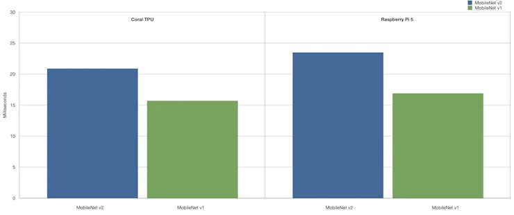
For more info, please see the complete article: Benchmarking TensorFlow and TensorFlow Lite on Raspberry Pi 5.

Raspberry Pi Active Cooler

We suggest installing an Active Cooler, a dedicated clip-on cooling solution for Raspberry Pi 5 (Raspi-5), for this lab. It combines an aluminum heatsink with a temperature-controlled blower fan to keep the Raspi-5 operating comfortably under heavy loads, such as running SLMs.

The Active Cooler has pre-applied thermal pads for heat transfer and is mounted directly to the Raspberry Pi 5 board using spring-loaded push pins. The Raspberry Pi firmware actively manages it: at 60°C, the blower’s fan will be turned on; at 67.5°C, the fan speed will be increased; and finally, at 75°C, the fan increases to full speed. The blower’s fan will spin down automatically when the temperature drops below these limits.

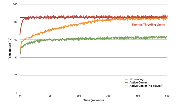
To prevent overheating, all Raspberry Pi boards begin to throttle the processor when the temperature reaches 80°Cand throttle even further when it reaches the maximum temperature of 85°C (more detail here).

Generative AI (GenAI)

Generative AI is an artificial intelligence system capable of creating new, original content across various mediums such as text, images, audio, and video. These systems learn patterns from existing data and use that knowledge to generate novel outputs that didn’t previously exist. Large Language Models (LLMs), Small Language Models (SLMs), and multimodal models can all be considered types of GenAI when used for generative tasks.

GenAI provides the conceptual framework for AI-driven content creation, with LLMs serving as powerful general-purpose text generators. SLMs adapt this technology for edge computing, while multimodal models extend GenAI capabilities across different data types. Together, they represent a spectrum of generative AI technologies, each with its strengths and applications, collectively driving AI-powered content creation and understanding.

Large Language Models (LLMs)

Large Language Models (LLMs) are advanced artificial intelligence systems that understand, process, and generate human-like text. These models are characterized by their massive scale in terms of the amount of data they are trained on and the number of parameters they contain. Critical aspects of LLMs include:

Size: LLMs typically contain billions of parameters. For example, GPT-3 has 175 billion parameters, while some newer models exceed a trillion parameters.
Training Data: They are trained on vast amounts of text data, often including books, websites, and other diverse sources, amounting to hundreds of gigabytes or even terabytes of text.
Architecture: Most LLMs use transformer-based architectures, which allow them to process and generate text by paying attention to different parts of the input simultaneously.
Capabilities: LLMs can perform a wide range of language tasks without specific fine-tuning, including:
- Text generation
- Translation
- Summarization
- Question answering
- Code generation
- Logical reasoning
Few-shot Learning: They can often understand and perform new tasks with minimal examples or instructions.
Resource-Intensive: Due to their size, LLMs typically require significant computational resources to run, often needing powerful GPUs or TPUs.
Continual Development: The field of LLMs is rapidly evolving, with new models and techniques constantly emerging.
Ethical Considerations: The use of LLMs raises important questions about bias, misinformation, and the environmental impact of training such large models.
Applications: LLMs are used in various fields, including content creation, customer service, research assistance, and software development.
Limitations: Despite their power, LLMs can produce incorrect or biased information and lack true understanding or reasoning capabilities.

We must note that we use large models beyond text, calling them multi-modal models. These models integrate and process information from multiple types of input simultaneously. They are designed to understand and generate content across various forms of data, such as text, images, audio, and video.

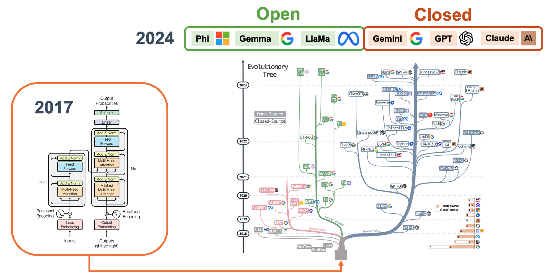
Certainly. Let’s define open and closed models in the context of AI and language models:

Closed vs Open Models:

Closed models, also called proprietary models, are AI models whose internal workings, code, and training data are not publicly disclosed. Examples: GPT-4 (by OpenAI), Claude (by Anthropic), Gemini (by Google).

Open models, also known as open-source models, are AI models whose underlying code, architecture, and often training data are publicly available and accessible. Examples: Gemma (by Google), LLaMA (by Meta) and Phi (by Microsoft).

Open models are particularly relevant for running models on edge devices like Raspberry Pi as they can be more easily adapted, optimized, and deployed in resource-constrained environments. Still, it is crucial to verify their Licenses. Open models come with various open-source licenses that may affect their use in commercial applications, while closed models have clear, albeit restrictive, terms of service.

Adapted from https://arxiv.org/pdf/2304.13712

Small Language Models (SLMs)

In the context of edge computing on devices like Raspberry Pi, full-scale LLMs are typically too large and resource-intensive to run directly. This limitation has driven the development of smaller, more efficient models, such as the Small Language Models (SLMs).

SLMs are compact versions of LLMs designed to run efficiently on resource-constrained devices such as smartphones, IoT devices, and single-board computers like the Raspberry Pi. These models are significantly smaller in size and computational requirements than their larger counterparts while still retaining impressive language understanding and generation capabilities.

Key characteristics of SLMs include:

Reduced parameter count: Typically ranging from a few hundred million to a few billion parameters, compared to two-digit billions in larger models.
Lower memory footprint: Requiring, at most, a few gigabytes of memory rather than tens or hundreds of gigabytes.
Faster inference time: Can generate responses in milliseconds to seconds on edge devices.
Energy efficiency: Consuming less power, making them suitable for battery-powered devices.
Privacy-preserving: Enabling on-device processing without sending data to cloud servers.
Offline functionality: Operating without an internet connection.

SLMs achieve their compact size through various techniques such as knowledge distillation, model pruning, and quantization. While they may not match the broad capabilities of larger models, SLMs excel in specific tasks and domains, making them ideal for targeted applications on edge devices.

We will generally consider SLMs, language models with less than 5 billion parameters quantized to 4 bits.

Examples of SLMs include compressed versions of models like Meta Llama, Microsoft PHI, and Google Gemma. These models enable a wide range of natural language processing tasks directly on edge devices, from text classification and sentiment analysis to question answering and limited text generation.

For more information on SLMs, the paper, LLM Pruning and Distillation in Practice: The Minitron Approach, provides an approach applying pruning and distillation to obtain SLMs from LLMs. And, SMALL LANGUAGE MODELS: SURVEY, MEASUREMENTS, AND INSIGHTS, presents a comprehensive survey and analysis of Small Language Models (SLMs), which are language models with 100 million to 5 billion parameters designed for resource-constrained devices.

Ollama

ollama logo

Ollama is an open-source framework that allows us to run language models (LMs), large or small, locally on our machines. Here are some critical points about Ollama:

Local Model Execution: Ollama enables running LMs on personal computers or edge devices such as the Raspi-5, eliminating the need for cloud-based API calls.
Ease of Use: It provides a simple command-line interface for downloading, running, and managing different language models.
Model Variety: Ollama supports various LLMs, including Phi, Gemma, Llama, Mistral, and other open-source models.
Customization: Users can create and share custom models tailored to specific needs or domains.
Lightweight: Designed to be efficient and run on consumer-grade hardware.
API Integration: Offers an API that allows integration with other applications and services.
Privacy-Focused: By running models locally, it addresses privacy concerns associated with sending data to external servers.
Cross-Platform: Available for macOS, Windows, and Linux systems (our case, here).
Active Development: Regularly updated with new features and model support.
Community-Driven: Benefits from community contributions and model sharing.

To learn more about what Ollama is and how it works under the hood, you should see this short video from Matt Williams, one of the founders of Ollama:

Matt has an entirely free course about Ollama that we recommend:

Installing Ollama

Let’s set up and activate a Virtual Environment for working with Ollama:

python3 -m venv ~/ollama
source ~/ollama/bin/activate

And run the command to install Ollama:

curl -fsSL https://ollama.com/install.sh | sh

As a result, an API will run in the background on 127.0.0.1:11434. From now on, we can run Ollama via the terminal. For starting, let’s verify the Ollama version, which will also tell us that it is correctly installed:

ollama -v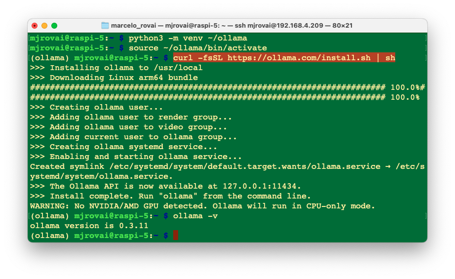

On the Ollama Library page, we can find the models Ollama supports. For example, by filtering by Most popular, we can see Meta Llama, Google Gemma, Microsoft Phi, LLaVa, etc.

Meta Llama 3.2 1B/3B

Let’s install and run our first small language model, Llama 3.2 1B (and 3B). The Meta Llama 3.2 series comprises a set of multilingual generative language models available in 1 billion and 3 billion parameter sizes. These models are designed to process text input and generate text output. The instruction-tuned variants within this collection are specifically optimized for multilingual conversational applications, including tasks involving information retrieval and summarization with an agentic approach. When compared to many existing open-source and proprietary chat models, the Llama 3.2 instruction-tuned models demonstrate superior performance on widely-used industry benchmarks.

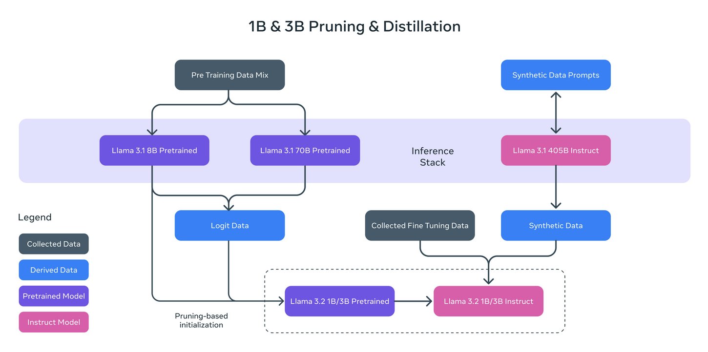
The 1B and 3B models were pruned from the Llama 8B, and then logits from the 8B and 70B models were used as token-level targets (token-level distillation). Knowledge distillation was used to recover performance (they were trained with 9 trillion tokens). The 1B model has 1,24B, quantized to integer (Q8_0), and the 3B, 3.12B parameters, with a Q4_0 quantization, which ends with a size of 1.3 GB and 2GB, respectively. Its context window is 131,072 tokens.

Install and run the Model

ollama run llama3.2:1b

Running the model with the command before, we should have the Ollama prompt available for us to input a question and start chatting with the LLM model; for example,

>>> What is the capital of France?

Almost immediately, we get the correct answer:

The capital of France is Paris.

Using the option --verbose when calling the model will generate several statistics about its performance (The model will be polling only the first time we run the command).

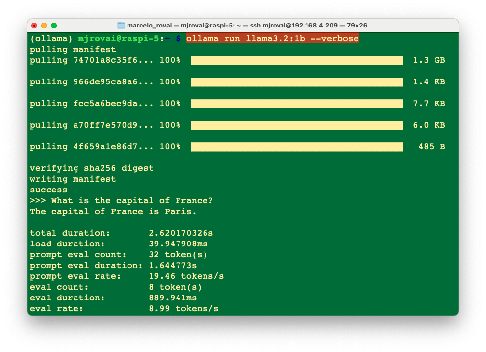
Each metric gives insights into how the model processes inputs and generates outputs. Here’s a breakdown of what each metric means:

Total Duration (2.620170326s): This is the complete time taken from the start of the command to the completion of the response. It encompasses loading the model, processing the input prompt, and generating the response.
Load Duration (39.947908ms): This duration indicates the time to load the model or necessary components into memory. If this value is minimal, it can suggest that the model was preloaded or that only a minimal setup was required.
Prompt Eval Count (32 tokens): The number of tokens in the input prompt. In NLP, tokens are typically words or subwords, so this count includes all the tokens that the model evaluated to understand and respond to the query.
Prompt Eval Duration (1.644773s): This measures the model’s time to evaluate or process the input prompt. It accounts for the bulk of the total duration, implying that understanding the query and preparing a response is the most time-consuming part of the process.
Prompt Eval Rate (19.46 tokens/s): This rate indicates how quickly the model processes tokens from the input prompt. It reflects the model’s speed in terms of natural language comprehension.
Eval Count (8 token(s)): This is the number of tokens in the model’s response, which in this case was, “The capital of France is Paris.”
Eval Duration (889.941ms): This is the time taken to generate the output based on the evaluated input. It’s much shorter than the prompt evaluation, suggesting that generating the response is less complex or computationally intensive than understanding the prompt.
Eval Rate (8.99 tokens/s): Similar to the prompt eval rate, this indicates the speed at which the model generates output tokens. It’s a crucial metric for understanding the model’s efficiency in output generation.

This detailed breakdown can help understand the computational demands and performance characteristics of running SLMs like Llama on edge devices like the Raspberry Pi 5. It shows that while prompt evaluation is more time-consuming, the actual generation of responses is relatively quicker. This analysis is crucial for optimizing performance and diagnosing potential bottlenecks in real-time applications.

Loading and running the 3B model, we can see the difference in performance for the same prompt;

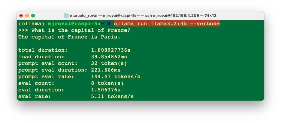
The eval rate is lower, 5.3 tokens/s versus 9 tokens/s with the smaller model.

When question about

>>> What is the distance between Paris and Santiago, Chile?

The 1B model answered 9,841 kilometers (6,093 miles), which is inaccurate, and the 3B model answered 7,300 miles (11,700 km), which is close to the correct (11,642 km).

Let’s ask for the Paris’s coordinates:

>>> what is the latitude and longitude of Paris?

The latitude and longitude of Paris are 48.8567° N (48°55' 
42" N) and 2.3510° E (2°22' 8" E), respectively.

Both 1B and 3B models gave correct answers.

Google Gemma 2 2B

Let’s install Gemma 2, a high-performing and efficient model available in three sizes: 2B, 9B, and 27B. We will install Gemma 2 2B, a lightweight model trained with 2 trillion tokens that produces outsized results by learning from larger models through distillation. The model has 2.6 billion parameters and a Q4_0 quantization, which ends with a size of 1.6 GB. Its context window is 8,192 tokens.

Install and run the Model

ollama run gemma2:2b --verbose

Running the model with the command before, we should have the Ollama prompt available for us to input a question and start chatting with the LLM model; for example,

>>> What is the capital of France?

Almost immediately, we get the correct answer:

The capital of France is **Paris**. 🗼

And it’ statistics.

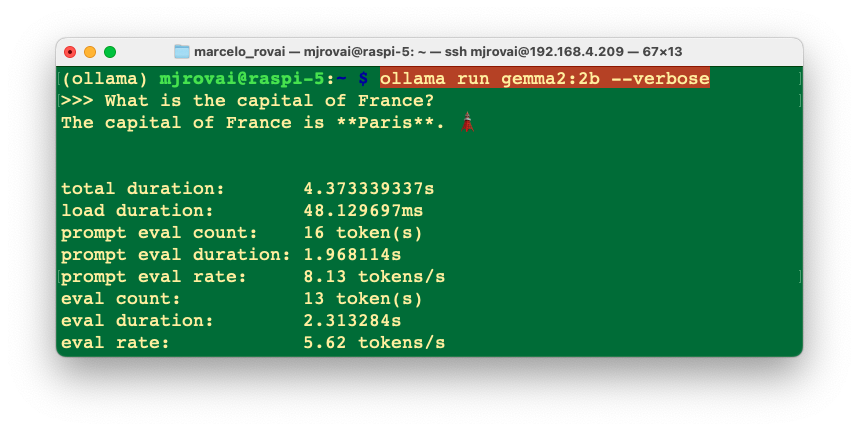
We can see that Gemma 2:2B has around the same performance as Lama 3.2:3B, but having less parameters.

Other examples:

>>> What is the distance between Paris and Santiago, Chile?

The distance between Paris, France and Santiago, Chile is 
approximately **7,000 miles (11,267 kilometers)**. 

Keep in mind that this is a straight-line distance, and actual 
travel distance can vary depending on the chosen routes and any 
stops along the way. ✈️`

Also, a good response but less accurate than Llama3.2:3B.

>>> what is the latitude and longitude of Paris?

You got it! Here are the latitudes and longitudes of Paris, 
France:

* **Latitude:** 48.8566° N (north)
* **Longitude:** 2.3522° E (east) 

Let me know if you'd like to explore more about Paris or its 
location! 🗼🇫🇷

A good and accurate answer (a little more verbose than the Llama answers).

Microsoft Phi3.5 3.8B

Let’s pull a bigger (but still tiny) model, the PHI3.5, a 3.8B lightweight state-of-the-art open model by Microsoft. The model belongs to the Phi-3 model family and supports 128K token context length and the languages: Arabic, Chinese, Czech, Danish, Dutch, English, Finnish, French, German, Hebrew, Hungarian, Italian, Japanese, Korean, Norwegian, Polish, Portuguese, Russian, Spanish, Swedish, Thai, Turkish and Ukrainian.

The model size, in terms of bytes, will depend on the specific quantization format used. The size can go from 2-bit quantization (q2_k) of 1.4GB (higher performance/lower quality) to 16-bit quantization (fp-16) of 7.6GB (lower performance/higher quality).

Let’s run the 4-bit quantization (Q4_0), which will need 2.2GB of RAM, with an intermediary trade-off regarding output quality and performance.

ollama run phi3.5:3.8b --verbose

You can use run or pull to download the model. What happens is that Ollama keeps note of the pulled models, and once the PHI3 does not exist, before running it, Ollama pulls it.

Let’s enter with the same prompt used before:

>>> What is the capital of France?

The capital of France is Paris. It' extradites significant 
historical, cultural, and political importance to the country as 
well as being a major European city known for its art, fashion, 
gastronomy, and culture. Its influence extends beyond national 
borders, with millions of tourists visiting each year from around 
the globe. The Seine River flows through Paris before it reaches 
the broader English Channel at Le Havre. Moreover, France is one 
of Europe's leading economies with its capital playing a key role 

...

The answer was very “verbose”, let’s specify a better prompt:

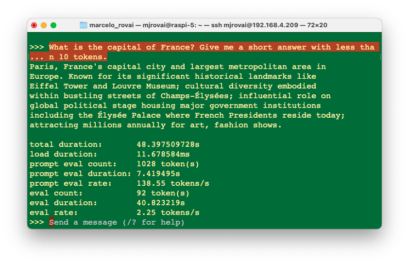
In this case, the answer was still longer than we expected, with an eval rate of 2.25 tokens/s, more than double that of Gemma and Llama.

Choosing the most appropriate prompt is one of the most important skills to be used with LLMs, no matter its size.

When we asked the same questions about distance and Latitude/Longitude, we did not get a good answer for a distance of 13,507 kilometers (8,429 miles), but it was OK for coordinates. Again, it could have been less verbose (more than 200 tokens for each answer).

We can use any model as an assistant since their speed is relatively decent, but on September 24 (2023), the Llama2:3B is a better choice. You should try other models, depending on your needs. 🤗 Open LLM Leaderboard can give you an idea about the best models in size, benchmark, license, etc.

The best model to use is the one fit for your specific necessity. Also, take into consideration that this field evolves with new models everyday.

Multimodal Models

Multimodal models are artificial intelligence (AI) systems that can process and understand information from multiple sources, such as images, text, audio, and video. In our context, multimodal LLMs can process various inputs, including text, images, and audio, as prompts and convert those prompts into various outputs, not just the source type.

We will work here with LLaVA-Phi-3, a fine-tuned LLaVA model from Phi 3 Mini 4k. It has strong performance benchmarks that are on par with the original LLaVA (Large Language and Vision Assistant) model.

The LLaVA-Phi-3 is an end-to-end trained large multimodal model designed to understand and generate content based on visual inputs (images) and textual instructions. It combines the capabilities of a visual encoder and a language model to process and respond to multimodal inputs.

Let’s install the model:

ollama run llava-phi3:3.8b --verbose

Let’s start with a text input:

>>> You are a helpful AI assistant. What is the capital of France?

As an AI language model, I can tell you that the capital of France 
is Paris. It's not only the largest city in the country but also 
serves as its political and administrative center. Paris is known 
for its iconic landmarks such as the Eiffel Tower, Notre-Dame 
Cathedral, and the Louvre Museum. The city has a rich history, 
beautiful architecture, and is widely considered to be one of the 
most romantic cities in the world.

The response took around 30s, with an eval rate of 3.93 tokens/s! Not bad!

But let us know to enter with an image as input. For that, let’s create a directory for working:

cd Documents/
mkdir OLLAMA
cd OLLAMA

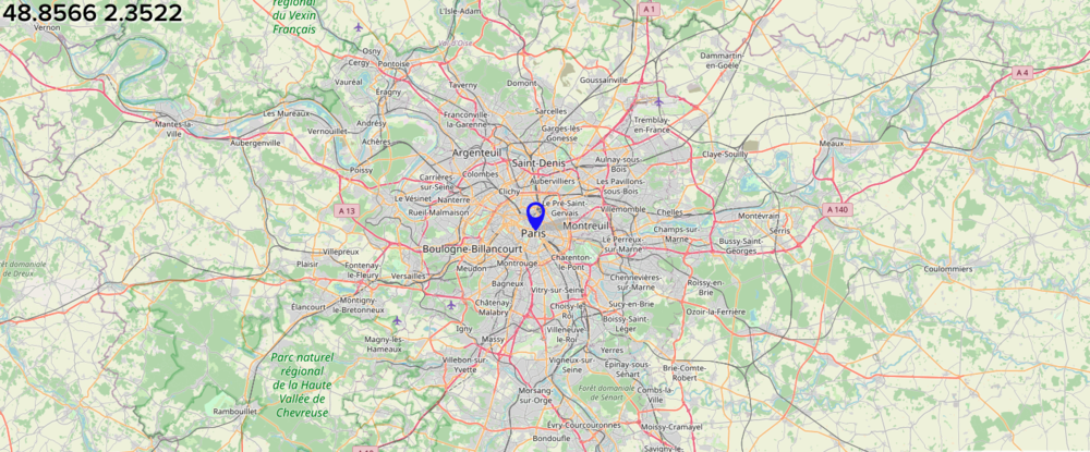
Let’s download a 640x320 image from the internet, for example (Wikipedia: Paris, France):

Using FileZilla, for example, let’s upload the image to the OLLAMA folder at the Raspi-5 and name it image_test_1.jpg. We should have the whole image path (we can use pwd to get it).

/home/mjrovai/Documents/OLLAMA/image_test_1.jpg

If you use a desktop, you can copy the image path by clicking the image with the mouse’s right button.

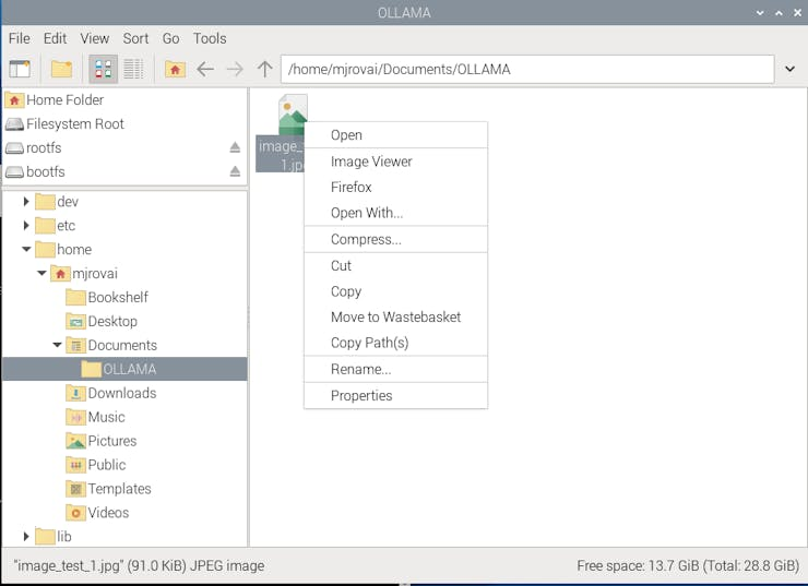
Let’s enter with this prompt:

>>> Describe the image /home/mjrovai/Documents/OLLAMA/image_test_1.jpg

The result was great, but the overall latency was significant; almost 4 minutes to perform the inference.

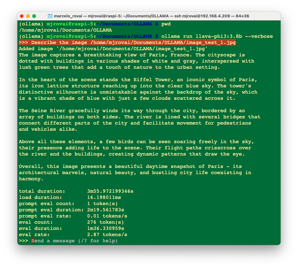
Inspecting local resources

Using htop, we can monitor the resources running on our device.

htop

During the time that the model is running, we can inspect the resources:

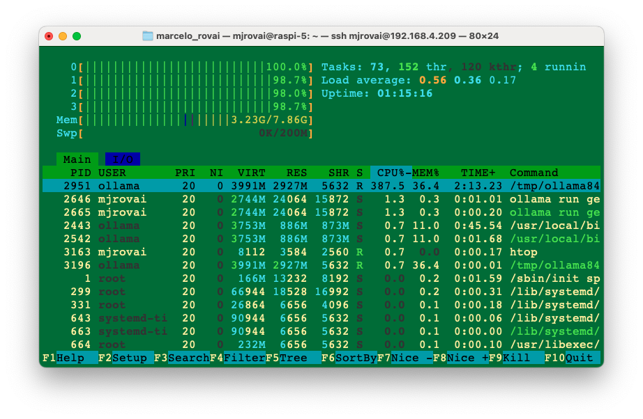
All four CPUs run at almost 100% of their capacity, and the memory used with the model loaded is 3.24GB. Exiting Ollama, the memory goes down to around 377MB (with no desktop).

It is also essential to monitor the temperature. When running the Raspberry with a desktop, you can have the temperature shown on the taskbar:

If you are “headless”, the temperature can be monitored with the command:

vcgencmd measure_temp

If you are doing nothing, the temperature is around 50°C for CPUs running at 1%. During inference, with the CPUs at 100%, the temperature can rise to almost 70°C. This is OK and means the active cooler is working, keeping the temperature below 80°C / 85°C (its limit).

Ollama Python Library

So far, we have explored SLMs’ chat capability using the command line on a terminal. However, we want to integrate those models into our projects, so Python seems to be the right path. The good news is that Ollama has such a library.

The Ollama Python library simplifies interaction with advanced LLM models, enabling more sophisticated responses and capabilities, besides providing the easiest way to integrate Python 3.8+ projects with Ollama.

For a better understanding of how to create apps using Ollama with Python, we can follow Matt Williams’s videos, as the one below:

Installation:

In the terminal, run the command:

pip install ollama

We will need a text editor or an IDE to create a Python script. If you run the Raspberry OS on a desktop, several options, such as Thonny and Geany, have already been installed by default (accessed by [Menu][Programming]). You can download other IDEs, such as Visual Studio Code, from [Menu][Recommended Software]. When the window pops up, go to [Programming], select the option of your choice, and press [Apply].

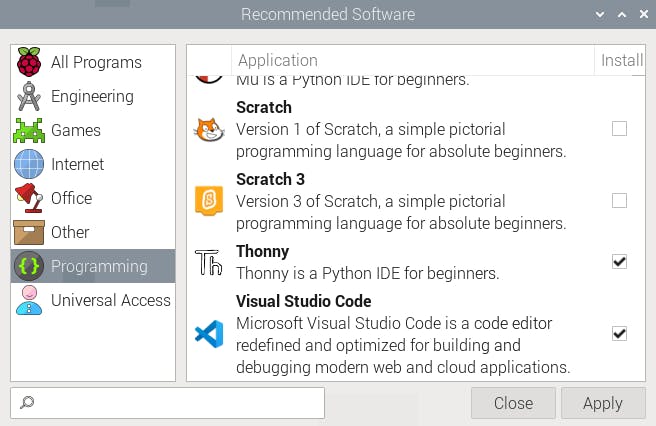
If you prefer using Jupyter Notebook for development:

pip install jupyter
jupyter notebook --generate-config

To run Jupyter Notebook, run the command (change the IP address for yours):

jupyter notebook --ip=192.168.4.209 --no-browser

On the terminal, you can see the local URL address to open the notebook:

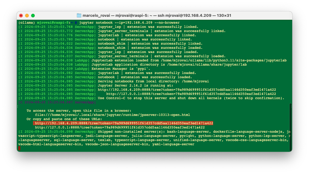
We can access it from another computer by entering the Raspberry Pi’s IP address and the provided token in a web browser (we should copy it from the terminal).

In our working directory in the Raspi, we will create a new Python 3 notebook.

Let’s enter with a very simple script to verify the installed models:

import ollama
ollama.list()

All the models will be printed as a dictionary, for example:

  {'name': 'gemma2:2b',
   'model': 'gemma2:2b',
   'modified_at': '2024-09-24T19:30:40.053898094+01:00',
   'size': 1629518495,
   'digest': '8ccf136fdd5298f3ffe2d69862750ea7fb56555fa4d5b18c04e3fa4d82ee09d7',
   'details': {'parent_model': '',
    'format': 'gguf',
    'family': 'gemma2',
    'families': ['gemma2'],
    'parameter_size': '2.6B',
    'quantization_level': 'Q4_0'}}]}

Let’s repeat one of the questions that we did before, but now using ollama.generate() from Ollama python library. This API will generate a response for the given prompt with the provided model. This is a streaming endpoint, so there will be a series of responses. The final response object will include statistics and additional data from the request.

MODEL = 'gemma2:2b'
PROMPT = 'What is the capital of France?'

res = ollama.generate(model=MODEL, prompt=PROMPT)
print (res)

In case you are running the code as a Python script, you should save it, for example, test_ollama.py. You can use the IDE to run it or do it directly on the terminal. Also, remember that you should always call the model and define it when running a stand-alone script.

python test_ollama.py

As a result, we will have the model response in a JSON format:

{'model': 'gemma2:2b', 'created_at': '2024-09-25T14:43:31.869633807Z', 
'response': 'The capital of France is **Paris**. 🇫🇷 \n', 'done': True, 
'done_reason': 'stop', 'context': [106, 1645, 108, 1841, 603, 573, 6037, 576,
6081, 235336, 107, 108, 106, 2516, 108, 651, 6037, 576, 6081, 603, 5231, 29437, 
168428, 235248, 244304, 241035, 235248, 108], 'total_duration': 24259469458, 
'load_duration': 19830013859, 'prompt_eval_count': 16, 'prompt_eval_duration': 
1908757000, 'eval_count': 14, 'eval_duration': 2475410000}

As we can see, several pieces of information are generated, such as:

response: the main output text generated by the model in response to our prompt.
- The capital of France is **Paris**. 🇫🇷
context: the token IDs representing the input and context used by the model. Tokens are numerical representations of text used for processing by the language model.
- [106, 1645, 108, 1841, 603, 573, 6037, 576, 6081, 235336, 107, 108, 106, 2516, 108, 651, 6037, 576, 6081, 603, 5231, 29437, 168428, 235248, 244304, 241035, 235248, 108]

The Performance Metrics:

total_duration: The total time taken for the operation in nanoseconds. In this case, approximately 24.26 seconds.
load_duration: The time taken to load the model or components in nanoseconds. About 19.83 seconds.
prompt_eval_duration: The time taken to evaluate the prompt in nanoseconds. Around 16 nanoseconds.
eval_count: The number of tokens evaluated during the generation. Here, 14 tokens.
eval_duration: The time taken for the model to generate the response in nanoseconds. Approximately 2.5 seconds.

But, what we want is the plain ‘response’ and, perhaps for analysis, the total duration of the inference, so let’s change the code to extract it from the dictionary:

print(f"\n{res['response']}")
print(f"\n [INFO] Total Duration: {(res['total_duration']/1e9):.2f} seconds")

Now, we got:

The capital of France is **Paris**. 🇫🇷 

 [INFO] Total Duration: 24.26 seconds

Using Ollama.chat()

Another way to get our response is to use ollama.chat(), which generates the next message in a chat with a provided model. This is a streaming endpoint, so a series of responses will occur. Streaming can be disabled using "stream": false. The final response object will also include statistics and additional data from the request.

PROMPT_1 = 'What is the capital of France?'

response = ollama.chat(model=MODEL, messages=[
{'role': 'user','content': PROMPT_1,},])
resp_1 = response['message']['content']
print(f"\n{resp_1}")
print(f"\n [INFO] Total Duration: {(res['total_duration']/1e9):.2f} seconds")

The answer is the same as before.

An important consideration is that by using ollama.generate(), the response is “clear” from the model’s “memory” after the end of inference (only used once), but If we want to keep a conversation, we must use ollama.chat(). Let’s see it in action:

PROMPT_1 = 'What is the capital of France?'
response = ollama.chat(model=MODEL, messages=[
{'role': 'user','content': PROMPT_1,},])
resp_1 = response['message']['content']
print(f"\n{resp_1}")
print(f"\n [INFO] Total Duration: {(response['total_duration']/1e9):.2f} seconds")

PROMPT_2 = 'and of Italy?'
response = ollama.chat(model=MODEL, messages=[
{'role': 'user','content': PROMPT_1,},
{'role': 'assistant','content': resp_1,},
{'role': 'user','content': PROMPT_2,},])
resp_2 = response['message']['content']
print(f"\n{resp_2}")
print(f"\n [INFO] Total Duration: {(response['total_duration']/1e9):.2f} seconds")

In the above code, we are running two queries, and the second prompt considers the result of the first one.

Here is how the model responded:

The capital of France is **Paris**. 🇫🇷 

 [INFO] Total Duration: 2.82 seconds

The capital of Italy is **Rome**. 🇮🇹 

 [INFO] Total Duration: 4.46 seconds

Getting an image description:

In the same way that we have used the LlaVa-PHI-3 model with the command line to analyze an image, the same can be done here with Python. Let’s use the same image of Paris, but now with the ollama.generate():

MODEL = 'llava-phi3:3.8b'
PROMPT = "Describe this picture"

with open('image_test_1.jpg', 'rb') as image_file:
    img = image_file.read()

response = ollama.generate(
    model=MODEL,
    prompt=PROMPT,
    images= [img]
)
print(f"\n{response['response']}")
print(f"\n [INFO] Total Duration: {(res['total_duration']/1e9):.2f} seconds")

Here is the result:

This image captures the iconic cityscape of Paris, France. The vantage point 
is high, providing a panoramic view of the Seine River that meanders through 
the heart of the city. Several bridges arch gracefully over the river, 
connecting different parts of the city. The Eiffel Tower, an iron lattice 
structure with a pointed top and two antennas on its summit, stands tall in the 
background, piercing the sky. It is painted in a light gray color, contrasting 
against the blue sky speckled with white clouds.

The buildings that line the river are predominantly white or beige, their uniform
color palette broken occasionally by red roofs peeking through. The Seine River 
itself appears calm and wide, reflecting the city's architectural beauty in its 
surface. On either side of the river, trees add a touch of green to the urban 
landscape.

The image is taken from an elevated perspective, looking down on the city. This 
viewpoint allows for a comprehensive view of Paris's beautiful architecture and 
layout. The relative positions of the buildings, bridges, and other structures 
create a harmonious composition that showcases the city's charm.

In summary, this image presents a serene day in Paris, with its architectural 
marvels - from the Eiffel Tower to the river-side buildings - all bathed in soft 
colors under a clear sky.

 [INFO] Total Duration: 256.45 seconds

The model took about 4 minutes (256.45 s) to return with a detailed image description.

In the 10-Ollama_Python_Library notebook, it is possible to find the experiments with the Ollama Python library.

Function Calling

So far, we can observe that by using the model’s response into a variable, we can effectively incorporate it into real-world projects. However, a major issue arises when the model provides varying responses to the same input. For instance, let’s assume that we only need the name of a country’s capital and its coordinates as the model’s response in the previous examples, without any additional information, even when utilizing verbose models like Microsoft Phi. To ensure consistent responses, we can employ the ‘Ollama function call,’ which is fully compatible with the OpenAI API.

But what exactly is “function calling”?

In modern artificial intelligence, function calling with Large Language Models (LLMs) allows these models to perform actions beyond generating text. By integrating with external functions or APIs, LLMs can access real-time data, automate tasks, and interact with various systems.

For instance, instead of merely responding to a query about the weather, an LLM can call a weather API to fetch the current conditions and provide accurate, up-to-date information. This capability enhances the relevance and accuracy of the model’s responses and makes it a powerful tool for driving workflows and automating processes, transforming it into an active participant in real-world applications.

For more details about Function Calling, please see this video made by Marvin Prison:

Let’s create a project.

We want to create an app where the user enters a country’s name and gets, as an output, the distance in km from the capital city of such a country and the app’s location (for simplicity, We will use Santiago, Chile, as the app location).

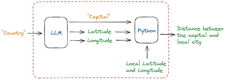
Once the user enters a country name, the model will return the name of its capital city (as a string) and the latitude and longitude of such city (in float). Using those coordinates, we can use a simple Python library (haversine) to calculate the distance between those 2 points.

The idea of this project is to demonstrate a combination of language model interaction, structured data handling with Pydantic, and geospatial calculations using the Haversine formula (traditional computing).

First, let us install some libraries. Besides Haversine, the main one is the OpenAI Python library, which provides convenient access to the OpenAI REST API from any Python 3.7+ application. The other one is Pydantic (and instructor), a robust data validation and settings management library engineered by Python to enhance the robustness and reliability of our codebase. In short, Pydantic will help ensure that our model’s response will always be consistent.

pip install haversine
pip install openai 
pip install pydantic 
pip install instructor

Now, we should create a Python script designed to interact with our model (LLM) to determine the coordinates of a country’s capital city and calculate the distance from Santiago de Chile to that capital.

Let’s go over the code:

1. Importing Libraries

import sys
from haversine import haversine
from openai import OpenAI
from pydantic import BaseModel, Field
import instructor

sys: Provides access to system-specific parameters and functions. It’s used to get command-line arguments.
haversine: A function from the haversine library that calculates the distance between two geographic points using the Haversine formula.
openAI: A module for interacting with the OpenAI API (although it’s used in conjunction with a local setup, Ollama). Everything is off-line here.
pydantic: Provides data validation and settings management using Python-type annotations. It’s used to define the structure of expected response data.
instructor: A module is used to patch the OpenAI client to work in a specific mode (likely related to structured data handling).

2. Defining Input and Model

country = sys.argv[1]       # Get the country from command-line arguments
MODEL = 'phi3.5:3.8b'     # The name of the model to be used
mylat = -33.33              # Latitude of Santiago de Chile
mylon = -70.51              # Longitude of Santiago de Chile

country: On a Python script, getting the country name from command-line arguments is possible. On a Jupyter notebook, we can enter its name, for example,
- country = "France"
MODEL: Specifies the model being used, which is, in this example, the phi3.5.
mylat and mylon: Coordinates of Santiago de Chile, used as the starting point for the distance calculation.

3. Defining the Response Data Structure

class CityCoord(BaseModel):
    city: str = Field(..., description="Name of the city")
    lat: float = Field(..., description="Decimal Latitude of the city")
    lon: float = Field(..., description="Decimal Longitude of the city")

CityCoord: A Pydantic model that defines the expected structure of the response from the LLM. It expects three fields: city (name of the city), lat (latitude), and lon (longitude).

4. Setting Up the OpenAI Client

client = instructor.patch(
    OpenAI(
        base_url="http://localhost:11434/v1",  # Local API base URL (Ollama)
        api_key="ollama",                      # API key (not used)
    ),
    mode=instructor.Mode.JSON,                 # Mode for structured JSON output
)

OpenAI: This setup initializes an OpenAI client with a local base URL and an API key (ollama). It uses a local server.
instructor.patch: Patches the OpenAI client to work in JSON mode, enabling structured output that matches the Pydantic model.

5. Generating the Response

resp = client.chat.completions.create(
    model=MODEL,
    messages=[
        {
            "role": "user",
            "content": f"return the decimal latitude and decimal longitude \
            of the capital of the {country}."
        }
    ],
    response_model=CityCoord,
    max_retries=10
)

client.chat.completions.create: Calls the LLM to generate a response.
model: Specifies the model to use (llava-phi3).
messages: Contains the prompt for the LLM, asking for the latitude and longitude of the capital city of the specified country.
response_model: Indicates that the response should conform to the CityCoord model.
max_retries: The maximum number of retry attempts if the request fails.

6. Calculating the Distance

distance = haversine((mylat, mylon), (resp.lat, resp.lon), unit='km')
print(f"Santiago de Chile is about {int(round(distance, -1)):,} \
        kilometers away from {resp.city}.")

haversine: Calculates the distance between Santiago de Chile and the capital city returned by the LLM using their respective coordinates.
(mylat, mylon): Coordinates of Santiago de Chile.
resp.city: Name of the country’s capital
(resp.lat, resp.lon): Coordinates of the capital city are provided by the LLM response.
unit=‘km’: Specifies that the distance should be calculated in kilometers.
print: Outputs the distance, rounded to the nearest 10 kilometers, with thousands of separators for readability.

Running the code

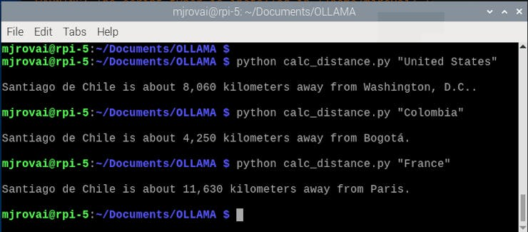
If we enter different countries, for example, France, Colombia, and the United States, We can note that we always receive the same structured information:

Santiago de Chile is about 8,060 kilometers away from Washington, D.C..
Santiago de Chile is about 4,250 kilometers away from Bogotá.
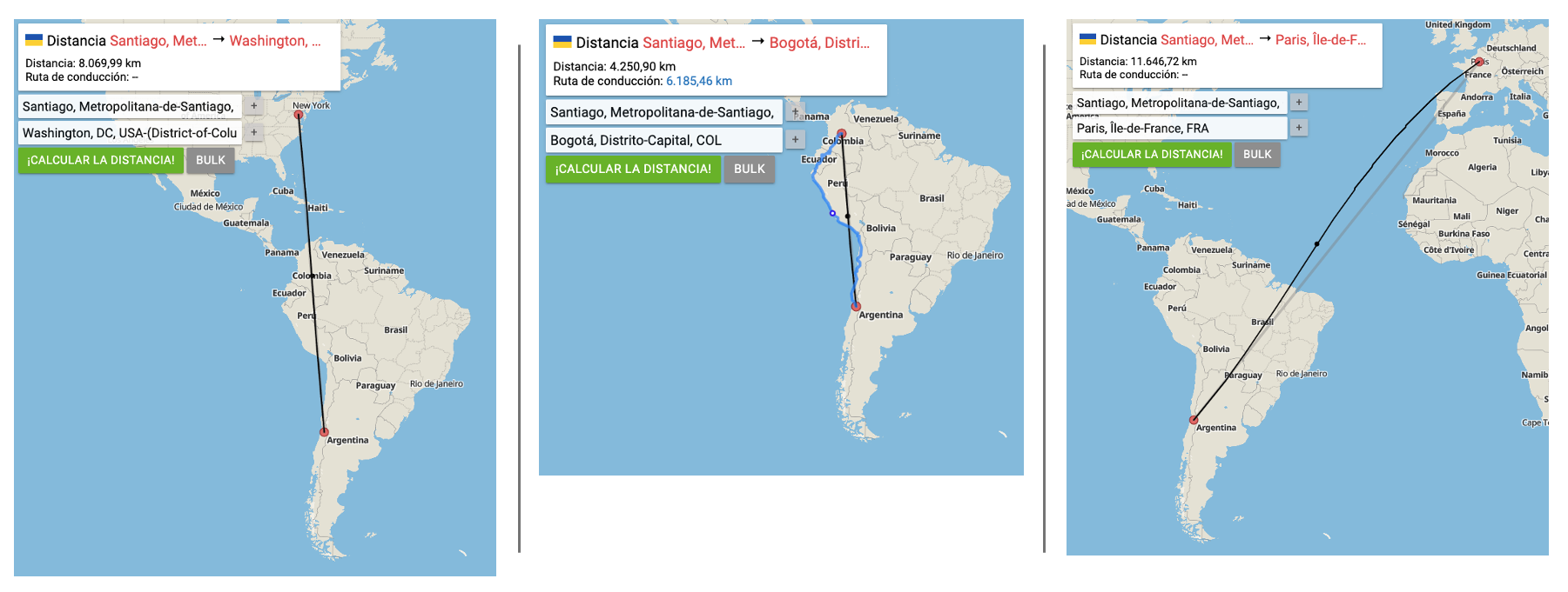
Santiago de Chile is about 11,630 kilometers away from Paris.

If you run the code as a script, the result will be printed on the terminal:

And the calculations are pretty good!

In the 20-Ollama_Function_Calling notebook, it is possible to find experiments with all models installed.

Adding images

Now it is time to wrap up everything so far! Let’s modify the script so that instead of entering the country name (as a text), the user enters an image, and the application (based on SLM) returns the city in the image and its geographic location. With those data, we can calculate the distance as before.

For simplicity, we will implement this new code in two steps. First, the LLM will analyze the image and create a description (text). This text will be passed on to another instance, where the model will extract the information needed to pass along.

We will start importing the libraries

import sys
import time
from haversine import haversine
import ollama
from openai import OpenAI
from pydantic import BaseModel, Field
import instructor

We can see the image if you run the code on the Jupyter Notebook. For that we need also import:

import matplotlib.pyplot as plt
from PIL import Image

Those libraries are unnecessary if we run the code as a script.

Now, we define the model and the local coordinates:

MODEL = 'llava-phi3:3.8b'
mylat = -33.33
mylon = -70.51

We can download a new image, for example, Machu Picchu from Wikipedia. On the Notebook we can see it:

# Load the image
img_path = "image_test_3.jpg"
img = Image.open(img_path)

# Display the image
plt.figure(figsize=(8, 8))
plt.imshow(img)
plt.axis('off')
#plt.title("Image")
plt.show()

Now, let’s define a function that will receive the image and will return the decimal latitude and decimal longitude of the city in the image, its name, and what country it is located

def image_description(img_path):
    with open(img_path, 'rb') as file:
        response = ollama.chat(
            model=MODEL,
            messages=[
              {
                'role': 'user',
                'content': '''return the decimal latitude and decimal longitude 
                              of the city in the image, its name, and 
                              what country it is located''',
                'images': [file.read()],
              },
            ],
            options = {
              'temperature': 0,
              }
      )
    #print(response['message']['content'])
    return response['message']['content']

We can print the entire response for debug purposes.

The image description generated for the function will be passed as a prompt for the model again.

start_time = time.perf_counter()  # Start timing

class CityCoord(BaseModel):
    city: str = Field(..., description="Name of the city in the image")
    country: str = Field(..., description="""Name of the country where"
                                             the city in the image is located
                                             """)
    lat: float = Field(..., description="""Decimal Latitude of the city in"
                                            the image""")
    lon: float = Field(..., description="""Decimal Longitude of the city in"
                                           the image""")

# enables `response_model` in create call
client = instructor.patch(
    OpenAI(
        base_url="http://localhost:11434/v1",
        api_key="ollama"
    ),
    mode=instructor.Mode.JSON,
)

image_description = image_description(img_path)
# Send this description to the model
resp = client.chat.completions.create(
    model=MODEL,
    messages=[
        {
            "role": "user",
            "content": image_description,
        }
    ],
    response_model=CityCoord,
    max_retries=10,
    temperature=0,
)

If we print the image description , we will get:

The image shows the ancient city of Machu Picchu, located in Peru. The city is
perched on a steep hillside and consists of various structures made of stone. It 
is surrounded by lush greenery and towering mountains. The sky above is blue with
scattered clouds. 

Machu Picchu's latitude is approximately 13.5086° S, and its longitude is around
72.5494° W.

And the second response from the model (resp) will be:

CityCoord(city='Machu Picchu', country='Peru', lat=-13.5086, lon=-72.5494)

Now, we can do a “Post-Processing”, calculating the distance and preparing the final answer:

distance = haversine((mylat, mylon), (resp.lat, resp.lon), unit='km')

print(f"\n The image shows {resp.city}, with lat:{round(resp.lat, 2)} and \
      long: {round(resp.lon, 2)}, located in {resp.country} and about \
            {int(round(distance, -1)):,} kilometers away from \
            Santiago, Chile.\n")

end_time = time.perf_counter()  # End timing
elapsed_time = end_time - start_time  # Calculate elapsed time
print(f" [INFO] ==> The code (running {MODEL}), took {elapsed_time:.1f} \
      seconds to execute.\n")

And we will get:

 The image shows Machu Picchu, with lat:-13.16 and long: -72.54, located in Peru
 and about 2,250 kilometers away from Santiago, Chile.

 [INFO] ==> The code (running llava-phi3:3.8b), took 491.3 seconds to execute.

In the 30-Function_Calling_with_images notebook, it is possible to find the experiments with multiple images.

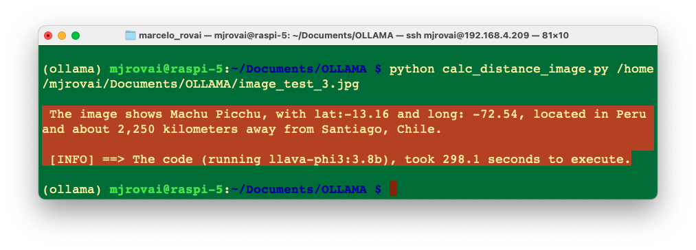
Let’s now download the script calc_distance_image.py from the GitHub and run it on the terminal with the command:

python calc_distance_image.py /home/mjrovai/Documents/OLLAMA/image_test_3.jpg

Enter with the Machu Picchu image full patch as an argument. We will get the same previous result.

How about Paris?

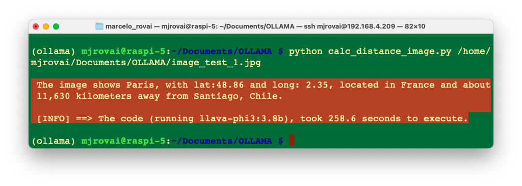
Of course, there are many ways to optimize the code used here. Still, the idea is to explore the considerable potential of function calling with SLMs at the edge, allowing those models to integrate with external functions or APIs. Going beyond text generation, SLMs can access real-time data, automate tasks, and interact with various systems.

SLMs: Optimization Techniques

Large Language Models (LLMs) have revolutionized natural language processing, but their deployment and optimization come with unique challenges. One significant issue is the tendency for LLMs (and more, the SLMs) to generate plausible-sounding but factually incorrect information, a phenomenon known as hallucination. This occurs when models produce content that seems coherent but is not grounded in truth or real-world facts.

Other challenges include the immense computational resources required for training and running these models, the difficulty in maintaining up-to-date knowledge within the model, and the need for domain-specific adaptations. Privacy concerns also arise when handling sensitive data during training or inference. Additionally, ensuring consistent performance across diverse tasks and maintaining ethical use of these powerful tools present ongoing challenges. Addressing these issues is crucial for the effective and responsible deployment of LLMs in real-world applications.

The fundamental techniques for enhancing LLM (and SLM) performance and efficiency are Fine-tuning, Prompt engineering, and Retrieval-Augmented Generation (RAG).

Fine-tuning, while more resource-intensive, offers a way to specialize LLMs for particular domains or tasks. This process involves further training the model on carefully curated datasets, allowing it to adapt its vast general knowledge to specific applications. Fine-tuning can lead to substantial improvements in performance, especially in specialized fields or for unique use cases.
Prompt engineering is at the forefront of LLM optimization. By carefully crafting input prompts, we can guide models to produce more accurate and relevant outputs. This technique involves structuring queries that leverage the model’s pre-trained knowledge and capabilities, often incorporating examples or specific instructions to shape the desired response.
Retrieval-Augmented Generation (RAG) represents another powerful approach to improving LLM performance. This method combines the vast knowledge embedded in pre-trained models with the ability to access and incorporate external, up-to-date information. By retrieving relevant data to supplement the model’s decision-making process, RAG can significantly enhance accuracy and reduce the likelihood of generating outdated or false information.

For edge applications, it is more beneficial to focus on techniques like RAG that can enhance model performance without needing on-device fine-tuning. Let’s explore it.

RAG Implementation

In a basic interaction between a user and a language model, the user asks a question, which is sent as a prompt to the model. The model generates a response based solely on its pre-trained knowledge. In a RAG process, there’s an additional step between the user’s question and the model’s response. The user’s question triggers a retrieval process from a knowledge base.

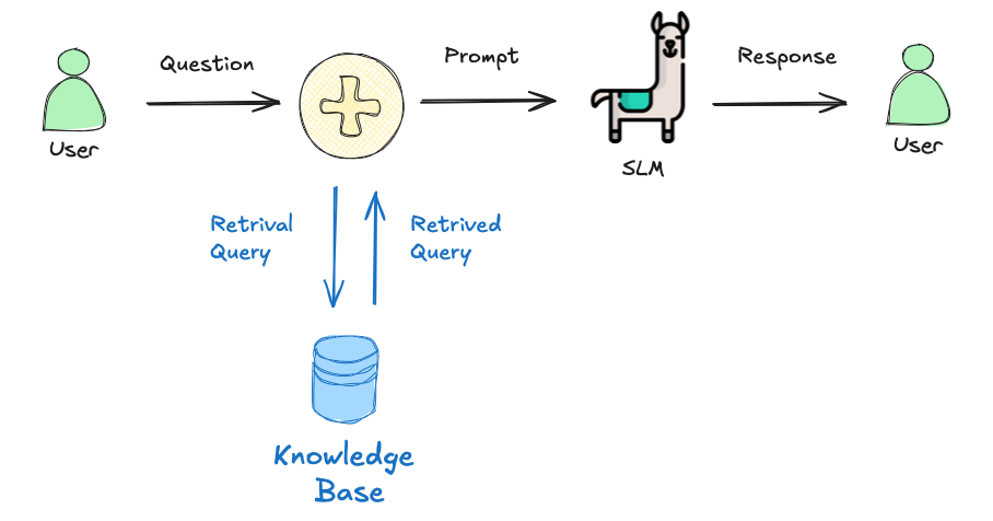
A simple RAG project

Here are the steps to implement a basic Retrieval Augmented Generation (RAG):

Determine the type of documents you’ll be using: The best types are documents from which we can get clean and unobscured text. PDFs can be problematic because they are designed for printing, not for extracting sensible text. To work with PDFs, we should get the source document or use tools to handle it.
Chunk the text: We can’t store the text as one long stream because of context size limitations and the potential for confusion. Chunking involves splitting the text into smaller pieces. Chunk text has many ways, such as character count, tokens, words, paragraphs, or sections. It is also possible to overlap chunks.
Create embeddings: Embeddings are numerical representations of text that capture semantic meaning. We create embeddings by passing each chunk of text through a particular embedding model. The model outputs a vector, the length of which depends on the embedding model used. We should pull one (or more) embedding models from Ollama, to perform this task. Here are some examples of embedding models available at Ollama.

Model Parameter Size Embedding Size

mxbai-embed-large 334M 1024

nomic-embed-text 137M 768

all-minilm 23M 384

Generally, larger embedding sizes capture more nuanced information about the input. Still, they also require more computational resources to process, and a higher number of parameters should increase the latency (but also the quality of the response).
Store the chunks and embeddings in a vector database: We will need a way to efficiently find the most relevant chunks of text for a given prompt, which is where a vector database comes in. We will use Chromadb, an AI-native open-source vector database, which simplifies building RAGs by creating knowledge, facts, and skills pluggable for LLMs. Both the embedding and the source text for each chunk are stored.
Build the prompt: When we have a question, we create an embedding and query the vector database for the most similar chunks. Then, we select the top few results and include their text in the prompt.

Model	Parameter Size	Embedding Size
mxbai-embed-large	334M	1024
nomic-embed-text	137M	768
all-minilm	23M	384

The goal of RAG is to provide the model with the most relevant information from our documents, allowing it to generate more accurate and informative responses. So, let’s implement a simple example of an SLM incorporating a particular set of facts about bees (“Bee Facts”).

Inside the ollama env, enter the command in the terminal for Chromadb instalation:

pip install ollama chromadb

Let’s pull an intermediary embedding model, nomic-embed-text

ollama pull nomic-embed-text

And create a working directory:

cd Documents/OLLAMA/
mkdir RAG-simple-bee
cd RAG-simple-bee/

Let’s create a new Jupyter notebook, 40-RAG-simple-bee for some exploration:

Import the needed libraries:

import ollama
import chromadb
import time

And define aor models:

EMB_MODEL = "nomic-embed-text"
MODEL = 'llama3.2:3B'

Initially, a knowledge base about bee facts should be created. This involves collecting relevant documents and converting them into vector embeddings. These embeddings are then stored in a vector database, allowing for efficient similarity searches later. Enter with the “document,” a base of “bee facts” as a list:

documents = [
    "Bee-keeping, also known as apiculture, involves the maintenance of bee \
    colonies, typically in hives, by humans.",
    "The most commonly kept species of bees is the European honey bee (Apis \
    mellifera).",
    
    ...
    
    "There are another 20,000 different bee species in the world.",  
    "Brazil alone has more than 300 different bee species, and the \
    vast majority, unlike western honey bees, don’t sting.", 
    "Reports written in 1577 by Hans Staden, mention three native bees \
    used by indigenous people in Brazil.",
    "The indigenous people in Brazil used bees for medicine and food purposes",
    "From Hans Staden report: probable species: mandaçaia (Melipona \
    quadrifasciata), mandaguari (Scaptotrigona postica) and jataí-amarela \
    (Tetragonisca angustula)."
]

We do not need to “chunk” the document here because we will use each element of the list and a chunk.

Now, we will create our vector embedding database bee_facts and store the document in it:

client = chromadb.Client()
collection = client.create_collection(name="bee_facts")

# store each document in a vector embedding database
for i, d in enumerate(documents):
  response = ollama.embeddings(model=EMB_MODEL, prompt=d)
  embedding = response["embedding"]
  collection.add(
    ids=[str(i)],
    embeddings=[embedding],
    documents=[d]
  )

Now that we have our “Knowledge Base” created, we can start making queries, retrieving data from it:

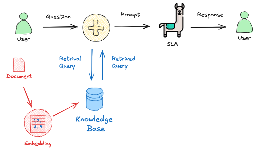
User Query: The process begins when a user asks a question, such as “How many bees are in a colony? Who lays eggs, and how much? How about common pests and diseases?”

prompt = "How many bees are in a colony? Who lays eggs and how much? How about\
          common pests and diseases?"

Query Embedding: The user’s question is converted into a vector embedding using the same embedding model used for the knowledge base.

response = ollama.embeddings(
  prompt=prompt,
  model=EMB_MODEL
)

Relevant Document Retrieval: The system searches the knowledge base using the query embedding to find the most relevant documents (in this case, the 5 more probable). This is done using a similarity search, which compares the query embedding to the document embeddings in the database.

results = collection.query(
  query_embeddings=[response["embedding"]],
  n_results=5
)
data = results['documents']

Prompt Augmentation: The retrieved relevant information is combined with the original user query to create an augmented prompt. This prompt now contains the user’s question and pertinent facts from the knowledge base.

prompt=f"Using this data: {data}. Respond to this prompt: {prompt}",

Answer Generation: The augmented prompt is then fed into a language model, in this case, the llama3.2:3b model. The model uses this enriched context to generate a comprehensive answer. Parameters like temperature, top_k, and top_p are set to control the randomness and quality of the generated response.

output = ollama.generate(
  model=MODEL,
  prompt=f"Using this data: {data}. Respond to this prompt: {prompt}",
  options={
    "temperature": 0.0,
    "top_k":10,
    "top_p":0.5                          }
)

Response Delivery: Finally, the system returns the generated answer to the user.

print(output['response'])

Based on the provided data, here are the answers to your questions:

1. How many bees are in a colony?
A typical bee colony can contain between 20,000 and 80,000 bees.

2. Who lays eggs and how much?
The queen bee lays up to 2,000 eggs per day during peak seasons.

3. What about common pests and diseases?
Common pests and diseases that affect bees include varroa mites, hive beetles,
and foulbrood.

Let’s create a function to help answer new questions:

def rag_bees(prompt, n_results=5, temp=0.0, top_k=10, top_p=0.5):
    start_time = time.perf_counter()  # Start timing
    
    # generate an embedding for the prompt and retrieve the data 
    response = ollama.embeddings(
      prompt=prompt,
      model=EMB_MODEL
    )
    
    results = collection.query(
      query_embeddings=[response["embedding"]],
      n_results=n_results
    )
    data = results['documents']
    
    # generate a response combining the prompt and data retrieved
    output = ollama.generate(
      model=MODEL,
      prompt=f"Using this data: {data}. Respond to this prompt: {prompt}",
      options={
        "temperature": temp,
        "top_k": top_k,
        "top_p": top_p                          }
    )
    
    print(output['response'])
    
    end_time = time.perf_counter()  # End timing
    elapsed_time = round((end_time - start_time), 1)  # Calculate elapsed time
    
    print(f"\n [INFO] ==> The code for model: {MODEL}, took {elapsed_time}s \
          to generate the answer.\n")

We can now create queries and call the function:

prompt = "Are bees in Brazil?"
rag_bees(prompt)

Yes, bees are found in Brazil. According to the data, Brazil has more than 300
different bee species, and indigenous people in Brazil used bees for medicine and
food purposes. Additionally, reports from 1577 mention three native bees used by
indigenous people in Brazil.

 [INFO] ==> The code for model: llama3.2:3b, took 22.7s to generate the answer.

By the way, if the model used supports multiple languages, we can use it (for example, Portuguese), even if the dataset was created in English:

prompt = "Existem abelhas no Brazil?"
rag_bees(prompt)

Sim, existem abelhas no Brasil! De acordo com o relato de Hans Staden, há três 
espécies de abelhas nativas do Brasil que foram mencionadas: mandaçaia (Melipona
quadrifasciata), mandaguari (Scaptotrigona postica) e jataí-amarela (Tetragonisca
angustula). Além disso, o Brasil é conhecido por ter mais de 300 espécies diferentes de abelhas, a maioria das quais não é agressiva e não põe veneno.

 [INFO] ==> The code for model: llama3.2:3b, took 54.6s to generate the answer.

Going Further

The small LLM models tested worked well at the edge, both in text and with images, but of course, they had high latency regarding the last one. A combination of specific and dedicated models can lead to better results; for example, in real cases, an Object Detection model (such as YOLO) can get a general description and count of objects on an image that, once passed to an LLM, can help extract essential insights and actions.

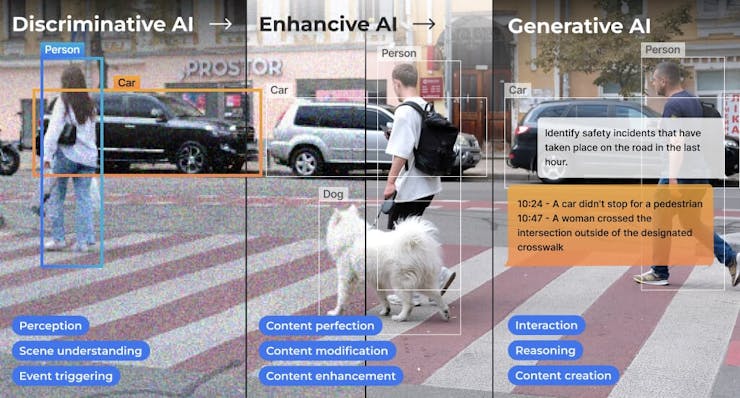
According to Avi Baum, CTO at Hailo,

In the vast landscape of artificial intelligence (AI), one of the most intriguing journeys has been the evolution of AI on the edge. This journey has taken us from classic machine vision to the realms of discriminative AI, enhancive AI, and now, the groundbreaking frontier of generative AI. Each step has brought us closer to a future where intelligent systems seamlessly integrate with our daily lives, offering an immersive experience of not just perception but also creation at the palm of our hand.

Conclusion

This lab has demonstrated how a Raspberry Pi 5 can be transformed into a potent AI hub capable of running large language models (LLMs) for real-time, on-site data analysis and insights using Ollama and Python. The Raspberry Pi’s versatility and power, coupled with the capabilities of lightweight LLMs like Llama 3.2 and LLaVa-Phi-3-mini, make it an excellent platform for edge computing applications.

The potential of running LLMs on the edge extends far beyond simple data processing, as in this lab’s examples. Here are some innovative suggestions for using this project:

1. Smart Home Automation:

Integrate SLMs to interpret voice commands or analyze sensor data for intelligent home automation. This could include real-time monitoring and control of home devices, security systems, and energy management, all processed locally without relying on cloud services.

2. Field Data Collection and Analysis:

Deploy SLMs on Raspberry Pi in remote or mobile setups for real-time data collection and analysis. This can be used in agriculture to monitor crop health, in environmental studies for wildlife tracking, or in disaster response for situational awareness and resource management.

3. Educational Tools:

Create interactive educational tools that leverage SLMs to provide instant feedback, language translation, and tutoring. This can be particularly useful in developing regions with limited access to advanced technology and internet connectivity.

4. Healthcare Applications:

Use SLMs for medical diagnostics and patient monitoring. They can provide real-time analysis of symptoms and suggest potential treatments. This can be integrated into telemedicine platforms or portable health devices.

5. Local Business Intelligence:

Implement SLMs in retail or small business environments to analyze customer behavior, manage inventory, and optimize operations. The ability to process data locally ensures privacy and reduces dependency on external services.

6. Industrial IoT:

Integrate SLMs into industrial IoT systems for predictive maintenance, quality control, and process optimization. The Raspberry Pi can serve as a localized data processing unit, reducing latency and improving the reliability of automated systems.

7. Autonomous Vehicles:

Use SLMs to process sensory data from autonomous vehicles, enabling real-time decision-making and navigation. This can be applied to drones, robots, and self-driving cars for enhanced autonomy and safety.

8. Cultural Heritage and Tourism:

Implement SLMs to provide interactive and informative cultural heritage sites and museum guides. Visitors can use these systems to get real-time information and insights, enhancing their experience without internet connectivity.

9. Artistic and Creative Projects:

Use SLMs to analyze and generate creative content, such as music, art, and literature. This can foster innovative projects in the creative industries and allow for unique interactive experiences in exhibitions and performances.

10. Customized Assistive Technologies:

Develop assistive technologies for individuals with disabilities, providing personalized and adaptive support through real-time text-to-speech, language translation, and other accessible tools.