Robust AI
DALL·E 3 Prompt: Create an image featuring an advanced AI system symbolized by an intricate, glowing neural network, deeply nested within a series of progressively larger and more fortified shields. Each shield layer represents a layer of defense, showcasing the system’s robustness against external threats and internal errors. The neural network, at the heart of this fortress of shields, radiates with connections that signify the AI’s capacity for learning and adaptation. This visual metaphor emphasizes not only the technological sophistication of the AI but also its resilience and security, set against the backdrop of a state-of-the-art, secure server room filled with the latest in technological advancements. The image aims to convey the concept of ultimate protection and resilience in the field of artificial intelligence.

Purpose
How do we develop fault-tolerant and resilient machine learning systems for real-world deployment?
Machine learning systems in real-world applications require fault-tolerant execution across diverse operational conditions. These systems face multiple challenges degrading their capabilities, including hardware anomalies, adversarial attacks, and unpredictable real-world data distributions that diverge from training assumptions. These vulnerabilities require AI systems to prioritize robustness and trustworthiness throughout design and deployment phases. Building resilient machine learning systems requires safe and effective operation in dynamic and uncertain environments. Understanding robustness principles enables engineers to design systems withstanding hardware failures, resisting malicious attacks, and adapting to distribution shifts. This capability enables deploying ML systems in safety-critical applications where failures can have severe consequences, from autonomous vehicles to medical diagnosis systems operating in unpredictable real-world conditions.
Classify hardware faults affecting ML systems into transient, permanent, and intermittent categories with their distinctive characteristics
Analyze how bit flips, memory errors, and component failures propagate through neural network computations to degrade model performance
Compare detection mechanisms for hardware faults including BIST, error detection codes, and redundancy voting systems
Design fault tolerance strategies combining hardware-level protection with software-implemented monitoring for ML deployments
Evaluate adversarial attack vectors including gradient-based, optimization-based, and transfer-based techniques on neural networks
Implement defense strategies against data poisoning attacks through anomaly detection, sanitization, and robust training methods
Assess distribution shift impacts on model accuracy using monitoring techniques and statistical drift detection methods
Integrate robustness principles across the complete ML pipeline from data ingestion through model deployment and monitoring
Introduction to Robust AI Systems
When traditional software fails, it often does so loudly: a server crashes, an application throws an error, users receive clear failure messages. When a machine learning system fails, it often fails silently. A self-driving car’s perception system doesn’t crash; it simply misclassifies a truck as the sky. A demand forecasting model doesn’t error out; it just starts making wildly inaccurate predictions. A medical diagnosis system doesn’t shut down; it quietly provides incorrect classifications that could endanger patient lives. This ‘silent failure’ mode makes robustness a unique and critical challenge in AI systems. Engineers must defend not just against bugs in code, but against a world that refuses to conform to training data.
This silent failure challenge is amplified as ML systems expand across diverse deployment contexts, from cloud-based services to edge devices and embedded systems, where hardware and software faults have pronounced impacts on performance and reliability. The increasing complexity of these systems and their deployment in safety-critical applications1 makes robust and fault-tolerant designs essential for maintaining system integrity.
1 Safety-Critical Applications: Systems where failure could result in loss of life, significant property damage, or environmental harm. Examples include nuclear power plants, aircraft control systems, and medical devices, domains where ML deployment requires the highest reliability standards.
Building on the adaptive deployment challenges introduced in Chapter 14: On-Device Learning and the security vulnerabilities examined in Chapter 15: Security & Privacy, we now turn to comprehensive system reliability. ML systems operate across diverse domains where systemic failures, including hardware and software faults, malicious inputs such as adversarial attacks and data poisoning, and environmental shifts, can have severe consequences ranging from economic disruption to life-threatening situations.
To address these risks, researchers and engineers must develop advanced techniques for fault detection, isolation, and recovery that go beyond security measures alone. While Chapter 15: Security & Privacy established how to protect against deliberate attacks, ensuring reliable operation requires addressing the full spectrum of potential failures, both intentional and unintentional, that can compromise system behavior.
This imperative for fault tolerance establishes what we define as Robust AI:
This chapter examines robustness challenges through our unified three-category framework, building upon adaptive deployment challenges from Chapter 14: On-Device Learning and security vulnerabilities from Chapter 15: Security & Privacy. Our systematic approach ensures comprehensive system reliability before operational deployment.
Positioning Within the Narrative Arc: While Chapter 14: On-Device Learning established adaptive deployment challenges in resource-constrained environments, and Chapter 15: Security & Privacy addressed the vulnerabilities these adaptations create, this chapter ensures system-wide reliability across all failure modes: intentional attacks, unintentional faults, and natural variations. This comprehensive reliability framework becomes essential for the operational workflows detailed in Chapter 13: ML Operations.
The first category, systemic hardware failures, presents significant challenges across computing systems (Chapter 2: ML Systems). Whether transient2, permanent, or intermittent, these faults can corrupt computations and degrade system performance. The impact ranges from temporary glitches to complete component failures, requiring robust detection and mitigation strategies to maintain reliable operation. This hardware-centric perspective extends beyond the algorithmic optimizations of other chapters to address physical layer vulnerabilities.
2 Transient vs Permanent Faults: Transient faults are temporary disruptions (lasting microseconds to seconds) often caused by cosmic rays or electromagnetic interference, while permanent faults cause lasting damage requiring component replacement. Transient faults are 1000\(\times\) more common than permanent faults in modern systems (Baumann 2005).
Malicious manipulation represents our second category, where we examine adversarial robustness from an engineering perspective rather than the security-first approach of Chapter 15: Security & Privacy. While that chapter addresses authentication, access control, and privacy preservation, we focus on maintaining model performance when under attack. Adversarial attacks, data poisoning attempts, and prompt injection vulnerabilities can cause models to misclassify inputs or produce unreliable outputs, requiring specialized defensive mechanisms distinct from traditional security measures.
Complementing these deliberate threats, environmental changes introduce our third category of robustness challenges. Unlike the operational monitoring discussed in Chapter 13: ML Operations, we examine how models maintain accuracy as data distributions shift naturally over time. Bugs, design flaws, and implementation errors within algorithms, libraries, and frameworks can propagate through the system, creating systemic vulnerabilities3 that transcend individual component failures. This systems-level view of robustness encompasses the entire ML pipeline from data ingestion through inference.
3 Systemic Vulnerabilities: Weaknesses that affect entire system architectures rather than individual components. Unlike isolated bugs, these can cascade across multiple layers, potentially compromising thousands of interconnected services simultaneously.
4 Hardening Strategies: Techniques to increase system resilience against faults and attacks, including redundancy, input validation, and fail-safe mechanisms. Edge systems often use selective hardening, protecting only critical components due to resource constraints.
The specific approaches to achieving robustness vary significantly based on deployment context and system constraints. While Chapter 9: Efficient AI establishes efficiency principles for optimization, large-scale cloud computing environments typically emphasize fault tolerance through redundancy and sophisticated error detection mechanisms. Edge devices from Chapter 14: On-Device Learning must address robustness challenges within strict computational, memory, and energy limitations, requiring specialized hardening strategies appropriate for resource-constrained environments. These constraints require careful optimization and targeted hardening strategies4 appropriate for resource-constrained environments.
Despite these contextual differences, the essential characteristics of a robust ML system include fault tolerance, error resilience, and sustained performance. By understanding and addressing these multifaceted challenges, engineers can develop reliable ML systems capable of operating effectively in real-world environments.
Robust AI systems inevitably require additional computational resources compared to basic implementations, creating direct tensions with the sustainability principles established in Chapter 18: Sustainable AI. Error correction mechanisms consume 12-25% additional memory bandwidth, redundant processing increases energy consumption by 2-3\(\times\), and continuous monitoring adds 5-15% computational overhead. These robustness measures also generate additional heat, exacerbating thermal management challenges that constrain deployment density and require enhanced cooling infrastructure. Understanding these sustainability trade-offs enables engineers to make informed decisions about where robustness investments provide the greatest value while minimizing environmental impact.
This chapter systematically examines these multidimensional robustness challenges, exploring detection and mitigation techniques across hardware, algorithmic, and environmental domains. Building on the deployment strategies from edge systems (Chapter 14: On-Device Learning) and resource efficiency principles from Chapter 18: Sustainable AI, we develop comprehensive approaches that address fault tolerance requirements across all computing environments while considering energy and thermal constraints. The systematic examination of robustness challenges provided here establishes the foundation for building reliable AI systems that maintain performance and safety in real-world deployments, transforming robustness from an afterthought into a core design principle for production machine learning systems.
Real-World Robustness Failures
Understanding the importance of robustness in machine learning systems requires examining how faults manifest in practice. Real-world case studies illustrate the consequences of hardware and software faults across cloud, edge, and embedded environments. These examples highlight the critical need for fault-tolerant design, rigorous testing, and robust system architectures to ensure reliable operation in diverse deployment scenarios.
Cloud Infrastructure Failures
In February 2017, Amazon Web Services (AWS) experienced a significant outage due to human error during routine maintenance. An engineer inadvertently entered an incorrect command, resulting in the shutdown of multiple servers across the US-East-1 region. This 4-hour outage disrupted over 150 AWS services, affecting approximately 54% of all internet traffic according to initial estimates and causing estimated losses of $150 million across affected businesses. Amazon’s AI-powered assistant, Alexa, serving over 40 million devices globally, became completely unresponsive during the outage. Voice recognition requests that normally process in 200-500 ms failed entirely, demonstrating the cascading impact of infrastructure failures on ML services. This incident underscores the impact of human error on cloud-based ML systems and the importance of robust maintenance protocols and failsafe mechanisms5.
5 Failsafe Mechanisms: Systems designed to automatically shift to a safe state when a fault occurs. Examples include circuit breakers that prevent cascading failures and graceful degradation that maintains core functionality when components fail.
6 Silent Data Corruption (SDC): Hardware or software errors that corrupt data without triggering error detection mechanisms. Studies show SDC affects 1 in every 1,000-10,000 computations in large-scale systems (Vangal et al. 2021), making it a major reliability concern.
In another case (Vangal et al. 2021), Facebook encountered a silent data corruption (SDC)6 issue in its distributed querying infrastructure, illustrated in Figure 1. SDC refers to undetected errors during computation or data transfer that propagate silently through system layers. Facebook’s system processed SQL-like queries across datasets and supported a compression application designed to reduce data storage footprints. Files were compressed when not in use and decompressed upon read requests. A size check was performed before decompression to ensure the file was valid. However, an unexpected fault occasionally returned a file size of zero for valid files, leading to decompression failures and missing entries in the output database. The issue appeared sporadically, with some computations returning correct file sizes, making it particularly difficult to diagnose.

This case illustrates how silent data corruption can propagate across multiple layers of the application stack, resulting in data loss and application failures in large-scale distributed systems. Left unaddressed, such errors can degrade ML system performance, particularly affecting training processes (Chapter 8: AI Training). For example, corrupted training data or inconsistencies in data pipelines due to SDC may compromise model accuracy and reliability. The prevalence of such issues is confirmed by similar challenges reported across other major companies. As shown in Figure 2, Jeff Dean, Chief Scientist at Google DeepMind and Google Research, highlighted these issues in AI hypercomputers7 during a keynote at MLSys 2024 (Dean 2024).
7 AI Hypercomputers: Massive computing systems specifically designed for AI workloads, featuring thousands of specialized processors (TPUs/GPUs) interconnected with high-bandwidth networks. Google’s latest systems contain over 100,000 accelerators working in parallel.
Edge Device Vulnerabilities
Moving from centralized cloud environments to distributed edge deployments, self-driving vehicles provide prominent examples of how faults can critically affect ML systems in the edge computing domain8. These vehicles depend on machine learning for perception, decision-making, and control, making them particularly vulnerable to both hardware and software faults.
8 Edge Computing: Processing data near its source rather than in centralized cloud servers, reducing latency from ~100 ms to <10 ms. Critical for autonomous vehicles where millisecond delays can mean the difference between collision avoidance and catastrophic failure.

In May 2016, a fatal crash occurred when a Tesla Model S operating in Autopilot mode9 collided with a white semi-trailer truck. The system, relying on computer vision and ML algorithms, failed to distinguish the trailer against a bright sky, leading to a high-speed impact. The driver, reportedly distracted at the time, did not intervene, as shown in Figure 3. This incident raised serious concerns about the reliability of AI-based perception systems and emphasized the need for robust failsafe mechanisms in autonomous vehicles.
9 Autopilot: Tesla’s driver assistance system that provides semi-autonomous capabilities like steering, braking, and acceleration while requiring active driver supervision.
Reinforcing these concerns, a similar case occurred in March 2018, when an Uber self-driving test vehicle struck and killed a pedestrian in Tempe, Arizona. The accident was attributed to a flaw in the vehicle’s object recognition software, which failed to classify the pedestrian as an obstacle requiring avoidance.
Embedded System Constraints
Extending beyond edge computing to even more constrained environments, embedded systems10 operate in resource-constrained and often safety-critical environments. As AI capabilities are increasingly integrated into these systems, the complexity and consequences of faults grow significantly.
10 Embedded Systems: Computer systems designed for specific control functions within larger systems, often with real-time constraints. Range from 8-bit microcontrollers with kilobytes of memory to complex systems-on-chip, typically operating for years without human intervention.
One example comes from space exploration. In 1999, NASA’s Mars Polar Lander mission experienced a catastrophic failure due to a software error in its touchdown detection system (Figure 4). The lander’s software misinterpreted the vibrations from the deployment of its landing legs as a successful touchdown, prematurely shutting off its engines and causing a crash. This incident demonstrates the importance of rigorous software validation and robust system design, particularly for remote missions where recovery is impossible. As AI becomes more integral to space systems, ensuring robustness and reliability becomes necessary for mission success.

The consequences of embedded system failures extend beyond space exploration to commercial aviation. In 2015, a Boeing 787 Dreamliner experienced a complete electrical shutdown mid-flight due to a software bug in its generator control units. This failure highlights the critical importance of safety-critical systems11 meeting stringent reliability requirements. The failure stemmed from a scenario in which powering up all four generator control units simultaneously after 248 days of continuous power (approximately 8 months), caused them to enter failsafe mode, disabling all AC electrical power.
11 ASIL (Automotive Safety Integrity Levels): Safety standards defined in ISO 26262 that classify automotive systems based on risk levels from ASIL A (lowest) to ASIL D (highest). Safety-critical automotive ML systems like autonomous driving must meet ASIL C or D requirements, demanding 99.999% reliability and comprehensive fault tolerance mechanisms including redundant sensors, fail-safe behaviors, and rigorous validation protocols.
“If the four main generator control units (associated with the engine-mounted generators) were powered up at the same time, after 248 days of continuous power, all four GCUs will go into failsafe mode at the same time, resulting in a loss of all AC electrical power regardless of flight phase.” — Federal Aviation Administration directive (2015)
As AI is increasingly applied in aviation, including tasks such as autonomous flight control and predictive maintenance, the robustness of embedded systems affects passenger safety.
The stakes become even higher when we consider implantable medical devices. For instance, a smart pacemaker that experiences a fault or unexpected behavior due to software or hardware failure could place a patient’s life at risk. As AI systems take on perception, decision-making, and control roles in such applications, new sources of vulnerability emerge, including data-related errors, model uncertainty12, and unpredictable behaviors in rare edge cases. The opaque nature of some AI models complicates fault diagnosis and recovery.
12 Model Uncertainty: The inadequacy of a machine learning model to capture the full complexity of the underlying data-generating process.
These real-world failure scenarios underscore the critical need for systematic approaches to robustness evaluation and mitigation. Each failure—whether the AWS outage affecting millions of voice interactions, autonomous vehicle perception errors leading to fatal crashes, or spacecraft software bugs causing mission loss—reveals common patterns that inform robust system design.
Building on these concrete examples of system failures across deployment environments, we now establish a unified framework for understanding and addressing robustness challenges systematically.
A Unified Framework for Robust AI
The real-world failures examined above share common characteristics despite their diverse causes and contexts. Whether examining AWS outages that disable voice assistants, autonomous vehicle perception failures, or spacecraft software errors, these incidents reveal patterns that inform systematic approaches to building robust AI systems.
Building on Previous Concepts
Before establishing our robustness framework, we connect these challenges to foundational concepts from earlier chapters. Hardware acceleration architectures (Chapter 11: AI Acceleration) established how GPU memory hierarchies, interconnect fabrics, and specialized compute units create complex fault propagation paths that robustness systems must address. The security frameworks from Chapter 15: Security & Privacy introduced threat modeling principles that directly inform our understanding of adversarial attacks and defensive strategies. Operational monitoring systems from Chapter 13: ML Operations provide the infrastructure foundation for detecting and responding to robustness threats in production environments.
These earlier concepts converge in robust AI systems where GPU memory errors can corrupt model weights, adversarial inputs exploit learned vulnerabilities, and operational monitoring must detect anomalies across hardware, algorithmic, and environmental dimensions. The efficiency optimizations from Chapter 9: Efficient AI become critical constraints when implementing redundancy and error correction mechanisms within acceptable performance budgets.
From ML Performance to System Reliability
To understand these failure patterns systematically, we must bridge the gap between ML system performance concepts familiar from earlier chapters and the reliability engineering principles essential for robust deployment. In traditional ML development (Chapter 2: ML Systems), we focus on metrics like model accuracy, inference latency, and throughput. However, real-world deployment introduces an additional dimension: the reliability of the underlying computational substrate that executes our models.
Consider how hardware reliability directly impacts ML performance: a single bit flip in a critical neural network weight can degrade ResNet-50 classification accuracy from 76.0% (top-1) to 11% on ImageNet, while memory subsystem failures during training corrupt gradient updates and prevent model convergence. Modern transformer models (such as GPT-3 with 175 B parameters) execute 10^15 floating-point operations per inference, creating over one million opportunities for hardware faults during a single forward pass. GPU memory systems operating at up to 900 GB/s bandwidth (e.g., V100 HBM2) process 10^11 bits per second, where base error rates of 10^-17 errors per bit translate to multiple potential faults per hour of operation.
This connection between hardware reliability and ML performance requires us to adopt concepts from reliability engineering13, including fault models that describe how failures occur, error detection mechanisms that identify problems before they impact results, and recovery strategies that restore system operation. These reliability concepts complement the performance optimization techniques covered in Chapter 9: Efficient AI by ensuring that optimized systems continue to operate correctly under real-world conditions.
13 Reliability Engineering: An engineering discipline focused on ensuring systems perform their intended function without failure over specified time periods. Originated in aerospace and nuclear industries where failures have catastrophic consequences, now essential for AI systems in safety-critical applications.
Building on this conceptual bridge, we establish a unified framework for understanding robustness challenges across all dimensions of ML systems. This framework provides the conceptual foundation for understanding how different types of faults, whether originating from hardware, adversarial inputs, or software defects, share common characteristics and can be addressed through systematic approaches.
The Three Pillars of Robust AI
Robust AI systems must address three primary categories of challenges that can compromise system reliability and performance. Figure 5 illustrates this three-pillar framework, showing how system-level faults, input-level attacks, and environmental shifts each represent distinct but interconnected threats to ML system robustness:

System-level faults encompass all failures originating from the underlying computing infrastructure. These include transient hardware errors from cosmic radiation, permanent component degradation, and intermittent faults that appear sporadically. System-level faults affect the physical substrate upon which ML computations execute, potentially corrupting calculations, memory access patterns, or communication between components.
Input-level attacks comprise deliberate attempts to manipulate model behavior through carefully crafted inputs or training data. Adversarial attacks exploit model vulnerabilities by adding imperceptible perturbations to inputs, while data poisoning corrupts the training process itself. These threats target the information processing pipeline, subverting the model’s learned representations and decision boundaries.
Environmental shifts represent the natural evolution of real-world conditions that can degrade model performance over time. Distribution shifts, concept drift, and changing operational contexts challenge the core assumptions underlying model training. Unlike deliberate attacks, these shifts reflect the dynamic nature of deployment environments and the inherent limitations of static training paradigms.
Common Robustness Principles
These three categories of challenges stem from different sources but share several key characteristics that inform our approach to building resilient systems:
Detection and monitoring form the foundation of any robustness strategy. Hardware monitoring systems typically sample metrics at 1-10 Hz frequencies, detecting temperature anomalies (±5°C from baseline), voltage fluctuations (±5% from nominal), and memory error rates exceeding 10^-12 errors per bit per hour. Adversarial input detection leverages statistical tests with p-value thresholds of 0.01-0.05, achieving 85-95% detection rates with false positive rates below 2%. Distribution monitoring using MMD tests processes 1,000-10,000 samples per evaluation, detecting shifts with Cohen’s d > 0.3 within 95% confidence intervals.
Building on this detection capability, graceful degradation ensures that systems maintain core functionality even when operating under stress. Rather than catastrophic failure, robust systems should exhibit predictable performance reduction that preserves critical capabilities. ECC memory systems recover from single-bit errors with 99.9% success rates while adding 12.5% bandwidth overhead. Model quantization from FP32 to INT8 reduces memory requirements by 75% and inference time by 2-4\(\times\), trading 1-3% accuracy for continued operation under resource constraints. Ensemble fallback systems maintain 85-90% of peak performance when primary models fail, with switchover latency under 10 ms.
Adaptive response enables systems to adjust their behavior based on detected threats or changing conditions. Adaptation might involve activating error correction mechanisms, applying input preprocessing techniques, or dynamically adjusting model parameters. The key principle is that robustness is not static but requires ongoing adjustment to maintain effectiveness.
These principles extend beyond fault recovery to encompass comprehensive performance adaptation strategies that appear throughout ML system design. Detection strategies form the foundation for monitoring systems, graceful degradation guides fallback mechanisms when components fail, and adaptive response enables systems to evolve with changing conditions.
Integration Across the ML Pipeline
Robustness cannot be achieved through isolated techniques applied to individual components. Instead, it requires systematic integration across the entire ML pipeline, from data collection through deployment and monitoring. This integrated approach recognizes that vulnerabilities in one component can compromise the entire system, regardless of protective measures implemented elsewhere.
With this unified foundation established, the detection and mitigation strategies we explore in subsequent sections, whether for hardware faults, adversarial attacks, or software errors, all build upon these common principles while addressing the specific characteristics of each threat category. Understanding these shared foundations enables the development of more effective and efficient approaches to building robust AI systems.
The following sections examine each pillar systematically, providing the conceptual foundation necessary to understand specialized tools and frameworks used for robustness evaluation and improvement.
Hardware Faults
Having established our unified framework, we now examine each pillar in detail, beginning with system-level faults. Hardware faults represent the foundational layer of robustness challenges because all ML computations ultimately execute on physical hardware that can fail in various ways.
Hardware Fault Impact on ML Systems
Understanding why hardware reliability particularly matters for machine learning workloads requires examining several key factors. ML systems differ from traditional applications in several ways that amplify the impact of hardware faults:
- Computational Intensity: Modern ML workloads perform millions of operations per second, creating many opportunities for faults to corrupt results
- Long-Running Training: Training jobs may run for days or weeks, increasing the probability of encountering hardware faults
- Parameter Sensitivity: Small corruptions in model weights can cause large changes in output predictions
- Distributed Dependencies: Large-scale training depends on coordination across many processors, where single-point failures can disrupt entire workflows
Building on these ML-specific considerations, hardware faults fall into three main categories based on their temporal characteristics and persistence, each presenting distinct challenges for ML system reliability.
To illustrate the direct impact of hardware faults on neural networks, consider a single bit-flip in a weight matrix. If a critical weight in a ResNet-50 model flips from 0.5 to -0.5 due to a transient fault affecting the sign bit in the IEEE 754 floating-point representation, it changes the sign of a feature map, causing a cascade of errors through subsequent layers. Research has shown that a single, targeted bit-flip in a key layer can drop ImageNet accuracy from 76% to less than 10% (Reagen et al. 2018). This demonstrates why hardware reliability directly affects model performance, not merely infrastructure stability. Unlike traditional software where a single bit error might cause a crash or incorrect calculation, in neural networks it can silently corrupt the learned representations that determine system behavior.
Transient faults are temporary disruptions caused by external factors such as cosmic rays or electromagnetic interference. These non-recurring events, exemplified by bit flips in memory, cause incorrect computations without permanent hardware damage. For ML systems, transient faults can corrupt gradient updates during training or alter model weights during inference, leading to temporary but potentially significant performance degradation.
Permanent faults represent irreversible damage from physical defects or component wear-out, such as stuck-at faults or device failures that require hardware replacement. These faults are particularly problematic for long-running ML training jobs, where hardware failure can result in days or weeks of lost computation and require complete job restart from the most recent checkpoint.
Intermittent faults appear and disappear sporadically due to unstable conditions like loose connections or aging components, making them particularly challenging to diagnose and reproduce. These faults can cause non-deterministic behavior in ML systems, leading to inconsistent results that compromise model validation and reproducibility.
Understanding this fault taxonomy provides the foundation for designing fault-tolerant ML systems that can detect, mitigate, and recover from hardware failures across different operational environments. The impact of these faults on ML systems extends beyond traditional computing applications due to the computational intensity, distributed nature, and long-running characteristics of modern AI workloads.
Transient Faults
Beginning our detailed examination with the most common category, transient faults in hardware can manifest in various forms, each with its own unique characteristics and causes. These faults are temporary in nature and do not result in permanent damage to the hardware components.
Transient Fault Properties
Transient faults are characterized by their short duration and non-permanent nature. They do not persist or leave any lasting impact on the hardware. However, they can still lead to incorrect computations, data corruption, or system misbehavior if not properly handled. A classic example is shown in Figure 6, where a single bit in memory unexpectedly changes state, potentially altering critical data or computations.
These manifestations encompass several distinct categories. Common transient fault types include Single Event Upsets (SEUs)14 from cosmic rays and ionizing radiation, voltage fluctuations (Reddi and Gupta 2013) from power supply instability, Electromagnetic Interference (EMI)15 from external electromagnetic fields, Electrostatic Discharge (ESD) from sudden static electricity flow, crosstalk16 from unintended signal coupling, ground bounce from simultaneous switching of multiple outputs, timing violations from signal timing constraint breaches, and soft errors in combinational logic (Mukherjee, Emer, and Reinhardt, n.d.). Understanding these fault types enables designing robust hardware systems that can mitigate their impact and ensure reliable operation.
14 Single Event Upsets (SEUs): Radiation-induced bit flips in memory or logic caused by cosmic rays or alpha particles. Modern DRAM exhibits error rates of approximately 1 per 10^17 bits accessed, occurring roughly once per gigabit per month at sea level (Baumann 2005). For AI systems processing large datasets, a 1 TB model checkpoint experiences an expected 80 bit flips during a single read operation, making error detection essential for reliable ML training.
15 Electromagnetic Interference (EMI): Disturbance caused by external electromagnetic sources that can disrupt electronic circuits. Common sources include cell phones, WiFi, and nearby switching power supplies, requiring careful shielding in sensitive systems.
16 Crosstalk: Unwanted signal coupling between adjacent conductors due to parasitic capacitance and inductance. Becomes increasingly problematic as circuit densities increase, potentially causing timing violations and data corruption.
Fault Analysis and Performance Impact
Modern ML systems require precise understanding of fault rates and their performance implications to make informed engineering decisions. The quantitative analysis of transient faults reveals significant patterns that inform robust system design.
Advanced semiconductor processes exhibit dramatically higher soft error rates. Modern 7 nm processes experience approximately 1000\(\times\) higher soft error rates compared to 65 nm nodes due to reduced node capacitance and charge collection efficiency (Baumann 2005). For ML accelerators fabricated on cutting-edge processes, this translates to base error rates of approximately 1 error per 10^14 operations, requiring systematic error detection and correction strategies.
17 Mean Time Between Failures (MTBF): A reliability metric measuring the average operational time between system failures. Formalized by the U.S. military in the 1960s (MIL-HDBK-217, 1965) building on 1950s reliability theory, MTBF calculations assume exponential failure distributions during the useful life period. For AI systems, MTBF analysis guides checkpoint frequency - a system with 50,000-hour MTBF should checkpoint every 1-2 hours to minimize recovery overhead while maintaining <1% performance impact from fault tolerance.
These theoretical fault rates translate into practical reliability metrics that vary significantly with deployment environment and workload characteristics. Typical AI accelerators demonstrate Mean Time Between Failures (MTBF)17 values that differ substantially across deployment contexts:
- Cloud AI accelerators (Tesla V100, A100): MTBF of 50,000-100,000 hours under controlled data center conditions
- Edge AI processors (NVIDIA Jetson, Intel Movidius): MTBF of 20,000-40,000 hours in uncontrolled environments
- Mobile AI chips (Apple Neural Engine, Qualcomm Hexagon): MTBF of 30,000-60,000 hours with thermal and power constraints
These MTBF values compound significantly in distributed training scenarios. A cluster of 1,000 accelerators with individual MTBF of 50,000 hours experiences an expected failure every 50 hours, necessitating robust checkpointing and recovery mechanisms.
Beyond understanding failure rates, system designers must account for protection costs. Hardware fault tolerance mechanisms introduce measurable performance and energy penalties that must be considered in system design. Table 1 quantifies these trade-offs across different protection mechanisms:
| Protection Mechanism | Performance Overhead | Energy Overhead | Area Overhead |
|---|---|---|---|
| Single-bit ECC | 2-5% | 3-7% | 12-15% |
| Double-bit ECC | 5-12% | 8-15% | 25-30% |
| Triple Modular Redundancy | 200-300% | 200-300% | 200-300% |
| Checkpoint/Restart | 10-25% | 15-30% | 5-10% |
These overhead values have particularly significant impact on memory bandwidth utilization, a critical constraint in ML workloads. ECC memory18 reduces effective bandwidth by 12.5% due to additional storage requirements (8 ECC bits per 64 data bits). Memory scrubbing operations for error detection consume additional 5-15% of available bandwidth depending on scrubbing frequency and memory configuration.
18 Error-Correcting Code (ECC) Memory: Memory technology that automatically detects and corrects bit errors using redundant information. Developed at IBM in the 1960s, ECC memory adds 8 bits of error correction data per 64 bits of user data, enabling single-bit error correction and double-bit error detection. Critical for AI systems where memory errors can corrupt model weights - a single-bit flip in a key parameter can degrade accuracy by 10-50% depending on the affected layer.
These bandwidth overheads have direct performance implications. For typical transformer training workloads that are memory bandwidth-bound, these bandwidth reductions directly translate to proportional training time increases. A model requiring 900 GB/s of memory bandwidth with ECC protection effectively receives only 787 GB/s, extending training time by approximately 14%.
Memory Hierarchy and Bandwidth Impact
Memory subsystems represent the most vulnerability-prone components in modern ML systems, with fault tolerance mechanisms significantly impacting both bandwidth utilization and overall system performance. Understanding memory hierarchy robustness requires analyzing the interplay between different memory technologies, their error characteristics, and the bandwidth implications of protection mechanisms.
This complexity stems from the diverse characteristics of memory technologies, which exhibit distinct fault patterns and protection requirements. Table 2 shows how ECC protection affects memory bandwidth across different technologies:
- DRAM: Base error rate of 1 per 10^17 bits, dominated by single-bit soft errors. Requires refresh-based error detection and correction.
- HBM (High Bandwidth Memory): 10\(\times\) higher error rates due to 3D stacking effects and thermal density. Advanced ECC required for reliable operation.
- SRAM (Cache): Lower soft error rates (1 per 10^19 bits) but higher vulnerability to voltage variations and process variations.
- NVM (Non-Volatile Memory): Emerging technologies like 3D XPoint with unique error patterns requiring specialized protection schemes19.
19 Non-Volatile Memory (NVM) Technologies: Storage-class memory that bridges DRAM and traditional storage, including Intel’s 3D XPoint (Optane) and emerging resistive RAM technologies. Introduced commercially in 2017, NVM provides 1000\(\times\) faster access than SSDs while maintaining data persistence, enabling new ML system architectures where models can remain memory-resident across power cycles.
- GDDR: Optimized for bandwidth over reliability, typically 2-3\(\times\) higher error rates than standard DRAM.
The choice of memory technology and protection mechanism directly affects available bandwidth for ML workloads:
| Memory Technology | Base Bandwidth (GB/s) | ECC Overhead (%) | Effective Bandwidth (GB/s) |
|---|---|---|---|
| DDR4-3200 | 51.2 | 12.5% | 44.8 |
| HBM2 | 900 | 12.5% | 787 |
| HBM3 | 1,600 | 12.5% | 1,400 |
| GDDR6X | 760 | Typically none | 760 |
Modern memory systems implement continuous background error detection through memory scrubbing, which periodically reads and rewrites memory locations to detect and correct accumulating soft errors. This background activity consumes memory bandwidth and creates interference with ML workloads:
- Scrubbing Rate: Typical 24-hour full memory scan consumes 2-5% of total bandwidth
- Priority Arbitration: ML memory requests must compete with scrubbing operations, increasing latency variance by 10-15%
- Thermal Impact: Scrubbing increases memory power consumption by 3-8%, affecting thermal design and cooling requirements
Advanced ML systems implement hierarchical protection schemes that balance performance and reliability across the memory hierarchy:
- L1/L2 Cache: Parity protection with immediate detection and replay capability
- L3 Cache: Single-bit ECC with error logging and gradual cache line retirement
- Main Memory: Double-bit ECC with advanced syndrome analysis and predictive failure detection
- Persistent Storage: Reed-Solomon codes with distributed redundancy across multiple devices
Modern AI accelerators integrate memory protection with compute pipeline design to minimize performance impact:
- Error Detection Pipelining: Memory ECC checking overlapped with arithmetic operations to hide protection latency
- Adaptive Protection Levels: Dynamic adjustment of protection strength based on workload criticality and error rate monitoring
- Bandwidth Allocation Policies: Quality-of-service mechanisms that prioritize critical ML memory traffic over background protection operations

Transient Fault Origins
External environmental factors represent the most significant source of the transient fault types described above. As illustrated in Figure 7, cosmic rays, high-energy particles from outer space, strike sensitive hardware areas like memory cells or transistors, inducing charge disturbances that alter stored or transmitted data. Electromagnetic interference (EMI) from nearby devices creates voltage spikes or glitches that temporarily disrupt normal operation. Electrostatic discharge (ESD) events create temporary voltage surges that affect sensitive electronic components.
Complementing these external environmental factors, power and signal integrity issues constitute another major category of transient fault causes, affecting hardware systems (Chapter 11: AI Acceleration). Voltage fluctuations due to power supply noise or instability (Reddi and Gupta 2013) can cause logic circuits to operate outside their specified voltage ranges, leading to incorrect computations. Ground bounce, triggered by simultaneous switching of multiple outputs, creates temporary voltage variations in the ground reference that can affect signal integrity. Crosstalk, caused by unintended signal coupling between adjacent conductors, can induce noise that temporarily corrupts data or control signals, impacting training processes (Chapter 8: AI Training).
Timing and logic vulnerabilities create additional pathways for transient faults. Timing violations occur when signals fail to meet setup or hold time requirements due to process variations, temperature changes, or voltage fluctuations. These violations can cause incorrect data capture in sequential elements. Soft errors in combinational logic can affect circuit outputs even without memory involvement, particularly in deep logic paths where noise margins are reduced (Mukherjee, Emer, and Reinhardt, n.d.).
Transient Fault Propagation
Building on these underlying causes, transient faults can manifest through different mechanisms depending on the affected hardware component. In memory devices like DRAM or SRAM, transient faults often lead to bit flips, where a single bit changes its value from 0 to 1 or vice versa. This can corrupt the stored data or instructions. In logic circuits, transient faults can cause glitches20 or voltage spikes propagating through the combinational logic21, resulting in incorrect outputs or control signals. Graphics Processing Units (GPUs)22 used extensively in ML workloads exhibit significantly higher error rates than traditional CPUs, with studies showing GPU error rates 10-1000\(\times\) higher than CPU errors due to their parallel architecture, higher transistor density, and aggressive voltage/frequency scaling. This disparity makes GPU-accelerated AI systems particularly vulnerable to transient faults during training and inference operations. Transient faults can also affect communication channels, causing bit errors or packet losses during data transmission. In distributed AI training systems, network partitions23 occur with measurable frequency - studies of large-scale clusters report partition events affecting 1-10% of nodes daily, with recovery times ranging from seconds to hours depending on the partition type and detection mechanisms.
20 Glitches: Momentary deviation in voltage, current, or signal, often causing incorrect operation.
21 Combinational logic: Digital logic, wherein the output depends only on the current input states, not any past states.
22 GPU Fault Characteristics: Graphics processors experience dramatically higher error rates than CPUs due to thousands of simpler cores operating at higher frequencies with aggressive power optimization. NVIDIA’s V100 contains 5,120 CUDA cores versus 24-48 cores in server CPUs, creating 100\(\times\) more potential failure points. Additionally, GPU memory (HBM2) operates at up to 1.6 TB/s bandwidth in the V100 with minimal error correction, making AI training particularly vulnerable to silent data corruption.
23 Network Partitions: Temporary loss of communication between groups of nodes in a distributed system, violating network connectivity assumptions. First studied systematically by Lamport in 1978, partitions affect large-scale ML training where thousands of nodes must synchronize gradients. Modern solutions include gradient compression, asynchronous updates, and Byzantine-fault-tolerant protocols that maintain training progress despite 10-30% node failures. These network disruptions can cause training job failures, parameter synchronization issues, and data inconsistencies that require robust distributed coordination protocols to maintain system reliability.
Transient Fault Effects on ML
A common example of a transient fault is a bit flip in the main memory. If an important data structure or critical instruction is stored in the affected memory location, it can lead to incorrect computations or program misbehavior. For instance, a bit flip in the memory storing a loop counter can cause the loop to execute indefinitely or terminate prematurely. Transient faults in control registers or flag bits can alter the flow of program execution, leading to unexpected jumps or incorrect branch decisions. In communication systems, transient faults can corrupt transmitted data packets, resulting in retransmissions or data loss.
These general impacts become particularly pronounced in ML systems, where transient faults can have significant implications during the training phase (He et al. 2023). ML training involves iterative computations and updates to model parameters based on large datasets. If a transient fault occurs in the memory storing the model weights or gradients24, it can lead to incorrect updates and compromise the convergence and accuracy of the training process. For example, a bit flip in the weight matrix of a neural network can cause the model to learn incorrect patterns or associations, leading to degraded performance (Wan et al. 2021). Transient faults in the data pipeline, such as corruption of training samples or labels, can also introduce noise and affect the quality of the learned model.
24 Gradients and Convergence: Core training concepts where gradients are mathematical derivatives indicating how to adjust model parameters, and convergence refers to the training process reaching a stable, optimal solution. These fundamental concepts are covered in detail in Chapter 8: AI Training.
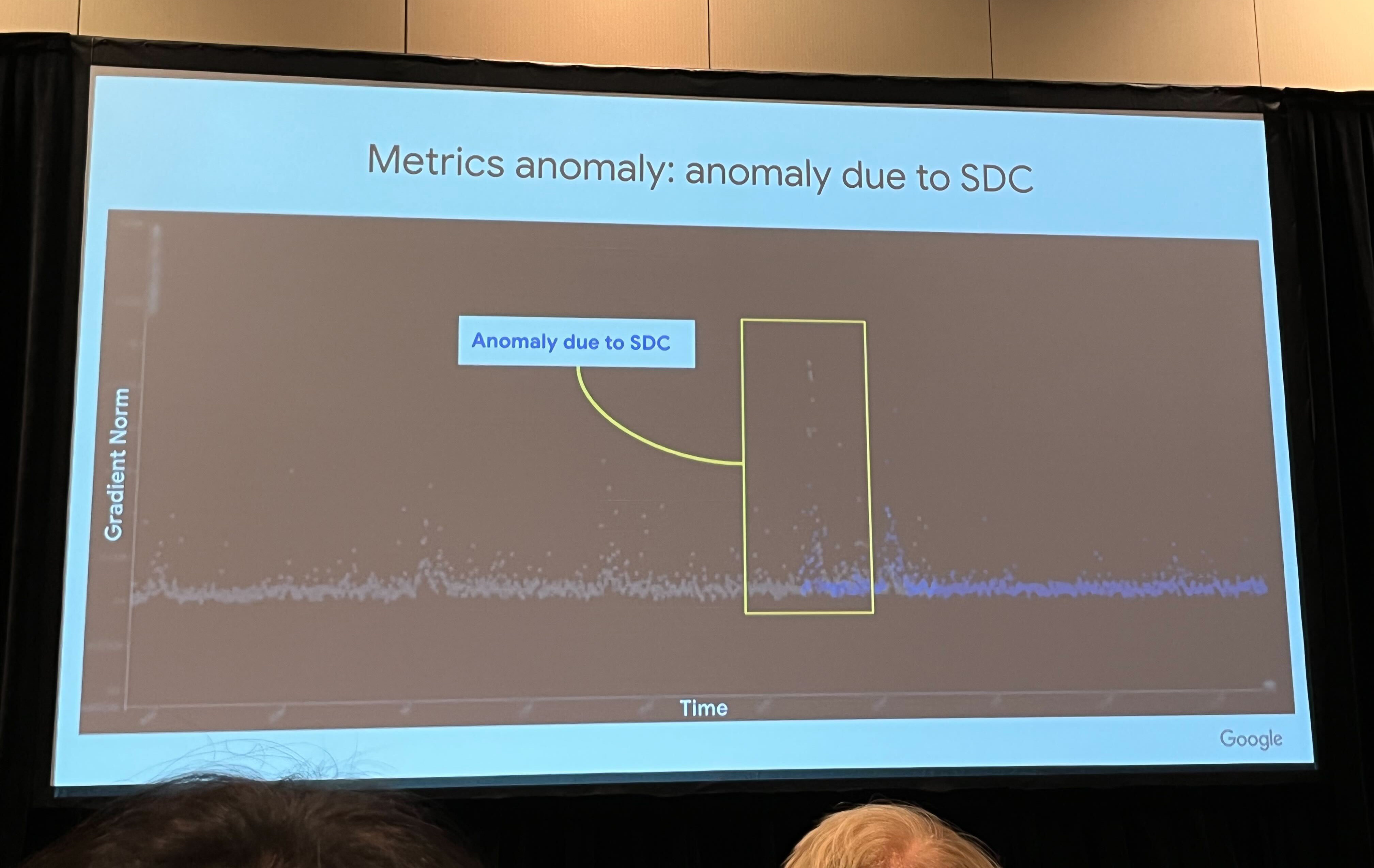
As shown in Figure 8, a real-world example from Google’s production fleet highlights how an SDC anomaly caused a significant deviation in the gradient norm, a measure of the magnitude of updates to the model parameters. Such deviations can disrupt the optimization process, leading to slower convergence or failure to reach an optimal solution.
During the inference phase, transient faults can impact the reliability and trustworthiness of ML predictions. If a transient fault occurs in the memory storing the trained model parameters or during the computation of inference results, it can lead to incorrect or inconsistent predictions. For instance, a bit flip in the activation values of a neural network can alter the final classification or regression output (Mahmoud et al. 2020). In safety-critical applications25, these faults can have severe consequences, resulting in incorrect decisions or actions that may compromise safety or lead to system failures (G. Li et al. 2017; Jha et al. 2019).
25 Safety-Critical Applications: Systems where failure could result in loss of life, significant property damage, or environmental harm. Examples include nuclear power plants, aircraft control systems, and medical devices, domains where ML deployment requires the highest reliability standards.
26 Stochastic Computing: A collection of techniques using random bits and logic operations to perform arithmetic and data processing, promising better fault tolerance.
These vulnerabilities are particularly amplified in resource-constrained environments like TinyML, where limited computational and memory resources exacerbate their impact. One prominent example is Binarized Neural Networks (BNNs) (Courbariaux et al. 2016), which represent network weights in single-bit precision to achieve computational efficiency and faster inference times. While this binary representation is advantageous for resource-constrained systems, it also makes BNNs particularly fragile to bit-flip errors. For instance, prior work (Aygun, Gunes, and De Vleeschouwer 2021) has shown that a two-hidden-layer BNN architecture for a simple task such as MNIST classification suffers performance degradation from 98% test accuracy to 70% when random bit-flipping soft errors are inserted through model weights with a 10% probability. To address these vulnerabilities, techniques like flip-aware training and emerging approaches such as stochastic computing26 are being explored to enhance fault tolerance.
Permanent Faults
Transitioning from temporary disruptions to persistent issues, permanent faults are hardware defects that persist and cause irreversible damage to the affected components. These faults are characterized by their persistent nature and require repair or replacement of the faulty hardware to restore normal system functionality.
Permanent Fault Properties
Permanent faults cause persistent and irreversible malfunctions in hardware components. The faulty component remains non-operational until it is repaired or replaced. These faults are consistent and reproducible, meaning the faulty behavior is observed every time the affected component is used. They can impact processors, memory modules, storage devices, or interconnects, potentially leading to system crashes, data corruption, or complete system failure.
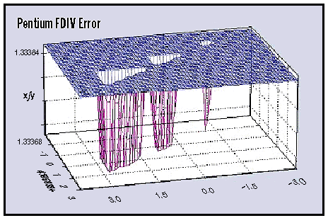
To illustrate the serious implications of permanent faults, a notable example is the Intel FDIV bug, discovered in 1994. This flaw affected the floating-point division (FDIV) units of certain Intel Pentium processors, causing incorrect results for specific division operations and leading to inaccurate calculations.
The FDIV bug occurred due to an error in the lookup table27 used by the division unit. In rare cases, the processor would fetch an incorrect value, resulting in a slightly less precise result than expected. For instance, Figure 9 shows a fraction 4195835/3145727 plotted on a Pentium processor with the FDIV fault. The triangular regions highlight where erroneous calculations occurred. Ideally, all correct values would round to 1.3338, but the faulty results showed 1.3337, indicating a mistake in the 5th digit.
27 Lookup Table: A data structure used to replace a runtime computation with a simpler array indexing operation.
Although the error was small, it could compound across many operations, affecting results in precision-critical applications such as scientific simulations, financial calculations, and computer-aided design. The bug ultimately led to incorrect outcomes in these domains and underscored the severe consequences permanent faults can have.
The FDIV bug serves as a cautionary tale for ML systems. In such systems, permanent faults in hardware components can result in incorrect computations, impacting model accuracy and reliability. For example, if an ML system relies on a processor with a faulty floating-point unit, similar to the FDIV bug, it could introduce persistent errors during training or inference. These errors may propagate through the model, leading to inaccurate predictions or skewed learning outcomes.
This is especially critical in safety-sensitive applications28 explored in Chapter 19: AI for Good, where the consequences of incorrect computations can be severe. ML practitioners must be aware of these risks and incorporate fault-tolerant techniques, including hardware redundancy, error detection and correction, and robust algorithm design, to mitigate them. Thorough hardware validation and testing can help identify and resolve permanent faults before they affect system performance and reliability.
28 Safety-Critical Applications: Systems where failure could result in loss of life, significant property damage, or environmental harm. Examples include nuclear power plants, aircraft control systems, and medical devices, domains where ML deployment requires the highest reliability standards.
Permanent Fault Origins
Permanent faults can arise from two primary sources: manufacturing defects and wear-out mechanisms.
The first category, Manufacturing defects, comprises flaws introduced during the fabrication process, including improper etching, incorrect doping, or contamination. These defects may result in non-functional or partially functional components. In contrast, wear-out mechanisms occur over time due to prolonged use and operational stress. Phenomena like electromigration29, oxide breakdown30, and thermal stress31 degrade component integrity, eventually leading to permanent failure.
29 Electromigration: The movement of metal atoms in a conductor under the influence of an electric field.
30 Oxide Breakdown: The failure of an oxide layer in a transistor due to excessive electric field stress.
31 Thermal Stress: Degradation caused by repeated cycling through high and low temperatures. Modern AI accelerators commonly experience thermal throttling under sustained workloads, leading to performance degradation of 20-60% as processors reduce clock speeds to prevent overheating. This throttling directly impacts ML training times and inference throughput, making thermal management critical for maintaining consistent AI system performance in production environments.
Permanent Fault Propagation
Permanent faults manifest through several mechanisms, depending on their nature and location. A common example is the stuck-at fault (Seong et al. 2010), where a signal or memory cell becomes permanently fixed at either 0 or 1, regardless of the intended input, as shown in Figure 10. This type of fault can occur in logic gates, memory cells, or interconnects and typically results in incorrect computations or persistent data corruption.

Other mechanisms include device failures, in which hardware components such as transistors or memory cells cease functioning entirely due to manufacturing defects or degradation over time. Bridging faults, which occur when two or more signal lines are unintentionally connected, can introduce short circuits or incorrect logic behaviors that are difficult to isolate.
In more subtle cases, delay faults can arise when the propagation time of a signal exceeds the allowed timing constraints. The logical values may be correct, but the violation of timing expectations can still result in erroneous behavior. Similarly, interconnect faults, including open circuits caused by broken connections, high-resistance paths that impede current flow, and increased capacitance that distorts signal transitions, can significantly degrade circuit performance and reliability.
Memory subsystems are particularly vulnerable to permanent faults. Transition faults can prevent a memory cell from successfully changing its state, while coupling faults result from unwanted interference between adjacent cells, leading to unintentional state changes. Neighborhood pattern sensitive faults occur when the state of a memory cell is incorrectly influenced by the data stored in nearby cells, reflecting a more complex interaction between circuit layout and logic behavior.
Permanent faults can also occur in critical infrastructure components such as the power supply network or clock distribution system. Failures in these subsystems can affect circuit-wide functionality, introduce timing errors, or cause widespread operational instability.
Taken together, these mechanisms illustrate the varied and often complex ways in which permanent faults can undermine the behavior of computing systems. For ML applications in particular, where correctness and consistency are vital, understanding these fault modes is essential for developing resilient hardware and software solutions.
Permanent Fault Effects on ML
Permanent faults can severely disrupt the behavior and reliability of computing systems. For example, a stuck-at fault in a processor’s arithmetic logic unit (ALU) can produce persistent computational errors, leading to incorrect program behavior or crashes. In memory modules, such faults may corrupt stored data, while in storage devices, they can result in bad sectors or total data loss. Interconnect faults may interfere with data transmission, leading to system hangs or corruption.
For ML systems, these faults pose significant risks in both training and inference phases. As with transient faults (Section X.X.X), permanent faults during training cause similar gradient calculation errors and parameter corruption, but persist until hardware replacement, requiring more comprehensive recovery strategies (He et al. 2023). Unlike transient faults that may only temporarily disrupt training, permanent faults in storage can compromise entire training datasets or saved models, affecting long-term consistency and reliability.
In the inference phase, faults can distort prediction results or lead to runtime failures. For instance, errors in the hardware storing model weights might lead to outdated or corrupted models being used, while processor faults could yield incorrect outputs (J. J. Zhang et al. 2018).
Mitigating permanent faults requires comprehensive fault-tolerant design combining hardware redundancy and error-correcting codes (Kim, Sullivan, and Erez 2015) with software approaches like checkpoint and restart mechanisms32 (Egwutuoha et al. 2013).
32 Checkpoint and Restart Mechanisms: Techniques that periodically save a program’s state so it can resume from the last saved state after a failure.
Regular monitoring, testing, and maintenance help detect and replace failing components before critical errors occur.
Intermittent Faults
Intermittent faults are hardware faults that occur sporadically and unpredictably in a system. An example is illustrated in Figure 11, where cracks in the material can introduce increased resistance in circuitry. These faults are particularly challenging to detect and diagnose because they appear and disappear intermittently, making it difficult to reproduce and isolate the root cause. Depending on their frequency and location, intermittent faults can lead to system instability, data corruption, and performance degradation.

Intermittent Fault Properties
Intermittent faults are defined by their sporadic and non-deterministic behavior. They occur irregularly and may manifest for short durations, disappearing without a consistent pattern. Unlike permanent faults, they do not appear every time the affected component is used, which makes them particularly difficult to detect and reproduce. These faults can affect a variety of hardware components, including processors, memory modules, storage devices, and interconnects. As a result, they may lead to transient errors, unpredictable system behavior, or data corruption.
Their impact on system reliability can be significant. For instance, an intermittent fault in a processor’s control logic may disrupt the normal execution path, causing irregular program flow or unexpected system hangs. In memory modules, such faults can alter stored values inconsistently, leading to errors that are difficult to trace. Storage devices affected by intermittent faults may suffer from sporadic read/write errors or data loss, while intermittent faults in communication channels can cause data corruption, packet loss, or unstable connectivity. Over time, these failures can accumulate, degrading system performance and reliability (Rashid, Pattabiraman, and Gopalakrishnan 2015).
Intermittent Fault Origins
The causes of intermittent faults are diverse, ranging from physical degradation to environmental influences. One common cause is the aging and wear-out of electronic components. As hardware endures prolonged operation, thermal cycling, and mechanical stress, it may develop cracks, fractures, or fatigue that introduce intermittent faults. For instance, solder joints in ball grid arrays (BGAs) or flip-chip packages can degrade over time, leading to intermittent open circuits or short circuits.
Manufacturing defects and process variations can also introduce marginal components that behave reliably under most circumstances but fail intermittently under stress or extreme conditions. For example, Figure 12 shows a residue-induced intermittent fault in a DRAM chip that leads to sporadic failures.

Environmental factors such as thermal cycling, humidity, mechanical vibrations, or electrostatic discharge can exacerbate these weaknesses and trigger faults that would not otherwise appear. Loose or degrading physical connections, including those found in connectors or printed circuit boards, are also common sources of intermittent failures, particularly in systems exposed to movement or temperature variation.
Intermittent Fault Propagation
Intermittent faults can manifest through various physical and logical mechanisms depending on their root causes. One such mechanism is the intermittent open or short circuit, where physical discontinuities or partial connections cause signal paths to behave unpredictably. These faults may momentarily disrupt signal integrity, leading to glitches or unexpected logic transitions.
Another common mechanism is the intermittent delay fault (J. Zhang et al. 2018), where signal propagation times fluctuate due to marginal timing conditions, resulting in synchronization issues and incorrect computations. In memory cells or registers, intermittent faults can appear as transient bit flips or soft errors, corrupting data in ways that are difficult to detect or reproduce. Because these faults are often condition-dependent, they may only emerge under specific thermal, voltage, or workload conditions, adding further complexity to their diagnosis.
Intermittent Fault Effects on ML
Intermittent faults pose significant challenges for ML systems by undermining computational consistency and model reliability. During the training phase, such faults in processing units or memory can cause sporadic errors in the computation of gradients, weight updates, or loss values. These errors may not be persistent but can accumulate across iterations, degrading convergence and leading to unstable or suboptimal models. Intermittent faults in storage may corrupt input data or saved model checkpoints, further affecting the training pipeline (He et al. 2023).
In the inference phase, intermittent faults may result in inconsistent or erroneous predictions. Processing errors or memory corruption can distort activations, outputs, or intermediate representations of the model, particularly when faults affect model parameters or input data. Intermittent faults in data pipelines, such as unreliable sensors or storage systems, can introduce subtle input errors that degrade model robustness and output accuracy. In high-stakes applications like autonomous driving or medical diagnosis, these inconsistencies can result in dangerous decisions or failed operations.
Mitigating the effects of intermittent faults in ML systems requires a multi-layered approach (Rashid, Pattabiraman, and Gopalakrishnan 2012). At the hardware level, robust design practices, environmental controls, and the use of higher-quality or more reliable components can reduce susceptibility to fault conditions. Redundancy and error detection mechanisms can help identify and recover from transient manifestations of intermittent faults.
At the software level, techniques such as runtime monitoring, anomaly detection, and adaptive control strategies can provide resilience, integrating with the framework capabilities detailed in Chapter 7: AI Frameworks and deployment strategies from Chapter 13: ML Operations. Data validation checks, outlier detection, model ensembling, and runtime model adaptation are examples of fault-tolerant methods that can be integrated into ML pipelines to improve reliability in the presence of sporadic errors.
Designing ML systems that can gracefully handle intermittent faults maintains their accuracy, consistency, and dependability. This involves proactive fault detection, regular system monitoring, and ongoing maintenance to ensure early identification and remediation of issues. By embedding resilience into both the architecture and operational workflow detailed in Chapter 13: ML Operations, ML systems can remain robust even in environments prone to sporadic hardware failures.
Effective fault tolerance extends beyond detection to encompass adaptive performance management under varying system conditions. Comprehensive resource management strategies, including load balancing and dynamic scaling under fault conditions, are covered in Chapter 13: ML Operations. For resource-constrained scenarios, adaptive model complexity reduction techniques, such as dynamic quantization and selective pruning in response to thermal or power constraints, are detailed in Chapter 10: Model Optimizations and Chapter 9: Efficient AI.
Hardware Fault Detection and Mitigation
Fault detection techniques, including hardware-level and software-level approaches, and effective mitigation strategies enhance the resilience of ML systems. Resilient ML system design considerations, case studies, and research in fault-tolerant ML systems provide insights into building robust systems.
Robust fault mitigation requires coordinated adaptation across the entire ML system stack. While the focus here is on fault detection and basic recovery mechanisms, comprehensive performance adaptation strategies are implemented through dynamic resource management (Chapter 13: ML Operations), fault-tolerant distributed training approaches (Chapter 8: AI Training), and adaptive model optimization techniques that maintain performance under resource constraints (Chapter 10: Model Optimizations, Chapter 9: Efficient AI). These adaptation strategies ensure that ML systems not only detect and recover from faults but also maintain optimal performance through intelligent resource allocation and model complexity adjustment. The future paradigms for more robust architectures that address fundamental vulnerabilities are explored in Chapter 20: AGI Systems.
Hardware Fault Detection Methods
Fault detection techniques identify and localize hardware faults in ML systems, building on the performance measurement principles from Chapter 12: Benchmarking AI. These techniques can be broadly categorized into hardware-level and software-level approaches, each offering unique capabilities and advantages.
Hardware-Level Detection
Hardware-level fault detection techniques are implemented at the physical level of the system and aim to identify faults in the underlying hardware components. Several hardware techniques exist, which can be categorized into the following groups.
Built-in self-test (BIST) Mechanisms
BIST is a powerful technique for detecting faults in hardware components (Bushnell and Agrawal 2002). It involves incorporating additional hardware circuitry into the system for self-testing and fault detection. BIST can be applied to various components, such as processors, memory modules, or application-specific integrated circuits (ASICs). For example, BIST can be implemented in a processor using scan chains33, which are dedicated paths that allow access to internal registers and logic for testing purposes.
33 Scan Chains: Dedicated paths incorporated within a processor that grant access to internal registers and logic for testing.
During the BIST process, predefined test patterns are applied to the processor’s internal circuitry, and the responses are compared against expected values. Any discrepancies indicate the presence of faults. Intel’s Xeon processors, for instance, include BIST mechanisms to test the CPU cores, cache memory, and other critical components during system startup.

Error Detection Codes
Error detection codes are widely used to detect data storage and transmission errors (Hamming 1950)34. These codes add redundant bits to the original data, allowing the detection of bit errors. Example: Parity checks are a simple form of error detection code shown in Figure 1335. In a single-bit parity scheme, an extra bit is appended to each data word, making the number of 1s in the word even (even parity) or odd (odd parity).
34 Hamming (1950): R. W. Hamming’s seminal paper introduced error detection and correction codes, significantly advancing digital communication reliability.
35 Parity Checks: In parity checks, an extra bit accounts for the total number of 1s in a data word, enabling basic error detection.
36 Cyclic Redundancy Check (CRC): Error detection algorithm developed by W. Wesley Peterson in 1961, widely used in digital communications and storage. CRC computes a polynomial checksum that can detect up to 99.9% of transmission errors with minimal computational overhead. Essential for ML data pipelines where corrupted training data can silently degrade model performance - modern distributed training systems use CRC-32 to validate gradient updates across thousands of nodes. The checksum is recalculated at the receiving end and compared with the transmitted checksum to detect errors. Error-correcting code (ECC) memory modules, commonly used in servers and critical systems, employ advanced error detection and correction codes to detect and correct single-bit or multi-bit errors in memory.
When reading the data, the parity is checked, and if it doesn’t match the expected value, an error is detected. More advanced error detection codes, such as cyclic redundancy checks (CRC)36, calculate a checksum based on the data and append it to the message.
Hardware redundancy and voting mechanisms
Hardware redundancy involves duplicating critical components and comparing their outputs to detect and mask faults (Sheaffer, Luebke, and Skadron 2007). Voting mechanisms, such as double modular redundancy (DMR)37 or triple modular redundancy (TMR)38, employ multiple instances of a component and compare their outputs to identify and mask faulty behavior (Arifeen, Hassan, and Lee 2020).
37 Double Modular Redundancy (DMR): A fault-tolerance process in which computations are duplicated to identify and correct errors.
38 Triple Modular Redundancy (TMR): A fault-tolerance process where three instances of a computation are performed to identify and correct errors.
In a DMR or TMR system, two or three identical instances of a hardware component, such as a processor or a sensor, perform the same computation in parallel. The outputs of these instances are fed into a voting circuit, which compares the results and selects the majority value as the final output. If one of the instances produces an incorrect result due to a fault, the voting mechanism masks the error and maintains the correct output. TMR is commonly used in aerospace and aviation systems, where high reliability is critical. For instance, the Boeing 777 aircraft employs TMR in its primary flight computer system to ensure the availability and correctness of flight control functions (Yeh, n.d.).
Tesla’s self-driving computers, on the other hand, employ a DMR architecture to ensure the safety and reliability of critical functions such as perception, decision-making, and vehicle control, as shown in Figure 14. In Tesla’s implementation, two identical hardware units, often called “redundant computers” or “redundant control units,” perform the same computations in parallel. Each unit independently processes sensor data, executes algorithms, and generates control commands for the vehicle’s actuators, such as steering, acceleration, and braking (Bannon et al. 2019).

The outputs of these two redundant units are continuously compared to detect any discrepancies or faults. If the outputs match, the system assumes that both units function correctly, and the control commands are sent to the vehicle’s actuators. However, if a mismatch occurs between the outputs, the system identifies a potential fault in one of the units and takes appropriate action to ensure safe operation.
DMR in Tesla’s self-driving computer provides an extra safety and fault tolerance layer. By having two independent units performing the same computations, the system can detect and mitigate faults that may occur in one of the units. This redundancy helps prevent single points of failure and ensures that critical functions remain operational despite hardware faults.
The system may employ additional mechanisms to determine which unit is faulty in a mismatch. This can involve using diagnostic algorithms, comparing the outputs with data from other sensors or subsystems, or analyzing the consistency of the outputs over time. Once the faulty unit is identified, the system can isolate it and continue operating using the output from the non-faulty unit.
Tesla also incorporates redundancy mechanisms beyond DMR. For example, they use redundant power supplies, steering and braking systems, and diverse sensor suites39 (e.g., cameras, radar, and ultrasonic sensors) to provide multiple layers of fault tolerance.
39 Sensor Fusion: Integration of data from multiple sensor types to create more accurate and reliable perception than any single sensor. Pioneered in military applications in the 1980s, sensor fusion combines cameras (visual spectrum), LiDAR (depth/distance), radar (weather-resistant), and ultrasonic (short-range) sensors. Tesla’s approach processes 8 cameras, 12 ultrasonic sensors, and forward radar simultaneously, generating 40 GB of sensor data per hour to enable robust autonomous decision-making. These redundancies collectively contribute to the overall safety and reliability of the self-driving system.
While DMR provides fault detection and some level of fault tolerance, TMR may provide a different level of fault masking. In DMR, if both units experience simultaneous faults or the fault affects the comparison mechanism, the system may be unable to identify the fault. Therefore, Tesla’s SDCs rely on a combination of DMR and other redundancy mechanisms to achieve a high level of fault tolerance.
The use of DMR in Tesla’s self-driving computer highlights the importance of hardware redundancy in applications requiring high reliability. By employing redundant computing units and comparing their outputs, the system can detect and mitigate faults, enhancing the overall safety and reliability of the self-driving functionality.
Another approach to hardware redundancy is the use of hot spares40, as employed by Google in its data centers to address SDC during ML training. Unlike DMR and TMR, which rely on parallel processing and voting mechanisms to detect and mask faults, hot spares provide fault tolerance by maintaining backup hardware units that can seamlessly take over computations when a fault is detected. As illustrated in Figure 15, during normal ML training, multiple synchronous training workers process data in parallel. However, if a worker becomes defective and causes SDC, an SDC checker automatically identifies the issues. Upon detecting the SDC, the SDC checker moves the training to a hot spare and sends the defective machine for repair. This redundancy safeguards the continuity and reliability of ML training, effectively minimizing downtime and preserving data integrity.
40 Hot Spares: In a system redundancy design, these are the backup components kept ready to instantaneously replace failing components without disrupting the operation.

Watchdog timers
Watchdog timers are hardware components that monitor the execution of critical tasks or processes (Pont and Ong 2002). They are commonly used to detect and recover from software or hardware faults that cause a system to become unresponsive or stuck in an infinite loop. In an embedded system, a watchdog timer can be configured to monitor the execution of the main control loop, as illustrated in Figure 16. The software periodically resets the watchdog timer to indicate that it functions correctly. Suppose the software fails to reset the timer within a specified time limit (timeout period). In that case, the watchdog timer assumes that the system has encountered a fault and triggers a predefined recovery action, such as resetting the system or switching to a backup component. Watchdog timers are widely used in automotive electronics, industrial control systems, and other safety-critical applications to ensure the timely detection and recovery from faults.

Software-Level Detection
Software-level fault detection techniques rely on software algorithms and monitoring mechanisms to identify system faults. These techniques can be implemented at various levels of the software stack, including the operating system, middleware, or application level.
Runtime monitoring and anomaly detection
Runtime monitoring involves continuously observing the behavior of the system and its components during execution (Francalanza et al. 2017), extending the operational monitoring practices from Chapter 13: ML Operations. It helps detect anomalies, errors, or unexpected behavior that may indicate the presence of faults. For example, consider an ML-based image classification system deployed in a self-driving car. Runtime monitoring can be implemented to track the classification model’s performance and behavior (Mahmoud et al. 2021).
Anomaly detection algorithms can be applied to the model’s predictions or intermediate layer activations, such as statistical outlier detection or machine learning-based approaches (e.g., One-Class SVM or Autoencoders) (Chandola, Banerjee, and Kumar 2009). Figure 17 shows example of anomaly detection. Suppose the monitoring system detects a significant deviation from the expected patterns, such as a sudden drop in classification accuracy or out-of-distribution samples. In that case, it can raise an alert indicating a potential fault in the model or the input data pipeline. This early detection allows for timely intervention and fault mitigation strategies to be applied.

Consistency checks and data validation
Consistency checks and data validation techniques ensure data integrity and correctness at different processing stages in an ML system (Lindholm et al. 2019). These checks help detect data corruption, inconsistencies, or errors that may propagate and affect the system’s behavior. Example: In a distributed ML system where multiple nodes collaborate to train a model, consistency checks can be implemented to validate the integrity of the shared model parameters. Each node can compute a checksum or hash of the model parameters before and after the training iteration, as shown in Figure 17. Any inconsistencies or data corruption can be detected by comparing the checksums across nodes. Range checks can be applied to the input data and model outputs to ensure they fall within expected bounds. For instance, if an autonomous vehicle’s perception system detects an object with unrealistic dimensions or velocities, it can indicate a fault in the sensor data or the perception algorithms (Wan et al. 2023).
Heartbeat and timeout mechanisms
Heartbeat mechanisms and timeouts are commonly used to detect faults in distributed systems and ensure the liveness and responsiveness of components (Kawazoe Aguilera, Chen, and Toueg 1997). These are quite similar to the watchdog timers found in hardware. For example, in a distributed ML system, where multiple nodes collaborate to perform tasks such as data preprocessing, model training, or inference, heartbeat mechanisms can be implemented to monitor the health and availability of each node. Each node periodically sends a heartbeat message to a central coordinator or its peer nodes, indicating its status and availability. Suppose a node fails to send a heartbeat within a specified timeout period, as shown in Figure 18. In that case, it is considered faulty, and appropriate actions can be taken, such as redistributing the workload or initiating a failover mechanism. Given that network partitions affect 1-10% of nodes daily in large distributed training clusters, these heartbeat systems must distinguish between node failures and network connectivity issues to avoid unnecessary failover operations that could disrupt training progress. Timeouts can also be used to detect and handle hanging or unresponsive components. For example, if a data loading process exceeds a predefined timeout threshold, it may indicate a fault in the data pipeline, and the system can take corrective measures.

Software-implemented fault tolerance (SIFT) techniques
SIFT techniques introduce redundancy and fault detection mechanisms at the software level to improve the reliability and fault tolerance of the system (Reis et al., n.d.). Example: N-version programming is a SIFT technique where multiple functionally equivalent software component versions are developed independently by different teams. This can be applied to critical components such as the model inference engine in an ML system. Multiple versions of the inference engine can be executed in parallel, and their outputs can be compared for consistency. It is considered the correct result if most versions produce the same output. A discrepancy indicates a potential fault in one or more versions, triggering appropriate error-handling mechanisms. Another example is using software-based error correction codes, such as Reed-Solomon codes (Plank 1997), to detect and correct errors in data storage or transmission, as shown in Figure 19. These codes add redundancy to the data, enabling detecting and correcting certain errors and enhancing the system’s fault tolerance.

Hardware Fault Summary
Table 3 provides a comparative analysis of transient, permanent, and intermittent faults. It outlines the primary characteristics or dimensions that distinguish these fault types. Here, we summarize the relevant dimensions we examined and explore the nuances that differentiate transient, permanent, and intermittent faults in greater detail.
While hardware faults represent one dimension of system vulnerability, they rarely occur in isolation. The physical failures we have examined often interact with and expose weaknesses in the algorithmic components of AI systems. This interconnection becomes particularly evident when we consider how adversaries might exploit model vulnerabilities through carefully crafted inputs—the focus of our next section on Input-Level Attacks.
| Dimension | Transient Faults | Permanent Faults | Intermittent Faults |
|---|---|---|---|
| Duration | Short-lived, temporary | Persistent, remains until repair or replacement | Sporadic, appears and disappears intermittently |
| Persistence | Disappears after the fault condition passes | Consistently present until addressed | Recurs irregularly, not always present |
| Causes | External factors (e.g., electromagnetic interference cosmic rays) | Hardware defects, physical damage, wear-out | Unstable hardware conditions, loose connections, aging components |
| Manifestation | Bit flips, glitches, temporary data corruption | Stuck-at faults, broken components, complete device failures | Occasional bit flips, intermittent signal issues, sporadic malfunctions |
| Impact on ML | Introduces temporary errors | Causes consistent errors or | Leads to sporadic and unpredictable errors, |
| Systems | or noise in computations | failures, affecting reliability | challenging to diagnose and mitigate |
| Detection | Error detection codes, comparison with expected values | Built-in self-tests, error detection codes, consistency checks | Monitoring for anomalies, analyzing error patterns and correlations |
| Mitigation | Error correction codes, redundancy, checkpoint and restart | Hardware repair or replacement, component redundancy, failover mechanisms | Robust design, environmental control, runtime monitoring, fault-tolerant techniques |
Intentional Input Manipulation
Input-level attacks represent a different threat model from unintentional hardware failures. Unlike random bit flips and component failures, these attacks involve deliberate manipulation of data to compromise system behavior. These sophisticated attempts manipulate ML model behavior through carefully crafted inputs or corrupted training data. These attack vectors can amplify the impact of hardware faults, for instance, when adversaries craft inputs specifically designed to trigger edge cases in fault-compromised hardware.
Adversarial Attacks
Conceptual Foundation
At its core, an adversarial attack is surprisingly simple: add tiny, calculated changes to an input that fool a model while remaining invisible to humans. Imagine adjusting a few pixels in a photo of a cat, changes so subtle you cannot see them, yet the model suddenly classifies it as a toaster with 99% confidence. This counterintuitive vulnerability stems from how neural networks process information differently than humans do.
To understand the underlying mechanism through analogy, consider a person who has learned to identify cats by looking primarily for pointy ears. An adversarial attack is like showing this person a picture of a dog, but carefully drawing tiny, almost invisible pointy ears on top of the dog’s floppy ears. Because the person’s algorithm is overly reliant on the pointy ear feature, they confidently misclassify the dog as a cat. This is how adversarial attacks work: they find the specific, often superficial, features a model relies on and exploit them, even if the changes are meaningless to a human observer.
ML models learn statistical patterns rather than semantic understanding. They operate in high-dimensional spaces where decision boundaries can be surprisingly fragile. Small movements in this space, imperceptible in the input domain, can cross these boundaries and trigger misclassification.
Technical Mechanisms
Adversarial attacks exploit ML models’ sensitivity to small input perturbations that are imperceptible to humans but cause dramatic changes in model outputs. These attacks reveal vulnerabilities in how models learn decision boundaries and generalize from training data. The mathematical foundation relies on the model’s gradient information to identify the most effective perturbation directions.
Fast Gradient Sign Method (FGSM) (Goodfellow, Shlens, and Szegedy 2014) represents one of the earliest and most influential adversarial attack techniques. FGSM generates adversarial examples by adding small perturbations in the direction of the gradient with respect to the loss function, effectively “pushing” inputs toward misclassification boundaries. For ImageNet classifiers, FGSM attacks with ε = 8/255 (barely perceptible perturbations) can reduce accuracy from 76% to under 10%, demonstrating the fragility of deep networks to small input modifications.
Projected Gradient Descent (PGD) attacks (Madry et al. 2017) extend FGSM by iteratively applying small perturbations and projecting back to the allowed perturbation space. PGD attacks with 40 iterations and step size α = 2/255 achieve nearly 100% attack success rates against undefended models, dropping CIFAR-10 accuracy from 95% to under 5%. These attacks are considered among the strongest first-order adversaries and serve as benchmarks for evaluating defensive mechanisms.
Physical-world attacks pose particular challenges for deployed AI systems. Research has demonstrated that adversarial examples can be printed, photographed, or displayed on screens while maintaining their attack effectiveness (Kurakin, Goodfellow, and Bengio 2016). Stop sign attacks achieve 87% misclassification rates when physical patches are placed on traffic signs, causing autonomous vehicle classifiers to interpret “STOP” signs as “Speed Limit 45” with potentially catastrophic consequences. Laboratory studies show that adversarial examples maintain effectiveness across different lighting conditions (2,000-10,000 lux), viewing angles (±30 degrees), and camera distances (2-15 meters).
Data Poisoning Attacks
Data poisoning attacks target the training phase by injecting malicious samples into training datasets, causing models to learn incorrect associations or exhibit specific behaviors on targeted inputs. These attacks are particularly concerning in scenarios where training data is collected from untrusted sources or through crowdsourcing.
Label flipping attacks modify the labels of training examples to introduce incorrect associations. Research demonstrates that flipping just 3% of labels in CIFAR-10 reduces target class accuracy from 92% to 11%, while overall model accuracy drops only 2-4%, making detection difficult. For ImageNet, corrupting 0.5% of labels (6,500 images) can cause targeted misclassification rates above 90% for specific classes while maintaining 94% clean accuracy.
Backdoor attacks inject training samples with specific trigger patterns that cause models to exhibit attacker-controlled behavior when the trigger is present in test inputs (Gu, Dolan-Gavitt, and Garg 2017). Studies show that inserting backdoor triggers in just 1% of training data achieves 99.5% attack success rates on trigger-bearing test inputs. The model performs normally on clean inputs but consistently misclassifies inputs containing the backdoor trigger, with clean accuracy typically dropping less than 1%.
Gradient-based poisoning crafts training samples that appear benign but cause gradient updates during training to move the model toward attacker objectives (Shafahi et al. 2018). These attacks require precise optimization but can be devastating: poisoning 50 crafted images in CIFAR-10 (0.1% of training data) achieves target misclassification rates above 70%. The computational cost is significant, requiring 15-20\(\times\) more training time to generate optimal poisoning samples, but the attack remains undetectable through visual inspection.
Detection and Mitigation Strategies
Robust AI systems employ multiple defense mechanisms against input-level attacks, following the detection, graceful degradation, and adaptive response principles established in our unified framework.
Input sanitization applies preprocessing techniques to remove or reduce adversarial perturbations before they reach the model. JPEG compression with quality factor 75% neutralizes 60-80% of adversarial examples while reducing clean accuracy by only 1-2%. Image denoising with Gaussian filters (σ = 0.5) blocks 45% of FGSM attacks but requires careful tuning to avoid degrading legitimate inputs. Geometric transformations like random rotations (±15°) and scaling (0.9-1.1\(\times\)) provide 30-50% defense effectiveness with minimal clean accuracy loss.
Adversarial training (Madry et al. 2017) incorporates adversarial examples into the training process, teaching models to maintain correct predictions in the presence of adversarial perturbations. PGD adversarial training on CIFAR-10 achieves 87% robust accuracy against ε = 8/255 attacks compared to 0% for undefended models, though clean accuracy drops from 95% to 84%. Training time increases 6-10\(\times\) due to adversarial example generation during each epoch, requiring specialized hardware acceleration for practical implementation.
Certified defenses provide mathematical guarantees about model robustness within specified perturbation bounds (Cohen, Rosenfeld, and Kolter 2019). Randomized smoothing achieves 67% certified accuracy on ImageNet for ℓ2 perturbations with σ = 0.5, compared to 76% clean accuracy. The certification radius increases to ε = 1.0 for 54% of test inputs, providing provable robustness guarantees. However, inference time increases 100-1000\(\times\) due to Monte Carlo sampling requirements (typically 1,000 samples per prediction).
Ensemble methods leverage multiple models or detection mechanisms to identify and filter adversarial inputs (Tramèr et al. 2017). Ensembles of 5 independently trained models achieve 94% detection rates for adversarial examples using prediction entropy thresholds (τ = 1.5), with false positive rates below 2% on clean data. Computational overhead scales linearly with ensemble size, requiring \(5\times\) inference time and memory for the 5-model ensemble, making real-time deployment challenging.
While input-level attacks represent intentional attempts to compromise model behavior, AI systems must also contend with natural variations in their operational environments that can be equally disruptive. These environmental challenges emerge organically from the evolving nature of real-world deployments.
Environmental Shifts
The third pillar of robust AI addresses the natural evolution of real-world conditions that can degrade model performance over time. Unlike the deliberate manipulations of input-level attacks or the random failures of hardware faults, environmental shifts reflect the inherent challenge of deploying static models in dynamic environments where data distributions, user behavior, and operational contexts continuously evolve. These shifts can interact synergistically with other vulnerability types. For example, a model experiencing distribution shift becomes more susceptible to adversarial attacks, while hardware errors may manifest differently under changed environmental conditions.
Distribution Shift and Concept Drift
Intuitive Understanding
Consider a medical diagnosis model trained on X-ray images from a modern hospital. When deployed in a rural clinic with older equipment, the model’s accuracy plummets not because the underlying medical conditions have changed, but because the image characteristics differ. This exemplifies distribution shift: the world the model encounters differs from the world it learned from.
Distribution shifts occur naturally as environments evolve. User preferences change seasonally, language evolves with new slang, and economic patterns shift with market conditions. Unlike adversarial attacks that require malicious intent, these shifts emerge organically from the dynamic nature of real-world systems.
Technical Categories
Covariate shift occurs when the input distribution changes while the relationship between inputs and outputs remains constant (Quiñonero-Candela et al. 2008). Autonomous vehicle perception models trained on daytime images (luminance 1,000-100,000 lux) experience 15-30% accuracy degradation when deployed in nighttime conditions (0.1-10 lux), despite unchanged object recognition tasks. Weather conditions introduce additional covariate shift: rain reduces object detection mAP by 12%, snow by 18%, and fog by 25% compared to clear conditions.
Concept drift represents changes in the underlying relationship between inputs and outputs over time (Widmer and Kubat 1996). Credit card fraud detection systems experience concept drift with 6-month correlation decay rates of 0.2-0.4, requiring model retraining every 90-120 days to maintain performance above 85% precision. E-commerce recommendation systems show 15-20% accuracy degradation over 3-6 months due to seasonal preference changes and evolving user behavior patterns.
Label shift affects the distribution of output classes without changing the input-output relationship (Lipton, Wang, and Smola 2018). COVID-19 caused dramatic label shift in medical imaging: pneumonia prevalence increased from 12% to 35% in some hospital systems, requiring recalibration of diagnostic thresholds. Seasonal label shift in agriculture monitoring shows crop disease prevalence varying by 40-60% between growing seasons, necessitating adaptive decision boundaries for accurate yield prediction.
Monitoring and Adaptation Strategies
Effective response to environmental shifts requires continuous monitoring of deployment conditions and adaptive mechanisms that maintain model performance as conditions change.
Statistical distance metrics quantify the degree of distribution shift by measuring differences between training and deployment data distributions. Maximum Mean Discrepancy (MMD) with RBF kernels (γ = 1.0) provides detection sensitivity of 0.85 for shifts with Cohen’s d > 0.5, processing 10,000 samples in 150 ms on modern hardware. Kolmogorov-Smirnov tests achieve 95% detection rates for univariate shifts with 1,000+ samples, but scale poorly to high-dimensional data. Population Stability Index (PSI) thresholds of 0.1-0.25 indicate significant shift requiring model investigation.
Online learning enables models to continuously adapt to new data while maintaining performance on previously learned patterns (Shalev-Shwartz 2011). Stochastic Gradient Descent with learning rates η = 0.001-0.01 achieves convergence within 100-500 samples for concept drift adaptation. Memory overhead typically requires 2-5 MB for maintaining sufficient historical context, while computation adds 15-25% inference latency for real-time adaptation. Techniques like Elastic Weight Consolidation prevent catastrophic forgetting with regularization coefficients λ = 400-40,000.
Model ensembles and selection maintain multiple models specialized for different environmental conditions, dynamically selecting the most appropriate model based on detected environmental characteristics (Ross, Gordon, and Bagnell 2011). Ensemble systems with 3-7 models achieve 8-15% better accuracy than single models under distribution shift, with selection overhead of 2-5 ms per prediction. Dynamic weighting based on recent performance (sliding windows of 500-2,000 samples) provides optimal adaptation to gradual drift.
Federated learning enables distributed adaptation across multiple deployment environments while preserving privacy. FL systems with 50-1,000 participants achieve convergence in 10-50 communication rounds, each requiring 10-100 MB of parameter transmission depending on model size. Local training typically requires 5-20 epochs per round, with communication costs dominating when bandwidth falls below 1 Mbps. Differential privacy (ε = 1.0-8.0) adds noise but maintains model utility above 90% for most applications.
Robustness Evaluation Tools
Having examined the three pillars of robust AI—hardware faults, input-level attacks, and environmental shifts—students now have the conceptual foundation to understand specialized tools and frameworks for robustness evaluation and improvement. These tools implement the detection, graceful degradation, and adaptive response principles across all three threat categories.
Hardware fault injection tools like PyTorchFI and TensorFI enable systematic testing of ML model resilience to the transient, permanent, and intermittent faults described earlier. Adversarial attack libraries implement FGSM, PGD, and certified defense techniques for evaluating input-level robustness. Distribution monitoring frameworks provide the statistical distance metrics and drift detection capabilities essential for environmental shift management.
Modern robustness tools integrate directly with popular ML frameworks (PyTorch, TensorFlow, Keras), enabling seamless incorporation of robustness evaluation into development workflows established in Chapter 13: ML Operations. The comprehensive examination of these tools and their practical applications appears in Section 1.10, providing detailed implementation guidance for building robust AI systems.
Input-Level Attacks and Model Robustness
While hardware faults represent unintentional disruptions to the underlying computing infrastructure, model robustness concerns extend to deliberate attacks targeting the AI system’s decision-making processes and natural variations in operational environments. The transition from hardware reliability to model robustness reflects a shift from protecting the physical substrate of computation to defending the learned representations and decision boundaries that define model behavior.
This shift requires a change in perspective. Hardware faults typically manifest as corrupted calculations, memory errors, or communication failures that propagate through the system in predictable ways guided by the underlying computational graph. In contrast, model robustness challenges exploit or expose core limitations in the model’s understanding of its problem domain. Adversarial attacks craft inputs specifically designed to trigger misclassifications, data poisoning corrupts the training process itself, and distribution shifts reveal the brittleness of models when deployed beyond their training assumptions.
Following our three-category robustness framework from Section 1.3, different challenge types require complementary defense strategies. While hardware fault mitigation often relies on redundancy, error detection codes, and graceful degradation, model robustness demands techniques like adversarial training, input sanitization, domain adaptation, and continuous monitoring of model behavior in deployment.
The importance of this dual perspective becomes clear when we consider that real-world AI systems face compound threats where hardware faults and model vulnerabilities can interact in complex ways. A hardware fault that corrupts model weights might create new adversarial vulnerabilities, while adversarial attacks might trigger error conditions that resemble hardware faults. Our unified framework from Section 1.3 provides the conceptual foundation for addressing these interconnected challenges systematically.
Adversarial Attacks
Adversarial attacks represent counterintuitive vulnerabilities in modern machine learning systems. These attacks exploit core characteristics of how neural networks learn and represent information, revealing extreme model sensitivity to carefully crafted modifications that remain imperceptible to human observers. These attacks often involve adding small, carefully designed perturbations to input data, which can cause the model to misclassify it, as shown in Figure 20.
Understanding the Vulnerability
Understanding why these attacks are so effective requires examining how they expose core limitations in neural network architectures. The existence of adversarial examples reveals a core mismatch between human and machine perception41.
41 Human vs Machine Perception: Fundamental difference in how humans and neural networks process visual information. Human vision emphasizes object invariance and semantic understanding, while machine vision learns statistical patterns from training data, creating brittle decision boundaries vulnerable to imperceptible perturbations. First highlighted by Szegedy et al. in 2013, this gap reveals how small perturbations can dramatically change model predictions while leaving semantic content unchanged from human perspective.
42 Neural Network Learning Mechanisms: The fundamental processes by which neural networks learn patterns from data, including gradient-based optimization, decision boundary formation, and high-dimensional feature representation. These core concepts are introduced comprehensively in Chapter 3: Deep Learning Primer.
43 Curse of Dimensionality in Adversarial Settings: In high-dimensional spaces (e.g., 224×224×3 = 150,528 dimensions for ImageNet images), tiny perturbations accumulate significantly. With ε=0.01 per dimension, total perturbation magnitude can reach √150,528 × 0.01 ≈ 3.88, enough to alter model predictions while remaining imperceptible to humans who process images holistically. Non-linear decision boundaries create complex separations that make models sensitive to precise input modifications.
This vulnerability stems from several characteristics of neural network learning42. High-dimensional input spaces43 provide numerous dimensions that attackers can exploit simultaneously.
This deep understanding of why adversarial examples exist is crucial for developing effective defenses. The vulnerability reflects core properties of how neural networks represent and process information in high-dimensional spaces, rather than being merely a software bug or training artifact. The theoretical foundations explaining why neural networks44 are inherently vulnerable to adversarial perturbations are comprehensively detailed in Chapter 3: Deep Learning Primer.
44 Neural Network Theoretical Foundations: The mathematical and algorithmic principles underlying how neural networks process information, learn representations, and make predictions in high-dimensional spaces. Complete theoretical coverage is provided in Chapter 3: Deep Learning Primer.
Attack Categories and Mechanisms
Adversarial attacks can be organized into several categories based on their approach to crafting perturbations and the information available to the attacker. Each category exploits different aspects of model vulnerability and requires distinct defensive considerations.
Gradient-based Attacks
The most direct and widely studied category comprises gradient-based attacks, which exploit a core aspect of neural network training: the same gradient information used to train models can be weaponized to attack them. These attacks represent the most direct approach to adversarial example generation by leveraging the model’s own learning mechanism against itself.
Conceptual Foundation
The key insight behind gradient-based attacks is that neural networks compute gradients to understand how changes to their inputs affect their outputs. During training, gradients guide weight updates to minimize prediction errors. For attacks, these same gradients reveal which input modifications would maximize prediction errors—essentially running the training process in reverse.
To illustrate this concept, consider an image classification model that correctly identifies a cat in a photo. The gradient with respect to the input image shows how sensitive the model’s prediction is to changes in each pixel. An attacker can use this gradient information to determine the most effective way to modify specific pixels to change the model’s prediction, perhaps causing it to misclassify the cat as a dog while keeping the changes imperceptible to human observers.
Fast Gradient Sign Method (FGSM)
The Fast Gradient Sign Method45 exemplifies the elegance and danger of gradient-based attacks46. FGSM takes the conceptually simple approach of moving in the direction that most rapidly increases the model’s prediction error.
45 Fast Gradient Sign Method (FGSM): The first practical adversarial attack method, proposed by Goodfellow et al. in 2014. Generates adversarial examples in a single step by moving in the direction of the gradient’s sign, making it computationally efficient but often less effective than iterative methods.
46 Gradient-Based Attacks: Adversarial techniques that use the model’s gradients to craft perturbations. Discovered by Ian Goodfellow in 2014, these attacks revealed that neural networks are vulnerable to imperceptible input modifications, spurring an entire research field in adversarial machine learning.
The underlying mathematical formulation captures this intuitive process:
\[ x_{\text{adv}} = x + \epsilon \cdot \text{sign}\big(\nabla_x J(\theta, x, y)\big) \]
Where the components represent:
- \(x\): the original input (e.g., an image of a cat)
- \(x_{\text{adv}}\): the adversarial example that will fool the model
- \(\nabla_x J(\theta, x, y)\): the gradient showing which input changes most increase prediction error
- \(\text{sign}(\cdot)\): extracts only the direction of change, ignoring magnitude differences
- \(\epsilon\): controls perturbation strength (typically 0.01-0.3 for normalized inputs)
- \(J(\theta, x, y)\): the loss function measuring prediction error
The gradient \(\nabla_x J(\theta, x, y)\) quantifies how the loss function changes with respect to each input feature, indicating which input modifications would most effectively increase the model’s prediction error. The \(\text{sign}(\cdot)\) function extracts the direction of steepest ascent, while the perturbation magnitude \(\epsilon\) controls the strength of the modification applied to each input dimension.
This approach generates adversarial examples by taking a single step in the direction that increases the loss most rapidly, as illustrated in Figure 21.
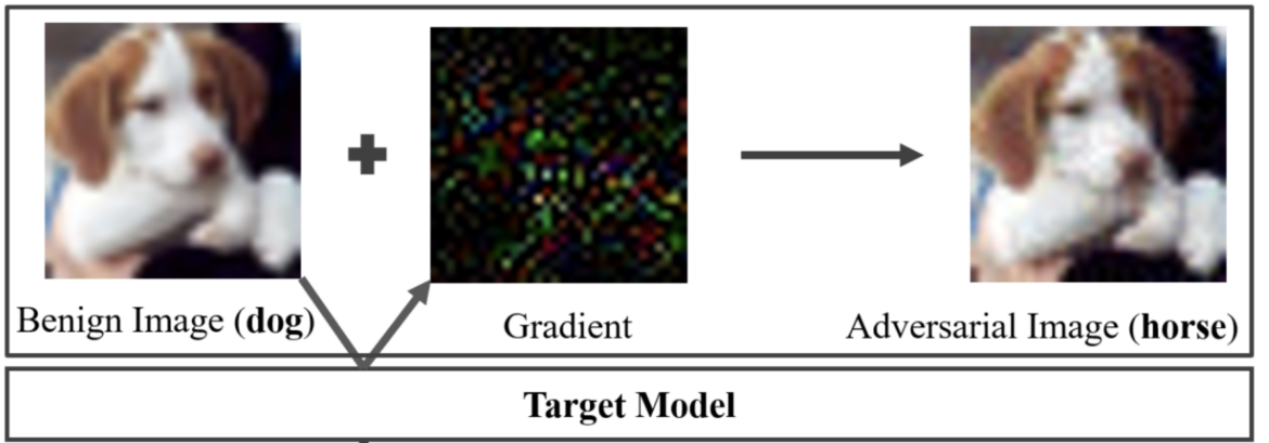
Building on this foundation, the Projected Gradient Descent (PGD) attack (Kurakin, Goodfellow, and Bengio 2016) extends FGSM by iteratively applying the gradient update step, allowing for more refined and powerful adversarial examples. PGD projects each perturbation step back into a constrained norm ball around the original input, ensuring that the adversarial example remains within a specified distortion limit. This makes PGD a stronger white-box attack and a benchmark for evaluating model robustness.
The Jacobian-based Saliency Map Attack (JSMA) (Papernot, McDaniel, Jha, et al. 2016) is another gradient-based approach that identifies the most influential input features and perturbs them to create adversarial examples. By constructing a saliency map based on the Jacobian of the model’s outputs with respect to inputs, JSMA selectively alters a small number of input dimensions that are most likely to influence the target class. This makes JSMA more precise and targeted than FGSM or PGD, often requiring fewer perturbations to fool the model.
Gradient-based attacks are particularly effective in white-box settings47, where the attacker has access to the model’s architecture and gradients. Their efficiency and relative simplicity have made them popular tools for both attacking and evaluating model robustness in research.
47 White-Box Attacks: Adversarial attacks where the attacker has complete knowledge of the target model, including architecture, weights, and training data. More powerful than black-box attacks but less realistic in practice, as attackers rarely have full model access.
Optimization-based Attacks
While gradient-based methods offer speed and simplicity, optimization-based attacks formulate the generation of adversarial examples as a more sophisticated optimization problem. The Carlini and Wagner (C&W) attack (Carlini and Wagner 2017)48 is a prominent example in this category. It finds the smallest perturbation that can cause misclassification while maintaining the perceptual similarity to the original input. The C&W attack employs an iterative optimization process to minimize the perturbation while maximizing the model’s prediction error. It uses a customized loss function with a confidence term to generate more confident misclassifications.
48 Carlini and Wagner (C&W) Attack: Developed in 2017, this sophisticated attack method finds minimal perturbations by solving an optimization problem with carefully designed loss functions. Often considered the strongest white-box attack, it successfully breaks many defensive mechanisms that stop simpler attacks.
C&W attacks are especially difficult to detect because the perturbations are typically imperceptible to humans, and they often bypass many existing defenses. The attack can be formulated under various norm constraints (e.g., L2, L∞) depending on the desired properties of the adversarial perturbation.
Extending this optimization framework, the Elastic Net Attack to DNNs (EAD) incorporates elastic net regularization (a combination of L1 and L2 penalties) to generate adversarial examples with sparse perturbations. This can lead to minimal and localized changes in the input, which are harder to identify and filter. EAD is particularly useful in settings where perturbations need to be constrained in both magnitude and spatial extent.
These attacks are more computationally intensive than gradient-based methods but offer finer control over the adversarial example’s properties, often requiring specialized optimization techniques detailed in Chapter 10: Model Optimizations. They are often used in high-stakes domains where stealth and precision are critical.
Transfer-based Attacks
Moving from direct optimization to exploiting model similarities, transfer-based attacks exploit the transferability property49 of adversarial examples. Transferability refers to the phenomenon where adversarial examples crafted for one ML model can often fool other models, even if they have different architectures or were trained on different datasets. This enables attackers to generate adversarial examples using a surrogate model and then transfer them to the target model without requiring direct access to its parameters or gradients.
49 Transferability: A surprising property discovered in 2015 showing that adversarial examples often transfer between different neural networks. Success rates typically range from 30-70% across models, enabling practical black-box attacks without direct model access.
This transferability property underlies the feasibility of black-box attacks, where the adversary cannot query gradients but can still fool a model by crafting attacks on a publicly available or similar substitute model. Transfer-based attacks are particularly relevant in practical threat scenarios, such as attacking commercial ML APIs, where the attacker can observe inputs and outputs but not internal computations.
Attack success often depends on factors like similarity between models, alignment in training data, and the regularization techniques used. Techniques like input diversity (random resizing, cropping) and momentum during optimization can be used to increase transferability.
Physical-world Attacks
Physical-world attacks bring adversarial examples into real-world scenarios. These attacks involve creating physical objects or manipulations that can deceive ML models when captured by sensors or cameras. Adversarial patches, for example, are small, carefully designed patterns that can be placed on objects to fool object detection or classification models. These patches are designed to work under varying lighting conditions, viewing angles, and distances, making them robust in real-world environments.
When attached to real-world objects, such as a stop sign or a piece of clothing, these patches can cause models to misclassify or fail to detect the objects accurately. Notably, the effectiveness of these attacks persists even after being printed out and viewed through a camera lens, bridging the digital and physical divide in adversarial ML.
Adversarial objects, such as 3D-printed sculptures or modified road signs, can also be crafted to deceive ML systems in physical environments. For example, a 3D turtle object was shown to be consistently classified as a rifle by an image classifier, even when viewed from different angles. These attacks underscore the risks facing AI systems deployed in physical spaces, such as autonomous vehicles, drones, and surveillance systems, raising critical considerations for responsible AI deployment covered in Chapter 17: Responsible AI.
Research into physical-world attacks also includes efforts to develop universal adversarial perturbations, perturbations that can fool a wide range of inputs and models. These threats raise serious questions about safety, robustness, and generalization in AI systems.
Summary
Table 4 provides a concise overview of the different categories of adversarial attacks, including gradient-based attacks (FGSM, PGD, JSMA), optimization-based attacks (C&W, EAD), transfer-based attacks, and physical-world attacks (adversarial patches and objects). Each attack is briefly described, highlighting its key characteristics and mechanisms.
The mechanisms of adversarial attacks reveal the intricate interplay between the ML model’s decision boundaries, the input data, and the attacker’s objectives. By carefully manipulating the input data, attackers can exploit the model’s sensitivities and blind spots, leading to incorrect predictions. The success of adversarial attacks highlights the need for a deeper understanding of ML models’ robustness and generalization properties.
| Attack Category | Attack Name | Description |
|---|---|---|
| Gradient-based | Fast Gradient Sign Method (FGSM) Projected Gradient Descent (PGD) Jacobian-based Saliency Map Attack (JSMA) | Perturbs input data by adding small noise in the gradient direction to maximize prediction error. Extends FGSM by iteratively applying the gradient update step for more refined adversarial examples. Identifies influential input features and perturbs them to create adversarial examples. |
| Optimization-based | Carlini and Wagner (C&W) Attack Elastic Net Attack to DNNs (EAD) | Finds the smallest perturbation that causes misclassification while maintaining perceptual similarity. Incorporates elastic net regularization to generate adversarial examples with sparse perturbations. |
| Transfer-based | Transferability-based Attacks | Exploits the transferability of adversarial examples across different models, enabling black-box attacks. |
| Physical-world | Adversarial Patches Adversarial Objects | Small, carefully designed patches placed on objects to fool object detection or classification models. Physical objects (e.g., 3D-printed sculptures, modified road signs) crafted to deceive ML systems in real-world scenarios. |
Defending against adversarial attacks requires the multifaceted defense strategies detailed in Section 1.8.4.1.2, including adversarial training, defensive distillation, input preprocessing, and ensemble methods.
As adversarial machine learning evolves, researchers explore new attack mechanisms and develop more sophisticated defenses. The arms race between attackers and defenders drives constant innovation and vigilance in securing ML systems against adversarial threats. Understanding attack mechanisms is crucial for developing robust and reliable ML models that can withstand evolving adversarial examples.
Impact on ML
The impact of adversarial attacks on ML systems extends far beyond simple misclassification, as demonstrated in Figure 22. These vulnerabilities create systemic risks across deployment domains.

One striking example of the impact of adversarial attacks was demonstrated by researchers in 2017. They experimented with small black and white stickers on stop signs (Eykholt et al. 2017). To the human eye, these stickers did not obscure the sign or prevent its interpretability. However, when images of the sticker-modified stop signs were fed into standard traffic sign classification ML models, a shocking result emerged. The models misclassified the stop signs as speed limit signs over 85% of the time.
This demonstration shed light on the alarming potential of simple adversarial stickers to trick ML systems into misreading critical road signs. The implications of such attacks in the real world are significant, particularly in the context of autonomous vehicles. If deployed on actual roads, these adversarial stickers could cause self-driving cars to misinterpret stop signs as speed limits, leading to dangerous situations, as shown in Figure 23. Researchers warned that this could result in rolling stops or unintended acceleration into intersections, endangering public safety.
Microsoft’s Tay chatbot provides a stark example of how adversarial users can exploit lack of robustness safeguards in deployed AI systems. Within 24 hours of launch, coordinated users manipulated Tay’s learning mechanisms to generate inappropriate and offensive content. The system lacked content filtering, user input validation, and behavioral monitoring safeguards that could have detected and prevented the exploitation. This incident highlights the critical need for comprehensive input validation, content filtering systems, and continuous behavioral monitoring in deployed AI systems, particularly those that learn from user interactions.

This demonstration illustrates how adversarial examples exploit fundamental vulnerabilities in ML pattern recognition. The attack’s simplicity—minor input modifications invisible to humans causing dramatic prediction changes—reveals deep architectural limitations rather than superficial bugs.
Beyond performance degradation, adversarial vulnerabilities create cascading systemic risks. In healthcare, attacks on medical imaging could enable misdiagnosis (M.-J. Tsai, Lin, and Lee 2023). Financial systems face manipulation of trading algorithms leading to economic losses. These vulnerabilities fundamentally undermine model trustworthiness by exposing reliance on superficial patterns rather than robust concept understanding (Fursov et al. 2021).
Defending against adversarial attacks often requires additional computational resources and can impact the overall system performance. Techniques like adversarial training, where models are trained on adversarial examples to improve robustness, can significantly increase training time and computational requirements (Bai et al. 2021). Runtime detection and mitigation mechanisms, such as input preprocessing (Addepalli et al. 2020) or prediction consistency checks, introduce latency and affect the real-time performance of ML systems.
The presence of adversarial vulnerabilities also complicates the deployment and maintenance of ML systems. System designers and operators must consider the potential for adversarial attacks and incorporate appropriate defenses and monitoring mechanisms. Regular updates and retraining of models become necessary to adapt to new adversarial techniques and maintain system security and performance over time.
These vulnerabilities highlight the urgent need for the comprehensive defense strategies examined in Section 1.8.4.
Data Poisoning
Data poisoning presents a critical challenge to the integrity and reliability of machine learning systems. By introducing carefully crafted malicious data into the training pipeline, adversaries can subtly manipulate model behavior in ways that are difficult to detect through standard validation procedures.
A key distinction from adversarial attacks emerges in their timing and targeting. While adversarial attacks happen after a model is trained (adding noise to test inputs), data poisoning happens before training (contaminating the training data itself). This difference is analogous to fooling a trained student during an exam versus giving a student wrong information while they’re learning. Both can cause incorrect answers, but they exploit different vulnerabilities at different stages:
- Adversarial attacks target deployed models, affecting inference, and can be detected by monitoring outputs
- Data poisoning targets training data, affecting learning, and is much harder to detect because the model honestly learned wrong patterns
Unlike adversarial examples, which target models at inference time, poisoning attacks exploit upstream components of the system, such as data collection, labeling, or ingestion. As ML systems are increasingly deployed in automated and high-stakes environments, understanding how poisoning occurs and how it propagates through the system is essential for developing effective defenses.
Data Poisoning Properties
Data poisoning50 is an attack in which the training data is deliberately manipulated to compromise the performance or behavior of a machine learning model, as described in (Biggio, Nelson, and Laskov 2012) and illustrated in Figure 24. Attackers may alter existing training samples, introduce malicious examples, or interfere with the data collection pipeline. The result is a model that learns biased, inaccurate, or exploitable patterns.
50 Data Poisoning: Attack method first formalized by Biggio et al. in 2012, where adversaries inject malicious samples into training data to compromise model behavior. Unlike adversarial examples that target inference, poisoning attacks the learning process itself, making them harder to detect and defend against.

In most cases, data poisoning unfolds in three stages. In the injection stage, the attacker introduces poisoned samples into the training dataset. These samples may be altered versions of existing data or entirely new instances designed to blend in with clean examples. While they appear benign on the surface, these inputs are engineered to influence model behavior in subtle but deliberate ways. The attacker may target specific classes, insert malicious triggers, or craft outliers intended to distort the decision boundary.
During the training phase, the machine learning model incorporates the poisoned data and learns spurious or misleading patterns. These learned associations may bias the model toward incorrect classifications, introduce vulnerabilities, or embed backdoors. Because the poisoned data is often statistically similar to clean data, the corruption process typically goes unnoticed during standard model training and evaluation.
Finally, in the deployment stage, the attacker leverages the compromised model for malicious purposes. This could involve triggering specific behaviors, including the misclassification of an input that contains a hidden pattern, or simply exploiting the model’s degraded accuracy in production. In real-world systems, such attacks can be difficult to trace back to training data, especially if the system’s behavior appears erratic only in edge cases or under adversarial conditions.
The consequences of such manipulation are especially severe in high-stakes domains like healthcare, where even small disruptions to training data can lead to dangerous misdiagnoses or loss of trust in AI-based systems (Marulli, Marrone, and Verde 2022).
Four main categories of poisoning attacks have been identified in the literature (Oprea, Singhal, and Vassilev 2022). In availability attacks, a substantial portion of the training data is poisoned with the aim of degrading overall model performance. A classic example involves flipping labels, for instance, systematically changing instances with true label \(y = 1\) to \(y = 0\) in a binary classification task. These attacks render the model unreliable across a wide range of inputs, effectively making it unusable.
In contrast, targeted poisoning attacks aim to compromise only specific classes or instances. Here, the attacker modifies just enough data to cause a small set of inputs to be misclassified, while overall accuracy remains relatively stable. This subtlety makes targeted attacks especially hard to detect.
Backdoor poisoning51 introduces hidden triggers into training data, subtle patterns or features that the model learns to associate with a particular output. When the trigger appears at inference time, the model is manipulated into producing a predetermined response. These attacks are often effective even if the trigger pattern is imperceptible to human observers.
51 Backdoor Attacks: Introduced by Gu et al. in 2017, these attacks embed hidden triggers in training data that activate malicious behavior when specific patterns appear at inference time. Success rates can exceed 99% while maintaining normal accuracy on clean inputs, making them particularly dangerous.
Subpopulation poisoning focuses on compromising a specific subset of the data population. While similar in intent to targeted attacks, subpopulation poisoning applies availability-style degradation to a localized group, for example, a particular demographic or feature cluster, while leaving the rest of the model’s performance intact. This distinction makes such attacks both highly effective and especially dangerous in fairness-sensitive applications.
A common thread across these poisoning strategies is their subtlety. Manipulated samples are typically indistinguishable from clean data, making them difficult to identify through casual inspection or standard data validation. These manipulations might involve small changes to numeric values, slight label inconsistencies, or embedded visual patterns, each designed to blend into the data distribution while still affecting model behavior.
Such attacks may be carried out by internal actors, like data engineers or annotators with privileged access, or by external adversaries who exploit weak points in the data collection pipeline. In crowdsourced environments or open data collection scenarios, poisoning can be as simple as injecting malicious samples into a shared dataset or influencing user-generated content.
Crucially, poisoning attacks often target the early stages of the ML pipeline, such as collection and preprocessing, where there may be limited oversight. If data is pulled from unverified sources or lacks strong validation protocols, attackers can slip in poisoned data that appears statistically normal. The absence of integrity checks, robust outlier detection, or lineage tracking only heightens the risk.
The goal of these attacks is to corrupt the learning process itself. A model trained on poisoned data may learn spurious correlations, overfit to false signals, or become vulnerable to highly specific exploit conditions. Whether the result is a degraded model or one with a hidden exploit path, the trustworthiness and safety of the system are severely compromised.
Data Poisoning Attack Methods
Data poisoning can be implemented through a variety of mechanisms, depending on the attacker’s access to the system and understanding of the data pipeline. These mechanisms reflect different strategies for how the training data can be corrupted to achieve malicious outcomes.
One of the most direct approaches involves modifying the labels of training data. In this method, an attacker selects a subset of training samples and alters their labels, flipping \(y = 1\) to \(y = 0\) or reassigning categories in multi-class settings. As shown in Figure 25, even small-scale label inconsistencies can lead to significant distributional shifts and learning disruptions.

Another mechanism involves modifying the input features of training examples without changing the labels. This might include imperceptible pixel-level changes in images, subtle perturbations in structured data, or embedding fixed patterns that act as triggers for backdoor attacks. These alterations are often designed using optimization techniques that maximize their influence on the model while minimizing detectability.
More sophisticated attacks generate entirely new, malicious training examples. These synthetic samples may be created using adversarial methods, generative models, or even data synthesis tools. The aim is to carefully craft inputs that will distort the decision boundary of the model when incorporated into the training set. Such inputs may appear natural and legitimate but are engineered to introduce vulnerabilities.
Other attackers focus on weaknesses in data collection and preprocessing. If the training data is sourced from web scraping, social media, or untrusted user submissions, poisoned samples can be introduced upstream. These samples may pass through insufficient cleaning or validation checks, reaching the model in a “trusted” form. This is particularly dangerous in automated pipelines where human review is limited or absent.
In physically deployed systems, attackers may manipulate data at the source—for example, altering the environment captured by a sensor. A self-driving car might encounter poisoned data if visual markers on a road sign are subtly altered, causing the model to misclassify it during training. This kind of environmental poisoning blurs the line between adversarial attacks and data poisoning, but the mechanism, which involves compromising the training data, is the same.
Online learning systems represent another unique attack surface. These systems continuously adapt to new data streams, making them particularly susceptible to gradual poisoning. An attacker may introduce malicious samples incrementally, causing slow but steady shifts in model behavior. This form of attack is illustrated in Figure 26.

Insider collaboration adds a final layer of complexity. Malicious actors with legitimate access to training data, including annotators, researchers, or data vendors, can craft poisoning strategies that are more targeted and subtle than external attacks. These insiders may have knowledge of the model architecture or training procedures, giving them an advantage in designing effective poisoning schemes.
Defending against these diverse mechanisms requires a multi-pronged approach: secure data collection protocols, anomaly detection, robust preprocessing pipelines, and strong access control. Validation mechanisms must be sophisticated enough to detect not only outliers but also cleverly disguised poisoned samples that sit within the statistical norm.
Data Poisoning Effects on ML
The effects of data poisoning extend far beyond simple accuracy degradation. In the most general sense, a poisoned dataset leads to a corrupted model. But the specific consequences depend on the attack vector and the adversary’s objective.
One common outcome is the degradation of overall model performance. When large portions of the training set are poisoned, often through label flipping or the introduction of noisy features, the model struggles to identify valid patterns, leading to lower accuracy, recall, or precision. In mission-critical applications like medical diagnosis or fraud detection, even small performance losses can result in significant real-world harm.
Targeted poisoning presents a different kind of danger. Rather than undermining the model’s general performance, these attacks cause specific misclassifications. A malware detector, for instance, may be engineered to ignore one particular signature, allowing a single attack to bypass security. Similarly, a facial recognition model might be manipulated to misidentify a specific individual, while functioning normally for others.
Some poisoning attacks introduce hidden vulnerabilities in the form of backdoors or trojans. These poisoned models behave as expected during evaluation but respond in a malicious way when presented with specific triggers. In such cases, attackers can “activate” the exploit on demand, bypassing system protections without triggering alerts.
Bias is another insidious impact of data poisoning. If an attacker poisons samples tied to a specific demographic or feature group, they can skew the model’s outputs in biased or discriminatory ways. Such attacks threaten fairness, amplify existing societal inequities, and are difficult to diagnose if the overall model metrics remain high.
Ultimately, data poisoning undermines the trustworthiness of the system itself. A model trained on poisoned data cannot be considered reliable, even if it performs well in benchmark evaluations. This erosion of trust has profound implications, particularly in fields like autonomous systems, financial modeling, and public policy.
Case Study: Art Protection via Poisoning
Interestingly, not all data poisoning is malicious. Researchers have begun to explore its use as a defensive tool, particularly in the context of protecting creative work from unauthorized use by generative AI models.
A compelling example is Nightshade, developed by researchers at the University of Chicago to help artists prevent their work from being scraped and used to train image generation models without consent (Shan et al. 2023). Nightshade allows artists to apply subtle perturbations to their images before publishing them online. These changes are invisible to human viewers but cause serious degradation in generative models that incorporate them into training.
When Stable Diffusion was trained on just 300 poisoned images, the model began producing bizarre outputs, such as cows when prompted with “car,” or cat-like creatures in response to “dog.” These results, visualized in Figure 27, show how effectively poisoned samples can distort a model’s conceptual associations.

What makes Nightshade especially potent is the cascading effect of poisoned concepts. Because generative models rely on semantic relationships between categories, a poisoned “car” can bleed into related concepts like “truck,” “bus,” or “train,” leading to widespread hallucinations.
However, like any powerful tool, Nightshade also introduces risks. The same technique used to protect artistic content could be repurposed to sabotage legitimate training pipelines, highlighting the dual-use dilemma52 at the heart of modern machine learning security.
52 Dual-use Dilemma: In AI, the challenge of mitigating misuse of technology that has both positive and negative potential uses.
Distribution Shifts
Distribution shifts represent one of the most prevalent and challenging robustness issues in deployed machine learning systems. Unlike adversarial attacks or data poisoning, distribution shifts often occur naturally as environments evolve, making them a core concern for system reliability. This section examines the characteristics of different types of distribution shifts, the mechanisms through which they occur, their impact on machine learning systems, and practical approaches for detection and mitigation.
Distribution Shift Properties
Distribution shift refers to the phenomenon where the data distribution encountered by a machine learning model during deployment differs from the distribution it was trained on, challenging the generalization capabilities established through the training methodologies in Chapter 8: AI Training and architectural design choices from Chapter 4: DNN Architectures, as shown in Figure 28. This change in distribution is not necessarily the result of a malicious attack. Rather, it often reflects the natural evolution of real-world environments over time. In essence, the statistical properties, patterns, or assumptions in the data may change between training and inference phases, which can lead to unexpected or degraded model performance.

A distribution shift typically takes one of several forms:
- Covariate shift, where the input distribution \(P(x)\) changes while the conditional label distribution \(P(y \mid x)\) remains stable.
- Label shift, where the label distribution \(P(y)\) changes while \(P(x \mid y)\) stays the same.
- Concept drift, where the relationship between inputs and outputs, \(P(y \mid x)\), evolves over time.
These formal definitions help frame more intuitive examples of shift that are commonly encountered in practice.
One of the most common causes is domain mismatch, where the model is deployed on data from a different domain than it was trained on. For example, a sentiment analysis model trained on movie reviews may perform poorly when applied to tweets, due to differences in language, tone, and structure. In this case, the model has learned domain-specific features that do not generalize well to new contexts.
Another major source is temporal drift, where the input distribution evolves gradually or suddenly over time. In production settings, data changes due to new trends, seasonal effects, or shifts in user behavior. For instance, in a fraud detection system, fraud patterns may evolve as adversaries adapt. Without ongoing monitoring or retraining, models become stale and ineffective. This form of shift is visualized in Figure 29.
Contextual changes arise when deployment environments differ from training conditions due to external factors such as lighting, sensor variation, or user behavior. For example, a vision model trained in a lab under controlled lighting may underperform when deployed in outdoor or dynamic environments.
Another subtle but critical factor is unrepresentative training data. If the training dataset fails to capture the full variability of the production environment, the model may generalize poorly. For example, a facial recognition model trained predominantly on one demographic group may produce biased or inaccurate predictions when deployed more broadly. In this case, the shift reflects missing diversity or structure in the training data.

Distribution shifts like these can dramatically reduce the performance and reliability of ML models in production. Building robust systems requires not only understanding these shifts, but actively detecting and responding to them as they emerge.
Tesla’s Autopilot system demonstrates how distribution shifts in real-world deployment can challenge even sophisticated ML systems. Vision systems trained primarily on highway driving data showed degraded performance in construction zones, unusual road configurations, and varying weather conditions that differed significantly from training scenarios. The system struggled with edge cases like construction barriers, unusual lane markings, and temporary traffic patterns not well-represented in training data. This highlights the critical importance of diverse training data collection and robust handling of distribution shift, particularly in safety-critical applications where edge cases can have severe consequences.
Distribution Shift Mechanisms
Distribution shifts arise from a variety of underlying mechanisms—both natural and system-driven. Understanding these mechanisms helps practitioners detect, diagnose, and design mitigation strategies.
One common mechanism is a change in data sources. When data collected at inference time comes from different sensors, APIs, platforms, or hardware than the training data, even subtle differences in resolution, formatting, or noise can introduce significant shifts. For example, a speech recognition model trained on audio from one microphone type may struggle with data from a different device.
Temporal evolution refers to changes in the underlying data over time. In recommendation systems, user preferences shift. In finance, market conditions change. These shifts may be slow and continuous or abrupt and disruptive. Without temporal awareness or continuous evaluation, models can become obsolete, frequently without prior indication. To illustrate this, Figure 30 shows how selective breeding over generations has significantly changed the physical characteristics of a dog breed. The earlier version of the breed exhibits a lean, athletic build, while the modern version is stockier, with a distinctively different head shape and musculature. This transformation is analogous to how data distributions can shift in real-world systems—initial data used to train a model may differ substantially from the data encountered over time. Just as evolutionary pressures shape biological traits, dynamic user behavior, market forces, or changing environments can shift the distribution of data in machine learning applications. Without periodic retraining or adaptation, models exposed to these evolving distributions may underperform or become unreliable.

Domain-specific variation arises when a model trained on one setting is applied to another. A medical diagnosis model trained on data from one hospital may underperform in another due to differences in equipment, demographics, or clinical workflows. These variations often require explicit adaptation strategies, such as domain generalization or fine-tuning.
Selection bias occurs when the training data does not accurately reflect the target population. This may result from sampling strategies, data access constraints, or labeling choices. The result is a model that overfits to specific segments and fails to generalize. Addressing this requires thoughtful data collection and continuous validation.
Feedback loops are a particularly subtle mechanism. In some systems, model predictions influence user behavior, which in turn affects future inputs. For instance, a dynamic pricing model might set prices that change buying patterns, which then distort the distribution of future training data. These loops can reinforce narrow patterns and make model behavior difficult to predict.
Lastly, adversarial manipulation can induce distribution shifts deliberately. Attackers may introduce out-of-distribution samples or craft inputs that exploit weak spots in the model’s decision boundary. These inputs may lie far from the training distribution and can cause unexpected or unsafe predictions.
These mechanisms often interact, making real-world distribution shift detection and mitigation complex. From a systems perspective, this complexity necessitates ongoing monitoring, logging, and feedback pipelines—features often absent in early-stage or static ML deployments.
Distribution Shift Effects on ML
Distribution shift can affect nearly every dimension of ML system performance, from prediction accuracy and latency to user trust and system maintainability.
A common and immediate consequence is degraded predictive performance. When the data at inference time differs from training data, the model may produce systematically inaccurate or inconsistent predictions. This erosion of accuracy is particularly dangerous in high-stakes applications like fraud detection, autonomous vehicles, or clinical decision support.
Another serious effect is loss of reliability and trustworthiness. As distribution shifts, users may notice inconsistent or erratic behavior. For example, a recommendation system might begin suggesting irrelevant or offensive content. Even if overall accuracy metrics remain acceptable, loss of user trust can undermine the system’s value.
Distribution shift also amplifies model bias. If certain groups or data segments are underrepresented in the training data, the model may fail more frequently on those groups. Under shifting conditions, these failures can become more pronounced, resulting in discriminatory outcomes or fairness violations.
ML models trained on data from specific hospitals frequently show degraded performance when deployed at different institutions, illustrating a classic distribution shift problem in healthcare. Models trained at academic medical centers with specific patient populations, equipment types, and clinical protocols failed to generalize to community hospitals with different demographics, imaging equipment, and clinical workflows. For example, diagnostic models trained on data from one hospital’s CT scanners showed reduced accuracy when applied to images from different scanner manufacturers or imaging protocols. This demonstrates how seemingly minor differences in data collection procedures and equipment can create significant distribution shifts that impact model performance and potentially patient safety.
Uncertainty and operational risk also increase. In many production settings, model decisions feed directly into business operations or automated actions. Under shift, these decisions become less predictable and harder to validate, increasing the risk of cascading failures or poor decisions downstream.
From a system maintenance perspective, distribution shifts complicate retraining and deployment workflows. Without robust mechanisms for drift detection and performance monitoring, shifts may go unnoticed until performance degrades significantly. Once detected, retraining may be required—raising challenges related to data collection, labeling, model rollback, and validation. This creates friction in continuous integration and deployment (CI/CD) workflows and can significantly slow down iteration cycles.
Distribution shift also increases vulnerability to adversarial attacks. Attackers can exploit the model’s poor calibration on unfamiliar data, using slight perturbations to push inputs outside the training distribution and cause failures. This is especially concerning when system feedback loops or automated decisioning pipelines are in place.
From a systems perspective, distribution shift is not just a modeling concern—it is a core operational challenge. It requires end-to-end system support: mechanisms for data logging, drift detection, automated alerts, model versioning, and scheduled retraining. ML systems must be designed to detect when performance degrades in production, diagnose whether a distribution shift is the cause, and trigger appropriate mitigation actions. This might include human-in-the-loop review, fallback strategies, model retraining pipelines, or staged deployment rollouts.
In mature ML systems, handling distribution shift becomes a matter of infrastructure, observability, and automation, not just modeling technique. Failing to account for it risks silent model failure in dynamic, real-world environments—precisely where ML systems are expected to deliver the most value.
A summary of common types of distribution shifts, their effects on model performance, and potential system-level responses is shown in Table 5.
| Type of Shift | Cause or Example | Consequence for Model | System-Level Response |
|---|---|---|---|
| Covariate Shift | Change in input features (e.g., sensor calibration drift) | Model misclassifies new inputs despite consistent labels | Monitor input distributions; retrain with updated features |
| Label Shift | Change in label distribution (e.g., new class frequencies in usage) | Prediction probabilities become skewed | Track label priors; reweight or adapt output calibration |
| Concept Drift | Evolving relationship between inputs and outputs (e.g. fraud tactics) | Model performance degrades over time | Retrain frequently; use continual or online learning |
| Domain Mismatch | Train on reviews, deploy on tweets | Poor generalization due to different vocabularies or styles | Use domain adaptation or fine-tuning |
| Contextual Change | New deployment environment (e.g., lighting, user behavior) | Performance varies by context | Collect contextual data; monitor conditional accuracy |
| Selection Bias | Underrepresentation during training | Biased predictions for unseen groups | Validate dataset balance; augment training data |
| Feedback Loops | Model outputs affect future inputs (e.g., recommender systems) | Reinforced drift, unpredictable patterns | Monitor feedback effects; consider counterfactual logging |
| Adversarial Shift | Attackers introduce OOD inputs or perturbations | Model becomes vulnerable to targeted failures | Use robust training; detect out-of-distribution inputs |
System Implications of Distribution Shifts
Input Attack Detection and Defense
Building on the theoretical understanding of model vulnerabilities, we now examine practical defense strategies.
Adversarial Attack Defenses
Having established the mechanisms and impacts of adversarial attacks, we examine their detection and defense.
Detection Techniques
Detecting adversarial examples is the first line of defense against adversarial attacks. Several techniques have been proposed to identify and flag suspicious inputs that may be adversarial.
Statistical methods represent one approach to detecting adversarial examples by analyzing the distributional properties of input data. These methods compare the input data distribution to a reference distribution, such as the training data distribution or a known benign distribution. Techniques like the Kolmogorov-Smirnov (Berger and Zhou 2014) test53 or the Anderson-Darling test can measure the discrepancy between distributions and flag inputs that deviate significantly from the expected distribution.
53 Kolmogorov-Smirnov Test: Non-parametric statistical test developed by Kolmogorov (1933) and Smirnov (1939) to compare probability distributions. In adversarial detection, K-S tests compare input feature distributions against training data, with p-values <0.05 indicating potential adversarial manipulation. Computationally efficient (O(n log n)) but limited to univariate distributions, requiring dimension reduction for high-dimensional inputs like images.
54 Feature Squeezing: Defense technique that reduces input complexity by limiting precision (e.g., 8-bit to 4-bit quantization) or spatial resolution (e.g., median filtering). Proposed by Xu et al. in 2017, feature squeezing exploits the fact that adversarial perturbations often require high precision to be effective. Reduction from 256 to 16 color levels can eliminate 70-90% of adversarial examples while maintaining 95%+ clean accuracy, making it practical for real-time deployment. Inconsistencies between model predictions on original and squeezed inputs indicate potential adversarial manipulation.
Beyond distributional analysis, input transformation methods offer an alternative detection strategy. Feature squeezing54 (Panda, Chakraborty, and Roy 2019) reduces input space complexity through dimensionality reduction or discretization, eliminating the small, imperceptible perturbations that adversarial examples typically rely on.
Model uncertainty estimation provides yet another detection paradigm by quantifying the confidence associated with predictions. Since adversarial examples often exploit regions of high uncertainty in the model’s decision boundary, inputs with elevated uncertainty can be flagged as suspicious. Several approaches exist for uncertainty estimation, each with distinct trade-offs between accuracy and computational cost.
Bayesian neural networks55 provide the most principled uncertainty estimates by treating model weights as probability distributions, capturing both aleatoric (data inherent) and epistemic (model) uncertainty through approximate inference methods. Ensemble methods (detailed further in Section 1.8.4.1.2) achieve uncertainty estimation by combining predictions from multiple independently trained models, using prediction variance as an uncertainty measure. While both approaches offer robust uncertainty quantification, they incur significant computational overhead.
55 Bayesian Neural Networks: Advanced neural network architectures that incorporate probabilistic inference by treating weights as probability distributions rather than fixed values. This specialized approach requires understanding of basic neural network concepts covered in Chapter 3: Deep Learning Primer.
56 Dropout Mechanism: A regularization technique that randomly deactivates neurons during training to prevent overfitting and improve generalization. This method requires understanding of neural network architecture and training processes detailed in Chapter 3: Deep Learning Primer.
Dropout56, originally designed as a regularization technique to prevent overfitting during training (Hinton et al. 2012), works by randomly deactivating a fraction of neurons during each training iteration, forcing the network to avoid over-reliance on specific neurons and improving generalization. This mechanism can be repurposed for uncertainty estimation through Monte Carlo dropout at inference time, where multiple forward passes with different dropout masks approximate the uncertainty distribution. However, this approach provides less precise uncertainty estimates since dropout was not specifically designed for uncertainty quantification but rather for preventing overfitting through enforced redundancy. Hybrid approaches that combine dropout with lightweight ensemble methods or Bayesian approximations can balance computational efficiency with estimation quality, making uncertainty-based detection more practical for real-world deployment.
Defense Strategies
Once adversarial examples are detected, various defense strategies can be employed to mitigate their impact and improve the robustness of ML models.
Adversarial training is a technique that involves augmenting the training data with adversarial examples and retraining the model on this augmented dataset. Exposing the model to adversarial examples during training teaches it to classify them correctly and becomes more robust to adversarial attacks. Listing 1 demonstrates the core implementation pattern.
Adversarial training provides improved robustness but comes with significant computational overhead that must be carefully managed in production systems.
Training time increases 3-10\(\times\) due to adversarial example generation during each training step. On-the-fly adversarial example generation requires additional forward and backward passes through the model, substantially increasing computational requirements. Memory requirements increase 2-3\(\times\) for storing both clean and adversarial examples, along with gradients computed during attack generation. Specialized infrastructure may be needed for efficient adversarial example generation, particularly when using iterative attacks like PGD that require multiple optimization steps.
Robust models typically sacrifice 2-8% clean accuracy for improved adversarial robustness, representing a fundamental trade-off in the robust optimization objective. Inference time may increase if ensemble methods or uncertainty estimation techniques are integrated with adversarial training. Model size often increases with robustness-enhancing architectural modifications, such as wider networks or additional normalization layers that improve gradient stability.
Hyperparameter tuning becomes significantly more complex when balancing robustness and performance objectives. Validation procedures must evaluate both clean and adversarial performance using multiple attack methods to ensure comprehensive robustness assessment. Deployment infrastructure must support the additional computational requirements for adversarial training, including GPU memory for gradient computation and storage for adversarial example caches.
def adversarial_training_step(model, data, labels, epsilon=0.1):
    # Generate adversarial examples using FGSM
    data.requires_grad_(True)
    outputs = model(data)
    loss = F.cross_entropy(outputs, labels)

    model.zero_grad()
    loss.backward()

    # Create adversarial perturbation and mix with clean data
    adv_data = data + epsilon * data.grad.sign()
    adv_data = torch.clamp(adv_data, 0, 1)

    mixed_data = torch.cat([data, adv_data])
    mixed_labels = torch.cat([labels, labels])

    return F.cross_entropy(model(mixed_data), mixed_labels)
The implementation in Listing 1 generates adversarial examples on-the-fly during training by computing gradients with respect to input data (line 2190), applying the sign function to extract perturbation direction (line 2196), and mixing the resulting adversarial examples with clean training data (lines 2199-2200). The torch.clamp() operation ensures pixel values remain valid, while the final concatenation doubles the effective batch size by combining clean and adversarial examples. This approach requires careful tuning of the perturbation budget \(\epsilon\) and typically increases training time by 2-3\(\times\) compared to standard training (Shafahi et al. 2019).
Production deployment patterns, MLOps pipeline integration, and monitoring strategies for robust ML systems are covered in detail in Chapter 13: ML Operations, while distributed robustness coordination and fault tolerance at scale are addressed in distributed training contexts within Chapter 8: AI Training.
Defensive distillation (Papernot, McDaniel, Wu, et al. 2016) is a technique that trains a second model (the student model) to mimic the behavior of the original model (the teacher model). The student model is trained on the soft labels produced by the teacher model, which are less sensitive to small perturbations. Using the student model for inference can reduce the impact of adversarial perturbations, as the student model learns to generalize better and is less sensitive to adversarial noise.
Input preprocessing and transformation techniques try to remove or mitigate the effect of adversarial perturbations before feeding the input to the ML model. These techniques include image denoising, JPEG compression, random resizing, padding, or applying random transformations to the input data. By reducing the impact of adversarial perturbations, these preprocessing steps can help improve the model’s robustness to adversarial attacks.
Ensemble methods combine multiple models to make more robust predictions. The ensemble can reduce the impact of adversarial attacks by using a diverse set of models with different architectures, training data, or hyperparameters. Adversarial examples that fool one model may not fool others in the ensemble, leading to more reliable and robust predictions. Model diversification techniques, such as using different preprocessing techniques or feature representations for each model in the ensemble, can further enhance the robustness.
Evaluation and Testing
Conduct thorough evaluation and testing to assess the effectiveness of adversarial defense techniques and measure the robustness of ML models.
Adversarial robustness metrics quantify the model’s resilience to adversarial attacks. These metrics can include the model’s accuracy on adversarial examples, the average distortion required to fool the model, or the model’s performance under different attack strengths. By comparing these metrics across different models or defense techniques, practitioners can assess and compare their robustness levels.
Standardized adversarial attack benchmarks and datasets provide a common ground for evaluating and comparing the robustness of ML models. These benchmarks include datasets with pre-generated adversarial examples and tools and frameworks for generating adversarial attacks. Examples of popular adversarial attack benchmarks include the MNIST-C, CIFAR-10-C, and ImageNet-C (Hendrycks and Dietterich 2019) datasets, which contain corrupted or perturbed versions of the original datasets.
Practitioners can develop more robust systems by leveraging the detection techniques and defense strategies outlined in this section. Adversarial robustness remains an ongoing research area requiring multi-layered approaches that combine multiple defense mechanisms and regular testing against evolving threats.
Data Poisoning Defenses
Data poisoning attacks aim to corrupt training data used to build ML models, targeting the data collection and preprocessing stages detailed in Chapter 6: Data Engineering, undermining their integrity. As illustrated in Figure 31, these attacks can manipulate or pollute the training data in ways that cause models to learn incorrect patterns, leading to erroneous predictions or undesirable behaviors when deployed. Given the foundational role of training data in ML system performance, detecting and mitigating data poisoning is critical for maintaining model trustworthiness and reliability.

Anomaly Detection Techniques
Statistical outlier detection methods identify data points that deviate significantly from most data. These methods assume that poisoned data instances are likely to be statistical outliers. Techniques such as the Z-score method, Tukey’s method, or the Mahalanobis distance can be used to measure the deviation of each data point from the central tendency of the dataset. Data points that exceed a predefined threshold are flagged as potential outliers and considered suspicious for data poisoning.
Clustering-based methods group similar data points together based on their features or attributes. The assumption is that poisoned data instances may form distinct clusters or lie far away from the normal data clusters. By applying clustering algorithms like K-means, DBSCAN, or hierarchical clustering, anomalous clusters or data points that do not belong to any cluster can be identified. These anomalous instances are then treated as potentially poisoned data.
Autoencoders57 are neural networks trained to reconstruct the input data from a compressed representation, as shown in Figure 32. They can be used for anomaly detection by learning the normal patterns in the data and identifying instances that deviate from them. During training, the autoencoder is trained on clean, unpoisoned data. At inference time, the reconstruction error for each data point is computed. Data points with high reconstruction errors are considered abnormal and potentially poisoned, as they do not conform to the learned normal patterns.
57 Autoencoders: Specialized neural network architectures designed to learn efficient data representations by training to reconstruct input data from compressed encodings. This architecture requires foundational knowledge of neural networks covered in Chapter 3: Deep Learning Primer.

Sanitization and Preprocessing
Data poisoning can be avoided by cleaning data, which involves identifying and removing or correcting noisy, incomplete, or inconsistent data points. Techniques such as data deduplication, missing value imputation, and outlier removal can be applied to improve the quality of the training data. By eliminating or filtering out suspicious or anomalous data points, the impact of poisoned instances can be reduced.
Data validation involves verifying the integrity and consistency of the training data. This can include checking for data type consistency, range validation, and cross-field dependencies. By defining and enforcing data validation rules, anomalous or inconsistent data points indicative of data poisoning can be identified and flagged for further investigation.
Data provenance and lineage tracking involve maintaining a record of data’s origin, transformations, and movements throughout the ML pipeline. By documenting the data sources, preprocessing steps, and any modifications made to the data, practitioners can trace anomalies or suspicious patterns back to their origin. This helps identify potential points of data poisoning and facilitates the investigation and mitigation process.
Robust Training
Robust optimization techniques can be used to modify the training objective to minimize the impact of outliers or poisoned instances. This can be achieved by using robust loss functions less sensitive to extreme values, such as the Huber loss or the modified Huber loss58. Regularization techniques59, such as L1 or L2 regularization, can also help in reducing the model’s sensitivity to poisoned data by constraining the model’s complexity and preventing overfitting.
58 Huber Loss: A loss function used in robust regression that is less sensitive to outliers in data than squared error loss.
59 Regularization: A method used in neural networks to prevent overfitting in models by adding a cost term to the loss function.
60 Minimax: A decision-making strategy, used in game theory and decision theory, which tries to minimize the maximum possible loss.
Robust loss functions are designed to be less sensitive to outliers or noisy data points. Examples include the modified Huber loss, the Tukey loss (Beaton and Tukey 1974), and the trimmed mean loss. These loss functions down-weight or ignore the contribution of abnormal instances during training, reducing their impact on the model’s learning process. Robust objective functions, such as the minimax60 or distributionally robust objective, aim to optimize the model’s performance under worst-case scenarios or in the presence of adversarial perturbations.
Data augmentation techniques involve generating additional training examples by applying random transformations or perturbations to the existing data Figure 33. This helps in increasing the diversity and robustness of the training dataset. By introducing controlled variations in the data, the model becomes less sensitive to specific patterns or artifacts that may be present in poisoned instances. Randomization techniques, such as random subsampling or bootstrap aggregating, can also help reduce the impact of poisoned data by training multiple models on different subsets of the data and combining their predictions.

Secure Data Sourcing
Implementing the best data collection and curation practices can help mitigate the risk of data poisoning. This includes establishing clear data collection protocols, verifying the authenticity and reliability of data sources, and conducting regular data quality assessments. Sourcing data from trusted and reputable providers and following secure data handling practices can reduce the likelihood of introducing poisoned data into the training pipeline.
Strong data governance and access control mechanisms are essential to prevent unauthorized modifications or tampering with the training data. This involves defining clear roles and responsibilities for data access, implementing access control policies based on the principle of least privilege,61 and monitoring and logging data access activities. By restricting access to the training data and maintaining an audit trail, potential data poisoning attempts can be detected and investigated.
61 Principle of Least Privilege: A security concept in which a user is given the minimum levels of access necessary to complete his/her job functions.
62 Data Sanitization: The process of deliberately, permanently, and irreversibly removing or destroying the data stored on a memory device to make it unrecoverable.
Detecting and mitigating data poisoning attacks requires a multifaceted approach that combines anomaly detection, data sanitization,62 robust training techniques, and secure data sourcing practices. Data poisoning remains an active research area requiring proactive and adaptive approaches to data security.
Distribution Shift Adaptation
Distribution shifts pose ongoing challenges for deployed machine learning systems, requiring systematic approaches for both detection and mitigation. This subsection focuses on practical techniques for identifying when shifts occur and strategies for maintaining system performance despite these changes. We explore statistical methods for shift detection, algorithmic approaches for adaptation, and implementation considerations for production systems.
Detection and Mitigation
Recall that distribution shifts occur when the data distribution encountered by an ML model during deployment differs from the distribution it was trained on. These shifts can significantly impact the model’s performance and generalization ability, leading to suboptimal or incorrect predictions. Detecting and mitigating distribution shifts is crucial to ensure the robustness and reliability of ML systems in real-world scenarios.
Detection Techniques
Statistical tests can be used to compare the distributions of the training and test data to identify significant differences. Listing 2 demonstrates a practical implementation for monitoring distribution shift in production:
from scipy.stats import ks_2samp
from sklearn.ensemble import RandomForestClassifier
from sklearn.metrics import roc_auc_score


def detect_distribution_shift(
    reference_data, new_data, threshold=0.05
):
    """Detect distribution shift using statistical tests"""

    # Kolmogorov-Smirnov test for feature-wise comparison
    ks_pvalues = []
    for feature_idx in range(new_data.shape[1]):
        _, p_value = ks_2samp(
            reference_data[:, feature_idx], new_data[:, feature_idx]
        )
        ks_pvalues.append(p_value)

    # Domain classifier to detect overall distributional
    # differences
    X_combined = np.vstack([reference_data, new_data])
    y_labels = np.concatenate(
        [np.zeros(len(reference_data)), np.ones(len(new_data))]
    )

    clf = RandomForestClassifier(n_estimators=50, random_state=42)
    clf.fit(X_combined, y_labels)
    domain_auc = roc_auc_score(
        y_labels, clf.predict_proba(X_combined)[:, 1]
    )

    return {
        "ks_shift_detected": any(p < threshold for p in ks_pvalues),
        "domain_shift_detected": domain_auc > 0.8,
        "severity_score": domain_auc,
    }
Techniques such as the Kolmogorov-Smirnov test or the Anderson-Darling test measure the discrepancy between two distributions and provide a quantitative assessment of the presence of distribution shift. Applying these tests to the input features or the model’s predictions enables practitioners to detect statistically significant differences between the training and test distributions.
Divergence metrics quantify the dissimilarity between two probability distributions. Commonly used divergence metrics include the Kullback-Leibler (KL) divergence and the Jensen-Shannon (JS) divergence. By calculating the divergence between the training and test data distributions, practitioners can assess the extent of the distribution shift. High divergence values indicate a significant difference between the distributions, suggesting the presence of a distribution shift.
Uncertainty quantification techniques, such as Bayesian neural networks63 or ensemble methods64, can estimate the uncertainty associated with the model’s predictions. When a model is applied to data from a different distribution, its predictions may have higher uncertainty. By monitoring the uncertainty levels, practitioners can detect distribution shifts. If the uncertainty consistently exceeds a predetermined threshold for test samples, it suggests that the model is operating outside its trained distribution.
63 Bayesian Neural Networks: Neural networks that incorporate probability distributions over their weights, enabling uncertainty quantification in predictions and more robust decision making.
64 Ensemble Methods: An ML approach that combines several models to improve prediction accuracy.
In addition, domain classifiers are trained to distinguish between different domains or distributions. Practitioners can detect distribution shifts by training a classifier to differentiate between the training and test domains. If the domain classifier achieves high accuracy in distinguishing between the two domains, it indicates a significant difference in the underlying distributions. The performance of the domain classifier serves as a measure of the distribution shift.
Mitigation Techniques
Transfer learning leverages knowledge gained from one domain to improve performance in another, as shown in Figure 34. By using pre-trained models or transferring learned features from a source domain to a target domain, transfer learning can help mitigate the impact of distribution shifts. The pre-trained model can be fine-tuned on a small amount of labeled data from the target domain, allowing it to adapt to the new distribution. Transfer learning is particularly effective when the source and target domains share similar characteristics or when labeled data in the target domain is scarce.

Continual learning, also known as lifelong learning, enables ML models to learn continuously from new data distributions while retaining knowledge from previous distributions. Techniques such as elastic weight consolidation (EWC) (Kirkpatrick et al. 2017) or gradient episodic memory (GEM) (Lopez-Paz and Ranzato 2017) allow models to adapt to evolving data distributions over time. These techniques aim to balance the plasticity of the model (ability to learn from new data) with the stability of the model (retaining previously learned knowledge). By incrementally updating the model with new data and mitigating catastrophic forgetting, continual learning helps models stay robust to distribution shifts.
Data augmentation techniques, such as those we have seen previously, involve applying transformations or perturbations to the existing training data to increase its diversity and improve the model’s robustness to distribution shifts. By introducing variations in the data, such as rotations, translations, scaling, or adding noise, data augmentation helps the model learn invariant features and generalize better to unseen distributions. Data augmentation can be performed during training and inference to improve the model’s ability to handle distribution shifts.
Ensemble methods, as described in Section 1.8.4.1.2 for adversarial defense, also provide robustness against distribution shifts. When presented with a shifted distribution, the ensemble can leverage the strengths of individual models to make more accurate and stable predictions.
Regularly updating models with new data from the target distribution is crucial to mitigate the impact of distribution shifts. As the data distribution evolves, models should be retrained or fine-tuned on the latest available data to adapt to the changing patterns, leveraging continuous learning approaches detailed in Chapter 14: On-Device Learning. Monitoring model performance and data characteristics can help detect when an update is necessary. By keeping the models up to date, practitioners can ensure they remain relevant and accurate in the face of distribution shifts.
Evaluating models using robust metrics less sensitive to distribution shifts can provide a more reliable assessment of model performance. Metrics such as the area under the precision-recall curve (AUPRC) or the F1 score65 are more robust to class imbalance and can better capture the model’s performance across different distributions. Using domain-specific evaluation metrics that align with the desired outcomes in the target domain can provide a more meaningful measure of the model’s effectiveness.
65 F1 Score: A measure of a model’s accuracy that combines precision (correct positive predictions) and recall (proportion of actual positives identified) into a single metric. Calculated as the harmonic mean of precision and recall.
Detecting and mitigating distribution shifts is an ongoing process that requires continuous monitoring, adaptation, and improvement. By employing the detection and mitigation techniques described in this section, practitioners can proactively address distribution shifts in real-world deployments.
Self-Supervised Learning for Robustness
Self-supervised learning (SSL) approaches may provide a path toward more robust AI systems by learning from data structure rather than memorizing input-output mappings. Unlike supervised learning that relies on labeled examples, SSL methods discover representations by solving pretext tasks that require understanding underlying data patterns and relationships.
Self-supervised approaches potentially address several core limitations that contribute to neural network brittleness. SSL methods learn representations from environmental regularities and data structure, capturing invariant features that remain consistent across different conditions. Contrastive learning techniques encourage representations that capture invariant features across different views of the same data, promoting robustness to transformations and perturbations. Masked language modeling and similar techniques in vision learn to predict based on context rather than surface patterns, potentially developing more generalizable internal representations.
Self-supervised representations often demonstrate superior transfer capabilities compared to supervised learning representations, suggesting they capture more essential aspects of data structure. Learning from data structure rather than labels may be inherently more robust because it relies on consistent patterns present across domains and conditions. SSL approaches can leverage larger amounts of unlabeled data, potentially improving generalization by exposing models to broader ranges of natural variation. This exposure to diverse unlabeled data may help models develop representations that are more resilient to the distribution shifts commonly encountered in deployment.
Several strategies can incorporate self-supervised learning into robust system design. Pre-training models using self-supervised objectives before fine-tuning for specific tasks provides a robust foundation that may transfer better across domains. Multi-task approaches that combine self-supervised and supervised objectives during training can balance representation learning with task performance. SSL-learned representations can serve as the foundation for subsequent robust fine-tuning approaches, potentially requiring fewer labeled examples to achieve robustness.
While promising, self-supervised learning for robustness remains an active research area with important limitations. Current SSL methods may still be vulnerable to adversarial attacks, particularly when attackers understand the pretext tasks. The theoretical understanding of why and when SSL improves robustness remains incomplete. Computational overhead for SSL pre-training can be substantial, requiring careful consideration of resource constraints.
This direction indicates an evolving research area that may change how we approach robust AI system development, moving beyond defensive techniques toward learning approaches that are inherently more reliable.
The three pillars we have examined—hardware faults, input-level attacks, and environmental shifts—each target different aspects of AI systems. Yet they all operate within and depend upon complex software infrastructures that present their own unique vulnerabilities.
Software Faults
The robustness challenges we have examined so far—hardware faults, input-level attacks, and environmental shifts—each compromise different system layers. Hardware faults corrupt physical computation, adversarial attacks exploit algorithmic boundaries, and environmental shifts challenge model generalization. Software faults introduce a fourth dimension that can amplify all three: bugs and implementation errors in the complex software ecosystems that support modern AI deployments.
This third category differs from the previous two. Unlike hardware faults, which typically arise from physical phenomena, or model robustness issues, which stem from core limitations in learning algorithms, software faults result from human errors in system design and implementation. These faults can corrupt any aspect of the AI pipeline, from data preprocessing and model training to inference and result interpretation, often in subtle ways that may not be immediately apparent.
Software faults in AI systems are particularly challenging because they can interact with and amplify the other robustness threats we have discussed. A bug in data preprocessing might create distribution shifts that expose model vulnerabilities. Implementation errors in numerical computations might manifest similarly to hardware faults but without the benefit of hardware-level error detection mechanisms. Race conditions in distributed training might cause model corruption that resembles adversarial attacks on the learned representations.
These interactions arise from the inherent complexity of modern AI software stacks—spanning frameworks, libraries, runtime environments, distributed systems, and deployment infrastructure—which creates numerous opportunities for faults to emerge and propagate. Understanding and mitigating these software-level threats is essential for building truly robust AI systems that can operate reliably in production environments despite the inherent complexity of their supporting software infrastructure.
Machine learning systems rely on complex software infrastructures that extend far beyond the models themselves. These systems are built on top of frameworks detailed in Chapter 7: AI Frameworks, libraries, and runtime environments that facilitate model training, evaluation, and deployment. As with any large-scale software system, the components that support ML workflows are susceptible to faults—unintended behaviors resulting from defects, bugs, or design oversights in the software, creating operational challenges beyond the standard practices detailed in Chapter 13: ML Operations. These faults can manifest across all stages of an ML pipeline and, if not identified and addressed, may impair performance, compromise security, or even invalidate results. This section examines the nature, causes, and consequences of software faults in ML systems, as well as strategies for their detection and mitigation.
Software Fault Properties
Understanding how software faults impact ML systems requires examining their distinctive characteristics. Software faults in ML frameworks originate from various sources, including programming errors, architectural misalignments, and version incompatibilities. These faults exhibit several important characteristics that influence how they arise and propagate in practice.
One defining feature of software faults is their diversity. Faults can range from syntactic and logical errors to more complex manifestations such as memory leaks, concurrency bugs, or failures in integration logic. The broad variety of potential fault types complicates both their identification and resolution, as they often surface in non-obvious ways.
Complicating this diversity, a second key characteristic is their tendency to propagate across system boundaries. An error introduced in a low-level module, such as a tensor allocation routine or a preprocessing function, can produce cascading effects that disrupt model training, inference, or evaluation. Because ML frameworks are often composed of interconnected components, a fault in one part of the pipeline can introduce failures in seemingly unrelated modules.
Some faults are intermittent, manifesting only under specific conditions such as high system load, particular hardware configurations, or rare data inputs. These transient faults are notoriously difficult to reproduce and diagnose, as they may not consistently appear during standard testing procedures.
Perhaps most concerning for ML systems, software faults may subtly interact with ML models themselves. For example, a bug in a data transformation script might introduce systematic noise or shift the distribution of inputs, leading to biased or inaccurate predictions. Similarly, faults in the serving infrastructure may result in discrepancies between training-time and inference-time behaviors, undermining deployment consistency.
The consequences of software faults extend to a range of system properties. Faults may impair performance by introducing latency or inefficient memory usage; they may reduce scalability by limiting parallelism; or they may compromise reliability and security by exposing the system to unexpected behaviors or malicious exploitation.
Adding another layer of complexity, the manifestation of software faults is often shaped by external dependencies, such as hardware platforms, operating systems, or third-party libraries. Incompatibilities arising from version mismatches or hardware-specific behavior may result in subtle, hard-to-trace bugs that only appear under certain runtime conditions.
A thorough understanding of these characteristics is essential for developing robust software engineering practices in ML. It also provides the foundation for the detection and mitigation strategies described later in this section.
Software Fault Propagation
These characteristics illustrate how software faults in ML frameworks arise through a variety of mechanisms, reflecting the complexity of modern ML pipelines and the layered architecture of supporting tools. These mechanisms correspond to specific classes of software failures that commonly occur in practice.
One prominent class involves resource mismanagement, particularly with respect to memory. Improper memory allocation, including the failure to release buffers or file handles, can lead to memory leaks and, eventually, to resource exhaustion. This is especially detrimental in deep learning applications, where large tensors and GPU memory allocations are common. As shown in Figure 35, inefficient memory usage or the failure to release GPU resources can cause training procedures to halt or significantly degrade runtime performance.
Beyond resource management issues, another recurring fault mechanism stems from concurrency and synchronization errors. In distributed or multi-threaded environments, incorrect coordination among parallel processes can lead to race conditions, deadlocks, or inconsistent states. These issues are often tied to the improper use of asynchronous operations, such as non-blocking I/O or parallel data ingestion. Synchronization bugs can corrupt the consistency of training states or produce unreliable model checkpoints.
Compatibility problems frequently arise from changes to the software environment, extending the framework compatibility issues discussed in Chapter 7: AI Frameworks. For example, upgrading a third-party library without validating downstream effects may introduce subtle behavioral changes or break existing functionality. These issues are exacerbated when the training and inference environments differ in hardware, operating system, or dependency versions. Reproducibility in ML experiments often hinges on managing these environmental inconsistencies.
Faults related to numerical instability are also common in ML systems, particularly in optimization routines. Improper handling of floating-point precision, division by zero, or underflow/overflow conditions can introduce instability into gradient computations and convergence procedures. As described in this resource, the accumulation of rounding errors across many layers of computation can distort learned parameters or delay convergence.
Exception handling, though often overlooked, plays a crucial role in the stability of ML pipelines. Inadequate or overly generic exception management can cause systems to fail silently or crash under non-critical errors. Ambiguous error messages and poor logging practices impede diagnosis and prolong resolution times.
These fault mechanisms, while diverse in origin, share the potential to significantly impair ML systems. Understanding how they arise provides the basis for effective system-level safeguards.
Software Fault Effects on ML
The mechanisms through which software faults arise inform their impact on ML systems. The consequences of software faults can be profound, affecting not only the correctness of model outputs but also the broader usability and reliability of an ML system in production.
The most immediately visible impact is performance degradation, a common symptom often resulting from memory leaks, inefficient resource scheduling, or contention between concurrent threads. These issues tend to accumulate over time, leading to increased latency, reduced throughput, or even system crashes. As noted by (Maas et al. 2024), the accumulation of performance regressions across components can severely restrict the operational capacity of ML systems deployed at scale.
In addition to slowing system performance, faults can lead to inaccurate predictions. For example, preprocessing errors or inconsistencies in feature encoding can subtly alter the input distribution seen by the model, producing biased or unreliable outputs. These kinds of faults are particularly insidious, as they may not trigger any obvious failure but still compromise downstream decisions. Over time, rounding errors and precision loss can amplify inaccuracies, particularly in deep architectures with many layers or long training durations.
Beyond accuracy concerns, reliability is also undermined by software faults. Systems may crash unexpectedly, fail to recover from errors, or behave inconsistently across repeated executions. Intermittent faults are especially problematic in this context, as they erode user trust while eluding conventional debugging efforts. In distributed settings, faults in checkpointing or model serialization can cause training interruptions or data loss, reducing the resilience of long-running training pipelines.
Security vulnerabilities frequently arise from overlooked software faults. Buffer overflows, improper validation, or unguarded inputs can open the system to manipulation or unauthorized access. Attackers may exploit these weaknesses to alter the behavior of models, extract private data, or induce denial-of-service conditions. As described by (Q. Li et al. 2023), such vulnerabilities pose serious risks, particularly when ML systems are integrated into critical infrastructure or handle sensitive user data.
Finally, the presence of faults complicates development and maintenance. Debugging becomes more time-consuming, especially when fault behavior is non-deterministic or dependent on external configurations. Frequent software updates or library patches may introduce regressions that require repeated testing. This increased engineering overhead can slow iteration, inhibit experimentation, and divert resources from model development.
Taken together, these impacts underscore the importance of systematic software engineering practices in ML—practices that anticipate, detect, and mitigate the diverse failure modes introduced by software faults.
Software Fault Detection and Prevention
Given the significant impact of software faults on ML systems, addressing these issues requires an integrated strategy that spans development, testing, deployment, and monitoring, building upon the operational best practices from Chapter 13: ML Operations. An effective mitigation framework should combine proactive detection methods with robust design patterns and operational safeguards.
To help summarize these techniques and clarify where each strategy fits in the ML lifecycle, Table 6 below categorizes detection and mitigation approaches by phase and objective. This table provides a high-level overview that complements the detailed explanations that follow.
| Category | Technique | Purpose | When to Apply |
|---|---|---|---|
| Testing and Validation | Unit testing, integration testing, regression testing | Verify correctness and identify regressions | During development |
| Static Analysis and Linting | Static analyzers, linters, code reviews | Detect syntax errors, unsafe operations, enforce best practices | Before integration |
| Runtime Monitoring & Logging | Metric collection, error logging, profiling | Observe system behavior, detect anomalies | During training and deployment |
| Fault-Tolerant Design | Exception handling, modular architecture, checkpointing | Minimize impact of failures, support recovery | Design and implementation phase |
| Update Management | Dependency auditing, test staging, version tracking | Prevent regressions and compatibility issues | Before system upgrades or deployment |
| Environment Isolation | Containerization (e.g., Docker, Kubernetes), virtual environments | Ensure reproducibility, avoid environment-specific bugs | Development, testing, deployment |
| CI/CD and Automation | Automated test pipelines, monitoring hooks, deployment gates | Enforce quality assurance and catch faults early | Continuously throughout development |
The first line of defense involves systematic testing. Unit testing verifies that individual components behave as expected under normal and edge-case conditions. Integration testing ensures that modules interact correctly across boundaries, while regression testing detects errors introduced by code changes. Continuous testing is essential in fast-moving ML environments, where pipelines evolve rapidly and small modifications may have system-wide consequences. As shown in Figure 36, automated regression tests help preserve functional correctness over time.
Static code analysis tools complement dynamic tests by identifying potential issues at compile time. These tools catch common errors such as variable misuse, unsafe operations, or violation of language-specific best practices. Combined with code reviews and consistent style enforcement, static analysis reduces the incidence of avoidable programming faults.
Runtime monitoring is critical for observing system behavior under real-world conditions. Logging frameworks should capture key signals such as memory usage, input/output traces, and exception events. Monitoring tools can track model throughput, latency, and failure rates, providing early warnings of software faults. Profiling, as illustrated in this Microsoft resource, helps identify performance bottlenecks and inefficiencies indicative of deeper architectural issues.
Robust system design further improves fault tolerance. Structured exception handling and assertion checks prevent small errors from cascading into system-wide failures. Redundant computations, fallback models, and failover mechanisms improve availability in the presence of component failures. Modular architectures that encapsulate state and isolate side effects make it easier to diagnose and contain faults. Checkpointing techniques, such as those discussed in (Eisenman et al. 2022), enable recovery from mid-training interruptions without data loss.
Keeping ML software up to date is another key strategy. Applying regular updates and security patches helps address known bugs and vulnerabilities. However, updates must be validated through test staging environments to avoid regressions. Reviewing release notes and change logs ensures teams are aware of any behavioral changes introduced in new versions.
Containerization technologies like Docker and Kubernetes allow teams to define reproducible runtime environments that mitigate compatibility issues. By isolating system dependencies, containers prevent faults introduced by system-level discrepancies across development, testing, and production.
Finally, automated pipelines built around continuous integration and continuous deployment (CI/CD) provide an infrastructure for enforcing fault-aware development. Testing, validation, and monitoring can be embedded directly into the CI/CD flow. As shown in Figure 37, such pipelines reduce the risk of unnoticed regressions and ensure only tested code reaches deployment environments.

Together, these practices form a complete approach to software fault management in ML systems. When adopted systematically, they reduce the likelihood of system failures, improve long-term maintainability, and foster trust in model performance and reproducibility.
Fault Injection Tools and Frameworks
Given the importance of developing robust AI systems, in recent years, researchers and practitioners have developed a wide range of tools and frameworks building on the software infrastructure from Chapter 7: AI Frameworks to understand how hardware faults manifest and propagate to impact ML systems. These tools and frameworks play a crucial role in evaluating the resilience of ML systems to hardware faults by simulating various fault scenarios and analyzing their impact on the system’s performance, complementing the evaluation methodologies described in Chapter 12: Benchmarking AI. This enables designers to identify potential vulnerabilities and develop effective mitigation strategies, ultimately creating more robust and reliable ML systems that can operate safely despite hardware faults, supporting the deployment strategies detailed in Chapter 13: ML Operations. This section provides an overview of widely used fault models66 in the literature and the tools and frameworks developed to evaluate the impact of such faults on ML systems.
66 Fault Models: Formal specifications describing how hardware faults manifest and propagate through systems. Examples include stuck-at models (bits permanently 0 or 1), single-bit flip models (temporary bit inversions), and Byzantine models (arbitrary malicious behavior). Essential for designing realistic fault injection experiments.
Fault and Error Models
As discussed previously, hardware faults can manifest in various ways, including transient, permanent, and intermittent faults. In addition to the type of fault under study, how the fault manifests is also important. For example, does the fault happen in a memory cell or during the computation of a functional unit? Is the impact on a single bit, or does it impact multiple bits? Does the fault propagate all the way and impact the application (causing an error), or does it get masked quickly and is considered benign? All these details impact what is known as the fault model, which plays a major role in simulating and measuring what happens to a system when a fault occurs.
To study and understand the impact of hardware faults on ML systems, understanding the concepts of fault models and error models is essential. A fault model describes how a hardware fault manifests itself in the system, while an error model represents how the fault propagates and affects the system’s behavior.
Fault models are often classified by several key properties. First, they can be defined by their duration: transient faults are temporary and vanish quickly; permanent faults persist indefinitely; and intermittent faults occur sporadically, making them particularly difficult to identify or predict. Another dimension is fault location, with faults arising in hardware components such as memory cells, functional units, or interconnects. Faults can also be characterized by their granularity—some faults affect only a single bit (e.g., a bitflip), while others impact multiple bits simultaneously, as in burst errors.
Error models, in contrast, describe the behavioral effects of faults as they propagate through the system. These models help researchers understand how initial hardware-level disturbances might manifest in the system’s behavior, such as through corrupted weights or miscomputed activations in an ML model. These models may operate at various abstraction levels, from low-level hardware errors to higher-level logical errors in ML frameworks.
The choice of fault or error model is central to robustness evaluation. For example, a system built to study single-bit transient faults (Sangchoolie, Pattabiraman, and Karlsson 2017) will not offer meaningful insight into the effects of permanent multi-bit faults (Wilkening et al. 2014), since its design and assumptions are grounded in a different fault model entirely.
It’s also important to consider how and where an error model is implemented. A single-bit flip at the architectural register level, modeled using simulators like gem5 (Binkert et al. 2011), differs meaningfully from a similar bit flip in a PyTorch model’s weight tensor. While both simulate value-level perturbations, the lower-level model captures microarchitectural effects that are often abstracted away in software frameworks.
Interestingly, certain fault behavior patterns remain consistent regardless of abstraction level. For example, research has consistently demonstrated that single-bit faults cause more disruption than multi-bit faults, whether examining hardware-level effects or software-visible impacts (Sangchoolie, Pattabiraman, and Karlsson 2017; Papadimitriou and Gizopoulos 2021). However, other important behaviors like error masking (Mohanram and Touba, n.d.) may only be observable at lower abstraction levels. As illustrated in Figure 38, this masking phenomenon can cause faults to be filtered out before they propagate to higher levels, meaning software-based tools may miss these effects entirely.

To address these discrepancies, tools like Fidelity (He, Balaprakash, and Li 2020) have been developed to align fault models across abstraction layers. By mapping software-observed fault behaviors to corresponding hardware-level patterns (Cheng et al. 2016), Fidelity offers a more accurate means of simulating hardware faults at the software level. While lower-level tools capture the true propagation of errors through a hardware system, they are generally slower and more complex. Software-level tools, such as those implemented in PyTorch or TensorFlow, are faster and easier to use for large-scale robustness testing, albeit with less precision.
Hardware-Based Fault Injection
Hardware-based fault injection methods allow researchers to directly introduce faults into physical systems and observe their effects on ML models. These approaches are essential for validating assumptions made in software-level fault injection tools and for studying how real-world hardware faults influence system behavior. While most error injection tools used in ML robustness research are software-based, because of their speed and scalability, hardware-based approaches remain critical for grounding higher-level error models. They are considered the most accurate means of studying the impact of faults on ML systems by manipulating the hardware directly to introduce errors.
As illustrated in Figure 39, hardware faults can arise at various points within a deep neural network (DNN) processing pipeline. These faults may affect the control unit, on-chip memory (SRAM), off-chip memory (DRAM), processing elements, and accumulators, leading to erroneous results. In the depicted example, a DNN tasked with recognizing traffic signals correctly identifies a red light under normal conditions. However, hardware-induced faults, caused by phenomena such as aging, electromigration, soft errors, process variations, and manufacturing defects, can introduce errors that cause the DNN to misclassify the signal as a green light, potentially leading to catastrophic consequences in real-world applications.
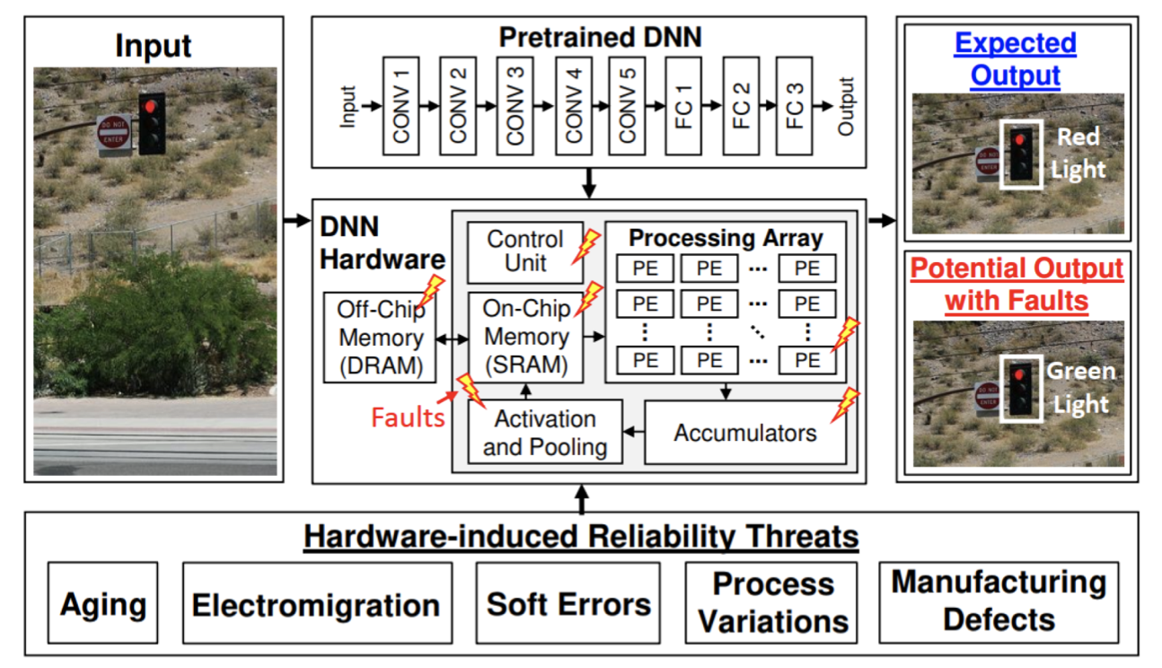
These methods enable researchers to observe the system’s behavior under real-world fault conditions. Both software-based and hardware-based error injection tools are described in this section in more detail.
Hardware Injection Methods
Two of the most common hardware-based fault injection methods are FPGA-based fault injection and radiation or beam testing.
FPGA-based Fault Injection. Field-Programmable Gate Arrays (FPGAs)67 are reconfigurable integrated circuits that can be programmed to implement various hardware designs. In the context of fault injection, FPGAs offer high precision and accuracy, as researchers can target specific bits or sets of bits within the hardware. By modifying the FPGA configuration, faults can be introduced at specific locations and times during the execution of an ML model. FPGA-based fault injection allows for fine-grained control over the fault model, enabling researchers to study the impact of different types of faults, such as single-bit flips or multi-bit errors. This level of control makes FPGA-based fault injection a valuable tool for understanding the resilience of ML systems to hardware faults.
67 Field-Programmable Gate Arrays (FPGAs): Reconfigurable hardware devices containing millions of logic blocks that can be programmed to implement custom digital circuits. Originally developed by Xilinx in 1985, FPGAs bridge the gap between software flexibility and hardware performance, enabling rapid prototyping and specialized accelerators.
While FPGA-based methods allow precise, controlled fault injection, other approaches aim to replicate fault conditions found in natural environments.
Radiation or Beam Testing. Radiation or beam testing (Velazco, Foucard, and Peronnard 2010) exposes hardware running ML models to high-energy particles like protons or neutrons. As shown in Figure 40, specialized test facilities enable controlled radiation exposure to induce bitflips and other hardware-level faults. This approach is widely regarded as one of the most accurate methods for measuring error rates from particle strikes during application execution. Beam testing provides highly realistic fault scenarios that mirror conditions in radiation-rich environments, making it particularly valuable for validating systems destined for space missions or particle physics experiments. However, while beam testing offers exceptional realism, it lacks the precise targeting capabilities of FPGA-based injection - particle beams cannot be aimed at specific hardware bits or components with high precision. Despite this limitation and its significant operational complexity and cost, beam testing remains a trusted industry practice for rigorously evaluating hardware reliability under real-world radiation effects.
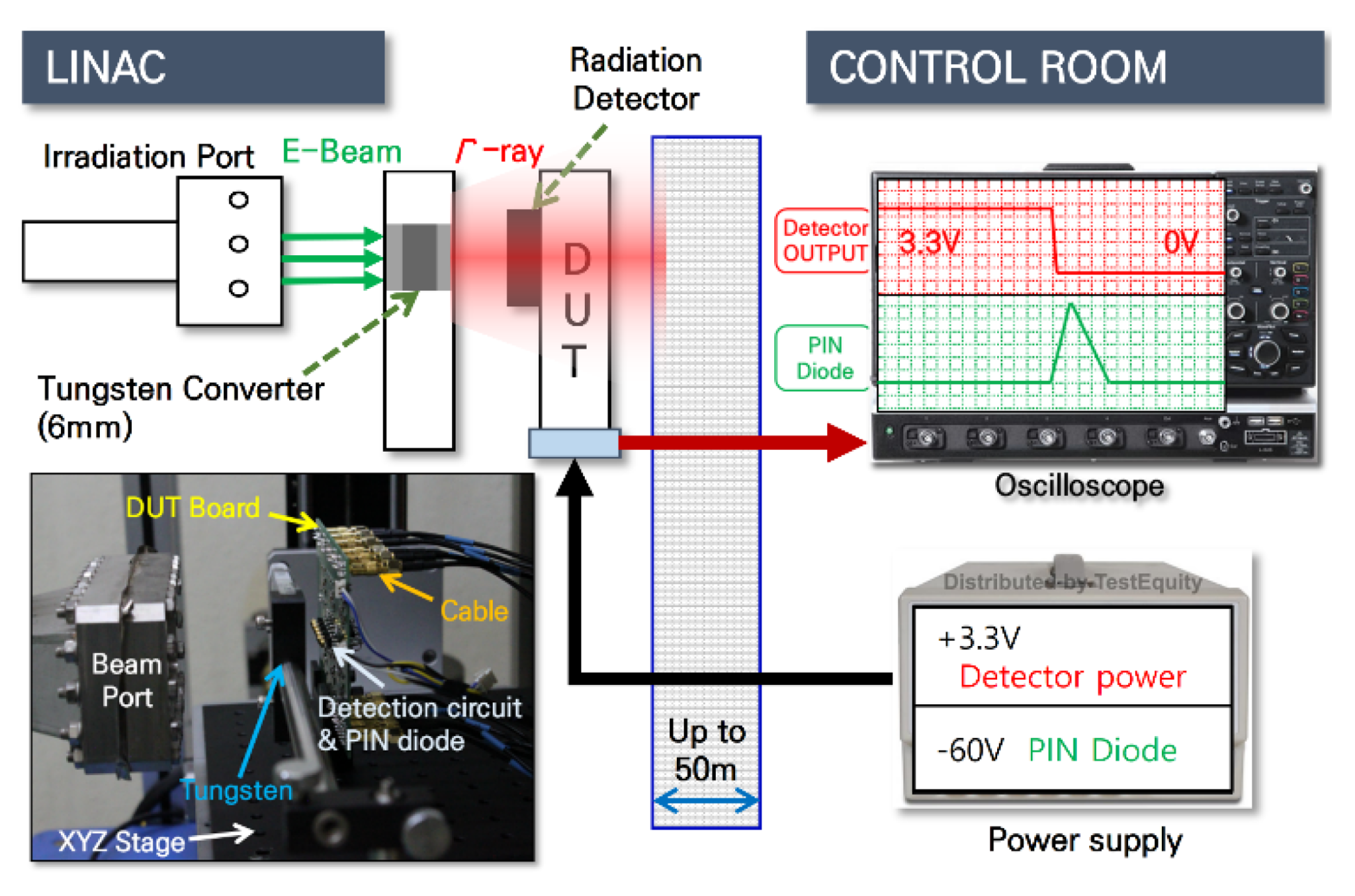
Hardware Injection Limitations
Despite their high accuracy, hardware-based fault injection methods have several limitations that can hinder their widespread adoption.
First, cost is a major barrier. Both FPGA-based and beam testing68 approaches require specialized hardware and facilities, which can be expensive to set up and maintain. This makes them less accessible to research groups with limited funding or infrastructure.
68 Beam Testing: A testing method that exposes hardware to controlled particle radiation to evaluate its resilience to soft errors. Common in aerospace, medical devices, and high-reliability computing.
Second, these methods face challenges in scalability. Injecting faults and collecting data directly on hardware is time-consuming, which limits the number of experiments that can be run in a reasonable timeframe. This is especially restrictive when analyzing large ML systems or performing statistical evaluations across many fault scenarios.
Third, flexibility limitations exist. Hardware-based methods may not be as adaptable as software-based alternatives when modeling a wide variety of fault and error types. Changing the experimental setup to accommodate a new fault model often requires time-intensive hardware reconfiguration.
Despite these limitations, hardware-based fault injection remains essential for validating the accuracy of software-based tools and for studying system behavior under real-world fault conditions. By combining the high fidelity of hardware-based methods with the scalability and flexibility of software-based tools, researchers can develop a more complete understanding of ML systems’ resilience to hardware faults and craft effective mitigation strategies.
Software-Based Fault Injection
As machine learning frameworks like TensorFlow, PyTorch, and Keras have become the dominant platforms for developing and deploying ML models, software-based fault injection tools have emerged as a flexible and scalable way to evaluate the robustness of these systems to hardware faults. Unlike hardware-based approaches, which operate directly on physical systems, software-based methods simulate the effects of hardware faults by modifying a model’s underlying computational graph, tensor values, or intermediate computations.
These tools have become increasingly popular in recent years because they integrate directly with ML development pipelines, require no specialized hardware, and allow researchers to conduct large-scale fault injection experiments quickly and cost-effectively. By simulating hardware-level faults, including bit flips in weights, activations, or gradients, at the software level, these tools enable efficient testing of fault tolerance mechanisms and provide valuable insight into model vulnerabilities.
In the remainder of this section, we will examine the advantages and limitations of software-based fault injection methods, introduce major classes of tools (both general-purpose and domain-specific), and discuss how they contribute to building resilient ML systems.
Software Injection Trade-offs
Software-based fault injection tools offer several advantages that make them attractive for studying the resilience of ML systems.
One of the primary benefits is speed. Since these tools operate entirely within the software stack, they avoid the overhead associated with modifying physical hardware or configuring specialized test environments. This efficiency enables researchers to perform a large number of fault injection experiments in significantly less time. The ability to simulate a wide range of faults quickly makes these tools particularly useful for stress-testing large-scale ML models or conducting statistical analyses that require thousands of injections.
These tools also offer flexibility. Software-based fault injectors can be easily adapted to model various types of faults. Researchers can simulate single-bit flips, multi-bit corruptions, or even more complex behaviors such as burst errors or partial tensor corruption. Software tools allow faults to be injected at different stages of the ML pipeline, at the stages of training, inference, or gradient computation, enabling precise targeting of different system components or layers.
These tools are also highly accessible, as they require only standard ML development environments. Unlike hardware-based methods, software tools require no costly experimental setups, custom circuitry, or radiation testing facilities. This accessibility opens up fault injection research to a broader range of institutions and developers, including those working in academia, startups, or resource-constrained environments.
However, these advantages come with certain trade-offs. Chief among them is accuracy. Because software-based tools model faults at a higher level of abstraction, they may not fully capture the low-level hardware interactions that influence how faults actually propagate. For example, a simulated bit flip in an ML framework may not account for how data is buffered, cached, or manipulated at the hardware level, potentially leading to oversimplified conclusions.
Closely related is the issue of fidelity. While it is possible to approximate real-world fault behaviors, software-based tools may diverge from true hardware behavior, particularly when it comes to subtle interactions like masking, timing, or data movement. The results of such simulations depend heavily on the underlying assumptions of the error model and may require validation against real hardware measurements to be reliable.
Despite these limitations, software-based fault injection tools play an indispensable role in the study of ML robustness. Their speed, flexibility, and accessibility allow researchers to perform wide-ranging evaluations and inform the development of fault-tolerant ML architectures. In subsequent sections, we explore the major tools in this space, highlighting their capabilities and use cases.
Software Injection Limitations
While software-based fault injection tools offer significant advantages in terms of speed, flexibility, and accessibility, they are not without limitations. These constraints can impact the accuracy and realism of fault injection experiments, particularly when assessing the robustness of ML systems to real-world hardware faults.
One major concern is accuracy. Because software-based tools operate at higher levels of abstraction, they may not always capture the full spectrum of effects that hardware faults can produce. Low-level hardware interactions, including subtle timing errors, voltage fluctuations, and architectural side effects, can be missed entirely in high-level simulations. As a result, fault injection studies that rely solely on software models may under- or overestimate a system’s true vulnerability to certain classes of faults.
Closely related is the issue of fidelity. While software-based methods are often designed to emulate specific fault behaviors, the extent to which they reflect real-world hardware conditions can vary. For example, simulating a single-bit flip in the value of a neural network weight may not fully replicate how that same bit error would propagate through memory hierarchies or affect computation units on an actual chip. The more abstract the tool, the greater the risk that the simulated behavior will diverge from physical behavior under fault conditions.
Because software-based tools are easier to modify, they risk unintentionally deviating from realistic fault assumptions. This can occur if the chosen fault model is overly simplified or not grounded in empirical data from actual hardware behavior. As discussed later in the section on bridging the hardware-software gap, tools like Fidelity (He, Balaprakash, and Li 2020) attempt to address these concerns by aligning software-level models with known hardware-level fault characteristics.
Despite these limitations, software-based fault injection remains a critical part of the ML robustness research toolkit. When used appropriately, particularly when used in conjunction with hardware-based validation, these tools provide a scalable and efficient way to explore large design spaces, identify vulnerable components, and develop mitigation strategies. As fault modeling techniques continue to evolve, the integration of hardware-aware insights into software-based tools will be key to improving their realism and impact.
Software Injection Tool Categories
Over the past several years, software-based fault injection tools have been developed for a wide range of ML frameworks and use cases. These tools vary in their level of abstraction, target platforms, and the types of faults they can simulate. Many are built to integrate with popular machine learning libraries such as PyTorch and TensorFlow, making them accessible to researchers and practitioners already working within those ecosystems.
One of the earliest and most influential tools is Ares (Reagen et al. 2018), initially designed for the Keras framework. Developed at a time when deep neural networks (DNNs) were growing in popularity, Ares was one of the first tools to systematically explore the effects of hardware faults on DNNs. It provided support for injecting single-bit flips and evaluating bit-error rates (BER) across weights and activation values. Importantly, Ares was validated against a physical DNN accelerator implemented in silicon, demonstrating its relevance for hardware-level fault modeling. As the field matured, Ares was extended to support PyTorch, allowing researchers to analyze fault behavior in more modern ML settings.
Building on this foundation, PyTorchFI (Mahmoud et al. 2020) was introduced as a dedicated fault injection library for PyTorch. Developed in collaboration with Nvidia Research, PyTorchFI allows fault injection into key components of ML models, including weights, activations, and gradients. Its native support for GPU acceleration makes it especially well-suited for evaluating large models efficiently. As shown in Figure 41, even simple bit-level faults can cause severe visual and classification errors, including the appearance of ‘phantom’ objects in images, which could have downstream safety implications in domains like autonomous driving.
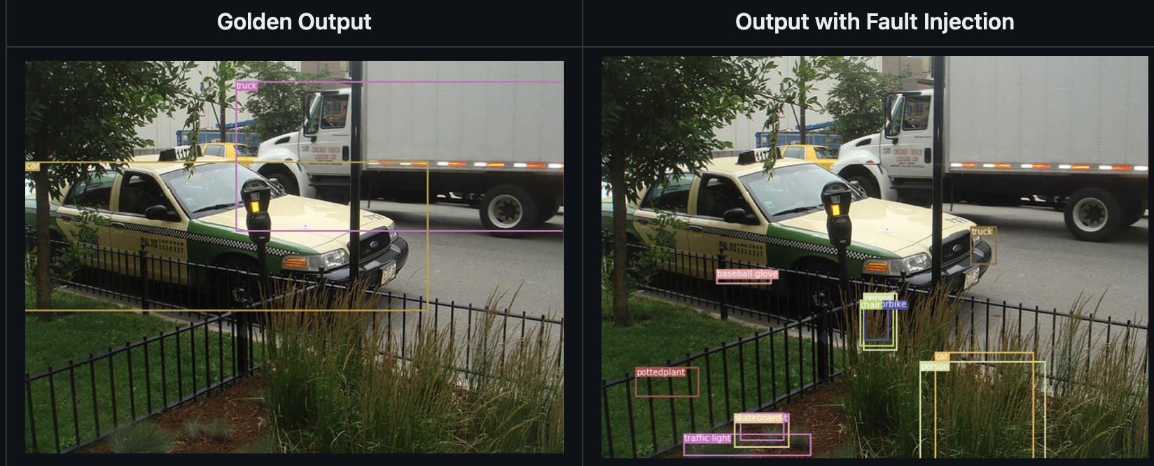
The modular and accessible design of PyTorchFI has led to its adoption in several follow-on projects. For example, PyTorchALFI (developed by Intel xColabs) extends PyTorchFI’s capabilities to evaluate system-level safety in automotive applications. Similarly, Dr. DNA (Ma et al. 2024) from Meta introduces a more streamlined, Pythonic API to simplify fault injection workflows. Another notable extension is GoldenEye (Mahmoud et al. 2022), which incorporates alternative numeric datatypes, including AdaptivFloat (Tambe et al. 2020) and BlockFloat, with bfloat16 as a specific example, to study the fault tolerance of non-traditional number formats under hardware-induced bit errors.
For researchers working within the TensorFlow ecosystem, TensorFI (Chen et al. 2020) provides a parallel solution. Like PyTorchFI, TensorFI enables fault injection into the TensorFlow computational graph and supports a variety of fault models. One of TensorFI’s strengths is its broad applicability—it can be used to evaluate many types of ML models beyond DNNs. Additional extensions such as BinFi (Chen et al. 2019) aim to accelerate the fault injection process by focusing on the most critical bits in a model. This prioritization can help reduce simulation time while still capturing the most meaningful error patterns.
At a lower level of the software stack, NVBitFI (T. Tsai et al. 2021) offers a platform-independent tool for injecting faults directly into GPU assembly code. Developed by Nvidia, NVBitFI is capable of performing fault injection on any GPU-accelerated application, not just ML workloads. This makes it an especially powerful tool for studying resilience at the instruction level, where errors can propagate in subtle and complex ways. NVBitFI represents an important complement to higher-level tools like PyTorchFI and TensorFI, offering fine-grained control over GPU-level behavior and supporting a broader class of applications beyond machine learning.
Together, these tools offer a wide spectrum of fault injection capabilities. While some are tightly integrated with high-level ML frameworks for ease of use, others enable lower-level fault modeling with higher fidelity. By choosing the appropriate tool based on the level of abstraction, performance needs, and target application, researchers can tailor their studies to gain more actionable insights into the robustness of ML systems. The next section focuses on how these tools are being applied in domain-specific contexts, particularly in safety-critical systems such as autonomous vehicles and robotics.
ML-Specific Injection Tools
To address the unique challenges posed by specific application domains, researchers have developed specialized fault injection tools tailored to different ML systems. In high-stakes environments such as autonomous vehicles and robotics, domain-specific tools play a crucial role in evaluating system safety and reliability under hardware fault conditions. This section highlights three such tools: DriveFI and PyTorchALFI, which focus on autonomous vehicles, and MAVFI, which targets uncrewed aerial vehicles (UAVs). Each tool enables the injection of faults into mission-critical components, including perception, control, and sensor systems, providing researchers with insights into how hardware errors may propagate through real-world ML pipelines.
DriveFI (Jha et al. 2019) is a fault injection tool developed for autonomous vehicle systems. It facilitates the injection of hardware faults into the perception and control pipelines, enabling researchers to study how such faults affect system behavior and safety. Notably, DriveFI integrates with industry-standard platforms like Nvidia DriveAV and Baidu Apollo, offering a realistic environment for testing. Through this integration, DriveFI enables practitioners to evaluate the end-to-end resilience of autonomous vehicle architectures in the presence of fault conditions.
69 Multimodal Sensor Data: Information collected simultaneously from multiple types of sensors (e.g., cameras, LiDAR, radar) to provide complementary perspectives of the environment. Critical for robust perception in autonomous systems.
PyTorchALFI (Gräfe et al. 2023) extends the capabilities of PyTorchFI for use in the autonomous vehicle domain. Developed by Intel xColabs, PyTorchALFI enhances the underlying fault injection framework with domain-specific features. These include the ability to inject faults into multimodal sensor data69, such as inputs from cameras and LiDAR systems. This allows for a deeper examination of how perception systems in autonomous vehicles respond to underlying hardware faults, further refining our understanding of system vulnerabilities and potential failure modes.
MAVFI (Hsiao et al. 2023) is a domain-specific fault injection framework tailored for robotics applications, particularly uncrewed aerial vehicles. Built atop the Robot Operating System (ROS), MAVFI provides a modular and extensible platform for injecting faults into various UAV subsystems, including sensors, actuators, and flight control algorithms. By assessing how injected faults impact flight stability and mission success, MAVFI offers a practical means for developing and validating fault-tolerant UAV architectures.
Together, these tools demonstrate the growing sophistication of fault injection research across application domains. By enabling fine-grained control over where and how faults are introduced, domain-specific tools provide actionable insights that general-purpose frameworks may overlook. Their development has greatly expanded the ML community’s capacity to design and evaluate resilient systems—particularly in contexts where reliability, safety, and real-time performance are critical.
Bridging Hardware-Software Gap
While software-based fault injection tools offer many advantages in speed, flexibility, and accessibility, they do not always capture the full range of effects that hardware faults can impose on a system. This is largely due to the abstraction gap: software-based tools operate at a higher level and may overlook low-level hardware interactions or nuanced error propagation mechanisms that influence the behavior of ML systems in critical ways.
As discussed in the work by (Bolchini et al. 2023), hardware faults can exhibit complex spatial distribution patterns that are difficult to replicate using purely software-based fault models. They identify four characteristic fault propagation patterns: single point, where the fault corrupts a single value in a feature map; same row, where a partial or entire row in a feature map is corrupted; bullet wake, where the same location across multiple feature maps is affected; and shatter glass, a more complex combination of both same row and bullet wake behaviors. These diverse patterns, visualized in Figure 42, highlight the limits of simplistic injection strategies and emphasize the need for hardware-aware modeling when evaluating ML system robustness.

To address this abstraction gap, researchers have developed tools that explicitly aim to map low-level hardware error behavior to software-visible effects. One such tool is Fidelity, which bridges this gap by studying how hardware-level faults propagate and become observable at higher software layers. The next section discusses Fidelity in more detail.
Simulation Fidelity Challenges
Fidelity (He, Balaprakash, and Li 2020) is a tool designed to model hardware faults more accurately within software-based fault injection experiments. Its core goal is to bridge the gap between low-level hardware fault behavior and the higher-level effects observed in machine learning systems by simulating how faults propagate through the compute stack.
The central insight behind Fidelity is that not all faults need to be modeled individually at the hardware level to yield meaningful results. Instead, Fidelity focuses on how faults manifest at the software-visible state and identifies equivalence relationships that allow representative modeling of entire fault classes. To accomplish this, it relies on several key principles:
First, fault propagation is studied to understand how a fault originating in hardware can move through various layers, including architectural registers, memory hierarchies, and numerical operations, eventually altering values in software. Fidelity captures these pathways to ensure that injected faults in software reflect the way faults would actually manifest in a real system.
Second, the tool identifies fault equivalence, which refers to grouping hardware faults that lead to similar observable outcomes in software. By focusing on representative examples rather than modeling every possible hardware bit flip individually, Fidelity allows more efficient simulations without sacrificing accuracy.
Finally, Fidelity uses a layered modeling approach, capturing the system’s behavior at various abstraction levels—from hardware fault origin to its effect in the ML model’s weights, activations, or predictions. This layering ensures that the impact of hardware faults is realistically simulated in the context of the ML system.
By combining these techniques, Fidelity allows researchers to run fault injection experiments that closely mirror the behavior of real hardware systems, but with the efficiency and flexibility of software-based tools. This makes Fidelity especially valuable in safety-critical settings, where the cost of failure is high and an accurate understanding of hardware-induced faults is essential.
Hardware Behavior Modeling
Capturing the true behavior of hardware faults in software-based fault injection tools is critical for advancing the reliability and robustness of ML systems. This fidelity becomes especially important when hardware faults have subtle but significant effects that may not be evident when modeled at a high level of abstraction.
Several reasons explain why accurately reflecting hardware behavior is essential. First, accuracy is paramount. Software-based tools that mirror the actual propagation and manifestation of hardware faults provide more dependable insights into how faults influence model behavior. These insights are crucial for designing and validating fault-tolerant architectures and ensuring that mitigation strategies are grounded in realistic system behavior.
Second, reproducibility is improved when hardware effects are faithfully captured. This allows fault injection results to be reliably reproduced across different systems and environments, which is a cornerstone of rigorous scientific research. Researchers can better compare results, validate findings, and ensure consistency across studies.
Third, efficiency is enhanced when fault models focus on the most representative and impactful fault scenarios. Rather than exhaustively simulating every possible bit flip, tools can target a subset of faults that are known, through accurate modeling, to affect the system in meaningful ways. This selective approach saves computational resources while still providing thorough insights.
Finally, understanding how hardware faults appear at the software level is essential for designing effective mitigation strategies. When researchers know how specific hardware-level issues affect different components of an ML system, they can develop more targeted hardening techniques—such as retraining specific layers, applying redundancy selectively, or improving architectural resilience in bottleneck components.
Tools like Fidelity are central to this effort. By establishing mappings between low-level hardware behavior and higher-level software effects, Fidelity and similar tools empower researchers to conduct fault injection experiments that are not only faster and more scalable, but also grounded in real-world system behavior.
As ML systems continue to increase in scale and are deployed in increasingly safety-critical environments, this kind of hardware-aware modeling will become even more important. Ongoing research in this space aims to further refine the translation between hardware and software fault models and to develop tools that offer both efficiency and realism in evaluating ML system resilience. These advances will provide the community with more powerful, reliable methods for understanding and defending against the effects of hardware faults.
Fallacies and Pitfalls
The complexity and interconnected nature of robustness threats often leads to misconceptions about effective defense strategies, particularly around the assumption that robustness techniques provide universal protection without trade-offs or limitations.
Fallacy: Adversarial robustness can be achieved through defensive techniques without trade-offs.
This misconception leads teams to believe that robustness techniques like adversarial training or input preprocessing provide complete protection without costs. Adversarial defenses often introduce significant trade-offs including reduced clean accuracy, increased computational overhead, or brittleness to new attack methods. Many defensive techniques that appear effective against specific attacks fail when evaluated against stronger or adaptive adversaries. The arms race between attacks and defenses means that robustness is not a solved problem but an ongoing engineering challenge that requires continuous adaptation and evaluation against evolving threats.
Pitfall: Testing robustness only against known attack methods rather than comprehensive threat modeling.
Many practitioners evaluate model robustness by testing against a few standard adversarial attacks without considering the full spectrum of potential threats. This approach provides false confidence when models perform well against limited test cases but fail catastrophically against novel attack vectors. Real-world threats include not only sophisticated adversarial examples but also hardware faults, data corruption, distribution shifts, and software vulnerabilities that may not resemble academic attack scenarios. Comprehensive robustness evaluation requires systematic threat modeling that considers the full attack surface rather than focusing on a narrow set of known vulnerabilities.
Fallacy: Distribution shift can be solved by collecting more diverse training data.
This belief assumes that dataset diversity alone ensures robustness to distribution shifts encountered in deployment. While diverse training data helps, it cannot anticipate all possible distribution changes that occur in dynamic real-world environments. Training datasets remain inherently limited compared to the infinite variety of deployment conditions. Some distribution shifts are inherently unpredictable, emerging from changing user behavior, evolving data sources, or external environmental factors. Effective robustness requires adaptive systems with monitoring, detection, and response capabilities rather than relying solely on comprehensive training data.
Pitfall: Assuming that robustness techniques designed for one threat category protect against all failure modes.
Teams often apply robustness techniques developed for specific threats without understanding their limitations against other failure modes. Adversarial training designed for gradient-based attacks may not improve robustness against hardware faults or data poisoning. Similarly, techniques that handle benign distribution shifts might fail against adversarial distribution shifts designed to exploit model weaknesses. Each threat category requires specialized defenses, and effective robustness necessitates layered protection strategies that address the full spectrum of potential failures rather than assuming cross-domain effectiveness.
Fallacy: Different failure modes operate independently and can be addressed in isolation.
This assumption overlooks the complex interactions between different fault types that can create compound vulnerabilities exceeding the sum of individual threats. Real-world failures often involve cascading effects where one vulnerability enables or amplifies others. Consider these compound scenarios:
Hardware-adversarial interactions illustrate how bit flips in model weights can inadvertently create adversarial vulnerabilities not present in the original model. An attacker discovering these corruptions could craft targeted adversarial examples that exploit the specific weight perturbations, achieving 95% attack success rates compared to 20% on uncorrupted models. Conversely, adversarial training meant to improve robustness increases model complexity by 2-3\(\times\), raising the probability of hardware faults due to increased memory and computation requirements.
Environmental-software cascades occur when gradual distribution shift may go undetected due to bugs in monitoring software that fail to log outlier samples. As the shift progresses over 3-6 months, the model’s accuracy degrades by 40%, but the faulty monitoring system reports normal operation. When finally discovered, the compounded data drift and delayed detection require complete model retraining rather than incremental adaptation, incurring 10\(\times\) higher recovery costs.
Attack-enabled distribution exploitation involves an adversary observing natural distribution shift in a deployed system and crafting poisoning attacks that accelerate the drift in specific directions. By injecting just 0.1% poisoned samples that align with natural drift patterns, attackers can cause 5\(\times\) faster performance degradation while evading detection systems calibrated for either pure adversarial or pure drift scenarios.
Triple-threat scenarios demonstrate the most severe compound vulnerabilities. Consider an autonomous vehicle where cosmic ray-induced bit flips corrupt perception model weights, adversarial road markings exploit these corruptions, and seasonal weather changes create distribution shift. The combination results in 85% misclassification of stop signs under specific conditions, while each individual threat would cause only 15-20% degradation.
These compound scenarios demonstrate that robust AI systems must consider threat interactions through comprehensive failure mode analysis, cross-domain testing that evaluates combined vulnerabilities, and defense strategies that account for cascading failures rather than treating each threat in isolation.
Summary
This chapter established robust AI as a core requirement for reliable machine learning systems operating in real-world environments. Through examination of concrete failures across cloud, edge, and embedded deployments, we demonstrated that robustness challenges span multiple dimensions and require systematic approaches to detection, mitigation, and recovery.
The unified framework developed here organizes robustness challenges into three interconnected pillars that share common principles while requiring specialized approaches. System-level faults address the physical substrate reliability that underlies all ML computations, from transient cosmic ray effects to permanent hardware degradation. Input-level attacks encompass deliberate attempts to manipulate model behavior through adversarial examples and data poisoning techniques. Environmental shifts represent the natural evolution of deployment conditions that challenge static model assumptions through distribution drift and concept changes.
Across these three pillars, robust AI systems implement common principles of detection and monitoring to identify threats before they impact system behavior, graceful degradation to maintain core functionality under stress, and adaptive response to adjust system behavior based on detected conditions. These principles manifest differently across pillar types but provide a unified foundation for building comprehensive robustness solutions.
The practical implementation of robust AI requires integration across the entire ML pipeline, from data collection through deployment and monitoring. Hardware fault tolerance mechanisms must coordinate with adversarial defenses and drift detection systems to provide comprehensive protection. This robustness foundation establishes the reliability guarantees necessary for the operational frameworks detailed in Chapter 13: ML Operations, where these fault-tolerant systems will be deployed, monitored, and maintained at scale. Without the comprehensive reliability mechanisms developed here, the operational workflows in the next chapter would lack the fundamental resilience required for production deployment.
Table 7 provides a practical reference mapping each of the three main fault categories to their primary detection and mitigation strategies, serving as an engineering guide for implementing comprehensive robustness solutions:
| Fault Category | Detection Methods | Mitigation Strategies |
|---|---|---|
| System-Level | ECC Memory | Redundancy (TMR/DMR) |
| Faults | BIST (Built-In Self-Test) Watchdog Timers Voltage/Temperature Monitoring | Checkpointing Hardware Redundancy Error Correction Codes |
| Input-Level | Input Sanitization | Adversarial Training |
| Attacks | Anomaly Detection Statistical Testing Behavioral Analysis | Defensive Distillation Input Preprocessing Model Ensembles |
| Environmental | Statistical Monitoring (MMD, PSI) | Continuous Learning |
| Shifts | Distribution Comparison Performance Degradation Tracking Concept Drift Detection | Model Retraining Adaptive Thresholds Ensemble Methods |
- Robust AI systems must address three interconnected threat categories: system-level faults, input-level attacks, and environmental shifts
- Common principles of detection, graceful degradation, and adaptive response apply across all threat types while requiring specialized implementations
- Hardware reliability directly impacts ML performance, with single-bit errors capable of degrading model accuracy by 10-50%
- Real-world robustness requires integration across the entire ML pipeline rather than isolated protection mechanisms
- Modern AI deployments require systematic approaches to robustness evaluation and mitigation
Building on these robustness foundations, the following chapters examine complementary aspects of trustworthy AI systems. Privacy and security considerations (Chapter 15: Security & Privacy) layer additional operational requirements onto robust deployment infrastructure, requiring specialized techniques for protecting sensitive data while maintaining system reliability. The principles developed here for detecting and responding to threats provide foundational patterns that extend to privacy-preserving and secure AI system design, creating comprehensive frameworks for trustworthy AI deployment across diverse environments and applications.
Building robust AI systems requires embedding robustness considerations throughout the development process, from initial design through deployment and maintenance, validated through systematic evaluation methods detailed in Chapter 12: Benchmarking AI and aligned with responsible AI principles from Chapter 17: Responsible AI. Critical applications in autonomous vehicles, medical devices, and infrastructure systems demand proactive approaches that anticipate failure modes and implement extensive safeguards. The challenge extends beyond individual components to encompass system-level interactions, requiring comprehensive approaches that ensure reliable operation under diverse and evolving conditions encountered in real-world deployments while considering the sustainability implications of robust system design covered in Chapter 18: Sustainable AI.