Model Optimizations
DALL·E 3 Prompt: Illustration of a neural network model represented as a busy construction site, with a diverse group of construction workers, both male and female, of various ethnicities, labeled as ‘pruning’, ‘quantization’, and ‘sparsity’. They are working together to make the neural network more efficient and smaller, while maintaining high accuracy. The ‘pruning’ worker, a Hispanic female, is cutting unnecessary connections from the middle of the network. The ‘quantization’ worker, a Caucasian male, is adjusting or tweaking the weights all over the place. The ‘sparsity’ worker, an African female, is removing unnecessary nodes to shrink the model. Construction trucks and cranes are in the background, assisting the workers in their tasks. The neural network is visually transforming from a complex and large structure to a more streamlined and smaller one.

Purpose
How does the mismatch between research-optimized models and production deployment constraints create critical engineering challenges in machine learning systems?
Machine learning research prioritizes accuracy above all considerations, producing models with remarkable performance that cannot deploy where needed most: resource-constrained mobile devices, cost-sensitive cloud environments, or latency-critical edge applications. Model optimization bridges theoretical capability and practical deployment, transforming computationally intensive research models into efficient systems preserving performance while meeting stringent constraints on memory, energy, latency, and cost. Without systematic optimization techniques, advanced AI capabilities remain trapped in research laboratories. Understanding optimization principles enables engineers to democratize AI capabilities by making sophisticated models accessible across diverse deployment contexts, from billion-parameter language models running on mobile devices to embedded sensors.
Compare model optimization techniques including pruning, quantization, knowledge distillation, and neural architecture search in terms of their mechanisms and applications
Evaluate trade-offs between numerical precision levels and their effects on model accuracy, energy consumption, and hardware compatibility
Apply the tripartite optimization framework (model representation, numerical precision, architectural efficiency) to design deployment strategies for specific hardware constraints
Analyze how hardware-aware design principles influence model architecture decisions and computational efficiency across different deployment platforms
Implement sparsity exploitation and dynamic computation techniques to improve inference performance while managing accuracy preservation
Design integrated optimization pipelines that combine multiple techniques to achieve specific deployment objectives within resource constraints
Assess automated optimization approaches and their role in discovering novel optimization strategies beyond manual tuning
Model Optimization Fundamentals
Successful deployment of machine learning systems requires addressing the tension between model sophistication and computational feasibility. Contemporary research in machine learning has produced increasingly powerful models whose resource demands often exceed the practical constraints of real-world deployment environments. This represents the classic engineering challenge of translating theoretical advances into viable systems, affecting the accessibility and scalability of machine learning applications.
The magnitude of this resource gap is substantial and multifaceted. State-of-the-art language models may require several hundred gigabytes of memory for full-precision parameter storage (Brown et al. 2020; Chowdhery et al. 2022), while target deployment platforms such as mobile devices typically provide only a few gigabytes of available memory. This disparity extends beyond memory constraints to encompass computational throughput, energy consumption, and latency requirements. The challenge is further compounded by the heterogeneous nature of deployment environments, each imposing distinct constraints and performance requirements.
Production machine learning systems operate within a complex optimization landscape characterized by multiple, often conflicting, performance objectives. Real-time applications impose strict latency bounds, mobile deployments require energy efficiency to preserve battery life, embedded systems must operate within thermal constraints, and cloud services demand cost-effective resource utilization at scale. These constraints collectively define a multi-objective optimization problem that requires systematic approaches to achieve satisfactory solutions across all relevant performance dimensions.
The engineering discipline of model optimization has evolved to address these challenges through systematic methodologies that integrate algorithmic innovation with hardware-aware design principles. Effective optimization strategies require deep understanding of the interactions between model architecture, numerical precision, computational patterns, and target hardware characteristics. This interdisciplinary approach transforms optimization from an ad hoc collection of techniques into a principled engineering discipline guided by theoretical foundations and empirical validation.
This chapter establishes a comprehensive theoretical and practical framework for model optimization organized around three interconnected dimensions: structural efficiency in model representation, numerical efficiency through precision optimization, and computational efficiency via hardware-aware implementation. Through this framework, we examine how established techniques such as quantization achieve memory reduction and inference acceleration, how pruning methods eliminate parameter redundancy while preserving model accuracy, and how knowledge distillation enables capability transfer from complex models to efficient architectures. The overarching objective transcends simple performance metrics to enable the deployment of sophisticated machine learning capabilities across the complete spectrum of computational environments and application domains.
Optimization Framework
The optimization process operates through three interconnected dimensions that bridge software algorithms and hardware execution, as illustrated in Figure 1. Understanding these dimensions and their relationships provides the conceptual foundation for all techniques explored in this chapter.

Understanding these layer interactions reveals the systematic nature of optimization engineering. Model representation techniques (pruning, distillation, structured approximations) reduce computational complexity while creating opportunities for numerical precision optimization. Quantization and reduced-precision arithmetic exploit hardware capabilities for faster execution, while architectural efficiency techniques align computation patterns with processor designs. Software optimizations establish the foundation for hardware acceleration by creating structured, predictable workloads that specialized processors can execute efficiently.
This chapter examines each optimization layer through an engineering lens, providing specific algorithms for quantization (post-training and quantization-aware training), pruning strategies (magnitude-based, structured, and dynamic), and distillation procedures (temperature scaling, feature transfer). We explore how these techniques combine synergistically and how their effectiveness depends on target hardware characteristics. The framework guides systematic optimization decisions, ensuring that model transformations align with deployment constraints while preserving essential capabilities.
This chapter transforms the efficiency concepts from earlier foundations into actionable engineering practices through systematic application of optimization principles. Mastery of quantization, pruning, and distillation techniques provides practitioners with the essential tools for deploying sophisticated machine learning models across diverse computational environments. The optimization framework presented bridges the gap between theoretical model capabilities and practical deployment requirements, enabling machine learning systems that deliver both performance and efficiency in real-world applications.
Deployment Context
Machine learning models operate as part of larger systems with complex constraints, dependencies, and trade-offs. Model optimization cannot be treated as a purely algorithmic problem; it must be viewed as a systems-level challenge that considers computational efficiency, scalability, deployment feasibility, and overall system performance. Operational principles from Chapter 13: ML Operations provide the foundation for understanding the systems perspective on model optimization, highlighting why optimization is important, the key constraints that drive optimization efforts, and the principles that define an effective optimization strategy.
Practical Deployment
Modern machine learning models often achieve impressive accuracy on benchmark datasets, but making them practical for real-world use is far from trivial. Machine learning systems operate under computational, memory, latency, and energy constraints that significantly impact both training and inference (Choudhary et al. 2020). Models that perform well in research settings may prove impractical when integrated into broader systems, regardless of deployment context including cloud environments, smartphone integration, or microcontroller implementation.
1 Microcontroller Constraints: Arduino Uno has 2KB SRAM vs. 32KB flash storage. ARM Cortex-M4 implementations typically have 256KB flash, 64KB RAM, running at up to 168MHz vs. modern GPUs with 3000+ MHz clocks and 16-80GB memory, representing a 10,000x+ resource gap.
Beyond these deployment complexities, real-world feasibility encompasses efficiency in training, storage, and execution rather than accuracy alone.1
Efficiency requirements manifest differently across deployment contexts. In large-scale cloud ML settings, optimizing models helps minimize training time, computational cost, and power consumption, making large-scale AI workloads more efficient (Dean, Patterson, and Young 2018). In contrast, edge ML2 requires models to run with limited compute resources, necessitating optimizations that reduce memory footprint and computational complexity. Mobile ML introduces additional constraints, such as battery life and real-time responsiveness, while tiny ML3 pushes efficiency to the extreme, requiring models to fit within the memory and processing limits of ultra-low-power devices (Banbury et al. 2020).
2 Edge ML: Computing paradigm where ML inference occurs on local devices (smartphones, IoT sensors, autonomous vehicles) rather than cloud servers. Reduces latency from 100-500ms cloud round-trip to <10ms local processing, but constrains models to 10-500MB vs. multi-GB cloud models.
3 Tiny ML: Ultra-low-power ML systems operating under 1mW power budget with <1MB memory. Enables always-on AI in hearing aids, smart sensors, and wearables. Models typically 10-100KB vs. GB-scale cloud models, representing 10,000x size reduction.
Optimization contributes to sustainable and accessible AI deployment, following sustainability principles established in Chapter 18: Sustainable AI. Reducing a model’s energy footprint is important as AI workloads scale, helping mitigate the environmental impact of large-scale ML training and inference (Patterson et al. 2021). At the same time, optimized models can expand the reach of machine learning, supporting applications in low-resource environments, from rural healthcare to autonomous systems operating in the field.
Balancing Trade-offs
The tension between accuracy and efficiency drives optimization decisions across all dimensions. Increasing model capacity generally enhances predictive performance while increasing computational cost, resulting in slower, more resource-intensive inference. These improvements introduce challenges related to memory footprint4, inference latency, power consumption, and training efficiency. As machine learning systems are deployed across a wide range of hardware platforms, balancing accuracy and efficiency becomes a key challenge in model optimization.
4 Memory Bandwidth: Modern GPUs achieve 3.0 TB/s memory bandwidth (H100 SXM5) vs. 25-50 GB/s for high-end mobile SoCs. Large language models require 1-2x model size in GPU memory for training (16GB model needs 32GB+ GPU memory), creating the “memory wall” bottleneck.
This tension manifests differently across deployment contexts. Training requires computational resources that scale with model size, while inference demands strict latency and power constraints in real-time applications.
Optimization Dimensions
Each optimization dimension merits detailed examination. As shown in Figure 1, model representation optimization reduces what computations are performed, numerical precision optimization changes how computations are executed, and architectural efficiency optimization ensures operations run efficiently on target hardware.
Model Representation
The first dimension, model representation optimization, focuses on eliminating redundancy in the structure of machine learning models. Large models often contain excessive parameters5 that contribute little to overall performance but significantly increase memory footprint and computational cost. Optimizing model representation involves techniques that remove unnecessary components while maintaining predictive accuracy. These include pruning, knowledge distillation, and automated architecture search methods that refine model structures to balance efficiency and accuracy. These optimizations primarily impact how models are designed at an algorithmic level, ensuring that they remain effective while being computationally manageable.
5 Overparameterization: Modern neural networks typically have 10-100x more parameters than theoretically needed. GPT-3’s 175B parameters could theoretically be compressed to 1-10B while maintaining 95% performance, but overparameterization enables faster training convergence and better generalization during the learning process.
Numerical Precision
While representation techniques modify what computations are performed, precision optimization changes how those computations are executed by reducing the numerical fidelity of weights, activations, and arithmetic operations. The second dimension, numerical precision optimization, addresses how numerical values are represented and processed within machine learning models. The precision optimization techniques detailed in this section address these efficiency challenges. Quantization techniques map high-precision weights and activations to lower-bit representations, enabling efficient execution on hardware accelerators such as GPUs, TPUs, and specialized AI chips (Chapter 11: AI Acceleration). Mixed-precision training6 dynamically adjusts precision levels during training to strike a balance between efficiency and accuracy.
6 Mixed-Precision Training: Uses FP16 for forward pass and FP32 for gradient computation, achieving 1.5-2x training speedup with ~50% memory reduction. NVIDIA’s automatic mixed precision (AMP) maintains FP32 accuracy while delivering approximately 1.6x speedup on V100 and up to 2.2x on A100 GPUs.
Careful numerical precision optimization enables significant computational cost reductions while maintaining acceptable accuracy levels, providing sophisticated model access in resource-constrained environments.
Architectural Efficiency
The third dimension, architectural efficiency, addresses efficient computation performance during training and inference. Well-designed model structure proves insufficient when execution remains suboptimal. Many machine learning models contain redundancies in their computational graphs, leading to inefficiencies in how operations are scheduled and executed. Sparsity7 represents a key architectural efficiency technique where models exploit zero-valued parameters to reduce computation.
7 Sparsity: Percentage of zero-valued parameters in a model. 90% sparse models have only 10% non-zero weights, reducing memory by 10x and computation by 10x (with specialized hardware). Modern transformers naturally exhibit 80-95% activation sparsity during inference.
8 Matrix Factorization: Decomposes large weight matrices (e.g., 4096×4096) into smaller matrices (4096×256 × 256×4096), reducing parameters from 16M to 2M (8x reduction). SVD and low-rank approximations maintain 95%+ accuracy while enabling 3-5x speedup on mobile hardware.
Architectural efficiency involves techniques that exploit sparsity in both model weights and activations, factorize large computational components into more efficient forms8, and dynamically adjust computation based on input complexity.
These architectural optimization methods improve execution efficiency across different hardware platforms, reducing latency and power consumption. These efficiency principles extend naturally to training scenarios, where techniques such as gradient checkpointing and low-rank adaptation9 help reduce memory overhead and computational demands.
9 LoRA (Low-Rank Adaptation): Fine-tuning technique that freezes pretrained weights and adds small trainable matrices, reducing trainable parameters by over 99% (from 175B to approximately 1.2M for GPT-3 scale). Achieves comparable performance while reducing training memory and computation by 3x.
Three-Dimensional Optimization Framework
The interconnected nature of this three-dimensional framework emerges when examining technique interactions. Pruning primarily addresses model representation but also affects architectural efficiency by reducing inference operations. Quantization focuses on numerical precision but impacts memory footprint and execution efficiency. Understanding these interdependencies enables optimal optimization combinations.
This interconnected nature means that the choice of optimizations is driven by system constraints, which define the practical limitations within which models must operate. A machine learning model deployed in a data center has different constraints from one running on a mobile device or an embedded system. Computational cost, memory usage, inference latency, and energy efficiency all influence which optimizations are most appropriate for a given scenario. A model that is too large for a resource-constrained device may require aggressive pruning and quantization, while a latency-sensitive application may benefit from operator fusion10 and hardware-aware scheduling.
10 Operator Fusion: Graph-level optimization that combines multiple operations into single kernels, reducing memory bandwidth by 30-50%. In ResNet-50, fusing Conv+BatchNorm+ReLU operations achieves 1.8x speedup on V100 GPUs, while BERT transformer blocks show 25% latency reduction through attention fusion.
The constraint-dimension mapping established in Table 1 demonstrates interdependence between optimization strategies and real-world constraints. These relationships extend beyond one-to-one correspondence, as many optimization techniques affect multiple constraints simultaneously.
Systematic examination of each dimension begins with model representation optimization, encompassing techniques that modify neural network structure and parameters to eliminate redundancy while preserving accuracy.
Structural Model Optimization Methods
Model representation optimization modifies neural network structure and parameters to improve efficiency while preserving accuracy. Modern models often prioritize accuracy over efficiency, containing excessive parameters that increase costs and slow inference. This optimization addresses inefficiencies through two objectives: eliminating redundancy (exploiting overparameterization where models achieve similar performance with fewer parameters) and structuring computations for efficient hardware execution through techniques like gradient checkpointing11 and parallel processing patterns12.
11 Gradient Checkpointing: Memory optimization technique that trades computation for memory by recomputing intermediate activations during backpropagation instead of storing them. Reduces memory usage by 20-50% in transformer models, enabling larger batch sizes or model sizes within same GPU memory.
12 Parallel Processing in ML: High-end datacenter GPUs have 5,000-10,000+ cores vs. CPU’s 8-64 cores. NVIDIA H100 delivers 989 TFLOPS tensor performance vs. Intel Xeon 3175-X’s ~1.5 TFLOPS (double precision), representing a 650x compute density advantage for parallelizable ML workloads.
13 Pareto Frontier: In model optimization, the curve where improving one metric (speed) requires sacrificing another (accuracy). EfficientNet family demonstrates optimal accuracy-FLOPS trade-offs: EfficientNet-B0 (77.1% ImageNet, 390M FLOPs) to B7 (84.4%, 37B FLOPs), showing diminishing returns at scale.
The optimization challenge lies in balancing competing constraints13. Aggressive compression risks accuracy degradation that renders models unreliable for production use, while insufficient optimization leaves models too large or slow for target deployment environments. Selecting appropriate techniques requires understanding trade-offs between model size, computational complexity, and generalization performance.
Three key techniques address this challenge: pruning eliminates low-impact parameters, knowledge distillation transfers capabilities to smaller models, and NAS automates architecture design for specific constraints. Each technique offers distinct optimization pathways while maintaining model performance.
These three techniques represent distinct but complementary approaches within our optimization framework. Pruning and knowledge distillation reduce redundancy in existing models, while NAS addresses building optimized architectures from the ground up. In many cases, they can be combined to achieve even greater optimization.
Pruning
The memory wall constrains system performance: as models grow larger, memory bandwidth becomes the bottleneck rather than computational capacity. Pruning directly addresses this constraint by lowering memory requirements through parameter elimination. State-of-the-art machine learning models often contain millions or billions of parameters, many of which contribute minimally to final predictions. While large models enhance representational power and generalization, they also introduce inefficiencies in memory footprint, computational cost, and scalability that impact both training and deployment across cloud, edge, and mobile environments.
Parameter necessity for accuracy maintenance varies considerably. Many weights contribute minimally to decision-making processes, enabling significant efficiency improvements through removal without substantial performance degradation. This redundancy exists because modern neural networks are heavily overparameterized, meaning they have far more weights than are strictly necessary to solve a task. This overparameterization serves important purposes during training by providing multiple optimization paths and helping avoid poor local minima, but it creates opportunities for compression during deployment. Model compression preserves performance through information-theoretic principles from Chapter 3: Deep Learning Primer, where neural networks’ overparameterization creates compression opportunities. This observation motivates pruning, a class of optimization techniques that systematically removes redundant parameters while preserving model accuracy.
Pruning enables models to become smaller, faster, and more efficient without requiring architectural redesign. By eliminating redundancy, pruning directly addresses the memory, computation, and scalability constraints of machine learning systems, making it essential for deploying models across diverse hardware platforms.
Modern frameworks provide built-in APIs that make these optimization techniques readily accessible. PyTorch offers torch.nn.utils.prune for pruning operations, while TensorFlow provides the Model Optimization Toolkit14 with functions like tfmot.sparsity.keras.prune_low_magnitude(). These tools transform complex research algorithms into practical function calls, making optimization achievable for practitioners at all levels.
14 TensorFlow Model Optimization: TensorFlow Model Optimization Toolkit provides production-ready quantization (achieving 4x model size reduction), pruning (up to 90% sparsity), and clustering techniques. Used by YouTube, Gmail, and Google Photos to deploy models on 4+ billion devices worldwide.
Pruning Example
Pruning can be illustrated through systematic example. Pruning identifies weights contributing minimally to model predictions and removes them while maintaining accuracy. The most intuitive approach examines weight magnitudes, as weights with small absolute values typically have minimal impact on outputs, making them candidates for removal.
Listing 1 demonstrates magnitude-based pruning on a 3×3 weight matrix, showing how a simple threshold rule creates sparsity.
import torch
import torch.nn.utils.prune as prune

# Original dense weight matrix
weights = torch.tensor(
    [[0.8, 0.1, -0.7], [0.05, -0.9, 0.03], [-0.6, 0.02, 0.4]]
)

# Simple magnitude-based pruning: remove weights with magnitude < 0.5
threshold = 0.5
mask = torch.abs(weights) >= threshold
pruned_weights = weights * mask

print("Original:", weights)
print("Pruned:", pruned_weights)
# Result: 4 out of 9 weights remain (56% sparsity)
This example illustrates the core pruning objective: minimize the number of parameters while maintaining model performance. We reduced nonzero parameters from 9 to 4 (keeping only 4 weights, hence a budget of \(k=4\)). The weights with smallest magnitudes (0.4, 0.1, 0.05, 0.03, 0.02) were removed, while the four largest magnitude weights (0.8, -0.7, -0.9, -0.6) were preserved.
Extending this intuition to full neural networks requires considering both how many parameters to remove (the sparsity level) and which parameters to remove (the selection criterion). The next visualization shows this applied to larger weight matrices.
As illustrated in Figure 2, pruning reduces the number of nonzero weights by eliminating small-magnitude values, transforming a dense weight matrix into a sparse representation. This explicit enforcement of sparsity aligns with the \(\ell_0\)-norm constraint in our optimization formulation.

Mathematical Formulation
The goal of pruning can be stated simply: we want to find the version of our model that has the fewest non-zero weights (the smallest size) while causing the smallest possible increase in the prediction error (the loss). This intuitive goal translates into a mathematical optimization problem that guides practical pruning algorithms.
The pruning process can be formalized as an optimization problem. Given a trained model with parameters \(W\), we seek a sparse version \(\hat{W}\) that retains only the most important parameters. The objective is expressed as:
\[ \min_{\hat{W}} \mathcal{L}(\hat{W}) \quad \text{subject to} \quad \|\hat{W}\|_0 \leq k \]
where \(\mathcal{L}(\hat{W})\) represents the model’s loss function after pruning, \(\hat{W}\) denotes the pruned model’s parameters, \(\|\hat{W}\|_0\) is the L0-norm (number of nonzero parameters), and \(k\) is the parameter budget constraining maximum model size.
The L0-norm directly measures model size by counting nonzero parameters, which determines memory usage and computational cost. However, L0-norm minimization is NP-hard, making this optimization challenging. Practical pruning algorithms use heuristics like magnitude-based selection, gradient-based importance, or second-order sensitivity to approximate solutions efficiently.
In Listing 1, this constraint becomes concrete: we reduced \(\|\hat{W}\|_0\) from 9 to 4 (satisfying \(k=4\)), with the magnitude threshold acting as our selection heuristic. Alternative formulations using L1 or L2 norms encourage small weights but don’t guarantee exact zeros, failing to reduce actual memory or computation without explicit thresholding.
To make pruning computationally feasible, practical methods replace the hard constraint with a soft regularization term: \[ \min_W \mathcal{L}(W) + \lambda \| W \|_1 \] where \(\lambda\) controls sparsity degree. The \(\ell_1\)-norm encourages smaller weight values and promotes sparsity but does not strictly enforce zero values. Other methods use iterative heuristics, where parameters with smallest magnitudes are pruned in successive steps, followed by fine-tuning to recover lost accuracy (Gale, Elsen, and Hooker 2019a; Labarge, n.d.).
Target Structures
Pruning methods vary based on which structures within a neural network are removed. The primary targets include neurons, channels, and layers, each with distinct implications for the model’s architecture and performance.
Neuron pruning removes entire neurons along with their associated weights and biases, reducing the width of a layer. This technique is often applied to fully connected layers.
Channel pruning (or filter pruning), commonly used in convolutional neural networks, eliminates entire channels or filters. This reduces the depth of feature maps, which impacts the network’s ability to extract certain features. Channel pruning is particularly valuable in image-processing tasks where computational efficiency is a priority.
Layer pruning removes entire layers from the network, significantly reducing depth. While this approach can yield significant efficiency gains, it requires careful balance to ensure the model retains sufficient capacity to capture complex patterns.
Figure 3 illustrates the differences between channel pruning and layer pruning. When a channel is pruned, the model’s architecture must be adjusted to accommodate the structural change. Specifically, the number of input channels in subsequent layers must be modified, requiring alterations to the depths of the filters applied to the layer with the removed channel. In contrast, layer pruning removes all channels within a layer, necessitating more significant architectural modifications. In this case, connections between remaining layers must be reconfigured to bypass the removed layer. Regardless of the pruning approach, fine-tuning is important to adapt the remaining network and restore performance.

Unstructured Pruning
Unstructured pruning removes individual weights while preserving the overall network architecture. During training, some connections become redundant, contributing little to the final computation. Pruning these weak connections reduces memory requirements while preserving most of the model’s accuracy.
The mathematical foundation for unstructured pruning helps understand how sparsity is systematically introduced. Mathematically, unstructured pruning introduces sparsity into the weight matrices of a neural network. Let \(W \in \mathbb{R}^{m \times n}\) represent a weight matrix in a given layer of a network. Pruning removes a subset of weights by applying a binary mask \(M \in \{0,1\}^{m \times n}\), yielding a pruned weight matrix: \[ \hat{W} = M \odot W \] where \(\odot\) represents the element-wise Hadamard product. The mask \(M\) is constructed based on a pruning criterion, typically weight magnitude. A common approach is magnitude-based pruning, which removes a fraction \(s\) of the lowest-magnitude weights. This is achieved by defining a threshold \(\tau\) such that: \[ M_{i,j} = \begin{cases} 1, & \text{if } |W_{i,j}| > \tau \\ 0, & \text{otherwise} \end{cases} \] where \(\tau\) is chosen to ensure that only the largest \((1 - s)\) fraction of weights remain. This method assumes that larger-magnitude weights contribute more to the network’s function, making them preferable for retention.
The primary advantage of unstructured pruning is memory efficiency. By reducing the number of nonzero parameters, pruned models require less storage, which is particularly beneficial when deploying models to embedded or mobile devices with limited memory.
However, unstructured pruning does not necessarily improve computational efficiency on modern machine learning hardware. Standard GPUs and TPUs are optimized for dense matrix multiplications, and a sparse weight matrix often cannot fully utilize hardware acceleration unless specialized sparse computation kernels are available. Therefore, unstructured pruning primarily benefits model storage rather than inference acceleration. While unstructured pruning improves model efficiency at the parameter level, it does not alter the structural organization of the network.
Structured Pruning
While unstructured pruning removes individual weights from a neural network, structured pruning15 eliminates entire computational units, such as neurons, filters, channels, or layers. This approach is particularly beneficial for hardware efficiency, as it produces smaller dense models that can be directly mapped to modern machine learning accelerators. Unlike unstructured pruning, which results in sparse weight matrices that require specialized execution kernels to exploit computational benefits, structured pruning leads to more efficient inference on general-purpose hardware by reducing the overall size of the network architecture.
15 Structured Pruning: Filter pruning in ResNet-34 achieves 50% FLOP reduction with only 1.0% accuracy loss on CIFAR-10. Channel pruning in MobileNetV2 reduces parameters by 73% while maintaining 96.5% of original accuracy, enabling 3.2x faster inference on ARM processors.
Structured pruning is motivated by the observation that not all neurons, filters, or layers contribute equally to a model’s predictions. Some units primarily carry redundant or low-impact information, and removing them does not significantly degrade model performance. The challenge lies in identifying which structures can be pruned while preserving accuracy.
Figure 4 illustrates the key differences between unstructured and structured pruning. On the left, unstructured pruning removes individual weights (depicted as dashed connections), creating a sparse weight matrix. This can disrupt the original network structure, as shown in the fully connected network where certain connections have been randomly pruned. While this reduces the number of active parameters, the resulting sparsity requires specialized execution kernels to fully utilize computational benefits.
In contrast, structured pruning (depicted in the middle and right sections of the figure) removes entire neurons or filters while preserving the network’s overall structure. In the middle section, a pruned fully connected network retains its fully connected nature but with fewer neurons. On the right, structured pruning is applied to a CNN by removing convolutional kernels or entire channels (dashed squares). This method maintains the CNN’s core convolutional operations while reducing the computational load, making it more compatible with hardware accelerators.

A common approach to structured pruning is magnitude-based pruning, where entire neurons or filters are removed based on the magnitude of their associated weights. The intuition behind this method is that parameters with smaller magnitudes contribute less to the model’s output, making them prime candidates for elimination. The importance of a neuron or filter is often measured using a norm function, such as the \(\ell_1\)-norm or \(\ell_2\)-norm, applied to the weights associated with that unit. If the norm falls below a predefined threshold, the corresponding neuron or filter is pruned. This method is straightforward to implement and does not require additional computational overhead beyond computing norms across layers.
Another strategy is activation-based pruning, which evaluates the average activation values of neurons or filters over a dataset. Neurons that consistently produce low activations contribute less information to the network’s decision process and can be safely removed. This method captures the dynamic behavior of the network rather than relying solely on static weight values. Activation-based pruning requires profiling the model over a representative dataset to estimate the average activation magnitudes before making pruning decisions.
Gradient-based pruning uses information from the model’s training process to identify less significant neurons or filters. The key idea is that units with smaller gradient magnitudes contribute less to reducing the loss function, making them less important for learning. By ranking neurons based on their gradient values, structured pruning can remove those with the least impact on model optimization. Unlike magnitude-based or activation-based pruning, which rely on static properties of the trained model, gradient-based pruning requires access to gradient computations and is typically applied during training rather than as a post-processing step.
Each of these methods presents trade-offs in terms of computational complexity and effectiveness. Magnitude-based pruning is computationally inexpensive and easy to implement but does not account for how neurons behave across different data distributions. Activation-based pruning provides a more data-driven pruning approach but requires additional computations to estimate neuron importance. Gradient-based pruning leverages training dynamics but may introduce additional complexity if applied to large-scale models. The choice of method depends on the specific constraints of the target deployment environment and the performance requirements of the pruned model.
Dynamic Pruning
Traditional pruning methods, whether unstructured or structured, typically involve static pruning, where parameters are permanently removed after training or at fixed intervals during training. However, this approach assumes that the importance of parameters is fixed, which is not always the case. In contrast, dynamic pruning adapts pruning decisions based on the input data or training dynamics, allowing the model to adjust its structure in real time.
Dynamic pruning can be implemented using runtime sparsity techniques, where the model actively determines which parameters to utilize based on input characteristics. Activation-conditioned pruning exemplifies this approach by selectively deactivating neurons or channels that exhibit low activation values for specific inputs (J. Hu et al. 2023). This method introduces input-dependent sparsity patterns, effectively reducing the computational workload during inference without permanently modifying the model architecture.
For instance, consider a convolutional neural network processing images with varying complexity. During inference of a simple image containing mostly uniform regions, many convolutional filters may produce negligible activations. Dynamic pruning identifies these low-impact filters and temporarily excludes them from computation, improving efficiency while maintaining accuracy for the current input. This adaptive behavior is particularly advantageous in latency-sensitive applications, where computational resources must be allocated judiciously based on input complexity, connecting to performance measurement strategies (Chapter 12: Benchmarking AI).
Another class of dynamic pruning operates during training, where sparsity is gradually introduced and adjusted throughout the optimization process. Methods such as gradual magnitude pruning start with a dense network and progressively increase the fraction of pruned parameters as training progresses. Instead of permanently removing parameters, these approaches allow the network to recover from pruning-induced capacity loss by regrowing connections that prove to be important in later stages of training.
Dynamic pruning presents several advantages over static pruning. It allows models to adapt to different workloads, potentially improving efficiency while maintaining accuracy. Unlike static pruning, which risks over-pruning and degrading performance, dynamic pruning provides a mechanism for selectively reactivating parameters when necessary. However, implementing dynamic pruning requires additional computational overhead, as pruning decisions must be made in real-time, either during training or inference. This makes it more complex to integrate into standard machine learning pipelines compared to static pruning, requiring sophisticated production deployment strategies and monitoring frameworks covered in Chapter 13: ML Operations.
Despite its challenges, dynamic pruning is particularly useful in edge computing and adaptive AI systems (Chapter 14: On-Device Learning), where resource constraints and real-time efficiency requirements vary across different inputs. The next section explores the practical considerations and trade-offs involved in choosing the right pruning method for a given machine learning system.
Pruning Trade-offs
Pruning techniques offer different trade-offs in terms of memory efficiency, computational efficiency, accuracy retention, hardware compatibility, and implementation complexity. The choice of pruning strategy depends on the specific constraints of the machine learning system and the deployment environment, integrating with operational considerations (Chapter 13: ML Operations).
Unstructured pruning is particularly effective in reducing model size and memory footprint, as it removes individual weights while keeping the overall model architecture intact. However, since machine learning accelerators are optimized for dense matrix operations, unstructured pruning does not always translate to significant computational speed-ups unless specialized sparse execution kernels are used.
Structured pruning, in contrast, eliminates entire neurons, channels, or layers, leading to a more hardware-friendly model. This technique provides direct computational savings, as it reduces the number of floating-point operations (FLOPs)16 required during inference.
16 FLOPs (Floating-Point Operations): Computational complexity metric counting multiply-add operations. ResNet-50 requires approximately 3.8 billion FLOPs per inference (K. He et al. 2015), GPT-3 training required an estimated 3.14E23 FLOPs (Patterson et al. 2021). Modern GPUs achieve 100-300 TFLOPS (trillion FLOPs/second), making FLOP reduction important for efficiency.
The downside is that modifying the network structure can lead to a greater accuracy drop, requiring careful fine-tuning to recover lost performance.
Dynamic pruning introduces adaptability into the pruning process by adjusting which parameters are pruned at runtime based on input data or training dynamics. This allows for a better balance between accuracy and efficiency, as the model retains the flexibility to reintroduce previously pruned parameters if needed. However, dynamic pruning increases implementation complexity, as it requires additional computations to determine which parameters to prune on-the-fly.
Table 2 summarizes the key structural differences between these pruning approaches, outlining how each method modifies the model and impacts its execution.
| Aspect | Unstructured Pruning | Structured Pruning | Dynamic Pruning |
|---|---|---|---|
| What is removed? | Individual weights in the model | Entire neurons, channels, filters, or layers | Adjusts pruning based on runtime conditions |
| Model structure | Sparse weight matrices; original architecture remains unchanged | Model architecture is modified; pruned layers are fully removed | Structure adapts dynamically |
| Impact on memory | Reduces model storage by eliminating nonzero weights | Reduces model storage by removing entire components | Varies based on real-time pruning |
| Impact on computation | Limited; dense matrix operations still required unless specialized sparse computation is used | Directly reduces FLOPs and speeds up inference | Balances accuracy and efficiency dynamically |
| Hardware compatibility | Sparse weight matrices require specialized execution support for efficiency | Works efficiently with standard deep learning hardware | Requires adaptive inference engines |
| Fine-tuning required? | Often necessary to recover accuracy after pruning | More likely to require fine-tuning due to larger structural modifications | Adjusts dynamically, reducing the need for retraining |
| Use cases | Memory-efficient model compression, particularly for cloud deployment | Real-time inference optimization, mobile/edge AI, and efficient training | Adaptive AI applications, real-time systems |
Pruning Strategies
Beyond the broad categories of unstructured, structured, and dynamic pruning, different pruning workflows can impact model efficiency and accuracy retention. Two widely used pruning strategies are iterative pruning and one-shot pruning, each with its own benefits and trade-offs.
Iterative Pruning
Iterative pruning implements a gradual approach to structure removal through multiple cycles of pruning followed by fine-tuning. During each cycle, the algorithm removes a small subset of structures based on predefined importance metrics. The model then undergoes fine-tuning to adapt to these structural modifications before proceeding to the next pruning iteration. This methodical approach helps prevent sudden drops in accuracy while allowing the network to progressively adjust to reduced complexity.
To illustrate this process, consider pruning six channels from a convolutional neural network as shown in Figure 5. Rather than removing all channels simultaneously, iterative pruning eliminates two channels per iteration over three cycles. Following each pruning step, the model undergoes fine-tuning to recover performance. The first iteration, which removes two channels, results in an accuracy decrease from 0.995 to 0.971, but subsequent fine-tuning restores accuracy to 0.992. After completing two additional pruning-tuning cycles, the final model achieves 0.991 accuracy, which represents only a 0.4% reduction from the original, while operating with 27% fewer channels. By distributing structural modifications across multiple iterations, the network maintains its performance capabilities while achieving improved computational efficiency.

One-shot Pruning
One-shot pruning removes multiple architectural components in a single step, followed by an extensive fine-tuning phase to recover model accuracy. This aggressive approach compresses the model quickly but risks greater accuracy degradation, as the network must adapt to significant structural changes simultaneously.
Consider applying one-shot pruning to the same network from the iterative pruning example. Instead of removing two channels at a time over multiple iterations, one-shot pruning eliminates all six channels simultaneously, as illustrated in Figure 6. Removing 27% of the network’s channels simultaneously causes the accuracy to drop significantly, from 0.995 to 0.914. Even after fine-tuning, the network only recovers to an accuracy of 0.943, which is a 5% degradation from the original unpruned network. While both iterative and one-shot pruning ultimately produce identical network structures, the gradual approach of iterative pruning better preserves model performance.

The choice of pruning strategy requires careful consideration of several key factors that influence both model efficiency and performance. The desired level of parameter reduction, or sparsity target, directly impacts strategy selection. Higher reduction targets often necessitate iterative approaches to maintain accuracy, while moderate sparsity goals may be achievable through simpler one-shot methods.
Available computational resources significantly influence strategy choice. Iterative pruning demands significant resources for multiple fine-tuning cycles, whereas one-shot approaches require fewer resources but may sacrifice accuracy. This resource consideration connects to performance requirements, where applications with strict accuracy requirements typically benefit from gradual, iterative pruning to carefully preserve model capabilities. Use cases with more flexible performance constraints may accommodate more aggressive one-shot approaches.
Development timeline also impacts pruning decisions. One-shot methods enable faster deployment when time is limited, though iterative approaches generally achieve superior results given sufficient optimization periods. Finally, target platform capabilities significantly influence strategy selection, as certain hardware architectures may better support specific sparsity patterns, making particular pruning approaches more advantageous for deployment.
The choice between pruning strategies requires careful evaluation of project requirements and constraints. One-shot pruning enables rapid model compression by removing multiple parameters simultaneously, making it suitable for scenarios where deployment speed is prioritized over accuracy. However, this aggressive approach often results in greater performance degradation compared to more gradual methods. Iterative pruning, on the other hand, while computationally intensive and time-consuming, typically achieves superior accuracy retention through structured parameter reduction across multiple cycles. This methodical approach enables the network to adapt progressively to structural modifications, preserving important connections that maintain model performance. The trade-off is increased optimization time and computational overhead. By evaluating these factors systematically, practitioners can select a pruning approach that optimally balances efficiency gains with model performance for their specific use case.
Lottery Ticket Hypothesis
Pruning is widely used to reduce the size and computational cost of neural networks, but the process of determining which parameters to remove is not always straightforward. While traditional pruning methods eliminate weights based on magnitude, structure, or dynamic conditions, recent research suggests that pruning is not just about reducing redundancy; it may also reveal inherently efficient subnetworks that exist within the original model.
This perspective leads to the Lottery Ticket Hypothesis17 (LTH), which challenges conventional pruning workflows by proposing that within large neural networks, there exist small, well-initialized subnetworks, referred to as ‘winning tickets’, that can achieve comparable accuracy to the full model when trained in isolation. Rather than viewing pruning as just a post-training compression step, LTH suggests it can serve as a discovery mechanism to identify these efficient subnetworks early in training.
17 Lottery Ticket Hypothesis: The lottery ticket hypothesis (Frankle and Carbin 2018) demonstrates that ResNet-18 subnetworks at 10-20% original size achieve 93.2% accuracy vs. 94.1% for full model on CIFAR-10. BERT-base winning tickets retain 97% performance with 90% fewer parameters, requiring 5-8x less training time to converge.
LTH is validated through an iterative pruning process, illustrated in Figure 7. A large network is first trained to convergence. The lowest-magnitude weights are then pruned, and the remaining weights are reset to their original initialization rather than being re-randomized. This process is repeated iteratively, gradually reducing the network’s size while preserving performance. After multiple iterations, the remaining subnetwork, referred to as the ‘winning ticket’, proves capable of training to the same or higher accuracy as the original full model.

The implications of the Lottery Ticket Hypothesis extend beyond conventional pruning techniques. Instead of training large models and pruning them later, LTH suggests that compact, high-performing subnetworks could be trained directly from the start, eliminating the need for overparameterization. This insight challenges the traditional assumption that model size is necessary for effective learning. It also emphasizes the importance of initialization, as winning tickets only retain their performance when reset to their original weight values. This finding raises deeper questions about the role of initialization in shaping a network’s learning trajectory.
The hypothesis further reinforces the effectiveness of iterative pruning over one-shot pruning. Gradually refining the model structure allows the network to adapt at each stage, preserving accuracy more effectively than removing large portions of the model in a single step. This process aligns well with practical pruning strategies used in deployment, where preserving accuracy while reducing computation is important.
Despite its promise, applying LTH in practice remains computationally expensive, as identifying winning tickets requires multiple cycles of pruning and retraining. Ongoing research explores whether winning subnetworks can be detected early without full training, potentially leading to more efficient sparse training techniques. If such methods become practical, LTH could corely reshape how machine learning models are trained, shifting the focus from pruning large networks after training to discovering and training only the important components from the beginning.
While LTH presents a compelling theoretical perspective on pruning, practical implementations rely on established framework-level tools to integrate structured and unstructured pruning techniques.
Pruning Practice
Several machine learning frameworks provide built-in tools to apply structured and unstructured pruning, fine-tune pruned models, and optimize deployment for cloud, edge, and mobile environments.
Machine learning frameworks such as PyTorch, TensorFlow, and ONNX offer dedicated pruning utilities that allow practitioners to efficiently implement these techniques while ensuring compatibility with deployment hardware.
In PyTorch, pruning is available through the torch.nn.utils.prune module, which provides functions to apply magnitude-based pruning to individual layers or the entire model. Users can perform unstructured pruning by setting a fraction of the smallest-magnitude weights to zero or apply structured pruning to remove entire neurons or filters. PyTorch also allows for custom pruning strategies, where users define pruning criteria beyond weight magnitude, such as activation-based or gradient-based pruning. Once a model is pruned, it can be fine-tuned to recover lost accuracy before being exported for inference.
TensorFlow provides pruning support through the TensorFlow Model Optimization Toolkit (TF-MOT). This toolkit integrates pruning directly into the training process by applying sparsity-inducing regularization. TensorFlow’s pruning API supports global and layer-wise pruning, dynamically selecting parameters for removal based on weight magnitudes. Unlike PyTorch, TensorFlow’s pruning is typically applied during training, allowing models to learn sparse representations from the start rather than pruning them post-training. TF-MOT also provides export tools to convert pruned models into TFLite format, making them compatible with mobile and edge devices.
ONNX18, an open standard for model representation, does not implement pruning directly but provides export and compatibility support for pruned models from PyTorch and TensorFlow. Since ONNX is designed to be hardware-agnostic, it allows models that have undergone pruning in different frameworks to be optimized for inference engines such as TensorRT19, OpenVINO, and EdgeTPU. These inference engines can further leverage structured and dynamic pruning for execution efficiency, particularly on specialized hardware accelerators.
18 ONNX Deployment: ONNX Runtime achieves 1.3-2.9x speedup over TensorFlow and 1.1-1.7x over PyTorch across various models on CPU platforms. ResNet-50 inference drops from 7.2ms to 2.8ms on CPU, while BERT-Base reduces from 45ms to 23ms with ONNX Runtime optimizations including graph fusion and memory pooling.
19 TensorRT Optimization: NVIDIA TensorRT delivers up to 40x speedup for inference compared to CPU baselines, with typical GPU optimization improvements of 5-8x on V100. ResNet-50 INT8 inference achieves 1.2ms vs. 4.8ms FP32, while BERT-Large drops from 10.4ms to 2.1ms. Layer fusion reduces kernel launches by 80%, memory bandwidth by 50%.
Although framework-level support for pruning has advanced significantly, applying pruning in practice requires careful consideration of hardware compatibility and software optimizations. Standard CPUs and GPUs often do not natively accelerate sparse matrix operations, meaning that unstructured pruning may reduce memory usage without providing significant computational speed-ups. In contrast, structured pruning is more widely supported in inference engines, as it directly reduces the number of computations needed during execution. Dynamic pruning, when properly integrated with inference engines, can optimize execution based on workload variations and hardware constraints, making it particularly beneficial for adaptive AI applications.
At a practical level, choosing the right pruning strategy depends on several key trade-offs, including memory efficiency, computational performance, accuracy retention, and implementation complexity. These trade-offs impact how pruning methods are applied in real-world machine learning workflows, influencing deployment choices based on resource constraints and system requirements.
To help guide these decisions, Table 3 provides a high-level comparison of these trade-offs, summarizing the key efficiency and usability factors that practitioners must consider when selecting a pruning method.
These trade-offs underscore the importance of aligning pruning methods with practical deployment needs. Frameworks such as PyTorch, TensorFlow, and ONNX enable developers to implement these strategies, but the effectiveness of a pruning approach depends on the underlying hardware and application requirements.
| Criterion | Unstructured Pruning | Structured Pruning | Dynamic Pruning |
|---|---|---|---|
| Memory Efficiency | ↑↑ High | ↑ Moderate | ↑ Moderate |
| Computational Efficiency | → Neutral | ↑↑ High | ↑ High |
| Accuracy Retention | ↑ Moderate | ↓↓ Low | ↑↑ High |
| Hardware Compatibility | ↓ Low | ↑↑ High | → Neutral |
| Implementation Complexity | → Neutral | ↑ Moderate | ↓↓ High |
For example, structured pruning is commonly used in mobile and edge applications because of its compatibility with standard inference engines, whereas dynamic pruning is better suited for adaptive AI workloads that need to adjust sparsity levels on the fly. Unstructured pruning, while useful for reducing memory footprints, requires specialized sparse execution kernels to fully realize computational savings.
Understanding these trade-offs is important when deploying pruned models in real-world settings. Several high-profile models have successfully integrated pruning to optimize performance. MobileNet, a lightweight convolutional neural network designed for mobile and embedded applications, has been pruned to reduce inference latency while preserving accuracy (Howard et al. 2017). BERT20, a widely used transformer model for natural language processing, has undergone structured pruning of attention heads and intermediate layers to create efficient versions such as DistilBERT21 and TinyBERT, which retain much of the original performance while reducing computational overhead (Sanh et al. 2019). In computer vision, EfficientNet22 has been pruned to remove unnecessary filters, optimizing it for deployment in resource-constrained environments (Tan and Le 2019a).
20 BERT Compression: BERT-Base (110M params) can be compressed to 67M params (39% reduction) with only 1.2% GLUE score drop. Attention head pruning removes 144 of 192 heads with minimal impact, while layer pruning reduces 12 layers to 6 layers maintaining 97.8% performance.
21 DistilBERT: Achieves 97% of BERT-Base performance with 40% fewer parameters (66M vs. 110M) and 60% faster inference. On SQuAD v1.1, DistilBERT scores 86.9 F1 vs. BERT’s 88.5 F1, while reducing memory from 1.35GB to 0.54GB and latency from 85ms to 34ms.
22 EfficientNet Pruning: EfficientNet-B0 with 70% structured pruning maintains 75.8% ImageNet accuracy (vs. 77.1% original) with 2.8x speedup on mobile devices. Channel pruning reduces FLOPs from 390M to 140M while keeping inference under 20ms on Pixel 4.
Knowledge Distillation
Imagine a world-class professor (the teacher model) who has read thousands of books and has a deep, nuanced understanding of a subject. Now, imagine a bright student (the student model) who needs to learn the subject quickly. Instead of just giving the student the textbook answers (the hard labels), the professor provides rich explanations, pointing out why one answer is better than another and how different concepts relate (the soft labels). The student learns much more effectively from this rich guidance than from the textbook alone. This is the essence of knowledge distillation.
Knowledge distillation trains a smaller student model using guidance from a larger pre-trained teacher, learning from the teacher’s rich output distributions rather than simple correct/incorrect labels. This distinction matters because teacher models provide richer learning signals than ground-truth labels. Consider image classification: a ground-truth label might say “this is a dog” (one-hot encoding: [0, 1, 0, 0, …]). But a trained teacher model might output [0.02, 0.85, 0.08, 0.05, …], revealing that while “dog” is most likely, the image shares some features with “wolf” (0.08) and “fox” (0.05). This inter-class similarity information helps the student learn feature relationships that hard labels cannot convey.
Knowledge distillation differs from pruning. While pruning removes parameters from an existing model, distillation trains a separate, smaller architecture using guidance from a larger pre-trained teacher (Gou et al. 2021). The student model optimizes to match the teacher’s soft predictions (probability distributions over classes) rather than simply learning from labeled data (Jiong Lin et al. 2020).
Figure 8 illustrates the distillation process. The teacher model produces probability distributions using a softened softmax function with temperature \(T\), and the student model trains using both these soft targets and ground truth labels.

The training process for the student model incorporates two loss terms:
- Distillation loss: A loss function (often based on Kullback-Leibler (KL) divergence23) that minimizes the difference between the student’s and teacher’s soft label distributions.
- Student loss: A standard cross-entropy loss that ensures the student model correctly classifies the hard labels.
23 Kullback-Leibler (KL) Divergence: Information-theoretic measure quantifying difference between probability distributions, introduced by Kullback & Leibler (Kullback and Leibler 1951). In knowledge distillation, typical KL divergence values range 0.1-2.0 nats; values >3.0 indicate poor teacher-student alignment requiring temperature adjustment or architecture modification.
The combination of these two loss functions enables the student model to absorb both structured knowledge from the teacher and label supervision from the dataset. This approach allows smaller models to reach accuracy levels close to their larger teacher models, making knowledge distillation a key technique for model compression and efficient deployment.
Knowledge distillation allows smaller models to reach a level of accuracy that would be difficult to achieve through standard training alone. This makes it particularly useful in ML systems where inference efficiency is a priority, such as real-time applications, cloud-to-edge model compression, and low-power AI systems (Sun et al. 2019).
Distillation Theory
Knowledge distillation is based on the idea that a well-trained teacher model encodes more information about the data distribution than just the correct class labels. In conventional supervised learning, a model is trained to minimize the cross-entropy loss24 between its predictions and the ground truth labels. However, this approach only provides a hard decision boundary for each class, discarding potentially useful information about how the model relates different classes to one another (Hinton, Vinyals, and Dean 2015).
24 Cross-Entropy Loss: Standard loss function for classification tasks measuring difference between predicted and true probability distributions. For binary classification, ranges 0-∞ (lower is better); values >2.3 indicate poor performance (worse than random guessing). Computed as -log(predicted probability for true class).
Knowledge distillation addresses this limitation by transferring additional information through the soft probability distributions produced by the teacher model. Instead of training the student model to match only the correct label, it is trained to match the teacher’s full probability distribution over all possible classes. This is achieved by introducing a temperature-scaled softmax function, which smooths the probability distribution, making it easier for the student model to learn from the teacher’s outputs (Gou et al. 2021).
Distillation Mathematics
To formalize this temperature-based approach, let \(z_i\) be the logits (pre-softmax outputs) of the model for class \(i\). The standard softmax function computes class probabilities as: \[ p_i = \frac{\exp(z_i)}{\sum_j \exp(z_j)} \] where higher logits correspond to higher confidence in a class prediction.
In knowledge distillation, we introduce a temperature parameter25 \(T\) that scales the logits before applying softmax: \[ p_i(T) = \frac{\exp(z_i / T)}{\sum_j \exp(z_j / T)} \] where a higher temperature produces a softer probability distribution, revealing more information about how the model distributes uncertainty across different classes.
25 Temperature Parameter: Controls softness of probability distributions in knowledge distillation. T=1 gives standard softmax, T=3-5 typical for distillation (revealing inter-class relationships), T=20+ creates nearly uniform distributions. Optimal temperatures: T=3 for CIFAR-10, T=4 for ImageNet, T=6 for language models like BERT.
The student model is then trained using a loss function that minimizes the difference between its output distribution and the teacher’s softened output distribution. The most common formulation combines two loss terms: \[ \mathcal{L}_{\text{distill}} = (1 - \alpha) \mathcal{L}_{\text{CE}}(y_s, y) + \alpha T^2 \sum_i p_i^T \log p_{i, s}^T \] where:
- \(\mathcal{L}_{\text{CE}}(y_s, y)\) is the standard cross-entropy loss between the student’s predictions \(y_s\) and the ground truth labels \(y\).
- The second term minimizes the Kullback-Leibler (KL) divergence between the teacher’s softened predictions \(p_i^T\) and the student’s predictions \(p_{i, s}^T\).
- The factor \(T^2\) ensures that gradients remain appropriately scaled when using high-temperature values.
- The hyperparameter \(\alpha\) balances the importance of the standard training loss versus the distillation loss.
By learning from both hard labels and soft teacher outputs, the student model benefits from the generalization power of the teacher, improving its ability to distinguish between similar classes even with fewer parameters.
Distillation Intuition
By learning from both hard labels and soft teacher outputs, the student model benefits from the generalization power of the teacher, improving its ability to distinguish between similar classes even with fewer parameters. Unlike conventional training, where a model learns only from binary correctness signals, knowledge distillation allows the student to absorb a richer understanding of the data distribution from the teacher’s predictions.
A key advantage of soft targets is that they provide relative confidence levels rather than just a single correct answer. Consider an image classification task where the goal is to distinguish between different animal species. A standard model trained with hard labels will only receive feedback on whether its prediction is right or wrong. If an image contains a cat, the correct label is “cat,” and all other categories, such as “dog” and “fox,” are treated as equally incorrect. However, a well-trained teacher model naturally understands that a cat is more visually similar to a dog than to a fox, and its soft output probabilities might look like Figure 9, where the relative confidence levels indicate that while “cat” is the most likely category, “dog” is still a plausible alternative, whereas “fox” is much less likely.

Rather than simply forcing the student model to classify the image strictly as a cat, the teacher model provides a more nuanced learning signal, indicating that while “dog” is incorrect, it is a more reasonable mistake than “fox.” This subtle information helps the student model build better decision boundaries between similar classes, making it more robust to ambiguity in real-world data.
This effect is particularly useful in cases where training data is limited or noisy. A large teacher model trained on extensive data has already learned to generalize well, capturing patterns that might be difficult to discover with smaller datasets. The student benefits by inheriting this structured knowledge, acting as if it had access to a larger training signal than what is explicitly available.
Another key benefit of knowledge distillation is its regularization effect. Because soft targets distribute probability mass across multiple classes, they prevent the student model from overfitting to specific hard labels. This regularization improves model generalization and reduces sensitivity to adversarial inputs. Instead of confidently assigning a probability of 1.0 to the correct class and 0.0 to all others, the student learns to make more calibrated predictions, which improves its generalization performance. This is especially important when the student model has fewer parameters, as smaller networks are more prone to overfitting.
Finally, distillation helps compress large models into smaller, more efficient versions without major performance loss. This compression capability directly enables the sustainable AI practices Chapter 18: Sustainable AI by reducing the environmental impact of model deployment while maintaining performance standards. Training a small model from scratch often results in lower accuracy because the model lacks the capacity to learn the complex representations that a larger network can capture. However, by using the knowledge of a well-trained teacher, the student can reach a higher accuracy than it would have on its own, making it a more practical choice for real-world ML deployments, particularly in edge computing, mobile applications, and other resource-constrained environments explored in Chapter 14: On-Device Learning.
Efficiency Gains
Knowledge distillation’s efficiency benefits span three key areas: memory efficiency, computational efficiency, and deployment flexibility. Unlike pruning which modifies trained models, distillation trains compact models from the start using teacher guidance, enabling accuracy levels difficult to achieve through standard training alone (Sanh et al. 2019), supporting structured evaluation approaches in Chapter 12: Benchmarking AI.
Memory and Model Compression
A key advantage of knowledge distillation is that it enables smaller models to retain much of the predictive power of larger models, significantly reducing memory footprint. This is particularly useful in resource-constrained environments such as mobile and embedded AI systems, where model size directly impacts storage requirements and load times.
For instance, models such as DistilBERT (Sanh et al. 2019) in NLP and MobileNet distillation variants (Howard et al. 2017) in computer vision have been shown to retain up to 97% of the accuracy of their larger teacher models while using only half the number of parameters. This level of compression is often superior to pruning, where aggressive parameter reduction can lead to deterioration in representational power.
Another key benefit of knowledge distillation is its ability to transfer robustness and generalization from the teacher to the student. Large models are often trained with extensive datasets and develop strong generalization capabilities, meaning they are less sensitive to noise and data shifts. A well-trained student model inherits these properties, making it less prone to overfitting and more stable across diverse deployment conditions. This is particularly useful in low-data regimes, where training a small model from scratch may result in poor generalization due to insufficient training examples.
Computation and Inference Speed
By training the student model to approximate the teacher’s knowledge in a more compact representation, distillation results in models that require fewer FLOPs per inference, leading to faster execution times. Unlike unstructured pruning, which may require specialized hardware support for sparse computation, a distilled model remains densely structured, making it more compatible with existing machine learning accelerators such as GPUs, TPUs, and edge AI chips (Jiao et al. 2020).
In real-world deployments, this translates to:
- Reduced inference latency, which is important for real-time AI applications such as speech recognition, recommendation systems, and self-driving perception models.
- Lower energy consumption, making distillation particularly relevant for low-power AI on mobile devices and IoT systems.
- Higher throughput in cloud inference, where serving a distilled model allows large-scale AI applications to reduce computational cost while maintaining model quality.
For example, when deploying transformer models for NLP, organizations often use teacher-student distillation to create models that achieve similar accuracy at 2-4\(\times\) lower latency, making it feasible to serve billions of requests per day with significantly lower computational overhead.
Deployment and System Considerations
Knowledge distillation is also effective in multi-task learning scenarios, where a single teacher model can guide multiple student models for different tasks. For example, in multi-lingual NLP models, a large teacher trained on multiple languages can transfer language-specific knowledge to smaller, task-specific student models, enabling efficient deployment across different languages without retraining from scratch. Similarly, in computer vision, a teacher trained on diverse object categories can distill knowledge into specialized students optimized for tasks such as face recognition, medical imaging, or autonomous driving.
Once a student model is distilled, it can be further optimized for hardware-specific acceleration using techniques such as pruning, quantization, and graph optimization. This ensures that compressed models remain inference-efficient across multiple hardware environments, particularly in edge AI and mobile deployments (Gordon, Duh, and Andrews 2020).
Despite its advantages, knowledge distillation has some limitations. The effectiveness of distillation depends on the quality of the teacher model, a poorly trained teacher may transfer incorrect biases to the student. Distillation introduces an additional training phase, where both the teacher and student must be used together, increasing computational costs during training. In some cases, designing an appropriate student model architecture that can fully benefit from the teacher’s knowledge remains a challenge, as overly small student models may not have enough capacity to absorb all the relevant information.
Trade-offs
Compared to pruning, knowledge distillation preserves accuracy better but requires higher training complexity through training a new model rather than modifying an existing one. However, pruning provides a more direct computational efficiency gain, especially when structured pruning is used. In practice, combining pruning and distillation often yields the best trade-off, as seen in models like DistilBERT and MobileBERT, where pruning first reduces unnecessary parameters before distillation optimizes a final student model. Table 4 summarizes the key trade-offs between knowledge distillation and pruning.
| Criterion | Knowledge Distillation | Pruning |
|---|---|---|
| Accuracy retention | High – Student learns from teacher, better generalization | Varies – Can degrade accuracy if over-pruned |
| Training cost | Higher – Requires training both teacher and student | Lower – Only fine-tuning needed |
| Inference speed | High – Produces dense, optimized models | Depends – Structured pruning is efficient, unstructured needs special support |
| Hardware compatibility | High – Works on standard accelerators | Limited – Sparse models may need specialized execution |
| Ease of implementation | Complex – Requires designing a teacher-student pipeline | Simple – Applied post-training |
Knowledge distillation remains an important technique in ML systems optimization, often used alongside pruning and quantization for deployment-ready models. Understanding how distillation interacts with these complementary techniques is essential for building effective multi-stage optimization pipelines.
Structured Approximations
Approximation-based compression techniques restructure model representations to reduce complexity while maintaining expressive power, complementing the pruning and distillation methods discussed earlier.
Rather than eliminating individual parameters, approximation methods decompose large weight matrices and tensors into lower-dimensional components, allowing models to be stored and executed more efficiently. These techniques leverage the observation that many high-dimensional representations can be well-approximated by lower-rank structures, thereby reducing the number of parameters without a significant loss in performance. Unlike pruning, which selectively removes connections, or distillation, which transfers learned knowledge, factorization-based approaches optimize the internal representation of a model through structured approximations.
Among the most widely used approximation techniques are:
- Low-Rank Matrix Factorization (LRMF): A method for decomposing weight matrices into products of lower-rank matrices, reducing storage and computational complexity.
- Tensor Decomposition: A generalization of LRMF to higher-dimensional tensors, enabling more efficient representations of multi-way interactions in neural networks.
Both methods improve model efficiency in machine learning, particularly in resource-constrained environments such as edge ML and Tiny ML. Low-rank factorization and tensor decomposition accelerate model training and inference by reducing the number of required operations. The following sections will provide a detailed examination of low-rank matrix factorization and tensor decomposition, including their mathematical foundations, applications, and associated trade-offs.
Low-Rank Factorization
Many machine learning models contain a significant degree of redundancy in their weight matrices, leading to inefficiencies in computation, storage, and deployment. In the previous sections, pruning and knowledge distillation were introduced as methods to reduce model size, pruning by selectively removing parameters and distillation by transferring knowledge from a larger model to a smaller one. However, these techniques do not alter the structure of the model’s parameters. Instead, they focus on reducing redundant weights or optimizing training processes.
Low-Rank Matrix Factorization (LRMF) provides an alternative approach by approximating a model’s weight matrices with lower-rank representations, rather than explicitly removing or transferring information. This technique restructures large parameter matrices into compact, lower-dimensional components, preserving most of the original information while significantly reducing storage and computational costs. Unlike pruning, which creates sparse representations, or distillation, which requires an additional training process, LRMF is a purely mathematical transformation that decomposes a weight matrix into two or more smaller matrices.
This structured compression is particularly useful in machine learning systems where efficiency is a primary concern, such as edge computing, cloud inference, and hardware-accelerated ML execution. By using low-rank approximations, models can achieve significant reductions in parameter storage while maintaining predictive accuracy, making LRMF a valuable tool for optimizing machine learning architectures.
Training Mathematics
LRMF is a mathematical technique used in linear algebra and machine learning systems to approximate a high-dimensional matrix by decomposing it into the product of lower-dimensional matrices. This factorization enables a more compact representation of model parameters, reducing both memory footprint and computational complexity while preserving important structural information. In the context of machine learning systems, LRMF plays a important role in optimizing model efficiency, particularly for resource-constrained environments such as edge AI and embedded deployments.
Formally, given a matrix \(A \in \mathbb{R}^{m \times n}\), LRMF seeks two matrices \(U \in \mathbb{R}^{m \times k}\) and \(V \in \mathbb{R}^{k \times n}\) such that: \[ A \approx UV \] where \(k\) is the rank of the approximation, typically much smaller than both \(m\) and \(n\). This approximation is commonly obtained through singular value decomposition (SVD), where \(A\) is factorized as: \[ A = U \Sigma V^T \] where \(\Sigma\) is a diagonal matrix containing singular values, and \(U\) and \(V\) are orthogonal matrices. By retaining only the top \(k\) singular values, a low-rank approximation of \(A\) is obtained.
Figure 10 illustrates the decrease in parameterization enabled by low-rank matrix factorization. Observe how the matrix \(M\) can be approximated by the product of matrices \(L_k\) and \(R_k^T\). For intuition, most fully connected layers in networks are stored as a projection matrix \(M\), which requires \(m \times n\) parameters to be loaded during computation. However, by decomposing and approximating it as the product of two lower-rank matrices, we only need to store \(m \times k + k \times n\) parameters in terms of storage while incurring an additional compute cost of the matrix multiplication. So long as \(k < n/2\), this factorization has fewer total parameters to store while adding a computation of runtime \(O(mkn)\) (Gu 2023).

LRMF is widely used to enhance the efficiency of machine learning models by reducing parameter redundancy, particularly in fully connected and convolutional layers. In the broader context of machine learning systems, factorization techniques contribute to optimizing model inference speed, storage efficiency, and adaptability to specialized hardware accelerators.
Fully connected layers often contain large weight matrices, making them ideal candidates for factorization. Instead of storing a dense \(m \times n\) weight matrix, LRMF allows for a more compact representation with two smaller matrices of dimensions \(m \times k\) and \(k \times n\), significantly reducing storage and computational costs. This reduction is particularly valuable in cloud-to-edge ML pipelines, where minimizing model size can facilitate real-time execution on embedded devices.
Convolutional layers can also benefit from LRMF by decomposing convolutional filters into separable structures. Techniques such as depthwise-separable convolutions leverage factorization principles to achieve computational efficiency without significant loss in accuracy. These methods align well with hardware-aware optimizations used in modern AI acceleration frameworks.
LRMF has been extensively used in collaborative filtering for recommendation systems. By factorizing user-item interaction matrices, latent factors corresponding to user preferences and item attributes can be extracted, enabling efficient and accurate recommendations. Within large-scale machine learning systems, such optimizations directly impact scalability and performance in production environments.
Factorization Efficiency and Challenges
By factorizing a weight matrix into lower-rank components, the number of parameters required for storage is reduced from \(O(mn)\) to \(O(mk + kn)\), where \(k\) is significantly smaller than \(m, n\). However, this reduction comes at the cost of an additional matrix multiplication operation during inference, potentially increasing computational latency. In machine learning systems, this trade-off is carefully managed to balance storage efficiency and real-time inference speed.
Choosing an appropriate rank \(k\) is a key challenge in LRMF. A smaller \(k\) results in greater compression but may lead to significant information loss, while a larger \(k\) retains more information but offers limited efficiency gains. Methods such as cross-validation and heuristic approaches are often employed to determine the optimal rank, particularly in large-scale ML deployments where compute and storage constraints vary.
In real-world machine learning applications, datasets may contain noise or missing values, which can affect the quality of factorization. Regularization techniques, such as adding an \(L_2\) penalty, can help mitigate overfitting and improve the robustness of LRMF, ensuring stable performance across different ML system architectures.
Low-rank matrix factorization provides an effective approach for reducing the complexity of machine learning models while maintaining their expressive power. By approximating weight matrices with lower-rank representations, LRMF facilitates efficient inference and model deployment, particularly in resource-constrained environments such as edge computing. Within machine learning systems, factorization techniques contribute to scalable, hardware-aware optimizations that enhance real-world model performance. Despite challenges such as rank selection and computational overhead, LRMF remains a valuable tool for improving efficiency in ML system design and deployment.
Tensor Decomposition
While low-rank matrix factorization provides an effective method for compressing large weight matrices in machine learning models, many modern architectures rely on multi-dimensional tensors rather than two-dimensional matrices. Convolutional layers, attention mechanisms, and embedding representations commonly involve multi-way interactions that cannot be efficiently captured using standard matrix factorization techniques. In such cases, tensor decomposition provides a more general approach to reducing model complexity while preserving structural relationships within the data.

Tensor decomposition (TD) extends the principles of low-rank factorization to higher-order tensors, allowing large multi-dimensional arrays to be expressed in terms of lower-rank components (see Figure 11). Given that tensors frequently appear in machine learning systems as representations of weight parameters, activations, and input features, their direct storage and computation often become impractical. By decomposing these tensors into a set of smaller factors, tensor decomposition significantly reduces memory requirements and computational overhead while maintaining the integrity of the original structure.
Tensor decomposition improves efficiency across various machine learning architectures. In convolutional neural networks, it enables approximation of convolutional kernels with lower-dimensional factors, reducing parameters while preserving representational power. In natural language processing, high-dimensional embeddings can be factorized into more compact representations, leading to faster inference and reduced memory consumption. In hardware acceleration, tensor decomposition helps optimize tensor operations for execution on specialized processors, ensuring efficient utilization of computational resources.
Training Mathematics
A tensor is a multi-dimensional extension of a matrix, representing data across multiple axes rather than being confined to two-dimensional structures. In machine learning, tensors naturally arise in various contexts, including the representation of weight parameters, activations, and input features. Given the high dimensionality of these tensors, direct storage and computation often become impractical, necessitating efficient factorization techniques.
Tensor decomposition generalizes the principles of low-rank matrix factorization by approximating a high-order tensor with a set of lower-rank components. Formally, for a given tensor \(\mathcal{A} \in \mathbb{R}^{m \times n \times p}\), the goal of decomposition is to express \(\mathcal{A}\) in terms of factorized components that require fewer parameters to store and manipulate. This decomposition reduces the memory footprint and computational requirements while retaining the structural relationships present in the original tensor.
Several factorization methods have been developed for tensor decomposition, each suited to different applications in machine learning. One common approach is CANDECOMP/PARAFAC (CP) decomposition, which expresses a tensor as a sum of rank-one components. In CP decomposition, a tensor \(\mathcal{A} \in \mathbb{R}^{m \times n \times p}\) is approximated as \[ \mathcal{A} \approx \sum_{r=1}^{k} u_r \otimes v_r \otimes w_r \] where \(u_r \in \mathbb{R}^{m}\), \(v_r \in \mathbb{R}^{n}\), and \(w_r \in \mathbb{R}^{p}\) are factor vectors and \(k\) is the rank of the approximation.
Another widely used approach is Tucker decomposition, which generalizes singular value decomposition to tensors by introducing a core tensor \(\mathcal{G} \in \mathbb{R}^{k_1 \times k_2 \times k_3}\) and factor matrices \(U \in \mathbb{R}^{m \times k_1}\), \(V \in \mathbb{R}^{n \times k_2}\), and \(W \in \mathbb{R}^{p \times k_3}\), such that \[ \mathcal{A} \approx \mathcal{G} \times_1 U \times_2 V \times_3 W \] where \(\times_i\) denotes the mode-\(i\) tensor-matrix multiplication.
Another method, Tensor-Train (TT) decomposition, factorizes high-order tensors into a sequence of lower-rank matrices, reducing both storage and computational complexity. Given a tensor \(\mathcal{A} \in \mathbb{R}^{m_1 \times m_2 \times \dots \times m_d}\), TT decomposition represents it as a product of lower-dimensional tensor cores \(\mathcal{G}^{(i)}\), where each core \(\mathcal{G}^{(i)}\) has dimensions \(\mathbb{R}^{r_{i-1} \times m_i \times r_i}\), and the full tensor is reconstructed as \[ \mathcal{A} \approx \mathcal{G}^{(1)} \times \mathcal{G}^{(2)} \times \dots \times \mathcal{G}^{(d)} \] where \(r_i\) are the TT ranks.
These tensor decomposition methods play a important role in optimizing machine learning models by reducing parameter redundancy while maintaining expressive power. The next section will examine how these techniques are applied to machine learning architectures and discuss their computational trade-offs.
Tensor Decomposition Applications
Tensor decomposition methods are widely applied in machine learning systems to improve efficiency and scalability. By factorizing high-dimensional tensors into lower-rank representations, these methods reduce memory usage and computational requirements while preserving the model’s expressive capacity. This section examines several key applications of tensor decomposition in machine learning, focusing on its impact on convolutional neural networks, natural language processing, and hardware acceleration.
In convolutional neural networks (CNNs), tensor decomposition is used to compress convolutional filters and reduce the number of required operations during inference. A standard convolutional layer contains a set of weight tensors that define how input features are transformed. These weight tensors often exhibit redundancy, meaning they can be decomposed into smaller components without significantly degrading performance. Techniques such as CP decomposition and Tucker decomposition enable convolutional filters to be approximated using lower-rank tensors, reducing the number of parameters and computational complexity of the convolution operation. This form of structured compression is particularly valuable in edge and mobile machine learning applications, where memory and compute resources are constrained.
In natural language processing (NLP), tensor decomposition is commonly applied to embedding layers and attention mechanisms. Many NLP models, including transformers, rely on high-dimensional embeddings to represent words, sentences, or entire documents. These embeddings can be factorized using tensor decomposition to reduce storage requirements without compromising their ability to capture semantic relationships. Similarly, in transformer-based architectures, the self-attention mechanism requires large tensor multiplications, which can be optimized using decomposition techniques to lower the computational burden and accelerate inference.
Hardware acceleration for machine learning also benefits from tensor decomposition by enabling more efficient execution on specialized processors such as GPUs, tensor processing units (TPUs), and field-programmable gate arrays (FPGAs). Many machine learning frameworks include optimizations that leverage tensor decomposition to improve model execution speed and reduce energy consumption. Decomposing tensors into structured low-rank components aligns well with the memory hierarchy of modern hardware accelerators, facilitating more efficient data movement and parallel computation.
Despite these advantages, tensor decomposition introduces certain trade-offs that must be carefully managed. The choice of decomposition method and rank significantly influences model accuracy and computational efficiency. Selecting an overly aggressive rank reduction may lead to excessive information loss, while retaining too many components diminishes the efficiency gains. The factorization process itself can introduce a computational overhead, requiring careful consideration when applying tensor decomposition to large-scale machine learning systems.
TD Trade-offs and Challenges
While tensor decomposition provides significant efficiency gains in machine learning systems, it introduces trade-offs that must be carefully managed to maintain model accuracy and computational feasibility. These trade-offs primarily involve the selection of decomposition rank, the computational complexity of factorization, and the stability of factorized representations.
One of the primary challenges in tensor decomposition is determining an appropriate rank for the factorized representation. In low-rank matrix factorization, the rank defines the dimensionality of the factorized matrices, directly influencing the balance between compression and information retention. In tensor decomposition, rank selection becomes even more complex, as different decomposition methods define rank in varying ways. For instance, in CANDECOMP/PARAFAC (CP) decomposition, the rank corresponds to the number of rank-one tensors used to approximate the original tensor. In Tucker decomposition, the rank is determined by the dimensions of the core tensor, while in Tensor-Train (TT) decomposition, the ranks of the factorized components dictate the level of compression. Selecting an insufficient rank can lead to excessive information loss, degrading the model’s predictive performance, whereas an overly conservative rank reduction results in limited compression benefits.
Another key challenge is the computational overhead associated with performing tensor decomposition. The factorization process itself requires solving an optimization problem, often involving iterative procedures such as alternating least squares (ALS) or optimization algorithms such as stochastic gradient descent. These methods can be computationally expensive, particularly for large-scale tensors used in machine learning models. During inference, the need to reconstruct tensors from their factorized components introduces additional matrix and tensor multiplications, which may increase computational latency. The efficiency of tensor decomposition in practice depends on striking a balance between reducing parameter storage and minimizing the additional computational cost incurred by factorized representations.
Numerical stability is another concern when applying tensor decomposition to machine learning models. Factorized representations can suffer from numerical instability, particularly when the original tensor contains highly correlated structures or when decomposition methods introduce ill-conditioned factors. Regularization techniques, such as adding constraints on factor matrices or applying low-rank approximations incrementally, can help mitigate these issues. The optimization process used for decomposition must be carefully tuned to avoid convergence to suboptimal solutions that fail to preserve the important properties of the original tensor.
Despite these challenges, tensor decomposition remains a valuable tool for optimizing machine learning models, particularly in applications where reducing memory footprint and computational complexity is a priority. Advances in adaptive decomposition methods, automated rank selection strategies, and hardware-aware factorization techniques continue to improve the practical utility of tensor decomposition in machine learning. The following section will summarize the key insights gained from low-rank matrix factorization and tensor decomposition, highlighting their role in designing efficient machine learning systems.
LRMF vs. TD
Both low-rank matrix factorization and tensor decomposition serve as core techniques for reducing the complexity of machine learning models by approximating large parameter structures with lower-rank representations. While they share the common goal of improving storage efficiency and computational performance, their applications, computational trade-offs, and structural assumptions differ significantly. This section provides a comparative analysis of these two techniques, highlighting their advantages, limitations, and practical use cases in machine learning systems.
One of the key distinctions between LRMF and tensor decomposition lies in the dimensionality of the data they operate on. LRMF applies to two-dimensional matrices, making it particularly useful for compressing weight matrices in fully connected layers or embeddings. Tensor decomposition, on the other hand, extends factorization to multi-dimensional tensors, which arise naturally in convolutional layers, attention mechanisms, and multi-modal learning. This generalization allows tensor decomposition to exploit additional structural properties of high-dimensional data that LRMF cannot capture.
Computationally, both methods introduce trade-offs between storage savings and inference speed. LRMF reduces the number of parameters in a model by factorizing a weight matrix into two smaller matrices, thereby reducing memory footprint while incurring an additional matrix multiplication during inference. In contrast, tensor decomposition further reduces storage by decomposing tensors into multiple lower-rank components, but at the cost of more complex tensor contractions, which may introduce higher computational overhead. The choice between these methods depends on whether the primary constraint is memory storage or inference latency.
Table 5 summarizes the key differences between LRMF and tensor decomposition:
| Feature | Low-Rank Matrix Factorization (LRMF) | Tensor Decomposition |
|---|---|---|
| Applicable Data Structure | Two-dimensional matrices | Multi-dimensional tensors |
| Compression Mechanism | Factorizes a matrix into two or more lower-rank matrices | Decomposes a tensor into multiple lower-rank components |
| Common Methods | Singular Value Decomposition (SVD), Alternating Least Squares (ALS) | CP Decomposition, Tucker Decomposition, Tensor-Train (TT) |
| Computational Complexity | Generally lower, often $ O(mnk) $ for a rank-$ k $ approximation | Higher, due to iterative optimization and tensor contractions |
| Storage Reduction | Reduces storage from $ O(mn) $ to $ O(mk + kn) $ | Achieves higher compression but requires more complex storage representations |
| Inference Overhead | Requires additional matrix multiplication | Introduces additional tensor operations, potentially increasing inference latency |
| Primary Use Cases | Fully connected layers, embeddings, recommendation systems | Convolutional filters, attention mechanisms, multi-modal learning |
| Implementation Complexity | Easier to implement, often involves direct factorization methods | More complex, requiring iterative optimization and rank selection |
Despite these differences, LRMF and tensor decomposition are not mutually exclusive. In many machine learning models, both methods can be applied together to optimize different components of the architecture. For example, fully connected layers may be compressed using LRMF, while convolutional kernels and attention tensors undergo tensor decomposition. The choice of technique ultimately depends on the specific characteristics of the model and the trade-offs between storage efficiency and computational complexity.
Neural Architecture Search
Pruning, knowledge distillation, and other techniques explored in previous sections rely on human expertise to determine optimal model configurations. While these manual approaches have led to significant advancements, selecting optimal architectures requires extensive experimentation, and even experienced practitioners may overlook more efficient designs (Elsken, Metzen, and Hutter 2019a). Neural Architecture Search (NAS) automates this process by systematically exploring large spaces of possible architectures to identify those that best balance accuracy, computational cost, memory efficiency, and inference latency.
26 Hardware-Aware NAS: MnasNet achieves 78.1% ImageNet accuracy with 315M FLOPs vs. MobileNetV2’s 72.0% with 300M FLOPs. EfficientNet-B0 delivers 77.1% accuracy with 390M FLOPs, 23% better accuracy/FLOP ratio than ResNet-50, enabling 4.9x faster mobile inference.
Figure 12 illustrates the NAS process. NAS26 operates through three interconnected stages: defining the search space (architectural components and constraints), applying search strategies (reinforcement learning(Zoph and Le 2017a), evolutionary algorithms, or gradient-based methods) to explore candidate architectures, and evaluating performance to ensure discovered designs satisfy accuracy and efficiency objectives. This automation enables the discovery of novel architectures that often match or surpass human-designed models while requiring substantially less expert effort.

NAS search strategies employ diverse optimization techniques. Reinforcement learning27 treats architecture selection as a sequential decision problem, using accuracy as reward signal. Evolutionary algorithms28 evolve populations of architectures through mutation and crossover. Gradient-based methods enable differentiable architecture search, reducing computational cost.
27 Reinforcement Learning NAS: Uses RL controller networks to generate architectures, with accuracy as reward signal. Google’s NASNet controller was trained for 22,400 GPU-hours on 800 GPUs, but discovered architectures achieving 82.7% ImageNet accuracy—28% better than human-designed ResNet at similar FLOP budgets.
28 Evolutionary NAS: Treats architectures as genes, evolving populations through mutation and crossover. AmoebaNet required 3,150 GPU-days but achieved 83.9% ImageNet accuracy. Real et al.’s evolution approach discovered architectures that matched manually tuned models with 7,000x less human effort.
Model Efficiency Encoding
NAS operates in three key stages: defining the search space, exploring candidate architectures, and evaluating their performance. The search space defines the architectural components and constraints that NAS can modify. The search strategy determines how NAS explores possible architectures, selecting promising candidates based on past observations. The evaluation process ensures that the discovered architectures satisfy multiple objectives, including accuracy, efficiency, and hardware suitability.
Search Space Definition: This stage establishes the architectural components and constraints NAS can modify, such as the number of layers, convolution types, activation functions, and hardware-specific optimizations. A well-defined search space balances innovation with computational feasibility.
Search Strategy: NAS explores the search space using methods such as reinforcement learning, evolutionary algorithms, or gradient-based techniques. These approaches guide the search toward architectures that maximize performance while meeting resource constraints.
Evaluation Criteria: Candidate architectures are assessed based on multiple metrics, including accuracy, FLOPs, memory consumption, inference latency, and power efficiency. NAS ensures that the selected architectures align with deployment requirements.
NAS unifies structural design and optimization into a singular, automated framework. The result is the discovery of architectures that are not only highly accurate but also computationally efficient and well-suited for target hardware platforms.
Search Space Definition
The first step in NAS is determining the set of architectures it is allowed to explore, known as the search space. The size and structure of this space directly affect how efficiently NAS can discover optimal models. A well-defined search space must be broad enough to allow innovation while remaining narrow enough to prevent unnecessary computation on impractical designs.
A typical NAS search space consists of modular building blocks that define the structure of the model. These include the types of layers available for selection, such as standard convolutions, depthwise separable convolutions, attention mechanisms, and residual blocks. The search space also defines constraints on network depth and width, specifying how many layers the model can have and how many channels each layer should include. NAS considers activation functions, such as ReLU, Swish, or GELU, which influence both model expressiveness and computational efficiency.
Other architectural decisions within the search space include kernel sizes, receptive fields, and skip connections, which impact both feature extraction and model complexity. Some NAS implementations also incorporate hardware-aware optimizations, ensuring that the discovered architectures align with specific hardware, such as GPUs, TPUs, or mobile CPUs.
The choice of search space determines the extent to which NAS can optimize a model. If the space is too constrained, the search algorithm may fail to discover novel and efficient architectures. If it is too large, the search becomes computationally expensive, requiring extensive resources to explore a vast number of possibilities. Striking the right balance ensures that NAS can efficiently identify architectures that improve upon human-designed models.
Search Space Exploration
Once the search space is defined, NAS must determine how to explore different architectures effectively. The search strategy guides this process by selecting which architectures to evaluate based on past observations. An effective search strategy must balance exploration (testing new architectures) with exploitation (refining promising designs).
Several methods have been developed to explore the search space efficiently. Reinforcement learning-based NAS formulates the search process as a decision-making problem, where an agent sequentially selects architectural components and receives a reward signal based on the performance of the generated model. Over time, the agent learns to generate better architectures by maximizing this reward. While effective, reinforcement learning-based NAS can be computationally expensive because it requires training many candidate models before converging on an optimal design.
An alternative approach uses evolutionary algorithms, which maintain a population of candidate architectures and iteratively improve them through mutation and selection. Stronger architectures, which possess higher accuracy and efficiency, are retained, while modifications such as changing layer types or filter sizes introduce new variations. This approach has been shown to balance exploration and computational feasibility more effectively than reinforcement learning-based NAS.
More recent methods, such as gradient-based NAS, introduce differentiable parameters that represent architectural choices. Instead of treating architectures as discrete entities, gradient-based methods optimize both model weights and architectural parameters simultaneously using standard gradient descent. This significantly reduces the computational cost of the search, making NAS more practical for real-world applications.
The choice of search strategy has a direct impact on the feasibility of NAS. Early NAS methods that relied on reinforcement learning required weeks of GPU computation to discover a single architecture. More recent methods, particularly those based on gradient-based search, have significantly reduced this cost, making NAS more efficient and accessible.
Candidate Architecture Evaluation
Every architecture explored by NAS must be evaluated based on a set of predefined criteria. While accuracy is a core metric, NAS also optimizes for efficiency constraints to ensure that models are practical for deployment. The evaluation process determines whether an architecture should be retained for further refinement or discarded in favor of more promising designs.
The primary evaluation metrics include computational complexity, memory consumption, inference latency, and energy efficiency29. Computational complexity, often measured in FLOPs, determines the overall resource demands of a model. NAS favors architectures that achieve high accuracy while reducing unnecessary computations. Memory consumption, which includes both parameter count and activation storage, ensures that models fit within hardware constraints. For real-time applications, inference latency is a key factor, with NAS selecting architectures that minimize execution time on specific hardware platforms. Finally, some NAS implementations explicitly optimize for power consumption, ensuring that models are suitable for mobile and edge devices.
29 NAS Evaluation Metrics: Multi-objective optimization considers accuracy (top-1/top-5), latency (ms on target hardware), memory (MB activations + parameters), and energy (mJ per inference). Pareto-optimal architectures provide 15-40% better efficiency frontiers than manual designs.
30 FBNet: Achieves 74.9% ImageNet accuracy with 375M FLOPs and 23ms latency on Samsung S8, 15% faster than MobileNetV2 with comparable accuracy. The latency-aware search uses device-specific lookup tables for actual hardware performance measurement (B. Wu et al. 2019).
For example, FBNet30, a NAS-generated architecture optimized for mobile inference, incorporated latency constraints into the search process.
By integrating these constraints into the search process, NAS systematically discovers architectures that balance accuracy, efficiency, and hardware adaptability. Instead of manually fine-tuning these trade-offs, NAS automates the selection of optimal architectures, ensuring that models are well-suited for real-world deployment scenarios.
The NAS Optimization Problem
Neural Architecture Search can be formulated as a bi-level optimization problem that simultaneously searches for the optimal architecture while evaluating its performance. The outer loop searches the architecture space, while the inner loop trains candidate architectures to measure their quality.
Formally, NAS seeks to find the optimal architecture \(\alpha^*\) from a search space \(\mathcal{A}\) that minimizes validation loss \(\mathcal{L}_{\text{val}}\) while respecting deployment constraints \(C\) (latency, memory, energy):
\[ \alpha^* = \arg\min_{\alpha \in \mathcal{A}} \mathcal{L}_{\text{val}}(w^*(\alpha), \alpha) \quad \text{subject to} \quad C(\alpha) \leq C_{\text{max}} \]
where \(w^*(\alpha)\) represents the optimal weights for architecture \(\alpha\), obtained by minimizing training loss:
\[ w^*(\alpha) = \arg\min_{w} \mathcal{L}_{\text{train}}(w, \alpha) \]
This formulation reveals the core challenge of NAS: evaluating each candidate architecture requires expensive training to convergence, making exhaustive search infeasible. A search space with just 10 design choices per layer across 20 layers yields \(10^{20}\) possible architectures. Training each for 100 epochs would require millions of GPU-years. Efficient NAS methods address this challenge through three key design decisions: defining a tractable search space, employing efficient search strategies, and accelerating architecture evaluation.
Search Space Design
The search space defines what architectures NAS can discover. Well-designed search spaces incorporate domain knowledge to focus search on promising regions while remaining flexible enough to discover novel patterns.
Cell-Based Search Spaces
Rather than searching entire network architectures, cell-based NAS searches for reusable computational blocks (cells) that can be stacked to form complete networks. For example, a convolutional cell might choose from operations like 3×3 convolution, 5×5 convolution, depthwise separable convolution, max pooling, or identity connections. A simplified cell with 4 nodes and 2 operations per edge yields roughly 10,000 possible cell designs, far more tractable than searching full architectures. EfficientNet uses this approach to discover scalable cell designs that generalize across different model sizes.
Hardware-Aware Search Spaces
Hardware-aware NAS extends search spaces to include deployment constraints as first-class objectives. Rather than optimizing solely for accuracy and FLOPs, the search explicitly minimizes actual latency on target hardware (mobile CPUs, GPUs, edge accelerators). MobileNetV3’s search space includes a latency prediction model that estimates inference time for each candidate architecture on Pixel phones without actually deploying them. This hardware-in-the-loop approach ensures discovered architectures run efficiently on real devices rather than just achieving low theoretical FLOP counts.
Search Strategies
Search strategies determine how to navigate the architecture space efficiently without exhaustive enumeration. Different strategies make different trade-offs between search cost, architectural diversity, and optimality guarantees, as summarized in Table 6.
| Strategy | Search Efficiency | When to Use | Key Challenge |
|---|---|---|---|
| Reinforcement Learning | 400-1000 GPU-days | Novel domains, unconstrained search | High computational cost |
| Evolutionary Algorithms | 200-500 GPU-days | Parallel infrastructure available | Requires large populations |
| Gradient-Based (DARTS) | 1-4 GPU-days | Limited compute budget | May converge to suboptimal local minima |
Reinforcement learning based NAS treats architecture search as a sequential decision problem where a controller generates architectures and receives accuracy as reward. The controller (typically an LSTM) learns to propose better architectures over time through policy gradient optimization. While this approach discovered groundbreaking architectures like NASNet, the sequential nature limits parallelism and requires hundreds of GPU-days.
Evolutionary algorithms maintain a population of candidate architectures and iteratively apply mutations (changing operations, adding connections) and crossover (combining parent architectures) to generate offspring. Fitness-based selection retains high-performing architectures for the next generation. AmoebaNet used evolution to achieve state-of-the-art results, with massive parallelism amortizing the cost across thousands of workers.
Gradient-based methods like DARTS (Differentiable Architecture Search) represent the search space as a continuous relaxation where all possible operations are weighted combinations. Rather than discrete sampling, DARTS optimizes architecture weights and model weights jointly using gradient descent. By making the search differentiable, DARTS reduces search cost from hundreds to just 1-4 GPU-days, though the continuous relaxation may miss discrete architectural patterns that discrete search methods discover.
NAS in Practice
Hardware-aware NAS moves beyond FLOPs as a proxy for efficiency, directly optimizing for actual deployment metrics. MnasNet’s search incorporates a latency prediction model trained on thousands of architecture-latency pairs measured on actual mobile phones. The search objective combines accuracy and latency through a weighted product:
\[ \text{Reward}(\alpha) = \text{Accuracy}(\alpha) \times \left(\frac{L(\alpha)}{L_{\text{target}}}\right)^\beta \]
where \(L(\alpha)\) is measured latency, \(L_{\text{target}}\) is the latency constraint, and \(\beta\) controls the accuracy-latency trade-off. This formulation penalizes architectures that exceed latency targets while rewarding those that achieve high accuracy within the budget. MnasNet discovered that inverted residuals with varying expansion ratios achieve better accuracy-latency trade-offs than uniform expansion, a design insight that manual exploration likely would have missed.
When to Use NAS
Neural Architecture Search is a powerful tool, but its significant computational cost demands careful consideration of when the investment is justified.
NAS becomes worthwhile when dealing with novel hardware platforms with unique constraints (new accelerator architectures, extreme edge devices) where existing architectures are poorly optimized. It also makes sense for deployment at massive scale (billions of inferences) where even 1-2% efficiency improvements justify the upfront search cost, or when multiple deployment configurations require architecture families (cloud, edge, mobile) that can amortize one search across many variants.
Conversely, avoid NAS when working with standard deployment constraints (e.g., ResNet-50 accuracy on NVIDIA GPUs) where well-optimized architectures already exist. Similarly, if the compute budget is limited (less than 100 GPU-days available), even efficient NAS methods like DARTS become infeasible. Rapidly changing requirements also make NAS impractical, as architecture selection may become obsolete before the search completes.
For most practitioners, starting with existing NAS-discovered architectures (EfficientNet, MobileNetV3, MnasNet) provides better ROI than running NAS from scratch. These architectures are highly tuned and generalize well across tasks. Reserve custom NAS for scenarios with truly novel constraints or deployment scales that justify the investment.
Architecture Examples
NAS has been successfully used to design several state-of-the-art architectures that outperform manually designed models in terms of efficiency and accuracy. These architectures illustrate how NAS integrates scaling optimization, computation reduction, memory efficiency, and hardware-aware design into an automated process.
One of the most well-known NAS-generated models is EfficientNet, which was discovered using a NAS framework that searched for the most effective combination of depth, width, and resolution scaling. Unlike traditional scaling strategies that independently adjust these factors, NAS optimized the model using compound scaling, which applies a fixed set of scaling coefficients to ensure that the network grows in a balanced way. EfficientNet achieves higher accuracy with fewer parameters and lower FLOPs than previous architectures, making it ideal for both cloud and mobile deployment.
Another key example is MobileNetV3, which used NAS to optimize its network structure for mobile hardware. The search process led to the discovery of inverted residual blocks with squeeze-and-excitation layers, which improve accuracy while reducing computational cost. NAS also selected optimized activation functions and efficient depthwise separable convolutions, leading to a \(5\times\) reduction in FLOPs compared to earlier MobileNet versions.
FBNet, another NAS-generated model, was specifically optimized for real-time inference on mobile CPUs. Unlike architectures designed for general-purpose acceleration, FBNet’s search process explicitly considered latency constraints during training, ensuring that the final model runs efficiently on low-power hardware. Similar approaches have been used in TPU-optimized NAS models, where the search process is guided by hardware-aware cost functions to maximize parallel execution efficiency.
NAS has also been applied beyond convolutional networks. NAS-BERT explores transformer-based architectures, searching for efficient model structures that retain strong natural language understanding capabilities while reducing compute and memory overhead. NAS has been particularly useful in designing efficient vision transformers (ViTs) by automatically discovering lightweight attention mechanisms tailored for edge AI applications.
Each of these NAS-generated models demonstrates how automated architecture search can uncover novel efficiency trade-offs that may not be immediately intuitive to human designers. Explicit encoding of efficiency constraints into the search process enables NAS to systematically produce architectures that are more computationally efficient, memory-friendly, and hardware-adapted than those designed manually (Radosavovic et al. 2020).
Model representation optimization has delivered substantial improvements. Through structured pruning and knowledge distillation, we transformed a 440MB BERT-Base model (Devlin et al. 2018) into a 110MB variant, decreasing memory footprint by 75% with only 0.8% accuracy loss. The pruned model eliminates 40% of attention heads and intermediate dimensions, significantly reducing parameter count. This success creates a natural question: with the model structurally optimized, why does mobile deployment still fail to meet our 50ms latency target, consistently running at 120ms?
Profiling reveals the answer. While we eliminated 75% of parameters, each remaining matrix multiplication still uses 32-bit floating-point operations (FP32). The 27.5 million remaining parameters consume excessive memory bandwidth: loading weights from DRAM to compute units dominates execution time. The model structure is optimized, but numerical representation is not. Each parameter occupies 4 bytes, and limited mobile memory bandwidth (25-35 GB/s versus 900 GB/s on server GPUs) creates a bottleneck that structural optimization alone cannot resolve.
This illustrates why model representation optimization represents only the first dimension of a comprehensive efficiency strategy. Representation techniques modify what computations are performed (which operations, which parameters, which layers execute). Numerical precision optimization, the second dimension, changes how those computations are executed by reducing the numerical fidelity of weights, activations, and arithmetic operations. Moving from 32-bit to 8-bit representations reduces memory traffic by 4x and enables specialized integer arithmetic units that execute 4-8x faster than floating-point equivalents on mobile processors.
These precision optimizations work synergistically with representation optimizations. The pruned 110MB BERT model, when further quantized to INT8 precision, shrinks to 28MB while inference latency drops to 45ms, finally meeting the deployment target. The quantization provides the missing piece: structural efficiency (fewer parameters) combined with numerical efficiency (lower precision per parameter) delivers compound benefits that neither technique achieves alone.
Quantization and Precision Optimization
While model representation optimization determines what computations are performed, the efficiency of those computations depends critically on numerical precision—the second dimension of our optimization framework.
Numerical precision determines how weights and activations are represented during computation, directly affecting memory usage, computational efficiency, and power consumption. Many state-of-the-art models use high-precision floating-point formats like FP32 (32-bit floating point), which offer numerical stability and high accuracy (Gupta et al. 2015) but increase storage requirements, memory bandwidth usage, and power consumption. Modern AI accelerators include dedicated hardware for low-precision computation, allowing FP16 and INT8 operations to run at significantly higher throughput than FP32 (Y. E. Wang, Wei, and Brooks 2019). Reducing precision introduces quantization error that can degrade accuracy, with tolerance depending on model architecture, dataset properties, and hardware support.
The relationship between precision reduction and system performance proves more complex than hardware specifications suggest. While aggressive precision reduction (e.g., INT8) can deliver impressive chip-level performance improvements (often 4x higher TOPS compared to FP32), these micro-benchmarks may not translate to end-to-end system benefits. Ultra-low precision training often requires longer convergence times, complex mixed-precision orchestration, and sophisticated accuracy recovery techniques that can offset hardware speedups. Precision conversions between numerical formats introduce computational overhead and memory bandwidth pressure that chip-level benchmarks typically ignore. Balanced approaches, such as FP16 mixed-precision training, often provide optimal compromise between hardware efficiency and training convergence, avoiding the systems-level complexity that accompanies more aggressive quantization strategies.
This section examines precision optimization techniques across three complexity tiers: post-training quantization for rapid deployment, quantization-aware training for production systems, and extreme quantization (binarization and ternarization) for resource-constrained environments. We explore trade-offs between precision formats, hardware-software co-design considerations, and methods for minimizing accuracy degradation while maximizing efficiency gains.
Precision and Energy
Efficient numerical representations enable significant reductions in storage requirements, computation latency, and power usage, making them particularly beneficial for mobile AI, embedded systems, and cloud inference. Precision levels can be tuned to specific hardware capabilities, maximizing throughput on AI accelerators such as GPUs, TPUs, NPUs, and edge AI chips.
Energy Costs
Beyond computational and memory benefits, the energy costs associated with different numerical precisions further highlight the benefits of reducing precision. As shown in Figure 13, performing a 32-bit floating-point addition (FAdd) consumes approximately 0.9 pJ, whereas a 16-bit floating-point addition only requires 0.4 pJ. Similarly, a 32-bit integer addition costs 0.1 pJ, while an 8-bit integer addition is significantly lower at just 0.03 pJ. These savings compound when considering large-scale models operating across billions of operations, supporting the sustainability goals outlined in Chapter 18: Sustainable AI. The energy efficiency gained through quantization also enhances the security posture discussed in Chapter 15: Security & Privacy by reducing the computational resources available to potential attackers.

Beyond direct compute savings, reducing numerical precision has a significant impact on memory energy consumption, which often dominates total system power. Lower-precision representations reduce data storage requirements and memory bandwidth usage, leading to fewer and more efficient memory accesses. This is important because accessing memory, particularly off-chip DRAM, is far more energy-intensive than performing arithmetic operations. For instance, DRAM accesses require orders of magnitude more energy (1.3–2.6 nJ) compared to cache accesses (e.g., 10 pJ for an 8 KB L1 cache access). The breakdown of instruction energy underscores the cost of moving data within the memory hierarchy, where an instruction’s total energy can be significantly impacted by memory access patterns31.
31 Energy Efficiency Metrics: INT8 quantization reduces energy consumption by 4-8x over FP32 on supported hardware. MobileNetV2 INT8 consumes 47mJ vs. 312mJ FP32 per inference on Cortex-A75. ResNet-50 on TPU v4 achieves 0.9 TOPS/Watt vs. 0.3 TOPS/Watt on V100 GPU.
By reducing numerical precision, models can not only execute computations more efficiently but also reduce data movement, leading to lower overall energy consumption. This is particularly important for hardware accelerators and edge devices, where memory bandwidth and power efficiency are key constraints.
Performance Gains
Figure 14 illustrates the impact of quantization on both inference time and model size using a stacked bar chart with a dual-axis representation. The left bars in each category show inference time improvements when moving from FP32 to INT8, while the right bars depict the corresponding reduction in model size. The results indicate that quantized models achieve up to \(4\times\) faster inference while reducing storage requirements by a factor of \(4\times\), making them highly suitable for deployment in resource-constrained environments.

However, reducing numerical precision introduces trade-offs. Lower-precision formats can lead to numerical instability and quantization noise, potentially affecting model accuracy. Some architectures, such as large transformer-based NLP models, tolerate quantization well, whereas others may experience significant degradation. Thus, selecting the appropriate numerical precision requires balancing accuracy constraints, hardware support, and efficiency gains.
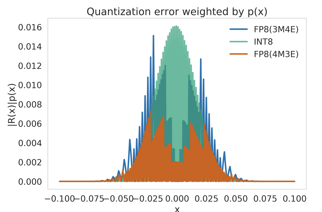
Figure 15 illustrates the quantization error weighted by the probability distribution of values, comparing different numerical formats (FP8 variants and INT8). The error distribution highlights how different formats introduce varying levels of quantization noise across the range of values, which in turn influences model accuracy and stability.
Numeric Encoding and Storage
The representation of numerical data in machine learning systems extends beyond precision levels to encompass encoding formats and storage mechanisms, both of which significantly influence computational efficiency. The encoding of numerical values determines how floating-point and integer representations are stored in memory and processed by hardware, directly affecting performance in machine learning workloads. As machine learning models grow in size and complexity, optimizing numeric encoding becomes increasingly important for ensuring efficiency, particularly on specialized hardware accelerators (Mellempudi et al. 2019).
Floating-point representations, which are widely used in machine learning, follow the IEEE 754 standard, defining how numbers are represented using a combination of sign, exponent, and mantissa (fraction) bits. Standard formats such as FP32 (single precision) and FP64 (double precision) provide high accuracy but demand significant memory and computational resources. To enhance efficiency, reduced-precision formats such as FP16, bfloat16, and FP8 have been introduced, offering lower storage requirements while maintaining sufficient numerical range for machine learning computations. Unlike FP16, which allocates more bits to the mantissa, bfloat16 retains the same exponent size as FP32, allowing it to represent a wider dynamic range while reducing precision in the fraction. This characteristic makes bfloat16 particularly effective for machine learning training, where maintaining dynamic range is important for stable gradient updates.
Integer-based representations, including INT8 and INT4, further reduce storage and computational overhead by eliminating the need for exponent and mantissa encoding. These formats are commonly used in quantized inference, where model weights and activations are converted to discrete integer values to accelerate computation and reduce power consumption. The deterministic nature of integer arithmetic simplifies execution on hardware, making it particularly well-suited for edge AI and mobile devices. At the extreme end, binary and ternary representations restrict values to just one or two bits, leading to significant reductions in memory footprint and power consumption. However, such aggressive quantization can degrade model accuracy unless complemented by specialized training techniques or architectural adaptations.
Emerging numeric formats seek to balance the trade-off between efficiency and accuracy. TF32, introduced by NVIDIA for Ampere GPUs, modifies FP32 by reducing the mantissa size while maintaining the exponent width, allowing for faster computations with minimal precision loss. Similarly, FP8, which is gaining adoption in AI accelerators, provides an even lower-precision floating-point alternative while retaining a structure that aligns well with machine learning workloads (Micikevicius et al. 2022). Alternative formats such as Posit, Flexpoint, and BF16ALT are also being explored for their potential advantages in numerical stability and hardware adaptability.
The efficiency of numeric encoding is further influenced by how data is stored and accessed in memory. AI accelerators optimize memory hierarchies to maximize the benefits of reduced-precision formats, using specialized hardware such as tensor cores, matrix multiply units (MMUs), and vector processing engines to accelerate lower-precision computations. On these platforms, data alignment, memory tiling, and compression techniques play a important role in ensuring that reduced-precision computations deliver tangible performance gains.
As machine learning systems evolve, numeric encoding and storage strategies will continue to adapt to meet the demands of large-scale models and diverse hardware environments. The ongoing development of precision formats tailored for AI workloads highlights the importance of co-designing numerical representations with underlying hardware capabilities, ensuring that machine learning models achieve optimal performance while minimizing computational costs.
Numerical Format Comparison
Table 7 compares commonly used numerical precision formats in machine learning, highlighting their trade-offs in storage efficiency, computational speed, and energy consumption. Emerging formats like FP8 and TF32 have been introduced to further optimize performance, particularly on AI accelerators.
| Precision Format | Bit-Width | Storage Reduction (vs FP32) | Compute Speed (vs FP32) | Power Consumption | Use Cases |
|---|---|---|---|---|---|
| FP32 (Single-Precision Floating Point) | 32-bit | Baseline (1×) | Baseline (1×) | High | Training & inference (general-purpose) |
| FP16 (Half-Precision Floating Point) | 16-bit | 2× smaller | 2× faster on FP16-optimized hardware | Lower | Accelerated training, inference (NVIDIA Tensor Cores, TPUs) |
| bfloat16 (Brain Floating Point) | 16-bit | 2× smaller | Similar speed to FP16, better dynamic range | Lower | Training on TPUs, transformer-based models |
| TF32 (TensorFloat-32) | 19-bit | Similar to FP16 | Up to 8× faster on NVIDIA Ampere GPUs | Lower | Training on NVIDIA GPUs |
| FP8 (Floating-Point 8-bit) | 8-bit | 4× smaller | Faster than INT8 in some cases | Significantly lower | Efficient training/inference (H100, AI accelerators) |
| INT8 (8-bit Integer) | 8-bit | 4× smaller | 4–8× faster than FP32 | Significantly lower | Quantized inference (Edge AI, mobile AI, NPUs) |
| INT4 (4-bit Integer) | 4-bit | 8× smaller | Hardware-dependent | Extremely low | Ultra-low-power AI, experimental quantization |
| Binary/Ternary (1-bit / 2-bit) | 1–2-bit | 16–32× smaller | Highly hardware-dependent | Lowest | Extreme efficiency (binary/ternary neural networks) |
FP16 and bfloat16 formats provide moderate efficiency gains while preserving model accuracy. Many AI accelerators, such as NVIDIA Tensor Cores and TPUs, include dedicated support for FP16 computations, enabling \(2\times\) faster matrix operations compared to FP32. BFloat16, in particular, retains the same 8-bit exponent as FP32 but with a reduced 7-bit mantissa, allowing it to maintain a similar dynamic range (~\(10^{-38}\) to \(10^{38}\)) while sacrificing precision. In contrast, FP16, with its 5-bit exponent and 10-bit mantissa, has a significantly reduced dynamic range (~\(10^{-5}\) to \(10^5\)), making it more suitable for inference rather than training. Since BFloat16 preserves the exponent size of FP32, it better handles extreme values encountered during training, whereas FP16 may struggle with underflow or overflow. This makes BFloat16 a more robust alternative for deep learning workloads that require a wide dynamic range.
Figure 16 highlights these differences, showing how bit-width allocations impact the trade-offs between precision and numerical range.

INT8 precision offers more aggressive efficiency improvements, particularly for inference workloads. Many quantized models use INT8 for inference, reducing storage by \(4\times\) while accelerating computation by 4–8\(\times\) on optimized hardware. INT8 is widely used in mobile and embedded AI, where energy constraints are significant.
Binary and ternary networks represent the extreme end of quantization, where weights and activations are constrained to 1-bit (binary) or 2-bit (ternary) values. This results in massive storage and energy savings, but model accuracy often degrades significantly unless specialized architectures are used.
Precision Reduction Trade-offs
Reducing numerical precision in machine learning systems offers significant gains in efficiency, including lower memory requirements, reduced power consumption, and increased computational throughput. However, these benefits come with trade-offs, as lower-precision representations introduce numerical error and quantization noise, which can affect model accuracy. The extent of this impact depends on multiple factors, including the model architecture, the dataset, and the specific precision format used.
Models exhibit varying levels of tolerance to quantization. Large-scale architectures, such as convolutional neural networks and transformer-based models, often retain high accuracy even when using reduced-precision formats such as bfloat16 or INT8. In contrast, smaller models or those trained on tasks requiring high numerical precision may experience greater degradation in performance. Not all layers within a neural network respond equally to precision reduction. Certain layers, such as batch normalization and attention mechanisms, may be more sensitive to numerical precision than standard feedforward layers. As a result, techniques such as mixed-precision training, where different layers operate at different levels of precision, can help maintain accuracy while optimizing computational efficiency.
Hardware support is another important factor in determining the effectiveness of precision reduction. AI accelerators, including GPUs, TPUs, and NPUs, are designed with dedicated low-precision arithmetic units that enable efficient computation using FP16, bfloat16, INT8, and, more recently, FP8. These architectures exploit reduced precision to perform high-throughput matrix operations, improving both speed and energy efficiency. In contrast, general-purpose CPUs often lack specialized hardware for low-precision computations, limiting the potential benefits of numerical quantization. The introduction of newer floating-point formats, such as TF32 for NVIDIA GPUs and FP8 for AI accelerators, seeks to optimize the trade-off between precision and efficiency, offering an alternative for hardware that is not explicitly designed for extreme quantization.
In addition to hardware constraints, reducing numerical precision impacts power consumption. Lower-precision arithmetic reduces the number of required memory accesses and simplifies computational operations, leading to lower overall energy use. This is particularly advantageous for energy-constrained environments such as mobile devices and edge AI systems. At the extreme end, ultra-low precision formats, including INT4 and binary/ternary representations, provide significant reductions in power and memory usage. However, these formats often require specialized architectures to compensate for the accuracy loss associated with such aggressive quantization.
To mitigate accuracy loss associated with reduced precision, various quantization strategies can be employed. Ultimately, selecting the appropriate numerical precision for a given machine learning model requires balancing efficiency gains against accuracy constraints. This selection depends on the model’s architecture, the computational requirements of the target application, and the underlying hardware’s support for low-precision operations. By using advancements in both hardware and software optimization techniques, practitioners can effectively integrate lower-precision numerics into machine learning pipelines, maximizing efficiency while maintaining performance.
Precision Reduction Strategies
Reducing numerical precision is an important optimization technique for improving the efficiency of machine learning models. By lowering the bit-width of weights and activations, models can reduce memory footprint, improve computational throughput, and decrease power consumption. However, naive quantization can introduce quantization errors, leading to accuracy degradation. To address this, different precision reduction strategies have been developed, allowing models to balance efficiency gains while preserving predictive performance.
Quantization techniques can be applied at different stages of a model’s lifecycle. Post-training quantization reduces precision after training, making it a simple and low-cost approach for optimizing inference. Quantization-aware training incorporates quantization effects into the training process, enabling models to adapt to lower precision and retain higher accuracy. Mixed-precision training leverages hardware support to dynamically assign precision levels to different computations, optimizing execution efficiency without sacrificing accuracy.
To help navigate this increasing complexity, Figure 17 organizes quantization techniques into three progressive tiers based on implementation complexity, resource requirements, and target use cases.

Post-Training Quantization
Quantization is the specific algorithmic technique that enables significant memory bandwidth reduction when addressing the memory wall. These quantization methods provide standardized APIs across different platforms, showing exactly how to implement the efficiency principles established earlier.
Post-training quantization (PTQ) reduces numerical precision after training, converting weights and activations from high-precision formats (FP32) to lower-precision representations (INT8 or FP16) without retraining (Jacob et al. 2018a). This achieves smaller model sizes, faster computation, and reduced energy consumption, making it practical for resource-constrained environments such as mobile devices, edge AI systems, and cloud inference platforms (H. Wu et al. 2020).
PTQ’s key advantage is low computational cost—it requires no retraining or access to training data. However, reducing precision introduces quantization error that can degrade accuracy, particularly for tasks requiring fine-grained numerical precision. Machine learning frameworks (TensorFlow Lite, ONNX Runtime, PyTorch) provide built-in PTQ support.
PTQ Functionality
PTQ converts a trained model’s weights and activations from high-precision floating-point representations (e.g., FP32) to lower-precision formats (e.g., INT8 or FP16). This process reduces the memory footprint of the model, accelerates inference, and lowers power consumption. However, since lower-precision formats have a smaller numerical range, quantization introduces rounding errors, which can impact model accuracy.
The core mechanism behind PTQ is scaling and mapping high-precision values into a reduced numerical range. A widely used approach is uniform quantization, which maps floating-point values to discrete integer levels using a consistent scaling factor. In uniform quantization, the interval between each quantized value is constant, simplifying implementation and ensuring efficient execution on hardware. The quantized value \(q\) is computed as: \[ q = \text{round} \left(\frac{x}{s} \right) \] where:
- \(q\) is the quantized integer representation,
- \(x\) is the original floating-point value,
- \(s\) is a scaling factor that maps the floating-point range to the available integer range.
Listing 2 demonstrates uniform quantization from FP32 to INT8.
import torch

# Original FP32 weights
weights_fp32 = torch.tensor(
    [0.127, -0.084, 0.392, -0.203], dtype=torch.float32
)
print(f"Original FP32: {weights_fp32}")
print(f"Memory per weight: 32 bits")

# Simple uniform quantization to INT8 (-128 to 127)
# Step 1: Find scale factor
max_val = weights_fp32.abs().max()
scale = max_val / 127  # 127 is max positive INT8 value

# Step 2: Quantize using our formula q = round(x/s)
weights_int8 = torch.round(weights_fp32 / scale).to(torch.int8)
print(f"Quantized INT8: {weights_int8}")
print(f"Memory per weight: 8 bits (reduced from 32)")

# Step 3: Dequantize to verify
weights_dequantized = weights_int8.float() * scale
print(f"Dequantized: {weights_dequantized}")
print(
    f"Quantization error: "
    f"{(weights_fp32 - weights_dequantized).abs().mean():.6f}"
)
This example demonstrates the compression from 32 bits to 8 bits per weight, with minimal quantization error.
For example, in INT8 quantization, the model’s floating-point values (typically ranging from \([-r, r]\)) are mapped to an integer range of \([-128, 127]\). The scaling factor ensures that the most significant information is retained while reducing precision loss. Once the model has been quantized, inference is performed using integer arithmetic, which is significantly more efficient than floating-point operations on many hardware platforms (Gholami et al. 2021). However, due to rounding errors and numerical approximation, quantized models may experience slight accuracy degradation compared to their full-precision counterparts.
Once the model has been quantized, inference is performed using integer arithmetic, which is significantly more efficient than floating-point operations on many hardware platforms. However, due to rounding errors and numerical approximation, quantized models may experience slight accuracy degradation compared to their full-precision counterparts.
In addition to uniform quantization, non-uniform quantization can be employed to preserve accuracy in certain scenarios. Unlike uniform quantization, which uses a consistent scaling factor, non-uniform quantization assigns finer-grained precision to numerical ranges that are more densely populated. This approach can be beneficial for models with weight distributions that concentrate around certain values, as it allows more details to be retained where it matters most. However, non-uniform quantization typically requires more complex calibration and may involve additional computational overhead. While it is not as commonly used as uniform quantization in production environments, non-uniform techniques can be effective for preserving accuracy in models that are particularly sensitive to precision changes.
PTQ is particularly effective for computer vision models, where CNNs often tolerate quantization well. However, models that rely on small numerical differences, such as NLP transformers or speech recognition models, may require additional tuning or alternative quantization techniques, including non-uniform strategies, to retain performance.
Calibration
An important aspect of PTQ is the calibration step, which involves selecting the most effective clipping range [\(\alpha\), \(\beta\)] for quantizing model weights and activations. During PTQ, the model’s weights and activations are converted to lower-precision formats (e.g., INT8), but the effectiveness of this reduction depends heavily on the chosen quantization range. Without proper calibration, the quantization process may cause significant accuracy degradation, even if the overall precision is reduced. Calibration ensures that the chosen range minimizes loss of information and helps preserve the model’s performance after precision reduction.
The overall workflow of post-training quantization is illustrated in Figure 18. The process begins with a pre-trained model, which serves as the starting point for optimization. To determine an effective quantization range, a calibration dataset, which is a representative subset of training or validation data, is passed through the model. This step allows the calibration process to estimate the numerical distribution of activations and weights, which is then used to define the clipping range for quantization. Following calibration, the quantization step converts the model parameters to a lower-precision format, producing the final quantized model, which is more efficient in terms of memory and computation.

For example, consider quantizing activations that originally have a floating-point range between –6 and 6 to 8-bit integers. Simply using the full integer range of –128 to 127 for quantization might not be the most effective approach. Instead, calibration involves passing a representative dataset through the model and observing the actual range of the activations. The observed range can then be used to set a more effective quantization range, reducing information loss.
Calibration Methods
There are several commonly used calibration methods:
Max: This method uses the maximum absolute value seen during calibration as the clipping range. While simple, it is susceptible to outlier data. For example, in the activation distribution shown in Figure 19, we see an outlier cluster around 2.1, while the rest of the values are clustered around smaller values. The Max method could lead to an inefficient range if the outliers significantly influence the quantization.
Entropy: This method minimizes information loss between the original floating-point values and the values that could be represented by the quantized format, typically using KL divergence. This is the default calibration method used by TensorRT and works well when trying to preserve the distribution of the original values.
Percentile: This method sets the clipping range to a percentile of the distribution of absolute values seen during calibration. For example, a 99% calibration would clip the top 1% of the largest magnitude values. This method helps avoid the impact of outliers, which are not representative of the general data distribution.
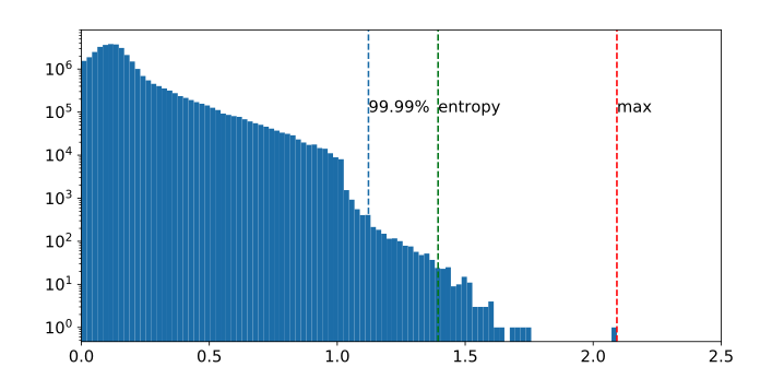
The quality of calibration directly affects the performance of the quantized model. A poor calibration could lead to a model that suffers from significant accuracy loss, while a well-calibrated model can retain much of its original performance after quantization. There are two types of calibration ranges to consider:
- Symmetric Calibration: The clipping range is symmetric around zero, meaning both the positive and negative ranges are equally scaled.
- Asymmetric Calibration: The clipping range is not symmetric, which means the positive and negative ranges may have different scaling factors. This can be useful when the data is not centered around zero.
Choosing the right calibration method and range is important for maintaining model accuracy while benefiting from the efficiency gains of reduced precision.
Calibration Ranges
A key challenge in post-training quantization is selecting the appropriate calibration range \([\alpha, \beta]\) to map floating-point values into a lower-precision representation. The choice of this range directly affects the quantization error and, consequently, the accuracy of the quantized model. As illustrated in Figure 20, there are two primary calibration strategies: symmetric calibration and asymmetric calibration.

On the left side of Figure 20, symmetric calibration is depicted, where the clipping range is centered around zero. The range extends from \(\alpha = -1\) to \(\beta = 1\), mapping these values to the integer range \([-127, 127]\). This method ensures that positive and negative values are treated equally, preserving zero-centered distributions. A key advantage of symmetric calibration is its simplified implementation, as the same scale factor is applied to both positive and negative values. However, this approach may not be optimal for datasets where the activation distributions are skewed, leading to poor representation of significant portions of the data.
On the right side, asymmetric calibration is shown, where \(\alpha = -0.5\) and \(\beta = 1.5\). Here, zero is mapped to a shifted quantized value \(-Z\), and the range extends asymmetrically. In this case, the quantization scale is adjusted to account for non-zero mean distributions. Asymmetric calibration is particularly useful when activations or weights exhibit skew, ensuring that the full quantized range is effectively utilized. However, it introduces additional computational complexity in determining the optimal offset and scaling factors.
The choice between these calibration strategies depends on the model and dataset characteristics:
- Symmetric calibration is commonly used when weight distributions are centered around zero, which is often the case for well-initialized machine learning models. It simplifies computation and hardware implementation but may not be optimal for all scenarios.
- Asymmetric calibration is useful when the data distribution is skewed, ensuring that the full quantized range is effectively utilized. It can improve accuracy retention but may introduce additional computational complexity in determining the optimal quantization parameters.
Many machine learning frameworks, including TensorRT and PyTorch, support both calibration modes, enabling practitioners to empirically evaluate the best approach. Selecting an appropriate calibration range is important for PTQ, as it directly influences the trade-off between numerical precision and efficiency, ultimately affecting the performance of quantized models.
Granularity
After determining the clipping range, the next step in optimizing quantization involves adjusting the granularity of the clipping range to ensure that the model retains as much accuracy as possible. In CNNs, for instance, the input activations of a layer undergo convolution with multiple convolutional filters, each of which may have a unique range of values. The quantization process, therefore, must account for these differences in range across filters to preserve the model’s performance.
As illustrated in Figure 21, the range for Filter 1 is significantly smaller than that for Filter 3, demonstrating the variation in the magnitude of values across different filters. The precision with which the clipping range [\(\alpha\), \(\beta\)] is determined for the weights becomes a important factor in effective quantization. This variability in ranges is a key reason why different quantization strategies, based on granularity, are employed.

Several methods are commonly used to determine the granularity of quantization, each with its own trade-offs in terms of accuracy, efficiency, and computational cost.
Layerwise Quantization
In this approach, the clipping range is determined by considering all weights in the convolutional filters of a layer. The same clipping range is applied to all filters within the layer. While this method is simple to implement, it often leads to suboptimal accuracy due to the wide range of values across different filters. For example, if one convolutional kernel has a narrower range of values than another in the same layer, the quantization resolution of the narrower range may be compromised, resulting in a loss of information.
Groupwise Quantization
Groupwise quantization divides the convolutional filters into groups and calculates a shared clipping range for each group. This method can be beneficial when the distribution of values within a layer is highly variable. For example, the Q-BERT model (Shen et al. 2019) applied this technique when quantizing Transformer models (Chen et al. 2018), particularly for the fully-connected attention layers. While groupwise quantization offers better accuracy than layerwise quantization, it incurs additional computational cost due to the need to account for multiple scaling factors.
Channelwise Quantization
Channelwise quantization assigns a dedicated clipping range and scaling factor to each convolutional filter. This approach ensures a higher resolution in quantization, as each channel is quantized independently. Channelwise quantization is widely used in practice, as it often yields better accuracy compared to the previous methods. By allowing each filter to have its own clipping range, this method ensures that the quantization process is tailored to the specific characteristics of each filter.
Sub-channelwise Quantization
Sub-channelwise quantization subdivides each convolutional filter into smaller groups, each with its own clipping range. Although it provides very fine-grained control over quantization, it introduces significant computational overhead as multiple scaling factors must be managed for each group within a filter. As a result, sub-channelwise quantization is generally only used in scenarios where maximum precision is required, despite the increased computational cost.
Among these methods, channelwise quantization is the current standard for quantizing convolutional filters. It strikes a balance between the accuracy gains from finer granularity and the computational efficiency needed for practical deployment. Adjusting the clipping range for each individual kernel provides significant improvements in model accuracy with minimal overhead, making it the most widely adopted approach in machine learning applications.
Weights vs. Activations
Weight Quantization involves converting the continuous, high-precision weights of a model into lower-precision values, such as converting 32-bit floating-point (Float32) weights to 8-bit integer (INT8) weights. As illustrated in Figure 22, weight quantization occurs in the second step (red squares) during the multiplication of inputs. This process significantly reduces the model size, decreasing both the memory required to store the model and the computational resources needed for inference. For example, a weight matrix in a neural network layer with Float32 weights like \([0.215, -1.432, 0.902,\ldots]\) might be mapped to INT8 values such as \([27, -183, 115, \ldots]\), leading to a significant reduction in memory usage.

Activation Quantization refers to the process of quantizing the activation values, or outputs of the layers, during model inference. This quantization can reduce the computational resources required during inference, particularly when targeting hardware optimized for integer arithmetic. It introduces challenges related to maintaining model accuracy, as the precision of intermediate computations is reduced. For instance, in a CNN, the activation maps (or feature maps) produced by convolutional layers, originally represented in Float32, may be quantized to INT8 during inference. This can significantly accelerate computation on hardware capable of efficiently processing lower-precision integers.
Recent advancements have explored Activation-aware Weight Quantization (AWQ) for the compression and acceleration of large language models (LLMs). This approach focuses on protecting only a small fraction of the most salient weights, approximately 1%, by observing the activations rather than the weights themselves. This method has been shown to improve model efficiency while preserving accuracy, as discussed in (Ji Lin et al. 2023).
Static vs. Dynamic Quantization
After determining the type and granularity of the clipping range, practitioners must decide when the clipping ranges are calculated in their quantization algorithms. Two primary approaches exist for quantizing activations: static quantization and dynamic quantization.
Static Quantization is the more commonly used approach. In static quantization, the clipping range is pre-calculated and remains fixed during inference. This method does not introduce any additional computational overhead during runtime, which makes it efficient in terms of computational resources. However, the fixed range can lead to lower accuracy compared to dynamic quantization. A typical implementation of static quantization involves running a series of calibration inputs to compute the typical range of activations (Jacob et al. 2018a; Yao et al. 2021).
In contrast, Dynamic Quantization dynamically calculates the range for each activation map during runtime. This approach allows the quantization process to adjust in real time based on the input, potentially yielding higher accuracy since the range is specifically calculated for each input activation. However, dynamic quantization incurs higher computational overhead because the range must be recalculated at each step. Although this often results in higher accuracy, the real-time computations can be expensive, particularly when deployed at scale.
The following table, Table 8, summarizes the characteristics of post-training quantization, quantization-aware training, and dynamic quantization, providing an overview of their respective strengths, limitations, and trade-offs. These methods are widely deployed across machine learning systems of varying scales, and understanding their pros and cons is important for selecting the appropriate approach for a given application.
| Aspect | Post Training Quantization | Quantization-Aware Training | Dynamic Quantization |
|---|---|---|---|
| Pros | |||
| Simplicity | ✓ | ✗ | ✗ |
| Accuracy Preservation | ✗ | ✓ | ✓ |
| Adaptability | ✗ | ✗ | ✓ |
| Optimized Performance | ✗ | ✓ | Potentially |
| Cons | |||
| Accuracy Degradation | ✓ | ✗ | Potentially |
| Computational Overhead | ✗ | ✓ | ✓ |
| Implementation Complexity | ✗ | ✓ | ✓ |
| Tradeoffs | |||
| Speed vs. Accuracy | ✓ | ✗ | ✗ |
| Accuracy vs. Cost | ✗ | ✓ | ✗ |
| Adaptability vs. Overhead | ✗ | ✗ | ✓ |
PTQ Advantages
One of the key advantages of PTQ is its low computational cost, as it does not require retraining the model. This makes it an attractive option for the rapid deployment of trained models, particularly when retraining is computationally expensive or infeasible. Since PTQ only modifies the numerical representation of weights and activations, the underlying model architecture remains unchanged, allowing it to be applied to a wide range of pre-trained models without modification.
PTQ also provides significant memory and storage savings by reducing the bit-width of model parameters. For instance, converting a model from FP32 to INT8 results in a \(4\times\) reduction in storage size, making it feasible to deploy larger models on resource-constrained devices such as mobile phones, edge AI hardware, and embedded systems. These reductions in memory footprint also lead to lower bandwidth requirements when transferring models across networked systems.
In terms of computational efficiency, PTQ allows inference to be performed using integer arithmetic, which is inherently faster than floating-point operations on many hardware platforms. AI accelerators such as TPUs and Neural Processing Units (NPUs) are optimized for lower-precision computations, enabling higher throughput and reduced power consumption when executing quantized models. This makes PTQ particularly useful for applications requiring real-time inference, such as object detection in autonomous systems or speech recognition on mobile devices.
PTQ Challenges and Limitations
Despite its advantages, PTQ introduces quantization errors due to rounding effects when mapping floating-point values to discrete lower-precision representations. While some models remain robust to these changes, others may experience notable accuracy degradation, especially in tasks that rely on small numerical differences.
The extent of accuracy loss depends on both the model architecture and the task domain. CNNs for image classification are generally tolerant to PTQ, often maintaining near-original accuracy even with aggressive INT8 quantization. Transformer-based models used in NLP and speech recognition tend to be more sensitive, as these architectures rely on the precision of numerical relationships in attention mechanisms.
To mitigate accuracy loss, calibration techniques such as KL divergence-based scaling or per-channel quantization are commonly applied to fine-tune the scaling factor and minimize information loss. Some frameworks, including TensorFlow Lite and PyTorch, provide automated quantization tools with built-in calibration methods to improve accuracy retention.
Another limitation of PTQ is that not all hardware supports efficient integer arithmetic. While GPUs, TPUs, and specialized edge AI chips often include dedicated support for INT8 inference, general-purpose CPUs may lack the optimized instructions for low-precision execution, resulting in suboptimal performance improvements.
PTQ is not always suitable for training purposes. Since PTQ applies quantization after training, models that require further fine-tuning or adaptation may benefit more from alternative approaches, such as quantization-aware training (discussed next), to ensure that precision constraints are adequately considered during the learning process.
Post-training quantization remains one of the most practical and widely used techniques for improving inference efficiency. It provides significant memory and computational savings with minimal overhead, making it an ideal choice for deploying machine learning models in resource-constrained environments. However, the success of PTQ depends on model architecture, task sensitivity, and hardware compatibility. In scenarios where accuracy degradation is unacceptable, alternative quantization strategies, such as quantization-aware training, may be required.
Post-training quantization provides the foundation for more advanced quantization methods. The core concepts—quantization workflows, numerical format trade-offs, and calibration methods—remain essential throughout all precision optimization techniques. For rapid deployment scenarios with production deadlines under two weeks and acceptable accuracy loss of 1-2%, PTQ with min-max calibration often provides a complete solution. Production systems requiring less than 1% accuracy loss should consider Quantization-Aware Training, which recovers accuracy through fine-tuning with quantization simulation at the cost of 20-50% additional training time. Extreme constraints like sub-1MB models or sub-10mW power budgets may require INT4 or binary quantization, accepting 5-20% accuracy degradation that necessitates architectural changes.
Quantization-Aware Training
QAT integrates quantization constraints directly into the training process, simulating low-precision arithmetic during forward passes to allow the model to adapt to quantization effects (Jacob et al. 2018a). This approach proves particularly important for models requiring fine-grained numerical precision, such as transformers used in NLP and speech recognition systems (Nagel et al. 2021b). Figure 23 illustrates the QAT process: quantization is applied to a pre-trained model, followed by fine-tuning to adapt weights to low-precision constraints.

In many cases, QAT can also build off PTQ (discussed in detail in the previous section), as shown in Figure 24. Instead of starting from a full-precision model, PTQ is first applied to produce an initial quantized model using calibration data. This quantized model then serves as the starting point for QAT, where additional fine-tuning with training data helps the model better adapt to low-precision constraints. This hybrid approach combines PTQ’s efficiency with QAT’s accuracy preservation, reducing the degradation typically associated with post-training approaches alone.

Training Mathematics
During forward propagation, weights and activations are quantized and dequantized to mimic reduced precision. This process is typically represented as: \[ q = \text{round} \left(\frac{x}{s} \right) \times s \] where \(q\) represents the simulated quantized value, \(x\) denotes the full-precision weight or activation, and \(s\) is the scaling factor mapping floating-point values to lower-precision integers.
Although the forward pass utilizes quantized values, gradient calculations during backpropagation remain in full precision. This is achieved using the Straight-Through Estimator (STE)32, which approximates the gradient of the quantized function by treating the rounding operation as if it had a derivative of one. This approach prevents the gradient from being obstructed due to the non-differentiable nature of the quantization operation, thereby allowing effective model training (Y. Bengio, Léonard, and Courville 2013a).
32 Straight-Through Estimator (STE): Gradient approximation technique for non-differentiable functions, introduced by Bengio et al. (Y. Bengio, Léonard, and Courville 2013a). Sets gradient of step function to 1 everywhere, enabling backpropagation through quantization layers. Crucial for training binarized neural networks and quantization-aware training, despite theoretical limitations around zero.
Integrating quantization effects during training enables the model to learn an optimal distribution of weights and activations that minimizes the impact of numerical precision loss. The resulting model, when deployed using true low-precision arithmetic (e.g., INT8 inference), maintains significantly higher accuracy than one that is quantized post hoc (Krishnamoorthi 2018).
QAT Advantages
A primary advantage of QAT33 is its ability to maintain model accuracy, even under low-precision inference conditions. Incorporating quantization during training helps the model to compensate for precision loss, reducing the impact of rounding errors and numerical instability. This is important for quantization-sensitive models commonly used in NLP, speech recognition, and high-resolution computer vision (Gholami et al. 2021).
33 Quantization-Aware Training: QAT enables INT8 inference with minimal accuracy loss - ResNet-50 maintains 76.1% vs. 76.2% FP32 ImageNet accuracy, while MobileNetV2 achieves 71.8% vs. 72.0%. BERT-Base INT8 retains 99.1% of FP32 performance on GLUE, compared to 96.8% with post-training quantization alone.
Another major benefit is that QAT permits low-precision inference on hardware accelerators without significant accuracy degradation. AI processors such as TPUs, NPUs, and specialized edge devices include dedicated hardware for integer operations, permitting INT8 models to run much faster and with lower energy consumption compared to FP32 models. Training with quantization effects in mind ensures that the final model can fully leverage these hardware optimizations (H. Wu et al. 2020).
QAT Challenges and Trade-offs
Despite its benefits, QAT introduces additional computational overhead during training. Simulated quantization at every forward pass slows down training relative to full-precision methods. The process adds complexity to the training schedule, making QAT less practical for very large-scale models where the additional training time might be prohibitive.
QAT introduces extra hyperparameters and design considerations, such as choosing appropriate quantization schemes and scaling factors. Unlike PTQ, which applies quantization after training, QAT requires careful tuning of the training dynamics to ensure that the model suitably adapts to low-precision constraints (Gong et al. 2019).
Table 9 summarizes the key trade-offs of QAT compared to PTQ:
| Aspect | QAT (Quantization-Aware Training) | PTQ (Post-Training Quantization) |
|---|---|---|
| Accuracy Retention | Minimizes accuracy loss from quantization | May suffer from accuracy degradation |
| Inference Efficiency | Optimized for low-precision hardware (e.g., INT8 on TPUs) | Optimized but may require calibration |
| Training Complexity | Requires retraining with quantization constraints | No retraining required |
| Training Time | Slower due to simulated quantization in forward pass | Faster, as quantization is applied post hoc |
| Deployment Readiness | Best for models sensitive to quantization errors | Fastest way to optimize models for inference |
Integrating quantization into the training process preserves model accuracy more effectively than post-training quantization, although it requires additional training resources and time.
PTQ vs. QAT
The choice between PTQ and QAT depends on trade-offs between accuracy, computational cost, and deployment constraints. PTQ provides computationally inexpensive optimization requiring only post-training conversion, making it ideal for rapid deployment. However, effectiveness varies by architecture—CNNs tolerate PTQ well while NLP and speech models may experience degradation due to reliance on precise numerical representations.
QAT proves necessary when high accuracy retention is critical. Integrating quantization effects during training allows models to adapt to lower-precision arithmetic, reducing quantization errors (Jacob et al. 2018b). While achieving higher low-precision accuracy, QAT requires additional training time and computational resources. In practice, a hybrid approach starting with PTQ and selectively applying QAT for accuracy-critical models provides optimal balance between efficiency and performance.
Extreme Quantization
Beyond INT8 and INT4 quantization, extreme quantization techniques use 1-bit (binarization) or 2-bit (ternarization) representations to achieve dramatic reductions in memory usage and computational requirements (Courbariaux, Bengio, and David 2016). Binarization constrains weights and activations to two values (typically -1 and +1, or 0 and 1), drastically reducing model size and accelerating inference on specialized hardware like binary neural networks (Rastegari et al. 2016). However, this constraint severely limits model expressiveness, often degrading accuracy on tasks requiring high precision such as image recognition or natural language processing (Hubara et al. 2018).
Ternarization extends binarization by allowing three values (-1, 0, +1), providing additional flexibility that slightly improves accuracy over pure binarization (Zhu et al. 2017). The zero value enables greater sparsity while maintaining more representational power. Both techniques require gradient approximation methods like Straight-Through Estimator (STE) to handle non-differentiable quantization operations during training (Y. Bengio, Léonard, and Courville 2013b), with QAT integration helping mitigate accuracy loss (Choi et al. 2018).
Challenges and Limitations
Despite enabling ultra-low-power machine learning for embedded systems and mobile devices, binarization and ternarization face significant challenges. Performance maintenance proves difficult with such drastic quantization, requiring specialized hardware capable of efficiently handling binary or ternary operations (Umuroglu et al. 2017). Traditional processors lack optimization for these computations, necessitating custom hardware accelerators.
Accuracy loss remains a critical concern. These methods suit tasks where high precision is not critical or where QAT can compensate for precision constraints. Despite challenges, the ability to drastically reduce model size while maintaining acceptable accuracy makes them attractive for edge AI and resource-constrained environments (Jacob et al. 2018b). Future advances in specialized hardware and training techniques will likely enhance their role in efficient, scalable AI.
Multi-Technique Optimization Strategies
Having explored quantization techniques (PTQ, QAT, binarization, and ternarization), pruning methods, and knowledge distillation, we now examine how these complementary approaches can be systematically combined to achieve superior optimization results. Rather than applying techniques in isolation, integrated strategies leverage the synergies between different optimization dimensions to maximize efficiency gains while preserving model accuracy.
Each optimization technique addresses distinct aspects of model efficiency: quantization reduces numerical precision, pruning eliminates redundant parameters, knowledge distillation transfers capabilities to compact architectures, and NAS optimizes structural design. These techniques exhibit complementary characteristics that enable powerful combinations.
Pruning and quantization create synergistic effects because pruning reduces parameter count while quantization reduces precision, creating multiplicative compression effects. Applying pruning first reduces the parameter set, making subsequent quantization more effective and reducing the search space for optimal quantization strategies. This sequential approach can achieve compression ratios exceeding either technique alone.
Knowledge distillation integrates effectively with quantization by mitigating accuracy loss from aggressive quantization. This approach trains student models to match teacher behavior rather than just minimizing task loss, proving particularly effective for extreme quantization scenarios where direct quantization would cause unacceptable accuracy degradation.
Neural architecture search enables co-design approaches that optimize model structures specifically for quantization constraints, identifying architectures that maintain accuracy under low-precision operations. This co-design approach produces models inherently suited for subsequent optimization, improving the effectiveness of both quantization and pruning techniques.
As shown in Figure 25, different compression strategies such as pruning, quantization, and singular value decomposition (SVD) exhibit varying trade-offs between model size and accuracy loss. While pruning combined with quantization (red circles) achieves high compression ratios with minimal accuracy loss, quantization alone (yellow squares) also provides a reasonable balance. In contrast, SVD (green diamonds) requires a larger model size to maintain accuracy, illustrating how different techniques can impact compression effectiveness.

Quantization differs from pruning, knowledge distillation, and NAS in that it specifically focuses on reducing the numerical precision of weights and activations. While quantization alone can provide significant computational benefits, its effectiveness can be amplified when combined with the complementary techniques of pruning, distillation, and NAS. These methods, each targeting a different aspect of model efficiency, work together to create more compact, faster, and energy-efficient models, enabling better performance in constrained environments.
Our optimization journey continues. We pruned BERT-Base from 440MB to 110MB through structured pruning and knowledge distillation, then quantized it to INT8, reducing the model to 28MB with inference latency dropping from 120ms to 45ms on mobile hardware. These optimizations transformed an unusable model into one approaching deployment viability. Yet profiling reveals a puzzling inefficiency: theoretical FLOP count suggests inference should complete in 25ms, yet actual execution takes 45ms. Where does the remaining 20ms disappear?
Detailed profiling exposes the answer. While quantization reduced precision, the model still computes zeros unnecessarily. Structured pruning removed entire attention heads, but the remaining sparse weight matrices are stored in dense format, wasting both memory bandwidth and computation on zero-valued elements. Layer normalization operations run sequentially despite their inherent parallelism. The model processes all tokens identically, even though simple inputs could exit early from shallow layers. The GPU spends 40% of execution time idle, waiting for memory transfers rather than executing operations.
These observations reveal why model representation and numerical precision optimizations, while necessary, are insufficient. Representation techniques determine what computations are performed. Precision techniques determine how individual operations execute. But neither addresses how computations are organized and scheduled to maximize hardware utilization. This is the domain of architectural efficiency optimization, the third dimension of our framework.
Architectural efficiency techniques transform the execution pattern itself. Exploiting sparsity through specialized kernels eliminates computation on pruned weights. Operator fusion combines sequential operations (layer norm, attention, feedforward) into single GPU kernels, reducing memory traffic by 40%. Dynamic computation enables simple inputs to exit after 6 layers rather than processing all 12 layers. Hardware-aware scheduling parallelizes operations to maintain high GPU utilization. Applying these techniques to our optimized BERT model reduces inference from 45ms to 22ms, finally achieving the 25ms theoretical target and making deployment truly viable.
This progression illustrates why all three optimization dimensions must work in concert. Model representation provides structural efficiency (fewer parameters). Numerical precision provides computational efficiency (lower precision arithmetic). Architectural efficiency provides execution efficiency (optimized scheduling and hardware utilization). The compound effect, 440MB/120ms → 28MB/22ms (16x memory reduction, 5.5x latency improvement), emerges only when all dimensions are addressed systematically.
Architectural Efficiency Techniques
Architectural efficiency optimization ensures that computations execute efficiently on target hardware by aligning model operations with processor capabilities and memory hierarchies. Unlike representation optimization (which determines what computations to perform) and precision optimization (which determines numerical fidelity), architectural efficiency addresses how operations are scheduled, how memory is accessed, and how workloads adapt to input characteristics and hardware constraints.
This optimization dimension proves particularly important for resource-constrained scenarios (Chapter 14: On-Device Learning), where theoretical FLOP reductions from pruning and quantization may not translate to actual speedups without architectural modifications. Sparse weight matrices stored in dense format waste memory bandwidth. Sequential operations that could execute in parallel underutilize GPU cores. Fixed computation graphs process simple and complex inputs identically, wasting resources on unnecessary work.
This section examines four complementary approaches to architectural efficiency: hardware-aware design principles that proactively integrate deployment constraints during model development, sparsity exploitation techniques that accelerate computation on pruned models, dynamic computation strategies that adapt workload to input complexity, and operator fusion methods that reduce memory traffic by combining operations. These techniques transform algorithmic optimizations into realized performance gains.
Hardware-Aware Design
Hardware-aware design incorporates target platform constraints—memory bandwidth, processing power, parallelism capabilities, and energy budgets—directly into model architecture decisions. Rather than optimizing models after training, this approach ensures computational patterns, memory access, and operation types match hardware capabilities from the outset, maximizing efficiency across diverse deployment platforms.
Efficient Design Principles
Designing machine learning models for hardware efficiency requires structuring architectures to account for computational cost, memory usage, inference latency, and power consumption, all while maintaining strong predictive performance. Unlike post-training optimizations, which attempt to recover efficiency after training, hardware-aware model design proactively integrates hardware considerations from the outset. This ensures that models are computationally efficient and deployable across diverse hardware environments with minimal adaptation.
Central to this proactive approach, a key aspect of hardware-aware design is using the strengths of specific hardware platforms (e.g., GPUs, TPUs, mobile or edge devices) to maximize parallelism, optimize memory hierarchies, and minimize latency through hardware-optimized operations. As summarized in Table 10, hardware-aware model design can be categorized into several principles, each addressing a core aspect of computational and system constraints.
| Principle | Goal | Example Networks |
|---|---|---|
| Scaling Optimization | Adjust model depth, width, and resolution to balance efficiency and hardware constraints. | EfficientNet, RegNet |
| Computation Reduction | Minimize redundant operations to reduce computational cost, utilizing hardware-specific optimizations (e.g., using depthwise separable convolutions on mobile chips). | MobileNet, ResNeXt |
| Memory Optimization | Ensure efficient memory usage by reducing activation and parameter storage requirements, using hardware-specific memory hierarchies (e.g., local and global memory in GPUs). | DenseNet, SqueezeNet |
| Hardware-Aware Design | Optimize architectures for specific hardware constraints (e.g., low power, parallelism, high throughput). | TPU-optimized models, MobileNet |
The principles in Table 10 work synergistically: scaling optimization sizes models appropriately for available resources, computation reduction eliminates redundant operations through techniques like depthwise separable convolutions34, memory optimization aligns access patterns with hardware hierarchies, and hardware-aware design ensures architectural decisions match platform capabilities. Together, these principles enable models that balance accuracy with efficiency while maintaining consistent behavior across deployment environments.
34 Depthwise Separable Convolutions: Factorizes standard convolution into depthwise (per-channel) and pointwise (1×1) operations, reducing computation by 8-9x. MobileNetV2 achieves 72% ImageNet accuracy with 300M FLOPs vs. ResNet-50’s 76% with 4.1B FLOPs (13.7x fewer operations). Enables real-time inference on mobile devices.
Scaling Optimization
Scaling a model’s architecture involves balancing accuracy with computational cost, and optimizing it to align with the capabilities of the target hardware. Each component of a model, whether its depth, width, or input resolution, impacts resource consumption. In hardware-aware design, these dimensions should not only be optimized for accuracy but also for efficiency in memory usage, processing power, and energy consumption, especially when the model is deployed on specific hardware like GPUs, TPUs, or edge devices.
From a hardware-aware perspective, it is important to consider how different hardware platforms, such as GPUs, TPUs, or edge devices, interact with scaling dimensions. For instance, deeper models can capture more complex representations, but excessive depth can lead to increased inference latency, longer training times, and higher memory consumption, issues that are particularly problematic on resource-constrained platforms. Similarly, increasing the width of the model to process more parallel information may be beneficial for GPUs and TPUs with high parallelism, but it requires careful management of memory usage. In contrast, increasing the input resolution can provide finer details for tasks like image classification, but it exponentially increases computational costs, potentially overloading hardware memory or causing power inefficiencies on edge devices.
Mathematically, the total FLOPs for a convolutional model can be approximated as: \[ \text{FLOPs} \propto d \cdot w^2 \cdot r^2, \] where \(d\) is depth, \(w\) is width, and \(r\) is the input resolution. Increasing all three dimensions without considering the hardware limitations can result in suboptimal performance, especially on devices with limited computational power or memory bandwidth.
For efficient model scaling, managing these parameters in a balanced way becomes essential, ensuring that the model remains within the limits of the hardware while maximizing performance. This is where compound scaling comes into play. Instead of adjusting depth, width, and resolution independently, compound scaling balances all three dimensions together by applying fixed ratios \((\alpha, \beta, \gamma)\) relative to a base model: \[ d = \alpha^\phi d_0, \quad w = \beta^\phi w_0, \quad r = \gamma^\phi r_0 \] Here, \(\phi\) is a scaling coefficient, and \(\alpha\), \(\beta\), and \(\gamma\) are scaling factors determined based on hardware constraints and empirical data. This approach ensures that models grow in a way that optimizes hardware resource usage, keeping them efficient while improving accuracy.
For example, EfficientNet, which employs compound scaling, demonstrates how carefully balancing depth, width, and resolution results in models that are both computationally efficient and high-performing. Compound scaling reduces computational cost while preserving accuracy, making it a key consideration for hardware-aware model design. This approach is particularly beneficial when deploying models on GPUs or TPUs, where parallelism can be fully leveraged, but memory and power usage need to be carefully managed, connecting to the performance evaluation methods in Chapter 12: Benchmarking AI.
This principle extends beyond convolutional models to other architectures like transformers. Adjusting the number of layers, attention heads, or embedding dimensions impacts computational efficiency similarly. Hardware-aware scaling has become central to optimizing model performance across various computational constraints, particularly when working with large models or resource-constrained devices.
Computation Reduction
Modern architectures leverage factorized computations to decompose complex operations into simpler components, reducing computational overhead while maintaining representational power. Standard convolutions apply filters uniformly across all spatial locations and channels, creating computational bottlenecks on resource-constrained hardware. Factorization techniques address this inefficiency by restructuring operations to minimize redundant computation.
Depthwise separable convolutions, introduced in MobileNet, exemplify this approach by decomposing standard convolutions into two stages: depthwise convolution (applying separate filters to each input channel independently) and pointwise convolution (1×1 convolution mixing outputs across channels). The computational complexity of standard convolution with input size \(h \times w\), \(C_{\text{in}}\) input channels, and \(C_{\text{out}}\) output channels is: \[ \mathcal{O}(h w C_{\text{in}} C_{\text{out}} k^2) \] where \(k\) is kernel size. Depthwise separable convolutions reduce this to: \[ \mathcal{O}(h w C_{\text{in}} k^2) + \mathcal{O}(h w C_{\text{in}} C_{\text{out}}) \] eliminating the \(k^2\) factor from channel-mixing operations, achieving 5×-10× FLOP reduction. This directly translates to reduced memory bandwidth requirements and improved inference latency on mobile and edge devices.
Complementary factorization techniques extend these benefits. Grouped convolutions (ResNeXt) partition feature maps into independent groups processed separately before merging, maintaining accuracy while reducing redundant operations. Bottleneck layers (ResNet) apply 1×1 convolutions to reduce feature dimensionality before expensive operations, concentrating computation where it provides maximum value. Combined with sparsity and hardware-aware scheduling, these techniques maximize accelerator utilization across GPUs, TPUs, and specialized edge processors.
Memory Optimization
Memory optimization35 addresses performance bottlenecks arising when memory demands for activations, feature maps, and parameters exceed hardware capacity on resource-constrained devices. Modern architectures employ memory-efficient strategies to reduce storage requirements while maintaining performance, ensuring computational tractability and energy efficiency on GPUs, TPUs, and edge AI platforms.
35 Memory Optimization: DenseNet-121 reduces memory consumption by 50% compared to ResNet-50 through feature reuse, requiring only 7.9MB vs. 15.3MB activation memory on ImageNet. MobileNetV3 achieves 73% memory reduction with depth-wise separable convolutions, enabling deployment on 2GB mobile devices.
One effective technique for memory optimization is feature reuse, a strategy employed in DenseNet. In traditional convolutional networks, each layer typically computes a new set of feature maps, increasing the model’s memory footprint. However, DenseNet reduces the need for redundant activations by reusing feature maps from previous layers and selectively applying transformations. This method reduces the total number of feature maps that need to be stored, which in turn lowers the memory requirements without sacrificing accuracy. In a standard convolutional network with \(L\) layers, if each layer generates \(k\) new feature maps, the total number of feature maps grows linearly: \[ \mathcal{O}(L k) \]
In contrast, DenseNet reuses feature maps from earlier layers, reducing the number of feature maps stored. This leads to improved parameter efficiency and a reduced memory footprint, which is important for hardware with limited memory resources.
Another useful technique is activation checkpointing36, which is especially beneficial during training. In a typical neural network, backpropagation requires storing all forward activations for the backward pass. This can lead to a significant memory overhead, especially for large models. Activation checkpointing reduces memory consumption by only storing a subset of activations and recomputing the remaining ones when needed.
36 Activation Checkpointing: Memory-time trade-off technique that stores only selected activations during forward pass, recomputing others during backpropagation. Reduces memory usage by 20-50% in large transformers with only 15-20% training time overhead. Essential for training models like GPT-3 on limited GPU memory.
If an architecture requires storing \(A_{\text{total}}\) activations, the standard backpropagation method requires the full storage: \[ \mathcal{O}(A_{\text{total}}) \]
With activation checkpointing, however, only a fraction of activations is stored, and the remaining ones are recomputed on-the-fly, reducing storage requirements to: \[ \mathcal{O}\Big(\sqrt{A_{\text{total}}}\Big) \]
Feature reuse can significantly reduce peak memory consumption, making it particularly useful for training large models on hardware with limited memory.
Parameter reduction is another important technique, particularly for models that use large filters. For instance, SqueezeNet uses a novel architecture where it applies \(1\times 1\) convolutions to reduce the number of input channels before applying standard convolutions. By first reducing the number of channels with \(1\times 1\) convolutions, SqueezeNet reduces the model size significantly without compromising the model’s expressive power. The number of parameters in a standard convolutional layer is: \[ \mathcal{O}(C_{\text{in}} C_{\text{out}} k^2) \]
By reducing \(C_{\text{in}}\) using \(1\times 1\) convolutions, SqueezeNet37 reduces the number of parameters, achieving a 50x reduction in model size compared to AlexNet while maintaining similar performance. This method is particularly valuable for edge devices that have strict memory and storage constraints.
37 SqueezeNet: DeepScale/Berkeley architecture using fire modules (squeeze + expand layers) achieves AlexNet-level accuracy (57.5% top-1 ImageNet) with 50x fewer parameters (1.25M vs 60M). Model size drops from 240MB to 0.5MB uncompressed, enabling deployment on smartphones and embedded systems with limited storage.
Feature reuse, activation checkpointing, and parameter reduction form key components of hardware-aware model design, allowing models to fit within memory limits of modern accelerators while reducing power consumption through fewer memory accesses. Specialized accelerators like TPUs and GPUs leverage memory hierarchies, caching, and high bandwidth memory to efficiently handle sparse or reduced-memory representations, enabling faster inference with minimal overhead.
Adaptive Computation Methods
Dynamic computation enables models to adapt computational load based on input complexity, allocating resources more effectively than traditional fixed-architecture approaches. While conventional models apply uniform processing to all inputs regardless of complexity—wasting resources on simple cases and increasing power consumption—dynamic computation allows models to skip layers or operations for simple inputs while processing deeper networks for complex cases.
This adaptive approach optimizes computational efficiency, reduces energy consumption, minimizes latency, and preserves predictive performance. Dynamic adjustment based on input complexity proves essential for resource-constrained hardware in mobile devices, embedded systems, and autonomous vehicles where computational efficiency and real-time processing are critical.
Dynamic Schemes
Dynamic schemes enable models to selectively reduce computation when inputs are simple, preserving resources while maintaining predictive performance. The approaches discussed below, beginning with early exit architectures, illustrate how to implement this adaptive strategy effectively.
Early Exit Architectures
Early exit architectures allow a model to make predictions at intermediate points in the network rather than completing the full forward pass for every input. This approach is particularly effective for real-time applications and energy-efficient inference, as it enables selective computation based on the complexity of individual inputs (Teerapittayanon, McDanel, and Kung 2017).
The core mechanism in early exit architectures involves multiple exit points embedded within the network. Simpler inputs, which can be classified with high confidence early in the model, exit at an intermediate layer, reducing unnecessary computations. Conversely, more complex inputs continue processing through deeper layers to ensure accuracy.
A well-known example is BranchyNet38, which introduces multiple exit points throughout the network. For each input, the model evaluates intermediate predictions using confidence thresholds. If the prediction confidence exceeds a predefined threshold at an exit point, the model terminates further computations and outputs the result. Otherwise, it continues processing until the final layer (Teerapittayanon, McDanel, and Kung 2017). This approach minimizes inference time without compromising performance on challenging inputs.
38 BranchyNet: Pioneered adaptive inference with early exit branches at multiple network depths, achieving 2-5x speedup on CIFAR-10 with <1% accuracy loss. Reduces average inference time from 100% to 20-40% for simple inputs while maintaining full computation for complex cases, enabling real-time processing on mobile devices.
Another example is multi-exit vision transformers, which extend early exits to transformer-based architectures. These models use lightweight classifiers at various transformer layers, allowing predictions to be generated early when possible (Scardapane, Wang, and Panella 2020). This technique significantly reduces inference time while maintaining robust performance for complex samples.
Early exit models are particularly advantageous for resource-constrained devices, such as mobile processors and edge accelerators. By dynamically adjusting computational effort, these architectures reduce power consumption and processing latency, making them ideal for real-time decision-making (B. Hu, Zhang, and Fu 2021).
When deployed on hardware accelerators such as GPUs and TPUs, early exit architectures can be further optimized by exploiting parallelism. For instance, different exit paths can be evaluated concurrently, thereby improving throughput while preserving the benefits of adaptive computation (Yu, Li, and Wang 2023). This approach is illustrated in Figure 26, where each transformer layer is followed by a classifier and an optional early exit mechanism based on confidence estimation or latency-to-accuracy trade-offs (LTE). At each stage, the system may choose to exit early if sufficient confidence is achieved, or continue processing through deeper layers, enabling dynamic allocation of computational resources.

Conditional Computation
Conditional computation refers to the ability of a neural network to decide which parts of the model to activate based on the input, thereby reducing unnecessary computation. This approach can be highly beneficial in resource-constrained environments, such as mobile devices or real-time systems, where reducing the number of operations directly translates to lower computational cost, power consumption, and inference latency (E. Bengio et al. 2015).
In contrast to Early Exit Architectures, where the decision to exit early is typically made once a threshold confidence level is met, conditional computation works by dynamically selecting which layers, units, or paths in the network should be computed based on the characteristics of the input. This can be achieved through mechanisms such as gating functions or dynamic routing, which “turn off” parts of the network that are not needed for a particular input, allowing the model to focus computational resources where they are most required.
One example of conditional computation is SkipNet, which uses a gating mechanism to skip layers in a CNN when the input is deemed simple enough. The gating mechanism uses a lightweight classifier to predict if the layer should be skipped. This prediction is made based on the input, and the model adjusts the number of layers used during inference accordingly (X. Wang et al. 2018). If the gating function determines that the input is simple, certain layers are bypassed, resulting in faster inference. However, for more complex inputs, the model uses the full depth of the network to achieve the necessary accuracy.
Another example is Dynamic Routing Networks, such as in the Capsule Networks (CapsNets), where routing mechanisms dynamically choose the path that activations take through the network. In these networks, the decision-making process involves selecting specific pathways for information flow based on the input’s complexity, which can significantly reduce the number of operations and computations required (Sabour, Frosst, and Hinton 2017). This mechanism introduces adaptability by using different routing strategies, providing computational efficiency while preserving the quality of predictions.
These conditional computation strategies have significant advantages in real-world applications where computational resources are limited. For example, in autonomous driving, the system must process a variety of inputs (e.g., pedestrians, traffic signs, road lanes) with varying complexity. In cases where the input is straightforward, a simpler, less computationally demanding path can be taken, whereas more complex scenarios (such as detecting obstacles or performing detailed scene understanding) will require full use of the model’s capacity. Conditional computation ensures that the system adapts its computation based on the real-time complexity of the input, leading to improved speed and efficiency (Huang, Chen, and Zhang 2023).
Gate-Based Computation
Gate-based conditional computation introduces learned gating mechanisms that dynamically control which parts of a neural network are activated based on input complexity. Unlike static architectures that process all inputs with the same computational effort, this approach enables dynamic activation of sub-networks or layers by learning decision boundaries during training (Shazeer et al. 2017).
Gating mechanisms are typically implemented using binary or continuous gating functions, wherein a lightweight control module (often called a router or gating network) predicts whether a particular layer or path should be executed. This decision-making occurs dynamically at inference time, allowing the model to allocate computational resources adaptively.
A well-known example of this paradigm is the Dynamic Filter Network (DFN), which applies input-dependent filtering by selecting different convolutional kernels at runtime. DFN reduces unnecessary computation by avoiding uniform filter application across inputs, tailoring its computations based on input complexity (Jia et al. 2016).
Another widely adopted strategy is the Mixture of Experts (MoE) framework. In this architecture, a gating network selects a subset of specialized expert subnetworks to process each input (Shazeer et al. 2017). This allows only a small portion of the total model to be active for any given input, significantly improving computational efficiency without sacrificing model capacity. A notable instantiation of this idea is Google’s Switch Transformer, which extends the transformer architecture with expert-based conditional computation (Fedus, Zoph, and Shazeer 2021).

As shown in Figure 27, the Switch Transformer replaces the traditional feedforward layer with a Switching FFN Layer. For each token, a lightweight router selects a single expert from a pool of feedforward networks. The router outputs a probability distribution over available experts, and the highest-probability expert is activated per token. This design enables large models to scale parameter count without proportionally increasing inference cost.
Gate-based conditional computation is particularly effective for multi-task and transfer learning settings, where inputs may benefit from specialized processing pathways. By enabling fine-grained control over model execution, such mechanisms allow for adaptive specialization across tasks while maintaining efficiency.
However, these benefits come at the cost of increased architectural complexity. The routing and gating operations themselves introduce additional overhead, both in terms of latency and memory access. Efficient deployment, particularly on hardware accelerators such as GPUs, TPUs, or edge devices, requires careful attention to the scheduling and batching of expert activations (Lepikhin et al. 2020).
Adaptive Inference
Adaptive inference refers to a model’s ability to dynamically adjust its computational effort during inference based on input complexity. Unlike earlier approaches that rely on predefined exit points or discrete layer skipping, adaptive inference continuously modulates computational depth and resource allocation based on real-time confidence and task complexity (Yang et al. 2020).
This flexibility allows models to make on-the-fly decisions about how much computation is required, balancing efficiency and accuracy without rigid thresholds. Instead of committing to a fixed computational path, adaptive inference enables models to dynamically allocate layers, operations, or specialized computations based on intermediate assessments of the input (Yang et al. 2020).
One example of adaptive inference is Fast Neural Networks (FNNs), which adjust the number of active layers based on real-time complexity estimation. If an input is deemed straightforward, only a subset of layers is activated, reducing inference time. However, if early layers produce low-confidence outputs, additional layers are engaged to refine the prediction (Jian Wu, Cheng, and Zhang 2019).
A related approach is dynamic layer scaling, where models progressively increase computational depth based on uncertainty estimates. This technique is particularly useful for fine-grained classification tasks, where some inputs require only coarse-grained processing while others need deeper feature extraction (Contro et al. 2021).
Adaptive inference is particularly effective in latency-sensitive applications where resource constraints fluctuate dynamically. For instance, in autonomous systems, tasks such as lane detection may require minimal computation, while multi-object tracking in dense environments demands additional processing power. By adjusting computational effort in real-time, adaptive inference ensures that models operate within strict timing constraints without unnecessary resource consumption.
On hardware accelerators such as GPUs and TPUs, adaptive inference leverages parallel processing capabilities by distributing workloads dynamically. This adaptability maximizes throughput while minimizing energy expenditure, making it ideal for real-time, power-sensitive applications.
Implementation Challenges
Dynamic computation introduces flexibility and efficiency by allowing models to adjust their computational workload based on input complexity. However, this adaptability comes with several challenges that must be addressed to make dynamic computation practical and scalable. These challenges arise in training, inference efficiency, hardware execution, generalization, and evaluation, each presenting unique difficulties that impact model design and deployment.
Training and Optimization Difficulties
Unlike standard neural networks, which follow a fixed computational path for every input, dynamic computation requires additional control mechanisms, such as gating networks, confidence estimators, or expert selection strategies. These mechanisms determine which parts of the model should be activated or skipped, adding complexity to the training process. One major difficulty is that many of these decisions are discrete, meaning they cannot be optimized using standard backpropagation. Instead, models often rely on techniques like reinforcement learning or continuous approximations, but these approaches introduce additional computational costs and can slow down convergence.
Training dynamic models also presents instability because different inputs follow different paths, leading to inconsistent gradient updates across training examples. This variability can make optimization less efficient, requiring careful regularization strategies to maintain smooth learning dynamics. Dynamic models introduce new hyperparameters, such as gating thresholds or confidence scores for early exits. Selecting appropriate values for these parameters is important to ensuring the model effectively balances accuracy and efficiency, but it significantly increases the complexity of the training process.
Overhead and Latency Variability
Although dynamic computation reduces unnecessary operations, the process of determining which computations to perform introduces additional overhead. Before executing inference, the model must first decide which layers, paths, or subnetworks to activate. This decision-making process, often implemented through lightweight gating networks, adds computational cost and can partially offset the savings gained by skipping computations. While these overheads are usually small, they become significant in resource-constrained environments where every operation matters.
An even greater challenge is the variability in inference time. In static models, inference follows a fixed sequence of operations, leading to predictable execution times. In contrast, dynamic models exhibit variable processing times depending on input complexity. For applications with strict real-time constraints, such as autonomous driving or robotics, this unpredictability can be problematic. A model that processes some inputs in milliseconds but others in significantly longer time frames may fail to meet strict latency requirements, limiting its practical deployment.
Hardware Execution Inefficiencies
Modern hardware accelerators, such as GPUs and TPUs, are optimized for uniform, parallel computation patterns. These accelerators achieve maximum efficiency by executing identical operations across large batches of data simultaneously. However, dynamic computation introduces conditional branching, which can disrupt this parallel execution model. When different inputs follow different computational paths, some processing units may remain idle while others are active, leading to suboptimal hardware utilization.
This divergent execution pattern creates significant challenges for hardware efficiency. For example, in a GPU where multiple threads process data in parallel, conditional branches cause thread divergence, where some threads must wait while others complete their operations. Similarly, TPUs are designed for large matrix operations and achieve peak performance when all processing units are fully utilized. Dynamic computation can prevent these accelerators from maintaining high throughput, potentially reducing the cost-effectiveness of deployment at scale.
The impact is particularly pronounced in scenarios requiring real-time processing or high-throughput inference. When hardware resources are not fully utilized, the theoretical computational benefits of dynamic computation may not translate into practical performance gains. This inefficiency becomes more significant in large-scale deployments where maximizing hardware utilization is important for managing operational costs and maintaining service-level agreements.
Memory access patterns also become less predictable in dynamic models. Standard machine learning models process data in a structured manner, optimizing for efficient memory access. In contrast, dynamic models require frequent branching, leading to irregular memory access and increased latency. Optimizing these models for hardware execution requires specialized scheduling strategies and compiler optimizations to mitigate these inefficiencies, but such solutions add complexity to deployment.
Generalization and Robustness
Because dynamic computation allows different inputs to take different paths through the model, there is a risk that certain data distributions receive less computation than necessary. If the gating functions are not carefully designed, the model may learn to consistently allocate fewer resources to specific types of inputs, leading to biased predictions. This issue is particularly concerning in safety-important applications, where failing to allocate enough computation to rare but important inputs can result in catastrophic failures.
Another concern is overfitting to training-time computational paths. If a model is trained with a certain distribution of computational choices, it may struggle to generalize to new inputs where different paths should be taken. Ensuring that a dynamic model remains adaptable to unseen data requires additional robustness mechanisms, such as entropy-based regularization or uncertainty-driven gating, but these introduce additional training complexities.
Dynamic computation also creates new vulnerabilities to adversarial attacks. In standard models, an attacker might attempt to modify an input in a way that alters the final prediction. In dynamic models, an attacker could manipulate the gating mechanisms themselves, forcing the model to choose an incorrect or suboptimal computational path. Defending against such attacks requires additional security measures that further complicate model design and deployment.
Evaluation and Benchmarking
Most machine learning benchmarks assume a fixed computational budget, making it difficult to evaluate the performance of dynamic models. Traditional metrics such as FLOPs or latency do not fully capture the adaptive nature of these models, where computation varies based on input complexity. As a result, standard benchmarks fail to reflect the true trade-offs between accuracy and efficiency in dynamic architectures.
Another issue is reproducibility. Because dynamic models make input-dependent decisions, running the same model on different hardware or under slightly different conditions can lead to variations in execution paths. This variability complicates fair comparisons between models and requires new evaluation methodologies to accurately assess the benefits of dynamic computation. Without standardized benchmarks that account for adaptive scaling, it remains challenging to measure and compare dynamic models against their static counterparts in a meaningful way.
Despite these challenges, dynamic computation remains a promising direction for optimizing efficiency in machine learning. Addressing these limitations requires more robust training techniques, hardware-aware execution strategies, and improved evaluation frameworks that properly account for dynamic scaling. As machine learning continues to scale and computational constraints become more pressing, solving these challenges will be key to unlocking the full potential of dynamic computation.
Sparsity Exploitation
Sparsity in machine learning refers to the condition where a significant portion of the elements within a tensor, such as weight matrices or activation tensors, are zero or nearly zero. More formally, for a tensor \(T \in \mathbb{R}^{m \times n}\) (or higher dimensions), the sparsity \(S\) can be expressed as: \[ S = \frac{\Vert \mathbf{1}_{\{T_{ij} = 0\}} \Vert_0}{m \times n} \] where \(\mathbf{1}_{\{T_{ij} = 0\}}\) is an indicator function that yields 1 if \(T_{ij} = 0\) and 0 otherwise, and \(\Vert \cdot \Vert_0\) represents the L0 norm, which counts the number of non-zero elements.
Due to the nature of floating-point representations, we often extend this definition to include elements that are close to zero. This leads to: \[ S_{\epsilon} = \frac{\Vert \mathbf{1}_{\{|T_{ij}| < \epsilon\}} \Vert_0}{m \times n} \] where \(\epsilon\) is a small threshold value.
Sparsity can emerge naturally during training, often as a result of regularization techniques, or be deliberately introduced through methods like pruning, where elements below a specific threshold are forced to zero. Effectively exploiting sparsity leads to significant computational efficiency, memory savings, and reduced power consumption, which are particularly valuable when deploying models on devices with limited resources, such as mobile phones, embedded systems, and edge devices.
Sparsity Types
Sparsity in neural networks can be broadly classified into two types: unstructured sparsity and structured sparsity.
Unstructured sparsity occurs when individual weights are set to zero without any specific pattern. This type of sparsity can be achieved through techniques like pruning, where weights that are considered less important (often based on magnitude or other criteria) are removed. While unstructured sparsity is highly flexible and can be applied to any part of the network, it can be less efficient on hardware since it lacks a predictable structure. In practice, exploiting unstructured sparsity requires specialized hardware or software optimizations to make the most of it.
In contrast, structured sparsity involves removing entire components of the network, such as filters, neurons, or channels, in a more structured manner. By eliminating entire parts of the network, structured sparsity is more efficient on hardware accelerators like GPUs or TPUs, which can leverage this structure for faster computations. Structured sparsity is often used when there is a need for predictability and efficiency in computational resources, as it enables the hardware to fully exploit regular patterns in the network.
Sparsity Utilization Methods
Exploiting sparsity effectively requires specialized techniques and hardware support to translate theoretical parameter reduction into actual performance gains (Hoefler, Alistarh, Ben-Nun, Dryden, and Peste 2021). Pruning introduces sparsity by removing less important weights (unstructured) or entire components like filters, channels, or layers (structured) (Han et al. 2015). Structured pruning proves more hardware-efficient, enabling accelerators like GPUs and TPUs to fully exploit regular patterns.
Sparse matrix operations skip zero elements during computation, significantly reducing arithmetic operations. For example, multiplying a dense \(4\times 4\) matrix with a vector typically requires 16 multiplications, while a sparse-aware implementation computes only the 6 nonzero operations: \[ \begin{bmatrix} 2 & 0 & 0 & 1 \\ 0 & 3 & 0 & 0 \\ 4 & 0 & 5 & 0 \\ 0 & 0 & 0 & 6 \end{bmatrix} \begin{bmatrix} x_1 \\ x_2 \\ x_3 \\ x_4 \end{bmatrix} = \begin{bmatrix} 2x_1 + x_4 \\ 3x_2 \\ 4x_1 + 5x_3 \\ 6x_4 \end{bmatrix} \]
A third important technique for exploiting sparsity is low-rank approximation. In this approach, large, dense weight matrices are approximated by smaller, lower-rank matrices that capture the most important information while discarding redundant components. This reduces both the storage requirements and computational cost. For instance, a weight matrix of size \(1000 \times 1000\) with one million parameters can be factorized into two smaller matrices, say \(U\) (size \(1000 \times 50\)) and \(V\) (size \(50 \times 1000\)), which results in only 100,000 parameters, much fewer than the original one million. This smaller representation retains the key features of the original matrix while significantly reducing the computational burden (Denton, Chintala, and Fergus 2014).
Low-rank approximations, such as Singular Value Decomposition, are commonly used to compress weight matrices in neural networks. These approximations are widely applied in recommendation systems and natural language processing models to reduce computational complexity and memory usage without a significant loss in performance (Joulin et al. 2017).
In addition to these core methods, other techniques like sparsity-aware training can also help models to learn sparse representations during training. For instance, using sparse gradient descent, where the training algorithm updates only non-zero elements, can help the model operate with fewer active parameters. While pruning and low-rank approximations directly reduce parameters or factorize weight matrices, sparsity-aware training helps maintain efficient models throughout the training process (Liu et al. 2018).
Sparsity Hardware Support
While sparsity theoretically reduces computational cost, memory usage, and power consumption, achieving actual speedups requires overcoming hardware-software mismatches. General-purpose processors like CPUs lack optimization for sparse matrix operations (Han, Mao, and Dally 2016), while modern accelerators (GPUs, TPUs, FPGAs) face architectural challenges in efficiently processing irregular sparse data patterns. Hardware support proves integral to model optimization—specialized accelerators must efficiently process sparse data to translate theoretical compression into actual performance gains during training and inference.
Sparse operations can also be well mapped onto hardware via software. For example, MegaBlocks (Gale et al. 2022) reformulates sparse Mixture of Experts training into block-sparse operations and develops GPU specific kernels to efficiently handle the sparsity of these computations on hardware and maintain high accelerator utilization.
Structured Patterns
Various sparsity formats have been developed, each with unique structural characteristics and implications. Two of the most prominent are block sparse matrices and N:M sparsity patterns. Block sparse matrices generally have isolated blocks of zero and non-zero dense submatrices such that a matrix operation on the large sparse matrix can be easily re-expressed as a smaller (overall arithmetic-wise) number of dense operations on submatrices. This sparsity allows more efficient storage of the dense submatricies while maintaining shape compatibility for operations like matrix or vector products. For example, Figure 28 shows how NVIDIA’s cuSPARSE library supports sparse block matrix operations and storage. Several other works, such as Monarch matrices (Dao et al. 2022), have extended on this block-sparsity to strike an improved balance between matrix expressivity and compute/memory efficiency.

Similarly, the \(N\):\(M\) sparsity pattern is a structured sparsity format where, in every set of \(M\) consecutive elements (e.g., weights or activations), exactly \(N\) are non-zero, and the other two are zero (Zhou et al. 2021). This deterministic pattern facilitates efficient hardware acceleration, as it allows for predictable memory access patterns and optimized computations. By enforcing this structure, models can achieve a balance between sparsity-induced efficiency gains and maintaining sufficient capacity for learning complex representations. Figure 29 below shows a comparison between accelerating dense versus 2:4 sparsity matrix multiplication, a common sparsity pattern used in model training. Later works like STEP (Lu et al. 2023) have examined learning more general \(N\):\(M\) sparsity masks for accelerating deep learning inference under the same principles.

GPUs and Sparse Operations
Graphics Processing Units (GPUs) are widely recognized for their ability to perform highly parallel computations, making them ideal for handling the large-scale matrix operations that are common in machine learning. Modern GPUs, such as NVIDIA’s Ampere architecture, include specialized Sparse Tensor Cores that accelerate sparse matrix multiplications. These tensor cores are designed to recognize and skip over zero elements in sparse matrices, thereby reducing the number of operations required (Abdelkhalik et al. 2022). This is particularly advantageous for structured pruning techniques, where entire filters, channels, or layers are pruned, resulting in a significant reduction in the amount of computation. By skipping over the zero values, GPUs can speed up matrix multiplications by a factor of two or more, resulting in lower processing times and reduced power consumption for sparse networks.
GPUs leverage their parallel architecture to handle multiple operations simultaneously. This parallelism is especially beneficial for sparse operations, as it allows the hardware to exploit the inherent sparsity in the data more efficiently. However, the full benefit of sparse operations on GPUs requires that the sparsity is structured in a way that aligns with the underlying hardware architecture, making structured pruning more advantageous for optimization (Hoefler, Alistarh, Ben-Nun, Dryden, and Peste 2021).
TPUs and Sparse Optimization
TPUs, developed by Google, are custom-built hardware accelerators specifically designed to handle tensor computations at a much higher efficiency than traditional processors. TPUs, such as TPU v4, have built-in support for sparse weight matrices, which is particularly beneficial for models like transformers, including BERT and GPT, that rely on large-scale matrix multiplications (Jouppi et al. 2021). TPUs optimize sparse weight matrices by reducing the computational load associated with zero elements, enabling faster processing and improved energy efficiency.
The efficiency of TPUs comes from their ability to perform operations at high throughput and low latency, thanks to their custom-designed matrix multiply units. These units are able to accelerate sparse matrix operations by directly processing the non-zero elements, making them well-suited for models that incorporate significant sparsity, whether through pruning or low-rank approximations. As the demand for larger models increases, TPUs continue to play a important role in maintaining performance while minimizing the energy and computational cost associated with dense computations.
FPGAs and Sparse Computations
Field-Programmable Gate Arrays (FPGAs) are another important class of hardware accelerators for sparse networks. Unlike GPUs and TPUs, FPGAs are highly customizable, offering flexibility in their design to optimize specific computational tasks. This makes them particularly suitable for sparse operations that require fine-grained control over hardware execution. FPGAs can be programmed to perform sparse matrix-vector multiplications and other sparse matrix operations with minimal overhead, delivering high performance for models that use unstructured pruning or require custom sparse patterns.
One of the main advantages of FPGAs in sparse networks is their ability to be tailored for specific applications, which allows for optimizations that general-purpose hardware cannot achieve. For instance, an FPGA can be designed to skip over zero elements in a matrix by customizing the data path and memory management, providing significant savings in both computation and memory usage. FPGAs also allow for low-latency execution, making them well-suited for real-time applications that require efficient processing of sparse data streams.
Memory and Energy Optimization
One of the key challenges in sparse networks is managing memory bandwidth, as matrix operations often require significant memory access. Sparse networks offer a solution by reducing the number of elements that need to be accessed, thus minimizing memory traffic. Hardware accelerators detailed in Chapter 11: AI Acceleration are optimized for these sparse matrices, utilizing specialized memory access patterns that skip zero values, reducing the total amount of memory bandwidth used (Baraglia and Konno 2019).
For example, GPUs and TPUs are designed to minimize memory access latency by taking advantage of their high memory bandwidth. By accessing only non-zero elements, these accelerators ensure that memory is used more efficiently. The memory hierarchies in these devices are also optimized for sparse computations, allowing for faster data retrieval and reduced power consumption.
The reduction in the number of computations and memory accesses directly translates into energy savings39. Sparse operations require fewer arithmetic operations and fewer memory fetches, leading to a decrease in the energy consumption required for both training and inference. This energy efficiency is particularly important for applications that run on edge devices, where power constraints are important, as explored in Chapter 14: On-Device Learning.
39 Sparse Energy Savings: 90% sparsity in BERT reduces training energy by 2.3x and inference energy by 4.1x on V100. Structured 2:4 sparsity patterns deliver 1.6x energy savings on A100 GPUs while maintaining 99% of dense model accuracy. Hardware accelerators like TPUs and GPUs are optimized to handle these operations efficiently, making sparse networks not only faster but also more energy-efficient (Cheng et al. 2022).
Future: Hardware and Sparse Networks
As hardware continues to evolve, we can expect more innovations tailored specifically for sparse networks. Future hardware accelerators may offer deeper integration with sparsity-aware training and optimization algorithms, allowing even greater reductions in computational and memory costs. Emerging fields like neuromorphic computing, inspired by the brain’s structure, may provide new avenues for processing sparse networks in energy-efficient ways (Davies et al. 2021). These advancements promise to further enhance the efficiency and scalability of machine learning models, particularly in applications that require real-time processing and run on power-constrained devices, connecting to the sustainable AI principles in Chapter 18: Sustainable AI.
Challenges and Limitations
While exploiting sparsity offers significant advantages in reducing computational cost and memory usage, several challenges and limitations must be considered for the effective implementation of sparse networks. Table 11 summarizes some of the challenges and limitations associated with sparsity optimizations.
| Challenge | Description | Impact |
|---|---|---|
| Unstructured Sparsity Optimization | Irregular sparse patterns make it difficult to exploit sparsity on hardware. | Limited hardware acceleration and reduced computational savings. |
| Algorithmic Complexity | Sophisticated pruning and sparse matrix operations require complex algorithms. | High computational overhead and algorithmic complexity for large models. |
| Hardware Support | Hardware accelerators are optimized for structured sparsity, making unstructured sparsity harder to optimize. | Suboptimal hardware utilization and lower performance for unstructured sparsity. |
| Accuracy Trade-off | Aggressive sparsity may degrade model accuracy if not carefully balanced. | Potential loss in performance, requiring careful tuning and validation. |
| Energy Efficiency | Overhead from sparse matrix storage and management can offset the energy savings from reduced computation. | Power consumption may not improve if the overhead surpasses savings from sparse computations. |
| Limited Applicability | Sparsity may not benefit all models or tasks, especially in domains requiring dense representations. | Not all models or hardware benefit equally from sparsity. |
One of the main challenges of sparsity is the optimization of unstructured sparsity. In unstructured pruning, individual weights are removed based on their importance, leading to an irregular sparse pattern. This irregularity makes it difficult to fully exploit the sparsity on hardware, as most hardware accelerators (like GPUs and TPUs) are designed to work more efficiently with structured data. Without a regular structure, these accelerators may not be able to skip zero elements as effectively, which can limit the computational savings.
Another challenge is the algorithmic complexity involved in pruning and sparse matrix operations. The process of deciding which weights to prune, particularly in an unstructured manner, requires sophisticated algorithms that must balance model accuracy with computational efficiency. These pruning algorithms can be computationally expensive themselves, and applying them across large models can result in significant overhead. The optimization of sparse matrices also requires specialized techniques that may not always be easy to implement or generalize across different architectures.
Hardware support is another important limitation. Although modern GPUs, TPUs, and FPGAs have specialized features designed to accelerate sparse operations, fully optimizing sparse networks on hardware requires careful alignment between the hardware architecture and the sparsity format. While structured sparsity is easier to leverage on these accelerators, unstructured sparsity remains a challenge, as hardware accelerators may struggle to efficiently handle irregular sparse patterns. Even when hardware is optimized for sparse operations, the overhead associated with sparse matrix storage formats and the need for specialized memory management can still result in suboptimal performance.
There is always a trade-off between sparsity and accuracy. Aggressive pruning or low-rank approximation techniques that aggressively reduce the number of parameters can lead to accuracy degradation. Finding the right balance between reducing parameters and maintaining high model performance is a delicate process that requires extensive experimentation. In some cases, introducing too much sparsity can result in a model that is too small or too underfit to achieve high performance.
While sparsity can lead to energy savings, energy efficiency is not always guaranteed. Although sparse operations require fewer floating-point operations, the overhead of managing sparse data and ensuring that hardware optimally skips over zero values can introduce additional power consumption. In edge devices or mobile environments with tight power budgets, the benefits of sparsity may be less clear if the overhead associated with sparse data structures and hardware utilization outweighs the energy savings.
There is a limited applicability of sparsity to certain types of models or tasks. Not all models benefit equally from sparsity, especially those where dense representations are important for performance. For example, models in domains such as image segmentation or some types of reinforcement learning may not show significant gains when sparsity is introduced. Sparsity may not be effective for all hardware platforms, particularly for older or lower-end devices that lack the computational power or specialized features required to take advantage of sparse matrix operations.
Combined Optimizations
While sparsity in neural networks is a powerful technique for improving computational efficiency and reducing memory usage, its full potential is often realized when it is used alongside other optimization strategies. These optimizations include techniques like pruning, quantization, and efficient model design. Understanding how sparsity interacts with these methods is important for effectively combining them to achieve optimal performance (Hoefler, Alistarh, Ben-Nun, Dryden, and Ziogas 2021).
Sparsity and Pruning
Pruning and sparsity are closely related techniques. When pruning is applied, the resulting model may become sparse, but the sparsity pattern, such as whether it is structured or unstructured, affects how effectively the model can be optimized for hardware. For example, structured pruning (e.g., pruning entire filters or layers) typically results in more efficient sparsity, as hardware accelerators like GPUs and TPUs are better equipped to handle regular patterns in sparse matrices (Elsen et al. 2020). Unstructured pruning, on the other hand, can introduce irregular sparsity patterns, which may not be as efficiently processed by hardware, especially when combined with other techniques like quantization.
Pruning-generated sparse patterns must align with underlying hardware architecture to achieve computational savings (Gale, Elsen, and Hooker 2019b). Structured pruning proves particularly effective for hardware optimization.
Sparsity and Quantization
Combining sparsity and quantization yields significant reductions in memory usage and computation, but presents unique challenges (Nagel et al. 2021a). Unstructured sparsity exacerbates low-precision weight processing challenges, particularly on hardware lacking efficient support for irregular sparse matrices. GPUs and TPUs amplify sparse matrix acceleration when combined with low-precision arithmetic, while CPUs struggle with combined overhead (Zhang et al. 2021).
Sparsity and Model Design
Efficient model design creates inherently efficient architectures through techniques like depthwise separable convolutions, low-rank approximation, and dynamic computation. Sparsity amplifies these benefits by further reducing memory and computation requirements (Dettmers and Zettlemoyer 2019). However, efficient sparse models require hardware support for sparse operations to avoid suboptimal performance. Hardware alignment ensures both computational cost and memory usage minimization (Elsen et al. 2020).
Sparsity and Optimization Challenges
Coordinating sparsity with pruning, quantization, and efficient design involves managing accuracy trade-offs (Labarge, n.d.). Hardware accelerators like GPUs and TPUs optimize for structured sparsity but struggle with unstructured patterns or sparsity-quantization combinations. Optimal performance requires selecting appropriate technique combinations aligned with hardware capabilities (Gale, Elsen, and Hooker 2019b), carefully balancing model accuracy, computational cost, memory usage, and hardware efficiency.
Implementation Strategy and Evaluation
We now examine systematic application strategies. The individual techniques we have studied rarely succeed in isolation; production systems typically employ coordinated optimization strategies that balance multiple constraints simultaneously. Effective deployment requires structured approaches for profiling systems, measuring optimization impact, and combining techniques to achieve deployment goals.
This section provides methodological guidance for moving from theoretical understanding to practical implementation, addressing three critical questions: Where should optimization efforts focus? How do we measure whether optimizations achieve their intended goals? How do we combine multiple techniques without introducing conflicts or diminishing returns?
Profiling and Opportunity Analysis
The foundation of optimization lies in thorough profiling to identify where computational resources are being consumed and which components offer the greatest optimization potential. However, a critical first step is determining whether model optimization will actually improve system performance, as model computation often represents only a fraction of total system overhead in production environments.
Modern machine learning models exhibit heterogeneous resource consumption patterns, where specific layers, operations, or data paths contribute disproportionately to memory usage, computational cost, or latency. Understanding these patterns is important for prioritizing optimization efforts and achieving maximum impact with minimal accuracy degradation.
Effective profiling begins with establishing baseline measurements across all relevant performance dimensions. Memory profiling reveals both static memory consumption (model parameters and buffers) and dynamic memory allocation patterns during training and inference. Computational profiling identifies bottleneck operations, typically measured in FLOPS and actual wall-clock execution time. Energy profiling becomes important for battery-powered and edge deployment scenarios, where power consumption directly impacts operational feasibility. Latency profiling measures end-to-end response times and identifies which operations contribute most to inference delay.
Consider profiling a Vision Transformer (ViT) for edge deployment. Using PyTorch Profiler reveals attention layers consuming 65% of total FLOPs (highly amenable to structured pruning), layer normalization consuming 8% of latency despite only 2% of FLOPs (memory-bound operation), and the final classification head consuming 1% of computation but 15% of parameter memory. This profile suggests applying magnitude-based pruning to attention layers as priority one (high FLOP reduction potential), quantizing the classification head to INT8 as priority two (large memory savings, minimal accuracy impact), and fusing layer normalization operations as priority three (reduces memory bandwidth bottleneck).
Extending beyond these baseline measurements, modern optimization requires understanding model sensitivity to different types of modifications. Not all parameters contribute equally to model accuracy, and structured sensitivity analysis helps identify which components can be optimized aggressively versus those that require careful preservation. Layer-wise sensitivity analysis reveals which network components are most important for maintaining accuracy, guiding decisions about where to apply aggressive pruning or quantization versus where to use conservative approaches.
Measuring Optimization Effectiveness
Optimization requires rigorous measurement frameworks that go beyond simple accuracy metrics to capture the full impact of optimization decisions. Effective measurement considers multiple objectives simultaneously, including accuracy preservation, computational efficiency gains, memory reduction, latency improvement, and energy savings. The challenge lies in balancing these often-competing objectives while maintaining structured decision-making processes.
The measurement framework should establish clear baselines before applying any optimizations, capturing thorough performance profiles across all relevant metrics. Accuracy baselines include not only top-line metrics like classification accuracy but also more nuanced measures such as calibration, fairness across demographic groups, and robustness to input variations. Efficiency baselines capture computational cost (FLOPS, memory bandwidth), actual execution time across different hardware platforms, peak memory consumption during training and inference, and energy consumption profiles.
When quantizing ResNet-50 from FP32 to INT8, baseline metrics show Top-1 accuracy of 76.1%, inference latency on V100 of 4.2ms, model size of 98MB, and energy per inference of 0.31J. Post-quantization metrics reveal Top-1 accuracy of 75.8% (0.3% degradation), inference latency of 1.3ms (3.2x speedup), model size of 25MB (3.9x reduction), and energy per inference of 0.08J (3.9x improvement). Additional analysis shows per-class accuracy degradation ranging from 0.1% to 1.2% with highest impact on fine-grained categories, calibration error increasing from 2.1% to 3.4%, and INT8 quantization providing 3.2x speedup on GPU but only 1.8x on CPU, demonstrating hardware-dependent gains.
With these comprehensive baselines in place, the measurement framework must track optimization impact systematically. Rather than evaluating techniques in isolation, applying our three-dimensional framework requires understanding how different approaches interact when combined. Sequential application can lead to compounding benefits or unexpected interactions that diminish overall effectiveness.
Multi-Technique Integration Strategies
The most significant optimization gains emerge from combining multiple techniques across our three-dimensional framework. Model representation techniques (pruning) reduce parameter count, numerical precision techniques (quantization) reduce computational cost per operation, and architectural efficiency techniques (operator fusion, dynamic computation) reduce execution overhead. These techniques operate at different optimization dimensions, providing multiplicative benefits when sequenced appropriately.
Sequencing critically impacts results. Consider deploying BERT-Base on mobile devices through three stages. Stage one applies structured pruning, removing 30% of attention heads and 40% of intermediate FFN dimensions, resulting in 75% parameter reduction with accuracy dropping from 76.2% to 75.1%. Stage two uses knowledge distillation to recover accuracy to 75.9%. Stage three applies quantization-aware training with INT8 quantization, achieving 4x additional memory reduction with final accuracy of 75.6%. The combined impact shows 16x memory reduction (440MB to 28MB), 12x inference speedup on mobile CPU, and 0.6% final accuracy loss versus 2.1% if quantization had been applied before pruning.
This example illustrates why sequencing matters: pruning first concentrates important weights into smaller ranges, making subsequent quantization more effective. Applying quantization before pruning reduces numerical precision available for importance-based pruning decisions, degrading final accuracy. Effective combination requires understanding these dependencies and developing application sequences that maximize cumulative benefits. Modern automated approaches, explored in the following AutoML section, leverage our dimensional framework to discover effective technique combinations systematically.
AutoML and Automated Optimization Strategies
As machine learning models grow in complexity, optimizing them for real-world deployment requires balancing multiple factors, including accuracy, efficiency, and hardware constraints. We have explored various optimization techniques, including pruning, quantization, and neural architecture search, each of which targets specific aspects of model efficiency. However, applying these optimizations effectively often requires extensive manual effort, domain expertise, and iterative experimentation.
Automated Machine Learning (AutoML) aims to streamline this process by automating the search for optimal model configurations, building on the training methodologies from Chapter 8: AI Training. AutoML frameworks leverage machine learning algorithms to optimize architectures, hyperparameters, model compression techniques, and other important parameters, reducing the need for human intervention (Hutter, Kotthoff, and Vanschoren 2019). By systematically exploring the vast design space of possible models, AutoML can improve efficiency while maintaining competitive accuracy, often discovering novel solutions that may be overlooked through manual tuning (Zoph and Le 2017b).
AutoML does not replace the need for human expertise but rather enhances it by providing a structured and scalable approach to model optimization. As illustrated in Figure 30, the key difference between traditional workflows and AutoML is that preprocessing, training and evaluation are automated in the latter. Instead of manually adjusting pruning thresholds, quantization strategies, or architecture designs, practitioners can define high-level objectives, including latency constraints, memory limits, and accuracy targets, and allow AutoML systems to explore configurations that best satisfy these constraints (Feurer et al. 2019), enabling the robust deployment strategies detailed in Chapter 16: Robust AI.

This section explores the core aspects of AutoML, starting with the key dimensions of optimization, followed by the methodologies used in AutoML systems, and concluding with challenges and limitations. This examination reveals how AutoML serves as an integrative framework that unifies many of the optimization strategies discussed earlier.
AutoML Optimizations
AutoML is designed to optimize multiple aspects of a machine learning model, ensuring efficiency, accuracy, and deployability. Unlike traditional approaches that focus on individual techniques, such as quantization for reducing numerical precision or pruning for compressing models, AutoML takes a holistic approach by jointly considering these factors. This enables a more thorough search for optimal model configurations, balancing performance with real-world constraints (Y. He et al. 2018).
One of the primary optimization targets of AutoML is neural network architecture search. Designing an efficient model architecture is a complex process that requires balancing layer configurations, connectivity patterns, and computational costs. NAS automates this by structuredally exploring different network structures, evaluating their efficiency, and selecting the most optimal design (Elsken, Metzen, and Hutter 2019b). This process has led to the discovery of architectures such as MobileNetV3 and EfficientNet, which outperform manually designed models on key efficiency metrics (Tan and Le 2019b).
Beyond architecture design, AutoML also focuses on hyperparameter optimization40, which plays a important role in determining a model’s performance. Parameters such as learning rate, batch size41, weight decay, and activation functions must be carefully tuned for stability and efficiency.
40 Hyperparameter Optimization: Learning rate search alone can improve model accuracy by 5-15%. Grid search over 4 hyperparameters with 10 values each requires 10,000 training runs. Bayesian optimization reduces this to 100-200 runs while achieving comparable results, saving weeks of computation.
41 Batch Size Effects: Large batches (512-2048) improve throughput by 2-4x but require gradient accumulation for memory constraints. Linear scaling rule maintains convergence: learning rate scales linearly with batch size, enabling ImageNet training in 1 hour with batch size 8192.
42 Bayesian Optimization: Uses probabilistic models to guide hyperparameter search, modeling objective function uncertainty. Requires 10-50x fewer evaluations than random search. GPyOpt and Optuna frameworks enable practical Bayesian optimization for neural networks with multi-objective constraints.
Instead of relying on trial and error, AutoML frameworks employ structured search strategies, including Bayesian optimization42, evolutionary algorithms, and adaptive heuristics, to efficiently identify the best hyperparameter settings for a given model and dataset (Bardenet et al. 2015).
Another important aspect of AutoML is model compression. Techniques such as pruning and quantization help reduce the memory footprint and computational requirements of a model, making it more suitable for deployment on resource-constrained hardware. AutoML frameworks automate the selection of pruning thresholds, sparsity patterns, and quantization levels, optimizing models for both speed and energy efficiency (Jiaxiang Wu et al. 2016). This is particularly important for edge AI applications, where models need to operate with minimal latency and power consumption (Chowdhery et al. 2021).
Finally, AutoML considers deployment-aware optimization, ensuring that the final model is suited for real-world execution. Different hardware platforms impose varying constraints on model execution, such as memory bandwidth limitations, computational throughput, and energy efficiency requirements. AutoML frameworks incorporate hardware-aware optimization techniques, tailoring models to specific devices by adjusting computational workloads, memory access patterns, and execution strategies (Cai, Gan, and Han 2020).
Optimization across these dimensions enables AutoML to provide a unified framework for enhancing machine learning models, streamlining the process to achieve efficiency without sacrificing accuracy. This holistic approach ensures that models are not only theoretically optimal but also practical for real-world deployment across diverse applications and hardware platforms.
Optimization Strategies
AutoML systems systematically explore different configurations to identify optimal combinations of architectures, hyperparameters, and compression strategies. Unlike manual tuning requiring extensive domain expertise, AutoML leverages algorithmic search methods to navigate the vast design space while balancing accuracy, efficiency, and deployment constraints.
NAS forms the foundation of AutoML by automating architecture design through reinforcement learning, evolutionary algorithms, and gradient-based optimization (Zoph and Le 2017b). By systematically evaluating candidate architectures, NAS identifies structures that outperform manually designed models (Real et al. 2019). Hyperparameter optimization (HPO) complements this by fine-tuning training parameters—learning rate, batch size, weight decay—using Bayesian optimization and adaptive heuristics that converge faster than grid search (Feurer et al. 2019).
Model compression optimization automatically selects pruning and quantization strategies based on deployment requirements, evaluating trade-offs between model size, latency, and accuracy. This enables efficient deployment on resource-constrained devices (Chapter 14: On-Device Learning) without manual tuning. Data processing strategies further enhance performance through automated feature selection, adaptive augmentation policies, and dataset balancing that improve robustness (Chapter 16: Robust AI) without computational overhead.
Meta-learning approaches represent recent advances where knowledge from previous optimization tasks accelerates searches for new models (Vanschoren 2018). By learning from prior experiments, AutoML systems intelligently explore the optimization space, reducing training and evaluation costs while enabling faster adaptation to new tasks and datasets.
Finally, many modern AutoML frameworks offer end-to-end automation, integrating architecture search, hyperparameter tuning, and model compression into a single pipeline. Platforms such as Google AutoML, Amazon SageMaker Autopilot, and Microsoft Azure AutoML provide fully automated workflows that streamline the entire model optimization process (Li et al. 2017).
The integration of these strategies enables AutoML systems to provide a scalable and efficient approach to model optimization, reducing the reliance on manual experimentation. This automation not only accelerates model development but also enables the discovery of novel architectures and configurations that might otherwise be overlooked, supporting the structured evaluation methods in Chapter 12: Benchmarking AI.
AutoML Optimization Challenges
While AutoML offers a powerful framework for optimizing machine learning models, it also introduces several challenges and trade-offs that must be carefully considered. Despite its ability to automate model design and hyperparameter tuning, AutoML is not a one-size-fits-all solution. The effectiveness of AutoML depends on computational resources, dataset characteristics, and the specific constraints of a given application.
One of the most significant challenges in AutoML is computational cost. The process of searching for optimal architectures, hyperparameters, and compression strategies requires evaluating numerous candidate models, each of which must be trained and validated. Methods like NAS can be particularly expensive, often requiring thousands of GPU hours to explore a large search space. While techniques such as early stopping, weight sharing, and surrogate models help reduce search costs, the computational overhead remains a major limitation, especially for organizations with limited access to high-performance computing resources.
Another challenge is bias in search strategies, which can influence the final model selection. The optimization process in AutoML is guided by heuristics and predefined objectives, which may lead to biased results depending on how the search space is defined. If the search algorithm prioritizes certain architectures or hyperparameters over others, it may fail to discover alternative configurations that could be more effective for specific tasks. Biases in training data can propagate through the AutoML process, reinforcing unwanted patterns in the final model.
Generalization and transferability present additional concerns. AutoML-generated models are optimized for specific datasets and deployment conditions, but their performance may degrade when applied to new tasks or environments. Unlike manually designed models, where human intuition can guide the selection of architectures that generalize well, AutoML relies on empirical evaluation within a constrained search space. This limitation raises questions about the robustness of AutoML-optimized models when faced with real-world variability.
Interpretability is another key consideration. Many AutoML-generated architectures and configurations are optimized for efficiency but lack transparency in their design choices. Understanding why a particular AutoML-discovered model performs well can be challenging, making it difficult for practitioners to debug issues or adapt models for specific needs. The black-box nature of some AutoML techniques limits human insight into the underlying optimization process.
Beyond technical challenges, there is also a trade-off between automation and control. While AutoML reduces the need for manual intervention, it also abstracts away many decision-making processes that experts might otherwise fine-tune for specific applications. In some cases, domain knowledge is important for guiding model optimization, and fully automated systems may not always account for subtle but important constraints imposed by the problem domain.
Despite these challenges, AutoML continues to evolve, with ongoing research focused on reducing computational costs, improving generalization, and enhancing interpretability. As these improvements emerge, AutoML is expected to play an increasingly prominent role in the development of optimized machine learning models, making AI systems more accessible and efficient for a wide range of applications.
The optimization techniques explored—spanning model representation, numerical precision, architectural efficiency, and automated selection—provide a comprehensive toolkit for efficient machine learning systems. However, practical implementation requires robust software infrastructure bridging the gap between optimization research and deployment through easy-to-use APIs, efficient implementations, and seamless workflow integration.
Implementation Tools and Software Frameworks
The theoretical understanding of model optimization techniques like pruning, quantization, and efficient numerics is important, but their practical implementation relies heavily on robust software support. Without extensive framework development and tooling, these optimization methods would remain largely inaccessible to practitioners. Implementing quantization would require manual modification of model definitions and careful insertion of quantization operations throughout the network. Pruning would involve direct manipulation of weight tensors, tasks that become prohibitively complex as models scale.
Modern machine learning frameworks provide high-level APIs and automated workflows that abstract away implementation complexity, making sophisticated optimization techniques accessible to practitioners. Frameworks address key challenges: providing pre-built modules for common optimization techniques, assisting with hyperparameter tuning (pruning schedules, quantization bit-widths), managing accuracy-compression trade-offs through automated evaluation, and ensuring hardware compatibility through device-specific code generation.
This software infrastructure transforms theoretical optimization techniques into practical tools readily applied in production environments (Chapter 13: ML Operations). Production optimization workflows involve additional considerations including model versioning strategies, monitoring optimization impact on data pipelines, managing optimization artifacts across development and deployment environments, and establishing rollback procedures when optimizations fail. This accessibility bridges the gap between academic research and industrial applications, enabling widespread deployment of efficient machine learning models.
Model Optimization APIs and Tools
Leading frameworks such as TensorFlow, PyTorch, and MXNet provide comprehensive APIs enabling practitioners to apply optimization techniques without implementing complex algorithms from scratch (Chapter 7: AI Frameworks). These built-in optimizations enhance model efficiency while ensuring adherence to established best practices.
TensorFlow’s Model Optimization Toolkit facilitates quantization, pruning, and clustering. QAT converts floating-point models to lower-precision formats (INT8) while preserving accuracy, systematically managing both weight and activation quantization across diverse architectures. Pruning algorithms introduce sparsity by removing redundant connections at varying granularity levels—individual weights to entire layers—allowing practitioners to tailor strategies to specific requirements. Weight clustering groups similar weights for compression while preserving functionality, providing multiple pathways for improving model efficiency.
Similarly, PyTorch offers thorough optimization support through built-in modules for quantization and pruning. The torch.quantization package provides tools for converting models to lower-precision representations, supporting both post-training quantization and quantization-aware training, as shown in Listing 3.
import torch
from torch.quantization import QuantStub, DeQuantStub,
     prepare_qat

# Define a model with quantization support
class QuantizedModel(torch.nn.Module):
    def __init__(self):
        super().__init__()
        self.quant = QuantStub()
        self.conv = torch.nn.Conv2d(3, 64, 3)
        self.dequant = DeQuantStub()

    def forward(self, x):
        x = self.quant(x)
        x = self.conv(x)
        return self.dequant(x)

# Prepare model for quantization-aware training
model = QuantizedModel()
model.qconfig = torch.quantization.get_default_qat_qconfig()
model_prepared = prepare_qat(model)
For pruning, PyTorch provides the torch.nn.utils.prune module, which supports both unstructured and structured pruning. An example of both pruning strategies is given in Listing 4.
import torch.nn.utils.prune as prune

# Apply unstructured pruning
module = torch.nn.Linear(10, 10)
prune.l1_unstructured(module, name="weight", amount=0.3)
# Prune 30% of weights

# Apply structured pruning
prune.ln_structured(module, name="weight", amount=0.5, n=2, dim=0)
These tools integrate seamlessly into PyTorch’s training pipelines, enabling efficient experimentation with different optimization strategies.
Built-in optimization APIs offer significant benefits that make model optimization more accessible and reliable. By providing pre-tested, production-ready tools, these APIs dramatically reduce the implementation complexity that practitioners face when optimizing their models. Rather than having to implement complex optimization algorithms from scratch, developers can leverage standardized interfaces that have been thoroughly vetted.
The consistency provided by these built-in APIs is particularly valuable when working across different model architectures. The standardized interfaces ensure that optimization techniques are applied uniformly, reducing the risk of implementation errors or inconsistencies that could arise from custom solutions. This standardization helps maintain reliable and reproducible results across different projects and teams.
These frameworks also serve as a bridge between cutting-edge research and practical applications. As new optimization techniques emerge from the research community, framework maintainers incorporate these advances into their APIs, making state-of-the-art methods readily available to practitioners. This continuous integration of research advances ensures that developers have access to the latest optimization strategies without needing to implement them independently.
The comprehensive nature of built-in APIs enables rapid experimentation with different optimization approaches. Developers can easily test various strategies, compare their effectiveness, and iterate quickly to find the optimal configuration for their specific use case. This ability to experiment efficiently is important for finding the right balance between model performance and resource constraints.
As model optimization continues to evolve, major frameworks maintain and expand their built-in support, further reducing barriers to efficient model deployment. The standardization of these APIs has played a important role in democratizing access to model efficiency techniques while ensuring high-quality implementations remain consistent and reliable.
Hardware-Specific Optimization Libraries
Hardware optimization libraries in modern machine learning frameworks covered in Chapter 7: AI Frameworks enable efficient deployment of optimized models across different hardware platforms. These libraries integrate directly with training and deployment pipelines to provide hardware-specific acceleration for various optimization techniques across model representation, numerical precision, and architectural efficiency dimensions.
For model representation optimizations like pruning, libraries such as TensorRT, XLA43, and OpenVINO provide sparsity-aware acceleration through optimized kernels that efficiently handle sparse computations. TensorRT specifically supports structured sparsity patterns, allowing models trained with techniques like two-out-of-four structured pruning to run efficiently on NVIDIA GPUs. Similarly, TPUs leverage XLA’s sparse matrix optimizations, while FPGAs enable custom sparse execution through frameworks like Vitis AI.
43 XLA (Accelerated Linear Algebra): Google’s domain-specific compiler achieves 1.15-1.4x speedup on ResNet-50 inference and 1.2-1.7x on BERT-Large training through operator fusion and memory optimization. XLA reduces HBM traffic by 25-40% through aggressive kernel fusion, delivering 15-30% energy savings on TPUs.
44 TVM (Tensor Virtual Machine): Apache TVM’s auto-tuning delivers 1.2-2.8x speedup over vendor libraries on ARM CPUs and 1.5-3.2x on mobile GPUs. TVM’s graph-level optimizations reduce inference latency by 40-60% on edge devices through operator scheduling and memory planning.
Knowledge distillation benefits from hardware-aware optimizations that help compact student models achieve high inference efficiency. Libraries like TensorRT, OpenVINO, and SNPE optimize distilled models for low-power execution, often combining distillation with quantization or architectural restructuring to meet hardware constraints. For models discovered through neural architecture search (NAS), frameworks such as TVM44 and TIMM provide compiler support to tune the architectures for various hardware backends.
In terms of numerical precision optimization, these libraries offer extensive support for both PTQ and QAT. TensorRT and TensorFlow Lite implement INT8 and INT4 quantization during model conversion, reducing computational complexity while using specialized hardware acceleration on mobile SoCs and edge AI chips. NVIDIA TensorRT incorporates calibration-based quantization using representative datasets to optimize weight and activation scaling.
More granular quantization approaches like channelwise and groupwise quantization are supported in frameworks such as SNPE and OpenVINO. Dynamic quantization capabilities in PyTorch and ONNX Runtime enable runtime activation quantization, making models adaptable to varying hardware conditions. For extreme quantization, techniques like binarization and ternarization are optimized through libraries such as CMSIS-NN, enabling efficient execution of binary-weight models on ARM Cortex-M microcontrollers.
Architectural efficiency techniques integrate tightly with hardware-specific execution frameworks. TensorFlow XLA and TVM provide operator-level tuning through aggressive fusion and kernel reordering, improving efficiency across GPUs, TPUs, and edge devices.
The widespread support for sparsity-aware execution spans multiple hardware platforms. NVIDIA GPUs utilize specialized sparse tensor cores for accelerating structured sparse models, while TPUs implement hardware-level sparse matrix optimizations. On FPGAs, vendor-specific compilers like Vitis AI enable custom sparse computations to be highly optimized.
This thorough integration of hardware optimization libraries with machine learning frameworks enables developers to effectively implement pruning, quantization, NAS, dynamic computation, and sparsity-aware execution while ensuring optimal adaptation to target hardware, supporting the deployment strategies detailed in Chapter 13: ML Operations. The ability to optimize across multiple dimensions, including model representation, numerical precision, and architectural efficiency, is important for deploying machine learning models efficiently across diverse platforms.
Optimization Process Visualization
Model optimization techniques alter model structure and numerical representations, but their impact can be difficult to interpret without visualization tools. Dedicated frameworks help practitioners understand how pruning, quantization, and other optimizations affect model behavior through graphical representations of sparsity patterns, quantization error distributions, and activation changes.
Visualizing Quantization Effects
Quantization reduces numerical precision, introducing rounding errors that can impact model accuracy. Visualization tools provide direct insight into how these errors are distributed, helping diagnose and mitigate precision-related performance degradation.
One commonly used technique is quantization error histograms, which depict the distribution of errors across weights and activations. These histograms reveal whether quantization errors follow a Gaussian distribution or contain outliers, which could indicate problematic layers. TensorFlow’s Quantization Debugger and PyTorch’s FX Graph Mode Quantization tools allow users to analyze such histograms and compare error patterns between different quantization methods.
Activation visualizations also help detect overflow issues caused by reduced numerical precision. Tools such as ONNX Runtime’s quantization visualization utilities and NVIDIA’s TensorRT Inspector allow practitioners to color-map activations before and after quantization, making saturation and truncation issues visible. This enables calibration adjustments to prevent excessive information loss, preserving numerical stability. For example, Figure 31 is a color mapping of the AlexNet convolutional kernels.
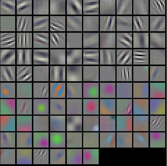
Beyond static visualizations, tracking quantization error over the training process is important. Monitoring mean squared quantization error (MSQE) during quantization-aware training (QAT) helps identify divergence points where numerical precision significantly impacts learning. TensorBoard and PyTorch’s quantization debugging APIs provide real-time tracking, highlighting instability during training.
By integrating these visualization tools into optimization workflows, practitioners can identify and correct issues early, ensuring optimized models maintain both accuracy and efficiency. These empirical insights provide a deeper understanding of how sparsity, quantization, and architectural optimizations affect models, guiding effective model compression and deployment strategies.
Visualizing Sparsity Patterns
Sparsity visualization tools provide detailed insight into pruned models by mapping out which weights have been removed and how sparsity is distributed across different layers. Frameworks such as TensorBoard (for TensorFlow) and Netron (for ONNX) allow users to inspect pruned networks at both the layer and weight levels.
One common visualization technique is sparsity heat maps, where color gradients indicate the proportion of weights removed from each layer. Layers with higher sparsity appear darker, revealing the model regions most impacted by pruning, as shown in Figure 32. This type of visualization transforms pruning from a black-box operation into an interpretable process, enabling practitioners to better understand and control sparsity-aware optimizations.
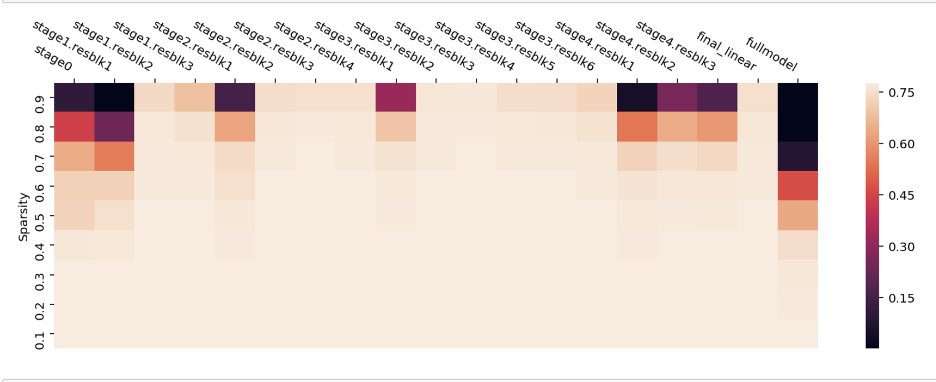
Beyond static snapshots, trend plots track sparsity progression across multiple pruning iterations. These visualizations illustrate how global model sparsity evolves, often showing an initial rapid increase followed by more gradual refinements. Tools like TensorFlow’s Model Optimization Toolkit and SparseML’s monitoring utilities provide such tracking capabilities, displaying per-layer pruning levels over time. These insights allow practitioners to fine-tune pruning strategies by adjusting sparsity constraints for individual layers.
Libraries such as DeepSparse’s visualization suite and PyTorch’s pruning utilities enable the generation of these visualization tools, helping analyze how pruning decisions affect different model components. By making sparsity data visually accessible, these tools help practitioners optimize their models more effectively.
Technique Comparison
Having explored the three major optimization approaches in depth, a comparative analysis reveals how different techniques address distinct aspects of the efficiency-accuracy trade-off. This comparison guides technique selection based on deployment constraints and available resources.
| Technique | Primary Goal | Accuracy Impact | Training Cost | Hardware Dependency | Best For |
|---|---|---|---|---|---|
| Pruning | Reduce FLOPs/Size | Moderate | Low (fine-tuning) | High (for sparse ops) | Latency-critical apps |
| Quantization | Reduce Size/Latency | Low | Low (PTQ) / High (QAT) | High (INT8 support) | Edge/Mobile deployment |
| Distillation | Reduce Size | Low-Moderate | High (retraining) | Low | Creating smaller, high-quality models |
Understanding these trade-offs enables systematic technique selection (Table 12). Pruning works best when sparse computation hardware is available and when reducing floating-point operations is critical. Quantization provides the most versatile approach with broad hardware support, making it ideal for diverse deployment scenarios. Knowledge distillation requires significant computational investment but produces consistently high-quality compressed models, making it valuable when accuracy preservation is paramount.
These techniques combine synergistically, with quantization often applied after pruning or distillation to achieve compound compression benefits. Production systems frequently employ sequential application: initial pruning reduces parameter count, quantization optimizes numerical representation, and fine-tuning through distillation principles recovers any accuracy loss. Sequential application enables compression ratios of 10-50x while maintaining competitive accuracy across diverse deployment scenarios.
Fallacies and Pitfalls
Model optimization represents one of the most technically complex areas in machine learning systems, where multiple techniques must be coordinated to achieve efficiency gains without sacrificing accuracy. The sophisticated nature of pruning, quantization, and distillation techniques—combined with their complex interdependencies—creates numerous opportunities for misapplication and suboptimal results that can undermine deployment success.
Fallacy: Optimization techniques can be applied independently without considering their interactions.
This misconception leads teams to apply multiple optimization techniques simultaneously without understanding how they interact. Combining pruning with aggressive quantization might compound accuracy losses beyond acceptable levels, while knowledge distillation from heavily pruned models may transfer suboptimal behaviors to student networks. Different optimization approaches can interfere with each other’s effectiveness, creating complex trade-offs that require careful orchestration. Successful optimization requires understanding technique interactions and applying them in coordinated strategies rather than as independent modifications.
Pitfall: Optimizing for theoretical metrics rather than actual deployment performance.
Many practitioners focus on reducing parameter counts, FLOPs, or model size without measuring actual deployment performance improvements. A model with fewer parameters might still have poor cache locality, irregular memory access patterns, or inefficient hardware utilization that negates theoretical efficiency gains. Quantization that reduces model size might increase inference latency on certain hardware platforms due to format conversion overhead. Effective optimization requires measuring and optimizing for actual deployment metrics rather than relying on theoretical complexity reductions.
Fallacy: Aggressive quantization maintains model performance with minimal accuracy loss.
This belief drives teams to apply extreme quantization levels without understanding the relationship between numerical precision and model expressiveness. While many models tolerate moderate quantization well, extreme quantization can cause catastrophic accuracy degradation, numerical instability, or training divergence. Different model architectures and tasks have varying sensitivity to quantization, requiring careful analysis rather than assuming universal applicability. Some operations like attention mechanisms or normalization layers may require higher precision to maintain functionality.
Pitfall: Using post-training optimization without considering training-aware alternatives.
Teams often apply optimization techniques after training completion to avoid modifying existing training pipelines. Post-training optimization is convenient but typically achieves inferior results compared to optimization-aware training approaches. Quantization-aware training, gradual pruning during training, and distillation-integrated training can achieve better accuracy-efficiency trade-offs than applying these techniques post-hoc. The convenience of post-training optimization comes at the cost of suboptimal results that may not meet deployment requirements.
Pitfall: Focusing on individual model optimization without considering system-level performance bottlenecks.
Many optimization efforts concentrate solely on reducing model complexity without analyzing the broader system context where models operate, requiring the structured profiling approaches detailed in Chapter 12: Benchmarking AI. A highly optimized model may provide minimal benefit if data preprocessing pipelines, I/O operations, or network communication dominate overall system latency. Memory bandwidth limitations, cache misses, or inefficient batch processing can negate the advantages of aggressive model optimization. Similarly, optimizing for single-model inference may miss opportunities for throughput improvements through batch processing, model parallelism, or request pipelining. Effective optimization requires profiling the entire system to identify actual bottlenecks and ensuring that model-level improvements translate to measurable system-level performance gains. This systems perspective is particularly important in multi-model ensembles, real-time serving systems, or edge deployments where resource constraints extend beyond individual model efficiency. The holistic optimization approach connects directly to the operational excellence principles Chapter 13: ML Operations by ensuring that optimizations contribute to overall system reliability and maintainability.
Summary
Model optimization represents the important bridge between theoretical machine learning advances and practical deployment realities, where computational constraints, memory limitations, and energy efficiency requirements demand sophisticated engineering solutions. This chapter demonstrated how the core tension between model accuracy and resource efficiency drives a rich ecosystem of optimization techniques that operate across multiple dimensions simultaneously. Rather than simply reducing model size or complexity, modern optimization approaches strategically reorganize model representations, numerical precision, and computational patterns to preserve important capabilities while dramatically improving efficiency characteristics.
Our optimization framework demonstrates how different aspects of model design can be systematically refined to meet deployment constraints. The journey from a 440MB BERT-Base model (Devlin et al. 2018) to a 28MB deployment-ready version exemplifies the power of combining complementary techniques: structural pruning shrinks the model to 110MB, knowledge distillation with DistilBERT (Sanh et al. 2019) maintains performance while further reducing size, and INT8 quantization achieves the final 28MB target. The integration of hardware-aware design principles ensures that optimization strategies align with underlying computational architectures, maximizing practical benefits across different deployment environments.
- Model optimization requires coordinated approaches across representation, precision, and architectural efficiency—as demonstrated by BERT’s 16x compression through combined pruning, distillation, and quantization
- Hardware-aware optimization aligns model characteristics with computational architectures to maximize practical performance benefits
- Automated optimization through AutoML can discover novel combinations of techniques that outperform manual optimization strategies
- Optimization techniques must balance accuracy preservation with deployment constraints—DistilBERT retains 97% of BERT’s performance with 40% fewer parameters
- Success requires understanding that no single technique provides a universal solution; the optimal strategy depends on specific deployment constraints, hardware characteristics, and application requirements
The emergence of AutoML frameworks for optimization represents a paradigm shift toward automated discovery of optimization strategies that can adapt to specific deployment contexts and performance requirements. These automated approaches build on training methodologies while pointing toward the emerging frontiers of self-optimizing systems. Such systems enable practitioners to explore vast optimization spaces more systematically than manual approaches, often uncovering novel combinations of techniques that achieve superior efficiency-accuracy trade-offs. As models grow larger and deployment contexts become more diverse, mastering these optimization techniques becomes increasingly critical for bridging the gap between research accuracy and production efficiency.