ML Systems
DALL·E 3 Prompt: Illustration in a rectangular format depicting the merger of embedded systems with Embedded AI. The left half of the image portrays traditional embedded systems, including microcontrollers and processors, detailed and precise. The right half showcases the world of artificial intelligence, with abstract representations of machine learning models, neurons, and data flow. The two halves are distinctly separated, emphasizing the individual significance of embedded tech and AI, but they come together in harmony at the center.
Purpose
How do the environments where machine learning operates shape the nature of these systems, and what drives their widespread deployment across computing platforms?
Machine learning systems must adapt to radically different computational environments, each imposing distinct constraints and opportunities. Cloud deployments leverage massive computational resources but face network latency, while mobile devices offer user proximity but operate under severe power limitations. Embedded systems minimize latency through local processing but constrain model complexity, and tiny devices enable widespread sensing while restricting memory to kilobytes. These deployment contexts fundamentally determine system architecture, algorithmic choices, and performance trade-offs. Understanding environment-specific requirements establishes the foundation for engineering decisions in machine learning systems. This knowledge enables engineers to select appropriate deployment paradigms and design architectures that balance performance, efficiency, and practicality across computing platforms.
Explain the physical constraints (speed of light, power wall, memory wall) that necessitate diverse ML deployment paradigms
Distinguish Cloud, Edge, Mobile, and TinyML paradigms by resource profiles and optimal use cases
Analyze resource trade-offs (computational power, latency, privacy, energy efficiency) to determine appropriate deployment strategies for specific applications
Apply the systematic deployment decision framework to evaluate privacy, latency, computational, and cost requirements for ML applications
Design hybrid ML architectures integrating multiple deployment paradigms
Evaluate real-world ML systems to identify which deployment paradigms are being used and assess their effectiveness
Critique common deployment fallacies and misconceptions to avoid poor architectural decisions in ML systems design
Synthesize universal design principles to create ML systems that effectively balance performance, efficiency, and practicality across deployment contexts
Deployment Paradigm Framework
The preceding introduction established machine learning systems as comprising three fundamental components: data, algorithms, and computing infrastructure. While this triadic framework provides a theoretical foundation, the transition from conceptual understanding to practical implementation introduces a critical dimension that fundamentally governs system design: the deployment environment. This chapter analyzes how computational context shapes architectural decisions in machine learning systems, establishing the theoretical basis for deployment-driven design principles.
Contemporary machine learning applications demonstrate remarkable architectural diversity driven by deployment constraints. Consider the domain of computer vision1: a convolutional neural network trained for image classification manifests as distinctly different systems when deployed across environments. In cloud-based medical imaging, the system exploits virtually unlimited computational resources to implement ensemble methods2 and sophisticated preprocessing pipelines. When deployed on mobile devices for real-time object detection, the same fundamental algorithm undergoes architectural transformation to satisfy stringent latency requirements while preserving acceptable accuracy. Factory automation applications further constrain the design space, prioritizing power efficiency and deterministic response times over model complexity. These variations represent distinctly different architectural solutions to the same computational problem, shaped by environmental constraints rather than algorithmic considerations.
1 Computer Vision: Field of AI enabling machines to interpret and understand visual information from images and videos. Requires processing 2-50 megapixels per image at 30+ fps for real-time applications, creating massive computational and memory bandwidth demands that drive specialized hardware like GPUs and vision processing units.
2 Ensemble Methods: ML technique combining predictions from multiple models to improve accuracy and robustness. Requires training and running 5-100+ models simultaneously, increasing compute requirements by 10-50x but enabling 2-5% accuracy improvements that justify cloud deployment costs.
This chapter presents a systematic taxonomy of machine learning deployment paradigms, analyzing four primary categories that span the computational spectrum from cloud data centers to microcontroller-based embedded systems. Each paradigm emerges from distinct operational requirements: computational resource availability, power consumption constraints, latency specifications, privacy requirements, and network connectivity assumptions. The theoretical framework developed here provides the analytical foundation for making informed architectural decisions in production machine learning systems.
Modern deployment strategies transcend traditional dichotomies between centralized and distributed processing. Contemporary applications increasingly implement hybrid architectures that strategically allocate computational tasks across multiple paradigms to optimize system-wide performance. Voice recognition systems exemplify this architectural sophistication: wake-word detection operates on ultra-low-power embedded processors to enable continuous monitoring, speech-to-text conversion utilizes mobile processors to maintain privacy and minimize latency, while semantic understanding leverages cloud infrastructure for complex natural language processing. This multi-paradigm approach reflects the engineering reality that optimal machine learning systems require architectural heterogeneity.
The deployment paradigm space exhibits clear dimensional structure. Cloud machine learning maximizes computational capabilities while accepting network-induced latency constraints. Edge computing positions inference computation proximate to data sources when latency requirements preclude cloud-based processing. Mobile machine learning extends computational capabilities to personal devices where user proximity and offline operation represent critical requirements. Tiny machine learning enables distributed intelligence on severely resource-constrained devices where energy efficiency supersedes computational sophistication.
Through comprehensive analysis of these deployment paradigms, this chapter develops the systems engineering perspective necessary for designing machine learning architectures that effectively balance algorithmic capabilities with operational constraints. This systems-oriented approach provides essential methodological foundations for translating theoretical machine learning advances into production systems that demonstrate reliable performance at scale. The analysis culminates with paradigm integration strategies for hybrid architectures and identification of core design principles that govern all machine learning deployment contexts.
Figure 1 illustrates how computational resources, latency requirements, and deployment constraints create this deployment spectrum. While Chapter 7: AI Frameworks explores the software tools that enable ML across these paradigms, and Chapter 11: AI Acceleration examines the specialized hardware that powers them, this chapter focuses on the fundamental deployment trade-offs that govern system architecture decisions. The subsequent analysis addresses each paradigm systematically, building toward an understanding of how they integrate into modern ML systems.
The Deployment Spectrum
The deployment spectrum from cloud to embedded systems exists not by choice, but by necessity imposed by physical laws that govern computing systems. These immutable constraints create hard boundaries that no engineering advancement can overcome, forcing the evolution of specialized deployment paradigms optimized for different operational contexts.
The speed of light establishes absolute minimum latencies that constrain real-time applications. Light traveling through optical fiber covers approximately 200,000 kilometers per second, creating a theoretical minimum 40ms round-trip time between California and Virginia. Internet routing, DNS resolution, and processing overhead typically add another 60-460ms, resulting in total latencies of 100-500ms for cloud services. This physics-imposed delay makes cloud deployment impossible for safety-critical applications requiring sub-10ms response times, such as autonomous vehicle emergency braking or industrial robotics precision control.
The power wall, resulting from the breakdown of Dennard scaling around 2005, transformed computing economics. Transistor shrinking no longer reduces power density, meaning chips cannot be made arbitrarily fast without proportional increases in power consumption and heat generation. This constraint forces trade-offs between computational performance and energy efficiency, directly driving the need for specialized low-power architectures in mobile and embedded systems. Data centers now dedicate 30-40% of their power budget to cooling, while mobile devices must implement thermal throttling to prevent component damage.
The memory wall represents the growing gap between processor speed and memory bandwidth. While computational capacity scales linearly through additional processing units, memory bandwidth scales approximately as the square root of chip area due to physical routing constraints. This creates an increasingly severe bottleneck where processors become data-starved, spending more time waiting for memory transfers than performing calculations. Large machine learning models exacerbate this problem, requiring parameter datasets that exceed available memory bandwidth by orders of magnitude.
Economics of scale create significant cost-per-unit differences that justify different deployment approaches. A cloud server costing $50,000 can support thousands of users through virtualization, achieving per-user costs under $50. However, applications requiring guaranteed response times or private data processing cannot share resources, eliminating this economic advantage. Meanwhile, embedded processors costing $5-50 enable deployment at billions of endpoints where individual cloud connections would be economically infeasible.
These physical constraints are not temporary engineering challenges but permanent limitations that shape the computational landscape. Understanding these boundaries explains why the deployment spectrum exists and provides the theoretical foundation for making informed architectural decisions in machine learning systems.

Deployment Paradigm Foundations
The deployment spectrum illustrated in Figure 1 exists not through design preference, but from necessity driven by immutable physical and hardware constraints. Understanding these limitations reveals why ML systems cannot adopt uniform approaches and must instead span the complete deployment spectrum from cloud to embedded devices.
Chapter 1: Introduction established the three foundational components of ML systems (data, algorithms, and infrastructure) as a unified framework that these deployment paradigms now optimize differently based on physical constraints. Cloud ML prioritizes algorithmic complexity through abundant infrastructure, while Mobile ML emphasizes data locality with constrained infrastructure, and Tiny ML maximizes algorithmic efficiency under extreme infrastructure limitations.
The most critical bottleneck in modern computing stems from memory bandwidth scaling differently than computational capacity. While compute power scales linearly through additional processing units, memory bandwidth scales approximately as the square root of chip area due to physical routing constraints. This creates a progressively worsening bottleneck where processors become data-starved. In practice, this manifests as ML models spending more time awaiting memory transfers than performing calculations, particularly problematic for large models3 that require more data than can be efficiently transferred.
3 Memory Bottleneck: When the rate of data transfer from memory to processor becomes the limiting factor in computation. Large models require so many parameters that memory bandwidth, rather than computational capacity, determines performance.
4 Dennard Scaling: Named after Robert Dennard (IBM, 1974), the observation that as transistors became smaller, they could operate at higher frequencies while consuming the same power density. This scaling enabled Moore’s Law until 2005, when physics limitations forced the industry toward multi-core architectures and specialized processors like GPUs and TPUs.
Compounding these memory challenges, the breakdown of Dennard scaling4 transformed computing constraints around 2005, when transistor shrinking stopped reducing power density. Power dissipation per unit area now remains constant or increases with each technology generation, creating hard limits on computational density. For mobile devices, this translates to thermal throttling that reduces performance when sustained computation generates excessive heat. Data centers face similar constraints at scale, requiring extensive cooling infrastructure that can consume 30-40% of total power budget. These power density limits directly drive the need for specialized low-power architectures in mobile and embedded contexts, and explain why edge deployment becomes necessary when power budgets are constrained.
Beyond power considerations, physical limits impose minimum latencies that no engineering optimization can overcome. The speed of light establishes an inherent 80ms round-trip time between California and Virginia, while internet routing, DNS resolution, and processing overhead typically contribute another 20-420ms. This 100-500ms total latency renders real-time applications infeasible with pure cloud deployment. Network bandwidth faces physical constraints: fiber optic cables have theoretical limits, and wireless communication remains bounded by spectrum availability and signal propagation physics. These communication constraints create hard boundaries that necessitate local processing for latency-sensitive applications and drive edge deployment decisions.
Heat dissipation emerges as an additional limiting factor as computational density increases. Mobile devices must throttle performance to prevent component damage and maintain user comfort, while data centers require extensive cooling systems that limit placement options and increase operational costs. Thermal constraints create cascading effects: elevated temperatures reduce semiconductor reliability, increase error rates, and accelerate component aging. These thermal realities necessitate trade-offs between computational performance and sustainable operation, driving specialized cooling solutions in cloud environments and ultra-low-power designs in embedded systems.
These fundamental constraints drove the evolution of the four distinct deployment paradigms outlined in this overview (Section 1.2). Understanding these core constraints proves essential for selecting appropriate deployment paradigms and establishing realistic performance expectations.
These theoretical constraints manifest in concrete hardware differences across the deployment spectrum. To understand the practical implications of these physical limitations, Table 1 provides representative hardware platforms for each category. These examples demonstrate the range of computational resources, power requirements, and cost considerations5 across the ML systems spectrum, illustrating the practical implications of each deployment approach.6
5 ML Hardware Cost Spectrum: The cost range spans 6 orders of magnitude, from $10 ESP32-CAM modules to multi-million dollar TPU Pod systems. This 100,000x+ cost difference reflects proportional differences in computational capability, enabling deployment across vastly different economic contexts and use cases, from hobbyist projects to hyperscale cloud infrastructure.
6 Power Usage Effectiveness (PUE): Data center efficiency metric measuring total facility power divided by IT equipment power. A PUE of 1.0 represents perfect efficiency (impossible in practice), while 1.1-1.3 indicates highly efficient facilities using advanced cooling and power management. Google’s data centers achieve PUE of 1.12 compared to industry average of 1.8.
These quantitative thresholds reflect essential relationships between computational requirements, energy consumption, and deployment feasibility. These scaling relationships determine when distributed cloud deployment becomes advantageous relative to edge or mobile alternatives. Understanding these quantitative trade-offs enables informed deployment decisions across the spectrum of ML systems.
Figure 2 illustrates the differences between Cloud ML, Edge ML, Mobile ML, and Tiny ML in terms of hardware specifications, latency characteristics, connectivity requirements, power consumption, and model complexity constraints. As systems transition from Cloud to Edge to Tiny ML, available resources decrease dramatically, presenting significant challenges for machine learning model deployment. This resource disparity becomes particularly evident when deploying ML models on microcontrollers, the primary hardware platform for Tiny ML. These devices possess severely constrained memory and storage capacities that prove insufficient for conventional complex ML models.
| Category | Example Device | Processor | Memory | Storage | Power | Price Range | Example Models/Tasks | Quantitative Thresholds |
|---|---|---|---|---|---|---|---|---|
| Cloud ML | Google TPU v4 Pod | 4,096x TPU v4 chips (1.1 exaflops peak) | 131 TB HBM2 | Cloud-scale (PB-scale) | ~3 MW | Cloud service (rental only) | Large language models, massive-scale training | >1000 TFLOPS compute, real-time video processing, >100GB/s memory bandwidth, PUE 1.1-1.3, 100-500ms latency |
| Edge ML | NVIDIA DGX Spark | GB10 Grace Blackwell Superchip (20-core Arm, 1 PFLOPS AI) | 128 GB LPDDR5x | 4 TB NVMe | ~200 W | ~$5,000 | Model fine-tuning, on-premise inference, prototype development | ~1 PFLOPS AI compute, >270 GB/s memory bandwidth, desktop deployment, local processing |
| Mobile ML | iPhone 15 Pro | A17 Pro (6-core CPU, 6-core GPU) | 8 GB RAM | 128 GB-1 TB | 3-5 W | $999+ | Face ID, computational photography, voice recognition | 1-10 TOPS compute, <2W sustained power, <50ms UI response |
| Tiny ML | ESP32-CAM | Dual-core @ 240MHz | 520 KB RAM | 4 MB Flash | 0.05-0.25 W | $10 | Image classification, motion detection | <1 TOPS compute, <1mW power, microsecond response times |

Cloud ML: Maximizing Computational Power
Having established the constraints and evolutionary progression that shape ML deployment paradigms, this analysis addresses each paradigm systematically, beginning with Cloud ML, the foundation from which other paradigms emerged. This approach maximizes computational resources while accepting latency constraints, providing the optimal choice when computational power matters more than response time. Cloud deployments prove ideal for complex training tasks and inference workloads that can tolerate network delays.
Cloud Machine Learning leverages the scalability and power of centralized infrastructures7 to handle computationally intensive tasks: large-scale data processing, collaborative model development, and advanced analytics. Cloud data centers utilize distributed architectures and specialized resources to train complex models and support diverse applications, from recommendation systems to natural language processing8. The subsequent analysis addresses the deployment characteristics that make cloud ML systems effective for large-scale applications.
7 Cloud Infrastructure Evolution: Cloud computing for ML emerged from Amazon’s decision in 2002 to treat their internal infrastructure as a service. AWS launched in 2006, followed by Google Cloud (2008) and Azure (2010). By 2024, global cloud infrastructure spending reached approximately $138 billion annually, with total public cloud services exceeding $675 billion.
8 NLP Computational Demands: Modern language models like GPT-3 required 3,640 petaflop-days of compute for training, equivalent to running 1,000 NVIDIA V100 GPUs continuously for 355 days (Strubell, Ganesh, and McCallum 2019). This computational scale drove the need for massive cloud infrastructure.
Figure 3 provides an overview of Cloud ML’s capabilities, which we will discuss in greater detail throughout this section.

Cloud Infrastructure and Scale
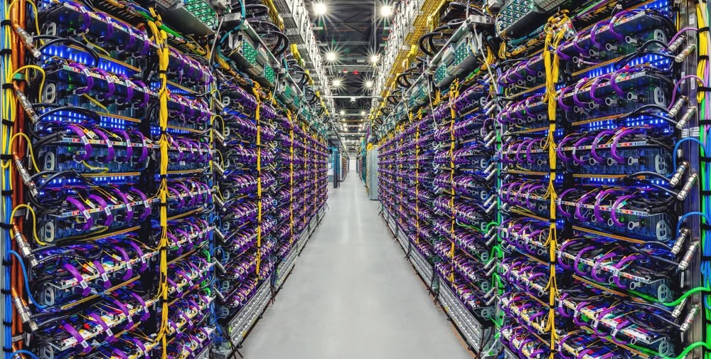
To understand cloud ML’s position in the deployment spectrum, we must first consider its defining characteristics. Cloud ML’s primary distinguishing feature is its centralized infrastructure operating at unprecedented scale. Figure 4 illustrates this concept with an example from Google’s Cloud TPU9 data center. As detailed in Table 1, cloud systems like Google’s TPU v4 Pod represent a 100-1000x computational advantage over mobile devices, with >1000 TFLOPS compute power and megawatt-scale power consumption. Cloud service providers offer virtual platforms with >100GB/s memory bandwidth housed in globally distributed data centers10. These centralized facilities enable computational workloads impossible on resource-constrained devices. However, this centralization introduces critical trade-offs: network round-trip latency of 100-500ms eliminates real-time applications, while operational costs scale linearly with usage.
9 Tensor Processing Unit (TPU): Google’s custom ASIC designed specifically for tensor operations, first used internally in 2015 for neural network inference. A single TPU v4 Pod contains 4,096 chips and delivers 1.1 exaflops of peak performance, representing one of the world’s largest publicly available ML clusters.
10 Hyperscale Data Centers: These facilities contain 5,000+ servers and cover 10,000+ square feet. Microsoft’s data centers span over 200 locations globally, with some individual facilities consuming enough electricity to power 80,000 homes.
Cloud ML excels in processing massive data volumes through parallelized architectures. Through techniques detailed in Chapter 10: Model Optimizations, distributed training across hundreds of GPUs enables processing that would require months on single devices, while Chapter 11: AI Acceleration covers the memory bandwidth analysis underlying this performance. This enables training on datasets requiring hundreds of terabytes of storage and petaflops of computation, resources impossible on constrained devices.
The centralized infrastructure creates exceptional deployment flexibility through cloud APIs11, making trained models accessible worldwide across mobile, web, and IoT platforms. Seamless collaboration enables multiple teams to access projects simultaneously with integrated version control. Pay-as-you-go pricing models12 eliminate upfront capital expenditure while resources scale elastically with demand.
11 ML APIs: Application Programming Interfaces that democratized AI by providing pre-trained models as web services. Google’s Vision API launched in 2016, processing over 1 billion images monthly within two years, enabling developers to add AI capabilities without ML expertise.
12 Pay-as-You-Go Pricing: Revolutionary model where users pay only for actual compute time used, measured in GPU-hours or inference requests. Training a model might cost $50-500 on demand versus $50,000-500,000 to purchase equivalent hardware.
A common misconception assumes that Cloud ML’s vast computational resources make it universally superior to alternative deployment approaches. Cloud infrastructure offers exceptional computational power and storage, yet this advantage doesn’t automatically translate to optimal solutions for all applications. Cloud deployment introduces significant trade-offs including network latency (often 100-500ms round trip), privacy concerns when transmitting sensitive data, ongoing operational costs that scale with usage, and complete dependence on network connectivity. Edge and embedded deployments excel in scenarios requiring real-time response (autonomous vehicles need sub-10ms decision making), strict data privacy (medical devices processing patient data), predictable costs (one-time hardware investment versus recurring cloud fees), or operation in disconnected environments (industrial equipment in remote locations). The optimal deployment paradigm depends on specific application requirements rather than raw computational capability.
Cloud ML Trade-offs and Constraints
Cloud ML’s substantial advantages carry inherent trade-offs that shape deployment decisions. Latency represents the most significant physical constraint. Network round-trip delays typically range from 100-500ms, making cloud processing unsuitable for real-time applications requiring sub-10ms responses, such as autonomous vehicles and industrial control systems. Beyond basic timing constraints, unpredictable response times complicate performance monitoring and debugging across geographically distributed infrastructure.
Privacy and security present significant challenges when adopting cloud deployment. Transmitting sensitive data to remote data centers creates potential vulnerabilities and complicates regulatory compliance. Organizations handling data subject to regulations like GDPR13 or HIPAA14 must implement comprehensive security measures including encryption, strict access controls, and continuous monitoring to meet stringent data handling requirements.
13 GDPR (General Data Protection Regulation): European privacy law effective 2018, imposing fines up to €20 million or 4% of global revenue for violations. Forces ML systems to implement “right to be forgotten” and data processing transparency.
14 HIPAA (Health Insurance Portability and Accountability Act): US healthcare privacy law requiring strict data security measures. ML systems handling medical data must implement encryption, access controls, and audit trails, adding 30-50% to development costs.
Cost management introduces operational complexity as expenses scale with usage. Consider a production system serving 1 million daily inferences at $0.001 each: annual costs reach $365,000, compared to $100,000 for equivalent edge hardware purchased once. The break-even point occurs around 100,000-1,000,000 requests, directly influencing deployment strategy. Unpredictable usage spikes further complicate budgeting, requiring sophisticated monitoring and cost governance frameworks.
Network dependency creates another critical constraint. Any connectivity disruption directly impacts system availability, proving particularly problematic where network access is limited or unreliable. Vendor lock-in further complicates the landscape, as dependencies on specific tools and APIs create portability and interoperability challenges when transitioning between providers. Organizations must carefully balance these constraints against cloud benefits based on application requirements and risk tolerance, with resilience strategies detailed in Chapter 16: Robust AI.
Large-Scale Training and Inference
Cloud ML’s computational advantages manifest most visibly in consumer-facing applications requiring massive scale. Virtual assistants like Siri and Alexa exemplify cloud ML’s ability to handle computationally intensive natural language processing, leveraging extensive computational resources to process vast numbers of concurrent interactions while continuously improving through exposure to diverse linguistic patterns and use cases.
Recommendation engines deployed by Netflix and Amazon demonstrate another compelling application of cloud resources. These systems process massive datasets using collaborative filtering15 and other machine learning techniques to uncover patterns in user preferences and behavior. Cloud computational resources enable continuous updates and refinements as user data grows, with Netflix processing over 100 billion data points daily to deliver personalized content suggestions that directly enhance user engagement.
15 Collaborative Filtering: Recommendation technique analyzing user behavior patterns to predict preferences. Netflix’s algorithm contributes to 80% of watched content and saves $1 billion annually in customer retention.
Financial institutions have revolutionized fraud detection through cloud ML capabilities. By analyzing vast amounts of transactional data in real-time, ML algorithms trained on historical fraud patterns can detect anomalies and suspicious behavior across millions of accounts, enabling proactive fraud prevention that minimizes financial losses.
These applications demonstrate how cloud ML’s computational advantages translate into transformative capabilities for large-scale, complex processing tasks. Beyond these flagship applications, cloud ML permeates everyday online experiences through personalized advertisements on social media, predictive text in email services, product recommendations in e-commerce, enhanced search results, and security anomaly detection systems that continuously monitor for cyber threats at scale.
Edge ML: Reducing Latency and Privacy Risk
Cloud ML’s computational advantages come with inherent trade-offs that limit its applicability for many real-world scenarios. The 100-500ms latency and privacy concerns that we examined create fundamental barriers for applications requiring immediate response or local data processing. Edge ML emerged as a direct response to these specific limitations, moving computation closer to data sources and trading unlimited computational resources for sub-100ms latency and local data sovereignty.
This paradigm shift becomes essential for applications where cloud’s 100-500ms round-trip delays prove unacceptable. Autonomous systems requiring split-second decisions and industrial IoT16 applications demanding real-time response cannot tolerate network delays. Similarly, applications subject to strict data privacy regulations must process information locally rather than transmitting it to remote data centers. Edge devices (gateways and IoT hubs17) occupy a middle ground in the deployment spectrum, maintaining acceptable performance while operating under intermediate resource constraints.
16 Industrial IoT: Manufacturing generates over 1 exabyte of data annually, but less than 1% is analyzed due to connectivity constraints. Edge ML enables real-time analysis, with predictive maintenance alone saving manufacturers $630 billion globally by 2025.
17 IoT Hubs: Central connection points that aggregate data from multiple sensors before cloud transmission. A typical smart building might have 1 hub managing 100-1000 IoT sensors, reducing cloud traffic by 90% while enabling local decision-making.
Figure 5 provides an overview of Edge ML’s key dimensions, which this analysis addresses in detail.

Distributed Processing Architecture
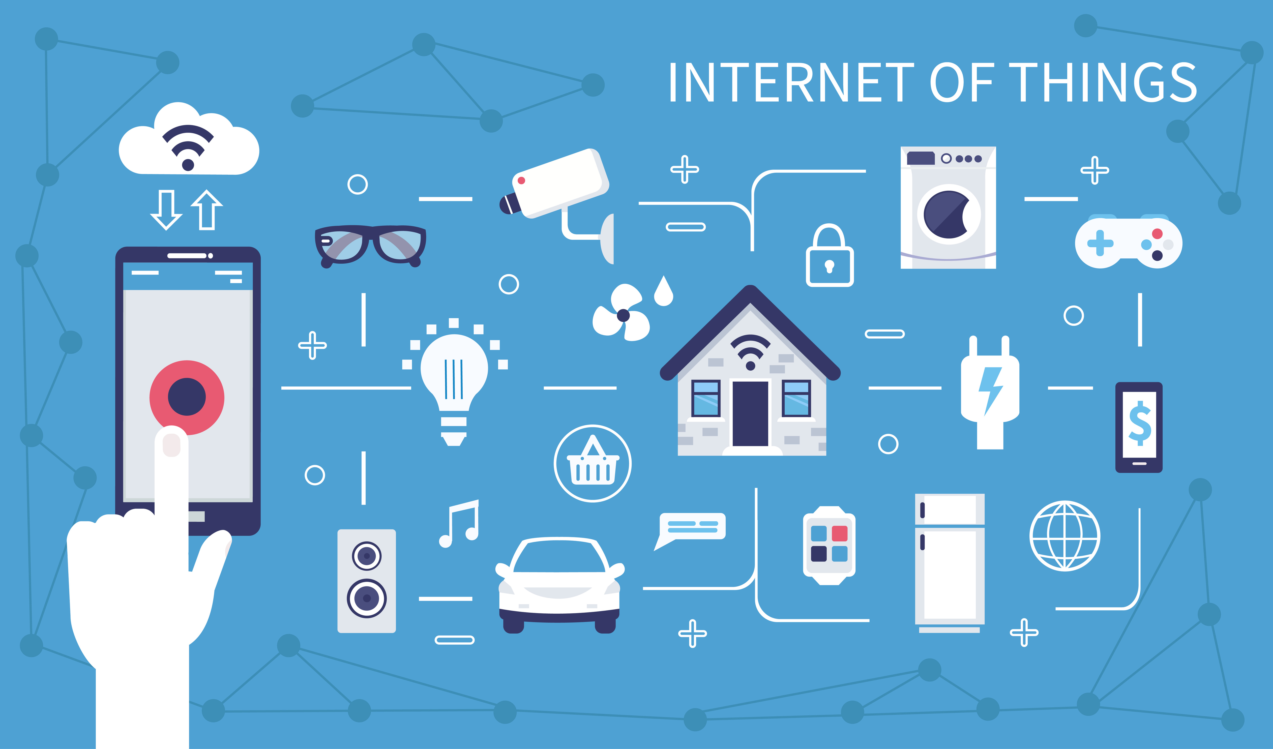
Edge ML’s diversity spans wearables, industrial sensors, and smart home appliances, devices that process data locally18 without depending on central servers (Figure 6). Edge devices occupy the middle ground between cloud systems and mobile devices in computational resources, power consumption, and cost. Memory bandwidth at 25-100 GB/s enables models requiring 100MB-1GB parameters, using optimization techniques (Chapter 10: Model Optimizations) to achieve 2-4x speedup compared to cloud models. Local processing eliminates network round-trip latency, enabling <100ms response times while generating substantial bandwidth savings: processing 1000 camera feeds locally avoids 1Gbps uplink costs and reduces cloud expenses by $10,000-100,000 annually.
18 IoT Device Growth: From 8.4 billion connected devices in 2017 to a projected 25.4 billion by 2030. Each device generates 2.5 quintillion bytes of data daily, making edge processing essential for bandwidth management.
Edge ML Benefits and Deployment Challenges
Edge ML provides quantifiable benefits that address key cloud limitations. Latency reduction from 100-500ms in cloud deployments to 1-50ms at the edge enables safety-critical applications19 requiring real-time response. Bandwidth savings prove equally substantial: a retail store with 50 cameras streaming video can reduce bandwidth requirements from 100 Mbps (costing $1,000-2,000 monthly) to less than 1 Mbps by processing locally and transmitting only metadata, a 99% reduction. Privacy improves through local processing, eliminating transmission risks and simplifying regulatory compliance. Operational resilience ensures systems continue functioning during network outages, proving critical for manufacturing, healthcare, and building management applications.
19 Latency-Critical Applications: Autonomous vehicles require <10ms response times for emergency braking decisions. Industrial robotics needs <1ms for precision control. Cloud round-trip latency typically ranges from 100-500ms, making edge processing essential for safety-critical applications.
20 Edge Server Constraints: Typical edge servers have 1-8GB RAM and 2-32GB storage, versus cloud servers with 128-1024GB RAM and petabytes of storage. Processing power differs by 10-100x, necessitating specialized model compression techniques.
21 Edge Network Coordination: For n edge devices, the number of potential communication paths is n(n-1)/2. A network of 1,000 devices has 499,500 possible connections. Kubernetes K3s and similar platforms help manage this complexity.
These benefits carry corresponding limitations. Limited computational resources20 significantly constrain model complexity: edge servers typically provide 10-100x less processing power than cloud infrastructure, limiting deployable models to millions rather than billions of parameters. Managing distributed networks introduces complexity that scales nonlinearly with deployment size. Coordinating version control and updates across thousands of devices requires sophisticated orchestration systems21. Security challenges intensify with physical accessibility—edge devices deployed in retail stores or public infrastructure face tampering risks requiring hardware-based protection mechanisms. Hardware heterogeneity further complicates deployment, as diverse platforms with varying capabilities demand different optimization strategies. Initial deployment costs of $500-2,000 per edge server create substantial capital requirements. Deploying 1,000 locations requires $500,000-2,000,000 upfront investment, though these costs are offset by long-term operational savings.
Real-Time Industrial and IoT Systems
Industries deploy Edge ML widely where low latency, data privacy, and operational resilience justify the additional complexity of distributed processing. Autonomous vehicles represent perhaps the most demanding application, where safety-critical decisions must occur within milliseconds based on sensor data that cannot be transmitted to remote servers. Systems like Tesla’s Full Self-Driving process inputs from eight cameras at 36 frames per second through custom edge hardware, making driving decisions with latencies under 10ms, a response time physically impossible with cloud processing due to network delays.
Smart retail environments demonstrate edge ML’s practical advantages for privacy-sensitive, bandwidth-intensive applications. Amazon Go stores process video from hundreds of cameras through local edge servers, tracking customer movements and item selections to enable checkout-free shopping. This edge-based approach addresses both technical and privacy concerns: transmitting high-resolution video from hundreds of cameras would require over 200 Mbps sustained bandwidth, while local processing ensures customer video never leaves the premises, addressing privacy concerns and regulatory requirements.
The Industrial IoT22 leverages edge ML for applications where millisecond-level responsiveness directly impacts production efficiency and worker safety. Manufacturing facilities deploy edge ML systems for real-time quality control, with vision systems inspecting welds at speeds exceeding 60 parts per minute, and predictive maintenance23 applications that monitor over 10,000 industrial assets per facility. This approach has demonstrated 25-35% reductions in unplanned downtime across various manufacturing sectors.
22 Industry 4.0: Fourth industrial revolution integrating cyber-physical systems into manufacturing. Expected to increase productivity by 20-30% and reduce costs by 15-25% globally.
23 Predictive Maintenance: ML-driven maintenance scheduling based on equipment condition. Reduces unplanned downtime by 35-45% and costs by 20-25%. GE saves $1.5 billion annually using predictive analytics.
Smart buildings utilize edge ML to optimize energy consumption while maintaining operational continuity during network outages. Commercial buildings equipped with edge-based building management systems process data from 5,000-10,000 sensors monitoring temperature, occupancy, air quality, and energy usage, with edge processing reducing cloud transmission requirements by 95% while enabling sub-second response times. Healthcare applications similarly leverage edge ML for patient monitoring and surgical assistance, maintaining HIPAA compliance through local processing while achieving sub-100ms latency for real-time surgical guidance.
Mobile ML: Personal and Offline Intelligence
While Edge ML addressed the latency and privacy limitations of cloud deployment, it introduced new constraints: the need for dedicated edge infrastructure, ongoing network connectivity, and substantial upfront hardware investments. The proliferation of billions of personal computing devices (smartphones, tablets, and wearables) created an opportunity to extend ML capabilities even further by bringing intelligence directly to users’ hands. Mobile ML represents this next step in the distribution of intelligence, prioritizing user proximity, offline capability, and personalized experiences while operating under the strict power and thermal constraints inherent to battery-powered devices.
Mobile ML integrates machine learning directly into portable devices like smartphones and tablets, providing users with real-time, personalized capabilities. This paradigm excels when user privacy, offline operation, and immediate responsiveness matter more than computational sophistication. Mobile ML supports applications such as voice recognition24, computational photography25, and health monitoring while maintaining data privacy through on-device computation. These battery-powered devices must balance performance with power efficiency and thermal management, making them ideal for frequent, short-duration AI tasks.
24 Voice Recognition Evolution: Apple’s Siri (2011) required cloud processing with 200-500ms latency. By 2017, on-device processing reduced latency to <50ms while improving privacy. Modern smartphones process 16kHz audio at 20-30ms latency using specialized neural engines.
25 Computational Photography: Combines multiple exposures and ML algorithms to enhance image quality. Google’s Night Sight captures 15 frames in 6 seconds, using ML to align and merge them. Portrait mode uses depth estimation ML models to create professional-looking bokeh effects in real-time.
This section analyzes Mobile ML across four key dimensions, revealing how this paradigm balances capability with constraints. Figure 7 provides an overview of Mobile ML’s capabilities.

Battery and Thermal Constraints
Mobile devices exemplify intermediate constraints: 8GB RAM, 128GB-1TB storage, 1-10 TOPS AI compute through Neural Processing Units26 consuming 3-5W power. System-on-Chip architectures27 integrate computation and memory to minimize energy costs. Memory bandwidth of 25-50 GB/s limits models to 10-100MB parameters, requiring aggressive optimization (Chapter 10: Model Optimizations). Battery constraints (18-22Wh capacity) make energy optimization critical: 1W continuous ML processing reduces device lifetime from 24 to 18 hours. Specialized frameworks (TensorFlow Lite28, Core ML29) provide hardware-optimized inference enabling <50ms UI response times.
26 Neural Processing Unit (NPU): Specialized processors optimized for neural network operations. Apple’s Neural Engine performs 600 billion operations per second. Qualcomm’s Hexagon NPU delivers up to 75 TOPS while consuming <1W.
27 Mobile System-on-Chip: Modern flagship SoCs integrate CPU, GPU, NPU, and memory controllers on a single chip. Apple’s A17 Pro contains 19 billion transistors in a 3nm process.
28 TensorFlow Lite: Google’s mobile ML framework launched in 2017, designed to run models <100MB with <100ms inference time. Used in over 4 billion devices worldwide.
29 Core ML: Apple’s framework introduced in iOS 11 (2017), optimized for on-device inference. Supports models from 1KB to 1GB, with automatic optimization for Apple Silicon.
Mobile ML Benefits and Resource Constraints
Mobile ML excels at delivering responsive, privacy-preserving user experiences. Real-time processing achieves sub-10ms latency, enabling imperceptible response: face detection operates at 60fps with under 5ms latency, while voice wake-word detection responds within 2-3ms. Privacy guarantees emerge from complete data sovereignty through on-device processing. Face ID processes biometric data entirely within a hardware-isolated Secure Enclave30, keyboard prediction trains locally on user data, and health monitoring maintains HIPAA compliance without complex infrastructure requirements. Offline functionality eliminates network dependency: Google Maps analyzes millions of road segments locally for navigation, translation31 supports 40+ language pairs using 35-45MB models that achieve 90% of cloud accuracy, and music identification matches against on-device databases. Personalization reaches unprecedented depth by leveraging behavioral data accumulated over months: iOS predicts which app users will open next with 70-80% accuracy, notification management optimizes delivery timing based on individual patterns, and camera systems continuously adapt to user preferences through implicit feedback.
30 Mobile Face Detection: Apple’s Face ID processes biometric data entirely on-device using the Secure Enclave, making extraction practically impossible even with physical device access.
31 Real-Time Translation: Google Translate processes 40+ languages offline using on-device neural networks. Models are 35-45MB versus 2GB+ cloud versions, achieving 90% accuracy while enabling instant translation without internet.
32 Mobile Device Constraints: Flagship phones typically have 12-24GB RAM and 512GB-2TB storage, versus cloud servers with 256-2048GB RAM and unlimited storage. Mobile processors operate at 15-25W peak power compared to server CPUs at 200-400W.
These benefits require accepting significant resource constraints. Flagship phones allocate only 100MB-1GB to individual ML applications, representing just 0.5-5% of total memory, forcing models to remain under 100-500MB compared to cloud’s ability to deploy 350GB+ models. Battery life32 presents visible user impact: processing 100 inferences per hour at 0.1 joules each consumes 0.36% of battery daily, compounding with baseline drain; video processing at 30fps can reduce battery life from 24 hours to 6-8 hours. Thermal throttling unpredictably limits sustained performance, with the A17 Pro chip achieving 35 TOPS peak performance but sustaining only 10-15 TOPS during extended operation, requiring adaptive performance strategies. Development complexity multiplies across platforms, demanding separate implementations for Core ML and TensorFlow Lite, while device heterogeneity—particularly Android’s span from $100 budget phones to $1,500 flagships—requires multiple model variants. Deployment friction adds further challenges: app store approval processes taking 1-7 days prevent rapid bug fixes that cloud deployments can deploy instantly.
Personal Assistant and Media Processing
Mobile ML has achieved transformative success across diverse applications that showcase the unique advantages of on-device processing for billions of users worldwide. Computational photography represents perhaps the most visible success, transforming smartphone cameras into sophisticated imaging systems. Modern flagships process every photo through multiple ML pipelines operating in real-time: portrait mode33 uses depth estimation and segmentation networks to achieve DSLR-quality bokeh effects, night mode captures and aligns 9-15 frames with ML-based denoising that reduces noise by 10-20dB, and systems like Google Pixel process 10-15 distinct ML models per photo for HDR merging, super-resolution, and scene optimization.
33 Portrait Mode Photography: Uses dual cameras or LiDAR for depth maps, then ML segmentation to separate subjects from backgrounds, achieving DSLR-quality depth-of-field effects in real-time.
Voice-driven interactions demonstrate mobile ML’s transformation of human-device communication. These systems combine ultra-low-power wake-word detection consuming less than 1mW with on-device speech recognition achieving under 10ms latency for simple commands. Keyboard prediction has evolved to context-aware neural models achieving 60-70% phrase prediction accuracy, reducing typing effort by 30-40%. Real-time camera translation processes over 100 languages at 15-30fps entirely on-device, enabling instant visual translation without internet connectivity.
Health monitoring through wearables like Apple Watch extracts sophisticated insights from sensor data while maintaining complete privacy. These systems achieve over 95% accuracy in activity detection and include FDA-cleared atrial fibrillation detection with 98%+ sensitivity, processing extraordinarily sensitive health data entirely on-device to maintain HIPAA compliance. Accessibility features demonstrate transformative social impact through continuous local processing: Live Text detects and recognizes text from camera feeds, Sound Recognition alerts deaf users to environmental cues through haptic feedback, and VoiceOver generates natural language descriptions of visual content.
Augmented reality frameworks leverage mobile ML for real-time environment understanding at 60fps. ARCore and ARKit track device position with centimeter-level accuracy while simultaneously mapping 3D surroundings, enabling hand tracking that extracts 21-joint 3D poses and face analysis of 50+ landmark meshes for real-time effects. These applications demand consistent sub-16ms frame times, making only on-device processing viable for delivering the seamless experiences users expect.
Despite mobile ML’s demonstrated capabilities, a common pitfall involves attempting to deploy desktop-trained models directly to mobile or edge devices without architecture modifications. Models developed on powerful workstations often fail dramatically when deployed to resource-constrained devices. A ResNet-50 model requiring 4GB memory for inference (including activations and batch processing) and 4 billion FLOPs per inference cannot run on a device with 512MB of RAM and a 1 GFLOP/s processor. Beyond simple resource violations, desktop-optimized models may use operations unsupported by mobile hardware (specialized mathematical operations), assume floating-point precision unavailable on embedded systems, or require batch processing incompatible with single-sample inference. Successful deployment demands architecture-aware design from the beginning, including specialized architectural techniques for mobile devices (Howard et al. 2017), integer-only operations for microcontrollers, and optimization strategies that maintain accuracy while reducing computation.
Tiny ML: Ubiquitous Sensing at Scale
The progression from Cloud to Edge to Mobile ML demonstrates the increasing distribution of intelligence across computing platforms, yet each step still requires significant resources. Even mobile devices, with their sophisticated processors and gigabytes of memory, represent a relatively privileged position in the global computing landscape, demanding watts of power and hundreds of dollars in hardware investment. For truly ubiquitous intelligence (sensors in every surface, monitor on every machine, intelligence in every object), these resource requirements remain prohibitive. Tiny ML completes the deployment spectrum by pushing intelligence to its absolute limits, using devices costing less than $10 and consuming less than 1 milliwatt of power. This paradigm makes ubiquitous sensing not just technically feasible but economically practical at massive scales.
Where mobile ML still requires sophisticated hardware with gigabytes of memory and multi-core processors, Tiny Machine Learning operates on microcontrollers with kilobytes of RAM and single-digit dollar price points. This extreme constraint forces a significant shift in how we approach machine learning deployment, prioritizing ultra-low power consumption and minimal cost over computational sophistication. The result enables entirely new categories of applications impossible at any other scale.
Tiny ML brings intelligence to the smallest devices, from microcontrollers34 to embedded sensors, enabling real-time computation in severely resource-constrained environments. This paradigm excels in applications requiring ubiquitous sensing, autonomous operation, and extreme energy efficiency. Tiny ML systems power applications such as predictive maintenance, environmental monitoring, and simple gesture recognition while optimized for energy efficiency35, often running for months or years on limited power sources such as coin-cell batteries36. These systems deliver actionable insights in remote or disconnected environments where power, connectivity, and maintenance access are impractical.
34 Microcontrollers: Single-chip computers with integrated CPU, memory, and peripherals, typically operating at 1-100MHz with 32KB-2MB RAM. Arduino Uno uses an ATmega328P with 32KB flash and 2KB RAM, while ESP32 provides WiFi capability with 520KB RAM, still thousands of times less than a smartphone.
35 Energy Efficiency in TinyML: Ultra-low power consumption enables deployment in remote locations. Modern ARM Cortex-M0+ microcontrollers consume <1µW in sleep mode and 100-300µW/MHz when active. Efficient ML inference can run for years on a single coin-cell battery.
36 Coin-Cell Batteries: Small, round batteries (CR2032 being most common) providing 200-250mAh at 3V. When powering TinyML devices at 10-50mW average consumption, these batteries can operate devices for 1-5 years, enabling “deploy-and-forget” IoT applications.
This section analyzes Tiny ML through four critical dimensions that define its unique position in the ML deployment spectrum. Figure 8 encapsulates the key aspects of Tiny ML discussed in this section.

Extreme Resource Constraints
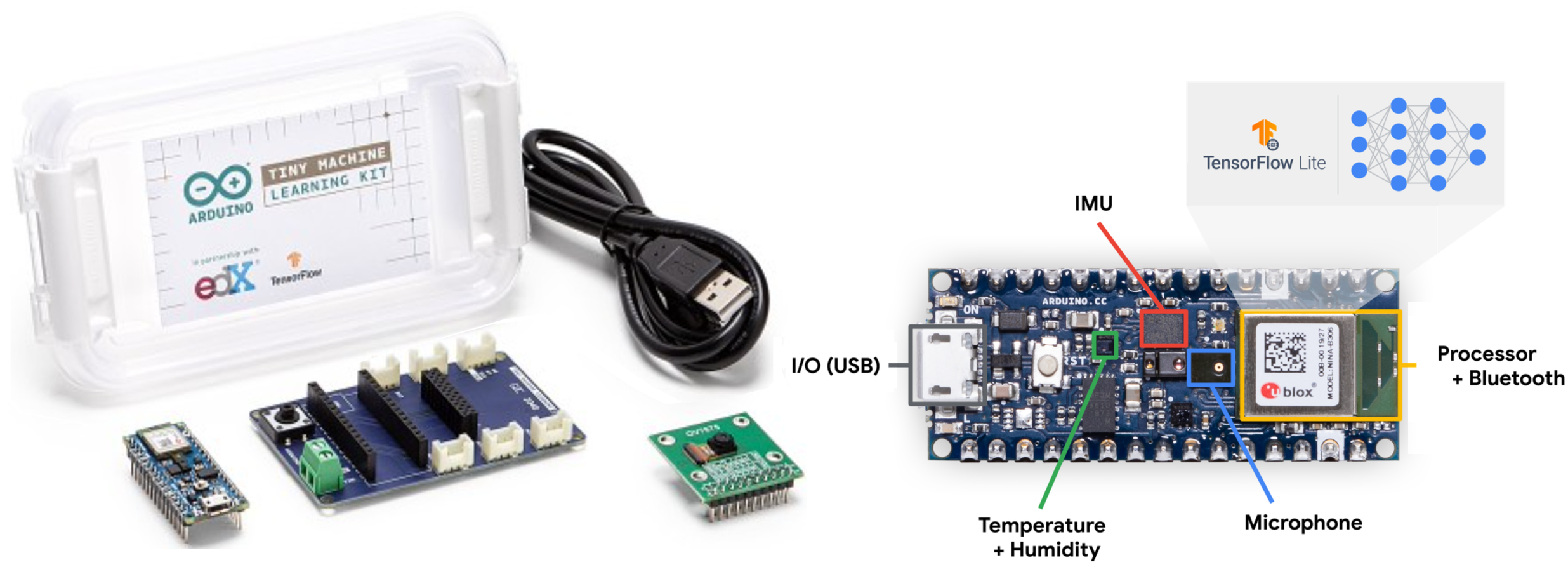
TinyML operates at hardware extremes: Arduino Nano 33 BLE Sense (256KB RAM, 1MB Flash, 0.02-0.04W, $35) and ESP32-CAM (520KB RAM, 4MB Flash, 0.05-0.25W, $10) represent 30,000-50,000x memory reduction versus cloud systems and 160,000x power reduction (Figure 9). These constraints enable months or years of autonomous operation37 but demand specialized algorithms delivering acceptable performance at <1 TOPS compute with microsecond response times. Devices range from palm-sized to 5x5mm chips38, enabling ubiquitous sensing in previously impossible contexts.
37 On-Device Training Constraints: Microcontrollers rarely support full training due to memory limitations. Instead, they use transfer learning with minimal on-device adaptation or federated learning aggregation.
38 TinyML Device Scale: The smallest ML-capable devices measure just 5x5mm (Syntiant NDP chips). Google’s Coral Dev Board Mini (40x48mm) includes WiFi and full Linux capability.
TinyML Advantages and Operational Trade-offs
TinyML’s extreme resource constraints enable unique advantages impossible at other scales. Microsecond-level latency eliminates all transmission overhead, achieving 10-100μs response times that enable applications requiring sub-millisecond decisions: industrial vibration monitoring processes 10kHz sampling at under 50μs latency, audio wake-word detection analyzes 16kHz audio streams under 100μs, and precision manufacturing systems inspect over 1000 parts per minute. Economic advantages prove transformative for massive-scale deployments: complete ESP32-CAM systems cost $8-12, enabling 1000-sensor deployments for $10,000 versus $500,000-1,000,000 for cellular alternatives. Agricultural monitoring can instrument buildings for $5,000 versus $50,000+ for camera-based systems, while city-scale networks of 100,000 sensors become economically viable at $1-2 million versus $50-100 million for edge alternatives. Energy efficiency enables 1-10 year operation on coin-cell batteries consuming just 1-10mW, supporting applications like wildlife tracking for years without recapture, structural health monitoring embedded in concrete during construction, and agricultural sensors deployed where power infrastructure doesn’t exist. Energy harvesting from solar, vibration, or thermal sources can even enable perpetual operation. Privacy surpasses all other paradigms through physical data confinement—data never leaves the sensor, providing mathematical guarantees impossible in networked systems regardless of encryption strength.
These capabilities require substantial trade-offs. Computational constraints impose severe limits: microcontrollers provide 256KB-2MB RAM versus smartphones’ 12-24GB (a 5,000-50,000x difference), forcing models to remain under 100-500KB with 10,000-100,000 parameters compared to mobile’s 1-10 million parameters. Development complexity requires expertise spanning neural network optimization, hardware-level memory management, embedded toolchains, and specialized debugging using oscilloscopes and JTAG debuggers across diverse microcontroller architectures. Model accuracy suffers from extreme compression: TinyML models typically achieve 70-85% of cloud model accuracy versus mobile’s 90-95%, limiting suitability for applications requiring high precision. Deployment inflexibility constrains adaptation, as devices typically run single fixed models requiring power-intensive firmware flashing for updates that risk bricking devices. With operational lifetimes spanning years, initial deployment decisions become critical. Ecosystem fragmentation39 across microcontroller vendors and ML frameworks creates substantial development overhead and platform lock-in challenges.
39 TinyML Model Optimization: Specialized techniques dramatically reduce model size. A typical 50MB smartphone model might optimize to 250KB for microcontroller deployment while retaining 95% accuracy (detailed in Chapter 10: Model Optimizations).
Environmental and Health Monitoring
Tiny ML succeeds remarkably across domains where its unique advantages—ultra-low power, minimal cost, and complete data privacy—enable applications impossible with other paradigms. Industrial predictive maintenance demonstrates TinyML’s ability to transform traditional infrastructure through distributed intelligence. Manufacturing facilities deploy thousands of vibration sensors operating continuously for 5-10 years on coin-cell batteries while consuming less than 2mW average power. These sensors cost $15-50 compared to traditional wired sensors at $500-2,000 per point, reducing deployment costs from $5-20 million to $150,000-500,000 for 10,000 monitoring points. Local anomaly detection provides 7-14 day advance warning of equipment failures, enabling companies to achieve 25-45% reductions in unplanned downtime.
Wake-word detection represents TinyML’s most visible consumer application, with billions of devices employing always-listening capabilities at under 1mW continuous power consumption. These systems process 16kHz audio through neural networks containing 5,000-20,000 parameters compressed to 10-50KB, detecting wake phrases with over 95% accuracy. Amazon Echo devices use dedicated TinyML chips like the AML05 that consume less than 10mW for detection, only activating the main processor when wake words trigger—reducing average power consumption by 10-20x40.
40 TinyML in Fitness Trackers: Apple Watch detects falls using accelerometer data and on-device ML, automatically calling emergency services. The algorithm analyzes motion patterns in real-time using <1mW power.
Precision agriculture leverages TinyML’s economic advantages where traditional solutions prove cost-prohibitive. Monitoring 100 hectares requires approximately 1,000 monitoring points, which TinyML enables for $15,000-30,000 compared to $100,000-200,000+ for cellular-connected alternatives. These sensors operate 3-5 years on batteries while analyzing temporal patterns locally, transmitting only actionable insights rather than raw data streams.
Wildlife conservation demonstrates TinyML’s transformative potential for remote environmental monitoring. Researchers deploy solar-powered audio sensors consuming 100-500mW that process continuous audio streams for species identification. By performing local analysis, these systems reduce satellite transmission requirements from 4.3GB per day to 400KB of detection summaries, a 10,000x reduction that makes large-scale deployments of 100-1,000 sensors economically feasible. Medical wearables achieve FDA-cleared cardiac monitoring with 95-98% sensitivity while processing 250-500 ECG samples per second at under 5mW power consumption. This efficiency enables week-long continuous monitoring versus hours for smartphone-based alternatives, while reducing diagnostic costs from $2,000-5,000 for traditional in-lab studies to under $100 for at-home testing.
Hybrid Architectures: Combining Paradigms
Our examination of individual deployment paradigms—from cloud’s massive computational power to tiny ML’s ultra-efficient sensing—reveals a spectrum of engineering trade-offs, each with distinct advantages and limitations. Cloud ML maximizes algorithmic sophistication but introduces latency and privacy constraints. Edge ML reduces latency but requires dedicated infrastructure and constrains computational resources. Mobile ML prioritizes user experience but operates within strict battery and thermal limitations. Tiny ML achieves ubiquity through extreme efficiency but severely constrains model complexity. Each paradigm occupies a distinct niche, optimized for specific constraints and use cases.
Yet in practice, production systems rarely confine themselves to a single paradigm, as the limitations of each approach create opportunities for complementary integration. A voice assistant that uses tiny ML for wake-word detection, mobile ML for local speech recognition, edge ML for contextual processing, and cloud ML for complex natural language understanding demonstrates a more powerful approach. Hybrid Machine Learning formalizes this integration strategy, creating unified systems that leverage each paradigm’s complementary strengths while mitigating individual limitations.
Multi-Tier Integration Patterns
Hybrid ML design patterns provide reusable architectural solutions for integrating paradigms effectively. Each pattern represents a strategic approach to distributing ML workloads across computational tiers, optimized for specific trade-offs in latency, privacy, resource efficiency, and scalability.
This analysis identifies five essential patterns that address common integration challenges in hybrid ML systems.
Train-Serve Split
One of the most common hybrid patterns is the train-serve split, where model training occurs in the cloud but inference happens on edge, mobile, or tiny devices. This pattern takes advantage of the cloud’s vast computational resources for the training phase while benefiting from the low latency and privacy advantages of on-device inference41. For example, smart home devices often use models trained on large datasets in the cloud but run inference locally to ensure quick response times and protect user privacy. In practice, this might involve training models on powerful cloud systems like TPU Pods with exaflop-scale compute and hundreds of terabytes of memory, before deploying optimized versions to edge servers or embedded edge devices for efficient inference. Similarly, mobile vision models for computational photography are typically trained on powerful cloud infrastructure but deployed to run efficiently on phone hardware.
41 Train-Serve Split Economics: Training large models can cost $1-10M (GPT-3: $4.6M in compute costs) but inference costs <$0.01 per query when deployed efficiently (Brown et al. 2020). This 1,000,000x cost difference drives the pattern of expensive cloud training with cost-effective edge inference.
Hierarchical Processing
Hierarchical processing creates a multi-tier system where data and intelligence flow between different levels of the ML stack. This pattern effectively combines the capabilities of Cloud ML systems (like the large-scale training infrastructure discussed in previous sections) with multiple Edge ML systems (like edge servers and embedded devices from our edge deployment examples) to balance central processing power with local responsiveness. In industrial IoT applications, tiny sensors might perform basic anomaly detection, edge devices aggregate and analyze data from multiple sensors, and cloud systems handle complex analytics and model updates. For instance, we might see ESP32-CAM devices (from our Tiny ML examples) performing basic image classification at the sensor level with their minimal 520 KB RAM, feeding data up to edge servers or embedded systems for more sophisticated analysis, and ultimately connecting to cloud infrastructure for complex analytics and model updates.
This hierarchy allows each tier to handle tasks appropriate to its capabilities. Tiny ML devices handle immediate, simple decisions; edge devices manage local coordination; and cloud systems tackle complex analytics and learning tasks. Smart city installations often use this pattern, with street-level sensors feeding data to neighborhood-level edge processors, which in turn connect to city-wide cloud analytics.
Progressive Deployment
Progressive deployment creates tiered intelligence architectures by adapting models across computational tiers through systematic compression. A model might start as a large cloud version, then be progressively optimized for edge servers, mobile devices, and finally tiny sensors using techniques detailed in Chapter 10: Model Optimizations.
Amazon Alexa exemplifies this pattern: wake-word detection uses <1KB models on TinyML devices consuming <1mW, edge processing handles simple commands with 1-10MB models at 1-10W, while complex natural language understanding requires GB+ models in cloud infrastructure. This tiered approach reduces cloud inference costs by 95% while maintaining user experience.
However, progressive deployment introduces operational complexity: model versioning across tiers, ensuring consistency between generations, managing failure cascades during connectivity loss, and coordinating updates across millions of devices. Production teams must maintain specialized expertise spanning TinyML optimization, edge orchestration, and cloud scaling.
Federated Learning
Federated learning42 enables learning from distributed data while maintaining privacy. Google’s production system processes 6 billion mobile keyboards, training improved models while keeping typed text local. Each training round involves 100-10,000 devices contributing model updates, requiring orchestration to manage device availability, network conditions, and computational heterogeneity.
42 Federated Learning Architecture: Coordinates learning across millions of devices without centralizing data (McMahan et al. 2017). Google’s federated learning processes 6 billion mobile keyboards, training improved models while keeping all typed text local. Each round involves 100-10,000 devices contributing model updates.
Production deployments face significant operational challenges: device dropout rates of 50-90% during training rounds, network bandwidth constraints limiting update frequency, and differential privacy mechanisms preventing information leakage. Aggregation servers must handle intermittent connectivity, varying device capabilities, and ensure convergence despite non-IID data distributions. This requires specialized monitoring infrastructure to track distributed training progress and debug issues without accessing raw data.
Collaborative Learning
Collaborative learning enables peer-to-peer learning between devices at the same tier, often complementing hierarchical structures.43 Autonomous vehicle fleets, for example, might share learning about road conditions or traffic patterns directly between vehicles while also communicating with cloud infrastructure. This horizontal collaboration allows systems to share time-sensitive information and learn from each other’s experiences without always routing through central servers.
43 Tiered Voice Processing: Amazon Alexa uses a 3-tier system: tiny wake-word detection on-device (<1KB model), edge processing for simple commands (1-10MB models), and cloud processing for complex queries (GB+ models). This reduces cloud costs by 95% while maintaining functionality.
Production System Case Studies
Real-world implementations integrate multiple design patterns into cohesive solutions rather than applying them in isolation. Production ML systems form interconnected networks where each paradigm plays a specific role while communicating with others, following integration patterns that leverage the strengths and address the limitations established in our four-paradigm framework (Section 1.2).
Figure 10 illustrates these key interactions through specific connection types: “Deploy” paths show how models flow from cloud training to various devices, “Data” and “Results” show information flow from sensors through processing stages, “Analyze” shows how processed information reaches cloud analytics, and “Sync” demonstrates device coordination. Notice how data generally flows upward from sensors through processing layers to cloud analytics, while model deployments flow downward from cloud training to various inference points. The interactions aren’t strictly hierarchical. Mobile devices might communicate directly with both cloud services and tiny sensors, while edge systems can assist mobile devices with complex processing tasks.

Production systems demonstrate these integration patterns across diverse applications where no single paradigm could deliver the required functionality. Industrial defect detection exemplifies model deployment patterns: cloud infrastructure trains vision models on datasets from multiple facilities, then distributes optimized versions to edge servers managing factory operations, tablets for quality inspectors, and embedded cameras on manufacturing equipment. This demonstrates how a single ML solution flows from centralized training to inference points at multiple computational scales.
Agricultural monitoring illustrates hierarchical data flow: soil sensors perform local anomaly detection, transmit results to edge processors that aggregate data from dozens of sensors, which then route insights to cloud infrastructure for farm-wide analytics while simultaneously updating farmers’ mobile applications. Information traverses upward through processing layers, with each tier adding analytical sophistication appropriate to its computational resources.
Fitness trackers exemplify gateway patterns between Tiny ML and mobile devices: wearables continuously monitor activity using algorithms optimized for microcontroller execution, sync processed data to smartphones that combine metrics from multiple sources, then transmit periodic updates to cloud infrastructure for long-term analysis. This enables tiny devices to participate in large-scale systems despite lacking direct network connectivity.
These integration patterns reveal how deployment paradigms complement each other through orchestrated data flows, model deployments, and cross-tier assistance. Industrial systems compose capabilities from Cloud, Edge, Mobile, and Tiny ML into distributed architectures that optimize for latency, privacy, cost, and operational requirements simultaneously. The interactions between paradigms often determine system success more than individual component capabilities.
Shared Principles Across Deployment Paradigms
Despite their diversity, all ML deployment paradigms share core principles that enable systematic understanding and effective hybrid combinations. Figure 11 illustrates how implementations spanning cloud to tiny devices converge on core system challenges: managing data pipelines, balancing resource constraints, and implementing reliable architectures. This convergence explains why techniques transfer effectively between paradigms and hybrid approaches work successfully in practice.

Figure 11 reveals three distinct layers of abstraction that unify ML system design across deployment contexts.
The top layer represents ML system implementations—the four deployment paradigms examined throughout this chapter. Cloud ML operates in data centers with training at scale, Edge ML performs local processing focused on inference, Mobile ML runs on personal devices for user applications, and TinyML executes on embedded systems under severe resource constraints. Despite their apparent differences, these implementations share deeper commonalities that emerge in the underlying layers.
The middle layer identifies core system principles that unite all paradigms. Data pipeline management (Chapter 6: Data Engineering) governs information flow from collection through deployment, maintaining consistent patterns whether processing petabytes in cloud data centers or kilobytes on microcontrollers. Resource management creates universal challenges in balancing competing demands for computation, memory, energy, and network capacity across all scales. System architecture principles guide the integration of models, hardware, and software components regardless of deployment context. These foundational principles remain remarkably consistent even as implementations vary by orders of magnitude in available resources.
The bottom layer shows how system considerations manifest these principles across practical dimensions. Optimization and efficiency strategies (Chapter 10: Model Optimizations) take different forms at each scale: cloud GPU cluster training, edge model compression, mobile thermal management, and TinyML numerical precision, yet all pursue maximizing performance within available resources. Operational aspects (Chapter 13: ML Operations) address deployment, monitoring, and updates with paradigm-specific approaches that tackle fundamentally similar challenges. Trustworthy AI (Chapter 17: Responsible AI, Chapter 16: Robust AI) requirements for security, privacy, and reliability apply universally, though implementation techniques necessarily adapt to each deployment context.
This three-layer structure explains why techniques transfer effectively between scales. Cloud-trained models deploy successfully to edge devices because training and inference optimize similar objectives under different constraints. Mobile optimization insights inform cloud efficiency strategies because both manage the same fundamental resource trade-offs. TinyML innovations drive cross-paradigm advances precisely because extreme constraints force solutions to core problems that exist at all scales. Hybrid approaches work effectively (train-serve splits, hierarchical processing, federated learning) because underlying principles align across paradigms, enabling seamless integration despite vast differences in available resources.
Comparative Analysis and Selection Framework
Building from this understanding of shared principles, systematic comparison across deployment paradigms reveals the precise trade-offs that should drive deployment decisions and highlights scenarios where each paradigm excels, providing practitioners with analytical frameworks for making informed architectural choices.
The relationship between computational resources and deployment location forms one of the most important comparisons across ML systems. As we move from cloud deployments to tiny devices, we observe a dramatic reduction in available computing power, storage, and energy consumption. Cloud ML systems, with their data center infrastructure, can leverage virtually unlimited resources, processing data at the scale of petabytes and training models with billions of parameters. Edge ML systems, while more constrained, still offer significant computational capability through specialized hardware like edge GPUs and neural processing units. Mobile ML represents a middle ground, balancing computational power with energy efficiency on devices like smartphones and tablets. At the far end of the spectrum, TinyML operates under severe resource constraints, often limited to kilobytes of memory and milliwatts of power consumption.
| Aspect | Cloud ML | Edge ML | Mobile ML | Tiny ML |
|---|---|---|---|---|
| Performance | ||||
| Processing Location | Centralized cloud servers (Data Centers) | Local edge devices (gateways, servers) | Smartphones and tablets | Ultra-low-power microcontrollers and embedded systems |
| Latency | High (100 ms-1000 ms+) | Moderate (10-100 ms) | Low-Moderate (5-50 ms) | Very Low (1-10 ms) |
| Compute Power | Very High (Multiple GPUs/TPUs) | High (Edge GPUs) | Moderate (Mobile NPUs/GPUs) | Very Low (MCU/tiny processors) |
| Storage Capacity | Unlimited (petabytes+) | Large (terabytes) | Moderate (gigabytes) | Very Limited (kilobytes-megabytes) |
| Energy Consumption | Very High (kW-MW range) | High (100 s W) | Moderate (1-10 W) | Very Low (mW range) |
| Scalability | Excellent (virtually unlimited) | Good (limited by edge hardware) | Moderate (per-device scaling) | Limited (fixed hardware) |
| Operational | ||||
| Data Privacy | Basic-Moderate (Data leaves device) | High (Data stays in local network) | High (Data stays on phone) | Very High (Data never leaves sensor) |
| Connectivity Required | Constant high-bandwidth | Intermittent | Optional | None |
| Offline Capability | None | Good | Excellent | Complete |
| Real-time Processing | Dependent on network | Good | Very Good | Excellent |
| Deployment | ||||
| Cost | High ($1000s+/month) | Moderate ($100s-1000s) | Low ($0-10s) | Very Low ($1-10s) |
| Hardware Requirements | Cloud infrastructure | Edge servers/gateways | Modern smartphones | MCUs/embedded systems |
| Development Complexity | High (cloud expertise needed) | Moderate-High (edge+networking) | Moderate (mobile SDKs) | High (embedded expertise) |
| Deployment Speed | Fast | Moderate | Fast | Slow |
Table 2 quantifies these paradigm differences across performance, operational, and deployment dimensions, revealing clear gradients in latency (cloud: 100-1000ms → edge: 10-100ms → mobile: 5-50ms → tiny: 1-10ms) and privacy guarantees (strongest with TinyML’s complete local processing).
Figure 12 visualizes performance and operational characteristics through radar plots. Plot a) contrasts compute power and scalability (Cloud ML’s strengths) against latency and energy efficiency (TinyML’s advantages), with Edge and Mobile ML occupying intermediate positions.

Plot b) emphasizes operational dimensions where TinyML excels (privacy, connectivity independence, offline capability) versus Cloud ML’s dependency on centralized infrastructure and constant connectivity.
Development complexity varies inversely with hardware capability: Cloud and TinyML require deep expertise (cloud infrastructure and embedded systems respectively), while Mobile and Edge leverage more accessible SDKs and tooling. Cost structures show similar inversion: Cloud incurs ongoing operational expenses ($1000s+/month), Edge requires moderate upfront investment ($100s-1000s), Mobile leverages existing devices ($0-10s), and TinyML minimizes hardware costs ($1-10s) while demanding higher development investment.
Understanding these trade-offs proves crucial for selecting appropriate deployment strategies that align application requirements with paradigm capabilities.
A critical pitfall in deployment selection involves choosing paradigms based solely on model accuracy metrics without considering system-level constraints. Teams often select deployment strategies by comparing model accuracy in isolation, overlooking critical system requirements that determine real-world viability. A cloud-deployed model achieving 99% accuracy becomes useless for autonomous emergency braking if network latency exceeds reaction time requirements. Similarly, a sophisticated edge model that drains a mobile device’s battery in minutes fails despite superior accuracy. Successful deployment requires evaluating multiple dimensions simultaneously: latency requirements, power budgets, network reliability, data privacy regulations, and total cost of ownership. Establish these constraints before model development to avoid expensive architectural pivots late in the project.
Decision Framework for Deployment Selection
Selecting the appropriate deployment paradigm requires systematic evaluation of application constraints rather than organizational biases or technology trends. Figure 13 provides a hierarchical decision framework that filters options through critical requirements: privacy (can data leave the device?), latency (sub-10ms response needed?), computational demands (heavy processing required?), and cost constraints (budget limitations?). This structured approach ensures deployment decisions emerge from application requirements, grounded in the physical constraints (Section 1.2.1) and quantitative comparisons (Section 1.9) established earlier.

The framework evaluates four critical decision layers sequentially. Privacy constraints form the first filter, determining whether data can be transmitted externally. Applications handling sensitive data under GDPR, HIPAA, or proprietary restrictions mandate local processing, immediately eliminating cloud-only deployments. Latency requirements establish the second constraint through response time budgets: applications requiring sub-10ms response times cannot use cloud processing, as physics-imposed network delays alone exceed this threshold. Computational demands form the third evaluation layer, assessing whether applications require high-performance infrastructure that only cloud or edge systems provide, or whether they can operate within the resource constraints of mobile or tiny devices. Cost considerations complete the framework by balancing capital expenditure, operational expenses, and energy efficiency across expected deployment lifetimes.
Technical constraints alone prove insufficient for deployment decisions. Organizational factors critically shape success by determining whether teams possess the capabilities to implement and maintain chosen paradigms. Team expertise must align with paradigm requirements: Cloud ML demands distributed systems knowledge, Edge ML requires device management capabilities, Mobile ML needs platform-specific optimization skills, and TinyML requires embedded systems expertise. Organizations lacking appropriate skills face extended development timelines and ongoing maintenance challenges that undermine technical advantages. Monitoring and maintenance capabilities similarly determine viability at scale: edge deployments require distributed device orchestration, while TinyML demands specialized firmware management that many organizations lack. Cost structures further complicate decisions through their temporal patterns: Cloud incurs recurring operational expenses favorable for unpredictable workloads, Edge requires substantial upfront investment offset by lower ongoing costs, Mobile leverages user-provided devices to minimize infrastructure expenses, and TinyML minimizes hardware and connectivity costs while demanding significant development investment.
Successful deployment emerges from balancing technical optimization against organizational capability. Paradigm selection represents systems engineering challenges that extend well beyond pure technical requirements, encompassing team skills, operational capacity, and economic constraints. These decisions remain constrained by fundamental scaling laws explored in AI Scaling Laws, with operational aspects detailed in Chapter 13: ML Operations and benchmarking approaches covered in Chapter 12: Benchmarking AI.
Fallacies and Pitfalls
Understanding deployment paradigms requires recognizing common misconceptions that can lead to poor architectural decisions. These fallacies often stem from oversimplified thinking about the core trade-offs governing ML systems design.
Fallacy: “One Paradigm Fits All” - The most pervasive misconception assumes that one deployment approach can solve all ML problems. Teams often standardize on cloud, edge, or mobile solutions without considering application-specific constraints. This fallacy ignores the physics-imposed boundaries discussed in Section 1.2.1. Real-time robotics cannot tolerate cloud latency, while complex language models exceed tiny device capabilities. Effective systems often require hybrid architectures that leverage multiple paradigms strategically.
Fallacy: “Edge Computing Always Reduces Latency” - Many practitioners assume edge deployment automatically improves response times. However, edge systems introduce processing delays, load balancing overhead, and potential network hops that can exceed direct cloud connections. A poorly designed edge deployment with insufficient local compute power may exhibit worse latency than optimized cloud services. Edge benefits emerge only when local processing time plus reduced network distance outweighs the infrastructure complexity costs.
Fallacy: “Mobile Devices Can Handle Any Workload with Optimization” - This misconception underestimates the fundamental constraints imposed by battery life and thermal management. Teams often assume that model compression techniques can arbitrarily reduce resource requirements while maintaining performance. However, mobile devices face hard physical limits: battery capacity scales with volume while computational demand scales with model complexity. Some applications require computational resources that no amount of optimization can fit within mobile power budgets.
Fallacy: “Tiny ML is Just Smaller Mobile ML” - This fallacy misunderstands the qualitative differences between resource-constrained paradigms. Tiny ML operates under constraints so severe that different algorithmic approaches become necessary. The microcontroller environments impose memory limitations measured in kilobytes, not megabytes, requiring specialized techniques like quantization beyond what mobile optimization employs. Applications suitable for tiny ML represent a fundamentally different problem class, not simply scaled-down versions of mobile applications.
Fallacy: “Cost Optimization Equals Resource Minimization” - Teams frequently assume that minimizing computational resources automatically reduces costs. This perspective ignores operational complexity, development time, and infrastructure overhead. Cloud deployments may consume more compute resources while providing lower total cost of ownership through reduced maintenance, automatic scaling, and shared infrastructure. The optimal cost solution often involves accepting higher per-unit resource consumption in exchange for simplified operations and faster development cycles.
Summary
This chapter analyzed the diverse landscape of machine learning systems, revealing how deployment context directly shapes every aspect of system design. From cloud environments with vast computational resources to tiny devices operating under extreme constraints, each paradigm presents unique opportunities and challenges that directly influence architectural decisions, algorithmic choices, and performance trade-offs. The spectrum from cloud to edge to mobile to tiny ML represents more than just different scales of computation; it reflects a significant evolution in how we distribute intelligence across computing infrastructure.
The evolution from centralized cloud systems to distributed edge and mobile deployments shows how resource constraints drive innovation rather than simply limiting capabilities. Each paradigm emerged to address specific limitations of its predecessors: Cloud ML leverages centralized power for complex processing but must navigate latency and privacy concerns. Edge ML brings computation closer to data sources, reducing latency while introducing intermediate resource constraints. Mobile ML extends these capabilities to personal devices, balancing user experience with battery life and thermal management. Tiny ML pushes the boundaries of what’s possible with minimal resources, enabling ubiquitous sensing and intelligence in previously impossible deployment contexts. This evolution showcases how thoughtful system design can transform limitations into opportunities for specialized optimization.
- Deployment context drives architectural decisions more than algorithmic preferences
- Resource constraints create opportunities for innovation, not just limitations
- Hybrid approaches are emerging as the future of ML system design
- Privacy and latency considerations increasingly favor distributed intelligence
These paradigms reflect an ongoing shift toward systems that are finely tuned to specific operational requirements, moving beyond one-size-fits-all approaches toward context-aware system design. As these deployment models mature, hybrid architectures emerge that combine their strengths: cloud-based training paired with edge inference, federated learning across mobile devices, and hierarchical processing that optimizes across the entire spectrum. This evolution demonstrates how deployment contexts will continue driving innovation in system architecture, training methodologies, and optimization techniques, creating more sophisticated and context-aware ML systems.
Yet deployment context represents only one dimension of system design. The algorithms executing within these environments equally influence resource requirements, computational patterns, and optimization strategies. A neural network requiring gigabytes of memory and billions of floating-point operations demands fundamentally different deployment approaches than a decision tree requiring kilobytes and integer comparisons. The next chapter (Chapter 3: Deep Learning Primer) examines the mathematical foundations of neural networks, revealing why certain deployment paradigms suit specific algorithms and how algorithmic choices propagate through the entire system stack.