AI Frameworks
DALL·E 3 Prompt: Illustration in a rectangular format, designed for a professional textbook, where the content spans the entire width. The vibrant chart represents training and inference frameworks for ML. Icons for TensorFlow, Keras, PyTorch, ONNX, and TensorRT are spread out, filling the entire horizontal space, and aligned vertically. Each icon is accompanied by brief annotations detailing their features. The lively colors like blues, greens, and oranges highlight the icons and sections against a soft gradient background. The distinction between training and inference frameworks is accentuated through color-coded sections, with clean lines and modern typography maintaining clarity and focus.

Purpose
Why do machine learning frameworks represent the critical abstraction layer that determines system scalability, development velocity, and architectural flexibility in production AI systems?
Machine learning frameworks serve as the critical abstraction layer that bridges theoretical concepts and practical implementation, transforming abstract mathematical concepts into efficient, executable code while providing standardized interfaces for hardware acceleration, distributed computing, and model deployment. Without frameworks, every ML project would require reimplementing core operations like automatic differentiation and parallel computation, making large-scale development economically infeasible. This abstraction layer enables two crucial capabilities: development acceleration through pre-optimized implementations and hardware portability across CPUs, GPUs, and specialized accelerators. Framework selection becomes one of the most consequential engineering decisions, determining system architecture constraints, performance characteristics, and deployment flexibility throughout the development lifecycle.
Trace the evolutionary progression of ML frameworks from numerical computing libraries through deep learning platforms to specialized deployment variants
Explain the architecture and implementation of computational graphs, automatic differentiation, and tensor operations in modern frameworks
Compare static and dynamic execution models by analyzing their trade-offs in development flexibility, debugging capabilities, and production optimization
Analyze the design philosophies underlying major frameworks (research-first, production-first, functional programming) and their impact on system architecture
Evaluate framework selection criteria by systematically assessing model requirements, hardware constraints, and deployment contexts
Design framework selection strategies for specific deployment scenarios including cloud, edge, mobile, and microcontroller environments
Critique common framework selection fallacies and assess their impact on system performance and maintainability
Framework Abstraction and Necessity
The transformation of raw computational primitives into machine learning systems represents one of the most significant engineering challenges in modern computer science. Building upon the data pipelines established in the previous chapter, this chapter examines the software infrastructure that enables the efficient implementation of machine learning algorithms across diverse computational architectures. While the mathematical foundations of machine learning (linear algebra operations, optimization algorithms, and gradient computations) are well-established, their efficient realization in production systems demands software abstractions that bridge theoretical formulations with practical implementation constraints.
The computational complexity of modern machine learning algorithms illustrates the necessity of these abstractions. Training a contemporary language model involves orchestrating billions of floating-point operations across distributed hardware configurations, requiring precise coordination of memory hierarchies, communication protocols, and numerical precision management. Each algorithmic component, from forward propagation through backpropagation, must be decomposed into elementary operations that can be mapped to heterogeneous processing units while maintaining numerical stability and computational reproducibility. The engineering complexity of implementing these systems from basic computational primitives would render large-scale machine learning development economically prohibitive for most organizations.
This complexity becomes immediately apparent when considering specific implementation challenges. Implementing backpropagation for a simple 3-layer multilayer perceptron manually requires hundreds of lines of careful calculus and matrix manipulation code. A modern framework accomplishes this in a single line: loss.backward(). Frameworks don’t just make machine learning easier; they make modern deep learning possible by managing the complexity of gradient computation, hardware optimization, and distributed execution across millions of parameters.
Machine learning frameworks constitute the essential software infrastructure that mediates between high-level algorithmic specifications and low-level computational implementations. These platforms address the core abstraction problem in computational machine learning: enabling algorithmic expressiveness while maintaining computational efficiency across diverse hardware architectures. By providing standardized computational graphs, automatic differentiation engines, and optimized operator libraries, frameworks enable researchers and practitioners to focus on algorithmic innovation rather than implementation details. This abstraction layer has proven instrumental in accelerating both research discovery and industrial deployment of machine learning systems.
The evolutionary trajectory of machine learning frameworks reflects the broader maturation of the field from experimental research to industrial-scale deployment. Early computational frameworks addressed primarily the efficient expression of mathematical operations, focusing on optimizing linear algebra primitives and gradient computations. Contemporary platforms have expanded their scope to encompass the complete machine learning development lifecycle, integrating data preprocessing pipelines, distributed training orchestration, model versioning systems, and production deployment infrastructure. This architectural evolution demonstrates the field’s recognition that sustainable machine learning systems require engineering solutions that address not merely algorithmic performance, but operational concerns including scalability, reliability, maintainability, and reproducibility.
The architectural design decisions embedded within these frameworks exert profound influence on the characteristics and capabilities of machine learning systems built upon them. Design choices regarding computational graph representation, memory management strategies, parallelization schemes, and hardware abstraction layers directly determine system performance, scalability limits, and deployment flexibility. These architectural constraints propagate through every development phase, from initial research prototyping through production optimization, establishing the boundaries within which algorithmic innovations can be practically realized.
This chapter examines machine learning frameworks as both software engineering artifacts and enablers of contemporary artificial intelligence systems. We analyze the architectural principles governing these platforms, investigate the trade-offs that shape their design, and examine their role within the broader ecosystem of machine learning infrastructure. Through systematic study of framework evolution, architectural patterns, and implementation strategies, students will develop the technical understanding necessary to make informed framework selection decisions and effectively leverage these abstractions in the design and implementation of production machine learning systems.
Historical Development Trajectory
To appreciate how modern frameworks achieved these capabilities, we can trace how they evolved from simple mathematical libraries into today’s platforms. The evolution of machine learning frameworks mirrors the broader development of artificial intelligence and computational capabilities, driven by three key factors: growing model complexity, increasing dataset sizes, and diversifying hardware architectures.
These driving forces shaped distinct evolutionary phases that reflect both technological advances and changing requirements of the AI community. This section explores how frameworks progressed from early numerical computing libraries to modern deep learning frameworks. This evolution builds upon the historical context of AI development introduced in Chapter 1: Introduction and demonstrates how software infrastructure has enabled the practical realization of the theoretical advances in machine learning.
Chronological Framework Development
The development of machine learning frameworks has been built upon decades of foundational work in computational libraries. From the early building blocks of BLAS and LAPACK to modern frameworks like TensorFlow, PyTorch, and JAX, this journey represents a steady progression toward higher-level abstractions that make machine learning more accessible and powerful.
The development trajectory becomes clear when examining the relationships between these foundational technologies. Looking at Figure 1, we can trace how these numerical computing libraries laid the groundwork for modern ML development. The mathematical foundations established by BLAS and LAPACK enabled the creation of more user-friendly tools like NumPy and SciPy, which in turn set the stage for today’s deep learning frameworks.

This progression demonstrates how frameworks achieve their capabilities through incremental innovation, building computational accessibility upon foundations established by their predecessors.
Foundational Mathematical Computing Infrastructure
The foundation for modern ML frameworks begins at the core level of computation: matrix operations. Machine learning computations are primarily matrix-matrix and matrix-vector multiplications because neural networks process data through linear transformations1 applied to multidimensional arrays. The Basic Linear Algebra Subprograms (BLAS)2, developed in 1979, provided these essential matrix operations that would become the computational backbone of machine learning (Kung and Leiserson 1979). These low-level operations, when combined and executed, enable the complex calculations required for training neural networks and other ML models.
1 Linear Transformations: Mathematical operations that preserve vector addition and scalar multiplication, typically implemented as matrix multiplication in neural networks. Each layer applies a learned linear transformation (weights matrix) followed by a non-linear activation function (like ReLU or sigmoid), enabling networks to learn complex patterns from simple mathematical building blocks.
2 BLAS (Basic Linear Algebra Subprograms): Originally developed at Argonne National Laboratory, BLAS became the de facto standard for linear algebra operations, with Level 1 (vector-vector), Level 2 (matrix-vector), and Level 3 (matrix-matrix) operations that still underpin every modern ML framework.
3 LAPACK (Linear Algebra Package): Succeeded LINPACK and EISPACK, introducing block algorithms that dramatically improved cache efficiency and parallel execution, innovations that became essential as datasets grew from megabytes to terabytes.
Building upon BLAS, the Linear Algebra Package (LAPACK)3 emerged in 1992, extending these capabilities with advanced linear algebra operations such as matrix decompositions, eigenvalue problems, and linear system solutions. This layered approach of building increasingly complex operations from basic matrix computations became a defining characteristic of ML frameworks.
This foundation of optimized linear algebra operations set the stage for higher-level abstractions that would make numerical computing more accessible. The development of NumPy in 2006 marked an important milestone in this evolution, building upon its predecessors Numeric and Numarray to become the primary package for numerical computation in Python. NumPy introduced n-dimensional array objects and essential mathematical functions, providing an efficient interface to these underlying BLAS and LAPACK operations. This abstraction allowed developers to work with high-level array operations while maintaining the performance of optimized low-level matrix computations.
The trend continued with SciPy, which built upon NumPy’s foundations to provide specialized functions for optimization, linear algebra, and signal processing, with its first stable release in 2008. This layered architecture, progressing from basic matrix operations to numerical computations, established the blueprint for future ML frameworks.
Early Machine Learning Platform Development
The next evolutionary phase represented a conceptual leap from general numerical computing to domain-specific machine learning tools. The transition from numerical libraries to dedicated machine learning frameworks marked an important evolution in abstraction. While the underlying computations remained rooted in matrix operations, frameworks began to encapsulate these operations into higher-level machine learning primitives. The University of Waikato introduced Weka in 1993 (Witten and Frank 2002), one of the earliest ML frameworks, which abstracted matrix operations into data mining tasks, though it was limited by its Java implementation and focus on smaller-scale computations.
This paradigm shift became evident with Scikit-learn, emerging in 2007 as a significant advancement in machine learning abstraction. Building upon the NumPy and SciPy foundation, it transformed basic matrix operations into intuitive ML algorithms. For example, what amounts to a series of matrix multiplications and gradient computations became a simple fit() method call in a logistic regression model. This abstraction pattern, hiding complex matrix operations behind clean APIs, would become a defining characteristic of modern ML frameworks.
Theano4, developed at the Montreal Institute for Learning Algorithms (MILA) and appearing in 2007, was a major advancement that introduced two revolutionary concepts: computational graphs5 and GPU acceleration (Team et al. 2016). Computational graphs represented mathematical operations as directed graphs, with matrix operations as nodes and data flowing between them. This graph-based approach allowed for automatic differentiation and optimization of the underlying matrix operations. More importantly, it enabled the framework to automatically route these operations to GPU hardware, dramatically accelerating matrix computations.
4 Theano: Named after the ancient Greek mathematician Theano of Croton, this framework pioneered the concept of symbolic mathematical expressions in Python, laying the groundwork for every modern deep learning framework.
5 Computational Graphs: First formalized in automatic differentiation literature by Wengert (1964), this representation became the backbone of modern ML frameworks, enabling both forward and reverse-mode differentiation at unprecedented scale.
6 Eager Execution: An execution model where operations are evaluated immediately as they are called, similar to standard Python execution. Pioneered by Torch in 2002, this approach prioritizes developer productivity and debugging ease over performance optimization, becoming the default mode in modern frameworks like PyTorch and TensorFlow 2.x.
A parallel development track emerged with Torch7 (the Lua-based predecessor to PyTorch), created at NYU in 2002, which took a different approach to handling matrix operations. It emphasized immediate execution of operations (eager execution6) and provided an adaptable interface for neural network implementations.
Torch’s design philosophy of prioritizing developer experience while maintaining high performance established design patterns that would later influence frameworks like PyTorch. Its architecture demonstrated how to balance high-level abstractions with efficient low-level matrix operations, introducing concepts that would prove crucial as deep learning complexity increased.
Deep Learning Computational Platform Innovation
The emergence of deep learning created unprecedented computational demands that exposed the limitations of existing frameworks. The deep learning revolution required a major shift in how frameworks handled matrix operations, primarily due to three factors: the massive scale of computations, the complexity of gradient calculations through deep networks, and the need for distributed processing. Traditional frameworks, designed for classical machine learning algorithms, could not handle the billions of matrix operations required for training deep neural networks.
This computational challenge sparked innovation in academic research environments that would reshape framework development. The foundations for modern deep learning frameworks emerged from academic research. The University of Montreal’s Theano, released in 2007, established the concepts that would shape future frameworks (Bergstra et al. 2010). It introduced key concepts such as computational graphs for automatic differentiation and GPU acceleration, demonstrating how to organize and optimize complex neural network computations.
Caffe, released by UC Berkeley in 2013, advanced this evolution by introducing specialized implementations of convolutional operations (Jia et al. 2014). While convolutions are mathematically equivalent to specific patterns of matrix multiplication, Caffe optimized these patterns specifically for computer vision tasks, demonstrating how specialized matrix operation implementations could dramatically improve performance for specific network architectures.
The next breakthrough came from industry, where computational scale demands required new architectural approaches. Google’s TensorFlow7, introduced in 2015, revolutionized the field by treating matrix operations as part of a distributed computing problem (Dean et al. 2012). It represented all computations, from individual matrix multiplications to entire neural networks, as a static computational graph8 that could be split across multiple devices. This approach enabled training of unprecedented model sizes by distributing matrix operations across clusters of computers and specialized hardware. TensorFlow’s static graph approach, while initially constraining, allowed for aggressive optimization of matrix operations through techniques like kernel fusion9 (combining multiple operations into a single kernel for efficiency) and memory planning10 (pre-allocating memory for operations).
7 TensorFlow: Named after tensor operations flowing through computational graphs, this framework democratized distributed machine learning by open-sourcing Google’s internal DistBelief system, instantly giving researchers access to infrastructure that previously required massive corporate resources.
8 Static Computational Graph: A pre-defined computation structure where the entire model architecture is specified before execution, enabling global optimizations and efficient memory planning. Pioneered by TensorFlow 1.x, this approach sacrifices runtime flexibility for maximum performance optimization, making it ideal for production deployments.
9 Kernel Fusion: An optimization technique that combines multiple separate operations (like matrix multiplication followed by bias addition and activation) into a single GPU kernel, reducing memory bandwidth requirements by up to 10x and eliminating intermediate memory allocations. This optimization is particularly crucial for complex deep learning models with thousands of operations.
10 Memory Planning: A framework optimization that pre-analyzes computational graphs to determine optimal memory allocation strategies, enabling techniques like in-place operations and memory reuse patterns that can reduce peak memory usage by 40-60% during training.
The deep learning framework ecosystem continued to diversify as distinct organizations addressed specific computational challenges. Microsoft’s CNTK entered the field in 2016, bringing implementations for speech recognition and natural language processing tasks (Seide and Agarwal 2016). Its architecture emphasized scalability across distributed systems while maintaining efficient computation for sequence-based models.
Simultaneously, Facebook’s PyTorch11, also launched in 2016, took a radically different approach to handling matrix computations. Instead of static graphs, PyTorch introduced dynamic computational graphs that could be modified on the fly (Paszke et al. 2019). This dynamic approach, while potentially sacrificing optimization opportunities, simplified debugging and analysis of matrix operation flow in their models for researchers. PyTorch’s success demonstrated that the ability to introspect and modify computations dynamically was equally important as raw performance for research applications.
11 PyTorch: Inspired by the original Torch framework from NYU, PyTorch brought “define-by-run” semantics to Python, enabling researchers to modify models during execution, a breakthrough that accelerated research by making debugging as simple as using a standard Python debugger.
Framework development continued to expand with Amazon’s MXNet, which approached the challenge of large-scale matrix operations by focusing on memory efficiency and scalability across different hardware configurations. It introduced a hybrid approach that combined aspects of both static and dynamic graphs, enabling adaptable model development while maintaining aggressive optimization of the underlying matrix operations.
These diverse approaches revealed that no single solution could address all deep learning requirements, leading to the development of specialized tools. As deep learning applications grew more diverse, the need for specialized and higher-level abstractions became apparent. Keras emerged in 2015 to address this need, providing a unified interface that could run on top of multiple lower-level frameworks (Chollet et al. 2015). This higher-level abstraction approach demonstrated how frameworks could focus on user experience while leveraging the computational power of existing systems.
12 JAX: Stands for “Just After eXecution” and combines NumPy’s API with functional programming transforms (jit, grad, vmap, pmap), enabling researchers to write concise code that automatically scales to TPUs and GPU clusters while maintaining NumPy compatibility.
Meanwhile, Google’s JAX12, introduced in 2018, brought functional programming principles to deep learning computations, enabling new patterns of model development (Bradbury et al. 2018). FastAI built upon PyTorch to package common deep learning patterns into reusable components, making advanced techniques more accessible to practitioners (Howard and Gugger 2020). These higher-level frameworks demonstrated how abstraction could simplify development while maintaining the performance benefits of their underlying implementations.
Hardware-Driven Framework Architecture Evolution
The evolution of frameworks has been inextricably linked to advances in computational hardware, creating a dynamic relationship between software capabilities and hardware innovations. Hardware developments have significantly reshaped how frameworks implement and optimize matrix operations. The introduction of NVIDIA’s CUDA platform13 in 2007 marked a critical moment in framework design by enabling general-purpose computing on GPUs (Nickolls et al. 2008). This was transformative because GPUs excel at parallel matrix operations, offering orders of magnitude speedup for the computations in deep learning. While a CPU might process matrix elements sequentially, a GPU can process thousands of elements simultaneously, significantly changing how frameworks approach computation scheduling.
13 CUDA (Compute Unified Device Architecture): NVIDIA’s parallel computing platform launched in 2007 that transformed ML by enabling general-purpose GPU computing. GPUs can execute thousands of threads simultaneously, providing 10-100x speedup for matrix operations compared to CPUs, fundamentally changing how ML frameworks approach computation scheduling.
Modern GPU architectures demonstrate quantifiable efficiency advantages for ML workloads. NVIDIA A100 GPUs provide 312 TFLOPS of tensor operations at FP16 precision with 1.6 TB/s memory bandwidth, compared to typical CPU configurations delivering 1-2 TFLOPS with 50-100 GB/s memory bandwidth. These hardware characteristics significantly change framework optimization strategies. Frameworks must design computational graphs that maximize GPU utilization by ensuring sufficient computational intensity (measured in FLOPS per byte transferred) to saturate the available memory bandwidth.
Memory bandwidth optimization becomes critical when frameworks target GPU acceleration. The memory bandwidth-to-compute ratio (bytes per FLOP) determines whether operations are compute-bound or memory-bound. Matrix multiplication operations with large dimensions (typically N×N where N > 1024) achieve high computational intensity and become compute-bound, enabling near-peak GPU utilization. However, element-wise operations like activation functions frequently become memory-bound, achieving only 10-20% of peak performance. Frameworks address this through operator fusion techniques, combining memory-bound operations into single kernels that reduce memory transfers.
Beyond general GPU acceleration, the development of hardware-specific accelerators further revolutionized framework design. Google’s Tensor Processing Units (TPUs)14, first deployed in 2016, were purpose-built for tensor operations, the essential building blocks of deep learning computations. TPUs introduced systolic array15 architectures, which are particularly efficient for matrix multiplication and convolution operations. This hardware architecture prompted frameworks like TensorFlow to develop specialized compilation strategies that could map high-level operations directly to TPU instructions, bypassing traditional CPU-oriented optimizations.
14 TPU (Tensor Processing Unit): Google’s first-generation TPU (v1) achieved 15-30x better performance-per-watt than contemporary GPUs and CPUs for neural networks, proving that domain-specific architectures could outperform general-purpose processors for ML workloads.
15 Systolic Array: A specialized parallel computing architecture invented by H.T. Kung (CMU) and Charles Leiserson (MIT) in 1978, where data flows through a grid of processing elements in a rhythmic, pipeline fashion. Each element performs simple operations on data flowing from neighbors, making it exceptionally efficient for matrix operations, which form the heart of neural network computations.
TPU architecture demonstrates specialized efficiency gains through quantitative metrics. TPU v4 chips achieve 275 TFLOPS of BF16 compute with 1.2 TB/s memory bandwidth while consuming 200W power, delivering 1.375 TFLOPS/W power efficiency. This represents a 3-5x energy efficiency improvement over contemporary GPUs for large matrix operations. However, TPUs optimize specifically for dense matrix operations and show reduced efficiency for sparse computations or operations requiring complex control flow. Frameworks targeting TPUs must design computational graphs that maximize dense matrix operation usage while minimizing data movement between on-chip high-bandwidth memory (32 GB at 1.2 TB/s) and off-chip memory.
Mobile hardware accelerators, such as Apple’s Neural Engine (2017) and Qualcomm’s Neural Processing Units, brought new constraints and opportunities to framework design. These devices emphasized power efficiency over raw computational speed, requiring frameworks to develop new strategies for quantization and operator fusion. Mobile frameworks like TensorFlow Lite (more recently rebranded to LiteRT) and PyTorch Mobile needed to balance model accuracy with energy consumption, leading to innovations in how matrix operations are scheduled and executed.
Mobile accelerators demonstrate the critical importance of mixed-precision computation for energy efficiency. Apple’s Neural Engine in the A17 Pro chip provides 35 TOPS (trillion operations per second) of INT8 performance while consuming approximately 5W, achieving 7.2 TOPS/W efficiency. This represents a 10-15x energy efficiency improvement over FP32 computation on the same chip. Frameworks targeting mobile hardware must provide automatic mixed-precision policies that determine optimal precision for each operation, balancing energy consumption against accuracy degradation.
Sparse computation frameworks address the memory bandwidth limitations of mobile hardware. Sparse neural networks can reduce memory traffic by 50-90% for networks with structured sparsity patterns, directly improving energy efficiency since memory access consumes 10-100x more energy than arithmetic operations on mobile processors. Frameworks like Neural Magic’s SparseML automatically generate sparse models that maintain accuracy while conforming to hardware sparsity support. Qualcomm’s Neural Processing SDK provides specialized kernels for 2:4 structured sparse operations, where 2 out of every 4 consecutive weights are zero, enabling 1.5-2x speedup with minimal accuracy loss.
The emergence of custom ASIC16 (Application-Specific Integrated Circuit) solutions has further diversified the hardware landscape. Companies like Graphcore, Cerebras, and SambaNova have developed unique architectures for matrix computation, each with different strengths and optimization opportunities. This growth in specialized hardware has driven frameworks to adopt more adaptable intermediate representations17 of matrix operations, enabling target-specific optimization while maintaining a common high-level interface.
16 ASIC (Application-Specific Integrated Circuit): Custom silicon chips designed for specific tasks, contrasting with general-purpose CPUs. In ML contexts, ASICs like Google’s TPUs and Tesla’s FSD chips sacrifice flexibility for 10-100x efficiency gains in matrix operations, though they require 2-4 years development time and millions in upfront costs.
17 Intermediate Representation (IR): A framework-internal format that sits between high-level user code and hardware-specific machine code, enabling optimizations and cross-platform deployment. Modern ML frameworks use IRs like TensorFlow’s XLA or PyTorch’s TorchScript to compile the same model for CPUs, GPUs, TPUs, and mobile devices.
The emergence of reconfigurable hardware added another layer of complexity and opportunity. Field Programmable Gate Arrays (FPGAs) introduced yet another dimension to framework optimization. Unlike fixed-function ASICs, FPGAs allow for reconfigurable circuits that can be optimized for specific matrix operation patterns. Frameworks responding to this capability developed just-in-time compilation strategies that could generate optimized hardware configurations based on the specific needs of a model.
This hardware-driven evolution demonstrates how framework design must constantly adapt to leverage new computational capabilities. Having traced how frameworks evolved from simple numerical libraries to platforms driven by hardware innovations, we now turn to understanding the core concepts that enable modern frameworks to manage this computational complexity. These key concepts (computational graphs, execution models, and system architectures) form the foundation upon which all framework capabilities are built.
Fundamental Concepts
Modern machine learning frameworks operate through the integration of four key layers: Fundamentals, Data Handling, Developer Interface, and Execution and Abstraction. These layers function together to provide a structured and efficient foundation for model development and deployment, as illustrated in Figure 2.

The Fundamentals layer establishes the structural basis of these frameworks through computational graphs. These graphs use the directed acyclic graph (DAG) representation, enabling automatic differentiation and optimization. By organizing operations and data dependencies, computational graphs provide the framework with the ability to distribute workloads and execute computations across a variety of hardware platforms.
Building upon this structural foundation, the Data Handling layer manages numerical data and parameters essential for machine learning workflows. Central to this layer are specialized data structures, such as tensors, which handle high-dimensional arrays while optimizing memory usage and device placement. Memory management and data movement strategies ensure that computational workloads are executed effectively, particularly in environments with diverse or limited hardware resources.
The Developer Interface layer provides the tools and abstractions through which users interact with the framework. Programming models allow developers to define machine learning algorithms in a manner suited to their specific needs. These are categorized as either imperative or symbolic. Imperative models offer flexibility and ease of debugging, while symbolic models prioritize performance and deployment efficiency. Execution models further shape this interaction by defining whether computations are carried out eagerly (immediately) or as pre-optimized static graphs.
At the bottom of this architectural stack, the Execution and Abstraction layer transforms these high-level representations into efficient hardware-executable operations. Core operations, encompassing everything from basic linear algebra to complex neural network layers, are optimized for diverse hardware platforms. This layer also includes mechanisms for allocating resources and managing memory dynamically, ensuring scalable performance in both training and inference settings.
These four layers work together through carefully designed interfaces and dependencies, creating a cohesive system that balances usability with performance. Understanding these interconnected layers is essential for leveraging machine learning frameworks effectively. Each layer plays a distinct yet interdependent role in facilitating experimentation, optimization, and deployment. By mastering these concepts, practitioners can make informed decisions about resource utilization, scaling strategies, and the suitability of specific frameworks for various tasks.
Our exploration begins with computational graphs because they form the structural foundation that enables all other framework capabilities. This core abstraction provides the mathematical representation underlying automatic differentiation, optimization, and hardware acceleration capabilities that distinguish modern frameworks from simple numerical libraries.
Computational Graphs
The computational graph is the central abstraction that enables frameworks to transform intuitive model descriptions into efficient hardware execution. This representation organizes mathematical operations and their dependencies to enable automatic optimization, parallelization, and hardware specialization.
Computational Graph Fundamentals
Computational graphs emerged as a key abstraction in machine learning frameworks to address the growing complexity of deep learning models. As models grew larger and more complex, efficient execution across diverse hardware platforms became necessary. The computational graph transforms high-level model descriptions into efficient low-level hardware execution (Baydin et al. 2017), representing a machine learning model as a directed acyclic graph18 (DAG) where nodes represent operations and edges represent data flow. This DAG abstraction enables automatic differentiation and efficient optimization across diverse hardware platforms.
18 Directed Acyclic Graph (DAG): In machine learning frameworks, DAGs represent computation where nodes are operations (like matrix multiplication or activation functions) and edges are data dependencies. Unlike general DAGs in computer science, ML computational graphs specifically optimize for automatic differentiation, enabling frameworks to compute gradients by traversing the graph in reverse order.
For example, a node might represent a matrix multiplication operation, taking two input matrices (or tensors) and producing an output matrix (or tensor). To visualize this, consider the simple example in Figure 3. The directed acyclic graph computes \(z = x \times y\), where each variable is just numbers.

This simple example illustrates the fundamental principle, but real machine learning models require much more complex graph structures. As shown in Figure 4, the structure of the computation graph involves defining interconnected layers, such as convolution, activation, pooling, and normalization, which are optimized before execution. The figure also demonstrates key system-level interactions, including memory management and device placement, showing how the static graph approach enables complete pre-execution analysis and resource allocation.

Layers and Tensors
Modern machine learning frameworks implement neural network computations through two key abstractions: layers and tensors. Layers represent computational units that perform operations like convolution, pooling, or dense transformations. Each layer maintains internal states, including weights and biases, that evolve during model training. When data flows through these layers, it takes the form of tensors, immutable mathematical objects that hold and transmit numerical values.
The relationship between layers and tensors mirrors the distinction between operations and data in traditional programming. A layer defines how to transform input tensors into output tensors, much like a function defines how to transform its inputs into outputs. However, layers add an extra dimension: they maintain and update internal parameters during training. For example, a convolutional layer not only specifies how to perform convolution operations but also learns and stores the optimal convolution filters for a given task.
This abstraction becomes particularly powerful when frameworks automate the graph construction process. When a developer writes tf.keras.layers.Conv2D, the framework constructs the necessary graph nodes for convolution operations, parameter management, and data flow, shielding developers from implementation complexities.
Neural Network Construction
The power of computational graphs extends beyond basic layer operations. Activation functions, essential for introducing non-linearity in neural networks, become nodes in the graph. Functions like ReLU, sigmoid, and tanh transform the output tensors of layers, enabling networks to approximate complex mathematical functions. Frameworks provide optimized implementations of these activation functions, allowing developers to experiment with different non-linearities without worrying about implementation details.
Modern frameworks extend this modular approach by providing complete model architectures as pre-configured computational graphs. Models like ResNet and MobileNet come ready to use, allowing developers to customize specific layers and leverage transfer learning from pre-trained weights.
System-Level Consequences
Using the computational graph abstraction established earlier, frameworks can analyze and optimize entire computations before execution begins. The explicit representation of data dependencies enables automatic differentiation for gradient-based optimization.
Beyond optimization capabilities, this graph structure also provides flexibility in execution. The same model definition can run efficiently across different hardware platforms, from CPUs to GPUs to specialized accelerators. The framework handles the complexity of mapping operations to specific hardware capabilities, optimizing memory usage, and coordinating parallel execution. The graph structure also enables model serialization, allowing trained models to be saved, shared, and deployed across different environments.
These system benefits distinguish computational graphs from simpler visualization tools. While neural network diagrams help visualize model architecture, computational graphs serve a deeper purpose. They provide the precise mathematical representation needed to transform intuitive model design into efficient execution. Understanding this representation reveals how frameworks transform high-level model descriptions into optimized, hardware-specific implementations, making modern deep learning practical at scale.
It is important to differentiate computational graphs from neural network diagrams, such as those for multilayer perceptrons (MLPs), which depict nodes and layers. Neural network diagrams visualize the architecture and flow of data through nodes and layers, providing an intuitive understanding of the model’s structure. In contrast, computational graphs provide a low-level representation of the underlying mathematical operations and data dependencies required to implement and train these networks.
These representational capabilities have far-reaching implications for framework design and performance. From a systems perspective, computational graphs provide several key capabilities that influence the entire machine learning pipeline. They enable automatic differentiation, which we will examine next, provide clear structure for analyzing data dependencies and potential parallelism, and serve as an intermediate representation that can be optimized and transformed for different hardware targets. However, the power of computational graphs depends critically on how and when they are executed, which brings us to the fundamental distinction between static and dynamic graph execution models.
Pre-Defined Computational Structure
Static computation graphs, pioneered by early versions of TensorFlow, implement a “define-then-run” execution model. In this approach, developers must specify the entire computation graph before execution begins. This architectural choice has significant implications for both system performance and development workflow, as we will examine later.
A static computation graph implements a clear separation between the definition of operations and their execution. During the definition phase, each mathematical operation, variable, and data flow connection is explicitly declared and added to the graph structure. This graph is a complete specification of the computation but does not perform any actual calculations. Instead, the framework constructs an internal representation of all operations and their dependencies, which will be executed in a subsequent phase.
This upfront definition enables powerful system-level optimizations. The framework can analyze the complete structure to identify opportunities for operation fusion, eliminating unnecessary intermediate results and reducing memory traffic by 3-10x through kernel fusion. Memory requirements can be precisely calculated and optimized in advance, leading to efficient allocation strategies. Static graphs enable compilation frameworks like XLA19 (Accelerated Linear Algebra) to perform aggressive optimizations. Graph rewriting can eliminate substantial numbers of redundant operations while hardware-specific kernel generation can provide significant speedups over generic implementations. This abstraction, while elegant, imposes fundamental constraints on expressible computations: static graphs achieve these performance gains by sacrificing flexibility in control flow and dynamic computation patterns. Once validated, the same computation can be run repeatedly with high confidence in its behavior and performance characteristics.
19 XLA (Accelerated Linear Algebra): TensorFlow’s domain-specific compiler that optimizes tensor operations for CPUs, GPUs, and TPUs. Achieves 3-10x speedups through operation fusion, memory layout optimization, and hardware-specific code generation, demonstrating how ML workloads benefit from specialized compilation strategies.
Figure 5 illustrates this fundamental two-phase approach: first, the complete computational graph is constructed and optimized; then, during the execution phase, actual data flows through the graph to produce results. This separation enables the framework to perform thorough analysis and optimization of the entire computation before any execution begins.

Runtime-Adaptive Computational Structure
Dynamic computation graphs, popularized by PyTorch, implement a “define-by-run” execution model. This approach constructs the graph during execution, offering greater flexibility in model definition and debugging. Unlike static graphs, which rely on predefined memory allocation, dynamic graphs allocate memory as operations execute, making them susceptible to memory fragmentation in long-running tasks. While dynamic graphs trade efficiency for flexibility in expressing control flow, they significantly limit compiler optimization opportunities. The inability to analyze the complete computation before execution prevents aggressive kernel fusion and graph rewriting optimizations that static graphs enable.
As shown in Figure 6, each operation is defined, executed, and completed before moving on to define the next operation. This contrasts sharply with static graphs, where all operations must be defined upfront. When an operation is defined, it is immediately executed, and its results become available for subsequent operations or for inspection during debugging. This cycle continues until all operations are complete.

Dynamic graphs excel in scenarios that require conditional execution or dynamic control flow, such as when processing variable-length sequences or implementing complex branching logic. They provide immediate feedback during development, making it easier to identify and fix issues in the computational pipeline. This flexibility aligns naturally with imperative programming patterns familiar to most developers, allowing them to inspect and modify computations at runtime. These characteristics make dynamic graphs particularly valuable during the research and development phase of ML projects.
Framework Architecture Trade-offs
The architectural differences between static and dynamic computational graphs have multiple implications for how machine learning systems are designed and executed. These implications touch on various aspects of memory usage, device utilization, execution optimization, and debugging, all of which play important roles in determining the efficiency and scalability of a system. We focus on memory management and device placement as foundational concepts, with optimization techniques covered in detail in Chapter 8: AI Training. This allows us to build a clear understanding before exploring more complex topics like optimization and fault tolerance.
Memory Management
Memory management occurs when executing computational graphs. Static graphs benefit from their predefined structure, allowing for precise memory planning before execution. Frameworks can calculate memory requirements in advance, optimize allocation, and minimize overhead through techniques like memory reuse. This structured approach helps ensure consistent performance, particularly in resource-constrained environments, such as Mobile and Tiny ML systems. For large models, frameworks must efficiently handle memory bandwidth requirements that can range from 100GB/s for smaller models to over 1TB/s for large language models with billions of parameters, making memory planning critical for achieving optimal throughput.
Dynamic graphs, by contrast, allocate memory dynamically as operations are executed. While this flexibility is invaluable for handling dynamic control flows or variable input sizes, it can result in higher memory overhead and fragmentation. These trade-offs are often most apparent during development, where dynamic graphs enable rapid iteration and debugging but may require additional optimization for production deployment. The dynamic allocation overhead becomes particularly significant when memory bandwidth utilization drops below 50% of available capacity due to fragmentation and suboptimal access patterns.
Device Placement
Device placement, the process of assigning operations to hardware resources such as CPUs, GPUs, or specialized ASICS like TPUs, is another system-level consideration. Static graphs allow for detailed pre-execution analysis, enabling the framework to map computationally intensive operations to devices while minimizing communication overhead. This capability makes static graphs well-suited for optimizing execution on specialized hardware, where performance gains can be significant.
Dynamic graphs, in contrast, handle device placement at runtime. This allows them to adapt to changing conditions, such as hardware availability or workload demands. However, the lack of a complete graph structure before execution can make it challenging to optimize device utilization fully, potentially leading to inefficiencies in large-scale or distributed setups.
Broader Perspective
The trade-offs between static and dynamic graphs extend well beyond memory and device considerations. As shown in Table 1, these architectures influence optimization potential, debugging capabilities, scalability, and deployment complexity. These broader implications are explored in detail in Chapter 8: AI Training for training workflows and Chapter 11: AI Acceleration for system-level optimizations.
These hybrid solutions aim to provide the flexibility of dynamic graphs during development while enabling the performance optimizations of static graphs in production environments. The choice between static and dynamic graphs often depends on specific project requirements, balancing factors like development speed, production performance, and system complexity.
| Aspect | Static Graphs | Dynamic Graphs |
|---|---|---|
| Memory Management | Precise allocation planning, optimized memory usage | Flexible but likely less efficient allocation |
| Optimization Potential | Comprehensive graph-level optimizations possible | Limited to local optimizations due to runtime |
| Hardware Utilization | Can generate highly optimized hardware-specific code | May sacrifice hardware-specific optimizations |
| Development Experience | Requires more upfront planning, harder to debug | Better debugging, faster iteration cycles |
| Debugging Workflow | Framework-specific tools, disconnected stack traces | Standard Python debugging (pdb, print, inspect) |
| Error Reporting | Execution-time errors disconnected from definition | Intuitive stack traces pointing to exact lines |
| Research Velocity | Slower iteration due to define-then-run requirement | Faster prototyping and model experimentation |
| Runtime Flexibility | Fixed computation structure | Can adapt to runtime conditions |
| Production Performance | Generally better performance at scale | May have overhead from graph construction |
| Integration with Legacy Code | More separation between definition and execution | Natural integration with imperative code |
| Memory Overhead | Lower memory overhead due to planned allocations | Higher overhead due to dynamic allocations |
| Deployment Complexity | Simpler deployment due to fixed structure | May require additional runtime support |
Graph-Based Gradient Computation Implementation
The computational graph serves as more than just an execution plan; it is the core data structure that makes reverse-mode automatic differentiation feasible and efficient. Understanding this connection reveals how frameworks compute gradients through arbitrarily complex neural networks.
During the forward pass, the framework constructs a computational graph where each node represents an operation and stores both the result and the information needed to compute gradients. This graph is not just a visualization tool but an actual data structure maintained in memory. When loss.backward() is called, the framework performs a reverse traversal of this graph in reverse topological order, systematically applying the chain rule at each node.
The key insight is that the graph structure encodes all the dependency relationships needed for the chain rule. Each edge in the graph represents a partial derivative, and reverse traversal automatically composes these partial derivatives according to the chain rule. The forward pass builds the computation history, and the backward pass is simply a graph traversal algorithm that accumulates gradients by following the recorded dependencies.
This design enables automatic differentiation to scale to networks with millions of parameters because the complexity is linear in the number of operations, not exponential in the number of variables. The graph structure ensures that each gradient computation is performed exactly once and that shared subcomputations are properly handled through the dependency tracking built into the graph representation.
Automatic Differentiation
Machine learning frameworks must solve a core computational challenge: calculating derivatives through complex chains of mathematical operations accurately and efficiently. This capability enables the training of neural networks by computing how millions of parameters require adjustment to improve the model’s performance (Baydin et al. 2017).
Listing 1 shows a simple computation that illustrates this challenge.
def f(x):
    a = x * x  # Square
    b = sin(x)  # Sine
    return a * b  # Product
Even in this basic example, computing derivatives manually would require careful application of calculus rules - the product rule, the chain rule, and derivatives of trigonometric functions. Now imagine scaling this to a neural network with millions of operations. This is where automatic differentiation (AD)20 becomes essential.
20 Automatic Differentiation: Invented by Robert Edwin Wengert in 1964, this technique achieves machine precision derivatives by applying the chain rule at the elementary operation level, making neural network training computationally feasible for networks with millions of parameters.
Automatic differentiation calculates derivatives of functions implemented as computer programs by decomposing them into elementary operations. In our example, AD breaks down f(x) into three basic steps:
- Computing
a = x * x(squaring) - Computing
b = sin(x)(sine function) - Computing the final product
a * b
For each step, AD knows the basic derivative rules:
- For squaring:
d(x²)/dx = 2x - For sine:
d(sin(x))/dx = cos(x) - For products:
d(uv)/dx = u(dv/dx) + v(du/dx)
By tracking how these operations combine and systematically applying the chain rule, AD computes exact derivatives through the entire computation. When implemented in frameworks like PyTorch or TensorFlow, this enables automatic computation of gradients through arbitrary neural network architectures, which becomes essential for the training algorithms and optimization techniques detailed in Chapter 8: AI Training. This fundamental understanding of how AD decomposes and tracks computations sets the foundation for examining its implementation in machine learning frameworks. We will explore its mathematical principles, system architecture implications, and performance considerations that make modern machine learning possible.
Forward and Reverse Mode Differentiation
Automatic differentiation can be implemented using two primary computational approaches, each with distinct characteristics in terms of efficiency, memory usage, and applicability to different problem types. This section examines forward mode and reverse mode automatic differentiation, analyzing their mathematical foundations, implementation structures, performance characteristics, and integration patterns within machine learning frameworks.
Forward Mode
Forward mode automatic differentiation computes derivatives alongside the original computation, tracking how changes propagate from input to output. Building on the basic AD concepts introduced in Section 1.3.2, forward mode mirrors manual derivative computation, making it intuitive to understand and implement.
Consider our previous example with a slight modification to show how forward mode works (see Listing 2).
def f(x):  # Computing both value and derivative
    # Step 1: x -> x²
    a = x * x  # Value: x²
    da = 2 * x  # Derivative: 2x

    # Step 2: x -> sin(x)
    b = sin(x)  # Value: sin(x)
    db = cos(x)  # Derivative: cos(x)

    # Step 3: Combine using product rule
    result = a * b  # Value: x² * sin(x)
    dresult = a * db + b * da  # Derivative: x²*cos(x) + sin(x)*2x

    return result, dresult
Forward mode achieves this systematic derivative computation by augmenting each number with its derivative value, creating what mathematicians call a “dual number.” The example in Listing 3 shows how this works numerically when x = 2.0, the computation tracks both values and derivatives:
x = 2.0  # Initial value
dx = 1.0  # We're tracking derivative with respect to x

# Step 1: x²
a = 4.0  # (2.0)²
da = 4.0  # 2 * 2.0

# Step 2: sin(x)
b = 0.909  # sin(2.0)
db = -0.416  # cos(2.0)

# Final result
result = 3.637  # 4.0 * 0.909
dresult = 2.805  # 4.0 * (-0.416) + 0.909 * 4.0
Implementation Structure
Forward mode AD structures computations to track both values and derivatives simultaneously through programs. The structure of such computations can be seen again in Listing 4, where each intermediate operation is made explicit.
def f(x):
    a = x * x
    b = sin(x)
    return a * b
When a framework executes this function in forward mode, it augments each computation to carry two pieces of information: the value itself and how that value changes with respect to the input. This paired movement of value and derivative mirrors how we think about rates of change as shown in Listing 5.
# Conceptually, each computation tracks (value, derivative)
x = (2.0, 1.0)  # Input value and its derivative
a = (4.0, 4.0)  # x² and its derivative 2x
b = (0.909, -0.416)  # sin(x) and its derivative cos(x)
result = (3.637, 2.805)  # Final value and derivative
This forward propagation of derivative information happens automatically within the framework’s computational machinery. The framework: 1. Enriches each value with derivative information 2. Transforms each basic operation to handle both value and derivative 3. Propagates this information forward through the computation
The beauty of this approach is that it follows the natural flow of computation - as values move forward through the program, their derivatives move with them. This makes forward mode particularly well-suited for functions with single inputs and multiple outputs, as the derivative information follows the same path as the regular computation.
Performance Characteristics
Forward mode AD exhibits distinct performance patterns that influence when and how frameworks employ it. Understanding these characteristics helps explain why frameworks choose different AD approaches for different scenarios.
Forward mode performs one derivative computation alongside each original operation. For a function with one input variable, this means roughly doubling the computational work - once for the value, once for the derivative. The cost scales linearly with the number of operations in the program, making it predictable and manageable for simple computations.
However, consider a neural network layer computing derivatives for matrix multiplication between weights and inputs. To compute derivatives with respect to all weights, forward mode would require performing the computation once for each weight parameter, potentially thousands of times. This reveals an important characteristic: forward mode’s efficiency depends on the number of input variables we need derivatives for.
Forward mode’s memory requirements are relatively modest. It needs to store the original value, a single derivative value, and temporary results during computation. The memory usage stays constant regardless of how complex the computation becomes. This predictable memory pattern makes forward mode particularly suitable for embedded systems with limited memory, real-time applications requiring consistent memory use, and systems where memory bandwidth is a bottleneck.
This combination of computational scaling with input variables but constant memory usage creates specific trade-offs that influence framework design decisions. Forward mode shines in scenarios with few inputs but many outputs, where its straightforward implementation and predictable resource usage outweigh the computational cost of multiple passes.
Use Cases
While forward mode automatic differentiation isn’t the primary choice for training full neural networks, it plays several important roles in modern machine learning frameworks. Its strength lies in scenarios where we need to understand how small changes in inputs affect a network’s behavior. Consider a data scientist seeking to understand why their model makes certain predictions. They may require analysis of how changing a single pixel in an image or a specific feature in their data affects the model’s output, as illustrated in Listing 6.
def analyze_image_sensitivity(model, image):
    # Forward mode tracks how changing one pixel
    # affects the final classification
    layer1 = relu(W1 @ image + b1)
    layer2 = relu(W2 @ layer1 + b2)
    predictions = softmax(W3 @ layer2 + b3)
    return predictions
As the computation moves through each layer, forward mode carries both values and derivatives, making it straightforward to see how input perturbations ripple through to the final prediction. For each operation, we can track exactly how small changes propagate forward.
Neural network interpretation presents another compelling application. When researchers generate saliency maps or attribution scores, they typically compute how each input element influences the output as shown in Listing 7.
def compute_feature_importance(model, input_features):
    # Track influence of each input feature
    # through the network's computation
    hidden = tanh(W1 @ input_features + b1)
    logits = W2 @ hidden + b2
    # Forward mode efficiently computes d(logits)/d(input)
    return logits
In specialized training scenarios, particularly those involving online learning where models update on individual examples, forward mode offers advantages. The framework can track derivatives for a single example through the network, though this approach becomes less practical when dealing with batch training or updating multiple model parameters simultaneously.
Understanding these use cases helps explain why machine learning frameworks maintain forward mode capabilities alongside other differentiation strategies. While reverse mode handles the heavy lifting of full model training, forward mode provides an elegant solution for specific analytical tasks where its computational pattern matches the problem structure.
Reverse Mode
Reverse mode automatic differentiation forms the computational backbone of modern neural network training. This isn’t by accident - reverse mode’s structure perfectly matches what we need for training neural networks. During training, we have one scalar output (the loss function) and need derivatives with respect to millions of parameters (the network weights). Reverse mode is exceptionally efficient at computing exactly this pattern of derivatives.
A closer look at Listing 8 reveals how reverse mode differentiation is structured.
def f(x):
    a = x * x  # First operation: square x
    b = sin(x)  # Second operation: sine of x
    c = a * b  # Third operation: multiply results
    return c
In this function shown in Listing 8, we have three operations that create a computational chain. Notice how ‘x’ influences the final result ‘c’ through two different paths: once through squaring (a = x²) and once through sine (b = sin(x)). Both paths must be accounted for when computing derivatives.
First, the forward pass computes and stores values, as illustrated in Listing 9.
 x = 2.0             # Our input value
 a = 4.0             # x * x = 2.0 * 2.0 = 4.0
 b = 0.909           # sin(2.0) ≈ 0.909
 c = 3.637           # a * b = 4.0 * 0.909 ≈ 3.637
Then comes the backward pass. This is where reverse mode shows its elegance. This process is demonstrated in Listing 10, where we compute the gradient starting from the output.
#| eval: false
dc/dc = 1.0    # Derivative of output with respect to itself is 1

# Moving backward through multiplication c = a * b
dc/da = b      # ∂(a*b)/∂a = b = 0.909
dc/db = a      # ∂(a*b)/∂b = a = 4.0

# Finally, combining derivatives for x through both paths
# Path 1: x -> x² -> c    contribution: 2x * dc/da
# Path 2: x -> sin(x) -> c contribution: cos(x) * dc/db
dc/dx = (2 * x * dc/da) + (cos(x) * dc/db)
      = (2 * 2.0 * 0.909) + (cos(2.0) * 4.0)
      = 3.636 + (-0.416 * 4.0)
      = 2.805
The power of reverse mode becomes clear when we consider what would happen if we added more operations that depend on x. Forward mode would require tracking derivatives through each new path, but reverse mode handles all paths in a single backward pass. This is exactly the scenario in neural networks, where each weight can affect the final loss through multiple paths in the network.
Implementation Structure
The implementation of reverse mode in machine learning frameworks requires careful orchestration of computation and memory. While forward mode simply augments each computation, reverse mode needs to maintain a record of the forward computation to enable the backward pass. Modern frameworks accomplish this through computational graphs and automatic gradient accumulation21.
21 Gradient Accumulation: A training technique where gradients from multiple mini-batches are computed and summed before updating model parameters, effectively simulating larger batch sizes without requiring additional memory. Essential for training large models where memory constraints limit batch size to as small as 1 sample per device.
We extend our previous example to a small neural network computation. See Listing 11 for the code structure.
def simple_network(x, w1, w2):
    # Forward pass
    hidden = x * w1  # First layer multiplication
    activated = max(0, hidden)  # ReLU activation
    output = activated * w2  # Second layer multiplication
    return output  # Final output (before loss)
During the forward pass, the framework doesn’t just compute values. It builds a graph of operations while tracking intermediate results, as illustrated in Listing 12.
x = 1.0
w1 = 2.0
w2 = 3.0

hidden = 2.0  # x * w1 = 1.0 * 2.0
activated = 2.0  # max(0, 2.0) = 2.0
output = 6.0  # activated * w2 = 2.0 * 3.0
Refer to Listing 13 for a step-by-step breakdown of gradient computation during the backward pass.
d_output = 1.0  # Start with derivative of output

d_w2 = activated  # d_output * d(output)/d_w2
# = 1.0 * 2.0 = 2.0
d_activated = w2  # d_output * d(output)/d_activated
# = 1.0 * 3.0 = 3.0

# ReLU gradient: 1 if input was > 0, 0 otherwise
d_hidden = d_activated * (1 if hidden > 0 else 0)
# 3.0 * 1 = 3.0

d_w1 = x * d_hidden  # 1.0 * 3.0 = 3.0
d_x = w1 * d_hidden  # 2.0 * 3.0 = 6.0
This example illustrates several key implementation considerations: 1. The framework must track dependencies between operations 2. Intermediate values must be stored for the backward pass 3. Gradient computations follow the reverse topological order of the forward computation 4. Each operation needs both forward and backward implementations
Memory Management Strategies
Memory management represents one of the key challenges in implementing reverse mode differentiation in machine learning frameworks. Unlike forward mode where we can discard intermediate values as we go, reverse mode requires storing results from the forward pass to compute gradients during the backward pass.
This requirement is illustrated in Listing 14, which extends our neural network example to highlight how intermediate activations must be preserved for use during gradient computation.
def deep_network(x, w1, w2, w3):
    # Forward pass - must store intermediates
    hidden1 = x * w1
    activated1 = max(0, hidden1)  # Store for backward
    hidden2 = activated1 * w2
    activated2 = max(0, hidden2)  # Store for backward
    output = activated2 * w3
    return output
Each intermediate value needed for gradient computation must be kept in memory until its backward pass completes. As networks grow deeper, this memory requirement grows linearly with network depth. For a typical deep neural network processing a batch of images, this can mean gigabytes of stored activations.
Frameworks employ several strategies to manage this memory burden. One such approach is illustrated in Listing 15.
def training_step(model, input_batch):
    # Strategy 1: Checkpointing
    with checkpoint_scope():
        hidden1 = activation(layer1(input_batch))
        # Framework might free some memory here
        hidden2 = activation(layer2(hidden1))
        # More selective memory management
        output = layer3(hidden2)

    # Strategy 2: Gradient accumulation
    loss = compute_loss(output)
    # Backward pass with managed memory
    loss.backward()
Modern frameworks automatically balance memory usage and computation speed. They might recompute some intermediate values during the backward pass rather than storing everything, particularly for memory-intensive operations. This trade-off between memory and computation becomes especially important in large-scale training scenarios.
Optimization Techniques
Reverse mode automatic differentiation in machine learning frameworks employs several key optimization techniques to enhance training efficiency. These optimizations become crucial when training large neural networks where computational and memory resources are pushed to their limits.
Modern frameworks implement gradient checkpointing22, a technique that strategically balances computation and memory. A simplified forward pass of such a network is shown in Listing 16.
22 Gradient Checkpointing: A memory optimization technique that trades computation time for memory by selectively storing only certain intermediate activations during the forward pass, then recomputing discarded values during gradient computation. Can reduce memory usage by 50-90% for deep networks while increasing training time by only 20-33%.
def deep_network(input_tensor):
    # A typical deep network computation
    layer1 = large_dense_layer(input_tensor)
    activation1 = relu(layer1)
    layer2 = large_dense_layer(activation1)
    activation2 = relu(layer2)
    # ... many more layers
    output = final_layer(activation_n)
    return output
Instead of storing all intermediate activations, frameworks can strategically recompute certain values during the backward pass. Listing 17 demonstrates how frameworks achieve this memory saving. The framework might save activations only every few layers.
# Conceptual representation of checkpointing
checkpoint1 = save_for_backward(activation1)
# Intermediate activations can be recomputed
checkpoint2 = save_for_backward(activation4)
# Framework balances storage vs recomputation
Another crucial optimization involves operation fusion23. Rather than treating each mathematical operation separately, frameworks combine operations that commonly occur together. Matrix multiplication followed by bias addition, for instance, can be fused into a single operation, reducing memory transfers and improving hardware utilization.
23 Operation Fusion: Compiler optimization that combines multiple sequential operations into a single kernel to reduce memory bandwidth and latency. For example, fusing matrix multiplication, bias addition, and ReLU activation can eliminate intermediate memory allocations and achieve 2-3x speedup on modern GPUs.
The backward pass itself can be optimized by reordering computations to maximize hardware efficiency. Consider the gradient computation for a convolution layer - rather than directly translating the mathematical definition into code, frameworks implement specialized backward operations that take advantage of modern hardware capabilities.
These optimizations work together to make the training of large neural networks practical. Without them, many modern architectures would be prohibitively expensive to train, both in terms of memory usage and computation time.
Framework Implementation of Automatic Differentiation
The integration of automatic differentiation into machine learning frameworks requires careful system design to balance flexibility, performance, and usability. Modern frameworks like PyTorch and TensorFlow expose AD capabilities through high-level APIs while maintaining the sophisticated underlying machinery.
Frameworks present AD to users through various interfaces. A typical example from PyTorch is shown in Listing 18.
# PyTorch-style automatic differentiation
def neural_network(x):
    # Framework transparently tracks operations
    layer1 = nn.Linear(784, 256)
    layer2 = nn.Linear(256, 10)

    # Each operation is automatically tracked
    hidden = torch.relu(layer1(x))
    output = layer2(hidden)
    return output


# Training loop showing AD integration
for batch_x, batch_y in data_loader:
    optimizer.zero_grad()  # Clear previous gradients
    output = neural_network(batch_x)
    loss = loss_function(output, batch_y)

    # Framework handles all AD machinery
    loss.backward()  # Automatic backward pass
    optimizer.step()  # Parameter updates
While this code appears straightforward, it masks considerable complexity. The framework must:
- Track all operations during the forward pass
- Build and maintain the computational graph
- Manage memory for intermediate values
- Schedule gradient computations efficiently
- Interface with hardware accelerators
This integration extends beyond basic training. Frameworks must handle complex scenarios like higher-order gradients, where we compute derivatives of derivatives, and mixed-precision training. The ability to compute second-order derivatives is demonstrated in Listing 19.
# Computing higher-order gradients
with torch.set_grad_enabled(True):
    # First-order gradient computation
    output = model(input)
    grad_output = torch.autograd.grad(output, model.parameters())

    # Second-order gradient computation
    grad2_output = torch.autograd.grad(
        grad_output, model.parameters()
    )
The Systems Engineering Breakthrough
While the mathematical foundations of automatic differentiation were established decades ago, the practical implementation in machine learning frameworks represents a significant systems engineering achievement. Understanding this perspective illuminates why automatic differentiation systems enabled the deep learning revolution.
Before automated systems, implementing gradient computation required manually deriving and coding gradients for every operation in a neural network. For a simple fully connected layer, this meant writing separate forward and backward functions, carefully tracking intermediate values, and ensuring mathematical correctness across dozens of operations. As architectures became more complex with convolutional layers, attention mechanisms, or custom operations, this manual process became error-prone and prohibitively time-consuming.
Addressing these challenges, the breakthrough in automatic differentiation lies not in mathematical innovation but in software engineering. Modern frameworks must handle memory management, operation scheduling, numerical stability, and optimization across diverse hardware while maintaining mathematical correctness. Consider the complexity: a single matrix multiplication requires different gradient computations depending on which inputs require gradients, tensor shapes, hardware capabilities, and memory constraints. Automatic differentiation systems handle these variations transparently, enabling researchers to focus on model architecture rather than gradient implementation details.
Beyond simplifying existing workflows, autograd systems enabled architectural innovations that would be impossible with manual gradient implementation. Modern architectures like Transformers involve hundreds of operations with complex dependencies. Computing gradients manually for complex architectural components, layer normalization, and residual connections would require months of careful derivation and debugging. Automatic differentiation systems compute these gradients correctly and efficiently, enabling rapid experimentation with novel architectures.
This systems perspective explains why deep learning accelerated dramatically after frameworks matured: not because the mathematics changed, but because software engineering finally made the mathematics practical to apply at scale. The computational graphs discussed earlier provide the infrastructure, but the automatic differentiation systems provide the intelligence to traverse these graphs correctly and efficiently.
Memory Management in Gradient Computation
The memory demands of automatic differentiation stem from a fundamental requirement: to compute gradients during the backward pass, we must remember what happened during the forward pass. This seemingly simple requirement creates interesting challenges for machine learning frameworks. Unlike traditional programs that can discard intermediate results as soon as they’re used, AD systems must carefully preserve computational history.
This necessity is illustrated in Listing 20, which shows what happens during a neural network’s forward pass.
def neural_network(x):
    # Each operation creates values that must be remembered
    a = layer1(x)  # Must store for backward pass
    b = relu(a)  # Must store input to relu
    c = layer2(b)  # Must store for backward pass
    return c
When this network processes data, each operation creates not just its output, but also a memory obligation. The multiplication in layer1 needs to remember its inputs because computing its gradient later will require them. Even the seemingly simple relu function must track which inputs were negative to correctly propagate gradients. As networks grow deeper, these memory requirements accumulate, as seen in Listing 21.
This memory challenge becomes particularly interesting with deep neural networks.
# A deeper network shows the accumulating memory needs
hidden1 = large_matrix_multiply(input, weights1)
activated1 = relu(hidden1)
hidden2 = large_matrix_multiply(activated1, weights2)
activated2 = relu(hidden2)
output = large_matrix_multiply(activated2, weights3)
Each layer’s computation adds to our memory burden. The framework must keep hidden1 in memory until gradients are computed through hidden2, after which it can be safely discarded. This creates a wave of memory usage that peaks when we start the backward pass and gradually recedes as we compute gradients.
Modern frameworks handle this memory choreography automatically. They track the lifetime of each intermediate value - how long it must remain in memory for gradient computation. When training large models, this careful memory management becomes as crucial as the numerical computations themselves. The framework frees memory as soon as it’s no longer needed for gradient computation, ensuring that our memory usage, while necessarily large, remains as efficient as possible.
Production System Integration Challenges
Automatic differentiation’s integration into machine learning frameworks raises important system-level considerations that affect both framework design and training performance. These considerations become particularly apparent when training large neural networks where efficiency at every level matters.
As illustrated in Listing 22, a typical training loop handles both computation and system-level interaction.
def train_epoch(model, data_loader):
    for batch_x, batch_y in data_loader:
        # Moving data between CPU and accelerator
        batch_x = batch_x.to(device)
        batch_y = batch_y.to(device)

        # Forward pass builds computational graph
        outputs = model(batch_x)
        loss = criterion(outputs, batch_y)

        # Backward pass computes gradients
        loss.backward()
        optimizer.step()
        optimizer.zero_grad()
This simple loop masks complex system interactions. The AD system must coordinate with multiple framework components: the memory allocator, the device manager, the operation scheduler, and the optimizer. Each gradient computation potentially triggers data movement between devices, memory allocation, and kernel launches on accelerators.
The scheduling of AD operations on modern hardware accelerators is illustrated in Listing 23.
def parallel_network(x):
    # These operations could run concurrently
    branch1 = conv_layer1(x)
    branch2 = conv_layer2(x)

    # Must synchronize for combination
    combined = branch1 + branch2
    return final_layer(combined)
The AD system must track dependencies not just for correct gradient computation, but also for efficient hardware utilization. It needs to determine which gradient computations can run in parallel and which must wait for others to complete. This dependency tracking extends across both forward and backward passes, creating a complex scheduling problem.
Modern frameworks handle these system-level concerns while maintaining a simple interface for users. Behind the scenes, they make sophisticated decisions about operation scheduling, memory allocation, and data movement, all while ensuring correct gradient computation through the computational graph.
These system-level concerns demonstrate the sophisticated engineering that modern frameworks handle automatically, enabling developers to focus on model design rather than low-level implementation details.
Framework-Specific Differentiation Strategies
While automatic differentiation principles remain consistent across frameworks, implementation approaches vary significantly and directly impact research workflows and development experience. Understanding these differences helps developers choose appropriate frameworks and explains performance characteristics they observe in practice.
PyTorch’s Dynamic Autograd System
PyTorch implements automatic differentiation through a dynamic tape-based system that constructs the computational graph during execution. This approach directly supports the research workflows and debugging capabilities discussed earlier in the dynamic graphs section.
Listing 24 demonstrates PyTorch’s approach to gradient tracking, which occurs transparently during forward execution.
import torch

# PyTorch builds computational graph during execution
x = torch.tensor(2.0, requires_grad=True)
y = torch.tensor(3.0, requires_grad=True)

# Each operation adds to the dynamic tape
z = x * y  # Creates MulBackward node
w = z + x  # Creates AddBackward node
loss = w**2  # Creates PowBackward node

# Graph exists only after forward pass completes
print(f"Computation graph: {loss.grad_fn}")
# Output: <PowBackward0 object>

# Backward pass traverses the dynamically built graph
loss.backward()
print(f"dx/dloss = {x.grad}")  # Immediate access to gradients
print(f"dy/dloss = {y.grad}")
PyTorch’s dynamic approach provides several advantages for research workflows. Operations are tracked automatically without requiring upfront graph definition, enabling natural Python control flow like conditionals and loops. Gradients become available immediately after backward pass completion, supporting interactive debugging and experimentation.
The dynamic tape system also handles variable-length computations naturally. Listing 25 shows how PyTorch adapts to runtime-determined computation graphs.
def dynamic_model(x, condition):
    # Computation graph varies based on runtime conditions
    hidden = torch.relu(torch.mm(x, weights1))

    if condition > 0.5:  # Runtime decision affects graph structure
        # More complex computation path
        hidden = torch.relu(torch.mm(hidden, weights2))
        hidden = torch.relu(torch.mm(hidden, weights3))

    output = torch.mm(hidden, final_weights)
    return output


# Different calls create different computational graphs
result1 = dynamic_model(input_data, 0.3)  # Shorter graph
result2 = dynamic_model(input_data, 0.7)  # Longer graph

# Both handle backpropagation correctly despite different structures
This flexibility comes with memory and computational overhead. PyTorch must maintain the entire computational graph in memory until backward pass completion, and gradient computation cannot benefit from global graph optimizations that require complete graph analysis.
TensorFlow’s Static Graph Optimization
TensorFlow’s traditional approach to automatic differentiation leverages static graph analysis to enable aggressive optimizations. While TensorFlow 2.x defaults to eager execution, understanding the static graph approach illuminates the trade-offs between flexibility and optimization.
The following examples use TensorFlow 1.x style code with placeholder, Session, and feed_dict patterns. These APIs are deprecated in TensorFlow 2.x, which uses eager execution by default. We include these examples because (1) they clearly illustrate the conceptual difference between graph and eager execution, (2) you may encounter legacy codebases using these patterns, and (3) understanding graph execution helps explain why modern frameworks like tf.function exist.
Listing 26 demonstrates TensorFlow’s static graph differentiation, which separates graph construction from execution.
import tensorflow.compat.v1 as tf

tf.disable_v2_behavior()

# Graph definition phase - no actual computation
x = tf.placeholder(tf.float32, shape=())
y = tf.placeholder(tf.float32, shape=())

# Define computation symbolically
z = x * y
w = z + x
loss = w**2

# Symbolic gradient computation during graph construction
gradients = tf.gradients(loss, [x, y])

# Execution phase - actual computation occurs
with tf.Session() as sess:
    # Same graph can be executed multiple times efficiently
    for step in range(1000):
        grad_vals, loss_val = sess.run(
            [gradients, loss], feed_dict={x: 2.0, y: 3.0}
        )
        # Optimized execution with compiled kernels
The static graph approach enables powerful optimizations unavailable to dynamic systems. TensorFlow can analyze the complete gradient computation graph and apply operation fusion, memory layout optimization, and parallel execution scheduling. These optimizations can provide 2-3x performance improvements for large models.
Static graphs also enable efficient repeated execution. Once compiled, the same graph can process multiple batches with minimal overhead, making static graphs particularly effective for production serving where the same model structure processes many requests.
However, this approach historically required more complex debugging workflows and limited flexibility for dynamic computation patterns. Modern TensorFlow addresses these limitations through eager execution while maintaining static graph capabilities through tf.function compilation.
JAX’s Functional Differentiation
JAX takes a fundamentally different approach to automatic differentiation based on functional programming principles and program transformation. This approach aligns with JAX’s functional programming philosophy, discussed further in the framework comparison section.
Listing 27 demonstrates JAX’s transformation-based approach to differentiation.
import jax
import jax.numpy as jnp


# Pure function definition
def compute_loss(params, x, y):
    z = x * params["w1"] + y * params["w2"]
    return z**2


# JAX transforms functions rather than tracking operations
grad_fn = jax.grad(compute_loss)  # Returns gradient function
value_and_grad_fn = jax.value_and_grad(compute_loss)

# Multiple gradient modes available
forward_grad_fn = jax.jacfwd(compute_loss)  # Forward mode
reverse_grad_fn = jax.jacrev(compute_loss)  # Reverse mode

# Function transformations compose naturally
batched_grad_fn = jax.vmap(grad_fn)  # Vectorized gradients
jit_grad_fn = jax.jit(grad_fn)  # Compiled gradients

# Execution with immutable parameters
params = {"w1": 2.0, "w2": 3.0}
gradients = grad_fn(params, 1.0, 2.0)
print(f"Gradients: {gradients}")
JAX’s functional approach provides several unique advantages. The same function can be transformed for different differentiation modes, execution patterns, and optimization strategies. Forward and reverse mode differentiation are equally accessible, enabling optimal choice based on problem characteristics.
The transformation approach also enables powerful composition patterns. Listing 28 shows how different transformations combine naturally.
# Compose multiple transformations
def model_step(params, batch_x, batch_y):
    predictions = model_forward(params, batch_x)
    return compute_loss(predictions, batch_y)


# Build complex training function through composition
batch_grad_fn = jax.vmap(jax.grad(model_step), in_axes=(None, 0, 0))
compiled_batch_grad_fn = jax.jit(batch_grad_fn)
parallel_batch_grad_fn = jax.pmap(compiled_batch_grad_fn)

# Result: vectorized, compiled, parallelized gradient function
# Created through simple function transformations
This functional approach requires immutable data structures and pure functions but enables mathematical reasoning about program transformations that would be impossible with stateful systems.
Research Productivity and Innovation Acceleration
These implementation differences have direct implications for research productivity and development workflows. PyTorch’s dynamic approach accelerates experimentation and debugging but may require optimization for production deployment. TensorFlow’s static graph capabilities provide production-ready performance but historically required more structured development approaches. JAX’s functional transformations enable powerful mathematical abstractions but require functional programming discipline.
Understanding these trade-offs helps researchers choose appropriate frameworks for their specific use cases and explains the performance characteristics they observe during development and deployment. The choice between dynamic flexibility, static optimization, and functional transformation often depends on project priorities: rapid experimentation, production performance, or mathematical elegance.
Automatic Differentiation System Design Principles
Automatic differentiation systems transform the mathematical concept of derivatives into efficient implementations. By examining forward and reverse modes, we see how frameworks balance mathematical precision with computational efficiency for modern neural network training.
The implementation of AD systems reveals key design patterns in machine learning frameworks. One such pattern is shown in Listing 29.
def computation(x, w):
    # Framework tracks operations
    hidden = x * w  # Stored for backward pass
    output = relu(hidden)  # Tracks activation pattern
    return output
This simple computation embodies several fundamental concepts:
- Operation tracking for derivative computation
- Memory management for intermediate values
- System coordination for efficient execution
As shown in Listing 30, modern frameworks abstract these complexities behind clean interfaces while maintaining high performance.
loss = model(input)  # Forward pass tracks computation
loss.backward()  # Triggers efficient reverse mode AD
optimizer.step()  # Uses computed gradients
The effectiveness of automatic differentiation systems stems from their careful balance of competing demands. They must maintain sufficient computational history for accurate gradients while managing memory constraints, schedule operations efficiently while preserving correctness, and provide flexibility while optimizing performance.
Understanding these systems proves essential for both framework developers and practitioners. Framework developers must implement efficient AD to enable modern deep learning, while practitioners benefit from understanding AD’s capabilities and constraints when designing and training models.
While automatic differentiation provides the computational foundation for gradient-based learning, its practical implementation depends heavily on how frameworks organize and manipulate data. This brings us to our next topic: the data structures that enable efficient computation and memory management in machine learning frameworks. These structures must not only support AD operations but also provide efficient access patterns for the diverse hardware platforms that power modern machine learning.
Future Framework Architecture Directions
The automatic differentiation systems we’ve explored provide the computational foundation for neural network training, but they don’t operate in isolation. These systems require efficient ways to represent and manipulate the data flowing through them. This brings us to our next topic: the data structures that machine learning frameworks use to organize and process information.
Consider how our earlier examples handled numerical values (Listing 31).
def neural_network(x):
    hidden = w1 * x  # What exactly is x?
    activated = relu(hidden)  # How is hidden stored?
    output = w2 * activated  # What type of multiplication?
    return output
These operations appear straightforward, but they raise important questions. How do frameworks represent these values? How do they organize data to enable efficient computation and automatic differentiation? How do they structure data to take advantage of modern hardware?
The next section examines how frameworks answer these questions through specialized data structures, particularly tensors, that form the basic building blocks of machine learning computations.
Data Structures
Machine learning frameworks extend computational graphs with specialized data structures, bridging high-level computations with practical implementations. These data structures have two essential purposes: they provide containers for the numerical data that powers machine learning models, and they manage how this data is stored and moved across different memory spaces and devices.
While computational graphs specify the logical flow of operations, data structures determine how these operations actually access and manipulate data in memory. This dual role of organizing numerical data for model computations while handling the complexities of memory management and device placement shapes how frameworks translate mathematical operations into efficient executions across diverse computing platforms.
The effectiveness of machine learning frameworks depends heavily on their underlying data organization. While machine learning theory can be expressed through mathematical equations, turning these equations into practical implementations demands thoughtful consideration of data organization, storage, and manipulation. Modern machine learning models must process enormous amounts of data during training and inference, making efficient data access and memory usage critical across diverse hardware platforms.
A framework’s data structures must excel in three key areas. First, they must deliver high performance, supporting rapid data access and efficient memory use across different hardware. This includes optimizing memory layouts for cache efficiency and enabling smooth data transfer between memory hierarchies and devices. Second, they must offer flexibility, accommodating various model architectures and training approaches while supporting different data types and precision requirements. Third, they should provide clear and intuitive interfaces to developers while handling complex memory management and device placement behind the scenes.
These data structures bridge mathematical concepts and practical computing systems. The operations in machine learning, such as matrix multiplication, convolution, and activation functions, set basic requirements for how data must be organized. These structures must maintain numerical precision and stability while enabling efficient implementation of common operations and automatic gradient computation. However, they must also work within real-world computing constraints, dealing with limited memory bandwidth, varying hardware capabilities, and the needs of distributed computing.
The design choices made in implementing these data structures significantly influence what machine learning frameworks can achieve. Poor decisions in data structure design can result in excessive memory use, limiting model size and batch capabilities. They might create performance bottlenecks that slow down training and inference, or produce interfaces that make programming error-prone. On the other hand, thoughtful design enables automatic optimization of memory usage and computation, efficient scaling across hardware configurations, and intuitive programming interfaces that support rapid implementation of new techniques.
By exploring specific data structures, we’ll examine how frameworks address these challenges through careful design decisions and optimization approaches. This understanding proves essential for practitioners working with machine learning systems, whether developing new models, optimizing existing ones, or creating new framework capabilities. The analysis begins with tensor abstractions, the fundamental building blocks of modern machine learning frameworks, before exploring more specialized structures for parameter management, dataset handling, and execution control.
Tensors
Machine learning frameworks process and store numerical data as tensors. Every computation in a neural network, from processing input data to updating model weights, operates on tensors. Training batches of images, activation maps in convolutional networks, and parameter gradients during backpropagation all take the form of tensors. This unified representation allows frameworks to implement consistent interfaces for data manipulation and optimize operations across different hardware architectures.
Tensor Structure and Dimensions
A tensor is a mathematical object that generalizes scalars, vectors, and matrices to higher dimensions. The dimensionality forms a natural hierarchy: a scalar is a zero-dimensional tensor containing a single value, a vector is a one-dimensional tensor containing a sequence of values, and a matrix is a two-dimensional tensor containing values arranged in rows and columns. Higher-dimensional tensors extend this pattern through nested structures; for instance, as illustrated in Figure 7, a three-dimensional tensor can be visualized as a stack of matrices. Therefore, vectors and matrices can be considered special cases of tensors with 1D and 2D dimensions, respectively.

In practical applications, tensors naturally arise when dealing with complex data structures. As illustrated in Figure 8, image data exemplifies this concept particularly well. Color images comprise three channels, where each channel represents the intensity values of red, green, or blue as a distinct matrix. These channels combine to create the full colored image, forming a natural 3D tensor structure. When processing multiple images simultaneously, such as in batch operations, a fourth dimension can be added to create a 4D tensor, where each slice represents a complete three-channel image. This hierarchical organization demonstrates how tensors efficiently handle multidimensional data while maintaining clear structural relationships.

In machine learning frameworks, tensors take on additional properties beyond their mathematical definition to meet the demands of modern ML systems. While mathematical tensors provide a foundation as multi-dimensional arrays with transformation properties, machine learning introduces requirements for practical computation. These requirements shape how frameworks balance mathematical precision with computational performance.
Framework tensors combine numerical data arrays with computational metadata. The dimensional structure, or shape, ranges from simple vectors and matrices to higher-dimensional arrays that represent complex data like image batches or sequence models. This dimensional information plays a critical role in operation validation and optimization. Matrix multiplication operations, for example, depend on shape metadata to verify dimensional compatibility and determine optimal computation paths.
Memory layout implementation introduces distinct challenges in tensor design. While tensors provide an abstraction of multi-dimensional data, physical computer memory remains linear. Stride patterns address this disparity by creating mappings between multi-dimensional tensor indices and linear memory addresses. These patterns significantly impact computational performance by determining memory access patterns during tensor operations. Figure 9 demonstrates this concept using a 2×3 tensor, showing both row-major and column-major memory layouts with their corresponding stride calculations.

Understanding these memory layout patterns is crucial for framework performance optimization. Row-major layout (used by NumPy, PyTorch) stores elements row by row, making row-wise operations more cache-friendly. Column-major layout (used by some BLAS libraries) stores elements column by column, optimizing column-wise access patterns. The stride values encode this layout information: in row-major layout for a 2×3 tensor, moving to the next row requires skipping 3 elements (stride[0]=3), while moving to the next column requires skipping 1 element (stride[1]=1).
Careful alignment of stride patterns with hardware memory hierarchies maximizes cache efficiency and memory throughput, with optimal layouts achieving 80-90% of theoretical memory bandwidth (typically 100-500GB/s on modern GPUs) compared to suboptimal patterns that may achieve only 20-30% utilization.
Type Systems and Precision
Tensor implementations use type systems to control numerical precision and memory consumption. The standard choice in machine learning has been 32-bit floating-point numbers (float32), offering a balance of precision and efficiency. Modern frameworks extend this with multiple numeric types for different needs. Integer types support indexing and embedding operations. Reduced-precision types like 16-bit floating-point numbers enable efficient mobile deployment. 8-bit integers allow fast inference on specialized hardware.
The choice of numeric type affects both model behavior and computational efficiency. Neural network training typically requires float32 precision to maintain stable gradient computations. Inference tasks can often use lower precision (int8 or even int4), reducing memory usage and increasing processing speed. Mixed-precision training approaches combine these benefits by using float32 for critical accumulations while performing most computations at lower precision.
Type conversions between different numeric representations require careful management. Operating on tensors with different types demands explicit conversion rules to preserve numerical correctness. These conversions introduce computational costs and risk precision loss. Frameworks provide type casting capabilities but rely on developers to maintain numerical precision across operations.
Device and Memory Management
The rise of heterogeneous computing has transformed how machine learning frameworks manage tensor operations. Modern frameworks must seamlessly operate across CPUs, GPUs, TPUs, and various other accelerators, each offering different computational advantages and memory characteristics. This diversity creates a fundamental challenge: tensors must move efficiently between devices while maintaining computational coherency throughout the execution of machine learning workloads.
Device placement decisions significantly influence both computational performance and memory utilization. Moving tensors between devices introduces latency costs and consumes precious bandwidth on system interconnects. Keeping multiple copies of tensors across different devices can accelerate computation by reducing data movement, but this strategy increases overall memory consumption and requires careful management of consistency between copies. Frameworks must therefore implement sophisticated memory management systems that track tensor locations and orchestrate data movement while considering these tradeoffs.
These memory management systems maintain a dynamic view of available device memory and implement strategies for efficient data transfer. When operations require tensors that reside on different devices, the framework must either move data or redistribute computation. This decision process integrates deeply with the framework’s computational graph execution and operation scheduling. Memory pressure on individual devices, data transfer costs, and computational load all factor into placement decisions. Modern systems must optimize for data transfer rates that range from PCIe Gen4’s 32GB/s for CPU-GPU communication to NVLink’s 600GB/s for GPU-to-GPU transfers, with network interconnects typically providing 10-100Gbps for cross-node communication.
The interplay between device placement and memory management extends beyond simple data movement. Frameworks must anticipate future computational needs to prefetch data efficiently, manage memory fragmentation across devices, and handle cases where memory demands exceed device capabilities. This requires close coordination between the memory management system and the operation scheduler, especially in scenarios involving parallel computation across multiple devices or distributed training across machine boundaries. Efficient prefetching strategies can hide latency costs by overlapping data movement with computation, maintaining sustained throughput even when individual transfers operate at only 10-20% of peak bandwidth.
Domain-Specific Data Organizations
While tensors are the building blocks of machine learning frameworks, they are not the only structures required for effective system operation. Frameworks rely on a suite of specialized data structures tailored to address the distinct needs of data processing, model parameter management, and execution coordination. These structures ensure that the entire workflow, ranging from raw data ingestion to optimized execution on hardware, proceeds seamlessly and efficiently.
Dataset Structures
Dataset structures handle the critical task of transforming raw input data into a format suitable for machine learning computations. These structures seamlessly connect diverse data sources with the tensor abstractions required by models, automating the process of reading, parsing, and preprocessing data.
Dataset structures must support efficient memory usage while dealing with input data far larger than what can fit into memory at once. For example, when training on large image datasets, these structures load images from disk, decode them into tensor-compatible formats, and apply transformations like normalization or augmentation in real time. Frameworks implement mechanisms such as data streaming, caching, and shuffling to ensure a steady supply of preprocessed batches without bottlenecks.
The design of dataset structures directly impacts training performance. Poorly designed structures can create significant overhead, limiting data throughput to GPUs or other accelerators. In contrast, well-optimized dataset handling can leverage parallelism across CPU cores, disk I/O, and memory transfers to feed accelerators at full capacity. Modern training pipelines must sustain data loading rates of 1-10GB/s to match GPU computational throughput, requiring careful optimization of storage I/O patterns and preprocessing pipelines. Frameworks achieve this through techniques like parallel data loading, batch prefetching, and efficient data format selection (e.g., optimized formats can reduce loading overhead from 80% to under 10% of training time).
In large, multi-system distributed training scenarios, dataset structures also handle coordination between nodes, ensuring that each worker processes a distinct subset of data while maintaining consistency in operations like shuffling. This coordination prevents redundant computation and supports scalability across multiple devices and machines.
Parameter Structures
Parameter structures store the numerical values that define a machine learning model. These include the weights and biases of neural network layers, along with auxiliary data such as batch normalization statistics and optimizer state. Unlike datasets, which are transient, parameters persist throughout the lifecycle of model training and inference.
The design of parameter structures must balance efficient storage with rapid access during computation. For example, convolutional neural networks require parameters for filters, fully connected layers, and normalization layers, each with unique shapes and memory alignment requirements. Frameworks organize these parameters into compact representations that minimize memory consumption while enabling fast read and write operations.
A key challenge for parameter structures is managing memory efficiently across multiple devices (Li et al. 2014). During distributed training, frameworks may replicate parameters across GPUs for parallel computation while keeping a synchronized master copy on the CPU. This strategy ensures consistency while reducing the latency of gradient updates. Parameter structures often leverage memory sharing techniques to minimize duplication, such as storing gradients and optimizer states in place to conserve memory. The communication costs for parameter synchronization can be substantial. Synchronizing a 7B parameter model across 8 GPUs requires transferring approximately 28GB of gradients (assuming FP32 precision), which at 25Gbps network speeds takes over 9 seconds without optimization, highlighting why frameworks implement gradient compression and efficient communication patterns like ring all-reduce.
Parameter structures must also adapt to various precision requirements. While training typically uses 32-bit floating-point precision for stability, reduced precision such as 16-bit floating-point or even 8-bit integers is increasingly used for inference and large-scale training. Frameworks implement type casting and mixed-precision management to enable these optimizations without compromising numerical accuracy.
Execution Structures
Execution structures coordinate how computations are performed on hardware, ensuring that operations execute efficiently while respecting device constraints. These structures work closely with computational graphs, determining how data flows through the system and how memory is allocated for intermediate results.
One of the primary roles of execution structures is memory management. During training or inference, intermediate computations such as activation maps or gradients can consume significant memory. Execution structures dynamically allocate and deallocate memory buffers to avoid fragmentation and maximize hardware utilization. For example, a deep neural network might reuse memory allocated for activation maps across layers, reducing the overall memory footprint.
These structures also handle operation scheduling, ensuring that computations are performed in the correct order and with optimal hardware utilization. On GPUs, for instance, execution structures can overlap computation and data transfer operations, hiding latency and improving throughput. When running on multiple devices, they synchronize dependent computations to maintain consistency without unnecessary delays.
Distributed training introduces additional complexity, as execution structures must manage data and computation across multiple nodes. This includes partitioning computational graphs, synchronizing gradients, and redistributing data as needed. Efficient execution structures minimize communication overhead, allowing distributed systems to scale linearly with additional hardware (McMahan et al. 2017). Figure 10 shows how distributed training can be defined over a grid of accelerators to parallelize over multiple dimensions for faster throughput.

Programming and Execution Models
The way developers write code (the programming model) is closely tied to how frameworks execute it (the execution model). Understanding this relationship reveals why different frameworks make different design trade-offs and how these decisions impact both development experience and system performance. This unified perspective shows how programming paradigms directly map to execution strategies, creating distinct framework characteristics that influence everything from debugging workflows to production optimization.
In machine learning frameworks, we can identify three primary paradigms that combine programming style with execution strategy: imperative programming with eager execution, symbolic programming with graph execution, and hybrid approaches with just-in-time (JIT) compilation. Each represents a different balance between developer flexibility and system optimization capabilities.
Declarative Model Definition and Optimized Execution
Symbolic programming involves constructing abstract representations of computations first and executing them later. This programming paradigm maps directly to graph execution, where the framework builds a complete computational graph before execution begins. The tight coupling between symbolic programming and graph execution enables powerful optimization opportunities while requiring developers to think in terms of complete computational workflows.
For instance, in symbolic programming, variables and operations are represented as symbols. These symbolic expressions are not evaluated until explicitly executed, allowing the framework to analyze and optimize the computation graph before running it.
Consider the symbolic programming example in Listing 32.
import tensorflow.compat.v1 as tf

tf.disable_v2_behavior()

# Expressions are constructed but not evaluated
weights = tf.Variable(tf.random.normal([784, 10]))
input_data = tf.placeholder(tf.float32, [None, 784])
output = tf.matmul(input_data, weights)

# Separate evaluation phase
with tf.Session() as sess:
    sess.run(tf.global_variables_initializer())
    result = sess.run(output, feed_dict={input_data: data})
This approach enables frameworks to apply global optimizations across the entire computation, making it efficient for deployment scenarios. Static graphs can be serialized and executed across different environments, enhancing portability. Predefined graphs also facilitate efficient parallel execution strategies. However, debugging can be challenging because errors often surface during execution rather than graph construction, and modifying a static graph dynamically is cumbersome.
Interactive Development with Immediate Execution
Imperative programming takes a more traditional approach, executing operations immediately as they are encountered. This programming paradigm maps directly to eager execution, where operations are computed as soon as they are called. The connection between imperative programming and eager execution creates dynamic computational graphs that evolve during execution, providing flexibility at the cost of optimization opportunities.
In this programming paradigm, computations are performed directly as the code executes, closely resembling the procedural style of most general-purpose programming languages. This is demonstrated in Listing 33, where each operation is evaluated immediately.
# Each expression evaluates immediately
weights = torch.randn(784, 10)
input = torch.randn(32, 784)
output = input @ weights  # Computation occurs now
The immediate execution model is intuitive and aligns with common programming practices, making it easier to use. Errors can be detected and resolved immediately during execution, simplifying debugging. Dynamic graphs allow for adjustments on-the-fly, making them ideal for tasks requiring variable graph structures, such as reinforcement learning or sequence modeling. However, the creation of dynamic graphs at runtime can introduce computational overhead, and the framework’s ability to optimize the entire computation graph is limited due to the step-by-step execution process.
Performance versus Development Productivity Balance
The choice between symbolic and imperative programming models significantly influences how ML frameworks manage system-level features such as memory management and optimization strategies.
Performance Considerations
In symbolic programming, frameworks can analyze the entire computation graph upfront. This allows for efficient memory allocation strategies. For example, memory can be reused for intermediate results that are no longer needed during later stages of computation. This global view also enables advanced optimization techniques such as operation fusion, automatic differentiation, and hardware-specific kernel selection. These optimizations make symbolic programming highly effective for production environments where performance is critical.
In contrast, imperative programming makes memory management and optimization more challenging since decisions must be made at runtime. Each operation executes immediately, which prevents the framework from globally analyzing the computation. This trade-off, however, provides developers with greater flexibility and immediate feedback during development. Beyond system-level features, the choice of programming model also impacts the developer experience, particularly during model development and debugging.
Development and Debugging
Symbolic programming requires developers to conceptualize their models as complete computational graphs. This often involves extra steps to inspect intermediate values, as symbolic execution defers computation until explicitly invoked. For example, in TensorFlow 1.x, developers must use sessions and feed dictionaries to debug intermediate results, which can slow down the development process.
Imperative programming offers a more straightforward debugging experience. Operations execute immediately, allowing developers to inspect tensor values and shapes as the code runs. This immediate feedback simplifies experimentation and makes it easier to identify and fix issues in the model. As a result, imperative programming is well-suited for rapid prototyping and iterative model development.
Managing Trade-offs
The choice between symbolic and imperative programming models often depends on the specific needs of a project. Symbolic programming excels in scenarios where performance and optimization are critical, such as production deployments. In contrast, imperative programming provides the flexibility and ease of use necessary for research and development.
Adaptive Optimization Through Runtime Compilation
Modern frameworks have recognized that the choice between programming paradigms doesn’t need to be binary. Hybrid approaches combine the strengths of both paradigms through just-in-time (JIT) compilation, allowing developers to write code in an imperative style while achieving the performance benefits of graph execution.
JIT compilation represents the modern synthesis of programming and execution models. Developers write natural, imperative code that executes eagerly during development and debugging, but the framework can automatically convert frequently executed code paths into optimized static graphs for production deployment. This approach provides the best of both worlds: intuitive development experience with optimized execution performance.
Examples of this hybrid approach include TensorFlow’s tf.function decorator, which converts imperative Python functions into optimized graph execution, and PyTorch’s torch.jit.script, which compiles dynamic PyTorch models into static graphs. JAX takes this further with its jit transformation that provides automatic graph compilation and optimization.
These hybrid approaches demonstrate how modern frameworks have evolved beyond the traditional symbolic vs. imperative divide, recognizing that programming model and execution model can be decoupled to provide both developer productivity and system performance.
Execution Model Technical Implementation
Having established the three primary programming-execution paradigms, we can examine their implementation characteristics and performance implications. Each paradigm involves specific trade-offs in memory management, optimization capabilities, and development workflows that directly impact system performance and developer productivity.
Eager Execution
Eager execution is the most straightforward and intuitive execution paradigm. In this model, operations are executed immediately as they are called in the code. This approach closely mirrors the way traditional imperative programming languages work, making it familiar to many developers.
Listing 34 demonstrates eager execution, where operations are evaluated immediately.
import tensorflow as tf

x = tf.constant([[1.0, 2.0], [3.0, 4.0]])
y = tf.constant([[1, 2], [3, 4]])
z = tf.matmul(x, y)
print(z)
In this code snippet, each line is executed sequentially. When we create the tensors x and y, they are immediately instantiated in memory. The matrix multiplication tf.matmul(x, y) is computed right away, and the result is stored in z. When we print z, we see the output of the computation immediately.
Eager execution offers several advantages. It provides immediate feedback, allowing developers to inspect intermediate values easily. This makes debugging more straightforward and intuitive. It also allows for more dynamic and flexible code structures, as the computation graph can change with each execution.
However, eager execution has its trade-offs. Since operations are executed immediately, the framework has less opportunity to optimize the overall computation graph. This can lead to lower performance compared to more optimized execution paradigms, especially for complex models or when dealing with large datasets.
Eager execution is particularly well-suited for research, interactive development, and rapid prototyping. It allows data scientists and researchers to quickly iterate on their ideas and see results immediately. Many modern ML frameworks, including TensorFlow 2.x and PyTorch, use eager execution as their default mode due to its developer-friendly nature.
Graph Execution
Graph execution, also known as static graph execution, takes a different approach to computing operations in ML frameworks. In this paradigm, developers first define the entire computational graph, and then execute it as a separate step.
Listing 35 illustrates an example in TensorFlow 1.x style, which employs graph execution.
import tensorflow.compat.v1 as tf

tf.disable_eager_execution()

# Define the graph
x = tf.placeholder(tf.float32, shape=(2, 2))
y = tf.placeholder(tf.float32, shape=(2, 2))
z = tf.matmul(x, y)

# Execute the graph
with tf.Session() as sess:
    result = sess.run(
        z,
        feed_dict={x: [[1.0, 2.0], [3.0, 4.0]], y: [[1, 2], [3, 4]]},
    )
    print(result)
In this code snippet, we first define the structure of our computation. The placeholder operations create nodes in the graph for input data, while tf.matmul creates a node representing matrix multiplication. No actual computation occurs during this definition phase.
The execution of the graph happens when we create a session and call sess.run(). At this point, we provide the actual input data through the feed_dict parameter. The framework then has the complete graph and can perform optimizations before running the computation.
Graph execution offers several advantages. It allows the framework to see the entire computation ahead of time, enabling global optimizations that can improve performance, especially for complex models. Once defined, the graph can be easily saved and deployed across different environments, enhancing portability. It’s particularly efficient for scenarios where the same computation is repeated many times with different data inputs.
However, graph execution also has its trade-offs. It requires developers to think in terms of building a graph rather than writing sequential operations, which can be less intuitive. Debugging can be more challenging because errors often don’t appear until the graph is executed. Implementing dynamic computations can be more difficult with a static graph.
Graph execution is well-suited for production environments where performance and deployment consistency are crucial. It is commonly used in scenarios involving large-scale distributed training and when deploying models for predictions in high-throughput applications.
Dynamic Code Generation and Optimization
Just-In-Time compilation24 is a middle ground between eager execution and graph execution. This paradigm aims to combine the flexibility of eager execution with the performance benefits of graph optimization.
24 Just-In-Time (JIT) Compilation: In ML frameworks, JIT compilation differs from traditional JIT by optimizing for tensor operations and hardware accelerators rather than general CPU instructions. ML JIT compilers like TensorFlow’s XLA and PyTorch’s TorchScript analyze computation patterns at runtime to generate optimized kernels for specific tensor shapes and device capabilities.
Listing 36 shows how scripted functions are compiled and reused in PyTorch.
import torch


@torch.jit.script
def compute(x, y):
    return torch.matmul(x, y)


x = torch.randn(2, 2)
y = torch.randn(2, 2)

# First call compiles the function
result = compute(x, y)
print(result)

# Subsequent calls use the optimized version
result = compute(x, y)
print(result)
In this code snippet, we define a function compute and decorate it with @torch.jit.script. This decorator tells PyTorch to compile the function using its JIT compiler. The first time compute is called, PyTorch analyzes the function, optimizes it, and generates efficient machine code. This compilation process occurs just before the function is executed, hence the term “Just-In-Time”.
Subsequent calls to compute use the optimized version, potentially offering significant performance improvements, especially for complex operations or when called repeatedly.
JIT compilation provides a balance between development flexibility and runtime performance. It allows developers to write code in a natural, eager-style manner while still benefiting from many of the optimizations typically associated with graph execution.
This approach offers several advantages. It maintains the immediate feedback and intuitive debugging of eager execution, as most of the code still executes eagerly. At the same time, it can deliver performance improvements for critical parts of the computation. JIT compilation can also adapt to the specific data types and shapes being used, potentially resulting in more efficient code than static graph compilation.
However, JIT compilation also has some considerations. The first execution of a compiled function may be slower due to the overhead of the compilation process. Some complex Python constructs may not be easily JIT-compiled, requiring developers to be aware of what can be optimized effectively.
JIT compilation is particularly useful in scenarios where you need both the flexibility of eager execution for development and prototyping, and the performance benefits of compilation for production or large-scale training. It’s commonly used in research settings where rapid iteration is necessary but performance is still a concern.
Many modern ML frameworks incorporate JIT compilation to provide developers with a balance of ease-of-use and performance optimization, as shown in Table 2. This balance manifests across multiple dimensions, from the learning curve that gradually introduces optimization concepts to the runtime behavior that combines immediate feedback with performance enhancements. The table highlights how JIT compilation bridges the gap between eager execution’s programming simplicity and graph execution’s performance benefits, particularly in areas like memory usage and optimization scope.
| Aspect | Eager Execution | Graph Execution | JIT Compilation |
|---|---|---|---|
| Approach | Computes each operation immediately when encountered | Builds entire computation plan first, then executes | Analyzes code at runtime, creates optimized version |
| Memory Usage | Holds intermediate results throughout computation | Optimizes memory by planning complete data flow | Adapts memory usage based on actual execution patterns |
| Optimization Scope | Limited to local operation patterns | Global optimization across entire computation chain | Combines runtime analysis with targeted optimizations |
| Debugging Approach | Examine values at any point during computation | Must set up specific monitoring points in graph | Initial runs show original behavior, then optimizes |
| Speed vs Flexibility | Prioritizes flexibility over speed | Prioritizes performance over flexibility | Balances flexibility and performance |
Distributed Execution
As machine learning models continue to grow in size and complexity, training them on a single device is often no longer feasible. Large models require significant computational power and memory, while massive datasets demand efficient processing across multiple machines. To address these challenges, modern AI frameworks provide built-in support for distributed execution, allowing computations to be split across multiple GPUs, TPUs, or distributed clusters. By abstracting the complexities of parallel execution, these frameworks enable practitioners to scale machine learning workloads efficiently while maintaining ease of use.
At the essence of distributed execution are two primary strategies: data parallelism25 and model parallelism26. Data parallelism allows multiple devices to train the same model on different subsets of data, ensuring faster convergence without increasing memory requirements. Model parallelism, on the other hand, partitions the model itself across multiple devices, allowing the training of architectures too large to fit into a single device’s memory. While model parallelism comes in several variations explored in detail in Chapter 8: AI Training, both techniques are essential for training modern machine learning models efficiently. These distributed execution strategies become increasingly important as models scale to the sizes discussed in Chapter 9: Efficient AI, and their implementation requires the hardware acceleration techniques covered in Chapter 11: AI Acceleration.
25 Data Parallelism: A distributed training strategy where identical model copies process different data subsets in parallel, then synchronize gradients. Enables near-linear speedup with additional devices but requires models that fit in single-device memory, making it ideal for training on datasets with billions of samples.
26 Model Parallelism: A strategy for training models too large for single devices by partitioning the model architecture across multiple processors. Essential for models like GPT-3 (175B parameters) that exceed GPU memory limits, though it requires careful optimization to minimize communication overhead between model partitions.
Data Parallelism
Data parallelism is the most widely used approach for distributed training, enabling machine learning models to scale across multiple devices while maintaining efficiency. In this method, each computing device holds an identical copy of the model but processes a unique subset of the training data, as illustrated in Figure 11. Once the computations are complete, the gradients computed on each device are synchronized before updating the model parameters, ensuring consistency across all copies. This approach allows models to learn from larger datasets in parallel without increasing memory requirements per device.

Data parallelism distributes training data across multiple devices while maintaining identical model copies on each device, enabling significant speedup for large datasets. AI frameworks provide built-in mechanisms to manage the key challenges of data parallel execution, including data distribution, gradient synchronization, and performance optimization. In PyTorch, the DistributedDataParallel (DDP) module automates these tasks, ensuring efficient training across multiple GPUs or nodes. TensorFlow offers tf.distribute.MirroredStrategy, which enables seamless gradient synchronization for multi-GPU training. Similarly, JAX’s pmap() function facilitates parallel execution across multiple accelerators, optimizing inter-device communication to reduce overhead. These frameworks abstract the complexity of gradient aggregation, which can require 10-100Gbps network bandwidth for large models. For instance, synchronizing gradients for a 175B parameter model across 1024 GPUs requires communicating approximately 700GB of data per training step (FP32 precision), necessitating sophisticated algorithms to achieve near-linear scaling efficiency.
By handling synchronization and communication automatically, these frameworks make distributed training accessible to a wide range of users, from researchers exploring novel architectures to engineers deploying large-scale AI systems. The implementation details vary, but the fundamental goal remains the same: enabling efficient multi-device training without requiring users to manually manage low-level parallelization.
Model Parallelism
While data parallelism is effective for many machine learning workloads, some models are too large to fit within the memory of a single device. Model parallelism addresses this limitation by partitioning the model itself across multiple devices, allowing each to process a different portion of the computation. Unlike data parallelism, where the entire model is replicated on each device, model parallelism divides layers, tensors, or specific operations among available hardware resources, as shown in Figure 12. This approach enables training of large-scale models that would otherwise be constrained by single-device memory limits.

Model parallelism addresses memory constraints by distributing different parts of the model across multiple devices, enabling training of models too large for a single device. AI frameworks provide structured APIs to simplify model parallel execution, abstracting away much of the complexity associated with workload distribution and communication. PyTorch supports pipeline parallelism through torch.distributed.pipeline.sync, enabling different GPUs to process sequential layers of a model while maintaining efficient execution flow. TensorFlow’s TPUStrategy allows for automatic partitioning of large models across TPU cores, optimizing execution for high-speed interconnects. Frameworks like DeepSpeed and Megatron-LM extend PyTorch by implementing advanced model sharding techniques, including tensor parallelism, which splits model weights across multiple devices to reduce memory overhead. These techniques must manage substantial communication overhead. Tensor parallelism typically requires 100-400GB/s inter-device bandwidth to maintain efficiency, while pipeline parallelism can operate effectively with lower bandwidth (10-50Gbps) due to less frequent but larger activation transfers between pipeline stages.
There are multiple variations of model parallelism, each suited to different architectures and hardware configurations. Multiple parallelism strategies exist for different architectures and hardware configurations. The specific trade-offs and applications of these techniques are explored in Chapter 8: AI Training for distributed training strategies, and Figure 13 shows some initial intuition in comparing parallelism strategies. Regardless of the exact approach, AI frameworks play an important role in managing workload partitioning, scheduling computations efficiently, and minimizing communication overhead, ensuring that even the largest models can be trained at scale.

Core Operations
Machine learning frameworks employ a three-layer operational hierarchy that transforms high-level model descriptions into efficient hardware computations. Figure 14 illustrates how hardware abstraction operations manage computing platform complexity, basic numerical operations implement mathematical computations, and system-level operations coordinate resources and execution.

Hardware Abstraction Operations
Hardware abstraction operations form the foundation layer, isolating higher levels from platform-specific details while maintaining computational efficiency. This layer handles compute kernel management, memory system abstraction, and execution control across diverse computing platforms.
Compute Kernel Management
Compute kernel management involves selecting and dispatching optimal implementations of mathematical operations for different hardware architectures. This requires maintaining multiple implementations of core operations and sophisticated dispatch logic. For example, a matrix multiplication operation might be implemented using AVX-512 vector instructions on modern CPUs, cuBLAS on NVIDIA GPUs, or specialized tensor processing instructions on AI accelerators. The kernel manager must consider input sizes, data layout, and hardware capabilities when selecting implementations. It must also handle fallback paths for when specialized implementations are unavailable or unsuitable.
Memory System Abstraction
Memory system abstractions manage data movement through complex memory hierarchies. These abstractions must handle various memory types (registered, pinned, unified) and their specific access patterns. Data layouts often require transformation between hardware-preferred formats - for instance, between row-major and column-major matrix layouts, or between interleaved and planar image formats. The memory system must also manage alignment requirements, which can vary from 4-byte alignment on CPUs to 128-byte alignment on some accelerators. Additionally, it handles cache coherency issues when multiple execution units access the same data.
Execution Control
Execution control operations coordinate computation across multiple execution units and memory spaces. This includes managing execution queues, handling event dependencies, and controlling asynchronous operations. Modern hardware often supports multiple execution streams that can operate concurrently. For example, independent GPU streams or CPU thread pools. The execution controller must manage these streams, handle synchronization points, and ensure correct ordering of dependent operations. It must also provide error handling and recovery mechanisms for hardware-specific failures.
Basic Numerical Operations
Building upon the hardware abstraction layer established above, frameworks implement fundamental numerical operations balancing mathematical precision with computational efficiency. General Matrix Multiply (GEMM) operations dominate ML computational costs, following the pattern C = \(\alpha\)AB + \(\beta\)C, where A, B, and C are matrices, and \(\alpha\) and \(\beta\) are scaling factors.
The implementation of GEMM operations requires sophisticated optimization techniques. These include blocking for cache efficiency, where matrices are divided into smaller tiles that fit in cache memory; loop unrolling to increase instruction-level parallelism; and specialized implementations for different matrix shapes and sparsity patterns. For example, fully-connected neural network layers typically use regular dense GEMM operations, while convolutional layers often employ specialized GEMM variants that exploit input locality patterns.
Beyond GEMM, frameworks must efficiently implement BLAS operations such as vector addition (AXPY), matrix-vector multiplication (GEMV), and various reduction operations. These operations require different optimization strategies. AXPY operations are typically memory-bandwidth limited, while GEMV operations must balance memory access patterns with computational efficiency.
Element-wise operations form another critical category, including both basic arithmetic operations (addition, multiplication) and transcendental functions (exponential, logarithm, trigonometric functions). While conceptually simpler than GEMM, these operations present significant optimization opportunities through vectorization and operation fusion. For example, multiple element-wise operations can often be fused into a single kernel to reduce memory bandwidth requirements. The efficiency of these operations becomes particularly important in neural network activation functions and normalization layers, where they process large volumes of data.
Modern frameworks must also handle operations with varying numerical precision requirements. For example, training often requires 32-bit floating-point precision for numerical stability, while inference can often use reduced precision formats like 16-bit floating-point or even 8-bit integers. Frameworks must therefore provide efficient implementations across multiple numerical formats while maintaining acceptable accuracy.
System-Level Operations
System-level operations build upon the computational graph foundation and hardware abstractions to manage overall computation flow and resource utilization through operation scheduling, memory management, and resource optimization.
Operation scheduling leverages the computational graph structure discussed earlier to determine execution ordering. Using the static or dynamic graph representation, the scheduler must identify parallelization opportunities while respecting dependencies. The implementation challenges differ between static graphs, where the entire dependency structure is known in advance, and dynamic graphs, where dependencies emerge during execution. The scheduler must also handle advanced execution patterns like conditional operations and loops that create dynamic control flow within the graph structure.
Memory management implements sophisticated strategies for allocating and deallocating memory resources across the computational graph. Different data types require different management strategies. Model parameters typically persist throughout execution and may require specific memory types for efficient access. Intermediate results have bounded lifetimes defined by the operation graph. For example, activation values are needed only during the backward pass. The memory manager employs techniques like reference counting for automatic cleanup, memory pooling to reduce allocation overhead, and workspace management for temporary buffers. It must also handle memory fragmentation, particularly in long-running training sessions where allocation patterns can change over time.
Resource optimization integrates scheduling and memory decisions to maximize performance within system constraints. A key optimization is gradient checkpointing, where some intermediate results are discarded and recomputed rather than stored, trading computation time for memory savings. The optimizer must also manage concurrent execution streams, balancing load across available compute units while respecting dependencies. For operations with multiple possible implementations, it selects between alternatives based on runtime conditions - for instance, choosing between matrix multiplication algorithms based on matrix shapes and system load.
Together, these operational layers build upon the computational graph foundation established in Section 1.3.1 to execute machine learning workloads efficiently while abstracting implementation complexity from model developers. The interaction between these layers determines overall system performance and sets the foundation for advanced optimization techniques discussed in Chapter 10: Model Optimizations and Chapter 11: AI Acceleration.
Having explored the fundamental concepts enabling framework functionality, we now examine how these concepts are packaged into practical development interfaces. Framework architecture defines how the underlying computational machinery is exposed to developers through APIs and abstractions that balance usability with performance.
Framework Architecture
While the fundamental concepts provide the computational foundation, practical framework usage depends on well-designed architectural interfaces that make this power accessible to developers. Framework architecture organizes the capabilities we have discussed (computational graphs, execution models, and optimized operations) into structured layers that serve different aspects of the development workflow. Understanding these architectural choices helps developers leverage frameworks effectively and select appropriate tools for their specific requirements.
APIs and Abstractions
The API layer of machine learning frameworks provides the primary interface through which developers interact with the framework’s capabilities. This layer must balance multiple competing demands: it must be intuitive enough for rapid development, flexible enough to support diverse use cases, and efficient enough to enable high-performance implementations.
Modern framework APIs implement multiple abstraction levels to address competing requirements. Low-level APIs provide direct access to tensor operations and computational graph construction, exposing the fundamental operations discussed previously for fine-grained control over computation, as illustrated in Listing 37.
import torch

# Manual tensor operations
x = torch.randn(2, 3)
w = torch.randn(3, 4)
b = torch.randn(4)
y = torch.matmul(x, w) + b

# Manual gradient computation
y.backward(torch.ones_like(y))
Building on this low-level foundation, frameworks provide higher-level APIs that package common patterns into reusable components. Neural network layers exemplify this approach, where pre-built layer abstractions handle implementation details rather than requiring manual tensor operations, as shown in Listing 38.
import torch.nn as nn


class SimpleNet(nn.Module):
    def __init__(self):
        super().__init__()
        self.conv = nn.Conv2d(3, 64, kernel_size=3)
        self.fc = nn.Linear(64, 10)

    def forward(self, x):
        x = self.conv(x)
        x = torch.relu(x)
        x = self.fc(x)
        return x
This layered approach culminates in comprehensive workflow automation. At the highest level (Listing 39), frameworks often provide model-level abstractions that automate common workflows. For example, the Keras API provides a highly abstract interface that hides most implementation details:
from tensorflow import keras

model = keras.Sequential(
    [
        keras.layers.Conv2D(
            64, 3, activation="relu", input_shape=(32, 32, 3)
        ),
        keras.layers.Flatten(),
        keras.layers.Dense(10),
    ]
)

# Automated training workflow
model.compile(
    optimizer="adam", loss="sparse_categorical_crossentropy"
)
model.fit(train_data, train_labels, epochs=10)
The organization of these API layers reflects fundamental trade-offs in framework design. Lower-level APIs provide maximum flexibility but require more expertise to use effectively. Higher-level APIs improve developer productivity but may constrain implementation choices. Framework APIs must therefore provide clear paths between abstraction levels, allowing developers to mix different levels of abstraction as needed for their specific use cases.
These carefully designed API layers provide the interface between developers and framework capabilities, but they represent only one component of the complete development experience. While APIs define how developers interact with frameworks, the complete development experience depends on the broader ecosystem of tools, libraries, and resources that surround the core framework. This ecosystem extends framework capabilities beyond basic model implementation to encompass the entire machine learning lifecycle.
Framework Ecosystem
Machine learning frameworks organize their fundamental capabilities into distinct components that work together to provide a complete development and deployment environment. These components create layers of abstraction that make frameworks both usable for high-level model development and efficient for low-level execution. Understanding how these components interact helps developers choose and use frameworks effectively, particularly as they support the complete ML lifecycle from data preprocessing Chapter 6: Data Engineering through training Chapter 8: AI Training to deployment Chapter 13: ML Operations. This ecosystem approach bridges the theoretical foundations presented in Chapter 3: Deep Learning Primer with the practical requirements of production ML systems described in Chapter 2: ML Systems.
Core Libraries
At the heart of every machine learning framework lies a set of core libraries, forming the foundation upon which all other components are built. These libraries provide the essential building blocks for machine learning operations, implementing fundamental tensor operations that serve as the backbone of numerical computations. Heavily optimized for performance, these operations often leverage low-level programming languages and hardware-specific optimizations to ensure efficient execution of tasks like matrix multiplication, a cornerstone of neural network computations.
These computational primitives support more sophisticated capabilities. Alongside these basic operations, core libraries implement automatic differentiation capabilities, enabling the efficient computation of gradients for complex functions. This feature is crucial for the gradient-based training that powers most neural network optimization. The implementation often involves intricate graph manipulation and symbolic computation techniques, abstracting away the complexities of gradient calculation from the end-user.
These foundational capabilities enable higher-level abstractions that accelerate development. Building upon these fundamental operations, core libraries typically provide pre-implemented neural network layers such as various neural network layer types. These ready-to-use components save developers from reinventing the wheel for common model architectures, allowing them to focus on higher-level model design rather than low-level implementation details. Similarly, optimization algorithms are provided out-of-the-box, further streamlining the model development process.
The integration of these components creates a cohesive development environment. A simplified example of how these components might be used in practice is shown in Listing 40.
import torch
import torch.nn as nn

# Create a simple neural network
model = nn.Sequential(nn.Linear(10, 20), nn.ReLU(), nn.Linear(20, 1))

# Define loss function and optimizer
loss_fn = nn.MSELoss()
optimizer = torch.optim.Adam(model.parameters(), lr=0.01)

# Forward pass, compute loss, and backward pass
x = torch.randn(32, 10)
y = torch.randn(32, 1)
y_pred = model(x)
loss = loss_fn(y_pred, y)
loss.backward()
optimizer.step()
This example demonstrates how core libraries provide high-level abstractions for model creation, loss computation, and optimization, while handling low-level details internally. The seamless integration of these components exemplifies how core libraries create the foundation for the broader framework ecosystem.
Extensions and Plugins
While core libraries offer essential functionality, the true power of modern machine learning frameworks often lies in their extensibility. Extensions and plugins expand the capabilities of frameworks, allowing them to address specialized needs and leverage recent research advances. Domain-specific libraries, for instance, cater to particular areas like computer vision or natural language processing, providing pre-trained models, specialized data augmentation techniques, and task-specific layers.
Beyond domain specialization, performance optimization drives another crucial category of extensions. Hardware acceleration plugins play an important role in performance optimization as it enables frameworks to take advantage of specialized hardware like GPUs or TPUs. These plugins dramatically speed up computations and allow seamless switching between different hardware backends, a key feature for scalability and flexibility in modern machine learning workflows.
The increasing scale of modern machine learning creates additional extension needs. As models and datasets grow in size and complexity, distributed computing extensions also become important. These tools enable training across multiple devices or machines, handling complex tasks like data parallelism, model parallelism, and synchronization between compute nodes. This capability is essential for researchers and companies tackling large-scale machine learning problems.
To support the research and development process, complementing these computational tools are visualization and experiment tracking extensions. Visualization tools provide invaluable insights into the training process and model behavior, displaying real-time metrics and even offering interactive debugging capabilities. Experiment tracking extensions help manage the complexity of machine learning research, allowing systematic logging and comparison of different model configurations and hyperparameters.
Integrated Development and Debugging Environment
Beyond the core framework and its extensions, the ecosystem of development tools surrounding a machine learning framework further enhances its effectiveness and adoption. Interactive development environments, such as Jupyter notebooks, have become nearly ubiquitous in machine learning workflows, allowing for rapid prototyping and seamless integration of code, documentation, and outputs. Many frameworks provide custom extensions for these environments to enhance the development experience.
The complexity of machine learning systems requires specialized development support. Debugging and profiling tools address the unique challenges presented by machine learning models. Specialized debuggers allow developers to inspect the internal state of models during training and inference, while profiling tools identify bottlenecks in model execution, guiding optimization efforts. These tools are essential for developing efficient and reliable machine learning systems.
As projects grow in complexity, version control integration becomes increasingly important. Tools that allow versioning of not just code, but also model weights, hyperparameters, and training data, help manage the iterative nature of model development. This comprehensive versioning approach ensures reproducibility and facilitates collaboration in large-scale machine learning projects.
Finally, deployment utilities streamline the transition between development and production environments. These tools handle tasks like model compression, conversion to deployment-friendly formats, and integration with serving infrastructure, streamlining the process of moving models from experimental settings to real-world applications.
System Integration
Moving from development environments to production deployment requires careful consideration of system integration challenges. System integration is about implementing machine learning frameworks in real-world environments. This section explores how ML frameworks integrate with broader software and hardware ecosystems, addressing the challenges and considerations at each level of the integration process.
Hardware Integration
Effective hardware integration is crucial for optimizing the performance of machine learning models. Modern ML frameworks must adapt to a diverse range of computing environments, from high-performance GPU clusters to resource-constrained edge devices.
This adaptation begins with accelerated computing platforms. For GPU acceleration, frameworks like TensorFlow and PyTorch provide robust support, allowing seamless utilization of NVIDIA’s CUDA platform. This integration enables significant speedups in both training and inference tasks. Similarly, support for Google’s TPUs in TensorFlow allows for even further acceleration of specific workloads.
In distributed computing scenarios, frameworks must efficiently manage multi-device and multi-node setups through sophisticated coordination abstractions. Data parallelism replicates the same model across devices and requires all-reduce communication patterns. Frameworks implement ring all-reduce algorithms that achieve O(N) communication complexity with optimal bandwidth utilization for large gradients, typically achieving 85-95% of theoretical network bandwidth on high-speed interconnects like InfiniBand (100-400Gbps). Model parallelism distributes different model partitions across hardware units, necessitating point-to-point communication between partitions and careful synchronization of forward and backward passes, with communication overhead often consuming 20-40% of total training time when network bandwidth falls below 25Gbps per node. At scale, failure becomes inevitable: Google reports TPU pod training jobs experience failures every few hours due to memory errors, hardware failures, and network partitions. Modern frameworks address this through elastic training capabilities that adapt to changing cluster sizes dynamically and checkpointing strategies that save model state every N iterations. Frameworks like Horovod27 and specialized systems like DeepSpeed have emerged to abstract these distributed training complexities across different backend frameworks, optimizing communication patterns to sustain training throughput even when aggregate network bandwidth utilization exceeds 80% of available capacity.
27 Horovod: Uber’s distributed deep learning training framework that provides a single API for data-parallel training across TensorFlow, Keras, PyTorch, and MXNet. Implements ring-allreduce algorithms achieving 85-95% of theoretical network bandwidth utilization on high-speed interconnects.
For edge deployment, frameworks are increasingly offering lightweight versions optimized for mobile and IoT devices. TensorFlow Lite and PyTorch Mobile, for instance, provide tools for model compression and optimization, ensuring efficient execution on devices with limited computational resources and power constraints.
Framework Infrastructure Dependencies
Integrating ML frameworks into existing software stacks presents unique challenges and opportunities. A key consideration is how the ML system interfaces with data processing pipelines. Frameworks often provide connectors to popular big data tools like Apache Spark or Apache Beam, allowing seamless data flow between data processing systems and ML training environments.
Containerization technologies like Docker have become essential in ML workflows, ensuring consistency between development and production environments. Kubernetes has emerged as a popular choice for orchestrating containerized ML workloads, providing scalability and manageability for complex deployments.
ML frameworks must also interface with other enterprise systems such as databases, message queues, and web services. For instance, TensorFlow Serving provides a flexible, high-performance serving system for machine learning models, which can be easily integrated into existing microservices architectures.
Production Environment Integration Requirements
Deploying ML models to production environments involves several critical considerations. Model serving strategies must balance performance, scalability, and resource efficiency. Approaches range from batch prediction for large-scale offline processing to real-time serving for interactive applications.
Scaling ML systems to meet production demands often involves techniques like horizontal scaling of inference servers, caching of frequent predictions, and load balancing across multiple model versions. Frameworks like TensorFlow Serving and TorchServe provide built-in solutions for many of these scaling challenges.
Monitoring and logging are crucial for maintaining ML systems in production. This includes tracking model performance metrics, detecting concept drift, and logging prediction inputs and outputs for auditing purposes. Tools like Prometheus and Grafana are often integrated with ML serving systems to provide comprehensive monitoring solutions.
End-to-End Machine Learning Pipeline Management
Managing end-to-end ML pipelines requires orchestrating multiple stages, from data preparation and model training to deployment and monitoring. MLOps practices have emerged to address these challenges, bringing DevOps principles to machine learning workflows.
Continuous Integration and Continuous Deployment (CI/CD) practices are being adapted for ML workflows. This involves automating model testing, validation, and deployment processes. Tools like Jenkins or GitLab CI can be extended with ML-specific stages to create robust CI/CD pipelines for machine learning projects.
Automated model retraining and updating is another critical aspect of ML workflow orchestration. This involves setting up systems to automatically retrain models on new data, evaluate their performance, and seamlessly update production models when certain criteria are met. Frameworks like Kubeflow provide end-to-end ML pipelines that can automate many of these processes. Figure 15 shows an example orchestration flow, where a user submits DAGs, or directed acyclic graphs of workloads to process and train to be executed.
Version control for ML assets, including data, model architectures, and hyperparameters, is essential for reproducibility and collaboration. Tools like DVC (Data Version Control) and MLflow have emerged to address these ML-specific version control needs.

Major Framework Platform Analysis
Having explored the fundamental concepts, architecture, and ecosystem components that define modern frameworks, we now examine how these principles manifest in real-world implementations. Machine learning frameworks exhibit considerable architectural complexity. Over the years, several machine learning frameworks have emerged, each with its unique strengths and ecosystem, but few have remained as industry standards. This section examines the established and dominant frameworks in the field, analyzing how their design philosophies translate the discussed concepts into practical development tools.
TensorFlow Ecosystem
TensorFlow was developed by the Google Brain team and was released as an open-source software library on November 9, 2015. It was designed for numerical computation using data flow graphs and has since become popular for a wide range of machine learning applications.
This comprehensive design approach reflects TensorFlow’s production-oriented philosophy. TensorFlow is a training and inference framework that provides built-in functionality to handle everything from model creation and training to deployment, as shown in Figure 16. Since its initial development, the TensorFlow ecosystem has grown to include many different “varieties” of TensorFlow, each intended to allow users to support ML on different platforms.
TensorFlow Core: primary package that most developers engage with. It provides a complete, flexible platform for defining, training, and deploying machine learning models. It includes tf.keras as its high-level API.
TensorFlow Lite: designed for deploying lightweight models on mobile, embedded, and edge devices. It offers tools to convert TensorFlow models to a more compact format suitable for limited-resource devices and provides optimized pre-trained models for mobile.
TensorFlow Lite Micro: designed for running machine learning models on microcontrollers with minimal resources. It operates without the need for operating system support, standard C or C++ libraries, or dynamic memory allocation, using only a few kilobytes of memory.
TensorFlow.js: JavaScript library that allows training and deployment of machine learning models directly in the browser or on Node.js. It also provides tools for porting pre-trained TensorFlow models to the browser-friendly format.
TensorFlow on Edge Devices (Coral): platform of hardware components and software tools from Google that allows the execution of TensorFlow models on edge devices, leveraging Edge TPUs for acceleration.
TensorFlow Federated (TFF): framework for machine learning and other computations on decentralized data. TFF facilitates federated learning, allowing model training across many devices without centralizing the data.
TensorFlow Graphics: library for using TensorFlow to carry out graphics-related tasks, including 3D shapes and point clouds processing, using deep learning.
TensorFlow Hub: repository of reusable machine learning model components to allow developers to reuse pre-trained model components, facilitating transfer learning and model composition.
TensorFlow Serving: framework designed for serving and deploying machine learning models for inference in production environments. It provides tools for versioning and dynamically updating deployed models without service interruption.
TensorFlow Extended (TFX): end-to-end platform designed to deploy and manage machine learning pipelines in production settings. TFX encompasses data validation, preprocessing, model training, validation, and serving components.

Production-Scale Deployment
Real-world production systems demonstrate how framework selection directly impacts system performance under operational constraints. Framework optimization often achieves dramatic improvements: production systems commonly see 4-10x latency reductions and 2-5x cost savings through systematic optimization including quantization, operator fusion, and hardware-specific acceleration.
However, these optimizations require significant engineering investment, typically 4-12 weeks of specialized effort for custom operator implementation, validation testing, and performance tuning. Framework selection emerges as a systems engineering decision that extends far beyond API preferences to encompass the entire optimization and deployment pipeline.
The detailed production deployment examples, optimization techniques, and quantitative trade-off analysis are covered comprehensively in Chapter 13: ML Operations, where operational constraints and deployment strategies are systematically addressed.
PyTorch
In contrast to TensorFlow’s production-first approach, PyTorch, developed by Facebook’s AI Research lab, has gained significant traction in the machine learning community, particularly among researchers and academics. Its design philosophy emphasizes ease of use, flexibility, and dynamic computation, which aligns well with the iterative nature of research and experimentation.
PyTorch’s research-oriented philosophy manifests in its dynamic computational graph system. Unlike TensorFlow’s traditional static graphs, PyTorch builds computational graphs on-the-fly during execution through its “define-by-run” approach. This enables intuitive model design, easier debugging, and standard Python control flow within models. The dynamic approach supports variable-length inputs and complex architectures while providing immediate execution and inspection capabilities.
PyTorch shares fundamental abstractions with other frameworks, including tensors as the core data structure and seamless CUDA integration for GPU acceleration. The autograd system automatically tracks operations for gradient-based optimization.
JAX
JAX represents a third distinct approach, developed by Google Research for high-performance numerical computing and advanced machine learning research. Unlike TensorFlow’s static graphs or PyTorch’s dynamic execution, JAX centers on functional programming principles and composition of transformations.
Built as a NumPy-compatible library with automatic differentiation and just-in-time compilation, JAX feels familiar to scientific Python developers while providing powerful optimization tools. JAX can differentiate native Python and NumPy functions, including those with loops, branches, and recursion, extending beyond simple transformations to enable vectorization and JIT compilation.
JAX’s compilation strategy leverages XLA more centrally than TensorFlow, optimizing Python code for various hardware accelerators. The functional programming approach uses pure functions and immutable data, creating predictable, easily optimized code. JAX’s composable transformations include automatic differentiation (grad), vectorization (vmap), and parallel execution (pmap), enabling powerful operations that distinguish it from imperative frameworks.
Quantitative Platform Performance Analysis
Table 3 provides a concise comparison of three major machine learning frameworks: TensorFlow, PyTorch, and JAX. These frameworks, while serving similar purposes, exhibit fundamental differences in their design philosophies and technical implementations.
| Aspect | TensorFlow | PyTorch | JAX |
|---|---|---|---|
| Graph Type | Static (1.x), Dynamic (2.x) | Dynamic | Functional transformations |
| Programming Model | Imperative (2.x), Symbolic (1.x) | Imperative | Functional |
| Core Data Structure | Tensor (mutable) | Tensor (mutable) | Array (immutable) |
| Execution Mode | Eager (2.x default), Graph | Eager | Just-in-time compilation |
| Automatic Differentiation | Reverse mode | Reverse mode | Forward and Reverse mode |
| Hardware Acceleration | CPU, GPU, TPU | CPU, GPU | CPU, GPU, TPU |
| Compilation Optimization | XLA: 3-10x speedup | TorchScript: 2x | XLA: 3-10x speedup |
| Memory Efficiency | 85% GPU utilization | 82% GPU util. | 91% GPU utilization |
| Distributed Scalability | 92% efficiency (1024 GPUs) | 88% efficiency | 95% efficiency (1024 GPUs) |
These architectural differences manifest in distinct programming paradigms and API design choices. The following example illustrates how the same simple neural network (a single linear layer mapping 10 inputs to 1 output) varies dramatically across these major frameworks, revealing their fundamental design philosophies.
The PyTorch implementation exemplifies object-oriented design with explicit class inheritance from nn.Module. Developers define model architecture in __init__() and computation flow in forward(), providing clear separation between structure and execution. This imperative style allows dynamic graph construction where the computational graph is built during execution, enabling flexible control flow and debugging.
In contrast, TensorFlow/Keras demonstrates declarative programming through sequential layer composition. The Sequential API abstracts away implementation details, automatically handling layer connections, weight initialization, and forward pass orchestration behind the scenes. When instantiated, Sequential creates a container that manages the computational graph, automatically connecting each layer’s output to the next layer’s input. This approach reflects TensorFlow’s evolution toward eager execution while maintaining compatibility with graph-based optimization for production deployment.
JAX takes a fundamentally different approach, embracing functional programming principles with immutable data structures28 and explicit parameter management. The simple_net function implements the linear transformation manually using jnp.dot(x, params['w']) + params['b'], explicitly performing the matrix multiplication and bias addition that PyTorch and TensorFlow handle automatically. Parameters are stored in a dictionary structure (params) containing weights 'w' and bias 'b', initialized separately using JAX’s random number generation with explicit seeding (random.PRNGKey(0)). This separation means the model function is stateless29; it contains no parameters internally and depends entirely on external parameter passing. This design enables powerful program transformations like automatic vectorization30 (vmap), just-in-time compilation31 (jit), and automatic differentiation (grad) because the function remains mathematically pure32 without hidden state or side effects.
28 Immutable Data Structures: Cannot be modified after creation. Any operation that appears to change the data actually creates a new copy, ensuring that the original data remains unchanged. This prevents accidental modifications and enables safe parallel processing.
29 Stateless Function: Produces the same output for the same inputs every time, without relying on or modifying any external state. This predictability is essential for mathematical optimization and parallel execution.
30 Automatic Vectorization: Transforms operations on single data points into operations on entire arrays or batches, significantly improving computational efficiency by leveraging SIMD (Single Instruction, Multiple Data) processor capabilities.
31 Just-in-Time (JIT) Compilation: Translates high-level code into optimized machine code at runtime, enabling performance optimizations based on actual data shapes and hardware characteristics.
32 Pure Function: Has no side effects and always returns the same output for the same inputs. Pure functions enable mathematical reasoning about code behavior and safe program transformations.
Framework Design Philosophy
Beyond technical specifications, machine learning frameworks embody distinct design philosophies that reflect their creators’ priorities and intended use cases. Understanding these philosophical approaches helps developers choose frameworks that align with their project requirements and working styles. The design philosophy of a framework influences everything from API design to performance characteristics, ultimately affecting both developer productivity and system performance.
Research-First Philosophy: PyTorch
PyTorch exemplifies a research-first philosophy, prioritizing developer experience and experimental flexibility over performance optimization. Key design decisions include eager execution for immediate inspection capabilities, embracing Python’s native control structures rather than domain-specific languages, and exposing computational details for precise researcher control. This approach enables rapid prototyping and debugging, driving adoption in academic settings where exploration and experimentation are paramount.
Scalability and Deployment-Optimized Design
TensorFlow prioritizes production deployment and scalability, reflecting Google’s experience with massive-scale machine learning systems. This production-first approach emphasizes static graph optimization through XLA compilation, providing 3-10x performance improvements via operation fusion and hardware-specific code generation. The framework includes comprehensive production tools like TensorFlow Serving and TFX, designed for distributed deployment and serving at scale. Higher-level abstractions like Keras prioritize reliability over flexibility, while API evolution emphasizes backward compatibility and gradual migration paths for production stability.
Mathematical Transformation and Composability Focus
JAX represents a functional programming approach emphasizing mathematical purity and program transformation capabilities. Immutable arrays and pure functions enable automatic vectorization (vmap), parallelization (pmap), and differentiation (grad) without hidden state concerns. Rather than ML-specific abstractions, JAX provides general program transformations that compose to create complex behaviors, separating computation from execution strategy. While maintaining NumPy compatibility, the functional constraints enable powerful optimization capabilities that make research code mirror mathematical algorithm descriptions.
Framework Philosophy Alignment with Project Requirements
These philosophical differences have practical implications for framework selection. Teams engaged in exploratory research often benefit from PyTorch’s research-first philosophy. Organizations focused on deploying models at scale may prefer TensorFlow’s production-first approach. Research groups working on fundamental algorithmic development might choose JAX’s functional approach for program transformation and mathematical reasoning.
Understanding these philosophies helps teams anticipate both current capabilities and future evolution. PyTorch’s research focus suggests continued investment in developer experience. TensorFlow’s production orientation implies ongoing deployment and scaling tool development. JAX’s functional philosophy points toward continued program transformation exploration.
The choice of framework philosophy often has lasting implications for a project’s development trajectory, influencing everything from code organization to debugging workflows to deployment strategies. Teams that align their framework choice with their fundamental priorities and working styles typically achieve better long-term outcomes than those who focus solely on technical specifications.
Deployment Environment-Specific Frameworks
Beyond the core framework philosophies explored above, machine learning frameworks have evolved significantly to meet the diverse needs of different computational environments. As ML applications expand beyond traditional data centers to encompass edge devices, mobile platforms, and even tiny microcontrollers, the need for specialized frameworks has become increasingly apparent.
This diversification reflects the fundamental challenge of deployment heterogeneity. Framework specialization refers to the process of tailoring ML frameworks to optimize performance, efficiency, and functionality for specific deployment environments. This specialization is crucial because the computational resources, power constraints, and use cases vary dramatically across different platforms.
The proliferation of specialized frameworks creates potential fragmentation challenges that the ML community has addressed through standardization efforts. Machine learning frameworks have addressed interoperability challenges through standardized model formats, with the Open Neural Network Exchange (ONNX)33 emerging as a widely adopted solution. ONNX defines a common representation for neural network models that enables seamless translation between different frameworks and deployment environments.
33 ONNX (Open Neural Network Exchange): Industry standard for representing ML models that enables interoperability between frameworks. Supported by Microsoft, Facebook, AWS, and others, ONNX allows models trained in PyTorch to be deployed in TensorFlow Serving or optimized with TensorRT, solving the framework fragmentation problem.
This standardization addresses practical workflow needs. The ONNX format serves two primary purposes. First, it provides a framework-neutral specification for describing model architecture and parameters. Second, it includes runtime implementations that can execute these models across diverse hardware platforms. This standardization eliminates the need to manually convert or reimplement models when moving between frameworks.
In practice, ONNX facilitates important workflow patterns in production machine learning systems. For example, a research team may develop and train a model using PyTorch’s dynamic computation graphs, then export it to ONNX for deployment using TensorFlow’s production-optimized serving infrastructure. Similarly, models can be converted to ONNX format for execution on edge devices using specialized runtimes like ONNX Runtime. This interoperability, illustrated in Figure 17, has become increasingly important as the machine learning ecosystem has expanded. Organizations frequently require leveraging different frameworks’ strengths at various stages of the machine learning lifecycle, from research and development.
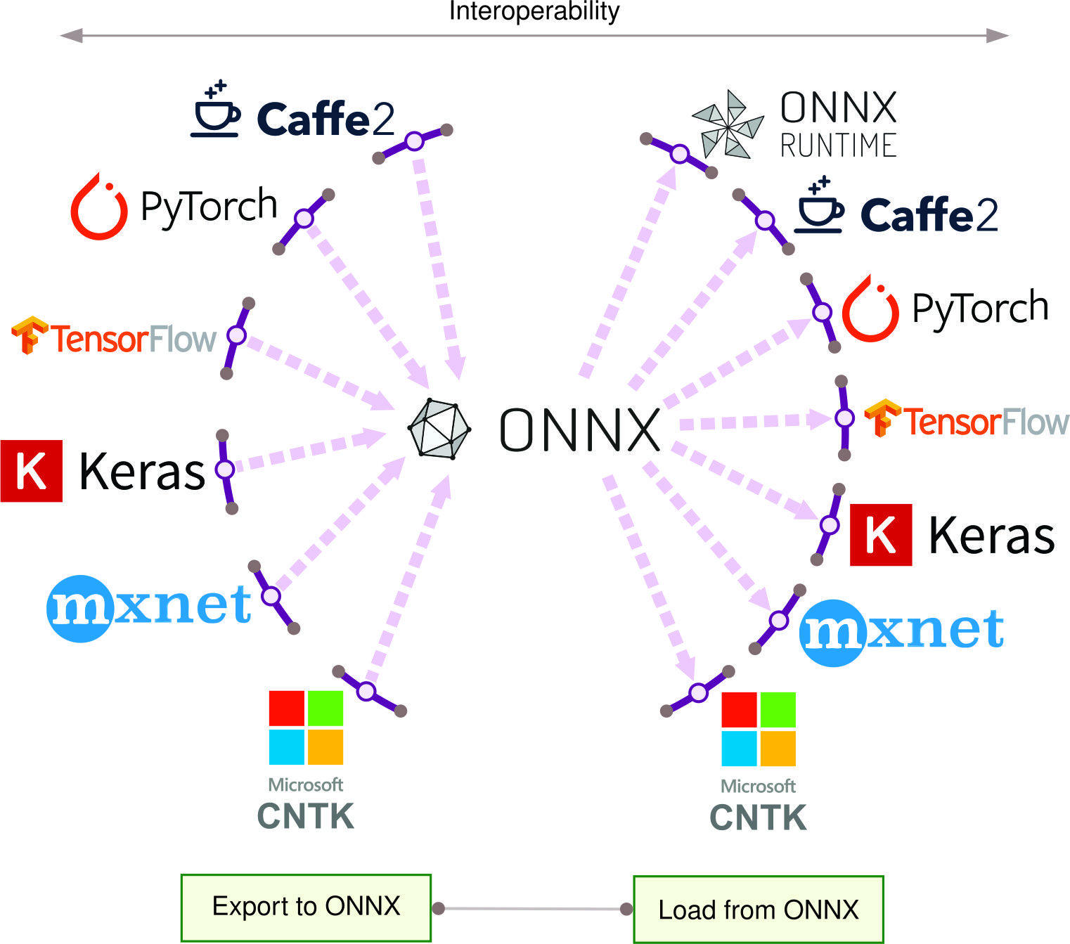
The diversity of deployment targets necessitates distinct specialization strategies for different environments. Machine learning deployment environments shape how frameworks specialize and evolve. Cloud ML environments leverage high-performance servers that offer abundant computational resources for complex operations. Edge ML operates on devices with moderate computing power, where real-time processing often takes priority. Mobile ML adapts to the varying capabilities and energy constraints of smartphones and tablets. Tiny ML functions within the strict limitations of microcontrollers and other highly constrained devices that possess minimal resources.
These environmental constraints drive specific architectural decisions. Each of these environments presents unique challenges that influence framework design. Cloud frameworks prioritize scalability and distributed computing. Edge frameworks focus on low-latency inference and adaptability to diverse hardware. Mobile frameworks emphasize energy efficiency and integration with device-specific features. TinyML frameworks specialize in extreme resource optimization for severely constrained environments.
We will explore how ML frameworks adapt to each of these environments. We will examine the specific techniques and design choices that enable frameworks to address the unique challenges of each domain, highlighting the trade-offs and optimizations that characterize framework specialization.
Distributed Computing Platform Optimization
Cloud environments offer the most abundant computational resources, enabling frameworks to prioritize scalability and sophisticated optimizations over resource constraints. Cloud ML frameworks are sophisticated software infrastructures designed to leverage the vast computational resources available in cloud environments. These frameworks specialize in three primary areas: distributed computing architectures, management of large-scale data and models, and integration with cloud-native services.
The first specialization area reflects the scale advantages available in cloud deployments. Distributed computing is a fundamental specialization of cloud ML frameworks. These frameworks implement advanced strategies for partitioning and coordinating computational tasks across multiple machines or graphics processing units (GPUs). This capability is essential for training large-scale models on massive datasets. Both TensorFlow and PyTorch, two leading cloud ML frameworks, offer robust support for distributed computing. TensorFlow’s graph-based approach (in its 1.x version) was particularly well-suited for distributed execution, while PyTorch’s dynamic computational graph allows for more flexible distributed training strategies.
The ability to handle large-scale data and models is another key specialization. Cloud ML frameworks are optimized to work with datasets and models that far exceed the capacity of single machines. This specialization is reflected in the data structures of these frameworks. For instance, both TensorFlow and PyTorch use mutable Tensor objects as their primary data structure, allowing for efficient in-place operations on large datasets. JAX, a more recent framework, uses immutable arrays, which can provide benefits in terms of functional programming paradigms and optimization opportunities in distributed settings.
Integration with cloud-native services is the third major specialization area. This integration enables automated resource scaling, seamless access to cloud storage, and incorporation of cloud-based monitoring and logging systems. The execution modes of different frameworks play a role here. TensorFlow 2.x and PyTorch both default to eager execution, which allows for easier integration with cloud services and debugging. JAX’s just-in-time compilation offers potential performance benefits in cloud environments by optimizing computations for specific hardware.
Hardware acceleration is an important aspect of cloud ML frameworks. All major frameworks support CPU and GPU execution, with TensorFlow and JAX also offering native support for Google’s TPU. NVIDIA’s TensorRT34 is an optimization tool dedicated for GPU-based inference, providing sophisticated optimizations like layer fusion, precision calibration, and kernel auto-tuning to maximize throughput on NVIDIA GPUs. These hardware acceleration options allow cloud ML frameworks to efficiently utilize the diverse computational resources available in cloud environments.
34 TensorRT: NVIDIA’s inference optimization library that maximizes throughput and minimizes latency for deep learning applications. Achieves 2-5x inference speedup through layer fusion, precision calibration, and kernel auto-tuning, making it essential for production deployment on NVIDIA hardware.
The automatic differentiation capabilities of these frameworks are particularly important in cloud settings where complex models with millions of parameters are common. While TensorFlow and PyTorch primarily use reverse-mode differentiation, JAX’s support for both forward and reverse-mode differentiation can offer advantages in certain large-scale optimization scenarios.
These specializations enable cloud ML frameworks to fully utilize the scalability and computational power of cloud infrastructure. However, this capability comes with increased complexity in deployment and management, often requiring specialized knowledge to fully leverage these frameworks. The focus on scalability and integration makes cloud ML frameworks particularly suitable for large-scale research projects, enterprise-level ML applications, and scenarios requiring massive computational resources.
Local Processing and Low-Latency Optimization
Moving from the resource-abundant cloud environment to edge deployments introduces significant new constraints that reshape framework priorities. Edge ML frameworks are specialized software tools designed to facilitate machine learning operations in edge computing environments, characterized by proximity to data sources, stringent latency requirements, and limited computational resources. Examples of popular edge ML frameworks include TensorFlow Lite and Edge Impulse. The specialization of these frameworks addresses three primary challenges: real-time inference optimization, adaptation to heterogeneous hardware, and resource-constrained operation. These challenges directly relate to the efficiency techniques discussed in Chapter 9: Efficient AI and require the hardware acceleration strategies covered in Chapter 11: AI Acceleration.
Real-time inference optimization is a critical feature of edge ML frameworks. This often involves leveraging different execution modes and graph types. For instance, while TensorFlow Lite (the edge-focused version of TensorFlow) uses a static graph approach to optimize inference, frameworks like PyTorch Mobile maintain a dynamic graph capability, allowing for more flexible model structures at the cost of some performance. The choice between static and dynamic graphs in edge frameworks often is a trade-off between optimization potential and model flexibility.
Adaptation to heterogeneous hardware is crucial for edge deployments. Edge ML frameworks extend the hardware acceleration capabilities of their cloud counterparts but with a focus on edge-specific hardware. For instance, TensorFlow Lite supports acceleration on mobile GPUs and edge TPUs, while frameworks like ARM’s Compute Library optimize for ARM-based processors. This specialization often involves custom operator implementations and low-level optimizations specific to edge hardware.
Operating within resource constraints is another aspect of edge ML framework specialization. This is reflected in the data structures and execution models of these frameworks. For instance, many edge frameworks use quantized tensors as their primary data structure, representing values with reduced precision (e.g., 8-bit integers instead of 32-bit floats) to decrease memory usage and computational demands. These quantization techniques, along with other optimization methods like pruning and knowledge distillation, are explored in detail in Chapter 10: Model Optimizations. The automatic differentiation capabilities, while crucial for training in cloud environments, are often stripped down or removed entirely in edge frameworks to reduce model size and improve inference speed.
Edge ML frameworks also often include features for model versioning and updates, allowing for the deployment of new models with minimal system downtime. Some frameworks support limited on-device learning, enabling models to adapt to local data without compromising data privacy. These on-device learning capabilities are explored in depth in Chapter 14: On-Device Learning, while the privacy implications are thoroughly covered in Chapter 15: Security & Privacy.
The specializations of edge ML frameworks collectively enable high-performance inference in resource-constrained environments. This capability expands the potential applications of AI in areas with limited cloud connectivity or where real-time processing is crucial. However, effective utilization of these frameworks requires careful consideration of target hardware specifications and application-specific requirements, necessitating a balance between model accuracy and resource utilization.
Resource-Constrained Device Optimization
Mobile environments introduce additional constraints beyond those found in general edge computing, particularly regarding energy efficiency and user experience requirements. Mobile ML frameworks are specialized software tools designed for deploying and executing machine learning models on smartphones and tablets. Examples include TensorFlow Lite and Apple’s Core ML. These frameworks address the unique challenges of mobile environments, including limited computational resources, constrained power consumption, and diverse hardware configurations. The specialization of mobile ML frameworks primarily focuses on on-device inference optimization, energy efficiency, and integration with mobile-specific hardware and sensors.
On-device inference optimization in mobile ML frameworks often involves a careful balance between graph types and execution modes. For instance, TensorFlow Lite, also a popular mobile ML framework, uses a static graph approach to optimize inference performance. This contrasts with the dynamic graph capability of PyTorch Mobile, which offers more flexibility at the cost of some performance. The choice between static and dynamic graphs in mobile frameworks is a trade-off between optimization potential and model adaptability, crucial in the diverse and changing mobile environment.
The data structures in mobile ML frameworks are optimized for efficient memory usage and computation. While cloud-based frameworks like TensorFlow and PyTorch use mutable tensors, mobile frameworks often employ more specialized data structures. For example, many mobile frameworks use quantized tensors, representing values with reduced precision (e.g., 8-bit integers instead of 32-bit floats) to decrease memory footprint and computational demands. This specialization is critical given the limited RAM and processing power of mobile devices.
Energy efficiency, a key concern in mobile environments, influences the design of execution modes in mobile ML frameworks. Unlike cloud frameworks that may use eager execution for ease of development, mobile frameworks often prioritize graph-based execution for its potential energy savings. For instance, Apple’s Core ML uses a compiled model approach, converting ML models into a form that can be efficiently executed by iOS devices, optimizing for both performance and energy consumption.
Integration with mobile-specific hardware and sensors is another key specialization area. Mobile ML frameworks extend the hardware acceleration capabilities of their cloud counterparts but with a focus on mobile-specific processors. For example, TensorFlow Lite can leverage mobile GPUs and neural processing units (NPUs) found in many modern smartphones. Qualcomm’s Neural Processing SDK is designed to efficiently utilize the AI accelerators present in Snapdragon SoCs. This hardware-specific optimization often involves custom operator implementations and low-level optimizations tailored for mobile processors.
Automatic differentiation, while crucial for training in cloud environments, is often minimized or removed entirely in mobile frameworks to reduce model size and improve inference speed. Instead, mobile ML frameworks focus on efficient inference, with model updates typically performed off-device and then deployed to the mobile application.
Mobile ML frameworks also often include features for model updating and versioning, allowing for the deployment of improved models without requiring full app updates. Some frameworks support limited on-device learning, enabling models to adapt to user behavior or environmental changes without compromising data privacy. The technical approaches and implementation strategies for on-device learning are detailed in Chapter 14: On-Device Learning, while privacy preservation techniques are covered in Chapter 15: Security & Privacy.
The specializations of mobile ML frameworks collectively enable the deployment of sophisticated ML models on resource-constrained mobile devices. This expands the potential applications of AI in mobile environments, ranging from real-time image and speech recognition to personalized user experiences. However, effectively utilizing these frameworks requires careful consideration of the target device capabilities, user experience requirements, and privacy implications, necessitating a balance between model performance and resource utilization.
Microcontroller and Embedded System Implementation
At the extreme end of the resource constraint spectrum, TinyML frameworks operate under conditions that push the boundaries of what is computationally feasible. TinyML frameworks are specialized software infrastructures designed for deploying machine learning models on extremely resource-constrained devices, typically microcontrollers and low-power embedded systems. These frameworks address the severe limitations in processing power, memory, and energy consumption characteristic of tiny devices. The specialization of TinyML frameworks primarily focuses on extreme model compression, optimizations for severely constrained environments, and integration with microcontroller-specific architectures.
Extreme model compression in TinyML frameworks takes the quantization techniques mentioned in mobile and edge frameworks to their logical conclusion. While mobile frameworks might use 8-bit quantization, TinyML often employs even more aggressive techniques, such as 4-bit, 2-bit, or even 1-bit (binary) representations of model parameters. Frameworks like TensorFlow Lite Micro exemplify this approach (David et al. 2021), pushing the boundaries of model compression to fit within the kilobytes of memory available on microcontrollers.
The execution model in TinyML frameworks is highly specialized. Unlike the dynamic graph capabilities seen in some cloud and mobile frameworks, TinyML frameworks almost exclusively use static, highly optimized graphs. The just-in-time compilation approach seen in frameworks like JAX is typically not feasible in TinyML due to memory constraints. Instead, these frameworks often employ ahead-of-time compilation techniques to generate highly optimized, device-specific code.
Memory management in TinyML frameworks is far more constrained than in other environments. While edge and mobile frameworks might use dynamic memory allocation, TinyML frameworks like uTensor often rely on static memory allocation to avoid runtime overhead and fragmentation. This approach requires careful planning of the memory layout at compile time, a stark contrast to the more flexible memory management in cloud-based frameworks.
Hardware integration in TinyML frameworks is highly specific to microcontroller architectures. Unlike the general GPU support seen in cloud frameworks or the mobile GPU/NPU support in mobile frameworks, TinyML frameworks often provide optimizations for specific microcontroller instruction sets. For example, ARM’s CMSIS-NN (Lai, Suda, and Chandra 2018) provides optimized neural network kernels for Cortex-M series microcontrollers, which are often integrated into TinyML frameworks.
The concept of automatic differentiation, central to cloud-based frameworks and present to some degree in edge and mobile frameworks, is typically absent in TinyML frameworks. The focus is almost entirely on inference, with any learning or model updates usually performed off-device due to the severe computational constraints.
TinyML frameworks also specialize in power management to a degree not seen in other ML environments. Features like duty cycling and ultra-low-power wake-up capabilities are often integrated directly into the ML pipeline, enabling always-on sensing applications that can run for years on small batteries.
The extreme specialization of TinyML frameworks enables ML deployments in previously infeasible environments, from smart dust sensors to implantable medical devices. However, this specialization comes with significant trade-offs in model complexity and accuracy, requiring careful consideration of the balance between ML capabilities and the severe resource constraints of target devices.
Performance and Resource Optimization Platforms
Beyond deployment-specific specializations, modern machine learning frameworks increasingly incorporate efficiency as a first-class design principle. Efficiency-oriented frameworks are specialized tools that treat computational efficiency, memory optimization, and energy consumption as primary design constraints rather than secondary considerations. These frameworks address the growing demand for practical AI deployment where resource constraints fundamentally shape algorithmic choices.
Traditional frameworks often treat efficiency optimizations as optional add-ons, applied after model development. In contrast, efficiency-oriented frameworks integrate optimization techniques directly into the development workflow, enabling developers to train and deploy models with quantization, pruning, and compression constraints from the beginning. This efficiency-first approach enables deployment scenarios where traditional frameworks would be computationally infeasible.
The significance of efficiency-oriented frameworks has grown with the expansion of AI applications into resource-constrained environments. Modern production systems require models that balance accuracy with strict constraints on inference latency (often sub-10ms requirements), memory usage (fitting within GPU memory limits), energy consumption (extending battery life), and computational cost (reducing cloud infrastructure expenses). These constraints create substantially different framework requirements compared to research environments with abundant computational resources.
Model Size and Computational Reduction Techniques
Efficiency-oriented frameworks distinguish themselves through compression-aware computational graph design. Unlike traditional frameworks that optimize mathematical operations independently, these frameworks optimize for compressed representations throughout the computation pipeline. This integration affects every layer of the framework stack, from data structures to execution engines.
Neural network compression techniques require framework support for specialized data types and operations. Quantization-aware training demands frameworks that can simulate reduced precision arithmetic during training while maintaining full-precision gradients for stable optimization. Intel Neural Compressor exemplifies this approach, providing APIs that seamlessly integrate INT8 quantization into existing PyTorch and TensorFlow workflows. The framework automatically inserts fake quantization operations during training, allowing models to adapt to quantization constraints while preserving accuracy.
Structured pruning techniques require frameworks that can handle sparse tensor operations efficiently. This involves specialized storage formats (such as compressed sparse row representations), optimized sparse matrix operations, and runtime systems that can take advantage of structural zeros. Apache TVM demonstrates advanced sparse tensor compilation, automatically generating efficient code for sparse operations across different hardware backends.
Knowledge distillation workflows represent another efficiency-oriented framework capability. These frameworks must orchestrate teacher-student training pipelines, managing the computational overhead of running multiple models simultaneously while providing APIs for custom distillation losses. Hugging Face Optimum provides comprehensive distillation workflows that automatically configure teacher-student training for various model architectures, reducing the engineering complexity of implementing efficiency optimizations.
Integrated Hardware-Framework Performance Tuning
Efficiency-oriented frameworks excel at hardware-software co-design, where framework architecture and hardware capabilities are optimized together. This approach moves beyond generic hardware acceleration to target-specific optimization strategies that consider hardware constraints during algorithmic design.
Mixed-precision training frameworks demonstrate this co-design philosophy. NVIDIA’s Automatic Mixed Precision (AMP) in PyTorch automatically identifies operations that can use FP16 arithmetic while maintaining FP32 precision for numerical stability. The framework analyzes computational graphs to determine optimal precision policies, balancing training speed improvements (up to 1.5-2x speedup on modern GPUs) against numerical accuracy requirements. This analysis requires deep integration between framework scheduling and hardware capabilities.
Sparse computation frameworks extend this co-design approach to leverage hardware sparsity support. Modern hardware like NVIDIA A100 GPUs includes specialized sparse matrix multiplication units that can achieve 2:4 structured sparsity (50% zeros in specific patterns) with minimal performance degradation. Frameworks like Neural Magic’s SparseML provide automated tools for training models that conform to these hardware-specific sparsity patterns, achieving significant speedups without accuracy loss.
Compilation frameworks represent the most sophisticated form of hardware-software co-design. Apache TVM and MLIR provide domain-specific languages for expressing hardware-specific optimizations. These frameworks analyze computational graphs to automatically generate optimized kernels for specific hardware targets, including custom ASICs and specialized accelerators. The compilation process considers hardware memory hierarchies, instruction sets, and parallelization capabilities to generate code that often outperforms hand-optimized implementations.
Real-World Deployment Performance Requirements
Efficiency-oriented frameworks address production deployment challenges through systematic approaches to resource management and performance optimization. Production environments impose strict constraints that differ substantially from research settings: inference latency must meet real-time requirements, memory usage must fit within allocated resources, and energy consumption must stay within power budgets.
Inference optimization frameworks like NVIDIA TensorRT and ONNX Runtime provide comprehensive toolchains for production deployment. TensorRT applies aggressive optimization techniques including layer fusion (combining multiple operations into single kernels), precision calibration (automatically determining optimal quantization levels), and memory optimization (reducing memory transfers between operations). These optimizations can achieve 3-7x inference speedup compared to unoptimized frameworks while maintaining accuracy within acceptable bounds.
Memory optimization represents a critical production constraint. DeepSpeed and FairScale demonstrate advanced memory management techniques that enable training and inference of models that exceed GPU memory capacity. DeepSpeed’s ZeRO optimizer partitions optimizer states, gradients, and parameters across multiple devices, reducing memory usage by 4-8x compared to traditional data parallelism. These techniques enable training of models with hundreds of billions of parameters on standard hardware configurations.
Energy-aware frameworks address the growing importance of computational sustainability. Power consumption directly impacts deployment costs in cloud environments and battery life in mobile applications. Frameworks like NVIDIA’s Triton Inference Server provide power-aware scheduling that can dynamically adjust inference batching and frequency scaling to meet energy budgets while maintaining throughput requirements.
Systematic Performance Assessment Methodologies
Evaluating efficiency-oriented frameworks requires comprehensive metrics that capture the multi-dimensional trade-offs between accuracy, performance, and resource consumption. Traditional ML evaluation focuses primarily on accuracy metrics, but efficiency evaluation must consider computational efficiency (FLOPS reduction, inference speedup), memory efficiency (peak memory usage, memory bandwidth utilization), energy efficiency (power consumption, energy per inference), and deployment efficiency (model size reduction, deployment complexity).
Quantitative framework comparison requires standardized benchmarks that measure these efficiency dimensions across representative workloads. MLPerf Inference provides standardized benchmarks for measuring inference performance across different frameworks and hardware configurations. These benchmarks measure latency, throughput, and energy consumption for common model architectures, enabling direct comparison of framework efficiency characteristics.
Performance profiling frameworks enable developers to understand efficiency bottlenecks in their specific applications. NVIDIA Nsight Systems and Intel VTune provide detailed analysis of framework execution, identifying memory bandwidth limitations, computational bottlenecks, and opportunities for optimization. These tools integrate with efficiency-oriented frameworks to provide actionable insights for improving application performance.
The evolution of efficiency-oriented frameworks represents a fundamental shift in ML systems design, where computational constraints shape algorithmic choices from the beginning of development. This approach enables practical AI deployment across resource-constrained environments while maintaining the flexibility and expressiveness that makes modern ML frameworks powerful development tools.
Systematic Framework Selection Methodology
Choosing the right machine learning framework requires a systematic evaluation that balances technical requirements with operational constraints. This decision-making process extends beyond simple feature comparisons to encompass the entire system lifecycle, from development through deployment and maintenance. Engineers must evaluate multiple interdependent factors: technical capabilities (supported operations, execution models, hardware targets), operational requirements (deployment constraints, performance needs, scalability demands), and organizational factors (team expertise, development timeline, maintenance resources).
The framework selection process follows a structured approach that considers three primary dimensions: model requirements determine which operations and architectures the framework must support, software dependencies define operating system and runtime requirements, and hardware constraints establish memory and processing limitations. These technical considerations must be balanced with practical factors like team expertise, learning curve, community support, and long-term maintenance commitments.
This decision-making process must also consider the broader system architecture principles outlined in Chapter 2: ML Systems and align with the deployment patterns detailed in Chapter 13: ML Operations. Different deployment scenarios often favor different framework architectures: cloud training requires high throughput and distributed capabilities, edge inference prioritizes low latency and minimal resource usage, mobile deployment balances performance with battery constraints, and embedded systems optimize for minimal memory footprint and real-time execution.
To illustrate how these factors interact in practice, we examine the TensorFlow ecosystem, which demonstrates the spectrum of trade-offs through its variants: TensorFlow, TensorFlow Lite, and TensorFlow Lite Micro. While TensorFlow serves as our detailed case study, the same selection methodology applies broadly across the framework landscape, including PyTorch for research-oriented workflows, ONNX for cross-platform deployment, JAX for functional programming approaches, and specialized frameworks for specific domains.
Table 4 illustrates key differences between TensorFlow variants. Each variant represents specific trade-offs between computational capability and resource requirements. These trade-offs manifest in supported operations, binary size, and integration requirements.
| TensorFlow | TensorFlow Lite | TensorFlow Lite for Microcontrollers | |
|---|---|---|---|
| Training | Yes | No | No |
| Inference | Yes (but inefficient on edge) | Yes (and efficient) | Yes (and even more efficient) |
| How Many Ops | ~1400 | ~130 | ~50 |
| Native Quantization Tooling | No | Yes | Yes |
Engineers analyze three primary aspects when selecting a framework:
- Model requirements determine which operations and architectures the framework must support
- Software dependencies define operating system and runtime requirements
- Hardware constraints establish memory and processing limitations
This systematic analysis enables engineers to select frameworks that align with their specific deployment requirements and organizational context. As we examine the TensorFlow variants in detail, we will explore how each selection dimension influences framework choice and shapes system capabilities, providing a methodology that can be applied to evaluate any framework ecosystem.
Model Requirements
Model architecture capabilities vary significantly across TensorFlow variants, with clear trade-offs between functionality and efficiency. Table 4 quantifies these differences across four key dimensions: training capability, inference efficiency, operation support, and quantization features.
A key architectural distinction between frameworks is their computational graph construction approach. Static graphs (TensorFlow 1.x) require defining the entire computation before execution, similar to compiling a program before running it. Dynamic graphs (PyTorch, TensorFlow 2.x eager mode) build the graph during execution, akin to interpreted languages. This affects debugging ease (dynamic graphs allow standard Python debugging), optimization opportunities (static graphs enable more aggressive optimization), and deployment complexity (static graphs simplify deployment but require more upfront design).
TensorFlow supports approximately 1,400 operations and enables both training and inference. However, as Table 4 indicates, its inference capabilities are inefficient for edge deployment. TensorFlow Lite reduces the operation count to roughly 130 operations while improving inference efficiency. It eliminates training support but adds native quantization tooling. TensorFlow Lite Micro further constrains the operation set to approximately 50 operations, achieving even higher inference efficiency through these constraints. Like TensorFlow Lite, it includes native quantization support but removes training capabilities.
This progressive reduction in operations enables deployment on increasingly constrained devices. The addition of native quantization in both TensorFlow Lite and TensorFlow Lite Micro provides essential optimization capabilities absent in the full TensorFlow framework. Quantization transforms models to use lower precision operations, reducing computational and memory requirements for resource-constrained deployments. These optimization techniques, detailed further in Chapter 10: Model Optimizations, must be considered alongside data pipeline requirements discussed in Chapter 6: Data Engineering when selecting appropriate frameworks for specific deployment scenarios.
Software Dependencies
Table 5 reveals three key software considerations that differentiate TensorFlow variants: operating system requirements, memory management capabilities, and accelerator support. These differences reflect each variant’s optimization for specific deployment
| TensorFlow | TensorFlow Lite | TensorFlow Lite for Microcontrollers | |
|---|---|---|---|
| Needs an OS | Yes | Yes | No |
| Memory Mapping of Models | No | Yes | Yes |
| Delegation to accelerators | Yes | Yes | No |
Operating system dependencies mark a fundamental distinction between variants. TensorFlow and TensorFlow Lite require an operating system, while TensorFlow Lite Micro operates without OS support. This enables TensorFlow Lite Micro to reduce memory overhead and startup time, though it can still integrate with real-time operating systems like FreeRTOS, Zephyr, and Mbed OS when needed.
Memory management capabilities also distinguish the variants. TensorFlow Lite and TensorFlow Lite Micro support model memory mapping, enabling direct model access from flash storage rather than loading into RAM. TensorFlow lacks this capability, reflecting its design for environments with abundant memory resources. Memory mapping becomes increasingly important as deployment moves toward resource-constrained devices.
Accelerator delegation capabilities further differentiate the variants. Both TensorFlow and TensorFlow Lite support delegation to accelerators, enabling efficient computation distribution. TensorFlow Lite Micro omits this feature, acknowledging the limited availability of specialized accelerators in embedded systems. This design choice maintains the framework’s minimal footprint while matching typical embedded hardware configurations.
Hardware Constraints
Table 6 quantifies the hardware requirements across TensorFlow variants through three metrics: base binary size, memory footprint, and processor architecture support. These metrics demonstrate the progressive optimization for constrained computing environments.
| TensorFlow | TensorFlow Lite | TensorFlow Lite for Microcontrollers | |
|---|---|---|---|
| Base Binary Size | ~3-5 MB (varies by platform and build configuration) | 100 KB | ~10 KB |
| Base Memory Footprint | ~5+ MB (minimum runtime overhead) | 300 KB | 20 KB |
| Optimized Architectures | X86, TPUs, GPUs | Arm Cortex A, x86 | Arm Cortex M, DSPs, MCUs |
As established in Table 4, binary size decreases dramatically across variants: from 3+ MB (TensorFlow) to 100 KB (TensorFlow Lite) to 10 KB (TensorFlow Lite Micro), reflecting progressive feature reduction and optimization.
Memory footprint follows a similar pattern of reduction. TensorFlow requires approximately 5 MB of base memory, while TensorFlow Lite operates within 300 KB. TensorFlow Lite Micro further reduces memory requirements to 20 KB, enabling deployment on highly constrained devices.
Processor architecture support aligns with each variant’s intended deployment environment. TensorFlow supports x86 processors and accelerators including TPUs and GPUs, enabling high-performance computing in data centers as detailed in Chapter 11: AI Acceleration. TensorFlow Lite targets mobile and edge processors, supporting Arm Cortex-A and x86 architectures. TensorFlow Lite Micro specializes in microcontroller deployment, supporting Arm Cortex-M cores, digital signal processors (DSPs), and various microcontroller units (MCUs) including STM32, NXP Kinetis, and Microchip AVR. The hardware acceleration strategies and architectures discussed in Chapter 11: AI Acceleration provide essential context for understanding these processor optimization choices.
Production-Ready Evaluation Factors
Framework selection for embedded systems extends beyond technical specifications of model architecture, hardware requirements, and software dependencies. Additional factors affect development efficiency, maintenance requirements, and deployment success. Framework migration presents significant operational challenges including backward compatibility breaks, custom operator migration between versions, and production downtime risks. These migration concerns are addressed comprehensively in Chapter 13: ML Operations, which covers migration planning, testing procedures, and rollback strategies. These factors require systematic evaluation to ensure optimal framework selection.
Performance Optimization
Performance in embedded systems encompasses multiple metrics beyond computational speed. Framework evaluation must consider quantitative trade-offs across efficiency dimensions:
Inference latency determines system responsiveness and real-time processing capabilities. For mobile applications, typical targets are 10-50ms for image classification and 1-5ms for keyword spotting. Edge deployments often require sub-millisecond response times for industrial control applications. TensorFlow Lite achieves 2-5x latency reduction compared to TensorFlow on mobile CPUs for typical inference workloads, while specialized frameworks like TensorRT can achieve 10-20x speedup on NVIDIA hardware through kernel fusion and precision optimization.
Memory utilization affects both static storage requirements and runtime efficiency. Framework memory overhead varies dramatically: TensorFlow requires 5+ MB baseline memory, TensorFlow Lite operates within 300KB, while TensorFlow Lite Micro runs in 20KB. Model memory scaling follows similar patterns: a MobileNetV2 model consumes approximately 14MB in TensorFlow but only 3.4MB when quantized in TensorFlow Lite, representing a 4x reduction while maintaining 95%+ accuracy.
Power consumption impacts battery life and thermal management requirements. Quantized INT8 inference consumes 4-8x less energy than FP32 operations on typical mobile processors. Apple’s Neural Engine achieves 7.2 TOPS/W efficiency for INT8 operations compared to 0.1-0.5 TOPS/W for CPU-based FP32 computation. Sparse computation can provide additional 2-3x energy savings when frameworks support structured sparsity patterns optimized for specific hardware.
Computational efficiency measured in FLOPS provides standardized performance comparison. Modern mobile frameworks achieve 10-50 GFLOPS on high-end smartphone processors, while specialized accelerators like Google’s Edge TPU deliver 4 TOPS (INT8) in 2W power budget. Framework optimization techniques including operator fusion can improve FLOPS utilization from 10-20% to 60-80% of theoretical peak performance on typical workloads.
Deployment Scalability
Scalability requirements span both technical capabilities and operational considerations. Framework support must extend across deployment scales and scenarios:
Device scaling enables consistent deployment from microcontrollers to more powerful embedded processors. Operational scaling supports the transition from development prototypes to production deployments. Version management facilitates model updates and maintenance across deployed devices. The framework must maintain consistent performance characteristics throughout these scaling dimensions.
The TensorFlow ecosystem demonstrates how framework design must balance competing requirements across diverse deployment scenarios. The systematic evaluation methodology illustrated through this case study (analyzing model requirements, software dependencies, and hardware constraints alongside operational factors) provides a template for evaluating any framework ecosystem. Whether comparing PyTorch’s dynamic execution model for research workflows, ONNX’s cross-platform standardization for deployment flexibility, JAX’s functional programming approach for performance optimization, or specialized frameworks for domain-specific applications, the same analytical framework guides informed decision-making that aligns technical capabilities with project requirements and organizational constraints.
Development Support and Long-term Viability Assessment
Framework selection extends beyond technical capabilities to encompass the broader ecosystem that determines long-term viability and development velocity. The community and ecosystem surrounding a framework significantly influence its evolution, support quality, and integration possibilities. Understanding these ecosystem dynamics helps predict framework sustainability and development productivity over project lifecycles.
Developer Resources and Knowledge Sharing Networks
The vitality of a framework’s community affects multiple practical aspects of development and deployment. Active communities drive faster bug fixes, more comprehensive documentation, and broader hardware support. Community size and engagement metrics (such as GitHub activity, Stack Overflow question volume, and conference presence) provide indicators of framework momentum and longevity.
PyTorch’s academic community has driven rapid innovation in research-oriented features, contributing to extensive support for novel architectures and experimental techniques. This community focus has resulted in excellent educational resources, research reproducibility tools, and advanced feature development. However, production tooling has historically lagged behind research capabilities, though initiatives like PyTorch Lightning and TorchServe have addressed many operational gaps.
TensorFlow’s enterprise community has emphasized production-ready tools and scalable deployment solutions. This focus has produced robust serving infrastructure, comprehensive monitoring tools, and enterprise integration capabilities. The broader TensorFlow ecosystem includes specialized tools like TensorFlow Extended (TFX) for production ML pipelines, TensorBoard for visualization, and TensorFlow Model Analysis for model evaluation and validation.
JAX’s functional programming community has concentrated on mathematical rigor and program transformation capabilities. This specialized focus has led to powerful research tools and elegant mathematical abstractions, but with a steeper learning curve for developers not familiar with functional programming concepts.
Supporting Infrastructure and Third-Party Compatibility
The practical utility of a framework often depends more on its ecosystem tools than its core capabilities. These tools determine development velocity, debugging effectiveness, and deployment flexibility.
Hugging Face has become a de facto standard for natural language processing model libraries, providing consistent APIs across PyTorch, TensorFlow, and JAX backends. The availability of high-quality pretrained models and fine-tuning tools can dramatically accelerate project development. TensorFlow Hub and PyTorch Hub provide official model repositories, though third-party collections often offer broader selection and more recent architectures.
PyTorch Lightning has abstracted much of PyTorch’s training boilerplate while maintaining research flexibility, addressing one of PyTorch’s historical weaknesses in structured training workflows. Weights & Biases and MLflow provide experiment tracking across multiple frameworks, enabling consistent workflow management regardless of underlying framework choice. TensorBoard has evolved into a cross-framework visualization tool, though its integration remains tightest with TensorFlow.
TensorFlow Serving and TorchServe provide production-ready serving solutions, though their feature sets and operational characteristics differ significantly. ONNX Runtime has emerged as a framework-agnostic serving solution, enabling deployment flexibility at the cost of some framework-specific optimizations. Cloud provider ML services (AWS SageMaker, Google AI Platform, Azure ML) often provide native integration for specific frameworks while supporting others through containerized deployments.
Framework-specific optimization tools can provide significant performance advantages but create vendor lock-in. TensorFlow’s XLA compiler and PyTorch’s TorchScript offer framework-native optimization paths, while tools like Apache TVM provide cross-framework optimization capabilities. The choice between framework-specific and cross-framework optimization tools affects both performance and deployment flexibility.
Long-term Technology Investment Considerations
Long-term framework decisions must consider ecosystem evolution and sustainability. Framework popularity can shift rapidly in response to technical innovations, community momentum, or corporate strategy changes. Organizations should evaluate ecosystem health through multiple indicators: contributor diversity (avoiding single-company dependence), funding stability, roadmap transparency, and backward compatibility commitments.
The ecosystem perspective also influences hiring and team development strategies. Framework choice affects the available talent pool, training requirements, and knowledge transfer capabilities. Teams must consider whether their framework choice aligns with local expertise, educational institution curricula, and industry hiring trends.
Integration with existing organizational tools and processes represents another critical ecosystem consideration. Framework compatibility with continuous integration systems, deployment pipelines, monitoring infrastructure, and security tooling can significantly affect operational overhead. Some frameworks integrate more naturally with specific cloud providers or enterprise software stacks, creating operational advantages or vendor dependencies.
While deep ecosystem integration can provide development velocity advantages, teams should maintain awareness of migration paths and cross-framework compatibility. Using standardized model formats like ONNX, maintaining framework-agnostic data pipelines, and documenting framework-specific customizations can preserve flexibility for future framework transitions.
The ecosystem perspective reminds us that framework selection involves choosing not just a software library, but joining a community and committing to an evolving technological ecosystem. Understanding these broader implications helps teams make framework decisions that remain viable and advantageous throughout project lifecycles.
Systematic Framework Performance Assessment
Systematic evaluation of framework efficiency requires comprehensive metrics that capture the multi-dimensional trade-offs between accuracy, performance, and resource consumption. Traditional machine learning evaluation focuses primarily on accuracy metrics, but production deployment demands systematic assessment of computational efficiency, memory utilization, energy consumption, and operational constraints.
Framework efficiency evaluation encompasses four primary dimensions that reflect real-world deployment requirements. Computational efficiency measures the framework’s ability to utilize available hardware resources effectively, typically quantified through FLOPS utilization, kernel efficiency, and parallelization effectiveness. Memory efficiency evaluates both peak memory usage and memory bandwidth utilization, critical factors for deployment on resource-constrained devices. Energy efficiency quantifies power consumption characteristics, essential for mobile applications and sustainable computing. Deployment efficiency assesses the operational characteristics including model size, initialization time, and integration complexity.
Quantitative Multi-Dimensional Performance Analysis
Standardized comparison requires quantitative metrics across representative workloads and hardware configurations. Table 7 provides systematic comparison of major frameworks across efficiency dimensions using benchmark workloads representative of production deployment scenarios.
| Framework | Inference Latency (ms) | Memory Usage (MB) | Energy (mJ/inference) | Model Size Reduction | Hardware Utilization (%) |
|---|---|---|---|---|---|
| TensorFlow | 45 | 2,100 | 850 | None | 35 |
| TensorFlow Lite | 12 | 180 | 120 | 4x (quantized) | 65 |
| TensorFlow Lite Micro | 8 | 32 | 45 | 8x (pruned+quant) | 75 |
| PyTorch | 52 | 1,800 | 920 | None | 32 |
| PyTorch Mobile | 18 | 220 | 180 | 3x (quantized) | 58 |
| ONNX Runtime | 15 | 340 | 210 | 2x (optimized) | 72 |
| TensorRT | 3 | 450 | 65 | 2x (precision opt) | 88 |
| Apache TVM | 6 | 280 | 95 | 3x (compiled) | 82 |
Standardized Benchmarking Protocols
Systematic framework evaluation requires standardized benchmarking approaches that capture efficiency characteristics across diverse deployment scenarios. The evaluation methodology employs representative model architectures (ResNet-50 for vision, BERT-Base for language processing, MobileNetV2 for mobile deployment), standardized datasets (ImageNet for vision, GLUE for language), and consistent hardware configurations (NVIDIA A100 for server evaluation, ARM Cortex-A78 for mobile assessment).
Performance profiling uses instrumentation to measure framework overhead, kernel efficiency, and resource utilization patterns. Memory analysis includes peak allocation measurement, memory bandwidth utilization assessment, and garbage collection overhead quantification. Energy measurement employs hardware-level power monitoring (NVIDIA-SMI for GPU power, specialized mobile power measurement tools) to capture actual energy consumption during inference and training operations.
Accuracy preservation validation ensures that efficiency optimizations maintain model quality within acceptable bounds. Quantization-aware training validates that INT8 models achieve <1% accuracy degradation. Pruning techniques verify that sparse models maintain target accuracy while achieving specified compression ratios. Knowledge distillation confirms that compressed models preserve teacher model capability.
Real-World Operational Performance Considerations
Framework efficiency evaluation must consider operational constraints that affect real-world deployment success. Latency analysis includes cold-start performance (framework initialization time), warm-up characteristics (performance stabilization requirements), and steady-state inference speed. Memory analysis encompasses both static requirements (framework binary size, model storage) and dynamic usage patterns (peak allocation, memory fragmentation, cleanup efficiency).
Scalability assessment evaluates framework behavior under production load conditions including concurrent request handling, batching efficiency, and resource sharing across multiple model instances. Integration testing validates framework compatibility with production infrastructure including container deployment, service mesh integration, monitoring system compatibility, and observability tool support.
Reliability evaluation assesses framework stability under extended operation, error handling capabilities, and recovery mechanisms. Performance consistency measurement identifies variance in execution time, memory usage stability, and thermal behavior under sustained load conditions.
Structured Framework Selection Process
Systematic framework selection requires structured evaluation that balances efficiency metrics against operational requirements and organizational constraints. The decision framework evaluates technical capabilities (supported operations, hardware acceleration, optimization features), operational requirements (deployment flexibility, monitoring integration, maintenance overhead), and organizational factors (team expertise, development velocity, ecosystem compatibility).
Efficiency requirements specification defines acceptable trade-offs between accuracy and performance, establishes resource constraints (memory limits, power budgets, latency requirements), and identifies critical optimization features (quantization support, pruning capabilities, hardware-specific acceleration). These requirements guide framework evaluation priorities and eliminate options that cannot meet fundamental constraints.
Risk assessment considers framework maturity, ecosystem stability, and migration complexity. Vendor dependency evaluation assesses framework governance, licensing terms, and long-term support commitments. Migration cost analysis estimates effort required for framework adoption, team training requirements, and infrastructure modifications.
The systematic approach to framework efficiency evaluation provides quantitative foundation for deployment decisions while considering the broader operational context that determines production success. This methodology enables teams to select frameworks that optimize for their specific efficiency requirements while maintaining the flexibility needed for evolving deployment scenarios.
Common Framework Selection Misconceptions
Machine learning frameworks represent complex software ecosystems that abstract significant computational complexity while making critical architectural decisions on behalf of developers. The diversity of available frameworks (each with distinct design philosophies and optimization strategies) often leads to misconceptions about their interchangeability and appropriate selection criteria. Understanding these common fallacies and pitfalls helps practitioners make more informed framework choices.
Fallacy: All frameworks provide equivalent performance for the same model.
This misconception leads teams to select frameworks based solely on API convenience or familiarity without considering performance implications. Different frameworks implement operations using varying optimization strategies, memory management approaches, and hardware utilization patterns. A model that performs efficiently in PyTorch might execute poorly in TensorFlow due to different graph optimization strategies. Similarly, framework overhead, automatic differentiation implementation, and tensor operation scheduling can create significant performance differences even for identical model architectures. Framework selection requires benchmarking actual workloads rather than assuming performance equivalence.
Pitfall: Choosing frameworks based on popularity rather than project requirements.
Many practitioners select frameworks based on community size, tutorial availability, or industry adoption without analyzing their specific technical requirements. Popular frameworks often target general-use cases rather than specialized deployment scenarios. A framework optimized for large-scale cloud training might be inappropriate for mobile deployment, while research-focused frameworks might lack production deployment capabilities. Effective framework selection requires matching technical capabilities to specific requirements rather than following popularity trends.
Fallacy: Framework abstractions hide all system-level complexity from developers.
This belief assumes that frameworks automatically handle all performance optimization and hardware utilization without developer understanding. While frameworks provide convenient abstractions, achieving optimal performance requires understanding their underlying computational models, memory management strategies, and hardware mapping approaches. Developers who treat frameworks as black boxes often encounter unexpected performance bottlenecks, memory issues, or deployment failures. Effective framework usage requires understanding both the abstractions provided and their underlying implementation implications.
Pitfall: Vendor lock-in through framework-specific model formats and APIs.
Teams often build entire development workflows around single frameworks without considering interoperability requirements. Framework-specific model formats, custom operators, and proprietary optimization techniques create dependencies that complicate migration, deployment, or collaboration across different tools. This lock-in becomes problematic when deployment requirements change, performance needs evolve, or framework development directions diverge from project goals. Maintaining model portability requires attention to standards-based formats and avoiding framework-specific features that cannot be translated across platforms. These considerations become particularly important when implementing responsible AI practices Chapter 17: Responsible AI that may require model auditing, fairness testing, or bias mitigation across different deployment environments.
Pitfall: Overlooking production infrastructure requirements when selecting development frameworks.
Many teams choose frameworks based on ease of development without considering how they integrate with production infrastructure for model serving, monitoring, and lifecycle management. A framework excellent for research and prototyping may lack robust model serving capabilities, fail to integrate with existing monitoring systems, or provide inadequate support for A/B testing and gradual rollouts. Production deployment often requires additional components for load balancing, caching, model versioning, and rollback mechanisms that may not align well with the chosen development framework. Some frameworks excel at training but require separate serving systems, while others provide integrated pipelines that may not meet enterprise security or scalability requirements. Effective framework selection must consider the entire production ecosystem including container orchestration, API gateway integration, observability tools, and operational procedures rather than focusing solely on model development convenience.
Summary
Machine learning frameworks represent software abstractions that transform mathematical concepts into practical computational tools for building and deploying AI systems. These frameworks encapsulate complex operations like automatic differentiation, distributed training, and hardware acceleration behind programmer-friendly interfaces that enable efficient development across diverse application domains. The evolution from basic numerical libraries to modern frameworks demonstrates how software infrastructure shapes the accessibility and capability of machine learning development.
This evolution has produced a diverse ecosystem with distinct optimization strategies. Contemporary frameworks embody different design philosophies that reflect varying priorities in machine learning development. Research-focused frameworks prioritize flexibility and rapid experimentation, enabling quick iteration on novel architectures and algorithms. Production-oriented frameworks emphasize scalability, reliability, and deployment efficiency for large-scale systems. Specialized frameworks target specific deployment contexts, from cloud-scale distributed systems to resource-constrained edge devices, each optimizing for distinct performance and efficiency requirements.
- Frameworks abstract complex computational operations like automatic differentiation and distributed training behind developer-friendly interfaces
- Different frameworks embody distinct design philosophies: research flexibility vs production scalability vs deployment efficiency
- Specialization across computing environments requires framework variants optimized for cloud, edge, mobile, and microcontroller deployments
- Framework architecture understanding enables informed tool selection, performance optimization, and effective debugging across diverse deployment contexts
Framework development continues evolving toward greater developer productivity, broader hardware support, and more flexible deployment options. Cross-platform compilation, dynamic optimization, and unified programming models aim to reduce the complexity of developing and deploying machine learning systems across diverse computing environments. Understanding framework capabilities and limitations enables developers to make informed architectural decisions for the model optimization techniques in Chapter 10: Model Optimizations, hardware acceleration strategies in Chapter 11: AI Acceleration, and deployment patterns in Chapter 13: ML Operations.