Efficient AI
DALL·E 3 Prompt: A conceptual illustration depicting efficiency in artificial intelligence using a shipyard analogy. The scene shows a bustling shipyard where containers represent bits or bytes of data. These containers are being moved around efficiently by cranes and vehicles, symbolizing the streamlined and rapid information processing in AI systems. The shipyard is meticulously organized, illustrating the concept of optimal performance within the constraints of limited resources. In the background, ships are docked, representing different platforms and scenarios where AI is applied. The atmosphere should convey advanced technology with an underlying theme of sustainability and wide applicability.

Purpose
What key trade-offs shape the pursuit of efficiency in machine learning systems, and why must engineers balance competing objectives?
Machine learning system efficiency requires balancing trade-offs across algorithmic complexity, computational resources, and data utilization. Improvements in one dimension often degrade performance in others, creating engineering tensions that require systematic approaches. Understanding these interdependent relationships enables engineers to design systems achieving maximum performance within practical constraints of time, energy, and cost.
Analyze scaling law relationships to determine optimal resource allocation strategies for computational budget, model size, and dataset requirements
Compare and contrast algorithmic, compute, and data efficiency trade-offs across cloud, edge, mobile, and TinyML deployment contexts
Evaluate machine learning systems using efficiency metrics including throughput, latency, energy consumption, and resource utilization
Apply compression techniques such as pruning, quantization, and knowledge distillation to optimize model performance within resource constraints
Design context-aware efficiency strategies by prioritizing optimization dimensions based on deployment requirements and operational constraints
Critique scaling-based approaches by identifying saturation points and proposing efficiency-driven alternatives
Assess the environmental and accessibility implications of efficiency choices in machine learning system design
The Efficiency Imperative
Machine learning efficiency has evolved from an afterthought to a fundamental discipline as models transitioned from simple statistical approaches to complex, resource-intensive architectures. The gap between theoretical capabilities and practical deployment has widened significantly, creating efficiency constraints that fundamentally affect system feasibility and scalability.
Large-scale language models exemplify this challenge. GPT-3 required training costs estimated at $4.6 million (Lambda Labs estimate) and energy consumption of 1,287 MWh (Patterson et al. 2021). The operational requirements, including memory footprints exceeding 700GB for inference (350GB for half-precision), create deployment barriers in resource-constrained environments. These constraints reveal a tension between model expressiveness and system practicality that requires rigorous analysis and optimization strategies.
Efficiency research extends beyond resource optimization to encompass the theoretical foundations of learning system design. Engineers must understand how algorithmic complexity, computational architectures, and data utilization strategies interact to determine system viability. These interdependencies create multi-objective optimization problems where improvements in one dimension may degrade performance in others.
This chapter establishes the framework for analyzing efficiency in machine learning systems within Part III’s performance engineering curriculum. The efficiency principles here inform the optimization techniques in Chapter 10: Model Optimizations, where quantization and pruning methods realize algorithmic efficiency goals, the hardware acceleration strategies in Chapter 11: AI Acceleration that maximize compute efficiency, and the measurement methodologies in Chapter 12: Benchmarking AI for validating efficiency improvements.
Defining System Efficiency
Consider building a photo search application for a smartphone. You face three competing pressures: the model must be small enough to fit in memory (an algorithmic challenge), it must run fast enough on the phone’s processor without draining the battery (a compute challenge), and it must learn from a user’s personal photos without requiring millions of examples (a data challenge). Efficient AI is the discipline of navigating these interconnected trade-offs.
Addressing these efficiency challenges requires coordinated optimization across three interconnected dimensions that determine system viability.
Understanding these interdependencies is necessary for designing systems that achieve maximum performance within practical constraints. Examining how the three dimensions interact in practice reveals how scaling laws expose these constraints.
Efficiency Interdependencies
The three efficiency dimensions are deeply intertwined, creating a complex optimization landscape. Algorithmic efficiency reduces computational requirements through better algorithms and architectures, but may increase development complexity or require specialized hardware. Compute efficiency maximizes hardware utilization through optimized implementations and specialized processors, but may limit model expressiveness or require specific algorithmic approaches. Data efficiency enables learning with fewer examples through improved training procedures and data utilization, but may require more sophisticated algorithms or additional computational resources.
A concrete example illustrates these interconnections through the design of a photo search application for smartphones. The system must fit in 2GB memory (compute constraint), achieve acceptable accuracy with limited training data (data constraint), and complete searches within 50ms (algorithmic constraint). Optimization of any single dimension in isolation proves inadequate:
Algorithmic Efficiency focuses on the model architecture. Using a compact vision-language model with 50 million parameters instead of a billion-parameter model reduces memory requirements from 4GB to 200MB and cuts inference time from 2 seconds to 100 milliseconds. However, accuracy decreases from 92% to 85%, necessitating careful evaluation of trade-off acceptability.
Compute Efficiency addresses hardware utilization. The optimized model runs efficiently on smartphone processors, consuming only 10% battery per hour. Techniques like 8-bit quantization reduce computation while maintaining quality, and batch processing1 handles multiple queries simultaneously. However, these optimizations necessitate algorithmic modifications to support reduced precision operations.
1 Batch Processing: Processing multiple inputs together to amortize computational overhead and maximize GPU utilization. Mobile vision models achieve 3-5× speedup with batch size 8 vs. individual processing, but introduces 50-200ms latency as queries wait for batch completion—a classic throughput vs. latency trade-off in ML systems.
Data Efficiency shapes how the model learns. Rather than requiring millions of labeled image-text pairs, the system leverages pre-trained foundation models and adapts using only thousands of user-specific examples. Continuous learning from user interactions provides implicit feedback without explicit labeling. This data efficiency necessitates more sophisticated algorithmic approaches and careful management of computational resources during adaptation.
Synergy between these dimensions produces emergent benefits: the smaller model (algorithmic efficiency) enables on-device processing (compute efficiency), which facilitates learning from private user data (data efficiency) without transmitting personal images to remote servers. This integration provides enhanced performance and privacy protection, demonstrating how efficiency enables capabilities unattainable with less efficient approaches.
These interdependencies appear across all deployment contexts, from cloud systems with abundant resources to edge devices with severe constraints. As illustrated in Figure 1, understanding these relationships is essential before examining how scaling laws reveal fundamental efficiency limits.

With this understanding of efficiency dimension interactions, we can examine why brute-force scaling alone cannot address real-world efficiency requirements. Scaling laws provide the quantitative framework for understanding these limitations.
AI Scaling Laws
Machine learning systems have followed a consistent pattern: increasing model scale through parameters, training data, and computational resources typically improves performance. This empirical observation has driven progress across natural language processing, computer vision, and speech recognition, where larger models trained on extensive datasets consistently achieve state-of-the-art results.
These scaling laws can be seen as the quantitative expression of Richard Sutton’s “Bitter Lesson” from Chapter 1: Introduction: performance in machine learning is primarily driven by leveraging general methods at massive scale. The predictable power-law relationships show how computation, when scaled, yields better models.
This scaling trajectory raises critical questions about efficiency and sustainability. As computational demands grow exponentially and data requirements increase, questions emerge regarding when scaling costs outweigh performance benefits. Researchers have developed scaling laws2 that quantify how model performance relates to training resources, revealing why efficiency becomes increasingly important as systems expand in complexity.
2 Scaling Laws: Empirical relationships discovered by OpenAI showing that language model performance follows predictable power-law relationships with model size (N), dataset size (D), and compute budget (C). These laws enable researchers to predict performance and optimal resource allocation before expensive training runs.
This section introduces scaling laws, examines their manifestation across different dimensions, and analyzes their implications for system design, establishing why the multi-dimensional efficiency optimization framework is a fundamental requirement.
Empirical Evidence for Scaling Laws
The rapid evolution in AI capabilities over the past decade exemplifies this scaling trajectory. GPT-1 (2018) contained 117 million parameters and demonstrated basic sentence completion capabilities. GPT-2 (2019) scaled to 1.5 billion parameters and achieved coherent paragraph generation. GPT-3 (2020) expanded to 175 billion parameters and demonstrated sophisticated text generation across diverse domains. Each increase in model size brought dramatically improved capabilities, but at exponentially increasing costs.
This pattern extends beyond language models. In computer vision, doubling neural network size typically yields consistent accuracy gains when training data increases proportionally. AlexNet (2012) had 60 million parameters, VGG-16 (2014) scaled to 138 million, and large modern vision transformers can exceed 600 million parameters. Each generation achieved better image recognition accuracy, but required proportionally more computational resources and training data.
The scaling hypothesis underlies this progress: larger models possess increased capacity to capture intricate data patterns, facilitating improved accuracy and generalization. However, this scaling trajectory introduces critical resource constraints. Training GPT-3 required approximately 314 sextillion3 floating-point operations (314 followed by 21 zeros), equivalent to running a modern gaming PC continuously for over 350 years, at substantial financial and environmental costs.
3 Sextillion: A number with 21 zeros (10²¹), representing an almost incomprehensible scale. To put this in perspective, there are estimated 10²² to 10²⁴ stars in the observable universe, making GPT-3’s training computation roughly 1/22nd of counting every star in the cosmos.
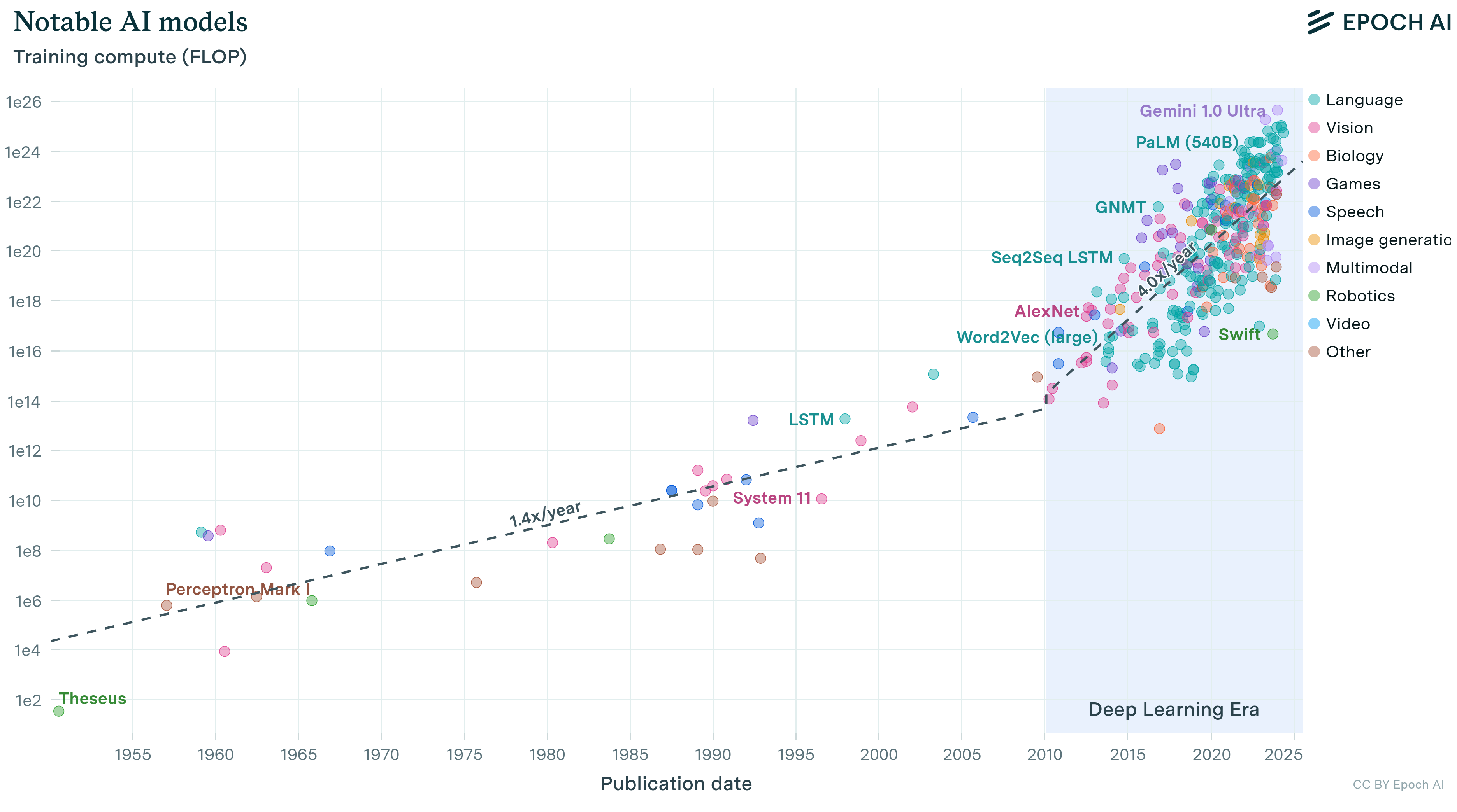
These resource demands reveal why understanding scaling laws is necessary for efficiency. Figure 2 shows computational demands of training state-of-the-art models escalating at an unsustainable rate, growing faster than Moore’s Law improvements in hardware.
Scaling laws provide a quantitative framework for understanding these trade-offs. They reveal that model performance exhibits predictable patterns as resources increase, following power-law relationships where performance improves consistently but with diminishing returns4. These laws show that optimal resource allocation requires coordinating model size, dataset size, and computational budget rather than scaling any single dimension in isolation.
4 Diminishing Returns: Economic principle where each additional input yields progressively smaller output gains. In ML, doubling compute from 1 to 2 hours might improve accuracy by 5%, but doubling from 100 to 200 hours might improve it by only 0.5%.
Recall from Chapter 4: DNN Architectures that transformers process sequences using self-attention mechanisms that compute relationships between all token pairs. This architecture’s computational cost scales quadratically with sequence length, making resource allocation particularly critical for language models. The term “FLOPs” (floating-point operations) quantifies total computational work, while “tokens” represent the individual text units (typically subwords) that models process during training.
Compute-Optimal Resource Allocation
Empirical studies of large language models (LLMs) reveal a key insight: for any fixed computational budget, there exists an optimal balance between model size and dataset size (measured in tokens5) that minimizes training loss.
5 Tokens: Individual units of text that language models process, created by breaking text into subword pieces using algorithms like Byte-Pair Encoding (BPE). GPT-3 trained on 300 billion tokens while PaLM used 780 billion tokens, requiring text corpora equivalent to millions of books from web crawls and digitized literature.
6 FLOPs: Floating-Point Operations, measuring computational work performed. Modern deep learning models require 10²²-10²⁴ FLOPs for training: GPT-3 used ~3.14 × 10²³ FLOPs (314 sextillion operations), equivalent to running a high-end gaming PC continuously for over 350 years.
7 Transformer: Neural network architecture introduced by Vaswani et al. (Chen et al. 2018) that revolutionized NLP through self-attention mechanisms. Unlike sequential RNNs, transformers enable parallel processing during training, forming the foundation of modern large language models including GPT, BERT, T5, and their derivatives.
8 Autoregressive Models: Language models that generate text by predicting each token based on all preceding tokens in the sequence. GPT-family models exemplify this approach, generating text left-to-right with causal attention masks to ensure each position only attends to previous positions.
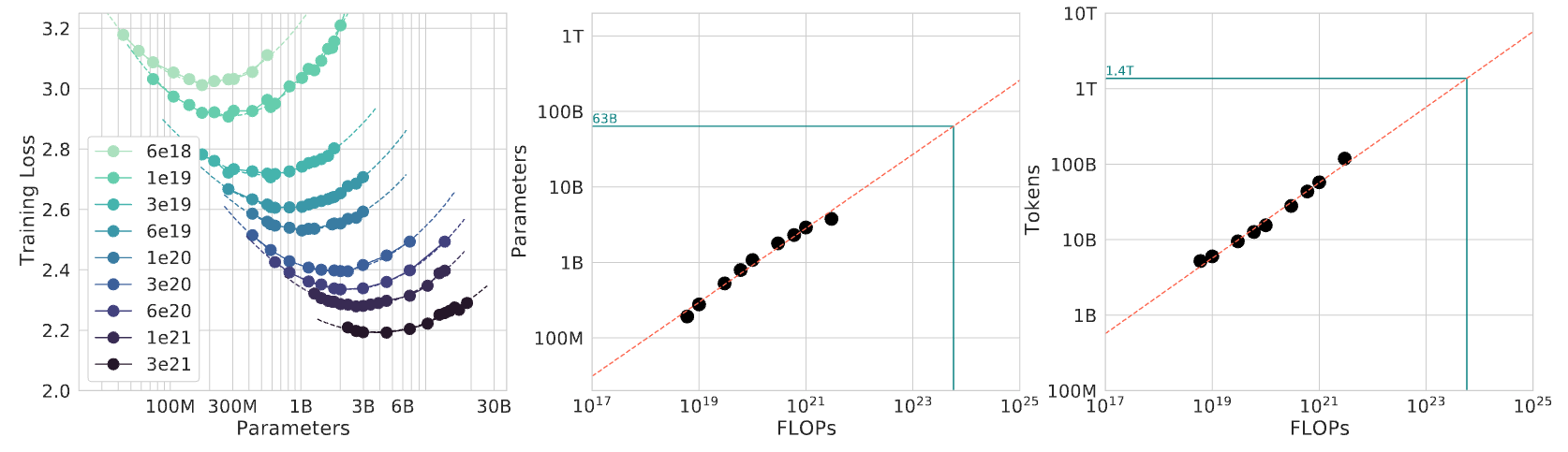
Figure 3 illustrates this principle through three related views. The left panel shows ‘IsoFLOP curves,’ where each curve corresponds to a constant number of floating-point operations (FLOPs6) during transformer7 training. The valleys in these curves identify the most efficient model size for each computational budget when training autoregressive8 language models. The center and right panels reveal how the optimal number of parameters and tokens scales predictably as computational budgets increase, demonstrating the necessity for coordinated scaling to maximize resource utilization.
Kaplan et al. (2020) demonstrated that transformer-based language models scale predictably with three factors: the number of model parameters, the volume of the training dataset (measured in tokens), and the total computational budget (measured in floating-point operations). When these factors are augmented proportionally, models exhibit consistent performance improvements without requiring architectural modifications or task-specific tuning.
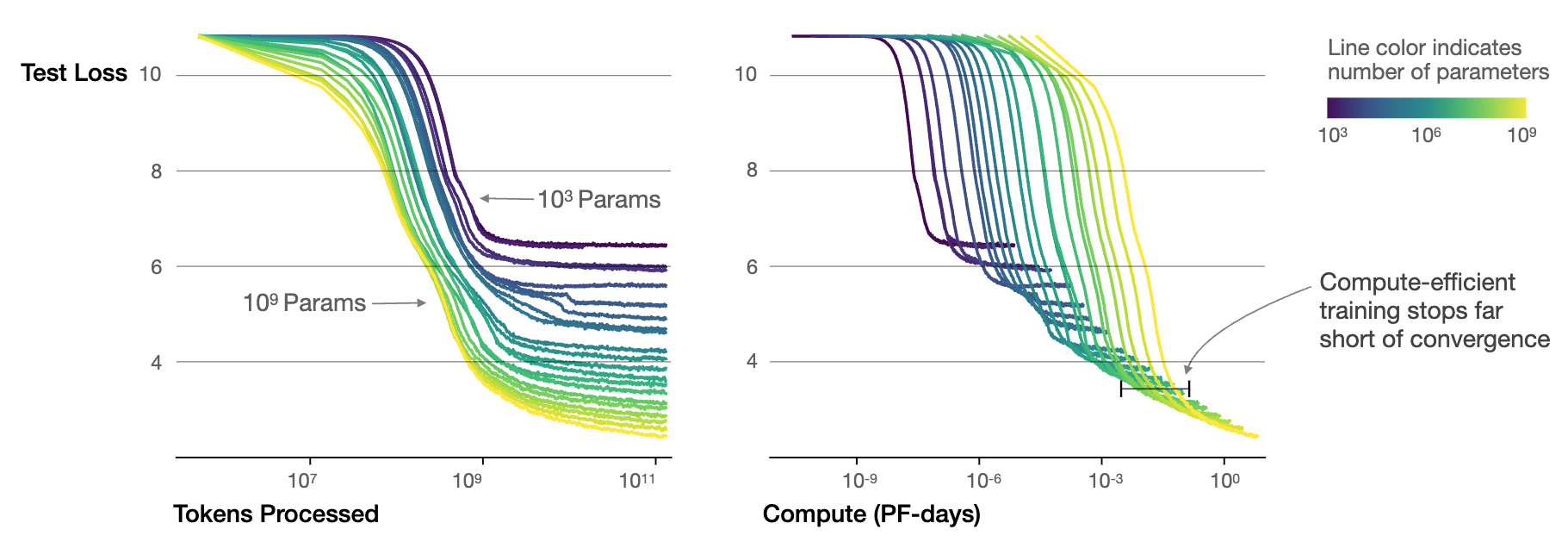
The practical manifestation of these patterns appears clearly in Figure 4, which presents test loss curves for models spanning from \(10^3\) to \(10^9\) parameters. The figure reveals two key insights. First, larger models demonstrate superior sample efficiency, achieving target performance levels with fewer training tokens. Second, as computational resources increase, the optimal model size correspondingly grows, with loss decreasing predictably when compute is allocated efficiently.
This theoretical scaling relationship defines optimal compute allocation: for a fixed budget, the relationship \(D \propto N^{0.74}\) (Hoffmann et al. 2022) shows that dataset size \(D\) and model size \(N\) must grow in coordinated proportions. This means that as model size increases, the dataset should grow at roughly three-quarters the rate to maintain compute-optimal efficiency.
These theoretical predictions assume perfect compute utilization, which becomes challenging in distributed training scenarios. Real-world implementations face communication overhead that scales unfavorably with system size, creating bandwidth bottlenecks that reduce effective utilization. Beyond 100 nodes, communication overhead can reduce expected performance gains by 20-40% depending on workload and interconnect, transforming predicted improvements into more modest real-world results.
Mathematical Foundations and Operational Regimes
The predictable patterns observed in scaling behavior can be expressed mathematically using power-law relationships, though understanding the intuition behind these patterns proves more important than precise mathematical formulation for most practitioners.
For readers interested in the formal mathematical framework, scaling laws can be expressed as power-law relationships. The general formulation is:
\[ \mathcal{L}(N) = A N^{-\alpha} + B \]
where loss \(\mathcal{L}\) decreases as resource quantity \(N\) increases, following a power-law decay with rate \(\alpha\), plus a baseline constant \(B\). Here, \(\mathcal{L}(N)\) represents the loss achieved with resource quantity \(N\), \(A\) and \(B\) are task-dependent constants, and \(\alpha\) is the scaling exponent that characterizes the rate of performance improvement. A larger value of \(\alpha\) signifies more efficient performance improvements with respect to scaling.
These theoretical predictions find strong empirical support across multiple model configurations. Figure 5 shows that early-stopped test loss varies predictably with both dataset size and model size, and learning curves across configurations can be aligned through appropriate parameterization.
Resource-Constrained Scaling Regimes
Applying scaling laws in practice requires recognizing three distinct resource allocation regimes that emerge from trade-offs between compute budget, data availability, and optimal resource allocation. These regimes provide practical guidance for system designers navigating resource constraints.
Compute-limited regimes characterize scenarios where available computational resources restrict scaling potential despite abundant training data. Organizations with limited hardware budgets or strict training time constraints operate within this regime. The optimal strategy involves training smaller models for longer periods, maximizing utilization of available compute through extended training schedules rather than larger architectures. This approach proves particularly relevant for academic institutions, startups, or projects with constrained infrastructure access.
Data-limited regimes emerge when computational resources exceed what can be effectively utilized given dataset constraints. High-resource organizations working with specialized domains, proprietary datasets, or privacy-constrained data often encounter this regime. The optimal strategy involves training larger models for fewer optimization steps, leveraging model capacity to extract maximum information from limited training examples. This regime commonly appears in specialized applications like medical imaging or proprietary commercial datasets.
Optimal regimes (Chinchilla Frontier) represent the balanced allocation of compute and data resources following compute-optimal scaling laws. This regime achieves maximum performance efficiency by scaling model size and training data proportionally, as demonstrated by DeepMind’s Chinchilla model, which outperformed much larger models through optimal resource allocation (Hoffmann et al. 2022). Operating within this regime requires sophisticated resource planning but delivers superior performance per unit of computational investment.
Recognizing these regimes enables practitioners to make informed decisions about resource allocation strategies, avoiding common inefficiencies such as over-parameterized models with insufficient training data or under-parameterized models that fail to utilize available computational resources effectively.

Scaling laws show that performance improvements follow predictable patterns that change depending on resource availability and exhibit distinct behaviors across different dimensions. Two important types of scaling regimes emerge: data-driven regimes that describe how performance changes with dataset size, and temporal regimes that describe when in the ML lifecycle we apply additional compute.
Data-Limited Scaling Regimes
The relationship between generalization error and dataset size exhibits three distinct regimes, as shown in Figure 6. When limited examples are available, high generalization error results from inadequate statistical estimates. As data availability increases, generalization error decreases predictably as a function of dataset size, following a power-law relationship that provides the most practical benefit from data scaling. Eventually, performance reaches saturation, approaching a floor determined by inherent data limitations or model capacity, beyond which additional data yields negligible improvements.

This three-regime pattern manifests across different resource dimensions beyond data alone. Operating within the power-law region provides the most reliable return on resource investment. Reaching this regime requires minimum resource thresholds, while maintaining operation within it demands careful allocation to avoid premature saturation.
Temporal Scaling Regimes
While data-driven regimes characterize how performance varies with dataset size, a complementary perspective examines temporal allocation of compute resources within the ML lifecycle. Recent research has identified three distinct temporal scaling regimes characterizing different stages of model development and deployment.
Pre-training scaling encompasses the traditional domain of scaling laws, characterizing how model performance improves with larger architectures, expanded datasets, and increased compute during initial training. Extensive study in foundation models has established clear power-law relationships between resources and capabilities.
Post-training scaling characterizes improvements achieved after initial training through techniques including fine-tuning, prompt engineering, and task-specific adaptation. This regime has gained prominence with foundation models, where adaptation rather than retraining frequently provides the most efficient path to enhanced performance under moderate resource requirements.
Test-time scaling characterizes how performance improvements result from additional compute allocation during inference without modifying model parameters. This encompasses methods including ensemble prediction, chain-of-thought prompting, and iterative refinement, enabling models to allocate additional processing time per input.
Figure 7 shows these temporal regimes exhibit distinct characteristics in computational resource allocation for performance improvement. Pre-training demands massive resources while providing broad capabilities, post-training offers targeted enhancements under moderate requirements, and test-time scaling enables flexible performance-compute trade-offs adjustable per inference.

Data-driven and temporal scaling regimes are crucial for system design, revealing multiple paths to performance improvement beyond scaling training resources alone. For resource-constrained deployments, post-training and test-time scaling may provide more practical approaches than complete model retraining, while data-efficient techniques enable effective system operation within the power-law regime using smaller datasets.
Practical Applications in System Design
Scaling laws provide powerful insights for practical system design and resource planning. Consistent observation of power-law trends indicates that within well-defined operational regimes, model performance depends predominantly on scale rather than idiosyncratic architectural innovations. However, diminishing returns phenomena indicate that each additional improvement requires exponentially increased resources while delivering progressively smaller benefits.
OpenAI’s development of GPT-3 demonstrates this principle. Rather than conducting expensive architecture searches, the authors applied scaling laws derived from earlier experiments to determine optimal training dataset size and model parameter count (Brown et al. 2020). They scaled an established transformer architecture along the compute-optimal frontier to 175 billion parameters and approximately 300 billion tokens, enabling advance prediction of model performance and resource requirements. This methodology demonstrated the practical application of scaling laws in large-scale system planning.
Scaling laws serve multiple practical functions in system design. They enable practitioners to estimate returns on investment for different resource allocations during resource budgeting. Under fixed computational budgets, designers can utilize empirical scaling curves to determine optimal performance improvement strategies across model size, dataset expansion, or training duration.
System designers can utilize scaling trends to identify when architectural changes yield significant improvements relative to gains achieved through scaling alone, thereby avoiding exhaustive architecture search. When a model family exhibits favorable scaling behavior, scaling the existing architecture may prove more effective than transitioning to more complex but unvalidated designs.
In edge and embedded environments with constrained resource budgets, understanding performance degradation under model scaling enables designers to select smaller configurations delivering acceptable accuracy within deployment constraints. By quantifying scale-performance trade-offs, scaling laws identify when brute-force scaling becomes inefficient and indicate the necessity for alternative approaches including model compression, efficient knowledge transfer, sparsity techniques, and hardware-aware design.
Scaling laws also function as diagnostic instruments. Performance plateaus despite increased resources may indicate dimensional saturation—such as inadequate data relative to model size—or inefficient computational resource utilization. This diagnostic capability renders scaling laws both predictive and prescriptive, facilitating systematic bottleneck identification and resolution.
Sustainability and Cost Implications
Scaling laws illuminate pathways to performance enhancement while revealing rapidly escalating resource demands. As models expand, training and deployment resource requirements grow disproportionately, creating tension between performance gains through scaling and system efficiency.
Training large-scale models necessitates substantial processing power, typically requiring distributed infrastructures9 comprising hundreds or thousands of accelerators. State-of-the-art language model training may require tens of thousands of GPU-days, consuming millions of kilowatt-hours of electricity. These distributed training systems introduce additional complexity around communication overhead, synchronization, and scaling efficiency, as detailed in Chapter 8: AI Training. Energy demands have outpaced Moore’s Law improvements, raising critical questions about long-term sustainability.
9 Distributed Infrastructure: Computing systems that spread ML workloads across multiple machines connected by high-speed networks. OpenAI’s GPT-4 training likely used thousands of NVIDIA A100 GPUs connected via InfiniBand, requiring careful orchestration to avoid communication bottlenecks.
Large models require extensive, high-quality, diverse datasets to achieve their full potential. Data collection, cleansing, and labeling processes consume considerable time and resources. As models approach saturation of available high-quality data, particularly in natural language processing, additional performance gains through data scaling become increasingly difficult to achieve. This reality underscores data efficiency as a necessary complement to brute-force scaling approaches.
The financial and environmental implications compound these challenges. Training runs for large foundation models can incur millions of dollars in computational expenses, and associated carbon footprints10 have garnered increasing scrutiny. These costs limit accessibility to cutting-edge research and exacerbate disparities in access to advanced AI systems. The democratization challenges introduced by efficiency barriers connect directly to accessibility goals addressed in Chapter 19: AI for Good. Comprehensive approaches to environmental sustainability in ML systems, including carbon footprint measurement and green computing practices, are explored in Chapter 18: Sustainable AI.
10 Carbon Emissions: Training GPT-3 generated approximately 502 tons of CO₂ equivalent, comparable to annual emissions of 123 gasoline-powered vehicles. Modern ML practices increasingly incorporate carbon tracking using tools like CodeCarbon and the ML CO2 Impact calculator.
These trade-offs demonstrate that scaling laws provide valuable frameworks for understanding performance growth but do not constitute unencumbered paths to improvement. Each incremental performance gain requires evaluation against corresponding resource requirements. As systems approach practical scaling limits, emphasis must transition from scaling alone to efficient scaling—a comprehensive approach balancing performance, cost, energy consumption, and environmental impact.
Scaling Law Breakdown Conditions
Scaling laws exhibit remarkable consistency within specific operational regimes but possess inherent limitations. As systems expand, they inevitably encounter boundaries where underlying assumptions of smooth, predictable scaling cease to hold. These breakdown points expose critical inefficiencies and emphasize the necessity for refined system design approaches.
For scaling laws to remain valid, model size, dataset size, and computational budget must be augmented in coordinated fashion. Over-investment in one dimension while maintaining others constant often results in suboptimal outcomes. For example, increasing model size without expanding training datasets may induce overfitting, while increasing computational resources without model redesign may lead to inefficient utilization (Hoffmann et al. 2022).
Large-scale models require carefully tuned training schedules and learning rates to fully utilize available resources. When compute is insufficiently allocated due to premature stopping, batch size misalignment, or ineffective parallelism, models may fail to reach performance potential despite significant infrastructure investment.
Scaling laws presuppose continued performance improvement with sufficient training data. However, in numerous domains, availability of high-quality, human-annotated data is finite. As models consume increasingly large datasets, they reach points of diminishing marginal utility where additional data contributes minimal new information. Beyond this threshold, larger models may exhibit memorization rather than generalization.
As models grow, they demand greater memory bandwidth11, interconnect capacity, and I/O throughput. These hardware limitations become increasingly challenging even with specialized accelerators. Distributing trillion-parameter models across clusters necessitates meticulous management of data parallelism, communication overhead, and fault tolerance.
11 Memory Bandwidth: The rate at which data can be read from or written to memory, measured in GB/s. NVIDIA H100 provides 3.35 TB/s memory bandwidth vs. typical DDR5 RAM’s 51 GB/s, a 65× difference critical for handling large model parameters.
At extreme scales, models may approach limits of what can be learned from training distributions. Performance on benchmarks may continue improving, but these improvements may no longer reflect meaningful gains in generalization or understanding. Models may become increasingly brittle, susceptible to adversarial examples, or prone to generating plausible but inaccurate outputs.
Table 1 synthesizes the primary causes of scaling failure, outlining typical breakdown types, underlying causes, and representative scenarios as a reference for anticipating inefficiencies and guiding balanced system design.
| Dimension Scaled | Type of Breakdown | Underlying Cause | Example Scenario |
|---|---|---|---|
| Model Size | Overfitting | Model capacity exceeds available data | Billion-parameter model on limited dataset |
| Data Volume | Diminishing Returns | Saturation of new or diverse information | Scaling web text beyond useful threshold |
| Compute Budget | Underutilized Resources | Insufficient training steps or inefficient use | Large model with truncated training duration |
| Imbalanced Scaling | Inefficiency | Uncoordinated increase in model/data/compute | Doubling model size without more data or time |
| All Dimensions | Semantic Saturation | Exhaustion of learnable patterns in the domain | No further gains despite scaling all inputs |
These breakdown points demonstrate that scaling laws describe empirical regularities under specific conditions that become increasingly difficult to maintain at scale. As machine learning systems continue evolving, discerning where and why scaling ceases to be effective becomes necessary, driving development of strategies that enhance performance without relying solely on scale.
Integrating Efficiency with Scaling
The limitations exposed by scaling laws (data saturation, infrastructure bottlenecks, and diminishing returns) demonstrate that brute-force scaling alone cannot deliver sustainable AI systems. These constraints necessitate a shift from expanding scale to achieving greater efficiency with reduced resources.
This transition requires coordinated optimization across three interconnected dimensions: algorithmic efficiency addresses computational intensity through better model design, compute efficiency maximizes hardware utilization to translate algorithmic improvements into practical gains, and data efficiency extracts maximum information from limited examples as high-quality data becomes scarce. Together, these dimensions provide systematic approaches to achieving performance goals that scaling alone cannot sustainably deliver, while addressing broader concerns about equitable access to AI capabilities and environmental impact.
Having examined how scaling laws reveal fundamental constraints, we now turn to the efficiency framework that provides concrete strategies for operating effectively within these constraints. The following section details how the three efficiency dimensions work together to enable sustainable, accessible machine learning systems.
The Efficiency Framework
The constraint identified through scaling laws (that continued progress requires systematic efficiency optimization) motivates three complementary efficiency dimensions. Each dimension addresses a specific limitation: algorithmic efficiency tackles computational intensity, compute efficiency addresses hardware utilization gaps, and data efficiency solves the data saturation problem.
Together, these three dimensions provide a systematic framework for addressing the constraints that scaling laws reveal. Targeted optimizations across algorithmic design, hardware utilization, and data usage can achieve what brute-force scaling cannot: sustainable, accessible, high-performance AI systems.
Multi-Dimensional Efficiency Synergies
Optimal performance requires coordinated optimization across multiple dimensions. No single resource—whether model parameters, training data, or compute budget—can be scaled indefinitely to achieve efficiency. Modern techniques demonstrate the potential: 10-100x gains in algorithmic efficiency through optimized architectures, 5-50x improvements in hardware utilization through specialized processors, and 10-1000x reductions in data requirements through advanced learning methods.
The power of this framework emerges from interconnections between dimensions, as depicted in Figure 8. Algorithmic innovations often enable better hardware utilization, while hardware advances unlock new algorithmic possibilities. Data-efficient techniques reduce computational requirements, while compute-efficient methods enable training on larger datasets. Understanding these synergies is essential for building practical ML systems.

The specific priorities vary across deployment environments. Cloud systems with abundant resources prioritize scalability and throughput, while edge devices face severe memory and power constraints. Mobile applications must balance performance with battery life, and TinyML deployments demand extreme resource efficiency. Understanding these context-specific patterns enables designers to make informed decisions about which efficiency dimensions to prioritize and how to address inevitable trade-offs between them.
Achieving Algorithmic Efficiency
Algorithmic efficiency achieves maximum performance per unit of computation through optimized model architectures and training procedures. Modern techniques achieve 10-100x improvements in computational requirements while maintaining or improving accuracy, providing the most direct path to practical AI deployment.
The foundation for these improvements lies in a key observation: most neural networks are dramatically overparameterized. The lottery ticket hypothesis reveals that networks contain sparse subnetworks, typically 10-20% of original parameters (though this varies significantly by architecture and task), that achieve comparable accuracy when trained in isolation (Frankle and Carbin 2019). This discovery transforms compression into a principled approach: large models serve as initialization strategies for finding efficient architectures.
Model Compression Fundamentals
Three major approaches dominate modern algorithmic efficiency, each targeting different aspects of model inefficiency:
Model Compression systematically removes redundant components from neural networks. Pruning techniques achieve 2-4x inference speedup with 1-3% accuracy loss by removing unnecessary weights and structures. Research demonstrates that ResNet-50 can be reduced to 20% of original parameters while maintaining 99% of ImageNet accuracy (Gholami et al. 2021). The specific pruning algorithms—including magnitude-based selection, structured vs. unstructured approaches, and layer-wise sensitivity analysis—are covered in detail in Chapter 10: Model Optimizations.
Precision Optimization reduces computational requirements through quantization, which maps high-precision floating-point values to lower-precision representations. Neural networks demonstrate inherent robustness to precision reduction, with INT8 quantization achieving 4x memory reduction and 2-4x inference speedup while typically maintaining 98-99% of FP32 accuracy (Jacob et al. 2018). Modern techniques range from simple post-training quantization to sophisticated quantization-aware training. The specific quantization algorithms, calibration methods, and training procedures are detailed in Chapter 10: Model Optimizations.
Knowledge Transfer distills capabilities from large teacher models into efficient student models. Knowledge distillation12 achieves 40-60% parameter reduction while retaining 95-97% of original performance, addressing both computational efficiency and data efficiency by requiring fewer training examples. The specific distillation algorithms, loss functions, and training procedures are covered in Chapter 10: Model Optimizations.
12 Knowledge Distillation: Technique where a large “teacher” model transfers knowledge to a smaller “student” model by training the student to mimic the teacher’s output probabilities. DistilBERT achieves ~97% of BERT’s performance on GLUE benchmark with 40% fewer parameters and 60% faster inference through distillation.
Hardware-Algorithm Co-Design
Algorithmic optimizations alone are insufficient; their practical benefits depend on hardware-software co-design. Optimization techniques must be tailored to target hardware characteristics (memory bandwidth, compute capabilities, and precision support) to achieve real-world speedups. For example, INT8 quantization achieves 2.3x speedup on NVIDIA V100 GPUs with tensor core support but may provide minimal benefit on hardware lacking specialized integer instructions.
Successful co-design requires understanding whether workloads are memory-bound (limited by data movement) or compute-bound (limited by processing capacity), then applying optimizations that address the actual bottleneck. Techniques like operator fusion reduce memory traffic by combining operations, while precision reduction exploits specialized hardware units. While Chapter 10: Model Optimizations covers the algorithmic aspects of hardware-aware optimization, Chapter 11: AI Acceleration details how systematic co-design approaches leverage specific hardware architectures for maximum efficiency.
Architectural Innovation for Efficiency
Modern efficiency requires architectures designed for resource constraints. Models like MobileNet13, EfficientNet14, and SqueezeNet15 demonstrate that compact designs can deliver high performance through architectural innovations rather than scaling up existing designs.
13 MobileNet: Efficient neural network architecture using depthwise separable convolutions, achieving ~50× fewer parameters than traditional models. MobileNet-v1 has only 4.2M parameters vs. VGG-16’s ~138M, enabling deployment on smartphones with <100MB memory.
14 EfficientNet: Architecture achieving state-of-the-art accuracy with superior parameter efficiency. EfficientNet-B7 achieves 84.3% ImageNet top-1 accuracy (84.4% in some reports) with 66M parameters, compared to ResNet-152’s 77.0% accuracy with approximately 60M parameters.
15 SqueezeNet: Compact CNN architecture achieving AlexNet-level accuracy with 50× fewer parameters (1.25M vs. 60M). Demonstrated that clever architecture design can dramatically reduce model size without sacrificing performance.
Different deployment contexts require different efficiency trade-offs. Cloud inference prioritizes throughput and can tolerate higher memory usage, favoring parallel-friendly operations. Edge deployment prioritizes latency and memory efficiency, requiring architectures that minimize memory access. Mobile deployment constrains energy usage, demanding architectures optimized for energy-efficient operations.
Parameter-Efficient Adaptation
Parameter-efficient fine-tuning16 techniques demonstrate how the three efficiency dimensions work together. These methods update less than 1% of model parameters while achieving full fine-tuning performance, addressing all three efficiency pillars: algorithmic efficiency through reduced parameter updates, compute efficiency through lower memory requirements and faster training, and data efficiency by leveraging pre-trained representations that require fewer task-specific examples.
16 Parameter-Efficient Fine-tuning: Methods like LoRA and Adapters that update <1% of model parameters while achieving full fine-tuning performance. Reduces memory requirements from gigabytes to megabytes for large model adaptation.
The practical impact is transformative: fine-tuning GPT-3 traditionally requires storing gradients for 175 billion parameters, consuming over 700GB of GPU memory. LoRA reduces this to under 10GB by learning low-rank decompositions of weight updates, enabling efficient adaptation on single consumer GPUs while requiring only hundreds of examples rather than thousands for effective adaptation.
As Figure 9 shows, the computational resources needed to train a neural network to achieve AlexNet17-level performance on ImageNet18 classification decreased by approximately \(44\times\) between 2012 and 2019. This improvement, which halved every 16 months, outpaced hardware efficiency gains of Moore’s Law19, demonstrating the role of algorithmic advancements in driving efficiency (Hernandez, Brown, et al. 2020).
17 AlexNet: Groundbreaking CNN by Krizhevsky, Sutskever, and Hinton (2012) that won ImageNet with 15.3% error rate, nearly halving the previous best of 26.2%. Used 60M parameters, two GPUs, and launched the deep learning revolution.
18 ImageNet: Large-scale visual recognition dataset with 14+ million images across 20,000+ categories. The annual ImageNet Large Scale Visual Recognition Challenge (ILSVRC) drove computer vision breakthroughs from 2010-2017.
19 Moore’s Law: Intel co-founder Gordon Moore’s 1965 observation that transistor density doubles every ~2 years. Traditional Moore’s Law predicted ~2x transistor density every 18-24 months, though this rate has slowed significantly since ~2015, while AI algorithmic efficiency improved 44x in 7 years (2012-2019).

The evolution of algorithmic efficiency, from basic compression to hardware-aware optimization and parameter-efficient adaptation, demonstrates the centrality of these techniques to machine learning progress. As the field advances, algorithmic efficiency will remain central to designing systems that are high-performing, scalable, and sustainable.
Compute Efficiency
Compute efficiency focuses on the effective use of hardware and computational resources to train and deploy machine learning models. It encompasses strategies for reducing energy consumption, optimizing processing speed, and leveraging hardware capabilities to achieve scalable and sustainable system performance. While this chapter focuses on efficiency principles and trade-offs, the detailed technical implementation of hardware acceleration—including GPU architectures, TPU design, memory systems, and custom accelerators—is covered in Chapter 11: AI Acceleration.
From CPUs to AI Accelerators
Compute efficiency’s evolution reveals why specialized hardware became essential. In the early days of machine learning, Central Processing Units (CPUs) shaped what was possible. CPUs excel at sequential processing and complex decision-making but have limited parallelism, typically 4-16 cores optimized for diverse tasks rather than the repetitive matrix operations that dominate machine learning. Training times for models were measured in days or weeks, as even relatively small datasets pushed hardware boundaries.
This CPU-constrained era ended as deep learning models like AlexNet and ResNet20 demonstrated the potential of neural networks, quickly surpassing traditional CPU capabilities. As shown in Figure 10, this marked the beginning of exponential growth in compute usage. OpenAI’s analysis reveals that compute used in AI training increased approximately 300,000 times from 2012 to 2018, doubling approximately every 3.4 months during this period—a rate far exceeding Moore’s Law (Amodei, Hernandez, et al. 2018).
20 ResNet: Residual Network architecture by He et al. (He et al. 2016) enabling training of very deep networks (152+ layers) through skip connections. Won ImageNet 2015 with 3.6% error rate, surpassing human-level performance for the first time.

This rapid growth was driven by adoption of Graphics Processing Units (GPUs), which offered unparalleled parallel processing capabilities. While CPUs might have 16 cores, modern high-end GPUs like the NVIDIA H100 contain over 16,000 CUDA cores21. Specialized hardware accelerators such as Google’s Tensor Processing Units (TPUs) further revolutionized compute efficiency by designing chips specifically for machine learning workloads, optimizing for specific data types and operations most common in neural networks.
21 CUDA Cores: NVIDIA’s parallel processing units optimized for floating-point operations. Unlike CPU cores (designed for complex sequential tasks), CUDA cores are simpler and work together, enabling a single H100 GPU to perform 16,896 parallel operations simultaneously for massive speedup in matrix computations.
Sustainable Computing and Energy Awareness
As systems scale further, compute efficiency has become closely tied to sustainability. Training state-of-the-art large language models requires massive computational resources, leading to increased attention on environmental impact. The projected electricity usage of data centers, shown in Figure 11, highlights this concern. Between 2010 and 2030, electricity consumption is expected to rise sharply, particularly under worst-case scenarios where it could exceed 8,000 TWh by 2030 (Jones 2018).

This dramatic growth underscores urgency for compute efficiency, as even large data centers face energy constraints due to limitations in electrical grid capacity. Efficiency improvements alone may not guarantee environmental benefits due to a phenomenon known as Jevons Paradox.
Consider the invention of the fuel-efficient car. While each car uses less gas per mile, the lower cost of driving encourages people to drive more often and live further from work. The result can be an increase in total gasoline consumption. This is Jevons Paradox: efficiency gains can be offset by increased consumption. In AI, this means making models 10x more efficient might lead to a 100x increase in their use, resulting in a net negative environmental impact if not managed carefully.
Addressing these challenges requires optimizing hardware utilization and minimizing energy consumption in both cloud and edge contexts while being mindful of potential rebound effects from increased deployment.
Key trends include adoption of energy-aware scheduling and resource allocation techniques that distribute workloads efficiently across available hardware (Patterson et al. 2021). Researchers are also developing methods to dynamically adjust precision levels during training and inference, using lower precision operations (e.g., mixed-precision training) to reduce power consumption without sacrificing accuracy.
22 Model Parallelism: Distributing model components across multiple processors due to memory constraints. GPT-3 (175B parameters) requires 350GB memory, exceeding A100’s 40GB capacity by 9×, necessitating tensor parallelism where each transformer layer splits across 8-16 GPUs with all-gather communication for activation synchronization.
23 Data Parallelism: Training method where the same model runs on multiple processors with different data batches. GPT-3 training used data parallelism across thousands of GPUs, processing multiple text sequences simultaneously.
Distributed systems achieve compute efficiency by splitting workloads across multiple machines. Techniques such as model parallelism22 and data parallelism23 allow large-scale models to be trained more efficiently, leveraging clusters of GPUs or TPUs to maximize throughput while minimizing idle time.
At the edge, compute efficiency addresses growing demand for real-time processing in energy-constrained environments. Innovations such as hardware-aware model optimization, lightweight inference engines, and adaptive computing architectures enable highly efficient edge systems critical for applications like autonomous vehicles and smart home devices.
Production Deployment Patterns
Real-world efficiency optimization demonstrates practical impact across deployment contexts. Production systems routinely achieve 5-10x efficiency gains through coordinated application of optimization techniques while maintaining 95%+ of original model performance.
Mobile applications achieve 4-7x model size reduction and 3-5x latency improvements through combined quantization, pruning, and distillation, enabling real-time inference on mid-range devices. Modern mobile AI systems distribute workloads across specialized processors (NPU for ultra-low power inference, GPU for parallel compute, CPU for control logic) based on power, performance, and real-time constraints.
Autonomous vehicle systems optimize for safety-critical <10ms latency requirements through hardware-aware architectural design and mixed-precision quantization, processing multiple high-bandwidth sensor streams within strict power and thermal constraints.
Cloud serving infrastructure reduces costs by 70-80% through systematic optimization combining dynamic batching, quantization, and knowledge distillation, serving 4-5x more requests at comparable quality levels.
Edge IoT deployments achieve month-long battery life through extreme model compression and duty-cycle optimization, operating on milliwatt power budgets while maintaining acceptable accuracy for practical applications.
These efficiency gains emerge from systematic optimization strategies that coordinate multiple techniques rather than applying individual optimizations in isolation. The specific optimization sequences, technique combinations, and engineering practices that enable these production results are detailed in Chapter 10: Model Optimizations.
Compute efficiency complements algorithmic and data efficiency. Compact models reduce computational requirements, while efficient data pipelines streamline hardware usage. The evolution of compute efficiency (from early reliance on CPUs through specialized accelerators to sustainable computing practices) remains central to building scalable, accessible, and environmentally responsible machine learning systems.
Data Efficiency
Data efficiency focuses on optimizing the amount and quality of data required to train machine learning models effectively. Data efficiency has emerged as a pivotal dimension, driven by rising costs of data collection, storage, and processing, as well as the limits of available high-quality data.
Maximizing Learning from Limited Data
In early machine learning, data efficiency was not a primary focus, as datasets were relatively small and manageable. The challenge was often acquiring enough labeled data to train models effectively. Researchers relied on curated datasets such as UCI’s Machine Learning Repository24, using feature selection and dimensionality reduction techniques like principal component analysis (PCA)25 to extract maximum value from limited data.
24 UCI Machine Learning Repository: Established in 1987 by the University of California, Irvine, one of the most widely-used resources for machine learning datasets. Contains over 600 datasets and has been cited in thousands of research papers.
25 Principal Component Analysis (PCA): Dimensionality reduction technique invented by Karl Pearson in 1901, identifies the most important directions of variation in data. Reduces computational complexity while preserving 90%+ of data variance in many applications.
The advent of deep learning in the 2010s transformed data’s role. Models like AlexNet and GPT-3 demonstrated that larger datasets often led to better performance, marking the beginning of the “big data” era. However, this reliance introduced inefficiencies. Data collection became costly and time-consuming, requiring vast amounts of labeled data for supervised learning.
Researchers developed techniques enhancing data efficiency even as datasets grew. Transfer learning26 allowed pre-trained models to be fine-tuned on smaller datasets, reducing task-specific data needs (Yosinski et al. 2014). Data augmentation27 artificially expanded datasets by creating new variations of existing samples. Active learning28 prioritized labeling only the most informative data points (Settles 2012a).
26 Transfer Learning: Technique where models pre-trained on large datasets are fine-tuned for specific tasks. ImageNet pre-trained models can achieve high accuracy on new vision tasks with <1000 labeled examples vs. millions needed from scratch.
27 Data Augmentation: Artificially expanding datasets through transformations like rotations, crops, or noise. Can improve model performance by 5-15% and reduce overfitting, especially when labeled data is scarce.
28 Active Learning: Iteratively selecting the most informative samples for labeling to maximize learning efficiency. Can achieve target performance with 50-90% less labeled data compared to random sampling.
29 Data-Centric AI: Paradigm shift from model-centric to data-centric development, popularized by Andrew Ng in 2021. Focuses on systematically improving data quality rather than just model architecture, often yielding greater performance gains.
As systems continue growing in scale, inefficiencies of large datasets have become apparent. Data-centric AI29 has emerged as a key paradigm, emphasizing data quality over quantity. This approach focuses on enhancing preprocessing, removing redundancy, and improving labeling efficiency. Research shows that careful curation and filtering can achieve comparable or superior performance while using only a fraction of original data volume (Penedo et al. 2024).
Several techniques support this transition. Self-supervised learning30 enables models to learn meaningful representations from unlabeled data, reducing dependency on expensive human-labeled datasets. Active learning strategies selectively identify the most informative examples for labeling, while curriculum learning31 structures training to progress from simple to complex examples, improving learning efficiency.
30 Self-Supervised Learning: Training method where models create their own labels from input data structure, like predicting masked words in BERT. Enables learning from billions of unlabeled examples.
31 Curriculum Learning: Training strategy where models learn from easy examples before progressing to harder ones, mimicking human education. Can improve convergence speed by 25-50% and final model performance.
32 Foundation Models: Large-scale, general-purpose AI models trained on broad data that can be adapted for many tasks. Term coined by Stanford HAI in 2021, includes models like GPT-3, BERT, and DALL-E.
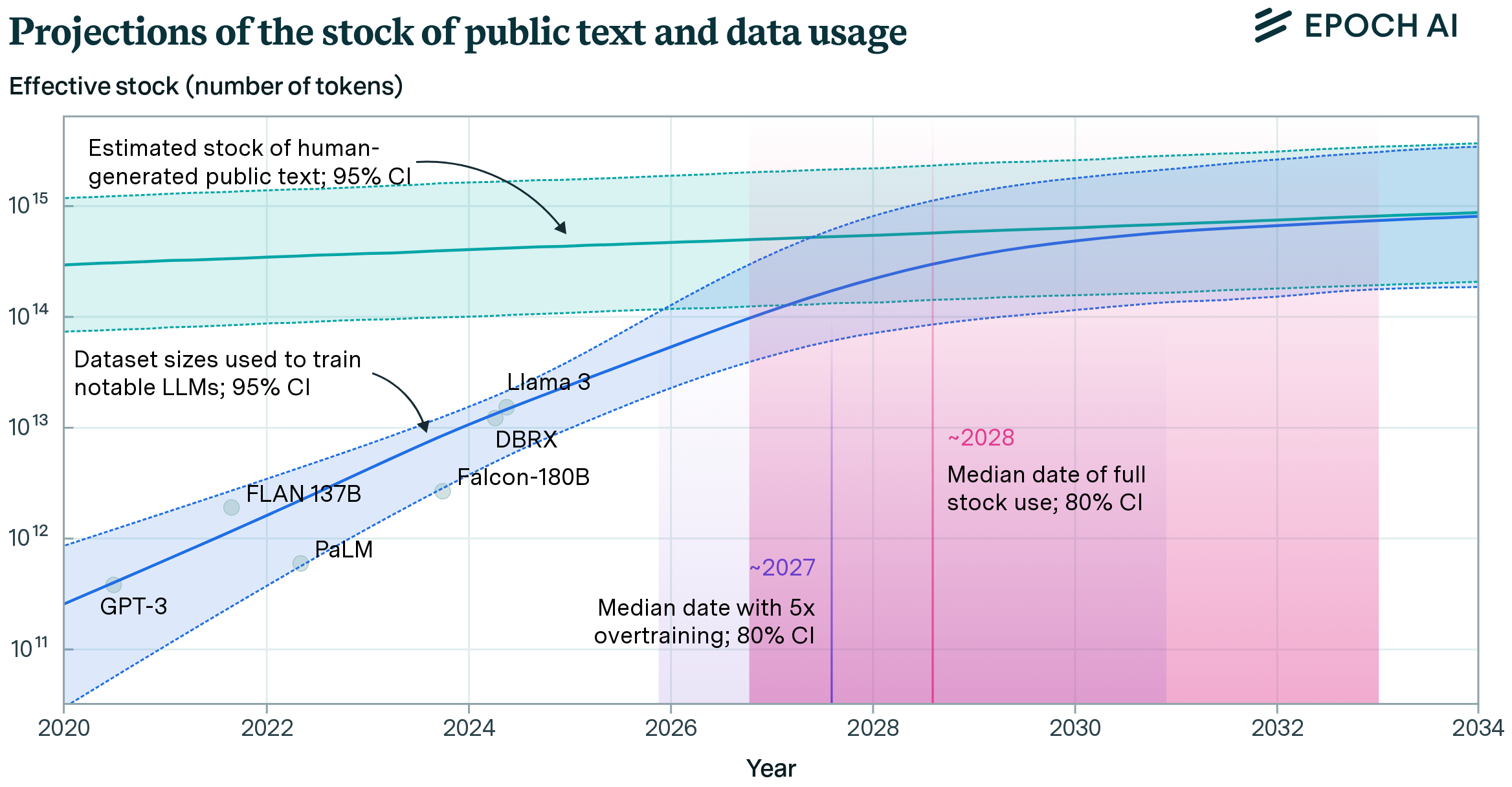
Data efficiency is particularly important in foundation models32. As these models grow in scale and capability, they approach limits of available high-quality training data, especially for language tasks, as shown in Figure 12. This scarcity drives innovation in data processing and curation techniques.
Evidence for data quality’s impact appears across different deployment scales. In Tiny ML33 applications, datasets like Wake Vision demonstrate how performance critically depends on careful data curation (Banbury et al. 2024). At larger scales, research on language models trained on web-scale datasets shows that intelligent filtering and selection strategies significantly improve performance on downstream tasks (Penedo et al. 2024). Chapter 12: Benchmarking AI establishes rigorous methodologies for measuring these data quality improvements.
33 TinyML: Machine learning on microcontrollers and edge devices with <1KB-1MB memory and <1mW power consumption. Enables AI in IoT devices, wearables, and sensors where traditional ML deployment is impossible.
This modern era of data efficiency represents a shift in how systems approach data utilization. By focusing on quality over quantity and developing sophisticated techniques for data selection and processing, the field is moving toward more sustainable and effective approaches to model training and deployment. Data efficiency is integral to scalable systems, impacting both model and compute efficiency. Smaller, higher-quality datasets reduce training times and computational demands while enabling better generalization. These principles complement the privacy-preserving techniques explored in Chapter 15: Security & Privacy, where minimizing data requirements enhances both efficiency and user privacy protection.
Real-World Efficiency Strategies
Having explored each efficiency dimension individually and their interconnections, we examine how these dimensions manifest across different deployment contexts. The efficiency of machine learning systems emerges from understanding relationships between algorithmic, compute, and data efficiency in specific operational environments.
Context-Specific Efficiency Requirements
The specific priorities and trade-offs vary dramatically across deployment environments. As our opening examples illustrated, these range from cloud systems with abundant resources to edge devices with severe memory and power constraints. Table 2 maps how these constraints translate into efficiency optimization priorities.
| Deployment Context | Primary Constraints | Efficiency Priorities | Representative Applications |
|---|---|---|---|
| Cloud | Cost at scale, energy consumption | Throughput, scalability, operational efficiency | Large language model APIs, recommendation engines, video processing |
| Edge | Latency, local compute capacity, connectivity | Real-time performance, power efficiency | Autonomous vehicles, industrial automation, smart cameras |
| Mobile | Battery life, memory, thermal limits | Energy efficiency, model size, responsiveness | Voice assistants, photo enhancement, augmented reality |
| TinyML | Extreme power/memory constraints | Ultra-low power, minimal model size | IoT sensors, wearables, environmental monitoring |
Understanding these context-specific patterns enables designers to make informed decisions about which efficiency dimensions to prioritize and how to navigate inevitable trade-offs.
Scalability and Sustainability
System efficiency serves as a driver of environmental sustainability. When systems are optimized for efficiency, they can be deployed at scale while minimizing environmental footprint. This relationship creates a positive feedback loop, as shown in Figure 13.

Efficient systems are inherently scalable. Reducing resource demands through lightweight models, targeted datasets, and optimized compute utilization allows systems to deploy broadly. When efficient systems scale, they amplify their contribution to sustainability by reducing overall energy consumption and computational waste. Sustainability reinforces the need for efficiency, creating a feedback loop that strengthens the entire system.
Efficiency Trade-offs and Challenges
The three efficiency dimensions can work synergistically under favorable conditions, but real-world systems often face scenarios where improving one dimension degrades another. The same resource constraints that make efficiency necessary force difficult choices: reducing model size may sacrifice accuracy, optimizing for real-time performance may increase energy consumption, and curating smaller datasets may limit generalization.
Fundamental Sources of Efficiency Trade-offs
These tensions manifest in various ways across machine learning systems. Understanding their root causes is essential for addressing design challenges. Each efficiency dimension influences the others, creating a dynamic interplay that shapes system performance.
Algorithmic Efficiency vs. Compute Requirements
Algorithmic efficiency focuses on designing compact models that minimize computational and memory demands. By reducing model size or complexity, deployment on resource-limited devices becomes feasible. Overly simplifying a model can reduce accuracy, especially for complex tasks. To compensate for this loss, additional computational resources may be required during training or deployment, placing strain on compute efficiency.
Compute Efficiency vs. Real-Time Needs
Compute efficiency aims to minimize resources required for training and inference, reducing energy consumption, processing time, and memory use. In scenarios requiring real-time responsiveness (autonomous vehicles, augmented reality), compute efficiency becomes harder to maintain. Figure 14 illustrates this challenge: real-time systems often require high-performance hardware to process data instantly, conflicting with energy efficiency goals or increasing system costs.

Data Efficiency vs. Model Generalization
Data efficiency seeks to minimize the amount of data required to train a model without sacrificing performance. By curating smaller, high-quality datasets, training becomes faster and less resource-intensive. Ideally, this reinforces both algorithmic and compute efficiency. However, reducing dataset size can limit diversity, making it harder for models to generalize to unseen scenarios. To address this, additional compute resources or model complexity may be required, creating tension between data efficiency and broader system goals.
Recurring Trade-off Patterns in Practice
The trade-offs between efficiency dimensions become particularly evident when examining specific scenarios. Complex models with millions or billions of parameters can achieve higher accuracy by capturing intricate patterns, but require significant computational power and memory. A recommendation system in a cloud data center might use a highly complex model for better recommendations, but at the cost of higher energy consumption and operating costs. On resource-constrained devices like smartphones or autonomous vehicles, compact models may operate efficiently but require more sophisticated data preprocessing or training procedures to compensate for reduced capacity.
Energy efficiency and real-time performance often pull systems in opposite directions. Real-time systems like autonomous vehicles or augmented reality applications rely on high-performance hardware to process large volumes of data quickly, but this typically increases energy consumption. An autonomous vehicle must process sensor data from cameras, LiDAR, and radar in real time to make navigation decisions, requiring specialized accelerators that consume significant energy. In edge deployments with battery power or limited energy sources, this trade-off becomes even more critical.
Larger datasets generally provide greater diversity and coverage, enabling models to capture subtle patterns and reduce overfitting risk. However, computational and memory demands of training on large datasets can be substantial. In resource-constrained environments like TinyML deployments, an IoT device monitoring environmental conditions might need a model that generalizes well across varying conditions, but collecting extensive datasets may be impractical due to storage and computational limitations. Smaller, carefully curated datasets or synthetic data may be used to reduce computational strain, but this risks missing key edge cases.
These trade-offs are not merely academic concerns but practical realities that shape system design decisions across all deployment contexts.
Strategic Trade-off Management
The trade-offs inherent in machine learning system design require thoughtful strategies to navigate effectively. Achieving the right balance involves difficult decisions heavily influenced by specific goals and constraints of the deployment environment. Designers can adopt a range of strategies that address unique requirements of different contexts.
Environment-Driven Efficiency Priorities
Efficiency goals are rarely universal. The specific demands of an application or deployment scenario heavily influence which dimension—algorithmic, compute, or data—takes precedence. Prioritizing the right dimensions based on context is the first step in effectively managing trade-offs.
In Mobile ML deployments, battery life is often the primary constraint, placing a premium on compute efficiency. Energy consumption must be minimized to preserve operational time, so lightweight models are prioritized even if it means sacrificing some accuracy or requiring additional data preprocessing.
In Cloud ML systems, scalability and throughput are paramount. These systems must process large volumes of data and serve millions of users simultaneously. While compute resources are more abundant, energy efficiency and operational costs remain important. Algorithmic efficiency plays a critical role in ensuring systems can scale without overwhelming infrastructure.
Edge ML systems present different priorities. Autonomous vehicles or real-time monitoring systems require low-latency processing for safe and reliable operation, making real-time performance and compute efficiency paramount, often at the expense of energy consumption. However, hardware constraints mean these systems must still carefully manage energy and computational resources.
TinyML deployments demand extreme efficiency due to severe hardware and energy limitations. Algorithmic and data efficiency are top priorities, with models highly compact and capable of operating on microcontrollers with minimal memory and compute power, while training relies on small, carefully curated datasets.
Dynamic Resource Allocation at Inference
System adaptability can be enhanced through dynamic resource allocation during inference. This approach recognizes that resource needs may fluctuate even within specific deployment contexts. By adjusting computational effort at inference time, systems can fine-tune performance to meet immediate demands.
For example, a cloud-based video analysis system might process standard streams with a streamlined model to maintain high throughput, but when a critical event is detected, dynamically allocate more resources to a complex model for higher precision. Similarly, mobile voice assistants might use lightweight models for routine commands to conserve battery, but temporarily activate resource-intensive models for complex queries.
Implementing test-time compute introduces new challenges. Dynamic resource allocation requires sophisticated monitoring and control mechanisms. There are diminishing returns—increasing compute beyond certain thresholds may not yield significant performance improvements. The ability to dynamically increase compute can also create disparities in access to high-performance AI, raising equity concerns. Despite these challenges, test-time compute offers a valuable strategy for enhancing system adaptability.
End-to-End Co-Design and Automated Optimization
Efficient machine learning systems are rarely the product of isolated optimizations. Achieving balance across efficiency dimensions requires an end-to-end co-design perspective, where each system component is designed in tandem with others. This holistic approach aligns model architectures, hardware platforms, and data pipelines to work seamlessly together.
Co-design becomes essential in resource-constrained environments. Models must align precisely with hardware capabilities—8-bit models require hardware support for efficient integer operations, while pruned models benefit from sparse tensor operations. Edge accelerators often optimize specific operations like convolutions, influencing model architecture choices. Detailed hardware architecture considerations are covered comprehensively in Chapter 11: AI Acceleration.
Automation and optimization tools help manage the complexity of navigating trade-offs. Automated machine learning (AutoML)34 enables exploration of different model architectures and hyperparameter configurations. Building on the systematic approach to ML workflows introduced in Chapter 5: AI Workflow, AutoML tools automate many efficiency optimization decisions that traditionally required extensive manual tuning.
34 AutoML: Automated machine learning that systematically searches through model architectures, hyperparameters, and data preprocessing options. Google’s AutoML achieved 84.3% ImageNet accuracy vs. human experts’ 78.5%, while reducing development time from months to hours.
35 Neural Architecture Search (NAS): Automated method for discovering optimal neural network architectures. EfficientNet-B7, discovered via NAS, achieved 84.3% ImageNet accuracy with 37M parameters vs. hand-designed ResNeXt-101’s 80.9% with 84M parameters.
Neural architecture search (NAS)35 takes automation further by designing model architectures tailored to specific hardware or deployment scenarios, evaluating a wide range of architectural possibilities to maximize performance while minimizing computational demands.
Data efficiency also benefits from automation. Tools that automate dataset curation, augmentation, and active learning reduce training dataset size without sacrificing performance, prioritizing high-value data points to speed up training and reduce computational overhead (Settles 2012b). Chapter 7: AI Frameworks explores how modern ML frameworks incorporate these automation capabilities.
Measuring and Monitoring Efficiency Trade-offs
Beyond technical automation lies the broader challenge of systematic evaluation. Efficiency optimization necessitates a structured approach assessing trade-offs that extends beyond purely technical considerations. As systems transition from research to production, success criteria must encompass algorithmic performance, economic viability, and operational sustainability.
Costs associated with efficiency improvements manifest across engineering effort (research, experimentation, integration), balanced against ongoing operational expenses of running less efficient systems. Benefits span multiple domains—beyond direct cost reductions, efficient systems often enable qualitatively new capabilities like real-time processing in resource-constrained environments or deployment to edge devices.
This evaluation framework must be complemented by ongoing assessment mechanisms. The dynamic nature of ML systems in production necessitates continuous monitoring of efficiency characteristics. As models evolve, data distributions shift, and infrastructure changes, efficiency properties can degrade. Real-time monitoring enables rapid detection of efficiency regressions, while historical analysis provides insight into longer-term trends, revealing whether efficiency improvements are sustainable under changing conditions.
Engineering Principles for Efficient AI
Designing an efficient machine learning system requires a holistic approach. True efficiency emerges when the entire system is considered as a whole, ensuring trade-offs are balanced across all stages of the ML pipeline from data collection to deployment. This end-to-end perspective transforms system design.
Holistic Pipeline Optimization
Efficiency is achieved not through isolated optimizations but by considering the entire pipeline as a unified whole. Each stage—data collection, model training, hardware deployment, and inference—contributes to overall system efficiency. Decisions at one stage ripple through the rest, influencing performance, resource use, and scalability.
Data collection and preprocessing are starting points. Chapter 6: Data Engineering provides comprehensive coverage of how data pipeline design decisions cascade through the entire system. Curating smaller, high-quality datasets can reduce computational costs during training while simplifying model design. However, insufficient data diversity may affect generalization, necessitating compensatory measures.
Model training is another critical stage. Architecture choice, optimization techniques, and hyperparameters must consider deployment hardware constraints. A model designed for high-performance cloud systems may emphasize accuracy and scalability, while models for edge devices must balance accuracy with size and energy efficiency.
Deployment and inference demand precise hardware alignment. Each platform offers distinct capabilities—GPUs excel at parallel matrix operations, TPUs optimize specific neural network computations, and microcontrollers provide energy-efficient processing. A smartphone speech recognition system might leverage an NPU’s dedicated convolution units for millisecond-level inference at low power, while an autonomous vehicle’s FPGA processes multiple sensor streams with microsecond-level latency.
An end-to-end perspective ensures trade-offs are addressed holistically rather than shifting inefficiencies between pipeline stages. This systems thinking approach becomes particularly critical when deploying to resource-constrained environments, as explored in Chapter 14: On-Device Learning.
Lifecycle and Environment Considerations
Efficiency needs differ significantly depending on lifecycle stage and deployment environment—from research prototypes to production systems, from high-performance cloud to resource-constrained edge.
In research, the primary focus is often model performance, with efficiency taking a secondary role. Prototypes are trained using abundant compute resources, enabling exploration of large architectures and extensive hyperparameter tuning. Production systems must prioritize efficiency to operate within practical constraints, often involving significant optimization like model pruning, quantization, or retraining. Production also requires continuous monitoring of efficiency metrics and operational frameworks for managing trade-offs at scale—comprehensive production efficiency management strategies are detailed in Chapter 13: ML Operations.
Cloud-based systems handle massive workloads with relatively abundant resources, though energy efficiency and operational costs remain critical. The ML systems design principles covered in Chapter 2: ML Systems provide architectural foundations for building scalable, efficiency-optimized cloud deployments. In contrast, edge and mobile systems operate under strict constraints detailed in our efficiency framework, demanding solutions prioritizing efficiency over raw performance.
Some systems like recommendation engines require frequent retraining to remain effective, depending heavily on data efficiency with actively labeled datasets and sampling strategies. Other systems like embedded models in medical devices require long-term stability with minimal updates. Chapter 16: Robust AI examines how reliability requirements in critical applications influence efficiency optimization strategies.
Societal and Ethical Implications
While efficiency in machine learning is often framed as a technical challenge, it is also deeply tied to broader questions about AI systems’ purpose and impact. Designing efficient systems involves navigating not only practical trade-offs but also complex ethical and philosophical considerations. Chapter 17: Responsible AI provides a comprehensive framework for addressing these ethical considerations.
Equity and Access
Efficiency has the potential to reduce costs, improve scalability, and expand accessibility. However, resources needed to achieve efficiency—advanced hardware, curated datasets, state-of-the-art optimization techniques—are often concentrated in well-funded organizations, creating inequities in who can leverage efficiency gains.
Training costs for state-of-the-art models like GPT-4 and Gemini Ultra require tens to hundreds of millions of dollars worth of compute (Maslej et al. 2024). Research by OECD.AI indicates that 90% of global AI computing capacity is centralized in only five countries (OECD.AI 2021). Academic institutions often lack hardware needed to replicate state-of-the-art results, stifling innovation in underfunded sectors. Energy-efficient compute technologies like accelerators for TinyML or Mobile ML present promising avenues for democratization. By enabling powerful processing on low-cost, low-power devices, these technologies allow organizations without high-end infrastructure access to build impactful systems.
Data efficiency is essential where high-quality datasets are scarce, but achieving it is unequally distributed. NLP for low-resource languages suffers from lack of sufficient training data, leading to significant performance gaps. Efforts like the Masakhane project building open-source datasets for African languages show how collaborative initiatives can address this, though scaling globally requires greater investment. Democratizing data efficiency requires more open sharing of pre-trained models and datasets. Initiatives like Hugging Face’s open access to transformers or Meta’s No Language Left Behind aim to make state-of-the-art NLP models available worldwide, reducing barriers for data-scarce regions.
Algorithmic efficiency plays a crucial role in democratizing ML by enabling advanced capabilities on low-cost, resource-constrained devices. AI-powered diagnostic tools on smartphones are transforming healthcare in remote areas, while low-power TinyML models enable environmental monitoring in regions without reliable electricity.
Technologies like TensorFlow Lite and PyTorch Mobile allow developers to deploy lightweight models on everyday devices, expanding access in resource-constrained settings. Open-source efforts to share pre-optimized models like MobileNet or EfficientNet play a critical role by allowing under-resourced organizations to deploy state-of-the-art solutions.
Balancing Innovation with Efficiency Demands
The pursuit of efficiency often brings tension between optimizing for what is known and exploring what is new. Equity concerns are intensified by this tension: resource concentration in well-funded organizations enables expensive exploratory research, while resource-constrained institutions must focus on incremental improvements.
Efficiency often favors established techniques proven to work well. Optimizing neural networks through pruning, quantization, or distillation typically refines existing architectures rather than developing entirely new ones. Consider the shift from traditional ML to deep learning: early neural network research in the 1990s-2000s required significant resources and often failed to outperform simpler methods, yet researchers persisted, eventually leading to breakthroughs defining modern AI.
Pioneering research often requires significant resources. Large language models like GPT-4 or PaLM are not inherently efficient—their training consumes enormous compute and energy. Yet these models have opened entirely new possibilities, prompting advancements that eventually lead to more efficient systems like smaller fine-tuned versions.
This reliance on resource-intensive innovation raises questions about who gets to participate. Well-funded organizations can afford to explore new frontiers, while smaller institutions may be constrained to incremental improvements prioritizing efficiency over novelty.
Efficiency-focused design often requires adhering to strict constraints like reducing model size or latency. While constraints can drive ingenuity, they can also limit exploration scope. However, the drive for efficiency can positively impact innovation—constraints force creative thinking, leading to new methods maximizing performance within tight resource budgets. Techniques like NAS and attention mechanisms arose partly from the need to balance performance and efficiency.
Organizations and researchers must recognize when to prioritize efficiency and when to embrace experimentation risks. Applied systems for real-world deployment may demand strict efficiency, while exploratory research labs can focus on pushing boundaries. The relationship between innovation and efficiency is not adversarial but complementary—efficient systems create foundations for scalable applications, while resource-intensive experimentation drives breakthroughs redefining what’s possible.
Optimization Limits
The tensions between equity, innovation, and efficiency ultimately stem from a fundamental characteristic of optimization: diminishing returns. Optimization is central to building efficient ML systems, but it is not infinite. As systems become more refined, each additional improvement requires exponentially more effort, time, or resources while delivering increasingly smaller benefits.
The No Free Lunch (NFL) theorems36 for optimization illustrate inherent limitations. According to NFL theorems, no single optimization algorithm can outperform all others across every possible problem, implying optimization technique effectiveness is highly problem-specific (Wolpert and Macready 1997).
36 No Free Lunch (NFL) Theorems: Mathematical proof by Wolpert and Macready (1997) showing that averaged over all possible optimization problems, every algorithm performs equally well. In ML context, no universal optimization technique exists—methods must be tailored to specific problem domains.
For example, compressing an ML model can initially reduce memory and compute requirements significantly with minimal accuracy loss. However, as compression progresses, maintaining performance becomes increasingly challenging. Achieving additional gains may necessitate sophisticated techniques like hardware-specific optimizations or extensive retraining, increasing complexity and cost. These costs extend beyond financial investment to include time, expertise, iterative testing, and potential trade-offs in robustness and generalizability.
The NFL theorems highlight that no universal optimization solution exists, emphasizing need to balance efficiency pursuits with practical considerations. Over-optimization risks wasted resources and reduced adaptability, complicating future updates. Identifying when a system is “good enough” ensures resources are allocated effectively.
Similarly, optimizing datasets for training efficiency may initially save resources, but excessively reducing dataset size risks compromising diversity and weakening generalization. Pushing hardware to performance limits may improve metrics like latency, yet associated reliability concerns and engineering costs can outweigh gains.
Understanding optimization limits is essential for creating systems balancing efficiency with practicality and sustainability. This perspective helps avoid over-optimization and ensures resources are invested in areas with meaningful returns.
Moore’s Law Case Study
One of the most insightful examples of optimization limits appears in Moore’s Law and the economic curve underlying it. While Moore’s Law is celebrated as a predictor of exponential computational power growth, its success relied on intricate economic balance. The relationship between integration and cost provides a compelling analogy for diminishing returns in ML optimization.
Figure 15 shows relative manufacturing cost per component as the number of components in an integrated circuit increases. Initially, as more components are packed onto a chip, cost per component decreases due to economies of scale—higher integration reduces need for packaging and interconnects. Moving from hundreds to thousands of components drastically reduced costs and improved performance (Moore 2021).

However, as integration continues, the curve begins to rise. Components packed closer together face reliability issues like increased heat dissipation and signal interference. Addressing these requires more sophisticated manufacturing techniques—advanced lithography, error correction, improved materials—increasing complexity and cost. This U-shaped curve captures the fundamental trade-off: early improvements yield substantial benefits, but beyond a certain point, each additional gain comes at greater cost.
The dynamics mirror ML optimization challenges. Compressing a deep learning model to reduce size and energy consumption follows a similar trajectory. Initial optimizations like pruning redundant parameters or reducing precision often lead to significant savings with minimal accuracy impact. However, as compression progresses, performance losses become harder to recover. Techniques like quantization or hardware-specific tuning can restore some performance, but these add complexity and cost.
Similarly, in data efficiency, reducing training dataset size often improves computational efficiency initially. Yet as datasets shrink further, they may lose diversity, compromising generalization. Addressing this often involves synthetic data or sophisticated augmentation, demanding additional engineering effort.
The Moore’s Law plot serves as a visual reminder that optimization is not infinite. The cost-benefit balance is always context-dependent, and the point of diminishing returns varies based on system goals and constraints. ML practitioners, like semiconductor engineers, must identify when further optimization ceases to provide meaningful benefits. Over-optimization can lead to wasted resources, reduced adaptability, and systems overly specialized to initial conditions.
Fallacies and Pitfalls
Efficiency in AI systems involves complex trade-offs between multiple competing objectives that often pull in different directions. The mathematical elegance of scaling laws can create false confidence about predictable optimization paths, while diverse deployment context requirements create misconceptions about universal efficiency strategies.
Fallacy: Efficiency optimizations always improve system performance across all metrics.
This misconception leads teams to apply efficiency techniques without understanding trade-offs and side effects. Optimizing for computational efficiency might degrade accuracy, improving memory efficiency could increase latency, and reducing model size often requires more complex training procedures. Efficiency gains in one dimension frequently create costs in others that may be unacceptable for specific scenarios. Effective efficiency optimization requires careful analysis of which metrics matter most and acceptance that some performance aspects will necessarily be sacrificed.
Pitfall: Assuming scaling laws predict efficiency requirements linearly across all model sizes.
Teams often extrapolate efficiency requirements based on scaling law relationships without considering breakdown points where these laws no longer apply. Scaling laws provide useful guidance for moderate increases, but fail to account for emergent behaviors, architectural constraints, and infrastructure limitations appearing at extreme scales. Applying scaling law predictions beyond validated ranges can lead to wildly inaccurate resource estimates and deployment failures. Successful efficiency planning requires understanding both utility and limits of scaling law frameworks.
Fallacy: Edge deployment efficiency requirements are simply scaled-down versions of cloud requirements.
This belief assumes edge deployment is merely cloud deployment with smaller models and less computation. Edge environments introduce qualitatively different constraints including real-time processing requirements, power consumption limits, thermal management needs, and connectivity variability. Optimization strategies working in cloud environments often fail catastrophically in edge contexts. Edge efficiency requires different approaches prioritizing predictable performance, energy efficiency, and robust operation under varying conditions.
Pitfall: Focusing on algorithmic efficiency while ignoring system-level efficiency factors.
Many practitioners optimize algorithmic complexity metrics like FLOPs or parameter counts without considering how improvements translate to actual system performance. Real system efficiency depends on memory access patterns, data movement costs, hardware utilization characteristics, and software stack overhead that may not correlate with theoretical complexity metrics. A model with fewer parameters might still perform worse due to irregular memory access patterns or poor hardware mapping. Comprehensive efficiency optimization requires measuring and optimizing actual system performance rather than relying solely on algorithmic complexity indicators.
Summary
Efficiency has emerged as a design principle that transforms how we approach machine learning systems, moving beyond simple performance optimization toward comprehensive resource stewardship. This chapter revealed how scaling laws provide empirical insights into relationships between model performance and computational resources, establishing efficiency as a strategic advantage enabling broader accessibility, sustainability, and innovation. The interdependencies between algorithmic, compute, and data efficiency create a complex landscape where decisions in one dimension cascade throughout the entire system, requiring a holistic perspective balancing trade-offs across the complete ML pipeline.
The practical challenges of designing efficient systems highlight the importance of context-aware decision making, where deployment environments shape efficiency priorities. Cloud systems leverage abundant resources for scalability and throughput, while edge deployments optimize for real-time performance within strict power constraints, and TinyML applications push the boundaries of what’s achievable with minimal resources. These diverse requirements demand sophisticated strategies including end-to-end co-design, automated optimization tools, and careful prioritization based on operational constraints. The emergence of scaling law breakdowns and tension between innovation and efficiency underscore that optimal system design requires addressing not just technical trade-offs but broader considerations of equity, sustainability, and long-term impact.
- Efficiency is a strategic enabler that democratizes access to AI capabilities across diverse deployment contexts
- Scaling laws provide predictive frameworks for resource allocation, but their limits reveal opportunities for architectural innovation
- Trade-offs between algorithmic, compute, and data efficiency are interconnected and context-dependent, requiring holistic optimization strategies
- Automation tools and end-to-end co-design approaches can transform efficiency constraints into opportunities for system synergy
Having established the three-pillar efficiency framework and explored scaling laws as the quantitative foundation for resource allocation, the following chapters provide the specific engineering techniques to achieve efficiency in each dimension. Chapter 10: Model Optimizations focuses on algorithmic efficiency through systematic approaches to reducing model complexity while preserving performance. The chapter covers quantization techniques that reduce numerical precision, pruning methods that eliminate redundant parameters, and knowledge distillation approaches that transfer capabilities from large models to smaller ones.
Chapter 11: AI Acceleration addresses compute efficiency by exploring how specialized hardware and optimized software implementations maximize performance per unit of computational resource. Topics include GPU optimization, AI accelerator architectures, and system-level optimizations that improve throughput and reduce latency. Chapter 12: Benchmarking AI provides the measurement methodologies essential for quantifying efficiency gains across all three dimensions, covering performance evaluation frameworks, energy measurement techniques, and comparative analysis methods.
This progression from principles to specific techniques to measurement methodologies reflects the systematic engineering approach necessary for achieving real-world efficiency in machine learning systems. Each subsequent chapter builds upon the foundational understanding established here, creating a comprehensive toolkit for performance engineering that addresses the complex, interconnected trade-offs that define efficient AI system design.
These efficiency principles establish the foundation for the specific optimization techniques explored in Chapter 10: Model Optimizations, where detailed algorithms for quantization, pruning, and knowledge distillation provide concrete tools for achieving the efficiency goals outlined here. As machine learning systems continue scaling in complexity and reach, the principles of efficient design will remain essential for creating systems that are not only performant but also sustainable, accessible, and aligned with broader societal goals of responsible AI development.