AI Training
DALL·E 3 Prompt: An illustration for AI training, depicting a neural network with neurons that are being repaired and firing. The scene includes a vast network of neurons, each glowing and firing to represent activity and learning. Among these neurons, small figures resembling engineers and scientists are actively working, repairing and tweaking the neurons. These miniature workers symbolize the process of training the network, adjusting weights and biases to achieve convergence. The entire scene is a visual metaphor for the intricate and collaborative effort involved in AI training, with the workers representing the continuous optimization and learning within a neural network. The background is a complex array of interconnected neurons, creating a sense of depth and complexity.

Purpose
Why do modern machine learning problems require new approaches to distributed computing and system architecture?
Machine learning training creates computational demands that exceed single machine capabilities, requiring distributed systems that coordinate computation across multiple devices and data centers. Training workloads have unique characteristics: massive datasets that cannot fit in memory, models with billions of parameters requiring coordinated updates, and iterative algorithms requiring continuous synchronization across distributed resources. These scale requirements create systems challenges in memory management, communication efficiency, fault tolerance, and resource scheduling that traditional systems were not designed to handle. As model complexity grows exponentially, understanding distributed training systems becomes necessary for any machine learning application of practical significance. The systems engineering principles developed for training at scale directly influence deployment architectures, cost structures, and feasibility of solutions across industries.
Explain how mathematical operations in neural networks (matrix multiplications, activation functions, backpropagation) translate to computational and memory system requirements
Analyze performance bottlenecks in training pipelines including data loading, memory bandwidth limitations, and compute utilization patterns
Design training pipeline architectures integrating data preprocessing, computation passes, and parameter updates efficiently
Apply single-machine optimization techniques including mixed-precision training, gradient accumulation, and activation checkpointing to maximize resource utilization
Compare distributed training strategies (data parallelism, model parallelism, pipeline parallelism) and select appropriate approaches based on model characteristics and hardware constraints
Evaluate specialized hardware platforms (GPUs, TPUs, FPGAs, ASICs) for training workloads and optimize code for specific architectural features
Implement optimization algorithms (SGD, Adam, AdamW) within training frameworks while understanding their memory and computational implications
Critique common training system design decisions to avoid performance pitfalls and scaling bottlenecks
Training Systems Evolution and Architecture
Training represents the most demanding phase in machine learning systems, where theoretical constructs become practical reality through computational optimization. Building upon the system design methodologies established in Chapter 2: ML Systems, data pipeline architectures explored in Chapter 6: Data Engineering, and computational frameworks examined in Chapter 7: AI Frameworks, this chapter examines how algorithmic theory, data processing, and hardware architecture converge in the iterative refinement of intelligent systems.
Training constitutes the most computationally demanding phase in the machine learning systems lifecycle, requiring careful orchestration of mathematical optimization processes with distributed systems engineering principles. Contemporary training workloads impose computational requirements that exceed conventional computing paradigms: models with billions of parameters demand terabytes of memory capacity, training corpora span petabyte-scale storage systems, and gradient-based optimization algorithms require synchronized computation across thousands of processing units. These computational scales create systems engineering challenges in memory hierarchy management, inter-node communication efficiency, and resource allocation strategies that distinguish training infrastructure from general-purpose computing architectures.
The design methodologies established in preceding chapters serve as architectural foundations during the training phase. The modular system architectures from Chapter 2: ML Systems enable distributed training orchestration, the engineered data pipelines from Chapter 6: Data Engineering provide continuous training sample streams, and the computational frameworks from Chapter 7: AI Frameworks supply necessary algorithmic abstractions. Training systems integration represents where theoretical design principles meet performance engineering constraints, establishing the computational foundation for the optimization techniques investigated in Part III.
This chapter develops systems engineering foundations for scalable training infrastructure. We examine the translation of mathematical operations in parametric models into concrete computational requirements, analyze performance bottlenecks within training pipelines including memory bandwidth limitations and computational throughput constraints, and architect systems that achieve high efficiency while maintaining fault tolerance guarantees. Through exploration of single-node optimization strategies, distributed training methodologies, and specialized hardware utilization patterns, this chapter develops the systems engineering perspective needed for constructing training infrastructure capable of scaling from experimental prototypes to production-grade deployments.
This chapter uses training GPT-2 (1.5 billion parameters) as a consistent reference point to ground abstract concepts in concrete reality. GPT-2 represents an ideal teaching example because it:
- Spans the scale spectrum: Large enough to require serious optimization, small enough to train without massive infrastructure
- Has well-documented architecture: 48 transformer layers, 1280 hidden dimensions, 20 attention heads
- Exhibits all key training challenges: Memory pressure, computational intensity, data pipeline complexity
- Represents modern ML systems: Transformer-based models dominate contemporary machine learning
Transformer Architecture Primer:
GPT-2 uses a transformer architecture (detailed in Chapter 4: DNN Architectures) that processes text through self-attention mechanisms. Understanding these key computational patterns provides essential context for the training examples throughout this chapter:
- Self-attention: Computes relationships between all words in a sequence through matrix operations (Query × Key^T), producing attention scores that weight how much each word should influence others
- Multi-head attention: Parallelizes attention across multiple “heads” (GPT-2 uses 20), each learning different relationship patterns
- Transformer layers: Stack attention with feed-forward networks (GPT-2 has 48 layers), enabling hierarchical feature learning
- Key computational pattern: Dominated by large matrix multiplications (attention score calculation, feed-forward networks) that benefit from GPU parallelization
This architecture’s heavy reliance on matrix multiplication and sequential dependencies creates the specific training system challenges we explore: massive activation memory requirements, communication bottlenecks in distributed training, and opportunities for mixed-precision optimization.
Key GPT-2 Specifications:
- Parameters: 1.542B (1,558,214,656 exact count)
- Training Data: OpenWebText (~40GB text, ~9B tokens)
- Batch Configuration: Typically 512 effective batch size across 8-32 GPUs
- Memory Footprint: ~3GB parameters (FP16: 16-bit floating point, using 2 bytes per value vs 4 bytes for FP32), ~18GB activations (batch_size=32)
- Training Time: ~2 weeks on 32 V100 GPUs
Note on precision formats: Throughout this chapter, we reference FP32 (32-bit) and FP16 (16-bit) floating-point formats. FP16 halves memory requirements and enables faster computation on modern GPUs with Tensor Cores. Mixed-precision training (detailed in Section 1.5.4) strategically combines FP16 for most operations with FP32 for numerical stability, achieving 2× memory savings and 2-3× speedups while maintaining accuracy.
🔄 GPT-2 Example Markers appear at strategic points where this specific model illuminates the concept under discussion. Each example provides quantitative specifications, performance tradeoffs, and concrete implementation decisions encountered in training this model.
Training Systems
The development of modern machine learning models relies on specialized computational frameworks that manage the complex process of iterative optimization. These systems differ from traditional computing infrastructures, requiring careful orchestration of data processing, gradient computation, parameter updates, and distributed coordination across potentially thousands of devices. Understanding what constitutes a training system and how it differs from general-purpose computing provides the foundation for the architectural decisions and optimization strategies that follow.
Designing effective training architectures requires recognizing that machine learning training systems represent a distinct class of computational workload with unique demands on hardware and software infrastructure. When you execute training commands in frameworks like PyTorch or TensorFlow, these systems must efficiently orchestrate repeated computations over large datasets while managing memory requirements and data movement patterns that exceed the capabilities of general-purpose computing architectures.
Training workloads exhibit three characteristics that distinguish them from traditional computing: extreme computational intensity from iterative gradient computations across massive models, substantial memory pressure from storing parameters, activations, and optimizer states simultaneously, and complex data dependencies requiring synchronized parameter updates across distributed resources. A single training run for large language models requires approximately \(10^{23}\) floating-point operations (Brown et al. 2020), memory footprints reaching terabytes when including activation storage, and coordination across thousands of devices—demands that general-purpose systems were never designed to handle.
Understanding why contemporary training systems evolved their current architectures requires examining how computing systems progressively adapted to increasingly demanding workloads. While training focuses on iterative optimization for learning, inference systems (detailed throughout this book) optimize for low-latency prediction serving. These represent two complementary but distinct computational paradigms. The architectural progression from general-purpose computing to specialized training systems reveals systems principles that inform modern training infrastructure design. Unlike traditional high-performance computing workloads, training systems exhibit specific characteristics that influence their design and implementation.
Computing Architecture Evolution for ML Training
Computing system architectures have evolved through distinct generations, with each new era building upon previous advances while introducing specialized optimizations for emerging application requirements (Figure 1). This evolution parallels the development of ML frameworks and software stacks detailed in Chapter 7: AI Frameworks, which have co-evolved with hardware to enable efficient utilization of these computational resources. This progression demonstrates how hardware adaptation to application needs shapes modern machine learning systems.

Electronic computation began with the mainframe era. ENIAC1 (1945) established the viability of electronic computation at scale, while the IBM System/3602 (1964) introduced architectural principles of standardized instruction sets and memory hierarchies. These basic concepts provided the foundation for all subsequent computing systems.
1 ENIAC (Electronic Numerical Integrator and Computer): Completed in 1946 at the University of Pennsylvania, ENIAC weighed 30 tons, consumed 150kW of power, and performed 5,000 operations per second. Its 17,468 vacuum tubes required constant maintenance, but it demonstrated electronic computation could be 1,000x faster than mechanical calculators.
2 IBM System/360: Launched in 1964 as a $5 billion gamble (equivalent to $40 billion today), System/360 introduced the revolutionary concept of backward compatibility across different computer models. Its standardized instruction set architecture became the foundation for modern computing, enabling software portability that drives today’s cloud computing.
3 CDC 6600: Designed by Seymour Cray and released in 1964, the CDC 6600 achieved 3 MFLOPS (million floating-point operations per second) using innovative parallel processing with 10 peripheral processors. Costing $8 million ($65 million today), it was the world’s fastest computer until 1969 and established supercomputing as a field.
4 Connection Machine CM-5: Released by Thinking Machines in 1991, the CM-5 featured up to 16,384 processors connected by a fat-tree network, delivering over 100 GFLOPS. Its $10-50 million price tag and specialized parallel architecture made it a favorite for scientific computing but ultimately commercially unsuccessful as commodity clusters emerged.
Building upon these foundational computing principles, high-performance computing (HPC) systems (Thornton 1965) specialized for scientific computation. The CDC 66003 and later systems like the CM-54 (Corporation 1992) optimized for dense matrix operations and floating-point calculations.
HPC systems implemented specific architectural features for scientific workloads: high-bandwidth memory systems for array operations, vector processing units for mathematical computations, and specialized interconnects for collective communication patterns. Scientific computing demanded emphasis on numerical precision and stability, with processors and memory systems designed for regular, predictable access patterns. The interconnects supported tightly synchronized parallel execution, enabling efficient collective operations across computing nodes.
As the demand for internet-scale processing grew, warehouse-scale computing marked the next evolutionary step. Google’s data center implementations5 (Barroso and Hölzle 2007) introduced new optimizations for internet-scale data processing. Unlike HPC systems focused on tightly coupled scientific calculations, warehouse computing handled loosely coupled tasks with irregular data access patterns.
5 Google Data Centers: Starting in 1998 with commodity PCs, Google pioneered warehouse-scale computing by 2003, managing over 100,000 servers across multiple facilities. By 2020, Google operated over 20 data centers consuming 12 TWh annually, equivalent to entire countries, while achieving industry-leading PUE (Power Usage Effectiveness) of 1.10 through innovative cooling.
WSC systems introduced architectural changes to support high throughput for independent tasks, with robust fault tolerance and recovery mechanisms. The storage and memory systems adapted to handle sparse data structures efficiently, moving away from the dense array optimizations of HPC. Resource management systems evolved to support multiple applications sharing the computing infrastructure, contrasting with HPC’s dedicated application execution model.
Neither HPC nor warehouse-scale systems fully addressed the unique demands of machine learning training. Each computing era optimized for distinct workload characteristics that only partially matched AI training requirements:
High-Performance Computing: Optimized for dense, floating-point heavy, tightly-coupled simulations. HPC established the foundation for high-bandwidth interconnects and parallel numerical computation essential for AI training, but focused on regular, predictable access patterns unsuited to the dynamic memory requirements of neural network training.
Warehouse-Scale Computing: Optimized for sparse, integer-heavy, loosely-coupled data processing. WSC demonstrated fault tolerance and massive scale essential for production AI systems, but emphasized independent parallel tasks that contrasted with the synchronized gradient updates required in distributed training.
AI Training: Presents the unique challenge of requiring both dense FP16/FP32 computation (like HPC) and massive data scale (like WSC), while adding the complexity of iterative, synchronized gradient updates. This unique combination of requirements—intensive parameter updates, complex memory access patterns, and coordinated distributed computation—drove the development of today’s specialized AI hypercomputing systems.
AlexNet’s6 (Krizhevsky, Sutskever, and Hinton 2017) success in 2012 demonstrated that existing systems could not efficiently handle this convergence of requirements. Neural network training demanded new approaches to memory management and inter-device communication that neither HPC’s tightly-coupled scientific focus nor warehouse computing’s loosely-coupled data processing had addressed.
6 AlexNet: Developed by Alex Krizhevsky, Ilya Sutskever, and Geoffrey Hinton, AlexNet won ImageNet 2012 with 15.3% error rate (vs. 26.2% for second place), using two GTX 580 GPUs for 5-6 days of training. This breakthrough launched the deep learning revolution and demonstrated that GPUs could accelerate neural network training by 10-50x over CPUs.
7 NVIDIA AI GPUs: From the 2012 GTX 580 (1.58 TFLOPS) used for AlexNet to the 2023 H100 (989 TFLOPS for sparse AI workloads, 312 TFLOPS dense), NVIDIA GPUs increased AI performance by over 300x in a decade. The H100 costs $25,000-40,000 but enables training models that would be impossible on older hardware, demonstrating specialized silicon’s critical role in AI advancement.
8 Google TPUs: First deployed internally in 2015, TPUs deliver 15-30x better price-performance than GPUs for specific AI workloads. The TPU v4 (2021) achieves 275 TFLOPS (bfloat16) with 32GB memory per chip, while TPU pods can scale to 1 exaFLOP. Google’s $billions investment in custom silicon has enabled training models like PaLM (540B parameters) cost-effectively.
This need for specialization ushered in the AI hypercomputing era, beginning in 2015, which represents the latest step in this evolutionary chain. NVIDIA GPUs7 and Google TPUs8 introduced hardware designs specifically optimized for neural network computations, moving beyond adaptations of existing architectures. These systems implemented new approaches to parallel processing, memory access, and device communication to handle the distinct patterns of model training. The resulting architectures balanced the numerical precision needs of scientific computing with the scale requirements of warehouse systems, while adding specialized support for the iterative nature of neural network optimization. The comprehensive design principles, architectural details, and optimization strategies for these specialized training accelerators are explored in detail in Chapter 11: AI Acceleration, while this chapter focuses on training system orchestration and pipeline optimization.
This architectural progression illuminates why traditional computing systems proved insufficient for neural network training. As shown in Table 1, while HPC systems provided the foundation for parallel numerical computation and warehouse-scale systems demonstrated distributed processing at scale, neither fully addressed the computational patterns of model training. Modern neural networks combine intensive parameter updates, complex memory access patterns, and coordinated distributed computation in ways that demanded new architectural approaches.
Understanding these distinct characteristics and their evolution from previous computing eras explains why modern AI training systems require dedicated hardware features and optimized system designs. This historical context provides the foundation for examining machine learning training system architectures in detail.
| Era | Primary Workload | Memory Patterns | Processing Model | System Focus |
|---|---|---|---|---|
| Mainframe | Sequential batch processing | Simple memory hierarchy | Single instruction stream | General-purpose computation |
| HPC | Scientific simulation | Regular array access | Synchronized parallel | Numerical precision, collective operations |
| Warehouse-scale | Internet services | Sparse, irregular access | Independent parallel tasks | Throughput, fault tolerance |
| AI Hypercomputing | Neural network training | Parameter-heavy, mixed access | Hybrid parallel, distributed | Training optimization, model scale |
Training Systems in the ML Development Lifecycle
Training systems function through specialized computational frameworks. The development of modern machine learning models relies on specialized systems for training and optimization. These systems combine hardware and software components that must efficiently handle massive datasets while maintaining numerical precision and computational stability. Training systems share common characteristics and requirements that distinguish them from traditional computing infrastructures, despite their rapid evolution and diverse implementations.
These training systems provide the core infrastructure required for developing predictive models. They execute the mathematical optimization of model parameters, converting input data into computational representations for tasks such as pattern recognition, language understanding, and decision automation. The training process involves systematic iteration over datasets to minimize error functions and achieve optimal model performance.
Training systems function as integral components within the broader machine learning pipeline, building upon the foundational concepts introduced in Chapter 1: Introduction. They interface with preprocessing frameworks that standardize and transform raw data, while connecting to deployment architectures that enable model serving. The computational efficiency and reliability of training systems directly influence the development cycle, from initial experimentation through model validation to production deployment. This end-to-end perspective connects training optimization with the broader AI system lifecycle considerations explored in Chapter 13: ML Operations.
This operational scope has expanded with recent architectural advances. The emergence of transformer architectures9 and large-scale models has introduced new requirements for training systems. Current implementations must efficiently process petabyte-scale datasets, orchestrate distributed training across multiple accelerators, and optimize memory utilization for models containing billions of parameters. The management of data parallelism10, model parallelism11, and inter-device communication presents technical challenges in modern training architectures. These distributed system complexities motivate the specialized AI workflow management tools (Chapter 5: AI Workflow) that automate many aspects of large-scale training orchestration.
9 Transformer Architectures: Detailed in Chapter 4: DNN Architectures. Transformer models use attention mechanisms to process sequences without recurrence, enabling parallel computation and capturing long-range dependencies more effectively than RNNs.
10 Data Parallelism Scaling: Linear scaling works until communication becomes the bottleneck, typically around 64-128 GPUs for most models. BERT-Large typically achieves 60-80x speedup on 128 GPUs (45-65% efficiency), while GPT-3 required 1,024 GPUs with only 45% efficiency. The key constraint is AllReduce communication cost scales as O(n) with number of devices, requiring high-bandwidth interconnects like InfiniBand.
11 Model Parallelism Memory Scaling: Enables training models too large for single GPUs. GPT-3 (175B parameters) needs 350GB for weights in FP16 (700GB in FP32), far exceeding any single GPU’s 80GB maximum. Model parallelism often achieves only 20-60% compute efficiency due to sequential dependencies between model partitions and communication overhead between devices.
Training systems also impact the operational considerations of machine learning development. System design must address multiple technical constraints: computational throughput, energy consumption, hardware compatibility, and scalability with increasing model complexity. While this chapter focuses on the computational and architectural aspects of training systems, energy efficiency and sustainability considerations are explored in Chapter 18: Sustainable AI. These factors determine the technical feasibility and operational viability of machine learning implementations across different scales and applications.
System Design Principles for Training Infrastructure
Training implementation requires a systems perspective. The practical execution of training models is deeply tied to system design. Training is not merely a mathematical optimization problem; it is a system-driven process that requires careful orchestration of computing hardware, memory, and data movement.
Training workflows consist of interdependent stages: data preprocessing, forward and backward passes, and parameter updates, extending the basic neural network concepts from Chapter 3: Deep Learning Primer. Each stage imposes specific demands on system resources. The data preprocessing stage, for instance, relies on storage and I/O subsystems to provide computing hardware with continuous input. The quality and reliability of this input data are critical—data validation, corruption detection, feature engineering, schema enforcement, and pipeline reliability strategies are covered in Chapter 6: Data Engineering. While Chapter 6: Data Engineering focuses on ensuring data quality and consistency, this chapter examines the systems-level efficiency of data movement, transformation throughput, and delivery to computational resources during training.
While traditional processors like CPUs handle many training tasks effectively, increasingly complex models have driven the adoption of hardware accelerators. Graphics Processing Units (GPUs) and specialized machine learning processors can process mathematical operations in parallel, offering substantial speedups for matrix-heavy computations. These accelerators, alongside CPUs, handle operations like gradient computation and parameter updates, enabling the training of hierarchical representations whose theoretical foundations are explored in Chapter 4: DNN Architectures. The performance of these stages depends on how well the system manages bottlenecks such as memory bandwidth and communication latency.
These interconnected workflow stages reveal how system architecture directly impacts training efficiency. System constraints often dictate the performance limits of training workloads. Modern accelerators are frequently bottlenecked by memory bandwidth, as data movement between memory hierarchies can be slower and more energy-intensive than the computations themselves (Patterson and Hennessy 2021a). In distributed setups, synchronization across devices introduces additional latency, with the performance of interconnects (e.g., NVLink, InfiniBand) playing an important role.
Optimizing training workflows overcomes these limitations through systematic approaches detailed in Section 1.5.1. Techniques like overlapping computation with data loading, mixed-precision training (Micikevicius et al. 2017), and efficient memory allocation address the three primary bottlenecks that constrain training performance. These low-level optimizations complement the higher-level model compression strategies covered in Chapter 10: Model Optimizations, creating an integrated approach to training efficiency.
Systems thinking extends beyond infrastructure optimization to design decisions. System-level constraints often guide the development of new model architectures and training approaches. The hardware-software co-design principles discussed in Chapter 11: AI Acceleration demonstrate how understanding system capabilities can inspire entirely new architectural innovations. For example, memory limitations have motivated research into more efficient neural network architectures (M. X. Chen et al. 2018), while communication overhead in distributed systems has influenced the design of optimization algorithms. These adaptations demonstrate how practical system considerations shape the evolution of machine learning approaches within given computational bounds.
12 Transformer Training: Large transformer models like GPT and BERT require specialized training techniques covered in Chapter 4: DNN Architectures, including attention computation optimization and sequence parallelism strategies.
For example, training large Transformer models12 requires partitioning data and model parameters across multiple devices. This introduces synchronization challenges, particularly during gradient updates. Communication libraries such as NVIDIA’s Collective Communications Library (NCCL) enable efficient gradient sharing, providing the foundation for distributed training optimization techniques. The benchmarking methodologies in Chapter 12: Benchmarking AI provide systematic approaches for evaluating these distributed training performance characteristics. These examples illustrate how system-level considerations influence the feasibility and efficiency of modern training workflows.
Mathematical Foundations
The systems perspective established above reveals why understanding the mathematical operations at the heart of training is essential. These operations are not abstract concepts but concrete computations that dictate every aspect of training system design. The computational characteristics of neural network mathematics directly determine hardware requirements, memory architectures, and parallelization constraints. When system architects choose GPUs over CPUs, design memory hierarchies, or select distributed training strategies, they are responding to the specific demands of these mathematical operations.
The specialized training systems discussed above are designed specifically to execute these operations efficiently. Understanding these mathematical foundations is essential because they directly determine system requirements: the type of operations dictates hardware specialization needs (why matrix multiplication units dominate modern accelerators), the memory access patterns influence cache design (why activation storage becomes a bottleneck), and the computational dependencies shape parallelization strategies (why some operations cannot be trivially distributed). When we discussed how AI hypercomputing differs from HPC systems earlier, the distinction emerges from differences in the mathematical operations each must perform.
Training systems must execute three categories of operations repeatedly. First, forward propagation computes predictions through matrix multiplications and activation functions. Second, gradient computation via backpropagation calculates parameter updates using stored activations and the chain rule. Third, parameter updates apply gradients using optimization algorithms that maintain momentum and adaptive learning rate state. Each category exhibits distinct computational patterns and system requirements that training architectures must accommodate.
The computational characteristics of these operations directly inform the system design decisions discussed previously. Matrix multiplications dominate forward and backward passes, accounting for 60-90% of training time (He et al. 2016), which explains why specialized matrix units (GPU tensor cores, TPU systolic arrays) became central to training hardware. This computational dominance shapes modern training architectures, from hardware design choices to software optimization strategies. Activation storage for gradient computation creates memory pressure proportional to batch size and network depth, motivating the memory hierarchies and optimization techniques like gradient checkpointing we will explore. The iterative dependencies between forward passes, gradient computations, and parameter updates prevent arbitrary parallelization, constraining the distributed training strategies available for scaling. Understanding these mathematical operations and their system-level implications provides the foundation for understanding how modern training systems achieve efficiency.
Neural Network Computation
Neural network training consists of repeated matrix operations and nonlinear transformations. These operations, while conceptually simple, create the system-level challenges that dominate modern training infrastructure. Foundational works by Rumelhart, Hinton, and Williams (1986) through the introduction of backpropagation and the development of efficient matrix computation libraries, e.g., BLAS (Dongarra et al. 1988), laid the groundwork for modern training architectures.
Mathematical Operations in Neural Networks
At the heart of a neural network is the process of forward propagation, which in its simplest case involves two primary operations: matrix multiplication and the application of an activation function. Matrix multiplication forms the basis of the linear transformation in each layer of the network. This equation represents how information flows through each layer of a neural network:
At layer \(l\), the computation can be described as: \[ A^{(l)} = f\left(W^{(l)} A^{(l-1)} + b^{(l)}\right) \] Where:
- \(A^{(l-1)}\) represents the activations from the previous layer (or the input layer for the first layer),
- \(W^{(l)}\) is the weight matrix at layer \(l\), which contains the parameters learned by the network,
- \(b^{(l)}\) is the bias vector for layer \(l\),
- \(f(\cdot)\) is the activation function applied element-wise (e.g., ReLU, sigmoid) to introduce non-linearity.
Matrix Operations
Understanding how these mathematical operations translate to system requirements requires examining the computational patterns in neural networks, which revolve around various types of matrix operations. Understanding these operations and their evolution reveals the reasons why specific system designs and optimizations emerged in machine learning training systems.
Dense Matrix-Matrix Multiplication
Building on the matrix multiplication dominance established above, the evolution of these computational patterns has driven both algorithmic and hardware innovations. Early neural network implementations relied on standard CPU-based linear algebra libraries, but the scale of modern training demanded specialized optimizations. From Strassen’s algorithm13, which reduced the naive \(O(n^3)\) complexity to approximately \(O(n^{2.81})\) (Strassen 1969), to contemporary hardware-accelerated libraries like cuBLAS, these innovations have continually pushed the limits of computational efficiency.
13 Strassen’s Algorithm: Developed by Volker Strassen in 1969, this breakthrough reduced matrix multiplication from O(n³) to O(n^2.807) by using clever algebraic tricks with 7 multiplications instead of 8. While theoretically faster, it’s only practical for matrices larger than 500×500 due to overhead. Modern implementations in libraries like Intel MKL switch between algorithms based on matrix size, demonstrating how theoretical advances require careful engineering for practical impact.
This computational dominance has driven system-level optimizations. Modern systems implement blocked matrix computations for parallel processing across multiple units. As neural architectures grew in scale, these multiplications began to demand significant memory resources, since weight matrices and activation matrices must both remain accessible for the backward pass during training. Hardware designs adapted to optimize for these dense multiplication patterns while managing growing memory requirements.
Each GPT-2 layer performs attention computations that exemplify dense matrix multiplication demands. For a single attention head with batch_size=32, sequence_length=1024, hidden_dim=1280:
Query, Key, Value Projections (3 separate matrix multiplications): \[ \text{FLOPS} = 3 \times (\text{batch} \times \text{seq} \times \text{hidden} \times \text{hidden}) \] \[ = 3 \times (32 \times 1024 \times 1280 \times 1280) = 161 \text{ billion FLOPS} \]
Attention Score Computation (Q × K^T): \[ \text{FLOPS} = \text{batch} \times \text{heads} \times \text{seq} \times \text{seq} \times \text{hidden/heads} \] \[ = 32 \times 20 \times 1024 \times 1024 \times 64 = 42.9 \text{ billion FLOPS} \]
Computation Scale
- Total for one attention layer: ~204B FLOPS forward pass
- With 48 layers in GPT-2: ~9.8 trillion FLOPS per training step
- At 50K training steps: ~490 petaFLOPS total training computation
System Implication: A V100 GPU (125 TFLOPS peak FP16 with Tensor Cores, 28 TFLOPS without) would require 79 seconds just for the attention computations per step at 100% utilization. Actual training steps take 180 to 220ms, requiring 8 to 32 GPUs to achieve this throughput.
Matrix-Vector Operations
Beyond matrix-matrix operations, matrix-vector multiplication became essential with the introduction of normalization techniques in neural architectures. Although computationally simpler than matrix-matrix multiplication, these operations present system challenges. They exhibit lower hardware utilization due to their limited parallelization potential. This characteristic influences hardware design and model architecture decisions, particularly in networks processing sequential inputs or computing layer statistics.
Batched Operations
Recognizing the limitations of matrix-vector operations, the introduction of batching14 transformed matrix computation in neural networks. By processing multiple inputs simultaneously, training systems convert matrix-vector operations into more efficient matrix-matrix operations. This approach improves hardware utilization but increases memory demands for storing intermediate results. Modern implementations must balance batch sizes against available memory, leading to specific optimizations in memory management and computation scheduling.
14 Batching in Neural Networks: Unlike traditional programming where data is processed one item at a time, ML systems process multiple examples simultaneously to maximize GPU utilization. A single example might achieve only 5-10% GPU utilization, while batches of 32-256 can reach 80-95%. This shift from scalar to tensor operations explains why ML systems require different programming patterns and hardware optimizations than traditional applications.
Hardware accelerators like Google’s TPU (Jouppi et al. 2017) reflect this evolution, incorporating specialized matrix units and memory hierarchies for these diverse multiplication patterns. These hardware adaptations enable training of large-scale models like GPT-3 (Brown et al. 2020) through efficient handling of varied matrix operations.
The matrix operations described above directly explain modern training hardware architecture. GPUs dominate training because:
- Massive parallelism: Matrix multiplication’s independent element calculations map perfectly to GPU’s thousands of cores (NVIDIA A100: 6,912 CUDA cores)
- Specialized hardware units: Tensor Cores accelerate matrix operations by 10-20× through dedicated hardware for the dominant workload
- Memory bandwidth optimization: Blocked matrix computation patterns enable efficient use of GPU memory hierarchy (L1/L2 cache → shared memory → global memory)
When GPT-2 examples later show why V100 GPUs achieve 2.4× speedup with mixed precision (line 2018), this acceleration comes from Tensor Cores executing the matrix multiplications we just analyzed. Understanding matrix operation characteristics is prerequisite for appreciating why pipeline optimizations like mixed-precision training provide such substantial benefits.
Activation Functions
In Chapter 3: Deep Learning Primer, we established that activation functions—sigmoid, tanh, ReLU, and softmax—provide the nonlinearity essential for neural networks to learn complex patterns. We examined their mathematical properties: sigmoid’s \((0,1)\) bounded output, tanh’s zero-centered \((-1,1)\) range, ReLU’s gradient flow advantages, and softmax’s probability distributions. Recall from ?@fig-activation-functions how each function transforms inputs differently, with distinct implications for gradient behavior and learning dynamics.
While activation functions are applied element-wise and contribute only 5-10% of total computation time compared to matrix operations, their implementation characteristics significantly impact training system performance. The question facing ML systems engineers is not what activation functions do mathematically—that foundation is established—but rather how to implement them efficiently at scale. Why does ReLU train 3× faster than sigmoid on CPUs but show different relative performance on GPUs? How do hardware accelerators optimize these operations? What memory access patterns do different activation functions create during backpropagation?
This section examines activation functions from a systems perspective, analyzing computational costs, hardware implementation strategies, and performance trade-offs that determine real-world training efficiency. Understanding these practical constraints enables informed architectural decisions when designing training systems for specific hardware environments.
Benchmarking Activation Functions
Activation functions in neural networks significantly impact both mathematical properties and system-level performance. The selection of an activation function directly influences training time, model scalability, and hardware efficiency through three primary factors: computational cost, gradient behavior, and memory usage.
Benchmarking common activation functions on an Apple M2 single-threaded CPU reveals meaningful performance differences, as illustrated in Figure 2. The data demonstrates that Tanh and ReLU execute more efficiently than Sigmoid on CPU architectures, making them particularly suitable for real-time applications and large-scale systems.

While these benchmark results provide valuable insights, they represent CPU-only performance without hardware acceleration. In production environments, modern hardware accelerators like GPUs can substantially alter the relative performance characteristics of activation functions. System architects must therefore consider their specific hardware environment and deployment context when evaluating computational efficiency.
Recall from Chapter 3: Deep Learning Primer that each activation function exhibits different gradient behavior, sparsity characteristics, and computational complexity. The question now is: how do these mathematical properties translate into hardware constraints and system performance? The following subsections examine each function’s implementation characteristics, focusing on software versus hardware trade-offs that determine real-world training efficiency:
Sigmoid
Sigmoid’s smooth \((0,1)\) bounded output makes it useful for probabilistic interpretation, but its vanishing gradient problem and non-zero-centered outputs present optimization challenges. From a systems perspective, the exponential function computation becomes the critical bottleneck. In software, this computation is expensive and inefficient15, particularly for deep networks or large datasets where millions of sigmoid evaluations occur per forward pass.
15 Sigmoid Computational Cost: Computing sigmoid requires expensive exponential operations. On CPU, exp() takes 10-20 clock cycles vs. 1 cycle for basic arithmetic. GPU implementations use 32-entry lookup tables with linear interpolation, reducing cost to 3-4 cycles but still 3x slower than ReLU. This overhead compounds in deep networks with millions of activations per forward pass.
These computational challenges are addressed differently in hardware. Modern accelerators like GPUs and TPUs typically avoid direct computation of the exponential function, instead using lookup tables (LUTs) or piece-wise linear approximations to balance accuracy with speed. While these hardware optimizations help, the multiple memory lookups and interpolation calculations still make sigmoid more resource-intensive than simpler functions like ReLU, even on highly parallel architectures.
Tanh
While tanh improves upon sigmoid with its \((-1,1)\) zero-centered outputs, it shares sigmoid’s computational burden. The exponential computations required for tanh create similar performance bottlenecks in both software and hardware implementations. In software, this computational overhead can slow training, particularly when working with large datasets or deep models.
In hardware, tanh uses its mathematical relationship with sigmoid (a scaled and shifted version) to optimize implementation. Modern hardware often implements tanh using a hybrid approach: lookup tables for common input ranges combined with piece-wise approximations for edge cases. This approach helps balance accuracy with computational efficiency, though tanh remains more resource-intensive than simpler functions. Despite these challenges, tanh remains common in RNNs and LSTMs16 where balanced gradients are necessary.
16 RNNs and LSTMs: Long Short-Term Memory networks are specialized RNN variants designed to handle long-range dependencies. Both architectures are detailed in Chapter 4: DNN Architectures.
ReLU
ReLU represents a shift in activation function design. Its mathematical simplicity—\(\max(0,x)\)—avoids vanishing gradients and introduces beneficial sparsity, though it can suffer from dying neurons. This straightforward form has profound implications for system performance. In software, ReLU’s simple thresholding operation results in dramatically faster computation compared to sigmoid or tanh, requiring only a single comparison rather than exponential calculations.
The hardware implementation of ReLU showcases why it has become the dominant activation function in modern neural networks. Its simple \(\max(0,x)\) operation requires just a single comparison and conditional set, translating to minimal circuit complexity17. Modern GPUs and TPUs can implement ReLU using a simple multiplexer that checks the input’s sign bit, allowing for extremely efficient parallel processing. This hardware efficiency, combined with the sparsity it introduces, results in both reduced computation time and lower memory bandwidth requirements.
17 ReLU Hardware Efficiency: ReLU requires just 1 instruction (max(0,x)) vs. sigmoid’s 10+ operations including exponentials. On NVIDIA GPUs, ReLU runs at 95% of peak FLOPS while sigmoid achieves only 30-40%. ReLU’s sparsity (typically 50% zeros) enables additional optimizations: sparse matrix operations, reduced memory bandwidth, and compressed gradients during backpropagation.
Softmax
Softmax differs from the element-wise functions above. Rather than processing inputs independently, softmax converts logits into probability distributions through global normalization, creating unique computational challenges. Its computation involves exponentiating each input value and normalizing by their sum, a process that becomes increasingly complex with larger output spaces. In software, this creates significant computational overhead for tasks like natural language processing, where vocabulary sizes can reach hundreds of thousands of terms. The function also requires keeping all values in memory during computation, as each output probability depends on the entire input vector.
At the hardware level, softmax faces unique challenges because it can’t process each value independently like other activation functions. Unlike ReLU’s simple threshold or even sigmoid’s per-value computation, softmax needs access to all values to perform normalization. This becomes particularly demanding in modern transformer architectures18, where softmax computations in attention mechanisms process thousands of values simultaneously. To manage these demands, hardware implementations often use approximation techniques or simplified versions of softmax, especially when dealing with large vocabularies or attention mechanisms.
18 Transformer Attention: The attention mechanism in transformers computes weighted relationships between all positions in a sequence simultaneously. This architecture is covered in Chapter 4: DNN Architectures.
Table 2 summarizes the trade-offs of these commonly used activation functions and highlights how these choices affect system performance.
| Function | Key Advantages | Key Disadvantages | System Implications |
|---|---|---|---|
| Sigmoid | Smooth gradients; bounded output in \((0, 1)\). | Vanishing gradients; non-zero-centered output. | Exponential computation adds overhead; limited scalability for deep networks on modern accelerators. |
| Tanh | Zero-centered output in \((-1, 1)\); stabilizes gradients. | Vanishing gradients for large inputs. | More expensive than ReLU; still commonly used in RNNs/LSTMs but less common in CNNs and Transformers. |
| ReLU | Computationally efficient; avoids vanishing gradients; introduces sparsity. | Dying neurons; unbounded output. | Simple operations optimize well on GPUs/TPUs; sparse activations reduce memory and computation needs. |
| Softmax | Converts logits into probabilities; sums to \(1\). | Computationally expensive for large outputs. | High cost for large vocabularies; hierarchical or sampled softmax needed for scalability in NLP tasks. |
The choice of activation function should balance computational considerations with their mathematical properties, such as handling vanishing gradients or introducing sparsity in neural activations. This data emphasizes the importance of evaluating both theoretical and practical performance when designing neural networks. For large-scale networks or real-time applications, ReLU is often the best choice due to its efficiency and scalability. However, for tasks requiring probabilistic outputs, such as classification, softmax remains indispensable despite its computational cost. Ultimately, the ideal activation function depends on the specific task, network architecture, and hardware environment.
While the table above covers classical activation functions, GPT-2 uses the Gaussian Error Linear Unit (GELU), defined as: \[ \text{GELU}(x) = x \cdot \Phi(x) = x \cdot \frac{1}{2}\left[1 + \text{erf}\left(\frac{x}{\sqrt{2}}\right)\right] \]
where \(\Phi(x)\) is the cumulative distribution function of the standard normal distribution.
Why GELU for GPT-2?
- Smoother gradients than ReLU, reducing the dying neuron problem
- Stochastic regularization effect: acts like dropout by probabilistically dropping inputs
- Better empirical performance on language modeling tasks
System Performance Tradeoff
- Computational cost: ~3 to 4x more expensive than ReLU (requires erf function evaluation)
- Memory: Same as ReLU (element-wise operation)
- Training time impact: For GPT-2’s 48 layers, GELU adds ~5 to 8% to total forward pass time
- Worth it: The improved model quality (lower perplexity) offsets the computational overhead
Fast Approximation: Modern frameworks (PyTorch, TensorFlow) implement GELU with optimized approximations:
# Fast GELU approximation (used in practice)
GELU(x) ≈ 0.5 * x * (1 + tanh(sqrt(2/π) * (x + 0.044715 * x³)))
This approximation reduces computational cost to ~1.5x ReLU while maintaining GELU’s benefits, demonstrating how production systems balance mathematical properties with implementation efficiency.
Activation functions reveal a critical systems principle: not all operations are compute-bound. While matrix multiplications saturate GPU compute units, activation functions often become memory-bandwidth-bound:
- Low arithmetic intensity: Element-wise operations perform few calculations per memory access (ReLU: 1 operation per load)
- Limited parallelism benefit: Simple operations complete faster than memory transfer time
- Bandwidth constraints: Modern GPUs have 10-100× more compute throughput than memory bandwidth
This explains why activation function choice matters less than expected—ReLU vs sigmoid shows only 2-3× difference despite vastly different computational complexity, because both are bottlenecked by memory access. The forward pass must carefully manage activation storage to prevent memory bandwidth from limiting overall training throughput.
Optimization Algorithms
Optimization algorithms play an important role in neural network training by guiding the adjustment of model parameters to minimize a loss function. This process enables neural networks to learn from data, and it involves finding the optimal set of parameters that yield the best model performance on a given task. Broadly, these algorithms can be divided into two categories: classical methods, which provide the theoretical foundation, and advanced methods, which introduce enhancements for improved performance and efficiency.
These algorithms explore the complex, high-dimensional loss function surface, identifying regions where the function achieves its lowest values. This task is challenging because the loss function surface is rarely smooth or simple, often characterized by local minima, saddle points, and sharp gradients. Effective optimization algorithms are designed to overcome these challenges, ensuring convergence to a solution that generalizes well to unseen data. While this section covers optimization algorithms used during training, advanced optimization techniques including quantization, pruning, and knowledge distillation are detailed in Chapter 10: Model Optimizations.
The selection and design of optimization algorithms have significant system-level implications, such as computation efficiency, memory requirements, and scalability to large datasets or models. Systematic approaches to hyperparameter optimization, including grid search, Bayesian optimization, and automated machine learning workflows, are covered in Chapter 5: AI Workflow. A deeper understanding of these algorithms is essential for addressing the trade-offs between accuracy, speed, and resource usage.
Gradient-Based Optimization Methods
Modern neural network training relies on variations of gradient descent for parameter optimization. These approaches differ in how they process training data, leading to distinct system-level implications.
Gradient Descent
Gradient descent is the mathematical foundation of neural network training, iteratively adjusting parameters to minimize a loss function. The basic gradient descent algorithm computes the gradient of the loss with respect to each parameter, then updates parameters in the opposite direction of the gradient: \[ \theta_{t+1} = \theta_t - \alpha \nabla L(\theta_t) \]
The effectiveness of gradient descent in training systems reveals deep questions in optimization theory. Unlike convex optimization where gradient descent guarantees finding the global minimum, neural network loss surfaces contain exponentially many local minima. Yet gradient descent consistently finds solutions that generalize well, suggesting the optimization process has implicit biases toward solutions with desirable properties. Modern overparameterized networks, with more parameters than training examples, paradoxically achieve better generalization than smaller models, challenging traditional optimization intuitions.
In training systems, this mathematical operation translates into specific computational patterns. For each iteration, the system must:
- Compute forward pass activations
- Calculate loss value
- Compute gradients through backpropagation
- Update parameters using the gradient values
The computational demands of gradient descent scale with both model size and dataset size. Consider a neural network with \(M\) parameters training on \(N\) examples. Computing gradients requires storing intermediate activations during the forward pass for use in backpropagation. These activations consume memory proportional to the depth of the network and the number of examples being processed.
Traditional gradient descent processes the entire dataset in each iteration. For a training set with 1 million examples, computing gradients requires evaluating and storing results for each example before performing a parameter update. This approach poses significant system challenges: \[ \text{Memory Required} = N \times \text{(Activation Memory + Gradient Memory)} \]
The memory requirements often exceed available hardware resources on modern hardware. A ResNet-50 model processing ImageNet-scale datasets would require hundreds of gigabytes of memory using this approach. Processing the full dataset before each update creates long iteration times, reducing the rate at which the model can learn from the data.
Stochastic Gradient Descent
These system constraints led to the development of variants that better align with hardware capabilities. The key insight was that exact gradient computation, while mathematically appealing, is not necessary for effective learning. This realization opened the door to methods that trade gradient accuracy for improved system efficiency.
These system limitations motivated the development of more efficient optimization approaches. SGD19 is a big shift in the optimization strategy. Rather than computing gradients over the entire dataset, SGD estimates gradients using individual training examples: \[ \theta_{t+1} = \theta_t - \alpha \nabla L(\theta_t; x_i, y_i) \] where \((x_i, y_i)\) represents a single training example. This approach drastically reduces memory requirements since only one example’s activations and gradients need storage at any time.
19 Stochastic Gradient Descent: Originally developed by Robbins and Monro in 1951 for statistical optimization, SGD was first applied to neural networks by Rosenblatt for the perceptron in 1958. The method remained largely theoretical until the 1980s when computational constraints made full-batch gradient descent impractical for larger networks. Today’s “mini-batch SGD” (processing 32-512 examples) represents a compromise between the original single-example approach and full-batch methods, enabling parallel processing on modern GPUs. The stochastic nature of these updates introduces noise into the optimization process, but this noise often helps escape local minima and reach better solutions.
However, processing single examples creates new system challenges. Modern accelerators achieve peak performance through parallel computation, processing multiple data elements simultaneously. Single-example updates leave most computing resources idle, resulting in poor hardware utilization. The frequent parameter updates also increase memory bandwidth requirements, as weights must be read and written for each example rather than amortizing these operations across multiple examples.
Mini-batch Processing
Mini-batch gradient descent emerges as a practical compromise between full-batch and stochastic methods. It computes gradients over small batches of examples, enabling parallel computations that align well with modern GPU architectures (Dean and Ghemawat 2008). \[ \theta_{t+1} = \theta_t - \alpha \frac{1}{B} \sum_{i=1}^B \nabla L(\theta_t; x_i, y_i) \]
Mini-batch processing aligns well with modern hardware capabilities. Consider a training system using GPU hardware. These devices contain thousands of cores designed for parallel computation. Mini-batch processing allows these cores to simultaneously compute gradients for multiple examples, improving hardware utilization. The batch size B becomes a key system parameter, influencing both computational efficiency and memory requirements.
The relationship between batch size and system performance follows clear patterns that reveal hardware-software trade-offs. Memory requirements scale linearly with batch size, but the specific costs vary dramatically by model architecture: \[ \begin{aligned} \text{Memory Required} = B \times (&\text{Activation Memory} \\ &+ \text{Gradient Memory} \\ &+ \text{Parameter Memory}) \end{aligned} \]
For concrete understanding, consider ResNet-50 training with different batch sizes. At batch size 32, the model requires approximately 8GB of activation memory, 4GB for gradients, and 200MB for parameters per GPU. Doubling to batch size 64 doubles these memory requirements to 16GB activations and 8GB gradients. This linear scaling quickly exhausts GPU memory, with high-end training GPUs typically providing 40-80GB of HBM.
Larger batches enable more efficient computation through improved parallelism and better memory access patterns. GPU utilization efficiency demonstrates this trade-off: batch sizes of 256 or higher typically achieve over 90% hardware utilization on modern training accelerators, while smaller batches of 16-32 may only achieve 60-70% utilization due to insufficient parallelism to saturate the hardware.
This establishes a central theme in training systems: the hardware-software trade-off between memory constraints and computational efficiency. Training systems must select batch sizes that maximize hardware utilization while fitting within available memory. The optimal choice often requires gradient accumulation when memory constraints prevent using efficiently large batches, trading increased computation for the same effective batch size.
Adaptive and Momentum-Based Optimizers
Advanced optimization algorithms introduce mechanisms like momentum and adaptive learning rates to improve convergence. These methods have been instrumental in addressing the inefficiencies of classical approaches (Kingma and Ba 2014).
Momentum-Based Methods
Momentum methods enhance gradient descent by accumulating a velocity vector across iterations. The momentum update equations introduce an additional term to track the history of parameter updates: \[\begin{gather*} v_{t+1} = \beta v_t + \nabla L(\theta_t) \\ \theta_{t+1} = \theta_t - \alpha v_{t+1} \end{gather*}\] where \(\beta\) is the momentum coefficient, typically set between 0.9 and 0.99. From a systems perspective, momentum introduces additional memory requirements. The training system must maintain a velocity vector with the same dimensionality as the parameter vector, effectively doubling the memory needed for optimization state.
Adaptive Learning Rate Methods
RMSprop modifies the basic gradient descent update by maintaining a moving average of squared gradients for each parameter: \[\begin{gather*} s_t = \gamma s_{t-1} + (1-\gamma)\big(\nabla L(\theta_t)\big)^2 \\ \theta_{t+1} = \theta_t - \alpha \frac{\nabla L(\theta_t)}{\sqrt{s_t + \epsilon}} \end{gather*}\]
This per-parameter adaptation requires storing the moving average \(s_t\), creating memory overhead similar to momentum methods. The element-wise operations in RMSprop also introduce additional computational steps compared to basic gradient descent.
Adam Optimization
Adam combines concepts from both momentum and RMSprop, maintaining two moving averages for each parameter: \[\begin{gather*} m_t = \beta_1 m_{t-1} + (1-\beta_1)\nabla L(\theta_t) \\ v_t = \beta_2 v_{t-1} + (1-\beta_2)\big(\nabla L(\theta_t)\big)^2 \\ \theta_{t+1} = \theta_t - \alpha \frac{m_t}{\sqrt{v_t + \epsilon}} \end{gather*}\]
The system implications of Adam are more substantial than previous methods. The optimizer must store two additional vectors (\(m_t\) and \(v_t\)) for each parameter, tripling the memory required for optimization state. For a model with 100 million parameters using 32-bit floating-point numbers, the additional memory requirement is approximately 800 MB.
Optimization Algorithm System Implications
The practical implementation of both classical and advanced optimization methods requires careful consideration of system resources and hardware capabilities. Understanding these implications helps inform algorithm selection and system design choices.
Optimization Trade-offs
The choice of optimization algorithm creates specific patterns of computation and memory access that influence training efficiency. Memory requirements increase progressively from basic gradient descent to more sophisticated methods: \[\begin{gather*} \text{Memory}_{\text{SGD}} = \text{Size}_{\text{params}} \\ \text{Memory}_{\text{Momentum}} = 2 \times \text{Size}_{\text{params}} \\ \text{Memory}_{\text{Adam}} = 3 \times \text{Size}_{\text{params}} \end{gather*}\]
These memory costs must be balanced against convergence benefits. While Adam often requires fewer iterations to reach convergence, its per-iteration memory and computation overhead may impact training speed on memory-constrained systems.
GPT-2 training uses the Adam optimizer with these hyperparameters:
- β₁ = 0.9 (momentum decay)
- β₂ = 0.999 (second moment decay)
- Learning rate: Warmed up from 0 to 2.5e-4 over first 500 steps, then cosine decay
- Weight decay: 0.01
- Gradient clipping: Global norm clipping at 1.0
Memory Overhead Calculation
For GPT-2’s 1.5B parameters in FP32 (4 bytes each):
- Parameters: 1.5B × 4 bytes = 6.0 GB
- Gradients: 1.5B × 4 bytes = 6.0 GB
- Adam first moment (m): 1.5B × 4 bytes = 6.0 GB
- Adam second moment (v): 1.5B × 4 bytes = 6.0 GB
- Total optimizer state: 24 GB
This explains why GPT-2 training requires 32GB+ V100 GPUs even before considering activation memory.
System Decisions Driven by Optimizer
- Mixed precision training (FP16 params, FP32 optimizer state) cuts this to ~15GB
- Gradient accumulation (splitting effective batches into smaller micro-batches, accumulating gradients across multiple forward/backward passes before updating, detailed in Section 1.5.5) allows effective batch_size=512 despite memory limits
- Optimizer state sharding (ZeRO-2) distributes Adam state across GPUs in distributed training
Convergence Tradeoff: Adam’s memory overhead is worth it. GPT-2 converges in ~50K steps vs. ~150K+ steps with SGD+Momentum, saving weeks of training time despite higher per-step cost.
Implementation Considerations
The efficient implementation of optimization algorithms in training frameworks hinges on strategic system-level considerations that directly influence performance. Key factors include memory bandwidth management, operation fusion techniques, and numerical precision optimization. These elements collectively determine the computational efficiency, memory utilization, and scalability of optimizers across diverse hardware architectures.
Memory bandwidth presents the primary bottleneck in optimizer implementation. Modern frameworks address this through operation fusion, which reduces memory access overhead by combining multiple operations into a single kernel. For example, the Adam optimizer’s memory access requirements can grow linearly with parameter size when operations are performed separately: \[ \text{Bandwidth}_{\text{separate}} = 5 \times \text{Size}_{\text{params}} \]
However, fusing these operations into a single computational kernel significantly reduces the bandwidth requirement: \[ \text{Bandwidth}_{\text{fused}} = 2 \times \text{Size}_{\text{params}} \]
These techniques have been effectively demonstrated in systems like cuDNN and other GPU-accelerated frameworks that optimize memory bandwidth usage and operation fusion (Chetlur et al. 2014; Jouppi et al. 2017).
Memory access patterns also play an important role in determining the efficiency of cache utilization. Sequential access to parameter and optimizer state vectors maximizes cache hit rates and effective memory bandwidth. This principle is evident in hardware such as GPUs and tensor processing units (TPUs), where optimized memory layouts significantly improve performance (Jouppi et al. 2017).
Numerical precision represents another important tradeoff in implementation. Empirical studies have shown that optimizer states remain stable even when reduced precision formats, such as 16-bit floating-point (FP16), are used. Transitioning from 32-bit to 16-bit formats reduces memory requirements, as illustrated for the Adam optimizer: \[ \text{Memory}_{\text{Adam-FP16}} = \frac{3}{2} \times \text{Size}_{\text{params}} \]
Mixed-precision training20 has been shown to achieve comparable accuracy while significantly reducing memory consumption and computational overhead (Micikevicius et al. 2017; Krishnamoorthi 2018).
20 Mixed-Precision Training: Introduced by NVIDIA in 2018, this technique uses FP16 for forward/backward passes while maintaining FP32 precision for loss scaling, enabling 2x memory savings and 1.6x speedups on Tensor Core GPUs while maintaining model accuracy.
The above implementation factors determine the practical performance of optimization algorithms in deep learning systems, emphasizing the importance of tailoring memory, computational, and numerical strategies to the underlying hardware architecture (T. Chen et al. 2015).
Optimizer Trade-offs
The evolution of optimization algorithms in neural network training reveals an intersection between algorithmic efficiency and system performance. While optimizers were primarily developed to improve model convergence, their implementation significantly impacts memory usage, computational requirements, and hardware utilization.
A deeper examination of popular optimization algorithms reveals their varying impacts on system resources. As shown in Table 3, each optimizer presents distinct trade-offs between memory usage, computational patterns, and convergence behavior. SGD maintains minimal memory overhead, requiring storage only for model parameters and current gradients. This lightweight memory footprint comes at the cost of slower convergence and potentially poor hardware utilization due to its sequential update nature.
| Property | SGD | Momentum | RMSprop | Adam |
|---|---|---|---|---|
| Memory Overhead | None | Velocity terms | Squared gradients | Both velocity and squared gradients |
| Memory Cost | \(1\times\) | \(2\times\) | \(2\times\) | \(3\times\) |
| Access Pattern | Sequential | Sequential | Random | Random |
| Operations/Parameter | 2 | 3 | 4 | 5 |
| Hardware Efficiency | Low | Medium | High | Highest |
| Convergence Speed | Slowest | Medium | Fast | Fastest |
Momentum methods introduce additional memory requirements by storing velocity terms for each parameter, doubling the memory footprint compared to SGD. This increased memory cost brings improved convergence through better gradient estimation, while maintaining relatively efficient memory access patterns. The sequential nature of momentum updates allows for effective hardware prefetching and cache utilization.
RMSprop adapts learning rates per parameter by tracking squared gradient statistics. Its memory overhead matches momentum methods, but its computation patterns become more irregular. The algorithm requires additional arithmetic operations for maintaining running averages and computing adaptive learning rates, increasing computational intensity from 3 to 4 operations per parameter.
Adam combines the benefits of momentum and adaptive learning rates, but at the highest system resource cost. Table 3 reveals that it maintains both velocity terms and squared gradient statistics, tripling the memory requirements compared to SGD. The algorithm’s computational patterns involve 5 operations per parameter update, though these operations often utilize hardware more effectively due to their regular structure and potential for parallelization.
Training system designers must balance these trade-offs when selecting optimization strategies. Modern hardware architectures influence these decisions. GPUs excel at the parallel computations required by adaptive methods, while memory-constrained systems might favor simpler optimizers. The choice of optimizer affects not only training dynamics but also maximum feasible model size, achievable batch size, hardware utilization efficiency, and overall training time to convergence. Beyond optimizer selection, learning rate scheduling strategies, including cosine annealing, linear warmup, and cyclical schedules, further influence convergence behavior and final model performance, with large-batch training requiring careful scaling adjustments as detailed in distributed training discussions.
Modern training frameworks continue to evolve, developing techniques like optimizer state sharding, mixed-precision storage, and fused operations to better balance these competing demands. Understanding these system implications helps practitioners make informed decisions about optimization strategies based on their specific hardware constraints and training requirements.
Framework Optimizer Interface
While the mathematical formulations of SGD, momentum, and Adam establish the theoretical foundations for parameter optimization, frameworks provide standardized interfaces that abstract these algorithms into practical training loops. Understanding how frameworks like PyTorch implement optimizer APIs demonstrates how complex mathematical operations become accessible through clean abstractions.
The framework optimizer interface follows a consistent pattern that separates gradient computation from parameter updates. This separation enables the mathematical algorithms to be applied systematically across diverse model architectures and training scenarios.
Framework optimizers implement a four-step training cycle that encapsulates the mathematical operations within a clean API. The following example demonstrates how Adam optimization integrates into a standard training loop:
import torch
import torch.nn as nn
import torch.optim as optim

# Initialize Adam optimizer with model parameters
# and learning rate
optimizer = optim.Adam(
    model.parameters(), lr=0.001, betas=(0.9, 0.999)
)
loss_function = nn.CrossEntropyLoss()

# Standard training loop implementing the four-step optimization cycle
for epoch in range(num_epochs):
    for batch_idx, (data, targets) in enumerate(dataloader):
        # Step 1: Clear accumulated gradients from previous iteration
        optimizer.zero_grad()

        # Step 2: Forward pass - compute model predictions
        predictions = model(data)
        loss = loss_function(predictions, targets)

        # Step 3: Backward pass - compute gradients via
        # automatic differentiation
        loss.backward()

        # Step 4: Parameter update - apply Adam optimization equations
        optimizer.step()
The optimizer.zero_grad() call addresses a critical framework implementation detail: gradients accumulate across calls to backward(), requiring explicit clearing between batches. This behavior enables gradient accumulation patterns for large effective batch sizes but requires careful management in standard training loops.
The optimizer.step() method encapsulates the mathematical update equations. For Adam optimization, this single call implements the momentum estimation, squared gradient tracking, bias correction, and parameter update computation automatically. The following code illustrates the mathematical operations that occur within the optimizer:
# Mathematical operations implemented by optimizer.step() for Adam
# These computations happen automatically within the framework

# Adam hyperparameters (typically β₁=0.9, β₂=0.999, ε=1e-8)
beta_1, beta_2, epsilon = 0.9, 0.999, 1e-8
learning_rate = 0.001

# For each parameter tensor in the model:
for param in model.parameters():
    if param.grad is not None:
        grad = param.grad.data  # Current gradient

        # Step 1: Update biased first moment estimate
        # (momentum)
        # m_t = β₁ * m_{t-1} + (1-β₁) * ∇L(θₜ)
        momentum_buffer = (
            beta_1 * momentum_buffer + (1 - beta_1) * grad
        )

        # Step 2: Update biased second moment estimate
        # (squared gradients)
        # v_t = β₂ * v_{t-1} + (1-β₂) * (∇L(θₜ))²
        variance_buffer = beta_2 * variance_buffer + (
            1 - beta_2
        ) * grad.pow(2)

        # Step 3: Compute bias-corrected estimates
        momentum_corrected = momentum_buffer / (
            1 - beta_1**step_count
        )
        variance_corrected = variance_buffer / (
            1 - beta_2**step_count
        )

        # Step 4: Apply parameter update
        # θ_{t+1} = θₜ - α * m_t / (√v_t + ε)
        param.data -= (
            learning_rate
            * momentum_corrected
            / (variance_corrected.sqrt() + epsilon)
        )
Framework implementations also handle the memory management challenges in optimizer trade-offs. The optimizer automatically allocates storage for momentum terms and squared gradient statistics, managing the 2-3x memory overhead transparently while providing efficient memory access patterns optimized for the underlying hardware.
Learning Rate Scheduling Integration
Frameworks integrate learning rate scheduling directly into the optimizer interface, enabling dynamic adjustment of the learning rate α during training. This integration demonstrates how frameworks compose multiple optimization techniques through modular design patterns.
Learning rate schedulers modify the optimizer’s learning rate according to predefined schedules, such as cosine annealing, exponential decay, or step-wise reductions. The following example demonstrates how to integrate cosine annealing with Adam optimization:
import torch
import torch.optim as optim
import torch.optim.lr_scheduler as lr_scheduler
import math

# Initialize optimizer with initial learning rate
optimizer = optim.Adam(
    model.parameters(), lr=0.001, weight_decay=1e-4
)

# Configure cosine annealing scheduler
# T_max: number of epochs for one complete cosine cycle
# eta_min: minimum learning rate (default: 0)
scheduler = lr_scheduler.CosineAnnealingLR(
    optimizer,
    T_max=100,  # Complete cycle over 100 epochs
    eta_min=1e-6,  # Minimum learning rate
)

# Training loop with integrated learning rate scheduling
for epoch in range(num_epochs):
    # Track learning rate for monitoring
    current_lr = optimizer.param_groups[0]["lr"]
    print(f"Epoch {epoch}: Learning Rate = {current_lr:.6f}")

    # Standard training loop
    for batch_idx, (data, targets) in enumerate(dataloader):
        optimizer.zero_grad()
        predictions = model(data)
        loss = loss_function(predictions, targets)
        loss.backward()
        optimizer.step()

    # Update learning rate at end of epoch
    # Implements: lr = eta_min + (eta_max - eta_min) * (1 + cos(π * epoch / T_max)) / 2
    scheduler.step()
This composition pattern allows practitioners to combine base optimization algorithms (SGD, Adam) with scheduling strategies (cosine annealing, linear warmup) without modifying the core mathematical implementations. The framework handles the coordination between components while maintaining the mathematical properties of each algorithm.
The optimizer interface exemplifies how frameworks balance mathematical rigor with practical usability. The underlying algorithms implement the precise mathematical formulations we studied, while the API design enables practitioners to focus on model architecture and training dynamics rather than optimization implementation details.
Backpropagation Mechanics
The backpropagation algorithm21 computes gradients by systematically moving backward through a neural network’s computational graph. While earlier discussions introduced backpropagation’s mathematical principles, implementing this algorithm in training systems requires careful management of memory, computation, and data flow.
21 Backpropagation Algorithm: Independently rediscovered multiple times, backpropagation was popularized by Rumelhart, Hinton, and Williams in 1986 (though similar ideas appeared in Werbos 1974). This breakthrough enabled training of deep networks by efficiently computing gradients in O(n) time vs. naive O(n²) approaches. Modern implementations require careful memory management since storing all activations for a ResNet-50 consumes 1.2GB per image.
Backpropagation Algorithm Mechanics
Neural networks learn by adjusting their parameters to reduce errors through the backpropagation algorithm, which computes how much each parameter contributed to the error by systematically moving backward through the network’s computational graph.
During the forward pass, each layer performs computations and produces activations that must be stored for the backward pass: \[\begin{gather*} z^{(l)} = W^{(l)}a^{(l-1)} + b^{(l)} \\ a^{(l)} = f(z^{(l)}) \end{gather*}\] where \(z^{(l)}\) represents the pre-activation values and \(a^{(l)}\) represents the activations at layer \(l\). The storage of these intermediate values creates specific memory requirements that scale with network depth and batch size.
The backward pass computes gradients by applying the chain rule, starting from the network’s output and moving toward the input: \[\begin{gather*} \frac{\partial L}{\partial z^{(l)}}=\frac{\partial L}{\partial a^{(l)}} \odot f'(z^{(l)}) \\ \frac{\partial L}{\partial W^{(l)}}=\frac{\partial L}{\partial z^{(l)}}\big(a^{(l-1)}\big)^T \end{gather*}\]
For a network with parameters \(W_i\) at each layer, computing \(\frac{\partial L}{\partial W_i}\) determines how much the loss L changes when adjusting each parameter. The chain rule provides a systematic way to organize these computations: \[ \frac{\partial L_{full}}{\partial L_{i}} = \frac{\partial A_{i}}{\partial L_{i}} \frac{\partial L_{i+1}}{\partial A_{i}} ... \frac{\partial A_{n}}{\partial L_{n}} \frac{\partial L_{full}}{\partial A_{n}} \]
This equation reveals key requirements for training systems. Computing gradients for early layers requires information from all later layers, creating specific patterns in data storage and access. Each gradient computation requires access to stored activations from the forward pass, creating a specific pattern of memory access and computation that training systems must manage efficiently. These patterns directly influence the efficiency of optimization algorithms like SGD or Adam discussed earlier. Modern training systems use autodifferentiation22 to handle these computations automatically, but the underlying system requirements remain the same.
22 Automatic Differentiation: Not to be confused with symbolic or numerical differentiation, autodiff constructs a computational graph at runtime and applies the chain rule systematically. PyTorch uses “define-by-run” (dynamic graphs built during forward pass) while TensorFlow v1 used static graphs. This enables complex architectures like RNNs and transformers where graph structure changes dynamically, but requires careful memory management since the entire forward computation graph must be preserved for the backward pass.
Activation Memory Requirements
Training systems must maintain intermediate values (activations) from the forward pass to compute gradients during the backward pass. This requirement compounds the memory demands of optimization algorithms. For each layer l, the system must store:
- Input activations from the forward pass
- Output activations after applying layer operations
- Layer parameters being optimized
- Computed gradients for parameter updates
Consider a batch of training examples passing through a network. The forward pass computes and stores: \[\begin{gather*} z^{(l)} = W^{(l)}a^{(l-1)} + b^{(l)} \\ a^{(l)} = f(z^{(l)}) \end{gather*}\]
Both \(z^{(l)}\) and \(a^{(l)}\) must be cached for the backward pass. This creates a multiplicative effect on memory usage: each layer’s memory requirement is multiplied by the batch size, and the optimizer’s memory overhead (discussed in the previous section) applies to each parameter.
The total memory needed scales with:
- Network depth (number of layers)
- Layer widths (number of parameters per layer)
- Batch size (number of examples processed together)
- Optimizer state (additional memory for algorithms like Adam)
This creates a complex set of trade-offs. Larger batch sizes enable more efficient computation and better gradient estimates for optimization, but require proportionally more memory for storing activations. More sophisticated optimizers like Adam can achieve faster convergence but require additional memory per parameter.
For GPT-2 with batch_size=32, seq_len=1024, hidden_dim=1280, 48 layers:
Per-Layer Activation Memory
- Attention activations:
batch × seq × hidden × 4(Q, K, V, output) = 32 × 1024 × 1280 × 4 × 2 bytes (FP16) = 335 MB - FFN activations:
batch × seq × (hidden × 4)(intermediate expansion) = 32 × 1024 × 5120 × 2 bytes = 335 MB - Layer norm states: Minimal (~10 MB per layer)
- Total per layer: ~680 MB
Full Model Activation Memory
- 48 layers × 680 MB = 32.6 GB just for activations
- Parameters (FP16): 3 GB
- Gradients: 3 GB
- Optimizer state (Adam, FP32): 12 GB
- Peak memory during training: ~51 GB
This exceeds a single V100’s 32GB capacity.
System Solutions Applied
- Gradient checkpointing: Recompute activations during backward pass, reducing activation memory by 75% (to ~8 GB) at cost of 33% more compute
- Activation CPU offloading: Store some activations in CPU RAM, transfer during backward pass
- Mixed precision: FP16 activations (already applied above) vs FP32 (would be 65 GB)
- Reduced batch size: Use batch_size=16 per GPU + gradient accumulation over 2 steps = effective batch_size=32
Training Configuration: Most GPT-2 implementations use gradient checkpointing + batch_size=16 per GPU, fitting comfortably in 32GB V100s while maintaining training efficiency.
Memory-Computation Trade-offs
Training systems must balance memory usage against computational efficiency. Each forward pass through the network generates a set of activations that must be stored for the backward pass. For a neural network with \(L\) layers, processing a batch of \(B\) examples requires storing: \[ \text{Memory per batch} = B \times \sum_{l=1}^L (s_l + a_l) \] where \(s_l\) represents the size of intermediate computations (like \(z^{(l)}\)) and \(a_l\) represents the activation outputs at layer l.
This memory requirement compounds with the optimizer’s memory needs discussed in the previous section. The total memory consumption of a training system includes both the stored activations and the optimizer state: \[ \text{Total Memory} = \text{Memory per batch} + \text{Memory}_{\text{optimizer}} \]
To manage these substantial memory requirements, training systems use several sophisticated strategies. Gradient checkpointing is a basic approach, strategically recomputing some intermediate values during the backward pass rather than storing them. While this increases computational work, it can significantly reduce memory usage, enabling training of deeper networks or larger batch sizes on memory-constrained hardware (T. Chen et al. 2016).
The efficiency of these memory management strategies depends heavily on the underlying hardware architecture. GPU systems, with their high computational throughput but limited memory bandwidth, often encounter different bottlenecks than CPU systems. Memory bandwidth limitations on GPUs mean that even when sufficient storage exists, moving data between memory and compute units can become the primary performance constraint (Jouppi et al. 2017).
These hardware considerations naturally guide the implementation of backpropagation in modern training systems. Responding to these constraints, specialized memory-efficient algorithms for operations like convolutions compute gradients in tiles or chunks, adapting to available memory bandwidth. Dynamic memory management tracks the lifetime of intermediate values throughout the computation graph, deallocating memory as soon as tensors become unnecessary for subsequent computations (Paszke et al. 2019).
Mathematical Foundations System Implications
The mathematical operations we have examined—forward propagation, gradient computation, and parameter updates—define what training systems must compute. Understanding these operations in mathematical terms provides essential knowledge, but implementing them in practical training systems requires translating mathematical abstractions into orchestrated computational workflows. This translation introduces distinct challenges centered on resource coordination, timing, and data movement.
Efficiently executing training requires coordinating these mathematical operations with data loading pipelines, preprocessing workflows, hardware accelerators, and monitoring systems. The matrix multiplications that dominate forward and backward passes must be scheduled to overlap with data transfer operations to prevent GPU idle time. Activation storage requirements from forward propagation influence batch size selection and memory allocation strategies. The sequential dependencies imposed by backpropagation constrain parallelization opportunities and shape distributed training architectures. These system-level considerations transform mathematical operations into concrete computational pipelines.
Pipeline Architecture
The mathematical operations examined above define what training systems must compute. Pipeline architecture determines how to orchestrate these computations efficiently across real hardware with finite memory and bandwidth constraints. A training pipeline provides the organizational framework that coordinates mathematical operations with data movement, system resources, and operational monitoring. This architectural perspective enables optimization not just of individual operations, but their orchestration across the entire training process.
As shown in Figure 3, the training pipeline consists of three main components: the data pipeline for ingestion and preprocessing, the training loop that handles model updates, and the evaluation pipeline for assessing performance. These components work together in a coordinated manner, with processed batches flowing from the data pipeline to the training loop, and evaluation metrics providing feedback to guide the training process.

Architectural Overview
To understand how these mathematical operations translate into practical systems, the architecture of a training pipeline is organized around three interconnected components: the data pipeline, the training loop, and the evaluation pipeline. These components collectively process raw data, train the model, and assess its performance, ensuring that the training process is efficient and effective.
This modular organization enables efficient resource utilization and clear separation of concerns. The data pipeline initiates the process by ingesting raw data and transforming it into a format suitable for the model. This data is passed to the training loop, where the model performs its core computations to learn from the inputs. Periodically, the evaluation pipeline assesses the model’s performance using a separate validation dataset. This modular structure ensures that each stage operates efficiently while contributing to the overall workflow.
Data Pipeline
Understanding each component’s role begins with the data pipeline, which manages the ingestion, preprocessing, and batching of data for training. Raw data is typically loaded from local storage and transformed dynamically during training to avoid redundancy and enhance diversity. For instance, image datasets may undergo preprocessing steps like normalization, resizing, and augmentation to improve the robustness of the model. These operations are performed in real time to minimize storage overhead and adapt to the specific requirements of the task (LeCun et al. 1998). Once processed, the data is packaged into batches and handed off to the training loop.
Training Loop
The training loop is the computational core of the pipeline, where the model learns from the prepared data. Figure 4 illustrates this process, highlighting the forward pass, loss computation, and parameter updates on a single GPU:

Each iteration of the training loop involves several key steps:
Step 1 – Forward Pass: A batch of data from the dataset is passed through the neural network on the GPU to generate predictions. The model applies matrix multiplications and activation functions to transform the input into meaningful outputs.
Step 2 – Compute Gradients: The predicted values are compared with the ground truth labels to compute the error using a loss function. The loss function outputs a scalar value that quantifies the model’s performance. This error signal is then propagated backward through the network using backpropagation, which applies the chain rule of differentiation to compute gradients for each layer’s parameters. These gradients indicate the necessary adjustments required to minimize the loss.
Step 3 – Update Parameters: The computed gradients are passed to an optimizer, which updates the model’s parameters to minimize the loss. Different optimization algorithms, such as SGD or Adam, influence how the parameters are adjusted. The choice of optimizer impacts convergence speed and stability.
This process repeats iteratively across multiple batches and epochs, gradually refining the model to improve its predictive accuracy.
Evaluation Pipeline
Completing the pipeline architecture, the evaluation pipeline provides periodic feedback on the model’s performance during training. Using a separate validation dataset, the model’s predictions are compared against known outcomes to compute metrics such as accuracy or loss. These metrics help to monitor progress and detect issues like overfitting or underfitting. Evaluation is typically performed at regular intervals, such as at the end of each epoch, ensuring that the training process aligns with the desired objectives.
Component Integration
Having examined each component individually, we can now understand how they work together. The data pipeline, training loop, and evaluation pipeline are tightly integrated to ensure a smooth and efficient workflow. Data preparation often overlaps with computation, such as when preprocessing the next batch while the current batch is being processed in the training loop. Similarly, the evaluation pipeline operates in tandem with training, providing insights that inform adjustments to the model or training procedure. This integration minimizes idle time for the system’s resources and ensures that training proceeds without interruptions.
Data Pipeline
We can now examine each component in detail, starting with the data pipeline. The data pipeline moves data from storage to computational devices during training. Like a highway system moving vehicles from neighborhoods to city centers, the data pipeline transports training data through multiple stages to reach computational resources.
While this section focuses on the systems aspects of data movement and preprocessing for training efficiency, the upstream data engineering practices—including data quality assurance, feature engineering, schema validation, and dataset versioning—are covered in Chapter 6: Data Engineering. Together, these practices ensure both high-quality training data and efficient data delivery to computational resources. This chapter examines how to optimize the throughput, memory usage, and coordination of data pipelines once data engineering has prepared validated, properly formatted datasets.

The data pipeline running on the CPU serves as a bridge between raw data storage and GPU computation. As shown in Figure 5, the pipeline consists of three main zones: storage, CPU preprocessing, and GPU training. Each zone plays a distinct role in preparing and delivering data for model training.
In the storage zone, raw data resides on disk, typically in formats like image files for computer vision tasks or text files for natural language processing. The CPU preprocessing zone handles the transformation of this raw data through multiple stages. For example, in an image recognition model, these stages include:
- Format conversion: Reading image files and converting them to standardized formats
- Processing: Applying operations like resizing, normalization, and data augmentation
- Batching: Organizing processed examples into batches for efficient GPU computation
The final zone shows multiple GPUs receiving preprocessed batches for training. This organization ensures that each GPU maintains a steady supply of data, maximizing computational efficiency and minimizing idle time. The effectiveness of this pipeline directly impacts training performance, as any bottleneck in data preparation can leave expensive GPU resources underutilized.
Core Components
The performance of machine learning systems is primarily constrained by storage access speed, which determines the rate at which training data can be retrieved. The data engineering practices described in Chapter 6: Data Engineering—including data format selection (Parquet, TFRecord, Arrow), data partitioning strategies, and data locality optimization—directly impact these storage performance characteristics. This section examines the systems-level implications of data access patterns and throughput constraints during training.
This access speed is governed by two primary hardware constraints: disk bandwidth and network bandwidth. The maximum theoretical throughput is determined by the following relationship: \[T_{\text{storage}} =\min(B_{\text{disk}}, B_{\text{network}})\] where \(B_{\text{disk}}\) is the physical disk bandwidth (the rate at which data can be read from storage devices) and \(B_{\text{network}}\) represents the network bandwidth (the rate of data transfer across distributed storage systems). Both quantities are measured in bytes per second.
The actual throughput achieved during training operations falls below this theoretical maximum due to non-sequential data access patterns. The effective throughput can be expressed as: \[T_{\text{effective}} = T_{\text{storage}} \times F_{\text{access}}\] where \(F_{\text{access}}\) represents the access pattern factor. In typical training scenarios, \(F_{\text{access}}\) approximates 0.1, indicating that effective throughput achieves only 10% of the theoretical maximum. This significant reduction occurs because storage systems are optimized for sequential access patterns rather than the random access patterns common in training procedures.
This relationship between theoretical and effective throughput has important implications for system design and training optimization. Understanding these constraints allows practitioners to make informed decisions about data pipeline architecture and training methodology.
Preprocessing
As the data becomes available, data preprocessing transforms raw input data into a format suitable for model training. This process, traditionally implemented through Extract-Transform-Load (ETL) or Extract-Load-Transform (ELT) pipelines23, is a critical determinant of training system performance. The throughput of preprocessing operations can be expressed mathematically as: \[T_{\text{preprocessing}} = \frac{N_{\text{workers}}}{t_{\text{transform}}}\]
23 ETL vs ELT in ML: Traditional data warehousing used ETL (extract, transform, load) with expensive transformation on powerful central servers. Modern ML systems often prefer ELT (extract, load, transform) where raw data is loaded first, then transformed on-demand during training. This shift enables data augmentation (rotating images, adding noise) to create virtually unlimited training variations from the same source data, a technique impossible in traditional ETL where transformations are fixed. The broader data pipeline design patterns, including data quality validation, feature engineering strategies, and schema enforcement that precede training-time preprocessing, are detailed in Chapter 6: Data Engineering.
This equation captures two key factors:
- \(N_{\text{workers}}\) represents the number of parallel processing threads
- \(t_{\text{transform}}\) represents the time required for each transformation operation
Modern training architectures employ multiple processing threads to ensure preprocessing keeps pace with the consumption rates. This parallel processing approach is essential for maintaining efficient high processor utilization.
The final stage of preprocessing involves transferring the processed data to computational devices (typically GPUs). The overall training throughput is constrained by three factors, expressed as: \[T_{\text{training}} =\min(T_{\text{preprocessing}}, B_{\text{GPU\_transfer}}, B_{\text{GPU\_compute}})\] where:
- \(B_{\text{GPU\_transfer}}\) represents GPU memory bandwidth
- \(B_{\text{GPU\_compute}}\) represents GPU computational throughput
This relationship illustrates a key principle in training system design: the system’s overall performance is limited by its slowest component. Whether preprocessing speed, data transfer rates, or computational capacity, the bottleneck stage determines the effective training throughput of the entire system. Understanding these relationships enables system architects to design balanced training pipelines where preprocessing capacity aligns with computational resources, ensuring optimal resource utilization.
Training language models like GPT-2 requires a specialized data pipeline optimized for text processing.
Pipeline Stages
- Raw Text Storage (Storage Zone)
- OpenWebText dataset: ~40GB raw text files
- Stored on NVMe SSD: 3.5 GB/s sequential read bandwidth
- Random access to different documents: ~0.35 GB/s effective (F_access ≈ 0.1)
- Tokenization (CPU Preprocessing Zone)
- BPE (Byte-Pair Encoding) tokenizer (50,257 vocabulary) converts text to token IDs
- BPE segments text into subword units (e.g., “unbreakable” → [“un”, “break”, “able”])
- Processing rate: ~500K tokens/second per CPU core
- For batch_size=32, seq_len=1024: need 32K tokens/batch
- Single core: 32K tokens ÷ 500K tokens/s = 64ms per batch
- Bottleneck: GPU forward pass only takes 80ms
- Batching & Padding (CPU)
- Pad sequences to uniform length (1024 tokens)
- Pack into tensors: [32, 1024] int64 = 256KB per batch
- Trivial time: <5ms
- GPU Transfer (PCIe)
- PCIe Gen3 x16: 15.75 GB/s theoretical
- 256KB per batch ÷ 15.75 GB/s = 0.016ms (negligible)
Bottleneck Analysis
- Tokenization: 64ms
- GPU compute: 80ms
- Transfer: <1ms
System is balanced (tokenization ≈ GPU compute), but tokenization becomes bottleneck with faster GPUs (A100: 45ms compute means tokenization limits throughput).
Optimization Applied
- Multi-worker dataloading: 8 CPU workers tokenize in parallel → 64ms ÷ 8 = 8ms
- Prefetching: Tokenize next batch while GPU processes current batch
- Result: GPU utilization >95%, training throughput: 380 samples/second on 8×V100
Key Insight: Text tokenization is CPU-bound (unlike image preprocessing which is I/O-bound). Language model training requires different pipeline optimizations than vision models.
Byte-Pair Encoding is a subword tokenization algorithm that segments text into frequent subword units rather than complete words, enabling efficient representation with fixed vocabulary size while handling rare words through composition. This preprocessing step transforms variable-length text into fixed-length integer sequences suitable for neural network processing.
System Implications
The relationship between data pipeline architecture and computational resources directly determines the performance of machine learning training systems. This relationship can be simply expressed through a basic throughput equation: \[T_{\text{system}} =\min(T_{\text{pipeline}}, T_{\text{compute}})\] where \(T_{\text{system}}\) represents the overall system throughput, constrained by both pipeline throughput (\(T_{\text{pipeline}}\)) and computational speed (\(T_{\text{compute}}\)).
To illustrate these constraints, consider image classification systems. The performance dynamics can be analyzed through two critical metrics. The GPU Processing Rate (\(R_{\text{GPU}}\)) represents the maximum number of images a GPU can process per second, determined by model architecture complexity and GPU hardware capabilities. The Pipeline Delivery Rate (\(R_{\text{pipeline}}\)) is the rate at which the data pipeline can deliver preprocessed images to the GPU.
In this case, at a high level, the system’s effective training speed is governed by the lower of these two rates. When \(R_{\text{pipeline}}\) is less than \(R_{\text{GPU}}\), the system experiences underutilization of GPU resources. The degree of GPU utilization can be expressed as: \[\text{GPU Utilization} = \frac{R_{\text{pipeline}}}{R_{\text{GPU}}} \times 100\%\]
Consider an example. A ResNet-50 model implemented on modern GPU hardware might achieve a processing rate of 1000 images per second. However, if the data pipeline can only deliver 200 images per second, the GPU utilization would be merely 20%, meaning the GPU remains idle 80% of the time. This results in significantly reduced training efficiency. This inefficiency persists even with more powerful GPU hardware, as the pipeline throughput becomes the limiting factor in system performance. This demonstrates why balanced system design, where pipeline and computational capabilities are well-matched, is necessary for optimal training performance.
Data Flows
Machine learning systems manage complex data flows through multiple memory tiers24 while coordinating pipeline operations. The interplay between memory bandwidth constraints and pipeline execution directly impacts training performance. The maximum data transfer rate through the memory hierarchy is bounded by: \[T_{\text{memory}} =\min(B_{\text{storage}}, B_{\text{system}}, B_{\text{accelerator}})\] Where bandwidth varies significantly across tiers:
24 Memory Hierarchy in ML: Unlike traditional CPU programs that focus on cache locality, ML training creates massive data flows between storage (TB datasets), system RAM (GB models), and GPU memory (GB activations). The 1000x bandwidth gap between storage (1-2 GB/s) and GPU memory (900+ GB/s) forces ML systems to use sophisticated prefetching and caching strategies. Traditional cache optimization (spatial/temporal locality) is less relevant than managing bulk data transfers efficiently.
- Storage (\(B_{\text{storage}}\)): NVMe storage devices provide 1-2 GB/s
- System (\(B_{\text{system}}\)): Main memory transfers data at 50-100 GB/s
- Accelerator (\(B_{\text{accelerator}}\)): GPU memory achieves 900 GB/s or higher
These order-of-magnitude differences create distinct performance characteristics that must be carefully managed. The total time required for each training iteration comprises multiple pipelined operations: \[t_{\text{iteration}} =\max(t_{\text{fetch}}, t_{\text{process}}, t_{\text{transfer}})\]
This equation captures three components: storage read time (\(t_{\text{fetch?}}\)), preprocessing time (\(t_{\text{process}}\)), and accelerator transfer time (\(t_{\text{transfer}}\)).
Modern training architectures optimize performance by overlapping these operations. When one batch undergoes preprocessing, the system simultaneously fetches the next batch from storage while transferring the previously processed batch to accelerator memory.
This coordinated movement requires precise management of system resources, particularly memory buffers and processing units. The memory hierarchy must account for bandwidth disparities while maintaining continuous data flow. Effective pipelining minimizes idle time and maximizes resource utilization through careful buffer sizing and memory allocation strategies. The successful orchestration of these components enables efficient training across the memory hierarchy while managing the inherent bandwidth constraints of each tier.
Practical Architectures
The ImageNet dataset serves as a canonical example for understanding data pipeline requirements in modern machine learning systems. This analysis examines system performance characteristics when training vision models on large-scale image datasets.
Storage performance in practical systems follows a defined relationship between theoretical and practical throughput: \[T_{\text{practical}} = 0.5 \times B_{\text{theoretical}}\]
To illustrate this relationship, consider an NVMe storage device with 3GB/s theoretical bandwidth. Such a device achieves approximately 1.5GB/s sustained read performance. However, the random access patterns required for training data shuffling further reduce this effective bandwidth by 90%. System designers must account for this reduction through careful memory buffer design.
The total memory requirements for the system scale with batch size according to the following relationship: \[M_{\text{required}} = (B_{\text{prefetch}} + B_{\text{processing}} + B_{\text{transfer}}) \times S_{\text{batch}}\]
In this equation, \(B_{\text{prefetch}}\) represents memory allocated for data prefetching, \(B_{\text{processing}}\) represents memory required for active preprocessing operations, \(B_{\text{transfer}}\) represents memory allocated for accelerator transfers, and \(S_{\text{batch}}\) represents the training batch size.
Preprocessing operations introduce additional computational requirements. Common operations such as image resizing, augmentation, and normalization consume CPU resources. These preprocessing operations must satisfy a basic time constraint: \[t_{\text{preprocessing}} < t_{\text{GPU\_compute}}\]
This inequality determines system efficiency. When preprocessing time exceeds GPU computation time, accelerator utilization decreases proportionally. The relationship between preprocessing and computation time thus establishes efficiency limits in training system design.
Forward Pass
With the data pipeline providing prepared batches, we can now examine how the training loop processes this data. The forward pass implements the mathematical operations described in Section 1.3.1.1, where input data propagates through the model to generate predictions. While the conceptual flow follows the layer-by-layer transformation \(A^{(l)} = f\left(W^{(l)} A^{(l-1)} + b^{(l)}\right)\) established earlier, the system-level implementation poses several challenges critical for efficient execution.
Compute Operations
The forward pass orchestrates the computational patterns introduced in Section 1.3.1.2, optimizing them for specific neural network operations. Building on the matrix multiplication foundations, the system must efficiently execute the \(N \times M \times B\) floating-point operations required for each layer, where typical layers with dimensions of \(512\times1024\) processing batches of 64 samples execute over 33 million operations.
Modern neural architectures extend beyond these basic matrix operations to include specialized computational patterns. Convolutional networks25, for instance, perform systematic kernel operations across input tensors. Consider a typical input tensor of dimensions \(64 \times 224 \times 224 \times 3\) (batch size \(\times\) height \(\times\) width \(\times\) channels) processed by \(7 \times 7\) kernels. Each position requires 147 multiply-accumulate operations, and with 64 filters operating across \(218 \times 218\) spatial dimensions, the computational demands become substantial.
25 Convolutional Operations: Convolution operations apply learned filters across spatial dimensions to detect features. The mathematical details and implementation considerations are covered in Chapter 4: DNN Architectures.
26 Attention Mechanisms: Attention allows models to focus on relevant parts of input sequences when making predictions. The mathematical formulation and architectural implementations are detailed in Chapter 4: DNN Architectures.
Transformer architectures introduce attention mechanisms26, which compute similarity scores between sequences. These operations combine matrix multiplications with softmax normalization, requiring efficient broadcasting and reduction operations across varying sequence lengths. The computational pattern here differs significantly from convolutions, demanding flexible execution strategies from hardware accelerators.
Throughout these networks, element-wise operations play an important supporting role. Activation functions like ReLU and sigmoid transform values independently. While conceptually simple, these operations can become bottlenecked by memory bandwidth rather than computational capacity, as they perform relatively few calculations per memory access. Batch normalization presents similar challenges, computing statistics and normalizing values across batch dimensions while creating synchronization points in the computation pipeline.
Modern hardware accelerators, particularly GPUs, optimize these diverse computations through massive parallelization. Achieving peak performance requires careful attention to hardware architecture. GPUs process data in fixed-size blocks of threads called warps (in NVIDIA architectures) or wavefronts (in AMD architectures). Peak efficiency occurs when matrix dimensions align with these hardware-specific sizes. For instance, NVIDIA GPUs typically achieve optimal performance when processing matrices aligned to \(32\times32\) dimensions.
Libraries like cuDNN address these challenges by providing optimized implementations for each operation type. These systems dynamically select algorithms based on input dimensions, hardware capabilities, and memory constraints. The selection process balances computational efficiency with memory usage, often requiring empirical measurement to determine optimal configurations for specific hardware setups.
These hardware utilization patterns reinforce the efficiency principles established earlier. When batch size decreases from 32 to 16, GPU utilization often drops due to incomplete warp occupation. The tension between larger batch sizes (better utilization) and memory constraints (forcing smaller batches) exemplifies how the central hardware-software trade-offs permeate all levels of training system design.
Memory Management
Memory management is a critical challenge in general, but it is particularly important during the forward pass when intermediate activations must be stored for subsequent backward propagation. The total memory footprint grows with both network depth and batch size, following a basic relationship. \[ \text{Total Memory} \sim B \times \sum_{l=1}^{L} A_l \] where \(B\) represents the batch size, \(L\) is the number of layers, and \(A_l\) represents the activation size at layer \(l\). This simple equation masks considerable complexity in practice.
Consider a representative large model like ResNet-50 (a widely-used image classification architecture) processing images at \(224\times224\) resolution with a batch size of 32. The initial convolutional layer produces activation maps of dimension \(112\times112\times64\). Using single-precision floating-point format (4 bytes per value), this single layer’s activation storage requires approximately 98 MB. As the network progresses through its 50 layers, the cumulative memory demands grow substantially: the complete forward pass activations total approximately 8GB, gradients require an additional 4GB, and model parameters consume 200MB. This 12.2GB total represents over 30% of a high-end A100 GPU’s 40GB memory capacity for a single batch.
The memory scaling patterns reveal critical hardware utilization trade-offs. Doubling the batch size to 64 increases activation memory to 16GB and gradient memory to 8GB, totaling 24.2GB and approaching memory limits. Training larger models at the scale of GPT-3 (175B parameters, representing current large language models) requires approximately 700GB just for parameters in FP32 (350GB in FP16), necessitating distributed memory strategies across multiple high-memory nodes.
Modern GPUs typically provide between 40-80 GB of memory in high-end training configurations, which must accommodate not just these activations but also model parameters, gradients, and optimization states. This constraint has motivated several memory management strategies:
Activation checkpointing trades computational cost for memory efficiency by strategically discarding and recomputing activations during the backward pass. Rather than storing all intermediate values, the system maintains checkpoints at selected layers. During backpropagation, it regenerates necessary activations from these checkpoints. While this approach can reduce memory usage by 50% or more, it typically increases computation time by 20-30%.
Mixed precision training offers another approach to memory efficiency. By storing activations in half-precision (FP16) format instead of single-precision (FP32), memory requirements are immediately halved. Modern hardware architectures provide specialized support for these reduced-precision operations, often maintaining computational throughput while saving memory.
The relationship between batch size and memory usage creates practical trade-offs in training regimes. While larger batch sizes can improve computational efficiency, they proportionally increase memory demands. A machine learning practitioner might start with large batch sizes during initial development on smaller networks, then adjust downward when scaling to deeper architectures or when working with memory-constrained hardware.
This memory management challenge becomes particularly acute in state-of-the-art models. Recent transformer architectures can require tens of gigabytes just for activations, necessitating sophisticated memory management strategies or distributed training approaches. Understanding these memory constraints and management strategies proves essential for designing and deploying machine learning systems effectively.
Backward Pass
Following the forward pass’s computation of predictions and loss, the backward pass implements the backpropagation algorithm detailed in Section 1.3.3.1. This computationally intensive phase propagates gradients through the network using the chain rule formulations established earlier. The system-level implementation involves complex interactions between computation and memory systems, requiring careful analysis of both computational demands and data movement patterns.
Compute Operations
The backward pass executes the gradient computations described in Section 1.3.3.1, processing parameter gradients in reverse order through the network’s layers. As established in the algorithm mechanics section, computing gradients requires matrix operations that combine stored activations with gradient signals, demanding twice the memory compared to forward computation.
The gradient computation \(\frac{\partial L}{\partial W^{(l)}} = \delta^{(l)} \cdot \left(a^{(l-1)}\right)^T\) forms the primary computational load, where gradient signals multiply with transposed activations as detailed in the mathematical framework. For layers with 1000 input features and 100 output features, this results in millions of floating-point operations as calculated in the algorithm mechanics analysis.
Memory Operations
The backward pass moves large amounts of data between memory and compute units. Each time a layer computes gradients, it orchestrates a sequence of memory operations. The GPU first loads stored activations from memory, then reads incoming gradient signals, and finally writes the computed gradients back to memory.
To understand the scale of these memory transfers, consider a convolutional layer processing a batch of 64 images. Each image measures \(224\times 224\) pixels with 3 color channels. The activation maps alone occupy 0.38 GB of memory, storing 64 copies of the input images. The gradient signals expand this memory usage significantly - they require 8.1 GB to hold gradients for each of the layer’s 64 filters. Even the weight gradients, which only store updates for the convolutional kernels, need 0.037 GB.
The backward pass in neural networks requires coordinated data movement through a hierarchical memory system. During backpropagation, each computation requires specific activation values from the forward pass, creating a pattern of data movement between memory levels. This movement pattern shapes the performance characteristics of neural network training.
These backward pass computations operate across a memory hierarchy that balances speed and capacity requirements. When computing gradients, the processor must retrieve activation values stored in HBM or system memory, transfer them to fast static RAM (SRAM) for computation, and write results back to larger storage. Each gradient calculation triggers this sequence of memory transfers, making memory access patterns a key factor in backward pass performance. The frequent transitions between memory levels introduce latency that accumulates across the backward pass computation chain.
Production Considerations
Consider training a ResNet-50 model on the ImageNet dataset with a batch of 64 images. The first convolutional layer applies 64 filters of size \(7 \times 7\) to RGB images sized \(224\times 224\). During the backward pass, this single layer’s computation requires: \[ \text{Memory per image} = 224 \times 224 \times 64 \times 4 \text{ bytes} \]
The total memory requirement multiplies by the batch size of 64, reaching approximately 3.2 GB just for storing gradients. When we add memory for activations, weight updates, and intermediate computations, a single layer approaches the memory limits of many GPUs.
Deeper in the network, layers with more filters demand even greater resources. A mid-network convolutional layer might use 256 filters, quadrupling the memory and computation requirements. The backward pass must manage these resources while maintaining efficient computation. Each layer’s computation can only begin after receiving gradient signals from the subsequent layer, creating a strict sequential dependency in memory usage and computation patterns.
This dependency means the GPU must maintain a large working set of memory throughout the backward pass. As gradients flow backward through the network, each layer temporarily requires peak memory usage during its computation phase. The system cannot release this memory until the layer completes its gradient calculations and passes the results to the previous layer.
Parameter Updates and Optimizers
Completing the training loop cycle, the process of updating model parameters is a core operation in machine learning systems. During training, after gradients are computed in the backward pass, the system must allocate and manage memory for both the parameters and their gradients, then perform the update computations. The choice of optimizer determines not only the mathematical update rule, but also the system resources required for training.
Listing 1 shows the parameter update process in a machine learning framework.
loss.backward()  # Compute gradients
optimizer.step()  # Update parameters
These operations initiate a sequence of memory accesses and computations. The system must load parameters from memory, compute updates using the stored gradients, and write the modified parameters back to memory. Different optimizers vary in their memory requirements and computational patterns, directly affecting system performance and resource utilization.
Optimizer Memory Requirements
The choice of optimizer is not just an algorithmic decision; it is a primary driver of memory consumption and system resource allocation. While advanced optimizers like Adam can accelerate convergence, they do so at the cost of a 2-3x increase in memory usage compared to simpler methods like SGD, as they must store historical gradient information. This trade-off becomes critical in memory-constrained environments where optimizer state can exceed model parameter memory requirements.
Gradient descent, the most basic optimization algorithm that we discussed earlier, illustrates the core memory and computation patterns in parameter updates. From a systems perspective, each parameter update must:
- Read the current parameter value from memory
- Access the computed gradient from memory
- Perform the multiplication and subtraction operations
- Write the new parameter value back to memory
Because gradient descent only requires memory for storing parameters and gradients, it has relatively low memory overhead compared to more complex optimizers. However, more advanced optimizers introduce additional memory requirements and computational complexity that directly impact system design. For example, as we discussed previously, Adam maintains two extra vectors for each parameter: one for the first moment (the moving average of gradients) and one for the second moment (the moving average of squared gradients). This triples the memory usage but can lead to faster convergence—a classic systems trade-off between memory efficiency and training speed. Consider the situation where there are 100,000 parameters, and each gradient requires 4 bytes (32 bits):
- Gradient Descent: 100,000 \(\times\) 4 bytes = 400,000 bytes = 0.4 MB
- Adam: 3 \(\times\) 100,000 \(\times\) 4 bytes = 1,200,000 bytes = 1.2 MB
This problem becomes especially apparent for billion parameter models, as model sizes (without counting optimizer states and gradients) alone can already take up significant portions of GPU memory. As one way of solving this problem, the authors of GaLoRE tackle this by compressing optimizer state and gradients and computing updates in this compressed space (Zhao et al. 2024), greatly reducing memory footprint as shown below in Figure 6.

Computational Load
The computational cost of parameter updates also depends on the optimizer’s complexity. For gradient descent, each update involves simple gradient calculation and application. More sophisticated optimizers like Adam require additional calculations, such as computing running averages of gradients and their squares. This increases the computational load per parameter update.
The efficiency of these computations on modern hardware like GPUs and TPUs depends on how well the optimizer’s operations can be parallelized. While matrix operations in Adam may be efficiently handled by these accelerators, some operations in complex optimizers might not parallelize well, potentially leading to hardware underutilization.
the choice of optimizer directly impacts both system memory requirements and computational load. More sophisticated optimizers often trade increased memory usage and computational complexity for potentially faster convergence, presenting important considerations for system design and resource allocation in ML systems.
Batch Size and Parameter Updates
Batch size, a critical hyperparameter in machine learning systems, significantly influences the parameter update process, memory usage, and hardware efficiency. It determines the number of training examples processed in a single iteration before the model parameters are updated.
Larger batch sizes generally provide more accurate gradient estimates, potentially leading to faster convergence and more stable parameter updates. However, they also increase memory demands proportionally: \[ \text{Memory for Batch} = \text{Batch Size} \times \text{Size of One Training Example} \]
This increase in memory usage directly affects the parameter update process, as it determines how much data is available for computing gradients in each iteration.
Building on the efficiency patterns established in previous sections, larger batches improve hardware utilization, particularly on GPUs and TPUs optimized for parallel processing. This leads to more efficient parameter updates and faster training times, provided sufficient memory is available.
As discussed earlier, this computational efficiency comes with memory costs. Systems with limited memory must reduce batch size, creating the same fundamental trade-offs that shape training system architecture throughout.
The choice of batch size interacts with various aspects of the optimization process. For instance, it affects the frequency of parameter updates: larger batches result in less frequent but potentially more impactful updates. Batch size influences the behavior of adaptive optimization algorithms, which may need to be tuned differently depending on the batch size. In distributed training scenarios, batch size often determines the degree of data parallelism, impacting how gradient computations and parameter updates are distributed across devices.
Determining the optimal batch size involves balancing these factors within hardware constraints. It often requires experimentation to find the sweet spot that maximizes both learning efficiency and hardware utilization while ensuring effective parameter updates.
Pipeline Optimizations
Even well-designed pipeline architectures rarely achieve optimal performance without targeted optimization. The gap between theoretical hardware capability and realized training throughput often reaches 50-70%: GPUs advertised at 300 TFLOPS may deliver only 90-150 TFLOPS for training workloads, and distributed systems with aggregate 1000 TFLOPS capacity frequently achieve under 500 TFLOPS effective throughput (L. Wang et al. 2018). This efficiency gap stems from systematic bottlenecks that optimization techniques can address.
The following table provides a roadmap for matching optimization techniques to the bottlenecks they solve, serving as a practical guide for systematic performance improvement:
| Bottleneck | Primary Solution(s) |
|---|---|
| Data Movement Latency | Prefetching & Pipeline Overlapping |
| Compute Throughput | Mixed-Precision Training |
| Memory Capacity | Gradient Accumulation & Activation Checkpointing |
Training pipeline performance is constrained by three primary bottlenecks that determine overall system efficiency (Table 4): data movement latency, computational throughput limitations, and memory capacity constraints. Data movement latency emerges when training batches cannot flow from storage through preprocessing to compute units fast enough to keep accelerators utilized. Computational throughput limitations occur when mathematical operations execute below hardware peak performance due to suboptimal parallelization, precision choices, or kernel inefficiencies. Memory capacity constraints restrict both the model sizes we can train and the batch sizes we can process, directly limiting both model complexity and training efficiency. These bottlenecks manifest differently across system scales—a 100GB model faces different constraints than a 1GB model—but their systematic identification and mitigation follows consistent principles.
These bottlenecks interact in complex ways. When data loading becomes a bottleneck, GPUs sit idle waiting for batches. When computation is suboptimal, memory bandwidth goes underutilized. When memory is constrained, we resort to smaller batches that reduce GPU efficiency. The optimization challenge involves identifying which bottleneck currently limits performance, then selecting techniques that address that specific constraint without introducing new bottlenecks elsewhere.
Systematic Optimization Framework
The pipeline architecture established above creates opportunities for targeted optimizations. Effective optimization follows a systematic methodology that applies regardless of system scale or model architecture. This three-phase framework provides the foundation for all optimization work: profile to identify bottlenecks, select appropriate techniques for the identified constraints, and compose solutions that address multiple bottlenecks simultaneously without creating conflicts.
The profiling phase employs tools like PyTorch Profiler, TensorFlow Profiler, or NVIDIA Nsight Systems to reveal where time is spent during training iterations. These are the same profiling approaches introduced in the overview—now applied systematically to quantify which bottleneck dominates. A profile might show 40% of time in data loading, 35% in computation, and 25% in memory operations—clearly indicating data loading as the primary target for optimization.
The selection phase matches optimization techniques to identified bottlenecks. Each technique we examine targets specific constraints: prefetching addresses data movement latency, mixed-precision training tackles both computational throughput and memory constraints, and gradient accumulation manages memory limitations. Selection requires understanding not just which bottleneck exists, but the characteristics of the hardware, model architecture, and training configuration that influence technique effectiveness.
The composition phase combines multiple techniques to achieve cumulative benefits. Prefetching and mixed-precision training complement each other—one addresses data loading, the other computation and memory—allowing simultaneous application. However, some combinations create conflicts: aggressive prefetching increases memory pressure, potentially conflicting with memory-constrained configurations. Successful composition requires understanding technique interactions and dependencies.
This systematic framework—profile, select, compose—applies three core optimization techniques to the primary bottleneck categories. Prefetching and overlapping targets data movement latency by coordinating data transfer with computation. Mixed-precision training addresses both computational throughput and memory constraints through reduced precision arithmetic. Gradient accumulation and checkpointing manages memory constraints by trading computation for memory usage. These techniques are not mutually exclusive; effective optimization often combines multiple approaches to achieve cumulative benefits.
Production Optimization Decision Framework
While the systematic framework establishes methodology, production environments introduce additional operational constraints. The production decision framework extends the systematic approach with operational factors that influence technique selection in real deployment contexts.
Production optimization decisions must balance performance improvements against implementation complexity, operational monitoring requirements, and system reliability. Four factors guide technique selection: performance impact potential quantifies expected speedup or memory savings, implementation complexity assesses development and debugging effort required, operational overhead evaluates ongoing monitoring and maintenance needs, and system reliability implications examines how techniques affect fault tolerance and reproducibility.
High-impact, low-complexity optimizations like data prefetching should be implemented first, providing immediate benefits with minimal risk. Complex optimizations such as gradient checkpointing require careful cost-benefit analysis including development time, debugging complexity, and ongoing maintenance requirements. We examine each optimization technique through this production lens, providing specific guidance on implementation priorities, monitoring requirements, and operational considerations that enable practitioners to make informed decisions for their specific deployment environments.
Data Prefetching and Pipeline Overlapping
To illustrate the systematic framework in action, we begin with prefetching and overlapping techniques that target data movement latency bottlenecks by coordinating data transfer with computation. This optimization proves most effective when profiling reveals that computational units remain idle while waiting for data transfers to complete.
Training machine learning models involves significant data movement between storage, memory, and computational units. The data pipeline consists of sequential transfers: from disk storage to CPU memory, CPU memory to GPU memory, and through the GPU processing units. In standard implementations, each transfer must complete before the next begins, as shown in Figure 7, resulting in computational inefficiencies.

Prefetching addresses these inefficiencies by loading data into memory before its scheduled computation time. During the processing of the current batch, the system loads and prepares subsequent batches, maintaining a consistent supply of ready data (Abadi et al. 2015).
Overlapping builds upon prefetching by coordinating multiple pipeline stages to execute concurrently. The system processes the current batch while simultaneously preparing future batches through data loading and preprocessing operations. This coordination establishes a continuous data flow through the training pipeline, as illustrated in Figure 8.

These optimization techniques demonstrate particular value in scenarios involving large-scale datasets, preprocessing-intensive data, multi-GPU training configurations, or high-latency storage systems. The following section examines the specific mechanics of implementing these techniques in modern training systems.
Prefetching Mechanics
Prefetching and overlapping optimize the training pipeline by enabling different stages of data processing and computation to operate concurrently rather than sequentially. These techniques maximize resource utilization by addressing bottlenecks in data transfer and preprocessing.
As you recall, training data undergoes three main stages: retrieval from storage, transformation into a suitable format, and utilization in model training. An unoptimized pipeline executes these stages sequentially. The GPU remains idle during data fetching and preprocessing, waiting for data preparation to complete. This sequential execution creates significant inefficiencies in the training process.
Prefetching eliminates waiting time by loading data asynchronously during model computation. Data loaders operate as separate threads or processes, preparing the next batch while the current batch trains. This ensures immediate data availability for the GPU when the current batch completes.
Overlapping extends this efficiency by coordinating all three pipeline stages simultaneously. As the GPU processes one batch, preprocessing begins on the next batch, while data fetching starts for the subsequent batch. This coordination maintains constant activity across all pipeline stages.
Modern machine learning frameworks implement these techniques through built-in utilities. PyTorch’s DataLoader class demonstrates this implementation. An example of this usage is shown in Listing 2.
loader = DataLoader(
    dataset, batch_size=32, num_workers=4, prefetch_factor=2
)
The parameters num_workers and prefetch_factor control parallel processing and data buffering. Multiple worker processes handle data loading and preprocessing concurrently, while prefetch_factor determines the number of batches prepared in advance.
Buffer management plays a key role in pipeline efficiency. The prefetch buffer size requires careful tuning to balance resource utilization. A buffer that is too small causes the GPU to wait for data preparation, reintroducing the idle time these techniques aim to eliminate. Conversely, allocating an overly large buffer consumes memory that could otherwise store model parameters or larger batch sizes.
The implementation relies on effective CPU-GPU coordination. The CPU manages data preparation tasks while the GPU handles computation. This division of labor, combined with storage I/O operations, creates an efficient pipeline that minimizes idle time across hardware resources.
These optimization techniques yield particular benefits in scenarios involving slow storage access, complex data preprocessing, or large datasets. These techniques offer specific advantages in different training contexts depending on the computational and data characteristics.
Prefetching Benefits
Prefetching and overlapping are techniques that significantly enhance the efficiency of training pipelines by addressing key bottlenecks in data handling and computation. To illustrate the impact of these benefits, Table 5 presents the following comparison:
| Aspect | Traditional Pipeline | With Prefetching & Overlapping |
|---|---|---|
| GPU Utilization | Frequent idle periods | Near-constant utilization |
| Training Time | Longer due to sequential operations | Reduced through parallelism |
| Resource Usage | Often suboptimal | Maximized across available hardware |
| Scalability | Limited by slowest component | Adaptable to various bottlenecks |
One of the most critical advantages of these methods is the improvement in GPU utilization. In traditional, unoptimized pipelines, the GPU often remains idle while waiting for data to be fetched and preprocessed. This idle time creates inefficiencies, especially in workflows where data augmentation or preprocessing involves complex transformations. By introducing asynchronous data loading and overlapping, these techniques ensure that the GPU consistently has data ready to process, eliminating unnecessary delays.
Another important benefit is the reduction in overall training time. Prefetching and overlapping allow the computational pipeline to operate continuously, with multiple stages working simultaneously rather than sequentially. For example, while the GPU processes the current batch, the data loader fetches and preprocesses the next batch, ensuring a steady flow of data through the system. This parallelism minimizes latency between training iterations, allowing for faster completion of training cycles, particularly in scenarios involving large-scale datasets.
These techniques are highly scalable and adaptable to various hardware configurations. Prefetching buffers and overlapping mechanisms can be tuned to match the specific requirements of a system, whether the bottleneck lies in slow storage, limited network bandwidth, or computational constraints. By aligning the data pipeline with the capabilities of the underlying hardware, prefetching and overlapping maximize resource utilization, making them invaluable for large-scale machine learning workflows.
Overall, prefetching and overlapping directly address some of the most common inefficiencies in training pipelines. By optimizing data flow and computation, these methods not only improve hardware efficiency but also enable the training of more complex models within shorter timeframes.
Data Pipeline Optimization Applications
Prefetching and overlapping are highly versatile techniques that can be applied across various machine learning domains and tasks to enhance pipeline efficiency. Their benefits are most evident in scenarios where data handling and preprocessing are computationally expensive or where large-scale datasets create potential bottlenecks in data transfer and loading.
One of the primary use cases is in computer vision, where datasets often consist of high-resolution images requiring extensive preprocessing. Tasks such as image classification, object detection, or semantic segmentation typically involve operations like resizing, normalization, and data augmentation, all of which can significantly increase preprocessing time. By employing prefetching and overlapping, these operations can be carried out concurrently with computation, ensuring that the GPU remains busy during the training process.
For example, a typical image classification pipeline might include random cropping (10 ms), color jittering (15 ms), and normalization (5 ms). Without prefetching, these 30 ms of preprocessing would delay each training step. Prefetching allows these operations to occur during the previous batch’s computation.
NLP workflows also benefit from these techniques, particularly when working with large corpora of text data. For instance, preprocessing text data involves tokenization (converting words to numbers), padding sequences to equal length, and potentially subword tokenization. In a BERT model training pipeline, these steps might process thousands of sentences per batch. Prefetching allows this text processing to happen concurrently with model training. Prefetching ensures that these transformations occur in parallel with training, while overlapping optimizes data transfer and computation. This is especially useful in transformer-based models like BERT or GPT, which require consistent throughput to maintain efficiency given their high computational demand.
Distributed training systems involve multiple GPUs or nodes, present another critical application for prefetching and overlapping. In distributed setups, network latency and data transfer rates often become the primary bottleneck. Prefetching mitigates these issues by ensuring that data is ready and available before it is required by any specific GPU. Overlapping further optimizes distributed training pipelines by coordinating the data preprocessing on individual nodes while the central computation continues, thus reducing overall synchronization delays.
Beyond these domains, prefetching and overlapping are particularly valuable in workflows involving large-scale datasets stored on remote or cloud-based systems. When training on cloud platforms, the data may need to be fetched over a network or from distributed storage, which introduces additional latency. Using prefetching and overlapping in such cases helps minimize the impact of these delays, ensuring that training proceeds smoothly despite slower data access speeds.
These use cases illustrate how prefetching and overlapping address inefficiencies in various machine learning pipelines. By optimizing the flow of data and computation, these techniques enable faster, more reliable training workflows across a wide range of applications.
Pipeline Optimization Implementation Challenges
While prefetching and overlapping are useful techniques for optimizing training pipelines, their implementation comes with certain challenges and trade-offs. Understanding these limitations is important for effectively applying these methods in real-world machine learning workflows.
One of the primary challenges is the increased memory usage that accompanies prefetching and overlapping. By design, these techniques rely on maintaining a buffer of prefetched data batches, which requires additional memory resources. For large datasets or high-resolution inputs, this memory demand can become significant, especially when training on GPUs with limited memory capacity. If the buffer size is not carefully tuned, it may lead to out-of-memory errors, forcing practitioners to reduce batch sizes or adjust other parameters, which can impact overall efficiency.
For example, with a prefetch factor of 2 and batch size of 256 high-resolution images (\(1024\times1024\) pixels), the buffer might require an additional 2 GB of GPU memory. This becomes particularly challenging when training vision models that already require significant memory for their parameters and activations.
Another difficulty lies in tuning the parameters that control prefetching and overlapping. Settings such as num_workers and prefetch_factor in PyTorch, or buffer sizes in other frameworks, need to be optimized for the specific hardware and workload. For instance, increasing the number of worker threads can improve throughput up to a point, but beyond that, it may lead to contention for CPU resources or even degrade performance due to excessive context switching. Determining the optimal configuration often requires empirical testing, which can be time-consuming. A common starting point is to set num_workers to the number of CPU cores available. However, on a 16-core system processing large images, using all cores for data loading might leave insufficient CPU resources for other essential operations, potentially slowing down the entire pipeline.
Debugging also becomes more complex in pipelines that employ prefetching and overlapping. Asynchronous data loading and multithreading or multiprocessing introduce potential race conditions, deadlocks, or synchronization issues. Diagnosing errors in such systems can be challenging because the execution flow is no longer straightforward. Developers may need to invest additional effort into monitoring, logging, and debugging tools to ensure that the pipeline operates reliably.
There are scenarios where prefetching and overlapping may offer minimal benefits. For instance, in systems where storage access or network bandwidth is significantly faster than the computation itself, these techniques might not noticeably improve throughput. In such cases, the additional complexity and memory overhead introduced by prefetching may not justify its use.
Finally, prefetching and overlapping require careful coordination across different components of the training pipeline, such as storage, CPUs, and GPUs. Poorly designed pipelines can lead to imbalances where one stage becomes a bottleneck, negating the advantages of these techniques. For example, if the data loading process is too slow to keep up with the GPU’s processing speed, the benefits of overlapping will be limited.
Despite these challenges, prefetching and overlapping remain essential tools for optimizing training pipelines when used appropriately. By understanding and addressing their trade-offs, practitioners can implement these techniques effectively, ensuring smoother and more efficient machine learning workflows.
Mixed-Precision Training
While prefetching optimizes data movement, mixed-precision training addresses both computational throughput limitations and memory capacity constraints by strategically using reduced precision arithmetic where possible while maintaining numerical stability. This technique proves most effective when profiling reveals that training is constrained by GPU memory capacity or when computational units are not fully utilized due to memory bandwidth limitations.
Mixed-precision training combines different numerical precisions during model training to optimize computational efficiency. This approach uses combinations of FP32, 16-bit floating-point (FP16), and brain floating-point (bfloat16) formats to reduce memory usage and speed up computation while preserving model accuracy (Micikevicius et al. 2017; Y. Wang and Kanwar 2019).
A neural network trained in FP32 requires 4 bytes per parameter, while both FP16 and bfloat16 use 2 bytes. For a model with \(10^9\) parameters, this reduction cuts memory usage from 4 GB to 2 GB. This memory reduction enables larger batch sizes and deeper architectures on the same hardware.
The numerical precision differences between these formats shape their use cases. FP32 represents numbers from approximately \(\pm1.18 \times 10^{-38}\) to \(\pm3.4 \times 10^{38}\) with 7 decimal digits of precision. FP16 ranges from \(\pm6.10 \times 10^{-5}\) to \(\pm65,504\) with 3-4 decimal digits of precision. Bfloat16, developed by Google Brain, maintains the same dynamic range as FP32 (\(\pm1.18 \times 10^{-38}\) to \(\pm3.4 \times 10^{38}\)) but with reduced precision (3-4 decimal digits). This range preservation makes bfloat16 particularly suited for deep learning training, as it handles large and small gradients more effectively than FP16.
The hybrid approach proceeds in three main phases, as illustrated in Figure 9. During the forward pass, input data converts to reduced precision (FP16 or bfloat16), and matrix multiplications execute in this format, including activation function computations. In the gradient computation phase, the backward pass calculates gradients in reduced precision, but results are stored in FP32 master weights. Finally, during weight updates, the optimizer updates the main weights in FP32, and these updated weights convert back to reduced precision for the next forward pass.

Modern hardware architectures are specifically designed to accelerate reduced precision computations. GPUs from NVIDIA include Tensor Cores optimized for FP16 and bfloat16 operations (Jia et al. 2018). Google’s TPUs natively support bfloat16, as this format was specifically designed for machine learning workloads. These architectural optimizations typically enable an order of magnitude higher computational throughput for reduced precision operations compared to FP32, making mixed-precision training particularly efficient on modern hardware.
FP16 Computation
The majority of operations in mixed-precision training, such as matrix multiplications and activation functions, are performed in FP16. The reduced precision allows these calculations to be executed faster and with less memory consumption compared to FP32. FP16 operations are particularly effective on modern GPUs equipped with Tensor Cores, which are designed to accelerate computations involving half-precision values. These cores perform FP16 operations natively, resulting in significant speedups.
FP32 Accumulation
While FP16 is efficient, its limited precision can lead to numerical instability, especially in critical operations like gradient updates. To mitigate this, mixed-precision training retains FP32 precision for certain steps, such as weight updates and gradient accumulation. By maintaining higher precision for these calculations, the system avoids the risk of gradient underflow or overflow, ensuring the model converges correctly during training.
Loss Scaling
One of the key challenges with FP16 is its reduced dynamic range27, which increases the likelihood of gradient values becoming too small to be represented accurately. Loss scaling addresses this issue by temporarily amplifying gradient values during backpropagation. Specifically, the loss value is scaled by a large factor (e.g., \(2^{10}\)) before gradients are computed, ensuring they remain within the representable range of FP16.
27 FP16 Dynamic Range: IEEE 754 half-precision (FP16) has only 5 exponent bits vs. 8 in FP32, limiting its range to ±65,504 (vs. ±3.4×10³⁸ for FP32). More critically, FP16’s smallest representable positive number is 6×10⁻⁸, while gradients in deep networks often fall below 10⁻¹⁰. This mismatch causes gradient underflow, where tiny but important gradients become zero, stalling training, hence the need for loss scaling techniques. Once the gradients are computed, the scaling factor is reversed during the weight update step to restore the original gradient magnitude. This process allows FP16 to be used effectively without sacrificing numerical stability.
Modern machine learning frameworks, such as PyTorch and TensorFlow, provide built-in support for mixed-precision training. These frameworks abstract the complexities of managing different precisions, enabling practitioners to implement mixed-precision workflows with minimal effort. For instance, PyTorch’s torch.cuda.amp (Automatic Mixed Precision) library automates the process of selecting which operations to perform in FP16 or FP32, as well as applying loss scaling when necessary.
Combining FP16 computation, FP32 accumulation, and loss scaling allows us to achieve mixed-precision training, resulting in a significant reduction in memory usage and computational overhead without compromising the accuracy or stability of the training process. The following sections will explore the practical advantages of this approach and its impact on modern machine learning workflows.
Mixed-Precision Benefits
Mixed-precision training offers advantages that make it an optimization technique for modern machine learning workflows. By reducing memory usage and computational load, it enables practitioners to train larger models, process bigger batches, and achieve faster results, all while maintaining model accuracy and convergence.
Mixed-precision training reduces memory consumption. FP16 computations require only half the memory of FP32 computations, which directly reduces the storage required for activations, weights, and gradients during training. For instance, a transformer model with 1 billion parameters requires 4 GB of memory for weights in FP32, but only 2 GB in FP16. This memory efficiency allows for larger batch sizes, which can lead to more stable gradient estimates and faster convergence. With less memory consumed per operation, practitioners can train deeper and more complex models on the same hardware, unlocking capabilities that were previously limited by memory constraints.
Mixed-precision training also accelerates computations. Modern GPUs, such as those equipped with Tensor Cores, are specifically optimized for FP16 operations. These cores enable hardware to process more operations per cycle compared to FP32, resulting in faster training times. Leveraging the matrix multiplication patterns detailed earlier, FP16 can achieve 2-3\(\times\) speedup compared to FP32 for these dominant operations. This computational speedup becomes noticeable in large-scale models, such as transformers and convolutional neural networks, where these patterns concentrate the computational workload.
Mixed-precision training also improves hardware utilization by better matching the capabilities of modern accelerators. In traditional FP32 workflows, the computational throughput of GPUs is often underutilized due to their design for parallel processing. FP16 operations, being less demanding, allow more computations to be performed simultaneously, ensuring that the hardware operates closer to its full capacity.
Finally, mixed-precision training aligns well with the requirements of distributed and cloud-based systems. In distributed training, where large-scale models are trained across multiple GPUs or nodes, memory and bandwidth become critical constraints. By reducing the size of tensors exchanged between devices, mixed precision not only speeds up inter-device communication but also decreases overall resource demands. This makes it particularly effective in environments where scalability and cost-efficiency are priorities.
Overall, the benefits of mixed-precision training extend beyond performance improvements. By optimizing memory usage and computation, this technique enables machine learning practitioners to train advanced models more efficiently, making it a cornerstone of modern machine learning.
GPT-2 training heavily relies on mixed-precision (FP16) to fit within GPU memory constraints.
Memory Savings
FP32 Baseline:
- Parameters: 1.5B × 4 bytes = 6.0 GB
- Activations (batch=32): ~65 GB
- Gradients: 6.0 GB
- Total: ~77 GB (exceeds any single GPU)
FP16 Mixed Precision:
- Parameters (FP16): 1.5B × 2 bytes = 3.0 GB
- Activations (FP16): ~32.6 GB
- Gradients (FP16): 3.0 GB
- Optimizer state (FP32 master weights): 12.0 GB (Adam m, v)
- Total: ~51 GB (still tight, but manageable with optimizations)
With Mixed Precision + Gradient Checkpointing:
- Activations reduced to ~8 GB (recompute during backward)
- Total: ~26 GB → fits comfortably in 32GB V100
Computational Speedup
On NVIDIA V100 (Tensor Cores enabled):
- FP32 throughput: ~90 samples/sec
- FP16 throughput: ~220 samples/sec
- Speedup: 2.4× faster training
Critical Implementation Details
Loss Scaling: Start with scale=2^15, dynamically reduce if overflow detected. Gradients in attention layers can range from 10^-6 to 10^3, so loss scaling prevents underflow.
FP32 Master Weights: Optimizer updates in FP32 prevent weight stagnation. Small learning rate (2.5e-4) × FP16 gradient might round to zero; FP32 accumulation preserves these tiny updates.
Selective FP32 Operations:
- LayerNorm: Computed in FP32 (requires high precision for variance calculation)
- Softmax: Computed in FP32 (exponentials need full range)
- All else: FP16
Training Cost Impact
- FP32: ~$50,000 for 2 weeks on 32 V100s
- FP16: ~$28,000 for 1.2 weeks on 32 V100s
- Savings: $22,000 + 6 days faster iteration
Quality Impact: Minimal. GPT-2 perplexity within 0.5% of FP32 baseline, well within noise margin.
Mixed-Precision Training Applications
Mixed-precision training has become essential in machine learning workflows, particularly in domains and scenarios where computational efficiency and memory optimization are critical. Its ability to enable faster training and larger model capacities makes it highly applicable across a variety of machine learning tasks and architectures.
One of the most prominent use cases is in training large-scale machine learning models. In natural language processing, models such as BERT (345M parameters), GPT-3 (175B parameters), and Transformer-based architectures exemplify the computational patterns discussed throughout this chapter. Mixed-precision training allows these models to operate with larger batch sizes or deeper configurations, facilitating faster convergence and improved accuracy on massive datasets.
In computer vision, tasks such as image classification, object detection, and segmentation often require handling high-resolution images and applying computationally intensive convolutional operations. By leveraging mixed-precision training, these workloads can be executed more efficiently, enabling the training of advanced architectures like ResNet, EfficientNet, and vision transformers within practical resource limits.
Mixed-precision training is also particularly valuable in reinforcement learning (RL), where models interact with environments to optimize decision-making policies. RL often involves high-dimensional state spaces and requires substantial computational resources for both model training and simulation. Mixed precision reduces the overhead of these processes, allowing researchers to focus on larger environments and more complex policy networks.
Another critical application is in distributed training systems. When training models across multiple GPUs or nodes, memory and bandwidth become limiting factors for scalability. Mixed precision addresses these issues by reducing the size of activations, weights, and gradients exchanged between devices. For example, in a distributed training setup with 8 GPUs, reducing tensor sizes from FP32 to FP16 can halve the communication bandwidth requirements from 320 GB/s to 160 GB/s. This optimization is beneficial in cloud-based environments, where resource allocation and cost efficiency are critical.
Mixed-precision training is increasingly used in areas such as speech processing, generative modeling, and scientific simulations. Models in these fields often have large data and parameter requirements that can push the limits of traditional FP32 workflows. By optimizing memory usage and leveraging the speedups provided by Tensor Cores, practitioners can train advanced models faster and more cost-effectively.
The adaptability of mixed-precision training to diverse tasks and domains underscores its importance in modern machine learning. Whether applied to large-scale natural language models, computationally intensive vision architectures, or distributed training environments, this technique empowers researchers and engineers to push the boundaries of what is computationally feasible.
Mixed-Precision Training Limitations
While mixed-precision training offers significant advantages in terms of memory efficiency and computational speed, it also introduces several challenges and trade-offs that must be carefully managed to ensure successful implementation.
One of the primary challenges lies in the reduced precision of FP16. While FP16 computations are faster and require less memory, their limited dynamic range \((\pm65,504)\) can lead to numerical instability, particularly during gradient computations. Small gradient values below \(6 \times 10^{-5}\) become too small to be represented accurately in FP16, resulting in underflow. While loss scaling addresses this by multiplying gradients by factors like \(2^{8}\) to \(2^{14}\), implementing and tuning this scaling factor adds complexity to the training process.
Another trade-off involves the increased risk of convergence issues. While many modern machine learning tasks perform well with mixed-precision training, certain models or datasets may require higher precision to achieve stable and reliable results. For example, recurrent neural networks with long sequences often accumulate numerical errors in FP16, requiring careful gradient clipping and precision management. In such cases, practitioners may need to experiment with selectively enabling or disabling FP16 computations for specific operations, which can complicate the training workflow.
Debugging and monitoring mixed-precision training also require additional attention. Numerical issues such as NaN (Not a Number) values in gradients or activations are more common in FP16 workflows and may be difficult to trace without proper tools and logging. For instance, gradient explosions in deep networks might manifest differently in mixed precision, appearing as infinities in FP16 before they would in FP32. Frameworks like PyTorch and TensorFlow provide utilities for debugging mixed-precision training, but these tools may not catch every edge case, especially in custom implementations.
Another challenge is the dependency on specialized hardware. Mixed-precision training relies heavily on GPU architectures optimized for FP16 operations, such as Tensor Cores in NVIDIA’s GPUs. While these GPUs are becoming increasingly common, not all hardware supports mixed-precision operations, limiting the applicability of this technique in some environments.
Finally, there are scenarios where mixed-precision training may not provide significant benefits. Models with relatively low computational demand (less than 10M parameters) or small parameter sizes may not fully utilize the speedups offered by FP16 operations. In such cases, the additional complexity of mixed-precision workflows may outweigh their potential advantages.
Despite these challenges, mixed-precision training remains a highly effective optimization technique for most large-scale machine learning tasks. By understanding and addressing its trade-offs, practitioners can use its benefits while minimizing potential drawbacks, ensuring efficient and reliable training workflows.
Gradient Accumulation and Checkpointing
Complementing mixed-precision’s approach to memory optimization, gradient accumulation and checkpointing techniques address memory capacity constraints by trading computational time for reduced memory usage. These techniques prove most effective when profiling reveals that training is limited by available memory rather than computational throughput, enabling larger models or batch sizes on memory-constrained hardware.
Training large machine learning models often requires significant memory resources, particularly for storing three key components: activations (intermediate layer outputs), gradients (parameter updates), and model parameters (weights and biases) during forward and backward passes. However, memory constraints on GPUs can limit the batch size or the complexity of models that can be trained on a given device.
Gradient accumulation and activation checkpointing are two techniques designed to address these limitations by optimizing how memory is utilized during training. Both techniques enable researchers and practitioners to train larger and more complex models, making them indispensable tools for modern deep learning workflows. Understanding when to apply these techniques requires careful analysis of memory usage patterns and performance bottlenecks in specific training scenarios.
Gradient Accumulation and Checkpointing Mechanics
Gradient accumulation and activation checkpointing operate on distinct principles, but both aim to optimize memory usage during training by modifying how forward and backward computations are handled.
Gradient Accumulation
Gradient accumulation simulates larger batch sizes by splitting a single effective batch into smaller “micro-batches.” As illustrated in Figure 10, during each forward and backward pass, the gradients for a micro-batch are computed and added to an accumulated gradient buffer. Instead of immediately applying the gradients to update the model parameters, this process repeats for several micro-batches. Once the gradients from all micro-batches in the effective batch are accumulated, the parameters are updated using the combined gradients.

This process allows models to achieve the benefits of training with larger batch sizes, such as improved gradient estimates and convergence stability, without requiring the memory to store an entire batch at once. For instance, in PyTorch, this can be implemented by adjusting the learning rate proportionally to the number of accumulated micro-batches and calling optimizer.step() only after processing the entire effective batch.
The key steps in gradient accumulation are:
- Perform the forward pass for a micro-batch.
- Compute the gradients during the backward pass.
- Accumulate the gradients into a buffer without updating the model parameters.
- Repeat steps 1-3 for all micro-batches in the effective batch.
- Update the model parameters using the accumulated gradients after all micro-batches are processed.
Activation Checkpointing
Activation checkpointing reduces memory usage during the backward pass by discarding and selectively recomputing activations. In standard training, activations from the forward pass are stored in memory for use in gradient computations during backpropagation. However, these activations can consume significant memory, particularly in deep networks.
With checkpointing, only a subset of the activations is retained during the forward pass. When gradients need to be computed during the backward pass, the discarded activations are recomputed on demand by re-executing parts of the forward pass, as illustrated in Figure 11. This approach trades computational efficiency for memory savings, as the recomputation increases training time but allows deeper models to be trained within limited memory constraints. The figure shows how memory is saved by avoiding storage of unnecessarily large intermediate tensors from the forward pass, and simply recomputing them on demand in the backwards pass.
The implementation involves:
- Splitting the model into segments.
- Retaining activations only at the boundaries of these segments during the forward pass.
- Recomputing activations for intermediate layers during the backward pass when needed.

Frameworks like PyTorch provide tools such as torch.utils.checkpoint to simplify this process. Checkpointing is particularly effective for very deep architectures, such as transformers or large convolutional networks, where the memory required for storing activations can exceed the GPU’s capacity.
The synergy between gradient accumulation and checkpointing enables training of larger, more complex models. Gradient accumulation manages memory constraints related to batch size, while checkpointing optimizes memory usage for intermediate activations. Together, these techniques expand the range of models that can be trained on available hardware.
Memory and Computational Benefits
Gradient accumulation28 and activation checkpointing29 provide solutions to the memory limitations often encountered in training large-scale machine learning models. By optimizing how memory is used during training, these techniques enable the development and deployment of complex architectures, even on hardware with constrained resources.
28 Gradient Accumulation Impact: Enables effective batch sizes of 2048+ on single GPUs with only 32-64 mini-batch size, essential for transformer training. BERT-Large training uses effective batch size of 256 (accumulated over 8 steps) achieving 99.5% of full-batch performance while reducing memory requirements by 8x. The technique trades 10-15% compute overhead for massive memory savings.
29 Activation Checkpointing Trade-offs: Reduces memory usage by 50-90% at the cost of 15-30% additional compute time due to recomputation. For training GPT-3 on V100s, checkpointing enables 2.8x larger models (from 1.3B to 3.7B parameters) within 32GB memory constraints, making it essential for memory-bound large model training despite the compute penalty.
One of the primary benefits of gradient accumulation is its ability to simulate larger batch sizes without increasing the memory requirements for storing the full batch. Larger batch sizes are known to improve gradient estimates, leading to more stable convergence and faster training. With gradient accumulation, practitioners can achieve these benefits while working with smaller micro-batches that fit within the GPU’s memory. This flexibility is useful when training models on high-resolution data, such as large images or 3D volumetric data, where even a single batch may exceed available memory.
Activation checkpointing, on the other hand, significantly reduces the memory footprint of intermediate activations during the forward pass. This allows for the training of deeper models, which would otherwise be infeasible due to memory constraints. By discarding and recomputing activations as needed, checkpointing frees up memory that can be used for larger models, additional layers, or higher resolution data. This is especially important in advanced architectures, such as transformers or dense convolutional networks, which require substantial memory to store intermediate computations.
Both techniques enhance the scalability of machine learning workflows. In resource-constrained environments, such as cloud-based platforms or edge devices, these methods provide a means to train models efficiently without requiring expensive hardware upgrades. They enable researchers to experiment with larger and more complex architectures, pushing the boundaries of what is computationally feasible.
Beyond memory optimization, these techniques also contribute to cost efficiency. By reducing the hardware requirements for training, gradient accumulation and checkpointing lower the overall cost of development, making them valuable for organizations working within tight budgets. This is particularly relevant for startups, academic institutions, or projects running on shared computing resources.
Gradient accumulation and activation checkpointing provide both technical and practical advantages. These techniques create a more flexible, scalable, and cost-effective approach to training large-scale models, empowering practitioners to tackle increasingly complex machine learning challenges.
GPT-2’s training configuration demonstrates the essential role of gradient accumulation.
Memory Constraints
- V100 32GB GPU with gradient checkpointing: Can fit batch_size=16 (as shown in activation memory example)
- Desired effective batch_size: 512 (optimal for transformer convergence)
- Problem: 512 ÷ 16 = 32 GPUs needed just for batch size
Gradient Accumulation Solution
Instead of 32 GPUs, use 8 GPUs with gradient accumulation:
Configuration:
- Per-GPU micro-batch: 16
- Accumulation steps: 4
- Effective batch per GPU: 16 × 4 = 64
- Global effective batch: 8 GPUs × 64 = 512 ✓
Training Loop:
optimizer.zero_grad()
for step in range(4):  # Accumulation steps
    micro_batch = next(dataloader)  # 16 samples
    loss = model(micro_batch) / 4  # Scale loss
    loss.backward()  # Accumulate gradients
# Now gradients represent 64 samples
all_reduce(gradients)  # Sync across 8 GPUs
optimizer.step()  # Update with effective batch=512
Performance Impact
Without Accumulation (naive approach):
- 32 GPUs × batch_size=16 = 512 effective batch
- Gradient sync: 32 GPUs → high communication overhead
- Cost: $16/hour × 32 GPUs = $512/hour
With Accumulation (actual GPT-2 approach):
- 8 GPUs × (16 × 4 accumulation) = 512 effective batch
- Gradient sync: Only every 4 steps, only 8 GPUs
- Cost: $16/hour × 8 GPUs = $128/hour
- Savings: $384/hour = 75% cost reduction
Tradeoff Analysis
- Compute overhead: 4× forward passes per update = ~8% slower (pipeline overlaps some cost)
- Memory overhead: Gradient accumulation buffer = negligible (gradients already needed)
- Communication benefit: Sync frequency reduced by 4× → communication time drops by 75%
- Cost benefit: Training 2 weeks on 8 GPUs = $21.5K vs. 32 GPUs = $86K
Convergence Quality
- Effective batch 512 with accumulation: Perplexity 18.3
- True batch 512 without accumulation: Perplexity 18.2
- Difference: 0.5% (within noise margin)
Why This Works: Gradient accumulation is mathematically equivalent to larger batches because gradients are additive: \[ \nabla L_{\text{batch}} = \frac{1}{N}\sum_{i=1}^N \nabla L(x_i) = \frac{1}{4}\sum_{j=1}^4 \left[\frac{1}{16}\sum_{k=1}^{16} \nabla L(x_{jk})\right] \]
Key Insight: For memory-bound models like GPT-2, gradient accumulation + moderate GPU count is more cost-effective than scaling to many GPUs with small batches.
Gradient Accumulation and Checkpointing Applications
Gradient accumulation and activation checkpointing are particularly valuable in scenarios where hardware memory limitations present significant challenges during training. These techniques are widely used in training large-scale models, working with high-resolution data, and optimizing workflows in resource-constrained environments.
A common use case for gradient accumulation is in training models that require large batch sizes to achieve stable convergence. For example, models like GPT, BERT, and other transformer architectures30 often benefit from larger batch sizes due to their improved gradient estimates. However, these batch sizes can quickly exceed the memory capacity of GPUs, especially when working with high-dimensional inputs or multiple GPUs. By accumulating gradients over multiple smaller micro-batches, gradient accumulation enables the use of effective large batch sizes without exceeding memory limits. This is particularly beneficial for tasks like language modeling, sequence-to-sequence learning, and image classification, where batch size significantly impacts training dynamics.
30 Transformer Batch Size Scaling: Research shows transformers achieve optimal performance with batch sizes of 256-4096 tokens, requiring gradient accumulation on most hardware. GPT-2 training improved perplexity by 0.3-0.5 points when increasing from batch size 32 to 512, demonstrating the critical importance of large effective batch sizes for language model convergence.
Activation checkpointing enables training of deep neural networks with numerous layers or complex computations. In computer vision, architectures like ResNet-152, EfficientNet, and DenseNet require substantial memory to store intermediate activations during training. Checkpointing reduces this memory requirement through strategic recomputation of activations, making it possible to train these deeper architectures within GPU memory constraints.
In the domain of natural language processing, models like GPT-3 or T5, with hundreds of layers and billions of parameters, rely heavily on checkpointing to manage memory usage. These models often exceed the memory capacity of a single GPU, making checkpointing a necessity for efficient training. Similarly, in generative adversarial networks (GANs), which involve both generator and discriminator models, checkpointing helps manage the combined memory requirements of both networks during training.
Another critical application is in resource-constrained environments, such as edge devices or cloud-based platforms. In these scenarios, memory is often a limiting factor, and upgrading hardware may not always be a viable option. Gradient accumulation and checkpointing provide a cost-effective solution for training models on existing hardware, enabling efficient workflows without requiring additional investment in resources.
These techniques are also indispensable in research and experimentation. They allow practitioners to prototype and test larger and more complex models, exploring novel architectures that would otherwise be infeasible due to memory constraints. This is particularly valuable for academic researchers and startups operating within limited budgets.
Gradient accumulation and activation checkpointing solve core challenges in training large-scale models within memory-constrained environments. These techniques have become essential tools for practitioners in natural language processing, computer vision, generative modeling, and edge computing, enabling broader adoption of advanced machine learning architectures.
Memory-Computation Trade-off Challenges
While gradient accumulation and activation checkpointing are useful tools for optimizing memory usage during training, their implementation introduces several challenges and trade-offs that must be carefully managed to ensure efficient and reliable workflows.
One of the primary trade-offs of activation checkpointing is the additional computational overhead it introduces. By design, checkpointing saves memory by discarding and recomputing intermediate activations during the backward pass. This recomputation increases the training time, as portions of the forward pass must be executed multiple times. For example, in a transformer model with 12 layers, if checkpoints are placed every 4 layers, each intermediate activation would need to be recomputed up to three times during the backward pass. The extent of this overhead depends on how the model is segmented for checkpointing and the computational cost of each segment. Practitioners must strike a balance between memory savings and the additional time spent on recomputation, which may affect overall training efficiency.
Gradient accumulation, while effective at simulating larger batch sizes, can lead to slower parameter updates. Since gradients are accumulated over multiple micro-batches, the model parameters are updated less frequently compared to training with full batches. This delay in updates can impact the speed of convergence, particularly in models sensitive to batch size dynamics. Gradient accumulation requires careful tuning of the learning rate. For instance, if accumulating gradients over 4 micro-batches to simulate a batch size of 128, the learning rate typically needs to be scaled up by a factor of 4 to maintain the same effective learning rate as training with full batches. The effective batch size increases with accumulation, necessitating proportional adjustments to the learning rate to maintain stable training.
Debugging and monitoring are also more complex when using these techniques. In activation checkpointing, errors may arise during recomputation, making it more difficult to trace issues back to their source. Similarly, gradient accumulation requires ensuring that gradients are correctly accumulated and reset after each effective batch, which can introduce bugs if not handled properly.
Another challenge is the increased complexity in implementation. While modern frameworks like PyTorch provide utilities to simplify gradient accumulation and checkpointing, effective use still requires understanding the underlying principles. For instance, activation checkpointing demands segmenting the model appropriately to minimize recomputation overhead while achieving meaningful memory savings. Improper segmentation can lead to suboptimal performance or excessive computational cost.
These techniques may also have limited benefits in certain scenarios. For example, if the computational cost of recomputation in activation checkpointing is too high relative to the memory savings, it may negate the advantages of the technique. Similarly, for models or datasets that do not require large batch sizes, the complexity introduced by gradient accumulation may not justify its use.
Despite these challenges, gradient accumulation and activation checkpointing remain indispensable for training large-scale models under memory constraints. By carefully managing their trade-offs and tailoring their application to specific workloads, practitioners can maximize the efficiency and effectiveness of these techniques.
Optimization Technique Comparison
As summarized in Table 6, these techniques vary in their implementation complexity, hardware requirements, and impact on computation speed and memory usage. The selection of an appropriate optimization strategy depends on factors such as the specific use case, available hardware resources, and the nature of performance bottlenecks in the training process.
| Aspect | Prefetching and Overlapping | Mixed-Precision Training | Gradient Accumulation and Checkpointing |
|---|---|---|---|
| Primary Goal | Minimize data transfer delays and maximize GPU utilization | Reduce memory consumption and computational overhead | Overcome memory limitations during backpropagation and parameter updates |
| Key Mechanism | Asynchronous data loading and parallel processing | Combining FP16 and FP32 computations | Simulating larger batch sizes and selective activation storage |
| Memory Impact | Increases memory usage for prefetch buffer | Reduces memory usage by using FP16 | Reduces memory usage for activations and gradients |
| Computation Speed | Improves by reducing idle time | Accelerates computations using FP16 | May slow down due to recomputations in checkpointing |
| Scalability | Highly scalable, especially for large datasets | Enables training of larger models | Allows training deeper models on limited hardware |
| Hardware Requirements | Benefits from fast storage and multi-core CPUs | Requires GPUs with FP16 support (e.g., Tensor Cores) | Works on standard hardware |
| Implementation Complexity | Moderate (requires tuning of prefetch parameters) | Low to moderate (with framework support) | Moderate (requires careful segmentation and accumulation) |
| Main Benefits | Reduces training time, improves hardware utilization | Faster training, larger models, reduced memory usage | Enables larger batch sizes and deeper models |
| Primary Challenges | Tuning buffer sizes, increased memory usage | Potential numerical instability, loss scaling needed | Increased computational overhead, slower parameter updates |
| Ideal Use Cases | Large datasets, complex preprocessing | Large-scale models, especially in NLP and computer vision | Very deep networks, memory-constrained environments |
While these three techniques represent core optimization strategies in machine learning, they are part of broader optimization approaches that extend beyond single-machine boundaries. At some point, even perfectly optimized single-machine training reaches limits: memory capacity constraints prevent larger models, computational throughput bounds limit training speed, and dataset sizes exceed single-machine storage capabilities.
The systematic profiling methodology established for single-machine optimization extends to determining when distributed approaches become necessary. When profiling reveals that bottlenecks cannot be resolved through single-machine techniques, scaling to multiple machines becomes the logical next step.
Multi-Machine Scaling Fundamentals
The transition from single-machine to distributed training represents a shift in optimization strategy and system complexity. While single-machine optimization focuses on efficiently utilizing available resources through techniques we have explored—prefetching, mixed precision, gradient accumulation—distributed training introduces qualitatively different challenges that require new conceptual frameworks and engineering approaches.
Multi-Machine Training Requirements
Three concrete signals indicate that distributed training has become necessary rather than merely beneficial. First, memory exhaustion occurs when model parameters, optimizer states, and activation storage exceed single-device capacity even after applying gradient checkpointing and mixed precision. For transformer models, this threshold typically occurs around 10-20 billion parameters on current generation GPUs with 40-80GB memory (Rajbhandari et al. 2020). Second, unacceptable training duration emerges when single-device training would require weeks or months to converge, making iteration impossible. Training GPT-3 on a single V100 GPU would require approximately 355 years (Brown et al. 2020), making distributed approaches not optional but essential. Third, dataset scale exceeds single-machine storage when training data reaches multiple terabytes, as occurs in large-scale vision or language modeling tasks.
Distributed Training Complexity Trade-offs
Distributed training introduces three primary complexity dimensions absent from single-machine scenarios. Communication overhead emerges from gradient synchronization, where each training step must aggregate gradients across all devices. For a model with \(N\) parameters distributed across \(D\) devices, all-reduce operations must transfer approximately \(2N(D-1)/D\) bytes per step. On commodity network infrastructure (10-100 Gbps), this communication can dominate computation time for models under 1 billion parameters (Sergeev and Balso 2018). Fault tolerance requirements increase exponentially with cluster size: a 100-node cluster with 99.9% per-node reliability experiences failures every few hours on average, necessitating checkpoint and recovery mechanisms. Algorithmic considerations change because distributed training alters optimization dynamics—large batch sizes from data parallelism affect convergence behavior, requiring learning rate scaling and warmup strategies that single-machine training does not require (Goyal et al. 2017).
Single-Machine to Distributed Transition
The systematic optimization methodology established for single-machine training extends to distributed environments with important adaptations. Profiling must now capture inter-device communication patterns and synchronization overhead in addition to computation and memory metrics. Tools like NVIDIA Nsight Systems and PyTorch’s distributed profiler reveal whether training is communication-bound or computation-bound, guiding the choice between parallelization strategies. The solution space expands from single-machine techniques to include data parallelism (distributing training examples), model parallelism (distributing model parameters), pipeline parallelism (distributing model layers), and hybrid approaches that combine multiple strategies. The principles remain consistent—identify bottlenecks, select appropriate techniques, compose solutions—but the implementation complexity increases substantially.
Distributed Systems
Building upon our single-machine optimization foundation, distributed training extends our systematic optimization framework to multiple machines. When single-machine techniques have been exhausted—prefetching eliminates data loading bottlenecks, mixed-precision maximizes memory efficiency, and gradient accumulation reaches practical limits—distributed approaches provide the next level of scaling capability.
The progression from single-machine to distributed training follows a natural scaling path: optimize locally first, then scale horizontally. This progression ensures that distributed systems operate efficiently at each node while adding the coordination mechanisms necessary for multi-machine training. Training machine learning models often requires scaling beyond a single machine due to increasing model complexity and dataset sizes. The demand for computational power, memory, and storage can exceed the capacity of individual devices, especially in domains like natural language processing, computer vision, and scientific computing. Distributed training31 addresses this challenge by spreading the workload across multiple machines, which coordinate to train a single model efficiently.
31 Distributed Training: Google’s DistBelief (2012) pioneered large-scale distributed neural network training, enabling models with billions of parameters across thousands of machines. This breakthrough led to modern frameworks like Horovod (2017) and PyTorch’s DistributedDataParallel, democratizing distributed training for researchers worldwide.
This coordination relies on consensus protocols and synchronization primitives to ensure parameter updates remain consistent across nodes. While basic barrier synchronization suffices for research, production deployments require careful fault tolerance, checkpointing, and recovery mechanisms covered in later chapters on operational practices.
The path from single-device to distributed training involves distinct complexity stages, each building upon the previous level’s challenges. Single GPU training requires only local memory management and straightforward forward/backward passes, establishing the baseline computational patterns. Scaling to multiple GPUs within a single node introduces high-bandwidth communication requirements, typically handled through NVLink32 or PCIe connections with NCCL33 optimization, while preserving the single-machine simplicity of fault tolerance and scheduling.
32 NVLink: NVIDIA’s proprietary high-speed interconnect providing up to 600 GB/s bidirectional bandwidth between GPUs, roughly 10x faster than PCIe Gen4. Essential for efficient multi-GPU training as it enables rapid gradient synchronization and tensor exchanges between devices.
33 NCCL (NVIDIA Collective Communications Library): Optimized library implementing efficient collective operations (AllReduce, Broadcast, etc.) for multi-GPU and multi-node communication. Automatically selects optimal communication patterns based on hardware topology, critical for distributed training performance. The leap to multi-node distributed training brings substantially greater complexity: network communication overhead, fault tolerance requirements, and cluster orchestration challenges. Each scaling stage compounds the previous challenges—communication bottlenecks intensify, synchronization overhead grows, and failure probability increases. This progression underscores why practitioners should optimize single-GPU performance before scaling, ensuring efficient resource utilization at each level.
While frameworks like PyTorch (FSDP) and DeepSpeed abstract away much of the complexity, implementing distributed training efficiently remains a significant engineering challenge. Production deployments require careful network configuration (e.g., InfiniBand), infrastructure management (e.g., Kubernetes, Slurm), and debugging of complex, non-local issues like synchronization hangs or communication bottlenecks. For most teams, leveraging managed cloud services is often more practical than building and maintaining this infrastructure from scratch.
The distributed training process itself involves splitting the dataset into non-overlapping subsets, assigning each subset to a different GPU, and performing forward and backward passes independently on each device. Once gradients are computed on each GPU, they are synchronized and aggregated before updating the model parameters, ensuring that all devices learn in a consistent manner. Figure 12 illustrates this process, showing how input data is divided, assigned to multiple GPUs for computation, and later synchronized to update the model collectively.

This coordination introduces several key challenges that distributed training systems must address. A distributed training system must orchestrate multi-machine computation by splitting up the work, managing communication between machines, and maintaining synchronization throughout the training process. Understanding these basic requirements provides the foundation for examining the main approaches to distributed training: data parallelism, which divides the training data across machines; model parallelism, which splits the model itself; pipeline parallelism, which combines aspects of both; and hybrid approaches that integrate multiple strategies.
Distributed Training Efficiency Metrics
Before examining specific parallelism strategies, understanding the quantitative metrics that govern distributed training efficiency is essential. These metrics provide the foundation for making informed decisions about scaling strategies, hardware selection, and optimization approaches.
Communication overhead represents the primary bottleneck in distributed training systems. AllReduce operations consume 10-40% of total training time in data parallel systems, with this overhead increasing significantly at scale. For BERT-Large on 128 GPUs, communication overhead reaches 35% of total runtime, while GPT-3 scale models experience 55% overhead on 1,024 GPUs. The communication time scales as O(n) for ring-AllReduce and O(log n) for tree-based reduction, making interconnect selection critical for large-scale deployments.
The bandwidth requirements for efficient distributed training are substantial, particularly for transformer models. Efficient systems require 100-400 GB/s aggregate bandwidth per node for transformer architectures. BERT-Base needs 8 GB parameter synchronization per iteration across 64 GPUs, demanding 200 GB/s sustained bandwidth for <50ms synchronization latency. Language models with 175B parameters require 700 GB/s aggregate bandwidth to maintain 80% parallel efficiency, necessitating InfiniBand HDR or equivalent interconnects.
Synchronization frequency presents a trade-off between communication efficiency and convergence behavior. Gradient accumulation reduces synchronization frequency but increases memory requirements and may impact convergence. Synchronizing every 4 steps reduces communication overhead by 60% while increasing memory usage by 3x for gradient storage. Asynchronous methods eliminate synchronization costs entirely but introduce staleness that degrades convergence by 15-30% for large learning rates.
Scaling efficiency follows predictable patterns across different GPU counts. In the linear scaling regime of 2-32 GPUs, systems typically achieve 85-95% parallel efficiency as communication overhead remains minimal. The communication bound regime emerges at 64-256 GPUs, where efficiency drops to 60-80% even with optimal interconnects. Beyond 512 GPUs, coordination overhead becomes dominant, limiting efficiency to 40-60% due to collective operation latency.
Hardware selection critically impacts these scaling characteristics. NVIDIA DGX systems with NVLink achieve 600 GB/s bisection bandwidth, enabling 90% parallel efficiency up to 8 GPUs per node. Multi-node scaling requires InfiniBand networks, where EDR (100 Gbps) supports efficient training up to 64 nodes, while HDR (200 Gbps) enables scaling to 256+ nodes with >70% efficiency.
These efficiency metrics directly influence the choice of parallelism strategy. Data parallelism works well in the linear scaling regime but becomes communication-bound at scale. Model parallelism addresses memory constraints but introduces sequential dependencies that limit efficiency. Pipeline parallelism reduces device idle time but introduces complexity in managing microbatches. Understanding these trade-offs enables architects to select appropriate strategies for their specific workloads.
Data Parallelism
Building on the efficiency characteristics outlined above, data parallelism represents the most straightforward distributed approach, particularly effective in the linear scaling regime where communication overhead remains manageable. This method distributes the training process across multiple devices by splitting the dataset into smaller subsets. Each device trains a complete copy of the model using its assigned subset of the data. For example, when training an image classification model on 1 million images using 4 GPUs, each GPU would process 250,000 images while maintaining an identical copy of the model architecture.
It is particularly effective when the dataset size is large but the model size is manageable, as each device must store a full copy of the model in memory. This method is widely used in scenarios such as image classification and natural language processing, where the dataset can be processed in parallel without dependencies between data samples. For instance, when training a ResNet model on ImageNet, each GPU can independently process its portion of images since the classification of one image doesn’t depend on the results of another.
The effectiveness of data parallelism stems from a property of stochastic gradient descent established in our optimization foundations. Gradients computed on different minibatches can be averaged while preserving mathematical equivalence to single-device training. This property enables parallel computation across devices, with the mathematical foundation following directly from the linearity of expectation.
Consider a model with parameters \(θ\) training on a dataset \(D\). The loss function for a single data point \(x_i\) is \(L(θ, x_i)\). In standard SGD with batch size \(B\), the gradient update for a minibatch is: \[ g = \frac{1}{B} \sum_{i=1}^B \nabla_θ L(θ, x_i) \]
In data parallelism with \(N\) devices, each device \(k\) computes gradients on its own minibatch \(B_k\): \[ g_k = \frac{1}{|B_k|} \sum_{x_i \in B_k} \nabla_θ L(θ, x_i) \]
The global update averages these local gradients: \[ g_{\text{global}} = \frac{1}{N} \sum_{k=1}^N g_k \]
This averaging is mathematically equivalent to computing the gradient on the combined batch \(B_{\text{total}} = \bigcup_{k=1}^N B_k\): \[ g_{\text{global}} = \frac{1}{|B_{\text{total}}|} \sum_{x_i \in B_{\text{total}}} \nabla_θ L(θ, x_i) \]
This equivalence shows why data parallelism maintains the statistical properties of SGD training. The approach distributes distinct data subsets across devices, computes local gradients independently, and averages these gradients to approximate the full-batch gradient.
The method parallels gradient accumulation, where a single device accumulates gradients over multiple forward passes before updating parameters. Both techniques use the additive properties of gradients to process large batches efficiently.
Data parallelism in production environments involves several operational considerations beyond the theoretical framework:
- Communication efficiency: AllReduce operations for gradient synchronization become the bottleneck at scale. Production systems use optimized libraries like NCCL with ring or tree communication patterns to minimize overhead
- Fault tolerance: Node failures during large-scale training require checkpoint/restart strategies. Production systems implement hierarchical checkpointing with both local and distributed storage
- Dynamic scaling: Cloud environments require elastic scaling capabilities to add/remove workers based on demand and cost constraints, complicated by the need to maintain gradient synchronization
- Cost optimization: Production data parallelism considers cost per GPU-hour across different instance types and preemptible instances, balancing training time against infrastructure costs
- Network bandwidth requirements: Large models require careful network topology planning as gradient communication can consume 10-50% of training time depending on model size and batch size
Production teams typically benchmark communication patterns and scaling efficiency before deploying large distributed training jobs to identify optimal configurations.
Data Parallelism Implementation
The process of data parallelism can be broken into a series of distinct steps, each with its role in ensuring the system operates efficiently. These steps are illustrated in Figure 13.

Dataset Splitting
The first step in data parallelism involves dividing the dataset into smaller, non-overlapping subsets. This ensures that each device processes a unique portion of the data, avoiding redundancy and enabling efficient utilization of available hardware. For instance, with a dataset of 100,000 training examples and 4 GPUs, each GPU would be assigned 25,000 examples. Modern frameworks like PyTorch’s DistributedSampler handle this distribution automatically, implementing prefetching and caching mechanisms to ensure data is readily available for processing.
Device Forward Pass
Once the data subsets are distributed, each device performs the forward pass independently. During this stage, the model processes its assigned batch of data, generating predictions and calculating the loss. For example, in a ResNet-50 model, each GPU would independently compute the convolutions, activations, and final loss for its batch. The forward pass is computationally intensive and benefits from hardware accelerators like NVIDIA V100 GPUs or Google TPUs, which are optimized for matrix operations.
Backward Pass and Calculation
Following the forward pass, each device computes the gradients of the loss with respect to the model’s parameters during the backward pass. Modern frameworks like PyTorch and TensorFlow handle this automatically through their autograd systems. For instance, if a model has 50 million parameters, each device calculates gradients for all parameters but based only on its local data subset.
Gradient Synchronization
To maintain consistency across the distributed system, the gradients computed by each device must be synchronized. This coordination represents a distributed systems challenge: achieving global consensus while minimizing communication complexity. The ring all-reduce algorithm exemplifies this trade-off, organizing devices in a logical ring where each GPU communicates only with its neighbors. The algorithm complexity is O(n) in communication rounds but requires sequential dependencies that can limit parallelism.
For example, with 8 GPUs sharing gradients for a 100 MB model, ring all-reduce requires only 7 communication steps instead of the 56 steps needed for naive all-to-all synchronization. The ring topology creates bottlenecks: the slowest link in the ring determines the overall synchronization time, and network partitions can halt the entire training process. Alternative algorithms like tree-reduce achieve O(log n) latency at the cost of increased bandwidth requirements on root nodes. Modern systems often implement hierarchical topologies, using high-speed links within nodes and lower-bandwidth connections between nodes to optimize these trade-offs.
Parameter Updating
After gradient aggregation, each device independently updates model parameters using the chosen optimization algorithm, such as SGD with momentum or Adam. This decentralized update strategy, implemented in frameworks like PyTorch’s DistributedDataParallel (DDP), enables efficient parameter updates without requiring a central coordination server. Since all devices have identical gradient values after synchronization, they perform mathematically equivalent updates to maintain model consistency across the distributed system.
For example, in a system with 8 GPUs training a ResNet model, each GPU computes local gradients based on its data subset. After gradient averaging via ring all-reduce, every GPU has the same global gradient values. Each device then independently applies these gradients using the optimizer’s update rule. If using SGD with learning rate 0.1, the update would be weights = weights - 0.1 * gradients. This process maintains mathematical equivalence to single-device training while enabling distributed computation.
This process, which involves splitting data, performing computations, synchronizing results, and updating parameters, repeats for each batch of data. Modern frameworks automate this cycle, allowing developers to focus on model architecture and hyperparameter tuning rather than distributed computing logistics.
Data Parallelism Advantages
Data parallelism offers several key benefits that make it the predominant approach for distributed training. By splitting the dataset across multiple devices and allowing each device to train an identical copy of the model, this approach effectively addresses the core challenges in modern AI training systems.
The primary advantage of data parallelism is its linear scaling capability with large datasets. As datasets grow into the terabyte range, processing them on a single machine becomes prohibitively time-consuming. For example, training a vision transformer on ImageNet (1.2 million images) might take weeks on a single GPU, but only days when distributed across 8 GPUs. This scalability is particularly valuable in domains like language modeling, where datasets can exceed billions of tokens.
Hardware utilization efficiency represents another important benefit. Data parallelism maintains high GPU utilization rates, typically, above 85%, by ensuring each device actively processes its data portion. Modern implementations achieve this through asynchronous data loading and gradient computation overlapping with communication. For instance, while one batch computes gradients, the next batch’s data is already being loaded and preprocessed.
Implementation simplicity sets data parallelism apart from other distribution strategies. Modern frameworks have reduced complex distributed training to just a few lines of code. For example, converting a PyTorch model to use data parallelism often requires only wrapping it in DistributedDataParallel and initializing a distributed environment. This accessibility has contributed significantly to its widespread adoption in both research and industry.
The approach also offers flexibility across model architectures. Whether training a ResNet (vision), BERT (language), or Graph Neural Network (graph data), the same data parallelism principles apply without modification. This universality makes it particularly valuable as a default choice for distributed training.
Training time reduction is perhaps the most immediate benefit. Given proper implementation, data parallelism can achieve near-linear speedup with additional devices. Training that takes 100 hours on a single GPU might complete in roughly 13 hours on 8 GPUs, assuming efficient gradient synchronization and minimal communication overhead.
While these benefits make data parallelism compelling, achieving these advantages requires careful system design. Several challenges must be addressed to fully realize these benefits.
This example demonstrates how data parallelism scales in practice, including efficiency degradation.
Single GPU Baseline
- Batch size: 16 (with gradient checkpointing, fits in 32GB)
- Time per step: 1.8 seconds
- Training throughput: ~9 samples/second
- Time to 50K steps: 25 hours
8 GPUs: Single Node with NVLink
Configuration:
- Per-GPU batch: 16, global batch: 128
- Gradient synchronization: 3GB @ 600 GB/s (NVLink) = 5ms
Performance results:
- Computation: 180ms per step
- Communication: 5ms per step
- Total: 185ms per step
- Speedup: 1.8s ÷ 0.185s = 9.7× (not quite 8×)
- Parallel efficiency: 9.7 ÷ 8 = 121%
Why over 100% efficiency? Larger global batch (128 vs 16) improves GPU utilization from 72% to 89%. This “super-linear” speedup is common in ML at small scales when the baseline has poor utilization.
Training time: 25 hours ÷ 9.7 = 2.6 hours
32 GPUs: 4 Nodes with InfiniBand
Configuration:
- Per-GPU batch: 16, global batch: 512
- Intra-node communication: 5ms (NVLink)
- Inter-node communication: 3GB @ 12.5 GB/s (InfiniBand) = 240ms
Performance results:
- Computation: 180ms (42% of time)
- Communication: 245ms (58% of time)
- Total: 425ms per step
- Speedup: 1.8s ÷ 0.425s = 4.2× faster → 5.9 hours
- Parallel efficiency: 4.2 ÷ 32 = 13%
Communication dominates and becomes the bottleneck.
Better Approach: 8 GPUs with Gradient Accumulation
- Configuration: 8 GPUs × batch 16 × 4 accumulation steps = 512 effective batch
- Communication overhead: 5ms ÷ (4 × 180ms) = 0.7%
- Training time: 3.8 hours
- Cost: $128/hour × 3.8 hours = $486 vs. $3,021 for 32 GPUs
- Savings: $2,535 (84% reduction) with only 1 hour longer training
Key Insights
- NVLink enables efficient scaling within single nodes (97% efficiency)
- Inter-node communication kills efficiency (drops to 13%)
- Gradient accumulation beats naive scaling for memory-bound models
- Sweet spot for GPT-2: 8 GPUs per node with gradient accumulation, not naive scaling to 32+ GPUs
OpenAI’s GPT-2 paper reports training on 32 V100s across 4 nodes using optimized communication (likely gradient accumulation combined with pipeline parallelism), not pure data parallelism.
Data Parallelism Limitations
While data parallelism is an effective approach for distributed training, it introduces several challenges that must be addressed to achieve efficient and scalable training systems. These challenges stem from the inherent trade-offs between computation and communication, as well as the limitations imposed by hardware and network infrastructures.
Communication overhead represents the most significant bottleneck in data parallelism. During gradient synchronization, each device must exchange gradient updates, often hundreds of megabytes per step for large models. With 8 GPUs training a 1-billion-parameter model, each synchronization step might require transferring several gigabytes of data across the network. While high-speed interconnects like NVLink (300 GB/s) or InfiniBand (200 Gb/s) help, the overhead remains substantial. NCCL’s ring-allreduce algorithm34 reduces this burden by organizing devices in a ring topology, but communication costs still grow with model size and device count.
34 AllReduce Algorithm: A collective communication primitive where each process contributes data and all processes receive the same combined result (typically a sum). Naive implementations require O(n²) messages for n devices. The ring-allreduce algorithm, developed for high-performance computing in the 1980s, reduces this to O(n) by organizing devices in a logical ring where each device communicates only with its neighbors, making it scalable for modern ML with hundreds of GPUs.
Scalability limitations become apparent as device count increases. While 8 GPUs might achieve \(7\times\) speedup (87.5% scaling efficiency), scaling to 64 GPUs typically yields only 45-50\(\times\) speedup (70-78% efficiency) due to growing synchronization costs. Scaling efficiency, calculated as speedup divided by the number of devices—quantifies how effectively additional hardware translates to reduced training time. Perfect linear scaling would yield 100% efficiency, but communication overhead and synchronization barriers typically degrade efficiency as device count grows. This non-linear scaling means that doubling the number of devices rarely halves the training time, particularly in configurations exceeding 16-32 devices.
Memory constraints present a hard limit for data parallelism. Consider a transformer model with 175 billion parameters, which requires approximately 350 GB just to store model parameters in FP32. When accounting for optimizer states and activation memories, the total requirement often exceeds 1 TB per device. Since even high-end GPUs typically offer 80 GB or less, such models cannot use pure data parallelism.
Workload imbalance affects heterogeneous systems significantly. In a cluster mixing A100 and V100 GPUs, the A100s might process batches \(1.7\times\) faster, forcing them to wait for the V100s to catch up. This idle time can reduce cluster utilization by 20-30% without proper load balancing mechanisms.
Finally, there are critical challenges related to fault tolerance and reliability in distributed training systems. Node failures become inevitable at scale: with 100 GPUs running continuously, hardware failures occur multiple times per week as detailed in Chapter 16: Robust AI. A training run that costs millions of dollars cannot restart from scratch each time a single GPU fails. Modern distributed training systems implement sophisticated checkpointing strategies, storing model state every N iterations to minimize lost computation. Checkpoint frequency creates trade-offs: frequent checkpointing reduces the potential loss from failures but increases storage I/O overhead and training latency. Production systems typically checkpoint every 100-1000 iterations, balancing fault tolerance against performance.
Implementation complexity compounds these reliability challenges. While modern frameworks abstract much of the complexity, implementing robust distributed training systems requires significant engineering expertise. Graceful degradation when subsets of nodes fail, consistent gradient synchronization despite network partitions, and automatic recovery from transient failures demand deep understanding of both machine learning and distributed systems principles.
Despite these challenges, data parallelism remains an important technique for distributed training, with many strategies available to address its limitations. Monitoring these distributed systems requires specialized tooling for tracking gradient norms, communication patterns, and hardware utilization across nodes—production monitoring strategies are covered in Chapter 13: ML Operations, while system-level failure handling and training reliability are addressed in Chapter 16: Robust AI. Model parallelism provides another strategy for scaling training that is particularly well-suited for handling extremely large models that cannot fit on a single device.
Model Parallelism
While data parallelism scales dataset processing, some models themselves exceed the memory capacity of individual devices. Model parallelism splits neural networks across multiple computing devices when the model’s parameters exceed single-device memory limits. Unlike data parallelism, where each device contains a complete model copy, model parallelism assigns different model components to different devices (Shazeer et al. 2017).
Several implementations of model parallelism exist. In layer-based splitting, devices process distinct groups of layers sequentially. For instance, the first device might compute layers 1-4 while the second handles layers 5-8. Channel-based splitting divides the channels within each layer across devices, such as the first device processing 512 channels while the second manages the remaining ones. For transformer architectures, attention head splitting distributes different attention heads to separate devices.
This distribution method enables training of large-scale models. GPT-3, with 175 billion parameters, relies on model parallelism for training. Vision transformers processing high-resolution 16k \(\times\) 16k pixel images use model parallelism to manage memory constraints. Mixture-of-Expert architectures use this approach to distribute their conditional computation paths across hardware.
Device coordination follows a specific pattern during training. In the forward pass, data flows sequentially through model segments on different devices. The backward pass propagates gradients in reverse order through these segments. During parameter updates, each device modifies only its assigned portion of the model. This coordination ensures mathematical equivalence to training on a single device while enabling the handling of models that exceed individual device memory capacities.
Model Parallelism Implementation
Model parallelism divides neural networks across multiple computing devices, with each device computing a distinct portion of the model’s operations. This division allows training of models whose parameter counts exceed single-device memory capacity. The technique encompasses device coordination, data flow management, and gradient computation across distributed model segments. The mechanics of model parallelism are illustrated in Figure 14. These steps are described next:

Model Partitioning
The first step in model parallelism is dividing the model into smaller segments. For instance, in a deep neural network, layers are often divided among devices. In a system with two GPUs, the first half of the layers might reside on GPU 1, while the second half resides on GPU 2. Another approach is to split computations within a single layer, such as dividing matrix multiplications in transformer models across devices.
Model Forward Pass
During the forward pass, data flows sequentially through the partitions. For example, data processed by the first set of layers on GPU 1 is sent to GPU 2 for processing by the next set of layers. This sequential flow ensures that the entire model is used, even though it is distributed across multiple devices. Efficient inter-device communication is important to minimize delays during this step (Research 2021).
Backward Pass and Calculation
The backward pass computes gradients through the distributed model segments in reverse order. Each device calculates local gradients for its parameters and propagates necessary gradient information to previous devices. In transformer models, this means backpropagating through attention computations and feed-forward networks across device boundaries.
For example, in a two-device setup with attention mechanisms split between devices, the backward computation works as follows: The second device computes gradients for the final feed-forward layers and attention heads. It then sends the gradient tensors for the attention output to the first device. The first device uses these received gradients to compute updates for its attention parameters and earlier layer weights.
Parameter Updates
Parameter updates occur independently on each device using the computed gradients and an optimization algorithm. A device holding attention layer parameters applies updates using only the gradients computed for those specific parameters. This localized update approach differs from data parallelism, which requires gradient averaging across devices.
The optimization step proceeds as follows: Each device applies its chosen optimizer (such as Adam or AdaFactor) to update its portion of the model parameters. A device holding the first six transformer layers updates only those layers’ weights and biases. This local parameter update eliminates the need for cross-device synchronization during the optimization step, reducing communication overhead.
Iterative Process
Like other training strategies, model parallelism repeats these steps for every batch of data. As the dataset is processed over multiple iterations, the distributed model converges toward optimal performance.
Parallelism Variations
Model parallelism can be implemented through different strategies for dividing the model across devices. The three primary approaches are layer-wise partitioning, operator-level partitioning, and pipeline parallelism, each suited to different model structures and computational needs.
Layer-wise Partitioning
Layer-wise partitioning assigns distinct model layers to separate computing devices. In transformer architectures, this translates to specific devices managing defined sets of attention and feed-forward blocks. As illustrated in Figure 15, a 24-layer transformer model distributed across four devices assigns six consecutive transformer blocks to each device. Device 1 processes blocks 1-6, device 2 handles blocks 7-12, and so forth.

This sequential processing introduces device idle time, as each device must wait for the previous device to complete its computation before beginning work. For example, while device 1 processes the initial blocks, devices 2, 3, and 4 remain inactive. Similarly, when device 2 begins its computation, device 1 sits idle. This pattern of waiting and idle time reduces hardware utilization efficiency compared to other parallelization strategies.
Layer-wise partitioning assigns distinct model layers to separate computing devices. In transformer architectures, this translates to specific devices managing defined sets of attention and feed-forward blocks. A 24-layer transformer model distributed across four devices assigns six consecutive transformer blocks to each device. Device 1 processes blocks 1-6, device 2 handles blocks 7-12, and so forth.
Pipeline Parallelism
Pipeline parallelism extends layer-wise partitioning by introducing microbatching to minimize device idle time, as illustrated in Figure 16. Instead of waiting for an entire batch to sequentially pass through all devices, the computation is divided into smaller segments called microbatches (Narayanan et al. 2019). Each device, as represented by the rows in the drawing, processes its assigned model layers for different microbatches simultaneously. For example, the forward pass involves devices passing activations to the next stage (e.g., \(F_{0,0}\) to \(F_{1,0}\)). The backward pass transfers gradients back through the pipeline (e.g., \(B_{3,3}\) to \(B_{2,3}\)). This overlapping computation reduces idle time and increases throughput while maintaining the logical sequence of operations across devices.

In a transformer model distributed across four devices, device 1 would process blocks 1-6 for microbatch \(N+1\) while device 2 computes blocks 7-12 for microbatch \(N\). Simultaneously, device 3 executes blocks 13-18 for microbatch \(N-1\), and device 4 processes blocks 19-24 for microbatch \(N-2\). Each device maintains its assigned transformer blocks but operates on a different microbatch, creating a continuous flow of computation.
The transfer of hidden states between devices occurs continuously rather than in distinct phases. When device 1 completes processing a microbatch, it immediately transfers the output tensor of shape [microbatch_size, sequence_length, hidden_dimension] to device 2 and begins processing the next microbatch. This overlapping computation pattern maintains full hardware utilization while preserving the model’s mathematical properties.
Operator-level Parallelism
Operator-level parallelism divides individual neural network operations across devices. In transformer models, this often means splitting attention computations. Consider a transformer with 64 attention heads and a hidden dimension of 4096. Two devices might split this computation as follows: Device 1 processes attention heads 1-32, computing queries, keys, and values for its assigned heads. Device 2 simultaneously processes heads 33-64. Each device handles attention computations for [batch_size, sequence_length, 2048] dimensional tensors.
Matrix multiplication operations in feed-forward networks also benefit from operator-level splitting. A feed-forward layer with input dimension 4096 and intermediate dimension 16384 can split across devices along the intermediate dimension. Device 1 computes the first 8192 intermediate features, while device 2 computes the remaining 8192 features. This division reduces peak memory usage while maintaining mathematical equivalence to the original computation.
Summary
Each of these partitioning methods addresses specific challenges in training large models, and their applicability depends on the model architecture and the resources available. By selecting the appropriate strategy, practitioners can train models that exceed the limits of individual devices, enabling the development of advanced machine learning systems.
Model Parallelism Advantages
Model parallelism offers several significant benefits, making it an essential strategy for training large-scale models that exceed the capacity of individual devices. These advantages stem from its ability to partition the workload across multiple devices, enabling the training of more complex and resource-intensive architectures.
Memory scaling represents the primary advantage of model parallelism. Current transformer architectures contain up to hundreds of billions of parameters. A 175 billion parameter model with 32-bit floating point precision requires 700 GB of memory just to store its parameters. When accounting for activations, optimizer states, and gradients during training, the memory requirement multiplies several fold. Model parallelism makes training such architectures feasible by distributing these memory requirements across devices.
Another key advantage is the efficient utilization of device memory and compute power. Since each device only needs to store and process a portion of the model, memory usage is distributed across the system. This allows practitioners to work with larger batch sizes or more complex layers without exceeding memory limits, which can also improve training stability and convergence.
Model parallelism also provides flexibility for different model architectures. Whether the model is sequential, as in many natural language processing tasks, or composed of computationally intensive operations, as in attention-based models or convolutional networks, there is a partitioning strategy that fits the architecture. This adaptability makes model parallelism applicable to a wide variety of tasks and domains.
Finally, model parallelism is a natural complement to other distributed training strategies, such as data parallelism and pipeline parallelism. By combining these approaches, it becomes possible to train models that are both large in size and require extensive data. This hybrid flexibility is especially valuable in advanced research and production environments, where scaling models and datasets simultaneously is critical for achieving optimal performance.
While model parallelism offers these benefits, its effectiveness depends on careful partitioning strategy design, with specific challenges addressed in the following sections and the trade-offs involved in its use.
Model Parallelism Limitations
While model parallelism provides an effective approach for training large-scale models, it also introduces unique challenges. These challenges arise from the complexity of partitioning the model and the dependencies between partitions during training. Addressing these issues requires careful system design and optimization.
One major challenge in model parallelism is balancing the workload across devices. Not all parts of a model require the same amount of computation. For instance, in layer-wise partitioning, some layers may perform significantly more operations than others, leading to an uneven distribution of work. Devices responsible for the heavier computations may become bottlenecks, leaving others underutilized. This imbalance reduces overall efficiency and slows down training. Identifying optimal partitioning strategies is critical to ensuring all devices contribute evenly.
Another challenge is data dependency between devices. During the forward pass, activation tensors of shape [batch_size, sequence_length, hidden_dimension] must transfer between devices. For a typical transformer model with batch size 32, sequence length 2048, and hidden dimension 2048, each transfer moves approximately 512 MB of data at float32 precision. With gradient transfers in the backward pass, a single training step can require several gigabytes of inter-device communication. On systems using PCIe interconnects with 64 GB/s theoretical bandwidth, these transfers introduce significant latency.
Model parallelism also increases the complexity of implementation and debugging. Partitioning the model, ensuring proper data flow, and synchronizing gradients across devices require detailed coordination. Errors in any of these steps can lead to incorrect gradient updates or even model divergence. Debugging such errors is often more difficult in distributed systems, as issues may arise only under specific conditions or workloads.
A further challenge is pipeline bubbles in pipeline parallelism. With m pipeline stages, the first \(m-1\) steps operate at reduced efficiency as the pipeline fills. For example, in an 8-device pipeline, the first device begins processing immediately, but the eighth device remains idle for 7 steps. This warmup period reduces hardware utilization by approximately \((m-1)/b\) percent, where \(b\) is the number of batches in the training step.
Finally, model parallelism may be less effective for certain architectures, such as models with highly interdependent operations. In these cases, splitting the model may lead to excessive communication overhead, outweighing the benefits of parallel computation. For such models, alternative strategies like data parallelism or hybrid approaches might be more suitable.
Despite these challenges, model parallelism remains an indispensable tool for training large models. With careful optimization and the use of modern frameworks, many of these issues can be mitigated, enabling efficient distributed training at scale.
Hybrid Parallelism
Recognizing that both data and model constraints can occur simultaneously, hybrid parallelism combines model parallelism and data parallelism when training neural networks (Narayanan et al. 2021). A model might be too large to store on one GPU (requiring model parallelism) while simultaneously needing to process large batches of data efficiently (requiring data parallelism).
Training a 175-billion parameter language model on a dataset of 300 billion tokens demonstrates hybrid parallelism in practice. The neural network layers distribute across multiple GPUs through model parallelism, while data parallelism enables different GPU groups to process separate batches. The hybrid approach coordinates these two forms of parallelization.
This strategy addresses two key constraints. First, memory constraints arise when model parameters exceed single-device memory capacity. Second, computational demands increase when dataset size necessitates distributed processing.
Hybrid Parallelism Implementation
Hybrid parallelism operates by combining the processes of model partitioning and dataset splitting, ensuring efficient utilization of both memory and computation across devices. This integration allows large-scale machine learning systems to overcome the constraints imposed by individual parallelism strategies.
Model and Data Partitioning
Hybrid parallelism divides both model architecture and training data across devices. The model divides through layer-wise or operator-level partitioning, where GPUs process distinct neural network segments. Simultaneously, the dataset splits into subsets, allowing each device group to train on different batches. A transformer model might distribute its attention layers across four GPUs, while each GPU group processes a unique 1,000-example batch. This dual partitioning distributes memory requirements and computational workload.
Forward Pass
During the forward pass, input data flows through the distributed model. Each device processes its assigned portion of the model using the data subset it holds. For example, in a hybrid system with four devices, two devices might handle different layers of the model (model parallelism) while simultaneously processing distinct data batches (data parallelism). Communication between devices ensures that intermediate outputs from model partitions are passed seamlessly to subsequent partitions.
Backward Pass and Gradient Calculation
During the backward pass, gradients are calculated for the model partitions stored on each device. Data-parallel devices that process the same subset of the model but different data batches aggregate their gradients, ensuring that updates reflect contributions from the entire dataset. For model-parallel devices, gradients are computed locally and passed to the next layer in reverse order. In a two-device model-parallel configuration, for example, the first device computes gradients for layers 1-3, then transmits these to the second device for layers 4-6. This combination of gradient synchronization and inter-device communication ensures consistency across the distributed system.
Parameter Updates
After gradient synchronization, model parameters are updated using the chosen optimization algorithm. Devices working in data parallelism update their shared model partitions consistently, while model-parallel devices apply updates to their local segments. Efficient communication is critical in this step to minimize delays and ensure that updates are correctly propagated across all devices.
Iterative Process
Hybrid parallelism follows an iterative process similar to other training strategies. The combination of model and data distribution allows the system to process large datasets and complex models efficiently over multiple training epochs. By balancing the computational workload and memory requirements, hybrid parallelism enables the training of advanced machine learning models that would otherwise be infeasible.
Parallelism Variations
Hybrid parallelism can be implemented in different configurations, depending on the model architecture, dataset characteristics, and available hardware. These variations allow for tailored solutions that optimize performance and scalability for specific training requirements.
Hierarchical Parallelism
Hierarchical hybrid parallelism applies model parallelism to divide the model across devices first and then layers data parallelism on top to handle the dataset distribution. For example, in a system with eight devices, four devices may hold different partitions of the model, while each partition is replicated across the other four devices for data parallel processing. This approach is well-suited for large models with billions of parameters, where memory constraints are a primary concern.
Hierarchical hybrid parallelism ensures that the model size is distributed across devices, reducing memory requirements, while data parallelism ensures that multiple data samples are processed simultaneously, improving throughput. This dual-layered approach is particularly effective for models like transformers, where each layer may have a significant memory footprint.
Intra-layer Parallelism
Intra-layer hybrid parallelism combines model and data parallelism within individual layers of the model. For instance, in a transformer architecture, the attention mechanism can be split across multiple devices (model parallelism), while each device processes distinct batches of data (data parallelism). This fine-grained integration allows the system to optimize resource usage at the level of individual operations, enabling training for models with extremely large intermediate computations.
This variation is particularly useful in scenarios where specific layers, such as attention or feedforward layers, have computationally intensive operations that are difficult to distribute effectively using model or data parallelism alone. Intra-layer hybrid parallelism addresses this challenge by applying both strategies simultaneously.
Inter-layer Parallelism
Inter-layer hybrid parallelism focuses on distributing the workload between model and data parallelism at the level of distinct model layers. For example, early layers of a neural network may be distributed using model parallelism, while later layers use data parallelism. This approach aligns with the observation that certain layers in a model may be more memory-intensive, while others benefit from increased data throughput.
This configuration allows for dynamic allocation of resources, adapting to the specific demands of different layers in the model. By tailoring the parallelism strategy to the unique characteristics of each layer, inter-layer hybrid parallelism achieves an optimal balance between memory usage and computational efficiency.
Hybrid Parallelism Advantages
The adoption of hybrid parallelism in machine learning systems addresses some of the most significant challenges posed by the ever-growing scale of models and datasets. By blending the strengths of model parallelism and data parallelism, this approach provides a solution to scaling modern machine learning workloads.
One of the most prominent benefits of hybrid parallelism is its ability to scale seamlessly across both the model and the dataset. Modern neural networks, particularly transformers used in natural language processing and vision applications, often contain billions of parameters. These models, paired with massive datasets, make training on a single device impractical or even impossible. Hybrid parallelism enables the division of the model across multiple devices to manage memory constraints while simultaneously distributing the dataset to process vast amounts of data efficiently. This dual capability ensures that training systems can handle the computational and memory demands of the largest models and datasets without compromise.
Another critical advantage lies in hardware utilization. In many distributed training systems, inefficiencies can arise when devices sit idle during different stages of computation or synchronization. Hybrid parallelism mitigates this issue by ensuring that all devices are actively engaged. Whether a device is computing forward passes through its portion of the model or processing data batches, hybrid strategies maximize resource usage, leading to faster training times and improved throughput.
Flexibility is another hallmark of hybrid parallelism. Machine learning models vary widely in architecture and computational demands. For instance, convolutional neural networks prioritize spatial data processing, while transformers require intensive operations like matrix multiplications in attention mechanisms. Hybrid parallelism adapts to these diverse needs by allowing practitioners to apply model and data parallelism selectively. This adaptability ensures that hybrid approaches can be tailored to the specific requirements of a given model, making it a versatile solution for diverse training scenarios.
Hybrid parallelism reduces communication bottlenecks, a common issue in distributed systems. By striking a balance between distributing model computations and spreading data processing, hybrid strategies minimize the amount of inter-device communication required during training. This efficient coordination not only speeds up the training process but also enables the effective use of large-scale distributed systems where network latency might otherwise limit performance.
Finally, hybrid parallelism supports the ambitious scale of modern AI research and development. It provides a framework for leveraging advanced hardware infrastructures, including clusters of GPUs or TPUs, to train models that push the boundaries of what’s possible. Without hybrid parallelism, many of the breakthroughs in AI, including large language models and advanced vision systems, would remain unattainable due to resource limitations.
By enabling scalability, maximizing hardware efficiency, and offering flexibility, hybrid parallelism has become an essential strategy for training the most complex machine learning systems. It is not just a solution to today’s challenges but also a foundation for the future of AI, where models and datasets will continue to grow in complexity and size.
Hybrid Parallelism Limitations
While hybrid parallelism provides a robust framework for scaling machine learning training, it also introduces complexities that require careful consideration. These challenges stem from the intricate coordination needed to integrate both model and data parallelism effectively. Understanding these obstacles is crucial for designing efficient hybrid systems and avoiding potential bottlenecks.
One of the primary challenges of hybrid parallelism is communication overhead. Both model and data parallelism involve significant inter-device communication. In model parallelism, devices must exchange intermediate outputs and gradients to maintain the sequential flow of computation. In data parallelism, gradients computed on separate data subsets must be synchronized across devices. Hybrid parallelism compounds these demands, as it requires efficient communication for both processes simultaneously. If not managed properly, the resulting overhead can negate the benefits of parallelization, particularly in large-scale systems with slower interconnects or high network latency.
Another critical challenge is the complexity of implementation. Hybrid parallelism demands a nuanced understanding of both model and data parallelism techniques, as well as the underlying hardware and software infrastructure. Designing efficient hybrid strategies involves making decisions about how to partition the model, how to distribute data, and how to synchronize computations across devices. This process often requires extensive experimentation and optimization, particularly for custom architectures or non-standard hardware setups. While modern frameworks like PyTorch and TensorFlow provide tools for distributed training, implementing hybrid parallelism at scale still requires significant engineering expertise.
Workload balancing also presents a challenge in hybrid parallelism. In a distributed system, not all devices may have equal computational capacity. Some devices may process data or compute gradients faster than others, leading to inefficiencies as faster devices wait for slower ones to complete their tasks. Additionally, certain model layers or operations may require more resources than others, creating imbalances in computational load. Managing this disparity requires careful tuning of partitioning strategies and the use of dynamic workload distribution techniques.
Memory constraints remain a concern, even in hybrid setups. While model parallelism addresses the issue of fitting large models into device memory, the additional memory requirements for data parallelism, such as storing multiple data batches and gradient buffers, can still exceed available capacity. This is especially true for models with extremely large intermediate computations, such as transformers with high-dimensional attention mechanisms. Balancing memory usage across devices is essential to prevent resource exhaustion during training.
Lastly, hybrid parallelism poses challenges related to fault tolerance and debugging. Distributed systems are inherently more prone to hardware failures and synchronization errors. Debugging issues in hybrid setups can be significantly more complex than in standalone model or data parallelism systems, as errors may arise from interactions between the two approaches. Ensuring robust fault-tolerance mechanisms and designing tools for monitoring and debugging distributed systems are essential for maintaining reliability.
Despite these challenges, hybrid parallelism remains an indispensable strategy for training large-scale machine learning models. By addressing these obstacles through optimized communication protocols, intelligent partitioning strategies, and robust fault-tolerance systems, practitioners can unlock the full potential of hybrid parallelism and drive innovation in AI research and applications.
Parallelism Strategy Comparison
The features of data parallelism, model parallelism, pipeline parallelism, and hybrid parallelism are summarized in Table 7. This comparison highlights their respective focuses, memory requirements, communication overheads, scalability, implementation complexity, and ideal use cases. By examining these factors, practitioners can determine the most suitable approach for their training needs.
| Aspect | Data Parallelism | Model Parallelism | Pipeline Parallelism | Hybrid Parallelism |
|---|---|---|---|---|
| Focus | Distributes dataset across devices, each with a full model copy | Distributes the model across devices, each handling a portion of the model | Distributes model stages in pipeline, processing microbatches concurrently | Combines multiple parallelism strategies for balanced scalability |
| Memory Requirement per Device | High (entire model on each device) | Low (model split across devices) | Low to Moderate (stages split across devices) | Moderate (splits model and dataset across devices) |
| Communication Overhead | Moderate to High (gradient synchronization across devices) | High (communication for intermediate activations and gradients) | Moderate (activation passing between stages) | Very High (requires synchronization for both model and data) |
| Scalability | Good for large datasets with moderate model sizes | Good for very large models with smaller datasets | Good for deep models with many layers | Excellent for extremely large models and datasets |
| Implementation Complexity | Low to Moderate (relatively straightforward with existing tools) | Moderate to High (requires careful partitioning and coordination) | Moderate to High (requires pipeline scheduling and microbatch management) | High (complex integration of multiple parallelism strategies) |
| Ideal Use Case | Large datasets where model fits within a single device | Extremely large models that exceed single-device memory limits | Deep models with sequential stages that can tolerate microbatch latency | Training massive models on vast datasets in large-scale systems |
Figure 17 provides a general guideline for selecting parallelism strategies in distributed training systems. While the chart offers a structured decision-making process based on model size, dataset size, and scaling constraints, it is intentionally simplified. Real-world scenarios often involve additional complexities such as hardware heterogeneity, communication bandwidth, and workload imbalance, which may influence the choice of parallelism techniques. The chart is best viewed as a foundational tool for understanding the trade-offs and decision points in parallelism strategy selection. Practitioners should consider this guideline as a starting point and adapt it to the specific requirements and constraints of their systems to achieve optimal performance.

Framework Integration
While the theoretical foundations of distributed training establish the mathematical principles for scaling across multiple devices, modern frameworks provide abstractions that make these concepts accessible to practitioners. Understanding how frameworks like PyTorch translate distributed training theory into practical APIs bridges the gap between mathematical concepts and implementation.
Data Parallel Framework APIs
The data parallelism mechanisms we explored earlier—gradient averaging, AllReduce communication, and parameter synchronization—are abstracted through framework APIs that handle the complex coordination automatically. PyTorch provides two primary approaches that demonstrate different trade-offs between simplicity and performance.
torch.nn.DataParallel represents the simpler approach, automatically replicating the model across available GPUs within a single node. This API abstracts the gradient collection and averaging process, requiring minimal code changes to existing single-GPU training scripts. However, this simplicity comes with performance limitations, as the implementation uses a parameter server approach that can create communication bottlenecks when scaling beyond 4-8 GPUs.
# Simple data parallelism - framework handles gradient synchronization
model = torch.nn.DataParallel(model)
# Training loop remains unchanged - framework automatically:
# 1. Splits batch across GPUs
# 2. Replicates model on each device
# 3. Gathers gradients and averages them
# 4. Broadcasts updated parameters
For production scale training, torch.distributed provides the high-performance alternative that implements the efficient AllReduce communication patterns discussed earlier. This API requires explicit initialization of process groups and distributed coordination but enables the linear scaling characteristics essential for large-scale training.
# Production distributed training - explicit control over communication
import torch.distributed as dist

dist.init_process_group(backend="nccl")  # NCCL for GPU communication
model = torch.nn.parallel.DistributedDataParallel(model)
# Framework now uses optimized AllReduce instead of parameter server
The key insight is that DistributedDataParallel implements the efficient ring AllReduce algorithm automatically, transforming the O(n) communication complexity we discussed into practical code that achieves 90%+ parallel efficiency at scale. The framework handles device placement, gradient bucketing for efficient communication, and overlapping computation with communication.
Model Parallel Framework Support
Model parallelism requires more explicit coordination since frameworks must manage cross-device tensor placement and data flow. PyTorch addresses this through manual device placement and the emerging torch.distributed.pipeline API for pipeline parallelism.
# Manual model parallelism - explicit device placement
class ModelParallelNet(nn.Module):
    def __init__(self):
        super().__init__()
        self.layers_gpu0 = nn.Sequential(...).to("cuda:0")
        self.layers_gpu1 = nn.Sequential(...).to("cuda:1")

    def forward(self, x):
        x = self.layers_gpu0(x.to("cuda:0"))
        x = self.layers_gpu1(
            x.to("cuda:1")
        )  # Cross-GPU data transfer
        return x
This manual approach exposes the sequential dependencies and communication overhead inherent in model parallelism, requiring careful management of tensor movement between devices. The framework automatically handles the backward pass gradient flow across device boundaries, but practitioners must consider the performance implications of frequent device transfers.
Communication Primitives
Modern frameworks expose the communication operations that enable distributed training through high-level APIs. These primitives abstract the low-level NCCL operations while maintaining performance:
# Framework-provided collective operations
dist.all_reduce(tensor)  # Gradient averaging across all devices
dist.broadcast(tensor, src=0)  # Parameter broadcasting from master
dist.all_gather(
    tensor_list, tensor
)  # Collecting tensors from all devices
These APIs translate directly to the NCCL collective operations that implement the efficient communication patterns discussed earlier, demonstrating how frameworks provide accessible interfaces to complex distributed systems concepts while maintaining the performance characteristics essential for production training.
The framework abstractions enable practitioners to focus on model architecture and training dynamics while leveraging sophisticated distributed systems optimizations. This separation of concerns—mathematical foundations handled by the framework, model design controlled by the practitioner—exemplifies how modern ML systems balance accessibility with performance.
Performance Optimization
Building upon our understanding of pipeline optimizations and distributed training approaches, efficient training of machine learning models relies on identifying and addressing the factors that limit performance and scalability. This section explores a range of optimization techniques designed to improve the efficiency of training systems. By targeting specific bottlenecks, optimizing hardware and software interactions, and employing scalable training strategies, these methods help practitioners build systems that effectively utilize resources while minimizing training time.
Bottleneck Analysis
Effective optimization of training systems requires a systematic approach to identifying and addressing performance bottlenecks. Bottlenecks can arise at various levels, including computation, memory, and data handling, and they directly impact the efficiency and scalability of the training process.
Computational bottlenecks can significantly impact training efficiency. One common bottleneck occurs when computational resources, such as GPUs or TPUs, are underutilized. This can happen due to imbalanced workloads or inefficient parallelization strategies. For example, if one device completes its assigned computation faster than others, it remains idle while waiting for the slower devices to catch up. Such inefficiencies reduce the overall training throughput.
Memory-related bottlenecks are particularly challenging when dealing with large models. Insufficient memory can lead to frequent swapping of data between device memory and slower storage, significantly slowing down the training process. In some cases, the memory required to store intermediate activations during the forward and backward passes can exceed the available capacity, forcing the system to employ techniques such as gradient checkpointing, which trade off computational efficiency for memory savings.
Data handling bottlenecks can severely limit the utilization of computational resources. Training systems often rely on a continuous supply of data to keep computational resources fully utilized. If data loading and preprocessing are not optimized, computational devices may sit idle while waiting for new batches of data to arrive. This issue is particularly prevalent when training on large datasets stored on networked file systems or remote storage solutions. As illustrated in Figure 18, profiling traces can reveal cases where the GPU remains underutilized due to slow data loading, highlighting the importance of efficient input pipelines.

Identifying these bottlenecks typically involves using profiling tools to analyze the performance of the training system. Tools integrated into machine learning frameworks, such as PyTorch’s torch.profiler or TensorFlow’s tf.data analysis utilities, can provide detailed insights into where time and resources are being spent during training. By pinpointing the specific stages or operations that are causing delays, practitioners can design targeted optimizations to address these issues effectively.
System-Level Techniques
After identifying the bottlenecks in a training system, the next step is to implement optimizations at the system level. These optimizations target the underlying hardware, data flow, and resource allocation to improve overall performance and scalability.
One essential technique is profiling training workloads35. Profiling involves collecting detailed metrics about the system’s performance during training, such as computation times, memory usage, and communication overhead. These metrics help reveal inefficiencies, such as imbalanced resource usage or excessive time spent in specific stages of the training pipeline. Profiling tools such as NVIDIA Nsight Systems or TensorFlow Profiler can provide actionable insights, enabling developers to make informed adjustments to their training configurations.
35 Training Profiling Tools: NVIDIA Nsight Systems can identify that data loading consumes 20-40% of training time in poorly optimized pipelines, while TensorFlow Profiler reveals GPU utilization rates (optimal: >90%). Intel VTune showed that memory bandwidth often limits performance more than raw compute—typical deep learning workloads achieve only 30-50% of peak FLOPS due to memory bottlenecks.
Leveraging hardware-specific features is another critical aspect of system-level optimization. Modern accelerators, such as GPUs and TPUs, include specialized capabilities that can significantly enhance performance when utilized effectively. For instance, mixed precision training, which uses lower-precision floating-point formats like FP16 or bfloat16 for computations, can dramatically reduce memory usage and improve throughput without sacrificing model accuracy. Similarly, tensor cores in NVIDIA GPUs are designed to accelerate matrix operations, a common computational workload in deep learning, making them ideal for optimizing forward and backward passes.
Data pipeline optimization is also an important consideration at the system level. Ensuring that data is loaded, preprocessed, and delivered to the training devices efficiently can eliminate potential bottlenecks caused by slow data delivery. Techniques such as caching frequently used data, prefetching batches to overlap computation and data loading, and using efficient data storage formats like TFRecord or RecordIO can help maintain a steady flow of data to computational devices.
Software-Level Techniques
In addition to system-level adjustments, software-level optimizations focus on improving the efficiency of training algorithms and their implementation within machine learning frameworks.
One effective software-level optimization is the use of fused kernels. In traditional implementations, operations like matrix multiplications, activation functions, and gradient calculations are often executed as separate steps. Fused kernels combine these operations into a single optimized routine, reducing the overhead associated with launching multiple operations and improving cache utilization. Many frameworks, such as PyTorch and TensorFlow, automatically apply kernel fusion where possible, but developers can further optimize custom operations by explicitly using libraries like cuBLAS or cuDNN.
Dynamic graph execution is another useful technique for software-level optimization. In frameworks that support dynamic computation graphs, such as PyTorch, the graph of operations is constructed on-the-fly during each training iteration. This flexibility allows for fine-grained optimizations based on the specific inputs and outputs of a given iteration. Dynamic graphs also enable more efficient handling of variable-length sequences, such as those encountered in natural language processing tasks.
Gradient accumulation is an additional strategy that can be implemented at the software level to address memory constraints. Instead of updating model parameters after every batch, gradient accumulation allows the system to compute gradients over multiple smaller batches and update parameters only after aggregating them. This approach effectively increases the batch size without requiring additional memory, enabling training on larger datasets or models.
Scale-Up Strategies
Scaling techniques aim to extend the capabilities of training systems to handle larger datasets and models by optimizing the training configuration and resource allocation.
One common scaling technique is batch size scaling. Increasing the batch size can reduce the number of synchronization steps required during training, as fewer updates are needed to process the same amount of data. This approach contrasts with the dynamic batching strategies used in inference serving, where the goal is optimizing throughput for variable-length requests rather than training convergence. However, larger batch sizes may introduce challenges, such as slower convergence or reduced generalization. Techniques like learning rate scaling and warmup schedules36 can help mitigate these issues, ensuring stable and effective training even with large batches.
36 Learning Rate Schedules: Critical for training stability and convergence. Cosine annealing (introduced in 2016) and linear warmup (from BERT 2018) became standard after showing 2-5% accuracy improvements. Large batch training requires linear scaling rule: multiply learning rate by batch size ratio (batch 512 → LR 0.1, batch 4096 → LR 0.8), discovered through extensive experimentation by Facebook and Google teams.
Layer-freezing strategies provide another method for scaling training systems efficiently. In many scenarios, particularly in transfer learning, the lower layers of a model capture general features and do not need frequent updates. By freezing these layers and allowing only the upper layers to train, memory and computational resources can be conserved, enabling the system to focus its efforts on fine-tuning the most critical parts of the model.
While distributed training techniques provide one dimension of scaling, the computational efficiency of individual devices within distributed systems determines overall performance. The optimization techniques and parallelization strategies we have explored achieve their full potential only when executed on hardware architectures designed to maximize throughput for machine learning workloads. This motivates our examination of specialized hardware platforms that accelerate the mathematical operations underlying all training scenarios.
Hardware Acceleration
The optimization techniques we have discussed operate within the constraints imposed by underlying hardware architectures. The evolution of specialized machine learning hardware represents an important development in addressing the computational demands of modern training systems. Each hardware architecture, such as GPUs, TPUs, FPGAs, and ASICs, embodies distinct design philosophies and engineering trade-offs that optimize for specific aspects of the training process. These specialized processors have significantly altered the scalability and efficiency constraints of machine learning systems, enabling advances in model complexity and training speed. This hardware evolution builds upon the foundational understanding of ML system design principles established in Chapter 2: ML Systems. We briefly examine the architectural principles, performance characteristics, and practical applications of each hardware type, highlighting their important role in shaping the future capabilities of machine learning training systems.
GPUs
Machine learning training systems demand immense computational power to process large datasets, perform gradient computations, and update model parameters efficiently. GPUs have emerged as a critical technology to meet these requirements (Figure 19), primarily due to their highly parallelized architecture and ability to execute the dense linear algebra operations central to neural network training (Dally, Keckler, and Kirk 2021).
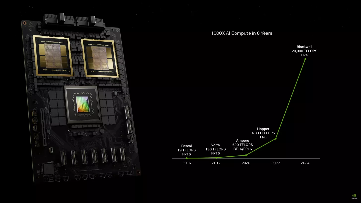
From the perspective of training pipeline architecture, GPUs address several key bottlenecks. The large number of cores in GPUs allows for simultaneous processing of thousands of matrix multiplications, accelerating the forward and backward passes of training. In systems where data throughput limits GPU utilization, prefetching and caching mechanisms help maintain a steady flow of data. These optimizations, previously discussed in training pipeline design, are critical to unlocking the full potential of GPUs (Patterson and Hennessy 2021b).
37 NVIDIA NCCL (Collective Communications Library): Optimized for multi-GPU communication, NCCL achieves 90-95% of theoretical bandwidth on modern interconnects. On DGX systems with NVLink, NCCL can transfer 600 GB/s between 8 GPUs—50x faster than PCIe—making efficient distributed training possible. It implements optimized AllReduce algorithms that reduce communication from O(n²) to O(n).
38 GPT-3 Training Scale: Used 10,000 NVIDIA V100 GPUs for 3-4 months, consuming an estimated 1,287 MWh of energy (roughly equivalent to 120 US homes for a year). The training cost was estimated at $4-12 million (varying by infrastructure and energy costs), demonstrating how specialized hardware and distributed systems enable training at previously impossible scales while highlighting the enormous resource requirements.
In distributed training systems, GPUs enable scalable strategies such as data parallelism and model parallelism. NVIDIA’s ecosystem, including tools like NCCL37 for multi-GPU communication, facilitates efficient parameter synchronization, a frequent challenge in large-scale setups. For example, in training large models like GPT-338, GPUs were used in tandem with distributed frameworks to split computations across thousands of devices while addressing memory and compute scaling issues (Brown et al. 2020).
Hardware-specific features further enhance GPU performance. NVIDIA’s tensor cores39, for instance, are optimized for mixed-precision training, which reduces memory usage while maintaining numerical stability (Micikevicius et al. 2017). This directly addresses memory constraints, a common bottleneck in training massive models. Combined with software-level optimizations like fused kernels, GPUs deliver substantial speedups in both single-device and multi-device configurations.
39 Tensor Cores: Introduced with NVIDIA’s Volta architecture (2017), Tensor Cores deliver 4x speedup for mixed-precision training by performing 4x4 matrix operations in a single clock cycle. The H100’s 4th-gen Tensor Cores achieve 989 TFLOPS for FP16 operations—roughly 6x faster than traditional CUDA cores—enabling training of larger models with the same hardware budget.
A case study that exemplifies the role of GPUs in machine learning training is OpenAI’s use of NVIDIA hardware for large language models. Training GPT-3, with its 175 billion parameters, required distributed processing across thousands of V100 GPUs. The combination of GPU-optimized frameworks, advanced communication protocols, and hardware features enabled OpenAI to achieve this ambitious scale efficiently (Brown et al. 2020). The privacy and security implications of such large-scale training—including data governance and model security—are addressed integratedly in Chapter 15: Security & Privacy.
Despite their advantages, GPUs are not without challenges. Effective utilization of GPUs demands careful attention to workload balancing and inter-device communication. Training systems must also consider the cost implications, as GPUs are resource-intensive and require optimized data centers to operate at scale. However, with innovations like NVLink and CUDA-X libraries40, these challenges are continually being addressed.
40 CUDA Programming Model: Introduced by NVIDIA in 2007, CUDA (Compute Unified Device Architecture) transformed GPUs from graphics processors into general-purpose parallel computing platforms. Unlike CPU programming with 4-16 cores, CUDA enables programming thousands of lightweight threads (32 threads per “warp”). ML frameworks like PyTorch and TensorFlow abstract away CUDA complexity, but understanding concepts like memory coalescing, shared memory, and occupancy remains crucial for optimizing custom ML operations.
GPUs are indispensable for modern machine learning training systems due to their versatility, scalability, and integration with advanced software frameworks. The architectural principles discussed here extend beyond training to influence inference deployment strategies, as detailed in Chapter 11: AI Acceleration, where similar parallelization concepts apply to production environments. By addressing key bottlenecks in computation, memory, and distribution, GPUs play a foundational role in enabling large-scale training pipelines.
Hardware selection significantly impacts GPT-2 training economics and timeline. This comparison shows real-world performance differences.
Training Throughput (samples/second)
| GPU Generation | FP32 | FP16 (Mixed Precision) | Memory | Cost/hour |
|---|---|---|---|---|
| V100 (2017) | 90 | 220 | 32GB | $3.06 |
| A100 (2020) | 180 | 450 | 80GB | $4.10 |
| H100 (2022) | 320 | 820 | 80GB | $8.00 |
Training Time to 50K Steps (8 GPUs)
- V100: 14 days, cost: approximately $10,252
- A100: 7 days, cost: approximately $6,877
- H100: 3.5 days, cost: approximately $6,720
Note: Cloud pricing varies significantly and changes frequently by provider.
Key Hardware-Driven Tradeoffs
- Memory capacity enables larger batches: V100’s 32GB limits batch_size=16, while A100’s 80GB allows batch_size=32 → faster convergence
- Tensor Core generations: H100’s 4th-gen Tensor Cores provide 3.7× speedup over V100 for FP16 operations
- NVLink bandwidth: H100’s 900 GB/s (vs V100’s 300 GB/s) reduces gradient synchronization time by 65%
Why H100 Wins Despite Higher $/hour
- Total cost lower due to 4× faster training
- Frees GPUs for other workloads sooner
- Reduced energy consumption (3.5 vs 14 days runtime)
Hardware Selection Heuristic: For models like GPT-2 where training runs take days/weeks, newer GPUs with higher throughput typically offer better total cost of ownership despite higher hourly rates. For quick experiments (<1 hour), older GPUs may be more cost-effective.
TPUs
Tensor Processing Units (TPUs) and other custom accelerators have been purpose-built to address the unique challenges of large-scale machine learning training. Unlike GPUs, which are versatile and serve a wide range of applications, TPUs are specifically optimized for the computational patterns found in deep learning, such as matrix multiplications and convolutional operations (Jouppi et al. 2017). These devices mitigate training bottlenecks by offering high throughput, specialized memory handling, and tight integration with machine learning frameworks.
As illustrated in Figure 20, TPUs have undergone significant architectural evolution, with each generation introducing enhancements tailored for increasingly demanding AI workloads. The first-generation TPU, introduced in 2015, was designed for internal inference acceleration. Subsequent iterations have focused on large-scale distributed training, memory optimizations, and efficiency improvements, culminating in the most recent Trillium architecture. These advancements illustrate how domain-specific accelerators continue to push the boundaries of AI performance and efficiency.
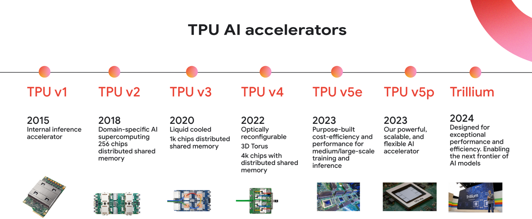
Machine learning frameworks can achieve substantial gains in training efficiency through purpose-built AI accelerators such as TPUs. However, maximizing these benefits requires careful attention to hardware-aware optimizations, including memory layout, dataflow orchestration, and computational efficiency.
Google developed TPUs with a primary goal: to accelerate machine learning workloads at scale while reducing the energy and infrastructure costs associated with traditional hardware. Their architecture is optimized for tasks that benefit from batch processing, making them particularly effective in distributed training systems where large datasets are split across multiple devices. A key feature of TPUs is their systolic array architecture41, which performs efficient matrix multiplications by streaming data through a network of processing elements. This design minimizes data movement overhead, reducing latency and energy consumption—critical factors for training large-scale models like transformers (Jouppi et al. 2017).
41 Systolic Array Architecture: Developed at Carnegie Mellon in 1978, systolic arrays excel at matrix operations by streaming data through a grid of processing elements. Google’s TPU v4 achieves 275 TFLOPS (bfloat16) with ~200W typical power consumption—achieving approximately 1.38 TFLOPS/W efficiency, roughly 2-3x more energy-efficient than comparable GPUs for ML workloads.
From the perspective of training pipeline optimization, TPUs simplify integration with data pipelines in the TensorFlow ecosystem. Features such as the TPU runtime and TensorFlow’s tf.data API enable seamless preprocessing, caching, and batching of data to feed the accelerators efficiently (Abadi et al. 2016). TPUs are designed to work in pods—clusters of interconnected TPU devices that allow for massive parallelism. In such setups, TPU pods enable hybrid parallelism strategies by combining data parallelism across devices with model parallelism within devices, addressing memory and compute constraints simultaneously.
TPUs have been instrumental in training large-scale models, such as BERT and T5. For example, Google’s use of TPUs to train BERT demonstrates their ability to handle both the memory-intensive requirements of large transformer models and the synchronization challenges of distributed setups (Devlin et al. 2018). By splitting the model across TPU cores and optimizing communication patterns, Google achieved excellent results while significantly reducing training time compared to traditional hardware.
Beyond TPUs, custom accelerators such as AWS Trainium and Intel Gaudi chips are also gaining traction in the machine learning ecosystem. These devices are designed to compete with TPUs by offering similar performance benefits while catering to diverse cloud and on-premise environments. For example, AWS Trainium provides deep integration with the AWS ecosystem, allowing users to seamlessly scale their training pipelines with services like Amazon SageMaker.
While TPUs and custom accelerators excel in throughput and energy efficiency, their specialized nature introduces limitations. The trade-offs between specialized hardware performance and deployment flexibility become particularly important when considering edge deployment scenarios, as explored in Chapter 14: On-Device Learning. TPUs, for example, are tightly coupled with Google’s ecosystem, making them less accessible to practitioners using alternative frameworks. Similarly, the high upfront investment required for TPU pods may deter smaller organizations or those with limited budgets. Despite these challenges, the performance gains offered by custom accelerators make them a compelling choice for large-scale training tasks.
TPUs and custom accelerators address many of the key challenges in machine learning training systems, from handling massive datasets to optimizing distributed training. Their unique architectures and deep integration with specific ecosystems make them powerful tools for organizations seeking to scale their training workflows. As machine learning models and datasets continue to grow, these accelerators are likely to play an increasingly central role in shaping the future of AI training.
FPGAs
Field-Programmable Gate Arrays (FPGAs) are versatile hardware solutions that allow developers to tailor their architecture for specific machine learning workloads. Unlike GPUs or TPUs, which are designed with fixed architectures, FPGAs can be reconfigured dynamically, offering a unique level of flexibility. This adaptability makes them particularly valuable for applications that require customized optimizations, low-latency processing, or experimentation with novel algorithms.
Microsoft had been exploring the use of FPGAs for a while, as seen in Figure 21, with one prominent example being Project Brainwave. This initiative uses FPGAs to accelerate machine learning workloads in the Azure cloud. Microsoft chose FPGAs for their ability to provide low-latency inference (not training) while maintaining high throughput. This approach benefits scenarios where real-time predictions are critical, such as search engine queries or language translation services. By integrating FPGAs directly into their data center network42, Microsoft has achieved significant performance gains while minimizing power consumption.
42 Microsoft FPGA Deployment: Project Catapult deployed FPGAs across Microsoft’s entire datacenter fleet by 2016, with one FPGA per server (>1 million total). This $1 billion investment improved Bing search latency by 50% and Azure ML inference by 2x, while reducing power consumption by 10-15% through specialized acceleration of specific algorithms.
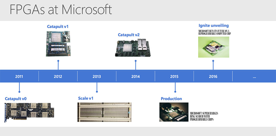
From a training perspective, FPGAs offer unique advantages in optimizing training pipelines. Their reconfigurability allows them to implement custom dataflow architectures tailored to specific model requirements. While this training-focused customization differs from the inference-oriented FPGA applications more commonly deployed, both approaches use the flexibility that distinguishes FPGAs from fixed-function accelerators. For instance, data preprocessing and augmentation steps, which can often become bottlenecks in GPU-based systems, can be offloaded to FPGAs, freeing up GPUs for core training tasks. FPGAs can be programmed to perform operations such as sparse matrix multiplications, which are common in recommendation systems and graph-based models but are less efficient on traditional accelerators (Putnam et al. 2014).
In distributed training systems, FPGAs provide fine-grained control over communication patterns. This control allows developers to optimize inter-device communication and memory access, addressing challenges such as parameter synchronization overheads. For example, FPGAs can be configured to implement custom all-reduce algorithms for gradient aggregation, reducing latency compared to general-purpose hardware.
Despite their benefits, FPGAs come with challenges. Programming FPGAs requires expertise in hardware description languages (HDLs) like Verilog or VHDL, which can be a barrier for many machine learning practitioners. To address this, frameworks like Xilinx’s Vitis AI and Intel’s OpenVINO have simplified FPGA programming by providing tools and libraries tailored for AI workloads. However, the learning curve remains steep compared to the well-established ecosystems of GPUs and TPUs.
Microsoft’s use of FPGAs highlights their potential to integrate seamlessly into existing machine learning workflows. This approach demonstrates the versatility of FPGAs, which serve different but complementary roles in training acceleration compared to their more common application in inference optimization, particularly in edge deployments. By incorporating FPGAs into Azure, Microsoft has demonstrated how these devices can complement other accelerators, optimizing end-to-end pipelines for both training and inference. This hybrid approach uses the strengths of FPGAs for specific tasks while relying on GPUs or CPUs for others, creating a balanced and efficient system.
FPGAs offer a compelling solution for machine learning training systems that require customization, low latency, or novel optimizations. While their adoption may be limited by programming complexity, advancements in tooling and real-world implementations like Microsoft’s Project Brainwave demonstrate their growing relevance in the AI hardware ecosystem.
ASICs
Application-Specific Integrated Circuits (ASICs) represent a class of hardware designed for specific tasks, offering unparalleled efficiency and performance by eschewing the general-purpose flexibility of GPUs or FPGAs. Among the most innovative examples of ASICs for machine learning training is the Cerebras Wafer-Scale Engine (WSE), as shown in Figure 22, which stands apart for its unique approach to addressing the computational and memory challenges of training massive machine learning models.
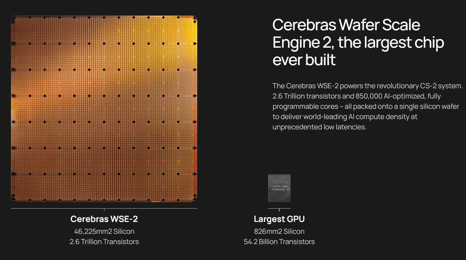
The Cerebras WSE is unlike traditional chips in that it is a single wafer-scale processor, spanning the entire silicon wafer rather than being cut into smaller chips. This architecture enables Cerebras to pack 2.6 trillion transistors and 850,000 cores onto a single device43. These cores are connected via a high-bandwidth, low-latency interconnect, allowing data to move across the chip without the bottlenecks associated with external communication between discrete GPUs or TPUs (Feldman et al. 2020).
43 Wafer-Scale Engine Specifications: The WSE-2 (2021) contains 2.6 trillion transistors on a 21cm x 21cm wafer—the largest chip ever manufactured. With 850,000 cores and 40GB on-chip memory, it delivers 15-20x speedup vs. GPU clusters for large language models while consuming 15kW (comparable to 16-20 V100 GPUs but with orders of magnitude less communication overhead).
From a machine learning training perspective, the WSE addresses several critical bottlenecks:
- Data Movement: In traditional distributed systems, significant time is spent transferring data between devices. The WSE eliminates this by keeping all computations and memory on a single wafer, drastically reducing communication overhead.
- Memory Bandwidth: The WSE integrates 40 GB of high-speed on-chip memory directly adjacent to its processing cores. This proximity allows for near-instantaneous access to data, overcoming the latency challenges that GPUs often face when accessing off-chip memory.
- Scalability: While traditional distributed systems rely on complex software frameworks to manage multiple devices, the WSE simplifies scaling by consolidating all resources into one massive chip. This design is particularly well-suited for training large language models and other deep learning architectures that require significant parallelism.
A key example of Cerebras’ impact is its application in natural language processing. Organizations using the WSE have demonstrated substantial speedups in training transformer models, which are notoriously compute-intensive due to their reliance on attention mechanisms. The responsible deployment of such powerful training capabilities—including considerations of energy consumption, accessibility, and societal impact—is explored in Chapter 17: Responsible AI. By leveraging the chip’s massive parallelism and memory bandwidth, training times for models like BERT have been significantly reduced compared to GPU-based systems (Brown et al. 2020).
However, the Cerebras WSE also comes with limitations. Its single-chip design is optimized for specific use cases, such as dense matrix computations in deep learning, but may not be as versatile as multi-purpose hardware like GPUs or FPGAs. The cost of acquiring and integrating such a specialized device can be prohibitive for smaller organizations or those with diverse workloads.
Cerebras’ strategy of targeting the largest models aligns with previously discussed trends, such as the growing emphasis on scaling techniques and hybrid parallelism strategies. The WSE’s unique design addresses challenges like memory bottlenecks and inter-device communication overhead, making it a pioneering solution for next-generation AI workloads.
The Cerebras Wafer-Scale Engine exemplifies how ASICs can push the boundaries of what is possible in machine learning training. By addressing key bottlenecks in computation and data movement, the WSE offers a glimpse into the future of specialized hardware for AI, where the integration of highly optimized, task-specific architectures unlocks unprecedented performance.
Fallacies and Pitfalls
Training represents the most computationally intensive phase of machine learning system development, where complex optimization algorithms, distributed computing challenges, and resource management constraints intersect. The scale and complexity of modern training workloads create numerous opportunities for misconceptions about performance optimization, resource utilization, and system design choices.
Fallacy: Training larger models always yields better performance.
This widespread belief drives teams to continuously scale model size without considering the relationship between model capacity and available data. While larger models can capture more complex patterns, they also require exponentially more data and computation to train effectively. Beyond certain thresholds, increasing model size leads to overfitting on limited datasets, diminishing returns in performance improvements, and unsustainable computational costs. Effective training requires matching model capacity to data availability and computational resources rather than pursuing size for its own sake.
Pitfall: Assuming that distributed training automatically accelerates model development.
Many practitioners expect that adding more devices will proportionally reduce training time without considering communication overhead and synchronization costs. Distributed training introduces coordination complexity, gradient aggregation bottlenecks, and potential convergence issues that can actually slow down training. Small models or datasets might train faster on single devices than distributed systems due to communication overhead. Successful distributed training requires careful analysis of model size, batch size requirements, and communication patterns to achieve actual speedup benefits.
Fallacy: Learning rate schedules that work for small models apply directly to large-scale training.
This misconception assumes that hyperparameters, particularly learning rates, scale linearly with model size or dataset size. Large-scale training often requires different optimization dynamics due to gradient noise characteristics, batch size effects, and convergence behavior changes. Learning rate schedules optimized for small-scale experiments frequently cause instability or poor convergence when applied to distributed training scenarios. Effective large-scale training requires hyperparameter adaptation specific to the scale and distributed nature of the training environment.
Pitfall: Neglecting training reproducibility and experimental tracking.
Under pressure to achieve quick results, teams often sacrifice training reproducibility by using random seeds inconsistently, failing to track hyperparameters, or running experiments without proper versioning. This approach makes it impossible to reproduce successful results, compare experiments fairly, or debug training failures. Complex distributed training setups amplify these issues, where subtle differences in device configuration, data loading order, or software versions can create significant result variations. Systematic experiment tracking and reproducibility practices are essential engineering disciplines, not optional overhead.
Pitfall: Underestimating infrastructure complexity and failure modes in distributed training systems.
Many teams approach distributed training as a straightforward scaling exercise without adequately planning for the infrastructure challenges that emerge at scale. Distributed training systems introduce complex failure modes including node failures, network partitions, memory pressure from unbalanced load distribution, and synchronization deadlocks that can cause entire training runs to fail hours or days into execution. Hardware heterogeneity across training clusters creates performance imbalances where slower nodes become bottlenecks, while network topology and bandwidth limitations can make communication costs dominate computation time. Effective distributed training requires robust checkpoint and recovery mechanisms, load balancing strategies, health monitoring systems, and fallback procedures for handling partial failures. The infrastructure must also account for dynamic resource allocation, spot instance interruptions in cloud environments, and the operational complexity of maintaining consistent software environments across distributed workers.
Summary
Training represents the computational heart of machine learning systems, where mathematical algorithms, memory management strategies, and distributed computing architectures converge to transform data into intelligent models. Throughout this chapter, we have seen how the seemingly simple concept of iterative parameter optimization requires careful engineering solutions to handle the scale and complexity of modern machine learning workloads. The operations of forward and backward propagation become orchestrations of matrix operations, memory allocations, and gradient computations that must be carefully balanced against hardware constraints and performance requirements.
Our exploration from single-device training to distributed systems demonstrates how computational bottlenecks drive architectural innovation rather than simply limiting capabilities. Data parallelism enables scaling across multiple devices by distributing training examples, while model parallelism addresses memory limitations by partitioning model parameters across hardware resources. Advanced techniques like gradient accumulation, mixed precision training, and pipeline parallelism showcase how training systems can optimize memory usage, computational throughput, and convergence stability simultaneously. The interplay between these strategies reveals that effective training system design requires deep understanding of both algorithmic properties and hardware characteristics to achieve optimal resource utilization.
This co-design principle—where algorithms, software frameworks, and hardware architectures evolve together—shapes modern training infrastructure. Matrix operation patterns drove GPU Tensor Core development, which frameworks exposed through mixed-precision APIs, enabling algorithmic techniques like FP16 training that further influenced next-generation hardware design. Understanding this feedback loop between computational requirements and system capabilities enables practitioners to make informed architectural decisions that leverage the full potential of modern training systems.
The training optimizations explored throughout this chapter provide the foundation for the model-level efficiency techniques and deployment strategies examined in subsequent chapters. These systems principles extend naturally from training infrastructure to production inference systems, demonstrating how the engineering insights gained from optimizing training workflows inform the broader machine learning system lifecycle.
- Training efficiency depends on optimizing the entire pipeline from data loading through gradient computation and parameter updates
- Distributed training strategies must balance communication overhead against computational parallelism to achieve scaling benefits
- Memory management techniques like gradient checkpointing and mixed precision are essential for training large models within hardware constraints
- Successful training systems require co-design of algorithms, software frameworks, and hardware architectures
These principles and techniques provide the foundation for understanding how model optimization, hardware acceleration, and deployment strategies build upon training infrastructure to create complete machine learning systems. As models continue growing in size and complexity, these training techniques become increasingly critical for making advanced AI capabilities accessible and practical across diverse application domains and computational environments.