Trajectory Planning
11 Trajectory Planning
Purpose
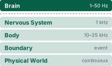
Physical AI stack focus for this chapter.
Why must every motion a robot follows already contain the stop it will probably never use?
A moving robot cannot pause its momentum while a learned policy computes the next piece of its motion. Each new plan must take over from motion already under way. A plan that matches only the arm’s position leaves a jump in velocity or acceleration, which the motors can meet only with a sudden step in torque. A real drive refuses such a step or converts it into vibration, wear, and a spilled load. A path that clears every obstacle can still ask for more joint speed, torque, or current than the body can supply, and the fastest timing along that path demands exactly the abrupt changes a drive cannot make. The next plan can also arrive late, because inference time has a long tail, and a machine that keeps moving while it waits spends the distance it needs to stop. Without trajectory planning, a correct decision about where to go becomes a command the body cannot follow, or motion that cannot be halted in the room that remains. Planning attaches timing, a smooth join to the present state, and a stop that runs without the proposer. Those three properties decide whether a command that crosses the causal boundary can still be brought to rest before its energy reaches something that cannot be undone.
Learning Objectives
- Distinguish prediction horizon, executed prefix, renewal cadence, and evidence age when budgeting trajectory replacement
- Map tool-space speed limits to joint rates through the manipulator Jacobian, explain why the mapping fails near a singularity, and bound an inverse-kinematics step there with damped least squares
- Evaluate a timed trajectory and its time parameterization against actuator torque, current-slew, and voltage limits, including reflected rotor inertia (\(\GearReductionRatio^2 \RotorInertia\))
- Synthesize closed-form quintic spline bridges, anchored at the projected seam state rather than a stale sampled pose, that eliminate acceleration steps and bound commanded jerk across replanning seams
- Size a jerk-limited \(\DifferentiabilityClass^2\) stopping suffix from deceleration and jerk bounds and verify stopping clearance (\(\StoppingDistance \le \ClearDistance\))
- Compare sampling-based search, trajectory optimization, and learned action chunking by the work each performs and the checks its output still requires
- Construct trajectory records whose two-tier deadlines (high-rate chunk lease and hardware commitment cutoff) keep motion out of inevitable collision states (ICS) and support independent per-tick permission decisions
Explore the concepts in this chapter
The volume’s concept map, opened on this chapter. Select a concept to read how it connects to ideas in other chapters. Open the full map ↗
11.1 Continuous Trajectory Generation
The arm of the warehouse mobile manipulator is reaching for a mug that drifts along a moving conveyor when an inference pass is delayed by operating-system scheduling contention. The intent lease still names the mug as a valid target, but a lease grants a target, never a path. A target coordinate paired with an expiration timestamp specifies neither velocity nor acceleration, so it cannot tell the arm what to do while the next pass is late. The arm cannot freeze abruptly, and it cannot extrapolate blind setpoints into space no check has covered. Planning must supply a concrete, time-parameterized path, an admissible transition from the motion already under way, and a precomputed stop that runs even if the next inference pass never returns.
↩︎ The intent lease, whose expiry bounds the validity window of every trajectory, is established in The Intent Lease Specification and Contract.
Classical robotics split this problem into two stages. A search first finds a collision-free geometric path through a configuration space, and a time parameterization then assigns timing that respects kinematic and torque limits. Learned sensorimotor policies change both stages. Instead of searching a static, pre-mapped scene, a policy emits short chunks of future setpoints conditioned directly on live camera observations, and because it replans while the machine moves, each new trajectory must splice into motion already under way rather than start from rest. Neural inference also has variable, heavy-tailed latency, and the hardware keeps moving along its previous trajectory while it waits. Geometric clearance therefore does not settle a plan. A plan must also establish how long the proposed motion remains executable, how it joins the retiring trajectory, and how the machine comes to a controlled stop if later inference passes stall.
On this machine, the arm’s low-level joint tracking loop evaluates feedback and setpoints at 1 kHz (datasheet; see the Reader Guide); however, this high-rate servo clock does not specify the physical stopping response. Above this loop sits the Brain, where learned policies such as Action Chunking with Transformers (ACT) (Zhao et al. 2023) or Diffusion Policy (Chi et al. 2025) process sensory observations on the host application processor to synthesize future reference paths.1 The machine’s chunk policy operates with an illustrative budget of 40 ms per pass at p99, vision included. Even so, memory contention, direct memory access (DMA) traffic, or thread preemption can stretch tail latency beyond 150 ms. The real-time controller therefore cannot block synchronously on policy execution; it requires both buffered nominal motion and an immediately dispatchable, pre-validated stop.
1 Action chunking representations: ACT and Diffusion Policy, the 2023-era chunk policies, carry no boundary-derivative constraints. Real-time chunking (Black et al. 2025) conditions each new chunk on the actions already committed, which makes a consistent join more likely without guaranteeing one, so the planner still proposes a transition bridge across each replanning seam and the permission path checks it before admission.
Black, Kevin, Manuel Y. Galliker, and Sergey Levine. 2025. “Real-Time Execution of Action Chunking Flow Policies.” Advances in Neural Information Processing Systems (NeurIPS).
↩︎ The kinetic energy a trajectory commits, and the stopping distance that energy demands, are established in Kinematic stopping distance and pre-brake delay.
Whether candidate motions originate from sampling-based search, numerical trajectory optimization, or learned action chunking (section 11.6), the generator serves strictly as an unprivileged proposer. Time parameterization exposes instantaneous velocity, acceleration, and jerk to dynamic validation, and the independent safety permission path must verify that motor windings can generate the required torques under dynamic load and that sufficient clearance exists along the arm’s swept stopping volume before any motion is admitted.
↪ The runtime gatekeeper that checks every admitted setpoint against live state is developed in The Per-Tick Gatekeeper.
2 \(\DifferentiabilityClass^2\) continuity at the motor: In permanent-magnet synchronous motors, electromagnetic torque couples directly to quadrature stator current (\(\MotorTorque = \MotorTorqueConstant \TorqueProducingCurrent\)). Under this model an acceleration step requires a finite step in torque and current, while a velocity step implies an ideal acceleration impulse, which no drive can supply.
A multi-step action chunk delivers a finite horizon of future setpoints that the low-level tracking controller consumes sequentially while the proposer computes the next chunk. Splicing successive chunks introduces an execution seam: the temporal and kinematic boundary where the retiring setpoints hand off control to the incoming plan. Matching position alone across this seam leaves a discontinuous velocity step, and matching velocity while neglecting acceleration leaves an instantaneous acceleration step. Because physical links and payloads carry inertia, discontinuous accelerations demand instantaneous steps in motor torque, exciting mechanical vibrations and risking overcurrent faults. The trajectory generator must therefore enforce continuity through position, velocity, and acceleration (the \(\DifferentiabilityClass^2\) continuity condition) while verifying that dynamic torques and swept clearance throughout the transition segment remain within safe physical envelopes.2
Decoupling the execution rate from the inference rate allows the low-level tracking controller to service motor loops on a rigid real-time clock while neural inference runs asynchronously. Setpoint buffering absorbs latency jitter, but buffered motion cannot remain valid indefinitely. Sensor observations age, dynamic obstacles shift, and localization drift accumulates over time. Consequently, the planner’s replacement deadline must account for the worst-case inference tail, guaranteeing sufficient lead time to commit to a feasible, controlled stop before either the buffered trajectory drains or the supporting environmental evidence expires.
Every admitted proposal must therefore arrive as a self-contained bundle: the active trajectory segment continuous through acceleration (\(\DifferentiabilityClass^2\)), its explicit validity deadlines, and a pre-verified stopping suffix whose required deceleration distance fits within verified obstacle clearance (\(\StoppingDistance \le \ClearDistance\)). An isolated safety microcontroller (MCU) inspects and validates this bundle across the proposal boundary before arming actuator outputs, caching the emergency stopping continuation in local real-time memory so it can be autonomously dispatched if communications falter.
The machine meets these obligations in a fixed order. What the planner hands to the tracking controller and the permission path comes first, together with the map from tool coordinates to the joint limits the drives enforce. Replacement timing is then sized against the inference tail, a timed candidate and its seams are checked against what the actuators can follow, and the jerk-limited stop that every admitted plan must carry is sized. The generators that propose candidates, from sampling-based search to learned action chunks, can be compared only after those obligations are fixed.
11.2 The Planning Handoff and the Trajectory Record
If the planner hands over raw joint setpoints for the reach toward the mug without binding them to the obstacle geometry, the active intent lease, and a pre-checked stop, the arm can chase an expired target or coast past its clearance the moment the next inference cycle stalls. To prevent that failure, the planner consumes the belief record, which supplies obstacle geometry and clearance. It also consumes the intent lease, which supplies the grounded goal, task tolerances, effort ceilings, and the expiry time that bounds the lease (\(\IntentLeaseExpiry\)). Throughout, the planner must respect the actuator and transmission limits of the physical body. The handoff connects those inputs to the checks that permit execution, and two things must be fixed before any replacement timing can be budgeted. The first is the map between the tool coordinates in which clearance is measured and the joint coordinates whose limits the drives enforce. The second is the record that carries a candidate across the proposal boundary, with the deadlines and the stop that bound its authority.
↩︎ The belief record and the state invariants it carries are established in The Spatial Memory Handoff and State Invariants.
11.2.1 Mapping tool motion to joint limits
A path that keeps the tool inside its speed limit and clear of obstacles in workspace can still command a joint near a straightened elbow to spin faster than its drive allows, tripping a velocity fault mid-reach. Catching that mismatch requires translating workspace motion into the manipulator’s joint coordinates. A configuration \((\JointPosition_1, \dots, \JointPosition_n)\) collects the joint positions into a single point in the configuration space3 \(\ConfigurationSpace\), and removing configurations occupied by obstacles leaves the collision-free subset \(\FreeConfigurationSpace = \ConfigurationSpace \setminus \ObstacleConfigurationSet\) (Lozano-Pérez 1983). Because a geometric path through \(\FreeConfigurationSpace\) still lacks timing, an executable trajectory assigns physical timestamps to the path, generating continuous state references \(\MechanicalPlantState(\TimeInstant) = [\GeneralizedCoordinates(\TimeInstant)^\top, \GeneralizedVelocities(\TimeInstant)^\top]^\top\) and acceleration profiles \(\GeneralizedAccelerations(\TimeInstant)\) alongside feedforward torque profiles \(\FeedforwardJointTorque(\TimeInstant)\). Whereas the kinematic references state the intended position, velocity, and acceleration, the feedforward terms supply the torque predicted by the rigid-body model. The complete candidate crosses the proposal boundary for independent checking, and only admitted actuator commands cross the causal boundary to the drives.
3 Configuration space: Lozano-Pérez (1983) shrank the moving body to a point by growing each obstacle by the body’s shape, and in the same year Schwartz and Sharir (1983) treated the “piano movers’ problem” as a search of exactly this space. The reduction turns a collision query into a membership test on \(\ObstacleConfigurationSet\), but the space gains a dimension with every joint, which is why collision queries dominate the run time of the sampling planners in section 11.6.
Lozano-Pérez, Tomás. 1983. “Spatial Planning: A Configuration Space Approach.” IEEE Transactions on Computers C-32 (2): 108–20. https://doi.org/10.1109/TC.1983.1676196.
Schwartz, Jacob T., and Micha Sharir. 1983. “On the ‘Piano Movers’ Problem. II. General Techniques for Computing Topological Properties of Real Algebraic Manifolds.” Advances in Applied Mathematics 4 (3): 298–351. https://doi.org/10.1016/0196-8858(83)90014-3.
The drives track joint angles, but clearance is measured in the task space where the tool, the mug, and the conveyor guard sit. In a planar two-link abstraction of the arm’s shoulder, elbow, and wrist with upper-arm length \(\LinkLength_1\) and forearm length \(\LinkLength_2\), forward kinematics gives the tool position directly as a function of the joint angles:
\[\ToolPlanarAbscissa = \LinkLength_1\cos \JointPosition_1 + \LinkLength_2\cos(\JointPosition_1+\JointPosition_2), \qquad \ToolPlanarOrdinate = \LinkLength_1\sin \JointPosition_1 + \LinkLength_2\sin(\JointPosition_1+\JointPosition_2) \tag{1}\]
Differentiating equation 1 gives tool velocity \(\EndEffectorVelocity = \ManipulatorJacobian(\GeneralizedCoordinates)\,\GeneralizedVelocities\), where the manipulator Jacobian4 \(\ManipulatorJacobian = \partial\CartesianPosition/\partial\GeneralizedCoordinates\) changes with configuration. It is the same map that showed, in Kinematic topology mismatches and null-space projection, why a Cartesian action label can force a different arm through a singularity; here it prices the arm’s own reach. For the two-link arm its determinant is \(\LinkLength_1 \LinkLength_2 \sin \JointPosition_2\), which vanishes when the elbow straightens, the singular pose at which no joint motion moves the tool along the arm.
4 Manipulator Jacobian: It is the same object automatic differentiation builds, the matrix of first derivatives of an output with respect to its inputs, here tool position with respect to joint angles. Reverse-mode autograd never forms the matrix; it computes products \(\ManipulatorJacobian^\top\UpstreamGradientVector\), and the manipulator equation uses that same transpose product to map a tool wrench into joint torques (equation 8). A planner is the unusual consumer that must invert \(\ManipulatorJacobian\), and it is the inverse, not the Jacobian, that fails at a singularity.
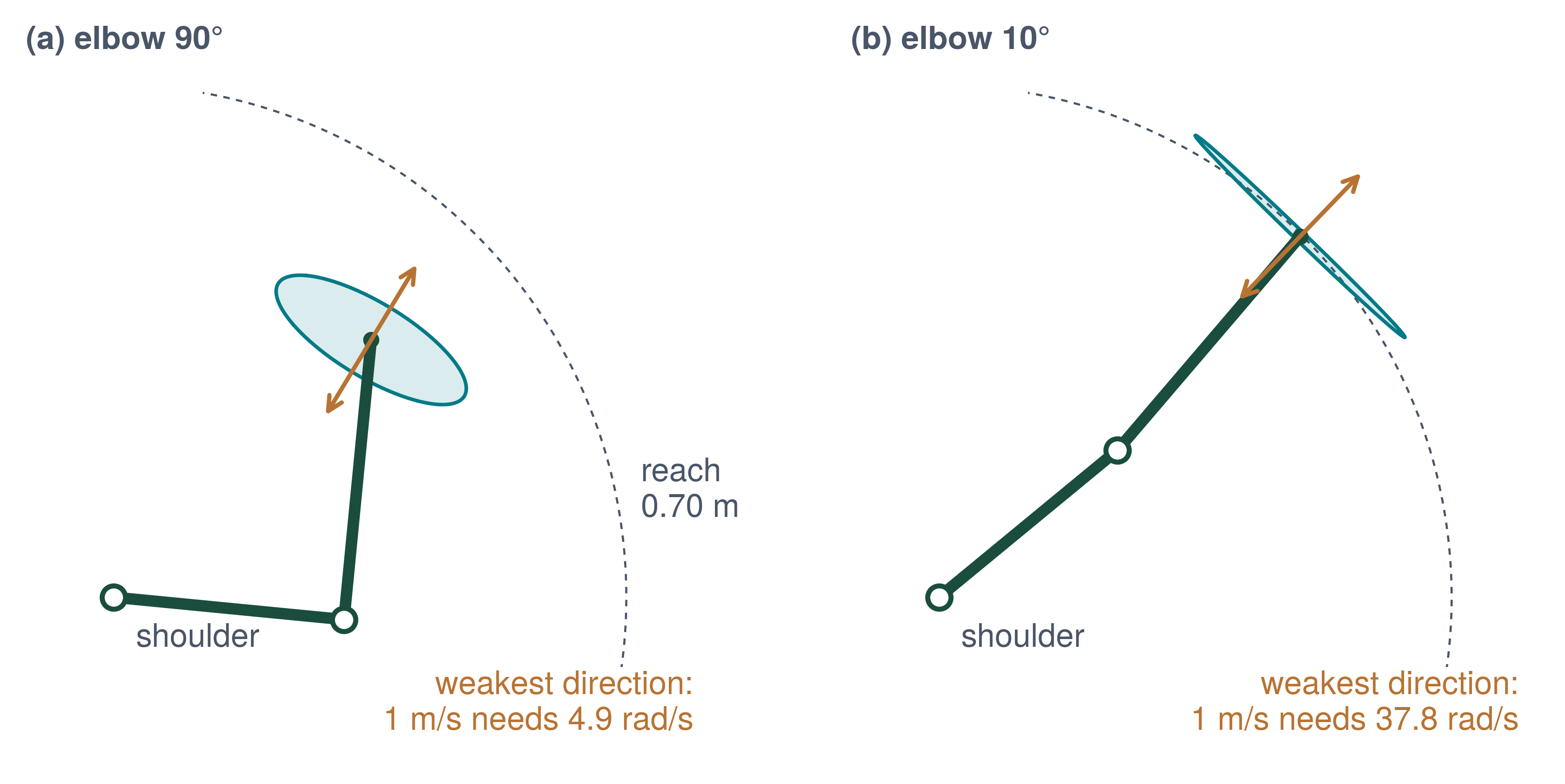
Consider the link lengths from the arm’s published kinematic chain: 0.316 m and 0.384 m, which yield a 0.70 m planar reach (Franka Robotics GmbH 2023). The arm’s weakest direction is the tool direction that a unit of joint rate moves least, set by the smallest singular value \(\SmallestJacobianSingularNumber\) of \(\ManipulatorJacobian\), so that \(\|\GeneralizedVelocities\| = \ToolSpeedLimit/\SmallestJacobianSingularNumber\). Moving the tool in that direction at the 1 m/s tool center point (TCP) limit requires a joint-rate vector of magnitude 4.9 rad/s at a 90° elbow. With two joints, the larger component of a vector is at least its norm divided by \(\sqrt{2}\), so at least one joint must then turn at 3.5 rad/s, above the published 2.175 rad/s limit of the shoulder and elbow joints. Straightening the arm makes the demand far worse. The image of a unit joint-rate circle under \(\ManipulatorJacobian\), the manipulability ellipse of tool velocities, is broad at the 90° elbow and collapses into a narrow sliver across the links at 10° (figure 1). Sustaining 1 m/s along the arm, the ellipse’s minor axis, then needs a joint-rate magnitude of 37.8 rad/s. A tool-speed limit bounds no joint speed near a singularity. Every tool-space quantity this chapter checks (the TCP limit, the stopping distance, and the swept clearance) must therefore be mapped back through \(\ManipulatorJacobian\) to the joint limits the drives enforce. This holds even on a seven-joint arm, whose extra degrees of freedom help the planner steer around singular poses that this planar abstraction omits.
↪ Forward kinematics, the manipulator Jacobian, singularities, and the damped least-squares inverse are developed for \(\JointCount\) joints in Forward kinematics and singularities.
The same map must also run in reverse. A proposal stated in tool space, whether a grasp pose from the intent lease or a Cartesian velocity from a policy or a teleoperation device, leaves the planner to find the joint motion that produces it, the inverse kinematics problem. The two-link arm has a closed-form inverse. A seven-joint arm replanning chunk by chunk is solved by differential steps instead: linearize at the current configuration and solve \(\ManipulatorJacobian\,\FiniteChange\GeneralizedCoordinates = \FiniteChange\CartesianPosition\) for the joint step that moves the tool by \(\FiniteChange\CartesianPosition\), then repeat from the new configuration. Where \(\ManipulatorJacobian\) is invertible the exact step is \(\FiniteChange\GeneralizedCoordinates = \ManipulatorJacobian^{-1}\FiniteChange\CartesianPosition\). Written along the singular directions of \(\ManipulatorJacobian\), this step divides the part of \(\FiniteChange\CartesianPosition\) along each tool direction by that direction’s singular value \(\JacobianSingularNumber\). The weakest direction therefore receives the largest joint step, \(1/\SmallestJacobianSingularNumber\) per unit of tool motion, which is exactly the joint-rate demand that figure 1 charts diverging along the minor axis as the elbow straightens. An exact inverse passes the singularity’s arithmetic straight to the drives.
Damped least squares gives up exactness to bound the step (Wampler 1986; Nakamura and Hanafusa 1986). Instead of demanding \(\ManipulatorJacobian\,\FiniteChange\GeneralizedCoordinates = \FiniteChange\CartesianPosition\), it chooses the joint step that best trades tool error against joint motion, with a damping length \(\InverseKinematicsDamping\) that sets the exchange rate:
Wampler, Charles W., II. 1986. “Manipulator Inverse Kinematic Solutions Based on Vector Formulations and Damped Least-Squares Methods.” IEEE Transactions on Systems, Man, and Cybernetics 16 (1): 93–101. https://doi.org/10.1109/TSMC.1986.289285.
Nakamura, Yoshihiko, and Hideo Hanafusa. 1986. “Inverse Kinematic Solutions with Singularity Robustness for Robot Manipulator Control.” Journal of Dynamic Systems, Measurement, and Control 108 (3): 163–71. https://doi.org/10.1115/1.3143764.
\[\FiniteChange\DampedStepConfiguration = \arg\min_{\FiniteChange\GeneralizedCoordinates} \left(\|\ManipulatorJacobian\,\FiniteChange\GeneralizedCoordinates-\FiniteChange\CartesianPosition\|^2 + \InverseKinematicsDamping^2\|\FiniteChange\GeneralizedCoordinates\|^2\right) = \ManipulatorJacobian^\top\!\left(\ManipulatorJacobian\ManipulatorJacobian^\top+\InverseKinematicsDamping^2\IdentityMatrix\right)^{-1}\FiniteChange\CartesianPosition \tag{2}\]
Setting the gradient of the objective to zero gives \((\ManipulatorJacobian^\top\ManipulatorJacobian+\InverseKinematicsDamping^2\IdentityMatrix)\,\FiniteChange\GeneralizedCoordinates = \ManipulatorJacobian^\top\FiniteChange\CartesianPosition\), and moving \(\ManipulatorJacobian^\top\) through the inverse yields the form in equation 2, which needs only a \(2 \times 2\) solve for the planar arm. A reader who has trained a model will recognize ridge regression, with \(\InverseKinematicsDamping^2\) as the weight-decay coefficient. Along each singular direction the gain changes from \(1/\JacobianSingularNumber\) to \(\JacobianSingularNumber/(\JacobianSingularNumber^2+\InverseKinematicsDamping^2)\). Far from the singularity, where \(\JacobianSingularNumber \gg \InverseKinematicsDamping\), the two agree. As \(\JacobianSingularNumber\) falls toward zero the damped gain falls with it instead of diverging, and it never exceeds \(1/(2\InverseKinematicsDamping)\), reached where \(\JacobianSingularNumber = \InverseKinematicsDamping\). The damping thus places a configuration-independent ceiling on the joint step, which no choice of pose can breach.
With an illustrative \(\InverseKinematicsDamping\) of 50 mm, the weakest-direction request at the 1 m/s TCP limit needs 4.6 rad/s of joint rate at the 90° elbow, against 4.9 rad/s undamped, and the tool still realizes 94.3 percent of the requested motion. At the 10° elbow the damped command is 8.3 rad/s instead of 37.8 rad/s, and no pose can demand more than 10 rad/s. The price is paid where the damping acts: the tool realizes only 21.9 percent of the requested motion along the arm, so the step lags its target in exactly the direction the arm cannot move well. That residual is a tracking error the planner must carry into the trajectory’s timing and clearance checks rather than discard. A larger \(\InverseKinematicsDamping\) lowers the ceiling and enlarges the error everywhere, which is why practical solvers raise the damping only as \(\SmallestJacobianSingularNumber\) approaches it.
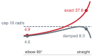
As the elbow straightens, the exact inverse climbs from 4.9 rad/s to 37.8 rad/s; damping caps it at 10 rad/s.
Damping bounds the inverse-kinematics step; it does not make the step feasible. Even the damped 8.3 rad/s exceeds the 2.175 rad/s joint limit, so the planner must still slow the tool through time parameterization (section 11.4.5), and the permission path still checks every joint rate against the limits the drives enforce. Damped least squares is a better proposal, not a permission.
11.2.2 The trajectory record and its deadlines
If a candidate trajectory crosses from the planner to the controller without an immutable expiration time and a pre-checked stop, a hung host process leaves the drives tracking the last command into an obstacle. What the planner hands over is therefore a trajectory record, the ninth record in the record chain and the immutable proposal that the tracking controller follows and the permission path admits. The trajectory record consumes the geometric obstacle bounds from the belief record and the task target and lease window from the intent lease. It binds an untrusted sequence proposal to checked physical limits across the formal boundary between the unprivileged, asynchronous Brain and the deterministic, hard real-time Nervous System. Its header names its coordinate frame \(\TrajectoryRecordFrame\), evidence time \(\EvidenceEpoch\), initial reference state, and active intent lease expiry \(\IntentLeaseExpiry\). The header also carries four deadlines defined in the MCU monotonic clock domain (into which host and sensor timestamps are converted with a bounded synchronization error). Nominal tracking begins at \(\TrackingStartInstant\), the nominal setpoints end at \(\NominalPlanExpiry\), the matched stop must physically begin at \(\CommitmentInstant\), and the admitted stop finishes at \(\StopCompletionInstant\). Beside these header fields, an assumption sidecar declares the payload, friction, obstacle-map epoch, and other conditions under which the candidate was checked (section 11.8). Within the planner itself, each replacement is scheduled against an earlier internal milestone, the blend deadline \(\BlendDeadline\), by which a preferred successor should clear validation. The latest replacement-admission decision on the MCU precedes physical stop onset at \(\CommitmentInstant\) by the reserved decision, transport, and actuator delay.
The permission path permits nominal TRACK only while the intent lease and trajectory record remain valid, so an expired intent lease terminates nominal tracking immediately, regardless of what the trajectory’s own timestamps allow. To manage asynchronous inference latency tails and hardware faults without compromising safety, the architecture enforces a strict two-tier deadline hierarchy:
- Fast Nervous System periodic chunk lease (\(\ChunkLease\), 60 ms): This high-rate heartbeat governs the real-time execution contract between Brain and Nervous System. The chunk policy proposes base velocity and arm joint targets together, so one chunk lease governs both bodies, and only an admitted replacement chunk renews it, with a desired admission interval of 50 ms on this machine. Qualification must bound successful-admission interarrival, not merely inference or request cadence. If an upstream inference pass hangs or communication drops, the lease lapses 10 ms after its expected renewal, immediately requesting a controlled stop whose onset follows the reserved response delay.
- Trajectory commitment deadline: The record names the latest physical onset of its matched stop. Replacement admission must close early enough to dispatch that stop and absorb actuator response delay. This geometric limit does not replace the running machine’s shorter chunk lease; the later worked timeline examines an explicitly different, longer-lease configuration.
↩︎ The chunk lease and its sizing from the stopping budget are established in Chunk Lease Sizing from the Stopping Budget.
Two stopping responses back these deadlines. A matched stop suffix, latched at admission, begins at \(\CommitmentInstant\) if no successor has been admitted; a state-matched fallback, built from the measured state, answers any earlier invalidation, such as a lapsed lease (section 11.5.1). Either stop remains authorized after nominal tracking expires, provided its own state, clearance, sensing, and drive-energy premises still hold.
Definition 11.1: Stopping suffix
Stopping suffix is the bounded continuation, checked and latched with a trajectory at admission, that brings the machine from a declared entry state to rest along the already-checked path, within the clearance that remains and without further input from the proposer.
- Significance: It is the term that makes \(\StoppingDistance \le \ClearDistance\) checkable before motion begins. From the arm’s 1 m/s TCP limit, the worked suffix sized in section 11.5.2 travels 137.5 mm of an illustrative 300 mm of clearance, the free distance along the checked path between the tool and the nearest obstacle. The stop alone therefore claims nearly half the room before any response delay is charged.
- Distinction: The matched suffix is anchored at the nominal state expected at \(\CommitmentInstant\); the state-matched fallback is built from the measured state when authority ends earlier. Both are controlled stops along the checked path, unlike a drive inhibit or brake, whose motion is not planned.
- Common pitfall: Treating the last nominal setpoint, or a hold at the final position, as the stop. A hold is not a deceleration profile, and a suffix sized with constant deceleration understates the distance any drive that ramps its deceleration will travel.
The two execution consumers read distinct subsets of the trajectory record. The downstream tracking controller interpolates admitted setpoints, timestamps, and feedforward torque terms to drive the motor inverters along a continuous profile fetched from the real-time execution jitter buffer. Simultaneously, the independent permission path inspects the record’s lineage, timing bounds, dynamic assumptions, validity envelopes, and verified stopping continuation (\(\StoppingDistance \le \ClearDistance\)). The permission path monitors current limits and physical tracking error on every millisecond tick without inheriting the planner’s feasibility claim as proof. An unmodeled obstacle, payload slip, or contact wrench immediately revokes TRACK authority and activates the state-matched fallback. Because every contract field maps to an explicit hardware or software gate, the Nervous System safely executes fast physical motion without presuming that subsequent neural inference cycles will complete on schedule. A record of this kind is short-lived by design, so the next constraint is how often a successor must arrive and how long producing one takes.
11.3 Replacement Timing and the Planning Horizon
On the mug reach, the arm needs an admitted replacement every 50 ms and loses tracking authority 60 ms after the last one. Whether a replacement can arrive that often depends on how long it takes to produce one, and producing one is more than a single inference pass. The observation behind the candidate must be captured, the proposer must run, and the candidate must cross to the safety MCU and pass validation before it is admitted. Every generator, from numerical trajectory optimization to an autoregressive policy, pays for that pipeline. The timing questions therefore come before the choice of generator: how long a replacement takes, how deep into its latency tail the design must look, how much motion one record must cover, and from which state the next candidate must be planned.
11.3.1 Action chunk horizons and reaction lag
If a replacement chunk takes longer from camera capture to MCU admission than the active chunk’s lease allows, the arm drops into its stopping fallback before the new plan arrives. If the executed prefix is stretched to hide that latency, the arm reacts too slowly when the mug or an obstacle shifts. Sizing the prediction horizon \(\ActionChunkHorizon\) therefore starts from an end-to-end latency budget for replacement, one that spans host accelerator memory, the inter-processor link, and real-time microcontroller firmware.
The scheduling metric that governs every handoff is replacement latency \(\ReplacementLatency\): the total elapsed wall-clock time from the initial physical capture of the sensor observation on which a candidate trajectory proposal rests to the formal admission of that proposal into the real-time execution queue. Formulated in the event taxonomy of The capture-to-brake-onset timing budget of the running machine, \(\ReplacementLatency\) spans the interval from capture to admission. It is the direct sum of two intervals. The first is the capture-to-dispatch perception age \(\DispatchObservationAge\) established in The latency waterfall. The second is the dispatch-to-admission interval \(\DispatchAdmissionInterval\), a design allocation whose stages are listed next and which The board-link budget and the dispatch-to-admission interval later tests against the hardware: \[\ReplacementLatency = \underbrace{\DispatchObservationAge}_{\text{capture}\,\to\,\text{dispatch}} + \underbrace{\DispatchAdmissionInterval}_{\text{dispatch}\,\to\,\text{admission}}, \qquad \DispatchAdmissionInterval = \ProposerInferenceTime + \ProposalLinkTransportTime + \ProposalDeserializationTime + \CombinedPlanValidationAllowance + \ActivationStagingTime + \PermissionTickWaitTime \tag{3}\] On the physical machine, sensor data is already 51.6 ms old when planning dispatches. The subsequent dispatch-to-admission allocation \(\DispatchAdmissionInterval\) of 63.3 ms accounts for the chunk policy’s full 40 ms neural network forward pass and 18 ms of whole-plan kinematic validation. The balance is a few milliseconds of inter-board link transport, message deserialization, activation staging, and synchronization wait until the next discrete permission tick. The board-link budget and the dispatch-to-admission interval itemizes this balance when it tests the allocation on the selected hardware. These stages combine to yield an overall replacement latency \(\ReplacementLatency\) of 114.9 ms. \(\ReplacementLatency\) is a latency, not a period. It exceeds both the 50 ms renewal period and the 60 ms lease, so the renewal cadence can be sustained only by overlapping requests, several in flight at once, a throughput condition the timeline below returns to. Charging the entire neural inference pass after dispatch intentionally bills the visual encoding stage twice, since that stage is already inside \(\DispatchObservationAge\), which makes the budget deliberately conservative. When pipelined stages execute concurrently or contend for shared memory buses, the sum of independent stage percentiles does not equal the percentile of the sum (The end-to-end sense-to-actuation latency pipeline). Sizing the planning horizon therefore demands evaluating the empirical end-to-end distribution of \(\ReplacementLatency\), measured directly between physical sensor capture interrupts and microcontroller admission timestamps.
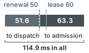
A 114.9 ms replacement path outlasts the 50 ms renewal, so requests must overlap.
Trajectory validation represents the motion planner’s dedicated compute contribution within this latency budget. The 18 ms validation allowance covers the combined elapsed contribution of host geometry validation and bounded local MCU admission, including scheduling delays, rather than overhead silently absorbed into the millisecond actuator tick. Its split between processors remains to be qualified. Formal admission requires bounded staging memory, candidate spline and stopping coefficients, and qualified local clearance evidence; the host processor’s full, multi-gigabyte scene representation need not reside on the embedded MCU. The real-time scheduler must preserve deterministic per-tick enforcement while background admission executes, refreshing the seam boundary check immediately prior to commitment. System architects must allocate and qualify this compute and memory footprint under worst-case shared-bus interference. Because each term in equation 3 represents an illustrative design allocation, neither \(\ReplacementLatency\) nor its constituent stages serve as unverified static bounds; both intervals remain explicit qualification obligations on the physical hardware.
Prediction length and execution duration are separate architectural parameters. While the prediction horizon \(\ActionChunkHorizon\FiniteChange \TimeInstant\) specifies how far into the future the sequence proposer forecasts, the executed prefix represents only the initial slice dispatched to actuators before an admitted replacement plan supersedes it. Expanding the prediction horizon supplies candidate continuity well past the next planned handoff, but does not grant the robot authority to execute that trajectory unchecked. The production controller targets an admitted renewal every 50 ms, enforcing hard lease expiry at 60 ms following the most recent admission. The evidence horizon of the upstream target observation can be shorter still.
Compute amortization depends strictly on inference dispatch frequency rather than the raw number of future setpoints generated in a forward pass. Executing a longer trajectory prefix lowers invocation frequency and amortizes accelerator workload, yet it simultaneously inflates closed-loop reaction lag, delaying task corrections when the environment drifts. Conversely, predicting farther into the future while maintaining a high renewal rate increases proposer compute without reducing inference duty. Emergency protective stopping remains governed by an independent hardware permission path and its certified reaction latency. Sizing the prediction horizon therefore balances closed-loop reactivity, pipeline renewal throughput, sensor evidence freshness, and fallback transition rates under realistic system loads; no universal optimal horizon emerges from trajectory buffer capacity alone.
↩︎ Action chunking as a supply lever is established in Action chunking.
11.3.2 Tail latency budgeting across a mission
When the resident fallback works as certified, a late replacement costs availability rather than safety. A missed replanning deadline becomes a collision hazard only if the resident stop is kinematically infeasible, corrupted in memory, or delayed beyond its budgeted stopping distance. Over a long mission, however, the number of handoffs makes tail latency decide whether the mission completes,5 even when a stopping profile safely absorbs every individual miss. The analysis below therefore bounds how often handoffs miss their deadlines, not how often the machine collides.
5 Tail at scale: Dean and Barroso (2013) showed that a distributed request fanned out across many servers is bottlenecked by the slowest tail response, transforming rare single-server delays into frequent user-facing latencies. A continuous mission comprising thousands of sequential handoffs maps this same fan-out onto the time domain. Because every individual handoff must meet its admission deadline to avoid triggering a stop, the complete mission inherits the worst-case tail latency, rendering conventional per-handoff p99 benchmarks insufficient for assessing end-to-end mission reliability.
Dean, Jeffrey, and Luiz André Barroso. 2013. “The Tail at Scale.” Communications of the ACM 56 (2): 74–80.
The component breakdown in equation 3 defines the latency of a single replacement cycle. Because an autonomous mission executes this handoff cycle repeatedly, the tail of the latency distribution dictates system behavior. A mission requiring \(\MissionHandoffCount\) successive plan handoffs fails its continuous execution target if even one handoff misses its deadline. Partitioning a cumulative mission exceedance budget \(\MissionExceedanceBudget\) uniformly across all \(\MissionHandoffCount\) handoffs yields an upper bound on allowable per-handoff failure probability via the union bound:
\[\HandoffExceedanceProbability \le \frac{\MissionExceedanceBudget}{\MissionHandoffCount} \tag{4}\]
Napkin Math 11.1: Handoff deadlines across a mission
Problem: A generic replanner, slower than this machine’s chunk renewal, meets a p99 replacement budget on each handoff. Over a ten-minute mission, how likely is it that every handoff arrives on time, and what per-handoff tail must the design target instead?
Variables:
- Mission length 600 s and replanning rate 5 Hz (illustrative)
- Per-handoff exceedance of the p99 budget, \(\LateHandoffProbability=0.01\) (definitional)
- Mission exceedance target \(\MissionExceedanceBudget=1 \times 10^{-3}\) (chosen)
- Independent misses (assumption)
Math:
- Handoff count: 600 s \(\times\) 5 Hz gives \(\MissionHandoffCount=3000\), and \(\MissionHandoffCount\LateHandoffProbability=3000\times0.01=30\) handoffs are expected late.
- Every handoff on time: \((0.99)^{3000}\approx8 \times 10^{-14}\).
- Design tail (equation 4): \(\HandoffExceedanceProbability\le\MissionExceedanceBudget/\MissionHandoffCount\approx3.3 \times 10^{-7}\), the \(\text{p99.99997}\) quantile, deeper than the p99 budget by \(0.01/(3.3 \times 10^{-7})\approx3 \times 10^{4}\).
Result: A mission almost never completes with every handoff inside a p99 budget, and the tail a mission target implies lies more than four orders of magnitude deeper.
Systems insight: The quantile a design must target is set by how many handoffs a mission makes, not by the per-handoff budget, and it lies beyond what a test campaign of practical size observes. A late handoff must degrade service availability, not safety clearance. Preserving \(\StoppingDistance \le \ClearDistance\) relies on the resident stop profile (the pre-validated stopping suffix latched in MCU memory at admission and triggered without the host), not on optimistic assumptions about latency tails.
This per-handoff quantile functions as a design quantile target, a risk allocation across the software stack rather than an observed tail latency. In practice, resource contention across shared memory, PCIe buses, and hardware accelerators introduces temporal correlation, clustering deadline misses and violating independent-failure assumptions. Hardware-in-the-loop stress testing under maximum bus and memory saturation can expose deadline misses, but establishing this deep quantile requires a stated statistical model, sufficient observations, and evidence that the operating conditions match. The mission architecture must tolerate fallback frequencies that the available evidence cannot rule out without requiring human intervention.
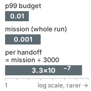
Spread over 3000 handoffs, a mission target demands a \(\text{p99.99997}\) deadline, far past p99.
To maintain continuous tracking, the client dispatches the next planning request at an offset no later than \(\ReplanRequestOffset\) after the active chunk begins executing. Plan admission must complete before a hard decision cutoff that precedes physical commitment \(\CommitmentInstant\) by the actuator response allowance, rather than running up against the final nominal setpoint. Given a replacement-latency quantile target \(\DesignLatencyQuantile(\ReplacementLatency)\) and a safety reserve \(\ReplacementTimingReserve\), a sufficient conservative timing requirement is \(\CommitmentInstant-\TrackingStartInstant\ge \ReplanRequestOffset+\DesignLatencyQuantile(\ReplacementLatency)+\ReplacementTimingReserve\). This requirement charges the complete capture-to-admission quantile after request dispatch, conservatively charging the preceding capture-to-dispatch age again. That extra age charge is separate from the visual-encoding overlap in equation 3. A tighter dispatch-relative requirement would use an independently characterized dispatch-to-admission distribution; subtracting marginal latency quantiles would not establish it. The reserve parameter \(\ReplacementTimingReserve\) includes both scheduling slack before preferred admission and the physical decision-to-onset allowance. Furthermore, executing the resident stop requires an additional time window \(\StoppingDuration\) under dedicated MCU authority. Consequently, the time horizon \(\TrajectoryRecordDuration\) that an admitted trajectory record must cover, whether stored as dense setpoint arrays or polynomial splines, satisfies the corresponding conservative design requirement:
\[\TrajectoryRecordDuration\ge \ReplanRequestOffset+\DesignLatencyQuantile(\ReplacementLatency)+\ReplacementTimingReserve+\StoppingDuration \tag{5}\]
In the baseline warehouse configuration, the chunk policy outputs a discrete setpoint every 25 ms across a 16-step horizon, producing 400 ms of nominal forward trajectory. Under nominal operation, an admitted replacement supersedes this trajectory after 50 ms. If renewal fails, the active lease lapses at 60 ms past the preceding admission tick. Unexecuted setpoints beyond that cutoff serve as candidate references for continuous handoffs rather than extended tracking authority.
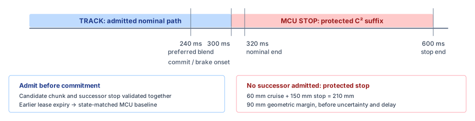
On this running schedule the second tier, the record’s commitment deadline, never acts, because a stalled proposer lets the 60 ms chunk lease lapse long before commitment arrives. To show how a record’s own deadlines coordinate nominal motion with its stop, the worked timeline therefore uses an alternate longer-lease schedule for the same arm, one whose chunk lease is long enough not to lapse before the commitment cutoff. The commitment tier can then be seen on its own. On this schedule the planner issues its request 60 ms after the active chunk begins (later than the running machine’s 50 ms renewal, which only a longer lease permits). It budgets 160 ms as its design-tail replacement latency \(\DesignLatencyQuantile(\ReplacementLatency)\) above the 114.9 ms nominal sum, as a chosen stand-in for the deep quantile that equation 4 implies. It then adds 20 ms of scheduling slack to set a preferred admission deadline at 240 ms. Adding the 22 ms decision-to-onset response allowance to the scheduling slack gives the 42 ms full reserve of equation 5 and a conservative minimum stop onset of 262 ms. Selecting a slightly later physical stopping onset at 300 ms leaves 60 ms between preferred admission and commitment. Replacement admission can therefore close as late as 278 ms (one 22 ms decision-to-onset delay before commitment). The pre-validated 275 ms stopping suffix (section 11.5.2) then brings the arm to rest at 575 ms, provided clearance holds through that entire window.
This alternate profile serves to contrast buffer structure with the production policy. Its window spans 23 setpoint periods, yet it stays compact in memory because the stop is stored as an analytical profile (jerk limits, acceleration limits, and phase durations) rather than as a dense array of setpoints. Set on one time axis, the two schedules spend clearance differently (figure 2). On the running lease, the lease lapses at 60 ms, the tick, bus, and onset allowance delays the resident stop to 82 ms, and the arm uses 219.5 mm of the 300 mm clearance, leaving 80.5 mm. On the alternate schedule, admission must close by 278 ms, after the preferred 240 ms, so that the matched stop begins at the 300 ms commitment and reaches rest at 575 ms with 102.5 mm to spare. The nominal setpoints that run on to 400 ms are never executed.
Sustaining the continuous 50 ms renewal cadence of the running lease requires verifying pipeline throughput alongside latency. Because the illustrative 114.9 ms replacement latency exceeds the 50 ms renewal period, the system must pipeline consecutive planning requests. Pipelining maintains real-time throughput only when intermediate hardware stages provide non-blocking queue capacity and bounded bus arbitration delay; pipelined concurrency cannot be established from latency sums alone. Until comprehensive load testing validates multi-request pipelining under peak bus contention, the specified resident fallback responds to missed renewal only under its stated state, clearance, sensing, energy, drive-response, deceleration, and jerk assumptions.
Both lease architectures remain bounded by the validity lifespan of upstream perceptual evidence. Even when employing a qualified local object tracker, the tracked evidence horizon derived in Expiring Goals and Temporal Validity Leases is shorter than the alternate commitment duration, so a single vision observation of a target object cannot justify that entire duration. Instead, the manipulator uses a staged perceptual approach. It follows an admitted prefix through a certified clear corridor, triggers fresh visual acquisition from a wrist-mounted camera at closer proximity, and re-anchors subsequent trajectory segments to updated state estimates. Embedded firmware then admits the terminal grasp maneuver only when the complete motion profile satisfies current target tolerances within an active validity envelope. Although an overall reaching motion may span several observation cycles, every executed trajectory slice requires fresh evidentiary support. Generating a new trajectory proposal cannot refresh stale sensor evidence, and losing perceptual tracking immediately transitions the robot into a state-matched stopping fallback.
On the Push-T manipulation benchmark (Chi et al. 2025), frequent closed-loop replanning lets an articulated planar arm recover from live disturbances as it guides a T-shaped block toward a designated pose. A diffusion policy generates \(\ActionChunkHorizon = 16\) future steps and executes an initial prefix of \(\ExecutedActionStepCount = 6\) steps before replanning. It recovers dynamically from transient camera occlusions, external block displacements during approach, and perturbations near the terminal pose. However, these empirical trials demonstrate task-level reactive correction rather than certified derivative continuity or deterministic stopping under compute starvation. A safety-critical production system still requires an independently executable stopping suffix verified against known kinematic clearance bounds.
11.3.3 Conditioning on the state at splice time
While a joint rotates at 0.50 rad/s during an illustrative 80 ms compute and transport delay (somewhat longer than the 63.3 ms dispatch-to-admission allocation), a joint pose sampled when the replacement request was dispatched lags the advancing reference by 0.040 rad (2.29°). Mapped through the arm’s forward kinematics (equation 1) at its 0.70 m maximum planar reach, that angular lag displaces the tool center point by up to 28 mm. This is more than the entire lateral swept-volume clearance budgeted for a reach past the conveyor guard (section 11.7.2). That clearance is a sideways allowance, distinct from the 300 mm of free path ahead of the tool that a stop consumes. Conditioning a motion plan on sensor feedback captured when inference begins therefore induces the stale-state paradox. By the time the generative policy completes its forward pass, the physical arm has already advanced along its prior trajectory. Initializing the new plan from the request-time state then commands the actuators to step backward across the distance traversed during computation, which injects step discontinuities into commanded position, velocity, and acceleration. To eliminate boundary discontinuities, the sequence proposer must instead condition its action generation on the forward-projected reference state6 of the active trajectory at the designated replanning seam \(\SeamInstant\):
6 Smith predictor: Smith (1957) handled known dead time in feedback control loops by projecting a plant model forward across the delay interval rather than closing feedback against delayed measurements. Future-state conditioning adapts this idea to trajectory planning by anchoring prospective trajectories to the reference state expected at the handoff seam. It also inherits the weakness of any dead-time predictor: external disturbances during the delay interval go uncompensated until physical feedback arrives, which is why the MCU must check measured joint states against strict error bounds at activation.
Smith, Otto J. M. 1957. “Closer Control of Loops with Dead Time.” Chemical Engineering Progress 53 (5): 217–19.
\[\FiniteChange \ReferenceJointPosition=\int_{t_0}^{\SeamInstant}\RetiringChunkJointVelocity(\TimeInstant)\,d\TimeInstant,\qquad \ProjectedSeamState=\RetiringChunkReferenceState(\SeamInstant) \tag{6}\]
The left-hand integral is the joint-space gap that a stale anchor would leave, the 0.040 rad of the example, while the right-hand state is the anchor the proposer uses instead. Because the projected seam state \(\ProjectedSeamState\) in equation 6 exists strictly in reference trajectory space, external contact forces, mechanical compliance, and closed-loop tracking errors invariably displace the physical plant from this nominal point. Rather than presuming an unobservable future measurement, admission verification prior to the seam evaluates a bounded reachable-state envelope, confirming that feasible polynomial bridges and certified stopping profiles exist across all reachable states within that set. At activation, embedded MCU firmware reads fresh optical encoder measurements and state-estimator error bounds to validate the actual boundary discrepancy \((\FiniteChange \JointPosition, \FiniteChange\JointVelocity, \FiniteChange\JointAcceleration)\) against that certified envelope. It then instantiates the bounded fifth-degree \(\DifferentiabilityClass^2\) bridge of section 11.4.4 and checks its joint-space derivatives against actuator velocity, torque, and jerk limits within the reserved real-time tick before dispatching motor commands. If measured tracking errors or bridge derivatives exceed admitted bounds, the MCU rejects the replacement and maintains the active plan only while its tracking error, target evidence, lease duration, and stopping clearances satisfy safety invariants; otherwise, it triggers the pre-latched fallback profile. Matching two reference profiles guarantees derivative continuity across reference commands, but it never eliminates physical tracking errors in the underlying mechanical hardware.
Recent generative imitation learning architectures incorporate delay compensation directly into their sampling algorithms. Real-time chunking (Black et al. 2025) computes upcoming action sequences concurrently with active chunk execution. Because setpoints scheduled to run during the inference delay window are already committed to the actuator queue, the model fixes those initial steps to their committed values and samples subsequent actions conditioned on this prefix, applying decaying consistency weights across the overlap window. Although empirical evaluations show that control throughput remains stable under artificial latency injection, the formulation provides no formal continuity or stability guarantees. In contrast, bidirectional decoding (Liu et al. 2024) samples a diverse candidate batch of trajectory chunks, scoring and selecting the proposal whose trajectory matches the previously executed actions most smoothly. Conditioning generation on the committed trajectory prefix promotes smooth kinematic transitions and reduces boundary tracking discrepancies, yet it cannot substitute for formal safety verification. Embedded microcontroller logic must still evaluate actual physical states against the admitted safety envelope before committing any new chunk to execution.
Liu, Yuejiang, Jubayer Ibn Hamid, Annie Xie, Yoonho Lee, Maximilian Du, and Chelsea Finn. 2024. “Bidirectional Decoding: Improving Action Chunking via Guided Test-Time Sampling.” arXiv Preprint arXiv:2408.17355.
Definition 11.2: Future-state conditioning
Future-state conditioning is the practice of generating candidate motion plans anchored to the anticipated state at execution time rather than the stale state measured at plan initiation.
- Significance: Offsets computational and transport latency \(\FiniteChange \PlanningStartInstant\), eliminating boundary step discontinuities at trajectory handoffs without forcing zero-velocity pauses between consecutive chunks.
- Distinction: Differs from state estimation or Kalman filtering; it is a forward reference-planning technique that propagates an admitted nominal trajectory rather than filtering sensor noise.
- Common pitfall: Conflating forward-projected reference states with actual physical plant positions. If external contact forces or tracking lag displace the mechanism during planning, activation remains contingent upon the MCU verifying actual encoder feedback and bridge feasibility at the handoff seam.
Trajectory replacement therefore comes down to three sizing decisions. The prediction horizon must be long enough to carry kinematically feasible motion together with a certified stopping profile, the executed prefix short enough to keep closed-loop responses to a changing environment fast, and the renewal cadence one that the pipelined compute can sustain deterministically. Perceptual evidence freshness dictates the maximum lifespan over which any target estimate justifies physical motion. Even when replacement plans arrive strictly within latency budgets, timely delivery alone cannot guarantee that physical joint actuators can track the synthesized trajectory or bridge seamlessly from their measured state.
Checkpoint 11.1: Action chunk horizon and tail latency
Verify your understanding of replacement timing budgets, tail latency exposure, and delay compensation mechanisms before examining kinodynamic feasibility:
11.4 Kinodynamic Feasibility
A candidate trajectory that clears every obstacle in workspace and arrives before its deadline will still fault on the hardware if it asks a joint for more speed, torque, or current slew than the drive can supply. What an embodied model generates is a geometric and timed proposal, not permission to move. While high-level motion planners and learned policies navigate free configuration space \(\FreeConfigurationSpace\), physical actuators operate under fixed electromotive, thermal, and structural limits. Kinodynamic feasibility bridges geometric intent and mechanical reality, ensuring that reference trajectories respect actuator torque limits, velocity boundaries, and transmission dynamics before the low-level controller dispatches setpoints to motor drives.
Definition 11.3: Kinodynamic feasibility envelope
Kinodynamic feasibility envelope is the set of initial states from which the machine can track a candidate trajectory, including its transition seams and terminal stop, while every joint remains within its configured position, velocity, acceleration, jerk (the rate of change of acceleration), torque, and stator current limits.
- Significance: Obstacle clearance in configuration space is necessary but insufficient. At the 1 m/s TCP speed limit, a collision-free reach in the arm’s weakest kinematic direction at a right-angle elbow demands 3.5 rad/s from a single joint against its 2.175 rad/s ceiling. The spatial geometry succeeds while the timing fails. The envelope defines the state region where dynamic models predict trackable motion, which admission and runtime monitors must continuously verify.
- Distinction: Kinematic reachability evaluates whether a mechanism can geometrically achieve a configuration. Kinodynamic feasibility introduces time and momentum: the time derivatives that a trajectory profile implies, the dynamic torques produced through the manipulator equation, the effective inertia reflected through gear trains, and the physical stopping distance required to brake safely.
- Common pitfall: Evaluating feasibility solely at discrete waypoints. The continuous-time interpolant between discrete samples can overshoot velocity bounds or demand severe torque steps even when every discrete sample satisfies constraints.
11.4.1 Rigid-body dynamics and continuous collision checks
A trajectory can stay completely clear of obstacles in \(\FreeConfigurationSpace\) and still fail on the physical machine because it demands actuator torques that saturate motor inverters, induces base accelerations that tip the platform, or drives current slew rates that trip motor protection circuits. Classical kinematic motion planning checked only whether the swept volume avoided obstacles; a moving body with momentum must satisfy configuration-space clearance and time-domain dynamic limits together.
On a single joint, such as the manipulator’s shoulder lifting a grasped payload, the balance of torques obeys the scalar equation of motion:
\[\CommandedJointTorque = \EffectiveJointInertia\,\JointAcceleration + \Mass \Gravity \PayloadLeverArm\cos \JointPosition + \JointFrictionTorque \tag{7}\]
where \(\EffectiveJointInertia\) represents the effective inertia driven by the joint, \(\Mass\) is a concentrated mass whose center of gravity lies at distance \(\PayloadLeverArm\) from the joint axis, \(\JointPosition\) is the joint angle measured from the horizontal plane, and \(\JointFrictionTorque\) is friction torque opposing motion. Mechanical inertia resists angular acceleration, while gravity exerts a static load proportional to the horizontal moment arm \(\PayloadLeverArm\cos \JointPosition\). Holding the rated 3 kg payload horizontally at the manipulator’s full 0.70 m planar reach requires 20.6 N·m of static holding torque, which consumes 23.7 percent of the joint’s 87 N·m torque limit before motion begins (Franka Robotics GmbH 2023). The actuator’s reflected rotor inertia is the \(\GearReductionRatio^2\)-amplified rotor term of Reflected rotor inertia and optimal inertia matching, which the seam analysis below prices for a Panda-class joint. Adding it to the payload inertia produces an effective joint inertia of 1.65 kg·m² that every commanded acceleration must accelerate. Structural link mass and distributed inertia add to this baseline. Because manufacturer datasheets rarely provide link mass distributions, empirical evaluations rely on published identified parameters (Gaz et al. 2019); an operational deployment requires system identification on the physical arm and attached tooling.
Gaz, Claudio, Marco Cognetti, Alexander Oliva, Paolo Robuffo Giordano, and Alessandro De Luca. 2019. “Dynamic Identification of the Franka Emika Panda Robot with Retrieval of Feasible Parameters Using Penalty-Based Optimization.” IEEE Robotics and Automation Letters 4 (4): 4147–54. https://doi.org/10.1109/LRA.2019.2931248.
Craig, John J. 2005. Introduction to Robotics: Mechanics and Control. 3rd ed. Pearson Prentice Hall.
In multi-degree-of-freedom manipulators, dynamic coupling interconnects the joints. The scalar terms generalize into the matrix terms of the manipulator equation, derived from the Euler-Lagrange equations of motion (Craig 2005; Lynch and Park 2017):
\[\JointTorque(\TimeInstant) = \GeneralizedInertiaMatrix(\GeneralizedCoordinates)\GeneralizedAccelerations + \CoriolisCentrifugalMatrix(\GeneralizedCoordinates, \GeneralizedVelocities)\GeneralizedVelocities + \GravitationalTorqueVector(\GeneralizedCoordinates) - \ManipulatorJacobian^\top(\GeneralizedCoordinates)\ExternalWrench \tag{8}\]
Here, the symmetric, positive-definite inertia matrix \(\GeneralizedInertiaMatrix(\GeneralizedCoordinates)\) generalizes scalar inertia \(\EffectiveJointInertia\) from equation 7. Off-diagonal elements capture cross-joint inertial coupling (accelerating the elbow induces reaction torques at the shoulder), and matrix values vary continuously as the arm articulates. The quadratic velocity term \(\CoriolisCentrifugalMatrix(\GeneralizedCoordinates, \GeneralizedVelocities)\GeneralizedVelocities\) aggregates centrifugal and Coriolis torques, which scale quadratically with joint velocity, while the gravity vector \(\GravitationalTorqueVector(\GeneralizedCoordinates)\) generalizes \(\Mass \Gravity \PayloadLeverArm\cos \JointPosition\) to represent configuration-dependent static holding torque. The geometric Jacobian from equation 1 maps an external wrench \(\ExternalWrench\) acting on the end effector into equivalent joint torques via the transpose \(\ManipulatorJacobian^\top(\GeneralizedCoordinates)\); external contact wrenches that assist motion reduce actuator torque demands, while resistive loads increase them. Evaluating equation 8 along a prospective trajectory \(\GeneralizedCoordinates(\TimeInstant)\) is the problem of inverse dynamics. The recursive Newton-Euler algorithm computes inverse dynamics for an \(\JointCount\)-joint serial arm in \(\mathcal{O}(\JointCount)\) arithmetic operations per trajectory sample (Luh et al. 1980; Lynch and Park 2017). An admission filter scanning an \(\TrajectorySampleCount\)-sample candidate trajectory therefore performs \(\mathcal{O}(\TrajectorySampleCount \JointCount)\) operations whose worst-case execution time must fit within the system’s admission latency allowance.
Luh, John Y. S., Michael W. Walker, and Richard P. C. Paul. 1980. “On-Line Computational Scheme for Mechanical Manipulators.” Journal of Dynamic Systems, Measurement, and Control 102 (2): 69–76. https://doi.org/10.1115/1.3149599.
Before dispatching a proposed trajectory chunk, the planning runtime screens it against the kinodynamic feasibility envelope, verifying that the physical state at the handoff seam satisfies position, velocity, torque, stator current, contact force, and collision boundaries over the planning horizon. For robotic arms, the rigid-body model maps joint trajectories \(\GeneralizedCoordinates(\TimeInstant)\), \(\GeneralizedVelocities(\TimeInstant)\), and \(\GeneralizedAccelerations(\TimeInstant)\) to joint torques \(\JointTorque(\TimeInstant)\) via equation 8. Those torques convert to quadrature-axis motor currents \({\TorqueProducingCurrent}_i(\TimeInstant) = \CommandedJointTorque_i(\TimeInstant) / {\JointTorqueConstant}_i\) using the joint-effective torque constant \({\JointTorqueConstant}_i\). (When using motor-side torque constants, the conversion must explicitly incorporate gear ratios and transmission mechanical efficiencies.) Initial screening by an unprivileged planner, however, does not constitute system admission. The real-time safety MCU executes an independent, deterministic verification check, admitting a bounded trajectory chunk only if configured dynamic limits and certified stop clearances hold for the verified initial state. Once admitted, the MCU monitors control tracking error, plan freshness, and stopping distance margins on every servo cycle.
Numerical optimizers can smooth geometric paths and expand obstacle clearance, but motion permission resides strictly in the admitted trajectory chunk and its resident stopping suffix. For example, the cuRobo motion-generation framework uses massively parallel GPU compute to generate collision-free, minimum-jerk trajectories across kinematic configurations (Sundaralingam et al. 2023). Its collision pipeline evaluates signed distance fields across sampled swept-sphere volumes under a linear-motion approximation, leaving continuous inter-sample swept volume evaluation as an open requirement. Following trajectory optimization, cuRobo identifies the limiting time step where joint velocity, acceleration, or jerk encounters actuator bounds, rescaling trajectory duration before re-optimizing. This uniform temporal scaling represents an initial form of the rigorous time parameterization developed in section 11.4.5. Because cuRobo’s algorithmic formulation focuses on kinematic derivatives rather than full multi-body dynamics, torque boundaries, winding thermal accumulation, continuous swept-volume containment, and admission deadlines remain external system-level requirements. Under this systems architecture, the GPU trajectory generator operates as an unprivileged proposer, while the real-time safety MCU independently validates prospective trajectories and seam constraints within a strict admission deadline, latching an executable stopping continuation before authorizing motion.
11.4.2 Overshoot between samples and contracted limits
When the admission filter checks a candidate only at discrete waypoints spaced \(\SamplingPeriod\) apart, two consecutive joint samples \(\TimeInstant_k = \SetpointSampleIndex \SamplingPeriod\) that sit just below the velocity ceiling \(\SpeedBound\) can still bracket an overspeed fault midway between them. The reason is that physical actuators track a continuous interpolant across \((\TimeInstant_k, \TimeInstant_{k+1})\). If that interpolator can command accelerations up to \(\ProfileAccelerationBound\) within a sample period, an acceleration sign reversal across the midpoint lets continuous velocity rise above the values recorded at both endpoints.
Under acceleration-bounded interpolation, the maximum velocity excursion between two consecutive samples sharing equal velocity arises from a bang-bang acceleration reversal: \(+\ProfileAccelerationBound\) applied over \([0, \SamplingPeriod/2]\), followed immediately by \(-\ProfileAccelerationBound\) over \([\SamplingPeriod/2, \SamplingPeriod]\) to restore endpoint velocity. The velocity excursion reaches its maximum at the midpoint, corresponding to the integrated area of the initial acceleration phase:
\[\FiniteChange \JointVelocity = \ProfileAccelerationBound \cdot \frac{\SamplingPeriod}{2} = \frac{1}{2} \ProfileAccelerationBound \SamplingPeriod \tag{9}\]
As equation 9 demonstrates, two consecutive waypoint samples evaluated just beneath velocity ceiling \(\SpeedBound\) can bracket an interior velocity peak that exceeds the limit, tripping drive overspeed protection between individually valid samples. To ensure continuous-time velocity compliance without evaluating an infinite continuum of points, the admission filter tests discrete waypoints against an analytically contracted velocity threshold:
\[|\JointVelocity_k| \le \SpeedBound - \frac{1}{2} \ProfileAccelerationBound \SamplingPeriod \tag{10}\]
The shaded acceleration area in figure 3 becomes the velocity rise between the sampled endpoints. Placing both endpoints one full rise below the physical ceiling keeps the continuous peak at that ceiling.
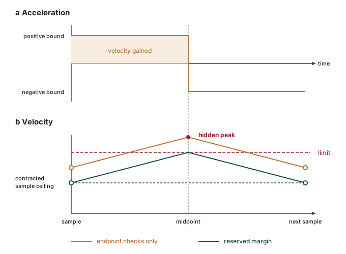
The endpoint check succeeds only when the interpolant obeys the assumptions used to reserve the margin. A sampled value below the physical ceiling alone supplies no such guarantee.
This contraction creates a safety margin that absorbs the worst-case overshoot any acceleration-bounded interpolator can generate across a sample period \(\SamplingPeriod\). A smaller reserve requires additional boundary conditions. If consecutive samples have equal velocity and zero acceleration, and the interpolator enforces \(\JerkLimit \le 4\ProfileAccelerationBound/\SamplingPeriod\), the extremal reversal consists of a positive triangular acceleration pulse followed by its negative counterpart, each of base \(\SamplingPeriod/2\). Their peaks reach \(\ProfileAccelerationBound\) only at equality in the jerk condition, so \(\frac{1}{4} \ProfileAccelerationBound \SamplingPeriod\) is a conservative velocity reserve for this restricted interpolation. A jerk bound alone does not justify that reserve when endpoint accelerations are nonzero. For polynomial spline interpolants, the admission filter can instead compute exact interior extrema analytically before certifying continuous-time feasibility.
11.4.3 Seam acceleration jumps and reflected rotor inertia
When the arm hands off from one action chunk to the next while moving, two chunks that are each feasible in isolation can still form an infeasible seam between them. Matching joint positions alone (\(\DifferentiabilityClass^0\) continuity) leaves an unconstrained velocity step across the boundary. Matching both position and velocity (\(\DifferentiabilityClass^1\) continuity) eliminates velocity jumps but leaves an instantaneous acceleration discontinuity, which demands an immediate step in joint torque. Under a rigid-inertia approximation, commanding a velocity step \(\FiniteChange\JointVelocity\) across a single servo period \(\SamplingPeriod\) requires an inertial torque of:
\[\SeamStepTorque = \EffectiveJointInertia \frac{\FiniteChange\JointVelocity}{\SamplingPeriod} \tag{11}\]
where \(\EffectiveJointInertia = \LoadInertia + \GearReductionRatio^2 \RotorInertia\) in equation 11 represents the total effective inertia referenced to the joint output. This term adds link and payload inertia \(\LoadInertia\) to the reflected rotor inertia established in Reflected rotor inertia and optimal inertia matching, the motor rotor inertia \(\RotorInertia\) seen through gear reduction ratio \(\GearReductionRatio\). Because the rotor turns \(\GearReductionRatio\) times faster than the joint, its kinetic energy, written in joint velocity, carries the factor \(\GearReductionRatio^2\):
\[\KineticEnergy = \frac{1}{2} \RotorInertia \RotorAngularSpeed^2 = \frac{1}{2} \RotorInertia (\GearReductionRatio \JointVelocity)^2 = \frac{1}{2} (\GearReductionRatio^2 \RotorInertia) \JointVelocity^2\]
In precision robotic manipulators equipped with high-ratio strain-wave gearing7 (\(\GearReductionRatio = 50\text{--}100\)), reflected rotor inertia is magnified by a factor of \(2{,}500\) to \(10{,}000\). It can then rival or exceed link inertia, most often for an unloaded arm or a folded pose, although a rated payload held at full reach outweighs it. In the one-joint example the payload supplies most of the 1.65 kg·m² total, against 0.18 kg·m² from the rotor. Either way, the reflected term sits in every joint’s \(\EffectiveJointInertia\) regardless of payload, and on its own it makes seam torque spikes large. At a \(\DifferentiabilityClass^0\) boundary, an instantaneous velocity step implies an idealized Dirac acceleration impulse \(\UnitImpulseFunction(\TimeInstant)\), which no physical motor drive can supply. At a \(\DifferentiabilityClass^1\) boundary, an acceleration jump \(\FiniteChange\JointAcceleration\) demands a step change in electromagnetic torque, \(\FiniteChange\CommandedJointTorque = \EffectiveJointInertia \FiniteChange\JointAcceleration\). Such abrupt torque transients excite structural resonance in flexible transmissions, accelerate mechanical wear, and degrade control tracking. On the strain-wave joint priced in the notebook below, an unblended one-tick velocity step of 0.2 rad/s asks the reflected rotor inertia for a 36.7 N·m torque pulse, while a 50 ms \(\DifferentiabilityClass^2\) quintic bridge closing the same gap peaks at 1.1 N·m (figure 4). Commercial industrial arms enforce this exact discipline at their low-level control interfaces. For example, the Franka Research 3 arm samples setpoints at 1 kHz, comparing each incoming command against the previous cycle. If inter-cycle setpoint differences exceed factory derivative thresholds, the drive immediately aborts motion with an unrecoverable discontinuity fault (such as joint_motion_generator_velocity_discontinuity) (Franka Robotics GmbH 2026, 2023). An unblended seam can therefore abort nominal tracking before repeated transitions accumulate mechanical fatigue. Physical stopping still requires the drive’s qualified response delay and deceleration profile.
7 Strain-wave (harmonic) gearing: In the mechanism Musser (1959) patented, an elliptical wave generator flexes a thin toothed cup, the flexspline, so that it meshes with a rigid ring carrying two more teeth, and each turn of the generator advances the cup by only that difference. The result is a high reduction in one compact stage with almost no backlash. The flexspline is also the joint’s main compliance, so the same gearing that multiplies rotor inertia by \(\GearReductionRatio^2\) supplies the compliant coupling of the two-inertia model below.
Musser, C. Walton. 1959. Strain Wave Gearing. U.S. Patent 2,906,143, filed March 21, 1955, issued September 29, 1959.
Franka Robotics GmbH. 2026. Troubleshooting. Franka Control Interface documentation.
When the arm carries an open cup of liquid, steady velocity does not spill the contents, whereas rapid acceleration transitions and high jerk provoke sloshing and spillage (section 11.5.2 models this deceleration threshold directly). A trajectory interface that continuously matches position, velocity, and acceleration constitutes a \(\DifferentiabilityClass^2\) spline seam. Enforcing \(\DifferentiabilityClass^2\) continuity eliminates reference acceleration steps and prevents the associated torque jump \(\FiniteChange\CommandedJointTorque = \EffectiveJointInertia\FiniteChange\JointAcceleration\). Concurrently, bounding trajectory jerk (\(\JointJerk=\Glyph{\dot{a}}=\dddot{\Glyph{x}}\)) limits the rate at which joint acceleration changes. Neither mathematical property alone guarantees payload stability or mechanical longevity, however; an interpolating bridge that matches boundary conditions perfectly can still violate velocity, jerk, actuator torque, or obstacle clearance limits in its interior.
Mechanical transmissions govern how actuator torque couples into physical link motion. In a standard two-inertia drivetrain comprising load inertia \(\LoadInertia\), reflected rotor inertia \(\ReflectedRotorInertia=\GearReductionRatio^2\RotorInertia\), and torsional coupling stiffness \(\TransmissionTorsionalStiffness\), the antiresonance and resonance frequencies (Li et al. 2024) are:
Li, Peng, Zhenguo Nie, Zihao Li, and Xinjun Liu. 2024. “Optimal Design of the Modular Joint Drive Train for Enhancing Cobot Load Capacity and Dynamic Performance.” Chinese Journal of Mechanical Engineering 37 (1): 57. https://doi.org/10.1186/s10033-024-01041-5.
\[\DrivetrainAntiresonanceFrequency = \frac{1}{2\pi}\sqrt{\frac{\TransmissionTorsionalStiffness}{\LoadInertia}}, \qquad \DrivetrainResonanceFrequency = \frac{1}{2\pi}\sqrt{\TransmissionTorsionalStiffness\left(\frac{1}{\LoadInertia} + \frac{1}{\ReflectedRotorInertia}\right)}\]
In robot joints constructed with strain-wave gearing, large reflected inertia coupled with flexspline torsional compliance amplifies high-frequency setpoint harmonics. An admission checker must therefore verify prospective bridges against the joint’s identified, load-dependent vibrational modes, evaluating derivative extrema, peak torques, and drive current limits against empirical structural parameters. The two frequencies reach the checker through the bridge duration. A short bridge can excite these modes, but duration alone does not determine its spectral content or the joint’s response. Identified modal frequencies and damping therefore inform qualified bridge-duration and derivative limits alongside the torque-rate limit. Structural stiffness, resonance modes, and admissible jerk envelopes never transfer between robot platforms without direct system identification.
11.4.4 Quintic splines and C\(^2\) boundary matching
Closing the position, velocity, and acceleration gap between retiring chunk \(\Glyph{A}\) and incoming chunk \(\Glyph{B}\) over a finite blend duration \(\SeamBridgeDuration\) requires online \(\DifferentiabilityClass^2\) trajectory spline blending. The blend duration is a physical execution interval, distinct from the computational blend deadline \(\BlendDeadline\). Blending synthesizes a dedicated polynomial bridge \(\SeamBridgePosition(\TimeInstant)\), which must undergo the exact same kinodynamic feasibility checks as the primary chunks rather than acting as a cosmetic filter.8 A localized seam bridge must satisfy position, velocity, and acceleration constraints at both boundary states, which gives six independent boundary conditions. A cubic polynomial has only four degrees of freedom and cannot satisfy them. A fifth-degree quintic polynomial provides the six required coefficients. This localized endpoint-matching formulation differs from fitting a globally continuous cubic spline across an entire offline sequence of knots.
8 Minimum jerk: Flash and Hogan (1985) found that unconstrained human reaching follows the trajectory that minimizes integrated squared jerk, which for a rest-to-rest reach is a quintic polynomial in time. The jerk term of equation 20 inherits that smoothness but not a bound, so a minimum-jerk bridge can still exceed the drive’s limits, and its extrema are checked through equation 13.
Flash, Tamar, and Neville Hogan. 1985. “The Coordination of Arm Movements: An Experimentally Confirmed Mathematical Model.” The Journal of Neuroscience 5 (7): 1688–703. https://doi.org/10.1523/JNEUROSCI.05-07-01688.1985.
The six boundary conditions are \[\JointPosition(0) = \JointPosition_0, \quad \JointVelocity(0) = \JointVelocity_0, \quad \JointAcceleration(0) = \JointAcceleration_0\] \[\JointPosition(\SeamBridgeDuration) = \JointPosition_1, \quad \JointVelocity(\SeamBridgeDuration) = \JointVelocity_1, \quad \JointAcceleration(\SeamBridgeDuration) = \JointAcceleration_1\] where \((\JointPosition_0, \JointVelocity_0, \JointAcceleration_0)\) is the terminal physical state of chunk \(\Glyph{A}\) at the seam instant, and \((\JointPosition_1, \JointVelocity_1, \JointAcceleration_1)\) is the target state on incoming chunk \(\Glyph{B}\) at \(\TimeInstant = \SeamBridgeDuration\). The six conditions fix the six coefficients (\(\PolynomialTrajectoryCoefficient_0 \dots \PolynomialTrajectoryCoefficient_5\)) of the fifth-degree polynomial: \[\JointPosition(\TimeInstant) = \PolynomialTrajectoryCoefficient_0 + \PolynomialTrajectoryCoefficient_1 \TimeInstant + \PolynomialTrajectoryCoefficient_2 \TimeInstant^2 + \PolynomialTrajectoryCoefficient_3 \TimeInstant^3 + \PolynomialTrajectoryCoefficient_4 \TimeInstant^4 + \PolynomialTrajectoryCoefficient_5 \TimeInstant^5\]
Evaluating boundary conditions at \(\TimeInstant = 0\) directly yields the first three coefficients: \(\PolynomialTrajectoryCoefficient_0 = \JointPosition_0\), \(\PolynomialTrajectoryCoefficient_1 = \JointVelocity_0\), and \(\PolynomialTrajectoryCoefficient_2 = \frac{1}{2}\JointAcceleration_0\). The remaining three coefficients \([\PolynomialTrajectoryCoefficient_3, \PolynomialTrajectoryCoefficient_4, \PolynomialTrajectoryCoefficient_5]^\top\) satisfy the \(3 \times 3\) linear system evaluated at duration \(\Time = \SeamBridgeDuration\):
\[\begin{bmatrix} \SeamBridgeDuration^3 & \SeamBridgeDuration^4 & \SeamBridgeDuration^5 \\ 3\SeamBridgeDuration^2 & 4\SeamBridgeDuration^3 & 5\SeamBridgeDuration^4 \\ 6\SeamBridgeDuration & 12\SeamBridgeDuration^2 & 20\SeamBridgeDuration^3 \end{bmatrix} \begin{bmatrix} \PolynomialTrajectoryCoefficient_3 \\ \PolynomialTrajectoryCoefficient_4 \\ \PolynomialTrajectoryCoefficient_5 \end{bmatrix} = \begin{bmatrix} \JointPosition_1 - \left(\JointPosition_0 + \JointVelocity_0 \SeamBridgeDuration + \frac{1}{2}\JointAcceleration_0 \SeamBridgeDuration^2\right) \\ \JointVelocity_1 - \left(\JointVelocity_0 + \JointAcceleration_0 \SeamBridgeDuration\right) \\ \JointAcceleration_1 - \JointAcceleration_0 \end{bmatrix} \tag{12}\]
Analytically inverting equation 12 yields closed-form expressions for \([\PolynomialTrajectoryCoefficient_3, \PolynomialTrajectoryCoefficient_4, \PolynomialTrajectoryCoefficient_5]^\top\), given in Smooth Trajectories and Bumpless Transfer, that require deterministic arithmetic operations per joint. Differentiating \(\JointPosition(\TimeInstant)\) three times produces the continuous commanded jerk profile:
\[\JointJerk(\TimeInstant) = \dddot{\JointPosition}(\TimeInstant) = 6 \PolynomialTrajectoryCoefficient_3 + 24 \PolynomialTrajectoryCoefficient_4 \TimeInstant + 60 \PolynomialTrajectoryCoefficient_5 \TimeInstant^2 \tag{13}\]
Because \(\JointJerk(\TimeInstant)\) in equation 13 is a quadratic function of time, its extrema over the interval \([0, \Time]\) occur exclusively at the domain boundaries (\(\TimeInstant = 0\) or \(\TimeInstant = \Time\)) or at the interior stationary point \(\TimeInstant^* = -\PolynomialTrajectoryCoefficient_4 / (5 \PolynomialTrajectoryCoefficient_5)\). The interior point applies when \(\PolynomialTrajectoryCoefficient_5 \ne 0\) and \(\TimeInstant^* \in (0, \Time)\). If \(\PolynomialTrajectoryCoefficient_5 = 0\), jerk varies linearly or remains constant, and evaluating the boundaries alone suffices. The safety microcontroller can therefore compute exact peak jerk \(|\PeakBridgeJerk|\) analytically in \(\mathcal{O}(1)\) operations without executing iterative numerical line searches. An identical principle governs lower derivatives: acceleration extrema occur at the roots of the quadratic jerk, and velocity extrema occur at the roots of cubic acceleration, both solvable in closed form.
Evaluating coupled joint torques across the bridge presents an entirely different challenge. Along a polynomial trajectory \(\GeneralizedCoordinates(\TimeInstant)\), the right-hand side of equation 8 is non-polynomial because the inertia matrix \(\GeneralizedInertiaMatrix(\GeneralizedCoordinates)\), Coriolis matrix \(\CoriolisCentrifugalMatrix(\GeneralizedCoordinates, \GeneralizedVelocities)\), and gravity vector \(\GravitationalTorqueVector(\GeneralizedCoordinates)\) contain transcendental trigonometric functions of joint positions. Consequently, peak torque possesses no closed-form analytic solution. The safety monitor therefore evaluates torque at discrete sample waypoints and bounds inter-sample torque variation using the contraction principles established in section 11.4.2.
Bounding trajectory jerk directly protects actuator health, preserves motor inverter voltage headroom, and prevents premature transmission wear. When a trajectory generator outputs time-parameterized splines, it transforms kinematic waypoints into continuous reference functions whose derivatives map directly onto physical electrical and mechanical states. In permanent-magnet synchronous motors operated under field-oriented control, joint torque rate couples to jerk through the time derivative of the manipulator equation: \(\JointTorqueSlew(\TimeInstant) = \GeneralizedInertiaMatrix(\GeneralizedCoordinates) \dddot{\GeneralizedCoordinates}(\TimeInstant) + \InertiaMatrixDerivative(\GeneralizedCoordinates) \GeneralizedAccelerations(\TimeInstant) + \dots\). For a single joint with constant effective inertia \(\EffectiveJointInertia = \LoadInertia + \GearReductionRatio^2 \RotorInertia\), neglecting changing gravity, friction, and external-load torques reduces the output torque rate to \(\CommandedJointTorqueSlew = \EffectiveJointInertia \JointJerk(\TimeInstant)\). Defining a joint-effective torque constant \(\JointTorqueConstant\) such that output torque satisfies \(\CommandedJointTorque = \JointTorqueConstant \TorqueProducingCurrent\), commanding an output torque rate \(\CommandedJointTorqueSlew\) demands a proportional quadrature-axis stator current slew rate:
\[\frac{d\TorqueProducingCurrent}{d\TimeInstant} = \frac{\EffectiveJointInertia}{\JointTorqueConstant} \JointJerk(\TimeInstant)\]
Here, \(\JointTorqueConstant\) incorporates both the gear reduction ratio and transmission mechanical efficiency; directly substituting a raw motor-side torque constant without gear scaling would incorrectly pair motor torque with output-side inertia. Motor winding inductance \(\PhaseInductance\) and available DC bus voltage impose hard electrical limits on current slew rate. During positive motoring operations with resistive and back-electromotive force (back-EMF) drops, a simplified necessary condition for voltage headroom is:
\[\DcBusVoltage \ge \PhaseInductance \frac{d\TorqueProducingCurrent}{d\TimeInstant} + \PhaseResistance\, \TorqueProducingCurrent + \MotorBackEmfConstant \ElectricalAngularSpeed \tag{14}\]
where \(\PhaseResistance\) represents phase winding resistance, \(\MotorBackEmfConstant\) is the motor back-EMF constant, and \(\ElectricalAngularSpeed\) denotes motor electrical speed. In operational motor drives, space-vector pulse-width modulation limits the maximum usable quadrature-axis voltage to a fraction of the total DC bus voltage. A complete electrical feasibility check must evaluate available voltage against the fully coupled, signed motor equations, including regenerative braking and inductive flyback, rather than treat a scalar approximation as sufficient qualification.
↩︎ Phase inductance, back-EMF, and the current-slew limits they impose are established in Electrical time constants, back-EMF, and current clamping.
An acceleration discontinuity in a motion plan demands an instantaneous step in electromagnetic torque and stator current. Because finite bus voltage and nonzero winding inductance prevent physical inverters from supplying infinite current slew rates (\(d\TorqueProducingCurrent/d\TimeInstant\)), the physical actuator lags the commanded reference. The resulting tracking error, inverter saturation, and thermal protection response depend on drive gains and mechanical compliance. An unbounded mathematical jerk demand does not instantly cause an overcurrent shutdown, but it induces severe tracking lag, mechanical vibration, and drive stress. A valid bridge must satisfy both continuous mathematical derivative bounds and the physical bandwidth limits of the actuator drive.
Satisfying the six boundary conditions guarantees acceleration continuity at chunk interfaces, but it does not guarantee that interior jerk, torque, or current slew rates remain within actuator ratings. The admission filter evaluates closed-form derivative extrema from equation 13 against the electrical constraints of equation 14, checks sampled multi-body torques against inter-sample contraction bounds, and rejects any bridge violating physical thresholds. Evaluating a fixed-degree polynomial requires bounded arithmetic operations per joint. Spline coefficient synthesis and trajectory extrema verification take place prior to trajectory dispatch; the qualified worst-case execution bound, accounting for memory access latency and register operations, must remain strictly within the configured admission deadline.
While a local quintic bridge resolves seam continuity through explicit boundary matching, global trajectory representations provide alternative verification properties. Uniform B-splines9 parameterize joint trajectories as \(\GeneralizedCoordinates(\TimeInstant) = \sum_{i=0}^\SplineFinalControlIndex \SplineControlPoint_i {\BsplineBasisFunction}_{i,\SplineDegree}(\TimeInstant)\), where \(\SplineControlPoint_i\) represent geometric control points, \({\BsplineBasisFunction}_{i,\SplineDegree}\) are polynomial basis functions of degree \(\SplineDegree\), and \(\SplineKnotTime_i\) denote knot timestamps. Using simple knot sequences, uniform B-splines ensure \(\DifferentiabilityClass^{\SplineDegree-1}\) continuity by construction. Furthermore, the convex hull property ensures that the continuous trajectory lies entirely within the convex hull formed by its control points, enabling spatial collision checkers to prune entire collision volumes without dense sampling. Differentiating a B-spline yields a derivative spline whose control points are \(\DerivativeSplineControlPoint_i = \frac{\SplineDegree}{\SplineKnotTime_{i+\SplineDegree+1}-\SplineKnotTime_{i+1}}(\SplineControlPoint_{i+1} - \SplineControlPoint_i)\), allowing difference operations on control points to establish conservative upper bounds on velocity, acceleration, and jerk. These geometric bounds accelerate screening, though they do not replace full dynamic inverse dynamics or swept-volume collision checks. In streaming replanning architectures, the trajectory representation must also support rapid coefficient joining within the real-time admission deadline; table 1 separates the continuity supplied by each representation from the dynamic checks still required before execution.
9 Spline (a draftsman’s bending strip): The word named the thin flexible strip that shipwrights and draftsmen bent through fixed points, held in place by lead weights, to draw a fair curve. Schoenberg (1946) borrowed it for piecewise polynomials, and Boor (1978) made B-splines practical to compute with a stable recursion. The convex-hull property that construction supplies is what lets a checker bound a whole segment’s derivatives from a few control-point differences.
Schoenberg, Isaac J. 1946. “Contributions to the Problem of Approximation of Equidistant Data by Analytic Functions. Part A. On the Problem of Smoothing or Graduation. A First Class of Analytic Approximation Formulae.” Quarterly of Applied Mathematics 4 (1): 45–99. https://doi.org/10.1090/qam/15914.
Boor, Carl de. 1978. A Practical Guide to Splines. Vol. 27. Applied Mathematical Sciences. Springer. https://doi.org/10.1007/978-1-4612-6333-3.
| Representation | Native seam property | Checks before execution |
|---|---|---|
| Cubic polynomial (\(\DifferentiabilityClass^1\)) | Matches \(\JointPosition, \JointVelocity\); adjoining acceleration need not match. | Check acceleration matching and interior limits; position and velocity matching alone are insufficient. |
| Quintic bridge (\(\DifferentiabilityClass^2\)) | Matches \(\JointPosition,\JointVelocity,\JointAcceleration\) at both ends; jerk is quadratic within each bridge. | Check interior extrema, torque rates, inverter headroom, and clearance. |
| Septic polynomial (\(\DifferentiabilityClass^3\)) | Can match derivatives through jerk at both endpoints. | Check interior derivatives and actuator limits; endpoint matching does not bound their magnitudes. |
| Uniform B-spline (degree \(\SplineDegree\)) | \(\DifferentiabilityClass^{\SplineDegree-1}\) continuity; convex hull bounds spatial curve. | Constrain control point differences for velocity/jerk; check global knot system. |
| Neural action chunk (ACT, Diffusion) | Discrete samples; continuity depends on interpolation and seam constraints. | Project onto feasibility manifold via numerical solver or \(\DifferentiabilityClass^2\) quintic bridge; latch stop. |
| Online jerk-limited generator | Reaches a target \((\JointPosition,\JointVelocity,\JointAcceleration)\) from any current state within per-axis \(\SpeedBound\), \(\ProfileAccelerationBound\), \(\JerkLimit\) bounds; the generator picks the duration. | Check coupled torque, clearance, evidence age, and the configured limits themselves; kinematic feasibility by construction is not admission. |
Napkin Math 11.2: The seam spike
Problem: At a replanning seam the incoming chunk’s reference runs 0.2 rad/s faster than the active one. Should the joint close that gap in one servo tick or over a \(\DifferentiabilityClass^2\) bridge, and what does each ask of the drive?
Variables:
- Joint: a CSG-25-50 strain-wave gear driven by a TQ-RoboDrive ILM 70x18 motor, a Panda-class stand-in because Franka does not publish the Panda’s joint internals (datasheet parts); reflected rotor inertia \(\EffectiveJointInertia = \GearReductionRatio^2 \RotorInertia =\) 0.18 kg·m² (derived; link and payload inertia excluded, so here \(\EffectiveJointInertia\) is the reflected inertia \(\ReflectedRotorInertia\) of Reflected rotor inertia and optimal inertia matching alone)
- Ratings 51 N·m rated and 127 N·m repeated peak (datasheet); the arm’s torque-rate limit 1,000 N·m/s (datasheet)
- Velocity gap \(\FiniteChange\JointVelocity =\) 0.2 rad/s (illustrative) and servo tick \(\SamplingPeriod =\) 1 ms (chosen)
- Bridge duration \(\SeamBridgeDuration =\) 50 ms (illustrative), zero acceleration at both ends, ending on chunk B’s reference, a position residual \(\FiniteChange\JointVelocity\,\SeamBridgeDuration/2 =\) 0.005 rad (chosen)
Math:
- One tick (equation 11): \(\EffectiveJointInertia\,\FiniteChange\JointVelocity/\SamplingPeriod =\) 36.7 N·m, below the rating. Reaching it within the tick needs at least 36.7 N·m per 1 ms, or 36,700 N·m/s, 36.7× the torque-rate limit.
- Quintic bridge (equation 12): Because a symmetric velocity transition from \(\JointVelocity_0\) to \(\JointVelocity_0 + \FiniteChange\JointVelocity\) averages \(\JointVelocity_0 + \frac{1}{2}\FiniteChange\JointVelocity\) across the bridge, the joint advances by \(\FiniteChange\JointVelocity\,\SeamBridgeDuration/2\) beyond chunk A’s constant-velocity extrapolation; with that position residual and zero boundary accelerations, the system gives \(\PolynomialTrajectoryCoefficient_5 = 0\), \(\PolynomialTrajectoryCoefficient_4=-\FiniteChange\JointVelocity/(2\SeamBridgeDuration^3)=-800\ \text{rad/s}^4\), and \(\PolynomialTrajectoryCoefficient_3=\FiniteChange\JointVelocity/\SeamBridgeDuration^2=80\ \text{rad/s}^3\).
- Bridge peaks: Acceleration peaks at mid-bridge at \(1.5\,\FiniteChange\JointVelocity/\SeamBridgeDuration =\) 6 rad/s², a torque of 1.1 N·m. Jerk (equation 13) peaks at both ends at \(6\PolynomialTrajectoryCoefficient_3 =\) 480 rad/s³, a torque rate \(\EffectiveJointInertia\,\JointJerk\) of 88.1 N·m/s, 8.8 percent of the limit.
- Half the duration: Peak torque scales as \(1/\SeamBridgeDuration\) and jerk as \(1/\SeamBridgeDuration^2\), so a bridge half as long needs 2.2 N·m, 1,920 rad/s³, and 352.3 N·m/s, still inside the limit.
Result: The one-tick step passes a torque check and asks for 36.7× the torque-rate limit; the bridge passes both with a 33.3× smaller torque peak.
Systems insight: Evaluating torque magnitude alone is an inadequate feasibility screen at a trajectory seam. Actuator drives fail on the rate of change of torque, which grows quadratically (\(1/\SeamBridgeDuration^2\)) as blending duration compresses. When late trajectory admission forces the system to compress bridge duration \(\SeamBridgeDuration\), required jerk and torque slew rates increase fourfold for every twofold reduction in duration. An admission monitor must explicitly re-evaluate the compressed bridge rather than inheriting validity from the uncompressed nominal profile. Furthermore, link inertia, payload mass, gravity, and joint friction compound this inertial baseline, requiring independent peak torque and thermal budget verification. The torque verdict of step 1 depends on that exclusion. With the payload inertia of equation 7 included, 1.65 kg·m² in place of 0.18 kg·m², the one-tick request grows by the same ratio and exceeds even the 127 N·m repeated peak, so the one-tick step fails the torque check as well.
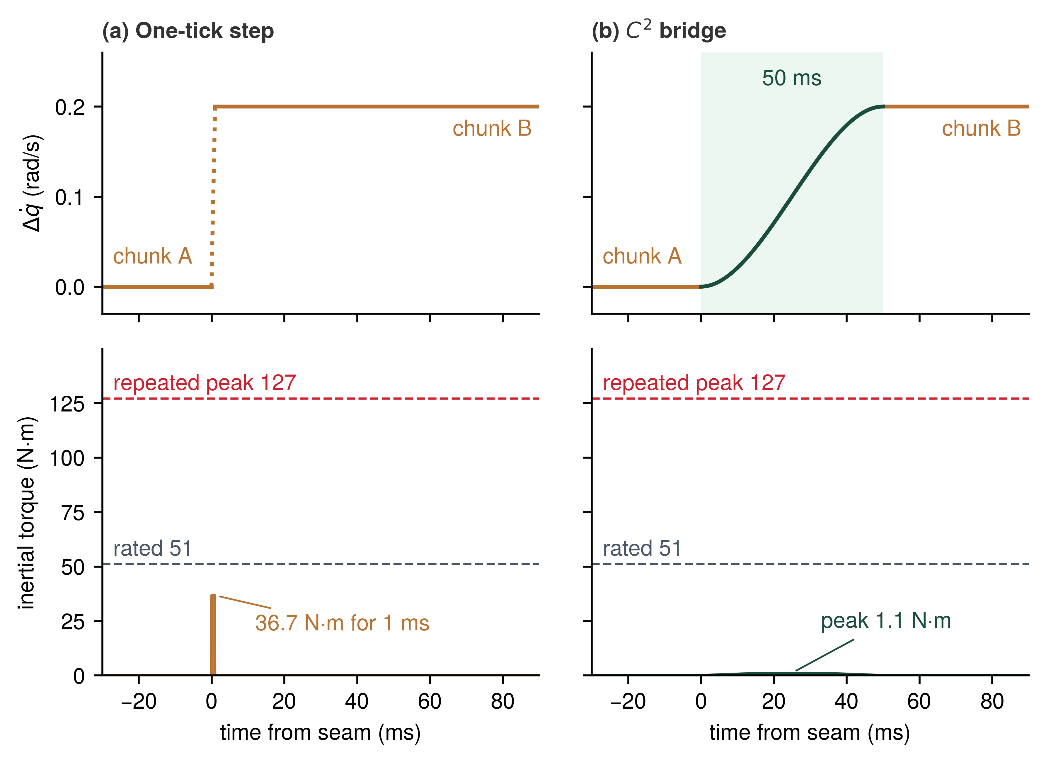
High-frequency chatter in learned policy outputs represents an identical physical hazard under a different guise. Stochastic sampling policies, such as diffusion policies or action-chunking transformers, often generate consecutive trajectory chunks where individual waypoints satisfy static position and velocity limits, yet commanded accelerations reverse sign erratically between steps. Each acceleration reversal demands an immediate torque reversal from the actuator, triggering rapid current transitions and severe \(\TorqueProducingCurrent^2 \PhaseResistance\) resistive heating in the motor windings. In physical AI systems, engineers must treat this high-frequency variance as a direct cause of thermal rise and transmission fatigue rather than cosmetic jitter. A trajectory candidate that excites structural resonances or exceeds drive thermal dissipation limits is infeasible, regardless of how closely its geometric path resembles demonstration data.
11.4.5 Time parameterization under torque and jerk bounds
A collision-free curve through configuration space says where the arm goes. It says nothing about how fast the arm may travel along that curve without saturating a joint’s torque limit on the way up or demanding an impossible torque step when it switches to braking. Geometric search and neural proposal generators determine only the spatial path of motion: a curve \(\GeneralizedCoordinates(\PathCoordinate)\) parameterized by scalar path coordinate \(\PathCoordinate \in [0, 1]\). The timing law \(\PathCoordinate(\TimeInstant)\) governs the physical motion, determining every joint velocity, acceleration, and torque required along the trajectory. Establishing a valid timing profile \(\PathCoordinate(\TimeInstant)\) subject to physical actuator limits is the problem of time parameterization. Applying the chain rule to the joint coordinates yields:
\[\GeneralizedVelocities = \JointPathTangent(\PathCoordinate)\,\PathVelocity, \qquad \GeneralizedAccelerations = \JointPathTangent(\PathCoordinate)\,\PathAcceleration + \JointPathCurvature(\PathCoordinate)\,\PathVelocity^2\]
where primes denote differentiation with respect to path coordinate \(\PathCoordinate\) (\(\DerivativeOperator\GeneralizedCoordinates/d\PathCoordinate\) and \(\DerivativeOperator^2\GeneralizedCoordinates/d\PathCoordinate^2\)). Substituting these path derivatives into the unconstrained manipulator equation from equation 8 expresses joint torque as a function of three path-dependent terms:
\[\JointTorque = \PathAccelerationTorqueCoefficient(\PathCoordinate)\,\PathAcceleration + \PathVelocitySquaredTorqueCoefficient(\PathCoordinate)\,\PathVelocity^2 + \GravitationalTorqueVector(\PathCoordinate) \tag{15}\]
with vector coefficients \(\PathAccelerationTorqueCoefficient(\PathCoordinate) = \GeneralizedInertiaMatrix(\GeneralizedCoordinates)\JointPathTangent(\PathCoordinate)\), \(\PathVelocitySquaredTorqueCoefficient(\PathCoordinate) = \GeneralizedInertiaMatrix(\GeneralizedCoordinates)\JointPathCurvature(\PathCoordinate) + \CoriolisCentrifugalMatrix(\GeneralizedCoordinates,\JointPathTangent)\,\JointPathTangent(\PathCoordinate)\), and \(\GravitationalTorqueVector(\PathCoordinate) = \GravitationalTorqueVector(\GeneralizedCoordinates)\). Each actuator torque bound \(|\CommandedJointTorque_i| \le {\JointTorqueLimit}_i\) translates into an admissible interval of path acceleration, \(\PathAccelerationLowerBound(\PathCoordinate,\PathVelocity) \le \PathAcceleration \le \PathAccelerationUpperBound(\PathCoordinate,\PathVelocity)\), at every coordinate of the phase plane \((\PathCoordinate, \PathVelocity)\). Actuator velocity and acceleration limits introduce equivalent bounding intervals. As path velocity \(\PathVelocity\) increases, the centrifugal and Coriolis term \(\PathVelocitySquaredTorqueCoefficient(\PathCoordinate)\PathVelocity^2\) grows quadratically until the admissible acceleration interval closes entirely (\(\PathAccelerationLowerBound = \PathAccelerationUpperBound\)). The locus of phase-plane points where this interval collapses defines the maximum velocity curve, representing an upper speed envelope that no feasible parameterization can exceed.
Because total motion duration is \(\Time = \int_0^1 \frac{1}{\PathVelocity}\,d\PathCoordinate\), the minimum-time profile maintains the highest permissible path velocity \(\PathVelocity\) at every point along the path. Under torque constraints alone, the time-optimal solution takes a bang-bang form (Bobrow et al. 1985). The system accelerates along the upper bound \(\PathAccelerationUpperBound\) until its phase-plane trajectory encounters a braking curve integrated backward from the goal at lower bound \(\PathAccelerationLowerBound\). It then decelerates along \(\PathAccelerationLowerBound\) to reach the target at rest. Switch points mark the phase-plane coordinates where the trajectory transitions between maximum acceleration and maximum braking. The TOPP-RA algorithm (Pham and Pham 2018) solves this phase-plane parameterization efficiently by transforming it into a convex optimization problem. By substituting squared path velocity \(\SquaredPathVelocity = \PathVelocity^2\) and path acceleration \(\PathAccelerationInput = \PathAcceleration\), the torque constraints in equation 15 and the differential step equation \(\SquaredPathVelocity_{i+1} = \SquaredPathVelocity_i + 2\,\FiniteChange \PathCoordinate\,\PathAccelerationInput_i\) become linear across a grid of \(\PathGridPointCount\) path waypoints. (This linear step relation follows from \(d\SquaredPathVelocity/d\PathCoordinate = 2\PathVelocity\,(\DerivativeOperator\PathVelocity/d\PathCoordinate) = 2\PathAcceleration\), matching the kinematic equation \(\Glyph{v}^2 = 2\Glyph{a} \Glyph{d}\)). A backward integration pass computes the controllable interval of \(\SquaredPathVelocity\) at each grid point from which the terminal state remains reachable, solving a single linear program per point. A subsequent forward pass selects the largest admissible acceleration \(\PathAccelerationInput\) at each step. The complete pass runs in \(\mathcal{O}(\PathGridPointCount)\) time, and an empty feasible interval at any point provides constructive proof that no parameterization satisfies the bounds on that grid. Kinematic variants that constrain only joint velocity and acceleration compute this timing structure with lower overhead (Kunz and Stilman 2012). The Kunz and Stilman algorithm serves as the default time-parameterization method in MoveIt 2, which can apply a downstream jerk-limiting filter (MoveIt 2 Documentation 2026).
Kunz, Tobias, and Mike Stilman. 2012. “Time-Optimal Trajectory Generation for Path Following with Bounded Acceleration and Velocity.” Robotics: Science and Systems (RSS) VIII. https://doi.org/10.15607/RSS.2012.VIII.027.
MoveIt 2 Documentation. 2026. Time Parameterization. MoveIt 2 tutorials, PickNik Robotics.
Napkin Math 11.3: Time-optimal swing of one joint
Problem: The shoulder lifts the rated payload at full planar reach through 0.5 rad, from rest to rest. How fast can it swing, and what does the fastest timing ask of the drive?
Variables:
- Swing \(\FiniteChange \JointPosition =\) 0.5 rad (illustrative), with the joint angle itself as the path parameter (\(\PathCoordinate = \JointPosition\), measured from the start)
- Inertia \(\EffectiveJointInertia =\) 1.65 kg·m² and payload gravity torque \(\PayloadGravityTorque =\) 20.6 N·m, held at its horizontal value (derived, payload only)
- Joint limits: torque \(\JointTorqueLimit =\) 87 N·m, acceleration 7.5 rad/s², velocity 2.175 rad/s, torque rate \(\TorqueRateLimit =\) 1000 N·m/s (datasheet (Franka Robotics GmbH 2023))
Math:
- Binding acceleration: The torque limit allows \((\JointTorqueLimit-\PayloadGravityTorque)/\EffectiveJointInertia =\) 40.2 rad/s² upward and \((\JointTorqueLimit+\PayloadGravityTorque)/\EffectiveJointInertia =\) 65.1 rad/s² braking, an asymmetry that gravity creates. The published 7.5 rad/s² is tighter than both, so it binds in both directions.
- Time-optimal swing: The accelerating curve \(\PathVelocity^2 = 2\ProfileAccelerationBound \PathCoordinate\) meets the braking curve at mid-swing, where speed peaks at \(\sqrt{\ProfileAccelerationBound\,\FiniteChange \JointPosition} =\) 1.94 rad/s, below the velocity limit. The swing takes \(2\sqrt{\FiniteChange \JointPosition/\ProfileAccelerationBound} =\) 516.4 ms.
- Switch-point step: Acceleration reverses from \(+\ProfileAccelerationBound\) to \(-\ProfileAccelerationBound\), a torque step \(2\EffectiveJointInertia{}\ProfileAccelerationBound =\) 24.8 N·m, which needs at least 24.8 ms at the torque-rate limit. That limit bounds jerk at \(\TorqueRateLimit/\EffectiveJointInertia =\) 604.8 rad/s³.
- Jerk-limited swing: A rest-to-rest double-S profile with no cruise covers \(\FiniteChange \JointPosition = \ProfileAccelerationBound\,\SCurveAccelerationPhaseTime\,(\SCurveAccelerationPhaseTime + \ProfileAccelerationBound/\JerkLimit)\) in \(\Time = 2(\SCurveAccelerationPhaseTime + \ProfileAccelerationBound/\JerkLimit)\). Because the accelerating half of the swing consists of a constant-acceleration hold framed by two jerk ramps of duration \(\ProfileAccelerationBound/\JerkLimit\) (one ramping acceleration up to \(\ProfileAccelerationBound\) and one ramping it back to zero at mid-swing), \(\SCurveAccelerationPhaseTime = \Time/2 - \ProfileAccelerationBound/\JerkLimit\) is half the swing less one jerk ramp (the constant-acceleration hold plus one ramp), giving the trapezoidal acceleration pulse an area equal to the peak speed \(\ProfileAccelerationBound \SCurveAccelerationPhaseTime\). With \(\ProfileAccelerationBound/\JerkLimit =\) 12.4 ms, the swing needs \(\SCurveAccelerationPhaseTime =\) 252.1 ms and takes 528.9 ms.
Systems insight: Enforcing the torque-rate limit incurs an execution penalty of 12.6 ms, a modest 2.4 percent increase in motion duration, while eliminating the instantaneous torque step entirely. For the payload alone, torque was not the binding constraint; the published kinematic limits governed the trajectory, though identified link inertia would narrow this torque headroom. A valid time parameterization must incorporate every constraint capable of binding in practice. The theoretical time-optimal profile without a jerk bound is an unexecutable mathematical abstraction that physical drives reject.
Franka Robotics GmbH. 2023. Robot and Interface Specifications. Franka Control Interface documentation.
In the phase plane the two profiles differ only near their corners (figure 5). The torque limits alone would permit steeper accelerating and braking parabolas, but the published 7.5 rad/s² acceleration limit contracts both arcs, and the bang-bang path rides them to its 1.94 rad/s switch point, well below the velocity limit. The jerk-limited path rounds the start, the apex, and the finish just inside those arcs. That rounding is where its extra 2.4 percent of duration goes, and it is what removes the 24.8 N·m torque step at the switch point.
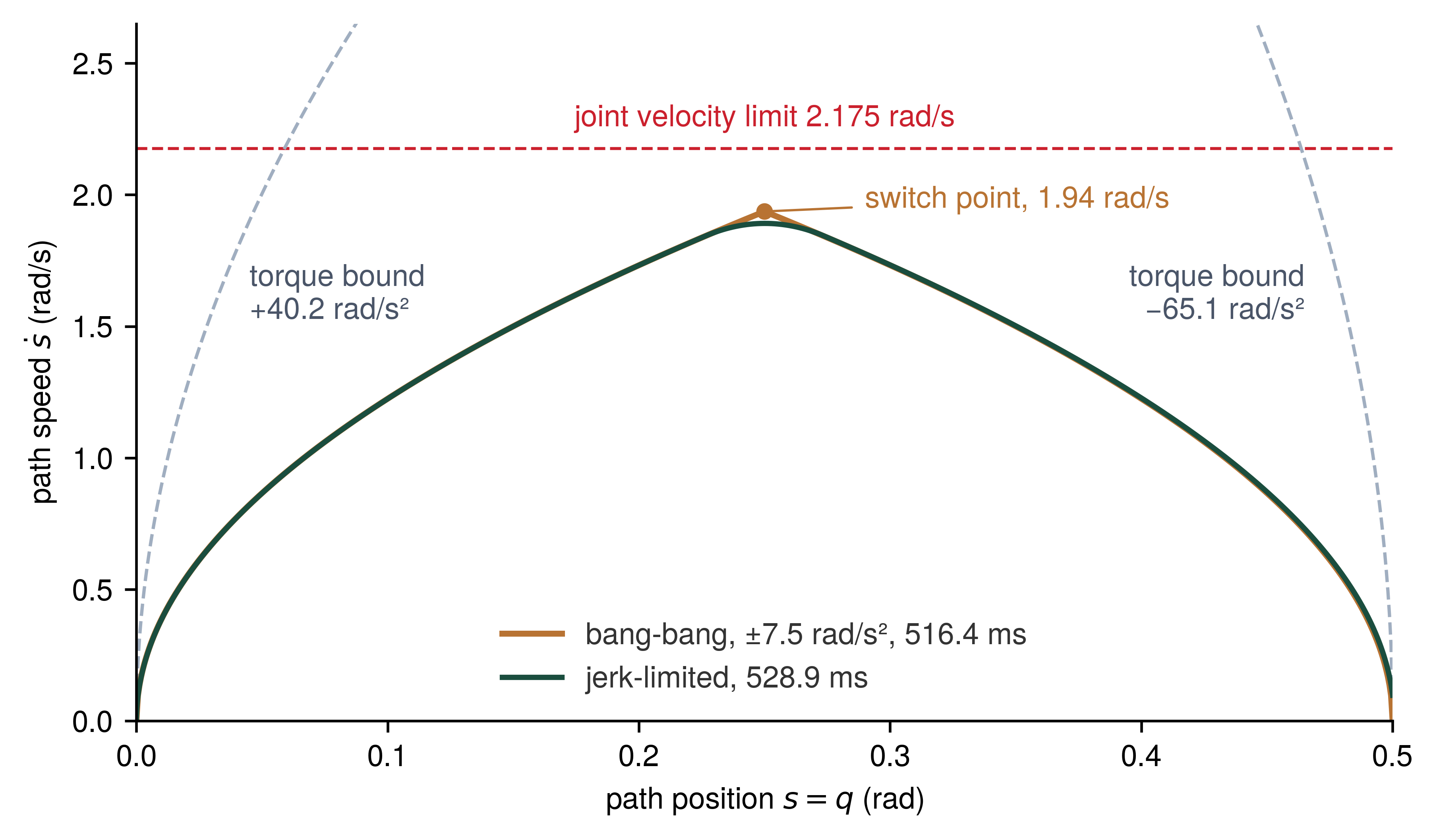
The time-optimal bang-bang solution produces precisely the derivative discontinuities that safe seam execution forbids. Every transition between maximum acceleration and maximum braking represents a step change in acceleration, demanding an instantaneous step in electromagnetic torque that actuator drives cannot deliver within finite voltage and current slew limits. Incorporating an explicit jerk bound transforms the problem into a third-order trajectory formulation. As the shoulder swing notebook shows, the time cost of bounding jerk is small next to the torque step it removes. Modern motion pipelines therefore parameterize paths under coupled torque and velocity limits and enforce explicit jerk bounds downstream, or constrain jerk directly during parameterization.
An identical jerk-limited profile, synthesized from the robot’s verified state, resolves both seam blending and safe stopping. An online trajectory generator receives the instantaneous position, velocity, and acceleration of each joint together with a target boundary state, returning a time-optimal profile that satisfies per-axis velocity, acceleration, and jerk limits (Kröger and Wahl 2010). For example, the Ruckig algorithm (Berscheid and Kröger 2021) evaluates arbitrary initial and target states across seven distinct constant-jerk phases, calculating profile durations analytically for most trajectory classes and using a bounded polynomial root solver for asymmetric edge cases. In published benchmarks, Ruckig achieved an average execution latency of 19.8 μs and a worst-case latency of 123 μs for 7 axes on a desktop processor, making it fast enough to re-solve within a 1 kHz control cycle. This formulation differs structurally from the fixed-duration quintic bridge in section 11.4.4. The quintic approach fixes blending duration \(\SeamBridgeDuration\) upfront and risks exceeding joint limits during aggressive maneuvers, so downstream extrema checks must reject invalid solutions. An online trajectory generator instead solves for minimum duration as an optimization variable, which guarantees that kinematic derivative bounds hold by construction. The S-curve stopping trajectory examined in section 11.5.2 represents this exact profile structure evaluated toward a zero-velocity terminal state.
Kinematic feasibility by construction, however, does not grant permission to move. An online generator guarantees only the mathematical bounds explicitly configured in its parameters. Single-axis velocity, acceleration, and jerk bounds cannot account for multi-joint dynamic coupling in equation 8, spatial swept-volume collisions, or stale perception data. Furthermore, configuration errors or numerical solver faults can directly compromise the guarantees the generator claims to provide. Real-time benchmarks reported on high-performance desktop CPUs also do not represent execution latency on a constrained safety MCU. Online generators produce higher-quality proposals that satisfy kinematic constraints by design, but the deterministic safety controller must independently validate dynamic feasibility, collision margins, and temporal deadlines before granting execution permission. Even a candidate trajectory that passes every internal dynamic and seam continuity check remains unsafe without an admitted contingency. The system must therefore continuously maintain a certified stopping suffix to handle replacement chunks that fail to arrive before the admission deadline.
Checkpoint 11.2: Followable motion and the seam
A collision-free candidate becomes followable only after its joint rates, its seams, and its timing fit the body’s limits.
Mapping and sampling
Pricing the seam
11.5 Behavior at the Seam
When the replacement does not arrive, because inference stalls on scheduling interference, a bus fault, or an unhandled exception, the arm reaches the end of its authority with no successor in hand. The runtime must then bring it to rest without violating the limits derived above or exhausting its stopping clearance. Three things decide the outcome: which deadline has passed, which stop the MCU runs, and how much clearance that stop consumes.
11.5.1 Replacement deadlines and commitment cutoffs
A single timeout cannot protect both a fast control loop against a hung proposer and a moving arm against overrunning its obstacle clearance. A lease short enough to catch a dropped packet fires long before the geometric point of no return. A cutoff placed at the point of no return leaves a stalled policy coasting blind in the meantime. The two tiers named with the trajectory record in section 11.2, the periodic chunk lease and the commitment cutoff, therefore answer different questions: whether a replacement has renewed tracking authority recently enough, and whether the reserved stop can still begin in time. The planner also uses a soft blend deadline (\(\BlendDeadline\)), a scheduling target for a smooth replacement. Missing that target need not end tracking if the current lease and evidence remain valid and a checked replacement can still arrive before the admission cutoff that precedes physical commitment (\(\CommitmentInstant\)). The earlier admission cutoff leaves the response interval needed for the matched stopping suffix to begin at commitment, before its reserved clearance is spent.
The two deadlines call for two different stops:
- Matched stop suffix (planned termination at \(\TimeInstant = \CommitmentInstant\)): A pre-computed, jerk-limited \(\DifferentiabilityClass^2\) slowdown along the admitted path, anchored specifically at the nominal state expected at \(\CommitmentInstant\), checked at admission to satisfy \(\StoppingDistance \le \ClearDistance\). If no successor is admitted before the earlier admission cutoff, the controller dispatches the stop early enough that the body smoothly transfers to this pre-latched suffix at commitment, decelerating to rest without requiring runtime replanning.
- State-matched fallback (reactive termination at \(\TimeInstant < \CommitmentInstant\)): If the high-rate chunk lease lapses, the parent intent expires, or a runtime safety monitor detects an unmodeled obstacle or torque fault before reaching \(\CommitmentInstant\), the robot cannot use the matched stop suffix (which is anchored at the future state \(\CommitmentInstant\)). Instead, the MCU selects or constructs a validated state-matched fallback from current state estimates \((\JointPosition, \JointVelocity, \JointAcceleration)\) within reserved clearance. Encoder-derived velocity and acceleration have their own error bounds; bounded polynomial evaluation does not eliminate sensing, dispatch, or actuator response delay.
Both are the stopping suffix that every admitted trajectory carries (definition 11.1), differing only in the entry state from which they start. For the running mug reach, a stalled proposer expires the shared lease 60 ms after the last admission. The MCU then requests its state-matched fallback; physical onset follows the separately budgeted response delay. All timeout checks use the MCU monotonic clock. The longer-lease comparison isolates the geometric limit: even with tracking evidence continually renewed, the controller must dispatch the matched stop early enough to begin at commitment. A host progress report changes neither cutoff. Both stops also inherit the seam’s continuity requirement, and that requirement fixes their shape and therefore their length.
11.5.2 The C\(^2\) stopping suffix and jerk-limited braking
A moving robot carries continuous momentum. If an emergency brake uses an idealized constant-deceleration profile (\(\StopAxisAcceleration(\TimeInstant) = -\CredibleBrakingDeceleration\)), the commanded acceleration steps discontinuously from zero to \(-\CredibleBrakingDeceleration\) at \(\CommitmentInstant\), and steps discontinuously back to zero when velocity reaches zero. This instantaneous switch demands an infinite jerk impulse (\(\dddot{\StopAxisPosition} = \infty\)) and an instantaneous step jump in actuator braking torque (\(\FiniteChange\CommandedJointTorque = \EffectiveJointInertia \CredibleBrakingDeceleration\)). A real drive can only approximate that step. Whether the response loses traction, disturbs the payload, or exceeds structural limits depends on the load and controller, so the worked design chooses an explicitly smooth profile.
Two bounds describe what the load and the drive tolerate during that stop: a peak deceleration \(\ProfileAccelerationBound\) and a peak jerk \(\JerkLimit\), the rate at which deceleration may change. A \(\DifferentiabilityClass^2\) stop keeps position, velocity, and acceleration continuous at both ends, so it must ramp its deceleration up from zero and back down to zero, and the jerk bound limits how quickly it can do either. Within those bounds, the shape of the profile decides how far the machine travels. Consider a cruise entry with position \(\StopAxisPosition(\CommitmentInstant) = \CommitmentPathPosition\), cruise speed \(\CruiseSpeed > 0\), and zero entry acceleration. One smooth candidate is the lowest-order polynomial that matches position, velocity, and acceleration at both ends, written in the normalized time \(\StopProgress = (\TimeInstant - \CommitmentInstant) / \StoppingDuration \in [0, 1]\):
\[\StopAxisPosition(\StopProgress) = \CommitmentPathPosition + \CruiseSpeed \StoppingDuration \left(\StopProgress - \StopProgress^3 + \frac{1}{2} \StopProgress^4\right), \qquad \StopAxisAcceleration(\StopProgress) = -\frac{6 \CruiseSpeed}{\StoppingDuration} \StopProgress(1 - \StopProgress), \qquad \dddot{\StopAxisPosition}(\StopProgress) = -\frac{6 \CruiseSpeed}{\StoppingDuration^2} (1 - 2\StopProgress) \tag{16}\]
Its deceleration is an inverted parabola that peaks at the midpoint, \(\PeakStopDeceleration = 1.5\,\CruiseSpeed/\StoppingDuration\), and its jerk is largest at the two ends, \(6\CruiseSpeed/\StoppingDuration^2\). Holding the peak at \(\ProfileAccelerationBound\) gives \(\StoppingDuration = 1.5\,\CruiseSpeed/\ProfileAccelerationBound\) and a distance of \(\frac{1}{2}\CruiseSpeed \StoppingDuration = 0.75\,\CruiseSpeed^2/\ProfileAccelerationBound\), which is \(1.5\) times the constant-deceleration distance \(\CruiseSpeed^2/2\ProfileAccelerationBound\). That factor is a property of this polynomial, not of smooth stopping. The polynomial touches its peak deceleration only at the midpoint and spends half the stop below three quarters of it, so it gives away distance that its own bounds would allow it to use.
The profile that uses those bounds fully is the jerk-limited S-curve (trapezoidal acceleration, the “double S” velocity profile) (Biagiotti and Melchiorri 2008). It ramps deceleration from zero to \(\ProfileAccelerationBound\) at the jerk limit, holds \(\ProfileAccelerationBound\), and ramps back to zero at the jerk limit just as velocity reaches zero. Each ramp lasts \(\ProfileAccelerationBound/\JerkLimit\). The velocity profile is point-symmetric about its midpoint, so the distance is half the entry speed times the duration:
\[\StoppingDistance(\SpeedAtDetection) = \begin{cases} \dfrac{\SpeedAtDetection^2}{2\ProfileAccelerationBound} + \dfrac{\SpeedAtDetection\,\ProfileAccelerationBound}{2\JerkLimit}, & \SpeedAtDetection \ge \ProfileAccelerationBound^2/\JerkLimit \\[1.2ex] \SpeedAtDetection\sqrt{\SpeedAtDetection/\JerkLimit}, & \SpeedAtDetection < \ProfileAccelerationBound^2/\JerkLimit \end{cases} \qquad \StoppingDuration(\SpeedAtDetection) = \begin{cases} \dfrac{\SpeedAtDetection}{\ProfileAccelerationBound} + \dfrac{\ProfileAccelerationBound}{\JerkLimit}, & \SpeedAtDetection \ge \ProfileAccelerationBound^2/\JerkLimit \\[1.2ex] 2\sqrt{\SpeedAtDetection/\JerkLimit}, & \SpeedAtDetection < \ProfileAccelerationBound^2/\JerkLimit \end{cases} \tag{17}\]
Above the threshold speed \(\ProfileAccelerationBound^2/\JerkLimit\), the stop costs constant-deceleration braking at \(\ProfileAccelerationBound\) plus cruise over half of one jerk ramp, \(\ProfileAccelerationBound/2\JerkLimit\), so a finite jerk limit acts like extra reaction time. Below the threshold the stop is too short to reach \(\ProfileAccelerationBound\), and its deceleration peaks at \(\sqrt{\SpeedAtDetection\,\JerkLimit}\). Among stops that respect both bounds and never reverse, this profile reaches rest in the least time and the least distance. The shape of the stop, not physics, sets the distance beyond \(\SpeedAtDetection^2/2\ProfileAccelerationBound\), and for given deceleration and jerk bounds the S-curve spends the least. A slower profile remains admissible, but it must be charged at its own distance.
The jerk bound belongs to the load. The loaded tote rack and the mug tolerate a deceleration only if it is reached gradually, and the registry does not yet hold a measured jerk tolerance for either. The worked design therefore sets each body’s \(\JerkLimit\) to the peak jerk of equation 16 at that body’s peak deceleration and top speed, a jerk the polynomial already asked the load to accept. A loaded stopping trial that measures the tolerable jerk would replace this stipulation, and equation 17 would then give the distance directly.
The stop is also a slowdown along the admitted path, not a new path. The planner fixes the geometry \(\GeneralizedCoordinates(\PathCoordinate)\) it checked for clearance, and the S-curve governs only the speed \(\PathVelocity(\TimeInstant)\) along that geometry. The stop therefore sweeps no volume outside the corridor already checked, and the one-dimensional comparison \(\StoppingDistance \le \ClearDistance\) applies along the path. A stop computed separately for each joint would leave that path and would need its own swept-volume check. A nonzero measured entry acceleration requires a profile matched to the actual \((\JointPosition,\JointVelocity,\JointAcceleration)\) at entry with zero terminal velocity and acceleration; the permission path checks its interior speed, acceleration, jerk, torque, and clearance.
In the alternate longer-lease arm case, the blend deadline is 240 ms, matched commitment 300 ms, nominal setpoint end 400 ms, and stop end 575 ms, so the stop lasts 275 ms. At the arm’s 1 m/s TCP speed limit, the S-curve suffix with a 5 m/s² deceleration bound and a 66.7 m/s³ jerk bound travels 137.5 mm, compared with 150 mm for the polynomial of equation 16 with the same peaks. Because the blend deadline is the preferred admission instant on this schedule, the last scheduled validation and clearance evidence finish at 240 ms. The 60 mm of cruise between 240 ms and physical brake onset at 300 ms must therefore be charged against that clearance alongside the stop. Together they consume 197.5 mm in all, leaving 102.5 mm of the 300 mm obstacle clearance before sensing and model error are deducted. Because 300 ms is physical suffix onset, the MCU must close replacement admission and pretrigger any communication or actuator delay \(\UnreservedStopDelay\) by that instant minus \(\UnreservedStopDelay\). Otherwise, the arm travels an extra \(\CruiseSpeed\UnreservedStopDelay\), shifts the stop end later, and shrinks the 102.5 mm margin. Nominal setpoints end at 400 ms while MCU STOP continues to 575 ms, assuming fresh target evidence keeps TRACK valid until stop dispatch (section 11.3).
On the running machine, as the alternate schedule’s introduction noted, a stall never reaches commitment because the chunk lease lapses first, so its stop is the state-matched fallback. From zero-acceleration cruise the S-curve matches the arm at whatever instant it starts, and it slows the tool along the path already checked, so the state-matched fallback travels the same distance as the matched stop suffix. On the arm, as on the base, the chunk lease is a term of the stopping budget, the rule established in Chunk Lease Sizing from the Stopping Budget; the arm’s own speed, stop, and clearance set what that term costs.
Napkin Math 11.4: The stall runway
Problem: The proposer stalls while the arm reaches at its TCP limit, and no replacement is admitted. How much of the obstacle clearance does the arm use between its last admission and rest, and how much remains?
Variables:
- Chunk lease \(\ChunkLease =\) 60 ms (chosen); permission tick 1 ms (derived) and bus cycle 1 ms (illustrative); onset 20 ms (illustrative, the base’s registered brake onset charged conservatively to the arm)
- Speed \(\SpeedAtDetection =\) 1 m/s (chosen, TCP limit)
- Deceleration bound \(\ProfileAccelerationBound =\) 5 m/s² (illustrative) and jerk bound \(\JerkLimit =\) 66.7 m/s³ (derived, the peak jerk of equation 16 at the same peak)
- Clearance \(\ClearDistance =\) 300 mm (illustrative)
Math:
- Response path: 60 ms \(+\) 1 ms \(+\) 1 ms \(+\) 20 ms \(=\) 82 ms from last admission to stop onset, which is 82 mm at \(\SpeedAtDetection\).
- Branch test (equation 17): \(\ProfileAccelerationBound^2/\JerkLimit =\) 0.375 m/s, below \(\SpeedAtDetection\), so the stop reaches \(\ProfileAccelerationBound\).
- Stop: \(\SpeedAtDetection^2/2\ProfileAccelerationBound + \SpeedAtDetection\,\ProfileAccelerationBound/2\JerkLimit =\) 100 mm \(+\) 37.5 mm \(=\) 137.5 mm, in \(\SpeedAtDetection/\ProfileAccelerationBound + \ProfileAccelerationBound/\JerkLimit =\) 200 ms \(+\) 75 ms \(=\) 275 ms.
- Clearance: 82 mm \(+\) 137.5 mm \(=\) 219.5 mm of 300 mm.
Result: The stall leaves 80.5 mm of geometric margin, before sensing and model reserves.
Systems insight: The travel before the stop begins is 59.6 percent of the stop itself, and at this speed every millisecond of lease costs a millimeter. The remaining margin equals only 80.5 ms of further lease, so the lease length is a term of \(\StoppingDistance \le \ClearDistance\) exactly as the deceleration bound is.
While hardware qualification must establish the arm’s actual response in place of the charged onset allowance, the two schedules leave different geometric margins because they date their clearance evidence differently (figure 2). The running lease charges travel from the last admission (82 mm) plus the 137.5 mm stop, which keeps 80.5 mm. The alternate schedule charges only the cruise from its blend deadline, when clearance was last checked, to commitment (60 mm) plus the same stop, which keeps 102.5 mm. The alternate schedule’s 278 ms admission cutoff is therefore an offset on its own time axis rather than a lease length that the running clearance could support. Any lease, whatever its length, must fit its own evidence age, response travel, stop, and uncertainty reserve, just as the running lease does in the notebook above.
Although the free-space deceleration bound suits the empty-gripper reach toward the mug, it is too aggressive once the arm carries an open mug of liquid away from the conveyor, because container acceleration tilts the free surface and excites sloshing (Mayer and Krechetnikov 2012). Under a steady deceleration \(\SteadyDeceleration\), the free surface settles perpendicular to the effective gravity, tilting by \(\tan\FreeSurfaceTiltAngle = \SteadyDeceleration/\Gravity\) and raising the liquid at the wall by \(\ContainerInnerRadius\,\SteadyDeceleration/\Gravity\) for inner radius \(\ContainerInnerRadius\). In an illustrative mug of 40 mm inner radius filled to 10 mm below the rim, the free-space stop’s 5 m/s² deceleration raises the liquid 20.4 mm at the wall, well past the rim. Keeping even the steady tilt inside the freeboard \(\FreeboardHeight\) (a necessary condition, since dynamic sloshing overshoots the steady tilt) limits deceleration to \(\Gravity\,\FreeboardHeight/\ContainerInnerRadius\), or 2.45 m/s². At that gentler bound, with the jerk the polynomial reaches at the same peak, the stop from the 1 m/s TCP limit lengthens to 280.4 mm and, together with the running lease path, demands 362.4 mm of the 300 mm clearance. The loaded carry must therefore run slower than the empty reach. Before sensing and model reserves are deducted, the highest speed whose lease path and stop fit that clearance is 0.89 m/s. The trajectory record’s assumption sidecar must declare which payload regime and measured slosh limit (or lid) the record assumes.
Mayer, Hans C., and Rouslan Krechetnikov. 2012. “Walking with Coffee: Why Does It Spill?” Physical Review E 85 (4): 046117. https://doi.org/10.1103/PhysRevE.85.046117.
At the TCP limit, the open mug’s gentler stop overruns the clearance the empty reach fits.
The commitment deadline forbids waiting. In the alternate arm schedule, commitment preserves the 102.5 mm margin computed from clearance dated at 240 ms. Missing the 278 ms admission cutoff and delaying stop dispatch by 200 ms would delay physical stop onset that far past commitment. Cruise at the TCP limit would add 200 mm before the same stop and breach the 300 mm clearance by 97.5 mm. A later stop must still match its actual entry state; this counterfactual holds cruise speed constant only to show the lost clearance. An arm that waits that long may already occupy a state from which no admissible control avoids the obstacle.
11.5.3 Inevitable collision states
An arm or base that is still clear of every obstacle at the current millisecond can already be doomed to hit one if its speed and remaining distance leave no control input inside its drive and traction limits that can bring it to rest in time. Classical path planning misses this trap when it treats obstacle avoidance as a static geometric query that asks only whether the robot’s configuration overlaps an obstacle volume at the current instant. Because a mobile manipulator moving with momentum and finite braking torque cannot halt instantaneously, its dynamic state (position, velocity, and acceleration, under its traction limits) can cross a boundary beyond which every admissible control trajectory leads to collision long before geometric contact occurs. Such states are inevitable collision states (ICS)10 (Fraichard and Asama 2004).
10 Inevitable collision states and viability: Within the free states, the complement of the ICS set is what Aubin (1991) calls the viability kernel, the states from which some admissible control keeps the system inside its constraints forever. Planning must therefore keep the commitment state inside that kernel, not merely outside the obstacle, and against static obstacles a verified stop to rest is the witness that it is there.
Aubin, Jean-Pierre. 1991. Viability Theory. Systems & Control: Foundations & Applications. Birkhäuser.
Definition 11.4: Inevitable collision state
Inevitable collision state (ICS) is any dynamic plant state \(\MechanicalPlantState(\TimeInstant) \in \PlantStateSpace\) from which every physically admissible future control trajectory \(\FutureControlTrajectory \in \AdmissibleControlSet\) inevitably produces collision with an obstacle or constraint boundary: \[\MechanicalPlantState \in \text{ICS}(\ObstacleStateSet) \iff \forall \ControlInput(\cdot) \in \AdmissibleControlSet, \; \exists \FutureTimeInstant \ge \TimeInstant \text{ such that } \MechanicalPlantState(\FutureTimeInstant) \in \ObstacleStateSet\] where \(\AdmissibleControlSet\) denotes the admissible control input set bounded by actuator torque, traction, and deceleration limits.
- Significance: Sets the commitment deadline \(\CommitmentInstant\) in receding-horizon planning; continuing nominal motion past it without an admitted successor can carry the plant into an ICS, and no later replanning can bring it back out.
- Distinction: Unlike static geometric collision checks that evaluate only instantaneous spatial overlap (\(\MechanicalPlantState \in \ObstacleStateSet\)), an ICS identifies dynamically trapped states where current momentum and finite braking torque make future boundary breach physically unavoidable.
- Common pitfall: Delaying emergency braking in the expectation that an overdue neural planner will complete an evasive path, ignoring that moving mass enters an ICS long before geometric contact occurs.
The commitment deadline \(\CommitmentInstant\) and the admission-checked stopping suffix are co-designed precisely so that the machine initiates braking before its dynamic state enters an inevitable collision state, \(\text{ICS}(\ObstacleStateSet)\). If an action chunk’s stopping suffix requires distance \(\StoppingDistance > \ClearDistance\), that suffix cannot justify admitting the chunk. Failure of this particular stop does not establish that every admissible maneuver collides, as the definition of an inevitable collision state requires. The architecture nevertheless refuses the proposal because it lacks the independently executable stop on which its permission depends. The safety microcontroller therefore enforces the hard admission invariant: \[\StoppingDistance(\CommitmentInstant) \le \ClearDistance(\CommitmentInstant) \tag{18}\] If the controller delays braking past commitment in the hope that an overdue neural replanner will deliver an evasive path, physical momentum can carry the machine into an ICS from which no admissible control input can prevent impact. The commitment deadline is the deadline form of this boundary, fixed at planning time. Its set form, the recoverable set of plant states from which the resident stop still succeeds, is the stopping envelope that Stopping Envelopes develops for the runtime check.
These deadlines and the stop they protect are fixed at admission, before motion begins. The candidate declares payload, contact, effort, and obstacle assumptions. The MCU first validates its fixed header and lineage. It then checks the complete bounded trajectory and suffix, including the seam \((\JointPosition,\JointVelocity,\JointAcceleration)\) against the reachable state envelope from its current estimate, interior extrema, clearance, stopping distance, and a feasible response from every state reachable through physical stop onset. A scan over \(\TrajectorySampleCount\) setpoints is \(\mathcal{O}(\TrajectorySampleCount)\), even with a fixed maximum \(\TrajectorySampleCount\) and measured worst-case execution time; after admission, a distinct \(\mathcal{O}(1)\) per-tick check reads the current state and local reference. A replacement received after the blend deadline passes the same check with a compressed bridge, whose higher acceleration and torque its extrema must still clear. If the check cannot finish before the earlier admission cutoff, the MCU retains the current record only while its own lease, evidence, and fallback remain valid. A candidate received after commitment cannot restore the spent runway.
The planner proposes the suffix. The MCU latches the validated payload and stop profile into protected memory before enabling TRACK, and it dispatches that resident path before commitment without reading host DRAM. A host crash, bus stall, or corrupted shared packet therefore cannot erase the stop. If the measured state falls outside the latched suffix’s entry region, the MCU uses the state-matched fallback. Torque disable or a spring brake is not a universal substitute for a controlled stop, especially with a suspended load (The Fallback Ladder).
11.5.4 Base stopping budget under jerk-limited deceleration
On the mobile base approaching the rack end at its 1.5 m/s drive limit, the loaded tote rack tolerates the machine’s credible 2 m/s² deceleration only when that deceleration is ramped gradually rather than applied as an abrupt step. The base’s stop is therefore the S-curve of equation 17 with \(\ProfileAccelerationBound\) at 2 m/s² and a jerk bound of 7.11 m/s³. That jerk bound is the peak jerk of the polynomial stop from the 1.5 m/s drive limit and the stop jerk bound already listed on the machine card (The running machine's card). Under it, every speed above 0.5625 m/s reaches the deceleration plateau. At the drive limit, this suffix lasts 1,031.25 ms and travels 773.44 mm, compared with 562.5 mm for constant-deceleration braking in equation 2.2 and 843.75 mm for the polynomial with the same peaks. Because the jerk ramps cost the equivalent of 140.6 ms of cruise, the suffix adds 210.94 mm to the budget that The latency waterfall left at 912.9 mm. This raises the running total to 1,123.84 mm and exceeds the 1.10 m rack-end clear distance by 23.84 mm. Because this partial total still omits the unqualified dispatch-to-admission interval, which can only add travel, the 23.84 mm overrun is a conditional design deficit rather than a complete measured response bound.
Plotted as velocity against time, the area under each curve is its stopping distance, and the jerk ramps appear as the rounded start and finish that stretch the S-curve and the polynomial past the constant-deceleration line (figure 6). Stacked onto the budget’s other terms, only the constant-deceleration stop, which no drive can execute, ends inside the 1.10 m rack-end clearance.
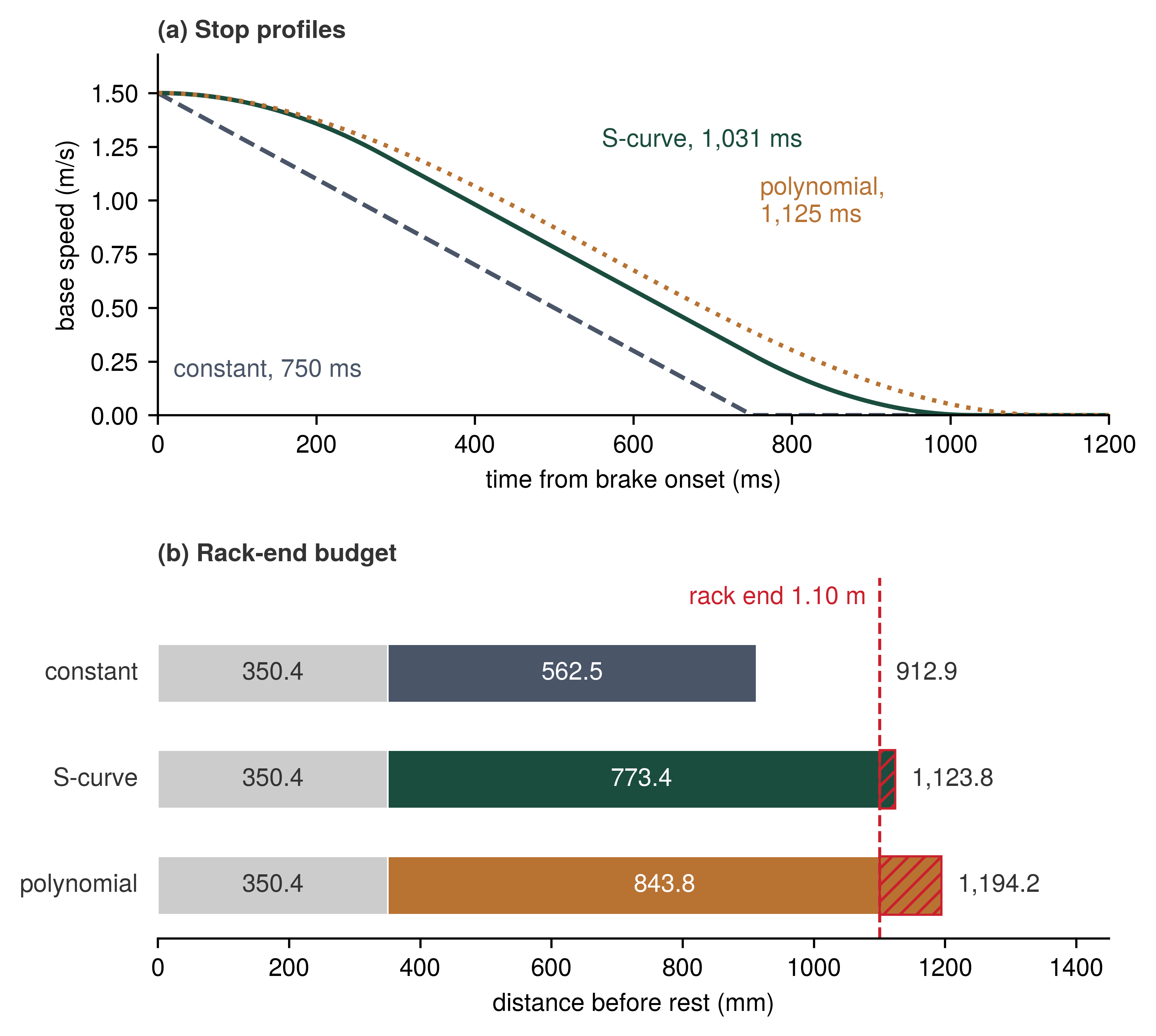
Even the shortest stop under the stipulated bounds leaves a 23.84 mm deficit at the 1.5 m/s drive limit, so the robot cannot cruise at that limit in this aisle under the stated deceleration and jerk bounds. The deficit is narrow and it rests on a stipulated jerk bound, so a measured jerk tolerance could move it in either direction. The machine must either derate its operating speed or detect the boundary with more usable clearance ahead; a longer prediction or evidence lifetime alone creates no stopping room. This is the first law’s stopping condition (principle 1) with one more term, because a stop the load can tolerate is a longer stop and the distance it adds comes out of the same clear distance. This calculation concerns the fixed rack-end boundary. A person entering the aisle requires separately qualified moving-actor bounds and crossing control or an operating restriction; this static clearance calculation does not establish that protection. Under the selected body and aisle constraints, reducing speed can recover clearance. Stopping Envelopes adds the tracking allowance and derives a candidate speed; permission to operate still requires complete capture-to-admission timing, positive stopping reserve, and qualification under the declared conditions.
↩︎ The intrusion distance an approaching pedestrian adds to the stopping budget, and the site controls it demands, are established in Forward State Propagation and Occlusion Decay.
For either body, the admission and fallback decisions in table 2 are distinct from an emergency power cut. The mug reach and the aisle approach now have a complete execution argument: a timed prefix, a checked seam, and a stop reserved under stated conditions. With those obligations fixed, trajectory generators can be compared by the candidate work they perform rather than by treating their outputs as permission.
| State | Trigger | MCU action and required evidence |
|---|---|---|
| TRACK, ordinary handoff | Replacement passes the complete admission check before the admission cutoff preceding commitment. | Latch the new nominal path and its own stop, then transfer at a checked \(\DifferentiabilityClass^2\) seam. |
| TRACK, late candidate | Candidate arrives after the blend deadline but before the admission cutoff preceding commitment. | Admit only if the compressed bridge, full path, stop, and timing still fit; otherwise retain the current record only while its own permission remains valid. |
| STOP, matched suffix | No successor admitted by the earlier cutoff. | MCU follows its protected suffix from the validated entry state; nominal tracking may end while STOP continues. |
| STOP, earlier invalidation | Lease lapse, intent expiry, contact, state mismatch, or fault before physical stop onset. | MCU selects the state-matched fallback with reserved clearance. |
| Fault response | Controlled stop cannot be assured from measured state. | Use the machine-specific risk response (which may include drive inhibit, brake, or compliance) only under its validated load and timing assumptions. |
Checkpoint 11.3: Commitment and full stopping clearance
Before committing an autonomous machine to an action chunk, verify your understanding of commitment deadlines, stopping budgets, and trajectory continuity:
11.6 Choosing a Trajectory Generator
When a mobile manipulator reaches around a conveyor guard, a planner that searches configuration space can run out of time before finding a route. A local trajectory optimizer can get trapped in a non-convex pocket behind the guard. A learned action-chunk policy can propose a smooth reach that clips the guard or exceeds a joint’s torque limit. The three algorithmic families that propose motion, geometric search, continuous optimization, and learned action chunking, each fail in a different way if treated as self-certifying. In all three paradigms, deciding where the body can travel geometrically remains separate from determining how quickly actuators can safely traverse that path. Regardless of which family generates a proposal, the resulting trajectory remains an unverified candidate that requires exhaustive dynamic validation before the execution engine commits it to the hardware.
The conveyor reach also fixes what each family can afford. A replacement must be admitted every 50 ms, and 18 ms of every replacement’s dispatch-to-admission allocation is already reserved for whole-plan validation, while a chunk policy spends another 40 ms of it on inference. To sustain the intended renewal cadence, the generation pipeline must provide both the allocated latency and the throughput that overlapping requests require. A solver without a bounded completion time needs a timeout that leaves the resident fallback executable; it can also run outside the renewal loop, planning the route around the guard and handing the loop a corridor to follow. That deadline, more than the quality of the motion, sorts the three families below.
Sampling-based geometric planners explore configuration space without requiring an explicit algebraic representation of obstacles. Probabilistic Roadmaps (PRM) (Kavraki et al. 1996) construct multi-query roadmaps by sampling collision-free configurations and connecting nearby neighbors with local collision-free segments, amortizing graph construction costs across multiple tasks. Conversely, Rapidly-exploring Random Trees (RRT) (LaValle 1998) target single-query problems by growing a space-filling tree from the initial configuration toward unexplored territory. Its asymptotically optimal counterpart, RRT* (Karaman and Frazzoli 2011), continuously rewires parent connections within local neighborhoods as samples accumulate, ensuring that the discovered path cost converges almost surely to the theoretical optimum (Karaman and Frazzoli 2011). These methods resolve geometric routes through complex obstacle geometry, yet their completeness guarantees remain strictly probabilistic: the probability of discovering a feasible path approaches one only as the number of samples approaches infinity. When a sampling planner exhausts its computation budget without finding a path, its timeout provides no proof that the route is obstructed. The admission logic must therefore treat planner silence as an unresolved proposal rather than a verified safety determination. Furthermore, evaluating configuration samples and connecting edges requires repeated collision queries against environment geometry, usually accelerated by enclosing the manipulator links in bounding spheres or capsules, and these queries dominate the planner’s run time. Even when successful, search yields only an un-timed geometric path with discontinuous derivative transitions. The system must still apply time parameterization, smooth corner blends, joint torque verification, and a valid stopping continuation before dispatching the trajectory to physical actuators.
Schulman, John, Yan Duan, Jonathan Ho, Alex Lee, Ibrahim Awwal, Henry Bradlow, Jia Pan, Sachin Patil, Ken Goldberg, and Pieter Abbeel. 2014. “Motion Planning with Sequential Convex Optimization and Convex Collision Checking.” The International Journal of Robotics Research 33 (9): 1251–70. https://doi.org/10.1177/0278364914528132.
The complementary classical formulation is constrained continuous trajectory optimization, exemplified by Covariant Hamiltonian Optimization for Motion Planning (CHOMP) (Ratliff et al. 2009), TrajOpt (Schulman et al. 2014), and receding-horizon Model Predictive Control (MPC) (Tedrake 2023; Lynch and Park 2017). Rather than evaluating discrete graph nodes, continuous trajectory optimization represents motion as a continuous, time-indexed curve \(\GeneralizedCoordinates(\TimeInstant)\) and minimizes an objective functional that balances dynamic smoothness against obstacle proximity:
\[\min_{\GeneralizedCoordinates(t)} \quad \TrajectoryOptimizationObjective[\GeneralizedCoordinates] = \int_0^\Time \left( \frac{1}{2} \|\dddot{\GeneralizedCoordinates}(\TimeInstant)\|^2 + \ObstacleCostWeight \ObstacleProximityCost(\GeneralizedCoordinates(\TimeInstant)) \right) d\TimeInstant\]
subject to physical boundary conditions and actuator invariants: \[\GeneralizedCoordinates(0) = \GeneralizedCoordinates_0, \quad \GeneralizedVelocities(0) = \GeneralizedVelocities_0, \quad \GeneralizedAccelerations(0) = \GeneralizedAccelerations_0\] \[\GeneralizedCoordinates(\Time) = \GoalConfiguration, \quad \GeneralizedVelocities(\Time) = \ZeroVector, \quad \GeneralizedAccelerations(\Time) = \ZeroVector\] \[|\GeneralizedVelocities(\TimeInstant)| \le \JointVelocityLimit, \quad |\GeneralizedInertiaMatrix(\GeneralizedCoordinates)\GeneralizedAccelerations + \CoriolisCentrifugalMatrix(\GeneralizedCoordinates, \GeneralizedVelocities)\GeneralizedVelocities + \GravitationalTorqueVector(\GeneralizedCoordinates)| \le \JointTorqueUpperLimit\]
While CHOMP performs functional gradient descent and TrajOpt solves sequential convex subproblems using signed-distance collision constraints, both rely on local optimization. Consequently, non-convex obstacle geometry can trap the solver in infeasible local minima or geometric dead ends. Graphs of Convex Sets (GCS) resolve this susceptibility when the collision-free configuration space can be partitioned beforehand into convex regions. Finding the global sequence of regions and optimizing the polynomial spline within them then formulates as a mixed-integer convex program whose convex relaxation can be solved efficiently (Marcucci et al. 2023). Because generating these convex decompositions requires substantial offline computation, GCS suits static structures such as the conveyor guard far better than dynamic, rapidly shifting environments. Although geometric search or learned policies can propose alternative routes around unforeseen obstructions, any candidate motion must still undergo explicit verification against dynamic torque limits and actuator constraints.
Marcucci, Tobia, Mark Petersen, David von Wrangel, and Russ Tedrake. 2023. “Motion Planning Around Obstacles with Convex Optimization.” Science Robotics 8 (84): eadf7843. https://doi.org/10.1126/scirobotics.adf7843.
11 Model predictive control: MPC began in the process industries of the 1970s, in refineries and chemical plants whose slow dynamics left seconds to minutes for each solve; Qin and Badgwell (2003) trace its industrial lineage from the first IDCOM and dynamic matrix control installations. Moving the same receding-horizon loop onto an arm tracked at 1 kHz shrinks that time to milliseconds, which is why a solver’s deadline, and not its optimum, decides what reaches admission.
Qin, S. Joe, and Thomas A. Badgwell. 2003. “A Survey of Industrial Model Predictive Control Technology.” Control Engineering Practice 11 (7): 733–64. https://doi.org/10.1016/S0967-0661(02)00186-7.
Tedrake, Russ. 2023. Robotic Manipulation: Perception, Planning, and Control. Massachusetts Institute of Technology.
Repeatedly re-optimizing from an updated state estimate forms the operational foundation of classical Model Predictive Control (MPC)11. In this receding-horizon paradigm, an optimizer computes an optimal trajectory over a finite horizon \(\Time\), dispatches an initial prefix to the actuator controllers, and re-solves the problem from the newly observed state on the subsequent cycle. The objective functional ranks candidate motions by performance, while hard constraints eliminate trajectories that exceed physical limits. Classical discrete-time MPC frames this trade-off as a constrained numerical optimization problem over steps \(\HorizonStepIndex = 0, \dots, \MpcPredictionHorizon-1\) (Tedrake 2023; Lynch and Park 2017):
\[\begin{aligned} \min_{\MpcControlSequence} \quad & \sum_{k=0}^{\MpcPredictionHorizon-1} \ell(\MechanicalPlantState_k, \ControlInput_k) + \MpcTerminalCost(\TerminalPlantState) \\ \text{subject to} \quad & \MechanicalPlantState_{k+1} = \DiscretePlantDynamics(\MechanicalPlantState_k, \ControlInput_k), \quad \HorizonStepIndex = 0, \dots, \MpcPredictionHorizon-1 \\ & \MechanicalPlantState_k \in \SafeStateSet, \quad \ControlInput_k \in \AdmissibleControlSet, \quad \HorizonStepIndex = 0, \dots, \MpcPredictionHorizon-1 \\ & \TerminalPlantState \in \TerminalInvariantSet \end{aligned} \tag{19}\]
The variables in equation 19 decouple the predicted state sequence \(\MechanicalPlantState_k\) from the selected control inputs \(\ControlInput_k\). The dynamic transition map \(\DiscretePlantDynamics(\MechanicalPlantState_k, \ControlInput_k)\) propagates the system state forward, requiring every intermediate step to remain admissible. The stage cost \(\ell(\MechanicalPlantState_k, \ControlInput_k)\) penalizes tracking error and control effort, while the safe state set \(\SafeStateSet\) enforces collision margins derived from the spatial perception pipeline. The admissible control set \(\AdmissibleControlSet\) bounds actuator torques and voltages according to verified hardware limits.
The terminal constraint forces the horizon endpoint into a terminal invariant set, \(\TerminalPlantState \in \TerminalInvariantSet\). In classical control theory, recursive feasibility guarantees that if a feasible solution exists at control cycle \(\ControlCycleIndex\), a feasible solution remains provably discoverable at cycle \(\ControlCycleIndex+1\). Establishing this property requires an accurate dynamic model and a terminal set \(\TerminalInvariantSet\) within which an invariant fallback control law maintains safety indefinitely. In an embodied robotic system, this terminal invariant is implemented through a validated braking continuation that brings the machine to rest within verified spatial clearance (\(\StoppingDistance \le \ClearDistance\)). Bringing the machine to a standstill does not guarantee indefinite safety on its own, because dynamic obstacles can move into the workspace of a stationary robot unless external interlocks preserve the boundary.
Continuous-time optimal control problems are typically transcribed into finite-dimensional nonlinear programs through direct shooting or direct collocation.12 Direct shooting forward-integrates the control trajectory \(\ControlInput(\TimeInstant)\), yielding a compact optimization problem that can nonetheless become ill-conditioned over long horizons. Direct collocation parameterizes both states and controls using piecewise polynomial splines, enforcing dynamic defect constraints \(\PlantDynamicsFunction(\MechanicalPlantState_k, \ControlInput_k) - \PlantStateRate_k = \ZeroVector\) at interior knots to generate large, sparse nonlinear programs that converge rapidly near smooth trajectories (Hargraves and Paris 1987). However, theoretical MPC guarantees hold only when the dynamic model is accurate, constraints are satisfied, and the numerical solver finishes before its real-time deadline. Contact transitions, stick-slip friction, and unexpected loads degrade solver convergence, often causing iterations to time out. Learned action chunking eliminates online numerical solves during inference, but neural policies do not enforce the terminal invariant constraint \(\TerminalPlantState \in \TerminalInvariantSet\). An unvalidated action chunk can easily end at high velocity where the robot lacks adequate braking room.
12 Direct collocation defects in real-time solvers: Direct collocation, introduced for trajectory optimization by Hargraves and Paris (1987), turns a continuous-time control problem into a finite nonlinear program by requiring the defect \(\CollocationDefect_k = \PlantStateRate(\TimeInstant_k) - \PlantDynamicsFunction(\MechanicalPlantState_k, \ControlInput_k) = \ZeroVector\) at each collocation point. Contact transitions and unmodeled friction make the problem non-smooth, and the solver then loses its fast local convergence and needs more iterations than a fixed control deadline may allow.
Hargraves, Charles R., and Stephen W. Paris. 1987. “Direct Trajectory Optimization Using Nonlinear Programming and Collocation.” Journal of Guidance, Control, and Dynamics 10 (4): 338–42. https://doi.org/10.2514/3.20223.
Decoupling generation into a learned proposer and a constrained optimizer reconciles statistical representation with physical safety. The learned policy acts as a proposer, generating behavioral candidates conditioned on raw visual tokens and task semantics. A constrained trajectory generator then adjusts the proposed trajectory to satisfy boundary conditions, actuator limits, and spatial clearances. Because this numerical projection can become infeasible or miss its real-time deadline, it operates entirely on the untrusted proposal side of the architecture, upstream of independent safety admission.
Mathematically, this dual-stage architecture formulates trajectory generation as a constrained projection operator \(\FeasibleTrajectoryProjection(\LearnedActionProposal)\):
\[\GeneralizedCoordinates^*(\TimeInstant) = \FeasibleTrajectoryProjection(\LearnedActionProposal) = \arg\min_{\GeneralizedCoordinates(t)} \int_0^\Time \|\GeneralizedCoordinates(\TimeInstant) - \LearnedNominalTrajectory(\TimeInstant)\|_{\StateTrackingWeightMatrix}^2 d\TimeInstant + \int_0^\Time \|\dddot{\GeneralizedCoordinates}(\TimeInstant)\|_{\JerkWeightMatrix}^2 d\TimeInstant \tag{20}\]
The projection begins at the planned activation seam, so its initial-state constraints refer to that seam rather than to the state measured when the planning request begins. Upstream synthesis uses the projected reference and its reachable-state envelope; at activation, the MCU instantiates and checks the bounded bridge against measured state. The candidate remains subject to physical boundary conditions and safety invariants across the execution interval \(\TimeInstant \in [0, \Time]\): \[\GeneralizedCoordinates(0) = \SeamActualConfiguration, \quad \GeneralizedVelocities(0) = \SeamActualVelocities, \quad \GeneralizedAccelerations(0) = \SeamActualAccelerations\] \[\GeneralizedCoordinates(\TimeInstant) \in \FreeConfigurationSpace, \quad |\GeneralizedVelocities(\TimeInstant)| \le \JointVelocityLimit, \quad |\GeneralizedInertiaMatrix(\GeneralizedCoordinates)\GeneralizedAccelerations + \CoriolisCentrifugalMatrix(\GeneralizedCoordinates, \GeneralizedVelocities)\GeneralizedVelocities + \GravitationalTorqueVector(\GeneralizedCoordinates)| \le \JointTorqueUpperLimit\] \[\StoppingDistance(\GeneralizedCoordinates(\CommitmentInstant), \GeneralizedVelocities(\CommitmentInstant)) \le \ClearDistance(\CommitmentInstant)\]
In equation 20, the primary term penalizes tracking deviation from the learned nominal trajectory \(\LearnedNominalTrajectory(\TimeInstant)\) using positive semidefinite state weights \(\StateTrackingWeightMatrix\), while the regularization term penalizes joint jerk \(\|\dddot{\GeneralizedCoordinates}(\TimeInstant)\|_{\JerkWeightMatrix}^2\) to minimize mechanical vibration and wear. The weighted quadratic norm is defined as \(\|\WeightedNormArgument\|_{\NormWeightMatrix}^2 = \WeightedNormArgument^\top \NormWeightMatrix \WeightedNormArgument\), and \(\FeasibleTrajectorySet\) denotes the feasible set of trajectories satisfying the displayed physical constraints. These constraints enforce the dynamic invariants that unconstrained learned models cannot guarantee: \(\DifferentiabilityClass^2\) continuity with the currently executing state, collision avoidance within the free configuration space \(\FreeConfigurationSpace\), kinematic joint speed bounds, full rigid-body inverse dynamics torque limits, and certified stopping viability at the commitment horizon \(\CommitmentInstant\). Even when the optimizer finds a feasible trajectory, that solution remains contingent on model assumptions regarding payload mass and obstacle positions; the independent admission gate must verify those assumptions before granting hardware permission.
Altering the proposer modifies the computational budget and latency profile, but leaves the physical safety obligations unchanged. Action Chunking with Transformers (ACT) (Zhao et al. 2023) infers an entire chunk of future joint setpoints in a single forward pass and smooths replanning boundaries by ensembling overlapping temporal chunks. However, simple coordinate averaging across predictions fails to enforce higher-order boundary derivatives, which can induce severe acceleration transients at chunk transitions. Diffusion policies (Chi et al. 2025) capture complex, multimodal behavioral distributions through iterative score-based denoising, but the multiple neural network evaluations required during inference add substantial latency to the replacement planning path. Alternatively, a neural model can warm-start a numerical trajectory optimizer by providing initial collocation knots. While a good warm-start drastically reduces sequential quadratic programming iterations, an out-of-distribution observation can seed the optimizer in an infeasible basin of attraction, causing solver divergence and missed execution deadlines. Generator selection therefore balances configuration-space exploration, constrained local tracking, and multimodal perceptual synthesis against the strict temporal deadlines required to validate and admit candidate trajectories. Table 3 compares the inputs, constraints, and seam obligations of these synthesis methods. Its sampling-based MPC row, model predictive path integral control (MPPI), rolls many sampled control sequences through the dynamics model and returns their cost-weighted average. MPPI reappears as a base controller in section 11.6.1.
| Trajectory paradigm | Input representation | Dynamic and safety guarantees | Dominant workload | Boundary continuity across replanning |
|---|---|---|---|---|
| Sampling-Based Graph Search (PRM, RRT*) | Configuration samples \(\GeneralizedCoordinates \in \FreeConfigurationSpace\) | Route quality depends on the search; dynamics need separate checks | Collision queries | Piecewise-linear (\(\DifferentiabilityClass^0\)); discontinuous \(\GeneralizedAccelerations\) |
| Classical Numerical MPC | Low-dimensional state vector \(\MechanicalPlantState \in \mathbb{R}^\StateDimension\) | Constraint and stability guarantees depend on model and assumptions | Constrained solve | Continuity requires explicit boundary constraints |
| Sampling-Based MPC (MPPI) | State vector and a Euclidean signed distance field (ESDF) | Constraint treatment depends on the formulation and solver | Rollouts or optimization | Requires spline smoothing or terminal costs |
| Generative Action Chunking (ACT, Diffusion) | High-dimensional multimodal tokens (vision, text) | Empirical demonstration distribution; no formal safety guarantee | Model inference | Discrete samples; requires checked interpolation and seam |
The mechanisms in this chapter are durable; the systems that implement them change quickly. Table 4 records the named systems a practitioner meets today, each tied to the mechanism it implements. Its final row shifts from the seven-joint arm to the wheeled mobile base, whose rolling wheels constrain the velocity space directly.
| Job in this chapter | System | Mechanism | Reported figure |
|---|---|---|---|
| Time parameterization | TOPP-RA (Pham and Pham 2018) | Reachability analysis over a path grid (section 11.4.5) | \(\mathcal{O}(\PathGridPointCount)\) small linear programs for \(\PathGridPointCount\) grid points |
| Online jerk-limited generation | Ruckig (Berscheid and Kröger 2021) | Time-optimal constant-jerk phases from an arbitrary state | 19.8 μs mean, 123 μs worst case for 7 axes on a desktop processor |
| Parallel trajectory optimization | cuRobo (Sundaralingam et al. 2023) | Parallel optimizer seeds, sphere collision model, time step rescaled to the limits | Kinematics and position derivatives only; full dynamics left open |
| Learned chunk proposals | \(\pi_0\) (Black et al. 2024) | Flow-matching action chunks executed open loop | 50-action chunks; 50 Hz robots re-infer after 25 actions (0.5 s) |
| Chunk-boundary conditioning | Real-time chunking (Black et al. 2025) | Freeze the actions that run during inference, generate the rest to agree with them | No continuity guarantee stated |
| Mobile-base local control | Nav2 DWB and MPPI controllers (Macenski et al. 2023) | Velocity-space arcs scored by plugin critics, or sampled control sequences by cost | Both ship in the ROS 2 navigation stack |
Sundaralingam, Balakumar, Siva Kumar Sastry Hari, Adam Fishman, Caelan Garrett, Karl Van Wyk, Valts Blukis, Alexander Millane, et al. 2023. “CuRobo: Parallelized Collision-Free Robot Motion Generation.” IEEE International Conference on Robotics and Automation (ICRA), 11124–31.
Black, Kevin, Noah Brown, Danny Driess, Adnan Esmail, Michael Equi, Chelsea Finn, Niccolo Fusai, et al. 2024. “\(\pi_0\): A Vision-Language-Action Flow Model for General Robot Control.” arXiv Preprint arXiv:2410.24164.
11.6.1 Mobile-base planning under nonholonomic constraints
Unlike the seven-joint arm, the mobile base cannot follow a straight line interpolated between two poses in the warehouse aisle, because its two coaxial drive wheels roll without slipping and therefore cannot slide sideways along their axle. Expressed in terms of heading angle \(\HeadingAngle\), forward linear speed \(\BaseForwardSpeed\), and yaw rate \(\YawRate\), the differential-drive (unicycle) kinematics satisfy
\[\BaseAbscissaVelocity = \BaseForwardSpeed\cos\HeadingAngle, \qquad \BaseOrdinateVelocity = \BaseForwardSpeed\sin\HeadingAngle, \qquad \BaseHeadingRate = \YawRate, \qquad \BaseAbscissaVelocity\sin\HeadingAngle - \BaseOrdinateVelocity\cos\HeadingAngle = 0 \tag{21}\]
The non-integrable relation in equation 21 forms a nonholonomic constraint,13 restricting the instantaneous velocity space without diminishing the dimension of the reachable configuration space \(\PlanarSpecialEuclideanGroup\) (Siciliano et al. 2009). The base can reach any planar pose in the aisle, but not with any velocity. It can drive forward at \(\BaseForwardSpeed\) and turn at \(\YawRate\) about the center of its axle, while the no-slip condition forbids translation along the axle (figure 7). A pure sideways offset is therefore reached as a maneuver rather than a step: turn in place, drive along the new heading, and turn back. A base planner must therefore search directly over kinematically admissible control trajectories rather than straight geometric paths in configuration space. Furthermore, each wheel’s tangential speed equals \(\BaseForwardSpeed \pm \YawRate \WheelTrackWidth/2\) for track width \(\WheelTrackWidth\), so hardware motor limits constrain linear velocity and turning rate jointly.
13 Holonomic (Greek holos, whole, and nomos, law): Hertz (1894) introduced the term for systems whose constraints obey integral laws, relations among positions alone, in contrast to material systems in general, which obey only differential laws. A wheel’s no-slip rule is a differential law that cannot be integrated into such a relation. The distinction decides the planner’s search space, since a holonomic arm can be planned as a path through configuration space while the base must be planned through its controls.
Hertz, Heinrich. 1894. Die Prinzipien Der Mechanik in Neuem Zusammenhange Dargestellt. Vol. 3. Gesammelte Werke. Johann Ambrosius Barth.
Siciliano, Bruno, Lorenzo Sciavicco, Luigi Villani, and Giuseppe Oriolo. 2009. Robotics: Modelling, Planning and Control. Springer Science & Business Media.
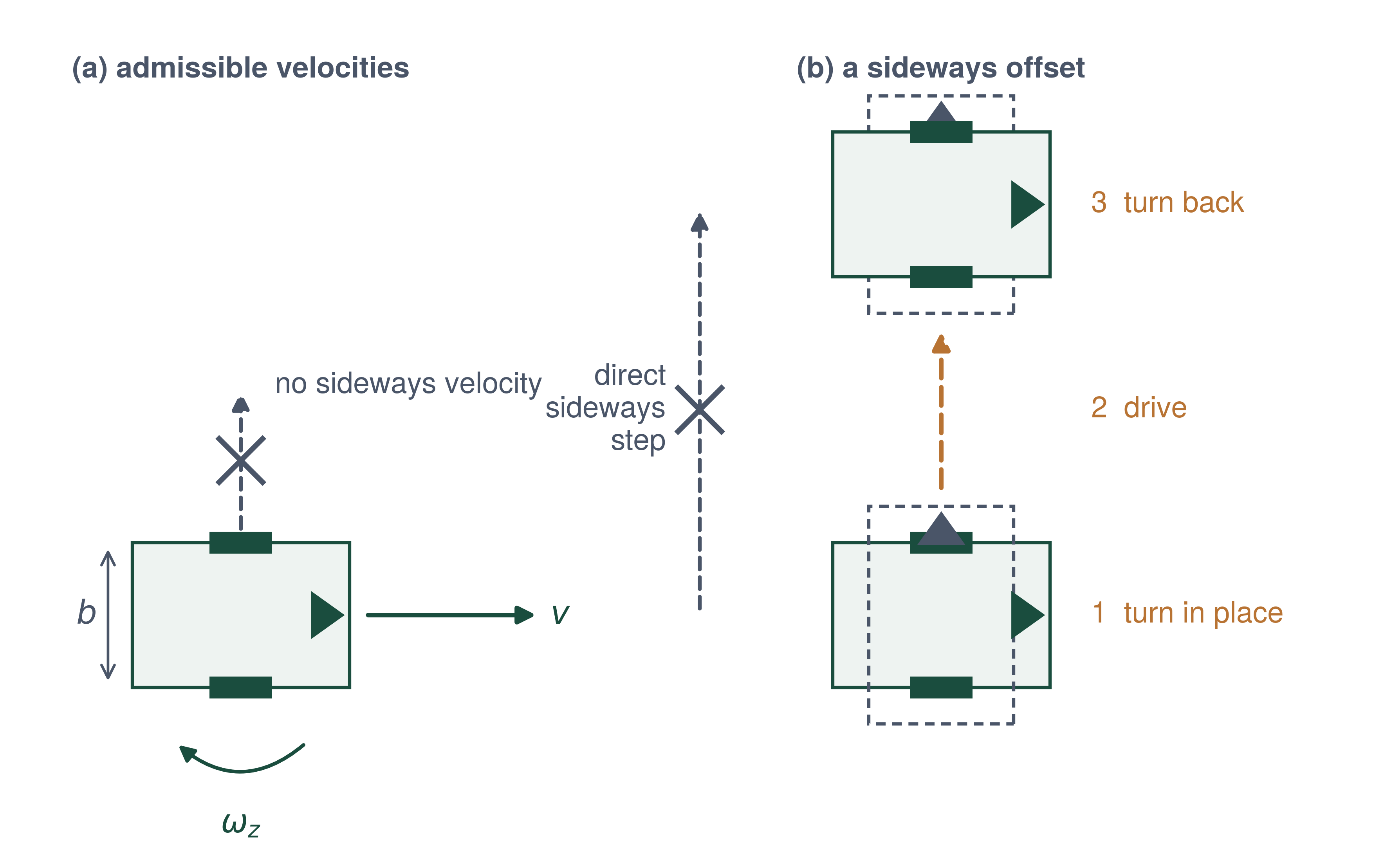
Local base planners enforce nonholonomic constraints by planning directly in velocity space over a receding time horizon. The dynamic window approach (DWA) (Fox et al. 1997) maps each control pair \((\BaseForwardSpeed, \YawRate)\) to a circular trajectory arc and evaluates candidate pairs through two nested dynamic criteria. Reachable velocities comprise pairs achievable within actuator acceleration limits over the replanning window. With the mobile manipulator’s base acceleration limit of 2 m/s² and a 50 ms chunk renewal interval, this dynamic window spans 0.1 m/s on either side of the current forward velocity. Admissible velocities select the subset from which the base can decelerate to a complete stop before reaching the nearest obstacle along that arc, satisfying \(\BaseForwardSpeed \le \sqrt{2\,\ArcObstacleDistance(\BaseForwardSpeed,\YawRate)\,\CredibleBrakingDeceleration}\). From these admissible candidates, DWA selects the control pair maximizing an objective that balances target heading alignment, obstacle clearance, and forward speed. MPPI (Williams et al. 2017), the sampling-based MPC of table 3, replaces this deterministic velocity grid by rolling forward thousands of stochastic control sequences through the dynamic model on a GPU, synthesizing an optimal control action as a cost-weighted trajectory distribution. Production navigation frameworks such as ROS 2 Nav2 incorporate both controller families (Macenski et al. 2023).
Fox, Dieter, Wolfram Burgard, and Sebastian Thrun. 1997. “The Dynamic Window Approach to Collision Avoidance.” IEEE Robotics & Automation Magazine 4 (1): 23–33. https://doi.org/10.1109/100.580977.
Williams, Grady, Nolan Wagener, Brian Goldfain, Paul Drews, James M. Rehg, Byron Boots, and Evangelos A. Theodorou. 2017. “Information Theoretic MPC for Model-Based Reinforcement Learning.” IEEE International Conference on Robotics and Automation (ICRA), 1714–21. https://doi.org/10.1109/ICRA.2017.7989202.
Macenski, Steve, Tom Moore, David V. Lu, Alexey Merzlyakov, and Michael Ferguson. 2023. “From the Desks of ROS Maintainers: A Survey of Modern & Capable Mobile Robotics Algorithms in the Robot Operating System 2.” Robotics and Autonomous Systems 168: 104493. https://doi.org/10.1016/j.robot.2023.104493.
The admissibility test applies the core stopping requirement across candidate arcs, yet its classical textbook formulation assumes instantaneous, constant-deceleration braking. On a straight trajectory with 1.10 m of rack-end clearance, this simplified test admits forward speeds up to 2.10 m/s, well above the physical drive limit of 1.5 m/s. However, when evaluated against the conditional stopping subtotal derived in section 11.5.4 (which accounts for sensor latency, communication delays, localization uncertainty margins, and jerk-limited deceleration), that same clearance fails to guarantee safety even at the nominal drive limit. A mobile-base trajectory generator, whether a classical DWA planner or a learned chunk policy, is therefore a proposer of candidate velocities. The real-time permission path must also charge dispatch-to-admission travel before validating each proposed trajectory against the full stopping budget.
The choice of trajectory generator governs how candidate motions are discovered and determines the computational burden placed on downstream verification. However, the system’s safety enforcement mechanisms must respond consistently regardless of how a proposal was generated. In particular, the execution architecture must cleanly differentiate between rejecting an invalid replacement candidate and responding to unexpected environmental changes. Rejecting an unvalidated proposal leaves the active trajectory in control only while its state, evidence, lease, and stopping reserve remain valid, whereas detecting an unexpected obstacle incursion along the executed path demands an immediate transition to verified braking.
11.7 Trajectory Planning Failure Modes and Infeasible Seams
On the mug reach, a replacement trajectory can fail in three distinct regimes: within the candidate itself, along the boundary where it joins the executing motion, or during execution when the environment changes. The point where a failure first manifests dictates which subsystem has the sensory evidence to reject the trajectory, as well as how much time and clearance remain to bring the machine to a safe stop. Pre-execution candidate and boundary checks intercept the first two failure modes before setpoints can reach actuator registers, whereas runtime monitoring guards against the third.
11.7.1 Checking limits and boundaries before execution
If an unvalidated chunk reaches actuator registers directly, a single out-of-bounds waypoint or an unblended velocity step at the splice instant will fault the drive before feedback monitoring can react. Before any proposed trajectory setpoint can influence actuator registers, a deterministic safety MCU therefore screens the candidate record through two independent admission gates within a measured worst-case execution budget. Fixed-degree seam calculations require bounded compute per axis, whereas checking a complete setpoint sequence scales with the candidate horizon length:
- Pre-execution Bound Checker: Evaluates the proposed neural action chunk in isolation across the full candidate horizon \([\TrackingStartInstant, \NominalPlanExpiry]\) against intrinsic kinematic, dynamic, and stopping invariants. The checker evaluates margin functions \(\LimitMarginFunction(\TimeInstant) = \CheckedSignalLimit - |\CheckedSignal(\TimeInstant)|\) across the signals it checks. Joint positions \(\JointPosition(\TimeInstant)\) are checked against their limits. Joint velocities are checked against contracted limits \(|\JointVelocity(\TimeInstant)| \le \SpeedBound - \frac{1}{2} \ProfileAccelerationBound \SamplingPeriod\) (equation 10, or the \(\frac{1}{4}\) reserve under the equal-velocity, zero-acceleration endpoint conditions and jerk bound of section 11.4.2). Free-space inverse-dynamics joint torques are sampled with a bound on their inter-sample variation and checked against the rated torque, \(|\JointTorque(\TimeInstant)| = |\GeneralizedInertiaMatrix(\GeneralizedCoordinates)\GeneralizedAccelerations + \CoriolisCentrifugalMatrix(\GeneralizedCoordinates, \GeneralizedVelocities)\GeneralizedVelocities + \GravitationalTorqueVector(\GeneralizedCoordinates)| \le \RatedJointTorque\). The checker also enforces the binding stopping invariant: the candidate’s matched stopping suffix must satisfy \(\StoppingDistance \le \ClearDistance\) throughout observed free space. If any knot point or interior interval yields \(\LimitMarginFunction(\TimeInstant) < 0\) or causes the stopping runway to breach available clearance, the gate immediately rejects the candidate and logs a diagnostic fault record containing the joint index, timestamp, and negative margin. Gate rejection causes neither mechanical shudder nor physical pause, because the low-level tracking controller continues along the previously admitted trajectory as long as that trajectory’s state, sensor evidence, lease, and stopping reserve remain valid. A rejected replacement simply fails to renew that lease.
- Boundary Checker: Evaluates the transition seam between the currently executing trajectory \(\Glyph{A}\) and the candidate replacement \(\Glyph{B}\) at transition time \(\SeamInstant\). Because unconstrained sequence decoders predict open-loop action tokens without terminal derivative matching, concatenating raw chunks frequently produces sharp acceleration steps. The boundary checker addresses this in two stages. During early admission, it screens the reachable seam-state envelope projected from trajectory \(\Glyph{A}\). At activation, it incorporates real-time encoder estimates \((\MeasuredSeamConfiguration, \MeasuredSeamVelocities, \MeasuredSeamAccelerations)\) and their error bounds to calculate the physical seam gap \((\FiniteChange\GeneralizedCoordinates, \FiniteChange\GeneralizedVelocities, \FiniteChange\GeneralizedAccelerations)\). It then evaluates whether an analytical \(\DifferentiabilityClass^2\) quintic bridge (equation 12) can reconcile the boundary without violating torque limits or the motor drive’s voltage and current-slew constraints. A fast one-tick estimate, \(\SeamStepTorque = \EffectiveJointInertia \frac{\FiniteChange\JointVelocity}{\SamplingPeriod}\), diagnoses the demand of an unblended one-tick transition. Failure of that estimate cannot reject a finite bridge by itself; admission checks the bridge at its actual duration, with its endpoint states, interior derivatives, torque and electrical bounds, and swept clearance.
For the CSG-25-50 joint in the seam analysis, an idealized calculation accounts solely for its 0.18 kg·m² reflected rotor inertia over a single 1 ms tick and allocates the entire 127 N·m repeated-peak rating purely to acceleration. It yields an idealized ceiling of 0.69 rad/s on that hypothetical one-tick step \(\FiniteChange\JointVelocity\), not on a finite-duration bridge. In practice, the available torque margin is substantially smaller once link and payload inertia, gravity, friction, feedforward torque commands, coil current rise times, and thermal or DC-bus limits are deducted. The admission path must evaluate the finite bridge against this state-dependent torque margin and the drive’s measured step response. The gate nevertheless rejects a step velocity discontinuity outright, even one whose idealized single-tick torque falls below that ceiling, because continuous physical motion requires a smooth, bounded \(\DifferentiabilityClass^2\) bridge that satisfies its own interior limit checks.14
14 Drive and resonance response: A sharp command can excite a joint’s identified flexible modes, but their frequencies and damping depend on the transmission and load. Current limiting, desaturation detection, DC-bus response, and shutdown depend on the selected driver and its configuration; one vendor’s desaturation-protection design note shows how such trip thresholds are set (Chen and Ramachandran 2025).
Chen, Tilden, and Akshaya Ramachandran. 2025. How TPSI3133 DESAT Can Protect Your Expensive SiC MOSFETs and IGBTs. Application Note No. SLVAG18. Texas Instruments.
11.7.2 Runtime tracking monitors and unexpected contact
↪ The cyclic checking that enforces these trips on every tick, and the independence the monitor needs from the proposer, are developed in Admission, Cyclic Checking, and Monitor Independence.
When the arm reaches past the conveyor guard with 0.020 m of budgeted swept-volume clearance, a slipping payload or an unexpected contact after admission can invalidate the dynamic and geometric assumptions under which the plan was cleared. Independent runtime monitors must detect this divergence while remaining obstacle clearance still allows a controlled stop. They track four primary signals on every tick: joint state divergence, tracking error velocity, unexpected contact wrenches, and violations of the geometric assumptions declared in the trajectory record’s sidecar (section 11.8). This monitoring relies on spatial margin budgeting, in which geometric obstacle clearance is not simply awarded to control tracking error. Mechanical compliance under load, structural deflection, and drivetrain backlash consume physical clearance before any feedback tracking error becomes observable at the encoders. The tracking error allowance \(\TrackingErrorAllowance\) therefore equals the total swept-volume clearance minus the structural deflection and gearbox compliance allowance \(\DeflectionComplianceAllowance\).
On the conveyor-guard reach, once payload deflection and gearbox compliance claim an allowance \(\DeflectionComplianceAllowance\) of 0.005 m, the nominal tracking allowance \(\TrackingErrorAllowance\) drops from 0.020 m to 0.015 m. This remainder represents an upper ceiling on allocatable margin rather than a direct trip threshold, because latencies across detection, dispatch, and actuator response, along with state-estimation uncertainty and the swept motion of the fallback maneuver, all require dedicated clearance reserves. The arm tracker’s validated tracking bound, the arm’s counterpart to the base tracking bound \(\TrackingErrorBound\) that The Tracker Handoff and Dynamic Reference Envelopes derives, must fit within these 0.015 m and is checked by the real-time safety loop on every control tick. If the measured Cartesian tool-position error \(\|\MeasuredTrackedPosition(\TimeInstant)-\ReferencePosition(\TimeInstant)\|\) exceeds \(\TrackingErrorBound\), or if a wrist-mounted six-axis force-torque sensor detects an unmodeled 10 N contact during free-space transit, the monitor immediately revokes nominal tracking and commands the validated state-matched fallback. Active physical deceleration begins once the measured detection, communication, and actuator-onset delays elapse.
A trajectory plan can also exhaust its nominal setpoints before a subsequent candidate passes admission. The safety MCU cannot simply allow the execution pointer to overrun the trajectory buffer, nor can it treat a stationary position-hold setpoint as an active, verified stop. Instead, the two deadline tiers of section 11.5.1 end the window of validity on the MCU’s monotonic clock, whichever fires first. Furthermore, computing stopping clearance requires accounting for the full physical chain: sensing and detection delays, dispatch latency, actuator torque rise times, and the swept volume across the deceleration profile. Elementary calculations assuming instantaneous or constant deceleration fail to model the true physical trajectory of a smooth \(\DifferentiabilityClass^2\) stopping suffix.
Every checker and monitor described here depends on an explicit execution contract between the upstream trajectory generator and the downstream real-time controller. If a planner delivers only a raw sequence of Cartesian or joint waypoints, without its validity lease, clearance margins, boundary derivative bounds, and certified stopping suffix, the low-level permission path has no principled way to distinguish safe nominal motion from dangerous dynamic drift. Safe autonomous execution requires that geometry, dynamics, and timing be verified together before setpoints ever reach actuator registers.
11.8 The Trajectory Record
Suppose the planner hands the low-level controller a bare array of 16 joint setpoints for the reach toward the mug, without the obstacle epoch, payload assumption, and pre-checked stopping suffix under which those setpoints were cleared. The MCU then has no way to tell whether the plan is still safe to run when the host stalls or the load changes. The trajectory record, handed over immutably at every replanning cycle, lets the low-level permission path decide whether to admit those setpoints without consulting the high-level planner again. The record carries the header, four deadlines, two deadline tiers, and assumption sidecar defined with the planning handoff in section 11.2.2. It works as a cyber-physical contract rather than a passive message format. Every field encodes a physical invariant that the downstream runtime can verify before a command crosses the causal boundary.
By pairing a staged admission check with the latched stopping profile of section 11.5.3, the record lets the MCU evaluate safety independently of the host planner. Even if the host operating system crashes mid-motion, the resident emergency stop profile remains intact on the real-time controller. Bringing the physical machine to rest still demands operational sensors, DC bus energy, and mechanical braking authority. The belief record and intent lease consumed at the planning handoff remain embedded in the record’s lineage. The completed record binds these physical assumptions directly to the proposed motion before forwarding them to the runtime enforcer, where live sensor feedback governs per-tick tracking permission.
Every field in the contract captures an explicit condition of admission. Kinematic boundary derivatives define how the trajectory must mesh with ongoing motion at the seam. Real-time deadlines dictate exactly when nominal tracking must yield to a safe stop. The accompanying sidecar documents the precise geometric and inertial assumptions under which the validator certified the plan. Instead of taking the planner’s assertion of feasibility on faith, the execution runtime uses the record to hold the motion accountable to physical reality.
Hierarchically, the trajectory record answers to the intent lease. The cryptographic digest binds the record to the exact parent lease whose target and effort ceilings the permission path must check against the proposed motion. The motion itself is stored as discrete setpoint arrays or continuous spline coefficients, parameterized by an explicit sample cadence (a 25 ms timestep \(\SetpointStepInterval\) on the running machine, a 40 Hz stream). The record also carries the nominal trajectory expiration \(\NominalPlanExpiry\) (400 ms for a single chunk) and canonical SI units. Pairing this explicit cadence and unit specification with the reference coordinate frame and evidence timestamp established in section 11.2 allows the joint controller to interpolate setpoints and evaluate higher-order derivatives cleanly, eliminating coordinate-frame ambiguities and any reliance on unsynchronized host clocks.
Physical feasibility is never unconditional; it holds only under the environmental geometry and dynamic loads assumed during planning. The immutable sidecar captures these conditions, recording the obstacle-map epoch, payload mass, surface friction coefficients, kinematic limits, validator software version, certified clearance margins, and the source observation identifiers. A cryptographic digest in the fixed header immutably binds this sidecar to the setpoint payload. Because safety proofs cannot extrapolate beyond validated boundaries, the payload and friction values declared in the sidecar must fall strictly within the target operational design domain (ODD) declared in The Evaluation Record. If live sensor feedback indicates that the robot has drifted outside these operating assumptions, the permission path immediately revokes the TRACK state, recognizing that clearance margins computed for one world state do not hold in another. Diagnostic metadata, such as random solver seeds and neural model weight hashes, belongs in this audit sidecar for offline postmortem analysis, keeping the per-tick servo loop lean and deterministic.
↪ Conditional permission, the per-tick safe-set test that holds a clearance margin valid only for the live state, is developed in Safe Sets as Conditional Permission.
On this machine, the chunk policy generates only the nominal motion profile, which the planning runtime then packages into a self-contained record by appending the seam state, the four operational deadlines, and a matched stopping suffix. Inside the fixed header, lineage fields record a monotonic sequence number, the evidence timestamp \(\EvidenceEpoch\), and the digest of the parent intent lease, while timing fields encode the four deadlines from section 11.2.2. Seam fields then define the reference frame, each joint’s initial state \((\JointPosition,\JointVelocity,\JointAcceleration)\) at handoff, and the representation of an admission-checked stopping profile satisfying \(\StoppingDistance \le \ClearDistance\). Content fields specify the payload format, byte length, and an integrity digest spanning both the setpoint payload and the sidecar.
Both the variable-length setpoint sequence and the immutable assumption sidecar sit immediately outside the fixed header. The MCU verifies their composite digest before running the admission checks described in section 11.5. This dual-digest design decouples integrity from provenance: the payload digest validates contents, while the parent digest anchors lineage. Because the permission path admits a motion proposal based entirely on whether its physical invariants check out rather than on the identity of the process that generated it (Supervisory timers and proposal wire contracts), the record deliberately omits cryptographic signatures or origin tags.
↪ Byte layout: Trajectory payload illustrates a record carrying a single polynomial stopping suffix; it does not encode the worked piecewise S-curve.
Instantiated for the warehouse reach toward the mug, the record carries its own deadlines, which are those of the alternate timeline, while the running chunk lease decides how long tracking actually continues. Its parent digest points directly to the mug-acquisition intent lease, its coordinates are expressed in the robot base frame, and every timestamp references the MCU’s monotonic clock. Measured relative to \(\TrackingStartInstant\), the timing fields record the commitment deadline at 300 ms, the nominal trajectory end at 400 ms (derived from 16 setpoints spaced at 25 ms), and the final safe-stop horizon at 575 ms. The 240 ms blend deadline remains a planner scheduling target outside the fixed header. Four candidates can end tracking authority: the admission cutoff at 278 ms, the lease timeout 60 ms after the last admitted chunk, the intent lease expiry, and evidence staleness. On the running machine the lease timeout binds first. The commitment fields then serve as a backstop that acts only under a lease long enough to outlast the cutoff.
The worked seam specifies a 275 ms, jerk-limited \(\DifferentiabilityClass^2\) stopping suffix bounded by peak acceleration 5 m/s² and jerk 66.7 m/s³. It is anchored at the commitment state and brings the arm safely to rest from its 1 m/s TCP velocity limit within 137.5 mm. Serializing and admitting this analytical S-curve requires a specified bounded profile encoding and decoder, bound to the admitted path and stop-entry state, with decoding and validation included in the admission budget (a representation not supplied by the illustrative single-polynomial wire layout). Under the running lease, a lease timeout triggers the state-matched fallback built from the measured state. From zero-acceleration cruise that fallback follows the same S-curve and travels the same distance (section 11.5.2), so the lease path and stop together consume 219.5 mm of the available 300 mm clearance. The 278 ms commitment cutoff never extends the lease. In the sidecar, the planner asserts a payload mass bounded by 3 kg, unobstructed free space leading up to the grasp contact, and operating conditions inside the target ODD. The real-time permission path evaluates all of these upon admission and audits them on every control cycle.
In this concrete trajectory, the temporal ordering strictly satisfies \(\TrackingStartInstant\le \CommitmentInstant<\NominalPlanExpiry<\StopCompletionInstant\), and the MCU enforces these timing boundaries according to the TRACK and STOP transition rules developed in section 11.2. Because safety requires both temporal validity and physical realizability, a well-formed timestamp in the header cannot compensate for an unviable stopping suffix. To make latency and timing jitter auditable, the system logs the timestamps for evidence capture, plan request, validation completion, admission, activation, control transfer, and stop completion in a synchronized time domain, exposing the end-to-end response delay of the entire perception-planning-control pipeline.
Every artifact in this runtime chain, from the observation contract and the belief record through the intent lease to the trajectory record itself, declares its physical dependencies and its expiration deadline. The trajectory record proves only what the planner could verify at plan time: that a collision-free stop remains physically feasible from any state the robot might reach before commitment, given the obstacle scene and dynamic payload asserted in its sidecar. Common design pitfalls often mistake this bounded, conditional guarantee for unconditional safety, overlooking what happens when physical reality deviates from the planner’s model.
11.9 Fallacies and Pitfalls
A planned trajectory remains physically feasible only as long as its environmental, dynamic, and computational assumptions hold true. In embodied systems, failures rarely stem from minor mathematical errors along the nominal interior of a path. Instead, they emerge at operational and physical seams: when dynamic obstacles intrude into an active swept volume, when concatenated action chunks excite mechanical resonances, when host inference pipelines miss scheduling deadlines, or when controllers attempt to stop faster than actuator dynamics permit. Both the trajectory admission gate and the real-time execution monitor must defend against these five failure modes.
Fallacy: Static admission checks protect a machine against obstacle displacements during active execution.
Static geometry confirms clear space only at admission time; dynamic workspaces demand continuous runtime monitoring. Consider a robotic manipulator reaching toward an assembly target. When the trajectory is first admitted, the swept volume between the end-effector and the target is completely clear. Halfway through execution, however, an operator slides a storage tote into the arm’s path. Although the admission check was mathematically correct when computed, the physical workspace has changed. Static pre-screening guarantees only that a trajectory was safe in the past; it cannot guarantee that the path remains clear as time elapses. Execution monitoring must continuously track obstacle clearances and initiate deceleration while adequate stopping distance remains. Systems architects must explicitly budget sensor bus latency and vision pipeline transit times, reserving enough spatial stopping margin to ensure the machine can halt before an encroaching obstacle breaches its swept volume.
Architect’s countermeasure: Pair high-level spatial screening on the host with low-latency local clearance sensing processed directly by the MCU. Explicitly allocate the sensing refresh rate, bus transit latency, and MCU memory footprint. If an unmodeled obstacle breaches the reserved spatial safety margin \(\ProtectiveClearanceMargin\), immediately abort nominal tracking and engage the pre-validated, state-matched fallback trajectory.
Pitfall: Checking each action chunk alone without examining the motion the chunks compose.
Individual chunk feasibility does not guarantee smooth motion across seams; stochastic neural chatter can overstress a mechanical transmission. When generative sequence policies (such as diffusion models or action-chunking transformers) are sampled stochastically, successive chunks frequently disagree in direction or mismatch acceleration at their boundary. While every individual chunk satisfies kinematic position and velocity bounds in isolation, concatenating them without boundary constraints induces rapid torque reversals \(\FiniteChange\CommandedJointTorque = \EffectiveJointInertia \FiniteChange\JointAcceleration\). Amplified by the reflected rotor inertia (\(\GearReductionRatio^2 \RotorInertia\)), this high-frequency chatter excites flexible structural modes, accelerates gearbox wear, and causes severe Joule heating (\(\TorqueProducingCurrent^2 \PhaseResistance\)) in the stator windings. The admission pipeline must evaluate derivative continuity across every chunk boundary seam, enforce \(\DifferentiabilityClass^2\) quintic smoothing, and track recent motion history to reject oscillating command sequences before they reach the motor drives.
Architect’s countermeasure: Enforce multi-chunk frequency and reversal monitoring across a sliding execution window. Reject any trajectory candidate whose frequency spectrum or repeated effort exceeds the motor’s identified mechanical or thermal envelope. If smoothing filters alter a candidate chunk, re-run the full kinematic, seam continuity, and terminal stop checks on the modified trajectory prior to admission.
Pitfall: Delaying fallback transition past the hard stopping horizon in the hope that delayed compute finishes.
An overdue compute cycle never justifies extending a physical commitment deadline. In an alternate schedule operating with an admission cutoff of 278 ms, the active trajectory record supplies nominal setpoints that expire at 400 ms. The record carries a 275 ms matched stopping suffix that must finish deceleration by 575 ms. To guarantee physical braking onset by 300 ms, the MCU must dispatch the fallback trajectory no later than the 278 ms cutoff unless a verified replacement plan has already arrived. If the host application processor reports that neural inference is nearly complete but has not yet delivered a validated plan, delaying the fallback transition consumes the runway reserved for stopping. The MCU must dispatch the resident stopping suffix by the earlier cutoff so its physical onset occurs at commitment. Progress reports cannot extend a mechanical stopping budget; only an admitted, physically verifiable trajectory justifies continued forward motion.
Architect’s countermeasure: Bind the physical commitment deadline \(\CommitmentInstant\) strictly to a monotonic hardware timer on the MCU. When the timer reaches the admission cutoff, close the admission window and dispatch the resident stopping suffix immediately, disregarding any speculative progress updates from the host processor.
Pitfall: Relying solely on feedforward dynamic models when physical contact or payload mass can change abruptly.
Feedforward model inversion without closed-loop disturbance bounds can drive an unloaded arm beyond its admitted trajectory. Consider an arm lifting a heavy workpiece near its 3 kg payload limit. To track the aggressive trajectory, the controller injects feedforward torque computed from an inverse dynamics model of the fully loaded arm. If the workpiece slips from the gripper mid-lift, the drives continue applying the large lifting torque intended for the heavy load to an arm that is now empty. Without a timely feedback correction or torque clamp, the excess torque accelerates the arm above its planned rate. While the admitted trajectory has not changed, the physical mass properties that justified those torque commands have vanished. High-bandwidth feedback monitoring must detect the resulting tracking error and clamp torque commands before the arm strikes a mechanical joint stop or triggers inverter thermal derating. Feedforward dynamic models significantly reduce tracking lag under nominal conditions, but they must never run without closed-loop supervisory bounds.
Architect’s countermeasure: Implement real-time torque limiters and tracking-error monitoring (\(\|\MeasuredTrackedPosition - \ReferencePosition\| \le \TrackingErrorBound\)) directly inside the 1 kHz servo loop. If an abrupt payload drop or unexpected contact causes acceleration to spike, clamp motor currents immediately and transition the system to compliance mode or an emergency stop.
Fallacy: A trajectory can omit an achievable terminal stopping suffix if replacement plans are expected to arrive in time.
A trajectory without a pre-latched stopping continuation is an unhedged bet on infinite compute availability. Traveling at its drive limit of 1.5 m/s, a mobile manipulator’s base requires 1,031.25 ms for even the shortest deceleration profile its kinematic bounds permit. That minimum stop follows an S-curve profile \(\Time=\CruiseSpeed/\ProfileAccelerationBound+\ProfileAccelerationBound/\JerkLimit\) evaluated at a credible braking acceleration 2 m/s² and jerk limit 7.11 m/s³. Sizing a proposed stopping suffix using the idealized constant-deceleration formula \(\CruiseSpeed/\CredibleBrakingDeceleration\) yields 750 ms. However, no physical actuator can ramp deceleration instantaneously without infinite jerk. Forcing a stop into that truncated duration inevitably violates the acceleration bound, the jerk limit, or both, exceeding what the chassis and its payload can tolerate. Expecting the next plan to arrive on time does not make an unfeasible fallback executable. The admission gate must verify that the terminal stopping suffix strictly respects \(\ProfileAccelerationBound\) and \(\JerkLimit\) throughout its duration. With an S-curve, this requires validating \(\StoppingDuration\) against equation 17 and confirming that the stopping distance satisfies \(\StoppingDistance \le \ClearDistance\) within verified clearance. The admission gate must reject any record that fails this test. Every admitted trajectory requires a physically executable termination path to protect the machine when upstream inference stalls.
Architect’s countermeasure: Require every candidate trajectory record to incorporate a complete, closed-form \(\DifferentiabilityClass^2\) stopping profile along its admitted corridor. Deceleration and jerk along this profile must remain strictly within vehicle and payload stability limits, while the stopping distance must satisfy \(\StoppingDistance \le \ClearDistance\) within verified clear space. Reject any record at the admission gate that lacks this independently executable stopping guarantee.
11.10 Summary
A trajectory transforms a high-level goal into timed physical motion. On an active machine, it must resolve three questions that a geometric path leaves unanswered: how long the motion remains valid and executable, how it splices smoothly into the motion already under way, and how the machine stops safely if no replacement arrives. A multi-step task such as the reach for a mug progresses through a continuous sequence of renewed, validated trajectory prefixes without forcing the entire task into a single observation window. Predictive models and planners generate candidate trajectories, but the runtime system grants execution authority only after verifying fresh sensor evidence, admission deadlines, and the machine’s true state. When a replacement trajectory arrives late, the controller falls back to its resident stopping maneuver. Tail latency bounds (\(\DesignLatencyQuantile(\ReplacementLatency)\)) therefore quantify the expected frequency of service degradation to this safe fallback, while the machine’s physical safety rests on the stopping profile itself.
Whether a physical system can track a candidate trajectory is distinct from whether that trajectory avoids obstacles. Kinematic feasibility alone can fail in subtle ways. Near kinematic singularities, the manipulator Jacobian maps modest Cartesian end-effector velocities into unbounded joint rates. Damped least-squares inversion caps these joint steps, but does so by accepting tracking error that can still push joints against their limits. Dynamic feasibility imposes even stricter constraints. The rigid-body manipulator equations translate planned motions into actuator torques, where reflected rotor inertia amplifies any velocity or acceleration discontinuity across trajectory seams into severe torque spikes. A quintic bridge matches position, velocity, and acceleration across the boundary, eliminating these impulsive torque requests. Similarly, time-optimal path parameterization drives actuators along their torque envelopes, but bang-bang acceleration profiles demand instantaneous torque steps that physical drives cannot achieve. Enforcing an explicit jerk bound rounds these transitions at minimal time cost, turning theoretical path timings into executable motor commands. Whether candidates originate from sampling-based search, trajectory optimization, or learned action chunking, the underlying physical obligations remain unchanged. Each planning method generates a prospective motion proposal, but never a license to execute without validation.
Real-time execution relies on strict timing contracts between the planner and the low-level controller. A 60 ms lease halts a stalled proposal stream using a state-matched stopping response, reserving an illustrative 80.5 mm safety buffer to absorb sensing delay and model uncertainty. In an alternate longer-lease configuration, replacement admission closes strictly by 278 ms so that physical deceleration can initiate no later than 300 ms. Both regimes enforce the identical systems invariant: every active trajectory must reserve sufficient travel to accommodate perception-action latency and the entire stopping maneuver. The base faces the same arithmetic. Its jerk-limited S-curve, the shortest stop under the stipulated load bounds, raises the partial stopping budget at the drive limit to 1,123.84 mm (row 6 of The warehouse mobile manipulator's stopping budget). Because this exceeds the available 1.10 m rack-end clearance, the runtime controller must proactively restrict operating speed. Table 5 lists the equations behind these admission decisions, detailing the physical limit each bounds and where it is derived in this chapter.
| Equation | What it bounds or decides | Derived in |
|---|---|---|
| \(\FiniteChange\DampedStepConfiguration = \ManipulatorJacobian^\top(\ManipulatorJacobian\ManipulatorJacobian^\top+\InverseKinematicsDamping^2\IdentityMatrix)^{-1}\FiniteChange\CartesianPosition\) | The inverse-kinematics step near a singularity, capped at \(\ToolSpeedLimit/(2\InverseKinematicsDamping)\) at the price of tool error | equation 2 |
| \(\ReplacementLatency = \DispatchObservationAge + \DispatchAdmissionInterval\) | Replacement latency from capture to admission, which the renewal schedule must absorb | equation 3 |
| \(\HandoffExceedanceProbability \le \MissionExceedanceBudget/\MissionHandoffCount\) | The per-handoff tail that a mission target implies, far beyond p99 | equation 4 |
| \(\TrajectoryRecordDuration \ge \ReplanRequestOffset + \DesignLatencyQuantile(\ReplacementLatency) + \ReplacementTimingReserve + \StoppingDuration\) | Conservative capture-latency charge; full reserve includes scheduling slack and response; stop included | equation 5 |
| \(\JointTorque = \GeneralizedInertiaMatrix\GeneralizedAccelerations + \CoriolisCentrifugalMatrix\GeneralizedVelocities + \GravitationalTorqueVector - \ManipulatorJacobian^\top\ExternalWrench\) | The torque a planned motion demands, evaluated by inverse dynamics at admission | equation 8 |
| \(\lvert\JointVelocity_k\rvert \le \SpeedBound - \tfrac{1}{2}\ProfileAccelerationBound{}\SamplingPeriod\) | A sampled velocity limit that still holds between samples | equation 10 |
| \(\SeamStepTorque = \EffectiveJointInertia\,\FiniteChange\JointVelocity/\SamplingPeriod\) | The torque a seam’s velocity step asks of the reflected inertia | equation 11 |
| \(\JointJerk(\TimeInstant) = 6\PolynomialTrajectoryCoefficient_3 + 24\PolynomialTrajectoryCoefficient_4\TimeInstant + 60\PolynomialTrajectoryCoefficient_5\TimeInstant^2\) | The jerk of a quintic bridge, whose extrema the checker evaluates in closed form | equation 13 |
| \(\DcBusVoltage \ge \PhaseInductance\,d\TorqueProducingCurrent/d\TimeInstant + \PhaseResistance\, \TorqueProducingCurrent + \MotorBackEmfConstant\ElectricalAngularSpeed\) | Whether the drive has the voltage for the current slew a bridge demands | equation 14 |
| \(\JointTorque = \PathAccelerationTorqueCoefficient(\PathCoordinate)\PathAcceleration + \PathVelocitySquaredTorqueCoefficient(\PathCoordinate)\PathVelocity^2 + \GravitationalTorqueVector(\PathCoordinate)\) | The path accelerations the torque limits allow, and so the fastest timing of a path | equation 15 |
| \(\StoppingDistance = \SpeedAtDetection^2/2\ProfileAccelerationBound + \SpeedAtDetection\,\ProfileAccelerationBound/2\JerkLimit\) | The shortest stop within deceleration and jerk bounds, above the plateau speed \(\ProfileAccelerationBound^2/\JerkLimit\) | equation 17 |
| \(\StoppingDistance(\CommitmentInstant) \le \ClearDistance(\CommitmentInstant)\) | Whether a trajectory may be admitted at all | equation 18 |
Key Takeaways: Timed motion and independent stopping
- Prediction is not execution authority: A long predicted path can guide motion, but the controller executes only short, validated prefixes. While renewal cadence dictates how frequently new plans are requested, target evidence retains its own capture-based timestamp, and its evidence horizon bounds how long it stays valid.
- Reserve a stopping response from the current state: A stopping suffix is mathematically valid only for its declared entry state. If an execution lease or sensor observation expires, the machine must possess a pre-validated fallback trajectory, sufficient reserve energy, and enough physical clearance to absorb both response latency and full deceleration.
- Admission precedes physical commitment: The alternate arm schedule closes replacement admission strictly by 278 ms to ensure a physical stop can initiate at 300 ms. A late planner proposal cannot spend or delay this reserved response window.
- A collision-free path is not inherently executable: Near singularities, Cartesian end-effector speeds demand infeasible joint velocities. Damped least squares bounds the inverse-kinematics step only by introducing tracking error. Similarly, time-optimal path timing produces discontinuous torque demands that trigger actuator saturation. Adding quintic seams and jerk bounds smooths transitions, but interior joint limits, inverter voltage headroom, and clearance remain binding constraints.
- Trajectory smoothness dictates stopping distance: Finite jerk bounds make smooth stopping profiles significantly longer than ideal constant-deceleration braking. An S-curve profile pays the least, the equivalent of cruising for half of one jerk ramp, yet that overhead still sets operating speed limits near rack ends and obstacles.
- Candidate rejection does not require immediate stopping: The running trajectory continues executing normally as long as its state, sensor evidence, lease deadline, and fallback trajectory remain valid. Rejecting an invalid replacement proposal simply leaves those original expiration boundaries unchanged.
- Admission and runtime enforcement require separate system budgets: Evaluating a candidate plan requires an asynchronous, bounded scan over the entire trajectory chunk, whereas per-tick enforcement performs strict real-time checks against current state and local sensor data. System designers must isolate their CPU time, memory footprints, and bus interference to prevent high-level planning from disrupting the low-level control loop.
A plan stays valid only while the stop it carries can still be executed. When a timing, seam, or clearance check fails, the remedy is to shorten the lease, slow the motion, or lengthen the bridge until every check passes with the resident stop still inside the clearance, never to wait for a better proposal. The stall runway shows which term to work on. If the travel before stop onset rivals the stop itself, the lease is the term to shorten. If the stop dominates, the deceleration or jerk bound the load tolerates is the term to measure.
For motion, the third law, proposal is not permission (principle 3), reduces to a clearance test. However smooth, collision-free, and timely a candidate is, the MCU admits it only with an independently executable stop that fits the clearance that remains, and that test does not depend on how the candidate was generated. Admission is not a waiver either. The conditions certified at admission remain obligations on every control tick, so the machine must keep checking live state against the clearance it has left.
11.11 Historical Perspective and Further Reading
Motion planning became a concrete computational discipline when Lozano-Pérez (1983) mapped geometric collision avoidance into configuration-space search, shrinking the geometry of a complex moving body to a single point. In the same year, Schwartz and Sharir (1983) formulated the piano movers’ problem through exact algebraic decomposition. While theoretically complete, exact algebraic methods scale doubly exponentially with degrees of freedom, rendering them intractable for multi-joint manipulators. In the 1990s, randomized sampling bypassed this geometric bottleneck by trading exact completeness for probabilistic guarantees. Probabilistic roadmaps (Kavraki et al. 1996) introduced multi-query graph construction across free configuration space, while rapidly-exploring random trees (LaValle 1998) solved single-query kinodynamic problems by incrementally biasing search trees toward unexplored regions. Later, RRT* (Karaman and Frazzoli 2011) proved that standard random trees almost surely fail to find optimal paths, introducing local edge rewiring to guarantee asymptotic convergence toward the optimum. Together, these foundational algorithms resolve where a robot may safely pass, which represents the geometric half of motion planning.
Kavraki, Lydia E., Petr Švestka, Jean-Claude Latombe, and Mark H. Overmars. 1996. “Probabilistic Roadmaps for Path Planning in High-Dimensional Configuration Spaces.” IEEE Transactions on Robotics and Automation 12 (4): 566–80. https://doi.org/10.1109/70.508439.
LaValle, Steven M. 1998. Rapidly-Exploring Random Trees: A New Tool for Path Planning. TR 98-11. Computer Science Department, Iowa State University.
Karaman, Sertac, and Emilio Frazzoli. 2011. “Sampling-Based Algorithms for Optimal Motion Planning.” The International Journal of Robotics Research 30 (7): 846–94. https://doi.org/10.1177/0278364911406761.
Bobrow, James E., Steven Dubowsky, and J. S. Gibson. 1985. “Time-Optimal Control of Robotic Manipulators Along Specified Paths.” The International Journal of Robotics Research 4 (3): 3–17. https://doi.org/10.1177/027836498500400301.
Pham, Hung, and Quang-Cuong Pham. 2018. “A New Approach to Time-Optimal Path Parameterization Based on Reachability Analysis.” IEEE Transactions on Robotics 34 (3): 645–59. https://doi.org/10.1109/TRO.2018.2819195.
Berscheid, Lars, and Torsten Kröger. 2021. “Jerk-Limited Real-Time Trajectory Generation with Arbitrary Target States.” Robotics: Science and Systems (RSS) XVII. https://doi.org/10.15607/RSS.2021.XVII.015.
Ratliff, Nathan, Matt Zucker, J. Andrew Bagnell, and Siddhartha Srinivasa. 2009. “CHOMP: Gradient Optimization Techniques for Efficient Motion Planning.” IEEE International Conference on Robotics and Automation (ICRA), 489–94. https://doi.org/10.1109/ROBOT.2009.5152817.
The second half, timing and dynamics, followed an independent line of work. Bobrow et al. (1985) showed that the fastest traversal along a pre-specified path under actuator torque limits follows a bang-bang structure in the phase plane, switching between maximum acceleration and maximum deceleration. Decades later, TOPP-RA (Pham and Pham 2018) reformulated time-optimal path parameterization through reachability analysis, casting the search into a sequence of linear programs that execute in time linear in the number of path waypoints. Pure time-optimal trajectories command discontinuous accelerations, however, and the resulting infinite jerk excites mechanical resonances that degrade physical drives. To produce smoother execution, roboticists drew inspiration from biology: Flash and Hogan (1985) showed that human reaching movements naturally minimize jerk. In robotic manipulation, Kröger and Wahl (2010) demonstrated that complete, jerk-limited trajectory profiles could be synthesized deterministically from an arbitrary initial state within a single millisecond-scale control cycle. Ruckig (Berscheid and Kröger 2021) generalized this formulation to arbitrary target kinematic states and asymmetric limits, establishing the fast, closed-form generator that produces this chapter’s stopping profiles. Trajectory optimization reached robotics along a parallel route. Direct collocation (Hargraves and Paris 1987) originated in aerospace trajectory design to transcribe continuous optimal control into sparse nonlinear programs. Receding-horizon control matured in the process industries (Qin and Badgwell 2003), where slow chemical plant dynamics afforded ample time for numerical convergence. Later, algorithms like CHOMP (Ratliff et al. 2009) brought functional gradient optimization directly to robotic arms, optimizing trajectory smoothness and obstacle clearance simultaneously.
The commitment problem, deciding when a planned motion becomes irrevocable and keeping execution safe after that point, is the most recent to mature. Because physical systems possess inertia, safety cannot be judged solely by examining whether the current state is collision-free. Fraichard and Asama (2004) formalized inevitable collision states, establishing that a planner must verify that a system never enters a state from which every future control trajectory culminates in a crash. This formulation gave a robotic form to the viability kernels that Aubin (1991) had introduced in control theory. Modern learning-based methods have transformed how candidate motions are generated. Action chunking (Zhao et al. 2023) and diffusion policies (Chi et al. 2025) predict multi-step action trajectories directly from visual observations, capturing dexterous behaviors without explicit geometric reconstruction. To bridge the latency gap between neural network inference and high-frequency actuation, real-time chunking (Black et al. 2025) conditions incoming predictions on the action sequence already committed to the hardware controller. Regardless of how candidate motions are generated, the execution runtime must enforce physical safety. The trajectory record binds the admitted trajectory to its initial seam state, enforces hard commitment deadlines, and guarantees a deterministically executable stopping suffix whenever the policy stalls.
Zhao, Tony Z., Vikash Kumar, Sergey Levine, and Chelsea Finn. 2023. “Learning Fine-Grained Bimanual Manipulation with Low-Cost Hardware.” Robotics: Science and Systems (RSS). https://doi.org/10.15607/RSS.2023.XIX.016.
For further reading, six works trace the lineage from classical planning to modern learned proposals:
- Qin and Badgwell (2003) provides a comprehensive survey of industrial model predictive control, charting its progression from early petrochemical applications to commercial implementations and illustrating how receding-horizon optimization operates on physical systems whose long time constants tolerate multi-second solve times.
- Fraichard and Asama (2004) formalizes inevitable collision states and defines the dynamic conditions required for provable motion safety under actuator limits, establishing the theoretical foundation for the commitment deadlines analyzed in section 11.5.3.
- Biagiotti and Melchiorri (2008) provides an exhaustive reference on trajectory generation profiles across robotics and industrial automation, detailing the analytical formulation of polynomial splines, filter-based smoothers, and the double-S profile used for the \(\DifferentiabilityClass^2\) stopping suffix in section 11.5.2.
- Kröger and Wahl (2010) develops the mathematical framework for online trajectory generation, deriving algorithms that compute kinematically feasible, jerk-limited motion profiles from arbitrary initial states within single-cycle real-time deadlines.
- Lynch and Park (2017) offers a unified, geometrically rigorous treatment of configuration space, kinematics, rigid-body dynamics, time scaling, and motion planning, serving as a comprehensive companion to Forward kinematics and singularities.
- Chi et al. (2025) details diffusion policies for robotic manipulation, examining receding-horizon execution of predicted action sequences and presenting the modern learned proposers whose seams, deadlines, and fallback stopping profiles this chapter evaluates.
Fraichard, Thierry, and Hajime Asama. 2004. “Inevitable Collision States: A Step Towards Safer Robots?” Advanced Robotics 18 (10): 1001–24. https://doi.org/10.1163/1568553042674662.
Biagiotti, Luigi, and Claudio Melchiorri. 2008. Trajectory Planning for Automatic Machines and Robots. Springer. https://doi.org/10.1007/978-3-540-85629-0.
Kröger, Torsten, and Friedrich M. Wahl. 2010. “Online Trajectory Generation: Basic Concepts for Instantaneous Reactions to Unforeseen Events.” IEEE Transactions on Robotics 26 (1): 94–111. https://doi.org/10.1109/TRO.2009.2035744.
Lynch, Kevin M, and Frank C Park. 2017. Modern Robotics: Mechanics, Planning, and Control. Cambridge University Press.
Chi, Cheng, Zhenjia Xu, Siyuan Feng, Eric Cousineau, Yilun Du, Benjamin Burchfiel, Russ Tedrake, and Shuran Song. 2025. “Diffusion Policy: Visuomotor Policy Learning via Action Diffusion.” The International Journal of Robotics Research 44 (10-11): 1684–704. https://doi.org/10.1177/02783649241273668.
What’s Next: From admitted plans to per-tick permission
Admission judges a trajectory against the state the planner predicted, but the machine executes it against the state it actually reaches. Between the two, the body lags its reference, a person can step into the aisle, and an actuator can run short of torque, and the stopping budget assembled here has not yet charged the first of these. On the base the gap is already decisive, because the jerk-limited stop carries the partial budget to 1,123.84 mm against 1.10 m of rack-end clearance at the drive limit before the body’s departure from its reference is priced. Safety Enforcement begins with the per-tick gatekeeper, the permission-path check that runs on every control tick against live state. It prices tracking error as an inset on the stopping distance and derives a candidate aisle speed whose timing and braking premises still require qualification. When a check fails, it selects among fallback responses that include the resident stopping suffix latched at admission.