Physical Data

5 Physical Data

Lecture slides for this chapter

Purpose

Physical AI stack focus for this chapter.

Why can a large archive of successful demonstrations leave a robot unable to recover from its first mistake?

A successful demonstration shows how one machine completed a task under one set of conditions. It shows almost nothing about what to do after a slip, a shifted fixture, or a worn gripper, yet a learned policy’s first error carries it into exactly those states, where the archive holds no instruction. Repeating the demonstration enlarges the archive without filling that gap. The recorded motion also carries the operator’s delay, the machine’s limits, and every correction the permission path applied, so a training process that cannot separate these influences learns a safeguard’s intervention or a mechanical limitation as if it were skill. Gathering the missing experience costs operator time and component life, and the collection itself must stay within the machine’s physical limits. Physical data must therefore be engineered, from the choice of experiences to the meaning, timing, and physical origin of every label and the conditions the archive leaves uncovered. Because every collected action crosses the causal boundary, its irreversible costs decide what a machine can learn and where its evidence stops.

Learning Objectives

• Explain how endogenous covariate shift yields the conditional quadratic imitation-cost bound, and distinguish dataset occupancy from evaluated closed-loop competence
• Select the action tap a dataset imitates and align multi-rate sensor and action streams to hardware exposure-midpoint timestamps within the task’s spatial tolerance
• Estimate usable demonstration yield from collection time, operator rest, and physical reset overhead, and budget the mechanical component wear a campaign consumes
• Identify collection gaps by joining empirical state-action occupancy against a required scenario table
• Separate failed autonomous actions from admissible human recovery across the divergence, takeover, and stabilization timestamps of an intervention episode
• Evaluate whether an embodiment’s mechanical, sensing, and timing assumptions transfer to another machine without falling into the normalization fallacy
• Detect silent calibration and plant drift in a demonstration archive using kinematic reprojection and repeated excitation trajectories
• Design an immutable provenance record linking each observation to its four-stream action taps (\(\RequestedActionTap, \MappedCommandTap, \EnforcedCommandTap, \MeasuredResponseTap\)) and to the collecting plant

Explore the concepts in this chapter

The volume’s concept map, opened on this chapter. Select a concept to read how it connects to ideas in other chapters. Open the full map ↗

5.1 Endogenous Experience

In most machine learning, the dataset exists before the engineering begins. A text corpus or an image benchmark is gathered independently of the model, costs little per additional example, and does not change in response to anything the model predicts. A physical machine has no such corpus. Collecting demonstrations on the robot consumes operator time and component life; robot-free and synthetic sources avoid that robot wear but still require qualification for the target machine. Every telemetry record reflects who commanded the action, what the permission path admitted, and how the physical body moved. Because each executed action changes the physical state of the system, it dictates what subsequent observations can reveal. Physical data is therefore an engineered artifact. The central challenge of physical data engineering is deciding which experiences to collect, and what to record about them, so that a policy learns the task rather than the idiosyncrasies of its collection. Answering this challenge requires four elements: accounting for collection costs in operator time and hardware wear, defining an unambiguous meaning for every recorded action label, establishing a metric for state-space coverage independent of the archive’s internal contents, and explicitly auditing what the archive omits.

Consider a warehouse mobile manipulator tasked with opening a spring-latched cage door. The robot can flawlessly enforce its low-level motion limits and yet fail because it lacks the operational experience to unlatch the door. During a demonstration, a human operator commands motion, the safety permission path checks and filters it, and the robot’s physical body drives against the mechanical latch. The onboard sensor log captures the output of that entire coupled loop. The limits and handoffs recorded earlier for this machine, in the limit record of The six elements of a limit record and the handoff record of The Handoffs Matrix, therefore become preconditions on the training data fed to the learned policy proposer. Every logged command was shaped by them before the body moved. Choosing which physical experiences to collect demands a rigorous accounting of how control inputs shift future sensory states. Choosing what to imitate requires cleanly separating the operator’s raw request from the safety-filtered command and the measured physical response.

A policy fit by supervised imitation to nominal, clean teleoperated demonstrations of door openings (behavioral cloning, defined below) can execute flawlessly in simulation yet jam the latch during its first autonomous deployment. The primary culprit is the distribution shift that the machine’s own closed-loop actions induce. Unlike passive inference on a fixed benchmark, an action executed within an embodied Markov decision process (MDP), in which the next state depends on the current state and action, physically alters the robot’s spatial trajectory, camera viewpoint, and contact states. That displacement changes the probability distribution of every subsequent sensory observation (\(\DecisionProcessState_{t+1} \sim \EnvironmentTransitionDistribution(\DecisionProcessState \mid \DecisionProcessState_{t}, \CognitivePolicyAction_{t})\)).

↪ The Markov decision process, with its transition model and reward, is developed for the latch task in The latch task as a reward problem.

Definition 5.1: Endogenous covariate shift

Endogenous covariate shift is the closed-loop distribution discrepancy wherein an embodied agent’s executed actions alter its subsequent physical states and sensory observations (\(\DecisionProcessState_{t+1} \sim \EnvironmentTransitionDistribution(\DecisionProcessState \mid \DecisionProcessState_{t}, \CognitivePolicyAction_{t})\)), driving the system into state-space regimes unsupported by its training demonstrations.

1. Significance: Explains how offline behavioral cloning can fail during closed-loop physical execution: a perturbation may drive the system into states where the policy lacks training support.
2. Distinction: Unlike exogenous dataset shift caused by changing ambient lighting or seasonal weather, endogenous shift is actively generated by the agent’s own closed-loop actions altering its subsequent observation distribution.
3. Common pitfall: Attempting to fix closed-loop policy failure by collecting more nominal expert demonstrations, which only increases data density along the success manifold without providing the corrective recovery data needed to escape boundary excursions.

This distribution shift is how the second law, endogenous data (principle 2), shows up in data collection, where the machine’s own actions choose the states its archive must later answer for. An archive composed exclusively of flawless executions without recovery trajectories becomes an operational liability. The moment the autonomous policy commits its first sub-millimeter tracking error, the robot enters states never encountered during training. Two distinct physical mechanisms govern how fast that departure grows (section 5.2).

5.2 Mechanics of Endogenous Covariate Shift

When an image classifier misidentifies a dog as a cat, the mistake does not alter the pixels of the next photograph in the test set. When a door-opening policy misses the latch centerline by a millimeter, that motion shifts the camera viewpoint, changes the contact geometry, and alters every observation that follows. Classical empirical risk minimization assumes the first setting, drawing independent and identically distributed (i.i.d.) samples from an exogenous, stationary distribution \(\ExogenousDataDistribution\). Even when passive machine learning studies covariate shift, it treats the shift as an open-loop observational change: the marginal input distribution \(\InputDistribution\) shifts (such as evaluating a daytime-trained vision model at night) while the conditional data-generating function \(\ConditionalDistribution\) stays fixed. Because a passive model’s predictions \(\PassiveModelPrediction\) exert no physical back-action on the world, an inference error never mutates the next input. Imitation learning on a machine operates inside the closed-loop counterpart to this setting.

↩︎ The closed loop through which a flawed proposal carries the machine into states missing from its training distribution is established in From a proposed action to motion.

In an embodied physical system, two distinct mechanisms distort what the learner encounters. The first shifts the states that the policy visits even when the hardware stays unchanged; the second alters how the physical plant responds to any given control input:

1. Endogenous state distribution shift: The policy’s executed actions \(\CognitivePolicyAction_{t} = \Policy(\MultimodalObservation_{t})\) directly drive the physical state transition \(\DecisionProcessState_{t+1} \sim \EnvironmentTransitionDistribution(\DecisionProcessState \mid \DecisionProcessState_{t}, \CognitivePolicyAction_{t})\), choosing the sensory observations \(\MultimodalObservation_{t+1}\) the robot sees next. A single control error moves the body into an unvisited region of the state space and changes the incoming observation distribution on the next tick.
2. Active physical plant drift: The physical plant is a continuous dynamical system governed by differential equations of motion \(\PlantStateRate = \PlantDynamicsFunction(\MechanicalPlantState, \ControlInput; \PlantDynamicsParameters(\TimeInstant))\) whose parameters drift over operational time. Actuator Joule heating (\(\TorqueProducingCurrent^2 \ElectricalResistance(\WindingTemperature)\)) raises winding temperature and copper resistance via \(\ElectricalResistance(\WindingTemperature) = \ElectricalResistance_0(1 + \CopperTemperatureCoefficient \JouleanTemperatureRise)\), compressing the motor drive’s voltage headroom and capping peak torque at high joint speeds. Over extended operating cycles, continuous loading degrades strain-wave gearbox lubrication, lowering torsional stiffness and expanding mechanical lost motion. Compliant elastomer gripper pads wear down and deform, shrinking the Coulomb friction cone (\(\lVert \TangentialContactShear \rVert \le \CoulombFrictionCoefficient \NormalContactForce\)). Finally, physical workpieces vary in mass, center of gravity, and surface texture across trials, perturbing both the inertial loads the arm accelerates and the gravitational torques the joints sustain.

Together, the policy’s closed-loop actions and the plant’s response induce an endogenous state visitation distribution \(\LearnerStateVisitationDistribution(\DecisionProcessState)\), the expected fraction of time steps that a rollout of policy \(\pi\) spends in state \(\DecisionProcessState\). When an agent is trained by offline behavioral cloning on demonstrations from an expert policy \(\pi^*\), empirical risk minimization fits the imitation objective only over the expert’s occupancy distribution \(\ExpertStateVisitationDistribution(\DecisionProcessState)\). During autonomous execution, the learned policy instead acts under its own induced distribution \(\LearnerStateVisitationDistribution(\DecisionProcessState)\). Wherever \(\LearnerStateVisitationDistribution\) departs from \(\ExpertStateVisitationDistribution\), the policy encounters states that hold no demonstrated corrective action.

Definition 5.2: Behavioral cloning

Behavioral cloning is imitation learning posed as supervised learning: a policy is fit to map each recorded observation to the action the demonstrator took there, with the loss weighted by the demonstrator’s own state occupancy \(\ExpertStateVisitationDistribution\).

1. Significance: Training error is measured only on states the demonstrator visited, while deployment cost accrues on the states the learned policy visits. Under a 0–1 action loss (one whenever the policy’s action differs from the expert’s, zero otherwise) the worst-case excess cost can therefore grow with the square of the horizon \(\BehaviorCloningHorizon\), the episode length in control steps, rather than linearly, as the next section derives.
2. Distinction: Unlike corrective aggregation, which obtains expert labels at states the learner itself reaches (section 5.8 develops it), behavioral cloning never observes the consequences of its own mistakes; unlike reinforcement learning, it needs demonstrations but no reward.
3. Common pitfall: Reading a low held-out loss as evidence of closed-loop competence. A held-out split drawn from the same demonstrations shares their occupancy, so it cannot contain the states the policy’s first error reaches.

Because behavioral cloning weights its loss solely by the demonstrator’s occupancy \(\ExpertStateVisitationDistribution\), a single step off the demonstrated path places the policy in states where training never penalized an error. How fast that first departure compounds over an episode depends on whether the archive holds any actions that steer the machine back (section 5.3).

5.3 Recovery and Compounding Error

Opening a latch from a nominal centered approach and recovering from an off-axis sideways slip require different physical actions (figure 1). Every retained demonstration guides the gripper forward along the narrow corridor centered on the strike plate, which populates the archive with thousands of forward-progress actions. The archive contains zero demonstrations that start from a gripper displaced a few millimeters toward the fixture and return it to the centerline. Because a skilled human operator rarely lets the gripper drift into those boundary regions, and because teleoperation runs that drifted noticeably were aborted or discarded during curation, nothing in the training data constrains the policy’s output at such a displaced state.¹ The recoverability problem is this absence of demonstrated corrective actions that steer the system back into the nominal corridor.

¹ ALVINN (Autonomous Land Vehicle in a Neural Network): Pomerleau’s road-following network learned to steer from a human driver who kept the van centered, so its training images held almost no off-center views (Pomerleau 1989). His remedy shifted each camera image sideways in software and corrected the steering label to match, synthesizing recovery examples about 20 years before Dataset Aggregation (DAgger, section 5.8) (Pomerleau 1991). A warp could fill that gap because the missing state was only a viewpoint of a flat road, whereas a gripper displaced toward the fixture also lacks contact forces that no image transform can manufacture, so its recoveries must be demonstrated or collected.

Pomerleau, Dean A. 1989. “ALVINN: An Autonomous Land Vehicle in a Neural Network.” Advances in Neural Information Processing Systems (NeurIPS) 1: 305–13.

Pomerleau, Dean A. 1991. “Efficient Training of Artificial Neural Networks for Autonomous Navigation.” Neural Computation 3 (1): 88–97. https://doi.org/10.1162/neco.1991.3.1.88.

Figure 1: The latch corridor seen from above: Retained demonstrations supply dense forward-progress actions inside a narrow corridor centered on the strike plate. A gripper displaced toward the fixture sits where the archive holds no demonstration, so nothing in the data specifies the action that returns it to the corridor, and an unconstrained output can carry it farther toward contact.

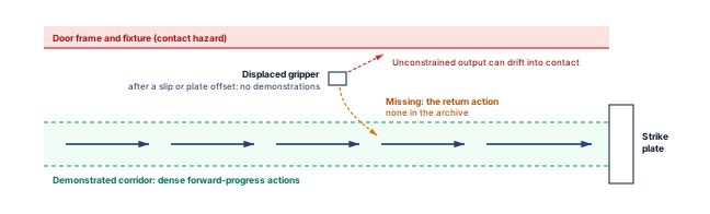
Whether this missing return action leads to task failure depends on the closed-loop dynamics of the complete physical plant. Because the robot’s physical state encompasses joint coordinates, joint velocities, motor drive currents, contact wrenches (combined three-axis contact forces and torques), and raw camera streams, a nominal demonstration traces an infinitesimally thin manifold through a high-dimensional state space. Almost any unmodeled disturbance displaces the system off this path. If the physical plant and its low-level joint controllers inherently restore small lateral displacements toward the centerline through compliant passive dynamics, an imperfect policy output near the corridor boundary will naturally attenuate. If the system dynamics lack this self-centering stability, the tracking error will persist or compound until a learned recovery policy, the safety permission path, or a human supervisor intervenes. While production demonstration archives often contain occasional human corrections, their coverage cannot be assumed; it must be audited against an explicit scenario table (section 5.7).

The quadratic worst-case scaling of behavioral cloning can be derived through a discrete summation over horizon steps. Suppose an autonomous agent follows the expert trajectory until encountering its first execution error at step \(\FirstErrorStepIndex \in \{1, \dots, \BehaviorCloningHorizon\}\). If this error propels the system into an unsupported state from which it never recovers, the agent incurs an adverse task cost at every remaining step (\(\BehaviorCloningHorizon - \FirstErrorStepIndex\)). Assigning each time step an upper bound \(\SingleStepImitationError\) on the probability of committing a first error and normalizing the per-step cost to unity (\(\ImmediateTaskCostScore_t = 1\)) yields the following worst-case cost accumulation. This discrete summation serves as an upper-bound derivation rather than an exact expectation over independent failure events: \[\sum_{\FirstErrorStepIndex=1}^\BehaviorCloningHorizon \SingleStepImitationError (\BehaviorCloningHorizon - \FirstErrorStepIndex) = \SingleStepImitationError \left( \BehaviorCloningHorizon^2 - \sum_{\FirstErrorStepIndex=1}^\BehaviorCloningHorizon \FirstErrorStepIndex \right) = \SingleStepImitationError \left( \BehaviorCloningHorizon^2 - \frac{\BehaviorCloningHorizon(\BehaviorCloningHorizon+1)}{2} \right) = \frac{\BehaviorCloningHorizon(\BehaviorCloningHorizon-1)}{2} \SingleStepImitationError \approx \frac{1}{2} \BehaviorCloningHorizon^2 \SingleStepImitationError.\] In open-loop supervised learning, by contrast, if per-step inference errors were independent and exerted zero feedback on subsequent model inputs, an error rate of \(\SingleStepImitationError\) per step would scale linearly over \(\BehaviorCloningHorizon\) steps as \(\sum_{t=1}^\BehaviorCloningHorizon \SingleStepImitationError = \BehaviorCloningHorizon\SingleStepImitationError\). The extra factor of \(\BehaviorCloningHorizon\) appearing in \(\CovariateDriftBound\) is the mathematical signature of closed-loop endogenous feedback.

This quadratic bound characterizes the accumulation of task cost over time, not the physical trajectory of the machine. The result does not imply that spatial tracking errors grow quadratically as \(\TimeInstant^2\). Closed-loop contact forces, mechanical compliance, and actuator saturation govern how physical trajectories evolve; the derivation formalizes only the cost of operating in states where the policy lacks training support.

Writing \(\ExpectedTaskCostSum(\pi)\) and \(\ExpectedTaskCostSum(\pi^*)\) for the expected cumulative task costs of the learned policy \(\pi\) and expert policy \(\pi^*\) over those \(\BehaviorCloningHorizon\) steps, let \(\SingleStepImitationError\) bound the single-step action disagreement across expert-visited states under a 0–1 action loss: \(\mathbb{E}_{\DecisionProcessState \sim \ExpertStateVisitationDistribution} [\IndicatorFunction(\pi(\DecisionProcessState) \ne \pi^*(\DecisionProcessState))] \le \SingleStepImitationError\). Assuming per-step task costs lie in \([0,1]\), behavioral cloning admits the worst-case bound (equation 1) derived by Ross and Bagnell (2010) and restated by Ross et al. (2011): \[\ExpectedTaskCostSum(\pi)-\ExpectedTaskCostSum(\pi^*) \le \BehaviorCloningHorizon^2\SingleStepImitationError. \tag{1}\] The published theorem carries a constant of one rather than the sketch’s one half; both are worst-case bounds, and their quadratic dependence on the horizon is the same.

In practice, this theoretical bound can exceed the maximum possible cost achievable in a finite episode. Because per-step costs are bounded in \([0,1]\), the excess cost is trivially bounded by \(\BehaviorCloningHorizon\); hence, \(\min(\BehaviorCloningHorizon, \BehaviorCloningHorizon^2\SingleStepImitationError)\) represents the operational upper bound. Once the quadratic expression surpasses \(\BehaviorCloningHorizon\), it provides no meaningful prediction regarding physical failure rates or contact severity. The practical engineering value of this bound lies in exposing why behavioral cloning has no defense in states its demonstrations never reached, rather than in predicting exact physical collision rates.

↪ The full derivation of the quadratic bound, with its loss and cost assumptions, is developed in Imitation Learning and Compounding Covariate Shift.

Foster, Dylan J., Adam Block, and Dipendra Misra. 2024. “Is Behavior Cloning All You Need? Understanding Horizon in Imitation Learning.” Advances in Neural Information Processing Systems (NeurIPS) 37: 120602–66. https://doi.org/10.52202/079017-3834.

Simchowitz, Max, Daniel Pfrommer, and Ali Jadbabaie. 2025. “The Pitfalls of Imitation Learning When Actions Are Continuous.” Proceedings of the Thirty Eighth Conference on Learning Theory (COLT), Proceedings of machine learning research, vol. 291: 5248–351.

The actual scaling with horizon length depends heavily on the chosen loss function, the action space, and the closed-loop plant stability. Consequently, equation 1 reflects a classical result for discrete 0–1 loss rather than an absolute law for all imitation architectures. When trained under logarithmic loss (minimizing the negative log-probability assigned to expert actions) over a well-specified policy class containing the expert, behavioral cloning can achieve a sample complexity that does not grow with the horizon length. This result holds provided total reward is bounded and the policy class capacity is controlled (Foster et al. 2024). Continuous action spaces, however, introduce the opposite challenge. Even when the physical closed loop is exponentially stable (small mechanical perturbations decay at a fixed rate) and the expert policy is smooth and deterministic, any smooth, deterministic imitator can accumulate closed-loop execution errors that scale exponentially with horizon length relative to its training loss (Simchowitz et al. 2025). The same analysis identifies two ways around this compounding (Simchowitz et al. 2025). The first changes the policy class. A policy that is non-smooth, that is non-Markovian (its action depends on recent history rather than solely the current observation), or whose action distribution is multimodal (it can place probability on several distinct actions at once, rather than averaging them) escapes the result. Action chunking and diffusion decoders have these properties. The second changes the data, using demonstrations deliberately spread across a wide tube surrounding the nominal trajectory. That second remedy is a data-collection decision, and section 5.8 returns to it as noise injection during teleoperation. Because the mobile manipulator operates in a continuous control space, closed-loop success ultimately hinges on whether the combined policy and low-level controllers actively restore a displaced gripper to the nominal path.

↩︎ Action chunking, in which the policy emits a short sequence of setpoints per inference, is established in Action chunking.

Collecting more nominal expert demonstrations does not resolve endogenous covariate shift. Adding another thousand hours of clean, centered door openings merely increases sample density along the nominal trajectory; the empirical support outside this narrow tube remains strictly zero (\(\ExpertStateVisitationDistribution(\DecisionProcessState) = 0\)). This pitfall is the nominal demonstration trap. Beyond this coverage limitation, logging physical robot experience carries direct hardware costs. While a web crawler scrapes static text with zero marginal mechanical wear, every recorded second of robot telemetry consumes actuator fatigue life, heats motor windings (\(d\WindingTemperature/d\TimeInstant\)), wears down gearbox teeth, and depletes battery reserves. In practical data-collection campaigns, required pauses for operator fatigue, sensor recalibration, scene resets, and discarded trials often leave less than one quarter of scheduled workcell time as usable demonstration data (section 5.6). Physical telemetry is scarce, wear-intensive, and costly; collecting it without modeling closed-loop recovery dynamics compromises policy training.

↩︎ Actuator thermal dissipation (\(d\WindingTemperature/d\TimeInstant\)) and winding damage limits are established in Thermal Duty Cycles.

A physical command also changes meaning as it crosses the control stack toward the actuators. In a system partitioned by the proposal boundary, an operator’s or policy’s requested action is mapped into a trajectory setpoint, checked and potentially clamped by the safety permission path, and executed by the physical plant to produce a measured response. Logging only the raw requested action trains the policy on commands the plant may be physically incapable of executing; logging only the measured plant response teaches the policy to copy link flexure, gear backlash, and contact stalls as if they were intentional human skill. A physical data-collection campaign must therefore settle two decisions before recording its first trajectory. The first is which collection path generates the actions (section 5.4). The second is which of the four representations of one command (the request, the mapped setpoint, the admitted command, or the measured response) the dataset preserves as its training label (section 5.5).

↩︎ The proposal boundary, which separates a learned proposer from the permission path that alone may admit an action, is established in The Machine in Five Levels.

5.4 Physical Telemetry Sources and Collection Paths

When an engineer records demonstrations of the warehouse cage-door latch, the choice of collection rig decides which contact forces, hesitations, and recovery maneuvers ever reach the archive. Guiding the robot arm by hand gives the demonstrator direct tactile feel of the binding latch, but the demonstrator’s torso blocks the onboard cameras. Puppeteering the arm over a network clears the camera view, but display delay makes the operator inch forward in a stop-and-go hunt. Running a scripted spline produces clean, repeatable approaches that jam the moment the strike plate shifts by a millimeter. Because every attempt on the physical robot spends facility hours, joint life, and human effort, choosing a collection path trades collection cost against the behaviors the resulting archive can support. Seven collection paths appear in practice, six on physical hardware and a seventh in simulation:

1. In kinesthetic teaching, a colocated human demonstrator physically grasps and guides the unpowered or gravity-compensated links of the mechanism. The logging pipeline records joint encoder positions at the native controller rate without network transport delays. However, human biomechanics govern the motion’s bandwidth, moving far more slowly than the controller’s sampling loop, while labor costs scale \(1:1\) with demonstrator time. The demonstrator’s body also frequently occludes onboard camera views, introducing systematic visual distribution shifts relative to autonomous operation.
2. In teleoperation, a remote operator manipulates an input device to puppet the follower robot across a network fabric.² Teleoperation interfaces differ in how operator inputs map to robot actuators and how much physical contact information reflects back to the human. Joint-space leader-follower arms such as ALOHA (Zhao et al. 2023) and GELLO (Wu et al. 2024) mirror the follower’s joint topology, often at reduced scale, streaming joint angles directly to the follower without inverse kinematics (computing the joint angles that place the tool at a commanded pose). In contrast, tracked spatial controllers and rate-controlled space mice command Cartesian tool poses or velocities that require inverse kinematics solvers at runtime, while force-reflecting bilateral arms actively transmit measured contact forces back to the operator’s hands. Table 2 compares these interfaces and names the artifact each leaves in the recording.
3. In scripted collection, a deterministic trajectory generator executes automated motion primitives, such as cubic splines or impedance-governed state machines. Ingestion rates are high and predictable (\(50\text{--}500\text{ Hz}\)), but trajectories traverse rigid, repetitive manifolds. Because these paths fail to generate corrective recovery data during off-nominal contact, the manipulator risks jamming whenever workpiece dimensions deviate by even a millimeter.
4. In exploratory collection, an active neural policy or reinforcement learning agent selects actions to maximize an information-theoretic objective, such as epistemic entropy or intrinsic curiosity. Although data throughput matches the robot’s peak policy cadence (\(50\text{--}100\text{ Hz}\)), unconstrained exploratory actions risk high-energy collisions, tripping hardware safety tripwires or degrading mechanical gearboxes through repeated high-torque shock loads.
5. In autonomous deployment logging, production policies control actuators during routine factory or warehouse operation, streaming multimodal telemetry into local circular buffers in situ. This channel yields zero-marginal-labor data at the system’s full execution rate (\(10\text{--}50\text{ Hz}\) for high-level policies, \(1\text{ kHz}\) for joint servos). However, runtime safety barriers heavily censor the recorded state distribution, capturing almost exclusively nominal operating regimes while excluding boundary failures.
6. In robot-free demonstration, the operator carries a hand-held gripper fitted with a wrist camera and performs tasks directly in the physical environment, as in the Universal Manipulation Interface (UMI) (Chi et al. 2024). Collection incurs zero robot operating hours or actuator wear, allowing a single demonstrator to gather data across locations where no robot is deployed. The engineering cost shifts to label synthesis: because the hand-held rig records its own Cartesian trajectory and visual feed without robot joint states, actions must be expressed relative to the gripper’s pose frame and executed downstream through the target robot’s controller. The deployed robot’s observation and actuation latencies must also be calibrated to match the recording timing (section 5.5.2).

² Bilateral Telemanipulation: Raymond Goertz’s 1949 master-slave manipulator at Argonne National Laboratory moved tongs behind radiation shielding in exact correspondence with a master handle, and its mechanical linkage returned the forces at the tongs to the operator’s hand (Goertz 1949; Hokayem and Spong 2006). Remote manipulation therefore began with contact force inside the loop. A demonstration recorded through an interface that drops that force channel cannot contain the contact corrections the operator would have made by feel.

Goertz, Raymond C. 1949. Master-Slave Manipulator. ANL-4311. Argonne National Laboratory. https://doi.org/10.2172/1054625.

Hokayem, Peter F., and Mark W. Spong. 2006. “Bilateral Teleoperation: An Historical Survey.” Automatica 42 (12): 2035–57. https://doi.org/10.1016/j.automatica.2006.06.027.

A seventh source removes physical hardware entirely. Simulation pipelines eliminate mechanical wear by substituting a numerical contact model for the physical plant, generating synthetic demonstrations at scale. Trajectory generators can expand a few hundred human seed demonstrations across novel object poses and scene layouts, replaying them in physics engines to synthesize tens of thousands of varied trajectories (Mandlekar et al. 2023). Downstream policies can then co-train on simulated and real telemetry at a specified mixing ratio. However, these synthetic streams require rigorous metadata tagging: records must log their source generator, physics engine build, integrator step size, and contact solver parameters. The dataset’s scenario table, the list of required operating conditions that section 5.7.1 builds, must also flag every condition covered solely by synthetic rollouts, ensuring that training diagnostics can isolate simulation artifacts from measured physical plant behavior. The provenance requirements for synthetic telemetry appear under dataset degradation (section 5.10.2).

Because the collection source determines how the machine interacts with its physical environment, these data streams occupy disjoint state-action manifolds even when executing identical manipulation tasks. Consider releasing the warehouse mobile manipulator’s cage-door latch. A colocated demonstrator guiding the arm feels the latch bind through direct tactile resistance and immediately adjusts wrist compliance, whereas a remote teleoperator watching a compressed video stream lacks haptic feedback and falls into step-and-wait hunting, pausing repeatedly to check strike-plate contact. By contrast, a scripted controller advances along a fixed geometric path at constant velocity and produces the same rigid contact-force spike on every repetition, while an exploratory policy approaches at oblique angles that bind the latch until safety tripwires abort the trial. Far from representing noisy variations of a single ground-truth trajectory, these recorded streams reflect distinct dynamical systems with different bandwidths, transport latencies, and mechanical compliance profiles, as summarized in table 1.

Table 1: Systems trade-offs across physical demonstration and telemetry sources: Seven collection sources compared across control dynamics, contact awareness, human labor economics, and the boundary conditions that collection must satisfy.

Physical Data Source	Ingestion Bandwidth & Cadence	Contact Compliance & Force Awareness	Scaling Labor Economics	Collection Boundary Conditions to Check
Kinesthetic teaching	Controller rate; motion bandwidth set by the human arm	High (direct physical feel of binding and compliance)	Very high (\(1:1\) dedicated human demonstrator)	Human contact with links; qualified force and speed limits
Teleoperation (bilateral/isomorphic)	Moderate (\(20\text{--}50\text{ Hz}\), network + human latency)	Moderate to high (depends on haptic force feedback)	High (\(1:1\) human operator per active cell)	Bounded delay and visibility; isolation and qualified response
Scripted primitives	High (\(50\text{--}500\text{ Hz}\), deterministic trajectory generators)	Low (rigid trajectories unless impedance-governed)	Low (automated once authored; engineering upfront)	Fixture mismatch and contact; guarded trajectory
Exploratory policy	High (\(50\text{--}100\text{ Hz}\), active neural exploration)	Variable (learned or randomized contact behaviors)	Very low (fully autonomous hardware execution)	Bounded exploration; qualified containment
Autonomous deployment logging	Full system rate (\(10\text{--}50\text{ Hz}\) policy, \(1\text{ kHz}\) joint servos)	Operational (reflects live deployed closed-loop control)	Zero marginal labor (harvested passively during production)	Qualified operating domain and runtime enforcement
Robot-free hand-held device	Device camera and pose rate; no robot joint stream	High (operator feels real contact through the device)	Moderate (one person per device; no robot time or wear)	No robot actuation during capture; target execution separately qualified
Synthetic generation	Simulator step rate, limited by compute	Modeled (contact set by engine and parameters)	Low after seed demonstrations are recorded	No physical actuation during generation; model fidelity and target qualification

The cheapest sources in table 1 also produce the highest volume of records. This abundance frequently invites a misconception borrowed from disembodied machine learning, where empirical scaling laws correlate model capability directly with raw token count or pretraining dataset volume (\(\RawRecordCount\)). In physical telemetry, treating every logged control step as an independent observation is a category error. An edge logger sampling at 1 kHz records 3.6 × 10⁶ state-action pairs every hour, yet adjacent timesteps carry near-total temporal autocorrelation (\(\SerialAutocorrelation \to 1.0\)) because successive kinematic readings sampled 1 ms apart differ only by sub-millimeter structural displacements and sensor quantization noise. For a stationary scalar telemetry statistic with geometrically decaying autocorrelation \(\SerialAutocorrelation_k = \SerialAutocorrelation^\AutocorrelationLagIndex\), as characterized by a first-order autoregressive AR(1) process, the large-sample effective sample size (ESS)³ for estimating its mean is: \[\EffectiveSampleSize = \RawRecordCount \frac{1 - \SerialAutocorrelation}{1 + \SerialAutocorrelation}. \tag{2}\] Under this autoregressive model, an autocorrelation of \(\SerialAutocorrelation =\) 0.999 across 3.6 × 10⁶ raw records yields only 1,800 statistically independent observations. While lag-1 correlation alone does not govern ESS across every non-stationary telemetry stream, high-frequency sampling still cannot substitute for operational diversity. Whereas consecutive tokens in language modeling represent high-entropy transitions across a large vocabulary, high-rate robot telemetry mostly oversamples the same physical trajectory. It can resolve fast contact transients when they occur, but raising the logger’s clock frequency never populates an unvisited scenario cell. Physical dataset coverage expands instead through independent physical episodes, diverse workpiece placements, varying illumination, and shifting friction coefficients. A curated archive containing several hundred episodes that systematically sweep initial geometric and mechanical conditions provides far richer empirical support than millions of repetitive timesteps collected across a static test bench.

³ Effective Sample Size: The factor \((1-\SerialAutocorrelation)/(1+\SerialAutocorrelation)\) is the effective-sample-size correction for the mean of a first-order autoregressive series, the correction climatologists apply to serially correlated weather records before testing a trend (Thiébaux and Zwiers 1984). At the correlation used here it turns an hour of permission-tick records into about 1,800 independent ones, so a step count overstates the independent information available for estimating this statistic’s mean by three orders of magnitude before coverage is even considered.

Thiébaux, H. J., and Francis W. Zwiers. 1984. “The Interpretation and Estimation of Effective Sample Size.” Journal of Climate and Applied Meteorology 23 (5): 800–811. https://doi.org/10.1175/1520-0450(1984)023<0800:TIAEOE>2.0.CO;2.

5.4.1 Human demonstration idiosyncrasies and mechanical artifacts

When a behavioral cloning policy is trained directly on raw teleoperated joint velocities, the deployed robot arm often chatters its harmonic drives at \(8\text{--}12\text{ Hz}\) or stalls for \(300\text{ ms}\) a few millimeters in front of the latch strike plate. Neither defect comes from the network architecture. Because a human operator executed the training motions, the recorded telemetry embeds the demonstrator’s neuromuscular bursts, perceptual delays, and visual blind spots alongside the intended trajectory:

• Neuromuscular sub-movements and physiological tremor: Human motor control operates through discrete motor unit recruitment bursts rather than continuous, smooth trajectories. These neuromuscular dynamics introduce corrective sub-movements at \(2\text{--}3\text{ Hz}\) overlaid with involuntary physiological tremor at \(8\text{--}12\text{ Hz}\). If a high-frequency behavioral cloning policy trains on raw joint velocities without low-pass filtering, the neural network imitates this biological tremor as high-frequency torque chatter, accelerating mechanical fatigue in the robot’s harmonic drives and gearboxes.
• Visual latency and step-and-wait hunting: When an operator guides a manipulator toward a contact fixture using 2D camera monitors, monocular depth ambiguity and video compression latency force an unnatural step-and-wait hunting cycle. The operator inches the gripper forward by a few millimeters, pauses for \(200\text{--}400\text{ ms}\) to visually confirm clearance or contact across the video stream, and only then resumes motion. An imitation policy trained on uncurated velocity streams treats these latency-induced pauses as deliberate actions, yielding deployed behaviors that stutter, oscillate, or stall mid-trajectory.
• Attentional narrowing and gaze-conditioned bias: Human demonstrators naturally focus visual attention on the active tool center point (TCP). Because the operator rarely tracks the peripheral links of the arm during fine manipulation, the robot’s elbow or shoulder links frequently sweep perilously close to structural supports or table edges. An imitation policy trained on these demonstrations inherits trajectories that graze workspace obstacles, yet lacks the human’s peripheral situational awareness or rapid collision avoidance reflexes.

Because an ingestion logger records every physical tremor, visual hesitation, and marginal joint clearance as part of the demonstration, imitation policies reproduce these flaws unless the training pipeline filters or abstracts them. Choosing a telemetry source decides what raw experience reaches the archive; choosing which control signal serves as the action label decides whether the policy learns the operator’s intent, the safety filter’s clamp, or the plant’s compliance (section 5.5).

5.5 Action Label Selection across the Control Boundary

Suppose a teleoperator pushes the gripper into the cage-door strike plate aggressively enough to trip a velocity clamp, or stalls against the latch while the wrist motor holds torque. A logger that records only the operator’s raw command teaches the policy to repeat a move the machine refused to execute, whereas a logger that records only the measured encoder velocity teaches it that stalling against a latch is a deliberate command to stop. By the time the gripper contacts the strike plate, a single operator motion has become four different numerical signals across two decoupled processing domains:

• The unprivileged Linux application processor executes perception pipelines, handles video frame ingestion, runs teleoperation input mapping, and computes the neural policy forward pass (\(\Policy(\MultimodalObservation_{t})\)).
• On the permission side of the proposal boundary, a hard real-time safety microcontroller (MCU) runs joint and permission checks at the chosen 1 kHz cadence. Dedicated motor-drive logic closes the faster field-oriented current loop; its current samples remain distinct from the telemetry retained at each permission tick.⁴

⁴ Hardware Input Capture: On real-time MCUs, a timer’s input-capture unit latches encoder counts and current-shunt conversions at a hardware edge, and Direct Memory Access (DMA) moves them to memory without waiting on software. Sampling jitter stays within microseconds, so the denominator of a numerically differentiated velocity or acceleration carries no scheduling noise.

5.5.1 The four-stream action tap tuple

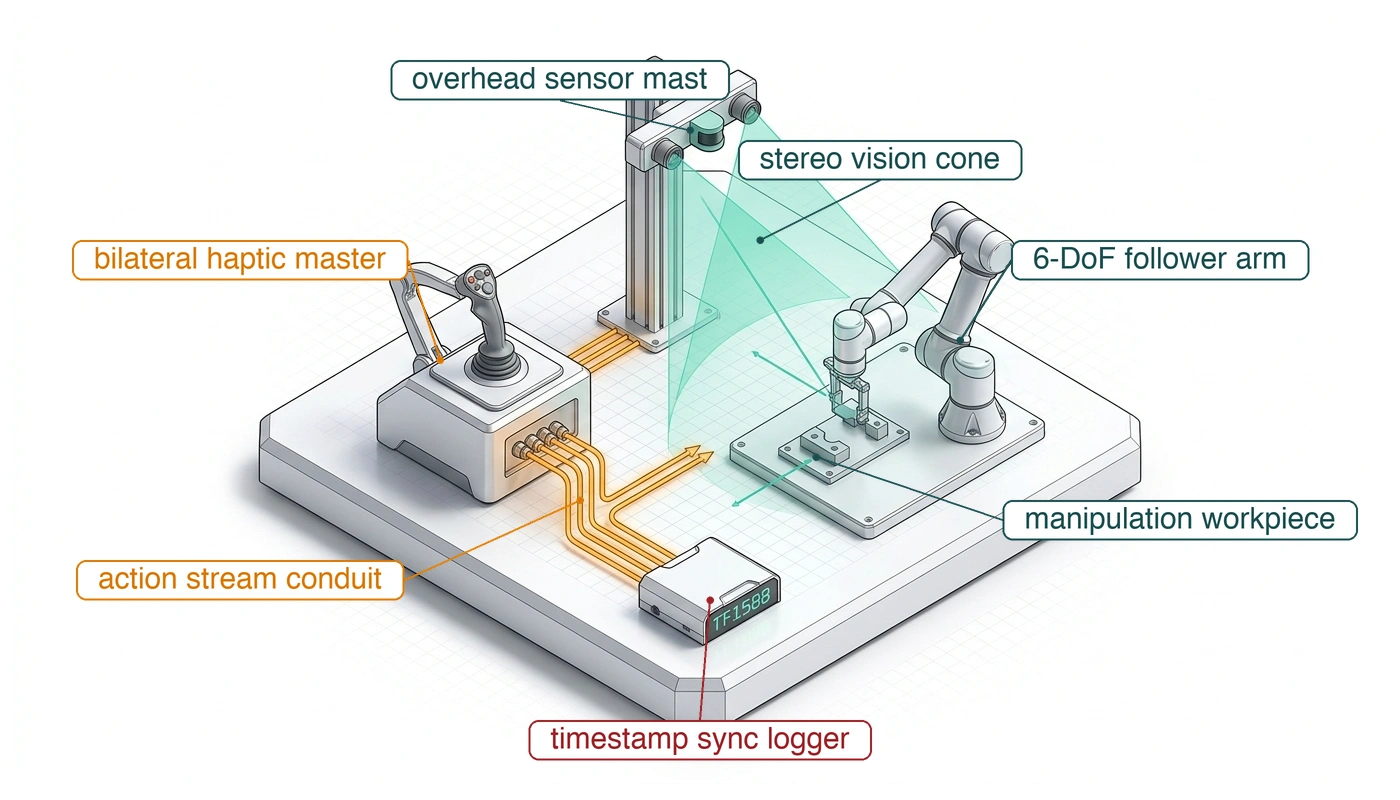
If a dataset keeps only one signal from those two processing domains, any discrepancy between what the operator asked for and how the arm actually moved becomes impossible to diagnose. A command must therefore be logged at each of the four causal stages it passes through. The four-stream action tap \((\RequestedActionTap, \MappedCommandTap, \EnforcedCommandTap, \MeasuredResponseTap)\) records all four in one hardware-synchronized telemetry log (figure 2). Two are logged on the unprivileged Linux host before the black-channel link, and two on the discrete safety MCU after the 1 kHz permission check. Logged together, the taps keep interventions and tracking errors auditable.

Figure 2: Four-stream action tap tuple: Four places a command can be logged, from raw policy intent on the application processor through to measured plant response. Which tap a dataset records decides what the model learns to imitate. The four-tap decomposition is this book’s construct; the teleoperation rigs it instruments follow Zhao et al. (2023) and Wu et al. (2024).

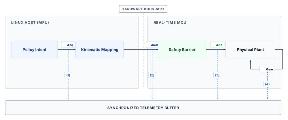
Dividing telemetry logging across the unprivileged Linux host and the hard real-time MCU captures four distinct physical signals:

• Tap 1: The requested action (\(\RequestedActionTap\), “Asked”): Logged in user space on the application processor, this represents unconstrained human operator input (from a leader arm or joystick) or the raw forward-pass output from an unverified policy, tagged with its native coordinate frame and issue timestamp prior to software validation. This proposal reflects unadulterated human or policy intent, but it frequently demands infeasible joint accelerations or violates spatial bounding envelopes.
• Tap 2: The mapped command (\(\MappedCommandTap\), “Mapped”): The kinematically retargeted setpoint (such as Cartesian end-effector velocities converted to joint space setpoints via inverse kinematics), incorporating coordinate frame transformations, trajectory interpolation, and workspace limits before transmission across the black-channel board link to the safety MCU.
• Tap 3: The enforced command (\(\EnforcedCommandTap\), “Allowed”): Logged on the bare-metal MCU on the permission side of the boundary, this represents the command after the permission path has checked or modified the proposal. The checks include deterministic Control Barrier Functions (CBFs, safety filters that keep states within a forward-invariant safe set), velocity and acceleration clamps, torque saturation envelopes, and collision guards. Whichever tap a dataset chooses as its label, the imitation loss has the same form; written for the admitted command, it is: \[\PolicyImitationLoss(\ModelParameters) = \mathbb{E}_{(\MultimodalObservation_{t}, \EnforcedCommandLabel) \sim \DemonstrationDataset} \left[ \LossFunction(\Policy(\MultimodalObservation_{t}), \EnforcedCommandLabel) \right],\] Here the training dataset must contain curated, correctly attributed targets. Passing the permission check does not make a command an expert demonstration, because a clamp or emergency stop may be a safeguard’s response to a poor request. Override flags and companion taps determine which records can serve as imitation targets and which remain evidence of intervention.
• Tap 4: The measured response (\(\MeasuredResponseTap\), “Done”): The physical plant reaction measured by optical joint encoders and motor current shunt resistors over the executed control tick, recording actual mechanical displacement and electrical effort. This measured response serves as proprioceptive state input (\(\NextProprioceptiveObservation\)) for subsequent policy steps rather than an action label.

↪ Control barrier functions and the forward-invariant safe sets they enforce are developed in Safe Sets as Conditional Permission.

These distinctions become critical when commanded intent and physical motion diverge. If a teleoperator requests an aggressive movement that the safety permission path clamps, the resulting state transition follows the enforced command (\(\EnforcedCommandTap\)), not the unconstrained request (\(\RequestedActionTap\)). Pairing that transition only with the request conceals the safety intervention and teaches a policy to repeat demands the physical machine cannot execute.

At the latch, the opposite ambiguity arises. Contact resistance can bring measured joint velocities to zero (\(\MeasuredJointVelocities \approx \ZeroVector\)) while the motors continue exerting holding torque against the strike plate. Treating that response as a deliberate zero-velocity target loses the distinction between maintaining effort against the latch and choosing to stop. The appropriate imitation target depends on the policy’s action interface; the other taps explain how that target became physical motion.

Retaining all four streams is what makes any single choice of label interpretable. A policy trained on the request alone learns commands the permission path would have clamped, and one trained on the measured response alone learns the arm’s compliance, backlash, and external disturbances as if they were intended control. A log that keeps only the final encoder state or only the operator’s input discards exactly the stages at which software and safety hardware changed the command. The tuple is also only as reliable as its shared clock. The application processor and the MCU must stamp their taps in one hardware-synchronized timebase, such as the IEEE 1588 Precision Time Protocol (PTP), written \(\PtpHardwareTimestamp\). A few milliseconds of skew between them misaligns each visual observation from the torque it prompted (section 5.5.2).

For the latch campaign, the imitation target is the mapped command whenever it represents an expert request that the permission path accepted unchanged. In that case \(\MappedCommandTap\) and \(\EnforcedCommandTap\) carry the same value, so the choice between the two taps matters only for commands the permission path modified. A modified command remains a separate, attributed intervention; a curated recovery can later supply an expert target at that state. Each training pair therefore carries two times. The observation is dated when its physics was true, at the exposure midpoint (the instant halfway through the interval over which the camera integrates light), and the command is dated when the operator issued it. The gap between them is part of the demonstration and is recorded rather than erased, because it contains the operator’s own reaction time (section 5.6.1). The alignment developed below supplies the first of these times.

↪ The capture timestamp, taken in hardware at the exposure midpoint, is enforced for every sensor in Dating and Placing the Measurement.

5.5.2 Multi-rate time synchronization and exposure-midpoint alignment

Recording the right action tap still leaves open when each recorded observation was physically true, because a robot’s sensors run at different rates and transport delays. A naive data loader that latches the latest available sensor sample pairs each action with a camera frame whose optical exposure was centered \(25\text{--}40\text{ ms}\) before the frame arrived in host memory, recording that delayed image as the present state. Trained on those pairs, the policy learns to map historical visual states to present actions, baking an artificial phase lag into its weights that shows up at deployment as overshoot and chattering against the latch. Across the machine, cameras integrate photons over exposure windows of \(10\text{--}35\text{ ms}\) at \(30\text{--}60\text{ Hz}\), 6-axis force-torque sensors stream over a Serial Peripheral Interface (SPI) or Controller Area Network (CAN) bus at \(100\text{--}500\text{ Hz}\), joint and permission telemetry is retained at the MCU’s chosen \(1\text{ kHz}\) tick while motor-drive current sampling serves the faster local current loop, and neural policy models dispatch setpoints at \(10\text{--}50\text{ Hz}\). Unlike the operator’s reaction time, this pairing error belongs to the logging pipeline rather than the demonstration, so stamping each sample at its physical capture instant lets the alignment pipeline remove it.

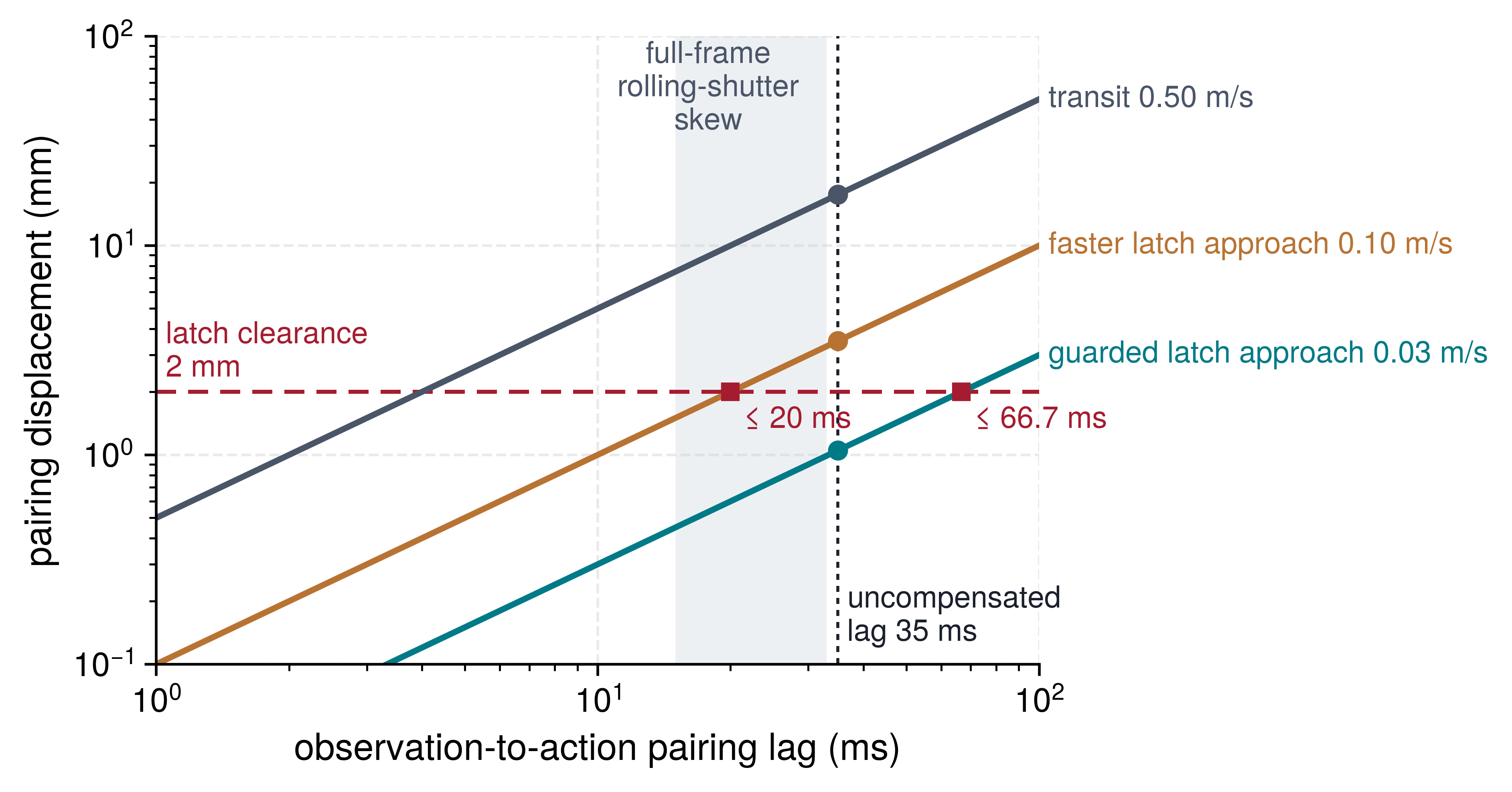
To quantify the physical hazard of temporal misalignment, consider the spatial tracking error \(\SyncPairingDisplacement\) injected into the dataset when an observation and an action are paired across an uncompensated phase lag \(\ObservationPairingLag\): \[\SyncPairingDisplacement(\TimeInstant) = \int_{t - \ObservationPairingLag}^{\TimeInstant} \Velocity(\IntegrationDummyTime)\,d\IntegrationDummyTime \approx \Velocity(\TimeInstant) \cdot \ObservationPairingLag. \tag{3}\] The latch campaign moves far more slowly than an arm in transit, and notebook 5.1 applies equation 3 at both speeds.

Napkin Math 5.1: The pairing lag

Problem: A logger pairs each action with a camera frame whose exposure midpoint lies an uncompensated 35 ms earlier. Does the resulting pairing error fit the 2 mm latch clearance at transit speed and at the latch campaign’s two approach speeds, and how much lag can each approach tolerate?

Variables:

• Uncompensated lag \(\ObservationPairingLag =\) 35 ms (illustrative; exposure-to-arrival delay of an untimed logger)
• Latch clearance \(\LatchClearance =\) 2 mm (illustrative)
• Transit speed 0.50 m/s (illustrative); guarded approach 0.03 m/s and faster approach 0.10 m/s (illustrative scenario speeds of the running machine)

Math:

1. Transit: 0.50 m/s \(\times\) 35 ms \(=\) 17.5 mm, 8.8× the clearance.
2. Guarded approach: 0.03 m/s \(\times\) 35 ms \(=\) 1.05 mm, inside the clearance.
3. Faster approach: 0.10 m/s \(\times\) 35 ms \(=\) 3.5 mm, outside it.
4. Lag ceilings: \(\PairingLagCeiling = \LatchClearance/\ApproachSpeed\), so 2 mm \(/\) 0.03 m/s \(=\) 66.7 ms and 2 mm \(/\) 0.10 m/s \(=\) 20 ms.

Result: The same lag fits the modeled pairing-error allocation at the guarded approach and exceeds it at the faster one.

Systems insight: A timing error becomes a position error at the speed of the motion, just as observation age becomes blind travel \(\SpeedAtDetection\,\PrebrakeDelay\) in the stopping budget derived in Kinematic stopping distance and pre-brake delay. The faster approach cannot be collected without the exposure-midpoint alignment of the four-stage pipeline in section 5.5.2.3.

When an imitation learning model trains on misaligned pairs, it fits a relationship in which the action appears to precede the visual evidence that prompted it. During closed-loop deployment, that artificial phase lag appears as overshoot, control hunting, and chattering against rigid surfaces. Because displacement grows linearly with lag, each approach speed has a lag ceiling equal to the clearance divided by the speed, and figure 3 places those ceilings beside a second timing error the notebook did not count. A rolling-shutter sensor exposes its pixel rows one after another rather than all at once, so the bottom row of a frame is captured later than the top (section 5.5.2.2 quantifies the delay). A full-frame rolling-shutter skew of 15 ms to 33 ms is comparable to the uncompensated lag, so a logger that stamps every frame correctly can still breach the faster approach’s 20 ms ceiling through readout alone.

Figure 3: One lag, three verdicts: Pairing an observation with an action across an uncompensated lag displaces the recorded state by speed times lag. At 35 ms the transit pairing is 17.5 mm off, the faster latch approach exceeds the 2 mm clearance, and the guarded approach stays inside it. The clearance tolerates at most 20 ms of lag at 0.10 m/s and 66.7 ms at 0.03 m/s; a full-frame rolling-shutter skew alone spans 15 ms to 33 ms.

Hardware timestamps vs. software arrival timestamps

The 35 ms pairing lag in notebook 5.1 arises when a logger stamps a sensor packet with the clock reading at the instant a Linux thread wakes up to read it rather than when the hardware captured the sample. Even on the \(1.0\text{ ms}\) kinematic stream, half a millisecond of kernel scheduling jitter cuts a nominal tick in half or stretches it by half, doubling or shrinking the finite-difference velocity label for the exact same physical motion. Both errors come from confusing when an optical or electrical event happened in hardware with when the operating system noticed it in software:

• Software arrival timestamps (\(\HostArrivalTimestamp\)): In naive logging pipelines, an image frame or CAN packet is timestamped when the Linux kernel handles the device interrupt or when a user-space thread dequeues the buffer from Video4Linux2 (V4L2) or a socket. This host timestamp incorporates camera pixel readout time, USB 3 or MIPI CSI-2 bus serialization, Direct Memory Access (DMA) latency, and operating system scheduling jitter: \[\HostArrivalTimestamp = \ExposureMidpointTime + \frac{\ExposureDuration}{2} + \FrameReadoutTime + \BusSerializationTime + \DriverInterruptLatency + \TimestampJitterDelay.\] Host timestamps lag physical reality by \(20\text{--}45\text{ ms}\). In an untuned system, operating system scheduling jitter (\(\TimestampJitterDelay = \pm 5\text{--}15\text{ ms}\)), driven by kernel preemption latency, CPU C-state power wake-up transitions, and USB host controller interrupt coalescing (where packets are held in hardware buffers until a threshold count or timer expires), corrupts numerical differentiation. When joint velocities are computed via backward difference: \[\GeneralizedVelocities_k = \frac{\GeneralizedCoordinates_k - \GeneralizedCoordinates_{k-1}}{\TimeInstant_k - \TimeInstant_{k-1}},\] a nominal \(1\text{ kHz}\) sampling interval (\(\FiniteChange \TimeInstant = 1.0\text{ ms}\)) perturbed by software timestamp jitter \(\TimestampJitterDelay = \pm 0.5\text{ ms}\) causes the denominator to fluctuate between \(0.5\text{ ms}\) and \(1.5\text{ ms}\). The effect is doubling the inferred velocity at the shorter interval and reducing it by one third at the longer interval, for the same measured displacement. If thread preemption reverses packet dequeuing order (\(\TimeInstant_k < \TimeInstant_{k-1}\)), the computed velocity reverses sign, injecting spurious velocity spikes into the training targets.
• Hardware PTP timestamps (\(\PtpHardwareTimestamp\)): Hardware timestamps isolate the physical event from host scheduling delays. IEEE 1588 Precision Time Protocol (PTP) estimates clock offset across distributed nodes using a deterministic two-way message exchange.⁵ The reference clock sends at \(\TimeInstant_1\) and receives the reply at \(\TimeInstant_4\); the remote clock receives at \(\TimeInstant_2\) and replies at \(\TimeInstant_3\). Under symmetric path delays, the propagation delay and offset are: \[\PtpPropagationDelay = \frac{(\TimeInstant_4 - \TimeInstant_1) - (\TimeInstant_3 - \TimeInstant_2)}{2}, \qquad \ClockOffset = \frac{(\TimeInstant_2 - \TimeInstant_1) - (\TimeInstant_4 - \TimeInstant_3)}{2}.\] Because the forward timestamp difference \(\TimeInstant_2 - \TimeInstant_1 = \PtpPropagationDelay + \ClockOffset\) adds the remote clock offset to the one-way propagation delay while the return difference \(\TimeInstant_4 - \TimeInstant_3 = \PtpPropagationDelay - \ClockOffset\) subtracts that same offset, adding the two differences cancels \(\ClockOffset\) to isolate the propagation delay and subtracting them cancels \(\PtpPropagationDelay\) to isolate the clock offset. Hardware timestamping bounds uncertainty, but a network packet timestamp does not automatically equal an optical exposure midpoint. Production logs must preserve the capture event, clock domain identity, and bounded conversion error. The key collection decision is whether that uncertainty fits within the task’s spatial alignment tolerance.

⁵ Precision Time Protocol (PTP): IEEE 1588 was first published in 2002 for test-and-measurement and industrial-automation networks, and its current revision dates from 2019 (IEEE 2020). It reaches sub-microsecond agreement only when both endpoints timestamp packets in hardware at the network interface. Its weak point is the symmetric-path assumption in the offset formula, because a link whose two directions differ in delay biases the computed offset by half that difference, and every observation-action pairing in the archive inherits the bias.

IEEE. 2020. IEEE Std 1588-2019: IEEE Standard for a Precision Clock Synchronization Protocol for Networked Measurement and Control Systems. Institute of Electrical; Electronics Engineers. https://doi.org/10.1109/IEEESTD.2020.9120376.

↪ Protocol: The IEEE 1588 message exchange, its clock servo, and its path-asymmetry uncertainty are developed in Clock Synchronization and Network Timestamps.

Rolling shutter skew across camera streams

When a camera with a rolling shutter pans past the cage door or rides on a moving link, straight vertical bars bend into diagonal arcs because the bottom pixel row is exposed up to \(33\text{ ms}\) later than the top row. This distortion is rolling shutter skew: low-cost consumer sensors and webcams expose pixel rows one after another rather than all at once. For a sensor with \(\ImageHeight\) vertical scanlines and line readout duration \(\RollingShutterRowReadout\), row \(\SensorRowIndex \in [0, \ImageHeight-1]\) begins its exposure at \(\RowExposureStartTime(\SensorRowIndex)\), and its exposure midpoint, half an exposure later, depends linearly on its vertical coordinate: \[\RowExposureStartTime(\SensorRowIndex) + \frac{\ExposureDuration}{2} = \ExposureStartTime + \SensorRowIndex \, \RollingShutterRowReadout + \frac{\ExposureDuration}{2}.\] Across a full frame, the temporal skew between the top row (\(\SensorRowIndex = 0\)) and bottom row (\(\SensorRowIndex = \ImageHeight - 1\)) accumulates to: \[\RollingShutterFrameSkew = (\ImageHeight - 1) \, \RollingShutterRowReadout, \tag{4}\] which for common sensors lies between about 15 ms and 33 ms, the upper end being one full frame period at 30 Hz. When the robot arm or camera moves at 0.50 m/s, the bottom of the manipulator in the image is captured while the physical link has moved up to 16.5 mm relative to the top of the link in the same frame. Even at the faster latch approach of 0.10 m/s, the worst-case skew moves the gripper 3.3 mm within one frame, exceeding the 2 mm clearance. This geometric warping (the “jello effect”) deforms straight edges into curved arcs and breaks rigid-body geometry.

Independent rolling shutters can depict the same moving arm at different poses within nominally simultaneous frames. Hardware-triggered global shutters simplify alignment; rolling shutters require a row-time model and a motion bound or correction. Sensor choice must follow the task tolerance rather than an unyielding demand for a single shutter architecture.

↪ The same row timing as a spatial error on a moving base, charged against clearance and removed by per-row motion compensation, is developed in Capture Physics and Calibration.

A four-stage alignment pipeline

Hardware timestamps fix when each sample was taken, and the row-time model fixes when each part of an image was exposed. A collection pipeline still has to turn those facts into training pairs whose pairing error fits inside the clearance budget of notebook 5.1. It can implement that alignment contract in four stages:

1. Hardware-triggered optical exposure midpoint: The real-time MCU dispatches hardware GPIO sync pulses or PTP-synchronized trigger packets to every triggerable camera. The rig mixes shutter types. The wrist camera’s global shutter exposes all rows together, while the navigation camera and the external cameras’ color sensors read out row by row, so their frames also need the row-time model above to assign each row its own midpoint. The camera latches the trigger at \(\ExposureStartTime\), and the driver calculates the true optical midpoint \(\ExposureMidpointTime = \ExposureStartTime + \ExposureDuration / 2\) in hardware PTP clock units (\(\PtpHardwareTimestamp\)), avoiding host arrival time as the exposure timestamp.⁶
2. Lock-free time-sorted jitter compensation: Because network and bus transfers experience variable transport delay \(\TimestampJitterDelay\), incoming sensor packets are stamped with their hardware PTP capture timestamp and inserted into a lock-free, time-sorted jitter ring buffer in shared memory. An asynchronous consumer thread advances a playhead lagging real-time by a fixed, bounded window (\(\JitterBufferPlayoutDelay = 15\text{--}25\text{ ms}\)), absorbing transport bursts and re-ordering packets into monotonic hardware timestamp sequence.
3. Cubic Hermite kinematic interpolation: Because joint encoders sample at \(1\text{ kHz}\) (\(1\text{ ms}\) period) while cameras capture at \(30\text{ Hz}\) or \(60\text{ Hz}\), the camera midpoint \(\ExposureMidpointTime\) falls between two discrete MCU telemetry ticks \(\TimeInstant_k\) and \(\TimeInstant_{k+1}\). The synchronization thread interpolates joint angles \(\GeneralizedCoordinates(\ExposureMidpointTime)\) using cubic Hermite splines across the bounding kinematic records \((\TimeInstant_k, \GeneralizedCoordinates_k, \GeneralizedVelocities_k)\) and \((\TimeInstant_{k+1}, \GeneralizedCoordinates_{k+1}, \GeneralizedVelocities_{k+1})\): \[\GeneralizedCoordinates(\ExposureMidpointTime) = \HermiteBasisFunction_{00}(\HermiteInterpolationFraction) \GeneralizedCoordinates_k + \HermiteBasisFunction_{10}(\HermiteInterpolationFraction) \TelemetryTickInterval \GeneralizedVelocities_k + \HermiteBasisFunction_{01}(\HermiteInterpolationFraction) \GeneralizedCoordinates_{k+1} + \HermiteBasisFunction_{11}(\HermiteInterpolationFraction) \TelemetryTickInterval \GeneralizedVelocities_{k+1},\] where \(\TelemetryTickInterval = \TimeInstant_{k+1} - \TimeInstant_k = 1\text{ ms}\), \(\HermiteInterpolationFraction = (\ExposureMidpointTime - \TimeInstant_k)/\TelemetryTickInterval \in [0, 1]\) is the fraction of the tick elapsed at the exposure midpoint, and \(\HermiteBasisFunction_{ij}(\HermiteInterpolationFraction)\) are the cubic Hermite basis functions (Smooth Trajectories and Bumpless Transfer). This gives a smooth state estimate between valid samples. The interpolation error still needs a bound, especially across contact or missing telemetry.
4. Pre-serialization alignment: Container formats store multi-rate topics with the timestamps provided by the logger. Alignment may occur during capture or in a versioned preprocessing pass. Preserve the raw timestamps and interpolation provenance in either case, so the training pair carries an estimated state and its uncertainty rather than an assertion of exact simultaneity.

⁶ Hardware Exposure Triggering: A dedicated GPIO or TTL pulse from the real-time microcontroller starts every camera’s exposure on the same electrical edge, instead of a software trigger issued through the host’s driver stack. Triggered global-shutter cameras then begin exposing within microseconds of one another, which leaves the exposure duration, not the trigger path, as the dominant term in the midpoint timestamp.

The same pairing contract governs deployment. A policy trained on aligned pairs must also be fed aligned observations and have its actions executed when the training data implies. UMI measures each observation stream’s latency and aligns all streams to the slowest, usually the camera. It then sends commands ahead of time to cover the arm’s and gripper’s execution latency, and it discards actions whose execution time has already passed. With latency matching disabled, the same policy’s motion became visibly jittery (Chi et al. 2024). UMI also expresses actions relative to the gripper’s current pose rather than in a fixed robot frame, which removes the dependence on a base calibration and lets one policy run on more than one arm.

Checkpoint 5.1: Action labels and pairing time

A training pair is only as trustworthy as the tap it imitates and the time it assigns to each observation.

• Clamped request: A teleoperator requests a motion that the permission path clamps. Which tap does the resulting state transition follow, and where does the record keep the evidence of the clamp?
• Stalled latch: Measured joint velocity is zero while the motors hold torque against the latch. Why is \(\MeasuredResponseTap\) the wrong imitation target at that step?
• Unchanged mapped command: Under what condition can \(\MappedCommandTap\) serve as the expert target, and what happens to the pair when that condition fails?
• Lag budget: A tighter strike plate leaves only 1 mm of clearance. At the faster approach of 0.10 m/s, what is the largest uncompensated lag the pairing tolerates, and does a logger with the 35 ms lag of notebook 5.1 meet it?

A tap and a timestamp are only as good as the loop that produced them. In teleoperation that loop runs through a human, and the interface between human and machine shapes the recorded dynamics, storage bandwidth, and hardware wear long before the data reaches a model (section 5.6).

5.6 Teleoperation Demonstration Costs

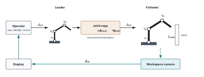
When an operator guides a leader arm to unlatch the warehouse cage door, every corrective nudge must traverse a multi-stage physical loop before the robot can respond. Teleoperation is a data-generation pipeline with a human embedded in the real-time feedback loop. It charges for each demonstration in three currencies: the phase lag and stability margin of the loop itself, the write bandwidth and storage the session demands, and the cell time and component life a campaign consumes. The loop comes first (figure 4). The operator sees the scene on a display after a delay \(\DisplayPipelineLatency\) and perceives, decides, and moves the leader in \(\OperatorResponseLatency\). The command crosses to the follower in \(\TeleoperationCommandLatency\). The follower’s actuators then accelerate the links against inertia, drivetrain friction, and contact in \(\FollowerMechanicalLatency\), before the camera shows the result on the next cycle.

↪ Where a deployment moves operators’ labor, and which uses of their recorded sessions it must bar, is developed in The Labor the Machine Moves.

Figure 4: Kinematically isomorphic teleoperation loop: The operator moves a leader arm whose joints mirror the follower’s, and the host copies joint angles across, as in low-cost leader-follower rigs such as GELLO (Wu et al. 2024). Because the leader shares the follower’s joint structure, the interface needs no inverse kinematics and inherits none of its singularities (configurations where joints align and the arm loses a direction of motion), preserving the operator’s direct joint-level coordination. The loop still closes through the operator: human reaction, command transfer, mechanical response, and display delay all enter the recording as phase lag, so the demonstration carries the operator’s delay as if it were policy.

Wu, Philipp, Yiyang Shentu, Zhonghe Yi, Xingyu Lin, Ken Goldberg, and Pieter Abbeel. 2024. “GELLO: A General, Low-Cost, and Intuitive Teleoperation Framework for Robot Manipulation.” IEEE/RSJ International Conference on Intelligent Robots and Systems (IROS).

By mapping each leader joint directly to the corresponding follower joint (\(\LeaderJointPositions \equiv \FollowerJointPositions\)), this isomorphic leader-follower topology sidesteps numerical inverse kinematics and algorithmic kinematic singularities. Even without software kinematic conversion, however, every recorded trajectory remains bound to the physical transport and neuromuscular delays of the complete loop, placing hard upper bounds on corrective bandwidth.

5.6.1 Human-in-the-loop latency and bilateral passivity breakdown

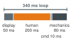
The operator’s own reaction is 58.8 percent of the 340 ms correction loop.

Suppose the follower gripper grazes the side of the latch strike plate at time \(\TimeInstant\). If a logger naively pairs the observation \(\MultimodalObservation_{t}\) captured at that instant with the command the operator issued at \(\TimeInstant\), it pairs a contact state with an action chosen for a trajectory state 250 ms earlier, before the contact ever happened. A behavioral cloning policy trained on those pairs learns that delay as intentional strategy and, when run autonomously at high control frequencies, over-corrects into destructive oscillations. That stale pairing arises because every stage of the teleoperation loop adds phase delay. In an illustrative reference setup with a high-speed camera and a wired local network, display pipeline processing takes \(\DisplayPipelineLatency =\) 50 ms across sensor exposure, H.264 decoding, and display raster refresh. Human visual perception, motor planning, and neuromuscular transmission add an operator response latency of \(\OperatorResponseLatency =\) 200 ms. Command quantization, packetization, and fieldbus transport add \(\TeleoperationCommandLatency =\) 10 ms. Actuator torque ramp-up against link inertia then adds a mechanical response latency of \(\FollowerMechanicalLatency =\) 80 ms before the arm reaches the commanded acceleration. Their sum is the teleoperation round-trip latency \(\TeleoperationRoundTripLatency\), the elapsed time from a physical contact disturbance to the corrective actuator response: \[\TeleoperationRoundTripLatency = \DisplayPipelineLatency + \OperatorResponseLatency + \TeleoperationCommandLatency + \FollowerMechanicalLatency. \tag{5}\]

Following the contact at time \(\TimeInstant\) through those four stages shows why the recorded command lags the state. The operator sees the error on the display 50 ms later and commands a physical correction at \(\TimeInstant +{}\) 250 ms. The follower arm finally pushes back at \(\TimeInstant +{}\) 340 ms, after drifting under momentum and contact compliance throughout the interval. Round-trip latency is therefore a property of the resulting dataset rather than just an artifact of the rig, because it injects a systematic phase lag into every recorded demonstration, dominated by the operator’s own reaction time (58.8 percent of the loop in this setup).

This delay differs in kind from the sensor-pipeline delay of section 5.5.2. That one was a pairing artifact of the logger, and exposure-midpoint stamping lets the alignment pipeline account for it. The operator’s delay is a real property of the demonstrator, so no timestamp correction can remove it, and silently erasing it would misstate what the demonstration contains. The logger therefore keeps both times of every pair (the observation’s exposure midpoint and the command’s issue time) and records the session’s measured loop latency. Training can then treat the observation-to-action interval as a declared part of the demonstration, either by conditioning the policy on enough observation history to span it or by pairing each command with the earlier frame the operator was answering. Deployment can then match the interval it was trained with, as UMI’s latency matching does (section 5.5.2.3). Because the operator’s reaction varies from command to command, no single fixed shift recovers the exact frame each command answered, which is why the latch campaign records the interval instead of baking one correction into the archive.

Force reflection introduces a deeper stability challenge into the collection interface. In bilateral teleoperation, the operator manipulates the leader device while measured contact forces from the follower arm reflect back across a delayed communication channel. Over a closed motion cycle of period \(\MotionCyclePeriod\), the net mechanical energy delivered at that port is: \[\PortCycleNetEnergy = \int_0^{\MotionCyclePeriod} \ReflectedContactForce(\TimeInstant - \PureTransportDelay) \PortVelocity(\TimeInstant)\,d\TimeInstant.\] The sign of \(\PortCycleNetEnergy\) depends on the force–velocity phase relationship. Under the declared port orientation, energy delivered in excess of received and initially stored energy violates passivity;⁷ a positive value over one cycle alone does not establish that excess. In an undelayed elastic contact, the reflected force opposes the leader handle during compression and drops as the handle rebounds, whereas transmission delay \(\PureTransportDelay\) causes peak contact force to continue pushing the leader handle after the operator has already reversed direction, aligning force with rebound velocity \(\PortVelocity(\TimeInstant)\) to pump net mechanical energy into each oscillation cycle and excite contact instability (Anderson and Spong 1989). The wave-variable transformation derived in Passivity and Energy-Bounded Interaction keeps the ideal delayed channel passive and lossless under its constant-delay model, while passivity observers (monitors that track the energy a port has generated and dissipate any excess) restore passivity by injecting variable damping. Preserving channel passivity imposes a force-fidelity cost at contact. Injected damping, and the explicit low-pass filtering often added to delayed force channels, suppress the fastest components of the reflected force first, so a stabilized channel behaves as a low-pass filter on contact. In data collection, this imposes an unavoidable label-fidelity trade-off. The filtering that stabilizes delayed haptic feedback also attenuates the sharp contact transients the operator needs to demonstrate precise tactile insertion. System builders must log the active feedback architecture and filter cutoffs alongside raw trajectories to document this phase distortion.

⁷ Passivity: A passive system cannot deliver more energy through its ports than it has received or initially stored. A well-posed, power-conserving interconnection of passive components preserves their combined passivity inequality. Stronger stability conclusions require bounds on stored energy and appropriate strictness or detectability conditions, as developed in Passivity and Energy-Bounded Interaction. Anderson and Spong (1989) showed that a delayed communication channel need not be passive and restored passivity for any constant delay with a scattering transformation, and Niemeyer and Slotine (1991) recast the idea as wave variables. The price is paid in force fidelity at contact, and the demonstrations record that price.

Anderson, Robert J., and Mark W. Spong. 1989. “Bilateral Control of Teleoperators with Time Delay.” IEEE Transactions on Automatic Control 34 (5): 494–501. https://doi.org/10.1109/9.24201.

Niemeyer, Günter, and Jean-Jacques E. Slotine. 1991. “Stable Adaptive Teleoperation.” IEEE Journal of Oceanic Engineering 16 (1): 152–62. https://doi.org/10.1109/48.64895.

The mechanical interface therefore filters which behaviors can reach the archive at all. A force-reflecting leader allows an operator to feel mechanical binding and ease off insertion forces. A visual-only Cartesian rate controller instead forces the step-and-wait hunting of section 5.4.1, because the operator must wait for display frames to confirm each small motion. A backdriven joint-space leader such as ALOHA, recorded at \(50\text{ Hz}\) (Zhao et al. 2023), occupies an intermediate design point, providing inertial and friction feedback from the leader mechanism itself without reflecting follower contact forces. Across all these interfaces, human operators instinctively decelerate prior to contact, because closing a high-gain corrective loop around round-trip latency \(\TeleoperationRoundTripLatency\) would erode phase margin to zero. Table 2 categorizes the dominant teleoperation architectures and the specific data collection artifacts they produce.

Table 2: Teleoperation interface mechanisms for physical demonstration collection: Mapping and feedback determine what the operator can demonstrate, and the last column names the artifact to check on a given rig, task, and operator.

Interface and feedback	Command mapping	Contact information available to operator	Possible collection artifact to check
Force-reflecting bilateral leader	Leader motion mapped to follower joints; measured follower force reflected to leader	Vision and physical contact force, subject to link delay and fidelity	Contact corrections and oscillation when delayed force reflection loses passivity
Backdriven joint-space leader (ALOHA) (Zhao et al. 2023)	Leader joint positions copied to follower; demonstration recorded at \(50\text{ Hz}\)	Vision and leader mechanism feel, without active follower force reflection	Joint-space posture preferences and unobserved follower contact forces
Rate-controlled 3D mouse	Device deflection mapped to Cartesian velocity, then inverse kinematics	Primarily visual feedback unless a separate haptic channel exists	Step-and-wait motion and zero-velocity pauses under delayed feedback
Tracked spatial controller	Tracked hand pose mapped to tool pose with clutching and scale	Visual feedback; optional vibration is not directional force reflection	Clutch discontinuities and pose-tracking gaps
Instrumented exoskeleton	Wearable joint motion retargeted to robot joints	Depends on whether active force feedback is fitted	Biomechanical calibration and retargeting bias

Zhao, Tony Z., Vikash Kumar, Sergey Levine, and Chelsea Finn. 2023. “Learning Fine-Grained Bimanual Manipulation with Low-Cost Hardware.” Robotics: Science and Systems (RSS). https://doi.org/10.15607/RSS.2023.XIX.016.

5.6.2 Ingestion rate and the preservation requirement

The loop’s latency is the first cost a demonstration carries; the second is what it takes to write everything the loop produced to disk without silent data loss. If an onboard logger tries to stream raw multi-camera video and \(1\text{ kHz}\) kinematics onto a SATA solid-state drive, write buffers overflow within seconds, dropping either the camera frames or the four action taps of section 5.5.1 that explain what the permission path did. Whether an edge collection computer can sustain a teleoperated session without dropping samples is storage-bus arithmetic: the aggregate write rate set against the sequential write bandwidth of the drive.

Napkin Math 5.2: The cheapest stream

Problem: One teleoperated door-opening session on the warehouse mobile manipulator logs every camera and every axis raw. What sustained write rate and storage does it demand, and what share of the bytes carries the four action taps?

Variables (camera geometry is datasheet; logging formats and shift length are chosen):

• Navigation camera: 4056 by 3040 px at 60 Hz, logged as 24-bit RGB (3 bytes/px).
• Wrist camera: 1440 by 1080 px at 60 Hz, logged the same way.
• External cameras: 2 RGB-D cameras viewing the door, color at 1920 by 1080 px and 30 Hz, with depth aligned to the color frame as raw uint16 millimeters (2 bytes/px).
• Kinematics: 9 axes (two base wheels, seven arm joints) logged at 1 kHz. Each step stores, for every axis, 6 values of 4 bytes (position and velocity, which form the measured response \(\MeasuredResponseTap\); measured torque; and the requested, mapped, and enforced commands), plus one 8-byte timestamp.
• Shift: 8 hours of collection on one machine.

Math:

1. Kinematic stream: 9 \(\times\) 6 \(\times\) 4 B \(+\) 8 B \(=\) 224 B per step, and at 1 kHz that is 0.22 MB/s.
2. Navigation camera: 4056 \(\times\) 3040 px \(\times\) 3 B \(\times\) 60 Hz \(=\) 2219.44 MB/s. The wrist camera’s product is 279.94 MB/s.
3. External pair: 2 \(\times\) 1920 \(\times\) 1080 px \(\times\) (3 B \(+\) 2 B) \(\times\) 30 Hz \(=\) 622.08 MB/s, of which 373.25 MB/s is color and 248.83 MB/s depth.
4. Total and storage: The streams sum to 3121.68 MB/s, about 3.12 GB/s; over one hour that is 11.24 TB, and over the shift 89.9 TB.

Result: Raw logging needs a sustained 3.12 GB/s write path, and the kinematic stream is 0.007 percent of the bytes.

Systems insight: The navigation camera alone writes 4.0× what a SATA SSD sustains (550 MB/s). The full session fits within a Gen4 NVMe drive’s 7 GB/s, but only by consuming storage at 11.24 TB per hour. Intra-frame video compression at an illustrative 8× brings the rate to about 390.2 MB/s (1.40 TB per hour) at the cost of encoder latency and artifacts in the frames the policy will train on. The kinematic stream carries all four action taps, so the record that preserves the causal chain is the cheapest stream to log, and a logger that drops data under buffer pressure must never drop it first.

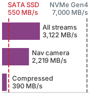
The navigation camera alone writes 4.0× what a SATA SSD sustains; only the compressed session fits under it.

Keeping that write rate under the drive ceiling with video compression trades storage bandwidth against visual fidelity, because lossy encoders discard fine spatial detail at the latch edge and inject blocking artifacts into the frames the policy trains on. A session can be stored in custom HDF5 files, ROS 2 MCAP bags (a container format for multimodal robotics data), or standardized schemas such as LeRobot (Cadene et al. 2024). Whichever format is used, the logger must flush complete chunks to non-volatile storage before a power drop or process halt can truncate the write buffer. It must also carry all four control taps, hardware timestamps, clock-domain identifiers, missing-sample flags, and spatial calibration parameters through every format conversion. Otherwise, a file that deserializes without error proves only that its byte layout is intact, not that its sensory and motor streams remain physically synchronized.

5.6.3 Operational yield and mechanical fatigue budgeting

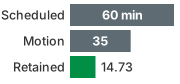
In this illustrative session, setup, rest, resets, and rejected attempts leave under a quarter of the scheduled hour as retained demonstrations.

Sizing the NVMe drive settles what one hour in the workcell writes to disk, but less than a quarter of that scheduled hour survives as usable demonstration motion. Before the arm records a single latch opening, a scheduled hour in the workcell pays for bus synchronization, camera and torque-sensor calibration, and mandatory operator rest. The active motion window that remains is further divided among door-reset strokes, mid-trial contact trips, and offline quality filtering. Because every attempt, whether retained or discarded, flexes the wrist cable harness and reverses load on the harmonic drive, a collection campaign is bounded as much by component fatigue life as by facility reservations.

The ultimate metric of collection efficiency is demonstration yield: the number of validated, policy-ready trajectory records produced in a scheduled session after accounting for cell startup, sensor calibration, operator rest, mechanical resets, and offline quality filtering. Given an active motion window \(\ActiveMotionDuration\), an attempt-and-reset cycle duration \(\AttemptCycleDuration = \AttemptDuration + \ResetDuration\), and an end-to-end retention rate \(\DemonstrationRetentionRate\), the session yields: \[\UsableDemonstrationYield = \left\lfloor \frac{\ActiveMotionDuration}{\AttemptCycleDuration} \right\rfloor \DemonstrationRetentionRate. \tag{6}\] Mechanical fatigue accumulates per physical motion cycle rather than per facility hour. This illustrative accounting assigns the same stress-cycle counts to failed and successful attempts and assumes component ratings expressed under the \(\RatedFatigueLife\) convention. Under it, the rating is the cumulative cycle count at which 10 percent of an identical component population is statistically expected to fail.⁸ Notebook 5.3 evaluates an illustrative door-opening collection session and its full campaign in both currencies: facility hours and component fatigue cycles.

⁸ \(\RatedFatigueLife\) Rated Life: The convention comes from rolling-bearing fatigue theory, where Lundberg and Palmgren (1949) modeled the scatter of bearing life as a probability of survival and rated a bearing by the life that 90 percent of a population reaches. A rating chosen that way is a population statistic, not a guarantee for one part. A fleet of ten collection arms, each run to its cable’s rated life, should therefore expect about one cable to fail before the budget says it will.

Lundberg, Gustaf, and Arvid Palmgren. 1949. “Dynamic Capacity of Rolling Bearings.” Journal of Applied Mechanics 16 (2): 165–72. https://doi.org/10.1115/1.4009930.

Napkin Math 5.3: The flex-cable ceiling

Problem: The latch campaign must retain 5,000 demonstrations. How much scheduled cell time does that cost, and which wrist component’s rated life does it spend fastest?

Variables (illustrative except the chosen session length and target):

• Session \(\ScheduledSessionDuration =\) 60 min (chosen), leaving an active window \(\ActiveMotionDuration =\) 35 min after startup, calibration, and operator rest
• Attempt \(\AttemptDuration =\) 25 s, one teleoperated opening; reset \(\ResetDuration =\) 15 s, the door re-latched by its fixture
• In-trial failure rate 20 percent; post-collection quality filtering 15 percent
• Wear per attempt: \(\GearTorqueReversalCount =\) 14 torque reversals of the wrist’s strain-wave gear; \(\CableFlexCycleCount =\) 8 flex cycles of its internal cable bundle (6 while opening, 2 on the return stroke)
• Rated lives \(\GearRatedFatigueLife =\) 5,000,000 stress cycles and \(\CableRatedFatigueLife =\) 200,000 bending cycles

Math:

1. Session: \(\AttemptCycleDuration =\) 25 s \(+\) 15 s \(=\) 40 s, and \(\lfloor\) 35 min \(/\) 40 s \(\rfloor =\) 52 attempts, with 20 s left idle.
2. Yield (equation 6): \(\DemonstrationRetentionRate = (1 -\) 0.20\()(1 -\) 0.15\() =\) 0.68, so \(\UsableDemonstrationYield =\) 52 \(\times\) 0.68 \(=\) 35.36 episodes, 14.73 min of validated motion, 24.6 percent of the scheduled hour.
3. Campaign: \(\lceil\) 5,000 \(/\) 0.68 \(\rceil =\) 7,353 attempts at 52 per session, or 141.4 h of scheduled cell time, 4.07× the 5,000 \(\times\) 25 s of motion the campaign keeps.
4. Wear: 7,353 \(\times\) 14 \(=\) 102,942 gear cycles, 2.1 percent of \(\GearRatedFatigueLife\); 7,353 \(\times\) 8 \(=\) 58,824 cable bends, 29.4 percent of \(\CableRatedFatigueLife\).

Result: Less than a quarter of each scheduled hour survives as retained demonstration time, and one campaign spends far more of the cable’s rated life than of the gear’s.

Systems insight: The internal flex cable consumes the larger fraction of its assumed rating, informing maintenance planning rather than setting an individual replacement schedule. Three campaigns on one machine would consume most of its rated life, and an intermittent conductor break corrupts the very sensor streams being recorded. Because every attempt costs wear whether or not it is retained, the retention rate \(\DemonstrationRetentionRate\) divides both bills, while a faster reset shortens only the cell time.

Operator rest requirements and fatigue rates depend heavily on interface ergonomics and cognitive task difficulty; teams must empirically calibrate sustained operator throughput and retention on their specific hardware. A collection campaign must therefore be budgeted in both validated trajectory time and consumed fatigue life, not in facility clock hours. Table 3 breaks down the time and mechanical wear budgets of the illustrative session stage by stage.

↪ Per-cycle wear accounting for trial-based learning on the machine is developed in Reinforcement Learning and Environment Interaction.

Table 3: Physical demonstration collection budget across a scheduled 60-minute session: Illustrative facility clock time, yield losses, and component wear by stage for one session of the latch campaign (\(\SessionAttemptCount =\) 52 attempts of \(\AttemptDuration =\) 25 s, reset \(\ResetDuration =\) 15 s). The 20 s of active time left after the last full cycle is idle and has no row. Less than a quarter of the hour survives as retained demonstration data.

Session Stage / Activity	Allocated Duration (\(\FiniteChange \TimeInstant\))	Wall-Clock Share (%)	Physical Operation & Control State	Hardware Stress & Wear Mechanism	Net Trajectory Output (\(\StageEpisodeCount\) / \(\ValidatedMotionDuration\))
Cell Startup & Bus Sync	8 min (480 s)	13.3%	Bus synchronization (EtherCAT/CANopen), safety watchdog verification, optical homing	Power-on electrical inrush; thermal warm-up in motor windings and sensor bridges	\(\StageEpisodeCount = 0\text{ ep}\), \(0.0\text{ min}\) yield
Sensor Calibration & Nulling	7 min (420 s)	11.7%	Camera intrinsic/extrinsic sweep, joint-torque bias nulling, encoder homing	Static holding torque; sensor bridge thermal stabilization; zero dynamic gear wear	\(\StageEpisodeCount = 0\text{ ep}\), \(0.0\text{ min}\) yield
Operator Rest & Ergonomics	10 min (600 s)	16.7%	Mandatory operator breaks to mitigate visual fatigue, cognitive saturation, and tremor drift	Passive standby; electromagnetic brakes engaged or zero-velocity holding current	\(\StageEpisodeCount = 0\text{ ep}\), \(0.0\text{ min}\) yield
Physical Scene Resets	13 min (780 s)	21.7%	Door closed and re-latched by its fixture, arm return stroke (15 s per attempt)	52 return strokes \(\times\) 2 bends \(=\) 104 cable flex cycles; zero contact payload	\(\StageEpisodeCount = 0\text{ ep}\), \(0.0\text{ min}\) yield
Active Teleoperated Attempts	21.67 min (1,300 s)	36.1%	Real-time human teleoperation guiding handle approach, latch release, and door swing (25 s per attempt)	52 \(\times\) 14 \(=\) 728 torque reversals on harmonic drive; 52 \(\times\) 6 \(=\) 312 cable flex cycles; contact monitored against the 15 N tripwire	\(\StageEpisodeCount =\) 52 raw attempts, 21.67 min gross motion
In-Trial Failures (Labeled)	-4.33 min (-260 s)	-7.2%	Handle slip, latch bind, contact tripwire above 15 N (20% loss)	High-force contact transients; abrasive wear on gripper silicone pads	-10.4 ep from success yield; valid logs kept
Post-Collection QA Filtering	-2.60 min (-156 s)	-4.3%	Offline filtering: link latency \(>100\text{ ms}\), visual occlusion, operator hesitation (15% loss)	Zero hardware wear (offline computational validation pass)	-6.24 ep discarded
Net Validated Dataset Yield	14.73 min (884 s)	24.6%	High-quality synchronized multi-modal trajectories (\(\PhysicalWorldState_{t}, \DemonstrationActionLabel_t\)) admitted into training buffer	Consumes 2.1% of wrist gear life and 29.4% of internal flex cable life per 5,000-episode campaign	\(\UsableDemonstrationYield =\) 35.36 episodes

Public collection shows what that yield arithmetic produces at community scale. The open-source LeRobot toolchain records teleoperated sessions in a common format and publishes them to the Hugging Face Hub with an auto-generated metadata card (Cadene et al. 2024). Figure 5 plots, from the Hub’s own listing, how many such datasets exist and how many episodes each holds.

Cadene, Rémi, Simon Alibert, Alexander Toshev, Thomas Sen, Quentin Gallouédec, Adil Zouitine, et al. 2024. LeRobot: State-of-the-Art Machine Learning for Real-World Robotics in PyTorch.

Figure 5: Many datasets, few episodes each: (a) Cumulative count of public datasets tagged with the LeRobot format on the Hugging Face Hub, by creation month; only datasets still public at retrieval are counted, so earlier values are lower bounds. (b) Episodes per dataset for the datasets whose card records a count, in power-of-two bins on a logarithmic axis. The count of datasets has grown by orders of magnitude while the typical dataset remains a single short session. Data retrieved from the Hub API on 2026-10-12.

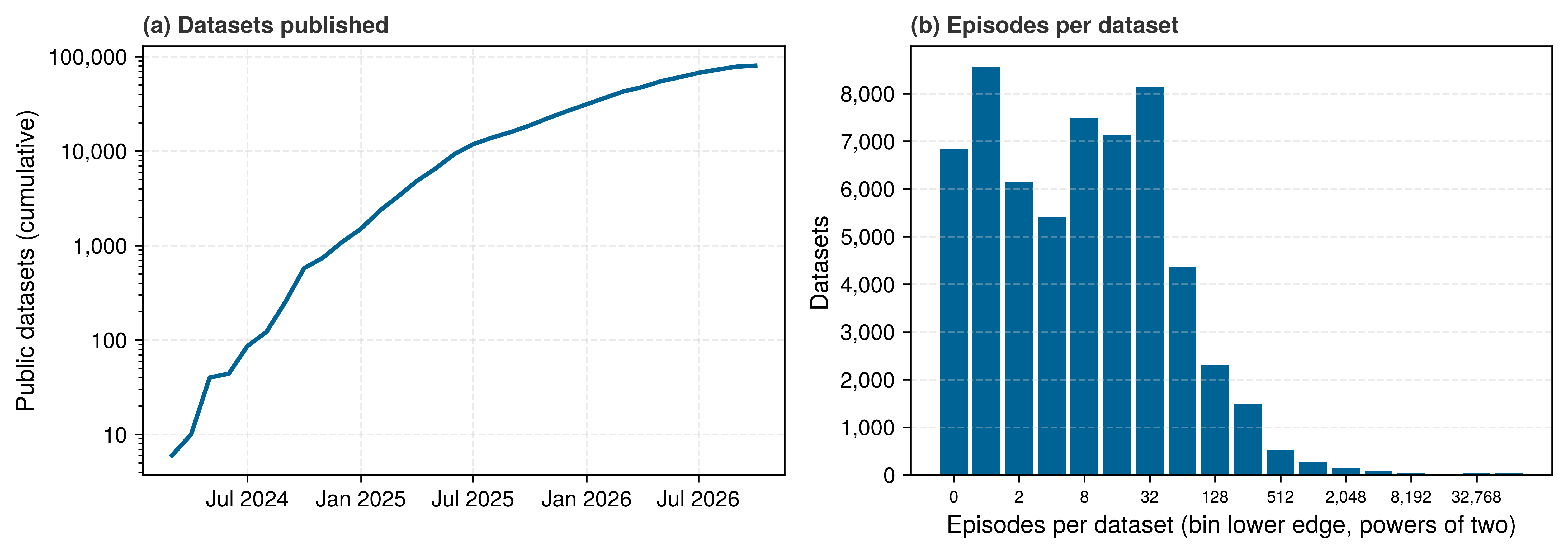
The Hub held 1,085 such datasets at the end of 2024, 26,548 a year later, and 80,132 by the retrieval date. Episode counts tell a different story. Of the 59,031 datasets whose card records one, 58 percent hold fewer than 16 episodes, and only 2 percent hold 512 or more. The median dataset falls in the 8 to 15 episode bin, less than the roughly 35 validated demonstrations of the illustrative hour in table 3. Community data therefore grows wide rather than deep. The archive gains embodiments, scenes, and operators far faster than it gains repeated coverage of any one machine’s states, and pooling it inherits the transfer problem of section 5.9.1.

The three costs compound into a fourth that no bill shows. Teleoperated demonstrations are bounded by what a human operator can perceive through video displays, coordinate through mechanical input devices, and stabilize against closed-loop delays. A campaign that pays for every attempt in cell time and cable life spends its budget where the operator is comfortable. The resulting dataset reflects the behavioral envelope of the coupled human-machine composite rather than the robot’s full physical dynamics. That selection bias decides which situations the archive covers, and measuring it requires a standard outside the archive (section 5.7).

5.7 Collection Policy Coverage

Every logged latch record carries an ingestion cost, an attributed action label, and a hardware timestamp, yet those fields say nothing about which physical situations the archive covers. In an illustrative contact task where a gripper aligns with a workpiece edge across contact angles \(\GripperContactAngle \in [-15.0^\circ, +15.0^\circ]\) and normal forces up to \(20.0\text{ N}\), binning at \(1.0^\circ\) and \(1.0\text{ N}\) forms an operational grid of 600 discrete cells. Suppose two collection policies each record \(1{,}000{,}000\) transitions at \(100\text{ Hz}\) with identical sensors. A cautious teleoperator keeps contact within \(\pm 2.0^\circ\) of perpendicular under \(4.0\text{ to }6.0\text{ N}\) of normal force, populating 8 cells and leaving 98.7 percent of the grid empty. An exploratory policy approaches across the full angular range, slips, and loads the contact between \(1.0\text{ and }18.0\text{ N}\), filling 510 cells and leaving 15.0 percent empty. Although both datasets have identical record counts, storage sizes, and hardware timestamps, they answer different operational questions. Record count therefore fails as a measure twice over: correlated control steps hold few independent samples (equation 2), and even independent samples support only the cells where they land.

That disparity arises because a physical dataset comes from running a closed-loop policy on hardware and logging the resulting transitions, violating the independent-and-identically-distributed assumption of standard empirical risk minimization (section 5.2). Instead, it traces an empirical state-action occupancy distribution (Spencer et al. 2021) \(\CollectionStateVisitationDistribution(\DecisionProcessState, \DemonstrationActionLabel)\) generated by a specific collecting policy \(\pi_{\text{col}}\) under its own control biases, interface delays, and risk tolerance. Formally, imitation learning minimizes prediction error weighted solely by this empirical occupancy: \[\BehaviorCloningLoss(\ModelParameters) = \mathbb{E}_{(\DecisionProcessState, \DemonstrationActionLabel) \sim \CollectionStateVisitationDistribution} \left[ \ell(\Policy(\DecisionProcessState), \DemonstrationActionLabel) \right].\] The learned policy \(\Policy\) therefore receives supervisory gradient updates only over the empirical support hull \(\text{supp}(\CollectionStateVisitationDistribution) = \{ \DecisionProcessState \in \WorldStateSpace \mid \CollectionStateVisitationDistribution(\DecisionProcessState) > 0 \}\). Outside this narrow support hull, the network’s outputs are unconstrained by training demonstrations.

Supervisory labels exist only where the collecting policy visited and commanded an actuator action. In unvisited states, the dataset contains neither an optimal control response nor proof that a safe trajectory exists. Supervised loss functions cannot distinguish an inherently unstable physical configuration from a benign unvisited state or an outright collision hazard. Whether an autonomous policy generalizes in such regions, fails silently, or triggers a safety stop cannot be deduced from the archive alone; resolving that uncertainty requires targeted recovery demonstrations, expert relabeling, or explicit run-time gating. Consider a policy trained exclusively on the cautious teleoperation data. If unexpected surface friction perturbs the gripper to contact angle \(\GripperContactAngle = +4.5^\circ\), outside the eight demonstrated cells, the policy network evaluates an input unconstrained by demonstrations. One control step later, its ungrounded action drives the contact to \(+6.0^\circ\) at \(11.0\text{ N}\), another state lacking corrective labels in the training corpus. Compounding errors push the manipulator progressively farther from the nominal corridor until the gripper jams against the fixture. This cascade illustrates endogenous covariate shift (definition 5.1) triggered by a coverage gap.

5.7.1 Choosing a tractable coverage table

The contact-angle example uses a compact grid because it isolates the parameters relevant to a single mating feature. Extending that dense discretization across all robot state variables triggers the curse of dimensionality in continuous physical interaction.⁹ Consider a mobile manipulator with a 7-degree-of-freedom (7-DoF) arm, a 2-DoF differential-drive base, a 6-axis force-torque sensor at the wrist, and a 6-DoF target workpiece pose. The continuous state space has dimension: \[\StateSpaceDimension = 7\text{ (joint angles)} + 7\text{ (joint velocities)} + 2\text{ (wheel speeds)} + 6\text{ (wrench components)} + 6\text{ (workpiece pose)} = 28.\]

⁹ Curse of Dimensionality: Bellman coined the phrase for dynamic programming, whose value tables grow exponentially with the number of state variables (Bellman 1957). A raw physical coverage table meets the same combinatorial barrier. Dynamic programming scaled by approximating value functions over compact feature spaces; a physical coverage table stays tractable the same way, by listing the few task parameters that determine success rather than the dense continuous state.

Bellman, Richard. 1957. Dynamic Programming. Princeton University Press.

If an engineering team partitions each dimension into a crude \(\DiscretizationBinCount = 10\) bins (\(36^\circ\) per angle bin and \(10\text{ N}\) per wrench bin, far too coarse to guide contact tasks whose tolerances are a few millimeters), the discretized state space contains \(\DiscretizationBinCount^{\StateSpaceDimension} = 10^{28}\) cells. A fleet of 1,000 robots logging at \(1\text{ kHz}\) since the universe began, about 13.8 billion years ago, would hold 4.35 × 10²³ records, enough to visit at most 0.004 percent of those cells even if every record landed in a different one. At a resolution fine enough to guide contact (\(\DiscretizationBinCount = 100\) bins per axis), the count grows to \(10^{56}\) cells. Brute-force observation cannot cover a continuous physical state space; a coverage table must describe the task with a few parameters instead.

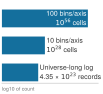
A fleet logging since the universe began could visit at most 0.004 percent of even the coarse grid.

Evaluating dataset completeness against the empirical extremes of collected values is fundamentally circular. A collection logger that records forces exclusively between \(4.0\text{ N}\) and \(6.0\text{ N}\) trivially reports full coverage of that observed interval. Coverage must instead be evaluated against the operational conditions that deployment demands, formulated before any demonstration data is collected.

Definition 5.3: Operational design domain

Operational design domain (ODD) is the declared set of conditions (object poses, surface conditions, payloads, speeds, and disturbances) under which a machine is intended to operate, stated independently of any data collected within it.

1. Significance: The ODD serves as the denominator for every coverage claim. For example, the latch archive, as the join later in this section shows, populates only a single cell of the scenario table its door mechanism requires, a fraction that no volume of redundant nominal episodes can increase. Subsequent verification, evaluation, and release records can assert operational authority only over explicitly supported regions of the ODD.
2. Distinction: Deployment requirements define the ODD, whereas the collecting policy defines empirical occupancy. Coverage measured against observed telemetry extremes merely restates empirical occupancy in ODD terminology, producing an illusion of completeness. A scenario table partitions the continuous ODD into structured discrete cells so that deployment requirements and empirical occupancy can be joined.
3. Common pitfall: Defining the ODD post hoc based on conditions where the machine has already operated successfully rather than where it is required to function. Letting the dataset define its own requirements masks known unvisited failure modes.

In high-dimensional continuous systems, a scenario table avoids voxelizing raw camera pixel streams or continuous joint spaces, which would trigger an intractable combinatorial explosion. Instead, it parameterizes low-dimensional task invariants and environmental boundaries, such as workpiece pose offsets (\(\pm 5\text{ mm}\)), surface friction coefficients, approach speeds, lighting variations (\(100\text{--}1000\text{ lux}\)), and payload masses (\(0\text{--}2\text{ kg}\)). These parameters ground verification in concrete physical operating constraints. While this relational join identifies where the dataset holds empirical experience, populating a cell does not demonstrate that a model trained on those samples executes successfully. A populated cell provides supervisory targets, but verifying autonomous competence still requires closed-loop policy evaluation.

The missing recovery actions identified in figure 1 demonstrate why even a tractable scenario table must list off-nominal perturbations as cells of their own. Repeatedly executing a flawless motion samples progress along the nominal path, whereas corrective demonstrations supply actions that return the machine after an unexpected displacement. A sound scenario table distinguishes recovery experiences from nominal runs rather than treating repeated nominal cycles as coverage of the adjacent state space.

Unsupported operational regimes are exposed by a support envelope relational join, which cross-references empirical occupancy \(\CollectionStateVisitationDistribution(\DecisionProcessState,\DemonstrationActionLabel)\) (where the machine went) against the scenario table \(\RequiredScenarioSet\) (where the machine must be able to go). The table declares a count unit (transitions, independent episodes, or retained demonstrations), an eligibility and retention rule, and a minimum in that same unit. For each cell, the join tallies \(\ScenarioCellRecordCount\) under this policy and partitions the table into cells meeting the minimum (\(\ScenarioCellRecordCount \ge \MinimumCellSupportCount\)), low-count cells, and unvisited blind spots (\(\ScenarioCellRecordCount = 0\)). A populated cell has a nonzero count; it need not meet the minimum. The contact-angle example counts transitions, while the latch campaign’s table counts retained demonstrations. These bins define collection categories. The threshold \(\MinimumCellSupportCount\) represents a declared data requirement rather than a test of policy competence; neither an occupied cell nor a large sample count confers autonomous deployment authority.

A held-out validation split drawn from the same collecting policy can evaluate action prediction accuracy over that occupancy while remaining completely blind to gaps in the required operational domain. The comparison in table 4 separates collection coverage metrics from downstream policy outcomes. Its loss row is the root-mean-square error, in radians, of the predicted action on held-out records, and the cautious archive posts the lower value precisely because a narrow, repetitive archive is easier to fit. Low validation loss does not demonstrate recovery capability in unvisited conditions, just as wide exploratory coverage does not prove that collected corrective labels are dynamically stabilizing. Closed-loop evaluation must test the candidate policy directly against the declared task population.

Table 4: Empirical coverage and validation loss metrics across operational scenario bins: Illustrative counts and held-out losses compare two collection distributions; neither column supplies measured closed-loop capability.

Metric	Cautious Teleoperation (\(\TeleoperationStateVisitationDistribution\))	Exploratory Policy (\(\ExploratoryStateVisitationDistribution\))	Systems Consequence
Recorded Transitions	\(1{,}000{,}000\) transitions (\(100\text{ Hz}\))	\(1{,}000{,}000\) transitions (\(100\text{ Hz}\))	Equivalent dataset scale
Operational Grid Coverage	\(8\,/\,600\) bins (\(1.3\%\))	\(510\,/\,600\) bins (\(85.0\%\))	Populated collection cells
Zero-Count Blind Spots (\(\ScenarioCellRecordCount = 0\))	\(592\,/\,600\) bins (\(98.7\%\))	\(90\,/\,600\) bins (\(15.0\%\))	Collection gaps
Held-Out RMS Action Error (\(\ValidationLoss\))	\(0.001\text{ rad}\)	\(0.012\text{ rad}\)	Validation loss is non-diagnostic
Closed-Loop Capability	Not established by occupancy	Not established by occupancy	Requires candidate evaluation
Collection Decision	Target missing cells	Inspect labels and remaining gaps	Occupancy guides collection

The cage-door latch campaign illustrates this relational join for the running machine. Its six-cell example records occupancy, without supplying per-cell counts or a minimum-count requirement. Every retained episode approaches the strike plate at the guarded speed of 0.03 m/s with the plate aligned within ±0.5 mm of nominal, and every successful demonstration stays below the illustrative 15 N detection threshold. This observation does not itself qualify the collection response. Evaluated against an uncritical table containing only the nominal plate position at the guarded speed, the archive appears exhaustive. Against the scenario table the deployment actually demands, three plate positions (nominal and ±3 mm) crossed with two approach speeds (0.03 m/s and 0.10 m/s), the identical dataset populates only one cell of six. Every off-nominal plate displacement and every fast approach at 0.10 m/s contains zero demonstrations. The raw logged telemetry does not change between these two assessments; the difference lies entirely in the standard of audit applied. The five unvisited cells therefore travel with the dataset into training as documented operational absences, establishing that the current demonstrations provide no empirical foundation for competence claims in those regimes. Targeted collection can acquire the missing recovery trajectories, but downstream training and closed-loop testing must verify what the resulting policy achieves. Figure 6 sets the two audits side by side and adds a third, the stipulated recovery collection latch-recovery-02 of section 5.8, which fills one more cell and still leaves four known absences.

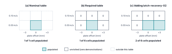
Figure 6: Scenario-table join for the latch: The same retained demonstrations joined against tables of strike-plate offset and approach speed. Against a table holding only the nominal plate at 0.03 m/s (a), the archive looks complete. Against the table the door needs (b), it fills one cell of six and the other five hold zero demonstrations. The stipulated recovery collection latch-recovery-02 (c) adds the positive-offset guarded cell and leaves four known absences. Occupancy describes available experience, not evaluated competence or permission to act.

Checkpoint 5.2: Empirical occupancy and scenario table joins

Before evaluating policy coverage across an operational design domain, audit dataset occupancy and scenario-table counts against these criteria:

• Empirical support vs. validation loss: Explain why an imitation policy can achieve near-zero validation loss on held-out test data while leaving 98 percent of the ODD’s required cells unsupported.
• Unsupported states: What can an unvisited scenario cell establish about policy behavior, and what additional evidence or refusal decision is needed?
• Scenario table joins: Distinguish cells meeting the declared minimum, low-count cells, and unvisited cells when joining telemetry against an operational scenario table.
• Table growth: If the latch scenario table adds a third approach speed between the two it holds, how many cells does it contain, and how many of them are known absences for the original archive?

Logging additional nominal demonstrations along an unperturbed trajectory cannot eliminate coverage blind spots. Exposing the policy to recovery dynamics requires forcing the system toward its operational boundaries, either through deliberate demonstrator noise injection or through expert supervisory interventions (Kelly et al. 2019; Laskey et al. 2017). Before collecting either, a team must know why each empty cell is empty, and recorded interventions add a harder question, because they mix the learner’s commands and the expert’s in one trace (section 5.8).

5.8 Intervention and Recovery Data

A scenario cell, such as the cage-door latch displaced by \(+3\text{ mm}\), may hold zero demonstrations in the training archive. That zero count alone cannot tell an engineer whether the robot never drifted there, whether the 15 N contact tripwire aborted every attempt that reached it, whether a safety supervisor took over beforehand, or whether an ingestion script threw the failed episodes away. Treating those four absences as interchangeable either trains the policy to imitate a safety abort or discards the exact boundary states needed for recovery. An absent state in an empirical log arises from one of four physical mechanisms during collection:

1. Unvisited nominal path: The collecting policy never visited the state because nominal rollouts remained entirely within the primary task corridor. This absence represents unmonitored nominal operation, verifiable by cross-referencing trajectory logs against the scenario table.
2. Permission-path interception: An active safety barrier or deterministic reflex in the permission path detected an impending boundary violation and truncated the motion before reaching the state, as the 15 N contact tripwire does during a misaligned latch attempt. The permission path logs record this barrier trip directly.
3. Human supervisory takeover: A human safety operator perceived a developing hazard and disengaged the autonomous policy before contact occurred. The permission path’s log flags this disengagement explicitly.
4. Post-collection censoring: The machine entered the hazardous state and collided with an obstacle or jammed a joint, but an automated ingestion script discarded the episode as corrupt or incomplete. Dataset inspection cannot detect this absence because the failure transitions were purged before the training arrays were serialized to disk.

Each mechanism produces an identical zero count in the scenario table, yet each calls for a different response. An unvisited cell calls for targeted collection. An intercepted state belongs to the permission path, which already refuses it, and is not a target for the policy to learn. A takeover leaves learner-visited states that curation can turn into corrective supervision. A censored episode is a pipeline defect, recoverable only if the raw recording still exists. Conflating them leads to wrong conclusions about closed-loop policy stability, and the third mechanism needs the most care.

Human takeovers and automated disengagements introduce a selection trap into fleet data. An intervention occurs when the autonomous policy enters a region of state space it handles poorly and its tracking error or uncertainty crosses a threshold. A trajectory recorded after takeover therefore shows an expert recovering from an edge-case disturbance, not nominal task execution. The distribution of states visited during these rescues, \(\TakeoverStateVisitationDistribution\), is conditioned on policy failure. Treating intervention logs as if they were drawn from the nominal distribution \(\ExpertStateVisitationDistribution\) distorts the training distribution toward states that exist only because the prior policy failed.

Appending a rescued episode directly to a behavioral cloning dataset can make unsafe policy commands look like expert demonstrations. Before takeover, the learned policy may issue commands that compound heading error or contact force; after takeover, the expert issues corrective commands from states the learner visited. Those drift states are valuable for corrective aggregation (expert labeling of the states the learner itself reaches, developed below) when an expert can label a safe action there. If a pipeline trains on the entire recorded trajectory without curation, it commits learner-action contamination. The failing policy’s own commands enter the dataset as expert labels. The network then learns to answer the visual cues of an approaching hazard (such as the gripper sliding off the handle or the base drifting toward a rack upright) with the high-risk commands that produced them, which accelerates divergence rather than correcting it. Learner-action contamination corrupts the training targets directly by injecting errant commands, whereas causal confusion occurs when a policy trained on uncorrupted expert targets locks onto spurious correlations (Haan et al. 2019). The driving example from that work is a brake indicator on the dashboard. The light turns on because the expert braked, so it predicts the braking label almost perfectly, and a policy can learn to brake when the light is on rather than when an obstacle appears. At the latch, a measured joint current that climbs because the operator has already begun to push could play the same role, a consequence of the label that a policy mistakes for its cause.

Haan, Pim de, Dinesh Jayaraman, and Sergey Levine. 2019. “Causal Confusion in Imitation Learning.” Advances in Neural Information Processing Systems (NeurIPS) 32.

Separating these labels requires locating the divergence point where the autonomous policy departed the nominal path, rather than treating takeover as the first error. The divergence precedes the takeover by at least the time a supervisor needs to respond. A remote operator who was not watching continuously must notice the hazard, reorient to the scene, and take control. The running machine’s card in The running machine budgets that out-of-loop takeover at 4.47 s, from published take-over studies plus console video and handshake (Human reaction time and travel before braking derives it). Edge loggers therefore keep a circular ring buffer spanning a fixed lookback window \(\PreTriggerWindowDuration =\) 5 s, that takeover time rounded up to whole seconds. Because dynamic memory allocation during safety-critical events introduces non-deterministic latency spikes, the buffer is pre-allocated in locked memory (mlock) or non-volatile storage and populated deterministically at the permission tick rate (1 kHz). When a human safety supervisor hits an override button or an MCU safety enforcer trips a barrier, the pipeline latches the intervention timestamp \(\TakeoverInstant\) and freezes the preceding ring buffer. An out-of-loop supervisory takeover takes longer than the teleoperation loop’s continuous correction (section 5.6); at an illustrative 100 Hz, that delay spans hundreds of control cycles, all logged under the learner’s authority.

↪ The authority record, which logs on every control cycle which entity held authority and the root cause of any preemption, is developed in The Authority Record.

Detecting the divergence instant \(\DivergenceInstant\), estimated below as \(\EstimatedDivergenceInstant\), in offline ingestion pipelines requires searching backwards in time from the physical override timestamp across this synchronized pre-trigger telemetry buffer. For the latch, \(\TrajectoryDivergenceResidual(\TimeInstant)\) is the lateral gripper-position error between measured and planned kinematics in the declared fixture frame, and \(\DivergenceTolerance\) is its positive tolerance in meters. The divergence estimate is: \[\begin{aligned} \EstimatedDivergenceInstant = \min \Bigl\{ \TimeInstant \in [\TakeoverInstant - \PreTriggerWindowDuration, \TakeoverInstant] \;\Big|\; &|\TrajectoryDivergenceResidual(\TimeInstant)| > \DivergenceTolerance \\ &\lor\; \text{Tr}(\PolicyEnsembleCovariance(\TimeInstant)) > \EnsembleSpreadThreshold^2 \Bigr\}. \end{aligned} \tag{7}\] The pipeline scans the lookback window for the first threshold crossing. The policy ensemble covariance is computed after normalizing each action component by its declared scale, so its trace and variance threshold are dimensionless. In unstructured contact manipulation where no static reference trajectory exists, divergence detection instead evaluates declared physical residuals against admissible safety envelope boundaries, such as velocity-to-obstacle clearance margins or anomalous contact force derivatives \(d\ContactForceMagnitude/d\TimeInstant\). The detection thresholds are scenario-specific and calibrated to the sensor noise floor. The minimum defines an estimate only when the retained window contains a threshold crossing from below; an empty set or a residual already above threshold at the start of the window leaves the onset unresolved.

The protocol of intervention curation separates learner commands, expert labels on learner-visited states, and post-takeover recovery at timestamps the permission path logs for every takeover, the entries of the authority record that Supervisory Intervention formalizes. The takeover instant \(\TakeoverInstant\) is the permission tick at which the authority commit revokes the policy’s ownership of the arm, and the three curation rules below are measured from it:

1. Quarantine drift commands: The actions issued by the failing autonomous policy during the drift window \([\DivergenceInstant, \TakeoverInstant)\) are retained in the forensic audit log with their safety flags, but masked out (\(\TrainingLabelMask = 0\)) from imitation training targets.
2. Preserve drift states for relabeling: The physical states visited during \([\DivergenceInstant, \TakeoverInstant)\) capture off-nominal boundary conditions that are absent from nominal demonstrations. These states are admitted to training only when an automated expert, such as a planner with privileged state, supplies corrective labels (\(\DemonstrationActionLabel^*(\DecisionProcessState)\)); a person replaying a logged state cannot reliably say what they would have commanded while closing the loop on it.
3. Admit only stabilized recovery: The post-takeover trajectory is not one demonstration. It opens with the enforcer’s blend, in which the enforcer, still the only writer to the drives, ramps its single admitted command smoothly from the learner’s last checked reference to the operator’s. The actuators therefore never see a step, and no two sources ever command them at once. The operator’s reorientation follows. Neither interval is expert behavior, and both stay masked. Only the segment after the operator’s measured stabilization \(\OperatorStabilizationInstant\), the instant the operator’s corrections settle into a steady return toward the corridor, up to recovery at \(\RecoveryCompletionInstant\), and only where the episode passes task-validity review, becomes an expert recovery demonstration. It teaches the policy how to steer from boundary states back to the nominal manifold. Causal masking and recovery eligibility defines the blend, reorientation, and stabilization intervals and the criterion that ends reorientation.

For the latch campaign, consider a stipulated follow-up collection, latch-recovery-02, at the positive 3 mm strike-plate offset and the guarded 0.03 m/s approach. The same 15 N tripwire remains active. An expert takes over from a misaligned approach, withdraws and reseats the gripper, then releases the latch. The stipulated archive contains valid, reviewed recovery sequences; this is a worked teaching branch, not a report of collected trials or measured improvement.

The three rules decide what this archive keeps. The unsuccessful learner commands are retained for diagnosis, expert relabeling is used only where a corrective target is available, and the expert’s recovery is admitted only from its stabilized, reviewed segment. A new provenance digest binds those labels to the displaced fixture, the original plant contract, and the collection safeguards. The original archive remains immutable. Its successor now contains experience for the positive-offset guarded cell, while the negative-offset and faster-approach cells remain known absences. Policy Training uses this archive to construct the candidate latch-bc-recovery-02, and closed-loop evaluation must test recovery and nominal-task regressions before any expanded competence claim follows.

↪ The qualification of latch-bc-recovery-02 against fresh nominal and displaced-plate trials is developed in Qualifying a recovery update.

The states between divergence and takeover are the second law, endogenous data, made concrete. The learner’s own control actions chose them, and the original nominal archive supplied no corrective supervision there; they are exactly the off-corridor states of figure 1, now visited and logged. Curated, they supply the missing return actions. Training on nominal expert demonstrations alone leaves the compounding-error problem of section 5.3 in place, bounded in the worst case by the quadratic growth of equation 1, \(\CovariateDriftBound\). Labeling the states the learner itself reaches changes how that bound grows.

In corrective aggregation, such as Dataset Aggregation (DAgger) (Ross et al. 2011), an expert labels states visited by the learner, including eligible pre-takeover drift states. Training on states sampled from the learner’s induced distribution (\(\DecisionProcessState \sim \LearnerStateVisitationDistribution\)), rather than solely the expert’s distribution (\(\DecisionProcessState \sim \ExpertStateVisitationDistribution\)), directly counters the covariate shift that nominal demonstrations leave unaddressed. The resulting performance guarantee depends on a constant determined by plant dynamics and task geometry rather than the learning algorithm. After \(\AggregationRoundCount\) rounds of aggregation, at least one policy \(\AggregationLearnedPolicy\) in the sequence satisfies \[\ExpectedTaskCostSum(\AggregationLearnedPolicy) \le \ExpectedTaskCostSum(\pi^*) + \DeviationDisadvantage\,\BehaviorCloningHorizon\,\AggregatedSurrogateLoss + \mathcal{O}(1), \tag{8}\] where \(\AggregatedSurrogateLoss\) represents the surrogate loss of the best single policy on the aggregated learner-visited states (a different quantity from the per-step disagreement \(\SingleStepImitationError\) of equation 1). The symbol \(\DeviationDisadvantage\) is the recoverability constant, the maximum increase in the expert’s remaining cost-to-go incurred by a single errant action before the expert resumes control.¹⁰ This bound scales linearly with the task horizon \(\BehaviorCloningHorizon\) only while \(\DeviationDisadvantage\) remains bounded, which is to say only while the expert can undo any single mistake at a bounded price. If \(\DeviationDisadvantage\) scales in proportion to \(\BehaviorCloningHorizon\), the product \(\DeviationDisadvantage \BehaviorCloningHorizon\AggregatedSurrogateLoss\) reverts to \(\mathcal{O}(\BehaviorCloningHorizon^2\AggregatedSurrogateLoss)\), wiping out the linear advantage over behavioral cloning; Ross et al. (2011) observed this exact failure mode in their predecessor forward-training scheme.

¹⁰ Corrective Aggregation Error Bound: The bound is Theorem 3.2 of Ross et al. (2011). It holds for some policy in the sequence of \(\AggregationRoundCount\) iterations, with \(\AggregationRoundCount\) of order \(\DeviationDisadvantage \BehaviorCloningHorizon\) up to logarithmic factors, and \(\DeviationDisadvantage\) bounds the change in the expert’s cost-to-go after any single action. Imitation Learning and Compounding Covariate Shift states the finite-sample form, in which the same constant appears as \(\Glyph{u_{\max}}\).

Ross, Stéphane, Geoffrey Gordon, and J. Andrew Bagnell. 2011. “A Reduction of Imitation Learning and Structured Prediction to No-Regret Online Learning.” Proceedings of the Fourteenth International Conference on Artificial Intelligence and Statistics (AISTATS) 15: 627–35.

For a horizon of \(\BehaviorCloningHorizon =\) 500 steps (5 s at 100 Hz) and \(\SingleStepImitationError =\) 0.001, the behavioral cloning bound \(\BehaviorCloningHorizon^2\SingleStepImitationError =\) 250. The aggregation term \(\DeviationDisadvantage\,\BehaviorCloningHorizon\AggregatedSurrogateLoss\) in equation 8 evaluates to 0.5 for a recoverable task with \(\DeviationDisadvantage = 1\) and matching per-step error. In this setting, the quadratic cloning bound equals half the episode’s maximum budget, while the leading aggregation term is less than the cost of a single control step. This comparison is conceptual, since the two error terms evaluate losses over different state distributions and both bounds omit problem-dependent leading constants. The quadratic bound becomes vacuous whenever \(\SingleStepImitationError\) exceeds \(1/\BehaviorCloningHorizon =\) 0.002, at which point \(\BehaviorCloningHorizon^2\SingleStepImitationError\) exceeds the maximum possible episode cost of \(\BehaviorCloningHorizon\). Figure 7 joins the two halves of this section, the feedback loop that makes cloning’s worst case quadratic and the curation timeline that turns one takeover into labels the linear bound can use.

The worst case, where \(\DeviationDisadvantage\) grows in proportion to the remaining horizon, is the first law, irreversibility (principle 1), written in the language of imitation bounds. Once the plant enters an unrecoverable state, such as a bent latch, a sheared cable harness, or a dropped brittle workpiece, no subsequent expert command can restore the lost objective. In these failure modes, the cost penalty spans the entire remaining task horizon (\(\DeviationDisadvantage \sim \BehaviorCloningHorizon\)), and aggregating additional learner states cannot recover linear error bounds. A policy cannot learn recovery from states where recovery is physically impossible; the deterministic permission path must prevent entry into those states altogether. The latch campaign draws this boundary explicitly. Withdrawing and reseating a misaligned gripper is recoverable, so latch-recovery-02 records corrections there. Contact forces approaching the illustrative 100 N component damage threshold are unrecoverable; the illustrative 15 N tripwire is a detection threshold, not a contact-force ceiling. Its use requires a qualified collection-response envelope accounting for detection, command and actuator response, and peak-force overshoot below the damage threshold. Without that evidence, the lower threshold alone cannot authorize collection. Those damaging states belong to the safety-enforcer domain rather than the policy learning targets.

Gathering expert supervision on learner-visited states takes several architectural forms, and the curation rules detailed above instantiate one of them. Classical DAgger requires an expert to query and label every state visited during autonomous execution, an impossible requirement for a human supervisor when the policy issues commands at control rates. The framework of human-gated aggregation resolves this bottleneck by allowing a human supervisor to take over only when necessary, appending labels exclusively from the resulting intervention episodes (Kelly et al. 2019). The three curation rules refine this approach by keeping quarantined learner commands, relabeled drift states, and expert recovery actions under separate provenance. Where standard human-gated aggregation retains the entire human takeover stream, rule 3 also filters out the transitional controller blend and operator reorientation intervals. Two refinements address the scarcity of supervisor attention. One queries the expert only when policy uncertainty or novelty exceeds a threshold, spending a fixed intervention budget where the policy is least sure (Hoque et al. 2022). The other upweights the sparse recovery segments relative to the dense nominal trajectories during training, so a few minutes of rescue are not drowned by hours of nominal motion (Mandlekar et al. 2020).

Hoque, Ryan, Ashwin Balakrishna, Ellen Novoseller, Albert Wilcox, Daniel S. Brown, and Ken Goldberg. 2022. “ThriftyDAgger: Budget-Aware Novelty and Risk Gating for Interactive Imitation Learning.” Proceedings of the Conference on Robot Learning (CoRL), Proceedings of machine learning research, vol. 164: 598–608.

Mandlekar, Ajay, Danfei Xu, Roberto Martín-Martín, Yuke Zhu, Li Fei-Fei, and Silvio Savarese. 2020. “Human-in-the-Loop Imitation Learning Using Remote Teleoperation.” arXiv Preprint arXiv:2012.06733.

A team can also avoid online interventions entirely, and this is the wide-tube remedy promised in section 5.3. Injecting small noise perturbations into the teleoperator’s commands pushes the robot off the nominal path during ordinary collection, so the operator’s corrections back toward the corridor appear in the initial demonstration set itself (Laskey et al. 2017). Each perturbation consumes hardware life from the fatigue budget in section 5.6.3 and must stay within recoverable bounds. Ingestion pipelines therefore log the collection mode of every episode explicitly (nominal, noise-injected, or gated intervention), because the three modes put different kinds of states and labels into the archive.

Figure 7: Covariate shift and intervention curation: (a) The learned policy’s own actions choose the states it sees next. The worst-case cost bound grows as \(\CovariateDriftBound\) for behavioral cloning and as \(\mathcal{O}(\DeviationDisadvantage\BehaviorCloningHorizon\AggregatedSurrogateLoss)\) for aggregation on a recoverable task; these are bound orders, not measured drift. (b) One takeover. The 5 s lookback reaches back past the divergence point; states between divergence and takeover are eligible for expert relabeling while the learner’s commands there are masked. After takeover, the enforcer’s blend and the operator’s reorientation are retained for diagnosis but excluded from expert imitation targets, and only the reviewed segment from measured stabilization to recovery becomes an expert demonstration. Based on Ross et al. (2011) and Spencer et al. (2021).

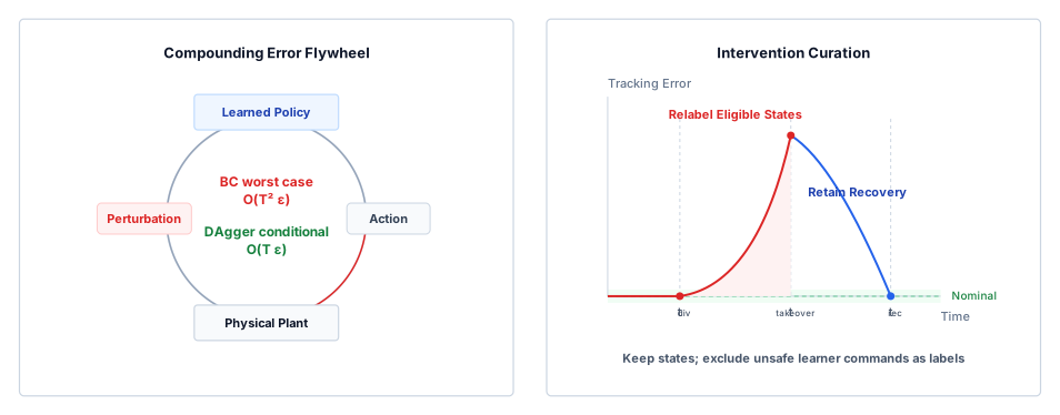
Spencer, Jonathan, Sanjiban Choudhury, Arun Venkatraman, Brian Ziebart, and J. Andrew Bagnell. 2021. “Feedback in Imitation Learning: The Three Regimes of Covariate Shift.” arXiv Preprint arXiv:2102.02872.

Learner-action contamination compounds across policy generations. Suppose a first policy drifts toward a joint torque limit until a supervisor intervenes with an override pendant. A successor trained on those uncurated drift-window commands as expert demonstrations reinforces the behavior that produced the departure, drives harder toward the limit in deployment, and forces operators to intervene earlier and more often. A pipeline that monitors only offline validation loss misses the cascade, because loss on the mislabeled validation split keeps improving as the network memorizes the corrupt labels while physical stability degrades.

Preventing this cascade requires the permission path to record every takeover or safety-barrier trip as an explicit entry in the authority record.¹¹ A boolean disengagement tag overlaid on video is not enough. The ingestion pipeline requires a populated pre-trigger ring buffer matching the declared lookback window (5 s), hardware-synchronized sensor observations and actuator taps, monotonic override timestamps, unique authority identifiers, and precise timestamps marking the blend completion and supervisor stabilization. Without this synchronized pre-trigger telemetry, ingestion pipelines cannot locate the divergence point \(\DivergenceInstant\) and therefore cannot isolate errant learner commands from the boundary states eligible for expert relabeling.

¹¹ Event Data Recorder: US vehicle rules under 49 CFR Part 563 require an automotive event data recorder to preserve a fixed window of telemetry recorded prior to a crash trigger, recognizing that the root cause of an incident precedes the trigger event itself (National Highway Traffic Safety Administration 2024). Human supervisory takeovers have the same temporal structure, because the initial divergence \(\DivergenceInstant\) always precedes the override timestamp \(\TakeoverInstant\). A logging pipeline that begins capturing telemetry only upon trigger activation has already discarded the critical drift data required for policy curation.

National Highway Traffic Safety Administration. 2024. Event Data Recorders: Final Rule (49 CFR Part 563). 89 FR 102810. U.S. Department of Transportation.

Checkpoint 5.3: Intervention curation and error bounds

Before curating human intervention logs for policy retraining, audit compounding error dynamics and timestamp attribution against these criteria:

• Takeover vs. divergence timestamps: Why retain learner-visited drift states for possible expert relabeling while excluding their unsafe learner commands from expert imitation targets?
• Retraining cascade progression: Describe how training successive policy generations on uncurated intervention logs accelerates policy degradation despite improving training metrics.
• Conditional error bounds: Which assumptions distinguish the behavioral-cloning quadratic worst-case cost bound from DAgger’s linear-horizon result?
• Bound threshold: For an episode twice as long as the 5 s comparison, at the same 100 Hz control rate, above what per-step error \(\SingleStepImitationError\) does the quadratic bound stop constraining the cost?

Even with expert labels on learner-visited states, the resulting demonstration archive remains tethered to the kinematics and dynamics of the collecting machine. Pooling demonstrations across robot arms, bases, and end-effectors raises the cross-embodiment questions in section 5.9.

5.9 Cross-Embodiment Transfer

Borrowing manipulation demonstrations from another robot arm looks effortless in tensor space, because both datasets store image frames and seven-element action vectors. That ease disappears when a trajectory recorded on a wide-stroke, \(50\text{ Hz}\) gripper drives a narrower, \(20\text{ Hz}\) gripper into its mechanical endstops or misses a moving conveyor part by centimeters. Physical demonstration trajectories never represent a task in the abstract. Every recorded stream of sensor observations and actuator commands embeds the link lengths, joint velocity limits, camera optical paths, bus latencies, and contact-surface compliances of the logging hardware directly into its numbers. Reusing demonstration datasets across robots therefore requires separating environmental task invariants from machine-specific realizations, checking kinematic and dynamic compatibility, and resolving topological mismatches. This applies whenever the warehouse manipulator supplements its local latch demonstrations with data from foreign arms and grippers.

5.9.1 Embodiment contracts and the normalization fallacy

Suppose a training pipeline rescales gripper commands from two different robots to the unit interval \([0, 1]\) so a single network head can predict both. A normalized command that opens a wide-stroke donor gripper far enough to clear a workpiece will open a narrower target gripper to only a fraction of that span, driving its fingers straight into the part. That failure occurs because an observation-action trajectory \((\MultimodalObservation_{t}, \DemonstrationActionLabel_t)\) permanently encodes the embodiment contract between a specific machine and its physical surroundings. This contract covers the sensor geometry and optical calibration and the sampling period and transport latency of the perception bus. It also covers the coordinate frames and kinematic limits of the actuators, the torque-speed saturation curves of the motors (including reflected rotor inertia \(\GearReductionRatio^2 \RotorInertia\) in geared transmissions), and the friction and compliance of the contact interface. For the running machine’s recorded teleoperation, the contract specifies a rolling-shutter navigation camera at 4056 by 3040 px and 60 Hz, a global-shutter wrist camera at 1440 by 1080 px on its dedicated bracket. The contract also specifies a 9-axis kinematic log sampled at the 1 kHz permission tick (notebook 5.2). Every latch demonstration in that archive reflects that camera suite, that sensor bracket, and that exact arm. Altering any parameter in this contract alters the mapping between commanded inputs and physical state transitions. Even when two robots follow an identical Cartesian tool trajectory \(\ToolCartesianPose(\TimeInstant)\), their required actuator torques diverge. Written per joint, Newton’s second law for a serial manipulator yields the manipulator equation, met earlier as the model classical control inverts: \[\JointTorque = \GeneralizedInertiaMatrix(\GeneralizedCoordinates)\GeneralizedAccelerations + \CoriolisCentrifugalMatrix(\GeneralizedCoordinates, \GeneralizedVelocities)\GeneralizedVelocities + \GravitationalTorqueVector(\GeneralizedCoordinates) + \ExternalContactTorque,\] where \(\GeneralizedCoordinates\) denotes joint positions, \(\GeneralizedInertiaMatrix(\GeneralizedCoordinates)\) is the configuration-dependent mass matrix, \(\CoriolisCentrifugalMatrix(\GeneralizedCoordinates, \GeneralizedVelocities)\) collects Coriolis and centrifugal forces, \(\GravitationalTorqueVector(\GeneralizedCoordinates)\) is the gravitational torque vector, and \(\ExternalContactTorque\) represents torques exerted by external contact forces. Rigid-body dynamics and continuous collision checks builds this equation up from the single-joint case. Because every term depends directly on link masses, rotor inertias, and gear ratios, the same tool trajectory demands different torque profiles across different robot embodiments.

↩︎ The manipulator equation, which classical control inverts to compute joint torques, is established in The Classical Wall.

↩︎ Reflected rotor inertia, \(\GearReductionRatio^2 \RotorInertia\), and its effect on joint dynamics are established in Reflected rotor inertia and optimal inertia matching.

While the embodiment contract defines the physics of a single machine, the cross-embodiment compatibility contract determines whether trajectories logged under one embodiment contract can safely serve as action targets on another. This compatibility contract defines the forward kinematics mapping (translating joint angles to tool pose), control-rate transformations (\(\FiniteChange \TimeInstant\)), and actuator effort bounds. These bounds prevent a high-force profile or rapid spatial velocity demonstrated on a rigid industrial arm from driving a lightweight cobot beyond its structural limits. Large pooled corpora rarely provide such guarantees. Open X-Embodiment maps action fields into a coarsely aligned seven-dimensional end-effector format and normalizes each dataset independently. However, it deliberately leaves coordinate frames unaligned and allows action vectors to represent either absolute or relative poses and velocities across different sub-corpora (Open X-Embodiment Collaboration et al. 2024). A multi-task model trained on this pool learns to interpret identical action vectors differently based on embodiment tokens. In contrast, DROID sidesteps embodiment mismatch altogether by collecting all data on a single standardized robot model (Khazatsky et al. 2024). Demonstrations from diverse robots can enrich representation learning without an explicit compatibility contract, but such a contract becomes strictly mandatory the moment borrowed actions are imitated directly as supervisory labels or dispatched to a physical plant.

How much work the compatibility contract has to do is visible in the largest pooled robot corpus. The Open X-Embodiment collection merges independently recorded datasets into one training mixture and publishes, for each, its episode count, robot morphology, scene type, and command rate (Open X-Embodiment Collaboration et al. 2024). Figure 8 weights each dataset by its episodes.

Figure 8: What a pooled corpus actually contains: Episodes of the Open X-Embodiment collection, weighted by dataset size, (a) by robot morphology on a logarithmic axis and (b) by the command rate each dataset declares. Single-arm table-top manipulation dominates, and the declared rates cluster at or below 10 Hz; a large share declares no rate at all because its actions are primitive skills or quasi-static moves. Green marks the running machine’s class in (a) and its chunk renewal rate in (b). Data from the collection’s published dataset overview (Open X-Embodiment Collaboration et al. 2024).

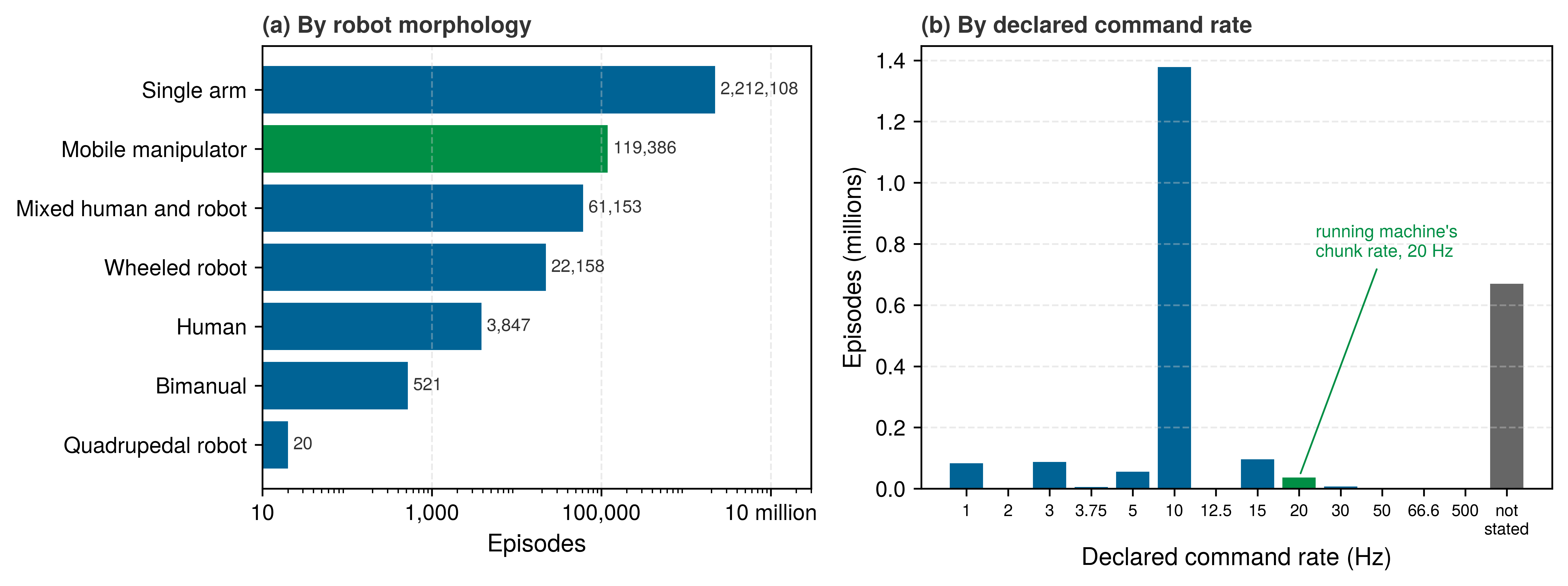
Of the 2.4 million episodes across 72 datasets, 91 percent come from single arms and 89 percent from table-top scenes. Mobile manipulators, the class of the running machine, contribute 5 percent, and two datasets supply 95 percent of those. The command rates are as uneven: 57 percent of episodes were logged at 10 Hz, 28 percent declare no rate, and only 2 percent were recorded at or above the machine’s 20 Hz chunk rate. Corpus size therefore says little about coverage of one machine’s contract. Almost every episode in the mixture needs the rate transformation and morphology mapping of the compatibility contract before it can serve as an action target here.

A data-reuse pipeline must separate environmental task invariants from embodiment-specific realizations. A task invariant is a geometric or dynamical condition imposed by the physical process, for example bringing a compliant probe into contact with a terminal pad within \(5^\circ\) of the surface normal while sustaining a normal contact force between \(2.0\text{ N}\) and \(5.0\text{ N}\). An embodiment realization is the concrete sequence of joint encoder counts, pulse-width modulation duty cycles, perception transport latencies, and sensor pixel rasters used to achieve that condition on a particular test rig. While the contact goal exists in world coordinates, the dataset stores only the realization. When a model trains directly on raw hardware realizations, it internalizes the idiosyncratic mechanics of the source testbed, including structural flexure, drive backlash, and sensor mounting oscillations.

Consider transferring a demonstration dataset collected on Machine A to Machine B for an identical pick-and-place task:

• Machine A operates a parallel-jaw gripper with a stroke of \(0\text{ to }100\text{ mm}\), a \(50\text{ Hz}\) command rate (\(20\text{ ms}\) period), a continuous grasp force limit of \(40\text{ N}\), and a wrist camera mounted \(45\text{ mm}\) behind the tool center point with a \(15\text{ ms}\) transport delay.
• Machine B operates a compact gripper with a stroke of \(0\text{ to }60\text{ mm}\), a \(20\text{ Hz}\) command rate (\(50\text{ ms}\) period), a continuous force limit of \(15\text{ N}\), and a wrist camera mounted \(20\text{ mm}\) behind the tool center point with a \(35\text{ ms}\) transport delay.

Projecting Machine A’s demonstrations directly through the physical constraints of Machine B reveals immediate points of hardware failure. For a workpiece of width \(75\text{ mm}\), Machine A commands a gripper aperture of \(80\text{ mm}\). That command exceeds Machine B’s mechanical stroke by \(20\text{ mm}\), driving its leadscrew into the mechanical endstop. During the hold phase, Machine A applies \(30\text{ N}\) of clamping force; executing that command on Machine B doubles its continuous rating of \(15\text{ N}\) and forces its motor amplifier into current saturation. In the time domain, subsampling the \(50\text{ Hz}\) trajectory onto Machine B’s \(20\text{ Hz}\) bus aliases rapid contact dynamics and increases the half-period average hold age \(\FiniteChange \TimeInstant / 2\) from \(10\text{ ms}\) to \(25\text{ ms}\), introducing \(15\text{ ms}\) of additional zero-order hold phase lag (Discrete-time sampling and zero-order hold phase lag). Compounded by the \(20\text{ ms}\) difference in camera transport delay (\(35\text{ ms} - 15\text{ ms}\)), the added low-frequency phase-equivalent delay is \(35\text{ ms}\), of which the camera difference contributes \(20\text{ ms}\). At the assumed constant approach velocity of \(0.10\text{ m/s}\), that phase approximation corresponds to an equivalent displacement of \(3.5\text{ mm}\). Actual contact overrun requires measured or bounded sampling phase, capture and transport, computation, actuation, and plant response; the phase-equivalent value does not establish when the first correction dispatches. Meanwhile, the \(25\text{ mm}\) disparity in wrist camera mounting introduces optical parallax that shifts the apparent position of the workpiece boundary across the camera raster.

Standard machine learning pipelines often try to reconcile these discrepancies by normalizing observation and action channels to \([0, 1]\) or \([-1, 1]\). That rescaling aligns tensor ranges while leaving the physical mismatch intact. Normalizing gripper travel to \([0, 1]\) turns Machine A’s safe \(80\text{ mm}\) opening (\(\NormalizedActionCommand = 0.80\)) into a \(48\text{ mm}\) opening on Machine B (\(0.80 \times 60\text{ mm}\)) that drives its fingers into the \(75\text{ mm}\) workpiece during approach. Normalizing feature ranges rescales numbers, but it cannot lengthen a leadscrew, lower motor coil resistance, or recover bus transport delay. Demonstration trajectories plotted in normalized unit spaces may look identical, yet only the subset inside the physical intersection (apertures below \(60\text{ mm}\), forces under \(15\text{ N}\), and command frequencies below \(20\text{ Hz}\)) can run on the target hardware without saturation or contact damage. Even within that intersection, two arms with different joint layouts can collide with the workspace when they share a single Cartesian command (section 5.9.2).

5.9.2 Kinematic topology mismatches and null-space projection

Even when end-effectors, force ratings, and control rates align, differences in arm geometry can break a transferred trajectory. When a 7-DoF arm’s demonstration is compressed into a 6-DoF Cartesian hand displacement so it can be pooled with other robots, the log discards the arm’s elbow posture; replaying that 6-DoF stream through a target robot’s inverse kinematics solver can swing the elbow into a shelf upright or drive a lighter arm through a singularity, even though the hand follows the exact demonstrated path. Combining robots with different kinematic structures introduces two topological conflicts:

1. Action space incompatibility: A 7-DoF arm records joint positions \(\GeneralizedCoordinates \in \mathbb{R}^7\), a bimanual workstation records \(\GeneralizedCoordinates \in \mathbb{R}^{14}\), and a mobile base logs planar velocities \((\BaseLongitudinalVelocity, \BaseLateralVelocity, \BaseHeadingRate)\). Because joint-space commands cannot transfer directly across distinct kinematic arrangements, multi-embodiment models project action sequences into a common Cartesian end-effector displacement: \[\FiniteChange \ToolCartesianPose_t = (\FiniteChange \EndEffectorFirstAxisPosition, \FiniteChange \EndEffectorSecondAxisPosition, \FiniteChange \EndEffectorThirdAxisPosition, \FiniteChange \EndEffectorRollAngle, \FiniteChange \EndEffectorPitchAngle, \FiniteChange \EndEffectorYawAngle) \in \mathbb{R}^{6}, \quad \GripperOpeningCommand \in [0, 1],\] where the final three elements represent local roll, pitch, and yaw increments under a declared rotation convention. This displacement vector is not itself a member of the Special Euclidean group \(\SpecialEuclideanGroup\); any numerical integration must handle angle wrapping and representation singularities. Projecting into Cartesian space standardizes spatial geometry, but it strips away actuator dynamics. A Cartesian step that an industrial arm executes effortlessly near its nominal pose can force a lighter arm through a kinematic singularity, a configuration in which aligned joints leave the tool unable to move in some direction. The manipulator Jacobian \(\ManipulatorJacobian(\GeneralizedCoordinates)\), a configuration-dependent matrix that Mapping tool motion to joint limits develops on the machine’s own arm, maps joint velocities to tool spatial velocities through \(\ToolCartesianVelocity = \ManipulatorJacobian(\GeneralizedCoordinates)\GeneralizedVelocities\). When \(\ManipulatorJacobian(\GeneralizedCoordinates)\) loses row rank at a singularity, no finite joint velocity can generate motion along the lost Cartesian direction. Commanded displacements near such poses demand joint velocities that immediately exceed the target machine’s actuator velocity bounds.
2. Null-space projection and elbow swivel ambiguity: Away from singularities, mapping a 7-DoF arm into a 6-DoF Cartesian delta projects out the one-dimensional null space (\(7 - 6 = 1\) redundant degree of freedom). For a redundant manipulator with Jacobian \(\ManipulatorJacobian(\GeneralizedCoordinates) \in \mathbb{R}^{6 \times 7}\), the general kinematic relationship between Cartesian velocity \(\ToolCartesianVelocity\) and joint velocity \(\GeneralizedVelocities\) is: \[\GeneralizedVelocities = \JacobianPseudoinverse(\GeneralizedCoordinates) \ToolCartesianVelocity + \left( \IdentityMatrix - \JacobianPseudoinverse(\GeneralizedCoordinates) \ManipulatorJacobian(\GeneralizedCoordinates) \right) \NullSpaceVelocityBias,\] where \(\JacobianPseudoinverse = \ManipulatorJacobian^\top (\ManipulatorJacobian \ManipulatorJacobian^\top)^{-1}\) is the Moore-Penrose pseudoinverse (the minimum-norm joint velocity producing \(\ToolCartesianVelocity\) whenever \(\ManipulatorJacobian\) has full row rank), and the projection operator \((\IdentityMatrix - \JacobianPseudoinverse \ManipulatorJacobian)\) filters an arbitrary joint-velocity bias \(\NullSpaceVelocityBias \in \mathbb{R}^7\) into self-motion that leaves the end-effector still. For an anthropomorphic arm with shoulder and wrist geometry that admits this construction, a fixed end-effector pose in \(\SpecialEuclideanGroup\) and a fixed shoulder anchor leave an elbow orbit around the shoulder-to-wrist axis, parameterized by the elbow swivel angle \(\ElbowSwivelAngle\). A general redundant arm instead requires its own configuration parameter or the full joint vector; one redundant degree of freedom does not imply this circular geometry. Discarding this internal degree of freedom to impose a uniform 6-DoF action representation erases the human operator’s postural intent. When the target robot receives this 6-DoF command stream, its local inverse kinematics (IK) solver must resolve the redundancy using an arbitrary mathematical heuristic, such as joint-limit centering or manipulability maximization. Without the original swivel angle, the solver may adopt an elbow posture that drives joints into hard stops or sweeps the elbow into nearby shelving, fixtures, or personnel during a motion that was entirely collision-free in the source environment. Preserving the applicable redundancy parameter, or the complete joint-state vector, within the trajectory’s provenance metadata retains the operator’s postural intent for target-specific retargeting and collision checks. The running mobile manipulator archive maintains this intent directly: its arm has redundant kinematics, and its logger captures all 9 axes of the arm and base at the 1 kHz permission tick. Any pooled 6-DoF delta generated from a latch-servicing trajectory can always be traced back to the demonstrator’s original elbow posture.

↪ Forward kinematics, the manipulator Jacobian, its singularities, and the pseudoinverse are developed in Forward kinematics and singularities.

Reusing physical data across different robots therefore requires two validation gates at the ingestion boundary, corresponding to two distinct roles in training:

• The pretraining admission gate evaluates whether a trajectory can safely contribute to general representation learning. This gate validates data provenance, observation integrity, coordinate frame conventions, action semantics (reference frame, absolute vs. relative representations, position vs. velocity modes), and sampling rates. In particular, source actions admitted at this gate need not be physically executable on the target robot. Multi-embodiment foundation models rely on this gate to ingest broad visual and task structures across dozens of robot morphologies before fine-tuning on target hardware (Open X-Embodiment Collaboration et al. 2024; Black et al. 2024).
• The target-label gate applies whenever recorded actions serve as direct imitation labels or execution setpoints on the physical plant. This gate maps the source trajectory through target forward kinematics to verify coordinate consistency (Lynch and Park 2017). It confirms that commanded joint velocities and accelerations remain within the target plant’s dynamic envelope (Tedrake 2023). It also verifies that task-critical features remain within the field of view and dynamic range of the target sensors. When commanded trajectories violate kinematic reach or motor torque limits, an ingestion pipeline cannot simply clamp the values to target boundaries. Clamping distorts velocity profiles, alters phase relationships, and destroys the causal link between observed spatial errors and corrective control outputs. Trajectories that satisfy the target dynamics pass untouched; trajectories that admit valid geometric retargeting through inverse kinematics are relabeled; and trajectories that demand unobtainable actuator authority or rely on unobservable states are rejected.

Lynch, Kevin M, and Frank C Park. 2017. Modern Robotics: Mechanics, Planning, and Control. Cambridge University Press.

Tedrake, Russ. 2023. Robotic Manipulation: Perception, Planning, and Control. Massachusetts Institute of Technology.

Evaluating the two-gripper scenario of section 5.9.1 through this target-label gate resolves each trajectory segment systematically. The initial opening phase must be rejected rather than relabeled, because satisfying the task invariant (clearing the \(75\text{ mm}\) workpiece) demands an aperture that Machine B cannot physically achieve. The \(30\text{ N}\) grasp hold is rejected on identical grounds, as it exceeds Machine B’s continuous motor rating. Conversely, the \(50\text{ Hz}\) trajectory can be resampled and relabeled onto Machine B’s \(20\text{ Hz}\) control bus only if the slower command stream preserves the task-critical contact dynamics and remains within the target’s verified tracking and force limits. The data record must also log the added zero-order hold lag and camera transport delay so that policy training accounts for the altered timing. An ingestion pipeline lacking this gate injects dynamically invalid trajectories into the training distribution. A policy trained on such unvetted data fails in deployment not because of neural network underfitting, but because its training labels were physically valid only on the donor hardware. For the latch-servicing campaign, the target plant is the mobile manipulator’s own arm and gripper. Every borrowed trajectory proposed as a latch training label must pass this gate against the mobile manipulator’s verified limit record, regardless of the donor platform’s reported capabilities.

↩︎ The limit record, which states each measured limit with its operating conditions, uncertainty, and margin, is established in The six elements of a limit record.

The warehouse conveyor pick demonstrates a transfer mismatch rooted in task dynamics rather than robot kinematics. At the sorting station, the arm grasps a workpiece moving along a belt at 0.20 m/s. The workpiece translates 5 mm during each 25 ms control step and advances 80 mm over a single 16-step action chunk of 400 ms, a displacement of 5.3× the allowable 15 mm grasp tolerance. A borrowed tabletop demonstration recorded on a stationary bench defines its grasp trajectory entirely in the static table frame. If a policy imitates that trajectory unchanged at the conveyor, an open-loop action chunk aims at the spatial location the part occupied when the chunk was generated. The target-label gate can adapt such a static trajectory only by transforming the end-effector path into the moving workpiece coordinate frame. This coordinate transformation requires both the instantaneous object pose in the donor metadata and the conveyor velocity in the target environment record. An external trajectory lacking this telemetry can enter the pipeline solely through the pretraining admission gate. Teleoperation data collected directly on the warehouse machine requires no such mathematical rescue, as the human operator generated the demonstration commands with the conveyor in motion.

5.9.3 Choosing pooled experience for the target task

Pretraining on a million pooled trajectories from foreign robots does not help the warehouse manipulator open a displaced latch if the training mixture drowns out the machine’s own contact dynamics. The same holds if the mixture adds ten thousand repetitions of a single tabletop scene instead of covering new operating cells. Large-scale pooled corpora such as DROID (Khazatsky et al. 2024), BridgeData v2 (Walke et al. 2023), and Open X-Embodiment (Open X-Embodiment Collaboration et al. 2024) offer broad scene diversity and multi-robot demonstrations, but their value to a specific deployment depends on what information survives the admission gates of section 5.9.2. Even when kinematic mismatches prevent direct imitation of donor joint commands, foreign demonstrations can supply visual representations, object affordances, and high-level task structures, provided the campaign measures how those additions fill its scenario table.

Belkhale, Suneel, Yuchen Cui, and Dorsa Sadigh. 2023. “Data Quality in Imitation Learning.” Advances in Neural Information Processing Systems (NeurIPS) 36: 80375–95. https://doi.org/10.52202/075280-3524.

Empirical scaling studies since 2024 support the premise behind the scenario table, that policies generalize with the number of distinct environmental conditions in their data rather than with repetitions of the same ones. In an extensive empirical evaluation spanning more than 40,000 demonstrations collected with handheld grippers, policy success across novel environments and unseen objects scaled as a power law with the count of distinct training environments and objects. Adding further demonstrations within existing environments yielded sharply diminishing returns once a modest baseline was achieved. A dataset collecting 50 demonstrations across each of 32 environments achieved 90 percent on novel environment-object pairs (Lin et al. 2025). Similarly, evaluating mobile manipulation across residential settings revealed steady performance gains as the training distribution expanded from 3 to 104 homes. At 104 locations, the generalized model matched the performance of an in-domain baseline trained exclusively within the evaluation homes (Black et al. 2025). Viewed through the scenario table, the primary scaling axis is the count of distinct operational cells populated by the corpus. The declared minimum coverage threshold \(\MinimumCellSupportCount\) identifies cells that still need collection; it does not establish that additional trajectories within a populated cell have no value. Populating operational cells is necessary but not sufficient on its own. As Belkhale et al. (2023) demonstrate, dataset utility depends on two additional quality metrics: action divergence (the discrepancy between expert actions and learned policy outputs at reachable states) and transition diversity (the stochasticity of outcomes from given state-action pairs). Uncurated state diversity does not automatically yield performance improvements.

These demonstration corpora also diverge in how they acquire operational diversity. Open X-Embodiment aggregates 60 distinct datasets across 22 different robotic embodiments with different, unaligned action spaces; despite this lack of structural alignment, joint pretraining improved success rates across the smaller constituent datasets (Open X-Embodiment Collaboration et al. 2024). DROID and AgiBot World instead hold the embodiment contract constant while maximizing environmental and task diversity. DROID deploys a single manipulator model across 564 in-the-wild environments (Khazatsky et al. 2024). AgiBot World scales this principle with a homogeneous fleet of more than 100 identical robots, producing pretraining data that demonstrated superior downstream transfer compared to Open X-Embodiment (AgiBot-World-Contributors et al. 2025). A homogeneous fleet removes nominal kinematic mismatches, but each unit must still satisfy the target-label gate through verified calibration and dynamic compatibility. The fleet also remains vulnerable to the shared kinematic blind spots of that specific platform. Conversely, a multi-robot corpus can broaden perceptual learning through the pretraining gate; its actions become target labels only after passing the target-label gate. Balancing these disparate data streams requires deliberate weighting within the training mixture; dynamically weighting datasets to safeguard the worst-performing target domain significantly outperforms uniform data sampling across Open X-Embodiment (Hejna et al. 2025).

Hejna, Joey, Chethan Anand Bhateja, Yichen Jiang, Karl Pertsch, and Dorsa Sadigh. 2025. “ReMix: Optimizing Data Mixtures for Large Scale Imitation Learning.” Proceedings of the 8th Conference on Robot Learning (CoRL), Proceedings of machine learning research, vol. 270: 145–64.

Levine, Sergey, Peter Pastor, Alex Krizhevsky, Julian Ibarz, and Deirdre Quillen. 2018. “Learning Hand-Eye Coordination for Robotic Grasping with Deep Learning and Large-Scale Data Collection.” The International Journal of Robotics Research 37 (4-5): 421–36.

Kalashnikov, Dmitry, Alex Irpan, Peter Pastor, Julian Ibarz, Alexander Herzog, Eric Jang, Deirdre Quillen, et al. 2018. “Scalable Deep Reinforcement Learning for Vision-Based Robotic Manipulation.” Proceedings of the 2nd Conference on Robot Learning, Proceedings of machine learning research, vol. 87: 651–73.

Black, Kevin, Noah Brown, Danny Driess, Adnan Esmail, Michael Equi, Chelsea Finn, Niccolo Fusai, et al. 2024. “\(\pi_0\): A Vision-Language-Action Flow Model for General Robot Control.” arXiv Preprint arXiv:2410.24164.

Placing these landmark robot archives alongside community uploads and web-scale foundation-model corpora exposes both how physical collection has scaled and where its ceiling sits (figure 9). Across 11 major physical collection campaigns since 2015 (figure 9, panel a), robot datasets progressed from single-lab grasping farms (50,000 to 800,000 trials in a fixed bin (Levine et al. 2018; Kalashnikov et al. 2018)) through multi-scene teleoperation (60,096 trajectories in BridgeData V2 and 76,000 in DROID (Walke et al. 2023; Khazatsky et al. 2024)) to million-episode pooled and fleet archives (2,419,193 episodes in Open X-Embodiment and 1,001,552 in AgiBot World (Open X-Embodiment Collaboration et al. 2024; AgiBot-World-Contributors et al. 2025)). Those pooled campaigns sit five orders of magnitude above the 8–15 episode median of single-session community uploads in figure 5. Even million-episode robot campaigns, however, confront the cross-domain gap in panel b. Across 902 language, vision, and robotics models with disclosed training dataset sizes in the Epoch AI catalog (Epoch AI 2026), frontier language and vision corpora reach \(10^{13}\) to \(10^{14}\) tokens or images, whereas \(\pi_0\)’s \(10{,}000\)-hour robot pretraining corpus (1,000,000,000 state-action steps (Black et al. 2024)) sits 14,800× below DeepSeek-V3’s 14.8 trillion tokens.

Figure 9: Physical robot demonstration scaling and the cross-domain data gap: (a) Reported trajectory or episode counts of 11 landmark physical robot corpora from 2015 to 2025 on a logarithmic axis, grouped by collection regime alongside the median episode bin of community LeRobot Hub uploads (figure 5). (b) Training dataset sizes in datapoints across language, vision, and robotics models in the Epoch AI catalog from 2018 to 2026 (Epoch AI 2026). While multi-robot pooling and homogeneous fleets pushed physical archives past \(10^6\) episodes, real-world robot corpora remain four orders of magnitude smaller than web-scraped language and vision datasets because physical collection is bounded by real-time actuation.

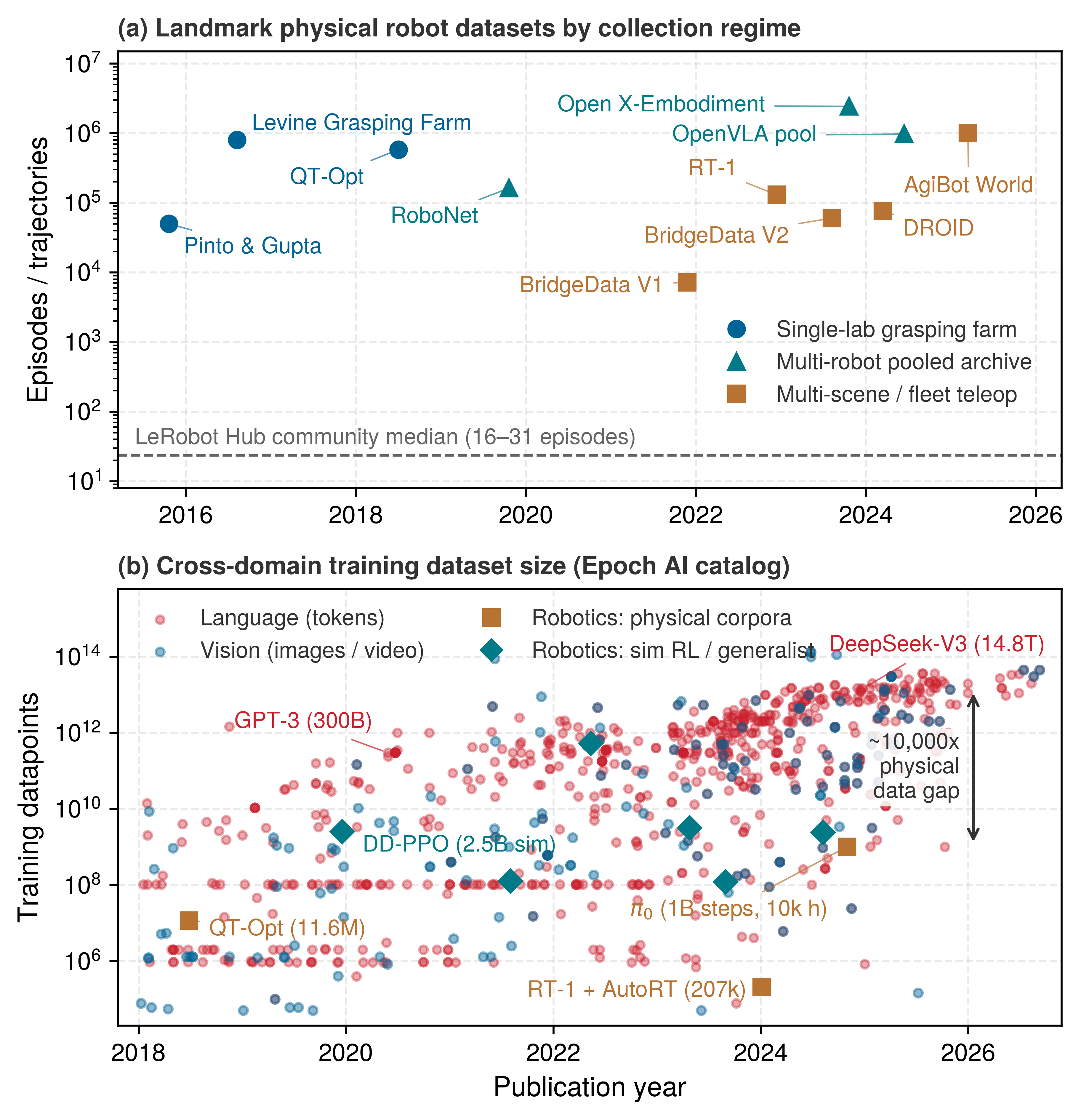
Epoch AI. 2026. Data on AI Models.

Because every physical trajectory is throttled by real-time motor execution and session yield (equation 6), robot learning cannot close a four-order-of-magnitude data gap by brute-force teleoperation alone. Deployed pipelines instead inherit broad semantic priors from web-pretrained vision-language backbones, use synthetic expansion or co-training where provenance allows, and spend their scarce physical episodes on the cells that scenario-table coverage and compatibility gates confirm they need, as the benchmark systems in table 5 illustrate.

Table 5: State of practice in robot demonstration data, as of 2026: Named systems illustrate the mechanisms of this chapter at one point in time; each scale and result is as reported by the cited paper, measured on that paper’s own tasks and not comparable across rows.

System (year)	Collection regime	Reported scale	What it shows for the scenario table
Open X-Embodiment (2024) (Open X-Embodiment Collaboration et al. 2024)	Heterogeneous pool of existing datasets	60 datasets, 22 embodiments; RT-1-X 50% higher mean success than the original methods	Breadth without aligned actions; target labels require the target-label gate
DROID (2024) (Khazatsky et al. 2024)	One robot model, distributed in-the-wild collection	76,000 trajectories, 350 h, 564 scenes	Scene diversity under a single embodiment contract
UMI (2024) (Chi et al. 2024)	Robot-free hand-held grippers	Relative-trajectory actions; latency matched at deployment	Collection decoupled from robot time and wear
Data scaling study (2025) (Lin et al. 2025)	Hand-held grippers across many environments	40,000 demonstrations; power law in environments and objects	Fill more cells before adding episodes per cell
AgiBot World (2025) (AgiBot-World-Contributors et al. 2025)	Homogeneous fleet of identical robots	1,001,552 trajectories, 217 tasks; 30% average gain over pretraining on Open X-Embodiment	Shared embodiment; unit compatibility still requires verification
\(\pi_{0.5}\) (2025) (Black et al. 2025)	Mobile manipulators in homes, co-trained with other sources	About 400 h in homes; 3 to 104 training locations	Generalization grows with the number of locations
MimicGen (2023) (Mandlekar et al. 2023)	Synthetic generation from seed demonstrations	Over 50,000 from about 200 human demonstrations, 18 tasks	Cells filled only by synthetic data must be marked as such
Sim-and-real co-training (2025) (Maddukuri et al. 2025)	Simulated and real demonstrations mixed in training	38% average gain in real-robot success	Synthetic data helps when its provenance is kept

Chi, Cheng, Zhenjia Xu, Chuer Pan, Eric Cousineau, Benjamin Burchfiel, Siyuan Feng, Russ Tedrake, and Shuran Song. 2024. “Universal Manipulation Interface: In-the-Wild Robot Teaching Without in-the-Wild Robots.” Robotics: Science and Systems (RSS). https://doi.org/10.15607/RSS.2024.XX.045.

Lin, Fanqi, Yingdong Hu, Pingyue Sheng, Chuan Wen, Jiacheng You, and Yang Gao. 2025. “Data Scaling Laws in Imitation Learning for Robotic Manipulation.” International Conference on Learning Representations (ICLR), 54877–910.

AgiBot-World-Contributors, Qingwen Bu, Jisong Cai, Li Chen, Xiuqi Cui, Yan Ding, Siyuan Feng, Shenyuan Gao, et al. 2025. “AgiBot World Colosseo: A Large-Scale Manipulation Platform for Scalable and Intelligent Embodied Systems.” IEEE/RSJ International Conference on Intelligent Robots and Systems (IROS), 3549–56. https://doi.org/10.1109/IROS60139.2025.11247088.

Black, Kevin, Noah Brown, James Darpinian, Karan Dhabalia, Danny Driess, Adnan Esmail, Michael Robert Equi, et al. 2025. “\(\pi_{0.5}\): A Vision-Language-Action Model with Open-World Generalization.” Proceedings of the Conference on Robot Learning (CoRL), Proceedings of machine learning research, vol. 305: 17–40.

Mandlekar, Ajay, Soroush Nasiriany, Bowen Wen, Iretiayo Akinola, Yashraj Narang, Linxi Fan, Yuke Zhu, and Dieter Fox. 2023. “MimicGen: A Data Generation System for Scalable Robot Learning Using Human Demonstrations.” Proceedings of the Conference on Robot Learning (CoRL), Proceedings of machine learning research, vol. 229: 1820–64.

The core engineering decision is whether incorporating compatible pooled experience improves target-task policy performance relative to an identical baseline trained strictly on in-domain data. Rigorous evaluation requires fixing the target task distribution and test protocol, maintaining full data provenance, and benchmarking both nominal task completion and recovery behavior. Merely increasing the number of embodiments in a dataset does not guarantee positive transfer. In the mobile manipulator’s displaced-latch campaign, the control baseline is a policy trained exclusively on 5,000 retained teleoperation demonstrations from the machine itself, populating a single cell within the six-cell scenario table. An expanded multi-robot corpus justifies its training overhead and ingestion complexity only if the resulting policy improves robustness on long-tail target conditions without regressing nominal latch-servicing performance.

While cross-embodiment compatibility contracts guard the ingestion boundary against hardware mismatches, demonstration data collected on the native machine can fail through internal mechanisms. Teleoperator drift, sensor calibration drift, fixture flexure, and misclassified execution failures corrupt physical datasets without altering tensor dimensions or triggering schema errors (section 5.10).

5.10 Dataset Degradation and Physical Distribution Shift

A demonstration archive can pass every schema check and fill its scenario table on paper while silently rotting from within. A technician may bump a camera mount by \(3\text{ mm}\) between shifts, a hot motor winding may lose peak torque during an afternoon session, or a curation script may mistake dropped force-sensor packets for a clean trajectory. Because physical datasets capture closed-loop interactions between controllers and hardware rather than static observations, verifying an archive requires auditing the mechanical, optical, and temporal meaning of recorded trajectories alongside array shapes and scenario-table counts.

5.10.1 Silent plant drift and kinematic reprojection verification

Suppose afternoon latch demonstrations begin missing the strike plate by two millimeters even though the same operator is running the same cell. Before an engineer can decide whether to relabel the afternoon runs, recalibrate the wrist camera, or service the arm, the pipeline must separate three sources of drift that occur inside a single supported scenario cell. These are changes in the physical plant, changes in the human operator’s control habits, and silent shifts in sensor calibration.

Passive covariate shift vs. physical dynamics shift

In those afternoon runs, the first question is whether the world around the arm changed or the arm itself changed, which is the distinction between passive observation shift and active plant drift introduced in section 5.2. Shifting afternoon sunlight across the cage door alters camera pixel intensities without changing how the joints respond to a torque command, whereas hot motor windings, worn gearbox teeth, abraded gripper pads, and varying door friction alter the plant dynamics directly. Before an ingestion pipeline pools or partitions demonstration episodes, it must determine which underlying physical conditions have shifted. Motor heating shows why the answer depends on where in its envelope the machine operated. A hot winding has higher resistance, which leaves the drive less voltage headroom. Inside the current-regulated region of the torque-speed envelope the drive still delivers the commanded torque, so the modeled voltage-headroom effect alone does not distinguish slow, hot and slow, cold demonstrations; other thermal and plant changes still require checking. Near the voltage limit at high joint speed, the same resistance rise caps the current and lowers the available torque, as section 5.2 described, so a fast demonstration recorded hot reflects a weaker plant than one recorded cold.

↩︎ The torque-speed envelope and the back-EMF roll-off at high speed are established in Torque-speed operating envelopes and back-EMF roll-off.

That dependence is why pipelines stratify episodes before pooling them. Stratifying by measured actuator temperatures, maintenance logs, and workpiece wear enables engineers to verify whether identical actuation commands yield consistent plant dynamics. The standard diagnostic tool for this verification is a repeatable excitation trajectory. At the start of each operating shift, the manipulator replays a predetermined joint-space trajectory while stationary. If the tracking error residual exceeds an established threshold, the pipeline flags the plant as mechanically altered. Logging timestamps alone cannot establish that a machine degraded during an operational shift; dataset curation pipelines must justify pooling across sessions based on verified physical invariants and intended training objectives rather than superficial uniformity of array dimensions.

Demonstration collection policies drift just as readily as mechanical hardware. Across 141.4 h of scheduled cell time, teleoperators naturally adapt their control strategies. An operator who initially moved cautiously, executing small corrective sub-movements and pausing deliberately before striking a latch plate, gradually develops muscle memory. Over time, that operator rounds corners, anticipates contact forces, and exploits system momentum. These mature demonstrations rely on feedforward compensation and tight timing rather than reflecting changes in joint friction. Partitioning datasets into temporal windows and monitoring episode durations, corrective jerk counts, command amplitudes, and teleoperator intervention rates exposes these subtle shifts in human behavior. This behavioral tracking reveals whether later trajectories contribute advanced manipulation skills or introduce an entirely distinct behavioral regime that requires segregated dataset splits or specialized behavioral labels.

Sensor calibration also deteriorates silently across operating sessions. Standard storage containers such as HDF5, Zarr, and Apache Parquet preserve array topologies, data types, and chunk structures, but they cannot verify whether stored coordinates correspond to physical reality. If a robot is serviced, bumped by personnel, or re-zeroed between collection sessions, joint encoder offsets and external camera poses shift. A camera mount displaced by merely \(3\text{ mm}\) moves workpiece pixels across image frames while the stored arrays remain syntactically valid. Clock synchronization drift across distributed fieldbus controllers introduces comparable corruption, skewing the temporal alignment between visual frames and tactile force measurements by tens of milliseconds.

↩︎ Distributed-clock synchronization across fieldbus drive nodes is established in Event-triggered and time-triggered bus architectures.

¹² Camera Calibration: In practice \(\CameraIntrinsicCalibrationMatrix\) is estimated from a few views of a planar checkerboard, the method Zhang (2000) introduced, and the extrinsics come from a separate hand-eye calibration. Both describe one mounting at one time. The reprojection residual is therefore a calibration test repeated every session, not a setup step performed once.

Zhang, Zhengyou. 2000. “A Flexible New Technique for Camera Calibration.” IEEE Transactions on Pattern Analysis and Machine Intelligence 22 (11): 1330–34. https://doi.org/10.1109/34.888718.

To detect this silent drift, automated ingestion pipelines rely on kinematic reprojection verification, formulated below and evaluated across a photographic mosaic in figure 10. Let \(\GeneralizedCoordinates \in \mathbb{R}^\JointCount\) denote the joint angles latched from optical encoders at the optical exposure midpoint. Forward kinematics \(\ForwardKinematicsMap(\GeneralizedCoordinates)\) maps these angles to the 3D surface vertices of the robot’s links in the base coordinate frame, \(\BaseFramePoint \in \mathbb{R}^3\). The camera’s extrinsic spatial transformation \(\BaseToCameraTransform = \begin{bmatrix} \DirectionalCosineMatrix & \RigidTransformTranslation \\ \ZeroVector^\top & 1 \end{bmatrix} \in \SpecialEuclideanGroup\) maps base coordinates into the camera’s optical frame (\(\CameraFramePoint = \DirectionalCosineMatrix \BaseFramePoint + \RigidTransformTranslation\)). Under the pinhole camera model parameterized by intrinsic matrix \(\CameraIntrinsicCalibrationMatrix \in \mathbb{R}^{3 \times 3}\),¹² link points project to homogeneous image pixel coordinates \(\HomogeneousPixelCoordinates = [\PixelColumnCoordinate, \PixelRowCoordinate, 1]^\top\): \[\CameraFrameDepth \begin{bmatrix} \PixelColumnCoordinate \\ \PixelRowCoordinate \\ 1 \end{bmatrix} = \CameraIntrinsicCalibrationMatrix \left( \DirectionalCosineMatrix \, \ForwardKinematicsMap(\GeneralizedCoordinates) + \RigidTransformTranslation \right) = \begin{bmatrix} \HorizontalFocalLength & 0 & \PrincipalPointColumn \\ 0 & \VerticalFocalLength & \PrincipalPointRow \\ 0 & 0 & 1 \end{bmatrix} \left( \DirectionalCosineMatrix \, \ForwardKinematicsMap(\GeneralizedCoordinates) + \RigidTransformTranslation \right),\] where \(\CameraFrameDepth\) is the point’s depth along the camera’s optical axis, the scale that division removes when the projection \(\operatorname{proj}_{\CameraIntrinsicCalibrationMatrix}\) maps a camera-frame point to its pixel. An automated check run on every recording session evaluates the reprojection residual between the projected link wireframe and the observed physical arm in the image: \[\ReprojectionResidual = \left\| \ObservedPixelCoordinates - \operatorname{proj}_{\CameraIntrinsicCalibrationMatrix}\left( \BaseToCameraTransform \, \ForwardKinematicsMap(\GeneralizedCoordinates) \right) \right\|_2. \tag{9}\] If mechanical vibration, fastener relaxation, or an accidental impact displaces the camera bracket by even \(\FiniteChange \RigidTransformTranslation = 3\text{ mm}\) or tilts it by extrinsic misalignment \(\FiniteChange \CameraMountTiltAngle = 0.5^\circ\), the reprojection residual \(\ReprojectionResidual\) rises from its calibrated baseline of roughly one pixel to a large geometric offset. The focal length and working distance determine the size of that offset. While the underlying HDF5 or Zarr arrays remain syntactically flawless, an end-to-end visuomotor policy trained on shifted frames learns an erroneous spatial mapping between pixel coordinates and the end-effector tool center point (TCP). During closed-loop autonomous deployment, the policy issues reaching commands that miss physical targets by the uncompensated calibration offset, converting valid demonstrations into persistent latching jams or collisions with fixtures.

Figure 10 displays this verification pipeline across a \(7 \times 7\) grid of workspace scenes from the DROID dataset. In each, a colored silhouette of the robot arm, rendered from its Unified Robot Description Format (URDF) kinematic mesh at the recorded joint angles, is projected through each camera’s extrinsic calibration matrix and overlaid directly onto the raw photographic frame. Where the mask and the physical arm coincide, camera extrinsics and joint encoders are geometrically aligned; where the colored silhouette departs from the links, the check exposes camera mount slippage before corrupted trajectory pairs enter training. The DROID corpus showed how easily mount drift escapes standard checks. Although its cameras were initially calibrated with checkerboard targets during data collection, independent re-analysis revealed that rendered kinematic masks barely overlapped visible robot links across numerous recorded episodes (Lu et al. 2025). The DROID research team subsequently evaluated stored extrinsics by measuring mask intersection-over-union, discarded failed sessions, re-estimated camera poses using learning-based hand-eye estimators, and published updated calibrations for approximately 36,000 episodes (Khazatsky et al. 2024). This calibration error shipped within a major open-source corpus because it was transparent to standard file format parsers. To prevent these silent failures, ingestion architectures must bind every recorded episode to an immutable calibration identifier and real-time clock synchronization metrics. Trajectories collected under conflicting geometric or temporal calibrations force neural policies to average incompatible sensorimotor distributions within identical state spaces.

Lu, Jingpei, Zekai Liang, Tristin Xie, Florian Richter, Shan Lin, Sainan Liu, and Michael C. Yip. 2025. “CtRNet-X: Camera-to-Robot Pose Estimation in Real-World Conditions Using a Single Camera.” IEEE International Conference on Robotics and Automation (ICRA), 1914–20. https://doi.org/10.1109/ICRA55743.2025.11128065.

Figure 10: Camera-to-robot calibration check on DROID scenes: Randomly chosen DROID scenes with a robot mask rendered from the robot’s URDF mesh at the recorded joint angles and projected through each camera’s audited calibration, from the dataset’s own post-hoc recalibration (Khazatsky et al. 2024). Where the mask and the visible arm coincide, the extrinsics are consistent with the joint encoders; a displaced camera shows up as a mask that misses the arm, before any corrupted trajectory reaches the training pipeline. Source: Khazatsky et al., Fig. 13, CC BY 4.0.

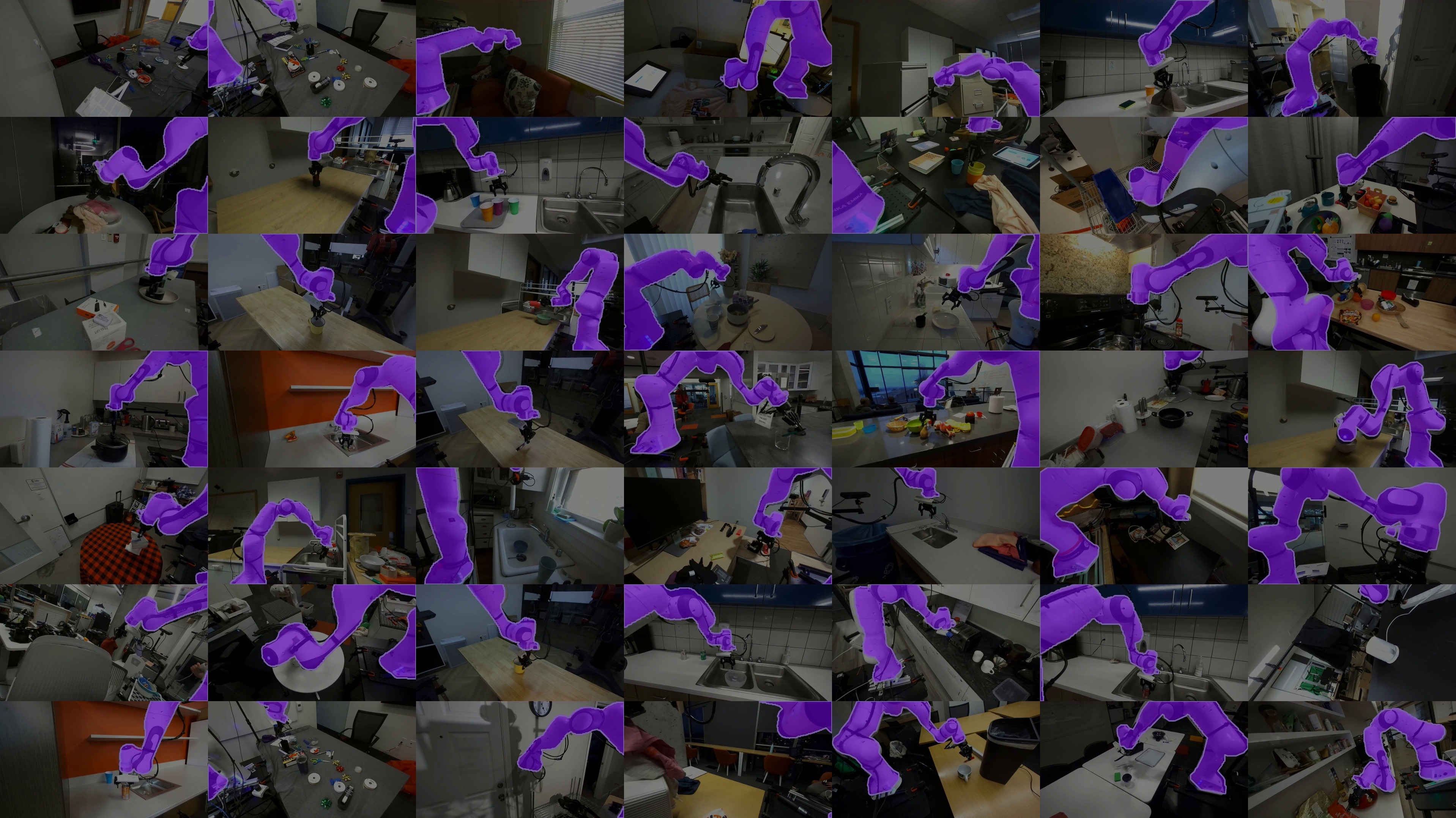
5.10.2 Sim-to-real transfer artifacts in rigid-body simulators

In a rigid-body simulator with a relaxed soft-contact solver, a scripted gripper can interpenetrate a jammed latch plate by a millimeter and slide it open without binding. A behavioral cloning policy trained on those synthetic trajectories learns to push straight through resistance that stalls the physical arm. Because synthetic data generation replaces hardware wear with numerical approximations, degradation in a simulated dataset comes from the solver’s contact model rather than from slipped camera brackets or fatigued operators. Discrete-time physics engines resolve contact constraints once per integration step, and the chosen formulation (whether strict complementarity constraints (Stewart and Trinkle 1996), convex soft-contact relaxations (Todorov et al. 2012), or penalty-based spring-damper models) sets penetration depths, slip thresholds, and drivetrain compliance. Whereas reinforcement learning agents actively exploit numerical quirks to maximize synthetic reward, behavioral cloning policies passively inherit whatever unphysical contact impulses, penetrations, or frictionless transitions the simulator produces. Co-training on simulated and physical demonstrations can nonetheless improve real-world policy success despite discrepancies between the two regimes (table 5) (Maddukuri et al. 2025). A physical ingestion pipeline cannot enforce exact contact fidelity across arbitrary geometries; its job is to preserve provenance. Every synthetic trajectory must record its simulation engine, software version, contact solver parameters, and integration time step. The scenario table also flags cells populated solely by synthetic rollouts (table 6), so downstream training and diagnostics can separate solver artifacts from hardware behavior (The sim-to-real contact exploit).

Stewart, David E., and Jeffrey C. Trinkle. 1996. “An Implicit Time-Stepping Scheme for Rigid Body Dynamics with Inelastic Collisions and Coulomb Friction.” International Journal for Numerical Methods in Engineering 39 (15): 2673–91. https://doi.org/10.1002/(SICI)1097-0207(19960815)39:15<2673::AID-NME972>3.0.CO;2-I.

Todorov, Emanuel, Tom Erez, and Yuval Tassa. 2012. “MuJoCo: A Physics Engine for Model-Based Control.” IEEE/RSJ International Conference on Intelligent Robots and Systems (IROS), 5026–33. https://doi.org/10.1109/IROS.2012.6386109.

Maddukuri, Abhiram, Zhenyu Jiang, Lawrence Yunliang Chen, Soroush Nasiriany, Yuqi Xie, Yu Fang, Wenqi Huang, et al. 2025. “Sim-and-Real Co-Training: A Simple Recipe for Vision-Based Robotic Manipulation.” Robotics: Science and Systems (RSS). https://doi.org/10.15607/RSS.2025.XXI.109.

↪ The decomposition of transfer discrepancies into dynamics, sensing, appearance, and timing channels, sized from paired command-response traces, is developed in Physical Channels of the Sim-to-Real Gap.

5.10.3 Rig-to-rig divergence across nominally identical fleets

When a worn secondary manipulator with \(0.35^\circ\) of gearbox backlash and a \(22\text{ ms}\) torque-response lag records latch demonstrations for a fleet, the human operator unconsciously adds aggressive lead compensation to overcome the deadband. Replaying or imitating those demonstrations on a newly commissioned arm with \(0.02^\circ\) of backlash drives the new arm into limit-cycle oscillations. Even among factory-identical robots of the same model number, individual units differ in gearbox wear, thermal dissipation, and motor-controller filter tunings. To keep fleet-wide pooling from mixing incompatible plants, data ingestion pipelines must bind each unit’s embodiment contract (its kinematic parameters, actuator serial numbers, controller firmware revisions, and identified dynamic models) to every recorded file. They then filter out trajectories from units that violate the target platform’s compatibility bounds.

Aggregating fleet data also exposes a second failure mode: confusing physical task failures with telemetry logging faults. A failed attempt is a complete, physically valid sequence in which the robot tried a task and missed the goal. Discarding those episodes introduces survivorship bias¹³ and strips the dataset of the boundary states, recovery paths, and negative outcomes needed to train stabilizing policies. A failed recording, by contrast, is an infrastructure fault, such as a dropped network packet, a torn image frame, or a ring-buffer overrun. Ingesting a corrupted recording without tracking gaps presents missing or uneven sample intervals as a continuous fixed-rate stream, corrupting finite-difference state derivatives. Data pipelines must therefore sort every session into one of three categories: a retained success, a retained physical failure, or an excluded logging fault tagged with diagnostic error codes. In the door-latching campaign, an episode halted by the 15 N contact tripwire is a valid physical failure and stays in the provenance archive, whereas a run in which the 6-axis force-torque sensor dropped packets is quarantined with its bus error code. Retaining a physical failure does not make its commands expert imitation targets; only stabilized, reviewed recovery segments or expert-relabeled states qualify under the intervention curation rules.

¹³ Survivorship Bias: During the Second World War, Abraham Wald of Columbia’s Statistical Research Group estimated the vulnerability of combat aircraft from the damage on the planes that came back; the planes that were hit in the most vulnerable places were the ones missing from the sample (Mangel and Samaniego 1984). A demonstration archive filtered to successes has the same hole. The attempts that reached the failure boundary are exactly the ones absent, so the archive understates how often the boundary is reached and holds no states from it.

Mangel, Marc, and Francisco J. Samaniego. 1984. “Abraham Wald’s Work on Aircraft Survivability.” Journal of the American Statistical Association 79 (386): 259–67. https://doi.org/10.1080/01621459.1984.10478038.

Even when every packet arrives intact, a fleet interface can still corrupt an archive by recording numbers in the wrong physical units or coordinate frame. Because standard schema validators check only data types and value ranges, such mismatches pass ingestion silently until a downstream consumer interprets the numbers under a different convention (war story 5.1).

War Story 5.1: Mars Climate Orbiter unit mismatch (1999)

Context: During its nine-month cruise to Mars in 1998 and 1999, the Mars Climate Orbiter fired small thrusters to desaturate its reaction wheels, and the navigation team on the ground folded the resulting velocity changes into the trajectory models used to plan each correction maneuver (Stephenson et al. 1999).

Mechanism: A ground software file (called “Small Forces” in the investigation) reported thruster impulse in pound-force-seconds (\(\text{lbf}\cdot\text{s}\)), while the trajectory models that consumed it assumed newton-seconds (\(\text{N}\cdot\text{s}\)) as the interface specification required. Because \(1\text{ lbf}\cdot\text{s} = 4.45\text{ N}\cdot\text{s}\), every desaturation event entered the models too small by a factor of \(4.45\). The values were well formed, in range, and of the expected type, so no schema check could flag them.

Impact: The accumulated error was never resolved during cruise. At orbit insertion the spacecraft passed about \(57\text{ km}\) above the surface instead of the planned \(226\text{ km}\) and was lost.

Response: The Mishap Investigation Board traced the loss to the missing unit conversion in the ground file. It recommended that the Mars Polar Lander project verify consistent units throughout design and operations and audit all data transferred between JPL and Lockheed Martin Astronautics for compliance with the interface specification, along with stronger navigation review and anomaly escalation.

Systems lesson: A number carries its meaning only together with its units and its frame. A robot dataset runs the same risk on every action tap and every calibration. A record that stores a value without the units, frame, and calibration identifier it was produced under lets a mismatched rig pass every tensor check, which is why the provenance record of section 5.11 binds each tap to them.

Stephenson, Arthur G. et al. 1999. Mars Climate Orbiter Mishap Investigation Board Phase i Report. National Aeronautics; Space Administration.

5.10.4 Operational design domain blind spots and unsafe interpolation

If the warehouse manipulator contacts the cage door during a fast 0.10 m/s approach, an unpopulated cell in its scenario table, a policy trained on the latch-recovery-02 archive can trigger the same withdraw-and-reseat motion that worked during a slow 0.03 m/s approach. The motion yanks the gripper back before impact strain has dissipated and bends the latch pin. Encountering an unobserved operational state does not make a neural controller pause; the network continues emitting commands, often replaying familiar recovery primitives in regimes where their physical preconditions fail. Each recovery primitive therefore needs its own scenario-table coverage for the physical states in which it executes, rather than a log of the failure conditions that trigger it. Collection supplies experience, and closed-loop evaluation must establish competence in the conditions where the policy is to operate. A qualified permission restriction or physical constraint must exclude regimes that remain unsupported. The 2023 Cruise pullover recounted in When the Responsibilities Fail Together is the same failure at road scale. A familiar maneuver, the pullover toward a minimal-risk condition, ran in a state no one had covered, with a pedestrian beneath the vehicle (The four rungs of the fallback ladder gives the full account).

Sensor calibrations, human operator habits, actuator wear states, and operational design domain boundaries define the physical semantics of every recorded trajectory. If data ingestion pipelines strip these physical metadata to generate flat, uniform tensors, downstream evaluations cannot determine whether an autonomous failure stems from model capacity limitations or from unmodeled distribution shifts embedded within the training corpus. The structured provenance schema of section 5.11 defines the mechanisms that preserve this physical context throughout the dataset lifecycle.

5.11 The Dataset Schema

Consider an audit of two trajectory files from the latch campaign, each holding the exact same number of state-action pairs logged at the same frequency. File A records trajectories from four authorized operators across several days, with no permission-path clamps and consistent fingertip pads throughout. File B records a single operator, logs 620 steps where safety logic clamped joint velocities, and spans an unannounced force-sensor re-zeroing midway through the session. A standard validation script checking only tensor dimensions and value ranges accepts both files without complaint. Treating them as interchangeable training data introduces silent, corrupting bugs. File B requires explicit intervention attribution and recalibration metadata before an engineer can interpret its action labels correctly. Neither file’s tensor geometry reveals which physical latch conditions the recorded data actually covers.

The dataset schema organizes the contextual evidence required to make ingestion decisions safely. It preserves the physical origin and timing of every signal, logs collection costs and dropouts, and documents which physical conditions the archive covers or omits. These fields reflect the mechanical and operational realities of the collection cell. While complete metadata cannot guarantee that a learned policy will operate successfully in closed loop, omitting it ensures that downstream pipelines will misinterpret physical signals.

The provenance record is the immutable, machine-readable artifact bound directly to a demonstration archive. It links every recorded trajectory to the specific plant, sensor calibrations, component wear state, four action taps, collection denominators, and scenario-table join (\(\OccupiedScenarioCellCount / \RequiredScenarioCellCount\)), including its count unit, eligibility and retention rule, and minimum, under which data collection occurred. Standard tensor shapes and training loss curves cannot validate a physical dataset. By recording an archive’s empirical boundaries, the provenance record allows the policy manifest (the record that training attaches to each candidate policy) and the safety case to distinguish demonstrated historical experience from the operational competence that physical testing must establish. Datasheets for datasets (Gebru et al. 2021) standardize documentation for static corpora; embodied archives additionally require tracking physical wear, permission-path interventions, and tap histories across the causal boundary. This record must travel with the trajectory data itself. Because detachable sidecar files easily separate from their payloads during format conversions, engineers serialize the record as an immutable, hashed header within the container’s root metadata, such as an MCAP top-level metadata record or a Zarr root attribute dictionary.

↪ The sixteen-record chain, in which the provenance record is the third record, is developed in The record register.

The provenance record chains Part I’s hardware records directly to Part II’s training and evaluation records. It inherits the actuator and thermal bounds from the limit record and the clock domains and jitter budgets from the handoff record, while the proposal boundary determines which entity held control at each of the four action taps. As episodes are logged, the collection runtime adds the plant identifier, calibration matrices, component wear counts, yield denominators, and scenario-table join. The runtime then hands that complete record forward to the policy manifest, so closed-loop evaluation can test the policy against the exact conditions its data covered.

↩︎ The handoff record, which extends each limit with the handoff and clock domain that locate it in the machine, is established in The Handoffs Matrix.

Every trajectory admitted into the training corpus must identify its collection source, collector policy, and execution authority. For human teleoperation, the record logs the operator identifier, the interface hardware, and transport timing characteristics, for example a 6-DoF leader arm sampled at \(100\text{ Hz}\) with \(0.8\text{ ms}\) of input jitter. Storing an operator identifier, or capturing human faces on peripheral camera streams, makes an episode a record of people as well as of the robot. The schema therefore documents the legal and institutional basis under which each person was recorded, the authorized deployment purposes, and strict retention schedules. This governance ensures that an episode collected to teach latch insertion is not repurposed to evaluate the worker who demonstrated it. When data originates from an autonomous or mixed controller, the record stores the exact policy checkpoint, the planner version, and the active enforcement configuration, including Cartesian bounding boxes, joint velocity limits, and contact-force clamping thresholds. Trajectories must also record the active retention rule, documenting whether the runtime committed an episode automatically upon task completion, retained it after explicit operator review, or flagged it for inclusion as an instructive failure recovery.

↪ Purpose limits and retention schedules for records that capture people are enforced in Recorded people as a standing condition.

A physical machine cannot be identified by a generic catalog name or model string. In real hardware, two nominally identical robot arms behave differently because of manufacturing tolerances and component aging, so the data record specifies the individual plant through its intrinsic and extrinsic sensor calibrations, embodiment contract (section 5.9.1), motor-drive firmware revisions, and component wear state. Even replaceable contact surfaces alter the governing dynamics. A parallel gripper fitted with compliant silicone pads of Shore 30A hardness (a durometer scale for rubbers, on which higher numbers are stiffer) produces vastly different friction and compliance than the same mechanism fitted with worn Shore 60A polyurethane pads under identical joint commands. Maintenance milestones such as cable retensioning, drive-belt replacements, gearbox swaps, and camera remounts therefore belong directly in the machine state record. If technicians recalibrated joint offsets between morning and afternoon collection shifts, the dataset exposes that boundary, so downstream imitation learning does not attempt to resolve two conflicting kinematic mappings into a single policy.

Collection denominators reconcile every physical attempt as a retained success, a retained failure, or an excluded recording, while exposing the wall-clock time spent resetting the scene. Alongside those yield counts, the four action taps of section 5.5.1, override flags, and exclusion codes preserve the critical distinction between demonstrated behavior and permission-path intervention. When safety logic intervenes to clamp velocity or limit contact forces, the data pipeline must attribute those adjustments correctly rather than misinterpreting supervisory interventions as expert demonstrations.

The scenario join records dataset-supported cells (configurations containing retained demonstrations) and catalogs known absences where no empirical data exists. The count-policy digest binds the count unit, eligibility and retention rule, and declared minimum; when a minimum is specified, the record distinguishes occupied cells from those meeting it. Here, dataset support reflects historical logging coverage and must not be conflated with the evaluated support of a deployed policy. For the latch campaign, the record below connects collection cost to coverage; table 6 maps its field groups to the decisions they support.

• Denominators: 52 attempts per scheduled session at a net retention rate of 0.68, so 5,000 retained successful demonstrations cost 7,353 attempts over 141.4 h of scheduled cell time.
• Retention rule: an attempt whose contact force crosses the 15 N tripwire triggers the qualified collection response and is kept as a labeled failure, outside the demonstration count, when its telemetry is valid; a recording that fails quality filtering is excluded with its exclusion code.
• Scenario table: plate offset (nominal, +3 mm, −3 mm) crossed with approach speed (0.03 m/s, 0.10 m/s), six cells, held with the count and retention policy in the record as a digest rather than as a copy.
• supported_cells: the nominal plate at 0.03 m/s, the only cell the original retained demonstrations occupy.
• known_absences: the other five cells, every displaced plate and every approach at 0.10 m/s.

Table 6: Demonstration dataset provenance schema: Evidence retained and the admission check applied to each field group of the provenance record; the embodiment, sensor calibration, and contact wear groups bind the individual plant that collected the data.

Provenance record	Evidence retained	Admission decision
Session	Collector, operator, policy version, source type (physical, robot-free, or synthetic with generator and engine versions), collection mode (nominal, noise-injected, or gated intervention), sample rate, and timing jitter.	Check operator authorization and the session jitter budget.
Embodiment	Robot identity, geometry, gearing, backlash, firmware, and the redundancy parameter (elbow swivel angle or full joint vector).	Check reach, dynamics, and joint limits on the target plant.
Sensor calibration	Camera geometry, clock synchronization, and force/torque bias.	Check calibration age and timebase error.
Contact wear	End-effector material, hardness, friction, flex cycles, and maintenance history.	Revalidate contact data after material or compliance changes.
Four action taps	Requested, mapped, enforced, and measured values, each with its units and frame, plus override and clamp codes.	Compare aligned values; attribute modified commands before choosing labels.
Transition timing	Times of exposure midpoint, action issue, mapping, enforcement, response start, and response end, with clock IDs and synchronization errors.	Check causal order and the declared response window.
Collection denominators	Scheduled cell time, motion time, attempts, retained successes and failures, excluded recordings, and task configurations.	Reconcile attempts against retained and excluded episodes.
Scenario support	Scenario-table and count-policy digest (unit, eligibility, retention, minimum), occupied cells, cells meeting any declared minimum, synthetic-only cells, and known absences.	Identify collection gaps; require separate evidence for deployment claims.
Consent and retention	People recorded (operator and any bystander in view), the consent or other basis for recording each, the declared purposes, the retention period, and who may read the record.	Admit an episode only for a purpose its basis covers; delete or de-identify it when retention ends.

The policy manifest of The Policy Manifest cites each contributing archive by digest, including latch-recovery-02 in the stipulated follow-up branch. The original record continues to describe the original campaign; new experience receives new provenance rather than rewriting old absences. Operator and override history also informs supervisory evaluation, while coverage and calibration evidence contributes to the release argument. Binding the metadata to the trajectory container helps preserve these relationships through ingestion, but cryptographic hashes do not automatically prevent misuse. Data loaders and ingestion pipelines must verify that trajectory arrays remain bound to their declared schema and calibration headers before training begins, because skipping any part of that check leads to the recurring collection failures cataloged next (section 5.12).

↪ The release manifest, which binds this provenance record and its operating-domain coverage into the release argument, is developed in The Release Manifest.

5.12 Fallacies and Pitfalls

In pure software systems, data collection can often treat storage growth as an unvarnished positive, since more web pages, text tokens, or labeled images generally broaden coverage. In physical artificial intelligence, however, datasets are tightly coupled to the mechanical dynamics, calibration state, and physical limits of the collection hardware. A dataset that passes every structural schema check, with zero dropped packets and consistent tensor dimensions, can still leave a deployed machine entirely blind to critical operational states. The operational distribution of physical data reflects three intertwined factors: the collecting policy (whether driven by human teleoperation or automated planning), the physical capabilities and wear of the collection rig, and the curation filters applied before admission to the archive. Neglecting these physical constraints leads to predictable engineering fallacies and costly operational pitfalls.

Fallacy: Massive sample volume compensates for lack of operational state-space coverage.

Suppose a surface-tracking policy must operate reliably across 500 distinct combinations of normal force, surface friction, and contact angle, but the archive covers only 45. Logging another collection run that adds \(72{,}000\) control steps by repeating nominal trajectories through those same 45 states inflates the database, but it leaves physical coverage unchanged. High-frequency sampling in familiar regions merely records the same dynamic trajectory more densely, adding zero evidence about the unvisited friction regimes or steep contact angles. Ingestion pipelines that report growing data volume and zero dropped packets can create a false sense of security while leaving downstream policies brittle. A collection campaign earns its cost by addressing a declared coverage, label-quality, or evidence deficit. A populated cell may still need more or better demonstrations, while nominal repetition alone supplies no evidence about unvisited regimes.

Architect’s countermeasure: Gate dataset admission on a support envelope relational join against an explicit scenario table, rather than step counts or raw byte volume. Require that new data collection campaigns specify which coverage, label-quality, or evidence deficit they target, and track scenario coverage (\(\OccupiedScenarioCellCount / \RequiredScenarioCellCount\)) as a primary engineering KPI alongside validation loss.

Pitfall: Assuming physical demonstration labels survive mechanical or contact hardware maintenance.

Archived demonstrations do not retain physical validity when the underlying hardware changes, even if array shapes and data schemas remain identical. Consider what happens when a technician replaces a parallel gripper’s compliant fingertips with stiffer pads and re-torques an adjacent camera bracket. The historical dataset still passes every automated pipeline check: sensor channels, array dimensions, and datatypes match expected specifications. If the camera bracket shifts, a known transformation matrix allows mathematical reprojection of visual coordinates. Contact mechanics, however, cannot be reprojected geometrically. The stiffer pads alter normal compliance and contact friction, causing grasp slip at substantially lower shear thresholds than the compliant material tolerated. Telemetry recorded before the swap captures the physical behavior of an obsolete body; training a closed-loop force controller on those historical tactile profiles will cause grasping failures on the modified hardware. Data provenance must track the full mechanical and calibration state of the collection rig so that any hardware alteration immediately triggers targeted review and recollected baselines.

Architect’s countermeasure: Bind every trajectory file to an immutable hardware state hash that captures camera extrinsics, motor serial numbers, and contact surface material specifications. When maintenance events alter contact stiffness or camera mountings, invalidate historical tactile and force labels for that cell until an automated revalidation protocol verifies dynamic equivalence.

Pitfall: Filtering out aborted safety interventions to sanitize the demonstration dataset.

Purging aborted demonstrations to produce a flawless training set introduces severe survivorship bias into physical policies. Consider an automated peg-insertion pipeline spanning 1,000 recorded attempts. Of these, 180 runs triggered a safety cutoff when contact forces reached or exceeded a \(15.0\text{ N}\) trip threshold, leaving 820 nominal runs that succeeded with an 82 percent yield. A curation script discards the 180 aborted and recovery episodes, preserving only the smooth runs where forces stayed comfortably below \(8.0\text{ N}\). When deployed in production, minor surface misalignment inevitably pushes an insertion force to \(9.5\text{ N}\). Although this force remains below the \(15.0\text{ N}\) trip threshold, the policy encounters a state outside its training support. Because the sanitization script erased every observation between nominal tracking and failure, the archive supplies no supervision for these near-boundary dynamics, so recovery behavior remains unsupported. Pruning near-boundary and intervention data strips away the exact state-action pairs the policy needs to regain stability after a disturbance.

Architect’s countermeasure: Implement three-way intervention curation at data ingestion. Quarantine learner commands between divergence (\(\DivergenceInstant\)) and takeover (\(\TakeoverInstant\)) for safety auditing only. Preserve the visited boundary states for expert relabeling via corrective aggregation (DAgger). Admit the subsequent human recovery as an expert sequence only after the operator’s measured stabilization (\(\OperatorStabilizationInstant\)), masking the blend and reorientation that precede it.

Pitfall: Merging demonstrations collected across kinematically asymmetric leader interfaces.

Merging trajectories across disparate teleoperation input interfaces can quietly bake kinematic dead zones into the dataset. Suppose two operators collect snap-fit assembly demonstrations using different leader devices to puppet identical follower arms. The first leader mechanism features detented wrist mechanics that restrict roll to two discrete positions (\(\LeaderWristRollAngle \in \{0.0^\circ, 90.0^\circ\}\)). The second leader uses a continuous gimbal that mechanically limits roll travel to \([-15.0^\circ, +15.0^\circ]\). Merging the two collections yields 4,000 episodes and increases overall sample volume, but neither interface can express orientations between \(20.0^\circ\) and \(70.0^\circ\). Even though the follower arm can navigate that full range, the combined archive contains zero training targets within this \(50.0^\circ\) gap. Pooling data from different input devices cannot fill gaps that neither device can mechanically traverse. Downstream imitation policies trained on the combined dataset will fail whenever initial conditions or part tolerances demand intermediate orientations.

Architect’s countermeasure: Apply the cross-embodiment compatibility contract to the leader interface itself, checking before recording that the leader and follower share the required reachable poses, joint motion ranges, and ability to move in the required directions. Enforce continuous orientation coverage checks across task-space degrees of freedom during data QA to detect mechanical dead-zones.

Fallacy: Physical data collection scales linearly with labor hours just like internet scraping scales with compute.

Treating physical data collection as an easily parallelized, linear process like web scraping ignores the mechanical entropy and human fatigue inherent to physical experimentation. Teams often extrapolate campaign timelines from early pilot runs, for example by projecting that an initial pace of 50 successful episodes per operator-hour will scale linearly across weeks of shifts. In reality, continuous operation degrades both hardware and teleoperator consistency. Repetitive contact impacts cause backlash and tooth wear in strain-wave gearboxes, thermal expansion and sensor drift cause uncalibrated joint encoders to drift away from physical ground truth, and human fatigue introduces latency spikes and jerky trajectories. As wear accumulates, the proportion of episodes passing quality filtering steadily drops, even while scheduled labor hours remain constant. Pilot runs conducted on pristine hardware systematically overstate long-term collection yield. Campaign planning must budget for routine recalibration, mechanical maintenance, ergonomic rests, and discarded runs alongside raw operator hours.

Architect’s countermeasure: Budget collection campaigns in net validated demonstration yield (\(\UsableDemonstrationYield = \lfloor \ActiveMotionDuration / \AttemptCycleDuration \rfloor \cdot \DemonstrationRetentionRate\)) and component fatigue cycles (\(\RatedFatigueLife\) ratings for strain-wave gears and internal flex harnesses), rather than gross scheduled operator hours. Estimate the overhead multiplier from the campaign’s calibration, reset, retention, and rest assumptions; validate it against sustained collection yield.

5.13 Summary

A physical machine manufactures its own training data, so every record carries the loop that produced it: the operator’s request, the permission path’s admission, and the body’s response, all under the machine’s current calibration and wear. Collecting that data is costly in a way scraping is not. In the latch campaign, only 24.6 percent of each scheduled hour survives as retained demonstration motion once startup, calibration, operator rest, resets, failed attempts, and quality filtering are paid for, and the wrist’s flex cable consumes the larger fraction of its assumed fatigue rating. Because every attempt spends cell time and component life whether or not it is kept, and because correlated control steps hold few independent samples, a campaign earns its cost by addressing a declared coverage, label-quality, or evidence deficit, including inadequate evidence within a populated cell.

Which states the archive holds is a question the archive cannot answer about itself. Coverage is a join between empirical occupancy and a scenario table derived from the declared operational design domain, and against the table the door actually demands, the baseline latch archive fills one cell of six. Inside even a populated cell, a cloned policy’s first error carries it off the demonstrated corridor into states where nothing in the archive constrains its output, which is why behavioral cloning’s worst-case cost grows with the square of the horizon. Interventions supply the missing learner-visited states, but only after curation at the divergence, takeover, and stabilization timestamps separates the learner’s commands from the expert’s recovery. Aggregating expert labels on those states makes the worst-case cost linear in the horizon only while the recoverability constant stays bounded; where a mistake cannot be undone, the state belongs to the permission path, not to the dataset.

A label is only as meaningful as the tap, clock, and plant behind it. Imitating the request teaches commands the permission path would have clamped, imitating the measured response teaches compliance and backlash as intent, and pairing either with a misdated frame converts timing error into position error at the speed of the motion. Range normalization cannot carry a label to another embodiment, and a bumped camera bracket or worn pad silently changes what a stored tuple means. The provenance record binds each archive to its taps, timestamps, plant, calibration, collection denominators, and known absences, so that training and evaluation can tell demonstrated experience from evaluated competence. Table 7 summarizes the load-bearing equations introduced throughout this chapter, detailing the physical boundaries each expression defines, the architectural decisions it governs, and its formal derivation.

Table 7: Key equations of physical data: Each load-bearing equation of the chapter, the limit it bounds or the decision it settles, and the equation where it is derived.

Equation	What it bounds or decides	Derived in
\(\ExpectedTaskCostSum(\pi)-\ExpectedTaskCostSum(\pi^*) \le \BehaviorCloningHorizon^2\SingleStepImitationError\)	The worst-case excess cost of cloning on expert states under a 0–1 action loss; the bound becomes uninformative once \(\SingleStepImitationError > 1/\BehaviorCloningHorizon\)	equation 1
\(\ExpectedTaskCostSum(\AggregationLearnedPolicy) \le \ExpectedTaskCostSum(\pi^*) + \DeviationDisadvantage\,\BehaviorCloningHorizon\,\AggregatedSurrogateLoss + \mathcal{O}(1)\)	The cost after aggregating expert labels on learner-visited states, linear in \(\BehaviorCloningHorizon\) only while the recoverability constant \(\DeviationDisadvantage\) stays bounded	equation 8
\(\EffectiveSampleSize = \RawRecordCount(1-\SerialAutocorrelation)/(1+\SerialAutocorrelation)\)	The effective number of independent observations contained in a serially correlated telemetry stream for a single statistic	equation 2
\(\SyncPairingDisplacement \approx \Velocity\,\ObservationPairingLag\)	The spatial error introduced by inter-sensor pairing latency, defining the maximum allowable delay for a specified task clearance	equation 3
\(\RollingShutterFrameSkew = (\ImageHeight - 1)\,\RollingShutterRowReadout\)	The temporal skew across a rolling-shutter frame, which end-effector motion translates into geometric image distortion	equation 4
\(\TeleoperationRoundTripLatency = \DisplayPipelineLatency + \OperatorResponseLatency + \TeleoperationCommandLatency + \FollowerMechanicalLatency\)	The round-trip phase lag in teleoperation between an observed state and the physical execution of the human correction	equation 5
\(\UsableDemonstrationYield = \lfloor \ActiveMotionDuration/\AttemptCycleDuration \rfloor \DemonstrationRetentionRate\)	The yield of usable demonstrations per scheduled session, determining the cell time and mechanical wear required for a campaign target	equation 6
\(\EstimatedDivergenceInstant\): first threshold crossing, when captured, in \([\TakeoverInstant - \PreTriggerWindowDuration,\, \TakeoverInstant]\)	The estimated onset of trajectory drift before human takeover, determining whether the lookback window captures the causal error	equation 7
\(\ReprojectionResidual = \lVert \ObservedPixelCoordinates - \operatorname{proj}_{\CameraIntrinsicCalibrationMatrix}(\BaseToCameraTransform\,\ForwardKinematicsMap(\GeneralizedCoordinates)) \rVert_2\)	The extrinsic reprojection residual used to verify that camera calibration remains aligned with kinematic joint encoders	equation 9

Key Takeaways: Physical data collection and provenance

• Coverage measures distinct physical configurations rather than sample volume: Repeated nominal trajectories add millions of telemetry rows without expanding scenario coverage. Adjacent control steps are so strongly autocorrelated that an hour of permission-tick records holds only about 1,800 independent samples for a slowly varying statistic, and even independent samples support only the cells where they land. An engineering team must measure dataset completeness by joining logged trajectories against an explicit scenario table that spans the operational design domain, rather than relying on raw row counts or the archive’s own observed extremes.
• Offline validation loss cannot detect coverage deficits: Because conventional train-validation splits sample from the same underlying trajectory distribution, a policy can achieve near-zero validation loss while leaving critical operational cells unvisited. Only auditing the dataset against an independent scenario table reveals these silent omissions before deployment.
• Every action tap represents a distinct physical control signal: An operator’s commanded request, the resolved kinematic setpoint, the safety-filtered actuator command, and the measured joint response diverge whenever hardware limiters, friction, or permission guards intervene. Logging each tap alongside synchronized timestamps ensures the supervisory target remains causal and preserves unambiguous evidence of physical interventions.
• Preserve aborted runs and interventions with rigorous causal attribution: Discarding failed attempts discards the most valuable boundary-adjacent states in the operational envelope. Autonomous commands preceding a human takeover must be archived for fault analysis and counterfactual relabeling rather than misattributed as expert demonstrations, while the subsequent corrective maneuver should be reviewed, trimmed, and stored as an explicit recovery trajectory.
• Physical telemetry remains bound to specific hardware embodiments: While optical perspectives can be reprojected across camera geometries, dynamic properties such as joint friction, structural compliance, and gearbox backlash are embedded directly into recorded force and torque signals. Simple range normalization masks these physical discrepancies without resolving them, requiring thorough re-calibration and verification whenever data is transferred across hardware platforms.
• Targeted recovery data broadens operational competence under new provenance: An immutable dataset records the boundary conditions of a specific collection campaign, but engineers can systematically expand policy capabilities by appending verified recovery sequences under separate provenance tags. Asserting an expanded operational claim, however, requires end-to-end closed-loop validation on the physical machine under those target conditions.

Each latch archive in this chapter ended the same way, with a short list of supported cells and a longer list of known absences. That ratio is not a defect of one campaign. It is what the second law, endogenous data (principle 2), costs in practice. A machine whose actions choose its next states can only record the states its collecting policy chose, and every additional state it records is paid for in cell time and component life. The known absences in the provenance record are the price list. They say which experience the machine never bought, and therefore which claims no amount of training on this archive can support.

Read that way, the engineering question shifts from how much data a campaign collected to which absences it retired and what each one cost. The displaced-plate cell that latch-recovery-02 fills moves from the absence list to the supported list under new provenance. The faster approach, which no one collected, stays on the list, and the permission path must keep refusing it until evidence arrives.

5.14 Historical Perspective and Further Reading

Demonstration in robotics began not as data collection for machine learning, but as teleoperation for hazardous environments. At Argonne National Laboratory, Raymond Goertz developed mechanically coupled master-slave manipulators to handle radioactive materials behind heavy shielding (Goertz 1949). These early systems linked the operator’s handle directly to remote mechanical tongs through cables and counterweights; because the transmission was entirely mechanical, contact forces against objects reflected instantly and passively back to the operator’s hand.

The systems challenge shifted radically when electrical servos and digital communication networks replaced mechanical linkages. Introducing transmission latency into the bilateral loop between the operator interface and the actuated follower can inject artificial energy into the feedback channel, quickly driving the coupled system into violent instability. Anderson and Spong (1989) proved that even small transmission delays can destabilize a bilateral teleoperator and established a framework that preserves delayed-channel passivity under its constant-delay model. Stability of the complete loop also depends on the connected systems and their interconnection conditions. Niemeyer and Slotine (1991) reformulated this remedy through wave variables, transforming power variables (force and velocity) into traveling wave representations that behave as passive transmission lines under the constant-delay model. In their comprehensive survey, Hokayem and Spong (2006) trace the progression from Goertz’s early linkages to modern delay-robust control schemes. Every teleoperation data-collection interface operates under the compromise these works describe, balancing faithful haptic transparency against the conditions needed to preserve passivity. The physical trajectories, contact transitions, and actuation commands captured in an embodied training archive inherently reflect the compromises of the collection hardware.

Synthesizing feedback controllers directly from recorded demonstrations followed an equally grounded trajectory. In one of the earliest end-to-end vision-based driving systems, ALVINN mapped camera frames to steering angles for an autonomous van (Pomerleau 1989, 1991). ALVINN immediately ran into the recovery gap. Because expert drivers kept the van centered within the lane, the recorded dataset contained virtually no examples of drifting off course or recovering from road shoulders. Pomerleau resolved this issue through an early form of data augmentation, synthetically warping camera images and computing the corresponding corrective steering angles to teach the network how to return to the road center.

Ross, Stéphane, and J. Andrew Bagnell. 2010. “Efficient Reductions for Imitation Learning.” Proceedings of the Thirteenth International Conference on Artificial Intelligence and Statistics (AISTATS) 9: 661–68.

Kelly, Michael, Chelsea Sidrane, Katherine Driggs-Campbell, and Mykel J. Kochenderfer. 2019. “HG-DAgger: Interactive Imitation Learning with Human Experts.” IEEE International Conference on Robotics and Automation (ICRA), 8077–83. https://doi.org/10.1109/ICRA.2019.8793698.

Laskey, Michael, Jonathan Lee, Roy Fox, Anca Dragan, and Ken Goldberg. 2017. “DART: Noise Injection for Robust Imitation Learning.” Proceedings of the Conference on Robot Learning (CoRL), Proceedings of machine learning research, vol. 78: 143–56.

As the field matured, Argall et al. (2009) unified robot learning from demonstration into a comprehensive framework, formalizing how data collection methods shape policy representations and analyzing the kinematic correspondence problem between the demonstrator and the physical robot. The theoretical mechanics of compounding execution errors were established by Ross and Bagnell (2010), who proved that naive behavioral cloning yields an error bound that grows quadratically with the task horizon (\(\CovariateDriftBound\)) under covariate shift. To escape this quadratic penalty, Ross et al. (2011) introduced Dataset Aggregation (DAgger), demonstrating that rolling out the learner while querying the expert along the induced state distribution achieves an optimal linear bound (\(\mathcal{O}(\BehaviorCloningHorizon\SingleStepImitationError)\)), provided the environment satisfies a finite recoverability condition. Practical robotics deployments adapted this theoretical machinery to human supervisors who cannot label millions of counterfactual query states. Human-gated DAgger (Kelly et al. 2019) transferred control to a human expert only during critical trajectory deviations, while DART (Laskey et al. 2017) injected continuous stochastic noise into the actuators during teleoperation to force human demonstrators to execute recovery maneuvers naturally. The empirical intervention strategies and recovery curation workflows in section 5.8 trace directly to these foundational methods.

The accounting of state-space coverage and sampling validity borrows from older statistical and control foundations. Bellman (1957) named the curse of dimensionality to describe the exponential explosion of discrete state spaces in dynamic programming. In environmental time series, climatologists demonstrated that serially correlated records dramatically reduce the effective degrees of freedom, requiring explicit adjustments to compute true sample sizes (Thiébaux and Zwiers 1984). Simultaneously, Abraham Wald’s wartime analysis of returning aircraft showed that evaluating only surviving samples systematically blinds the observer to critical failure modes (Mangel and Samaniego 1984).

Walke, Homer Rich, Kevin Black, Tony Z. Zhao, Quan Vuong, Chongyi Zheng, Philippe Hansen-Estruch, Andre Wang He, et al. 2023. “BridgeData V2: A Dataset for Robot Learning at Scale.” Proceedings of the 7th Conference on Robot Learning (CoRL), Proceedings of machine learning research, vol. 229: 1723–36.

Khazatsky, Alexander, Karl Pertsch, Suraj Nair, Ashwin Balakrishna, Sudeep Dasari, Siddharth Karamcheti, Soroush Nasiriany, et al. 2024. “DROID: A Large-Scale in-the-Wild Robot Manipulation Dataset.” Robotics: Science and Systems (RSS). https://doi.org/10.15607/RSS.2024.XX.120.

Robot learning confronted all three phenomena as datasets evolved from isolated laboratory demonstrations into massive multi-robot corpora (Walke et al. 2023; Khazatsky et al. 2024; Open X-Embodiment Collaboration et al. 2024). While cross-institution pooling supplies visual and environmental variations that no single robotic cell can generate, it also pools mismatched actuator dynamics, unmodeled camera latencies, and latent operator selection biases. Standardizing such corpora requires both an explicit compatibility contract across kinematics and a rigorous accounting of unobserved conditions. Although dataset documentation frameworks (Gebru et al. 2021) originally addressed provenance and social biases in digital corpora, physical robotics demands tracking hardware-level ground truths. The physical dataset schema and provenance architecture detailed in section 5.11 extend these documentation principles to capture actuator tap points, calibration matrices, dynamic delays, and known boundary omissions.

The following readings chart the progression from classical bilateral teleoperation to modern pooled robot corpora:

• Hokayem and Spong (2006) provides an exhaustive survey of bilateral teleoperation control, charting the historical transition from mechanically coupled manipulators to passivity-based and wave-variable architectures. It explains the core control-theoretic tension between transparent force reflection and robust stability when non-negligible communication delays separate the operator from the robot.
• Pomerleau (1991) presents a compact, highly practical diagnosis of the recovery gap and compounding errors in end-to-end behavioral cloning. The paper details how synthetic visual transformations of road images generated corrective training labels, demonstrating the necessity of off-trajectory recovery data decades before formal distribution-shift theory was codified.
• Argall et al. (2009) synthesizes robot learning from demonstration into a foundational taxonomy based on demonstration collection mechanisms and policy derivation techniques. It highlights the correspondence problem across differing human and robotic kinematic structures, which section 5.9 formalizes as a strict cross-embodiment mapping contract.
• Ross et al. (2011) introduces the Dataset Aggregation (DAgger) algorithm and establishes the formal reduction of imitation learning to online convex optimization. It proves that querying an expert along the learner’s visited trajectory distribution converts the quadratic error growth of behavioral cloning into a linear bound, defining the critical recoverability constant presented in equation 8.
• Open X-Embodiment Collaboration et al. (2024) documents the Open X-Embodiment initiative, pooling over one million trajectories across dozens of robot platforms and institutions. The paper is essential reading for systems engineers, illustrating both the positive transfer enabled by scale and the severe architectural challenges of normalizing disparate action spaces, sampling rates, and sensor configurations.
• Gebru et al. (2021) establishes the foundational methodology for documenting dataset motivation, composition, collection workflows, and intended use. Contrasting this general framework with table 6 clarifies the specialized physical, electrical, and dynamical metadata required to safely train and deploy embodied controllers.

Argall, Brenna D., Sonia Chernova, Manuela Veloso, and Brett Browning. 2009. “A Survey of Robot Learning from Demonstration.” Robotics and Autonomous Systems 57 (5): 469–83. https://doi.org/10.1016/j.robot.2008.10.024.

Open X-Embodiment Collaboration, Abby O’Neill, Abdul Rehman, Abhinav Gupta, Abhiram Maddukuri, Abhishek Gupta, et al. 2024. “Open X-Embodiment: Robotic Learning Datasets and RT-X Models.” IEEE International Conference on Robotics and Automation (ICRA), 6892–903. https://doi.org/10.1109/ICRA57147.2024.10611477.

Gebru, Timnit, Jamie Morgenstern, Briana Vecchione, Jennifer Wortman Vaughan, Hanna Wallach, Hal Daumé III, and Kate Crawford. 2021. “Datasheets for Datasets.” Communications of the ACM 64 (12): 86–92. https://doi.org/10.1145/3458723.

What’s Next: From demonstrations to policies

A policy trained on an archive whose provenance record lists more absences than supported cells learns strictly from those supported cells; its training score gives no sign of where the absences begin. The baseline latch archive covers only the nominal strike plate at the guarded approach. Policy Training opens with two candidates built on it: latch-bc-01, cloned from those demonstrations, and latch-sim-02, distilled from a simulator teacher that learned the fast approach no one collected on the machine. Each improves in training while hiding a dependency the hardware will expose. That chapter then carries the curated latch-recovery-02 archive into a recovery candidate and writes each candidate’s evidence into a policy manifest whose declared operating domain cannot exceed the cells its provenance supports. Closed-Loop Evaluation then tests whether that declared domain holds on the machine.