The Physical Body

2 The Physical Body

Lecture slides for this chapter

Purpose

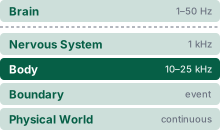
Physical AI stack focus for this chapter.

Why can a correctly chosen action still demand more than the machine’s body can deliver?

A mobile manipulator can recognize an obstacle correctly and still strike it if its body cannot stop within the remaining distance. The same machine can hold a payload without moving while its motor windings overheat, or lose its controller when a sudden demand for current pulls the supply voltage too low. These failures arise from limits that prediction accuracy alone cannot reveal. Physical AI engineering requires connecting a proposed action to the motion, heat, and electrical demand it creates, then establishing which limit the assembled machine reaches first. Measurements must also establish the conditions under which those limits hold, because a change in payload, floor surface, cooling, or battery state changes what the machine can deliver. The body’s limits therefore govern what the permission path may admit before a command crosses the causal boundary and produces irreversible physical work.

Learning Objectives

• Calculate observation freshness limits from measurement age and the machine’s allowable motion
• Calculate stopping distance and the admissible speed ceiling from pre-brake delay, credible deceleration, and clearance overheads
• Evaluate actuator and transmission choices against response limits, reflected inertia, and mechanical impedance
• Estimate sustainable motor duty cycles from heat generation, cooling, and operating conditions
• Budget electrical supply margins for simultaneous actuation, computation, and regenerative braking
• Specify the elements of a limit record that states a measured limit’s conditions, uncertainty, margin, runtime detector, and evidence category
• Evaluate maneuver-specific binding budgets from qualified evidence and justify holding up the permission supply through covered faults

Explore the concepts in this chapter

The volume’s concept map, opened on this chapter. Select a concept to read how it connects to ideas in other chapters. Open the full map ↗

2.1 The Five Physical Budgets

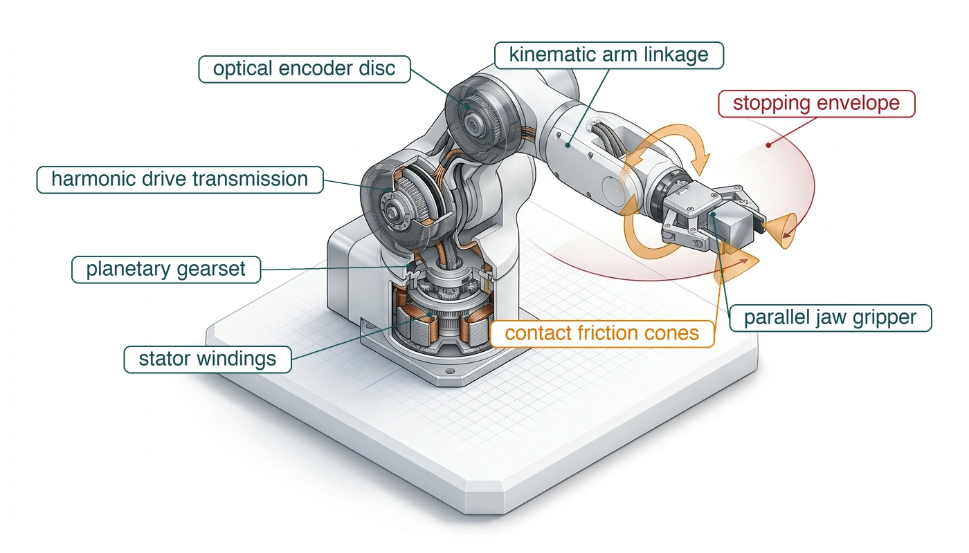
Every action a learned model proposes ultimately manifests as electrical current flowing through a motor winding, and from that instant physics governs execution. Machine learning practice rarely contends with this transition. Policies trained in simulation typically interact with idealized plants where commanded torque appears instantaneously, heat never accumulates in windings, and direct current (DC) bus voltages never sag under load. A physical machine honors none of these simplifications. The physical body is the coupled assembly of actuators, mechanical transmissions, structural linkages, power electronics, and sensors that translates digital commands into mechanical motion. Its physical dynamics bound what even a mathematically optimal policy can achieve. An emergency brake command requires finite time to develop mechanical retarding force and clearance distance to dissipate kinetic energy. Similarly, commanding a manipulator to hold a heavy payload motionless draws continuous phase current, dissipating resistive heat into the stator even though the joint does zero mechanical work.

The proposal boundary in The Machine in Five Levels assigns the permission path responsibility for admitting action, and the body provides the concrete physical envelopes that make that gating decision meaningful. Before committing a command to hardware registers, the permission path must evaluate five physical budgets. It must confirm that the sensor observation remains fresh, that the moving machine can stop within available clearance, that the actuator can deliver the required torque trajectory, that the winding can tolerate the resulting thermal rise, and that the electrical bus can support the transient current demand. These mechanisms form a direct causal chain. Sensor and pipeline latencies consume allowable stopping distance. Arresting momentum demands delivered actuator torque. Generating that torque dissipates heat in motor coils and pulls current from a shared power rail. For any given maneuver, the governing systems question is which of these physical budgets binds first, under what operational stress, and on what empirical evidence.

1. Measurement freshness (\(\ObservationAge\)): The observation must remain valid until the mechanical plant responds. Latency accumulated across sensor exposure, data transport, neural inference, and low-level drive dispatch consumes allowable tracking margins as the physical world continues to move.
2. Kinetic momentum (\(\KineticEnergy, \LinearMomentum\)): A moving machine carries kinetic energy (\(\KineticEnergy = \frac{1}{2} \Mass \BodySpeed^2\)) and linear or angular momentum (\(\LinearMomentum = \Mass \BodySpeed\)). Bringing the plant to rest demands applying retarding force over finite distance and time; safe operating velocity must therefore preserve a stopping envelope well within available physical clearance.
3. Actuator bandwidth and reflected inertia (\(\GearReductionRatio^2 \RotorInertia\)): Winding inductance and supply voltage limit the rate at which torque can change. A gearhead with reduction ratio \(\GearReductionRatio\) multiplies delivered torque by \(\GearReductionRatio\), but it also scales the motor rotor’s inertia \(\RotorInertia\) by \(\GearReductionRatio^2\) as seen at the joint output (section 2.4.3), which constrains instantaneous acceleration.
4. Thermal capacity (\(\EstimatedWindingTemperature\)): Resistive losses (\(\WindingLossPower = \TorqueProducingCurrent^2 \EffectiveLossResistance\), with \(\EffectiveLossResistance\) the winding’s effective loss resistance) deposit thermal energy directly into the stator windings and inverter switching stages. Heat dissipation limits sustained continuous torque, while the thermal mass of the coils constrains the magnitude, duration, and repetition rate of transient torque bursts.
5. Electrical power integrity (\(\DcRailVoltage\)): Onboard compute clusters and motor inverters draw from a shared DC power rail. Peak motor accelerations must not drag the bus voltage below digital logic thresholds, while regenerative braking must provide an electrical sink so returned kinetic energy does not overvoltage the bus.

Under the simultaneous admission invariant, motion permission requires a non-negative margin in every budget before the permission path commits torque to hardware registers. Each margin must be checked in its own units; time, distance, torque, temperature, and voltage are separate constraints, not interchangeable quantities: \[\begin{aligned} \ObservationAge &\le \TelemetryFreshnessBound, \\ \StoppingDistance &\le \ClearDistance, \\ |\CommandedJointTorque| &\le \OutputTorqueCeiling, \\ \EstimatedWindingTemperature &\le \WindingTemperatureLimit, \\ \MinimumRailVoltage &\ge \ConverterLockoutVoltage. \end{aligned}\] Here \(\CommandedJointTorque\) is requested torque and \(\OutputTorqueCeiling\) is the maximum deliverable output torque under current electrical and thermal conditions. The estimated winding temperature \(\EstimatedWindingTemperature\) must remain below its limit, while the lowest rail voltage \(\MinimumRailVoltage\) must remain above the undervoltage-lockout threshold \(\ConverterLockoutVoltage\) at which the supply regulator shuts down. The fifth line checks only undervoltage. Permission must also require regenerative braking to stay below the qualified upper operating-voltage limit of the supplied components, with an available absorption or dissipation path. Two lines state their budgets in derived form. The kinetic budget appears as the stopping distance it demands, \(\StoppingDistance \le \ClearDistance\). The actuator line checks only torque magnitude, because the slew-rate limit that winding inductance and reflected inertia impose enters the stopping line instead, through the brake-onset term of the pre-brake delay \(\PrebrakeDelay\). All five inequalities must hold simultaneously. A surplus in four budgets cannot compensate for a deficit in the fifth. A fresh observation cannot prevent a stop from overrunning if kinetic energy exceeds available clearance, and abundant battery energy cannot prevent an actuator from burning out if thermal dissipation limits are violated.

Systems Perspective 2.1: Why physical limits bound physical AI architecture

The permission path requires concrete bounds on physical behavior, not abstract software promises. Accepting a torque command does not guarantee that the inverter can deliver the requested current against the back electromotive force (back-EMF) the spinning motor induces in its own windings, nor does cutting motor power guarantee that friction will arrest the plant before it breaches a clearance zone. The five physical budgets bridge this gap, tying software proposals to verifiable, empirical responses under declared operating conditions.

The warehouse mobile manipulator that this book follows draws on all five. Loaded to at most 368 kg and moving at its 1.5 m/s drive limit (illustrative; see the Reader Guide), it carries 414 J of kinetic energy through aisles it shares with people. Each budget establishes an empirical operating boundary on the assembled machine under declared thermal and electrical stress. Each ends the chapter as a limit record, the six-element record that The Architecture of This Book sketched from the stopping notebook: a value, the conditions under which it holds, its uncertainty, the margin defended, a runtime detector, and the provenance of its evidence. The first budget is the age of the measurement on which every command rests, which runs from physical transduction, well before any software process receives the raw sensor data.

2.2 Measurement Freshness

Software benchmarks in machine learning frequently report latency as isolated accelerator execution time, for example 18.5 ms for the vision backbone of the arm’s wrist-camera grasp path on an edge neural processing unit (NPU), a different pipeline from the navigation backbone that the stopping budget of Delay consumes stopping clearance charges. This narrow focus fosters the illusion of an agile 54.1 Hz control loop. In physical AI systems, however, that compute kernel represents only one intermediate segment in an end-to-end silicon-to-plant dataflow pipeline. A sensor measurement begins decaying the moment physical transduction occurs; what governs physical performance is its total age when torque actually appears at the actuator joint. That physical age spans the entire interval from the moment photons strike a photodiode array, magnetic flux sweeps past a Hall sensor, or strain deflects a piezoresistor to the moment motor inverter switches build stator magnetic flux that alters link acceleration. If a perception policy evaluates an obstacle bounding box in 18.5 ms, while exposure integration, sensor readout, Peripheral Component Interconnect Express (PCIe) transport, kernel scheduling, fieldbus dispatch, and motor current rise consume an additional 16.5 ms at the median, the true physical age of the observation when the joint accelerates is 35 ms. The distribution tail extends farther still.

Throughout that capture-to-onset window, the physical environment continues to evolve unobserved. In distributed data systems, read-after-write consistency windows govern whether a client observes stale or linearized state. In physical AI, the physical plant acts as an autonomous, unpausable concurrent writer: spatial position \(\CartesianPosition(\TimeInstant)\) evolves along continuous trajectories at velocity \(\Velocity(\TimeInstant)\). An observation age \(\ObservationAge\) converts directly into unobserved physical displacement \(\FiniteChange \CartesianPosition \approx \int_0^{\ObservationAge} \Velocity(\TimeInstant)\,d\TimeInstant\). High-speed machines inevitably act on historical state.

The rate of world-state change dictates how long a measurement remains valid before acting on it introduces intolerable error. Let \(\PositionErrorCeiling\) denote the maximum acceptable error in a tracked state, such as a joint angle or the position of a part on a conveyor, and let \(\SpeedBound\) denote the fastest credible velocity at which that state can evolve. The freshness deadline \(\TelemetryFreshnessBound\) is the upper bound on measurement age before a control action based on that measurement becomes invalid, defined by the inequality \[\TelemetryFreshnessBound \le \frac{\PositionErrorCeiling}{\SpeedBound} \tag{1}\]

Definition 2.1: Freshness deadline

Freshness deadline (\(\TelemetryFreshnessBound\)) is the largest age, counted from the capture of a measurement to the onset of the actuator’s response, that the measurement of a moving target may reach before the target’s motion alone spends the allowable position error \(\PositionErrorCeiling\) (equation 1).

1. Significance: It converts a spatial tolerance into a time budget that every stage from exposure to torque onset must share. A 12 mm tolerance on a target moving at 0.20 m/s leaves 60 ms for sensing, inference, transport, and current rise together.
2. Distinction: Unlike an inference-latency budget, which times one stage, the deadline bounds the age at onset; unlike a control-loop period, it is set by the target’s speed and the tolerance rather than by the loop rate. When the machine moves toward a stationary obstacle instead, the same age becomes the first term of the pre-brake delay \(\PrebrakeDelay\) and is paid as blind travel \(\SpeedAtDetection\,\PrebrakeDelay\) in the stopping distance.
3. Common pitfall: Treating the deadline as a property of the sensor or the model. It changes whenever the target moves faster or the tolerance shrinks, so a pipeline qualified on a slow conveyor can miss on a faster one without any change in its own timing.

↪ The same deadline applied to a stored belief, which lapses once its region falls out of view, is developed in Forward State Propagation and Occlusion Decay.

The running machine meets this bound at its pick station, where the arm grasps a mug from a moving conveyor. The belt carries the mug at speeds up to \(\ConveyorSpeed =\) 0.20 m/s, and the gripper mechanism tolerates \(\PositionalTaskTolerance =\) 15 mm of position error. Initial handle-pose estimation already consumes \(\InitialTrackingError =\) 3 mm of this margin. Consequently, the mug’s physical motion may spend at most \(\PositionErrorCeiling = \PositionalTaskTolerance - \InitialTrackingError =\) 12 mm, with \(\SpeedBound = \ConveyorSpeed\). Notebook 2.1 evaluates this resulting deadline against the ages an integrated camera-to-joint pipeline delivers in practice. The deadline governs any target that moves while its observation ages. For moving workpieces, it limits motion-induced tracking drift under bounded relative velocity and valid initial observations. Sensing and state-estimation noise consume separate slices of the tolerance budget, just as \(\InitialTrackingError\) does here. Conversely, when the robot approaches a stationary obstacle, such as a person standing in a warehouse aisle, the target does not move. Instead, the mobile base drives toward the person during the latency interval. Observation age then converts directly into unguided vehicular travel before braking begins, which section 2.3 charges against the kinetic stopping envelope.

2.2.1 Transduction physics, quantization noise, and Nyquist limits

If a 12-bit magnetic encoder jumps by a single count between two 1 ms servo ticks, backward differencing reports a sudden 88°/s velocity spike. If an unshielded cooling fan vibrates an inertial unit above half its sampling rate, the vibration folds into the low-frequency band and looks like chassis acceleration. Every sensor trades error tolerance against time: it must resolve the physical state of interest, and the analog filtering, sampling, or serial scanning needed to extract a clean signal must fit inside the freshness deadline. Four physical mechanisms set this trade:

1. Optical Encoders and Velocity Quantization Noise: An encoder measures joint position in discrete angular increments. An \(\EncoderBitCount\)-bit encoder discretizes the continuous \(2\pi\text{ rad}\) circle into an angular resolution of \(\QuantizationStep \EncoderAngle = \frac{2\pi}{2^\EncoderBitCount}\). For an 18-bit absolute optical encoder, \(\QuantizationStep \EncoderAngle \approx 2.4 \times 10^{-5}\text{ rad}\) (\(0.0014^\circ\)); for a 12-bit magnetic encoder, \(\QuantizationStep \EncoderAngle \approx 1.53 \times 10^{-3}\text{ rad}\) (\(0.088^\circ\)). Feedback controllers, which compute each command from the measured difference between the desired and the actual state, estimate joint velocity from successive position samples across a discrete control cycle \(\FiniteChange \TimeInstant\): \[{\EncoderVelocityEstimate{}}_{k} \approx \frac{{\EncoderAngle}_{k} - {\EncoderAngle}_{k-1}}{\FiniteChange \TimeInstant}\] Backward differencing acts as an effective high-pass filter, scaling high-frequency position fluctuations by \(1/\FiniteChange \TimeInstant\). Under an idealized model where successive quantization errors are independent and uniformly distributed across one encoder count, each sample has variance \((\QuantizationStep\EncoderAngle)^2/12\). Differencing two independent samples sums their variances to \((\QuantizationStep\EncoderAngle)^2/6\), yielding a velocity-error standard deviation of \(\EncoderVelocityNoise = \frac{\QuantizationStep\EncoderAngle}{\sqrt{6}\,\FiniteChange \TimeInstant}\). At a \(1\text{ kHz}\) servo update rate (\(\FiniteChange \TimeInstant = 1\text{ ms}\)), a single-count jump on a 12-bit encoder (\(1.53\text{ mrad}\)) registers as an abrupt velocity spike of \(1.53\text{ rad/s}\) (\(88^\circ/\text{s}\)). If routed directly into velocity feedback loops or neural policy state inputs, these discrete impulses cause severe torque chatter and excite mechanical resonances. Downstream low-pass filters or state observers (models that infer a quantity such as velocity from a stream of measurements) smooth this quantization noise, but filter group delay introduces phase lag, consuming milliseconds of the freshness budget.

2. Inertial Measurement Units (IMUs) and Nyquist Aliasing: An inertial measurement unit measures linear acceleration and angular velocity. Sampling must isolate macroscopic body dynamics from high-frequency structural vibration. Under the Nyquist-Shannon sampling theorem (Nyquist 1928; Shannon 1949), continuous signals require a sampling frequency strictly greater than twice their highest spectral component (\(\SamplingRate > 2 \HighestSignalFrequency\)). Mechanical sources, including gear mesh harmonics, cooling fans, and motor inverter switching, generate vibrations reaching kilohertz frequencies. Without adequate analog anti-aliasing filters before the analog-to-digital converter (ADC), structural vibrations above the Nyquist frequency fold back into baseband frequencies (\(1\text{--}20\text{ Hz}\)). The state estimator, which combines sensor readings into an estimate of the machine’s motion, cannot distinguish these aliased artifacts from genuine chassis acceleration, introducing cumulative drift into dead-reckoning integrations. Raising downstream software loop rates cannot reconstruct information already corrupted at the sensor hardware interface.

3. Tactile Sensor Arrays and Scanning Bandwidth: Tactile arrays measure contact pressure across a robot gripper using discrete sensing elements called taxels. To minimize cabling across robotic wrists, hardware architectures multiplex taxels across shared row and column lines. Scanning these elements sequentially forces an entire frame to span the multiplexing period. This serial scan time adds directly to the measurement age and limits the bandwidth for detecting rapid contact events, such as the onset of localized slip. Increasing the taxel density without scaling the underlying ADC readout rate produces older tactile observations.

4. Cameras and Rolling-Shutter Readout: A rolling-shutter CMOS camera exposes and transfers pixel rows sequentially, so a single frame spans its entire readout duration. Image timestamps must therefore anchor to a defined reference, such as the exposure midpoint of a designated row, rather than the frame-arrival interrupt.

Across all four mechanisms, a measurement begins aging at physical transduction, milliseconds before any software driver receives a buffer. Bounding how much of the freshness deadline remains at actuation therefore requires tracing the signal across every stage between transduction and motor current.

↪ Rolling-shutter distortion on the navigation camera, and its compensation before images enter the state estimator, is developed in Capture Physics and Calibration.

2.2.2 The end-to-end sense-to-actuation latency pipeline

A measurement’s physical age begins at capture, the moment of physical transduction, rather than when an operating system process first receives the data buffer. Three subsequent boundary events demarcate the pipeline from transduction to mechanical work. Dispatch is when perception publishes dated perceptual evidence to the action proposer. Admission is when the real-time permission path validates and accepts a proposal built using that evidence. Onset is when electrical current in the motor stator windings begins driving physical acceleration at the joint. The four events recur throughout the book, and The capture-to-brake-onset timing budget of the running machine later budgets the intervals between them for the running machine. For the freshness deadline, capture and onset form the bounding endpoints, and the deadline limits the cumulative delay between them.

An illustrative camera-to-joint pipeline reveals how latency compounds across physical and digital boundaries (table 1). Between capture and dispatch, the CMOS sensor integrates exposure and reads out raw scanlines over MIPI CSI-2.¹ Direct memory access (DMA) transfers the frame into host memory, and the vision backbone executes. In this representative architecture, the policy network executes in the same inference pass as the backbone, spanning the dispatch boundary. Between dispatch and admission, inter-process communication (IPC) transmits the proposed trajectory to the safety microcontroller, a dedicated real-time processor that executes the deterministic permission path. Between admission and onset, an EtherCAT fieldbus² delivers target setpoints to individual motor drives, where power-inverter gate drivers switch to ramp up stator current. Neural inference occupies one of the eight stages. Under memory bus contention and scheduling delays, the peripheral system stages expand the latency tail substantially more than the neural network execution itself.

¹ MIPI CSI-2 (Camera Serial Interface 2): The Mobile Industry Processor Interface camera link carries raw frames from the image sensor to the system-on-chip and marks the start and end of each frame with short packets. Latching a hardware timestamp on the frame-start packet ties the frame to a fixed offset from its exposure rather than to the moment software first sees it, which is what lets transduction time, not arrival time, anchor the age budget.

² EtherCAT: An industrial Ethernet fieldbus in which one frame passes through every drive on the segment, each node reading and writing its own slice of the frame as it passes. Frame length and node count, not contention for the wire, fix the cycle time, which is why the fieldbus row of table 1 has equal \(\text{p50}\) and \(\text{p99}\). Comparing bus occupancy on CAN FD and EtherCAT sizes that cycle for the running machine.

³ Quantile Convolution: In general, the quantile of a sum of delays does not equal the sum of their individual quantiles (\(\LatencyQuantileFunction(\UpstreamStageLatency + \DownstreamStageLatency) \ne \LatencyQuantileFunction(\UpstreamStageLatency) + \LatencyQuantileFunction(\DownstreamStageLatency)\)). Even when stages are independent, adding their \(\text{p99}\) values is not a worst-case bound, and shared buses and queues correlate the stages so that the end-to-end tail must be measured across the whole pipeline.

Systems engineers sometimes estimate worst-case pipeline latency by summing the 99th-percentile (\(\text{p99}\)) latencies of individual stages. However, the percentile of a sum does not equal the sum of the percentiles.³ In embedded system-on-chip (SoC) architectures, shared hardware resources couple stage delays. For example, PCIe DMA bursts during camera readout contend for memory-controller bandwidth with neural accelerators, while CPU cache evictions during kernel message passing induce thread scheduling jitter. The end-to-end distribution of sense-to-torque latency must therefore be profiled empirically on the integrated hardware platform under concurrent production workloads. Furthermore, an empirical percentile remains a statistical measurement; it does not replace the formal worst-case bounds required for hard real-time safety guarantees. Under continuous inference load, each stage in table 1 carries its own tail, and the two bottom rows separate the arithmetic column sums from the end-to-end age the system actually delivers.

Table 1: Illustrative sense-to-actuation latency decomposition: Stage and system-level timings show why the arithmetic sum of stage percentiles is not the end-to-end tail. The example’s \(\text{p99.9}\) of 68.4 ms exceeds the 60 ms freshness deadline of the mug on the pick-station conveyor, although its median fits.

Pipeline Stage	Physical Mechanism / Contention Source	\(\text{p50}\) (ms)	\(\text{p99}\) (ms)	Max (ms)
1–2. Sensor Exposure & Readout	\(60\text{ Hz}\) rolling shutter exposure midpoint	11.2	16.6	16.7
3–4. Host Transport & DMA	PCIe DMA transfer into host memory	1.4	3.2	6.8
5. Vision Backbone & Policy	Onboard accelerator inference (memory throttling tail)	18.5	24.1	38.4
6. OS Scheduling & IPC	Kernel preemption and mailbox hand-off to safety microcontroller	0.6	2.1	12.3
7. Fieldbus Transmission	Deterministic EtherCAT cyclic packet exchange	1	1	2
8. Actuator Current Rise	Gate driver switching and stator flux buildup	2.3	3	4.5
Arithmetic Stage Sum	Sum of each column’s stage values; not an end-to-end quantile	35	50	80.7
End-to-End Age	System-level profile, capture to onset; max bounded within the illustrative profile	35	46.2	\(\le\) 80.7

The 50 ms sum of individual stage percentiles overstates the system-level \(\text{p99}\) latency of 46.2 ms because pipeline stages rarely experience worst-case contention simultaneously. For the same reason, the sum of the stage maxima enters the end-to-end row only as an upper bound within the stated illustrative profile and conditions. A measured maximum needs a separately justified allowance or bound before it can support a hard real-time deadline. Coupling pushes the other way. Stages that slow down together, because they contend for the same memory controller or scheduler, fatten the end-to-end tail toward the stage sum, while stages that vary independently usually leave that sum pessimistic, as here. The end-to-end median in the table is set equal to the stage-median sum, a simplification of the illustrative profile that a measured one need not share. Notebook 2.1 evaluates how this illustrative profile behaves against the conveyor’s physical deadline.

Napkin Math 2.1: The freshness deadline

Problem: The arm grasps a mug riding the pick-station conveyor, acting on camera observations of the handle. Suppose the grasp path had the illustrative age profile of table 1. Does it deliver those observations within the freshness deadline, and how far does the mug move at the median and at the tail of the observation age?

Variables:

• Grasp tolerance \(\PositionalTaskTolerance =\) 15 mm, of which the initial estimate spends \(\InitialTrackingError =\) 3 mm (illustrative)
• Conveyor speed \(\SpeedBound = \ConveyorSpeed =\) 0.20 m/s (illustrative)
• Median backbone time 18.5 ms, median end-to-end age 35 ms, and \(\text{p99.9}\) age 68.4 ms (illustrative profile of table 1)

Math:

1. Deadline: \(\PositionErrorCeiling = \PositionalTaskTolerance - \InitialTrackingError =\) 12 mm, so \(\TelemetryFreshnessBound = \PositionErrorCeiling/\SpeedBound =\) 12 mm \(/\) 0.20 m/s \(=\) 60 ms (equation 1).
2. Backbone alone: 18.5 ms is less than 60 ms, so the one stage a benchmark times fits with room to spare.
3. Median chain: 0.20 m/s \(\times\) 35 ms \(=\) 7 mm of mug travel, 5 mm inside the tolerance.
4. Tail: 0.20 m/s \(\times\) 68.4 ms \(=\) 13.7 mm, 1.7 mm past the tolerance.

Result: Inference and the median chain both meet the deadline, but the stated \(\text{p99.9}\) age exceeds it. The profile therefore does not establish that 99.9 percent of grasps meet the freshness deadline.

Systems insight: The whole path from exposure to torque onset spends the freshness deadline, not the model alone, and its tail, not its median, decides whether the grasp holds. When the machine instead drives toward a stationary obstacle, the same age enters the pre-brake delay \(\PrebrakeDelay\) as its first term and is paid as blind travel \(\SpeedAtDetection\,\PrebrakeDelay\), the first term of the stopping distance that section 2.3 sets against the clear distance.

Excessive feedback delay can also degrade closed-loop tracking or destabilize motor control loops,⁴ but the freshness calculation requires no frequency-domain model: at the latency tail, the mug has already moved beyond mechanical capture tolerance. System architectures must therefore preserve the observation’s true physical capture timestamp. Hardware timers synchronized through IEEE 802.1AS, the generalized Precision Time Protocol (gPTP),⁵ or hardware capture strobes associated with the MIPI CSI-2 receiver provide a common physical timebase. The sensor’s exposure and readout characteristics determine how that hardware timestamp maps to the measurement midpoint. Once latched, this capture timestamp accompanies the observation through every subsequent compute kernel.

⁴ Transport Delay and Feedback Stability: Transport delay makes a controller act on historical state. Whether delayed corrections destabilize the loop depends on the plant, controller, and total response. Discrete-time sampling and zero-order hold phase lag develops the phase-margin calculation; delay alone does not establish a particular oscillation or damage outcome.

⁵ IEEE 802.1AS (gPTP): The generalized Precision Time Protocol of IEEE 802.1AS is a profile of the IEEE 1588 Precision Time Protocol (IEEE 2020a) for time-sensitive Ethernet networks (IEEE 2020b). It synchronizes clocks by exchanging packets timestamped in hardware at the network interface, which keeps the operating-system scheduler’s jitter out of the measurement. The age \(\ObservationAge = \CurrentWallClockTime - \TransductionInstant\) means something only when the camera, the host, and the drives read one timebase; an offset between their clocks enters the freshness budget as an error that no timestamp reveals.

IEEE. 2020a. IEEE Std 1588-2019: IEEE Standard for a Precision Clock Synchronization Protocol for Networked Measurement and Control Systems. Institute of Electrical; Electronics Engineers. https://doi.org/10.1109/IEEESTD.2020.9120376.

IEEE. 2020b. IEEE Std 802.1AS-2020: IEEE Standard for Local and Metropolitan Area Networks, Timing and Synchronization for Time-Sensitive Applications. Institute of Electrical; Electronics Engineers.

Brooks, Rodney. 1986. “A Robust Layered Control System for a Mobile Robot.” IEEE Journal on Robotics and Automation 2 (1): 14–23.

At the admission boundary, the real-time permission path computes the observation’s total elapsed age, \(\ObservationAge = \CurrentWallClockTime - \TransductionInstant\), and adds the bounded remaining admission-to-onset interval for fieldbus dispatch and motor current rise. Capture and clock-synchronization uncertainty must also fit the qualified age budget. The permission path rejects the proposed trajectory update if its projected onset age exceeds the freshness deadline. Rejecting a stale trajectory replacement does not require cutting motor torque immediately; an executing command may continue while its qualified physical margin remains valid. If that margin expires before fresh, valid observations arrive, the permission path triggers a qualified fallback maneuver within the remaining stopping distance (Brooks 1986).

Systems Perspective 2.2: The publish timestamp anti-pattern

A widespread architectural bug in robotics systems is timestamping sensor observations inside user-space publishers, such as a Robot Operating System 2 (ROS 2) node transmitting over Data Distribution Service (DDS) middleware. Latching timestamps in application software discards the duration of sensor exposure, rolling-shutter integration, sensor readout, DMA transfers, and kernel queueing. The latency budget therefore loses stages 1 through 4 of table 1 (exposure, readout, transport, and DMA), along with any kernel queueing before the publisher runs. Hardware strobes must latch timestamps directly at the physical silicon interface (such as MIPI CSI-2 Start-of-Frame interrupts or Ethernet physical-layer transceiver timestamps synchronized via IEEE 802.1AS) before data enters operating-system queues.

Bounding measurement age ensures that control policies act on valid observations rather than historical artifacts, but freshness alone cannot guarantee collision avoidance. Throughout that capture-to-onset interval, the body continues moving under unguided momentum, consuming physical clearance before braking can begin. Halting that physical mass requires dissipating its stored kinetic energy across real distance, an irreversible mechanical process governed by momentum rather than processor clock rates.

2.3 Kinetic Momentum

When the loaded mobile manipulator drives down a warehouse aisle at its 1.5 m/s drive limit and a pedestrian steps out from behind a rack 1.10 m ahead, the capture-to-onset age from section 2.2 becomes unguided travel toward the pedestrian. Even after the brake command arrives, halting the base is not instantaneous: the moving chassis carries linear momentum (\(\LinearMomentum = \Mass \SpeedAtDetection\)) and stores kinetic energy (\(\KineticEnergy = \frac{1}{2}\Mass \SpeedAtDetection^2\)) that must be dissipated across real space through mechanical work (\(\MechanicalWork = \int \AppliedForce \, d\TravelPosition\)). Stopping distance grows linearly with pre-brake delay but quadratically with velocity, so above the crossover speed of the elementary stopping budget, the braking term rather than the delay dominates the stop.

2.3.1 Kinematic stopping distance and pre-brake delay

As in the elementary stopping budget, a stop divides into two phases, pre-brake delay and active braking. During the pre-brake delay \(\PrebrakeDelay\), the vehicle travels forward without any retarding force. This latency accounts for the age of the sensory observation when perception hands it downstream, followed by the communication transit, safety validation, and actuator-onset intervals required before mechanical braking begins. It excludes the dispatch-to-admission interval, in which the proposer and the permission path turn that observation into an admitted command, because Sizing the composite stopping budget charges that interval separately. An independent protective response need not wait for a motion planning proposal; safety enforcement can trigger immediately along a fast-path monitor. The safety budget must trace whichever concrete execution path initiates braking. Furthermore, if an obstacle can enter the path between sensing cycles, the budget must include an allowance for camera exposure and sampling intervals. The budget conservatively credits zero retarding force during this total pre-brake delay and assumes approximately constant forward speed \(\SpeedAtDetection\), which gives the blind travel distance \[\BlindTravelDistance = \SpeedAtDetection\,\PrebrakeDelay\]

↩︎ The two-phase stopping budget is established in Delay consumes stopping clearance.

Once the selected braking mechanism engages, the system enters the active braking phase. Mechanical work done by the retarding braking force \(\BrakingForce\) over the physical braking distance \(\BrakingDistance\) must dissipate the machine’s stored kinetic energy, \(\MechanicalWork = \FiniteChange \KineticEnergy\). How that retarding force arises depends on the physical hardware. A powered motor stop requires functioning drive inverters, sufficient bus-voltage headroom, and a circuit capable of absorbing or dissipating returned electrical power. A mechanical brake, by contrast, operates independently of electrical power but carries distinct engagement latencies and thermal dissipation limits. In any safety certification, the credible deceleration must reflect the specific mechanism available during the fault scenario under analysis.

In an embodied machine, stored kinetic energy includes rotating powertrain components as well as the translating chassis. A component spinning at angular velocity \(\RotatingBodyAngularSpeed\) stores rotational energy \(\frac{1}{2} \RotatingBodyInertia \RotatingBodyAngularSpeed^2\), where its moment of inertia \(\RotatingBodyInertia\) (in \(\text{kg}\cdot\text{m}^2\)) measures resistance to rotational acceleration. It plays the same role that mass plays in translational energy \(\frac{1}{2} \Mass \SpeedAtDetection^2\). A transmission with gear ratio \(\GearReductionRatio\) turns the motor shaft \(\GearReductionRatio\) times for every revolution of the wheel, multiplying motor torque by \(\GearReductionRatio\) while dividing speed by \(\GearReductionRatio\). The machine’s total kinetic energy sums the translational energy of the chassis and payload (\(\TranslationalKineticEnergy = \frac{1}{2} \Mass \SpeedAtDetection^2\)) and the rotational energy of its wheels, gearboxes, and motor rotors (\(\RotationalKineticEnergy = \sum_i \frac{1}{2} {\RotorInertia}_i {\RotorAngularSpeed}_i^2\)). Because a drive with gear ratio \({\GearReductionRatio}_i\) spins its rotor at angular speed \({\RotorAngularSpeed}_i = {\GearReductionRatio}_i \frac{\SpeedAtDetection}{\WheelRadius}\), the rotor’s rotational kinetic energy reflects into the translational frame scaled by the square of the gear ratio: \[\TotalKineticEnergy = \frac{1}{2} \Mass \SpeedAtDetection^2 + \sum_i \frac{1}{2} {\RotorInertia}_i \left({\GearReductionRatio}_i \frac{\SpeedAtDetection}{\WheelRadius}\right)^2 = \frac{1}{2} \left(\Mass + \sum_i \frac{{\GearReductionRatio}_i^2 {\RotorInertia}_i}{\WheelRadius^2}\right) \SpeedAtDetection^2\] This formulation reveals that the effective translational inertia of the machine is \(\EffectiveImpactMass = \Mass + \sum_i \frac{{\GearReductionRatio}_i^2 {\RotorInertia}_i}{\WheelRadius^2}\). For a platform decelerating to rest under sustained retarding force \(\BrakingForce = \EffectiveImpactMass \CredibleBrakingDeceleration\), the work-energy theorem balances mechanical work against total kinetic energy: \[\EffectiveImpactMass \CredibleBrakingDeceleration \BrakingDistance = \frac{1}{2} \EffectiveImpactMass \SpeedAtDetection^2\] Dividing both sides by effective mass yields the kinematic braking travel: \[\BrakingDistance = \frac{\SpeedAtDetection^2}{2 \CredibleBrakingDeceleration}\] If an engineer evaluates braking capacity using bare chassis mass alone (\(\NominalBrakingDeceleration = \BrakingForce / \Mass\)), they omit the kinetic energy stored in the spinning motor rotors. The result overestimates deceleration by the factor \(\EffectiveImpactMass / \Mass\) and underestimates stopping travel by \(\frac{\EffectiveImpactMass - \Mass}{\Mass} = \sum_i \frac{{\GearReductionRatio}_i^2 {\RotorInertia}_i}{\Mass \WheelRadius^2}\). On the running machine, this correction remains modest. Its two driven wheels use direct-drive hub motors (\({\GearReductionRatio}_i = 1\)), and because no portion of a hub motor lies outside its tire circumference, each rotor term \({\RotorInertia}_i/\WheelRadius^2\) cannot exceed the motor’s 9.5 kg total mass. The rotating parts add at most 5.2 percent to the 368 kg loaded mass. However, because the inertia reflection scales with \({\GearReductionRatio}_i^2\), this rotational overhead becomes substantial on lightweight robot platforms driven through high-ratio planetary or harmonic gearboxes.

The parameter \(\CredibleBrakingDeceleration\) is the credible sustained deceleration the physical plant can reliably exert against the environment, not an idealized rating copied from an actuator datasheet. The retarding force \(\BrakingForce = \EffectiveImpactMass \CredibleBrakingDeceleration\) must fit beneath three independent physical ceilings. First, tire-floor traction imposes a strict friction ceiling. Only the braked wheels transmit retarding shear to the ground, and friction there can reach at most \(\CoulombFrictionCoefficient\) times the normal force they support, \(\DrivenWheelLoadFraction \Mass \Gravity\). This caps deceleration at \(\CredibleBrakingDeceleration \le \CoulombFrictionCoefficient \Gravity \DrivenWheelLoadFraction\), where \(\CoulombFrictionCoefficient\) is the tire-floor friction coefficient and \(\DrivenWheelLoadFraction\) is the fraction of total vehicle weight carried by the driven wheels. Second, vehicle pitch stability limits deceleration through dynamic load transfer. While braking force acts at the floor contact patch, inertial force acts forward through the center of gravity at height \(\GravityCenterHeight\) above it. Taking moments about the leading ground support, a horizontal distance \(\LeadingSupportDistance\) ahead of the center of gravity, the overturning inertial moment \(\Mass \CredibleBrakingDeceleration \GravityCenterHeight\) opposes the restoring gravitational moment \(\Mass \Gravity \LeadingSupportDistance\). The platform stays on all wheels only so long as \(\CredibleBrakingDeceleration \le \Gravity\,\LeadingSupportDistance/\GravityCenterHeight\). Raising or extending a robotic arm alters both \(\GravityCenterHeight\) and \(\LeadingSupportDistance\) in real time, making this pitch-stability boundary state-dependent. Third, the electromechanical actuators limit retarding force through the maximum torque their inverter current limit allows, a ceiling that section 2.4.2 derives from the motor torque constant. If an inverter restricts phase current, or if the back-EMF of the spinning rotor leaves the inverter too little headroom to control current, the drive cannot deliver the required braking torque. Deceleration \(\CredibleBrakingDeceleration\) degrades silently, expanding braking travel without software notification. The rotor’s rotational inertia is already counted in the effective mass \(\EffectiveImpactMass\) and must not be charged a second time. These three ceilings act simultaneously on the loaded chassis (figure 1), and notebook 2.3 checks them against the running machine’s numbers once the next section derives the drive’s torque ceiling.

Figure 1: Three ceilings on the braking base: (a) Only the driven wheels brake against the floor, so friction there caps the retarding force at \(\CoulombFrictionCoefficient \DrivenWheelLoadFraction \Mass \Gravity\); the credible 2 m/s² needs \(\CoulombFrictionCoefficient \ge\) 0.204 with all the weight on those wheels and 0.250 at their rated load share. The inertial load \(\Mass \CredibleBrakingDeceleration\) acts at the center of gravity, a height \(\GravityCenterHeight\) above the floor, and pitches the body about its leading support unless \(\GravityCenterHeight/\LeadingSupportDistance \le\) 4.90; neither length has been measured. (b) Each direct-drive hub wheel turns its 60 N·m current-limited torque into a floor force \(\DriveBrakingTorqueCeiling/\WheelRadius\), 902.3 N for the pair, and the spinning parts are already counted in \(\EffectiveImpactMass\). The layout is schematic, not to scale.

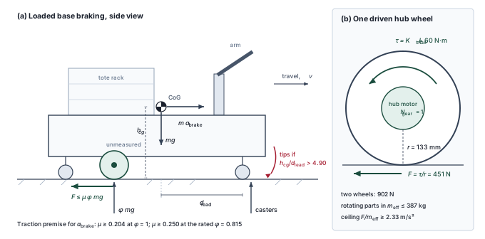
The constant-deceleration model requires a level surface and a qualified braking response. A conservative implementation charges the transient interval required to develop full retarding force into \(\PrebrakeDelay\), then applies a certified lower bound \(\CredibleBrakingDeceleration\). The actuator brake-onset allowance (\(\ActuatorResponseTime\)) enters that delay once. Any subsequent calculation that models a finite torque ramp must reconcile its ramp travel with this allowance rather than add the same interval twice. Furthermore, empirical stopping trials across declared operating conditions establish the credible deceleration, its distribution, and its safety margin. A sample percentile alone does not constitute a certified lower bound.

In unstructured environments, an autonomous machine cannot allocate its entire clearance to nominal stopping dynamics. Obstacle tracking carries state estimation uncertainty, sensor calibration drifts over time, and localization algorithms introduce position error. The stopping distance \(\StoppingDistance\) that the system defends must therefore include a spatial localization uncertainty bound \(\LocalizationBound\) and a minimum physical clearance margin \(\ProtectiveClearanceMargin\):⁶ \[\StoppingDistance = \SpeedAtDetection\,\PrebrakeDelay + \frac{\SpeedAtDetection^2}{2 \CredibleBrakingDeceleration} + \LocalizationBound + \ProtectiveClearanceMargin \tag{2}\] The sum \(\LocalizationBound + \ProtectiveClearanceMargin\) is fixed spatial overhead that must remain unoccupied when the body comes to a complete rest.

⁶ Protective Separation Distance: For speed and separation monitoring of robot arms, the collaborative-application requirements that ISO 10218-2:2025 incorporates from ISO/TS 15066 (which itself remains published and under revision) write the protective separation distance as \(\ProtectiveSeparationDistance = \PersonApproachTravel + \RobotReactionTravel + \RobotStoppingTravel + \IntrusionDistance + \PersonPositionUncertainty + \RobotPositionUncertainty\): the person’s travel, the robot’s travel during its reaction time and while stopping, an intrusion distance set by the sensing, and the position uncertainties of person and robot (International Organization for Standardization 2016, 2025; Marvel and Norcross 2017). The robot’s terms map onto equation 2, with \(\SpeedAtDetection\,\PrebrakeDelay\) as \(\RobotReactionTravel\), \(\SpeedAtDetection^2/2\CredibleBrakingDeceleration\) as \(\RobotStoppingTravel\), and \(\LocalizationBound\) as \(\RobotPositionUncertainty\), although ISO 10218-2:2025 excludes the hazards specific to a manipulator riding a mobile platform, the running machine’s case. For a learned policy, an unbounded compute tail lengthens the reaction time, which enlarges both \(\PersonApproachTravel\) and \(\RobotReactionTravel\) and forces the protective field outward.

International Organization for Standardization. 2016. ISO/TS 15066:2016: Robots and Robotic Devices, Collaborative Robots. International Organization for Standardization.

International Organization for Standardization. 2025. ISO 10218-2:2025: Robotics, Safety Requirements, Part 2: Industrial Robot Applications and Robot Cells. International Organization for Standardization.

Marvel, Jeremy A., and Rick Norcross. 2017. “Implementing Speed and Separation Monitoring in Collaborative Robot Workcells.” Robotics and Computer-Integrated Manufacturing 44: 144–55. https://doi.org/10.1016/j.rcim.2016.08.001.

↪ The localization bound \(\LocalizationBound\) and its dependence on map corrections are developed in Localization drift and map frames that jump.

Definition 2.2: Dynamic stopping distance

Dynamic stopping distance (\(\StoppingDistance\)) is the minimum physical clearance required to bring a moving mass to a complete halt from its speed \(\SpeedAtDetection\) when the hazard is first imaged. It sums three parts. The first is the travel during the pre-brake delay \(\PrebrakeDelay\), which spans the observation age of the frame that shows the hazard and the lease, tick, bus, and brake-onset intervals that follow until retarding force begins (the decomposition of Delay consumes stopping clearance), and which excludes the separately charged dispatch-to-admission interval. The second is the braking travel under the credible deceleration \(\CredibleBrakingDeceleration\). The last is the localization bound \(\LocalizationBound\) and protective clearance \(\ProtectiveClearanceMargin\), as equation 2 states.

1. Significance: Quantifies the non-negotiable physical spatial margin that software proposals must clear before motion permission can be granted.
2. Distinction: Unlike static geometric obstacle clearance in classical kinematics, dynamic stopping distance depends on the machine’s own speed and on every delay before braking, so each velocity setpoint and each delay term changes it.
3. Common pitfall: Assuming an emergency stop command halts the machine instantaneously, ignoring that moving mass carries kinetic energy (\(\KineticEnergy = \frac{1}{2}\Mass \SpeedAtDetection^2\)) that requires finite mechanical work and braking distance to dissipate.

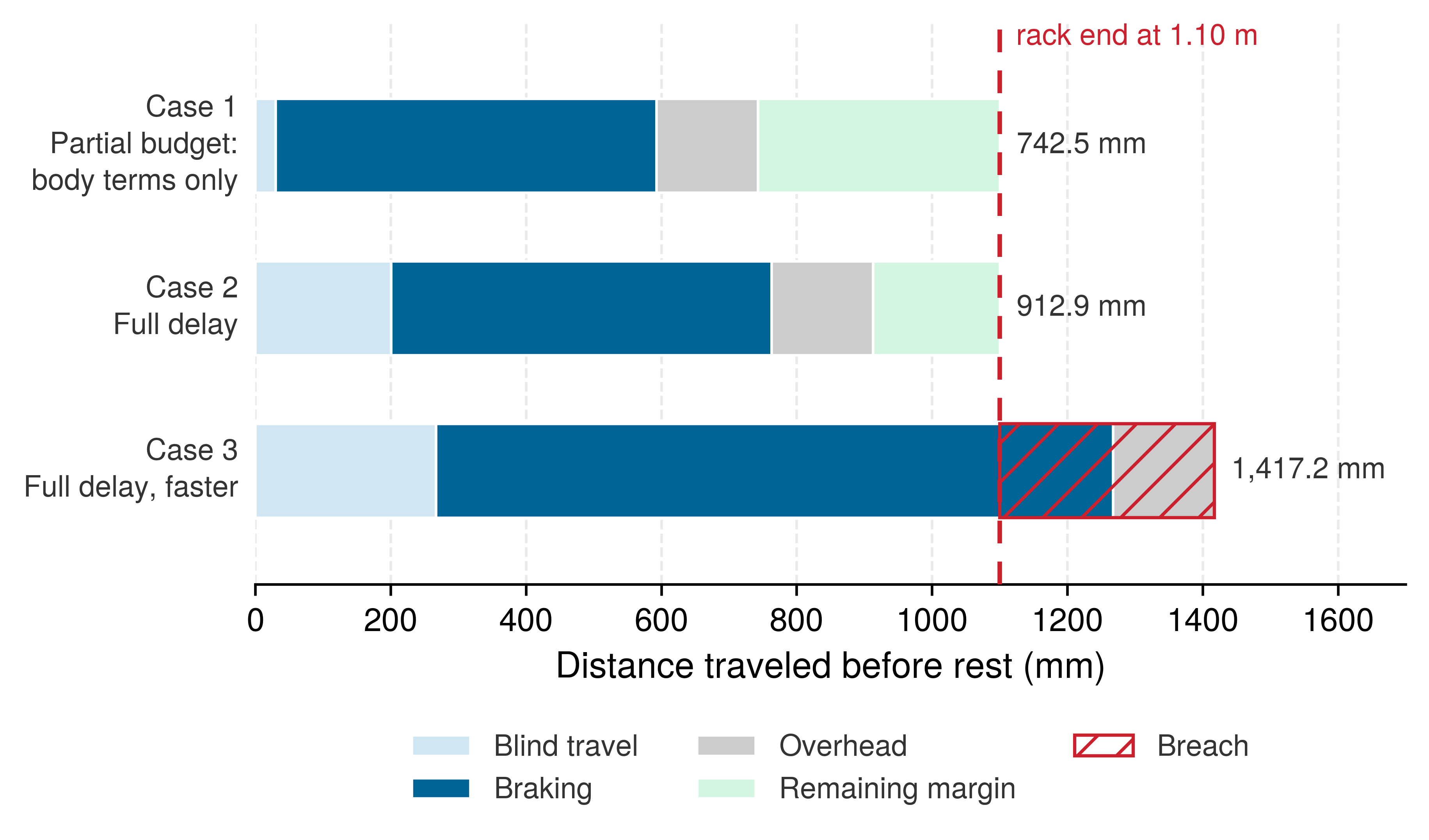
Three cases on the running machine show how the terms trade against one another (figure 2). With only the terms the body owns, the stop needs 742.5 mm. Charging the full 133.6 ms pre-brake delay of the elementary stopping budget (Delay consumes stopping clearance), whose terms later chapters measure one by one, gives that elementary stop plus the 150 mm fixed overhead, or 912.9 mm. That stop still fits the 1.10 m clear distance. Raising speed above the drive limit with that same delay pushes the stop to 1,417.2 mm, past the rack end, because speed enters the blind travel linearly and the braking travel quadratically. Notebook 2.2 works the first case term by term.

Figure 2: Stopping distance of the warehouse mobile manipulator: Each bar splits the stop into blind travel during the pre-brake delay, braking travel under the credible deceleration, and the fixed overhead of the localization bound and protective clearance, against the 1.10 m rack-end clear distance. Case 1 counts only the terms the body owns at the 1.5 m/s drive limit and stops within 742.5 mm. Case 2 charges the full 133.6 ms pre-brake delay of the elementary stopping budget (the kinematic roofline); at 912.9 mm it still fits, although later chapters add a stop profile and a tracking bound. Case 3 raises speed to a hypothetical 2 m/s, above the drive limit, with the same delay; braking travel grows by 77.8 percent and the stop, at 1,417.2 mm, breaches the clear distance.

2.3.2 Dynamic velocity ceilings and clearance budgeting

Because braking travel grows quadratically with speed while blind travel scales linearly with delay (figure 2), autonomous systems cannot rely on static, scene-independent speed limits. They require a dynamic velocity ceiling parameterized by instantaneous obstacle clearance. For a stationary obstacle detected at distance \(\ClearDistance\), such as a person standing at an aisle intersection or a dropped storage tote, safe operation demands that defended stopping distance remain strictly within the available clear path: \(\StoppingDistance \le \ClearDistance\). This constraint is how the first law, irreversibility (principle 1), binds every motion cycle, with each parameter in \(\StoppingDistance\) grounded in the machine’s verified physical limits. Using conservative bounds for actuation delay and retarding acceleration, the permission path solves this inequality to determine the maximum permissible command velocity \(\SpeedBound\). The symbol is the one that equation 1 used for the speed of a tracked target, but here it bounds the machine’s own speed. Taking the positive physical root of the resulting quadratic relation⁷ yields: \[\SpeedBound = -\CredibleBrakingDeceleration \PrebrakeDelay + \sqrt{(\CredibleBrakingDeceleration \PrebrakeDelay)^2 + 2 \CredibleBrakingDeceleration (\ClearDistance - \LocalizationBound - \ProtectiveClearanceMargin)} \tag{3}\] Whenever perceptual range degrades or an obstacle obstructs the trajectory, \(\ClearDistance\) contracts, continuously lowering the velocity ceiling. When available distance collapses to zero, the allowable forward velocity becomes zero. If the machine is already in motion, however, issuing a zero-velocity setpoint cannot instantaneously eliminate its accumulated kinetic energy. A negative available distance signals that the platform has already breached safe stopping margins, demanding immediate, full-authority emergency braking.

⁷ Kinematic Velocity Root: Grouping the fixed distance terms into the available braking distance \(\AvailableBrakingDistance = \ClearDistance - \LocalizationBound - \ProtectiveClearanceMargin\) gives the quadratic inequality \(\frac{1}{2 \CredibleBrakingDeceleration} \SpeedAtDetection^2 + \PrebrakeDelay \SpeedAtDetection - \AvailableBrakingDistance \le 0\). Multiplying by \(2 \CredibleBrakingDeceleration\) gives \(\SpeedAtDetection^2 + 2 \CredibleBrakingDeceleration \PrebrakeDelay \SpeedAtDetection - 2 \CredibleBrakingDeceleration \AvailableBrakingDistance \le 0\). Applying the quadratic formula and taking the positive root sets the speed ceiling.

Napkin Math 2.2: The body's stopping distance

Problem: The loaded warehouse mobile manipulator drives toward a rack end at its drive limit, and a person stands in the aisle at the clear distance. The body owns three terms of equation 2: braking travel, the fixed overhead, and the brake onset that enters \(\PrebrakeDelay\). How much of the clear distance do these terms use, what speed would they alone permit, and how do speed and added delay change the answer?

Variables:

• Loaded mass at most 368 kg (derived upper bound, full tote rack) and drive limit \(\SpeedAtDetection =\) 1.5 m/s (illustrative)
• Clear distance \(\ClearDistance =\) 1.10 m (illustrative)
• Credible deceleration \(\CredibleBrakingDeceleration =\) 2 m/s² (illustrative; loaded, dry floor)
• Localization bound \(\LocalizationBound =\) 50 mm (illustrative) and protective clearance \(\ProtectiveClearanceMargin =\) 100 mm (chosen)
• Brake onset \(\ActuatorResponseTime =\) 20 ms (illustrative)

Math:

1. Braking travel: For the same credible deceleration, mass cancels from the work-energy balance. The loaded machine’s 414 J sets the energy the stopping system must absorb or dissipate, while the specified deceleration sets the braking distance. A different payload can change that deceleration and requires a new bound: \[d_{\text{brake}} = \frac{v^2}{2 a_{\text{brake}}} = \frac{(1.5 m/s)^2}{2 \times 2 m/s²} = 562.5 mm\] The stopping distance so far is 562.5 mm.

2. Fixed overhead: \[\delta_{\text{loc}} + \delta_{\text{margin}} = 50 mm + 100 mm = 150 mm\] The running total rises to 712.5 mm.

3. Brake onset: Between the brake command and the first retarding force, the base still moves at full speed: \[v\,T_{\text{act}} = (1.5 m/s) \times (20 ms) = 30 mm\] \[d_{\text{stop}}\big|_{\text{body}} = 562.5 mm + 150 mm + 30 mm = 742.5 mm\] The body’s own terms leave 357.5 mm of the 1.10 m clear distance for every delay the body does not own.

4. The body-only ceiling: Solving equation 2 for speed with \(\PrebrakeDelay = \ActuatorResponseTime\): \[v_{\max} = -a_{\text{brake}} T_{\text{act}} + \sqrt{(a_{\text{brake}} T_{\text{act}})^2 + 2 a_{\text{brake}} (D_{\text{clear}} - \delta_{\text{loc}} - \delta_{\text{margin}})} \approx 1.91 m/s\] The body alone would permit 1.91 m/s, above the drive limit. The remaining delay terms, added in later chapters, spend part of this headroom.

5. Speed vs. delay: At a hypothetical 2 m/s, above the drive limit, the braking term alone grows to 1,000 mm, 77.8 percent more than at the drive limit. At the drive limit, each additional 100 ms of pre-brake delay adds 150 mm.

Systems insight: Platform velocity is the most sensitive variable in the stopping budget. Accelerating from 1.5 m/s to 2 m/s adds 437.5 mm in braking travel, as much distance as 291.7 ms of additional pre-brake delay at the drive limit. A velocity setpoint may therefore rise only after re-evaluating the clearance quadratic. Because physical braking distance scales with \(\SpeedAtDetection^2\), granting an aggressive velocity setpoint expands the defended stopping envelope and rapidly exhausts the clear distance margin defended by \(\StoppingDistance \le \ClearDistance\).

↪ The chunk lease, the time an admitted trajectory segment may keep executing without a replacement, is one of the delay terms that spend this headroom. Its sizing from this stopping distance is developed in Chunk Lease Sizing from the Stopping Budget.

2.3.3 Applying the velocity ceiling

A dynamic speed ceiling protects the machine only when an independent check on the permission path tests each new velocity request against it before execution. The learned policy proposes an action. The safety check evaluates clearance, delay, and available deceleration to determine whether that request fits the stopping budget. Requesting a lower speed alters future trajectory points but cannot erase the distance required to stop from the current speed. Consequently, the check must evaluate the platform’s instantaneous state alongside candidate commands, keeping the machine inside the region from which it can still stop between control ticks under strict bounds on timing jitter, obstacle motion, and actuator response. That per-tick validation belongs to the permission path; Phase portraits and speed ceilings formalizes it around the jerk-limited deceleration profiles executed on the physical platform. What the physical body contributes is the ceiling itself: a clearance-dependent boundary grounded in physical constraints that drops whenever traction degrades, actuator response slows, or localization uncertainty expands.

Enforcing this speed limit assumes the permission path can demand the deceleration \(\CredibleBrakingDeceleration\) whenever safety requires it. Commanding rapid deceleration, however, requires sudden, large mechanical torque from the drive motors and gearboxes. If the permission path requests a torque step that exceeds what the actuator bandwidth budget allows, the mechanical body cannot deliver the required deceleration, invalidating the model-based stopping ceiling and risking collision. The same drives also shape what happens if the stop falls short. The reflected rotor energy counted in \(\EffectiveImpactMass\) then reaches the obstacle and the gear teeth through the transmission’s compliance, so the stopping calculation cannot substitute for a contact-load assessment.

2.4 Actuator Transmission Limits

When a policy writes a 50 N·m torque setpoint to a joint register or dispatches an emergency brake command over a Controller Area Network (CAN) bus or EtherCAT, the drive electronics may clamp the current at half that request while returning a clean acknowledgement packet in sub-millisecond time. In digital software, an execution target either accepts an instruction or raises a fault; in physical hardware, stator winding inductance, DC bus voltage headroom, magnetic saturation, and transmission elasticity bound what the joint actually delivers. The systems engineering challenge is to specify an actuator contract at the physical plant interface, written in delivered force, torque, slew-rate limits, response latency, and tracking error rather than digital setpoints, and to expose those limits directly to the runtime permission path before an unachievable command causes a collision.

2.4.1 Actuation mechanisms and the actuator contract

What that actuator contract must bound depends on how the joint converts stored energy into mechanical force. Electric drives dominate mobile manipulation and power the running machine of this book, where current in copper windings pulls on rotor magnets through a gear train. Other robots rely on pressurized fluid or calibrated mechanical springs, and each mechanism trades peak force density against bandwidth, compliance, and maintenance overhead.

On the sense-plan-act (S·P·A) triad (The Sense–Plan–Act Paradigm), the actuator contract sits at the Act node, where a command must become delivered force.

Across the broader field, three non-rigid or fluid alternatives illustrate how the physical medium reshapes the contract:

• Hydraulic servovalves: For heavy machinery, construction robots, and high-load dynamic platforms, fluid power trades magnetic force for pressure. A cylinder’s force is supply pressure times piston area, \(\CylinderForce = \HydraulicSupplyPressure \PistonArea\), so raising the pressure lets a compact actuator deliver a large force. An electric motor’s force, by contrast, is bounded by the magnetic field its magnets and copper can sustain. The miniature servovalves on hydraulic legged robots respond fast, with bandwidths of hundreds of hertz (Scully 2015), so the valve is rarely the slow element. Hydraulic control is bounded instead by fluid compressibility (oil bulk modulus \(\OilBulkModulus\)), nonlinear orifice flow, and the plumbing, pumps, and cooling needed to keep the fluid within its operating range. That maintenance burden is one reason Boston Dynamics retired its hydraulic Atlas humanoid in 2024 in favor of an all-electric successor (Boston Dynamics 2024).
• Pneumatics and soft actuation: Pneumatic artificial muscles and elastomeric chambers provide physical compliance that naturally cushions impacts. However, gas compressibility, valve flow restrictions, and acoustic transport delays limit closed-loop bandwidth to tens of hertz. Stored pneumatic energy can also discharge violently during rapid venting or line rupture. Safety validation requires qualifying the envelope of peak chamber pressure, flow rates, and measured contact dynamics.
• Series elastic actuators (SEAs): By placing a calibrated spring directly between the gearbox and the output link (as in the ANYbotics ANYdrive), an SEA incorporates mechanical compliance into the drivetrain itself. The spring acts as a low-pass mechanical filter: it isolates delicate gear teeth from shock loads and decouples the large reflected rotor inertia (\(\GearReductionRatio^2 \RotorInertia\)) from the environment during impact. Its measured deflection also serves as a direct force sensor, since spring stiffness times deflection yields output torque (Pratt and Williamson 1995). Rather than dissipating energy, the spring stores elastic potential (\(\ElasticPotentialEnergy = \frac{1}{2} \SeriesElasticStiffness \FiniteChange\JointAngle^2\)) at the joint and can return that energy into an obstacle. The engineering trade-off is reduced closed-loop position bandwidth and low-frequency structural resonance. The safety system and permission path must therefore monitor physical spring deflection directly instead of assuming rigid load tracking.

Scully, Leah. 2015. Hydraulic Quadruped Uses Mini Servovalves. Power & Motion.

Boston Dynamics. 2024. An Electric New Era for Atlas. Boston Dynamics blog.

2.4.2 Electrical time constants, back-EMF, and current clamping

The running machine’s wheels and arm joints are electric, so the electric drive is the plant whose limits the stopping budget depends on. To a policy, a torque command is a number written to a register; to the motor, it is a current that must be built up in a coil. Three results from introductory physics describe that conversion (Lynch and Park 2017). First, a wire carrying current across a magnetic field feels a force proportional to the current. Wound around a rotor, those forces produce a torque proportional to current, \(\MotorTorque = \MotorTorqueConstant \WindingCurrent\), where the torque constant \(\MotorTorqueConstant\) (in \(\text{N}\cdot\text{m/A}\)) collects the magnet strength and the winding geometry. Second, the same wires, swept through the same field by the spinning rotor, have a voltage induced in them. A spinning motor is therefore also a generator, and its back-EMF (back electromotive force) \(\BackEmfVoltage = \MotorBackEmfConstant \RotorAngularSpeed\) opposes the supply. Energy conservation ties the two constants together. The electrical power the motor converts, \(\BackEmfVoltage\,\WindingCurrent\), equals the mechanical power it delivers, \(\MotorTorque \RotorAngularSpeed\), so \(\MotorBackEmfConstant\) and \(\MotorTorqueConstant\) are the same number in SI units. A three-phase drive’s current and voltage conventions scale them by constant factors, which is why both must be identified under one convention. Third, the winding is a coil, and a coil opposes any change in its current, \(\InductiveVoltage = \PhaseInductance\,d\WindingCurrent/d\TimeInstant\) for inductance \(\PhaseInductance\). Current, and therefore torque, cannot jump.

⁸ Field-Oriented Control (FOC): Holding the stator current at right angles to the rotor field is the arrangement that a brushed DC motor’s commutator enforces mechanically. An AC machine controlled this way behaves like a DC motor whose torque is set by a single current, \(\TorqueProducingCurrent\). That is what lets a policy command torque at all, because its request becomes a current target whose arrival the winding inductance and the voltage headroom then pace.

The budget needs two results from the motor controller: the torque delivered for a given current and the delay before that current appears. In a three-phase motor, field-oriented control (FOC) measures the winding currents and adjusts the inverter voltages so that the torque-producing current \(\TorqueProducingCurrent\) stays at right angles to the rotor’s magnetic field as the rotor turns. Torque is then \(\MotorTorque = \MotorTorqueConstant \TorqueProducingCurrent\).⁸ The controller splits the stator current into two components that turn with the rotor. The quadrature, or \(\Glyph{q}\)-axis, current \(\TorqueProducingCurrent\) lies at right angles to the rotor field and produces torque. The direct, or \(\Glyph{d}\)-axis, current \(\DirectAxisCurrent\) lies along the field, produces none, and is normally held at zero. The coordinate transformations inside the drive appear in section 2.4.6.

The delay between commanding a torque and delivering it begins in the stator windings. Adding the three effects around one winding circuit, the supply voltage must cover the resistive drop, the inductive voltage, and the back-EMF, which is Kirchhoff’s voltage law for the torque-producing current: \[\PhaseInductance \frac{d\TorqueProducingCurrent(\TimeInstant)}{d\TimeInstant} + \PhaseResistance \TorqueProducingCurrent(\TimeInstant) = \QuadratureAxisVoltage(\TimeInstant) - \BackEmfVoltage(\TimeInstant)\] where \(\PhaseInductance\) is phase inductance, \(\PhaseResistance\) is phase resistance, \(\QuadratureAxisVoltage(\TimeInstant)\) is the applied quadrature voltage from the inverter bridge, \(\TorqueProducingCurrent(\TimeInstant)\) is the quadrature-axis (torque-producing) current, and \(\BackEmfVoltage(\TimeInstant) = \MotorBackEmfConstant \RotorAngularSpeed(\TimeInstant)\) is the back-EMF. The stator electrical time constant is: \[\ElectricalTimeConstant = \frac{\PhaseInductance}{\PhaseResistance}\]

If the inverter applied an uncontrolled voltage step, the current would approach its steady state exponentially along \(\TorqueProducingCurrent(\TimeInstant) = \SteadyStateCurrent(1 - e^{-\TimeInstant/\ElectricalTimeConstant})\), taking an entire time constant \(\ElectricalTimeConstant\) to reach 63 percent of the target. A closed-loop current controller drives the winding much faster. It applies full bus voltage until current reaches the setpoint, forcing a ramp rate of nearly \((\DcBusVoltage - \BackEmfVoltage)/\PhaseInductance\). At that point the current loop throttles the voltage to maintain regulation. On the running machine, this electrical rise is rapid. The hub motor windings (line inductance 1.885 mH, line resistance 0.7 Ω) yield \(\ElectricalTimeConstant =\) 2.7 ms. Starting from rest on a depleted 42 V pack, the initial current slope gives a resistance-free rise estimate of 1.1 ms, only 5.6 percent of the 20 ms brake onset budgeted for the platform. The resistive drop slows the ramp as current builds, so this estimate is optimistic and the full winding response must be measured. When braking from forward speed, the rotor continues spinning in the positive direction while the controller reverses the sign of the torque-producing current to oppose motion, so the positive back-EMF reinforces the inverter’s negative current drive, accelerates the current ramp further, and reduces the terminal voltage required to sustain peak braking current from \(\BackEmfVoltage + \InverterCurrentLimit \ElectricalResistance\) to \(\BackEmfVoltage - \InverterCurrentLimit \ElectricalResistance\). In this architecture, electrical rise time does not bottleneck emergency braking. Tire traction, maximum inverter current, and voltage headroom at high speed govern the stopping distance, as detailed in notebook 2.3.

Torque tracks current directly, which means available voltage headroom also dictates the maximum torque slew rate: \[\frac{\DerivativeOperator\MotorTorque}{d\TimeInstant} = \MotorTorqueConstant \frac{d\TorqueProducingCurrent}{d\TimeInstant} \le \frac{\MotorTorqueConstant (\DcBusVoltage - \MotorBackEmfConstant \RotorAngularSpeed)}{\PhaseInductance}\] Inductance and voltage conventions must align consistently: line-to-line values reported on manufacturer datasheets pair with the full DC bus voltage. Per-phase values modeled under space-vector modulation scale by an amplitude of approximately \(\DcBusVoltage/\sqrt{3}\), the modulation voltage limit stated in Actuator Electrical and Thermal Dynamics. At low wheel speeds, ample voltage headroom enables steep torque ramps. As rotational velocity climbs, back-EMF consumes that headroom, throttling the rate at which the inverter can inject current. An unconstrained policy setpoint requesting an instantaneous torque step is transformed by the motor hardware into a finite physical ramp; any demand exceeding this maximum slew rate produces severe tracking error. The safety stopping budget must account for this rate-limited response.

Voltage headroom bounds the rate of current rise; power electronics define the maximum current that can safely flow. Inverter bridges enforce a strict current ceiling \(\InverterCurrentLimit\) to protect the switching power transistors from thermal failure and prevent magnetic core saturation in the stator. For a motor coupled to a mechanical transmission with gear ratio \(\GearReductionRatio\) and mechanical efficiency \(\GearboxTransmissionEfficiency\), this ceiling caps joint output torque at: \[\OutputTorqueCeiling = \GearboxTransmissionEfficiency \GearReductionRatio \MotorTorqueConstant \InverterCurrentLimit \tag{4}\]

This current limit settles a central safety requirement: whether the drives can sustain the deceleration demanded by the supervisory permission path. A motor drive may silently clamp current setpoints while continuing to acknowledge network commands; the safety path must interrogate measured output currents and status flags rather than inferring torque delivery from successful packet transmission. If emergency braking demands more torque than this ceiling allows, the assumed deceleration model breaks down. Any change to inverter current limits therefore invalidates the robot’s qualified stopping envelope and requires recomputing the stopping limit record (section 2.7).

Napkin Math 2.3: Can the drives deliver the credible deceleration?

The running machine brakes through two driven wheels, each a direct-drive 10-inch hub motor (the ZLTECH ZLLG10ASM800, with no gearbox, so \(\GearReductionRatio = 1\) and \(\GearboxTransmissionEfficiency \approx 1\)) (Shenzhen Zhongling Technology 2022) with rolling radius \(\WheelRadius =\) 133 mm. Its torque constant \(\MotorTorqueConstant =\) 2.4 N·m/A is the datasheet’s peak torque divided by its peak current, and the drive’s current limit is set at that peak, \(\InverterCurrentLimit =\) 25 A. Casters carry the rest of the weight.

Problem: Does the loaded machine’s credible deceleration \(\CredibleBrakingDeceleration =\) 2 m/s² fit under the traction, tip-over, and drive-torque ceilings, and does the drive keep control of its current at the 1.5 m/s drive limit?

Math:

1. Traction: Only the driven wheels brake, so \(\CredibleBrakingDeceleration \le \CoulombFrictionCoefficient \Gravity \DrivenWheelLoadFraction\). With all the weight on them (\(\DrivenWheelLoadFraction = 1\)), the floor must supply \(\CoulombFrictionCoefficient \ge \CredibleBrakingDeceleration/\Gravity =\) 0.204. The hub motors are rated to carry 300 kg per pair, so on the 368 kg machine \(\DrivenWheelLoadFraction \le\) 0.815 and the floor must supply at least \(\CoulombFrictionCoefficient =\) 0.250. The dry floor (\(\CoulombFrictionCoefficient =\) 0.60) meets that whenever the driven wheels carry at least a fraction 0.34 of the weight, and at the rated load share it supports \(\CoulombFrictionCoefficient \Gravity \DrivenWheelLoadFraction =\) 4.80 m/s². The inspected floor, a sealed low-traction surface whose friction a facility inspection certifies only down to \(\CoulombFrictionCoefficient =\) 0.12, supports only 1.18 m/s² even with every kilogram on the driven wheels.
2. Tip-over: The machine stays on its wheels while \(\CredibleBrakingDeceleration \le \Gravity\,\LeadingSupportDistance/\GravityCenterHeight\), so the credible deceleration requires \(\GravityCenterHeight/\LeadingSupportDistance \le \Gravity/\CredibleBrakingDeceleration =\) 4.90. The machine’s specification gives neither the loaded center-of-gravity height nor its distance to the leading support, and extending the arm forward shortens \(\LeadingSupportDistance\). This ceiling cannot yet be checked.
3. Drive torque: Each wheel delivers \(\MotorTorqueConstant \InverterCurrentLimit =\) 60 N·m, so the floor sees \(\DriveBrakingForceCeiling = 2 \MotorTorqueConstant \InverterCurrentLimit/\WheelRadius =\) 902.3 N. With the rotating-mass bound of section 2.3.1, \(\EffectiveImpactMass \le\) 387 kg, and the torque ceiling is \(\DriveBrakingForceCeiling/\EffectiveImpactMass \ge\) 2.33 m/s², at least 16.6 percent above the credible deceleration. With the current limit set at the rated 8.5 A instead, each wheel gives its rated 20 N·m and the ceiling falls to 0.78 m/s².
4. Voltage at the drive limit: At 1.5 m/s the wheel turns at \(\RotorAngularSpeed = \SpeedBound/\WheelRadius =\) 107.7 rpm, and the line-to-line back-EMF is \(\BackEmfVoltage = \MotorBackEmfConstant \RotorAngularSpeed =\) 28.2 V. Braking current flows with the back-EMF, so holding \(\InverterCurrentLimit\) through the 0.7 Ω line resistance requires only \(\BackEmfVoltage - \InverterCurrentLimit \ElectricalResistance =\) 10.7 V at the terminals. Even a depleted 42 V pack sits 13.8 V above \(\BackEmfVoltage\). Driving at the same current would need \(\BackEmfVoltage + \InverterCurrentLimit \ElectricalResistance =\) 45.7 V, more than the depleted pack supplies.

Result: The drives clear 2 m/s² by at least 16.6 percent, but only with the current limit at the motor’s peak. Traction holds on the dry floor if the driven wheels carry at least a fraction 0.34 of the weight, and it fails on the inspected floor. The tip-over ceiling remains unverified until the loaded center of gravity is measured, by weighing each wheel on corner scales or by a tilt test, with the arm stowed and extended.

Systems insight: The credible deceleration is a conjunction of three ceilings owned by different parts of the machine: the floor, the mass distribution that the arm changes, and the drive configuration. A current limit lowered to protect the windings cuts the torque ceiling below the stopping premise without any software change, so the configured current limit belongs in the limit record’s conditions.

Shenzhen Zhongling Technology. 2022. ZLLG10ASM800 Robot Hub Motor: Motor Parameters. Product drawing and datasheet.

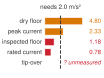
A 2 m/s² stop must clear every ceiling; two fall short and one is unmeasured.

⁹ Inverter Dead Time: A short hardware-inserted interval in which both switches of an inverter half-bridge are off, so that the high-side and low-side switches of one leg never conduct together and short the DC bus, a failure called shoot-through. The interval distorts the applied voltage most at low speed and near each current zero crossing, so delivered torque departs from the request exactly where slow, fine contact force is commanded.

Current regulation also incurs electrical and switching losses. Any stator current vector misaligned with the quadrature axis produces resistive heating without contributing shaft torque. Inverter pulse-width modulation and required protective dead times introduce further nonlinear voltage distortion.⁹ Consequently, dynamic torque tracking must be verified through physical dynamometer measurements on the assembled actuator rather than inferred from current setpoints alone.

2.4.3 Reflected rotor inertia and optimal inertia matching

Once electromagnetic torque leaves the motor shaft, mechanical gearing introduces a dynamic asymmetry between torque and inertia. High-reduction joints employ gear ratios between \(50{:}1\) and \(160{:}1\) to multiply the output torque of compact, lightweight motors. While this reduces the motor torque required by a factor of \(\GearReductionRatio\), the motor rotor must spin \(\GearReductionRatio\) times faster than the actuated joint. When an external contact backdrives the joint, it must accelerate that rotor at \(\GearReductionRatio\) times the joint’s angular acceleration. Because rotational kinetic energy scales with the square of velocity (\(\frac{1}{2} \RotorInertia \RotorAngularSpeed^2\)), the rotor’s physical inertia \(\RotorInertia\) resists load-side acceleration multiplied by the square of the gear ratio (definition 2.3).

Through a 100:1 transmission, a small 50 g rotor imposes the apparent inertia of a heavy 11.2 kg flywheel with a 10 cm radius at the output shaft (Lynch and Park 2017). When the end-effector collides with a rigid surface, the contact force must instantly decelerate this equivalent flywheel through the drivetrain, generating extreme peak stresses that can fracture gear teeth at their roots, as documented in figure 4.

Definition 2.3: Reflected rotor inertia

Reflected rotor inertia (\(\ReflectedRotorInertia\)) is the apparent rotational inertia of an actuator rotor at the load-side joint output, scaling with the square of the transmission gear ratio: \[\ReflectedRotorInertia = \GearReductionRatio^2 \RotorInertia\]

1. Significance: In high-reduction transmissions (\(\GearReductionRatio \ge 100\)) it dominates the apparent load, capping joint acceleration \(\JointAcceleration\) and setting impact shock loads.
2. Distinction: Unlike rotor inertia \(\RotorInertia\) or link inertia \(\LoadInertia\), it acts through transmission stiffness and backlash, so backdriving from the environment meets an \(\GearReductionRatio^2\) barrier.
3. Common pitfall: Ignoring reflected rotor inertia during collision and contact modeling. Under sudden obstacle impact, the reflected kinetic energy of the spinning rotor concentrates stress directly on gear teeth before drive current can be interrupted.

The combined equation of motion for a geared joint driving load inertia \(\LoadInertia\) with motor torque \(\MotorTorque\) is: \[ \JointAcceleration = \frac{\GearReductionRatio \MotorTorque}{\LoadInertia + \GearReductionRatio^2 \RotorInertia} \] Maximizing delivered load acceleration \(\JointAcceleration\) with respect to transmission ratio \(\GearReductionRatio\), by setting \(\DerivativeOperator\JointAcceleration/d\GearReductionRatio = 0\), gives \(\LoadInertia = \GearReductionRatio^2 \RotorInertia\): acceleration peaks when the reflected rotor inertia equals the load inertia. Solving for \(\GearReductionRatio\) establishes the classical inertia matching ratio:¹⁰ \[ \InertiaMatchingRatio = \sqrt{\frac{\LoadInertia}{\RotorInertia}} \tag{5}\]

¹⁰ Inertia Matching: At \(\InertiaMatchingRatio\) the reflected rotor inertia equals the load inertia, the mechanical twin of impedance matching in a circuit, where a source delivers the most power to a load whose impedance equals its own. The analogy carries the same caveat: the matched ratio maximizes acceleration, not efficiency or safety, so practical arms choose lower ratios to protect gear teeth from shock, keep the joint backdrivable, and raise top speed.

Below \(\InertiaMatchingRatio\), joint acceleration is torque-limited: increasing \(\GearReductionRatio\) multiplies motor torque to accelerate the heavy load faster. Above \(\InertiaMatchingRatio\), more gearing decreases delivered joint acceleration, because the motor expends most of its electromagnetic torque accelerating its own spinning rotor (\(\GearReductionRatio^2 \RotorInertia\)) rather than the external link. For the 50 g rotor above driving an illustrative link of \(\LoadInertia =\) 8.5 × 10⁻³ kg·m², the matched ratio is \(\InertiaMatchingRatio \approx\) 39. At 100:1 the same motor torque delivers only 67.7 percent of the matched-ratio acceleration, because \(\JointAcceleration(\GearReductionRatio)/\JointAcceleration(\InertiaMatchingRatio) = 2\NormalizedGearRatio/(1+\NormalizedGearRatio^2)\) with \(\NormalizedGearRatio = \GearReductionRatio/\InertiaMatchingRatio\). The extra gearing has cost 32.3 percent of the joint’s acceleration.

The gear ratio also magnifies the mechanical resistance an external contact meets when attempting to move the link. This resistance to imposed motion constitutes the joint’s mechanical impedance. Because link inertia, joint damping, torsional compliance, and seal friction all shape this response, the gear ratio alone does not establish contact forces or structural fracture limits. Transmission selection must balance delivered joint acceleration against the impedance presented to accidental impacts.

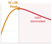
Past \(\InertiaMatchingRatio \approx\) 39, gearing chokes acceleration; 100:1 keeps 67.7 percent.

Abrupt changes in commanded torque excite the torsional elasticity of geared joints before the physical link responds. Bounding joint acceleration and jerk moderates this excitation, but software trajectory smoothing cannot override mechanical resonance. Trajectory generators formulate control profiles that respect these physical boundaries (Lynch and Park 2017). The hardware platform must provide the empirical response rates and contact stiffness limits required to tune them.

↪ Trajectory timing under joint torque and jerk bounds is developed in Time parameterization under torque and jerk bounds.

2.4.4 Transmission compliance, contact impedance, and tooth fracture

Mechanical gearboxes introduce backlash and elasticity that decouple the motor from the driven link. Upon direction reversal, the motor shaft traverses mechanical clearance before the gear teeth engage the opposing flank. Concurrently, as illustrated by the disassembled strain wave gear set in figure 3, torsional compliance in gear teeth and flexible elements¹¹ transforms the rigid link into an elastic system (Spong 1987). Its dynamics follow the flexible-joint formulation given in Flexible joint dynamics and singular perturbations. Step changes in torque excite this structural spring, driving the drivetrain into limit-cycle¹² chatter. Motor-side encoders conceal this deadband completely. The motor rotates smoothly while the output shaft remains pinned, causing link position \(\LinkOutputPosition\) to diverge from \(\MotorShaftPosition / \GearReductionRatio\) by a load-dependent deflection \(\LostMotionDeflection\). The motor controller observes flawless setpoint tracking while the end-effector stalls, eventually experiencing an impulsive impact when the gear teeth make contact. Repeated shock cycles culminate in the root fatigue failure shown in figure 4.

¹¹ Strain Wave Gearing: Musser (1959) patented the mechanism, now sold as the Harmonic Drive: an elliptical wave generator flexes a thin toothed cup inside a rigid ring that carries two more teeth, so a single stage yields a high ratio with near-zero backlash. The flexing that makes the ratio possible is also the joint’s torsional compliance, which makes the link elastic.

Musser, C. Walton. 1959. Strain Wave Gearing. U.S. Patent 2,906,143, filed March 21, 1955, issued September 29, 1959.

¹² Limit Cycle: A self-sustained oscillation of fixed amplitude that a nonlinear feedback loop settles into, here excited by the backlash deadband as the motor crosses the gap, the teeth strike, and the controller corrects back across it. Unlike an instability, it does not grow, so it can run unnoticed through a shift while every cycle adds a tooth impact to the fatigue count.

Figure 3: Strain wave gear set: The three parts of a Harmonic Drive strain wave gear, disassembled: the elliptical wave generator with its thin-race ball bearing (top left), the flexspline cup with external teeth on its open rim (top right), and the rigid circular spline ring with internal teeth (bottom). The wave generator bends the flexspline so that its teeth mesh with the circular spline at two opposite zones; because the flexspline carries slightly fewer teeth, each turn of the wave generator advances it by only that difference, which gives a high reduction with little backlash. (Credit: Pieceofmetalwork, Wikimedia Commons, CC BY-SA 4.0.)

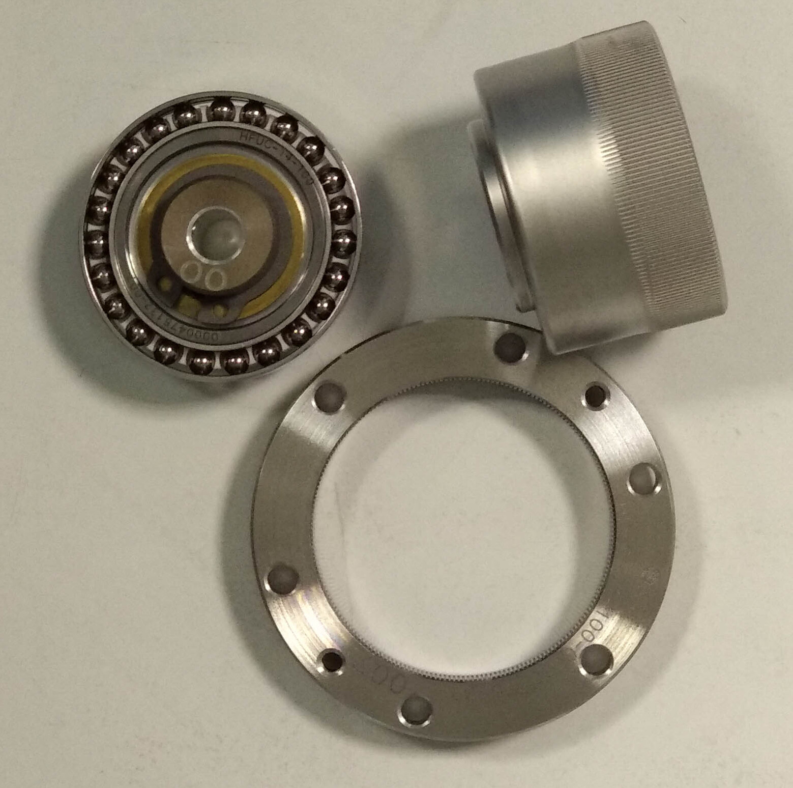
The strain wave gear of figure 3 packs a high reduction into a compact joint by deforming its flexspline continuously, and that elasticity has a cost. This intentional compliance decouples rotor position from link position under dynamic loading: while the motor encoder registers smooth rotation, the flexspline winds up like a torsion spring, introducing unmeasured end-effector deflection.

Figure 4: Broken gear tooth: A spur gear from gear research at the NASA Lewis (now Glenn) Research Center, photographed in 1974, with one tooth broken away at its root and the fragment lying in the gap. The root is where a tooth’s bending stress concentrates, so repeated or impulsive loading that the transmission passes to the teeth ends here. (Credit: Martin Brown, NASA Glenn Research Center, via the U.S. National Archives, NARA 17417956, public domain.)

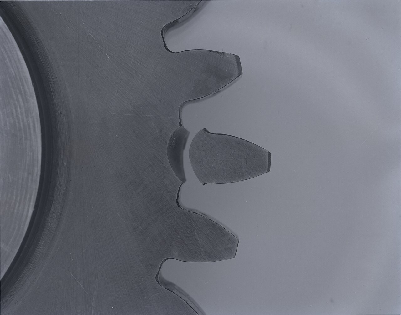
A tooth broken off at its root (figure 4) is the end state of that loading. Such failures show why dynamic impact loads, rather than static payload ratings alone, must govern actuator and transmission selection: repeated torque spikes and unmodeled contact shocks concentrate destructive stresses directly at the tooth root fillet. While smooth motion plans mitigate drivetrain vibration, safe physical interaction depends on measuring output torque and enforcing strict mechanical load boundaries.

Systems Perspective 2.3: Impedance control for contact safety

When a position-controlled robot encounters a rigid surface (contact stiffness \(\ContactStiffness \ge 10^5\text{ N/m}\)), a minor setpoint tracking error of \(\FiniteChange \ContactPointPosition = 1\text{ mm}\) escalates the contact force to \(\ContactForce = \ContactStiffness \FiniteChange \ContactPointPosition = 100\text{ N}\) within milliseconds as the inverter commands maximum current against the obstacle. On the mobile manipulator, the gripper contacting the spring-latched door strikes a steel plate with stiffness 4.0 × 10⁵ N/m. Once impact occurs, contact force ramps at \(\ContactForce = \ContactStiffness \ContactApproachSpeed \TimeInstant\): 12 N/ms under a guarded approach velocity of 0.03 m/s, and 40 N/ms at an unconstrained 0.10 m/s, rapidly exceeding the latch’s 100 N structural limit.

Impedance control (Hogan 1985) reformulates contact interactions away from pure position or force control. An impedance takes motion in and returns force; an admittance takes force in and returns motion. Because a rigid environment behaves as an admittance, yielding motion only when pushed, the manipulator is made to behave as an impedance, which answers a deviation in position and velocity with a restoring force (\(\ContactForce = \MechanicalImpedanceMap(\ContactDirectionVelocity)\), force as a function of the imposed motion). The joint drive controller realizes this relationship by emulating a virtual spring-damper system: \[\ContactForce = \PidProportionalGain (\DesiredContactPosition - \ContactPointPosition) + \PidDerivativeGain (\DesiredContactVelocity - \ContactDirectionVelocity)\] The stiffness \(\PidProportionalGain\) multiplies the position error and the damping \(\PidDerivativeGain\) the velocity error, the roles a proportional and a derivative gain play in a feedback controller. Tuning them in software causes the arm to yield compliantly under tracking errors, shedding peak impact loads. However, closed-loop impedance behavior is physically bounded by current-loop update rates, inverter voltage headroom, and unmodeled joint elasticity. Algebraic control laws cannot alter the unyielding inertia of the rotor during the first milliseconds of an impact. The runtime permission path must therefore enforce approach speed limits derived from physical contact qualification rather than relying on software compliance alone. The impedance command interface, through which a learned policy proposes these gains and the permission path validates them before admission, is defined in What a proposal may command.

2.4.5 Actuation regimes and gear reduction trade-offs

The scaling disparity underlying inertia matching, in which output torque scales linearly with ratio (\(\JointOutputTorque = \GearboxTransmissionEfficiency \GearReductionRatio \MotorTorque\)) while reflected inertia scales quadratically (\(\GearReductionRatio^2\)), divides robotic actuation into three primary regimes. These regimes trade continuous torque density against mechanical backdrivability, distinguished by gear design, stage count, and reduction ratio (table 2): at the lowest ratios, quasi-direct drive (QDD) pairs a high-torque motor with a single compact planetary stage; at intermediate ratios, multistage planetary gearboxes reduce motor size at the cost of moderate reflected inertia and backlash; and at the highest ratios, strain-wave gears pack large torque multiplication into a compact joint at the cost of extreme reflected inertia and torsional compliance.

Table 2: Actuator transmission trade-off: Reduction ratio (\(\GearReductionRatio\)), reflected rotor inertia scaling (\(\GearReductionRatio^2\)), and the consequence for learned control policies across quasi-direct-drive (a single low-ratio planetary stage), multistage planetary, and strain wave transmissions. The strain wave range is that of one catalog series (Harmonic Drive AG 2014).

Transmission	Gear Ratio (\(\GearReductionRatio\))	Reflected Inertia (\(\GearReductionRatio^2\))	Implication for Learned Policies
Quasi-Direct Drive (single-stage planetary)	\(3:1\text{--}10:1\) (\(\GearReductionRatio \le 10\))	\(\GearReductionRatio^2 \le 100\) (Low)	Lower reflected inertia supports backdriving and current-based torque estimation; contact response still requires qualification.
Multistage Planetary	\(15:1\text{--}50:1\) (\(\GearReductionRatio \approx 30\))	\(\GearReductionRatio^2 \approx 225\text{--}2{,}500\) (Moderate)	Semi-backdrivable; a smaller motor than QDD for the same output torque; gear backlash requires load-side joint sensing.
Strain Wave (Harmonic Drive)	\(50:1\text{--}160:1\) (\(\GearReductionRatio \ge 50\))	\(\GearReductionRatio^2 \ge 2{,}500\text{--}25{,}600\) (Extreme)	High reflected inertia; zero initial backlash; torsional compliance and impact loading require qualification.

Actuator selection must satisfy continuous torque targets and permissible contact dynamics simultaneously. Direct-drive configurations eliminate gear backlash entirely, but require large, heavy motors to produce holding torque (Asada and Kanade 1983). Increasing the gear ratio permits a much smaller motor to produce equivalent output torque, but introduces reflected inertia, friction, and transmission compliance.

Motor thermal limits and torque requirements intersect in an electromagnetic figure of merit. Stator resistive losses follow \(\WindingLossPower = \TorqueProducingCurrent^2 \EffectiveLossResistance\), where \(\EffectiveLossResistance\) is the winding’s effective loss resistance, while electromagnetic torque follows \(\MotorTorque = \MotorTorqueConstant \TorqueProducingCurrent\). Combining these expressions reveals that resistive dissipation scales with the square of motor torque: \(\WindingLossPower = (\MotorTorque / \MotorConstant)^2\). Here the motor constant \(\MotorConstant = \MotorTorqueConstant / \sqrt{\EffectiveLossResistance}\) (in \(\text{N}\cdot\text{m}/\sqrt{\text{W}}\)) captures the motor’s torque-producing capacity per square root of dissipated heat. Motor datasheets specify this parameter directly (TQ-Systems 2014). Section 2.5.1 relates \(\EffectiveLossResistance\) to the phase and line-to-line resistances of section 2.4.2. When driving a mechanical transmission of ratio \(\GearReductionRatio\) and efficiency \(\GearboxTransmissionEfficiency\), the motor must supply an internal torque of \(\JointOutputTorque/(\GearboxTransmissionEfficiency \GearReductionRatio)\), resulting in: \[\WindingLossPower = \left(\frac{\JointOutputTorque}{\GearboxTransmissionEfficiency \GearReductionRatio \MotorConstant}\right)^2, \qquad \ReflectedTransmissionInputInertia = \GearReductionRatio^2 \TransmissionInputInertia\] where \(\TransmissionInputInertia\) represents total input inertia (the rotor plus the transmission input stage), and \(\ReflectedTransmissionInputInertia\) is that combined inertia reflected to the joint output. Increasing the reduction ratio \(\GearReductionRatio\) reduces winding heat by \(\GearReductionRatio^2\) while multiplying reflected inertia by \(\GearReductionRatio^2\). Consequently, for a selected motor and gearbox geometry, their product is invariant to the gear ratio: \[\WindingLossPower\,\ReflectedTransmissionInputInertia = \frac{\JointOutputTorque^2\,\TransmissionInputInertia}{\GearboxTransmissionEfficiency^2 \MotorConstant^2} \tag{6}\] Adjusting \(\GearReductionRatio\) relocates the actuator along a fixed trade-off curve between thermal dissipation and reflected inertia. Improving both characteristics concurrently requires selecting a motor with a superior ratio of \(\MotorConstant^2/\TransmissionInputInertia\). Notebook 2.4 evaluates this trade-off for the mobile manipulator’s arm joints.

Napkin Math 2.4: What does the gear ratio cost?

The running machine’s arm is a seven-joint, torque-sensing manipulator in the class of the Franka Emika Panda (Franka Emika GmbH 2018), whose joints use strain-wave gears (The machine data sheet). Franka does not publish the motors in those joints, so this example, like the thermal examples of section 2.5, uses a sourced stand-in. The stand-in is a TQ-RoboDrive ILM 70x18 frameless motor (TQ-Systems 2014) with \(\MotorTorqueConstant =\) 0.187 N·m/A and effective loss resistance \(\EffectiveLossResistance =\) 0.495 Ω, driving a CSG-25 strain-wave gear (Harmonic Drive AG 2014), whose catalog lists one input inertia for all of that size’s ratios. Rotor plus gear input give \(\TransmissionInputInertia =\) 7.34 × 10⁻⁵ kg·m². The joint must hold the arm’s maximum joint torque \(\JointOutputTorque =\) 87 N·m through a gear of efficiency \(\GearboxTransmissionEfficiency =\) 0.85 (illustrative).

Problem: How do the copper loss and the reflected inertia change if the same motor drives the joint through 50:1, 100:1, or a quasi-direct-drive ratio of 10:1?

Math:

1. Motor constant: \(\MotorConstant = \MotorTorqueConstant/\sqrt{\EffectiveLossResistance} =\) 0.266 N·m/√W, the value the motor’s data sheet publishes.
2. At 50:1: The motor supplies \(\JointOutputTorque/(\GearboxTransmissionEfficiency \GearReductionRatio) =\) 2.05 N·m, dissipating \((\MotorTorque/\MotorConstant)^2 =\) 59.3 W, and the joint reflects \(\GearReductionRatio^2 \TransmissionInputInertia =\) 0.183 kg·m².
3. At 100:1: The motor supplies 1.02 N·m, the loss falls fourfold to 14.8 W, and the reflected inertia rises fourfold to 0.734 kg·m². The product \(\WindingLossPower \ReflectedTransmissionInputInertia\) is unchanged.
4. At 10:1: The motor would have to supply 10.2 N·m, 2.5× its 4.05 N·m peak torque. No current can make this motor hold the load.

Result: Doubling the ratio buys a fourfold cut in holding heat with a fourfold rise in the inertia that an impact must accelerate, and lowering the ratio toward quasi-direct drive fails outright with this motor. The gear ratio moves the joint along a fixed trade; only the motor sets the trade itself.

Systems insight: A low-ratio, backdrivable joint requires a motor with a much larger torque per square root of watt, the route quasi-direct drive takes. A high-ratio arm joint instead accepts the reflected inertia and recovers contact sensitivity by measuring torque at its output.

Mechanical backdrivability measures the ease with which an external load applied at the joint output rotates the motor shaft backward through the transmission. The external torque required to backdrive a geared joint is: \[\ExternalJointTorque = \GearReductionRatio^2 \RotorInertia \JointAcceleration + \JointFrictionTorque\] where \(\JointFrictionTorque\) denotes total joint friction referred to the output link. This friction varies dynamically with operating state (Lynch and Park 2017): breakaway static friction dominates at rest, Coulomb friction opposes motion at constant levels, and viscous damping grows with velocity. The Stribeck effect, a dip in friction just after sliding begins, shapes the response at near-zero speeds. Furthermore, gear tooth mesh friction scales with transmitted load, ambient temperature, and lubrication aging. At low velocities, friction dominates the resistance of high-reduction gearboxes; during sudden impacts, reflected rotor inertia dominates. As a result, backdrivability must be verified through empirical load testing on the assembled joint rather than inferred from the reduction ratio alone.

Quasi-direct drive actuation takes the low-ratio route of notebook 2.4, using large-diameter, high-torque motors so a single modest reduction stage suffices (Seok et al. 2015; Wensing et al. 2017; Katz et al. 2019). Minimizing reflected inertia and internal friction maximizes mechanical transparency, the fidelity with which external interaction forces translate into measurable motor motion and winding currents. The penalty is a substantially heavier motor demand for any given output torque.

Katz, Benjamin, Jared Di Carlo, and Sangbae Kim. 2019. “Mini Cheetah: A Platform for Dynamic Locomotion.” IEEE International Conference on Robotics and Automation (ICRA), 3295–301. https://doi.org/10.1109/ICRA.2019.8793865.

Mechanical transparency also dictates what motor currents reveal about contact states. In high-friction gearboxes, motor current primarily overcomes internal transmission losses rather than external loads. Conversely, when transmission friction and inertial resistance remain small, output torque simplifies to: \[\JointOutputTorque \approx \GearboxTransmissionEfficiency \GearReductionRatio \MotorTorqueConstant \TorqueProducingCurrent\] This relationship enables proprioceptive sensing, allowing the controller to estimate interaction forces directly from motor current without specialized external sensors. However, accurate estimation requires rigorous calibration across operating temperatures and speeds; current setpoints measure motor electromagnetic effort, portions of which are absorbed by acceleration and drivetrain losses. While backdrivability allows external collisions to displace the joint without shearing gear teeth, low gearing and motor current sensing do not guarantee safe contact forces. High link velocities can still impart severe impulsive shock before the current controller can respond. Safe interaction mandates qualifying the total closed-loop contact response.

High-reduction joints overcome transmission friction by sensing torque directly at the joint output. Strain gauge torque sensors mounted on the output side of strain wave gearboxes measure delivered torque directly, allowing closed-loop current controllers to cancel gearbox friction and cogging torque (Lynch and Park 2017). The running machine’s arm adopts this approach, integrating torque sensors within each of its seven joints (Franka Emika GmbH 2018) to achieve transparency through measurement rather than low mechanical reduction. The engineering cost includes increased joint complexity, elevated mass, and the torsional compliance of the strain wave flexsplines, which complicates high-bandwidth motion tracking.

Franka Emika GmbH. 2018. Panda Datasheet. Product datasheet (reseller-hosted copy).

Whether mechanical transparency originates by construction (quasi-direct drive) or by active measurement (output torque sensing), contact operations require qualifying joint compliance, closed-loop torque response, and dynamic sensing fidelity against the operating environment. Dual-encoder architectures and load-side torque sensors expose internal transmission windup and mechanical backlash that motor-side encoders conceal. When load-side deflection departs from the qualified dynamic envelope, the runtime safety system can immediately intercede and reject subsequent motion commands.

2.4.6 Supporting drive and impedance models

Deliverable motor torque and contact shock isolation rest on two compact models of how the drive and transmission transform effort and motion: the rotating-frame torque law behind \(\MotorTorque = \MotorTorqueConstant \TorqueProducingCurrent\) (section 2.4.2), and the series-spring impedance that isolates reflected rotor inertia during a fast impact (section 2.4.4). Inside the physical drive, FOC holds the \(\Glyph{d}\)-axis current \(\DirectAxisCurrent\) of section 2.4.2 at zero, which minimizes stator losses and makes output torque proportional to the \(\Glyph{q}\)-axis current alone (Actuator Electrical and Thermal Dynamics states the voltage equations that govern both currents in the rotating frame): \[\MotorTorque = \frac{3}{2} \RotorPolePairCount \PermanentMagnetFluxLinkage \TorqueProducingCurrent = \MotorTorqueConstant \TorqueProducingCurrent\] where \(\RotorPolePairCount\) is the number of magnetic pole pairs on the rotor and \(\PermanentMagnetFluxLinkage\) is the permanent-magnet flux linkage, the magnetic flux from the rotor magnets that threads each winding. The \(\frac{3}{2}\) scaling factor arises from the amplitude-invariant transformation convention adopted in this chapter. Motor drive firmware must enforce a transformation convention consistent with the identified torque constant \(\MotorTorqueConstant\).

For frequency-domain dynamic analysis, mechanical impedance quantifies the joint’s physical resistance to imposed environmental motion. The Laplace variable \(\LaplaceVariable\) stands for differentiation in time, so that for a sinusoidal motion of angular frequency \(\AngularFrequency\) it can be read as \(\LaplaceVariable = \ImaginaryUnit\AngularFrequency\). An impedance term \(\LaplaceVariable \RotatingBodyInertia\) grows with frequency like an inertia, and a term \(\RotationalSpringStiffness/\LaplaceVariable\) falls with frequency like a spring. The apparent mechanical impedance \(\JointOutputImpedance(\LaplaceVariable) = \ExternalJointTorque(\LaplaceVariable) / \JointVelocity(\LaplaceVariable)\) evaluated at the joint output flange couples the load dynamics directly to the reflected rotor dynamics through the drivetrain’s torsional stiffness \(\TransmissionTorsionalStiffness\). An external torque applied at the joint flange splits between two paths that share the same output velocity \(\JointVelocity(\LaplaceVariable)\), one accelerating the output link inertia \(\LoadInertia\) directly and the other twisting the transmission spring against the reflected rotor. Along that second path, the transmission spring and the reflected rotor act in series so both stages bear equal transmitted torque while their relative angular velocities sum, causing the spring impedance \(\TransmissionTorsionalStiffness/\LaplaceVariable\) and reflected rotor impedance to combine through their reciprocal sum before adding to the output link impedance (Spong 1987): \[\JointOutputImpedance(\LaplaceVariable) = \LaplaceVariable \LoadInertia + \OutputBearingDamping + \left[\frac{1}{\LaplaceVariable \GearReductionRatio^2 \RotorInertia + \GearReductionRatio^2 \MotorShaftDamping} + \frac{\LaplaceVariable}{\TransmissionTorsionalStiffness}\right]^{-1}\] The coefficients \(\OutputBearingDamping\) and \(\MotorShaftDamping\) account for viscous damping in the output bearings and motor shaft. At low interaction frequencies, the series spring behaves rigidly relative to the rotor, and the environment experiences the aggregate inertia \(\LoadInertia + \GearReductionRatio^2 \RotorInertia\) assumed in rigid-body kinematic models. Above the transmission’s natural resonance frequency, the bracketed impedance term simplifies toward \(\TransmissionTorsionalStiffness/\LaplaceVariable\): external collision forces compress the joint compliance against the link inertia \(\LoadInertia\), temporarily isolating the rotor’s reflected inertia. This series compliance cushions sudden impacts in flexible drivetrains and series elastic actuators, reinforcing why the flexible-joint dynamic model is necessary to calculate contact loads during manipulation.

Checkpoint 2.1: Actuator limits

The drives decide whether the stopping premise can be delivered, and the transmission decides what that delivery costs in heat and inertia.

• Torque ceiling: Can you compute the deceleration ceiling of the two hub drives when their current limit is set at the motor’s rated current rather than its peak, and explain why a current limit lowered to protect the windings breaks the stopping premise without any software change?
• Current rise: Can you estimate how long the hub-motor current takes to reach its limit from rest on a depleted pack, and explain why back-EMF at speed helps a braking current but can starve a driving one?
• Inertia matching: Can you explain why the gear ratio that maximizes link acceleration makes reflected rotor inertia equal load inertia (\(\GearReductionRatio^2 \RotorInertia = \LoadInertia\)), and why oversizing the gearbox for static torque lowers dynamic joint acceleration?
• Heat vs. reflected inertia: Can you explain why, for a given motor and gear, the ratio cannot reduce holding heat and reflected inertia together, and what must change to improve both?

Operating near these electrical and mechanical ceilings exacts an inevitable thermodynamic toll. Every ampere driving the motor against reflected rotor inertia or sustaining peak clamping torque dissipates resistive heat (\(\WindingLossPower = \TorqueProducingCurrent^2 \EffectiveLossResistance\)) in the stator windings. That thermal energy accumulates directly in the motor’s thermal mass, bounding the operational duration of peak torque before winding insulation suffers accelerated thermal degradation.

2.5 Thermal Duty Cycles

Holding a load motionless at full reach places deceptive demands on an articulated arm such as the mobile manipulator’s. Maintaining a static load against gravity demands continuous phase current through the stator coils, actively converting electrical energy into accumulating heat. Heat arrives in seconds and leaves in minutes, making duty cycle a primary design variable.

2.5.1 Thermal capacity and insulation breakdown thresholds

Although a stationary joint performs zero mechanical work (\(\MechanicalWork = \int \AppliedForce \cdot d\BodyDisplacement = 0\)), sustaining its holding torque against gravity requires continuous phase current to produce magnetic Lorentz force (\(\MotorTorque = \MotorTorqueConstant \TorqueProducingCurrent\)). The lumped thermal model uses \(\TorqueProducingCurrent\) in the same convention as its torque constant \(\MotorTorqueConstant\). Here \(\EffectiveLossResistance\) denotes the effective aggregate loss resistance for that current, so total winding copper loss is: \[\WindingLossPower = \TorqueProducingCurrent^2 \EffectiveLossResistance = \frac{\MotorTorque^2}{\MotorTorqueConstant^2} \EffectiveLossResistance\] For the amplitude-invariant drive convention above, with balanced phase currents and \(\DirectAxisCurrent=0\), this effective resistance is \(\EffectiveLossResistance=\frac{3}{2}\PhaseResistance\), where \(\PhaseResistance\) is resistance per phase. Three resistances of one winding therefore appear in this chapter. The phase resistance \(\PhaseResistance\) belongs in the Kirchhoff equation of section 2.4.2. Datasheets quote the line-to-line value measured between two terminals, which for a star-connected winding spans two phases, \(2\PhaseResistance\). The hub-motor current-rise example used that line value with the line inductance, whose ratio gives the same time constant. The thermal calculations use \(\EffectiveLossResistance = \frac{3}{2}\PhaseResistance\), three quarters of the line-to-line value, and every winding resistance in them, including \(\ElectricalResistance(\WindingTemperature)\), is this effective resistance. The following illustrative thermal examples stipulate it and the matching current convention.

The copper-loss equation ties torque to current and current to heat. Commanded torque scales linearly with current (\(\MotorTorque = \MotorTorqueConstant \TorqueProducingCurrent\)), but stator copper loss scales quadratically with torque (\(\MotorTorque^2\)). Demanding twice the torque requires four times the thermal dissipation. Because heat has no fast exit, thermal accumulation limits how long an arm can maintain static poses or execute dynamic bursts without mechanical brakes.

Reducing motor current to shed heat also reduces holding torque. A loaded arm therefore needs a response that preserves support, such as transferring the load to a mechanical brake, rather than assuming that thermal derating leaves the task unchanged. Excess winding temperature can damage electrical insulation, while excess rotor temperature can permanently reduce magnet strength. Those material limits bound the allowable temperature trajectory.

The winding and housing respond on different timescales. Copper heats rapidly under current, while the larger core and housing absorb and reject heat more slowly. A case temperature measurement can therefore lag the winding hotspot during a torque burst. The stator in figure 5 failed from overheating, and its damage sits where this model puts the heat: in the copper windings and the insulation between them.

Figure 5: Motor stator damaged by overheating: The opened stator of an electric motor that failed from overheating, showing the copper phase windings bound with tape at left, the insulating slot liners where the windings leave the laminated iron core, and the end bell with its bearing seat at right. The windings are where resistive heat (\(\WindingLossPower = \TorqueProducingCurrent^2 \EffectiveLossResistance\)) is generated, and the insulation between them is what accumulated heat ages. (Credit: K. Kudelina, Wikimedia Commons, CC BY 4.0.)

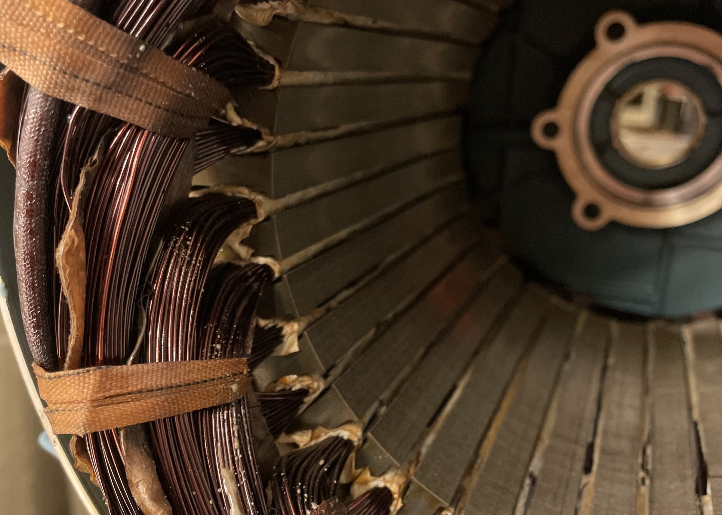
A thermal model follows the same energy accounting as the stopping calculation: energy accumulates where the rate entering exceeds the rate leaving. Here the winding receives electrical losses and transfers heat to the core; the core transfers heat to the surroundings. Thermal capacitance measures how much energy raises a component’s temperature, while thermal resistance measures how strongly the heat-flow path resists that transfer. Representing the winding and core separately gives the two-node lumped-parameter thermal ordinary differential equation (ODE) system: \[\begin{aligned} \WindingThermalCapacitance \frac{d\WindingTemperature(\TimeInstant)}{d\TimeInstant} &= \WindingLossPower(\TimeInstant) - \frac{\WindingTemperature(\TimeInstant) - \StatorCoreTemperature(\TimeInstant)}{\WindingCoreThermalResistance} \\ \CoreThermalCapacitance \frac{d\StatorCoreTemperature(\TimeInstant)}{d\TimeInstant} &= \frac{\WindingTemperature(\TimeInstant) - \StatorCoreTemperature(\TimeInstant)}{\WindingCoreThermalResistance} - \frac{\StatorCoreTemperature(\TimeInstant) - \AmbientTemperature}{\CoreAmbientThermalResistance} \end{aligned}\] where \(\WindingLossPower(\TimeInstant) = \TorqueProducingCurrent^2(\TimeInstant) \ElectricalResistance(\WindingTemperature) = \frac{\MotorTorque^2(\TimeInstant)}{\MotorTorqueConstant^2} \ElectricalResistance(\WindingTemperature)\) is the Joule dissipation source deposited directly into the copper coils, \(\WindingThermalCapacitance\) is the small thermal capacitance of the winding, \(\CoreThermalCapacitance\) is the large thermal capacitance of the laminated stator core and housing, \(\WindingCoreThermalResistance\) is the conductive thermal resistance from winding to core, and \(\CoreAmbientThermalResistance\) is the convective thermal resistance from core to ambient air.

This separation of timescales creates a dangerous observability gap. Because \(\WindingThermalCapacitance \ll \CoreThermalCapacitance\), under a sudden peak torque burst or sustained stall against gravity, the stator core temperature \(\StatorCoreTemperature\) remains virtually clamped over the initial seconds by its large thermal inertia. The internal copper winding temperature surges at the initial adiabatic rate: \[\left.\frac{d\WindingTemperature}{d\TimeInstant}\right|_{t=0} \approx \frac{\WindingLossPower}{\WindingThermalCapacitance}\] Under sustained peak torque, the internal copper hotspot \(\WindingTemperature\) can climb past the 155 °C Class F rating within tens of seconds (notebook 2.5) while an external thermistor bonded to the motor casing still reads far below the hotspot. The class temperature is not a cliff at which the insulation fails. IEC 60085 assigns it as the hot-spot temperature at which an insulation system reaches its rated life (International Electrotechnical Commission 2007), and insulation aging¹³ proceeds as a chemical reaction whose rate grows exponentially with temperature (Dakin 1948). Every excursion above the rating therefore spends insulation life faster than the rating assumes, and the accumulated aging culminates in the insulation charring and turn-to-turn electrical failures documented in figure 5. A thermal budget must count accumulated exposure as well as the instantaneous peak.

¹³ Thermal Aging as an Exchange Rate: The engineering practice predates the chemistry. Montsinger (1930) proposed loading transformers by the temperature their insulation reaches rather than by current alone, and Dakin (1948) later explained the exponential dependence as Arrhenius reaction kinetics. The consequence is an exchange rate rather than a threshold. Time spent above the rating costs life at a rate that grows exponentially with the excess, so the limit record must count time at temperature rather than merely the peak.

Montsinger, V. M. 1930. “Loading Transformers by Temperature.” Transactions of the American Institute of Electrical Engineers 49 (2): 776–90. https://doi.org/10.1109/T-AIEE.1930.5055572.

Dakin, Thomas W. 1948. “Electrical Insulation Deterioration Treated as a Chemical Rate Phenomenon.” Transactions of the American Institute of Electrical Engineers 67 (1): 113–22. https://doi.org/10.1109/T-AIEE.1948.5059649.

A first-order approximation can summarize heating over a characterized operating range, with an effective winding temperature \(\WindingTemperature\) and fitted thermal parameters: \[\StatorThermalCapacitance \frac{d\WindingTemperature(\TimeInstant)}{d\TimeInstant} = \WindingLossPower(\TimeInstant) - \frac{\WindingTemperature(\TimeInstant) - \AmbientTemperature}{\ThermalResistance}\] where \(\ThermalResistance = \WindingCoreThermalResistance + \CoreAmbientThermalResistance\) represents the winding-to-ambient steady-state thermal resistance. The effective capacitance \(\StatorThermalCapacitance\) sets the fitted time constant \(\ThermalTimeConstant = \ThermalResistance \StatorThermalCapacitance\). This approximation does not resolve a fast winding hotspot separately from the housing. Its transient predictions require validation before they can bound a burst.

At thermal steady state (\(d\WindingTemperature/d\TimeInstant = 0\)), heat generation balances heat dissipation to ambient: \[\SustainableCopperLossPower =\frac{\WindingTemperatureLimit - \AmbientTemperature}{\ThermalResistance}\] Substituting the copper loss identity \(\WindingLossPower = \frac{\MotorTorque^2}{\MotorTorqueConstant^2} \ElectricalResistance(\WindingTemperatureLimit)\) reveals the continuous thermal torque ceiling: \[\ContinuousTorque = \MotorTorqueConstant \sqrt{\frac{\WindingTemperatureLimit - \AmbientTemperature}{\ElectricalResistance(\WindingTemperatureLimit) \ThermalResistance}} \tag{7}\] Continuous torque is limited by thermal dissipation, not by the peak current ratings of the drive electronics or the battery. The arm’s stand-in motor, for example, is rated for 4.05 N·m peak but only 1.25 N·m continuous, a ratio of 3.2 (TQ-Systems 2014). A brief torque burst of several seconds causes a rapid transient temperature rise that stays within the insulation rating (\(\WindingTemperatureLimit =\) 155 °C) if its peak does. However, sustained holding torque or high-frequency cycling drives the winding toward an asymptotic thermal equilibrium \(\EquilibriumWindingTemperature = \AmbientTemperature + \AverageCopperLossPower \ThermalResistance\). If that equilibrium exceeds the rating, continuous operation ages the winding insulation far faster than its rated life allows and ends in phase-to-phase short circuits.

The loss term must also change with temperature. Copper’s positive temperature coefficient (\(\CopperTemperatureCoefficient \approx 0.00393\text{ K}^{-1}\)) increases the effective winding resistance by 47.2 percent from 20 °C to 140 °C, according to \(\ElectricalResistance(\WindingTemperature) = \ReferenceWindingResistance [1 + \CopperTemperatureCoefficient(\WindingTemperature - \CopperReferenceTemperature)]\). That upper temperature is the engineering ceiling \(\EngineeringTemperatureCeiling\), a working limit chosen below the 155 °C insulation rating \(\WindingTemperatureLimit\) to leave room for the error of the thermal model. The burst horizons and the stall derating below are checked against the rating itself. A schedule of repeated bursts is held to the ceiling, as is the installed continuous rating that the datasheet pitfall of section 2.9 obtains by evaluating equation 7 at \(\EngineeringTemperatureCeiling\) in place of \(\WindingTemperatureLimit\). Holding the same torque at the ceiling therefore dissipates 47.2 percent more winding power than at the reference. A fixed-resistance calculation omits this feedback. The burst example below uses that approximation explicitly, and the subsequent stall calculation restores it.

Datasheet thermal ratings are optimistic because they are measured on an unconstrained motor mounted to a large heat sink in free air at \(20^\circ\text{C}\) or \(25^\circ\text{C}\). Installed in a sealed chassis beside power electronics, battery packs, and other joints, the motor loses convective airflow, which raises \(\ThermalResistance\). Neighboring loads raise its local ambient above the test ambient before its own coils carry current. Thermal margins must therefore be budgeted from heating and cooling time constants measured with the enclosure sealed and adjacent loads at their \(\text{p99}\) power draw.

2.5.2 Transient thermal bursts and periodic duty cycles

Because thermal capacity integrates power over time, a peak torque¹⁴ or peak current rating is meaningless without four parameters: the initial winding temperature \(\WindingTemperature(0)\), the allowed duration \(\ActuatorOnTime\), the ambient \(\AmbientTemperature\), and the recovery time \(\ActuatorOffTime\). An actuator that can produce three times its continuous torque sustains it only while the integral of copper loss (\(\WindingLossPower = \TorqueProducingCurrent^2 \EffectiveLossResistance\)) stays within the margin below the insulation limit. From a cold winding, that can last tens of seconds, and from a heat-soaked one a fraction of that (notebook 2.5).

¹⁴ Duty Type and RMS Torque: IEC 60034-1 rates a motor for a duty type: S1 is continuous running at constant load long enough to reach thermal equilibrium, and S3 is an intermittent periodic duty of identical load-and-rest cycles too short to reach it (International Electrotechnical Commission 2022). Because copper loss grows with \(\MotorTorque^2\), the torque that heats the winding over a cycle short compared with the thermal time constant is the root-mean-square value \(\RmsMotorTorque = \sqrt{\frac{1}{\Time}\int_0^\Time \MotorTorque^2\,d\TimeInstant}\), and it is the RMS, not the peak, that must stay under the continuous rating. A peak rating means nothing without its duty type, which is why figure 6 draws the S1 and S3 regions separately.

International Electrotechnical Commission. 2022. IEC 60034-1:2022: Rotating Electrical Machines, Part 1: Rating and Performance. International Electrotechnical Commission.

Napkin Math 2.5: Thermal accumulation across duty cycles

This example uses the arm’s sourced stand-in joint of notebook 2.4: a CSG-25-50 strain-wave gear (Harmonic Drive AG 2014) driven by a TQ-RoboDrive ILM 70x18 frameless motor (TQ-Systems 2014), whose rated current is \(\ContinuousCurrent =\) 6.7 A. The motor has effective aggregate loss resistance \(\EffectiveLossResistance =\) 0.495 Ω, lumped thermal capacitance \(\StatorThermalCapacitance =\) 120 J/K, and installed thermal resistance \(\ThermalResistance =\) 2.5 K/W (both thermal values illustrative, because the motor’s data sheet leaves them to the installation). It runs in an enclosed ambient \(\AmbientTemperature =\) 40 °C with Class F insulation rated to 155 °C. The thermal time constant is \(\ThermalTimeConstant = \ThermalResistance \StatorThermalCapacitance =\) 300 s.

Problem: How does the initial winding temperature change how long a threefold rated-current burst can last before the insulation limit?

Math:

1. Continuous equilibrium: At \(\ContinuousCurrent =\) 6.7 A the winding settles at \(\RatedCurrentEquilibriumTemperature = \AmbientTemperature + \ContinuousCurrent^2 \EffectiveLossResistance\,\ThermalResistance =\) 95.6 °C, below the limit.
2. Peak burst: At \(\PeakCurrent =\) 20.1 A the dissipation rises ninefold to \(\PeakCopperLossPower =\) 200.0 W, whose asymptote \(\EquilibriumWindingTemperature = \AmbientTemperature + \PeakCopperLossPower \ThermalResistance =\) 540.0 °C lies far above the limit.
3. Survival horizons: With \(\WindingTemperature(\TimeInstant) = \EquilibriumWindingTemperature - (\EquilibriumWindingTemperature - \WindingTemperature(0))\,e^{-\TimeInstant/\ThermalTimeConstant}\), the time to reach the limit is \[\BurstSurvivalTime = \ThermalTimeConstant \ln\frac{\EquilibriumWindingTemperature - \WindingTemperature(0)}{\EquilibriumWindingTemperature - \WindingTemperatureLimit}\] which gives 78.4 s from a cold start at ambient and 43.1 s from a heat-soaked start at \(\RatedCurrentEquilibriumTemperature\).

Result: The heat-soaked joint holds the burst 45.1 percent less time than the cold one, so peak torque cannot be budgeted without tracking thermal history.

Systems insight: Peak torque is a stock of heat margin that thermal history spends, not a fixed rating. The admission check \(\EstimatedWindingTemperature \le \WindingTemperatureLimit\) must use the current estimate of the winding temperature, and these first-order horizons are optimistic, because the winding hotspot of the two-node model runs ahead of the lumped temperature.

TQ-Systems. 2014. ILM Series Frameless Servo Kits Data Sheet. TQ-RoboDrive product datasheet.

Harmonic Drive AG. 2014. Engineering Data CSG-2UH Units. Product documentation 1019642.

¹⁵ Periodic steady-state thermal peak: Over a repeating cycle of period \(\ActuatorCyclePeriod = \ActuatorOnTime + \ActuatorOffTime\), summing the heating and cooling exponentials gives the periodic peak temperature rise: \(\FiniteChange \PeriodicPeakWindingTemperature = \PeakCopperLossPower \ThermalResistance\frac{1 - e^{-\ActuatorOnTime/\ThermalTimeConstant}}{1 - e^{-\ActuatorCyclePeriod/\ThermalTimeConstant}}\). As the cycle period \(\ActuatorCyclePeriod \to 0\), this peak approaches the average-power screen (\(\ActuatorDutyCycle \PeakCopperLossPower \ThermalResistance\)); for any finite burst length, the peak winding temperature exceeds the average.

For repeated cycles of period \(\ActuatorCyclePeriod = \ActuatorOnTime + \ActuatorOffTime\), the engineering ceiling \(\EngineeringTemperatureCeiling =\) 140 °C sets a cycle-average power ceiling \(\CycleAveragePowerCeiling = (\EngineeringTemperatureCeiling - \AmbientTemperature)/\ThermalResistance =\) 40 W. With peak dissipation during \(\ActuatorOnTime\) and none during \(\ActuatorOffTime\), this average-power screen bounds the duty cycle \(\ActuatorDutyCycle = \ActuatorOnTime/\ActuatorCyclePeriod\) by \[\ActuatorDutyCycle \le \frac{\EngineeringTemperatureCeiling - \AmbientTemperature}{\PeakCopperLossPower \ThermalResistance} \tag{8}\] which here is 20.0 percent, so a 3 s burst calls for a recovery of \(\ActuatorOffTime = \ActuatorOnTime(1 - \ActuatorDutyCycle)/\ActuatorDutyCycle \approx\) 12 s. The average does not bound the hottest instant. Because heat arrives in seconds during bursts but dissipates over minutes during recovery, the peak transient hotspot temperature during periodic pulsing strictly exceeds the time-averaged calculation,¹⁵ reaching 142.0 °C (above the ceiling) before the rise of \(\ElectricalResistance(\WindingTemperature)\) adds more. Average-power screening is optimistic, and a burst schedule is certified only against the transient hotspot trajectory.

2.5.3 Torque-speed operating envelopes and back-EMF roll-off

The burst calculation limits duration, while the back-EMF relation in section 2.4.2 limits torque at speed. A feasible maneuver must satisfy both. At low speed, the drive can supply the current needed for a burst, but the winding temperature limits how long it may do so. At higher speed, back-EMF consumes voltage headroom and can prevent that current from appearing at all. On the arm’s stand-in joint motor, voltage headroom and thermal history bound the usable torque-speed region simultaneously (figure 6). Because steady-state operation at full supply voltage splits the bus voltage between the resistive drop \(\TorqueProducingCurrent \PhaseResistance\) and the back-EMF \(\MotorBackEmfConstant \RotorAngularSpeed\), rising torque demands more current, consumes a larger resistive voltage drop, and pulls the motor’s voltage-limited speed linearly down from 2,110 rpm at no load to 1,570 rpm at peak torque, while the burst that a cold winding sustains for 78.4 s reaches the insulation class in only 43.1 s from continuous-duty equilibrium.

Figure 6: Torque, speed, and time on one joint motor: (a) The TQ-RoboDrive ILM 70x18 of the arm’s stand-in joint on its 48 V supply. Continuous duty \(\Glyph{S_1}\) extends up to the 1.25 N·m rated torque; intermittent duty \(\Glyph{S_3}\) extends to the 4.05 N·m peak. Both end where back-EMF plus the resistive drop uses up the supply, from the 2,110 rpm no-load speed down to 1,570 rpm at peak torque; winding inductance, neglected here, pulls that boundary lower. (b) The winding temperature of the threefold-current burst of notebook 2.5, a first-order rise toward 540.0 °C with \(\ThermalTimeConstant =\) 300 s. From ambient the burst reaches the 155 °C insulation class after 78.4 s; from the continuous-duty equilibrium it gets there after 43.1 s. The thermal values are illustrative, because the data sheet leaves them to the installation.

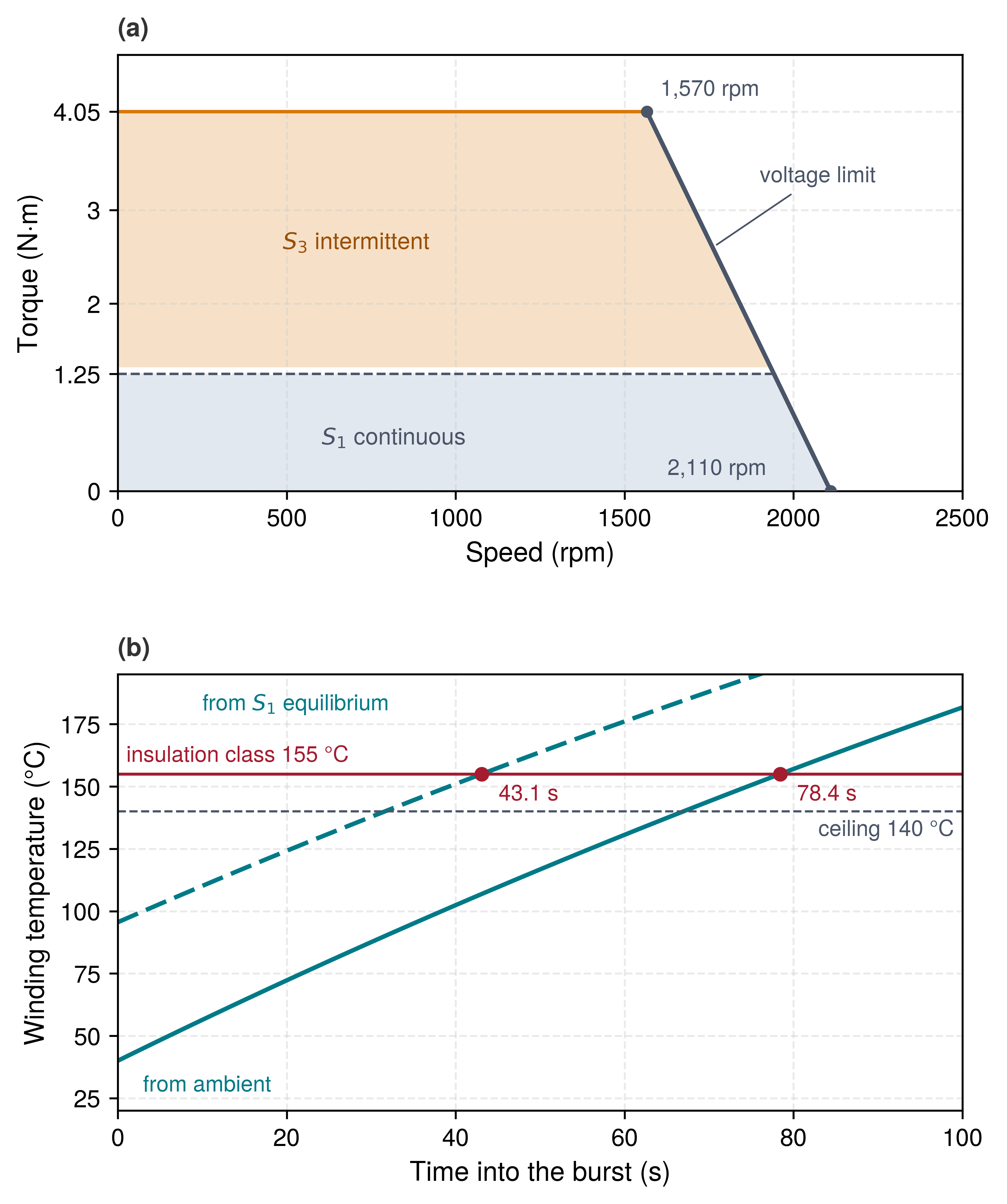
The continuous-duty region (\(\Glyph{S}_1\)) permits sustained operation under the declared cooling conditions. The larger intermittent region (\(\Glyph{S}_3\)) permits periodic bursts only with the starting temperature, duration, and recovery interval established above. Both regions narrow when speed consumes the drive’s voltage headroom. Their intersection with the current thermal state, rather than the catalog peak, gives the available torque for the next maneuver.

A simulator that uses only a fixed torque clamp can therefore teach a policy an unavailable action: maximum torque while the rotor is already near its voltage-limited speed, or a repeated burst without recovery. The actuator model and permission limits must include speed and thermal history. Temperature-dependent winding resistance further shrinks the available region during a sustained hold.

The standard remedy in legged-robot sim-to-real transfer replaces the clamp with an actuator model identified on the hardware. For the series elastic actuators of the ANYmal quadruped, Hwangbo et al. (2019) trained a small network on a few minutes of logged joint data to map a short history of position errors and velocities to the torque the actuator actually delivered. The network then ran inside the simulator in place of an ideal actuator. The ideal model, which assumes any commanded torque appears instantly, failed to predict the measured torque. The same structure carries the envelope of this section into training: an actuator model that also takes speed, bus voltage, and winding temperature as inputs lets the simulator deny the torque the hardware cannot deliver.

↪ How actuator dynamics mismatch is measured and closed in the training simulator is developed in Physical Channels of the Sim-to-Real Gap.

2.5.4 Copper resistance feedback and stall thermal runaway

The copper-resistance rise calculated in section 2.5.1 must enter the runtime estimate as well as the design calculation. An external thermistor can lag the winding hotspot, so a thermal observer combines measured current with the characterized heating and cooling model. A discrete update of the lumped energy balance is: \[{\EstimatedWindingTemperature{}}_{k+1} = {\EstimatedWindingTemperature{}}_{k} + \frac{\FiniteChange \TimeInstant}{\StatorThermalCapacitance} \left[ {\TorqueProducingCurrent}_{k}^2 \ElectricalResistance({\EstimatedWindingTemperature{}}_{k}) - \frac{{\EstimatedWindingTemperature{}}_{k} - \AmbientTemperature}{\ThermalResistance} \right]\] where \(\ElectricalResistance({\EstimatedWindingTemperature{}}_{k}) = \ReferenceWindingResistance [1 + \CopperTemperatureCoefficient({\EstimatedWindingTemperature{}}_{k} - \CopperReferenceTemperature)]\). The update interval, model error, and temperature uncertainty must fit the thermal margin. As the estimate approaches its ceiling, the permission path reduces admissible effort or transfers the load to a qualified support mechanism. Removing holding current without securing a gravity-loaded arm would exchange a thermal fault for uncontrolled motion. A static hold shows how copper’s feedback changes the sustainable torque (notebook 2.6).

Napkin Math 2.6: Static holding torque and stall derating

The arm’s elbow, the same Panda-class stand-in joint as notebook 2.5, is asked to hold the arm’s maximum joint torque \(\HoldingTorque =\) 87 N·m at stall (\(\RotorAngularSpeed = 0\)) through its \(\GearReductionRatio =\) 50:1 strain-wave gear (\(\GearboxTransmissionEfficiency =\) 0.85, illustrative). Its motor has \(\MotorTorqueConstant =\) 0.187 N·m/A and cold effective aggregate loss resistance \(\ReferenceWindingResistance =\) 0.495 Ω at \(\CopperReferenceTemperature =\) 20 °C. The illustrative installed thermal resistance is \(\ThermalResistance =\) 1.80 K/W, lower than the 2.5 K/W of the burst example and so a better-cooled installation. The Class F limit is 155 °C, and the limb ambient is \(\AmbientTemperature =\) 40 °C.

Problem: With copper’s resistance rising with temperature, where does the stalled winding settle, and what holding torque is thermally sustainable?

Math:

1. Stall current: \(\MotorTorque = \HoldingTorque/(\GearboxTransmissionEfficiency \GearReductionRatio) =\) 2.05 N·m, so \(\TorqueProducingCurrent = \MotorTorque/\MotorTorqueConstant =\) 10.9 A and the cold dissipation is \(\ColdCopperLossPower = \TorqueProducingCurrent^2 \ReferenceWindingResistance =\) 59.3 W.

2. Runaway: With \(\ElectricalResistance(\WindingTemperature) = \ReferenceWindingResistance[1 + \CopperTemperatureCoefficient(\WindingTemperature - \CopperReferenceTemperature)]\), the steady rise satisfies \[\JouleanTemperatureRise = \TorqueProducingCurrent^2 \ReferenceWindingResistance \left[1 + \CopperTemperatureCoefficient(\AmbientTemperature - \CopperReferenceTemperature + \JouleanTemperatureRise)\right] \ThermalResistance\] Rearranging terms yields \(\JouleanTemperatureRise = \frac{\TorqueProducingCurrent^2 \ReferenceWindingResistance [1 + \CopperTemperatureCoefficient(\AmbientTemperature - \CopperReferenceTemperature)] \ThermalResistance}{1 - \TorqueProducingCurrent^2 \ReferenceWindingResistance \ThermalResistance \CopperTemperatureCoefficient}\). The denominator establishes the thermal runaway criterion: if the positive feedback loop gain satisfies \(\TorqueProducingCurrent^2 \ReferenceWindingResistance \ThermalResistance \CopperTemperatureCoefficient \ge 1\), this fixed-current, linear-resistance model cannot settle to a stable thermal equilibrium. Above one, heat generation increases with temperature faster than heat removal, producing exponential growth. At exactly one, the temperature-dependent terms cancel and the remaining positive heating causes linear growth. In this stall scenario, the feedback factor is 0.4196 \(< 1\), so temperature settles at a finite (yet fatal) equilibrium given by \(\JouleanTemperatureRise =\) 115.16 \(+\) 0.4196 \(\JouleanTemperatureRise\). This yields \(\JouleanTemperatureRise =\) 198.4 K and drives the winding to 238.4 °C, far above its rating.

3. Derating: At the limit the allowable rise is 115 K, so the sustainable dissipation is \(\SustainableCopperLossPower = \FiniteChange \WindingTemperatureLimit/\ThermalResistance =\) 63.89 W. At the hot resistance \(\ElectricalResistance(\WindingTemperatureLimit) \approx\) 0.758 Ω, that allows \(\ContinuousCurrent = \sqrt{\SustainableCopperLossPower/\ElectricalResistance(\WindingTemperatureLimit)} \approx\) 9.18 A and a hold of \(\SustainableHoldingTorque = \GearboxTransmissionEfficiency \GearReductionRatio \MotorTorqueConstant \ContinuousCurrent \approx\) 73.0 N·m.

Result: Held without control, the stall drives the winding toward 238.4 °C, and staying within the insulation rating requires a 16.1 percent derating, from 87 N·m to 73.0 N·m.

Systems insight: At stall the motor does no mechanical work, so every watt it draws becomes heat, and copper’s rising resistance makes that heat grow with temperature. Continuous gravity holding above the thermally sustainable torque therefore needs another support mechanism, such as a friction brake or counterweight, in the premise the permission path admits; holding within that torque can remain electrically sustained under the stated thermal conditions.

Thermal capacity governs how long an actuator can sustain torque before winding insulation degrades or thermal runaway occurs, bounding continuous holds and transient bursts by the plant’s ability to reject heat. Motor windings, however, do not generate those thermal loads in isolation. Delivering the current pulses that drive these torque trajectories simultaneously stresses the upstream power distribution network, shifting the engineering constraint from heat dissipation in copper to transient voltage stability on the shared direct-current bus.

2.6 Electrical Power Integrity

When the mobile manipulator swerves hard to avoid a collision, every drive motor, joint inverter, and accelerator demands peak current at once from one direct-current distribution bus. In simulation, current flows from an idealized source. On hardware, delivery is bounded by finite capacity, source impedance, and transient voltage stability. A machine that browns out mid-motion fails physically; the electrical supply is a shared resource.

Rail sag, regenerative overvoltage, and thermal accumulation are manifestations of one bounded energy network on different time scales. Of the three, voltage moves fastest, within microseconds to milliseconds whenever current demand exceeds what the source can deliver at that instant. Compute, sensing, and motor inverters draw from a common bus, so when a policy commands coordinated accelerations across several joints, the sum of their currents changes the voltage delivered to every node on the machine.

2.6.1 Power distribution impedance, transient droop, and brownout resets

The mobile machine’s battery, harnesses, connectors, and protection switches all contribute source impedance.¹⁶ Local capacitors supply part of a sudden load increase, so current drawn by the loads need not equal current arriving through the harness. For a source feeding one bus node through resistance and inductance, \[\SourceVoltage(\TimeInstant)-\DcBusVoltage(\TimeInstant)=\PowerRailResistance{}\SourceCurrent(\TimeInstant)+\PowerRailInductance\frac{d\SourceCurrent}{d\TimeInstant} \tag{9}\] where \(\PowerRailResistance\) is the lumped source resistance, \(\PowerRailInductance\) is the loop inductance, and \(\SourceCurrent\) is the current through that source path. The local capacitor bank \(\DcBusBulkCapacitance\) supplies the difference between load current \(\LoadCurrent\) and source current. In the ideal-capacitor model, charge removed from that bank lowers the same bus voltage: \[\DcBusVoltage(0)-\DcBusVoltage(\TimeInstant)=\frac{1}{\DcBusBulkCapacitance}\int_0^\TimeInstant\left[\LoadCurrent(\IntegrationTimeInstant)-\SourceCurrent(\IntegrationTimeInstant)\right]d\IntegrationTimeInstant.\] These equations jointly determine the voltage response; the capacitor’s voltage change is not an additional drop to add to equation 9.

¹⁶ Source Resistance: The lumped source resistance is \(\PowerRailResistance = \BatteryCellResistance + \HarnessConnectorResistance + \ProtectionSwitchResistance\), the sum of battery cell, harness and connector, and protection-switch on-state resistances. The cell term is the one that moves. It rises as the pack ages and as it cools, so a sustained screen passed at commissioning can fail on a cold morning years later. That drift belongs in the rail’s limit record as a condition, with a detector that measures the drop under load.

↪ Sizing the bus capacitance against that droop, and the undervoltage lockout it must avoid, is developed in DC Bus Power Distribution and Energy Absorption.

Compute and motion must be budgeted together because they share this path. An obstacle response can require fresh inference at the same time as a large drive-current change, so testing each load separately misses the combined step that the supply must support. Harness inductance limits how quickly source current can rise. Local capacitors supply the initial current deficit, while harness resistance continues to lower the rail after source current catches up with a sustained load. Once the currents settle, the inductive voltage is zero and the sustained drop is \(\SourceCurrent\PowerRailResistance\). The worked example below screens that sustained condition. It does not establish the minimum voltage during the transient. If the actual voltage crosses a regulator’s undervoltage threshold, computation or communication may stop or reset. Power qualification must establish the voltage at the supplied devices during coincident load and the physical response if those devices lose power.

2.6.2 Unpowered states and unmanaged fallback dynamics

A brownout reset turns the electrical fault into a mechanical one. Voltage supervisors pull the reset line on microcontrollers and gate drivers, clocks halt, register configurations vanish, and communication buses float. An acceleration command issued just before the reset stays physically active until the gate-driver stage collapses. If the driver then floats, phase current ceases, torque falls to zero, and the body coasts under gravity and inertia into workpieces or hardstops. If it instead shorts the low-side switches for dynamic braking, back-EMF (\(\BackEmfVoltage = \MotorBackEmfConstant \RotorAngularSpeed\)) produces an immediate, abrupt counter-torque that jerks the mechanics at the joint limits.

Power removal is an unmanaged state transition, not an automatic return to safety. Cutting power leaves an actuator in one of three unpowered states, namely free coasting, phase-short dynamic braking, or spring-engaged mechanical braking, and each enforces a distinct mechanical behavior. Free coasting simply allows gravity to accelerate unconstrained joints without any resistance. An electromechanical friction brake requires 30 ms to 80 ms for its mechanical spring to overcome magnetic coil decay and engage its friction pads, during which gravity accelerates an overhead arm downward.

Phase-short dynamic braking generates a counter-torque that at low speed grows in proportion to angular velocity (\(\MotorTorque \approx \frac{\MotorTorqueConstant \MotorBackEmfConstant}{\PhaseResistance} \RotorAngularSpeed\)) and gives zero holding torque at zero velocity. The proportionality does not last. As speed rises, the winding inductance limits the short-circuit current. The shorted winding is a resistance and an inductance driven by the back-EMF \(\MotorBackEmfConstant\RotorAngularSpeed\), which alternates at the electrical speed \(\RotorPolePairCount\RotorAngularSpeed\). An inductance opposes an alternating current in proportion to its frequency, with reactance \(\RotorPolePairCount\RotorAngularSpeed \PhaseInductance\), and that opposition adds to the resistance in quadrature. The current is therefore \(\MotorBackEmfConstant\RotorAngularSpeed/\sqrt{\PhaseResistance^2 + (\RotorPolePairCount\RotorAngularSpeed \PhaseInductance)^2}\). The braking torque, the power dissipated in \(\PhaseResistance\) divided by \(\RotorAngularSpeed\), is \(\MotorTorqueConstant \MotorBackEmfConstant \RotorAngularSpeed \PhaseResistance/(\PhaseResistance^2 + (\RotorPolePairCount\RotorAngularSpeed \PhaseInductance)^2)\). That torque peaks where the electrical speed \(\RotorPolePairCount \RotorAngularSpeed\) equals \(\PhaseResistance/\PhaseInductance\) and falls beyond it, so above that speed a phase short brakes less the faster the joint turns. For the base’s hub motors that peak lies at 177.3 rpm of the wheel, above the 107.7 rpm of the drive limit, so braking torque still rises across the base’s speed range, though not strictly in proportion to speed. A fast, high-ratio joint motor has no such guarantee.

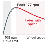
Phase-short braking peaks at 177.3 rpm, above the base’s 107.7 rpm limit.

Industrial machine stop categories and drive safety functions sequence these states. The machinery standard defines three stop categories (International Electrotechnical Commission 2016a): remove power at once, stop under control and then remove power, or stop under control and keep power applied. Each category still requires specific physical evidence before a safety case can credit it (Stop functions and physical response). Beneath every category lies one physical fact. Once torque is removed, a joint enters one of the three unpowered states above. A drive’s Safe Torque Off (STO) therefore leaves a moving joint in free coast until a brake engages. The trajectory a machine follows after an electrical cutoff must be measured under full mechanical payload, not deduced from circuit diagrams. The choice of which safe fallback state the machine should enter belongs to system safety architecture, but the physical dynamics of an unpowered joint are unalterable mechanical constraints of the body.

↪ The placement of Safe Torque Off in the machine’s hardwired interlock is developed in Actuation Authority.

2.6.3 Regenerative overvoltage surges and dynamic brake choppers

Regenerative deceleration drives the bus toward its opposite boundary, overvoltage, as part of the machine’s kinetic energy returns electrically. Returned braking energy needs an absorption or dissipation path, and a battery cannot be assumed to accept it under every state of charge, temperature, or protection state. If the battery management system disconnects charge input, the remaining bus components must handle the regenerated energy without exceeding their voltage ratings.

Under the conservative assumption that the battery management system has disconnected and the local bus capacitance \(\DcBusBulkCapacitance\) must absorb the entire returned kinetic energy \(\RegeneratedBrakingEnergy\) without dissipation, the terminal DC bus voltage rises to: \[\FinalBusVoltage = \sqrt{\InitialBusVoltage^2 + \frac{2 \RegeneratedBrakingEnergy}{\DcBusBulkCapacitance}} \tag{10}\] where \(\InitialBusVoltage\) is the bus voltage when deceleration begins (DC Bus Power Distribution and Energy Absorption derives this energy balance). The worst case is a full pack, the state in which the battery management system refuses further charge.

The capacitor-only endpoint is a screening calculation: if it exceeds a component rating, the stop requires another energy path. A dynamic brake chopper switches an absorption resistor across the bus when voltage reaches a chosen clamp threshold. Its resistor must handle both the peak regenerated power and the pulse energy, with enough recovery between stops. The worked bus calculation below sizes the peak-power requirement for the warehouse machine.

Power integrity is an architectural constraint. The design sets coordinated power budgets and current slew-rate limits across accelerators and drives. The permission path arbitrates simultaneous multi-axis accelerations so that their \(d\ConductorCurrent/d\TimeInstant\) transients do not compound. Brake choppers protect the inverters from regenerative feedback during emergency stops. Notebook 2.7 works both halves of that budget, the bus’s sag and the stop’s regenerative surge, on the mobile manipulator’s 48 V drive bus.

Napkin Math 2.7: DC bus voltage sag and regenerative surge

The mobile manipulator’s lithium-ion pack feeds a 47.7 V nominal drive bus, with the voltage envelope of a commercial 48 V-class mobile robot’s pack (Mobile Industrial Robots 2025). The bus carries the wheel drives, the arm’s joint drives, and a 48-to-24 V converter that supplies the application processor and control electronics. The converter shuts off when its input falls to 33 V (MEAN WELL 2026).

Problem: Under the coincident current step of an inference burst and the drive motors, and then a stop from the drive limit, does the bus remain within the operating limits of the converter and the motor inverters?

Math:

1. Parameters:
   • Machine mass, travel speed, and credible deceleration: \(\Mass =\) 368 kg (upper bound, full tote rack), \(\SpeedAtDetection =\) 1.5 m/s, \(\CredibleBrakingDeceleration =\) 2 m/s²
   • Bus characteristics: pack voltage from 54 V at full charge to 42 V depleted, source resistance \(\PowerRailResistance =\) 60 mΩ (illustrative), bulk link capacitance \(\DcBusBulkCapacitance =\) 22,000 μF
   • Operating limits: converter lockout \(\ConverterLockoutVoltage =\) 33 V, converter continuous input maximum 67.2 V, inverter switch rating \(\SwitchBreakdownVoltage =\) 100 V
2. Sustained-load screen:
   • As an illustrative coincident load, the two drive motors and the arm’s joint drives add 68.6 A while the application processor, drawing its 60 W thermal design power (TDP) through the converter at 91 percent efficiency, adds 1.4 A. Their aggregate increase is \(\FiniteChange \ConductorCurrent =\) 70 A. Assume the stated pack voltage is the unloaded source voltage and this coincident demand is the total load in the screen.
   • After source current settles to the increased load, the additional resistive drop is: \[\Delta V_{\text{sustained}} = \Delta I R_{\text{bus}} = 4.2 V\]
   • The resulting sustained bus voltage at full charge and when depleted is: \[V_{\text{bus, sustained}} = 54 V - 4.2 V = 49.8 V \text{ (full)}, \quad 42 V - 4.2 V = 37.8 V \text{ (depleted)}\]
   • Even from the depleted pack, the bus stays 4.8 V above the converter’s lockout; it would take a 150 A step to spend the 9 V between the depleted pack and the lockout. This screen does not establish the transient minimum, which inductance and capacitor depletion push lower.
3. Regenerative surge:
   • During a stop from the drive limit, the loaded machine’s kinetic energy must be dissipated: \[E_k = \tfrac{1}{2} m v^2 = \tfrac{1}{2}\,(368 kg)(1.5 m/s)^2 = 414 J\]
   • A full pack is the worst case, because that is when the battery management system refuses charge. If it disconnects charge input and an illustrative 75 percent of kinetic energy returns to the bus (\(\RegeneratedBrakingEnergy =\) 310.5 J), an unprotected, lossless capacitor-only energy balance would end at: \[V_{\text{final}} = \sqrt{V_{\text{full}}^2 + \frac{2 E_{\text{regen}}}{C_{\text{bus}}}} \approx 176.5 V\]
   • Failure mechanism: Raising the capacitor from full charge to the 60 V clamp absorbs only 7.5 J of the 310.5 J, so long before the bus reached that endpoint it would cross the converter’s input maximum and then the 100 V switch rating.
4. Dynamic braking clamp:
   • Under constant deceleration over \(\StoppingDuration =\) 750 ms, speed falls linearly, so the regenerated power, force times speed, falls linearly from its peak to zero. The peak is twice the average \(\RegeneratedBrakingEnergy/\StoppingDuration\): \[P_{\text{regen, peak}} \approx \frac{2 E_{\text{regen}}}{t_{\text{stop}}} = 828 W\]
   • The clamp \(\ChopperClampVoltage =\) 60 V sits above the full-charge voltage, so it never fires while charging, and within the converter’s input range. To hold it there, the brake chopper must divert this peak power through an absorption resistor. A resistor across the bus at the clamp voltage dissipates \(\ChopperClampVoltage^2/\BrakeChopperResistance\), which must be at least the peak power: \[R_{\text{brake}} \le \frac{V_{\text{clamp}}^2}{P_{\text{regen, peak}}} \approx 4.35 Ω\]

Result: The sustained-load screen leaves the bus at 49.8 V from a full pack and 37.8 V from a depleted one, 4.8 V above the converter lockout. Unbuffered regenerative braking would drive the bus past the converter’s input maximum and the 100 V switch rating, which calls for a dynamic brake chopper whose resistor is no larger than 4.35 Ω and absorbs an 828 W peak (satisfied by an illustrative 3.9 Ω, 1 kW component).

Systems insight: Mechanical motion and electrical power are bidirectionally coupled. Acceleration requires a supply that sustains the coincident current demand; deceleration requires an adequate absorption or dissipation path. On this 48 V bus the depleted pack still sits 9 V above the converter lockout, more than twice this step’s resistive drop, so the sustained screen passes. The transient minimum, pulse energy, repetition, cooling, and component tolerances still require qualification.

MEAN WELL. 2026. DDR-240 Series 240 W DIN Rail Type DC-DC Converter Specification. Product datasheet.

Mobile Industrial Robots. 2025. MiR250 Specifications. Product specification.

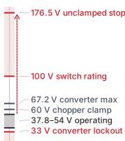
The bus must stay between the 33 V lockout and the clamp; an unclamped stop reaches 176.5 V.

Checkpoint 2.2: Freshness, stopping, heat, and supply

The actuator budget was checked in checkpoint 2.1. Before measuring these limits on an assembled machine, verify your understanding of the other four:

• Freshness deadline: Can you calculate the maximum allowable measurement age for the mug riding the pick-station conveyor at 0.20 m/s, with a 15 mm grasp tolerance of which the initial estimate already spends 3 mm? Can you explain why that age is counted from exposure on the sensor rather than from the start of inference, and why the base’s stop for a standing person instead charges age as blind travel?
• Velocity ceiling: Can you solve \(\StoppingDistance \le \ClearDistance\) for the admissible speed on the running machine’s numbers, and explain why doubling the pre-brake delay expands the stopping distance linearly while doubling travel speed expands the braking term quadratically?
• Thermal horizons and runaway: Can you explain why an actuator can produce three times its rated torque for seconds but overheats its winding insulation if held there for minutes, and distinguish a sustained stall that reaches an excessive finite equilibrium from one in which copper’s resistance feedback causes thermal runaway?
• Rail sag and regeneration: Can you explain how a coincident compute and drive current step sags a shared rail through resistance, inductance, and capacitor depletion, and why a stop from speed pumps energy back into the bus that a brake chopper must divert?

Preserving power integrity ensures that transient acceleration spikes do not trigger brownout resets and that regenerative braking does not overvoltage the bus, completing the analytical formulation of the five physical budgets. Calculating these envelopes from datasheets and circuit models, however, cannot guarantee operational safety on a physical robot. In deployment, source impedances rise as batteries age, contact friction varies across facility floors, and enclosed packaging degrades thermal dissipation. Defending these budgets in production requires measuring what the integrated hardware actually delivers under live operational stress.

2.7 Measuring a Machine’s Own Limits

A brake that stops an unloaded base on a cool laboratory floor has not established how the loaded mobile manipulator stops after repeated maneuvers. Characterization must connect each calculation to measurements under the conditions in which the machine will use it. A dynamometer, a test stand that applies a controlled mechanical load, isolates actuator behavior, just as the instrumented propulsion test stand in figure 7 evaluates an assembled electromechanical powertrain under live aerodynamic and structural loads. Integrated trials then establish what changes when the actuator shares a chassis, cooling path, and power supply with the rest of the machine. A defensible limit states what was measured, how uncertain the result is, and which conditions must remain true for a later decision to rely on it.

2.7.1 Dynamometer testing and instrument intrusion

On a dynamometer, a controlled load machine resists the actuator while torque, speed, current, and voltage are measured on a shared timebase. Four tests connect the earlier models to measurable parameters:

• Torque and back-EMF transduction (\(\MotorTorqueConstant\) and \(\MotorBackEmfConstant\)): By commanding the inverter’s Field-Oriented Control (FOC) current loop across a sweep of quadrature phase currents \(\TorqueProducingCurrent\) while the dynamometer absorbs torque at constant speed, engineers measure electromechanical torque transduction: \[\MotorTorque = \MotorTorqueConstant \TorqueProducingCurrent\] Driving the unpowered motor at known speed and measuring open-circuit voltage supplies the corresponding back-EMF constant \(\MotorBackEmfConstant = \BackEmfVoltage / \RotorAngularSpeed\). These tests establish the conversion factors used in section 2.4.2.

• Electrical rise time and inductive bandwidth (\(\ElectricalTimeConstant = \PhaseInductance/\PhaseResistance\)): With the rotor held so that the test current produces no torque, the inverter applies a small voltage step \(\StepTestVoltage\) across the winding. The current response: \[\InstantaneousPhaseCurrent(\TimeInstant) = \frac{\StepTestVoltage}{\PhaseResistance}\left(1 - e^{-\TimeInstant/\ElectricalTimeConstant}\right)\] reveals the electrical time constant. The step must stay small, because its steady current \(\StepTestVoltage/\PhaseResistance\) flows through a winding of low resistance: the full 42 V of a depleted pack across a hub motor’s 0.7 Ω would drive 60 A, 2.4× the motor’s peak current. The current probe and acquisition path must resolve the rise; otherwise the instrument smooths the response being measured and hides the actuator limit.

• Enclosed thermal resistance (\(\ThermalResistance\)) and continuous torque ceilings: A heating trial under the installed cooling conditions measures the winding temperature rise and loss power, establishing \(\ThermalResistance = \JouleanTemperatureRise / \WindingLossPower\). The continuous torque ceiling from section 2.5.1 is then: \[\ContinuousTorque = \MotorTorqueConstant \sqrt{\frac{\WindingTemperatureLimit - \AmbientTemperature}{\ElectricalResistance(\WindingTemperatureLimit) \ThermalResistance}}\] The test must reproduce the enclosure and neighboring heat loads under which that ceiling will be used. An open-bench rating overstates continuous capacity whenever the installed shroud restricts airflow or adjacent actuators warm the mounting frame.

• Backdrive friction and impact dynamics: By driving the actuator output shaft with the dynamometer load motor, the testbed measures the torque needed to backdrive the joint across speed, load, and temperature: \[\ExternalJointTorque = \GearReductionRatio^2 \RotorInertia \JointAcceleration + \JointFrictionTorque\] The measured response establishes whether the transmission can yield under the intended external load and maps the friction term that section 2.4.5 shows is not a constant. Contact qualification must additionally exercise the relevant compliance and impact conditions. The backdrive model alone does not predict tooth failure.

Figure 7: An instrumented propulsion test stand: An electric motor with its propeller, speed controller, and wiring secured at the top of the Airvolt test stand at the NASA Armstrong Flight Research Center in 2016, instrumented to collect data on the propulsion system under load. A stand like this measures what a data sheet only asserts, on the assembled drive under stated conditions. (Credit: Lauren Hughes, NASA Armstrong Flight Research Center, AFRC2016-0100-05, public domain.)

Measurement can change the plant. A series current shunt lowers the supplied voltage, and an embedded temperature probe changes a local heat-flow path. These effects belong in the uncertainty budget along with sensor resolution, bandwidth, and clock alignment.

The sensor mechanisms in section 2.2.1 also affect characterization. Velocity estimated from encoder samples by backward differencing trades resolution against latency, and that trade-off must enter the reported uncertainty and response time. Vibration above the sensor’s sampled bandwidth can likewise appear as slower motion: \[\AliasedVibrationFrequency = |\VibrationFrequency - \AliasingHarmonicIndex \SamplingRate|\] The integer \(\AliasingHarmonicIndex\) identifies the sampling-frequency multiple that folds the vibration into the observed band. Qualification must distinguish that measurement artifact from the motion used to establish the limit.

A limit means nothing without the context of its test. Every recorded limit states the payload, ambient temperature, supply voltage, enclosure state, firmware version, and concurrent computational workload of the run. A thermal time constant measured on an open bench does not transfer to the same actuator in a sealed fairing in sunlight, because enclosing the motor raises \(\ThermalResistance\) and with it \(\ThermalTimeConstant = \ThermalResistance \StatorThermalCapacitance\). The hotter ambient also shrinks the margin below the insulation rating. A rail characterization that omits whether vision-language model inference (Brohan, Brown, Carbajal, Chebotar, Dabis, et al. 2023; Brohan, Brown, Carbajal, Chebotar, Chen, et al. 2023) was running during motor stalls describes an idle board rather than the combined draw of full compute and peak torque.

Brohan, Anthony, Noah Brown, Justice Carbajal, Yevgen Chebotar, Joseph Dabis, Chelsea Finn, Keerthana Gopalakrishnan, et al. 2023. “RT-1: Robotics Transformer for Real-World Control at Scale.” Robotics: Science and Systems (RSS). https://doi.org/10.15607/RSS.2023.XIX.025.

Brohan, Anthony, Noah Brown, Justice Carbajal, Yevgen Chebotar, Xi Chen, Krzysztof Choromanski, Tianli Ding, et al. 2023. “RT-2: Vision-Language-Action Models Transfer Web Knowledge to Robotic Control.” arXiv Preprint arXiv:2307.15818.

2.7.2 Zero-failure bounds and wear over life

The absence of a failure during testing bounds the failure rate statistically; it does not establish safety. If the mobile manipulator completes \(\ZeroFailureTrialCount =\) 3,000 loaded stops without a brownout or an overrun, the data support only a per-stop failure rate below roughly \(3/\ZeroFailureTrialCount\), the rule of three, which is about one stop in 1,000 at 95 percent confidence. The bound holds only if the trials are independent and stationary, so that one trial does not influence another and the failure probability stays the same from trial to trial.

↪ The rule of three, and the trial campaigns it sizes, is developed in Confidence from a Finite Campaign.

Thermal history and wear can change the conditions between trials:

• Heating across consecutive trials: Repeated stops heat the windings, changing resistance and the available torque response. Trials taken at different starting temperatures do not characterize the same operating condition.
• Rising battery resistance over life: Battery aging increases source resistance, reducing the voltage margin under a current step.
• Growing gearbox backlash: Transmission wear changes reversal response and tracking error, invalidating a limit measured on a less worn assembly.

These changes make characterization a standing obligation. Lifecycle degradation changes the conditions behind a limit, so its record must identify when recalibration or a reduced operating envelope is required.

2.7.3 The six elements of a limit record

The stopping and power calculations become usable by other layers only when their assumptions travel with their values. A limit record carries those assumptions together with the evidence that supports the limit. The learned proposer uses the limits to constrain candidate actions, while the independent permission path checks them before actuation. Recording a value does not certify it: the illustrative entries below still require measurements and uncertainty estimates before they can support operation. The six elements in table 3 make that missing evidence visible for the mobile manipulator’s credible deceleration, the drive torque ceiling that must support it, and the drive bus’s undervoltage lockout.

↪ The handoff record that carries each limit record to the permission path is developed in The Handoffs Matrix.

Two of the elements are easily conflated. Uncertainty describes what is not known about the measurement (observation noise, instrument tolerance, sensor bandwidth, and calibration drift). Margin is the physical clearance the machine defends against what is not known. The provenance element then says how far the value itself can be trusted, by naming its evidence category. Every number that governs a machine falls in one of five categories: a direct measurement, a value derived from measurements through a stated model, a datasheet rating, an illustrative example, or a budget the designer chose. Only the first two can support a safety margin or a timeout. A value computed from datasheet inputs, such as the drive torque ceiling below, keeps the datasheet’s weaker standing until measurements replace its inputs. A chosen budget, such as the protective clearance \(\ProtectiveClearanceMargin\), binds only once it is checked against the measured number it must fit.

Table 3: The limit record on the mobile manipulator: The six elements of a limit record, filled in for the credible deceleration that sets the stopping distance, for the drive torque ceiling that must support it, and for the converter lockout that bounds the shared drive bus. None of the three yet has samples or an established uncertainty, and the provenance element names the measurement that would replace each.

Element	What the record states	Credible deceleration \(\CredibleBrakingDeceleration\)	Drive torque ceiling	Drive-bus converter lockout
Value	The value or empirical distribution, with its sample count and the tail percentiles it reports	2 m/s², taken as the credible low tail of loaded stops; no samples yet	At least 2.33 m/s² from 60 N·m per wheel; computed from datasheet values, no samples yet	33 V at the 48-to-24 V converter input; no samples on the assembled bus
Conditions	The context listed earlier under which it was established, plus the surface for any limit that depends on traction	Loaded to at most 368 kg; \(\CoulombFrictionCoefficient\,\DrivenWheelLoadFraction \ge\) 0.204, so \(\CoulombFrictionCoefficient \ge\) 0.250 at the hub motors’ rated load share and never on the inspected floor (\(\CoulombFrictionCoefficient =\) 0.12); tip-over geometry not yet measured; usable powered braking and energy absorption; tires at commissioning wear	Drive current limit at 25 A; both driven wheels in traction; rotating mass within the 9.5 kg per-wheel bound; windings and bus within their rated ranges	Sustained coincident load on the 48 V bus; the permission path isolated on its held-up rail; drive power and physical stopping behavior require separate qualification
Uncertainty	The measurement uncertainty of each instrument, with its observation point and bandwidth	Not established	Datasheet tolerances only; the torque constant’s tolerance is not published	Not established
Margin	The engineering margin separating the operating target from the breakdown threshold	No justified deceleration margin yet; the chosen 100 mm protective clearance must be checked against the eventual uncertainty bound	At least 16.6% above \(\CredibleBrakingDeceleration\); none if the current limit falls to the rated 8.5 A	4.8 V from a depleted pack under sustained coincident load; transient minimum not established
Detector	The runtime check that catches an excursion while the machine runs, such as a phase-current sensor, an optical interrupter, or a supply-rail monitor	Deceleration monitor comparing commanded with measured deceleration from the wheel encoders and the Bosch BMI088 inertial unit, on every stop	Drive saturation flag and measured phase current against the configured limit, read on every stop	Bus-voltage monitor flags undervoltage; the permission path selects a response whose power and mechanical premises still hold
Provenance	The evidence category and the instrument or model that produced the value	Illustrative, from the base’s class profile; to be replaced by loaded stopping trials	Datasheet standing: computed from the hub motor’s datasheet values; to be replaced by wheel-torque measurements at the current limit on a loaded braking trial	Converter datasheet; source resistance illustrative; to be replaced by a bus characterization under coincident load

The detector element matters most once the machine leaves the test stand, because operation can carry a limit outside the conditions under which it was established. The saturation duration against which the Schiaparelli lander’s inertial unit had been accepted was such a limit. The lander’s loss in 2016 shows what follows when a limit’s conditions are exceeded in operation and nothing downstream checks the result.

War Story 2.1: ExoMars Schiaparelli IMU saturation (2016)

Context: On October 19, 2016, the European Space Agency’s ExoMars Schiaparelli lander executed its atmospheric entry and descent toward the Martian surface, relying on an onboard Guidance, Navigation, and Control (GNC) computer to fuse Inertial Measurement Unit (IMU) gyroscopes with a Doppler radar altimeter (ESA Investigation Board 2017).

Mechanism: About three minutes after atmospheric entry, the parachute inflated and set the lander oscillating. The IMU measured a pitch rate larger than expected and raised a saturation flag, which persisted longer than the 15 ms assumed when the unit was accepted. While the flag was set, the GNC software integrated the saturation threshold rate as though it were the true rate, although the lander was in reality oscillating, and its attitude estimate drifted by about \(165^{\circ}\), nearly upside down. When the radar altimeter later returned valid slant ranges, the software projected them onto that attitude and computed a negative altitude. No onboard check tested that altitude for plausibility.

Impact: Taking the negative altitude as a valid estimate, the guidance logic released the parachute and backshell, fired the braking thrusters for \(3\text{ seconds}\) instead of the planned \(30\text{ seconds}\), and activated its on-ground systems as if it had landed. The lander was still about \(3.7\text{ km}\) above the surface. It fell freely for about half a minute and struck the ground at about \(150\text{ m/s}\) (\(540\text{ km/h}\)).

Response: The ESA inquiry board recommended robust sanity checks in the onboard software, among them that altitude cannot be negative and cannot change from \(3.7\text{ km}\) to a negative value in one second, and a design that handles IMU saturation explicitly, for example by inhibiting IMU inputs during parachute deployment.

Systems lesson: A physical body cannot transcend the saturation ranges of its sensory transducers. When a sensor’s physical limit (a gyroscope’s rate ceiling or an accelerometer’s dynamic range) is exceeded, a state estimator that integrates the saturated measurement as if it were valid drifts away from the physical state. The saturation duration against which the IMU had been accepted was a limit with conditions, and once descent exceeded them, no detector checked the estimate before it commanded an irreversible action.

ESA Investigation Board. 2017. ExoMars 2016 - Schiaparelli Anomaly Inquiry. European Space Agency.

Checkpoint 2.3: Limit records

A limit governs a decision only together with the conditions, evidence, and detector that travel with it.

• Uncertainty vs. margin: Can you distinguish the uncertainty of a measured deceleration from the margin the machine defends, and explain why only a measured value, or one derived from measurements, can support that margin?
• Zero-failure bound: Can you estimate how many failure-free loaded stops would bound the per-stop failure rate below one in 10,000 at 95 percent confidence, and state the two assumptions about the trials that the bound requires?
• Record conditions: Can you name the condition of the credible-deceleration record that a lowered drive current limit, the inspected floor, and an arm extended forward would each violate?
• Detector: Can you explain why the Schiaparelli lander’s accepted saturation duration failed as a limit in flight, and which detector in table 3 plays the missing role for the credible deceleration?

Measured and recorded one at a time, the five limits describe the body budget by budget, each under its own conditions. In operation, however, a single maneuver draws on all five budgets at once, and a change in one budget’s state can erode the margin of another. Which limit binds first therefore depends on both the machine’s physical class and the specific command under evaluation.

2.8 Which Physical Budget Binds First

A single command from an action-chunking policy to accelerate a loaded mobile manipulator draws concurrently against all five physical budgets, which is why the simultaneous admission invariant of section 2.1 admits it only when every margin is non-negative at once. The command executes against a camera frame that has already aged during neural inference, so that age enters the pre-brake delay. At the same time, the acceleration injects kinetic energy into the chassis, which friction brakes or regenerative drives must eventually dissipate. Generating that motion forces the arm’s geared joints to accelerate reflected rotor inertia, while the base’s direct-drive hubs add their rotating inertia to the stopping load. The phase currents that produce those torques dump resistive Joule heat into stator windings, which shed thermal energy only over minutes. The same currents pull transient current from the shared DC rail that powers the onboard compute host. Each of the five budgets pairs a governing physical law against the software assumption it invalidates, exposing a characteristic vulnerability by machine class and demanding a hardware-enforced runtime invariant (table 4).

2.8.1 Which budget binds in each machine class

A mobile manipulator integrates two of the machine classes from Three Machine Classes onto a single chassis: a Class 1 wheeled base governed primarily by chassis momentum and stopping distance, and a Class 2 articulated arm constrained by reflected rotor inertia, contact compliance, and static holding heat. While the classes identify the primary vulnerabilities, the instantaneous maneuver determines which budget binds first. For instance, holding a heavy payload in a cantilevered pose can drive joint windings toward their thermal dissipation limit over tens of seconds. Conversely, a sudden multi-axis acceleration burst coupled with full neural network execution can deplete electrical bus margins within milliseconds. The coupled calculations below compare the evidence behind the running machine’s limits and identify a stopping qualification priority. They do not establish an ordering of all five physical margins for an unspecified maneuver.

Table 4: Cross-class physical constraint matrix: The five budgets, the law that governs each, the assumption a software-trained policy makes about it, the class characteristically vulnerable, and the runtime invariant that answers it.

Physical Budget / Factor	Governing First Principle & Scaling Law	Software Illusion vs. Hardware Ground Truth	Characteristic Vulnerability by Class	Systems Architect Takeaway & Runtime Invariant
1. Measurement Freshness & Age	\(\TelemetryFreshnessBound \le \frac{\PositionErrorCeiling}{\SpeedBound}\); \(\QuantizationStep \EncoderAngle = \frac{2\pi}{2^\EncoderBitCount}\); end-to-end age measured from exposure	Illusion: High inference rate (\(50\text{ Hz}\)) guarantees real-time control. Truth: Age begins at exposure; encoder differentiation amplifies quantization noise; vibration harmonics alias into IMU attitude drift.	Class 1 & 2: Erodes clearance margins and destabilizes high-gain contact loops.	Tag frames with hardware timestamps; enforce \(\ObservationAge \le\) the budgeted age at motor registers; drop stale commands.
2. Momentum & Stopping Distance	\(\StoppingDistance = \SpeedAtDetection\,\PrebrakeDelay + \frac{\SpeedAtDetection^2}{2 \CredibleBrakingDeceleration} + \LocalizationBound + \ProtectiveClearanceMargin \le \ClearDistance\); \(\EffectiveImpactMass = \Mass + \sum_i \frac{{\GearReductionRatio}_i^2 {\RotorInertia}_i}{\WheelRadius^2}\)	Illusion: Deceleration can be commanded instantaneously. Truth: Braking distance scales quadratically (\(\SpeedAtDetection^2\)); retarding torque must decelerate reflected rotor inertia; the stopping system must absorb or dissipate energy.	Class 1 (Mobility): Primary constraint. Doubling speed quadruples the braking term.	Solve clearance quadratic \(\SpeedBound(\ClearDistance, \PrebrakeDelay)\) on the safety microcontroller at the rate the stopping budget sets; clamp policy velocity.
3. Actuator & Reflected Inertia	\(\ReflectedRotorInertia = \GearReductionRatio^2 \RotorInertia\); \(\MotorTorque = \MotorTorqueConstant \TorqueProducingCurrent\); \(\ElectricalTimeConstant = \frac{\PhaseInductance}{\PhaseResistance}\); \(\frac{\DerivativeOperator\MotorTorque}{d\TimeInstant} \le \frac{\MotorTorqueConstant(\DcBusVoltage - \BackEmfVoltage)}{\PhaseInductance}\)	Illusion: Motor torque tracks policy tensors instantaneously. Truth: Current rise limits response; gearboxes square rotor inertia (\(\GearReductionRatio^2\)); high ratios increase resistance to rapid contact motion.	Class 2 (Manipulation): Contact stiffness and reflected inertia constrain interaction.	Limit acceleration and torque slew; measure load-side response; select gearing and compliance for the qualified contact envelope.
4. Thermal Limits & Duty Cycle	\(\StatorThermalCapacitance \frac{d\WindingTemperature}{d\TimeInstant} = \frac{\MotorTorque^2}{\MotorTorqueConstant^2} \ElectricalResistance(\WindingTemperature) - \frac{\JouleanTemperatureRise}{\ThermalResistance}\); \(\ContinuousTorque = \MotorTorqueConstant \sqrt{\frac{\WindingTemperatureLimit - \AmbientTemperature}{\ElectricalResistance(\WindingTemperatureLimit) \ThermalResistance}}\)	Illusion: Motors deliver catalog peak torque continuously. Truth: Torque is current, current is heat (\(\WindingLossPower \propto \MotorTorque^2\)); continuous torque is limited by heat rejection at the characterized winding-temperature limit \(\WindingTemperatureLimit\).	Class 3 (Thermal) & Class 2: Holding above the qualified continuous torque can overheat the windings.	Run discrete \(\WindingCurrent^2 \TimeInstant\) thermal observers on the safety microcontroller; dynamically derate speed and torque when hotspot models approach limits.
5. Electrical Power Integrity	\(\SourceVoltage-\DcBusVoltage=\PowerRailResistance{}\SourceCurrent+\PowerRailInductance\frac{d\SourceCurrent}{d\TimeInstant}\); \(\DcBusBulkCapacitance\frac{d\DcBusVoltage}{d\TimeInstant}=\SourceCurrent-\LoadCurrent\); \(\FinalBusVoltage = \sqrt{\InitialBusVoltage^2 + \frac{2 \RegeneratedBrakingEnergy}{\DcBusBulkCapacitance}}\)	Illusion: Power rails act as infinite, ideal voltage sources. Truth: Bus impedance collapses rail voltage under combined compute+motor bursts; braking surges overvoltage.	Class 1 & 3: Peak multi-axis acceleration trips microcontroller brownout resets; regen surges destroy inverter FETs.	Enforce coordinated compute-actuation power budgets and \(d\SourceCurrent/d\TimeInstant\) limits; install dynamic brake choppers; characterize unpowered fallbacks.

2.8.2 Cross-budget coupling and permission rail isolation

When an autonomous agent commands an aggressive multi-axis acceleration, the physical margins do not degrade in isolation. They deplete together. Drive inverters draw substantial current to overcome both chassis inertia and reflected rotor inertia. This transient current surge causes the shared DC bus voltage to sag, even as resistive losses (\(\WindingLossPower = \TorqueProducingCurrent^2 \EffectiveLossResistance\)) steadily deposit thermal energy into motor windings. Because motor phase currents are pulse-width modulated by inverters and do not map directly to battery draw, systems architects must evaluate input current at the primary DC bus. This coincident load step establishes the true operating baseline across all subsystems.

On the 48 V drive bus, the sustained electrical screen passes under its stated assumptions. As shown in the coincident power step of notebook 2.7, a depleted battery pack at 42 V sags to 37.8 V under the coincident load step. Even under that sustained step, the rail keeps a 4.8 V buffer above the 33 V undervoltage lockout (UVLO) threshold of the 48-to-24 V converter, although the sustained screen does not establish the transient minimum.

The stopping dynamics expose a concrete qualification priority. Under emergency braking, the drive motors clear the required deceleration by only 16.6 percent, and only with phase current at the motor’s catalog peak. The chassis tip-over boundary has not been measured at all. For the arm, the optimistic stand-in thermal model gives a heat-soaked joint a threefold current burst of 43.1 s before its winding reaches the insulation rating. Additionally, the chassis stopping distance at the full 1.5 m/s travel limit leaves 357.5 mm of clearance to accommodate perception latency, communication jitter, and tracking variance. The whole stopping budget inherits the credible-deceleration premise, which rests on the peak current limit and the unmeasured center of gravity, so that premise requires qualification before relying on the stop. The transient rail minimum and installed arm thermal response remain unresolved too. Ranking the budgets requires a specified maneuver and duration, with comparably qualified limits for each.

Modern SoC architectures deploy dynamic voltage and frequency scaling (DVFS) algorithms to regulate die temperature and energy consumption. While DVFS protects silicon from thermal degradation, its timing penalties propagate directly into physical workspace clearance: \[\text{SoC thermal dissipation} \longrightarrow \text{DVFS clock throttling} \longrightarrow \text{vision latency stretch} \longrightarrow \text{observation age inflation} \longrightarrow \text{pre-brake travel expansion} \longrightarrow \text{clearance margin erosion}\] When sustained motor currents and high-throughput perception pipelines elevate temperatures across the shared enclosure, the host kernel throttles the clock frequencies of onboard CPU and GPU accelerators. On the running machine, this thermal intervention stretches the navigation backbone that the stopping budget charges, not the grasp path of table 1, from 22 ms to 33 ms. This delay adds 11 ms directly to the end-to-end observation age \(\ObservationAge\), inflating the pre-braking reaction time \(\PrebrakeDelay\). When traveling at the maximum base velocity of 1.5 m/s, this algorithmic latency injects 16.5 mm of unmonitored chassis travel before emergency brakes can even begin mechanical engagement. In this manner, a standard operating-system power policy designed for digital silicon silently shrinks the robot’s stopping margin.

↪ Thermal clock throttling on the shared die, and the placement decisions that bound its effect on the safety path, are developed in Thermal and Timing Coupling.

Surviving a sustained bus voltage drop does not qualify the shared power rail to support safety-critical control channels. Transient dips during motor reversals remain difficult to bound completely, and electrical faults such as an open circuit breaker, a battery management system (BMS) overcurrent disconnect, or a blown DC-DC stage drop bus voltage to zero instantly. The running machine addresses these common supply faults with a dual-rail architecture that decouples motor dynamics from safety enforcement. In this design, the primary shared bus powers high-current traction inverters and steps down voltage for the primary application processor. An isolated, reverse-blocked permission rail separately powers the safety microcontroller, deterministic fieldbus transceivers, and holding-brake release coils. Under the drive-rail faults covered by its isolation and hold-up qualification, this separate supply preserves the permission loads. It does not make the detector, controller, or communication path infallible.

The permission rail incorporates local capacitive energy storage to preserve control availability during a loss of its upstream supply. For the stated constant 70 W permission load, ideal energy sizing gives an onboard 2.025 F supercapacitor bank 140 J of usable energy between its minimum nominal charge voltage (21.5 V) and regulator dropout (18 V), targeting 2 s of hold-up. Establishing a minimum available duration requires qualification of initial charge, capacitance tolerance and aging, conversion losses, equivalent series resistance, current demand, and regulator behavior. The 750 ms stop from the drive limit plus the 80 ms slow end of spring-brake engagement is a comparison for the powered stopping model only. Total main-battery failure does not establish that this model remains available. The qualified control interval must cover detection and decision, the duration of the response available under the fault, and brake engagement when those stages are sequential, or their actual sequence when they overlap. The Fallback Ladder checks the hold-up against the longest stop its fallback ladder commands.

Under the qualified rail and intact detector and controller assumptions, maintaining permission-rail power preserves the opportunity to detect power loss and initiate a response, but it does not supply the mechanical energy or high-current paths necessary for controlled regenerative braking. A controlled, powered stop requires intact inverter switching, sufficient bus voltage, and an operational energy dump, such as a dynamic brake chopper or a regenerative battery sink, to absorb kinetic deceleration energy. When a catastrophic power fault removes the supply or absorption path needed for a powered stop, that stopping model no longer applies. Under such conditions, stopping distances must be governed by the unpowered physical fallbacks analyzed in section 2.6.2. A held-up permission rail does not change what the mechanical brakes deliver. Powering their release coils from that rail lets the permission logic choose when the spring brakes engage, but it does not give them the deceleration of a powered drive stop. Systems architects must treat stopping performance as conditional: isolate the safety supervisory rail, and then characterize the exact deceleration capabilities that remain active across every distinct electrical fault state. Downstream runtime enforcement and hardware qualification must preserve these underlying electrical premises.

2.9 Fallacies and Pitfalls

Physical limits rarely respect subsystem boundaries. In embodied machine learning systems, an architecture whose individual component budgets balance cleanly on paper can fail catastrophically when thermal rise, bus latency, power supply sag, and mechanical dynamics interact under compound operational load.

Fallacy: Model inference time defines the measurement freshness latency.

Consider an engineering team that compresses its vision backbone, cutting neural network inference time from \(30\text{ ms}\) to \(10\text{ ms}\). While this optimization provides a threefold compute speedup, the physical robot still executes actions based on visual state that traversed camera exposure, sensor readout, DMA transfers, and kernel queuing delays. Once the model outputs an action, that command must traverse a real-time network fieldbus before motor drive inverters can slew coil currents and produce physical force. A \(45\text{ ms}\) scheduling or transport jitter spike elsewhere along this pipeline eclipses the \(20\text{ ms}\) compute gain, consuming safety margins before the robot can react. Real-time control requires budgeting and bounding the worst-case tail of the entire capture-to-onset pipeline across synchronized hardware clocks, rather than certifying loop safety from isolated model benchmarks.

Architect’s countermeasure: Measure the true capture-to-onset latency tail on synchronized hardware clocks; never certify real-time safety from neural network inference benchmarks alone.

Fallacy: Software step commands deliver instantaneous physical torque.

Reinforcement learning policies trained in simulation routinely issue piecewise-constant torque or position setpoints at \(50\text{ Hz}\), implicitly assuming the physical actuator behaves as an ideal, memoryless force source. In physical reality, an electric drive is an electromechanical dynamic system governed by electromagnetic and inertial limits. Developing torque requires inner Field-Oriented Control (FOC) loops whose current rise rate is strictly bounded by stator winding electrical time constants (\(\ElectricalTimeConstant = \PhaseInductance/\PhaseResistance\)) and DC bus voltage headroom (\(\frac{\DerivativeOperator\MotorTorque}{d\TimeInstant} \le \frac{\MotorTorqueConstant(\DcBusVoltage - \BackEmfVoltage)}{\PhaseInductance}\)). Mechanically, a high-ratio gearhead amplifies rotor inertia quadratically (\(\ReflectedRotorInertia = \GearReductionRatio^2 \RotorInertia\)), imposing a steep low-pass filter on achievable link acceleration.

When a discrete tensor update demands an abrupt torque step, substantial electromagnetic effort is diverted into accelerating the spinning rotor rather than moving the external link. Transmission compliance and joint elasticity convert these high-frequency torque transients into structural vibration and limit-cycle oscillations. Simultaneously, repeated high-current corrections waste energy as resistive heat dissipation (\(\WindingLossPower = \frac{\MotorTorque^2}{\MotorTorqueConstant^2} \EffectiveLossResistance\)), rapidly burning through the actuator’s thermal margin. Systems architects must filter and shape setpoints against actual plant dynamics, validating commanded trajectories against delivered physical response rather than assuming numerical smoothness in software guarantees smooth physical execution.

Architect’s countermeasure: Bound acceleration and torque slew using measured actuator response, include electrical current rise and reflected inertia in the model, and qualify the chosen transmission and controller for the intended contact task.

Pitfall: Treating isolated component datasheets as operational system guarantees.

Hardware component datasheets report performance envelopes measured under idealized bench conditions. When a motion planner adopts a motor vendor’s continuous torque rating or an IMU vendor’s nominal noise floor as operational bounds, it ignores the harsh realities of system packaging. A motor catalog rating reflects vendor test benches (section 2.5), typically an open motor bolted to an enormous aluminum heatsink in still air at \(25\text{ }^\circ\text{C}\), not a sealed robotic joint housing tucked inside an unventilated composite limb on a chassis dissipating heat from a 60 W application processor.

In physical deployment, an actuator’s continuous torque is strictly constrained by steady-state heat dissipation up to the winding’s engineering ceiling \(\EngineeringTemperatureCeiling\), so the installed rating is equation 7 evaluated at the ceiling rather than the insulation rating: \[\ContinuousTorque = \MotorTorqueConstant \sqrt{\frac{\EngineeringTemperatureCeiling - \AmbientTemperature}{\ElectricalResistance(\EngineeringTemperatureCeiling) \ThermalResistance}}\] Given a 140 °C engineering ceiling, shifting the motor from the vendor’s 25 °C bench into the 40 °C interior of an enclosed chassis strips away 6.7 percent of continuous torque. Because thermal dissipation scales inversely with the square root of thermal resistance (\(1/\sqrt{\ThermalResistance}\)), eliminating forced convection and heatsink mass degrades capacity even further: doubling \(\ThermalResistance\) inside the arm housing cuts total usable continuous torque by 34.1 percent relative to the catalog rating. If trajectory planners treat catalog continuous torque as achievable duty, persistent copper losses (\(\WindingLossPower = \frac{\MotorTorque^2}{\MotorTorqueConstant^2} \EffectiveLossResistance\)) will exceed heat dissipation rates, triggering thermal cutouts or permanently degrading winding insulation.

Sensors suffer the same systemic degradation: inertial measurement units and optical encoders calibrated on quiet granite surface plates suffer severe vibration rectification, thermal drift, and mechanical aliasing once bolted near high-frequency switching inverters and planetary gearsets. System limits must reflect empirical measurements collected on the fully assembled machine under peak operational stress rather than pristine standalone datasheets.

Architect’s countermeasure: Calibrate actuator continuous torque ceilings and sensor noise profiles on fully assembled, enclosed hardware across the entire operational temperature envelope rather than copying open-bench catalog numbers into planner configuration files.

Pitfall: Treating dynamic voltage and frequency scaling (DVFS) as a transparent software optimization.

In server computing, DVFS operates as an invisible operating-system service that reduces clock frequency and core voltages to prevent silicon junction overtemperature. In an embodied system, however, DVFS directly degrades the real-time control contract. Consider a mobile manipulator whose high-current drive motors heat a shared structural chassis during intense maneuvering. As heat conducts into the compute bay, the application processor throttles its clock frequency to avoid thermal shutdown.

The system kernel treats clock throttling as an isolated power-management decision. However, a downclocked vision backbone adds observation age, and observation age at speed is unmodeled blind travel before the safety monitor can command braking. Section 2.8.2 prices that travel on the running machine. Although thermal throttling successfully shields the processor silicon, the vehicle’s dynamic stopping envelope silently expands beyond calibrated safety margins.

Architect’s countermeasure: Feed SoC thermal and clock-frequency telemetry directly into the motion safety monitor, dynamically derating maximum travel speed whenever compute throttling inflates perception age.

Pitfall: Scaling operational velocity without recalculating quadratic braking distances and thermal dissipation.

Facility operators frequently seek to increase robot throughput by raising maximum cruise velocity in software configurations. This operational change couples two punishing physical nonlinearities. First, the braking term grows with the square of speed, which is why Case 3 of figure 2 breaches the clear distance at 2 m/s.

Second, absorbing the kinetic energy of the faster machine demands large dynamic braking currents that dump heat directly into motor stator windings and drive electronics via Joule heating (\(\WindingLossPower = \TorqueProducingCurrent^2 \EffectiveLossResistance\)). An isolated emergency stop performed during commissioning may pass thermal checks when the machine starts cold. However, when an autonomous vehicle repeats that higher-speed duty cycle across an eight-hour shift, winding temperatures compound across successive maneuvers, rapidly outstripping the chassis thermal dissipation budget. System planners must treat operating velocity as a gated admission parameter: any commanded speed increase requires re-evaluating both the expanded quadratic stopping envelope and the cumulative multi-cycle thermal duty budget.

Architect’s countermeasure: Treat operating speed as an admission parameter that re-evaluates both quadratic stopping envelopes and multi-cycle thermal accumulation before granting velocity increases.

Fallacy: Compute accelerators and motor inverters operate on independent, ideal power rails.

Software architectures typically treat accelerator power consumption and motor drive power as decoupled subsystems, verifying each against isolated power supply ratings. In physical mobile machines, however, both systems draw from a shared, unregulated DC battery bus.

Consider a scenario where a heavy neural network vision burst coincides precisely with the drive motors accelerating to push the mobile base over an uneven threshold. On the shared 47.7 V electrical bus, this coincident current surge demands a combined 70 A step. Drawn through the 60 mΩ source resistance of cell, harness, and switch, this sudden draw induces a sustained 4.2 V voltage sag. That sag consumes nearly half of the 9 V voltage margin separating a depleted battery pack from the 33 V UVLO threshold of the application processor’s DC-DC converter, even before harness inductance and bulk capacitor discharge deepen the dynamic transient. A step of 150 A, or the identical current demand drawn from an aging or cold battery with sufficiently elevated internal impedance, reaches the UVLO threshold and can interrupt the primary processor’s supply.

If safety microcontrollers and brake solenoids share that unbuffered power rail, the resulting brownout crashes the safety supervisor simultaneously. The machine is plunged into the uncontrolled, unpowered fail states described in section 2.6 while carrying significant physical momentum, rather than executing an orderly, controlled deceleration. Software power budgets must acknowledge electrical coupling at the physical bus. System qualification demands testing coincident worst-case compute and motor loads at minimum battery state of charge, while ensuring safety permission logic and electro-mechanical brakes operate on an isolated, held-up power rail (section 2.8).

Architect’s countermeasure: Isolate the permission logic and brake releases, then qualify both their hold-up and the physical stopping response under coincident motor and compute load at minimum battery state of charge. A powered stop also requires the drive rail and energy-absorption path to remain usable.

Fallacy: Passing isolated single-variable bench tests guarantees physical survival under compound operational stress.

Development teams often qualify physical AI systems through single-variable stress testing: a robotic manipulator verifies maximum payload capacity inside a \(20^\circ\text{C}\) air-conditioned laboratory, then undergoes thermal validation inside a \(45^\circ\text{C}\) environmental chamber with an unloaded gripper. Neither benchmark, however, validates whether the manipulator can lift maximum payload in high ambient heat while operating from a depleted battery pack.

Physical failure modes couple nonlinearly across subsystem domains. Under simultaneous operational stress, manipulating maximum payload demands sustained high motor currents that dramatically increase resistive winding losses (\(\WindingLossPower = \TorqueProducingCurrent^2 \EffectiveLossResistance\)). An ambient temperature of \(45^\circ\text{C}\) severely compresses the thermal gradient required to reject that heat to the environment, accelerating stator insulation degradation. Concurrently, a low battery state of charge depresses DC bus voltage, stripping away the voltage headroom required to overcome motor back-EMF (\(\BackEmfVoltage\)) and severely degrading current slew rates (\(\frac{d\TorqueProducingCurrent}{d\TimeInstant}\)). An arm that moves smoothly in isolated tests may experience joint stall, severe tracking errors, or premature thermal shutdown under their compound interaction. Hardware and software qualification cannot rely on orthogonal single-variable test sweeps. Engineering teams must validate boundary envelopes on fully integrated machines subjected to simultaneous peak stresses across payload, thermal ambient, battery state of charge, and control frequency.

Architect’s countermeasure: Test boundary envelopes under worst-case simultaneous physical stress (maximum payload, elevated ambient temperature, depleted battery, and high-frequency actuation) to catch multi-budget coupling failures.

2.10 Summary

Every motion plan in physical AI must ultimately satisfy hardware invariants. Five coupled budgets translate a high-level trajectory request into concrete engineering constraints: observation age, stopping distance, delivered torque, winding temperature, and supply voltage. Because these budgets are tightly coupled, no single limit can be evaluated in isolation. Consider the warehouse robot operating on a 48 V drive bus: while the sustained electrical draw clears the converter lockout even from a depleted battery pack, the stopping budget rests on fragile assumptions. The machine’s credible deceleration margin is narrow and holds only while the drive current limit stays at the motor’s peak. Furthermore, its traction model depends on dynamic wheel loading, and its anti-tip threshold lacks empirical center-of-mass validation. Isolating and sustaining the safety permission path on a dedicated capacitor-backed supply protects digital control availability during bus transients. Certifying the physical safety envelope, however, still requires verifying the actual drive power or passive braking dynamics available during an electrical fault.

To make these boundaries enforceable, a physical limit cannot be treated as a bare scalar. Instead, systems engineers structure each boundary as a limit record that documents valid operating conditions, measurement uncertainty, safety margins, runtime detection mechanisms, and calibration provenance. On the reference mobile manipulator traveling at its 1.5 m/s drive limit, mechanical stopping dynamics consume 742.5 mm of the 1.10 m clearance distance. That figure already includes the localization bound and protective clearance, so the remaining 357.5 mm is a design budget. It covers the delay terms the body does not own (observation age, chunk lease, permission tick, and bus cycle), stopping-profile shaping, and the tracking bound that later chapters add. These are the first three rows of the stopping budget, which The warehouse mobile manipulator's stopping budget completes term by term, with the chapter that prices each one. These analytical values guide initial system architecture, while physical characterization of the fully assembled robot establishes the empirical envelopes that production controllers enforce across the governing relations of all five budgets (table 5).

Table 5: Key equations of the physical body: Each load-bearing equation of the chapter, the limit it bounds or the decision it settles, and the equation where it is derived; \(\AvailableBrakingDistance = \ClearDistance - \LocalizationBound - \ProtectiveClearanceMargin\).

Equation	What it bounds or decides	Derived in
\(\TelemetryFreshnessBound \le \PositionErrorCeiling/\SpeedBound\)	The largest observation age before a moving target’s own motion spends the position tolerance	equation 1
\(\StoppingDistance = \SpeedAtDetection\,\PrebrakeDelay + \frac{\SpeedAtDetection^2}{2 \CredibleBrakingDeceleration} + \LocalizationBound + \ProtectiveClearanceMargin\)	Whether the body stops within the clear distance, \(\StoppingDistance \le \ClearDistance\)	equation 2
\(\SpeedBound = -\CredibleBrakingDeceleration\PrebrakeDelay + \sqrt{(\CredibleBrakingDeceleration\PrebrakeDelay)^2 + 2 \CredibleBrakingDeceleration \AvailableBrakingDistance}\)	The admissible speed for a given clearance, pre-brake delay, and credible deceleration	equation 3
\(\OutputTorqueCeiling = \GearboxTransmissionEfficiency \GearReductionRatio \MotorTorqueConstant \InverterCurrentLimit\)	The largest torque the configured current limit allows, and so whether \(\CredibleBrakingDeceleration\) is deliverable	equation 4
\(\InertiaMatchingRatio = \sqrt{\LoadInertia/\RotorInertia}\)	The gear ratio that maximizes joint acceleration for a given motor torque	equation 5
\(\WindingLossPower \ReflectedTransmissionInputInertia = \JointOutputTorque^2 \TransmissionInputInertia/(\GearboxTransmissionEfficiency^2 \MotorConstant^2)\)	The fixed trade between holding heat and reflected inertia that the gear ratio cannot escape	equation 6
\(\ContinuousTorque = \MotorTorqueConstant \sqrt{(\WindingTemperatureLimit - \AmbientTemperature)/(\ElectricalResistance(\WindingTemperatureLimit)\,\ThermalResistance)}\)	The torque a winding sustains indefinitely under the declared cooling	equation 7
\(\ActuatorDutyCycle \le (\EngineeringTemperatureCeiling - \AmbientTemperature)/(\PeakCopperLossPower\,\ThermalResistance)\)	An average-power screen on a burst schedule, optimistic against the transient peak	equation 8
\(\SourceVoltage - \DcBusVoltage = \PowerRailResistance \SourceCurrent + \PowerRailInductance\,d\SourceCurrent/d\TimeInstant\)	Rail droop under a coincident current step, against the undervoltage lockout	equation 9
\(\FinalBusVoltage = \sqrt{\InitialBusVoltage^2 + 2 \RegeneratedBrakingEnergy/\DcBusBulkCapacitance}\)	The capacitor-only bus voltage after a regenerative stop, and so whether a brake chopper is needed	equation 10

Key Takeaways: The physical body and invariant budgets

• Age begins at physical transduction: The data freshness budget spans the entire timeline from physical photon or contact arrival to mechanical force delivery. Because stage latencies vary dynamically, an end-to-end tail percentile is never the simple sum of individual stage percentiles. Robust software must preserve hardware capture timestamps, account for downstream actuation lag, and reject any action proposal whose underlying sensory evidence will be stale when the actuator responds.
• Speed sets the stopping envelope: The clearance quadratic in speed determines an admissible velocity ceiling only while runtime state, stopping mechanics, and credible deceleration satisfy its mathematical premises. In turn, credible deceleration cannot exceed the strictest bound among tire traction, vehicle tip-over thresholds, and available motor braking torque.
• Gearing trades torque for reflected inertia: A transmission multiplies actuator torque linearly by the gear ratio \(\GearReductionRatio\), but reflects rotor inertia back to the joint by \(\GearReductionRatio^2\). Because physical motion also depends on current rise times, inverter voltage headroom, mechanical compliance, and joint friction, software acceptance of a setpoint command never guarantees physical trajectory tracking.
• Thermal history limits available torque: Resistive copper loss (\(\WindingLossPower = \TorqueProducingCurrent^2 \EffectiveLossResistance\)) scales quadratically with current, and winding resistance increases as internal temperatures climb. Actuator burst schedules must therefore respect transient thermal peaks rather than relying on average power limits. Furthermore, reducing holding current to alleviate thermal strain requires mechanical brakes or counterbalancing mechanisms capable of supporting static gravity loads.
• The supply rail is shared: Motor inverters and digital compute share a common DC bus. Coincident acceleration demands induce inductive rail droop, rapidly depleting voltage headroom above converter undervoltage lockouts, while unclamped regenerative braking can elevate bus voltage and damage inverter stages. An isolated, capacitor-backed power domain preserves safety permission logic through transient brownouts. However, completing a controlled emergency stop still requires sufficient braking torque, energy absorption, and stopping clearance; otherwise, the machine must rely entirely on a qualified unpowered response.
• A limit is a record, not a number: An engineering threshold safely governs an execution decision only when coupled with its valid operating regime, measurement uncertainty, safety margin, fault detector, and calibration provenance. Moreover, these limits lapse as hardware degrades (rising thermal resistance, increasing battery internal impedance, transmission backlash wear), so they require continuous lifecycle monitoring and recalibration.

Every budget in this chapter ends the same way, as a number the permission path can compare against a proposal before that proposal becomes current in a winding. That comparison is how the first law, irreversibility (principle 1), enters the machine as engineering rather than as a warning. Work delivered across the causal boundary cannot be recalled, so each command must remain subject to refusal before it produces physical work. Refusing it takes a limit that states its value, the conditions under which it holds, how uncertain it is, and what detects its violation. In operation, each relevant limit record must support the proposed maneuver under its actual conditions. On the running machine, the electrical budget passes only its sustained screen, and the arm’s illustrative thermal model gives a burst lasting tens of seconds. The credible deceleration rests on peak drive current, a dry floor, and an unmeasured center of gravity, and every stopping calculation inherits those conditions. When a budget looks comfortable, the first question is which condition of its record the next maneuver could violate, and the second is whether a detector would notice before the stop is needed.

2.11 Historical Perspective and Further Reading

The freshness budget rests on foundations established well before the advent of digital control. Nyquist (1928) quantified the transmission capacity of telegraph channels relative to available bandwidth. Shannon (1949) formalized the sampling theorem in the form used throughout this chapter: a continuous signal band-limited below half the sampling frequency is completely determined by discrete samples, whereas unattenuated higher-frequency dynamics fold back into the passband as aliasing distortion. Clock synchronization subsequently migrated from software operating systems directly into physical networking silicon. The Precision Time Protocol (IEEE 2020a) and its profile for time-sensitive Ethernet (IEEE 2020b) capture packet timestamps at the physical layer interface. They allow an embodied system to preserve each sensor measurement’s capture timestamp under bounded capture and clock-synchronization uncertainty as it travels through the compute fabric.

Nyquist, Harry. 1928. “Certain Topics in Telegraph Transmission Theory.” Transactions of the American Institute of Electrical Engineers 47 (2): 617–44. https://doi.org/10.1109/T-AIEE.1928.5055024.

Shannon, Claude E. 1949. “Communication in the Presence of Noise.” Proceedings of the IRE 37 (1): 10–21. https://doi.org/10.1109/JRPROC.1949.232969.

Asada, Haruhiko, and Takeo Kanade. 1983. “Design of Direct-Drive Mechanical Arms.” ASME Journal of Vibration, Acoustics, Stress, and Reliability in Design 105 (3): 312–16. https://doi.org/10.1115/1.3269094.

Seok, Sangok, Albert Wang, Meng Yee Chuah, Dong Jin Hyun, JaeJun Lee, David M. Otten, Jeffrey H. Lang, and Sangbae Kim. 2015. “Design Principles for Energy-Efficient Legged Locomotion and Implementation on the MIT Cheetah Robot.” IEEE/ASME Transactions on Mechatronics 20 (3): 1117–29.

Modern actuator architectures trace back to two distinct engineering lineages. The first lineage eliminated mechanical transmissions entirely to maximize backdrivability. Asada and Kanade (1983) developed early direct-drive robot arms to bypass the nonlinear friction, backlash, and torque ripple inherent in high-ratio gearboxes. Three decades later, the MIT Cheetah quadruped revisited this architecture with the quasi-direct drive of section 2.4.5, coupling high-torque-density motors with low-ratio single-stage planetary gearsets to keep most of that transparency while adding impact resilience (Seok et al. 2015; Wensing et al. 2017). The second lineage treated transmission compliance not as an unwanted defect, but as an explicit design variable. Musser (1959) patented the strain wave gear (harmonic drive), whose compact form factor and high reduction ratio trade off torsional stiffness for torque density. To analyze these mechanics, Spong (1987) introduced the flexible-joint model, demonstrating how elastic coupling dynamically decouples motor inertia from the load link. Moving beyond rigid position tracking, Hogan (1985) reframed physical contact as an exchange of energy governed by a programmed mechanical impedance. Building directly on this concept, Pratt and Williamson (1995) introduced series elastic actuators, deliberately placing an elastic element between the gearbox and the output link so that spring deflection provides reliable force sensing while shielding gear teeth from shock impacts. Learned policies successfully mastered these compliant systems once Hwangbo et al. (2019) replaced idealized torque sources in simulation with compact neural networks identified directly from physical hardware.

Thermal and electrical budgets descend from classical electrical machine design and power systems engineering. Montsinger (1930) demonstrated that operational limits for electrical machines should be governed by winding insulation temperature rather than instantaneous current thresholds alone. Dakin (1948) modeled this insulation degradation as a chemical reaction obeying Arrhenius kinetics, proving that thermal aging accelerates exponentially with operating temperature. Modern international standards such as IEC 60085 (International Electrotechnical Commission 2007) still formalize this trade-off between operating temperature and motor operational lifespan. Similarly, standardized stop categories and drive safety functions (International Electrotechnical Commission 2016a, 2016b) codify decades of industrial safety practice for removing power from moving physical mass under fault conditions. Physical AI introduces a new challenge: learned policy proposers operate without built-in guarantees regarding these physical budgets. Deterministic safety monitors must therefore enforce these boundaries directly, translating thermal, electrical, and kinematic constraints into explicit limit records checked along the permission path.

International Electrotechnical Commission. 2007. IEC 60085:2007: Electrical Insulation, Thermal Evaluation and Designation. International Electrotechnical Commission.

International Electrotechnical Commission. 2016a. IEC 60204-1:2016: Safety of Machinery, Electrical Equipment of Machines, Part 1: General Requirements. International Electrotechnical Commission.

International Electrotechnical Commission. 2016b. IEC 61800-5-2:2016: Adjustable Speed Electrical Power Drive Systems, Part 5-2: Safety Requirements, Functional. International Electrotechnical Commission.

• Mechanics and actuation from first principles (Lynch and Park 2017). A comprehensive derivation of rigid-body dynamics, kinematic chains, gearing, and contact mechanics.
• Impedance control (Hogan 1985). The seminal paper establishing contact manipulation as dynamic interaction rather than pure position or force control, introducing the virtual spring-damper formulations used to regulate interaction forces.
• Flexible-joint dynamics (Spong 1987). The analytical foundation modeling elastic transmission compliance as a torsional spring, demonstrating why motor-side encoders cannot certify link motion or guarantee end-effector trajectory tracking.
• Series elastic actuators (Pratt and Williamson 1995). The deliberate introduction of mechanical compliance to trade control bandwidth for impact tolerance, energy storage, and accurate force sensing.
• Proprioceptive actuator design (Wensing et al. 2017). Details how low-ratio transmissions paired with high-torque electric motors allow motor current to serve as a reliable contact-force signal, highlighting the associated thermal limits and torque-density trade-offs.
• Learned actuator models (Hwangbo et al. 2019). Demonstrates that compact neural networks trained on minutes of empirical hardware data close the reality gap between idealized simulator torques and nonlinear physical actuators.

Lynch, Kevin M, and Frank C Park. 2017. Modern Robotics: Mechanics, Planning, and Control. Cambridge University Press.

Hogan, Neville. 1985. “Impedance Control: An Approach to Manipulation: Part i–Theory, Part II–Implementation, Part III–Applications.” Journal of Dynamic Systems, Measurement, and Control 107 (1): 1–24.

Spong, Mark W. 1987. “Modeling and Control of Elastic Joint Robots.” Journal of Dynamic Systems, Measurement, and Control 109 (4): 310–19.

Pratt, Gill A., and Matthew M. Williamson. 1995. “Series Elastic Actuators.” Proceedings of the 1995 IEEE/RSJ International Conference on Intelligent Robots and Systems (IROS) 1: 399–406. https://doi.org/10.1109/IROS.1995.525827.

Wensing, Patrick M., Albert Wang, Sangok Seok, David Otten, Jeffrey H. Lang, and Sangbae Kim. 2017. “Proprioceptive Actuator Design in the MIT Cheetah: Impact Mitigation and High-Bandwidth Physical Interaction for Dynamic Legged Robots.” IEEE Transactions on Robotics 33 (3): 509–22.

Hwangbo, Jemin, Joonho Lee, Alexey Dosovitskiy, Dario Bellicoso, Vassilios Tsounis, Vladlen Koltun, and Marco Hutter. 2019. “Learning Agile and Dynamic Motor Skills for Legged Robots.” Science Robotics 4 (26): eaau5872. https://doi.org/10.1126/scirobotics.aau5872.

What’s Next: From body limits to brain proposals

Every budget in this chapter now ends as a limit record, and all five can hold while the machine still does nothing useful. At the pick station the observation can be fresh, the stop inside its clearance, the windings cool, and the bus above lockout, yet nothing in the body says which object on the conveyor is the mug or where its handle is. That judgment comes from a learned proposer, and The Cognitive Brain opens with the cost of supplying it in time. A model large enough to recognize unfamiliar objects streams its weights through the same onboard processor that sensing and control depend on, so it renews its proposal far more slowly than the servo loops run. The chapter derives the two-speed brain that the machine card commits to, a slow intent model above a fast chunk policy, and shows why an action chunk keeps the arm supplied without keeping its evidence fresh. The freshness deadline and stopping budget derived here are the windows those proposals must arrive within, and The Nervous System joins the two, admitting each chunk only under a bounded lease that the body’s limit records define.