The Cognitive Brain

3 The Cognitive Brain

Purpose

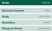
Physical AI stack focus for this chapter.

Why can a robot recognize what to do yet still be too late to act?

Learned models are what let a physical machine handle objects and scenes that no engineer enumerated, and they are also the largest and least predictable computation the machine carries. A model that recognizes the right object still has to move its weights through an onboard processor that sensing and control also depend on, and a larger model that recognizes more takes longer to answer. While it computes, the world keeps moving, so a correct answer can arrive after the conditions that justified it have changed. Predicting a sequence of future motions keeps the actuators supplied between model updates, but it cannot make those motions respond to observations the model has not yet received, and a proposal that arrives on time can still be wrong in ways the model’s own confidence does not reveal. An engineer who treats the learned model as a function that returns actions cannot size the processor, set the rates at which proposals are renewed, or say how long the machine may keep moving on an answer that has gone stale. Because motion beyond the causal boundary cannot be recalled, every learned proposal must remain a request that an independent permission path can refuse in time.

Learning Objectives

• Compare classical analytical pipelines and learned representations on coverage, sensory robustness, and formal verifiability
• Calculate the memory wall bound on a model’s fresh-evaluation rate (\(\ProposerEvaluationRate \le \SustainedMemoryBandwidth / \WeightMemory\)) under the embodied batch size 1 constraint, and explain why weight-only quantization shortens the bandwidth-bound decode but not the compute-bound prefill
• Estimate key-value cache expansion from multi-camera tokenization, hidden dimensions, and retained history windows
• Explain how action chunking (\(\ActionChunkHorizon\)) amortizes off-chip weight transfers without improving closed-loop reaction latency, and why that gap requires a second, smaller proposer
• Compare autoregressive, one-pass, and iterative action decoders by the sequential evaluations and off-chip transfers one chunk costs
• Apply replanning period, inference latency, and target drift to size an action chunk for a dynamic target
• Evaluate the interface between a slow and a fast proposer by what the permission path can check against its own evidence
• Diagnose cognitive failure modes: semantic hallucinations, uncalibrated softmax overconfidence, perceptual chattering, and expired intent leases
• Identify the trajectory, timestamps, and validity information a proposer must hand to independent real-time verification

3.1 The Embodied Brain

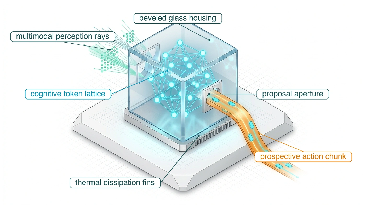
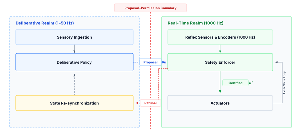
The body’s limit records tell the permission path what it must refuse, but they cannot say what the machine should do next. That choice belongs to the Brain, the deliberative layer that interprets incoming sensor telemetry and proposes what the physical body should execute next. Over the past decade, physical AI architectures have transitioned from hand-authored geometric pipelines and finite-state machines to learned models, notably vision-language-action (VLA) architectures that map natural language instructions and camera pixels directly to candidate end-effector motions for objects no engineer explicitly modeled. This shift places the machine’s most computationally intensive workloads on its least predictable path. A deep neural proposer requires billions of operations, contends for shared memory bus bandwidth with low-latency sensing and control tasks, and predicts future actions for an environment that continues to evolve during inference. A fundamental physical constraint governs this interaction: a learned proposal remains useful only if it arrives, and remains physically valid, within the time window permitted by environmental dynamics. Furthermore, every candidate trajectory remains strictly a proposal. The hard-real-time permission path beneath the proposal boundary holds exclusive authority to validate and admit candidate motions before they actuate physical hardware.

The warehouse mobile manipulator illustrates this boundary concretely. The robot can operate within every torque, thermal, voltage, and braking limit of its body, and meet the freshness deadline that the body’s budgets set for this same pick-station grasp, yet still fail to grasp an unfamiliar ceramic mug traveling along an active conveyor. Low-level limits safeguard physical actuators against structural and electrical damage, but they cannot identify the geometry of a graspable handle or plan an obstacle-free trajectory around a coworker’s arm. A learned vision-action model supplies this missing perceptual interpretation. However, because this proposer’s training and task performance do not establish the closed-loop guarantee needed here, every generated action sequence remains an unverified candidate until the permission path checks it against fresh telemetry and established safety envelopes.

↩︎ The mobile manipulator’s torque, thermal, voltage, and braking limits are established in The Five Physical Budgets.

This division exposes a timing dilemma, because physical dynamics do not pause while inference runs. As the vision model evaluates sensory frames, the conveyor belt advances, and the manipulator must continue tracking previously admitted waypoints without stalling or jerking. Deploying a larger foundation model can enhance open-world object recognition, but the resulting inference latency delays subsequent updates. Systems architects must therefore decouple three distinct temporal quantities: the observation frequency at which the proposer ingests fresh sensor frames, the trajectory horizon spanning the future waypoints contained within each proposal, and the validity window over which those predictions remain physically accurate. Synthesizing longer action horizons can bridge execution between inference cycles, but generating additional waypoints does not refresh the perceptual evidence that produced them.

The machine card of The running machine already commits the running machine to one answer, the two-speed brain architecture: a slow intent model revised at 2 Hz above a fast chunk policy renewed at 20 Hz, both proposing to a permission path that checks measured state on a 1 kHz tick (figure 1). The card states these rates; this chapter prices and checks that design. The slow intent model names a target; the fast chunk policy emits an action chunk, the short sequence of future setpoints from one inference that From Prediction to Action introduced, so the drives below have motion to track between evaluations (Zhao et al. 2023; Chi et al. 2025). The sections that follow test the three claims that govern this split. Because no single large model can renew its proposal fast enough to supply the arm, the fast policy must emit multi-step chunks, yet a chunk keeps the arm supplied without keeping the evidence behind it fresh. Consequently, the permission path can evaluate and refuse the slow model’s intent alongside the fast model’s candidate motion only when that intent arrives as a target checkable against independent depth measurements and time: a metric pose stamped with the capture time of the frame that generated it (section 3.5.3).

Figure 1: Two-speed brain architecture: Above the proposal boundary, two learned proposers run at their own rates, an intent model at 2 Hz and a chunk policy renewing at 20 Hz. Below it, the permission path checks each proposal against measured state on a 1 kHz tick, and the drives close their own current and velocity loops. A proposal carries no authority until it is admitted; a refusal returns the proposers to a plan from measured state.

A learned proposer earns its place in an embodied system when training distribution coverage generalizes beyond preprogrammed edge cases. In the conveyor pick task, this capability translates into interpreting natural language instructions, recognizing the target mug amid visual clutter, and proposing reachable grasp affordances. However, high-level semantic identification alone cannot direct a robot arm; the system must project proposed grasp regions into metric Cartesian space using calibrated depth sensing and forward kinematics. Furthermore, environmental challenges such as specular reflections, dynamic shadows, and transient occlusions inevitably induce perceptual errors. Whatever algorithmic sophistication a proposer introduces, its execution demands must conform to the throughput, memory bandwidth, and thermal dissipation envelope of the onboard processor.

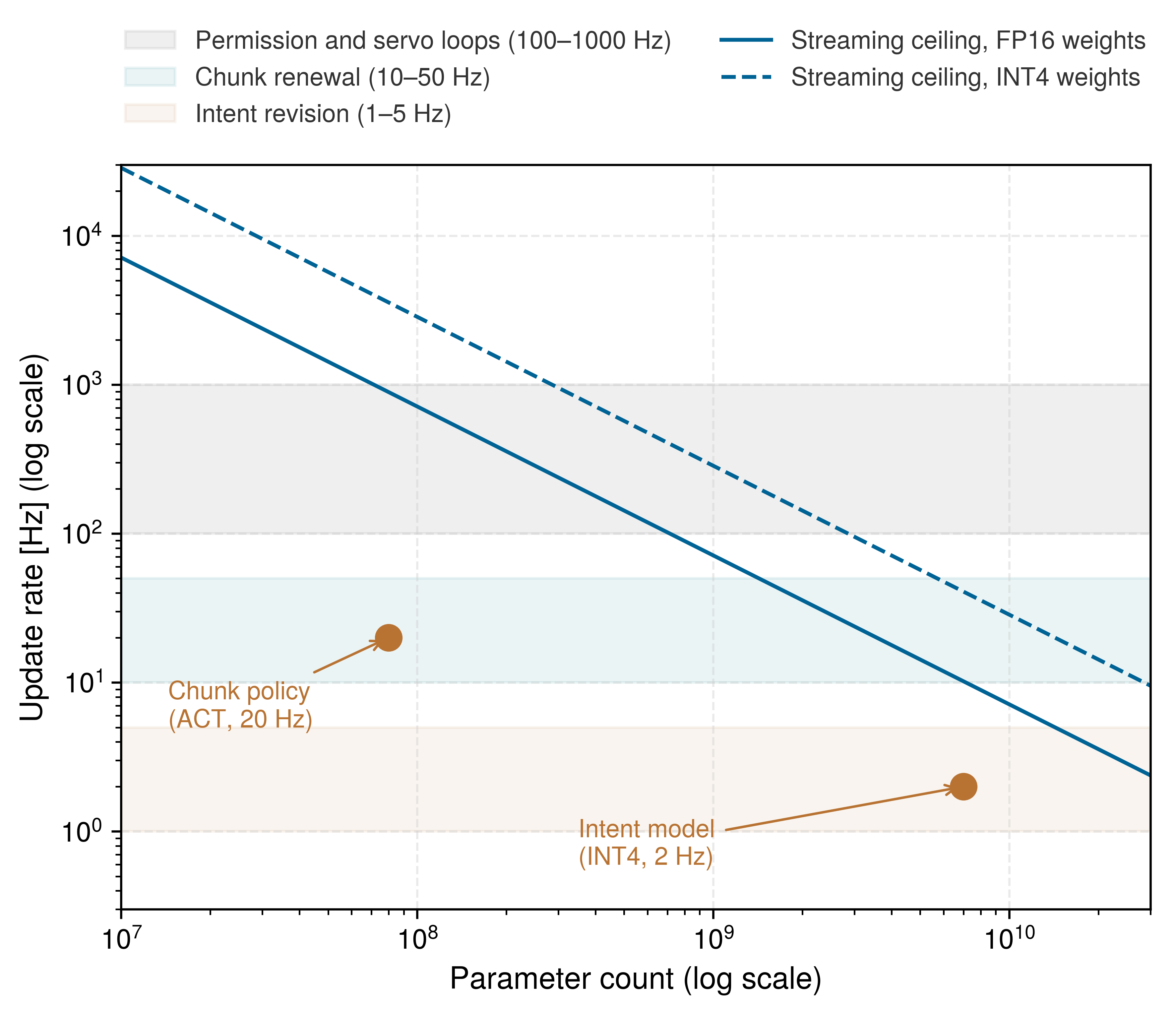
A first estimate shows why one model cannot do both jobs. If every fresh evaluation must stream all of a model’s weights from off-chip memory, its renewal rate can be no higher than the sustained bandwidth divided by the bytes of weights, a ceiling that falls in proportion to parameter count (figure 2). The intent model stores its weights as 4-bit integers (INT4, priced in section 3.4.2) rather than 16-bit floating point (FP16), which raises its ceiling fourfold. Both of the machine’s proposers still sit below their ceilings, because reading the input tokens in one pass through the model (the prefill) and then decoding the output add work that weight streaming alone ignores, and neither approaches the kilohertz rate at which the permission path and the servo loops run. The design problem is therefore deciding which computation can finish before the observation it started from goes stale. Section 3.4.1 derives the ceiling and the work above it; the figure is a preview of where the derivation lands.

Figure 2: Cadence regimes on the machine’s processor: The weight-streaming ceiling \(\ProposerEvaluationRate \le \SustainedMemoryBandwidth/\WeightMemory\) on the mobile manipulator’s application processor for FP16 and INT4 weights (16-bit floating-point and 4-bit integer representations, section 3.4.2) plotted against model parameter counts, alongside the operating points for the machine’s intent model and chunk policy. This ceiling establishes an upper bound on throughput rather than an achieved operating frequency, because input token prefill, vision encoding, and autoregressive generation consume execution cycles beyond raw DRAM weight traffic (section 3.4.1).

Testing the two-speed design takes four steps. Classical pipelines built on hand-authored geometry and rigid state machines show why a learned proposer is needed at all, because open-world variability exhausts manual rule sets (section 3.2). Learned representations restore semantic breadth but pay for it in tokens, cache, and bus traffic (section 3.3). Pricing one fresh evaluation of the intent model on the application processor then exposes the memory wall and what quantization can and cannot do about it (section 3.4), and sizing the chunks that keep the arm supplied separates the motion a chunk supplies from the time its evidence stays true (section 3.5). Because a proposal can arrive on schedule and still be wrong, the last step examines the failures that leave the permission path to refuse an on-time proposal (section 3.6).

3.2 The Classical Wall

In a fixed industrial workcell, a robotic gripper can approach the exact same fixture along an identical trajectory on every production cycle. Engineers can specify such repetitive motions through analytical geometry, rigid-body equations of motion, and deterministic state transitions. Classical control theory and traditional robotics flourish within this analytical formulation (Wiener 1948; Kalman 1960; Craig 2005). The engineering challenge sharpens, however, when moving from a rigid fixture to an unconstrained scenario, such as retrieving a randomly oriented mug from a moving conveyor belt, where the engineer cannot enumerate every combination of object geometry, pose, and physical contact in advance.

Wiener, Norbert. 1948. Cybernetics: Or Control and Communication in the Animal and the Machine. Wiley.

Kalman, Rudolph Emil. 1960. “A New Approach to Linear Filtering and Prediction Problems.” Journal of Basic Engineering 82 (1): 35–45. https://doi.org/10.1115/1.3662552.

Craig, John J. 2005. Introduction to Robotics: Mechanics and Control. 3rd ed. Pearson Prentice Hall.

¹ End-Effector: The tool, gripper, or hand at the distal tip of a manipulator, the only part of the arm meant to touch the workpiece. Workspace and keep-out checks are written against its pose rather than against joint angles, which is why the proposal payload later in this chapter carries end-effector poses alongside joint targets.

² Manipulator Equation: Classical control computes joint torques from \(\GeneralizedInertiaMatrix(\GeneralizedCoordinates)\GeneralizedAccelerations + \CoriolisCentrifugalMatrix(\GeneralizedCoordinates, \GeneralizedVelocities)\GeneralizedVelocities + \GravitationalTorqueVector(\GeneralizedCoordinates) = \JointTorque\), with a configuration-dependent inertia matrix \(\GeneralizedInertiaMatrix\), Coriolis and centripetal terms \(\CoriolisCentrifugalMatrix\), and gravity \(\GravitationalTorqueVector\). Torque is linear in inertia, and a link’s inertia grows with the square of its distance from the joint, so an outstretched arm needs more torque for the same angular acceleration. Unmodeled contact, friction, or deformable objects break this rigid-body model, which is the gap learned proposers enter; Feedback linearization: Transforming nonlinear dynamics into decoupled double integrators shows how classical control inverts this model to compute torque.

Analytical kinematics and dynamics map target end-effector¹ trajectories into joint angles, velocities, and actuator torques.² Classical perception routines register incoming sensor point clouds against reference computer-aided design (CAD) models, while a synchronous finite-state machine steps the manipulator through sequential phases: approaching, aligning, grasping, and retracting. In a calibrated workcell, these analytical components reliably solve bounded manipulation tasks under explicit operational assumptions. Their computational latency and real-time execution bounds depend strictly on the chosen numerical solver, processor throughput, and contact dynamics model.

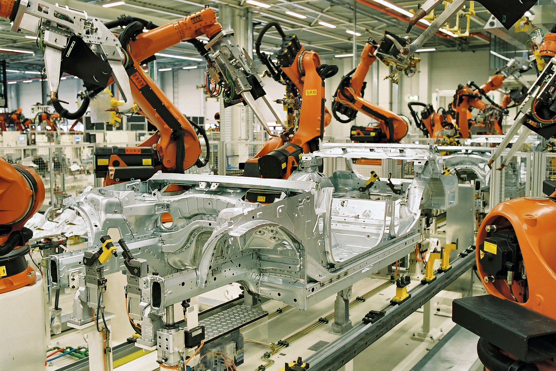
Where the operational environment remains structured and bounded, classical methods provide dependable behavior within their modeled operating envelopes. In a body shop (figure 3), the chassis sits in submillimeter tooling fixtures, and controlled lighting and interlock fencing constrain variation under stated fixture, access, and model assumptions. This controlled regime permits explicit physical modeling, servo timing analysis, and formal Lyapunov stability analysis.³ Establishing selected trajectory tracking error bounds (\(\lVert \TrackingErrorVector(\TimeInstant) \rVert \le \TrackingErrorBound\)), stability properties, or software execution guarantees requires justified model, implementation, and execution evidence; the absence of training data does not establish those properties.

³ Lyapunov Stability: Aleksandr Lyapunov’s 1892 method establishes stability near an equilibrium using a positive-definite, energy-like function whose derivative along the modeled dynamics is nonpositive; asymptotic convergence requires stronger decrease or invariance conditions (Slotine and Li 1991). Applying the method requires a justified closed-loop dynamics model and verified certificate conditions; a learned proposer does not acquire such a certificate merely from training. The barrier certificates of Safe Sets as Conditional Permission reuse the idea to keep the machine inside a safe set rather than at a point.

Slotine, Jean-Jacques E, and Weiping Li. 1991. Applied Nonlinear Control. Prentice Hall.

↩︎ The causal boundary, where an admitted command becomes physical work, is established in Defining the Causal Boundary.

Figure 3: Industrial spot-welding workcell: Multiple six-degree-of-freedom articulated robots execute preprogrammed spot welding paths on stamped automotive chassis at the BMW Leipzig plant. The calibrated setting uses repeatable fixtures and safety interlock cages to constrain the conditions for those preprogrammed motions. (Credit: BMW Werk Leipzig, Wikimedia Commons, CC BY-SA 2.0 DE.)

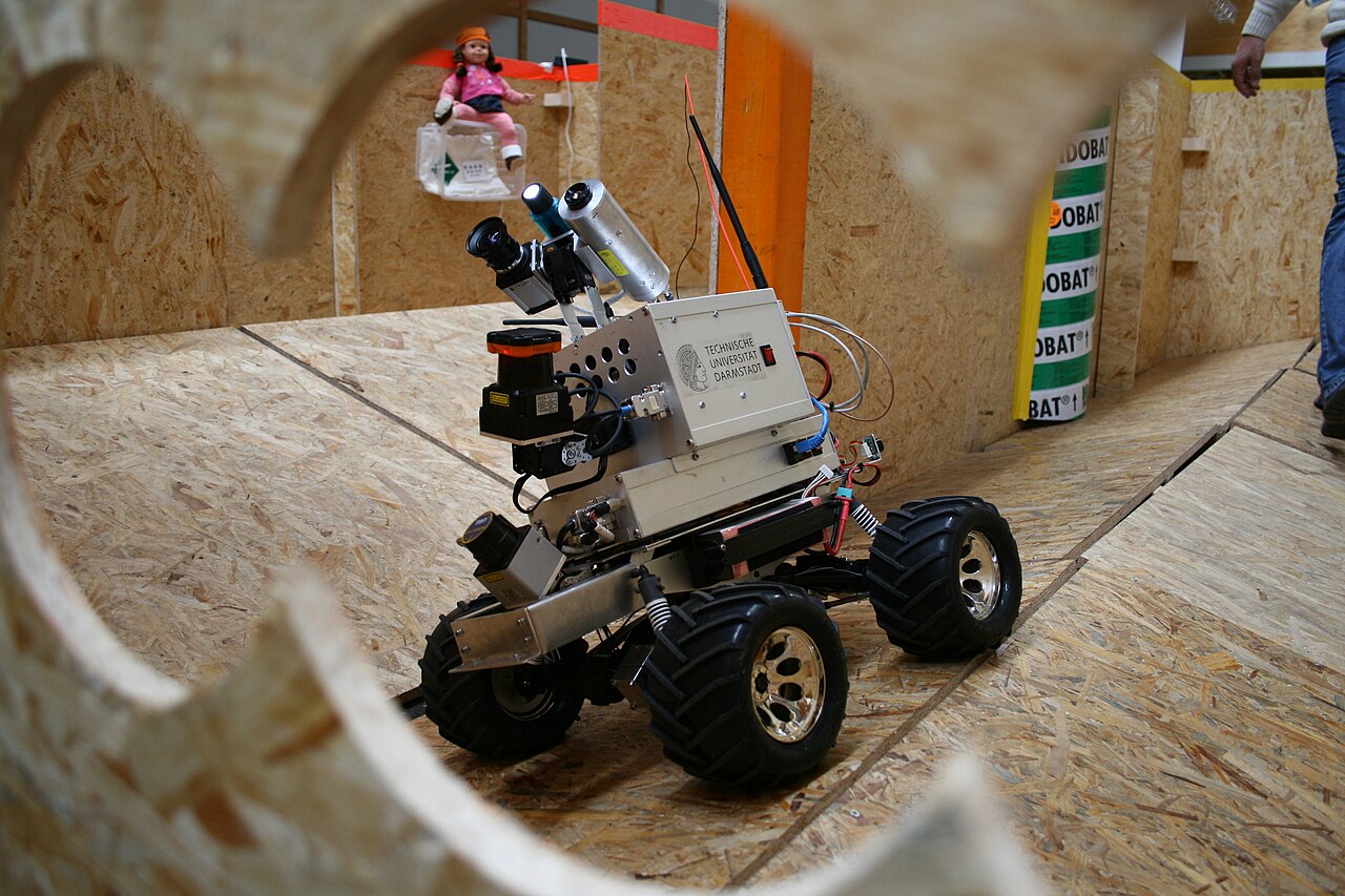
When an embodied machine steps outside the structured factory cage into unstructured, open-world environments, however, this analytical paradigm hits the classical wall (Brooks 1991; Levine et al. 2018). Physical reality defies closed-form geometric modeling: real objects deform under contact, ambient illumination shifts unpredictably, and scenes present near-infinite visual and mechanical variety. A rescue test arena of tilted ramps and a victim dummy on a high shelf (figure 4) has none of the fixtures that made the welding cell analyzable: no part arrives at a known pose, and no template describes the terrain. In such unmapped, irregular settings, preauthored geometric templates and rigid state machines lose state coverage and fail to generalize.

Brooks, Rodney A. 1991. “Intelligence Without Representation.” Artificial Intelligence 47 (1–3): 139–59.

Levine, Sergey, Peter Pastor, Alex Krizhevsky, Julian Ibarz, and Deirdre Quillen. 2018. “Learning Hand-Eye Coordination for Robotic Grasping with Deep Learning and Large-Scale Data Collection.” The International Journal of Robotics Research 37 (4-5): 421–36.

Figure 4: Unstructured search-and-rescue robot: A four-wheeled rescue robot carrying cameras and a laser scanner on a pan-tilt mast works through a test arena of tilted ramps and narrow openings, with a victim dummy placed on a high shelf. In such unmapped environments, preauthored geometric models and rigid state machines can lose coverage; learned policies may help infer spatial affordances and traversability from sensory streams. (Credit: Hector, Technische Universität Darmstadt, at the 2010 RoboCup German Open; photo by Mike1024, Wikimedia Commons, public domain.)

Outside structured fixtures, the analytical perception-and-control pipeline breaks down whenever scenes vary beyond its hand-coded rules. A rigid CAD template fails on deformable cloth or irregular food items; glare or cast shadows can wipe out the depth edges needed to separate adjacent parcels; and an unexpected obstacle invalidates the guard conditions of a preauthored grasping state machine. Engineers can add templates, heuristic thresholds, and recovery branches to patch each failure, but the cases multiply faster than they can be tuned and tested.

Machine learning exits this trap by learning from diverse physical interactions and demonstrations rather than enumerating geometric rules by hand. Neural models extract graspable features and motion policies directly from high-dimensional sensor streams without a bespoke CAD model for every object. Those learned models do not replace the downstream analytical controller: deterministic feedback loops still enforce kinematic bounds and track trajectories at high rates. Instead, learning inserts a compute-heavy proposal stage whose memory traffic, arithmetic cost, and latency must fit inside the timing contract of the real-time controller.

3.3 Learned Representations

When commanded to pick an unfamiliar ceramic mug from a conveyor, a learned model relates the text prompt to visual features of the handle and proposes a plausible grasp region without an exact CAD model. VLA models combine multi-camera imagery, natural-language instructions, and proprioceptive robot state to produce candidate actions (Brohan, Brown, Carbajal, Chebotar, Dabis, et al. 2023; Brohan, Brown, Carbajal, Chebotar, Chen, et al. 2023; Kim et al. 2024). These systems descend from early embodied language models such as SayCan and PaLM-E, which emitted high-level semantic plans rather than low-level motor commands (Ahn et al. 2022; Driess et al. 2023). The operational value of a VLA stems from broad generalization across diverse objects and ambient environments acquired during large-scale pretraining, rather than formal guarantees of correct scene interpretation.

Ahn, Michael, Anthony Brohan, Yevgen Chebotar, et al. 2022. “Do as I Can, Not as I Say: Grounding Language in Robotic Affordances.” Proceedings of the 6th Conference on Robot Learning (CoRL), Proceedings of machine learning research, vol. 205: 287–318.

Driess, Danny, Fei Xia, Mehdi SM Sajjadi, Corey Lynch, Aakanksha Chowdhery, Brian Ichter, Ayzaan Wahid, et al. 2023. “PaLM-e: An Embodied Multimodal Language Model.” International Conference on Machine Learning (ICML), 8469–88.

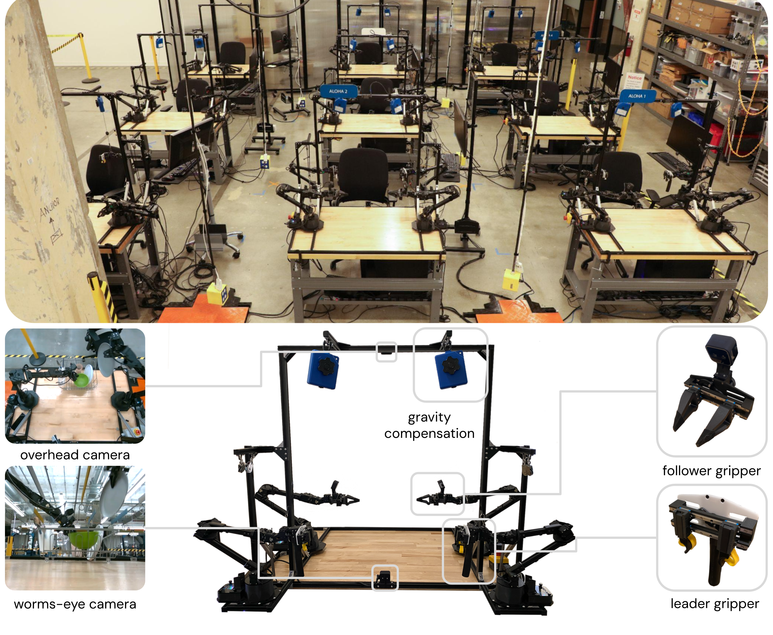
Teleoperated demonstrations can likewise teach coordinated sensorimotor policies for tasks whose contacts and structural deformations resist analytic kinematic modeling. In a bimanual teleoperation workcell (figure 5), an operator moves low-cost leader arms while follower arms with parallel grippers reproduce the motion, and overhead and wrist cameras record what the followers saw; those recordings become the training data for policies that later act alone (Zhao et al. 2023; Chi et al. 2025). The running machine’s chunk policy takes its size from ACT, which was trained on exactly such recordings, and what such a policy learns from them is the action chunk itself, a short stretch of the operator’s motion predicted from one view. How demonstrations become a policy belongs to Policy Training; this chapter prices what the trained policy costs to run. Although learned representations tolerate sensory variations captured across training distributions, executing any proposed motion safely still demands calibrated spatial geometry and strict physical boundary enforcement. Empirical task success demonstrates capability over tested operating envelopes, but out-of-distribution shifts in illumination, surface friction, or payload dynamics can quickly induce behavioral drift or outright failure.

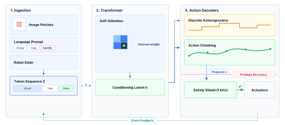
The computational cost of this capability depends directly on the model’s underlying representation. A transformer does not read pixels or words directly; it reads tokens, embedding vectors that each represent one slice of input, such as an image patch, a word fragment, or a joint angle. Across a VLA model, that token sequence flows from camera patches and prompt embeddings through self-attention to candidate action chunks (figure 6). Multi-view camera frames consume significant memory bandwidth during ingestion, historical context expands key-value (KV) cache footprints in memory, and the inference engine must produce subsequent actions before the physical state diverges from the initial observation. Evaluating an embodied learned model alongside a classical perception-planning pipeline requires assessing both task generalization and the end-to-end latency required to refresh action proposals.

Figure 5: Bimanual teleoperation workcell: Dual-arm teleoperation setup featuring two six-degree-of-freedom follower arms, two leader arms for kinesthetic teleoperation, multi-view cameras (overhead and wrist-mounted), and parallel grippers mounted to an extruded aluminum frame. The physical AI policy ingests synchronized multi-camera streams to predict continuous end-effector trajectories, and the permission path must refuse any proposal that would cause self-collision or motor over-torquing during closed-loop execution. (Credit: ALOHA 2 Team, ALOHA 2: An Enhanced Low-Cost Hardware for Bimanual Teleoperation, arXiv:2405.02292, CC BY 4.0.)

Figure 6: Embodied Vision-Language-Action (VLA) architecture: A representative dataflow. (1) Camera patches receive 2D image-position and camera identifiers alongside language and robot-state tokens; metric depth still requires calibrated evidence. (2) Self-attention mixes the combined token sequence; the colored grid illustrates internal attention weights, not a verified affordance or grasp pose. (3) Autoregressive token decoders emit tokens sequentially, whereas one-pass chunk heads and iterative action experts generate candidate multi-step chunks (\(\PolicyActionWindow\)) in one pass or over several refinement steps. (4) An independent permission path checks candidate motion against sensed state and modeled limits before actuation. (Synthesized from Brohan et al. (Brohan, Brown, Carbajal, Chebotar, Dabis, et al. 2023; Brohan, Brown, Carbajal, Chebotar, Chen, et al. 2023), Kim et al. (Kim et al. 2024), and Octo Model Team (Octo Model Team et al. 2024)).

Octo Model Team, Dibya Ghosh, Homer Walke, Karl Pertsch, Kevin Black, Oier Mees Nair, et al. 2024. “Octo: An Open-Source Generalist Robot Policy.” arXiv Preprint arXiv:2404.08839.

To grasp the mug, the model turns camera images and a language instruction into candidate trajectories in three learned stages: tokenization, attention across the tokens in a backbone, and an action decoder that projects the backbone’s output into proposed motion. A proposal boundary separates all three from actuation, so every candidate action passes independent permission checks before it reaches the motor drives. Evaluating this pipeline from a systems perspective means tracing what each stage stores in memory, transfers across the memory bus, and delivers to the controllers below it:

1. Sensory ingestion and spatial tokenization (the inputs). A vision transformer (ViT) frontend (Dosovitskiy et al. 2021) slices each incoming camera frame into a grid of non-overlapping pixel patches of size \(\VitPatchSize{\times}\VitPatchSize\) (typically \(14{\times}14\) or \(16{\times}16\) pixels). Each patch is linearly projected into a vector of width \(\HiddenDimension\), augmented with a position embedding (learned in the SigLIP and DINOv2 encoders that OpenVLA uses (Kim et al. 2024), sinusoidal in some other designs), and tagged with a learned camera identifier.

   In an illustrative three-camera configuration (left wrist, right wrist, and an overhead torso mount) capturing \(224{\times}224\) images, the image frontend prepares a buffer for each view. Each frame yields \((224 / 14)^2 =\) 256 spatial patches. Across 3 cameras, ingestion injects 768 visual tokens into the model’s sequence on every perceptual step. When concatenated with tokenized natural language commands (about 32 tokens) and proprioceptive joint state embeddings (about 16 tokens), the initial context runs slightly past 800 tokens, which the estimates below round to \(\SequenceLength \approx\) 800. In 16-bit floating-point (FP16) precision (\(2\,\text{bytes}\) per element) with hidden dimension \(\HiddenDimension =\) 4096, the token embeddings for one such step occupy \[M_{\text{embed}} = S \times d \times 2\,\text{bytes} = 800 \times 4096 \times 2 \approx 6.55\,\text{MB}\] a few megabytes, negligible beside the multi-gigabyte weights that section 3.4.1 prices. Tokens therefore cost the machine through the arithmetic every weight performs on each of them and through the cache they leave behind, not through the storage of the embeddings themselves. Neither 2D image coordinates nor internal attention patterns constitute metric depth. Projecting an end-effector into physical 3D space requires calibrated extrinsic camera matrices and depth telemetry.

2. Multimodal alignment and attention (the backbone). For the illustrative backbone, the token sequence passes through \(\LayerCount =\) 32 transformer layers where standard multi-head self-attention computes pairwise token interactions (Vaswani et al. 2017). To relate each new token to the earlier ones, every layer keeps a key and a value vector for every token it has already processed, the KV cache. The arithmetic of attention grows with the square of the sequence length (\(\mathcal{O}(\SequenceLength^2 \HiddenDimension)\) FLOPs), but the memory the cache occupies grows only linearly with it, as equation 1 gives: \[\KvCacheMemory = 2 \times \LayerCount \times \HiddenDimension \times \SequenceLength \times \ElementStorageSize \tag{1}\] The estimate assumes full-width keys and values, meaning every attention head in every layer stores its own. For a 32-layer model with \(\HiddenDimension =\) 4096 using FP16 storage, each context token then claims 524,288 bytes, about 0.524 MB, of KV cache, so an observation step of several hundred tokens holds hundreds of megabytes.

   Whether the machine pays that charge more than once depends on what the model keeps between evaluations. Single-observation VLAs such as OpenVLA rebuild their context from each new frame and carry no cache across control steps, and the running machine’s intent model is one of them. Only a design that conditions on retained history rereads the cache on every step, and section 3.5.2 prices what retaining several seconds of history would cost. Such rereading is not free, because the processor uses a unified memory architecture (UMA), in which the CPU, the GPU, and the camera interfaces share one DRAM. Every byte of cache read is bus time taken from weight streaming and from the direct memory access (DMA) transfers that deliver sensor frames. Grouped-query attention (GQA) narrows the cache by letting several query heads share one key and value; cross-attention can instead limit which retained representations the decoder reads. Either saving depends on the architecture, and action chunking does not provide it.

   Attention weights are also not geometry. A strong weight between the language tokens “mug handle” and a visual patch does not establish a graspable affordance⁴ or collision-free clearance, and the KV cache does not keep track of an object while it is occluded. The formal patch-embedding, position-encoding, and attention formulations appear in Visual patch tokenization, attention, and 3D metric lifting.

3. Specialized action decoders (the outputs). Instead of generating open-ended conversational text, the final hidden representation \(\ContextHiddenRepresentation \in \mathbb{R}^\HiddenDimension\) is routed to specialized action decoders. The running machine’s chunk policy proposes base velocity and arm targets together in one whole-body stream (section 3.5.2), so its decoder is a manipulation decoder whose outputs include the base; separate navigation models that decode waypoints over a topological map of the building (figure 7) follow the same proposal rules but are not part of this machine. Manipulation (VLA) models diverge sharply in how they bridge semantic representations to physical motion:

   Discrete action decoders map each action dimension to a categorical token by dividing its continuous range into bins (Brohan, Brown, Carbajal, Chebotar, Dabis, et al. 2023; Brohan, Brown, Carbajal, Chebotar, Chen, et al. 2023; Kim et al. 2024). Autoregressive decoders such as RT-2 and OpenVLA then generate those tokens sequentially, requiring one complete model evaluation per action dimension (Brohan, Brown, Carbajal, Chebotar, Chen, et al. 2023; Kim et al. 2024). However, discretization does not fundamentally mandate sequential decoding. RT-1 predicts all action tokens simultaneously in a single forward pass, and its authors demonstrated that autoregressively conditioning each action dimension on preceding dimensions yielded no accuracy gains while more than doubling inference latency (Brohan, Brown, Carbajal, Chebotar, Dabis, et al. 2023).

   What separates modern decoders in systems practice is the computational cost of generating a trajectory chunk and the volume of model weights reread during inference. Three architectural families dominate implementations as of 2026:

   • Autoregressive tokens. Each token requires a separate sequential evaluation. With one token per action dimension per control step, predicting a chunk of \(\ActionChunkHorizon\) timesteps across \(\ActionDimension\) dimensions demands \(\ActionChunkHorizon \ActionDimension\) sequential evaluations, causing inference latency to scale with both horizon and degree of freedom. Per-step binning also breaks down at high control frequencies: consecutive continuous setpoints differ negligibly, producing runs of identical token targets from which next-token training learns almost nothing. Frequency-space action sequence tokenization (FAST) resolves this scaling bottleneck by applying a discrete cosine transform across each action dimension over the chunk horizon, representing the trajectory as a linear combination of cosine basis functions (Pertsch et al. 2025). Smooth physical motions concentrate energy in low-frequency coefficients, allowing aggressive truncation. FAST quantizes these coefficients and compresses them with byte-pair encoding, which repeatedly merges the most frequent adjacent pair of symbols into a new token, tying token counts directly to trajectory information complexity rather than \(\ActionChunkHorizon \ActionDimension\). On a 50 Hz bimanual task, FAST compressed 700 raw binned tokens to 53, achieving a 13.2× reduction (Pertsch et al. 2025). Token generation nevertheless remains sequential. The authors report an inference latency of approximately 750 ms per chunk for FAST-\(\pi_0\), compared to 100 ms for the flow-matching variant on an identical desktop GPU.
   • One-pass chunk heads. Action Chunking with Transformers (ACT) regresses an entire trajectory chunk in a single feedforward decoder pass (Zhao et al. 2023). OpenVLA-OFT adapts an autoregressive VLA into a one-pass generator by passing placeholder action tokens through bidirectional self-attention and directly regressing continuous values for all action steps in parallel, increasing throughput by 26× on 8-step chunks (Kim et al. 2025). However, deterministic regression heads trained with mean squared error struggle with multimodal demonstration data: when presented with two equally valid paths around an obstacle, a naive regression loss averages them into an infeasible trajectory directly through the obstacle (Chi et al. 2025). Mode averaging when demonstrations split develops this mode averaging from the training side. ACT mitigates it by conditioning its decoder on a latent style variable, a code that records which of several demonstrated ways of doing the task a trajectory follows, learned with a conditional variational autoencoder (CVAE, Mode averaging and the decoders that avoid it).
   • Iterative action experts. Diffusion Policy formulates action generation as iterative denoising, starting a candidate chunk from random noise and repeatedly removing the noise a network predicts, adapting continuous diffusion processes originally developed for generative vision models (Ho et al. 2020; Chi et al. 2025). The \(\pi_0\) architecture pairs a 300M-parameter flow-matching⁵ action expert with a pretrained vision-language model, yielding 3.3B total parameters (Black et al. 2024). The large vision-language backbone processes perceptual observations once and caches its key-value activations; the action expert then generates the continuous trajectory chunk across 10 numerical integration steps while attending to that static cache. Each integration step is a forward Euler step. The expert starts the candidate from Gaussian noise, evaluates a learned velocity field that says which direction moves it toward a plausible action chunk, and moves the candidate a small distance that way; after 10 steps the candidate is the chunk. Each step requires a forward pass only through the lightweight action expert and its cross-attention reads into the cached backbone KV activations, avoiding any re-evaluation of the multi-billion-parameter vision-language backbone. Subsequent designs such as \(\pi_{0.5}\) and GR00T N1 employ this exact decoupling (Black, Brown, et al. 2025; Bjorck et al. 2025), with \(\pi_{0.5}\) combining FAST-token pretraining on the backbone with flow-expert execution at runtime.

   Across all three families, the continuous output forms a multi-step trajectory chunk: \[\PolicyActionWindow = [\CognitivePolicyAction_{t}, \CognitivePolicyAction_{t+1}, \dots, \CognitivePolicyAction_{t+\ActionChunkHorizon-1}] \in \mathbb{R}^{\ActionChunkHorizon \times \ActionDimension}\] Here \(\ActionChunkHorizon\) specifies the future prediction horizon in discrete setpoints and \(\ActionDimension\) denotes the degrees of freedom per action; section 3.5.1 states the formal definition (3.2) once the memory wall has shown why chunks are needed. Published horizons span from tens to hundreds of setpoints: Diffusion Policy predicts 16 steps and executes the initial 8 (Chi et al. 2025), \(\pi_0\) predicts 50 steps (Black et al. 2024), and ACT predicts 100 steps at 50 Hz (Zhao et al. 2023). The structural gap between prediction and execution horizons resurfaces in section 3.5.2 as the interface between asynchronous trajectory generation and real-time permission filtering. A trajectory chunk provides an open-loop sequence of future setpoints derived from a single sensory context, amortizing inference latency without incorporating intervening sensor observations. Section 3.5.1 evaluates the computational efficiency of these three decoder families on target silicon, while Mode averaging and the decoders that avoid it gives the discrete tokenization rule and details how generative decoders capture multimodal demonstration distributions without averaging conflicting trajectories.

4. The proposal boundary (isolation from actuators). Whether the model plans navigation or manipulation, its output is an unprivileged candidate proposal strictly outside the proposal boundary (definition 1.3). Under the concrete machine model established in The Machine in Five Levels, the foundation model runs in unprivileged user space on the host application processor and has no direct memory-mapped access to pulse-width modulation (PWM) registers or motor coil current drivers. Instead, the Brain hands candidate motion, stamped with the capture times of the sensory frames that generated it, to a permission path whose kilohertz loops a slow inference cannot preempt or bypass. That path refuses proposals that would collide, violate joint limits, or drive the arm into a kinematic singularity (an arm configuration in which the joints lose the ability to move the end effector in some direction). Actuation Authority isolates this gating logic on a dedicated real-time safety microcontroller, completely segregated from the application processor hosting the learned model.

⁴ Affordance: Gibson’s term for the action possibilities an environment offers an agent, defined jointly by object properties and agent physical capabilities (Gibson 1979). A handle affords a grasp only when its physical dimensions and clearance accommodate the robot’s gripper geometry and kinematics. While self-attention weights across image patches highlight semantically relevant features such as a handle, they do not certify mechanical grasp stability or kinematic reachability, the failure mode section 3.6.1 analyzes.

Gibson, James J. 1979. The Ecological Approach to Visual Perception. Houghton Mifflin.

⁵ Flow Matching: A method that trains a neural network to predict a continuous velocity field carrying samples from Gaussian noise to the target data distribution along nearly straight paths (Lipman et al. 2022). Because those paths are straight, numerical solvers can generate samples in a handful of Euler steps, whereas older denoising diffusion models needed hundreds of sequential steps (Ho et al. 2020). On an embedded robot processor, the step count directly sets latency because each solver step rereads the action expert’s weights and cached visual context from off-chip memory.

Lipman, Yaron, Ricky TQ Chen, Heli Ben-Hamu, Maximilian Nicklas, and Matt Le. 2022. “Flow Matching for Generative Modeling.” arXiv Preprint arXiv:2210.02747.

Ho, Jonathan, Ajay Jain, and Pieter Abbeel. 2020. “Denoising Diffusion Probabilistic Models.” Advances in Neural Information Processing Systems (NeurIPS) 33: 6840–51.

Figure 7: Topological vision-language navigation: Embodied navigation architecture executing natural-language spatial instructions. Panoramic visual observations are encoded into perceptual tokens, matched against prompt embeddings, and cross-referenced with a dynamically updated topological navigation graph. The action decoder prunes unreachable nodes and emits metric waypoint offsets \((\FiniteChange \GroundPlaneAbscissa, \FiniteChange \GroundPlaneOrdinate)\) and heading setpoints to guide the chassis along traversable semantic frontiers without requiring an exact geometric prior map. (Adapted from An et al. (2023), arXiv:2304.03047, CC BY 4.0.)

An, Dong, Yuankai Qi, Yang Huang, Yan Wei, Liang Wang, Tieniu Tan, et al. 2023. “ETPNav: Evolving Topological Planner for Vision-Language Navigation in Continuous Environments.” arXiv Preprint arXiv:2304.03047.

The choice of sensory representation and action decoder dictates the memory traffic and latency profile of every control cycle. Maintaining historical token context accumulates KV cache overhead that consumes memory bus bandwidth, while running multi-billion-parameter backbones on resource-constrained embedded systems demands massive weight streaming from off-chip DRAM. An embodied agent needs both semantic breadth and rapid trajectory renewal, and these costs suggest that one monolithic model on an embedded processor cannot deliver both. Whether it can is a question of numbers, and the place to get them is one fresh evaluation of the machine’s intent model on its own application processor.

3.4 The Cost of a Fresh Evaluation

At the pick station the mobile manipulator’s arm consumes a new setpoint every few tens of milliseconds, while the mug keeps moving along the conveyor. Whether one large model could supply those setpoints depends on how long one fresh evaluation of it takes on the application processor, and that time depends on which resource the evaluation exhausts first, the memory bus or the arithmetic units. The intent model’s evaluation is priced first, together with what quantization can buy back; section 3.5 then checks the motion buffer that the selected split relies on against the target’s drift. The single large-model cases below are alternatives used to expose the trade-off, not changes to the selected machine.

After ingestion (the tokenization of section 3.3), four learned stages turn those tokens into action proposals, and each hands the next a record that ages (figure 8). Across the proposal boundary, an isolated safety microcontroller (MCU) running the permission path on a 1 kHz tick decides whether candidate setpoints become admitted drive commands. These stages describe what the machine must compute, not how its networks are divided; the three learned stages of section 3.3 describe the inside of one transformer. On the running machine, the intent model recognizes the mug and names the target (perception and intent), a tracker carries the mug’s estimate from frame to frame (memory), and the chunk policy, reading its own camera frames, turns the target into setpoints (planning). Memory here means the belief the machine keeps about the world, not DRAM. The chapters of Part III, beginning with Sensor Perception, develop each stage in depth; here they matter only for what each hands downstream and how quickly that record goes stale.

Perception grounds what it recognizes in metric coordinates relative to the base, so that the mug has a 3D position and orientation (an \(\SpecialEuclideanGroup\) pose)⁶ and a graspable handle rather than an abstract semantic label; its output ages from the moment of capture. Memory carries those estimates through occlusion and must let each one expire when the evidence behind it does. Intent decomposes a task such as “take the ceramic mug off the conveyor and hand it to the coworker at the packing station” into subgoals, and because the mug moves while the intent model deliberates, it hands the planner a target that expires, an intent lease in the vocabulary of Part III. Planning converts that target into candidate setpoints for the base and the arm, the proposals the permission path will judge.

⁶ SE(3) Pose: SE(3), the special Euclidean group in three dimensions, is the set of rigid-body poses, a rotation plus a translation with six degrees of freedom; “special” excludes mirror reflections, which no rigid object can undergo. A pose can be compared with measured depth and aged from its capture time, while a semantic label such as “mug handle” can be neither, which is why the handoff to planning is a pose and not a label.

↪ The observation contract that dates each perception output from its capture epoch is developed in The Observation Contract.

↪ The intent lease and the deadlines that end it are developed in The Intent Lease Specification and Contract.

Figure 8: The physical AI cognitive flow: The learned stages run on the application processor and each hands the next a record that ages: ingestion produces tokens, perception a metric pose with its age, memory a belief with its evidence epoch, intent an intent lease, and planning candidate setpoints. Everything up to planning is proposal. Only the permission path, on its own 1 kHz tick across the proposal boundary, can turn a proposal into an admitted command for the drives.

These stages, and the ingestion before them, all run on the application processor and draw on the same unified memory bus, which is where the machine’s cadence is decided. On an edge robotics system-on-chip (SoC), memory bandwidth, arithmetic rate, and power envelope are fixed allocations, and model weights, sensor transfers, and host computation share that bandwidth. A policy cannot budget the full bus for itself while assuming that new camera frames arrive without interference, and scaling the model up only draws harder against the same ceiling. The transfer bound below is therefore a lower bound on evaluation time; the worked comparison later uses an assumed sustained fraction of peak bandwidth, and Contention for Shared Resources models how weight fetches, camera transfers, and telemetry writes queue for the shared memory controller.

↩︎ That every added layer of onboard compute draws against fixed memory bandwidth, electrical power, and thermal dissipation is established in The Four Bedrock Laws.

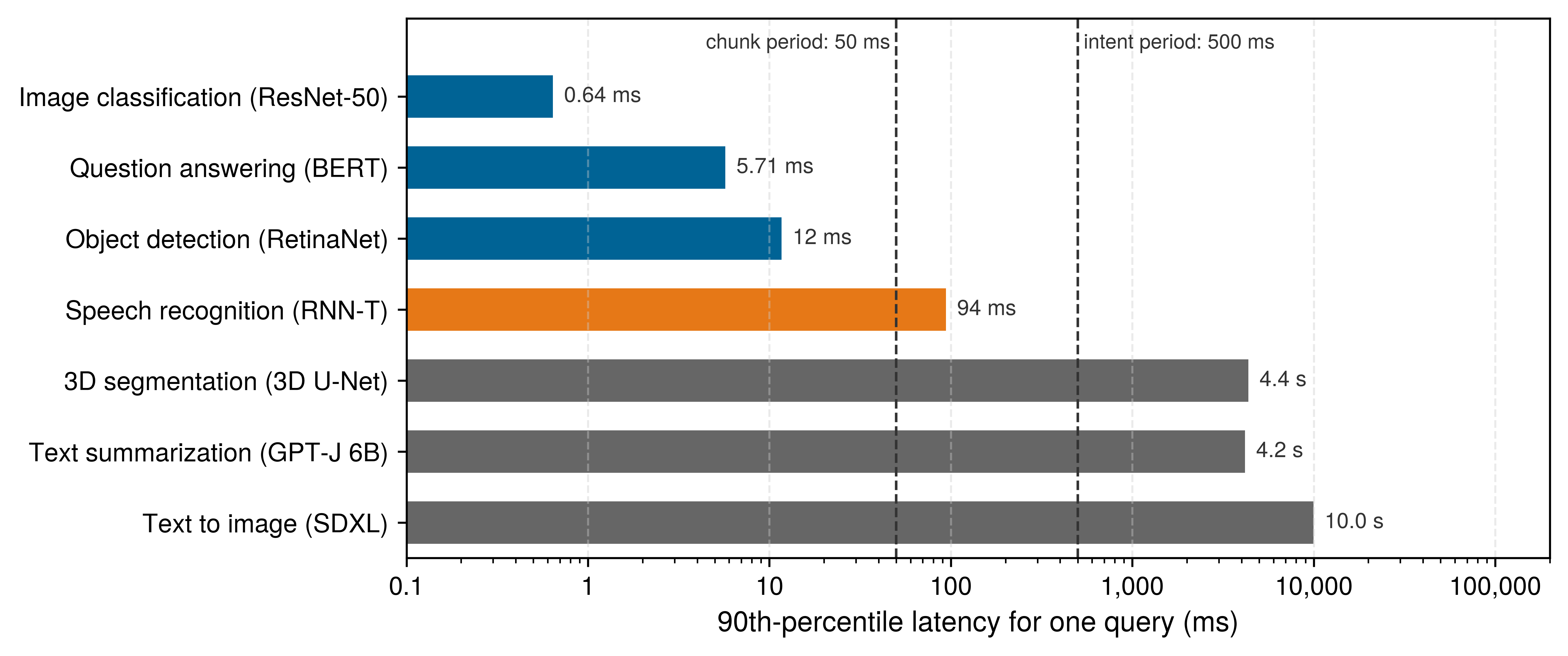
Published measurements on the machine’s own module show how far apart those costs sit before any of that arithmetic. The MLPerf Inference edge suite times one query at a time, its single-stream scenario, for a fixed set of reference models (Reddi et al. 2019). Vendor submissions for the 64 GB Jetson AGX Orin place those reference latencies directly against the three cadences of the running machine (figure 9).

Figure 9: Measured single-query latency on the application processor: The 90th-percentile time to answer one query, on a logarithmic axis, for each MLPerf Inference edge reference model on the 64 GB Jetson AGX Orin, the module in the running machine. Dashed lines mark the machine’s chunk renewal period and intent revision period; blue bars finish within one chunk period, the orange bar within the intent period, and gray bars within neither. The reference models span four orders of magnitude on the same silicon, so which proposer a design can afford is fixed by the model class before any tuning. Vendor submissions, latest round per model (v3.1, or v4.1 for the two generative models); data from the MLCommons inference results repositories (Reddi et al. 2019).

Reddi, Vijay Janapa, Christine Cheng, David Kanter, Peter Mattson, Guenther Schmuelling, Carole-Jean Wu, et al. 2019. “MLPerf Inference Benchmark.” arXiv Preprint arXiv:1911.02549.

Only three of the seven reference models answer inside the 50 ms chunk period: classification in 0.64 ms, question answering, and detection in 11.7 ms. A six-billion-parameter language model takes 4.2 s to produce one summary, 8× the 500 ms intent period, and the span from fastest to slowest is about 16,000×. The figure is a measured version of the two-speed argument. A language-model proposer on this module can revise intent only at a fraction of the rate the arm consumes setpoints. The same submission also shows that the cost is not fixed by the silicon alone. The language model’s latency was 10.2 s one round earlier on identical hardware, so the software stack sets the cost as much as the silicon does. Which bytes that software moves per evaluation is what the memory-wall analysis below quantifies.

3.4.1 The memory wall

Why does a multi-billion-parameter model take hundreds of milliseconds on a processor rated at tens of tera-operations per second? Its weights do not fit in on-chip static RAM (SRAM) or cache, so every fresh evaluation must stream them from off-chip low-power DRAM (LPDDR5) across a narrower shared bus. On-chip SRAM and caches can reuse weights and intermediate state without another external transfer only while the working set fits the memory allocated to that workload, and nominal chip-wide capacity does not guarantee that even a small action head stays resident when competing tasks share the processor. When operands cannot reach the arithmetic units as fast as those units can multiply them, memory bandwidth, not arithmetic speed, limits the update rate. That ceiling is the memory wall, and on a moving robot its cost is a delayed proposal while the body keeps traveling.

Consider a robot that generates continuous motor actions one discrete step at a time through an autoregressive foundation model, such as a multi-billion-parameter VLA. Its weights are nonresident, too large to stay in on-chip memory, so each token step streams them across the external DRAM bus. In single-token decoding with FP16 weights and request batch size \(\BatchSize = 1\), the dense weight projections become matrix-vector operations (\(\LayerOutputVector = \WeightMatrix\LayerInputVector\)), in which each fetched weight takes part in a single multiply-add before it is discarded. The bus, not the arithmetic, then sets the pace. The sustained memory bandwidth \(\SustainedMemoryBandwidth\) and model weight footprint \(\WeightMemory\) bound the maximum fresh-evaluation frequency, as equation 2 states: \[\ProposerEvaluationRate \le \frac{\SustainedMemoryBandwidth}{\WeightMemory} \tag{2}\] This bound must use the bandwidth actually available to the policy and the weights it transfers at the selected precision. It prices only the weight transfer. A fresh evaluation first reads its input tokens (image patches and the instruction) through the backbone in one pass, the prefill, and that pass reuses every fetched weight across all of those tokens, so arithmetic rather than bandwidth can bind it. Notebook 3.1 prices both terms for the mobile manipulator’s intent model. When a decoder emits one token per action dimension, each action dimension requires another token; if each token revisits off-chip parameters, that decode latency scales linearly with degrees of freedom.

Single-token decoding at batch size 1 Servers can combine independent requests so that a weight matrix multiplies several input vectors at once, reusing fetched weights. A robot waiting for its next action token often has only one such request. Waiting for future observations to form a batch would add delay, and sequentially dependent action tokens cannot all be evaluated at once by an autoregressive decoder. This limits reuse in those projections. It does not make every operation in an embodied model a matrix-vector product. Image patches, multiple camera views, prompt tokens, and parallel action decoders can expose matrix-matrix work within one robot’s request. The one-use-per-fetch estimate therefore describes the single-token weight sweep, not the complete perception-and-action workload.

Whether a phase of the evaluation meets the memory wall or the arithmetic limit is decided by how much work it does per byte it moves, its arithmetic intensity (\(\ArithmeticIntensity\)), defined in equation 3 as: \[\ArithmeticIntensity = \frac{\text{FLOPs}}{\text{Bytes transferred from off-chip memory}} \tag{3}\] For the dense weight projections of single-token decoding at batch size 1, each a matrix-vector product \(\LayerOutputVector = \WeightMatrix\LayerInputVector\), counting weight traffic alone gives an optimistic estimate, because activation and context traffic add further bytes. In FP16 each weight occupies 2 bytes and participates in exactly one multiply-accumulate operation (2 FLOPs), so \[\HalfPrecisionGemvIntensity = \frac{2\,\text{FLOPs}}{2\,\text{Bytes}} = 1.0\,\text{FLOP/byte}\] The roofline model (Williams et al. 2009) turns that ratio into a bound (figure 10). It plots attainable throughput against arithmetic intensity as two roofs. Below a crossover, the ridge point, throughput is capped by a sloped roof equal to bandwidth times the intensity; above it, by a flat roof equal to the processor’s peak arithmetic rate. It is read the same way as the stopping-budget plot of Delay consumes stopping clearance, where delay travel and braking travel trade dominance at a crossover speed; both plots show two regimes and the point at which one gives way to the other.

Figure 10: Illustrative embodied roofline: Arithmetic intensity (operations per byte moved from off-chip memory, equation 3) against attainable throughput using the application processor’s dense FP16 GPU ceiling and rounded peak memory bandwidth. Single-token weight streaming sits deep in the memory-bound region, while the intent model’s prefill, which reuses each fetched weight across all of its input tokens, lies past the ridge, the intensity at which the bandwidth roof meets the compute roof, where compute binds. Chunk length alone does not determine arithmetic intensity; chunked workloads require measured operations and memory traffic. A separate real-time loop executes accepted waypoints between fresh model updates.

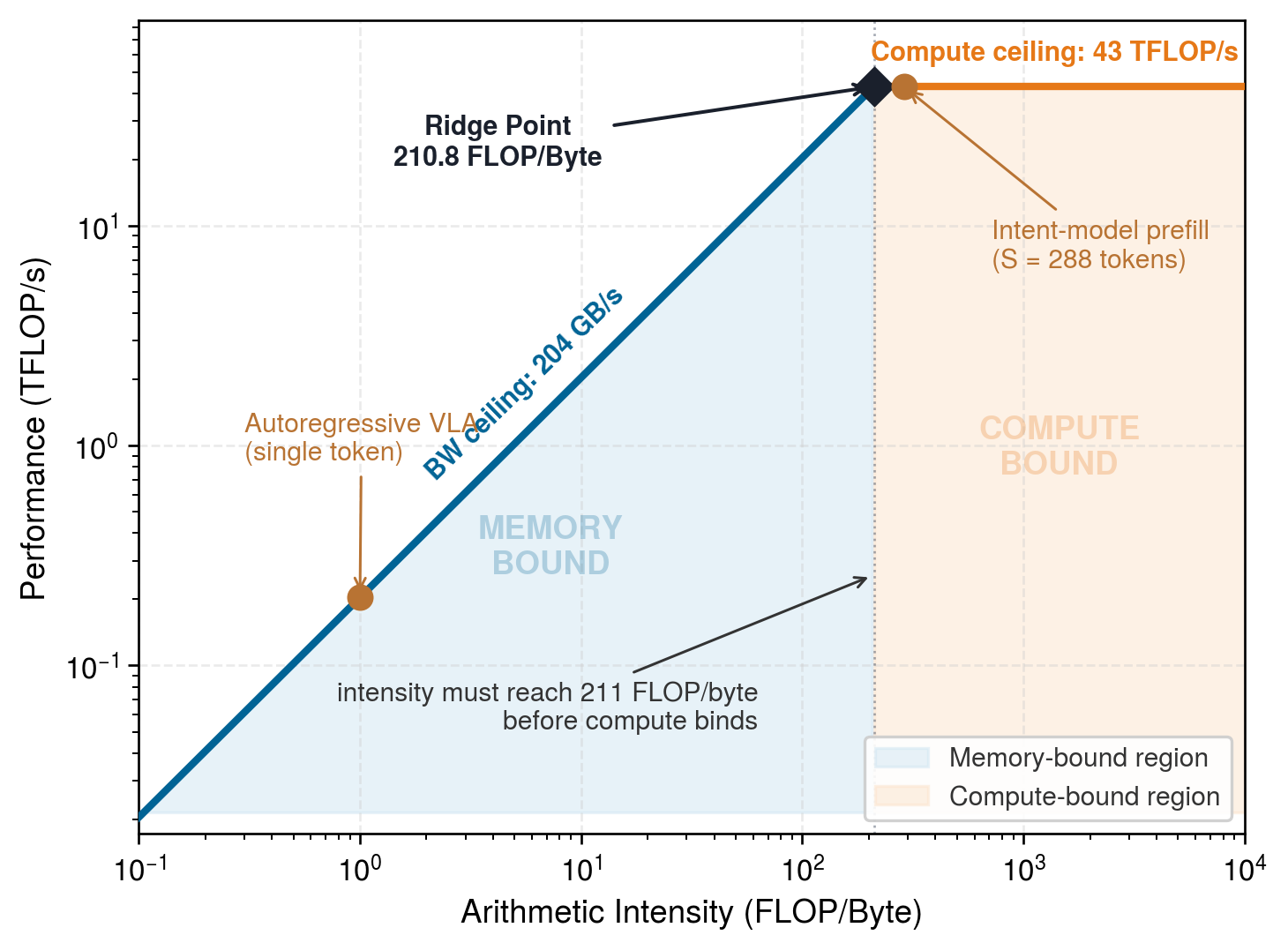
The mobile manipulator’s application processor is a Jetson AGX Orin module (The machine data sheet). In its 60 W maximum-performance power mode, its dense FP16 GPU Tensor Core ceiling is 43 TFLOP/s; the aggregate sparse INT8 rating cannot be used for this FP16 workload. Using the registry’s rounded peak memory bandwidth of 204 GB/s, the hardware ridge point occurs at: \[I_{\text{ridge}} = \frac{R_{\text{peak}}}{\text{BW}} = \frac{43 TFLOP/s}{204 GB/s} \approx 210.8 FLOP/byte\] For this weight-streaming example, \(\HalfPrecisionGemvIntensity = 1.0\,\text{FLOP/byte}\) is far below 210.8 FLOP/byte, so memory bandwidth sets the roofline ceiling. Attainable throughput is bounded by the peak bandwidth times \(\HalfPrecisionGemvIntensity\), or 0.204 TFLOP/s, about 0.47 percent of the dense FP16 peak; the sustained bandwidth that the notebook below uses lowers it further. That ratio is a workload throughput bound, not a measurement of how many cores are idle. Both roofs also assume the maximum-performance mode. A battery-powered base often runs a lower power mode, down to 15 W on this module, where lower clocks drop both the compute and the bandwidth roof; the chassis thermal budget sets the mode the machine can sustain.

Definition 3.1: Memory wall

Memory wall is the limit on a workload’s rate that arises when its operands cannot reach the arithmetic units as fast as those units could consume them, so that the bytes moved from off-chip memory, not the operations performed, set the time per evaluation.

1. Significance: A proposer whose weights do not stay on chip must stream them at least once per fresh evaluation, which gives equation 2. On the machine’s application processor, the intent model’s 14 GB of FP16 weights at 142.8 GB/s sustained allow at most 10.2 Hz before any vision or decoding work, two orders of magnitude below the 1 kHz permission tick.
2. Distinction: A compute bound yields to faster arithmetic; the memory wall yields only to fewer bytes per evaluation (fewer or narrower weights, or weights that stay resident on chip) or to more bandwidth. It is also distinct from memory capacity: a model can fit in DRAM and still be too slow to stream.
3. Common pitfall: A frequent misconception is that a processor’s peak arithmetic rating predicts its batch-1 inference rate. Single-token weight streaming on this processor reaches only about 0.47 percent of its dense FP16 peak, so the rating overstates the attainable rate by orders of magnitude.

On the mobile manipulator’s application processor, then, the memory wall⁷ caps the intent model’s fresh-evaluation rate, before any vision or decoding work, far below the 100–1000 Hz at which stabilization, joint impedance control, and reflex-level collision avoidance run (notebook 3.1). Each of those loop rates is set by the physical time constant of the motion its loop must stabilize, a derivation carried out in Multi-Rate Cadences. A model renewed that slowly can say where the arm should go, but it cannot close the loop on moving mass, so it proposes waypoints and a faster loop below it tracks them. That conclusion is about timing only. The separate requirement that learned outputs remain proposals, even when they arrive in time, comes from the failures of section 3.6.

⁷ Wulf and McKee: Their short paper named the memory wall (Wulf and McKee 1995), observing that processor speed was improving far faster than DRAM latency, so that memory access would eventually dominate run time whatever the processor did. Caches postponed the wall for workloads that reuse their data, but a batch-1 model on a robot meets it directly. When each weight is used once per fetch, the bus, not the arithmetic, sets how often a fresh proposal can arrive.

Wulf, Wm. A., and Sally A. McKee. 1995. “Hitting the Memory Wall: Implications of the Obvious.” ACM SIGARCH Computer Architecture News 23 (1): 20–24. https://doi.org/10.1145/216585.216588.

Repeated off-chip transfers also consume memory-system energy. Their power cost depends on the DRAM, controller, access pattern, and transfer rate, so a bandwidth calculation alone does not establish battery drain or actuator heating. Whatever the processor dissipates is heat released inside the same sealed chassis as the joint motors, and it raises the ambient temperature against which Thermal capacity and insulation breakdown thresholds rates each motor’s continuous torque.

A fresh evaluation is not a single point on the roofline. Its prefill reuses each fetched weight across all of its input tokens and lands past the ridge, while its decode returns to the memory-bound point, one full weight sweep per token. For a decoder that emits \(\EmittedTokenCount\) tokens one after another, equation 4 adds the two phases: \[\ProposerInferenceTime \approx \max\!\left(\frac{\PrefillOperations}{\EfficiencyHw\,\PeakRate},\ \frac{\WeightMemory}{\SustainedMemoryBandwidth}\right) + (\EmittedTokenCount-1)\,\frac{\WeightMemory}{\SustainedMemoryBandwidth} \tag{4}\] Here \(\PrefillOperations\) counts the prefill’s operations, \(\PeakRate\) is the processor’s peak arithmetic rate at the activation precision, and \(\EfficiencyHw\) is the fraction of that rate the prefill achieves. The prefill cannot finish before its own weight sweep, hence the maximum; the prefill emits the first token, and each of the other \(\EmittedTokenCount - 1\) tokens costs one more sweep. Notebook 3.1 prices both phases for the machine’s intent model.

Napkin Math 3.1: Pricing one intent-model evaluation

Problem: The mobile manipulator’s intent model is a 7B-parameter vision-language model sized after OpenVLA (Kim et al. 2024), running on the application processor. Where OpenVLA decodes a step of end-effector motion, the machine’s model decodes the same number of tokens to name a target pose (section 3.5.3). How long does one fresh evaluation take, which resource binds each part of it, and what renewal rate can the machine therefore state?

Variables:

• Parameters \(\Parameters =\) 7B in \(\LayerCount =\) 32 layers of width \(\HiddenDimension =\) 4096 (Datasheet). The decoder emits \(\EmittedTokenCount =\) 7 tokens, one per output dimension, one after another (Datasheet).
• Input tokens \(\SequenceLength =\) 288: 256 patches from one \(224{\times}224\) view (Derived) plus 32 instruction tokens (Illustrative).
• Dense FP16 peak \(\PeakRate =\) 43 TFLOP/s (Datasheet), of which the prefill achieves \(\EfficiencyHw =\) 50 percent (Illustrative).
• Peak bandwidth 204 GB/s (Datasheet), of which 70 percent is sustained (Illustrative), so \(\SustainedMemoryBandwidth =\) 142.8 GB/s.
• Stored weights: FP16 (2 bytes per parameter) or INT4 (half a byte), with activations kept in 16 bits (Chosen).

Math:

The memory wall. FP16 weights occupy 14 GB. If every evaluation streams them once, the bound above gives \[t_{\text{sweep}} = \frac{M_{\text{weights}}}{\text{BW}_{\text{mem}}} = \frac{14 GB}{142.8 GB/s} \approx 98.0 ms, \qquad f \le \frac{1}{t_{\text{sweep}}} \approx 10.2 Hz\]

The prefill binds on arithmetic. All \(\SequenceLength\) input tokens pass through the backbone together, costing two FLOPs per parameter per token (each weight multiplies one input value and adds the product to a running sum) plus a small attention term: \[O_{\text{prefill}} \approx 2 N S + 2 N_{L} d S^2 = 4.03 \times 10^{12} + 2.17 \times 10^{10} \approx 4.05 \times 10^{12}\ \text{FLOP}\] Each fetched weight now serves \(\SequenceLength\) tokens, so the intensity is about \(\SequenceLength \approx\) 288 FLOP/byte, beyond the 210.8 FLOP/byte ridge of figure 10. Arithmetic binds, and the weight sweep runs underneath it: \[t_{\text{prefill}} = \frac{O_{\text{prefill}}}{\eta_{\text{hw}}\,R_{\text{peak}}} = \frac{4.05 \times 10^{12}\ \text{FLOP}}{0.5 \times 43 TFLOP/s} \approx 188.5 ms\]

The decode binds on bandwidth. The prefill emits the first action token. Each of the remaining \(\EmittedTokenCount - 1 =\) 6 tokens is a matrix-vector pass that rereads every weight: \[t_{\text{FP16}} = t_{\text{prefill}} + (S_{\text{out}}-1)\,t_{\text{sweep}} \approx 189 ms + 6 \times 98.0 ms \approx 189 ms + 588 ms = 777 ms\] That is about 1.3 Hz.

INT4 weights shrink only the bandwidth term. Storing the weights in four bits cuts them to 3.5 GB and each sweep to 24.5 ms, but the prefill still multiplies 16-bit activations at the FP16 rate: \[t_{\text{INT4}} \approx 189 ms + 6 \times 24.5 ms \approx 189 ms + 147 ms = 336 ms, \qquad f \le 2.98 Hz\]

Sensitivity. Parallel decoding (Kim et al. 2025) moves the action tokens into the prefill (\(\SequenceLength + \EmittedTokenCount =\) 295) and removes the decode sweeps, giving 194 ms, only 2.9 percent inside a 200 ms period with the processor busy for all of it. Three camera views (\(\SequenceLength \approx\) 800) raise the INT4 total to 676 ms.

Result: At INT4 one evaluation takes about 336 ms. A published measurement of the same model and quantization on this processor reports 336 ms per frame (Franklin 2024), a gap of 0.1 percent. That agreement is closer than two illustrative factors deserve. It shows that the model has the right terms, not that \(\EfficiencyHw\) and the sustained fraction are exactly right. A 3 Hz rate would need a 333 ms period, so the machine runs its intent model at 2 Hz, one evaluation per 500 ms.

Systems insight: The binding resource depends on the phase. Prefill reuses weights across tokens and is compute-bound; decode rereads them per token and is bandwidth-bound (Pope et al. 2023). Weight-only quantization attacks only the second, so after INT4 the compute-bound prefill is most of the latency, and the next gain must come from fewer input tokens, lower-precision arithmetic that the processor’s kernels support, or a faster compute roof. Section 3.4.2 develops that choice and its accuracy cost.

3.4.2 Quantizing the intent model

The memory wall leaves two levers on the weight term, fewer weights or fewer bytes per weight. A smaller model may lose task recognition capability, which requires task evidence, so the selected design keeps the 7B-parameter model and pulls the second lever. Quantization stores each weight as a low-precision integer plus a shared scale, and reconstructs an approximate weight when the kernel needs it. In the common symmetric form, the weights are divided into groups of \(\QuantizationBlockSize\), each group keeps one 16-bit scale \(\QuantizationScale\), and each weight \(\FullPrecisionWeight_i\) becomes a \(\QuantizationBitWidth\)-bit integer \(\IntegerWeightCode_i\) (Jacob et al. 2018; Lin et al. 2024): \[\QuantizationScale = \frac{\max_{i \in \text{group}} |\FullPrecisionWeight_i|}{2^{\QuantizationBitWidth-1} - 1}, \qquad \IntegerWeightCode_i = \operatorname{clamp}\!\left(\operatorname{round}\!\left(\frac{\FullPrecisionWeight_i}{\QuantizationScale}\right),\, -2^{\QuantizationBitWidth-1},\, 2^{\QuantizationBitWidth-1} - 1\right), \qquad \ReconstructedWeight_i = \QuantizationScale\, \IntegerWeightCode_i\] Rounding moves each reconstructed weight \(\ReconstructedWeight_i\) at most \(\QuantizationScale/2\) from \(\FullPrecisionWeight_i\), so one large weight in a group coarsens the step for all the others; choosing which weights to protect from that error is where quantization methods differ. The stored size is \(\QuantizationBitWidth/8\) bytes per weight plus the scales’ share. At \(\QuantizationBitWidth = 4\) with the 128-weight groups that activation-aware weight quantization (AWQ) uses (Lin et al. 2024), the scales add 3.1 percent to the four-bit payload, which the half-byte-per-parameter figure used here leaves out.

Two families of quantization act on different terms of the latency. Weight-only quantization, the machine’s choice, restores each weight to 16 bits inside the kernel just before the multiply. It shrinks the bytes every decode sweep rereads, but the arithmetic still runs at the 16-bit rate, so the compute-bound prefill does not move. Weight-and-activation quantization makes both operands integers, so the multiplications themselves run on integer units and can shorten the prefill as well. It pays off only when three conditions hold: the processor has fast integer units for that precision, the runtime has kernels for the model’s layer shapes, and the activations tolerate the coarser grid. A format without a kernel is only a smaller file. Evaluating the intent model at three weight precisions with the prefill-plus-decode model of notebook 3.1 shows how closely the two-term estimate tracks measurements of the same model on the same module (table 1) (Franklin 2024).

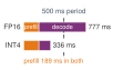
INT4 shrinks the decode; the 189 ms prefill it cannot touch now dominates.

Table 1: Weight-only quantization of the intent model: Computed latency uses the sustained bandwidth and the illustrative prefill utilization of section 3.4.1; measured latency and action scores are the Jetson AI Lab means over BridgeData V2 episodes on the 64 GB Jetson AGX Orin module (Franklin 2024). The episodes were included in training; the reported score is one minus the mean range-normalized root-mean-square error against their recorded actions, not agreement with FP16 or a closed-loop task-success rate. The source labels its 8-bit build FP8, but runs it in a mode that stores 8-bit weights and computes in 16 bits, the same weight-only form the computed row assumes. The FP16 measurement used a general-purpose runtime (Hugging Face) rather than the optimized one (MLC) used for the other two.

Weight format	Bytes per parameter	Weights	Weight sweep	Computed latency	Measured latency	Action score (1 − mean NRMSE)
FP16	2	14 GB	98.0 ms	777 ms	840 ms	95.3%
8-bit	1	7 GB	49.0 ms	483 ms	471 ms	95.2%
INT4 (deployed)	0.5	3.5 GB	24.5 ms	336 ms	336 ms	90.1%

The computed and measured columns agree within 2.5 percent for the 8-bit format and 0.1 percent for INT4. The model underestimates the FP16 run by 7.5 percent, consistent with that run’s slower runtime, so the comparison supports the model’s two terms rather than its exact constants. The table also shows where weight-only quantization stops paying. Each halving of the bytes halves the sweep, but the 188.5 ms prefill is untouched, and at INT4 it is already 56 percent of the latency. Even weights that cost no bytes at all would leave the prefill, so no weight-only format can lift the intent model above 5.3 Hz. Beyond that ceiling, the gain must come from integer arithmetic in the prefill, fewer input tokens, or a processor with a higher compute roof.

The last column carries the cost. On this module the INT4 build’s action score fell from 95.3 percent to 90.1 percent (Franklin 2024). OpenVLA’s authors, measuring task success on a real robot with a desktop GPU, found a different pattern. INT4 weights kept 71.9 percent success against 71.3 percent for bfloat16, while INT8 weights through a general-purpose quantization library fell to 58.1 percent. The cause was time, not rounding. The library’s added quantization operations cost more than the saved bytes, so the INT8 policy ran at 1.2 Hz on the evaluation GPU, against the 5 Hz control rate of its training data, and the robot met each observation later than the demonstrations had (Kim et al. 2024). On the module an 8-bit format was nearly free and INT4 reduced the offline action score; on the desktop GPU the 8-bit build lost success through its slower loop and INT4 was nearly free. The two 8-bit results used different software and kernels, and the two studies scored different tasks, so the pair shows that a bit width alone does not predict the outcome; the quantization method, the kernels, the control rate they allow, and the task together do.

Franklin, Dustin. 2024. OpenVLA: Vision/Language Action Models for Embodied Robotics. NVIDIA Jetson AI Lab tutorial.

A quantized checkpoint is therefore a different model. It must be evaluated on the machine’s own contact tasks at the deployed precision, carry its own calibration, and be named as such by the model_id of the proposal payload (section 3.5.4). The footprint saving also has a systems value: dropping from 14 GB to 3.5 GB of weights returns memory that retained context and perception also need, though how much of the computed latency saving survives when the cameras and the chunk policy share the bus must be measured under load. Even with that saving, quantization leaves the machine’s intent model at 2 Hz, one fresh proposal every 500 ms, while the arm below it consumes setpoints tens of times faster. No lever on the weight term closes a gap that large, and the gap raises two questions the weights cannot answer: how the arm stays supplied between evaluations, and how long whatever supplies it stays true.

Checkpoint 3.1: The memory wall and its levers

One fresh evaluation of a large proposer pays a compute-bound prefill and a bandwidth-bound decode, and each lever moves only one of them.

• Weight-streaming ceiling: Given a model’s parameter count, its bytes per parameter, and a sustained bandwidth, can you compute the ceiling of equation 2 and say what it leaves out?
• Prefill vs. decode: Can you explain, from arithmetic intensity, why the intent model’s prefill lands past the ridge of figure 10 while each decode token sits on the sloped roof?
• Weight-only quantization: Which term of equation 4 does INT4 shrink, and why does that leave a rate ceiling that no weight-only format can pass?
• Shorter-input estimate: The INT4 evaluation is a 189 ms prefill of \(\SequenceLength =\) 288 tokens plus 6 sweeps of 24.5 ms. Treating the prefill as proportional to \(\SequenceLength\), estimate whether halving the input tokens would fit one evaluation inside the 200 ms period of a 5 Hz rate.

3.5 Chunk Supply and Evidence Validity

One INT4 evaluation of the intent model takes 336 ms. Over that interval the mug keeps riding the conveyor, and an arm tracking a new setpoint every few tens of milliseconds would have nothing to track if each proposal named a single setpoint. Predicting a sequence of setpoints per evaluation solves the supply problem but raises a second one that the memory wall never touched. Every setpoint in such a sequence descends from one observation, so the sequence can outlast the evidence behind it. Sizing those sequences for the machine’s two proposers leads to three further questions: how long the supply stays true, what the slow proposer should hand the fast one, and what a proposal must carry for the permission path to refuse it.

3.5.1 Action chunking

If a proposer emits only one future setpoint per evaluation and takes longer than one setpoint step to finish the next inference pass, the controller runs out of planned motion while the processor is still computing. To keep dense waypoints flowing despite slow full-model inference, modern physical AI policies employ action chunking (definition 3.2), predicting a multi-step trajectory segment in a single pass (Zhao et al. 2023; Chi et al. 2025). Each chunk crosses the proposal boundary as one packet, reusing one evaluation across several outputs, though it does not make the next fresh camera observation arrive any sooner.

Definition 3.2: Temporal action chunking

Temporal action chunking is the policy formulation that predicts an entire horizon of \(\ActionChunkHorizon\) future continuous actions \(\PolicyActionWindow = [\CognitivePolicyAction_{t}, \dots, \CognitivePolicyAction_{t+\ActionChunkHorizon-1}]\) in a single neural evaluation or diffusion rollout, amortizing parameter memory transfers across extended physical execution windows.

1. Significance: Chunking divides the weight traffic per supplied setpoint by \(\ActionChunkHorizon\), 16 on the mobile manipulator, but leaves the delay before a new observation can change the motion at one renewal period plus one inference, 90 ms for its chunk policy. It does not make fresh observations or policy decisions arrive at the waypoint rate; a downstream controller tracks the accepted trajectory between model updates.
2. Distinction: Unlike single-step policies \(\CognitivePolicyAction_{t} \sim \pi(\cdot \mid \MultimodalObservation_{t})\), which condition only on the current observation and re-evaluate the full neural network at every control step, action chunking deliberately generates multi-step feedforward trajectories, executing only the start of each before the next replaces it (receding-horizon execution) and blending across overlapping chunks to reconcile slow neural deliberation with fast closed-loop control.
3. Common pitfall: Executing action chunks open-loop, without smoothing across chunk boundaries or a check by the permission path. Without smooth blending across overlapping chunk boundaries, switching between independently generated horizons injects acceleration jumps and torque shocks that excite mechanical gearbox resonances.

Predicting a horizon⁸ of \(\ActionChunkHorizon\) actions per forward pass spreads the multi-gigabyte DRAM weight streaming cost over \(\ActionChunkHorizon \times \SetpointStepInterval\) seconds of physical execution. On the mobile manipulator’s application processor, a 7B FP16 model (14 GB) generating single-step actions at the 40 Hz setpoint rate would demand 40 \(\times\) 14 GB \(=\) 560 GB/s of memory bandwidth, 3.9 times the 142.8 GB/s it can sustain. A chunk of \(\ActionChunkHorizon =\) 16 waypoints cuts that demand to 35 GB/s, 24.5 percent of the sustained bandwidth, if one sweep supplies each full chunk. More frequent replanning, decoder work, and competing memory traffic consume additional bandwidth. The saving is in weight traffic per supplied waypoint, not an equal gain in arithmetic intensity: predicting a chunk adds decoder work, and its position on the roofline depends on the operations performed and the bytes actually transferred. Predicting a sequence also changes how a learned policy uses recent actions, so this supply calculation establishes only the weight traffic for the stated schedule, not that the policy attends to the right evidence or recovers from an unfamiliar contact.

⁸ Receding Horizon: Model predictive control optimizes over a fixed horizon, executes only the first part of the plan, and then replans from the newly measured state, so the horizon recedes as time advances (Mayne et al. 2000). A chunked policy is the learned analog and inherits the same rule: the unexecuted tail of a chunk is a buffer that the next evaluation may overwrite, never a commitment the machine owes to finish.

Mayne, David Q., James B. Rawlings, Christopher V. Rao, and Pierre O. M. Scokaert. 2000. “Constrained Model Predictive Control: Stability and Optimality.” Automatica 36 (6): 789–814. https://doi.org/10.1016/S0005-1098(99)00214-9.

Supply rate vs. closed-loop reaction latency On the running machine, the smaller chunk policy follows its own illustrative schedule, in which three quantities separate the rate at which setpoints reach the servos from the delay before a new observation changes a proposal:

• Setpoint supply cadence (\(\ActionExecutionRate = 1/\SetpointStepInterval =\) 40 Hz, \(\SetpointStepInterval =\) 25 ms): The rate at which the trajectory queue delivers discrete waypoints to the joint servo loop.
• Policy replanning rate (\(\ChunkRenewalRate =\) 20 Hz, period \(\ChunkRenewalPeriod =\) 50 ms): The cadence at which the smaller chunk policy begins an evaluation from fresh sensory frames. The period is chosen as a whole number of setpoint steps, here 2, so that every renewal begins on a setpoint boundary.
• Closed-loop reaction latency (\(\ChunkReactionLatency = \ChunkRenewalPeriod + \ProposerInferenceTime =\) 50 ms \(+\) 40 ms \(=\) 90 ms): The worst sampling-phase wait plus the assumed inference time until a revised proposal is available, excluding further admission and physical response delay.

In this illustrative schedule, a disturbance immediately after capture can wait up to 90 ms for a revised learned proposal, before any additional admission and actuation delay. The independent permission path need not wait for that revision. Current qualified evidence, meaning measurements whose error bound and age have been established for this use (Spatial Error and Clearance Bounds develops how), can trigger a protective response while the policy computes. Its ability to detect the relevant obstacle and complete a feasible response needs its own timing and sensing evidence. Chunking keeps candidate waypoints available; it establishes neither that response nor its deadline.

Pricing the decoder families The three decoder families of section 3.3 differ in how they turn one observation into a chunk, and the machine’s processor prices that difference. Suppose the intent-sized backbone, with its deployed INT4 weights, produced one fresh chunk of \(\ActionChunkHorizon =\) 16 setpoints of 7 values each. Every family first pays the same compute-bound prefill of the observation, about 189 ms, and then the families part ways:

• Binned autoregressive tokens need 112 sequential decode steps, each rereading the backbone weights, for about 2.9 s.
• FAST tokens cut the sequence to about 30 tokens, the count its authors report per arm for a one-second chunk and therefore generous for this shorter chunk, about 899 ms, still sequential.
• A parallel head folds every action into one longer prefill, about 264 ms.
• A \(\pi_0\)-sized action expert of 600 MB in 16-bit weights integrates 10 steps. Each step rereads the expert and the backbone’s 151 MB of cached keys and values rather than the backbone weights, about 5.3 ms per step on bandwidth, for about 241 ms in all. Continuous trajectory diffusion and flow matching derives the noise-prediction and flow-matching objectives these experts train on.

The decoder choice spans 12× in latency on the same backbone, the cost that parallel decoding and action experts were introduced to remove (Kim et al. 2025; Black et al. 2024). In the expert design, weights of hundreds of megabytes far exceed the processor’s on-chip caches, so each refinement step pays another off-chip transfer; a head small enough to stay resident would change that term, and reducing the number of refinement steps shortens the decoder provided the proposals keep the required task quality, though neither touches the prefill of a fresh observation. None of the four therefore renews within the chunk policy’s 50 ms period, because the prefill alone exceeds it. A large backbone that reads each observation fresh cannot also be the fast renewer on this processor, whatever its decoder. Deployed dual systems reach the same conclusion by assigning renewal to a separate, smaller model, as table 2 records, and the machine does the same with its ACT chunk policy.

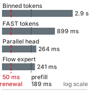
No decoder renews within 50 ms; the prefill alone is too slow.

Whatever the decoder, chunking creates one more problem, chunk seam continuity. Because each action chunk is generated independently from rolling sensory observations, the tail of chunk \(\ActionChunkIndex\) and the head of chunk \(\ActionChunkIndex+1\) may show slight positional and velocity discrepancies. If a controller concatenated these chunks directly, the resulting step-discontinuities in acceleration would inject large jerk (\(\dddot{\GeneralizedCoordinates}\)) into the physical linkages, inducing mechanical shock, acoustic vibration, gear-tooth wear, and motor overcurrent faults. To reduce discontinuities between overlapping chunks, systems can implement temporal ensembling, blending overlapping trajectory predictions via exponentially weighted averaging:

\[\CognitivePolicyAction_{t} = \frac{\sum_{k=0}^{\EnsemblingWindowLength-1} \ChunkEnsemblingWeight_k \, \CognitivePolicyAction_{t}^{(\ActionChunkIndex)}}{\sum_{k=0}^{\EnsemblingWindowLength-1} \ChunkEnsemblingWeight_k}, \quad \ChunkEnsemblingWeight_k = \exp(-\EnsemblingDecayRate \cdot \ActionChunkIndex)\]

where \(\CognitivePolicyAction_{t}^{(\ActionChunkIndex)}\) is the action for step \(\ControlStepIndex\) predicted by the \(\ActionChunkIndex\)-th oldest of the \(\EnsemblingWindowLength\) chunks that cover step \(\ControlStepIndex\) (\(\ActionChunkIndex = 0\) is the oldest), and \(\EnsemblingDecayRate > 0\) is a tunable weighting rate. Following ACT, the oldest prediction receives the largest weight, which favors smoothness over responsiveness; a smaller \(\EnsemblingDecayRate\) lets new observations enter the blend faster (Zhao et al. 2023). The formula assumes that the policy is queried at every control step, as ACT does, so that \(\EnsemblingWindowLength = \min(\ControlStepIndex + 1, \ActionChunkHorizon)\). The mobile manipulator’s chunk policy renews every 2 setpoints instead, and because its 50 ms renewal period is a whole number of 25 ms steps, each new chunk starts on a setpoint boundary. The waypoints use capture-relative times, so elapsed entries are not newly executed when a chunk arrives. The first setpoint is dated at capture, and each following interval advances by 25 ms, so the last interval reaches the capture-relative horizon. At arrival, the first 2 entries are already past; the next 2 setpoints precede replacement. The same formula then applies with \(\ActionChunkIndex\) counting renewals rather than steps. A 16-setpoint chunk renewed every 2 setpoints gives at most \(\EnsemblingWindowLength =\) 8 overlapping predictions at any step. A renewal period that fell between setpoints would leave each chunk’s first action off the grid, and the blend would first have to interpolate every chunk onto common setpoint times. Below the proposal boundary, the permission path interpolates the admitted waypoints into a setpoint for every bus cycle, and the drives close their own velocity and current loops on those setpoints.

↪ The interpolation that turns admitted waypoints into per-cycle setpoints, and the fallback it executes when waypoints stop arriving, is developed in Rate interpolation and boundary fallback execution.

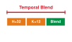
Each chunk runs 2 of its 16 steps; later chunks overlap the rest.

Ensembling has two limits. It averages, and the average of two valid predictions need not be valid, the same mode averaging that defeats a regression head. If an older chunk passes left of an obstacle and a newer one passes right, the blend steers between them (Black, Galliker, et al. 2025). It also ignores what executes while the policy computes. With the assumed 40 ms inference and 25 ms setpoints, the arm consumes 2 setpoints of the previous chunk before the new one exists, so no new prediction can change them. Real-time chunking treats those setpoints as committed. It freezes the part of the previous chunk that will execute during inference and has a flow or diffusion policy fill in the rest of the new chunk so that it agrees with that frozen prefix, rather than blending afterward (Black, Galliker, et al. 2025). The method arrives from the learning side at this chapter’s distinction, in which the committed prefix is motion already admitted and the tail is a buffer that the next evaluation may still rewrite.

↪ The chunk-prediction objective and the modal commitment it buys in training are developed in Action chunking and multi-step trajectory prediction.

Systems Perspective 3.1: The temporal ensembling jerk trap

Exponentially weighted temporal ensembling averages overlapping predictions, but averaging sampled setpoints alone guarantees neither continuous position nor continuous velocity between samples or at chunk boundaries. The interpolator on the permission path determines those properties. If successive chunks disagree in slope, a controller can receive a step in commanded velocity even when position remains continuous. In joint proportional-derivative (PD) tracking (\(\JointTorque = \ProportionalGainMatrix \TrackingErrorVector + \DerivativeGainMatrix \TrackingErrorRate\)), that velocity jump produces a finite torque step. With an illustrative derivative gain for one joint, the diagonal entry \(\PidDerivativeGain = 40\,\text{N}\cdot\text{m}\cdot\text{s/rad}\) of \(\DerivativeGainMatrix\), and an illustrative velocity discontinuity \(\FiniteChange \JointVelocity = 0.5\,\text{rad/s}\), the derivative term changes by \(\FiniteChange \CommandedJointTorque = \PidDerivativeGain \FiniteChange \JointVelocity = 20\,\text{N}\cdot\text{m}\). Dividing by the servo period would instead describe a torque slew rate, not a torque. Abrupt torque changes can excite mechanical resonances or exceed drive limits. Interpolation must match position, velocity, and acceleration at adjoining segments, the property called \(\Glyph{C}^2\) continuity, while enforcing the machine’s velocity, acceleration, and torque limits. Smoothness alone does not establish that the requested motion is feasible.

↪ The quintic spline that matches position, velocity, and acceleration across a chunk seam is developed in Quintic splines and C^2 boundary matching.

A chunked policy therefore has two rates that a single “action rate” conflates: the spacing of the waypoints it supplies and the interval between the fresh observations that change them. Supplying more waypoints from one sensory context does not refresh the observation on which they depend. A downstream controller can use current state measurements while tracking admitted waypoints between renewals, and its feedback corrects tracking errors within its capabilities, but a newly perceived obstacle still requires a timely checking or replanning response. The mobile manipulator’s own budget makes this distinction quantitative, first for supply and then for the time the evidence behind a chunk stays true.

3.5.2 Two proposers and the evidence horizon

Chunking reduces the cost per waypoint, but the decoder pricing showed that each fresh context still waits for the large backbone’s prefill, whatever the decoder. The split that follows, a slow intent model above a fast chunk policy, can now be budgeted on the warehouse mobile manipulator, and the chunks the fast policy supplies can be checked against how long they stay true. Budgeting that split also uses a term that the stopping budget of Delay consumes stopping clearance already charged, a lease, authority that lapses unless it is renewed. The motion the chunk policy proposes runs under a chunk lease, the longest an admitted chunk may keep driving the actuators without an admitted successor, which Chunk Lease Sizing from the Stopping Budget sizes against the stopping budget so that a late renewal is contained by that lease rather than by the length of the chunk. Notebook 3.2 applies the memory bound to the split and checks whether chunking alone could give the larger model the required renewal cadence.

Napkin Math 3.2: The renewal gap

Problem: Chunking spreads one weight sweep across many setpoints. Can it let the intent model renew proposals within the chunk policy’s 50 ms period, or does the machine need a second, smaller proposer, and how much of the shared bus do the two proposers then take?

Variables:

• Intent model: 14 GB of FP16 or 3.5 GB of INT4 weights (Derived), an INT4 evaluation of 336 ms that decodes \(\EmittedTokenCount =\) 7 tokens (Derived, notebook 3.1), run at 2 Hz (Chosen).
• Chunk policy: 80M parameters, ACT’s size (Datasheet), 0.16 GB in FP16 (Derived), renewed at 20 Hz (Chosen).
• Chunk of \(\ActionChunkHorizon =\) 16 setpoints at \(\SetpointStepInterval =\) 25 ms (Chosen); sustained bandwidth \(\SustainedMemoryBandwidth =\) 142.8 GB/s (Derived).

Math:

Amortization. Counting weight traffic only, as section 3.5.1 did, and setting aside the prefill’s arithmetic and the other decode sweeps, one FP16 sweep that emitted a whole chunk would be shared by \(\ActionChunkHorizon\) setpoints: \[t_{\text{amort}} = \frac{t_{\text{stream}}}{H} = \frac{98.0 ms}{16\text{ setpoints}} \approx 6.1 ms\text{ per setpoint}\]

Renewal. A fresh chunk still waits for a whole INT4 evaluation, prefill and decode together, while the chunk policy streams its own weights in about a millisecond; the rest of its inference target goes to vision encoding and the decoder’s arithmetic: \[\frac{t_{\text{INT4}}}{T_{\text{chunk}}} = \frac{336 ms}{50 ms} \approx 6.7\text{ renewal periods}, \qquad \frac{0.16 GB}{142.8 GB/s} \approx 1.12 ms\]

Bus share. The INT4 intent model streams its weights \(\EmittedTokenCount\) times per evaluation, once under the prefill and once per remaining token (equation 4); the chunk policy streams its weights once per renewal: \[S_{\text{out}}\,M_{\text{INT4}}\,f_{\text{intent}} + M_{\text{chunk}}\,f_{\text{chunk}} = 7 \times 3.5 GB \times 2 Hz + 0.16 GB \times 20 Hz = 49 GB/s + 3.2 GB/s = 52.2 GB/s\]

Result: Amortization cuts the weight time per setpoint to 6.1 ms, but each fresh intent-model chunk arrives 6.7 renewal periods after its capture. The chunk policy’s sweep takes 2.2 percent of its period. Together the two proposers average 52.2 GB/s of weight traffic, 37 percent of the sustained bandwidth.

Systems insight: Amortization is a supply lever, not a renewal lever, so the machine renews with a second, smaller proposer. The average hides the timing. For 147 ms of every 500 ms, the intent model’s decode sweeps are modeled at the full sustained bandwidth, so a chunk-policy evaluation that overlaps them competes for the same bus, and its latency target holds only if it is measured under that contention. A late renewal is not free: the arm keeps moving on the previous chunk, and the chunk lease bounds how far.

The selected design follows. The 80M-parameter chunk policy uses ACT as its size reference and is assumed to be adapted to the mobile manipulator. It proposes base velocity and arm joint targets together at 20 Hz (a 50 ms replanning period), emitting waypoints spaced at \(\SetpointStepInterval =\) 25 ms (a 40 Hz supply rate), within a 40 ms p99 inference target that includes vision, while the permission path interpolates admitted waypoints into per-cycle setpoints and the drives close their velocity and current loops at their own faster rates. The intent model revises its target at 2 Hz. That is a candidate architecture, not a measured timing result. Loaded execution must establish the inference target, and a percentile target still permits overruns; the chunk lease contains a missed renewal.

What retained history would cost The intent model as deployed reads one frame and keeps nothing between evaluations, so the budget above is complete for it. A variant that conditioned on several seconds of history would add memory pressure that the weights alone do not show, and the cost is worth knowing before anyone proposes one. The per-token charge from section 3.3, 0.52 MB of full-width FP16 keys and values across all 32 layers through equation 1, now scales with history. One synchronized set of 3 \(224{\times}224\) frames (3 \(\times\) 256 \(=\) 768 patch tokens) adds 402.7 MB. This is a standard multi-head attention estimate for a hypothetical multi-camera extension, not a measured cache footprint for the published OpenVLA checkpoint. Counting language and proprioception tokens along with the visual patches raises each step to \(\SequenceLength \approx\) 800 tokens, so each observation step adds 419.4 MB of KV cache. Retaining an unpruned 5 s historical context window at 10 Hz would yield 21.0 GB of KV cache. This hypothetical history exceeds the published OpenVLA checkpoint’s configured context window; the calculation exposes the storage cost of such an extension, rather than claiming that the checkpoint supports it. Combined with the intent model’s 14 GB of weights, this example claims 35.0 GB, about half of the application processor’s 68.7 GB (the module sold as 64 GB counts in binary gigabytes, \(64 \times 2^{30}\) bytes) before runtime overhead, memory that perception, mapping, and the chunk policy also need. Even where memory capacity permits, reading a large cache is further traffic on that same bus. Bounding retained history therefore serves both capacity and timely renewal. Spatial pooling or cross-attention can reduce context traffic; fixed-horizon action output does not by itself bound the observation history retained by the backbone.

5 s of retained context outweighs the 14 GB of weights.

The split fixes how often each proposer renews. The moving target fixes how long each renewal stays true. At the pick station the arm takes the mug from a moving conveyor, and a chunk is useful only while the mug stays within the grasp tolerance \(\PositionalTaskTolerance\) of where the chunk’s evidence placed it, starting from the handle estimate’s initial error \(\InitialTrackingError\). Untracked, the belt’s steady speed \(\ConveyorSpeed\) uses up the margin \(\PositionalTaskTolerance - \InitialTrackingError\) within the freshness deadline \(\PositionErrorCeiling/\SpeedBound\) of Measurement Freshness, here with \(\PositionErrorCeiling = \PositionalTaskTolerance - \InitialTrackingError\) and \(\SpeedBound = \ConveyorSpeed\). A tracker removes that steady motion. It is the memory stage of the pipeline, re-estimating the mug’s position and velocity from each new frame, and a chunk computed from its estimate aims at where the mug will be if the belt keeps its speed. What that extrapolation cannot foresee is a change of speed after capture, the mug slipping on the belt at a residual acceleration \(\SlipAccelerationBound\). The chunk’s setpoints were fixed at its capture, so later frames do not correct them, and extrapolation over an evidence age \(\Time\) drifts by \(\tfrac{1}{2} \SlipAccelerationBound \Time^2\). Setting that drift equal to the margin gives the evidence horizon of the tracked mug, the longest time the evidence behind a chunk keeps the mug within tolerance, in equation 5: \[\EvidenceHorizon = \sqrt{\frac{2\,(\PositionalTaskTolerance - \InitialTrackingError)}{\SlipAccelerationBound}} \tag{5}\] When inference meets the stated target and no further admission delay is charged, a chunk is replaced one renewal period plus one inference after the capture it was computed from, the reaction latency \(\ChunkRenewalPeriod + \ProposerInferenceTime\) of section 3.5.1. That span must fit inside \(\EvidenceHorizon\), and the chunk must carry enough setpoints to bridge it, as equation 6 requires: \[\MinimumChunkSetpointCount = \left\lceil \frac{\ChunkRenewalPeriod + \ProposerInferenceTime}{\SetpointStepInterval} \right\rceil \tag{6}\] Together, equation 5 and equation 6 distinguish the setpoint buffer a chunk carries from the duration its evidence remains valid. Notebook 3.3 applies both bounds to the machine’s schedule.

Napkin Math 3.3: Buffer, not permission

Problem: The chunk policy renews every 50 ms, is assumed to need 40 ms per evaluation, and emits 16 setpoints 25 ms apart. Does the schedule depend on tracking the mug, how many setpoints must a chunk carry, and how much of each chunk may the arm execute on the evidence behind it?

Variables:

• Conveyor speed \(\ConveyorSpeed =\) 0.20 m/s and residual slip acceleration \(\SlipAccelerationBound =\) 0.50 m/s² (Illustrative).
• Grasp tolerance \(\PositionalTaskTolerance =\) 15 mm (Chosen) and initial handle error \(\InitialTrackingError =\) 3 mm (Illustrative), a margin of 12 mm.
• Renewal period \(\ChunkRenewalPeriod =\) 50 ms, setpoint step \(\SetpointStepInterval =\) 25 ms, and \(\ActionChunkHorizon =\) 16 (Chosen); inference \(\ProposerInferenceTime =\) 40 ms, a p99 target that includes vision (Illustrative).

Math:

Untracked deadline. The belt alone uses up the margin in \[\frac{r_{\text{tol}} - e_0}{v_{\text{conv}}} = \frac{12\ \text{mm}}{0.20\ \text{m/s}} = 60\ \text{ms}\]

Tracked horizon. With the steady motion removed, equation 5 gives \[\tau_{\text{ev}} = \sqrt{\frac{2 \times 12\ \text{mm}}{0.50\ \text{m/s}^2}} \approx 219\ \text{ms}\]

Age at replacement and supply. equation 6 and the drift over the evidence age since capture give \[T_{\text{chunk}} + t_{\text{infer}} = 50 + 40 = 90\ \text{ms}, \quad \tfrac{1}{2} a_{\text{slip}} T^2 = \tfrac{1}{2} \times 0.50 \times (0.09\ \text{s})^2 \approx 2.0\ \text{mm}, \quad h_{\min} = \left\lceil \tfrac{90}{25} \right\rceil = 4\]

The whole chunk. Executed open-loop to its end, one chunk would carry the mug to \[H\,\Delta t_{\text{step}} = 16 \times 25\ \text{ms} = 400\ \text{ms}, \quad e_0 + \tfrac{1}{2} \times 0.50 \times (0.40\ \text{s})^2 = 3 + 40 = 43\ \text{mm} > 15\ \text{mm}\]

Sensitivity. Renewing at 10 Hz instead raises the age at replacement to 140 ms, still inside \(\EvidenceHorizon\), and \(\MinimumChunkSetpointCount\) to 6.

Result: Untracked, the mug leaves tolerance after 60 ms, before the first replacement at 90 ms, so this schedule depends on the tracker. Tracked, the evidence holds for about 219 ms: 4 setpoints bridge each renewal, and the 90 ms evidence age at replacement permits drift of only 2.0 mm. The 400 ms chunk outlasts its evidence by 181 ms.

Systems insight: The chunk is sized for supply, not for execution. Its tail beyond \(\EvidenceHorizon\) keeps setpoints flowing if a renewal slips, but it is not permission to finish the motion, because the drift it would carry the arm through cannot be taken back once the gripper closes on the wrong place. The permission path therefore ages each chunk’s evidence against \(\EvidenceHorizon\), and when renewal stops, the chunk lease, not the chunk length, bounds how far the arm may keep going.

On one clock, the schedule looks like figure 11. With direct replacement, each chunk is in force for only 50 ms before its successor replaces it, so motion computed from that capture ends when the capture is 90 ms old, inside the 219 ms evidence horizon. Temporal ensembling instead retains contributions from older chunks. A blend must exclude contributions whose evidence has expired and carry the oldest capture time among the contributions it retains; the direct-replacement timing strip does not bound the age of that blend. If the chunk policy overruns its inference target, the notebook’s assumption no longer holds, and if renewal stops altogether, a further setpoint remains eligible only while both its evidence and the active chunk lease remain valid. If the implementation uses temporal ensembling, it must filter expired contributions before blending and date the result from the oldest retained evidence; seam continuity and feasibility still require independent checks.

Figure 11: Chunk supply against the evidence horizon: With direct replacement, time runs from the capture that the first chunk is computed from. The chunk policy renews every 50 ms and needs 40 ms per evaluation, so each chunk is in force for one renewal period and is replaced when its evidence is 90 ms old. The first chunk predicts a capture-relative horizon of 400 ms, including the prefix already elapsed before arrival, but the tracked mug stays within the grasp tolerance only for the 219 ms evidence horizon; the hatched tail is supply that keeps the setpoint stream full if renewal slips, not permission to execute it.

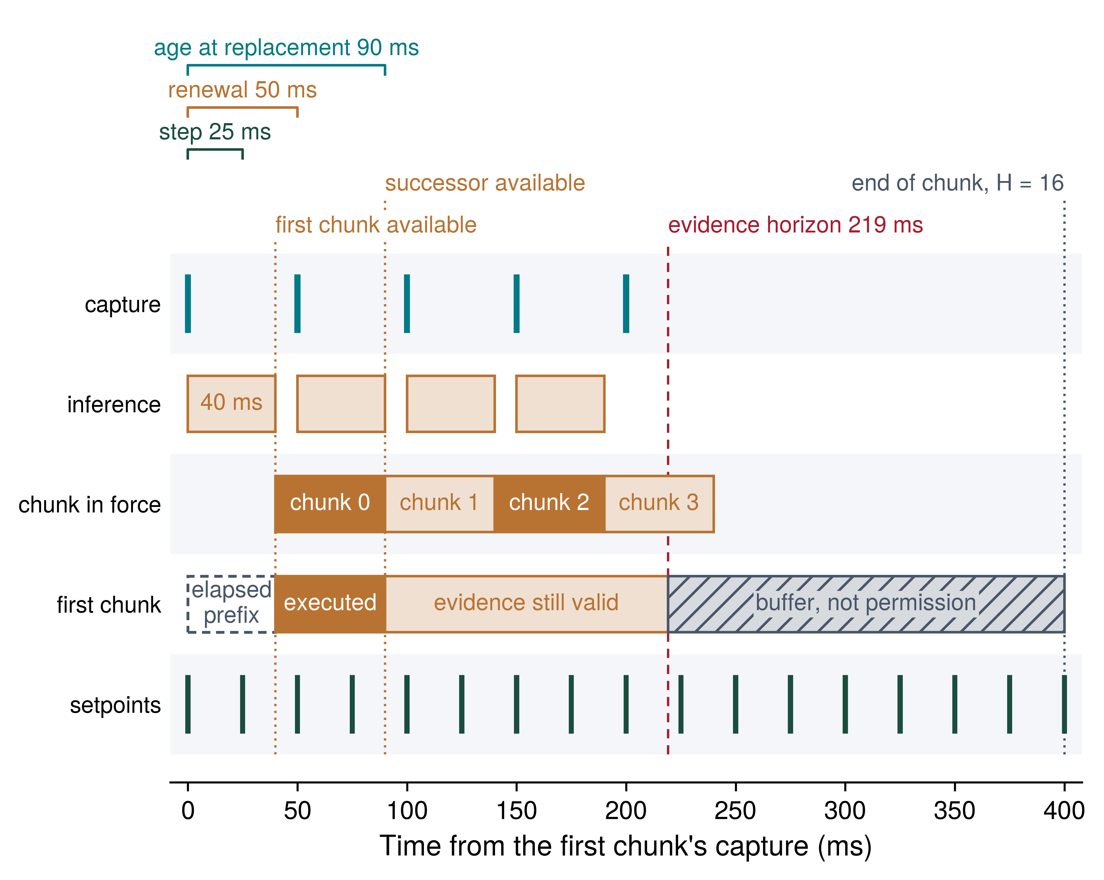
Under the stated assumptions, the conveyor calculation supplies the quantities needed to connect cognition to physical permission. One chunk covers 400 ms of motion, a new chunk is assumed to meet its 40 ms inference target, and the evidence stays within the stated grasp tolerance for about 219 ms. The Nervous System must combine these proposer limits with the body’s measured limits to establish its handoff record. That requires more information than a trajectory tensor alone. Timely delivery and usable evidence bound how long a proposal can remain eligible; they do not establish that the proposed grasp was correct.

3.5.3 Handing intent to the chunk policy

The split between a slow semantic model and a fast visuomotor policy is not peculiar to this machine. Helix runs a 7B-parameter vision-language model at 7 to 9 Hz above an 80M-parameter policy at 200 Hz (Figure AI 2025), and GR00T N1 runs its vision-language model at 10 Hz above a flow-matching transformer at 120 Hz (Bjorck et al. 2025). Across these and other published designs (table 2), the reported rates bracket the machine’s own 2 Hz and 20 Hz. What separates them is less their rates than what the slow model hands the fast one, and that choice decides what the permission path can check.

Deployed systems use three kinds of interface between the two tiers. With a latent vector, Helix’s slow model passes a single continuous latent that conditions the fast policy (Figure AI 2025), and GR00T N1’s policy attends to token embeddings taken from an intermediate layer of its vision-language model (Bjorck et al. 2025); because a latent is trained end to end, it carries whatever the fast policy finds useful and costs no decoding. Other architectures pass a language subtask: \(\pi_{0.5}\) first predicts the next subtask as text and then generates actions conditioned on it (Black, Brown, et al. 2025), while the orchestrating model of Gemini Robotics 1.5 sends its action model natural-language step instructions (Gemini Robotics Team 2025a). Still others emit an explicit geometric target, as in Gemini Robotics-ER, which predicts points, two- and three-dimensional boxes, trajectories, and grasps with coordinates in the scene (Gemini Robotics Team 2025b).

The permission path can check only a claim it can compare with its own evidence, and the three interfaces differ exactly there. A latent vector means something only to the network that reads it. No independent checker can tell whether it refers to the mug or to the photograph of a mug on a carton (section 3.6.1), and it carries no position that could age against the evidence horizon \(\EvidenceHorizon\). A text subtask can be checked against the task predicates the permission path has admitted, but “pick up the mug” names no location, so it can be neither compared with measured depth nor aged against drift. A geometric target allows both checks. It can be compared with calibrated depth and keep-out geometry, and aged from the capture time of the frame it came from. This geometric interface lets the machine’s intent lease be enforced, because that lease names a grounded target, never a path, and expires at the earliest of the time its evidence stays valid and the deadlines the permission path sets. With a latent or a text interface, the permission path can still check each chunk’s motion under the chunk lease, but the target behind that motion lacks this independent grounded-position check.

The mobile manipulator therefore has its intent model emit a target: a position, an orientation, and a gripper command, the same seven values OpenVLA decodes as a step of motion, together with the capture time of the frame it read. The timing shows why that target cannot stand alone. One evaluation takes 336 ms, longer than the 219 ms evidence horizon of the tracked mug, so the pose the intent model read is stale before its target arrives. The intent model therefore contributes which object to take and approximately where, and the tracker of section 3.5.2 supplies where that object is now. The tracker binds the target to its own latest estimate of the mug, and the 80M-parameter chunk policy aims at that fresh pose. The two leases then age against different clocks. The intent lease ages from the capture time of the tracker’s latest estimate and is renewed each time the tracker confirms the same mug, so it lapses when tracking is lost or a permission-path deadline passes. Each chunk carries the capture time of the oldest observation behind it, normally the frame the chunk policy itself read, and its evidence ages from that time against \(\EvidenceHorizon\).

The geometric bottleneck costs capability. A target pose cannot say how to fold a shirt or where to regrasp a cable, information a latent carries without a schema, so a checkable interface limits the tasks a single target can express. The machine accepts that limit in exchange for an intent the permission path can refuse. The same reasoning applies one level down to the chunk policy’s action space. Joint targets can be checked directly against joint limits and end-effector poses against workspace keep-out regions, which is why the proposal payload of section 3.5.4 carries both.

Table 2: State of practice in learned proposers, as of 2026: Published decoder mechanisms, sizes, and rates, with the interface each dual system passes from its slow model to its fast one. Rates and latencies are as the authors report them on different hardware, so they compare designs, not processors; none was measured on the machine’s application processor.

System (year)	Decoder mechanism	Reported sizes and rates	Slow-to-fast interface
OpenVLA (2024) (Kim et al. 2024)	Autoregressive binned tokens, one per action dimension	7B; about 6 Hz on a desktop GPU	None (single model)
OpenVLA-OFT (2025) (Kim et al. 2025)	Parallel decoding, continuous regression head	109.7 Hz against 4.2 Hz throughput for OpenVLA, 8-step chunks	None (single model)
\(\pi_0\) (2024) (Black et al. 2024)	Vision-language backbone with a flow-matching action expert	3.3B including a 300M expert; \(\ActionChunkHorizon =\) 50, 10 integration steps; 73 ms per chunk on a desktop GPU; control up to 50 Hz	None (single model)
\(\pi_0\)-FAST (2025) (Pertsch et al. 2025)	Autoregressive compressed (DCT and byte-pair) tokens	About 30 tokens per arm per one-second chunk (60 for two arms); about 750 ms per chunk against about 100 ms for \(\pi_0\)	None (single model)
\(\pi_{0.5}\) (2025) (Black, Brown, et al. 2025)	One model: text subtask, then flow-matching action expert	10 integration steps; control at 50 Hz; one text subtask decoded before each action chunk	Language subtask
Helix (2025) (Figure AI 2025)	Vision-language model above a cross-attention visuomotor transformer	7B at 7–9 Hz; 80M at 200 Hz over 35 degrees of freedom; onboard embedded GPUs	Latent vector
GR00T N1 (2025) (Bjorck et al. 2025)	Vision-language model above a flow-matching transformer	2.2B total, 1.34B in the language model; 10 Hz and 120 Hz; \(\ActionChunkHorizon =\) 16, 4 steps; 63.9 ms per chunk on a data center GPU	Intermediate-layer token embeddings (latent)
Gemini Robotics (2025) (Gemini Robotics Team 2025b, 2025a)	Cloud-hosted backbone with an on-robot action decoder; embodied-reasoning model as orchestrator	Backbone under 160 ms; about 250 ms end to end; 50 Hz control with chunks	Points, boxes, and grasps (ER); language step instructions (1.5)
This machine	INT4 intent model above an ACT chunk policy	7B at 2 Hz (336 ms computed); 80M at 20 Hz, \(\ActionChunkHorizon =\) 16 at 25 ms	Target pose with capture time

Kim, Moo Jin, Chelsea Finn, and Percy Liang. 2025. “Fine-Tuning Vision-Language-Action Models: Optimizing Speed and Success.” Robotics: Science and Systems XXI. https://doi.org/10.15607/RSS.2025.XXI.017.

Pertsch, Karl, Kyle Stachowicz, Brian Ichter, Danny Driess, Suraj Nair, Quan Vuong, Oier Mees, Chelsea Finn, and Sergey Levine. 2025. “FAST: Efficient Action Tokenization for Vision-Language-Action Models.” arXiv Preprint arXiv:2501.09747.

Black, Kevin, Noah Brown, James Darpinian, Karan Dhabalia, Danny Driess, Adnan Esmail, Michael Robert Equi, et al. 2025. “\(\pi_{0.5}\): A Vision-Language-Action Model with Open-World Generalization.” Proceedings of the Conference on Robot Learning (CoRL), Proceedings of machine learning research, vol. 305: 17–40.

Gemini Robotics Team. 2025b. “Gemini Robotics: Bringing AI into the Physical World.” arXiv Preprint arXiv:2503.20020.

Gemini Robotics Team. 2025a. “Gemini Robotics 1.5: Pushing the Frontier of Generalist Robots with Advanced Embodied Reasoning, Thinking, and Motion Transfer.” arXiv Preprint arXiv:2510.03342.

3.5.4 Information the proposer must supply

The conveyor budget gives each payload field a physical purpose. The receiver needs the candidate motion, the capture time from which its evidence ages, and the conditions limiting its validity. The following illustration groups that information with delivery metadata; it is not a new evidence record in the book’s record chain. Supervisory timers and proposal wire contracts wraps this payload in the proposal header the permission path validates, and the Nervous System’s handoff record combines this supply with the body’s limits.

The proposal payload \(\ProposalPayload\) is the typed candidate motion that the unprivileged Brain sends to the real-time Nervous System, packaged with the capture time of its evidence, the time after which it lapses, and the provenance the receiver needs to check it: \[\ProposalPayload = \langle \EvidenceCaptureInstant, \ProposalExpiryInstant, \ActionChunkHorizon, \SetpointStepInterval, \ProposedJointPositionSequence, \ProposedJointVelocitySequence, \ProposedEndEffectorPoseSequence, \ProposedGripperCommandSequence, \text{model\_id}, \text{lease\_id}, \ProposerConfidenceScore, \text{crc} \rangle\] The capture and validity times let the receiver compare the motion with freshness and calibration requirements it establishes independently; for the conveyor pick, \(\ProposalExpiryInstant\) can lie no later than \(\EvidenceCaptureInstant + \EvidenceHorizon\). The payload requests motion. It is neither execution permission nor the handoff evidence record, and a payload that omits its observation time or validity horizon invites the receiver to execute a proposal computed from a scene that no longer exists.

The fields in table 3 illustrate the information needed to interpret a candidate trajectory, rather than prescribing a second wire format. The proposer supplies trajectory and observation information. Validity claims require supporting evidence, while the receiver applies the separately established chunk lease. A lease_id associates the request with that permission process; it does not let the proposer grant itself authority. The header and handoff record specify delivery, admission, and expiration.

Table 3: Illustrative proposal payload fields: Candidate-motion information and associated metadata. The proposal header and handoff record belong to the Nervous System; this illustration adds no separate qualification record.

Field	Type	Unit	Systems Semantics and Verification Rule
t_capture	uint64_t	\(\text{ns}\)	Hardware timestamp of oldest sensory observation conditioning the proposal.
t_valid	uint64_t	\(\text{ns}\)	Monotonic time after which proposal expires (\(\le \EvidenceCaptureInstant + \EvidenceHorizon\)).
horizon_H	uint16_t	count	Number of prospective trajectory setpoints (\(\ActionChunkHorizon =\) 16 on this machine).
delta_t	uint32_t	\(\MicroUnitPrefix\text{s}\)	Temporal interval between consecutive waypoints (\(\SetpointStepInterval =\) 25,000 \(\MicroUnitPrefix\text{s}\), a 40 Hz supply rate).
q_traj	float32[H][n]	\(\text{rad}\)	Candidate joint trajectory array across \(\GeneralizedCoordinateCount\) degrees of freedom.
q_dot_traj	float32[H][n]	\(\text{rad/s}\)	Velocity setpoints; checked for continuity when adjoining chunks meet.
x_cartesian	position + orientation[H]	\(\text{m}, \text{quat}\)	End-effector target poses; verified against workspace keep-out boundaries.
gripper_cmd	float32[H]	\([0, 1]\)	Gripper closure target; evaluated against grasp force and slip limits.
model_id	uint32_t	identifier	Identifier resolving to the model architecture, weights checkpoint, and calibration profile.
confidence	float32	\([0, 1]\)	Score \(\ProposerConfidenceScore\) from the method named in the calibration profile (softmax margin for token decoders; sample dispersion, ensemble disagreement, or a conformal set for continuous decoders); absent when no method is qualified.
lease_id	uint64_t	identifier	Identifier linking the proposal to a time-limited permission record.
crc32	uint32_t	checksum	Integrity checksum protecting shared-memory ring buffer payload.

↪ Byte layout: The wire format that carries a chunk’s evidence time, expiry, horizon, and joint setpoints, with offsets, types, and checks, is given in Proposal header and chunk payload.

Checkpoint 3.2: Chunk supply and evidence horizons

Before analyzing runtime failure modes, check that you can separate what a chunk supplies from how long the evidence behind it holds.

• Amortization vs. renewal: Can you explain why a chunk cuts the intent model’s weight time per setpoint to 6.1 ms yet leaves each fresh intent-model chunk several renewal periods late, and why that forces a second proposer?
• KV cache growth: Can you use equation 1 to size the cache for a retained history, and explain why reading that cache competes with current sensor transfers on the same bus?
• Supply vs. validity: Can you explain why a chunk must carry at least \(\MinimumChunkSetpointCount\) setpoints to bridge one renewal, why the evidence age of motion from one observation must stay inside \(\EvidenceHorizon\), and why the remaining setpoints are a buffer rather than a plan?
• Slip estimate: If residual slip on the conveyor quadrupled, by what factor would equation 5 shrink \(\EvidenceHorizon\), and would the 90 ms age at replacement still fit inside it?

3.6 Cognitive Vulnerabilities

A chunk proposed by a mobile manipulator’s policy can arrive within its 40 ms execution budget, with every joint setpoint smooth and within kinematic limits, and yet still collide the gripper into the rim of the mug. The trajectory meets its real-time deadline, but its physical content is wrong, and the most consequential failures of learned physical AI systems sit in that gap. Learned foundation models expand task coverage across open-world environments, but no general proof of their integrated, closed-loop behavior across unconstrained state spaces is available. Engineering practice must instead analyze verified components within explicitly bounded operating regions.

Without a verified input domain and sensitivity bound, small sensing changes to a learned proposer can yield unexpectedly large changes in proposed motion, a sensitivity demonstrated early by imperceptible image perturbations that flipped image classification outputs (Szegedy et al. 2013). Benchmark success does not establish closed-loop stability, timing bounds, or physical safety under unseen operating conditions; those guarantees require independent evidence across the model, the software runtime, and the physical plant.⁹ Even when a valid sensitivity bound exists, it characterizes only the relationship between input perturbations and output deviations over a specified domain. It provides no proof that the nominal proposed action is collision-free or physically admissible, meaning analytical bounds can inform, but never replace, an independent permission decision.

Szegedy, Christian, Wojciech Zaremba, Ilya Sutskever, Joan Bruna, Dumitru Erhan, Ian Goodfellow, and Rob Fergus. 2013. “Intriguing Properties of Neural Networks.” arXiv Preprint arXiv:1312.6199.

⁹ Lipschitz Continuity in Neural Policies: Although neural networks with smooth activations are continuous on compact domains, a sensitivity bound \(\PolicyLipschitzBound = \sup_{\MechanicalPlantState_1 \ne \MechanicalPlantState_2} \frac{\lVert \pi(\MechanicalPlantState_1) - \pi(\MechanicalPlantState_2) \rVert}{\lVert \MechanicalPlantState_1 - \MechanicalPlantState_2 \rVert}\) must be established over a stated operating region. Where that bound holds, sensor error \(\lVert \FiniteChange \MechanicalPlantState \rVert \le \SensorErrorBound\) bounds the action change by \(\lVert \FiniteChange \CognitivePolicyAction \rVert \le \PolicyLipschitzBound\SensorErrorBound\); an unverified \(\PolicyLipschitzBound\) gives no usable action-error guarantee. Full derivations appear in Lipschitz continuity and spectral normalization.

A numerical interface easily traps malformed tensors, NaN values, and out-of-range floating-point setpoints, but it cannot detect a wrong grasp plan. Both classical pipelines and learned models can emit well-formed yet wrong commands; learning, however, adds failures rooted in high-dimensional latent features, out-of-distribution hallucinations, and uncalibrated confidence scores. Independent safety monitors can reject proposals that contradict measured geometry or joint limits, but they cannot infer true task intent. Safe operation in the physical world requires examining each of these failure modes and stating the evidence checks needed beyond packet formatting.

3.6.1 Semantic hallucinations

Consider a mobile manipulator clearing items near a conveyor. A discarded shipping carton carries a high-resolution printed photograph of a ceramic mug. The robot’s vision backbone attends to the visual texture, and the policy proposes an end-effector trajectory that closes the parallel jaws around the printed handle. The trajectory tensor is numerically flawless: smooth, within joint velocity and acceleration bounds, and clear of modeled obstacles. The handle it targets, however, is flat ink on cardboard. In web-scale vision models, attention maps track statistical correlations across 2D pixel arrays rather than measured 3D geometry.

Independent geometric evidence exposes this hallucination directly. A runtime validator compares the proposed grasp pose against calibrated depth returns to check whether physical relief supports the handle. If the depth sensor shows a flat cardboard surface within measurement resolution, the runtime rejects the proposal; if sensor dropouts or occlusion leave the region uncertain, the grasp remains unverified and must not be admitted. In neither case can a 2D attention map stand in for a 3D depth measurement. The proposer must therefore supply both its target coordinate frame and the supporting observation timestamps so that downstream checks can separate a physically grounded motion plan from an unverified visual guess.

↪ How depth error is bounded and qualified before a spatial claim can be trusted is developed in Spatial Error and Clearance Bounds.

3.6.2 The softmax illusion and out-of-distribution overconfidence

Deployment interfaces frequently conflate mathematical normalization with the physical probability of task success. In discrete classification, classification-based tokenization, or categorical action heads, raw output logits are transformed via the softmax operator:¹⁰ \[\SoftmaxFunction(\LogitVector)_i = \frac{e^{\OutputLogit_i}}{\sum_{j=1}^\ClassCount e^{\OutputLogit_j}}\] whose outputs sum to one purely by algebraic construction. When an embodied machine encounters out-of-distribution (OOD) observations, such as novel visual textures, intense specular glare, dynamic shadows, or water droplets on camera lenses, the network can still emit confidence scores near one for physically disastrous actions. Modern deep networks are often overconfident even on in-distribution inputs (Guo et al. 2017), and networks constructed from rectified linear units provably approach maximum confidence on inputs far from their training distribution (Hein et al. 2019).

¹⁰ Softmax (soft arg max): Bridle (1990) named the normalized exponential “softmax” because it is a differentiable version of the winner-take-all operation that picks the largest input. A function built to pick a winner keeps doing so far from its training data, pushing its top output toward one whenever one logit separates from the rest, whether or not the input resembles anything the model has seen.

Bridle, John S. 1990. “Probabilistic Interpretation of Feedforward Classification Network Outputs, with Relationships to Statistical Pattern Recognition.” In Neurocomputing: Algorithms, Architectures and Applications, edited by Françoise Fogelman Soulié and Jeanny Hérault, vol. 68. NATO ASI Series f: Computer and Systems Sciences. Springer. https://doi.org/10.1007/978-3-642-76153-9_28.

Guo, Chuan, Geoff Pleiss, Yu Sun, and Kilian Q. Weinberger. 2017. “On Calibration of Modern Neural Networks.” International Conference on Machine Learning (ICML) 70: 1321–30.

Hein, Matthias, Maksym Andriushchenko, and Julian Bitterwolf. 2019. “Why ReLU Networks Yield High-Confidence Predictions Far Away from the Training Data and How to Mitigate the Problem.” IEEE/CVF Conference on Computer Vision and Pattern Recognition (CVPR).

Calibration evaluates how closely a model’s predicted confidence aligns with observed empirical success rates under specified conditions. A confidence score is useful for selecting or abstaining from a proposal only to the extent that this relationship holds for the deployed task. Softmax overconfidence and calibration error formalizes binned expected calibration error and post-hoc temperature scaling. From a systems perspective, the execution runtime must bind calibration metadata directly to the model identity (model_id), preventing supervisory layers from mistaking uncalibrated algebraic certainty for physical permission.

In modern physical AI systems, populating the action payload’s confidence field is rarely as straightforward as extracting a softmax probability, because contemporary chunking policies do not operate as discrete classifiers. Action Chunking with Transformers (ACT), for example, decodes each multi-step chunk deterministically at inference time by clamping its latent style variable to the prior mean (Zhao et al. 2023). Similarly, diffusion and flow-matching policies iteratively denoise trajectories from Gaussian noise vectors. Neither architecture natively emits a normalized score. For these continuous decoders, confidence must be derived through an explicit, qualified estimation technique. Three primary architectures are used in practice:

• Sample dispersion. The system draws multiple trajectory chunks for the identical sensory observation by varying random diffusion noise seeds or sampling latent vectors. Measuring geometric dispersion across these trajectories describes the policy’s sampled output variability. Wide dispersion can reflect several valid motions as well as uncertainty; it does not by itself isolate uncertainty caused by missing knowledge.
• Ensemble disagreement. Multiple independently trained policy heads evaluate the same sensory input simultaneously. Downstream monitors measure the variance among their trajectory proposals, treating significant disagreement as an indicator of model uncertainty.
• Conformal thresholds. To convert heuristic dispersion or disagreement metrics into actionable statistical guarantees, the runtime applies inductive conformal prediction. Using a held-out calibration dataset, the system establishes an empirical threshold such that, under the assumption of exchangeability,¹¹ the predicted set covers the calibrated target with a chosen marginal coverage probability. Physical validity still requires independent checks against current geometry and plant limits. If the conformal set is empty or contains mutually conflicting actions, the runtime refuses the candidate or abstains; if active motion is no longer admissible, it requires a physically qualified response or operator intervention (Ren et al. 2023; Angelopoulos and Bates 2023).

¹¹ Exchangeability: The conformal guarantee assumes only that the calibration trials and the new trial are exchangeable, a weaker condition than independent and identically distributed data (Vovk et al. 2005). A deployed robot can break even that weaker assumption because its actions change the scenes it meets next, the endogenous data of the second law (The Four Bedrock Laws). A threshold calibrated under one policy therefore has to be re-established after every policy or deployment change, and its stated coverage lapses in between.

Vovk, Vladimir, Alex Gammerman, and Glenn Shafer. 2005. Algorithmic Learning in a Random World. Springer. https://doi.org/10.1007/b106715.

Ren, Allen Z., Anushri Dixit, Alexandra Bodrova, Sumeet Singh, Stephen Tu, Noah Brown, Peng Xu, et al. 2023. “Robots That Ask for Help: Uncertainty Alignment for Large Language Model Planners.” Proceedings of the 7th Conference on Robot Learning, Proceedings of machine learning research, vol. 229: 661–82.

Angelopoulos, Anastasios N., and Stephen Bates. 2023. “Conformal Prediction: A Gentle Introduction.” Foundations and Trends in Machine Learning 16 (4): 494–591. https://doi.org/10.1561/2200000101.

Each uncertainty estimation strategy incurs distinct hardware and memory-bandwidth costs. Generating multiple samples from a single observation can reuse visual backbone features and batch each decoding iteration through the policy head, sharing a weight read across samples. Iterative decoders still revisit their weights across refinement steps, and the balance between arithmetic and memory traffic depends on the batch and kernels. In contrast, an ensemble of disparate models requires reading separate sets of weights across the memory bus for every head, multiplying memory bandwidth traffic by the number of heads. The action payload must therefore treat the confidence scalar \(\ProposerConfidenceScore\) as meaningful only when accompanied by the identifier of the method that produced it and the corresponding calibration record, both resolved through model_id. A model lacking a qualified estimation pipeline must omit the confidence score entirely rather than emit an ungrounded default value.

The stipulated values in table 4 illustrate how environmental and hardware shifts can open a gap between confidence and success; they describe nominal illustrative regimes rather than a single deployed benchmark. The near-OOD row is a covariate shift, a change in the inputs the deployed model meets while the task stays the same. Across all shifted regimes, reported confidence significantly outstrips actual task success. A supervisory filter relying solely on an uncalibrated score threshold would mistakenly admit hazardous trajectories. Choosing an appropriate supervisory response depends on the integrity of the remaining sensor streams and the physical capabilities of the machine; a confidence discrepancy alone cannot dictate whether the robot should slow down, collect additional sensor frames, or execute an emergency stop.

Table 4: Illustrative Confidence–Success gaps under distribution shift: Stipulated confidence and task-success rates for four operating regimes, with candidate responses requiring separate physical justification. These values are illustrative, not test results.

Distribution Shift Regime	Physical & Environmental Trigger	Conf. vs. Success (\(\text{conf} \text{ vs. } \text{success}\))	Confidence–Success Gap (\(\text{conf}-\text{acc}\))	Downstream Supervisory Action
In-Distribution (Nominal Baseline)	Clean optics, structured laboratory lighting, nominal workpiece textures	\(\text{conf}=0.91, \, \text{acc}=0.89\)	\(+0.02\)	Apply independent limits before nominal execution
Near-OOD Shift (Covariate Shift)	Specular reflections, lens water droplets, dynamic shadow transitions	\(\text{conf}=0.89, \, \text{acc}=0.52\)	\(+0.37\)	Abstain or seek new evidence; permit probing only with a qualified contact policy
Far-OOD Shift (Semantic Shift)	Uncataloged deformable obstacles, human limb intrusion into workspace	\(\text{conf}=0.78, \, \text{acc}=0.08\)	\(+0.70\)	Reject proposal; use feasible controlled response
Sensor Degradation (Hardware Drift)	Photodetector thermal noise (\(>75^\circ\text{C}\)), focal blur from vibration	\(\text{conf}=0.84, \, \text{acc}=0.31\)	\(+0.53\)	Restrict operation to modes supported despite the sensor degradation

3.6.3 Perceptual chattering and covariate shift

When sensory observations hover near a boundary between competing object classes or grasp modes, small frame-to-frame noise flips the winning label back and forth, a failure known as perceptual chattering. If a motion planner treats each label flip as an abrupt change in the physical world, it discards and resets its trajectory on every frame. In the fatal 2018 Tempe autonomous vehicle collision, the National Transportation Safety Board record documents this failure in the automated driving system: the perception module alternated between classifying a pedestrian pushing a bicycle as a vehicle, a bicycle, and “other.” After each reclassification the path predictor dropped the object’s earlier locations, preventing the motion planner from seeing that the obstacle was crossing the vehicle’s path (National Transportation Safety Board 2019). Covariate shift, the near-OOD regime of table 4 in which the inputs change while the task stays the same, pushes more frames toward those boundaries; Mechanics of Endogenous Covariate Shift develops it.

National Transportation Safety Board. 2019. Collision Between Vehicle Controlled by Developmental Automated Driving System and Pedestrian, Tempe, Arizona, March 18, 2018. HAR-19/03. National Transportation Safety Board.

↩︎ The tracking-history loss under classification changes in the 2018 Tempe collision is established in Tracking history loss under classification churn.

In robotic manipulation, perceptual chattering injects rapid direction reversals into joint trajectory setpoints. Over a discrete control interval \(\FiniteChange \TimeInstant\), a sharp step in commanded velocity demands an instantaneous acceleration \(\FiniteChange \GeneralizedVelocities / \FiniteChange \TimeInstant\) beyond what the actuators can deliver. PD joint controllers react to the resulting velocity errors by commanding large opposing motor torques, the same derivative-gain torque step that the temporal-ensembling jerk trap of section 3.5.1 priced at a single chunk seam, now repeated at every flip. The resulting current spikes, tracking errors, and heat strain the power stage and gearbox, risking protective drive faults or structural vibration. Physical AI runtimes suppress perceptual chattering with three defenses:

1. Temporal hysteresis and debouncing. Requiring a newly observed class or spatial mode to persist across \(\DebounceFrameCount\) consecutive perception frames before committing a state change, just like switch debouncing¹² in embedded firmware.
2. Recursive state filtering. Fusing successive observations into a running estimate so that a single noisy frame cannot overwrite an established world state.
3. Rate and jerk limiting. Enforcing joint acceleration and jerk bounds in the real-time controller so that high-level label flicker cannot reach the motor shafts as torque shocks.

¹² Debouncing: The contacts of a mechanical switch bounce for milliseconds when pressed, so embedded firmware accepts a new switch state only after it has persisted for a set interval. The same \(\DebounceFrameCount\)-frame rule applied to class labels suppresses chattering, but it delays every genuine change by \(\DebounceFrameCount\) frames, time charged to the observation-age budget before any proposal is renewed.

↪ Recursive state estimation, which accumulates evidence across frames instead of trusting the latest one, is developed in Estimating State from Dated Measurements.

3.6.4 When intent expires

Notebook 3.3 already showed a chunk outliving its evidence, and the same failure applies one level up, to intent. Renewing a high-level goal identifier, or retransmitting a previous trajectory, does not refresh the observation that placed the mug. High-capacity intent models, which deliberate over long time horizons at low update rates, must therefore provide goals whose validity can be continuously audited against fresh, real-time telemetry while high-frequency reactive policies stream immediate motion.

The execution receiver must distinguish between rejecting a stale proposal and terminating an active, executing trajectory. Dropping an incoming proposal that failed its arrival deadline or validity check does not automatically invalidate the chunk currently running on the motors. The active chunk continues executing so long as its own chunk lease, the intent lease governing its target, the evidence behind it, its state bounds, and its safety margins all remain valid. If the active chunk lease or the governing intent lease expires, or the evidence behind the active chunk lapses, the supervisory permission path must end nominal tracking and engage the qualified fallback unless a valid successor restores the required authority. Because holding position, decelerating to a controlled stop, and removing torque require distinct physical preconditions, The Fallback Ladder develops the formal fallback ladder across these operational regimes.

Each of the four vulnerabilities ends the same way. Hallucination, overconfidence, chattering, and expiry cannot be reliably ruled out by the proposer’s own output and require checks against independently qualified evidence, which is why the opening comparison of classical and learned methods resolves into a partition rather than a choice. Physical AI architectures assign semantic interpretation to the learned proposer and execution authority to the permission path (table 5). Learned foundation models supply flexible task coverage across unstructured environments, but their lack of closed-loop formal guarantees requires treating their outputs as unprivileged proposals. Conversely, classical analytical checks enforce strict physical invariances and real-time bounds, yet their guarantees remain conditional on accurate kinematic models and fresh sensor data. Safety therefore rests on the interface, which must never let an unverified proposal bypass the checks of the permission path.

Table 5: Classical analytical methods vs. learned foundation models: Trade-offs across generalizability, verifiability, pacing, and fallback, with the synthesis that partitions proposal capability from execution authority.

Systems Dimension	Classical Analytical Methods	Learned Foundation Models	Physical AI Architectural Synthesis
Foundational Principle	Analytical differential equations, geometry, CAD models, Lyapunov stability	High-capacity neural representations fitted to empirical multimodal data	Hybrid Hierarchy: Learned intent proposals gated by the permission path
Generalizability & Perception	Model-dependent: Explicit geometry and features may lose coverage under shift	Data-dependent: Open-vocabulary grounding can improve coverage but may fail under shift	Unprivileged Deliberation: Foundation models synthesize continuous semantic goals
Mathematical Verifiability	Conditional: Selected properties can be proved within model assumptions	Limited: Empirical behavior needs separate bounds and runtime evidence	Proposal Boundary: Gate checks modeled limits using independent evidence
Temporal Pacing	Boundable: Selected controllers support real-time deadlines under stated execution assumptions	Multi-Rate: Full inference, chunk refresh, and waypoint execution have distinct rates	Split Proposers: A small chunk policy renews while the intent model revises goals
Failure Modes & Fallback	Implementation defects; model mismatch; failure on uncataloged objects	Semantic hallucinations; out-of-distribution overconfidence; expired intent	Conditional Fallback: Reject detected violations and execute a feasible response

Checkpoint 3.3: Proposals that arrive on time and are wrong

A proposal can meet every deadline and still target the wrong thing, so the receiver needs evidence the proposer cannot supply about itself.

• Classical vs. learned: For the welding cell and the conveyor mug pick, which approach would you use to propose motion in each, and which properties could you still prove or measure for each?
• Interface checkability: Can you explain why the permission path can enforce this geometric intent lease on a target pose with a capture time but not on an ungrounded latent vector alone?
• Hallucination vs. staleness: For the grasp on the carton photograph and for a smooth chunk that arrives after \(\EvidenceHorizon\), which payload field or independent measurement lets the receiver refuse each?
• Threshold estimate: Assuming every attempt in a regime receives its tabulated confidence score, if the receiver admitted every proposal scoring above the far-OOD confidence in table 4, which regimes would pass, and what stipulated fraction of near-OOD attempts would fail?

3.7 Fallacies and Pitfalls

Learned models expand the behavioral repertoire of robotic systems, but their predictions remain ungrounded hypotheses until verified against physical dynamics and environmental constraints. In deployed systems, critical failures emerge when software architectures treat statistical confidence, numerical formatting, or kinematic smoothness as an unconditional license to command hardware. Avoiding these hazards requires separating candidate generation from deterministic safety enforcement.

Fallacy: An engineering team must choose entirely between formal classical safety proofs and learned empirical capability.

Engineers often frame robot control as a mutual exclusion: either adopt a classical controller with provable stability guarantees, or deploy an expressive neural policy that achieves broad task coverage through empirical learning. Consider an assembly plant routing flexible wiring harnesses. A classical model-based controller enforces rigid kinematic constraints and workspace boundaries, yet it struggles to model the nonlinear dynamics of deformable cables. Conversely, a learned diffusion policy navigates cable deformation successfully, but occasionally proposes motions that exceed physical clearance limits.

The proposal boundary dissolves this dilemma. The diffusion policy proposes, and an independent minimal-intervention filter corrects any command that would cross a clearance limit before it reaches the actuators. The correction preserves the modeled safety constraint without guaranteeing completion of the harness insertion, so systems architects must track task completion, proposer error distribution, and protective intervention frequency as independent performance metrics.

↪ The minimal-intervention filter, which replaces an inadmissible command with the smallest correction that satisfies the physical constraints, is developed in The Minimal Intervention Principle and Optimization Filters.

Pitfall: Allowing a neural model’s high confidence to bypass deterministic geometric boundaries.

A cleanroom manipulator handling reagent vials mistakes specular glare on a transparent glass partition for open workspace and plans a reach directly through the barrier. The resulting action packet satisfies standard transport validation: joint coordinates are finite and in range, the command arrives on schedule, and the neural proposer reports an output confidence of \(\ProposerConfidenceScore = 0.98\). However, a high score indicates only that one output dominated the alternatives, and section 3.6.2 showed that a network can be most confident on inputs far from anything it was trained on. The same specular reflection that deceived the perceptual front-end also corrupts the confidence head, producing an assertive proposal for an impossible motion.

Actuation permission must always derive from deterministic geometric validation rather than statistical self-assessment. Before energizing motor drives, the real-time execution monitor must validate candidate trajectories against qualified local geometric boundaries derived from independent sensors, such as acoustic rangefinders, time-of-flight sensors, or calibrated structural keep-out zones. Because an isolated microcontroller or real-time checker lacks the memory and compute budget to evaluate a full host-resident 3D occupancy grid, the boundary handoff contract must deliver explicit spatial bounds along with verified validity intervals before motors receive current.

Fallacy: Raw softmax probabilities or predicted confidence scores reflect true physical success rates.

An industrial bin-picking policy can assign near-unity scores to grasp candidates that fail immediately under altered lighting or surface conditions. The softmax function merely transforms unbounded real-valued logits into an artificial probability distribution that sums to one across the discrete candidate set. This mathematical normalization quantifies relative preference across the model’s training distribution rather than mechanical stability in physical contact.

Post-hoc calibration methods, such as temperature scaling, align predicted probabilities with empirical accuracy only while operating under conditions identical to the calibration distribution. As the illustrative gaps in table 4 depict, calibration can degrade sharply when lighting, surface friction, or geometry shifts out of distribution. Relying on an abstention threshold applied to raw model scores will silently allow unstable grasps or collisions during operational shifts. Production systems must backstop model proposals with independent physical verification, including tactile slip sensing, force-torque thresholds, and deterministic geometric checks.

Pitfall: Coupling high-frequency semantic classifications directly to motor setpoints without continuous filtering.

A delivery robot navigates past reflective tarps flapping over traffic cones. At every perception update (\(20\,\text{Hz}\)), the vision pipeline alternates its discrete classification between an open corridor, a rigid obstacle, and a compliant drape. If the motion planner maps these discrete classification switches directly into motor setpoints, perceptual noise commands instantaneous velocity reversals. Each reversal is a step in velocity reference, which a PD servo loop turns into the derivative-gain torque step that the temporal ensembling jerk trap computed for a single chunk seam, repeated at every flip. Chattering commands of this kind saturate motor drive currents, cause mechanical backlash wear, and excite dangerous structural resonances throughout the chassis.

Physical architectures must decouple discrete semantic classification from continuous motor control. Engineers introduce temporal debouncing, Bayesian belief filters, or hysteresis thresholds to suppress semantic switching noise. Furthermore, the permission path’s interpolator must hold setpoints within explicit acceleration and jerk limits before dispatching them to the drives. Even when the resulting trajectory appears smooth, the real-time execution engine must verify dynamic feasibility against hardware torque and thermal limits.

Fallacy: A numerically valid and smooth action chunk can safely be executed whenever it arrives.

Modern action-chunking architectures generate sequences of future setpoints to bridge the rate mismatch between slow neural inference on an application processor and fast motor control loops. Consider a mobile manipulator grasping an item from a moving conveyor. A host policy computes a smooth, multi-step arm trajectory toward the target, but operating system scheduling jitter, memory paging, or bus stalls delay packet delivery beyond the sensor evidence horizon. When the action chunk finally reaches the motor controller, its waypoints remain mathematically continuous and within joint kinematic limits. Meanwhile, conveyor motion has shifted the actual object outside the grasp envelope.

Executing an outdated chunk causes the arm to track a phantom path. A motor controller must reject stale packets regardless of their internal smoothness. Action chunks must carry explicit timestamps and temporal validity leases tied to the freshness of their underlying sensor observations. The real-time receiver may execute an active trajectory only while its lease remains valid. If an expected chunk fails to arrive before the lease expires, the controller must execute a qualified deceleration or compliant hold to keep the hardware within safe operational limits. Kinematic smoothness cannot compensate for expired temporal validity.

3.8 Summary

Learned representations give the mobile manipulator what hand-authored geometry could not, the ability to recognize and act on objects no engineer enumerated, and the machine pays for that breadth in memory traffic, arithmetic, and time. A fresh evaluation splits into a compute-bound prefill and a bandwidth-bound decode, so weight-only quantization shortens one term and leaves the other, and a large intent model on an embedded processor renews only a few times per second. Supply and validity are therefore separate budgets. A chunk keeps the arm supplied between renewals, but every setpoint in it descends from one observation, so the time the target stays within tolerance, not the length of the chunk, bounds how much of it may run. What the slow proposer hands the fast one decides what the permission path can check, and because a proposal can arrive on time and still be wrong, every proposal must carry its capture time, validity limit, and provenance so that it remains refusable. Six core quantitative relations govern these trade-offs across the chapter, each bounding a distinct stage of proposal generation and expiration (table 6).

Table 6: Key equations of the cognitive brain: The bounds that price a learned proposer on the machine’s processor and size its chunks against a moving target, with the place each is derived.

Equation	What it bounds or decides	Derived
\(\ProposerEvaluationRate \le \SustainedMemoryBandwidth/\WeightMemory\)	The memory wall: the peak renewal frequency when every evaluation cycle streams nonresident weights from memory before performing additional work	equation 2
\(\ArithmeticIntensity = \text{FLOPs}/\text{bytes transferred}\)	Arithmetic intensity vs. the processor ridge point, determining whether a workload phase is bandwidth-bound or compute-bound (batch-1 decode sits near one FLOP per byte; prefill approaches \(\SequenceLength\) FLOPs per byte)	equation 3
\(\ProposerInferenceTime \approx \max\!\left(\frac{\PrefillOperations}{\EfficiencyHw\,\PeakRate}, \frac{\WeightMemory}{\SustainedMemoryBandwidth}\right) + (\EmittedTokenCount-1)\frac{\WeightMemory}{\SustainedMemoryBandwidth}\)	The latency of a complete evaluation, combining compute-bound prefill with bandwidth-bound decode sweeps; weight-only quantization reduces only the second term	equation 4
\(\KvCacheMemory = 2 \times \LayerCount \times \HiddenDimension \times \SequenceLength \times \ElementStorageSize\)	The memory capacity occupied and reread by retained context, scaling linearly with the preserved token sequence length	equation 1
\(\MinimumChunkSetpointCount = \left\lceil (\ChunkRenewalPeriod + \ProposerInferenceTime)/\SetpointStepInterval \right\rceil\)	The minimum setpoint count an action chunk must deliver to keep actuators supplied across a complete replanning and inference cycle	equation 6
\(\EvidenceHorizon = \sqrt{2(\PositionalTaskTolerance - \InitialTrackingError)/\SlipAccelerationBound}\)	The evidence horizon during which target tracking remains within physical tolerance; the total latency span \(\ChunkRenewalPeriod + \ProposerInferenceTime\) must fit inside this limit	equation 5

Key Takeaways: Learned proposers and deliberation limits

• Memory traffic and arithmetic both bound fresh inference: When an evaluation cycle streams nonresident weights from memory, the total weight footprint and sustained memory bandwidth establish a hard latency floor. Fetching the intent model’s 14 GB of FP16 weights requires 98.0 ms. Input token prefill operates in the compute-bound regime, whereas per-token autoregressive decoding is bandwidth-bound. Consequently, even with INT4 weights, a single evaluation consumes approximately 336 ms. This supports the selected intent renewal rate of 2 Hz, which is far too slow to drive real-time actuator chunk renewal directly.
• Chunking supplies motion without refreshing evidence: Generating a chunk of 16 setpoints amortizes a single backbone evaluation across 400 ms of candidate motion. Although this amortizes memory bus traffic across waypoints, the robot executes that motion without incorporating new visual evidence until the subsequent policy evaluation completes.
• Supply and validity bound different horizons: In the conveyor pick task, actuator continuity requires a minimum supply horizon of 4 setpoints to bridge neural renewal intervals, whereas target drift constrains the sensory evidence horizon to approximately 219 ms. A deeper queue of setpoints cannot extend that validity. A setpoint stays eligible only while the evidence behind it holds and the active chunk lease runs, and when renewal stops, the chunk lease bounds how far the arm continues.
• Retained context competes with current sensing: Retaining the hypothetical five-second history at the stated sampling rate occupies 21.0 GB of key-value cache memory. Because storing and rereading past attention state directly contends for DRAM bandwidth with incoming sensory observations and proposal generation, temporal context retention must be explicitly managed within the system timing and memory budget.
• Proposer interfaces dictate runtime verifiability: An opaque latent embedding passed from a high-level intent model to a low-level policy cannot be cross-referenced with measured workspace geometry or aged against target drift. Conversely, an explicit Cartesian target pose accompanied by an observation timestamp provides a checkable contract. This auditable geometric interface allows the machine’s permission path to enforce its intent lease alongside the high-rate chunk lease.
• Reported confidence requires independent physical validation: A softmax probability or normalized confidence score emitted by a learned model cannot guarantee physical execution success under real-world distribution shift. While calibration validates score reliability across known operating regimes, runtime safety demands independent geometric constraints, kinematic limits, and physical contact monitoring.
• Proposals must remain rejectable: Trajectory proposals must bundle explicit observation timestamps, kinematic assumptions, and validity envelopes alongside their raw setpoints. The Nervous System combines these proposer constraints with real-time body state measurements to validate trajectory headers, manage handoffs between successive chunks, and enforce fail-safe execution windows.

The conveyor pick separates two kinds of inadequacy that call for different fixes. A proposer that cannot renew before its evidence expires has design remedies: fewer input tokens, a smaller or differently quantized model, more bandwidth, or a slower target. A proposer that renews in time and still proposes a wrong grasp is not repaired by any of them, which is why its output stays a proposal however fast it arrives. Both cases end at the first law (principle 1). Motion executed on evidence that has gone stale, or toward an affordance that does not exist, delivers energy that cannot be recalled, so the time a proposal may keep driving the machine has to be set below the proposer, from the body’s stopping budget, rather than by the proposer’s own schedule.

3.9 Historical Perspective and Further Reading

The two-speed architecture developed throughout this chapter, which couples a slow deliberative proposer with a high-frequency execution loop that continuously services the actuators, is robotics’ recurring answer to a fundamental timing constraint. Physical machines have wrestled with this division since Shakey’s deliberative planning (Nilsson 1984), Brooks’ reactive subsumption layers (Brooks 1986), and ALVINN’s direct learned steering (Pomerleau 1989). The classical industrial pipelines examined in section 3.2 retained explicit geometric representations by restricting robot operation to structured, calibrated workcells where rigid kinematic models hold, while end-to-end learning gained broad behavioral coverage from data at the cost of formal analytical guarantees.

Nilsson, Nils J. 1984. Shakey the Robot. Technical Note No. 323. Artificial Intelligence Center, SRI International.

Pomerleau, Dean A. 1989. “ALVINN: An Autonomous Land Vehicle in a Neural Network.” Advances in Neural Information Processing Systems (NeurIPS) 1: 305–13.

↩︎ The lineage from Shakey’s deliberative planning through Brooks’ subsumption layers to ALVINN’s learned steering is established in From Prediction to Action.

Vaswani, Ashish, Noam Shazeer, Niki Parmar, Jakob Uszkoreit, Llion Jones, Aidan N. Gomez, Łukasz Kaiser, and Illia Polosukhin. 2017. “Attention Is All You Need.” Advances in Neural Information Processing Systems (NeurIPS) 30.

Jacob, Benoit, Skirmantas Kligys, Bo Chen, Menglong Zhu, Matthew Tang, Andrew Howard, Hartwig Adam, and Dmitry Kalenichenko. 2018. “Quantization and Training of Neural Networks for Efficient Integer-Arithmetic-Only Inference.” 2018 IEEE/CVF Conference on Computer Vision and Pattern Recognition, 2704–13. https://doi.org/10.1109/cvpr.2018.00286.

Lin, Ji, Jiaming Tang, Haotian Tang, Shang Yang, Wei-Ming Chen, Wei-Chen Wang, Guangxuan Xiao, Xingyu Dang, Chuang Gan, and Song Han. 2024. “AWQ: Activation-Aware Weight Quantization for on-Device LLM Compression and Acceleration.” Proceedings of Machine Learning and Systems 6: 87–100.

The hardware bottlenecks that govern modern policy inference stem from a parallel evolution in computer architecture. Wulf and McKee (1995) identified the widening memory wall, observing that processor speed was improving far faster than DRAM access time. Williams et al. (2009) formalized this relationship into the roofline model, establishing operational arithmetic intensity, the ratio of floating-point operations performed to memory bytes transferred, as the metric that reveals whether an execution phase is memory-bandwidth-bound or compute-bound. Modern autoregressive models collide directly with these bandwidth ceilings. The Transformer architecture requires every newly generated token to attend over cached keys and values from all preceding context tokens (Vaswani et al. 2017). As Pope et al. (2023) demonstrated through analytical modeling of distributed Transformer inference, generating one token at a time splits execution into a compute-bound prompt prefill phase, which processes all input tokens together, and a memory-bandwidth-bound autoregressive decoding phase. In embodied setups, where real-time interactive control requires generating action tokens with a batch size of 1, the memory wall dominates the decode, as notebook 3.1 prices for the machine and checks against a published measurement on its processor. To alleviate this memory traffic, integer-only quantization demonstrated that low-precision arithmetic could run efficiently on mobile processors with small accuracy loss on the vision networks it evaluated (Jacob et al. 2018). As the intent-model measurements of table 1 show, however, the cost of a given bit width depends on the method, the kernels, and the task; modern weight-only formats such as AWQ protect salient weight channels while cutting the bytes transferred across the memory bus on each decoding pass (Lin et al. 2024).

Learned proposers emerged when these sequence architectures were adapted to robot sensorimotor trajectories. The Vision Transformer demonstrated that self-attention could replace convolutional feature extractors on raw image patches without losing spatial coherence (Dosovitskiy et al. 2021). RT-1 and RT-2 extended this foundation to robotics by tokenizing continuous physical actions directly into the vocabulary of large vision-language models (Brohan, Brown, Carbajal, Chebotar, Dabis, et al. 2023; Brohan, Brown, Carbajal, Chebotar, Chen, et al. 2023), while OpenVLA established an open, reproducible seven-billion-parameter architecture that enabled systematic hardware profiling and fine-tuning (Kim et al. 2024). However, evaluating large transformer backbones autoregressively at every single control step proved computationally impractical for low-latency physical loops. Action Chunking with Transformers (ACT) and Diffusion Policy resolved this bottleneck by shifting the unit of prediction from isolated steps to short trajectories (Zhao et al. 2023; Chi et al. 2025), amortizing inference latency over multiple timesteps and reducing the compounding of per-step errors. Advancing this approach, \(\pi_0\) coupled a high-capacity vision-language backbone with a flow-matching action expert capable of generating high-frequency motor commands (Black et al. 2024). Real-time action chunking hid the inference delay behind execution by freezing the setpoints that run during inference and generating the rest of the next chunk to agree with them (Black, Galliker, et al. 2025), a formulation that recasts classical receding-horizon model predictive control through the lens of deep learning (Mayne et al. 2000). Modern embodied platforms, including Helix (Figure AI 2025) and GR00T N1 (Bjorck et al. 2025), adopt the same two-speed separation. The contract between the two tiers remains an open design question. Deployed systems pass latent vectors, language, or geometry from the slow model to the fast one (table 2), and this chapter’s case for a checkable geometric target, together with the invariants a real-time monitor must enforce on it, is one position in that question rather than a settled standard.

Dosovitskiy, Alexey, Lucas Beyer, Alexander Kolesnikov, Dirk Weissenborn, Xiaohua Zhai, Thomas Unterthiner, Mostafa Dehghani, et al. 2021. “An Image Is Worth 16x16 Words: Transformers for Image Recognition at Scale.” International Conference on Learning Representations (ICLR).

Brohan, Anthony, Noah Brown, Justice Carbajal, Yevgen Chebotar, Joseph Dabis, Chelsea Finn, Keerthana Gopalakrishnan, et al. 2023. “RT-1: Robotics Transformer for Real-World Control at Scale.” Robotics: Science and Systems (RSS). https://doi.org/10.15607/RSS.2023.XIX.025.

Brohan, Anthony, Noah Brown, Justice Carbajal, Yevgen Chebotar, Xi Chen, Krzysztof Choromanski, Tianli Ding, et al. 2023. “RT-2: Vision-Language-Action Models Transfer Web Knowledge to Robotic Control.” arXiv Preprint arXiv:2307.15818.

Black, Kevin, Noah Brown, Danny Driess, Adnan Esmail, Michael Equi, Chelsea Finn, Niccolo Fusai, et al. 2024. “\(\pi_0\): A Vision-Language-Action Flow Model for General Robot Control.” arXiv Preprint arXiv:2410.24164.

Black, Kevin, Manuel Y. Galliker, and Sergey Levine. 2025. “Real-Time Execution of Action Chunking Flow Policies.” Advances in Neural Information Processing Systems (NeurIPS).

Figure AI. 2025. Helix: A Vision-Language-Action Model for Generalist Humanoid Control. Figure AI technical report (web).

Bjorck, Johan, Fernando Castañeda, Nikita Cherniadev, Xingye Da, Runyu Ding, Linxi Fan, Yu Fang, et al. 2025. “GR00T N1: An Open Foundation Model for Generalist Humanoid Robots.” arXiv Preprint arXiv:2503.14734.

Six works trace this lineage from reactive robotics to modern vision-language-action architectures:

• Brooks (1986) introduces the subsumption architecture, organizing autonomous robots into layered, asynchronous behaviors that each close their own sensorimotor loop. The paper presents the foundational systems argument that fast reactive loops must never block on deliberative planning, establishing the conceptual basis for modern two-speed execution.
• Williams et al. (2009) introduces the roofline model, a visual bound relating arithmetic intensity to processor compute and memory bandwidth ceilings. The paper provides the standard methodology for diagnosing whether an inference kernel is memory-bound or compute-bound before undertaking hardware optimization.
• Pope et al. (2023) models Transformer inference from first principles, demonstrating how batch size, sequence length, and tensor partitioning dictate whether execution binds on memory bandwidth or arithmetic execution units. This analysis underpins the performance characterization of batch-size-1 policy inference explored throughout this chapter.
• Zhao et al. (2023) introduces Action Chunking with Transformers (ACT) and temporal ensembling for precise bimanual manipulation. The authors demonstrate that predicting action sequences rather than individual steps dampens compounding tracking errors and stabilizes learned policies, establishing the trajectory chunking approach that real-time learned policies now rely on.
• Chi et al. (2025) develops Diffusion Policy, demonstrating why multimodal human demonstrations with multiple valid solutions require expressive generative decoders rather than unimodal regression. The paper explicitly characterizes the systems cost of iterative refinement, quantifying the computational latency required to evaluate multiple diffusion steps per action chunk.
• Kim et al. (2024) provides a complete, open-source seven-billion-parameter vision-language-action model, detailing its training pipeline, data mixture, and deployment trade-offs. The paper includes 4-bit and 8-bit quantization benchmarks, which make it a common reference point for profiling learned embodied policies on edge hardware.

Brooks, Rodney. 1986. “A Robust Layered Control System for a Mobile Robot.” IEEE Journal on Robotics and Automation 2 (1): 14–23.

Williams, Samuel, Andrew Waterman, and David Patterson. 2009. “Roofline: An Insightful Visual Performance Model for Multicore Architectures.” Communications of the ACM 52 (4): 65–76.

Pope, Reiner, Sholto Douglas, Aakanksha Chowdhery, Jacob Devlin, James Bradbury, Jonathan Heek, Kefan Xiao, Shivani Agrawal, and Jeff Dean. 2023. “Efficiently Scaling Transformer Inference.” Proceedings of Machine Learning and Systems (MLSys) 5: 606–24.

Zhao, Tony Z., Vikash Kumar, Sergey Levine, and Chelsea Finn. 2023. “Learning Fine-Grained Bimanual Manipulation with Low-Cost Hardware.” Robotics: Science and Systems (RSS). https://doi.org/10.15607/RSS.2023.XIX.016.

Chi, Cheng, Zhenjia Xu, Siyuan Feng, Eric Cousineau, Yilun Du, Benjamin Burchfiel, Russ Tedrake, and Shuran Song. 2025. “Diffusion Policy: Visuomotor Policy Learning via Action Diffusion.” The International Journal of Robotics Research 44 (10-11): 1684–704. https://doi.org/10.1177/02783649241273668.

Kim, Moo Jin, Karl Pertsch, Siddharth Karamcheti, Ted Xiao, Ashwin Balakrishna, Suraj Nair, Rafael Rafailov, et al. 2024. “OpenVLA: An Open-Source Vision-Language-Action Model.” arXiv Preprint arXiv:2406.09246.

What’s Next: From learned proposals to the permission path

A physical machine cannot allow a candidate proposal to continue driving hardware indefinitely when its successor fails to arrive. The mobile manipulator’s chunk policy targets a proposal period of 50 ms, whereas the intent model updates at a slower cadence, and either level can stall, miss its deadline, or misjudge the target object. A check that waits on the proposer it checks stalls along with it, so The Nervous System begins with where the permission path must run to stay independent of the learned models, then derives each tier’s rate from a physical time constant and passes proposals between tiers without letting a slow writer block a fast reader. Only then does it price the chunk lease from the body’s stopping budget and the proposer’s renewal floor, ensuring that an admitted chunk commands the joints for a bounded interval before a deterministic fail-safe response begins.