Optimization Tier (Modules 14-19)
Measure the trade-offs behind faster, smaller ML systems.
What You’ll Learn
The Optimization tier teaches you how to make ML systems fast, small, and deployable. You’ll learn systematic profiling, model compression through quantization and pruning, inference acceleration with caching and batching, and comprehensive benchmarking methodologies.
By the end of this tier, you’ll understand:
- How to identify performance bottlenecks through profiling
- How quantization trades precision for storage, and how to measure accuracy changes
- How pruning creates zeros, and why storage savings require a suitable representation
- What KV-caching does to accelerate transformer inference
- How to compare optimization candidates on your hardware
Module Progression
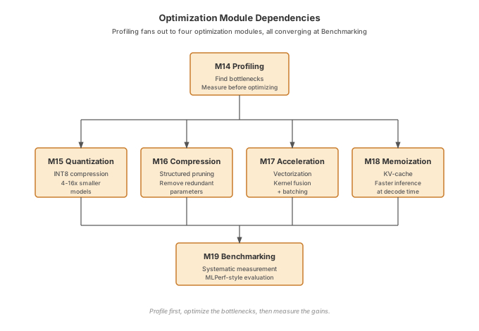
Module Details
14. Profiling - Measure Before Optimizing
What it is: Tools and techniques to identify computational bottlenecks in ML systems.
Why it matters: “Premature optimization is the root of all evil.” Profiling tells you WHERE to optimize: which operations consume the most time, memory, or energy. Without profiling, you’re guessing.
What you’ll build: Memory profilers, timing utilities, and FLOPs counters to analyze model performance.
Systems focus: Time complexity, space complexity, computational graphs, hotspot identification
Key insight: Don’t optimize blindly. Profile first, then optimize the bottlenecks.
15. Quantization - Smaller Models, Similar Accuracy
What it is: Converting FP32 weights to INT8 to reduce model size and speed up inference.
Why it matters: Packed INT8 weights use one byte per value versus four for FP32, excluding metadata. TinyTorch demonstrates rounding and reconstruction in dense tensors; actual storage, latency, and accuracy must be measured separately.
What you’ll build: Post-training quantization (PTQ) for weights and activations with calibration.
Systems focus: Numerical precision, scale/zero-point calculation, quantization-aware operations
Impact: Compare quantization error and held-out accuracy against the original model, and distinguish modeled packed bytes from actual array bytes.
16. Compression - Pruning Unnecessary Parameters
What it is: Removing unimportant weights and neurons through structured pruning.
Why it matters: Pruning reveals which weights a model can lose while preserving accuracy. Zeroing weights in a dense array preserves its allocation and dense arithmetic; sparse storage or structural changes are needed to reduce those costs.
What you’ll build: Magnitude-based pruning, structured pruning (entire channels/layers), and measuring what each technique costs in accuracy.
Systems focus: Sparsity patterns, memory layout, retraining strategies
Impact: Measure sparsity and accuracy independently of dense storage size and latency.
17. Acceleration - Vectorization and Fusion
What it is: BLAS-backed matrix multiplication, explicit block reuse, and grouped NumPy expressions as a bridge to production kernel fusion.
Why it matters: Python loop overhead and memory access patterns can dominate runtime. Comparing implementations exposes these costs; gains depend on the operation, input size, and hardware.
What you’ll build: Vectorized and explicitly tiled matrix multiplication, grouped and staged GELU implementations, and an im2col/col2im convolution lowering. The NumPy function named fused_gelu still allocates intermediate arrays.
Systems focus: Cache locality, SIMD utilization, memory bandwidth optimization, loop tiling, memory layouts for convolution lowering
Impact: Measure matrix multiplication, activation runtimes, and convolution lowering speed and memory against their baselines.
18. Memoization - KV-Cache for Fast Generation
What it is: Caching key-value pairs in transformers to avoid recomputing attention for previously generated tokens.
Why it matters: For a prefix of length n, full-prefix attention computes O(n²) scores per generation step. With cached keys and values, the new token needs O(n) scores. Cache management adds overhead, so small workloads can be slower.
What you’ll build: KV-cache implementation for transformer inference with proper memory management.
Systems focus: Cache management, memory vs speed trade-offs, incremental computation
Impact: Compare cached and uncached outputs, then measure their speed ratio and cache memory use.
19. Benchmarking - Systematic Measurement
What it is: Rigorous methodology for measuring model performance across multiple dimensions.
Why it matters: “What gets measured gets managed.” Benchmarking provides apples-to-apples comparisons of accuracy, speed, memory, and energy: essential for production decisions.
What you’ll build: Comprehensive benchmarking suite measuring accuracy, latency, throughput, and memory.
Systems focus: Measurement methodology, statistical significance, performance metrics
Historical context: MLCommons’ MLPerf (founded 2018) established systematic benchmarking as AI systems grew too complex for ad-hoc evaluation.
What You Can Build After This Tier
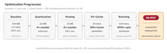
After completing the Optimization tier, you’ll be able to:
- Milestone 06 (2018): Evaluate optimization candidates:
- Compare rounded and pruned weights independently against the baseline
- Distinguish modeled packed storage from actual dense bytes
- Validate cached generation and measure its speed ratio
- Milestone 07 (2024): Verify your custom kernels, then compare them with native ones:
- YOUR tiled matmul, fused GELU, and im2col convolution checked against NumPy on ragged shapes
- Timed against bundled C++ SIMD (AVX2/NEON, OpenMP), Apple Metal MPS, and OpenAI Triton kernels
- Use measurements to reason about deployment constraints on:
- Edge devices (Raspberry Pi, mobile phones)
- Cloud infrastructure (cost-effective serving)
- Real-time applications (low-latency requirements)
Prerequisites
Required:
- Architecture Tier (Modules 09-13) completed
- Understanding of CNNs and/or transformers
- Experience training models on real datasets
- Basic understanding of systems concepts (memory, CPU/GPU, throughput)
Helpful but not required:
- Production ML experience
- Systems programming background
- Understanding of hardware constraints
Time Commitment
Per module: 3 to 7 hours; each module page gives its own estimate
Total tier: 25-37 hours, the sum of the per-module estimates for modules 14-19
Recommended pace: 1 module per week (this tier is dense!)
Learning Approach
Each module follows Measure → Optimize → Validate:
- Measure: Profile baseline performance (time, memory, accuracy)
- Optimize: Implement optimization technique (quantize, prune, cache)
- Validate: Benchmark improvements and understand trade-offs
This mirrors production ML workflows where optimization is an iterative, data-driven process.
Key Achievement: MLPerf Benchmarks
After Module 19, you’ll complete the MLPerf Benchmarks milestone (2018):
tito milestone run 06 # compare baseline, rounded, and pruned models, then time cached generationWhat makes this special: You’ll have built the entire optimization pipeline from scratch: profiling tools, quantization engine, pruning algorithms, caching systems, and benchmarking infrastructure.
Two Optimization Categories
The Optimization tier follows a deliberate pedagogical structure: Measure → Model-Level → Runtime → Validate.
Model-Level Optimizations (Modules 15-16)
These techniques change the model itself: they permanently modify weights and architecture:
- Quantization (15): Round weights and model their packed INT8 storage
- Compression (16): Zero selected weights and measure sparsity and accuracy
After model-level optimization, measure the changed model. Dense tensors retain their allocation even when values are rounded or zeroed.
Runtime Optimizations (Modules 17-18)
These techniques change how execution happens without modifying model weights:
- Acceleration (17): Vectorization reduces Python overhead, and tiling exposes block reuse. Grouped NumPy expressions introduce the comparison with production kernel fusion.
- Memoization (18): KV-cache stores past keys and values. For a prefix of length n, attention scores for a new token require O(n) work per step rather than O(n²) full-prefix recomputation.
Note the progression: general-purpose optimization (acceleration) comes before domain-specific optimization (KV-cache). This matches the pedagogical principle of teaching foundational concepts before specialized applications.
Why This Order?
The order below spells out that cycle, Measure → Model-Level → Runtime → Validate:
Profile (14) → Model-Level (15-16) → Runtime (17-18) → Benchmark (19)
   ↓              ↓                      ↓                ↓
 "What's slow?"  "Shrink the model"   "Speed up execution"  "Did it work?"
Why Model-Level before Runtime?
Model-level optimizations (quantization, pruning) are one-time transformations you apply before deployment. Runtime optimizations (acceleration, memoization) are ongoing techniques applied during every inference. It makes sense to first prepare the model, then optimize how it runs.
Why Acceleration (17) before Memoization (18)?
- Acceleration teaches general-purpose optimization: vectorization, cache locality, kernel fusion. These techniques apply to any numerical computation: matrix multiplication, convolutions, attention, everything.
- Memoization (KV-cache) is domain-specific optimization for transformer autoregressive generation. It only applies to transformers generating sequences.
The pedagogical principle: general before specific. Once you understand how to make any code fast (acceleration), you can appreciate the specialized optimization that makes LLM inference economically viable (KV-cache).
Both tracks start from Module 14 (Profiling) and converge at Module 19 (Benchmarking).
Recommendation: Complete modules in order (14→15→16→17→18→19) to build a complete understanding of the optimization landscape.
Going Further: Hardware Extensions (Optional)
Everything in this tier runs on NumPy. The package also ships tinytorch.extensions, optional native kernels that show what Module 17’s ideas look like on real silicon:
simd_matmulandsimd_fused_bias_gelu: C++ kernels called throughctypesand compiled on first use. The matrix multiply is cache-blocked with a vectorized inner loop, and uses several cores when an OpenMP runtime is installed;simd_build_info()tells you whether yours is.triton_fused_gelu: a Triton GPU kernel that fuses a bias add and GELU into one pass, for NVIDIA GPUs.mps_matmul: a matrix multiply on the Apple GPU through PyTorch’s Metal Performance Shaders backend.
Each one checks for its hardware or toolchain (has_simd_support(), has_triton_support(), has_mps_support()) and falls back to NumPy when it is missing, so no module depends on them and nothing is graded on them. The two GPU paths need PyTorch, installed separately. The book’s final chapter, Extending TinyTorch, walks the code and measures each one against NumPy, including where it loses.
Milestone 07: Custom Kernels (tito milestone run 07) grades your own Module 17 kernels and then times these hardware kernels against them; you can also explore the architectural strategies in Extending TinyTorch.
Real-World Impact
The techniques in this tier are used by every production ML system:
- Quantization: TensorFlow Lite, ONNX Runtime, Apple Neural Engine
- Pruning: Mobile ML, edge AI, efficient transformers
- KV-Cache: All transformer inference engines (vLLM, TGI, llama.cpp)
- Batching: Cloud serving (AWS SageMaker, GCP Vertex AI)
- Benchmarking: MLPerf industry standard for AI performance
After this tier, you’ll understand how real ML systems achieve production performance.
Next Steps
Ready to optimize?
# Start the Optimization tier
tito module start 14

# Follow the measure → optimize → validate cycle
Or explore other tiers:
- Foundation Tier (Modules 01-08): Mathematical foundations
- Architecture Tier (Modules 09-13): CNNs and transformers
- Torch Olympics (Module 20): Final integration challenge