Agent Economics

Purpose

Why can a model with a tenth of the token price make an agent cost more for every task it finishes?

A team that prices an agent the way it prices a chat service multiplies tokens by the provider’s rate and is surprised by the bill. The agent does not buy tokens; it buys finished tasks, and each finished task carries every turn, re-sent context, sandbox second, test run, retry, and human review that it took to get one result past verification, plus the cost of every attempt that never passed. A cheaper model that fails more often multiplies all of those terms, a faster model barely moves a trajectory whose time goes to tests and tool waits, and a delegation tree with no reserved budgets can spend money that no rollback returns. Economics therefore decides which model to call, what to cache, how much reasoning to buy, when to escalate, how much capacity to hold, and whether a task deserves an agent at all, each judged by cost and time per accepted task. Horizon sets how many turns are paid for, state sets how much context is re-sent on each of them, and authority sets how much verification and approval each result must clear, so the price of an accepted task is the price of closing all three exposures.

Learning Objectives

Calculate cost per accepted task from whole-trajectory cost and acceptance rate, and explain why per-token price misleads.
Estimate how prefix-cache hits, compaction, and reasoning or retry budgets change the dollar cost of a multi-turn trajectory.
Diagnose a trajectory’s critical path from its trace and decide when faster inference, including speculative decoding, pays.
Design a verifier-gated model cascade and compute its expected cost, tail latency, and false-accept penalty.
Size capacity for trajectories using Little’s law and provider rate limits, and find the break-even between dedicated serving and per-token APIs.
Design hierarchical budget reservations and spend-rate limits that bound money across a delegation tree.
Evaluate whether a task warrants a fixed workflow, a bounded agent loop, or several agents by pricing each per accepted task.

Cost per Accepted Task

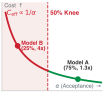
Below half acceptance, the cost of failed attempts outruns any discount on tokens.

A platform team replaces the frontier model behind its bug-fixing agent with one whose tokens cost a tenth as much. The following month the bill for fixed bugs goes up. Nothing in the serving logs explains it, because the serving logs count tokens, and tokens were never what the agent was buying. A chat service bills per call, so its cost is tokens times price. An agent runs a trajectory, and what the organization pays for is a trajectory whose result passed verification. Trajectory goodput (Micro-efficiency versus macro-efficiency) already counts only the resources spent on verified trajectories, and The multi-layer evaluation contract defined the accepted task that verification produces. This section puts a price on each accepted task and shows which parts of the system that price actually buys.

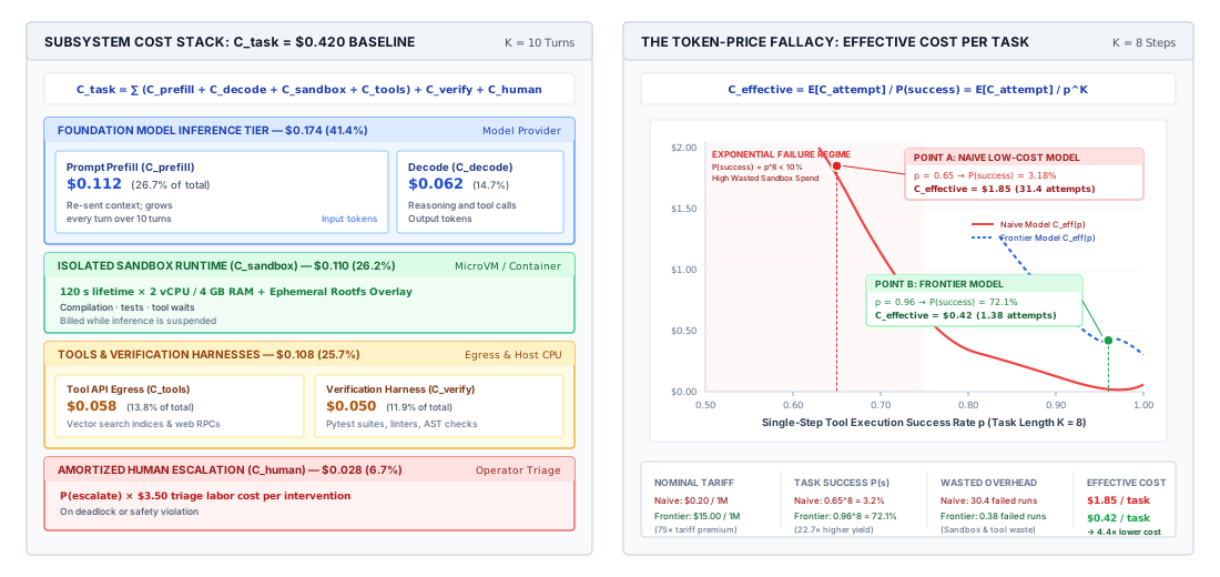
Figure 1: **Where an Agent Task’s Money Goes**: Left, an illustrative whole-trajectory cost stack in which model input and output tokens are less than half of the bill and sandbox hosting, tool fees, verification, and amortized human escalation make up the rest. Right, effective cost per accepted task as a function of single-step success rate for an eight-step task, where a low-priced model at modest step accuracy costs more per accepted task than a frontier model at high step accuracy.

The left panel of figure 1 decomposes one illustrative task. Model tokens, split between re-sent input and generated output, are less than half of the bill. The rest pays for the sandbox that runs the agent’s commands, the tools it calls, the tests that verify its result, and a share of the human review that failed attempts trigger. Across a trajectory of $K$ turns, the whole-trajectory cost of one attempt is

\[C_{\text{attempt}} = \sum_{k=1}^K \left( C_{\text{in}, k} + C_{\text{out}, k} + C_{\text{tools}, k} + C_{\text{sandbox}, k} \right) + C_{\text{verify}} + C_{\text{human}} \tag{1}\]

where $C_{\text{in}, k}$ pays for the context sent on turn $k$ (system prompt, tool definitions, the transcript so far, and the newest tool result), $C_{\text{out}, k}$ pays for the tokens the model generates, including reasoning tokens and tool-call arguments, $C_{\text{tools}, k}$ covers fees charged by external services, $C_{\text{sandbox}, k}$ covers the isolated environment that executes the agent’s commands, $C_{\text{verify}}$ covers the tests and checks that decide acceptance, and $C_{\text{human}}$ covers review when the runtime escalates. The input term of equation 1 grows with every turn, because the model keeps nothing between calls and each turn re-sends a longer context (Accelerator Serving Latency). That growth is why the next section treats caching as the first lever.

One attempt is not one accepted task. The right panel of figure 1 shows why. If each step of an eight-step task succeeds independently with probability $p$, the whole task succeeds with probability $p^8$, and every failed attempt is paid for in full before it is discarded. Trajectory goodput and the accepted task (principle $\ref{pri-vol3-trajectory-goodput}$) names what a fleet must therefore minimize, the effective cost per accepted task. If a fleet makes $N$ attempts and $N_{\text{acc}}$ of them are accepted,

\[C_{\text{eff}} = \frac{\sum_{i=1}^N C_{\text{attempt}, i}}{N_{\text{acc}}} = C_{\text{succ}} + \frac{1 - \alpha}{\alpha} C_{\text{fail}} \tag{2}\]

where $\alpha = N_{\text{acc}}/N$ is the acceptance rate, $C_{\text{succ}}$ is the mean cost of an attempt that passes, and $C_{\text{fail}}$ is the mean cost of one that fails before it is abandoned. The odds ratio $(1 - \alpha)/\alpha$ counts how many failed attempts each accepted task carries. It is small near $\alpha = 1$ and grows without bound as $\alpha$ falls, which is the steep left edge of the margin figure.

Definition 0.1: Whole-trajectory cost

Whole-trajectory cost is the total spent on model tokens, tools, sandboxes, verification, and human review across every attempt, divided by the number of attempts whose results were accepted, $C_{\text{eff}} = C_{\text{succ}} + \frac{1 - \alpha}{\alpha} C_{\text{fail}}$.

Significance: It is the quantity that model choice, caching, routing, and capacity decisions must lower, and it can rise when token prices fall.
Distinction: Per-token pricing bills what the model emits whether or not the task succeeds; whole-trajectory cost charges every failed attempt and every non-model term to the tasks that were accepted.
Common pitfall: Budgeting an agent from a provider’s price sheet, which ignores both the non-model terms and the odds ratio $\frac{1 - \alpha}{\alpha}$ that multiplies failed attempts.

Napkin Math 0.1: The token-price fallacy in automated bug repair

Problem: A bug-fixing agent can run on a frontier model or on a low-cost model whose input tokens are 10× cheaper. The illustrative workload in table 1 retries each ticket until an attempt passes the regression tests. Which model costs less per accepted fix?

Table 1: Illustrative Bug-Repair Workload: Scenario prices, trajectory lengths, and acceptance rates for a frontier model and a low-cost model.

Parameter	Frontier model	Low-cost model
Input / output price per 10⁶ tokens	$3 / $15	$0.30 / $1.20
Turns per attempt	4	7
Input / output tokens per turn	16,000 / 800	28,000 / 1,200
Acceptance rate $\alpha$	0.75	0.25
Sandbox and tools per turn	$0.03	$0.03
Verification per attempt	$0.05	$0.05
Human triage per failed attempt	$10	$10

Math: On tokens alone, one attempt costs $0.240 on the frontier model and $0.069 on the low-cost model, which looks 3.5× cheaper. The low-cost model needs more turns, and every turn pays for the sandbox, so with hosting and verification the attempts cost $0.410 and $0.329, a gap of only 20 percent. Dividing by acceptance rate (equation 2 with $C_{\text{fail}} = C_{\text{succ}}$) gives $0.55 per accepted fix for the frontier model and $1.32 for the low-cost model, which carries 3 failed attempts per success against 0.33. When each failed attempt also costs $10 of engineer triage, the figures become $3.88 and $31.32.

Systems insight: The low-cost model is 2.4× more expensive per accepted fix without triage and 8.1× more expensive with it. The token discount was real, and it was spent many times over on turns, sandbox time, and failed attempts.

Reporting follows from the same account. An agent evaluated only on success rate hides what the success cost, and an agent evaluated only on cost hides what it failed to finish. A result is complete when it reports acceptance rate with its confidence interval (Statistical evaluation rigor) and cost per accepted task on the same runs, so that designs can be placed on a cost-accuracy plane and a design that is both cheaper and more accurate than another dominates it. Repository-level issue benchmarks (Jimenez et al. 2024) make this concrete, since each resolved issue has a verifiable test outcome and a measurable bill. Comparisons between designs are made at a matched budget (Latent potential decoupling), because a design allowed to spend more can buy success with money alone. Throughout this chapter, the reciprocal of $C_{\text{eff}}$, accepted tasks per dollar, is the number every lever is judged by.

Jimenez, Carlos E., John Yang, Alexander Wettig, Shunyu Yao, Kexin Pei, Ofir Press, and Karthik Narasimhan. 2024. “SWE-Bench: Can Language Models Resolve Real-World GitHub Issues?” International Conference on Learning Representations (ICLR).

The whole-trajectory account also shows where to push first. In most agent trajectories the largest token term is not what the model writes but what the runtime re-sends to it on every turn.

Caching and Reasoning Budgets

By turn thirty, a coding agent sends the model a context of tens of thousands of tokens, almost all of which it already sent on turn twenty-nine. Paying full price for that repetition is the default, and it is avoidable. Accelerator Serving Latency counted the tokens a trajectory re-sends (equation) and introduced prefix caching, which reuses the attention state for a prompt prefix the service has already processed. Context engineering arranged the context so that the prefix stays stable (Staging the Next Invocation), and Prefix Caching Across Turns showed how the serving system shares that state. Both rest on the fact that the attention state is a function of the exact token prefix (principle $\ref{pri-vol3-prefix-coherence}$). This section prices the result in dollars and then prices the other budget the runtime controls on every call, how much reasoning and how many attempts to buy.

What a cache hit is worth

Providers that support prompt caching bill input tokens read from a cached prefix at a fraction of the normal input price, and bill only the tokens after the prefix at full price. With an append-only transcript, turn $k$ extends turn $k-1$, so under ideal reuse each turn pays full price only for what it appended. The same trajectory that Accelerator Serving Latency counted in tokens can now be priced.

Napkin Math 0.2: Pricing a thirty-turn trajectory with and without a cache

Problem: The coding agent of Accelerator Serving Latency runs 30 turns. Its first prompt is 8,000 tokens, each turn appends 1,500 tokens, and each turn emits 200 output tokens. Input costs $3 and output $15 per million tokens, and cached input is billed at 10 percent of the input price. What does the trajectory cost with and without prefix caching?

Math: The trajectory sends 892,500 input tokens in total, which cost $2.68 at full price. With an append-only context, only the first prompt and each turn’s appended tokens, 51,500 in all, are billed at full price and the rest are cache reads, so input falls to $0.41. Output costs $0.09 either way. The trajectory costs $2.77 without the cache and $0.50 with it.

Systems insight: Prefix caching makes the same trajectory 5.6× cheaper, and it changes no model and no answer. It is also fragile. A timestamp at the head of the system prompt, a reordered tool list, or an edit to an early message turns every turn back into a full-price read.

The layout rules of Staging the Next Invocation exist to protect this saving, and the cache-hit rate belongs on the harness dashboard beside cost per accepted task. Two qualifications keep the estimate honest. Some providers charge a premium to write a prefix into the cache and expire cached prefixes after minutes of inactivity, so a trajectory that pauses on a long tool wait or an approval (Approval Gates) can return to a cold cache. The serving-side view of the same decision, whether to keep the attention state resident during the wait, belongs to Retain, Evict, Recompute, or Offload.

The price of compaction

Compaction (Context Compaction) shrinks the context when it grows too long, usually by replacing old turns with a summary. On a cached trajectory, compaction has a price that is easy to miss. The summary is new text, so the turn after compaction reads its whole context at full price, and the summary itself costs a model call. In the notebook’s trajectory, suppose the runtime compacts at turn 16, when the context holds 30,500 tokens, down to 12,000 tokens, with a summary call that emits 1,500 tokens. Without compaction, the remaining 15 turns cost $0.245 in input. With it, they cost $0.190, plus $0.036 for the summary, $0.226 in all. Compaction pays back its cache miss and its summary call only after about 11 more turns.

Two consequences follow. Compacting early in a long trajectory saves money, and compacting near the end costs money, so a runtime that compacts on a fixed schedule should at least compare the expected remaining horizon against the break-even. More often the decision is not about money at all. Compaction is justified by the context window and by decision quality as the context fills with stale material (Context Invalidation), and the dollar account only says what that quality costs.

Reasoning and retry budgets

The other per-call budget the runtime sets is how much deliberation to buy. The call surface exposes a reasoning-token budget (The Invocation Contract), and reasoning tokens are billed as output tokens, the expensive kind, and generated serially, so a larger budget raises both price and latency on every call that uses it. Three Compute Allocation Axes decided when more deliberation raises the evidence for a decision. The economic question here is narrower. For a task with a sealed verifier, the runtime can buy a better answer from one expensive call or several attempts from a cheaper one, and the two options have different costs per accepted task.

With a verifier that the runtime trusts, retries can stop at the first accepted result. If each attempt of a cheap configuration succeeds with probability $p$ at cost $c$, and attempts are independent, the expected cost per accepted task of sequential retry is $c/p$ however many retries are allowed, because each allowed retry is used only when the previous one failed. The retry cap $k$ changes coverage, $1 - (1-p)^k$, not cost per accepted task. Running $k$ attempts in parallel buys latency instead, at cost $kc$ per task and $kc/(1-(1-p)^k)$ per accepted task. Pass@$k$ as a selection ceiling (Candidate Selection) is the coverage term in both cases.

Take an illustrative cheap configuration that succeeds with probability 0.30 at $0.10 per attempt, and a stronger one (a larger model or a larger reasoning budget) that succeeds with probability 0.70 at $0.40. With a cap of 5 attempts, sequential retry of the cheap configuration covers 83 percent of tasks, uses 2.8 attempts on average, and costs $0.33 per accepted task. The stronger configuration costs $0.57 per accepted task in one attempt. Sampling 5 cheap attempts in parallel is fastest and dearest at $0.60. The cheap configuration wins on cost and loses on latency and coverage, the stronger one wins on latency, and the parallel option is justified only when the deadline pays for it.

The comparison has two conditions that decide whether it holds in practice. The verifier must be trustworthy, because retrying against a verifier that sometimes accepts a wrong answer converts retries into false accepts (principle $\ref{pri-vol3-verification-asymmetry}$). Attempts must also fail independently, and they rarely do. Attempts from the same model on the same task share its blind spots, so coverage flattens well below $1 - (1-p)^k$, and the gap between pass@$k$ and reliability over repeated runs (Latent potential decoupling) is the measured form of that correlation. The per-task stopping rules of Search Stopping Criteria then cap how much of the budget a hopeless task can consume.

Caching lowers what each turn costs, and the reasoning and retry budget decides how many turns and attempts are bought. Neither says how long the task takes. A trajectory can be cheap and still too slow to be useful, and time has its own account.

Critical-Path Latency

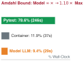
Test execution in the sandbox dominates wall-clock time, capping what faster inference can buy.

A coding agent takes 420 seconds to repair a failing test, and its model spends 84 of those seconds generating tokens. The platform team moves it to a serving tier that generates tokens 4× faster. The next run takes 357 seconds, a 15 percent improvement for a large investment, because the other 336 seconds belong to container startup, test execution, file synchronization, and package downloads, and none of them got faster. The duration identity of Trajectory duration accounting already splits each turn into model, tool, wait, and runtime time and bounds the payoff of a faster model with Amdahl’s law. This section turns that bound into a diagnostic. The trace identifies the critical path, the runtime shortens what lies on it, and faster inference is worth buying only when the model is what lies on it.

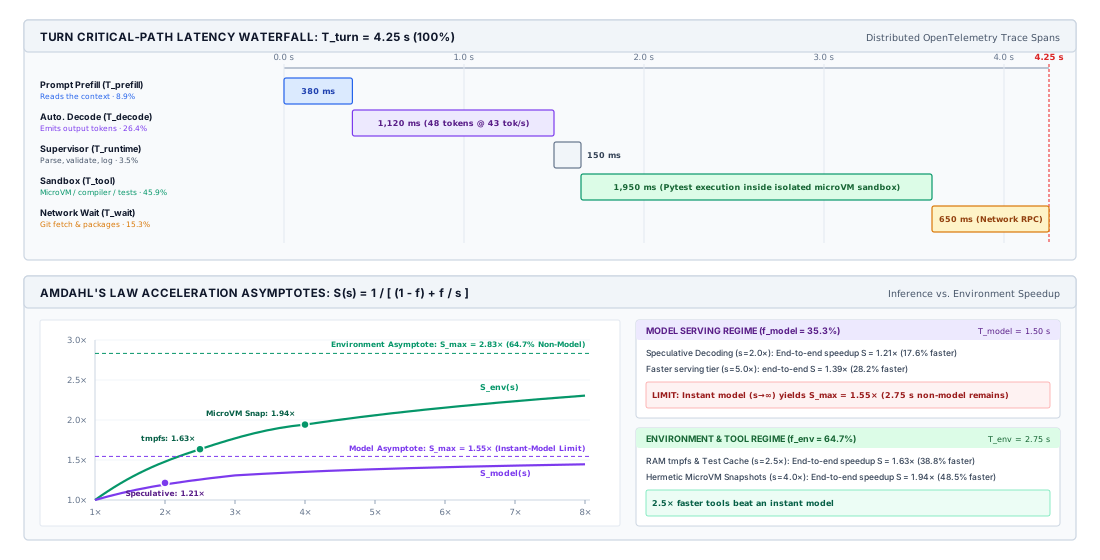
Figure 2: **Where One Agent Turn Spends Its Time**: Top, an illustrative turn decomposed into trace spans for reading the context, generating output, runtime validation, tool execution in the sandbox, and a network wait. Bottom, Amdahl’s-law speedup curves for accelerating the model versus accelerating tools and waits; the model curve flattens at the bound set by the non-model share, while a moderate speedup of the environment exceeds it.

The turn in figure 2 takes 4.25 s, of which the model’s two phases, reading the context and generating output, take 1.5 s, or 35.3 percent. No model speedup can make this turn more than 1.55× faster. A 2× faster model gives 1.21×. Making tools and waits 2.5× faster, through warm sandbox pools, cached builds, and test selection, gives 1.63×, more than an instant model could. Which side to invest in is therefore a measurement, not an opinion, and the measurement is the trace.

Critical paths from traces

A trajectory’s trace (Distributed trajectory tracing) records every model call, tool call, sandbox operation, and wait as a span with a start time, a duration, and a parent. Real trajectories branch, retry, and run tools in parallel, so the spans form a directed acyclic graph in which an edge $(u, v)$ means $v$ could not start until $u$ finished. It is the task graph of Coordination topologies at the finer grain of single calls, and as there, the time of the trajectory is the length of its longest path,

\[T_{\text{critical}} = \max_{\pi \in \Pi} \sum_{v \in \pi} t(v) \tag{3}\]

where $\Pi$ is the set of source-to-sink paths and $t(v)$ is the duration of span $v$. A span off the critical path has slack, and shortening it changes nothing the user sees. The spans that matter differ in what bounds them and in what shortens them, as table 2 summarizes.

Table 2: Trajectory Span Types: What bounds each kind of span on an agent’s critical path and which techniques shorten it.

Span	What sets its duration	What shortens it
Model, reading input	Context length, prefix-cache misses, queueing	Cache-stable layout, smaller context, less queueing
Model, generating	Output and reasoning tokens	Shorter outputs, smaller reasoning budget, speculative decoding
Sandbox and tools	Build size, test-suite size, cold starts	Warm pools, snapshots, build caches, test selection, parallel tool calls
Network and services	Round trips, payload size, provider throttling	Response caching, prefetching, rate-limit headroom
Runtime	Parsing, validation, logging, snapshotting	Streaming parsers, incremental snapshots

Table 3 shows an illustrative trace of a three-turn repair trajectory, with durations of the kind a harness collects.

Table 3: An Illustrative Trace: Span durations for a three-turn repair trajectory, with the model’s spans summed.

Span	Duration (s)
Runtime initialization	0.12
Sandbox creation	14.80
Turn 1, read context	1.20
Turn 1, generate	8.40
Tool: repository status	0.08
Turn 2, read context	1.85
Turn 2, generate	11.20
Tool: run test suite	245.60
Turn 3, read context	2.10
Turn 3, generate	4.50
Sandbox snapshot export	22.55
All model spans	29.25
Trajectory	312.40

All six model spans together take 9.4 percent of the trajectory. The test run takes 78.6 percent, and creating and exporting the sandbox take another 12 percent. An instant model would make this trajectory at most 1.10× faster. The team that reads this trace works on test selection and sandbox snapshots, not on inference.

Compressing the critical path

Once the trace names the critical path of equation 3, three techniques shorten it without changing what the model sees. The first is running independent tool calls in parallel. When the model requests several reads in one turn, as the call surface allows (The Invocation Contract), the runtime can execute them concurrently, and the turn waits only for the slowest, $T_{\text{tools}} = \max_i T_{\text{tool}, i}$ rather than their sum.

The second is starting work while the model is still generating. Tool calls arrive in a streamed response, and the tool name and early arguments are known before the call is complete, so the runtime can take a sandbox from a warm pool or fetch the target file while the rest of the call streams in. The work is speculative and must be discarded if the completed call fails validation, which is safe only for preparation that has no side effects.

The third is ending tool runs early. A test suite streams its results, and the first failed assertion is often enough for the model’s next decision. A runtime that forwards failures as they occur and stops the remaining tests turns a minute-long run into seconds on the failing path, at the price of a less complete observation.

When speculative decoding pays

When the trace does show generation on the critical path, as it does for long patches and long plans, faster generation becomes worth buying, and speculative decoding is the standard way to buy it. A small draft model proposes several tokens, and the target model checks all of them in one pass, keeping the prefix it agrees with (Autoregressive Generation). Because generation for a single stream is bounded by memory bandwidth, not arithmetic (principle $\ref{pri-vol3-memory-bandwidth-decoding}$), checking several tokens costs about as much time as generating one, and an acceptance rule makes the output distribution identical to the target model’s (Leviathan et al. 2023; C. Chen et al. 2023). Why Output Costs More Than Input derives the first fact and Decode-Loop Mechanics the acceptance rule behind the second. The agent engineer’s question is only when the technique pays.

Leviathan, Yaniv, Matan Kalman, and Yossi Matias. 2023. “Fast Inference from Transformers via Speculative Decoding.” Proceedings of the 40th International Conference on Machine Learning 202: 19274–86.

Chen, C., S. Borgeaud, G. Irving, J.-B. Lespiau, L. Sifre, and J. Jumper. 2023. “Accelerating Large Language Model Decoding with Speculative Sampling.” arXiv Preprint arXiv:2302.01318.

If the draft proposes $\gamma$ tokens per round, a draft token costs a fraction $r$ of a target step, and the target accepts $\bar{\alpha}$ draft tokens per round on average, each round advances $\bar{\alpha} + 1$ tokens in the time of $\gamma r + 1$ target steps, so the speedup is

\[S_{\text{spec}} = \frac{\bar{\alpha} + 1}{\gamma r + 1} \tag{4}\]

and the technique pays only when $\bar{\alpha} > \gamma r$. Acceptance depends on how predictable the output is. Structured output and code scaffolding are predictable, and a draft model agrees with the target on most tokens. Open-ended planning and high-temperature sampling are not, and the draft’s work is wasted. Table 4 evaluates equation 4 for illustrative acceptance rates across agent workloads.

Table 4: Speculative Decoding by Agent Workload: Illustrative accepted draft tokens per round and the resulting speedup with a draft token costing 0.08 of a target step; speculation pays whenever more than 0.4 draft tokens are accepted per round.

Agent workload	Output predictability	Accepted tokens per round ($\gamma =$ 5)	Speedup $S_{\text{spec}}$
Structured output (JSON, YAML)	Very high	4.4	3.86×
Code edits and scaffolding	High	3.6	3.29×
Error-trace diagnosis	Medium	2.5	2.50×
Algorithmic planning	Low	1.4	1.71×
Open-ended, high temperature	Very low	0.6	1.14×

Two conditions outside the table decide whether to turn speculation on. The first is the critical path. A 3.29× faster generator applied to a trajectory whose model share is under a tenth changes its duration by a few percent, so speculation belongs on the latency-critical calls that the trace shows on the path, not everywhere. The second is load. Speculation spends extra arithmetic to save time for one stream, which is free only while the serving system has idle arithmetic. Under heavy batching the arithmetic is no longer idle, the draft model also occupies memory that would otherwise hold other trajectories’ attention state, and speculation can lower the throughput of the whole fleet. Serving systems therefore enable it when queues are short and a request is latency-critical, and disable it when the batch is full. The same rule applies to every acceleration in this section, which pays only on the critical path and only while its resource cost is slack.

Checkpoint 0.1: Cost and time per accepted task

Before routing calls across models, check the accounting so far:

Failed attempts: With acceptance rate $\alpha = 0.25$, how many failed attempts does each accepted task carry, and why does that make a ten-times token discount a poor predictor of cost?
Cache layout: Which single change to a system prompt turns every turn of a cached trajectory back into a full-price read?
Compaction: Why can compacting a context near the end of a trajectory raise its cost even though it lowers the token count?
Critical path: A trace shows model spans at one tenth of the trajectory. What is the most any model speedup can buy, and where should the team look instead?

Critical-path analysis says when faster calls matter. For the many calls that do not sit on the critical path, and for the many that do not need the most capable model at all, the larger saving comes from not making the expensive call in the first place.

Model Cascades and Routing

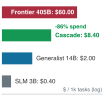
A verifier-gated cascade resolves most tasks on small models and cuts expected cost by an order of magnitude.

An agent that sends every call to its most capable model pays frontier prices to format JSON, extract a file path from a stack trace, and summarize a log. An agent that sends every call to a small model saves on those calls and fails on the ones that need planning or diagnosis, and every failure costs a full attempt. Most turns in a trajectory need much less than the best model, and a few need all of it. A model cascade exploits that spread. It tries a cheaper model first and escalates only when a check says the result is not good enough (L. Chen et al. 2023). The check is what makes the cascade safe, and the verifiers of Process Verification are what the runtime has to check with.

Tiers and routes

A production runtime typically has three kinds of callee, summarized in table 5. Deterministic code and small models handle transformations with little ambiguity. Mid-sized generalists handle routine tool use and local edits. Frontier models handle planning, diagnosis across many files, and recovery after the smaller tiers have failed.

Table 5: Cascade Tiers: The callees, roles, and escalation gates of a three-tier model cascade.

Tier	Typical callee	Typical agent role	Gate that decides escalation
1: Deterministic and small	Parsers, regular expressions, small language models	Argument extraction, schema repair, log triage, command filtering	Schema and syntax checks
2: Mid-sized generalist	Instruction-tuned models of moderate size	Single-file edits, routine tool calls, summarization	Type checks, builds, fast unit tests
3: Frontier	The most capable available model	Planning, cross-file diagnosis, recovery from lower-tier failure	Full regression suite, approval if required

A runtime can choose a tier in two ways. Static routing classifies each call before it is made, from the task description or the call’s features, and sends it to one tier. It adds almost nothing to latency, and it fails in a predictable way. A request that looks simple (“fix the failing assertion in the lock test”) may require tracing a race across many files, and a router that judges by the request sends it to a model that loops until the budget runs out. Escalation routing tries the cheapest plausible tier and moves up only when that tier’s output fails a check. It pays for the failed attempts, and in return its decisions rest on evidence about the output rather than a guess about the input.

Learned routers sit between the two. The harness’s own logs (Distributed trajectory tracing) record which tier’s output passed verification on which kind of call, which is exactly the labeled data a router needs, and a classifier trained on it predicts whether a cheap tier is likely to pass. The router’s errors have asymmetric costs. Routing down wrongly costs one failed cheap attempt plus the escalation. Routing up wrongly costs the price difference between tiers. Its threshold should be set from those two costs, and its predictions still feed an escalation gate, so a router that is wrong costs money but not correctness.

Figure 3: **A Verifier-Gated Model Cascade**: Tasks enter a small-model tier whose output must pass a schema and syntax gate; failures escalate with only the verifier’s diagnostic to a generalist tier gated by builds and fast tests, and remaining failures escalate to a frontier tier gated by the full regression suite. In this illustrative example 60 percent of tasks exit at tier 1 and 28 percent at tier 2, so the expected cost is $0.0084 per task against $0.0600 for sending every task to the frontier model, with a mean latency of 1.32 s.

Expected cost and latency of a cascade

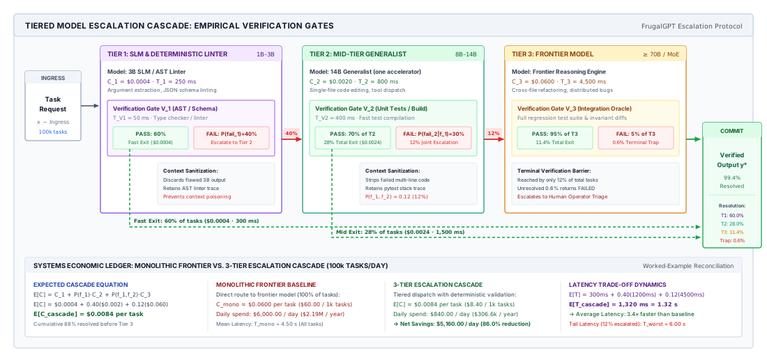
In figure 3, every task enters tier 1. Its candidate output is held in the runtime’s pending-proposal buffer and checked by a schema and syntax gate. If it passes, the task exits. If not, the runtime escalates to tier 2 with the verifier’s diagnostic, and only the tasks that also fail tier 2’s build and test gate reach tier 3. Let $C_j$ be the cost of a call at tier $j$, with $C_1 \ll C_2 \ll C_3$, and let $P(\text{fail}_1)$ and $P(\text{fail}_1, \text{fail}_2)$ be the probabilities that a task fails tier 1 and fails both lower tiers. The expected cost per task is

\[E[C_{\text{cascade}}] = C_1 + P(\text{fail}_1) \cdot C_2 + P(\text{fail}_1, \text{fail}_2) \cdot C_3 \tag{5}\]

and the cascade beats sending everything to tier 3 when

\[C_1 + P(\text{fail}_1) \cdot C_2 < \Big(1 - P(\text{fail}_1, \text{fail}_2)\Big) \cdot C_3 \tag{6}\]

The right-hand side of equation 6 is the frontier cost avoided on tasks the lower tiers resolve. Because frontier calls typically cost one to two orders of magnitude more than small-model calls, the inequality holds even when the lower tiers resolve a modest share of tasks.

Latency moves the other way for the tasks that escalate. With tier latencies $T_j$ and gate latencies $T_{V,j}$, a task that reaches the top pays for every tier on the way,

\[T_{\text{worst}} = T_1 + T_{V,1} + T_2 + T_{V,2} + T_3 \tag{7}\]

while the expected latency is

\[E[T_{\text{cascade}}] = T_1 + T_{V,1} + P(\text{fail}_1) \cdot \Big(T_2 + T_{V,2}\Big) + P(\text{fail}_1, \text{fail}_2) \cdot T_3 \tag{8}\]

so a cascade usually lowers mean latency and always raises the tail, whose upper bound is equation 7.

Napkin Math 0.3: Cost and latency in a three-tier cascade

Problem: A coding fleet serves 100,000 small editing tasks a day. Tier calls cost $0.0004, $0.0020, and $0.0600 and take 250, 800, and 4,500 ms. The tier 1 and tier 2 gates take 50 and 400 ms. Tier 1 fails with probability 0.40, and tier 2 fails 0.30 of what it receives. Should the fleet cascade, and what does it cost in latency?

Math: A share 0.12 of tasks reaches tier 3. By equation 5 the expected cost is $0.0084 per task, 86 percent below the frontier-only $0.0600, and daily spend falls from $6,000 to $840. By equation 8 the mean latency is 1.32 s, 3.4× faster than the frontier model’s 4.5 s. A task that escalates through every tier takes 6 s, 33 percent longer than a direct frontier call.

Systems insight: The cascade is cheaper and faster on average and slower in the tail. Whether that trade is acceptable depends on whether escalated tasks sit on a deadline-bound critical path.

The false-accept penalty and escalation discipline

Equation 5 assumes the gates never accept a wrong output. They do. A gate that checks syntax passes a patch that parses and drops an authorization check, and the cascade stops at tier 2 with a broken invariant in the workspace. If $\alpha_{\text{FA}}$ is the rate at which a gate accepts a wrong output and $C_{\text{recovery}}$ is the cost of finding and undoing it later, the effective cost is

\[C_{\text{eff}} = E[C_{\text{cascade}}] + \alpha_{\text{FA}} \cdot C_{\text{recovery}} \tag{9}\]

and because recovery can involve rollback (The Trajectory Saga Pattern) or human review, a small $\alpha_{\text{FA}}$ in equation 9 can erase the cascade’s savings. The gate therefore has to check the property that matters, which for code means running tests, not only linting. Under the verification asymmetry (principle $\ref{pri-vol3-verification-asymmetry}$), a learned judge can rank candidates or decide which tier to try, but the gate that lets an output stand must be a check whose errors are known and small.

A second failure is self-inflicted. A runtime that escalates by appending the failed attempt, its stack trace, and the original prompt to the next tier’s context pays to re-send a long wrong answer and invites the stronger model to build on it. Escalation should pass the task and the verifier’s diagnostic, not the failed output, as the following dispatcher does.

def dispatch_with_escalation(task, tiers, sandbox):
    feedback = []
    for tier in tiers:
        # the prompt carries the task and the last verifier diagnostic only
        prompt = build_prompt(task, verifier_feedback=feedback)
        candidate = tier.generate(prompt, max_tokens=tier.token_limit)

        # the candidate stays pending until an external check accepts it
        result = sandbox.run_verifier(candidate)
        if result.passed:
            sandbox.commit(candidate)
            return StepResult(status="ACCEPTED", tier=tier.name, output=candidate)

        # drop the failed output; keep a short, deterministic diagnostic
        feedback = [f"tier {tier.name} failed: {result.diagnostic}"]
    return StepResult(status="ESCALATION_EXHAUSTED", tier=None, output=None)

Escalation itself needs a stopping rule. Moving from tier $j$ to tier $j+1$ costs $\Delta C_{j \to j+1}$ and raises the probability of acceptance by $\Delta P_{j \to j+1}$. If $V_{\text{task}}$ is what an accepted task is worth, escalation pays only when

\[\Delta C_{j \to j+1} < \Delta P_{j \to j+1} \cdot V_{\text{task}} \tag{10}\]

and otherwise the runtime should stop and report a bounded failure. Equation 10 is the cascade’s version of the stopping rules in Search Stopping Criteria, and it keeps a cheap task from escalating into an expensive one.

Cascades and caching lower the cost of each call a trajectory makes. A fleet must also have somewhere to make those calls, and the capacity an agent fleet needs is not the capacity a request-serving system needs.

Capacity for Trajectories

A team sizes its agent platform the way it sized its chat service, from the rate of model calls and their service time, and finds it both starved and idle. Calls queue behind a provider’s rate limit while the dedicated nodes it reserved sit half empty, and trajectories that hold sandboxes and cached context for twenty minutes crowd out new ones. The unit that holds resources is the trajectory, not the call (principle $\ref{pri-vol3-heavy-tailed-scheduling}$). This section sizes capacity in that unit and then decides where the capacity should come from.

Trajectory concurrency

A model call lasts seconds. A trajectory lasts minutes, most of which it spends waiting on tools, and for all of that time it holds a sandbox, a slot in the runtime, and often cached attention state on a serving node. Little’s law, which Analytical capacity formulations applied to the trajectories resident on one serving node, gives the number in flight across the fleet,

\[L_{\text{traj}} = \lambda_{\text{traj}} \cdot \mathbb{E}[T_{\text{traj}}] \tag{11}\]

where $\lambda_{\text{traj}}$ is the rate at which trajectories start and $\mathbb{E}[T_{\text{traj}}]$ is their mean lifetime. Sizing sandboxes, runtime workers, and cache memory from the call rate and call duration, rather than from equation 11, undercounts concurrency by the ratio of trajectory lifetime to call duration, which is two to three orders of magnitude. What a trajectory holds while it waits is a design choice. Retain, Evict, Recompute, or Offload decides whether its attention state stays resident, is evicted and recomputed, or is offloaded during a tool wait, and Queueing for Trajectories derives how tool waits inflate concurrency.

Two consequences follow from how trajectories issue calls. Calls arrive in correlated bursts, when a trajectory fans out tool calls or a coordinator launches subagents, and their service times range from a few tokens to thousands. Queueing delay grows with that variability and rises steeply as utilization approaches saturation, and Kingman’s approximation for a single queue (Queueing for Trajectories) puts a number on both effects. With bursty arrivals ($c_a^2 =$ 2) and generation lengths with $c_s^2 =$ 4, the variability factor $(c_a^2 + c_s^2)/2$ is 3, and a serving pool at 70 percent utilization makes the average call wait about 7 mean service times, while one at 90 percent makes it wait about 27. Capacity is therefore provisioned to run below the knee of the utilization curve. Tail delays also compound along a trajectory, the serial counterpart of the fan-out stragglers of Cancellation cascades. A trajectory of 30 serial calls, each of which meets a 99th-percentile delay with probability 0.01, meets at least one such delay with probability 0.26, so a fleet sized for good mean latency still delivers slow trajectories routinely (Dean and Barroso 2013).

Dean, Jeffrey, and Luiz André Barroso. 2013. “The Tail at Scale.” Communications of the ACM 56 (2): 74–80.

Provider rate limits

For a team that calls a hosted model, the first capacity limit it meets is usually not hardware but the provider’s quota, expressed as tokens per minute and requests per minute. The quota caps the rate at which trajectories can run, not how many can be open. Each trajectory needs a fixed number of tokens to finish, so in steady state token demand is the trajectory rate times tokens per trajectory, whatever the trajectories’ lifetimes. Suppose trajectories start at 1 per minute, and each makes 60 calls of 30,000 input tokens, 1,800,000 tokens per trajectory. Against a limit of 2,000,000 tokens per minute, demand uses 90 percent of the quota, and the fleet can sustain at most 1.11 trajectories per minute. With a lifetime of 20 minutes, Little’s law puts 20 trajectories in flight, each issuing about 3 calls per minute.

Running this close to a quota has the same consequence as running a server close to saturation. Throttled calls retry after backoff, trajectories live longer, they hold sandboxes and cache longer, and their deadlines slip. Three levers apply. Prefix caching lowers the bill, and whether it also lowers usage against the quota depends on how the provider counts cached tokens, which the capacity plan must check rather than assume. Short, reliable trajectories consume fewer tokens per accepted task, which raises the accepted-task rate under a fixed quota as directly as a higher quota would. Discounted batch endpoints, which return results within hours, suit single-call work such as offline evaluation runs, trajectory scoring, and curation, but not a multi-turn loop in which each turn must wait for the previous one.

Priority lanes

Interactive trajectories, where a person waits on the result, and batch trajectories, such as overnight issue triage or evaluation runs, share the same models and quota and have very different deadlines. Mixed in one first-come queue, a burst of long batch generations delays every short interactive call behind it. The runtime separates them into lanes with different priorities and gives the interactive lane admission control and reserved headroom. Within a serving system, a scheduler that cannot know how long a generation will run can still demote calls that exceed a token quantum to a lower-priority queue, so short calls never wait behind long ones (principle $\ref{pri-vol3-heavy-tailed-scheduling}$). Batch work then fills the capacity interactive work leaves idle, which matters most for the decision that closes this section, whether to own that capacity.

Queueing dynamics

Because agent platforms cannot decouple accelerator scheduling from the stochastic nature of agent behavior, sizing a fleet requires queueing-theoretic models that capture extreme variability. Standard introductory systems analysis frequently relies on $M/M/1$ or $M/M/k$ formulations, which presume Poisson arrival processes (exponential inter-arrival distributions) and memoryless, exponentially distributed service durations. In production agent fleets, both assumptions are demonstrably invalid.

The arrival process of model invocations generated by autonomous agents is structurally bursty. When an orchestrator spawns parallel verification sub-agents or when an agent executes a multi-step planning loop, requests hit the serving layer in tightly correlated batches rather than uncorrelated Poisson streams. The squared coefficient of variation of inter-arrival times, defined as $C_a^2 = \sigma_a^2 / (\mathbb{E}[T_a])^2$, routinely exceeds unity ($C_a^2 > 1$).

Simultaneously, the distribution of model service times is radically non-exponential. An agent fleet processes a bimodal mixture of workloads: lightweight, low-latency classification probes, JSON schema validations, and single-token tool-routing decisions consuming tens of milliseconds ($S \ll 100\text{ ms}$), juxtaposed against heavy, multi-thousand-token chain-of-thought generations and complex code syntheses lasting several seconds ($S > 10\text{ s}$). This bimodal dispersion yields a service time squared coefficient of variation substantially greater than one ($C_s^2 = \sigma_s^2 / (\mathbb{E}[S])^2 \gg 1$).

To estimate expected waiting times in queues characterized by arbitrary arrival and service distributions without resorting immediately to cycle-accurate discrete-event simulations, systems engineers rely on Kingman’s heavy-traffic approximation for a $G/G/1$ queue (equation 12):

\[W_q \approx \left( \frac{C_a^2 + C_s^2}{2} \right) \left( \frac{\rho}{1 - \rho} \right) \frac{1}{\mu} \tag{12}\]

where $\rho = \lambda / \mu$ denotes server utilization, and $\mu = 1 / \mathbb{E}[S]$ is the mean service rate. Kingman’s formula decomposes mean queue wait time $W_q$ into three explicit multiplicative components:

The Variability Factor $\frac{C_a^2 + C_s^2}{2}$: This term scales latency directly by the combined dispersion of the arrival and service processes. In an idealized $M/M/1$ system where $C_a^2 = C_s^2 = 1$, this factor equals 1. In an agent fleet where correlated bursts and bimodal generation lengths push $C_a = 1.8$ and $C_s = 2.4$, the variability factor reaches $\frac{1.8^2 + 2.4^2}{2} = \frac{3.24 + 5.76}{2} = 4.5$. The system experiences a $4.5\times$ amplification in mean queue delay purely due to workload variance, holding hardware throughput and mean arrival rates identical.
The Utilization Factor $\frac{\rho}{1 - \rho}$: This hyperbolic penalty governs the non-linear asymptote as server utilization approaches saturation. As $\rho$ advances from $0.70$ to $0.90$, the multiplier jumps from $2.33$ to $9.00$—nearly a four-fold increase.
The Base Service Scale $\frac{1}{\mu}$: The unweighted mean processing duration of the underlying model.

As Jeffrey Dean and Luiz André Barroso articulated in The Datacenter as a Computer, tail latency—not mean latency—dictates the user-perceived performance of distributed systems. In an agent trajectory comprising $N$ serial model calls, the probability of completing without hitting a 99th-percentile queue delay decays as $(1 - 0.01)^N$.

In an enterprise fleet operating $k$ parallel accelerator instances, the single-server $G/G/1$ model transitions to an aggregate multi-server $G/G/k$ system. Using the Allen-Cunneen approximation, multi-server queue waiting time scales proportional to the Erlang-C waiting probability $P_{\text{wait}}(M/M/k)$ (equation 13):

\[W_q(G/G/k) \approx \left( \frac{C_a^2 + C_s^2}{2} \right) \frac{P_{\text{wait}}(M/M/k)}{k\mu(1 - \rho)} \tag{13}\]

While pooling $k$ accelerators into a unified serving cluster provides statistical multiplexing benefits that dampen average wait times relative to isolated single-server silos, it exacerbates tail-latency amplification across multi-turn trajectories. If an agent workflow requires $N = 30$ sequential model invocations to complete an end-to-end task, and the runtime operates at an aggressive hardware utilization $\rho = 0.85$, the likelihood that the trajectory encounters an extreme tail delay ($P_{99}$) on at least one critical-path turn is:

\[P(\text{Tail Incident}) = 1 - (1 - 0.01)^{30} = 1 - 0.7397 \approx 0.26\]

More than one-quarter of all executed agent trajectories will suffer an extreme tail delay. Because an agent trajectory executes synchronously across sequential turns, a single tail delay on turn 7 cascades directly into the total time-to-completion, often causing the host orchestrator to breach its global Service Level Objective (SLO).

Napkin Math 0.4: Queue sizing under heavy-tailed traffic

An infrastructure team operates an inference cluster dedicated to serving intermediate agent reasoning loops. The cluster processes an aggregate arrival rate of $\lambda = 160\text{ requests/sec}$ distributed across pooled accelerator workers. Profiling reveals that the mean model service time is $\mathbb{E}[S] = 20\text{ ms}$ ($\mu = 50\text{ req/sec/worker}$), but the workload exhibits extreme bimodality: 80 percent of requests are fast JSON schema evaluations ($\mathbb{E}[S_1] = 5\text{ ms}$), while 20 percent are extended chain-of-thought generations ($\mathbb{E}[S_2] = 80\text{ ms}$). Empirical measurements indicate an arrival coefficient of variation $C_a = 1.4$ and a service coefficient of variation $C_s = 2.2$.

The engineering lead proposes provisioning $k = 4$ worker nodes to run at an average utilization of $\rho = \frac{\lambda}{k \mu} = \frac{160}{4 \times 50} = 0.80$. Compute the expected queue wait time $W_q$ under this configuration using the Allen-Cunneen approximation, and contrast it with an alternative provisioning plan of $k = 5$ workers ($\rho = 0.64$).

Step 1: Compute the variability scaling factor. \[\frac{C_a^2 + C_s^2}{2} = \frac{1.4^2 + 2.2^2}{2} = \frac{1.96 + 4.84}{2} = \frac{6.80}{2} = 3.40\]

Step 2: Evaluate Erlang-C waiting probability for $k = 4$ at $\rho = 0.80$. For an $M/M/4$ queue with offered load $A = k\rho = 3.2\text{ Erlangs}$: \[P_{\text{wait}}(M/M/4) = \frac{\frac{A^4}{4!(1 - \rho)}}{\sum_{n=0}^{3} \frac{A^n}{n!} + \frac{A^4}{4!(1 - \rho)}} \approx 0.554\]

Step 3: Calculate $W_q$ for $k = 4$. \[W_q \approx 3.40 \times \frac{0.554}{4 \times 50 \times (1 - 0.80)} = 3.40 \times \frac{0.554}{200 \times 0.20} = 3.40 \times \frac{0.554}{40} = 3.40 \times 0.01385\text{ s} \approx 47.1\text{ ms}\] Under $k = 4$ workers, the average queue wait time ($47.1\text{ ms}$) exceeds the mean execution time of the request itself ($20\text{ ms}$) by more than $2.3\times$.

Step 4: Evaluate the cluster over-provisioned to $k = 5$ at $\rho = 0.64$. For $M/M/5$ with $A = 3.2\text{ Erlangs}$, the waiting probability drops sharply to $P_{\text{wait}}(M/M/5) \approx 0.237$. \[W_q \approx 3.40 \times \frac{0.237}{5 \times 50 \times (1 - 0.64)} = 3.40 \times \frac{0.237}{250 \times 0.36} = 3.40 \times \frac{0.237}{90} = 3.40 \times 0.00263\text{ s} \approx 8.95\text{ ms}\]

Takeaway: Increasing capacity by a single accelerator node ($25\%$ hardware expansion) reduces average queue waiting time from $47.1\text{ ms}$ down to $8.95\text{ ms}$—a latency reduction of over $80\%$. In heavy-tailed agent serving environments, operating below the knee of the utilization curve ($\rho \le 0.70$) is mandatory to absorb variance and protect multi-turn trajectory critical paths.

Multi-level feedback queueing for agent workloads

When an agent serving cluster schedules all requests through an undifferentiated First-Come-First-Served (FCFS) queue, it encounters the classic head-of-line blocking pathology. A massive, multi-step code-generation invocation requiring 4,096 output tokens will occupy an accelerator’s continuous batching slots for several contiguous seconds. If an interactive user or an latency-critical supervisory agent submits a 10-token routing query behind this massive job, the short query is delayed behind the long-running decode phase. This degradation violates the core scheduling objective of computing systems: minimizing mean response time by prioritizing short jobs (Shortest Job First), without possessing prior knowledge of exact execution durations.

Because the host runtime cannot predict the exact token length of an autoregressive generation prior to inference, it cannot implement pure Shortest Processing Time (SPT) scheduling. Instead, the cluster must employ an adaptive Multi-Level Feedback Queue (MLFQ) discipline tailored to the memory and compute mechanics of token generation (figure 4).

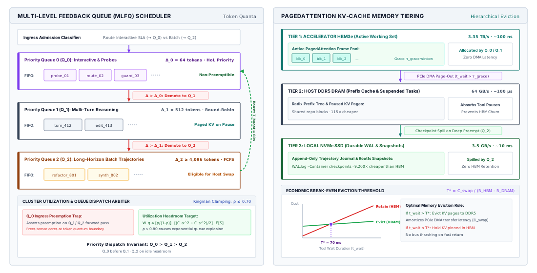
Figure 4: **Multi-Level Feedback Queue (MLFQ) Serving Architecture and KV-Cache Memory Tiering**: The left scheduling engine isolates interactive probes, multi-turn reasoning loops, and background batch trajectories into discrete priority queues ($Q_0, Q_1, Q_2$) with token-based quanta ($\Delta_0 = 64, \Delta_1 = 512, \Delta_2 \ge 4{,}096\text{ tokens}$) and starvation prevention ($T_{\text{boost}} = 60\text{ s}$). The right panel illustrates the corresponding physical memory hierarchy, where PagedAttention dynamically manages HBM block allocations across active batch slots, staging evicted pages into host DDR5 memory via asynchronous DMA transfers and NVMe storage based on an economic eviction threshold $T^* \approx 70\text{ ms}$.

As detailed in the systems schematic of figure 4, the architecture bifurcates between an active priority scheduler on the left and a physical memory hierarchy on the right. In the scheduling plane, all incoming agent jobs enter $Q_0$ with an initial non-preemptible token quantum of $\Delta_0 = 64\text{ tokens}$. Short semantic classifier probes and tool-dispatch decisions complete within this quantum and exit the system with sub-millisecond queue delay. Jobs requiring extended deliberation exhaust $\Delta_0$ and are demoted to $Q_1$ ($\Delta_1 = 512\text{ tokens}$, round-robin scheduling), while long-horizon code-generation and repository-refactoring passes demote to $Q_2$ ($\Delta_2 \ge 4{,}096\text{ tokens}$, FCFS batching). Starvation of background jobs is physically prevented by the upward priority boost arc, which atomically flushes all pending requests across $Q_1$ and $Q_2$ back to $Q_0$ every $T_{\text{boost}} = 60\text{ seconds}$.

Simultaneously, the right panel of figure 4 demonstrates how the scheduler interfaces with PagedAttention memory management across physical hardware tiers. When a $Q_1$ or $Q_2$ request yields its continuous batching slot during preemption, its key-value cache blocks in accelerator HBM are protected by a grace period $\tau_{\text{grace}}$ to prevent thrashing. Under sustained memory pressure, the memory manager activates PCIe Gen5 DMA channels to migrate inactive pages to host DDR5 RAM ($64\text{ GB/s}$ bidirectional transfer). If idle times exceed the economic eviction break-even threshold ($T^* \approx 70\text{ ms}$), pages spill to local NVMe storage ($7\text{ GB/s}$), ensuring high HBM residency for latency-critical $Q_0$ invocations without discarding expensive prefill state.

The agent-aware MLFQ structures accelerator capacity into distinct priority tiers, governing preemption, batch assembly, and memory tenancy:

Priority Queue 0 ($Q_0$, Interactive & Probes): All newly arriving model invocations enter $Q_0$. This tier is allocated the highest dispatch priority and a strictly bounded token generation quantum (for example, $\Delta_0 = 64\text{ tokens}$). Invocations in $Q_0$ consist of interactive user queries, fast semantic classifier probes, tool-call routing decisions, and safety guardrail checks. If an invocation completes its generation within $\Delta_0$ tokens (emitting an EOS token or tool-dispatch sequence), it exits the system immediately, achieving minimal queue wait time and near-zero tail latency.
Priority Queue 1 ($Q_1$, Multi-Turn Reasoning): If an invocation exhausts its $Q_0$ token quantum without terminating, the scheduler preempts its forward pass at the token boundary, demotes the task to $Q_1$, and context-switches its execution state. $Q_1$ operates with a larger quantum (for example, $\Delta_1 = 512\text{ tokens}$) and intermediate dispatch priority. It accommodates routine agent deliberation turns, standard code edits, and multi-sentence reasoning steps.
Priority Queue 2 ($Q_2$, Long-Horizon Batch Trajectories): Tasks that exceed $\Delta_1$ tokens are demoted to $Q_2$, the lowest-priority background queue. $Q_2$ operates with expansive token quanta ($\Delta_2 \ge 4,096\text{ tokens}$) or unconstrained run-to-completion mechanics. This tier processes asynchronous background tasks: extensive repository-wide refactoring passes, synthetic test-suite generation, offline embedding pipelines, and non-urgent verification passes. Invocations in $Q_2$ are explicitly preemptible; if $Q_0$ or $Q_1$ experiences an arrival surge, active $Q_2$ requests yield their continuous batching slots. The operational parameters across these tiers are summarized in table 6.

Table 6: Multi-Level Feedback Queue Priority Tier Configuration: Queue priorities, token quanta allocations, target workload profiles, and preemption policies.

Queue Level	Priority	Token Quantum ($\Delta$)	Target Workload	Preemption Policy
$Q_0$	Highest	64 tokens	Interactive UI, Guardrails, Tool-call routing probes	Non-preemptible within quantum
$Q_1$	Medium	512 tokens	Standard reasoning loops, Single-file code generation	Preemptible by $Q_0$
$Q_2$	Lowest	4,096+ tokens	Repository refactoring, Test generation, Batch evaluation	Preemptible by $Q_0$/$Q_1$; Eligible for host swap

To maintain architectural stability, an agent MLFQ must resolve two critical systems challenges: starvation and KV-cache memory churn.

If high-priority interactive traffic in $Q_0$ and $Q_1$ saturates the cluster, long-running batch trajectories in $Q_2$ will starve indefinitely. To enforce forward progress invariants, the scheduler implements periodic priority boosting. At regular time intervals $T_{\text{boost}}$ (e.g., every 60 seconds), all unserviced tasks across all priority tiers are flushed back into $Q_0$, resetting their elapsed quantum counters and ensuring that background trajectories periodically advance ($\ref{not-17-mlfq-transition-protocol}$).

Multi-level feedback queue discipline

The cluster scheduler partitions agent inference jobs into prioritized execution tiers with deterministic transition rules:

Ingress Allocation: All incoming invocations enter highest-priority queue $Q_0$ allocated an initial token quantum of $\Delta_0 = 64$ tokens.
Quantum Exhaustion Demotion: If an execution thread exhausts its assigned quantum without completing or issuing an I/O wait, it demotes downward: \[Q_k \xrightarrow{\text{exhausts } \Delta_k} Q_{k+1}\] specifically transitioning from $Q_0 \to Q_1$ ($\Delta_1 = 512\text{ tokens}$) and $Q_1 \to Q_2$ ($\Delta_2 \ge 4{,}096\text{ tokens}$).
Completion Exit: An invocation that finishes decoding or yields for tool execution within its quantum $\Delta_k$ immediately exits the scheduling queue and returns results.
Periodic Priority Boosting: To eliminate long-horizon starvation in $Q_2$, every $T_{\text{boost}}$ seconds all active tasks across $Q_1$ and $Q_2$ are atomically promoted back to $Q_0$ with reset quanta.
Tiered Memory Retention: Preempted $Q_1$ tasks retain physical HBM allocations during grace interval $\tau_{\text{grace}}$; prolonged memory pressure migrates $Q_2$ blocks to host memory via PagedAttention.

The second challenge involves physical memory management during preemption. When a $Q_2$ job is preempted to free tensor cores for an incoming $Q_0$ burst, evicting its accumulated 4,000-token KV cache to host CPU RAM consumes valuable interconnect bandwidth. If the preempted task is re-admitted milliseconds later, swapping those physical pages back into HBM creates severe PCIe/NVLink thrashing. The MLFQ scheduler mitigates this via tiered eviction thresholds: preempted $Q_1$ tasks retain their physical HBM page allocations in a suspended state for a grace period $\tau_{\text{grace}}$. Only if memory pressure persists and $Q_0$ exhausts the free HBM frame pool does the PagedAttention memory manager trigger asynchronous page migration to host DDR5 memory. The comparative trade-offs among classical and adaptive queueing disciplines are evaluated in table 7.

Table 7: Comparative Analysis of Cluster Scheduling Disciplines for Agent Inferences: Mean wait times, tail latency bounds, starvation risks, preemption overheads, and memory retention characteristics.

Scheduling Discipline	Mean Wait ($W_q$)	Tail Latency ($P_{99}$)	Starvation Risk	Preemption Overhead	Memory Efficiency (KV Cache)
First-Come-First-Served (FCFS)	High	Severe (HoL blocking)	None	Zero	Low (pinned memory stalls)
Shortest Processing Time (SPT)	Optimal	Low for short jobs; High for long	Severe for large tasks	Zero (requires oracle)	High (fast job clearance)
Multi-Level Feedback Queue (MLFQ)	Near-Optimal	Low across $Q_0/Q_1$; Bounded on $Q_2$	Bounded via $T_{\text{boost}}$	Low to Moderate (quantum boundaries)	High (tiered memory migration)

Dedicated capacity versus per-token APIs

A team can pay for model calls per token or reserve dedicated serving capacity and run models itself. Per-token pricing converts every cost into a variable one and hands queueing, throttling, and multi-tenant interference to the provider. Dedicated capacity costs the same per hour whether it is busy or idle, and in return removes the quota, fixes the tail, and allows serving choices such as speculation and cache policy to be tuned to the workload. Which is cheaper depends on how busy the dedicated capacity would be.

Let $C_{\text{node}}$ be the hourly cost of a dedicated node, including amortized hardware or lease, power, and operations, and let the node sustain $R_{\text{out}}$ output tokens per second on the workload’s traces. If the workload sends $\kappa$ input tokens for each output token and the API charges $P_{\text{in}}$ and $P_{\text{out}}$ per token, the hour of work that a fully busy node does would cost

\[V_{\text{node}} = 3600 \cdot R_{\text{out}} \cdot \left( P_{\text{out}} + \kappa \cdot P_{\text{in}} \right) \tag{14}\]

at API prices. A node busy a fraction $\rho$ of the time does $\rho V_{\text{node}}$ of API-priced work, so dedicated capacity is cheaper when $\rho$ exceeds the break-even utilization, $C_{\text{node}}$ divided by equation 14,

\[\rho^* = \frac{C_{\text{node}}}{3600 \cdot R_{\text{out}} \cdot \left( P_{\text{out}} + \kappa \cdot P_{\text{in}} \right)} \tag{15}\]

The input term deserves care. Agent workloads have large $\kappa$ because every turn re-sends its context, and an API’s cached-input discount lowers the effective $P_{\text{in}}$, which raises $\rho^*$ and makes dedicated capacity harder to justify. The comparison should use the cached input price the workload actually pays, not the list price.

Napkin Math 0.5: Break-even for dedicated serving capacity

Problem: A software-engineering agent fleet sends 5 input tokens per output token. The API charges $3 per million input and $15 per million output tokens. A reserved node costs $28 per hour and sustains 1,200 output tokens per second on the fleet’s traces. The fleet’s load would keep dedicated nodes busy 0.52 of the time. Should it reserve capacity?

Math: Each output token and its inputs cost $30 per million at API prices, so a fully busy node does $129.60 of API-priced work per hour, and by equation 15 the break-even utilization is 0.22. At the projected utilization a node does $67.39 of work per hour for its $28, saving $39.39 per hour, 58 percent of the API bill.

Systems insight: Token-heavy agent workloads reach break-even at low utilization, but only with the list input price. A cached-input discount shrinks the API bill for the same work, and the break-even must be recomputed with it before capacity is reserved.

Most fleets end up with both, as table 8 shows. A dedicated pool is sized for the base load and kept below the knee of its utilization curve, interactive trajectories get priority on it, batch trajectories fill its idle hours, and bursts beyond it overflow to per-token APIs.

Table 8: Hybrid Provisioning: A dedicated pool for base load with per-token overflow for bursts.

Provisioning tier	Capacity source	Sized for	Cost model	Workload
Dedicated pool	Reserved serving nodes	Base load, below the knee	Fixed per hour	Interactive lane first; batch trajectories fill idle time
Per-token API	Hosted model endpoints	Bursts above the base load	Per token	Overflow, and models the fleet does not host

Checkpoint 0.2: Capacity for trajectories

Before governing spend, check the capacity model:

Concurrency: Trajectories start at two per minute and live fifteen minutes. How many are in flight, and why does sizing from calls per second miss this?
Quotas: Why does a token-per-minute quota cap the rate of trajectories rather than their number, and what raises accepted tasks per hour under a fixed quota?
Lanes: Why should batch trajectories share dedicated capacity with interactive ones rather than run on a separate pool?
Break-even: How does a cached-input discount change the utilization at which dedicated capacity pays?

Capacity bounds how fast a fleet can spend. It does not bound how much. A trajectory stuck in a loop, or a tree of subagents that keeps delegating, will spend whatever capacity it is given, and the runtime needs limits on money itself.

Spending Governance

The harness budget of Budgets and Ceilings stops one trajectory’s runaway loop (A Runaway Loop and the Budget That Ends It). Delegation opens a failure that no single-trajectory budget sees. A coordinator with two dollars left launches two subagents. Each reads the shared balance, sees two dollars free, and starts a call that costs almost two dollars. Both checks pass, both calls run, and together they spend nearly twice what the parent had. A sandbox write can be rolled back, but money spent on tokens and tool fees cannot, which makes spending the one resource an agent consumes that no recovery mechanism restores. Invariant closure (principle $\ref{pri-invariant-closure}$) applies directly. The model cannot be trusted to meter its own spending or to notice when it should stop, so the bound must come from a check the runtime makes before each dispatch. This section extends the dollar budget of Budgets and Ceilings to many agents spending concurrently from one allocation, and adds a limit on the rate of spending.

The spending invariant

Let $C(t)$ be what a task has spent by step $t$. Every billable operation adds a positive amount, so $C(t)$ only rises. The runtime also knows what it has committed but not yet paid for. A model call in flight will cost at most its maximum output tokens times the output price plus its input, and a tool call has a known fee. Let $R(t)$ be the sum of those reservations. The runtime maintains

\[C(t) + R(t) \le B_{\text{task}} \tag{16}\]

for the task’s budget $B_{\text{task}}$ at every step. Before dispatching an operation, it reserves the operation’s worst-case cost; if the reservation would violate the inequality, it does not dispatch and instead returns a typed budget-exceeded observation, the control action of Control Actions. When the operation completes, the reservation is replaced by the actual cost and the difference is released. Using the call’s maximum-output field (The Invocation Contract) as the reservation makes the bound hold even if the call runs to its limit.

Hierarchical budget reservations

With one agent, equation 16 is a counter. With a coordinator and subagents (The delegation trade-off), several agents spend at once, and a shared balance invites the race that opened this section. Monotonic delegation (principle $\ref{pri-vol3-monotonic-delegation}$) supplies the rule that removes the race. Whatever budget a child receives is withheld from the parent until the child returns it. Attenuated capability delegation applied that rule to authority. Here it becomes a budget reservation ledger, traced through one delegation in figure 5.

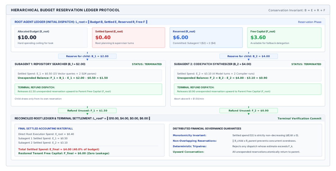
Every node $k$ in the delegation tree keeps a ledger $\mathcal{L}_k = \langle B_k, E_k, R_k, F_k \rangle$ of its budget $B_k$, settled spending $E_k$, reserved amount $R_k$, and free balance $F_k$, subject to

\[B_k = E_k + R_k + F_k, \quad E_k, R_k, F_k \ge 0 \tag{17}\]

Settled spending only grows. Reserved money covers calls in flight and children’s budgets, and cannot be pledged again. Only free money can fund a new operation. Table 9 gives the four transitions, each of which preserves equation 17.

Table 9: Budget Ledger Transitions: Preconditions and updates for spawning a child, dispatching and settling a call, and closing a child.

Transaction	Precondition	Parent ledger	Child ledger
Spawn child	$\Delta B \le F_P$	$R_P \leftarrow R_P + \Delta B$, $F_P \leftarrow F_P - \Delta B$	$B_C = F_C = \Delta B$, $E_C = R_C = 0$
Dispatch call	$c_{\text{est}} \le F_C$	unchanged	$R_C \leftarrow R_C + c_{\text{est}}$, $F_C \leftarrow F_C - c_{\text{est}}$
Settle call	actual cost $c$ known	unchanged	$E_C \leftarrow E_C + c$, $R_C \leftarrow R_C - c_{\text{est}}$, $F_C \leftarrow F_C + (c_{\text{est}} - c)$
Child finishes	child stopped, for any reason	$E_P \leftarrow E_P + E_C$, $R_P \leftarrow R_P - B_C$, $F_P \leftarrow F_P + (B_C - E_C)$	closed

A child can see only its own ledger and cannot draw on its parent’s free balance; a grandchild is funded from its parent’s free balance in turn. Because every reservation is subtracted before it is spent and every child’s spending is bounded by its reservation, no sequence of spawns and calls can spend more than the root budget, however deep or concurrent the tree. A child that loops exhausts its own reservation and stops, and its siblings and parent are untouched. The ledger also answers a question operators ask of every fleet, who spent the money. With one root per tenant or per ticket, cost attribution is a read of the root ledgers.

Napkin Math 0.6: A budget ledger through a failed subagent

Problem: An operator authorizes $5 for a repair task. The coordinator plans with one frontier call of 8,000 input and 1,200 output tokens, then delegates a trace analysis with a $1.20 reservation and a fuzzing run with $2.50. The trace agent finds the fault for $0.38. The fuzzing agent hits a sandbox timeout, retries in a loop, and is stopped by progress detection (Semantic Watchdog Timers) after spending $0.85. What does the root ledger hold at the end?

Math: Planning settles $0.042, leaving $4.958 free. Delegation reserves $3.70, leaving $1.258 free for the coordinator’s own calls. When both children stop, their spending settles into the root and their unspent reservations, $0.82 and $1.65, return to its free balance. The root ends with $1.272 spent, nothing reserved, and $3.728 free.

Systems insight: The looping child could never have spent more than its reservation, whatever it did, and the coordinator keeps enough to try another approach. The bound came from the ledger, not from the child’s behavior.

Ledger accounting invariants

Every node $k$ in the agent delegation tree maintains an independent, isolated ledger context defined by a four-tuple:

\[\mathcal{L}_k = \langle B_k, E_k, R_k, F_k \rangle\]

The semantics of these fields represent distinct physical and financial states of capital:

Allocated Budget ($B_k$): The total upper bound of capital granted to node $k$ by its immediate parent. This value is static throughout the lifetime of node $k$.
Settled Expenditure ($E_k$): The non-recoverable capital permanently debited for completed inference passes, finalized tool executions, and completed child processes. Settled expenditure increases monotonically.
Escrow Reservation ($R_k$): Capital actively earmarked for in-flight child agents or pending asynchronous tool invocations. Escrowed capital cannot be pledged to new operations.
Free Capital ($F_k$): The uncommitted, unreserved balance immediately available for dispatching new operations.

These variables are governed by the strict Conservation Invariant:

\[B_k = E_k + R_k + F_k, \quad \text{where } E_k \ge 0, \; R_k \ge 0, \; F_k \ge 0\]

Multi-rate circuit breakers

While a static cumulative spending ceiling $B_{\text{task}}$ guarantees that an agent cannot exceed an absolute fiscal budget, static caps represent a dangerously coarse control mechanism. If an autonomous agent with a $\$50.00$ ceiling enters a pathological code generation loop that burns $\$10.00$ per minute, a static cap allows the system to run uncontrolled for five full minutes, generating hundreds of useless files and thrashing execution sandboxes before halting.

The tool circuit breakers of Tool Circuit Breakers already let the runtime cut off a failing dependency without the model’s cooperation. Here the same tri-state breaker watches different signals, financial burn velocity and epistemic utility decay, rather than socket timeouts and error ratios.

The Circuit Breaker Analogy In electrical grids, a circuit breaker trips when current draw ($I = \frac{dQ}{dt}$) spikes dangerously, preventing fires. In agentic systems, the breaker trips when the financial burn rate ($\frac{dC}{dt}$) exceeds safe envelope bounds.

An agentic circuit breaker acts as a dynamic supervisor wrapped around the model dispatch pipeline. It continuously transitions between three operational states:

CLOSED (Nominal): Operations dispatch normally. Incurred costs and state deltas are logged to a rolling sliding window.
OPEN (Tripped): The breaker has detected an invariant violation. All subsequent inference requests, tool dispatches, and child agent initializations fail immediately (fail-fast). The active trajectory is suspended, and the runtime invokes automated rollback or human operator escalation.
HALF-OPEN (Canary Probing): After a cooldown interval or an environmental checkpoint restore, the runtime permits a single, bounded “canary” probe (such as an inexpensive reflection pass or a single deterministic unit test) to verify whether the agent has recovered coherence. If the probe fails, the breaker immediately reverts to OPEN. The state transitions and operational invariants governing this control loop are formalized in table 10.

Table 10: Circuit Breaker State Machine: Agentic Circuit Breaker Finite State Machine and Transition Semantics.

Current State	Transition Trigger / Condition	Target State	Invariant Guard & Operational Semantics	System Recovery Action
CLOSED (Nominal)	Velocity spike ($\bar{\nu}_W > \nu_{\max}$), utility decay ($\Delta \mathcal{U} < \epsilon$), or invariant breach	OPEN	Immediate fail-fast trap; halts inference and tool dispatches	Suspends trajectory, cancels pending child jobs, logs alert
OPEN (Tripped)	Cooldown window elapsed ($\Delta t > \tau_{\text{cool}}$) or checkpoint rollback complete	HALF-OPEN	Permits isolated, single-step canary evaluation probe	Emits bounded introspection or isolated unit test
HALF-OPEN (Canary)	Canary probe fails or re-triggers invariant breach	OPEN	Enforces exponential cooldown backoff ($\tau_{\text{cool}} \leftarrow 2 \tau_{\text{cool}}$)	Escalates to human operator or terminates trajectory
HALF-OPEN (Canary)	Canary probe succeeds and state verification passes	CLOSED	Resets consecutive failure counter and clears escrow hold	Restores normal multi-turn model dispatch pipeline

To provide comprehensive defense-in-depth, the host runtime implements three distinct, orthogonal circuit breaker triggers.

Financial velocity limiting

The financial velocity breaker monitors the instantaneous first derivative of expenditure with respect to time: $\nu(t) = \frac{dC}{dt}$. In a discrete runtime, this is computed over a backward-looking sliding window of duration $W$ (e.g., 60 seconds):

\[\bar{\nu}_W(t) = \frac{C(t) - C(t - W)}{W}\]

If $\bar{\nu}_W(t)$ exceeds an authorized burn-rate threshold $\nu_{\max}$ (e.g., $\$2.00 / \text{minute}$), the circuit breaker immediately trips to OPEN. Velocity spikes typically signify that an agent has spawned a wide fan-out of uncoordinated sub-agents, entered an unthrottled polling loop against external APIs, or triggered an autoregressive loop that saturates local GPU prefill engines with redundant context windows.

Cumulative trajectory caps

The cumulative breaker enforces the hard boundary condition $C(t) + R(t) \ge B_{\text{task}}$. Unlike the velocity breaker, which triggers on rates, the cumulative breaker enforces total volume. It acts as the ultimate fail-safe against low-velocity, highly persistent agent trajectories that make minimal progress over hours of execution. When tripped, the runtime preserves the current sandbox state, dumps a diagnostic execution trace, and transitions the agent to a quiescent state awaiting human authorization for budget expansion.

Marginal epistemic utility decay

The most subtle and destructive failure mode in autonomous systems is the epistemic loop: an agent remains well within its financial velocity limit and has consumed only a fraction of its total budget, but it has ceased making measurable progress toward task completion. The agent generates code, runs a unit test, observes an assertion error, modifies an unrelated comment or variable name, runs the test again, and repeats the cycle indefinitely.

To detect this pathology, the runtime evaluates the marginal epistemic utility of the trajectory. Let $\mathcal{S}_t$ represent the observable state of the environment at turn $t$ (e.g., the directory tree of source code, compiler diagnostic vectors, and test execution outcomes). We define a progress metric $\mathcal{M}(\mathcal{S}_t) \in [0, 1]$ that measures objective proximity to goal invariants:

\[\mathcal{M}(\mathcal{S}_t) = w_1 \cdot \text{PassRatio}(\mathcal{S}_t) + w_2 \cdot (1 - \text{LintErrors}(\mathcal{S}_t)) + w_3 \cdot \text{DiffConvergence}(\mathcal{S}_t)\]

where $w_1, w_2, w_3$ represent normalized domain weights. The marginal utility across an evaluation window of $K$ turns is defined as:

\[\Delta \mathcal{M}_K(t) = \mathcal{M}(\mathcal{S}_t) - \mathcal{M}(\mathcal{S}_{t - K})\]

If the runtime observes that over $K$ consecutive turns, cumulative spending has increased significantly ($\sum_{j=t-K+1}^t c_j > \theta_C$) while the marginal progress metric has remained stagnant or decayed:

\[\Delta \mathcal{M}_K(t) \le \epsilon_{\text{progress}}\]

the epistemic decay breaker trips to OPEN. The runtime halts the loop, diagnosing that the model has exhausted its reasoning capability for the current environmental state and that continuing execution will merely burn financial capital without increasing the probability of goal satisfaction. The monitored metrics, mathematical trigger conditions, and mitigated failure modes across the three circuit breakers are summarized in table 11.

Table 11: Multi-Rate Circuit Breaker Triggers and Failure-Mode Mitigations: Monitored metrics, mathematical trigger conditions, and primary failure modes for agent financial safety.

Circuit Breaker	Monitored Metric	Mathematical Trigger Condition	Primary Failure Mode Mitigated
Velocity Limiter	Burn Rate $\frac{dC}{dt}$	$\frac{C(t) - C(t - W)}{W} > \nu_{\max}$	Concurrent child fan-out explosions; unthrottled API polling loops
Cumulative Cap	Total Exposure	$C(t) + R(t) \ge B_{\text{task}}$	Long-running creeping exhaustion; unauthorized project budget overruns
Epistemic Decay	Marginal Utility $\frac{\Delta \mathcal{M}}{\Delta C}$	$\Delta \mathcal{M}_K \le \epsilon$ while $\Delta C_K > \theta_C$	Flailing retry loops; cosmetic code shuffling; cyclic reasoning traps

Once spending is mathematically bounded by monotonic ledgers, hierarchical escrow, and multi-rate circuit breakers, the systems engineer can safely deploy autonomous agents into production environments. However, enforcing spending bounds addresses only the negative risk of fleet operations—preventing economic catastrophe. The positive design challenge remains: given a specific production task with known latency, budget, and accuracy constraints, how does an architect determine whether to solve it with a deterministic compiler script, a single model invocation with structured outputs, a sequential chain of specialized models, or a fully dynamic multi-agent system? Synthesizing these operational variables into a principled selection rubric is the subject of the next section.

Pricing the Choice of Architecture

A team with a working agent is tempted to point it at every task. Architectural decision matrix: Workflows versus model-directed loops gave the decision of whether a task needs a model-directed loop at all. With cost per accepted task, critical-path latency, and spending risk in hand, that decision can now be priced, and the price often decides it. Agency is the most expensive and least predictable way to complete a task, and it is worth buying only where cheaper ways fail.

The spectrum, priced

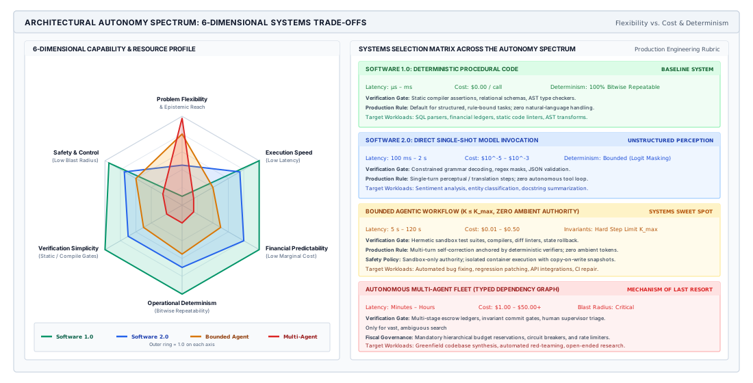
Table 12 places four designs along the spectrum that the four questions of Architectural decision matrix: Workflows versus model-directed loops select from: deterministic code, a single model call inside a fixed workflow, a bounded agent loop, and several agents on one task. The latency and cost columns give orders of magnitude, not measurements. Each step to the right buys flexibility and pays in cost, latency, variance, and the closure the runtime must supply.

Table 12: The Architecture Spectrum, Priced: Control flow, orders of magnitude of latency and cost, carried state, recovery, and verification for four designs.

Dimension	Deterministic code	Single model call	Bounded agent loop	Several agents
Control flow	Fixed in code	Fixed pipeline, one model step	Model-directed within a turn cap	Task graph with typed handoffs
Latency	Microseconds to milliseconds	Hundreds of milliseconds to seconds	Seconds to minutes	Minutes to hours
Cost per task	Negligible	Fixed per call, $10^{-5}$ to $10^{-3}$ dollars	Sum over turns, $10^{-2}$ to $10^{-1}$ dollars	Dollars to tens of dollars
State carried	Program variables and tables	None beyond the request	Context, workspace, trajectory record	Partitioned contexts and workspaces
Failure recovery	Exceptions and retries	Re-parse, fallback model	Retry with feedback, rollback, compensation	Re-planning at the coordinator, human escalation
Verification basis	Unit tests and types	Schema checks	Tests and checks in the sandbox	Invariant gate per commit, end-to-end tests, human review

Figure 6 maps these dimensional trade-offs across the architectural autonomy spectrum.

Figure 6: **Dimensional Trade-Offs Across the Architectural Autonomy Spectrum and Systems Selection Matrix**: A six-dimensional systems evaluation comparing Software 1.0 (deterministic procedural code), Software 2.0 (direct single-shot model inference), Bounded Agentic Workflows ($K \le K_{\max}$, $A_1$), and Autonomous Multi-Agent Fleets. Expanding autonomy monotonically increases flexibility at the cost of operational determinism, execution speed, financial predictability, verification simplicity, and blast radius safety. The accompanying systems selection matrix establishes definitive decision boundaries based on epistemic ambiguity, state mutability, latency tolerance, and verifiable ground truth.

The four questions, priced

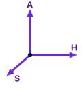
Horizon, state, and authority each set the closure a task must pay for.

The four questions of Architectural decision matrix: Workflows versus model-directed loops place a task by its three H·S·A exposures (The H·S·A exposures) and by the closure evidence (Closure evidence levels) the runtime can collect for it. Each has a price that this chapter can now state.

Horizon is priced in time and in the odds ratio. Every turn adds critical-path time and re-sent context, and a task with a deadline of a second or two cannot afford a loop whose turns each take seconds. Longer horizons also compound per-step failure, so a task whose natural length is many turns needs either a high per-step success rate or verified intermediate milestones to keep $(1-\alpha)/\alpha$ small.

State is priced in context. A transformation from input to output with no state to carry is a single call, and wrapping it in a loop adds re-sent context and failure modes without adding value. A task that must observe and change a workspace pays for the context growth of section 2 on every turn, and the cache layout and compaction policy decide how much.

Authority is priced in approvals and in the cost of mistakes. A task whose effects stay in a disposable sandbox ($A_1$) can run as a bounded loop. A task whose effects are compensable ($A_2$) can too, provided each timed-out action is settled before it is retried (principle $\ref{pri-vol3-exactly-once-settlement}$), and it pays for compensation machinery. A task with irreversible effects ($A_3$) pays for an approval gate (Approval Gates) on every such action, and its $C_{\text{human}}$ term is no longer occasional.

Closure evidence is priced in verification, and it is the question that most often decides. If a fast, trustworthy check exists, such as a test suite or a compiler, a cheap model can iterate against it and the cost per accepted task falls with every attempt the check filters. If no such check exists, more turns and more agents do not converge on correctness; they add cost, and the result still needs human review. Such tasks belong in a single call with review, whose cost is dominated by $C_{\text{human}}$.

Where a loop pays

The comparison that most often matters is between a single strong call and a bounded loop around a cheaper model. For a loop of at most $K$ turns against a verifier, with conditional success probability $r_k$ on turn $k$ given earlier failures, the probability of producing an accepted result is

\[p_{\text{loop}}(K) = 1 - \prod_{k=1}^K (1 - r_k) \tag{18}\]

and its expected cost is the per-turn cost times the expected number of turns taken. When unresolved tasks go to a person at cost $C_{\text{human}}$, each design’s cost per ticket is its compute cost plus $(1 - p) C_{\text{human}}$, and the human term usually decides.

Napkin Math 0.7: Pricing three designs for dependency upgrades

Problem: A team handles 10,000 security-advisory tickets a month, each requiring a dependency upgrade, edits to deprecated calls, and a passing build and test run. A ticket that automation fails costs $35 to fix by hand. A rule-based rewriter costs $0.001 per ticket and succeeds with probability 0.32. One frontier call that proposes a diff costs $0.045 and succeeds with probability 0.68. A bounded loop around a cheaper model costs $0.006 per turn plus $0.002 per test run, runs at most three turns, and succeeds on each turn, given earlier failures, with probability 0.55, 0.42, and 0.30. Which design costs least per ticket?

Math: By equation 18 the loop succeeds with probability 0.82 in 1.71 turns on average, for $0.014 of compute and about 12.3 s per ticket. Adding human handling of failures, a ticket costs $23.80 with the rewriter, $11.24 with the single call, and $6.41 with the loop, or $238,010, $112,450, and $64,082 a month.

Systems insight: The loop costs 43 percent less than the single call and 73 percent less than the rewriter, although its compute is cheaper than the call’s by only cents. Its advantage is the test suite. A cheap model that can see a failing build and try again converts inexpensive attempts into accepted fixes. Without that check, the loop would have nothing to iterate against.

Several agents follow the same logic one step further. A multi-agent design earns its place only by beating one agent with the same total budget on cost per accepted task, time, or acceptance without losing on the others (principle $\ref{pri-vol3-tri-axial-evaluation}$), and it pays the coordination tax (principle $\ref{pri-vol3-coordination-tax}$) whether or not it does. Autonomy should grow only while the returns on accepted tasks exceed the added cost of turns, verification, coordination, and governance, and the accounting of this chapter is how to tell.

Serving economics synthesis

A cluster administrator who independently optimizes model serving, tool execution, and scheduling policies inevitably discovers that local efficiencies compound into catastrophic fleet-level inefficiencies. Accelerating an autoregressive decode kernel via custom flash-attention or speculative verification reduces GPU-bound decode latency by $2.5\times$, yet total trajectory wall-clock time drops by less than $6\%$ if the agent runtime spends $82\%$ of its critical path stalled on synchronous container re-imaging and external sandbox RPCs. Similarly, deploying aggressive model cascades that route queries to sub-billion-parameter models slashes nominal token inference fees, but if the cheaper model’s lower instruction compliance triggers repeated syntax retries and trajectory rollbacks, the cumulative cost per accepted task explodes.

Economic viability in autonomous agent fleets is not an intrinsic property of the underlying neural weights or inference kernels, but an emergent property of the closed-loop control system that governs their invocation. Maximizing the system’s economic return requires unifying whole-trajectory cost accounting, critical-path latency decomposition, speculative acceleration, tiered model routing, and queueing-theoretic cluster provisioning into a single, self-balancing operational runtime. When these subsystems operate in isolation, they generate impedance mismatches: schedulers flood GPU memory with long-context trajectories that starve interactive queries, while routing cascades dispatch complex reasoning tasks to low-capacity models that consume disproportionate tool and verification budgets before failing.

The multi-tier economic control loop

To prevent these failure modes, a production agent platform must structure its control flow as a five-stage pipelined closed-loop feedback engine (figure 7). Each stage enforces a formal systems contract, transforming an unprivileged user intent into verified external state modifications while actively minimizing resource consumption.

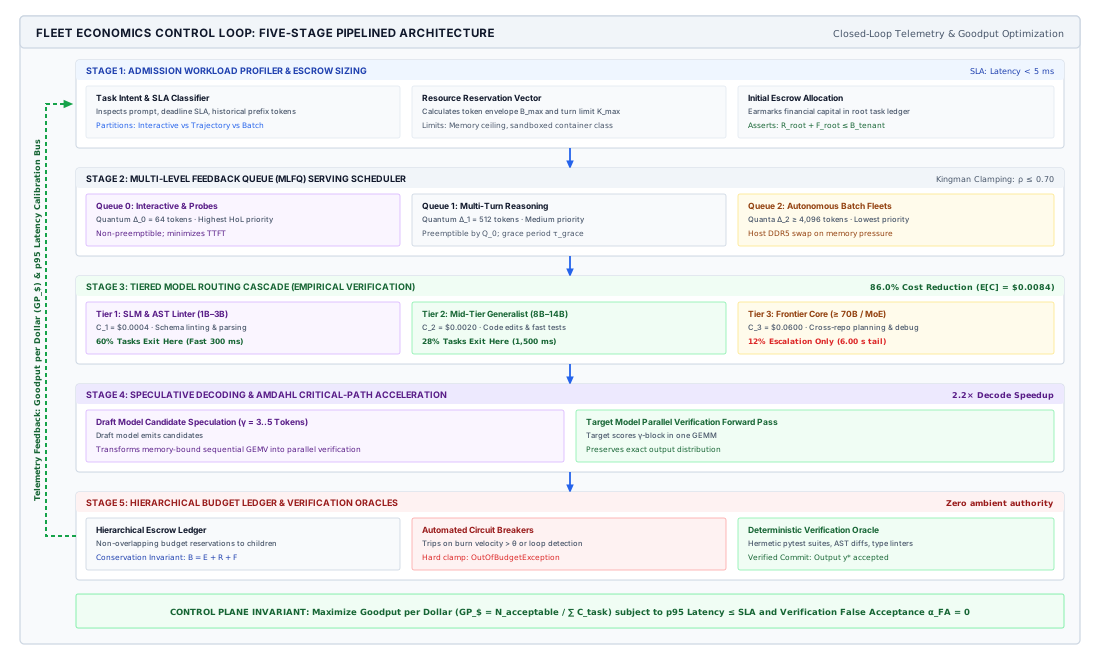
Figure 7: **The Fleet Economics Closed-Loop Control Architecture**: A five-stage pipelined serving engine integrating admission workload profiling and escrow reservation, MLFQ cluster scheduling ($\rho \le 0.70$), tiered model routing cascades (60 percent SLM exit at $0.0004, 28 percent generalist exit at $0.0024, 12 percent frontier escalation), speculative decoding acceleration ($\gamma = 3..5$), and hierarchical budget ledger accounting under zero ambient authority. Telemetry from verified task completions feeds an outer Goodput per Dollar feedback bus that dynamically retunes admission escrows, queue quanta, and cascade confidence thresholds.

As traced across the end-to-end pipeline of figure 7, an incoming request traverses five coordinated systems barriers before committing mutations to the external environment. In Stage 1 (Workload Profiler & Escrow), the ingress router parses prompt semantics, establishes SLA deadlines, and provisions an initial financial escrow envelope ($B_{\text{task}}$). In Stage 2 (MLFQ Cluster Scheduler), requests enter priority queue $Q_0$ under Kingman-safe cluster utilization targets ($\rho \le 0.70$), isolating interactive probes from batch trajectories via token quanta ($\Delta_0=64, \Delta_1=512, \Delta_2\ge 4{,}096$) and preventing starvation via periodic priority boosts ($T_{\text{boost}} = 60\text{ s}$).

In Stage 3 (Tiered Routing Cascade), the execution turn attempts resolution at the cheapest viable tier: $60\%$ of syntactic turns terminate cleanly at the SLM tier ($C_1 = \$0.0004$), $28\%$ resolve at the mid-tier generalist ($C_2 = \$0.0024$), and only $12\%$ escalate to the frontier model, achieving an expected turn cost of $E[C] = \$0.0084$. In Stage 4 (Speculative Decoding Engine), heavy frontier invocations are accelerated directly on GPU tensor cores using an aligned draft model that speculatively generates $\gamma = 3..5$ tokens per forward pass ($\alpha_{\text{accept}} = 0.75$), collapsing critical-path decode latency. Finally, in Stage 5 (Hierarchical Ledger & Verifier), the model holds zero ambient authority and every proposed action executes in an isolated sandbox; only when deterministic mechanical verifiers certify correctness does the transaction commit, returning unexpended escrow to the tenant. The entire pipeline is enclosed by a global feedback bus that continuously optimizes cluster Goodput per Dollar ($\text{GP}_{\$}$), dynamically tuning routing thresholds and queue quanta based on real-time defect rates.

The first stage of this engine is the Workload Profiler. When a task request arrives at the platform ingress, the profiler inspects the prompt payload, user-specified deadline, historical trajectory characteristics of the requesting tenant, and tool capability requirements. Rather than treating all requests as homogeneous token sequences, the profiler partitions incoming traffic into distinct execution profiles: short, bounded interactive queries; multi-turn deterministic workflows; and unbounded exploratory agent trajectories. By extracting structural invariants—such as whether the query requires arbitrary code execution or merely structured data extraction—the profiler computes an initial resource reservation vector containing memory bounds, tool rate limits, and an initial financial escrow.

The second stage is the Multi-Level Feedback Queue (MLFQ) Cluster Scheduler. The scheduler prevents the catastrophic head-of-line blocking that occurs when long-lived, stochastic agent trajectories share physical compute queues with single-turn interactive requests. Incoming tasks enter the highest-priority queue ($Q_0$), which grants an immediate, small compute quantum optimized for time-to-first-token (TTFT) and rapid initial planning. If a task exhausts its quantum without terminating or entering an external wait state, the scheduler demotes it to lower-priority, high-throughput batch queues ($Q_1, Q_2$). This separation ensures that long-running trajectories run on clusters configured for high-density continuous batching and throughput, while latency-sensitive user turns run on under-subscribed, low-latency nodes.

The third stage is the Tiered Routing Cascade, which operationalizes the principles established by L. Chen et al. (2023) in FrugalGPT. When a scheduled agent turn requires neural inference, the runtime does not default to the most capable frontier model. Instead, it dispatches the context to a lightweight Small Language Model (SLM) configured to produce intermediate scratchpads, schema-validated tool calls, or candidate verification checks. The SLM output passes through an unprivileged output validator. If the SLM generates an invalid tool schema, exhibits low logit confidence on critical tokens, or signals an inability to resolve the prompt’s dependency graph, the cascade escalates the call to a mid-tier or frontier reasoning model. By resolving the vast majority of syntactic formatting, tool routing, and status summarization steps at the lowest tier, the cascade preserves expensive frontier model capacity for complex planning and error recovery.

Chen, Lingjiao, Matei Zaharia, and James Zou. 2023. “FrugalGPT: How to Use Large Language Models While Reducing Cost and Improving Performance.” arXiv Preprint arXiv:2305.05176.

The fourth stage is the Speculative Decoding Engine, embedded directly within the physical inference cluster. When an escalated task must run on a massive target model ($M_{\text{target}}$), the runtime couples the target model with an aligned draft model ($M_{\text{draft}}$). The draft model speculatively emits $\gamma$ candidate tokens along the Amdahl critical path. The target model evaluates these $\gamma$ tokens in a single parallel forward pass (GEMM), accepting prefixes that match its own probability distribution and falling back to its own distribution on the first rejection. Because speculative decoding guarantees mathematical equivalence to sampling directly from $M_{\text{target}}$, the runtime dramatically accelerates autoregressive generation without introducing stochastic drift or degrading task success rates.

The fifth stage is the Hierarchical Budget Ledger and Invariant Escrow. Every downstream execution—whether a speculative forward pass, an SLM routing check, a containerized compiler run, or an external SaaS API invocation—must be authorized against a strictly monotonic budget ledger. As child subagents are spawned to execute sub-problems, the parent agent splits its own resource escrow, delegating smaller, non-renewable allowances to its children. If a subagent enters a repetitive retry cycle or fails to produce state advancement within its allocated budget, the ledger trips a hard circuit breaker. The agent’s modified state is held in escrow; only when an external, deterministic test suite passes does the runtime commit the mutation to the authoritative production store. The contracts, mechanisms, optimization targets, and failure modes across these five stages are synthesized in table 13.

Table 13: Mechanics and Interfaces of the Fleet Economics Control Loop: Input contracts, core mechanisms, optimization targets, and failure modes across the five control loop stages.

Control Loop Stage	Input Contract	Primary Mechanism	Optimization Target	Failure Modes Mitigated
1. Workload Profiler	Raw Task & Historical Metadata	Context & dependency static analysis	SLA classification; escrow sizing	Over-provisioning; sandbox starvation
2. MLFQ Scheduler	Profiler Class & Turn Quantum	Dynamic quantum demotion	P99 interactive TTFT; cluster throughput	Head-of-line blocking; KV-cache exhaustion
3. Routing Cascade	Validated Context & Intent Tier	Staged capability escalation (SLM $\to$ Frontier)	Cost per intermediate step ($C_{\text{turn}}$)	Frontier model over-utilization
4. Speculative Decoding	Active Token Stream & Draft Model	Parallel validation of $\gamma$ draft tokens	Inter-token decode latency ($T_{\text{decode}}$)	Memory-bandwidth compute underutilization
5. Hierarchical Ledger	Allocated Escrow & Execution Diffs	Monotonic accounting & circuit breakers	Task financial bounded error	Runaway infinite loops; budget exhaustion

Goodput per dollar: The unified objective

Optimizing an agent fleet requires a metric that bridges the gap between hardware efficiency and enterprise utility. Traditional machine learning infrastructure metrics—such as tokens per second, FLOP efficiency, or GPU utilization—are actively misleading in agentic systems. A cluster running an unconstrained agent in an infinite loop can achieve $98\%$ model FLOPs utilization (MFU) and generate tens of thousands of tokens per second while producing zero functional value. Conversely, an infrastructure metric based purely on raw cost per million tokens rewards the selection of cheap, degraded models that cannot solve the user’s task.

At fleet scale the accepted-task objective of section 1 appears as Goodput per Dollar ($\text{GP}_{\$}$), the number of verified, defect-free tasks completed per unit of total economic expenditure. It is the reciprocal of $C_{\text{effective}}$. Where the trajectory goodput of Micro-efficiency versus macro-efficiency measures the share of resources that reaches accepted tasks, goodput per dollar measures how many accepted tasks each dollar buys:

\[\text{GP}_{\$} = \frac{N_{\text{acceptable}}}{\sum_{i=1}^M C_{\text{task}}^{(i)}}\]

In this formulation, $M$ represents the total number of tasks admitted to the cluster, and $C_{\text{task}}^{(i)}$ represents the comprehensive, whole-trajectory cost of task $i$. As established in our task cost accounting framework, $C_{\text{task}}$ encompasses every resource consumed across the attempt lifecycle:

\[C_{\text{task}} = \sum_{k=1}^K \left( C_{\text{prefill}}^{(k)} + C_{\text{decode}}^{(k)} + C_{\text{tool}}^{(k)} + C_{\text{sandbox}}^{(k)} \right) + C_{\text{verify}} + C_{\text{human}}\]

The numerator, $N_{\text{acceptable}}$, represents the count of tasks that satisfy all functional invariants without unbudgeted human intervention:

\[N_{\text{acceptable}} = \sum_{i=1}^M \mathbf{1}\left( \text{Verified}(i) \land \neg \text{Defect}(i) \right)\]

Here, $\text{Verified}(i)$ is a binary indicator denoting that the task’s final output successfully passed the external, deterministic validation harness (such as unit test suites, integration linters, or schema checkers). The term $\neg \text{Defect}(i)$ ensures that false acceptances—solutions that pass syntactic tests but introduce latent regressions or security vulnerabilities—are excluded.

Definition 0.2: Goodput per dollar

The definitive economic objective metric $\text{GP}_{\$} = \frac{N_{\text{acceptable}}}{\sum_{i=1}^M C_{\text{task}}^{(i)}}$ that quantifies the number of verified, defect-free agent task completions achieved per unit of total financial expenditure. By coupling deterministic post-condition verification with whole-trajectory cost accounting, goodput per dollar aligns accelerator scheduling, model selection, and execution caching with true enterprise utility.

Napkin Math 0.8: Evaluation of fleet goodput per dollar

Consider an enterprise software engineering benchmark consisting of $M = 1{,}000$ code repair tasks. We compare two operational configurations: a Naive Monolithic Architecture that routes every interaction directly to an unassisted frontier model, and a Synthesized Control-Loop Architecture that deploys profiling, MLFQ scheduling, tiered cascades, and speculative decoding.

1. Hardware and Provider Pricing Basis:

Frontier Model ($M_{\text{target}}$): $\$10.00$ per $10^6$ prefill tokens; $\$30.00$ per $10^6$ decode tokens.
Small Language Model ($M_{\text{draft}}$ / Cascade Tier 1): $\$0.20$ per $10^6$ prefill tokens; $\$0.60$ per $10^6$ decode tokens.
Ephemeral Execution Sandbox: $\$0.06$ per CPU-hour ($\$1.67 \times 10^{-5}$ per second).
Deterministic Verification Suite: $\$0.02$ per execution run.
Human Escalation Triage: $\$15.00$ per defect remediation.

2. Baseline: Naive Monolithic Architecture

Trajectory dynamics: Every task runs on $M_{\text{target}}$. Average trajectory requires $K = 6$ turns.
Per turn: $4{,}000$ prefill tokens, $500$ decode tokens, $45$ seconds of sandbox execution.
Task accuracy: First-pass acceptance rate is $p = 0.65$. The remaining $35\%$ fail verification and are discarded without human remediation ($N_{\text{acceptable}} = 650$).
Turn token cost: $(4{,}000 \times 10^{-5}) + (500 \times 3 \times 10^{-5}) = \$0.040 + \$0.015 = \$0.055$.
Turn sandbox cost: $45 \times (1.67 \times 10^{-5}) = \$0.00075$.
Trajectory cost ($6$ turns): $6 \times (\$0.055 + \$0.00075) = \$0.3345$.
Verification cost: $\$0.02$. Total cost per task: $\$0.3545$.
Fleet total cost: $1{,}000 \times \$0.3545 = \$354.50$.
Baseline Goodput: \[\text{GP}_{\$}^{\text{naive}} = \frac{650 \text{ tasks}}{\$354.50} \approx \mathbf{1.83 \text{ accepted tasks / dollar}}\]

3. Synthesized Architecture:

Workload Profiling & Cascading: $60\%$ of all turns (file searching, syntax linting, git staging) are resolved entirely by $M_{\text{draft}}$. Only $40\%$ of turns escalate to $M_{\text{target}}$ for complex algorithmic synthesis.
Speculative Decoding: Applied to all $M_{\text{target}}$ invocations with draft model $M_{\text{draft}}$ ($\gamma = 4$, mean acceptance rate $\alpha = 0.75$). Decoding wall-clock time drops by $2.1\times$, reducing sandbox hold times during generation.
Turn token cost (Cascade Tier 1 - SLM, 60 percent of turns): \[(4{,}000 \times 2 \times 10^{-7}) + (500 \times 6 \times 10^{-7}) = \$0.0008 + \$0.0003 = \$0.0011\]
Turn token cost (Cascade Tier 2 - Frontier + Speculative Draft, 40 percent of turns): Frontier cost remains $\$0.055$. Draft generation overhead adds $500 \times \gamma \times (6 \times 10^{-7}) \approx \$0.0012$. Total turn token cost: $\$0.0562$.
Average turn token cost: $(0.60 \times \$0.0011) + (0.40 \times \$0.0562) = \$0.00066 + \$0.02248 = \$0.02314$.
Sandbox cost per turn: Reduced latency lowers sandbox residency from $45\text{s}$ to $28\text{s}$: \[28 \times (1.67 \times 10^{-5}) = \$0.00047\]
Task success and retries: Hierarchical budgeting allows up to $K = 8$ turns for difficult tasks. First-pass acceptance rises to $p = 0.82$. For the remaining $180$ tasks, $100$ are resolved via an automated escalation retry (adding $3$ turns of Tier 2), and $80$ fail cleanly and are flagged for human review ($C_{\text{human}}$ omitted for rejected batch, or resolved: assume $N_{\text{acceptable}} = 820 + 75 = 895$).
Effective average turns across 1,000 tasks: $6.8$ turns.
Trajectory execution cost: $6.8 \times (\$0.02314 + \$0.00047) = \$0.1605$.
Verification cost: $\$0.02$. Average cost per task: $\$0.1805$.
Fleet total cost: $1{,}000 \times \$0.1805 = \$180.50$.
Synthesized Goodput: \[\text{GP}_{\$}^{\text{synth}} = \frac{895 \text{ tasks}}{\$180.50} \approx \mathbf{4.96 \text{ accepted tasks / dollar}}\]

The synthesized system achieves a $2.71\times$ improvement in Goodput per Dollar, simultaneously cutting fleet expenditure by $49.1\%$ and boosting task yield by $37.7\%$.

Maximizing Goodput per Dollar reveals the fundamental trade-off of serving economics: spending more money per task is economically rational if and only if the marginal expenditure yields a super-linear increase in the probability of task acceptance. Conversely, cost reduction strategies that depress task success rates—even slightly—frequently crater Goodput per Dollar because the fixed costs of tool infrastructure, prefill tokens, and verification are squandered on unrecoverable failures.

The fleet economic operating envelope

Scaling an agent fleet beyond a single isolated instance introduces severe non-linearities governed by queueing theory and shared resource contention. To maintain economic solvency and satisfy Service Level Agreements (SLAs), an infrastructure architect must define the system’s Economic Operating Envelope. This envelope represents the multidimensional parameter space—bounded by arrival rate ($\lambda$), concurrency ($N$), task complexity ($K$), and budget ceilings ($B$)—within which the fleet operates stably.

Neil J. Gunther’s Universal Scalability Law models system capacity under concurrency $N$: \[C(N) = \frac{N}{1 + \sigma(N - 1) + \kappa N(N - 1)}\] where $\sigma$ measures contention for serialization bottlenecks and $\kappa$ measures crosstalk or coherency delays.

When modeling fleet scaling, simple linear capacity assumptions fail. We apply Neil J. Gunther’s Universal Scalability Law (USL) to characterize the effective capacity $C(N)$ of an agent serving cluster under concurrent trajectory load $N$. In an agentic system, the contention parameter $\sigma$ captures queuing for shared physical resources: high-bandwidth memory (HBM) on GPU worker nodes, limits on concurrent container instantiations within the container hypervisor, and provider rate limits on external tool APIs. The coherency parameter $\kappa$ captures retrograde effects arising from coordination and crosstalk: distributed lock contention in shared budget ledgers, context cache invalidations across cluster nodes, and database serialization during parallel state commits.

If an operator pushes concurrency $N$ beyond the peak of the USL curve ($N_{\max} = \lfloor \sqrt{(1 - \sigma)/\kappa} \rfloor$), the system enters a retrograde collapse regime. Queues back up, prefill activations spill from GPU SRAM to host system DRAM, and sandbox initialization times experience extreme tail latency amplification. Because agent trajectories are governed by sequential dependency chains, a latency spike in turn $k$ delays turns $k+1$ through $K$. If the latency exceeds client timeouts, the entire trajectory aborts, reducing $N_{\text{acceptable}}$ to zero while retaining $100\%$ of the incurred cost.

To enforce operation strictly within the stable envelope, the synthesized runtime implements three hard boundary invariants:

First, the Dynamic Admission Boundary regulates entry based on current cluster queue depths. Using the $M/G/k$ queueing models developed in our capacity provisioning framework, the scheduler rejects or sheds low-priority background trajectories when the estimated wait time in $Q_0$ threatens the P95 TTFT SLA of interactive sessions:

\[W_{Q_0}(\lambda) + \mathbb{E}[T_{\text{prefill}}] \le \text{SLA}_{\text{interactive}}\]

Second, the Monotonic Escalation Ceiling limits the depth and financial velocity of model cascading. An agent is forbidden from invoking a higher-tier reasoning model unless the expected information gain exceeds the cost delta. Formally, if an escalation from model tier $j$ to tier $j+1$ incurs an incremental cost $\Delta C_{j \to j+1}$, the escalation is permitted if and only if:

\[\Delta C_{j \to j+1} < \left( \mathbb{P}_{j+1}(\text{Success}) - \mathbb{P}_j(\text{Success}) \right) \cdot V_{\text{task}}\]

where $V_{\text{task}}$ represents the economic value of successfully completing the task. If this condition is not met, the runtime terminates the trajectory, reporting a bounded failure rather than burning capital on low-probability recovery attempts.

Third, the Amdahl Efficiency Gate dictates speculative decoding and acceleration investments. The runtime continuously measures the fraction of critical-path wall-clock time spent in autoregressive decode ($\alpha_{\text{decode}}$) versus tool and sandbox execution ($\alpha_{\text{env}} = 1 - \alpha_{\text{decode}}$). If profiling reveals that $\alpha_{\text{decode}} < 0.20$, the runtime disables speculative drafting for that task profile. When environmental latencies dominate the critical path, dedicating GPU memory bandwidth and compute cores to speculative draft verification yields negligible end-to-end speedup while wasting memory capacity that could otherwise support larger batch sizes for parallel requests.

By continuously balancing admission rates, model tiers, decode acceleration, and budget ledgers against empirical operating bounds, the synthesized architecture ensures that the fleet operates at peak Goodput per Dollar.

Yet, translating these architectural principles into production systems is fraught with hazard. When system designers move from theoretical formulations to practical implementations, they frequently fall victim to intuitive but catastrophic operational traps. Refuting these common systems misconceptions and delineating the precise physical fallacies of foundation model deployment is the necessary final step in mastering serving economics.

Fallacies and pitfalls

Designing and operating production agent systems requires navigating the treacherous gap between micro-benchmarked inference latency and macroeconomic fleet stability. Hardware accelerators, network fabrics, and foundation model APIs exhibit non-linear cost surfaces that punish naive operational assumptions. When systems engineers treat non-deterministic agent trajectories as equivalent to traditional stateless Remote Procedure Calls (RPCs), the resulting architectures suffer catastrophic financial runaway, severe throughput collapse, and wasted engineering effort. The following fallacies and pitfalls illuminate the specific physical and economic failure modes that emerge across agent serving infrastructures.

Fallacy: Evaluating model cost strictly by per-token API prices identifies the most economical model.

Foundation model providers publish headline pricing denominated in dollars per million tokens, establishing an intuitive but perilous heuristic: that substituting a cheaper model directly reduces operational expenditure. This micro-level price metric is structurally deceptive because it isolates raw token ingestion and generation from the stochastic state-space traversal required to resolve an autonomous task. In an agentic runtime, total financial expenditure is governed not by unit token rates, but by the whole-trajectory cost equation:

\[C_{\text{effective}} = \frac{\mathbb{E}[C_{\text{task}}] + (1 - p_{\text{success}}) C_{\text{human}}}{p_{\text{success}}}\]

where $\mathbb{E}[C_{\text{task}}] = \sum_{k=1}^K C_{\text{turn}, k} + C_{\text{tool}} + C_{\text{runtime}} + C_{\text{verify}}$ captures the cumulative prefill and decode expense across $K$ sequential trajectory steps, sandboxed environment execution fees, tool invocation overhead, and deterministic verification runs. The parameter $p_{\text{success}}$ represents the empirical probability that the generated trajectory passes all ground-truth acceptance tests without violating environment invariants, and $C_{\text{human}}$ denotes the post-hoc triage cost incurred when a failed or corrupted state must be inspected and remediated by an engineer.

When an unprivileged predictor exhibits lower latent capability, the trajectory dynamics degrade along three interdependent axes. First, the model generates malformed tool calls, invalid schemas, and hallucinated file paths, triggering iterative self-correction loops that dramatically inflate trajectory length $K$. Because every conversational step appends preceding tool outputs to the working context, input token prefill scales quadratically:

\[\text{Total Tokens} \approx \sum_{k=1}^K (S_{\text{prompt}} + k \cdot \Delta S)\]

where $S_{\text{prompt}}$ is the base system prompt and $\Delta S$ is the incremental context accumulated per turn. A nominally cheap model requiring $K=12$ turns to complete a task processes far more aggregate tokens than an advanced frontier model that plans correctly in $K=2$ turns.

Second, weaker models execute extraneous and destructive tool actions. Each supplementary turn incurs external sandboxed compute costs, database read/write units, and network egress fees that frequently dwarf inference API charges. Third, and most crucially, lower reasoning capability degrades the terminal pass rate $p_{\text{success}}$. Because downstream business processes cannot tolerate unverified hallucinations, failures that escape automated sandboxes spill over into human review queues. If human engineering triage costs $\$60.00$ per hour ($\$1.00$ per minute) and reviewing a flawed patch requires five minutes ($C_{\text{human}} = \$5.00$), a failure rate of $30\%$ adds an amortized overhead of $\$2.14$ per task attempt—swamping any fractional-cent savings achieved on token discounts.

The architectural defense demands shifting telemetry from unit token consumption to effective cost per accepted task completion ($C_{\text{effective}}$). Production serving harnesses must instrument end-to-end accounting ledgers that track full trajectory lifecycles, binding token usage, sandbox runtime hours, tool API fees, and verification overhead to the binary outcome of the task verification suite. Optimization targets must be defined across the Pareto frontier of verified yield per dollar, routing tasks to cheaper models only when their empirical single-pass success probability $p_{\text{success}}$ matches the operational threshold.

Pitfall: Optimizing token generation speed when tool wait time dominates the critical path.

When an interactive agent displays sluggish responsiveness, systems engineers frequently focus their optimization efforts on inference serving: tuning autoregressive decode kernels, implementing speculative decoding, or migrating from 16-bit floating-point weights (FP16) to 4-bit integer quantization (INT4). While these interventions increase generation throughput, they routinely fail to produce perceptible improvements in end-to-end task wall-clock time.

This misallocation of engineering effort stems from ignoring the sequential dependencies governing an agent trajectory. The critical path latency $T_{\text{trajectory}}$ is partitioned across three disjoint execution domains:

\[T_{\text{trajectory}} = \sum_{k=1}^K \left( T_{\text{model}, k} + T_{\text{tool}, k} + T_{\text{runtime}, k} \right)\]

where $T_{\text{model}, k}$ is the combined prefill and autoregressive decode duration for turn $k$, $T_{\text{tool}, k}$ represents external API or environment interaction latency, and $T_{\text{runtime}, k}$ encompasses host overhead, including IPC serialization, sandboxed container isolation barriers, and context reconstruction. Amdahl’s Law dictates that the theoretical speedup $S_{\text{task}}$ achievable by accelerating the inference component is strictly bounded by the fraction of execution time that the model occupies:

\[S_{\text{task}} = \frac{1}{(1 - f_{\text{model}}) + \frac{f_{\text{model}}}{s_{\text{model}}}}, \quad \text{where } f_{\text{model}} = \frac{\sum_{k=1}^K T_{\text{model}, k}}{T_{\text{trajectory}}}\]

In the trace of table 3, the model accounts for 9.4 percent of wall-clock time, so a 4× faster model makes the trajectory only 1.08× faster, and an instant one only 1.10×. The test run alone takes 78.6 percent. The remedy is to read the trace before investing: warm sandbox pools, build caches, test selection, and parallel tool calls shorten what is actually on the critical path.

In autonomous software engineering, data analysis, or multi-service orchestration agents, $f_{\text{model}}$ is routinely small. Consider a software engineering agent executing a test suite: a frontier model may generate a bash command in $1.5\text{ s}$ ($T_{\text{model}} = 1.5\text{ s}$), but executing that command requires spinning up an isolated container, compiling an abstract syntax tree, pulling package dependencies, and executing a test suite taking $45\text{ s}$ ($T_{\text{tool}} = 45\text{ s}$), followed by $1.0\text{ s}$ of runtime log truncation and sandbox synchronization ($T_{\text{runtime}} = 1.0\text{ s}$). In this scenario, $f_{\text{model}} \approx 0.031$ (the model accounts for roughly $3.1\%$ of the critical path). Quadrupling inference decode speed from $30\text{ tokens/s}$ to $120\text{ tokens/s}$ ($s_{\text{model}} = 4.0$) compresses generation time from $1.5\text{ s}$ to $0.375\text{ s}$, yielding an end-to-end task speedup of:

\[S_{\text{task}} = \frac{1}{(1 - 0.031) + \frac{0.031}{4.0}} = \frac{1}{0.969 + 0.00775} \approx 1.024\]

The engineering intervention expends significant architectural complexity to achieve an imperceptible $2.4\%$ overall latency reduction.

The correct systems mitigation requires strict distributed tracing of the critical path before embarking on optimization. By propagating distributed trace context headers across agent loop iterations, engineers isolate the actual structural bottlenecks: cold-start container initialization, blocking network I/O, synchronous database polling, and redundant environment state teardown. Mitigations must focus where $f$ is highest: pre-warming warm pools of container sandboxes with Copy-on-Write (CoW) memory forks, parallelizing independent tool calls via asynchronous runtimes, caching deterministic tool outputs, and streaming execution logs to initiate speculative prefill before tool completion.

Fallacy: Speculative decoding reduces model resource usage across all serving loads.

Speculative decoding leverages a lightweight draft model $M_{\text{draft}}$ to predict a sequence of $\gamma$ candidate tokens, which are subsequently verified in parallel by the primary target model $M_{\text{target}}$ within a single modified forward pass. Because verification transforms $\gamma$ sequential memory-bound vector-matrix multiplications (GEMVs) into a single compute-bound matrix-matrix multiplication (GEMM), speculative decoding substantially reduces per-token decoding latency for isolated, single-batch inference requests. This latency reduction frequently misleads system architects into assuming that speculative decoding unconditionally conserves hardware compute resources and should be enabled globally across all serving tiers.

The failure mechanism arises from a fundamental physical trade-off: speculative decoding trades raw computational floating-point operations (FLOPs) to buy down wall-clock latency. For each verification step generating an accepted sequence of length $\alpha \le \gamma + 1$, the serving system expends the computational effort of running $\gamma$ forward passes through $M_{\text{draft}}$ plus one forward pass through $M_{\text{target}}$ across $\gamma + 1$ tokens. Because the speculative acceptance rate is strictly less than unity ($\beta < 1.0$), rejected draft tokens represent discarded computation. The total FLOPs consumed per verified token generated is rigorously higher under speculative decoding than under standard autoregressive decoding:

\[\text{FLOPs}_{\text{speculative}} = \frac{\gamma \cdot \text{FLOPs}(M_{\text{draft}}) + (\gamma + 1) \cdot \text{FLOPs}_{\text{attn+proj}}(M_{\text{target}}) + \text{FLOPs}_{\text{FFN}}(M_{\text{target}})}{\mathbb{E}[\alpha]}\]

Under low-concurrency serving workloads where batch size is minimal ($B \approx 1$), the GPU memory bus is the binding operational bottleneck. The hardware sits deep within the memory-bound regime of the Roofline model, with arithmetic intensity far below the saturation threshold of the accelerator’s Tensor Cores. Under these conditions, the extra FLOPs executed on cached weights are effectively “free,” hidden behind the memory fetch latency of $M_{\text{target}}$, yielding net wall-clock speedups without throughput penalties.

However, in production agent fleets serving hundreds of concurrent trajectories, the inference cluster operates under heavy saturation at high aggregate batch sizes ($B \gg 1$). At this operating point, batching saturates memory bandwidth, pushing the engine into the compute-bound regime where Tensor Core arithmetic utilization approaches physical capacity. In this state, arithmetic cycles are no longer free. The redundant FLOPs executed by $M_{\text{draft}}$ and the validation of discarded draft branches directly compete with concurrent requests for execution pipelines, functional units, and SRAM register files. Furthermore, co-locating $M_{\text{draft}}$ consumes critical high-bandwidth memory (HBM), stealing capacity that would otherwise be allocated to the PagedAttention physical KV cache pool. The resulting contraction of KV cache frames forces the scheduler to preempt active sequences or artificially constrain maximum batch sizes, directly depressing overall cluster throughput ($tokens/second$) and inflating queueing delay $W$ in the scheduling pool.

The architectural defense mandates load-aware, dynamic speculative decoding gating. Runtimes must continuously monitor accelerator compute utilization, active batch sizes, and scheduling queue depths. Speculative decoding should be dynamically engaged only for latency-critical, unbatched tasks executing on the critical path, and automatically disengaged the moment serving clusters enter compute-bound saturation where global aggregate Goodput per Dollar must be maximized.

Pitfall: Allowing subagents to spawn child workers without hierarchical budget reservations.

Complex agent frameworks frequently implement dynamic task decomposition, allowing a parent agent to instantiate specialized child subagents to execute auxiliary subroutines, run parallel web searches, or investigate code compilation failures. A widespread and catastrophic implementation anti-pattern grants child workers ambient access to the parent’s organizational API credentials or global spending limits. When subagents possess unmetered, ambient authority to allocate compute, recursive delegation creates an unbounded distributed resource exhaustion vulnerability.

The mechanism of failure stems from the non-deterministic nature of unprivileged model planning combined with cyclic fault-recovery trajectories. If a child agent encounters an ambiguous tool failure or unresolvable environment state, its internal prompt loop may determine that decomposing the issue into multiple parallel sub-tasks is the optimal recovery strategy. If each child subagent can in turn spawn further workers without structural bounds, the system generates an uncontrolled cascade of asynchronous processes:

\[N_{\text{active}}(d) = \prod_{i=0}^d b_i\]

where $b_i$ is the branching factor of spawned workers at recursion depth $d$. If an upstream tool API experiences a transient outage or semantic schema change, every active worker encounters the same error simultaneously. Interpreting the fault as a problem requiring further decomposition, the fleet initiates a recursive explosion of remedial workers, each reading lengthy error traces into their working contexts.

Because token ingestion cost compounds across all active branches, an unconstrained subagent cascade drains thousands of dollars in commercial API credits or starves an on-premise GPU cluster’s KV cache within minutes. Furthermore, child workers running in unmetered concurrency generate distributed denial-of-service (DDoS) conditions against internal sandboxes, saturating container daemon socket queues, exhausting ephemeral network ports, and triggering database connection pool depletion. Post-hoc cancellations sent by the parent process traverse asynchronous queues, often arriving after the child workers have already executed extensive chains of redundant, fee-incurring inference calls.

The architectural mitigation requires the rigorous implementation of Hierarchical Budget Reservation Ledgers governed by the principle of least privilege. In this architecture, subagent creation is mediated by a transactional credit escrow system (table 14):

Table 14: Budget Ledger Invariants for Subagent Cascade Mitigation: Architectural enforcement mechanisms and systems failures prevented under hierarchical delegation.

Budget Ledger Invariant	Architectural Enforcement Mechanism	Systems Failure Prevented
Zero ambient authority	Child workers receive strictly ephemeral, cryptographically scoped session tokens containing hard token and currency caps.	Prevents workers from billing against global organization keys or parent pool accounts.
Strict Conservation of Budgets	A parent with remaining allocation $B_{\text{parent}}$ spawning child $k$ must escrow a slice $B_{\text{child}} \le B_{\text{parent}} - B_{\text{reserved}}$, decrementing its own ledger.	Eliminates infinite financial expansion; the total fleet expenditure tree is strictly bounded by the root user allocation: $\sum B_{\text{leaves}} \le B_{\text{root}}$.
Monotonic Non-Replenishing Limits	Child ledgers can only decrease; budget replenishment requires an explicit, blocking RPC request to the parent supervisor.	Halts runaway looping; when a child exhausts its micro-budget, it is forcibly paused and placed into runtime escrow.
Velocity Circuit Breakers	The host supervisor evaluates instantaneous burn rate $dC/dt$ across sliding windows.	Trips deterministic shutdown if token burn rate exceeds safe operational parameters, isolating buggy recursion before quota depletion.

Under this regime, when a child worker exhausts its allocated escrow, the runtime supervisor intercepts the boundary violation, terminates speculative execution branches, reclaims unused KV cache blocks, and forces the parent to handle the failure deterministically rather than spawning unchecked remedial workers.

Mastering the physical and economic boundaries of model serving dismantles the illusion that agent fleets can be engineered as stateless, decoupled software modules. The interplay of whole-trajectory cost accounting, critical-path Amdahl limits, dynamic speculative decoding thresholds, and hierarchical escrow governance demonstrates that dependability and economic viability are emergent properties of the entire runtime supervisor. Synthesizing these economic invariants into a unified systems discipline provides the foundation for sustainable fleet operations.

Summary

An agent is paid for by the task it finishes, not by the tokens it emits, and every design decision in a fleet is judged by cost and time per accepted task. That cost includes every turn, every re-sent context, every sandbox second and test run, and every failed attempt, which the odds ratio $(1-\alpha)/\alpha$ charges to the attempts that succeeded. The largest token term in a long trajectory is re-sent context, so prefix caching with a stable layout is the first lever, compaction pays only over a long enough remaining horizon, and reasoning and retry budgets are chosen by whether a trustworthy verifier lets cheap attempts stop at the first success. Time follows the critical path in the trace, where tools and sandboxes often dominate, so faster inference and speculative decoding pay only for the calls on that path and only while serving capacity is slack. Verifier-gated cascades keep the frontier model off calls that do not need it, provided the gates check what matters. Capacity is sized in trajectories through Little’s law and, for hosted models, by the provider’s quota, and dedicated capacity pays above a break-even utilization that caching discounts raise. Money is the one resource no recovery restores, so reservations bound what any subtree can spend and spend-rate limits bound how fast, and the same accounting decides whether a task deserves an agent at all.

Key Takeaways: Price the accepted task, not the token

Failed attempts set the price: Cost per accepted task charges every failed attempt and every non-model term to the successes, so a model with far cheaper tokens can cost several times more per finished task.
Re-sent context is the largest token term: On a long trajectory, prefix caching with an append-only layout cuts the bill several-fold; one volatile field at the head of the prompt forfeits it, and compaction pays only over a long remaining horizon.
The trace decides where time goes: Faster inference, including speculative decoding, shortens a trajectory only in proportion to the model’s share of the critical path, which tools and sandboxes often dominate.
Cheap models need trustworthy gates: Cascades and retries lower cost only when an external check stops wrong outputs; a weak gate turns savings into false accepts and recovery work.
Capacity and money are held by trajectories: Size concurrency from trajectory lifetimes and quotas from tokens per trajectory, and reserve every child’s budget before it spends, because spent money is never rolled back.

The chapter gave quantitative form to three principles. Trajectory goodput and the accepted task (principle $\ref{pri-vol3-trajectory-goodput}$) became the whole-trajectory cost equation and its odds ratio, and it judged every lever, from caching and cascades to dedicated capacity. Trajectory-lifetime capacity and tail-aware scheduling (principle $\ref{pri-vol3-heavy-tailed-scheduling}$) became trajectory concurrency under Little’s law, the observation that a provider quota caps the rate of trajectories, and the compounding of tail delays across serial calls. Monotonic delegation (principle $\ref{pri-vol3-monotonic-delegation}$) became a reservation ledger that no concurrent child can overdraw, which matters because a sandbox write can be rolled back and a dollar cannot.

What’s Next: From priced parts to one trajectory

With every part of the system priced, who owns each transition when all of them run on one trajectory, and what remains that no subsystem can own?

Multi-Agent Coordination decided when splitting a task pays, and this chapter priced each accepted task, provisioned capacity for trajectory lifetimes, and held spending to reserved budgets. Conclusion runs every subsystem the book has built on a single trajectory, gives each state transition an owner, and ends at the boundary the runtime cannot cross, the specification of what the task was for.