1 Introduction
Purpose
Agent stack focus for this chapter.
Why can a model that generates a fluent, correct action still fail to complete an autonomous task?
The difference between answering a prompt and completing a delegated task marks the boundary of agentic machine learning systems. A foundation model can propose the exact line of code needed to fix a race condition, yet the repository remains broken until software inspects the source tree, applies the patch, runs regression tests, and verifies the outcome. Delegating autonomous work therefore requires building an engineered machine around the model, not merely selecting capable weights. That machine resembles a complete computer, with components that compute, remember, act on the external world, supervise execution, recover from faults, and learn from experience. However, its central processing element differs fundamentally from any classical processor: it is an autoregressive model whose outputs are stochastic proposals rather than deterministic execution. A fluent proposal can be subtly wrong, and the model cannot vouch for its own correctness. The surrounding system exists to contain that reality. The runtime determines what data the model perceives, bounds the actions it may execute, persists critical state across interruptions, and verifies whether the task actually succeeded. Every decision consumes computational time and monetary budget that only accepted outcomes justify. Building an agentic system is thus an exercise in systems engineering: sizing the runtime machinery to the horizon, state, and authority that the task demands.
Learning Objectives
- Trace the architectural evolution from predictive and generative machine learning to autonomous agentic systems
- Explain why a model’s stochastic proposals require an external runtime to close the interaction loop, and trace one turn through the runtime’s six phases
- Analyze which isolated-request assumptions a multi-turn trajectory breaks, and why the runtime accounts for cost, state, and authority per trajectory
- Classify a delegated task by horizon, state, and authority to identify its systems engineering obligations
- Distinguish mechanically enforced sandbox bounds from the external evidence that catches plausible but wrong results before task acceptance
- Calculate unchecked task reliability and cost per accepted task across multi-turn horizons, and use them to decide between a fixed workflow and a model-directed loop
- Specify a five-part task contract that separates goal, environment, permitted actions, observations, and completion criteria
Explore the concepts in this chapter
The volume’s concept map, opened on this chapter. Select a concept to read how it connects to ideas in other chapters. Open the full map ↗
1.1 The Evolution of Machine Learning Systems
A prediction service returns a score, a conversational assistant proposes a patch, and an agentic system applies and checks that patch under delegated authority. These three deployment arrangements trace the progression from predictive pipelines through conversational foundation models to autonomous workloads. They overlap historically: predictive models can participate in feedback loops, and a foundation model can serve any of the three arrangements. The engineering distinction is who controls the actions and checks the outcome, as three representative arrangements illustrate:
- Predictive Machine Learning Systems: A predictive model maps a supplied input to a structured output (\(\ExampleLabel = \ModelPredictor(\ModelInput)\)), as in image classification, recommendation ranking, or fraud scoring. Application code supplies the input and consumes the returned score, so the serving call needs no conversational memory or tool loop, even when the application feeds its scores into a broader process. Systems engineering concentrates on serving throughput, memory layout, and batch latency.
- Generative Foundation Models: Large autoregressive transformers trained on internet-scale corpora generate open-ended text, code, and multimodal tokens. In standard conversational deployment, however, the interaction remains open-loop and human-mediated. A developer working with a conversational assistant acts as the runtime controller, issuing a prompt, inspecting the response, copying code into an editor, running commands in a terminal, and pasting compiler errors and stack traces back into the prompt window. The model generates candidate tokens; the human provides the execution environment, carries working memory across turns, diagnoses failures, and verifies correctness.
- Agentic Machine Learning Systems: Agentic systems replace the human in the inner control loop with a software runtime. Instead of requesting advice, a user delegates an end-to-end objective: clone a software repository, reproduce a reported defect, synthesize a candidate fix, run the full test suite in an isolated sandbox, iterate until regressions clear, and return a verified patch. The foundation model shifts from an advisory partner to an action-proposing component inside an active feedback loop.
Replacing the human operator in the interaction loop with a software runtime defines an agentic system and shifts what engineering optimizes (table 1).
| Era | Interaction pattern | Who closes the loop | What engineering optimizes |
|---|---|---|---|
| Predictive systems | One fixed input mapped to one structured output | Application code consumes the score in this arrangement | Serving throughput, batch latency, and memory layout |
| Generative foundation models | Open-loop prompt and response | A human, who runs the tools and carries errors back to the prompt | Tokens per second, tail latency, and accelerator utilization |
| Agentic systems | Closed loop of proposal, action, and observation | The runtime, which dispatches granted actions and checks the result | Task completion rate, cost per accepted task, and reliability over turns |
Definition 1.1: Agentic system
Agentic system is an autonomous software system in which a runtime places a foundation model in a closed control loop with context, state, tools, and an environment, dispatching the model’s authorized proposals and returning their environmental observations to subsequent calls until the task is accepted, halted, or escalated.
- Significance: The unit of systems optimization shifts from the isolated model call to the complete task trajectory. Unchecked errors compound exponentially across sequential turns (section 1.6), and every attempt, accepted or aborted, is charged to the task’s cost per accepted result.
- Distinction: In conversational interfaces, a human executes tools, verifies output, and bridges state between turns. In an agentic system, software executes these operations under delegated authority, meaning the model’s output is strictly a proposal that holds no standing authority of its own.
- Common pitfall: Treating agency as a capability inherent to the model’s weights. A more capable model produces more accurate candidate actions, but permission enforcement, sandbox isolation, durable state persistence, and completion verification belong entirely to the surrounding software runtime.
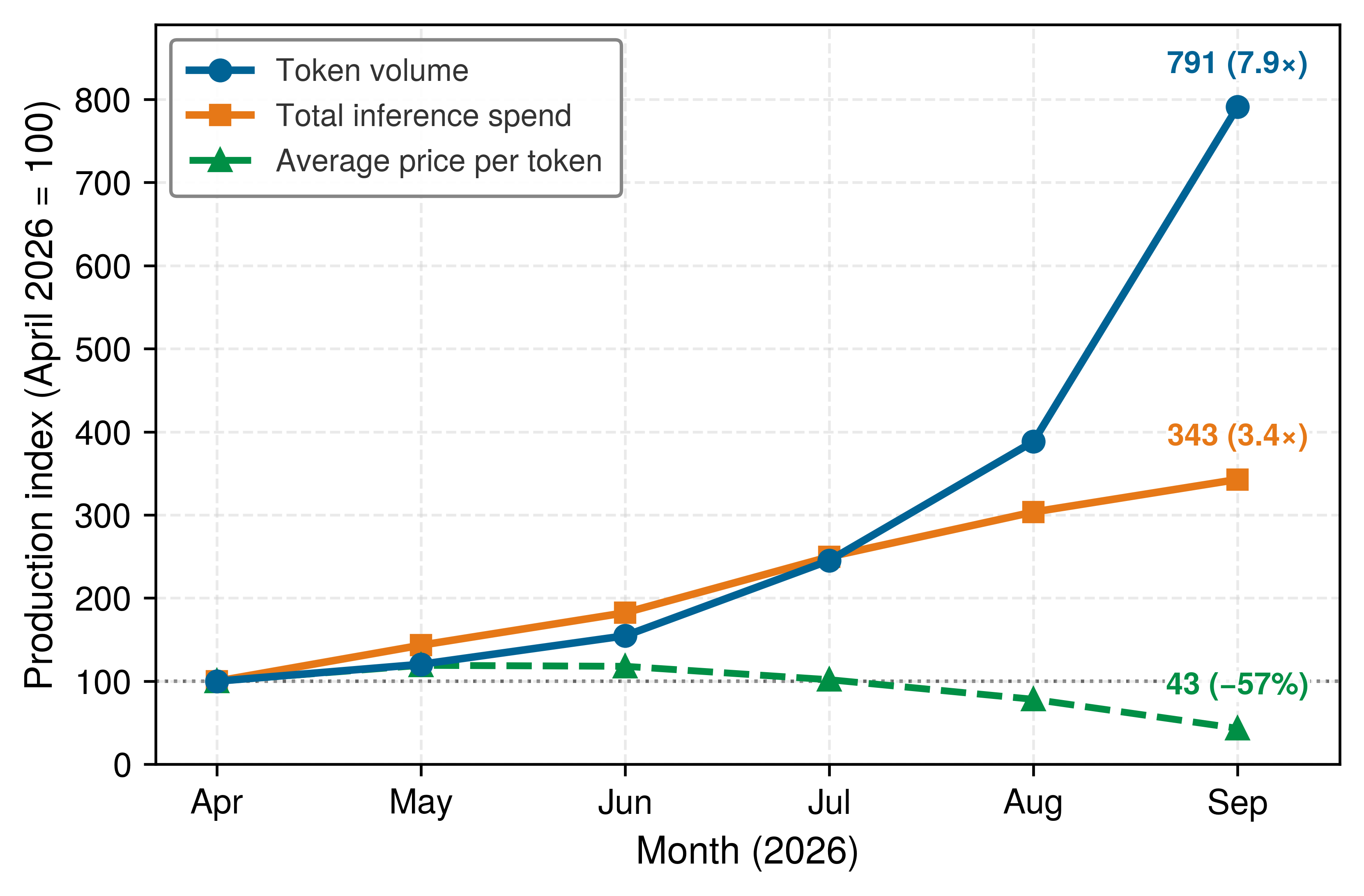
Production traffic shows how rapidly that third arrangement has overtaken the volume of isolated prompts. Across a multi-provider inference gateway serving more than 200,000 production teams (Vercel 2026), the share of requests ending in a tool call nearly doubled over six months, rising from 11.4 percent to 22.2 percent. Because each tool-using turn carries accumulated history and environment output, those 22.2 percent of requests already consumed 58.9 percent of all production tokens (up from 31.6 percent), or 5.0× as many tokens per request as calls without tools. Figure 1 tracks the aggregate token volume, total inference spend, and average price per token over the following five months on the same gateway.
Vercel. 2026. AI Gateway Production Index.
As the average price per token fell by 57 percent (to an index of 43.3), teams did not pocket the savings on a fixed request volume; they deployed multi-turn loops that consumed 7.9× as many tokens (reaching 790.8) and raised total expenditure 3.4× (to 342.7). Lower per-token prices made multi-step delegation affordable, and multi-step delegation in turn broke the assumptions of isolated-request serving. An isolated-request service accounts for each call separately, retains no task state after the response, and treats an HTTP 200 status as success. None of those conventions holds when a delegated task spans dozens of dependent steps, accumulates context and serving state between calls (the attention key-value cache retained for the growing prefix, so that the next turn need not recompute it, can occupy gigabytes of accelerator memory), and triggers side effects that permanently alter external systems. Turning a model’s candidate output into a completed task therefore requires examining everything that must happen between a useful proposal and an accepted outcome.
1.2 From a Useful Proposal to an Accepted Task
That gap between a model response and a finished job is concrete when an engineering team delegates a repository repair: diagnosing and fixing an intermittent race condition in a distributed key-value store.1 A foundation model2 can inspect the issue description and propose an edit to the connection-pool locking logic. Emitting that patch text, however, leaves the repository untouched. Resolving the defect requires an agent to locate the relevant source files, draft an edit, execute compilers and test runners inside an isolated environment, interpret diagnostic logs when a build fails, and verify that the resulting code satisfies the repository’s regression test suite.
1 Repository Repair as a Benchmark Task: SWE-bench established repository repair as a standard benchmark for agentic systems: each instance pairs a real GitHub issue with the unit and integration tests from the patch that fixed it (Jimenez et al. 2024). A candidate patch is evaluated by whether those tests pass after application. The model is never permitted to inspect the evaluation tests directly, ensuring that acceptance rests on independent, untampered evidence rather than self-reported success.
Jimenez, Carlos E., John Yang, Alexander Wettig, Shunyu Yao, Kexin Pei, Ofir Press, and Karthik Narasimhan. 2024. “SWE-Bench: Can Language Models Resolve Real-World GitHub Issues?” International Conference on Learning Representations (ICLR).
2 Foundation Model: Bommasani and colleagues introduced the term in 2021 to describe models trained on large, diverse datasets at scale that can be adapted to an expansive range of downstream tasks (Bommasani et al. 2021). Because a foundation model is general-purpose, its weights encode neither the security permissions nor the specific acceptance criteria of a given production task; those boundaries must be defined and enforced by the surrounding runtime.
Bommasani, Rishi, Drew A. Hudson, Ehsan Adeli, Russ Altman, Simran Arora, Sydney von Arx, Michael S. Bernstein, et al. 2021. “On the Opportunities and Risks of Foundation Models.” arXiv Preprint arXiv:2108.07258.
An agentic system comes into existence when software closes this interaction loop. Rather than relying on an engineer to copy prompts and error traces back and forth, the surrounding software feeds the foundation model an objective alongside fresh environmental observations and captures the model’s proposed action. It then dispatches that action and returns structured execution feedback to guide the next decision.
The surrounding software, the runtime, enforces the boundary between what the model proposes and what the environment executes. All execution authority resides with the runtime. Because a model outputs only text or token streams, generating an operation’s name confers no permission to run it. The runtime parses the proposed action, checks that it complies with current access policies, and dispatches the call through a designated tool. A tool provides a structured interface to an environmental action, such as reading file contents, editing source code, running a shell command, or running a test suite. The part of the runtime that drives this loop is often called the agent harness, and The Agent Harness develops it as a component of the runtime rather than a separate system. In the conversational arrangement of figure 2 (panel A), a developer carries every command and every error by hand; in the agentic arrangement (panel B), the runtime dispatches only the actions it grants and routes verifier evidence back to itself rather than trusting the model’s account of what happened.
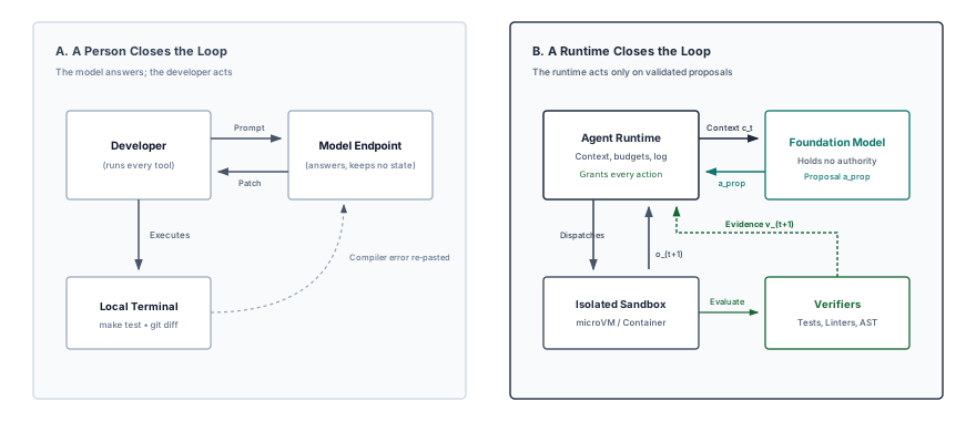
Panel B is the arrangement this book engineers. A capable model served by an optimized inference engine supplies proposals, but it cannot manage its own execution authority, maintain state across tool failures, or verify its actions against external reality. Those responsibilities fall on the surrounding software, so engineering an agent is the discipline of designing, securing, and operating the closed-loop system around the model. Analyzing and building that system requires four foundational instruments:
- The Stochastic Computer: An architectural map that relates the parts of an agentic system to the parts of a classical computer and marks where the comparison fails (section 1.3).
- The H·S·A Exposure Space: An analytical coordinate system that measures how far a delegated task departs from stateless model inference along three operational dimensions: execution horizon (\(\TurnHorizon\)), persistent state (\(\StateExposureLevel_0\) to \(\StateExposureLevel_3\)), and external authority (\(\AuthorityExposureLevel_0\) to \(\AuthorityExposureLevel_3\)) (section 1.4).
- The Invariant Closure Principle: A governance rule stipulating that safety and security invariants must be mechanically enforced by the runtime below the model, while task acceptance must be verified against independent evidence above the model (section 1.5). Below the model means between its proposal and the environment, where the runtime decides what may execute; above it means between the finished result and whoever accepts it, where the runtime decides what counts as done.
- Horizon Reliability and Cost Arithmetic: Mathematical relations that quantify how single-step error rates compound across multi-turn trajectories, showing how retry budgets and recovery mechanisms set the true compute cost per accepted task (section 1.6).
Section 1.4 also places four recurring reference workloads, which the book calls lighthouses, in the exposure space; the repair task is one of them. Once all four instruments are in hand, section 1.7 follows the repair task turn by turn to show where each one acts, and section 1.8 maps the instruments onto the structure of the book.
1.3 The Stochastic Computer
Repairing the connection-pool race condition requires more than a model call: the system must hold source files and test logs in working and persistent memory, invoke compilers and test runners that read and modify the workspace, supervise which commands may run, and improve future repairs from recorded runs. A classical computer organizes the same requirements, which makes it a convenient map of how the subsystems of an agentic system fit together.
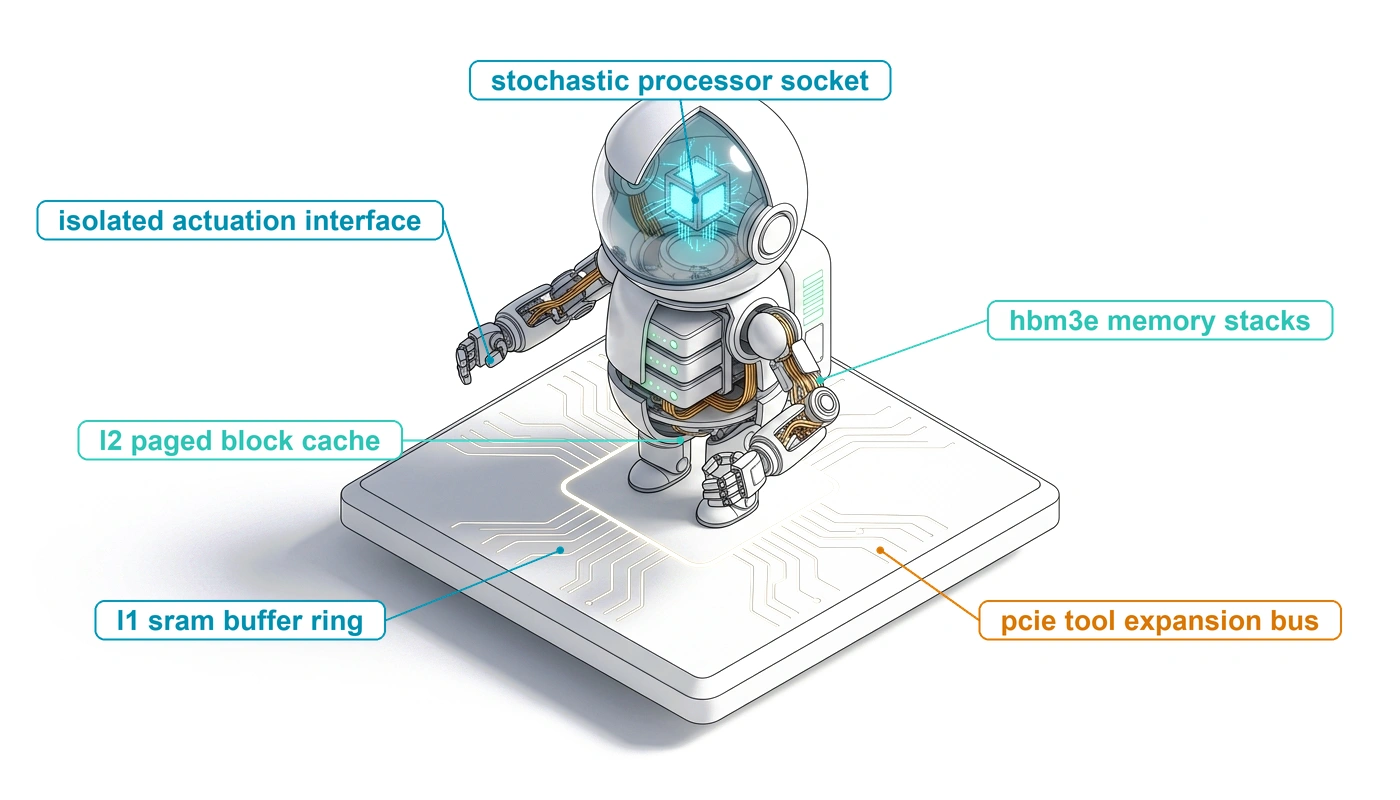
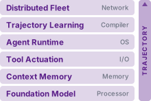
The stochastic computer names that map (figure 3).3 Its upper band is the live execution loop of a single task, and its lower band acts across tasks. In the live band, the foundation model plays the processor. Context and external stores play the memory hierarchy, from the active context window to long-term retrieval indices. Tools play input and output. The agent runtime plays the operating system, scheduling model calls, mediating every privileged operation, and enforcing access control. Across tasks, learning from recorded runs plays the role of recompiling a program from measurements of its earlier executions, refining the model’s policy without changing the runtime’s safety boundaries. Coordinating many agents mirrors scale-out across a network, where agents divide one workload and contend for shared state and resource limits.
3 The Stored-Program Organization: Von Neumann’s 1945 draft report on the EDVAC partitioned a computer into central arithmetic, central control, memory, and input/output organs (Neumann 1945). In von Neumann’s architecture, central control holds the absolute authority to fetch and execute instructions. In an agentic system, that authority is deliberately inverted: authority resides strictly within the surrounding runtime, while the learned model only proposes actions. Trust is decided outside the processor.
Neumann, John von. 1945. First Draft of a Report on the EDVAC. Moore School of Electrical Engineering, University of Pennsylvania.
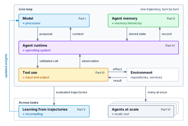
The analogy breaks at the processor, and that break defines the discipline of agentic systems engineering. A conventional processor executes instructions deterministically, so that identical machine state yields repeatable, auditable execution. A foundation model samples tokens from a distribution learned during training and conditioned on the observations supplied in its context, and that conditioning guarantees neither that the observations are complete and current nor that the proposed action is correct. Its outputs are candidate proposals, not certified computations. A response can be fluent yet factually wrong, or syntactically correct yet semantically destructive, and nothing in the generated text can vouch for its own validity.
A classical kernel trusts the processor to execute instructions faithfully. An agentic runtime cannot trust the model even to report its own status, since a model may report a successful return code that no tool returned, or actions it never took. The runtime therefore closes the control loop independently, enforcing permissions mechanically below the model and verifying results against external evidence above it (section 1.5.2). Memory diverges as sharply. A processor addresses memory directly, whereas the context presented to a model is a selective, lossy projection of the environment’s state. Authoritative state resides in external databases, filesystems, and version-control trees, and the context holds only a transient working representation of it.
The map therefore marks where classical systems guarantees carry over and where new mechanisms are required. The engineering problem is the deterministic runtime around the model (context management, execution sandboxes, and verification) that lets a model whose proposals may be wrong drive reliable autonomous work. Not every workload needs the same runtime defenses, however, so sizing that runtime starts by measuring how far a delegated task departs from a single model call.
1.4 The H·S·A Exposure Space
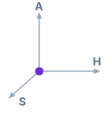
Agents depart from a single model call along horizon, state, and authority.
A single model call reads a static prompt, returns one completion, and leaves the outside world untouched. When a runtime instead stretches execution across dozens of turns, carries files and memory forward, and invokes tools that modify external systems, a single mistaken proposal can compound across steps, corrupt shared state, or trigger an irreversible outage. Sizing the runtime’s defenses to a task therefore starts from the book’s central runtime artifact, the trajectory, which records the complete sequence of steps the runtime must govern.
Definition 1.2: Trajectory
Trajectory is the ordered sequence of recorded states, proposed actions, runtime decisions, and observations through which one delegated task proceeds, from its initial context to its ultimate acceptance, termination, or escalation.
- Significance: The trajectory length defines the operational horizon \(\TurnHorizon\), which governs how compounding errors degrade system reliability. Its complete span (encompassing rejected actions, retries, and failed branches) establishes the true accounting boundary when computing cost and latency per accepted task.
- Distinction: While a conversational transcript captures the tokens exchanged between a model and a user, a trajectory preserves the full causal history of execution. It records which action proposals the runtime approved, modified, or rejected, alongside the raw observations returned by external tools, linking every decision to the exact evidence available at that step.
- Common pitfall: Preserving only the final deliverable. Storing just the accepted patch or completed document hides the computational cost of discarded attempts, masks transient faults, and discards the intermediate verification evidence that justified accepting the work.
In compact notation, the trajectory is
\[\Trajectory = (\TrajectoryState_0, \TrajectoryAction_0, \TrajectoryObservation_1, \TrajectoryState_1, \TrajectoryAction_1, \TrajectoryObservation_2, \dots, \TrajectoryState_{\TurnHorizon})\]
where \(\TrajectoryState_{t}\) is the recorded state available at decision step \(\TurnIndex\), \(\TrajectoryAction_{t}\) is the action the model proposes, and \(\TrajectoryObservation_{t+1}\) is the observation returned by the execution environment. Each transition from \(\TrajectoryState_{t}\) to \(\TrajectoryState_{t+1}\) is one turn: one model call paired with the runtime’s mediation of the resulting proposal. The notation establishes a total ordering across interactions, where each \(\TrajectoryState_{t}\) reflects the runtime’s partially observed view of the broader environment. The repair trajectory that section 1.7.1 follows turn by turn shows why the runtime must manage cost, state, and authority over this whole sequence rather than per call.
Each trajectory \(\Trajectory\) departs from an isolated model call along three operational dimensions: how many turns \(\TurnHorizon\) execution continues, what state \(\TrajectoryState_{t}\) persists across steps, and what external side effects the actions \(\TrajectoryAction_{t}\) can trigger. This book models these dimensions as the Horizon, State, and Authority (H·S·A) exposure space.
Definition 1.3: H·S·A exposure space
H·S·A exposure space is the three-dimensional coordinate system quantifying how far a delegated task departs from an isolated model call: its horizon \(\TurnHorizon\) measured in sequential turns, the state \(\StateExposureLevel_0\) through \(\StateExposureLevel_3\) carried between invocations, and the authority \(\AuthorityExposureLevel_0\) through \(\AuthorityExposureLevel_3\) exercised over external systems.
- Significance: Each axis identifies a concrete operational exposure that the runtime must bound. Horizon determines how rapidly unverified errors compound, state dictates the working memory and durable artifacts carried forward, and authority establishes the maximum blast radius of an errant action. Later divisions of this book systematically address how to close these exposures: Part II governs state, Part III controls authority, and Part IV bounds horizon.
- Distinction: A coordinate in this space describes the exposure a task carries, which is a property of the task and its environment. The runtime’s validation gates, sandboxes, and compensating operations are its response to that exposure, which section 1.5 develops as closure. Closure is what the runtime builds; the coordinate is where the task sits.
- Common pitfall: Inferring authority from syntax or command names alone. Authority reflects the operational consequence of an action within its specific environment; an identical file deletion is discardable inside an ephemeral sandbox, but irreversible when executed directly against an unversioned production datastore.
Horizon \(\TurnHorizon\) tracks the length of execution in sequential turns. Every additional turn gives the agent another chance to invoke a tool with bad arguments, act on stale observations, or drift from the goal. Section 1.6 shows mathematically how unchecked step-level error rates compound into severe task-level failure rates across long sequences. Turn count and wall-clock latency are distinct budgets that require separate limits. A three-turn workflow that triggers a large remote build cluster can run for hours, whereas a hundred-turn in-memory code refactoring completes in seconds. Production runtimes must meter both, bounding turns to restrict error compounding and bounding wall-clock time to release compute and network resources.
State (\(\StateExposureLevel_0\) to \(\StateExposureLevel_3\)) describes the data, memory, and workspace artifacts that persist across turns. At \(\StateExposureLevel_0\), the system is stateless, carrying no task context past a single call; stepping to \(\StateExposureLevel_1\) adds conversational working state, including the tokenized context window and inference-tier serving state such as cached key-value (KV) attention pairs. Once the agent modifies task-local working artifacts within an isolated workspace (such as a private source tree, an ephemeral container, or an in-memory scratchpad), it reaches \(\StateExposureLevel_2\). \(\StateExposureLevel_3\) covers execution that reads or writes durable shared state outliving the task session, such as an authoritative database, a shared object store, or a central code repository. Because realistic workloads routinely span several tiers at once, this classification establishes what data the runtime must checkpoint or isolate, sets cache invalidation boundaries, and decides which storage system remains authoritative when local scratchpad views diverge.
Authority (\(\AuthorityExposureLevel_0\) to \(\AuthorityExposureLevel_3\)) defines the blast radius of actions delegated to the task. At \(\AuthorityExposureLevel_0\), access is strictly read-only, although exfiltration remains a risk if retrieved secrets leak into output text. Stepping up to \(\AuthorityExposureLevel_1\) permits mutations, but confines them entirely to a disposable workspace where unintended modifications carry zero external impact. At \(\AuthorityExposureLevel_2\), actions affect external systems, yet every mutating operation pairs with an explicit compensating transaction4 executed under verified preconditions and a separate retry policy that prevents duplicate effects. Finally, \(\AuthorityExposureLevel_3\) covers non-compensable actions (such as modifying unversioned production records, issuing financial transactions, or publishing public communications) for which no automated reversal exists. Authority reflects the operational consequence within the specific execution environment rather than command syntax. Because a trusted runtime mediates every action against an explicit per-task capability grant, restricting this grant provides the first and most cost-effective line of defense before deploying complex validation machinery.5
4 Compensating Transactions: Garcia-Molina and Salem introduced sagas for long-lived distributed transactions where holding locks across the entire workflow is impractical: a saga consists of a sequence of local transactions, each paired with a compensating transaction that semantically undoes earlier steps if the overall workflow aborts (Garcia-Molina and Salem 1987). Compensation is an active forward recovery action rather than an atomic rollback; concurrent processes can observe intermediate states, and the compensating action itself may fail. An \(\AuthorityExposureLevel_2\) capability grant therefore requires an executable compensation handler before dispatching the initial mutating effect.
Garcia-Molina, Hector, and Kenneth Salem. 1987. “Sagas.” Proceedings of the 1987 ACM SIGMOD International Conference on Management of Data, 249–59. https://doi.org/10.1145/38713.38742.
5 Least Privilege and Complete Mediation: Saltzer and Schroeder’s protection principles state that every program should run with the smallest set of privileges needed to complete its task (least privilege), and that every access to every object should be checked for authority (complete mediation) (Saltzer and Schroeder 1975). Checking capability grants on every tool call applies both principles to a non-deterministic model whose proposals cannot be trusted on their own. Restricting the task’s initial capability grant remains the most dependable way to limit damage when runtime verification checks fail to catch an unsafe request.
Saltzer, J. H., and M. D. Schroeder. 1975. “The Protection of Information in Computer Systems.” Proceedings of the IEEE 63 (9): 1278–308. https://doi.org/10.1109/proc.1975.9939.
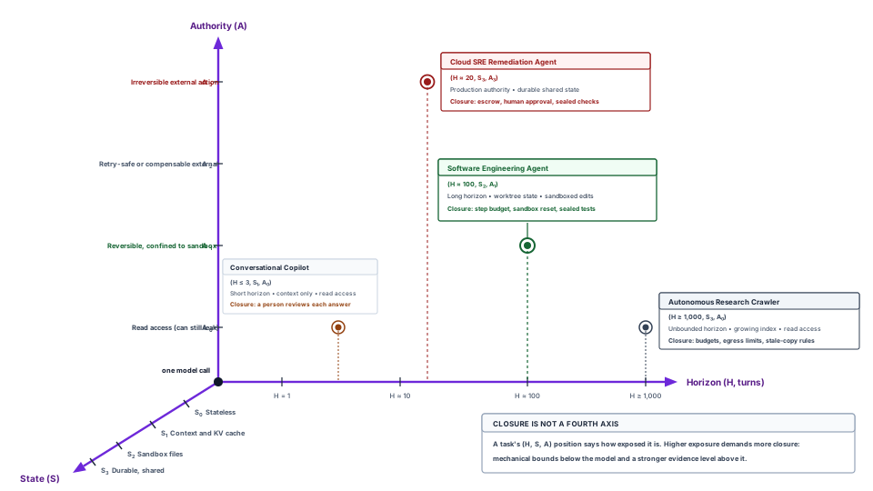
The coordinate space in figure 4 maps agentic workloads across three operational exposure axes: horizon (\(\TurnHorizon\), turns along the horizontal), authority (\(\AuthorityExposureLevel_0\) to \(\AuthorityExposureLevel_3\) on the vertical), and carried state (\(\StateExposureLevel_0\) to \(\StateExposureLevel_3\) on the depth axis). This space serves as an analytical lens rather than a rigid taxonomy: two workloads occupying the same cell may still demand different runtime controls if their data sensitivity, tool reliability, or failure thresholds differ. Changing the execution environment can shift a task into a completely different cell even when its foundation model and turn horizon remain identical, as shown in example 1.1. The four workloads plotted in the space are the book’s lighthouse workloads, described in section 1.4.1.
Example 1.1: A working copy and the only copy
Scenario: A coding assistant must repair a software defect while preserving adjacent, uncommitted edits authored by a developer. Consider two execution environments: an isolated, ephemeral sandbox containing a working copy of the project vs. direct access to the developer’s sole authoritative workspace. The foundation model, repair objective, and expected turn horizon remain identical in both configurations. In each case, the assistant issues a command to delete files while cleaning up intermediate build artifacts.
Diagnosis: Inside the ephemeral sandbox, the source files are \(\StateExposureLevel_2\) working state and the mutation authority is bounded at \(\AuthorityExposureLevel_1\). Tearing down the sandbox discards any bad modifications without corrupting the developer’s original files. In the authoritative workspace, however, that identical command targets \(\StateExposureLevel_3\) state. Although one person uses it, the workspace is durable state the task shares with its developer, it outlives the task, and it holds the only copy of the developer’s edits. If the deleted files contain unique, unstaged edits missing from version control history, the operation escalates to \(\AuthorityExposureLevel_3\) irreversible data loss. Version control alone does not prevent this loss, because uncommitted working-tree changes have no snapshots. A sound systems contract grants the agent access strictly to an isolated clone, excludes unrelated edits from the agent’s context, and reserves the integration of reviewed patches for a separate gate. The runtime must enforce that isolation boundary through tool authorization rather than relying on prompt instructions asking the model to be careful.
Systems lesson: The failure boundary shifted even though the model, prompt, and turn horizon remained unchanged. Automated test suites check functional behavior, and diff reviews check patch cleanliness, but neither prevents an unauthorized deletion command from wiping out working state. Sound systems engineering enforces safety at the infrastructure boundary, preventing destructive operations from reaching authoritative state, rather than relying on post-hoc checks to detect irreversible side effects.
1.4.1 Four lighthouse workloads
A mechanism that halves latency or cost for a short interactive query can be dead weight for a hundred-turn code repair or a dangerous shortcut for a live production rollback. To test mechanisms against concrete bottlenecks rather than in the abstract, the four workloads plotted across the H·S·A exposure space of figure 4 serve as this book’s lighthouses: the support agent, remediation agent, repository repair agent, and research agent. Like a lighthouse, each is a fixed reference point that the reader can steer by as the mechanisms change from chapter to chapter. Each is bounded by a different systems bottleneck. Automated repository repair serves as the primary running example, while the other three appear whenever a chapter examines failure modes or constraints that repository repair does not trigger.
Lighthouse 1.1: Repair agent (long-horizon worker)
Workload: A repository coding agent diagnoses and fixes a defect in an isolated working copy, submitting a verified patch for review. The connection-pool race condition in this chapter serves as the concrete running example; its reference harness budgets 30 steps inside a 128,000-token context window.
Exposure: Long horizon (tens to hundreds of turns), a task-local working copy (\(\StateExposureLevel_2\)), and filesystem edits confined strictly to that disposable sandbox (\(\AuthorityExposureLevel_1\)) until a human-reviewed patch is exported.
Binding constraint: Compounding errors across the trajectory, and repeated input whose cumulative token count grows quadratically with the number of turns. Each turn adds only one step of output and tool observations to the prompt, but resending that growing history on every turn means the model re-reads every earlier turn at each step. Without compatible prefix reuse (serving a repeated history from state already computed for it), this repeated input can dominate aggregate inference work and cost, while acceptance depends strictly on immutable test suites that the agent cannot modify.
Lighthouse 1.2: Research agent (untrusted reader)
Workload: A deep-research agent answers an open-ended question by querying, retrieving, and synthesizing external web sources, frequently delegating sub-queries to parallel worker agents.
Exposure: Horizons from tens of turns for one question to thousands for a standing crawl, an expanding knowledge store of ingested documents (\(\StateExposureLevel_3\)), and read-only authority (\(\AuthorityExposureLevel_0\)).
Binding constraint: Ingested content is untrusted data. Through indirect prompt injection, in which a retrieved page carries text the model may follow as an instruction, it can redirect the trajectory or exfiltrate private context (Greshake et al. 2023), so read-only access is still a serious security exposure. Aggregate token consumption from retrieved documents and worker fan-out dominates total execution cost.
Lighthouse 1.3: Remediation agent (irreversible actor)
Workload: An automated site-reliability agent diagnoses a live production incident and applies configuration or infrastructure changes to restore service. One Incident Through the System analyzes one such remediation end to end.
Exposure: A moderate horizon (tens of turns), mutable shared production infrastructure (\(\StateExposureLevel_3\)), and non-compensable or irreversible operations (\(\AuthorityExposureLevel_3\)).
Binding constraint: A single erroneous action can incur outages costing orders of magnitude more than all trajectory compute combined. Human-in-the-loop approval latency and the blast radius of incorrect decisions dominate systems design, requiring strict approval gates, compensating actions, and explicit points of no return before execution begins.
Lighthouse 1.4: Support agent (interactive responder)
Workload: A customer-operations agent resolves billing and booking inquiries while the user waits synchronously.
Exposure: Short sessions of a few turns each across thousands of concurrent users, with session context combined with sensitive enterprise database records (\(\StateExposureLevel_1\) with \(\StateExposureLevel_3\)). Authority escalates from read-only queries (\(\AuthorityExposureLevel_0\)) to compensable updates such as a seat hold that can be released (\(\AuthorityExposureLevel_2\)), and on to actions with no automated reversal such as a refund paid out to an external account (\(\AuthorityExposureLevel_3\)).
Binding constraint: Strict tail latency under high concurrency, combined with verifiable adherence to enterprise policy. Serving throughput and the aggregate memory overhead of retaining active session state across thousands of simultaneous connections dominate systems cost.
Comparing these four lighthouses shows why systems mechanisms cannot be evaluated in the abstract. Proactive context summarization is necessary for a multi-turn repository repair agent, but superfluous for a three-turn support session. An on-call remediation agent can read diagnostic telemetry under a prior grant while requiring explicit approval for production changes. A read-only researcher can likewise run under a bounded grant, though disclosing sensitive context may still require approval. The task boundary, rather than the workload label, decides where those gates belong. Each later chapter ties its mechanisms directly to the lighthouse whose binding constraints they resolve. Placing a workload in the space shows where it is exposed; how the runtime closes each exposure without trusting the model to do so is the subject of invariant closure.
1.5 Invariant Closure
Each axis of the H·S·A space names a way an autonomous run can fail: an agent with write authority can touch the wrong resource, carried state can accumulate silent corruption, and a multi-turn trajectory can end with a fluent claim that the job is done while the defect remains live. Because the model cannot vouch for the safety or correctness of its own outputs, the surrounding runtime must close those exposures from outside the model. Doing so requires understanding the fault pattern characteristic of generative models, enforcing mechanical bounds and empirical checks on either side of the model, and writing both into an explicit task contract before execution begins.
1.5.1 The fail-plausible fault
In an autonomous repository repair loop, an agent can finish its run with a confident, well-reasoned summary declaring that a race condition is fixed, even though the underlying defect remains. The generated patch may be syntactically clean yet remove thread safety by deleting a synchronization lock, or the test suite may exit with return code zero only because the model commented out the failing assertions. Both failures are instances of the fail-plausible fault, in which the output looks well formed and credible while the required property remains unsatisfied.6
6 Signaled and Unsignaled Failures: The standard dependability taxonomy classifies failures by detectability as well as by kind: a signaled failure raises a warning when the service goes wrong, and an unsignaled one does not (Avizienis et al. 2004). A fail-plausible fault is an unsignaled content failure (the delivered result is wrong and nothing announces it), so a runtime that watches only for crashes, timeouts, and error codes will record it as a success.
Avizienis, Algirdas, Jean-Claude Laprie, Brian Randell, and Carl Landwehr. 2004. “Basic Concepts and Taxonomy of Dependable and Secure Computing.” IEEE Transactions on Dependable and Secure Computing 1 (1): 11–33. https://doi.org/10.1109/TDSC.2004.2.
7 Fail-Stop and Byzantine Faults: Schlichting and Schneider defined a fail-stop processor as one that halts on failure without first making an erroneous state transition, so that other processors can detect the halt (Schlichting and Schneider 1983). Lamport, Shostak, and Pease showed that reaching agreement when some components may send arbitrary, conflicting messages requires more than two-thirds of the components to be correct, the origin of the \(3\ByzantineFaultCount+1\) replica bound for tolerating \(\ByzantineFaultCount\) such faults (Lamport et al. 1982).
Schlichting, Richard D., and Fred B. Schneider. 1983. “Fail-Stop Processors: An Approach to Designing Fault-Tolerant Computing Systems.” ACM Transactions on Computer Systems 1 (3): 222–38. https://doi.org/10.1145/3149.3150.
Lamport, Leslie, Robert Shostak, and Marshall Pease. 1982. “The Byzantine Generals Problem.” ACM Transactions on Programming Languages and Systems 4 (3): 382–401. https://doi.org/10.1145/357172.357176.
Classical fault models show why this failure pattern needs its own category. In distributed systems, a fail-stop component halts when it faults, so a supervisor can detect the failure through missing heartbeats or nonzero exit codes (Schlichting and Schneider 1983). A Byzantine component may behave arbitrarily or deceptively, but Byzantine fault-tolerant agreement uses redundancy under a stated bound on the number of faulty replicas (Lamport et al. 1982).7 A plausible wrong answer evades both crash monitoring and agreement among model samples. Because the model process neither crashes nor halts, fail-stop monitors record a normal return. Sampling repeatedly from the same foundation model sets no bound on how many samples are wrong, because shared blind spots can make the samples agree on an incorrect answer. The fail-plausible fault is therefore an unsignaled semantic failure that looks like success on the surface.
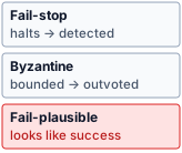
Crash detection and agreement leave plausible wrong answers needing an outside check.
8 The Confused Deputy: Hardy described a compiler that held a license to write files in its own directory; a user passed it the name of the billing file as an output path, and the compiler, acting with its own authority rather than the user’s, overwrote the billing records (Hardy 1988). Authority that comes from where a program runs rather than from the request it serves can be steered by whoever supplies the names, which is exactly the position of a model whose tool calls run with host credentials while it reads untrusted text.
Hardy, Norm. 1988. “The Confused Deputy: (Or Why Capabilities Might Have Been Invented).” ACM SIGOPS Operating Systems Review 22 (4): 36–38. https://doi.org/10.1145/60609.60611.
To keep fail-plausible faults from corrupting system state, the execution environment enforces zero ambient authority: the model holds no standing privileges of its own, and every external side effect must pass through an explicit grant checked by the runtime.8 Generated tokens cannot authorize commands, alter the runtime’s execution records, or declare acceptance. Instead, the runtime gathers environmental evidence strictly through designated tools and deterministic checks. For repository repair, this means separating the raw patch text the model proposed from the diff the runtime actually applied on disk (the two differ whenever a patch fails to apply cleanly). It also means keeping model-written summaries of test runs separate from actual process exit codes.
Every external check establishes a bounded claim that is narrower than the overall task goal. A clean compile shows only that the program obeys grammar and type rules under one build configuration. A passing regression test records only that the code ran cleanly for the inputs and thread schedules tested. As Dijkstra observed, testing can show the presence of defects, but never prove their absence (Dijkstra 1970).
1.5.2 The invariant closure principle
Containing fail-plausible faults therefore joins two distinct guarantees that the working-copy comparison in example 1.1 already separated: zero ambient authority prevents unauthorized actions, while external checks test whether an allowed action met the engineering goal. A filesystem boundary mechanically blocks writes outside the assigned workspace, whereas checking whether a patch inside that workspace repairs a race condition requires empirical evidence of how the program behaves. Invariant closure assigns both jobs to explicit mechanisms around the model rather than trusting the model’s own assurances. Limits are enforced mechanically below the model, and acceptance rests on evidence gathered above it. The principle below measures both against the task contract, the explicit specification of what may execute and what counts as done, which section 1.5.3 defines. It also states the cost of leaving steps unchecked in terms of a per-step error rate \(\PerStepErrorRate\), a result that section 1.6 derives.
Principle 1: Invariant closure
Invariant: Constraints never rest on the model; bounds close mechanically below it, acceptance on evidence above it. Each enforced bound names the property and assumptions under which it holds, and each acceptance decision names the evidence standard it applies. Without either, a trajectory of \(\TurnHorizon\) independent steps, each correct with probability \(1-\PerStepErrorRate\), succeeds only with probability \[ \Pr(\text{success}) = (1-\PerStepErrorRate)^{\TurnHorizon} \] while an enforced bound rejects the violations it blocks, and a check rejects those it detects.
Implication: Under the independent-step model without recovery, unchecked reliability decays exponentially with horizon; raising step accuracy does not remove the need for runtime bounds and checks. The runtime mediates permitted effects and resource use independently of the model’s compliance. It accepts completion only when evidence meets the task contract, preserving the distinction between a passing check and a guarantee beyond that check’s coverage. The contract itself is adopted by authorized people: the model can draft it but cannot adopt, relax, or certify against it. Greater operational exposure requires stronger justification for both the boundaries and the evidence.
Mechanical enforcement sets concrete execution boundaries. A filesystem restriction blocks writes to protected paths as long as all file operations pass through the enforcement layer and its isolation assumptions hold. That boundary controls where edits land, while leaving the correctness of those edits as a separate question. Likewise, schema validation checks that a tool request is syntactically well formed, while authorization remains a separate check. The design rule is to keep each enforced property narrower than the full task claim and state explicitly what guarantee it provides.
Acceptance decisions rely on evidence organized across distinct closure evidence levels. The classical end-to-end argument explains why the levels differ (Saltzer et al. 1984). An end-to-end task property can be checked only by an endpoint that knows the full task requirements, so correct behavior at a lower layer, such as generating well-typed code, cannot establish end-to-end correctness. Ordered from the weakest default grounding to the strongest, the five levels are:
- Self-report: The agent’s own account is an unverified claim rather than an observation of the environment.
- Static analysis: Analysis checks structural and type invariants without running the code.
- Visible tests: Tests run cases that the agent can inspect directly. They help during iterative diagnosis, but they expose test cases that candidate solutions can overfit.
- Sealed tests: Tests withhold their definitions from the agent and run inside tamper-proof sandboxes, protecting the evaluation from modification.
- Formal verification: A proof establishes that an implementation satisfies an explicit mathematical model, though confirming that the specification captures what the user actually wanted remains a human judgment.
The ordering is a default rather than an absolute ranking, because a level’s strength also depends on how complete its tests or its specification are. A thorough sealed test suite gives more practical confidence than a mathematical proof built on an incomplete specification.
In the race-condition repair, passing a sequential unit test gives evidence only for single-threaded execution. Sealing that test protects its assertions from modification, but does not widen its coverage. Showing that the concurrency bug is fixed requires running multi-threaded stress workloads that force thread interleavings across varied schedules. Human code review then checks operational assumptions that the test harness cannot probe. Because an automated verdict can be completely repeatable yet miss whole classes of inputs, acceptance claims must stay within what the test suite actually measured.
Some completion criteria cannot be reduced to executable boolean checks and require qualitative evaluation. An automated or human evaluator scores these outcomes against an explicit rubric, recording who owns the decision and what uncertainty remains while mechanical permission bounds stay in force. When the evidence falls short of the task contract, the runtime reports an unresolved outcome or escalates to human operators rather than treating a plausible narrative as verified completion.
Even executable verifiers differ in how often they accept an outcome that is in fact wrong, a false-acceptance rate that must be measured rather than assumed. Placed inside the loop, intermediate checks can shorten the unchecked horizon, but only for the error classes they actually cover and only when a failed check triggers repair or state restoration. Catching a bad edit without rolling back the workspace leaves the corrupted state in place for the next turn to build on, while errors outside the check’s coverage pass straight through into the compounding analyzed in section 1.6.
↪ Measuring a grader’s false-acceptance rate against independent reference assessment is developed in Grader error rates.
1.5.3 The five-part task contract
Even with invariant closure in place, the runtime cannot enforce bounds or check completion against a bare instruction such as “repair the race condition.” Left to that five-word prompt, a proposed patch can delete the lock altogether, passing a sequential regression check while worsening concurrency failures under production load. A cleanup step can likewise wipe out uncommitted source files in a shared repository alongside scratch build artifacts. Before an execution engine dispatches any action, it needs an explicit specification of what resources may be modified and what evidence is required to accept the result.9
9 Wiener’s Warning on Delegated Purpose: In 1960 Wiener argued that when a mechanical agency acts too fast and irrevocably for anyone to intervene before the action completes, “we had better be quite sure that the purpose put into the machine is the purpose which we really desire” (Wiener 1960). The warning binds hardest where authority is irreversible, which is why the contract that follows is written and adopted before the loop runs rather than repaired after an effect lands.
Wiener, N. 1960. “Some Moral and Technical Consequences of Automation: As Machines Learn They May Develop Unforeseen Strategies at Rates That Baffle Their Programmers.” Science 131 (3410): 1355–58. https://doi.org/10.1126/science.131.3410.1355.
10 Design by Contract: Meyer framed a software component’s interface as a contract of preconditions the caller must establish, postconditions the supplier guarantees, and invariants both preserve, each written as a checkable assertion (Meyer 1992). The task contract borrows the structure but not the trust: in classical design by contract the supplier’s own code checks its postconditions, whereas here the supplier is the model, so the completion criteria must be checked by the runtime and tools rather than asserted by the component that produced the result.
Meyer, Bertrand. 1992. “Applying ‘Design by Contract’.” Computer 25 (10): 40–51. https://doi.org/10.1109/2.161279.
A task specification turns an informal request into an enforceable contract. The contract is a five-part tuple, \(\TaskContract = \langle \TaskContractGoal, \TaskEnvironment, \PermittedActions, \AvailableObservations, \CompletionCriteria \rangle\), which separates the goal from the execution environment, permitted actions, available observations, and completion criteria. That separation matters because natural-language instructions state intent without giving the runtime the rules it needs to authorize actions or check completion.10
Definition 1.4: Task contract
Task contract is the explicit specification of a delegated task that separates its goal, environment, permitted actions, available observations, and completion criteria, so that the runtime, not the model, decides what may execute and when the task is done.
- Significance: The completion criteria define what counts as accepted, which fixes the denominator of cost per accepted task. Two systems, or two versions of one system, can be compared only under the same contract.
- Distinction: A prompt communicates intent to the model; a contract is enforced by the runtime and the tool environment. The same sentence can appear in both, but only the contract constrains what executes.
- Common pitfall: Writing the permitted actions into the prompt alone. The model reads the limit, and the host process still allows everything its credentials allow.
In the repository repair task (table 2), the goal \(\TaskContractGoal\) includes an explicit negative scope, the set of existing behaviors and invariants that must stay untouched outside the reported defect. The environment \(\TaskEnvironment\) names the source baseline, runtime dependencies, and working copy where edits happen. Permitted actions \(\PermittedActions\) allow bounded file edits, directory listing, and test runs, while blocking network egress and writes to parent directories. Available observations \(\AvailableObservations\) limit returned payloads to source excerpts, bounded test logs, and Git diffs. Finally, completion criteria \(\CompletionCriteria\) name the sealed test suites that must pass alongside human review gates for behaviors the tests do not cover.
| Contract Component | Formal Symbol | Systems Role | Concrete Engineering Artifact |
|---|---|---|---|
| Goal | \(\TaskContractGoal\) | Desired end state and explicit negative scope | Repair request that preserves unrelated behavior |
| Environment | \(\TaskEnvironment\) | Target state and execution conditions | Source baseline and designated working copy |
| Permitted Actions | \(\PermittedActions\) | Operations and resources within delegated authority | Allowed edit paths and test commands |
| Available Observations | \(\AvailableObservations\) | Information the task may obtain and return | Source excerpts, bounded test output, and diff |
| Completion Criteria | \(\CompletionCriteria\) | Evidence and decision rule for accepting the result | Required regression checks and review decision |
Each part of the contract blocks a specific failure mode. Leaving negative scope out of the goal invites degenerate fixes, such as silencing a concurrency bug by deleting the failing assertion or removing multi-threaded access paths altogether. Similarly, if the environment is not isolated, agent edits and ad hoc package installs pollute shared host state and break reproducibility. At the tool boundary, omitting explicit action limits lets tool calls run with whatever ambient privileges the host process holds, while unbounded observations let large search outputs flood the context window, crowding out instructions and raising token costs. Finally, without formal completion criteria, the runtime has nothing to stop on except the model’s own claim that it is done.
Environments that keep changing on their own require the contract to separate what the agent changed from what the world changed. During live incident triage by the remediation agent (lighthouse 1.3), traffic and error rates keep shifting while the agent works. Unless the contract records which observations follow from the agent’s own configuration change and which reflect outside load, a coincidental drop in traffic reads as a successful fix. Observation rules must also distinguish an empty query result from a truncated response. When the runtime truncates a long test log to fit the token budget, it must mark the truncation in the prompt; otherwise, the model may treat the missing error message as proof that no error occurred.
Resource limits and stopping rules accompany the contract. Every delegated task needs turn limits, wall-clock deadlines, dollar ceilings, and clear rules for what happens when a budget runs out. Stopping on an exhausted budget yields an unresolved outcome, meaning the evidence gathered so far neither accepts nor rejects the work. That differs from a failure, where evidence shows the attempt missed the contract, and from a silent crash, which leaves no record at all. The runtime saves the intermediate diff, logs the incomplete checks, and escalates to a human engineer.
Writing a contract also reveals what cannot be safely delegated. Vague goals such as “improve maintainability” cannot be checked by automated tests alone. In those cases, the engineer must define measurable proxy checks, assign a human reviewer, or keep the subjective judgment out of the autonomous loop. The task contract makes these boundaries explicit so the runtime can enforce them mechanically.
Later chapters build each part of the contract. Tool Calling defines permitted actions and structured observation schemas, Agent Sandboxes builds the isolated containers and virtual machines that contain untrusted code, and The Agent Harness builds the harness that enforces goals, budgets, and stopping rules. Agent Evaluation establishes the statistical and empirical evidence that completion criteria require, and Operating Agents carries that evidence into live operation.
The invariant closure principle and the five-part task contract establish the governance boundaries for autonomous execution. Enforcing isolation below the model protects shared infrastructure, and checking empirical evidence above the model grounds acceptance in the task contract. Those checks and boundaries, however, are not free: running sealed regression suites, provisioning ephemeral sandboxes, and checking intermediate invariants all spend latency and compute budgets. Weighing those costs requires pricing how errors compound across turns and how retries and checks change the cost per accepted task.
1.6 Reliability and Cost over a Horizon
A realistic agentic trajectory spans dozens of sequential turns, with each turn building directly on observations and state modifications from the preceding step. A misdiagnosed deadlock trace leads the model to inspect the wrong source file; an erroneous patch to that file cascades into compilation failures or silently corrupts unrelated business logic. Because foundation models generate fluent rationalizations even when mistaken, nothing in the model’s generated text signals the exact moment execution derailed. An extended autonomous task can easily fail even when individual per-turn accuracy appears high.
The invariant closure principle (1) stated the cost of leaving steps unchecked without deriving it. Elementary probability supplies the derivation and shows why the principle places verifiers inside the execution loop. Suppose each of \(\TurnHorizon\) sequential steps is correct with probability \(1-\PerStepErrorRate\), errors are statistically independent, and no step is verified before subsequent steps build upon it. The overall task succeeds only if every intermediate step succeeds:
\[\Pr(\text{success}) = (1-\PerStepErrorRate)^{\TurnHorizon} \tag{1}\]
Equation 1 applies classic series-reliability analysis11 to the sequential turns of a trajectory. The resulting reliability collapse is horizon compounding. Statistical independence is an idealization; in practice, errors correlate and models occasionally recover from bad states. Under the independent-step model without recovery, unchecked success decays exponentially with horizon length (notebook 1.1); correlation and recovery can change the shape of that decline.
11 Reliable Systems from Unreliable Components: Von Neumann posed the problem in 1956 for logic networks whose every element errs with some fixed probability, so that errors accumulate through the depth of the computation (Neumann 1956). His remedy interleaved redundant computation with “restoring organs” that re-establish a correct signal at intervals, keeping the error bounded however deep the network grows. Checks paired with restoration play the same structural role for the errors they detect, limiting their accumulation to the distance between successful restorations.
Neumann, John von. 1956. “Probabilistic Logics and the Synthesis of Reliable Organisms from Unreliable Components.” In Automata Studies, edited by Claude E. Shannon and John McCarthy, vol. 34. Annals of Mathematics Studies. Princeton University Press. https://doi.org/10.1515/9781400882618-003.
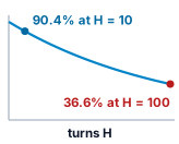
Under the independent-step model without recovery, unchecked success falls exponentially with the horizon.
Napkin Math 1.1: Horizon compounding
Problem: Each step of a repair agent is correct with probability 99 percent, independently, and no step is checked before the next one builds on it. What fraction of tasks succeed at horizons of 10 and 100 turns, and what per-step error rate would hold the longer horizon at 90 percent success?
Math: By equation 1, \(0.99^{10} \approx 0.904\), so 90.4 percent of tasks succeed at 10 turns, while \(0.99^{100} \approx 0.366\) leaves 36.6 percent at 100 turns. Holding 90 percent at 100 turns requires \(\PerStepErrorRate = 1 - 0.90^{1/100} \approx 0.00105\), about 0.11 percent per step and 9.5× lower than the assumed 1 percent. For small \(\PerStepErrorRate\), \((1-\PerStepErrorRate)^\TurnHorizon \approx e^{-\PerStepErrorRate \TurnHorizon}\), and the requirement reads \(\PerStepErrorRate \TurnHorizon \approx 0.105\) at any horizon.
Systems insight: The product \(\PerStepErrorRate \TurnHorizon\), not step accuracy alone, sets task reliability. A tenfold longer horizon demands a tenfold lower per-step error to hold the same success rate. The cheaper engineering knob is usually the unchecked horizon itself: a check that reliably detects an error, followed by restoration and a successful retry, bounds the segment over which that error can compound. Under the notebook’s independence assumption, perfect detection and restoration turn the extended task into a sequence of short segments. Supplying and enforcing those checks is the primary responsibility of the runtime, as formalized by the invariant closure principle (1).
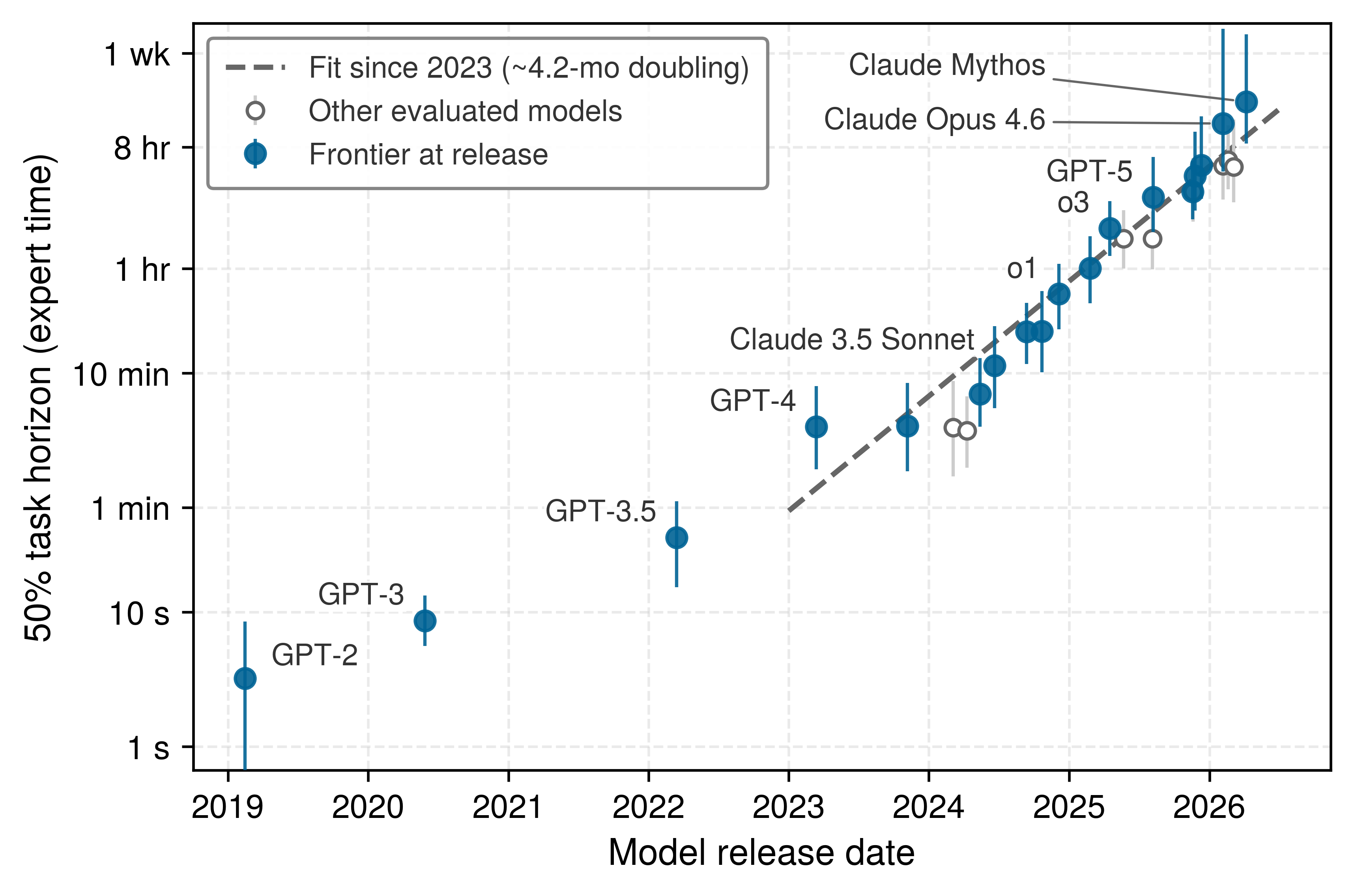
The horizon in equation 1 belongs to the delegated task, and the tasks delegated to agents have lengthened quickly. Kwa et al. (2025) express that length in human terms. They time people with the relevant expertise on a suite of software and research tasks, then report each model’s 50 percent time horizon at release: the length of task, in expert time, that an agent built on the model completes in half its attempts (figure 5).
Kwa, Thomas, Ben West, Joel Becker, Amy Deng, Katharyn Garcia, Max Hasin, Sami Jawhar, et al. 2025. “Measuring AI Ability to Complete Long Software Tasks.” arXiv Preprint arXiv:2503.14499.
Among the frontier models in figure 5, the 50 percent horizon grew from about 3 seconds to about 17 hours, a factor of roughly 19,000. That is a doubling every 6.2 months across the whole period and every 4.2 months since 2023. Equation 1 turns that trend into an engineering obligation. A task that occupies an expert for hours instead of minutes spans many more dependent steps, and at a fixed per-step error, doubling the unchecked horizon squares the probability of success. Each doubling of the delegated task therefore requires either halving the per-step error or inserting checks that halve the unchecked segment between them. Model improvement supplies the first; only the runtime can supply the second, and the measured horizon is itself a reminder that half the attempts at that length still fail.
Checking converts a silent failure into an explicit, rejected attempt, and a rejected attempt still consumes real resources. Suppose each attempt at a task is accepted with probability \(\AcceptanceProbability\), independently of earlier attempts, and the runtime retries until one is accepted. The number of attempts follows a geometric distribution with mean \(1/\AcceptanceProbability\). Each attempt costs \(\AttemptCost\) in expectation, tallying model tokens, tool execution, test sandboxes, and human review, all of which a failed attempt consumes as completely as a successful one. The expected cost per accepted task is therefore
\[\CostPerAcceptedTask = \frac{\mathbb{E}[\AttemptCost]}{\AcceptanceProbability} \tag{2}\]
Production runtimes bound the retry budget, so some tasks end without acceptance, and their spend must still be charged to the tasks that were accepted. Measured over a cohort, cost per accepted task is therefore the total spend of every initiated task divided by the number accepted; the accounting pitfall in section 1.9 prices what omitting the failed attempts hides. Even in its expected-value form, equation 2 exposes a trade-off between unit model pricing and acceptance, which notebook 1.2 prices for the repair task.
↪ Whole-trajectory cost and the cohort cost per accepted task, which charges failed and abandoned attempts to the accepted ones, are developed in Cost per Accepted Task.
Napkin Math 1.2: Cheaper tokens or more acceptances
Problem: An attempt at the repair task spends $1.30 on model tokens and $0.80 on the sandbox, tests, and review, and is accepted with probability 40 percent. Which lowers cost per accepted task more: halving the token price, or raising acceptance to 60 percent through a context or tool improvement?
Math: The baseline attempt costs $2.10, and the task needs 2.5 attempts on average, so equation 2 gives \(2.10 / 0.40 = 5.25\) dollars per accepted task. Halving the token price lowers the attempt to $1.45, giving \(1.45 / 0.40 \approx 3.63\) dollars. Raising acceptance at the original attempt cost gives \(2.10 / 0.60 = 3.50\) dollars. To find the acceptance that the price cut is worth, set the cheaper attempt’s cost per accepted task, \(\AttemptCost(1 - \text{cut} \times \text{share})/\AcceptanceProbability\), equal to \(\AttemptCost/\BreakEvenAcceptanceProbability\) at the original attempt cost. Here cut is the fraction of the token price removed, and share is the tokens’ share of the attempt cost. Solving gives \(\BreakEvenAcceptanceProbability = \AcceptanceProbability/(1 - \text{cut} \times \text{share})\). Tokens are 62 percent of the attempt, so the price cut matches an acceptance of \(0.40 / (1 - 0.5 \times 0.62) \approx 0.58\).
Systems insight: The two levers act on different amounts. A price cut can remove at most the share of the attempt that the cheaper component represents, whereas acceptance divides the whole attempt cost (sandbox, tests, and review included). Halving the token price removes half of the tokens’ 62 percent share, which is worth the same as gaining 18 percentage points of acceptance (40 percent to 58 percent). Here the two options land close together, and the acceptance gain wins only narrowly. Any context enhancement or tool refinement that lifts acceptance beyond that threshold outperforms the price cut, because higher acceptance amortizes sandbox overhead, environment setup, and verification spend across fewer discarded runs. Systems engineers must evaluate interventions by their net effect on \(\CostPerAcceptedTask\) under a rigorous acceptance contract, never by inference tariffs alone.
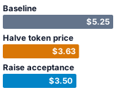
Acceptance divides every cost in an attempt, so a modest gain in it can outweigh halving the token price.
Equation 1 and equation 2 form the quantitative basis for systems design throughout this book. Equation 1 shows how fast reliability falls across unchecked trajectories, and equation 2 sets the economic bar for any runtime mechanism. An intermediate check, a sandbox boundary, or a prompt cache (which reuses the serving state already computed for a repeated prompt prefix, so later calls skip recomputing it) changes both terms of that ratio. Writing \(\MechanismAttemptCost\) and \(\MechanismAcceptanceProbability\) for the attempt cost and acceptance with the mechanism in place, the mechanism pays for its overhead only when \(\MechanismAttemptCost/\MechanismAcceptanceProbability < \AttemptCost/\AcceptanceProbability\). Equivalently, it must lower \(\mathbb{E}[\AttemptCost]\) by a larger fraction than it reduces \(\AcceptanceProbability\), or raise \(\AcceptanceProbability\) by a factor that outweighs its added per-attempt cost.
Neither equation depends on how control decisions are chosen. Both apply to deterministic programs with fixed control flow and to autonomous loops where foundation models choose each next action. That neutrality makes them the right tools for choosing between fixed workflows and model-directed loops.
1.6.1 Workflows vs. model-directed loops
In the software repair task, letting a foundation model decide how to clone the repository, install dependencies, and start the linter wastes tokens and adds failure points to steps whose order never changes. Hardcoding a script to diagnose an unknown race condition, by contrast, breaks the moment the deadlock trace points to an unexpected file. The first group of steps fits a fixed workflow, where the sequence of operations is specified in advance. Diagnosing the race condition requires inspecting source files, forming test hypotheses, and reading logs that depend on what the previous turn uncovered. A model-directed loop, in which the model chooses its next tool call from intermediate observations, earns its keep at those open-ended branches whenever its acceptance gains outweigh the variance and token cost it adds.
A fixed workflow is not limited to a straight-line script: it can take conditional branches, manage retries, and run parallel tasks as long as its control graph is fixed in advance. Because the model calls inside a workflow are still stochastic, a fixed control graph guarantees neither identical outputs nor bounded latency. When comparing a fixed workflow with a model-directed loop, engineers must test both under the same task contract and acceptance checks. By equation 2, a model-directed loop pays for itself only when its open-ended exploration raises \(\AcceptanceProbability\) by a larger factor than its extra model calls raise \(\mathbb{E}[\AttemptCost]\).
↪ Economic feasibility envelopes for choosing between deterministic workflows and model-directed loops are developed in When a bounded loop beats a single call.
Authorization policies stay separate from whichever control structure chooses the steps. A fixed workflow can require human approval before running an external side effect, just as a model-directed diagnostic loop can run without prompts inside an isolated sandbox. The runtime allows exploratory actions inside a safe boundary while gating irreversible operations such as production deployment. An approved grant only authorizes an action to run; it does not show that the resulting state is correct, which still requires independent verification.
Checkpoint 1.1: Changing the task boundary
A repair agent can inspect and edit a disposable working copy and return a patch for review. Its contract grants no access to the deployment service.
Reading the boundary
Pricing the choice
1.7 Anatomy of a Repair Trajectory
Up to this point, the stochastic computer map, the H·S·A exposure space, invariant closure, and horizon arithmetic have appeared one instrument at a time. During an actual run of the race-condition repair (section 1.2), all four act on the same sequence of steps at once: every proposed edit tests the workspace boundary, draws down the turn and dollar budget, and produces compiler or test output that shapes the next decision. Governing that loop requires the runtime to work at two scales: across the trajectory as a whole, where state, permissions, and cost accumulate from turn to turn, and inside each individual turn, where a proposal is checked, executed, and recorded before the next call begins.
1.7.1 Why the runtime manages the trajectory, not the single call
Execution begins when the runtime provisions an isolated working copy of the repository and supplies the initial task description. The model proposes running the failing test. After validating that this command is authorized, the runtime invokes the test runner and records its output. When the runner reports a deadlock, the runtime supplies the diagnostic output to the next model call. The model then proposes inspecting the connection-pool implementation, and the returned source code reveals the locking logic that requires repair.
Guided by this inspection, the model proposes a patch. As section 1.3 established, that patch is a candidate rather than a certified computation. Before modifying the working copy, the runtime checks that the edit targets permitted files. That path check is a mechanical bound below the model, and it keeps this \(\AuthorityExposureLevel_1\) edit inside the \(\StateExposureLevel_2\) working copy. The step also separates three things that a single-call view conflates: the model’s generated diff is a proposal, the modified file is an effect, and the tool’s execution report is an observation. When the next build reports an unclosed bracket, that observation steers the following turn. The model proposes a corrected patch, which the runtime applies before rerunning the build. The compiler has acted as an intermediate check in the sense of the horizon notebook (1.1), catching the syntax error one turn after it happened; the corrected patch and clean rebuild keep that error from carrying into the remaining turns. Once compilation succeeds and visible unit tests pass, the runtime collects regression evidence from the contract’s sealed suite, which the editing tools cannot touch, raising the closure evidence above the model from visible tests to sealed tests. It then records the resulting deliverable alongside these verification records. If the results satisfy the contract’s completion criteria, the runtime submits the repair; otherwise, it can continue iterating, abort, or escalate to a human engineer.
What the tools return shapes the next turn: a thread deadlock calls for a different fix than a syntax error, and a clean build never proves that a race condition is gone. Even a broad regression suite can miss a thread schedule that triggers the bug under load. An agent runtime therefore needs both a way to fold new evidence into the next call and a clear rule for when that evidence is enough to stop. The loop itself is old, since feedback control12 and reinforcement learning have long organized action around observations of an environment (Wiener 1948; Sutton and Barto 2018), and ReAct showed foundation models interleaving reasoning, actions, and observations in the same way (Yao et al. 2023). What the runtime adds is accountability for that loop, which is why fault isolation, access control, and recovery remain necessary when a generated proposal can be wrong or destructive.
12 Cybernetics: Wiener’s 1948 book named the study of control through feedback, in which a system measures the result of its own action and uses the difference from its goal to choose the next one (Wiener 1948). The loop corrects errors only if the measurement comes from the environment; a runtime that feeds back the model’s own account of what it did has closed a loop around a claim rather than around the result.
Wiener, Norbert. 1948. Cybernetics: Or Control and Communication in the Animal and the Machine. Wiley.
Because dependencies cross turn boundaries, the runtime must manage the whole trajectory rather than isolated calls. The corrected patch depends on compiler errors produced several turns earlier, each edit draws down the task’s cumulative token and dollar budget, and every action must be checked against the task’s permissions. A single model request ends as soon as its response stream finishes, whereas the delegated task, along with any background tool runs, finishes only when the runtime settles it. Even the prompt itself compounds from turn to turn: in a recorded repository repair from the benchmark in section 1.2, each turn appends the model’s command and the shell’s output to the conversation history before invoking the model again (figure 6).
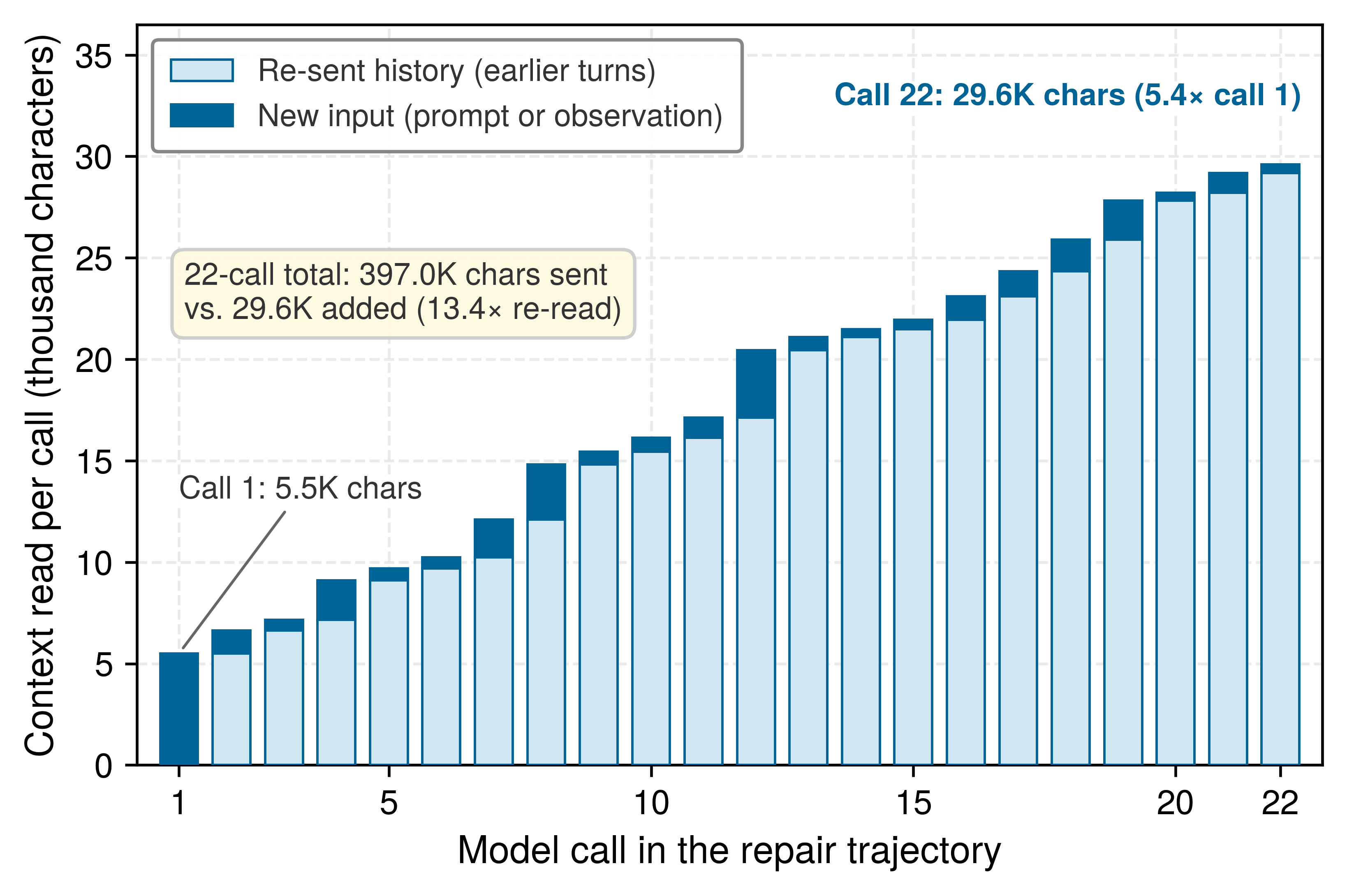
django__django-12050), decomposed into re-sent history from earlier turns and new prompt or tool observation text added on that turn. Each bar’s light lower segment equals the previous bar’s full height because the stateless model interface resends the entire prior transcript on every turn. Data from Jimenez et al. (2024) and Yang et al. (2024).
Yang, John, Carlos E Jimenez, Alexander Wettig, Kilian Lieret, Shunyu Yao, Karthik Narasimhan, and Ofir Press. 2024. “SWE-Agent: Agent-Computer Interfaces Enable Automated Software Engineering.” Advances in Neural Information Processing Systems.
Across the 22 model calls of that trajectory, the first call reads 5,499 characters of task prompt and system instructions, whereas by call 22 the context read on a single turn has grown to 29,594 characters (5.4× the initial call). Because every call resends the accumulated transcript of earlier turns, the trajectory transmits 396,997 characters of input across its 22 calls even though only 29,594 distinct characters enter the transcript (13.4× retransmission). That quadratic growth in cumulative input explains why multi-turn tool use dominates gateway token volume (figure 1) and why context compaction (Context Engineering) and key-value cache reuse across turns (KV Cache Management) are foundational runtime responsibilities.
Context accumulation is only one of the assumptions that break when a service built for isolated requests hosts a multi-turn trajectory (table 3). Stateful services may already provide some of these mechanisms; the comparison names engineering responsibilities that later chapters develop rather than limits built into web services.
| Concern | Isolated-request baseline | Trajectory requirement | Developed in |
|---|---|---|---|
| Cost | Each call has a bounded, independent cost | Cost accumulates across turns and includes failed attempts | The Foundation Model, Agent Economics |
| Memory | State is discarded when the response returns | Context, serving state, and the workspace must survive between turns | Context Engineering, KV Cache Management |
| Authority | A credential is granted to the whole service | Each action is checked against a grant scoped to the task | Tool Calling, Agent Sandboxes |
| Recovery | A failed request can be retried | Repeating an effect can duplicate it; recovery may require compensation | Durable Execution, Failure Recovery |
| Evidence | A success status ends the request | A success status is one observation; acceptance needs an independent check | Agent Evaluation |
| Placement | Any replica can serve any request | Later turns benefit from reaching the retained serving state and the task’s workspace | KV Cache Management |
A naive implementation might write this multi-turn interaction as a bare while-loop. As shown in listing 1, dispatching parsed commands directly and stopping whenever the model prints a completion token leaves every one of those responsibilities unaddressed.
prompt = task_description
while True:
    response = generate(prompt)
    command = parse_command(response)
    output = run_with_host_permissions(command)
    prompt += format_observation(command, output)
    if "TASK_COMPLETE" in response:
        break
Consider what happens when the first test fails and the model searches the host filesystem for the target function name. Because the loop has no authorization boundary, the search command runs with the full privileges of the host process rather than inside the repository copy. Whatever output the search produces is appended straight to the prompt without pagination, truncation, or filtering. If the command dumps thousands of lines of output, the context window overflows or drives up token costs on every later turn. Those failures come not from using a loop, but from leaving out authorization checks and context management.
The same loop also lets the model decide when the task is done. If the model falls into a cycle, proposing small variations of a broken patch turn after turn, the loop runs forever and burns budget without fixing the bug. Worse, if the host process crashes after writing a file edit to disk but before recording the test result, the in-memory transcript is lost while the modified file stays on disk. A restart from the original prompt then runs against a dirty, inconsistent working tree. Handling durability, rollbacks, and recovery requires knowing whether a workspace is disposable and whether actions have outside effects; an unmediated loop tracks neither.
These problems are familiar systems responsibilities (access control, durability, and resource accounting) operating across an entire task. A short, throwaway script can get by with simple retries, whereas an agent modifying shared production infrastructure needs durable checkpoints and compensating actions. In both cases, the runtime needs explicit components to check permissions, persist state, enforce budgets, and verify completion. Keeping those jobs outside the model’s unverified output closes the loop under the five-part task contract of section 1.5.3, and it dictates how the runtime mediates each individual turn from context assembly to contract assessment.
1.7.2 The six phases of a turn
Consider the turn in which the repository repair agent proposes changing mutex acquisition in the connection pool. If the runtime ran that output straight against the shell, a truncated response or an out-of-scope file path would hit the workspace unchecked. Instead, each turn passes through six phases across the runtime, model, and tools:
- Context assembly: The runtime builds the next context from the task contract, current workspace state, and relevant observations. It checks that remaining token and dollar budgets allow another model call, pruning or summarizing older turns to stay within the window while keeping the history of workspace edits clear.
- Model invocation: The model reads that context and returns an action proposal along with call metadata. The runtime treats cut-off generations, network drops, or malformed outputs as failed calls rather than commands to execute, keeping serving and network errors out of the tool layer.
- Validate and authorize: The runtime checks the proposed operation against the tool’s schema and the task’s capability grant. For a code patch, it checks that the target files sit inside the allowed repository paths and that the patch format is valid. The runtime rejects unauthorized operations before dispatch or pauses the turn if human approval is required.
- Tool execution: The tool runs the authorized operation inside an isolated environment under strict timeouts and resource limits. Applying a patch, for example, modifies files in the sandboxed workspace before the repair passes verification. The runtime tracks running tools asynchronously rather than treating dispatch as completion.
- Observation and evidence: The runtime captures the tool’s raw output and formats it as evidence for later turns. A compiler failure produces error logs; passing tests produce exit codes and test results. The runtime’s audit log records what happened to every proposal. A rejected proposal leaves external state untouched, whereas a network call whose reply is lost leaves its outcome unknown, because the remote service may have applied the change before the connection dropped. The runtime therefore marks timed-out or truncated runs as unresolved rather than treating silence as success.
- Assess against contract: The runtime checks the updated task state against the contract’s completion criteria. Depending on the result, it can start another turn, wait on background jobs, ask the user for clarification, stop the trajectory as unresolved, or accept the deliverable. That decision rests on external evidence and remaining budgets rather than the model’s own report.
These six phases mark boundaries of responsibility rather than a rigid synchronous schedule. In production, authorized tools may run asynchronously against remote services, and a model call may propose a final answer instead of a tool call. Implementations can overlap independent work, but causality fixes the order of decisions: a runtime cannot authorize an action from observations that arrive after dispatch, and it cannot tell whether an external effect succeeded from the proposal alone. Figure 7 draws the phases as a U in which only an authorized request drops from validation to the tool. Its dashed paths carry the exceptions. A rejected request returns to the observation history as error feedback without touching any tool, approvals and background jobs pause the turn, and assessment at the end of the turn either starts the next turn, accepts the deliverable, or stops without acceptance.
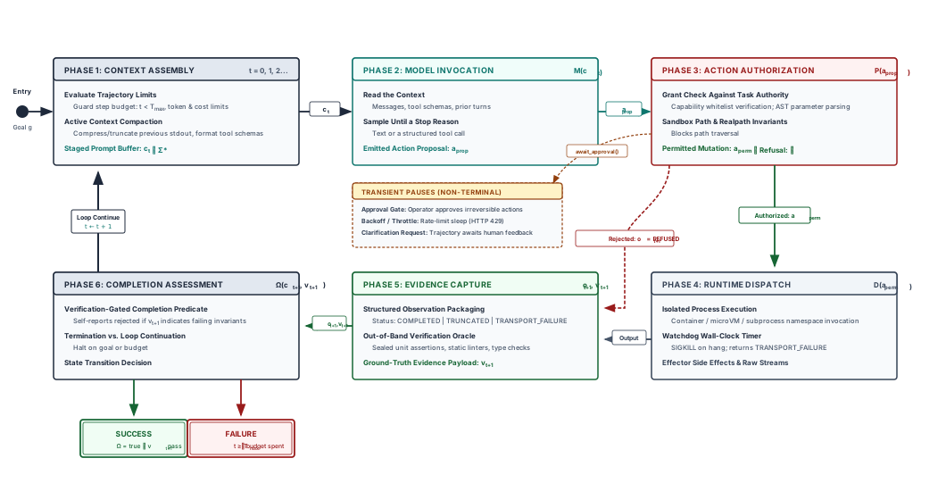
The lifecycle also gives each piece of evidence its own record, which keeps the bounded claims of section 1.5.1 from merging into one. Phase 4 records that a patch modified a file. Phase 5 records that compilation succeeded or that a named test passed on the schedules it exercised. Only phase 6 asks whether those records together meet the contract’s completion criteria. A runtime that logged one undifferentiated stream could not tell intermediate execution from verified resolution.
Whether these components run inside one local process or across services in a cluster, the core rule stays the same: authority is separate from generation. Permissions come from the runtime’s grant, completion criteria come from the task contract, and execution records come from tool observations, never from model text, unverified tool replies, or the agent’s own completion tokens.
In practice, running a test suite often takes much longer than generating the patch that triggered it. During that wait, the task stays active even though model inference is idle. The runtime must keep enough context to process the test results when they return. Holding serving state in high-bandwidth accelerator memory throughout a long tool wait, however, wastes scarce capacity, while evicting the key-value cache too early forces expensive recomputation on the next turn. Separating the lifetime of a task from the lifetime of its serving memory is therefore a central systems problem. Holding accelerator memory idle during slow external operations is the tool-wait problem; Paused-State Policies prices the trade-offs of keeping, offloading, or evicting that state.
The same distinction applies to context history. Keeping full diagnostic logs in durable storage for later audits does not mean resending every compiler warning in every prompt. Inference latency, accelerator memory, tool duration, and dollar cost pull in different directions when the runtime decides what to keep, recompute, or summarize. Giving every data record a clear owner and lifetime lets the runtime manage caches and context deliberately, and the same division of responsibilities organizes the rest of the book.
1.8 Book Organization
Improving a model’s proposals does not grant it permission to run a shell command, and sandboxing a tool call does not stop a fifty-turn trajectory from drifting off course or losing its state on a crash. Because none of the layers of the stochastic computer map (figure 3) can do another layer’s job, the parts of this book follow those layers in dependency order. Each part builds on the guarantees beneath it and closes one exposure before the pieces assemble into a complete runtime.
1.8.1 The causal order of the parts
That dependency order starts with a single model call, because every later guarantee depends on what one invocation reads, returns, and costs. Once the runtime chains calls across turns, it must first bound the growing state in context and memory, then contain the authority of tool calls, and finally supervise the multi-turn horizon across crashes, retries, and evaluation. Only after the runtime produces verified records of what happened can an engineering team train on those trajectories or scale across multiple agents. Table 4 maps this dependency chain onto the seven parts of the book.
| Part | Governing Problem | New Capability | Exposure Addressed |
|---|---|---|---|
| Part I: The Model | A fallible model proposal consumes time and resources. | Interpret the call contract and decide when additional inference is worthwhile. | Origin, then horizon within one decision |
| Part II: Agent Memory | Growing histories compete for limited context and can contain stale information. | Manage the next call’s context, its serving state, and information retained across tasks. | State |
| Part III: Tool Use | Proposed actions need permission, containment, and protection against untrusted input. | Define tool interactions, bound execution, and constrain misuse of legitimate access. | Authority |
| Part IV: The Agent Runtime | A sequence of permitted actions can still stall, lose state, or fail its task. | Supervise execution, survive interruption, recover from failures, evaluate, and release. | Horizon |
| Part V: Learning from Trajectories | Execution records do not automatically constitute suitable learning data. | Curate trajectories, teach demonstrated behavior, and improve policies using outcome rewards. | None; changes the model, not the exposure |
| Part VI: Agents at Scale | Delegation and concurrency introduce coordination costs and shared resource limits. | Compare multi-agent designs and provision resources per accepted task. | All three, multiplied |
| Part VII: Synthesis | Component-level guarantees leave obligations at their interfaces. | Follow an incident-remediation task through the system and justify its acceptance. | All three, together |
Within the parts, the chapters follow the same causal order. In Part I, The Foundation Model fixes the contract around a single model call (what a request supplies, how a response reports completion, and what its input and output cost). Test-Time Compute decides when another token, candidate, check, or call is worth its price. Part II addresses state. Context Engineering selects the working set each call receives. KV Cache Management prices the attention state that context leaves in accelerator memory and decides whether to keep, move, or drop it while an agent waits on a tool. Long-Term Memory keeps knowledge across sessions as claims that carry their provenance. Part III addresses authority. Tool Calling places the runtime between a proposed call and its effect; Agent Sandboxes enforces the task’s limits beneath the executing code; and Agent Security defends against inputs that turn legitimate permissions toward an attacker’s ends.
Part IV builds the runtime that governs the horizon. The Agent Harness keeps the decision to continue outside the model, driving the loop under budgets and approval gates. Durable Execution records each intended action before dispatching it, so that a successor can resume after a crash without repeating an effect unsafely. Because restoring a snapshot does not undo an effect on an external system, Failure Recovery decides among retry, repair, compensation, and escalation by the cost still ahead, and halts trajectories that make no progress. Agent Evaluation establishes what evidence supports a claim about a configuration, and Operating Agents carries that evidence into live work through traces, postmortems, and staged releases.
Part V changes the model without expanding its exposure. Trajectory Curation decides whether a failure belongs in the weights at all and which records serve which learner. Trajectory Fine-Tuning trains on the responses curation selects and releases an update only when closed-loop acceptance improves. Reinforcement Learning from Verifiable Rewards replaces demonstrations with a programmatic check and defends that check against an optimizer that searches it for gaps. Part VI examines how scale multiplies all three exposures. Multi-Agent Coordination asks when splitting a task across workers beats a single controller with the same tools and budget, and Agent Economics measures cost per accepted task over a cohort and prices each lever the runtime controls against it. Finally, Conclusion follows one incident remediation, a configuration rollback whose acknowledgment never arrives, across every boundary the book builds.
Each part opens with the systems principles it develops. Each principle is stated formally where it first appears and cited wherever later components depend on its guarantees, beginning with the invariant closure principle (1).
↪ The full table of foundational systems principles, with each principle’s core statement and what it predicts, is developed in The Principles of the Book.
The same ordering of parts also gives a practical order for fixing production failures, because the parts run from changes in what the model reads to changes in the model’s weights. Changing what a model sees in its context is cheap, fast, and easy to roll back. Retraining or fine-tuning model weights is the most expensive and least reversible fix, and it risks hurting performance on tasks the failure never touched. Fixes to schema constraints, tool interfaces, and runtime checks sit between those two ends, ordered by cost and reversibility. That sequence is a sensible default rather than a rigid ladder that every incident must climb step by step.
↪ The intervention ladder, which orders remedies from context assembly through tool schemas and runtime controls to fine-tuning and reinforcement learning by cost and reversibility, is developed in The intervention ladder.
This dependency order is also why evaluation comes before offline learning in this book. A trace can record an action that was allowed and ran cleanly yet failed to advance the task; conversely, an accepted run often contains an earlier failed attempt that showed the agent how to recover. Offline learning methods need those distinctions so they train on genuine recovery rather than brittle luck. For the same reason, multi-agent coordination comes only after a complete single-agent runtime is in place: teams should compare the coordination cost, latency, and variance of multiple agents against a well-engineered single-agent baseline rather than a fragile while-loop.
This sequence is a teaching order rather than a mandate to deploy every mechanism on every workload. A production system needs only the safeguards its exposures demand, and a bounded, read-only query needs far less machinery than an agent authorized to modify live database clusters. The conclusion applies the full framework to the remediation agent (lighthouse 1.3), from an automated latency alert through an operator-approved configuration rollback to verified recovery.
1.8.2 Reading paths by role
An infrastructure engineer sizing KV-cache pools, a platform engineer writing tool schemas, and a post-training researcher curating trajectories all touch different parts of an agent stack, yet a failure in one layer routinely shows up as a symptom in another. To keep those cross-layer dependencies clear without forcing every reader to know accelerator microarchitecture in advance, the main sequence assumes familiarity with foundation-model prompting, autoregressive token generation, systems programming, processes, virtual memory, file systems, networking, remote procedure calls, and basic probability. Beyond those basics, the book is self-contained: agent-specific concepts are defined where they first appear, and the appendices hold the serving-cost and mathematical derivations.
↪ Serving cost derivations for model invocations are developed in Inference Cost Foundations.
Readers with a specific role can weight their focus while keeping this dependency order intact. Infrastructure engineers will lean on model serving contracts, KV-cache memory management, sandboxed execution, durability guarantees, and fleet economics. Platform and application engineers will focus on context engineering, tool interfaces, security containment, the agent harness, failure recovery, and evaluation benchmarks. Post-training researchers will concentrate on test-time compute, trajectory curation, fine-tuning, and reinforcement learning from verifiable rewards. Every path starts with the task model in this chapter and finishes with the end-to-end trajectory in the conclusion.
1.8.3 The book’s three questions
Without a shared cost metric, teams add autonomous loops where a fixed script would win. Without an exposure model, they overbuild sandboxes for read-only tasks or under-protect production databases. Without independent checks, they mistake a fluent completion message for a finished job. Every chapter that follows therefore answers three questions:
- When does a model-directed loop justify its cost over a fixed workflow? Cost per accepted task decides this trade-off. Each chapter develops mechanisms that either raise the probability of acceptance or cut the spend on failed attempts.
- What runtime machinery must surround the model? The H·S·A exposure space sizes it. Parts II through IV build the mechanisms that manage context across memory tiers, bound delegated authority against untrusted input, and supervise long horizons.
- How do operators know that an autonomous task actually succeeded? Invariant closure governs the answer. A model’s fluent self-report cannot replace external checks; acceptance rests on evidence gathered independently from the environment and judged against a contract adopted before the work begins.
↪ Answers to the three questions, tested with the complete architecture assembled, are developed in Answers to the Three Questions.
1.9 Fallacies and Pitfalls
These three questions frame every mechanism in the book, and they also expose the common traps that appear when teams build or measure agents without them. A patch can compile cleanly without resolving the underlying defect, just as an agent can consume its turn budget without producing fresh evidence. Autonomous execution fails when system designers mistake churn inside the loop for genuine task completion.
Fallacy: A larger context window removes the need to manage task state.
Expanding a context window increases how many tokens a single call can read, but it does not settle which state is current. In an append-only trajectory, stale observations and obsolete file edits pile up alongside current versions. Consider the software repair harness under a 30-turn budget. Starting from an initial prompt of 8,000 tokens and appending 1,500 tokens per turn, the final model call reads 51,500 tokens. This uses only 40 percent of a 128,000-token window, so buffer capacity never forces eviction. Yet without active state pruning, superseded revisions of edited files sit right beside their latest patches. Repeatedly resending earlier turns forces the system to read 892,500 cumulative input tokens, 17.3× the final context size. Even when an entire history fits in memory, raw capacity guarantees neither relevance nor freshness. The runtime must assemble the working context explicitly and mark which state is authoritative rather than leaving the model to untangle conflicting snapshots.
↪ The quadratic input-token cost of resending an append-only history is developed in How multi-turn history drives up input cost.
Pitfall: Appending every failure and retrying until the model reports progress.
Independent retries can improve acceptance, whereas retries that repeat the same failure provide no gain. With a per-attempt acceptance rate of 40 percent, a budget of \(\IndependentAttemptCount\) = 5 independent attempts succeeds with probability \(1-(1-\AcceptanceProbability)^{\IndependentAttemptCount}\), here 92 percent. When an agent appends every failure trace into its prompt, however, the model tends to fixate on its earlier bad assumptions. If every retry repeats the same mistake, 5 attempts succeed no more often than the first attempt while spending 5 times the budget. A well-structured runtime keeps the full diagnostic history in an audit log and feeds the model only the distilled evidence needed for the next decision, under hard retry limits. Recovering from repeated failure requires a new hypothesis, a state change, or fresh evidence from the environment before another repair turn. Alternatively, a declared resampling policy can achieve genuinely independent retries by drawing fresh candidates from the clean starting prompt under a finite budget and independent acceptance checks, though another sample on its own is not evidence of progress. When resetting the prompt for a fresh attempt, the runtime must also roll back the workspace, because truncating or rewriting the working context changes only what the model reads while external effects that have already run persist on disk.
Fallacy: A coherent model report establishes that the task is complete.
A model’s natural-language claim that it has fixed an issue is an unverified hypothesis, not proof of completion. On the closure evidence levels of section 1.5.2 it sits at the bottom, below even a compiler check, because a fail-plausible run produces the same confident report as a correct one. The horizon notebook (1.1) shows the size of the error. Under its assumptions, an unchecked 100-turn repair is correct in only 36.6 percent of runs. If every run ends with a confident completion message, a runtime that trusts that message accepts all of them, and most of its acceptances are wrong. The runtime must instead check the workspace against an explicit evidence standard (sealed tests, static analysis, and the stress runs a concurrency fix requires) and record both the verification artifacts and any remaining gaps.
Pitfall: Expressing an authority limit only as an instruction to the model.
Telling an agent in its prompt to modify files only within a project directory expresses intent, but it provides no protection against model mistakes or prompt injections hidden in untrusted source files. If the host environment exposes raw execution primitives, an agent can be steered into leaking secrets or modifying infrastructure. Read-only file access is not safe on its own either: an agent that reads an API secret from an environment variable and sends it in an outbound network request leaks data without touching a single local file. The execution boundary, not the prompt, must enforce permissions. Runtimes isolate agent processes with operating-system primitives (containers, isolated network namespaces, short-lived credentials, and scoped tool interfaces) that block unauthorized actions regardless of what the model asks to run.
Fallacy: Environmental variation always requires a model-directed loop.
Calling a foundation model to choose the next step after a predictable unit-test failure wastes time and tokens when the fix is a known fallback or a fixed retry sequence. Traditional software workflows handle most routine variation with deterministic control flow: branches, parameterized retries, state machines, and exponential backoffs. Model-directed decisions earn their keep only when choosing the next action requires interpreting open-ended evidence that fixed rules cannot parse, such as combining compiler and test diagnostics to edit several files. Engineers should benchmark agent loops against deterministic workflows under the same acceptance criteria; a loop is worth its latency, token spend, and variance only when it lowers the cost per accepted task.
Pitfall: Charging only the successful final trajectory to the accepted result.
Autonomous task completion frequently requires multiple attempts before a candidate patch satisfies the acceptance checks. Every abandoned branch, failed test run, and discarded attempt consumes compute and wall-clock time, even if its code never merges into the final repository. With a per-attempt acceptance rate of 40 percent, accounting only for the winning trajectory yields an apparent cost of $2.10 per repair, whereas the true expected cost is $5.25, a 2.5× understatement. Complete system accounting must also capture sandbox provisioning, tool execution overhead, and the cost of human triaging. Measured over a cohort, the numerator charges every initiated task, accepted or not, while the denominator counts only tasks accepted under the stated evidence standard. That cohort form, the measured counterpart to equation 2, is developed in Cost per Accepted Task.
Each of these traps comes from mistaking a property of a single model call for a guarantee across the task. A working runtime keeps state current, enforces permissions in the execution layer rather than the prompt, and gates acceptance on independent evidence, judging the system by the cost of its verified outcomes rather than the fluency of its turns.
1.10 Summary
A foundation model generates candidate reasoning traces and actions, yet it cannot verify its own output or safely modify external systems. Four instruments govern the design of the runtime that surrounds it. The stochastic computer map compares an agent to a classical computer and locates where the analogy breaks: because the model only proposes, a deterministic runtime must manage persistent state, enforce permissions, and close the loop. The H·S·A exposure space sizes that runtime along three dimensions: execution horizon (\(\TurnHorizon\)), accumulated state (\(\StateExposureLevel_0\) to \(\StateExposureLevel_3\)), and delegated authority (\(\AuthorityExposureLevel_0\) to \(\AuthorityExposureLevel_3\)). Invariant closure then pairs hard execution boundaries below the model with independent, artifact-based acceptance checks above it.
Two economic relations price those choices. Under the independent-step model without recovery, unchecked multi-turn runs compound step errors exponentially, so catching and repairing errors early shortens the effective horizon over which mistakes accumulate. Measuring performance by cost per accepted task charges every wasted model call, sandbox run, and human review across failed attempts to the verified deliverables that pass. As the repository repair walkthrough and the four lighthouse systems show, runtime machinery should scale with exposure: an agent needs only the safeguards that its horizon, state, and authority demand.
Table 5 summarizes the quantitative relations used throughout this chapter to evaluate reliability and cost across an execution horizon, where \(\PerStepErrorRate\) is the per-step error rate, \(\TurnHorizon\) is the horizon length in turns, and \(\IndependentAttemptCount\) is the allocated retry budget. Cost per Accepted Task measures cost per accepted task over a whole cohort of initiated tasks.
| Equation | What it bounds or decides | Where derived |
|---|---|---|
| \(\Pr(\text{success}) = (1-\PerStepErrorRate)^{\TurnHorizon}\) | Task success probability when all \(\TurnHorizon\) independent steps must succeed without intermediate checks or recovery | equation 1 |
| \((1-\PerStepErrorRate)^{\TurnHorizon} \approx e^{-\PerStepErrorRate \TurnHorizon}\) | Under the independent-step model without recovery and at small step error, the product \(\PerStepErrorRate \TurnHorizon\) governs reliability | section 1.6 |
| \(\CostPerAcceptedTask = \mathbb{E}[\AttemptCost]/\AcceptanceProbability\) | Expected cost per accepted task under independent retries; acceptance rate scales effective attempt cost | equation 2 |
| \(\MechanismAttemptCost/\MechanismAcceptanceProbability < \AttemptCost/\AcceptanceProbability\) | Economic condition determining whether an added check, boundary, cache, or prompt optimization justifies its cost | section 1.6 |
| \(1-(1-\AcceptanceProbability)^{\IndependentAttemptCount}\) | Cumulative acceptance probability within a budget of \(\IndependentAttemptCount\) attempts, assuming independent failures | section 1.9 |
Key Takeaways: Agency is a property of the system, not the model
- Stochastic proposals need a closing runtime: An agent resembles a classical computer, but its foundation model only proposes. It generates candidate tokens and actions, leaving the validation of correctness and actual execution to external software. The surrounding runtime must enforce permissions, preserve state across steps, and govern the full trajectory through failures and retries.
- Task exposure dictates architectural obligations: The H·S·A dimensions (horizon length, accumulated state, and delegated authority) pinpoint where an autonomous workflow requires protective sandboxes, durable checkpoints, human intervention, and verifiable evidence. System mechanisms should scale with this exposure profile; tasks with short horizons and constrained authority do not require the heavyweight control loops of high-exposure systems.
- Runtime enforcement and empirical evidence serve distinct roles: Structural boundaries enforce hard constraints on permitted actions, preventing catastrophic side effects regardless of model behavior. By contrast, verification checks produce empirical evidence only for the specific properties they measure. Task acceptance requires evaluating this evidence against a defined contract. Passing tests support claims only within their measured coverage; an eloquent report alone supplies no independent evidence.
- Two numbers price every mechanism, autonomy included: Under the independent-step model without recovery, unchecked task success decays exponentially with horizon length, so detecting and repairing errors before later turns depend on them can improve reliability without changing the model. Meanwhile, the cost per accepted task amortizes all wasted inference, compute infrastructure, and human oversight across verified deliverables. An autonomous loop justifies its operational complexity only when it reduces this net cost under the task contract.
1.11 Historical Perspective and Further Reading
The closed-loop architecture at the core of agentic systems predates modern machine learning by decades. In founding cybernetics, Norbert Wiener established feedback as the organizing principle of control: a system observes its environment, measures the discrepancy between current state and a target goal, and applies corrective actions (Wiener 1948). Writing a decade later, Wiener warned of the operational hazard inherent in rapid feedback: when an automated machine acts faster than a human operator can intervene, it must be constrained to the exact purpose intended (Wiener 1960). Artificial intelligence adopted this structure through the rational agent framework, defining an agent by its continuous cycle of perception and environment interaction (Russell and Norvig 2020). Reinforcement learning subsequently formalized that cycle, treating the iterative trajectory of states, actions, rewards, and observations as the central object of learning (Sutton and Barto 2018).
Russell, Stuart, and Peter Norvig. 2020. Artificial Intelligence: A Modern Approach. 4th ed. Pearson.
What transformed with foundation models was the capability of the component driving the loop. Rather than relying on specialized heuristics or hand-crafted policies, a general-purpose model pretrained across diverse data distributions can now synthesize reasoning traces and emit concrete actions in text and code (Bommasani et al. 2021). The ReAct architecture demonstrated that interleaving model-generated reasoning with tool execution feedback allows language models to operate effectively in open software environments (Yao et al. 2023). Real-world software engineering benchmarks crystallized this shift, demonstrating that an agent’s capability must be measured not by fluency on static prompts, but by whether its proposed patches pass unseen repository test suites (Jimenez et al. 2024).
The scaffolding surrounding the model builds on classical systems research addressing unreliable components. John von Neumann first investigated how to synthesize dependable computational systems from failure-prone parts, demonstrating that modular redundancy, majority voting, and periodic state restoration can bound compound failure rates (Neumann 1956). Subsequent distributed systems research formalized the fault assumptions that supervisors must accommodate. These range from fail-stop models, where damaged components halt detectably (Schlichting and Schneider 1983), to Byzantine failure models, where components behave arbitrarily or deceptively (Lamport et al. 1982). The modern dependability taxonomy codified the causal sequence linking latent faults, runtime errors, and observable system failures, drawing an essential distinction between errors that trigger overt alarms and those that silently corrupt downstream execution (Avizienis et al. 2004).
Dijkstra, Edsger W. 1970. “Structured Programming.” Software Engineering Techniques: Report on a Conference Sponsored by the NATO Science Committee, 84–87.
Because foundation models generate probabilistic outputs, verification cannot be offloaded to the generator itself. The end-to-end argument in system design established that complete correctness checks cannot be delegated to intermediate subcomponents; they must ultimately reside at the endpoint that understands application-level task requirements (Saltzer et al. 1984). At the same time, Dijkstra’s foundational observation that software testing demonstrates the presence of bugs rather than their absence bounds the certainty that any validation suite can provide (Dijkstra 1970).
Managing delegation and authority safely relies on principles developed across operating systems and distributed transaction design. Capability-based addressing, introduced by Dennis and Van Horn, bound access rights directly to unforgeable, fine-grained object references rather than ambient process identities (Dennis and Van Horn 1966). Saltzer and Schroeder codified these patterns into enduring design principles for computer protection, emphasizing least privilege, complete mediation of access requests, and economy of mechanism (Saltzer and Schroeder 1975). Hardy later uncovered the hazard of ambient authority: in a confused deputy attack, an unprivileged client manipulates a privileged utility into misusing permissions granted by its environment rather than by the specific caller (Hardy 1988).
Dennis, Jack B., and Earl C. Van Horn. 1966. “Programming Semantics for Multiprogrammed Computations.” Communications of the ACM 9 (3): 143–55. https://doi.org/10.1145/365230.365252.
Greshake, Kai, Sahar Abdelnabi, Shailesh Mishra, Christoph Endres, Thorsten Holz, and Mario Fritz. 2023. “Not What You’ve Signed up for: Compromising Real-World LLM-Integrated Applications with Indirect Prompt Injection.” Proceedings of the 16th ACM Workshop on Artificial Intelligence and Security, 79–90. https://doi.org/10.1145/3605764.3623985.
Extended autonomous execution also confronts the reality that multi-step external workflows cannot be rolled back atomically. Garcia-Molina and Salem developed sagas to manage long-running transactions, coordinating forward progress through predefined compensating actions when operations fail midway (Garcia-Molina and Salem 1987). At interface boundaries, Meyer’s design by contract established that modular software reliability depends on explicit, executable preconditions, postconditions, and invariants (Meyer 1992). Autonomous agents reopen each of these classical security and reliability challenges simultaneously. Because language models interleave data interpretation with control flow, external data cannot be assumed benign. Greshake et al. (2023) demonstrated that indirect prompt injection turns untrusted external content into instructions the model may follow. The result shows that for an agent guided by natural language, read access is itself an exposure, because what the agent reads can steer every action it proposes, even though only the runtime can grant those actions.
- The Protection of Information in Computer Systems (Saltzer and Schroeder 1975). The classic formulation of protection mechanisms for computer systems, including least privilege, complete mediation, and fail-safe defaults. This paper provides the conceptual foundation for modern tool authorization, sandboxing, and privilege boundaries in agent architectures.
- End-to-End Arguments in System Design (Saltzer et al. 1984). The foundational rationale for placing validation checks at the application endpoints that maintain task semantics. In agent engineering, it clarifies why intermediate generation fluency cannot certify end-to-end task completion.
- Basic Concepts and Taxonomy of Dependable and Secure Computing (Avizienis et al. 2004). The standard taxonomy distinguishing faults, errors, and failures across computing systems. It provides the disciplined vocabulary needed to diagnose agent failure modes, including the fail-plausible errors characteristic of foundation models.
- Principles of Computer System Design (Saltzer and Kaashoek 2009). A comprehensive textbook on system decomposition, atomicity, virtualization, and protection. It supplies the essential systems foundation for building resilient agent orchestrators, runtimes, and tool harnesses.
- Reinforcement Learning: An Introduction (Sutton and Barto 2018). The definitive treatise on sequential decision-making in dynamic environments. It provides the formal vocabulary of states, actions, rewards, and environment trajectories that underpins the execution model in this chapter.
- ReAct: Synergizing Reasoning and Acting in Language Models (Yao et al. 2023). The seminal paper demonstrating that interleaving reasoning traces with tool invocations enables language models to solve multi-step problems. Reading it alongside this chapter highlights the boundary between the model’s proposed actions and the external system responsible for executing and verifying them.
Saltzer, Jerome H., David P. Reed, and David D. Clark. 1984. “End-to-End Arguments in System Design.” ACM Transactions on Computer Systems 2 (4): 277–88. https://doi.org/10.1145/357401.357402.
Saltzer, Jerome H., and M. Frans Kaashoek. 2009. Principles of Computer System Design: An Introduction. Morgan Kaufmann.
Sutton, Richard S., and Andrew G. Barto. 2018. Reinforcement Learning: An Introduction. 2nd ed. MIT Press.
Yao, Shunyu, Jeffrey Zhao, Dian Yu, Nan Du, Izhak Shafran, Karthik Narasimhan, and Yuan Cao. 2023. “ReAct: Synergizing Reasoning and Acting in Language Models.” International Conference on Learning Representations (ICLR).
1.12 Exercises
All quantities below are hypothetical problem givens, chosen to be round, and describe no particular model, provider, or deployment. Unless a problem says otherwise, assume step errors are independent, each attempt costs the same in expectation, and “accepted” means accepted under a fixed task contract.
1. How far can an unchecked repair run? (Basic). A repair agent takes steps that are each correct with probability 0.98, and no step is checked before the next one builds on it.
- Using equation 1, compute task success at horizons of 20 and 60 turns.
- Find the per-step error rate that would hold the 60-turn task at 80 percent success, and how many times lower it is than the current error rate. Confirm the answer with the small-\(\PerStepErrorRate\) form \(\PerStepErrorRate \TurnHorizon \approx -\ln(0.8)\).
- Instead of a better model, the runtime inserts a check after every 10 turns that detects any incorrect step in that segment and reruns the segment from the preceding checkpoint. Assuming the check is perfect and free, compute the expected number of turns to finish the 60-turn task, and compare it with rerunning the whole unchecked trajectory until it succeeds. State which lever to pull first and the property of the check on which the answer depends.
2. A token discount or a better context? (Basic). An attempt at a repair task spends $1.80 on model tokens and $1.20 on the sandbox, tests, and review, and 25 percent of attempts are accepted. The runtime retries until acceptance.
- Compute the expected number of attempts and the cost per accepted task from equation 2.
- A provider offers a 40 percent token discount; alternatively, a context change raises acceptance to 30 percent at the original attempt cost. Compute the cost per accepted task under each, and under both together.
- Find the acceptance probability that matches the discount. Explain why the comparison comes out differently from the chapter’s notebook (1.2), naming the quantity that decides which lever wins.
3. Placing a workload in H·S·A (Basic). A log-triage agent runs about 15 turns per incident and spends $0.50 on tokens per task. Consider three versions of its grant: (i) it reads logs and writes a summary to a scratch file; (ii) it also opens tickets in a shared tracker, and any ticket can be closed again; (iii) it also rolls back a production deployment, and a wrong rollback causes an outage costing $2,000 that cannot be undone. In version (iii), 2 percent of rollbacks are wrong.
- Place each version on the state and authority axes of figure 4, justifying each level by the consequence of the operation rather than its name.
- For version (iii), compute the expected loss per task from wrong rollbacks and express it as a multiple of the token cost.
- A human approval step costs $5 per rollback and stops 90 percent of wrong ones. Compute the expected cost per task with approval, and state which exposure binds this workload.
- Specify all five task-contract fields for version (iii): the useful incident-triage goal and its negative scope, the deployment baseline and execution environment, the permitted actions and approval boundary, bounded diagnostic observations, and independent completion criteria. Name one limitation of the evidence that would require an unresolved outcome or further review.
4. Paying for checks inside the horizon (Intermediate). A repair task runs 50 turns with per-step error 0.02. Each turn costs $0.04 in tokens, and each attempt pays $1.00 to prepare a fresh sandbox. Under policy A, only a sealed test at the end checks the result; it accepts an attempt exactly when every step was correct, and a rejected attempt restarts from scratch. Under policy B, the same sandbox is kept and a check costing $0.10 runs after every 10 turns, detecting any incorrect step in that segment, which is then rerun from the last checkpoint.
- Compute the acceptance probability and cost per accepted task under policy A.
- Compute the expected cost per accepted task under policy B, and the expected number of turns under each policy.
- Find the per-check cost at which policy B stops paying. Then critique the assumption that makes B look so strong: what happens to the calculation if the intermediate check is a visible test the agent can fit its patch to? Specify independent final evidence and concurrency coverage appropriate to this repair, using section 1.5.2, and explain why sealing a sequential test alone would not establish that the race condition is fixed.
5. When the loss is not in the tokens (Intermediate; second lighthouse). The remediation agent (lighthouse 1.3) spends $2 on tokens per attempt. Each attempt ends by proposing one configuration change that is correct with probability 0.95; a wrong change that commits costs $20,000 in total. A human approval step costs $15 of on-call time and delays restoration by 6 minutes, during which the ongoing incident costs $50 per minute. Approval passes every correct change and rejects 90 percent of wrong ones; a rejected proposal starts a new attempt, which needs approval again.
- Without approval, every proposal commits. Compute the expected cost per task, including expected loss.
- With approval, compute the probability that an attempt ends in a commit, the expected attempts per task, the expected attempt spend, the probability the committed change is wrong, and the total expected cost per task.
- Find the incident cost per minute above which approval stops paying.
- For the repair agent, the chapter’s levers were acceptance and horizon. Show numerically why halving the token price is irrelevant here, and name the binding constraint of this lighthouse and the H·S·A level that makes it bind.
6. Workflow, loop, or both? (Intermediate). A fixed workflow attempt for a support query costs $0.60; a model-directed loop attempt costs $1.80. Half the queries are routine, where the workflow is accepted with probability 0.55 and the loop with 0.80. The other half are novel, where the workflow is accepted with probability 0.05 and the loop with 0.70. Each query retries its chosen architecture until acceptance.
- Compute the cost per accepted task for each architecture on each query class, and the mean over the population if every query uses the workflow, and if every query uses the loop.
- A perfect router sends routine queries to the workflow and novel ones to the loop. Compute the mean cost per accepted query.
- A real router costs $0.05 per query and sends a fraction \(\MisroutedQueryFraction\) of each class to the wrong architecture. Compute the mean cost at \(\MisroutedQueryFraction = 0.05\) and find the \(\MisroutedQueryFraction\) at which routing stops beating the loop alone. What does this imply about where to spend engineering effort, and what must be held fixed for the comparison to be valid?
7. Retries that repeat one mistake (Advanced). Each attempt at a repair task costs $2.00, and the retry budget allows 4 attempts. Of the tasks, 70 percent are easy, accepted with probability 0.70 per attempt; the rest are hard, and because each retry rereads the transcript and repeats the same mistaken hypothesis, a hard task is accepted with probability only 0.05 per attempt. Assume attempts are independent conditional on the task being easy or hard; the repeated hypothesis lowers the hard-task acceptance rate rather than making every retry share one outcome. Tasks not accepted within the budget end unresolved, and their spend stays in the numerator.
- An analyst pools the cohort into one mean acceptance probability and applies the independent-retry formulas. Compute the pooled acceptance, the predicted success within the budget, and the predicted cost per accepted task.
- Compute the actual acceptance within the budget, expected spend per task, and measured cost per accepted task under the mixture. By what factor did the pooled model understate the cost?
- Redesign the retry. Retries 2 through 4 start from a fresh context carrying only the failed test result, which costs $2.50 per retry and raises a hard task’s retry acceptance to 0.25 while leaving easy tasks unchanged. Compute the new acceptance within the budget and cost per accepted task, and argue whether the redesign should ship. What does the result say about treating \(\AcceptanceProbability\) as a property of the model rather than of the whole attempt?
8. Should the repair agent deploy its own patches? (Advanced). A team produces 200 patches that pass the sealed tests each day. Of these patches, 3 percent are in fact wrong. A wrong patch that reaches production costs $5,000. The team proposes letting the agent deploy directly. Two alternatives are on the table. A reviewer costing $25 per patch catches 80 percent of the wrong patches that tests pass, and waiting for review delays each patch by 4 hours valued at $10 per hour. Alternatively, a canary rollout costing $5 per patch exposes a small slice of traffic and rolls back automatically, bounding the cost of a wrong patch to $500.
- Place the direct-deploy proposal and the canary design on the H·S·A authority axis, and explain what changes the level.
- Compute the expected cost per patch and per day for direct deploy, review, and canary.
- Critique the canary design. Name one class of change for which automatic rollback is not an adequate reversal, state what authority level such a change returns to, and specify the contract change (permitted actions and completion criteria) that should route it back to review.
What’s Next: From task responsibilities to the model call
Of the six phases every turn passes through, only the second belongs to the model, and each of the other five depends on knowing exactly what that phase delivers. When the repair agent asks to inspect the connection pool, the runtime may receive a complete tool request, a request cut off before it is whole, or no response at all, and each outcome requires different handling. The Foundation Model follows that single inspection call from request to bill, establishing what one call reads, how its status reports completion, and what it costs. The single call sits at the origin of the H·S·A exposure space, so this invocation contract becomes the baseline from which every later part measures a departure.