2 The Foundation Model

Purpose

Agent stack focus for this chapter.

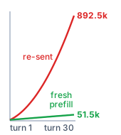
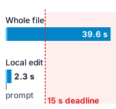
Why does a capable model still need a precise contract around every call?

A model call can return a response that parses cleanly yet violates the tool schema, arrives past its deadline, or claims a file edit succeeded before any tool has run. Because every capability an agent adds—tool dispatch, memory retrieval, sandboxed execution, and recovery—is built from individual model calls, any ambiguity at the call boundary spreads into every subsystem downstream. A foundation model is an ungrounded token predictor that emits candidate proposals across an untrusted boundary, not a verified state transition. The surrounding runtime must therefore enforce reliability at each call through token budgets, schema checks, and independent verification. Within the H·S·A exposure space, the single call sits at the origin: one bounded turn, zero carried state, and zero ambient authority.

Learning Objectives

• Explain the separate responsibilities of the foundation model, inference service, and agent runtime
• Construct a token-bounded request containing task messages, advertised tools, and generation limits
• Calculate how temperature and nucleus truncation reshape candidates without establishing correctness, and explain why only a recorded call replays exactly
• Diagnose response outcomes using completion status, structural validity, permission checks, and external evidence that self-review cannot supply
• Distinguish the guarantees of grammar-constrained decoding from learned formatting and correct task values
• Estimate call latency and repeated-input work under explicit serving and prefix-reuse assumptions
• Evaluate interface representations using accepted outcomes and resource use under matched task budgets

2.1 One Turn of the Repair Loop

A single call runs one turn, carries no state, and holds zero ambient authority.

Yao, Shunyu, Jeffrey Zhao, Dian Yu, Nan Du, Izhak Shafran, Karthik Narasimhan, and Yuan Cao. 2023. “ReAct: Synergizing Reasoning and Acting in Language Models.” International Conference on Learning Representations (ICLR).

The repair agent (Four lighthouse workloads) needs to inspect the connection-pool implementation before proposing a change. A model call that emits read_file("src/pool.py") produces only an unexecuted text string. Of the six phases of a turn (The six phases of a turn), only the call itself belongs to the model; checking the path, authorizing the read, running it, and returning the observation all belong to the runtime. This loop of model-generated proposals and runtime observations is the interaction pattern formalized by ReAct (Yao et al. 2023), and every runtime phase depends on knowing what the single model phase delivers.

In a chat window, a human reader spots a response cut off mid-sentence, judges whether a shell command is safe to run, and waits out variable generation delays. An autonomous agent removes that human reader. The runtime receives the response as data and must check in code what a person would judge by eye: whether the prompt fit inside the context window, whether generation finished normally or hit the output token limit, whether a well-formed tool request targets a path inside the allowed workspace, and how much time and budget the call spent. Raw reply text cannot answer those questions; a runtime that guesses call state by scraping output strings will eventually apply a truncated patch or run a command outside its workspace.

Preventing those failures requires an explicit call contract between the agent runtime and the inference service. That contract covers both directions of the call: the outbound request (message history, advertised tool definitions, and token and time limits) and the inbound response record (payload kind, stop reason, normalized status, and token usage). It also fixes the checks the runtime runs before dispatching any proposed action, along with the latency and input-recomputation costs of each call. Rather than assuming the model is reliable, the contract treats the inference service as an untrusted, probabilistic generator and keeps every control-flow decision in the runtime.

The chapter follows the repair agent’s single inspection call from request to bill, adding one runtime obligation at each step. Before the call is sent, the runtime must know who owns which decision (section 2.2) and whether the serialized request fits with room left for an answer (section 2.3). How the service then produces a candidate (section 2.4) explains why repeated calls differ and why generation can stop before the candidate is whole. That possibility fixes the order of the checks on the way back. The runtime first reads the call’s normalized status to learn whether a complete candidate arrived at all (section 2.5), then asks which property each check on a completed candidate actually establishes (section 2.6), and finally whether syntax errors can be prevented during generation instead of rejected after it (section 2.7). The last two sections price the call. Output length and re-sent history set its latency and work (section 2.8), and those costs decide how competing output representations should be compared, on accepted repairs under a matched budget (section 2.9).

2.2 The Model Call Boundary

If a runtime treats a model’s output string read_file("src/pool.py") as an already-authorized file read, a single hallucinated path can read outside the workspace before any check runs. Keeping a proposed action separate from an executed one requires splitting each call across three components: the foundation model, the inference service, and the agent runtime. The foundation model¹ computes conditional probability distributions over token sequences given a prompt context. The inference service hosts the model weights, runs forward passes on accelerators, applies sampling parameters, and packages the output tokens into a response record. The agent runtime drives the task: it builds the prompt, tracks budgets, checks candidate outputs, and decides whether an action is allowed to run in the host environment. Even when all three run in the same process on one machine, their interfaces keep generated text separate from the decision to act on it.

¹ Homogenization: The same report that named foundation models warned that, because many applications adapt one shared base model, a defect in that model passes into every system built on it (Bommasani et al. 2021). For autonomous agents the warning is concrete. Every runtime that invokes the same model and serving path inherits the same failure modes at once, so the runtime, rather than the model, must hold the operational checks.

Bommasani, Rishi, Drew A. Hudson, Ehsan Adeli, Russ Altman, Simran Arora, Sydney von Arx, Michael S. Bernstein, et al. 2021. “On the Opportunities and Risks of Foundation Models.” arXiv Preprint arXiv:2108.07258.

Definition 2.1: Proposal

A proposal is model output that specifies a candidate action or answer for the runtime to evaluate, carrying zero ambient authority and producing no external side effects until the runtime explicitly validates, authorizes, and executes it.

1. Significance: Every external effect of an agent depends on an explicit runtime decision. Because the model call possesses zero ambient authority, a rejected proposal costs one inference invocation rather than an unintended modification to the environment. That invocation still consumes resources and counts toward \(\AttemptCost\) in the cost per accepted task (equation 1.2).
2. Distinction: A proposal must not be confused with an effect (a state change executed by the runtime after authorization) or an observation (the runtime’s factual record of what an operation returned). Emitting read_file("src/pool.py") is merely a proposal; the file contents subsequently retrieved from disk and supplied to the next call constitute an observation.
3. Common pitfall: Logging a tool request as an executed action, or accepting a model’s textual claim that “the file has been read” as an empirical observation, allows fluent prose to stand in for operational evidence.

2.2.1 Messages and tool definitions

A model cannot tell an operator’s instruction, a user’s prompt, and a file excerpt returned by a tool apart unless the runtime labels each piece of the request, yet those labels alone do not make the content trustworthy. The runtime organizes the prompt as an ordered sequence of role-tagged messages: a system message sets task instructions and constraints, a user message supplies the task prompt, an assistant message records earlier model outputs, and a tool message carries the raw observation returned when an action runs. Role tags organize the token stream for the model’s attention mechanism, while the runtime remains responsible for checking whether the content is authentic and follows the task contract.

↩︎ The task contract, which fixes the goal, environment, permitted actions, available observations, and completion criteria, is established in The five-part task contract.

Alongside the message history, the request advertises the tools available to the model and gives their argument schemas. In listing 1, the runtime declares a file-reading tool with one required string parameter. The JSON-schema definition tells the model what syntax a valid proposal needs, while the runtime enforces workspace sandboxing and filesystem permissions independently.

Listing 1: A bounded inspection request: This provider-neutral record separates model-visible messages and tool definitions from the configuration and limits governing the call. Symbolic values stand for settings chosen by the runtime; the field names do not prescribe a vendor API.

model_config: repair-model/config-a
messages:
  - role: system
    content: Propose the next inspection for the assigned repair.
  - role: user
    content: Inspect the connection-pool locking logic in src/pool.py.
tools:
  - name: read_file
    arguments_schema:
      type: object
      properties: {path: {type: string}}
      required: [path]
      additionalProperties: false
limits:
  max_output_tokens: K_max
  deadline: T_deadline
sampling: selected_sampling_settings

The model_config field binds the request to a specific model version, weights checkpoint, and serving profile, while sampling controls how the service draws output tokens from the model’s predicted distribution. Two resource bounds protect the call from running away: max_output_tokens (\(\OutputLimit\)) caps how many tokens the call can generate, and deadline (\(\CompletionDeadline\)) sets a timeout against queue delays and serving stalls. Writing those bounds into the request works only when the inference service or client runtime enforces them during generation.

When generation finishes, the inference service returns free-form text, a tool proposal, or a service error, and a runtime adapter normalizes that provider-specific reply into a single envelope (listing 2). Here, the service reports a completed generation pass that produced a tool request to read src/pool.py—one diagnostic step before any repair is checked.

Listing 2: A returned tool proposal: Response kind identifies what the payload represents, while status and stop reason describe the invocation. Usage counts describe consumed generation resources, not progress on the repair.

kind: tool_request
payload:
  name: read_file
  arguments: {path: src/pool.py}
stop_reason: tool_request
status: COMPLETED
usage: {input_tokens: S, output_tokens: K}

Here, kind tells the runtime parser how to read the payload. The normalized status confirms that transport and generation finished under the adapter’s contract, while stop_reason records the stop reason reported by the serving engine: whether the model emitted a tool-call marker, hit an end-of-sequence token, or stopped at the token limit. The usage block counts \(\SequenceLength\) input tokens read and \(\OutputLength\) output tokens generated. Bare \(\SequenceLength\) is sequence length throughout this book, here the prompt a call reads; the State levels \(\Glyph{S}_0\) to \(\Glyph{S}_3\) always carry their subscript. Tracking usage across calls prevents context-window overflow and feeds cost accounting; if a provider omits token counts, the runtime records usage as missing rather than zero.

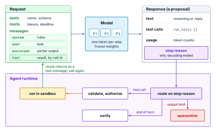
Every path out of the response ends in the runtime, and the stop reason chooses the path (figure 1). A tool call goes to validation and authorization before anything runs, a finished answer goes to verification, and output cut off at its limit goes to quarantine, where it is kept for diagnosis and never executed (section 2.5.2 states the rule).

Figure 1: The Model Call Surface: The request carries messages, tool definitions, and limits into a model with frozen weights, which returns a proposal with a stop reason and usage counts. Every arrow out of the response lands in the agent runtime. The runtime validates and authorizes a tool call before anything runs, returns the result as a new message for the next call, sends a finished answer to verification, and quarantines output cut off at its limit.

2.2.2 Proposals and observations

If the runtime ran a returned read_file proposal directly against the host filesystem, a path like ../../etc/passwd or a malformed argument would execute before any check caught it. Instead, the runtime passes every tool proposal through validation and authorization before anything runs. First, it checks structural conformance, confirming that the proposed arguments match the declared schema (for example, that path is a string rather than a shell command). Next, it checks the arguments against the task’s permission grant: advertising read_file lets the model propose file reads, but grants no right to read arbitrary paths. The runtime verifies that src/pool.py resolves inside the allowed workspace rather than escaping to host files through directory traversal. Once authorized, the tool runs outside the model call, inside an isolated sandbox or container with its own timeout.

After the tool finishes, the runtime records what happened and builds the next prompt. It appends the model’s assistant proposal paired with a tool message carrying the observation (here, the bounded file excerpt). That observation reports the actual outcome, including a missing file or a permission denial, and notes when the output was truncated; One mediated round trip develops how the runtime matches each result to the call it answers, records errors, and marks truncation.

The model on the next turn sees the tool output only because the runtime rebuilds and sends the updated context window. Foundation models are stateless token predictors with no internal memory of earlier requests or tool runs. Session identifiers or server-side prefix caching (reusing attention state the service already computed for a prompt prefix that repeats across turns, priced in section 2.8.3) can cut latency, but the runtime alone decides which messages enter the prompt. That separation also means an observation can go stale: a file excerpt in the prompt shows the file only as it stood when read, so if a later command edits the file on disk, the excerpt in context is out of date.

The gap between a proposal and an observation is where the fail-plausible fault enters. A model can emit a well-formed proposal targeting the wrong source module, or a convincing analysis grounded in an obsolete observation, and the tokens look the same either way. Agent engineering therefore requires treating status, schema structure, security authorization, and empirical evidence as distinct, non-fungible properties of the interaction. Table 1 summarizes what the runtime owns around every call, whether the model runs in the local process or behind a remote API.

↩︎ The fail-plausible fault, output that looks well formed and credible while the intended property fails, is established in The fail-plausible fault.

Table 1: What the runtime owns around a model call: Each feature of the call creates an obligation outside the model’s generated content. Satisfying one obligation does not discharge the others.

Model term	Runtime responsibility	Failure if the runtime ignores it
Context window	Count the complete input representation and reserve output headroom	Rejected request or insufficient room for a complete response
Sampling settings	Choose supported settings and retain them with the request and output	Unexplained variation or an unjustified assumption of reproducibility
Tool call	Check the proposal, authorize access, and return the actual tool observation	A proposed operation mistaken for an executed or permitted one
Stop reason	Interpret it with normalized status before treating the payload as complete	An interrupted or refused response treated as a finished candidate
Fluent but wrong output	Evaluate the relevant claim using checks and observations with stated limits	Credibility mistaken for evidence of the intended property
Successful response	Distinguish delivery and generation completion from task acceptance	A completed call recorded as a successful repair

The request and response records fix the boundary around a model call: messages supply context, tool definitions specify what the model may propose, and the runtime mediates every effect on external state. Before the service can run the call, however, the whole request must fit inside the model’s context window with room left for the response, and checking that fit requires counting tokens rather than characters, messages, or files.

2.3 Tokenizing the Request

When an automated repair agent appends a connection-pool source file and a compiler diagnostic to its message history, the payload expands rapidly. Naive metrics like file counts or raw character counts cannot determine whether the next request will fit within the model’s capacity. Role delimiters, tool schemas, system prompts, file paths, and source code all serialize into a single sequence of discrete units before entering the neural network. The operational budget is the token count of that fully assembled sequence, measured strictly against the model’s specific tokenizer and wire format.

2.3.1 Tokens in the serialized request

Estimating prompt size from character counts or source-code lexers fails because a model’s tokenizer slices text into vocabulary identifiers whose boundaries rarely match words, identifiers, or JSON fields. Subword methods represent common fragments compactly while splitting unfamiliar words and identifiers into smaller pieces (Sennrich et al. 2016). Byte-pair encoding (BPE)² learns repeated combinations of smaller units; other tokenizers use different segmentation rules, and some learn them directly from raw text without assuming word boundaries (Kudo and Richardson 2018). Because a single token may represent a word, part of a word, whitespace, punctuation, or a combination of these, small formatting changes alter the token sequence.

² Byte-Pair Encoding (BPE): The algorithm began as a data-compression scheme that repeatedly replaces the most frequent pair of adjacent bytes with an unused symbol (Gage 1994); Sennrich et al. (2016) repurposed the same merge rule to build open vocabularies for neural translation. Because the merges are learned from the training corpus’s frequencies, the token cost of a string reflects how common it was in that corpus, so an unusual identifier or path can split into more tokens than a common word of the same length, and the runtime must count rather than estimate.

Gage, Philip. 1994. “A New Algorithm for Data Compression.” C Users Journal 12 (2): 23–38.

Sennrich, Rico, Barry Haddow, and Alexandra Birch. 2016. “Neural Machine Translation of Rare Words with Subword Units.” Proceedings of the 54th Annual Meeting of the Association for Computational Linguistics (Volume 1: Long Papers), 1715–25. https://doi.org/10.18653/v1/P16-1162.

Kudo, Taku, and John Richardson. 2018. “SentencePiece: A Simple and Language Independent Subword Tokenizer and Detokenizer for Neural Text Processing.” Proceedings of the 2018 Conference on Empirical Methods in Natural Language Processing: System Demonstrations, 66–71. https://doi.org/10.18653/v1/D18-2012.

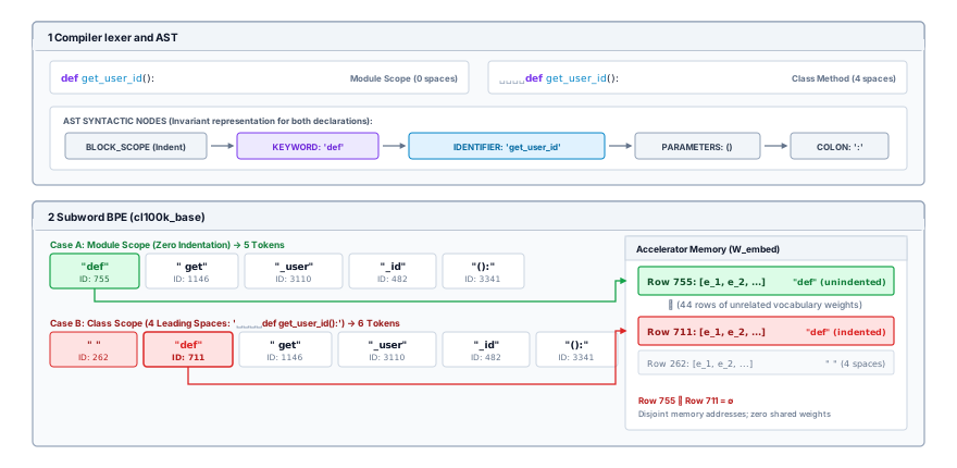
Indentation alone alters the resulting sequence. Under one widely used byte-pair vocabulary, cl100k_base, for example, the unindented line def get_user_id(): encodes as five tokens beginning with def (identifier 755). Indenting that exact line by four spaces yields six tokens: three leading spaces (262), followed by def with the fourth space fused to the keyword (711), and finally the remaining four tokens. A compiler lexer records indentation as block structure and emits the same keyword token at both levels; the model instead receives a different opening sequence of integer identifiers, with only the four tokens after the keyword shared (figure 2).

Figure 2: One Keyword, Two Token Sequences: The same Python line, unindented and indented by four spaces, drawn on one character grid, with a compiler lexer’s tokens above the characters and a byte-pair tokenizer’s tokens below. The lexer records indentation as block structure and emits the same keyword and identifier for both lines. The tokenizer absorbs the fourth space into the keyword, so the indented line opens with two tokens that do not appear in the unindented one; only the four tokens after the keyword are shared. Identifiers are from the cl100k_base vocabulary.

In an inspection request, the string src/pool.py is a single path argument at the tool interface, yet it splits into several subword tokens at the model interface. Changing a file path, adding indentation, or escaping source code inside JSON shifts token boundaries in ways a fixed character-to-token ratio cannot predict. Neither JSON framing nor punctuation adds a constant fraction of tokens over plain prose, so the runtime must tokenize the exact byte sequence it plans to send.

Wire framing adds further tokens beyond the visible text. Model APIs wrap messages in control tokens that mark roles, turn boundaries, and tool schemas. Counting only the user prompt or tool output misses that wrapper. When the runtime formats the wire payload locally, it must run the model’s own tokenizer over the complete formatted sequence; when a remote service applies its own chat template or hidden system wrapper, the runtime must use the provider’s token-counting endpoint and admission rules. Because vocabularies and merge tables differ across model families, a token count from one model does not carry over to another.

The same count applies to generated output. A compact tool call uses fewer output tokens than a long prose explanation wrapping the same call, though the exact count depends on how the call is serialized. Shorter schemas cut latency and token spend only when they keep the fields the runtime needs; dropping required arguments, file paths, or error variants to save a few tokens makes downstream execution brittle.

2.3.2 Output headroom

A prompt that fits inside the context window can still leave too little room for the model to finish its reply, cutting off a tool call mid-argument. To prevent a long prompt from starving the response, the admission check must reserve output headroom before sending the call. Let \(\SequenceLength\) denote the length of the fully serialized input prompt, \(\ContextWindow\) the total context window (the maximum sequence capacity spanning input and output tokens within a single invocation), and \(\OutputLimit\) the reserved generation allowance. Where input tokens and generated tokens share a unified context budget, an admission check must enforce:

\[\SequenceLength \le \ContextWindow - \OutputLimit \tag{1}\]

This inequality guarantees that an incoming prompt cannot fill the context buffer and leave the model no room to answer. Many services also cap input and output lengths separately alongside the shared window, so the runtime must satisfy both the individual caps and the combined bound. Reasoning models add another wrinkle: they emit intermediate reasoning tokens before the visible answer, and those hidden tokens count against \(\OutputLimit\) even when the caller never sees them. A three-line visible reply can exhaust a generous output allowance if the model spent hundreds of hidden reasoning tokens first.

↪ How reasoning models spend generated tokens on intermediate work, and how the runtime budgets them, is developed in How reasoning models spend output allowances.

Suppose the repair interface has a combined window of 8,192 tokens, and the runtime reserves 1,024 tokens for generation. Its input ceiling is \(\ContextWindow - \OutputLimit = 8,192 - 1,024 = 7,168\) tokens. If the fully serialized request occupies 6,000 tokens, \(7,168 - 6,000 = 1,168\) tokens of room remain for additional input while preserving the response allowance. The limits are scenario values, not a named model’s specification.

If an incoming tool observation exceeds this remaining headroom, the admission check fails. The runtime can then compress prompt history, extract a narrower file slice, or route the call to an execution profile with a larger context window. Shrinking the output allowance \(\OutputLimit\) to force admission is risky, as it leaves the model insufficient room to complete complex tool invocations or structured plans. Similarly, silently truncating tool outputs to squeeze them into the remaining margin can strip away the critical stack trace or diagnostic error that the agent needs to resolve the bug.

Even when a request satisfies admission checks, generation can still hit the output token ceiling mid-stream. The runtime must never confuse a syntactically well-formed prefix with a successfully terminated generation. A truncated JSON object may happen to pass a lenient parser if closed artificially, yet it remains an incomplete execution plan. While a partial payload provides valuable diagnostic telemetry, executing it as an intact tool call can cause downstream corruption. The invocation contract in section 2.5 turns this boundary into an explicit rule that reads the call’s status before its payload.

2.3.3 Counting multimodal inputs

Attaching a screenshot of a failing dashboard or user-interface (UI) render to a repair request can push a prompt that fit in text well past the context limit. A vision front-end maps each image into a sequence of context positions, and although vision transformers slice images into uniform patches (Dosovitskiy et al. 2021), preprocessing steps such as dynamic tiling, resolution scaling, and spatial pooling mean the billed token count rarely equals a simple patch count.

Dosovitskiy, Alexey, Lucas Beyer, Alexander Kolesnikov, Dirk Weissenborn, Xiaohua Zhai, Thomas Unterthiner, Mostafa Dehghani, et al. 2021. “An Image Is Worth 16x16 Words: Transformers for Image Recognition at Scale.” International Conference on Learning Representations (ICLR).

Consider the earlier budget when adding this visual artifact. If the service reports that the image and its framing tokens require an additional 2,048 context positions, the total request demand expands to \(6,000 + 2,048 + 1,024 = 9,072\) tokens. This total exceeds the 8,192-token context window by 880 tokens, triggering an immediate admission failure before dispatch. The runtime must step in before calling the model. Downscaling the image cuts its token count under some vision backends, but heavy compression can blur single-character error codes or fine trace lines. Budgeting multimodal inputs therefore trades visual detail against the context ceiling.

Checkpoint 2.1: Admitting the next repair request

The repair agent is about to add a source excerpt and a diagnostic image to its next call. Its output allowance must remain available for a complete proposal.

• Input budget: Can you identify which message and tool-definition framing must be counted beyond the visible source excerpt?
• Output headroom: With the window fixed at 8,192 tokens and the image added, would halving the output reservation make the request fit? Compute the remaining excess, and state what the smaller reservation risks.
• Generation status: If a returned fragment parses successfully after the output limit is reached, can you explain why it is still not a completed candidate?

Token accounting checks upfront that the full request fits with room reserved for the reply. Admission, however, covers only starting capacity. Once decoding begins, token-by-token autoregressive generation determines how that reserved headroom is spent and whether the call finishes cleanly or stops mid-stream.

2.4 Autoregressive Generation

Even when a request fixes the conversation history and the list of available tool schemas, the model’s reply remains open-ended and stochastic. On the same repair prompt, one call might propose read_file on a configuration path, a second might inspect a different directory, and a third might return prose instead of a tool call. Understanding how the serving engine generates tokens one step at a time explains how to set token budgets and sampling parameters, why repeating a live API call can produce a different trajectory, and why only replaying a recorded response reproduces downstream execution exactly.

2.4.1 Token-by-token generation

When a model emits a file path inside a read_file argument, it chooses each token from learned statistical patterns without checking the filesystem, and that early choice conditions every closing delimiter and reasoning token that follows. Autoregressive language models generate text by factoring the joint probability of a sequence into a product of conditional next-token distributions (Bengio et al. 2003). Let \(\InputTokenSequence\) denote the input tokens and \(\OutputTokenSequence\) an output sequence. Its conditional probability factors as

\[\Pr(\OutputTokenSequence \mid \InputTokenSequence) = \prod_{t=1}^{\OutputLength} \Pr(\OutputToken_t \mid \InputTokenSequence, \OutputTokenPrefix) \tag{2}\]

At output position \(\TokenIndex\), the model with parameters \(\ModelParameters\) produces one score, or logit, for each token in vocabulary \(\TokenVocabulary\):

\[\LogitVector_t = \NextTokenLogitFunction(\InputTokenSequence, \OutputTokenPrefix) \in \mathbb{R}^{|\TokenVocabulary|}\]

A decoding rule selects a token from these scores and appends it to the prefix for position \(\TokenIndex+1\), so early token choices cascade through the rest of the sequence. In an inference serving engine, the decode loop reads the prompt, computes next-token logits, picks an output token, appends it to the prefix, and repeats until a stop condition fires. Generation ends normally when the model emits an end-of-sequence token or matches a caller-supplied stop sequence. It can also stop early at the output token ceiling, or abort on a timeout or network drop. Serving interfaces must report which stop condition fired: an incomplete JSON object cut off at the token limit needs different handling than a finished tool call, and even a clean stop sequence says only that generation ended, not that the task succeeded.

Production Transformer implementations (Vaswani et al. 2017) avoid recomputing earlier tokens at every decode step by keeping a key-value (KV) cache:³ memory buffers holding the attention keys and values already computed for earlier positions. For a given full-attention architecture and precision, keeping more tokens in flight takes more cache memory. That cache is transient serving state, not an audit log of which tools ran or what they changed. KV Cache Management covers cache layout and sizing; for a single call, the key point is that both prompt tokens and generated tokens occupy memory during the call.

³ Key-Value (KV) Cache: In causal attention, key and value vectors at a given position depend solely on that token and its predecessors, so once computed they remain static throughout subsequent sequence expansion. Retaining them in device memory turns each new decode step from full-sequence recomputation into a single new row projection per layer alongside a read of stored rows. Consequently, cache capacity and memory bandwidth, rather than floating-point arithmetic, become the primary operational constraints as context windows expand.

⁴ Speculative Decoding: The target distribution is preserved by a modified rejection-sampling rule that accepts each drafted token with exactly the probability needed for the accepted sequence to follow the target model’s distribution (Leviathan et al. 2023; Chen et al. 2023). The guarantee is distributional, not bitwise. Speculative decoding reduces accelerator passes per generated token without changing which candidates can appear, so it leaves the reproducibility questions of section 2.4.3 unchanged.

Leviathan, Yaniv, Matan Kalman, and Yossi Matias. 2023. “Fast Inference from Transformers via Speculative Decoding.” Proceedings of the 40th International Conference on Machine Learning 202: 19274–86.

Chen, C., S. Borgeaud, G. Irving, J.-B. Lespiau, L. Sifre, and J. Jumper. 2023. “Accelerating Large Language Model Decoding with Speculative Sampling.” arXiv Preprint arXiv:2302.01318.

Because each generated token extends a dependent sequence, output length is a major cost variable of a call, and the serving implementation sets its realized latency. Although the conditional dependence in equation 2 fixes the mathematical order of token choices, it does not mandate that hardware evaluate each token in an isolated forward pass. Techniques such as speculative decoding,⁴ for example, draft candidate token blocks with a small auxiliary model and score them in parallel with the target model, provably preserving the target output distribution (Leviathan et al. 2023; Chen et al. 2023). The per-token decode floor derived in section 2.8 is therefore a property of plain one-token-per-pass decoding, not a law of the factorization.

2.4.2 Sampling controls

Lowering sampling randomness can make a model repeat its top-scoring token choice, yet the highest-scoring token is often a plausible guess rather than a valid file path or a working patch. For positive temperature⁵ \(\SamplingTemperature\) (subscripted to keep it distinct from the trajectory \(\Trajectory\)), softmax converts the logits into next-token probabilities:

⁵ Temperature: The term comes from statistical mechanics, where the Boltzmann distribution weights a state of energy \(\BoltzmannStateEnergy\) by \(\exp(-\BoltzmannStateEnergy/\BoltzmannConstant \BoltzmannTemperature)\); reading each negative logit as an energy makes equation 3 identical in form. In a physical system, high temperature spreads particles across many states, whereas low temperature concentrates them near the ground state. In language model decoding, scaling temperature trades candidate diversity against concentration on the mode without changing which token scores highest.

\[\Pr(\OutputToken_t = \VocabularyToken \mid \InputTokenSequence, \OutputTokenPrefix) = \frac{\exp\left(\OutputLogit_{t, \VocabularyToken} / \SamplingTemperature\right)}{\sum_{\NormalizerTokenIndex \in \TokenVocabulary} \exp\left(\OutputLogit_{t, \NormalizerTokenIndex} / \SamplingTemperature\right)} \tag{3}\]

Unit temperature (\(\SamplingTemperature = 1.0\)) leaves the logits unscaled. Lowering a positive temperature amplifies logit differences and concentrates probability mass on the highest-scoring tokens; raising it flattens the distribution, which approaches uniformity across a finite vocabulary as temperature grows without bound. Temperature therefore controls output entropy, not model confidence: because next-token cross-entropy training minimizes sequence prediction error rather than calibrating scores to task success, high token probability does not mean a completed response is correct.

Greedy decoding instead picks a highest-scoring token, \(\operatorname{argmax}_{\VocabularyToken \in \TokenVocabulary} \OutputLogit_{t, \VocabularyToken}\), with a tie-breaking rule. Given fixed logits and a fixed tie rule, that choice is deterministic. Serving APIs often expose greedy decoding as \(\SamplingTemperature = 0\), which the engine implements by taking the argmax directly rather than dividing by zero in equation 3. As positive temperature approaches zero, softmax puts all probability mass on the maximum, though if several tokens tie for the top logit, the limit alone does not pick among them.

Sampling can also restrict which tokens remain eligible. Top-\(\TopTokenSampleCount\) sampling (Fan et al. 2018) keeps the \(\TopTokenSampleCount\) highest-scoring tokens under a tie rule and renormalizes their probabilities. Top-\(\NucleusProbabilityMass\) sampling, or nucleus sampling, sorts tokens by descending probability, keeps the shortest prefix whose cumulative mass reaches \(\NucleusProbabilityMass\) (Holtzman et al. 2020), and renormalizes that set. Because top-\(\TopTokenSampleCount\) fixes the candidate count regardless of shape, it can keep unlikely tail tokens when the distribution is sharp and cut plausible options when the distribution is flat; top-\(\NucleusProbabilityMass\) lets the active pool expand or shrink with the distribution’s spread. When temperature scaling and truncation are used together, the order in which they run and the engine’s numerical conventions are part of the decoding configuration.

Neither filter tells valid file paths, true claims, or safe commands from wrong ones. A rare token may be the exact identifier a patch needs, while a high-probability continuation may name a file that does not exist. Truncation filters change which candidates reach the runtime; only checks against the environment and task contract tell whether that change helps.

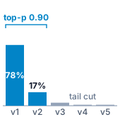
Nucleus truncation keeps the two tokens whose mass reaches 0.90 and zeroes the gray tail.

Napkin Math 2.1: Temperature and truncation on the same logits

Problem: A hypothetical vocabulary \(\TokenVocabulary = \{\VocabularyToken_1, \VocabularyToken_2, \VocabularyToken_3, \VocabularyToken_4, \VocabularyToken_5\}\) has logits \(\LogitVector_t = [12, 10.5, 9, 6, 3]\), held fixed so that differences arise strictly from the decoding configuration. How much probability mass concentrates onto the top token when halving the temperature, and which tokens survive nucleus truncation?

Math: At temperature \(\SamplingTemperature =\) 1, the exponentiated logits sum to 207596.9. Normalizing each exponential by this partition sum yields the baseline distribution:

\(\UnitTemperatureProbabilityVector \approx [0.7840, 0.1749, 0.0390, 0.0019, 0.0001]\).

Halving the temperature to \(\SamplingTemperature =\) 0.5 doubles the exponent of each term. Following normalization, the probability of the mode \(\VocabularyToken_1\) rises to 0.9503, capturing 95.0 percent of the total distribution. All lower-ranked tokens retain positive probability under untruncated softmax.

Returning to unit temperature and applying nucleus truncation with \(\NucleusProbabilityMass =\) 0.90 evaluates cumulative probability mass. The lead token \(\VocabularyToken_1\) provides 0.7840, which falls short of the threshold. Incorporating \(\VocabularyToken_2\) (0.1749) brings cumulative coverage to 0.9589, which satisfies the threshold and defines the active nucleus as \(\{\VocabularyToken_1, \VocabularyToken_2\}\). Renormalizing across this active set assigns probability 0.8176 to \(\VocabularyToken_1\) and 0.1824 to \(\VocabularyToken_2\), while strictly zeroing the remaining tail tokens \(\{\VocabularyToken_3, \VocabularyToken_4, \VocabularyToken_5\}\).

Systems insight: Temperature governs candidate diversity. Halving temperature compresses the non-top probability tail from 21.6 percent to 5.0 percent, achieving a 4.3× reduction, whereas nucleus truncation eliminates the tail entirely. Repeated calls produce diverse outputs only when probability mass occupies this tail, which is the stochastic resource that parallel candidate sampling draws on in Parallel sampling along the breadth axis. Because neither transformation ensures that the highest-scoring candidate is correct, engineering teams configure decoding parameters based on empirical task pass rates rather than raw model likelihood.

2.4.3 Repetition and replay

Greedy decoding removes sampling variance from a fixed logit vector, but it does not make served API calls reproducible end to end. In a production cluster, two identical requests can land on different server nodes, accelerator revisions, or kernel builds. Small differences in floating-point reduction order⁶ can shift nearly tied logits in their least significant bits, and flipping an argmax choice at position \(\TokenIndex=1\) changes the prefix for every token after it. Fixing a pseudorandom seed controls the sampler’s random number generator, but it cannot prevent numerical differences across backend kernels or dynamic batch sizes. Reproducing a call from scratch requires pinning the serving environment and kernels, not just setting \(\SamplingTemperature = 0\). A 2025 production incident shows how serving-fleet bugs alone can change model outputs while caller requests stay identical.

⁶ Floating-Point Reduction Order: Floating-point addition is not associative because each intermediate sum rounds (Goldberg 1991). Parallel attention and reduction kernels that sum dot products across different thread-block layouts or dynamic batch sizes add numbers in different orders, so the same request can produce logits that differ in their low bits depending on which other requests share its batch.

Goldberg, David. 1991. “What Every Computer Scientist Should Know about Floating-Point Arithmetic.” ACM Computing Surveys 23 (1): 5–48. https://doi.org/10.1145/103162.103163.

War Story 2.1: Three serving bugs behind unchanged requests (2025)

Context: Between August and early September 2025, three separate infrastructure bugs intermittently degraded the responses of Anthropic’s Claude models (Anthropic 2025). These defects stemmed entirely from the serving infrastructure rather than caller requests or model weights.

Mechanism: A front-end routing defect directed standard traffic to server clusters configured for extended context windows, while session stickiness (routing a client’s follow-up requests to the server that handled its earlier ones) kept those follow-up requests on the misconfigured nodes. Concurrently, an improperly deployed kernel optimization on a specialized accelerator cluster occasionally assigned outsized probability to improbable tokens. Finally, an optimization in the token-selection pipeline triggered a compiler bug: an approximate top-\(\TopTokenSampleCount\) routine with mixed-precision subroutines emitted incorrect tokens under specific dynamic batch sizes.

Impact: During peak impact, the routing failure corrupted 16 percent of requests to one production model, and approximately 30 percent of active coding agent users encountered at least one misrouted interaction. Generated responses contained foreign-language script insertions within English prose and syntax anomalies in generated source code. Automated regression suites initially missed these failures because a response often recovered from an isolated corrupted token later in generation, and intermittent runtime conditions meant an identical prompt could succeed on one invocation and fail on the next.

Fix: Engineers rolled back the offending kernel deployments, corrected cluster routing rules, and replaced the approximate top-\(\TopTokenSampleCount\) kernel with an exact selection routine running in 32-bit floating-point precision, trading a minor throughput penalty for numerical stability. Anthropic subsequently deployed continuous canary evaluations across production fleets to catch subtle generational drift.

Systems lesson: Output distributions reflect the concrete serving pipeline just as heavily as the model weights or input context. Corrupted tokens arrived packaged in well-formed HTTP payloads and cleanly closed generation blocks, a direct instance of the fail-plausible fault (The fail-plausible fault). Agent runtimes must log full call-level metadata (runtime versions, routing tags, and sampling parameters) while subjecting every proposed action to external environment validation regardless of nominal generation success.

Anthropic. 2025. A Postmortem of Three Recent Issues. Anthropic engineering incident report.

Incidents like this one set the logging baseline for an agent runtime. The runtime log should record the serialized prompt, model and tokenizer identifiers, sampling settings, token limits, and any routing or seed metadata, alongside the raw response payload, stop reason, and token usage. Those records also separate two kinds of debugging: replaying a recorded response tests the runtime’s downstream logic without model variance, whereas re-sending the live request tests how the agent handles variation across calls. Benchmarks should measure and report that call-to-call variance rather than judging a configuration from a single run.

An agent runtime therefore receives candidate tokens produced under a specific decoding configuration and ended by a specific stop condition. That stop condition is the first thing the runtime must read. A generation that ran into its output ceiling, was refused, or was cut off in transit can still deliver bytes that look like a finished proposal, and no check on the payload alone tells the difference. Before asking whether a read_file proposal names an existing, permitted path, the runtime needs a record of whether a complete candidate arrived at all.

2.5 The Invocation Contract

Suppose a model begins generating a cleanup command targeting the path /tmp/scratch/cache_dir, but reaches its token limit immediately after emitting /tmp/scratch. Both strings form syntactically valid shell commands, yet they specify different deletion boundaries. An execution engine inspecting only raw text cannot determine whether the shorter path represents an intended command or a truncated prefix. To prevent an unintended deletion, the host runtime requires an explicit execution outcome alongside the payload, pairing each request specification with a normalized response envelope at the invocation boundary so that every remote generation is governed by a unified contract.

Definition 2.2: Model invocation contract

Model invocation contract is the pair of records that bounds one model call: a request fixing the input, model configuration, sampling settings, and enforced output and time limits, and a normalized envelope reporting the call’s status, payload, and resource use.

1. Significance: The contract establishes each model call as a distinct, countable unit within an agent trajectory. Its usage record prices the call’s share of \(\AttemptCost\), and its status flag isolates completed generations from partial or failed calls. Consequently, the cost per accepted task (equation 1.2) can be computed from recorded telemetry rather than heuristically reconstructed from conversation transcripts.
2. Distinction: The invocation contract describes the model call rather than the overarching task. A generated tool request can fully conform to decoding limits without ever being dispatched, and a fully generated response can fail downstream validation. Dispatch authorization, tool execution, and task-level acceptance remain separate runtime decisions backed by their own evidence.
3. Common pitfall: Recording only the payload text. Without explicit status flags and usage accounting, a truncated fragment is indistinguishable from an intentional short response, and unrecorded token consumption silently distorts operational cost accounting as zero-cost execution.

2.5.1 What a request specifies

Leaving any part of a model request implicit—an unpinned model alias that silently updates, an unenforced token cap, or an unrecorded sampling setting—makes it impossible to price the call or explain why its behavior changed. At the generation interface, the bounded request fixes six fields:

\[\ModelCallRequest = \langle \RequestPromptTokens, \text{ModelID}, \OutputLimit, \CompletionDeadline, \StopSequenceSet, \SamplingParameters \rangle\]

The first field, \(\RequestPromptTokens = (\PromptToken_1, \PromptToken_2, \dots, \PromptToken_{\SequenceLength})\), encodes the serialized messages, role markers, advertised tool schemas, and formatting delimiters visible to the model, which the runtime builds from structured messages and tools inputs before serialization. Once the input sequence is fixed, ModelID and \(\SamplingParameters\) specify how the serving stack evaluates it. ModelID names the model weights and serving deployment selected through model_config, where engineers distinguish mutable provider aliases (such as model-latest) from pinned, immutable revisions (such as dated or content-addressed snapshots). The sampling parameters \(\SamplingParameters\), including temperature and top-\(\NucleusProbabilityMass\), then fix the selection rule used during decoding. Together with the serialized input and returned output, those fields document the call; exact regeneration also depends on the serving path, as war story 2.1 showed.

To bound how long that generation may run, the request pairs an output allowance \(\OutputLimit\) with a local waiting deadline \(\CompletionDeadline\). Because a system cannot rely on the model to stop on time, invariant closure (principle 1) places both limits below the model, where the host runtime and serving system enforce them mechanically. Before sending the call, the runtime checks that the prompt and output allowance fit inside the context window, and the adapter notes whether the provider bills hidden reasoning tokens against \(\OutputLimit\), since counting only visible text would understate what the call spent.

Generation can also end before reaching \(\OutputLimit\) when the output matches one of the stop sequences in \(\StopSequenceSet\), which halt decoding as soon as the serving engine encounters them. Because the engine matches raw byte or character sequences without parsing structure, a stop sequence that appears inside an argument or quoted string can cut off generation before the closing quotes or braces are emitted. The runtime must therefore record the provider’s stop reason and validate syntax separately.

Resource limits are enforced in two places: on the client host and on the remote serving cluster. Locally, the host runtime caps incoming response bytes and stops waiting when the deadline \(\CompletionDeadline\) expires. A local timeout ends the caller’s wait and marks the call failed, but it does not prove that the remote server stopped decoding or freed accelerator memory.⁷ Server-side token caps and cancellation protocols handle the remote side, so every limit should state which component enforces it and which resource it bounds.

⁷ Remote Call Semantics: Remote procedure call designers met this ambiguity first. In the design Birrell and Nelson (1984) describe, a call that returns normally executed exactly once, but a call that ends in a failure report may have executed once or not at all, because the caller cannot tell a lost request from a lost reply. A model call inherits the same gap: a timed-out generation may still have run to completion and been billed, which is why the normalized status for a failed delivery, TRANSPORT_FAILURE (table 2), records an unknown remote outcome rather than a call that never happened.

Birrell, Andrew D., and Bruce Jay Nelson. 1984. “Implementing Remote Procedure Calls.” ACM Transactions on Computer Systems 2 (1): 39–59. https://doi.org/10.1145/2080.357392.

2.5.2 The normalized status envelope

If a runtime inspects only the returned text or tool arguments, a partial string cut off by a token ceiling looks just like a finished proposal. To keep how a call ended attached to what it returned, the runtime wraps every response in a normalized status envelope:

\[\NormalizedStatusEnvelope = \langle \text{status}, \ResponsePayload, \ResponseMetadata \rangle\]

Here, \(\ResponsePayload\) is the returned payload, which may be complete, partial, or empty, and \(\ResponseMetadata\) holds the call’s telemetry: the response kind, the raw provider stop_reason, reported token usage, request identifiers, latency timestamps, and serving settings. Keeping \(\ResponsePayload\) paired with \(\ResponseMetadata\) prevents downstream code from reading the payload without its status, and records unreported usage as unknown rather than zero.

Because different model APIs report stop reasons, error codes, and transport failures in incompatible ways, the runtime adapter maps provider-specific signals onto the seven normalized statuses in table 2. Two of them, REJECTED and CANCELED, occur only while a response is streaming (section 2.5.3). Each status records what the host runtime verified locally; if two events race, such as a local cancellation crossing an incoming completion frame, the adapter resolves the status deterministically while keeping the raw provider signals in \(\ResponseMetadata\).

Table 2: Normalized invocation status envelope: Status controls admission to the candidate path. Completion is a generation outcome, while authorization, tool execution, and task acceptance remain separate decisions.

Status flag	Terminal condition	Payload integrity	Admissible host action
COMPLETED	Confirmed normal generation termination within the call’s limits	Fully generated according to the protocol; syntax and meaning remain unchecked	Admit to candidate validation, not directly to dispatch
TRUNCATED	Generation reaches a token or context ceiling before confirmed normal completion	Incomplete candidate that may nevertheless parse	Withhold from action; record the limit and diagnose
REFUSED	The model or service explicitly declines the request or response	Refusal notice, partial content, or no payload	Handle under the task’s refusal policy; do not treat as an action
TRANSPORT_FAILURE	Delivery fails or the local deadline expires without accepted completion	Missing or partial content; remote outcome may be unknown	Record uncertainty and apply bounded failure handling
REJECTED	A runtime monitor rejects the response during reception	Content observed before rejection	Withhold from action; record the rejection and request cancellation
CANCELED	Discretionary runtime or operator cancellation before accepted completion	Partial, missing, or otherwise unusable as a completed candidate	Stop local candidate processing; track remote termination separately
FAULTED	The service reports an execution failure	Missing, partial, or diagnostic content	Record the reported fault and route to failure handling

For a read_file request, kind="tool_request" tells the runtime which schema to check, while status="COMPLETED" confirms that generation finished normally. Neither field says that the tool ran or that the file read succeeded; completion describes generation, whereas tool execution and task acceptance are separate runtime decisions.

Applying invariant closure (principle 1) to the status field gives a hard gate: the quarantining rule. Under this rule, no payload whose status is anything other than COMPLETED may enter the candidate validation or tool-dispatch path. The runtime checks status before parsing or dispatching the payload. It can log an interrupted or malformed fragment for diagnosis, but that log entry cannot trigger a tool call or be promoted to a finished proposal. When later chapters sample several candidates for one task, any candidate cut off by a token limit obeys the same rule: a truncated payload is a diagnosable failure, never a partial action.

The cleanup command introduced earlier shows why parsing alone cannot replace this status check. Suppose the complete intended command is

rm -rf /tmp/scratch/cache_dir

If an exhausted token quota cuts off generation mid-path, the prefix is

rm -rf /tmp/scratch

That truncated prefix is valid shell syntax, yet it deletes the entire parent directory. Because the envelope marks the call TRUNCATED, the quarantining rule blocks the command before it reaches the shell. Conversely, status="COMPLETED" grants no permission to run; it establishes only that the model finished emitting its proposal. Listing 3 implements this admission check, passing only completed generations to the candidate path while leaving syntax, permissions, and task verification to later stages.

Listing 3: Completed-candidate admission: The status check admits only completed generations to the candidate path. Returning the payload grants no execution authority.

def completed_candidate(envelope):
    if envelope["status"] != "COMPLETED":
        raise ValueError("Response is not a completed candidate")
    # Syntax, permission, and task evidence remain unchecked.
    return envelope["payload"]

Incomplete payloads go to a diagnostic log with its own storage and access limits, keeping the partial byte stream and stop_reason for debugging. “Repairing” a truncated fragment by appending guessed arguments or closing braces invents a new candidate that the model never completed, and such patched fragments must never be marked COMPLETED.

2.5.3 Streaming and cancellation

Waiting for a four-thousand-token response to finish before checking its structure wastes seconds of accelerator time when the very first key violates the tool schema. Streaming delivers response fragments over the connection as generation proceeds, letting the runtime inspect prefixes early—provided its parser follows the provider’s framing protocol rather than assuming each network chunk holds one token. When an arriving prefix violates the required format, the stream monitor stops waiting immediately instead of buffering the rest of an unusable reply. Because generation is still in flight, the monitor checks whether the prefix can still be completed into a valid structure, not whether it is already complete.

Rejection and cancellation are distinct events. When the stream monitor spots a structural violation, the runtime sets the status to REJECTED and sends a cancel request to the service. When an operator or runtime policy aborts a compliant stream before completion, the runtime marks the status CANCELED. A local deadline that expires before completion maps instead to TRANSPORT_FAILURE (table 2), after which the runtime may also send a cancel request. Keeping the partial payload out of tool dispatch is a local guarantee the host enforces in all three cases. Stopping the remote decode loop and freeing accelerator memory, however, depends on the serving engine honoring the cancel signal; merely closing a client socket does not prove that remote decoding stopped.

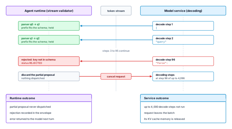
Consider a call with an output allowance of 4,096 tokens whose stream validator detects a schema violation at step \(\RejectionDecodeStep =\) 96. The runtime’s part of the response finishes at once. It records the rejection, discards the partial proposal, and sends a cancel request. The service’s part depends on whether that request is honored (figure 3).

Figure 3: Reject, Then Cancel: The runtime’s stream validator advances a parser state as each prefix arrives and holds the output rather than acting on it. At step 96 the proposal introduces a key outside the schema, so the runtime records a rejection, discards the partial proposal, and sends a cancel request. The runtime outcomes on the left hold regardless of the service; the service outcomes on the right hold only if the service receives and honors the cancel request.

The skipped-step count shown is an upper bound that requires provider cooperation. If the serving engine processes the cancellation promptly, it skips up to \(\OutputLimit - \RejectionDecodeStep =\) 4,000 autoregressive decode steps. In the reference unbatched deployment, each plain autoregressive decode step reads the model weights from accelerator memory, so the step takes at least the weight bytes divided by the memory bandwidth; for the reference deployment of section 2.8, that floor is 21.075 ms per generated token. At that reference floor, skipping all these steps avoids 84.3 s of estimated decode work. An honored cancellation also frees the request’s slot among the requests the serving engine decodes together and releases the call’s KV-cache allocations. If the remote service fails to honor the cancellation, the host runtime still quarantines the rejected payload locally, but the remote service may continue generating up to its token allowance.

Nonstreaming calls apply the same status gate once the whole response arrives. Streaming simply moves the check earlier in the call so the runtime can reject bad prefixes and reclaim resources sooner, without relaxing the rule that incomplete prefixes never run. Either way, the status gate settles only whether a complete candidate arrived. A COMPLETED read_file proposal can still name a missing file or a path outside the workspace, so the next question is what each subsequent check on that candidate actually proves.

2.6 Checking Candidate Outputs

Suppose the status gate has admitted a completed read_file proposal with path set to src/pool.py. Completion says only that generation finished, and, as the validation and authorization stages in section 2.2.2 showed, schema conformance says nothing about whether the file exists or lies inside the workspace. Generative inference produces a candidate token sequence; neither high statistical likelihood nor schema conformance determines whether the runtime environment can safely act on it.

The same distinction applies when the model emits a source code patch rather than an inspection request. A candidate patch can parse cleanly, compile against existing headers, and pass a sequential unit test while leaving the underlying race condition untouched. Each verification check answers a narrow, specific question rather than certifying overall task satisfaction. Candidate verification must track these separate kinds of evidence explicitly rather than collapsing them into a single notion of validity.

2.6.1 Why token likelihood cannot replace checks

A model often assigns high probability to an obsolete or nonexistent file path simply because that path matches common directory naming patterns in its training corpus. Autoregressive generation scores tokens by how well they fit training data and prompt context, not by whether a path exists on disk, whether the caller has permission to read it, or whether an edited function preserves a lock invariant.

Checking a candidate therefore means pairing each required property with the tool or gate that actually tests it. For a read_file proposal, a schema validator checks that the payload has only allowed keys and a string-valued path. Passing that check proves schema conformance—provided the validator implements the schema dialect faithfully and inspects the exact object passed to execution. Proving that the target file exists requires checking the filesystem, and proving permission requires checking the task’s capability grant against the host policy.

Static checks and dynamic tests likewise establish different claims. A compiler checks types and syntax under fixed flags, while a linter flags suspect patterns with static rules. Dynamic tests run concrete code paths and check runtime assertions, so a passing single-threaded checkout test says nothing about how the connection pool behaves under concurrent contention.

↩︎ The closure evidence levels, from self-report and static checks through visible and sealed tests to formal proof, are established in The invariant closure principle.

⁸ Complete Mediation: One of the design principles that Saltzer and Schroeder (1975) set out for protection systems: every access to every object is checked against current authority at the moment of access, not remembered from an earlier decision. The tool handler applies the same rule to a model’s proposal, so a path validated when the request was composed is checked again when the read executes, closing the gap in which the grant or the file could have changed.

Saltzer, J. H., and M. D. Schroeder. 1975. “The Protection of Information in Computer Systems.” Proceedings of the IEEE 63 (9): 1278–308. https://doi.org/10.1109/proc.1975.9939.

Because each check covers only its own scope, the runtime must treat model output as untrusted data rather than executable control flow. A candidate tool call stays passive data until an authorized tool handler validates and dispatches it, checking permissions at the moment of access⁸ regardless of what the model claims about its own rights. Running an untrusted code patch likewise executes arbitrary machine instructions and belongs inside an isolated sandbox even during early test runs.

2.6.2 Self-review and external evidence

Asking a model to review or refine its own patch can catch surface syntax mistakes or missing edge cases, yet self-review is just another generation step drawn from the same weights and conditioned on the same incomplete context. When the model starts from a mistaken assumption about an API or lock protocol, prompting it to critique its own answer usually repeats that assumption rather than catching it. Re-prompting does not create an independent check: across reasoning benchmarks, models asked to grade and revise their own answers without new external evidence rarely improve accuracy and often turn right answers into wrong ones (Huang et al. 2024).

Huang, Jie, Xinyun Chen, Swaroop Mishra, Huaixiu Steven Zheng, Adams Wei Yu, Xinying Song, and Denny Zhou. 2024. “Large Language Models Cannot Self-Correct Reasoning Yet.” International Conference on Learning Representations (ICLR).

Zheng, Lianmin, Wei-Lin Chiang, Ying Sheng, Siyuan Zhuang, Hao Wu, Yonghao Zhuang, Zi Lin, et al. 2023. “Judging LLM-as-a-Judge with MT-Bench and Chatbot Arena.” Advances in Neural Information Processing Systems (NeurIPS) 36: 46595–623.

Refining a candidate and certifying a property must therefore stay separate. A model’s critique can guide the next search step, but external tools (compilers, linters, sandboxed test runners, and kernel permission checks) must supply the evidence for the properties they test. No model critique—whether from the generator itself or from a separate learned judge (a second model prompted or trained to score the first model’s output)—carries authority to clear a security boundary or approve a release. When a pipeline uses a learned judge to rank or filter candidates, the runtime should treat its verdicts as noisy scores with measurable false-accept rates and known biases, such as favoring longer answers or particular list positions (Zheng et al. 2023). Even when a check returns a passing verdict, a conditional-probability calculation shows how much defect risk remains when the checker itself can pass a defective patch.

Systems Perspective 2.1: What a passing verdict leaves unresolved

Let \(\CandidateDefectRate\) denote the defect rate, the share of generated patches that violate a specified behavioral property (a local symbol here, distinct from the per-turn error rate of horizon compounding), and let \(\VerifierFalseAcceptanceRate\) denote the checker’s false-accept rate, the probability that it passes a defective patch. Suppose \(\CandidateDefectRate =\) 18 percent, \(\VerifierFalseAcceptanceRate =\) 0.65, and the checker passes valid patches with probability 0.85. Bayes’ rule gives the fraction of defective patches among the passing results:

\[\Pr(\text{Defective} \mid \text{PASS}) = \frac{\VerifierFalseAcceptanceRate \cdot \CandidateDefectRate}{\VerifierFalseAcceptanceRate \cdot \CandidateDefectRate + \Pr(\text{PASS} \mid \text{Valid}) \cdot (1 - \CandidateDefectRate)} \tag{4}\]

Substituting the assumed rates gives \(\frac{0.65 \times 0.18}{(0.65 \times 0.18) + (0.85 \times (1 - 0.18))}\approx 14.37\%\). The defect share among passing patches falls only from 18 percent to 14.37 percent, because the checker rejects 35 percent of defective patches while also rejecting 15 percent of valid ones. The lever is \(\VerifierFalseAcceptanceRate\): a checker with half the false-accept rate, 0.325, lowers the residual to 7.7 percent. Repeating the same check buys no such guarantee, because its behavior on the surviving candidates is correlated with the first pass. Every defective patch that passes also inflates the apparent acceptance probability \(\AcceptanceProbability\) in the cost per accepted task (equation 1.2).

A sound checker for the exact property drives \(\VerifierFalseAcceptanceRate\) to zero under its assumptions. Determinism alone does not supply soundness, and soundness for schema membership does not extend to patch behavior. The residual in equation 4 is one minus the precision \(\VerifierPrecision\) of a passing verdict in the verification asymmetry (principle 3), written there with valid-candidate rate \(\ValidCandidateRate = 1 - \CandidateDefectRate\) and false-reject rate \(\VerifierFalseRejectionRate = 1 - \Pr(\text{PASS} \mid \text{Valid})\). That principle holds that producing a candidate, selecting it, and establishing that it satisfies the task are different events, and it yields a design rule. Select each validation gate for the specific property it establishes and its false-accept rate, and let the task contract determine what residual defect rate the system can tolerate.

2.6.3 Staging checks by cost and scope

Running full end-to-end integration tests or sandboxed reproduction scripts on every model output is orders of magnitude more expensive than parsing JSON or running a static linter. The runtime therefore stages candidate checks from cheapest to most expensive, rejecting malformed or unauthorized requests early before spending compute on behavioral tests. Ordering checks by cost improves throughput, yet each gate tests a different property rather than a tighter approximation of overall correctness. Table 3 lists these four layers along with what each costs and what its passing result leaves open.

Table 3: Scoped candidate checks: A passing result supports a named claim, not every property needed for task acceptance. The runtime preserves these distinctions when composing the checks.

Verification layer	Gate mechanism	Property or evidence	Cost to account for	Limit of the claim
Syntax and schema	Parser and schema validator	Required fields, supported types, and declared value constraints	Parsing and validation	Does not establish permission or correct values beyond the schema
Authorization	Task permission check and enforcing tool handler	Requested operation and target fall within the current grant	Policy lookup and mediation	Permission does not establish that the operation serves the goal
Static analysis	Compiler, type checker, or linter	Properties covered by the selected analysis and configuration	Analysis of the candidate and its dependencies	Coverage depends on the checker and language assumptions
Behavioral evaluation	Controlled execution and designated tests	Observed outcomes for the exercised inputs and conditions	Environment preparation and execution	Passing cases do not establish untested behavior

Consider how this pipeline handles an inspection request versus a patch. Behind the status gate of section 2.5, a read_file proposal needs only the first two rows of table 3 before dispatch, because reading the file supplies an observation for the next turn rather than finishing the repair. When evaluating a proposed patch, by contrast, the pipeline checks patch syntax and target paths, applies the diff in an isolated scratch workspace, and runs the required unit and stress tests. Final acceptance follows the task contract’s evidence standard, escalating to human review when automated checks cannot settle safety or correctness.

The verification cascade inspects output the model has already generated. A streaming monitor can reject an invalid prefix before the response finishes, but the offending token has already been emitted, and recovering still costs a fresh call. When the required output structure is known before the call, the syntax constraint can move inside generation and prevent the malformed token instead of rejecting it after emission.

2.7 Grammar-Guided Decoding

Consider a software repair agent attempting to inspect an unfamiliar module by calling read_file(path) with argument "src/pool.py". If the model’s generated text omits the closing quotation mark before emitting an end-of-turn token, the runtime parser encounters malformed JSON and rejects the payload before dispatching the call. That parser check shields the execution boundary from syntactic corruption, yet resolving the failure demands another full call: queueing, prefill, and every decode step again, with a fresh chance of a different error. When the system knows the target output structure ahead of time, the inference engine can instead remove the tokens that would violate the required syntax during generation, so the defect never reaches the tool boundary.

Definition 2.3: Grammar-constrained decoding

Grammar-constrained decoding restricts next-token selection during autoregressive generation to tokens whose decoded text preserves a viable prefix of a target formal grammar.

1. Significance: Dynamic token masking guarantees that any completed generation sequence strictly satisfies the structural grammar, eliminating syntax errors at the model boundary when the constraint parser covers the target schema.
2. Distinction: Post-generation validation inspects an already emitted sequence and discards invalid payloads after full generation. Constrained decoding actively shapes the vocabulary distribution at every generation step. Even so, neither approach verifies whether a syntactically correct payload contains sensible parameter values or possesses valid execution permissions.
3. Common pitfall: Mistaking a viable prefix for a completed data structure. If token limits, request timeouts, or connection failures truncate generation early, the emitted sequence remains an unfinished prefix that cannot be safely dispatched.

2.7.1 Legal prefixes and completed structures

If a model emits an unquoted identifier or a stray comma after {"path":, the entire JSON payload breaks and no later token can repair it. To block illegal tokens before they are sampled, the constraint engine keeps a running parse state synchronized with the sequence generated so far. For a schema expecting a string-valued path parameter, once {"path": appears in the buffer, the grammar allows optional whitespace followed by an opening quotation mark, and forbids unquoted booleans, numbers, or bare identifiers. When the generator emits {"path":"src/, the text is a viable prefix:⁹ although incomplete as a JSON document, it can still be completed into a valid object by later string and delimiter tokens. Constrained decoding admits a candidate token only if it can extend the current prefix toward an accepting grammar state.

⁹ Legal (Viable) Prefix: The viable-prefix concept comes from classical compiler theory. The LR parsers introduced by Knuth (1965) read input strings left to right and report an error at the first symbol that cannot extend the prefix into any valid sentence of the language. A grammar mask applies the same property constructively, pruning invalid tokens from the vocabulary before sampling instead of catching syntax errors after generation finishes.

Knuth, Donald E. 1965. “On the Translation of Languages from Left to Right.” Information and Control 8 (6): 607–39. https://doi.org/10.1016/S0019-9958(65)90426-2.

At generation step \(\TokenIndex\), let \(\DecodingConstraintState_t\) represent the parser’s internal state, including nested scope tracking for recursive structures. Let \(\ValidTokenSet(\DecodingConstraintState_t)\) denote the set of vocabulary tokens whose decoded strings maintain a viable prefix under the target grammar. Because modern language models operate on subword tokens rather than individual characters, a single token can span multiple characters, punctuation marks, or whitespace segments (for example, a single token .py"} that finishes the extension, closes the string, and closes the object). The engine must therefore simulate the parser across the token’s full decoded byte sequence to confirm that every character transition is valid.

For each token index \(\MaskTokenIndex\) in vocabulary \(\TokenVocabulary\), the constraint engine constructs an additive logit mask:

\[\LogitMaskEntry_i(\DecodingConstraintState_t) = \begin{cases} 0 & \text{if } \MaskTokenIndex \in \ValidTokenSet(\DecodingConstraintState_t) \\ -\infty & \text{if } \MaskTokenIndex \notin \ValidTokenSet(\DecodingConstraintState_t) \end{cases}\]

Adding this mask to the unnormalized logit vector \(\LogitVector_t\) produces the filtered logit vector \(\MaskedLogitVector_t = \LogitVector_t + \LogitMask(\DecodingConstraintState_t)\). At unit temperature, the resulting softmax distribution becomes

\[\SoftmaxOutputProbability_{t, i} = \frac{\exp(\MaskedTokenLogit_{t, i})}{\sum_{j \in \TokenVocabulary} \exp(\MaskedTokenLogit_{t, j})} = \begin{cases} \frac{\exp(\OutputLogit_{t, i})}{\sum_{k \in \ValidTokenSet(\DecodingConstraintState_t)} \exp(\OutputLogit_{t, k})} & \text{if } \MaskTokenIndex \in \ValidTokenSet(\DecodingConstraintState_t) \\ 0 & \text{if } \MaskTokenIndex \notin \ValidTokenSet(\DecodingConstraintState_t) \end{cases} \tag{5}\]

Setting the logits of invalid tokens to \(-\infty\) forces their sampling probabilities to zero, renormalizing the distribution entirely across viable continuations. Once the sampler draws a token from this restricted set, the engine consumes that token’s characters and advances the parser to state \(\DecodingConstraintState_{t+1}\). This formulation assumes that \(\ValidTokenSet(\DecodingConstraintState_t)\) remains nonempty and that the sampling configuration respects the mask. The engine applies the mask before top-\(\TopTokenSampleCount\) or nucleus truncation so that these filters select among legal continuations. If an implementation instead truncates first and no retained token belongs to \(\ValidTokenSet(\DecodingConstraintState_t)\), the serving runtime must raise an explicit constraint-satisfaction error rather than silently disabling the mask. Positive finite temperature rescales the remaining probabilities without removing their support.

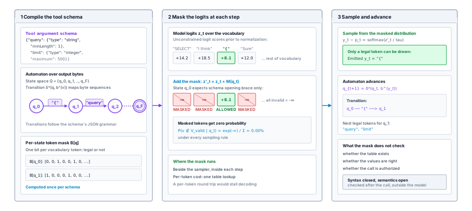
Recomputing \(\ValidTokenSet(\DecodingConstraintState_t)\) from scratch at every step would cost a scan of the whole vocabulary per token. Engines therefore compile the tool schema once into an automaton whose states each carry a precomputed mask \(\LogitMask(\DecodingConstraintState_t)\), so that each step is a lookup followed by a state transition (Willard and Louf 2023). Incremental parsing of this kind yields syntactically valid output even for a language as structured as SQL (Scholak et al. 2021). The automaton in figure 4 is compiled for a query tool with two fields, query and limit, rather than for read_file; the mechanism is identical.

Figure 4: Grammar-Constrained Decoding: A tool schema compiles once into an automaton whose states each carry a token mask. At every step the mask sets illegal tokens to \(-\infty\) before normalization, so only a legal continuation can be drawn, and the drawn token advances the automaton. The logit values are illustrative: a fluent but illegal continuation can outscore the legal one and still receive zero probability. A precomputed per-state mask suits a finite-state constraint; nested structures need additional parser state. The strip along the bottom lists what the mask leaves unchecked.

The resulting guarantee is conditional. The mask keeps every prefix viable, and the engine disallows the end-of-sequence (<eos>) token while required fields or closing delimiters remain unwritten, so an output that ends normally belongs to the enforced language. Nothing in the mask makes generation end normally within its token budget.

↪ The automaton behind the token mask, and the induction showing that a constrained output ending in a permitted end token belongs to the grammar, are developed in Finite-state constrained decoding.

Consider what happens when an inference request hits its maximum output token limit while emitting arguments, leaving the decoding buffer at {"path":"src/po. The string is a viable prefix under the schema, yet the envelope reports status: TRUNCATED, and the quarantining rule of section 2.5.2 applies. A heuristic repair parser that appends the closing quote and brace would fabricate the call read_file("src/po"), which the model never finished and which names a file nobody asked for. The mask governs which tokens can appear; it never promotes an interrupted generation to a completed one.

2.7.2 What a grammar mask guarantees

Grammar masking moves the first row of table 3 into generation and leaves every other row where it was. A masked {"path":"src/pool.py"} still names a file that may not exist or may lie outside the grant, because the mask operates strictly on the textual representation and never queries repository state or security policy. Property by property, the mask’s own reach is narrow (table 4).

Table 4: Reach of the grammar mask: A completed constrained output establishes membership in the enforced output language. Every other property keeps the check it needed without the mask.

Verification dimension	What the grammar mask establishes	Evidence still required
Syntactic conformance	All of it for the enforced grammar, once generation accepts	A COMPLETED status, since a legal prefix may be unfinished
Schema completeness	Only the constraints its compiler supports, at accepting completion	A final validation pass against the authoritative schema
Referential integrity	Nothing	Observation of the named resource in the relevant environment
Semantic invariants	Nothing	Checks or judgments covering the task property
Authorization bounds	Nothing; generated text grants no authority	A runtime permission decision for the proposed operation

How much a grammar mask guarantees depends on the grammar it compiles. Enforcing a general JSON grammar guarantees only RFC 8259 syntax (balanced braces, legal numbers, and escaped strings) without restricting keys or value types. Compiling a specific JSON Schema into the constraint engine goes further, enforcing required fields, distinguishing integers from floats, and restricting strings to declared regular expressions or enumerations.

Even a schema-aware mask has limits when a schema uses features that cannot be compiled into a finite-state or pushdown automaton. Keywords that enforce cross-field conditionals (if/then/else), unique array elements, or arbitrary lookahead often exceed what precomputed token masks support. Whenever an engine drops unsupported schema keywords, has a bug in its grammar compiler, or parses types differently from the downstream consumer, the guarantee stops holding. The runtime should therefore document which schema features its mask enforces and still run a final check against the authoritative schema before dispatch. Under invariant closure (principle 1), logit masking is a mechanical bound below the model: it enforces syntax without the model’s cooperation while leaving authorization and semantic checks above the model.

A strict schema can also force a model to guess when context is missing. If a schema requires a path string with no alternative branch, every completed output must supply a path even when the prompt gives no clue which file to inspect. Stripping out every token outside that single object shape leaves the model no way to report that information is missing, so it must invent a plausible path to reach an accepting parser state.

Adding an explicit unknown variant or a structured error branch to the schema avoids that forced guessing and lets the model report missing context cleanly. Those branches are semantic choices inside the payload, distinct from transport statuses and tool errors. They make an honest report possible without forcing one—the model can still guess a path when unknown is available, or pick unknown when the answer is already in the prompt—so the runtime handles each branch under the task contract, gathering another observation or asking the user when the model reports uncertainty.

2.7.3 Learned formatting and runtime constraints

Fine-tuning a model on tool examples makes well-formed arguments likely but still permits rare syntax slips on long contexts, whereas a grammar mask alone forces valid syntax even when the model has no idea which tool or argument fits the task. The two mechanisms work at different layers and complement each other. Supervised fine-tuning (further training on curated example responses, developed in Trajectory Fine-Tuning) and instruction tuning teach models to map prompts onto tool definitions and put high probability on appropriate arguments (Schick et al. 2023). Runtime logit masking fixes the support of the distribution at each step by setting illegal tokens to zero probability. A model tuned for tool use puts high logits on sensible tokens, and the runtime mask guarantees that sampling noise or long-context drift cannot emit broken syntax. Neither replaces the other: training alone gives no hard guarantee against syntax errors, and a grammar mask supplies no domain knowledge about which file path is right.

Schick, Timo, Jane Dwivedi-Yu, Roberto Dessı̀, Roberta Raileanu, Maria Lomeli, Luke Zettlemoyer, Nicola Cancedda, and Thomas Scialom. 2023. “Toolformer: Language Models Can Teach Themselves to Use Tools.” Advances in Neural Information Processing Systems (NeurIPS) 36: 68539–51.

Grammar constraints also carry their own costs. Compiling complex regular expressions or nested JSON schemas into deterministic automata consumes CPU time and memory. In dynamic environments where agents construct ad hoc schemas per request, compilation latency can offset the latency saved by avoiding syntax retries. Similarly, tracking parse states and computing masks across large vocabularies (\(|\TokenVocabulary| \ge 128{,}000\) tokens) adds per-token decoding overhead unless supported by precomputed lookup indices or bitmasks applied on the accelerator. Eliminating syntax retries lowers total cost only when compilation, mask memory, and per-token mask work together cost less than the retries they replace.

Checkpoint 2.2: Evaluating schema-constrained decoding

A repair agent uses constrained decoding for file-reading proposals. Its runtime records response kind and invocation status separately.

• Completion: If an output ceiling interrupts a legal JSON prefix, can you explain why grammar masking does not permit dispatch of the fragment?
• Constraint scope: If a completed request satisfies the schema but names a nonexistent file, can you identify which property was enforced and which observation is still needed?
• Response variants: A completed, schema-valid response selects the unknown variant. Decide what the runtime does next, and name the observation it should obtain before calling the model again.
• Combined mechanisms: Can you explain why a model trained for tool use can still benefit from runtime masks without either mechanism granting execution authority?

Constrained decoding removes one class of syntax failure before dispatch, but a structurally valid invocation still needs enough budget to finish and external evidence to justify execution. Whether a mask pays for itself, and what any call costs at all, depends on how prompt processing and token generation consume time on the serving hardware.

2.8 The Cost of a Model Call

When an automated repair agent requests a code fix, it can ask the model for a localized diff or for the entire modified file. Both formats describe the same underlying patch, but the full-file approach forces the model to regenerate hundreds of lines of unchanged syntax alongside the edit. The runtime absorbs the latency and compute cost of generating those redundant tokens long before a compiler or test runner can validate the candidate patch. An effective invocation contract must therefore budget prompt reading and output writing explicitly, rather than treating every model invocation as a uniform, black-box unit of work.

Input length and output length stress distinct subsystems in the inference serving stack. Prompt ingestion exposes many known token positions to parallel matrix computation across the accelerator’s execution units. Conversely, autoregressive token generation executes as a strictly sequential loop, where each new token depends on the hidden state of all preceding positions. Because hardware handles these two phases under different physical constraints, output length is the primary software lever for controlling generation latency. A very long prompt, a short reply, or a congested service queue can, however, shift the latency bottleneck elsewhere.

2.8.1 Where a call spends its time

A runtime that records only the total wall-clock time of a slow call cannot tell whether the delay came from a bloated prompt, a backed-up serving queue, or a long reply, yet each cause requires a different fix. To separate them, the runtime measures five non-overlapping phases from the moment it prepares the outbound request to the moment the normalized response is ready for validation: preparation (context assembly, serialization, and network send), queueing (waiting in the service’s admission queue), prefill (reading the prompt tokens in a parallel forward pass), decode (generating output tokens step by step), and postprocessing (response transfer, deserialization, and schema checks):

\[\CallLatency = \CallPreparationTime + \RequestQueueTime + \PrefillTime + \DecodeInterval + \CallPostprocessingTime \tag{6}\]

Each term in equation 6 is an elapsed time in seconds, measured with timestamps rather than estimated backward from token counts; when network transfer or local preparation overlaps server execution, the spans track non-overlapping intervals so nothing is counted twice. The first generated token needs careful accounting so it is not charged to both prefill and decode. In a standard Transformer, the prefill pass reads the whole prompt and produces the logits from which the first output token is drawn. On the client side, the time from sending the request to receiving that first token is the time to first token (TTFT), and the average spacing between later tokens is the time per output token (TPOT). Serving systems track TTFT and TPOT as separate objectives because prefill and decode contend for the same accelerator compute and memory bandwidth; disaggregated serving systems go further and run prefill and decode on separate accelerator pools so neither stalls the other (Zhong et al. 2024).

Zhong, Yinmin, Shengyu Liu, Junda Chen, Jianbo Hu, Yibo Zhu, Xuanzhe Liu, Xin Jin, and Hao Zhang. 2024. “DistServe: Disaggregating Prefill and Decoding for Goodput-Optimized Large Language Model Serving.” 18th USENIX Symposium on Operating Systems Design and Implementation (OSDI 24), July, 193–210.

When TTFT includes sampling and delivering the first token, the remaining decode interval covers only the next \(\OutputLength-1\) tokens in a completion of length \(\OutputLength\). For a streamed reply, adding client-measured TTFT, the \(\OutputLength-1\) inter-token intervals, and final deserialization gives the full call latency without double-counting the first token. Client-measured TTFT is larger than server prefill time because it also includes network transit and queueing, and because servers and networks often batch several streamed tokens into one network chunk, chunk arrival times on the client do not always match per-token step times on the accelerator.

Capping max_output_tokens bounds how many tokens the model can emit, not how fast the call returns; a congested queue can burn the entire deadline before prefill even starts. Latency benchmarks must therefore record the model, prompt and output lengths, prefix-cache hit rate, and cluster load. Even when a single agent runs one turn at a time, the serving cluster rarely runs that call alone: continuous batching schedules requests at each decode step (Yu et al. 2022), interleaving the agent’s tokens with dozens of other requests.

2.8.2 Estimating per-call hardware work

Counting input and output tokens together hides why a two-hundred-token reply can take longer on the accelerator than an eight-thousand-token prompt. Input processing and output generation hit different hardware bottlenecks, so a baseline work model gives them separate per-token time floors. A dense Transformer with \(\Parameters\) parameters executes approximately \(2\Parameters\) floating-point operations for each token it processes, in prefill and decode alike. What differs is how often the weights must be read. Prefill reads each weight tensor from accelerator memory once per call and reuses it across all \(\SequenceLength\) prompt positions, so a long prompt spreads one weight read over thousands of tokens of arithmetic, and each prompt token costs about \(2\Parameters\) operations at the peak arithmetic rate \(\PeakRate\). Single-stream decode produces one token per step, so it reads every weight once per generated token. Each output token therefore moves the full weight payload of \(\Parameters\,\ElementStorageSize\) bytes (with \(\ElementStorageSize\) bytes per parameter) across a memory interface of bandwidth \(\Bandwidth\), and its arithmetic finishes long before those bytes arrive.

These two regimes are the two limbs of the roofline model (Williams et al. 2009), which bounds attainable throughput by the lesser of the peak arithmetic rate and the memory bandwidth multiplied by the work done per byte moved. Prefill does much work per byte and sits under the arithmetic limb; low-batch decode does little and sits under the bandwidth limb, a split that empirical evaluations of Transformer inference confirm (Pope et al. 2023). The two floors are

Williams, Samuel, Andrew Waterman, and David Patterson. 2009. “Roofline: An Insightful Visual Performance Model for Multicore Architectures.” Communications of the ACM 52 (4): 65–76. https://doi.org/10.1145/1498765.1498785.

\[\PerTokenPrefillTime \approx \frac{2\Parameters}{\PeakRate}, \qquad \PerTokenDecodeTime \ge \frac{\Parameters\,\ElementStorageSize}{\Bandwidth} \tag{7}\]

The lowercase symbols are per-token floors. Under this model the phase durations of equation 6 are \(\PrefillTime \approx \SequenceLength\,\PerTokenPrefillTime\) and \(\DecodeInterval \approx \OutputLength\,\PerTokenDecodeTime\). Dividing the two floors cancels the parameter count \(\Parameters\):

\[\frac{\PerTokenDecodeTime}{\PerTokenPrefillTime} \approx \frac{\PeakRate \, \ElementStorageSize}{2 \, \Bandwidth} \tag{8}\]

Consider a concrete reference deployment: a dense model with 70.6B parameters stored in 8-bit precision (\(\ElementStorageSize = 1\) byte) on a single accelerator with an 8-bit peak rate of 1,979 TFLOP/s and a memory bandwidth of 3.35 TB/s. Each token costs 141.2 GFLOP of arithmetic, and dividing by the peak rate gives a prefill floor of 71.35 μs per prompt token. Each decode step reads 70.6 GB of weights, and dividing by the bandwidth gives a decode floor of 21.075 ms per generated token. Under equation 8, decoding a single output token therefore takes the same hardware time as ingesting roughly 295 prompt tokens. This asymmetry is the content of output-bound latency (principle 2), under which each plain, unbatched decode step incurs a full weight read in this model, so output volume can dominate call latency. The ratio reflects weight-dominated, unbatched decode against peak-throughput prefill, not a measured cloud service rate or a commercial billing tier.

↪ Both execution floors and their operating boundaries are developed in Cost Asymmetry Between Input Prefill and Output Generation.

This analytical budget charges each prompt token once at the prefill floor and reserves one decode floor step for each generated token. It is an idealized hardware baseline rather than a substitute for wall-clock measurement: it omits network transit, queueing delay, attention quadratics, and runtime software overhead. It also assumes standard autoregressive generation without speculative decoding. In production, a serving system that batches concurrent client requests, distributes model weights across tensor-parallel accelerators (sharding individual weight matrices across multiple devices), or reuses cached attention state substantially alters the relationship between token count and elapsed time. The analytical estimate is therefore suited to comparing interface formats and output volumes, but certifying a production deadline requires measuring latency directly under realistic serving load.

Applying this baseline to the first repair turn shows how output tokens dominate. A prompt of 8,000 tokens contributes 0.571 s of prefill work, while generating a reply of 200 tokens contributes 4.215 s of decode execution. The total call estimate is 4.786 s. Although output constitutes only 2.4 percent of the call’s total tokens, it accounts for 88.1 percent of the required processing time. Pruning redundant output tokens therefore reduces overall latency far more effectively than removing an identical number of prompt tokens. At the same time, an agent benefits from a cheaper invocation only if the model still receives sufficient diagnostic context to generate a correct candidate; engineers must prune verbosity from the output format, not critical evidence from the prompt.

2.8.3 How multi-turn history drives up input cost

Even when individual turns produce concise outputs, a multi-turn trajectory can still generate a large prompt-ingestion workload. Consider an agent runtime that maintains an append-only execution log and re-transmits the full cumulative history on every invocation. If the initial turn contains \(\BasePromptLength\) prompt tokens and each subsequent turn appends \(\TurnAppendLength\) tokens of combined model output and tool observations, a trajectory spanning a horizon of \(\TurnHorizon\) turns submits:

\[\PromptTokensSent = \sum_{j=0}^{\TurnHorizon-1} \left(\BasePromptLength + \PriorTurnCount\,\TurnAppendLength\right) = \TurnHorizon \BasePromptLength + \TurnAppendLength \frac{\TurnHorizon(\TurnHorizon-1)}{2} \tag{9}\]

prompt tokens in total. The quadratic growth in equation 9 comes from resending the growing history on every turn rather than from an inherent need of multi-turn reasoning. Sliding-window context buffers, trimmed tool outputs, or turn summaries can reduce the tokens sent, and a stateful serving endpoint can hold the conversation on the server to avoid resending the bytes over the network even when attention still spans the full history.

Re-sent input grows with the square of the horizon; prefix reuse keeps fresh prefill linear.

Repeated prompt input need not mean repeated computation. Prefix caching enables the inference engine to retain and reuse previously computed Key-Value (KV) activations for prompt prefixes that remain identical across consecutive requests (Zheng et al. 2024). Reuse holds only for an exact token prefix computed under the same model and serving configuration, so altering an early system instruction or a tool schema forces fresh prefill from that point onward. The full compatibility conditions are developed in Prefix compatibility.

To see how much work prefix reuse saves, suppose the inference service caches earlier prompt prefixes and runs fresh prefill only on the newly appended turn suffix (the model’s previous reply plus the new tool observation). Across all \(\TurnHorizon\) turns, the prompt tokens needing fresh prefill drop to \(\BasePromptLength + (\TurnHorizon-1)\,\TurnAppendLength\). That baseline conservatively assumes the server does not keep the KV state produced during decode; engines that retain decoded KV state as well avoid fresh prefill on the earlier model replies too.

Napkin Math 2.2: The price of an append-only trajectory

Problem: A coding agent runs 30 turns. Its first prompt has 8,000 tokens, each turn appends 1,500 tokens, and each call emits 200 output tokens. Assume that every prompt fits the service’s context limit and that compatible earlier prompt state remains available for reuse. How much input does the trajectory supply, and how does prompt-prefix reuse change its estimated processing work?

Math: Applying the arithmetic series in equation 9 gives \(30\times 8,000+1,500\times\frac{30\times 29}{2}=892,500\) prompt tokens. Total output is \(30\times 200=6,000\) tokens. Without reuse, input therefore accounts for 99.3 percent of the combined input and output token count, although it does not account for that share of processing time.

With prompt-prefix reuse, fresh prefill covers \(8,000+29\times 1,500=51,500\) tokens. Dividing the original input count by this fresh-prefill count gives a 17.3× reduction. At the reference prefill floor, the prefill-work estimate falls from 63.68 s to 3.67 s. Decode work stays at 126.45 s; caching earlier input does not remove the task’s new responses.

Systems insight: Append-only context makes input work grow with the square of the horizon. Doubling the trajectory to 60 turns multiplies re-sent input by 3.5× but fresh prefill under prefix reuse by only 1.9×, because reuse converts quadratic growth into a linear trajectory. Prefix reuse therefore serves as the primary lever for minimizing the input component of \(\AttemptCost\) in the cost per accepted task (equation 1.2), with its value compounding as horizons lengthen. While caching preserves the full decision context without loss of information, cache eviction and cross-worker request routing can dilute these theoretical savings in production.

In the illustrated repair turn, output length dominates the single-call estimate, yet uncached prefill can dominate the aggregate serving work of the same append-only trajectory. The two statements concern different accounts. Wall-clock latency governs the responsiveness of a single trajectory. Because each turn depends on the outcome of prior tool executions, an agent cannot parallelize its own dependent turns, and every output token remains a sequential step on the critical path even when the server batches that step with other requests. Computational work, by contrast, sets cluster throughput, hardware provisioning, and aggregate operating cost. When a serving cluster batches dozens of concurrent streams, the weight reads are amortized across requests, and the amortized service time per decoded token drops from the memory-bandwidth floor toward the compute-bound arithmetic limit \(2\Parameters/\PeakRate\) of equation 7, the same efficiency as prompt prefill (Cost Asymmetry Between Input Prefill and Output Generation derives the batched-step bound). Total cluster work then scales with aggregate token volume, which for an append-only agent is dominated by re-sent prompt history, provided the cluster sustains high batching and has memory for the attention state. Prefix reuse acts directly on that input component; its effect on end-to-end latency depends on how much the input contributes to the call a consumer waits on.

Which term an engineer should attack therefore depends on who waits for the output, and the repair agent alone cannot show the contrast. Its consumer is a compilation and test pipeline that must wait for a syntactically complete response. The support agent instead streams output tokens to a person reading as they arrive. The consumer requirements determine which latency terms these two illustrated workloads prioritize.

Lighthouse 2.1: Call latency for two lighthouses

Support agent: A customer-operations turn submits an 8,192-token prompt (consisting of policy documentation, customer account history, and recent dialogue) and streams an 150-token response to a human user in a live chat interface. At the chapter’s reference hardware floors, prefill takes 0.58 s and generating the full reply requires 3.2 s. However, token streaming displays the initial words immediately following queueing and prefill; the remaining tokens arrive at approximately 47 tokens per second, faster than a person reads. Under these lengths and streaming rates, TTFT governs how soon the user can begin reading. When 6,144 prompt tokens represent a common prefix of system instructions, organizational policies, and tool definitions shared across all concurrent sessions, prefix caching leaves only 2,048 tokens of fresh prefill, which takes just 0.15 s. In a loaded cluster, admission queueing becomes the dominant contributor to first-token latency.

Repair agent: The initial repair turn commits 88.1 percent of its estimated hardware work to generating a 200-token response. The agent runtime can parse, validate, and execute the generated patch only after receiving the entire payload. Decode duration dominates this repair estimate, making the compactness of the requested code representation its primary optimization lever.

Systems insight: The illustrated support turn prioritizes TTFT because the user can read while the remaining tokens arrive, whereas output volume dominates the illustrated repair call, whose consumer waits for a complete patch. Shortening the support reply does not directly remove queueing or prefill from first-token latency. Caching the repair prompt reduces its input work and input cost, but that saving contributes little to this output-dominated estimate. Different prompt lengths, streaming rates, or serving load can change the binding term; measured phase durations and queueing determine which intervention improves the latency the consumer waits on.

Prefix reuse is not free. A cached prefix occupies accelerator memory that concurrent requests cannot use, and holding it through a long tool wait pins memory that no generation is using. Eviction discards only derived attention state, never the context itself, so the runtime can rebuild the prompt from its own logs at the cost of fresh prefill. Which evidence the model sees and whether its attention state is worth keeping are therefore separate decisions.

↪ The choice to keep, move, or drop attention state held through a tool wait is developed in Paused-State Policies.

Billed dollars form a third account, separate from latency and hardware work. Providers bill uncached input, cached input, and output tokens at different rates, and on-premise hardware amortizes fixed costs across utilization, so token-count ratios do not translate directly into dollars; Pricing prefix cache hits prices a whole trajectory under such tariffs. The per-call estimate is one building block of a task budget that also carries failed tool executions, retries, validation runs, and idle reservations during tool waits.

Checkpoint 2.3: Pricing calls and trajectories

A call’s token count and its elapsed execution time quantify distinct facets of the overall system budget.

• Measurement boundary: If the time to first token already accounts for sampling and delivering the initial token, how many subsequent token-generation intervals remain in a completed completion of length \(\OutputLength\)?
• Horizon estimate: If an agent trajectory triples to 90 turns under fixed \(\BasePromptLength\) and \(\TurnAppendLength\), estimate the growth factor for uncached re-sent input vs. fresh prefill under prefix caching. Which term dictates whether scaling to longer trajectories remains computationally viable?
• Reuse assumptions: How does the analytical work estimate change if the inference server evicts the cached prefix from accelerator memory during a blocking tool execution?
• Cost denominator: Why does an overwhelming majority of input tokens fail to produce an equivalent majority of financial cost when providers bill cached input and generated output at starkly different rates?
• Interface estimate: A full-file replacement requires 1,850 output tokens, whereas a localized diff requires only 80. At the reference decode floor, which interface alternative can realistically operate within a 15 s latency deadline? Why is this analytical roofline model insufficient on its own to guarantee real-world service-level agreement (SLA) compliance?

Breaking down a call’s cost shows two main sources of waste: generating unchanged output tokens that the tool interface does not need, and recomputing prompt prefixes that the server could reuse. Cutting that waste helps only when the resulting output still solves the task—a short diff that fails to apply or a cached prompt that produces a broken edit wastes the entire call. Choosing an output interface therefore requires comparing candidate accuracy, failure modes, and total resource spend under the same task budget.

2.9 Comparing Output Interfaces

When an automated repair agent modifies connection-pool locking logic, its output payload does not need to repeat the entire source file. The model could emit a fully rewritten file, or it could target a specific code block and emit only the replacement text. Emitting a localized edit consumes far fewer generation tokens by omitting unchanged code, but it creates an operational dependency: the execution runtime must locate the exact target coordinates in the target file. The interface therefore determines both the computational cost of generating a candidate and the operational preconditions required for the runtime to apply it.

High schema parse rates alone cannot validate an interface design. A whole-file replacement might parse into valid JSON yet arrive long after the service deadline because the model spent tens of seconds generating unchanged lines. Conversely, a compact diff might arrive in about 2.3 s yet fail to match its target anchors against current repository state. Neither outcome delivers an accepted repair. A rigorous empirical comparison must track the model call’s completion status, account for all compute resources consumed across retries, and validate the resulting artifact against uniform acceptance criteria.

2.9.1 Three choices in an output interface

When a patch interface fails in production—timing out on long files, missing its target lines, or breaking JSON syntax—teams often swap the entire prompt format at once and cannot tell whether edit granularity, wire framing, or decoding constraints caused the failure. Because those three choices are independent, diagnosing a failure or comparing designs requires varying one dimension at a time.

The first choice, edit granularity, sets how much text the model must emit to describe a change. At one end, a whole-file format returns the entire file, regenerating hundreds of untouched lines alongside the edit. At the other end, a localized edit supplies only a target locator and the replacement lines. An anchored search-and-replace block, for instance, gives an exact snippet of source text to find and the new text to substitute; if that anchor snippet is missing from the file or appears more than once, the runtime cannot apply the edit uniquely. Rewriting the whole file avoids anchor mismatches, but forces the runtime to check that the model did not accidentally delete unrelated functions or overwrite concurrent edits.

Regardless of which granularity the interface chooses, serialization framing remains an independent decision. Either edit size can be wrapped in JSON—one schema carrying a path and full file body, another carrying a path, search snippet, and replacement block—or framed with Markdown code fences or unified diff headers. Token overhead comes from the tokenizer’s vocabulary and the wrapper markers, not from whether the outer wrapper is JSON or diff syntax; emitting thousands of tokens for an unchanged file is the price of whole-file granularity, not of JSON.

How the runtime enforces that framing—the constraint mechanism—is independent of both granularity and wire syntax. An engineer can get structured outputs through fine-tuning, few-shot examples in the prompt, or grammar masking during decoding, and can combine them by running a fine-tuned model under a grammar mask. As section 2.7 showed, a grammar mask guarantees grammatical form, not valid targets or working code: it cannot ensure that an anchor snippet exists in the file or that the edit fixes the race condition. Changing serialization and decoding constraints at the same time tests a bundle of choices rather than isolating which change helped.

2.9.2 Matched-budget comparison

Giving a brittle diff format free retries whenever its output fails to parse, or dropping timed-out whole-file calls from the denominator, makes a weak interface look more accurate than it is. A fair comparison holds every condition fixed except the interface itself. In the connection-pool repair benchmark, every trial starts from the same repository snapshot and defect description, under the same model weights, sampling parameters, tools, acceptance tests, resource ceilings, and retry policy. Matched budgets do not require equal token consumption, because prompt overhead and response length are properties of the interface under test; they require identical operating limits and accounting rules.

↪ Matched-budget comparison of complete agent policies, charging every initiated trial to the cost per accepted task, is developed in Matched-budget comparison.

Two deadlines bound the comparison. The invocation deadline ends when the runtime receives and normalizes the model’s response. The task deadline also covers parsing, patching, compilation, and tests, and every retry, unparsable output, and failing run draws against it. A benchmark that grants free retries after malformed responses therefore subsidizes the brittle interface.

The harness also records each intermediate stage separately from final acceptance (table 5). Every initiated trial stays in the denominator of the top-level success rate, because discarding unparsable responses or timed-out calls inflates reported accuracy. Conditional rates, such as the share of applied edits that pass tests, remain useful diagnostics when they state their filter explicitly.

Table 5: Interface evaluation measurements: Distinct observations prevent a formatting improvement from being mistaken for a task-level improvement. The same task fixtures, acceptance standard, and resource ceilings govern each design.

Measurement	What the trial records	What it does not establish
Invocation outcome	Completion status, elapsed time, and token usage	That a delivered candidate is valid
Structural validity	Whether a completed payload parses and satisfies the required schema	That its values describe the current environment
Applicability	Whether the authorized edit identifies its target and can be applied to the expected version	That the resulting program repairs the defect
Acceptance evidence	Results of the same required checks on the resulting artifact	Correctness beyond the checks’ coverage
Resource use	All calls and checks charged to the trial, including failed attempts	A benefit unless accepted outcomes justify the expenditure

Latency measurements also need their serving conditions. Cache hits, batching contention, and queueing change observed wall-clock time at fixed prompt and completion lengths, so a few favorable measurements during quiet periods do not establish deadline reliability; tail latency decides deadline violations in shared clusters (Dean and Barroso 2013). The engineering question is whether a representation leaves enough headroom under the tail of the latency distribution to generate and validate a candidate fix.

Dean, Jeffrey, and Luiz André Barroso. 2013. “The Tail at Scale.” Communications of the ACM 56 (2): 74–80.

2.9.3 Choosing an edit format under a deadline

When a repair call must finish inside a fifteen-second deadline, asking the model to rewrite an entire source file spends almost the whole budget copying unchanged lines before a single test can run. The per-token floors of section 2.8.2 put a concrete price on that unchanged text, and that price falls on edit granularity rather than on the outer wrapper format.

Generating unchanged code, not reading the prompt, pushes the whole file past the deadline.

Napkin Math 2.3: A repair representation under an invocation deadline

Problem: A repair invocation begins with 8,000 baseline context tokens and operates under an invocation deadline of 15 s. Emitting a whole-file replacement requires 350 additional instruction tokens and 1,850 output tokens. Emitting a localized edit requires 120 additional instruction tokens and 80 output tokens. These token counts represent scenario parameters. Using the prefill and autoregressive decoding rates established earlier, which interface representation fits within the simplified service-work budget?

Math: The service-work model charges prompt prefill at 71.35 μs per token and autoregressive decoding at 21.075 ms per token. To isolate inference execution, this baseline calculation omits request serialization, network transit, server-side queueing, and subsequent validation runs. Multiplying each interface’s token profile by these unit costs yields:

\((8,000+350)\times 0.00007135\,\text{s}+1,850\times 0.021075\,\text{s}\approx 39.58\,\text{s}\)

\((8,000+120)\times 0.00007135\,\text{s}+80\times 0.021075\,\text{s}\approx 2.27\,\text{s}\)

The whole-file estimate exceeds the deadline by a wide margin, whereas the localized edit finishes well within the allocated budget. The localized representation provides a 17.5× reduction in estimated service work, with token decoding accounting for 98.5 percent of the whole-file latency. In production, normalized invocation outcomes and observed wall-clock times determine whether the candidate arrived before deadline expiration.

To evaluate downstream yield, consider a second hypothetical scenario where localized edits complete on time with valid syntax, but only 95 percent resolve to an applicable edit on the codebase. Among those applicable edits, assume 60 percent pass the required test suite. The fraction of all initiated trials that yield an accepted repair is:

\(0.95\times 0.60=0.57\)

This 57 percent yield is the product of the applicability rate and the conditional test-pass rate, requiring no independence assumption between stages. Invocations that miss deadlines or emit invalid syntax reduce this end-to-end yield even further.

Systems insight: When output generation threatens an invocation deadline, shrinking representation granularity is the primary engineering lever. Because autoregressive decoding is memory-bandwidth bound, each generated token costs roughly 295 prompt prefill tokens at hardware reference floors (principle 2). Whole-file generation squanders almost all of its 39.6 s runtime emitting unchanged code, while the localized edit meets the deadline with a 6.6× safety margin. However, compact representations trade decoding latency for applicability risk: localized edits require exact anchor matching, which restricts the passing yield to 57 percent in this scenario. That hypothetical yield forms the acceptance probability \(\AcceptanceProbability\) that governs the amortized cost per accepted task (equation 1.2).

The call deadline acts as a hard filter: under these timing numbers, a whole-file response misses the cutoff before any test can run, so its code quality never comes into play. If the deadline is relaxed past the whole-file duration, the trade-off flips toward applicability and patch accuracy. With a generous time budget, a localized edit format that frequently misses stale anchors or ambiguous line ranges can lose to a whole-file format that applies cleanly every time.

Checkpoint 2.4: Reconsidering the interface when conditions change

The repair interface must be reassessed whenever the workspace state or resource budget shifts.

• Applicability: If the source file changes after the prompt is assembled, which measurement in the benchmark pipeline changes, and what preconditions must the runtime verify before applying either representation?
• Deadline: If the invocation deadline doubles while token lengths and accounting rates stay fixed, which representations fit the budget, and how do you distinguish that analytical estimate from an empirical completion guarantee?
• Serialization: If the localized edit is encoded as a JSON object rather than plain text delimiters, which latency benefits survive and which token counts must be re-profiled?
• Admission: How do you distinguish a COMPLETED but malformed request from a syntactically valid but TRUNCATED request? Which specific check prevents each from triggering downstream tool execution?
• Acceptance evidence: If an edit applies cleanly and passes a sequential test suite, what additional runtime evidence does a race-condition task still require before acceptance?

Interface benchmarking joins the call contract to the cost of the call. The request specifies the context and output allowances; the normalized response confirms whether the model delivered a completed payload before the deadline; and tiered evaluation metrics determine whether the proposed mutation reliably solves the task within resource constraints. Assuming that a valid schema implies an applicable patch, or that a fast diff implies defect-free code, collapses these stages into one and hides which of them failed.

2.10 Fallacies and Pitfalls

A code repair request can return promptly yet name the wrong file, or return the right patch long after its latency budget has expired. In autonomous execution loops, engineers frequently conflate distinct operational boundaries, confusing inference execution with total round-trip latency, syntactic validity with semantic correctness, and transport success with task completion. These failures expose several persistent mistaken assumptions about the model call.

Fallacy: One model response has a fixed cost.

Output length drives most of the execution time in the unbatched interface comparison. At its reference hardware floors, decoding a single output token takes far longer than reading a prompt token in parallel. Regenerating a whole file takes 39.6 s, whereas emitting a localized patch for the same bug takes 2.3 s—a 17.5× speedup that comes almost entirely from generating fewer tokens (section 2.8). Engineers must therefore budget input and output tokens separately rather than treating a model call as a fixed unit of work. Wall-clock budgets must also cover queueing and network transit; setting max_output_tokens caps how many tokens the model generates, not when the reply arrives.

Pitfall: Treating a completed invocation as a completed task.

A status of COMPLETED says only that the serving engine finished generating tokens within the call’s limits; it does not mean the output is right or even usable. In the interface comparison, every localized edit finished on time, yet only 57 percent of those trials produced patches that passed the repair checks. Conversely, a call cut off at the token ceiling can still leave a syntactically valid file path, which is why the runtime must check completion status before acting on the payload. Every call record needs two separate facts: whether a complete candidate arrived from the service, and whether independent checks confirm that it satisfies the task contract.

Fallacy: Valid JSON means a safe and correct tool call.

A JSON object passes schema validation whenever its fields match the declared types, whether the payload is safe, authorized, or sensible. A tool call with a string path passes schema checks whether that path names the intended file, a stale file, or a sensitive directory outside the workspace. As table 3 shows, schema validation checks structure, while permission gates and task checks govern safety and correctness. The same gap holds for behavioral checks: a test runner with a false-accept rate of 0.65 on defective patches still leaves 14.37 percent of its passing candidates defective under the assumed rates. Even under grammar-constrained decoding, a call cut off at the token limit remains an unfinished fragment even though every token emitted before truncation was legal.

Pitfall: Collapsing every unsuccessful outcome into the same retry.

Retrying a failed call with the exact same request repeats the cause of the failure when the fault is not transient. If a whole-file request misses a 15 s deadline, resending the identical prompt spends another 39.6 s of estimated work only to time out again—while the first call may still be running and billed on the server, since a local timeout leaves the remote outcome unknown. Likewise, a call that hits max_output_tokens will truncate at the same limit on retry, and a safety refusal will refuse again. Instead of treating every failure like a dropped packet, the runtime should route on the normalized status: bounded backoff for transient service faults, a larger output allowance or more compact output format for truncation, and a fresh file read when an edit anchor fails to match. Recovery actions and evidence develops which recovery action fits each failure class.

↪ The idempotency rules that decide when a timed-out call may be repeated are developed in Retrying Uncertain Actions.

Fallacy: Greedy decoding makes a served call reproducible.

Greedy selection fixes the token choice for a given logit vector, but the serving infrastructure computes that vector, and two distinct causes can change it. The first operates even on a healthy serving path, where batch-dependent floating-point reduction order shifts closely contested logits in their least significant bits, enough to flip an argmax and redirect every later token. The second is a change to the serving path itself. In war story 2.1, misrouting and a miscompiled top-\(\TopTokenSampleCount\) operation changed model outputs for identical requests, affecting 16 percent of one model’s requests at peak impact, so an identical prompt succeeded on one attempt and failed on the next. Pinning the temperature addresses neither cause. Systems engineers should record the model revision and serving configuration with every invocation, and replay recorded responses whenever the goal is to reproduce downstream runtime behavior deterministically.

Each of these traps blurs two separate runtime records: token usage measures spend, completion status tracks whether generation finished, schema validation checks form, and acceptance tests check the result. Keeping those records separate lets higher-level loops compose single model calls without mistaking a clean response envelope for a working repair.

2.11 Summary

A repair agent interacts with a foundation model through a bounded request-response contract. The request bundles messages, tool schemas, token and time limits, and sampling settings into a serialized payload without handing any execution authority to the model. On the way back, the normalized status envelope separates completed proposals from truncated, refused, or failed calls, leaving the runtime to authorize side effects and verify results against the task contract. That division of work is invariant closure (principle 1) applied to a single model call—the baseline that every later chapter builds on. Table 6 summarizes the quantitative relations governing model invocations, tracking admission constraints, generation dynamics, verification limits, and trajectory-level resource scaling.

Table 6: Key equations of the model call: Each relation holds only under the assumptions stated where it is derived, such as a combined input-and-output window, weight-dominated unbatched decode, or a reusable prefix that stays resident.

Equation	What it bounds or decides	Where derived
\(\SequenceLength \le \ContextWindow - \OutputLimit\)	Admissibility of a serialized request while preserving required output headroom	equation 1
\(\Pr(\OutputTokenSequence \mid \InputTokenSequence) = \prod_{t=1}^{\OutputLength} \Pr(\OutputToken_t \mid \InputTokenSequence, \OutputTokenPrefix)\)	Sequential probability factorization defining token-by-token autoregressive generation	equation 2
\(\Pr(\OutputToken_t = \VocabularyToken \mid \InputTokenSequence, \OutputTokenPrefix) \propto \exp\left(\OutputLogit_{t, \VocabularyToken} / \SamplingTemperature\right)\)	Temperature scaling trading sample diversity against distribution concentration	equation 3
\(\Pr(\text{Defective} \mid \text{PASS}) = \frac{\VerifierFalseAcceptanceRate \CandidateDefectRate}{\VerifierFalseAcceptanceRate \CandidateDefectRate + \Pr(\text{PASS} \mid \text{Valid})(1 - \CandidateDefectRate)}\)	Residual defect probability among candidate outputs accepted by a fallible checker	equation 4
\(\SoftmaxOutputProbability_{t, i} \propto \exp(\OutputLogit_{t, i})\) for \(\MaskTokenIndex \in \ValidTokenSet(\DecodingConstraintState_t)\), else \(0\)	Token logits masked by a grammar constraint to enforce syntactic form	equation 5
\(\CallLatency = \CallPreparationTime + \RequestQueueTime + \PrefillTime + \DecodeInterval + \CallPostprocessingTime\)	Stage decomposition of end-to-end invocation latency identifying operational bottlenecks	equation 6
\(\PerTokenPrefillTime \approx 2\Parameters/\PeakRate\), \(\; \PerTokenDecodeTime \ge \Parameters\,\ElementStorageSize/\Bandwidth\)	Per-token computational and memory bandwidth performance floors for prefill and unbatched decode	equation 7
\(\PerTokenDecodeTime/\PerTokenPrefillTime \approx \PeakRate \ElementStorageSize / (2\,\Bandwidth)\)	Relative hardware cost ratio of decode tokens to prefill tokens, independent of model size	equation 8
\(\PromptTokensSent = \TurnHorizon \BasePromptLength + \TurnAppendLength \frac{\TurnHorizon(\TurnHorizon-1)}{2}\); fresh prefill \(\BasePromptLength + (\TurnHorizon-1)\,\TurnAppendLength\) under prefix reuse	Quadratic token scaling in append-only trajectories vs. linear prefill work under prefix reuse	equation 9

Key Takeaways: A model call is a bounded proposal interface

• Budget the representation the service receives: Count serialized requests using the target model’s tokenizer and reserve explicit headroom for generated tokens. Context window limits, provider message caps, and network timeouts restrict distinct dimensions of the invocation; raw character counts never reliably predict actual token consumption or admission success.
• Completion admits a candidate, not an action: Inspect the response kind and normalized status before consuming the payload. While an incomplete generation provides useful diagnostic data for debugging, syntactic parseability alone never promotes a partial string into a valid candidate, nor does it grant permission to execute tool actions.
• Structural guarantees have a stated scope: Grammar constraints enforce syntactic validity under their schema assumptions, whereas permission checks govern permissible side effects and verifiers supply empirical acceptance evidence. A passing test supports only the properties exercised; model self-review remains a candidate assessment rather than independent confirmation.
• Output and repeated input incur different costs: One output token costs about 295 prompt tokens at the reference hardware floors. Generation length dominates the illustrated unbatched repair estimate; prompt length and queueing can bind under other conditions. An append-only conversational history causes re-sent input tokens to scale quadratically with the trajectory horizon. Compatible prefix reuse turns that quadratic growth into linear work, but cached key-value states must never serve as the authoritative record of task state.
• Compare accepted results within the same budget: Full-file replacements and localized patch edits trade generation volume against patch applicability constraints. Evaluate these alternatives by measuring end-to-end task completion, total token expenditure, and identical acceptance checks, rather than treating serialization format or schema parse rates as an engineering verdict.

2.12 Historical Perspective and Further Reading

The foundation model call joins two intellectual lineages that developed independently for decades. The first is statistical language modeling. Shannon (1948) framed natural language as a discrete stochastic process, treating English as a sequence of symbols drawn from conditional probability distributions and generating text from successively longer context windows. Bengio et al. (2003) replaced high-dimensional count tables with a continuous neural function over distributed word representations, establishing the autoregressive next-token factorization that modern architectures still use. The Transformer made that formulation parallelizable across token positions during training (Vaswani et al. 2017). In production serving, that same architectural choice creates a fundamental operational split: an initial prompt prefill phase often limited by arithmetic throughput, followed by a small-batch autoregressive generation loop often limited by memory bandwidth (Pope et al. 2023). Subword tokenization algorithms borrowed from data compression solved the out-of-vocabulary dilemma (Gage 1994; Sennrich et al. 2016), and scaling laws subsequently produced models capable of task execution directly from natural language prompts (Brown et al. 2020). Bommasani et al. (2021) formalized the concept of foundation models while warning of their central systems risk: when hundreds of applications build on a single upstream base model, any flaw, bias, or failure mode in that model propagates throughout the entire software stack.

Shannon, Claude E. 1948. “A Mathematical Theory of Communication.” Bell System Technical Journal 27 (3): 379–423. https://doi.org/10.1002/j.1538-7305.1948.tb01338.x.

Bengio, Yoshua, Réjean Ducharme, Pascal Vincent, and Christian Jauvin. 2003. “A Neural Probabilistic Language Model.” Journal of Machine Learning Research 3: 1137–55.

Vaswani, Ashish, Noam Shazeer, Niki Parmar, Jakob Uszkoreit, Llion Jones, Aidan N. Gomez, Lukasz Kaiser, and Illia Polosukhin. 2017. “Attention Is All You Need.” Advances in Neural Information Processing Systems (NeurIPS) 30: 5998–6008.

Brown, Tom B., Benjamin Mann, Nick Ryder, Melanie Subbiah, Jared Kaplan, Prafulla Dhariwal, Arvind Neelakantan, et al. 2020. “Language Models Are Few-Shot Learners.” Advances in Neural Information Processing Systems 33: 1877–901. https://doi.org/10.48550/arxiv.2005.14165.

Fan, Angela, Mike Lewis, and Yann Dauphin. 2018. “Hierarchical Neural Story Generation.” Proceedings of the 56th Annual Meeting of the Association for Computational Linguistics (Volume 1: Long Papers), 889–98. https://doi.org/10.18653/v1/P18-1082.

Yu, Gyeong-In, Joo Seong Jeong, Geon-Woo Kim, Soojeong Kim, and Byung-Gon Chun. 2022. “Orca: A Distributed Serving System for Transformer-Based Generative Models.” 16th USENIX Symposium on Operating Systems Design and Implementation (OSDI 22), 521–38.

Zheng, Lianmin, Liangsheng Ying, Zhenghao Yin, Cody Hao Liu, Eric Yu, Prakhar Patel, Zhipeng Yang, Anthony K. Joseph, and Ion Stoica. 2024. “SGLang: Efficient Execution of Structured Language Model Programs.” arXiv Preprint arXiv:2312.07104, ahead of print. https://doi.org/10.48550/arXiv.2312.07104.

Decoding strategies evolved alongside model scale to mitigate systematic failure modes in generation. Early inference relied on greedy search or beam search to maximize likelihood, but these objectives frequently trapped models in bland, repetitive loops. Truncated sampling addressed this degeneration by restricting candidates to the head of the output distribution, first through a fixed token count in top-\(\TopTokenSampleCount\) sampling (Fan et al. 2018) and subsequently through top-\(\NucleusProbabilityMass\) (nucleus) sampling, which adapts the truncation boundary dynamically to the distribution’s cumulative probability mass (Holtzman et al. 2020). Speculative decoding decoupled generation latency from model parameter scale by using a lightweight draft model to generate token candidates that the larger target model verifies in parallel (Leviathan et al. 2023; Chen et al. 2023). At the infrastructure level, serving engines moved beyond rigid static batching: Orca introduced iteration-level scheduling to interleave prefill and decode phases dynamically (Yu et al. 2022), while SGLang demonstrated how prefix caching across requests amortizes repetitive prompt computations (Zheng et al. 2024). Together, these runtime innovations transformed the per-token computational costs analyzed in this chapter into shared, schedulable execution pipelines.

The second lineage stems from distributed systems engineering and access mediation across untrusted boundaries. When Birrell and Nelson introduced remote procedure calls, their goal was to make remote execution feel like a local function call, yet they showed that network boundaries expose failure semantics that local calls never experience, most notably states in which the caller cannot determine whether an operation ran (Birrell and Nelson 1984). Decades of systems architecture reinforce that lower-level abstractions cannot reliably guarantee end-to-end semantics; as the end-to-end argument demonstrates, true correctness must ultimately be validated by the participating endpoints (Saltzer et al. 1984). In an agent runtime, an external service returning a COMPLETED status serves as an execution hint rather than a definitive guarantee of success. Similarly, classical security engineering established the principle of complete mediation (Saltzer and Schroeder 1975), which requires validating every access request against current authority rather than trusting past authorization, which is the discipline an agent runtime must enforce when dispatching model-proposed tool calls. Finally, parsing theory provides the formal prefix property (Knuth 1965) that underpins modern constrained decoding, ensuring token-by-token alignment with structured schema grammars (Scholak et al. 2021; Willard and Louf 2023). While sampling payloads dynamically across an open vocabulary is a modern capability, the defensive engineering required to govern those calls safely rests on these older systems foundations.

Scholak, Torsten, Nathan Schucher, and Dzmitry Bahdanau. 2021. “PICARD: Parsing Incrementally for Constrained Auto-Regressive Decoding from Language Models.” Proceedings of the 2021 Conference on Empirical Methods in Natural Language Processing, 9895–901. https://doi.org/10.18653/v1/2021.emnlp-main.779.

The following six papers provide essential reading on the conceptual and systems foundations of foundation model runtimes:

• Birrell and Nelson (1984) introduces the mechanics of remote procedure calls and catalogs their failure semantics. It remains the classic reference for why invocation contracts across process boundaries must handle network partitions, cancellations, and undecidable execution states.
• Saltzer et al. (1984) presents the end-to-end argument in system design, articulating why lower architectural layers cannot reliably guarantee higher-level application correctness. It underpins why an agent runtime cannot treat external service status codes (such as COMPLETED) as substitutes for independent outcome validation.
• Holtzman et al. (2020) analyzes the degeneration of likelihood-maximizing decoding in open-ended text generation and introduces nucleus (top-\(\NucleusProbabilityMass\)) sampling. It demonstrates that decoding algorithms represent deliberate engineering trade-offs that govern output entropy, coherence, and candidate diversity.
• Pope et al. (2023) develops an analytical roofline model of Transformer serving that separates compute-bound prompt prefill from memory-bandwidth-bound autoregressive decoding. It establishes the quantitative foundation for per-token latency floors, KV cache memory footprints, and batching trade-offs.
• Willard and Louf (2023) introduces efficient constrained decoding by compiling regular expressions and context-free grammars into finite-state machines indexed over the model’s token vocabulary. It demonstrates how to enforce strict structural schemas at runtime with minimal per-token computational overhead.
• Bommasani et al. (2021) surveys the technical capabilities and architectural risks of foundation models. Its analysis of model homogenization clarifies why centralized upstream dependencies require strict isolation boundaries, independent validation, and runtime guardrails across downstream applications.

Saltzer, Jerome H., David P. Reed, and David D. Clark. 1984. “End-to-End Arguments in System Design.” ACM Transactions on Computer Systems 2 (4): 277–88. https://doi.org/10.1145/357401.357402.

Holtzman, Ari, Jan Buys, Li Du, Maxwell Forbes, and Yejin Choi. 2020. “The Curious Case of Neural Text Degeneration.” Proceedings of the 8th International Conference on Learning Representations (ICLR 2020).

Pope, Reiner, Sholto Douglas, Aakanksha Chowdhery, Jacob Devlin, James Bradbury, Jonathan Heek, Kefan Xiao, Shivani Agrawal, and Jeff Dean. 2023. “Efficiently Scaling Transformer Inference.” Proceedings of Machine Learning and Systems (MLSys) 5: 606–24.

Willard, Brandon T., and Rémi Louf. 2023. “Efficient Guided Generation for Large Language Models.” arXiv Preprint arXiv:2307.09702.

2.13 Exercises

All quantities below are hypothetical problem givens, chosen to be round, and describe no particular model, accelerator, or service. Where a problem uses the per-token work floors of equation 7, take them as floors in the chapter’s sense, which exclude queueing, transfer, attention-dependent work, and serving overhead.

1. Admitting a request with a long observation (Basic). A repair call runs against an interface with a combined context window \(\ContextWindow = 32{,}768\) tokens, and the runtime reserves \(\OutputLimit = 4{,}096\) tokens of output headroom. System instructions and tool definitions serialize to 3,200 tokens and the retained conversation to 18,000. The newest tool observation, a test log, was estimated at 9,500 tokens by dividing its 38,000 characters by four.

1. Compute \(\SequenceLength\), the input ceiling, and whether the request is admitted. If not, find the largest observation that fits with the reservation unchanged.
2. A teammate proposes halving \(\OutputLimit\) instead of shortening the log. Does the request then fit? Past proposals in this workload have run to 3,000 output tokens; state what the smaller reservation risks and which status the runtime would then record.
3. The model’s tokenizer reports the log as 11,400 tokens, because indentation and escaped quotation marks split into many short tokens. Recompute both options, and state which measurement the runtime must take before any admission decision.

2. Where a call’s time goes (Basic). A dense model with \(\Parameters = 40\) billion parameters stores 8-bit weights (\(\ElementStorageSize = 1\) byte) on an accelerator with peak rate \(\PeakRate = 1{,}000\) TFLOP/s and memory bandwidth \(\Bandwidth = 4\) TB/s.

1. Compute \(\PerTokenPrefillTime\), \(\PerTokenDecodeTime\), and their ratio.
2. The first repair turn sends a 12,000-token prompt and generates a 300-token reply. Compute the prefill and decode times at these floors, the share of estimated work spent generating, and the share of tokens that are output.
3. Two optimizations are proposed: trimming 3,000 tokens of retrieved documentation from the prompt, or a terser proposal format that halves the reply. Compute the work each saves and choose one. Then say how 4-bit weights (\(\ElementStorageSize = 0.5\) byte) would change the floor ratio and whether they change your choice.

3. How much diversity a setting buys (Basic). At one decision point a model’s logits over four candidate tokens are \(\LogitVector_t = [8, 7, 5, 2]\), and a later selection stage wants a first token that differs from the top-scoring one so that it has a genuine alternative to compare.

1. At \(\SamplingTemperature = 1\), compute the four probabilities and the set retained by top-\(\NucleusProbabilityMass\) sampling with \(\NucleusProbabilityMass = 0.90\), with its renormalized probabilities.
2. Compute the probability that one draw differs from the top token under (i) top-\(\NucleusProbabilityMass\) at unit temperature and (ii) untruncated sampling at \(\SamplingTemperature = 0.5\). How many independent draws does each setting need so that at least one differs from the top token with probability at least 0.9?
3. An engineer concludes that the lower temperature is the “more accurate” setting because the top token receives more mass. Explain what the calculation does and does not show, and name what should choose the setting.

4. Paying for an append-only history (Intermediate). A repair trajectory runs \(\TurnHorizon = 40\) turns with \(\BasePromptLength = 10{,}000\) tokens and appends \(\TurnAppendLength = 2{,}000\) tokens per turn; each call generates 250 tokens. Hypothetical prices per million tokens are $3 for uncached input, $0.30 for cached input, and $15 for output.

1. Compute the total prompt tokens supplied, the fresh-prefill tokens under prompt-prefix reuse (section 2.8), and the total output tokens. Repeat the first two for \(\TurnHorizon = 80\) and report each growth factor.
2. Compute the trajectory’s dollar cost with no reuse and with every reused prefix billed as cached input. What share of the dollars is input in each case?
3. A developer adds the current timestamp to the first line of the system prompt so the model knows the time. Compute the new cost, explain the mechanism, and redesign the request so the model still receives the time.

5. Ordering fallible checks (Intermediate). Suppose 25 percent of generated connection-pool patches violate the required concurrency property. Checker A (compile and unit tests) passes defective patches with \(\VerifierFalseAcceptanceRate = 0.5\) and valid ones with probability 0.9, at $0.02 per run. Checker B (a concurrency stress test) has \(\VerifierFalseAcceptanceRate = 0.2\) and passes valid patches with probability 0.8, at $0.30 per run. The task contract tolerates at most 5 percent defective patches among those accepted.

1. Compute \(\Pr(\text{Defective} \mid \text{PASS})\) for A alone and for B alone. Does either meet the contract?
2. Assume the two checkers’ verdicts are conditionally independent given a patch’s validity. Compute the residual for requiring both, the fraction of candidates accepted, and the expected checking cost per candidate when A runs first and B runs only on A’s passes, and when B runs first.
3. Measurement shows that among defective patches that pass A, B passes 40 percent rather than 20 percent, because both miss races that the unit tests never schedule. Assume that the checkers’ verdicts remain conditionally independent for valid patches. Recompute the residual, state whether the pipeline still meets the contract, and propose one change to the checking design that attacks the correlation rather than adding another run of either checker.

6. Reject early, or never emit (Intermediate). A tool-calling service handles 10,000 proposals a day with prompts of 8,000 tokens and successful replies of 400 tokens, at \(\PerTokenPrefillTime = 80\) µs and \(\PerTokenDecodeTime = 10\) ms per token. Of these proposals, 6 percent violate the argument schema; the violation first appears at decode step 40 on average, and such a response otherwise runs 600 tokens before stopping. Every failed attempt is followed by one retry, which you may assume succeeds. Successful retries and completed grammar-constrained responses each contain 400 tokens. Measure added latency relative to one successful unmasked call; ignore cancellation signaling, validation, queueing, and transfer delays, and allow the retry to start immediately after local rejection. Three designs are proposed: validate after completion; validate the stream and cancel at the first illegal token (section 2.5); or grammar-constrained decoding, which removes schema violations but adds 0.3 ms of mask work to every generated token.

1. For the two rejection-and-retry designs, compute the latency a failed first attempt adds before its retry can start and the expected added latency per proposal. For grammar-constrained decoding, compute the added latency from mask work instead.
2. Compute the daily decode time the service spends on failed attempts under post-hoc validation and under streaming validation with an honored cancel. How does the second figure change if the service ignores cancellation, and which of the runtime’s guarantees survive?
3. Find the per-token mask overhead at which grammar-constrained decoding ties streaming validation on expected latency. Then argue which design to ship, naming one property none of the three establishes.

7. The same method, a different binding term (Intermediate; second lighthouse). The research agent answers one question with 8 parallel workers. Each worker makes \(\TurnHorizon = 12\) calls, starts from \(\BasePromptLength = 6{,}000\) tokens, and on every turn appends a 5,000-token retrieved page plus its own 100-token output, so \(\TurnAppendLength = 5{,}100\). Use the floors and prices of problems 2 and 4, and ignore prefix reuse throughout.

1. Compute the prompt tokens supplied per worker and across the question, the output tokens across the question, and input’s share of the uncached dollars.
2. For a worker’s final call, compute the prefill and decode times at the floors. Which term of equation 6 binds, and how does that compare with the repair agent’s first turn in this chapter?
3. One proposal copies the repair agent’s lever and halves every output to 50 tokens. Another keeps each retrieved page in full only for the call that reads it and replaces it afterward with a 400-token note. Compute the dollars each saves per question and choose one. What constraint of this lighthouse does neither calculation address?

8. Choosing a representation when the deadline moves (Advanced). A repair call starts from 9,000 context tokens, with the floors of problem 2 and the prices of problem 4. A whole-file response adds 300 instruction tokens and generates 1,200 output tokens; 98 percent apply to the expected version, and 60 percent of those pass the repair checks. A localized edit adds 100 instruction tokens and generates 120; 85 percent identify an applicable target, and 55 percent of those pass. Every attempt, whatever its outcome, also incurs a $0.05 check charge.

1. Under an invocation deadline of 10 s, which representations can produce an eligible candidate?
2. The deadline relaxes to 20 s. Compute \(\mathbb{E}[\AttemptCost]\), \(\AcceptanceProbability\), and \(\CostPerAcceptedTask\) (equation 1.2) for each design, and the estimated model time per accepted repair. Which design wins on each measure?
3. Find the applicability rate at which the localized edit ties the whole-file design on \(\CostPerAcceptedTask\). Then critique the benchmark: which of the two measures should decide for an agent whose trajectory has a wall-clock budget, what could raise the localized design’s applicability without lengthening its output, and what single measurement would you add before choosing?

9. A truncated command at the irreversible end (Advanced; second lighthouse). The remediation agent proposes 5,000 shell commands a month under an output allowance of 512 tokens, generated at \(\PerTokenDecodeTime = 10\) ms per token. Of these calls, 2 percent end TRUNCATED. Of the truncated fragments, 40 percent still parse as a complete command, as when --replicas=12 stops after --replicas=1. Executing a parseable fragment causes a wrong production change with probability 0.5, and each wrong change costs $20,000 to detect and reverse.

1. Compute the expected wrong changes and loss per month for a runtime that dispatches anything that parses, and for one that applies the quarantining rule of section 2.5.
2. For a truncated call, a blind retry at the same allowance truncates again with probability 0.9; a retry at a doubled allowance truncates with probability 0.1. Treating retries as independent and charging each attempt its full allowance as an upper bound, compute the expected attempts and decode time until a completed candidate under each policy.
3. A colleague proposes a “repair parser” that closes truncated fragments so they can proceed without a retry. Critique the proposal using this lighthouse’s binding constraint, and redesign the runtime’s handling of TRUNCATED for this agent, stating what evidence a completed command still needs before it may execute.

What’s Next: From one candidate to deliberate computation

The contract ends at one prompt and one candidate, and a completed candidate can still rest on the wrong diagnosis. When the repair agent’s first patch extends a timeout that may not have caused the stall, the runtime can spend more before committing: a longer derivation, more sampled candidates, or a targeted test that observes the running pool. Each option buys a different kind of evidence, and only the test adds a fact the model did not already have. Test-Time Compute examines how to divide a limited budget among these options, how to select from a candidate pool without being fooled by a plausible failure, and when to stop.