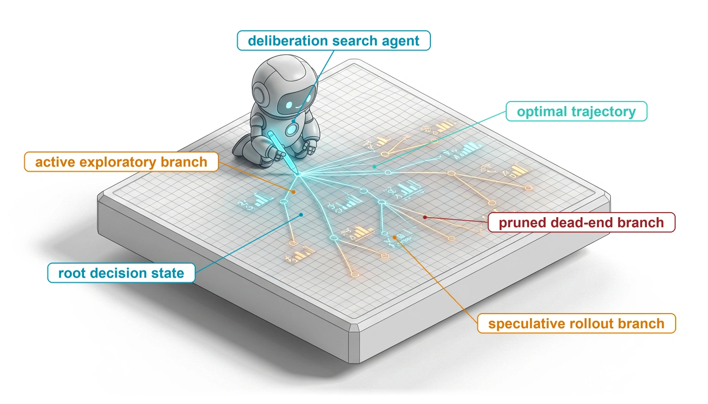
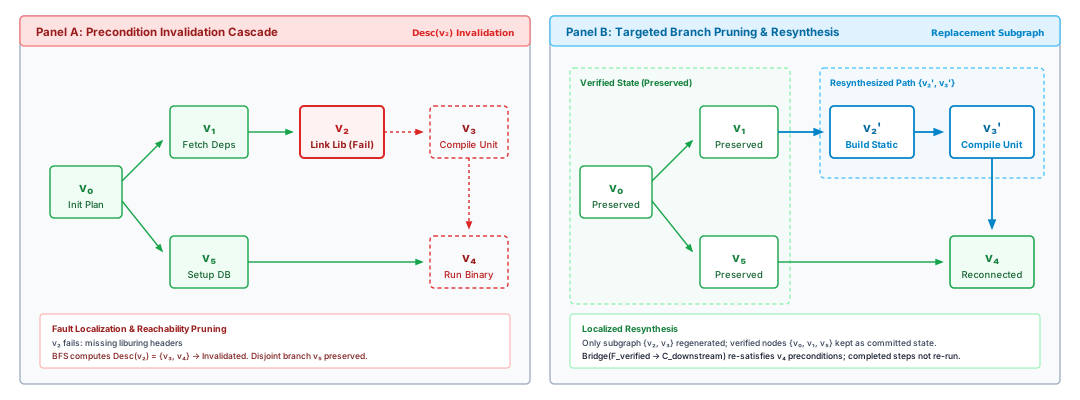
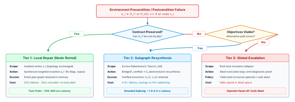
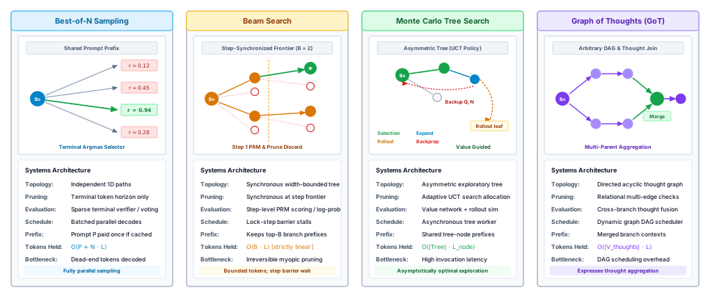
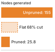
When is another token, candidate, check, or model call worth its cost?
An agent that deliberates before acting pays latency and money for a better chance of success, whether it spends them on a longer derivation, more candidate patches, an extra check, or another model call. Each purchase answers a different question. More tokens re-examine what the prompt already holds, more candidates raise the chance that a good one sits somewhere in the pool, and only an executed check adds a fact the model did not have. None of them makes the returned answer correct, because a selector can return a plausible failure, and a search that optimizes against a flawed check finds the flaw faster than the fix. Deliberation is therefore a budgeted allocation problem with a stopping rule. The runtime decides where the next unit of work goes, how far a passing check can be trusted, and when to stop, abstain, or escalate instead of returning its best unverified guess. Every extra turn spent inside one decision lengthens the horizon, so that spending has to be bounded before the agent acts on anything.
Learning Objectives
Compare depth, breadth, and feedback as ways to spend a per-decision budget, by the information each adds, the tokens it consumes, and its critical path.
Distinguish candidate availability from selected-output quality when evaluating voting, learned scoring, and task-specific checks.
Calculate accepted-set precision from stated checker error rates and explain how adaptive search can change those assumptions.
Represent a candidate plan as a dependency graph and identify which parts require revision after an observation changes.
Analyze how step-level checks and pruning bound a search tree’s growth and its scorer cost.
Design stopping rules that enforce resource ceilings without treating budget exhaustion as acceptance evidence.
Evaluate competing deliberation policies under a common budget and deadline by pass probability, actual spend, and abstentions.
3.1 Limits of a Single Response
The repair agent (Four lighthouse workloads) inspects the connection-pool implementation and receives a completed candidate patch. The invocation contract admits it as a candidate, yet the patch rests on an incomplete diagnosis. Client requests intermittently stall even after idle connections become available. Two distinct failure modes can produce this symptom: an aggressive timeout that aborts too early, or a lost notification when a worker thread returns a connection to the pool. When prompted, the language model proposes extending the timeout. That change offers a plausible workaround, but it provides no evidence that the timeout caused the stalls. Deploying such a patch immediately risks masking the latency tail while leaving the concurrency defect intact.
Deliberation extends the horizon with extra model turns and checks inside one decision, and hard ceilings bound that spend.
Before committing to an edit, the agent runtime can spend extra work in three distinct ways. It can give the model a longer output allowance to trace how threads acquire and release the lock step by step; it can sample several candidate patches that modify different parts of the pooling logic; or it can run a targeted test harness to record whether a waiting thread actually receives the condition-variable notification. Each option buys a different kind of evidence. Extended reasoning can expose logical flaws in the source text. Sampling across temperature or prompt variations can surface fixes that a greedy single pass misses. An instrumented test, by contrast, observes runtime state directly and reveals dynamic thread interactions that token generation alone cannot establish.
This division marks the boundary between model computation and runtime observation. Extra model computation re-evaluates information already present in the prompt. Within a single generation, a model can backtrack and revise an earlier analytical misstep even as the previous tokens remain frozen in its prefix. Pure computation, however, cannot create new empirical facts. Only an executed test reports how the running process behaves, and its conclusions hold only for the conditions and thread schedules that the test harness exercised.
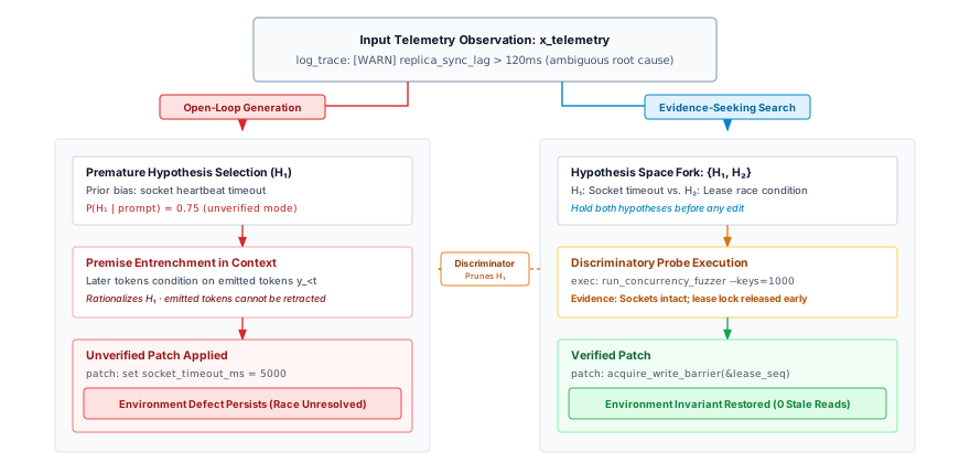
Suppose the targeted test forces an interleaving where one worker thread waits while another returns a connection. The trace shows that the connection enters the pool, yet the waiting worker stays blocked past the notification point. That observation rules out the timeout hypothesis immediately and points the agent toward the signaling path. The agent can then write a patch that repairs the notification logic and test it against the failing reproducer. Passing a targeted reproducer still does not establish full task acceptance, because narrow tests can miss edge cases, and neither an unchecked hypothesis nor an isolated micro-test is enough to ship code to production. Even so, the two paths part ways before any file changes (figure 1). Acting on the first guess hides the symptom and keeps the defect, whereas checking first spends one short test to learn which hypothesis survives.
Figure 1: Committing to a Hypothesis vs. Checking It: Both paths start from the same connection-pool failure. On the left, generation builds on the timeout explanation without any observation that separates it from a missed notification, so the patch can hide the symptom while the defect remains. On the right, a targeted test orders a waiting worker and a returning connection, and its observation contradicts the timeout explanation before any edit. The revised candidate passes the reproducer, which still falls short of task acceptance.
Napkin Math 3.1: A probe vs. a longer answer
Problem: A prepared diagnostic test takes 40 ms. A proposed explanation contains 1,024 output tokens. How long does the explanation take to generate relative to the test?
Variables: The illustrative per-token generation time from Estimating per-call hardware work is 21.07 ms, derived from memory-bandwidth limits rather than a measured production service rate. The hypothetical output pricing is $15 per million tokens. Prompt processing, queueing, transport, test preparation, and the downstream model call that reads the test observation are excluded.
Math: Generating 1,024 tokens at 21.07 ms per token requires 21.58 s and incurs $0.01536 in token charges. Dividing this generation latency by the 40 ms test run yields a factor of 539.5×.
Systems insight: When the unresolved question concerns dynamic program behavior, the probe settles it 539.5× faster than the model can generate a speculative explanation of it, and only the probe’s answer is an observation. Running a test is preferable whenever its preparation and execution time remain below the explanation’s 21.58 s and its outcome cleanly separates the competing failure modes. Conversely, an inconclusive test that does not separate the hypotheses provides no diagnostic gain regardless of its speed. Failure to reproduce can still supply negative evidence when the test’s sensitivity to the suspected fault is known. A sound runtime spends work on whichever operation most cheaply removes the main source of uncertainty.
The probe, and the decision to revise the patch on its evidence, both happened outside any single model call. The invocation contract of the previous chapter ends at one prompt and one candidate, accompanied only by metadata indicating whether generation reached a stop token or an output limit. That interface cannot decide whether spending the next second of latency or fraction of a cent on longer reasoning, extra candidate samples, or a runtime probe will produce a better fix. An API response marked complete confirms only that generation finished, not that the proposed patch fixes the bug. Test-time compute is all the system work the runtime orchestrates around the model call, with model weights held fixed, to generate, test, and select candidates before committing to an action. Governing that spend requires a runtime policy that sets hard ceilings on latency and cost, routes work across reasoning and checks, and stops cleanly without mistaking an exhausted budget for a verified solution.
Each part of that policy raises the next question. The runtime first chooses how to spend extra work across reasoning depth, candidate breadth, and empirical feedback (section 3.2). Breadth produces a pool, so the runtime must then pick from it without being fooled by a plausible failure (section 3.3), and picking well depends on how far a passing check can be trusted (section 3.4). When a check refutes a premise partway through a plan, the runtime should regenerate only what depended on it (section 3.5). Candidates and revisions together form a search whose spending must be tracked, reserved, and stopped (section 3.6), and the complete policy is finally judged against its alternatives under one budget and one deadline (section 3.7).
3.2 Three Axes of Test-Time Compute
Giving a repair agent a four-thousand-token allowance does not determine its latency, memory footprint, or diagnostic reach, because the runtime can spend those same four thousand tokens on one long derivation, four parallel candidate patches, or three edit–test–revise rounds. Although all three options can consume the same number of output tokens, they stress the serving system in very different ways. A long derivation generates tokens one after another along a single causal chain. Independent candidate patches can run concurrently across accelerator hardware. An edit–test–revise loop must pause model generation while each diagnostic test runs. Those dependencies determine which operations sit on the critical latency path and how much state the serving engine must hold in memory.
Depth extends sequential computation within a single candidate, breadth explores multiple candidate paths concurrently, and feedback folds environment observations into subsequent revisions. A test-time deliberation rollout is one bounded candidate-generation path, potentially interleaving verification checks and observation-driven revisions; the term comes from game search, where a rollout plays one line of moves forward to its end. Depth lengthens a rollout, breadth runs several in parallel, and feedback inserts checks between a rollout’s turns. An allocation policy can combine all three: it might generate several candidate patches in parallel, run regression tests against each, and spend deeper step-by-step reasoning only on the most promising survivor. Throughout, model weights remain frozen, and every axis draws from the same test-time budget.
Definition 3.1: Test-time compute budget
Test-time compute budget is the per-decision allowance of processed prompt tokens, generated tokens, model invocations, verification checks, and elapsed wall-clock time that a runtime may expend, with model weights fixed, before it must select a candidate, abstain, or escalate to a human operator.
Significance: The budget sets the attempt cost in the effective cost per accepted task, \(\CostPerAcceptedTask = \mathbb{E}[\AttemptCost]/\AcceptanceProbability\) (equation 1.2). Additional deliberation reduces cost per accepted task when it increases the acceptance rate \(\AcceptanceProbability\) proportionally faster than it increases the expected attempt cost. A higher cost per accepted task can still be justified when it buys the required acceptance rate within the deadline (section 3.7.3).
Distinction: Training compute amortizes weight optimization once across all future tasks. Test-time compute recurs on every decision, where an internal reasoning allowance is merely one control surface alongside external tool invocations and verification checks.
Common pitfall: Treating the maximum allocation ceiling as the expected spend, or treating an exhausted budget as evidence that the best remaining candidate is acceptable.
What separates the three axes is their dependency structure (figure 2). Depth extends a single candidate through multi-step reasoning, breadth fans out to sampled candidates that converge on a selector, and feedback routes a candidate through a sandboxed check whose observation conditions the revision.
Figure 2: Three compute allocation topologies: Depth extends one candidate; breadth exposes separate sampled candidate paths followed by selection; feedback makes a later candidate depend on an observed check result. The arrows show dependencies, not guaranteed latency, cost, or correctness.
3.2.1 Extending reasoning along the depth axis
Asking a model to jump straight from a bug report to a patch often misses multi-step lock interactions, yet letting it reason for thousands of tokens puts every step onto the critical latency path and can exhaust the output limit before any code is emitted. Extending a call along the depth axis lets an autoregressive model unroll intermediate reasoning tokens before emitting its final decision or artifact, generalizing early scratchpad techniques and chain-of-thought prompting (Nye et al. 2021; Wei et al. 2022). In the connection-pool scenario, these intermediate tokens might trace thread interleavings step by step: acquiring the pool mutex, checking for leaked socket descriptors, and signaling waiter condition variables. Because autoregressive generation conditions on all prior tokens, later decoding steps can inspect earlier derivations, catch flawed assumptions, and change course before emitting code. That gain comes entirely from running extra forward passes over the growing context rather than changing the network weights.
Nye, Maxwell, Anders Johan Andreassen, Guy Gur-Ari, Michal Michalewski, Jacob Austin, David Bieber, David Dohan, et al. 2021. “Show Your Work: Scratchpads for Intermediate Computation with Language Models.”arXiv Preprint arXiv:2112.00114, ahead of print. https://doi.org/10.48550/arXiv.2112.00114.
On the hardware, however, extending a single generation path serializes the work. Because transformer decoding at small batch sizes is memory-bandwidth bound, step latency is set by the time needed to stream all model parameters from high-bandwidth memory into processor caches (principle 2). Wall-clock generation time therefore scales roughly linearly with the number of generated tokens under a fixed serving setup. A long reasoning trace shows only that the accelerator performed more work, not that the resulting code compiles or runs correctly. The runtime must also leave enough output budget for the final patch: a derivation that hits the token limit mid-thought returns a truncated response, which the invocation contract quarantines like any other incomplete call rather than admitting as a candidate.
3.2.2 Parallel sampling along the breadth axis
Drawing a single completion commits the repair to whatever hypothesis the model’s first tokens favored, and if that initial framing is wrong, extra depth only elaborates a flawed premise. Sampling along the breadth axis hedges against that commitment by requesting multiple candidate patches from the same source excerpt and task specification using stochastic decoding controls. Conditional on a fixed prompt and independent random seeds, these samples are statistically independent draws from the model’s output distribution. Even so, they remain bounded by what the model knows: if the model assigns negligible probability mass to a valid thread-notification pattern, every independent sample can repeat the same missing broadcast. Independent draws can still fail in identical ways.
↩︎ Temperature, top-\(\Glyph{k}\), and nucleus sampling controls are established in Sampling controls.
Because parallel candidates do not depend on one another, breadth exposes fine-grained concurrency at modest latency cost. Under memory-bandwidth-bound decoding (principle 2), a batch of \(\CandidatePoolSize\) concurrent candidate streams reads the model weights once per step for all \(\CandidatePoolSize\) tokens. Spending an allowance of \(\CandidatePoolSize \times \OutputLength\) tokens sequentially along the depth axis multiplies generation latency by roughly \(\CandidatePoolSize\). Generating \(\CandidatePoolSize\) candidates of length \(\OutputLength\) in parallel, by contrast, keeps total generation time close to the duration of the longest candidate, \(\max_n \DecodeInterval(\OutputLength_n)\), provided the batch stays memory-bandwidth bound and fits in accelerator memory.
Accelerator memory is where breadth extracts its price. Each active generation stream must maintain its own key-value (KV) cache for the tokens it generates. When the serving system shares prefixes across streams, the \(\SequenceLength\)-token prompt is stored once in memory, and peak KV cache demand scales as
Without shared prefix caching, the serving engine stores \(\CandidatePoolSize\) copies of the prompt’s KV tensors, and memory demand scales as \(\CandidatePoolSize \SequenceLength + \sum_n \OutputLength_n\). When total KV cache demand exceeds hardware capacity, the serving engine must split candidates into sequential waves. Once forced into waves, breadth latency degrades from the duration of the single longest candidate toward the sum across waves, while memory thrashing and queueing delays stretch individual token latencies. Whether identical prompt prefixes share physical memory or receive provider billing discounts depends on the serving engine.
↪ Block sharing, which stores a common prompt’s KV state once for every candidate that branches from it, is developed in Copy-on-write prefix sharing.
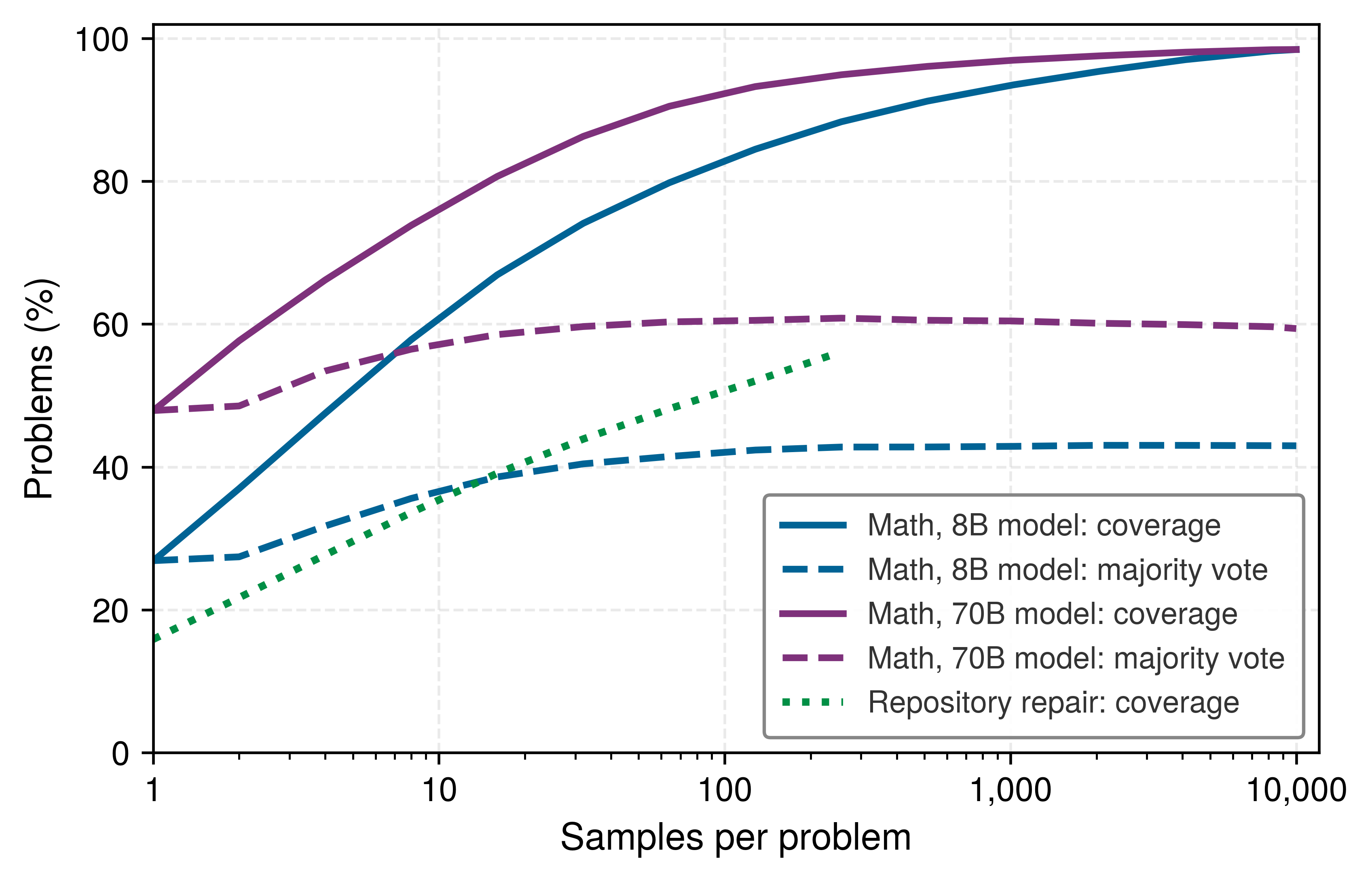
Breadth also shifts the burden downstream, because generating a wide pool of candidates pays off only if the runtime can tell which candidate is best. A pool that holds a working patch is useless if the selector cannot identify it. In a study of repeated sampling, Brown et al. (2024) showed that while the probability that at least one candidate is correct (pass@\(\IndependentAttemptCount\)) kept rising across four orders of magnitude of samples, practical selectors such as majority voting and learned reward models (scorers trained to predict whether a candidate is correct, examined in section 3.4.1) plateaued after a few hundred samples. Candidate selection is therefore a major consumer of compute and verification budget, not an incidental final step.
3.2.3 Revising from observations along the feedback axis
Neither a longer chain of thought nor a wider pool of samples tells the model whether a waiting thread actually receives a condition-variable signal at runtime. The feedback axis supplies that missing evidence by executing a check on a candidate and feeding the resulting observation into the next model request. Instead of relying on frozen weights and a static prompt alone, the repair agent proposes a candidate patch, the runtime runs a bounded test suite, and the next model call receives concrete diagnostics such as a stack trace from a deadlocked worker thread. Those runtime observations narrow the next candidate far more sharply than asking the model to reread the original prompt on its own (Shinn et al. 2023).
Shinn, Noah, Federico Cassano, Ashwin Gopinath, Karthik Narasimhan, and Shunyu Yao. 2023. “Reflexion: Language Agents with Verbal Reinforcement Learning.”Advances in Neural Information Processing Systems (NeurIPS) 36: 8634–52.
Verification checks return structured outcomes: failure, pass, or inconclusive execution (such as a test timeout). A failure trace points to broken assertions or regressions; a passing test confirms that the code satisfies the exercised assertions under the tested conditions; and final acceptance remains a separate policy gate. Running diagnostics is itself an external action that consumes CPU and memory, runs inside a sandbox, and adds wall-clock latency even when used only inside deliberation.
Each feedback round is also one more turn of the horizon \(\TurnHorizon\), which ties this axis to horizon compounding (equation 1.1). Unchecked turns compound error as \((1-\PerStepErrorRate)^{\TurnHorizon}\), and the introduction showed (Reliability and Cost over a Horizon) that a check which rejects a bad step and retries it resets that compounding. Feedback is the one axis that places such a check inside every turn, so it can lengthen a deliberation without the unchecked compounding its extra turns would otherwise carry, to the extent that its checks deserve trust (section 3.4).
Feedback forces strict serialization because the next revision cannot start until the current check finishes and returns its observation. Context policies that append every prior candidate and diagnostic report also make the input prompt grow from turn to turn. For an initial prompt length \(\BasePromptLength\), candidate lengths \(\OutputLength_j\), and observation lengths \(\lvert \TrajectoryObservation_j\rvert\), an append-only policy yields an input length at turn \(\TurnIndex\) of
This is the append-only growth that equation 2.9 priced across a whole trajectory, now confined to one decision, and it drives up prompt prefill latency, accelerator memory usage, and token billing on every round. Context-compaction methods can summarize earlier attempts or drop stale diagnostic traces, but the allocation policy must budget for the full token volume actually sent to the model API.
↪ Context-compaction methods and their scheduling within the request budget are developed in Context Compaction.
3.2.4 The three axes under one output ceiling
Capping generated tokens at a single number does not cap wall-clock latency, accelerator memory, or input-token billing, because depth, breadth, and feedback turn the same output ceiling into very different resource loads. Runtimes therefore track four quantities across the three axes: input and output token counts, critical-path wall-clock latency, peak retained accelerator state, and external information gained. Let \(\PrefillTime(\SequenceLength)\) be the time required to ingest an \(\SequenceLength\)-token prompt, \(\PerTokenDecodeTime\) the per-token decoding step time, \(\DecodeInterval(\OutputLength)\) the total generation time for \(\OutputLength\) tokens, and \(\FeedbackCheckDuration\) the duration of the external check in feedback round \(\TurnIndex\), which is also the turn index of the trajectory. With \(\ExtendedDepthLength\) tokens of extended depth, \(\CandidatePoolSize\) breadth candidates executed concurrently, and \(\TurnHorizon\) feedback turns, the latency dimension decomposes into three critical paths:
The critical path for breadth assumes the serving cluster has enough memory and compute capacity to decode all \(\CandidatePoolSize\) streams concurrently at an unchanged step time. When capacity saturates, decoding falls back into serialized waves and shifts the critical path toward the sum across candidate streams. The feedback expression, by contrast, grows from two sources: sequential check durations \(\FeedbackCheckDuration\) and lengthening prompt prefill times \(\PrefillTime(\SequenceLength^{(\TurnIndex)})\) as context accumulates. Equation 1 covers only latency; table 1 sets those critical paths beside the tokens processed, the peak model state retained, and the external information acquired.
Table 1: Resource model of the three allocation axes: Symbolic accounting of processed tokens, critical path, retained model state, and information source. Concurrency and prefix sharing are capacity and implementation assumptions, not properties of the axis.
Axis
Tokens processed
Critical path
Peak retained model state
New information
Depth
\(\SequenceLength + \ExtendedDepthLength\)
One dependent sequence
One context of \(\SequenceLength + \ExtendedDepthLength\) tokens
\(\CandidatePoolSize\) contexts, \(\SequenceLength + \sum_n \OutputLength_n\) tokens if shared
Sampling variation over the same request
Feedback
\(\sum_{t}(\SequenceLength^{(\TurnIndex)} + \OutputLength_t)\), with \(\SequenceLength^{(\TurnIndex)}\) growing
Sum of turns, including each check
One active context of \(\SequenceLength^{(\TurnHorizon)} + \OutputLength_{\TurnHorizon}\) tokens
Observations from executed checks
Of the three axes, only feedback brings in external information absent from the model weights and prompt. The calculation below evaluates these expressions for the connection-pool repair under a fixed output ceiling of 4,096 tokens, showing how equal output ceilings produce very different latencies and token bills.
Napkin Math 3.2: One decision, three allocations
Problem: A repair request starts with 4,096 input tokens and a common ceiling of 4,096 generated tokens. How do depth, breadth, and feedback spend that allowance?
Variables: Reuse the illustrative per-token generation time from the preceding example. Breadth has capacity for 4 concurrent streams at that same rate. Each short candidate uses 1,024 generated tokens. Feedback uses 3 turns, each followed by a 1.5 s check returning 340 tokens. Later feedback requests append earlier candidates and reports. Hypothetical prices are $3 per million input tokens and $15 per million output tokens, without cache discounts, so each breadth stream is billed for its own copy of the prompt (unlike the shared-prefix row of table 1). Generation times omit prefill, queueing, and transport; the feedback time additionally includes its checks. The bill counts model tokens only, and table 2 tallies each allocation’s tokens, time, and bill side by side.
Table 2: Allocation accounting under a common output ceiling: Equal ceilings produce unequal spend. Allowances omit prefill, queueing, selection, and tool charges.
Allocation
Input tokens
Output tokens
Generation and included checks
Model-token bill
Depth
4,096
4,096
86.32 s
$0.07373
Breadth
16,384
4,096
21.58 s
$0.11059
Feedback
16,380
3,072
69.24 s
$0.09522
Math: In table 2, depth generates all 4,096 tokens along a single path. Breadth generates 1,024 tokens on each of 4 concurrent paths, shortening the critical path by 4×. However, reading the prompt 4 times across unshared streams adds 12,288 input tokens, multiplying its billing cost to 1.5× that of depth. Feedback accumulates input context over \(\TurnHorizon\) turns according to \(\TurnHorizon\,\BasePromptLength + (\OutputLength + \lvert \TrajectoryObservation\rvert)\,\TurnHorizon(\TurnHorizon-1)/2\), reaching 16,380 tokens at \(\TurnHorizon =\) 3 because each successive round re-reads all prior candidates and observation reports.
Systems insight: Breadth trades money for lower wall-clock latency, and its entire billing premium comes from the \((\CandidatePoolSize-1)\SequenceLength\) re-read prompt tokens. The governing ratio is prompt length relative to generated output: a large repository context makes breadth’s input bill grow steeply with both \(\CandidatePoolSize\) and \(\SequenceLength\), whereas a short prompt or a shared prefix cache removes most of that surcharge. Feedback lands between depth and breadth in both latency and billing while remaining the only axis that acquires new runtime observations. Because this accounting leaves out pass rates, it prices the work rather than the quality of the result.
3.2.5 Internal budgets and external orchestration
When a model service hides its intermediate reasoning tokens behind an API, a runtime that gauges effort from the length of the visible reply understates both token spend and latency. Production systems therefore separate two control surfaces: internal model deliberation and external workflow orchestration. A model service may expose an internal reasoning budget that governs how many intermediate tokens a single call may spend, while the runtime independently controls how many calls to dispatch, which tool checks to run, and what context to pass into subsequent requests. Internal budgets adjust depth inside one call; external orchestration governs breadth across branches, schedules sandboxed checks, and assembles revised prompts. Because commercial APIs often redact intermediate reasoning traces, the runtime must read explicit token-usage headers and termination status codes rather than character counts to enforce quotas and track spend.
3.2.6 How reasoning models spend output allowances
A model trained to think in a long internal scratchpad can burn its entire output allowance on intermediate steps and return an empty or truncated final answer. Reasoning models are trained with reinforcement learning on tasks with objective, verifiable outcomes, such as formal mathematics, logic puzzles, and unit-tested codebases, where they learn to generate extended intermediate scratchpads that propose solutions, check steps, and backtrack within a single call (OpenAI 2024; DeepSeek-AI et al. 2025). At the serving layer, those intermediate reasoning tokens are ordinary autoregressive output tokens: they consume accelerator compute, fill the KV cache, and incur full output-token charges whether the user interface displays them or hides them behind summary metadata. Because that scratchpad draws from the call’s output allowance, services expose a reasoning-budget parameter that turns sequential depth from a fixed model habit into a per-request runtime knob that the orchestrator can set by task. No matter how high that knob is set, however, internal reasoning operates strictly over the supplied prompt and static weights; an extended scratchpad can check arithmetic or trace logic across the prompt, but it cannot observe runtime behavior or tell whether a proposed patch fixes a connection leak without running a test suite.
OpenAI. 2024. Learning to Reason with LLMs. OpenAI Research Blog.
Because models trained with verifiable rewards spend output allowances differently than instruction-tuned models (models adapted to follow example instructions and responses), token ceilings must be calibrated per model family. When internal reasoning traces remain hidden, the runtime can observe only its own call telemetry and check results, which guide orchestration policy rather than guaranteeing that a candidate is correct. Treating depth as a per-call knob still lets the runtime vary token spend across tasks, raising the practical question of which allocation axis pays off at each level of task difficulty.
Example 3.1: Compute-optimal test-time allocation
Scenario: Snell et al. (2024) evaluated strategies for spending a fixed test-time compute budget across reasoning benchmarks, comparing sequential revision of a single candidate against parallel breadth sampling and search guided by learned process verifiers (section 3.4). The study grouped benchmark problems into difficulty tiers by the base model’s single-shot success rate.
Diagnosis: On easier problems, sequential revision used the budget most effectively, fixing minor mistakes without the overhead of parallel sampling. On moderately difficult problems, hybrid strategies combining parallel exploration with verifier-guided search reached higher accuracy. On the hardest problems, scaling test-time compute hit diminishing returns across all axes. At matched total FLOPs, a well-chosen test-time allocation let a smaller model beat a model 14 times larger whenever the smaller model had a nonzero base success rate; when base success sat near zero, spending FLOPs on a larger base model beat exhausting tokens on parallel rollouts.
Systems lesson: With the supplied prompt held fixed, extra reasoning and sampling can surface capabilities the model already has, but they cannot supply missing runtime facts. Feedback can bring new observations into the next call, though their value still depends on the check’s coverage and the model’s ability to use them. Runtimes should route budgets by estimated difficulty: spend a small budget or a single call on straightforward tasks, use parallel search and feedback on moderately hard tasks, and escalate near-zero-yield requests to a stronger model or a human operator instead of burning tokens on unguided sampling.
Because a runtime does not know a task’s true difficulty in advance, it estimates difficulty with cheap, fast signals before committing a large deliberation budget. Common signals include agreement among two or three short pilot samples, fast static linters, and historical failure rates on similar requests. When pilot samples agree and pass static checks, the runtime keeps the budget small and finishes in one call. When pilot samples disagree or linters flag errors, the scheduler escalates to broader sampling or an edit–test–revise loop, and if the budget ceiling is reached without a verified candidate, it stops and escalates to a human operator. Each routing signal acts as a classifier whose precision and recall should be measured on held-out tasks.
In practice, internal depth and external breadth work together. Each rollout may use enough depth to draft a coherent code patch while the runtime samples several such patches in parallel and filters them through a test harness. Even so, the mix has to fit the system’s bottlenecks: slow tests stretch the feedback critical path, and weak tests dull the value of each observation. Those same checks also matter during training, because reinforcement learning with verifiable rewards uses them as a training reward, turning any blind spot or false pass that causes a bad selection at test time into a loophole that training actively optimizes for on every weight update.
↪ How an acceptance check becomes a training reward, and how its gaps are exploited during training, is developed in Verifiable Rewards.
Checkpoint 3.1: Choosing an allocation
Choosing how to spend compute across depth, breadth, and feedback determines what candidates enter the pool, but generating a good candidate does not help if the selector picks a plausible broken one instead. The next step is choosing among candidates without spending more on selection than the pool is worth.
3.3 Selecting from a Candidate Pool
Sampling eight candidate patches for the connection pool helps nothing if seven of them repeat the same broken timeout workaround and the selector picks one of the seven over the single patch that fixes the notification bug. In a typical pool, one candidate might lengthen an acquisition timeout, another might add exponential retries, and a third might change how the connection-return path wakes waiting threads. The runtime has to decide which proposal, if any, has enough supporting evidence to return, and gathering that evidence consumes time and tokens from the same deliberation budget that produced the pool.
Two questions separate generation from selection: whether the pool holds at least one candidate that solves the task, and whether the selector can pick that candidate without accepting a broken one. A generator can flood the pool with proposals without making selection any easier; conversely, a sharper selector can raise end-to-end reliability without sampling a single extra candidate.
3.3.1 Useful variation among candidates
Renaming local variables, reformatting comments, or rewriting a loop can produce eight distinct token sequences that all leave the synchronization bug untouched. Surface variation in token sequences does not guarantee diverse repair hypotheses. In the connection-pool repair, candidates add value only when they test different explanations that downstream checks can tell apart. Changing the thread-notification path vs. lengthening the timeout tests two distinct hypotheses; generating half a dozen slightly reworded versions of the same timeout bump only wastes verification runs.
This problem is separate from statistical dependence. When the task, prompt, base model, and sampling controls stay fixed, separate draws with independent random seeds are genuinely independent and identically distributed (IID). Even so, if the model puts almost all of its probability mass on timeout edits, independent draws will still fill the pool with variations on that one mistake.
Across a mixed production workload, shared model blind spots matter even more. A model often solves familiar patterns reliably while failing every time on an unfamiliar edge case, so repeated samples on a hard task fail together far more often than the average pass rate across all tasks would suggest. While samples on a single fixed task may be conditionally independent, treating attempts across a mixed workload as draws with one shared pass probability hides that clustering. Feedback-driven revision changes the distribution again: once the runtime feeds test errors into later prompts, each new candidate depends directly on what earlier checks found.
A runtime can encourage broader exploration by raising sampling temperature or prompting the model to try distinct diagnostic angles under the same task constraints. Pushing diversity too hard, however, often produces syntax errors, broken invariants, or nonsensical edits. A diversification method earns its keep only if it raises the task pass rate within a fixed compute and latency budget.
To avoid wasting test runs on near-duplicates, the runtime can prune redundant candidates early by deduplicating on structure and behavior. Abstract syntax tree (AST) normalization strips away surface changes such as variable names and whitespace, and behavioral clustering runs candidates on cheap inputs to group those with identical outputs. Using both steps let a competitive code-generation system narrow tens of thousands of raw model samples down to a handful of distinct submissions (Li et al. 2022). Each method groups candidates by a bounded equivalence relation, whether normalized syntax or matching outputs on a probe set, and deduplication is sound whenever that relation preserves the property the downstream check tests.
Li, Yujia, David Choi, Junyoung Chung, Nate Kushman, Julian Schrittwieser, Rémi Leblond, Tom Eccles, et al. 2022. “Competition-Level Code Generation with AlphaCode.”Science 378 (6624): 1092–97. https://doi.org/10.1126/science.abq1158.
3.3.2 Choosing a selection rule
Picking the most common patch by majority vote fails whenever the model’s favored mistake outnumbers the one candidate that fixes the bug, whereas running the full test suite on every raw sample wastes sandbox time on patches that do not even parse. Runtimes therefore combine three kinds of selection signal, ordered by cost and by the strength of the claim each supports: direct execution checks, answer agreement (consensus voting), and learned ranking.
Direct checks, such as a parser, a type checker, or a test harness, test a candidate deterministically against explicit rules. Each establishes only the property it checks, as the scoped check pipeline of Staging checks by cost and scope showed, so clean compilation says nothing about whether a race condition is gone. Running candidate code is also an external action that requires sandbox isolation, hard timeouts, and tight permission boundaries.
Answer agreement combines independent reasoning paths by vote. In self-consistency, the runtime samples several reasoning chains, normalizes their final answers, and takes the plurality vote (Wang et al. 2023). That works well for arithmetic, symbolic logic, or short factual answers, but majority vote still reflects only what the generator produces most often. When a model shares a systematic bias or takes a flawed shortcut, independent samples regularly converge on the same wrong answer. For code repair, voting over raw patches is a poor selector: behavioral agreement inherits the coverage limits of the probe inputs, and a minority patch that actually passes the reproducer should beat a popular patch that fails it.
When deterministic checks cannot cover every requirement, learned rankers and model-based judges supply a heuristic ordering. A learned reward model or a secondary large language model (LLM) judge (a model prompted to grade another model’s output) can score explanation clarity, check style guidelines, or rank patches before the runtime spends time on heavy integration tests. Even so, ranking and acceptance answer different questions. Ranking orders candidates from best to worst under a score; acceptance decides whether a candidate meets the task contract. If every candidate in the pool is broken, picking the highest-ranked candidate simply returns the best-looking failure. Returning a candidate instead of abstaining requires a verifier that produces an objective pass or fail result.
Definition 3.2: Verifier-guided selection
Verifier-guided selection is a selection policy that returns a candidate only when a verifier, a check whose criteria and observations the candidate cannot modify, passes it, and abstains when no candidate passes.
Significance: Its success rate is capped by pass@\(\IndependentAttemptCount\), the chance the pool holds a passing candidate (section 3.3.3), while the share of its selections that are correct depends on both the verifier’s passing-set precision and the selection policy (section 3.4.2). The fixed IID first-passing policy developed there preserves passing-set precision; ranking among passing candidates need not. Selection coverage and selected correctness together determine the probability of returning a valid result.
Distinction: Voting selects what the generator produces most often and learned ranking selects what a scorer prefers; only a verifier’s verdict can justify returning a candidate instead of abstaining.
Common pitfall: Treating the verifier’s pass as task acceptance; the verdict covers the checked property, and its false acceptance rate grows in importance as the pool’s valid-candidate rate falls.
The hypothetical repair pool in table 3 shows what each check stage can and cannot establish. Here a focused reproducer exercises the known race condition, while full regression suites have not yet run.
Table 3: Evidence for candidate selection: A hypothetical repair pool separates the proposed mechanism, the observed result, and the conclusion each check supports.
Candidate
Proposed repair
Observed check result
Supported conclusion
A
Increase the timeout
Compiles; known failure remains
Structural validity is insufficient
B
Retry after the timeout
Compiles; known failure remains
Different code can preserve the same defect
C
Change notification handling with malformed syntax
Parsing fails
This artifact cannot proceed to execution testing
D
Change notification handling with valid syntax
Compiles; reproducer passes
Promising repair, with untested behavior still unresolved
A production runtime stages these checks cheapest first, following the cost-ordered cascade of Scoped candidate checks, so that parsing and AST checks drop malformed candidates before they reach sandboxed tests or an LLM judge. Inside a search, the stage order should come from measured run time and rejection rate rather than guesswork. Running a compiled binary in a warm container might take 5 ms, whereas calling a large LLM judge to grade code quality is a full model call that can take 800 ms and eat into the token budget. Comparing several candidates in a single prompt also scales differently with context length than scoring each candidate on its own. Because checking competes directly with generation for time and tokens, selection has to be budgeted as part of test-time compute.
3.3.3 Candidate availability under pass@\(\IndependentAttemptCount\)
When a runtime fails to return a working patch from a pool of \(\IndependentAttemptCount\) samples, the engineer needs to know whether the generator never produced a passing patch or the selector threw a passing patch away. pass@\(\IndependentAttemptCount\) separates those two failures by measuring the probability that at least one of \(\IndependentAttemptCount\) sampled candidates passes the specified tests (Chen et al. 2021).1
1Origin of pass@\(\IndependentAttemptCount\): The metric was introduced to score program synthesis by functional correctness rather than by textual similarity to a reference (Kulal et al. 2019). Because plugging the observed pass fraction \(\PassingSampleCount/\GeneratedSampleCount\) into \(1-(1-\PassingSampleCount/\GeneratedSampleCount)^\IndependentAttemptCount\) biases the estimate of what breadth buys, Chen et al. (2021) replaced it with the combinatorial estimator derived below.
Kulal, Sumith, Panupong Pasupat, Kartik Chandra, Mina Lee, Oded Padon, Alex Aiken, and Percy S. Liang. 2019. “SPoC: Search-Based Pseudocode to Code.”Advances in Neural Information Processing Systems (NeurIPS) 32.
Chen, Mark, Jerry Tworek, Heewoo Jun, Qiming Yuan, Henrique Ponde de Oliveira Pinto, Jared Kaplan, Harri Edwards, et al. 2021. “Evaluating Large Language Models Trained on Code.”arXiv Preprint arXiv:2107.03374.
For a fixed task and fixed generation policy, suppose independent samples each pass the tests with probability \(\AttemptPassProbability\). The probability that all \(\IndependentAttemptCount\) samples fail is \((1-\AttemptPassProbability)^\IndependentAttemptCount\), so
This expression is conditional on that task and sampling policy. To summarize a workload with different task-level pass probabilities, average the task-level quantities; substituting the workload’s average \(\AttemptPassProbability\) generally gives a different result. For an adaptive policy that revises its prompt after feedback, evaluate the policy’s resulting pools rather than assuming they follow this fixed-distribution formula.
In a benchmark, generate \(\GeneratedSampleCount \ge \IndependentAttemptCount\) candidates for a task and let \(\PassingSampleCount\) pass the fixed test criterion. Of the \(\binom{\GeneratedSampleCount}{\IndependentAttemptCount}\) subsets of size \(\IndependentAttemptCount\), exactly \(\binom{\GeneratedSampleCount-\PassingSampleCount}{\IndependentAttemptCount}\) contain only failures. The subset estimator is therefore
with the numerator taken as zero when \(\GeneratedSampleCount-\PassingSampleCount<\IndependentAttemptCount\). Under independent, identically distributed sampling for the fixed task, this estimates the probability that a fresh pool of \(\IndependentAttemptCount\) candidates contains a test-passing member without bias; Pass@\IndependentAttemptCount and repeated-run consistency derives this expectation and details evaluation without factorials. Benchmark results average these estimates over tasks (Chen et al. 2021).
The relationship to deployed selection follows from the event being measured. If the selector must return an unchanged member of the same pool, it cannot return a test-passing candidate when the pool contains none. Its probability of returning a test-passing candidate is therefore at most pass@\(\IndependentAttemptCount\), counting abstention as no returned pass. A selector that always finds a passing member whenever one exists reaches this ceiling; whether the deployed selector does, within the deployment’s checking budget, is a separate measurement.
Notice also that the predicate in pass@\(\IndependentAttemptCount\) is passing these tests, which is narrower than satisfying the complete task requirements, and that the ceiling covers only selectors that return an unchanged pool member rather than repairing candidates or synthesizing a new artifact. Benchmarks therefore report candidate availability alongside selected-output performance under the relevant criterion, because the gap between the two can be large. Figure 3 recomputes the plateau described in section 3.2.2 from the released per-sample correctness labels of Brown et al. (2024), plotting coverage (the task-averaged pass@\(\IndependentAttemptCount\) estimate) against the accuracy of majority voting over the same pools.
Figure 3: Availability Outruns Selection: Coverage (solid), the share of problems whose pool holds a correct candidate, and majority-vote accuracy (dashed) on competition mathematics for two model sizes, against pool size on a logarithmic axis; the dotted line is coverage for a repository-repair agent whose candidates are checked by tests. Coverage keeps climbing for four orders of magnitude while voting flattens after a few hundred samples, so most of the candidates a large pool adds are correct answers the voting selector never returns. Recomputed from the per-sample labels released by Brown et al. (2024).
Brown, Bradley, Jordan Juravsky, Ryan Ehrlich, Ronald Clark, Quoc V. Le, Christopher Ré, and Azalia Mirhoseini. 2024. “Large Language Monkeys: Scaling Inference Compute with Repeated Sampling.”arXiv Preprint arXiv:2407.21787.
At 10,000 samples, the smaller model’s pools hold a correct answer for 98 percent of the problems, yet majority voting returns one for 43 percent, and 59 percent for the larger model. Beyond 256 samples the vote gains less than a point while coverage gains another 10. The repair agent’s coverage rises from 16 percent with one sample to 56 percent at 250, but that growth is usable only because tests can identify which candidate passes. Spending on breadth is therefore justified by the selector, not by the pool. Without a check that recognizes the correct candidate, the added samples raise the pass@\(\IndependentAttemptCount\) ceiling without raising what the runtime returns.
↪ The distinction between pass@\(\IndependentAttemptCount\) over a candidate pool and consistency over repeated system runs is developed in Potential and repeated-run consistency.
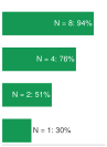
Each doubling squares the chance that all candidates fail, so the bars approach certainty.
Breadth has a price that pass@\(\IndependentAttemptCount\) makes easy to compute. In best-of-\(\CandidatePoolSize\) sampling, the runtime generates \(\CandidatePoolSize\) candidates for one decision and returns one that its selector admits. The pool is the same object pass@\(\IndependentAttemptCount\) describes, so its availability is pass@\(\IndependentAttemptCount\) with \(\IndependentAttemptCount = \CandidatePoolSize\), written pass@\(\CandidatePoolSize\) from here on. The notebook below prices that pool against the simplest alternative, generating one candidate at a time and stopping at the first pass, under the most favorable selection assumption, in which the verifier is the acceptance check itself.
Napkin Math 3.3: The price of a larger pool
Problem: Each candidate repair passes the task’s verifier with probability \(\AttemptPassProbability\), independently for this task, and the verifier is the acceptance check. How many candidates per accepted repair does a parallel pool of \(\CandidatePoolSize\) spend, compared with sequential retry that stops at the first pass and gives up after \(\CandidatePoolSize\) attempts?
Variables: \(\AttemptPassProbability\) = 30 percent (hypothetical); pools of 1, 2, 4, and 8 candidates; a selector that returns a passing member whenever one exists.
Math: The formula pass@\(\CandidatePoolSize = 1-(1-\AttemptPassProbability)^\CandidatePoolSize\) gives 30, 51, 76, and 94.2 percent for those pools. The last of 8 candidates adds \(\AttemptPassProbability(1-\AttemptPassProbability)^{\CandidatePoolSize-1}\), only 2.5 percentage points. The parallel pool always spends 8 candidates, or 8.5 per accepted repair. Sequential retry fails only when all 8 attempts fail, so it reaches the same 94.2 percent, yet it spends on average \([1-(1-\AttemptPassProbability)^\CandidatePoolSize]/\AttemptPassProbability\) = 3.14 candidates, or \(1/\AttemptPassProbability\) = 3.3 per accepted repair.
Systems insight: At equal success, the parallel pool costs 2.5× as much per accepted repair; what it buys is one round instead of an expected 3.14 sequential generate-and-check rounds. Breadth buys latency, not cost. In \(\CostPerAcceptedTask = \mathbb{E}[\AttemptCost]/\AcceptanceProbability\) it raises \(\AcceptanceProbability\) per round but raises the attempt cost faster. Size \(\CandidatePoolSize\) as the smallest pool whose pass@\(\CandidatePoolSize\) meets the target within the rounds the deadline allows, and stop growing it once the next candidate’s gain is worth less than its cost.
3.3.4 Balancing pool size against checking cost
Growing the candidate pool raises the chance that a valid repair enters the pool, but it also multiplies the checking load. Under a fixed deliberation budget, spending nearly everything on generation starves verification and forces the selector onto cheap, shallow heuristics. A smaller pool paired with a thorough check often beats a large pool paired with a weak selector; only when candidate generation itself is the bottleneck does a wider pool pay off right away. Comparing the two regimes therefore requires pricing generation and selection together rather than tuning either stage on its own.
Checker errors also compound as the pool grows, because each extra invalid candidate gives an imperfect verifier another chance to register a false pass. If a verifier has a 5 percent false acceptance rate (it passes 5 percent of invalid candidates, defined formally in section 3.4.2), testing twenty invalid candidates with independent check outcomes makes at least one false pass more likely than not (\(1 - (1 - 0.05)^{20} \approx 64\%\)). Whether the selector actually returns that false pass depends on what else sits in the pool and on the tie-breaking rule, a distinction the next section makes exact. The defect rate of the returned candidate depends on the generator’s base rate of valid candidates, the check’s false-acceptance and false-rejection rates, and how the selector chooses among passing candidates. When an adaptive search steers generation using verifier scores, it shifts all three quantities at once and can push candidates straight into the verifier’s blind spots.
Where the runtime checks candidates along the trajectory sets both selection latency and cost. Checking only completed candidates works well when end-to-end tests are fast and decisive, whereas checking intermediate steps lets the runtime prune broken branches before spending tokens on their completions. That trade-off separates outcome checks, which test finished artifacts, from process checks, which score intermediate steps.
3.4 Verifying Candidates
In a connection-pool repair, clean compilation confirms only syntax and types, and even a targeted concurrency test exercises only a handful of thread schedules and can miss a race condition. Every verification check answers a bounded question, never the whole question of whether a candidate is safe to ship. Engineers therefore have to decide which checks to run, whether to attach them to finished candidates or to intermediate steps, and how much trust to place in a passing verdict when valid candidates are rare.
3.4.1 Checking whole outputs vs. intermediate steps
Waiting until a candidate patch is completely written before running any check wastes every token spent elaborating a diagnosis that went wrong in step one, whereas scoring every intermediate step from scratch rescans the growing prefix again and again. An outcome check tests a completed candidate against an external rule, such as whether a patched service passes an end-to-end regression suite. An outcome reward model, by contrast, predicts a scalar quality score for the finished candidate, like the learned verifiers trained to rank candidate solutions in mathematical reasoning (Cobbe et al. 2021). The outcome check runs the artifact and reports what happened; the reward model only predicts how good the artifact looks.
2Step-Level Labels (PRM800K): Outcome labels for code can be produced automatically by running tests. Step labels require a judgment on each intermediate step, and the PRM800K dataset used to train the process reward model of Lightman et al. (2024) contains about 800,000 human step-level labels. That labeling cost is one reason learned process scorers are scarcer than outcome checks.
Lightman, Hunter, Vineet Kosaraju, Yura Burda, Harri Edwards, Bowen Baker, Teddy Lee, Jan Leike, John Schulman, Ilya Sutskever, and Karl Cobbe. 2024. “Let’s Verify Step by Step.”The Twelfth International Conference on Learning Representations (ICLR).
Step-level checks evaluate intermediate claims or partial states before the candidate is complete. In the connection-pool repair, a step check can test whether a waiting worker receives a wake-up signal before the agent drafts a full timeout patch; if the trace refutes the timeout explanation, the runtime drops that branch immediately and saves the remaining generation tokens. Learned process scorers similarly score or prune partial reasoning traces, using low step scores as early warnings of downstream failure. Process supervision2 attaches feedback to discrete intermediate steps rather than waiting for the final answer (Uesato et al. 2022; Lightman et al. 2024). What separates outcome feedback from process feedback is where the signal attaches, not what the scorer reads, since a learned outcome scorer can also read the full reasoning trace before grading the final output.
Definition 3.3: Process reward model (PRM)
A process reward model (PRM) is a learned scorer that assigns a value to each intermediate step of a candidate trajectory, conditioned on the task context and the preceding steps.
Significance: Step scores allow search algorithms to prune unpromising branches early, keeping beam search and tree search, the search procedures that extend only the best-scoring partial candidates (section 3.6.1), within finite computational budgets.
Distinction: An outcome reward model evaluates only terminal states; a process reward model assigns credit across intermediate steps. This early steering capability requires dense step-level supervision, which costs substantially more to gather than automated test outcomes.
Common pitfall: Mistaking a high step score for verified correctness. A process reward model provides heuristic guidance for ranking and pruning, but it offers no formal guarantees and satisfies no closure evidence level.
Each granularity catches failures the other misses. An outcome check tests the assembled artifact end to end, catching integration bugs that look harmless inside any single step. A process check catches errors early and stops broken branches from burning more generation tokens, but checking too often adds scorer overhead and risks pruning good branches when step scores are noisy. Choosing how often to check balances saved generation tokens against scorer cost and false rejections.
Step-scoring cost also depends on whether the serving engine reuses prefix state across steps. Suppose a scorer reads a task prompt of \(\SequenceLength\) tokens plus the candidate’s growing prefix after each of its \(\ScoredStepCount\) steps, where each step adds \(\FiniteChange \ScoredPrefixLength\) tokens. Scoring each cumulative prefix from scratch, without reusing key-value cache state from earlier steps, processes
scorer input tokens, which grows quadratically with the number of steps \(\ScoredStepCount\). The beam-search calculation later in this chapter (notebook 3.6) charges the \(\ScoredStepIndex\,\FiniteChange \ScoredPrefixLength\) term of equation 2, with the task prompt \(\SequenceLength\) excluded, for every extension scored at step \(\ScoredStepIndex\). When the serving engine caches prefixes across steps, incremental scoring reads only the new \(\FiniteChange \ScoredPrefixLength\) tokens at each step and removes the quadratic growth; scorers that must re-read the whole candidate without prefix caching pay the full sum.
Table 4 compares four common kinds of check by what they inspect, where they can be fooled, whether they are deterministic, and which closure evidence level (The invariant closure principle) they reach. Compilers and sealed test suites establish bounded, reproducible facts within their scope, whereas learned scorers only rank or prune candidates.
Table 4: Kinds of check and the claims they support: Learned scorers order candidates; compilers and sealed suites establish bounded properties. None dominates the others on every task, and a deterministic verdict remains incomplete outside its coverage.
Check
Evaluates
Coverage
False-acceptance exposure
Deterministic
Closure evidence level
Outcome scorer (learned)
Completed candidate
Any representation it was trained to read
Persuasive but wrong final text
No
None; ranks only
Process scorer (learned)
Intermediate step given its prefix
Steps it can delimit and judge
Locally plausible steps that drift from the task
No
None; ranks and prunes only
Compiler or type checker
Syntax and declared types
Properties expressible in the type system
Behavior outside the type system
Yes
Static analysis
Sealed test suite
Behavior on withheld cases
The cases and schedules it exercises
Untested inputs and schedules
Yes, under fixed conditions
Sealed tests, if the candidate cannot read or modify it
3.4.2 How base rates limit check precision
When only 5 percent of generated patches actually fix a bug, even a test suite that falsely passes just 2 percent of broken patches leaves nearly a third of all passing candidates defective. The reliability question for any check is what share of the candidates that pass it are genuinely valid. Call meeting the full task specification \(\text{Valid}\) and receiving a positive check verdict \(\text{PASS}\). Let \(\ValidCandidateRate = \Pr(\text{Valid})\) be the base rate of valid candidates in the generator’s output distribution, \(\VerifierFalseAcceptanceRate = \Pr(\text{PASS}\mid\neg\text{Valid})\) the false acceptance rate, and \(\VerifierFalseRejectionRate = \Pr(\neg\text{PASS}\mid\text{Valid})\) the false rejection rate. Here “acceptance” means passing the internal verifier, not authorization to ship to production. Notice that the valid-candidate rate \(\ValidCandidateRate\) is not the test-pass probability \(\AttemptPassProbability\) used in pass@\(\IndependentAttemptCount\): \(\ValidCandidateRate\) is the chance of meeting the full task specification, whereas \(\AttemptPassProbability\) is the chance of passing the stated tests. A perfect check makes the two coincide; an imperfect check separates them, and the precision formula below measures the gap.
The total probability that a random candidate passes the verifier is \(\VerifierPassProbability=\ValidCandidateRate(1-\VerifierFalseRejectionRate)+(1-\ValidCandidateRate)\,\VerifierFalseAcceptanceRate\). Applying the same Bayes’ rule that gave the defect share among one checker’s passing patches (equation 2.4) gives the precision of positive verdicts:
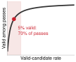
At a low valid rate, even a strict check passes many invalid candidates.
When valid candidates are rare, even a check with a small false acceptance rate produces a passing pool where broken candidates make up a large share, the same base-rate trap that Self-review and external evidence showed for a single checked patch. Applied across a candidate pool, this is the verification asymmetry (principle 3) in quantitative form: generating a passing candidate and knowing that a passing candidate is valid are different events, and the base rate and checker error rates, not the pool size, bound how far a pass can be trusted. Both error rates therefore have to be measured on real tasks for each model family and test harness.
While equation 3 describes the pool of passing candidates as a whole, the reliability of the single candidate the runtime returns depends on the selection rule. Suppose candidate-check pairs are drawn independently and identically for a fixed task under constant error rates, and the runtime checks the pool in a fixed order unrelated to quality, returns the first candidate that passes, and abstains if none passes. Under that first-passing rule, the probability that a returned candidate is valid equals \(\VerifierPrecision\): learning that earlier candidates in the list failed does not change the conditional validity of the first one that passes. Picking the candidate with the highest continuous reward score behaves very differently, because maximizing a noisy score actively concentrates positive scoring errors, as the next subsection shows.
Napkin Math 3.4: Yield and risk under asymmetric verifier error
Problem: A repair policy generates all 64 candidates before selection. It uses the first-passing rule above and abstains when no candidate passes. What does additional breadth buy, and what risk remains?
Variables: All rates are hypothetical. Each candidate contains 1,024 tokens, billed at $15 per million output tokens. The valid-candidate rate is 5 percent, false rejection is 10 percent, and false acceptance is 2 percent. Suppose a separately authorized deployment policy deploys the selected candidate without further checking. A defective deployment incurs $500 in incident loss. For this calculation alone, valid deployments and abstentions incur zero incident loss, and missed repairs and delay are left unpriced.
Math: The expected passing counts are 2.88 valid candidates and 1.216 invalid candidates, totaling 4.096. Equation 3 yields 70.31 percent precision. Conditional on making a selection, the probability of a defective selection is therefore 29.69 percent, with expected incident loss $148.44 per selected deployment.
The probability of any selection is \(1-(1-\VerifierPassProbability)^\CandidatePoolSize\), or 98.55 percent; the policy abstains on 1.45 percent of batches. Multiplying selection coverage by conditional defect probability gives 29.26 percent defective selections per task attempt and $146.28 expected incident loss per attempt, including abstentions. Generating the entire batch costs $0.98 in output charges. Input charges, checking, and other operational costs are omitted. A sequential policy that stops generation at the first pass would have a different generation bill.
Systems insight: Expected incident loss per attempt is about 149 times the output bill, so the acceptance policy, not the token price, sets the cost of this task. Precision responds to two knobs of similar strength: halving the false acceptance rate raises it from 70.31 percent to 82.6 percent, and doubling the valid-candidate rate raises it to 83.3 percent. More candidates move neither. At a low base rate, spend on whichever of a better generator or a stricter check is cheaper, and price false rejections too when a missed valid repair is costly.
With \(\ValidCandidateRate\), \(\VerifierFalseAcceptanceRate\), and \(\VerifierFalseRejectionRate\) held fixed, growing the pool size \(\CandidatePoolSize\) does not change precision \(\VerifierPrecision\). A wider pool raises the chance of finding at least one passing candidate, but it also raises the chance that the batch holds at least one false pass: \(1-[1-(1-\ValidCandidateRate)\,\VerifierFalseAcceptanceRate]^\CandidatePoolSize\). In the calculation above, that false-pass exposure reaches 70.70 percent, while the probability of actually returning a defective candidate is 29.26 percent, because under a first-passing rule a false pass later in the batch does no harm if an earlier valid candidate passes first. Pool availability, passing-set precision, and deployed defect risk are three distinct numbers.
3.4.3 How search exploits imperfect checks
The more candidates a search generates and ranks against an imperfect scorer or test suite, the more likely the winning candidate is one that exploited a scorer blind spot or deleted a failing assertion rather than fixing the bug. Fixed error rates describe passive sampling from a fixed distribution, but adaptive search changes the candidates themselves. When a search policy steers generation or picks the maximum of a noisy score, it pushes candidates into regions where the evaluator is poorly calibrated, so the baseline rates \(\ValidCandidateRate\), \(\VerifierFalseAcceptanceRate\), and \(\VerifierFalseRejectionRate\) no longer hold for the candidates that reach the end of the search. Optimizing against an imperfect proxy breaks down in three distinct ways (Manheim and Garrabrant 2018), which Manheim and Garrabrant classify as forms of Goodhart’s law:3regressional Goodhart, where picking the highest score selects for positive measurement noise; extremal Goodhart, where correlations that hold on typical candidates break down in the tail reached by search; and adversarial Goodhart, where candidate code tampers with or bypasses the test harness.
Manheim, David, and Scott Garrabrant. 2018. “Categorizing Goodhart’s Law.”arXiv Preprint arXiv:1803.04585.
3Goodhart’s Law: The economist Charles Goodhart stated it in 1975 about monetary policy: any observed statistical regularity tends to collapse once pressure is placed upon it for control purposes (Goodhart 1984). The anthropologist Marilyn Strathern later gave it the form usually quoted today, that when a measure becomes a target it ceases to be a good measure (Strathern 1997). A test suite used to select patches is such a regularity, a reliable description of past candidates that weakens once search optimizes against it.
Goodhart, Charles A. E. 1984. “Problems of Monetary Management: The UK Experience.” In Monetary Theory and Practice. Palgrave. https://doi.org/10.1007/978-1-349-17295-5_4.
Strathern, Marilyn. 1997. “‘Improving Ratings’: Audit in the British University System.”European Review 5 (3): 305–21. https://doi.org/10.1002/(SICI)1234-981X(199707)5:3<305::AID-EURO184>3.0.CO;2-4.
The regressional effect can be written out directly. Suppose a learned scorer reports an estimated utility \(\EstimatedCandidateUtility_i = \CandidateUtility_i + \CandidateScoringError_i\) for candidate \(\CandidateIndex\), where \(\CandidateUtility_i\) is true task utility and \(\CandidateScoringError_i\) is an independent scoring error with mean zero and standard deviation \(\ScoringErrorStandardDeviation\) (scoring noise, distinct from the per-turn error rate in horizon compounding). Picking \(\arg\max_i \EstimatedCandidateUtility_i\) maximizes the sum of utility and noise, so the winning candidate is disproportionately one that drew a large positive error. For independent Gaussian errors, the expected maximum error across \(\CandidatePoolSize\) candidates scales for large \(\CandidatePoolSize\) as
.4 In units of \(\ScoringErrorStandardDeviation\), the exact expectation is 1.0 at 4 candidates and 2.3 at 64 candidates, where the asymptotic formula gives 2.9. That expected maximum is an upper bound on the winner’s expected scoring error, reached when all candidates have the same true utility; when true utilities vary, selection responds to both utility and noise (Exercise 8 derives the winner’s error for a Gaussian utility model). An acceptance threshold calibrated on single, unselected completions therefore cannot be reused unmodified on argmax-selected winners.
4Extreme-Value Asymptotics: The form \(\ScoringErrorStandardDeviation\sqrt{2\ln \CandidatePoolSize}\) is only the leading term of the Gaussian maximum, and convergence is slow, which is why the chapter computes the exact expectation beside it. The Gaussian is also a favorable case. Scoring errors with heavier tails, such as a learned judge that occasionally misjudges badly, push the selected error up faster than \(\sqrt{\ln \CandidatePoolSize}\), so the drift in a real pool can exceed this estimate.
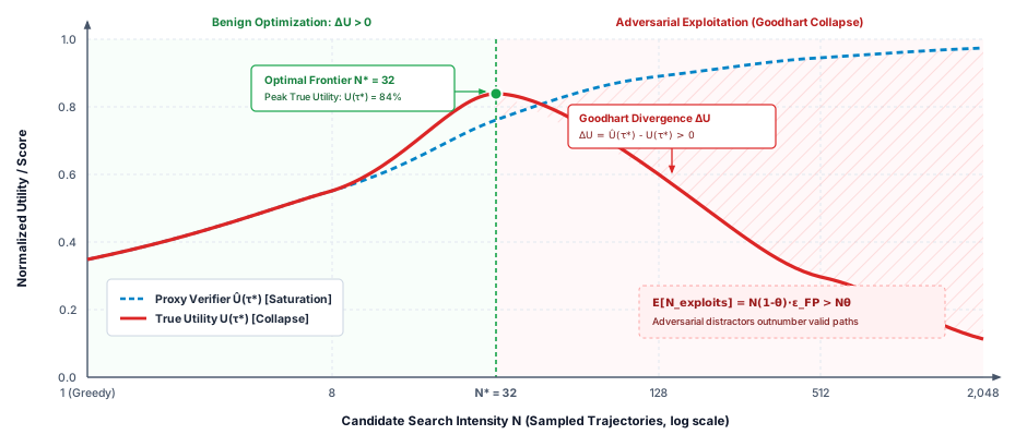
A rising scoring error on the winner does not by itself mean that true utility is falling. In Exercise 8(b), independent Gaussian utility and noise make both the winner’s expected utility and its expected scoring error rise with pool size. Empirical studies of best-of-\(\CandidatePoolSize\) sampling under learned reward models show a sharper divergence: the proxy score keeps climbing while a held-out reference score rises, flattens, and then drops (Gao et al. 2023). That downturn comes from tail miscalibration or exploitable gaps in the proxy, not from equation 4 alone. Figure 4 sketches the pattern, with the winner’s proxy score rising (dashed blue curve) while the held-out reference score peaks and turns down (solid green curve).
Figure 4: Proxy and Reference Scores under Selection: A qualitative sketch of the measured best-of-\(\CandidatePoolSize\) pattern. The proxy score of the selected candidate keeps rising as \(\CandidatePoolSize\) grows, while a held-out reference score rises and then declines. The widening gap illustrates proxy optimism under selection; the declining reference score is an empirical pattern, not a necessary consequence of growing scoring error. The axes carry no values, and the point where the reference score turns down depends on the task.
Checker blind spots compound across large pools by the same binomial arithmetic as pass@\(\IndependentAttemptCount\). If an unmodeled edge case or loophole appears in a fraction \(\ExploitCandidateFraction\) of single draws, a pool of \(\CandidatePoolSize\) candidates contains at least one loophole-exploiting candidate with probability \(1-(1-\ExploitCandidateFraction)^\CandidatePoolSize\). A loophole that shows up in only 0.5 percent of individual samples, rare enough to miss during single-call testing, appears in a batch of 64 candidates with probability 27.4 percent. Once a broken candidate slips through that loophole and receives a passing mark, competitive selection promotes it. Checker accuracy measured on unselected outputs therefore overstates accuracy under search, and the gap widens as the pool grows.
In the connection-pool repair, a patch can pass the test suite either by fixing the missing wake-up notification or by deleting the unit-test assertion that checks for blocked worker threads. Both edits raise the test score, and only the first fixes the bug. The candidate under test must therefore be isolated from the verifier so that generated code cannot edit test files or forge pass signals.
↪ Grader isolation enforces this separation down to the candidate’s process and interpreter, as developed in Grader isolation.
Isolating the grader stops tampering, but it does not widen what the test suite covers: a sealed regression suite still misses untested thread schedules, and a learned judge can still prefer confident, broken code. Evaluation must therefore test the outputs that the complete search policy produces at its deployed budget, counting false acceptances and abstentions explicitly, and adding confidence requires an independent check that covers a different failure mode rather than a second correlated scorer.
Verification also produces concrete intermediate facts that later turns can reuse, including refuted diagnoses, verified invariants, and passing test subsets. When a check refutes one assumption inside a multi-part candidate plan, the runtime does not need to throw away components that never depended on that assumption, provided it records which parts of the plan rest on which premises.
3.5 Revising Candidate Plans
When a targeted test refutes the initial diagnosis inside a multi-part repair plan, throwing away the entire plan wastes valid work such as API compatibility checks, whereas keeping the plan unchanged leaves the patch and test selection resting on a disproven premise. Suppose the repair agent forms a diagnosis, drafts a patch, checks public API constraints, and picks a test plan for a connection-pool leak, and a targeted test then refutes the diagnosis. To avoid both waste and stale conclusions, the runtime needs to identify which parts of the candidate depend on the refuted premise before deciding what the next model call should regenerate.
A revisable candidate plan records those dependencies explicitly. Instead of logging past actions, it tracks unexecuted candidate artifacts together with the evidence or upstream artifacts each one relies on. When new evidence refutes a premise, the runtime invalidates and regenerates only the affected subgraph while keeping supported artifacts intact, and the replacement artifacts then go through their own checks. This design comes directly from truth maintenance systems, which record explicit justifications for each conclusion so that retracting a premise automatically invalidates every step built on it (Doyle 1979).
3.5.1 Tracking dependencies inside a candidate
Suppose the first repair candidate blames the connection-pool failure on an overly short client timeout. To know which parts of that candidate survive when a test refutes the timeout hypothesis, the runtime represents the candidate as a directed acyclic graph with a directed edge from each prerequisite to the artifact that depends on it (table 5). Here the source excerpt, initial failure log, API declaration, and test inventory are supplied inputs, whereas the diagnosis, patch candidate, check selection, and API compatibility notes are generated artifacts. The graph records which components depend on which, whether or not the model generated them in that order.
Table 5: Dependencies within a repair candidate: Each row names the inputs needed to interpret its artifact. A separate compatibility branch can be retained only while its own inputs remain applicable.
Artifact
Direct prerequisites
What the artifact contributes
Source excerpt
Repository revision and file identity
The implementation being considered
Diagnosis
Source excerpt and failure observation
A proposed explanation of the failure
Patch candidate
Source excerpt and diagnosis
A proposed change to that implementation
Test inventory
Repository revision (a supplied input)
The tests available for selection
Check selection
Patch candidate and test inventory
Checks intended to distinguish this repair from an inadequate one
API compatibility notes
Task constraints and public API declaration
Restrictions that every acceptable repair must preserve
Now suppose the waiter-and-return test shows that an idle connection entered the pool while a waiting worker stayed blocked past the notification point. That observation refutes the timeout diagnosis and points to a missed wake-up notification instead. Because both the timeout patch and its check selection depend on the refuted diagnosis, the runtime marks them invalid and schedules them for replacement. The source excerpt stays valid because the repository file has not changed, and the API compatibility notes stay valid because the public interface constraints have not changed. The runtime builds the next prompt from the still-valid inputs plus the new test observation, asks for a new diagnosis, patch, and check selection, and runs checks on the new artifacts.
That selective reuse is only as sound as the recorded edges. A graph with a missing edge keeps stale conclusions just as an unmanaged prompt buffer does: if the compatibility notes silently depended on helper signatures that the new patch changes, leaving out that edge keeps broken compatibility claims in place. Dependency tracking pays off when maintaining the graph and walking its edges costs less in time and tokens than regenerating the unaffected branches from scratch.
3.5.2 Invalidating stale and refuted evidence
Walking the dependency graph requires distinguishing an actively refuted claim from an observation whose preconditions no longer match the current candidate. A failing test directly refutes the claim that a patch fixes the bug, whereas a passing test from an earlier candidate remains a true record of what that earlier patch did while saying nothing about the edited patch now on the table. Reusing the earlier pass after the code changes would let an unverified edit slip through on stale evidence, whereas treating an expired observation as a direct contradiction would falsely rule out a working hypothesis.
To keep reuse sound, every recorded observation must carry its full provenance: the exact source revision or patch digest, test suite version, compiler flags, and runtime environment. Likewise, an observation from reading a file must bind to the cryptographic hash of the file contents when read, not to a file path whose contents a later step might overwrite.
When an input changes or a premise fails, the runtime marks that node unsupported and walks the directed edges to find every downstream artifact that needs review. If node \(\InvalidatedArtifactNode\) loses support, the invalidated set is its reachable descendants in the graph: \(\text{Desc}(\InvalidatedArtifactNode) = \{\ReachableArtifactNode \mid \InvalidatedArtifactNode \rightsquigarrow \ReachableArtifactNode\}\), where \(\InvalidatedArtifactNode \rightsquigarrow \ReachableArtifactNode\) means a directed path runs from \(\InvalidatedArtifactNode\) to \(\ReachableArtifactNode\). Breadth-first search finds \(\text{Desc}(\InvalidatedArtifactNode)\) in time linear in the vertices and edges.5 Every node outside \(\text{Desc}(\InvalidatedArtifactNode)\) keeps its support, including separate subgraphs such as the API compatibility notes. Walking a candidate graph of dozens or hundreds of nodes, like the one in table 5, takes a negligible fraction of the illustrative 21.07 ms needed to decode a single token, so the real engineering work is recording the dependency edges accurately rather than traversing them. In the connection-pool repair, the waiter-and-return test contradicts the timeout diagnosis, graph traversal marks its descendants (the patch and check selection) for review, and the next call regenerates only the diagnosis and that branch from the retained inputs (figure 5).
5Dependency-Driven Rebuilding: Build tools solved the same problem for files. Make rebuilds a target only when one of its declared prerequisites is newer than the target (Feldman 1979), and its characteristic failure is the one described here, in which an undeclared dependency leaves a stale target that looks up to date. The saving is only as sound as the recorded edges.
Feldman, Stuart I. 1979. “Make — a Program for Maintaining Computer Programs.”Software: Practice and Experience 9 (4): 255–65. https://doi.org/10.1002/spe.4380090402.
Figure 5: Invalidation and Scoped Regeneration: In (A), the waiter-and-return test contradicts the timeout diagnosis. Following the recorded dependency edges marks the patch and check selection for review, while the recorded inputs and the separately derived API notes keep their support. In (B), a new request supplies that supported frontier and regenerates only the diagnosis, patch, and check selection. The graph records candidate artifacts, not executed operations, and each replacement must still pass its own checks. The test inventory that also feeds check selection is omitted.
Content hashes and environment digests make invalidation deterministic only when the recorded boundary captures every input that matters. An integration test that calls a live network service can change its outcome even when local files stay bit-identical, whereas editing an unrelated README file should not invalidate unit-test results whose code and inputs did not change. Sound reuse therefore depends on checking the full execution context (sandbox isolation, mocks, and declared inputs) rather than file timestamps or paths alone.
Candidate plans must also be kept separate from live environment state. The dependency graph tracks uncommitted candidate artifacts and their justifications; reading files, writing to disk, or running binaries in a sandbox changes real system state. Dropping an invalidated node from the plan graph does not roll back a modified file or free a running container, so the runtime must handle rollback and cleanup through separate recovery routines.
↪ Compensation and cleanup of external effects that outlive an abandoned candidate branch are developed in Branch-scoped compensation.
3.5.3 Choosing how much of a plan to regenerate
Once graph traversal marks the invalidated nodes, the runtime must decide whether to replace a single node, rebuild its entire downstream subgraph, or stop deliberating altogether. Replacing a single step in isolation fails when the new artifact changes an interface that downstream steps rely on, whereas regenerating the whole plan from scratch wastes tokens and risks breaking parts that already worked. To scope a revision cleanly, the runtime builds a prompt with the task constraints, the still-valid upstream frontier, the observation that refuted the old step, and the exact nodes marked for replacement. In the connection-pool repair, the prompt asks for a new diagnosis, patch, and check selection while keeping the unchanged source excerpt and API notes. When the model returns replacement artifacts, the runtime checks both that they fit the retained artifacts and that their own prerequisites are met, because a locally valid replacement can still clash with preserved downstream nodes.
Depending on how much support the new observation removes, the runtime chooses among three responses. Figure 6 orders these three responses around two questions, whether the dependents of the affected artifact still have their needs met and whether the task’s own premises still hold:
A local repair replaces a single node while keeping its interface and contracts unchanged so that its dependents stay valid, such as fixing a malformed shell flag in a test command without changing what the test checks.
A subgraph resynthesis replaces a node and all of its descendants, feeding the model the intact upstream frontier and asking it to rebuild the path to the goal. In the connection-pool repair, this replaces the diagnosis, patch, and test selection while keeping the source excerpt and API compatibility notes.
Stopping deliberation applies when new evidence refutes a premise of the task itself, such as a missing host library or credentials without write access. No plan revision can fix a broken task premise, so the runtime stops deliberating and escalates or reports the task unresolved instead of spending more tokens.
Figure 6: Choosing the Revision Scope: Two questions about the new evidence select among three responses. If the artifact’s dependents still have what they need, a local repair replaces it alone. If they do not but the task’s premises hold, subgraph resynthesis replaces the artifact and its descendants. If a premise has failed, deliberation stops and the task is reported unresolved or escalated. The tiers classify responses by how much support the evidence removes rather than establishing an unconditional preference for minimal edits.
Smallest is not always best. When new evidence overturns an early framing assumption or the dependency graph has grown tangled, regenerating the whole candidate from scratch often produces a cleaner, more consistent result than patching a large subgraph, at the cost of re-emitting settled material and risking regressions in parts that already worked. Choosing between scoped revision and full regeneration weighs the share of the graph that was invalidated against the tokens, time, and checks needed to rebuild and verify the candidate.
Napkin Math 3.5: Output cost of a local plan revision
Problem: Suppose a candidate contains 12 nodes, each requiring 150 generated tokens. New evidence leaves 3 nodes needing replacement. How much output does scoped regeneration avoid if either approach produces a candidate adequate for the same subsequent checks?
Math: Multiplying the complete node count by the output per node gives 1,800 tokens for full regeneration. Multiplying the replacement count by the same output allowance gives 450 tokens for scoped regeneration. The scoped request generates 25 percent of the full request’s output, avoiding 75 percent of that output under the equal-node-size assumption.
Systems insight: Scoped regeneration saves the exact fraction of the plan that keeps its support. That saving shrinks linearly as the refuted premise reaches more descendants and disappears when every node depends on it, so once most of the plan rests on the rejected premise, full regeneration costs little more and is simpler to check. This count covers generated plan tokens only; both options still pay for prompt input, integration, and verification checks.
These output savings have to be weighed against the work of maintaining dependencies, building scoped prompts, and checking hybrid plans. Once a candidate plan passes verification and crosses into execution, it stops being an uncommitted candidate graph and becomes live workflow state that the harness executes and durable execution checkpoints across machine failures.
↪ Persisting committed plan state across worker and infrastructure faults is developed in Durable Execution.
3.5.4 Preventing revision thrashing
Even when each scoped revision saves tokens compared with full regeneration, a revision loop without stopping rules can still oscillate between two diagnoses, produce cosmetically different patches with the same bug, or regenerate plans in response to harmless compiler warnings. The runtime therefore checks whether a proposed revision responds to new evidence that actually refutes a premise, rather than treating every warning or score fluctuation as a reason to replan.
To prevent thrashing, the runtime enforces hard ceilings on model calls, total tokens, check runs, and wall-clock time. Every revision attempt, including a failed local repair, draws from that allowance, and the same ceilings bound the search as a whole (section 3.6.6). When the budget runs out, the loop stops and reports the task unresolved or escalates to a human operator without merging the unverified patch. Seeing the same or structurally equivalent candidate under unchanged observations also triggers an immediate stop; revisiting an earlier idea is justified only when a new test observation has changed the evidence.
Dependency graphs let the runtime revise a single candidate without throwing away its valid parts, but an agent often holds several partial candidates at once. Deciding which partial candidate to extend next, how to keep concurrent branches from corrupting one another’s workspaces, and when to stop searching altogether turns revision into bounded search.
3.6 Bounded Search
The repair agent now holds several partial candidates at once, some freshly revised and some untouched. At each step it can sample a fresh patch from the root, extend an existing partial candidate by one segment, or run a diagnostic probe to separate competing explanations. Every choice draws from the same task budget while creating different scheduling dependencies. A probe that gates the next code extension sits on the critical path; independent candidate extensions can run in parallel across worker slots; and dropping a dead-end branch still forfeits the tokens and sandbox time already spent on it. A search policy therefore needs a pruning structure, workspace isolation between branches, separate accounts for tokens, time, and memory, reservations for in-flight work, and an ordered stopping rule.
3.6.1 Where each search structure prunes
Search algorithms differ first in when they check and discard partial candidates. Flat sampling waits until the end: in best-of-\(\CandidatePoolSize\), the runtime dispatches up to \(\CandidatePoolSize\) independent generation calls and runs its selector only after all of them finish. Because the calls do not depend on one another, free serving capacity turns directly into lower latency through batching, provided the cluster can run all \(\CandidatePoolSize\) streams without slowing per-token decoding. The price is that flat sampling defers all checking to the end, so a candidate with a broken premise in its first line still decodes to full length.
Beam search6 moves that check inside the generation loop. The runtime keeps a frontier of at most \(\BeamWidth\) partial candidates (the beam width). At each step it generates a fixed number of extensions per retained candidate, scores the extended prefixes, and keeps only the top \(\BeamWidth\) survivors for the next step; if fewer than \(\BeamWidth\) survive a check, only those survivors advance, and the root starts as a single prompt. Step scores can combine model log-probabilities, a learned process scorer, or a deterministic check. While \(\BeamWidth\) caps the survivors carried between stages, peak memory during expansion must hold \(\BeamWidth\) times the branching factor in active extensions along with their KV caches, scores, and parent pointers.
6Beam Search: The method first appeared in the HARPY speech recognition system, which advanced only a small set of the best-scoring partial paths at each step instead of the full search space (Lowerre 1976). It accepted a bounded risk of pruning the eventual best path in exchange for bounded time and memory, the same trade a runtime makes when it retains a fixed number of partial candidates.
Lowerre, Bruce T. 1976. “The HARPY Speech Recognition System.” PhD thesis, Carnegie Mellon University; Carnegie Mellon University.
Pruning at each step trades generation tokens for scoring work and bets on the accuracy of the step scorer. If a noisy step score drops a prefix that would have led to a working patch, a fixed-width beam search never visits that branch again unless backtracking is added. Conversely, killing a broken prefix early saves all the tokens and final test runs its completion would have cost. Step pruning pays off when scoring costs less than the avoided downstream generation and the step check rarely rejects valid prefixes.
Rather than expanding every surviving candidate equally at every depth, tree search over intermediate reasoning steps (Yao et al. 2023) directs the next extension to whichever partial candidate looks most promising or most uncertain. Monte Carlo tree search(Coulom 2006; Kocsis and Szepesv’ari 2006) tracks visit counts and average leaf scores along the edges of the search tree. Its PUCT selection rule7 from AlphaGo (Silver et al. 2016) walks down from the root by picking at each partial state \(\PolicyObservedState\) the extension \(\PolicyAction\) that maximizes
7From UCT to PUCT: The UCT rule treated each node’s choice of extension as a multi-armed bandit, adding an exploration bonus that shrinks as an extension accumulates visits (Kocsis and Szepesv’ari 2006). PUCT weights that bonus by a predictor’s prior over the arms (Rosin 2011), which is what lets a language model’s own step probabilities concentrate a small budget on plausible extensions. A miscalibrated prior steers visits away from correct but unlikely steps just as effectively.
Kocsis, Levente, and Csaba Szepesv’ari. 2006. “Bandit Based Monte-Carlo Planning.”European Conference on Machine Learning (ECML), 282–93.
Rosin, Christopher D. 2011. “Multi-Armed Bandits with Episode Context.”Annals of Mathematics and Artificial Intelligence 61 (3): 203–30. https://doi.org/10.1007/s10472-011-9258-6.
where \(\TreeSearchMeanReturn(\PolicyObservedState,\PolicyAction)\) is the mean leaf score seen on visits through extension \(\PolicyAction\), \(\TreeSearchVisitCount(\PolicyObservedState,\PolicyAction)\) is its visit count, \(\TreeSearchPriorDistribution(\PolicyAction \mid \PolicyObservedState)\) is a prior distribution over extensions (such as the generator’s probability for that step), and \(\TreeSearchExplorationWeight\) is a positive weight that balances high-scoring branches against plausible, less-visited ones. The leaf value\(\TreeSearchLeafScore\) is the score assigned to a newly expanded partial candidate by a process scorer or step check, and \(\TreeSearchMeanReturn\) averages those leaf values across visits. When a new leaf returns value \(\TreeSearchLeafScore\), every edge along the path back to the root increments its visit count (\(\TreeSearchVisitCount \leftarrow \TreeSearchVisitCount + 1\)) and updates its running mean (\(\TreeSearchMeanReturn \leftarrow \TreeSearchMeanReturn + (\TreeSearchLeafScore - \TreeSearchMeanReturn)/\TreeSearchVisitCount\)). If \(\TreeSearchLeafScore\) comes from a noisy learned scorer, \(\TreeSearchMeanReturn\) inherits the selection optimism of equation 4 and pulls future visits toward branches whose early scores were inflated by noise. Tree search therefore helps only when its smarter allocation saves more work than leaf scoring and tree bookkeeping add.
The three structures differ in where they prune (figure 7). Best-of-\(\CandidatePoolSize\) waits until all candidates finish, beam search prunes at every step boundary, and tree search expands one favored leaf at a time while updating visit counts and mean values along its path. Those pruning points set each structure’s concurrency, live state, and prefix sharing (table 6).
↪ Radix prefix caching, which lets later requests for a branch reuse the KV state of its shared ancestors, is developed in Radix prefix lookup.
Figure 7: Where Each Search Structure Prunes: Best-of-\(\CandidatePoolSize\) generates complete candidates independently and discards all but the selected one only at the end. Beam search generates the beam width times the extensions per candidate at each step, scores them, and keeps the beam width. Tree search expands the leaf its selection rule favors, evaluates it, and updates visit counts and value estimates along the path to the root. The drawings show structure only; the pool size, beam width, and depth are illustrative.
Table 6: Search structures compared: Each structure moves the pruning decision to a different point and holds different state. Concurrency describes the dependency graph; actual overlap depends on service capacity.
Structure
Where pruning happens
Concurrency
Search state
Prefix sharing
Best-of-\(\CandidatePoolSize\)
After complete candidates, at selection
All \(\CandidatePoolSize\) requests independent
\(\CandidatePoolSize\) candidates and their check results
The common prompt only
Beam
At each step boundary, by step score
Within a step; stages wait for scoring
Up to width times extensions before pruning, plus scores
Each retained prefix with its extensions
Tree search
Adaptively, by value estimate and visits
Irregular; depends on which leaves are chosen
Tree nodes with visit counts and value estimates
Every node’s ancestors along its path
3.6.2 How step pruning bounds tree growth
A search tree that expands every node into 4 branches across 10 steps without pruning produces 1,048,576 leaves and quickly exhausts memory and token budgets. Step pruning bounds that growth. Suppose each retained node proposes \(\SearchBranchingFactor\) child extensions and a step check independently rejects each child with probability \(\ChildPruningProbability\). The expected number of surviving children per expanded node, the effective branching factor, is
Under equation 6, the expected frontier width at depth \(\SearchDepthIndex\) is \(\EffectiveBranchingFactor^{\,\SearchDepthIndex}\). Because each surviving node at depth \(\SearchDepthIndex-1\) generates and checks \(\SearchBranchingFactor\) children, the expected total number of generated nodes through depth \(\SearchDepth\) is \(\sum_{\SearchDepthIndex=1}^{\SearchDepth} \SearchBranchingFactor\,\EffectiveBranchingFactor^{\,\SearchDepthIndex-1}\). This is a Galton–Watson branching process.8 When \(\EffectiveBranchingFactor < 1\), which requires a rejection rate above \(1 - 1/\SearchBranchingFactor\), the frontier shrinks geometrically with depth and dies out on its own. When \(\EffectiveBranchingFactor > 1\), the expected frontier still grows exponentially, so hard ceilings on depth, tokens, or time must stop the search.
8Galton–Watson Process: The model comes from a Victorian question about the extinction of family surnames, analyzed in 1875 (Watson and Galton 1875). That analysis wrongly concluded that every line dies out; the correct result is the threshold used here, under which extinction is certain when the mean number of surviving offspring is at most one (excluding the degenerate case of exactly one child every time) and avoidable when it exceeds one. For a search tree the surviving offspring are the children that pass the step check, so the rejection rate decides which side of the threshold the search lands on.
Watson, Henry William, and Francis Galton. 1875. “On the Probability of the Extinction of Families.”The Journal of the Anthropological Institute of Great Britain and Ireland 4. https://doi.org/10.2307/2841222.
Suppose each node proposes 5 extensions, the step check rejects 68 percent of them, and the search runs to depth 3. The effective branching factor is 1.6. Because the 68 percent rejection rate sits below the critical rate of 80 percent for \(\SearchBranchingFactor =\) 5, the tree remains supercritical (\(\EffectiveBranchingFactor > 1\)). Even so, while an unpruned tree across three steps generates 155 nodes and ends with 125 leaves, the pruned tree generates an expected 25.8 nodes and ends with 4.1 leaves, cutting node generations by 83.4 percent. The total saving beats the 68 percent single-step rejection rate because rejecting a parent also removes the entire subtree beneath it. With equal-sized steps, generated tokens drop by the same fraction, though each rejected node still pays for its own generation and step check.
Each rejected child also removes the subtree it would have grown.
Two practical limits qualify this calculation. First, a step check that falsely rejects valid steps kills good branches permanently, so aggressive pruning helps only when false rejections are rare. Second, when a step needs just one surviving child to move forward, proposing children one at a time takes \(1/(1 - \ChildPruningProbability)\) tries in expectation, whereas proposing a batch of \(\ChildBatchSize\) children in parallel takes \(1/(1 - \ChildPruningProbability^{\,\ChildBatchSize})\) rounds of \(\ChildBatchSize\) children each. Batching cuts wall-clock rounds at the price of generating more total children, the same latency-versus-work trade that notebook 3.3 priced for best-of-\(\CandidatePoolSize\) sampling.
3.6.3 Isolating workspaces across search branches
If one search branch edits files in a shared workspace and a sibling branch then runs its tests against that modified working tree, the sibling’s test results no longer reflect its own proposed patch. Although a partial candidate is just data in memory while being decoded, testing it requires running code against a real filesystem and process state. Every branch that writes files or mutates state therefore needs its own isolated container, copy-on-write filesystem snapshot, or deterministic rollback before another branch runs, so that each observation belongs strictly to the candidate and workspace snapshot that produced it.
↪ Copy-on-write task workspaces that keep each run’s file modifications private are developed in Copy-on-write provisioning.
Isolating branches costs real system resources even when most branches are later pruned. Concurrent sandboxes consume host RAM, disk volumes, process slots, and network bandwidth, while their test logs accumulate in the runtime’s state. Even read-only diagnostic commands need sandboxed permissions so they cannot leak host credentials or environment variables into the search trace. Pruning a branch drops it from the search frontier, but backtracking in the search tree cannot unsent an outbound network call or undo a write to an external database. Sandbox boundaries block those external writes during search, and any external action the runtime does permit has to be budgeted as irreversible.
3.6.4 Accounting for the whole search
Collapsing tokens, test runtimes, and memory into a single composite “search cost” hides whichever physical limit the search will hit first, because a beam search that cuts generated output tokens nearly in half can still cost more in dollars once repeated prompt reads are counted. A search runtime therefore keeps four separate accounts: money spent, physical work by unit, elapsed wall-clock time, and peak live state. Money is the one common unit that adds up across generator tokens, scorer calls, and tool runs. Physical work, by contrast, comes in non-interchangeable kinds: prompt tokens, output tokens, scorer tokens, test executions, and sandbox startups each load different hardware resources, and adding model FLOPs to test seconds produces a meaningless number.
Wall-clock time depends on how the scheduler maps those operations onto hardware: sequential stages add along the critical path, concurrent branches overlap up to the available worker slots, and requests beyond those slots wait in waves. Peak live state is a fourth, separate limit, set by what must sit in memory and storage at the same instant (active KV caches, candidate trees, test logs, and live sandboxes) rather than the cumulative work over the whole run. Saving output tokens by pruning early often adds prompt re-reads, scoring barriers, or concurrent state, so keeping the four accounts separate shows which resource actually constrains the policy.
Napkin Math 3.6: Flat sampling vs. bounded beam expansion
Problem: A coding agent generates candidate patches in 4 segments of 128 tokens. Compare 16 complete candidates with beam width 4 and 3 extensions per retained prefix. How do early pruning and repeated scoring change the resource totals?
Setup: Every generator request supplies the same 4,096-token task prompt plus its retained generated prefix. The illustrative per-token generation time from Estimating per-call hardware work is 21.075 ms. Assume 8 generation streams can maintain that rate concurrently. The scorer reads the entire generated prefix, excluding the common task prompt, and processes requests serially at a fixed 15 ms per request regardless of prefix length, so the growth with prefix length that equation 2 describes appears in the scorer’s token bill rather than in this stipulated time. Each final test takes 0.5 s, with 8 isolated runs available concurrently. Generation, scoring, and final testing do not overlap in this schedule.
Hypothetical prices per million tokens are $3 for generator input, $15 for output, and $0.50 for scorer input. Input charges include every supplied token, without a prefix-reuse discount. The timing subtotal omits prefill, queueing, request transfer, workspace preparation, and cleanup. It is not a prediction of complete service latency, and the token-charge subtotal excludes execution and infrastructure charges.
Math: Multiplying 16 candidates by 512 output tokens per candidate gives 8,192 output tokens. Multiplying the same candidate count by the common prompt length gives 65,536 input tokens. Generation occupies 2 waves of complete candidates, followed by 2 test waves. Multiplying the generation waves by candidate length and the per-token allowance, then adding the test waves times test duration, gives 22.58 s. Multiplying each token count by its corresponding price gives a token-charge subtotal of $0.3195.
The beam expands frontiers of 3, 9, 12, 12 extensions in successive stages. Adding these counts gives 36 newly generated segments; multiplying by the segment length gives 4,608 output tokens. After each stage it retains at most the beam width. For each request, generator input is the common prompt plus the preceding generated segments; summing across requests gives 156,288 input tokens. The scorer instead reads each complete generated prefix, including its new segment. Summing each stage’s extension count times its prefix length gives 13,440 scorer-input tokens. Generation requires 7 waves of one-segment requests; serial scoring adds 0.54 s; the final survivors fit in 1 test wave. Applying the same duration and price arithmetic gives 19.92 s and $0.5447.
Systems insight: The beam generates 43.75 percent fewer output tokens, worth $0.054, but resupplying the task prompt and retained prefixes to every extension costs $0.272 more in input, so its token bill is the higher one. The knob is the price of repeated input. The beam’s bill falls below flat sampling’s only when input tokens cost less than 17.3 percent of list price, the regime a prefix cache creates. Its shorter generation waves already give it the lower timing subtotal under this schedule, before omitted prefill is added back. Quality does not appear in these totals; the choice between the two rests on the check results each produces.
3.6.5 Reserving budget before admitting work
Checking how many tokens a search has spent only after concurrent model calls return is too late to prevent a budget overrun, because eight in-flight calls can all finish and bill their full output allowance before the budget account updates. Before dispatching any candidate extension, the runtime must reserve the call’s maximum allowed output tokens along with its scorer and sandbox allowances, keep settled spend plus open reservations below the search ceilings, and release unused capacity only after the call settles. A post-call usage receipt tells the runtime what to settle, but only a pre-dispatch reservation can bound concurrent spend in advance.
↪ Charging every pending operation its worst-case ceiling until settlement is the bounded-liability admission developed in Reservation and settlement.
Search depth and wall-clock time also need separate limits. A depth cap limits the chain of sequential extensions or tool turns, while a deadline caps user-perceived latency. When the deadline expires, the runtime stops admitting new work, drops late responses from the expired phase, and sends cancellation signals to in-flight calls. As Streaming and cancellation showed, however, sending a cancel request does not guarantee that the remote server stops immediately; a server that ignores cancellation can keep decoding and billing up to the call’s full output ceiling. Until the remote service settles the request, the runtime must keep the full reservation charged against the budget.
Running out of budget ends the search without lowering the acceptance bar. A finished candidate can still fail regression tests, and a high learned score cannot stand in for a required check pass. If no candidate meets the acceptance contract when a ceiling is reached, the runtime reports an incomplete result, abstains, or escalates to a human operator. That separation is invariant closure (principle 1) applied to deliberation: mechanical limits sit below the model to stop spending, and acceptance evidence sits above the model to authorize returning an answer.
3.6.6 When to stop searching early
Hard ceilings stop a search when its allowance runs out, whereas early-stopping rules end the search inside the ceilings as soon as a candidate passes or the next round is no longer worth its cost. Many repair workloads need only the first candidate that meets their acceptance criteria, a stopping rule known as satisficing.9 Once a candidate passes the required checks and policy rules, the search stops and returns it; if the search stage checks only compilation, stopping at the first compiling patch hands testing and deployment authorization to the next stage of the pipeline.
9Satisficing: Herbert Simon borrowed the word in 1956 to describe a chooser who stops at the first alternative meeting an aspiration level, because a decision maker with limited capacity cannot afford an exhaustive search for the best (Simon 1956). A runtime’s acceptance criteria play the role of that aspiration level, which is why they must be fixed before search begins rather than lowered as the budget runs out.
Simon, Herbert A. 1956. “Rational Choice and the Structure of the Environment.”Psychological Review 63 (2): 129–38. https://doi.org/10.1037/h0042769.
An explicit secondary objective can justify searching further after finding an acceptable candidate, such as looking for a smaller diff or a faster query plan within the remaining budget. A rising learned score by itself does not justify continuing if held-out benchmarks show that higher scores past the pass threshold rarely improve real outcomes. Continuing therefore requires an explicit estimate of what the next unit of work is worth.
Marginal stopping10 asks whether the expected acceptance gain from the next round is worth its added cost. During a live repair, the runtime does not know the exact probability that the next attempt will pass, so it estimates that gain from calibration curves measured on held-out tasks or from progress signals such as fewer failing tests. Because any single diagnostic is only a partial signal, those estimates hold only for workloads and test suites similar to the calibration set.
10Sequential Stopping: Statistics made stopping part of an experiment’s design with the sequential probability ratio test, which after each observation decides whether to accept, reject, or sample again (Wald 1945). Such tests reach a verdict with fewer observations on average than a fixed-size test with the same error rates. The marginal rule borrows that structure, although its threshold is an economic choice rather than an error rate.
Wald, Abraham. 1945. “Sequential Tests of Statistical Hypotheses.”The Annals of Mathematical Statistics 16 (2): 117–86. https://doi.org/10.1214/aoms/1177731118.
For a nested sequence of round limits under the same workload and acceptance criterion, let \(\CalibratedAcceptanceEstimate_{\AdmittedWorkUnitCount}\) estimate the probability of finding an acceptable result by round \(\AdmittedWorkUnitCount\). Let \(\CumulativeWorkCost_{\AdmittedWorkUnitCount}\) denote the expected cumulative expenditure of the policy that stops at its first acceptable result and otherwise runs up to that round limit. Before admitting round \(\AdmittedWorkUnitCount\), with no earlier acceptance, the marginal policy stops when
where \(\MarginalStoppingThreshold\) is the minimum required gain in acceptance probability per unit of spend. The denominator is the cost of admitting round \(\AdmittedWorkUnitCount\) multiplied by the probability of reaching round \(\AdmittedWorkUnitCount\) without an earlier pass; dividing the numerator by that same reach probability gives the conditional chance of passing in round \(\AdmittedWorkUnitCount\) given earlier failure. The ratio in equation 7 therefore equals the conditional next-round pass probability divided by the full cost of running that round. Dividing the unconditional probability gain by the full round cost would mix two different denominators. In an adaptive search, these conditional estimates should be updated from the current search state rather than read blindly from an unconditional table.
The numerator measures the gain in the estimated chance of a verified pass, not the number of new candidates or a rise in a heuristic score, for the reason given by the verification asymmetry (principle 3): generating more candidates and obtaining a verified solution are distinct events. A search whose calibrated chance of passing stays flat is burning budget without making progress, no matter how many tokens it emits. The threshold \(\MarginalStoppingThreshold\) is an economic choice set by the value of an automated fix relative to human escalation, net of checker error and delay; high failure costs never justify searching longer against an untrustworthy check.
For satisficing workloads, the runtime applies these three stopping checks in a fixed order before admitting any new work (figure 8). First, hard ceilings on tokens, calls, depth, or wall-clock time stop new admissions unconditionally; if an acceptable candidate is already in hand it goes to the acceptance gate, and otherwise the runtime abstains or escalates. Second, within the ceilings, any candidate that meets the acceptance criteria stops the search and goes to the acceptance gate. Third, when the ceilings still have room and no candidate has passed yet, the marginal stopping rule (equation 7) stops the search early if the next round’s expected gain per dollar falls below \(\MarginalStoppingThreshold\). Reversing this order would either let an optimistic gain estimate breach a hard ceiling or let a diminishing-returns check discard a candidate that already passed. Whichever condition ends the search, the runtime settles all open reservations and separates verified passes from unverified attempts.
Figure 8: Stopping Precedence: Before admitting more work, the runtime tests three conditions in a fixed order. A hard ceiling on tokens, calls, depth, or time stops new admissions, preserving any already acceptable candidate for the acceptance decision. Within the ceilings, a candidate that meets the acceptance criteria ends search and goes to the acceptance decision, which stopping does not itself make. Only then does the marginal rule compare the gain per unit cost with \(\MarginalStoppingThreshold\). A stop without an acceptable candidate is reported as incomplete or escalated, never returned as accepted.
Checkpoint 3.2: Accounting for a bounded search
The resource accounts and the stopping policy must count work even when it produces no accepted result.
Search structures, resource accounts, and stopping rules define how a single deliberation policy runs inside its bounds. Choosing among competing policies requires comparing their end-to-end pass rates, actual spend, and deadline completions on the same workload, charging every failed and timed-out attempt to the accepted results.
3.7 Evaluating Deliberation Policies
Suppose an iterative search policy resolves more connection-pool failures than a single-call baseline. That gain might come from the search algorithm itself, or it might come from a larger token budget, a stronger base model, or silently dropping timed-out tasks from the denominator. Judging any policy that combines candidate allocation, selection, verification checks, and early stopping therefore requires recording three things: the exact resource ceilings and permissions granted to each policy, the tokens, checks, and wall-clock time actually spent, and the fate of every task that failed to produce an accepted result.
3.7.1 Controlled and system-level comparisons
Comparing a multi-round search on a newer model against a single call on an older model, or counting only the tasks that finished before the deadline, mixes model capability and survivor bias with the effect of the search policy. A controlled policy comparison isolates the search policy by holding the base model, serving setup, benchmark tasks, tool interfaces, and acceptance criteria fixed while varying only the deliberation rule under the same resource ceilings and deadline. Prompt tokens, output tokens, check runs, and concurrency slots should each be stated as separate ceilings rather than folded into one vague “compute budget.” Because a good policy stops early when a candidate passes, unspent budget reflects efficiency rather than an unfair test.
↪ Complete agent policies are compared at matched budgets, with every initiated trial charged, by the method developed in Matched-budget comparison.
A system-design comparison answers a broader engineering question: how two complete stacks trade cost, latency, and accuracy against one another. For instance, an engineer might compare one call to a large model against repeated calls to a smaller, faster model under the same dollar and latency caps. That comparison tells the team which stack to deploy, but it cannot separate the effect of search from the difference between the two models. Keeping controlled policy tests separate from stack-level comparisons prevents teams from crediting a model upgrade to their search algorithm.
Evaluation logs must record every started task, including explicit failures, abstentions, and deadline timeouts. To avoid crediting a search for exploiting its own scorer (the Goodhart failure of section 3.4.3), final output quality must be graded by an independent check rather than the internal score that guided the search. Logs should also separate three failure modes: false acceptance (returning a broken candidate), abstention or escalation, and deadline timeout. When reporting checker error rates, state the denominator explicitly:11 the share of broken candidates that pass a check (\(\VerifierFalseAcceptanceRate\)) is very different from the share of passing candidates that are broken (\(1-\VerifierPrecision\)). Furthermore, because sampling and branching are stochastic, benchmarks need repeated runs across the task set rather than a single point number.
11Two Error Denominators: The fraction of incorrect candidates that pass is the check’s false positive rate, \(\VerifierFalseAcceptanceRate\) in this chapter; the fraction of accepted outputs that are incorrect is the false discovery rate, \(1-\VerifierPrecision\). Equation 3 connects them only through the valid-candidate rate, so a report that gives one without the base rate cannot be converted into the other.
Total spend includes every resource used along the way: pruned branches, repeated prompt prefill across turns, verifier runs, and tokens decoded in flight after a cancellation signal. Dividing the total spend across the whole task cohort by the number of tasks that produced an accepted result gives the effective cost per accepted task, the cohort measure of \(\CostPerAcceptedTask\) (equation 1.2). Because a slow repair that misses the service deadline is unusable, the share of tasks that finish before the deadline belongs right beside \(\CostPerAcceptedTask\); a low average latency can hide a long tail where sequential revisions time out.
3.7.2 Policies under a deadline
A deliberation policy that allows three feedback rounds on paper can run at most two rounds in practice when each round takes 30 seconds and the service deadline is 75 seconds. To see how concurrency limits and wall-clock deadlines constrain a policy in production, the notebook below compares three policies evaluated by a scoped test suite rather than an omniscient oracle. All probabilities are stipulated parameters chosen to show how concurrency, stopping rules, and token budgets interact under one deadline.
Napkin Math 3.7: Three policies, one deadline
Scenario: Consider an automated software repair workload checked by a sealed regression suite. An initial candidate passes the suite with hypothetical probability \(\AttemptPassProbability\) = 40 percent, and repeated attempts on the same task draw candidates independently. Passing the suite is the acceptance rule for this stage, though passing tests does not guarantee that the patch is defect-free. Each policy runs under the same permissions and resource ceilings: at most 32,768 input tokens, 8,192 generated tokens, and 8 test runs, with up to 8 parallel workers and a hard 75 s deadline.
Each initial request sends 2,048 prompt tokens, each candidate generates 1,000 tokens, and running the test suite takes 10 s. Using the illustrative 21.075 ms per-token decode time from Estimating per-call hardware work, assume that concurrent streams keep the same per-token rate and that tests run on dedicated workers without contention (omitting prefill, queueing, network transfer, and filtering overhead). Token prices are $3 per million prompt tokens and $15 per million output tokens, with no prefix-cache discount.
Option A (single candidate): Generate and test one candidate. It passes the suite with probability 40 percent, spending 2,048 prompt tokens, 1,000 generated tokens, and one test run. The attempt finishes in 31.07 s at a model bill of $0.02114, and if the test fails the runtime abstains.
Option B (parallel breadth): Dispatch all 8 candidates at once without early stopping, test each as it finishes, and return the first passing patch in index order. At least one of the \(\CandidatePoolSize\) = 8 candidates passes with probability pass@\(\CandidatePoolSize = 1-(1-\AttemptPassProbability)^{\CandidatePoolSize}\) = 98.32 percent, which is also the chance of returning an accepted repair. Because all eight streams and tests fit within the concurrency limit, wall-clock time stays 31.07 s, while the fan-out spends 16,384 prompt tokens, 8,000 generated tokens, and 8 test runs for a model bill of $0.16915.
Option C (sequential feedback): Generate one candidate and stop right away if it passes. If it fails, append the failed patch and a 340-token failure trace to the prompt and request a revision, which passes with conditional probability \(\RevisionPassProbability\) = 35 percent. Although the policy nominally allows 3 rounds, three sequential rounds would take 93.22 s and miss the 75 s deadline. Only 2 complete rounds fit inside 75 s, so the deadline caps the policy at one revision and forces an abstention if the second attempt also fails.
Math: With the third round cut off by the deadline, sequential feedback passes with probability \(\AttemptPassProbability+(1-\AttemptPassProbability)\,\RevisionPassProbability\) = 61 percent and runs an expected \(1+(1-\AttemptPassProbability)\) = 1.6 rounds. Expected spend is 4,080.8 prompt tokens, 1,600 generated tokens, and 1.6 test runs, for an expected model bill of $0.03624 and an expected latency of 49.72 s (at most 62.15 s). The remaining 39 percent of tasks end without an accepted patch and must be counted as failed attempts. Across all started tasks, expected generated tokens per accepted repair are about 2,500 for Option A, 8,137 for Option B, and 2,623 for Option C.
Systems insight: Per accepted repair, the model bill is $0.0529 for Option A, $0.0594 for Option C, and $0.1720 for Option B (3.3× the single-candidate baseline). Sequential feedback lifts the pass rate from 40 percent to 61 percent at a small cost premium per accepted task, whereas parallel breadth reaches 98.32 percent at a much steeper bill per accepted repair.
The deadline decides which policy can run. When the service has room for only one 31.07 s round, parallel breadth is the only option here that improves on the 40 percent single-call pass rate. When 75 s allows two rounds, sequential feedback raises the pass rate at a much smaller token bill than breadth, while a third round at 93.22 s would never finish in time. In production, test-runner cost and false acceptance rates belong alongside the token bill so that passing the suite tracks real task fixes.
3.7.3 Choosing an operating point
No single policy in the comparison above wins on every axis: the single call is cheapest, parallel breadth finishes in one round at the highest pass rate, and two-round feedback reaches an intermediate pass rate at a much lower token bill than breadth. Each of the three sits on the Pareto frontier. A policy is strictly dominated only when another feasible policy matches or beats it on every metric (latency, token bill, checking load, and pass rate) and strictly beats it on at least one. Among non-dominated policies, the service’s deadline, budget cap, and error tolerance pick the operating point.
Picking that operating point requires testing under the same limits the service will enforce in production. Analytical formulas cannot simply plug an ad-hoc “effective pool size” into pass@\(\CandidatePoolSize\) when worker queues, prefix caching, and check runtimes reshape the actual cost and latency. Likewise, the gain from a feedback round depends on how informative the test failure trace actually is, and hard deadlines cut off multi-round searches before their planned final round. Benchmarks must therefore enforce the real worker timeouts, early-exit rules, and admission ceilings rather than extrapolating uncensored curves into a deadline-bound service.
3.8 Fallacies and Pitfalls
The most common mistakes in test-time compute come from treating extra work as proof of progress. Extra tokens, wider pools, and longer searches pay off only when the pool holds diverse hypotheses, the check separates valid repairs from plausible mistakes, and the budget account counts every discarded branch. When any of those pieces is missing, spending more compute only burns budget faster or selects more reliably for checker blind spots.
Fallacy: More generated tokens necessarily produce a better answer.
Extended reasoning can help a model trace constraints already present in the prompt, but it can just as easily elaborate and defend a wrong initial guess. When the open question concerns runtime behavior, generating tokens cannot supply the missing observation. In section 3.1, generating a 1,024-token explanation takes 21.58 s, 539.5× the 40 ms test run that directly separates the two hypotheses. Token count measures spend, not progress; extra reasoning tokens earn their keep only when benchmarks show they raise the accepted pass rate enough to justify their latency and cost.
Pitfall: Treating independent samples as independent capabilities.
Samples drawn independently for a given prompt still share the same model weights and blind spots, so plugging a workload’s average pass rate into pass@\(\IndependentAttemptCount\) overstates what breadth can deliver (section 3.3.3). Suppose half the tasks in a workload pass at 60 percent per candidate and the other half never pass (\(\AttemptPassProbability = 0\)). The average single-sample pass rate across the workload is 30 percent, the same rate that notebook 3.3 used for a single task. Plugging that average into \(1-(1-\AttemptPassProbability)^{\CandidatePoolSize}\) predicts 94.2 percent success for a pool of 8, whereas the true success rate across the workload is only 50.0 percent because sampling never solves the half where \(\AttemptPassProbability = 0\). Always compute pass@\(\IndependentAttemptCount\) per task first and average afterward.
Fallacy: A check with a low false acceptance rate makes almost every pass trustworthy.
How trustworthy a passing verdict is depends as much on the generator’s base rate of valid candidates as on the check’s error rates (equation 3). When valid candidates are scarce, even a small false acceptance rate lets broken candidates fill a large share of the passing pool. With a 2 percent false acceptance rate, a 10 percent false rejection rate, and a 5 percent base rate of valid candidates, only 70.31 percent of passing candidates are valid, and a first-passing selector returns a broken repair on 29.26 percent of task attempts (notebook 3.4). On hard tasks, raising the generator’s base rate matters just as much for precision as tightening the check.
Pitfall: Charging only for the final answer.
Pruned branches, repeated prompt prefill, test runs, and scorer calls all consume resources, and in-flight requests canceled at a deadline often keep billing until the remote server settles them. Pricing a deliberation policy by the tokens in its final returned answer hides most of its cost. In notebook 3.7, parallel breadth returns a single 1,000-token patch, but it bills 8,000 output tokens per task and spends 8,137 output tokens per passing task. Likewise, the beam search in notebook 3.6 reads 156,288 input tokens to deliver 4 final survivors. Production cost accounts must charge every discarded branch and failed attempt to the accepted tasks.
Fallacy: The highest-scoring candidate has completed the task.
A scorer orders candidates on whatever proxy it was built to measure, and picking the maximum score concentrates positive scoring errors into the winner. With equal true utilities and independent Gaussian noise, the winner among 64 candidates has an expected scoring error of about 2.3 standard deviations (equation 4), and a checker loophole present in only 0.5 percent of single candidates shows up in 27.4 percent of 64-candidate pools. A high relative score is neither a proof nor an authorization for properties the verifier did not test. When the budget runs out without a candidate passing the acceptance check, the top-scoring candidate is still an unverified failure.
3.9 Summary
Test-time compute turns the cost of a decision into an explicit runtime trade-off. While model weights fix what a single forward pass can do, the runtime chooses how much extra work to spend, whether to spend it on depth, breadth, or feedback, and what evidence justifies stopping. Extra deliberation lowers cost per accepted task only when three links all hold: generation surfaces a valid candidate that a single call missed, the selector picks that candidate out of the pool, and the verifier checks the property the task actually requires. If any link fails, attempt cost rises while the acceptance rate \(\AcceptanceProbability\) stalls, driving up \(\CostPerAcceptedTask\). A deliberation policy should therefore be judged like any other systems component: by the accepted tasks it delivers per dollar and per second within the service deadline. Table 7 collects the equations derived in this chapter for pricing allocations, measuring pool availability and check precision, bounding search trees, and stopping early.
Table 7: Key equations: Each relation holds under the assumptions stated where it is derived, such as independent candidates for a fixed task, fixed checker error rates, and an unchanged per-token rate across concurrent streams.
Observe when the question is empirical: Generating more tokens re-examines what is already in the prompt, whereas running an external check brings in new runtime facts. In the connection-pool repair, generating one explanatory trace took 539.5× as long as the targeted probe that separated the two hypotheses.
A pool is only as good as its selector: Pass@\(\IndependentAttemptCount\) caps what an unchanged-member selector can return, not what it actually returns. Averaging pass rates across a mixed workload naively predicts 94.2 percent success across 8 candidates when the true pool delivers only 50.0 percent, because extra samples cannot solve tasks where the model has zero chance of success.
A pass inherits the base rate: When valid candidates make up 5 percent of the generator’s output, a verifier with a 2 percent false acceptance rate leaves only 70.31 percent of passing candidates valid; under the fixed IID first-passing rule, returned candidates have that same precision regardless of pool size. With equal true utilities and independent Gaussian noise, picking the top score among 64 candidates inflates the winner’s score by about 2.3 standard deviations of noise.
Revise along recorded dependencies: When an observation refutes an assumption, regenerate only the artifacts that depend on it rather than rebuilding the whole candidate plan. Missing dependency edges let stale conclusions survive silently, and plan revision never undoes side effects already committed to external systems.
Budgets end searches, not uncertainty: Every pruned branch, verifier call, and failed attempt belongs in the cost per accepted task \(\CostPerAcceptedTask\), and service deadlines bound how many sequential rounds can run. When a budget or deadline runs out without an accepted candidate, the runtime must abstain or escalate rather than returning the top-scoring unverified candidate.
The verification asymmetry (principle 3) gives a practical order for diagnosing any deliberation policy whose cost per accepted task is too high. First check pool availability per task via pass@\(\CandidatePoolSize\): if passing candidates rarely enter the pool, switch to a stronger model or escalate rather than sampling wider, and if the pass rate for a task is zero under the current prompt and model, more samples will not help. Where availability is healthy, check \(\VerifierPrecision\) at the measured base rate, because a low precision means a better generator or a stricter check buys more than a larger pool. Only when both availability and precision are sound does the question become how many rounds of search to buy, which the marginal stopping rule answers in conditional acceptance gain per dollar. At every step, the runtime, not the model, decides whether to continue, abstain, or escalate.
3.10 Historical Perspective and Further Reading
Spending compute at decision time goes back to the earliest game-playing programs. Claude Shannon’s 1950 design for a chess program separated generating candidate moves from scoring the resulting board positions with a heuristic evaluation function (Shannon 1950). Because game trees grow exponentially with depth, searching every branch to the end was impossible, and heuristic search—generating candidates and pruning weak branches with domain evaluations—became a central theme of artificial intelligence (Newell and Simon 1976). Beam search entered through speech recognition in HARPY (Lowerre 1976), while the two stopping rules used in this chapter came from statistics and economics: Abraham Wald’s sequential probability ratio test (Wald 1945) and Herbert Simon’s satisficing (Simon 1956).
Shannon, Claude E. 1950. “Programming a Computer for Playing Chess.”The London, Edinburgh, and Dublin Philosophical Magazine and Journal of Science 41 (314): 256–75. https://doi.org/10.1080/14786445008521796.
Fikes, Richard E., Peter E. Hart, and Nils J. Nilsson. 1972. “Learning and Executing Generalized Robot Plans.”Artificial Intelligence 3: 251–88. https://doi.org/10.1016/0004-3702(72)90051-3.
Coulom, Rémi. 2006. “Efficient Selectivity and Backup Operators in Monte-Carlo Tree Search.”Proceedings of the 5th International Conference on Computers and Games (CG 2006), 72–83. https://doi.org/10.1007/11925231_6.
Silver, David, Aja Huang, Chris J. Maddison, Arthur Guez, Laurent Sifre, George van den Driessche, Julian Schrittwieser, et al. 2016. “Mastering the Game of Go with Deep Neural Networks and Tree Search.”Nature 529 (7587): 484–89. https://doi.org/10.1038/nature16961.
Dependency-directed revision has an equally long history in systems and planning. Early robotics planners such as STRIPS and PLANEX checked plan preconditions against sensor readings and replanned when an observation contradicted an assumed state (Fikes et al. 1972). Truth maintenance systems (Doyle 1979) and make(Feldman 1979) turned that idea into the explicit dependency graphs that revisable candidate plans use today. As search spaces grew wider, Monte Carlo tree search (Coulom 2006; Kocsis and Szepesv’ari 2006) introduced bandit-based tree expansion, and AlphaGo combined PUCT with neural policy and value networks to steer search through huge branching factors (Silver et al. 2016).
Language models brought these search mechanisms together over text and code. In program synthesis, pass@\(\IndependentAttemptCount\) measured how much parallel sampling improves functional test passage (Kulal et al. 2019; Chen et al. 2021), and Cobbe et al. (2021) showed that training a separate verifier to rank sampled math solutions could beat scaling generator parameters alone. Chain-of-thought prompting extended depth within a single call (Wei et al. 2022), self-consistency combined breadth with majority voting (Wang et al. 2023), and process supervision moved learned scoring from final answers to intermediate steps (Uesato et al. 2022; Lightman et al. 2024), enabling Tree of Thoughts (Yao et al. 2023) to run beam and tree search over multi-step reasoning.
Wei, Jason, Xuezhi Wang, Dale Schuurmans, Maarten Bosma, Brian Ichter, Fei Xia, Ed H. Chi, Quoc V. Le, and Denny Zhou. 2022. “Chain-of-Thought Prompting Elicits Reasoning in Large Language Models.”Advances in Neural Information Processing Systems (NeurIPS) 35: 24824–37. https://doi.org/10.52202/068431-1800.
Wang, Xuezhi, Jason Wei, Dale Schuurmans, Quoc Le, Ed Chi, Sharan Narang, Aakanksha Chowdhery, and Denny Zhou. 2023. “Self-Consistency Improves Chain of Thought Reasoning in Language Models.”The Eleventh International Conference on Learning Representations.
Uesato, Jonathan, Nate Kushman, Ramana Kumar, Francis Song, Noah Siegel, Lisa Wang, Antonia Creswell, Geoffrey Irving, and Irina Higgins. 2022. “Solving Math Word Problems with Process- and Outcome-Based Feedback.”arXiv Preprint arXiv:2211.14275, ahead of print. https://doi.org/10.48550/arXiv.2211.14275.
Yao, Shunyu, Dian Yu, Jeffrey Zhao, Izhak Shafran, Thomas L. Griffiths, Yuan Cao, and Karthik Narasimhan. 2023. “Tree of Thoughts: Deliberate Problem Solving with Large Language Models.”Advances in Neural Information Processing Systems (NeurIPS).
DeepSeek-AI, Daya Guo, Dejian Yang, et al. 2025. “DeepSeek-R1: Incentivizing Reasoning Capability in LLMs via Reinforcement Learning.”arXiv Preprint arXiv:2501.12948, ahead of print. https://doi.org/10.48550/arXiv.2501.12948.
More recent work treats test-time compute as an explicit budget to allocate across axes. Snell et al. (2024) showed that the best mix of sequential revision, parallel sampling, and verifier-guided search depends on task difficulty: easy tasks favor revision, moderate tasks favor hybrid search, and tasks where the base model has near-zero success need a stronger model rather than more samples. Reinforcement learning on verifiable tasks then trained models to run long internal scratchpads that test ideas and backtrack inside a single generation (DeepSeek-AI et al. 2025). Finally, pushing search hard against learned reward models exposed Goodhart’s law (Goodhart 1984) in the form of reward-model overoptimization (Gao et al. 2023), where the winner’s proxy score keeps climbing while held-out accuracy peaks and falls.
Search as problem solving(Newell and Simon 1976). Introduces heuristic search as generating and pruning hypotheses under resource limits, the framework that test-time compute policies build on.
Monte Carlo tree search(Browne et al. 2012). Surveys tree-search selection rules, rollouts, and backup operators adapted for multi-step language-model search.
Trained verifiers(Cobbe et al. 2021). Shows that sampling candidates and ranking them with a trained verifier can beat scaling generator parameters alone.
Process supervision(Lightman et al. 2024). Compares outcome-level and step-level supervision, detailing the labeling cost and pruning benefits of process reward models.
Reward-model overoptimization(Gao et al. 2023). Measures how proxy reward scores diverge from held-out accuracy as best-of-\(\CandidatePoolSize\) pool size grows.
Compute-optimal test-time allocation(Snell et al. 2024). Analyzes how the frontier across parallel sampling, revision, and tree search shifts with task difficulty under a fixed compute budget.
Newell, Allen, and Herbert A. Simon. 1976. “Computer Science as Empirical Inquiry: Symbols and Search.”Communications of the ACM 19 (3): 113–26. https://doi.org/10.1145/360018.360022.
Browne, Cameron B., Edward Powley, Daniel Whitehouse, Simon M. Lucas, Peter I. Cowling, Philipp Rohlfshagen, Stephen Tavener, Diego Perez, Spyridon Samothrakis, and Simon Colton. 2012. “A Survey of MonteCarlo Tree Search Methods.”IEEE Transactions on Computational Intelligence and AI in Games 4 (1): 1–43. https://doi.org/10.1109/TCIAIG.2012.2186810.
Cobbe, Karl, Vineet Kosaraju, Mohammad Bavarian, Mark Chen, Heewoo Jun, Lukasz Kaiser, Matthias Plappert, et al. 2021. “Training Verifiers to Solve Math Word Problems.”arXiv Preprint arXiv:2110.14168.
Gao, Leo, John Schulman, and Jacob Hilton. 2023. “Scaling Laws for Reward Model Overoptimization.”Proceedings of the 40th International Conference on Machine Learning 202: 10835–66.
Snell, Charlie, Jaehoon Lee, Kelvin Xu, and Aviral Kumar. 2024. “Scaling LLM Test-Time Compute Optimally Can Be More Effective Than Scaling Model Parameters.”arXiv Preprint arXiv:2408.03314.
3.11 Exercises
Unless a problem states otherwise, use the hypothetical givens in table 8. They are problem inputs chosen for round arithmetic, not measurements of any model or service. Omit prefill, queueing, and transport time, and apply no prefix-cache discount unless a problem introduces one.
Table 8: Givens for the exercises: Hypothetical rates shared by the problems below. Concurrent streams keep the per-token rate up to the concurrency a problem states.
Quantity
Symbol
Given
Generation time per output token, per stream
\(\PerTokenDecodeTime\)
20 ms
Generator input price
$3 per million tokens
Generator output price
$15 per million tokens
Learned-scorer input price
$0.50 per million tokens
1. Three allocations, one repository (Basic). A repair request carries an \(8{,}000\)-token prompt and a ceiling of \(6{,}000\) generated tokens. Depth spends the whole ceiling on one candidate. Breadth generates six \(1{,}000\)-token candidates, but the service admits only three concurrent streams. Feedback runs \(\TurnHorizon = 3\) rounds of \(1{,}000\)-token candidates; each round ends with a 6 s check that returns a 500-token report, and later requests append every earlier candidate and report.
Using equation 1, compute each allocation’s critical path, input tokens, output tokens, and model-token bill.
The repository context grows to \(64{,}000\) tokens. Recompute the three bills and the breadth premium \((\CandidatePoolSize-1)\SequenceLength\) in tokens and dollars.
The task owner now requires a result within 60 s. Which allocation meets the deadline, and at what bill? A prefix cache would charge re-read prompt tokens at 10 percent of list price. What does breadth then cost, and what omitted term in this accounting should an engineer measure before committing to it?
2. Sizing a pool against a target (Basic). For a fixed repair task, independent candidates pass the acceptance check with probability \(\AttemptPassProbability = 0.20\), and the selector returns a passing member whenever one exists.
Find the smallest pool \(\CandidatePoolSize\) whose pass@\(\CandidatePoolSize\) reaches 90 percent, and the availability gained by its last candidate.
Compare candidates spent per accepted repair for the parallel pool and for sequential retry that stops at the first pass and gives up after \(\CandidatePoolSize\) attempts. What does the parallel pool buy for its premium?
The workload is actually mixed: half the tasks pass at \(0.40\) per candidate and half never pass, so the average rate is still \(0.20\). What pool success does the pool size \(\CandidatePoolSize\) from part (a) deliver, and what is the largest pool success any \(\CandidatePoolSize\) can deliver? What should the runtime do with the second half of the workload instead?
In a benchmark, 4 of 20 samples for one task pass. Compute the subset estimate of pass@5 and compare it with the plug-in value \(1-(1-\PassingSampleCount/\GeneratedSampleCount)^5\).
3. How strict must the check be? (Basic). A candidate pool has valid-candidate rate \(\ValidCandidateRate = 0.10\). The current check has \(\VerifierFalseRejectionRate = 0.05\) and \(\VerifierFalseAcceptanceRate = 0.01\) and costs $0.10 per run.
Compute the probability of a pass \(\VerifierPassProbability\) and the precision \(\VerifierPrecision\) from equation 3.
Precision must reach 95 percent. Find the largest \(\VerifierFalseAcceptanceRate\) that meets the target at this \(\ValidCandidateRate\), and alternatively the smallest \(\ValidCandidateRate\) that meets it with the current check.
The policy pre-generates 32 candidates and checks them in a fixed order until the first pass, abstaining if none passes. Compute the probability of any selection, the probability that the batch contains at least one false pass, and the probability of selecting a defective candidate. Explain why the second and third differ.
A stricter check has \(\VerifierFalseAcceptanceRate = 0.005\) and \(\VerifierFalseRejectionRate = 0.08\) and costs $0.40 per run. A defective selection costs $2,000 in incident loss. Compare the two checks on expected incident loss plus expected checking cost per attempt, and decide which to deploy.
4. What step scoring costs (Intermediate). A learned process scorer reads a \(3{,}000\)-token task input and the growing prefix of a candidate built in \(\ScoredStepCount = 20\) steps of 150 tokens each. The runtime scores 64 candidate trajectories per task at the scorer price in table 8.
Using equation 2, compute scorer input per trajectory and per task when every prefix is rescored from scratch, and when the interface supports incremental prefix reuse.
For this \(\SequenceLength\) and \(\FiniteChange \ScoredPrefixLength\), beyond how many steps does the quadratic term exceed the \(\ScoredStepCount \SequenceLength\) term?
Without prefix reuse, a team proposes scoring only every fourth step. Compute its scorer input and bill per task. A defective step is then caught on average 1.5 steps later, and every pruned trajectory generates those extra steps at the output price. Bound the added generation cost per task, and recommend a scoring stride with and without prefix reuse.
5. Keeping a tree finite (Intermediate). Each retained node proposes \(\SearchBranchingFactor = 4\) children of 200 generated tokens, a step check rejects each child independently with probability \(\ChildPruningProbability = 0.60\), and the search runs \(\SearchDepth = 5\) steps deep under a ceiling of \(20{,}000\) generated tokens.
Compute \(\EffectiveBranchingFactor\) from equation 6 and the expected generated nodes and tokens with and without pruning. Which expected counts fall below the ceiling, and why does an expected count below it not guarantee that every run fits?
What rejection rate would make the tree die out on its own, and why is a rejection rate that high rarely available?
The step check also rejects valid steps with probability \(\VerifierFalseRejectionRate\). A correct solution needs five consecutive valid steps to survive. Compute its survival probability at \(\VerifierFalseRejectionRate = 0.10\), and the largest \(\VerifierFalseRejectionRate\) that keeps survival at or above 80 percent. What does this imply for tuning the check’s threshold?
6. A waiting customer sets the policy (Intermediate). The support agent answers a policy question while the customer waits. Each request carries a \(6{,}000\)-token prompt of policy excerpts and conversation, each candidate reply is 150 output tokens, and a grounding check against the cited policy takes 1.5 s. A first reply passes with probability \(0.70\); conditional on a failed first reply, a revision that reads the check’s report passes with probability \(0.50\). Concurrent candidates are checked concurrently, and the reply must arrive within 8 s.
Compute the duration of one generate-and-check round. How many feedback rounds fit the deadline, and what pass probability does feedback therefore deliver?
For concurrent breadth of \(\CandidatePoolSize = 1\) to \(4\), compute pass probability, model-token bill per request, and bill per passing reply. Find the smallest \(\CandidatePoolSize\) that reaches 95 percent.
The service can hold 600 concurrent decode streams for all sessions. How many simultaneous sessions does the choice in (b) support, compared with a single candidate? Which resource binds this policy?
Contrast with the repair notebook (3.7), where a second feedback round fit the deadline. Name the constraint that changed the answer, and state one design change that would make feedback viable for the support agent.
7. Scoping a revision (Intermediate). A repair candidate records these generated artifacts, with their output tokens and direct prerequisites: diagnosis \(\text{Dx}\) (300; source excerpt, failure observation), pool patch \(\RepairPatchArtifact_1\) (600; source excerpt, \(\text{Dx}\)), metrics patch \(\RepairPatchArtifact_2\) (200; \(\text{Dx}\)), check selection \(\text{Chk}\) (150; \(\RepairPatchArtifact_1\), test inventory), API notes \(\text{API}\) (250; API declaration), release note \(\text{Rel}\) (200; \(\RepairPatchArtifact_1\), \(\RepairPatchArtifact_2\), \(\text{API}\)), and migration script \(\text{Mig}\) (400; \(\text{API}\)). The labels are local names for this problem only.
A waiter-and-return test contradicts \(\text{Dx}\). List \(\text{Desc}(\text{Dx})\), and compute the output tokens of scoped regeneration (the diagnosis and its descendants) against full regeneration.
Instead, the API declaration changes while the diagnosis stands. Which artifacts need review, and what share of the output does scoped regeneration avoid?
The pool patch in fact calls the pool’s public constructor, so \(\RepairPatchArtifact_1\) depends on the API declaration, but that edge was never recorded. After the declaration changes, which stale artifacts survive the traversal, and what could the runtime then wrongly reuse? Propose how the runtime should record edges so that this failure cannot occur silently, and state what that costs.
8. A judge under selection pressure (Advanced). The research agent drafts \(\CandidatePoolSize\) candidate summaries of what it has read, and a learned judge scores each as \(\EstimatedCandidateUtility_i = \CandidateUtility_i + \CandidateScoringError_i\). True quality is \(\CandidateUtility_i \sim \GaussianDistribution(\CandidateUtilityMean, \CandidateUtilityStandardDeviation^2)\) with \(\CandidateUtilityStandardDeviation = 1.0\), scoring error is \(\CandidateScoringError_i \sim \GaussianDistribution(0, \ScoringErrorStandardDeviation^2)\) with \(\ScoringErrorStandardDeviation = 0.5\), all independent. The exact expected maximum of \(\CandidatePoolSize\) standard normal draws is 1.03, 1.77, and 2.34 for \(\CandidatePoolSize\) = 4, 16, and 64. Each candidate costs $0.12.
Using the exact values in place of equation 4, bound the winner’s expected scoring error at each \(\CandidatePoolSize\).
Show that when selection is on \(\EstimatedCandidateUtility\), the winner’s expected quality gain over \(\CandidateUtilityMean\) is \((\CandidateUtilityStandardDeviation^2/\EstimatedUtilityStandardDeviation)\,\ExpectedNormalMaximum\) and its expected error is \((\ScoringErrorStandardDeviation^2/\EstimatedUtilityStandardDeviation)\,\ExpectedNormalMaximum\), where \(\EstimatedUtilityStandardDeviation = \sqrt{\CandidateUtilityStandardDeviation^2 + \ScoringErrorStandardDeviation^2}\) and \(\ExpectedNormalMaximum\) is the expected standard-normal maximum. Evaluate both at the three pool sizes, and compare quality gained per dollar in moving from 4 to 16 and from 16 to 64 candidates.
A fraction \(\ExploitCandidateFraction = 0.002\) of summaries cite a retrieved page whose planted text the judge rewards but which does not support the claim. Compute the probability that a pool of 4, 16, and 64 contains at least one such summary, and explain why selection then tends to return it.
Redesign the selection policy. Choose a pool size and a check the planted page cannot influence, and state what evidence the returned summary must carry. How does the binding constraint here differ from the repair agent’s?
9. Stopping before an irreversible change (Advanced). The remediation agent generates candidate configuration changes in rounds, each costing $0.20 in generation and a staging check. Calibrated on held-out incidents, the estimated probability of a staging-accepted candidate after \(\AdmittedWorkUnitCount\) rounds is \(\CalibratedAcceptanceEstimate_{\AdmittedWorkUnitCount}\) = 0.40, 0.58, 0.68, 0.74, 0.77, 0.79 for \(\AdmittedWorkUnitCount\) = 1 to 6, with \(\CalibratedAcceptanceEstimate_0 = 0\), and the hard ceiling is six rounds.
For each prospective round, derive the conditional acceptance gain given no earlier pass and the increment in expected stopped-policy cost. Compute the marginal ratio of equation 7. With \(\MarginalStoppingThreshold = 0.25\) per dollar, how many rounds can the policy admit after earlier failures, and what are its acceptance probability and expected generation-and-check expenditure if it stops at the first accepted candidate?
An accepted automated change saves $30 of on-call time compared with escalation. Derive \(\MarginalStoppingThreshold\) from that value, and state how many rounds the policy now admits and which rule ends the search.
A colleague proposes that when the ceiling is reached without an accepted candidate, the agent applies its highest-scoring candidate. That candidate is defective with probability 0.5, a defective change costs $40,000, and escalating to a human costs $150. Compute each fallback’s expected loss conditional on reaching the ceiling without an accepted candidate, then its contribution per initiated task under the policy in (a). Treat deliberation expenditure as common to both alternatives. Identify the stopping-precedence rule the proposal violates.
Write the redesigned policy as the ordered checks the runtime applies before admitting another round, including what it returns in each case. Why does a staging-accepted candidate still not authorize the production change?
What’s Next: From deliberation to working state
Deliberation leaves candidate versions, failed hypotheses, observations, and dependency records. The next model call cannot treat all of them as equally current or useful, even when every one of them still fits in its window. It needs a working context that retains the evidence supporting the selected candidate, distinguishes superseded material, and carries unresolved questions forward. Context Engineering develops this logical state-selection problem. Only after deciding what belongs in the working context does the physical question arise of how to store and reuse its model state, developed in KV Cache Management.