Why can a model with a tenth of the token price make an agent cost more for every task it finishes?
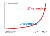
A model whose tokens cost a tenth as much looks like a large saving on the provider’s invoice and can still raise the price of every task the agent finishes. Token charges are only part of the account. An attempt also holds a sandbox open while its tools run, invokes tests and external services, waits for shared capacity, and may end in human review, and an attempt that fails pays for all of it without producing anything that ships. A cheaper model that needs more turns, retries more often, or passes assessment less often spreads those charges across fewer accepted tasks, so the bill per accepted result can rise while the token bill falls. The account that matters is kept over a cohort of tasks under one declared contract. It charges everything every attempt incurred, failed and canceled work included, to the tasks that contract accepted, and it keeps work still pending visible rather than dropping it. Reuse, retries, faster execution, model routing, added capacity, and delegation are each worth buying only when they lower that ratio or meet a deadline the objective values, and which lever matters depends on which term of the account dominates. Capacity enters the same account, because concurrent trajectories hold model servers, sandboxes, and reviewers while they wait, and an undersized pool turns waiting into cost. Horizon, state, and authority each set the closure a task must pay for, and an agent service is sustainable only when the accepted work it delivers covers that price.
Learning Objectives
Calculate cohort cost per accepted task while distinguishing attempt costs, human outcomes, and unsettled liabilities
Evaluate prefix caching, compaction, and retry purchases under explicit billing and acceptance assumptions
Diagnose which acceleration shortens a trajectory enough to pay for itself from the model’s share of its measured critical path
Evaluate model cascades under a common acceptance contract, including assessment costs and false-accept risk
Size resource occupancy for a target trajectory goodput (accepted tasks per unit time) and compare provisioning choices under declared workload, quota, and queueing assumptions
Design atomic budget reservations that preserve spending bounds across concurrent work and late settlement
Select a loop cap or architecture by pricing automated and human-completed outcomes under one acceptance contract
19.1 The Bill Behind an Accepted Repair
A team running the repair agent (Four lighthouse workloads) is offered a model whose tokens cost a tenth as much. On the provider’s invoice the switch looks like a large saving. In the team’s own accounts it can raise the price of every repair that ships. The cheaper model may need more turns to reach a passing patch, and each turn holds a sandbox open and invokes tools. More tickets may fail assessment, and each failure still paid for its model calls, its environment, its checks, and the engineer who triages it. The token discount is real, but it applies to only part of the account.
Horizon, state, and authority each set the closure a task must pay for.
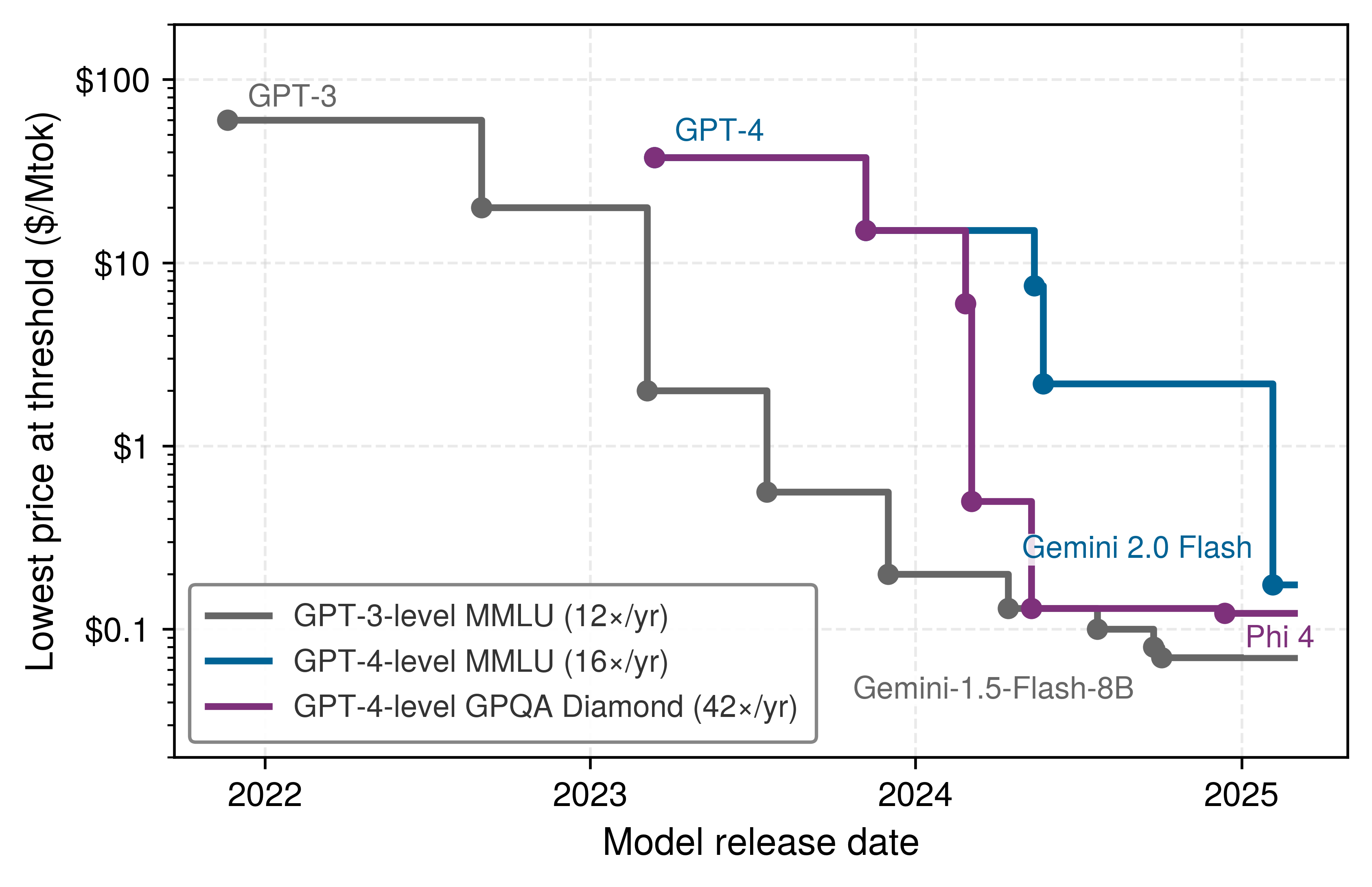
Offers like this one recur, because the price of a fixed capability falls quickly. Epoch AI (2025) track the cheapest model that reaches a fixed score on each of several benchmarks, and figure 1 plots three of those price series.
Figure 1: The Price of a Fixed Capability Falls Fast: Lowest price, in dollars per million tokens on a logarithmic axis, of any model that reaches a fixed benchmark score, plotted at each new low. Each line holds the capability constant, so its descent is price change alone, and the legend gives each series’ fitted decline per year. Prices are the source’s 3:1 blend of input and output rates; the series end in early 2025. Data from Epoch AI (2025).
Epoch AI. 2025. LLM Inference Prices Have Fallen Rapidly but Unequally Across Tasks.
Across all 21 capability thresholds in the source, the fitted decline runs from 9× to roughly 860× per year, with a median of 46×. A falling token price shrinks only the inference terms of the attempt cost. Sandbox lifetime, verification, cleanup, and human review are priced per turn, per check, and per hour of attention, not per token, so each price cut moves a larger share of the bill onto terms the provider’s discount never touches, and onto the acceptance probability in the denominator.
The runtime built so far can already say part of what the team needs. The evaluation discipline of Agent Evaluation decides which repairs count as accepted and how two policies are compared on matched tasks, and the harness’s budget ceilings stop any one task from spending without limit. Benchmarking Against a Single Agent joined the two once, deciding for one stated workload whether splitting a migration across workers repaid its coordination tax against a matched single controller. None of these says in general whether a policy is worth running. An accuracy figure reported without its cost cannot rank two designs, which is why cost-controlled evaluation reports the two jointly (Kapoor et al. 2024), and a ceiling that holds says nothing about how much of the spending under it bought accepted work.
↩︎ Per-task budget ceilings and the bounded-liability admission test that enforces them are established in Budgets and Ceilings.
What is missing is an account that joins spending to accepted outcomes. Reliability and Cost over a Horizon introduced cost per accepted task, the expected cost of an attempt divided by the probability that the attempt is accepted, as one of the book’s two quantitative fundamentals. Here that ratio becomes something a team can measure over a real cohort of tasks. Its numerator holds every charge an attempt incurs, its denominator counts only outcomes accepted under one declared contract, and each lever the runtime controls (reuse, retries, acceleration, routing, capacity, and delegation) is worth buying only if it lowers the ratio or buys a deadline the objective values.
The account comes first, in section 19.2, together with the rules that keep failed, canceled, and still-pending work inside it. Section 19.3 prices what the runtime pays to carry context from call to call and how many attempts it should buy. Section 19.4 finds where faster execution actually shortens a task, and section 19.5 decides which model should attempt the work at all. Section 19.6 sizes the services that concurrent trajectories hold and wait on, and section 19.7 makes spending limits hold across delegated children and late bills. Section 19.8 then compares whole architectures under one contract, and section 19.9 prices all four lighthouse workloads to show that each is bound by a different term of the same account.
19.2 Cost per Accepted Task
Before the team can say which model repairs tickets more cheaply, it must fix what a repair is. A configuration scored against visible tests cannot be compared with one scored against a sealed suite, however carefully the invoices are tallied, because the two denominators count different things. Acceptance is defined only under an explicitly declared contract, checker, and execution environment. Isolating the effect of one policy choice (model selection, prompt construction, or tool scaffolding) therefore takes a matched comparison that holds the task contract, evaluation harness, and resource ceilings fixed while only the policy varies. The cost accounting also needs an explicit task cohort, the declared set of initiated tasks whose charges and outcomes it covers, and a cutoff timestamp. Together they decide which initiated tasks are under review, which outcomes count as accepted before the cutoff, and which operations, assessments, or invoices are still pending.
19.2.1 Whole-trajectory cost and the task account
An invoice that tracks only model tokens misses the container lease, test suite, cleanup job, and engineer triage that continue long after the final token leaves the model server. Across an attempt of \(\TurnHorizon\) turns, an agent system incurs direct inference charges alongside substantial infrastructure costs to maintain the execution environment. This chapter numbers turns from one, \(\TurnIndex=1,\dots,\TurnHorizon\), so that the index matches the turn counts in its worked examples. The whole-trajectory cost of an attempt decomposes as
Inside the turn loop, the input (\(\TurnInputTokenCost^{(\TurnIndex)}\)) and output (\(\TurnOutputTokenCost^{(\TurnIndex)}\)) terms capture inference pricing under the provider’s rate card, including tiered rates and prompt-caching discounts, while tool invocation fees (\(\TurnToolFeeCost^{(\TurnIndex)}\)) cover billable external API requests and data lookups and the sandbox charge (\(\TurnSandboxCost^{(\TurnIndex)}\)) prices the wall-clock lifetime of virtual machines or containers, including idle waits while external tools run. Outside the turn loop, verification (\(\AttemptVerificationCost\)) covers post-execution checks and test suites not already billed as sandbox time, and cleanup (\(\AttemptCleanupCost\)) pays for state reset, storage teardown, or compensating transactions. Whenever rejected attempts or policy escalations trigger human review, \(\HumanReviewCost\) tallies manual engineering time within the declared system boundary, while runtime cost (\(\AttemptRuntimeOverheadCost\)) apportions orchestrator overhead, scheduler queues, and shared network telemetry. Every cost item must map to exactly one category so that an end-of-turn integration test billed as active sandbox compute time is never double-counted under verification.
Definition 19.1: Whole-trajectory cost
Whole-trajectory cost is the total expense attributed to a single execution attempt across its model calls, environment runtime, validation assessment, and required finalization within a declared accounting boundary.
Significance: It forms the fundamental numerator of cost per accepted task (\(\CostPerAcceptedTask\)), capturing every cost driver that standard per-token pricing hides: container provisioning, external API calls, test-suite grading, state teardown, and human escalation. Failed attempts accumulate these charges just as successful ones do.
Distinction: Whole-trajectory cost measures the expense of an individual attempt, whereas cost per accepted task amortizes all attempted and discarded work across the surviving accepted tasks in the cohort.
Common pitfall: Closing the accounts the instant the agent process emits its final token, ignoring trailing cloud resources, pending cleanup jobs, or downstream engineer triage.
A single initiated task may involve multiple sequential retries or parallel delegated branches. Its task account, denoted \(\TaskCost\), aggregates every attempt, failed branch, and abandoned speculative execution, along with the task’s assigned share of capacity and orchestration overhead. When a sub-agent branch crashes or is canceled, its incurred costs do not vanish; they remain permanently logged against the task.
In production environments, operations are rarely settled instantly. The harness’s reservations hold part of the allowance against work that has been admitted but not yet billed. Because these funds remain committed until all external side effects resolve, any snapshot taken at an intermediate cutoff must distinguish settled expenditures from outstanding liability, the reserved balance backing active, unbilled operations. The settled total serves merely as a lower bound on the final task cost until all pending obligations clear.
19.2.2 Cohort cost per accepted task
Averaging the cost of successful attempts alone hides every rejected, timed-out, or canceled trajectory whose bills the surviving repairs must carry. For a finite cohort of \(\InitiatedTasks\) initiated tasks with fully resolved accounting, let \(\AcceptedTasks\) represent the number of distinct tasks accepted under the declared contract. If an agent executes three successful retries on a single ticket, the system delivers exactly one accepted task; retries never inflate the denominator. For \(\AcceptedTasks>0\), the cohort cost per accepted task is
The numerator aggregates every dollar expended across all \(\InitiatedTasks\) initiated tasks, whether they succeeded, crashed, timed out, or were rejected by validation. Keeping failed and canceled work in the numerator and pending verdicts explicit is exactly what trajectory goodput and the accepted task (principle 15) demand of any account in this book. Only accepted tasks count as delivered work, and every charge incurred on the way to them stays on the bill. (This chapter defines trajectory goodput formally, as accepted tasks per unit time, when it sizes capacity in section 19.6.1.) If zero tasks are accepted (\(\AcceptedTasks = 0\)), the ratio is undefined; a transparent system report must present the total expenditure and the zero count directly rather than masking the failure behind an artificial floor. Whenever tasks or invoices remain in flight at the accounting cutoff, the report must flag the cutoff timestamp and qualify the calculation as provisional. An unexecuted test suite represents a pending task, not an immediate failure, just as an asynchronous cloud billing adjustment can shift \(\CostPerAcceptedTask\) hours after the code artifact is finalized.
Definition 19.2: Cohort cost per accepted task
Cohort cost per accepted task is the total cost of every initiated task in a cohort (failed, canceled, and still-pending work included) within a declared accounting boundary, divided by the number of distinct tasks accepted under one declared contract, checker, and environment by a stated cutoff.
Significance: It provides the empirical, measurable form of this book’s fundamental economic metric \(\CostPerAcceptedTask\). Because the count of accepted tasks divides every item in the numerator, a drop in task acceptance inflates the entire system bill, whereas a token price cut discounts only the inference fraction.
Distinction: Whole-trajectory cost measures the expense of an isolated attempt; cohort cost per accepted task loads all failed, canceled, and abandoned attempts onto the small fraction of work that actually passes inspection.
Common pitfall: Computing the average cost of successful trajectories alone. This survivor bias ignores the discarded attempts whose compute and environment bills must be paid by the surviving accepted tasks.
When all tasks in a cohort have reached a terminal state, the cohort acceptance rate is \(\AcceptanceFraction = \AcceptedTasks / \InitiatedTasks\). Let \(\AcceptedTaskMeanCost\) denote the mean cost of an accepted task, and let \(\UnacceptedTaskMeanCost\) denote the mean cost of an unaccepted task (encompassing outright failures, policy cancellations, and timed-out executions). When both subsets are non-empty, partitioning the numerator yields
The cohort fraction \(\AcceptanceFraction\) counts tasks, whereas the per-attempt acceptance probability \(\AcceptanceProbability\) of equation 1.2 counts attempts. When every task gets exactly one attempt, the two coincide, and \(\AcceptanceFraction\) estimates \(\AcceptanceProbability\). When a task may retry, \(\AcceptanceFraction\) estimates task-level coverage, the probability that some attempt on the task is accepted, while the per-attempt planning form stays \(\mathbb{E}[\AttemptCost]/\AcceptanceProbability\). Section 19.3.3 connects the two for sequential retry.
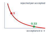
Each accepted task carries the rejected ones, and that load explodes as acceptance falls.
The factor \((1-\AcceptanceFraction)/\AcceptanceFraction\) represents the rejection multiplier, the number of failed tasks that each accepted task must pay for. This expression is an exact accounting identity for the cohort, not an asymptotic model or an assumption that retries will eventually converge. As the acceptance rate \(\AcceptanceFraction\) falls toward zero, the multiplier grows without bound. Whether a steep discount on model tokens yields lower overall operating costs depends on both groups’ costs, which is why no universal threshold decides model selection in isolation. The concrete bug-repair scenario below prices this trade-off directly.
Napkin Math 19.1: The token-price fallacy in automated bug repair
Problem: Two hypothetical configurations each process the same 100 tickets, with one bounded attempt per ticket and the same acceptance contract. Every attempt, rejected or not, uses the fixed per-attempt usage that table 1 assumes for its configuration, and all outcomes and charges are settled at the cutoff. The environment charge covers tool use, sandbox holding, and cleanup; the assessment charge covers checking not billed as sandbox time, together with allocated runtime overhead. Which configuration costs less per accepted repair?
Table 1: Illustrative Bug-Repair Cohort: Assumed prices, usage, and accepted counts for two configurations; these are arithmetic inputs, not observed measurements.
Parameter
Frontier configuration
Low-token-price configuration
Input/output price per million tokens
$3 / $15
$0.30 / $1.20
Turns per attempt
4
7
Input/output tokens per turn
16,000 / 800
28,000 / 1,200
Accepted tickets
75
25
Environment cost per turn
$0.03
$0.03
Additional assessment per attempt
$0.05
$0.05
Math: Applying the rates and usage in table 1 gives model charges per attempt of $0.240 and $0.069. Adding the other charges gives $0.410 and $0.329, respectively. The complete cohorts therefore cost $41 and $32.888. Dividing each total by its accepted count gives $0.55 and $1.32 per accepted repair. The lower-token-price configuration costs less per attempt but 2.4× as much per accepted task.
Now expand both accounting boundaries to include $10 of engineer triage for each rejected attempt. The frontier configuration has 25 rejected tickets and the other has 75. Total costs become $291 and $782.888; costs per accepted task become $3.88 and $31.32, a ratio of 8.1×. Triage adds no accepted repairs; if engineers also completed tickets, that combined service would need its own named account.
Systems insight: With one attempt per ticket, a cheaper configuration wins only if its attempt cost falls by more than its acceptance does. Here acceptance falls by 66.7 percent, so the low-price configuration needed attempts at least that much cheaper. Its token charges fall by 71.3 percent, but its all-in attempt cost falls by only 19.8 percent, because its extra turns each pay the environment charge. Each of its accepted repairs also carries 3 rejected attempts, against 0.33 for the frontier configuration, so every charge that scales with rejections, such as triage, widens the gap.
Systems Perspective 19.1: Reading a cost-per-accepted-task number
The cost per accepted task represents a cohort-level ratio of aggregate expenditures to accepted deliverables evaluated at an explicit cutoff timestamp. Engineers must avoid confusing this ratio with the arithmetic mean of individual task expenses; furthermore, in small cohorts, sample variability prevents this ratio from serving as an unbiased estimator of the theoretical planning ratio \(\mathbb{E}[\AttemptCost]/\AcceptanceProbability\). To be actionable, any reported \(\CostPerAcceptedTask\) figure must be accompanied by its full context: total cohort expenditure, accepted task count with statistical confidence bounds, end-to-end latency distributions, pending execution statuses, and outstanding liabilities. An isolated efficiency number shorn of these context markers cannot support valid comparisons between competing system policies.
A rigorous matched comparison holds the acceptance contract and maximum resource allowances fixed across configurations, rather than enforcing identical expenditures. A more aggressive search policy might intentionally spend more compute per ticket to meet stringent latency deadlines or maximize task coverage, provided the underlying system objective values those gains. Inverting this metric yields goodput per dollar (accepted tasks delivered per unit of currency, the per-dollar counterpart of the trajectory goodput defined in section 19.6.1), which keeps the same accounting boundary but reads it as throughput. In both formulations, acceptance confirms only that an artifact satisfied the automated contract within the designated test suite; it does not guarantee the complete absence of latent defects.
↩︎ Matched-budget comparison, which fixes the acceptance contract and resource envelope while each policy spends it differently, is established in Matched-budget comparison.
Decomposing the account this way shows where a lever can act before anyone pays for it. The dominant term varies across workloads, and section 19.9 prices all four lighthouses to show which term binds each. The levers the runtime controls most directly act on the inference term and on the number of attempts. In automated bug repair, re-sent prompt context makes up most of the inference charge, so prefix caching and context compaction act on that charge, while reasoning limits and retry budgets set how many model invocations an accepted task buys. Whether the inference term is the one worth attacking for a given workload is a separate question, and for the repair agent the answer turns out to be no.
19.3 Context Reuse and Retry Budgets
Across the turns of a repair, the same prompt prefix recurs call after call. Context engineering arranges the request so that the stable part comes first, and the serving system keeps the key-value (KV) attention state of that prefix so the next call need not recompute it. Reuse lowers cost, but it is not free, and it competes with two other purchases the runtime can make: compacting the context, which shortens the prompt but discards reusable state, and buying more attempts, which raises coverage but multiplies the bill. Each must be priced under the same acceptance contract before the runtime can tell which one lowers the cost per accepted task.
↩︎ The exact-prefix, execution-parameter, residency, and tenant conditions under which retained attention state may be reused are established in Prefix compatibility.
19.3.1 Pricing prefix cache hits
Re-sending an append-only conversation history on every turn makes logical input volume grow quadratically with trajectory length, even when the serving cluster already holds the earlier turns in memory. Evaluating multi-turn agent economics therefore requires distinguishing between logical input, physical computation, and billed tokens. A model provider often retains compatible KV state across calls even when an agent client retransmits the complete conversation transcript on every turn.1 Over an execution trajectory of \(\TurnHorizon\) turns, one call each, let \(\SequenceLength^{(\TurnIndex)}\) represent the logical input length on call \(\TurnIndex\), \(\EligibleCachedPrefixLength^{(\TurnIndex)}\) its eligible cached prefix length, and \(\OutputLength^{(\TurnIndex)}\) its billed output length. Under a published tariff with per-token rates \(\InputTokenPrice\) for fresh input, \(\CachedInputTokenPrice\) for cached input, and \(\OutputTokenPrice\) for generated output, the total token charge is
1Prefix Reuse: Serving systems make cross-request reuse practical by storing attention state in paged memory blocks that requests sharing a prefix can share (Kwon et al. 2023), and by indexing retained state in a radix tree so subsequent calls locate their longest cached prefix (Zheng et al. 2024). A discounted cached-input tariff reflects this underlying mechanism directly: only an exact, resident token prefix qualifies for the discount.
Kwon, Woosuk, Zhuohan Li, Siyuan Zhuang, Ying Sheng, Lianmin Zheng, Cody Hao Yu, Joseph Gonzalez, Hao Zhang, and Ion Stoica. 2023. “Efficient Memory Management for Large Language Model Serving with PagedAttention.”Proceedings of the 29th Symposium on Operating Systems Principles, 611–26. https://doi.org/10.1145/3600006.3613165.
Zheng, Lianmin, Liangsheng Ying, Zhenghao Yin, Cody Hao Liu, Eric Yu, Prakhar Patel, Zhipeng Yang, Anthony K. Joseph, and Ion Stoica. 2024. “SGLang: Efficient Execution of Structured Language Model Programs.”arXiv Preprint arXiv:2312.07104, ahead of print. https://doi.org/10.48550/arXiv.2312.07104.
Commercial pricing models often incorporate additional dimensions, including cache-write surcharges, hourly retention fees, and minimum eligible prefix thresholds. In an append-only agent transcript, each turn re-sends the cumulative history alongside newly observed tool outputs and model generations. With an initial prompt of \(\BasePromptLength\) tokens and \(\TurnAppendLength\) tokens appended per turn, the logical input over the whole trajectory is the quadratic re-send total \(\PromptTokensSent\) of equation 2.9, and ideal prefix reuse charges only \(\FreshInputTokenCount=\BasePromptLength+(\TurnHorizon-1)\TurnAppendLength\) of it at the fresh-input rate, once each for the initial prompt and every appended increment. Priced under the tariff, the total input bill is \(\InputTokenPrice{}\FreshInputTokenCount+\CachedInputTokenPrice(\PromptTokensSent-\FreshInputTokenCount)\). Because both \(\CachedInputTokenPrice\) and \(\TurnAppendLength\) remain positive, the quadratic growth term does not disappear; caching merely scales down its cost coefficient from \(\InputTokenPrice\) to \(\CachedInputTokenPrice\). These formulations account for billed input tokens, not the physical accelerator memory required to hold this reusable state across requests.
Prefix hits require strict alignment between the incoming token sequence and the cached execution context, including weights and adapters, token positions, attention masks, and applicable multimodal inputs, together with residency and tenant access conditions (principle 5). Reusability breaks at the first altered token. Output sampling settings alone need not change already computed prefix tensors; any additional provider cache-key restrictions belong to the service contract. In production deployments, distributed request routing, memory pressure and cache eviction, and protracted tool execution times degrade realized hit rates. Economic models must therefore price observed, eligible hits under the actual service contract rather than assuming theoretical upper bounds.
Napkin Math 19.2: Pricing an append-only trajectory
Problem: An agent trajectory runs 30 turns, starting with an initial prompt of 8,000 input tokens and appending 1,500 tokens on each subsequent turn. Each invocation generates 200 output tokens. The provider tariff charges $3 per million fresh input tokens, $15 per million output tokens, and 10 percent of the fresh-input price for cached reads, with no separate write or retention fees. How much does ideal prefix reuse reduce the token bill for this trajectory?
Math: Cumulative logical input across all turns reaches 892,500 tokens. Under ideal prefix reuse, only 51,500 tokens are billed at the fresh-input rate. Input processing therefore costs $2.678 without reuse vs. $0.407 with prefix caching. Combining this with the constant $0.090 output charge yields total bills of $2.768 and $0.497, representing a 5.6× cost reduction.
Systems insight: Cache hit rate governs financial efficiency. Because historical context constitutes almost all of this trajectory’s input, even small reductions in hit rate produce large absolute billing increases. If 10 percent of the eligible prefix misses (for example, because a volatile timestamp or session identifier sits near the prompt header), the session cost increases by $0.227, raising the cached bill by 45.7 percent. Prefix caching modifies only the model inference term in effective cost (\(\CostPerAcceptedTask\)): it lowers the cost of carrying context across turns while leaving delivered inputs, outputs, and task acceptance unchanged.
19.3.2 The price of compaction
Unlike prefix caching, context compaction actively alters the input transcript. Replacing prior conversation turns with an aggregated summary shortens the active prompt, though it risks invalidating cached attention state. If summarization preserves a stable system prefix, subsequent requests can still reuse those initial blocks. To price the cache-invalidation penalty explicitly, consider the case of a complete cache miss: the first compacted invocation shares no reusable prefix with prior turns, but subsequent calls resume append-only prefix reuse from the compacted prompt. The baseline comparison retains the full uncompacted context over the same remaining turns, holding future token additions and ordinary output lengths constant. This analysis isolates the pure token price of compaction; whether a given summary preserves downstream task acceptance is evaluated separately using the context-policy evaluation of Evaluating Context Policies.
Let \(\SequenceLength\) be the input length at the moment of compaction, \(\CompactedContextLength < \SequenceLength\) the compacted length, and \(\RemainingCallCount \ge 1\) the remaining ordinary invocations, including the first compacted call. Set the two call sequences side by side. Keeping the context makes \(\RemainingCallCount\) ordinary calls, the first of which reads the cached history plus one fresh increment. Compacting makes one summarization call followed by \(\RemainingCallCount\) ordinary calls on the compacted prompt. Assume the summarization call reads exactly what the keep path’s first call would have read, at the same cached and fresh prices; then its input charge equals that call’s input charge, and the two cancel when the paths are differenced. Ordinary outputs are equal call for call. What remains on the compaction side with no counterpart on the keep side is the summary’s generated tokens, \(\OutputTokenPrice{}\SummaryOutputLength\), and the first compacted call, which must send all \(\CompactedContextLength\) tokens as fresh input to rebuild server KV cache state. Relative to keeping the original context, the upfront investment \(\CompactionUpfrontCost\) is therefore
which combines the output generation fee of the summary with the fresh-input cost of repopulating the cache. Each subsequent call saves \(\CompactionPerCallSaving=\CachedInputTokenPrice(\SequenceLength-\CompactedContextLength)\) under the assumption of equal incremental growth. The cumulative cost difference across \(\RemainingCallCount\) remaining calls is therefore:
Here \(\CompactionPaybackCallCount\) represents the payback horizon: the minimum number of remaining invocations required for per-turn cache savings to offset the initial compaction surcharge. When \(\CompactionUpfrontCost \le 0\), compaction pays for itself on the very first call; when \(\CompactionPerCallSaving = 0\) and \(\CompactionUpfrontCost > 0\), compaction never recovers its cost on token pricing alone. Accounting for the first compacted call separately from later turns prevents off-by-one errors when estimating the remaining trajectory budget.
Napkin Math 19.3: Count the first compacted call
Problem: In the preceding scenario, suppose the agent triggers compaction at turn 16, compressing 30,500 tokens down to 12,000. The summarization call emits 1,500 tokens under standard cached-history pricing. If 15 ordinary calls remain (including the first compacted turn), what is the minimum remaining horizon required for compaction to cost no more than retaining the full context?
Math: Retaining the uncompressed context incurs $0.24525 in remaining input costs. Compaction incurs $0.19035 across remaining ordinary calls plus $0.03570 for the summarizer, totaling $0.22605. The upfront differential is $0.05850, against which each subsequent turn saves $0.00555. With 11 calls remaining, compaction still costs $0.00300 more than baseline. Reaching 12 remaining calls yields a net saving of $0.00255.
Systems insight: Compaction lowers total expenditure only when the remaining trajectory length meets or exceeds the payback horizon \(\CompactionPaybackCallCount\). \(\CompactionPaybackCallCount\) scales inversely with the cached read rate, because the upfront cost \(\CompactionUpfrontCost\) depends on \(\InputTokenPrice\) and \(\OutputTokenPrice\), whereas the per-call savings \(\CompactionPerCallSaving\) are proportional to \(\CachedInputTokenPrice\). If the cached read tariff drops from 10 percent to 5 percent of the fresh-input price, the break-even horizon extends to 23 calls. Because only 15 calls remain, compaction under this discounted rate loses money. As KV caching becomes cheaper, compaction must occur earlier in an execution trajectory to justify its cache-invalidation penalty. Late-stage compaction must be justified by context window limits or attention fidelity rather than token savings; an aggressive summary that drops a crucial constraint and lowers acceptance erases any marginal token economy.
19.3.3 Reasoning and retry budgets
Giving an agent a larger reasoning token limit or a higher retry cap raises the cost of every attempt without guaranteeing enough new acceptances to pay for it. When an agent runtime allocates budget dynamically by purchasing deeper internal reasoning within a single invocation or by funding multiple independent execution attempts, a configured reasoning token limit acts as an upper ceiling rather than a fixed spend. Financial accounting must track actual billed token consumption and its empirical effect on task acceptance under an identical evaluation contract. Because internal deliberation generates tokens serially, systems engineers must evaluate this extra compute against increased turn latency. The retry analysis below prices a reasoning budget too. Deeper reasoning raises the all-in attempt cost \(\MeanAttemptCost\) by the billed price of the extra tokens and is worth buying only if it raises acceptance \(\AttemptPassProbability\) by a larger proportion, so that \(\MeanAttemptCost/\AttemptPassProbability\) falls.
Consider a baseline model of sequential retry with early stopping, in which every attempt on a task has an identical acceptance probability \(\AttemptPassProbability > 0\). Conditioning on a fixed task prompt and external environment, attempts represent independent draws from the same agent configuration, each incurring an all-inclusive cost \(\MeanAttemptCost\) covering model inference, sandbox runtime, and output verification. Sequential retry terminates immediately upon the first accepted result or halts after exhausting a budget of \(\IndependentAttemptCount\) attempts. The overall task acceptance probability (or coverage) is \(\TaskCoverageProbability_k = 1 - (1 - \AttemptPassProbability)^\IndependentAttemptCount\), and the expected number of executed attempts is \(\sum_{j=0}^{\IndependentAttemptCount-1}(1-\AttemptPassProbability)^\SequentialAttemptIndex = \TaskCoverageProbability_k / \AttemptPassProbability\). Dividing the expected total spend by the expected accepted tasks yields \((\MeanAttemptCost \TaskCoverageProbability_k / \AttemptPassProbability) / \TaskCoverageProbability_k = \MeanAttemptCost / \AttemptPassProbability\). Under early stopping with independent trials, the expected cost per accepted task remains invariant to the attempt cap \(\IndependentAttemptCount\): raising \(\IndependentAttemptCount\) expands overall task coverage, while early termination holds the average cost per successful outcome at exactly \(\MeanAttemptCost / \AttemptPassProbability\), which is the per-attempt form of equation 1.2 with \(\MeanAttemptCost\) as the attempt cost.
In contrast, launching all \(\IndependentAttemptCount\) attempts concurrently in a parallel batch costs \(\IndependentAttemptCount \MeanAttemptCost / \TaskCoverageProbability_k\) per expected accepted task, provided the evaluation harness can identify and return an accepted candidate from the pool. These are the sequential and batch costs of equation 13.6, with the generation and checking charges folded into one attempt cost \(\MeanAttemptCost\). What this chapter adds is the comparison between buying more attempts from a cheap configuration and buying one attempt from a stronger one.
Napkin Math 19.4: What a retry cap buys
Problem: A lightweight agent configuration achieves an acceptance probability of 0.30 at an all-in cost of $0.10 per attempt. A stronger configuration achieves 0.70 acceptance but costs $0.40 per attempt. Allowing up to 5 lightweight attempts under the independent-trials model, which policy achieves the lowest cost per expected accepted task: sequential retry with early stopping, an unconditional parallel batch of 5 attempts, or a single attempt from the stronger model?
Math: Sequential retry achieves an expected coverage of 83.2 percent while consuming 2.773 attempts per task. This produces an expected spend of $0.277 per submitted task and $0.333 per accepted task. Running all 5 attempts in parallel yields identical coverage but requires $0.500 per submitted task, increasing the cost per accepted task to $0.601. A single invocation of the stronger model costs $0.571 per accepted task.
Systems insight: Under early stopping, sequentially retrying a cheaper model outperforms a single call to a stronger model whenever \(\CheapConfigurationAttemptCost/\CheapConfigurationPassProbability < \StrongConfigurationAttemptCost/\StrongConfigurationPassProbability\). In this scenario, sequential retry also delivers superior aggregate coverage (83.2 percent vs. 70 percent). Executing the batch concurrently secures that same coverage at a 1.8× multiplier in cost per accepted task, the ratio of \(\IndependentAttemptCount\) to the expected sequential attempt count. A parallel burst is justified only when strict wall-clock deadlines assign significant value to lower latency, offsetting the substantial financial premium.
Production workloads rarely have a single, uniform success probability \(\AttemptPassProbability\). Difficult tasks maintain persistently low acceptance rates across repeated attempts. Consequently, substituting an average per-task success rate into \(1-(1-\AttemptPassProbability)^\IndependentAttemptCount\) systematically overstates aggregate coverage, causing the realized cost per accepted task to drift above the idealized \(\MeanAttemptCost/\AttemptPassProbability\) ratio. Repeated-sampling studies show this effect. On benchmarks with automated verification, task coverage (the fraction of tasks solved by at least one sample) continues to climb across multiple orders of magnitude of generated samples, scaling roughly log-linearly rather than saturating as a single-parameter model would predict (Brown et al. 2024). Environmental feedback, service outages, and shared mutable state further complicate fixed-probability assumptions. Engineers must therefore evaluate retry policies using outcome distributions measured per task over repeated runs.
↩︎ Per-task acceptance probabilities, and the distinction between a task and a repeated run of it, are established in Tasks and repeated runs.
Generating extra candidate solutions also introduces verification risk. As analyzed in Balancing pool size against checking cost, repeated sampling raises the chance of a false acceptance, where a flawed candidate satisfies test assertions without truly solving the underlying task. Passing an automated check provides domain-specific verification evidence rather than an absolute guarantee of correctness. Ultimately, prefix caching, context compaction, and retry policies govern what compute resources an agent runtime purchases; determining how those purchased operations dictate end-to-end latency requires analyzing the critical execution path.
19.4 Critical-Path Latency
Accelerating a model call rarely yields a proportional reduction in end-to-end task time. In realistic agent workflows, container provisioning, repository setup, test suite execution, tool I/O, and consensus validation often dominate total elapsed time. Evaluating an acceleration technique therefore requires an end-to-end systems perspective that measures how much wall-clock time the proposed change strips from the critical path to a declared endpoint, what compute and memory resources it consumes, and whether the accelerated execution preserves the required acceptance evidence. Tracing exposes where time actually goes, while economic accounting determines whether accelerating that specific span is worth the operational cost.
19.4.1 Dependency graphs and elapsed time
Distributed tracing distinguishes enclosing parent spans from the nested operations within them. Summing a parent span’s duration with the durations of its children double-counts time. Similarly, summing concurrent sibling spans inflates apparent latency, whereas omitting queueing delays, network transit, or uninstrumented runtime pauses undercounts it. When profiling an agent runtime, uninstrumented intervals must remain explicitly accounted for as unexplained gaps rather than arbitrarily attributed to neighboring components.
2Recovering the Dependency Graph: The critical-path method and its float are introduced with agent traces in Span overlap and latency attribution. What pricing adds is the reconstruction step: distributed-systems work recovered the dependency model of production requests from existing component logs, precisely so that critical-path analysis could say which component’s speedup would shorten end-to-end latency (Chow et al. 2014). An agent trace needs the same reconstruction, from dispatch and join records rather than span nesting, before any acceleration is priced.
Chow, Michael, David Meisner, Jason Flinn, Daniel Peek, and Thomas F. Wenisch. 2014. “The Mystery Machine: End-to-End Performance Analysis of Large-Scale Internet Services.”11th USENIX Symposium on Operating Systems Design and Implementation (OSDI 14), 217–31.
Crucially, a span’s parent in a call tree denotes syntactic containment, which does not necessarily reflect an execution dependency. An agent runtime might spawn background log flushes or asynchronous cache warmers that outlive the caller without blocking the next step. Determining end-to-end latency requires constructing a directed acyclic execution graph based on true dispatch and join conditions, in which a directed edge indicates that the successor task cannot begin until its predecessor completes. Along any path, the critical path counts only disjoint, non-overlapping intervals rather than inclusive parent spans alongside their children. Over such a graph, with vertex durations \(\VertexSlotTime(\DependencyGraphVertex)\) and source-to-sink paths \(\SourceSinkPathSet\), the critical path is the longest path, the quantity every acceleration below is priced against:2
When the graph contains only mandatory computation, equation 2 establishes an idealized lower bound on completion time. The critical path matches the actual observed wall-clock interval only when the dependency graph incorporates real-world scheduling artifacts: thread scheduling delays, resource contention waits, queueing latencies, and sandbox initialization. Furthermore, the boundary of the graph depends on the system contract. Emitting an initial streamed token, evaluating a candidate patch against unit tests, and fully committing a validated pull request represent fundamentally different completion endpoints, each with its own dependency sink.
A non-critical branch can shrink without moving elapsed time, and a critical one pays off only until a parallel branch becomes the longest. For pricing, the first case is not worthless, because a faster off-path branch may still free cluster capacity or reduce hosting costs, and the second means every proposed optimization is priced against a recomputed critical path rather than by subtracting isolated component savings from total elapsed time.
19.4.2 The payoff of faster inference
When sandbox setup and test execution take minutes while model calls take seconds, paying a premium for faster inference barely moves completion time. Bounding the maximum possible wall-clock gain from model acceleration before buying faster serving hardware prevents teams from optimizing a tiny fraction of the critical path.
Napkin Math 19.5: How much does faster inference buy?
Problem: In a short hypothetical repair episode, far shorter than the 30-turn trajectory priced in notebook 19.2, how much elapsed time does a 4× acceleration of every model call save?
Variables: All intervals execute sequentially, from runtime initialization through final sandbox snapshot export, without queueing, overlapping execution, or uninstrumented gaps. The durations listed in table 2 represent disjoint, non-overlapping sums rather than nested spans. The proposed acceleration modifies only inference latency, leaving model outputs, tool operations, test evidence, scheduling decisions, and finalization unchanged.
Table 2: One serial repair episode: Categories partition elapsed time under the stated assumptions; the total is not an additional interval.
Disjoint category
Elapsed time
All model calls in the episode
29.25 s
Required test execution
245.60 s
Sandbox creation and snapshot export
37.35 s
Runtime initialization and repository status
0.20 s
Whole declared interval
312.40 s
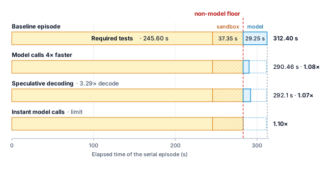
Math: If model execution occupies fraction \(\ModelTimeFraction\) of baseline duration \(\Time\) and accelerates by factor \(\AcceleratorGain \geq 1\), Amdahl’s law (The coordination tax) bounds the new duration: \(\AcceleratedEpisodeTime = \Time[(1-\ModelTimeFraction)+\ModelTimeFraction/\AcceleratorGain]\). This is the delegation bound of equation 18.1 with the overhead term set to zero and the worker count replaced by the acceleration factor; here the accelerated part is the model rather than the parallel work. In this episode, model work accounts for 9.4 percent of elapsed time. A 4× model acceleration reduces the episode to 290.46 s, saving 21.94 s for an overall speedup of 1.08×. Even instantaneous inference (\(\AcceleratorGain \to \infty\)) yields a whole-episode speedup of only 1.10× under these assumptions.
Systems insight: The theoretical speedup ceiling \(1/(1-\ModelTimeFraction)\) dictates whether paying for faster model inference can ever satisfy an operational deadline. Because this ceiling depends only on baseline profile measurements, engineers can evaluate its viability before investing in model optimization or specialized serving infrastructure. In this repair episode, halving test execution duration while maintaining identical coverage saves 122.8 s, far more than the 21.94 s gained from a 4× model acceleration, and it also lowers the sandbox leasing charges in \(\CostPerAcceptedTask\). When an engineering latency target exceeds what \(1/(1-\ModelTimeFraction)\) can theoretically deliver, engineering effort belongs on test execution and environment lifecycle optimizations. In non-linear, branching trajectories, this principle applies directly to the recomputed critical path of equation 2.
19.4.3 Span types and their levers
Once distributed traces identify the critical path, engineers must match each bottleneck span to the physical factors governing its duration and the levers that can compress it (table 3). Buying faster token decoding when container cold starts or serial tool calls dominate the critical path spends engineering budget without moving completion time.
Table 3: Trajectory Span Types: What bounds each kind of span on an agent’s critical path and which techniques shorten it. Each lever is admissible only if the accepted result still meets the same acceptance contract and coverage.
Span
What sets its duration
What shortens it
Model, reading input
Context length, prefix-cache misses, queueing
Cache-stable layout, smaller context, less queueing
When tool operations are independent, the runtime can dispatch them concurrently provided security policies, authorization boundaries, and resource reservations permit parallel execution. If three tool calls dispatch simultaneously without I/O contention and all three must complete before the agent continues, the synchronization join waits only for the longest operation rather than the sum of all three. However, concurrency gains diminish when tools contend for local resources, when dispatch is staggered, or when a downstream tool requires the output of an earlier call. In the sandbox domain, warm container pools, pre-baked filesystem snapshots, and persistent build caches shorten environment initialization spans, subject to strict isolation and teardown guarantees before each reuse.
↩︎ The reset contract that a pooled or snapshot-restored sandbox must satisfy before serving a new lease is established in The reset contract.
Environment preparation can overlap model generation if the runtime executes speculative setup within a sandboxed, isolated scope that commits no external side effects before the full model response is validated and authorized. Streaming tokens from a large language model (LLM) does not constitute an authorized execution intent; even a speculative read operation might violate an access boundary or leak uncommitted state. If the model output subsequently alters the required tool call or aborts, the runtime must discard speculative work, release allocated resources, and record any incurred compute charges in the task account.
Early stopping alters the evidentiary value of an execution as well as its duration. In a validation pipeline, a single failing assertion in a mandatory test immediately proves that a candidate solution is unacceptable, allowing the runtime to short-circuit the remaining suite. Conversely, an early pass confirms only a single check; it provides zero evidence regarding the remainder of the test suite. Test prioritization and streaming failure detection thus accelerate defect rejection during intermediate iterations. However, final task acceptance still demands full test coverage across the declared verification contract. Furthermore, canceling a running check does not instantly free resources; active worker processes must unwind cleanly, and any intermediate compute costs remain charged until the underlying jobs settle.
↩︎ Cancellation as an asynchronous control action, whose job may finish or keep running after the request and leave cleanup obligations unsettled, is established in Job supervision and cancellation.
19.4.4 When speculative decoding pays off
When a draft model’s token proposals are frequently rejected by the target model, speculative decoding spends extra compute on drafting and verification while slowing generation below baseline. As the serving lever of table 3 that shortens the generating span itself, speculative decoding must clear two boundaries: one inside the model call and one on the critical path. Inside the call, single-stream decoding is memory-bandwidth bound under the serving assumptions of Estimating per-call hardware work, which leaves room to check several proposed tokens for roughly the price of generating one.
In speculative decoding, a lightweight draft model3 proposes \(\DraftTokenCount\) candidate tokens per speculation round, and the larger target model verifies them in a single forward pass, accepting the longest matching prefix and generating one continuation token of its own (Leviathan et al. 2023; C. Chen et al. 2023). Let the computational cost of generating one draft token equal a fraction \(\DraftTokenCostRatio\) of a standard target decoding step, and let \(\MeanAcceptedDraftLength\) denote the mean number of draft tokens accepted per round. If evaluating \(\DraftTokenCount\) proposed tokens in parallel costs approximately one target step, each round yields \(\MeanAcceptedDraftLength + 1\) verified tokens in the time equivalent to \(\DraftTokenCount\DraftTokenCostRatio + 1\) target decoding steps. The resulting decoding speedup for an isolated stream is
3Draft-then-Verify Decoding: The idea predates large language models. Blockwise parallel decoding predicted several future positions at once and backed off to the longest prefix a scoring model validated (Stern et al. 2018). Speculative decoding moved the proposals into a separate small draft model and added an acceptance rule under which sampled outputs keep the target model’s distribution, which is why its savings are purely a cost and latency question rather than a quality trade.
Stern, Mitchell, Noam Shazeer, and Jakob Uszkoreit. 2018. “Blockwise Parallel Decoding for Deep Autoregressive Models.”Advances in Neural Information Processing Systems 31 (NeurIPS 2018).
Speculative execution accelerates the generation stream if and only if \(\MeanAcceptedDraftLength > \DraftTokenCount\DraftTokenCostRatio\), that is, when the average number of accepted draft tokens exceeds the amortized drafting cost. When acceptance falls below this break-even threshold, drafting overhead accumulates faster than verification saves time, actively degrading generation latency. Furthermore, the assumption that parallel verification takes no longer than a single decoding step holds only when single-stream generation is memory-bandwidth bound (principle 2). As concurrent serving loads increase and large batch sizes shift accelerator utilization toward compute saturation, evaluating \(\DraftTokenCount\) tokens concurrently incurs substantial arithmetic overhead, eroding the latency advantage.
This break-even condition describes arithmetic steps within an isolated model call. Under production load, the predicted gain is eroded by synchronizing the draft and target models, managing their KV caches, discarding drafts when early stopping cancels generation mid-trajectory, holding the draft model in accelerator memory that could otherwise serve concurrent requests, and scheduling variable-length verification batches. The condition therefore has to be confirmed under representative traffic by complete-call latency percentiles, accelerator utilization, queueing delays, and end-to-end task completion rates measured against the baseline configuration. A high token acceptance rate \(\MeanAcceptedDraftLength / \DraftTokenCount\) is an intermediate serving metric; it does not by itself establish a gain at the trajectory level.
On the critical path, speculative decoding shortens only the decode portion of each model call; prefill, queueing, and other call overhead join the non-model spans in the fixed part of the trajectory. Its trajectory-level effect follows from substituting the decode-stream speedup \(\SpeculativeDecodingSpeedup\) for the acceleration factor \(\AcceleratorGain\) in the Amdahl bound of notebook 19.5, with \(\ModelTimeFraction\) now the decode share of baseline elapsed time, so the trajectory-level speedup stays below \(1/(1-\ModelTimeFraction)\). The estimate below treats the model intervals of the serial episode as pure decode, which makes it an optimistic bound.
Consider a concrete deployment scenario where the draft model proposes 5 tokens per round at a relative cost of 0.08 per token. The break-even threshold requires the mean accepted draft count to exceed 0.4 draft tokens per round. If the draft model aligns well with the agent’s prompt distribution and achieves 3.6 accepted tokens per round, equation 3 yields a decode-stream speedup of 3.29×. Applying this factor to the decode subtotal under the zero-nondecode approximation within the serial episode of table 2 reduces total elapsed time from 312.40 s to 292.1 s, a modest 1.07× speedup for the overall episode. Conversely, if a complex reasoning task drops acceptance to 0.3 tokens per round, the system drops below break-even: decode-stream performance degrades to 0.93× of baseline speed, expanding total episode duration to 314.6 s. Drawn to scale, required tests and sandbox lifecycle operations form a non-model floor that no model acceleration crosses, so even instantaneous inference shortens this episode by less than a tenth (figure 2).
Figure 2: Faster Model Calls, a Barely Shorter Episode: The serial repair episode of table 2 drawn to scale, each bar partitioned into disjoint category sums rather than a chronological trace. Required tests and sandbox lifecycle form a non-model floor that no model acceleration crosses. A 4× model speedup and a 3.29× speculative decode speedup under the negligible-nondecode approximation each shorten the episode by less than a tenth, and even instant model calls stop at the floor. The runtime-status interval is too short to draw at this scale.
Accelerating a component on the critical path directly expands deadline headroom, whereas accelerating an off-critical operation primarily frees hardware capacity or lowers hosting costs. An optimization can justify higher operational expense if shaving critical-path latency satisfies a stringent user-facing service-level agreement (SLA); conversely, an optimization that boosts raw token generation rate should be rejected if interconnect contention or server overhead erases those savings at the workflow level. Deploying speculative decoding in an agent system therefore hinges on two distinct boundaries: the serving engine must satisfy the micro-level condition \(\MeanAcceptedDraftLength > \DraftTokenCount\DraftTokenCostRatio\) under realistic production concurrency, and the overall agent workflow must possess a sufficiently large decode fraction \(\ModelTimeFraction\) to make the macro-level ceiling \(1/(1-\ModelTimeFraction)\) worth pursuing.
Checkpoint 19.1: Cost and time per accepted task
Before routing calls across models, check the account and the clock.
19.5 Model Cascades and Routing
Sending every ticket to a frontier model overpays on routine code edits, whereas sending every ticket to a small model fails on hard bugs and multiplies retry and triage costs. Critical-path analysis reveals where faster execution accelerates an agent workflow, while routing decides which model configuration should attempt the work in the first place. A small, specialized model often completes a constrained code transformation at negligible cost, whereas a frontier model justifies its higher expense when diagnosing complex, ambiguous system failures. A model cascade4 evaluates a task through a sequence of configurations, beginning with an inexpensive tier and escalating only when necessary; FrugalGPT formalized this architecture for language model APIs (L. Chen et al. 2023). The economic value of a cascade depends directly on three operational quantities: the fraction of requests resolved by cheaper tiers, the overhead of their failed attempts, and the difficulty distribution of tasks that escalate.
4Generating Cascade: The verifier cascade of Staged Verifier Cascades already borrowed the classifier-cascade economics of cheap early rejection. A model cascade inverts the roles: each tier generates a candidate rather than only filtering one, so a task that escalates has paid for generation at every tier it reached, and the savings come only from a high early-exit rate.
Every exit from a cascade must satisfy the same declared acceptance contract. A schema check suffices for a purely syntactic transformation, but it cannot establish that a source patch preserves authentication behavior. An inexpensive tier never earns the right to dilute verification; a tier’s price neither strengthens nor weakens the contract. Passing an assessment gate yields an accepted candidate record, while publication and tool execution remain separate runtime decisions governed by effect authorization.
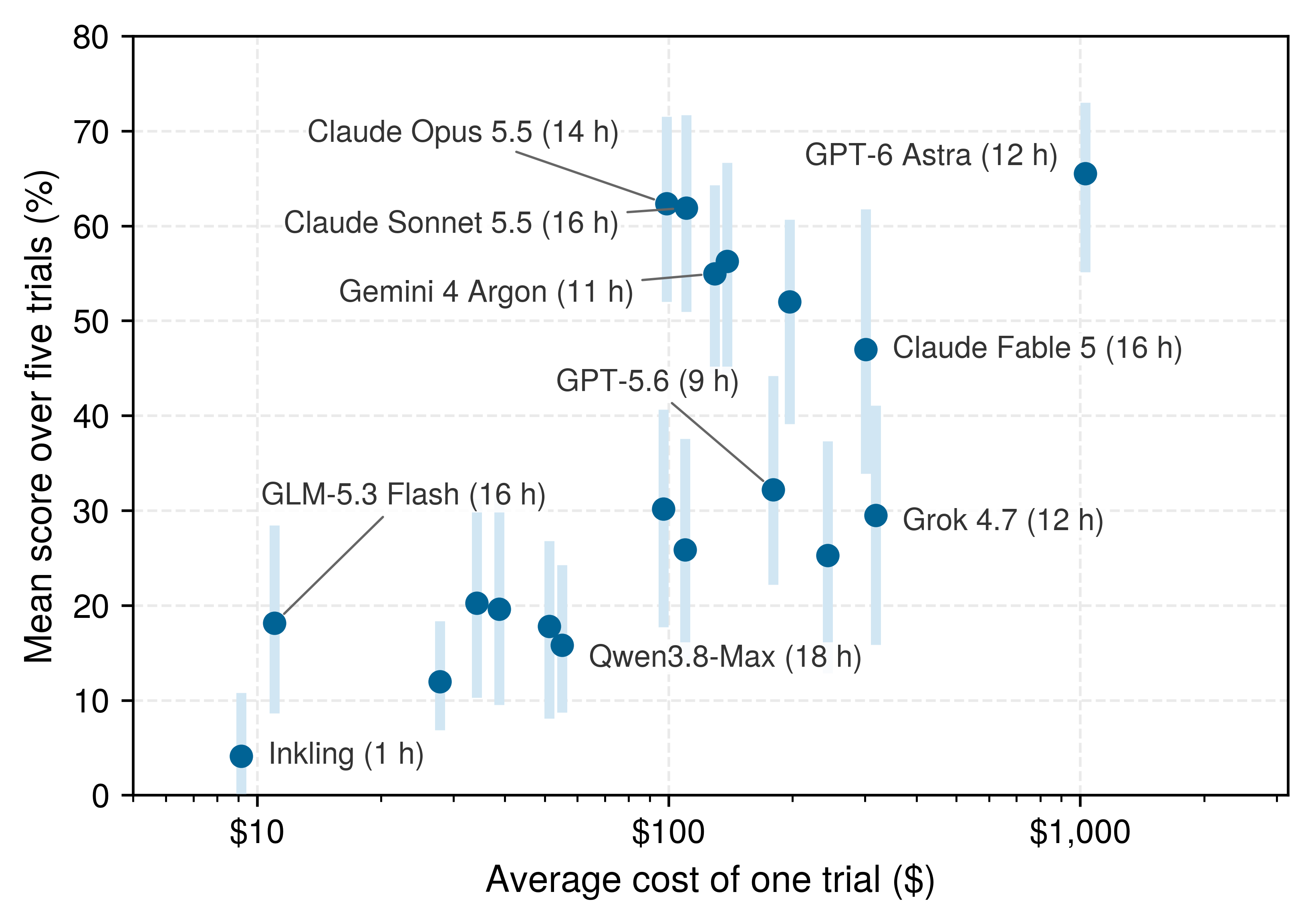
The price spread a router can exploit is wide, and it does not track capability closely. A long-horizon software benchmark runs each configuration five times on every task under a 20-hour budget per trial and reports the mean score, the best and worst of the five, and the average cost and duration of a trial (FrontierSWE 2026). Figure 3 plots those results against cost.
Figure 3: Cost per Trial Barely Tracks Score: Mean score over five trials against the average cost of one trial, on a logarithmic cost axis, for 19 configurations on long-horizon software tasks. Bars run from the worst to the best of the five trials, and parentheses give average hours per trial. Points at similar cost differ by tens of points, and the highest score sits an order of magnitude to the right of nearly equal ones. Data from FrontierSWE (2026) via Epoch AI (2026).
FrontierSWE. 2026. FrontierSWE: Benchmarking Software Engineering Skill at the Edge of Human Ability.
Epoch AI. 2026. Capabilities and Benchmarking.
Cost per trial spans $9 to $1,030 across the 19 configurations, and a single trial runs from 1 to 19 hours. The highest-scoring configuration costs 10× as much per trial as the runner-up for 3 points, while the median gap between a configuration’s best and worst trial is 21 points. Price is therefore a poor proxy for score, and the variation between repeated trials is larger than the difference between the top configurations. That is the opening a router or cascade exploits, and it is also why each tier’s acceptance must be measured on the tasks that actually reach it rather than read from its price.
19.5.1 Direct routing and conditional escalation
Choosing a model tier before generation risks assigning a complex task to an underpowered model or a routine query to an expensive frontier model, whereas trying a cheap tier first always pays for the failed attempt whenever the task has to escalate. A direct router makes the upfront choice by inspecting incoming task features prior to generation; a cascade instead speculatively executes an initial attempt on an inexpensive tier, assesses the candidate against an acceptance contract, and escalates only when that attempt fails.
For a three-tier cascade, let \(\StageConditionalAcceptanceProbability_j\) denote the conditional probability of acceptance at tier \(\CascadeTierIndex\), given that the request reached tier \(\CascadeTierIndex\). Assume every task not accepted at a lower tier continues to the next tier, with no additional retry, cancellation, or stopping branch. The reach probabilities, the probability that a task arrives at each tier, are \(\StageReachProbability_1=1\), \(\StageReachProbability_2=1-\StageConditionalAcceptanceProbability_1\), and \(\StageReachProbability_3=(1-\StageConditionalAcceptanceProbability_1)(1-\StageConditionalAcceptanceProbability_2)\). This product reflects the probability chain rule rather than an assumption that tiers fail independently. Because later tiers receive only the tasks earlier tiers failed, a difficulty-filtered remainder, their conditional acceptance rates cannot be copied from full-workload benchmarks.
Let \(\CascadeTierCost_j\) be the mean generation and associated execution cost conditional on reaching tier \(\CascadeTierIndex\), excluding its gate, and let \(\CascadeGateCost_j\) be that gate’s mean cost. Let \(\CascadeTierDuration_j\) and \(\CascadeGateDuration_j\) be the corresponding mean durations. Real systems must budget for prompt caching, sandbox preparation, and environment cleanup within these terms rather than pricing output tokens alone. Linearity of expectation gives
The final tier must pay for its verification gate as well. With deterministic stage durations, a task reaching every tier takes \(\sum_j(\CascadeTierDuration_j+\CascadeGateDuration_j)\); with variable durations and queueing, characterizing tail percentiles requires the measured empirical distribution. A policy that stops early or leaves assessments unresolved uses its actual reach probabilities and reports those outcomes separately.
The planning metric of cost per accepted task is \(\mathbb{E}[\CascadeTaskCost]/\AcceptanceProbability\), which amortizes the cost of every reached tier across accepted outcomes rather than crediting only successful paths. Evaluating a direct frontier policy requires measuring its baseline acceptance rate across the full target cohort, since its performance on that general distribution is a fundamentally different quantity from its rate on the filtered escalation subset.
Napkin Math 19.6: Price the accepted result at every exit
Problem: In a workload of 100,000 code-editing tasks, should an engineering team deploy a multi-tier cascade or route all requests directly to a frontier model to minimize cost per accepted result, and what latency penalty does the cascade incur?
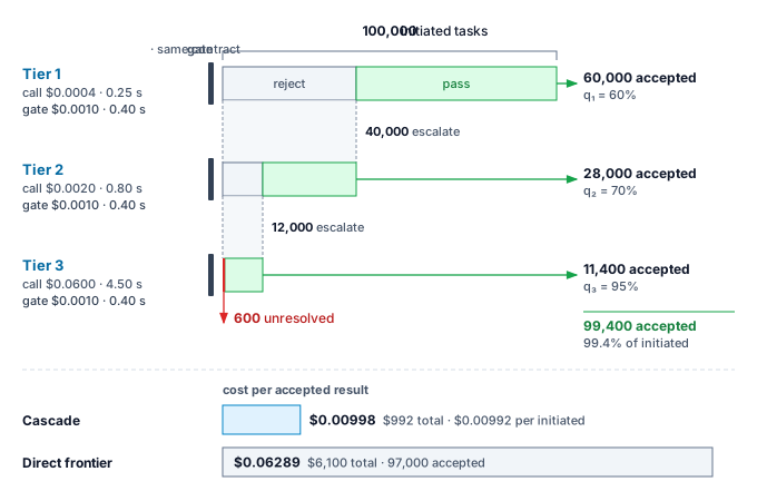
Variables: Each candidate output undergoes an identical verification check. In order of tiers, the cascade’s model invocation and execution costs (excluding gating) are $0.0004, $0.0020, $0.0600 per reached tier, with execution times of 0.25 s, 0.80 s, 4.50 s. Evaluating the verification gate costs $0.0010 and consumes 0.40 s at each reached tier, including the final one. These figures account for container setup, execution, and cleanup overhead; this baseline assumes zero queueing delay and immediate settlement upon completion.
The cascade resolves 60,000 tasks at tier 1. Of the 40,000 tasks advancing to tier 2, it resolves 28,000. Of the 12,000 tasks advancing to tier 3, it resolves 11,400. The resulting conditional acceptance rates are 60 percent, 70 percent, 95 percent, respectively. In comparison, a direct-to-frontier policy resolves 97,000 tasks on an identical cohort. This full-workload rate is an independent baseline parameter rather than an extrapolation from the cascade’s filtered residual. It is lower than the cascade’s total acceptance even though the cascade’s top tier is the frontier model, because the cheaper tiers solve some tasks the frontier model fails (the tiers’ failure sets differ), and every escalated task gets another attempt under the same gate.
Math: The cascade successfully resolves 99,400 tasks (99.4 percent) and leaves 600 unresolved. Across the entire cohort, the cascade expends $992, which is $0.00992 per initiated task and $0.00998 per accepted result. By contrast, direct frontier routing expends $6,100, or $0.06289 per accepted result. Lower-tier cascade attempts must be paid for regardless of whether their candidates pass verification.
Under these deterministic execution times, the cascade averages 1.718 s per task, but tasks that fail all the way through require 6.75 s. Direct frontier routing requires 4.90 s, including verification.
Systems insight: Direct frontier dispatch costs 6.3× as much per accepted result as the cascade because 60 percent of all tasks exit at tier 1, where execution and verification costs represent a negligible fraction of a frontier call. The cascade’s higher acceptance contributes only the ratio of the two accepted counts, 99,400 to 97,000; nearly all of the gap is spend per initiated task. The cascade trades latency for cost. Tasks that escalate through all tiers accumulate only $0.0044 in lower-tier tolls, but they incur 6.75 s of serialized latency compared to 4.90 s under direct dispatch. Because cost savings scale with the early exit rate, the critical architectural lever is hybrid routing: dispatching tasks predicted to fail early stages directly to the frontier tier eliminates the latency penalty for time-sensitive tasks while capturing cascade savings across the remaining workload.
The saving comes from the shape of the filter rather than from any one tier’s price. Reach falls tier by tier because accepted results exit where they are produced, while every reached gate charges its assessment whether or not its candidate passes (figure 4). The same structure explains the latency penalty: a task that escalates through every tier pays every gate’s duration in series.
Figure 4: A Gated Three-Tier Cascade: Every tier’s candidate faces the same acceptance contract, and every gate charges its assessment whether or not the candidate passes, including the final gate. Accepted results exit at the tier that produced them and only the rejected remainder escalates, so reach falls from 100,000 tasks to 12,000. The two bars at the bottom compare cost per accepted result, which charges every rejected attempt to the accepted outcomes, with the separately stipulated direct frontier baseline.
19.5.2 Gate errors and the decision to continue
When a cheap tier-1 lint check accepts a patch that breaks authentication in production, the cascade cost log records a sub-cent exit while the engineering team pays to diagnose and roll back an outage. Cost accounting records gate verdicts even when a gate is mistaken, because an observed accepted result is not automatically a correct result across every operational dimension. To price downstream consequences, define \(\text{FA}\) as the event that an initiated task is accepted by the gate yet violates an independently assessed operational criterion, and define \(\FalseAcceptHarmCost\) as its additional harm or remediation cost not already counted in the execution costs. The expected cost per initiated task including this risk term is
The harm term complements the cost per accepted task rather than redefining it, with its probability evaluated over initiated tasks. If an engineering team measures a false-accept fraction solely among accepted results, they must multiply that fraction by the overall acceptance probability to recover \(\Pr(\text{FA})\); similarly, the false acceptance rate of How base rates limit check precision, evaluated exclusively among invalid candidates, relies on a different conditioning denominator. Catastrophic or irreparable consequences must remain constrained by strict operational authority and safety limits, regardless of their expected monetary value.
When escalating across tiers, the runtime should pass bounded diagnostic evidence and the identity of the failed candidate, treated as untrusted input, rather than forwarding the full conversational transcript. Forwarding full failure transcripts inflates prompt token spend at the expensive tier and risks biasing the stronger model to repeat earlier mistakes. The orchestration layer must also distinguish pending or unavailable assessments from definitive rejections, ensuring that transient infrastructure faults do not trigger unnecessary tier escalation. A passing assessment yields an accepted-candidate record; publication still verifies current dependencies, operational authority, and required effect authorization before applying changes.
A learned router can estimate the probability and cost of each eligible remaining policy from offline evaluation data, for example by training on preference comparisons between stronger and weaker models (Ong et al. 2024). However, training records reflect only the configurations that were actually executed; logs collected under a selective routing policy omit counterfactual outcomes for untried alternatives.5 Whatever the estimates come from, the router applies one decision rule. For a simple monetary objective with acceptance probabilities \(\BaselinePolicyAcceptanceProbability,\CandidatePolicyAcceptanceProbability\), expected additional costs \(\BaselinePolicyCost,\CandidatePolicyCost\), and outcome value \(\AcceptedOutcomePayoff\) (with rejected outcomes valued at zero), policy \(\CandidateRoutingPolicy\) is economically preferable whenever
5Counterfactual Logs: Learning from the logs of a deployed selection policy is an off-policy causal inference challenge, studied extensively in online ad placement where a platform observes outcomes only for selected actions (Bottou et al. 2013). Estimating what an alternative policy would have achieved requires that the logging policy explored with known, nonzero probabilities: if a router never sends an easy-looking task to the frontier tier, the historical logs contain no empirical evidence about what that frontier route would have achieved.
Bottou, Léon, Jonas Peters, Joaquin Quiñonero-Candela, Denis X. Charles, D. Max Chickering, Elon Portugaly, Dipankar Ray, Patrice Simard, and Ed Snelson. 2013. “Counterfactual Reasoning and Learning Systems: The Example of Computational Advertising.”Journal of Machine Learning Research 14: 3207–60.
For direct routing, this decision rule compares two complete end-to-end policies before execution begins. After an initial cheap attempt fails, however, the router compares the remaining escalation policy against stopping or invoking human fallback, treating already incurred spend as a sunk cost. A cheap-then-frontier policy carries its own reach-weighted cost and compound duration, not merely the cheap model’s nominal price. In all cases, the decision rule must operate inside remaining budget, deadline, and operational authority limits; positive expected value never licenses spending past a hard limit or substitutes for explicit authorization.
System load further reshapes this comparison. Waiting for an overloaded model tier consumes wall-clock time and holds open active execution environments, such as containerized sandboxes. When the queue for an inexpensive tier backs up, routing a task directly to an idle frontier model can yield lower total cost and lower wall-clock latency, even at a higher nominal inference price. Production routers must therefore incorporate real-time queue depths and resource contention metrics into their execution-cost and completion-time estimates, linking dispatch decisions directly to underlying queuing and service capacity models.
19.6 Capacity for Trajectories
Admitting one 20-minute repair trajectory per minute holds 20 sandboxes open concurrently while sending 60 model calls per minute to the inference pool. Sizing an agent platform therefore differs from sizing a stateless web service: work enters the platform as a multi-step trajectory, but the operations that saturate hardware consist of individual model calls, tool executions, and resource leases, each with its own arrival rate, holding interval, and concurrency limit. A routing policy shapes the traffic arriving at each downstream model, tool sandbox, and external API, and capacity planning determines whether those services can sustain the offered load within strict latency and resource budgets.
19.6.1 Residence, service, and quota
A trajectory suspended for five minutes on an integration test or human approval consumes zero model-accelerator cycles while continuing to occupy a container lease and retained KV-cache memory. Because each resource is held over a different interval, a single concurrency counter cannot size the platform. In this capacity model, each admitted trajectory executes one distinct task policy, including its internal retries and delegated calls. For a stable population with finite long-run averages, Little’s law (theorem 5.1) relates the mean number of admitted trajectories present, \(\ConcurrentTrajectories\), to their admission rate \(\TrajectoryAdmissionRate\) and mean time from admission to departure, \(\mathbb{E}[\TrajectoryDuration]\):
↩︎ Little’s law, and the residency tax that a tool wait imposes on KV-cache occupancy, are established in Residence time and service rate.
Applying Little’s law requires rigorous accounting of system boundaries. Trajectories rejected at admission never enter the system population, whereas admitted trajectories that eventually fail or abort contribute fully to concurrency while active. Little’s law must be applied separately at each resource boundary (sandbox leases, retained key-value cache memory, active model inference workers, and pending external API calls), with the arrival rate and holding interval that govern that boundary.
↪ Little’s law applied per resource boundary to trajectories with tool waits, contrasting live trajectories with the attention-state memory they retain, is developed in Queueing for Trajectories.
Because Little’s law governs only long-run expectations, engineering a platform for high percentiles requires analyzing the underlying occupancy distributions. Peak concurrency and latency tail buffers depend heavily on state-retention policies and burst dynamics. Under stable flow, the overall demand for model calls depends on the average number of invocations per admitted trajectory, including internal retries, reflection loops, and delegated sub-agent calls: \(\ArrivalRate=\TrajectoryAdmissionRate\mathbb{E}[\TrajectoryCallCount]\). In practice, these model invocations rarely arrive as smooth Poisson streams. When an agent cohort encounters a shared external bottleneck or completes a parallel tool phase simultaneously, downstream inference clusters experience severe arrival bursts.
Task acceptance couples operational demand directly to the economic balance sheet. Delivering accepted tasks at goodput \(\TrajectoryGoodput\) when only an acceptance fraction \(\AcceptanceFraction\) of admitted tasks succeeds requires the platform to admit
for a pool of \(\WorkerCount\) model workers, each completing \(\ServiceRate\) calls per unit time; \(\ServingUtilization\) is then the fraction of the pool’s call capacity the admitted trajectories demand. The trajectory goodput \(\TrajectoryGoodput\) is the primary deliverable of the platform; failed or rejected tasks consume scarce cluster capacity without producing realized value.
Definition 19.3: Trajectory goodput
Trajectory goodput is the number of distinct tasks accepted under a declared contract per unit of elapsed observation time.
Significance: It represents the core throughput metric for sizing an agent platform. At acceptance fraction \(\AcceptanceFraction\), every unit of goodput requires admitting \(1/\AcceptanceFraction\) trajectories, so acceptance governs both the spending multiplier in effective cost \(\CostPerAcceptedTask\) and the offered server load \(\ServingUtilization(\AcceptanceFraction)\).
Distinction: Token, call, and raw trajectory throughput measure computational work performed; trajectory goodput isolates accepted outcomes. Similarly, goodput per dollar divides the accepted count by total cost rather than elapsed observation time.
Common pitfall: Counting redundant retries on a single task, or runs that complete outside the declared contract, as incremental goodput.
Sizing a concrete fleet from its trajectory admission rate means checking each resource boundary on its own unit of demand rather than looking for a single bottleneck counter. An admitted stream that fits comfortably inside its sandbox pool can still saturate its model workers or exhaust a provider’s token-per-minute allowance, as the steady-state fleet calculation below shows.
Napkin Math 19.7: One arrival rate, different resource demands
Problem: A hypothetical fleet has a trajectory admission rate of 1 per minute; an admitted trajectory remains present for 20 minutes on average. It makes 60 calls on average, each consuming 30,000 quota-accounted tokens on average across calls. In this scenario the provider counts input and output tokens, including cached input, toward a shared token-rate allowance of 2,000,000 tokens per minute. What mean concurrency and token demand does this imply?
Math: Apply equation 4 to admitted trajectories, and multiply the long-run call rate by mean tokens per call. The token average is call-weighted, not the unweighted mean of per-task averages.
Result: Mean trajectory concurrency is 20, while the mean call arrival rate is 60 calls per minute. The mean token demand is 1,800,000 per trajectory, giving a token rate of 1,800,000 tokens per minute and using 90 percent of the allowance. The quota alone permits a trajectory admission rate of at most 1.11 per minute at this workload mix in the long run.
Systems insight: The token quota sets the admission ceiling calculated here; concurrency, memory, sandbox, reviewer, and model-service limits still require their own checks. Holding goodput fixed, admissions scale as \(1/\AcceptanceFraction\), so a relative drop in acceptance of 10 percent pushes mean demand to the full allowance, leaving no headroom for bursts. A model or prompt change that lowers acceptance is therefore also a capacity change. Analyzing burst fit, deadline feasibility, and sandbox residency requires validating the quota’s actual window semantics against production traces on top of these steady-state means.
Upstream provider quotas count requests, tokens, or concurrent connections across sliding windows of varying duration, and admission control must match the specific contract. A billing discount on cached input does not relax a token-rate limit, which still counts those tokens at full weight, so prefix caching lowers the bill without raising this admission ceiling. Within the platform, reserving capacity for active trajectories can prevent wasted partial work. Such admission and scheduling decisions must depend on forward-looking attributes: remaining resource requirements, deadlines, tenant fairness, and expected task value. Money already spent is a sunk cost and provides no justification on its own for prioritizing a trajectory.
↩︎ The gates that admit each model call against its provider’s quota windows are established in Quota and capacity gates.
19.6.2 The price of queueing
In a shared platform, an agent’s model calls compete in a serving pool alongside every other active trajectory. If the serving cluster runs at 70 percent utilization, pushing utilization to 90 percent lowers the amortized hardware cost per call. The resulting throughput gains appear immediately on the infrastructure bill. The accompanying queue delays do not, because waiting time accumulates silently across every serial step of an active trajectory while sandboxes, execution environments, and attention state remain held.
The simplest model that quantifies this trade-off is a nonpreemptive, first-come-first-served queue fed by a stationary renewal stream. Interarrival times are independent and identically distributed with mean \(1/\ArrivalRate\), and service times \(\RequestServiceTime\) are independent and identically distributed with finite variance. The sequences are mutually independent, with no batching, priority preemption, abandonment, or feedback. Let \(\InterarrivalVariationCoefficient^2\) and \(\ServiceTimeVariationCoefficient^2\) denote the squared coefficients of variation6 (variance divided by squared mean) of interarrival and service times, and let \(\ServingUtilization=\ArrivalRate\mathbb{E}[\RequestServiceTime]<1\) denote server utilization. For this single-server system, the Kingman approximation7(Kingman 1961) estimates the mean waiting time before service begins:
6Squared Coefficient of Variation: The scale-free measure of burstiness, defined as \(\IntervalVariationCoefficient^2 = \IntervalStandardDeviation^2 / \IntervalMean^2\). Exponential interarrival or service times, characteristic of a Poisson stream, have a squared coefficient of variation of exactly one, whereas perfectly periodic events yield zero. Values exceeding one describe arrivals and service durations burstier than Poisson, which is the standard profile for agent traffic arriving in cohorts with divergent prompt lengths.
7Heavy Traffic: Kingman’s 1961 note showed that as load approaches saturation (\(\ServingUtilization \to 1\)), the steady-state waiting-time distribution of the single-server queue, appropriately normalized, converges to an exponential distribution (Kingman 1961). This property extends beyond the mean: near saturation, the entire waiting-time distribution, and with it every tail percentile, stretches by the factor \(\ServingUtilization/(1-\ServingUtilization)\), so percentile-based latency targets degrade just as rapidly as the mean.
Kingman, John Frank Charles. 1961. “The Single Server Queue in Heavy Traffic.”Mathematical Proceedings of the Cambridge Philosophical Society 57 (4): 902–4. https://doi.org/10.1017/S0305004100036094.
Near saturation, a little more utilization buys a lot more waiting.
Boon, Marko A. A., Augustus J. E. M. Janssen, and Johan S. H. van Leeuwaarden. 2023. “Heavy-Traffic Single-Server Queues and the Transform Method.”Indagationes Mathematicae 34 (5): 1014–37. https://doi.org/10.1016/j.indag.2023.02.004.
The factor \(\ServingUtilization/(1-\ServingUtilization)\) explains why queueing delays escalate steeply near full utilization. Equation 5 is a heavy-traffic approximation to the mean rather than an exact expectation or a percentile; Heavy-tailed queueing theory derives the corresponding Pollaczek–Khinchine waiting-time formula under general service distributions, and Boon et al. (2023) provides formal derivations and error bounds. Capturing correlated agent bursts, dynamic continuous batching, worker pools, and shared quotas requires queueing networks or trace-driven discrete-event simulations. Crucially, substituting an aggregate cluster service rate into a single-server formula does not turn it into a valid multi-server model. Two workable estimates remain for a pool. When a dispatcher pins each trajectory to one endpoint, every endpoint is its own single-server queue fed by its share of the arrivals, and equation 5 applies per endpoint. When workers share one queue, a trace-driven simulation of the pool, or the multi-server models in the further reading, replaces the single-server estimate.
Napkin Math 19.8: Pricing mean queue delay
Problem: In the hypothetical single-server model above, mean service takes 1 second, arrival variability \(\InterarrivalVariationCoefficient^2\) is 2, and service variability \(\ServiceTimeVariationCoefficient^2\) is 4. A waiting call holds resources costing $0.002 per second. How do estimated mean wait and holding cost change between 70 percent and 90 percent utilization?
Math: Apply equation 5, then multiply mean wait by the stated linear holding rate. The rate covers only resources retained during the queue interval, excluding model service, tool execution, and any separate valuation of user delay.
Result: Estimated mean wait rises from 7 seconds to 27 seconds, and the corresponding holding charge rises from $0.014 to $0.054 per call.
Systems insight: Moving from 70 percent to 90 percent utilization buys 28.6 percent more throughput from the same server, but it multiplies mean wait by 3.9× because the \(\ServingUtilization/(1-\ServingUtilization)\) factor dominates near saturation. While the holding charge for an isolated call appears small, this delay compounds across every serial step of an agent trajectory. Halving the variability term \((\InterarrivalVariationCoefficient^2+\ServiceTimeVariationCoefficient^2)/2\), for example by smoothing bursty admissions or standardizing prompt lengths, halves the wait at any utilization and provides a cost-effective lever before purchasing reserve capacity. Sizing that reserve ultimately depends on enforcing tail latency targets at measured percentiles.
A one-in-a-hundred delay per call becomes routine across a long trajectory.
Mean metrics also obscure how tail latency compounds across multi-step execution. If each of \(\SerialCallCount\) serial calls independently exceeds its 99th-percentile latency with probability \(\CallTailProbability\), the trajectory encounters at least one such delay with probability \(1-(1-\CallTailProbability)^\SerialCallCount\), which is the horizon compounding of equation 1.1 applied to latency rather than to correctness. For a trajectory of 30 serial calls, each with tail probability 0.01, the probability of experiencing at least one tail delay reaches 0.26. This is the probability of encountering a per-call tail event, not the probability of missing a trajectory deadline; the latter requires the complete duration distribution and the declared deadline. Sizing a fleet solely for acceptable per-call latency can therefore conceal end-to-end delays. This dynamic is the serial equivalent of the fan-out straggler problem in distributed systems (Dean and Barroso 2013). Correlated delays, such as a shared queue that remains backlogged across successive steps, alter the exact probability but not the operational conclusion, which is to provision and schedule against trajectory-level percentiles rather than per-call means (principle 15).
Integrating queueing delays completes the model-routing framework of section 19.5. A dynamic router compares eligible remaining paths, each priced with its queue and service delays, retained-resource costs, verification checks, and possible escalations, under an identical acceptance contract. Because dispatching decisions alter the arrival rates that produced the initial delay estimates, the router must refresh queue projections whenever traffic shifts. Separating interactive and batch pools, or enforcing priority scheduling, protects latency-bound work at a quantifiable cost in fairness and cluster utilization.
19.6.3 Dedicated capacity vs. per-token APIs
When an agent application’s token consumption becomes sustained and predictable, engineering teams must choose between paying on demand through per-token APIs and provisioning private infrastructure. Consider a dedicated deployment incurring a fixed infrastructure expense of $28 per hour plus $2 per million output tokens in marginal operating costs. Such private infrastructure represents dedicated capacity, a financial commitment paid continuously regardless of whether accelerators are busy or idle. The economic decision therefore turns entirely on sustained utilization.8 This comparison requires a strictly matched workload: equivalent task capability, acceptance criteria, data-privacy constraints, and feasible tail latency under representative traffic mixtures. A shared model architecture or nominal token rate alone does not establish equivalence.
8Pay-as-You-Go Economics: Mirroring the foundational economic argument for cloud computing, renting capacity on demand can cost less than owning dedicated infrastructure even at a higher hourly rate, because owned capacity must be financed across its average utilization while utility pricing shifts provisioning risk to the provider (Armbrust et al. 2010). A per-token API carries that logic to its finest granularity.
Armbrust, Michael, Armando Fox, Rean Griffith, Anthony D. Joseph, Randy Katz, Andy Konwinski, Gunho Lee, et al. 2010. “A View of Cloud Computing.”Communications of the ACM 53 (4): 50–58. https://doi.org/10.1145/1721654.1721672.
Fix the workload’s input/output token ratio and prompt-cache hit rate. Let \(\EffectiveApiOutputTokenPrice\) denote the effective API charge per output token including its associated input tokens, \(\DedicatedVariableTokenCost\) the variable cost per output token on dedicated capacity, and \(\DedicatedHourlyFixedCost\) the complete hourly fixed cost of the private deployment, including amortized hardware leases, provisioned failover headroom, and operational maintenance. Shared application costs cancel only when genuinely identical across both options; differential tool, verification, network egress, or support fees must enter the balance sheet. Let \(\FeasibleOutputTokenRate\) denote the measured feasible output token generation rate (in tokens per second) under the target latency objective, a token rate distinct from the per-worker call rate \(\ServiceRate\) of the capacity model. Let \(\DeliveredCapacityFraction\) represent the fraction of that reference capacity the workload actually delivers. Unlike the queueing utilization \(\ServingUtilization\), which measures offered load against raw service capacity, \(\DeliveredCapacityFraction\) is measured against a rate already chosen to meet the latency target, so \(\DeliveredCapacityFraction=1\) still meets that target by construction. In one hour, the system produces \(3600\FeasibleOutputTokenRate \DeliveredCapacityFraction\) output tokens, costing \(3600\FeasibleOutputTokenRate \DeliveredCapacityFraction\,\EffectiveApiOutputTokenPrice\) via a pay-as-you-go API and \(\DedicatedHourlyFixedCost+3600\FeasibleOutputTokenRate \DeliveredCapacityFraction\,\DedicatedVariableTokenCost\) on dedicated hardware. When \(\EffectiveApiOutputTokenPrice>\DedicatedVariableTokenCost\), the two expenditure curves cross at the break-even utilization
Owned capacity wins only above the load that repays its fixed cost.
If \(\BreakEvenUtilization>1\), the dedicated deployment cannot break even within its physical capacity envelope; if \(\EffectiveApiOutputTokenPrice\le \DedicatedVariableTokenCost\) while \(\DedicatedHourlyFixedCost>0\), self-hosting remains permanently more expensive. Execution deadlines and concurrency limits must be verified separately at the target operating point.
Napkin Math 19.9: Pricing idle capacity and cached input
Problem: Assume a hypothetical matched-capability workload uses 5 input tokens per output token, with 80 percent of inputs billed at the cached rate. API prices per million tokens are $3 for uncached input, $0.3 for cached input, and $15 for output. A dedicated deployment costs $28 per hour for its provisioned capacity and operations, plus $2 per million output tokens for differential variable costs. Its feasible reference output rate is 1,200 tokens/s under the same mix, reserve policy, and latency target. Which alternative costs less at 52 percent of that rate?
Math: Weight the two input prices by their billed volume fractions, then incorporate associated input costs into \(\EffectiveApiOutputTokenPrice\). Apply equation 6. Both options are feasible at this operating point, and shared tool, evaluation, and application costs cancel.
Result: Weighted input costs $0.84 per million input tokens. Factoring in associated inputs, the API costs $19.2 per million output tokens. The cost crossing occurs at 37.7 percent of reference capacity. At the stated load, generating 2,246,400 output tokens per hour costs $43.13 through the API vs. $32.49 on dedicated capacity, saving $10.64 per hour.
Systems insight: The economic break-even threshold shifts directly with the API’s effective token price. Without cached input, the same workload would cross at 23.1 percent of reference capacity instead of 37.7 percent. Aggressive prefix caching by API providers erodes the economic incentive to own capacity. Teams should commit to dedicated capacity only when sustained production load reliably exceeds \(\BreakEvenUtilization\) with the headroom demanded by latency targets. Operating below the crossing wastes capital on idle silicon, while owning hardware places queueing congestion, node failures, and capacity management entirely on internal engineering teams.
Checkpoint 19.2: Check the capacity boundary
Before bounding what an individual trajectory may spend, evaluate the platform capacity model:
Capacity planning sizes the collective infrastructure required to sustain admitted workload streams. It says nothing about how much any one trajectory, or the tree of children it delegates to, may spend. That bound needs a different mechanism, a budget account that admits and settles every charge atomically.
19.7 Spending Governance
When a coordinator admits concurrent sub-agents or child tasks, simple balance checks collapse under race conditions. If two children inspect the remaining free balance simultaneously before either records a reservation, both admission checks succeed, yet their combined liability immediately breaches the authorized task budget. Task cancellation introduces a second concurrency bug: returning a stopped child’s allocation to the free pool while its remote service call remains billable allows another worker to spend funds that are already committed to third-party infrastructure. The harness already solved this for one trajectory. Its bounded-liability admission reserves an operation’s maximum charge before dispatch and releases it only at settlement (Reservation and settlement). Trajectory-level encapsulation (principle 10) requires the same invariant to hold when the allowance is split across children, and to stay conserved across concurrent dispatch, node crashes, and late settlement.
19.7.1 Liability bounds and admission
If an admission gate reserves only the average token cost of a model call, a single request that hits its maximum completion cap or misses the prompt cache will settle above its reservation and breach the task’s spending ceiling. To prevent overruns, let \(\BudgetSettledCharges(\BudgetEvaluationTime)\) denote gross charges settled into a task’s budget account at time \(\BudgetEvaluationTime\) and \(\BudgetReservedFunds(\BudgetEvaluationTime)\) the funds withheld there for outstanding liabilities, delegated allocations, and protected finalization. A task with authorized budget \(\CostCeiling\) maintains the fundamental invariant
The harness’s bounded-liability test (equation 10.1) enforces this invariant at admission. Before dispatch, the runtime reserves a strict upper bound \(\OperationChargeBound\) on the operation’s maximum charge across every billing category (for a model call, including the maximum completion and hidden reasoning tokens) rather than an expected cost, funds teardown in advance, and under a hard-ceiling policy rejects or replaces any operation that lacks an enforceable bound.
Budget enforcement also depends on complete mediation, applied here to money: every billable interaction must pass through the accounting gateway. If worker nodes hold shared credentials that bypass the reservation gate, or if unmonitored retry loops dispatch billable requests off the books, the budget account’s guarantees no longer hold. Prompt caching and tiered volume discounts present a related operational subtlety: while cache hits reduce final settlement charges, they can reduce the upfront reservation \(\OperationChargeBound\) only if the provider contractually guarantees the discount prior to request dispatch. If a cache miss remains possible, the runtime must withhold the full un-discounted rate.
↩︎ Complete mediation, the requirement that every access pass through one checking point, is established for tool calls in Complete mediation.
The budget account tracks gross liabilities rather than net cash flows. Releasing an unspent reservation restores permission to spend money that was never actually charged. Subsequent provider credits, reconciliations, or post-hoc refunds are recorded as separate external adjustments that leave gross spending and historical authorizations intact. Crucially, fresh spending capacity enters the system only through an operator’s explicit budget grant, never through automatic replenishment from error recoveries or the speculative promise of a newly spawned candidate branch.
19.7.2 Budget conservation across descendants
If a fleet dashboard sums reserved balances across a parent and its children, it double-counts every delegated dollar; if it inspects only the parent’s settled charges, it misses active spending still accumulating in open child accounts. To keep balances conserved across a delegation tree, each node \(\BudgetNodeIndex\) maintains a runtime-owned budget account with the same structure, tracking its allocation \({\CostCeiling}_k\), settled gross charges \(\BudgetSettledCharges_k\), reservations \(\BudgetReservedFunds_k\), and free balance \(\BudgetFreeBalance_k\):
A budget reservation, the harness’s bounded-liability reservation applied at node \(\BudgetNodeIndex\), removes funds from the free balance \(\BudgetFreeBalance_k\) before an operation can be dispatched. Multi-agent coordination partitions consumable budgets into nested sub-budgets; what this section adds is the settlement side, how a delegated allocation is counted, when it may be released, and what happens when a bill arrives late or exceeds its bound. In a hierarchical agent tree, delegating an allocation \(\DelegatedAllocationAmount\) to a child node withholds those funds in the parent’s reservation pool \(\ParentReservedFunds\) while the child manages them within its own budget account (\(\ChildBudgetAllocation = \ChildFreeBalance = \DelegatedAllocationAmount\)). The parent’s reservation and the child’s entire account thus represent the same backing funds seen from two levels of the tree. Fleet-wide reporting attributes each charge exactly once through its unique operation record, while the tree hierarchy tracks which branch holds the authority to back it.
The state transitions summarized in table 4 are strictly atomic with respect to competing admissions and control-plane changes. Because spending represents an irreversible external commitment, budget updates must durably survive the failure domain specified in Durable Intent Before Dispatch before any billable request leaves the runtime. If a worker node crashes, a replacement coordinator reconstructs active reservations directly from this write-ahead log rather than resetting balances because the former worker disappeared. As in multi-agent delegation, budget differs from permission because it is consumed. A child’s read grant leaves the parent’s read access intact, whereas a delegated allocation withholds funds the parent could otherwise spend, which is why the budget account must track it as a reservation.
↩︎ Shared permissions, partitioned consumable budgets, and nested sub-budgets under delegation are established in Attenuated grants and split allowances.
Table 4: Conserved budget transitions: Each update preserves the allocated total. Closure requires financial settlement, not merely a stopped local process.
Budget event
Required condition
Conserved update
Allocate \(\DelegatedAllocationAmount\) to a child
Current authority and eligibility; \(\DelegatedAllocationAmount\le \ParentFreeBalance\)
Parent moves \(\DelegatedAllocationAmount\) from \(\ParentFreeBalance\) to \(\ParentReservedFunds\); child starts with \(\ChildBudgetAllocation=\ChildFreeBalance=\DelegatedAllocationAmount\)
Admit an operation bounded by \(\OperationChargeBound\)
Current guards pass; \(\OperationChargeBound\le \BudgetFreeBalance_k\)
Move \(\OperationChargeBound\) from \(\BudgetFreeBalance_k\) to \(\BudgetReservedFunds_k\) and record the operation and attempt binding
Final settlement with charge \(\SettledOperationCharge\)
Authenticated final evidence; \(0\le \SettledOperationCharge\le \OperationChargeBound\); reservation still owned
Remove \(\OperationChargeBound\) from \(\BudgetReservedFunds_k\), add \(\SettledOperationCharge\) to \(\BudgetSettledCharges_k\), and return \(\OperationChargeBound-\SettledOperationCharge\) to \(\BudgetFreeBalance_k\)
Stop a child with unsettled work
New admission is closed; outstanding records remain owned
Keep backing for its calls and descendants; stopping alone releases no liability
Close a fully settled child
No further admission; calls and descendants settled; \(\ChildReservedFunds=0\)
Parent removes \(\ChildBudgetAllocation\) from \(\ParentReservedFunds\), adds \(\ChildSettledCharges\) to \(\ParentSettledCharges\), and adds \(\ChildFreeBalance\) to \(\ParentFreeBalance\)
Every budget reservation is tied to a unique compound identifier binding the task, logical operation, transport attempt number, pricing tier, and cost bound \(\OperationChargeBound\). When downstream work finishes, settlement requires authenticated usage receipts evaluated against a durable settlement identity, the idempotency key under which the final charge is recorded in the budget account. It is settlement before retry (principle 8) applied to money. The operation and attempt identifiers that let a tool call be retried without duplicating its effect also let a bill be redelivered without duplicating its charge. If network retries cause the provider to deliver identical billing evidence multiple times, the runtime applies the state transition at most once, verifying that repeated deliveries contain identical payloads. A conflicting payload under an existing settlement identity indicates a reconciliation fault, which the runtime must neither blindly overwrite nor silently ignore. When long-running services report intermediate consumption, the runtime can incrementally move settled amounts into \(\BudgetSettledCharges_k\) while continuing to withhold a bound on remaining liabilities; it releases the reservation entirely only upon definitive finality. Deduplicating a remote side effect at an API endpoint and deduplicating an internal budget record serve two distinct contracts.
↩︎ Operation and attempt identifiers, which let a retried tool call be recognized as the same logical operation, are established in Operation identity and endpoint contracts.
If an external service reports a charge that exceeds its initial reservation (\(\SettledOperationCharge > \OperationChargeBound\)), the system’s foundational cost invariant has failed. Silently clamping the reported charge to \(\OperationChargeBound\) or allowing the free balance \(\BudgetFreeBalance_k\) to drop below zero would conceal a critical safety failure. Instead, the runtime immediately flags the discrepancy, halts further admissions within the affected subtree, and escalates the incident for reconciliation. Until an administrator or reconciliation procedure resolves the dispute, the system’s strict financial guarantee is temporarily suspended. Provided cost bounds remain valid, admissions execute atomically, and settlements are strictly deduplicated, every state transition preserves non-negative balances (\(\BudgetSettledCharges_k, \BudgetReservedFunds_k, \BudgetFreeBalance_k \ge 0\)) and guarantees that no child sub-agent can spend outside its allocated backing.
Cancellation is where conservation is most easily broken. The cancellation context tree of Cancellation context trees stops a child from admitting new billable work the moment control is revoked, but remote requests, inference batches, and cloud jobs the child already dispatched may keep running and billing until their own timeouts fire. The conservation rule therefore treats a stopped child as still open, and its whole allocation stays in the parent’s reservation until every outstanding operation reaches authenticated final settlement (the stop row of table 4). A runtime that does not want to keep an inactive child’s account in memory may hand it to a settlement coordinator, provided the handover carries every known charge, outstanding reservation, and unencumbered balance with its operation lineage, so that at no point can funds be released twice or a liability be left unbacked. The finalization reserve of the harness’s admission test, applied at each node, funds the status queries and sandbox teardown that settlement requires after ordinary admission has closed, without reopening general spending authority. Accounting reports that cross a cutoff boundary distinguish settled historical charges from active liabilities held in reserve. The notebook below traces this distinction for a canceled child that receives a late bill from an external provider.
Napkin Math 19.10: A canceled child with a late bill
Problem: A hypothetical repair has a $5 budget. Its planning charge has settled at $0.042, and it allocates $1.20 to trace analysis and $2.50 to fuzzing. The trace child closes with a final charge of $0.38. The fuzzing child has settled $0.85 and holds $1 for a remote operation when its local executor confirms termination. No further child work is admitted. The remote operation later terminates with a final additional bill of $0.70. All other charges and required finalization are included in these records, and neither child has descendants. When can the root release the fuzzing allocation?
Math: The entire child allocation remains reserved at the root until its account closes. Table 5 follows the root’s balances under the same conservation rule throughout.
Table 5: Root Balances Through a Late Bill: Local stopping retains the pending child’s allocation until its charges settle and its account closes.
Root account boundary
Settled \(\BudgetSettledCharges\)
Reserved \(\BudgetReservedFunds\)
Free \(\BudgetFreeBalance\)
Planning settled
$0.042
$0
$4.958
Both allocations granted
$0.042
$3.70
$1.258
Trace child closed
$0.422
$2.50
$2.078
Fuzzing locally stopped; bill pending
$0.422
$2.50
$2.078
Late bill settled; fuzzing child closed
$1.972
$0
$3.028
At local termination, the fuzzing child’s account has $0.65 free, but its remote reservation remains outstanding. Final settlement releases the unused part of that reservation, leaving $0.95 to return when the child closes. Re-delivery of the same final billing record changes none of these balances.
Systems insight: A premature release upon local process termination would have returned $1.65 (the allocation minus already-settled charges), even though only $0.65 was truly unencumbered. The subsequent $0.70 bill would then have landed on funds already committed to another child task. The governing invariant upon cancellation is strict: release at most the allocation minus settled charges minus the enforceable upper bound on outstanding work, and return the remainder only as each remote operation reaches final settlement. Financial safety is only as reliable as those upper bounds and the completeness of the budget records.
The conservation rule shows up visually as bars of equal length (figure 5). At every boundary of table 5, funds move among settled, reserved, and free balances without leaving the root’s budget, and the root’s reservation stays fixed from the fuzzing child’s local stop until its late bill settles.
Figure 5: Conservation Across a Canceled Child: The root’s balances at each boundary of table 5, drawn as bars of equal length that always sum to the same budget, with the initial reservation split between the trace and fuzzing children. Expanded beneath the stopped row, the fuzzing child’s own account at local stop holds settled charges, a pending remote reservation, and free balance, while the root still sees the whole allocation as reserved. Local stopping leaves the root’s reservation unchanged; only settlement of the late bill moves the fuzzing allocation into settled and free balances.
19.7.3 Spending alarms and admission limits
Even when a cumulative task budget is strictly conserved, an overall ceiling cannot prevent damaging expenditure spikes. If an unconstrained agent launches dozens of model calls concurrently, it can burn through its entire allocation in seconds. A retrospective spending alarm monitors the burn rate by dividing the gross charges settled over a trailing window of duration \(\SpendingWindowDuration\) by \(\SpendingWindowDuration\). However, because external billing is often delayed, a retrospective alarm can stay quiet while expensive requests are in flight and spike only after execution has already halted. While retrospective alarms are useful for triggering administrative alerts or throttling subsequent work, they act after the fact, on money that has already been spent.
To prevent rapid budget exhaustion, the runtime must enforce proactive admission limits that evaluate new financial commitments, in the form of reservations, before dispatch. For a spending rate limit permitting at most \(\WindowSpendingLimit\) in new liabilities over any trailing window of duration \(\SpendingWindowDuration\), a robust admission policy enforces
where \(\TimeInstant_i\) is the admission timestamp and \(\OperationChargeBound_i\) is the bounded charge of each billable operation.9 Every prospective admission atomically validates both this sliding-window limit and the cumulative budget balance. This window constraint applies across all child tasks within the coordinator’s scope, rather than granting a fresh window allowance to every newly spawned worker. Delegating an allocation down the agent tree is an internal balance partition, not a newly admitted billable dispatch. Furthermore, retaining \(\OperationChargeBound_i\) in the window calculation until its admission timestamp ages out prevents a rapid sequence of fast-completing calls from triggering an unbounded burst. This policy guarantees a strict upper bound on committed work over the interval, regardless of when external providers finish processing requests or transmit final invoices.
9Trailing Window vs. Token Bucket: Standard network and API rate limiters often employ token buckets, which permit an initial burst equal to the bucket capacity followed by a steady refill rate; over a short interval \(\FiniteChange \TimeInstant\), maximum consumption can reach capacity plus rate times \(\FiniteChange \TimeInstant\). In contrast, the trailing-window sum strictly caps committed liabilities across every continuous window of duration \(\SpendingWindowDuration\) at \(\WindowSpendingLimit\), irrespective of burst shape, at the modest implementation cost of retaining timestamped admission records until they age out of the window.
Rate-limiting policies must also protect capacity and budget for mandatory finalization routines. If an aggressive rate limiter blocks all outgoing traffic during a spending spike, it can starve the very cancellation and status queries required to terminate running tasks and settle outstanding reservations. Dedicating isolated execution lanes or explicit finalization allowances within the accounting policy prevents this deadlock. Furthermore, completing a diagnostic probe or clearing an operational alarm must never prematurely release funds held for unrelated active reservations.
When an agent enters a non-converging loop, evidenced by repeated execution failures or unvarying candidate artifacts, the runtime triggers a spending hold under its semantic watchdog policies. This intervention blocks new ordinary billable work before runaway iterations exhaust the task budget; already-dispatched work may continue accruing charges within its reserved bounds. The runtime enforces the designated cancellation or escalation workflow while keeping all outstanding liabilities reserved. Evaluating whether completed work meets task requirements remains the responsibility of the domain acceptance contract, rather than the spending controller.
↩︎ Semantic watchdogs, which detect a non-converging loop from its progress evidence and place the trajectory in an admission hold, are established in Semantic Watchdogs.
Budget reservations turn spending governance from after-the-fact telemetry into an enforceable contract under declared pricing and failure models. They decide what a design may spend, not whether it is worth spending on. With cost, latency, and residual liabilities bounded, the remaining choice is which design delivers enough accepted work for its expense: a deterministic workflow, a single foundation model invocation, a bounded loop, or a delegated tree of agents.
19.8 Pricing the Choice of Architecture
A spending bound makes a proposed architecture admissible under its budget, but cost per accepted task determines whether it is worth deploying. When choosing among deterministic code, a fixed model-assisted workflow, a bounded loop, and multi-agent delegation, system architects often frame the decision as an ideological debate between programmatic control and model autonomy. In production systems engineering, however, this decision is fundamentally an empirical optimization problem governed by an acceptance contract. The engineering objective comes first: minimizing expected financial cost subject to a completion requirement selects a fundamentally different architecture than minimizing tail latency or deadline misses under a spending ceiling.
19.8.1 Design alternatives
A fixed workflow that unconditionally calls a frontier model on every ticket can cost more than an adaptive, bounded loop that resolves simple cases on turn one with a lightweight model, and a single model call proposing a database deletion requires the same authorization checks as a ten-turn agent. Architectural alternatives differ primarily in who selects the next operation, as table 6 summarizes, yet control authority alone reveals little about execution cost, end-to-end latency, or permitted environmental side effects. Similarly, executing parallel delegated trajectories can cut wall-clock time while inflating total token consumption.
Table 6: Architecture Choices Under One Task Contract: The control structure changes the work to account for, not the required acceptance evidence or authorized effects.
Design
Who selects the next operation
Incremental obligation to price
Deterministic program
Program control flow
Maintenance, execution, assessment, and exception handling
Fixed model-assisted workflow
Program control flow around model calls
Model usage, output validation, and fallback paths
Bounded model-directed loop
Model proposals admitted by the runtime
Repeated observations, revision, stopping, and effect settlement
Delegated trajectories
Coordinator and children within assignment contracts
Child execution, communication, integration, cancellation, and residual liabilities
Every design can carry state, require crash recovery, and demand substantive verification. A rigorous comparison therefore holds the acceptance contract strictly constant across candidate designs. Verification is neither relaxed for a single model call nor tightened for an agentic loop or a delegated system.
19.8.2 Task obligations
Whether a dependency upgrade runs as a deterministic script or a multi-agent tree, it still has to pass the regression suite, retain workspace state across retries, and hold authorization before merging. The H·S·A exposures that have organized this book, together with the closure evidence the contract demands, do not dictate an architecture; they name the obligations each candidate design must pay for:
Horizon: A longer execution horizon expands the trajectory space, multiplying opportunities for resource consumption, transient network faults, and compounding drift. In cost accounting, these costs are priced not by hypothetical maximum depth, but by the expected distribution of steps that the runtime policy actually reaches.
State: State incurs retrieval overhead, storage retention, consistency maintenance, and checkpoint recovery mechanisms wherever it resides. An adaptive loop justifies this stateful overhead only when fresh observations yield updates that substantially improve downstream decisions, generating enough value to repay their operational cost.
Authority: The scope of authority determines which operations demand formal admission, evidence collection, and two-phase settlement. Irreversible actions, such as modifying financial records, sending customer emails, or deleting cloud infrastructure, require an explicit authorization and risk policy, often incorporating cryptographic audit trails or human approval gates. Any unresolved effect or outstanding external reservation remains an open liability on the account, regardless of the expected inference bill.
Closure evidence: Closure evidence governs what repeated attempts can actually establish. An automated, executable check, such as a compiler, test suite, or schema validator, supplies fast, inexpensive, and highly specific feedback. The economic value of this feedback depends directly on the test harness coverage and its false-acceptance rate. When no automated check exists, an agent must seek closure through additional observations, queries to independent data sources, or escalation to human review. Human review, however, introduces its own substantial hourly costs, queueing delays, and error rates. Crucially, routing an ambiguous task to a person does not count as completing it; the task counts as completed only when the human reviewer finishes the work and fulfills the acceptance contract.
19.8.3 When a bounded loop beats a single call
Consider an automated dependency-upgrade service. The engineering team can deploy a deterministic rule-based rewriter, a single frontier model call, or a smaller, cheaper model that retries for up to three turns within a bounded loop before escalating failed tickets to a human engineer. The deterministic rewriter and the single model call each have a single static acceptance rate, whereas the loop’s overall acceptance rate and aggregate spend depend on the exact distribution of turns it reaches before stopping.
For a bounded loop, let \(\StageConditionalAcceptanceProbability_t\) denote the probability that turn \(\TurnIndex\) produces an accepted candidate, conditional on reaching turn \(\TurnIndex\) after rejections on all preceding turns. Assuming that every reached turn undergoes a complete acceptance assessment, that execution halts immediately upon acceptance, and that the runtime enforces a hard budget of \(\TrajectoryTurnLimit\) turns, the cumulative automated acceptance probability is:
As with model cascading, this formulation applies the probability chain rule rather than assuming independence across turns. The system reaches turn \(\TurnIndex\) with probability \(\StageReachProbability_t=\prod_{j<t}(1-\StageConditionalAcceptanceProbability_j)\), where \(\StageReachProbability_1=1\). If \(\LoopTurnCost_t\) represents the comprehensive cost of turn \(\TurnIndex\) (model inference, tool execution, sandbox lease duration, and the assessment check), the expected automated cost per incoming ticket is \(\sum_{t=1}^{\TrajectoryTurnLimit} \StageReachProbability_t \LoopTurnCost_t\). When turns incur an identical per-turn cost \(\UniformLoopTurnCost\), this expectation simplifies to \(\UniformLoopTurnCost \sum_{t=1}^{\TrajectoryTurnLimit} \StageReachProbability_t\), where \(\sum_{t=1}^{\TrajectoryTurnLimit} \StageReachProbability_t\) is the expected number of executed turns. Operational exceptions, such as test harness outages or runtime abandonment triggered by safety filters, introduce distinct terminal states that must be accounted for as separate branches rather than conflated with normal test failures.
Accounting becomes more complex when human escalation enters the operational policy. Suppose an automated tier achieves acceptance probability \(\AttemptPassProbability\) at expected cost \(\MeanAttemptCost\), and routes every rejected ticket to a human fallback workflow that costs \(\HumanFallbackCost\) and achieves conditional resolution probability \(\HumanResolutionProbability\). The expected total expenditure per incoming ticket is \(\MeanAttemptCost+(1-\AttemptPassProbability)\HumanFallbackCost\), while the combined resolution probability across automated and human tiers is \(\AttemptPassProbability+(1-\AttemptPassProbability)\HumanResolutionProbability\). Dividing expected spend by combined resolution yields the true cost per resolved ticket under the end-to-end policy: \[\frac{\MeanAttemptCost + (1 - \AttemptPassProbability) \HumanFallbackCost}{\AttemptPassProbability + (1 - \AttemptPassProbability) \HumanResolutionProbability}\] In contrast, the isolated metric \(\MeanAttemptCost/\AttemptPassProbability\) captures only the cost per automated acceptance. Conflating these two metrics obscures the true cost structure of the system, particularly when automated acceptance is low. Neither ratio is well-defined when its respective denominator reaches zero. The same account sets a bounded loop’s cap. When the fallback resolves everything it receives (\(\HumanResolutionProbability=1\)), the denominator is fixed at one, so adding turn \(\TurnIndex\) changes only spend. The turn costs \(\StageReachProbability_t\LoopTurnCost_t\) and avoids \(\StageReachProbability_t\StageConditionalAcceptanceProbability_t\HumanFallbackCost\) of fallback spend, so extending the cap from the preceding turn to turn \(\TurnIndex\) lowers expected spend exactly when \(\StageConditionalAcceptanceProbability_t\HumanFallbackCost>\LoopTurnCost_t\). This adjacent-cap comparison assumes immediate, perfectly resolving fallback and unchanged earlier turns; it is not a general stopping rule for policies with further contingent choices. The executable model in notebook 19.11 illustrates why keeping these two metrics separate is essential for sound architectural selection.
Napkin Math 19.11: Pricing three designs for dependency upgrades
Problem: A software engineering team manages an influx of 10,000 dependency-upgrade pull requests each month. Every upgrade requires code modifications that must pass an identical build and regression test suite to be accepted. The team considers three architectural options:
A deterministic rule-based rewriter that costs $0.001 per attempt before verification and achieves automated acceptance on 32 percent of tickets.
A single frontier model call that costs $0.045 before verification and accepts 68 percent of tickets.
A bounded loop powered by a lightweight model that costs $0.006 per reached turn before verification. This loop halts immediately upon acceptance or caps execution at three turns, with conditional acceptance probabilities of 0.55 on turn 1, 0.42 on turn 2, and 0.30 on turn 3.
Every candidate generated by any automated tier incurs an identical $0.002 charge for build and regression testing. Automated costs comprehensively include model inference, process execution, sandbox container reservation, and workspace teardown. Any ticket rejected by automation escalates to a human engineer; human fallback incurs $35 per ticket (including manual triage, debugging, and final verification sign-off) and resolves 90 percent of escalated tickets. Under these population expectations, which architecture minimizes the total cost per resolved ticket while satisfying a mandatory service floor of 95 percent combined resolution?
Math: Applying equation 7, the bounded loop achieves an automated acceptance rate of 81.73 percent while executing 1.711 turns on average per ticket. The cost breakdown in table 7 separates automated acceptance from combined resolution, preventing expensive human resolutions from masquerading as automated successes.
Table 7: Dependency-Upgrade Decision Account: Expected spend includes rejected attempts and unsuccessful human fallback; the automated and combined denominators represent different outcomes.
Expected quantity
Rewriter
Single call
Bounded loop
Automated spend per incoming ticket, including checks
$0.003
$0.047
$0.013688
Automated spend per automated acceptance
$0.00937
$0.06912
$0.01675
Resolution probability, including human fallback
93.200%
96.800%
98.173%
Combined spend per incoming ticket
$23.803
$11.247
$6.408188
Combined spend per resolved ticket
$25.54
$11.62
$6.53
Systems insight: When human escalation follows automated rejection, fallback labor dominates the economics of the system. Because human handling costs $35, each percentage point of automated acceptance saves $0.35 in expected fallback expenditure per incoming ticket, several times the entire automated spend of any candidate architecture. Although the deterministic rewriter looks attractive under isolated automated accounting ($0.00937 per automated acceptance), it yields the highest combined cost ($25.54 per resolved ticket) and fails to satisfy the 95 percent resolution floor. The bounded loop wins ($6.53 per resolved ticket) because its second and third retry turns successfully salvage rejections that would otherwise trigger human intervention. Across 10,000 monthly tickets, the loop delivers an expected total spend of $64,081.88 for 9,817.3 successfully resolved upgrades. This ranking directly reflects the conditional acceptance yield of subsequent turns relative to human triage costs, relationships that engineering teams must empirically benchmark in production.
This steady-state model assumes that all verification jobs complete cleanly and that all resource charges settle immediately. In a live production evaluation, however, telemetry systems must track in-flight runs, timeout aborts, orphaned sandbox containers, and pending verifier verdicts at the observation cutoff, charging every initiated attempt to the cost total. Crucially, human fallback must be evaluated against the exact same task contract as automation: human reviewers must pass the identical build and regression suite rather than being granted informal operational waivers.
Furthermore, expected cost per resolved ticket does not tell the whole operational story. The model leaves queueing dynamics, completion-time distributions, and human engineering bandwidth unmodeled. If incoming tickets arrive in sudden bursts, or if the engineering staff has fixed capacity, routing even a small fraction of failures to human triage can saturate the queue and introduce long review delays. Under stringent service-level agreements or strict staffing limits, a team may deliberately select a direct frontier model call over a bounded loop or rewriter, even at higher automated spend, when measured acceptance is higher and fewer tickets escape to human queues. In the dependency-upgrade scenario, the bounded loop has higher automated acceptance than the single call, so it also sends fewer tickets to human fallback.
Multi-agent delegation obeys this same objective-first economic evaluation when benchmarked against a capable single controller. Decomposing a complex task across a coordinator and specialized child agents pays the coordination tax (principle 14) in two places. Handoffs, context delivery, and integration on the critical path enter equation 18.1 as the overhead term that holds any speedup below its serial-fraction ceiling, the same form of ceiling that capped faster inference at \(1/(1-\ModelTimeFraction)\) in notebook 19.5. Token amplification and child work off the critical path enter the numerator of cost per accepted task whether or not they shorten the task. Whether a given workload repays that premium, by meeting a deadline a sequential loop would miss or by higher conditional acceptance on subproblems, is the matched delegation decision of A complete delegation decision; in this accounting, delegation is one more architecture priced under the same contract. Economic viability does not require an architecture to dominate every competing design on both cost and latency simultaneously; Pareto dominance is sufficient, but in real systems engineering, meeting a critical operational deadline under an admissible budget is what actually decides the deployment.
19.8.4 Payback of an adaptation investment
A design that lowers the cost of each task can still carry a one-time cost of its own, and that cost must be recovered before the design saves money. Replacing a general model with a smaller adapted one is the common case. Let \(\AdaptationInvestmentCost\) denote the one-time cost of dataset curation, training compute, and offline evaluation, and let \(\BaselineTaskCost\) and \(\AdaptedTaskCost\) be the expected operating costs per assigned task under the baseline and adapted configurations, including failed attempts, retries, and downstream human review or recovery. Assuming stationary unit costs over the planning horizon, a positive per-task saving \(\FiniteChange \TaskCost = \BaselineTaskCost - \AdaptedTaskCost\) yields the continuous break-even threshold:
The relation is the payback horizon of context compaction (section 19.3.2) moved up one scale. There a one-time summarization surcharge is recovered over the remaining calls of one trajectory; here a one-time engineering investment is recovered over the tasks of a deployment. Because tasks arrive in whole units, the investment is recovered at \(\lceil \BreakEvenTaskCount \rceil\) tasks. If the per-task saving is nonpositive (\(\FiniteChange \TaskCost \le 0\)), the investment never breaks even on operating cost, and a more expensive configuration must be justified by quality, latency tails, a required capability, or reduced risk. If the two configurations accept different fractions of tasks, cost per assigned task misleads, and the comparison must use cost per accepted task (equation 1.2).
Napkin Math 19.12: Conditional payback of a smaller adapted model
Scenario: A cheaper model can repay its adaptation only where model tokens are a large share of each attempt, which rules out workloads whose cost is dominated by human approval or sandbox holding. Consider instead a short, high-volume workload whose token bill a smaller model does change. An engineering team is evaluating a smaller fine-tuned model for automated code review. Both configurations must meet identical acceptance criteria and latency bounds with equivalent acceptance rates, which offline and shadow evaluation must establish before any cost model can justify a rollout. Step and token figures are averages across all assigned reviews, including failed attempts and retries.
Variables: The generalist baseline consumes 12,000 billable input tokens and 800 billable output tokens per step across an average of 5 steps. Inference pricing stands at $3 per million input tokens and $15 per million output tokens. In contrast, the smaller adapted model operates with a distilled prompt consuming 1,500 input tokens and 800 output tokens across 4 steps, billed at $1 and $4 per million tokens, respectively. These figures assume standard on-demand token billing without prompt-caching discounts.
The upfront engineering investment entails $4,000 for data collection and curation, $500 for training compute, and $8,000 for rigorous evaluation and benchmark verification, totaling an incremental expenditure of $12,500. The expected deployment workload is 20,000 assigned reviews per month. All ancillary costs (developer tooling, human escalation, and infrastructure maintenance) are assumed equivalent across configurations and cancel out of the marginal equation.
Math: Executing a single step under the baseline policy costs 12,000 × $3 plus 800 × $15 per million tokens, yielding $0.048 per step and an expected task cost of $0.2400. A step under the adapted policy costs $0.0047, totaling $0.0188 per task. Under stationary cost assumptions, the intervention produces an incremental operational saving of $0.2212 per assigned task. Applying equation 8 yields a continuous break-even threshold of approximately 56,509.95 tasks. The discrete integer crossing occurs at 56,510 tasks; at steady monthly volume, this investment pays for itself in approximately 2.83 months.
Systems insight: Because break-even duration equals \(\BreakEvenTaskCount\) divided by monthly volume, the economic horizon is governed by deployment volume and verification overhead rather than raw training compute. Evaluation accounts for 64 percent of the initial investment, whereas training compute represents just 4 percent. On the operational side, reduced input tokens generate 79 percent of the net per-task savings, so the case depends on the adapted model staying competent under a much shorter prompt. If traffic drops to a quarter of anticipated volume (5,000 reviews per month), the payback timeline stretches to 11.3 months. These savings apply per assigned task; they translate to cost per accepted task only as long as end-to-end acceptance rates remain equal (equation 1.2). If the adapted model’s acceptance falls, the comparison must be rerun on cost per accepted task, and the human escalation and review costs assumed above to cancel no longer cancel, because each rejected review now creates human work the baseline did not.
An adaptation is therefore priced like any other architecture change on the task account, with its one-time engineering cost spread over the volume it serves and its operating saving conditional on unchanged acceptance. Stepping back from individual tasks to the four lighthouse workloads shows how the same account behaves when different cost terms dominate the numerator.
19.9 Cost per Accepted Task by Archetype
The dependency-upgrade notebook priced three competing architectures for a single, focused task, whereas the four lighthouse workloads test the chapter’s economic accounting framework under contrasting operating stresses: the software repair agent accumulates an expanding workspace context over long multi-turn trajectories, the research agent fans out parallel requests across untrusted external sources, the remediation agent exercises high-privilege authority over live production infrastructure, and the customer support agent processes high volumes of brief sessions against tight latency targets. Because a different cost term dominates each of these four archetypes, each workload responds to a different optimization lever.
Lighthouse 19.1: Cost per accepted task by archetype
Each lighthouse workload executes an attempt under its specific acceptance contract, priced in table 8 using the cost framework developed throughout this chapter. For the repair agent, the execution horizon reflects the step limit of the registry’s reference coding harness, with token costs derived from the prefix-cached, append-only trajectory in notebook 19.2. This repair row is a scenario of its own, independent of the opening cohort of notebook 19.1, whose short attempts and acceptance counts were chosen only to isolate the token-price effect. For the research agent, model costs scale according to the 15× token fan-out multiple reported for a production multi-agent research system (Hadfield et al. 2025), treated here as one measured baseline rather than a universal constant, applied to a standard conversational turn at the chapter’s base tariff. For the remediation agent, human costs reflect an on-call engineer reviewing and approving a high-stakes production patch. For the support agent, every failed or rejected session triggers an immediate escalation handoff to a human representative at $4. The support account counts automated accepted sessions in its denominator and includes handoff setup for rejected sessions in its numerator. Subsequent human resolution, its costs, and its completion delays lie outside this account. A combined service must add those costs and count verified human completions separately, as in section 19.8.3. All remaining inputs represent baseline scenario values.
Table 8: Cost per Accepted Task by Archetype: One attempt per lighthouse workload under the chapter’s tariff. Savings are sensitivity comparisons in cost per accepted task, holding other per-attempt costs fixed; the support acceptance change also reduces rejection-dependent handoff cost. Only the repair horizon (registry) and the research fan-out multiple (cited report) come from outside the scenario; every other value is an assumed input, not a measurement.
Quantity
Repair agent
Research agent
Remediation agent
Support agent
Horizon (turns)
30
20
10
6
Model tokens
$0.50
$0.90
$0.15
$0.03
Sandbox, tools, and services
$0.90
$0.10
$0.10
$0.01
Assessment
$0.10
$0.05
$0.20
$0.01
Human work (approval or expected handoff)
$0
$0
$20
$0.60
Attempt cost
$1.50
$1.05
$20.45
$0.65
Acceptance probability
0.40
0.60
0.70
0.85
Cost per accepted task
$3.74
$1.75
$29.21
$0.76
Largest term
Sandbox holding and tools
Fan-out tokens
Human approval
Escalation handoff
Saving from halving the token price
16.6%
42.9%
0.4%
2.3%
Saving from halving the largest term
30.1%
42.9%
48.9%
46.2%
Saving from 10 more points of acceptance
20%
14.3%
12.5%
65.6%
Systems insight: The economic trade-off between cheaper inference and higher task accuracy follows a direct mathematical relationship. Halving the unit token price saves half of the model’s share of the attempt. In contrast, raising the acceptance probability from \(\AttemptPassProbability\) to \(\AttemptPassProbability+\FiniteChange \AttemptPassProbability\) saves the fraction \(\FiniteChange \AttemptPassProbability/(\AttemptPassProbability+\FiniteChange \AttemptPassProbability)\) across all fixed per-attempt cost components in the repair, research, and remediation rows. Support also saves handoff setup as fewer sessions are rejected. Under these held-cost assumptions, higher acceptance gives the greater reduction whenever the model’s share of total attempt cost falls below \(2\FiniteChange \AttemptPassProbability/(\AttemptPassProbability+\FiniteChange \AttemptPassProbability)\).
For the software repair agent, this decision threshold sits at 40 percent. Because model tokens account for only 33.2 percent of the repair agent’s attempt cost, improving acceptance by 10 percentage points saves more money than cutting token tariffs in half under those assumptions. Selecting an intervention also requires pricing the work and latency that produce the acceptance improvement. In this account, the repair agent is economically bound by holding its sandbox and tools across 30 turns. That is non-model work again, much as tests and sandbox lifecycle rather than model calls dominated elapsed time in notebook 19.5, although here the binding term is residency cost rather than test time.
Each archetype exposes a different binding constraint. Only the research agent is bound by token expenditure, with model calls consuming 85.7 percent of its attempt cost due to combinatorial sub-agent fan-out; prefix caching, context compaction, and bounded search horizons are its primary economic levers. The remediation agent is dominated by senior engineer approval time. The approval escrow of Held proposals makes each wait cheap to hold but does not shorten it; systems architects shorten review by binding each approval to one exact configuration version and by grouping several reversible actions under one approval, balanced against the expected penalty of irreversible failures. Finally, the customer support agent is dominated by escalation handoffs. Because every failed session incurs an escalation fee, higher acceptance both raises the denominator and removes human labor from the numerator. Because the support agent’s cost per accepted task is well under a dollar, its interactive latency objective still requires separate fleet-capacity checks using the queueing models of section 19.6; a small financial ratio alone does not establish fleet saturation.
Hadfield, Jeremy, Barry Zhang, Kenneth Lien, Florian Scholz, Jeremy Fox, and Daniel Ford. 2025. How We Built Our Multi-Agent Research System. Anthropic Engineering Blog.
When transitioning from architectural design evaluations to continuous production monitoring, an engineering team must maintain consistent accounting boundaries within its operational reporting. Complete cost accounting must track aborted and canceled attempts, idle headroom in shared hosting pools, human review and escalation labor within the task contract, and unresolved liabilities at the accounting cutoff. Preserving this rigorous boundary allows teams to re-evaluate architectural rankings as operating conditions evolve. When an inference provider slashes model pricing, a product release shifts the difficulty distribution of incoming tasks, or an organization updates its safety and approval policies, the matched economic comparison must be re-run. A design that appears cheaper on paper should only be promoted to production after its sandbox environments, test runners, and reviewer pools have been validated under realistic peak admission rates.
19.10 Fallacies and Pitfalls
An economic evaluation can be mathematically precise yet fundamentally misleading if it tracks the wrong unit of work or quietly shifts the standard of acceptance. In agent systems, these errors typically occur when localized metrics, such as a model’s raw token tariff, an isolated inference speedup, or a child agent’s premature stopping condition, substitute for the end-to-end cost of completed, accepted tasks.
Fallacy: The lowest token price identifies the cheapest accepted task.
Selecting a model based solely on published input and output token rates ignores the operational overhead of lower model capability. Cheaper models often require longer prompts, take additional interactive turns, invoke tools redundantly, and fail validation gates more frequently. Because every rejected attempt still consumes compute, environment time, and assessment overhead, a low success rate rapidly erodes nominal token savings.
As demonstrated in notebook 19.1, switching to a lower-priced model cuts nominal token charges by 71.3 percent and reduces per-attempt cost by 19.8 percent. However, because its completion rate drops, the system costs 2.4× as much per accepted repair. Factoring in the manual triage required for rejected attempts widens the gap further, driving effective costs to 8.1× the baseline. To measure real economics, systems engineers must evaluate the total cost of all initiated work against the count of accepted solutions delivered under an identical task contract (section 19.2).
Pitfall: Buying faster generation without identifying what delays completion.
Accelerating token generation shortens only decode spans; accelerating complete model calls is a different hypothetical intervention that can also shorten input processing. When an agent spends most of its trajectory compiling code, executing sandbox tests, or waiting on remote APIs, Amdahl’s law strictly limits the returns of a faster model.
Consider the serial software repair episode evaluated in notebook 19.5. Applying a 4× model speedup trims 21.94 s from a 312.40 s trajectory, an overall gain of only 1.08×. Even if complete model calls were instantaneous, the trajectory speedup would cap out at 1.10×. By comparison, halving the test execution interval saves 122.8 s. Engineers should map the end-to-end critical path across non-overlapping execution phases, tool interactions, and queueing delays before investing in premium low-latency inference (section 19.4).
Fallacy: Prefix caching makes carried context nearly free.
While prompt prefix caching sharply discounts the cost of reading previously processed tokens, it does not alter the quadratic volume growth inherent to multi-turn interactions. As an agent’s context window expands turn by turn, the append-only input inference bill retains a quadratic growth term whenever the cached-read tariff is positive, even at heavily discounted rates. This need not dominate the complete operational account.
The analysis in notebook 19.2 shows that ideal cache reuse cuts the token bill by 5.6×. Nevertheless, re-reading cached history still constitutes 50.8 percent of the remaining token bill, growing with the square of the trajectory horizon. Moreover, these savings remain fragile: a modest drop of 10 percent in eligible cache hits raises the cached bill by 45.7 percent. Sustained efficiency requires maintaining strict prefix stability across requests and compacting conversational state only when the remaining horizon repays the rebuilding cost or context limits justify it, while preserving task acceptance (section 19.3).
Pitfall: Running shared model capacity near saturation to lower its unit cost.
Maximizing cluster utilization to amortize server hardware yields diminishing economic returns once queueing effects take hold. While throughput scales linearly with load, queue wait times surge hyperbolically as utilization approaches saturation. For multi-turn agents, this latency penalty does not occur in isolation; it compounds sequentially across every turn in the trajectory.
Notebook 19.8 illustrates this trade-off: driving utilization from 70 percent to 90 percent delivers 28.6 percent more throughput, but it multiplies the mean queue wait by 3.9×, and a serial trajectory pays that longer wait on every step. Under the independent per-call tail model, a run of 30 serial calls meets at least one call slower than its own 99th percentile with probability 0.26. This probability does not specify a trajectory deadline-miss rate. Near saturation, the single-server heavy-traffic approximation also predicts longer queue-delay percentiles. Correlated delays and shared serving pools require their own trajectory-level measurements. Infrastructure engineers should provision reserve headroom to satisfy end-to-end trajectory percentiles rather than optimizing for average single-call server utilization (section 19.6).
Fallacy: A cascade’s cheap first tier makes its savings independent of its gate.
Routing tasks to a cheaper model cascade yields net savings only if the validation gate reliably catches defective outputs. When an inexpensive early tier falsely accepts an incorrect result, the downstream cost of detecting and repairing that defect in production quickly outweighs any upstream token savings.
In notebook 19.6, the three-tier cascade saves $0.053 per accepted task over direct frontier model execution. Crucially, this saving assumes that early exits satisfy the exact same acceptance contract as escalated runs. If a relaxed tier-1 gate falsely accepts only 0.9 percent of its exits, and each defective output costs $10 to remediate, the resulting harm wipes out the cascade’s financial advantage entirely. Robust cascade design requires pricing gate evaluation, escalation overhead, and downstream failure remediation together under a unified quality contract (section 19.5).
Pitfall: Returning a canceled child’s unused-looking allowance to the spending pool at local stop.
In distributed multi-agent systems, local process termination does not guarantee remote financial settlement. When a coordinator terminates or cancels a child agent, asynchronous API calls and external tool invocations often remain in flight. Reallocating an agent’s unspent budget back to the common pool the moment it halts locally creates a race condition against incoming delayed charges.
Notebook 19.10 demonstrates this failure mode: releasing funds immediately upon local termination appears to free $1.65, whereas only $0.65 is truly uncommitted. When an in-flight tool run posts a late charge of $0.70, it overdraws funds already promised to a sibling task. Budget coordinators must calculate released funds as the initial allocation minus settled charges minus strict, enforceable upper bounds on outstanding work. Reliable governance depends on atomic budget reservations and idempotent settlement, which prevent concurrent sibling agents from double-spending unsettled allowances; retrospective spend alerts cannot prevent these overages (section 19.7).
19.11 Summary
An agent service is judged and funded by its accepted outcomes rather than its raw token consumption. Every operational expense the runtime incurs, on successful and failed attempts alike, is amortized across the cohort of accepted tasks under a given service contract. The central economic objective is therefore the effective cost per accepted task, \(\CostPerAcceptedTask\), evaluated across a settled cohort while explicitly accounting for cutoff thresholds and in-flight work. Any proposed optimization earns its keep only if it lowers \(\CostPerAcceptedTask\) or meets a latency deadline that the system objective values. Evaluating such changes requires a strictly matched comparison that holds the task contract constant while the underlying policy varies.
The largest cost component identifies a target worth evaluating; the most effective intervention also depends on what it costs to change that component. Token pricing governs the largest cost term only when inference charges dominate the task account. In many production systems, the primary expense lies elsewhere: container sandboxes, test-suite execution, human review, or a depressed acceptance rate that multiplies all other costs. A rigorous cost accounting reveals this governing term before an engineering team spends resources optimizing the wrong bottleneck. Table 9 gathers the governing economic relations developed throughout this chapter, along with the assumptions under which each holds, such as cohort settlement, ideal prefix reuse, independent retries, or stationary queueing.
Table 9: Key Equations of Agent Economics: Each relation holds only under the assumptions stated where it is derived, such as a settled cohort, ideal prefix reuse, conditionally independent attempts, a stationary single-server queue, or enforceable charge bounds.
\(\CompactionPaybackCallCount=1+\left\lceil \CompactionUpfrontCost/\CompactionPerCallSaving\right\rceil\), with \(\CompactionUpfrontCost=\OutputTokenPrice{}\SummaryOutputLength+\InputTokenPrice{}\CompactedContextLength\) and \(\CompactionPerCallSaving=\CachedInputTokenPrice(\SequenceLength-\CompactedContextLength)\)
Payback horizon of compaction; fewer remaining calls than \(\CompactionPaybackCallCount\) means compaction loses money on price alone
\(\TaskCoverageProbability_k=1-(1-\AttemptPassProbability)^\IndependentAttemptCount\) at \(\MeanAttemptCost/\AttemptPassProbability\) per acceptance; \(\LoopAcceptanceProbability(\TrajectoryTurnLimit)=1-\prod_{t=1}^{\TrajectoryTurnLimit}(1-\StageConditionalAcceptanceProbability_t)\)
Coverage and price of sequential retry with early stopping, and the yield of a bounded loop from its conditional turn rates
\(\SpeculativeDecodingSpeedup=\dfrac{\MeanAcceptedDraftLength+1}{\DraftTokenCount\DraftTokenCostRatio+1}\), then \(\AcceleratedEpisodeTime=\Time\left[(1-\ModelTimeFraction)+\ModelTimeFraction/\SpeculativeDecodingSpeedup\right]\)
Speculation accelerates decode only when \(\MeanAcceptedDraftLength>\DraftTokenCount\DraftTokenCostRatio\); with \(\ModelTimeFraction\) the decode share, the trajectory gains at most \(1/(1-\ModelTimeFraction)\)
\(\mathbb{E}[\CascadeTaskCost]=\sum_j \StageReachProbability_j(\CascadeTierCost_j+\CascadeGateCost_j)\) and \(\AcceptanceProbability=\sum_j \StageReachProbability_j\StageConditionalAcceptanceProbability_j\)
Reach-weighted price and acceptance of a gated cascade; every reached tier pays for its call and its gate
\(\ConcurrentTrajectories=\TrajectoryAdmissionRate\mathbb{E}[\TrajectoryDuration]\) and \(\ServingUtilization(\AcceptanceFraction)=\dfrac{\TrajectoryGoodput\,\mathbb{E}[\TrajectoryCallCount]}{\AcceptanceFraction \WorkerCount\ServiceRate}\)
Mean occupancy of each held resource, and the offered load a goodput target imposes; lower acceptance raises load as \(1/\AcceptanceFraction\)
\({\CostCeiling}_k=\BudgetSettledCharges_k+\BudgetReservedFunds_k+\BudgetFreeBalance_k\) with \(\BudgetSettledCharges(\BudgetEvaluationTime)+\BudgetReservedFunds(\BudgetEvaluationTime)\le \CostCeiling\)
Conserved spending across descendants; admission reserves a bound \(\OperationChargeBound\), and only settlement releases it
Key Takeaways: Price the accepted task, not the token
Acceptance divides the whole bill: A token discount reduces only the model’s direct share of an attempt, whereas the acceptance rate \(\AcceptanceFraction\) scales every operational expense. In addition, each successful task must absorb the amortized cost of \((1-\AcceptanceFraction)/\AcceptanceFraction\) nonaccepted tasks. In the repair cohort, the configuration with the lower nominal token price ultimately cost 2.4× as much per accepted repair.
Reuse and retries are investments, not free savings: Prefix caching reduces the slope of quadratic context growth but does not eliminate the re-read penalty. Context compaction pays off only after surviving beyond its payback horizon \(\CompactionPaybackCallCount\). Similarly, when a human fallback resolves every ticket the loop leaves, an additional execution turn makes economic sense only when the fallback spend it expects to avoid, \(\StageConditionalAcceptanceProbability_t\HumanFallbackCost\), exceeds the full cost of that turn.
Speed pays only on the critical path: Accelerating a model component shortens only its own spans along the trajectory’s execution graph; generation acceleration acts on decode spans. In the hypothetical serial repair episode, a 4× model speedup yielded only a 1.08× end-to-end speedup for the overall episode, because sandbox lifecycle operations and test suite runs formed the dominant latency floor.
A cascade is only as cheap as its gates: Tiered routing saves money only when every exit tier fulfills the identical acceptance contract. If an upstream gate erroneously accepts invalid outputs, even a tiny false-acceptance rate can completely erase the cascade’s cost advantage once downstream remediation and task failure costs enter the balance sheet.
Utilization is paid for in queueing delay: System throughput scales linearly with load, but mean queue wait grows nonlinearly as \(\ServingUtilization / (1 - \ServingUtilization)\). Because an agent trajectory pays this queueing latency across every sequential step, operating at excessive utilization quickly destroys interactive responsiveness. Moreover, falling acceptance forces the runtime to admit \(1/\AcceptanceFraction\) tasks per accepted outcome to sustain target goodput, directly coupling capacity planning to task reliability.
A spending limit holds only if reserved first: Admission control must atomically reserve an enforceable bound before execution begins, releasing unused funds only upon task settlement. Because terminating a child process does not instantly extinguish its pending provider billing, runtime tracking must strictly separate settled costs from in-flight liabilities. Monitoring burn rates merely observes cost overruns after the fact; strict upfront reservation prevents them.
The largest term identifies a target to evaluate: Trajectory horizon, working state size, and external authority determine which subsystem dominates execution cost: token generation in deep research agents, sandbox holding in code repair, human review delays in infrastructure remediation, or cross-system handoffs in customer workflows. An optimization that cuts total cost in half for one agent architecture may yield negligible savings for another.
Evaluating an agent system by trajectory goodput (principle 15) establishes a rigorous financial metric: the effective cost per accepted task, \(\CostPerAcceptedTask\), and its operational reciprocal, goodput per dollar. This principle requires system designers to account for resource residence and queueing overheads rather than focusing solely on active generation. In parallel, trajectory-level encapsulation (principle 10) preserves spending discipline across child tasks through two-phase reservation and settlement, maintaining an essential separation between reusable operational capabilities and consumable financial budgets.
19.12 Historical Perspective and Further Reading
The principles governing execution time and capacity planning in agent workflows trace directly back to mid-twentieth-century operations research. When project planners needed to isolate which activities determined an overall delivery date, Kelley and Walker introduced the critical-path method to identify the longest chain of dependent tasks (Kelley and Walker 1959). Queueing theory formalized the operational limits of shared capacity. Little proved that mean occupancy equals arrival rate multiplied by mean residence time under remarkably general conditions (Little 1961). In the same year, Kingman showed that waiting times in a single-server queue diverge nonlinearly, in proportion to \(1/(1-\ServingUtilization)\) as utilization approaches unity (Kingman 1961), and Kleinrock later synthesized these results into the queueing theory of computer systems (Kleinrock 1975). When early parallel computers promised order-of-magnitude speedups, Amdahl demonstrated that serial bottlenecks strictly bound the end-to-end performance gains achievable by accelerating isolated subroutines (Amdahl 1967). Each generation encountered the same dilemma confronting modern repair agents: placing a fast component inside a slow end-to-end pipeline yields little return unless engineers account for the performance of the system as a whole.
Kelley, James E., and Morgan R. Walker. 1959. “Critical-Path Planning and Scheduling.”Papers Presented at the December 1-3, 1959, Eastern Joint IRE-AIEE-ACM Computer Conference, 160–73. https://doi.org/10.1145/1460299.1460318.
Little, John D. C. 1961. “A Proof for the Queuing Formula: \(L = \lambda W\).”Operations Research 9 (3): 383–87. https://doi.org/10.1287/opre.9.3.383.
Kleinrock, L. 1975. Queueing Systems, Volume 1: Theory. Wiley-Interscience.
Amdahl, Gene M. 1967. “Validity of the Single Processor Approach to Achieving Large Scale Computing Capabilities.”Proceedings of the April 18-20, 1967, Spring Joint Computer Conference on - AFIPS ’67 (Spring), AFIPS ’67 (spring), 483–85. https://doi.org/10.1145/1465482.1465560.
Gray, Jim, and Andreas Reuter. 1992. Transaction Processing: Concepts and Techniques. Morgan Kaufmann.
The economics of budget enforcement and resource consumption descend from transaction processing and utility computing. High-concurrency database systems facing contention on hot account balances introduced escrow transactions to allocate fractional quantities without exclusive record locks (O’Neil 1986), establishing an early paradigm for concurrent budget reservations within the rigorous framework of atomic, durable, and recoverable updates (Gray and Reuter 1992). When compute resources transitioned to on-demand utility pricing, the trade-off between renting vs. owning infrastructure turned on workload variability, average capacity utilization, and which party absorbs provisioning risk (Armbrust et al. 2010). As distributed systems expanded across warehouse-scale infrastructure, Dean and Barroso demonstrated that tail latency across parallel RPCs quickly dominates overall response times (Dean and Barroso 2013), the parallel counterpart of how a multi-step agent trajectory compounds tool and service variability in series.
Machine learning contributed its own lineage of allocating computation adaptively based on instance difficulty. Viola and Jones demonstrated that a cascade of boosted classifiers could deliver real-time visual detection by rejecting straightforward negative examples in early stages (Viola and Jones 2001). That design pattern reemerged for foundation models in the form of cost-aware cascades and learned routers that dispatch queries across heterogeneous model endpoints (L. Chen et al. 2023; Ong et al. 2024). Similarly, speculative execution evolved from blockwise parallel decoding (Stern et al. 2018) into speculative decoding frameworks that pair small draft models with full target-model verification (Leviathan et al. 2023; C. Chen et al. 2023). In agentic workflows, repeated sampling strategies showed that additional generation attempts reliably expand solution coverage whenever verifiers can recognize task success (Brown et al. 2024). These results highlighted a critical requirement for evaluating production agents: benchmark assessments must report task accuracy alongside cumulative expenditure, establishing cost per accepted task as the central engineering metric (Kapoor et al. 2024).
Viola, Paul, and Michael J. Jones. 2001. “Rapid Object Detection Using a Boosted Cascade of Simple Features.”Proceedings of the 2001 IEEE Computer Society Conference on Computer Vision and Pattern Recognition. CVPR 2001 1: I-511-I-518. https://doi.org/10.1109/cvpr.2001.990517.
Chen, Lingjiao, Matei Zaharia, and James Zou. 2023. “FrugalGPT: How to Use Large Language Models While Reducing Cost and Improving Performance.”arXiv Preprint arXiv:2305.05176.
Ong, Isaac, Amjad Almahairi, Vincent Wu, Wei-Lin Chiang, Tianhao Wu, Joseph E. Gonzalez, M. Waleed Kadous, and Ion Stoica. 2024. “RouteLLM: Learning to Route LLMs with Preference Data.”arXiv Preprint arXiv:2406.18665.
Leviathan, Yaniv, Matan Kalman, and Yossi Matias. 2023. “Fast Inference from Transformers via Speculative Decoding.”Proceedings of the 40th International Conference on Machine Learning 202: 19274–86.
Chen, C., S. Borgeaud, G. Irving, J.-B. Lespiau, L. Sifre, and J. Jumper. 2023. “Accelerating Large Language Model Decoding with Speculative Sampling.”arXiv Preprint arXiv:2302.01318.
Brown, Bradley, Jordan Juravsky, Ryan Ehrlich, Ronald Clark, Quoc V. Le, Christopher Ré, and Azalia Mirhoseini. 2024. “Large Language Monkeys: Scaling Inference Compute with Repeated Sampling.”arXiv Preprint arXiv:2407.21787.
Further reading.
The Single Server Queue in Heavy Traffic(Kingman 1961). Three pages demonstrating why waiting time, rather than reduced throughput, is the steep price of operating near full capacity.
The Escrow Transactional Method(O’Neil 1986). The database foundation for budget reservations, showing how concurrent transactions can safely allocate portions of a shared balance without global record locking.
A View of Cloud Computing(Armbrust et al. 2010). The analysis of workload variability, capacity utilization, and risk transfer underlying rent vs. own decisions in utility computing.
Performance Modeling and Design of Computer Systems(Harchol-Balter 2013). A comprehensive guide to queueing theory in computer systems, covering multi-server architectures, heavy-tailed service distributions, and priority scheduling policies beyond basic single-server approximations.
The Tail at Scale(Dean and Barroso 2013). An analysis of why distributed services must optimize against high-percentile latency rather than mean response times when requests fan out across multiple components.
AI Agents That Matter(Kapoor et al. 2024). The empirical case for reporting agent accuracy and operational expense side by side, establishing the evaluation counterpart to cost per accepted task.
O’Neil, Patrick E. 1986. “The Escrow Transactional Method.”ACM Transactions on Database Systems 11 (4): 405–30. https://doi.org/10.1145/7239.7265.
Harchol-Balter, Mor. 2013. Performance Modeling and Design of Computer Systems: Queueing Theory in Action. Cambridge University Press. https://doi.org/10.1017/cbo9781139226424.
Dean, Jeffrey, and Luiz André Barroso. 2013. “The Tail at Scale.”Communications of the ACM 56 (2): 74–80.
Kapoor, Sayash, Benedikt Stroebl, Zachary S. Siegel, Nitya Nadgir, and Arvind Narayanan. 2024. “AI Agents That Matter.”arXiv Preprint arXiv:2407.01502.
19.13 Exercises
Every given below is a hypothetical problem input rather than a price, rate, or measurement of a real system. Each problem ends in a decision, and the calculation exists to justify it.
A cheaper configuration and a moving denominator (Basic). A repair cohort of \(\InitiatedTasks=200\) tickets runs one bounded attempt per ticket under a fixed contract. Configuration A accepts \(120\) tickets; its accepted tasks cost \(\AcceptedTaskMeanCost=\$1.20\) on average and its nonaccepted tasks \(\UnacceptedTaskMeanCost=\$1.80\), since they run to the turn cap. For configuration B under the same contract, accepted tickets cost \(30\) percent less than A’s accepted-ticket mean, and rejected tickets cost \(30\) percent less than A’s nonaccepted-ticket mean.
Compute \(\CostPerAcceptedTask\) for A from the cohort total and again from \(\AcceptedTaskMeanCost+\frac{1-\AcceptanceFraction}{\AcceptanceFraction}\UnacceptedTaskMeanCost\), and state how many nonaccepted tasks each accepted repair carries.
Find the smallest number of accepted tickets at which B costs no more per accepted task than A.
At the reporting cutoff B has \(85\) accepted, \(105\) rejected, and \(10\) pending tickets, with the accepted and rejected groups having B’s stated conditional means. Each of the ten identified pending tickets has final charges of \(\$1.26\), which are not repriced when its verdict arrives. All invoices, cleanup, and other costs are final; only acceptance verdicts remain pending. Compute the range of B’s provisional \(\CostPerAcceptedTask\) over the possible verdicts, and decide what the report may claim about B against A before the pending assessments complete. If a pending operation can still incur charges, what liability evidence is needed before this range bounds the final account?
When compaction pays (Basic). A repair trajectory holds \(\SequenceLength=40{,}000\) input tokens at a decision point. Compaction would reduce it to \(\CompactedContextLength=8{,}000\) tokens with a summary call that emits \(\SummaryOutputLength=2{,}000\) tokens, and the first compacted call misses the cache completely. The tariff charges \(\InputTokenPrice=\$3\), \(\CachedInputTokenPrice=\$0.30\), and \(\OutputTokenPrice=\$15\) per million tokens.
Compute the upfront increment \(\CompactionUpfrontCost\), the per-call saving \(\CompactionPerCallSaving\), and the payback horizon \(\CompactionPaybackCallCount\).
Five ordinary calls remain, including the first compacted one. Compute the price difference between compacting and keeping the context, and decide whether to compact on price alone.
The provider halves the cached rate to \(\$0.15\) per million. Recompute \(\CompactionPaybackCallCount\) and decide whether compaction pays with ten calls remaining. Explain why a cheaper cache pushes the profitable compaction point earlier in a trajectory, and name two reasons other than price that could still justify compacting.
How many turns before a person takes over (Basic). A repair loop costs \(\UniformLoopTurnCost=\$0.50\) per reached turn, including assessment and sandbox holding, and stops at the first accepted candidate. Its conditional acceptance probabilities for turns one through five are \(0.50\), \(0.30\), \(0.20\), \(0.10\), and \(0.01\). Every ticket the loop leaves unaccepted goes to an engineer who always resolves it for \(\HumanFallbackCost=\$30\).
Using equation 7, tabulate \(\LoopAcceptanceProbability(\TrajectoryTurnLimit)\), the expected number of turns, and the automated spend per ticket for \(\TrajectoryTurnLimit=1\) through \(5\).
Compute the combined spend per resolved ticket for each \(\TrajectoryTurnLimit\) and choose the cap. Confirm from the table that the chosen cap is the last turn satisfying the marginal rule \(\StageConditionalAcceptanceProbability_t\HumanFallbackCost>\UniformLoopTurnCost\) of section 19.8, and explain why that rule holds only while the engineer resolves every ticket the loop leaves.
A triage queue replaces the engineer and resolves every rejected ticket for \(\HumanFallbackCost=\$2\). Choose the cap again. Explain why ranking the caps by automated spend per automated acceptance would have chosen wrongly in both cases.
Retry, a stronger model, or a router (Intermediate). A cheap configuration costs \(\MeanAttemptCost=\$0.20\) per assessed attempt and may retry sequentially up to \(\IndependentAttemptCount=4\) times. Half the incoming tasks are easy, which the cheap configuration accepts with \(\AttemptPassProbability=0.8\) per attempt; the other half are hard, with \(\AttemptPassProbability=0.1\). A stronger configuration costs \(\$0.90\) per attempt, is run once, and accepts easy tasks with probability \(0.95\) and hard tasks with \(0.55\). Attempts are conditionally independent given the task.
A planner averages the cheap configuration’s rates to \(\AttemptPassProbability=0.45\). Compute the coverage and cost per accepted task this predicts for sequential retry.
Compute the actual coverage, expected attempts per task, and cost per accepted task for sequential retry over the mixed population, and compare it with running the stronger configuration on every task.
A direct router can identify each task’s class before generation. Price the policy that retries easy tasks on the cheap configuration and sends hard tasks to the stronger one. Decide among the three policies when the declared objective is minimum cost per accepted task subject to at least \(75\) percent coverage, and state what evidence the router’s class labels require before the comparison holds.
Recomputing the critical path (Intermediate). A repair episode has these dependencies and fixed durations. Sandbox creation (\(20\) s) precedes a planning call (\(12\) s). Two branches then run concurrently and must both finish before the test suite: a dependency build (\(60\) s), and static analysis (\(25\) s) followed by a model review of its findings (\(15\) s). The test suite (\(120\) s) is followed by a summary call (\(8\) s) and snapshot export (\(10\) s). For the speculation comparisons in parts (b) and (d), all stated model-call intervals consist entirely of decode with negligible prefill or queueing overhead; every other duration stays fixed.
Compute \(\CriticalPathDuration\) with equation 2, identify the critical path, and compute the model share \(\ModelTimeFraction\) on that path.
A speculative decoder drafts \(\DraftTokenCount=4\) tokens per round at \(\DraftTokenCostRatio=0.1\) of a target step and accepts \(\MeanAcceptedDraftLength=2.2\) tokens per round. Compute \(\SpeculativeDecodingSpeedup\) and its break-even \(\MeanAcceptedDraftLength\), apply the speedup to the model-call intervals under the stated approximation, and compute the new episode time.
A build cache instead cuts the build to \(10\) s. Compute the time saved and explain why it is not \(50\) s.
With the build cache in place, the suite is split into two concurrent shards of \(60\) s plus \(5\) s to merge results. Compute the episode time, then the time with speculation added. Rank the three interventions by elapsed time saved, and name the cost that sharding adds to the account.
A cascade under a deadline (Intermediate). Small repair tasks may run a two-tier cascade. Tier 1 costs \(\CascadeTierCost_1=\$0.05\) and \(\CascadeTierDuration_1=3\) s and accepts \(\StageConditionalAcceptanceProbability_1=0.50\) of tasks; tier 2 costs \(\CascadeTierCost_2=\$0.60\) and \(\CascadeTierDuration_2=12\) s and accepts \(\StageConditionalAcceptanceProbability_2=0.80\) of the tasks that reach it. Each gate costs \(\CascadeGateCost=\$0.02\) and takes \(\CascadeGateDuration=30\) s. Direct frontier execution costs \(\$0.62\) with its gate, takes \(42\) s, and accepts \(0.82\) of the full cohort.
Compute the cascade’s expected cost per initiated task, acceptance probability, cost per accepted task, and mean duration, and compare each with direct execution.
A team proposes replacing tier 1’s gate with a lint check costing \(\$0.005\) that exits the same share of tasks, but a fraction \(\LintFalseAcceptFraction\) of those exits violate the independently assessed criterion, each costing \(\$4\) to find and repair. Find the \(\LintFalseAcceptFraction\) at which the harm term erases the gate saving, and evaluate the proposal at a measured \(\LintFalseAcceptFraction=0.04\).
The service now requires \(90\) percent of tasks to finish within \(60\) s. Show that the cascade fails. A router sends \(45\) percent of tasks directly to the frontier tier, where they are accepted with probability \(0.70\); tier 1 accepts \(0.85\) of the rest, and tier 2 accepts \(0.80\) of what it receives. Check the deadline, and compute the routed policy’s cost per accepted task against both alternatives.
The support agent’s binding constraint (Intermediate, second-lighthouse transfer). Apply the chapter’s capacity model to the support agent. The service must deliver trajectory goodput \(\TrajectoryGoodput=30\) accepted sessions per minute at acceptance fraction \(\AcceptanceFraction=0.75\). An admitted session stays present for \(4\) minutes on average, including customer think time, and makes \(5\) serial model calls. Plan the model endpoint as the single-server queue of equation 5 with \(\mathbb{E}[\RequestServiceTime]=0.25\) s, \(\InterarrivalVariationCoefficient^2=2\), and \(\ServiceTimeVariationCoefficient^2=1\). The response target is a mean of at most \(1.0\) s of wait plus service per call. Each attempt costs \(\$0.30\) in total.
Compute \(\TrajectoryAdmissionRate\), the mean session concurrency, the call arrival rate \(\ArrivalRate\), \(\ServingUtilization\), and the mean response per call. Decide whether the target is met.
Find the largest \(\ServingUtilization\) that meets the target, and the goodput it permits at \(\AcceptanceFraction=0.75\).
Evaluate three levers: smoothing admissions to \(\InterarrivalVariationCoefficient^2=1\); smoothing plus raising acceptance to \(\AcceptanceFraction=0.85\); and a second, independent endpoint that takes half the sessions with unchanged variability. State which meet the target, and what happens to \(\ServingUtilization\) if acceptance instead falls to \(\AcceptanceFraction=0.60\) at the same goodput.
Compute \(\CostPerAcceptedTask\) and the probability that a session meets at least one per-call tail delay when each call exceeds its 99th percentile independently with probability \(0.01\), and compare with a \(30\)-call repair trajectory. Explain why this workload’s binding constraint differs from the repair agent’s, and why a design that meets a mean target can still miss a percentile target.
Renting or owning capacity for research fan-out (Advanced, critique and redesign). The research agent reads \(20\) input tokens per output token, and only \(30\) percent of its input is billed at the cached rate because its sources vary. The API charges \(\$3\) per million uncached input tokens, \(\$0.30\) per million cached input tokens, and \(\$15\) per million output tokens. A matched dedicated deployment costs \(\DedicatedHourlyFixedCost=\$40\) per hour plus \(\DedicatedVariableTokenCost=\$4\) per million output tokens, with a feasible reference output rate \(\FeasibleOutputTokenRate=800\) tokens per second at the latency target. The workload runs at \(\DeliveredCapacityFraction=0.6\) for \(8\) hours a day and is idle otherwise.
Compute \(\EffectiveApiOutputTokenPrice\) per output token including its associated input, and \(\BreakEvenUtilization\) from equation 6.
A colleague argues that because the busy-hour load exceeds \(\BreakEvenUtilization\), the team should commit to dedicated capacity around the clock. Compute the daily cost of the API and of that commitment, and critique the argument.
Redesign the commitment so that owning capacity pays, and compute its daily cost and saving.
Reordering sources to keep a stable prefix raises the cached share to \(80\) percent. Recompute \(\EffectiveApiOutputTokenPrice\), \(\BreakEvenUtilization\), and the saving from part (c). Decide which change the team should make first, and name two conditions the comparison must hold fixed for either conclusion to stand.
A remediation budget under concurrency and cancellation (Advanced, redesign). A remediation task has \(\CostCeiling=\$30\), of which \(\$4\) of diagnosis has settled. Two children, log analysis and canary replay, each request a \(\$15\) allocation at the same moment.
The coordinator reads the free balance, checks it against each request, and then records both reservations. Compute the overcommitment, and state the budget transition that prevents it and the largest allocation the second child can receive.
After the fix, log analysis receives \(\$15\) and canary replay \(\$11\). Log analysis closes with \(\$9\) settled. An operator then cancels canary replay when it has \(\$3\) settled and a remote load test outstanding with an enforced bound of \(\$6\); that test later bills \(\$4.20\). Tabulate the root’s \(\BudgetSettledCharges\), \(\BudgetReservedFunds\), and \(\BudgetFreeBalance\) at each boundary, and compute what a release at local stop would return against what may safely be returned.
A trailing-window limit allows \(\WindowSpendingLimit=\$8\) of admitted bounds per \(\SpendingWindowDuration=10\) minutes across all children. Requests arrive at minute \(0\) (\(\$3\)), minute \(2\) (\(\$4\)), minute \(6\) (\(\$2\)), and minute \(11\) (\(\$2\)); the first operation settles at minute \(1\) for \(\$1\). Decide each admission, and show what an implementation that credits early settlement back to the window would admit instead.
The agent now proposes renting a load-generation cluster whose provider enforces no duration or spending cap. Redesign the admission path so the task keeps a hard ceiling, and explain why an operator’s approval of the production change does not substitute for a budget reservation.
What’s Next: From priced parts to one trajectory
Who owns each transition between context, tools, execution, assessment, and settlement, and what evidence permits the next one? A policy this chapter justifies on price still crosses every one of those boundaries. Conclusion first returns to the three questions the introduction posed, answering the first with the cost per accepted task priced here. It then follows one remediation incident through the whole system, naming the owner and the record of each transition, putting the attempt on this chapter’s account, and examining the failures that occur at the seams. It ends at the specification boundary, where the runtime can enforce and measure a declared contract but cannot decide whether that contract captures what the task was for.